an environmental-economic framework to support multi ...
192
AN ENVIRONMENTAL-ECONOMIC FRAMEWORK TO SUPPORT MULTI-OBJECTIVE POLICY-MAKING A FARMING SYSTEMS APPROACH IMPLEMENTED FOR TUSCANY
-
Upload
khangminh22 -
Category
Documents
-
view
3 -
download
0
Transcript of an environmental-economic framework to support multi ...

AN ENVIRONMENTAL-ECONOMIC FRAMEWORK TO SUPPORT MULTI-OBJECTIVE POLICY-MAKING
A FARMING SYSTEMS APPROACH IMPLEMENTED FOR TUSCANY

Promotoren: Prof.dr.ir. R.B.M. Huirne
Professor of Farm Management Wageningen University Prof.dr. C. Vazzana Professor and Head Dept. Agronomy and Land Management University of Florence, Italy
Co-promotor: Dr.Ir. G.A.A. Wossink
Associate Professor Dept. Agriculture and Resource Economics North Carolina State University, USA Senior Lecturer and Researcher Farm Management Group Dept. Social Sciences Wageningen University
Samenstelling promotiecommissie: Prof.dr. L.O. Zorini, University of Florence, Italy Prof.dr.ir. L.C. Zachariasse, LEI-Wageningen University and Research Centre Prof.dr.ir. H. van Keulen, PRI-Wageningen University and Research Centre Prof.dr.ir. A.H.C. van Bruggen, Wageningen University

AN ENVIRONMENTAL-ECONOMIC FRAMEWORK TO SUPPORT MULTI-OBJECTIVE POLICY-MAKING
A FARMING SYSTEMS APPROACH IMPLEMENTED FOR TUSCANY
Gaio Cesare Pacini
Proefschrift ter verkrijging van de graad van doctor op gezag van de rector magnificus van Wageningen Universiteit Prof.dr.ir. L. Speelman in het openbaar te verdedigen op dinsdag 10 juni 2003 des namiddags te half twee in de Aula

ISBN: 90-6464-198-6

Abstract
There is a growing awareness in present-day society of the potential of sustainable farming systems
to enhance wildlife and the landscape and to decrease environmental harm caused by farming
practices. EU commitment to integrate environmental considerations into agricultural political
agenda has resulted in the adoption of environmental cross-compliance and agri-environment
support schemes. Sustainability can only be achieved through multi-objective policy tools.
Furthermore, more insight is needed into the environmental-economic tradeoffs of farming systems
to direct policy interventions towards sustainable development of rural areas. The main objective of
the present research is to provide an environmental-economic framework for the design and
evaluation of agricultural policy schemes aimed at the operationalisation of sustainability in
agricultural areas. The research involved designing and applying (1) an environmental accounting
information system (EAIS), and (2) an integrated ecological-economic model to evaluate
sustainability of farming systems. First, the EAIS together with a set of economic indicators was
applied to three case study farms representing organic, integrated and conventional farming
systems. Results showed that organic farming systems have the potential to improve the efficiency
of many environmental indicators in addition to being remunerative. Environmental performances
of all farming systems analysed were consistently affected by pedo-climatic factors on a regional as
well as on a site scale. Subsequently, the EAIS indicators were integrated with farm records from
one of the case studies and were used as a data source for the construction of an integrated
ecological-economic model. The model was first used to evaluate the impact of current (Agenda
2000) and previous (MacSharry reform) agro-environment regimes on sustainability of organic
farming systems. Then, the model was used to analyse the impact of Agenda 2000 common market
organisation and agri-environment schemes on conventional and organic farming systems. Results
indicated that the level of sustainability achieved with organic farming was satisfactory under both
the MacSharry reform and the Agenda 2000 regulations. Optimising the model under different
policy scenarios confirmed that organic farming systems are environmentally more beneficial than
conventional farming systems. Combining the model with sensitivity and scenario analyses enabled
an evaluation of the opportunity costs incurred by farmers to supply environmental amenities.
Finally, the use of such information to back policy decisions is discussed.
Keywords: environmental accounting, environmental indicators, farming systems, sustainability,
organic farming, ecological-economic modelling, spatial analysis, multi-objective policy-making,
opportunity cost.


Preface Everything started in the Summer of 1994, the same Summer I met Marta. I went to The Netherlands on holidays and visited the Wageningen University. In that occasion I met Ada Wossink. Four years and half passed before I started my PhD and other four years before I ended the research. This is not the place to narrate all the things that have happened to me since then. However, all these events have changed my existence and affected my professional life; on the other hand, my professional life has strongly influenced my existence, giving me the opportunity to meet new people and see many places, promoting my open-mindness, which is not one of my natural talents. This partially explains why also in the following thanks the professional and personal dimensions mix together. First of all, my thanks go to my mother Neva, because she has always been out there. I thank my father Giovanni for having taught me determination and that cool, bloody sense for life and family; and Gabriella, for her vitality. Thanks to my brother Giampiero, who is definitely the person who knows me better … and won’t say a word about it. I am most grateful to Maria and Giuseppe for giving birth to Marta. Thanks to Domenico to be my friend and to be my favourite interlocutor for intellectual and less-intellectual disputes. I want to thank Mary for being so clever and creatively disquiet. I would like to be able to express the great fondness that ties me to Marta A. and Dario: she is the living demonstration of how an excellent philosopher of logics can also be my favourite cook (Neva excluded), and his being so different from me never stops to arouse my curiosity. No need to say that they have been most supportive also in the “Dutch period”. Many thanks to Alessandra, Teresa, Rudy, Bianca, Cristina, Tommy, Sara and Marco, who have so often come to visit us, bringing with them loads of food and fondness. Many thanks to all the Farm Management Group for introducing me to all good Dutch habits and for standing my Dutch neologisms. I would like to thank all my promotoren, co-promotoren, supervisors and colleagues. I won’t stress here how much they helped me to carry out my research. I thank Ruud Huirne for his positive thinking; Concetta Vazzana, because she has inspired in me the passion for my studies, and Ada Wossink, to be always so illuminating and supportive. I Thank Luigi Omodei-Zorini because he is a model for me - as a teacher, a scientist, and a man. Many thanks go to Gerard Giesen, who has been my day-by-day supervisor and has seen me growing year after year. I think he has the special gift to be hard when it is needed and enjoy life when it is allowed. I thank Giulio Lazzerini for all those days spent together counting herbs and kilograms of nutrients: I guess we both have the merit to have believed in the “environmental accounting” project - accounting everything but the number of our working hours. Many thanks to my Lyceum Professor Spicci for having taught me much more Maths and discipline than she realized at that time. Special thanks go to Klaas Jan and my previous room-mates, Galina, Huybert and Mirella, for their good mood and friendliness: our relationship has gradually progressed from a front-line integration

issue to good heide honig (thanks again, Klaas). Thanks to the wonderful Hungarians, who have always one more smile and to Natalia, whose daughter’s gift has been the sweetest thing of my departure. Thanks to Paul for his morning salutes (“hello, how are you doing”) and patiently listening to the detailed report of my past 24 hours. Thanks to Christien, whose laugh has always waken me up everywhen I got stuck with my thesis. Ger, thanks for all those questions. Thanks to all the Utrecht’s witches, less-witches and non-witches: Rutvica, Ingrid, Erna, Sarah, Dragana, Felix and Chung Han. Additional thanks go to Chung Han and Guan Zhenf Fei, who have conferred me the great honour to be introduced into the Chinese culture. Thanks to Riccardo and Claudia, who have met me in a difficult period and brought me luck. Thanks to all the Wageningen’s and Raleigh’s friends: Lorenzo, Federico, Laura, Olga, Andy, Claudio, Maria José, Jeroen, Raul P., Paolo, Jantina, Edoardo, Marco, Antonella, Raul J., Amaral, Claudia, Tien, Maarten. Thanks to Birgit for having hosted us and protected our home, and thanks to The Netherlands for hosting me so long and being what I consider my second home-country. Thanks to Enrico for his spirit, to Gianni, who is popping in my memory every now and then, causing an uncontrollable wish to laugh. Many thanks to Emanuele (Nelino), Marco, Emanuele (Lele), Edo, Luigi, Andrea, Stefano and Massimo for all the parties and adventures enjoyed together. Thanks to nonna Tina, nonna Marta and nonna Rosina for keeping an eye on me. Hope you will carry on and I will deserve it. Inevitably, my thoughts go back to Marta. I haven’t thanked her here because this would take too long and what I feel for her is not precisely gratitude … but this is indeed another story. Cesare


TABLE OF CONTENTS
CHAPTER 1. GENERAL INTRODUCTION............................................................................1 1.1. BACKGROUND .......................................................................................................................2 1.2. PROBLEM STATEMENT ...........................................................................................................3 1.3. OBJECTIVES OF THE RESEARCH..............................................................................................3 1.4. OUTLINE OF THE THESIS.........................................................................................................4
CHAPTER 2. ENVIRONMENTAL ACCOUNTING IN AGRICULTURE: A METHODOLOGICAL APPROACH .........................................................................................7
2.1. INTRODUCTION ......................................................................................................................8 2.2. REQUIREMENTS OF ENVIRONMENTAL INFORMATION SYSTEMS ..............................................9 2.3. DESCRIPTION OF THE ENVIRONMENTAL ACCOUNTING INFORMATION SYSTEM ...................11
2.3.1. General Structure of the System..................................................................................12 2.3.2. The components of the system .....................................................................................13
2.4. APPLICATION OF THE ENVIRONMENTAL ACCOUNTING INFORMATION SYSTEM.....................16 2.4.1. EAIS Specification: the herbaceous plant biodiversity indicator (HPBI)...................16 2.4.2. EAIS Specification: Nitrogen Indicators.....................................................................18 2.4.3. Description of the three case-study farms...................................................................18 2.4.4. Results of the herbaceous plant biodiversity indicator ...............................................19 2.4.5. Results of the Nitrogen Indicators...............................................................................20
2.5. DISCUSSION AND CONCLUSIONS..........................................................................................21
CHAPTER 3. EVALUATION OF SUSTAINABILITY OF ORGANIC, INTEGRATED AND CONVENTIONAL FARMING SYSTEMS: A FARM AND FIELD SCALE ANALYSIS.............................................................................27
3.1. INTRODUCTION ....................................................................................................................28 3.2. MATERIALS AND METHODS..................................................................................................29
3.2.1. Defining organic, integrated and CFSs ......................................................................29 3.2.2. Selection of the farms and sites ...................................................................................31 3.2.3. Data collection and processing...................................................................................34
3.3. RESULTS..............................................................................................................................37 3.3.1. Indicator accounting framework .................................................................................37 3.3.2. Financial results..........................................................................................................39 3.3.3. Environmental results..................................................................................................40
3.4. DISCUSSION AND CONCLUSIONS ..........................................................................................45 3.4.1. Evaluation of sustainability based on environmental thresholds................................45 3.4.2. Future research ...........................................................................................................47 3.4.3. Conclusions .................................................................................................................47
CHAPTER 4. THE MODELLING FRAMEWORK...............................................................51 4.1. INTRODUCTION ....................................................................................................................52 4.2. DESCRIPTION OF AGRI-ENVIRONMENTAL AND ORGANIC AGRICULTURE LEGISLATION IN TUSCANY AND EUROPE ..........................................................................................................53
4.2.1 Regulation of organic production methods ..................................................................53 4.2.2 Cross-compliance regulation .......................................................................................53 4.2.3 Regulation of water quality ..........................................................................................54
4.3. DESCRIPTION OF THE CASE STUDY .......................................................................................54 4.3.1. The Mugello area ........................................................................................................54
4.3.2. The Sereni farm ...........................................................................................................55 4.4. MODEL DESCRIPTION...........................................................................................................58
4.4.1. General structure ........................................................................................................58 4.4.2. Animal production.......................................................................................................61 4.4.3. Feed production and purchase....................................................................................62 4.4.4. Environmental aspects ................................................................................................67
4.5. DISCUSSION AND CONCLUSIONS ..........................................................................................74 4.5.1. Assessment of the representativeness of the case study farm and of production performances .........................................................................................................................75 4.5.2. Assessment of the representativeness of the differences between CFSs and OFSs.....76 4.5.3. Overall conclusions.....................................................................................................77
CHAPTER 5. THE EU’S AGENDA 2000 REFORM AND THE SUSTAINABILITY OF ORGANIC FARMING IN TUSCANY: ECOLOGICAL-ECONOMIC MODELLING AT FIELD AND FARM LEVEL......................................................................................................81
5.1. INTRODUCTION ....................................................................................................................82 5.2. MATERIALS AND METHODS..................................................................................................84
5.2.1. The model ....................................................................................................................84 5.2.2. The analysis.................................................................................................................88
5.3. RESULTS AND DISCUSSION...................................................................................................90 5.3.1. Farm level analysis .....................................................................................................90 5.3.2. Site level analysis ........................................................................................................94 5.3.3. Sensitivity analysis ......................................................................................................96 5.3.4. Using the model to evaluate policy scenarios .............................................................98
5.4. DISCUSSION AND CONCLUSIONS ........................................................................................101 5.4.1. Farm and site level analysis......................................................................................101 5.4.2. Sensitivity analysis ....................................................................................................102 5.4.3. Evaluation of policy scenarios ..................................................................................102 5.4.4. Further research........................................................................................................102 5.4.5. Conclusions and practical applications ....................................................................103
CHAPTER 6. ECOLOGICAL-ECONOMIC MODELLING TO SUPPORT MULTI-OBJECTIVE POLICY MAKING: A FARMING SYSTEMS APPROACH IMPLEMENTED FOR TUSCANY ........................................................................................................................107
6.1. INTRODUCTION ..................................................................................................................108 6.2. THEORETICAL BACKGROUND.............................................................................................111 6.3. MATERIALS AND METHODS................................................................................................113
6.3.1. Policy scenarios ........................................................................................................114 6.3.2. Short description of the model...................................................................................116 6.3.3. The analysis...............................................................................................................117
6.4. RESULTS............................................................................................................................119 6.4.1. Comparison of conventional and organic farming systems under Agenda 2000 regulations and different scenarios.....................................................................................119 6.4.2. Incomes foregone for the production of environmental externalities .......................122
6.5. DISCUSSION AND CONCLUSIONS........................................................................................125 6.5.1. Comparing CFS and OFS performances to evaluate income foregone for the production of environmental benefits..................................................................................125 6.5.2. Evaluation of income foregone to comply with ESTs................................................126 6.5.3. Conclusions and policy implications.........................................................................127
CHAPTER 7. GENERAL DISCUSSION ...............................................................................133

7.1. INTRODUCTION ..................................................................................................................134 7.2. CONCEPTUAL ISSUES .........................................................................................................134 7.3. DATA ISSUES ON FARM ACCOUNTING AND MODELLING .....................................................136 7.4. METHODOLOGICAL ISSUES ON ENVIRONMENTAL ACCOUNTING .........................................137 7.5. METHODOLOGICAL ISSUES ON ECOLOGICAL-ECONOMIC MODELLING ................................138 7.6. APPLICABILITY FOR MULTI-OBJECTIVE AGRICULTURAL POLICY-MAKING ..........................140 7.7. MAIN CONCLUSIONS ..........................................................................................................142
APPENDIX. PROCESSING METHODS OF THE EAIS INDICATORS..........................145 SUMMARY................................................................................................................................159 SAMENVATTING....................................................................................................................165 RELATED PUBLICATIONS ..................................................................................................171 CURRICULUM VITAE ...........................................................................................................175


Chapter 1
General introduction

Chapter 1
2
1.1. Background
Sustainability has become a major issue for researchers, producers and policy-makers as the
relationship between agriculture, the environment and society had become undermined by serious
problems evoked by too intensive production methods.
Sustainability was one of the objectives of the EU’s Fifth Action Programme on the
Environment (CEC, 1992). In line with the Fifth Programme, the EU’s Sixth Environment Action
Programme (in course of adoption) encourages the integration of environmental considerations in
non-environmental areas of policy-making (CEC, 2002). The EU is therefore committed to
promoting sustainability through its common agricultural policy. Underpinned by article 130R of
the Maastricht Treaty, a growing EU commitment to integrate environmental considerations into the
agricultural political agenda led to the introduction of environmental cross-compliance (ECC) in the
EU’s agricultural policy (Spash and Falconer, 1997). Underlying ECC is the principle of farmers
providing protection and enhancement of the rural environment in return for income support
payments. Regulation 2078/92 of the 1992 MacSharry reform marked the acceptance of providing
technical and financial support to farmers to help conserve wildlife and the countryside. Principles
of Regulation 2078/92 have been further implemented under the Agenda 2000 reform by means of
the agri-environment schemes of the rural development Regulation 1257/99. Besides this shift
towards multi-functionality in agricultural policy, attention is also shifting in ecological circles
towards the preservation of wildlife within agricultural land use in addition to nature reserves and
other protected areas (Edwards and Abivardi, 1998). Bolstered by the stimuli from different
stakeholders of the agri-environmental sector, the role of farmers has gradually shifted from that of
mere food suppliers to that of custodians of the countryside and implementers of sustainability in
rural landscapes.
Although agri-environment schemes have been widely applied in Italy (and Tuscany), as in
many other regions in Europe, the actual ecological benefits have been poorly monitored (Donald et
al., 2002; Krebs et al., 1999), and the pedo-climatic impacts on environmental performances of
farming practices have been ignored. Besides, an increasing number of studies question the
effectiveness of the schemes from both an economical and environmental point of view (Cicia and
D’Ercole, 1997; Donald et al., 2002; Kleijn et al., 2001). Therefore, this research project funded by
the European Commission (EC), focuses on case studies in Italy and addresses the ecological and
economic dimensions of sustainability with special reference to agri-environment schemes.
A distinction between ecological and economic sustainability is commonly made. The
ecological dimension is fundamental to overall sustainability and a prerequisite for the economic

General introduction
3
dimension. Thus far the endeavours of experts have, in particular, concentrated on the exact
formulation of ecological sustainability, including scientific parameters that could allow a deeper
and accurate approach to this dimension of the sustanability problem. An increasing body of
literature has been developed on evaluation methods of sustainability (Van der Werf and Petit,
2002; Sands and Podmore, 2000; Schultink, 2000; Vereijken, 1999; Van Mansvelt and Van der
Lubbe, 1999; Pannell and Glenn, 2000). However, there are still few examples of studies that focus
on the use of these methods for the development of practical tools for policy decision-making. Such
tools would be particularly useful to support the design of policy schemes that could ensure the
operationalisation of sustainability in an efficient way (Falconer and Hodge, 2001).
1.2. Problem statement
Against this background, more insights are needed into the environmental-economic tradeoffs of
farm0ing systems to direct policy interventions towards sustainable development of rural areas.
Well-defined and targeted agri-environment schemes are required to put policy plans – like the
EU’s Agenda 2000 – into effect in a cost-effective way. Environmental-economics can provide
quantitative tools to support the complex multi-objective, decision-making process associated with
agri-environment policies.
Although there is general consensus on the final aims of sustainability and the necessity to
realise them, and there is availability of some conceptual and research tools to measure and evaluate
sustainability, these tools lack coherent organisation within a holistic framework and are often far
from being put into practice. The problem that is addressed in this thesis deals with the
identification of a holistic and effective framework comprised of methods to measure and optimise
sustainability for multi-objective policy-making in the agricultural sector.
1.3. Objectives of the research
The main objective of this research was to provide an environmental-economic framework for the
design and evaluation of agricultural policy schemes aimed at the operationalisation of
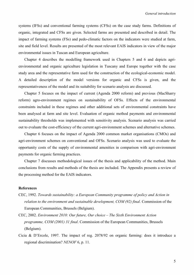
sustainability in agricultural areas. To achieve this objective, three phases were identified in the
research project (Figure 1):
1. To provide a system for farm environmental accounting
2. To develop an ecological-economic model to evaluate farm and field-level environmental-
economic tradeoffs

Chapter 1
4
3. To devise a procedure for the use of the accounting-modelling framework to support multi-objective agricultural policy-making
Phase 1
Designing and testing an
environmental accounting
information system (EAIS)
Phase 2
Combining environmental and economic
aspects in a an integrated ecological-
economic model at farm and field level
Phase 3
Applying the model to
support multi-objective
policy-making
Model
Outcomes
Figure 1. Research outline.
In phase 1 an environmental accounting information system (EAIS) was designed and tested on
three case study farms located in different physiographic regions of Tuscany, Italy. In this phase
economic data of the case study farms were collected as well. In phase 2 an integrated optimisation
model was developed to cover both the environmental and economic aspects of farm management.
The model was empirically implemented for one of the case study farms. In phase 3 the model was
used for sensitivity and scenario analyses to evaluate the impact of the EU’s MacSharry and
Agenda 2000 reforms on sustainability of organic farming systems in Tuscany.
1.4. Outline of the thesis
Chapter 2 describes the development of the EAIS, its general structure and elaboration of its
environmental indicators. Examples of data collection and indicators are discussed with special
reference to ecological modelling and biodiversity of herbaceous plants. Indicator test results are
presented for three case study farms.
In Chapter 3 the EAIS has been combined with farm economic records to evaluate the economic
and environmental aspects of sustainability of organic farming systems (OFSs), integrated farming
Integrated
Ecological Economic Optimisation Model
Multi-objective policy-making
EAIS
indicators
Economic
accounting data
General introduction
5
systems (IFSs) and conventional farming systems (CFSs) on the case study farms. Definitions of
organic, integrated and CFSs are given. Selected farms are presented and described in detail. The
impact of farming systems (FSs) and pedo-climatic factors on the indicators were studied at farm,
site and field level. Results are presented of the most relevant EAIS indicators in view of the major
environmental issues in Tuscan and European agriculture.
Chapter 4 describes the modelling framework used in Chapters 5 and 6 and depicts agri-
environmental and organic agriculture legislation in Tuscany and Europe together with the case
study area and the representative farm used for the construction of the ecological-economic model.
A detailed description of the model versions for organic and CFSs is given, and the
representativeness of the model and its suitability for scenario analysis are discussed.
Chapter 5 focuses on the impact of current (Agenda 2000 reform) and previous (MacSharry
reform) agro-environment regimes on sustainability of OFSs. Effects of the environmental
constraints included in these regimes and other additional sets of environmental constraints have
been analysed at farm and site level. Evaluation of organic method payments and environmental
sustainability thresholds was implemented with sensitivity analysis. Scenario analysis was carried
out to evaluate the cost-efficiency of the current agri-environment schemes and alternative schemes.
Chapter 6 focuses on the impact of Agenda 2000 common market organisations (CMOs) and
agri-environment schemes on conventional and OFSs. Scenario analysis was used to evaluate the
opportunity costs of the supply of environmental amenities in comparison with agri-environment
payments for organic farming practices.
Chapter 7 discusses methodological issues of the thesis and applicability of the method. Main
conclusions from results and methods of the thesis are included. The Appendix presents a review of
the processing method for the EAIS indicators.
References
CEC, 1992. Towards sustainability: a European Community programme of policy and Action in
relation to the environment and sustainable development, COM (92) final. Commission of the
European Communities, Brussels (Belgium).
CEC, 2002. Environment 2010: Our future, Our choice – The Sixth Environment Action
programme, COM (2001) 31 final. Commission of the European Communities, Brussels
(Belgium).
Cicia & D’Ercole, 1997. The impact of reg. 2078/92 on organic farming: does it introduce a
regional discrimination? NENOF 6, p. 11.

Chapter 1
6
Donald, P.F., Pisano, G., Rayment, M.D., Pain, D.J., 2002. The Common Agricultural Policy, EU
enlargement and the conservation of Europe’s farmland birds. Agriculture, Ecosystems &
Environment 89: 167-182.
Edwards, P.J. and C. Abivardi, 1998. The value of biodiversity: where ecology and economy blend.
Biological Conservation 83(3), 239-246.
Falconer, K., Hodge, I., 2001. Pesticide taxation and multi-objective policy-making: farm modelling
to evaluate profit/environment trade-offs. Ecological Economics 36, 263-279.
Kleijn, D., Berendse, F., Smit, R. and Gilissen, N., 2001. Agri-environment schemes do not
effectively protect biodiversity in Dutch agricultural landscapes. Nature 413, 723-725.
Krebs, J.R., Wilson, J.D., Bradbury, R.B., Siriwardena, G.M., 1999. The second Silent Spring?
Nature 400, 611-612.
Panell, D.J. and Glenn, N.A., 2000. A Framework for the economic evaluation and selection of
sustainability indicators in agriculture. Ecological Economics 33, 135-149.
Sands, G.R., Podmore, T.H., 2000. A generalized environmental sustainability index for agricultural
systems. Agriculture, Ecosystems & Environment 79, 29-41.
Schultink, G., 2000. Critical environmental indicators: performance indices and assessment models
for sustainable rural development planning. Ecological Modelling 130, 47-58.
Spash, C.L. and K. Falconer, 1997. Agro-environmental policies: cross-achievement and the role for
cross-compliance. In: F. Brouwer and W. Kleinhanss (eds.) The Implementation of Nitrate
Policies in Europe: Processes of Change in Environmental Policy and Agriculture.
Wissenschaftsverlag Vauk Kiel KG, Kiel, Germany.
Van der Werf, H.M.G., Petit, J., 2002. Evaluation of the environmental impact of agriculture at the
farm level: a comparison and analysis of 12 indicator-based methods. Agriculture, Ecosystems
& Environment 1922, 1-15.
Van Mansvelt, J. D. & Van Der Lubbe, M. J., 1999. Checklist for sustainable landscape
management. Elsevier Science B.V., Amsterdam, The Netherlands.
Vereijken, P., 1999. Manual for prototyping integrated and ecological arable farming systems
(I/EAFS) in interaction with pilot farms. AB-DLO, Wageningen, The Netherlands.

Chapter 2
Environmental accounting in agriculture: a methodological approach
Cesare Pacini1, Ada Wossink2,1, Gerard Giesen1, Concetta Vazzana3, Luigi Omodei-Zorini4, Ruud Huirne1
1 Farm Management Group – Dept. of Social Sciences, Wageningen University, The Netherlands. 2 Dept. of Agricultural & Resource Economics, NC State University, Raleigh, USA. 3 Dept. of Agronomy and Land Management, Florence University, Italy. 4 Dept. of Agricultural Economics, Florence University, Italy.
A previous version of this paper has been presented at the 2000 annual meeting of the American Agricultural Economics Association

Chapter 2
8
Abstract Policymakers need accounting and evaluation tools to be able to assess the potential of sustainable production practices and to provide appropriate agro-environmental policy measures. This study proposes a holistic environmental accounting information system (EAIS) at farm level to measure and evaluate the environmental externalities generated by farm productive cycles. The EAIS is organised in modules corresponding to several environmental processes distinguished in the farm agro-ecosystem. Environmental modules analysed were chosen as a function of critical environmental points observed in Tuscany. The main focus was on devising the general structure of the EAIS and the processing methods of its environmental indicators. An application is presented. Data collection and indicators are discussed with special reference to ecological-environmental modelling (GLEAMS) and biodiversity of herbaceous plants. The Information System was tested on three farms located in different physiographic areas. Keywords: environmental accounting, information systems, environmental indicators, systems approach, farming systems, multidisciplinary research.
2.1. Introduction
Modern society increasingly values the environmental benefits that arise as joint outputs with primary land use, including semi-natural habitats and wildlife. A growing EU commitment, underpinned by article 130R of the Maastricht Treaty, to integrate environmental considerations into the agricultural political agenda, has strengthened the appearance of environmental cross-compliance (ECC) on the policy agenda (Spash and Falconer, 1997). Underlying ECC, there is the principle of farmers providing protection and enhancement of the rural environment in return for support payments. Regulation 2078/92 marks the acceptance of supporting farmers financially to conserve wildlife and the countryside. Besides, in ecological circles attention is also shifting towards the preservation of wildlife within the major forms of primary land use in addition to nature reserves and other protected areas (Edwards and Abivardi, 1998).
The Polluter Pays Principle (PPP) implies that private agents should pay some or all of the costs associated with their production of negative externalities. Support payments are based on a symmetrically opposite principle (Provider Gets Principle or PGP) for private agents who produce positive externalities. Whether the PPP or the PGP apply could be based on a ‘with and without’ comparison; that is, whether (uncompensated) costs to third parties exist without the farming activity. If not, the specific farming practice gives rise to a negative externality (viz. water pollution) and any mitigating action (change in farming practice) has to be classified as reducing the negative externality. Alternatively, if uncompensated benefits to third parties are absent without the farmers’ action, then the farmer is producing a public good (Hanley et al., 1998).

Environmental accounting in agriculture: a methodological approach
9
The PGP requires the government to identify an appropriate level of supply for rural public goods and to direct public funds to the providers according to the marginal opportunity costs of supply. While this objective is easy to assert, it is less obvious how to achieve it in practice. There is particularly a need for (a) definition and measurement of environmental benefits in a way that enables qualities associated with different land use alternatives to be compared and gains and losses to be assessed, and (b) provision of information to policymakers that allows optimal choices to be made and effective policy incentives to be developed. In this context, ‘optimal’ means cost-efficient, so that targets set by public demand are met at minimum cost (Wossink et al., 1999). This paper particularly addresses the issue of defining and measuring environmental benefits of land use activities, that is environmental auditing in agriculture.
Environmental auditing has evolved in industry and commerce. It was first developed in the USA in the 1970s. It is a critical element of the European Union’s voluntary Eco-Management and Audit Scheme (EMAS), which came into operation in May 1995 (EU regulation 1836/93)1. Direct transfer of industry’s auditing practices to agriculture is neither practicable nor feasible for three main reasons. First, many producers are involved, whose production conditions differ widely. Second, agricultural pollution is primarily associated with non-point or diffuse source pollution rather than coming from specific point sources. Since emissions are non-point, costly to measure and stochastic, control must be targeted at estimated emissions rather than actual emissions. Third, farm businesses are relatively small, and are unlikely to have the ability to develop environmental audits individually.
Against this background this paper addresses the specifics of environmental accounting for agriculture. An integral Environmental Accounting Information System (EAIS) at farm level to measure the environmental externalities generated by the farm productive cycles is proposed. The main focus is on devising the general structure of the EAIS and the elaboration of its environmental indicators. Examples of data collection and indicators are discussed with special reference to ecological-environmental modelling (GLEAMS) and biodiversity of herbaceous plants. The Information System was tested on three farms located in different physiographic regions.
2.2. Requirements of environmental information systems
Effective and efficient management decisions depend on reliable information. This is true for environmental matters as well as for every other field of management action. Until recently, environmental monitoring played only a minor role compared to economic monitoring. The design issues of an information system specifically for environmental monitoring are in part specific to
1 Other examples of voluntary environmental codes include the British Standard BS 7750 and the ISO 14000 series. Environmental auditing schemes such as EMAS and ISO 14000 provide the management assurance that operations are managed in compliance with governmental standards, internal company policies and good industry practice (Gray, 1993).
Chapter 2
10
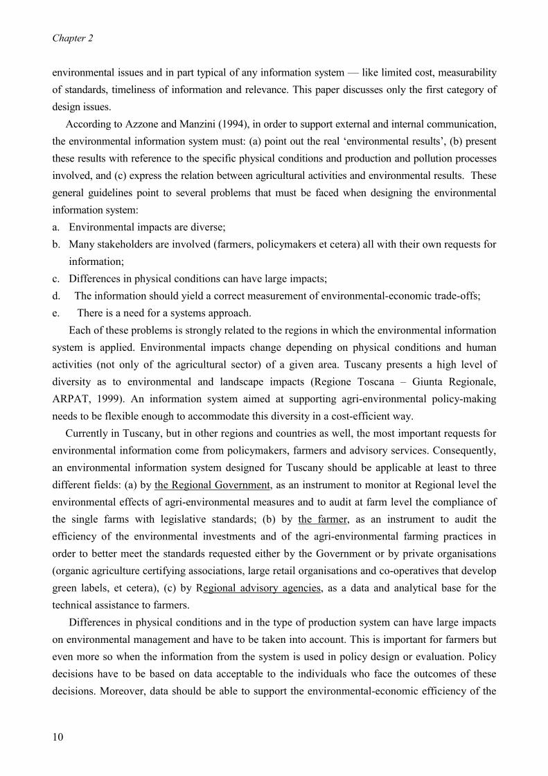
environmental issues and in part typical of any information system — like limited cost, measurability of standards, timeliness of information and relevance. This paper discusses only the first category of design issues.
According to Azzone and Manzini (1994), in order to support external and internal communication, the environmental information system must: (a) point out the real ‘environmental results’, (b) present these results with reference to the specific physical conditions and production and pollution processes involved, and (c) express the relation between agricultural activities and environmental results. These general guidelines point to several problems that must be faced when designing the environmental information system: a. Environmental impacts are diverse; b. Many stakeholders are involved (farmers, policymakers et cetera) all with their own requests for
information; c. Differences in physical conditions can have large impacts; d. The information should yield a correct measurement of environmental-economic trade-offs; e. There is a need for a systems approach.
Each of these problems is strongly related to the regions in which the environmental information system is applied. Environmental impacts change depending on physical conditions and human activities (not only of the agricultural sector) of a given area. Tuscany presents a high level of diversity as to environmental and landscape impacts (Regione Toscana – Giunta Regionale, ARPAT, 1999). An information system aimed at supporting agri-environmental policy-making needs to be flexible enough to accommodate this diversity in a cost-efficient way.
Currently in Tuscany, but in other regions and countries as well, the most important requests for environmental information come from policymakers, farmers and advisory services. Consequently, an environmental information system designed for Tuscany should be applicable at least to three different fields: (a) by the Regional Government, as an instrument to monitor at Regional level the environmental effects of agri-environmental measures and to audit at farm level the compliance of the single farms with legislative standards; (b) by the farmer, as an instrument to audit the efficiency of the environmental investments and of the agri-environmental farming practices in order to better meet the standards requested either by the Government or by private organisations (organic agriculture certifying associations, large retail organisations and co-operatives that develop green labels, et cetera), (c) by Regional advisory agencies, as a data and analytical base for the technical assistance to farmers.
Differences in physical conditions and in the type of production system can have large impacts on environmental management and have to be taken into account. This is important for farmers but even more so when the information from the system is used in policy design or evaluation. Policy decisions have to be based on data acceptable to the individuals who face the outcomes of these decisions. Moreover, data should be able to support the environmental-economic efficiency of the

Environmental accounting in agriculture: a methodological approach
11
policy measures. During the past years in Tuscany most of the environmental agri-environmental measures have been connected with Reg. (CEE) 2078/92. Application of this regulation was quite high compared to the other EU Member States. The EAGGF (European Agriculture Guidance and Guarantee Fund) expenditure by Italy under Regulation 2078/92 was the second highest in the 1993-1998 period, and the absolute highest in 1998. Input reduction and organic farming measures showed the highest levels of expenditure (66 %). Data of Tuscany mirror those at national level, which gave rise to a significant reduction in chemical use, both fertilisers and pesticides (CEC, 1998; Petersen, 1998; Omodei Zorini et al., 1997). However, benefits arising from this reduction were not monitored in terms of actual effects on the environment (e.g., reduction in nitrogen leaching, increase of biodiversity, etc.), disregarding the fact that same farming practices on different pedo-climates can induce considerably different impacts. Besides, use of averages to set the rates of payments and/or input reductions is likely to have caused over-compensation of farms in less intensive areas and under-compensation of farms in the most intensive, with the latter being discouraged from joining the schemes. Therefore, in order to allow for an appropriate evaluation of agri-environment schemes and to improve their cost effectiveness, an environmental information system should incorporate the specific pedo-climatic (production) conditions of the region2 in which the schemes are applied.
To enable a direct link between production on the farm and environmental results, the environmental data have to be collected in such a way that they can be related to the data gathered in the regular economic farm accounting systems (Tuscany Regional RICA-FADN3) and/or in the more technically oriented management systems.
In the literature evidence can be found on possible conflicts occurring between different government programmes or regulations as far as the environmental aims are concerned (Goodwin et al., 1999; Callens and Tyteca, 1999). To avoid these conflicts and achieve high levels of economic-environmental efficiency of the measures, policymakers need comprehensive evaluation tools and information systems which can consider all farm results (environmental and economic) integrally and simultaneously.
2.3. Description of the Environmental Accounting Information System
According to Hannon, (1991) “an ecological accounting system is a framework in which the quantified connections between organisms (individual species, collections of species) and their abiotic environment can be placed and balanced, without ambiguity, omission or double counting exchanges, at any scale which an investigator chooses”. In order to identify such a system, we need
2 Note that the agro-ecosystem analysis level "region" does not correspond in the present study to the administrative level "Tuscany Region". 3 RICA (Rete Italiana di Contabilità Agraria) is the Italian national network of the European FADN (Farm Accountancy Data Network).
Chapter 2
12
(a) to delimitate it in space and time, and (b) to choose a set of processes with their input and output products. The information system is aimed to measure environmental externalities produced by agro-ecosystems and to connect them with the farm economic accounting. Hence, the spatial boundaries of the present environmental (-ecological) accounting system coincide with those of the farm agro-ecosystem and the temporal limits are determined by the standard one-year period in financial accountancy. Farm economic processes were considered together with the environmental ones.
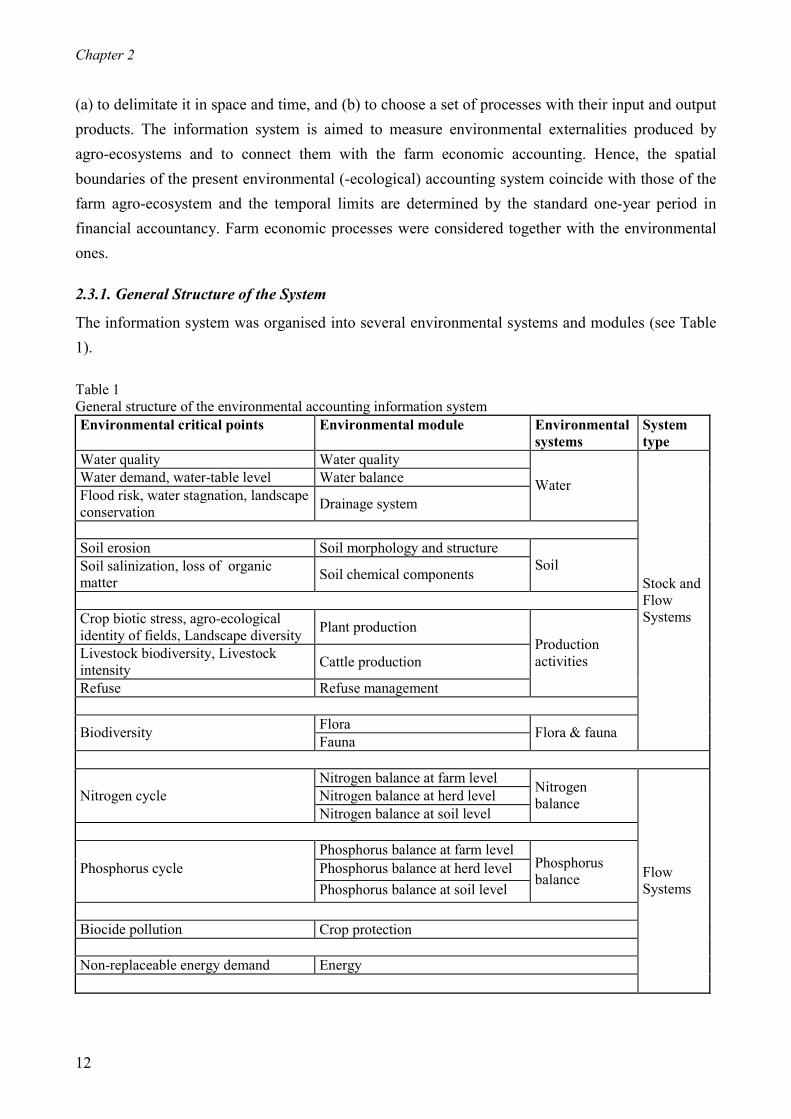
2.3.1. General Structure of the System
The information system was organised into several environmental systems and modules (see Table 1).
Table 1 General structure of the environmental accounting information system Environmental critical points Environmental module Environmental
systems System type
Water quality Water quality Water demand, water-table level Water balance Flood risk, water stagnation, landscape conservation Drainage system
Water
Soil erosion Soil morphology and structure Soil salinization, loss of organic matter Soil chemical components Soil
Crop biotic stress, agro-ecological identity of fields, Landscape diversity Plant production
Livestock biodiversity, Livestock intensity Cattle production
Refuse Refuse management
Production activities
Flora Biodiversity Fauna Flora & fauna
Stock and Flow Systems
Nitrogen balance at farm level Nitrogen cycle Nitrogen balance at herd level Nitrogen balance at soil level
Nitrogen balance
Phosphorus balance at farm level Phosphorus cycle Phosphorus balance at herd level Phosphorus balance at soil level
Phosphorus balance
Biocide pollution Crop protection Non-replaceable energy demand Energy
Flow Systems

Environmental accounting in agriculture: a methodological approach
13
Modules analysed were chosen on the basis of environmental critical points observed in Tuscany physiographic areas (Regione Toscana – Giunta Regionale, ARPAT, 1999; Vereijken, 1994; Vazzana et al., 1997). By means of this modular approach it is possible to activate only those modules relevant to the environmental critical points effectively present in the specific geographic area under survey.
Within each module a number of environmental processes take place, which affect the critical points listed in the table. The performance of the management of each environmental process is quantified by a set of environmental indicators. In order to integrate environmental aspects with financial accounting, indicators relevant to each environmental module were separated into two categories: • Stock indicators, describing the state of the farm environmental capital; • Flow indicators, which concern annual changes of environmental capital and, therefore,
represent both positive externalities or asset appreciations (i.e. production of environmental services) and negative externalities or asset depreciations (i.e. chemical input pollution, soil erosion et cetera) caused by farm production cycles. In this way an analogy between the EAIS and the balance sheet and the income statement in
financial accountancy can be made. For each environmental process an environmental balance sheet and an environmental profit-loss account can be produced. In the environmental balance sheet, assets are measured by stock indicators. This balance sheet is assessed once a year in correspondence with the financial one. Changes between two balance assessments are reported in the environmental profit-loss account and coincide with the flows of the environmental capital during the year. Changes in the profit-loss account are measured by flow indicators and correspond to depreciations (costs) or appreciations (revenues) of the assets.
In practice, depending on data availability and methods used, it is not always possible to calculate both stock and flow indicators for each environmental process. Flow indicators can be calculated directly, summing all appreciations and depreciations, and/or as a change between two balance assessments of two consecutive years. On the other hand, it is not possible to make an indirect computation of a stock indicator starting from a flow indicator.
2.3.2. The components of the system
The environmental accounting information system (EAIS) comprises a data recording system, a set of environmental performance indicators for the evaluation of the farm externalities and the estimate of the farm environmental capital and a set of processing methods to calculate the indicators from the recorded data. Data Collection Data for each environmental module were recorded in the information system together with the corresponding measurable units and values. Information sources were:

Chapter 2
14
• Farm accounting systems • Interviews with farmers • Regional public organisations • Bibliographical sources • Farm nutrient accounting systems • Farm maps • Observations in field • Chemical analyses
Data provided directly by farms or gathered in the field were restricted as much as possible in order to elevate the economic efficiency level of possible future policy measures. Each farm was divided into sites4 and different data were collected for each of them.
The purely financial accounting data were derived from the Tuscany Regional RICA-FADN. Moreover, standard crop record cards were completed for each site. They contain: preceding crop, area, yields and prices, compensation and agri-environment payments, types of cultivation, useful cultivation periods, tractors and other sources of power, agricultural machines, tractor and labour requirements, productive factors application and prices. Environmental Indicators and their processing methods The environmental and economic data collected were processed to produce a set of environmental indicators able to estimate the farm environmental capital and changes therein (Table 2). As shown in Table 2 there is a whole tool box of methodologies used to calculate the environmental indicators from the recorded data (numbers in square brackets relate to corresponding methods listed further in the text). It is not possible to give a detailed description of each of these methods. Instead, reference is made to the Appendix, which contains all this information.
Some of the indicator calculation methods were adopted [1] from studies carried out by Tuscany Regional Organisations (Pettini, 1999; Regione Toscana – Giunta Regionale, ARPAT, 1999; Giannini and Bagnoni, 2000), [2] from laws or regulations currently enforced or [3] literature (Sands and Podmore, 2000; Brunori et al., 1999; Smeding, 1995; Van Mansvelt and Van der Lubbe, 1999; Berentsen & Giesen, 1995; Breembroek et al., 1996; Spugnoli et al., 1993). [4] Nutrient, pesticide and soil erosion indicators were calculated with environmental-ecological models and yardsticks (GLEAMS, EPRIP) that use site-specific input data collected to estimate indicators of nutrient leaching, run-off and sediment, soil erosion and environmental potential risk for pesticides (Knisel 1993; Reus et al., 1999). [5] Other indicator methods were adopted from the “Research Network on Integrated and Ecological Arable Farming systems for EU and associated countries” (Vereijken, 1994 and 1999). They were previously tested in Tuscany at the Florence Agricultural Faculty experimental farm of Montepaldi (S.Casciano) (Vazzana et al., 1997). [6] Fauna, arboreous
4 A site is a geographic area having relatively homogeneous landforms, soil types, water table and climate.

Environmental accounting in agriculture: a methodological approach
15
plant and hedge biodiversity indicators resulted from a co-operation with the Agricultural and Forestry Pathology and Zoology Institute, the Natural History Museum and the Agronomy and Land Management Department, all of Florence University. [7] In some cases (landscape diversity and herbaceous plant biodiversity indicators) existing methods were selected, which were modified to better suit the research requirements (see Section 2.4.1). Table 2 Environmental Indicators
Environmental critical points Environmental Indicators M AT SA Water quality Water quality [1] S D Water demand Water use [1] S d Water-table level Groundwater resource index [3] S D Flood risk, water stagnation,
landscape conservation Surface and underground drainage system
lengths, Terrace length [3] S d
Soil erosion Soil erosion [3,4] F d Soil salinization Soil salinity [1] S d Loss of organic matter Soil organic matter content [3] S d Crop biotic stress Crop rotation blocks [5] S d Agro-ecological identity of fields Field size and max width/max length ratio [3,5] S d Landscape diversity Crop diversity [7] S d Livestock biodiversity Livestock biodiversity [2] S F Livestock intensity Livestock load [2] S F Refuse Dangerous waste load [2] F F Flora biodiversity Herbaceous plant biodiversity [7] S d Arboreous plant biodiversity [6] S d Hedge biodiversity [6] S d
Animal biodiversity [6] S D Fauna biodiversity Insect biodiversity [3,6] S d
Nitrogen cycle Nitrogen leaching, Nitrogen run-off [4] F d Phosphorus cycle Phosphorus sediment [4] F d Biocide pollution Environmental potential risks of pesticide use [4] F d Non-replaceable energy demand Energy use [3] F d 1 Legend: M, method sources (see text); AT, accountancy types (S, stock indicator; F, flow indicator); SA, spatial applicability of indicators (D, district; F, farm; d, detail level, both site and field levels).
The stock/flow classification in Table 1 is determined by the indicator methods. If one of the
EAIS methods is applied to measure an environmental asset, then its outcome will be a stock indicator. If it is not possible to measure the environmental asset at a specific moment in time, then only its changes over time will be measured and the method applied will produce a flow indicator. As stressed previously, from the stock indicator values of two consecutive years it is always

Chapter 2
16
possible to calculate the corresponding flow indicator (see for example the herbaceous plant biodiversity indicator in Section 2.4.1).
In Table 2, indicators were classified not only on the basis of their flow/stock features but also with reference to their spatial applicability. From the conceptual and technical point of view it is important to highlight the distinction between district indicators and the others, i.e. farm and field/site indicators. District indicators refer to the specific regions that the farms under survey belong to. Many of the current environmental policy problems related to land use and resource utilisation are problems that require analysis of agro-ecosystems at the regional (meso) level (Van den Bergh and Nijkamp, 1991). The characteristics that district indicators describe relate to a spatial context exceeding the farm biogeographical boundaries. Boundaries and dimensions of the districts to be evaluated by each indicator depend on the particular environmental aspect that is evaluated. Boundaries can coincide with hydrological districts in the case of the groundwater resource and water quality indicators or with animal species habitats for the animal biodiversity indicator.
2.4. Application of the environmental accounting information system
The EAIS was applied on three case study farms. In the following a short description of the case study farms is reported together with the herbaceous plant biodiversity and nitrogen indicator processing methods and application of the two indicators: EAIS data were recorded for each crop, site and farm during the years 1998, 1999 and 2000. Results are presented for the above-mentioned indicators of selected sites and wheat parcels on the case study farms.
2.4.1. EAIS Specification: the herbaceous plant biodiversity indicator (HPBI)
During the construction of the EAIS, particular attention was given to the accounting methods of the environmental indicators. In some cases methods and tools (i.e. Braun-Blanquet method or Shannon index - Cappelletti, 1976; Arrigoni et al., 1985; Önal, 1997) were selected that were modified to suit the research requirements better. New elements were added to the existing instruments and the results were tested on the farms under study. Here the method of the herbaceous plant biodiversity indicator is specified.
By using the herbaceous plant biodiveristy indicator, the state and changes in the farms’ environmental capital of herbaceous plants were investigated. Loss of biodiversity was the environmental critical point that we intended to investigate with this indicator.
Because of the large areas of the farms being surveyed, the wide range of crops and the high intra-field species variability, it was not possible to apply classic quantitative census methods based on the weighing and the counting of all individual species. In this study a simplified version of the Braun-Blanquet method was used. The Braun-Blanquet method is a commonly used census method that assesses vascular plants biodiversity by estimating the cover percentages of species and their distribution in the parcel observed. In our research only species cover was taken into account.
Environmental accounting in agriculture: a methodological approach
17
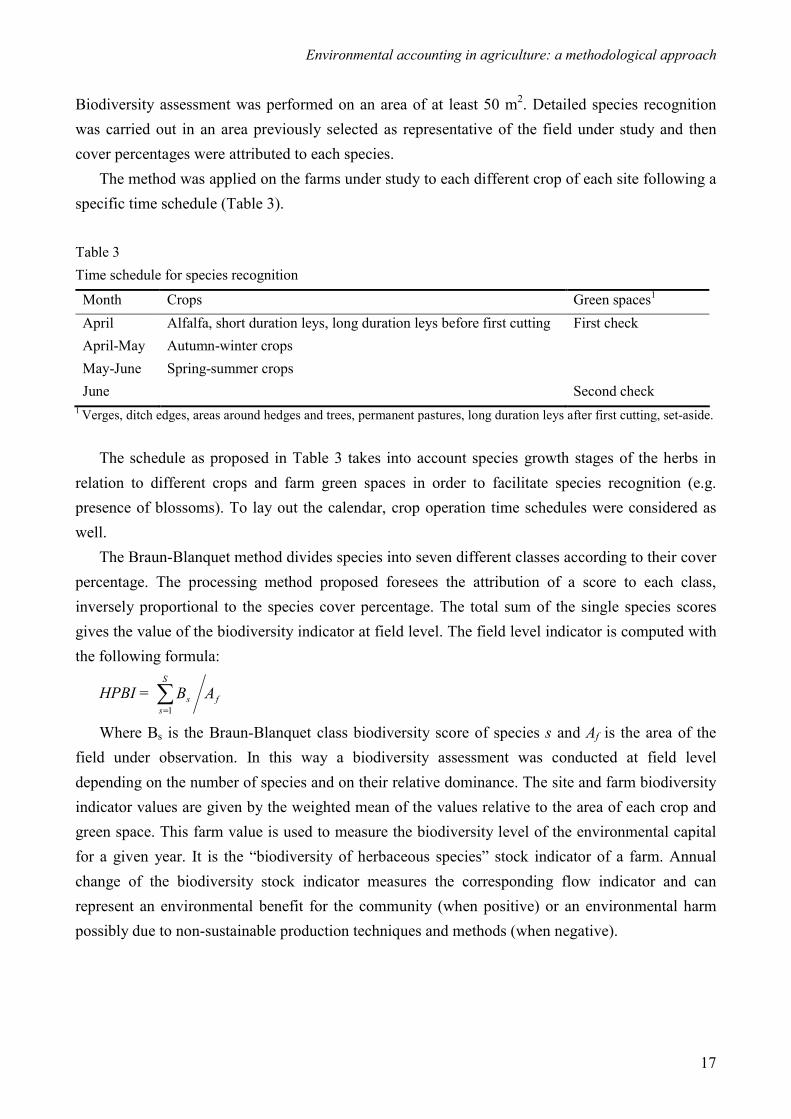
Biodiversity assessment was performed on an area of at least 50 m2. Detailed species recognition was carried out in an area previously selected as representative of the field under study and then cover percentages were attributed to each species.
The method was applied on the farms under study to each different crop of each site following a specific time schedule (Table 3).
Table 3 Time schedule for species recognition
Month Crops Green spaces1 April Alfalfa, short duration leys, long duration leys before first cutting First check April-May Autumn-winter crops May-June Spring-summer crops June Second check
1 Verges, ditch edges, areas around hedges and trees, permanent pastures, long duration leys after first cutting, set-aside.
The schedule as proposed in Table 3 takes into account species growth stages of the herbs in relation to different crops and farm green spaces in order to facilitate species recognition (e.g. presence of blossoms). To lay out the calendar, crop operation time schedules were considered as well.
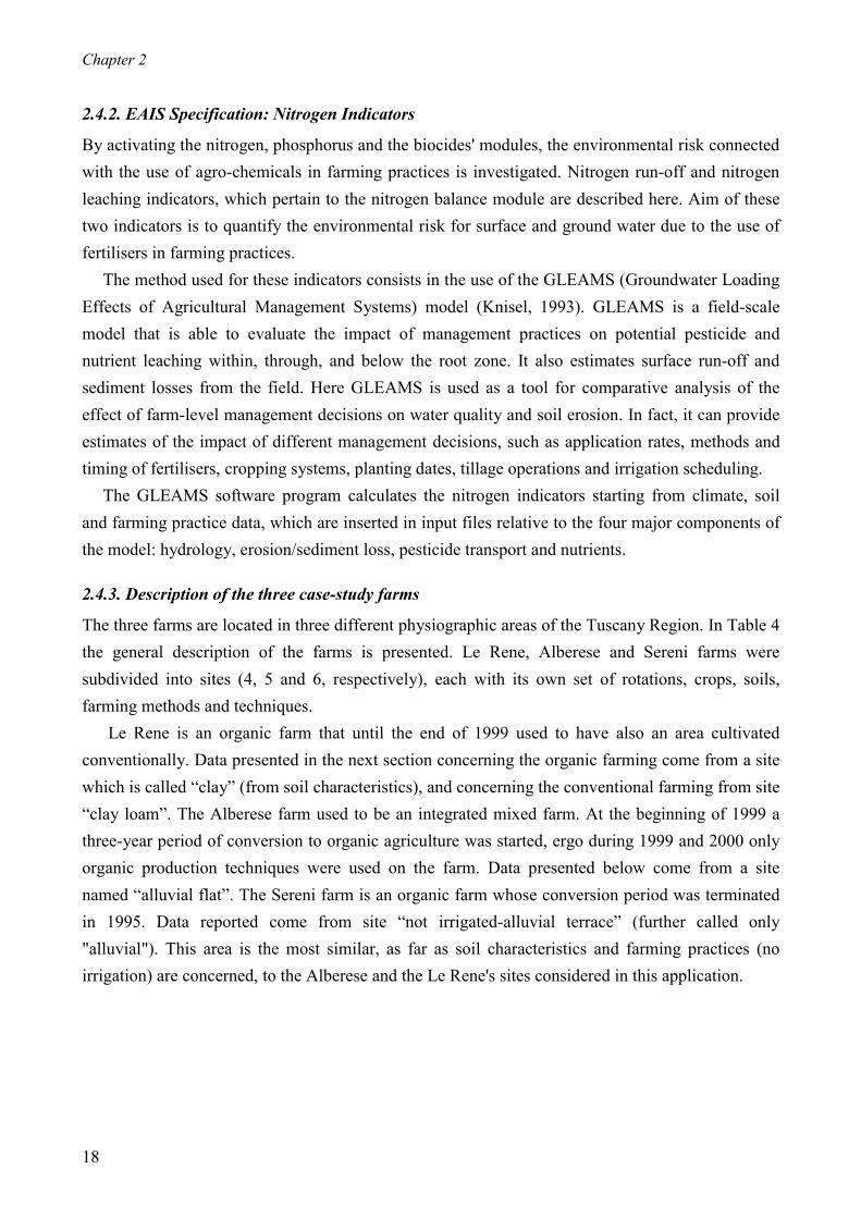
The Braun-Blanquet method divides species into seven different classes according to their cover percentage. The processing method proposed foresees the attribution of a score to each class, inversely proportional to the species cover percentage. The total sum of the single species scores gives the value of the biodiversity indicator at field level. The field level indicator is computed with the following formula:
HPBI = f
S
ss AB∑
=1
Where Bs is the Braun-Blanquet class biodiversity score of species s and Af is the area of the field under observation. In this way a biodiversity assessment was conducted at field level depending on the number of species and on their relative dominance. The site and farm biodiversity indicator values are given by the weighted mean of the values relative to the area of each crop and green space. This farm value is used to measure the biodiversity level of the environmental capital for a given year. It is the “biodiversity of herbaceous species” stock indicator of a farm. Annual change of the biodiversity stock indicator measures the corresponding flow indicator and can represent an environmental benefit for the community (when positive) or an environmental harm possibly due to non-sustainable production techniques and methods (when negative).
Chapter 2
18
2.4.2. EAIS Specification: Nitrogen Indicators
By activating the nitrogen, phosphorus and the biocides' modules, the environmental risk connected with the use of agro-chemicals in farming practices is investigated. Nitrogen run-off and nitrogen leaching indicators, which pertain to the nitrogen balance module are described here. Aim of these two indicators is to quantify the environmental risk for surface and ground water due to the use of fertilisers in farming practices.
The method used for these indicators consists in the use of the GLEAMS (Groundwater Loading Effects of Agricultural Management Systems) model (Knisel, 1993). GLEAMS is a field-scale model that is able to evaluate the impact of management practices on potential pesticide and nutrient leaching within, through, and below the root zone. It also estimates surface run-off and sediment losses from the field. Here GLEAMS is used as a tool for comparative analysis of the effect of farm-level management decisions on water quality and soil erosion. In fact, it can provide estimates of the impact of different management decisions, such as application rates, methods and timing of fertilisers, cropping systems, planting dates, tillage operations and irrigation scheduling.
The GLEAMS software program calculates the nitrogen indicators starting from climate, soil and farming practice data, which are inserted in input files relative to the four major components of the model: hydrology, erosion/sediment loss, pesticide transport and nutrients.
2.4.3. Description of the three case-study farms
The three farms are located in three different physiographic areas of the Tuscany Region. In Table 4 the general description of the farms is presented. Le Rene, Alberese and Sereni farms were subdivided into sites (4, 5 and 6, respectively), each with its own set of rotations, crops, soils, farming methods and techniques.
Le Rene is an organic farm that until the end of 1999 used to have also an area cultivated conventionally. Data presented in the next section concerning the organic farming come from a site which is called “clay” (from soil characteristics), and concerning the conventional farming from site “clay loam”. The Alberese farm used to be an integrated mixed farm. At the beginning of 1999 a three-year period of conversion to organic agriculture was started, ergo during 1999 and 2000 only organic production techniques were used on the farm. Data presented below come from a site named “alluvial flat”. The Sereni farm is an organic farm whose conversion period was terminated in 1995. Data reported come from site “not irrigated-alluvial terrace” (further called only "alluvial"). This area is the most similar, as far as soil characteristics and farming practices (no irrigation) are concerned, to the Alberese and the Le Rene's sites considered in this application.

Environmental accounting in agriculture: a methodological approach
19
Table 4 General description of the Le Rene farm (Coltano, Pisa), the Alberese farm (Alberese, Grosseto) and the Sereni farm (Borgo San Lorenzo, Florence), Tuscany
Le Rene Alberese Sereni Region S. Rossore Regional Park Maremma Regional Park Mugello basin Landform Flat Flat and hilly1 Flat and hilly Farm type Arable Mixed cattle-arable-
horticultural-arboricultural1 Mixed dairy-arboricultural1
Farming system Organic and Conventional (1998 and 1999, part of the farm)
Integrated (1998) and organic (1999 and 2000)
Conventional (before 1993) and organic (since 1993)
Total area 476 ha 3441 ha 352 ha AAU2 452 ha 593 ha 156 ha Crops Wheat, sunflower,
alfalfa, clover, sweet vetch, broad bean, rye, sugar-beet and spelt
Wheat, sunflower, barley, broad bean, maize, alfalfa, ryegrass, oats, vetch, clover, grassland, chickpea, bean, tomato, pasture
Barley, alfalfa, grassland, maize, broad bean
Livestock - CFS3 - - 313 dairy cows Livestock - IFS4 - 110 horses, 460 beef cows - Livestock - OFS5 - 102 horses, 389 beef cows 241 dairy cows
1 Arboricultural crops, which are disregarded in this paper, cover all the cropland on hilly landforms of the Alberese farm. Consequently, this portion of the Alberese cropland is disregarded as well 2 Agricultural area used (permanent pastures excluded) 3 Livestock under the conventional farming system on the Sereni farm (before 1993) 4 Livestock under the integrated farming system on the Alberese (before 1999) 5 Livestock under the organic farming system on the Alberese farm (since 1999) and on the Sereni farm (since 1993)
2.4.4. Results of the herbaceous plant biodiversity indicator
The processing method for the herbaceous plant indicator was applied to the above-mentioned sites. The site level results are summarised in Table 5 together with results coming from three wheat parcels (field level) in sites Le Rene clay and clay loam and Alberese alluvial flat. Broad bean results are presented for Le Rene site clay loam for the year 2000, because wheat was not grown in the first year of conversion. No wheat field results are reported from the Sereni farm, because it has only fodder crops grown to meet the herd feeding requirements.
Comparing the HPBIs of the Le Rene organic and conventional sites, the importance of different production methods in determining different levels of biodiversity can be seen. Both in 1998 and in 1999 the organic method produced a higher level of herbaceous plant biodiversity (i.e., HPBI increased from 56 to 71 and from 32 to 73, respectively). In 2000 the site clay loam, which was a conventional wheat monoculture in 1999, was converted into an organic broad bean

Chapter 2
20
monoculture. Results improved compared with the previous system by 50% at site level (i.e., from 32 to 48) and 80% (i.e., from 25 to 45) at field level, but they still did not reach the levels of the site clay. This is likely due to the difficulty of increasing biodiversity in a monoculture, regardless of the farming practice. Table 5 Results of the herbaceous plant biodiversity indicator (HPBI) Farms Le Rene Organic Le Rene Conventional Alberese Conversion Sereni Site/field Clay Wheat Clay loam Wheat B1 Alluvial flat Wheat Alluvial Year 98 99 00 98 99 00 98 99 00 98 99 00 98 99 00 98 99 00 98 99 00HPBI 71 73 63 83 56 55 56 32 48 43 25 45 71 123 131 1 73 38 51 49 -
1 Broad bean
The conversion of the Alberese farm from the integrated to the organic farming system also produced an increase in herbaceous plant biodiversity, both at site and field level (i.e. from 71 to 123 and 131 and from 1 to 73 and 38, respectively).
In table 5 the results of the herbaceous plant biodiversity stock indicators from the Sereni, the Le Rene organic and the Alberese organic-in-conversion areas confirm the importance of the region in determining the level of biodiversity. Alberese's site was found to have an 87% higher level of biodiversity compared with Le Rene (1999-2000, on average). A 154% increase was found on the Sereni farm (1998-1999, on average). The higher biodiversity may be due to the fact that the Alberese farm adjoins the most constrained areas of the Uccellina Regional Park and, consequently, has in its green spaces a very rich spontaneous flora. Notwithstanding that in 1998 the Alberese farm used integrated crop production methods and its biodiversity indicator at parcel level was very low (1), the biodiversity indicator at site level was equal to that of the Le Rene organic site (71) and higher than that of the Sereni site (51). In other words, the Alberese farm could achieve the same or even better results at site level with integrated production methods than was possible for the Le Rene and the Sereni farms by applying a more constrained organic regulation.
2.4.5. Results of the Nitrogen Indicators
GLEAMS was applied to the most representative rotations carried out in the sites mentioned for the HPBI. On sites Le Rene clay loam (1998-99) and Alberese alluvial flat (1998), a continuous wheat succession was applied. On site Le Rene clay a four-year sunflower-wheat-sweet vetch (for seed)-wheat rotation was applied. After the conversion on Alberese alluvial flat the continuous rotation was changed into a two-year sunflower-wheat rotation. On site Sereni alluvial a 6-years silage maize-barley-Italian rye-grass-alfalfa conventional rotation was converted into a 7-year silage maize-barley-broad bean-silage maize-alfalfa system. The data presented refer to the whole

Environmental accounting in agriculture: a methodological approach
21
rotations and are reported as rotation annual averages. In this way the effects of rotations on nitrogen indicators can be evaluated. Table 6 shows the results of the nitrogen indicators.
Table 6 Results of the nitrogen indicators
Farms Le Rene Le Rene Alberese Alberese Sereni Sereni Farming system Organic Conventional Organic Integrated Organic Conventional N leaching (KgN/ha) 10,8 21,4 10,8 18,3 29,1 43,8 N run-off (KgN/ha) 10,0 12,8 0,7 1,9 4,3 6,1 Total (KgN/ha) 20,8 34,2 11,5 20,2 33,4 49,9
Nitrogen losses into surface and ground water decreased similarly on the three farms from
conventional (Le Rene and Sereni) and integrated (Alberese) to organic production methods (-39%, -33% and -43% respectively). The highest decrease was found for the integrated-organic conversion. Also in this case regions (meteo and soil conditions) affected decisively the level of environmental pollution due to farming practices. Nitrogen losses of the 4-year organic rotation on the Le Rene farm almost equalled losses of the integrated monoculture on the Alberese farm. Heavier clay soils and more severe rain events caused higher levels of run-off on the Le Rene farm. Low contents in organic matter, high levels of sand in soils together with a high use of slurry caused nitrogen leaching to reach the highest values on the Sereni farm.
2.5. Discussion and Conclusions
The main objective of this paper was to illustrate the development of a holistic information system (the EAIS) which can be used for policy purposes to measure and evaluate environmental externalities produced by farms.
The EAIS was developed with special reference to the Tuscany situation. The system was designed with a modular approach that permits it to be fitted to the specific problems of all Tuscany physiographic areas, disregarding those processes that do not affect the environmental problems of a given area. The EAIS can comply with the requirements from the most important agents involved in farm management and land planning, i.e. the Regional Government, the farmers and the Regional advisory agencies.
During the implementation of the method described in this paper particular attention was given to the concepts of stock and flow indicators. A definition of these two types of environmental indicators was given and the applicability of the concepts to real farm situations was tested. Results give evidence of the possible practical applications of the “stock and flow” concepts. The variable “biodiversity” was measured by a stock indicator and successively also computed as a flow indicator. The stock form of the biodiversity indicator (and of the other EAIS indicators in general)

Chapter 2
22
can be used to verify the actual level of biodiversity of a farm compared to other regions. In this way Regional Governments wanting to implement policy measures for the conservation and enhancement of the biodiversity can supply incentives geared towards the real conditions of a given region. Only benefits effectively produced by the farms would be paid for, which would not be possible on the basis of only one benchmark for the entire Tuscany Region and for widely different production conditions of the farms. The flow form of the indicators can be used to evaluate progress of farms in environmental management. The biodiversity flow indicator could, for example, be inserted in an agro-environmental development farm plan to describe farm improvements in a tangible way and audit them.
GLEAMS uses site-specific inputs, which measure the stock features of a given environment (e.g., soil chemical components, slopes, temperatures, et cetera). In this way the sustainability of a given farming method is measured in relation to local physical conditions. Therefore, although GLEAMS produces flow indicators, these indicators can be matched with a specific region. The same can be stressed for EPRIP and the erosion indicator calculated with GLEAMS. Due to the high data requirements and its relatively high costs of application on ordinary farms, GLEAMS is anticipated to be applied for policy purposes only on farms representative of each Tuscany region. In these farms relations between the site-specific information supplied by GLEAMS and nitrogen losses calculated with nutrient balances in ordinary farms could be studied and the results could be used to improve the efficiency of agri-environmental measures at regional level.
For the environmental information system here proposed an explicit connection with the Tuscany Regional RICA-FADN was developed. In fact, the stock/flow framework of the EAIS enables a direct link between production of the farm and environmental results, making possible information trade-offs between economic and environmental processes.
The EAIS holistic approach can help in avoiding possible shortages connected with the application of conflicting regulations and in general in improving the evaluation of the farm environmental processes.
The design of the EAIS was started at research level to test the method for scientific reliability. Subsequently, the method was developed to suit to ordinary farms as well. In this way, a flexibility level was achieved which can fit both the planning and the auditing/monitoring phases of policy design and implementation. The EAIS can be applied on representative farms for research purposes aimed at the planning phase and can be used on ordinary farms for the implementation of the measures.
Many of the environmental and economic processes of farm productive cycles are considered conflicting (e.g., the intra-field biodiversity of herbaceous plants and crop productivity). As far as research purposes are concerned, the EAIS was also designed to supply data to evaluate environmental externalities. Integrated economic-ecological mathematical models, whose application is anticipated in further development of the research, may help to find a sustainability

Environmental accounting in agriculture: a methodological approach
23
threshold that is reliable both from the economic and from the eco-compatible point of view and to identify efficient agri-environmental measures to be applied by policymakers.
The results presented here are only an example of the environmental evaluations enabled by the EAIS methodology. Nevertheless, these results allow some observations on the methodology to be made. The assessment methodology of environmental capital reported appears to fit the high complexity of the environmental systems involved in farm production cycles. At the same time, the environmental capital changes depending on different types of farm management (organic, integrated and conventional) can be evaluated.
The EAIS with its stock/flow structure, the modular and holistic approach and its cost-efficient set of indicator methods appears to be a reliable and flexible tool for policy and also research purposes, which could improve the efficiency of agri-environment schemes in Tuscany as well as in other European Regions. In fact, the enforcement of a holistic environmental accounting system is the first step towards supporting and regulating sustainability in farming systems. Acknowledgements The study described in this paper is part of a research project entitled “Environmental Accounting in Agriculture”, funded by A.R.S.I.A. (Tuscany Agri-forestal Development and Innovation Agency) and directed by Association A.L.T. (Tuscany Environment and Labour Association). C. Pacini’s contribution to this project is part of his PhD research at the Farm Management Group of Wageningen University as part of a Community Training Project financed by the Commission of the European Communities in the specific Programme for Agriculture & Fisheries. The content of the publication is the sole responsibility of the authors and in no way represents the views of the Commission or its services. The authors gratefully acknowledge the comments of J. Brian Hardaker on an earlier version of this paper. References Azzone, G. and Manzini, R., 1994. Measuring strategic environmental performance. Business Strategy
and the Environment 3(1), 1-14. Arrigoni, P.V., Nardi, E. and Raffaelli, M., 1985. La vegetazione del parco naturale della
Maremma (toscana). Dipartimento di Biologia Vegetale dell’Universitá degli Studi di Firenze, Italy (in Italian).
Berentsen, P.B.M. & Giesen, G.W.J., 1995. An environmental-economic model at farm level to analyse institutional and technical change in dairy farming. Agricultural Systems 49, 153-175.
Breembroek, J.A., Koole, B., Poppe, K.J. & Wossink, G.A.A., 1996. Environmental Farm Accounting: The Case of the Dutch Nutrients Accounting System. Agricultural Systems 51, 29-40.

Chapter 2
24
Brunori, G., Omodei-Zorini, L., Lazzerini, G., Pacini, C., Rovai, M., Vazzana, C., 1999. Territorio, ambiente ed impresa agricola: modelli di gestione per lo sviluppo rurale. Seminario Internazionale dell'Università degli Studi di Perugia, Italy, 29 aprile 1999 (in Italian).
Callens, I. and Tyteca, D., 1999. Towards indicators of sustainable development for firms. A productive efficiency perspective. Ecological Economics 28, 41-53.
Cappelletti, C., 1976. Trattato di botanica. UTET, Italy (in Italian). CEC, 1998. State of application of Regulation (ECC) 2078/92: Evaluation of agri-environment
programmes, DGVI Commission working document VI/7655/98. Commission of the European Communities, Brussels (Belgium).
Edwards, P.J. and Abivardi, C., 1998. The value of biodiversity: where ecology and economy blend. Biological Conservation 83(3), 239-246.
Giannini, A. and Bagnoni, V., 2000. Schede di tecnica irrigua per l'agricoltura toscana. ARSIA, Florence, Italy, 134 p. (in Italian).
Goodwin, B.K., Smith, V.H. and Hammond, C., 1999. An ex-post evaluation of the Conservation Reserve Program: Participation, Erosion, and Interaction with Related programs. Unpublished manuscript, Department of Agricultural and Resource Economics, North Carolina State University, USA.
Gray, R., 1993. Accounting and the environment. Paul Chapman Pub., London, UK. Hanley, N., Kirkpatrick, H., Simpson, I. and Ogletorpe, D., 1998. Principles for the Provision of
Public Goods from Agriculture: Modeling Moorland Conservation in Scotland. Land Economics 74(1), 102-113.
Hannon, B., 1991. Accounting in Ecological Systems. In: Constanza, R. (ed.) Ecological Economics: the Science and Management of Sustainability. Columbia University Press, New York, USA, 234-252.
Knisel, G., 1993. GLEAMS Groundwater Loading Effects of Agricultural Management Systems – Version 2.10. University of Georgia-Coastal Plain Experiment Station-Biological and Agricultural Engineering Department Publication No.5, Tifton, Georgia, USA, 259 p.
Omodei Zorini, L., Fruttuosi A., and Franchini, G. (eds.), 1997. La Politica Agricola Comunitaria e l’agricoltura toscana. Analisi e valutazione dell’impatto della riforma MacSharry. ARSIA – Agenzia Regionale per lo Sviluppo e l’Innovazione nel Settore Agricolo-Forestale, Florence, Italy (in Italian).
Önal, H., 1997. A Computationally Convenient Diversity Measure: Theory and Application. Environmental and Resource Economics 9, 409–427.
Petersen, J.-E., 1998. Agri-environment schemes in Europe – Lessons for future rural policy. Report from the Conference in Konstanz, Germany, 25-27 February 1998.
Pettini, L., 1999. Monitoraggio chimico e biologico delle acque superficiali. In: Regione Toscana – Giunta Regionale, ARPAT – Agenzia Regionale per la Protezione dell’Ambiente della Toscana

Environmental accounting in agriculture: a methodological approach
25
(eds.) Rapporto sullo Stato dell’Ambiente della Regione Toscana ’98. Edizioni Regione Toscana, Florence, Italy (in Italian).
Regione Toscana – Giunta Regionale, ARPAT – Agenzia Regionale per la Protezione dell’Ambiente della Toscana (eds.), 1999. Rapporto sullo Stato dell’Ambiente della Regione Toscana ’98. Edizioni Regione Toscana, Florence, Italy (in Italian).
Reus, J., Leendertse, P., Bockstaller, C., Fomsgaard, I., Gutsche, V., Lewis, K., Nilsson, C., Pussemeier, L., Trevisan, M., van der Werf, H., Alfarroba, F., Blümel, S., Isart, J., McGrath, D., Seppälä, T., 1999. Comparing Environmental Risk Indicators for Pesticides – Results of the European CAPER Project. Center for Agriculture and Environment, Utrecht, The Netherlands.
Sands, G.R., Podmore, T.H., 2000. A generalized environmental sustainability index for agricultural systems. Agriculture, Ecosystems and Environment 79, 29-41.
Smeding, F.W., 1995. Protocol natuurplan. Department of Ecological Agriculture, Wageningen Agricultural University, The Netherlands, 83 p. (in Dutch).
Spash, C.L. and Falconer, K., 1997. Agro-environmental policies: cross-achievement and the role for cross-compliance. In: Brouwer, F. and Kleinhanss, W. (eds.) The Implementation of Nitrate Policies in Europe: Processes of Change in Environmental Policy and Agriculture. Wissenschaftsverlag Vauk Kiel, Germany.
Spugnoli, P., Baldi, F. and Parenti, A., 1993. L'analisi energetica per un miglior uso delle risorse nei processi agricoli. Rivista di Ingegneria Agraria 4, 225-233.
Van den Bergh, J.C.J. and Nijkamp, P., 1991. Operationalizing sustainable dynamic economic models. Ecological Economics 4, 11-13.
Van Mansvelt, J.D. & Van der Lubbe, M.J., 1999. Checklist for sustainable landscape management. Elsevier Science B.V., Amsterdam, The Netherlands.
Vazzana, C., Raso, E. and Pieri, S., 1997. Una nuova metodologia europea per la progettazione e gestione di agroecosistemi integrati ed ecologici: applicazione in un’area agricola toscana. Rivista di Agronomia 31(2), 423-440.
Vereijken, P., 1994. Designing Prototypes. Progress Reports of Research Network on Integrated and Ecological Arable Farming Systems for EU and associated countries. AB-DLO, Wageningen, The Netherlands.
Vereijken, P., 1999. Manual for prototyping integrated and ecological arable farming systems (I/EAFS) in interaction with pilot farms. AB-DLO, Wageningen, The Netherlands.
Wossink, G.A.A., Van Wenum, J.H., Jurgens, C.R. and De Snoo, G.R., 1999. Co-ordinating Economic, Behavioural and Spatial Aspects of Wildlife Preservation in Agriculture. European Review of Agricultural Economics 26(4), 443-460.


Chapter 3
Evaluation of sustainability of organic, integrated and conventional
farming systems: a farm and field scale analysis
Cesare Pacini1, Ada Wossink1,2, Gerard Giesen1, Concetta Vazzana3, Ruud Huirne1 1 Farm Management Group – Department of Social Sciences, Wageningen University 2 Department of Agricultural & Resource Economics, NC State University 3 Department of Agronomy and Land Management, Florence University
Agriculture, Ecosystems and Environment 95 (2003) 273-288
Chapter 3
28
Abstract Agricultural researchers widely recognise the importance of sustainable agricultural production systems and the need to develop appropriate methods to measure sustainability. The principal purpose of this paper is to evaluate the financial and environmental aspects of sustainability of organic, integrated and conventional farming systems (OFS, IFS, and CFS, respectively) at farm level and on more detailed spatial scales. This was achieved by applying an integrated economic-environmental accounting framework to three case study farms in Tuscany (Italy) covering different farming systems (FSs) and different spatial scales. The environmental performances of the FS were measured through the application of an environmental accounting information system (EAIS) at field, site and farm level. The EAIS indicators were then integrated with: (1) a set of financial indicators to evaluate the economic and environmental trade-offs between different FSs: and (2) with information on the regional and site-specific soil and climate conditions to study the impact of different pedo-climates on the environmental performances of the FSs. The gross margins of steady-state OFSs were found to be higher than the corresponding CFS gross margins. OFSs perform better than IFSs and CFSs with respect to nitrogen losses, pesticide risk, herbaceous plant biodiversity and most of the other environmental indicators. However, on hilly soils, erosion was found to be higher in OFSs than in CFSs. The pesticide and the nitrogen indicators in this study showed a similar environmental impact caused by integrated and conventional farming practices. Regional pedo-climatic factors were found to have a considerable impact on nutrient losses, soil erosion, pesticide risk and herbaceous plant biodiversity, site-specific factors on nutrient losses and soil erosion. Results at field level suggest that herbaceous plant biodiversity and crop production are not always conflicting variables. Results of the case study farms are discussed and compared with environmental sustainability thresholds reported from EU Directives on nitrate and pesticides in groundwater and the literature. Keywords: Sustainability, Farming Systems, Organic Agriculture, Pedo-climatic Impact.
3.1. Introduction
Agricultural researchers widely recognise the importance of sustainable agricultural production systems and the need to develop appropriate methods to measure sustainability. Modern society increasingly values sustainable farming systems (FSs) for their potential to enhance wildlife and the landscape and to decrease environmental harm caused by farming practices. Against this background an increasing body of literature has developed on the quantification of the sustainability of agricultural production.
Usually, this literature promotes the idea of monitoring a range of sustainability indicators recognising that sustainability cannot be condensed into a single definition (Pannell and Glenn, 2000). Most of these indicators are strongly ecological in focus and very detailed, or they are policy

Evaluation of sustainability of organic, integrated and conventional farming systems
29
oriented and developed at aggregate, sector or country level. So, indicators are developed that differ greatly in information content and condensation of this information (Figure 1). Scientists are most interested in uncondensed data that can be analysed statistically. Policymakers and the public in general can be assumed to prefer condensed data related to policy objectives and free of redundancy.
In either case these indicators lack a close link to farm management decision making. For example, farm management requires rather detailed data related to evaluation criteria and threshold values as set by policy objectives. Indicators at the level of the agricultural production processes enable the right balance to be found between production economics and environmental goals – right there where the production decisions are made (Halberg, 1999). This balance has to take into account both production and pedo-climatic factors at farm level and on more detailed spatial scales.
Figure 1. Relationships between indicators (Braat, 1991)
Hannon (1991) stressed the importance in ecosystem accounting of measuring the material,
energy and service trade-offs between all the ecological processes of a given ecosystem. Disregarding such aspects of accounting can also give cause for conflicts between different government programmes or regulations as far as the environmental aims are concerned (Hammond and Goodwin, 1997; Callens and Tyteca, 1999). For example, a regulation that stresses some peculiar components of the pollutant charge while ignoring others might result in a substitution between pollutants and therefore in an overall increase of the global pollutant charge (Meriläinen, 1995). Hardaker (1997) emphasised the need for a systems approach to any strategy that addresses sustainable agriculture and rural development. Such a strategy requires a comprehensive perspective that accounts for the interrelationships between the technical, environmental, social, economic, and
total quantity of information
Indicators for policy makers
Indicators for farmers
Indicators for scientists
Condensation of information

Chapter 3
30
political aspects of sustainability. However, little work has been done on measuring methods of sustainability at farm and lower levels that take into account the technical-economic and the environmental-ecological trade-offs of ecological and production processes.
Against this background, this paper was aimed at evaluating the financial and environmental aspects of sustainability of organic, integrated and conventional farming systems (CFSs) at farm level and on more detailed spatial scales. This was achieved by applying an integrated economic-environmental accounting framework to three farms in Tuscany. The accounting framework was extensively elaborated on a previous article (Pacini et al., 2001). Here, only its general structure is given together with the description of the most representative indicators of the present study. The impact of FSs and pedo-climatic factors on the indicators were studied at farm, site and field level. Results are presented of the selected indicators.
3.2. Materials and methods
3.2.1. Defining organic, integrated and CFSs
There are a variety of definitions of organic farming systems (OFSs) (Rigby and Cáceres, 2001). Mannion (1995) refers to organic farming as "a holistic view of agriculture that aims to reflect the profound interrelationship that exists between farm biota, its production and the overall environment". From an application viewpoint, the OFSs analysed in this study comply with stipulations of the EU Regulation 2092/91 on organic production of agricultural products and the Tuscany L.R. (Regional Law) 54/95 (recently updated by the EU Regulation 1804/99) on organic livestock production.
There is some semantic confusion surrounding the use of terms such as integrated farming systems (IFSs), Integrated Crop Management (ICM) and Integrated Pest Management (IPM). However, there appears to be agreement on the broad objectives of IFSs (Morris and Winter, 1999), which have been defined as "a holistic pattern of land use which integrates natural regulation processes with farming activities to achieve maximum replacement of off-farm inputs and to sustain farm income" (El Titi, 1992). The IFS analysed in this study meets the requirements of the integrated farming code of the EU Regulation 2078/92 Tuscany Region agri-environmental enforcement programme (recently updated by the 2000-2006 Tuscany Region Rural Development Plan (TRRDP), which enforces the EU Regulation 1257/99).
The term CFSs is often used in the literature to group a variety of farming systems that can be either more or less intensive. A reference definition for CFSs used in this study comes from the Code of Good Agricultural Practice (CGAP) set by the Italian Ministry of Agricultural and Forest Policies to enforce the EU Directive 91/676 (i.e., the so-called "nitrate directive"). All the CFSs under study comply with the CGAP.

Evaluation of sustainability of organic, integrated and conventional farming systems
31
3.2.2. Selection of the farms and sites
Measurement of sustainability was carried out for the 1998-2000 period on the case study farms covering different FSs (conventional, integrated and organic) on different spatial scales. Three farms were chosen, giving preference to the depth of the analysis rather than to the sample size. To achieve insight into the relationship between farm and environmental activities, farms were selected based on the following criteria: 1. Connection with different natural areas in Tuscany 2. Farming systems comprising the main important arable crops, livestock and environmental
activities in their reference area 3. Farmlands comprising the main important types of soils, landforms and hydrological conditions
of their reference area 4. Possibility of performing comparisons between different farming systems at farm and lower
level 5. Market-oriented farms but with a sound background of participation in experimental projects
Table 1 gives the general description of the three selected farms.
Table 1 General description of the Le Rene farm (Coltano, Pisa), the Alberese farm (Alberese, Grosseto) and the Sereni farm (Borgo San Lorenzo, Florence), Tuscany Le Rene Alberese Sereni Region S. Rossore Regional Park Maremma Regional Park Mugello basin Landform Flat Flat and hilly1 Flat and hilly Farm type Arable Mixed cattle-arable-
horticultural-arboricultural1 Mixed dairy-arboricultural1
Farming system Organic and Conventional (1998 and 1999, part of the farm)
Integrated (1998) and organic (1999 and 2000)
Conventional (before 1993) and organic (since 1993)
Total area 476 ha 3441 ha 352 ha AAU2 452 ha 593 ha 156 ha Livestock - CFS3 - - 313 dairy cows Livestock - IFS4 - 110 horses, 460 beef cows - Livestock - OFS5 - 102 horses, 389 beef cows 241 dairy cows
1 Arboricultural crops, which are disregarded in this paper, cover all the cropland on hilly landforms of the Alberese farm. Consequently, this portion of the Alberese cropland is disregarded as well 2 Agricultural area used (permanent pastures excluded) 3 Livestock under the conventional farming system on the Sereni farm (before 1993) 4 Livestock under the integrated farming system on the Alberese (before 1999) 5 Livestock under the organic farming system on the Alberese farm (since 1999) and on the Sereni farm (since 1993)

Chapter 3
32
Le Rene is an organic farm that until the end of 1999 also used to have an area which was cultivated conventionally. It was the reason why the OFS and the CFS were applied simultaneously on two different areas on this farm in 1998 and 1999, allowing for comparisons under common management and climatic conditions. The farm is located in the Migliarino-San Rossore-Massaciuccoli Regional Park (Pisa and Lucca Provinces), on Tuscany’s northern coast (latitude 44ºN). The climate is moist Mediterranean due to the vicinity to mountain areas (Alpi Apuane and Monte Pisano) with a mean annual rainfall of 950 mm. The Alberese farm used to be an integrated mixed farm. At the beginning of 1999 a three-year period of conversion to organic agriculture was started, thus during 1999 and 2000 only organic production techniques were used on the farm. It is located in the Maremma Regional Park (Grosseto Province), on the southern coast of Tuscany (latitude 43ºN). The climate is dry Mediterranean with a mean annual rainfall of 625 mm. The Sereni farm is an organic farm whose conversion period took from 1992 to 1995 and has operated as a fully-fledged organic farm since then. It is located in the Mugello basin, some 30 km north of Florence, northern Tuscany (latitude 44ºN). The Mugello district has a pre-mountain climate with a mean annual rainfall of 1000 mm.
To perform a detailed spatial scale analysis each farm was divided into several different sites (Table 2) according to landform, soil and irrigation conditions. Site-representative rotations were identified based on temporal succession and spatial distribution of the crops. Some minor changes were observed in the rotational schemes. For instance, on some fields of the Le Rene site 1 hard wheat was replaced by spelt (Triticum dicoccon Schrank) and rye (Secale cereale L.), which together comprised the 15% of the winter cereal area; sweet vetch for seed by berseem clover, alfalfa for seed and broadbean. On the Alberese site 3 hard wheat was replaced by barley (15% of the winter cereal area); berseem clover-oats ley by vetch-oats ley (Vicia sativa L.) and Italian ryegrass. In addition to the crops of the site-representative rotations, small portions of farmland were cropped with broad bean, tomato (Lycopersicon esculentum Mill.), chickpea (Cicer arietinum L.) and French bean (Phaseolus vulgaris L.) on the Alberese farm. On this farm, grasslands, which were cropped very extensively, were assimilated to permanent pasture from an environmental viewpoint. On the Le Rene site 3 in 1998 sugar beet (Beta vulgaris L.) had been cropped as well. In addition to the farm and the site levels, fields were identified as the lowest hierarchical levels on the basis of the ecological infrastructure network.
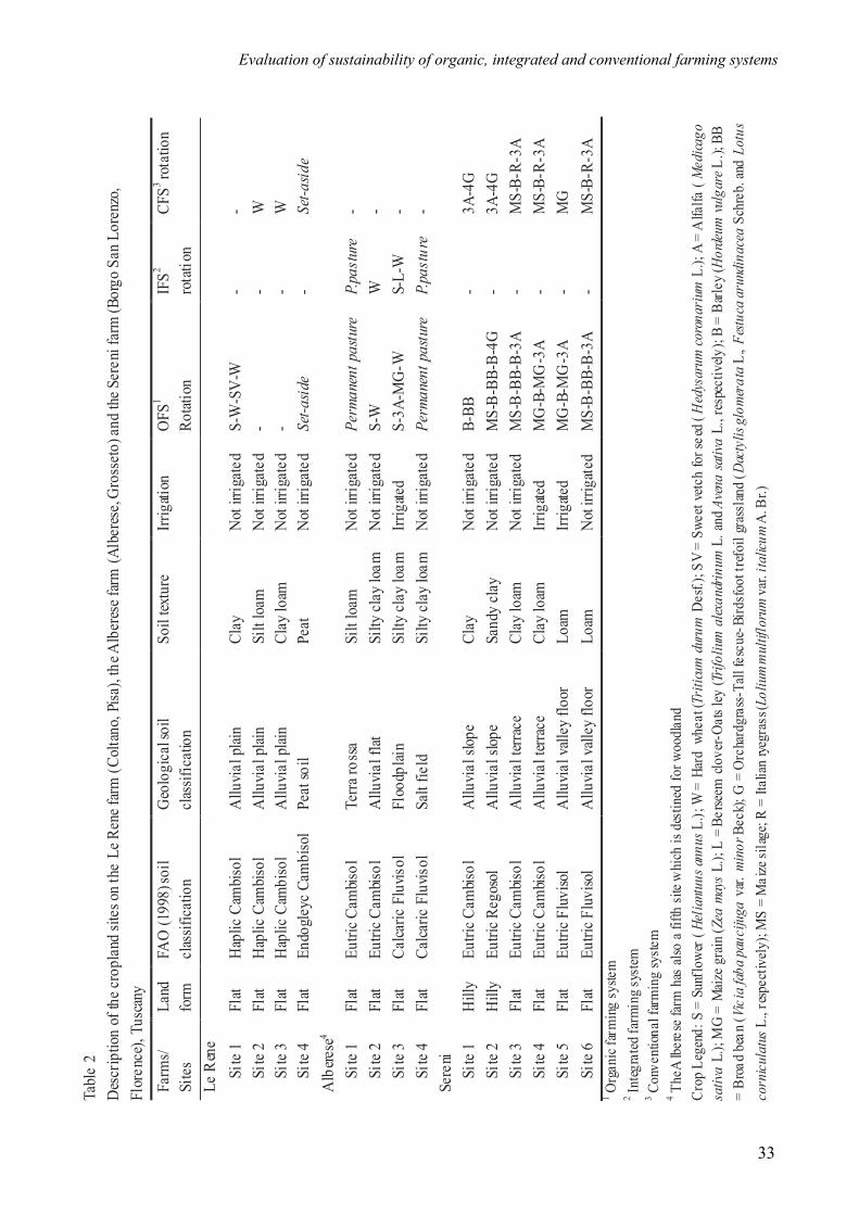
Evaluation of sustainability of organic, integrated and conventional farming systems
33
Tabl
e 2
Des
crip
tion
of th
e cro
plan
d sit
es o
n th
e Le
Ren
e far
m (C
olta
no, P
isa),
the A
lber
ese f
arm
(Alb
eres
e, G
ross
eto)
and
the S
eren
i far
m (B
orgo
San
Lor
enzo
, Fl
oren
ce),
Tusc
any
Farm
s/ Si
tes
Land
fo
rm
FAO
(199
8) so
il cl
assif
icat
ion
Geo
logi
cal s
oil
clas
sific
atio
n So
il tex
ture
Irr
igati
on
OFS
1 Ro
tatio
n IF
S2 ro
tatio
n CF
S3 rota
tion
Le R
ene
Site
1 Fl
at H
aplic
Cam
biso
l A
lluvi
al p
lain
Clay
N
ot ir
rigat
ed
S-W
-SV
-W
- -
Site
2 Fl
at H
aplic
Cam
biso
l A
lluvi
al p
lain
Silt
loam
N
ot ir
rigat
ed
- -
W
Site
3 Fl
at H
aplic
Cam
biso
l A
lluvi
al p
lain
Clay
loam
N
ot ir
rigat
ed
- -
W
Site
4 Fl
at En
dogl
eyc
Cam
biso
l Pe
at so
il Pe
at N
ot ir
rigat
ed
Set-a
side
- Se
t-asid
e A
lbere
se4
Site
1 Fl
at Eu
tric C
ambis
ol
Terra
ross
a Si
lt lo
am
Not
irrig
ated
Pe
rman
ent p
astu
re
P.pa
stur
e -
Site
2 Fl
at Eu
tric C
ambis
ol
Allu
vial
flat
Silty
cla
y lo
am
Not
irrig
ated
S-
W
W
- Si
te 3
Flat
Calca
ric F
luvis
ol
Floo
dplai
n Si
lty c
lay
loam
Irr
igate
d S-
3A-M
G-W
S-
L-W
-
Site
4 Fl
at Ca
lcaric
Flu
visol
Sa
lt fie
ld
Silty
cla
y lo
am
Not
irrig
ated
Pe
rman
ent p
astu
re
P.pa
stur
e -
Sere
ni
Si
te 1
Hill
y Eu
tric C
ambis
ol
Allu
vial
slop
e Cl
ay
Not
irrig
ated
B-
BB
- 3A
-4G
Site
2 H
illy
Eutri
c Reg
osol
A
lluvi
al sl
ope
Sand
y cl
ay
Not
irrig
ated
M
S-B-
BB-B
-4G
- 3A
-4G
Site
3 Fl
at Eu
tric C
ambis
ol
Allu
vial
terra
ce
Clay
loam
N
ot ir
rigat
ed
MS-
B-BB
-B-3
A -
MS-
B-R-
3A
Site
4 Fl
at Eu
tric C
ambis
ol
Allu
vial
terra
ce
Clay
loam
Irr
igate
d M
G-B
-MG
-3A
- M
S-B-
R-3A
Si
te 5
Flat
Eutri
c Flu
viso
l A
lluvi
al v
alley
floo
r Lo
am
Irrig
ated
MG
-B-M
G-3
A -
MG
Si
te 6
Flat
Eutri
c Flu
viso
l A
lluvi
al v
alley
floo
r Lo
am
Not
irrig
ated
M
S-B-
BB-B
-3A
- M
S-B-
R-3A
1
Org
anic
farm
ing
syste
m
2 In
tegra
ted f
arm
ing s
ystem
3 Co
nven
tiona
l far
min
g sy
stem
4 Th
e Albe
rese
farm
has
also
a fi
fth si
te w
hich
is d
estin
ed fo
r woo
dlan
d Cr
op L
egen
d: S
= S
unflo
wer
(He
liantu
us an
nus L
.); W
= H
ard
whea
t (Tr
iticu
m d
urum
Des
f.); S
V =
Swee
t vet
ch fo
r see
d (H
edys
arum
coro
nariu
m L
.); A
= A
lfalfa
(M
edica
go
sativ
a L.
); M
G =
Maiz
e gra
in (Z
ea m
ays L
.); L
= B
erse
em cl
over
-Oat
s ley
(Trif
olium
alex
andr
inum
L. a
nd A
vena
sativ
a L.
, res
pect
ively
); B
= B
arley
(Hor
deum
vulg
are L
.); B
B
= Br
oad
bean
(Vic
ia fa
ba pa
uciju
ga v
ar. m
inor
Bec
k); G
= O
rcha
rdgr
ass-
Tall
fesc
ue-B
irdsf
oot t
refo
il gr
assl
and
(Dac
tylis
glom
erat
a L.
, Fest
uca a
rund
inac
ea S
chre
b. an
d Lo
tus
corn
icula
tus L
., re
spec
tivel
y); M
S =
Mai
ze si
lage
; R =
Itali
an ry
egra
ss (L
oliu
m m
ultif
loru
m va
r. ita
licum
A. B
r.)

Chapter 3
34
3.2.3. Data collection and processing
Data collection and processing of the environmental indicators for the measurement of sustainability were performed through application of an environmental accounting information system (EAIS). The information system was holistically designed to simultaneously and integrally take into account all the ecological and production processes that potentially affect the state of the agro-ecosystem. The EAIS was organised into several systems and modules (i.e., sub-systems). Environmental critical points observed in physiographic areas in Tuscany formed the basis for selection of the modules, within which a number of environmental processes take place that affect the given critical points. The performance of the management of each environmental process was quantified by a set of environmental indicators. The structure of the EAIS enabled implementation at different levels of analysis ranging from (1) a high detailed level (a-level) to (2) a low detailed level (b-level). The a-level would apply to representative farms for research purposes aimed at the planning and monitoring phases of policy design. The b-level would apply to ordinary farms for the auditing and monitoring phases of policy implementation. In this paper results focus on the a-level. For more details on the EAIS structure, reference is made to Pacini et al. (2001).
Besides the environmental indicators, a set of financial indicators was calculated, namely the gross margins including revenues from production, compensation and agri-environment payments, costs of fertilisers and pesticides, maintenance costs of ecological infrastructures (surface drainage system and hedges) and other variable costs.
The EAIS indicators, together with the financial indicators, formed the integrated economic-environmental accounting framework that was used to evaluate the environmental and financial aspects of sustainability at farm level and on more detailed spatial scales.
In Figure 2 indicators are placed in relation to their corresponding calculation reference spatial scale. Depending on the specific purposes, each indicator can also be aggregated and used at higher levels. For example, the herbaceous plant biodiversity indicator can be used at field level to analyse the relation between biodiversity and crop production, at site level to analyse the impact of site-specific features (e.g., soil conditions and site intrinsic natural value) on biodiversity, and at farm level to asses the impact of different FSs as well as different regional pedo-climates. Four agronomic-physiographic spatial scales are used in this study, namely field (a portion of a site limited by ecological infrastructures), site (4-200 ha), landscape (200-4000 ha) and region1 (thousands of square kilometres). In this study the landscape scales coincide with the farm management units, chosen as representative of their corresponding regions.
1 Note that the agro-ecosystem analysis level "region" does not correspond in the present study with the administrative level "Tuscany Region".

Evaluation of sustainability of organic, integrated and conventional farming systems
35
Figure 2. general overview of environmental and financial indicators and their spatial scales.
SITE LEVEL ANALYSIS
Systems and Modules SITE ENVIRONMENTAL INDICATORS
Water balance Water use Drainage system Terrace and drainage system lengths Soil morphology and structure Soil erosion Soil chemical components Soil salinity, Soil organic matter content Plant production Crop diversity Flora Arboreous plant and Hedge biodiversity Nitrogen balance Nitrogen leaching, Nitrogen run-off Phosphorus balance Phosphorus sediment Crop protection Environmental potential risks of
pesticide use Energy Energy use
INC
REA
SED
SPA
TIA
L IN
FO D
ETA
IL
INC
RE
ASE
D A
NA
LY
SIS
AG
GR
EG
AT
ION
SITE FINANCIAL INDICATORS
FIELD LEVEL ANALYSIS
Systems and Modules FIELD ENVIRONMENTAL INDICATORS
Plant production Crop rotation blocks, Field size, Field max width/ max length ratio
Flora Herbaceous plant biodiversity Fauna Insect biodiversity
CROP FINANCIAL INDICATORS
FARM LEVEL ANALYSIS
FARM FINANCIAL INDICATORS
Systems and Modules FARM ENVIRONMENTAL INDICATORS
Refuse management Dangerous waste load Cattle production Livestock load, Livestock biodiversity

Chapter 3
36
Differences between the impacts of regional pedo-climates were studied by comparison of the three farms, i.e. landscapes. For the definitions of site, landscape and region and for further details on spatial and temporal scales in agro-ecosystem analysis and management, reference is made to Bailey (1988), Schleusner (1994), De Ridder (1997) and Prato (2000).
In this paper results are presented of selected environmental indicators, namely the nutrient, erosion, pesticide and biodiversity indicators. Nutrient and erosion indicators were calculated for site-representative fields on a rotational temporal scale using the groundwater loading effects of agricultural management systems (GLEAMS) model (Knisel, 1993). Results were reported as annual averages of the reference period. The pesticide indicator for site-representative fields on an annual scale was calculated with the EPRIP (environmental potential risk indicator for pesticides) yardstick (Trevisan et al., 1999). For comparison purposes, both GLEAMS and EPRIP programs were run using 1998 climatic data at landscape level for all the FSs. Common site-specific soil databases were employed for the comparison of different FSs on the same site. The Sereni 1994 CFS techniques were updated to meet standard techniques used in the Mugello area. On the Alberese farm the techniques of the system "in conversion" and of the steady-state system were assumed to be unaltered.
The herbaceous plant biodiversity indicator (HPBI) was measured using a simplified version of the Braun-Blanquet method (Cappelletti, 1976; Arrigoni et al., 1985). The Braun-Blanquet method is a commonly used census method that assesses the biodiversity of vascular plants by estimating the cover percentages of species and their distribution in the field observed. In this research only species cover was taken into account. This method was applied on the farms under study to each different crop and green space of each site. The site and farm biodiversity indicator values were calculated as the weighted mean of values relative to the area of each crop and green space.
The arboreous plant biodiversity indicator (APBI) represented the rate between the sum of the farm’s wooded areas, each multiplied by a coefficient that evaluates its type (Mediterranean macchia, broadleaved wood, conifer wood or reforestation area) and spatial distribution, and the total farm or site area. The hedge biodiversity indicator (HBI) represented the rate between the hedge length, multiplied by coefficients that assess age and endemic origins of the plants, and the total farm or site agricultural area used (less permanent pasture areas).
The crop diversity indicator (CDI) was used in this research to perform a conjoined evaluation of crop diversity within sites and non-adjacency among single fields. The method used for the calculation of the CDI was derived from the Shannon index. The Shannon index is a proportional abundance index that reflects both the evenness and species richness of a given vegetal or animal assembly, computed from the species shares in a given assembly (Önal, 1997). We applied the Shannon index to cultivated instead of spontaneous species and the shares were calculated from surfaces instead of numbers of individuals. Each site was divided into different crop diversity minimum areas (CDMA) calculated as a sum of the average field surfaces of each different crop

Evaluation of sustainability of organic, integrated and conventional farming systems
37
type present in the site. Finally, the Shannon index method was applied to each CDMA and the results were summed up (and multiplied by 1000) to give the CDI value at site level.
Data on the biodiversity indicators were collected at field (HPBI) and site level (APBI, HBI and CDI) during the 1998-2000 period. Results were reported as annual FS averages or, to study annual effects, on an annual scale.
Aggregation of the indicator values from field to site level and from site to farm level was done by means of a weighted mean of the field and site values of the corresponding areas. For more details on environmental indicator processing methods refer to Pacini et al. (2001).
As to the financial indicators, outcomes refer to 1998 except for Alberese OFS (1999) and Sereni CFS (1994). For comparison purposes, 1998 prices were also applied to Alberese OFS and Sereni CFS. For the Le Rene and the Alberese farms, prices, yields, area compensation payments (EU Regulation 1765/92), integrated and organic measure payments (EU Regulation 2078/92, further on mentioned also as agri-environment payments) were reported from the RICA-FADN. Net crop productive factor inputs were obtained by excluding the variable costs of ecological infrastructures from the RICA-FADN crop-attributed total value. For the Sereni farm, which does not participate in the Tuscany RICA-FADN, data were collected using crop record cards.
3.3. Results
3.3.1. Indicator accounting framework
The accounting framework was used here to compare the impact of conventional, integrated and OFSs on financial returns and the agro-ecosystems within farms. Comparisons between impacts of pedo-climatic factors at different spatial scales were considered as well (between farms belonging to different landscapes/regions and between sites of the same farm).
Because of space limitations, this paper only presents results of selected indicators, namely nutrient losses, soil erosion, environmental potential risks of pesticide use and biodiversity. These indicators and their results are representative of the entire list in Figure 2 as they cover the main environmental threats in the Tuscany Region (Regione Toscana – Giunta Regionale, ARPAT, 1999). The selected indicators allow conclusions to be drawn on the impact of pedo-climatic factors under different FSs, which is not possible for the larger set of indicators (e.g., water use and surface drainage system length). Not reported here are the indicators of dangerous waste load, livestock load, soil salinity and soil organic matter content that primarily pertain to the auditing purpose of the EAIS (see Section 3.2.3). The indicators of livestock biodiversity, underground drainage system length and terrace length were not applicable for the case study farms and the energy use indicator presented redundant information already covered by the nutrient and pesticide indicators. Results on crop rotation blocks, field size, and width/length ratio are very well summarised by the crop

Chapter 3
38
diversity indicator. Finally, results from the insect biodiversity indicator that was applied only during 2000 proved to be insignificant for FS comparisons and inconclusive as to the impact of the pedo-climatic factors.
Table 3 summarises the financial and environmental results of the selected indicators at the system level for the three case study farms.
Table 3 Summary of financial and environmental results of the organic, integrated and conventional farming systems at the Le Rene farm (Coltano, Pisa), the Alberese farm (Alberese, Grosseto) and the Sereni farm (Borgo San Lorenzo, Florence), Tuscany Farm Le Rene Alberese Sereni Farming system OFS1 CFS2 OFS IFS3 OFS CFSGross margin (€/ha AAU4 less p.p.5) 953 902 429 450 2191 2017
Nitrogen leaching (kg/ha AAU less p.p.) 10.8 25.8 10.6 32.0 17.1 28.3Nitrogen run-off (kg/ha AAU less p.p.) 10.0 10.9 1.5 1.3 3.9 10.5Nitrogen losses (kg/ha AAU less p.p.) 20.8 36.7 12.1 33.3 21.0 38.8Phosphorus sediment (kg/ha AAU less p.p.) 0.1 0.2 0.1 0.0 2.6 0.6Soil erosion (t/ha AAU less p.p.) 0.0 0.1 0.0 0.0 3.9 1.4
Nutrient, Erosion and Pesticide Indicators
EPRIP6 (score/ha AAU less p.p.) 0.0 7.8 0.0 1.0 0.0 41.0HPBI7 (score/ha total area less woodland) 69 52 124 117 82 n.a.8
APBI9 (% total area) 3.4 9.6 44.0 44.0 41.0 41.0HBI10 (m/ha AAU less p. p.) 9.3 0.0 23.8 23.8 67.3 0.0
Biodiversity Indicators
CDI11 (score/ha) 4.8 1.8 4.0 3.4 17.3 n.a.1 Organic farming system
2 Conventional farming system
3 Integrated farming system
4 Agricultural area used 5 Permanent pastures 6 Environmental Potential Risk Indicator for Pesticides 7 Herbaceous Plant Biodiversity Indicator 8 Not applicable 9 Arboreous Plant Biodiversity Indicator 10 Hedge Biodiversity Indicator 11 Crop Diversity Indicator
In the following sections, the results are analysed in more detail. Financial indicators are treated at farm level. As to the environmental indicators, results are presented at farm level for both system and pedo-climatic impacts. Site level analysis focuses on the soil component of the pedo-climatic impact (i.e., same climate but different soils) while the field level analysis treats system comparisons on a more detailed spatial scale.

Evaluation of sustainability of organic, integrated and conventional farming systems
39
3.3.2. Financial results
Table 4 summarises the financial results of the different FSs on the Le Rene, Alberese and Sereni farms. The OFS gross margins in the Le Rene and the Sereni farm were found to be 5.6% (953 versus 902 €/ha) and 8.6% higher (2191 versus 2017 €/ha), respectively than the corresponding CFS gross margins. In both cases the positive results of the OFS were mainly determined by a combination of higher prices for organic products, the organic agriculture payments and lower variable costs for fertilisers (only for Sereni OFS) and pesticides. Revenue increases due to all these factors were higher than the decreases caused by lower OFS yields. These results mirror those in previously published comparisons of OFSs and CFSs (see, for example, Lampkin and Padel, 1994). Table 4 Comparison of financial results (€/ha) of the organic, integrated and conventional farming systems at the Le Rene farm (Coltano, Pisa), the Alberese farm (Alberese, Grosseto) and the Sereni farm (Borgo San Lorenzo, Florence), Tuscany Farm Le Rene Alberese Sereni Farming system OFS1 CFS2 OFS IFS3 OFS CFS Revenues
Products 730 722 609 779 2135 2350 Compensation payments 333 480 263 324 207 126 Agri-environment payments 187 0 156 130 146 0 Total 1250 1202 1028 1233 2488 2476
Variable costs Fertilisers 90 71 40 61 0 46 Pesticides 0 28 0 33 0 61 Ecological infrastr. Maintenance 9 10 21 20 5 5 Other costs 198 191 538 669 292 347 Total 297 300 599 783 297 459
Gross margin 953 902 429 450 2191 2017 1 Organic farming system
2 Conventional farming system
3 Integrated farming system
On the Alberese farm the gross margin decreased by 4.7% (429 versus 450 €/ha) in the first year
of conversion, primarily due to the fact that while yields decreased, the farm products could not get higher prices as they could not be certified as organic before the end of the three-year conversion period. Higher agri-environment payments and lower costs for fertilisers and pesticides for the OFS only partially covered this difference. Systems undergoing conversion like the Alberese farm may experience serious financial difficulties also because in Tuscany the agri-environment measures tailored to conversion are limited. Implementation of organic farming methods depends rather on favourable market prices (or price expectations) for organic products.
Chapter 3
40
Ecological infrastructure maintenance costs on the case study farms were very low and therefore irrelevant. These results can be explained by the fact that these maintenance activities do not entail sensitive and visible effects on the farm productions in the short term. Moreover, farms on hilly sites may be not interested in investing in structures that would mostly benefit other farms located on the flat ground.
The Sereni farm agri-environment payments (146 €/ha) were lower than the gross margin difference between the OFS and the CFS (174 €/ha - 2191 versus 2017 €/ha). The OFS compensation payments on this farm were also higher. The agri-environment payments (187 €/ha) on the Le Rene farm were decisive for the achievement of the OFS higher gross margin (51 €/ha - 953 versus 902 €/ha). However, a large share of the agri-environment extra-income was used to compensate for the decrease of compensation payments as a result of extensification of the rotations under the OFS (147 €/ha - 333 versus 480 €/ha). On the Alberese farm the compensation payment decrease (61 €/ha - 263 versus 324 €/ha) greatly exceeded the revenue increase of agri-environment measure payments (26 €/ha - 156 versus 130 €/ha). There seems to be some discord between the agri-environment measures and the CAP producers' support system (at least for the Le Rene and the Alberese farms).
3.3.3. Environmental results
Nutrient losses and soil erosion Farm level analysis. In Table 3 results on nitrogen leaching, run-off, losses, phosphorus sediment and soil erosion are displayed. Results of these indicators are treated together because all of them were calculated with GLEAMS. As expected, the OFS performed better than the IFS and the CFS for nitrogen leaching on all the three farms. The lowest difference in nitrogen losses occurred on the Le Rene farm (20.8 versus 36.7 kg/ha). As to nitrogen run-off, phosphorus sediment and soil erosion, the OFS was almost equal to the CFS and the IFS on the Le Rene and the Alberese farm, respectively. On the Sereni farm that is partially hilly, the OFS was worse than the CFS as far as phosphorus sediment and soil erosion were concerned. This depends on the implementation of long rotations under the OFS, which implies the cropping on hilly ground of more tillage-requiring crops like maize, barley, broad bean, compared to grassland and alfalfa under the CFS. Coiner et al. (2001) arrive at the same conclusions for landscapes.
Nutrient losses were highly affected by regional pedo-climatic conditions. The OFS nitrogen losses on the Alberese farm (12.1 kg/ha) were lower than on the Le Rene (20.8 kg/ha) and the Sereni farm (21.0 kg/ha). The differences between the farm types and related rotations could affect these results in addition to the pedo-climatic factors. However, the last-mentioned seemed to be a particularly dominant factor. For example, on the Sereni farm, whose FS is more intensive and environmentally risky (dairy, with application of animal excreta) nitrogen losses were about equal to those of the Le Rene farm (arable, organic fertilisers). Specially considering the pedo-climatic

Evaluation of sustainability of organic, integrated and conventional farming systems
41
factor, and taking into account that the cattle graze on the permanent pastures (no excreta application on rotation crops), the performance of the IFS on the Alberese farm was no better for nitrogen losses than the CFS on the other two farms (33.3 versus 36.7 and 38.8 kg/ha), and was even worse for nitrogen leaching (32.0 versus 25.8 and 28.3 kg/ha). This seems to be due to a slight difference between the IFS and the CFSs with regard to the amount of fertiliser used and is consistent with reports in the literature. For example, Bailey et al. (1999) report that there is no significant difference between the two systems with respect to beetles and spiders, earthworms and nitrate residues.
Site level analysis. In Table 5 nitrogen losses of the three farms are shown for cropped sites. High differences in losses under the same FS are mainly attributable to rotations. But again the soil factor is very decisive. Simulation results for the same rotations on different sites of the same farm and under the same FS showed that the differences between nitrogen losses oscillated between a minimum of 15% on the Sereni OFS (28.8 on site 5 versus 33.1 kg/ha on site 4) and a maximum of 40% on the Le Rene CFS (34.2 on site 3 versus 47.9 kg/ha on site 2).
Table 5 Comparison of nitrogen (N) losses of the organic, integrated and conventional farming systems on cropped sites of the Le Rene farm (Coltano, Pisa), the Alberese farm (Alberese, Grosseto) and the Sereni farm (Borgo San Lorenzo, Florence), Tuscany Farm Le Rene Alberese Sereni Farming System OFS1 CFS2 OFS IFS3 OFS CFS Site 1 2 3 2 3 2 3 1 2 3 4 5 6 1 2 3 4 5 6 N losses (kg/ha) 20.8 47.9 34.2 11.5 12.2 20.2 34.6 18.1 7.3 33.4 33.1 28.8 16.8 12.9 15.9 38.3 43.0 73.7 37.71 Organic farming system
2 Conventional farming system
3 Integrated farming system
Table 6 presents a comparison of the impact of rotations and soil physical characteristics on
erosion. Results are shown for sites 1 and 2 of the Sereni farm, which are the only sloping cropped sites. Sites Sereni 1 and 2 have equal slopes but the alfalfa/grassland rotation on site CFS 1 produced a higher level of erosion than the same rotation on site CFS 2 (1.9 versus 1.5 t/ha). This is due to the different soil conditions of the two sites (clay in site 1, with higher runoff, and sandy clay in site 2). Results are even more emphasised under the OFS, where the erosion produced by the barley/broad bean rotation on site 1 was three times that of the maize silage-barley-broad bean-maize silage-grassland rotation on site 2 (16.7 versus 5.5 t/ha). In this case the management factor (rotation choice) magnified the effects induced by the environmental factor (soil characteristics).

Chapter 3
42
Table 6 Soil erosion of the organic and the conventional farming systems at site level on the Sereni farm (Borgo San Lorenzo, Florence), Tuscany
Farm Sereni Farming System OFS1 CFS2 Site 1 2 1 2 Soil erosion (t/ha) 16.7 5.5 1.9 1.51 Organic farming system
2 Conventional farming system
Pesticide risk Farm level analysis. Table 3 displays results on environmental risk due to pesticides. OFSs on the three farms posed no environmental risk. The performance of the Sereni CFS was very poor, possibly because of the more intensive crop plan and techniques used. In general EPRIP showed low impacts in relation to the EPRIP yardstick range of possible results (1-625). In fact, according to the EPRIP yardstick classification, the risk ranges from "none" on the Alberese farm (EPRIP<=1), to "negligible" on the Le Rene farm (2<=EPRIP<=16), to "small" on the Sereni farm (17<=EPRIP<=81).
In Table 7 the impacts of the different crop techniques (treatments, pesticide types) for winter cereals on representative sites of the three farms under survey are compared.
Table 7 Environmental Potential Risk Indicator for Pesticides score for winter cereals with different integrated and conventional crop protection techniques on representative sites of the Le Rene farm (Coltano, Pisa), the Alberese farm (Alberese, Grosseto) and the Sereni farm (Borgo San Lorenzo, Florence), Tuscany Farm Le Rene Alberese Sereni Crop technique CFSr1 IFS2 CFSs3 CFSr IFS CFSs CFSr IFS CFSs EPRIP (score/ha) 4 15 4 8 1 45 3 1 6 615 1 Conventional farming system crop technique of the Le Rene farm 2 Integrated farming system crop technique of the Alberese farm 3 Conventional farming system crop technique of the Sereni farm 4 Environmental Potential Risk Indicator for Pesticides
5 Results in bold refer to the actual crop techniques of each farm
Winter cereals, which are the only pesticide-treated crops on all the three farms are barley on the Sereni farm, and durum wheat on the Le Rene and the Alberese farm. CFSr (CFS crop technique of the le Rene farm) had the best EPRIP regardless of the pedo-climatic conditions or the farm type. On the Alberese farm the environmental impacts of the IFS crop technique, which is the actual technique applied on this farm, were the worst. This confirms what already stressed for the

Evaluation of sustainability of organic, integrated and conventional farming systems
43
nitrogen indicators and reported in the literature (Bailey et al., 1999). The performance of all three crop techniques was best on the Alberese farm and worst on the Sereni farm, which again emphasises the decisive role of the regional pedo-climate. The site level analysis revealed no relevant difference between site-specific results from the same farm.
Biodiversity Farm level analysis. Table 3 presents the biodiversity indicator results as averages of the annual values of each FS. The HPBI of the OFS was better than the CFS and the IFS on the Le Rene and the Alberese farm, respectively. But, as can be noted in Table 8, where the complete sequence of the HPBI annual values is displayed, this was achieved on the Alberese farm only in the second year of conversion (2000). Table 8 Year effect of the Herbaceous Plant Biodiversity Indicator (total farm value and green spaces absolute value) at the Le Rene farm (Coltano, Pisa), the Alberese farm (Alberese, Grosseto) and the Sereni farm (Borgo San Lorenzo, Florence), Tuscany
Farm Le Rene Alberese Sereni FS OFS1 CFS/OFS2 IFS/OFS3 OFS1
Reference area
Farm total value
(score/ha)
Green spaces absolute value
(score)
Farm total value
(score/ha)
Green spaces absolute value
(score)
Farm total value
(score/ha)
Green spaces absolute value
(score)
Farm total value
(score/ha)
Green spaces absolute value
(score)
1998 HPBI4 71 125 54 109 117 132 75 122 1999 HPBI 73 120 44 113 117 137 89 135 2000 HPBI 63 84 57 79 131 169 n.c.5 n.c. 1 Results of the organic farming system on the Le Rene site 1 and on the Sereni farm, respectively 2 Results of the conventional farming system (1998-1999) and of the organic farming system (2000) on the Le Rene site 2 and 3 3 Results of the integrated farming system (1998) and of the organic farming system (1999-2000) on the Alberese farm
4 Herbaceous Plant Biodiversity Indicator
5 Data not collected
Table 3 also shows minor differences in APBI between the FSs. As far as hedges are concerned,
both on the Le Rene and the Sereni farm, the crop technique conversion was accompanied by an improvement of these green infrastructures. The CDI of the OFSs was always higher. On the Alberese farm it increased during the conversion from 3.4 in 1998 to 4.6 in 2000. The management of biodiversity on the Sereni OFS as to ecological infrastructures (APBI and HBI) and crop plan (CDI) was the most accurate. This can explain the good HPBI result achieved despite the more intensive land use on this farm (see gross margins). As to the regional impact, the Alberese farm’s HPBI was far better than the OFS HPBI of the other two farms both under the OFS (Table 8, 1999

Chapter 3
44
year) and under the IFS (1998 year). Farm type related factors contributed to these results but, again, the regional factor, in this case expressed by the seed bank capacity of the given areas, played an important role. Farm averages of the 1998, 1999 and 2000 years show that the absolute values of the HPBI of the green spaces of the Alberese farm were higher than those of the Le Rene farm (both OFS and CFS) and the Sereni farm. Note, due to dry climatic conditions, the scores of the 2000 HPBI green spaces on the Le Rene farm were considerably lower than that of the previous two years.
Site level analysis. The HPBI trends during the conversion of the two cropped Alberese farm sites (sites 2 and 3) are shown in Table 9. Differences between site HPBI total values of the same farm appear to be more dependent on the crop plan and/or the green spaces share than on the site intrinsic natural value. The HPBI annual absolute values of wheat, other crops and green spaces were similar. Exceptions are particularly attributable to successful/unsuccessful weed control operations (e.g., site 2 wheat value in 1998), coincidental circumstances (e.g., site 2 1998 green spaces value, which was probably partly underestimated because of overgrazing in the sample), changing crop plans (e.g., values of the other crops) or to the seed bank capacity of the monitored fields. The other farms under survey also produced similar findings.
Table 9 Field level results of the Herbaceous Plant Biodiversity Indicator for two sites and different farming systems at the Alberese farm (Alberese, Grosseto), Tuscany
Farming system IFS1 (1998) OFS2 (1999) OFS (2000) Sites 2 3 2 3 2 3 Wheat HPBI3 absolute value (score) 1 33 73 71 38 49 Other crops HPBI absolute value (score) n.a.4 110 116 67 91 66 Green spaces HPBI absolute value (score) 86 149 136 141 145 151 Site HPBI Total value (score/ha total area5) 71 96 123 87 131 82 1 Integrated farming system
2 Organic farming system
3 Herbaceous Plant Biodiversity Indicator
4 Not applicable - no other crop on the site in 1998 5 Less woodland
Field level analysis. Table 9 presents the HPBI absolute values of wheat, which was the only
pesticide-treated crop under the IFS, other crops and green spaces. Wheat values increased in the first year of conversion and decreased again in 2000. This could have been due to the improved management crop technique ability under the OFS and to an improved reaction of the agro-ecosystem to the new techniques. Average absolute values of the other crops are decreasing year by year. This decrease under the OFS can be explained by the introduction in the crop plan of more

Evaluation of sustainability of organic, integrated and conventional farming systems
45
intensively-cultivated cash crops. Green spaces absolute values increased slightly during the 3-year period.
The 2000 OFS wheat average (43.5) of site 2 (38) and 3 (49) was 32% higher than the 1998 site 3 IFS value (33). Wheat cover decreased by less than 1% (from 100- to 99%) on the Alberese site 2 from 1998 to 2000 and even increased on site 3 (from 95 to 98%) during the same period. Steady-state FS changes differed. The Le Rene farm wheat HPBI was 34 for the CFS and 69 for the OFS (+103%). Cover percentages decreased from 93% in CFS to 88% in the OFS (-5%). These results can probably be attributed to the use of selective pesticides for the IFS and the CFS, and support the above-mentioned findings on the positive financial performances of OFS.
3.4. Discussion and conclusions
3.4.1. Evaluation of sustainability based on environmental thresholds
Besides a relative evaluation of sustainability among the FSs, an absolute evaluation can be done on the basis of environmental sustainability thresholds implemented by regulations and laws or found in the literature. In Table 10 the indicator results are compared to environmental thresholds in terms of compliance (Y) or non-compliance (N). The Phosphorus sediment compliance was linked to the threshold for soil erosion based on the processing method used for the calculation of this indicator. When necessary, the thresholds were adapted to EAIS equivalents (the fourth column) based on regional pedo-climatic features (water leaching and run-off) and EAIS indicator processing methods (i.e., HPBI and CDI).
OFSs comply with thresholds to a higher extent (17 indicators out of 24) than CFSs (9/14) and the IFS (5/8). A cross-view of the findings of Tables 3 and 10 reveals that the statement "Organic Agriculture = Sustainability" is not always valid from an environmental point of view, even though the performance of the OFSs was largely better than the other FSs. Some indicators that performed better in OFSs were nevertheless unsustainable when compared to their corresponding thresholds (see the Le Rene HBI and CDI and the Alberese CDI). On the other hand, many of the indicators that performed worse in the IFS and the CFSs complied with thresholds (10/15).
A limitation of the use of sustainability thresholds is that they are extremely difficult to determine, especially in relation to the intrinsic carrying capacity and resilience of a given ecosystem. Some of the thresholds reported in Table 10 (i.e., those of soil erosion and of field area) could be too restrictive under certain conditions (i.e., hilly landforms and arable farms, respectively) and this might lead to an incorrect evaluation of the environmental performances. For example, Zanchi (1983) proposes a soil erosion threshold of 8-9 t/ha for soils and landforms similar to those of the Sereni hilly sites. Nevertheless, thresholds are indispensable to operationalise sustainability

Chapter 3
46
both at farm management and at policy design level and, as this example demonstrates, to evaluate the differences between FSs in absolute terms.
Table 10 Compliance of farming systems with environmental sustainability thresholds at the Le Rene farm (Coltano, Pisa), the Alberese farm (Alberese, Grosseto) and the Sereni farm (Borgo San Lorenzo, Florence), Tuscany
Compliance Indicator
Environmental sustainability
threshold Source1 EAIS2 equivalent Le Rene Alberese Sereni
OFS3 CFS4 OFS IFS5 OFS CFS
Nitrogen leaching
50mg/l (a) Le Rene=33kgN/ha Alberese=16kgN/ha Sereni=27kgN/ha
Y6 Y Y N7 Y N
Nitrogen run-off
50mg/l (a) Le Rene=17kgN/ha Alberese=2kgN/ha Sereni=11kgN/ha
Y Y Y Y Y Y
Soil Erosion
1t/ha (b) 1t/ha Y Y Y Y N N
EPRIP8 81score/ha (c) 81score/ha Y Y Y Y Y Y HPBI9 50 species per farm (d) 48score/ha Y Y Y Y Y n.a.10
APBI11 5% (e) 5% N Y Y Y Y Y HBI12 1000-2000m/25ha (f) 60m/ha N N N N Y N
CDI13 Field area<=5ha
Crop adjacency=0 Rotation blocks>=4
(g) (h)
30score/ha N N N N N n.a.
1 Source legend: (a) EU Directive 91/676; (b) Pimentel et al., 1995, Kabourakis, 1996; (c) Trevisan et al., 1999, EU Directive 91/414; (d) and (e) Vereijken, 1999; (f) Schotman, 1988; (g) Smeding, 1995; (h) Vereijken, 1999 2 Environmental accounting information system
3 Organic farming system
4 Conventional farming system
5 Integrated farming system
6 Yes (compliance) 7 No (non-compliance) 8 Environmental Potential Risk Indicator for Pesticides 9 Herbaceous Plant Biodiversity Indicator
10 Not applicable 11 Arboreous Plant Biodiversity Indicator 12 Hedge Biodiversity Indicator 13 Crop Diversity Indicator

Evaluation of sustainability of organic, integrated and conventional farming systems
47
Section 3.3.2 shows that current agri-environment and support measures in certain situations prove to be conflicting. The application of environmental thresholds for the evaluation of FS sustainability in the planning phase of policy design can improve the environmental-economic effectiveness of agri-environment and support measures. This is particularly relevant under the current circumstances, where the EU aims to shift support from production to sustainability of rural systems and to shift farmers' role progressively from that of food suppliers to that of custodians of the countryside.
3.4.2. Future research
More extensive analysis needs to be carried out on instalment and maintenance cost (planting/building) of ecological infrastructures. The same applies to the underground drainage system and the terraces, which were not applicable to the case-study farms. With special reference to the EPRIP yardstick, the EAIS method should be tested on other farm types (e.g., wine, olive, etc.) and on different IFSs and CFSs, also on the basis of previously published works (Kabourakis, 1996). Regarding the insect biodiversity indicator, the results (not shown) of the case study were insufficient to draw conclusions either on FS or on the pedo-climatic impact. We can only speculate that the indicator processing method as such is applicable for different crops/green spaces of different regions, takes into account some site-specific features and that its results match well with those of the HPBI.
The EAIS could also be applied at district level to ordinary farms to check the procedures of data transfer from district representative farms to ordinary farms. On the former farms a more detailed EAIS could be applied for research purposes. On the other hand, a simplified EAIS could be used on ordinary farms for auditing and monitoring purposes; however, it should also rely on scientific evidence obtained from researches conducted on representative farms.
This paper discussed the financial-environmental trade-offs only at farm level because of the close interrelations between production processes belonging to different sites on the farms. However, these trade-offs can also be expected at site and field level. Mathematical Programming models are commonly used at farm level for the study of the economic-environmental trade-offs. By formulating the model structure so as to introduce the spatial variability of the environmental and (if necessary) production processes, these trade-offs could be considered right there where the production decisions are made (i.e., at field, site and farm level).
3.4.3. Conclusions
A holistic, integrated economic-environmental accounting framework was applied to three case-study farms to evaluate the sustainability of OFSs, IFSs and CFSs. The impact of farming systems on a number of indicators was studied together with that of pedo-climatic factors at farm, site and field level.
Chapter 3
48
Results provide evidence on three main aspects: 1) OFSs have the potential to improve the efficiency of many environmental indicators as well as being remunerative; 2) the environmental responses of OFSs, as well as IFSs and CFSs can be highly affected by the pedo-climatic factors, both at regional and at site scale; 3) the fact that OFSs in most cases environmentally perform better than IFSs and CFSs does not mean ipso facto that they are sustainable when compared to the intrinsic carrying capacity and resilience of a given ecosystem. Acknowledgements The study described in this paper is part of a research project entitled “Environmental Accounting in Agriculture”, funded by A.R.S.I.A. (Tuscany Agri-forestal Development and Innovation Agency) and directed by Association A.L.T. (Tuscany Environment and Labour Association). C. Pacini’s contribution to this project is part of his PhD research at the Farm Management Group of Wageningen University as part of a Community Training Project financed by the Commission of the European Communities in the specific Programme for Agriculture & Fisheries. The content of the publication is the sole responsibility of the authors and in no way represents the views of the Commission or its services. References Arrigoni, P.V., Nardi, E. and Raffaelli, M., 1985. La vegetazione del parco naturale della
Maremma (toscana). Dipartimento di Biologia Vegetale dell’Universitá degli Studi di Firenze, Italy (in Italian).
Bailey, A.P., Rehman, T., Park, J., Keatinge, J.D.H., Tranter, R.B., 1999. Towards a method for the economic evaluation of environmental indicators for UK integrated arable farming systems. Agriculture, Ecosystems and Environment 72, 145-158.
Bailey, R.G., 1988. Ecogeographic analysis: a guide to the ecological division of land for resource management. USDA Forest Service Misc. Publ. 1465, Washington, DC (USA).
Braat, L., 1991. The predictive meaning of sustainability indicators. In: Kuik, O. and Verbruggen, H. (eds.) In search of indicators of sustainable development. Kluwer Academic Pub., Dordrecht, The Netherlands.
Callens, I., Tyteca, D., 1999. Towards indicators of sustainable development for firms. A productive efficiency perspective. Ecological Economics 28, 41-53.
Cappelletti, C., 1976. Trattato di botanica. UTET, Italy (in Italian). Coiner, C., Wu, J., Polansky, S., 2001. Economic and environmental implications of alternative
landscape designs in the Walnut Creek Watershed of Iowa. Ecological Economics 38, 119-139. De Ridder, N., 1997. Hierarchical levels in agro-ecosystems: selective case studies on water and
nitrogen. Thesis Wageningen Agricultural University, The Netherlands.

Evaluation of sustainability of organic, integrated and conventional farming systems
49
El Titi, A., 1992. Integrated farming: an ecological farming approach in European agriculture. Outlook on Agriculture 21, 33-39.
FAO, 1998. World Reference Base for Soil Resources. FAO, ISRIC and ISSS, Rome, Italy. Hammond, C., Goodwin, B., 1997. An Ex-Post Evaluation of the Conservation Reserve Program:
Participation, Erosion, and Interaction with Related Programs. Paper presented at the 1997 AAEA Meeting in Toronto, Canada.
Halberg, N., 1999. Indicators of resource use and environmental impacts for use in a decision aid for Danish livestock farmers. Agriculture, Ecosystems and Environment 76, 17-30.
Hannon, B., 1991. Accounting in Ecological Systems. In: Constanza, R. (ed.) Ecological Economics: the Science and Management of Sustainability. Columbia University Press, New York , USA, 234-252 p.
Hardaker, J.B., 1997. Guidelines for the integration of sustainable agriculture and rural development into agricultural policies. FAO, Rome, Italy.
Kabourakis, E., 1996. Prototyping and dissemination of ecological olive production system: A methodology for designing and a first step towards validation and dissemination of prototype ecological olive production systems (EOPS) in Crete. Thesis Wageningen Agricultural University, Wageningen, The Netherlands.
Knisel, G., 1993. GLEAMS Groundwater Loading Effects of Agricultural Management Systems – Version 2.10. University of Georgia-Coastal Plain Experiment Station-Biological and Agricultural Engineering Department Publication No.5, 259 p., Tifton, Georgia (USA).
Lampkin, N.H. and Padel, S. (eds.), 1994. The economics of organic farming. CAB International, Wallingford, UK.
Mannion, A.M., 1995. Agriculture and environmental change. Temporal and spatial dimensions. Wiley, Sussex (UK).
Meriläinen, S., 1995. Does greening bring changes in management logics of action? A case study of Finland's biggest chemical company. Presented at the Greening of Management Workshop, European Institute for Advanced Studies in Management, Brussels, Belgium, 12-13 January 1995.
Morris, C., Winter, M., 1999. Integrated farming systems: the third way for European agriculture? Land Use Policy 16, 193-205.
Önal, H., 1997. A Computationally Convenient Diversity Measure: Theory and Application. Environmental and Resource Economics 9, 409–427.
Pacini, C., Wossink, A., Giesen, G., Vazzana, C., Omodei-Zorini, L., 2001. Environmental Accounting in Agriculture: a Methodological Approach. Submitted for publication to Agricultural Systems.
Panell, D.J. and Glenn, N.A., 2000. A Framework for the economic evaluation and selection of sustainability indicators in agriculture. Ecological Economics 33, 135-149.

Chapter 3
50
Pimentel, D., Harvey, C., Resosudarmo, P., Sinclair, K., Kurz, D., McNair, M., Crist, S., Shpritz, L., Fitton, L., Saffouri, L. and Balair, R., 1995. Environmental and economic costs of soil erosion and conservation benefits. Science 267, 1117-1121.
Prato, T., 2000. Multiple attribute evaluation of landscape management. Journal of Environmental Management 60, 325-337.
Regione Toscana – Giunta Regionale, ARPAT – Agenzia Regionale per la Protezione dell’Ambiente della Toscana (eds.), 1999. Rapporto sullo Stato dell’Ambiente della Regione Toscana ’98. Edizioni Regione Toscana, Florence, Italy (in Italian).
Rigby, D., Cáceres, D., 2001. Organic farming and the sustainability of agricultural systems. Agricultural Systems 68, 21-40.
Schleusner, D.P., 1994. Resources management perspective: practical considerations for using GIS and remote sensing at the field level. In: Sample, V.A. (ed.) Remote sensing and GIS in Ecosystem management. Island Press, Washington, DC (USA).
Schotman, A., 1988. Tussen bos en houtwal: broedvogels in een Twents cultuurlandschap. RIN-rapport 88/37, Leersum, The Netherlands (in Dutch).
Smeding, F.W., 1995. Protocol natuurplan. Department of Ecological Agriculture, Wageningen Agricultural University, The Netherlands, 83 p. (in Dutch).
Trevisan, M., Errera, G., Capri, E., Padovani, L. & Del Re, A.A.M., 1999. Environmental Potential Risk Indicator for Pesticides. In: Reus, J., Leendertse, P., Bockstaller, C., Fomsgaard, I., Gutsche, V., Lewis, K., Nilsson, C., Pussemeier, L., Trevisan, M., van der Werf, H., Alfarroba, F., Blümel, S., Isart, J., McGrath, D., Seppälä, T. (eds.) Comparing Environmental Risk Indicators for Pesticides – Results of the European CAPER Project. Center for Agriculture and Environment, Utrecht, The Netherlands).
Vereijken, P., 1999. Manual for prototyping integrated and ecological arable farming systems (I/EAFS) in interaction with pilot farms. AB-DLO, Wageningen, The Netherlands.
Zanchi, C., 1983. Primi risultati sperimentali sull'influenza di differenti colture (frumento, mais, prato) nei confronti del ruscellamento superficiale e dell'erosione. Annali dell'Istituto Sperimentale per lo Studio e la Difesa del Suolo - Firenze XIV, 277-288.

Chapter 4
The modelling framework
Cesare Pacini 1, Gerard Giesen 1, Ada Wossink 2,1, Ruud Huirne1 1 Farm Management Group – Department of Social Sciences, Wageningen University, The Netherlands. 2 Dept. of Agricultural & Resource Economics, NC State University, Raleigh, USA.

Chapter 4
52
Abstract The main purposes of this chapter are: 1) to present a detailed modelling framework to evaluate the impact of different scenarios of EU and Tuscan regulations on organic and conventional farming systems both at farm and field level, and 2) to discuss the use of the modelling framework for practical applications. To achieve this we took four identifiable steps: 1) to describe the agri-environmental and organic agriculture legislation in Tuscany and Europe, 2) to describe a Tuscan case study region and a representative farm used for the construction of the ecological-economic model, 3) to provide a description of the model versions for organic and conventional farming systems, and 4) to discuss the representativeness of the model and its ability for scenario analysis. It enabled us to draw conclusions on potential applications of the model and the representativeness of the model outcomes.
4.1. Introduction
The importance of sustainable agricultural production systems and the need to develop methods to assess sustainability is widely recognised by agricultural researchers. Against this background the main objective of the present project was to develop and apply a comprehensive toolkit of methods to evaluate sustainability of farming systems for multi-objective policy-making.
In previous studies (Pacini et al., 2002a; Pacini et al., 2002b) an environmental accounting information system (EAIS) was designed and applied to case study farms in Tuscany. Then, the EAIS was used for a descriptive analysis of differences between farming systems. Here, an ecological-economic linear programming (LP) model is presented, whose input data were gathered by combining the set of EAIS indicators with a set of economic data provided by a case study farm and the RICA-INEA1 database.
The main purposes of this chapter are: 1) to present a detailed modelling framework to evaluate the impact of different scenarios of EU and Tuscan regulations on organic and conventional farming systems both at farm and field level, and 2) to discuss the practical applications of the modelling framework. Four identifiable steps were taken: 1) to describe the agri-environmental and organic agriculture legislation in Tuscany and Europe; 2) to select and describe a case study area and a representative farm used for the construction of the ecological-economic model; 3) to supply a description of the model versions for organic and conventional farming systems; and 4) to discuss the representativeness of the model and its ability for scenario analysis. These four steps will be addressed in the course of this chapter.
Studies that report the results of the application of the model include Pacini et al. (2002c), which focused on the evaluation of sustainability aspects of farming systems on farm and field scale, and 1 RICA (Rete Italiana di Contabilità Agraria) is the Italian national network of the European FADN (Farm Accountancy Data Network), INEA (Istituto Nazionale di Economia Agraria) is the Italian national agricultural economics institute.

The modelling framework
53
Pacini et al. (2002d), which centred on the practical use of the model for regional multi-objective policy making.
4.2. Description of agri-environmental and organic agriculture legislation in Tuscany and Europe
Tuscany currently has a substantial legal framework that rules the environmental aspects of agricultural production, partly originating from the EU and partly from the Italian or the Tuscany Regional governments. The most important legislation concerning the agricultural sector can be grouped into three categories: (1) regulation of production methods, specifically regarding organic farming; (2) cross-compliance regulation; and (3) regulation of water quality, particularly with respect to nitrate levels. For more information on these laws see Pacini et al. (2002b).
4.2.1 Regulation of organic production methods
Organic farming used to be funded by EU Regulation 2078/92 Tuscany Region agri-environmental enforcement programme until Agenda 2000 came into force. The 2078 regulation was part of the so-called accompanying measures of the MacSharry reform, and was later modified by EU Regulation 2772/95. The programme was recently updated by the 2000-2006 Tuscany Region rural development plan, which enforces the Agenda 2000 EU regulation 1257/99.
Farmers who benefit from agri-environment support schemes must comply with specific commitments and rules, such as those that apply to organic agriculture. Organic production rules are included in EU Regulation 2092/91 on organic production of agricultural products. Additional requirements were enforced by the Tuscany L.R. (Regional Law) 54/95, which in turn was recently replaced by EU regulation 1804/99 on organic livestock production. Requirements of L.R. 54/95 included: a minimum of long fibre feedstuffs (6.0 kg per day of dry matter for cows; 4.0 kg per day for heifers and 2.5 kg per day for yearling heifers), a maximum of concentrates and conventional feedstuffs (30 and 15 % of total dry matter, respectively). Among other things, regulation 1804 prescribes daily rations of a minimum of 60 % roughage and a maximum of 10 % conventional feedstuffs, and a maximum stocking rate for cattle, which equals the constraint imposed by the nitrate directive on vulnerable areas.
4.2.2 Cross-compliance regulation
Agri-environment measures were instituted with the MacSharry reform, subsequently modified when the Agenda 2000 reform was introduced. Cross-compliance commitments were attached to the common agricultural policy (CAP) income support schemes for arable areas (EU Regulation 1765/92 for the MacSharry reform and EU Regulation 1251/99 for the Agenda 2000 reform). In order to benefit from EU Regulation 1765/92, which establishes a support system for producers of

Chapter 4
54
certain arable crops, farmers had to set-aside 15 % of the arable crop area. In 1999 this regulation was replaced by EU Regulation 1251/99 with a lower set-aside obligation of 10 %.
The EU Regulation 1259/99 lays down common rules for direct support schemes under the CAP. Member States are requested to implement appropriate environmental measures for the agricultural land used or the production concerned and the potential impact on the environment of agricultural activities. The Italian Ministry of Agricultural and Forest Policies enforced the measures of regulation 1259 by issuing two laws as of September 15, 2000 and March 8, 2001. Farmers who receive supports for arable crops, grain legumes, tobacco, seeds, rice and olive oil must meet the requirements governing a number of technical and agronomic interventions for the construction and the maintenance of their drainage systems.
4.2.3 Regulation of water quality
Important environmental regulations emanated from the EU Directive 91/676, the so-called "nitrate directive". This directive set a maximum on the total amount of manure applied in vulnerable areas of 170 kg of nitrogen per year/hectare of agricultural area used (AAU) leading to a maximum constraint on the total stocking density depending on the AAU and the herd composition. The EU nitrate directive was enforced in Italy by the Code of Good Agricultural Practice (CGAP - decreed by the Italian Ministry of Agricultural and Forest Policies of April 19, 2001) and by the D.L. 152/1999 (issued decree). The D.L. 152/1999 presents thresholds for nitrate in drinking water and principles for quantitative guardianship of the water resources.
4.3. Description of the case study
4.3.1. The Mugello area
The model was built using data from the Sereni farm, an organic dairy farm located in the Mugello basin (Borgo San Lorenzo municipality), some 30 km north of Florence, northern Tuscany (latitude 44°N). The Mugello area has a temperate climate with orographic rain regime and a mean annual rainfall of 1000 mm. From an economical viewpoint, the northern area of Florence Province, Mugello basin included, is defined as a zone with a prevailing mountain economy. This definition is based on the land-zoning scheme that was used in previous studies to evaluate the impact of the MacSharry reform in Tuscany (Omodei Zorini and Zammarchi, 1997). This area can be subdivided into the foothills and the mountainous area. Professional farms (farms with at least one full-time work unit) such as the Sereni farm are mainly located in the former area. In Tuscany 15% of all farms are professional farms and cover 70 % of the AAU (Omodei Zorini and Zammarchi, 1997). According to Contini (2002), agriculture in Mugello is mostly extensive. The average AAU by professional farms is quite high compared to other regions of Tuscany. Large holdings (defined as those with an AAU higher than 50 hectares) farm 67% of the AAU. Animal production (specifically

The modelling framework
55
dairy farming) has a central role in the Mugello area (53 % of the farms). The most common breed of dairy cow in Florence Province is the Italian Holstein (83 % of the total) (ARSIA et al., 2001). The Mugello AAU is subdivided into permanent grassland and pastures, which are mainly located in the mountain area (42% of AAU), fodder crops (23 %), arable crops (20 %), chestnuts (5 %), fruit orchards (2 %), vineyards (1 %), olive groves (1 %) and other crops (6 %).
4.3.2. The Sereni farm
The Sereni farm was selected for a case study analysis based on the criterion of representativeness of the Mugello area. For the selection criteria reference is also made to Pacini et al. (2002a). The Sereni farm has operated as a certified organic farm since its conversion which took from 1992 to 1995. This farm was used as a database for the construction of the model. Table 1 gives the general description of the Sereni farm. Table 1 General description of the Sereni farm (Borgo San Lorenzo, Florence), Tuscany
Landform Both flat and hilly Farm type Mixed dairy-arboricultural1 Farming system Conventional (before 1993) and organic (since 1993) Total area 352 ha Agricultural area used 156 ha Milk quota (1998) 1 132 500 kg/year Housing capacity 150 dairy cows (including young stock) Livestock – OFS2 241 head (dairy cows plus young stock) Livestock – CFS3 313 head (dairy cows plus young stock)
1 Fruit production, which is disregarded in this paper, covers 2 ha on the Sereni farm 2 Livestock under the organic farming system on the Sereni farm (since 1993) 3 Livestock under the conventional farming system on the Sereni farm (before 1993)
To perform a detailed spatial scale analysis six sites were identified according to soil landform,
FAO (1998) soil classification, geological soil classification, soil texture and irrigation conditions. A general description of the sites is given in Table 2 together with corresponding rotations.
Farm economic data used for the model were taken from 1998 record cards for the organic farming system (OFS) and from historical data on the conventional farming system (CFS). The latter were rectified for technical and price changes during the 1992-1998 period. Pedo-climatic, ecological and agronomic data were collected in the 1998-2000 period. A complete list of the collected data and a description of the integrated economic-environmental accounting framework applied are given in Pacini et al. (2002a, 2002b).

Chapter 4
56
Tabl
e 2
Des
crip
tion
of th
e site
s of t
he S
eren
i far
m (B
orgo
San
Lor
enzo
, Flo
renc
e), T
usca
ny
Site
s La
nd
Form
FA
O (1
998)
soil
clas
sific
atio
n So
il ge
olog
ical
cl
assi
ficat
ion
Soil
phys
ical
cl
assi
ficat
ion
Irrig
atio
n O
FS2
rota
tion
CFS
3 rota
tion
AA
U
(ha)
U
nplo
ughe
d la
nd (h
a)
Site
1
Hill
y Eu
tric
Cam
biso
l A
lluvi
al sl
ope
Cla
y N
ot ir
riga
ted
B-B
B 3A
-4G
21
.0
4.8
Site
2
Hill
y Eu
tric
Reg
osol
A
lluvi
al sl
ope
Sand
y cl
ay
Not
irri
gate
d M
S-B
-BB
-B-4
G
3A-4
G
48.0
10
.6
Site
3
Flat
Eu
tric
Cam
biso
l A
lluvi
al te
rrace
C
lay
loam
N
ot ir
riga
ted
MS-
B-B
B-B
-3A
M
S-B
-R-3
A
24.0
5.
4 Si
te 4
Fl
at
Eutri
c C
ambi
sol
Allu
vial
terra
ce
Cla
y lo
am
Irrig
ated
M
G-B
-MG
-3A
M
S-B
-R-3
A
5.0
1.1
Site
5
Flat
Eu
tric
Fluv
isol
A
lluvi
al v
alle
y flo
or
Loam
Irr
igat
ed
MG
-B-M
G-3
A
MG
40
.0
9.1
Site
6
Flat
Eu
tric
Fluv
isol
Allu
vial
val
ley
floor
Lo
am
Not
irri
gate
d M
S-B
-BB
-B-3
A
MS-
B-R
-3A
15
.0
3.3
Farm
tota
l are
as
15
3.0
34.3
1
Crop
Leg
end:
B =
Bar
ley (
Hor
deum
vul
gare
L.);
BB
= B
road
bea
n (
Vici
a fa
ba p
auci
juga
va
r. m
inor
Bec
k); 3
A =
Alfa
lfa (t
hree
year
s) (
Med
icag
o sa
tiva
L.);
4G
=
Orc
hard
gras
s-Ta
ll fe
scue
-Bird
sfoo
t tre
foil
gras
slan
d (fo
ur y
ears)
(D
acty
lis g
lom
erat
a L.
, Fes
tuca
aru
ndin
acea
Sch
reb.
and
Lotu
s cor
nicu
latu
s L.,
resp
ectiv
ely)
; MS
= M
aize
si
lage
(Zea
may
s L
.); R
= It
alia
n rye
gras
s (Lo
lium
mul
tiflo
rum
var
. ita
licum
A. B
r.); M
G =
Mai
ze g
rain
. 2 Or
gani
c far
min
g sy
stem
3 Co
nven
tion
al fa
rmin
g sy
stem
3 Ag
ricul
tura
l are
a us
ed

The modelling framework
57
The general structure of the farm animal and feed production activities is presented in this section, while more detailed data are presented in the following sections together with descriptions of their use in the model construction. The description of the general farm structure is based on the current situation of the farm (OFS) and major differences between the OFS and the previous CFS are mentioned.
The central element of the Sereni OFS is an Italian Holstein dairy herd. The herd is composed of six different cattle categories: dairy cows (older than 28 months), dried-off cows, heifers (12 months to calving), yearling heifers (70-365 days), heifer calves (0-70 days) and bull calves (0-10 days). The average daily milk production in 1998 amounted to 24.7 kg/d, corresponding to standard lactation (305 days) of 7550 kg per cow; fat content 3.6 % and protein content 3.2 %. The milk quota in 1998 amounted to 1132500 kg/year; housing capacity is 150 dairy cows including young stock. Herd size had dropped from 313 head (dairy cows plus young stock) under the CFS to 241 head under the OFS. The farm has a dairy cow replacement rate of 25 % and restocks only with heifers raised on the farm. Calving interval is 450 days and the calving rate is 0.8 calvings per cow per year. Its mortality rate is 7 % for calves and yearlings and 2 % for cows. A 14 % selection rate is applied to the heifer category. Bull calves are sold when 10 days old.
The transition from CFS to OFS did not significantly affected herd composition, category rates and housing capacity. Milk yield per cow had been steadily increasing during the 1992-1998 period but this was most likely the result of animal selection rather than the change of farming method. Milk quota changed according to herd size and yield per cow.
Crops grown on the farm are barley (Hordeum vulgare L.), broad bean (Vicia faba paucijuga var. minor Beck), maize (Zea mays L.), Orchardgrass-Tall fescue-Birdsfoot trefoil grass (Dactylis glomerata L., Festuca arundinacea Schreb. and Lotus corniculatus L., respectively) and alfalfa (Medicago sativa L.). Broad bean used not to be grown under the CFS, while Italian ryegrass (Lolium multiflorum var. italicum A. Br.), which used to be part of the conventional crop plan (also as trap crop), was excluded from the organic crop plan. Barley and broad bean are used for the production of grain and straw, maize for grain and silage, and grass and alfalfa for hay. Ryegrass was used for the production of silage. Against this backdrop site-representative rotations were identified based on temporal succession and spatial distribution of the crops under the OFS and the CFS. Rotations are presented in Table 2.

Chapter 4
58
4.4. Model description
4.4.1. General structure
The general structure of the model is shown in Table 3. The model was constructed starting from a standard LP economic model and the input-output matrix was extended to include emission and evaluation figures retrieved from ecological models. The model form is displayed as follows:
Maximise {Z = c’x} Subject to Ax ≤ b
and x ≥ 0 Where x is a vector of activities and environmental variables; c is a vector of gross margins or
costs per unit of activity; A is a matrix of technical-environmental coefficients; and b is a vector of technical-environmental right-hand-side (RHS) coefficients.
Three different versions of the model were constructed, namely the organic version, the conventional version and a combined version resulting from the integration of the other two. Crop rotations as well as technical and environmental coefficients of all activities were separately elaborated and computed for the conventional and organic versions.
Activities and constraints are simplified and grouped in Table 3. The model activities include: a number of crop rotations varying from 18 (conventional version), to 26 (organic version), to 44 (combined version), set-aside, green spaces, nitrogen and soil losses, pesticide use environmental risks, herbaceous plant biodiversity, maize grain sale, seasonal labour, purchase of fertiliser, purchase of organic and conventional feedstuffs, purchase of straw, animal production activities representing different herd categories and ecological infrastructure activities representing hedges and drainage system.
The rows of the matrix indicate the type and form of the constraints used: constraints of fixed assets (land requirements including site-minimum of green spaces, milk quota, housing requirements and tractor requirements), labour requirements, herd composition, feed requirements (fibre, energy value, protein and dry matter requirements), straw requirements, crop production constraints (manure and slurry requirements, rotation constraints), legal constraints (set-aside, cross-compliance, livestock intensity maximum, minimum of long fibre feedstuffs and roughage and maximum of concentrate and conventional feedstuff), tie rows, and environmental constraints (maximum of nitrogen leaching, nitrogen runoff, soil erosion, potential risks of pesticide use, water use and minimum of herbaceous plant biodiversity, hedges and drainage system. The objective function of the LP model is the farm gross margin, i.e., total revenues minus variable costs (including planting and maintenance costs of ecological infrastructures).

The modelling framework
59
Tabl
e 3
Gen
eral
stru
ctur
e of
the
LP m
odel
Si
te 1,
2 &
6
Farm
Si
te/fa
rm
A
ctiv
ities
C
onstr
aint
s
Cro
p ro
-ta
tions
Se
t-as
ide
Gre
en
spac
es N
itrog
en
and
soil
loss
es
Pest
icid
e us
e en
viro
n-m
enta
l risk
s
Her
bace
ous
plan
t bi
odiv
ersi
ty H
ired
la
bour
Purc
hase
ac
tiviti
es A
nim
al
pro-
du
ctio
n
Surf
ace
drai
nage
sy
stem
Hed
ges
Righ
t han
d sid
e L
and
requ
irem
ents
+1
+1
+1
<=
Av.
hec
tare
s M
ilk p
rodu
ctio
n
a i,j
<=A
v. q
uota
H
ousi
ng r
equi
rem
ent
a i,j
<=Av
. cow
pla
ces
Tra
ctor
requ
irem
ents
a i,
j a i,
j
a i,
j a i
,j
<=A
v. tr
acto
rs
Lab
our r
equi
rem
ents
a i,
j a i,
j
-a
i,j
a i,
j a i
,j a i,
j <=
Av.
labo
ur
Her
d ca
tego
ries
+/-a
i,j
=0
Feed
ing
requ
irem
ents
-a
i,j
-ai,j
a i,
j
<=
0 St
raw
requ
irem
ent
-ai,
j
-a
i,j
a i,j
<=0
Man
ure
and
slur
ry r
equi
rem
ents
a i,j
-ai,j
-a
i,j
<=0
Rot
atio
ns a
nd g
reen
spa
ces
+/-a
i,j
=0
Set-a
side
-a
i,j
a i,j
=0
Su
rfac
e dr
aina
ge s
yste
m
-ai,
j
a i
,j
>=0
Org
anic
pro
duct
ion
law
s and
nitr
ate
dire
ctiv
e
Vario
us
Lin
king
land
use
and
loss
es
-ai,
j -a
i,j
-ai,
j a i,
j
=0
Nitr
ogen
leac
hing
a i,j
<=
ebi,j
Nitr
ogen
run
-off
a i,j
<=
ebi,j
Soil
eros
ion
a i,j
<=
ebi,j
Wat
er b
alan
ce
+/-a
i,j
-ai,
j -a
i,j
a i,
j
<=
ebi,j
Lin
king
land
use
and
pes
ticid
e us
e -a
i,j
a i,j
=0
Pe
stic
ide
use
envi
ronm
enta
l ris
ks
a i,j
<=eb
i,j
Lin
king
land
use
and
bio
dive
rsity
-a
i,j
-ai,
j -a
i,j
a i,j
=0
H
erba
ceou
s pl
ant b
iodi
vers
ity
a i,
j
>=eb
i,j
Hed
ges
-ai,
j
a i,j
>=0
Obj
ectiv
e fu
nctio
n C
osts
/ g.
m.
G.m
.
C
osts
Cos
ts
G.m
. C
osts
C
osts
1 Leg
end:
ai,j
= te
chni
cal-e
nviro
nmen
tal c
oeff
icie
nts;
ebi,j
= e
nviro
nmen
tal r
ight
han
d si
de (
RHS)
coe
ffici
ents;
av.
= a
vaila
ble;
g.m
. = g
ross
mar
gins

Chapter 4
60
Two different spatial scales were used for the model: farm scale and field scale. Although data for the calculation of technical-environmental coefficients were collected at field level (when applicable), they were aggregated at the site level for reasons of simplicity and functionality of the model. As indicated at the top of Table 3, activities were divided into two groups: site-specific and farm-specific activities distinguishable by the spatially referenced calculation of their coefficients.
Based on activity and constraint types the model can be divided into an empirical economic sub-model and an empirical environmental-ecological sub-model. These two sub-models are integrated and partially overlap, however the constraints of fixed assets, labour, herd, crop production and regulations mainly pertain to the economic sub-model, while the mere environmental constraints pertain to the environmental-ecological sub-model.
The economic sub-model was built using previously presented data from the Sereni farm. Existing farms are commonly used in studies on policy-making evaluation (Falconer and Hodge, 2001). For the present study, the reason for the choice of building the model on an existing farm, and specifically a market-oriented one, was mainly: (a) to increase the credibility of the analysis conducted with the model (Law and Kelton, 1991), and (b) to collect data for the calculation of environmental coefficients, which otherwise would have been hard to construct.
Starting from farm data the environmental coefficients were calculated applying the following ecological models: (a) resource and pollution impact models (also known as emission models), and (b) ecological evaluation models. For more details on classification of ecological models and applicability for environmental economic analysis at the farm level please refer to Wossink et al. (1992), Wossink (1998), and Jarosch and Murschel (1989). Results from the ecological models were entered as coefficients into the input-output matrix. The Groundwater Loading Effects of Agricultural Management Systems (GLEAMS) model (Knisel, 1993) was selected to calculate the coefficients of nitrogen losses, soil losses and water balances. The impact of chemical crop protection was simulated by applying the environmental potential risk indicator for pesticides (EPRIP) yardstick (Trevisan et al., 1999; Reus et al., 2002). To calculate the herbaceous plant biodiversity coefficients a multidimensional evaluation approach was used based on the Braun-Blanquet census method (Cappelletti, 1976; Arrigoni et al., 1985). A monetary evaluation model simply based on the estimate criterion of the production cost value was used for the calculation of the hedge and drainage system coefficients (Brunori et al., 1999).
For more details on the application of these models to the Sereni farm as well as to other farm types, farming systems and regions of Tuscany, we refer to Pacini et al. (2002a, 2002b). In the following sections a detailed description of the model is given using the general structure of the LP model (Table 3) as basis. As far as the general structure of the Sereni farm is concerned the description of the model is centred on the current situation of the farm (OFS). Differences between the organic and the conventional versions of the model are included.

The modelling framework
61
4.4.2. Animal production
The central element of the model (Table 3) is the dairy herd, which reflects the general structure of the real herd on the Sereni farm (see description of the Sereni farm above). Critical coefficients of the animal production activities are milk yield per cow and milk quota. The milk yield per cow used for the model is that observed on the Sereni OFS in 1998. Backed by expert information and the farm’s management, we assumed the milk yield of the CFS to be the same as the OFS value. For reasons of comparison between the OFS and the CFS, the milk quota levels in both the organic and the conventional versions of the model were settled equal to that of the OFS in 1998 (see Table 1).
Labour and tractor requirements for the herd were calculated according to the time needed for cleaning, milking (two shifts), ration preparation and supply (two shifts, Unifeed system), calf supervision and care. Calculations were made for three different periods of the year on a 4-month basis. Milking/cleaning and feed production can also be done by hired labour, which is available at € 10.8 per hour. Labour cost per hour was based on farm records and the Florence Province temporary work agreement of 1998. We assumed that labour and tractor requirement of the herd for the OFS and the CFS are identical.
Feeding requirements were calculated according to the milk production and the young stock growth needs, following the criteria settled by the Tuscany Agri-forestal Development and Innovation Agency for the regional advisory services (Lucifero et al., 1993). They are expressed in terms of fibre, energy value, protein and dry matter per head of each herd category. The ration requirements imposed by the organic livestock production laws were also added (see Section 4.2). Finally, an additional constraint was included in the model to fulfil the straw requirements for litter of the herd and for additional feeding of dried-off cows. The organic livestock production laws give the only differences as to feeding and straw requirements.
The amount of manure and slurry supplied by the herd for the fertilisation of the crops was calculated from the faeces and urine excreted by the dairy cows, heifers, yearling heifers and heifer calves, 100 % of which collected in the barn. Dried-off cows mainly graze during the dry period so their excretions were disregarded like that of the bull calf category. The manure is composed of a mix of 3/8 of the excretions and the straw bedding. The remainder of the excretions diluted in 60 % of water constitutes the slurry. These coefficients are equal in the two versions of the model.
The main difference between the organic and the conventional versions of the model is given by the returns per dairy cow, which drop from € 2841 for the OFS to € 2462 for the CFS, the difference being due to the milk prices of the OFS and the CFS (€ 42.35 and € 36.67 per 100 kg of milk, respectively). For reasons of generality of the model, the organic and conventional milk prices were taken from the Tuscany rural development plan. They are based on the 1998 RICA-INEA database.
The variable costs per dairy and dried-off cow amount to € 91 and 24, respectively, which include artificial insemination and veterinarian charges, medicines, materials and plant maintenance. The return per heifer of € 200 is the result of the sale of culled heifers. Variable costs

Chapter 4
62
per heifer and yearling heifer are of € 56 and € 20, respectively, including costs of artificial insemination and plant maintenance (only for heifers), veterinarian, medicines and materials. The return per bull calf amounts to € 114. Variable costs per heifer calf and bull calf amount to € 72 and 18, respectively, including veterinarian charges, medicines, artificial milk (only for heifer calves) and materials. All variable costs are equal in the two versions of the model. Returns from culled heifer and bull calf sales are equal as well because these products are not certified as organic.
4.4.3. Feed production and purchase
Crops that can be grown in the model reflect the reality of the farm (see the previous farm description). They are barley, broad bean (only for the organic version), maize, grass (4 years), alfalfa (3 years) and Italian ryegrass (only for the conventional version). Crop yields of the organic and of the conventional version of the model are shown in Table 4 together with nutrition values of corresponding feedstuffs. While crop yields differ between the two versions, chemical composition and nutrition values remain unchanged.
Table 4 Crop yields and nutritional values
Yield CFS1
Yield OFS2
Dry matter3
Fibre content3
Protein content3
Energy content3
kg kg g/kg g/kg g/kg MJ NEL4/kg Barley 5 000 3 500 860 56 105 7.11 Broad bean - 2 000 870 77 263 7.32 Maize for silage 42 000 30 000 310 71 28 1.99 Maize for silage – irrigated 49 000 40 000 310 71 28 1.99 Maize for grain 7 000 - 870 25 105 7.82 Maize for grain – irrigated 9 500 5 000 870 25 105 7.82 Grassland 10 000 8 500 900 300 65 4.27 Alfalfa 10 000 8 000 870 280 130 4.12 Italian ryegrass 23 000 - 220 78 18 1.14
1 conventional farming system 2 organic farming system 3 nutrition values do not differ between the organic and the conventional versions of the model 4 megajoule net energy for lactation
We selected seven different crop rotations (eleven including the irrigation option), which together constitute the feed production element of the model (see Table 3). The selected rotations (or successions) are those applied on the Sereni farm under either the OFS or the CFS. Depending on the site-specific characteristics and the type of farming system, each site has a number of rotations that can be selected by the model simulations (see Table 5). The optional rotations for the

The modelling framework
63
organic version are 26 and 18 for the conventional version. Each rotation is characterised by a number of equality constraints.
Table 5 Optional rotations included in the conventional and organic version of the model
Site2 1 2 3 4 5 6 FS CFS3 OFS4 CFS OFS CFS OFS CFS OFS CFS OFS CFS OFS
Rotation 3A-4G X X X X B-BB X X X X X X MS-B-R-3A X X X X X X MSi-B-R-3A X X MS-B-BB-B-4G X X X X X X MSi-B-BB-B-4G X X MS-B-BB-B-3A X X X X X X MSi-B-BB-B-3A X X MG X X X X X X MG-I X X MGi-B-Mgi-3A X X
1 Crop legend: A, Alfalfa; G, Orchardgrass-Tall fescue-Birdsfoot trefoil grassland; B, Barley; BB, Broad bean; MS, Maize for silage; MSi, Maize for silage – irrigated; R, Italian ryegrass; MG, Maize for grain; MGi, Maize for grain - irrigated 2 sites 1 and 2 are hilly, sites 3 to 6 are flat, and sites 4 and 5 have irrigation facilities 3 conventional farming system 4 organic farming system
The OFS version has three rotations on each site: barley/broad bean (rotation OFS-1), maize for silage/barley/broad bean/barley/grassland (rotation OFS-2) and maize for silage/barley/broad bean/barley/alfalfa (rotation OFS-3). An alfalfa/grassland rotation (rotation OFS-4) was added on each of the hilly sites as an erosion-protecting option. On the irrigated sites three additional rotational options were given, namely, maize for grain/barley/maize for grain/alfalfa (rotation OFS-5) and the irrigated versions of rotations OFS-2 and OFS-3 (rotations OFS-6 and OFS-7). Rotations of the CFS version are: maize for silage/barley/Italian ryegrass/alfalfa (rotation CFS-1) and the maize for grain succession (succession CFS-2). In addition, rotation OFS-4 was included on each hilly site of the conventional version of the model. The irrigated versions of rotation/succession CFS-1 and CFS-2 (rotation CFS-3 and succession CFS-4) were added to the irrigated sites. Set-aside constraints on land were included in both versions of the model following the prescriptions in the legislation section.
Chapter 4
64
As mentioned above, farm production techniques and corresponding variable costs were taken from farm records. Data were crop referenced because no difference in crop techniques and yields (irrigation excluded) was observed between sites. Data on conventional feed production activities were adjusted according to common agricultural practices of the area. This was done to upgrade the conventional techniques - whose records refer to the period before 1993 - to current practices, and applies to all conventional feed production activities except for grass and alfalfa. Crop yields also varied as a result of the changed practices. Conventional crop yields reported in Table 4 were based on expert information.
Crop labour and tractor requirements of the two versions of the model were based on the time needed for grubbing, fertilisation, seed bed preparation, pesticide treatment (only for the CFS), sowing, hoeing, weeding, irrigation, harvesting, baling, ensiling and transport (see Table 6). Calculations for labour and tractor requirements for set-aside areas were based on the time needed for weed chopping, which came to two hours per year. Calculations for setting the constraints of labour and tractor requirements of crops and set-aside areas were made for three different periods of the year on a 4-monthly basis.
The manure and slurry requirements were included in the model based on the actual fertilising plans applied on the farm, which imply a manure application of 50 t/ha on maize for silage and 40 t/ha on maize for grain, a slurry application of 80 t/ha on maize for silage, 60 t/ha on maize for grain and grassland, and 100 t/ha on alfalfa (the last two only in the sowing year). The same figures apply to both versions of the model.
Table 7 shows revenues, variable costs and gross margins of the optional crops of the organic and conventional versions of the model. Maize returns refer to grain sales, and EU income and organic method support payments. Maize sales are settled at a price of € 17.00 per 100 kg of organic grain and € 15.00 per 100 kg of conventional grain. All other crop yields are used on the farm as feedstuffs, therefore, the only returns of these crops come from EU support payments. Barley and broad bean costs comprise chemically synthesised fertilisers and pesticides (only for the CFS), seeds, fuel and lubricants for seed bed preparation, sowing and transport. The costs of the contracted out harvesting have also been included. Maize silage and grain costs include costs of chemically synthesised fertilisers and pesticides (only for the CFS), seed, fuel and lubricants for grubbing, weeding (the latter three only for maize grain), irrigation, manure and slurry application, seedbed preparation, sowing, hoeing, harvesting, ensiling (the last two only for maize silage) and transport. Maize grain combined harvesting is also contracted out and costs have been included. Grassland and alfalfa costs include chemically synthesised fertilisers (only for conventional grassland), seed, fuel and lubricants for slurry application, seedbed preparation, sowing, mowing, tedding, raking, baling and transport.

The modelling framework
65
Tabl
e 6
La
bour
and
trac
tor r
equi
rem
ents
(hou
rs p
er h
ecta
re p
er tr
eatm
ent)
Cro
ps
Bar
ley
Bro
ad b
ean
Gra
in m
aize
Si
lage
mai
ze
Gra
ss
Alfa
lfa
It. ry
egra
ss
FS1
CFS
2 O
FS3
Onl
y O
FS
CFS
O
FS
CFS
O
FS
CFS
O
FS
CFS
O
FS
Onl
y C
FS
Lab
our
requ
irem
ents
G
rubb
ing
1.5
Fe
rtiliz
atio
n 1.
0
13
.0
12.0
17
.0
16.0
4.
04 +1.0
4.
04 8.
04 8.
04 1.
0+6.
0 Pl
ough
ing
3.0
3.0
3.0
3.0
3.0
3.5
3.5
3.54
3.54
3.04
3.04
3.0
Har
row
ing
1.5
1.5
3.0
3.5
3.5
3.0
4.5
Pe
stic
ide
treat
men
t 1.
0
1.
0
1.0
Sow
ing
1.5
1.5
1.0
1.0
1.0
1.0
1.0
2.04
2.04
1.54
1.54
1.5
Wee
ding
0.
5
Hoe
ing
1.
0 1.
0 1.
0 1.
0
Irrig
atio
n
4.0
4.0
4.0
4.0
H
arve
stin
g c.
w. 5
c.w
. c.
w.
c.w
. c.
w.
1.0
1.0
8.8
8.8
10.5
10
.5
3.0
Tran
spor
t 1.
0 1.
0 1.
0 1.
0 1.
0 3.
0 (4
.0)6
2.0
(3.0
)6 18
.0
15.0
22
.5
18.0
2.
0 En
silin
g
1.0
1.0
1.0
Trac
tor
req
uire
men
ts
Gru
bbin
g
1.
5
Ferti
lizat
ion
1.0
13.0
12
.0
17.0
16
.0
4.04 +1
.0
4.04
8.04
8.04
1.0+
6.0
Plou
ghin
g 3.
0 3.
0 3.
0 3.
0 3.
0 3.
5 3.
5 3.
54 3.
54 3.
04 3.
04 3.
0 H
arro
win
g 1.
5 1.
5 3.
0 3.
5 3.
5 3.
0 4.
5
Pest
icid
e tre
atm
ent
1.0
1.0
1.
0
So
win
g 1.
5 1.
5 1.
0 1.
0 1.
0 1.
0 1.
0 2.
04 2.
04 1.
54 1.
54 1.
5 W
eedi
ng
0.5
H
oein
g
1.0
1.0
1.0
1.0
Ir
rigat
ion
24
.0
24.0
24
.0
24.0
Har
vest
ing
c.
w.
c.w
. c.
w.
c.w
. 1.
0 1.
0 8.
8 8.
8 10
.5
10.5
3.
0 Tr
ansp
ort
1.
0 1.
0 1.
0 1.
0 3.
0 (4
.0)6
2.0
(3.0
)6 18
.0
15.0
22
.5
18.0
2.
0 En
silin
g
1.0
1.0
1.0
1 fa
rmin
g sys
tem
2 co
nven
tiona
l far
min
g sy
stem
3 or
gani
c fa
rmin
g sy
stem
4 on
ly f
or th
e fir
st y
ear
5 co
ntra
ct w
ork
6 ir
rigat
ed c
rop
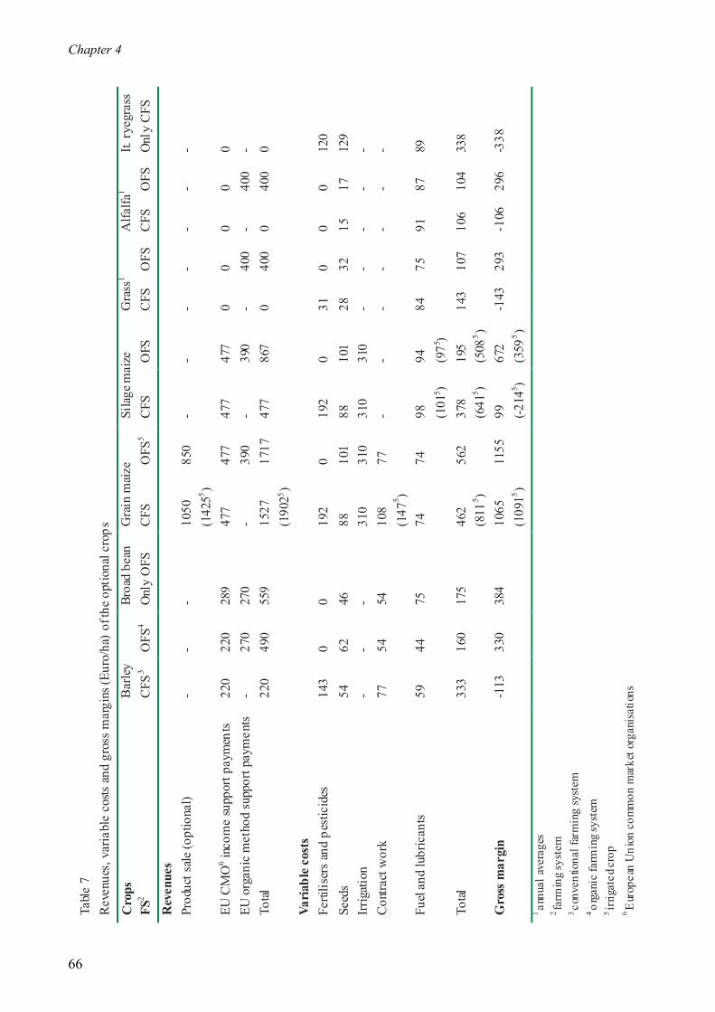
Chapter 4
66
Tabl
e 7
R
even
ues,
var
iabl
e co
sts a
nd g
ross
mar
gins
(Eur
o/ha
) of
the
optio
nal c
rops
Cro
ps
Bar
ley
Broa
d be
an
Gra
in m
aize
Si
lage
mai
ze
Gra
ss1
Alfa
lfa1
It. r
yegr
ass
FS2
CFS
3 O
FS4
Onl
y O
FS
CFS
O
FS5
CFS
O
FS
CFS
O
FS
CFS
O
FS
Onl
y C
FS
Rev
enue
s
Pr
oduc
t sal
e (o
ptio
nal)
- -
- 10
50
(142
55 ) 85
0 -
- -
- -
- -
EU C
MO
6 inco
me
supp
ort p
aym
ents
22
0 22
0 28
9 47
7 47
7 47
7 47
7 0
0 0
0 0
EU o
rgan
ic m
etho
d su
ppor
t pay
men
ts -
270
270
- 39
0 -
390
- 40
0 -
400
- To
tal
220
490
559
1527
(1
9025 )
1717
47
7 86
7 0
400
0 40
0 0
Varia
ble
cost
s
Ferti
liser
s an
d pe
stic
ides
14
3 0
0 19
2 0
192
0 31
0
0 0
120
Seed
s 54
62
46
88
10
1 88
10
1 28
32
15
17
12
9 Ir
rigat
ion
- -
- 31
0 31
0 31
0 31
0 -
- -
- -
Con
tract
wor
k 77
54
54
10
8
(147
5 ) 77
-
- -
- -
- -
Fuel
and
lubr
ican
ts 59
44
75
74
74
98
(1
015 )
94
(975 )
84
75
91
87
89
Total
33
3 16
0 17
5 46
2 (8
115 )
562
378
(6
415 )
195
(508
5 ) 14
3 10
7 10
6 10
4 33
8
Gro
ss m
argi
n -1
13
330
384
1065
(1
0915 )
1155
99
(-2
145 )
672
(359
5 ) -1
43
293
-106
29
6 -3
38
1 annu
al a
vera
ges
2 farm
ing
syst
em
3 conv
entio
nal f
arm
ing
syst
em
4 orga
nic
farm
ing
syst
em
5 irrig
ated
cro
p 6 E
urop
ean
Uni
on c
omm
on m
arke
t org
anis
atio
ns

The modelling framework
67
Returns of set-aside are given by the EU CMO income support scheme of arable crops. They amount to € 220 per hectare and apply both to OFS and to CFS. Costs for set-aside areas cover fuel and lubricants for weed chopping and amount to € 14 per hectare.
Feed requirements are met by on-farm produced feedstuffs or by the purchase of soybean, maize gluten and linseed cake, whose characteristics are shown in Table 8. Straw can be purchased at a price of € 50 per ton for the OFS and € 45 per ton for the CFS. Purchase of dehydrated manure is included as well to cover eventual on-farm shortages, at 120 €/t.
Table 8 Feedstuff that can be purchased with their price, fibre content, energy content, protein content and dry matter
Price Dry matter Fibre content Energy content Protein content €/t g/kg g/kg MJ NEL/kg1 g/kg Soybean2 200 880 60 8.3 380 Maize gluten3 480 893 17 7.7 600 Linseed cake3 190 910 86 7.5 350 1 megajoule net energy for lactation 2 organic feedstuff 3 conventional feedstuff
4.4.4. Environmental aspects
Environmental aspects included in the model refer to environmental processes (see Table 3) that can produce an environmental benefit for the community (positive externalities) or an environmental harm possibly due to non-sustainable farming practices (negative externalities). The environmental processes were selected on their relevance to environmental threats observed in the Tuscany Region (Regione Toscana – Giunta Regionale, ARPAT, 1999) and on their suitability to the LP assumptions.
Environmental coefficients of the farm activities were quantified and environmental constraints were imposed through the construction of a number of accounting/constraint rows. We grouped the rows into five categories as follows: nitrogen losses and soil erosion, water use, environmental potential risks of pesticide use, biodiversity and agroecological infrastructure management.
Environmental RHS coefficients were shaped in the model as environmental sustainability thresholds (ESTs) in compliance with legal constraints implemented by regulations and laws or indications of sustainable land management found in the literature. Reviews of the calculation of the coefficients and the construction of the environmental rows of the model are presented in the following subsections.

Chapter 4
68
Nitrogen losses and soil erosion This category groups together three different environmental aspects, namely, nitrogen leaching, nitrogen run-off and soil erosion. We used GLEAMS for this research. Assuming that each crop, set-aside and green space area of each site produces a given amount of nitrogen and soil losses, we made our calculation using the GLEAMS model and then introduced the coefficients in their corresponding row.
Calculation of the nitrogen and erosion coefficients took into account site-specific input data, and were done on a rotational basis using data retrieved from real management systems applied on the farm sites. Additionally, GLEAMS was applied to calculate losses from set-aside and green spaces and rotations that are not enforced on the farm under the organic either the conventional farming method but comprise crops implemented with the actual rotations. Besides, Some of the selected rotations are not applied on all sites of the farm. Coefficients of such “rotation/site” combinations were calculated proportionate to coefficients of corresponding rotations of other sites and site-specific coefficients of set-aside and green spaces. Nitrogen losses and soil erosion site-specific coefficients of the organic and conventional rotations of the model, of set-aside and green spaces are displayed in Tables 9, 10 and 11.
Table 9 Nitrogen leaching coefficients (kgN/ha) of rotations and green spaces/set-aside
Site 1 2 3 4 5 6 FS2 CFS3 OFS4 CFS OFS CFS OFS CFS OFS CFS OFS CFS OFS Rotation/crop 3A-4G 9.0 8.5 11.7 11.2 B-BB 14.0 15.6 17.8 17.8 16.6 16.6 MS-B-R-3A 26.1 29.1 33.2 33.2 31.0 31.0 MSi-B-R-3A 36.9 34.5 MS-B-BB-B-4G 3.6 4.0 4.6 4.6 4.3 4.3 MSi-B-BB-B-4G 4.6 4.3 MS-B-BB-B-3A 11.8 13.1 15.0 15.0 14.0 14.0 MSi-B-BB-B-3A 15.0 14.0 MG 28.4 31.6 36.0 36.0 33.7 33.7 Mgi 51.8 48.4 MGi-B-Mgi-3A 29.1 24.4 Green spaces/set-aside 9.7 9.7 10.8 10.8 12.3 12.3 12.3 12.3 11.5 11.5 11.5 11.5 1 Crop legend: A, Alfalfa; G, Grassland; B, Barley; BB, Broad bean; MS, Maize for silage; MSi, Maize for silage – irrigated; R, Italian ryegrass; MG, Maize for grain; MGi, Maize for grain – irrigated 2 farming system 3 conventional farming system 4 organic farming system

The modelling framework
69
Table 10 Nitrogen runoff coefficients (kgN/ha) of rotations and green spaces/set-aside Site 1 2 3 4 5 6 FS2 CFS
3 OFS4 CFS OFS CFS OFS CFS OFS CFS OFS CFS OFS
Rotation 3A-4G 3.9 2.4 4.2 2.2 B-BB 4.1 3.3 0.9 0.9 1.6 1.6 MS-B-R-3A 10.8 9.7 5.1 5.1 6.7 6.7 MSi-B-R-3A 6.1 8.0 MS-B-BB-B-4G 4.1 3.3 0.9 0.9 1.6 1.6 MSi-B-BB-B-4G 0.9 1.6 MS-B-BB-B-3A 7.2 5.8 1.6 1.6 2.8 2.8 MSi-B-BB-B-3A 1.6 2.8 MG 38.1 34.2 18.0 18.0 23.7 23.7 Mgi 19.2 25.3 MGi-B-MGi-3A 4.0 4.4 Green spaces/Set-aside 2.0 2.0 1.3 1.3 0.1 0.1 0.1 0.1 0.3 0.3 0.3 0.3 1 Crop legend: A, Alfalfa; G, Grassland; B, Barley; BB, Broad bean; MS, Maize for silage; MSi, Maize for silage – irrigated; R, Italian ryegrass; MG, Maize for grain; MGi, Maize for grain – irrigated 2 farming system 3 conventional farming system 4 organic farming system Table 11 Soil erosion coefficients (t/ha) of rotations and green spaces/set-aside Site 1 2 3 4 5 6 FS2 CFS3 OFS4 CFS OFS CFS OFS CFS OFS CFS OFS CFS OFS Rotation 3A-4G 1.9 2.0 1.5 1.5 B-BB 16.7 10.3 0.0 0.0 0.0 0.0 MS-B-R-3A 8.5 5.2 0.0 0.0 0.0 0.0 MSi-B-R-3A 0.0 0.0 MS-B-BB-B-4G 8.9 5.5 0.0 0.0 0.0 0.0 MSi-B-BB-B-4G 0.0 0.0 MS-B-BB-B-3A 10.2 6.3 0.0 0.0 0.0 0.0 MSi-B-BB-B-3A 0.0 0.0 MG 27.1 16.7 0.0 0.0 0.0 0.0 Mgi 0.0 0.0 MGi-B-MGi-3A 0.0 0.0 Green spaces/Set-aside 1.3 1.3 0.8 0.8 0.0 0.0 0.0 0.0 0.0 0.0 0.0 0.0 1 Crop legend: A, Alfalfa; G, Grassland; B, Barley; BB, Broad bean; MS, Maize for silage; MSi, Maize for silage – irrigated; R, Italian ryegrass; MG, Maize for grain; MGi, Maize for grain – irrigated 2 farming system 3 conventional farming system 4 organic farming system

Chapter 4
70
The EST of the nitrogen leaching row was calculated against the maximum standard for nitrate
in drinking water settled by the World Health Organisation (WHO) and adopted by the EU Directive 91/676 and other laws. The limit, which is 50 mg/l, was converted to 27 Kg/ha of nitrogen leaching to the groundwater table. This is the maximum amount per hectare of nitrogen leaching allowed, given the water percolation of the Sereni farm, in order not to exceed a nitrate concentration of 50 mg/l in the leaching groundwater. The Sereni water percolation was calculated as a weighted mean of the site values reported from the outcomes of the GLEAMS hydrology component applied to the real farm situation.
The same applies to the nitrogen run-off EST (11 kg/ha), which was calculated using the weighted mean of the site-specific water run-off values. The soil erosion EST was derived from the literature (Pimentel et al., 1995; Kabourakis, 1996; Van Mansvelt, 1999) and corresponds to 1 t/ha. Total farm EST of nitrogen losses were obtained multiplying the over-mentioned "per hectare" thresholds by the total farm area less woodland. Total erosion farm EST was calculated multiplying the 1 t/ha "per hectare" threshold by the total area (less woodland) of hilly sites.
Water use This category comprises two environmental aspects, namely, the ground and surface water use, both aspects are modelled through the construction of an input-output sub-model. Input coefficients of the groundwater use row are the amounts of water percolation per hectare of crop, set-aside areas and green spaces during the dry season. Each crop, set-aside and green space area of each site produces a given amount of percolation that contributes to recharging of the underlying aquifer. The input coefficients come from the hydrological component of the GLEAMS model. Output coefficients are the amounts per hectare of irrigation water and cattle consumption and correspond to the water withdrawals from the aquifer. The coefficients of the irrigated crops (maize grain and silage) represent the difference between the irrigation and the percolation amounts.
Farm needs of water are also met by withdrawal from water streams. Therefore, an input-output sub-model for surface water use similar to the above mentioned was constructed. The sub-model structure and part of the coefficients are equal to those of the groundwater use sub-model, but the stream flow recharge rates represent the water runoff amounts calculated using GLEAMS. Site-specific coefficients of the organic and conventional rotations, of set-aside areas and of green spaces during the dry season are presented in Tables 12 and 13.

The modelling framework
71
Table 12 Water leaching coefficients (m3/ha) of rotations and green spaces/set-aside during the dry season Site 1 2 3 4 5 6 FS2 CFS3 OFS4 CFS OFS CFS OFS CFS OFS CFS OFS CFS OFS Rotation/crop 3A-4G 0.0 8.0 0.0 8.0 B-BB 16.8 27.2 7.8 7.8 0.0 0.0 MS-B-R-3A 0.0 0.0 6.9 6.9 7.1 7.1 MSi-B-R-3A 95.1 95.1 MS-B-BB-B-4G 16.8 27.2 7.8 7.8 0.0 0.0 MSi-B-BB-B-4G 0.0 0.0 MS-B-BB-B-3A 16.8 27.2 7.8 7.8 0.0 0.0 MSi-B-BB-B-3A 0.0 0.0 MG 0.0 0.0 6.9 6.9 0.0 0.0 Mgi 230.0 230.0 MGi-B-MGi-3A 101.3 101.2 Green spaces/Set-aside 103.0 103.0 109.5 109.5 56.6 56.6 56.6 56.6 6.8 6.8 6.8 6.8 1 Crop legend: A, Alfalfa; G, Grassland; B, Barley; BB, Broad bean; MS, Maize for silage; MSi, Maize for silage – irrigated; R, Italian ryegrass; MG, Maize for grain; MGi, Maize for grain – irrigated 2 farming system 3 conventional farming system 4 organic farming system Table 13 Water runoff coefficients (m3/ha) of rotations and green spaces during the dry season Site 1 2 3 4 5 6 FS2 CFS3 OFS4 CFS OFS CFS OFS CFS OFS CFS OFS CFS OFS Rotation 3A-4G 2.6 3.0 7.6 3.0 B-BB 49.1 23.2 6.6 6.6 4.5 4.5 MS-B-R-3A 2.6 7.6 5.8 5.8 3.2 3.2 MSi-B-R-3A 46.3 46.3 MS-B-BB-B-4G 49.1 23.2 6.6 6.6 4.5 4.5 MSi-B-BB-B-4G 104.0 104.0 MS-B-BB-B-3A 49.1 23.2 6.6 6.6 4.5 4.5 MSi-B-BB-B-3A 104.0 104.0 MG 2.6 7.6 5.8 5.8 8.0 8.0 Mgi 214.7 214.7 MGi-B-MGi-3A 48.6 41.0 Green spaces/Set-aside 9.0 9.0 2.4 2.4 0.0 0.0 0.0 0.0 0.0 0.0 0.0 0.0 1 Crop legend: A, Alfalfa; G, Grassland; B, Barley; BB, Broad bean; MS, Maize for silage; MSi, Maize for silage – irrigated; R, Italian ryegrass; MG, Maize for grain; MGi, Maize for grain – irrigated 2 farming system 3 conventional farming system 4 organic farming system

Chapter 4
72
The ESTs for these two aspects reflect the quantitative guardianship principles for water resources indicated by the Italian D.L. 152/1999. At farm level, one of the criteria for the assignment of withdrawal permits is the rate between the quantity of water restitution and withdrawal. Edmunds (1996) identifies an environmental sustainability threshold for groundwater use at landscape/regional scale: "A threshold is crossed when the rate of abstraction exceeds the rate of recharge, and a sustainable renewable resource becomes a non-renewable mined one".
In the model, ESTs for ground and surface water use suggest that the water restitution from the farm to the aquifer (by percolation) and to the water streams (by runoff) must be larger or equal to the water withdrawal. Although these ESTs do not directly account for the availability/scarcity of water resources of a given landscape/region, they are indicative of the contribution of a single farm to the state of the regional water reservoirs. The ESTs mentioned above are for the irrigation season, which coincides with the dry season (July-August for the Sereni farm), as this is the period during which the aquifers are more vulnerable to water withdrawal.
Environmental potential risks of pesticide use The assumption is that each pesticide treated crop on each site potentially produces a given level of pesticide risks, calculated with the EPRIP yardstick and then introduced as a coefficient in the matrix of the LP model. This yardstick calculates the potential hazard for soil, groundwater by leaching, surface water by drift and run-off, and air by volatilisation. The ecotoxicological effects on aquatic organisms, soil organisms and toxicological effects on man are taken into account. These compartments and effects were chosen since they were derived from the environmental criteria used by the Italian ministry for its pesticides admission policy (CCPF, 1996) and were incorporated into the Uniform Principles of the EU (EU Directive n. 91/414) (Trevisan et al., 1999).
The indicator is based on comparison of predicted environmental concentration (PEC), estimated at a very local scale (field and surroundings), with toxicological parametres. It was obtained from an integrated classification system of 9 different environmental indices. The pesticide with higher EPRIP will have higher potential risk to environment and man. The EPRIP values are in a range between 1 to 625 points and divided in different classes of environmental potential risks based on expert judgement (Table 14) (Trevisan et al., 1999).
EPRIP values for each pesticide application were calculated using site-specific input data on pesticide properties, application rates, crops, soils, rainfall, temperature and ditches. As reported in previous studies (Pacini et al., 2002c), differences between site EPRIP scores appear to be more dependent on the type of crop than on the site pedo-climatic characteristics. The EPRIP yardstick can be applied both to conventional and organic pesticides (e.g., the copper pesticides). However, on the case study farm of this paper no pesticide is applied to the organic crops, which consequently were given a zero score. Table 15 presents crop specific EPRIP scores of the only pesticide-treated crops (barley and maize).

The modelling framework
73
Table 14 EPRIP (environmental potential risk indicator for pesticides) classification
EPRIP value Potential risk classification 1 None
2-16 Negligible 17-81 Small
82-256 Present 257-400 Large > 400 Very large
1 modified from Trevisan et al. (1999)
Table 15 EPRIP (environmental potential risk indicator for pesticides) (score/ha) coefficients of pesticide-treated crops
CFS1 OFS2 Barley 60 0 Maize (for grain and for silage ) 120 0 1 conventional farming system 2 organic farming systems
According to the model requirements either the “negligible risk” class upper score or that of the
"small risk" class give the EST for the pesticide risks in the model. The total farm EST of pesticide risks was obtained multiplying the above mentioned "per hectare" thresholds by the total farm area less woodland.
Herbaceous plant biodiversity The crops, set-aside areas and green spaces of each site produce a certain level of biodiversity, which was measured using a modified version of the Braun-Blanquet method and then introduced as coefficient in the corresponding row. As reported in previous studies (Pacini et al., 2002c), differences between site herbaceous plant biodiversity indicator (HPBI) values appear to be more dependent on the type of land use (different crops, set-aside and green spaces) than on the site intrinsic natural potential. Coefficients of the organic version were attributed only following the land use criterion as averages of a number of 62 field observations conducted in 1998 and 1999.
Because it was not possible for field observations to be done on the Sereni farm under the CFS (conversion to the organic method ended in 1995), the conventional coefficients were calculated from the organic coefficients of the Sereni farm and the difference between conventional crops, organic crops and green spaces of a previously investigated mixed organic-conventional farm (Pacini et al., 2002c). Crop specific coefficients of the organic and the conventional versions are shown in Table 16.
The EST of herbaceous plant biodiversity was calculated according to the indications supplied by Vereijken (1999) for the design of farm infrastructures for nature and recreation. Among other norms, Vereijken suggests a minimum farm value of Plant Species Diversity (PSD) amounting to 50 plant species per farm. By comparisons made on different farms (the Sereni farm included – Pacini et al., 2002c) between the farm total amount of plant species and the HPBI farm value, the 50 plant species threshold was converted in terms of HPBI value.

Chapter 4
74
Table 16 HPBI (herbaceous plant biodiversity indicator) (score/ha) coefficients of crops and green spaces/set/aside
CFS1 OFS2 Crop Barley 32 66 Broad bean - 63 Maize for silage 17 34 Maize for grain 25 51 Grassland 90 99 Alfalfa 66 73 Italian ryegrass 38 - Green spaces/ Set-aside
90 99
1 conventional farming system 2 organic farming system
The HPBI processing method implies the recognition of all species of each site of a farm. Joining the site databases and excluding double counts allowed a quantification of the total number of species of each farm. Assuming a proportional relation between the number of plant species at farm level and the farm HPBI value, the HPBI EST was calculated based on these two values and the plant species threshold indicated by Verijken following the proportion below:
HPBIfpsffps ESTESTHPBIn :: =
Where fpsn is the average of the total numbers of
plant species observed at farm level in the farms under
survey, fHPBI is the average of the farm HPBI values
of the farms under survey, fpsEST is the EST indicated
by Vereijken and HPBIEST is the same EST expressed in
terms of HPBI.
Agro-ecological infrastructure management This category groups together two environmental aspects, namely, the hedges and the drainage system management. They were shaped in the model as two environmental activities with given labour and tractor requirements and given annual costs. Both of the activities were measured in terms of (hundreds of) metres in length.
Annual costs per hundred metres amount to € 54 for hedges and € 25 for drainage system. Costs for hedges consist of annual fixed costs of plants, fertilisers and planting operations. Costs for drainage system comprise annual fixed costs for excavation and variable costs of fuel and lubricants for ditch maintenance.
The EST for hedge length was taken from Schotman (1988) and corresponds to 60 m/ha. The EST for drainage system taken from Landi (1999) is 140 m/ha and complies with the EU Regulation 1259/99 norms indicated in the legislation section. The total farm EST was obtained by multiplying the "per hectare" thresholds by the total farm area less woodland.
4.5. Discussion and conclusions
We now discuss the use of the model for practical application. The model was built for the purpose of supplying information to support regional multi-objective policy-making. The practicability of the use of the model for this purpose depends on its representativeness (in this case, for the Mugello

The modelling framework
75
area) and on the validity of the outcomes of the model. The representativeness of the model is discussed in the next sections and refers to the case study farm general structure, production performances, and pedo-climatic characteristics and to differences between the conventional and the organic versions of the model. Here, some remarks on the validation process of the model are given.
Both internal and external validations of the model were carried out. The description of the model in this paper provides the internal validation. External validation was implemented using data from reality (Pacini et al., 2002c) and performing model optimisations under different policy scenarios. Results of the optimisations proved to be logic for the farm under survey.
4.5.1. Assessment of the representativeness of the case study farm and of production performances
Observations from the previous description of the Mugello area point to the Sereni farm being representative of dairy farms in this region as far as farm size, cattle breed and crops are concerned. More specifically, it can be considered representative of dairy farms in the less extensive areas of Mugello.
In this section representativeness of production performances of the Sereni farm and, in general, of the model is also discussed backed by data of conventional farming because of its more easy availability compared to that of organic farming. Florence Province dairy holdings are mostly located in the northern mountainous areas and foothills. In 1998 the average milk yield per cow of Italian Holstein in the Florence Province was 7601 kg (datum from ANAFI2), which is quite close to the Sereni average (7550 kg).
Barley grain yield seems to be quite high for standards in central Italy. However, considering the abundance of water from rainfall in the Mugello area (1000 mm per year), a yield level of 5000 kg/ha, which is common in many regions of northern Italy (Baldoni and Giardini, 1989), also adjoining Mugello, is reasonable for conventional farming in Mugello as well. The maize grain yield average of irrigated and non-irrigated sites of the Sereni farm for conventional farming (8250 kg/ha) is very similar to the average yield of Florence Province inland hilly areas (which include also the Borgo San Lorenzo Municipality) indicated by the regionalisation plan for the EU arable crop support scheme (8134 kg /ha). Grassland and Alfalfa yields are consistent with values of Tuscany mountain areas found in the literature (ETSAF, 1992). The farm data on organic broad bean yield are comparable to values of conventional broad bean grown in Tuscany (ARSIA, 1994), given the differences of nutrients supply between the two farming systems.
Pedo-climatic representativeness of the Sereni farm is also an important issue because the ecological models applied are based on site-specific input data of soil and climate characteristics. Climate is quite uniform within the Mugello region. Combining a farming system approach with the need for representativeness of a case study is not an easy task because soil profile variability can be
2 ANAFI (Associazione Italina Allevatori Frisona Italiana) is the Italian association of Italian Holstein breeders.
Chapter 4
76
very high even over small areas and, to be size representative, a farm cannot be too large. On the other hand, the use of regional predominant soil profile data would conflict with the biodiversity processing method, which is based on farm empirical observations, and with the farming systems approach used in this research.
Six different sites were identified within the Sereni farm taking into consideration different landforms, resource availability and soil geo-physical characteristics. The combination of these sites with different land uses (crop successions and green spaces) and farming systems gave rise to the analysis of 50 different types of agro-ecosystems, which contributed to the achievement of a satisfactory level of representativeness of the case study.
In conclusion, the Sereni farm, which was selected for the case study and constitutes the basis for the model construction, can be considered representative of the Mugello dairy farms as to farm size, types of cattle breed and crops, corresponding production potentials and production conditions (i.e., pedo-climatic factors).
4.5.2. Assessment of the representativeness of the differences between CFSs and OFSs
Special attention has been given to yields, returns and variable costs of production activities, which are assumed to be the most sensitive parameters of the economic sub-model. In this part the focus is also on those sensitive parameters that are unchanged between the two versions of the model.
For reasons of generality, the organic and conventional milk prices were taken from the Tuscany rural development plan and are based on the 1998 RICA-INEA database. Milk yield per cow per year on the Sereni farm was taken as constant under the CFS and the OFS. This is consistent with what we found in the literature. Offermann and Nieberg (2000) conducted a comparative analysis of yields, prices and costs in organic and conventional farming in 18 European countries. They found that typical performance of organic farming was in the range of 80 % to 105 % of that on conventional farming. Padel and Lampkin (1994) reported that the choice of specialist breeds among organic farmers was an important factor to explain reduced milk yields under organic farming. The use of Italian Holstein (which is a highly productive breed) on the Sereni farm can partially explain the lack of difference in milk yields per cow. Besides, differences of yields per cow between conventional and organic farming are likely to occur more frequently in intensive livestock grazing systems (which is not the case of the Sereni farm) because of higher nitrogen supply giving higher energy content of feed. Restrictions of the amount of concentrate that can be fed to cows is also likely to result in a lower yearly milk production per cow, but this mostly affects intensive farming systems with high cattle density. Although animal health practices changed from the CFS to the OFS, variable veterinarian costs and of medicines are not different. In fact, the veterinarian of the Sereni farm charges an average price per cow (including medicines) irrespective of the treatment.

The modelling framework
77
The main differences between CFS and OFS as for crops have to do with yields and variable costs. Yield differences are very similar to those found in central and northern Italy: reference is made to Santucci and Chiorri (1996) for barley, Bartola et al. (1990) for grain maize, Zanoli et al. (1998) for alfalfa. Yield difference of silage maize is relatively less than that of grain maize. This can be explained away by the fact that grain production is more affected by phosphate shortages than the vegetative parts of the plant. The relative small decrease of grass production can be connected to low application of chemically synthesised fertilisers under the CFS (only 150 kg/ha of urea in the sowing year), which is common practice in extensive conventional farming.
For reasons of generality of the model, the organic and conventional maize grain prices were taken from the Tuscany rural development plan. They are based on the 1998 RICA-INEA database. Arable crop EU CMO income support payments apply to the organic and the conventional versions of the model and were taken from the EU regionalisation plan. EU organic method support payments were taken from the EU rural development plan of the Tuscany Region.
Variable costs of fertilizers, pesticides and contract work for grain harvesting for organic crops are lower than those of conventional crops. In fact, the organic crop management modelled does not include any application of fertilizers and pesticides, while contract work for harvesting increases for conventional crops because of higher yields. On the other hand, costs for seeds are higher for the OFS. This is consistent with evidence found in the literature on variable costs of dairy farming in different regions of central and northern Italy, and other Nations in Europe (Offermann and Nieberg, 2000). There are no significant differences between labour requirements in the two versions of the model. This is in line with what found in the literature (Offermann and Nieberg, 2000).
In conclusion, differences reported in the model between the CFS and the OFS animal and crop production yields, corresponding commodity prices and variable costs are consistent with what we found in the literature (with reference both to northern and central Italy conditions and to other regions of Europe), with current EU regulations applied to the case study region and with information from regional data networks. Therefore, it can be assumed that the model correctly represents those differences with respect to the Mugello area and hence can be used for a comparative evaluation of the economic-environmental impacts of CFS and OFS in the case study region.
4.5.3. Overall conclusions
The main purposes of this chapter were to present a modelling framework aimed at supplying information for multi-objective policy-making and to discuss the use of the model for practical applications. Given the description of the modelling framework and the following discussion on the representativeness and the validity of the model, we conclude that: 1) the model can be used for the
Chapter 4
78
evaluation of agri-environmental schemes applied to dairy farming in the Mugello area, and 2) outcomes of the model can be considered representative of this farm type and this area. References Arrigoni, P.V., Nardi, E. and Raffaelli, M., 1985 La vegetazione del parco naturale della Maremma
(toscana). Dipartimento di Biologia Vegetale dell’Universitá degli Studi di Firenze, Florence, Italy (in Italian).
ARSIA (ed.), 1994. Leguminose da granella. Florence, Italy (in Italian). ARSIA, IRPET, Regione Toscana (eds.), 2001. Terzo rapporto sull’economia agricola della
Toscana. Il Sole 24 ORE Spa, Rome, Italy (in Italian). Baldoni, R. and Giardini, L. (eds.), 1989. Coltivazioni erbacee. Pàtron Editore, Bologna, Italy (in
Italian). Bartola, A., Pollastri, F. and Zanoli, R. (1990). L’agricoltura biologica: produzione di qualità nel
rispetto dell’ambiente. Il caso dell’Emilia Romagna. Rivista di Economia Agraria 3. Brunori, G., Omodei-Zorini, L., Lazzerini, G., Pacini, C., Rovai, M., Vazzana, C., 1999. Territorio,
ambiente ed impresa agricola: modelli di gestione per lo sviluppo rurale. Presented at the International Seminar of Perugia University, Italy, 29 aprile 1999 (in Italian).
Cappelletti, C., 1976. Trattato di botanica. UTET, Italy (in Italian). CCPF – Commissione Consultiva per i Prodotti Fitosanitari, 1996. Criteri per la valutazione del
destino ambientale dei prodotti fitosanitari. Rome, Italy (in Italian). Contini, C., 2002. Description of the Mugello area. In: Farming and rural systems research and
extension. Local identities and globalisation. Proceedings Fifth International Farming Systems Association European Symposium. Florence, Italy, April 8-11, 2002.
Edmunds, W.M., 1996. Indicators in the groundwater environment of rapid environmental change. In: Berger, A.R. & Iams, W.J. (eds) Geoindicators: Assessing rapid environmental changes in earth systems. A.A. Balkema, Rotterdam, The Netherlands, p. 121-136.
ETSAF – Ente Toscano Sviluppo Agricolo Forestale (ed.), 1992. Le foraggere per le zone montane. ETSAF, Florence, Italy (in Italian).
Falconer, K., Hodge, I., 2001. Pesticide taxation and multi-objective policy-making: farm modelling to evaluate profit/environment trade-offs. Ecological Economics 36, 263-279.
FAO, 1998. World Reference Base for Soil Resources. FAO, ISRIC and ISSS, Rome, Italy. Jarosch, J. and Murschel, B., 1989. Methodik und Datenerfordernisse zur Integration ökonomischer
and ökologischer Ziele in einzelbetrieblicher Entscheidungs modelle. In: C.-H. Hanf, C.-H. and Scheper, W. (eds.) Neuere Forschungskonzepte und –Methoden in den Wirtschafts- und Sozialwissenschaftendes landbaues. Schriften der GEWISOLA, Band 25, Münster-Hiltrup: Landwirtschaftsverlag, Germany (in German).

The modelling framework
79
Kabourakis, E., 1996. Prototyping and dissemination of ecological olive production system: A methodology for designing and a first step towards validation and dissemination of prototype ecological olive production systems (EOPS) in Crete. Thesis Wageningen Agricultural University, The Netherlands.
Knisel, G., 1993. GLEAMS Groundwater Loading Effects of Agricultural Management Systems – Version 2.10. University of Georgia-Coastal Plain Experiment Station-Biological and Agricultural Engineering Department Publication No.5, Tifton, Georgia (USA), 259 p.
Landi R., 1999. Agronomia e ambiente. Edagricole, Bologna, Italy (in Italian). Law, A.M., Kelton, W.D., 1991. Simulation modelling & analysis. McGraw-Hill International
Editions, Singapore. Lucifero, M., Antongiovanni, M., Ferruzzi, G., Liponi, G.B., Sargentini, C., Sechiari, P., Trimarchi,
G., 1993. Guida all’utilizzazione razionale dei foraggi della Toscana. Regione Toscana – ETSAF, Florence, Italy (in Italian).
Offermann, F. and Nieberg, H., 2000. Economic performance of organic farms in Europe. University of Hohenheim/Department of Farm Economics, Stuttgart-Hohenheim, Germany.
Omodei Zorini, L., and Zammarchi, L., 1997. L’agricoltura toscana e la sua articolazione territoriale. In: Omodei Zorini, L., Fruttuosi A., and Franchini, G. (eds.) La Politica Agricola Comunitaria e l’agricoltura toscana. Analisi e valutazione dell’impatto della riforma MacSharry. ARSIA – Agenzia Regionale per lo Sviluppo e l’Innovazione nel Settore Agricolo-Forestale, Florence, Italy (in Italian).
Pacini, C., Wossink, A., Giesen, G., Vazzana, C., Huirne, R., 2002a. Evaluation of sustainability of organic, integrated and conventional farming systems: a farm and field scale analysis. Accepted for publication by Agriculture, Ecosystems and Environment.
Pacini, C., Wossink, A., Giesen, G., Vazzana, C., Omodei-Zorini, L., 2002b. Environmental Accounting in Agriculture: a Methodological Approach. Submitted.
Pacini, C., Wossink, A., Giesen, G., Omodei-Zorini, L., Huirne, R., 2002c. Ecological-economic modelling to evaluate sustainability of farming systems: a farm and field scale approach applied to a case study of organic farming in Tuscany. Submitted.
Pacini, C., Wossink, A., Giesen, L., Huirne, R., 2002d. Ecological-economic modelling to support multi-objective policy-making: a farming system approach implemented for Tuscany. Submitted.
Padel, S. and Lampkin, N., 1994. Farm-level performance of organic farming systems: an overview. In: Lampkin, N. and Padel, S. (eds.) The economics of organic farming. CAB International, Wallingford, UK, 201-221.
Pimentel, D., Harvey, C., Resosudarmo, P., Sinclair, K., Kurz, D., McNair, M., Crist, S., Shpritz L., Fitton, L., Saffouri, L. and Balair, R., 1995. Environmental and economic costs of soil erosion and conservation benefits. Science 267, 1117-1121.

Chapter 4
80
Regione Toscana – Giunta Regionale, ARPAT – Agenzia Regionale per la Protezione dell’Ambiente della Toscana (eds.), 1999. Rapporto sullo Stato dell’Ambiente della Regione Toscana ’98. Edizioni Regione Toscana, Florence, Italy (in Italian).
Reus, J., Leendertse, P., Bockstaller, C., Fomsgaard, I., Gutsche, V., Lewis, K., Nilsson, C., Pussemier,, L., Trevisan, M., Van der Werf, H., Alfarroba, F., Blümel, S., Isart, J., McGrath, D., Seppälä, T., 2002. Comparison and evaluation of eight pesticide environmental risk indicators developed in Europe and recommendations for future use. Agriculture, Ecosystems and Environment 90, 177-187.
Santucci, F.M. and Chiorri, M., 1996. Economia delle produzioni biologiche. Quaderni dell’Istituto di Economia e Politica Agraria di Perugia, Università di Perugia Italy (in Italian).
Schotman, A., 1988. Tussen bos en houtwal: broedvogels in een Twents cultuurlandschap. RIN-rapport 88/37, Leersum, The Netherlands (in Dutch).
Trevisan, M., Errera, G., Capri, E., Padovani, L. & Del Re, A.A.M., 1999. Environmental Potential Risk Indicator for Pesticides. In: Reus, J., Leendertse, P., Bockstaller, C., Fomsgaard, I., Gutsche, V., Lewis, K., Nilsson, C., Pussemeier, L., Trevisan, M., van der Werf, H., Alfarroba, F., Blümel, S., Isart, J., McGrath, D., Seppälä, T. (eds.), Comparing Environmental Risk Indicators for Pesticides – Results of the European CAPER Project. Center for Agriculture and Environment, Utrecht, The Netherlands.
Van Mansvelt, J. D. & Van der Lubbe, M. J., 1999. Checklist for sustainable landscape management. Elsevier Science B.V., Amsterdam, The Netherlands.
Vereijken, P., 1999. Manual for prototyping integrated and ecological arable farming systems (I/EAFS) in interaction with pilot farms. AB-DLO, Wageningen, The Netherlands.
Wossink, G.A.A., 1998. Environmental economics of the farm firm. Department of Farm Management, Wageningen Agricultural University, The Netherlands.
Wossink, G.A.A., De Koeijer, T.J., and Renkema, J.A., 1992. Environmental-economic policy assesment: a farm economic approach. Agricultural Systems 39, 421-438.
Zanoli, R., Fiorani, S. and Gambelli, D., 1998. Analisi dei risultati economici di un campione di aziende biologiche marchigiane (1994-1996). Università di Ancona, Italy (in Italian).

Chapter 5
The EU’s Agenda 2000 reform and the sustainability of organic farming in Tuscany: ecological-economic modelling at field and farm level
Cesare Pacini1, Gerard Giesen1, Ada Wossink2,1, Luigi Omodei-Zorini3, Ruud Huirne1
1 Farm Management Group – Dept. of Social Sciences, Wageningen University, The Netherlands 2 Dept. of Agricultural & Resource Economics, NC State University, Raleigh, USA 3 Dept. of Agricultural Economics, Florence University, Italy
Submitted to Agricultural Systems
Chapter 5
82
Abstract Sustainability has become a central issue in the agricultural sector, both for researchers, for producers and for policy-makers. The two main objectives of this paper are: (1) to present an holistically designed ecological-economic model to evaluate farm and field-level environmental-economic tradeoffs with special reference to multi-objective policy-making, and (2) to evaluate the impact of the Agenda 2000 reform on sustainability of organic farming. The model was implemented for the case of organic dairy farming in northern Tuscany (Italy). Minor differences were found between the environmental and technical results of the model under the MacSharry and Agenda 2000 reforms. However, gross margins under the Agenda 2000 regulations were considerably higher. The spatial detail of the model proved particularly useful in the evaluation of the impact of environmental sustainability thresholds. Sensitivity analysis indicated the environmental weak points of the farming system (in this case mainly soil erosion) and the feasible levels of the various sustainability aspects and their associated socio-economic costs. The application of the model for alternative policy scenarios provided insights into ways in which the cost economic efficiency of the Agenda 2000 agri-environment support scheme could be improved. The paper concludes with suggestions for further model research to contribute to the design of cost-efficient agri-environment payments schemes.
Keywords: ecological-economic modelling, farm and field scale analysis, sustainability, organic agriculture, multi-objective policy-making
5.1. Introduction
Sustainability has become a central issue in the agricultural sector, both for researchers, producers and policy-makers. An increasing body of literature has been developed on methods for the evaluation of sustainability (Van der Werf and Petit, 2002; Sands and Podmore, 2000; Schultink, 2000). In contrast, there is a lack of tools to support the design of policy schemes that would ensure the operationalisation of sustainability in an efficient way (Falconer and Hodge, 2001). This seems to be due on the one hand to the complexity of the ecological and production processes recalled by the concept of sustainability, and on the other hand to the necessary multi-objective approach of policy decision making. Sustainability implies the multiple objectives and policy makers are often faced with the problem of how to best allocate their limited funds over these objectives.
A number of studies in the literature address the evaluation of sustainability from a farm-level perspective. Many of the environmental impacts associated with agricultural production are location specific and are intrinsically connected with the production decisions. Mathematical programming techniques, such as linear programming (LP), have been applied frequently in farm-level studies. This kind of approach is well suited for mixed ecological-economic analyses (Falconer and Hodge,

The EU’s Agenda 2000 reform and the sustainability of organic farming in Tuscany
83
2001; De Koeijer et al., 2002). However, many of the studies involved with environmental-economic modelling that advocate a systems approach lack a holistic interpretation of the farm agro-ecosystem. The number of environmental impacts that is actually modelled is often limited (e.g., only total pesticide use and nitrogen losses). The omission of information on many environmental aspects can lead to serious misjudgments in the multi-objective policy-making process and conflicts between different government programmes or regulations.
Besides, only few farm-level studies take into account within-farm differences in environmental and economic aspects. While it is common that production decisions are taken at farm level, it has to be considered that the impacts of those decisions differ among within-farm areas depending on pedo-climatic site and field-specific conditions. In fact, spatial differentiation is required if environmental damages vary by location with the same set of farming practices (Weersink et al., 2002).
An integrated ecological-economic modelling approach implemented at a detailed spatial scale allows pedo-climatic characteristics, spatial aspects, impacts of alternative production practices and their economic performances to be addressed. Such an approach would be suitable to support the policy decision-making process and could supply useful information for farm management as well.
Sustainability is one of the objectives of the EU’s Fifth Action Programme on the Environment (CEC, 1992). In line with the Fifth Programme, the EU’s Sixth Environment Action Programme (in course of adoption) encourages the integration of environmental considerations in non-environmental areas of policy making (CEC, 2002). The EU is therefore committed to promoting sustainability also through its common agricultural policy. The so-called Agenda 2000 reform involves subsidies based on environmental considerations, a further reduction of production-related price support and a move towards hectare and animal subsidies.
Under the Agenda 2000 reform, agri-environment payments are offered for organic farming and other sustainable practices of land use, maintaining extensive systems, conservation of high nature-value farmed environments, upkeep of the landscape and historical features on agricultural land and environmental planning in farming practice. In practice agri-environmental schemes are relevant in particular for organic farming (European Commision, 1999; Stiftung Ökologie & Landbau, 2001). Besides, the switch from price support to area and animal related payments that are independent of output levels should increase the relative competitiveness of organic farming systems.
An important question is whether the Agenda 2000 reform is indeed an improvement, that is whether it will further enhance sustainability and whether this is achieved in a more cost-efficient manner compared with the 1992-1999 MacSharry regulation. Wier et al. (2002) reported in a modelling analysis of the effects of the Agenda 2000 reform for the agricultural sector in Denmark, that the Agenda 2000 reform had significant economic costs but almost no effects on the environment – either positive or negative. Winter and Gaskell (1998) found from a survey of both
Chapter 5
84
(conventional) arable and livestock farmers in the U.K. that the Agenda reform had relatively little impact on their operations, from an environmental quality perspective.
Against this background, the two main objectives of this paper are: To present an holistically designed ecological-economic model to evaluate farm and field-level
environmental-economic tradeoffs with special reference to multi-objective policy-making. To evaluate the impact of the Agenda 2000 reform on sustainability of organic farming. With respect to the first objective, the model was specifically developed to enable: (1) the
evaluation of the economic-environmental tradeoffs of cropping practices through a farm-level approach; (2) the provision of information on the wide array of environmental objectives included in sustainability; (3) within-farm variability in environmental and economic aspects to be addressed; and (4) regional carrying capacity and resilience to be included in the evaluation process.
Regarding the second objective, special attention is given to the specification of the EU agri-environment schemes1. These schemes indicate the general environmental aims to be pursued, but do not give environmental performance levels for farmers to be met in order to receive the support payments. So, although these schemes impose rules on farming practices it is unclear what the effect in terms of sustainability will be.
The farm and field scale ecological-economic LP model was implemented for organic dairy farming in northern Tuscany (Italy). In general, such LP models require a lot of specific data on farm ecological and economic characteristics. Results, in order to be useful for policy evaluation, need to be representative for the region and farm type analysed. It is not easy to combine the need for representativeness of the model with a holistic/systems approach and the heterogeneity of pedo-climatic and production conditions considered, which increases with the number of environmental objectives included in the analysis. Therefore, the model was implemented using data from a representative farm of the area under survey, in which all the necessary data have been collected at field level (Pacini et al., 2002a; 2002b). A case study approach was chosen, giving preference to the depth of the analysis rather than to the sample size. We proceed as follows: Section 5.2 describes the model and the organisation of the analysis, Section 5.3 focuses on the model application and on the simulation results. Discussion and conclusions are given in Section 5.4.
5.2. Materials and methods
5.2.1. The model
The general structure of the model is shown in Table 1. 1 Namely, the agri-environment schemes of the EU Regulations 2078/92 of the MacSharry reform and 1257/99 of the Agenda 2000 reform.

The EU’s Agenda 2000 reform and the sustainability of organic farming in Tuscany
85
Tabl
e 1
Gen
eral
stru
ctur
e of
the
LP m
odel
Si
te 1,
2 &
6
Farm
Si
te/fa
rm
A
ctiv
ities
C
onstr
aint
s
Cro
p ro
-ta
tions
Se
t-as
ide
Gre
en
spac
es N
itrog
en
and
soil
loss
es
Pest
icid
e us
e en
viro
n-m
enta
l risk
s
Her
bace
ous
plan
t bi
odiv
ersi
ty H
ired
la
bour
Purc
hase
ac
tiviti
es A
nim
al
pro-
du
ctio
n
Surf
ace
drai
nage
sy
stem
Hed
ges
Righ
t han
d sid
e L
and
requ
irem
ents
+1
+1
+1
<=
Av.
hec
tare
s M
ilk p
rodu
ctio
n
a i,j
<=A
v. q
uota
H
ousi
ng r
equi
rem
ent
a i,j
<=Av
. cow
pla
ces
Tra
ctor
requ
irem
ents
a i,
j a i,
j
a i,
j a i
,j
<=A
v. tr
acto
rs
Lab
our r
equi
rem
ents
a i,
j a i,
j
-a
i,j
a i,
j a i
,j a i,
j <=
Av.
labo
ur
Her
d ca
tego
ries
+/-a
i,j
=0
Feed
ing
requ
irem
ents
-a
i,j
-ai,j
a i,
j
<=
0 St
raw
requ
irem
ent
-ai,
j
-a
i,j
a i,j
<=0
Man
ure
and
slur
ry r
equi
rem
ents
a i,j
-ai,j
-a
i,j
<=0
Rot
atio
ns a
nd g
reen
spa
ces
+/-a
i,j
=0
Set-a
side
-a
i,j
a i,j
=0
Su
rfac
e dr
aina
ge s
yste
m
-ai,
j
a i
,j
>=0
Org
anic
pro
duct
ion
law
s and
nitr
ate
dire
ctiv
e
Vario
us
Lin
king
land
use
and
loss
es
-ai,
j -a
i,j
-ai,
j a i,
j
=0
Nitr
ogen
leac
hing
a i,j
<=
ebi,j
Nitr
ogen
run
-off
a i,j
<=
ebi,j
Soil
eros
ion
a i,j
<=
ebi,j
Wat
er b
alan
ce
+/-a
i,j
-ai,
j -a
i,j
a i,
j
<=
ebi,j
Lin
king
land
use
and
pes
ticid
e us
e -a
i,j
a i,j
=0
Pe
stic
ide
use
envi
ronm
enta
l ris
ks
a i,j
<=eb
i,j
Lin
king
land
use
and
bio
dive
rsity
-a
i,j
-ai,
j -a
i,j
a i,j
=0
H
erba
ceou
s pl
ant b
iodi
vers
ity
a i,
j
>=eb
i,j
Hed
ges
-ai,
j
a i,j
>=0
Obj
ectiv
e fu
nctio
n C
osts
/ g.
m.
G.m
.
C
osts
Cos
ts
G.m
. C
osts
C
osts
1 Leg
end:
ai,j
= te
chni
cal-e
nviro
nmen
tal c
oeff
icie
nts;
ebi,j
= e
nviro
nmen
tal r
ight
han
d si
de (
RHS)
coe
ffici
ents;
av.
= a
vaila
ble;
g.m
. = g
ross
mar
gins

Chapter 5
86
The model was constructed starting from a standard LP economic model: Maximise {Z = c’x} Subject to Ax ≤ b
and x ≥ 0 Where x is a vector of activities and environmental variables; c is a vector of gross margins or
costs per unit of activity; A is a matrix of technical-environmental coefficients; and b is a vector of technical-environmental right-hand-side (RHS) coefficients.
The model was built using data from the Sereni farm, an organic dairy farm located in the Mugello area (Borgo San Lorenzo municipality), some 30 km north of Florence, Northern Tuscany (latitude 44°N). For a description of the Sereni farm and a discussion on its representativeness for dairy farming in the Mugello area, reference is made to Pacini et al. (2002a). To provide the model for higher levels of generality, farm records were integrated with data from the Tuscany Regional RICA-INEA2.
Activities and constraints are simplified and grouped in Table 1. The model activities include: 26 crop rotations, set-aside, green spaces, nitrogen and soil losses, pesticide use environmental risks, herbaceous plant biodiversity, maize grain sale, seasonal labour, purchase of fertiliser, purchase of organic and conventional feedstuffs, purchase of straw, animal production activities representing different herd categories and ecological infrastructure activities representing hedges and drainage system.
The rows of the matrix indicate the type and number of the constraints used: constraints of fixed assets (land requirements including site-minima on green spaces, milk quota, housing requirements and tractor requirements), labour requirements, herd composition, feed requirements (fibre, energy value, protein and dry matter requirements), straw requirements, crop production constraints (manure and slurry requirements, rotation constraints), legal constraints (set-aside, cross-compliance, livestock intensity maximum, minima on long fibre feedstuffs and roughage and maximum on concentrates and conventional feedstuff), tie rows, and environmental constraints (maximum on nitrogen leaching, nitrogen runoff, soil erosion, water use, potential risks of pesticide use and minima on herbaceous plant biodiversity, hedges and drainage system). The objective function of the LP model is the farm gross margin, i.e. total revenues minus variable costs (including annual planting and maintenance costs of ecological infrastructures).
The model was organised according to two different spatial scales, namely farm scale and field scale. Data for the calculation of technical-environmental coefficients were collected at field level (when applicable). In the model, fields were aggregated to level of sites3 for reasons of simplicity.
2 RICA (Rete Italiana di Contabilità Agraria) is the Italian national network of the European FADN (Farm Accountancy Data Network), INEA (Istituto Nazionale di Economia Agraria) is the Italian national agricultural economics institute. 3 We consider a site as a geographic area having relatively homogeneous landforms, soil types, water table and climate. A field is a portion of a site limited by ecological infrastructures.
The EU’s Agenda 2000 reform and the sustainability of organic farming in Tuscany
87
As indicated at the top of Table 1, activities were divided into two groups, namely the site-specific and the farm-specific activities.
Based on activity and constraint types the model can be divided into an economic sub-model and an environmental-ecological sub-model. These two sub-models are integrated and partially overlap but, as far as constraints are concerned, a distinction can be traced between constraints of fixed assets, labour, herd, crop production and regulations, which mainly pertain the economic sub-model, and the merely environmental constraints, which predominantly compose the environmental-ecological sub-model.
The economic sub-model was built using data from a case study farm. The decision of a case study approach was inspired by the availability of site and field specific data for the calculation of the environmental coefficients, in particular. A case study approach would well combine with a holistic/systems approach because interactions between ecological and economic processes are taken into consideration together with the pedo-climatic and production characteristics that form the backdrop of those processes. Besides the credibility of analysis would benefit from the construction of the model after an existing farm, and specifically a market-oriented farm (Law and Kelton, 1991).
The environmental coefficients were calculated using the farm data in combination with different types of ecological models: (a) resource and pollution impact models (also known as emission models), and (b) ecological evaluation models. For more details on classification of ecological models and applicability for environmental economic analysis at the farm level reference is made to Wossink et al. (1992), Wossink (1998), and Jarosch and Murschel (1989). Results from the ecological models enter as coefficients the input-output matrix of the LP model.
The groundwater loading effects of agricultural management systems (GLEAMS) model (Knisel, 1993) was selected to calculate the coefficients of nitrogen losses, soil losses and water balances. The impact of chemical crop protection was simulated by applying the environmental potential risk indicator for pesticides (EPRIP) yardstick (Trevisan et al., 1999; Reus et al., 2002). For the calculation of the herbaceous plant biodiversity coefficients a multidimensional evaluation approach was used based on the Braun-Blanquet census method (Cappelletti, 1976; Arrigoni et al., 1985). A monetary evaluation model based on the simple criterion of the production cost value was used for the calculation of the hedge and drainage system coefficients (Brunori et al., 1999).
For a detailed description of the integrated ecological-economic model applied in this paper, reference is made to Pacini et al. (2002a). For more details on the application of the ecological models to other farm types, farming systems and regions of Tuscany, we refer to Pacini et al. (2002b, 2002c).

Chapter 5
88
5.2.2. The analysis
First, the model was used to evaluate farm level economic-environmental tradeoffs (i.e., sustainability performances) under previous and current EU agri-environment4 and common market organisations’ (CMOs) regulations, namely those of the MacSharry reform (1992-99) and the Agenda 2000 (since 2000) reform (see Table 2).
Table 2 Common market organizations’ (CMOs) support schemes for arable crops and organic method support schemes of the MacSharry and the Agenda 2000 reforms applied to Tuscany
MacSharry reform (payments in ECU1/ha)
Agenda 2000 (payments in €/ha)
CMOs’compensation/area payments - Barley - Broad bean - Maize - Long duration leys (grassland and
alfalfa) - Set-aside Organic method payments - Barley - Broad bean - Maize - Long duration leys (grassland and
alfalfa) Cross-compliance restrictions - Set-aside - Others
2002 2892 4312
0 2602
1813 1813 1813 603
15 %2
-
2204 2894 4774
0 2204
2705 2705 3905 4005
10 %4
Construction and maintenance
of the drainage system6 1 In 1998 1 ECU corresponded to 1973 It. Lire, currently 1.02 € 2 EU Regulations 1765/92, 3508/92 3 EU Regulations 2078/92, 2772/95, organic method payments are part of the agri-environment payments promoted by these regulations 4 EU Regulation 1251/99 5 EU Regulation 1257/99, organic method payments are part of the agri-environment payments promoted by this regulation 6 EU Regulation 1259/99
This analysis was done in three steps. In the first step we imposed (only) the cross-compliance
restrictions. These cross-compliance restrictions represent the environmental constraints as
4 In this paper the expression “agri-environment payment” refers to those payment of the agri-environment schemes aimed at supporting the organic method of production.

The EU’s Agenda 2000 reform and the sustainability of organic farming in Tuscany
89
currently included in the CMO regulations. In step two we added a set of environmental sustainability thresholds (ESTs) and in step three we also imposed the restriction of a closed nutrient cycle. ESTs were included in the model as RHS constraints reflecting legal limitations as imposed by law or reported in the literature. The ESTs are listed in Table 3.
Table 3 Environmental sustainability thresholds (ESTs)
Indicator EST Source1 EST Model equivalent2
Nitrogen leaching 50 mg/l (a) 27.0 kgN/ha Nitrogen run-off 50 mg/l (a) 11.0 kgN/ha Soil Erosion 1.5 t/ha (b) 1.5 t/ha Herbaceous Plant Biodiversity 50 species per farm (c) 48 HPBI3 score/ha Ground water balance in dry season 0 m3/ha (d) 0 m3/ha Surface water balance in dry season 0 m3/ha (d) 0 m3/ha Hedge length 1000-2000 m/25ha (e) 60 m/ha Surface drainage system length 140 m/ha (f) 140 m/ha 1 Source legend: (a) EU Directive 91/676; (b) Pimentel et al., 1995, Kabourakis, 1996; (c) and (e) Vereijken, 1999; (d) D.L. (Italian law by decree) 152/1999; (f) Landi, 1999. 2 for the processing methods of the model equivalents of ESTs reference is made to Pacini et al. (2002a). 3 herbaceous plant biodiversity indicator.
The ESTs for nitrogen leaching and nitrogen runoff reflect the maximum standard for nitrate in drinking water set by the World Health Organisation (WHO), EU Directive 91/676 and other laws. The WHO threshold of 50 mg/l was converted into kilograms of nitrogen leached and runoff per hectare using the amount of water leaching and runoff calculated by the GLEAMS hydrology component under the Sereni farm pedo-climatic conditions. The soil erosion EST was derived from the literature (Pimentel et al., 1995; Kabourakis, 1996; Van Mansvelt, 1999) and corresponds to 1 t/ha. The ESTs for water use reflects the ratio of the quantity of water restitution (by leaching and runoff) and withdrawal (from aquifers and water streams). The Italian D.L. 152/1999 uses this ratio as one of the criteria for the assignment of water permits. This ESTs is indicative of the contribution of a single farm to regional water reservoirs. The EST for herbaceous plant biodiversity is based on Vereijken (1999). This EST is based on the farm herbaceous plant biodiversity indicator (HPBI)
using the Braun-Blanquet method and is calculated as HPBIfpsffps ESTESTHPBIn :: = . Where fpsn
is the average of the total numbers of plant species observed at farm level, fHPBI is the average of
the farm HPBI value, fpsEST is the EST indicated by Vereijken and HPBIEST the same EST
expressed in terms of HPBI. The EST for hedge length was taken from Schotman (1988) and corresponds to 60 m/ha. The EST for drainage system was set at 140 m/ha in line with the EU environmental cross-compliance restrictions (Landi, 1999).

Chapter 5
90
Secondly, the analysis of the economic-environmental tradeoffs under the Agenda 2000 regulations was refined for the site level. Results of the previous simulations under the Agenda 2000 Regulations are presented at site level to relate environmental-economic tradeoffs to spatial differences in pedo-climatic and soil conditions.
Thirdly, a sensitivity analysis of agri-environment payments was conducted by means of model simulations for increasing levels of the organic method payments as supplied by the Agenda 2000 agri-environment scheme. A sensitivity analysis was also conducted for the set of additional ESTs (ecological infrastructures ESTs excluded).
Finally, the model was used to evaluate the economic-environmental efficiency of different alternative policy scenarios in order to analyse how Agenda 2000 funds could be directed to more efficient forms of intervention. Three different policy scenarios were constructed that include payment schemes to promote soil conservation and water saving practices.
5.3. Results and discussion
5.3.1. Farm level analysis
Technical and environmental results Table 4 presents the technical and environmental results of the model calculations for the MacSharry reform and Agenda 2000 regulations under: (a) the current cross-compliance restrictions given in Table 2, (b) cross-compliance plus the set of additional ESTs as given in Table 3, and (c) cross compliance, ESTs and a closed nutrient cycle. The extra-constraint of closed nutrient cycle means that no exchange of any fertiliser (manure, slurry or organic in general) is allowed between the farm and the outside.
The results show that the herd size were not changed by the policy change from MacSharry to Agenda 2000 when only the actual cross-compliance restrictions are imposed (150 dairy cows). Instead, small changes were found between the herd size with ESTs and that with ESTs plus a closed nutrient cycle (94 versus 102 dairy cows and 84 versus 88 dairy cows, respectively). This can be attributed to the legal constraints on feedstuff in organic livestock production under the MacSharry reform and Agenda 2000 regulations, respectively. Specifically, the combination of additional environmental constraints with the MacSharry constraints on concentrates and long fibre feedstuffs was found to be more limiting than the combination with the roughage constraint under the Agenda 2000 regulations (for a description of these Tuscan and European regulation refer to Pacini et al, 2002a).

91
Tabl
e 4
Com
paris
on a
t far
m le
vel o
f tec
hnic
al a
nd e
nviro
nmen
tal r
esul
ts fo
r the
Mac
Shar
ry a
nd th
e A
gend
a 20
00 re
form
s and
thre
e dif
fere
nt se
ts o
f cr
oss-
com
plia
nce
and
envi
ronm
enta
l con
stra
ints
Reg
ulat
ions
M
acSh
arry
A
gend
a 20
00
Mac
Shar
ry
Age
nda
2000
M
acSh
arry
A
gend
a 200
0 A
ctua
l cro
ss-c
ompl
ianc
e re
stri
ctio
ns
+ +
+ +
+ +
Envi
ronm
enta
l sus
tain
abili
ty th
resh
olds
-
- +
+ +
+ C
lose
d nu
trie
nt cy
cle
- -
- -
+ +
Cat
tle (n
. of d
airy
cow
s)
150
150
94
102
84
88
Cro
ps (h
a)
Bar
ley
34
.6
33.8
21
.1
21.0
23
.8
23.5
B
road
bea
n 17
.3
16.9
10
.5
10.5
11
.8
11.3
M
aize
sila
ge
11.7
11
.3
4.9
4.9
5.4
5.6
Mai
ze s
ilage
ir
rigat
ed
5.6
5.6
5.6
5.6
6.4
5.8
Mai
ze g
rain
ir
rigat
ed
0.0
0.0
0.0
0.0
0.0
1.5
Gra
ssla
nd
73.1
74
.9
45.2
45
.2
6.7
3.1
Alfa
lfa
2.9
5.4
2.4
2.4
35.3
38
.7
Set-
asid
e (ha
) 7.
8 5.
1 4.
7 3.
2 5.
3 3.
6 G
reen
spac
es (h
a)
34.3
34
.3
92.9
94
.5
92.6
94
.2
Tota
l (ha
) 18
7.3
187.
3 18
7.3
187.
3 18
7.3
187.
3 En
viro
nmen
tal i
ndic
ator
N
itrog
en le
achi
ng (k
g/ha
) 5.
9 6.
0 7.
8 (<
= 27
.0)1
7.9
(<=2
7.0)
12
.0 (<
=27.
0)
12.6
(<=2
7.0)
N
itrog
en ru
noff
(kg/
ha)
1.9
1.9
1.3
(<=
11.0
) 1.
3 (<
=11.
0)
1.8
(<=1
1.0)
1.
8 (<
=11.
0)
Soil
eros
ion
(t/ha
) 5.
0 4.
5 1.
0 (<
= 1.
0)
1.0
(<=1
.0)
1.0
(<=1
.0)
1.0
(<=1
.0)
Gro
und
wat
er b
alan
ce (m
3 /ha)
-2
.8
-2.1
26
.6 (>
= 0)
26
.2 (>
= 0
) 23
.8 (>
= 0)
23
.4 (>
= 0)
Su
rfac
e w
ater
bal
ance
(m3 /h
a)
20.2
18
.7
12.2
(>=
0)
12.2
(>=
0)
9.9
(>=
0)
5.6
(>=
0)
HPB
I2 (sco
re/h
a)
83
83
89 (>
= 48
) 89
(>=
48)
84 (>
= 48
) 83
(>=
48)
Hed
ges
(m/h
a)
0 0
60 (>
= 60
) 60
(>=
60)
60 (>
= 60
) 60
(>=
60)
Surf
ace
drai
nage
sys
tem
leng
th (m
/ha)
0
40
140
(>=1
40)
140
(>=1
40)
140
(>=1
40)
140
(>=1
40)
Man
ure
surp
lus (
t) 22
0 25
2 13
2 22
3 0
(=0)
0
(=0)
Sl
urry
surp
lus (
t) 86
7 81
7 55
9 69
1 0
(=0)
0
(=0)
1 nu
mbe
rs in
bra
cket
s ind
icat
e the
env
ironm
enta
l sus
tain
abili
ty th
resh
old
(EST
) app
lied
2 herb
aceo
us p
lant b
iodi
vers
ity in
dica
tor

Chapter 5
92
There were minor differences between the cropping plans under the MacSharry reform regulations and the Agenda 2000 regulations with only the actual cross-compliance restrictions. This applies also to most of the environmental results that are linked to the cropping plan. Small differences occurred regarding soil erosion and drainage system length. The difference for soil erosion can be attributed to the relative increase in the subsidies for long-term organic ley (grassland and alfalfa) under the Agenda 2000 regulation. The additional area in ley provides an increase in soil cover, which ultimately leads to a reduction of soil erosion. Drainage system length increased as a direct result of the cross-compliance restrictions under Agenda 2000. Minor differences were also found between the crop plans under the MacSharry reform and the Agenda 2000 regulations with extra constraints. The organic farm produces a surplus of manure under both the MacSharry reform and the Agenda 2000 regulations with cross compliance restrictions and ESTs imposed.
In general the environmental performances both under the MacSharry reform and the Agenda 2000 regulations proved to be satisfactory compared with the proposed ESTs. In fact, applying the ESTs revealed that only the constraint of soil erosion was really limiting. Soil erosion always reached the threshold in the various model simulations. The erosion EST led to a drastic change in both cattle density and also the cropping plan. These changes were further amplified under the closed nutrient cycle imposition. The ecological infrastructure ESTs which impose minimal lengths for hedges and drainage system were found to affect the farm management only to a minor extent. These thresholds act only on the labour requirements and, given the hiring-labour option, they mainly give cause to extra expenditures. The site level analysis in Section 5.3.2 provides more detailed insight in the effects of the environmental constraints on the technical results. Economic results Table 5 presents the economic results for the MacSharry reform and the Agenda 2000 regulations and the three sets of environmental constraints as before.
Gross margins under the Agenda 2000 regulations were considerably higher than those under the MacSharry reform regulations, see bottom row of Table 5. The average gross margins per ha increased by € 192 ha with only cross-compliance imposed, by € 163 ha in the case of ESTs, and by € 128 in the case of ESTs plus a closed nutrient cycle. This increase can be attributed mainly to the higher organic method payments under the Agenda 2000 regulations. Higher revenues for cattle products (only partially reduced by higher costs for concentrates) contributed to the above-mentioned result under the imposition of the ESTs with and without a closed nutrient cycle.

93
Tabl
e 5
Com
pari
son
at fa
rm le
vel o
f eco
nom
ic re
sults
for
the
Mac
Shar
ry a
nd th
e Age
nda
2000
refo
rms
and
thre
e di
ffere
nt s
ets o
f cro
ss-co
mpl
ianc
e an
d en
viro
nmen
tal
cons
trai
nts
Reg
ulat
ions
M
acSh
arry
A
gend
a 200
0 M
acSh
arry
A
gend
a 20
00
Mac
Shar
ry
Age
nda
2000
A
ctua
l cro
ss-c
ompl
ianc
e res
tric
tions
+
+ +
+
+ +
Envi
ronm
enta
l sus
tain
abili
ty th
resh
olds
-
- +
+
+ +
Clo
sed
nutr
ient
cyc
le
- -
- -
+ +
Rev
enue
s (Eu
ro/h
a)
Cattl
e pr
oduc
ts (m
ilk, s
ale o
f hei
fers
and
bul
l cal
ves)
2453
24
53
1537
16
68
1374
14
39
CMO
s1 com
pens
atio
n/ar
ea p
aym
ents
11
7 11
4 71
72
80
82
O
rgan
ic m
etho
d pa
ymen
ts 10
5 28
0 64
16
9 68
16
6 To
tal
2675
28
47
1672
19
09
1522
16
87
Vari
able
cost
s (E
uro/
ha)
Seas
onal
labo
ur
45
47
0 0
0 0
Conc
entr
ates
23
6 21
9 15
2 22
5 11
3
159
Ferti
lizer
s 0
0 0
0 10
7
Ecol
ogic
al in
fras
truc
ture
s 0
10
67
67
67
67
Oth
er c
osts
29
4 27
9 18
3 18
4 17
1 16
5 To
tal
575
555
402
476
361
398
Gro
ss m
argi
n (E
uro/
ha)
2100
22
92
1270
14
33
1161
12
89
1 co
mm
on m
arke
t org
aniz
atio
ns

Chapter 5
94
The imposition of additional ESTs and the closed nutrient cycle constraint had a drastic impact on gross margins both under the MacSharry reform and Agenda 2000 regulations. Gross margins dropped 39.5 % and 37.5 % (respectively) with the imposition of the ESTs and even more (44.7% and 43.8 %, respectively) adding the nutrient cycle constraint. The financial impact of the various ESTs varied greatly. The water use constraints caused only a minor decrease, in contrast to the soil erosion constraint.
5.3.2. Site level analysis
Technical results Table 6 presents the site level technical and environmental results of the model calculations for the Agenda 2000 regulations and three sets of constraints.
The comparison of the results reveals that with ESTs imposed on site 1 and 2 (hilly areas) a more erosion-preventative land use scheme was chosen. Areas of more erosion sensitive rotations (MS-B-BB-MS-4G) dropped from 8.4 ha and 48.0 ha (on site 1 and 2, respectively) to zero hectares while also areas of erosion-preventative rotations (3A-4G) considerably declined (from 12.6 to 5.5 ha). At the same time fallow areas (set-aside and green spaces) rose tremendously. Site 1 was completely fallow and on site 2 only 9.4 % of the area (5.5 of 58.6 ha) was cropped with the erosion-preventative rotation.
The imposition of the close nutrient cycle led to some remarkable results. On the one hand, the need to spread all the manure and the slurry on-farm caused an increase of the areas destined to more intensive rotations (e.g., MS-B-BB-B-3A instead of MS-B-BB-B-4G, MGi-B-MGi-3A and MSi-B-BB-B-3A instead of MSi-B-BB-B-4G). The other environmental constraints, on the other hand, required a shift to more environmentally-friendly land uses, which caused a high increase in green space and set-aside areas on hilly sites. Environmental results There were different tradeoffs in environmental impacts for the three sets of constraints. Nitrogen leaching increased with the imposition of the ESTs especially on site 1 and 2. On these sites the nitrogen runoff decreased because of its link with soil erosion. Biodiversity increased.
Also remarkable were the results of the application of the third set of environmental constraints. Hilly sites were almost completely fallow with optimal environmental performances on these sites. On the other hand, all the flat sites (i.e., site 3 to 6) had more intensive crop plans with higher environmental impacts (especially for nitrogen leaching and biodiversity). This shows how environmental aims can be conflicting.

95
Tabl
e 6
Com
paris
on a
t site
and
farm
leve
l of a
gron
omic
and
env
ironm
enta
l res
ults
of t
he A
gend
a 20
00 re
gula
tions
and t
hree
diff
eren
t sets
of c
ross
-com
plia
nce
and
envi
ronm
enta
l con
strai
nts
Site
/farm
1
2 3
4 5
6 Fa
rm
ECC2
+ +
+ +
+ +
+ +
+
+ +
+ +
+ +
+ +
+ +
+ +
ESTs
3 -
+ +
- +
+ -
+
+ -
+ +
- +
+ -
+ +
- +
+ c.n
.c. 4
- -
+ -
- +
- -
+ -
- +
- -
+ -
- +
- -
+ R
otat
ion
(ha)
B-BB
0.
0 0.
0 0.
0 M
S-B
-BB-
B-4
G
8.4
48.0
18
.9
24.0
15.0
15
.0
90
.3
39.0
0.
0 M
S-B
-BB-
B-3
A
24.0
15
.0
0.0
0.0
39.0
3A
-4G
12
.6
5.
5 5.
5
12
.6
5.5
5.5
MG
i-B-M
Gi-
3A
4.6
0.
0 0.
0 4.
6 M
Si-B
-BB-
B-4
G
5.0
5.0
40
.0 4
0.0
45.0
45
.0
0.0
MSi
-B-B
B-B
-3A
5.
0
35
.4
0.
0 0.
0 40
.4
Set-a
side (
ha)
3.
2
3.6
5.1
5.
1 3.
2 3.
6 G
reen
are
as (h
a)
4.8
22.6
25
.8
10.6
53
.1
49.4
5.
4 5.4
5.
4 1.
1 1.
1 1.
1 9.
1 9.
1 9.
1 3.
3 3.
3 3.
3 34
.3
94.6
94
.2
Tota
l (ha
) 25
.8 2
5.8
25.8
58
.6
58.6
58
.6
29.4
29
.4
29.4
6.
1 6.
1 6.
1 49
.1 4
9.1
49.1
18.
3 18
.3
18.3
18
7.3
187.3
187
.3
Envi
ronm
enta
l in
dica
tor
Nitr
ogen
leac
hing
(k
g/ha
) 7.1
9.
7 9.
7 5.
2 10
.8
10.8
7.
3 6.0
14
.5
6.0
6.0
14.5
5.
6 5.
6 14
.5
5.6
5.6
13.5
6.
0 7.
9 12
.6
Nitr
ogen
runo
ff (k
g/ha
) 2.9
2.
0 2.
0 2.
9 1.
4 1.
4 0.
6 0.8
1.
3 0.
8 0.
8 1.
3 1.
4 1.
4 2.
5 1.
4 1.
4 2.
3 1.
9 1.
3 1.
8
Soil
eros
ion
(t/
ha)
4.1
1.3
1.3
4.6
0.9
0.9
0.0
0.0
0.0
0.0
0.0
0.0
0.0
0.0
0.0
0.0
0.0
0.0
4.55
1.05
1.05
Gro
und
wate
r ba
lanc
e (m
3 /ha)
28
.5 1
03.0
103
.0 4
2.1
99.9
99
.9
25.2
16
.8
16.8
-1
12.7
-1
12.7
-1
30.3
-59
.8 -
59.8
-69
.8
1.2
1.2
1.2
1.86
28.8
6 25
.76
Surfa
ce w
ater
bala
nce
(m3 /h
a)
19.1
9.
0 9.
0 19
.5
2.5
2.5
4.2
5.4
5.4
85.2
85
.2
85.2
23
.6 2
3.6
-1.6
3.7
3.7
3.7
18.7
12
.2
5.6
HPB
I7 (sco
re/h
a)
87
99
99
82
98
98
86
82
70
82
82
70
82
82
71
82
82
70
83
89
83
1 Cr
op le
gend
: B =
Bar
ley;
BB
= B
road
bea
n; M
S =
Mai
ze si
lage
; G =
Gra
ssla
nd; A
= A
lfalfa
; MG
i = M
aize
gra
in
irri
gate
d; M
Si =
Mai
ze si
lage
ir
riga
ted
2 en
viro
nmen
tal c
ross
-com
plia
nce
3 en
viro
nmen
tal s
usta
inab
ility
thre
shol
ds
4 clo
sed
nutri
ent c
ycle
5 we
ight
ed m
ean
of h
illy
sites
6 he
rd w
ater
dem
and
excl
uded
7 he
rbac
eous
pla
nt bi
odiv
ersi
ty in
dica
tor
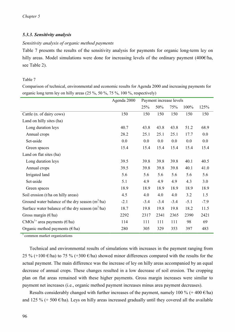
Chapter 5
96
5.3.3. Sensitivity analysis
Sensitivity analysis of organic method payments Table 7 presents the results of the sensitivity analysis for payments for organic long-term ley on hilly areas. Model simulations were done for increasing levels of the ordinary payment (400€/ha, see Table 2). Table 7 Comparison of technical, environmental and economic results for Agenda 2000 and increasing payments for organic long term ley on hilly areas (25 %, 50 %, 75 %, 100 %, respectively)
Payment increase levels
Agenda 2000 25% 50% 75% 100% 125%
Cattle (n. of dairy cows) 150 150 150 150 150 150 Land on hilly sites (ha)
Long duration leys 40.7 43.8 43.8 43.8 51.2 68.9 Annual crops 28.2 25.1 25.1 25.1 17.7 0.0 Set-aside 0.0 0.0 0.0 0.0 0.0 0.0 Green spaces 15.4 15.4 15.4 15.4 15.4 15.4
Land on flat sites (ha) Long duration leys 39.5 39.8 39.8 39.8 40.1 40.5 Annual crops 39.5 39.8 39.8 39.8 40.1 41.0 Irrigated land 5.6 5.6 5.6 5.6 5.6 5.6 Set-aside 5.1 4.9 4.9 4.9 4.3 3.0 Green spaces 18.9 18.9 18.9 18.9 18.9 18.9
Soil erosion (t/ha on hilly areas) 4.5 4.0 4.0 4.0 3.2 1.5 Ground water balance of the dry season (m3/ha) -2.1 -3.4 -3.4 -3.4 -5.1 -7.9 Surface water balance of the dry season (m3/ha) 18.7 19.8 19.8 19.8 18.2 11.5 Gross margin (€/ha) 2292 2317 2341 2365 2390 2421 CMOs1’ area payments (€/ha) 114 111 111 111 98 69 Organic method payments (€/ha) 280 305 329 353 397 483 1 common market organizations
Technical and environmental results of simulations with increases in the payment ranging from 25 % (+100 €/ha) to 75 % (+300 €/ha) showed minor differences compared with the results for the actual payment. The main difference was the increase of ley on hilly areas accompanied by an equal decrease of annual crops. These changes resulted in a low decrease of soil erosion. The cropping plan on flat areas remained with these higher payments. Gross margin increases were similar to payment net increases (i.e., organic method payment increases minus area payment decreases).
Results considerably changed with further increases of the payment, namely 100 % (+ 400 €/ha) and 125 % (+ 500 €/ha). Leys on hilly areas increased gradually until they covered all the available

The EU’s Agenda 2000 reform and the sustainability of organic farming in Tuscany
97
agricultural area at a payment increase of 125 %. Soil erosion dropped first to 3.2 t/ha for a 100% increase and then to 1.5 t/ha for a 125 % increase. Further improvements of the soil erosion performance were not possible because the ley cover on hilly sites could not be extended any further. The ground water balance deficit increased with the raise of the organic payment.
Gross margins increased less than payment net increases. Area payments declined to 98 €/ha with the 100 % increase in the payment for leys and to 69 €/ha for the 125 % increase. Socio-economic costs (area payments plus organic payments) increased from 394 €/ha to 552 €/ha.
Sensitivity analysis of thresholds Table 8 reports the results of the sensitivity analysis for the ESTs of nitrogen leaching, nitrogen runoff, soil erosion, herbaceous plant biodiversity and water use. We analysed the change in gross margin of less and more stringent threshold constraint. Constraint levels of the above-mentioned indicators were simultaneously and proportionally increased or decreased. Constraint levels of maximum ESTs, such as the nitrogen leaching EST, were changed by multiplying the previously identified ESTs (Table 3) by a constraint increase factor (<1) or by a constraint decrease factor (>1). For minimum ESTs (namely, the herbaceous plant biodiversity EST) this principle was applied accordingly. For the soil erosion EST, a minimum-multiplying factor of 0.95 was applied which corresponds to the soil erosion weighted mean of non-cultivated areas (green spaces). Further reducing this EST would lead to unfeasibility. The water use constraint with the EST given as water balance ≥ 0, was kept unaltered for all constraint increasing simulations. In the case of constraint decreasing simulations, the budget structure of the constraint was maintained and the water input coefficients of the balance were multiplied by the decrease factor, which corresponds to an extension of the time considered for the application of the balance beyond the dry season.
Values of each environmental threshold, the indicator performances and the gross margins at six significant EST constraint levels are reported in Table 8. The biodiversity threshold was limiting only for the most stringent general constraint increase factor of 0.5. The gross margin result of this simulation run appeared to be very low. This result can be explained by the slight difference between the herbaceous plant biodiversity threshold of a 0.5 factor, which is a minimum of 96 score/ha, and the maximum level of biodiversity that can be found in all the farm areas, which is 99 score/ha (green spaces and grassland).
The soil erosion threshold was found to be limiting between a factor of 0.5 and a factor of 2.0. Gross margins were found to be significantly affected (from € 1379 to € 446 per hectare) with maximum EST constraint factors of 0.95 or below. When these constraint factors are applied, hilly areas can not be cropped because of the restriction posed by the soil erosion threshold. Extending the soil erosion threshold to 1.5 t/ha gave rise to a sub-optimal level of gross margin (€ 2237 versus € 2292 per hectare). In this situation the hilly areas (permanent green spaces excluded) can be completely cropped. Beyond a factor of 2.0 only the soil erosion threshold was found to be still

Chapter 5
98
limiting. With a factor of 5.0, the gross margin reached the level of Agenda 2000 simulation without any extra-constraint. Finally, nitrogen and water use indicators were found to be non-limiting under all the constraint factors applied.
Table 8 Environmental sustainability thresholds (EST), environmental results and gross margins for six levels of EST constraint
Maximum EST constraint factors1 0.5 0.6 1.0 1.5 2.0 5.0 Nitrogen leaching EST (max) (kgN/ha) 13.5 16.2 27.0 40.5 54.0 135.0 Nitrogen leaching performance (kgN/ha) 10.2 7.9 7.9 7.9 7.4 6.0 Nitrogen runoff EST (max) (kgN/ha) 5.5 6.6 11.0 16.5 22.0 55.0 Nitrogen runoff performance (kgN/ha) 1.0 1.3 1.3 1.6 1.6 1.9 Soil erosion EST (max) (t/ha) 0.952 0.952 1.02 1.52 2.02 5.0 Soil erosion performance (t/ha) 0.95 0.95 1.0 1.5 2.0 4.5 Herbaceous plant biodiversity EST (min) (score/ha) 962 80 48 32 24 10 Herbaceous plant biodiversity performance (score/ha) 96 90 89 86 85 83 Ground water use EST (water balance >= 0) (m3/ha) >= 0 >= 0 >= 0 >= 0 >= 0 >= 0 Ground water balance (m3/ha) 49 29 26 1 13 82 Surface water use EST (water balance >= 0) (m3/ha) >= 0 >= 0 >= 0 >= 0 >= 0 >= 0 Surface water balance (m3/ha) 6 12 12 26 42 166 Gross margin (€/ha) 453 1403 1494 2237 2251 2292 1 for maximum ESTs correction factors <1 cause an increased level of constraint, while factors >1 lead to a decreased level of constraint. The concept is inverted for minimum ESTs (namely, the herbaceous plant biodiversity EST) 2 limiting
5.3.4. Using the model to evaluate policy scenarios
Additionally, three new policy scenarios were evaluated. For all three scenarios the focus was on targeting the organic method support scheme in order to improve the farm performances for soil erosion and water use. Soil erosion and water use were given special attention because in the simulations for Agenda 2000 their outcomes were unsustainable when compared with the corresponding ESTs (soil erosion ≤ 1 t/ha and water balance ≥ 0 m3/ha, respectively).
All three scenarios included increasing levels (25 %, 50 %, 75 %, 100 %) of the organic method payment of long duration leys (grassland and alfalfa) on hilly areas. Long duration leys on hilly areas can limit soil erosion to 2.0 t/ha on site 1 and to 1.5 t/ha on site 2, respectively.
In scenario 1 the additional payments on long duration leys were accompanied with an equal absolute decrease of the agri-environment payment levels of all other crops on hilly areas in order to compensate for the increase of socio-economic costs. In scenario 2 the payment decrease was extended to the irrigated crops (maize for grain and for silage) on the flat areas to consider also the
The EU’s Agenda 2000 reform and the sustainability of organic farming in Tuscany
99
indicator of water use. In scenario 3 the decrease was further extended to all the crops on the flat areas to further contain the socio-economic expenditures for agri-environment schemes to levels comparable to those of the Agenda 2000 scheme. Besides, scenario 3 includes a further absolute reduction of the agri-environment payment for the irrigated crops as an incentive to decrease water use. In the case the decrease of annual crop organic method payments was insufficient to cover the increase of long duration ley organic method payments, area payments of annual crops were decreased as well.
Table 9 presents the environmental and economic results of the three scenarios. Soil erosion did not reach the EST (1 t/ha) under any scenario. The lowest level of soil erosion (1.5 t/ha) was achieved for all three scenarios at a 75 % increase of long duration ley organic payments. This level is reached when all hilly agricultural area used is covered by long duration leys. In scenario 1 and 2, this same level of soil erosion was achieved with public costs of € 478 per hectare (€ 69 of area payments plus € 409 of organic payments) and a gross margin per hectare of € 2344 (scenario 1), and € 2341 scenario 2). In scenario 3, the same level was obtained with lower public costs (€ 419 per hectare, i.e. € 64 of area payments plus € 355 of organic payments) and a gross margin per hectare of € 2282 that is very close to the gross margin under the Agenda 2000 regulations without extra-constraints.
As previously stressed the water use EST has only a minor impact on farm management. A temperate climate with orographic rain regime and a mean annual rainfall of 1000 mm allow for a very low dry season ground water budget deficit (-2.1 m3/ha) and a surface water surplus under the Agenda 2000 regulations without any extra-constraint. Including water use disincentive schemes in scenario 2 and 3 allowed for compliance with the water use EST. Comparison of scenarios 1 and 2 which differ only in the water use disincentive show that the water use EST was met without a change in socio-economic costs and with only a minor decrease in gross margin per hectare (€ -3, i.e. € 2341 versus € 2344, respectively).
Compliance with all environmental indicators other than soil erosion and water use was maintained under all scenarios. Increasing ley payments more than 75 % did not gave cause for any environmental improvement under any scenario. Gross margin increases under all scenarios (€ 37 per hectare under scenario 1 and 2, and € 15 per hectare under scenario 3) were totally attributable to payment increases that lead to an increase in socio-economic cost.

Chapter 5
100
Tabl
e 9
Com
paris
on o
f pay
men
t sch
emes
, env
ironm
enta
l and
econ
omic
resu
lts o
f thr
ee p
olic
y sc
enar
ios
incl
udin
g di
ffere
nt o
rgan
ic m
etho
d pa
ymen
t inc
reas
es fo
r lo
ng d
urat
ion
leys
on
hilly
are
as (2
5 %
, 50
%, 7
5 %
, 100
%, r
espe
ctiv
ely)
app
lied
to th
e fa
rm m
odel
Sc
enar
io 1
1 Sc
enar
io 2
2 Sc
enar
io 3
3 Pa
ymen
t sch
eme
Long
dur
atio
n le
ys o
n hi
lly a
reas
+25%
+5
0%
+75%
+1
00%
+2
5%
+50%
+7
5%
+100
%
+25%
+5
0%
+75%
+1
00%
Ann
ual c
rops
on
hilly
are
as
(Eur
o/ha
) -1
004
-2
00
-3
00
-4
00
-1
00
-2
00
-3
00
-4
00
-1
00
-2
00
-3
00
-4
00
Irr
igat
ed c
rops
(E
uro/
ha)
=5 =
= =
-100
-200
-300
-400
-100
-200
-300
-400
Non
-irrig
atio
n in
cent
ive6
(Eur
o/ha
) =
= =
= =
= =
= =
-100
-200
-300
Ann
ual c
rops
on
flat a
reas
(E
uro/
ha)
= =
= =
= =
= =
-200
-300
-400
-500
Soil
eros
ion
(t/ha
on
hilly
are
as)
4.0
3.2
1.5
1.5
4.0
2.9
1.5
1.5
4.0
3.6
1.5
1.5
Gro
und
wate
r bal
ance
of t
he d
ry
seas
on (m
3 /ha)
-3
.4
-3.9
-7
.9
-7.9
-3
.4
11.5
12
.3
12.3
-3
.4
10.3
12
.3
12.3
Surf
ace
wate
r bal
ance
of t
he d
ry
seas
on (m
3 /ha)
19
.8
15.3
11
.5
11.5
19
.8
9.5
3.7
3.7
19.8
12
.4
3.7
3.7
Gro
ss m
argi
n
(Eur
o/ha
) 23
01
2313
23
44
2381
22
98
2309
23
41
2378
22
85
2274
22
82
2297
Are
a pa
ymen
ts
(Eur
o/ha
) 11
1 98
69
69
11
1 94
69
69
11
1 94
64
48
Agr
i-env
ironm
ent p
aym
ents
(Eur
o/ha
) 29
2 32
4 40
9 44
6 28
9 33
0 40
9 44
6 27
0 29
4 35
5 38
6
1 inclu
ding
pay
men
t dec
reas
e on
hill
y ar
eas
for a
ll cr
ops
othe
r tha
n lon
g du
ratio
n le
ys
2 inclu
ding
pay
men
t dec
reas
e on
hill
y ar
eas
for a
ll cr
ops
othe
r tha
n lon
g du
ratio
n le
ys a
nd o
n fla
t are
as fo
r irr
igat
ed c
rops
3 inclu
ding
pay
men
t dec
reas
e on
hill
y an
d fla
t are
as fo
r all
crop
s oth
er th
an lo
ng d
urat
ion
leys
and
a m
odul
atio
n of
the
decr
ease
for i
rriga
ted a
nd d
ry c
rops
(mai
ze)
4 am
ount
corr
espo
ndin
g to
a 2
5 %
incr
ease
of t
he lo
ng d
urat
ion
ley
orga
nic
met
hod
paym
ent
5 u
ncha
nged
6 a
pplie
d ex
clus
ivel
y to
com
mon
ly ir
rigate
d cr
ops
of th
e reg
ion

The EU’s Agenda 2000 reform and the sustainability of organic farming in Tuscany
101
5.4. Discussion and conclusions
The objectives of this paper were to present an ecological-economic model to evaluate farm and field-level environmental-economic tradeoffs and specifically to evaluate the impact of the Agenda 2000 reform for organic farming in Tuscany.
5.4.1. Farm and site level analysis
Changing from CMO and organic method support schemes of the MacSharry reform regulations to those of the Agenda 2000 regulations gave cause for small technical and environmental changes. The most significant environmental change was a decrease of soil erosion. In fact, the soil erosion threshold appeared to be the most limiting EST as far as the effect on farm gross margin was concerned. The other environmental performances proved to be satisfactory compared with ESTs reported from legislation and the literature, both under the MacSharry reform and the Agenda 2000 regulations.
The addition of a closed nutrient cycle gave cause for consistent change in farm technical and environmental results, and to a further decrease of the farm gross margin both under the MacSharry reform and Agenda 2000 regulations. The manure surplus at the farm level persisted in the model calculations for both with the extra ESTs only. Manure surpluses can cause serious problems for farm management. Where the delivery of this surplus to other organic-production holdings (which is allowed by the EU Regulation on organic livestock production) is not an option, a closed nutrient cycle will causes changes in the rotational scheme, ultimately leading to a decrease in the economic performance of the farm.
Gross margins under the Agenda 2000 regulations were considerably higher than those under the MacSharry reform regulations. This was mainly due to the higher organic method payments under the Agenda 2000 regulations. From a policy efficiency standpoint this means that the organic farming system generates environmental performances that are similar under the MacSharry reform and Agenda 2000 regulations but at higher socio-economic costs (costs of the support schemes) under Agenda 2000. This is in line with what found in the literature (Wier et al., 2002). The site level analysis confirmed the findings at farm level. A series of tradeoffs were observed between environmental indicators at the different sites. Especially in the case of a closed nutrient cycle, these economical-environmental tradeoffs contributed to the explanation of the apparently equivocal results at farm level. The imposition of conflicting environmental constraints (e.g., the soil erosion EST and the constraint of the closed nutrient cycle) caused highly different site crop plans. These associated site specific environmental and technical impacts could not have been evaluated with a farm-level aggregated analysis.

Chapter 5
102
5.4.2. Sensitivity analysis
Sensitivity analysis of organic payments and ESTs gave more insight in the environmental-economic tradeoffs of organic farming, indicated feasible targets for hypothetical policy scenarios and the socio-economic costs of the schemes to address these targets. Increasing parametrically the organic payments of leys on hilly areas substantial decreased soil erosion. In cosntrast, the ground water balance deficit increased, which confirms the risk of conflicts between different environmental aims (Callens and Tyteca, 1999).
The sensitivity analysis of the thresholds confirmed the sensitivity of the farm management plan to the soil erosion constraint. Limiting soil erosion to the EST of 1.5 t/ha affected the gross margin. However, the soil erosion EST used in this study is rather stringent. In fact, it was based on the average soil formation rate, which is 1 t/ha in temperate climate (Van Mansvelt, 1999). Other thresholds can be found in the literature that are higher and are still considered acceptable. For example, Zanchi (1983) proposes a soil erosion threshold of 8-9 t/ha for soils and landforms similar to those of the Sereni hilly sites. Therefore, applying a slightly (in absolute terms) higher erosion threshold could enable environmental health requirements to be met without severely affecting gross margin (before subsidies). Besides, the socio-economic costs of ESTs should be accounted for when designing new policy scenarios.
5.4.3. Evaluation of policy scenarios
The application of the model to policy scenarios provided insights into ways in which the cost economic efficiency of the Agenda 2000 organic method support scheme can be improved. Different scenarios were evaluated and an LP solution was found that (a) improves the various farm environmental performances to sustainable levels, (b) implies only a small increase of socio-economic costs and a small decrease of farm gross margins, and (c) takes into account and solves the issue of conflicting environmental objectives.
5.4.4. Further research
The model presented in this paper was only applied to organic farming. Other farming systems could be considered in further research. The model structure is also suitable for the analysis of the combination of integrated and conventional farming systems.
In the present model application to organic farming the environmental impact of pesticides use was not relevant. In previous studies were this was relevant we have used the environmental potential risk indicator for pesticides (EPRIP) (Pacini et al., 2002b).
The comparison of the payments required with the different policy scenarios and those required with the agri-environment scheme of the Agenda 2000 programme provides insights how the efficiency of the latter scheme could be improved considering a farm that is already enrolled in this scheme. This assessment does not address the issue of the total increase in environmental benefits

The EU’s Agenda 2000 reform and the sustainability of organic farming in Tuscany
103
upon enrolment and how this information could be used to enhance the environmental effectiveness of the scheme. Comparing different farming systems (organic and conventional) with regional carrying capacity and resilience can be a way to find out these environmental benefits, at least from a farm-level perspective.
5.4.5. Conclusions and practical applications
With reference to this case study, the main conclusions of the present paper are as follows: 1) The sustainability of organic farming proved to be satisfactory compared with ESTs from legislation and the literature, both under the MacSharry reform and Agenda 2000 regulations, with soil erosion being the only real environmental threat; 2) CMO and agri-environment schemes of the MacSharry reform and Agenda 2000 lead to similar environmental performances, with a minor decrease in soil erosion being the only notable improvement attributable to Agenda 2000; 3) Socio-economic costs of the Agenda 2000 schemes are higher than those of the MacSharry reform schemes; 4) Site level analysis is essential to study environmental-economic tradeoffs and to explain farm-level aggregated results; 5) Ecological-economic modelling combined with sensitivity and scenario analyses can contribute to better link organic method payments to environmental performances which would improve the cost efficiency of agri-environment schemes.
Results were calculated for a specific representative farm. Pedo-climatic conditions and production activities included are applicable for the total given region (Mugello area). Hence, re-arranging the model spatial structure to include shares of crops, hilly/flat areas, irrigated/non-irrigated land and ground/surface water withdrawal retrieved from aggregated data of the region, would allow the model to address agri-environment scheme changes for improvement of regional agro-ecosystem health.
Acknowledgements The study described in this paper is part of a research project entitled “Environmental Accounting in Agriculture”, funded by A.R.S.I.A. (Tuscany Agri-forestal Development and Innovation Agency) and directed by Association A.L.T. (Tuscany Environment and Labour Association). C. Pacini’s contribution to this project is part of his PhD research at the Farm Management Group of Wageningen University as part of a Community Training Project financed by the Commission of the European Communities in the specific Programme for Agriculture & Fisheries. The content of the publication is the sole responsibility of the authors and in no way represents the views of the Commission or its services.

Chapter 5
104
References Arrigoni, P.V., Nardi, E. and Raffaelli, M., 1985. La vegetazione del parco naturale della
Maremma (toscana). Dipartimento di Biologia Vegetale dell’Universitá degli Studi di Firenze, Florence, Italy (in Italian).
Brunori, G., Omodei-Zorini, L., Lazzerini, G., Pacini, C., Rovai, M., Vazzana, C. (1999). Territorio, ambiente ed impresa agricola: modelli di gestione per lo sviluppo rurale. Presented at the International Seminar of Perugia University, Italy, 29 aprile 1999 (in Italian).
Callens, I., Tyteca, D., 1999. Towards indicators of sustainable development for firms. A productive efficiency perspective. Ecological Economics 28, 41-53.
Cappelletti, C., 1976. Trattato di botanica. UTET, Italy (in Italian). CEC, 1992. Towards sustainability: a European Community programme of policy and Action in
relation to the environment and sustainable development, COM (92) final. Commission of the European Communities, Brussels, Belgium.
CEC, 2002. Environment 2010: Our future, Our choice – The Sixth Environment Action programme, COM (2001) 31 final. Commission of the European Communities, Brussels, Belgium.
De Koeijer, T.J., Wossink, G.A.A., Struik, P.C. and Renkema, J.A., 2002. Measuring Agricultural Sustainability in Terms of Efficiency. Journal of Environmental Management 66, 9-17.
European Commission, 1999. Agriculture, Environment, Rural Development: Facts and Figures - A Challenge for Agriculture, COM (1999) 22. Available at http://europa.eu.int/ comm/agriculture/envir /report/en/index.htm
Falconer, K., Hodge, I., 2001. Pesticide taxation and multi-objective policy-making: farm modelling to evaluate profit/environment trade-offs. Ecological Economics 36, 263-279.
FAO, 1998. World Reference Base for Soil Resources. FAO, ISRIC and ISSS, Rome, Italy. Jarosch, J. and Murschel, B., 1989. Methodik und Datenerfordernisse zut Integration ökonomischer
and ökologischer Ziele in einzelbetrieblicher Entscheidungs modelle. In: Hanf, C.-H., and Scheper, W. (eds.) Neuere Forschungskonzepte und –Methoden in den Wirtschafts- und Sozialwissenschaftendes landbaues. Schriften der GEWISOLA, Band 25, Münster-Hiltrup: Landwirtschaftsverlag, Germany (in German).
Kabourakis, E., 1996. Prototyping and dissemination of ecological olive production system: A methodology for designing and a first step towards validation and dissemination of prototype ecological olive production systems (EOPS) in Crete. Ph.D. thesis Wageningen Agricultural University, Wageningen, Netherlands.
Knisel, G., 1993. GLEAMS Groundwater Loading Effects of Agricultural Management Systems – Version 2.10. University of Georgia-Coastal Plain Experiment Station-Biological and Agricultural Engineering Department Publication No.5, 259 p., Tifton, Georgia (USA).
Landi R., 1999. Agronomia e ambiente. Edagricole, Bologna, Italy (in Italian).

The EU’s Agenda 2000 reform and the sustainability of organic farming in Tuscany
105
Law, A.M., Kelton, W.D., 1991. Simulation modelling & analysis. McGraw-Hill International Editions, Singapore.
Pacini, C., Giesen, G., Wossink, A., Huirne, R., 2002a. The modelling framework. In: Pacini, C., Economic-environmental accounting and modelling to evaluate sustainability of farming systems for multi-objective policy-making. PhD thesis Wageningen University, Wageningen, The Netherlands.
Pacini, C., Wossink, A., Giesen, G., Vazzana, C., Huirne, R., 2002b. Evaluation of sustainability of organic, integrated and conventional farming systems: a farm and field scale analysis. Accepted for publication by Agriculture, Ecosystems and Environment.
Pacini, C., Wossink, A., Giesen, G., Vazzana, C., Omodei-Zorini, L., 2002c. Environmental Accounting in Agriculture: a Methodological Approach. Submitted.
Pimentel, D., Harvey, C., Resosudarmo, P., Sinclair, K., Kurz, D., McNair, M., Crist,S., Shpritz, L., Fitton, L., Saffouri, L. and Balair, R., 1995. Environmental and economic costs of soil erosion and conservation benefits. Science 267, 1117-1121.
Regione Toscana – Giunta Regionale, ARPAT – Agenzia Regionale per la Protezione dell’Ambiente della Toscana (eds.), 1999. Rapporto sullo Stato dell’Ambiente della Regione Toscana ’98. Edizioni Regione Toscana, Florence, Italy (in Italian).
Reus, J., Leendertse, P., Bockstaller, C., Fomsgaard, I., Gutsche, V., Lewis, K., Nilsson, C., Pussemier, L., Trevisan, M., Van der Werf, H., Alfarroba, F., Blümel, S., Isart, J., McGrath, D., Seppälä, T., 2002. Comparison and evaluation of eight pesticide environmental risk indicators developed in Europe and recommendations for future use. Agriculture, Ecosystems & Environment 90, 177-187.
Sands, G.R., Podmore, T.H., 2000. A generalized environmental sustainability index for agricultural systems. Agriculture, Ecosystems and Environment 79, 29-41.
Schotman, A., 1988. Tussen bos en houtwal: broedvogels in een Twents cultuurlandschap. RIN-rapport 88/37, Leersum, The Netherlands (in Dutch).
Schultink, G., 2000. Critical environmental indicators: performance indices and assessment models for sustainable rural development planning. Ecological Modelling 130, 47-58. Stiftung Ökologie & Landbau, 2001. Organic Farming in Europe - Country Reports. Available at http://www.organic-europe.net/country_reports/default.asp
Trevisan, M., Errera, G., Capri, E., Padovani, L. & Del Re, A.A.M., 1999. Environmental Potential Risk Indicator for Pesticides. In: Reus, J., Leendertse, P., Bockstaller, C., Fomsgaard, I., Gutsche, V., Lewis, K., Nilsson, C., Pussemeier, L., Trevisan, M., van der Werf, H., Alfarroba, F., Blümel, S., Isart, J., McGrath, D., Seppälä, T. (eds.) Comparing Environmental Risk Indicators for Pesticides – Results of the European CAPER Project. Center for Agriculture and Environment, Utrecht, The Netherlands.

Chapter 5
106
Van der Werf, H.M.G., Petit, J., 2002. Evaluation of the environmental impact of agriculture at the farm level: a comparison and analysis of 12 indicator-based methods. Agriculture, Ecosystems and Environment 1922, 1-15 (in press).
Van Mansvelt, J. D. & Van der Lubbe, M. J., 1999. Checklist for sustainable landscape management. Elsevier Science B.V., Amsterdam, The Netherlands.
Vereijken, P., 1999. Manual for prototyping integrated and ecological arable farming systems (I/EAFS) in interaction with pilot farms. AB-DLO, Wageningen, The Netherlands.
Weersink, A., Jeffrey, S., and Pannell, D., 2002. Farm-level modeling for bigger issues. Review of Agricultural Economics 24 (1), 123-140.
Wier, M., Andersen, J.M., Jensen, J.D., Jensen, T.C., 2002. The EU’s Agenda 2000 reform for the agricultural sector: environmental and economic effects in Denmark. Ecological Economics 41, 345-359.
Winter, M. and Gaskell, P., 1998. The Agenda 2000 debate and CAP reform in Great Britain: is the environmental being sidelined? Land Use Policy 15(3), 217-231.
Wossink, G.A.A., 1998. Environmental economics of the farm firm. Department of Farm Management, Wageningen Agricultural University, The Netherlands.
Wossink, G.A.A., De Koeijer, T.J., and Renkema, J.A., 1992. Environmental-economic policy assesment: a farm economic approach. Agricultural Systems 39, 421-438.
Zanchi, C., 1983. Primi risultati sperimentali sull'influenza di differenti colture (frumento, mais, prato) nei confronti del ruscellamento superficiale e dell'erosione. Annali dell'Istituto Sperimentale per lo Studio e la Difesa del Suolo - Firenze XIV, 277-288 (in Italian).

Chapter 6
Ecological-economic modelling to support multi-objective policy making: a farming systems approach implemented for Tuscany
Cesare Pacini 1, Ada Wossink 2,1, Gerard Giesen 1, Ruud Huirne1 1 Farm Management Group – Department of Social Sciences, Wageningen University, The Netherlands. 2 Dept. of Agricultural & Resource Economics, NC State University, Raleigh, USA.
Submitted to Agriculture, Ecosystems and Environment

Chapter 6
108
Abstract Currently, there is a major concern in the EU regarding agri-environmental issues. Farmers are viewed not only as food suppliers but also as the custodians of the countryside. This role of farmers has been officially acknowledged in the Common Agricultural Policy (CAP) through a number of regulations that enforce agri-environment schemes and cross-compliance. However, under some circumstances these regulations have proved to be ineffective. Organic farming can play an important role for agri-environment schemes. The main aim of this study is to show the relevance of the assessment of the environmental performance of conventional and organic farming systems for the development of efficient agri-environment schemes under the Agenda 2000 regulations. A holistically designed ecological-economic model was applied under Agenda 2000 regulations and different policy scenarios. Spatial aspects, such as pedo-climatic conditions, were included in the model. The approach was implemented for the case of northern Tuscany. Results indicated that organic farming systems (OFSs) are environmentally more beneficial than conventional farming systems (CFSs) and that current Agenda 2000 CAP market and income support schemes give cause for an intensification of farm production and for an increase of environmental harm. They also showed that conventional farmers willing to produce environmental performances comparable to those of organic agriculture or to comply with environmental sustainability thresholds (ESTs) incur opportunity costs due to the need of application of organic crop management and/or extensification of the crop plan. Results were discussed with special reference to the development of efficient agri-environment schemes. Conclusions were drawn together with policy implications. Key words: ecological-economic modelling, multi-objective policy-making, farming systems, environmental externalities, opportunity cost, Tuscany.
6.1. Introduction
Currently, there is a major concern in the EU regarding agri-environmental issues. Farmers are viewed not only as food suppliers but also as the custodians of the countryside. The role of farmers as conservators of the landscape and as protectors of natural resources is officially acknowledged in the Common Agricultural Policy (CAP). Specifically, Regulation 2078/92 proposed agri-environmental schemes to compensate farmers for any income losses caused by reductions in output/or increases in costs and for the part they play in improving the environment. Here there are two distinct ideas, firstly there is a reference to forgone profit for less damaging farming, and secondly there is a reference to the value of public benefits provided by farmers.
The EU agri-environment schemes first introduced as part of the 1992 McSharry CAP-reform, proved to be potentially beneficial, but benefits have been poorly monitored over much of Europe (Donald et al., 2002). They showed also a low level of participation in intensive regions and for

Ecological-economic modelling to support multi-objective policy making
109
intensive farm types due to uncompetitive rates of payment. Lack of funds further contributed to the limited spread of these schemes — agri-environmental schemes account for less than 5 % of the total CAP-budget.
In contrast, market and income support payments, which are still the main forms of agricultural support under the CAP, have given cause for further agricultural intensification and environmental damage (Donald et al., 2002). This situation could not improve under the EU Agenda 2000 reform. For example, Wier et al. (2002) reported in a modelling analysis of the effects of the Agenda 2000 reform for the agricultural sector in Denmark, that the Agenda 2000 reform has significant economic costs but almost no effects on the environment – either positive or negative. Under the Agenda 2000 reform, agri-environment payments are offered for organic farming and other sustainable practices of land use, maintaining extensive systems, conservation of high nature-value farmed environments, upkeep of the landscape and historical features on agricultural land and environmental planning in farming practice. In practice agri-environmental schemes are relevant in particular for organic farming (European Commision, 1999; Stiftung Ökologie & Landbau, 2001).
To facilitate the performance of the CAP to improve, a radical reform to a system of production decoupled support payments is advocated by many parts (Beard and Swinbank, 2001). However, what types of schemes should replace the current payment system is still under debate. Particular focus is on the structure of the agri-environment schemes and their environmental-economic efficiency, which is strongly related to the calculation method of the payments. For example, income losses of organic production activities are calculated based on regional average market prices of inputs and outputs of organic and conventional products, respectively. Environmental benefits from organic farming are assumed but are not considered in the quantification of the payments. So there is no provision made for the production of environmental benefits. Besides, the level of agri-environment payments is set constant for a given administrative region, disregarding differences of environmental performances produced by farming systems (FSs) applied to different physiographic regions.
Support payments to the farm sector for the supply of environmental goods are well established in OECD countries (Hanley, 1995). In the literature, principles for the supply of environmental external benefits from agriculture have been reported (Brown, 1994; Blöchliger, 1994) and these could improve the efficiency of the above-mentioned agri-environment schemes. Hanley et al. (1998) proposed the application of the “provider gets principle” (PGP). According to these authors the PGP approach seeks to avoid compelling rural landowners to produce environmental improvements (or to avoid environmental damages), but rather to persuade them to do so by offering voluntary payments. The PGP requirements are (1) that the suppliers of amenities can be identified; (2) that a means be found of transferring funds to them according to the marginal opportunity costs of supply, (3) that funding is available to finance these transfers; and (4) the identification of an appropriate level of supply for rural public goods.
Chapter 6
110
The organic payments of the EU agri-environment scheme fit the description of the PGP requirements mentioned above. However, as far as the fourth requirement is concerned, the determination of the “appropriate level” of amenity under this scheme could give cause for shortages of environmental-economic efficiency of the payments because they are based on agronomic requirements of farming practices instead of on requirements regarding the provision of environmental benefits.
Organic farming is certainly more environmentally beneficial than conventional farming. Said that, it is important to evaluate how much it is better and for what amenities. Environmental externalities produced by FSs are multiple and strongly related to diverse regional pedo-climates. It can not be given for granted that organic farming performs better than conventional farming as for all environmental aspects, in all ecosystems and with the same economic results. Organic farming should be considered as a technique to achieve given environmental performances rather than a performance in itself. These aspects must be considered in the development of a multi-objective policy to address the provision of public goods from agriculture. Quantification of environmental externalities produced by different FSs must be carried out in detail as to increase the efficiency of the scheme payments. Once the levels of environmental externalities of different FS are clearly determined, a payment scheme might be devised based on the calculation of opportunity costs to undertake the FS practices which prove to be more beneficial.
Ecological-economic models can help to analyze the tradeoffs and calculate the opportunity costs of different FS in different pedo-climates to optimally calibrate agri-environment schemes. Linear programming (LP) models have been repeatedly applied for farm-level studies and are well suited to embrace mixed ecological-economic analysis (Falconer and Hodge, 2001; De Koeijer et al., 2002). However, within-farm variation in environmental and economic aspects is often disregarded. Besides, many of the studies involved with ecological-economic modelling often advocate a system approach, but lack a holistic interpretation of the farm agro-ecosystem. Environmental impacts modeled are often reduced in number (e.g., pesticides, nitrogen losses) and do not supply comprehensive information on many environmental aspects, this giving cause for possible misjudgments in the multi-objective policy-making process and for conflicts between different environmental goals. The introduction in a farm LP model of spatially referenced units of analysis combined with a holistic framework for the evaluation of environmental performances and a farming systems approach could solve these shortages, therefore facilitating the design of more effective agri-environment schemes.
With reference to the above, the main aim of this study is to show the relevance of the assessment of the environmental performance of conventional and organic FSs for the development of efficient agri-environment schemes under the Agenda 2000 regulations. Our approach includes three steps: 1) development of an ecological-economic farm model using the linear programming method, 2) assessment of the income foregone by conventional farmers for the production of

Ecological-economic modelling to support multi-objective policy making
111
environmental benefits comparable to those produced by organic agriculture, 3) assessment of the income foregone by farmers to comply with different sets of environmental sustainability thresholds (ESTs), representing the demand for environmental benefits by society. The approach was implemented for the case of Mugello area, northern Tuscany.
6.2. Theoretical background
The objective of this section is to develop a model of farmer behaviour under agri-environment schemes. Specifically we intend to address the issue of determination of the correct level of incentives to be offered by these schemes in order to stimulate the provision of environmental benefits by the individual farmer.
Based on the agronomic-economic literature, production at the farm level can be described by the transformation function Fi(Yi ,Xi; S) where i, i=1,…,I indexes the various outputs. Yi is the vector of outputs, Xi is the vector of variable inputs for output i, and S is a vector of biotic and abiotic factors that define the production conditions, including soil characteristics and climatic factors such as solar radiation, precipitation and temperature (Wossink et al., 2001).
The variable inputs Xi used in agricultural production can have multiple environmental effects. The type and level of input use affects the characteristics and the significance of environmentally critical processes such as water balance, soil erosion, pesticide leaching, biodiversity and the nitrogen cycle, see Figure 2 in Pacini et al. (2002c). The environmentally critical processes are also influenced by biotic and abiotic factors that are beyond the farmer’s control (cf. Turner et al., 2000, pp. 10-11). The generation of the ultimate environmental effects of agricultural production, Z, can then be described by Gi(Zi , Xi , Yi; S).
In the static situation the only linkage between the production processes of the various outputs on the farm is their demands for the common base of allocatable inputs at the farm, which is fixed
in the short run. Examples are land, labour and equipment. Let the vector B denote their stock. To summarise the aspects above, the restricted profit function of the individual farm can be
defined as the following planning problem:
[ ]
)1(
)1(,0);,,(
)1(,0);,(
)1(''(,
dBB
ciSYXZG
biSXYFtosubject
aCXwYpMax),B,Z,YX
i
iiii
iii
I
iiiB,Z,YX
*i
*i
*i
*i
iiii
≤
∀≤
∀≤
−−=
∑
∑π

Chapter 6
112
where p is the vector of output prices; w is the vector of prices of the variable inputs and C is the cost of the fixed inputs. The model allows both the variable input mix and the allocatable input mix (such as the area grown) to be modified for each output.
The model above is helpful in understanding farmers' response to an agri-environment scheme. Participation in an agri-environment scheme is voluntary for farmers in a designated area. Let us assume that participants receive standard payments in return for provision of environmental benefits1.
In the above presentation, it has been assumed for simplicity that there is only one (conventional) production technology. Under the agri-environment scheme a profit-maximizing farm will seek out an alternative technology, such as organic farming, that can enhance the environmental benefits of agricultural production. Assuming that such an alternative technology indeed is available for each output, the environmental effects/output ratio of an output then depends on both the production technique and the input mix chosen. The production technology chosen is also likely to affect fixed costs.
The price of output i from the alternative is assumed equal to that of conventional products. In fact, a desirable widespread application of an agri-environment scheme would give cause for a high increase of organic product supply and consequently to a decrease of prices towards price levels similar to those of conventional products. This, together with the non-stability of niche markets such as those of organic products, makes prices of organic products quite volatile.
Let φi be a production technology with φi ∈ Φi, where Φi is the technology set for crop i. The profit maximisation problem of the individual farm considering enrolling in the agri-environment scheme can now be defined as the following planning problem:
[ ]
)2(
)2(
)2(,0);,,(
)2(,0);,,(
)2(}''{),,,,(,,,
*****
eZZ
dBB
ciSYXZG
biSXYFtosubject
aCXwYpMaxBZYX
i
i
iiii
iiii
i
I
iiiBZYXiiiii
iiii
≤
≤
∀≤
∀≤
−−=
∑
∑
∑
φ
φφπ
1 It has to be noted that many agri-environment schemes require abiding certain restrictions on their husbandry, rather than the provision of given levels of environmental benefits. However, a scheme based on the actual environmental effects of farming practices is preferable as the link with the objective of the schemes is direct and the choice of means is left to the farmer (Van der Werf and Petit, 2002).

Ecological-economic modelling to support multi-objective policy making
113
where vector Z denotes the level of environmental performances required to join the agri-environment scheme.
In the equation set above, the optimal profit is conditional on the production technology chosen. The choice of technology affects the fixed costs as well as the optimal level of output, the optimal levels and types of variable inputs and the environmental impacts, see equations (2b) and (2c). The profit from a change in technology then is composed of the total net change in operational returns and a change in fixed cost.
Obviously, the agri-environment payment would not have to be higher than the difference between the unregulated profit as resulting from equation set (1) and the regulated profit as resulting from equation set (2). If the agri-environment agency has complete information on the farm's current operations, new technologies and on production conditions as in equation sets (1) and (2), it can derive this link and assess efficient agri-environment payments (cf. Bonnieux, 1998). Without this information, there is no direct link between the premium and the impact of the
constraint Z on the farm operations. The latter constraint may possibly not be binding. In the case
Z is met by the solution Z* of equation set (1), the farmer could enroll in the agri-environment scheme without modifying his technology/practices. Similarly, without information on the farm's
current operations and on the production conditions, S, there is no link between the constraint Z and the change in use of variable inputs, X.
In the framework above, production conditions, S, will be highly dependent on the location, which implies variation over space. Spatial variation in the abiotic environment is due to weather, soil factors and their interaction. Spatial variation within farms (among fields) leads to differences in optimal technology, input use, production and pollution, even for the same crop or rotation. Starting at the field level allows for taking both productivity and environmental effects of agri-environment schemes into account accurately. Spatial heterogeneity can be included in the framework above by specifying the production and pollution relationship for each output, F(·) and G(·), separately for each field (cf. Antle and Mc Gucking, 1993, p. 211-215).
6.3. Materials and methods
Technical, environmental and economic performances of conventional farming systems (CFSs) and organic farming systems (OFSs) were compared by applying different (conventional and organic, respectively) versions of an integrated ecological-economic model. The general structure of the model and the processing methods of its ecological and economic coefficients were organized according to criteria of generality and flexibility. In this paper the structure and the methods are applied to a dairy farm located in the Mugello region, Tuscany. Comparisons were made of CFSs and OFSs under the Agenda 2000 regulations and two different policy scenarios. Next, the

Chapter 6
114
conventional and the organic version of the LP model were integrated. This conventional-organic combined version of the model was used to evaluate production costs of environmental externalities produced by the organic method and externalities due to the imposition of ESTs.
6.3.1. Policy scenarios
Table 1 shows the discriminating features for the Agenda 2000 regulations and the two scenarios applied to CFSs and to OFSs. This paper deals with the development of agri-environment schemes alternative to the current production coupled support system of EU. It was therefore necessary to propose evaluation comparisons between the current Agenda 2000 policy, which is still based on production coupled support payments, and a scenario that does not comprise production coupled payments. Starting from the comparison of CFS and OFS performances under the no EU support scenario, the income foregone by conventional farmers for the production of environmental benefits comparable to those produced by organic agriculture (step 2) could be assessed without any prejudice due to the current policy circumstances. For instance, the income foregone calculated under this scenario would not be affected by the production intensification effects induced by the actual policy. The second scenario was settled to evaluate the impact of the current organic farming support scheme in the absence of market and income support schemes.
Discriminating features of the scenarios compared to the Agenda 2000 baseline were commitments required by EU to farmers to benefit from milk product (market) support payments, from arable crop (income) support payments, organic farming rules, EU corresponding support schemes and product prices.
Currently, farmers who want to benefit from the market support scheme of the EU common market organization (CMO) in milk and milk products must comply with milk quota assigned by the CMO (1132.5 t/year for the case study farm). Farmers who want to benefit from the income support scheme of the EU CMO in cereals must comply with cross-compliance commitments on set-aside and drainage system. Farmers who want to benefit from the EU organic method support scheme must comply with organic production rules. Main cross-compliance commitments and main organic production rules are included in Table 1.
The CFS under Agenda 2000 includes the application of the conventional production method to the Sereni FS with the Agenda XXI 2000/2001 CMOs’ commitments and support schemes. The OFS under Agenda 2000 includes the application of the organic method to the Sereni FS with the Agenda XXI 2000/2001 CMOs’ commitments and support schemes and, additionally, the organic production rules and corresponding support scheme.

Ecological-economic modelling to support multi-objective policy making
115
Table 1 Main discriminating features of Agenda 2000 and two scenarios applied to conventional farming systems (CFSs) and organic farming systems (OFSs) FS1 CFS2 OFS3
Agenda 2000/scenario Agenda 2000
No EU support
Agenda 2000
Only organic EU support
No EU support
EU CMOs4’ commitments Milk quota Yes No Yes No No Cross-compliance5 Yes No Yes No No EU Organic production rules6 No No Yes Yes Yes EU CMOs’ support schemes Market support scheme for milk sector Yes No Yes No No Income support scheme for arable crops Yes No Yes No No
Crop payments (€/ha) Barley 220 - 220 - - Broad bean 289 - 289 - - Maize (for grain and for silage) 477 - 477 - - Set-aside 234 - 234 - -
EU organic method support scheme Income support scheme for organic farming
Crop payments (€/ha) Barley - - 270 270 - Broad bean - - 270 270 - Maize (for grain and for silage) - - 390 390 - Leys (grassland and alfalfa) - - 400 400 -
Product prices (€ per 100kg) Milk price 36.67 25.72 42.35 29.70 29.70 Maize grain price 15.00 15.00 17.00 17.00 17.00 1 farming system 2 conventional farming system 3 organic farming system 4 European Union common market organizations 5 Main cross-compliance commitments are a 10% set-aside rate of areas subject to payment and the construction and maintenance of the drainage system. Sources for cross-compliance norms: EU Regulation 1251/99, EU Regulation 1259/99, Italian Law by Decree of September 15, 2000, Italian Law by Decree of March 8, 2001 6 Main organic production rules at the farm level are: ban on the use of chemically-synthesised fertilizers and plant protection products; ban on genetically modified organisms or products; cultivation of legumes, green manures or deep-rooting plants in an appropriate multiannual rotation programme; ban on landless animal production; at least 60% of the dry matter in daily rations of herbivores has to consist of roughage; livestock must be fed on organic produced feedstuffs for at least 90%; use of preventive measures, phytotherapeutic and homoeopathic products for animal-health; total amount of manure applied on the holding may not exceed 170 kg of nitrogen per ha of agricultural area used per year, as defined by the “Nitrate directive”. Sources for organic production rules: EU Regulation 2092/91, EU Regulation 1804/99, Basic Standards for Organic Production and Processing (IFOAM, 2000).

Chapter 6
116
The application of the no EU support scenario to the CFS and the OFS implied the removal of
the CMOs’ commitments connected with the market and income support schemes. This applied also to the scenario with only organic EU support. Consequently, in both scenarios applied to the OFS organic production rules were included and CMOs’ commitments were excluded. Although, organic farming support was included in only one of the scenarios applied to the OFS, organic production rules were kept in both of them because organic product prices were assumed.
The price for conventional milk under the no EU support scenario was assumed to be equal to the milk target price as from July 2007 settled by the EU Regulation 1255/1999. Regulation 1255 implements a gradual reduction of market support for milk and milk products starting from July 2005 and ending in July 2007. Market support measures will be gradually substituted by income support measures for milk producers under the form of a dairy premium. Consequently, the target price of July 2007 was assumed to be the price closest to the market price in the absence of price interventions. The milk price of both scenarios was settled starting from the conventional milk price, considering an increase proportional to the difference between the conventional and the organic milk prices of actual circumstances. This was done to attribute to organic milk under no market support circumstances an extra-price comparable to that of current circumstances. Conventional and organic maize grain prices of the scenarios were assumed to be equal to current prices.
6.3.2. Short description of the model
The model was constructed starting from a standard economic linear programming model and extending the input-output matrix to include emission and evaluation figures retrieved from ecological models. The model includes two different spatial scales, namely farm scale and site scale.
The economic sub-model was built empirically using data from a dairy farm recently converted from the conventional to the organic production method. The example farm is named “Sereni” and is located in the Mugello basin, some 30 km north of Florence, Northern Tuscany (latitude 44°N). To perform a detailed spatial scale analysis the farm was divided into several different sites according to landform, soil and irrigation conditions. For more details on the selection criteria of the farm, on the farm and the site description, and on the farm representativeness for the Mugello region, reference is made to Pacini et al. (2002a, 2002c).
Ecological models were used to calculate environmental indicators which entered as coefficients in the input-output matrix obtained by the extension of the economic sub-model. Indicators were selected based on a holistically designed framework (Pacini et al., 2002c, 2002d) according to the main environmental threats occurring in the Tuscany Region (Regione Toscana – Giunta Regionale and ARPAT, 1999) and on their suitability to the assumptions of linear programming. Indicator were calculated for each site of the Sereni farm. They were: nitrogen leaching, nitrogen run-off, soil

Ecological-economic modelling to support multi-objective policy making
117
erosion, ground and surface water balances, environmental potential risks of pesticide use, herbaceous plant biodiversity, hedge length, surface drainage system length, manure and slurry surpluses.
The Groundwater Loading Effects of Agricultural Management Systems (GLEAMS) model (Knisel, 1993) was selected to calculate the coefficients of nutrient losses, soil losses and water balances. Analysis of chemicals’ impacts was further deepened by applying the environmental potential risk indicator for pesticides (EPRIP) yardstick (Trevisan et al., 1999; Reus et al., 2002). Herbaceous plant biodiversity coefficients were calculated based on the Braun-Blanquet census method (Cappelletti, 1976; Arrigoni et al., 1985). A simple ecological monetary evaluation model based on the estimate criterion of the production cost value was used for the calculation of the hedge and drainage system coefficients (Brunori et al., 1999). Manure and slurry surpluses were calculated in the model by applying farm level budgets. For more details on the application of these models to the Sereni farm as well as to different farm types, FSs and regions of Tuscany, we refer to Pacini et al. (2002c, 2002d).
Three different version of the model were constructed, namely the conventional version, the organic version and a combined version resulting from the integration of the other two. Crop rotations as well as technical and environmental coefficients of all activities were separately elaborated and computed for the conventional and for the organic versions.
The model activities include: a number of rotations varying from 18 (conventional version), to 26 (organic version), to 44 (combined version), set-aside, green spaces, all the over-mentioned environmental variables, seasonal labor, purchase of fertilizer, feedingstuffs and straw, animal production activities representing different herd categories and ecological infrastructure activities representing hedges and drainage system. Constraints include: constraints on land, milk quota, housing and tractors, labour requirements, feeding constraints, herd constraints, manure and slurry requirements, rotation constraints, legal constraints (cross-compliance commitments, livestock intensity maximum, organic production rules), tie rows, environmental sustainability thresholds. The last rows contains the objective function of the LP model which consists in the farm gross margin, i.e. total revenues minus variable costs (including annual costs of ecological infrastructures). For a detailed description of the model reference is made to Pacini et al. (2002a).
6.3.3. The analysis
The analysis consisted of two comparison schemes. The former was based on comparisons between the results of the conventional and the organic versions of the model under Agenda 2000 and different scenarios. The latter was based on comparisons between the results of the combined version of the model under the no EU support scenario and subject to different sets of environmental constraints.
Chapter 6
118
The former comparison scheme was meant to study the impact of current market, income and organic farming support policies of the EU. Particular focus was given to the evaluation of CFS and OFS environmental performances under no EU support circumstances. This was an important step in the process of calculation of income foregone for environmental production. In fact, by assuming that the CFS is complying with the code of good agricultural practice (CGAP)2, environmental performances of the CFS can be used as a reference point to calculate the income foregone to produce an improvement of environmental performances achieved by more environmentally-friendly farming practices such as those of the organic method.
The aim of the latter comparison scheme was to compare gross margins achieved by a conventional farmer whose aims are to maximize gross margin and to improve environmental performances by applying available crop and land use management (both conventional and organic). More specifically, this comparison scheme brought together the final stages of steps 2 and 3 of the research main aim, which are the calculations of the income foregone by conventional farmers for the production of environmental benefits comparable to those of organic agriculture, and of the income foregone by farmers to comply with different sets of ESTs, respectively.
For step 2 we included in the model both conventional and organic crop management and optimized the objective function subject to constraints representing the environmental performances of the OFS model version under the no EU support scenario. The gross margin of the latter model was then compared with the gross margin of the CFS model version without EU support (reference point).
For step 3 we ran the combined version of the model imposing a set of ESTs as reported in Table 2. In a second run we imposed an even more restrictive set of thresholds based on safer thresholds to guarantee ecosystems health. Specifically, additional environmental thresholds were thresholds of nitrogen leaching and run-off of 13.5 and 5.5 kg/ha (reducing the corresponding ESTs by 50 %) and a threshold of pesticide risks of 16 EPRIP score/ha, corresponding to the level “negligible” of the EPRIP potential risk classification (see Table 2).
2 Set by the Italian Ministry of Agricultural and Forest Policies to enforce the EU Directive 91/676 (i.e., the so-called “nitrate directive”).

Ecological-economic modelling to support multi-objective policy making
119
Table 2 Environmental sustainability thresholds (ESTs)
Indicator EST1 Source2 EST Model equivalent3
Nitrogen leaching 50 mg/l (a) 27.0 kgN/ha (13.5 kgN/ha)4 Nitrogen run-off 50 mg/l (a) 11.0 kgN/ha (5.5 kgN/ha)4 Soil Erosion 1.5 t/ha (b) 1.5 t/ha Ground water balance in dry season 0 m3/ha (c) 0 m3/ha Surface water balance in dry season 0 m3/ha (c) 0 m3/ha Environmental Potential pesticide risks 81 EPRIP5 score/ha (d) 81 EPRIP score/ha
(16 EPRIP score/ha)4 Herbaceous Plant Biodiversity 50 species per farm (e) 48 HPBI6 score/ha Hedge length 1000-2000 m/25ha (f) 60 m/ha Surface drainage system length 140 m/ha (g) 140 m/ha 1 environmental sustainability threshold
2 Source legend: (a) EU Directive 91/676; (b) Pimentel et al., 1995, Kabourakis, 1996; (c) D.L. (Italian law by decree) 152/1999; (d) Trevisan et al., 1999, EU Directive 91/414; (e) and (f) Vereijken, 1999; (g) Landi, 1999 3 for the processing methods of the model equivalents of ESTs reference is made to Pacini et al. (2002a) 4 ESTs in brackets represent additional environmental constraints on agro-chemicals to further enhance the agro-ecosystem health 5 environmental potential risk indicator for pesticides
6 herbaceous plant biodiversity indicator
6.4. Results
6.4.1. Comparison of conventional and organic farming systems under Agenda 2000 regulations and different scenarios
Table 3 summarizes the results of the conventional and organic versions of the model. Results are presented of CFSs and OFSs under Agenda 2000 circumstances and under different scenarios. Technical and environmental results The comparisons of the CFS and the OFS under Agenda 2000 circumstances revealed that the number of dairy cows remained constant (150 heads), and that it was determined by the milk quota constraint. As expected, the CFS crop plan showed to be more intensive, with more extended areas of arable crops and irrigated land. Barley was found by far the most preferable arable crop under the OFS. Higher shares of arable crops under the CFS gave cause to more set-aside because of cross-compliance norms. Green spaces remained constant in the CFS and the OFS under Agenda 2000 and also under all scenarios. Their level was determined by a minimum constraint of uncultivated land.

Chapter 6
120
Table 3 Technical, environmental and financial results of the conventional and organic versions of the model, for different scenarios FS1 CFS2 OFS3
Agenda 2000/scenario Agenda 2000
No EU support
Agenda 2000
Only organic EU support
No EU support
Cattle (n. of dairy cows) 150 139 150 150 151 Crops (ha) Barley 8.3 11.7 33.8 35.7 36.7 Broad bean - - 16.9 17.8 18.3 Maize for silage 8.3 11.7 11.3 12.2 12.7 Maize for silage – irrigated 0.0 0.0 5.6 5.6 5.6 Maize for grain 5.7 0.0 - - - Maize for grain – irrigated 45.0 13.8 0.0 0.0 0.0 Grassland 26.2 39.4 74.9 77.3 77.0 Alfalfa 44.5 64.7 5.4 4.4 2.7 Italian ryegrass 8.3 11.7 - - - Set-aside (ha) 6.7 0.0 5.1 0.0 0.0 Green spaces (ha) 34.3 34.3 34.3 34.3 34.3 Total (ha) 187.3 187.3 187.3 187.3 187.3 Environmental indicators Nitrogen leaching (kg/ha) 26.1 21.6 6.0 5.7 5.6 Nitrogen runoff (kg/ha) 9.5 5.7 1.9 2.0 2.0 Soil erosion (t/ha) 2.2 1.5 4.5 4.7 5.0 Ground water balance (m3/ha) -92.1 -33.0 -2.1 -3.3 -3.1 Surface water balance (m3/ha) -73.1 -8.2 +18.7 +19.5 +20.4 Environmental potential pesticide risks (score/ha)
40 20 0 0 0
Herbaceous Plant Biodiversity (score/ha) 59 67 83 82 82 Hedge length (m/ha) 0 0 0 0 0 Surface drainage system length (m/ha) 55 0 40 0 0 Manure surplus (t) 0 541 252 176 145 Slurry surplus (t) 7 0 817 767 792 Revenues (€/ha) Cattle products (milk, sale of heifers and bull calves)
2150 1446 2453 1777 1788
Maize grain sale 138 36 0 0 0 EU CMOs4’ support payments for crops 168 0 114 0 0 EU Organic method support payments 0 0 280 289 0 Total 2456 1482 2847 2066 1788 Variable costs (€/ha) Seasonal labour 130 66 47 47 49 Concentrates 106 19 219 188 192 Fertilizers and pesticides 76 50 0 0 0 Ecological infrastructures 14 0 10 0 0 Other costs 348 230 279 283 285 Total 674 365 555 518 526 Gross margin (€/ha) 1782 1117 2292 1548 1222 1 farming system 2 conventional farming system 3 organic farming system 4 European Union common market organizations

Ecological-economic modelling to support multi-objective policy making
121
As a result of more extensive crop plan and farming practices, environmental indicators showed significantly better performances for the OFS except for soil erosion and surface drainage system length. The results for soil erosion can be explained by the application under the OFS of long rotations in all farm sites, which in turn calls for more arable crops on hilly sites. The longer drainage system of the CFS is due to cross-compliance norms, which relate it to the arable crop area. Manure and slurry surpluses were higher under the OFS. This is due to the fact that manure and slurry crop inputs are the same under the CFS and the OFS but the CFS crop plan requirements are higher because of the larger share of arable crops.
Comparisons between the CFS under Agenda 2000 and the no EU support scenario showed a decline of farming intensity. Dairy heads decreased 11 heads, which caused the milk quota to become non-limiting. The area under arable crops decreased almost by 50 % even though more arable land was available because of the non-application of cross-compliance norms. Irrigated land dropped as well. Environmental indicators improved with the exception of drainage system length, which is linked to the application of cross-compliance. Particularly sound improvements were found for environmental risks of pesticide use, which dropped from 40 scores/ha (Agenda 2000) to 20 scores/ha (scenario). Water balances consistently improved as well.
Comparisons between the OFS under Agenda 2000 circumstances and under the scenarios (“only organic EU support” and “no EU support”) revealed no big changes. Significantly, without a milk quota constraint, cattle size remained substantially unchanged under both the scenarios (150 heads under the scenario with only organic EU support and 151 heads under the no EU support scenario). Small changes were found, which were due to the application of cross-compliance to the OFS under Agenda 2000 regulations. In fact, under these circumstances minimum constraints of set-aside and drainage system were imposed. The release of the set-aside constraint gave cause for slight increases of soil erosion from 4.5 t/ha (Agenda 2000) to 4.7 t/ha (scenario with only organic support) to 5.0 t/ha (no EU support scenario).
Economic results Results of gross margins per hectare of the CFS and the OFS under Agenda 2000 showed a considerably better performance of the OFS (€ 1782 versus € 2292, respectively). This difference was mainly due to the extra-price of organic milk and to the organic method payments. Variable costs were lower for the OFS with the exception of costs for concentrates.
Comparisons between the CFS under Agenda 2000 and the CFS under the no EU support scenario mirrored the extensification of farming already mentioned for the technical and environmental results. Gross margins per hectare decreased from € 1782 (Agenda 2000) to € 1117 (scenario) mostly because of the removal of milk product and crop support interventions. Removal of intervention prices for milk products induced a per hectare decrease of revenues from cattle products of € 704 (€ 2150 under Agenda 2000 versus € 1446 under the scenario). Abolishment of

Chapter 6
122
support payments for crops gave cause for a revenue loss of € 168. Revenues from maize grain sale dropped as well. Variable costs under the scenario significantly fell compared to those under Agenda 2000. They were found even significantly lower than those of the OFSs under any circumstances. However, this could only partly cover the revenue losses.
Differences between the OFS under Agenda 2000 and the scenarios were primarily due to changes of revenues. Variable costs essentially remained constant. The gross margin decrease between the OFS under Agenda 2000 and the OFS under the scenario with only organic support was determined by the removal of milk product and crop support interventions, which caused a decrease of revenues of € 676 (see cattle products: € 2453 versus € 1777) and of € 114, respectively. The gross margin decrease between the OFSs under the scenario with only organic EU support and under the no EU support scenario was determined by the removal of organic method payments, which caused a decrease of revenue of € 289.
6.4.2. Incomes foregone for the production of environmental externalities
Table 4 summarizes the results of the combined conventional-organic version of the model under the no EU support scenario, subject to four different packages of environmental constraints. The latter were based on (1) the environmental performances achieved by the CFS, (2) environmental performances achieved by the OFS, (3) ESTs (Table 2), and (4) ESTs with imposition of additional environmental constraints on agro-chemicals to further enhance the agro-ecosystem health (Table 2 – ESTs in brackets). Results were compared with those of the previous simulations. Technical and environmental results Technical and environmental results of the combined version with environmental constraints retrieved from the CFS under the no EU support scenario were very similar to those of the CFS under the same scenario. Only 1.4 hectares of organically managed crops were enforced under this condition. This could be expected because in the combined version prices of products from organically managed crops were kept equal to those of conventional products, which makes the conventional crop management option preferable. Constraints on soil erosion and water balances were found to be limiting. This applied to an even higher extent to the combined version with constraints from the OFS under the no EU support scenario. In this case technical and environmental results perfectly coincide with those of the OFS under the same scenario. Conventionally managed crops were excluded because of the constraints, which were settled quite low. Most of environmental constraints were found to be limiting with the only exception of that of ground water balance.

Ecological-economic modelling to support multi-objective policy making
123
Table 4 Technical, environmental and financial results of the combined conventional-organic version of the model imposing four different packages of environmental constraints With
Environmental Constraints from CFS1
With environmental constraints from OFS2
With EST3
With more restrictive EST on chemical impacts
Cattle (n. of dairy cows) 139 151 149 142 Crops (ha) C4 O5 C O C O C O Barley 11.5 0.3 0.0 36.7 12.7 1.0 4.6 15.1 Broad bean - 0.2 - 18.3 - 0.5 - 7.6Maize for silage 11.5 0.2 0.0 12.7 12.7 0.5 4.6 7.5Maize for silage – irrigated 0.0 0.0 0.0 5.6 0.0 0.0 0.0 0.0Maize for grain 0.0 - 0.0 - 0.0 - 0.0 -Maize for grain – irrigated 13.8 0.0 0.0 0.0 3.7 0.0 0.0 0.0Grassland 39.4 0.7 0.0 77.0 39.3 2.0 39.3 13.5 Alfalfa 63.9 0.0 0.0 2.7 67.7 0.0 43.4 12.6 Italian ryegrass 11.5 - 0.0 - 12.7 - 4.6 -Set-aside (ha) - - - -Green spaces (ha) 34.3 34.3 34.5 34.5 Total (ha) 187.3 187.3 187.3 187.3 Environmental indicators Nitrogen leaching (kg/ha) 21.4 (<=21.6) 6 5.6 (<=5.6) 20.0 (<=27.0) 13.5 (<=13.5) Nitrogen runoff (kg/ha) 5.6 (<=5.7) 2.0 (<=2.0) 4.7 (<=11.0) 3.2 (<=5.5) Soil erosion (t/ha) 1.5 (<=1.5) 5.0 (<=5.0) 1.5 (<=1.5) 1.5 (<=1.5) Ground water balance (m3/ha) -33.0 (>=-33.0) -3.1 (>=-3.1) 0.0 (>=0.0) +10.0 (>=0.0) Surface water balance (m3/ha) -8.2 (>=-8.2) +20.4 (>=20.4) 0.0 (>=0.0) +4.8 (>=0.0) Environmental potential pesticide risks (score/ha)
20 (<= 20) 0 (<=0) 15 (<=81) 4 (<=16)
Herbaceous Plant Biodiversity (score/ha)
69 (>=67) 82 (>=82) 70 (>=48) 76 (>=48)
Hedge length (m/ha) 0 (>=0) 0 (>=0) 60 (>=60) 60 (>=60) Surface drainage system length (m/ha)
0 (>=0) 0 (>=0) 140 (>=140) 140 (>=140)
Manure surplus (t) 546 145 534 538 Slurry surplus (t) 0 792 0 74 Revenues (€/ha) Cattle products (milk, sale of heifers and bull calves)
1449 1572 1554 1481
Maize grain sale 36 0 10 0 EU CMOs7’ payments for crops - - - -EU Organic method payments - - - -Total 1485 1572 1564 1481 Variable costs (€/ha) Seasonal labour 65 49 143 84 Concentrates 21 192 25 45 Fertilizers and pesticides 49 0 41 18 Ecological infrastructures 0 0 67 67 Other costs 232 285 274 261 Total 367 526 550 475 Gross margin (€/ha) 1118 1046 1014 1006 1 conventional farming system 2 organic farming system 3 environmental sustainability thresholds
4 conventional crop management
5 organic crop management 6 numbers in brackets indicate the environmental constraint or threshold applied 7 European Union common market organizations

Chapter 6
124
Imposing the selected set of ESTs gave rise to small changes compared to the CFS constrained combined version. The number of organically managed hectares increased to 4.0 but the most relevant change was found to be the consistent decrease of irrigated grain maize (conventionally managed crop) from 13.8 to 3.7 ha. The number of dairy cows simultaneously increased to 149 heads. This combination gave cause for an improvement of the water balances, which achieved the level indicated by the corresponding EST, and of the potential risks of pesticide use. Lengths of hedges and drainage system increased as a result of the imposition of the corresponding ESTs.
Increasing the level of safety on chemicals with the imposition of stronger constraints produced a significant change of the crop plan and on the share between conventionally managed areas and organically managed areas, compared to the simple EST constrained combined version. Conventionally managed areas were found to be mostly cropped extensively with long duration leys (82.7 of 96.5 ha). Organically managed areas grew to 56.3 ha, whose 30.2 ha of arable crops. Irrigated land dropped further to zero hectares. All environmental constraints on the impact of chemicals were found to be limiting. Both water balances were positive and the herbaceous plant biodiversity increased from 70 to 76 score/ha. Compared to the OFS constrained combined version, this version proved to be less beneficial for nitrogen losses and more beneficial for soil erosion and ecological infrastructures. The others indicators performed better for the OFS constrained version but the difference was not remarkably high.
Economic results The financial results of the CFS restrained combined version mirrored the results of the CFS scenario. Releasing the CFS constraints did not substantially change the results. In fact, under the latter circumstances the gross margin result (not shown in tables) was € 1118 per hectare. In contrast, the economic results of the OFS constrained combined version changed compared to those of the OFS under the no EU support scenario. Although variable costs remained constant, revenues declined because of the lower price applied to milk.
The difference between the gross margins of the combined version subject to environmental constraints retrieved from the CFS and the OFS (respectively) amounted to €/ha 72 (€/ha 1118 versus €/ha 1046). This amount corresponds to the income foregone by a farmer to produce a level of marginal environmental benefit equal to that produced by the OFS under the no EU support scenario, in the absence of a price-premium for organic products.
The comparison of the gross margin of the combined version subject to constraints retrieved from CFS and that of the combined version subject to ESTs reveals a decrease per hectare of € 104 (€ 1118 versus € 1014, respectively). This decrease was mainly determined by the imposition of minima on hedge and drainage system lengths, which engendered an annual cost for ecological infrastructures of € 67 per hectare.

Ecological-economic modelling to support multi-objective policy making
125
A further slight decline was found between the gross margin of the combined version subject to ESTs and the combined version with more restrictive EST on chemical impacts. This amounted to € 8 per hectare and was due to the extensification of the cattle and crop production.
6.5. Discussion and Conclusions
In this paper an integrated ecological-economic model was applied to compare economic and environmental performances of the CFSs and the OFSs under the Agenda 2000 reform and different policy scenarios. The CFS and OFS performances were used then to calculate the income foregone for the production of environmental benefits from organic farming and due to the imposition of ESTs.
6.5.1. Comparing CFS and OFS performances to evaluate income foregone for the production of environmental benefits
Under Agenda 2000, the OFS was found to be by far more environmentally beneficial than the CFS, the only exception being soil erosion. This is consistent with what found in the literature (Stolze et al., 2000; Coiner et al., 2001). The OFS performed considerably better also with respect to gross margin. The policy scenario with removal of EU support engendered an extensification of the CFS with consequent improvement of environmental performances, which is in line with what reported in the literature on the environmental effects of the CAP (Donald et al., 2002).
Scenarios with removal of supports did not give cause for big changes of the OFS. Significantly, both for the CFS and for the OFS the abolishment of payments determined the milk quota constraint to become substantially non-limiting. Without the EU support for milk, production costs did not justify a herd size larger than the quota-size. The CFS financial accounts mirrored the above-mentioned extensification of the farm plan. The gross margin decrease was mostly determined by the removal of EU payments, which were only partially counterbalanced by lower variable costs. As for the OFS, gross margin decreases were substantially due to payment removal, as variable costs remained constant.
The income foregone by a farmer to produce a level of environmental benefits comparable to that produced by the OFS, which was calculated with the combined version of the model, amounted to € 72 per hectare. This is the amount that a farmer who had both conventional and organic farming practices in disposal should renounce to if he wanted to achieve the environmental performances of the OFS under a scenario without EU support and organic product extra-prices.
Conversion to organic farming incurs other costs that are not included in that amount. These are (excluding investment and education costs) costs incurred for analysis and certification of organic products and opportunity costs for the administration activities. Administration costs, which are often disregarded in the computation of agri-environment payments, can be high. For instance, according to Van der Smissen (2001), the 1257/99 programme is believed to be one of the most

Chapter 6
126
difficult EU programmes to apply for and this is a deterrent, especially for small farmers. Farmers’ involvement in the environmental auditing procedures would imply extra time, which would not strictly pertain to the farming operations. In an analysis conducted on the application of an environmental accounting information system on ordinary farms (ARSIA et al., 2001) was found that the auditing procedure would require 35-45 h per year per farm.
In the Tuscany rural development plan an amount of € 62 per cattle livestock unit is included in the calculation of the income losses due to the undertaking of organic production method as cost of product analysis and certification. This, given the characteristics of the farm modeled, would correspond with an amount of € 89 per hectare. The sum of this amount plus the foregone income would give a total amount of income foregone plus cost incurred of € 161 per hectare, which is between the organic payment revenues calculated with the model under the MacSharry and under the Agenda 2000 regulations (€ 105 and € 280 per hectare, respectively, see Pacini et al. 2002b).
The amount of € 89 is indicative because it takes into account neither administration costs (for application and auditing) nor the need to provide an incentive to undertake agri-environment commitments, which is stated in the EU rural development regulation. Besides, price assumptions that were used to determine the income foregone of € 72 are difficult to be tested and hardly predictable. However, price assumptions could be checked and new prices could be easily inserted in the model. In case a comprehensive calculation of incomes foregone and costs incurred would result in an amount lower than current payments, the difference could be re-directed to other farm types or to dairy farming in other pedo-climatic regions where environmental impacts are more harmful.
6.5.2. Evaluation of income foregone to comply with ESTs
The income foregone to comply with a set of ESTs amounted to € 104 per hectare. Adding extra-restrictions to the ESTs of chemical use gave cause for an opportunity cost of € 112 per hectare. These opportunity costs were mainly caused by construction and maintenance of ecological infrastructures (€ 67 per hectare). Construction and maintenance of ecological infrastructure was not included in the calculation of income foregone from organic agriculture. In fact, these environmental commitments are either part of the cross-compliance norms or part of the ESTs, both not enforced for the OFS under the no EU support scenario OFS, and do not belong to the organic production rules.
Regarding the other indicators, the extra-restricted EST combined version of the model performed very similarly to the OFS constrained combined version, with only nitrogen losses and soil erosion being remarkably worse and better (respectively) than it. From an efficiency viewpoint the extra-restricted EST version achieved environmental performances comparable to those of the OFS constrained version but to a lower income foregone per hectare (€ 45 – € 112 less 67 – versus € 161). This could be expected because the organic agriculture is not orientated to the achievement

Ecological-economic modelling to support multi-objective policy making
127
of given sustainability thresholds, rather environmental benefits arise from organic agriculture as externalities.
Achieving ESTs demanded by the society through an optimal combination of conventional and organic farming practices would be more efficient than merely implementing organic farming. However, it would be practically impossible to enforce control measures for combined conventional-organic farming. Viceversa, in Italy and other EU countries organic farming is subject to a double check by EN45011 standard-accredited certification bodies and by EU and national control agencies.
The analysis of the EST constrained versions could be aimed at directing the organic farming payments towards even more sustainable farming practices and crop plans so as to close the above-mentioned gap of efficiency. Once determined, the amount due to organic farmers for their environmental productions, this amount could be distributed among different alternative land uses (e.g., higher payments for less erosive crops) following information on corresponding environmental-economic tradeoffs achieved with EST modelling. Examples of this procedure can be found in Pacini et al. (2002b) and in Wu and Skelton-Groth (2002).
EST modelling could be used for other applications as well. Extending organic production rules to other requirements such as those regarding the management of ecological infrastructures and of soil erosion in line with EST modelling indications would allow to devise a region and farm type specific “best available technique” or “best eco-management practice” of land use as defined and recalled by ICCP (integrated pollution prevention and control) and EMAS (eco-management audit scheme) EU laws.
From this standpoint, organic farming would be considered as one of the available practices of land use that contribute to agro-ecosystems health enhancement. Other practices could be involved in this process such as, for instance, the construction and maintenance of ecological infrastructures, and animal biodiversity conservation practices.
6.5.3. Conclusions and policy implications
With reference to this case study, the main conclusions of the present paper are as follows: 1) OFSs are environmentally more beneficial than CFSs; 2) current Agenda 2000 CAP market and income support schemes give cause for an intensification of farm production and for an increase of environmental harm; 3) conventional farmers willing to produce environmental performances comparable to those of organic agriculture or to comply with ESTs incur opportunity costs due to the need of application of organic crop management and/or extensification of the crop plan; 4) EST modelling can help in directing organic farming payments towards even more sustainable (organic) farming practices and crop plans and, in general, in devising a region and farm type-specific “best eco-management practice”; 5) the modelling framework described in this paper provides a method for efficient multi-objective policy design because it is based on actual environmental

Chapter 6
128
performances, it takes into account site-specific pedo-climatic factors, it is holistically designed and considers tradeoffs between potentially conflicting environmental goals3.
Although applied to a case study farm, the modelling framework here proposed was built according to criteria of generality and flexibility. The method described in the present paper could be utilized in practice in combination with environmental accounting information tools (Pacini et al., 2002c, 2002d) for the design of multi-objective agri-environment schemes. Generalization of the results for different farm types and pedo-climatic regions made through the application of geographical information systems (GIS) (Hanley et al., 1998; Menozzi, 2002) would provide for responses on the enforcement of different land use policies at regional level. Some positive feedbacks of the combination of the PGP with auditing, optimization, and spatial data analysis tools are listed in the following with reference to multi-objective policy-making: 1) the environmental-economic efficiency of agri-environment schemes can be improved; 2) environmental benefits from sustainable land use practices such as organic agriculture could be made visible to the beneficiaries/payers (i.e., the community which funds the agri-environment schemes); 3) property rights of rural land managers would be acknowledged and their production of environmental benefits could be paid based on actual farm performances; 4) support payments to farmers would be actually decoupled from commodity production decisions and would thereby be permitted by the World Trade Organization (WTO) under the green box exemption.
Acknowledgements The study described in this paper is part of a research project entitled “Environmental Accounting in Agriculture”, funded by A.R.S.I.A. (Tuscany Agri-forestal Development and Innovation Agency) and directed by Association A.L.T. (Tuscany Environment and Labour Association). C. Pacini’s contribution to this project is part of his PhD research at the Farm Management Group of Wageningen University as part of a Community Training Project financed by the Commission of the European Communities in the specific Programme for Agriculture & Fisheries. The content of the publication is the sole responsibility of the authors and in no way represents the views of the Commission or its services. References Antle, J.M. and Just, R.E., 1992. Conceptual and Empirical Foundations for Agricultural
Environmental Policy Analysis. Journal of Environmental Quality 21(3), 307-316. Antle, J.M. and McGucking, T., 1993. Technological Innovation, Agricultural Productivity, and
Environmental Quality. In: Carlson, G.A., Zilberman, D. and Miranowski, J.A. (eds)
3 For more information on the influence of site-specific pedo-climatic factors on environmental performances, the application of the ecological sub-models to different regions and farm types, the within-farm analysis of environmental tradeoffs and the holistic framework for the evaluation of environmental performances, reference is made to Pacini et al. (2002b, 2002c, 2002d).

Ecological-economic modelling to support multi-objective policy making
129
Agricultural and Environmental Resource Economics. Oxford University Press, New York, USA, 175-220 p.
Arrigoni, P.V., Nardi, E. and Raffaelli, M., 1985. La vegetazione del parco naturale della Maremma (toscana). Dipartimento di Biologia Vegetale dell’Universitá degli Studi di Firenze, Italy (in Italian).
ARSIA, Ambiente e Lavoro Toscana onlus, Regione Toscana (eds.), 2002. Contabilità ambientale in agricoltura – Toscana. Il Sole 24 ORE Spa, Rome, Italy (in Italian).
Beard, N., Swinbank, A., 2001. Decoupled payments to facilitate CAP reform. Food Policy 26, 121-145.
Blöchliger, H-J., 1994. Main results of the study. In: The contribution of amenities to rural development. OECD, Paris, France.
Bonnieux, F., Rainelli, P. and Vermersch, D., 1998. Estimating the Supply of Environmental Benefits by Agriculture: A French Case Study. Environmental and Resource Economics 11, 135-153.
Brown, G., 1994. Rural amenities and the Beneficiaries Pay principle. In: The contribution of amenities to rural development. OECD, Paris, France.
Brunori, G., Omodei-Zorini, L., Lazzerini, G., Pacini, C., Rovai, M., Vazzana, C. (1999). Territorio, ambiente ed impresa agricola: modelli di gestione per lo sviluppo rurale. Presented at the International Seminar of Perugia University, Italy, April 29, 1999 (in Italian).
Cappelletti, C., 1976. Trattato di botanica. UTET, Italy (in Italian). Coiner, C., Wu, J., Polansky, S., 2001. Economic and environmental implications of alternative
landscape designs in the Walnut Creek Watershed of Iowa. Ecological Economics 38, 119-139. De Koeijer, T.J., Wossink, G.A.A., Struik, P.C. and Renkema, J.A., 2002. Measuring Agricultural
Sustainability in Terms of Efficiency. Journal of Environmental Management 66, 9-17. Donald, P.F., Pisano, G., Rayment, M.D., Pain, D.J., 2002. The Common Agricultural Policy, EU
enlargement and the conservation of Europe’s farmland birds. Agriculture, Ecosystems and Environment 89, 167-182.
European Commission, 1999. Agriculture, Environment, Rural Development: Facts and Figures - A Challenge for Agriculture, COM (1999) 22. Available at http://europa.eu.int/comm/agriculture/envir /report/en/index.htm
Falconer, K., Hodge, I., 2001. Pesticide taxation and multi-objective policy-making: farm modelling to evaluate profit/environment trade-offs. Ecological Economics 36, 263-279.
Hanley, N., 1995. Rural amenities and rural development: empirical evidence. Synthesis report to the rural development programme. OECD, Paris, France.
Hanley, N., Kirkpatrick, H., Simpson, I., and Oglethorpe, D., 1998. Principles for the Provision of Public Goods from Agriculture: Modeling Moorland Conservation in Scotland. Land Economics 74, 102-113.

Chapter 6
130
IFOAM, 2000. Basic Standards for Organic Production and Processing decided by the IFOAM General Assembly in BASEL, Switzerland, September 2000. Available at http://www.ifoam.org/standard/index_neu.html
Kabourakis, E., 1996. Prototyping and dissemination of ecological olive production system: A methodology for designing and a first step towards validation and dissemination of prototype ecological olive production systems (EOPS) in Crete. Ph.D. thesis Wageningen Agricultural University, Wageningen, Netherlands.
Knisel, G., 1993. GLEAMS Groundwater Loading Effects of Agricultural Management Systems – Version 2.10. University of Georgia-Coastal Plain Experiment Station-Biological and Agricultural Engineering Department Publication No.5, 259 p., Tifton, Georgia (USA).
Landi R., 1999. Agronomia e ambiente. Edagricole, Bologna, Italy (in Italian). Menozzi, D., 2002. Technological transfer of an MC-SDSS (multi-criteria spatial decision support
system) to Parma province identifying areas with environmental and socio-economic restrictions. In: Farming and rural systems research and extension. Local identities and globalisation. Proceedings Fifth International Farming Systems Association European Symposium. Florence, Italy, April 8-11, 2002.
Pacini, C., Giesen, G., Wossink, A., Huirne, R., 2002a. The modelling framework. In: Pacini, C., Economic-environmental accounting and modelling to evaluate sustainability of farming systems for multi-objective policy-making. PhD thesis Wageningen University, Wageningen, The Netherlands.
Pacini, C., Wossink, A., Giesen, G., Omodei-Zorini, L., Huirne, R., 2002b. Ecological-economic modelling to evaluate sustainability of farming systems: a farm and field scale approach applied to a case study of organic farming in Tuscany. Submitted.
Pacini, C., Wossink, A., Giesen, G., Vazzana, C., Huirne, R., 2002c. Evaluation of sustainability of organic, integrated and conventional farming systems: a farm and field scale analysis. Accepted for publication by Agriculture, Ecosystems and Environment.
Pacini, C., Wossink, A., Giesen, G., Vazzana, C., Omodei-Zorini, L., 2002d. Environmental Accounting in Agriculture: a Methodological Approach. Submitted.
Pimentel, D., Harvey, C., Resosudarmo, P., Sinclair, K., Kurz, D., McNair, M., Crist,S., Shpritz, L., Fitton, L., Saffouri, L. and Balair, R., 1995. Environmental and economic costs of soil erosion and conservation benefits. Science 267, 1117-1121.
Regione Toscana – Giunta Regionale, ARPAT – Agenzia Regionale per la Protezione dell’Ambiente della Toscana (eds.), 1999. Rapporto sullo Stato dell’Ambiente della Regione Toscana ’98. Edizioni Regione Toscana, Florence, Italy (in Italian).
Reus, J., Leendertse, P., Bockstaller, C., Fomsgaard, I., Gutsche, V., Lewis, K., Nilsson, C., Pussemier, L., Trevisan, M., Van der Werf, H., Alfarroba, F., Blümel, S., Isart, J., McGrath, D., Seppälä, T., 2002. Comparison and evaluation of eight pesticide environmental risk indicators
Ecological-economic modelling to support multi-objective policy making
131
developed in Europe and recommendations for future use. Agriculture, Ecosystems & Environment 90, 177-187.
Stiftung Ökologie & Landbau, 2001. Organic Farming in Europe - Country Reports. Available at http://www.organic-europe.net/country_reports/default.asp
Stolze, M., Piorr, A., Häring, A., Dabbert, S., 2000. Environmental and resource use impacts of organic farming in Europe. In: Organic Farming in Europe: Economics & Policy, Volume 6, University of Hohenheim, Stuttgart, Germany.
Trevisan, M., Errera, G., Capri, E., Padovani, L. & Del Re, A.A.M., 1999. Environmental Potential Risk Indicator for Pesticides. In: Reus, J., Leendertse, P., Bockstaller, C., Fomsgaard, I., Gutsche, V., Lewis, K., Nilsson, C., Pussemeier, L., Trevisan, M., van der Werf, H., Alfarroba, F., Blümel, S., Isart, J., McGrath, D., Seppälä, T. (eds.), Comparing Environmental Risk Indicators for Pesticides – Results of the European CAPER Project. Center for Agriculture and Environment, Utrecht, The Netherlands.
Turner, R.K., van den Berg, J.C.J.M., Söderqvist, Barendregt, A., van der Straaten, J., Maltby, E., and van Ierland, E.C., 2000. Ecological-economic analysis of wetlands: scientific integration for management and policy. Ecological Economics 35: 7-23.
Van der Smissen, N., 2002. Organic Farming in Greece [online]. Organic Europe Homepage (http://www.organic-europe.net). Published by Stiftung Ökologie & Landbau (SÖL) and Forschungsinstitut für biologischen Landbau (FiBL), Bad Dürkheim, Germany, and Frick, Switzerland. Available at http://www.organic-europe.net/country_reports/greece/default.asp
Van der Werf, H.M.G., Petit, J., 2002. Evaluation of the environmental impact of agriculture at the farm level: a comparison and analysis of 12 indicator-based methods. Agriculture, Ecosystems & Environment 1922: 1-15.
Vereijken, P., 1999. Manual for prototyping integrated and ecological arable farming systems (I/EAFS) in interaction with pilot farms. AB-DLO, Wageningen, The Netherlands
Wier, M., Andersen, J.M., Jensen, J.D., Jensen, T.C., 2002. The EU’s Agenda 2000 reform for the agricultural sector: environmental and economic effects in Denmark. Ecological Economics 41, 345-359.
Wossink, G.A.A., Oude Lansink, A.G.J.M., Struik, P.C., 2001. Non-separability and heterogeneity in integrated agronomic-economic analysis of nonpoint-source pollution. Ecological Economics 38, 345-357.
Wu, J.J., and Skelton-Groth, K., 2002. Targeting conservation efforts in the presence of threshold effects and ecosystem linkages. Ecological Economics 42, 313 - 331.


Chapter 7
General discussion

Chapter 7
134
7.1. Introduction
The main objective of the research presented in this thesis was to provide an environmental-economic framework for the design and evaluation of agricultural policy schemes aimed at the operationalisation of sustainability in agricultural areas. Three phases were identified in the research project: 1. To provide a system for farm environmental accounting 2. To develop an ecological-economic model to evaluate farm and field-level environmental-
economic tradeoffs 3. To devise a procedure for the use of the accounting-modelling framework to support multi-
objective agricultural policy-making Research tools and the procedure developed during the course of the study were applied to three
case study farms with different farming systems and pedo-climatic conditions, and under current and previous agri-environment schemes and policy scenarios.
This Chapter discusses research issues and reports on the main conclusions. Sections 7.2-7.5 deal with research issues, Section 7.2 specifically discusses the economic and environmental principles that served as a conceptual backdrop for the accounting-modelling framework. Section 7.3 discusses data issues concerning both environmental accounting (phase 1) end ecological-economic modelling (phase 2). Sections 7.4 and 7.5 focus on methodological issues of environmental accounting and ecological-economic modelling, respectively. Section 7.6 addresses the applicability of the environmental-economic framework for agri-environmental policy-making (phase 3). Finally, Section 7.7 presents the main conclusions on methodology and results achieved with this study.
7.2. Conceptual issues
The operational problem analysed in this thesis was to identify a procedure to support the design of environmental-economic agri-environment schemes. The main aim of agri-environment schemes in the EU is to compensate farmers for income losses caused by reductions in output or increases in costs and for the part they play in improving the environment. Here there are two distinct ideas: first, there is a reference to forgone profit for less damaging farming, and second is a reference to the value of public benefits provided by farmers.
The calculation of reimbursement to farmers for their production of environmental benefits has to be based on both economic and environmental principles. The economic question is: do farmers produce environmental benefits through applying sustainable farming methods (and should be supported accordingly) or do they reduce the environmental damage (and should be taxed according
General discussion
135
to the residual damage)? The Provider Gets Principle (PGP) and the Polluter Pays Principle (PPP) capture these viewpoints of supporting farmers who provide environmental benefits and taxing farmers who cause environmental harm. Both are widely applied in OECD countries (Hanley, 1995; Hanley et al., 1998).
Application of he PPP or the PGP can be based on three different environmental criteria. The first criterion is based on a ‘with and without’ comparison, that is, whether (uncompensated) costs to third parties would exist without the farming activity. If this is not the case then the specific farming practice gives rise to a negative externality (viz. water pollution). Alternatively, if uncompensated benefits to third parties are absent without the farmers’ action, then the farmer is producing an environmental benefit (Hanley et al., 1998).
The second environmental criterion is the reference point of environmental quality (Bromley and Hodge, 1990; Hodge, 1994). This reference point might be described as that level of environmental quality that society believes to be sustainable. Farmers whose environmental performances are below the reference point would be referred to as polluters, and those farmers whose performances are above the reference point would then be providers of environmental benefits.
The third environmental criterion is based on the code of good agricultural practice (CGAP) as defined by EU member States to enforce the EU Directive 91/676 (i.e., the so-called nitrate directive). The CGAP can also be considered as an environmental reference point. The difference is that it refers to an expected level of environmental performance achievable with the use of technically efficient and environmentally acceptable farming practices, instead of a given level of environmental performance indicated by society. Farmers whose performances are more harmful than the CGAP should be taxed, while farmers whose performances are more sustainable than the CGAP reference point should be rewarded through appropriate agri-environment schemes.
During the course of the research, all three environmental criteria were considered for practical application. Although the first criterion appears to be the least disputable from a theoretical viewpoint, it does not take into account the fact that agricultural activities are intrinsic to most ecosystems (i.e., agro-ecosystems) in Europe. In other words, agriculture has modelled natural landscape to the extent to which characteristic features of the landscape would be lost without agriculture, with an even higher potential for environmental and cultural damage. This criterion would be more applicable to natural ecosystems.
For the implementation of the second environmental criteria, a set of environmental sustainability thresholds (ESTs) was identified in this study. ESTs were used to evaluate the impact of farming systems on sustainability. The advantage of this criterion is that it allows policy decision-making on agri-environment issues to be directly connected to the societal demand for ecosystem health. A disadvantage is that it centres around society’s rights to environmental quality, and disregards farmers’ interests. Conversely, implementation of the third criterion places farmers’

Chapter 7
136
rights at the centre of the policy agenda. Besides, using the CGAP as reference point would enable agri-environment schemes to be more easily adopted because this reference point is given by farming production techniques, which enables farmers to make decisions based on their professional knowledge, in contrast to ESTs that can be difficult to interpret and put into practice.
Policy design should be based on the study of farming impacts according to both the EST criterion and the CGAP criterion. Finding the balance between these two criteria would create a balance between farmers’ property rights and society's environmental quality rights. Given the purpose of the research in this thesis, which involves agri-environment schemes to support sustainable farming systems, the EST and the CGAP criteria were applied in combination with the PGP.
7.3. Data issues on farm accounting and modelling
In this section, data issues of the first two phases of the research (environmental-economic accounting and modelling, respectively) are discussed. In the discussion the two phases partly overlap because the EAIS, which was developed and applied in the first part of the research, was developed also to serve as a data source for the coefficients of the farm model.
The cost of data collection was a major issue. One of the main limitations of economic research to improve the environmental-economic efficiency of agri-environment schemes is the lack of data on environmental effects of farming practices. Costs considerably increase with more detailed spatial scales and more detailed information on pedo-climatic factors.
Data collected for this research came from three case study farms in Tuscany. Representativeness of the case study farms for areas under survey constituted an important issue because it is related to the validity of the results for those areas and to the practical use of the EAIS and the model to support policy-making. Besides for data availability, farms were also selected according to criteria of representativeness of production activities, environmental threats, pedo-climatic conditions, differences between farming systems (e.g., organic yields versus conventional yields), farmers’ behavioural aspects.
Because of high costs of data collection, indicators based on farming practices are usually preferred for certification or establishment of payment schemes (Van der Werf and Petit, 2002). However, we decided to focus on the actual environmental effects as this enhances the credibility and the efficiency of the accounting system. For the same reasons we chose detailed spatial scales and included variation in pedo-climatic factors.
To cope with costs of data collection, two levels were identified for the EAIS: (1) a high detailed level (a-level) and (2) a low detailed-level (b-level). The a-level would apply for research aimed at the planning and monitoring phases of policy design. The b-level would apply to ordinary farms for the auditing and monitoring phases of policy implementation. The a-level was tested in

General discussion
137
this research, while the b-level was tested in a connected project on ten farms in Tuscany (ARSIA et al., 2001). The relationship between the two levels of the EAIS should be further investigated, particularly for the most data- intensive indicators included in the EAIS.
We believe that data collection on biodiversity should be extended because in some cases the relations between farming practices, pedo-climatic conditions and the biodiversity indicators are still illusive. To be more specific, biodiversity indicator scores seemed to be particularly affected by the seed bank at field level, which in turn can be affected more by the historic crop succession than by farming practices or regional pedo-climatic conditions.
7.4. Methodological issues on environmental accounting
The EAIS was implemented for case study farms. The decision of a case study approach was inspired by the availability of site and field specific data for the calculation of the EAIS indicators (see previous section).
A holistic approach was followed for the development of the EAIS, which enabled a comprehensive evaluation of farm environmental performances and the consideration of conflicts between different environmental objectives. Spatial heterogeneity and a set of environmental sustainability thresholds were also included in the EAIS structure. These are important steps in extending the range of tools available for sustainability evaluation. Many studies have focused on the development of sustainability indicators (Van der Werf and Petit, 2002; Sands and Podmore, 2000; Schultink, 2000), but only few of them have considered the issue of organising the indicators in a holistic framework including spatial heterogeneity and sustainability thresholds.
However, such a holistic approach led to considerable difficulties in development of the accounting structure and added to the problems arising from the fact that environmental auditing of agriculture is still in its infancy (Tellarini and Caporali, 2000; Williams and Wallcott, 2000). Examples to compare our study with were hard to find. Problems of structure were solved by organising the environmental systems in different partially independent modules based on potential interrelationships between inherent environmental processes. This gave the EAIS more flexibility, i.e. the option to focus on selected environmental critical points, but also decreased the potential of the holistic approach.
Another methodological issue for the development of the EAIS that we focused on had to do with the choice of ecological models for the processing of some environmental indicators. This choice was inspired by the use of effect-based indicators, which can be expensive. For instance, direct measurement of nitrogen leaching with lysimeters would be hardly replicable on non-experimental farms. At the same time, results could be affected by coincidental climatic circumstances, especially when the time span of the experiment is short. Other major advantages of using ecological models are that: (1) they enable evaluation of performances of alternative farming

Chapter 7
138
techniques also when those techniques are not actually applied on the farm, and (2) they allow incorporation of pedo-climatic factors (spatial heterogeneity) in the evaluation process. A disadvantage of using models is that outcomes are simulated and not directly measured which leads to the issue of calibration of the models. For instance, can GLEAMS, which was developed for north American environments, be applied to Tuscan or other European pedo-climatic conditions? All models included in the EAIS were either calibrated or developed for Italian or Tuscan environments and were (or have the potential to be) applied to a vast range of pedo-climatic conditions and farming practices. However, the research conducted in Tuscany (Bonari et al., 1996) recommended the use of GLEAMS only for comparison of different farming techniques because a validation of the model outcomes in absolute terms was not possible.
Another issue concerning the use of models pinpoints the way in which indicator results are presented. Among the models used, EPRIP and the methods for the biodiversity indicators express results as scores. According to Suter (1993), this is an inherently undesirable property because a score cannot be balanced against other values and complicates the use of real-world observations in the validation of the method. The advantage of score-indicators is that different (non-conflicting) aspects can be aggregated in one indicator (for instance, different pesticide risks, number of species and cover rates, crop diversity and non-adjacency), which simplifies the evaluation process.
All EAIS indicator methods selected were actually applied on the farms under survey, except for the indicators of livestock biodiversity, underground drainage system length and terrace length, which were not applicable for the case study farms. In addition to data collection problems, we faced problems of result presentation due to the fact that the holistic approach combined with the spatial analysis led to a wealth of environmental results. All these results had to be discussed also considering the relationships between the ecological and economic processes involved. Presenting a selection of in-depth indicator results solved this problem, but some information was lost in the discussion.
7.5. Methodological issues on ecological-economic modelling
We used the case study approach and the holistic approach (including spatial heterogeneity and sustainability thresholds) of the EAIS also for the development of a farm model, which enabled us to evaluate the sustainability of farming systems for different environmental constraints and policy scenarios. The advantages of farm level approaches have been extensively discussed in the literature (Wossink, 1993; Berentsen, 1999). One major advantage of such an approach is its proper reflection of the actual situation that decisions on production and pollution abating technologies are taken at the farm level. A major drawback for modelling at farm level compared to the sector level is the lack of a mechanism that controls supply and demand of inputs and outputs (Berentsen, 1999). This

General discussion
139
has consequences for input and output prices, notably sensitive parameters for organic products. However, representative farm models are also applied for aggregated analyses (Oskam et al., 1992).
Just like the EAIS, the decision to use a case study approach for the development and application of the model was inspired by the limited availability of site and field specific data. Moreover, by combining a case study approach with a holistic approach for the development of a farm model, interactions between ecological and economic processes can be taken into consideration together with the pedo-climatic and production characteristics that form the backdrop of those processes. At the same time the credibility of analysis would benefit from the construction of the model after an existing farm (Law and Kelton, 1991). In other studies (Berentsen, 1999; Wossink, 1992), farm models were constructed from average data for a given farm type and region. Such models are more representative of production structures, processes and techniques than models based on a case study approach. On the other hand, spatial heterogeneity in pedo-climatic conditions is very difficult to include in models based on average data, unless extensive and costly detailed information on those characteristics can be collected. Therefore, we carefully chose a case study farm that would be representative of both production and pedo-climatic conditions.
The modelling approach chosen for this research foresees the use of an LP model. According to Wossink et al. (2001), the main advantage of an LP optimisation framework is its capability of dealing with detailed agronomic information on technologies as well as information on the generation of externalities. These characteristics of LP go well with a case study/farm model approach. Another possible option for the economic analysis of production would be by econometric modelling. Econometric modelling is also used for integrated ecological-economic analyses of environmental pollution (see for instance Oude Lansink and Peerlings, 1997). An obvious advantage of econometric modelling compared to LP modelling is that variability among farms is captured in far more detail. However, an econometric approach needs series of consistent and comparable observations, which were not available for many of the environmental indicators included in this study.
Maximisation of farm gross margin was the objective function chosen in the LP calculations. Other sustainability objectives were included in the model as environmental sustainability thresholds and/or environmental activities. The regular LP technique was preferred over others such as multiple goal programming because of the structure of the abatement technologies analysed and corresponding agri-environment payment schemes. Under the schemes analysed, environmental benefits arise as joint-outputs of sustainable farming practices. This specific situation is better analysed starting from a profit maximising perspective than from a multiple objective perspective.
Further modelling issues are the spatial and temporal units of analysis. These issues were particular relevant to the modelling approach but also to environmental accounting. The EAIS units of analysis were chosen also with the purpose to integrate environmental indicators in an LP framework, and mainly coincide with the units used for LP. Spatial units of analysis incorporated in
Chapter 7
140
the model are the farm level and the site level. Farm level was chosen to facilitate study of the environmental-economic tradeoffs where production decisions are made. For the same reason, the analysis was deepened to encompass more detailed spatial scales. Processing methods of indicators incorporated in the model imply the use of data at different hierarchical levels, such as field-level data (e.g., the Braun-Blanquet method for the calculation of biodiversity) and site-level data (e.g., the GLEAMS model). Given the results of the application of the indicators (Chapter 3), and for reasons of simplicity and functionality of the model, only site and farm level were included in the construction of the model.
The temporal analysis unit of the optimisation model is that of a static model, i.e. annual time scale. Time aspects can have an important role in determining environmental responses and the limitation of the time frame to one year can potentially affect the evaluation of these responses, or even prevent the introduction of some EAIS indicators into the modelling framework. However, as also suggested by Weersink et al. (2002), dynamics may be approximated within a static model through the appropriate definition of activities or constraints, for example, by defining cropping activities as crop rotations (as opposed to individual crops). This approximation was implemented in the LP model for both the organisation of the cropping activities, including crop rotations, and the calculation of some coefficients of the environmental constraints, including coefficients of the constraints on nitrogen losses, soil erosion and hydrological balances, which were calculated with the GLEAMS model based on rotation temporal units.
7.6. Applicability for multi-objective agricultural policy-making
The third phase of the research dealt with the identification of a procedure for the use of the accounting-modelling framework to support multi-objective agricultural policy-making. Besides effective accounting and modelling tools, the proposed procedure also encompasses economic and environmental principles that make the use of these tools compatible with the demands of the whole society. As the research progressed, principles were identified and applied together with accounting and modelling tools and, finally (Chapter 6) we were able to demonstrate application of the whole principle-tool framework to support multi-objective agricultural policy-making.
Scientific reliability and suitability of the accounting-modelling framework were discussed in the previous sections of this chapter. From the results illustrated in the thesis, it can be deducted that, backed by the economic and environmental principles presented, this framework has the potential to indicate efficient and socially acceptable solutions for policy-making.
The procedure can be applied to different farm types and pedo-climatic regions to support agri-environment schemes such as those of the Agenda 2000 Rural Development Regulation. Advantages of applying such a procedure are: (1) that it includes important aspects mostly disregarded in the policy-making process such the holistic approach, the impact of pedo-climatic

General discussion
141
factors and the regional carrying capacity and resilience; (2) that data availability to calibrate the framework for different environmental threats and regions can be checked; (3) that methods for the determination of the environmental performances are replicable for a vast range of pedo-climatic conditions and farming practices; and (4) the ecological-economic model developed is capable of supplying information to improve the efficiency of agri-environment schemes and to determine the corresponding payments based on the PGP.
However, the use of this procedure to support regional policy-making would require data on other farm types and pedo-climatic regions in Tuscany, like those regions identified by the regionalisation plan for the EU arable crop support scheme, for instance. To take the inherent differences of farm types into consideration would imply high costs of data collection and processing. In this respect, to avoid double data entry integration between the EAIS and the FADN (European farm accountancy data network) would need to be improved. Besides, the a-level EAIS and the modelling approach could not be applied to large farm samples, because this would be far too expensive. This leads to the need of generalisation of results found on representative farms, which is a disputable matter.
For some indicators (nitrogen losses, for instance) it is reasonable to assume that farms of the same type and in the same pedo-climatic region will have similar environmental performances, provided their farming practices are the same. For other indicators, such as those of biodiversity, as generalisation would be hard to justify because their relationship with farming practices is less obvious, the simplified version of the EAIS (b-level) would need to be applied. Besides, application of the EAIS b-level would be required in particularly vulnerable areas or those designated high naturalistic value (e.g., natural parks).
An advantage of applying the EAIS b-level would be that auditing of the impacts of schemes could be done for each single farm. In contrast, auditing by certification systems, such as those of organic and integrated production, is commonly based on average practices, and this does not stimulate farmers to adopt more beneficial techniques apart from those required for the certification. A disadvantage of the additional application of the EAIS b-level would be an increase of the implementation costs of the schemes. However, costs of research to fine-tune the schemes (EAIS a-level plus LP modelling) and of auditing/monitoring (EAIS b-level) should always be compared with potential improvement of the cost-efficiency of the schemes.
Another important issue related to the applicability of the proposed procedure is the data maintenance work that would be needed for future implementations of the accounting-modelling framework. New indicators and new farm technologies would require an update of data sets for indicator processing and changes in yield levels, prices of inputs and outputs, as well as labour and machinery requirements and other coefficients of the model.

Chapter 7
142
7.7. Main conclusions
The following conclusions can be drawn from the results of the case studies analysed in this thesis: • The organic farming system performed better than the integrated and conventional farming
systems with respect to nitrogen losses (-43 to -64 %), pesticide risks (no risks versus negligible/small risks), herbaceous plant biodiversity (+6 % for OFS in conversion to +33 % for steady-state OFS) and most of the other environmental indicators.
• The environmental performances of organic, integrated and conventional farming systems can be greatly influenced by pedo-climatic factors, both on regional and on site scale.
• The sustainability of organic farming is satisfactory compared with environmental sustainability thresholds taken from environmental legislation and the literature, both under the MacSharry reform and Agenda 2000 regulations, with soil erosion being the only real environmental threat.
• The modification of the agri-environment and income support payment schemes can improve the environmental performances of organic farming systems, without increasing the schemes' expenditures.
• Results from the model under different policy scenarios such as scenarios without EU support confirmed that organic farming systems are consistently more beneficial to the environment than conventional farming systems.
• Current market and income support schemes of the EU’s Agenda 2000 give cause for an intensification of farm production and for an increase of environmental harm compared to a no-EU-support scenario.
• The assessment of agri-environment scheme payments should be based on the opportunity cost associated with the change in environmental performance not with the change in farming practices. For the case study analysed, the opportunity costs that a conventional farmer would incur to achieve environmental performances comparable to those of organic farming were quantified at 14 % of farm gross margin.
The following conclusions can be drawn from methodologies used in this thesis: • For the concept of agricultural sustainability to be implemented in practice, environmental
accounting methods are required that encompass a holistic environmental assessment and technical and economic information from the management units of the farm system.
• Useful indicators for environmental accounting information systems need: (1) to encompass scientifically reliable processing methods; (2) to clearly define the levels and the changes of environmental effects of farming practices; (3) to be closely linked to farm-level decision-making; (4) to incorporate different pedo-climatic conditions; and (5) to be generally applicable.
• The use of ecological models is of major importance in combined ecological-economic analysis because: (1) pedo-climatic conditions can be incorporated in the analysis, and (2) indicators
General discussion
143
otherwise expensive and difficult to measure can be simulated under different actual and hypothetical production practices.
• The framework of environmental-economic accounting and LP modelling as developed in this study offers a powerful tool for the evaluation and design of agricultural policy schemes aimed at the operationalisation of sustainability in agricultural areas.
References ARSIA, Ambiente e Lavoro Toscana onlus, Regione Toscana (eds.), 2002. Contabilità ambientale
in agricoltura – Toscana. Il Sole 24 ORE Spa, Rome, Italy (in Italian). Berentsen, P.B.M., 1999. Economic-environmental modelling of Dutch dairy farms incorporating
technical and institutional change. P.h.D. thesis Wageningen University, Netherlands. Bonari, E., Barberi, P., Mazoncini, M. and Silvestri, N., 1996. Utilizzazione del modello GLEAMS
per la simulazione del ruscellamento superficiale e dell’erosione da tecniche alternative di lavorazione del terreno nella collina toscana. Rivista di Agronomia 30 (3 Suppl.), 478-487.
Bromley, D.W., and Hodge, I., 1990. Private property rights and presumptive policy entitlements: reconsidering the premises or rural policy. European Review of Agricultural Economics 17(2), 197-214.
Hanley, N., 1995. Rural amenities and rural development: empirical evidence. Synthesis report to the rural development programme. OECD, Paris, France.
Hanley, N., Kirkpatrick, H., Simpson, I., and Oglethorpe, D., 1998. Principles for the Provision of Public Goods from Agriculture: Modeling Moorland Conservation in Scotland. Land Economics 74, 102-113.
Hodge, I., 1994. Rural amenity: property rights and policy mechanisms. In: The contribution of amenities to rural development. OECD, Paris, France.
Law, A.M., Kelton, W.D., 1991. Simulation modelling & analysis. McGraw-Hill International Editions, Singapore.
Oskam, A.J., Van Zeijts, H., Thijssen, G.J., Wossink, G.A.A., Vijftigschild, R., 1992. Pesticide use and pesticide policy in the Netherlands: an economic analysis of regulatory levies in agriculture. Wageningen Economic Studies No. 26. PUDOC, Wageningen, The Netherlands, 155 pp.
Oude Lansink, A., Peerlings, J., 1997. Effects of N-surplus taxes: combining technical and historical information. European Review of Agricultural Economics 24 (2), 231-248.
Sands, G.R., Podmore, T.H., 2000. A generalized environmental sustainability index for agricultural systems. Agriculture, Ecosystems and Environment 79, 29-41.
Schultink, G., 2000. Critical environmental indicators: performance indices and assessment models for sustainable rural development planning. Ecological Modelling 130, 47-58.
Suter, G.W., 1993. A critique of ecosystems health concepts and indexes. Environmental Toxicology and Chemistry 12, 1533-1539.

Chapter 7
144
Tellarini, V., Caporali, F., 2000. An input/output methodology to evaluate farms as sustainable agroecosystems: an application of indicators to farms in central Italy. Agriculture, Ecosystems and Environment 77, 111-123.
Van der Werf, H.M.G., Petit, J., 2002. Evaluation of the environmental impact of agriculture at the farm level: a comparison and analysis of 12 indicator-based methods. Agriculture, Ecosystems and Environment 1922, 1-15.
Weersink, A., Jeffrey, S., and Pannell, D., 2002. Farm-level modeling for bigger issues. Review of Agricultural Economics 24 (1), 123-140.
Williams, R. and Walcott, J., 1998. Environmental benchmarks for agriculture? Clarifying the framework in a federal system – Australia. Land Use Policy 15 (2), 149-163.
Wossink, G.A.A., 1993. Analysis of future agricultural change: a farm economic approach applied to Dutch arable farming. P.h.D. thesis Wageningen Agricultural University, The Netherlands.
Wossink, G.A.A., De Koeijer, T.J., and Renkema, J.A., 1992. Environmental-economic policy assesment: a farm economic approach. Agricultural Systems 39, 421-438.
Wossink, G.A.A., Oude Lansink, A.G.J.M., Struik, P.C., 2001. Non-separability and heterogeneity in integrated agronomic-economic analysis of nonpoint-source pollution. Ecological Economics 38, 345-357.

Appendix
Processing methods of the EAIS indicators

Appendix
146
Processing methods of the EAIS indicators The environmental and economic data collected with the EAIS were processed to produce a set of indicators able to estimate the farm environmental capital and changes therein. The set reported here was selected according to applicability requirements for policy, farm management and research purposes (Table 1). Table 1 Environmental Indicators
Environmental critical points Environmental Indicators M AT SA Water quality Water quality [1] S D Water demand Water use [1] S d Water-table level Groundwater resource index [3] S D Flood risk, water stagnation,
landscape conservation Surface and underground drainage system
lengths, Terrace length [3] S d
Soil erosion Soil erosion [3,4] F d Soil salinization Soil salinity [1] S d Loss of organic matter Soil organic matter content [3] S d Crop biotic stress Crop rotation blocks [5] S d Agro-ecological identity of fields Field size and max width/max length ratio [3,5] S d Landscape diversity Crop diversity [7] S d Livestock biodiversity Livestock biodiversity [2] S F Livestock intensity Livestock load [2] S F Refuse Dangerous waste load [2] F F Flora biodiversity Herbaceous plant biodiversity [7] S d Arboreous plant biodiversity [6] S d Hedge biodiversity [6] S d
Animal biodiversity [6] S D Fauna biodiversity Insect biodiversity [3,6] S d
Nitrogen cycle Nitrogen leaching, Nitrogen run-off [4] F d Phosphorus cycle Phosphorus sediment [4] F d Biocide pollution Environmental potential risks of pesticide use [4] F d Non-replaceable energy demand Energy use [3] F d 1 Legend: M, method sources (see text); AT, accountancy types (S, stock indicator; F, flow indicator); SA, spatial applicability of indicators (D, district; F, farm; d, detail level, both site and field levels).
From the conceptual and technical points of view it is important to highlight the distinction
between district indicators and the others. District indicators refer to areas the farms under survey belong to. The characteristics they consider have to be related to a spatial context that exceeds farm biogeographical boundaries. Boundaries and dimensions of the district to be evaluated by each

Processing methods of the EAIS indicators
147
indicator depend on the particular environmental aspects that are assessed. They can coincide with hydrological districts in the case of the water quality and groundwater resource indicators (which are part of the EAIS water quality and Water balance modules, respectively) or with animal species habitats regarding the animal biodiversity indicator (fauna module). Notwithstanding the fact that in our research the relations between district indicators and farm environmental and productive processes were not quantitatively evaluated, this kind of indicators is important as they supply indispensable support to calibrate agro-environmental policy measures that take into account the specific features of an area. District indicators provide information on the relative importance of given farm environmental externalities in broader spatial contexts. Processing methods of these indicators (Sands and Podmore, 2000; Pettini, 1999; Van Wenum et al., 1998) have been disregarded in the present analysis, which is mainly focussing on farm level interactions between environmental and economic productive processes.
Site and field indicators foresee the use of site-specific information. Results can be used for comparison purposes both at site/field level and, once aggregated, at farm or upper levels. Starting from the EAIS database a comprehensive range of different environmental indicators can be produced. Below indicators are grouped on the basis of their respective EAIS modules/systems. For each of the indicators, aims and definition, data recording and processing from data to indicator are reported. An introduction to the methods is added occasionally for some of the indicators which require more detailed information. When not specified differently, the aggregation of the indicator values from field to site level and from site to farm level was done by means of a weighted mean of the field and site values on the basis of the corresponding agricultural area used (less permanent pasture areas).
Water balance module
Water use – Aim of the water use indicator (WUI) is to assess the efficiency of water use on the farm and the impact of farm activities on the natural resource “water”. In addition to the efficiency of irrigation techniques, this indicator also considers the sustainability of the farm decision-making (e.g. choosing high or low water-demanding crop plans and livestock activity levels), given the water resource as scarce.
The water use indicator is calculated with the following formula: WUI = [(CIA/CDW * CID) + LWD]/FA Where CIA is the crop irrigation amount, CDW is the crop duty of water, CIA/CDW is the
water use efficiency for crops, LWD is the livestock water demand and FA is the total farm agricultural area used (less permanent pastures).
CIA is calculated depending on the irrigation system: a) fixed rain gun systems need data on pluviometric coefficients and irrigation times, b) rotary sprinkler systems require irrigator flow

Appendix
148
rates, throws and winding speeds and c) spray lines ask for distances between lines and nozzles, nozzle flow rates and irrigation times. CDW is computed by means of an hydrologic balance, which takes into account crop stages, rooting depth trends, potential evapotranspiration crop coefficients, irrigation operate thresholds, local potential evapotranspiration, rainfall, irrigation system efficiency, soil field capacity. A software program of the ARSIA1 irrigation service, which requires crop type, farm location and soil field capacity as input data, provides the CIA and CDW values (Giannini and Bagnoni, 2000). CIA value can be also supplied directly by interview with the farmer. LWD is calculated on the basis of annual averages for different species and categories.
Drainage system module
Aim of the terrace, underground and surface drainage length indicators is to measure the production levels of the soil conservation and water management activities carried out by farmers. To a given extent (i.e. in the case of terrace length) these indicators measure also the levels of benefits produced by farmers in the field of landscape conservation. For these indicators, the internalisation of the respective environmental externalities is foreseen to be done by giving them a price following the estimate criterion of the production cost value (Brunori et al., 1999). These indicators are computed by measuring the lengths on the farm map and performing in field observations on the state of maintenance of the structures.
Soil morphology and structure module
The Soil morphology and structure module comprises an indicator of soil erosion but, coinciding its processing method (GLEAMS model) with that of the nitrogen and phosphorus balance modules’ indicators, it has been reported in the corresponding section further on in this appendix.
Soil chemical components module
Soil salinity – Aim of this indicator is to monitor the farm soil conditions in relation to irrigation practices and water quality. Monitoring of salinity values is enforced with standard chemical analysis, which measure soil electric conductivity. Organic matter content – Aim of this indicator is to measure the level of organic matter in soils and successively to assess its depletion and enrichment in relation to farming practices. Monitoring of organic matter contents in time is enforced with standard chemical analysis.
1 Agenzia regionale per lo sviluppo e l’innovazione nel settore agricolo-forestale (Tuscan agri-forestal development and innovation agency).

Processing methods of the EAIS indicators
149
Plant production module
By using the plant production module the state of and changes in the farms’ environmental capital of agro-ecological and landscape variables are investigated. Land use and landscape diversity are the environmental critical points that require activation of this module in the EAIS. Crop rotation blocks, field size, field max width/max length ratio, crop diversity are the indicators of this module. The former three indicators come from the “Research Network on Integrated and Ecological Arable Farming systems for EU and associated countries” (Vereijken, 1994 and 1999) and were tested in Tuscany at the Florence Agricultural Faculty experimental farm of Montepaldi (S.Casciano) (Vazzana et al., 1997); the latter was formulated starting from the Shannon Indicator. Crop rotation blocks - The shorter crop rotation, the greater the biotic stress on the crops and the need for external inputs to control that stress (Vereijken, 1994). Long crop rotations favour sustainable conditions of soil fertility and the control of harmful species and weeds. Aim of this agro-ecological indicator is to give information at field level on crop diversification in time. Information for this indicator was directly taken from interviews of farmers. Rectification of the database was carried out by the authors taking into account the actual succession of crops in the period under study. Field size and field max width/max length ratio - Aim of these indicators is to check the agro-ecological identity (Vereijken, 1994) and diversity of the fields (Smeding, 1995). Indicator calculations are carried out on the farm map. Crop (or landscape) diversity - Aim of this indicator is to evaluate crop diversification in space, together with non-adjacency of crops. Spatial crop diversity is not only important as an agro-ecological indicator; in fact, it can also supply an assessment of the landscape from an aesthetic point of view. The indicator also values the presence of endangered crop species in the farm agro-ecosystem.
The method here proposed was formulated starting from the Shannon Index, which is one of the most widely used measures of species diversity. It is a proportional abundance index that reflects both the evenness and species richness of a given vegetal or animal assembly. It is computed starting from the species shares in a given assembly (Önal, 1997). In this research, the Shannon Index is applied to cultivated instead of spontaneous species and the shares are calculated by surfaces instead by numbers of individuals. The landscape diversity indicator was applied at site level. Each site was divided into different crop diversity minimum areas (CDMA) that were calculated as a sum of the average field surfaces of each different crop type present in the site. Computing the Shannon Indicator at CDMA level and summing all the results at site level, we can evaluate crop diversity within sites and non-adjacency among single fields as well. Successively,

Appendix
150
this value is multiplied by a correction factor that values the growing of endangered species. In this way a conjoined evaluation on three different agro-ecological and landscape aspects of a farming system can be performed at the same time with only one indicator.
The indicator is calculated by identifying on the farm map the spatial crop distribution of the fields and successively applying the above-mentioned method. Results at farm level are obtained as a weighted mean of the site values (multiplied by 1000).
Cattle production and Refuse modules
The EAIS was projected to be a multi-purpose information system. Information in it can supply the database for an integrated statement of farm income, production of environmental externalities and compliance with environmental laws’ constraints and indications. In the following some indicators coming from communitary regulations, national and regional laws are presented. Livestock biodiversity – Aim of this indicator is to evaluate the biodiversity of livestock species raised by the farmer. First Reg. 2078/92 and currently Reg. 1257/99 pay farmers with per head incentives for raising livestock endangered species. Both the 2078 pluri-annual executive plan and the 2000-2006 Regional Rural Development Plan1 have taken over these measures in Tuscany. The indicator simply implies counting the heads of the endangered species raised on farms. Livestock load – this is a sustainability indicator2, whose aim is to evaluate the livestock production activities in relation to the soil carrying capacity. It is computed with the following formula (derived from the “nitrate” Directive 91/676/CEE; Reg. (CE) n. 1804/1999):
FA
nmASC
ccc∑
=
⋅1
Where mASc is the minimum agricultural area used that can carry the load supplied by an animal of category c, nc is the number of heads for each animal category and FA is the total farm agricultural area used. Dangerous waste loads – In Italy an environmental law rules the management of dangerous waste products on farms (D.Lgs. 5 Febbraio 1997, n.22). Farmers are forced to have a bookkeeping system and vouch for the waste products’ disposal. Aim of the dangerous waste load indicators is to evaluate the production of waste materials (filters, batteries, agrochemicals’ packaging, plastic 1 Reg. (EC) n. 1257/99 executive plan approved for Tuscany by Commission's Decision n. C(2000) 2510. 2 For a definition of sustainability indicators, as well as of impact and pressure indicators refer to Van den Bergh (1996).

Processing methods of the EAIS indicators
151
films, waste oils, respectively). Indicators are given by the rate between the weight (kg) of each category of waste materials produced in one year (currently recorded in the MUD3) and the total farm agricultural area used.
Flora Module
By using the Flora module, the state and changes in the farms’ environmental capital of herbaceous plants, trees and hedges are investigated. Loss of biodiversity is the environmental critical point that requires activation of this module in the EAIS. Three different types of indicators are proposed here: The Herbaceous Plant Biodiversity Indicator, the Arboreous Plants Biodiversity Indicator and the Hedges Biodiversity Indicator. Herbaceous plant biodiversity - Classic quantitative census methods based on the weighing and counting of all individual species do not fit the requirements of information systems for landscape surveys, nor can be used for monitoring of agri-environmental measures. In this study a simplified version of the Braun-Blanquet method (Cappelletti, 1976; Arrigoni et al., 1985) was used. The Braun-Blanquet method is a commonly used census method that assesses vascular plants biodiversity by estimating the cover percentages of species and their distribution in the parcel observed. In this research only species cover was taken into account. Biodiversity assessment was performed on an area of at least 50 m2. Detailed species recognition was carried out in an area previously selected as representative of the field under study and then cover percentages were attributed to each species.
This method was applied on the farms under study to each different crop of each site following a specific timetable (Table 2). The schedule here proposed takes into account species growth stages of the herbs in relation to different crops and green spaces in order to facilitate species recognition (e.g. presence of blossoms). To lay out the calendar, crop operation time schedules were considered as well.
Table 3 Time schedule for species recognition
Month Crops Green spaces1 April Alfalfa, short duration leys, long duration leys before first cutting First check April-May Autumn-winter crops May-June Spring-summer crops June Second check
1 Verges, ditch edges, areas around hedges and trees, permanent pastures, long duration leys after first cutting, set-aside.
3 MUD – Modello Unico di Dichiarazione is the statement form in which the D.Lgs. 5 Febbraio 1997, n.22 require farmers to declare the flows of dangerous waste products from their farms.

Appendix
152
The Braun-Blanquet method divides species into seven different classes according to their cover
percentage. We constructed an environmental biodiversity indicator by ascribing a score to each class inversely proportional to the species cover percentage. The total sum of the single species scores gives the value of the biodiversity indicator at field level. The field level indicator is computed with the following formula:
HPBI = f
S
ss AB∑
=1
Where HPBI is the indicator of herbaceous plant biodiversity, Bs is the Braun-Blanquet class biodiversity score of species s and Af is the area of the field under observation. In this way a biodiversity assessment is conducted at field level depending on the number of species and on their relative dominance. The site and farm biodiversity indicator values are given by the weighted mean of the values relative to the area of each crop and green space. Arboreous plant biodiversity - Aim of this indicator is to evaluate the biodiversity level of Arboreous Plants. Indicator is expressed as the rate between the sum of farm woodlands, each multiplied by a coefficient that evaluates its type and spatial distribution, and total farm or site area. This indicator is computed by assessing woodland surfaces and their spatial distribution on the farm map and performing in field observations to determine what type of coenobiosys they are. Hedge biodiversity indicator - Aim of this indicator is to evaluate the biodiversity level of the farm hedges and the infrastructures’ capability of enabling wild species to estabilish and migrate and people to recreate. The indicator is expressed as hedge length multiplied by coefficients that assess age and endemic origins of the plants. This indicator is computed by measuring hedge length on the farm map and performing in field observations for species recognition.
Fauna module
Insect biodiversity – Aim of this indicator is to measure the diversity of entomofauna in agro-ecosystems. In literature evidence can be found of the use of Carabids’ species abundance and density to indicate biodiversity in agro-ecosystems (Van Mansvelt & Van der Lubbe, 1999). In this research, Carabids were considered representative of the Insecta class biodiversity. Presence, abundance and diversity of effective predatory Carabids in natural as well as agro-ecosystems, considerably reduce the need for pesticide use (Booij and Noorlander, 1992). Therefore, the present indicator, which consists in a score per hectare of agricultural area used dependent on the abundance and diversity of Carabids’ species, can give also a measure of the positive effects caused by desirable Insecta species. Method consists in: a) preparation of pitfall traps: 400 ml. plastic

Processing methods of the EAIS indicators
153
glasses (higher diameter = 9.3 cm) with 100 ml. of an attractant-preservative solution composed by vinegar and formaldehyde (1%); b) placing of the traps in each crop/green space of each site (10 in each field at a distance of 15 m); c) 3-5 samplings in the April-August period; d) species recognition, grouping following a size criterion (small/medium/large) and wing presence (alate or apterous species) and counting of individuals; f) score assignment.
Nutrients balance systems and Crop protection module
By activating these two modules the environmental risk connected with the use of agro-chemicals in farming practices is investigated. Nitrogen run-off, Nitrogen leaching, Phosphorus sediment and EPRIP (Environmental Potential Risk Indicator for Pesticides) are the indicators of these modules. Soil erosion, formally belonging to the "Soil morphology and structure" module, is presented here because its processing method (GLEAMS) coincides with that of the nutrient indicators. Nitrogen leaching, nitrogen run-off and phosphorus sediment - Aim of these three indicators is to quantify the environmental risk for surface and ground water due to the use of fertilisers in farming practices.
The method used for these indicators consists in the use of the GLEAMS (Groundwater Loading Effects of Agricultural Management Systems) model (Knisel, 1993). GLEAMS is a field scale model that is able to evaluate the impact of management practices on potential pesticide and nutrient leaching within, through, and below the root zone. It also estimates surface run-off and sediment losses from the field. In the present research, GLEAMS was used as a tool for comparative analysis of the effect of farm level management decisions on water quality. In fact, it can provide estimates of the impact of different management systems, such as application rates, methods and timing of fertilisers and pesticides, cropping systems, planting dates, tillage operations and irrigation scheduling. The GLEAMS software program calculates the nutrient indicators starting from local climate, soil and farming practice data, which are inserted in input files relative to the four major components of the model: hydrology, erosion/sediment yield, pesticide transport and nutrients. In table 3 the set of input data selected for the present study is shown. The EAIS framework foresees also the use of black box budgets for the assessment of the nutrient cycles within the farm agro-ecosystem (Berentsen and Giesen 1995; Breembroek et al. 1996). The use of this method is alternative or complementary with respect to GLEAMS depending on the purposes of the EAIS application (i.e., policy implementation or research purposes). For the application of the EAIS on ordinary farms for policy purposes, the exclusive use of black box budgets is foreseen. In this case GLEAMS would be applied on farms representative of each region

Appendix
154
to supply site-specific information (e.g., correlation between nitrogen balances and actual levels of nitrogen leaching and run-off) aimed at improving the efficiency of agro-environment schemes. Table 3 GLEAMS input data
Rainfall file Daily rainfall Temperature file Mean daily temperatures
Hydrology file Beginning date for hydrology simulation, total drainage area of the field, effective saturated conductivity of the soil horizon immediately below the root zone, fraction of plant available water in the soil when simulation begins, hydraulic slope of the field, ratio of field length to field width, effective rooting depth, mean sea level elevation, latitude. Soil porosity, field capacity, wilting point, saturated conductivity, organic matter content, texture, pH. Mean monthly maximum and minimum temperature, mean monthly solar radiation, mean monthly wind movement, mean monthly dew point temperature, rotation blocks, crop type, planting date, harvesting date, beginning and ending date of growth for perennial agricultural crops, irrigation schedule
Erosion file Beginning and ending years for erosion simulation. Field total drainage area, length, slope and soil erodibility factor. Rotation blocks, USLE soil loss ratio, contouring factor.
Nutrient file Beginning and ending years for nutrient simulation, rotation blocks, crop residue on the ground surface when simulation begins, nitrogen concentration in rainfall, concentration of nitrate-nitrogen in irrigation, concentration of labile-phosphorus in irrigation, soil total nitrogen, soil labile phosphorus concentration, Date and type of tillage and fertilisation operations, potential yield for the harvestable portion of the crop, fertilisation method, (biological and synthetic) fertiliser content of nitrate, ammonia and phosphorus, incorporation depth, depth of water applied for fertirrigation, application rate for animal waste, depth of animal waste injection, tillage depth
Soil erosion - Aim of this indicator is to evaluate the risk of soil erosion connected with different farming practices and crop plans. The indicator is computed with the GLEAMS model.
Both the soil erosion and the nutrient indicators are calculated with GLEAMS on a rotational basis. GLEAMS is applied to each different most representative rotation of each different site. The site and farm values are given by the weighted mean of the average annual values relative to the area of each rotation.

Processing methods of the EAIS indicators
155
Environmental Potential Risk Indicator for Pesticides (EPRIP)4 - Aim of this indicator is to evaluate the potential hazard for soil, groundwater by leaching, surface water by drift and run-off, air by volatilisation. The ecotoxicological effects on aquatic organisms, soil organisms and toxicological effects on man are taken into account. These compartments and effects were chosen since they were derived from the environmental criteria used by the Italian ministry for its pesticides admission policy (CCPF, 1996) and were incorporated into the Uniform Principles of the EU (91/414 EU) (Trevisan et al., 1999).
The indicator is based on comparison of predicted environmental concentration (PEC), estimated at a very local scale (field and surroundings), with toxicological parameters. It was obtained from an integrated classification system of 9 different environmental indices. The pesticide with higher EPRIP will have higher potential risk to environment and man. The EPRIP values are in a range between 1 to 625 points. The EPRIP values take into account potential risk to man (by groundwater and volatilisation), earthworms in soil, and fish, algae and crustaceans (the latter three in surface water by drift and run-off). It is possible to use the different indices separately to have an evaluation only for one compartment (Trevisan et al., 1999).
EPRIP values for each pesticide application are calculated using site-specific input data on pesticide properties, application rates, crops, soils, rainfall, temperature and ditches (see table 4). EPRIP is calculated for each different crop of each different site. The site and farm values are given by the weighted mean of the values relative to the area of each crop.
Table 4 EPRIP input data
Active ingredient data LC50 for fishes, EC50 for daphnia, EC50 for algae, LC50 for earthworms, LC50 for rats, application rate, solubility in water, DT50, sorption coefficient on organic matter (Koc), Henry's law constant, molecular weight, vapour pressure. Soil data Bulk density, soil organic carbon content, slope, water table depth, sand percentage, field capacity Climate data Annual rainfall, maximum daily rainfall in the survey period, net water table recharge, number of days with rainfall events higher than 30 mm Drainage system data Ditch depth and width Crop data Incorporation depth, number of applications, interval between applications, type of crop behaviour for run-off, average distance between crop and ditches, type of crop behaviour for drift, crop stage, type of crop behaviour for interception
4 EPRIP has been developed at the Institute of Environmental and Agricultural Chemistry, Università Cattolica del Sacro Cuore, Italy.

Appendix
156
Energy module
Energy use – Aim of this indicator is to measure the non-renewable energy consumption due to the use of both direct (fuel and other forms of energy) and indirect inputs (pesticides, fertilisers, et cetera) that can be related to the variable costs of the economic accountancy. The indicator is calculated summing the primary energy contents of the productive factors and dividing them by the agricultural area used. The energy coefficients needed for the input accounting come from a database that has been tested on Tuscany farms by the Agricultural Engineering Department of Florence University (Spugnoli et al., 1993). References Arrigoni, P. V., Nardi, E., Raffaelli, M., 1985. La vegetazione del parco naturale della Maremma
(toscana). Dipartimento di Biologia Vegetale dell’Universitá degli Studi di Firenze, Italy (in Italian).
Berentsen, P.B.M. & Giesen, G.W.J., 1995. An environmental-economic model at farm level to analyse institutional and technical change in dairy farming. Agricultural Systems 49, 153-175.
Booij, C.J.H. and Noorlander, J., 1992. Farming Systems and insect predators. Agriculture, Ecosystems and Environment 40, 125-135.
Breembroek, J.A., Koole, B., Poppe, K.J. & Wossink, G.A.A., 1996. Environmental Farm Accounting: The Case of the Dutch Nutrients Accounting System. Agricultural Systems 51, 29-40.
Brunori, G., Omodei-Zorini, L., Lazzerini, G., Pacini, C., Rovai, M., Vazzana, C., 1999. Territorio, ambiente ed impresa agricola: modelli di gestione per lo sviluppo rurale. Seminario Internazionale dell'Università degli Studi di Perugia, Italy, 29 aprile 1999 (in Italian).
Cappelletti, C., 1976. Trattato di botanica, UTET, Italy (in Italian). CCPF – Commissione Consultiva per i Prodotti Fitosanitari, 1996. Criteri per la valutazione del
destino ambientale dei prodotti fitosanitari. Rome, Italy (in Italian). Giannini, A. and Bagnoni, V., 2000. Schede di tecnica irrigua per l'agricoltura toscana. ARSIA,
Florence, Italy, 134 p. (in Italian). Knisel, G., 1993. GLEAMS Groundwater Loading Effects of Agricultural Management Systems –
Version 2.10. University of Georgia-Coastal Plain Experiment Station-Biological and Agricultural Engineering Department Publication No.5, Tifton, Georgia (USA), 259 p.
Önal, H., 1997. A Computationally Convenient Diversity Measure: Theory and Application. Environmental and Resource Economics 9, 409–427.
Pettini, L., 1999. Monitoraggio chimico e biologico delle acque superficiali. In: Regione Toscana – Giunta Regionale, ARPAT – Agenzia Regionale per la Protezione dell’Ambiente della Toscana (eds.) Rapporto sullo Stato dell’Ambiente della Regione Toscana ’98. Edizioni Regione Toscana, Florence, Italy (in Italian).
Processing methods of the EAIS indicators
157
Sands, G.R. and Podmore, T.H., 2000. A generalized environmental sustainability index for agricultural systems. Agriculture, Ecosystems and Environment 79, 29-41.
Smeding, F.W., 1995. Protocol natuurplan. Department of Ecological Agriculture, Wageningen Agricultural University, The Netherlands, 83 p. (in Italian).
Spugnoli, P., Baldi, F., Parenti, A., 1993. L'analisi energetica per un miglior uso delle risorse nei processi agricoli. Rivista di Ingegneria Agraria 4, 225-233.
Trevisan, M., Errera, G., Capri, E., Padovani, L. & Del Re, A.A.M., 1999. Environmental Potential Risk Indicator for Pesticides. In: Reus, J., Leendertse, P., Bockstaller, C., Fomsgaard, I., Gutsche, V., Lewis, K., Nilsson, C., Pussemeier, L., Trevisan, M., van der Werf, H., Alfarroba, F., Blümel, S., Isart, J., McGrath, D., Seppälä, T. (eds.) Comparing Environmental Risk Indicators for Pesticides – Results of the European CAPER Project. Center for Agriculture and Environment, Utrecht, The Netherlands.
Van Mansvelt, J. D. & Van der Lubbe, M. J., 1999. Checklist for sustainable landscape management. Elsevier Science B.V., Amsterdam, The Netherlands.
Van Wenum, J., Buys, J., and Wossink A., 1999. Nature quality indicators in agriculture. In: Brouwer, F. and Crabtree, B. (eds.) Environmental Indicators and Agricultural Policy. CABI Publishing, Oxford, UK.
Vazzana, C., Raso, E., Pieri, S., 1997. Una nuova metodologia europea per la progettazione e gestione di agroecosistemi integrati ed ecologici: applicazione in un’area agricola toscana. Rivista di Agronomia 31(2), 423-440.
Vereijken, P., 1994. Designing Prototypes. Progress Reports of Research Network on Integrated and Ecological Arable Farming Systems for EU and associated countries. AB-DLO, Wageningen, The Netherlands.
Vereijken, P., 1999. Manual for prototyping integrated and ecological arable farming systems (I/EAFS) in interaction with pilot farms. AB-DLO, Wageningen, The Netherlands.


Summary
Background and problem definition
There is a growing awareness in present-day society of the potential of sustainable farming systems to enhance wildlife and the landscape and to decrease environmental harm caused by farming practices. EU commitment to integrate environmental considerations into agricultural political agenda has resulted in the adoption of environmental cross-compliance and agri-environment support schemes.
Although agri-environment schemes have been widely applied in Italy (and Tuscany), as in many other regions in Europe, the actual ecological benefits have been poorly monitored, and the pedo-climatic impacts on environmental performances of farming practices have been ignored. Besides, an increasing number of studies question the effectiveness of the schemes from both an economical and environmental point of view. Against this background, more insights are needed into the environmental-economic tradeoffs of farming systems to direct policy interventions towards sustainable development of rural areas. Well-defined and targeted agri-environment schemes are required to put policy plans – like the EU’s Agenda 2000 – into effect in a cost-effective way. Environmental-economics can provide quantitative tools to support the complex multi-objective, decision-making process associated with agri-environment policies.
Although there is general consensus on the final aims of sustainability and the necessity to realise them, and there is availability of some conceptual and research tools to measure and evaluate sustainability, these tools lack coherent organisation within a holistic framework and are often far from being put into practice. The problem that is addressed in this thesis deals with the identification of a holistic and effective framework comprised of methods to measure and optimise sustainability for multi-objective policy-making in the agricultural sector. The main objective of this research was to provide an environmental-economic framework for the design and evaluation of agricultural policy schemes aimed at the operationalisation of sustainability in agricultural areas. To achieve this objective, three phases were identified in the research project (Figure 1): 1. To provide a system for farm environmental accounting 2. To develop an ecological-economic model to evaluate farm and field-level environmental-
economic tradeoffs 3. To devise a procedure for the use of the accounting-modelling framework to support multi-
objective agricultural policy-making

Summary
160
Phase 1
Designing and testing an
environmental accounting
information system (EAIS)
Phase 2
Combining environmental and economic
aspects in a an integrated ecological-
economic model at farm and field level
Phase 3
Applying the model to
support multi-objective
policy-making
Model
Outcomes
Figure 1. Research outline.
Designing and testing an environmental accounting information system
Chapter 2 reports on the design of an environmental accounting information system (EAIS) at farm level to measure and evaluate the environmental externalities generated by farm production. The EAIS was organised in modules corresponding to several environmental processes distinguished in the farm agro-ecosystem. Modules and their external relationships were structured following a systems approach. All the major production and environmental processes of farm agro-ecosystems and all major environmental threats of Tuscan and European agriculture were included making the EAIS holistic in nature. A number of indicators were selected for the EAIS based on the capability to display the effects of farming practices. The EAIS indicators were linked to farm management by including in the processing methods both production and pedo-climatic factors on farm, site and field scale. The indicator processing methods are presented in detail with reference to scientific reliability and suitability to the general aims of the research. Although EAIS indicators are locally referenced (because they use local reference input data), their processing methods are general and can be applied to different regions in Tuscany and Europe. Examples of the application of the EAIS are given with special reference to ecological-environmental modelling and biodiversity of herbaceous plants.
In Chapter 3 the focus is on the evaluation of sustainability of organic, integrated and conventional farming systems (OFSs, IFSs, and CFSs, respectively) at farm level and on more
Integrated
Ecological Economic Optimisation Model
Multi-objective policy-making
EAIS
indicators
Economic
accounting data
Summary
161
detailed spatial scales. The evaluation was conducted by applying the EAIS together with a set of economic indicators to three case study farms in Tuscany (Italy) covering different farming systems (FSs) and different spatial scales. Descriptions are given of the case study farms and sites. The environmental performances of the FSs were measured through the application of the EAIS indicators at field, site and farm level, and integrated with a set of economic indicators to evaluate the economic and environmental tradeoffs between different FSs. Gross margins of steady-state OFSs were found to be 5.6 % to 8.6 % higher than the corresponding CFS gross margins. OFSs performed better than IFSs and CFSs with respect to nitrogen losses (-43 to -64 %), pesticide risks (no risks versus negligible/small risks), herbaceous plant biodiversity (+6 % for OFS in conversion to +33 % for steady-state OFS) and most of the other environmental indicators. However, on hilly soils, erosion was found to be greater on OFSs than on CFSs (3.9 versus 1.4 t/ha). The pesticide and the nitrogen indicators in this study showed a similar environmental impact caused by integrated and conventional farming practices. Regional pedo-climatic factors were found to have a considerable impact on nutrient losses, soil erosion, pesticide risk and herbaceous plant biodiversity, site-specific factors on nutrient losses and soil erosion. Results at field level suggest that herbaceous plant biodiversity and crop production are not always conflicting variables. Results of the case study farms are discussed and compared with a set of environmental sustainability thresholds (ESTs).
Designing an integrated ecological-economic model
Chapter 4 reports on the development of a modelling framework to evaluate the impact of different scenarios of EU and Tuscan regulations on the sustainability of organic and conventional farming systems at both farm and field level. The use of the modelling framework for practical applications is also discussed. To begin with, an overview of the agri-environmental and organic agriculture legislation in Tuscany and Europe is given. Next, a Tuscan case study region and the representative farm used for the construction of the ecological-economic model are presented. Then, the model versions for organic and conventional farming systems are described in detail. Environmental aspects are treated together with production activities with reference to nitrogen losses, soil erosion, water use, risks of pesticide use, herbaceous plant biodiversity and management of agro-ecological infrastructures. Spatial aspects are included in the model, which is holistically designed. Finally, the representativeness of the model and its ability for scenario analysis are discussed. Given the description of the modelling framework and the discussion on the representativeness and the validity of the model, it was concluded that: 1) the model can be used for the evaluation of agri-environmental schemes applied to dairy farming in the case study area, and 2) outcomes of the model can be considered representative of this farm type and this area.

Summary
162
Applying the model to support multi-objective policy making
In Chapter 5 the model is used to test the impact of different agro-environmental and income support schemes on sustainability of organic dairy farming in northern Tuscany, Italy. Spatial implications are investigated together with the application of sensitivity and scenario analyses. Organic farming environmental performances proved to be satisfactory compared to ESTs reported from legislation and the literature, with soil erosion being the only real environmental threat. Minor differences were found between the environmental and technical results of the model under the MacSharry reform and Agenda 2000 regulations, respectively. However, gross margins under the Agenda 2000 regulations were considerably higher (+9 %). The site level analysis proved to be essential to study environmental-economic tradeoffs and to explain farm-level aggregated results. Sensitivity analysis of agri-environment payments and thresholds indicated the most impacting environmental threats of the farming system (in this case mainly soil erosion), feasible targets to improve farm performances and public costs of the schemes to address these targets. Applying the model to evaluate hypothetical policy scenarios gave rise to improvement of the environmental-economic efficiency of the Agenda 2000 agri-environment support scheme. Soil erosion decreased from 4.5 to 1.5 t/ha with corresponding minor differences of gross margin and public expenditure (-0.4 % and +6 %, respectively)
In Chapter 6 the model is used to compare the environmental-economic performances of OFSs and CFSs under the agro-environment and income support schemes of Agenda 2000 and other policy scenarios. The approach was implemented in northern Tuscany, Italy, as was done in the previous chapter. The final purpose of the analysis reported in this chapter was to assess the opportunity costs incurred by conventional farmers (a) to produce environmental benefits comparable to those produced by organic agriculture, or (b) to comply with different sets of environmental sustainability thresholds, representing the demand for environmental benefits by society. Results indicated that OFSs are environmentally more beneficial than CFSs and that current Agenda 2000 CMOs’ market and income support schemes give cause for an intensification of farm production and for an increase of environmental harm. Most importantly, they showed that conventional farmers, to achieve environmental performances comparable to those of organic agriculture or to comply with environmental sustainability thresholds incur opportunity costs (€ 72 and 104 per hectare, respectively), because of the need for application of organic crop management and/or extensification of the crop plan.
7.4. Main conclusions
The following conclusions can be drawn from the results of the case studies analysed in this thesis: • The organic farming system performed better than the integrated and conventional farming
systems with respect to nitrogen losses (-43 to -64 %), pesticide risks (no risks versus

Summary
163
negligible/small risks), herbaceous plant biodiversity (+6 % for OFS in conversion to +33 % for steady-state OFS) and most of the other environmental indicators.
• The environmental performances of organic, integrated and conventional farming systems can be greatly influenced by pedo-climatic factors, both on regional and on site scale.
• The sustainability of organic farming is satisfactory compared with environmental sustainability thresholds taken from environmental legislation and the literature, both under the MacSharry reform and Agenda 2000 regulations, with soil erosion being the only real environmental threat.
• The modification of the agri-environment and income support payment schemes can improve the environmental performances of organic farming systems, without increasing the schemes' expenditures.
• Results from the model under different policy scenarios such as scenarios without EU support confirmed that organic farming systems are consistently more beneficial to the environment than conventional farming systems.
• Current market and income support schemes of the EU’s Agenda 2000 give cause for an intensification of farm production and for an increase of environmental harm compared to a no-EU-support scenario.
• The assessment of agri-environment scheme payments should be based on the opportunity cost associated with the change in environmental performance not with the change in farming practices. For the case study analysed, the opportunity costs that a conventional farmer would incur to achieve environmental performances comparable to those of organic farming were quantified at 14 % of farm gross margin.
The following conclusions can be drawn from methodologies used in this thesis: • For the concept of agricultural sustainability to be implemented in practice, environmental
accounting methods are required that encompass a holistic environmental assessment and technical and economic information from the management units of the farm system.
• Useful indicators for environmental accounting information systems need: (1) to encompass scientifically reliable processing methods; (2) to clearly define the levels and the changes of environmental effects of farming practices; (3) to be closely linked to farm-level decision-making; (4) to incorporate different pedo-climatic conditions; and (5) to be generally applicable.
• The use of ecological models is of major importance in combined ecological-economic analysis because: (1) pedo-climatic conditions can be incorporated in the analysis, and (2) indicators otherwise expensive and difficult to measure can be simulated under different actual and hypothetical production practices.
• The framework of environmental-economic accounting and LP modelling as developed in this study offers a powerful tool for the evaluation and design of agricultural policy schemes aimed at the operationalisation of sustainability in agricultural areas.


Samenvatting Aanleiding en probleemstelling Er is een groeiende maatschappelijke bewustwording van de mogelijkheden van duurzame landbouw om natuur en landschap te verbeteren en de milieubelasting door de landbouw te verminderen. De afspraak in de Europese Unie (EU) om milieuzaken te integreren in het landbouwbeleid heeft geresulteerd in de adoptie van milieu “cross compliance” en “agro-milieu” ondersteuningsprogramma's. Hoewel agro-milieu ondersteuningsprogramma's net als in andere landen van de EU breed zijn toegepast in Italië, zijn de werkelijke ecologische voordelen ervan nauwelijks gecontroleerd en is de invloed van bodem en klimaat omstandigheden op de milieuresultaten van de landbouw niet bekend. Bovendien zet een toenemend aantal studies vraagtekens bij de effectiviteit van de programma’s, dit zowel uit oogpunt van economie als milieu. Er is dan ook meer inzicht nodig in de relatie tussen milieu en economie van landbouw bedrijfssystemen, dit om politieke maatregelen te kunnen richten op een duurzame ontwikkeling van rurale gebieden. Goed gedefinieerde en doelgerichte programma’s zijn nodig om plannen - zoals EU Agenda 2000 – op een kosteneffectieve wijze te implementeren. De milieu-economie kan kwantitatieve methoden aanreiken om het complexe beslissingsproces met meervoudige doelen, samenhangend met agro-milieu beleid, te ondersteunen. Er is een algemene consensus over de uiteindelijke doelen van duurzaamheid en de noodzaak om die te realiseren. Ook zijn er concepten en onderzoeksmethoden beschikbaar om duurzaamheid te meten en te evalueren. Echter deze methoden missen een onderlinge samenhang binnen een holistisch kader en zijn verre van praktisch toepasbaar. Dit proefschrift richtte zich op het probleem van de identificatie van een holistisch en effectief raamwerk, omvattende methoden voor meten en optimaliseren van duurzaamheid voor het ontwikkelen van een landbouwbeleid met meervoudige doelen. Het hoofddoel van dit onderzoek was een milieu-economisch raamwerk te ontwikkelen voor het maken en evalueren van landbouw beleidsprogramma’s gericht op het verwezenlijken van duurzame landbouw. Om dit doel te bereiken, werden drie fasen onderscheiden in het onderzoek (figuur 1): 1. Het ontwikkelen van een milieu accounting systeem op bedrijfsniveau 2. Het ontwikkelen van een ecologisch-economisch model om de relatie tussen milieu en
economie te evalueren op bedrijf en kavelniveau 3. Het ontwikkelen van een procedure voor het gebruik van het accounting-modellering raamwerk
om landbouwbeleid met meervoudige doelen te ondersteunen.

Samenvatting
166
Fase 1 Ontwikkelen en testen van een milieu accounting informatie systeem (MAIS)
Fase 2 Combineren van milieu en economische aspecten in een geïntegreerd ecologisch -economisch model op bedrijf en kavelniveau
Fase 3 Toepassing van het model ter ondersteuning van beleidsvorming bij meervoudige doelen
Model
Uitkomsten
Figuur 1. Opzet van het onderzoek Ontwikkelen en testen van een milieu accounting informatie systeem Hoofdstuk 2 behandelt de ontwikkeling van een milieu accounting informatie systeem (MAIS) op bedrijfsniveau om de milieubelasting door de landbouwproductie te meten en te evalueren. Het MAIS werd opgezet in modules corresponderend met verschillende in het agro-ecosysteem te onderscheiden milieuprocessen. De modules en hun externe relaties werden gestructureerd volgens een systeembenadering. Alle belangrijke productie- en milieuprocessen van agro-ecosystemen en alle belangrijke milieu bedreigingen van de landbouw in Toscane en Europa werden opgenomen, hetgeen het MAIS een holistisch karakter geeft. Voor het MAIS werd een reeks van indicatoren geselecteerd die de veschillende milieueffecten van de landbouwpraktijk weergeven. De MAIS indicatoren werden gerelateerd aan het management door in de berekeningsprocedures zowel productie als bodem en klimaat condities op bedrijf, kavel en perceelniveau mee te nemen. De berekeningsmethoden van de indicatoren worden in detail gepresenteerd met de wetenschappelijke betrouwbaarheid en geschiktheid voor de algemene doelen van het onderzoek. Hoewel de MAIS indicatoren gebaseerd zijn op lokale gegevens, zijn de berekeningsmethoden algemeen en kunnen ze worden toegepast in verschillende gebieden van Toscane en Europa. Voorbeelden van toepassing van MAIS worden gegeven betreffende ecologische-milieu modellering en biodiversiteit van kruidachtige planten.
In hoofdstuk 3 ligt de nadruk op de evaluatie van duurzaamheid van biologische, geïntegreerde en conventionele landbouw bedrijfssystemen (OLS, ILS, and CLS) op bedrijfsniveau
Geïntegreerd Ecologisch - Economisch Optimalisatie Model
Economische accounting
data
Mais indicators
Beleidsvorming bij
meervoudige doelen

Samenvatting
167
en op meer gedetailleerd ruimtelijke niveau. De evaluatie werd uitgevoerd door toepassing van het MAIS, aangevuld met een set van economische indicatoren, op drie case studie bedrijven in Toscane (Italië). De bedrijven bevatten de verschillende genoemde landbouw bedrijfssystemen. De milieuresultaten van de bedrijfssystemen werden gemeten met de indicatoren in MAIS op veld, kavel en bedrijfsniveau, en geïntegreerd met een set van economische indicatoren om de economische en milieuresultaten van de verschillende landbouwsystemen te evalueren en te vergelijken. De saldi van het OLS bleken 5,6 tot 8,6% hoger dan de corresponderende CLS saldi. OLS presteerde beter dan ILS en CLS voor wat betreft stikstofverliezen (-43 tot –64%), risico van pesticiden gebruik (geen risico versus verwaarloosbaar/ klein risico), biodiversiteit van kruidachtige planten (+6% voor OLS tijdens omschakeling tot +33% voor OLS in stabiele toestand) en de meeste van de andere indicatoren. Echter op heuvelachtig land bleek de bodemerosie bij OLS groter dan bij CLS (3,9 ton versus 1,4 ton). De pesticiden en stikstof indicatoren lieten in deze studie een zelfde resultaat zien voor geïntegreerde en conventionele landbouw. Regionale bodem en klimaat omstandigheden bleken een aanzienlijke invloed te hebben op de mineralenverliezen, bodemerosie, risico van pesticiden gebruik en biodiversiteit van kruidachtige planten, kavelspecifieke factoren op mineralenverliezen en bodemerosie. Resultaten op perceelsniveau suggereren dat biodiversiteit en gewasproductie niet altijd conflicteren. Ontwikkelen van een geïntegreerd ecologisch - economisch model Hoofdstuk 4 behandelt de ontwikkeling van een model raamwerk om de invloed van verschillende scenario’s van EU maatregelen en maatregelen in Toscane op de duurzaamheid van biologische en conventionele landbouw bedrijfssystemen op bedrijf en kavelniveau te evalueren. Het gebruik van het model voor toepassing in de praktijk wordt ook besproken. Eerst wordt een overzicht gegeven van de milieuwetgeving en van de wetgeving voor biologische landbouw in Toscane en de EU. Dan wordt een representatief bedrijf uit een regio in Toscane gepresenteerd dat gebruikt is voor de bouw van het ecologisch-economisch model. Vervolgens worden twee versies van het model in detail beschreven, een voor een biologische en een voor een conventioneel bedrijfssysteem. Milieu aspecten worden behandeld samen met de productieactiviteiten. De milieu aspecten betreffen stikstofverliezen, bodemerosie, watergebruik, risico van pesticiden gebruik, biodiversiteit van kruidachtige planten en management van de ecologische infrastructuur. In het model zijn ook ruimtelijke aspecten meegenomen. Tenslotte worden de representativiteit van het model en haar geschiktheid voor scenario analyse besproken. Geconcludeerd werd dat het model kan worden gebruikt voor de evaluatie van agro-milieu programma's voor de melkveehouderij in het case studie gebied in Toscane en dat de resultaten van het model representatief kunnen worden geacht voor dit bedrijfstype en dit gebied.

Samenvatting
168
Toepassing van het model om beleidsvorming met meervoudige doelen te ondersteunen In hoofdstuk 5 is het model gebruikt om de invloed van verschillende agro-milieu en inkomens ondersteuningsprogramma's op de duurzaamheid van biologische melkveehouderij in Noord Toscane te analyseren. Er zijn scenario's doorgerekend en gevoeligheidsanalyses toegepast, waarbij de implicaties op bedrijfsniveau als ook op kavel niveau zijn onderzocht. De milieuresultaten van biologische landbouw bleken te voldoen aan de gestelde milieu duurzaamheid normen, ontleend aan de wetgeving en de literatuur, met bodemerosie als de enige echte bedreiging. De technische en milieu resultaten van het model onder MacSharry maatregelen en onder Agenda 2000 maatregelen verschilden nauwelijks. Echter, de saldi onder Agenda 2000 waren aanzienlijk hoger (+9%). De analyse op kavelniveau bleek van essentieel belang om de relatie tussen economie en milieu te bestuderen en de resultaten op bedrijfsniveau te verklaren. Gevoeligheidsanalyses van de agro-milieu subsidies en milieu normen gaven inzicht in de meest invloedrijke bedreigingen van het landbouwsysteem voor het milieu (in dit geval bodemerosie), haalbare doelen om de milieuresultaten te verbeteren en de overheidskosten van programma's gericht op het bereiken van deze doelen. Berekeningen met hypothetische scenario’s gaven aanwijzingen voor verbetering van de milieu-economische efficiency van het agro-milieu ondersteuningsprogramma in Agenda 2000. De bodemerosie is te verlagen van 4,5 tot 1,5 ton per hectare, dit gaat gepaard met een minimale verandering in bedrijfssaldo (-0,4%). De overheidsuitgaven stijgen in dat geval met 6%. In hoofdstuk 6 is het model gebruikt om de milieu-economische resultaten van OLS en CLS te vergelijken onder verschillende agro-milieu en inkomens ondersteuningsprogramma's van Agenda 2000 en andere beleidsscenario's. De berekeningen werden net als in het vorige hoofdstuk uigevoerd voor Noord Italië. Het uiteindelijke doel van de analyse in dit hoofdstuk was om de kosten (opportunity costs) vast te stellen voor CFS-melkveehouders (a) om milieuresultaten te produceren gelijk aan die van OLS-collega's of (b) om te voldoen aan verschillende sets van milieu duurzaamheid normen, representerend de vraag naar milieuresultaten door de maatschappij. De resultaten geven aan dat OLS milieutechnisch aantrekkelijker is dan CLS en dat het huidige markt en prijsbeleid onder Agenda 2000 leidt tot een intensivering van de productie en een toename van de milieubelasting. Bovendien, en dat is het belangrijkste, laten de resultaten zien dat CLS-melkveehouders om milieuresultaten te halen die vergelijkbaar zijn met die van OLS-collega's of te voldoen aan de milieu duurzaamheid normen extra kosten hebben (respectievelijk € 72 en €104 per hectare), vanwege de noodzaak biologische productiemethoden toe te passen voor de verbouw van de gewassen en / of extensivering van het bouwplan.

Samenvatting
169
Hoofdconclusies De conclusies op basis van de resultaten van de geanalyseerde cases in dit proefschrift zijn: � De resultaten van het biologische bedrijfssysteem zijn beter dan van het geïntegreerde en
conventionele bedrijfssysteem voor wat betreft stikstofverliezen (-43 tot -64%), risico van pesticiden gebruik (geen risico versus verwaarloosbaar / klein risico), biodiversiteit van kruidachtige planten (+6% voor OLS tijdens omschakeling tot 33% voor OLS in stabiele toestand) en de meeste van de overige milieu indicatoren.
� De milieuresultaten van biologische, geïntegreerde en conventionele landbouw bedrijfssystemen kunnen in belangrijke mate worden beïnvloed door bodem en klimaat omstandigheden, zowel op regio als op bedrijf en kavelniveau.
� Het biologische bedrijfssysteem voldoet aan de milieu duurzaamheid normen ontleend aan de milieuwetgeving en de literatuur, zowel onder de MacSharry regeling als onder de Agenda 2000 regeling, met bodemerosie als de enige werkelijke bedreiging.
� Verandering van de agro-milieu en inkomens ondersteuningsprogramma's kan de milieuresultaten van biologische bedrijfssystemen verbeteren, zonder de uitgaven van de programma's te doen toenemen.
� De resultaten van modelberekeningen onder verschillende beleidsscenario's, zoals geen EU subsidies, bevestigen dat biologische bedrijfssystemen gunstiger zijn voor het milieu dan conventionele bedrijfssystemen.
� Het huidige markt- en inkomensprogramma onder Agenda 2000 leidt, ten opzichte van een scenario zonder EU-subsidie, tot een intensivering van de productie en een toename van de milieubelasting.
� Milieu subsidieprogramma's zouden moeten worden gebaseerd op de kosten verbonden aan de gerealiseerde verandering in milieuresultaat en niet aan de verandering in bedrijfsvoering. Voor de geanalyseerde case, bedragen de kosten voor een CLS melkveehouder om milieuresultaten te halen die vergelijkbaar zijn met die van zijn OLS collega, 14% van het bedrijfssaldo.
De conclusies met betrekking tot de gebruikte methodologie in dit proefschrift zijn: � Om het concept van duurzame landbouw in de praktijk te kunnen toepassen, zijn milieu
accounting methoden nodig met een holistische milieu benadering en gedetailleerde technische en economische informatie van het bedrijf.
� Indicatoren in milieu accounting informatie systemen moeten: (1) gebaseerd zijn op wetenschappelijk onderbouwde berekeningsmethoden, (2) duidelijk het niveau en de verandering van milieu effecten van de landbouwpraktijk weergeven, (3) nauw gerelateerd te

Samenvatting
170
zijn aan de bedrijfsbeslissingen, (4) verschillende bodem en klimaat omstandigheden in zich verenigen, en (5) algemeen toepasbaar te zijn.
� Het gebruik van ecologische modellen is van groot belang in een ecologisch-economische analyse omdat: (1) bodem en klimaat omstandigheden kunnen worden meegenomen, en (2) indicatoren die anders duur en moeilijk te meten zijn daarmee kunnen worden gesimuleerd bij verschillende werkelijke en hypothetische productiepraktijken.
� Het in dit proefschrift ontwikkelde raamwerk van milieu-economische accounting en LP modellering is een krachtig middel voor het opzetten en evalueren van beleidsprogramma’s gericht op de verwezenlijking van duurzaamheid in landbouwgebieden.

Related publications Peer-reviewed scientific papers Pacini, C., Wossink, A., Giesen, G., Vazzana, C., Huirne, R., 2003. Evaluation of sustainability of
organic, integrated and conventional farming systems: a farm and field-scale analysis. Agriculture, Ecosystems and Environment 95, 273-288.
Pacini, C., Wossink, A., Giesen, G., Huirne, R., 2002. Ecological-economic modelling to support
multi-objective policy making: a farming systems approach implemented for Tuscany. Submitted for publication to Agriculture, Ecosystems and Environment.
Pacini, C., Giesen, G., Wossink, A., Omodei-Zorini, L., Huirne, R., 2002. The EU’s Agenda 2000
reform and the sustainability of organic farming in Tuscany: ecological-economic modelling at field and farm level. Submitted for publication to Agricultural Systems.
Pacini, C., Vazzana, C., Omodei Zorini, L., 1998. A farm economic-environmental approach
applied to the evaluation of sustainability: the model of an organic dairy farm. In: Brossier, J., Dent, B. (eds.) Gestion des exploitations et des ressources rurales. Entreprendre, négocier, évaluer. Farm and rural management. New context, new constraints, new opportunities. Etud. Rech. Syst. Agraires Dév. 31, 191-204.
Papers in multi-author books Pacini, C., Lazzerini, G., Omodei-Zorini, L., Brunori, G., Rovai, M., Vazzana C., 1999.
Environmental accounting in agriculture. In: S. Stolton, B. Geier and J.A. McNeely (eds.) The relationship between nature conservation, biodiversity and organic agriculture. IFOAM, Germany, 220 p.
Conference papers Pacini, Giesen, G., Vazzana, C., Wossink, A., 2002. Sustainability of organic, integrated and
conventional farming systems in Tuscany. In: Proceedings 13th IFMA Congress of Farm Management. Feed the World – Please the Consumer – Maintain the Environment. Papendal Conference Center, Arnhem, The Netherlands, July 7-12, 2002.
Related publications
172
Pacini, C., Lazzerini, G., Giesen, G., Vazzana, C., Wossink, A., Huirne, R., 2002. An operational system for measuring sustainability of organic, integrated and conventional farming systems. In: Proceedings Fifth IFSA European Symposium. Florence, Italy, April 8-11, 2002.
Pacini, C., Wossink, A., Vazzana, C., Omodei-Zorini, L., 2000. Environmental accounting in
agriculture: a theoretical overview with special reference to Tuscany. In: Proceedings Meeting of the American Agricultural Economics Association. Tampa, Florida (USA), July 30 – August 2, 2000. Available at http://agecon.lib.umn.edu/ aaea00/sp00pa02.pdf
Omodei-Zorini, L. and Pacini, C., 1998. Environmental economics: an application of optimisation
models at farm level. In: Proceedings 7th ICCTA - International Congress for Computer Technology in Agriculture. Florence, Italy, November 15-18, 1998.
Lazzerini G., Vazzana C., Pacini C.G., 2001. Il ruolo degli indicatori per la costruzione di una
metodologia di contabilità ambientale aziendale in agricoltura. Simposio Internazionale “Le regioni: approcci per uno sviluppo sostenibile”. Trento, Italy, 6 – 7 dicembre 2001 (in Italian).
Lazzerini G., Vazzana C., Pacini C.G., Brunori G., Rovai M., Omodei Zorini L.,2001. La
contabilità ambientale: un nuovo strumento per valutare la sostenibilità in agricoltura. XI Congresso Nazionale Società Italiana di Ecologia. Sabaudia, Italy, 12 – 14 settembre 2001 (in Italian).
Brunori, G., Omodei-Zorini, L., Lazzerini, G., Pacini, C., Rovai, M., Vazzana, C., 1999. Territorio,
ambiente ed impresa agricola: modelli di gestione per lo sviluppo rurale. Seminario Internazionale dell'Università degli Studi di Perugia. Perugia, Italy, 29 aprile 1999 (in Italian).
Posters Pacini, C., Giesen, G., Omodei-Zorini, L., Vazzana, C., Wossink, A., Huirne R., 2000. A new
environmental accounting information system to measure environmental externalities in sustainable and conventional farming systems. Presented at the XXIV Conference of the International Association of Agricultural Economists. Berlin (D), August 13-18, 2000.

Related publications
173
Reports AA.VV., 2002. ARSIA, Ambiente e Lavoro Toscana onlus, Regione Toscana (eds.) Contabilità
ambientale in agricoltura – Toscana. Il Sole 24 ORE Spa, Rome, Italy (in Italian).


Curriculum vitae
Gaio Cesare Pacini was born on 8 October, 1970 in Pisa, Italy. In 1989 he graduates at the Scientific Lyceum “Guido Castelnuovo” in Florence, Italy. In September of that year he starts a 5-year degree course in Agricultural Sciences at the Florence University. In 1992 he collaborates in the study group on associationism and cooperation at the ENSAM (Ecole Nationale Supérieure Agronomique Montpellier), France. In 1994 he co-organizes the Annual Conference of ICA (Interfaculty Committee of Agraria) at the Florence University. In 1995 he joins the study group on educational systems at the Louvain University, Belgium and co-organizes a cycle of meetings on sustainable agriculture at the Florence University. In the same year, he carries out a 4-month stage period, as an Erasmus student, at the Farm Management Department of the Wageningen Agricultural University, The Netherlands. In 1996 he starts his civil service (one year), which is carried out at the Territorial Public Health Unit of the Italian Health Service. In March 1997 he graduates with distinction in Agricultural Sciences at the Florence University, with a thesis on farm-level environmental-economic modelling. In the same year he obtains the professional qualification of Agronomist and wins the "Marchi Foundation" grant. From June 1997 until December 1998 he collaborates with the Department of Agricultural Economics and the Department of Agronomy and Land Management at the University of Florence, working on projects on the conversion to organic farming and on environmental accounting. From March to December 1998 he works as a farmer advisor within the framework of the Tuscany Agricultural Development Services. In the same year he wins a "Marie Curie" grant of the European Commission, which finances a PhD to be carried out at the Farm Management Group of Wageningen University. From January 1999 until December 2002 he develops the doctoral program on the topic presented in this dissertation. From August to October 2000 he carries out part of the program at the Department of Agricultural & Resource Economics, NC State University, USA. Since January 2003 Cesare Pacini works as a Postdoc at the Department of Agronomy and Land Management at the Florence University, on a research program entitled: “Sustainable Agriculture and Environmental Protection for the Development of Rural Areas in Italy”.


Acknowledgements The research described in this thesis was developed at the Farm Management Group of Wageningen University as part of a Community Training Project financed by the Commission of the European Communities in the specific Programme for Agriculture & Fisheries. The content of the publication is the sole responsibility of the author and in no way represents the views of the Commission or its services. The author is grateful to the Commission and the Farm Management Group for the opportunity granted.
The author is grateful to A.R.S.I.A. (Agenzia Regionale per lo Sviluppo e l’Innovazione nel settore Agricolo-forestale della Toscana - Tuscany Agri-forestal Development and Innovation Agency) and A.L.T. (Associazione Ambiente Lavoro Toscana - Tuscany Environment and Labour Association) for the access to their databases on the Alberese and the Le Rene farm.
The author is grateful to the Alberese, Le Rene and Sereni management for their availability to take part in the research project and is grateful to the Department of Agronomy and Land Management and to the Department of Agricultural Economics of Florence University for their hospitality during the data collection period.
The author is grateful to Prof. Trevisan and Dr. Capri of the Institute of Environmental and Agricultural Chemistry, Università Cattolica del Sacro Cuore, Italy, to have provided EPRIP software and assistance. Print: Grafisch Bedrijf Ponsen & Looijen bv, Wageningen Cover photo: Paola Migliorini