Calibration Support to the Generic Framework program
102
Title: Calibration Support to the Generic Framework program Author: P.J.A. Gijsbers Institute: WL delft hydraulics & TU Delft - CiTG Author: D.P. Solomatine Institute: IHE Author: C.B.M. te Stroet Institute: TNO-NITG Author: B. Minnema Institute: TNO-NITG June 2003 Number of pages : 100 Keywords (3-5) : Calibration, process, techniques, model, groundwater, Generic Framework DC-Publication-number : DC1-627-2 Institute Publication-number (optional) : Report Type : Intermediary report or study : Final projectreport DUP-publication Type : DUP Standard DUP-Science Acknowledgement The Dutch water sector through the Dutch Generic Framework Program and the ICES-2 program has sponsored this research. The research is part of the Research program of Delft Cluster. Conditions of (re-)use of this publication The full-text of this report may be re-used under the condition of an acknowledgement and a correct reference to this publication. Other research project sponsor(s):
-
Upload
khangminh22 -
Category
Documents
-
view
2 -
download
0
Transcript of Calibration Support to the Generic Framework program
Title: Calibration Support to the Generic Framework program
Author: P.J.A. Gijsbers Institute: WL delft hydraulics & TU Delft - CiTG
Author: D.P. Solomatine Institute: IHE
Author: C.B.M. te Stroet Institute: TNO-NITG
Author: B. Minnema Institute: TNO-NITG
June 2003Number of pages : 100
Keywords (3-5) : Calibration, process, techniques, model, groundwater,Generic Framework
DC-Publication-number : DC1-627-2Institute Publication-number(optional) :
Report Type : Intermediary report or study
: Final projectreport
DUP-publication Type : DUP Standard
DUP-Science
AcknowledgementThe Dutch water sector through the Dutch Generic Framework Program and the ICES-2 program hassponsored this research. The research is part of the Research program of Delft Cluster.
Conditions of (re-)use of this publicationThe full-text of this report may be re-used under the condition of an acknowledgement and a correctreference to this publication.
Other research project sponsor(s):


Delft Cluster Publication: DC1-627-2
Date: June 2003 Calibration support to the Generic Framework program p. iii
Abstract
In the Dutch context, modelling and simulation plays a major to support proper decision making inintegrated water resources management issues. In the last few years, various institutes active in theDutch water sector, have initiated the so-called Generic Framework Water programme, with the aim todeveloped a joint model infrastructure for water management [Blind et al. 2000]. This programmefocused on issues such as:
• Good Modelling Practice (quality assurance for modelling studies)• a Generic Framework for model linkage (software architecture and implementation)l• an Umbrella Agreement for sharing models and data.
The Delft Cluster-project “Kennisinhoudelijke aanvulling Standaard Raamwerk” (DC-project 06.02.07)contributes to this programme by amongst others by investigating the needs for calibration supportwithin this Generic Framework programme.
Part I identifies the different needs to improve calibration of water related modelling in general. Itfocuses on the needs for guidance, as well as the software technical needs for linkage between modelcodes and calibration codes or toolboxes.
Some guidance items, identified in Part I are being addressed in Part II and Part III.Part II focuses on global optimization techniques. A number of those techniques are briefly describedand compared, based on their suitability for calibration purposes.
Part III focuses on the calibration process itself. It provides a cookbook how to apply calibrationtechniques in the practice of groundwater flow models. The report contains a description of a state-of-the-art methodology and ‘real-world’ examples on how to achieve a maximum amount of detail inthese models given the available information. The latter is a matter of balancing1. The degrees of freedom in the parameterization;2. The fit of the different parts in the objective function:
• the deviation from prior information (parameter adaptation),• the deviation from output measurements (measurement residual)• the deviation from the model equation (model reliability)
PROJECT NAME: Knowledge Based Support of theGeneric Framework Program PROJECT CODE: 06.02.07
BASEPROJECT NAME: Water Systems BASEPROJECT CODE: 06.02
T H E M E N A M E : Integrated Water ResourcesManagement T H E M E C O D E : 06


Delft Cluster Publication: DC1-627-2
Date: June 2003 Calibration support to the Generic Framework program p. v
Executive Summary
In the Dutch context, modelling and simulation plays a major to support proper decision making inintegrated water resources management issues. In the last few years, various institutes active in theDutch water sector, have initiated the so-called Generic Framework Water programme, with the aim todeveloped a joint model infrastructure for water management [Blind et al. 2000]. This programmefocused on issues such as:
• Good Modelling Practice (quality assurance for modelling studies)• a Generic Framework for model linkage (software architecture and implementation)l• an Umbrella Agreement for sharing models and data.
The Delft Cluster-project “Kennisinhoudelijke aanvulling Standaard Raamwerk” (DC1-project06.02.07) contributes to this programme by amongst others by investigating the needs for calibrationsupport within this Generic Framework programme.
Based on the type of problems faced by the modeller, Part I identifies the different needs to improvecalibration of water related modelling in general. It focuses on the needs for guidance and connectivitybetween model codes and calibration codes or toolboxes.With regard to guidance needs, it recommends to put effort put in:
• inventory of available guidance;• filling the gaps where needed;• improving access to guidance
With regard to linkages between model codes and calibration codes or toolboxes, it providesrecommendations on:
• the improvement of loose coupling connectivity between model codes and calibrationcodes/toolboxes
• the improvement of validation features of model codes (e.g. balnce checks)• the improvement of post processing and presentation features, dedicated to the type of questions
face during calibration.
Some guidance items, identified in Part I are being addressed in Part II and Part III.Part II focuses on global optimization techniques, discussing briefly Set (space) covering methods, puredirect-random search sampling methods, Controlled random search methods, Evolutionary methods andMulti-start & clustering methods and Adaptive Clustering Covering methods as well as derived methodsfrom the latter.A number of those techniques have been compared, based on their suitability for calibration purposes,effectiveness, efficiency and reliability (robustness).
Part III focuses on the calibration process itself. It provides a cookbook how to apply calibrationtechniques in the practice of groundwater flow models. The report contains a description of a state-of-the-art methodology and ‘real-world’ examples on how to achieve a maximum amount of detail inthese models given the available information. The latter is a matter of balancing1. The degrees of freedom in the parameterization (see Fig. A);2. The fit of the different parts in the objective function:
i) the deviation from prior information (parameter adaptation),ii) the deviation from output measurements (measurement residual)iii) the deviation from the model equation (model reliability)
Delft Cluster Publication: DC1-627-2
Date: June 2003 Calibration support to the Generic Framework program p. vi
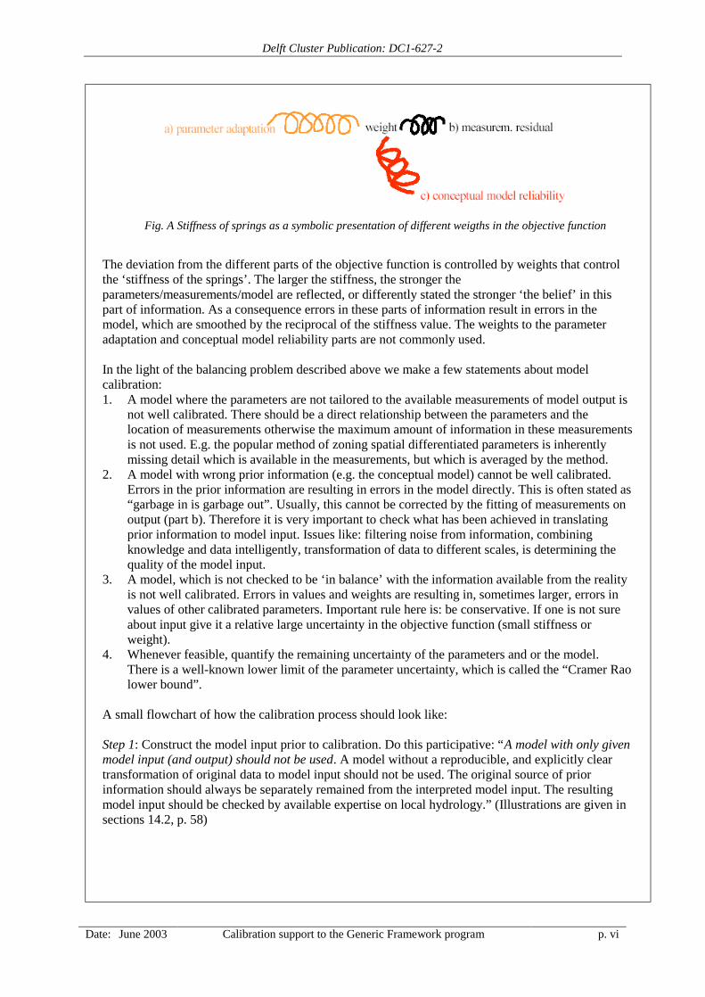
Fig. A Stiffness of springs as a symbolic presentation of different weigths in the objective function
The deviation from the different parts of the objective function is controlled by weights that controlthe ‘stiffness of the springs’. The larger the stiffness, the stronger theparameters/measurements/model are reflected, or differently stated the stronger ‘the belief’ in thispart of information. As a consequence errors in these parts of information result in errors in themodel, which are smoothed by the reciprocal of the stiffness value. The weights to the parameteradaptation and conceptual model reliability parts are not commonly used.
In the light of the balancing problem described above we make a few statements about modelcalibration:1. A model where the parameters are not tailored to the available measurements of model output is
not well calibrated. There should be a direct relationship between the parameters and thelocation of measurements otherwise the maximum amount of information in these measurementsis not used. E.g. the popular method of zoning spatial differentiated parameters is inherentlymissing detail which is available in the measurements, but which is averaged by the method.
2. A model with wrong prior information (e.g. the conceptual model) cannot be well calibrated.Errors in the prior information are resulting in errors in the model directly. This is often stated as“garbage in is garbage out”. Usually, this cannot be corrected by the fitting of measurements onoutput (part b). Therefore it is very important to check what has been achieved in translatingprior information to model input. Issues like: filtering noise from information, combiningknowledge and data intelligently, transformation of data to different scales, is determining thequality of the model input.
3. A model, which is not checked to be ‘in balance’ with the information available from the realityis not well calibrated. Errors in values and weights are resulting in, sometimes larger, errors invalues of other calibrated parameters. Important rule here is: be conservative. If one is not sureabout input give it a relative large uncertainty in the objective function (small stiffness orweight).
4. Whenever feasible, quantify the remaining uncertainty of the parameters and or the model.There is a well-known lower limit of the parameter uncertainty, which is called the “Cramer Raolower bound”.
A small flowchart of how the calibration process should look like:
Step 1: Construct the model input prior to calibration. Do this participative: “A model with only givenmodel input (and output) should not be used. A model without a reproducible, and explicitly cleartransformation of original data to model input should not be used. The original source of priorinformation should always be separately remained from the interpreted model input. The resultingmodel input should be checked by available expertise on local hydrology.” (Illustrations are given insections 14.2, p. 58)

Delft Cluster Publication: DC1-627-2
Date: June 2003 Calibration support to the Generic Framework program p. vii
Step 2: Check the prior model to serious mistakes by confronting it to the available measurements onoutput. We call this the ‘quest for mistakes in the (processing of) data’. Until the following checksare satisfied do this ‘by hand’, which means don’t use automatic calibration tools blindly (keepcontrol):
• Deviations between output and measurements divided by the corresponding weights (notrends, areas outside the 2*weights should be small);
• Deviations between prior and calibrated parameters;• Correct statistics of deviations between output and measurements (zero mean, residual sum
of squares equal to weights*[number of measurements - number of degrees of freedom], zerocorrelation between deviations and model output);
• No significant correlations between calibrated parameters;• Verification of model (model analysis checked by existing expertise of real system
behaviour, comparison with measurements of model output that is not used for calibration).In this stage it is important to ‘get the bias out’. Automatic tools are not used to fit as good aspossible, but to help the modeller doing the boring work of fitting quickly and efficiently and use theremaining time for thinking and analyzing. Goal is not to minimize deviations but to balance them inpositive and negative sense and to get them as uncorrelated as possible. We prefer larger errors abovebias. In this stage hydrological experience is most important to come to satisfiable solutions. (Forillustration see section 14.3.1, p.59)
Step 3: Final calibration with automatic tools. Do this for different combinations of weights in theobjective function. Make several optimized models. Make choices in participation with the users ofthe model. Think of the important rule: “be conservative. If one is not sure about input give it arelative large uncertainty in the objective function (small stiffness or weight).” Be sure that thestatistics are kept satisfiable while fitting with measurements. In this stage the goal is to fit as well aspossible but without producing erroneous parameters. Search for the point when one is ’living on theedge’ in order to squeeze out as much as detail out of the measurements while remaining in balancewith the given amount of information. (For illustration see sections 14.3.2 - 14.3.3)
Step 4 (optional): If feasible calculate the uncertainty of model parameters and model results. Theeasiest way is to do this by a sort of Monte Carle principle by running more than one possible model,just as given by the simple example in the previous section. In this case the range of the inputparameters determines the input uncertainty and ditto for the range of output results (this is notshown for the example in the previous section; but the reader can imagine that it is given implicitlyby the method). An analytical expression for the parameters uncertainty is given by the so called“Cramer Rao lower bound” which is depending on the squared expression of the linearized systembehaviour (represented by the system matrix A) and the inverse of the weights in the objectivefunction and which is given in most textbooks. Simply stated this Cramer Rao lower bound can beexplained by stating that the more coherence in the system behaviour and the less uncertainty in themeasurements, the more accurate model predictions are which makes sense intuitively. Using thisexpression for the parameters uncertainty the model output uncertainty can be calculated with MonteCarlo simulations or analytically by multiplying it with the system matrices again (see section 14.4,p.69).
PROJECT NAAM: Knowledge Based Support of theGeneric Framework Program PROJECT CODE: 06.02.07
BASISPROJECT NAAM: Water Systems BASISPROJECT CODE: 06.02
T H E M A N A A M : Integrated Water ResourcesManagement T H E M A C O D E : 06


Delft Cluster Publication: DC1-627-2
Date: June 2003 Calibration support to the Generic Framework program p. ix
Table of contents
Calibration Support to the Generic Framework program................................................................ 1
Abstract ......................................................................................................................................... iii
Executive Summary .............................................................................................................................. v
Preface .......................................................................................................................................... 1
PART I: Identification of needs to support calibration ..................................................................... 3
1 The need for calibration ............................................................................................................. 51.1 Why calibrate ? ................................................................................................................... 51.2 Typical context of a model study........................................................................................ 51.3 This part .............................................................................................................................. 5
2 Need for calibration support ...................................................................................................... 62.1 Different types of users....................................................................................................... 62.2 User wants guidance ........................................................................................................... 62.2.1 Analysis .............................................................................................................................. 62.2.2 Recommendation ................................................................................................................ 62.3 User wants software connectivity between models and calibration toolboxes ................... 72.3.1 Analysis .............................................................................................................................. 72.3.2 Recommendations............................................................................................................... 8
PART II: Using global optimisation algorithms in calibration........................................................ 9
3 Introduction............................................................................................................................... 113.1 Approaches to calibration ................................................................................................. 113.2 Calibration as an optimization problem............................................................................ 11
4 Approaches to solving optimization problems........................................................................ 13
5 Main approaches to global optimisation ................................................................................. 14
6 A tool for selecting calibration algorithms.............................................................................. 18
7 Comparing nine algorithms for calibration............................................................................ 19
8 Discussion................................................................................................................................... 22
9 Conclusions ................................................................................................................................ 23
References ........................................................................................................................................ 24
Delft Cluster Publication: DC1-627-2
Date: June 2003 Calibration support to the Generic Framework program p. x
PART III: Calibration of groundwater flow models....................................................................... 27
10 Introduction............................................................................................................................... 29
11 Vision of TNO-NITG ................................................................................................................ 30
12 State-of-the-art of calibration methodology ........................................................................... 3212.1 Key issues ......................................................................................................................... 3212.2 ‘Cookbook’ ....................................................................................................................... 3812.3 Algorithms ........................................................................................................................ 3912.3.1Self-calibrating method..................................................................................................... 3912.3.2Method of ‘representers’................................................................................................... 39
13 Methods that calibrate and parameterize ................................................................................ 4113.1 Self-calibrating method..................................................................................................... 4113.1.1Steps of the self-calibration method (SCM) algorithm..................................................... 4113.1.2The generation of a transmissivity field conditional to measured transmissivity data ..... 4113.1.3Penalty function ................................................................................................................ 4113.1.4Optimisation...................................................................................................................... 4213.1.5Parameterisation................................................................................................................ 4213.1.6Selecting the locations of the master points...................................................................... 4213.1.7Conclusion ........................................................................................................................ 4313.2 Representer method .......................................................................................................... 4313.2.1Motivation......................................................................................................................... 4313.2.2Theory............................................................................................................................... 4413.2.3Two dimensional x-z example .......................................................................................... 47
14 Real world cases to illustrate ‘cookbook’................................................................................ 5614.1 The ‘Veluwe’ case ............................................................................................................ 5614.1.1Short description ............................................................................................................... 5614.1.2Available input data .......................................................................................................... 5614.2 The ‘Shell Pernis’ case...................................................................................................... 5814.2.1Short description ............................................................................................................... 5814.2.25.2.2 Available input data ................................................................................................. 5814.3 Building the primary version of a model .......................................................................... 5914.3.1Filtering noise from information....................................................................................... 5914.3.2Combining data into best model input .............................................................................. 6114.3.3Transforming data to best model input ............................................................................. 6614.4 Calibration procedure of the Veluwe model ..................................................................... 6914.4.1Search for errors in the initial groundwater model ........................................................... 6914.4.2Sensitivity analysis............................................................................................................ 6914.4.3Correlation between model parameters............................................................................. 7114.4.4Parameter optimization ..................................................................................................... 7214.4.5Residuals ........................................................................................................................... 7314.5 Quantification and use of model uncertainty case Shell Pernis ........................................ 8114.5.1Optimisation...................................................................................................................... 8114.5.2Results of optimisation ..................................................................................................... 82

Delft Cluster Publication: DC1-627-2
Date: June 2003 Calibration support to the Generic Framework program p. xi
14.5.3Designing a monitoring network using uncertainty estimation ........................................ 84
References ........................................................................................................................................ 86
Delft Cluster Publication: DC1-627-2
Date: June 2003 Calibration support to the Generic Framework program p. xii
List of Figures
Fig. A Stiffness of springs as a symbolic presentation of different weigths in the objective function...vi
PART II: Using global optimisation algorithms in calibration
Figure 5-1 ACCO algorithm..................................................................................................................16Figure 7-1Typical examples of the minimization proces (averaged on 5 runs) for two hydrological
conceptual rainfall-runoff models (Sugawara-type tank model SIRT), and the distributedmodel ADM..............................................................................................................................20
PART III: Calibration of groundwater flow models
Figure 11-1 Vision of TNO-NITG how to combine information with modelling.................................30Figure 12-1 Stiffness of springs as a symbolic presentation of the different weights in the objective
function.....................................................................................................................................32Figure 12-2 Simple example with flow from left to right through a variable T-field ...........................33Figure 12-3 The groundwater head is measured at some points ...........................................................33Figure 12-4 Possible transmissivity fields on the basis of 2 known T-values.......................................34Figure 12-5 Calibrated transmissivities (pink) and prior transmissivities (blue) ..................................34Figure 12-6 Location of head measurements and their deviations before (yellow) and after calibration
(blue)) .......................................................................................................................................35Figure 12-7 Instability in calibrated transmissivities (pink lines in outlined light-blue areas) because of
too much detail in parameterization .........................................................................................35Figure 12-8 Calibration with a wrong measurement in the middle; the calibrated transmissivity fields
(pink) are becoming erroneous too (pink ‘hat’ in the middle of the cross-section)..................36Figure 12-9 As in Figure 12-8 but with smaller weight for the wrong measurements (pink ‘hat’ is
deminished). .............................................................................................................................36Figure 12-10 Instability in calibrated transmissivity (brown line) because of neglecting small model
errors in recharge. .....................................................................................................................37Figure 12-11 As Figure 12-10 but now the model error is reflected in smaller weight of the model part
in objective function (blue line) or when the model error is overestimated (yellow line)........37Figure 12-12 Parameterization using SCM for the simple example......................................................39Figure 13-1 Optimisation procedure of SCM........................................................................................43Figure 13-2 Optimisation procedure with representers .........................................................................45Figure 13-3 Visualisation of the update with representers; example containing the modelling of
concentrations...........................................................................................................................46Figure 13-4 Schematised situation of groundwater flow.......................................................................48Figure 13-5 Initial mobile concentrations [g/l]......................................................................................48Figure 13-6 Synthetic natural logarithms of the conductivities.............................................................48Figure 13-7 Real groundwater heads.....................................................................................................49Figure 13-8 Synthetic mobile concentrations at end of simulation .......................................................49Figure 13-9 Prior (gray scaled areas) and real (solid line) head distribution ........................................50Figure 13-10 Prior (gray scaled areas) and real (solid line) mobile concentration at end of simulation50Figure 13-11 Representer of the natural logarithm of the conductivities for head measurement at x,z =
(80,3). .......................................................................................................................................51Figure 13-12 Head representer for head measurement at x,z = (80,3) ..................................................51Figure 13-13 Mobile concentration representer at 400 days for head measurement at x,z = (80,3). ....52Figure 13-14 Representer of the natural logarithm of the conductivities for mobile concentration
measurement at x,z = 20,3 and t = 400 days.............................................................................52Figure 13-15 Head representer for mobile concentration measurement at x,z = 20,3 and t = 400 day.52Figure 13-16 Concentration representer at 400 days for a concentration measurement at x,z = 20,3 and
t = 400 days ..............................................................................................................................53Figure 13-17 Evolution of objective function .......................................................................................53
Delft Cluster Publication: DC1-627-2
Date: June 2003 Calibration support to the Generic Framework program p. xiii
Figure 13-18 Posterior (gray scaled areas) and real (solid line) head distribution; the asterisks denotethe locations of the head measurements ...................................................................................54
Figure 13-19 Posterior (gray scaled areas) and real (solid line) concentration distribution at the end ofthe simulation; the asterisks denote the locations of the concentration measurements ............54
Figure 13-20 Posterior natural logarithm of the conductivities.............................................................54Figure 13-21 Difference between real and posterior natural logarithm of the conductivities ...............55Figure 13-22 Posterior estimates of variance of natural logarithm of the conductivities......................55Figure 13-23 Histogram of normalised differences between real and posterior natural logarithm of the
conductivities; solid line denotes a normal distribution ...........................................................55Figure 14-1 Regional cross-section of the industrial terrain .................................................................58Figure 14-2 Geological cross-sections of the terrain, including the location of the sandy gullies ........59Figure 14-3 Part of the AHN database in the Regge and Dinkel area...................................................60Figure 14-4 Averaged AHN data base on a 25 m grid (so every pixel is an average of 5x5 original
data points) ...............................................................................................................................60Figure 14-5 Filtered AHN data base on a 25 m grid .............................................................................61Figure 14-6 Random spotting of stage in the watercourse or the watershed/border of the water course62Figure 14-7 Finally used hydrological AHN data base that is used to construct model input ..............62Figure 14-8 Profile of the Nuenen group near Best (x-z = 100 times 25 m) .........................................63Figure 14-9 Simulated profile of the Nuenen group near Best (same x-z = 100 times 25 m) together
with calculated heads and flowlines .........................................................................................63Figure 14-10 100 Simulated profiles of the Nuenen group near Best (x-z = 100 times 25 m) .............64Figure 14-11 100 Calculated flow lines belonging to profiles of Figure 14-8 ......................................64Figure 14-12 Relationship between fraction of sand and c-value for Nuenen formation .....................65Figure 14-13 Borehole information about fraction of sand combining with relationship with c-value 65Figure 14-14 Map of c-values ...............................................................................................................66Figure 14-15 Correction factor for stage of water course when bold grid cell size is used .................66Figure 14-16 A response time: number of years after which 85% of the effect of a model wide
increase of the net recharge has been realized..........................................................................67Figure 14-17 Model sensitivity for change of transmissivities; red: calculated head decrease, blue:
increase, as result of a fractional increase of the transmissivity per model layer .....................70Figure 14-18 Model sensitivity for change of vertical transmissivities of the separating aquitards; red:
calculated head decrease, blue: increase, as result of a fractional increase of the verticalhydraulic conductivity per model layer ....................................................................................71
Figure 14-19 Competition between a transmissivity value (kD-meting) and a head measurement(gemeten grondwaterstand) ......................................................................................................72
Figure 14-20 Histogram of residuals .....................................................................................................73Figure 14-21 Residuals of layer 1..........................................................................................................74Figure 14-22 Residuals of layer 2..........................................................................................................75Figure 14-23 Residuals of layer 3..........................................................................................................76Figure 14-24 Residuals of layer 4..........................................................................................................77Figure 14-25 Residuals of layer 5..........................................................................................................78Figure 14-26 Transmissivities and resistances after parameter optimization........................................79Figure 14-27 Calculated fluxes of the primairy, secundaire and tertairy system, the large canals and
rivers, and between the modellayers (mm/day) ........................................................................79Figure 14-28 Part of the model area in which surface and groundwater is believed to drain to the
Apeldoorns kanaal ....................................................................................................................80Figure 14-29 Piezometric heads before calibration of all 16 version of the groundwater model. Values
and locations of measured piezometric heads are indicated as classified dots .........................83Figure 14-30 Piezometric heads after calibration of all 16 version of the groundwater model. Values
and locations of measured piezometric heads are indicated as classified dots .........................83Figure 14-31 Multiplication factor of horizontal hydraulic conductivities being the a-priori values
divided by the calibrated values ...............................................................................................84Figure 14-32 Relation between the number of piezometric head measurements and the uncertainty of
the modelpredictions (calculated piezometric heads)...............................................................85

Delft Cluster Publication: DC1-627-2
Date: June 2003 Calibration support to the Generic Framework program p. xiv
List of Tables
PART II: Using global optimisation algorithms in calibration
Table 7-1 Functions used in comparing algorithms ..............................................................................19Table 14-1 Geohydrological schematisation of the model area of the terrain.......................................59Table 14-2 Number of observation filters per model layer ...................................................................68Table 14-3 Correlation between model parameters [-]..........................................................................72Table 14-4 A-priori average value of the conductivities .......................................................................81
Delft Cluster Publication: DC1-627-2
Date: June 2003 Calibration support to the Generic Framework program p. 1
PrefaceIn the Dutch context, modelling and simulation plays a major to support proper decision making inintegrated water resources management issues. In the last few years, various institutes active in theDutch water sector, have initiated the so-called Generic Framework Water programme, with the aimto developed a joint model infrastructure for water management [Blind et al. 2000]. This programmefocused on issues such as:
• Good Modelling Practice (quality assurance for modelling studies)• a Generic Framework for model linkage (software architecture and implementation)l• an Umbrella Agreement for sharing models and data.
The Delft Cluster-project “Kennisinhoudelijke aanvulling Standaard Raamwerk” (DC-project06.02.07) contributes to this programme by amongst others by investigating the needs for calibrationsupport within this Generic Framework programme.
Part I identifies the different needs to improve the calibration of water related modelling. It includesrecommendations to improve the applicability of available techniques and guidance on the process ofcalibration. Some recommendations have been picked up in Part II and Part III. Part II addresses theavailability of global optimization techniques for calibration, while Part III provides a cookbook howto apply calibration techniques in the practice of groundwater flow models.

Delft Cluster Publication: DC1-627-2
Date: June 2003 Calibration support to the Generic Framework programPart I: Identification of needs to support calibration
p. 3
Title: PART I: Identification of needs to support calibration
Author: P.J.A. Gijsbers Institute: WL delft hydraulics & TU Delft - CiTG
June 2003Number of pages : 4
Keywords (3-5) : model, calibration, support needs, Generic Framework

Delft Cluster Publication: DC1-627-2
Date: June 2003 Calibration support to the Generic Framework programPart I: Identification of needs to support calibration
p. 5
1 The need for calibration
1.1 Why calibrate ?The “ultimate goal of calibration is to make the model as reliable as possible, given the availableinformation. This means that information on model input (prior information) as well as information onmodel output (used for calibration) is used as good as possible. In mathematical terms this is the fieldof data-assimilation. If the prior information is used wrong, it is not possible to calibrate well. If thecalibration is done wrong (limited to the objective to fit the model output to measurements instead ofreducing uncertainty of model input), the value of prior information can be destroyed instead ofimproved.” (see Part III: p.29)
Or, very straightforward, the objective of calibration is “to reduce the uncertainty in a model”.
1.2 Typical context of a model studyMany ‘consultancy’ type model studies often can be characterized by the fact that models (and modelengines) incorporate detailed process description, which require many state variables and many (oftentoo many) model parameters. The data side often can be characterized prior information (e.g. surveydata), which is not always easy to express in system variables, spatial and temporal uncertainty due tolimited data samples, spatial gradients which are difficult to capture, limited monitoring data that canbe used for calibration and validation purposes etc.
In other words, modellers face problems with:• limited information content in the data.• highly correlated parameters or easy interchangeable parameters or parameter sets• large uncertainty contours• ill-defined systems• ill-support in terms of guidance (what to do/how to do);• ill-support in connectivity between models and tools
To develop a sound model given those difficult circumstances, expert judgement is still highly valued.In Part III, Minnema & te Stroet indicate that parameter estimation software or calibration tools canonly do a (small, but tedious) part of the job.
1.3 This partPart I of this report discusses in brief the recommendations for development of calibration supportfunctionality. On the one hand, the recommendations are based on the practical needs of the modelbuilder, which faces practical questions when he has to calibrate a model. On the other hand, therecommendations are formulated from a software technical perspective in order to create supportingtools, which are in line with a Generic Framework type of modelling environment.
The contents of Part I has been based on a workshop organised within the context of this DC-project,extended with results from discussions with partners in the Generic Framework programme andsimilar type of European research projects. The workshop, held within the context of this DC-projectwas workshop attended by experts from various domains such as groundwater, unsaturated zone,water quality, mathematical techniques, coming from various types of organisations (researchinstitutes, consultants, universities).
Delft Cluster Publication: DC1-627-2
Date: June 2003 Calibration support to the Generic Framework programPart I: Identification of needs to support calibration
p. 6
2 Need for calibration supportCalibration support needs to address both the knowledge/expertise part as well as the ease of use ofmathematical techniques in combination with the (integrated) modelling system. Different types ofusers do, however, require different types of support, which requires that support tools need to bededicated to their job.
2.1 Different types of usersIn general various types of modellers can be distinguished, where the largest difference is betweenresearch-oriented modellers and consultancy-oriented modellers. Research-oriented modellers oftendo their job with research software, which allows them to modify or intervene with the model code.This makes it easy to adapt the code where needed for interaction with standard calibration softwaretools (e.g. PEST).
Consultancy-oriented modellers tend to do their job with commercial or semi-commercial code (e.g.hydraulics and water quality), although some domains (e.g. groundwater) are highly based on public-domain model code, often encapsulated in a semi-commercial interface. These codes may have build-in calibration facilities. If not, some dedicated programming work might be needed to exchange databetween the model and the calibration algorithm. Few times, the existing codes already have createdaccessibility to the parameter set most commonly used for calibration.
2.2 User wants guidance
2.2.1 AnalysisUsers would like to have guidance. Quite some guidance documents have been written on calibrationin the various single domains (e.g. hydrological modelling, groundwater modelling, water qualitymodelling). However, seldom these documents pay attention to practical questions such as:
• data needs (prior and post) (per domain)• step-by-step description (per domain, maybe even code-specific)• valid parameter ranges (per domain)• what uncertainty ranges are acceptable• what type of formulations to choose for objective function and constraints (per domain)• what mathematical techniques (and tools) are suitable (per domain/model code), and what are
their pro’s and con’s ?• what tools are available for visualisation and assessment
In addition hardly any available literature pays attention to specific questions related to integratedmodelling such as:
• how to calibrate a 1-way model chain (i.e. a chain in which all matter propagates in onedirection)
• how to do a calibrate of a 2-way interacting model chain
Preferably this guidance is well organised and accessible in such way that different types of users gettailored access to the information resources needed.
2.2.2 Recommendation
Efforts in this field should focus upon:1. inventory of available guidance2. filling the gaps where needed

Delft Cluster Publication: DC1-627-2
Date: June 2003 Calibration support to the Generic Framework programPart I: Identification of needs to support calibration
p. 7
3. improving access to guidance
Efforts should not be put in:• rewriting existing guidance documents without adding new information
Inventory of available guidanceThis inventory should be based on a structure, which can contain:
• references to find the guidance source (i.e. author, title etc., URL etc.)• listing the domain(s) covered• listing the methods covered• indicating the type of readers audience• indicating the guidance topics covered• indicating the rate of applicability (i.e. some kind of quality/advice)
Based on an extensive search effort in libraries and the web, this inventory can be filled. The lastbullet requires a review to assess the applicability of this guidance document. Part II of this report, bySolomatine, contributes to the inventory and comparison of methodologies available for application.
Filling the gaps where neededIt can be expected that not all desired aspects are well covered. Especially, the integrated or multi-domain relations will be missing. These pieces of guidance, as well as extensions of existing guidancedocuments, need to be prepared by a small team of experts and discussed in a wider audience. Part IIIof this report, by te Stroet and Minnema, contributes to guidance by providing a cookbook forcalibration of groundwater models. This part is to be considered a refinement of the Good ModellingPractice.
Improving the access to guidanceImproving the access to guidance can be achieved in several ways. Examples are:
• a web-accessible searchable database of the inventory with guidance documents (a clearinghouse); this database may even contain the documents in a digital format; or
• an easy accessible knowledge base, in which all guidance documents are transformed into anorganized structure (or onthology) which enables combination and display of informationaccording to the type of user, type of domain (or domain combination) etc .
2.3 User wants software connectivity between models and calibration toolboxes
2.3.1 Analysis
Automated calibration and uncertainty analysis often leads to better results than manual ‘trial anderror’ efforts. Some model-codes provide build in functionality for these type of activities, either byincorporating User Interaction for manual calibration of by means of built-in automated calibrationtools. In other situations, stand alone parameter optimisation tools may be a suitable choice. Manytoolkits or code-libraries exist for this purpose, one of the best known being PEST. However, productssuch as Matlab also offer automated calibration toolkits, while many research groups have developedtheir own codes, e.g. GLOBE (see Part III).
Basically, two options are available to work with stand-alone calibration tools:1. develop a tight coupling by integrating the toolkit into the model code2. develop a loose coupling by only accessing the data (i.e. providing new parameter input) andinvoking the simulation engineOption 1 requires access to the model code. Option 2 requires a model code that is sufficient ‘open’with regard to model input and invocation/control of the computation.

Delft Cluster Publication: DC1-627-2
Date: June 2003 Calibration support to the Generic Framework programPart I: Identification of needs to support calibration
p. 8
Typically, option 1 is only applicable in a research context, as many consultants work with(semi)commercial software for which they don’t have access to the code.
Finally, to get more grip on the assessment/outcome, appropriate visualisation tools are welcome.Again, if this is not provided by built in functionality, the model code should be able to produceappropriate data and provide access to it.
2.3.2 RecommendationsTo simplify the calibration efforts of the modelling community dealing with integrated watermanagement, effort should be put the following items:
1. improve loose coupling connectivity between existing model-codes and existingcalibration tools and libraries:• develop an architecture/public interface with clear mechanisms to link models to
calibration tools;• open up model codes to meet this interface (i.e. accepting of externally provided data
and external invocations);• if needed adapt or wrap existing calibration tools/libraries so they can meet this
interface too and interact with the models;2. improve validation features of model codes (e.g. mass balance checks);
• identify relevant validation methods for each model type/domain• define a public interface to invoke these methods and obtain results• implement the associated algorithms and checks
3. improve post processing and presentation features dedicated to the type of questions facedduring calibration (e.g. aggregation functions, present 30 best runs, uncertainty data, massbalances, fluxes).• develop an architecture and associated public interfaces to:
o get access to produced data;o process this data into information answering the questions of end-users, and;o display this data in an user-friendly way
• implement code according to the architecture to create functionality dedicated to theanalysis of calibration (and uncertainty assessment) results
Effort should not (yet) be put in development of new calibration techniques

Delft Cluster Publication: DC1-627-2
Date: June 2003 Calibration support to the Generic Framework programPart II: Using global optimization algorithms in calibration
p. 9
Title: PART II:Using global optimisation algorithms in calibration
Author: D.P. Solomatine Institute: IHE
June 2003Number of pages : 16
Keywords (3-5) : global optimization, calibration

Delft Cluster Publication: DC1-627-2
Date: June 2003 Calibration support to the Generic Framework programPart II: Using global optimization algorithms in calibration
p. 11
3 Introduction
3.1 Approaches to calibrationA model is a simplified description of reality. It can be seen as a function depending on parameters Pand linking input X with the output Y:
Y = f (X, P)
The problem of finding appropriate P is the one of calibration and it is one of the crucial to solve forthe successful modelling. Calibration is tuning the parameters’ values of a model in such a way thatdifference (error) E between the calculated output and the observed one is minimal. This allows us tosay that the problem of calibration is basically an optimization model with the variables P and theobjective function E(P). The error function could be calculated in different ways; one of the widelyaccepted is the root mean square error.
There are several approaches to calibration:• trial-and-error, when parameters are changed by a modeller, results of model runs are
observed, error calculated, new changes to the model are made, etc.;• inverse modelling when an “inverse model” is built allowing to identify optimal parameters
analyically. This approach is only possible when the structure (equations) of the model areknown analytically and satisfy some strict conditions (like differentiability);
• using direct optimization when the model is run according to some algorithm, for each run theerror value is calculated the results are used to arrive to an optimal values of parameters P.This approach can use different methods to solve the optimization problem where the mostgeneral approach is treat the problem as a multi-extremum (global) optimization problem.
In this part of the report the third approach is considered.
3.2 Calibration as an optimization problem
Many issues related to water resources require the solution of optimization problems. These includereservoir optimization, problems of optimal allocation of resources and planning, calibration ofmodels, and many others. Traditionally, optimization problems were solved using linear and non-linear optimization techniques which normally assume that the minimized function (objectivefunction) is know in analytical form and that it has a single minimum. (Without a loss of generalitywe will assume that the optimization problem is minimization problem).
In practice, however there are many problems that cannot be described analytically and manyobjective functions have multiple extrema. In these cases it is necessary to pose multi-extreme(global) optimization problem (GOP) where the traditional optimization methods are not applicable,and other solutions must be investigated. One of these typical GOPs is that of automatic modelcalibration, or parameter identification. The objective function is then the discrepancy between themodel output and the observed data, i.e. the model error, measured normally as the weighted RMSE.One of the approaches to solve GOPs that has become popular during the recent years is the use of theso-called genetic algorithms (GAs) [Goldberg 1989, Michalewicz 1996]. A considerable number ofpublications related to water-resources are devoted to their use [Wang 1991, Babovic et al. 1994,Cieniawski 1995, Savic & Walters 1997, Franchini & Galeati 1997]. (Evolutionary algorithms (EA)are variations of the same idea used in GAs, but were developed by a different school. It is possible tosay that EAs include GAs as a particular case).

Delft Cluster Publication: DC1-627-2
Date: June 2003 Calibration support to the Generic Framework programPart II: Using global optimization algorithms in calibration
p. 12
Other GO algorithms are used for solving calibration problems as well [Duan et al., 1993, Kuczera1997], but GAs seem to be preferred. Our experience however, shows that many practitioners areunaware of the existence of other GO algorithms that are more efficient and effective than GAs. Thisserves as a motivation for writing this article, which has the following main objectives:- to classify and briefly describe GO algorithms;- to demonstrate the relative performance of several GO algorithms, including GAs, on a suiteof problems, including model calibration;- to give some recommendations to practitioners dealing with calibration whose problem isformulated as a GOP.
Delft Cluster Publication: DC1-627-2
Date: June 2003 Calibration support to the Generic Framework programPart II: Using global optimization algorithms in calibration
p. 13
4 Approaches to solving optimization problems
A global minimization problem with box constraints is considered: find an optimizer x* such thatgenerates a minimum of the objective function f (x) where x0X and f (x) is defined in the finite interval(box) region of the n-dimensional Euclidean space: X = x0Rn: a#x#b (component wise). Thisconstrained optimization problem can be transformed to an unconstrained optimization problem byintroducing the penalty function with a high value outside the specified constraints. In cases when theexact value of an optimizer cannot be found, we speak about its estimate and, correspondingly, aboutits minimum estimate.Approaches to solving this problem depend on the properties of f(x):
1. f(x) is a single-extreme function expressed analytically. If its derivatives can be computed,then gradient-based methods may be used: conjugate gradient methods; quasi-Newton orvariable metric methods, like DFP and BFGS methods [Jacobs 1977, Press et al. 1991]. Incertain particular cases, e.g. in the calibration of complex hydrodynamic models, if someassumptions are made about the model structure and/or the model error formulation, thenthere are several techniques available (like inverse modelling) that allow the speeding up ofthe solution [Van den Boogaard et al., 1993]. Inverse modelling is used in the USGS toolUCODE, tuned for calibration of a groundwater model MODFLOW (called MODFLOWP),see [Methods 1998].Many engineering applications use minimization techniques for single-extreme functions, butoften without investigating whether the functions are indeed single-extreme (uni-modal).They do recognize however, the problem of the Agood@ initial starting point for the searchof the minimum. Partly, this can be attributed to the lack of the wide awareness of theengineering community of the developments in the area of global optimization.
2. f(x) is a single-extreme function which is not analytically expressed. The derivatives cannotbe computed, and direct search methods can be used such as Nelder & Mead [1965]. Apartfrom that, the methods were developed that are based on the derivative-based methods of non-linear optimization but which however instead of analytically calculating derivatives use theirestimates. One of these is the so-called DUD algorithm [Ralston and Jennrich 1978].
3. No assumptions are made about the properties of f(x), so it is a multi-extreme function whichis not expressed analytically, and we have to talk about multi-extreme or global optimization.Most calibration problems belong to the third category of GO problems. At certain stages theGO techniques may use the single-extreme methods from category 2 as well.
Delft Cluster Publication: DC1-627-2
Date: June 2003 Calibration support to the Generic Framework programPart II: Using global optimization algorithms in calibration
p. 14
5 Main approaches to global optimisation
The reader is referred to Torn & Filinskas [1989], Pintér [1995] for an extensive coverage of variousmethods. It is possible to distinguish the following groups:• set (space) covering techniques;• random search methods;• evolutionary and genetic algorithms (can be attributed to random search methods);• methods based on multiple local searches (multi-start) using clustering;• other methods (simulated annealing, trajectory techniques, tunnelling approach, analysis methods
based on a stochastic model of the objective function).Several representatives of these groups are covered below.
Set (space) covering methods. In these the parameter space X is covered by N subsets X1,...,XN, suchthat their union covers the whole of X. Then the objective function is evaluated in N representativepoints x1, ..., xN, each one representing a subset, and a point with the smallest function value is takenas an approximation of the global value. If all previously chosen points x1, ..., xk and function valuesf(x1), ..., f(xk) are used when choosing the next point xk+1, then the algorithm is called a sequential(active) covering algorithm (and passive if there is no such dependency). These algorithms werefound to be inefficient.
The following algorithms belong to the group of random search methods.Pure direct random search (uniform sampling). N points are drawn from a uniform distribution inX and f is evaluated in these points; the smallest function value is the minimum f* assessment. If f iscontinuous then there is an asymptotic guarantee of convergence, but the number of functionevaluations grows exponentially with n. An improvement is to make the generation of evaluationpoints in a sequential manner taking into account already known function values when the next pointis chosen, producing thus an adaptive random search [Pronzato et al. 1984].
Controlled random search (CRS) is associated with the name of W.L.Price who proposed severalversions of an algorithm where the new trial point in search (parameter) space is generated on thebasis of a randomly chosen subset of previously generated points; the widely cited method is CRS2[Price 1983]. At each iteration, a simplex is formed from a sample and a new trial point is generatedas a reflection of one point in the centroid of the other points in this simplex. If the worst point in theinitially generated set is worse than the new one, the latter replaces it. The ideas of CRS algorithmshave been further extended by Ali and Storey [1994a] producing CRS4 and CRS5. In CRS4 if a newbest point is found, it is Arewarded@ by an additional search around it by sampling points from thebeta-distribution. This method is reportedly very efficient and was used for example for calibratingthe model of the Oosterschelde ecosystem [Scholten and van der Tol, 1994].
Evolutionary strategies and genetic algorithms. The family of evolutionary algorithms is based onthe idea of modelling the search process of natural evolution, though these models are crudesimplifications of biological reality. Evolutionary algorithms (EA) are variants of randomized search,and use the terminology from biology and genetics. For example, given a random sample at eachiteration, pairs of parent individuals (points), selected on the basis of their >fit= (function value),recombine and generate new >offspring=. The best of these are selected for the next generation.Offspring may also >mutate= that is randomly change their position in space. The idea is that fitparents are likely to produce even fitter children. In fact, any random search may be interpreted interms of biological evolution: generating a random point is analogous to a mutation, and the stepmade towards the minimum after a successful trial may be treated as a selection.Historically, evolution algorithms have been developed in three variations - evolution strategies (ES),evolutionary programming (EP), and genetic algorithms (GA). Back & Schwefel [1993] give an
Delft Cluster Publication: DC1-627-2
Date: June 2003 Calibration support to the Generic Framework programPart II: Using global optimization algorithms in calibration
p. 15
overview of these approaches, which differ mainly in the types of mutation, recombination andselection operators. In GA, the binary coding of coordinates is introduced, so that an l-bit binaryvariable is used to represent integer code of one coordinate xi, with the value ranging from 0 to 2l-1that can be mapped into the real-valued interval [ai,bi]. An overall binary string G of length nl called achromosome is obtained for each point by connecting the codings of all coordinates. The mutationoperator changes a randomly chosen bit in the string G to its negation. The recombination (orcrossover) operator is applied as follows: select two points (parents) S and T from the populationaccording to some rule (e.g., randomly), select a number ρ (e.g., randomly) between 1 and nl, andform either one new point S', or two new points S' and T', by taking left-hand side bits of coordinatevalues from the first parent S, and right-hand side bits from the other parent T.There are various versions of GA varying in the way crossover, selection and construction of the newpopulation is performed. In evolutionary strategies (ES), mutation of coordinates is performed withrespect to corresponding variances of a certain n-dimensional normal distribution, and variousversions of recombination are introduced. On GAs applications see, e.g., Wang [1991], Babovic et al.[1994], Cieniawski [1995], Savic & Walters [1997], Franchini & Galeati [1997].
Multi-start and clustering. The basic idea of the family of multi-start methods is to apply a searchprocedure several times, and then to choose an assessment of the global optimizer. One of the popularversions of multi-start used in global optimization is based on clustering, that is creating groups ofmutually close points that hopefully correspond to relevant regions of attraction of potential startingpoints [Torn & Filinskas 1989]. The region (area) of attraction of a local minimum x* is the set ofpoints in X starting from which a given local search procedure P converges to x*. For the globaloptimization tool GLOBE used in the present study, we developed two multistart algorithms - Multisand M-Simplex. They are both constructed according to the following pattern:
1. Generate a set of N random points and evaluate f at these points.2. (reduction). Reduce the initial set by choosing p best points (with the lowest fi).3. (local search). Launch local search procedures starting from each of p points. The best point
reached is the minimizer assessment.In Multis, at step 3 the Powell-Brent local search [see Powell 1964, Brent 1973, Press et al., 1991] isstarted. In M-Simplex the downhill simplex descent of Melder & Nead [1965] is used.The ACCO strategy developed by the author and covered below also uses clustering as the first step,but it is followed by the global randomized search, rather than local search.
Adaptive cluster covering (ACCO) [Solomatine 1995, 1998] is a workable combination of generallyaccepted ideas of reduction, clustering and covering.
1. Clustering. Clustering (identification of groups of mutually close points in search space) isused to identify the most promising sub-domains in which to continue the global search byactive space covering.
2. Covering shrinking sub-domains. Each sub-domain is covered randomly. The values of theobjective function are then assessed at the points drawn from the uniform or some otherdistribution. Covering is repeated multiple times and each time the sub-domain isprogressively reduced in size.
3. Adaptation. Adaptive algorithms update their algorithmic behaviour depending on the newinformation revealed about the problem. In ACCO, the sub-region of search is adapted byshifting, then shrinking, and finally changing the density (number of points) of each covering,- depending on the previous assessments of the global minimizer.
4. Periodic randomization. Due to the probabilistic character of points generation, any strategyof randomized search may simply miss a promising region for search. In order to reduce thisdanger, the initial population is re-randomized, i.e. the problem is solved several times.
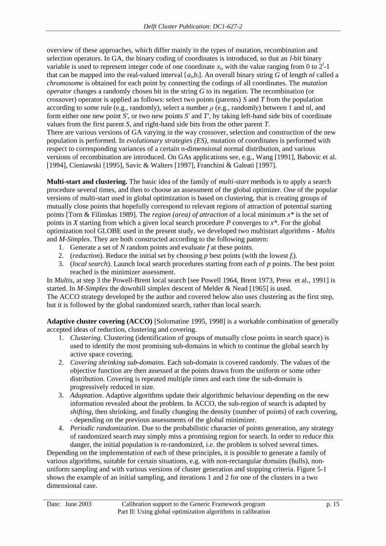
Depending on the implementation of each of these principles, it is possible to generate a family ofvarious algorithms, suitable for certain situations, e.g. with non-rectangular domains (hulls), non-uniform sampling and with various versions of cluster generation and stopping criteria. Figure 5-1shows the example of an initial sampling, and iterations 1 and 2 for one of the clusters in a twodimensional case.
Delft Cluster Publication: DC1-627-2
Date: June 2003 Calibration support to the Generic Framework programPart II: Using global optimization algorithms in calibration
p. 16
Figure 5-1 ACCO algorithm
ACCOL strategy is the combination of ACCO with the multiple local searches:1. ACCO phase. ACCO strategy is used to find several regions of attraction, represented by the
promising points that are close (such points we will call >potent=). The potent set P1 isformed by taking one best point found for each cluster during progress of ACCO. AfterACCO stops, the set P1 is reduced to P2 by leaving only several m (1...4) best points whichare also distant from each other, with the distance at each dimension being larger than, forexample, 10% of the range for this dimension;
2. Local search (LS) phase. An accurate algorithm of local search is started from each of thepotent points of P2 (multi-start) to find accurately the minimum; a version of the Powell-Brentsearch is used.
Experiments have shown, that in comparison to traditional multi-start, ACCOL brings significanteconomy in function evaluations.
ACD algorithm [Solomatine 1998] is also a random search algorithm, and it combines ACCO withthe downhill simplex descents (DSD) of Nelder & Mead [1965]. Its basic idea is to identify the areaaround the possible local optimizer by using clustering, and then to apply covering and DSD in thisarea. The main steps of ACD are:
• sample points (e.g., uniformly), and reduce the sample to contain only the best points;• cluster points, and reduce clusters to contain only the best points;• in each cluster, apply the limited number of steps of DSD to each point, thus moving them
closer to an optimizer;• if the cluster is potentially >good' that is contains points with low function values, cover the
proximity of several best points by sampling more points, e.g. from uniform or betadistribution;
• apply local search (e.g., DSD, or some other algorithm of direct optimization) starting fromthe best point in >good= clusters. In order to limit the number of steps, the fractional

Delft Cluster Publication: DC1-627-2
Date: June 2003 Calibration support to the Generic Framework programPart II: Using global optimization algorithms in calibration
p. 17
tolerance is set to be, say, 10 times greater than the final tolerance (that is, the accuracyachieved is somewhat average);
• apply the final accurate local search (again, DSD) starting from the very best point reached sofar; the resulting point is the assessment of the global optimizer.
ACDL algorithm, combining ACD with the multiple local searches, has been built and tested as well.
Delft Cluster Publication: DC1-627-2
Date: June 2003 Calibration support to the Generic Framework programPart II: Using global optimization algorithms in calibration
p. 18
6 A tool for selecting calibration algorithms
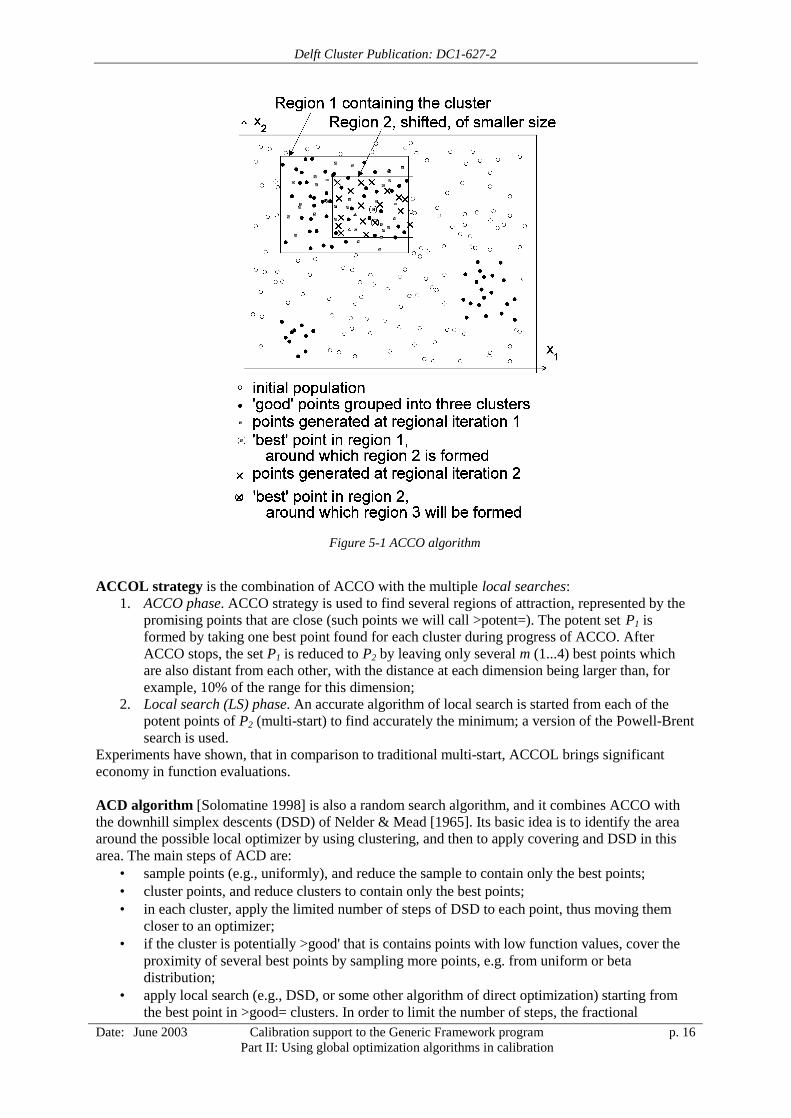
A PC-based system GLOBE incorporating nine GO algorithms was built. GLOBE can be configuredto use an external program as a supplier of the objective function values. The number of independentvariables and the constraints imposed on their values are supplied by the user in the form of a simpletext file. Figure 6-1 shows how GLOBE is used in the problems of automatic calibration. Model mustbe an executable module (program) which does not require any user input, and the user has to supplytwo transfer programs P1 and P2. These three programs (Model, P1, P2) are activated from GLOBEin a loop. GLOBE runs in DOS protected mode (DPMI) providing enough memory to load theprogram modules. A Windows version is being developed. The user interface includes severalgraphical windows displaying the progress of minimization in different coordinate planes projections.The parameters of the algorithms can be easily changed by the user.
Figure 6-1 Calibration with GLOBE
Currently, GLOBE includes the following nine algorithms described above:• CRS2 (controlled random search, by Price [1983]);• CRS4 (modification of the controlled random search by Ali & Storey[ 1994a]);• GA with a one-point crossover, and with a choice between the real-valued or binary coding
(15 bits were used in our experiments); with the standard random bit mutation; between thetournament and fitness rank selection; and between elitist and non-elitist versions.
• Multis – multi-start algorithm;• M-Simplex – multi-start algorithm;• adaptive cluster covering (ACCO)• adaptive cluster covering with local search (ACCOL)• adaptive cluster descent (ACD)• adaptive cluster descent with local search (ACDL)
Delft Cluster Publication: DC1-627-2
Date: June 2003 Calibration support to the Generic Framework programPart II: Using global optimization algorithms in calibration
p. 19
7 Comparing nine algorithms for calibration
Our experience of using GO algorithms includes:• traditional benchmark functions used in GO with known global optima [Dixon & Szegö 1978,
Duan et al. 1993, Solomatine 1995b];• calibration of a lumped hydrological model [Solomatine 1995b];• calibration of a 2D free-surface hydrodynamic model [Constantinescu 1996];• calibration of a distributed groundwater model [Solomatine et al 1998];• calibration of an ecological model of plant growth;• calibration of an electrostatic mirror model [Vdovine et al., 1995];• solution of a dynamic programming problem for reservoir optimization [Lee 1997];• optimization of a pipe network[Abebe & Solomatine 1998].
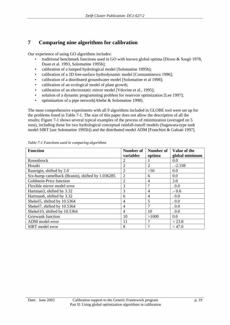
The most comprehensive experiments with all 9 algorithms included in GLOBE tool were set up forthe problems listed in Table 7-1. The size of this paper does not allow the description of all theresults; Figure 7-1 shows several typical examples of the process of minimization (averaged on 5runs), including those for two hydrological conceptual rainfall-runoff models (Sugawara-type tankmodel SIRT [see Solomatine 1995b]) and the distributed model ADM [Franchini & Galeati 1997].
Table 7-1 Functions used in comparing algorithms
Function Number ofvariables
Number ofoptima
Value of theglobal minimum
Rosenbrock 2 1 0.0Hosaki 2 2 . -2.338Rastrigin, shifted by 2.0 2 >50 0.0Six-hump camelback (Branin), shifted by 1.036285 2 6 0.0Goldstein-Price function 2 4 3.0Flexible mirror model error 3 ? . 0.0Hartman3, shifted by 3.32 3 4 .- 0.6Hartman6, shifted by 3.32 6 4 . 0.0Shekel5, shifted by 10.5364 4 5 . 0.0Shekel7, shifted by 10.5364 4 7 . 0.0Shekel10, shifted by 10.5364 4 10 . 0.0Griewank function 10 >1000 0.0ADM model error 11 ? < 23.8SIRT model error 8 ? < 47.0

Delft Cluster Publication: DC1-627-2
Date: June 2003 Calibration support to the Generic Framework programPart II: Using global optimization algorithms in calibration
p. 20
Figure 7-1Typical examples of the minimization proces (averaged on 5 runs) for two hydrologicalconceptual rainfall-runoff models (Sugawara-type tank model SIRT), and the distributed model ADM
The number N of points in the initial sample and the number of points in the reduced sample werechosen according to the rule that these numbers must grow linearly with the dimension n, from N=50at n=2, to N=300 at n=30. For CRS2 and CRS4 the formula recommended by their authors isN=10(n+1). In ACCOL, ACDL, Multis and M-Simplex the fractional tolerance of 0.001 was used. InGA fitness rank elitist selection is used together with a complex stopping rule preventing prematuretermination.Since GA uses discretized variables (we used the 15-bit coding, i.e. the range is 0...32767) an accuratecomparison would only be possible if the values of the variables for other algorithms were discretizedin the same range as well. This has been done for ACCO, ACD and CRS4. Other algorithms, includingthe local search stages of ACCOL and ACDL, use real-valued variables.Three main performance indicators were investigated:
• effectiveness (how close the algorithm gets to the global minimum);• efficiency (running time) of an algorithm measured by the number of function evaluations
needed (the running time of the algorithm itself is negligible compared with the former);• reliability (robustness) of the algorithms can be measured by the number of successes in
finding the global minimum, or at least approaching it sufficiently closely.
Effectiveness and efficiency. The plots on Figure 7-1 show the progress of minimization for some ofthe functions averaged across 5 runs (the last point represents the best function value found throughall five runs). The vertical line segment between the last two points means that the best function value

Delft Cluster Publication: DC1-627-2
Date: June 2003 Calibration support to the Generic Framework programPart II: Using global optimization algorithms in calibration
p. 21
has been reached in one of the runs earlier than shown by the abscissa of the last but one point. Notethat most points of the ACCOL plot correspond both to ACCO and ACCOL, and only some of the lastpoints correspond to the local search phase of ACCOL; the same applies to ACDL and ACD.The comparison results can be summarized briefly as follows. For functions of 2 variables, ACCOL,CRS4 and M-Simplex are the most efficient, that is, faster in getting to the minimum. In Hosaki,Rastrigin and six-hump camelback functions M-Simplex quite unexpectedly showed the best results.With functions of higher dimensions, ACCOL and CRS4 again performed best, and had similarperformance. M-Simplex was the worst with all Shekel 4-variable functions, but was even a bit betterthan ACCOL and CRS4 with Hartman 3- and 6-variable functions. ACDL was on average the thirdbest in performance after ACCOL and CRS4, being a >slow starter=. However, on some runs ACDLshowed very high efficiency. GA is the least efficient method, and is also ineffective with all Shekelfunctions. Multis and CRS2 are both effective, reaching the global minimum in most cases, but muchslower than other algorithms.
Reliability (robustness). Reliability can be measured as the number of successes in finding the globalminimum with the predefined accuracy. Because of the randomized character of search no algorithmcan be 100% reliable. For most functions of 2 variables most algorithms were quite reliable (with theexception of GA, which was often converging prematurely). Only the Rastrigin function with manyequidistant local minima with almost equal values presented difficulties.With the functions with more than two variables the situation was different. It can be seen fromFigure 7-1 that for most algorithms the ordinate of the last point can be considerably less than theordinate of the previous point. This means that the least function value was found in some runs, butnot in all of them. The CRS2 and Multis algorithms appeared to be the most reliable for functions ofhigher dimensions but were by far the least efficient. ACDL was not always reliable even though itshowed efficiency on some runs.In most cases, except for GA the found minimizer estimate is normally quite close to the globalminimum. Small differences could be attributed partly to the way the real-valued variables werecoded. A more accurate statistical analysis of single-start failure probabilities has yet to be done.
Delft Cluster Publication: DC1-627-2
Date: June 2003 Calibration support to the Generic Framework programPart II: Using global optimization algorithms in calibration
p. 22
8 Discussion
Algorithms, which are permanently oriented towards the whole function domain have to performmore function evaluations, that is, have low efficiency (CRS2 and Multis). The lower efficiency of GAcan also be attributed to the type of >crossover= used (exchange of some of the parents= coordinatevalues) which often leads to redundant evaluations of the >offspring= in the search space quite farfrom their highly fit parents, and hence normally with lower fitness. So the fitness gained by theparents may not be inherited by many of their offspring. It was also found that GA often convergesprematurely, especially in the variant with tournament selection. Whether this feature is inherent tothe whole class of evolutionary algorithms following the ideas of natural evolution, which are indeedquite appealing but highly redundant, or it is a feature of the version of a GA implemented in thisstudy, has yet to be investigated. It is worth mentioning that reportedly other types of crossover, likeintermediate recombination in evolutionary strategies [Back & Schwefel 1993] may improve theefficiency of evolutionary algorithms.The relatively higher efficiency of ACCOL and CRS4 can be explained by their orientation towardssmaller search domain,s which is especially efficient for high dimensions. ACDL on some runs hasshown high efficiency but its reliability was not the best.
Delft Cluster Publication: DC1-627-2
Date: June 2003 Calibration support to the Generic Framework programPart II: Using global optimization algorithms in calibration
p. 23
9 Conclusions
1. Our experience showed that GO techniques are useful in solving various classes ofoptimization problems. Among the GO algorithms compared ACCOL and CRS4 showed thehighest effectiveness, efficiency and reliability. In many practical problems where onefunction evaluation is expensive (slow), and their total number is then the critical parameter,ACCO (without the local search phase) would be the first choice to obtain a reasonableoptimizer assessment.ACDL algorithm proved to be efficient and effective on some of the runs with functions ofhigher dimensions. However, accurate tuning of its parameters is needed to improve itsreliability.M-Simplex performs very well with the functions of low dimension but in higher dimensionsit often converges prematurely to a local minimum.GA, CRS2, and Multis provide reasonable solutions as well. However, all of them requireconsiderably more function evaluations, and GA may also converge prematurely before itreaches the global minimum. So for problems involving >expensive= functions withcontinuous variables there are better alternatives like ACCOL or CRS4. Our other experiments[Abebe and Solomatine 1998] however, show that for certain classes of problems with highlydiscrete variables, e.g. in water distribution network optimization, GA, due to its inherentlydiscrete nature, can actually be more accurate than other algorithms built originally forcontinuous variables (being still less efficient than for example ACCO).
2. The choice between various methods of global optimization may depend on the type ofproblem, and more research is needed to compare reportedly efficient methods like simulatedannealing, evolution strategies, topological multilevel linkage, shuffled simplex evolution andothers [see Ali and Storey 1994b; Locatelli and Schoen 1996, Neumaier 1998, Duan 1993,Kuczera 1997]. The best results can probably be achieved by structural adaptation, that is,switching in the process of search between different algorithms.
3. Practically in all problems with continuous variables where the use of GAs was reported,other GO algorithms can be used as well.
4. GLOBE tool showed itself as an efficient engine for model calibration, more on its functionssee http://www.ihe.nl/hi/sol.
Delft Cluster Publication: DC1-627-2
Date: June 2003 Calibration support to the Generic Framework programPart II: Using global optimization algorithms in calibration
p. 24
ReferencesAbebe A.J. & Solomatine D.P. 1998.Application of global optimization to the design of pipe networks. Proc. Int. Conf. Hydroinformatics-‘98. Copenhagen, Denmark, Balkema, Rotterdam
Ali, M.M & Storey, C. 1994a.Modified controlled random search algorithms. Intern. J. Computer Math., 53, pp. 229-235.
Ali, M.M. & Storey, C. 1994b.Topographical multilevel single linkage. J. of Global Optimization, 5, pp. 349-358.
Babovic, V., Wu, Z. & Larsen L.C. 1994.Calibrating hydrodynamic models by means of simulated evolution, Proc. Int. Conf. onHydroinformatics, Delft, The Netherlands. Balkema, Rotterdam, pp.193-200.
Back, T. & Schwefel, H.-P. 1993.An overview of evolutionary algorithms for parameter optimization. Evolutionary Computation, 1,No. 1, pp. 1-23.
Brent, R.P. 1973.Algorithms for minimization without derivatives. Prentice-Hall, Englewood-Cliffs, N.J., 195p.
Cieniawski, S.E, Eheart, J.W. & Ranjithan, S. 1995.Using genetic algorithms to solve a multiobjective groundwater monitoring problem. Water Resour.Res., 31 (2), 399-409.
Constantinescu A. 1996.Calibration of hydrodynamic numerical models using global optimization techniques. M.Sc. thesis No.HH262, IHE, Delft, 85p.
Dixon, L.C.W. & Szego, G.P. (eds.) 1978.Towards global optimisation. North-Holland, Amsterdam, 472p.
Duan, Q., Gupta, V., Sorooshian, S. 1993.Shuffled complex evolution approach for effective and efficient global minimization. J. of Optimiz.Theory Appl., 76 (3), pp. 501-521.
Franchini, M. & Galeati, G. 1997.Comparing several genetic algorithm schemes for the calibration of conceptual rainfall-runoff models.Hydrol. Sci. J., 42 (3), 357 - 379.
Goldberg, D.E. 1989.Genetic algorithms in search, optimization and machine learning. Addison-Wesley Reading, MA:.
Griewank, A.O. 1981.Generalized descent for global optimization. J. Optimiz. Theory Appl., 34 (1), 11-39.
Jacobs, D.A.H. 1977.The state of the art in numerical analysis. Academic Press, London.
Kuczera, G. 1997
Delft Cluster Publication: DC1-627-2
Date: June 2003 Calibration support to the Generic Framework programPart II: Using global optimization algorithms in calibration
p. 25
Efficient subspace probabilistic parameter optimization for catchment models. Water Resour. Res, 33(1), 177-185, January.
Lee H. 1997.Optimal reservoir operation for flood control using a hybrid modelling approach. M.Sc. thesis No.HH319, IHE, Delft.
Locatelli, M. & Schoen, F. 1996Simple linkage: analysis of a threshold-accepting global optimization method. J. of GlobalOptimization, 5, pp. 95-111.
S. Maskey , A. Jonoski and D.P. Solomatine, 2002Groundwater remediation strategy using global optimization algorithms. ASCE Journal of WaterResources Planning and Management, 2002 (accepted).
US Geological SurveyMethods and guidelines for effective model calibration. Water-resources investigations report 98-4005. Denver, Colorado, USA, 1998.
Michalewicz, Z. 1996Genetic algorithms + data structures = evolution programs. Springer, Berlin.
Model Calibration (1997)Proc. Model Calibration Conference of the Dutch Hydrological Society. Special issue no. 2.,Nederlandse Hydrologische Vereniging (in Dutch).
Nelder, J.A & Mead, R. 1998A simplex method for function minimization. Computer J., vol. 7, No. 4 p. 308-313, 1965.
NeumaierWWW page. solon.cma.univie.ac.at/ ~neum/glopt.html.
Pintér, J. 1995.Global optimization in action. Kluwer, Amsterdam.
Powell, M.J.D. 1964.An efficient method of finding the minimum of a function of several variables without calculatingderivatives. Computer J., 7, 155-162.
Press, W.H., Flannery, B.P., Teukolsky, S.A., Vetterling, W.T. 1990Numerical recipes in Pascal. The art of scientific computing. Cambridge University Press,Cambridge, 759p..
Price W.L. 1983.Global optimization by controlled random search. J. Optimiz. Theory Appl., 40, 333-348.
Pronzato L., Walter E., Venot A., Lebruchec J.-F. 1984.A general purpose global optimizer: implementation and applications. Mathematics and Computers inSimulation, 26, 412-422.
M.L. Ralston and R.I. Jennrich, 1978Dud, a Derivative-free Algorithm for Non-linear Least Squares. Technometrics 20-1 (1978) 7.
Savic, D.A. & Walters, G.A. 1997.
Delft Cluster Publication: DC1-627-2
Date: June 2003 Calibration support to the Generic Framework programPart II: Using global optimization algorithms in calibration
p. 26
Genetic algorithms for least-cost design of water distribution networks. J. of Water Res. Planning andMngt., 123 (2), 67-77.
H. Scholten, M.W.F. van der Tol. 1994SMOES: a simulation model for the Oosterschelde ecosystem. Part II: Calibration and validation.Hydrobiologia 282/283: 453-474, 1994.
Solomatine, D.P. 1995aThe use of global random search methods for models calibration. Proc. XXVIth Congress of theInternational Association for Hydraulic Research (IAHR), vol.1, pp. 224-229, London, September.
Solomatine D.P. 1995bApplication of global optimization to models calibration. Presented at the Seminar Methods andsoftware for estimation of large-scale spatial interaction models, Netherlands InterdisciplinaryDemographics Inst., July, www.ihe.nl/hi/sol/sol.htm.
Solomatine, D.P. 1998.Two strategies of adaptive cluster covering with descent and their comparison to other algorithms.J. Global Optimiz., 1998.
Solomatine D.P. Gautam D., Franchini M. 1998.A conceptual rainfall-runoff model and tools for its automatic calibration, 1998.
Törn, A. & Filinskas, 1989.A Global optimization. Springer-Verlag, Berlin, 255pp.
Törn, A. & Viitanen, S. 1994.Topographical Global Optimization using pre-sampled points. J. of Global Optimization, 5, pp. 267-276.
Wang, Q.J. 1991.The genetic algorithm and its application to calibrating conceptual rainfall-runoff models. WaterResour. Res., 27 (9), 2467-2471.
Van den Boogaard, H.F.P., Hoogkamer, M.J.J. & Heemink, A.W. 1993.Parameter identification in particle models. Stochastic Hydrology and Hydraulics, 7, 109-130.
Vdovine, G., Middelhoek, S., Bartek, M., Sarro, P.M., & Solomatine, D.P. 1995.Technology, characterization and applications of adaptive mirrors fabricated with IC-compatiblemicromachining. Proc. Int. Symposium on Optical Science, Engineering and Instrumentation, vol.2534/13, San-Diego, USA, July 10-14.

Delft Cluster Publication: DC1-627-2
Date: June 2003 Calibration support to the Generic Framework programPart III: Calibration of groundwater flow models
p. 27
Title: PART III:Calibration of groundwater flow models
Author: C.B.M. te Stroet Institute: TNO-NITG
Author: B. Minnema Institute: TNO-NITG
June 2003Number of pages : 57
Keywords (3-5) : Groundwater, model, calibration
Institute Publication-number : NITG 03-048-A TNO-NITG
AcknowledgementThe Dutch water sector through the Dutch Generic Framework Program and the ICES-2 program hassponsored this research. The research is part of the Research program of Delft Cluster. We thank dr.P.J.A. Gijsbers for his critical comments on a draft of this report.
Conditions of (re-)use of this publicationThe full-text of this report may be re-used under the condition of an acknowledgement and a correctreference to this publication.© TNO-NTIG 2003


Delft Cluster Publication: DC1-627-2
Date: June 2003 Calibration support to the Generic Framework programPart III: Calibration of groundwater flow models
p. 29
10 IntroductionThis report is to support the “Generic Framework programme” which consists of a series of projectsto create a standard in the modelling processes that are used in water management issues. The topic ofsupport is the field of model calibration. TNO-NITG is elaborating the calibration of groundwaterflow models.
To gain insight in the geo-hydrological processes in space and/or time a geo-hydrologist makes use ofnumerical groundwater models. These groundwater models are based on characteristics of thesubsurface and the hydrological interfaces in the top-system. However, these characteristics are notknown exactly. In practice this means that the groundwater models need to be calibrated.
The goal of the research of TNO-NITG on the field of calibration of groundwater models is toproduce an applicable method suitable for the use in real world groundwater management problems.The modeller needs and objective an repeatable method for calibrating groundwater models, in whichall available information can be efficiently incorporated and the reliability of the data and theuncertainty of the results of the groundwater model can be quantified.
The report can be seen as a refinement of the “Handbook Good Modelling Practice” (Waveren et al.,1999) on the process of calibration. The handbook is describing requirements of a good modellingprocess in a broader context. So also very important issues like defining the goal of the model,creating a basis of trust by the users by communication during the building and presenting of resultsare the topic of this handbook. Although we are aware of the importance of these topics in order to geta ‘good’ model, this report is focusing on the calibration process: how is the data used, in the broadestsense, to get the best possible model.
In this report, first the vision of TNO-NITG on calibration of (groundwater) models is given inchapter 2. Chapter 3 presents a number of key issues in calibration; it describes the main line of thisreport. Chapter 4 describes two state-of-the art methodologies more in detail. This chapter can beskipped without losing the main line of the report. In Chapter 5 the presented key issues of chapter 2are illustrated with a few real world examples. Finally Chapter 6 presents the key issues and thecookbook out of chapter 3 again as a summary.
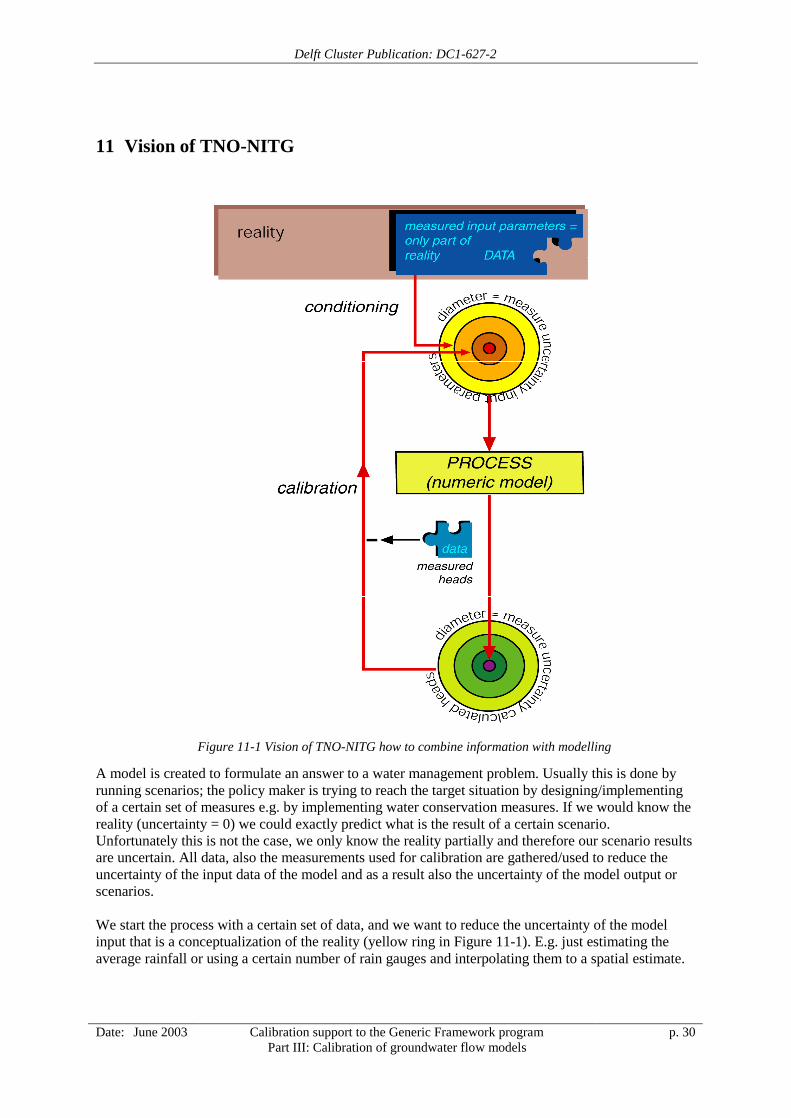
Delft Cluster Publication: DC1-627-2
Date: June 2003 Calibration support to the Generic Framework programPart III: Calibration of groundwater flow models
p. 30
11 Vision of TNO-NITG
Figure 11-1 Vision of TNO-NITG how to combine information with modelling
A model is created to formulate an answer to a water management problem. Usually this is done byrunning scenarios; the policy maker is trying to reach the target situation by designing/implementingof a certain set of measures e.g. by implementing water conservation measures. If we would know thereality (uncertainty = 0) we could exactly predict what is the result of a certain scenario.Unfortunately this is not the case, we only know the reality partially and therefore our scenario resultsare uncertain. All data, also the measurements used for calibration are gathered/used to reduce theuncertainty of the input data of the model and as a result also the uncertainty of the model output orscenarios.
We start the process with a certain set of data, and we want to reduce the uncertainty of the modelinput that is a conceptualization of the reality (yellow ring in Figure 11-1). E.g. just estimating theaverage rainfall or using a certain number of rain gauges and interpolating them to a spatial estimate.
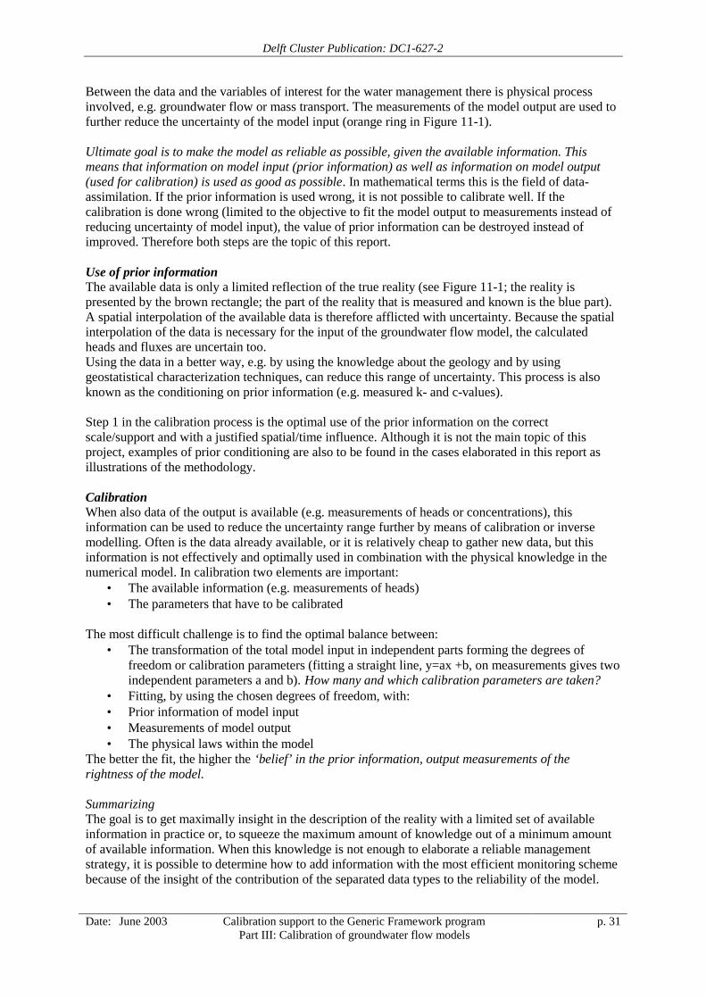
Delft Cluster Publication: DC1-627-2
Date: June 2003 Calibration support to the Generic Framework programPart III: Calibration of groundwater flow models
p. 31
Between the data and the variables of interest for the water management there is physical processinvolved, e.g. groundwater flow or mass transport. The measurements of the model output are used tofurther reduce the uncertainty of the model input (orange ring in Figure 11-1).
Ultimate goal is to make the model as reliable as possible, given the available information. Thismeans that information on model input (prior information) as well as information on model output(used for calibration) is used as good as possible. In mathematical terms this is the field of data-assimilation. If the prior information is used wrong, it is not possible to calibrate well. If thecalibration is done wrong (limited to the objective to fit the model output to measurements instead ofreducing uncertainty of model input), the value of prior information can be destroyed instead ofimproved. Therefore both steps are the topic of this report.
Use of prior informationThe available data is only a limited reflection of the true reality (see Figure 11-1; the reality ispresented by the brown rectangle; the part of the reality that is measured and known is the blue part).A spatial interpolation of the available data is therefore afflicted with uncertainty. Because the spatialinterpolation of the data is necessary for the input of the groundwater flow model, the calculatedheads and fluxes are uncertain too.Using the data in a better way, e.g. by using the knowledge about the geology and by usinggeostatistical characterization techniques, can reduce this range of uncertainty. This process is alsoknown as the conditioning on prior information (e.g. measured k- and c-values).
Step 1 in the calibration process is the optimal use of the prior information on the correctscale/support and with a justified spatial/time influence. Although it is not the main topic of thisproject, examples of prior conditioning are also to be found in the cases elaborated in this report asillustrations of the methodology.
CalibrationWhen also data of the output is available (e.g. measurements of heads or concentrations), thisinformation can be used to reduce the uncertainty range further by means of calibration or inversemodelling. Often is the data already available, or it is relatively cheap to gather new data, but thisinformation is not effectively and optimally used in combination with the physical knowledge in thenumerical model. In calibration two elements are important:
• The available information (e.g. measurements of heads)• The parameters that have to be calibrated
The most difficult challenge is to find the optimal balance between:• The transformation of the total model input in independent parts forming the degrees of
freedom or calibration parameters (fitting a straight line, y=ax +b, on measurements gives twoindependent parameters a and b). How many and which calibration parameters are taken?
• Fitting, by using the chosen degrees of freedom, with:• Prior information of model input• Measurements of model output• The physical laws within the model
The better the fit, the higher the ‘belief’ in the prior information, output measurements of therightness of the model.
SummarizingThe goal is to get maximally insight in the description of the reality with a limited set of availableinformation in practice or, to squeeze the maximum amount of knowledge out of a minimum amountof available information. When this knowledge is not enough to elaborate a reliable managementstrategy, it is possible to determine how to add information with the most efficient monitoring schemebecause of the insight of the contribution of the separated data types to the reliability of the model.
Delft Cluster Publication: DC1-627-2
Date: June 2003 Calibration support to the Generic Framework programPart III: Calibration of groundwater flow models
p. 32
12 State-of-the-art of calibration methodology
12.1 Key issuesGeneral objective is to achieve the maximum amount of detail in the model given the availableinformation by balancing:1. The degrees of freedom in the parameterization;2. The fit of the different parts in the objective function (Figure 12-1):
a) The deviation from prior information (parameter adaptation),b) The deviation from output measurements (measurement residual)c) The deviation from the model equation (model reliability)
Figure 12-1 Stiffness of springs as a symbolic presentation of the different weights in the objective function
The deviation from the different parts of the objective function is controlled by weights that controlthe ‘stiffness of the strings’. The larger the stiffness, the stronger the parameters/measurements/modelare reflected, or differently stated the stronger ‘the belief’ in this part of information. As aconsequence errors in these parts of information result in errors in the model, which are smoothed bythe reciprocal of the stiffness value. The weights to the parameter adaptation and conceptual modelreliability parts are not commonly used.
In the light of the balancing problem described a few statements are made about model calibration:1. A model where the parameters are not tailored to the available measurements of model
output is not well calibrated. There should be a direct relationship between the parametersand the location of measurements otherwise the maximum amount of information in thesemeasurements is not used. E.g. the popular method of zoning spatial differentiatedparameters is inherently disregarding detail which is available in the measurements, butwhich is averaged by the zonation method.
2. A model with wrong prior information (amongst others a conceptual model) cannot bewell calibrated. Errors in the prior information are resulting in errors in the modeldirectly. This is often stated as “garbage in, garbage out”. Usually, this cannot becorrected by the fitting of measurements on output (part b). Therefore it is very importantto check what has been achieved in translating prior information to model input. Issueslike: filtering noise from information, combining knowledge and data intelligently,transformation of data to different scales, are determining the quality of the model input.
3. A model, which is not checked to be ‘in balance’ with the information available from thereality is not well calibrated. Errors in values and weights are resulting in (sometimeslarger) errors in values of other calibrated parameters. Important rule here is: beconservative. If one is not sure about input give it a relative large uncertainty in theobjective function (small stiffness or small weight).
4. Whenever feasible, quantify the remaining uncertainty of the parameters and or themodel. There is a well-known lower limit of the parameter uncertainty, which is called the“Cramer Rao lower bound”.
Shorter and more polarizing with respect to the usual practice nowadays:1. Zonation or other forms of averaging should not be used;
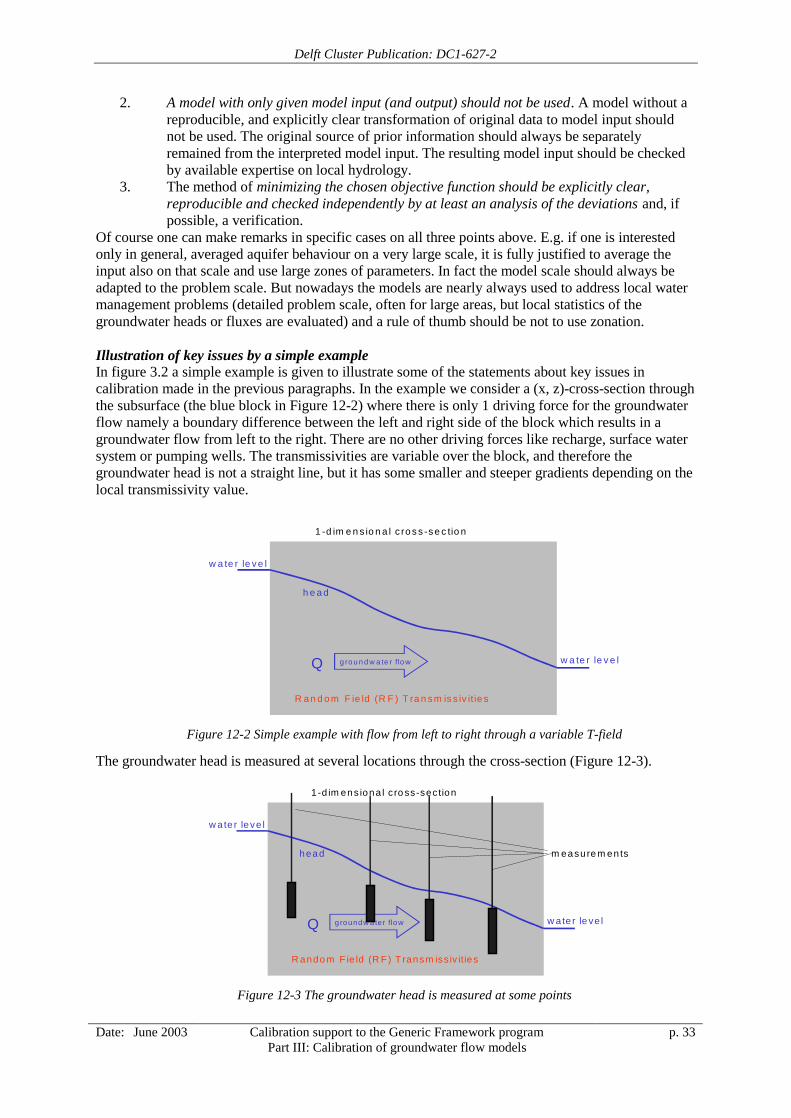
Delft Cluster Publication: DC1-627-2
Date: June 2003 Calibration support to the Generic Framework programPart III: Calibration of groundwater flow models
p. 33
2. A model with only given model input (and output) should not be used. A model without areproducible, and explicitly clear transformation of original data to model input shouldnot be used. The original source of prior information should always be separatelyremained from the interpreted model input. The resulting model input should be checkedby available expertise on local hydrology.
3. The method of minimizing the chosen objective function should be explicitly clear,reproducible and checked independently by at least an analysis of the deviations and, ifpossible, a verification.
Of course one can make remarks in specific cases on all three points above. E.g. if one is interestedonly in general, averaged aquifer behaviour on a very large scale, it is fully justified to average theinput also on that scale and use large zones of parameters. In fact the model scale should always beadapted to the problem scale. But nowadays the models are nearly always used to address local watermanagement problems (detailed problem scale, often for large areas, but local statistics of thegroundwater heads or fluxes are evaluated) and a rule of thumb should be not to use zonation.
Illustration of key issues by a simple exampleIn figure 3.2 a simple example is given to illustrate some of the statements about key issues incalibration made in the previous paragraphs. In the example we consider a (x, z)-cross-section throughthe subsurface (the blue block in Figure 12-2) where there is only 1 driving force for the groundwaterflow namely a boundary difference between the left and right side of the block which results in agroundwater flow from left to the right. There are no other driving forces like recharge, surface watersystem or pumping wells. The transmissivities are variable over the block, and therefore thegroundwater head is not a straight line, but it has some smaller and steeper gradients depending on thelocal transmissivity value.
Figure 12-2 Simple example with flow from left to right through a variable T-field
The groundwater head is measured at several locations through the cross-section (Figure 12-3).
Figure 12-3 The groundwater head is measured at some points
Q
R a n d o m F ie ld (R F ) T ra n sm is s iv it ie s
1 -d im e n s io n a l c ro s s -se c tio n
w a te r le v e l
w a te r le ve l
h e a d
g ro u n d w a te r f lo w
Q
R ando m F ie ld (R F ) T ransm iss iv ities
1 -d im ens iona l c ro ss-section
w ate r le ve l
w a te r leve l
head
groundw ater flow
m easure m ents

Delft Cluster Publication: DC1-627-2
Date: June 2003 Calibration support to the Generic Framework programPart III: Calibration of groundwater flow models
p. 34
From the transmissivity field a mean value is estimated and at two locations the transmissivity isknown because of small pumping tests. From geological knowledge it is know that the transmissivityfield has a smooth variation so that the difference at a small distance is limited. If we would generatea transmissivity field with this information the dark-blue lines of Figure 12-4 could be generated. Therange of values of these transmissivity fields (= blue lines) in Figure 12-4 reflects the uncertaintyrange of the input parameters of the model prior to calibration. The orange circle denotes this inFigure11-1. If we would not have the two measurements of T, the range of values of the transmissivitieswould increase which is reflected by an increasing uncertainty towards the yellow circle in Figure11-1.
Figure 12-4 Possible transmissivity fields on the basis of 2 known T-values
If we consider every transmissivity field (= blue line) in Figure 12-4 as a new model input prior tocalibration, each prior input can be calibrated separately one by one. We have 100 transmissivityfields (= 100 blue lines) so we get also 100 calibrated transmissivity fields. These are given in Figure12-5 by the pink lines. The range of values of these calibrated transmissivities (= pink lines) isdecreased in comparison to the range of the prior transmissivities before calibration (= blue lines)because of the information about the transmissivities in the measurements of the heads used forcalibration. In Figure 11-1 this is denoted by a decreasing uncertainty from the orange towards the redcircle. Furthermore it can be noticed that the calibrated transmissivities are better representing the truetransmissivity (= red line).
Figure 12-5 Calibrated transmissivities (pink) and prior transmissivities (blue)
Because of the calibration the deviation between the measured and modelled heads are reduced. Thisis shown in Figure 12-6 where the deviations of the model prior to calibration are given in yellow andthe deviations of the model after calibration are given in blue dots. The range of the prior deviationsare representing the uncertainty of the prior model denoted in Figure 11-1 by the middle green circle;the range of the calibrated deviations represent the uncertainty of the calibrated model denoted inFigure 11-1 by the dark green circle.
0
2
4
6
8
10
12
ln(T
) m2/
d
initia l s cmre a l ln(T )+
m e asure m e n ts o f T (p rio r in fo )
b e fo re ca lib ra tion
tru e ln (T )
F ro m n ow o n sa m e c ro ss -s e c tionb u t line s a re re p resen tin g ln (T ) va lu es !!
0
2
4
6
8
10
12
ln(T
) m2/
d
initia l scmlas t scmrea l ln(T )
+
b e fo re ca lib ra tion
tru e ln (T )a fte r ca lib ra tio n
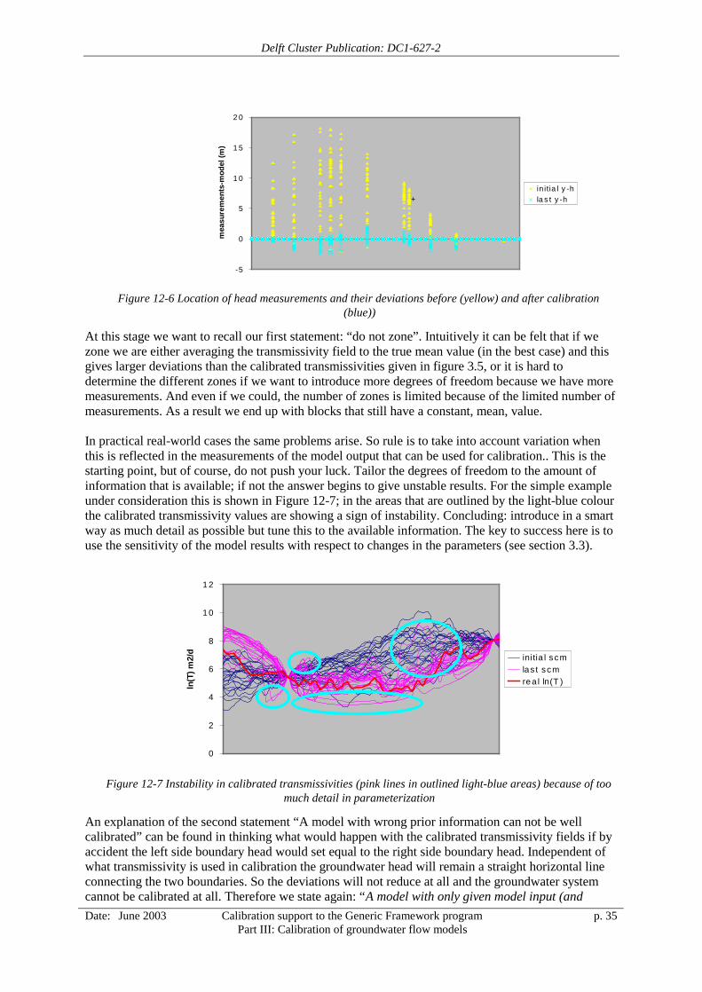
Delft Cluster Publication: DC1-627-2
Date: June 2003 Calibration support to the Generic Framework programPart III: Calibration of groundwater flow models
p. 35
Figure 12-6 Location of head measurements and their deviations before (yellow) and after calibration(blue))
At this stage we want to recall our first statement: “do not zone”. Intuitively it can be felt that if wezone we are either averaging the transmissivity field to the true mean value (in the best case) and thisgives larger deviations than the calibrated transmissivities given in figure 3.5, or it is hard todetermine the different zones if we want to introduce more degrees of freedom because we have moremeasurements. And even if we could, the number of zones is limited because of the limited number ofmeasurements. As a result we end up with blocks that still have a constant, mean, value.
In practical real-world cases the same problems arise. So rule is to take into account variation whenthis is reflected in the measurements of the model output that can be used for calibration.. This is thestarting point, but of course, do not push your luck. Tailor the degrees of freedom to the amount ofinformation that is available; if not the answer begins to give unstable results. For the simple exampleunder consideration this is shown in Figure 12-7; in the areas that are outlined by the light-blue colourthe calibrated transmissivity values are showing a sign of instability. Concluding: introduce in a smartway as much detail as possible but tune this to the available information. The key to success here is touse the sensitivity of the model results with respect to changes in the parameters (see section 3.3).
Figure 12-7 Instability in calibrated transmissivities (pink lines in outlined light-blue areas) because of toomuch detail in parameterization
An explanation of the second statement “A model with wrong prior information can not be wellcalibrated” can be found in thinking what would happen with the calibrated transmissivity fields if byaccident the left side boundary head would set equal to the right side boundary head. Independent ofwhat transmissivity is used in calibration the groundwater head will remain a straight horizontal lineconnecting the two boundaries. So the deviations will not reduce at all and the groundwater systemcannot be calibrated at all. Therefore we state again: “A model with only given model input (and
-5
0
5
1 0
1 5
2 0
mea
sure
men
ts-m
odel
(m)
in itia l y -hla s t y -h+
0
2
4
6
8
1 0
1 2
ln(T
) m2/
d
initia l scmlas t scmre a l ln(T )
+
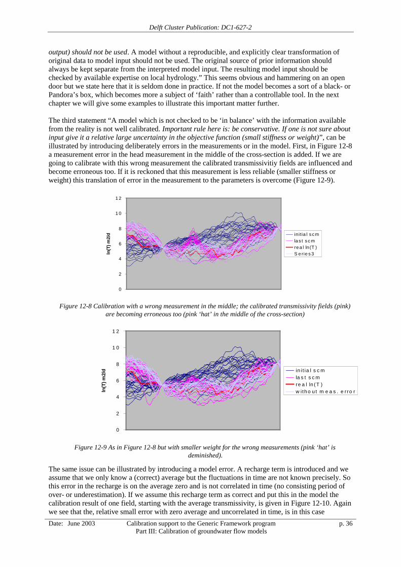
Delft Cluster Publication: DC1-627-2
Date: June 2003 Calibration support to the Generic Framework programPart III: Calibration of groundwater flow models
p. 36
output) should not be used. A model without a reproducible, and explicitly clear transformation oforiginal data to model input should not be used. The original source of prior information shouldalways be kept separate from the interpreted model input. The resulting model input should bechecked by available expertise on local hydrology.” This seems obvious and hammering on an opendoor but we state here that it is seldom done in practice. If not the model becomes a sort of a black- orPandora’s box, which becomes more a subject of ‘faith’ rather than a controllable tool. In the nextchapter we will give some examples to illustrate this important matter further.
The third statement “A model which is not checked to be ‘in balance’ with the information availablefrom the reality is not well calibrated. Important rule here is: be conservative. If one is not sure aboutinput give it a relative large uncertainty in the objective function (small stiffness or weight)”, can beillustrated by introducing deliberately errors in the measurements or in the model. First, in Figure 12-8a measurement error in the head measurement in the middle of the cross-section is added. If we aregoing to calibrate with this wrong measurement the calibrated transmissivitiy fields are influenced andbecome erroneous too. If it is reckoned that this measurement is less reliable (smaller stiffness orweight) this translation of error in the measurement to the parameters is overcome (Figure 12-9).
Figure 12-8 Calibration with a wrong measurement in the middle; the calibrated transmissivity fields (pink)are becoming erroneous too (pink ‘hat’ in the middle of the cross-section)
Figure 12-9 As in Figure 12-8 but with smaller weight for the wrong measurements (pink ‘hat’ isdeminished).
The same issue can be illustrated by introducing a model error. A recharge term is introduced and weassume that we only know a (correct) average but the fluctuations in time are not known precisely. Sothis error in the recharge is on the average zero and is not correlated in time (no consisting period ofover- or underestimation). If we assume this recharge term as correct and put this in the model thecalibration result of one field, starting with the average transmissivity, is given in Figure 12-10. Againwe see that the, relative small error with zero average and uncorrelated in time, is in this case
0
2
4
6
8
1 0
1 2
ln(T
) m2/
d in itia l s c mla s t s c mre a l ln(T )S e rie s 3
+
0
2
4
6
8
1 0
1 2
ln(T
) m2/
d in i t ia l s c mla s t s c mre a l ln (T )w ith o u t m e a s . e r ro r
+
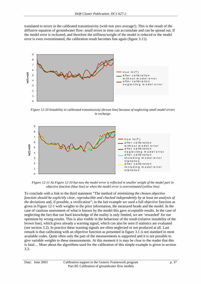
Delft Cluster Publication: DC1-627-2
Date: June 2003 Calibration support to the Generic Framework programPart III: Calibration of groundwater flow models
p. 37
translated to errors in the calibrated transmissivity (with non zero average!). This is the result of thediffusive equation of groundwater flow: small errors in time can accumulate and can be spread out. Ifthe model error is reckoned, and therefore the stiffness/weight of the model is reduced or the modelerror is even overestimated, the calibration result becomes fine again (figure 3.11).
Figure 12-10 Instability in calibrated transmissivity (brown line) because of neglecting small model errorsin recharge.
Figure 12-11 As Figure 12-10 but now the model error is reflected in smaller weight of the model part inobjective function (blue line) or when the model error is overestimated (yellow line)
To conclude with a link to the third statement “The method of minimizing the chosen objectivefunction should be explicitly clear, reproducible and checked independently by at least an analysis ofthe deviations and, if possible, a verification”; in the last example we used a full objective function asgiven in Figure 12-1 with weights to the prior information, the measured heads and the model. In thecase of cautious assessment of what is known by the model this gave acceptable results. In the case ofneglecting the fact that our hard knowledge of the reality is only limited, we are ‘rewarded’ for ouroptimism by wrong results. This is also visible in the behaviour of the result (relative instability of thebrown line), which gives already a warning signal, which can also be seen if statistics are evaluated(see section 3.2). In practice these warning signals are often neglected or not produced at all. Lastremark is that calibrating with an objective function as presented in figure 3.1 is not standard in mostavailable codes. Quite often only the part of the measurements is supported and it is not possible togive variable weights to these measurements. At this moment it is may be clear to the reader that thisis fatal… More about the algorithms used for the calibration of this simple example is given in section3.3.
0
1
2
3
4
5
6
7
8
9
ln(T
) m2/
d
r e a l ln ( T )r e p T 0 = 8 7 5n e g le c t i n g m o d e l e r r o r
+
t r u e ln ( T )a f t e r c a l ib r a t io nw i t h o u t m o d e l e r r o ra f t e r c a l ib r a t io nn e g le c t in g m o d e l e r r o r
0
1
2
3
4
5
6
7
8
9
ln(T
) m2/
d
r e a l ln ( T )
r e p T 0 = 8 7 5
c o r r e c t m o d e l e r r o r
o v e r e s t im a t in g m o d e le r r o rn e g le c t i n g m o d e l e r r o r
+
t r u e ln ( T )a f t e r c a l ib r a t io nw i t h o u t m o d e l e r r o ra f t e r c a l ib r a t io nn e g le c t in g m o d e l e r r o ra f t e r c a l ib r a t io nin c lu d in g m o d e l e r r o rs ta t is t ic sa f t e r c a l ib r a t io nin c lu d in g m o d e l e r r o rs ta t is t ic s
Delft Cluster Publication: DC1-627-2
Date: June 2003 Calibration support to the Generic Framework programPart III: Calibration of groundwater flow models
p. 38
12.2 ‘Cookbook’In this section we present a small flowchart of how the calibration process should look like.
Step 1: Construct the model input prior to calibration. Remember, do this participative: “A model withonly given model input (and output) should not be used. A model without a reproducible, andexplicitly clear transformation of original data to model input should not be used. The original sourceof prior information should always be kept separate from the interpreted model input. The resultingmodel input should be checked by available expertise on local hydrology.”
Step 2: Check the prior model to serious mistakes by confronting it to the available measurements onoutput. We call this the ‘quest for mistakes in the (processing of) data’. Until the following checks aresatisfiable do this ‘by hand’, which means don’t use automatic calibration tools blindly (keep control):
• Deviations between output and measurements divided by the corresponding weights (notrends, areas outside the 2*weights should be small);
• Deviations between prior and calibrated parameters;• Correct statistics of deviations between output and measurements (zero mean, residual sum of
squares equal to weights*[number of measurements - number of degrees of freedom], zerocorrelation between deviations and model output);
• No significant correlations between calibrated parameters;• Verification of model (model analysis checked by existing expertise of real system behaviour,
comparison with measurements of model output that is not used for calibration).In this stage it is important to ‘get the bias out’. Automatic tools are not used to fit as good aspossible, but to help the modeller doing the boring work of fitting quickly and efficiently and use theremaining time for thinking and analysing. Goal is not to minimize deviations but to balance them inpositive and negative sense and to get them as uncorrelated as possible. We prefer larger errors abovebias. In this stage hydrological experience is most important to come to satisfiable solutions.
Step 3: Final calibration with automatic tools. Do this for different combinations of weights in theobjective function. Make several optimised models. Make choices in participation with the users ofthe model. Think of the important rule: “be conservative. If one is not sure about input give it arelative large uncertainty in the objective function (small stiffness or weight).” Be sure that thestatistics are satisfied while fitting with measurements. In this stage the goal is to fit as well aspossible but without producing erroneous parameters. Search for the point when one is ’living on theedge’ in order to squeeze out as much as detail out of the measurements while remaining in balancewith the given amount of information.
Step 4 (optional): If feasible calculate the uncertainty of model parameters and model results. Theeasiest way is to do this by a sort of Monte Carle principle by running more than one possible model,just as given by the simple example in the previous section. In this case the range of the inputparameters determines the input uncertainty and ditto for the range of output results (this is not shownfor the example in the previous section; but the reader can imagine that it is given implicitly by themethod). An analytical expression for the parameter uncertainty is given by the so called “CramerRao lower bound” which is depending on the squared expression of the linearized system behaviour(represented by the system matrix A) and the inverse of the weights in the objective function andwhich is given in most textbooks. Simply stated this Cramer Rao lower bound can be explained bystating that the more coherence in the system behaviour and the less uncertainty in the measurements,the more accurate model predictions are which makes sense intuitively. Using this expression for theparameters uncertainty the model output uncertainty can be calculated with Monte Carlo simulationsor analytically by multiplying it with the system matrices again.
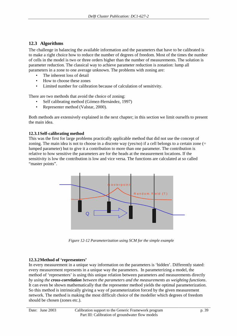
Delft Cluster Publication: DC1-627-2
Date: June 2003 Calibration support to the Generic Framework programPart III: Calibration of groundwater flow models
p. 39
12.3 AlgorithmsThe challenge in balancing the available information and the parameters that have to be calibrated isto make a right choice how to reduce the number of degrees of freedom. Most of the times the numberof cells in the model is two or three orders higher than the number of measurements. The solution isparameter reduction. The classical way to achieve parameter reduction is zonation: lump allparameters in a zone to one average unknown. The problems with zoning are:
• The inherent loss of detail• How to choose these zones• Limited number for calibration because of calculation of sensitivity.
There are two methods that avoid the choice of zoning:• Self calibrating method (Gómez-Hernández, 1997)• Representer method (Valstar, 2000).
Both methods are extensively explained in the next chapter; in this section we limit ourselfs to presentthe main idea.
12.3.1 Self-calibrating methodThis was the first for large problems practically applicable method that did not use the concept ofzoning. The main idea is not to choose in a discrete way (yes/no) if a cell belongs to a certain zone (=lumped parameter) but to give it a contribution to more than one parameter. The contribution isrelative to how sensitive the parameters are for the heads at the measurement locations. If thesensitivity is low the contribution is low and vice versa. The functions are calculated at so called“master points”.
Figure 12-12 Parameterization using SCM for the simple example
12.3.2 Method of ‘representers’In every measurement in a unique way information on the parameters is ‘hidden’. Differently stated:every measurement represents in a unique way the parameters. In parameterizing a model, themethod of ‘representers’ is using this unique relation between parameters and measurements directlyby using the cross-correlation between the parameters and the measurements as weighting functions.It can even be shown mathematically that the representer method yields the optimal parameterization.So this method is intrinsically giving a way of parameterization forced by the given measurementnetwork. The method is making the most difficult choice of the modeller which degrees of freedomshould be chosen (zones etc.).
Q
m a s te r p o in t
R a n d o m F ie ld ( T )

Delft Cluster Publication: DC1-627-2
Date: June 2003 Calibration support to the Generic Framework programPart III: Calibration of groundwater flow models
p. 40
Quantification of reliability (for example see section 5.4.2)When calibrating with representers also the uncertainty of the prior information and of the measuredheads is used to calculate the reliability of the calibrated model. This is important in order to be ableto investigate the significance of the calculated scenario results made with the numerical model as aninput for the policy maker.
Network optimisation (for example see section 5.4.3)The method of representers is also very attractive to be used when the measurement strategy shouldbe optimised. Crucial in seeing the origin of this statement is the observation that the direction of thearrow, from data to parameters (red arrow in Figure 11-1), also can be reversed. Differently stated:
If:We can determine with the help of representers which information about the parameters is hiddenin the measurements
then:We can also determine how we have to measure to be able to calibrate the parameters better.
This provides the basis for a measurement network designing strategy how to optimise an existingmeasurement network or how to design additional locations or a new network.
Delft Cluster Publication: DC1-627-2
Date: June 2003 Calibration support to the Generic Framework programPart III: Calibration of groundwater flow models
p. 41
13 Methods that calibrate and parameterize
13.1 Self-calibrating methodThe principles of the Self-Calibration Method (SCM), explained in this paragraph usingtransmissivities (T) as an example, are based on Gómez-Hérnandez et al (1997). The reader interestedin the theory of the joint generation of log10(K) and storativity is referred to Hendricks Franssen andGómez-Hérnandez (1999).
The goal is to generate multiple equally likely realisations of transmissivity fields, which honour bothtransmissivity data and piezometric data. The transmissivity field is conditional to the transmissivitydata at data locations, it displays the same pattern of spatial variability observed in the field, and thenumerical solution of the groundwater flow equation with given boundary conditions reproduces themeasured piezometric data. Given that all these requirements are satisfied, any of the transmissivityrealisations would be a plausible representation of the unknown reality. Additional information wouldbe required to discriminate among the different realisations.
13.1.1 Steps of the self-calibration method (SCM) algorithmThe steps of the SCM algorithm are:1) Generate a conditional realisation of the transmissivity honouring the measured transmissivity
values2) Solving the flow equation for given boundary conditions3) Modify (update) the transmissivity realisation to achieve the conditioning to the piezometric head
data.
Steps 1-3 are repeated for as many realisations as required.
13.1.2 The generation of a transmissivity field conditional to measured transmissivity dataFor the generation of a field the technique of multi-gaussian sequential simulation was used. See alsochapter 3, random fields. For a multi-gaussian log-transmissivity realisation over the aquifer domainthe following two characteristics are needed:1) A set of log-transmissivity measurements YI
m, i ∈ (ny)2) The variogram of log-transmissivities γYThe transmissivity realisation is obtained by taking the antilog of the log-transmissivity realisation:T(0)=eY(0). This initial log-transmissivity realisation is hereafter referred to as the seed realisation.The process of conditioning to heads is iterative, and the superindex (-) is used to indicate the iterationnumber. At this stage we are at iteration 0.
13.1.3 Penalty functionDiscretisation of the steady state equation for two-dimensional groundwater flow (using thecorresponding boundary conditions) by finite differences results in a set of linear equations that can berepresented in matricial form:
[ ] QhA =⋅ (4.1)
where [A] is an NxN conductance matrix, h is an Nx1 vector of unknown piezometric heads, andQ is an Nx1 vector of stresses (and boundary conditions) in the model domain. After solvingequation (4.1) for a given transmissivity field and boundary conditions, the reproduction of themeasured piezometric heads is analysed by the evaluation of the so-called penalty function:
Delft Cluster Publication: DC1-627-2
Date: June 2003 Calibration support to the Generic Framework programPart III: Calibration of groundwater flow models
p. 42
2
)()( i
mii
nihhwF
h
−= ∑∈
(4.2)
Function F is a generalised sum of squared differences between the measured heads him
, i ∈(nh) andthe heads resulting form the solution of equation (4.1). The weights wi are proportional to thecoefficients of the inverse of the head error covariance matrix. The head error covariance matrix caninclude measurement error and estimation errors of measured heads. The head errors are considered tobe independent from one location to another.
If the penalty function becomes smaller than some pre-specified small value, the transmissivity fieldused to obtain h is conditional to the head measurements. If the penalty function is still larger thanthe pre-specified small value we continue with the modification of the transmissivity field to obtain anew h with a better (smaller) value for F. The way the modification of the transmissivity field iscarried out is described in paragraph 4.1.7.
13.1.4 OptimisationSo we have an initial transmissivity field Y(0), that honours the variogram and the measurements of thetransmissivity. We want to find a transmissivity field, such that the value of the penalty function Freaches its ultimate maximum value 0, meaning a perfect reproduction of the calculated heads in thecells containing measured piezometric heads, or a pre-defined small value of F. In fact thetransmissivity field has to be updated: we want to determine the perturbation vector ∆Y, whichadded to the seed vectors results in a solution to equation (4.1) that reproduces the piezometric headmeasurements (small value of F).
13.1.5 ParameterisationIn a MODFLOW (McDonald and Harbaugh, 1988) model each transmissivity of each cell has to beupdated. However, that would result in a set of equations with too many unknowns. Therefore wemust parameterise. This is done as follows:
Initially the perturbations are only implemented in a few locations, hereafter referred to as masterpoints (mY), where mY represents a set of indices identifying the Y master locations.
A perturbation DY over the entire model domain could be described by:
∑∈
∆=∆)( Ymk
kk
ii YY λ (4.3)
where ∆Yk are the perturbations at the master locations, and the coefficients λik are the ordinary
kriging weights obtained by solving an ordinary kriging system based on the specified variogram γY.This approach has the advantage that only the perturbations ∆Yk at the master locations have to bedetermined. The master perturbations are propagating through the rest of the aquifer by kriging. Tomake sure that the new transmissivity field still honours the characteristics of the variogram, and thusthe transmissivity measurements, the transmissivity measurement locations nY are included in thevector of master location mY. In these nY locations the perturbations must be equal to 0.
13.1.6 Selecting the locations of the master pointsThe maximum number of master points is equal to the number of piezometric head measurements. InGómez-Hérnandez et al (1997) a pseudo-regular grid-wise distribution of the master points (mY) issuggested with a spacing in the order of one-third of the correlation range of the variogram γY. Fromour experiments we learned that a more effective strategy can be followed:
The sensitivity sj in a modelcell j can be expressed as follows:
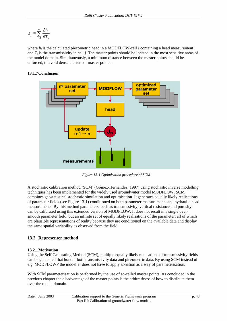
Delft Cluster Publication: DC1-627-2
Date: June 2003 Calibration support to the Generic Framework programPart III: Calibration of groundwater flow models
p. 43
∑= ∂
∂=
m
i j
ij T
hs1
where hi is the calculated piezometric head in a MODFLOW-cell i containing a head measurement,and Ti is the transmissivity in cell j. The master points should be located in the most sensitive areas ofthe model domain. Simultaneously, a minimum distance between the master points should beenforced, to avoid dense clusters of master points.
13.1.7 Conclusion
Figure 13-1 Optimisation procedure of SCM
A stochastic calibration method (SCM) (Gómez-Hernández, 1997) using stochastic inverse modellingtechniques has been implemented for the widely used groundwater model MODFLOW. SCMcombines geostatistical stochastic simulation and optimisation. It generates equally likely realisationsof parameter fields (see Figure 13-1) conditioned on both parameter measurements and hydraulic headmeasurements. By this method parameters, such as transmissivity, vertical resistance and porosity,can be calibrated using this extended version of MODFLOW. It does not result in a single over-smooth parameter field, but an infinite set of equally likely realisations of the parameter, all of whichare plausible representations of reality because they are conditioned on the available data and displaythe same spatial variability as observed from the field.
13.2 Representer method
13.2.1 MotivationUsing the Self Calibrating Method (SCM), multiple equally likely realisations of transmissivity fieldscan be generated that honour both transmissivity data and piezometric data. By using SCM instead ofe.g. MODFLOWP the modeller does not have to apply zonation as a way of parameterisation.
With SCM parameterisation is performed by the use of so-called master points. As concluded in theprevious chapter the disadvantage of the master points is the arbitrariness of how to distribute themover the model domain.

Delft Cluster Publication: DC1-627-2
Date: June 2003 Calibration support to the Generic Framework programPart III: Calibration of groundwater flow models
p. 44
With the method of representers this disadvantage can be overcome, as will be explained below.
13.2.2 TheoryThe theory of the representers is described below as a summary of some parts from the PhD thesis ofValstar (2000).A representer solution is introduced to reduce to number of independent parameters that have to beestimated. For each measurement a set of representer functions is introduced that can be imagined asthe influence function of the measurement on the adjoint and state variables and on the modelparameters. Each set of representer functions consists out of representer functions for both adjointvariables, one for the model parameters and two representer functions for both state variables.
The representers of the model parameters predict how the model parameters and model errors shouldbe changed and how the state variable will change consequently in order to effect the measurementprediction most efficiently, and keeping the model parameter and model error terms of objectivefunction as small as possible. All model parameters that have no influence on the model predictions ofthe measurements have values of zero for all parameter representers and their estimates will stay atthe prior mean. After all representer functions are known, they are multiplied by the representercoefficients, which depend on the misfit between the measurement values and their model predictions,in which the correlation with other measurement predictions is taken into account. It will be provedlater on that the parameter and state representers are equal to the linearized cross-covariances of themeasurement predictions with respect to the model parameters and the state variables respectively.
The representer coefficients are actually the only independent parameters and therefore therepresenters are a type of parameterisation. This type of parameterisation is in contrast to otherparameterisation techniques that were mentioned in the previous in which the solution was forced tobe in the special form that was determined by the modeller.Bennett, 1992 and Eknes and Evensen, 1996, who defined representer fields for the state variables andtheir adjoints, have used representer solutions in oceanography. That way they could decouple theEuler-Lagrange equations in a set of equations into a number of initial value problems, which can besolved sequentially.
Each state representer can be regarded as an influence function of a measurement on the update of theparameter and state fields. The parameter representer denotes the shape of the parameter field, whichcan adapt the model prediction of the measurement with minimal increase of the penalty terms for theparameters and model error terms in the objective function. The state representers denote how headand concentration fields change as the parameter and model error are adapted according to theirrepresenter fields. Multiplying these fields by the representer coefficients can make the parametersand states go up or down, depending on the initial misfit between the measurement value and themeasurement prediction.The update of both parameter and state fields is visualised in Figure 4.1b in which a 1-dimensionalgroundwater flow situation with two constant head boundaries h1 and h2 respectively. In this aquifer,two head measurements z1 and z2 are taken, which are used to update the unknown parameters. Theunknown parameters in this example are the natural logarithms of the transmissivities (theconductivity times the depth of the aquifer), which vary along the x-direction.
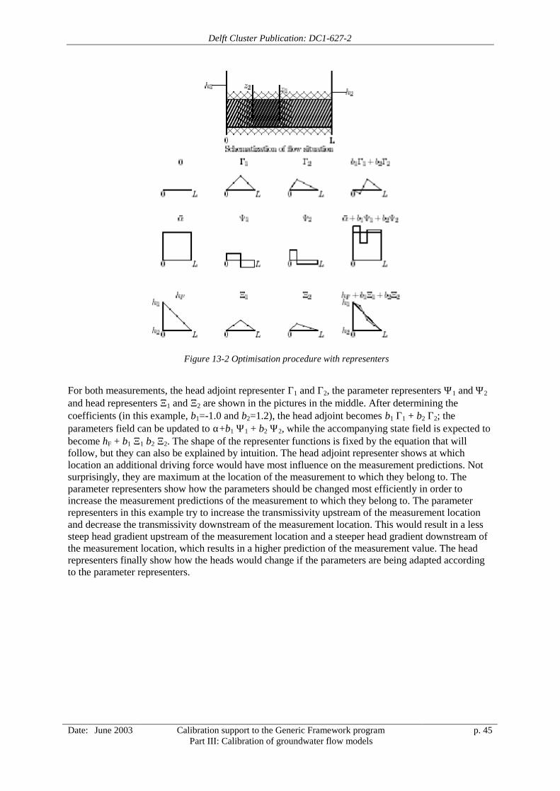
Delft Cluster Publication: DC1-627-2
Date: June 2003 Calibration support to the Generic Framework programPart III: Calibration of groundwater flow models
p. 45
Figure 13-2 Optimisation procedure with representers
For both measurements, the head adjoint representer Γ1 and Γ2, the parameter representers Ψ1 and Ψ2
and head representers Ξ1 and Ξ2 are shown in the pictures in the middle. After determining thecoefficients (in this example, b1=-1.0 and b2=1.2), the head adjoint becomes b1 Γ1 + b2 Γ2; theparameters field can be updated to α+b1 Ψ1 + b2 Ψ2, while the accompanying state field is expected tobecome hF + b1 Ξ1 b2 Ξ2. The shape of the representer functions is fixed by the equation that willfollow, but they can also be explained by intuition. The head adjoint representer shows at whichlocation an additional driving force would have most influence on the measurement predictions. Notsurprisingly, they are maximum at the location of the measurement to which they belong to. Theparameter representers show how the parameters should be changed most efficiently in order toincrease the measurement predictions of the measurement to which they belong to. The parameterrepresenters in this example try to increase the transmissivity upstream of the measurement locationand decrease the transmissivity downstream of the measurement location. This would result in a lesssteep head gradient upstream of the measurement location and a steeper head gradient downstream ofthe measurement location, which results in a higher prediction of the measurement value. The headrepresenters finally show how the heads would change if the parameters are being adapted accordingto the parameter representers.
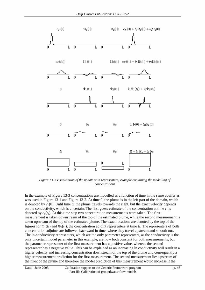
Delft Cluster Publication: DC1-627-2
Date: June 2003 Calibration support to the Generic Framework programPart III: Calibration of groundwater flow models
p. 46
Figure 13-3 Visualisation of the update with representers; example containing the modelling ofconcentrations
In the example of Figure 13-3 concentrations are modelled as a function of time in the same aquifer aswas used in Figure 13-1 and Figure 13-2. At time 0, the plume is in the left part of the domain, whichis denoted by cF(0). Until time t1 the plume travels towards the right, but the exact velocity dependson the conductivity, which is uncertain. The first guess estimate of the concentration at time t1 isdenoted by cF(t1). At this time step two concentration measurements were taken. The firstmeasurement is taken downstream of the top of the estimated plume, while the second measurement istaken upstream of the top of the estimated plume. The exact locations are denoted by the top of thefigures for Φ1(t1) and Φ2(t1), the concentration adjoint representers at time t1. The representers of bothconcentration adjoints are followed backward in time, where they travel upstream and smooth out.The ln-conductivity representers, which are the only parameter representers, as the conductivity is theonly uncertain model parameter in this example, are now both constant for both measurements, butthe parameter representer of the first measurement has a positive value, whereas the secondrepresenter has a negative value. This can be explained as an increasing ln conductivity will result in ahigher velocity and increasing concentration downstream of the top of the plume and consequently ahigher measurement prediction for the first measurement. The second measurement lies upstream ofthe front of the plume and therefore the model prediction of this measurement would increase if the
Delft Cluster Publication: DC1-627-2
Date: June 2003 Calibration support to the Generic Framework programPart III: Calibration of groundwater flow models
p. 47
conductivity would decrease. This can also be seen at the concentration representers Ω1(t1) and Ω2(t1).Adaptation according to the first representers shows an increase of the concentration at the firstmeasurement location and a decrease of the concentration at the second measurement location,whereas for second representer it is the other way around. Note that at time 0, the concentrationrepresenters are zero, as the initial condition is not allowed to change.
After the representer coefficients have been obtained, (in this example b1= 0.8, and b2= -0.5) therepresenter estimates of the adjoint, parameters and concentrations are given at the right of thepictures. In this second example the head representers are not shown. They are zero for bothconcentration measurements, as the adaptation of the conductivity according to the parameterrepresenters will not result in a change of the distribution of the heads in this specific example. For thesake of clearness, it should be mentioned that in case both head measurements of the first exampleand both concentration measurements of the second example would be known, they should be usedsimultaneously in which case different final representer estimates would be obtained. In these twoexamples, only the influence of the different representers is visualised.
13.2.3 Two dimensional x-z example
13.2.3.1 IntroductionThe inverse methodologies as described in the previous section are now being used in a syntheticexample. In the presented examples, synthetic model parameter and model errors (i.e. discrepanciesbetween the differential equations and the reality) are generated. Using these synthetic parameters andmodel errors, the real head and concentration distributions are calculated. Measurements will besampled from these head and concentration distributions. These measurements are together with theprior statistics of the model parameters and model errors the only information that will be used in theinverse model. The inverse model provides estimates of both model parameters and state variables, aswell as their accuracy estimates, which will be compared with the synthetic data. Afterwards theinverse model will be repeated using different measurement sets to investigate the relative value of themeasurements.
13.2.3.2 Description of the modelThe synthetic example that is discussed in this paragraph has been designed to become close to a realworld situation, while keeping the computational time feasible. The main simplification is that themodel has only 2 dimensions, a horizontal and a vertical dimension. In reality, the behaviour of acontamination is always three-dimensional.The aquifer itself is supposed to be considerable heterogeneous, while the correlation is supposed tomuch stronger in the horizontal direction than in the vertical direction. This feature is characteristicfor many sedimentary deposits (Bierkens, 1994).
The groundwater flow system is driven by two predefined fluxes at the top and the right boundary ofthe domain. These fluxes are 0.001 m/day and 0.016 m/day, respectively. The left boundary of thedomain is a constant head boundary hb=0.0 m. The lower boundary is impermeable and characterizedby a zero flux. The schematisation of this groundwater flow system is shown in Figure 13-4.
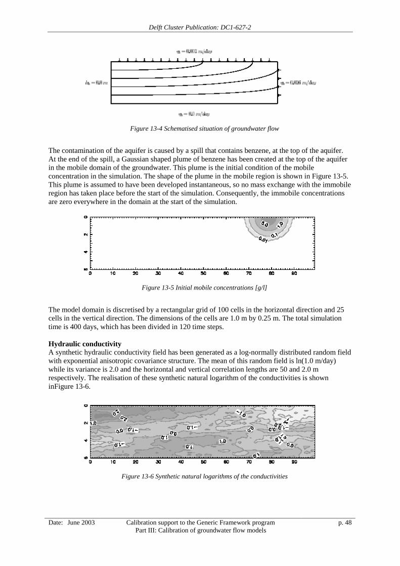
Delft Cluster Publication: DC1-627-2
Date: June 2003 Calibration support to the Generic Framework programPart III: Calibration of groundwater flow models
p. 48
Figure 13-4 Schematised situation of groundwater flow
The contamination of the aquifer is caused by a spill that contains benzene, at the top of the aquifer.At the end of the spill, a Gaussian shaped plume of benzene has been created at the top of the aquiferin the mobile domain of the groundwater. This plume is the initial condition of the mobileconcentration in the simulation. The shape of the plume in the mobile region is shown in Figure 13-5.This plume is assumed to have been developed instantaneous, so no mass exchange with the immobileregion has taken place before the start of the simulation. Consequently, the immobile concentrationsare zero everywhere in the domain at the start of the simulation.
Figure 13-5 Initial mobile concentrations [g/l]
The model domain is discretised by a rectangular grid of 100 cells in the horizontal direction and 25cells in the vertical direction. The dimensions of the cells are 1.0 m by 0.25 m. The total simulationtime is 400 days, which has been divided in 120 time steps.
Hydraulic conductivityA synthetic hydraulic conductivity field has been generated as a log-normally distributed random fieldwith exponential anisotropic covariance structure. The mean of this random field is ln(1.0 m/day)while its variance is 2.0 and the horizontal and vertical correlation lengths are 50 and 2.0 mrespectively. The realisation of these synthetic natural logarithm of the conductivities is showninFigure 13-6.
Figure 13-6 Synthetic natural logarithms of the conductivities
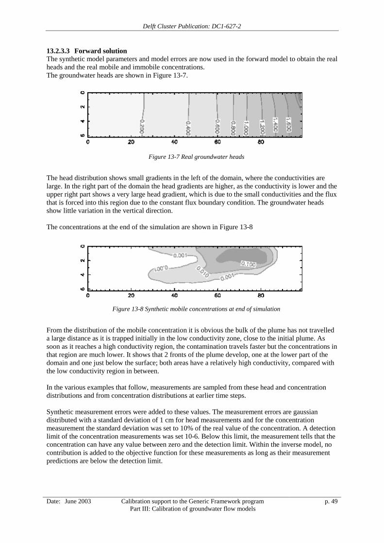
Delft Cluster Publication: DC1-627-2
Date: June 2003 Calibration support to the Generic Framework programPart III: Calibration of groundwater flow models
p. 49
13.2.3.3 Forward solutionThe synthetic model parameters and model errors are now used in the forward model to obtain the realheads and the real mobile and immobile concentrations.The groundwater heads are shown in Figure 13-7.
Figure 13-7 Real groundwater heads
The head distribution shows small gradients in the left of the domain, where the conductivities arelarge. In the right part of the domain the head gradients are higher, as the conductivity is lower and theupper right part shows a very large head gradient, which is due to the small conductivities and the fluxthat is forced into this region due to the constant flux boundary condition. The groundwater headsshow little variation in the vertical direction.
The concentrations at the end of the simulation are shown in Figure 13-8
Figure 13-8 Synthetic mobile concentrations at end of simulation
From the distribution of the mobile concentration it is obvious the bulk of the plume has not travelleda large distance as it is trapped initially in the low conductivity zone, close to the initial plume. Assoon as it reaches a high conductivity region, the contamination travels faster but the concentrations inthat region are much lower. It shows that 2 fronts of the plume develop, one at the lower part of thedomain and one just below the surface; both areas have a relatively high conductivity, compared withthe low conductivity region in between.
In the various examples that follow, measurements are sampled from these head and concentrationdistributions and from concentration distributions at earlier time steps.
Synthetic measurement errors were added to these values. The measurement errors are gaussiandistributed with a standard deviation of 1 cm for head measurements and for the concentrationmeasurement the standard deviation was set to 10% of the real value of the concentration. A detectionlimit of the concentration measurements was set 10-6. Below this limit, the measurement tells that theconcentration can have any value between zero and the detection limit. Within the inverse model, nocontribution is added to the objective function for these measurements as long as their measurementpredictions are below the detection limit.
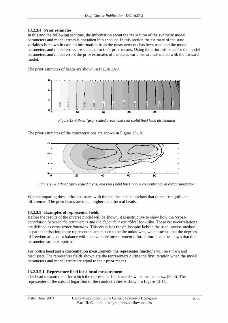
Delft Cluster Publication: DC1-627-2
Date: June 2003 Calibration support to the Generic Framework programPart III: Calibration of groundwater flow models
p. 50
13.2.3.4 Prior estimatesIn this and the following sections, the information about the realisation of the synthetic modelparameters and model errors is not taken into account. In this section the estimate of the statevariables is shown in case no information from the measurements has been used and the modelparameters and model errors are set equal to their prior means. Using the prior estimates for the modelparameters and model errors the prior estimates of the states variables are calculated with the forwardmodel.
The prior estimates of heads are shown in Figure 13-9.
Figure 13-9 Prior (gray scaled areas) and real (solid line) head distribution
The prior estimates of the concentrations are shown in Figure 13-10.
Figure 13-10 Prior (gray scaled areas) and real (solid line) mobile concentration at end of simulation
When comparing these prior estimates with the real heads it is obvious that there are significantdifferences. The prior heads are much higher than the real heads.
13.2.3.5 Examples of representer fieldsBefore the results of the inverse model will be shown, it is instructive to show how the ‘cross-correlation between the parameters and the dependent variables’ look like. These cross-correlationsare defined as representer functions. This visualises the philosophy behind the used inverse method:as parameterisation, these representers are chosen to be the unknowns, which means that the degreesof freedom are just in balance with the available measurement information. It can be shown that thisparameterisation is optimal.
For both a head and a concentration measurement, the representer functions will be shown anddiscussed. The representer fields shown are the representers during the first iteration when the modelparameters and model errors are equal to their prior means.
13.2.3.5.1 Representer field for a head measurementThe head measurement for which the representer fields are shown is located at x,z (80,3). Therepresenter of the natural logarithm of the conductivities is shown in Figure 13-11.
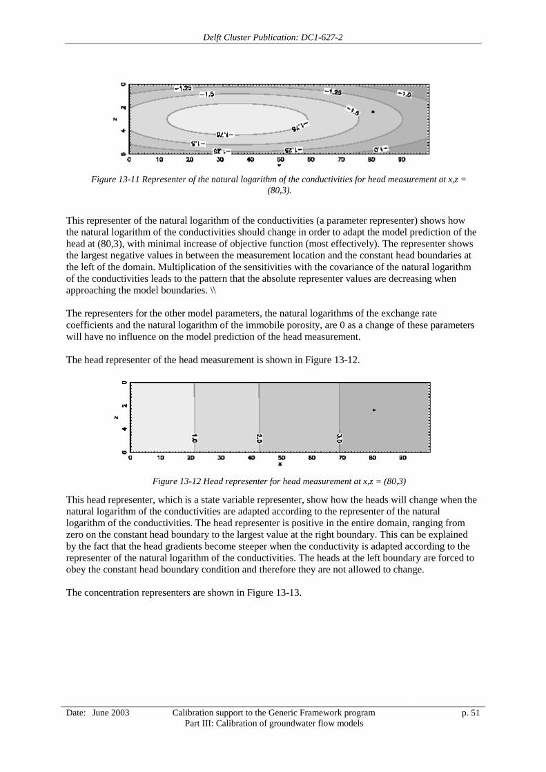
Delft Cluster Publication: DC1-627-2
Date: June 2003 Calibration support to the Generic Framework programPart III: Calibration of groundwater flow models
p. 51
Figure 13-11 Representer of the natural logarithm of the conductivities for head measurement at x,z =(80,3).
This representer of the natural logarithm of the conductivities (a parameter representer) shows howthe natural logarithm of the conductivities should change in order to adapt the model prediction of thehead at (80,3), with minimal increase of objective function (most effectively). The representer showsthe largest negative values in between the measurement location and the constant head boundaries atthe left of the domain. Multiplication of the sensitivities with the covariance of the natural logarithmof the conductivities leads to the pattern that the absolute representer values are decreasing whenapproaching the model boundaries. \\
The representers for the other model parameters, the natural logarithms of the exchange ratecoefficients and the natural logarithm of the immobile porosity, are 0 as a change of these parameterswill have no influence on the model prediction of the head measurement.
The head representer of the head measurement is shown in Figure 13-12.
Figure 13-12 Head representer for head measurement at x,z = (80,3)
This head representer, which is a state variable representer, show how the heads will change when thenatural logarithm of the conductivities are adapted according to the representer of the naturallogarithm of the conductivities. The head representer is positive in the entire domain, ranging fromzero on the constant head boundary to the largest value at the right boundary. This can be explainedby the fact that the head gradients become steeper when the conductivity is adapted according to therepresenter of the natural logarithm of the conductivities. The heads at the left boundary are forced toobey the constant head boundary condition and therefore they are not allowed to change.
The concentration representers are shown in Figure 13-13.
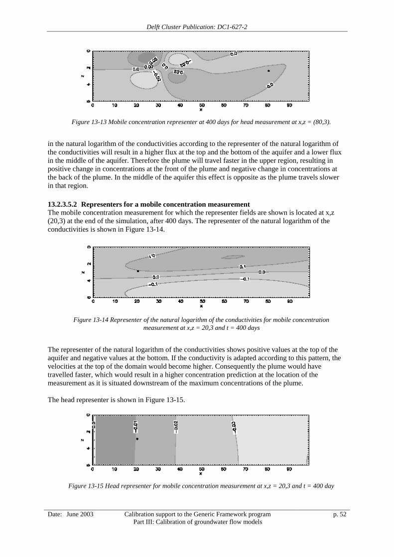
Delft Cluster Publication: DC1-627-2
Date: June 2003 Calibration support to the Generic Framework programPart III: Calibration of groundwater flow models
p. 52
Figure 13-13 Mobile concentration representer at 400 days for head measurement at x,z = (80,3).
in the natural logarithm of the conductivities according to the representer of the natural logarithm ofthe conductivities will result in a higher flux at the top and the bottom of the aquifer and a lower fluxin the middle of the aquifer. Therefore the plume will travel faster in the upper region, resulting inpositive change in concentrations at the front of the plume and negative change in concentrations atthe back of the plume. In the middle of the aquifer this effect is opposite as the plume travels slowerin that region.
13.2.3.5.2 Representers for a mobile concentration measurementThe mobile concentration measurement for which the representer fields are shown is located at x,z(20,3) at the end of the simulation, after 400 days. The representer of the natural logarithm of theconductivities is shown in Figure 13-14.
Figure 13-14 Representer of the natural logarithm of the conductivities for mobile concentrationmeasurement at x,z = 20,3 and t = 400 days
The representer of the natural logarithm of the conductivities shows positive values at the top of theaquifer and negative values at the bottom. If the conductivity is adapted according to this pattern, thevelocities at the top of the domain would become higher. Consequently the plume would havetravelled faster, which would result in a higher concentration prediction at the location of themeasurement as it is situated downstream of the maximum concentrations of the plume.
The head representer is shown in Figure 13-15.
Figure 13-15 Head representer for mobile concentration measurement at x,z = 20,3 and t = 400 day
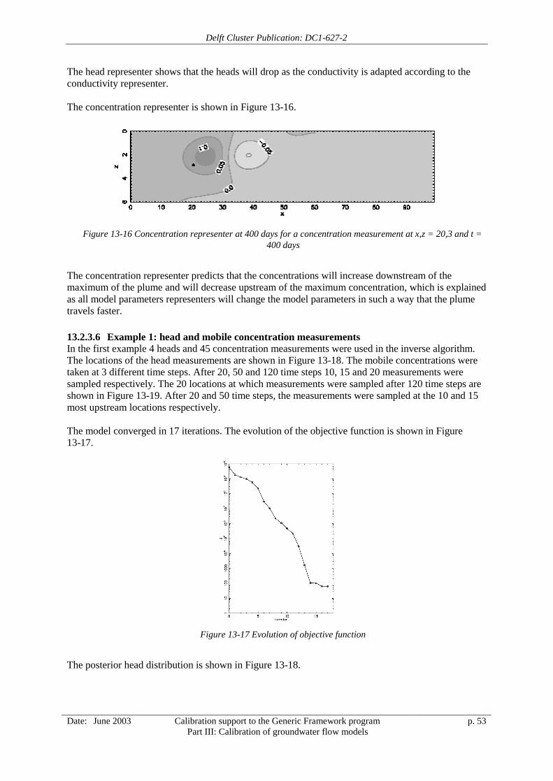
Delft Cluster Publication: DC1-627-2
Date: June 2003 Calibration support to the Generic Framework programPart III: Calibration of groundwater flow models
p. 53
The head representer shows that the heads will drop as the conductivity is adapted according to theconductivity representer.
The concentration representer is shown in Figure 13-16.
Figure 13-16 Concentration representer at 400 days for a concentration measurement at x,z = 20,3 and t =400 days
The concentration representer predicts that the concentrations will increase downstream of themaximum of the plume and will decrease upstream of the maximum concentration, which is explainedas all model parameters representers will change the model parameters in such a way that the plumetravels faster.
13.2.3.6 Example 1: head and mobile concentration measurementsIn the first example 4 heads and 45 concentration measurements were used in the inverse algorithm.The locations of the head measurements are shown in Figure 13-18. The mobile concentrations weretaken at 3 different time steps. After 20, 50 and 120 time steps 10, 15 and 20 measurements weresampled respectively. The 20 locations at which measurements were sampled after 120 time steps areshown in Figure 13-19. After 20 and 50 time steps, the measurements were sampled at the 10 and 15most upstream locations respectively.
The model converged in 17 iterations. The evolution of the objective function is shown in Figure13-17.
Figure 13-17 Evolution of objective function
The posterior head distribution is shown in Figure 13-18.
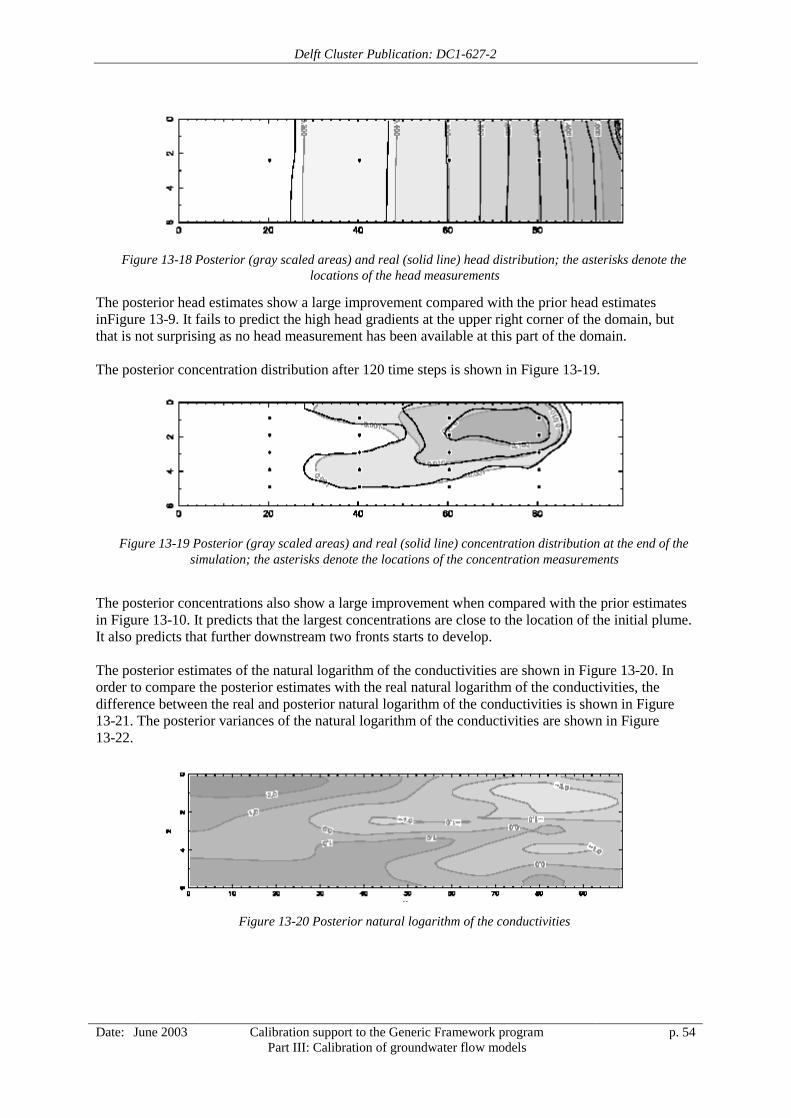
Delft Cluster Publication: DC1-627-2
Date: June 2003 Calibration support to the Generic Framework programPart III: Calibration of groundwater flow models
p. 54
Figure 13-18 Posterior (gray scaled areas) and real (solid line) head distribution; the asterisks denote thelocations of the head measurements
The posterior head estimates show a large improvement compared with the prior head estimatesinFigure 13-9. It fails to predict the high head gradients at the upper right corner of the domain, butthat is not surprising as no head measurement has been available at this part of the domain.
The posterior concentration distribution after 120 time steps is shown in Figure 13-19.
Figure 13-19 Posterior (gray scaled areas) and real (solid line) concentration distribution at the end of thesimulation; the asterisks denote the locations of the concentration measurements
The posterior concentrations also show a large improvement when compared with the prior estimatesin Figure 13-10. It predicts that the largest concentrations are close to the location of the initial plume.It also predicts that further downstream two fronts starts to develop.
The posterior estimates of the natural logarithm of the conductivities are shown in Figure 13-20. Inorder to compare the posterior estimates with the real natural logarithm of the conductivities, thedifference between the real and posterior natural logarithm of the conductivities is shown in Figure13-21. The posterior variances of the natural logarithm of the conductivities are shown in Figure13-22.
Figure 13-20 Posterior natural logarithm of the conductivities
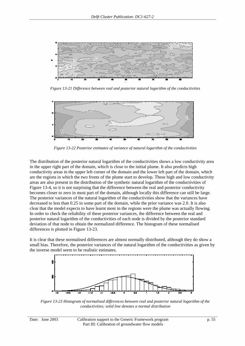
Delft Cluster Publication: DC1-627-2
Date: June 2003 Calibration support to the Generic Framework programPart III: Calibration of groundwater flow models
p. 55
Figure 13-21 Difference between real and posterior natural logarithm of the conductivities
Figure 13-22 Posterior estimates of variance of natural logarithm of the conductivities
The distribution of the posterior natural logarithm of the conductivities shows a low conductivity areain the upper right part of the domain, which is close to the initial plume. It also predicts highconductivity areas in the upper left corner of the domain and the lower left part of the domain, whichare the regions in which the two fronts of the plume start to develop. These high and low conductivityareas are also present in the distribution of the synthetic natural logarithm of the conductivities ofFigure 13-4, so it is not surprising that the difference between the real and posterior conductivitybecomes closer to zero in most part of the domain, although locally this difference can still be large.The posterior variances of the natural logarithm of the conductivities show that the variances havedecreased to less than 0.25 in some part of the domain, while the prior variance was 2.0. It is alsoclear that the model expects to have learnt most in the regions were the plume was actually flowing.In order to check the reliability of these posterior variances, the difference between the real andposterior natural logarithm of the conductivities of each node is divided by the posterior standarddeviation of that node to obtain the normalized difference. The histogram of these normaliseddifferences is plotted in Figure 13-23.
It is clear that these normalised differences are almost normally distributed, although they do show asmall bias. Therefore, the posterior variances of the natural logarithm of the conductivities as given bythe inverse model seem to be realistic estimates.
Figure 13-23 Histogram of normalised differences between real and posterior natural logarithm of theconductivities; solid line denotes a normal distribution
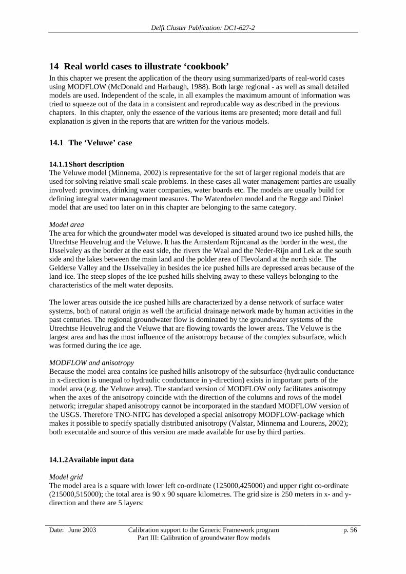
Delft Cluster Publication: DC1-627-2
Date: June 2003 Calibration support to the Generic Framework programPart III: Calibration of groundwater flow models
p. 56
14 Real world cases to illustrate ‘cookbook’In this chapter we present the application of the theory using summarized/parts of real-world casesusing MODFLOW (McDonald and Harbaugh, 1988). Both large regional - as well as small detailedmodels are used. Independent of the scale, in all examples the maximum amount of information wastried to squeeze out of the data in a consistent and reproducable way as described in the previouschapters. In this chapter, only the essence of the various items are presented; more detail and fullexplanation is given in the reports that are written for the various models.
14.1 The ‘Veluwe’ case
14.1.1 Short descriptionThe Veluwe model (Minnema, 2002) is representative for the set of larger regional models that areused for solving relative small scale problems. In these cases all water management parties are usuallyinvolved: provinces, drinking water companies, water boards etc. The models are usually build fordefining integral water management measures. The Waterdoelen model and the Regge and Dinkelmodel that are used too later on in this chapter are belonging to the same category.
Model areaThe area for which the groundwater model was developed is situated around two ice pushed hills, theUtrechtse Heuvelrug and the Veluwe. It has the Amsterdam Rijncanal as the border in the west, theIJsselvaley as the border at the east side, the rivers the Waal and the Neder-Rijn and Lek at the southside and the lakes between the main land and the polder area of Flevoland at the north side. TheGelderse Valley and the IJsselvalley in besides the ice pushed hills are depressed areas because of theland-ice. The steep slopes of the ice pushed hills shelving away to these valleys belonging to thecharacteristics of the melt water deposits.
The lower areas outside the ice pushed hills are characterized by a dense network of surface watersystems, both of natural origin as well the artificial drainage network made by human activities in thepast centuries. The regional groundwater flow is dominated by the groundwater systems of theUtrechtse Heuvelrug and the Veluwe that are flowing towards the lower areas. The Veluwe is thelargest area and has the most influence of the anisotropy because of the complex subsurface, whichwas formed during the ice age.
MODFLOW and anisotropyBecause the model area contains ice pushed hills anisotropy of the subsurface (hydraulic conductancein x-direction is unequal to hydraulic conductance in y-direction) exists in important parts of themodel area (e.g. the Veluwe area). The standard version of MODFLOW only facilitates anisotropywhen the axes of the anisotropy coincide with the direction of the columns and rows of the modelnetwork; irregular shaped anisotropy cannot be incorporated in the standard MODFLOW version ofthe USGS. Therefore TNO-NITG has developed a special anisotropy MODFLOW-package whichmakes it possible to specify spatially distributed anisotropy (Valstar, Minnema and Lourens, 2002);both executable and source of this version are made available for use by third parties.
14.1.2 Available input data
Model gridThe model area is a square with lower left co-ordinate (125000,425000) and upper right co-ordinate(215000,515000); the total area is 90 x 90 square kilometres. The grid size is 250 meters in x- and y-direction and there are 5 layers:
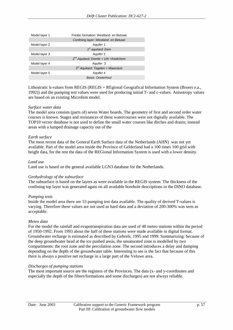
Delft Cluster Publication: DC1-627-2
Date: June 2003 Calibration support to the Generic Framework programPart III: Calibration of groundwater flow models
p. 57
Model layer 1 Freatic formation: Westland- en BetuweConfining layer: Westland- en Betuwe
Model layer 2 Aquifer 11st aquitard: Eem
Model layer 3 Aquifer 22nd Aquitard: Drente + Urk +Kedichem
Model layer 4 Aquifer 33rd Aquitard: Tegelen + Maassluis
Model layer 5 Aquifer 4Basis: Oosterhout
Lithostratic k-values from REGIS (REGIS = REgional Geografical Information System (Broers e.a.,1992)) and the pumping test values were used for producing initial T- and c-values. Anisotropy valuesare based on an existing Microfem model.
Surface water dataThe model area consists (parts of) seven Water boards. The geometry of first and second order watercourses is known. Stages and resistances of these watercourses were not digitally available. TheTOP10 vector database is not used to define the small water courses like ditches and drains; insteadareas with a lumped drainage capacity out of the
Earth surfaceThe most recent data of the General Earth Surface data of the Netherlands (AHN) was not yetavailable. Part of the model area inside the Province of Gelderland had a 100 times 100 grid withheight data, for the rest the data of the REGional Information System is used with a lower density.
Land useLand use is based on the general available LGN3 database for the Netherlands.
Geohydrology of the subsurfaceThe subsurface is based on the layers as were available in the REGIS system. The thickness of theconfining top layer was generated again on all available borehole descriptions in the DINO database.
Pumping testsInside the model area there are 53 pumping test data available. The quality of derived T-values isvarying. Therefore these values are not used as hard data and a deviation of 200-300% was seen asacceptable.
Meteo dataFor the model the rainfall and evapotranspiration data are used of 48 meteo stations within the periodof 1950-1992. From 1993 about the half of these stations were made available in digital format.Groundwater recharge is estimated as described by Gehrels, 1995 and 1999. Summarizing: because ofthe deep groundwater head at the ice pushed areas, the unsaturated zone is modelled by twocompartments: the root zone and the percolation zone. The second introduces a delay and dampingdepending on the depth of the groundwater table. Interesting to see is the fact that because of thisthere is always a positive net recharge in a large part of the Veluwe area.
Discharges of pumping stationsThe most important source are the registers of the Provinces. The data (x- and y-coordinates andespecially the depth of the filters/formations and some discharges) are not always reliable.
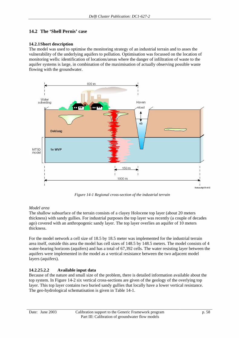
Delft Cluster Publication: DC1-627-2
Date: June 2003 Calibration support to the Generic Framework programPart III: Calibration of groundwater flow models
p. 58
14.2 The ‘Shell Pernis’ case
14.2.1 Short descriptionThe model was used to optimise the monitoring strategy of an industrial terrain and to asses thevulnerability of the underlying aquifers to pollution. Optimisation was focussed on the location ofmonitoring wells: identification of locations/areas where the danger of infiltration of waste to theaquifer systems is large, in combination of the maximisation of actually observing possible wasteflowing with the groundwater.
Figure 14-1 Regional cross-section of the industrial terrain
Model areaThe shallow subsurface of the terrain consists of a clayey Holocene top layer (about 20 metersthickness) with sandy gullies. For industrial purposes the top layer was recently (a couple of decadesago) covered with an anthropogenic sandy layer. The top layer overlies an aquifer of 10 metersthickness.
For the model network a cell size of 18.5 by 18.5 meter was implemented for the industrial terrainarea itself, outside this area the model has cell sizes of 148.5 by 148.5 meters. The model consists of 4water-bearing horizons (aquifers) and has a total of 67,392 cells. The water resisting layer between theaquifers were implemented in the model as a vertical resistance between the two adjacent modellayers (aquifers).
14.2.2 5.2.2 Available input dataBecause of the nature and small size of the problem, there is detailed information available about thetop system. In Figure 14-2 six vertical cross-sections are given of the geology of the overlying toplayer. This top layer contains two buried sandy gullies that locally have a lower vertical resistance.The geo-hydrological schematisation is given in Table 14-1.
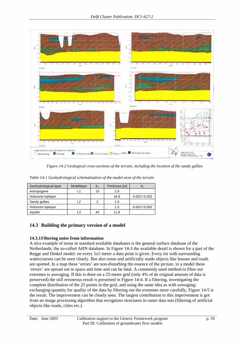
Delft Cluster Publication: DC1-627-2
Date: June 2003 Calibration support to the Generic Framework programPart III: Calibration of groundwater flow models
p. 59
Figure 14-2 Geological cross-sections of the terrain, including the location of the sandy gullies
Table 14-1 Geohydrological schematisation of the model area of the terrain
Geohydrological layer Modellayer Kh Thickness [m] Kv
Antropogene L1 10 1.9Holocene toplayer 16.9 0.0017-0.002Sandy gullies L2 2 1.9Holocene toplayer 1.3 0.0017-0.002Aquifer L3 40 11.9
14.3 Building the primary version of a model
14.3.1 Filtering noise from informationA nice example of noise in standard available databases is the general surface database of theNetherlands; the so-called AHN database. In Figure 14-3 the available detail is shown for a part of theRegge and Dinkel model: on every 5x5 meter a data point is given. Every lot with surroundingwatercourses can be seen clearly. But also noise and artificially made objects like houses and roadsare spotted. In a map these ‘errors’ are non-disturbing the essence of the picture, in a model these‘errors’ are spread out in space and time and can be fatal. A commonly used method to filter outextremes is averaging. If this is done on a 25-meter grid (only 4% of de original amount of data ispreserved) the still erroneous result is presented in Figure 14-4. If a filtering, investigating thecomplete distribution of the 25 points in the grid, and using the same idea as with averaging:exchanging quantity for quality of the data by filtering out the extremes more carefully, Figure 14-5 isthe result. The improvement can be clearly seen. The largest contribution to this improvement is gotfrom an image processing algorithm that recognizes structures in raster data sets (filtering of artificialobjects like roads, cities etc.).
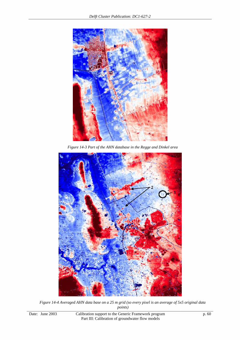
Delft Cluster Publication: DC1-627-2
Date: June 2003 Calibration support to the Generic Framework programPart III: Calibration of groundwater flow models
p. 60
Figure 14-3 Part of the AHN database in the Regge and Dinkel area
Figure 14-4 Averaged AHN data base on a 25 m grid (so every pixel is an average of 5x5 original datapoints)
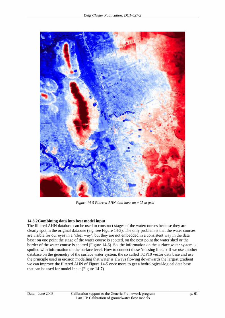
Delft Cluster Publication: DC1-627-2
Date: June 2003 Calibration support to the Generic Framework programPart III: Calibration of groundwater flow models
p. 61
Figure 14-5 Filtered AHN data base on a 25 m grid
14.3.2 Combining data into best model inputThe filtered AHN database can be used to construct stages of the watercourses because they areclearly spot in the original database (e.g. see Figure 14-3). The only problem is that the water coursesare visible for our eyes in a ‘clear way’, but they are not embedded in a consistent way in the database: on one point the stage of the water course is spotted, on the next point the water shed or theborder of the water course is spotted (Figure 14-6). So, the information on the surface water system isspoiled with information on the surface level. How to connect these ‘missing links’? If we use anotherdatabase on the geometry of the surface water system, the so called TOP10 vector data base and usethe principle used in erosion modelling that water is always flowing downwards the largest gradientwe can improve the filtered AHN of Figure 14-5 once more to get a hydrological-logical data basethat can be used for model input (Figure 14-7).
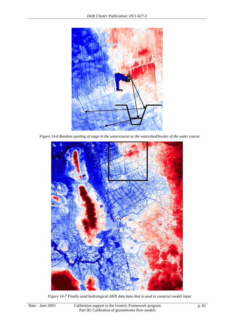
Delft Cluster Publication: DC1-627-2
Date: June 2003 Calibration support to the Generic Framework programPart III: Calibration of groundwater flow models
p. 62
Figure 14-6 Random spotting of stage in the watercourse or the watershed/border of the water course
Figure 14-7 Finally used hydrological AHN data base that is used to construct model input
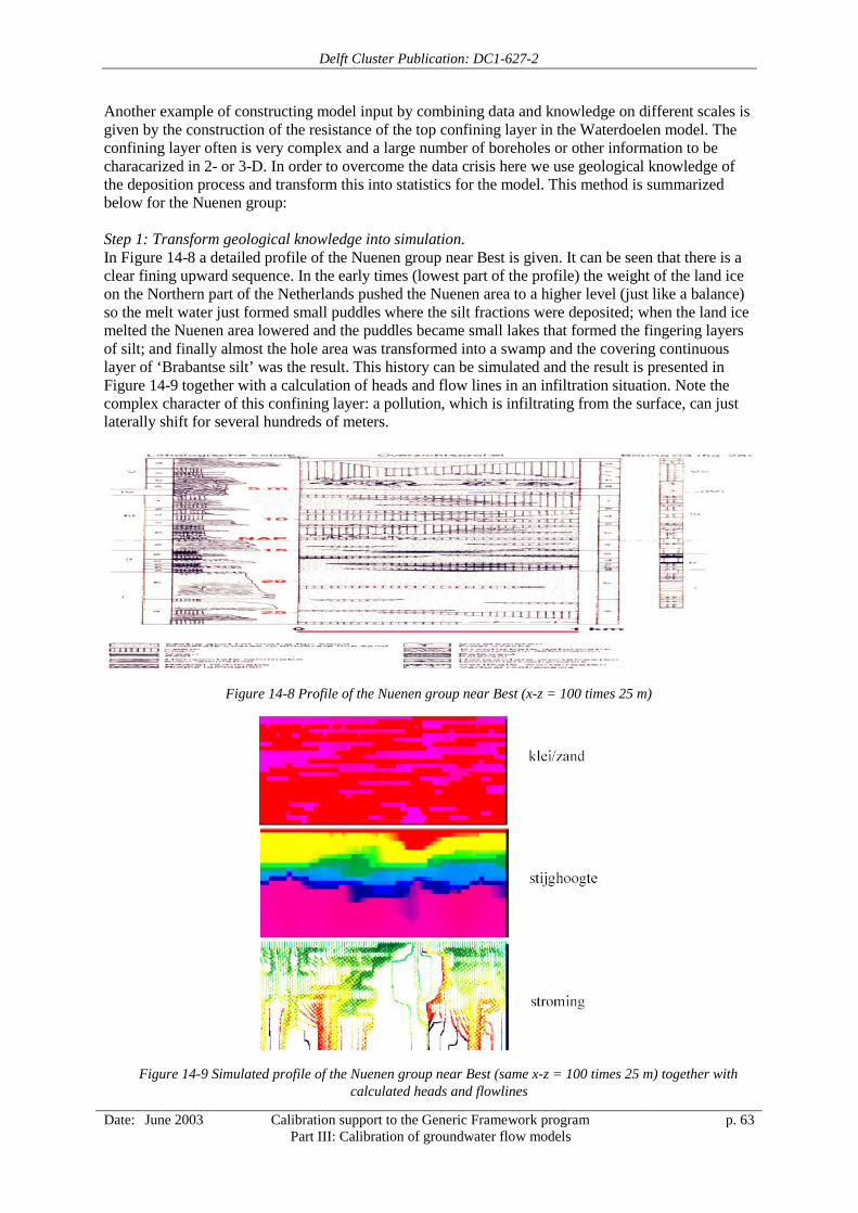
Delft Cluster Publication: DC1-627-2
Date: June 2003 Calibration support to the Generic Framework programPart III: Calibration of groundwater flow models
p. 63
Another example of constructing model input by combining data and knowledge on different scales isgiven by the construction of the resistance of the top confining layer in the Waterdoelen model. Theconfining layer often is very complex and a large number of boreholes or other information to becharacarized in 2- or 3-D. In order to overcome the data crisis here we use geological knowledge ofthe deposition process and transform this into statistics for the model. This method is summarizedbelow for the Nuenen group:
Step 1: Transform geological knowledge into simulation.In Figure 14-8 a detailed profile of the Nuenen group near Best is given. It can be seen that there is aclear fining upward sequence. In the early times (lowest part of the profile) the weight of the land iceon the Northern part of the Netherlands pushed the Nuenen area to a higher level (just like a balance)so the melt water just formed small puddles where the silt fractions were deposited; when the land icemelted the Nuenen area lowered and the puddles became small lakes that formed the fingering layersof silt; and finally almost the hole area was transformed into a swamp and the covering continuouslayer of ‘Brabantse silt’ was the result. This history can be simulated and the result is presented inFigure 14-9 together with a calculation of heads and flow lines in an infiltration situation. Note thecomplex character of this confining layer: a pollution, which is infiltrating from the surface, can justlaterally shift for several hundreds of meters.
Figure 14-8 Profile of the Nuenen group near Best (x-z = 100 times 25 m)
Figure 14-9 Simulated profile of the Nuenen group near Best (same x-z = 100 times 25 m) together withcalculated heads and flowlines
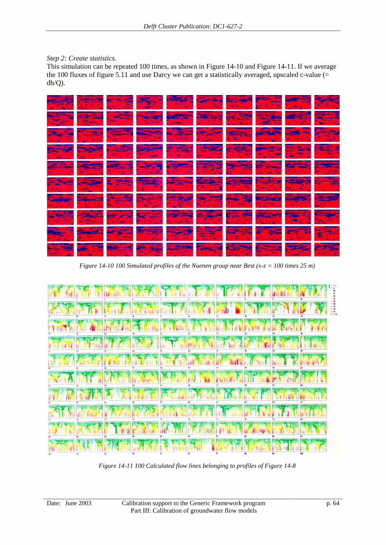
Delft Cluster Publication: DC1-627-2
Date: June 2003 Calibration support to the Generic Framework programPart III: Calibration of groundwater flow models
p. 64
Step 2: Create statistics.This simulation can be repeated 100 times, as shown in Figure 14-10 and Figure 14-11. If we averagethe 100 fluxes of figure 5.11 and use Darcy we can get a statistically averaged, upscaled c-value (=dh/Q).
Figure 14-10 100 Simulated profiles of the Nuenen group near Best (x-z = 100 times 25 m)
Figure 14-11 100 Calculated flow lines belonging to profiles of Figure 14-8
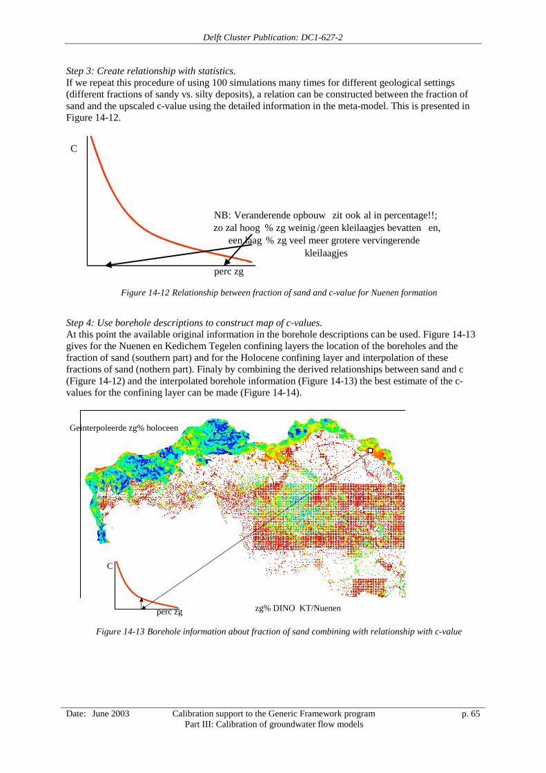
Delft Cluster Publication: DC1-627-2
Date: June 2003 Calibration support to the Generic Framework programPart III: Calibration of groundwater flow models
p. 65
Step 3: Create relationship with statistics.If we repeat this procedure of using 100 simulations many times for different geological settings(different fractions of sandy vs. silty deposits), a relation can be constructed between the fraction ofsand and the upscaled c-value using the detailed information in the meta-model. This is presented inFigure 14-12.
Figure 14-12 Relationship between fraction of sand and c-value for Nuenen formation
Step 4: Use borehole descriptions to construct map of c-values.At this point the available original information in the borehole descriptions can be used. Figure 14-13gives for the Nuenen en Kedichem Tegelen confining layers the location of the boreholes and thefraction of sand (southern part) and for the Holocene confining layer and interpolation of thesefractions of sand (nothern part). Finaly by combining the derived relationships between sand and c(Figure 14-12) and the interpolated borehole information (Figure 14-13) the best estimate of the c-values for the confining layer can be made (Figure 14-14).
Figure 14-13 Borehole information about fraction of sand combining with relationship with c-value
C
perc zg
NB: Veranderende opbouw zit ook al in percentage!!; zo zal hoog % zg weinig / geen kleilaagjes bevatten en,
een laag % zg veel meer grotere vervingerende kleilaagjes
C
perc zg
Geinterpoleerde zg% holoceen
zg% DINO KT/Nuenen

Delft Cluster Publication: DC1-627-2
Date: June 2003 Calibration support to the Generic Framework programPart III: Calibration of groundwater flow models
p. 66
Figure 14-14 Map of c-values
14.3.3 Transforming data to best model inputThe (filtered) information still has to be transformed to model input. E.g. if the stages out of thefiltered AHN (or another database like the “legger”) are used as model input directly, still largemistakes are made. Within the model grid size, by definition, there is no detail present. These stagesshould be corrected for the detail present in reality below the scale of the model grid (Figure 14-15).In fact the difference of the surface elevation and the stage of the water course (in Dutch“drooglegging”) is more important in creating model input stages of river branches than the actualstages itself.
Figure 14-15 Correction factor for stage of water course when bold grid cell size is used
This section has presented some examples of the first, and most important issue in calibration: use theavailable data in a right way. Make clear how original data is transformed into information and howthis information is used in the final model input. Be consistent en reproducible in these methods. Let
Q
Grove gridcellen
Schaal correctie
H grof model H fijn model!
Fijne gridcellen
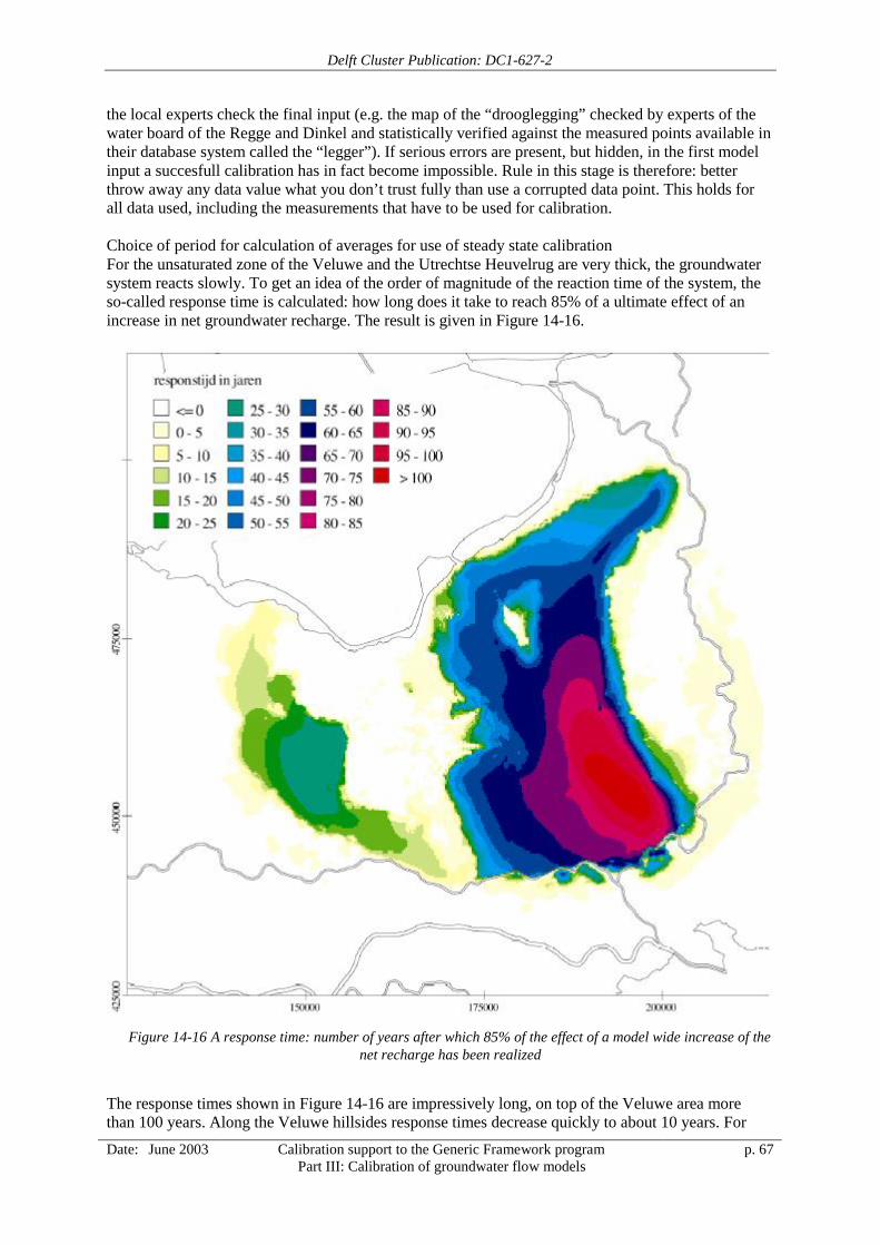
Delft Cluster Publication: DC1-627-2
Date: June 2003 Calibration support to the Generic Framework programPart III: Calibration of groundwater flow models
p. 67
the local experts check the final input (e.g. the map of the “drooglegging” checked by experts of thewater board of the Regge and Dinkel and statistically verified against the measured points available intheir database system called the “legger”). If serious errors are present, but hidden, in the first modelinput a succesfull calibration has in fact become impossible. Rule in this stage is therefore: betterthrow away any data value what you don’t trust fully than use a corrupted data point. This holds forall data used, including the measurements that have to be used for calibration.
Choice of period for calculation of averages for use of steady state calibrationFor the unsaturated zone of the Veluwe and the Utrechtse Heuvelrug are very thick, the groundwatersystem reacts slowly. To get an idea of the order of magnitude of the reaction time of the system, theso-called response time is calculated: how long does it take to reach 85% of a ultimate effect of anincrease in net groundwater recharge. The result is given in Figure 14-16.
Figure 14-16 A response time: number of years after which 85% of the effect of a model wide increase of thenet recharge has been realized
The response times shown in Figure 14-16 are impressively long, on top of the Veluwe area morethan 100 years. Along the Veluwe hillsides response times decrease quickly to about 10 years. For
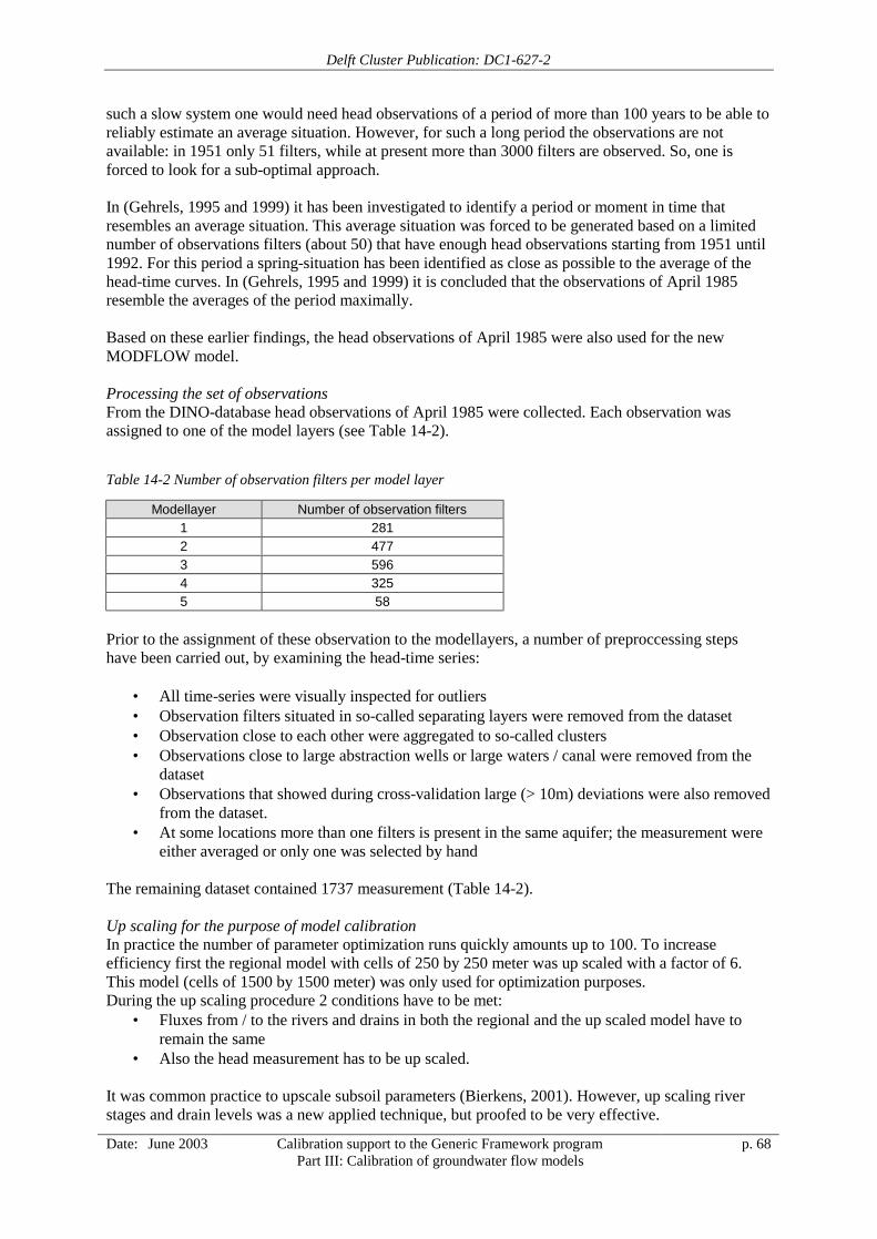
Delft Cluster Publication: DC1-627-2
Date: June 2003 Calibration support to the Generic Framework programPart III: Calibration of groundwater flow models
p. 68
such a slow system one would need head observations of a period of more than 100 years to be able toreliably estimate an average situation. However, for such a long period the observations are notavailable: in 1951 only 51 filters, while at present more than 3000 filters are observed. So, one isforced to look for a sub-optimal approach.
In (Gehrels, 1995 and 1999) it has been investigated to identify a period or moment in time thatresembles an average situation. This average situation was forced to be generated based on a limitednumber of observations filters (about 50) that have enough head observations starting from 1951 until1992. For this period a spring-situation has been identified as close as possible to the average of thehead-time curves. In (Gehrels, 1995 and 1999) it is concluded that the observations of April 1985resemble the averages of the period maximally.
Based on these earlier findings, the head observations of April 1985 were also used for the newMODFLOW model.
Processing the set of observationsFrom the DINO-database head observations of April 1985 were collected. Each observation wasassigned to one of the model layers (see Table 14-2).
Table 14-2 Number of observation filters per model layer
Modellayer Number of observation filters1 2812 4773 5964 3255 58
Prior to the assignment of these observation to the modellayers, a number of preproccessing stepshave been carried out, by examining the head-time series:
• All time-series were visually inspected for outliers• Observation filters situated in so-called separating layers were removed from the dataset• Observation close to each other were aggregated to so-called clusters• Observations close to large abstraction wells or large waters / canal were removed from the
dataset• Observations that showed during cross-validation large (> 10m) deviations were also removed
from the dataset.• At some locations more than one filters is present in the same aquifer; the measurement were
either averaged or only one was selected by hand
The remaining dataset contained 1737 measurement (Table 14-2).
Up scaling for the purpose of model calibrationIn practice the number of parameter optimization runs quickly amounts up to 100. To increaseefficiency first the regional model with cells of 250 by 250 meter was up scaled with a factor of 6.This model (cells of 1500 by 1500 meter) was only used for optimization purposes.During the up scaling procedure 2 conditions have to be met:
• Fluxes from / to the rivers and drains in both the regional and the up scaled model have toremain the same
• Also the head measurement has to be up scaled.
It was common practice to upscale subsoil parameters (Bierkens, 2001). However, up scaling riverstages and drain levels was a new applied technique, but proofed to be very effective.
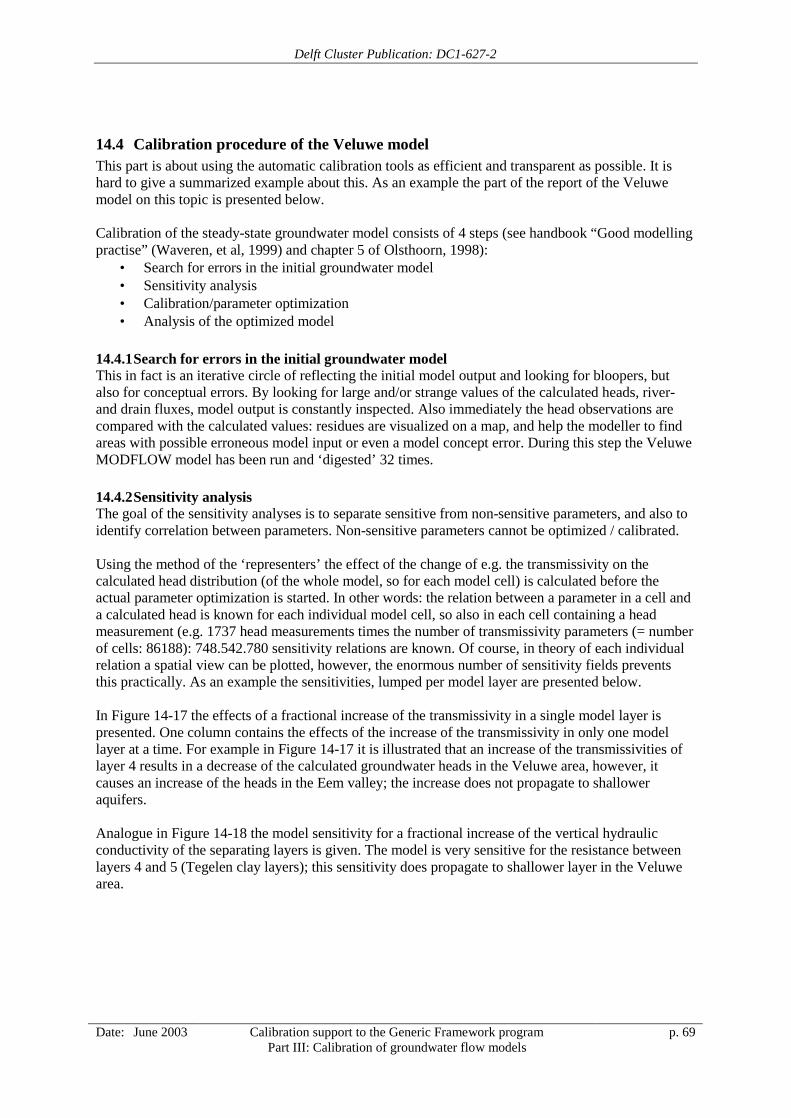
Delft Cluster Publication: DC1-627-2
Date: June 2003 Calibration support to the Generic Framework programPart III: Calibration of groundwater flow models
p. 69
14.4 Calibration procedure of the Veluwe modelThis part is about using the automatic calibration tools as efficient and transparent as possible. It ishard to give a summarized example about this. As an example the part of the report of the Veluwemodel on this topic is presented below.
Calibration of the steady-state groundwater model consists of 4 steps (see handbook “Good modellingpractise” (Waveren, et al, 1999) and chapter 5 of Olsthoorn, 1998):
• Search for errors in the initial groundwater model• Sensitivity analysis• Calibration/parameter optimization• Analysis of the optimized model
14.4.1 Search for errors in the initial groundwater modelThis in fact is an iterative circle of reflecting the initial model output and looking for bloopers, butalso for conceptual errors. By looking for large and/or strange values of the calculated heads, river-and drain fluxes, model output is constantly inspected. Also immediately the head observations arecompared with the calculated values: residues are visualized on a map, and help the modeller to findareas with possible erroneous model input or even a model concept error. During this step the VeluweMODFLOW model has been run and ‘digested’ 32 times.
14.4.2 Sensitivity analysisThe goal of the sensitivity analyses is to separate sensitive from non-sensitive parameters, and also toidentify correlation between parameters. Non-sensitive parameters cannot be optimized / calibrated.
Using the method of the ‘representers’ the effect of the change of e.g. the transmissivity on thecalculated head distribution (of the whole model, so for each model cell) is calculated before theactual parameter optimization is started. In other words: the relation between a parameter in a cell anda calculated head is known for each individual model cell, so also in each cell containing a headmeasurement (e.g. 1737 head measurements times the number of transmissivity parameters (= numberof cells: 86188): 748.542.780 sensitivity relations are known. Of course, in theory of each individualrelation a spatial view can be plotted, however, the enormous number of sensitivity fields preventsthis practically. As an example the sensitivities, lumped per model layer are presented below.
In Figure 14-17 the effects of a fractional increase of the transmissivity in a single model layer ispresented. One column contains the effects of the increase of the transmissivity in only one modellayer at a time. For example in Figure 14-17 it is illustrated that an increase of the transmissivities oflayer 4 results in a decrease of the calculated groundwater heads in the Veluwe area, however, itcauses an increase of the heads in the Eem valley; the increase does not propagate to shalloweraquifers.
Analogue in Figure 14-18 the model sensitivity for a fractional increase of the vertical hydraulicconductivity of the separating layers is given. The model is very sensitive for the resistance betweenlayers 4 and 5 (Tegelen clay layers); this sensitivity does propagate to shallower layer in the Veluwearea.

Delft Cluster Publication: DC1-627-2
Date: June 2003 Calibration support to the Generic Framework programPart III: Calibration of groundwater flow models
p. 70
Figure 14-17 Model sensitivity for change of transmissivities; red: calculated head decrease, blue: increase,as result of a fractional increase of the transmissivity per model layer
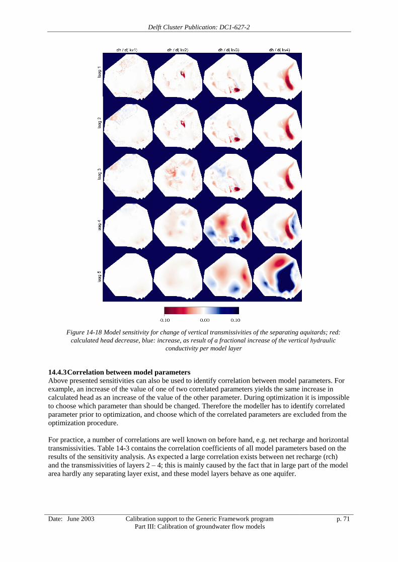
Delft Cluster Publication: DC1-627-2
Date: June 2003 Calibration support to the Generic Framework programPart III: Calibration of groundwater flow models
p. 71
Figure 14-18 Model sensitivity for change of vertical transmissivities of the separating aquitards; red:calculated head decrease, blue: increase, as result of a fractional increase of the vertical hydraulic
conductivity per model layer
14.4.3 Correlation between model parametersAbove presented sensitivities can also be used to identify correlation between model parameters. Forexample, an increase of the value of one of two correlated parameters yields the same increase incalculated head as an increase of the value of the other parameter. During optimization it is impossibleto choose which parameter than should be changed. Therefore the modeller has to identify correlatedparameter prior to optimization, and choose which of the correlated parameters are excluded from theoptimization procedure.
For practice, a number of correlations are well known on before hand, e.g. net recharge and horizontaltransmissivities. Table 14-3 contains the correlation coefficients of all model parameters based on theresults of the sensitivity analysis. As expected a large correlation exists between net recharge (rch)and the transmissivities of layers 2 – 4; this is mainly caused by the fact that in large part of the modelarea hardly any separating layer exist, and these model layers behave as one aquifer.
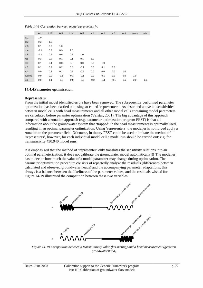
Delft Cluster Publication: DC1-627-2
Date: June 2003 Calibration support to the Generic Framework programPart III: Calibration of groundwater flow models
p. 72
Table 14-3 Correlation between model parameters [-]
kd1 kd2 kd3 kd4 kd5 vc1 vc2 vc3 vc4 rivcond rch
kd1 1.0
kd2 0.2 1.0
kd3 0.1 0.9 1.0
kd4 -0.1 0.8 0.9 1.0
kd5 -0.1 0.6 0.6 0.5 1.0
vc1 0.3 0.2 0.1 0.1 0.1 1.0
vc2 0.1 0.1 0.0 0.0 0.0 0.0 1.0
vc3 0.1 0.2 0.2 0.0 -0.1 0.0 0.1 1.0
vc4 0.0 0.2 0.2 0.2 -0.5 0.0 0.0 0.0 1.0
rivcond 0.0 0.0 -0.1 -0.1 -0.1 0.0 0.1 0.0 0.0 1.0
rch 0.0 -0.8 -0.8 -0.9 -0.6 -0.2 -0.1 -0.1 -0.2 0.0 1.0
14.4.4 Parameter optimization
RepresentersFrom the initial model identified errors have been removed. The subsequently performed parameteroptimization has been carried out using so-called ‘representers’. As described above all sensitivitiesbetween model cells with head measurements and all other model cells containing model parametersare calculated before paramter optimization (Valstar, 2001). The big advantage of this approachcompared with a zonation approach (e.g. parameter optimization program PEST) is that allinformation about the groundwater system that ‘trapped’ in the head measurements is optimally used,resulting in an optimal parameter optimization. Using ‘representers’ the modeller is not forced apply azonation to the parameter field. Of course, in theory PEST could be used to imitate the method of‘representers’, however, for each individual model cell a model run should be carried out: e.g. fortransmissivity 430.940 model runs.
It is emphasized that the method of ‘representer’ only translates the sensitivity relations into anoptimal parameterization: it does not calibrate the groundwater model automatically!!! The modellerhas to decide how much the value of a model parameter may change during optimization. Theparameter optimization procedure consists of repeatedly analyze the residuals (differences betweencalculated and observed groundwater heads) and the accompanying parameter adaptations; thisalways is a balance between the likeliness of the parameter values, and the residuals wished for.Figure 14-19 illustrated the competition between these two variables.
Figure 14-19 Competition between a transmissivity value (kD-meting) and a head measurement (gemetengrondwaterstand)
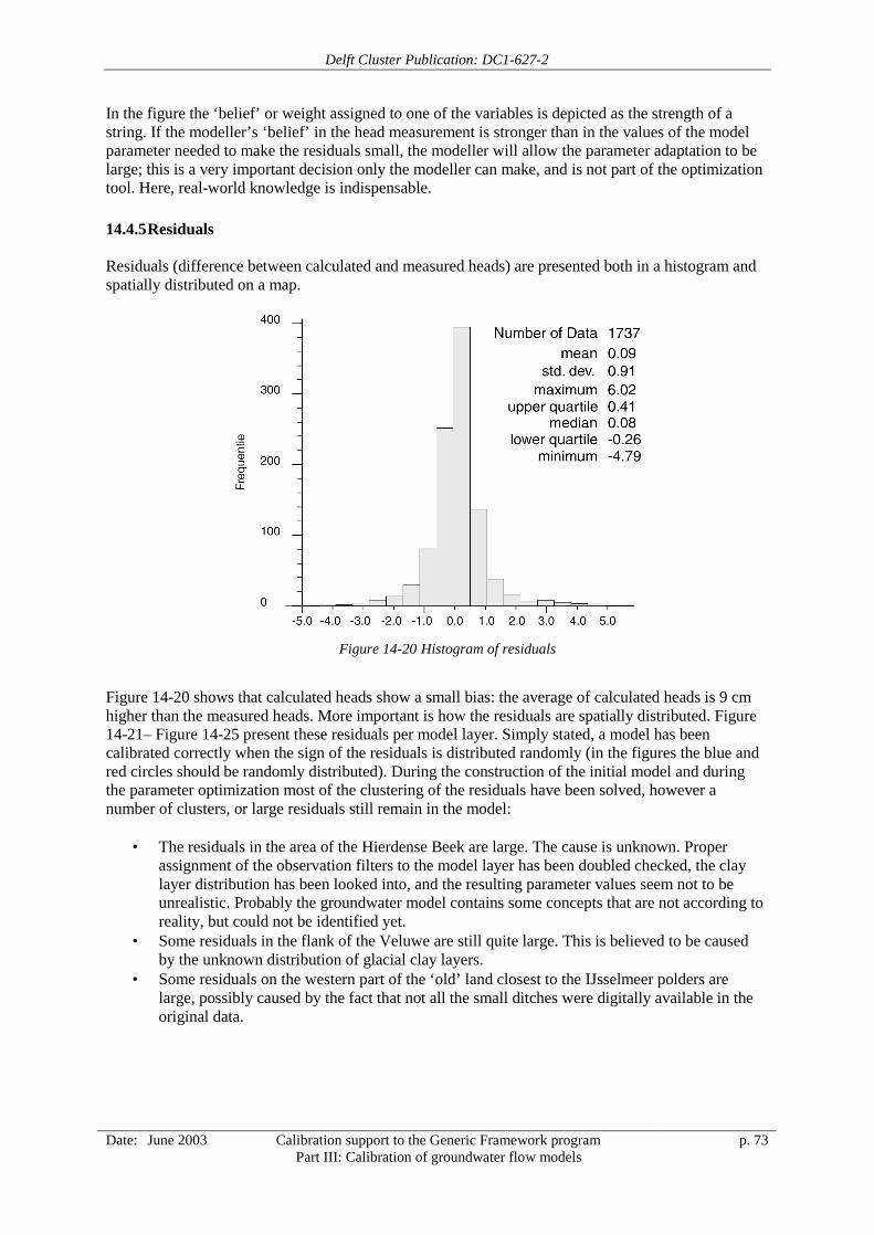
Delft Cluster Publication: DC1-627-2
Date: June 2003 Calibration support to the Generic Framework programPart III: Calibration of groundwater flow models
p. 73
In the figure the ‘belief’ or weight assigned to one of the variables is depicted as the strength of astring. If the modeller’s ‘belief’ in the head measurement is stronger than in the values of the modelparameter needed to make the residuals small, the modeller will allow the parameter adaptation to belarge; this is a very important decision only the modeller can make, and is not part of the optimizationtool. Here, real-world knowledge is indispensable.
14.4.5 Residuals
Residuals (difference between calculated and measured heads) are presented both in a histogram andspatially distributed on a map.
Figure 14-20 Histogram of residuals
Figure 14-20 shows that calculated heads show a small bias: the average of calculated heads is 9 cmhigher than the measured heads. More important is how the residuals are spatially distributed. Figure14-21– Figure 14-25 present these residuals per model layer. Simply stated, a model has beencalibrated correctly when the sign of the residuals is distributed randomly (in the figures the blue andred circles should be randomly distributed). During the construction of the initial model and duringthe parameter optimization most of the clustering of the residuals have been solved, however anumber of clusters, or large residuals still remain in the model:
• The residuals in the area of the Hierdense Beek are large. The cause is unknown. Properassignment of the observation filters to the model layer has been doubled checked, the claylayer distribution has been looked into, and the resulting parameter values seem not to beunrealistic. Probably the groundwater model contains some concepts that are not according toreality, but could not be identified yet.
• Some residuals in the flank of the Veluwe are still quite large. This is believed to be causedby the unknown distribution of glacial clay layers.
• Some residuals on the western part of the ‘old’ land closest to the IJsselmeer polders arelarge, possibly caused by the fact that not all the small ditches were digitally available in theoriginal data.
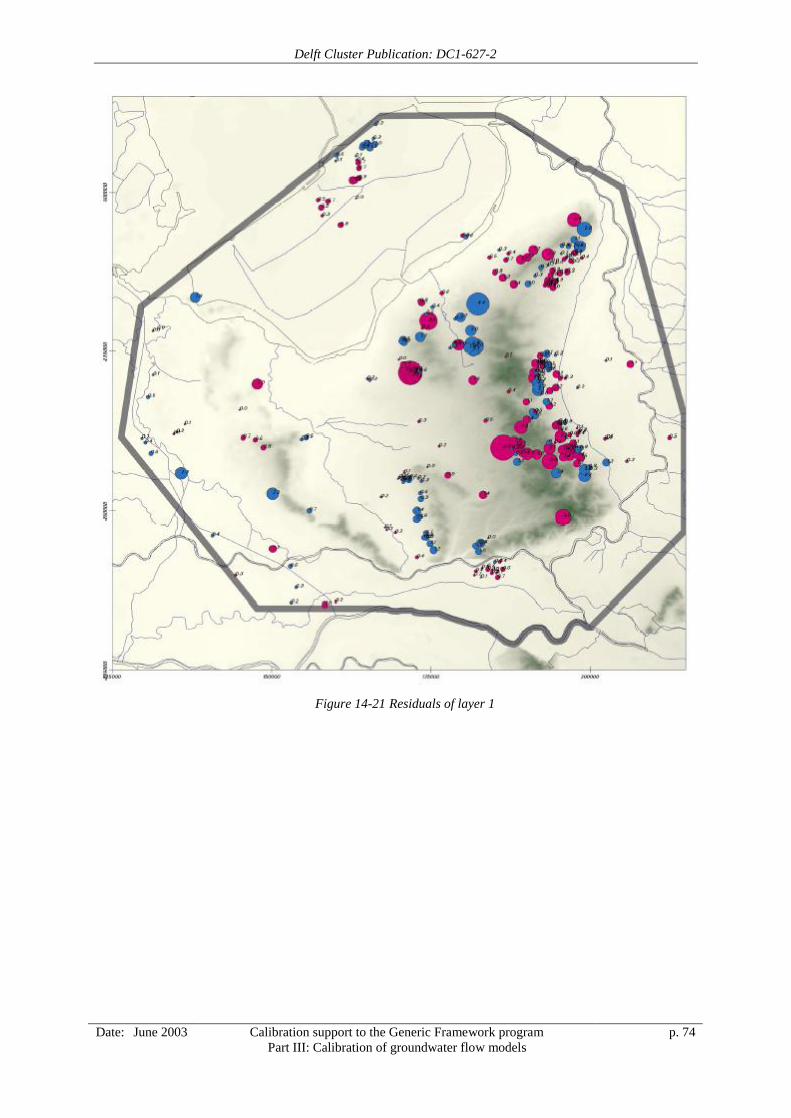
Delft Cluster Publication: DC1-627-2
Date: June 2003 Calibration support to the Generic Framework programPart III: Calibration of groundwater flow models
p. 74
Figure 14-21 Residuals of layer 1
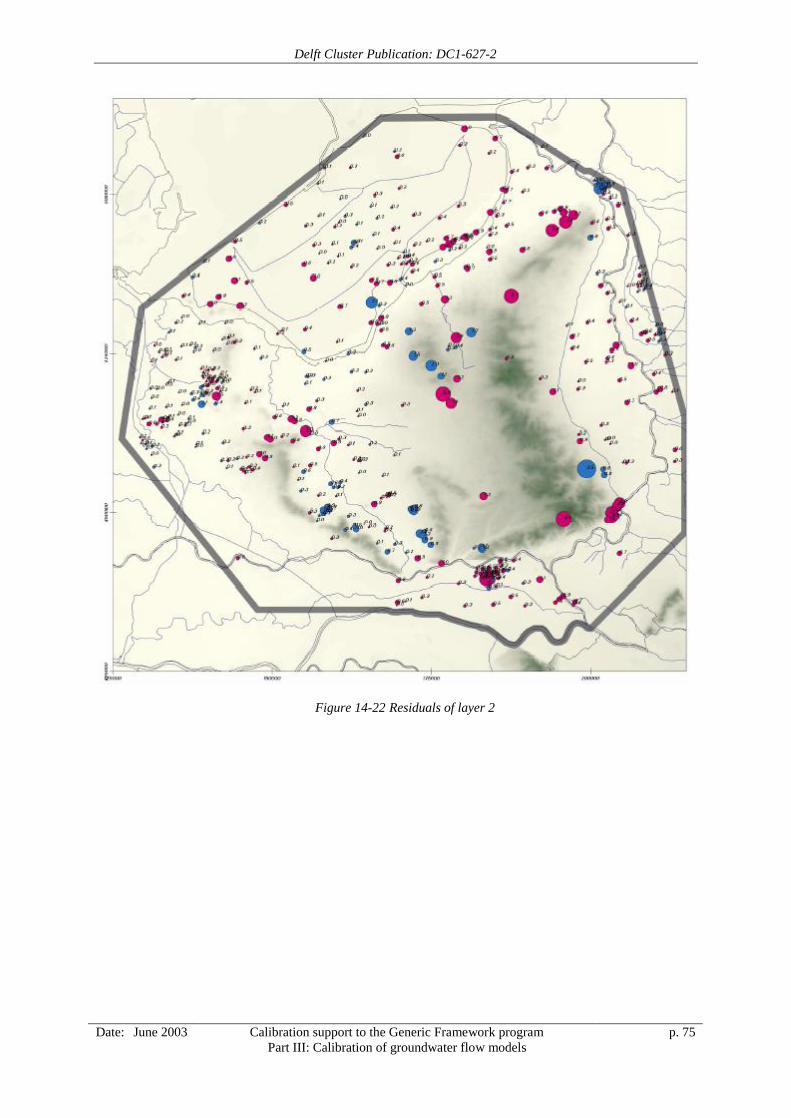
Delft Cluster Publication: DC1-627-2
Date: June 2003 Calibration support to the Generic Framework programPart III: Calibration of groundwater flow models
p. 75
Figure 14-22 Residuals of layer 2
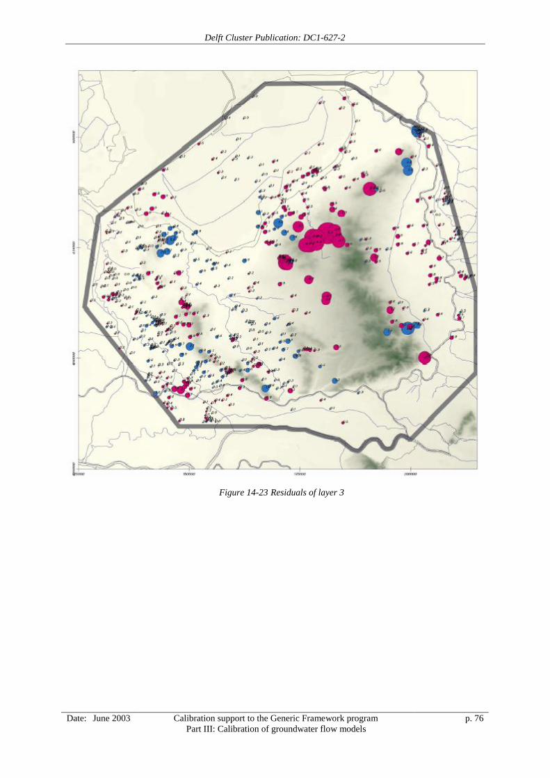
Delft Cluster Publication: DC1-627-2
Date: June 2003 Calibration support to the Generic Framework programPart III: Calibration of groundwater flow models
p. 76
Figure 14-23 Residuals of layer 3
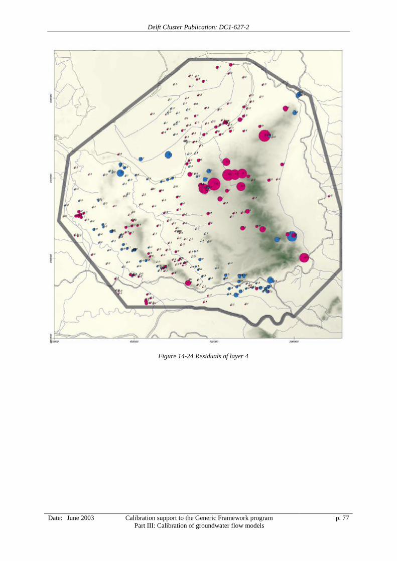
Delft Cluster Publication: DC1-627-2
Date: June 2003 Calibration support to the Generic Framework programPart III: Calibration of groundwater flow models
p. 77
Figure 14-24 Residuals of layer 4
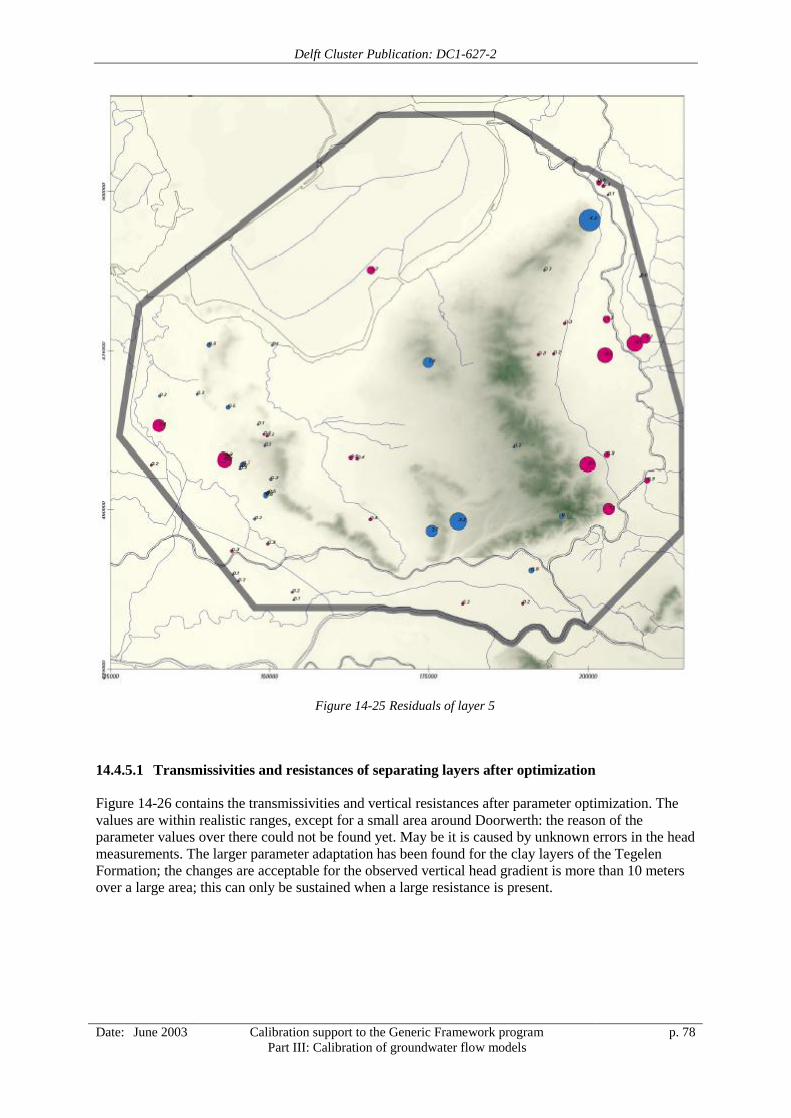
Delft Cluster Publication: DC1-627-2
Date: June 2003 Calibration support to the Generic Framework programPart III: Calibration of groundwater flow models
p. 78
Figure 14-25 Residuals of layer 5
14.4.5.1 Transmissivities and resistances of separating layers after optimization
Figure 14-26 contains the transmissivities and vertical resistances after parameter optimization. Thevalues are within realistic ranges, except for a small area around Doorwerth: the reason of theparameter values over there could not be found yet. May be it is caused by unknown errors in the headmeasurements. The larger parameter adaptation has been found for the clay layers of the TegelenFormation; the changes are acceptable for the observed vertical head gradient is more than 10 metersover a large area; this can only be sustained when a large resistance is present.

Delft Cluster Publication: DC1-627-2
Date: June 2003 Calibration support to the Generic Framework programPart III: Calibration of groundwater flow models
p. 79
Figure 14-26 Transmissivities and resistances after parameter optimization
14.4.5.2 Calculated fluxesAlso the fluxes to and from the rivers, drains and ditches are continuously monitored as calculated bythe groundwater model. The fluxes between the model layers are also analysed during theconstruction of the initial model and the parameter optimization. Figure 14-27 contains a visualizationof the flux-terms. The drainage pattern on the flanks of the Veluwe is clearly visible. The order ofmagnitude of the drainage fluxes coincides within expected ranges. Also the infiltration of theApeldoorns kanaal (about 1 mm per day) is considered to be reasonable.
Figure 14-27 Calculated fluxes of the primairy, secundaire and tertairy system, the large canals and rivers,and between the modellayers (mm/day)
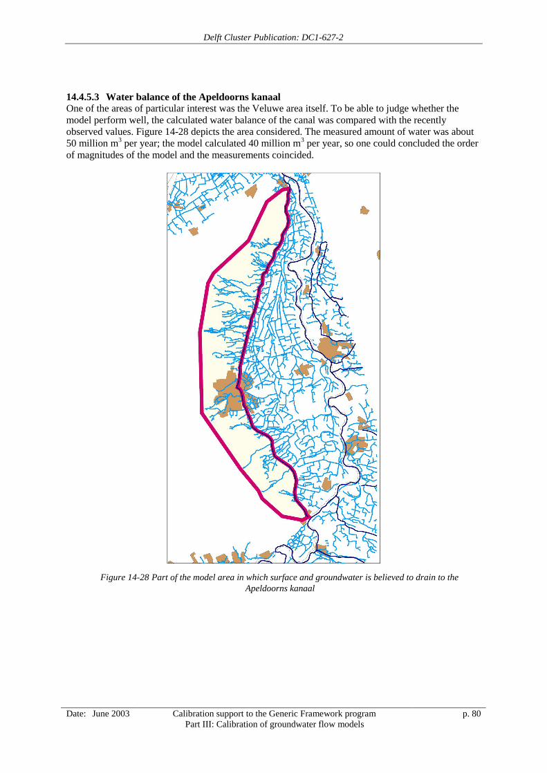
Delft Cluster Publication: DC1-627-2
Date: June 2003 Calibration support to the Generic Framework programPart III: Calibration of groundwater flow models
p. 80
14.4.5.3 Water balance of the Apeldoorns kanaalOne of the areas of particular interest was the Veluwe area itself. To be able to judge whether themodel perform well, the calculated water balance of the canal was compared with the recentlyobserved values. Figure 14-28 depicts the area considered. The measured amount of water was about50 million m3 per year; the model calculated 40 million m3 per year, so one could concluded the orderof magnitudes of the model and the measurements coincided.
Figure 14-28 Part of the model area in which surface and groundwater is believed to drain to theApeldoorns kanaal
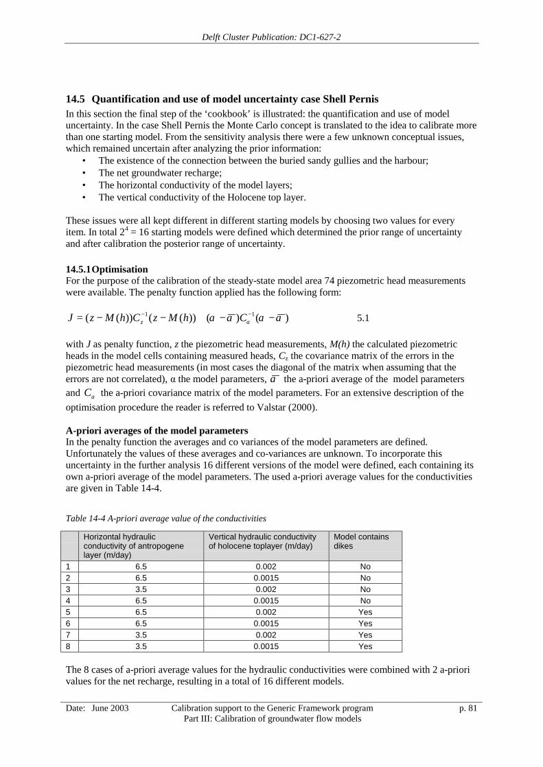
Delft Cluster Publication: DC1-627-2
Date: June 2003 Calibration support to the Generic Framework programPart III: Calibration of groundwater flow models
p. 81
14.5 Quantification and use of model uncertainty case Shell PernisIn this section the final step of the ‘cookbook’ is illustrated: the quantification and use of modeluncertainty. In the case Shell Pernis the Monte Carlo concept is translated to the idea to calibrate morethan one starting model. From the sensitivity analysis there were a few unknown conceptual issues,which remained uncertain after analyzing the prior information:
• The existence of the connection between the buried sandy gullies and the harbour;• The net groundwater recharge;• The horizontal conductivity of the model layers;• The vertical conductivity of the Holocene top layer.
These issues were all kept different in different starting models by choosing two values for everyitem. In total 24 = 16 starting models were defined which determined the prior range of uncertaintyand after calibration the posterior range of uncertainty.
14.5.1 OptimisationFor the purpose of the calibration of the steady-state model area 74 piezometric head measurementswere available. The penalty function applied has the following form:
)()())(())(( 11 αααα α −−+−−= −− ChMzChMzJ z 5.1
with J as penalty function, z the piezometric head measurements, M(h) the calculated piezometricheads in the model cells containing measured heads, Cz the covariance matrix of the errors in thepiezometric head measurements (in most cases the diagonal of the matrix when assuming that theerrors are not correlated), α the model parameters, α the a-priori average of the model parametersand αC the a-priori covariance matrix of the model parameters. For an extensive description of theoptimisation procedure the reader is referred to Valstar (2000).
A-priori averages of the model parametersIn the penalty function the averages and co variances of the model parameters are defined.Unfortunately the values of these averages and co-variances are unknown. To incorporate thisuncertainty in the further analysis 16 different versions of the model were defined, each containing itsown a-priori average of the model parameters. The used a-priori average values for the conductivitiesare given in Table 14-4.
Table 14-4 A-priori average value of the conductivities
Horizontal hydraulicconductivity of antropogenelayer (m/day)
Vertical hydraulic conductivityof holocene toplayer (m/day)
Model containsdikes
1 6.5 0.002 No2 6.5 0.0015 No3 3.5 0.002 No4 6.5 0.0015 No5 6.5 0.002 Yes6 6.5 0.0015 Yes7 3.5 0.002 Yes8 3.5 0.0015 Yes
The 8 cases of a-priori average values for the hydraulic conductivities were combined with 2 a-priorivalues for the net recharge, resulting in a total of 16 different models.
Delft Cluster Publication: DC1-627-2
Date: June 2003 Calibration support to the Generic Framework programPart III: Calibration of groundwater flow models
p. 82
Covariance of the model parametersThe co-variances of all model versions were kept constant. The co-variances of ln(transmissivity) andof the vertical hydraulic conductivity were estimated to be 0.65, resulting in a factor of change ofabout 5.
Minimising the penalty functionThe minimisation of the penalty function was done by the representer method. For each model version3 iterations were necessary for the model to convergence.
14.5.2 Results of optimisation
Piezometric headsFor each of the 16 model versions the inverse model optimisation process was executed. In Figure14-29 the a-priori piezometric head distribution are presented together with the locations and(classified) values of the measured piezometric heads.
Figure 14-30 shows the calculated piezometric heads after calibration. A number of mattersimmediately draw attention. All calculated piezometric head distributions more or less have the samepattern, independent from the a-priori estimations as presented in Figure 14-29. Also the calculatedpiezometric heads are for most points very close to the measured values of the piezometric heads.However, for a small number of the measurement locations the deviations are larger, which meansthat the change of the parameter values was not enough to meet the desired fit of calculated andmeasured heads; it is possible that some hydrological phenomena are unconsciously not incorporatedin the groundwater model. The use of a-priori averages and co-variances prevents that the values ofthe parameters are not being updated to value that are not realistic anymore.
ConductivitiesAmong others the transmissivities of the overlying anthropogenic layer were updated during theoptimisation process. Figure 14-31 contains a visualisation of the factors by which the a-priori valuehas been updated during optimisation. As can be seen in Figure 14-31 the factors are largest in thewestern-, south-centre and eastern part of the model area. The largest factor is caused by a relativelyhigh value of the piezometric levels near the IBC-systems. The IBC-system normally causedepressions in the piezometric head levels. These depressions are during optimisation beingneutralised by an increase of the horizontal hydraulic conductivities.
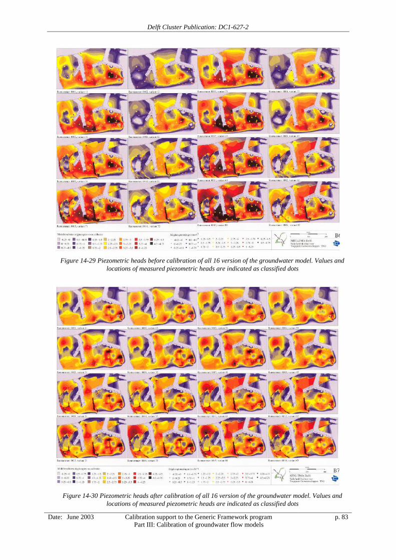
Delft Cluster Publication: DC1-627-2
Date: June 2003 Calibration support to the Generic Framework programPart III: Calibration of groundwater flow models
p. 83
Figure 14-29 Piezometric heads before calibration of all 16 version of the groundwater model. Values andlocations of measured piezometric heads are indicated as classified dots
Figure 14-30 Piezometric heads after calibration of all 16 version of the groundwater model. Values andlocations of measured piezometric heads are indicated as classified dots
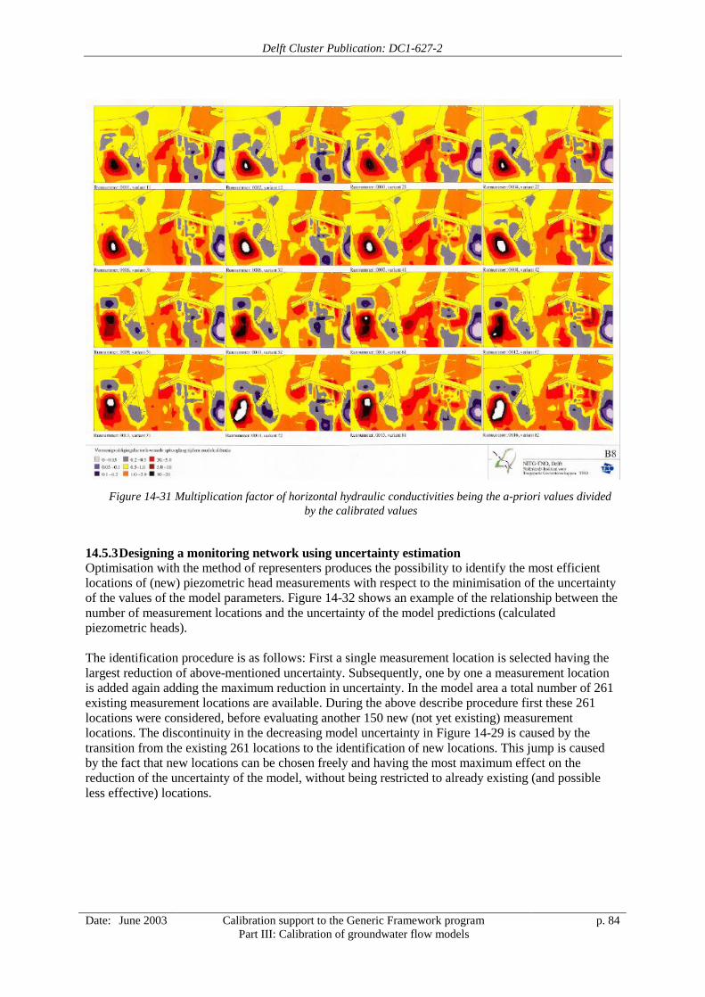
Delft Cluster Publication: DC1-627-2
Date: June 2003 Calibration support to the Generic Framework programPart III: Calibration of groundwater flow models
p. 84
Figure 14-31 Multiplication factor of horizontal hydraulic conductivities being the a-priori values dividedby the calibrated values
14.5.3 Designing a monitoring network using uncertainty estimationOptimisation with the method of representers produces the possibility to identify the most efficientlocations of (new) piezometric head measurements with respect to the minimisation of the uncertaintyof the values of the model parameters. Figure 14-32 shows an example of the relationship between thenumber of measurement locations and the uncertainty of the model predictions (calculatedpiezometric heads).
The identification procedure is as follows: First a single measurement location is selected having thelargest reduction of above-mentioned uncertainty. Subsequently, one by one a measurement locationis added again adding the maximum reduction in uncertainty. In the model area a total number of 261existing measurement locations are available. During the above describe procedure first these 261locations were considered, before evaluating another 150 new (not yet existing) measurementlocations. The discontinuity in the decreasing model uncertainty in Figure 14-29 is caused by thetransition from the existing 261 locations to the identification of new locations. This jump is causedby the fact that new locations can be chosen freely and having the most maximum effect on thereduction of the uncertainty of the model, without being restricted to already existing (and possibleless effective) locations.
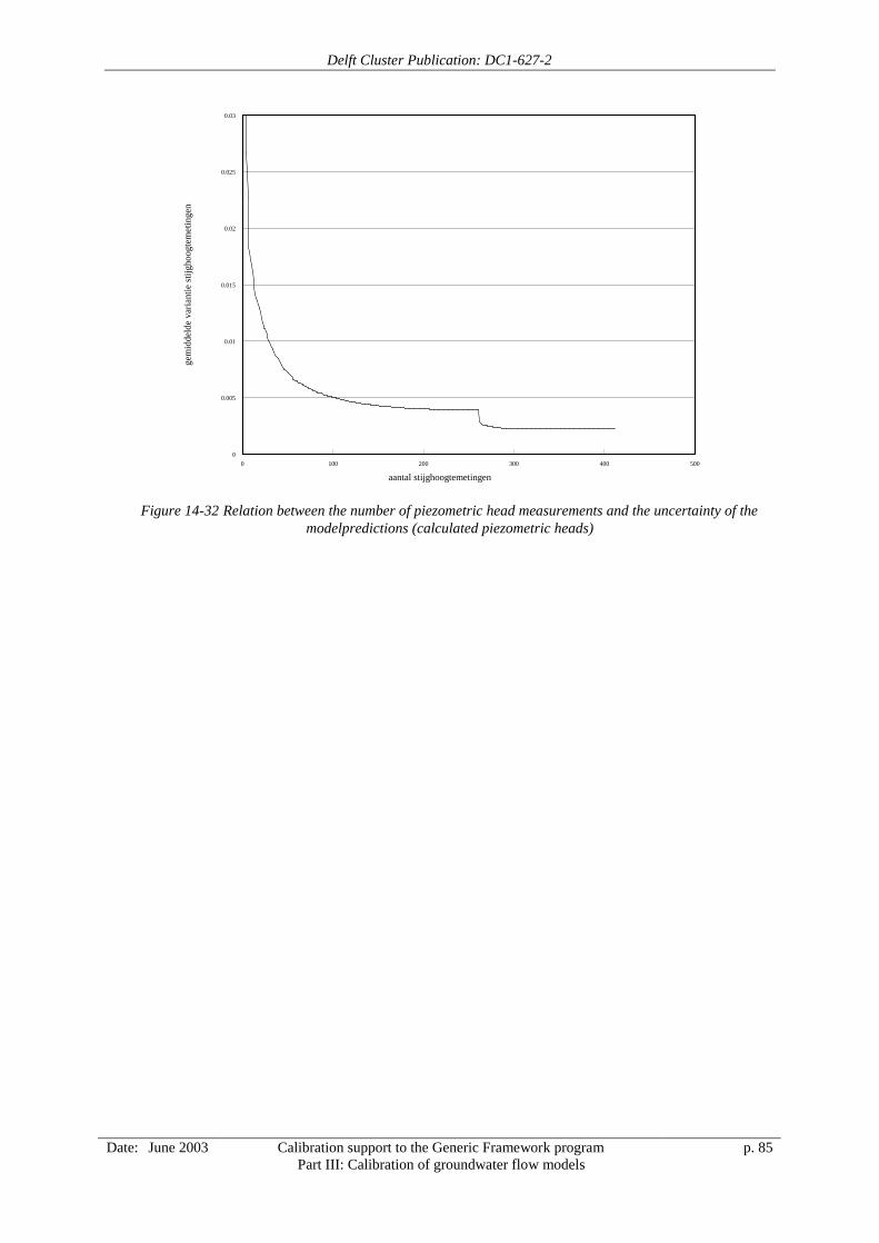
Delft Cluster Publication: DC1-627-2
Date: June 2003 Calibration support to the Generic Framework programPart III: Calibration of groundwater flow models
p. 85
0 100 200 300 400 5000
0.005
0.01
0.015
0.02
0.025
0.03
aantal stijghoogtemetingen
gem
idde
lde
varia
ntie
stijg
hoog
tem
etin
gen
Figure 14-32 Relation between the number of piezometric head measurements and the uncertainty of themodelpredictions (calculated piezometric heads)
Delft Cluster Publication: DC1-627-2
Date: June 2003 Calibration support to the Generic Framework programPart III: Calibration of groundwater flow models
p. 86
ReferencesBroers, H.P., J.H. Hoogendoorn en H. Houtman, 1992Opbouw van het geohydrologische lagenmodel van REGIS/Digitale Grondwaterkaart. TNO-rapportOS 92-01 A, tweede versie
Gehrels, J.C, 1999Groundwater level fluctuations. Separation of natural from antropogenic influences and determinationof groundwater recharge in the Veluwe are, the Netherlands. Vrije Universiteit, Amsterdam. ISBN 90-75739-04-4
Gómez-Hernández, J.J, A. Sahuquillo and J.E. Capilla. 1997Stochastic simulation of transmissivity fields conditional to both transmissivity and piezometric data--I. Theory. Journal of Hydrology, 203 (1997) pp. 162-174
NITG-TNO. 1998Regionaal Geohydrologisch Informatie Systeem. REGIS handleiding v2r3. NITG-TNO , januari 1998
Olsthoorn, T.N. 1998Groundwater modelling: calibration and the use of spreadsheets. Delft University Press. ISBN 90-407-1702-8 / CIP.
McDonald, M.G. and A.W. Harbaugh. 1998A modular Three-Dimensional Finite-Difference Ground-Water Flow Model. U.S. Geological Survey.
Minnema, B. 2002Modelleeromgeving Veluwe. TNO-rapport NITG 02-073-B., 2002.
Valstar, J.R. 2001Inverse modeling of groundwater flow and transport. Ph.D.-thesis. Technical University Delft, 2001.ISBN 9064640629.
Valstar, J.R. en B. Minnema, 2002Anisotropie in MODFLOW. TNO-rapport NITG 02-073-B
Waveren, R.H. van (Rijkswaterstaat), S. Groot (WL), H. Scholten (LUW), F.C. van Geer (TNO-NITG), J.H.M. Wösten (SC-DLO), R.D. Koeze (WL), J.J. Noort (STOWA), 1999Vloeiend modelleren in het waterbeheer. Handboek Good Modelling Practice. STOWA-rapport 99-05.Rijkswaterstaat-RIZA-rapport 99.036. ISBN-nr 90-5773-056-1.

Delft Cluster-publication: 627-2
Date: June 2003 Calibration support to the Generic Framework program p. 1
General Appendix: Delft Cluster Research Programme Information This publication is a result of the Delft Cluster research-program 1999-2002 (ICES-KIS-II), that consists of 7 research themes: ? Soil and structures, ? Risks due to flooding, ? Coast and river , ? Urban infrastructure, ? Subsurface management, ? Integrated water resources management, ? Knowledge management. This publication is part of:
Research Theme : Integrated Water Resources Management
Baseproject name : Water Systems
Project name : Knowledge based support of the Generic Framework Program
Projectleader/Institute Dr.Ir. P.J.A. Gijsbers WL|Delft Hydraulics
Project number : 06.02.07
Projectduration : 01-03-2000 - 31-12-2002
Financial sponsor(s) : Delft Cluster
Generic Framework program
Projectparticipants : WL|Delft Hydraulics
TNO-NITG
IHE – Delft
TU Delft - CiTG
Total Project-budget : € 136.400
Number of involved PhD-students : 0
Keverling Buismanweg 4 Tel: +31-15-269 37 93 Postbus 69 Fax: +31-15-269 37 99 2600 AB Delft [email protected] The Netherlands www.delftcluster.nl
Delft Cluster is an open knowledge network of five Delft-based institutes for long-term fundamental strategic research focussed on the sustainable development of densely populated delta areas.

Delft Cluster-publication: 627-2
Date: June 2003 Calibration support to the Generic Framework program p. 2
Theme Managementteam: Integrated Water Resources Management Name Organisation
Prof.Ir. E. van Beek WL|Delft Hydraulics
Prof.Dr.Ir. H.S. Savenije IHE - Delft
Projectgroup During the execution of the project the research team included: Name Organisation
1. P.J.A. Gijsbers WL|Delft Hydraulics & TU Delft - CiTG
2. G.P. Prinsen WL|Delft Hydraulics
3. J.A. van Gils WL|Delft Hydraulics
4. E. Brakkee WL|Delft Hydraulics
5. K-J. van Heeringen WL|Delft Hydraulics
6. B. Minnema TNO-NITG
7. C.B.M. te Stroet TNO-NITG
8. D.P. Solomatine IHE-Delft
Other Involved personnel The realisation of this report involved: Name Organisation
1.
2
3