1

Citation: Wadsworth, R., Balzter, H., Gerard, F., George, C., Comber, L. and Fisher, P. (2008): An environmental assessment of land cover and land use change in Central Siberia using quantified conceptual overlaps to reconcile inconsistent data sets, Journal of Land Use Science, 3:4, 251 – 264. DOI: 10.1080/17474230802559629

An environmental assessment of land cover and land use

change in Central Siberia using Quantified Conceptual

Overlaps to reconcile inconsistent data sets

Richard WADSWORTH

1, Heiko BALZTER

2, France GERARD

3, Charles GEORGE

3, Alexis

COMBER2 and Peter FISHER

2

1 Centre for Ecology and Hydrology, Lancaster Environment Centre, Library Avenue, Bailrigg,

Lancaster, LA1 4AP, UK, email rawad@ceh.ac.uk 2 Department of Geography, University of Leicester, Bennett Building, University Road, Leicester,

LE1 7RH, UK, email hb91@le.ac.uk 3 Centre for Ecology and Hydrology, Maclean Building, Benson Lane, Crowmarsh Gifford,

Wallingford, Oxfordshire, OX10 8BB, UK, email ffg@ceh.ac.uk

Abstract

Environmental monitoring and assessment frequently require remote sensing techniques to be

deployed. The production of higher level spatial datasets from remote sensing has often been driven

by short-term funding constraints and specific information requirements by the funding agencies. As

a result, a wide variety of historic datasets exists that were generated using different atmospheric

correction methods, classification algorithms, class labelling systems, training sites, map

projections, input data and spatial resolutions. Because technology, science and policy objectives are

continuously changing, repeated natural resource inventories rarely employ the same methods as in

previous surveys and often use class definitions that are inconsistent with earlier datasets (Comber

et al. 2003). Since it is generally not economically feasible to recreate these historic land cover /

land use datasets, often inconsistent datasets have to be compared.

An environmental assessment of land cover and land use change in Central Siberia is presented. It

utilises several different digital land cover maps generated from satellite data acquired in different

years. The specific characteristics of different land cover maps create difficulties in interpreting

change maps as either land cover / land use change or a pure data inconsistency. Many studies do

not explicitly deal with these inconsistencies. It is argued that a rigorous treatment of multi-temporal

datasets must include an explicit map of consistency between the multi-temporal land cover maps.

A method utilising aspects of quantified conceptual overlaps (Ahlqvist 2004) and semantic-

statistical approaches (Comber et al. 2004a; Comber et al. 2004b) is presented. The method is

applied to reconcile three independent land cover maps of Siberia, which differ in the number and

types of classes, spatial resolution, acquisition date, sensor used and purpose.

A map of inconsistency scores is presented that identifies areas of most likely land cover change

based on the maximum inconsistency between the maps. The method of Quantified Conceptual

Overlaps was used to identify regions where further investigations on the causes of the observed

inconsistencies seem warranted. The method highlights the value of assessing change between

inconsistent spatial datasets, provided that the inconsistency is adequately considered.

2

Keywords:

Inconsistent information, metadata, conceptual overlap, semantics, land cover.

1. Introduction

There is a common problem in the environmental sciences that frequently when a new survey is

conducted it creates a new “baseline” rather than faithfully repeating an established procedure.

There are good reasons why this happens: Scientific knowledge advances, policy objectives change

and technology develops. Unfortunately these developments can make it difficult to disentangle

changes in the phenomena from changes in their representation in the datasets. Of course for some

subjects, e.g. studies at geological time scales, we can be sure that our understanding of the

phenomena is changing faster than the phenomena itself is changing. With geological maps of the

same area we know that the differences represent changes in knowledge, technology and objectives,

not that the geology itself has changed (with very few exceptions). For phenomena like land cover

and land use, we are less certain whether an observed difference is “real” (the land cover or land use

has changed) or whether it is a different representation of the same entity.

In the past this problem was less acute because a given map was used to support a description of the

phenomena, libraries are full of hundreds of pages of monographs describing the issues, the

methods and the implications behind a particular survey. In these monographs the maps are usually

attached at the back of the book and are used in conjunction with the report. With the development

of GIS, web based mapping and the Internet, the “map” may be the only information that is

available; the monograph may not be available to the user and may not even have been produced

(Fisher 2003). Not only has the “balance of power” between the graphical (map) and textual

(monograph) changed, but crucially the user may wrongly treat the map as measured data and not as

information (an interpretation of the measurements). In the case of remote sensing data, the direct

measurements are top-of-atmosphere radiances at different wavelengths, and their interpretation

could be a classified land cover map.

The implication of not having the accompanying “monograph” to a data set is that the user may

assume that their “mental image” of the world prompted by the class labels exactly matches that of

the data producer. Everyone is familiar with land cover and land use, and hence there is an inbuilt

assumption that the common terms or labels, such as forest, wetland, grassland etc., relate to a

common physical reality. For example, if you say the word “forest” to someone then that word will

generate an image in their mind, they will have a clear idea of what they think you are talking about;

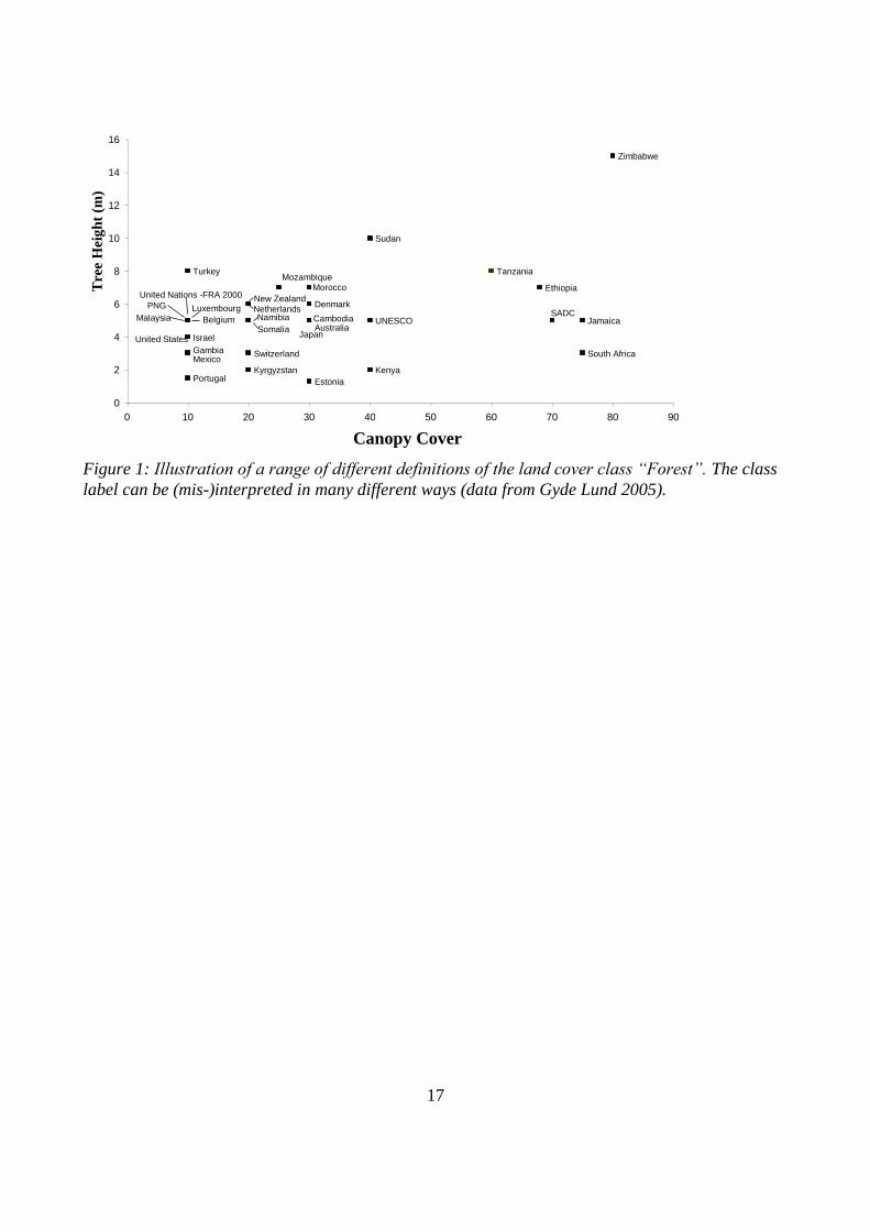
but, there is no guarantee that their image and your image are the same. Figure 1 illustrates some of

the differences between official definitions of forest used by different countries (Gyde Lund 2005).

In fact the situation is even more complex than Figure 1 indicates because some countries include

land where there is the intention to plant trees (for example the UK); other countries exclude land

where the trees are not growing fast enough (eg. Eire). Similarly, neighbouring countries can differ

as to whether or not to include bamboo and palms as “trees” for the purpose of defining a “forest”.

The objective of this paper is to introduce the approach and demonstrate the application of

“quantified conceptual overlaps” to a real study of land cover change in Siberia using inconsistent

land cover data that were generated by different producers and use different class definitions. The

general and widespread issue of reconciling inconsistent data sets is discussed.

2. Remote sensing data

All the presented maps are derived from satellite remote sensing and none of them has a significant

3

amount of local validation. Land cover data is available from two global data products and one

regional study:

IGBP (International Geosphere-Biosphere program) presents a global classification of 1 km

AVHRR (Advanced Very High Resolution Radiometer) data collected between April 1992 and

March 1993 with 17 classes in the study area.

GLC 2000 (Global Land Cover 2000) is a global classification based on 1 km SPOT-

VEGETATION (Satellite pour l’Observation de la Terre), AVHRR and other data collected

between November 1999 and December 2000 with 29 classes.

SUC (University of Wales at Swansea) is based on MODIS (Moderate Resolution Differential

Imaging Spectrometer) 500 m imagery with 16 classes, two maps were available corresponding

to data acquisition dates in 2003 and 2004.

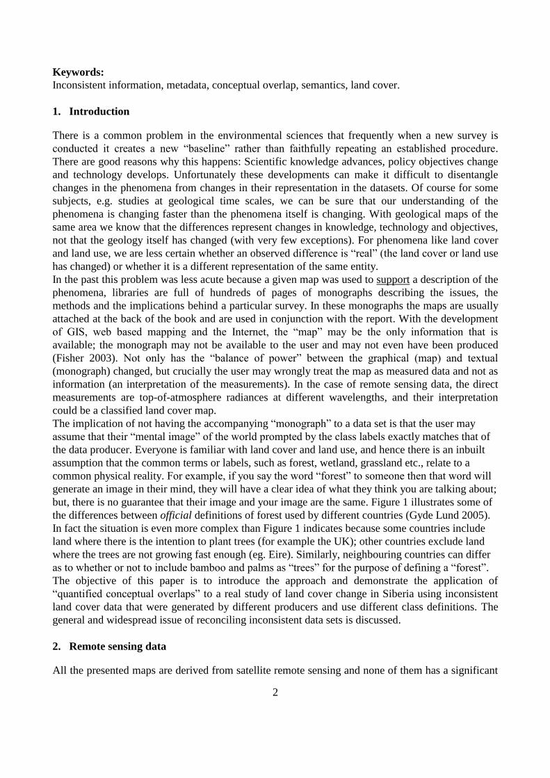
Figure 2 shows a small area of about 200 km across, centered on 55° 20’ N 92° 20’E in the Siberian

data sets. Arbitrary colours are used because the intention is to illustrate and emphasis that despite

the different class systems used some landscape features are apparent (some very high resolution

images and a few photographs of this regions are available through GoogleEarth). There are some

features that are clearly differentiated in some classification systems but not in others. Our approach

is to try and maximise the use of the inconsistent information available from these different remote

sensing surveys.

3. A Novel Approach to Inconsistent Data

The most common approach to inconsistent data is to thematically aggregate each data set into a

reduced number of common classes. This relies on the often implicit assumption that the

aggregations are significantly more similar than the initial classes and that each individual class of

each data set falls naturally and discretely into an aggregate class. An extreme example is Wulder et

al. (2004) who reduce the land cover of Canada to just two classes: “forest” and “not forest”. Even

in cases where the aggregation assumption is warranted aggregating classes reduces the thematic

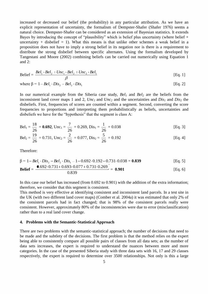
content of the data and hence the types of changes and comparisons that can be made. A less

extreme example of aggregation is shown in Figure 3 (Flety et al. 2004) where two land cover

schemes (the IGBP & GLC 2000 classifications) are aggregated into eight “super” classes.

The aggregation approach is based on expert opinion and it can be seen that in this case for

example, the expert considers that the “forest / cropland complex” should contribute to the “forest”

class and not to the cropland class. Under any aggregation scheme a class can contribute to only one

“super” class. Although not strictly mandatory it is typical in an aggregation approach to degrade the

spatial resolution of the information to the coarsest spatial scale.

To address these issues of lack of consistency and comparability, FAO has developed a Land Cover

Classification System (LCCS) to overcome the problems with aggregation (Di Gregorio and Jansen

2000). LCCS describes each land cover class in terms of the biophysical properties of that class in a

hierarchical tree structure. Studies adhering to this system will simplify cross-comparisons with

other LCCS-compatible projects although there will still be issues of how similar two classes

defined in the LCCS are to each other. However, still a whole range of historical datasets exist that

could be analysed if a method for dealing with uncertainty and inconsistency was available.

Recently an alternative approach to aggregation has been proposed in a series of papers (Comber et

al. 2004a; Comber et al. 2004b) and termed a combined semantic-statistical procedure. In essence

this extends the aggregation approach in two ways:

“many-to-one” relationships to “many-to-many” relationships

“yes/no” to “yes/don’t know/no”

4

Expert opinion is sought on the relationship between individual classes in each data set; the expert

expresses the relationship between all possible pairings as being “expected” (1 or yes),

“unexpected” (-1 or no) or “uncertain” (0 or don’t know). By “expected”, we mean that the presence

of that class increases our confidence in a particular attribution or that the classes are very similar,

by “unexpected” that it decreases our confidence or that they are very different and “uncertain” it

neither increases nor decreases our confidence in an attribution nor is the expert certain how similar

they are. These relationships are set out in a series of look-up-tables (LUT). One LUT is required

between each pair of data sets; a LUT is also required to specify the similarity between classes

within each dataset (this LUT captures information on the ability to separate classes in theory and in

practice). Table 1 illustrates part of an LUT from one expert comparing the SUC and the IGBP

classifications. It can be seen that in the area of interest there are three cases where there is an exact

one-to-one relationship: “evergreen needle-leaf forest”, “deciduous broadleaf forest” and

“deciduous needle-leaf forest”). This is indicated by a single “expected” (+1) relationship (note that

only the relevant part of the LUT is shown). In the case of the IGBP “mixed forest” class the expert

believes it has a positive relationship with several of the SUC classes; conversely the expert

attributes no more than an uncertain relationship from the IGBP “closed shrublands” class to any of

the SUC classes.

All commonly used algorithms to classify satellite remote sensing estimate how similar each pixel is

spectrally to any possible end point (classes). This distance between the attributes of pixel and the

exemplary classes can be considered a measure of the quality of the classification at that pixel. If the

pixel is very similar to a desired class it has a higher quality than if it is equidistant between two or

more alternative class clusters in the spectral feature space. Although these distance or quality

measures have to be calculated, they are very rarely provided to the user; the typical data producer

provides only a global rather than spatially explicit estimate of quality. If the landscape can be

thought of as a series of patches (objects, segments, polygons) each consisting of several pixels then

the diversity of pixels within the patch can be used as a surrogate for the consistency that is

calculated by the producer but not given to the user. It is this diversity of pixels within the segment

that is used with the LUT to estimate the extent to which the occurrence of classes in one data set

are consistent with the distribution of classes from a second data set.

The semantic-statistical approach can be considered in relation to a hypothetical segment shown in

Figure 4 together with the associated LUT. Note that we are explicitly saying that within a

classification some classes are more closely related to certain classes than to others and that the

landscape can be characterised as a series of objects, each larger than a single pixel, which are

represented by the segment structure.

The segment contains four different classes, (types A to D), for each possible class we can calculate

an expected, unexpected and uncertain score from the LUT. For example for class A the expected

score is 18, the uncertain score is 7 (4 class B pixels plus 3 class C pixels) and the unexpected score

is 1 (the single pixel of class D). For class B the expected score is 4, the unexpected score 21 (18

class A plus 3 class C) and the unexpected score is 1 (the single class D pixel); and so on for all

other classes. These scores can be converted from a count to a proportion by dividing by the total

number of pixels.

Suppose that we have a second map that uses similar but different classes, like those shown in

Figure 5. Using the LUT between the first and second data set we can calculate an expected,

unexpected and uncertain score that the segment is class A from the second data set without having

to aggregate any of the classes. In this case the expected score is 19 (class X), the uncertain score is

5 (class Z) and the unexpected score is 2 (class Y).

In cases where it is sensible to interpret proportions as probabilities, there are a number of

techniques to combine the scores to determine whether the new evidence from the second map has

5

increased or decreased our belief (the probability) in any particular attribution. As we have an

explicit representation of uncertainty, the formalism of Dempster-Shafer (Shafer 1976) seems a

natural choice. Dempster-Shafer can be considered as an extension of Bayesian statistics. It extends

Bayes by introducing the concept of “plausibility” which is belief plus uncertainty (where belief +

uncertainty + disbelief = 1). What this means is that unlike other schemes a weak belief in a

proposition does not have to imply a strong belief in its negation nor is there is a requirement to

distribute the strong disbelief between specific alternates. Using the formalism developed by

Tangestani and Moore (2002) combining beliefs can be carried out numerically using Equation 1

and 2:

Belief = 122121 BelUncBelUncBelBel [Eq. 1]

where β = 12211 DisBelDisBel [Eq. 2]

In our numerical example from the Siberia case study, Bel1 and Bel2 are the beliefs from the

inconsistent land cover maps 1 and 2, Unc1 and Unc2 and the uncertainties and Dis1 and Dis2 the

disbeliefs. First, frequencies of scores are counted within a segment. Second, converting the score

frequencies to proportions and interpreting them probabilistically as beliefs, uncertainties and

disbeliefs we have for the “hypothesis” that the segment is class A:

Bel1 = 26

18 = 0.692, Unc1 =

26

7 = 0.269, Dis1 =

26

1 = 0.038 [Eq. 3]

Bel2 = 26

19 = 0.731, Unc2 =

26

2 = 0.077, Dis2 =

26

5 = 0.192 [Eq. 4]

Therefore:

β = 038.0731.0192.0692.011 1221 DisBelDisBel = 0.839 [Eq. 5]

Belief = 839.0

269.0731.0077.0693.0731.0692.0 = 0.901 [Eq. 6]

In this case our belief has increased (from 0.692 to 0.901) with the addition of the extra information;

therefore, we consider that this segment is consistent.

This method is very effective at identifying consistent and inconsistent land parcels. In a test site in

the UK (with two different land cover maps) (Comber et al. 2004a) it was estimated that only 2% of

the consistent parcels had in fact changed; that is 98% of the consistent parcels really were

consistent. However, approximately 80% of the inconsistencies were due to error (misclassification)

rather than to a real land cover change.

4. Problems with the Semantic-Statistical Approach

There are two problems with the semantic-statistical approach; the number of decisions that need to

be made and the subtlety of the decisions. The first problem is that the method relies on the expert

being able to consistently compare all possible pairs of classes from all data sets; as the number of

data sets increases, the expert is required to understand the nuances between more and more

categories. In the case of the presented Siberia study with three data sets with 16, 17 and 29 classes

respectively, the expert is required to determine over 3500 relationships. Not only is this a large

6

number of decisions but the expert needs to maintain consistency across and between

classifications. In practice this is difficult if not impossible to achieve. The tendency is towards

iterative approaches where the data starts to influence the interpretation of meaning (semantics).

The second problem is that the allocations are still very “crisp”, i.e. a class cannot partially support

another class. Pairs of class definitions are either fully consistent, fully uncertain or fully

inconsistent. Going back to the fragment shown in Figure 2, the IGBP “closed shrubland” class is

some type of woody vegetation, but the only choice the expert has is to say it fully supports a forest

class attribution or that it does not provide any support but does not contradict the attribution either.

If more graduations of relationship are added then it might be more realistic but the expert is in even

more difficulty in maintaining consistency. The large number of comparisons that the expert is

required to make in the semantic-statistical approach is inconvenient and potentially error prone.

One of the reasons why it is difficult to maintain consistency across the decisions is that the choices

are “opaque”. It is not possible for an external scientist or data user to reconstruct why an expert

decided that a class relationship was fully consistent rather than fully inconsistent or uncertain. In

comparisons between experts (Comber et al. 2005) some differences can be inferred from their

relative familiarity with how the data was produced and their experience of using it within a

particular domain, but this does not help reconstruct the basic assumptions and knowledge leading

to the individual decisions.

A method has been sought to disaggregate the experts’ decisions so that it becomes possible to

“audit” the decisions and understand why a particular choice was made. Ahlqvist (2004) discusses a

number of different algorithms and weighting schemes to quantify the conceptual overlap and

distance/similarity between land cover classes. Experience with the semantic-statistical approach

shows that at least some experts consider the relationship between some land cover classes to be

asymmetric, therefore, measures of overlap (which can be asymmetric) are preferable to measures of

distance/similarity (which must be symmetric). The degree of overlap can be “mapped” onto the

expected, uncertain and unexpected classes used in the semantic-statistical approach or it can be

used directly to estimate a measure of consistency.

Using six classes from a widely used land use / land cover classification scheme (Anderson et al.

1976), Ahlqvist (2004) presents the degree of overlap and distance between the classes using four

“approximation spaces” or “domains” namely; intensity of use, food and fibre production, crown

closure and tree species (actually a binary choice between deciduous and evergreen). Each class can

be assessed more or less independently within each domain; complete independence is not possible

for a qualitative domain like “intensity of use” because the allocated value is relative to the other

classes. Measures from Bouchon-Meunier et al. (1996) can be applied to both continuous domains

(Equation 7) and to non-ordered qualitative domains (Equation 8).

dxxf

dxxfxfppO

pB

pBpA

BA

,min, [Eq. 7]

B

BA

BAp

ppppO

,min, [Eq. 8]

Where fpA(x) and fpB(x) represent the values of concept (classes) A and B at location x in domain p;

and pA and pB are the properties of concepts A and B in a domain p.

The overlap metric can vary from zero (no overlap) to one (class B is a subset of A). Classes will

overlap to a different degree in each of the domains. Once the overlap has been calculated for each

domain the total overlap can be calculated as the weighted sum of all the overlaps. For example

7

“deciduous broadleaf forest” is a subset of “forested land”; therefore the overlap between deciduous

broadleaf forest and forested land is 1. On the other hand, forested land contains several different

types of forest; therefore the overlap is less than one. Equal “salience weights” were used by

Ahlqvist (2004) to generate an average overlap across all the domains, here we take the inverse of

the breadth occupied within the domain as a measure of the diagnostic power.

For the Siberian data presented here, five domains were selected:

photosynthetic activity/biomass accumulation,

wetness,

human disturbance,

seasonality/phenology and

vegetation height.

In each domain the possible range of values was divided into 10 classes and treated as if they were

qualitative (i.e. equation 8 is used). Within the domain an individual class is categorised as being

present (1) or absent (0) from a particular division. One advantage of this method is that it allows an

explicit representation of why the expert considers certain classes to be similar. Table 2 illustrates

part of the table showing the relationship between classes in the “human disturbance” domain.

Classes from the GLC data are in black (g27 etc.), from the IGBP in blue (i13 etc.) and the SUC

classes in green (s3 etc.). From Table 2 it can be seen that in this domain the expert is assuming that

the “barren ground” and “bare soil / rock” classes are a natural climatic feature and not the result of

human disturbance (as they would be in some environments). The expert also believes that the

various cropland type classes overlap with urban and grassland type classes, but that there is no

overlap between urban/built classes and grassland classes. Using equation 8 on this domain the class

conceptual overlaps can be quantified as:

overlap(croplands, urban)=1.0, that is urban is a subset of croplands,

overlap(urban, croplands)=0.5,

overlap(cropland, grass)=0.67,

overlap(grass, cropland)=0.5,

overlap(urban, grassland)=0.0, that is they are disjoint concepts in this domain.

The overlap between all classes is calculated for all domains and then a “weighted average” overlap

is calculated. Weights for each class in each domain were derived from the specificity of the

allocation; the broader the range of values in a particular domain the lower the weight given to that

domain. It could be possible the use the degree of overlap directly as an indication of the belief that

two classes are consistent. Using the overlap directly tends to generate an unrealistically high level

of consistency between the maps; this is especially evident in the forest classes where the subtly of

the distinctions made in all three systems (SUC, GLC and IGBP) are not adequately reflected in the

five “domains” selected to describe the totality of the variation in land cover. Using the overlaps

directly leads to similar results to an aggressive aggregation approach. The overlaps were thus

translated into “expected”, “uncertain” and “unexpected” using the arbitrarily selected thresholds

≥0.9 for “expected”, 0.9 to 0.6 for “uncertain” and ≤0.6 “unexpected”. These thresholds were

chosen so that the proportions of expected, uncertain and unexpected were similar to the proportions

that experts use.

5. Results

The degree of overlap calculated using equations 3 and 4 resulted in similar patterns of conceptual

overlap as those produced by expert opinion following the Comber et al. (2004a; 2004b) semantic-

statistical methodology. Figure 6 illustrates a dendrogram based on the weighted average overlap

8

values. Some apparent idiosyncrasies are evident; for example two “wetlands” classes are more

closely related to “grasslands” than to “bogs”, which are themselves closely related to “tundra”

classes. It is evident from the values entered in the domains that the expert visualises the wetlands

as tall, lush fens at lower latitude while the “palsa bogs” and “sedge tundra” as high latitude, sparse,

stressed communities.

The most distinct classes - with the lowest average overlap and the largest number of zero overlaps

with any other classes - are found to be “permanent snow and ice” (GLC class 25) and “snow & ice”

(IGBP class 15). These have an average overlap of 0.16 with all other classes and they have no

overlap at all with half of the other classes. The next most distinct class is “salt pans” (GLC class

29) with an average overlap of 0.24. The least distinct class is “recent burns” (GLC class 19) which

has an average overlap of 0.48 with all other classes. Other classes with a high average overlap are

the “forest / natural vegetation complex” (GLC class 21) with an average overlap of 0.46 and seven

variously “mixed forest” classes with an average overlap of 0.45 (SUC classes 8&9, GLC classes

5&6, IGBP classes 3,4&5).

Eight test sites were selected corresponding to regions where Landsat data was available. Since they

had been unclassified, a visual assessment of the land cover in those regions was carried out. The

eight test sites cover a north-south range of just under a thousand kilometres spanning environments

from the “pure” tundra in the far north through the forest/taiga, dense forest to the (slightly) more

settled southern boundary.

To apply and test the proposed method, a single expert was asked to generate LUT between the

SUC, GLC and IGBP data sets. The consistency between the SUC04 land cover and SUC03, GLC

and IGBP data is shown in Table 3. Note that consistency is defined as parcels where the belief

increases or remains the same after addition of the extra information. This is a rather strict definition

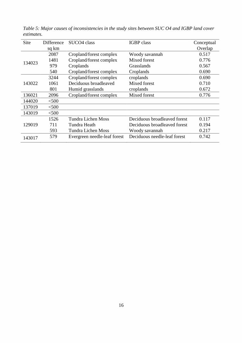
of consistency. Table 4 and Table 5 summarise the main causes of the major inconsistencies

between the SUC04 map and the GLC and with the IGBP data for each test site. A significant

discrepancy is considered to be 500 km2 or 5% of a study site. The “dominant” class is defined as

the most frequent class in the patch concerned. Because of the definition of consistency it is possible

to have a patch where the most frequent class in both data sets have a very high degree of overlap

but where the patch is still considered to be inconsistent. This is usually the result of the patch being

very heterogeneous in the earlier dataset, for example the discrepancy in five “croplands” to

“croplands” patches in site 134023.

The agreement between the SUC03 and SUC04 data sets is very high; as they are produced by the

same team using the same algorithm with data from the same satellite (MODIS) and the data are

only one year apart this is perhaps to be expected. Apparent disagreements between SUC03 and

SUC04 are concentrated in areas where the cropland or cropland/forest complex has become more

homogeneous over time.

Agreement and disagreement with the GLC and IGBP data indicate some general patterns. In the

heavily forested mid-latitudes which are dominated by evergreen needle-leaf forests there is good

agreement between all the data sets; the IGBP shows a little less consistency as it allocated more

land to the “mixed forest” class than either of the other data sets. In the south, the SUC “cropland /

forest complex” is mapped as a mixture of “forest” and “open” classes by GLC and as “mixed

forest” by IGBP. In the north there is confusion between “tundra” and “deciduous needle-leaf

forest” at one site in the GLC and between “tundra” and “woody savannah” in the IGBP datasets.

Several hypotheses can be suggested for the inconsistencies in the south of the study region:

There is more intensive exploitation of the landscape over time.

9

The landscape characterisation may be a function of the resolution as well as the “definition” of

the classes and the thresholds used.

Inadequacies of the expert opinion, especially over the extent of forest heterogeneity, may

confound the intercomparison.

Inconsistencies in the north of the region might represent a northward migration of the forest-tundra

ecotone that has been reported for some boreal / sub-arctic regions as a result of increasing

temperatures. As the data presented here only span a period of just over a decade these

inconsistencies are thought more likely to represent differences in how that ecotone is characterised

in the different datasets. In particular, it is unclear how thin and scattered the trees are before the

area appears as tundra and the extent to which the tree canopy influences reflectance with data at

500 meter and one kilometre resolution.

6. Conclusions

The standard way to manage inconsistent data is to aggregate. Aggregation is wasteful of

information and because the assumptions underlying the aggregation are rarely tested there is no

guarantee that the aggregation generates a more meaningful interpretation. If it is accepted that the

conceptual overlap can be quantified then aggregating classes must increase the range of any

domain they occupy, hence potentially increase the conceptual overlap with other classes. The

weighting system described above emphases domains where the concept has a narrow range

therefore reducing some of the impact. Alternatively the idea of a quantified conceptual overlap

could be used to determine the optimal aggregation to any number of classes. Generally, data

aggregation is a subjective process driven by expert opinion but how this opinion was used is not

always document well.

The semantic-overlap method appears successful in identifying inconsistent land parcels. In most

cases the inconsistency is more likely caused by misclassification in one or more of the maps than to

a real land cover change. Applying this methodology with all four land cover maps means that

parcels identified as being consistent are highly unlikely to have changed. When more than two data

sets have to be reconciled the semantic-overlap method reduces some of the complexity facing the

expert and by disaggregating their choices makes it slightly easier to identify and describe their

conception of what the classes mean.

Data producers routinely know much more about their data than they are willing to communicate to

the user. Metadata standards do little to encourage the producer to communicate the meaning of

class labels, how and why particular classes were chosen or the quality of the classified map in a

spatially explicit way, e.g. through a spatial accuracy assessment. The semantic-statistical method is

efficient at distinguishing between consistent and inconsistent parcels; over a short time period

misclassification is likely to be a more important component of inconsistency than change but the

method does allow the user to produce a refinement of where change is possible and where it is

unlikely. As the number of data sets and classes increases the semantic-statistical method becomes

increasingly difficult to apply as the number of decisions increases rapidly with no relaxation in the

need to maintain consistency. Simplifying the semantic-statistical method by adopting the ideas of

conceptual overlap allows the decisions to be disaggregated into smaller, simpler choices that are

also more explicit. Disaggregating the decision process makes it much easier for the expert to

10

review the consistency of their decisions and for others to understand the choices that were made. It

is not certain that the five domains used in this experiment are optimal. If an optimal set could be

determined and tested at other locations it may be possible to encourage data producers to

communicate more of what they know about the data by describing their classes in terms of agreed

universal domains.

The case study of Siberia that was discussed in this paper has shown that quantified conceptual

overlaps can provide a traceable method to overlay and analyse inconsistent spatial databases. It has

demonstrated how experts inform the process and make their decisions transparent in the

formalisation of inconsistencies between different classification keys.

Data inconsistency has become an increasing problem as it is becoming easier for data users to get

access to spatial data that they are unfamiliar with. At the same time, many data producers

document and communicate less about the data characteristics, despite metadata standards. The

approach suggested here provides one way to reconcile inconsistent data that preserves the thematic

content and spatial resolution of the data and allows a richer understanding of the complexity of a

landscape to be developed.

ACKNOWLEDGMENTS

Many of the ideas on the semantic-statistical approach were developed during the REVIGIS project

which was funded by the European Commission, (Project Number IST-1999-14189), Project

Coordinator Robert Jeansoulin Laboratoire d'Informatique de Marseille, CMI - Universite de

Provence, FRANCE. The SIBERIA-2 project, Multi-Sensor concepts for Greenhouse Gas

Accounting in Northern Eurasia, was supported by the 5th Framework Programme of the European

Commission, contract no.: EVG1-CT-2001-00048. Project coordination: Chris Schmullius,

Friedrich-Schiller University Jena. The Integrated Project GEOLAND, GMES products & services,

integrating Earth Observation monitoring capacities to support the implementation of European

directives and policies related to “land cover and vegetation”, was supported by the 6th Framework

Programme of the European Commission, proposal no.: FP-6-502871. Project coordination:

Alexander Kaptein, Infoterra Ltd., Germany. We wish to thank all our colleagues on these projects

for their assistance.

REFERENCES:

AHLQVIST O., 2004, A parameterized representation of uncertain conceptual spaces. Transactions in

GIS 8, 493-514.

ANDERSON J.R., HARDY E.E., ROACH J.T. AND WITMER R.E., 1976, A land use land cover

classification system for use with remote sensor data. Washington DC. US Geological Survey

Professional Paper 964.

BOUCHON-MEUNIER B., RIFQI M. AND BOTHOREL S., 1996, Towards general measures of

comparison objects. Fuzzy sets and systems 84, 143-153.

COMBER, A.J., FISHER, P.F. AND WADSWORTH, R.A., 2003, Actor Network Theory: a suitable

framework to understand how land cover mapping projects develop? Land Use Policy 20, 299-

309.

COMBER, A.J., FISHER, P.F. AND WADSWORTH, R.A., 2004a, Assessment of a Semantic Statistical

Approach to Detecting Land Cover Change Using Inconsistent Data Sets. Photogrammetric

Engineering and Remote Sensing 70, 931-938.

11

COMBER A.J., FISHER P.F. AND WADSWORTH R.A., 2004b, A semantic statistical approach to

negotiation heterogeneous ontologies. International Journal of Geographic Information

Science 18, 691-708.

COMBER A.J., FISHER P.F. AND WADSWORTH R.A., 2005, Comparing the consistency of expert land

cover knowledge. International Journal of Applied Earth Observation and Geoinformation 7,

189-201.

DI GREGORIO, A. AND JANSEN, L.J.M., 2000, Land Cover Classification System (LCCS):

Classification Concepts and User Manual,

http://www.fao.org/DOCREP/003/X0596E/X0596E00.HTM , accessed 27/9/2007.

FLETY, Y., GEORGE, C. AND BALZTER H., 2004, Generating a land cover change map and change

statistics by integrating historic digital land cover maps. Siberia II project report, published by

CEH, Monks Wood, UK.

FISHER, P.F., 2003, Multimedia reporting of the results of natural resource surveys. Transactions in

GIS 7, 309-324.

GYDE LUND, H., 2005, Definitions of Forest, Deforestation, Afforestation, and Reforestation. Forest

Information Services, Gainesville, VA, http://home.comcast.net/~gyde/DEFpaper.htm, date

accessed: 27/9/2007.

SHAFER, G., 1976, A mathematical theory of evidence. Princeton University Press, Princeton NJ,

USA.

TANGESTANI, M.H. AND MOORE, F., 2002, The use of Dempster-Shafer model and GIS in

integration of geoscientific data for porphyry copper potential mapping, north of Shahr-e-

Babak, Iran. International Journal of Applied Earth Observation and Geoinformation 4, 65-74.

WULDER, M.A., BOOTS, B., SEEMANN, D. AND WHITE, J.C., 2004, Map comparison using spatial

autocorrelation; an example using AVHRR derived land cover of Canada. Canadian Journal of

Remote Sensing 30, 573-592.

12

Table 1: Part of a Look-Up Table (LUT) comparing the SUC classes (rows) with the IGBP classes

(columns).

Relationship –

SUC (rows), IGBP (columns)

Ev

erg

reen

Need

le-l

ea

f F

orest

Ev

erg

reen

Bro

ad

lea

f F

orest

Decid

uo

us

Need

le-l

ea

f F

orest

Decid

uo

us

Bro

ad

lea

f F

orest

Mix

ed

Fo

rest

Clo

sed

Sh

ru

bla

nd

s

Etc

. e

tc.

1 Water -1 -1 -1 -1 -1 -1 …

2 Barren Ground -1 -1 -1 -1 -1 -1 …

3 Urban -1 -1 -1 -1 -1 -1 …

4 Croplands -1 -1 -1 -1 -1 -1 …

5 Cropland/Forest Complex 0 0 0 0 0 -1 …

6 Evergreen Needle-leaf 1 0 -1 -1 -1 -1 …

7 Deciduous Broadleaf -1 -1 0 1 0 0 …

8 Needle-leaf/Broadleaf Forest 0 0 0 0 1 0 …

9 Mixed Forest 0 0 0 0 1 0 …

10 Broadleaf/Needle-leaf Forest 0 -1 0 0 1 0 …

11 Deciduous Needle-leaf Forest -1 -1 1 0 0 0 …

12 Humid Grassland -1 -1 -1 -1 -1 -1 …

13 Wetland -1 -1 -1 -1 -1 -1 …

14 Steppe -1 -1 -1 -1 -1 -1 …

15 Tundra Lichen-Moss -1 -1 -1 -1 -1 -1 …

16 Tundra Heath -1 -1 -1 -1 -1 -1 …

13

Table 2: Fragment of the table showing some classes in the “human disturbance” domain.

Human disturbance

Most

Least

Urban (s 3) 1 1 0 0 0 0 0 0 0 0

Urban (g27) 1 1 0 0 0 0 0 0 0 0

Urban and Built-Up (i13) 1 1 0 0 0 0 0 0 0 0

Croplands (s 4) 1 1 1 1 0 0 0 0 0 0

Cropland (g20) 1 1 1 1 0 0 0 0 0 0

Croplands (i12) 1 1 1 1 0 0 0 0 0 0

Humid Grassland (s 12) 0 0 1 1 1 0 0 0 0 0

Humid Grassland (g10) 0 0 1 1 1 0 0 0 0 0

Cropland Grassland Complex (g23) 0 0 1 1 1 0 0 0 0 0

Cropland/Natural Vegetation Mosaic

(i14) 0 0 1 1 1 0 0 0 0 0

… … … … … … … … … … …

Sedge Tundra (g17) 0 0 0 0 0 0 0 0 1 1

Salt Pans (g29) 0 0 0 0 0 0 0 0 1 1

Barren Ground (s 2) 0 0 0 0 0 0 0 0 0 1

Bare soil Rock (g24) 0 0 0 0 0 0 0 0 0 1

Permanent Snow Ice (g25) 0 0 0 0 0 0 0 0 0 1

Snow and Ice (i15) 0 0 0 0 0 0 0 0 0 1

Barren or Sparsely Vegetated (i16) 0 0 0 0 0 0 0 0 0 1

14

Table 3: Consistency between the SUC04 land cover map and three other maps (SUC03, GLC and

IGBP) for selected test sites.

Site Dominant cover(s) in SUC 04 SUC 03 GLC IGBP

134023 Cropland/forest complex (49%)

Cropland (15%)

95.4% 40.1% 41.3%

143022

Cropland/forest complex (39%)

Deciduous broadleaved forest (25%)

Croplands (21%)

93.4% 50.1% 39.6%

136021 Evergreen needle-leaf forest (44%)

Cropland/forest complex (35%)

71.0% 68.7% 73.7%

144020 Deciduous broadleaved (87%) 99.1% 98.4% 98.3%

137019 Evergreen needle-leaf forest (84%) 99.8% 99.6% 99.8%

143019 Evergreen needle-leaf forest (83%) 94.1% 99.2% 96.7%

129019 Deciduous needle-leaf forest (49%)

Tundra lichen-moss (25%)

83.5% 60.3% 58.0%

143017 Evergreen needle-leaf forest (60%)

Deciduous needle-leaf forest (36%)

95.9% 97.1% 90.9%

15

Table 4: Major causes of inconsistencies in the study sites between SUC O4 and GLC land cover

estimates.

Site Difference

km2

SUCO4 class GLC class Conceptual

Overlap

134023

3757 Cropland/forest complex Deciduous needle-leaf forest 0.500

649 Croplands Deciduous needle-leaf forest 0.450

592 Croplands Croplands 1.000

143022 2131 Cropland/forest complex Croplands 0.690

814 Cropland/forest complex Crop/grassland complex 0.810

136021 1339 Cropland/forest complex Deciduous broadleaved forest 0.500

617 Cropland/forest complex Deciduous needle-leaf forest 0.500

144020 <500

137019 <500

143019 <500

129019

1371 Tundra Lichen Moss Deciduous needle-leaf forest 0.117

1175 Tundra Heath Deciduous needle-leaf forest 0.194

1074 Tundra Lichen Moss Shrub tundra 0.575

143017 <500

16

Table 5: Major causes of inconsistencies in the study sites between SUC O4 and IGBP land cover

estimates.

Site Difference

sq km

SUCO4 class IGBP class Conceptual

Overlap

134023

2087 Cropland/forest complex Woody savannah 0.517

1481 Cropland/forest complex Mixed forest 0.776

979 Croplands Grasslands 0.567

540 Cropland/forest complex Croplands 0.690

143022

3244 Cropland/forest complex croplands 0.690

1061 Deciduous broadleaved Mixed forest 0.710

801 Humid grasslands croplands 0.672

136021 2096 Cropland/forest complex Mixed forest 0.776

144020 <500

137019 <500

143019 <500

129019

1526 Tundra Lichen Moss Deciduous broadleaved forest 0.117

711 Tundra Heath Deciduous broadleaved forest 0.194

593 Tundra Lichen Moss Woody savannah 0.217

143017 579 Evergreen needle-leaf forest Deciduous needle-leaf forest 0.742

17

Portugal

Turkey

Kyrgyzstan Switzerland

Estonia

Denmark

Kenya

UNESCO

Sudan

Tanzania Ethiopia

South Africa

Jamaica

Zimbabwe

Gambia Mexico

Israel United States Belgium

Luxembourg Malaysia

PNG United Nations -FRA 2000

Namibia Somalia

Netherlands New Zealand

Mozambique

Australia Cambodia

Japan

Morocco

SADC

0

2

4

6

8

10

12

14

16

0 10 20 30 40 50 60 70 80 90

Canopy Cover

(%)

Tre

e H

eig

ht

(m)

Figure 1: Illustration of a range of different definitions of the land cover class “Forest”. The class

label can be (mis-)interpreted in many different ways (data from Gyde Lund 2005).

18

Figure 2: Fragments from the three land cover maps of Siberia, using arbitrary colours. Swansea =

Land cover map from 2002 derived by L. Skinner in the SIBERIA-II project; IGBP = DISCover land

cover map from 1994 produced by the US Geological Survey for the International Geosphere–

Biosphere Programme (IGBP); GLC = map from Global Land Cover 2000, derived by S. Bartalev

et al. The feature in the centre of the maps (55° 20’ N 92° 20’E) is the Krasnoyarsk “sea”. Area

covered about 200 km across.

19

Figure 3: Illustration of the aggregation strategy applied to the Siberian Land Cover data.

20

Figure 4: A segment of a hypothetical land cover map containing four different classes and the

associated LUT (showing the seperability between the classes)

21

Figure 5: The same hypothetical segment as in Figure 4 under a different classification and the

associated LUT (between the two data sets).

22

Figure 6: Dendrogram of all classes based on similarity in the five semantic domains.