International Journal of Computer Applications (0975 – 8887)

Volume 90 – No 17, March 2014

25

An Enhanced Approach for Classification in Web

Usage Mining using Neural Network Learning

Algorithms for Supervised Learning

Jaykumar Jagani

R.K. University R.K. University, Kasturbadham, Near Tramba, Rajkot - 360020

Kamlesh patel Professor, R.K. University

R.K. University, Kasturbadham, Near Tramba, Rajkot - 360020

ABSTRACT

Now a day data on the web is growing by a rapid speed, large

volume of data is available on web. So, extract useful

knowledge from large web data, efficient web mining

methods are required to handle those data and achieve various

functionalities such a as user trend analysis, web profile

analysis, Web AD market change analysis, etc. The concept of

neural network helps to handle large volume of data by its

characteristics [1]. Several neural network learning algorithms

provides better supervised learning. They are capable to

handle huge dynamic data. Specially, LVQ (Learning Vector

Quantization) algorithms are useful for supervised, dynamic

labeling or post-training map labeling and supervised version

of SOM through that the approximation of distribution of

class with less number of codebook vectors and able to

minimize classification errors respectively [9]. MLVQ and

HLVQ are both the techniques are following a concept of

multi pass in which more than one pass can be performed on

the same model and is very useful for gaining best desired

results [11]. Here in this paper, we are going to discuss a new

technique that will work on hierarchical as well as multi pass

approach that is having the advantages of both multi pass and

hierarchical approach by combining the benefits of both and

designed a new algorithm. That new technique will more

accurate, less time consuming and able to decrease learning

rate for neural network. The basic HLVQ approach will

follow the same algorithm for generation of all phases. In

addition to that HMLVQ provides better efficiency through

enhancing advantages the various approaches for the same

classification process.

General Terms

Web Usage Mining, Clustering and Artificial Neural

Networks.

Keywords

LVQ, MLVQ, HLVQ, Web log data, classification.

1. INTRODUCTION Web users are increasing day by day so the web data on the

web is growing more. [6] Now, any mega firms or IT

companies want to survive in the market, so they need to

analyze the current web data and historical web data as well

as the existing trends of current generation users and

prediction of future trends. All these are possible only by

analyzing web data. Various data mining techniques are

applied on huge web data to extract useful knowledge for

decision making by business Analysts [3].

As there are many web scaling problems such as user trend

analysis of surfing, traffic flow analysis, distributed control

handling, web traffic management and many more. Session

tracking and website reorganization, distributed traffic sharing

on distributed servers can be identified and analysis based on

web data can be possible through web mining. But for that the

large amount of rough data the accurate classification is

required and that classification can be possible using concepts

of neural network [1] [4] [6] [2].

In this Paper, the discussion is based on various neural

network learning algorithms that help to handle large web

data as well as better classification and clustering of data with

less number of errors. Self-Organizing Maps called SOM and

Learning Vector Quantization known as LVQ are very

constructive learning algorithms that classify and cluster the

web data successfully [9]. SOM are useful for supervised,

unsupervised learning, dynamic labeling or post-training map

labeling. Learning vector quantization is useful for the

approximation of distribution of class with less number of

codebook vectors and able to minimize classification errors

[9]. MLVQ and HLVQ techniques are following a concept of

multi pass in which more than one pass can be performed on

the same model using different algorithms and are very useful

for gaining best preferred results. So in this paper, the

discussion is based on a new technique that will work on

multi pass as well as on hierarchical approach. So the

advantages of both techniques will be achieved in single

algorithm.

2. WEB USAGE MINING Web Usage Mining in a simple term is to extract the usage

knowledge about the web users through various data mining

techniques from web data is web usage mining [4]. Web

Usage Mining is going to prove more useful method in current

and next generation‟s web exploring people world [6]. So,

there is a huge research scope available in this area to develop

and implement new ideas that how Usage Mining can be more

effective and as a result of that end user is able to get better

facilities as developer firms will able to identify user‟s interest

and will able to deliver the products likewise.

2.1 Sources of data for Web Usage Mining The data input for the various classification algorithms can be

found from (1) Web servers (2) Proxy Servers (3) Web

Clients [3]. The data is stored on the web in web log files.

Each and every user activity is stored in respective server. The

data is fetched from that server for analysis. The web data

available on the server is in a specific format known as

extended common log format (ECLF) [5].

ECLF Format

International Journal of Computer Applications (0975 – 8887)

Volume 90 – No 17, March 2014

26

Table 1 (various columns of ECLF format)

I/P Rfc 931 Auth User Req. Time

Stamp

Req.

Format

Status Bytes Referrer User

Agent

Important terms

Ipaddress- network address of user machine

Rfc 931- remote login name of user

Status- as success / page not found like errors

User agent- software or browser (web client)

Authuser – original user name

Bytes – size of transferred information [6]

2.2 Process of Web Usage Mining As per Figure 1, it is clear that process of web usage mining is

much similar to data mining process.

Figure-1 Common Process of Web Usage Mining

As per figure 1, The Only difference in data mining and web

mining is that at the Starting level in data will come from

various data bases, warehouses, and flat files and in web

mining data will come from server log files. In this Paper, the

focus is on initial phase of web usage mining process where

clustering and classification process are done to provide better

extraction and stability of data.

3. ROLE OF NEURAL NETWORK FOR

WEB USAGE MINING Neural network provides many supervised learning algorithms

that can be helpful in mining process, especially to give class

labels to uncategorized data i.e. classification. Here is some

brief about neural networks and its useful characteristics. The

network of highly connected, self-intelligent neurons (Nodes)

to do any task with once training is neural network.

3.1 Artificial Neural Network in brief Artificial neural network (ANN) is a knowledge processing

paradigm that inspired from biological nervous system. This

technology is more useful because of its unique structure of

system. ANN is the arrangement of large number of highly

connected processing elements, called neurons in medical

science as in brain, working together to solve a particular

problem [1]. ANN is configured i.e. initializes with training or

testing data to solve a particular problem such as, clustering or

classification. Neural networks are highly capable to do the

things such as meaning derivation from complex data. It is

mostly used in finding usage trends that are sometimes very

common but complex and even not carried out by machines.

Neural network has many advantages as follows: Self-adaptive learning

How to deal with problems based on initial training or

experience from the network.

Self-organization Artificial neural network creates its own organization

and behavior and representation of knowledge it accepts

while learning.

Real time operations Neural network computation may carry out parallel but

for that special hardware are required to design.

Fault tolerance via multiple information copies Partial destroys or failure of network cannot affect the

performance of the network [6].

Figure-2 Processing Architecture of Neural Network

As figure 2, shows the recurrent network of ANN map nodes

with its all three layers.

4. NEURAL NETWORK ALGORITHMS

FOR CLASSIFICATION IN WEB USAGE

MINING The list of such algorithm is big, but in this paper, discussion

on some of the best classifiers among them, described in

following sections.

Z2 Z1

X1 X2 X3 X4 X5

Output layer

Hidden Layer

Input layer

Pattern Analysis

Usage Path

Analysis

Sequence

Matching

Association

Rules

Classification

& Clustering

Converted Data

Integrated Data

Filtered Data

Clean Log

Web Log data

Pre-processing

Transaction Filtering

Data integration

Query process

Formation Usage functions

International Journal of Computer Applications (0975 – 8887)

Volume 90 – No 17, March 2014

27

4.1 Learning Vector Quantization (LVQ) It is a machine learning algorithm and supervised version of

SOM Algorithm. Through LVQ the approximation of

distribution of class with less number of codebook vectors and

is able to minimize classification errors. Codebook vectors are

considered as class boundary representations. The algorithm is

associated with neural network of class learning algorithms

[8].

4.1.1 Advantages of LVQ LVQ is capable to summarize large datasets to smaller

number of codebook vectors that are useful for visualization

and classification. Training rate is so fast compare to any

other network like back propagation. The Generated model

updated incrementally. Here some LVQ versions are

available.

4.2 Versions of LVQ They are denoted as LVQ1, LVQ2, LVQ3, OLVQ1, OLVQ3,

MLVQ and hierarchical LVQ [11].

4.2.1 LVQ1 Imagine that a number of 'codebook vectors' cvi (free bound

vectors) are located into the input gap to estimate various

domains of the input vector „v‟ by their quantized values [8].

Generally a number of codebook vectors are allocated to each

class of v values, and v is then decided to fit in to the same

class to which the adjacent cvi belongs.

Let𝒅 = 𝐚𝐫𝐠𝐦𝐢𝐧(||𝒗 − 𝒄𝒗𝒊||) describe the nearest cvi to v,

denoted by dc.

Standards for cvi that just about reduce the misclassification

errors in the over nearest-neighbor classification can be found

as asymptotic values in the subsequent learning process. Let

v(t) be a sample of input and let the cvi(t) stand for

sequences of the cvi in the discrete-time domain. Beginning

with properly defined initial values, the following equations

define LVQ1.

𝒅𝒄 𝒕 + 𝟏 = 𝒅𝒄 𝒕 + 𝒂𝒍𝒑𝒉𝒂 𝒕 [𝒗 𝒕 − 𝒅𝒄(𝒕)] (1)

If v and dc belong to the similar class,

𝒅𝒄 𝒕 + 𝟏 = 𝒅𝒄 𝒕 − 𝒂𝒍𝒑𝒉𝒂 𝒕 [𝒗 𝒕 − 𝒅𝒄(𝒕)] (2)

If x and mc belong to dissimilar classes,

𝒄𝒗𝒊 𝒕 + 𝟏 = 𝒄𝒗𝒊(𝒕) , for I is not in c.

Here 0 < alpha (t) < 1, and alpha (t) may be steady or decrease

monotonically with time. In the above basic LVQ1 it is

recommended that alpha should initially be lesser than 0.1;

linear decrement in time is used in this package. [8]

4.2.2 LVQ2 The classification verdict in this algorithm is the same with

that of the LVQ1. In learning, however, two codebook

vectors, cvi and cvj that are the adjoining neighbors to v, are

now updated concurrently [7]. One of them must be in the

right place to the correct class and the other to a wrong class,

correspondingly. Moreover, v must fall into a region of values

called 'window', which is defined around the mid plane of cvi and cvj. Assume that edi and edj are the Euclidean distances

of v from cvi &cvj, correspondingly [7]; then v is defined to

fall in a 'window' of qualified width w if,

𝐦𝐢𝐧(𝒆𝒅𝒊

𝒆𝒅𝒋,𝒆𝒅𝒋

𝒆𝒅𝒊) > 𝑆, where 𝒔 = (𝟏 − 𝒘)/ 𝟏 + 𝒘 (3)

Width w of the „window‟ should be 0.2 to 0.3

4.2.2.1 Algorithm 𝒄𝒗𝒊 𝒕 + 𝟏 = 𝒄𝒗𝒊 𝒕 − 𝒂𝒍𝒑𝒉𝒂(𝒕)[𝒗 𝒕 − 𝒄𝒗𝒊(𝒕)],

𝒄𝒗𝒋 𝒕 + 𝟏 = 𝒄𝒗𝒋 𝒕 + 𝒂𝒍𝒑𝒉𝒂(𝒕)[𝒗 𝒕 − 𝒄𝒗𝒋(𝒕)] (4)

Where cvi and cvj are the two closest codebook vectors to v

and whereby v and cvj belong to the same class, while v and

cvi belong to different classes, respectively [7]. Furthermore v

must fall into the 'window'.

4.2.3 LVQ3 The LVQ2 algorithm was based on the thought of

differentially changing the decision limitations towards the

Bayes restrictions, while no notice was paid to what might has

done to the location of the min the extended run if this process

were continued. As a result it seems like required having

corrections that make sure that the cvi continue resembling

the class distributions, at least more or less. Combining these

ideas, we now acquire an improved algorithm that is called

LVQ3 [9].

As per Equation 4,

𝒎𝒌 𝒕 + 𝟏 = 𝒎𝒌 𝒕 + 𝒆𝒑𝒔𝒊𝒍𝒐𝒏 𝒂𝒍𝒑𝒉𝒂(𝒕)[𝒗 𝒕 − 𝒎𝒌(𝒕)]

(5)

4.2.4 The Optimized LVQ (OLVQ1) The basic LVQ1 algorithm is now modified in such a way that

an individual learning rate alpha (t) is assigned to each cvi [7].

We then get the following discrete time learning process. Let

c be defined by Eq. (1). Then,

𝒅𝒄 𝒕 + 𝟏 = 𝒅𝒄 𝒕 + 𝒂𝒍𝒑𝒉𝒂 𝒕 [𝒗 𝒕 − 𝒅𝒄(𝒕)] If v is classified correctly,

𝒅𝒄 𝒕 + 𝟏 = 𝒅𝒄 𝒕 − 𝒂𝒍𝒑𝒉𝒂 𝒕 [𝒗 𝒕 − 𝒅𝒄(𝒕)] (6)

If the classification of v is incorrect, 𝑐𝑣𝑖(𝑡 + 1) = 𝑐𝑣𝑖(𝑡), for i not in c. We tackle the problem irrespective of the 𝑎𝑙𝑝ℎ𝑎𝑖 (𝑡) can be

firmed optimally for fastest possible convergence of eq. (6)

[7]. If we state (6) in the form,

𝑑𝑐 𝑡 + 1 = 1 − 𝑠 𝑡 𝑎𝑙𝑝ℎ𝑎𝑐 𝑡 𝑑𝑐 𝑡 + 𝑠 𝑡 𝑎𝑙𝑝ℎ𝑎𝑐 𝑡 𝑣 𝑡 (7)

Where 𝑠(𝑡) = +1 or −1 if the classification is accurate and

incorrect respectively, we primary straight see that 𝑑𝑐(𝑡) is

statistically liberated from 𝑣(𝑡). It may also be noticeable that

the statistical correctness of the learned codebook vector

values is optimal if the assets of the corrections made at

different times, when referring to the end of the learning

period, are of the same weight. Notice that 𝑑𝑐(𝑡 + 1)

contains a "trace" from 𝑣(𝑡) through the last term in (7), and

"traces" from the earlier 𝑣(𝑡′); 𝑡′ = 1,2, . . . 𝑡 − 1 through

𝑑𝑐(𝑡). The magnitude of the last "trace" from 𝑣(𝑡) is scaled

down by the factor a𝑙𝑝ℎ𝑎𝑐(𝑡), and, for instance, the "outline"

from 𝑥(𝑡 − 1) is scaled down by [1 − (𝑡)𝑎𝑙𝑝ℎ𝑎𝑐(𝑡)]

𝑎𝑙𝑝ℎ𝑎𝑐(𝑡 − 1) [7].

International Journal of Computer Applications (0975 – 8887)

Volume 90 – No 17, March 2014

28

Now we first specify that these two scaling must be identical:

𝑎𝑙𝑝ℎ𝑎𝑐(𝑡) = [1 − 𝑠(𝑡)𝑎𝑙𝑝ℎ𝑎𝑐(𝑡)]𝑎𝑙𝑝ℎ𝑎𝑐(𝑡 − 1)

(8)

If this condition is then made to hold for all t, by induction it

can be shown that the "traces" collected up to time t from all

the earlier x will be scaled down by an equal amount at the

end, and thus the "optimal" values of 𝑎𝑙𝑝ℎ𝑎𝑖(𝑡) are

determined by the recursion,

𝑎𝑙𝑝ℎ𝑎𝑐(𝑡) = 𝑎𝑙𝑝ℎ𝑎𝑐(𝑡 − 1)/ (1 + 𝑠(𝑡)𝑎𝑙𝑝ℎ𝑎𝑐(𝑡 − 1))

(9)

4.2.5 Multi pass LVQ It is like supervised version of multi pass SOM where quick

rough pass can be made on the model by using OLVQ1

algorithm and then the long fine tuning pass can be made on

the model through any of LVQ1, LVQ 2 or LVQ3 [11].

4.2.6 Hierarchical LVQ Here an LVQ model is constructed and each codebook vector

is treated as a cluster centroid. All codebook vectors are

evaluated and numbers are selected as candidates for sub-

models. Sub models are constructed for all candidate

codebook vectors and those sub models that outperform (in

terms of classification accuracy) their parent codebook vector

are kept as part of the model [10]. During testing a data

instance is first mapped onto its BMU, if that BMU has a sub-

model (that was not pruned during training), the sub model is

used for classification, otherwise the class value in the BMU

is used for classification. This algorithm has proven most

useful for large datasets where a low-complexity model is

used as the base model, and specialized LVQ models are used

at each codebook vector to better model the data [10].

4.2.7 General considerations and Comparison In LVQ, vector quantization is not worn to estimate to density

functions of the class samples, but to unswervingly define the

class borders along with the nearest-neighbor rule. The

accuracy reachable in any classification task to which the

LVQ algorithms are useful and the time needed for learning

depend on the subsequent factors:

An approximately most favorable number of codebook

vectors assigned to each class and their initial values, the

comprehensive algorithm, a proper learning rate applied

during the steps, and a proper condition for the stopping of

learning.

4.2.7.1 LVQ Algorithm Comparison

Table 2: All LVQ algorithm comparison with respect to various fields

Fields LVQ OLVQ MLVQ HLVQ

Version Basic Optimized Multiple passes Hierarchical

Accuracy Less More than LVQ More than OLVQ More than MLVQ

Time High Less than LVQ Less than OLVQ Less than MLVQ

Efficiency Low Medium High High

Codebooks More Moderate Less Less

Capacity Low Medium High High

5. PROPOSED WORK After discussing to the very basic concepts and algorithms of

neural network learning algorithms, now discussion is how

the accuracy of algorithms can be enhanced. Now, we are

proposing a new technique with the combination of HLVQ

and MLVQ approach that is known as HMLVQ.

5.1 Basic HLVQ Approach Here defined the steps for basics HLVQ:

Here, HLVQ is divided into two Stages like A is 1st and B is

2nd [10].

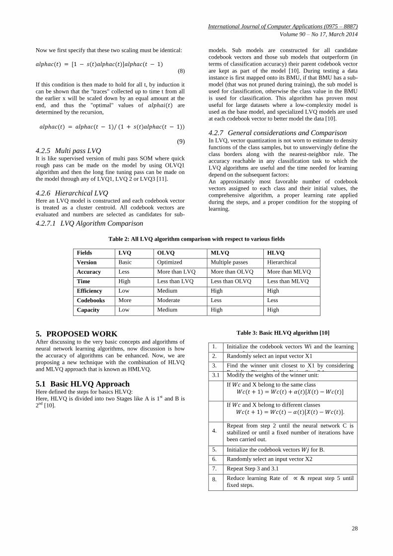
Table 3: Basic HLVQ algorithm [10]

1. Initialize the codebook vectors Wi and the learning

rate α for A. 2. Randomly select an input vector X1

3. Find the winner unit closest to X1 by considering

Euclidian Distance Wc to X. i.e. Step 3.1 3.1 Modify the weights of the winner unit:

If 𝑊𝑐 and X belong to the same class

𝑊𝑐(𝑡 + 1) = 𝑊𝑐(𝑡) + 𝛼(𝑡)[𝑋(𝑡) − 𝑊𝑐(𝑡)]

If 𝑊𝑐 and X belong to different classes

𝑊𝑐(𝑡 + 1) = 𝑊𝑐(𝑡) − 𝛼(𝑡)[𝑋(𝑡) − 𝑊𝑐(𝑡)].

4. Repeat from step 2 until the neural network C is

stabilized or until a fixed number of iterations have

been carried out.

5. Initialize the codebook vectors 𝑊𝑗 for B.

6. Randomly select an input vector X2

7. Repeat Step 3 and 3.1

8. Reduce learning Rate of ∝ & repeat step 5 until

fixed steps.

International Journal of Computer Applications (0975 – 8887)

Volume 90 – No 17, March 2014

29

5.2 Hierarchical Multi pass LVQ As it is obvious that multi pass and hierarchical LVQs are

having advantages such as multi pass LVQ is a hybrid of

basic and optimized LVQ so it has advantages of all basic

LVQs and it works in the pass, so speed achieved for even

more learning data is more and Hierarchical LVQ gives

accuracy as it works in detail with domains and sub domains

i.e. hierarchy levels also.

Now if any technique has the advantages of both multi pass

LVQ and Hierarchical LVQ, then it would be very good to

classify with it any large data within efficient time. Such

method is proposed as Hierarchical Multi pass LVQ. It has

advantage of both multi pass and hierarchical technique that is

speed and accuracy both. So, classification errors are reduced

and process speed is also increased that means the large raw

data can be classified in sufficient amount of time with more

accuracy.

5.2.1 Proposed steps of HMLVQ Here we are proposing the steps for HMLVQ:

Here 𝑖 is an input vector, C is codebook vector, and ∝ is

learning rate and N is Neural Network.

Table 4: Proposed HMLVQ algorithm

1. Initialize the codebook vectors C with fixed learning

rate α for first stage.

2. Give an input vector I and find the closest unit

nearby vector C using Euclidian distance between

them. 3. Update the weights of closest unit

3.1

If they are in same class then unit weight is added in

classification results and result is correct.

𝐶𝑖 (𝑡 + 1) = 𝐶𝑖 (𝑡) + ∝ (𝑡) [𝐼(𝑡) − 𝐶𝑖 (𝑡)]. If they are not in same class then unit weight is

subtracted and result is not accurate.

𝐶𝑖 (𝑡 + 1) = 𝐶𝑖 (𝑡) − ∝ (𝑡) [𝐼(𝑡) − 𝐶𝑖 (𝑡)].

4. Repeat from step 2 until the neural network N is

stabilized with fixed number of iterations.

5. Reduce learning rate at end of each level.

6. Repeat the same procedure for Second Stage by

considering the best result amongst the current stage

and all previous stage.

7. Select most accurate unit and discard all rest.

8. Repeat the procedure until the whole dataset is

classified.

5.2.2 Proposed working of HMLVQ For HMLVQ, an LVQ model is constructed using multi pass

and each codebook vector is treated as a cluster centroid. All

codebook vectors are evaluated and numbers are selected as

candidates for sub-models. Sub models are also constructed

using multi pass for all candidate codebook vectors and those

sub models that do not perform well (in terms of classification

accuracy), their parent codebook vector are kept as participant

of the model. During test phase a data instance is first mapped

to its BMU, if that BMU has a sub-model (that was not

pruned during training), the sub model is used for

classification, if that was pruned during training; the class

value in the BMU is used for classification.

So In short at each level the model is constructed using multi

pass LVQ and codebook vectors are evaluated and given

numbers as candidate for sub model. The sub model is also

constructed using multi pass LVQ specially OLVQ1. So, at

each and every hierarchy level the sub models are constructed

using multi pass LVQ if sub model is more inaccurate then it

is rejected and parent node is considered as an element in

model. By using this approach accuracy maintains at each and

every level and construction of sub models are also fast and

accurate.

5.2.3 Comparison of Both HLVQ and HMLVQ

Basic Approach My approach HMLVQ

It is basic hierarchical

approach with one

algorithms for all time

i.e. lvq3

Hierarchical approach with

different algorithms for all

stage classification

Parameters: Accuracy,

Time

Parameters: Accuracy, Time

Available Algorithms

For Initial Time: LVQ1,LVQ2, LVQ3, OLVQ1,OLVQ3

For Next Rounds (if exists): MLVQ, OLVQ1,OLVQ3

For first stage generation For first stage generation

Take Any one Approach Take the Same Approach

e.g. OLVQ1 e.g. OLVQ1

For Second stage

generation

For Second stage generation

Took the same Approach Here I changed Approach I

took

e.g. OLVQ1 MLVQ

Continues same for rest

of stages

Continues same for rest of

stages Reduce learning Rate

Result is benefit in accuracy and Time

Table 5: Comparison between Both approaches

5.2.4 Simulation of HMLVQ Here I have tried some simulation based on my approach and

I have found the new results comparatively better than old

approach with increase in efficiency with less execution time.

I have taken sample data and compare both the approaches.

Results are as follows gives the clear cut idea of it.

Data samples are:

Breast Cancer(BC)

Super Market(SM)

Log data(LOG)

Table 6: Simulation HLVQ vs. HMLVQ

Field Datasets

Algorithm Params BC SM LOG

HLVQ Accuracy 93.71 64.88 80.33

Time 13ms 64ms 12ms

HMLVQ Accuracy 95.46 66.80 80.48

Time 5ms 63ms 11ms

International Journal of Computer Applications (0975 – 8887)

Volume 90 – No 17, March 2014

30

6. CONCLUSION At the end, after studying, learning and comparing a lot, to

handle the large volume of web data, there would be a definite

need of neural network concept, because only through neural

network learning algorithms, such huge volume of web data

can be handled and applied to any application for knowledge

extraction. All neural network learning algorithms have their

own advantages and disadvantages. LVQ is a supervised

model of SOM and used for giving class label to data. LVQ is

capable to summarize large datasets to smaller number of

codebook vectors that are useful for visualization and

classification. Training rate is so fast compare to any other

network like back propagation. The Generated model updated

incrementally. Various versions of LVQ are having one or

more disadvantage such as LVQ need to be able to generate

useful distance measures for all attributes. They are highly

dependent on initialization parameters and training. So by

using more than one LVQ approach together will give

benefits in recovering from demerits of LVQ. HMLVQ is one

such technique that provides fast and accurate classification

with reduced size of codebooks. So, in short, by using

HMLVQ, the classification of large web data will become

easy. The basic HLVQ algorithm works on the same approach

in all hierarchy generation that will give the same static

classification results. When HMLVQ uses more than one

approach to classify the data, so the disadvantages of the same

method will excluded and only merits of both approaches are

enlighten for accurate classification. So, HMLVQ will be

proved as a great classification technique and will be useful

for huge datasets as well.

7. REFERENCES [1] Sonali muddalwar, Shashank Kawan, “Applying

artificial neural networks in web usage mining”,

international journal of computer science and

management research, vol. 1 issue 4 [Nov-12]

[2] Anshuman Sharma, “Web usage mining neural

network”, international journal of reviews in

computing, vol. 9, [10th april, 2012]

[3] Valishali A. Zilpe, Dr. Mohammad Atique, “Neural

network approach for web usage mining”, ETCSIT,

published in IJCA [2011]

[4] Jaydeep Srivastava, “Web Mining:

Accomplishments and future directions”,

[5] http://www.cs.unm.edu/faculty/srivastava.html

[6] John R. Punin, Mukkai S. Krishnamoorthy,

Mohammed J. Zaki, “Web usage mining- language

and algorithms”, rensseluer polytechnic institute,

troy NY 12180

[7] Jaykumar Jagani, Prof. Kamlesh Patel, “A survey of

web usage mining with neural network and

proposed solutions on several issues”, ISSN: 0975–

6760, Nov 12 To Oct 13, Volume – 02, Issue [02]

[8] Renata M. C. R. de Souza, Telmo de M. Silva

Filho,” Optimized Learning Vector Quantization

Classifier with an Adaptive Euclidean Distance”,

19th International Conference, Limassol, Cyprus,

September 14-17, 2009, volume 5768

[9] Diamantini, Claudia , Spalvieri, A. “Certain facts

about Kohonen's LVQ1 algorithm”, Circuits and

Systems, 1994. ISCAS '94., 1994 IEEE

International Symposium on (Volume:6 )

[10] Sang-Woon Kimy and B. J. Oommenz, “Enhancing

Prototype Reduction Schemes with LVQ3-Type

Algorithms”, Natural Sciences and Engineering

Research Council of Canada, and Myongji

University, Korea, kimsw@mju.ac.kr,

oommen@scs.carleton.ca

[11] R. R. Janghel, Ritu Tiwari, Anupam Shukla,” Breast

Cancer Diagnostic System using Hierarchical Learning Vector

Quantization”, IJCA Proceedings on National Seminar

on Application of Artificial Intelligence in Life

Sciences 2013

[12] Mahesh kumar, Uday Kumar,” Classification of

Parkinson‟s disease using Lvq, Logistic Model

Tree, K-star for Audioset” , Hogskolan Darlana

University, 2011, roda wagen 3s-781 88.

93.71

64.8880.33

13

64

12

95.46

66.8 80.48

5

63

11

BC SM LOG

HLVQ Vs HMLVQ with Parameters

Accuracy and Time

HLVQ Acc HLVQ Time HMLVQ Acc HMLVQ Time

IJCATM : www.ijcaonline.org