Automation in Construction 22 (2012) 271–276

Contents lists available at SciVerse ScienceDirect

Automation in Construction

j ourna l homepage: www.e lsev ie r .com/ locate /autcon

Supervised vs. unsupervised learning for construction crew productivity prediction

Mustafa Oral a,⁎, Emel Laptali Oral b, Ahmet Aydın c

a Çukurova Üniversitesi, Mühendislik Mimarlık Fakültesi, Bilgisayar Mühendisliği Bölümü, Balcalı, Adana, Turkeyb Çukurova Üniversitesi, Mühendislik Mimarlık Fakültesi, İnşaat Mühendisliği Bölümü, Balcalı, Adana, Turkeyc Çukurova Üniversitesi, Mühendislik Mimarlık Fakültesi, Elektrik Elektronik Mühendisliği Bölümü, Balcalı, Adana, Turkey

⁎ Corresponding author. Tel.: +90 322 338 60 84/26E-mail addresses: moral@cu.edu.tr (M. Oral), eoral@

aaydin@cu.edu.tr (A. Aydın).

0926-5805/$ – see front matter © 2011 Elsevier B.V. Alldoi:10.1016/j.autcon.2011.09.002

a b s t r a c t

a r t i c l e i n f o

Article history:Accepted 16 September 2011Available online 24 October 2011

Keywords:Supervised learningUnsupervised learningSelf Organizing MapsConstruction crewProductivity

Complex variability is a significant problem in predicting construction crew productivity. Neural Networksusing supervised learning methods like Feed Forward Back Propagation (FFBP) and General Regression Neu-ral Networks (GRNN) have proved to be more advantageous than statistical methods like multiple regression,considering factors like the modelling ease and the prediction accuracy. Neural Networks using unsupervisedlearning like Self Organizing Maps (SOM) have additionally been introduced as methods that overcome someof the weaknesses of supervised learning methods through their clustering ability. The objective of this articleis thus to compare the performances of FFBP, GRNN and SOM in predicting construction crew productivity.Related data has been collected from 117 plastering crews through a systematized time study and compari-son of prediction performances of the three methods showed that SOM have a superior performance in pre-dicting plastering crew productivity.

63 17; fax: +90 322 3386702.cu.edu.tr (E.L. Oral),

rights reserved.

© 2011 Elsevier B.V. All rights reserved.

1. Introduction

Realistic project scheduling is one of the vital issues for successfulcompletion of construction projects and this can only be achieved ifschedules are based on realistic man-hour values. Yet, determinationof realistic man-hour values has been a complicated issue due to thecomplex variability of construction labor productivity [1–9]. Thus,recent researches have focused on artificial neural network applica-tions which provide a flexible environment to deal with such kindof variability. These applications have been based on supervisedlearning methods, primarily Feed Forward Back Propagation (FFBP)[1–2,10–18], and recently General Regression Neural Network(GRNN) [19–20]. While strengths of these methods over multiple re-gression models, related with the modeling ease and the predictionaccuracy, have been well discussed; the weaknesses of the supervisedlearning process, i.e. requiring the output vector to be known fortraining, has also been pointed out [21–22]. In parallel, Self Organiz-ing Maps (SOM), based on unsupervised learning, have been intro-duced as applications which overcome the weaknesses of both thestatistical methods and the neural network applications based on su-pervised learning [21–25]. However, few researchers like Hwa andMiklas [26], Du et al. [27] andMochnache et al. [28] used SOM for pre-diction purposes and these were related with heavy metal removalperformance, oil temperature of transformers and thermal aging oftransformer oil, respectively. A recent application, alternatively, has

focused on prediction of construction crew man-hour values for con-crete, reinforcement and formwork crews [29] and prediction resultshave been compared with the results of previous research based onboth multi regression analysis and Feed Forward Back Propagation(FFBP) [2,30]. The objective of the current research, however, hasbeen to use a specific sample data and compare the prediction resultsof the models developed by using SOM, FFBP and GRNN.

2. Data collection and nature of the data

Collecting realistic and consistent productivity related data is oneof the key factors in arriving at realistic man-hour estimates by usingany of the prediction methods. Various work, labor and site relatedfactors affect construction labor/crew productivity and these have tobe observed and analyzed systematically in order to arrive at realisticman-hour values, and “time study” is a methodical process of directlyobserving and measuring work [31]. Thus, time study has been un-dertaken with 1181 construction crews in Turkey through the use ofstandard time study sheets between the years 2006 and 2008 and de-tails related with concrete pouring, reinforcement and formworkcrews have been presented in various publications [17,29,32]. Forplastering crews, quantity and details of plastering work undertakenby each crew were recorded together with work (location of thesite, location of the work on site, the type and the size of the materialused and the weather conditions), labor (age, education, experience,working hours, payment method, absenteeism and crew size), andsite (site congestion, transport distances, and the availability of the;crew, machinery, materials, equipments and site management) relat-ed factors for 31 crews initially. Man-hour values were then

InputLayer

HiddenLayers

OutputLayer

Experience

272 M. Oral et al. / Automation in Construction 22 (2012) 271–276

determined by calculating duration of undertaking 1 m2 plasteringwork. Required number of observations for the sample size to be rep-resentative within a targeted confidence interval (90%) was then de-termined by using Eq. 1 [31].

N′ ¼ A

ffiffiffiffiffiffiffiffiffiffiffiffiffiffiffiffiffiffiffiffiffiffiffiffiffiffiffiffiffiffiffiffiffiffiffiffiffiffiffiffiffiffiffiffiffiffiffiffiffiN∑n

i¼1Χ2i − ∑n

i¼1Χi

� �2q

∑ni¼1Χi

24

352

ð1Þ

where:

N' required number of observations within the targeted confi-dence interval.

A 20 for 90% confidence levelN number of observations during the pilot study.Xi unit output of the related labor (crew) during the ith

observation.n number of observations during the pilot study.

Calculations showed that a minimum of 71 crews were requiredfor the sample size to be representative of the population within90% confidence level. Data was then collected from 117 crews. Thenumber of crews was satisfactory regarding the sample size require-ment. Normality of the collected data was then tested by determiningthe skewness (to be between ±3), and kurtosis (to be between ±10)coefficients for productivity values [33]. Table 1 shows that normalityassumptions were satisfied by the data set.

Data analysis and selection, additionally focused on the fact thatproductivity models including fewer significant factors predict betterthan models based on many factors without considering significance[2]. Collected data/information related with the work and the site fac-tors showed that most of the data/information were unevenly distrib-uted; for example weather conditions were usually ‘very hot’ and ‘notrainy’ due to the prolonged draughts between 2006 and 2008 inTurkey, or there were usually no problems with the availability ofresources and so on. So labor related factors of age, education andexperience were decided to be used as independent variables in thedeveloped models. This decision was in good agreement with the lit-erature findings which recognize labor related factors to be the mostimportant factors affecting crew productivity [3,34–44].

3. Predictionmethods: supervised learning vs unsupervised learning

Supervised and unsupervised learning differ theoretically due tothe causal structure of the learning processes. While inputs are atthe beginning and outputs are at the end of the causal chain in super-vised learning, observations are at the end of the causal chain in unsu-pervised learning. Unlike supervised learning, output vector is notrequired to be known with unsupervised learning, i.e. the systemdoes not use pairs consisting of an input and the desired output fortraining but instead uses the input and the output patterns; and lo-cates remarkable patterns, regularities or clusters among them.Thus, learning task is often easier with unsupervised learning if; thecausal relationship between the input and the output observationshas a complex variability; there is a deep hierarchy in the model orsome of the input data are missing [45].

Table 1Distribution characteristics of productivity values for plastering crews.

Plastering (mh/m2)

Mean productivity 0.5Standard deviation 0.23Coefficient of Variation 0.47Skewness coefficient 1.08Kurtosis coefficient 2.53

3.1. Feed-Forward Back Propagation (FFBP)

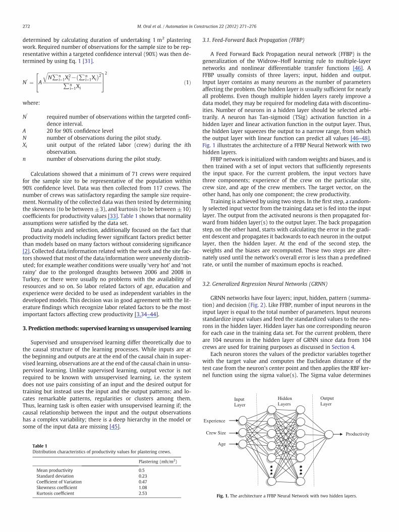
A Feed Forward Back Propagation neural network (FFBP) is thegeneralization of the Widrow–Hoff learning rule to multiple-layernetworks and nonlinear differentiable transfer functions [46]. AFFBP usually consists of three layers; input, hidden and output.Input layer contains as many neurons as the number of parametersaffecting the problem. One hidden layer is usually sufficient for nearlyall problems. Even though multiple hidden layers rarely improve adata model, they may be required for modeling data with discontinu-ities. Number of neurons in a hidden layer should be selected arbi-trarily. A neuron has Tan-sigmoid (TSig) activation function in ahidden layer and linear activation function in the output layer. Thus,the hidden layer squeezes the output to a narrow range, from whichthe output layer with linear function can predict all values [46–48].Fig. 1 illustrates the architecture of a FFBP Neural Network with twohidden layers.

FFBP network is initialized with randomweights and biases, and isthen trained with a set of input vectors that sufficiently representsthe input space. For the current problem, the input vectors havethree components; experience of the crew on the particular site,crew size, and age of the crew members. The target vector, on theother hand, has only one component; the crew productivity.

Training is achieved by using two steps. In the first step, a random-ly selected input vector from the training data set is fed into the inputlayer. The output from the activated neurons is then propagated for-ward from hidden layer(s) to the output layer. The back propagationstep, on the other hand, starts with calculating the error in the gradi-ent descent and propagates it backwards to each neuron in the outputlayer, then the hidden layer. At the end of the second step, theweights and the biases are recomputed. These two steps are alter-nately used until the network's overall error is less than a predefinedrate, or until the number of maximum epochs is reached.

3.2. Generalized Regression Neural Networks (GRNN)

GRNN networks have four layers; input, hidden, pattern (summa-tion) and decision (Fig. 2). Like FFBP, number of input neurons in theinput layer is equal to the total number of parameters. Input neuronsstandardize input values and feed the standardized values to the neu-rons in the hidden layer. Hidden layer has one corresponding neuronfor each case in the training data set. For the current problem, thereare 104 neurons in the hidden layer of GRNN since data from 104crews are used for training purposes as discussed in Section 4.

Each neuron stores the values of the predictor variables togetherwith the target value and computes the Euclidean distance of thetest case from the neuron's center point and then applies the RBF ker-nel function using the sigma value(s). The Sigma value determines

ProductivityCrew Size

Age

Fig. 1. The architecture a FFBP Neural Network with two hidden layers.

Output NodesWeightsInput Nodes

Age

*Productivity

Crew Size

Experience

Fig. 3. SOM structure.

D

÷

InputLayer

HiddenLayer

DecisionLayer

PatternLayer

N

Crew Size

Age

Experience

Productivity

Fig. 2. Schematic diagram of GRNN.

273M. Oral et al. / Automation in Construction 22 (2012) 271–276

the spread of RBF kernel function. The output value of a hidden neu-ron is passed to the two neurons in the pattern layer where one neu-ron is the denominator summation unit and the other is thenumerator summation unit. The denominator summation unit addsup the weight values coming from each of the hidden neurons andthe numerator summation unit adds up the weight values multipliedby the actual target value for each hidden neuron. The decision layerthen divides the value accumulated in the numerator summation unitby the value in the denominator summation unit and uses the resultas the predicted target value [49–50]. The prediction performance ofa GRNN strongly relies on the sigma value. It is the only parameterthat needs to be tuned by the user.

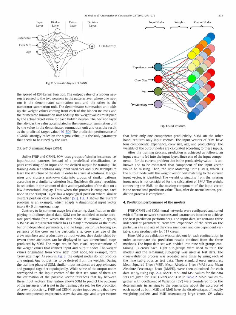
3.3. Self Organizing Maps (SOM)

Unlike FFBP and GRNN, SOM uses groups of similar instances, i.e.input/output patterns, instead of a predefined classification, i.e.pairs consisting of an input and the desired output for training. Thetraining data set contains only input variables and SOM attempts tolearn the structure of the data in order to arrive at solutions. It orga-nizes and clusters unknown data into groups of similar patternsaccording to a similarity criterion (e.g. Euclidean distance) resultingin reduction in the amount of data and organization of the data on alow dimensional display. Thus, when the process is complete, eachnode in the ‘Output Layer’ has a topological position where similarclusters position close to each other [51]. Fig. 3 shows the currentproblem as an example, which adapts 4 dimensional input vectorinto a 6×6 dimensional map.

Contrary to its common usage for; clustering, classification or dis-playing multidimensional data, SOM can be modified to make accu-rate predictions from which the data model is unknown. A typicalSOM has an input vector which has as many dimensions as the num-ber of independent parameters, and no target vector. By feeding ex-perience of the crew on the particular site, crew size, age of thecrew members and productivity as input vector, the relationships be-tween these attributes can be displayed in two dimensional mapsproduced by SOM. The maps are, in fact, visual representations ofthe weight values that connect input and output nodes. The weightvalues originating from ‘crew size’ input node, for example, form‘crew size map’. As seen in Fig. 3, the output nodes do not produceany output. Any output has to be derived from the weights. Duringthe training phase of SOM, similar input instances are approximatedand grouped together topologically. While some of the output nodescorrespond to the input vectors of the data set, some of them arethe estimation of the possible vector instances that lay betweenthese input vectors. This feature allows SOM to predict the outcomeof the instances that is not in the training data set. For the predictionof crew productivity, FFBP and GRNN require input vectors that havethree components; experience, crew size and age, and target vectors

that have only one component; productivity. SOM, on the otherhand, requires only input vectors. The input vectors of SOM havefour components; experience, crew size, age, and productivity. Theweights of the output nodes are calculated according to these inputs.

After the training process, prediction is achieved as follows: aninput vector is fed into the input layer. Since one of the input compo-nents – for the current problem that is the productivity value – is un-known and to be estimated, that component of the input vectorwould be missing. Then, the Best Matching Unit (BMU), which isthe output node with the weight vector best matching to the currentinput vector, is identified. The weight originating from the missinginput node is not considered for the calculation of BMU. The weightconnecting the BMU to the missing component of the input vectoris the normalized prediction value. Thus, after de-normalization, pre-diction process is completed.

4. Prediction performance of the models

FFBP, GRNN and SOM neural networks were configured and tunedwith different network structures and parameters in order to achievethe best prediction performances. The input data set contains threeindependent parameters; crew size, experience of the crew on theparticular site and age of the crew members, and one dependent var-iable; crew productivity for 117 crews.

Nine fold cross validation was carried out for each configuration inorder to compare the prediction results obtained from the threemethods. The input data set was divided into nine sub-groups con-taining 13 crews each. Eight sub-groups were used to train themodels and the remaining sub-group was used as test data. Thecross-validation process was repeated nine times by using each ofthe nine sub-groups as test data. Three standard error measures;Mean Squared Error (MSE), Mean Absolute Error (MAE) and MeanAbsolute Percentage Error (MAPE), were then calculated for eachdata set by using Eqs. 2–4. MAPE, MAE and MSE values for the datasets are given for FFBP, GRNN and SOM in Table 2. MAPE values to-gether with Coefficient of Variation (CV) were considered to be thedeterminants in arriving to the conclusions about the accuracy ofeach model as both MSE and MAE have the disadvantages of heavilyweighting outliers and MSE accentuating large errors. CV values

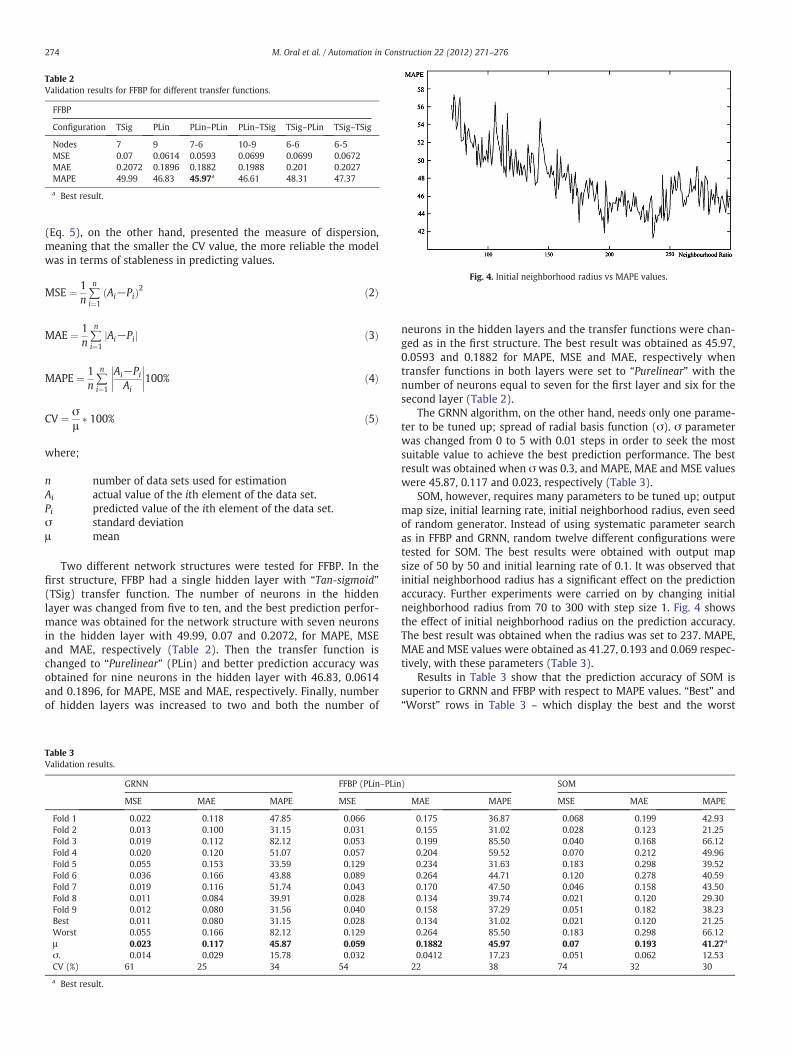
Fig. 4. Initial neighborhood radius vs MAPE values.

Table 2Validation results for FFBP for different transfer functions.

FFBP

Configuration TSig PLin PLin–PLin PLin–TSig TSig–PLin TSig–TSig

Nodes 7 9 7-6 10-9 6-6 6-5MSE 0.07 0.0614 0.0593 0.0699 0.0699 0.0672MAE 0.2072 0.1896 0.1882 0.1988 0.201 0.2027MAPE 49.99 46.83 45.97a 46.61 48.31 47.37

a Best result.

274 M. Oral et al. / Automation in Construction 22 (2012) 271–276

(Eq. 5), on the other hand, presented the measure of dispersion,meaning that the smaller the CV value, the more reliable the modelwas in terms of stableness in predicting values.

MSE ¼ 1n∑n

i¼1Ai−Pið Þ2 ð2Þ

MAE ¼ 1n∑n

i¼1Ai−Pij j ð3Þ

MAPE ¼ 1n∑n

i¼1

Ai−PiAi

��������100% ð4Þ

CV ¼ σμ� 100% ð5Þ

where;

n number of data sets used for estimationAi actual value of the ith element of the data set.Pi predicted value of the ith element of the data set.σ standard deviationμ mean

Two different network structures were tested for FFBP. In thefirst structure, FFBP had a single hidden layer with “Tan-sigmoid”(TSig) transfer function. The number of neurons in the hiddenlayer was changed from five to ten, and the best prediction perfor-mance was obtained for the network structure with seven neuronsin the hidden layer with 49.99, 0.07 and 0.2072, for MAPE, MSEand MAE, respectively (Table 2). Then the transfer function ischanged to “Purelinear” (PLin) and better prediction accuracy wasobtained for nine neurons in the hidden layer with 46.83, 0.0614and 0.1896, for MAPE, MSE and MAE, respectively. Finally, numberof hidden layers was increased to two and both the number of

Table 3Validation results.

GRNN FFBP (PLin–PLin

MSE MAE MAPE MSE

Fold 1 0.022 0.118 47.85 0.066Fold 2 0.013 0.100 31.15 0.031Fold 3 0.019 0.112 82.12 0.053Fold 4 0.020 0.120 51.07 0.057Fold 5 0.055 0.153 33.59 0.129Fold 6 0.036 0.166 43.88 0.089Fold 7 0.019 0.116 51.74 0.043Fold 8 0.011 0.084 39.91 0.028Fold 9 0.012 0.080 31.56 0.040Best 0.011 0.080 31.15 0.028Worst 0.055 0.166 82.12 0.129μ 0.023 0.117 45.87 0.059σ. 0.014 0.029 15.78 0.032CV (%) 61 25 34 54

a Best result.

neurons in the hidden layers and the transfer functions were chan-ged as in the first structure. The best result was obtained as 45.97,0.0593 and 0.1882 for MAPE, MSE and MAE, respectively whentransfer functions in both layers were set to “Purelinear” with thenumber of neurons equal to seven for the first layer and six for thesecond layer (Table 2).

The GRNN algorithm, on the other hand, needs only one parame-ter to be tuned up; spread of radial basis function (σ). σ parameterwas changed from 0 to 5 with 0.01 steps in order to seek the mostsuitable value to achieve the best prediction performance. The bestresult was obtained when σ was 0.3, and MAPE, MAE and MSE valueswere 45.87, 0.117 and 0.023, respectively (Table 3).

SOM, however, requires many parameters to be tuned up; outputmap size, initial learning rate, initial neighborhood radius, even seedof random generator. Instead of using systematic parameter searchas in FFBP and GRNN, random twelve different configurations weretested for SOM. The best results were obtained with output mapsize of 50 by 50 and initial learning rate of 0.1. It was observed thatinitial neighborhood radius has a significant effect on the predictionaccuracy. Further experiments were carried on by changing initialneighborhood radius from 70 to 300 with step size 1. Fig. 4 showsthe effect of initial neighborhood radius on the prediction accuracy.The best result was obtained when the radius was set to 237. MAPE,MAE and MSE values were obtained as 41.27, 0.193 and 0.069 respec-tively, with these parameters (Table 3).

Results in Table 3 show that the prediction accuracy of SOM issuperior to GRNN and FFBP with respect to MAPE values. “Best” and“Worst” rows in Table 3 – which display the best and the worst

) SOM

MAE MAPE MSE MAE MAPE

0.175 36.87 0.068 0.199 42.930.155 31.02 0.028 0.123 21.250.199 85.50 0.040 0.168 66.120.204 59.52 0.070 0.212 49.960.234 31.63 0.183 0.298 39.520.264 44.71 0.120 0.278 40.590.170 47.50 0.046 0.158 43.500.134 39.74 0.021 0.120 29.300.158 37.29 0.051 0.182 38.230.134 31.02 0.021 0.120 21.250.264 85.50 0.183 0.298 66.120.1882 45.97 0.07 0.193 41.27a

0.0412 17.23 0.051 0.062 12.5322 38 74 32 30

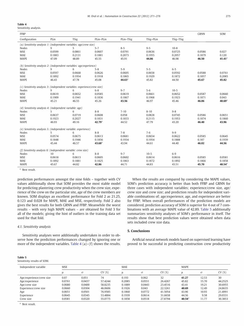
Table 4Sensitivity analysis.

FFBP GRNN SOM

Configuration PLin TSig PLin–PLin PLin–TSig TSig–PLin TSig–TSig

(a) Sensitivity analysis 1: (independent variables: age/crew size)Nodes 9 5 5-7 8-5 9-5 10-8MSE 0.0599 0.0861 0.0607 0.0791 0.0636 0.0725 0.0586 0.027MAE 0.1883 0.2131 0.1881 0.2073 0.1955 0.2057 0.1879 0.120MAPE 47.09 48.89 45.55 45.91 44.86 46.98 46.50 41.41a

(b) Sensitivity analysis 2: (independent variables: age/experience)Nodes 9 6 5-8 5-9 5-5 6-5MSE 0.0597 0.0668 0.0626 0.0605 0.0658 0.0592 0.0588 0.0761MAE 0.1892 0.1954 0.1918 0.1865 0.1929 0.1872 0.1857 0.2085MAPE 46.43 47.78 45.08 44.63a 45.82 44.50 45.67 45.82

(c) Sensitivity analysis 3: (independent variables: experience/crew size)Nodes 9 6 6-8 9-7 5-6 10-5MSE 0.0619 0.0652 0.0585 0.0619 0.0661 0.0652 0.0587 0.0660MAE 0.1909 0.1941 0.1836 0.1867 0.1968 0.1923 0.1871 0.043MAPE 45.21 46.55 45.26 43.56 46.97 45.46 46.06 40.69a

(d) Sensitivity analysis 4: (independent variable: age)Nodes 5 6 8-8 7-10 8-10 9-8MSE 0.0637 0.0719 0.0608 0.058 0.0828 0.0745 0.0586 0.0651MAE 0.1923 0.2027 0.1831 0.1833 0.2115 0.1953 0.1874 0.1860MAPE 46.93 49.16 42.79a 44.52 47.79 43.20 46.40 43.96

(e) Sensitivity analysis 5: (independent variable: experience)Nodes 5 6 8-8 7-8 7-6 9-9MSE 0.0574 0.0675 0.0613 0.0681 0.0654 0.0622 0.0585 0.0645MAE 0.1848 0.1946 0.1856 0.1934 0.1954 0.1888 0.187 0.1939MAPE 45.44 46.57 43.68a 43.94 44.61 44.40 46.02 44.56

(f) Sensitivity analysis 6: (independent variable: crew size)Nodes 10 6 8-8 9-7 10-5 6-9MSE 0.0618 0.0613 0.0605 0.0602 0.0614 0.0616 0.0585 0.0581MAE 0.1892 0.1881 0.1825 0.1863 0.1872 0.1892 0.1866 0.1858MAPE 45.67 44.82 42.86 44.71 44.83 43.51 45.70 40.54a

a Best result.

275M. Oral et al. / Automation in Construction 22 (2012) 271–276

prediction performances amongst the nine folds – together with CVvalues additionally show that SOM provides the most stable modelfor predicting plastering crew productivity when the crew size, expe-rience of the crew on the particular site, age of the crew members areknown. SOM displays an excellent performance for Fold 2 as 21.25,0.123 and 0.028 for MAPE, MAE and MSE, respectively. Fold 2 alsogives the best results for both GRNN and FFBP. Meanwhile the worstresults – with very high MAPE values – are obtained for Fold 3 forall of the models; giving the hint of outliers in the training data setused for that fold.

4.1. Sensitivity analysis

Sensitivity analyses were additionally undertaken in order to ob-serve how the prediction performances changed by ignoring one ormore of the independent variables. Table 4 (a)–(f) shows the results.

Table 5Sensitivity results of SOM.

Independent variable MSE MAE

μ σ CV (%) μ

Age/experience/crew size 0.07 0.051 74 0.19Age/experience 0.0761 0.0437 57.4244 0.20Age/crew size 0.0680 0.0400 58.8235 0.18Experience/crew size 0.0660 0.0304 46.0606 0.19Age 0.0651 0.0501 76.9585 0.18Experience 0.0645 0.0345 53.4884 0.19Crew size 0.0581 0.0320 55.0775 0.18

a Best result.

When the results are compared by considering the MAPE values,SOM's prediction accuracy is better than both FFBP and GRNN forthree cases with independent variables; experience/crew size, age/crew size and crew size; and prediction results for independent vari-able combinations of; age/experience, age, and experience are betterfor FFBP. When overall performances of the prediction models areconsidered, prediction accuracy of SOM is superior for 4 out of 7 com-binations with an average MAPE value of 42.89. Table 5 additionallysummarizes sensitivity analyses of SOM's performance in itself. Theresults show that best prediction values were obtained when datasets included crew size data.

5. Conclusions

Artificial neural network models based on supervised learning haveproved to be successful in predicting construction crew productivity

MAPE

σ CV (%) μ σ CV (%)

3 0.062 32 41.27 12.53 3085 0.0551 26.4267 45.82 15.70 44.252589 0.0443 23.4516 43.41 19.21 30.695526 0.043 22.3261 40.69 12.49 24.863560 0.0772 41.5054 43.96 10.93 21.499139 0.0614 31.6658 44.56 9.58 29.033158 0.0518 27.8794 40.54a 11.77 30.3853

276 M. Oral et al. / Automation in Construction 22 (2012) 271–276

significantly better than statistical methods like regression. Meanwhileapplications in various areas other than construction showed that if thecausal relation between input and output has a complex variability,learning task is often easier with unsupervised learning. Thus, currentresearch focused on application of both supervised and unsupervisedlearning based methods to plastering crew productivity data in orderto compare the prediction results. Results show that SOMhas a superiorperformance than FFBP and GRNN for plastering crew productivity pre-diction. SOM's performance has also been tested for concrete, reinforce-ment and formwork crews and superior prediction performance, incomparison to the previous models has been reported [29]. However,future work is required in order to compare the results with the perfor-mance of FFBP and GRNN for concrete, reinforcement and formworkcrews. Positive effect of crew size related data on the model's perfor-mance is also an additional point which can guide future data collec-tions and which can be investigated by the future applications.

Finally, it can be concluded that the current research proved SOMto be an alternative tool to the supervised learning based tools andSOM can be used in various prediction applications.

Acknowledgment

Data used in this paper has been collected during the researchproject 106M055 which is supported by TÜBİTAK (The Scientificand Technical Research Council of Turkey). The authors would liketo thank G. Mıstıkoglu, E. Erdis, E.M. Ocal, and O. Paydak for their in-valuable support during data collection.

References

[1] M. Radosavljevi, R.M. Horner, The evidence of complex variability in constructionlabour productivity, Construction Management and Economics 20 (1) (2002) 3–12.

[2] R. Sönmez, J.E. Rowings, Construction labor productivity modelling with neuralnetworks, Journl of Construction Engrg. and Mgmt. 124 (6) (1998) 498–504.

[3] A. Kazaz, S. Ulubeyli, A different approach to construction labour in Turkey: com-parative productivity analysis, Building and Environment 39 (2004) 93–100.

[4] R. Lane, G. Goodman, Wicked Problems: Righteous Solutions — Back to the Futureon Large Complex Projects, IGLC 8, Brighton, UK, 2000.

[5] S. Bertelsen, L. Koskela, Managing the Three Aspects of Production in Construc-tion, IGLC-10, Gramado, Brazil, 2002.

[6] S. Bertelsen, Complexity—Construction in a New Perspective, ILGC-11, Blacks-burg, Virginia, 2003.

[7] S. Emmit, S. Bertelsen, A. Dam, BygLOK—A Danish Experiement on Cooperation inConstruction, IGLC-12, Elsimore, Denmark, 2004.

[8] L. Koskela, G.A. Howell, The Underlying Theory of Project Management is Obso-lete, Project Management Institute, 2002.

[9] G.A. Howell, G. Ballard, I.D. Tommelein, L. Koskela, Discussion of “Reducing vari-ability to improve performance as a lean construction principle”, Journal of Con-struction Engineering Management 130 (2) (2004) 299–300.

[10] L. Chao, M.J. Skibniewski, Estimating construction productivity: neural-network-based approach, Journal of Computing in Civil Engineering 2 (1994) 234–251.

[11] A.S. Ezeldin, L.M. Sharar, Neural networks for estimating the productivity of concretingactivities, Journal of Construction Engineering Management 132 (2006) 650–656.

[12] J. Portas, S. AbouRizk, Neural network model for estimating construction produc-tivity, Journal of Construction Engineering Management 123 (4) (1997) 399–410.

[13] H.Y. Ersoz, Discussion of neural network model for estimating construction pro-ductivity, 125 (3), 1999, pp. 211–212.

[14] S. AbouRizk, P. Knowles, U.R. Hermann, Estimating labor production rates for in-dustrial construction activities, Journal of Construction Engineering Management127 (6) (2001) 502–511.

[15] C.O. Seung, K.S. Sunil, Construction equipment productivity estimation using arti-ficial neural network model, Construction Management and Economics 24 (2006)1029–1044.

[16] C.M. Tam, T. Tong, S. Tse, Artificial neural networks model for predicting excava-tor productivity, Engineering Construction and Architectural Management(2002) 446–452 5/6.

[17] E. Oral (Laptalı), E. Erdiş, G. Mıstıkoğlu, Kalıp işlerinde ekip profillerinin verimli-liğe etkileri, 4. İnşaat Yönetimi Kongresi, İstanbul, 30–31 Ekim, 2007.

[18] R. Noori, A. Khakpour, B. Omidvar, A. Farokhnia, Comparison of ANN and principalcomponent analysis-multivariate linear regression models for predicting the

river flow based on developed discrepancy ratio statistic, Expert Systems withApplications 37 (8) (2010) 5856–5862 10.1016/j.eswa.2010.02.020.

[19] M. Dissanayake, A.R. Fayek, A.D. Russell, W. Pedrycz, A Hybrid Neural Network forPredicting Construction Labour Productivity, Computing in Civil Engineering,ASCE, 2005.

[20] M. Dissanayake, A.R. Fayek, Soft computing approach to construction performanceprediction and diagnosis, Canadian Journal of Civil Engineering 35 (8) (2008).

[21] C.O. Seung, K.S. Sunil, Construction equipment productivity estimation using artifi-cial neural network model, Construction Management and Economics 24 (2006).

[22] A.K. Ghosh, P. Om, Neural models for predicting trajectory performance of an ar-tillery rocket, Journal of Aerospace Computing, Information, and Communication2 (Feb. 2004) 112–115.

[23] D.H. Grosse, W. Timm, T.W. Nattkemper, REEFSOM—a metaphoric data display forexploratory data mining, Brains, Minds and Media Vol.2, bmm305 (urn:nbn:de:0009-3-3051) (2006).

[24] M. Oja, S. Kaski, T. Kohonen, Bibliography of Self-Organizing Map (SOM) papers:1998–2001 addendum, Neural Computing Surveys 3 (2002) 1–156.

[25] M. Oral, E. Genç, İskenderun Körfezi'nde yaşayan Orfoz Balığı (Ephinephelus margin-atus Lowe 1834)’ ndaki parazitlenmeninÖzÖrgütlenmeli Haritalarla yeniden değer-lendirilmesi, Journal of Fisheries Sciences.com (2008) 293–300.

[26] L.B. Hwa, S. Miklas, Application of the Self-Organizing Map (SOM) to assess theheavy metal removal performance in experimental constructed wetlands,Water Research 40 (18) (2006) 3367–3374.

[27] H. Du, M. Inui, M. Ohki, M. Ohkita, Short-term prediction of oil temperature of atransformer during summer and winter by Self-Organizing Map, Applied Infor-matics (2002) 351.

[28] L. Mokhnache, A. Boubakeur, N. Nait Said, Comparison of Different Neural Net-works Algorithms Used in the Diagnosis and Thermal Ageing Prediction of Trans-former Oil, IEEE-SMC CD-ROM, paper WA2P1, 2002 Hammamat, Tunisia.

[29] E. Oral, M. Oral, Predicting construction crew productivity by using Self Organiz-ing Maps, Automation in Construction 19 (6) (2010) 791–797.

[30] S.C. Ok, K.S. Sinha, Construction equipment productivity estimation using artifi-cial neural network model, Construction Management and Economics 24(2006) 1029–1044 (October).

[31] B. Kobu, Üretim Yönetimi, 1999, Avcıol Basım, İstanbul.[32] M. Oral, E. Oral, A computer based system for documentation and monitoring of

construction labour productivity, CIB 24th W78 Conference, 2007, Maribor.[33] R.B. Kline, Principles and Practice Of Structural Equation Modelling, Guilford

Press, USA, 2004.[34] O.A. Akindele, Craftsmen and Labour Productivity in the Swaziland Construction

Industry, CIDB 1st Postgraduate Conference, Porth Elizabeth, South Africa, 2003.[35] J.D. Bocherding, L.F. Alaercon, Quantitative effects on construction productivity,

Construction Lawyer 11 (1) (1991) 36–48.[36] P.F. Kaming, P. Olomolaiye, G.D. Holt, F.C. Haris, Factors influencing craftsmen's

productivity in Indonesia, International Journal of Project Management 15 (1)(1997) 21–30.

[37] M. Kuruoğlu, F.İ. Bayoğlu, Yapı üretiminde adam saat değerlerinin belirlenmesiüzerine bir araştırma ve sonuçları. 16. İnşaat Mühendisliği Teknik Kongresi Anka-ra, No:65, 2001.

[38] L.S. Pheng, C.Y. Meng, Managing Productivity in Construction: JIT Operations andMeasurements, Ashgate, Singapore, 1997.

[39] D.G. Proverbs, G.D. Holt, P.O. Olomolaiye, Productivity rates and constructionmethods for high rise concrete construction: a comparative evaluation of UK,German and French contractors, Construction Management and Economics 17(1) (1999) 45–52.

[40] P. Olomolaiye, An evaluation of bricklayers' motivation and productivity. PhDthesis, Loughborough University of Technology, UK, 1988.

[41] M.E. Öcal, A. Tat, E. Erdiş, Analysis of Labour Productivity Rates in Public Works UnitPrice Book (Bayındırlık işleri birim fiyat analizlerindeki işgücü verimliliklerinin irde-lenmesi.), 3rd Construction Management Congress, İzmir, 2005.

[42] S. Wang, A Methodology for comparing the productivities of the RMC industriesin major cities. PhD thesis, The Hong Kong Polytechnic University, Hong Kong,1995.

[43] G. Winch, B. Carr, Benchmarking on-site productivity in France and the UK: a CALI-BRE approach, Construction Management and Economics 19 (6) (2001) 577–590.

[44] M. Zakeri, P.O. Olomolaiye, G.D. Holt, F.C. Harris, A survey of constraints on Irani-an construction operatives' productivity, Construction Management and Eco-nomics 14 (1996) 417–426.

[45] H. Valpola, Bayesian ensemble learning for nonlinear factor analysis, Acta Polytech-nica Scandinavica, Mathematics and Computing Series No. 108, , 2000, p. 54, Espoo.

[46] P.J. Werbos, The Roots of Back Propagation. From Ordered Derivatives to NeuralNetworks and Political Forecasting, John Wiley & Sons, Inc, New York, 1994.

[47] J. Lawrence, Introduction to Neural Networks, California Scientific Software Press,1994.

[48] T.L. Fine, Feedforward Neural Network Methodology, Springer, 1999.[49] http://www.dtreg.com/pnn.htm.[50] D.F. Specht, A generalized regression neural network, IEEE Transactions on Neural

Networks 2 (Nov. 1991) 568–576.[51] T. Kohonen, Self-organized formation of topologically correct feature maps, Bio-

logical Cybernetics 43 (1982) 59–69.