Engineering Fracture Mechanics 74 (2007) 1665–1682

www.elsevier.com/locate/engfracmech

An engineering solution for mesh size effects in the simulationof delamination using cohesive zone models

A. Turon a, C.G. Davila b, P.P. Camanho c,*, J. Costa a

a AMADE, Polytechnic School, University of Girona, Campus Montilivi s/n, 17071 Girona, Spainb NASA Langley Research Center, Hampton, VA, USA

c DEMEGI, Faculdade de Engenharia, Universidade do Porto, Rua Dr. Roberto Frias, 4200-465 Porto, Portugal

Received 4 July 2005; received in revised form 24 February 2006; accepted 21 August 2006Available online 27 October 2006

Abstract

A methodology to determine the constitutive parameters for the simulation of progressive delamination is proposed.The procedure accounts for the size of a cohesive finite element and the length of the cohesive zone to ensure the correctdissipation of energy. In addition, a closed-form expression for estimating the minimum penalty stiffness necessary for theconstitutive equation of a cohesive finite element is presented. It is shown that the resulting constitutive law allows the useof coarser finite element meshes than is usually admissible, which renders the analysis of large-scale progressive delamina-tion problems computationally tractable.� 2006 Elsevier Ltd. All rights reserved.

Keywords: Delamination; Fracture; Cohesive elements

1. Introduction

Delamination, or interfacial cracking between composite layers, is one of the most common types of dam-age in laminated fibre-reinforced composites due to their relatively weak interlaminar strengths. Delaminationmay arise under various circumstances, such as low velocity impacts, or bearing loads in structural joints. Thedelamination failure mode is particularly important for the structural integrity of composite structures becauseit is difficult to detect during inspection.

The simulation of delamination using the finite element method (FEM) is normally performed by means ofthe Virtual Crack Closure Technique (VCCT) [1], or using cohesive finite elements [2–12].

The VCCT is based on the assumption that the energy released during delamination propagation equals thework required to close the crack back to its original position. Based on this assumption, the components of theenergy release rate are computed from the nodal forces and nodal relative displacements [1]. Delamination

0013-7944/$ - see front matter � 2006 Elsevier Ltd. All rights reserved.

doi:10.1016/j.engfracmech.2006.08.025

* Corresponding author. Tel.: +351 22 5081753; fax: +351 22 5081584.E-mail address: pcamanho@fe.up.pt (P.P. Camanho).

1666 A. Turon et al. / Engineering Fracture Mechanics 74 (2007) 1665–1682

growth is predicted when a combination of the components of the energy release rate is equal to a criticalvalue.

There are some difficulties when using the VCCT in the simulation of progressive delamination. The calcu-lation of fracture parameters requires nodal variables and topological information from the nodes ahead andbehind the crack front. Such calculations are tedious to perform and may require remeshing for crackpropagation.

The use of cohesive finite elements can overcome some of these above difficulties. Cohesive finite elementscan predict both the onset and the non-self-similar propagation of delamination. However, the simulation ofprogressive delamination using cohesive elements poses numerical difficulties related to the proper definitionof the stiffness of the cohesive layer, the requirement of extremely refined meshes, and the convergence diffi-culties associated with problems involving softening constitutive models.

A procedure to determine the optimal value of the penalty stiffness of a cohesive element is proposed. Aclosed-form expression for the interface stiffness is developed, replacing the empirical definitions of the stiff-ness of the cohesive layer that are normally used. In addition, a solution that allows the use of coarse meshesin the simulation of delamination is proposed. The procedure is based on an artificial increase of the cohesivezone length that it is obtained by lowering the interfacial strength while keeping the fracture toughness con-stant. It is shown that it is possible to predict the propagation of delamination accurately in specimens withand without pre-existing cracks by using coarse meshes and their correspondingly adjusted constitutivemodels.

The methodologies proposed here are relevant for the use of cohesive zone models in the simulation ofdelamination in large composite structures used in the industry where the requirements of extremely finemeshes cannot be met.

The kinematics and constitutive model of a previously proposed cohesive element [11,12], formulated forthree-dimensional (3D) elements, is adapted to be used with two-dimensional (2D) finite element models. Sev-eral simulations of specimens with and without initial cracks are performed to demonstrate that the method-ology proposed can accurately predict both crack initiation and propagation using coarse meshes.

2. Selection of cohesive zone model parameters

2.1. Cohesive zone model approach

Cohesive finite elements are used to model material discontinuities. Consider a domain X containing amaterial discontinuity, Cd which divides the domain X into two parts, X+ and X�. Prescribed tractions, ti,are imposed on the boundary CF. The stress field inside the domain, rij, is related to the external loadingand to the closing tractions sþj ; s

�j in the material discontinuity through the equilibrium equations:

rij;j ¼ 0 in X ð1Þrijnj ¼ ti on CF ð2Þrijnþj ¼ sþi ¼ �s�i ¼ rijn�j on Cd ð3Þ

The formulation of the cohesive finite elements is based in the Cohesive Zone Model (CZM) approach. TheCZM approach [13–15] is one of the most commonly used tools to investigate interfacial fracture. The CZMapproach assumes that a cohesive damage zone develops near the crack tip. The CZM links the microstruc-tural failure mechanism to the continuum fields governing bulk deformations. Thus, a CZM is characterizedby the properties of the bulk material, the crack initiation condition, and the crack evolution function.

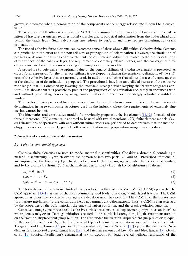
Cohesive damage zone models relate cohesive surface tractions, s, to displacement jumps, D, at an interfacewhere a crack may occur. Damage initiation is related to the interfacial strength, s0, i.e., the maximum tractionon the traction–displacement jump relation. The area under the traction–displacement jump relation is equalto the fracture toughness, Gc. There are several types of constitutive equations used in cohesive elements:Tvergaard and Hutchinson [16] proposed a trapezoidal law, Cui and Wisnom [17] a perfectly plastic rule, Nee-dleman first proposed a polynomial law, [18], and later an exponential law, Xu and Needleman [19]. Goyalet al. [10] adopted Needleman’s exponential law to account for load reversal without restoration of the

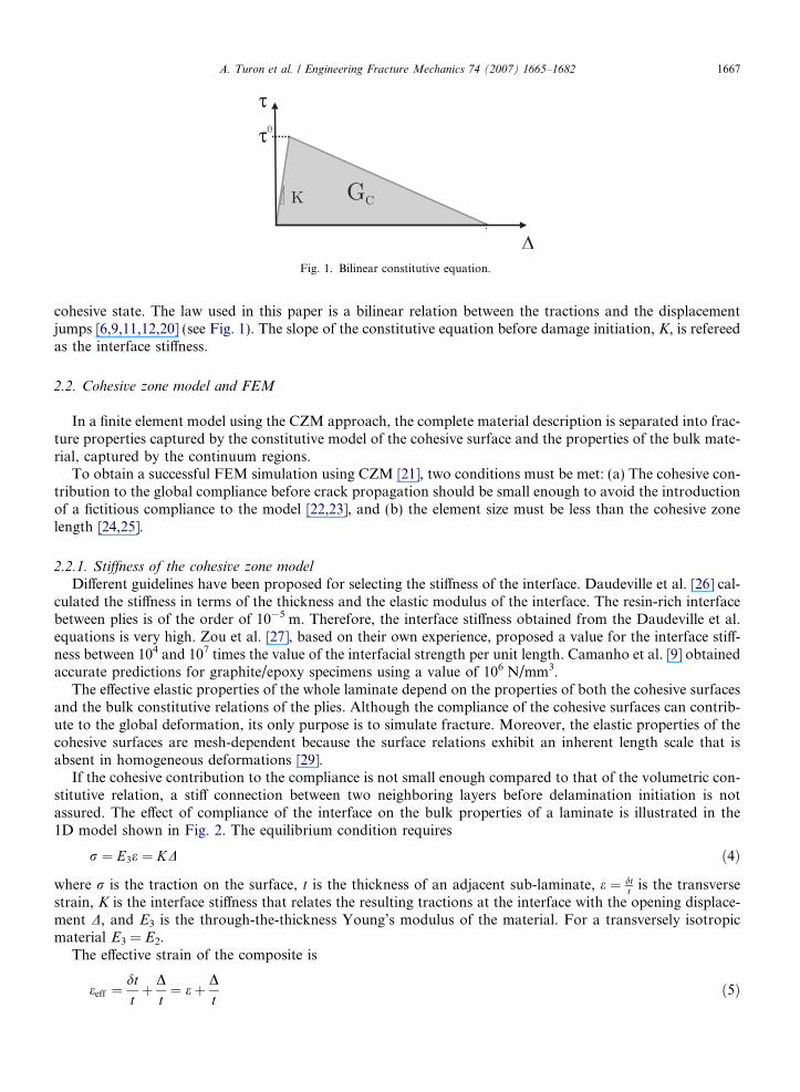
Fig. 1. Bilinear constitutive equation.

A. Turon et al. / Engineering Fracture Mechanics 74 (2007) 1665–1682 1667

cohesive state. The law used in this paper is a bilinear relation between the tractions and the displacementjumps [6,9,11,12,20] (see Fig. 1). The slope of the constitutive equation before damage initiation, K, is refereedas the interface stiffness.

2.2. Cohesive zone model and FEM

In a finite element model using the CZM approach, the complete material description is separated into frac-ture properties captured by the constitutive model of the cohesive surface and the properties of the bulk mate-rial, captured by the continuum regions.

To obtain a successful FEM simulation using CZM [21], two conditions must be met: (a) The cohesive con-tribution to the global compliance before crack propagation should be small enough to avoid the introductionof a fictitious compliance to the model [22,23], and (b) the element size must be less than the cohesive zonelength [24,25].

2.2.1. Stiffness of the cohesive zone model

Different guidelines have been proposed for selecting the stiffness of the interface. Daudeville et al. [26] cal-culated the stiffness in terms of the thickness and the elastic modulus of the interface. The resin-rich interfacebetween plies is of the order of 10�5 m. Therefore, the interface stiffness obtained from the Daudeville et al.equations is very high. Zou et al. [27], based on their own experience, proposed a value for the interface stiff-ness between 104 and 107 times the value of the interfacial strength per unit length. Camanho et al. [9] obtainedaccurate predictions for graphite/epoxy specimens using a value of 106 N/mm3.

The effective elastic properties of the whole laminate depend on the properties of both the cohesive surfacesand the bulk constitutive relations of the plies. Although the compliance of the cohesive surfaces can contrib-ute to the global deformation, its only purpose is to simulate fracture. Moreover, the elastic properties of thecohesive surfaces are mesh-dependent because the surface relations exhibit an inherent length scale that isabsent in homogeneous deformations [29].

If the cohesive contribution to the compliance is not small enough compared to that of the volumetric con-stitutive relation, a stiff connection between two neighboring layers before delamination initiation is notassured. The effect of compliance of the interface on the bulk properties of a laminate is illustrated in the1D model shown in Fig. 2. The equilibrium condition requires

r ¼ E3e ¼ KD ð4Þ

where r is the traction on the surface, t is the thickness of an adjacent sub-laminate, e ¼ dtt is the transverse

strain, K is the interface stiffness that relates the resulting tractions at the interface with the opening displace-ment D, and E3 is the through-the-thickness Young’s modulus of the material. For a transversely isotropicmaterial E3 = E2.

The effective strain of the composite is

eeff ¼dttþ D

t¼ eþ D

tð5Þ

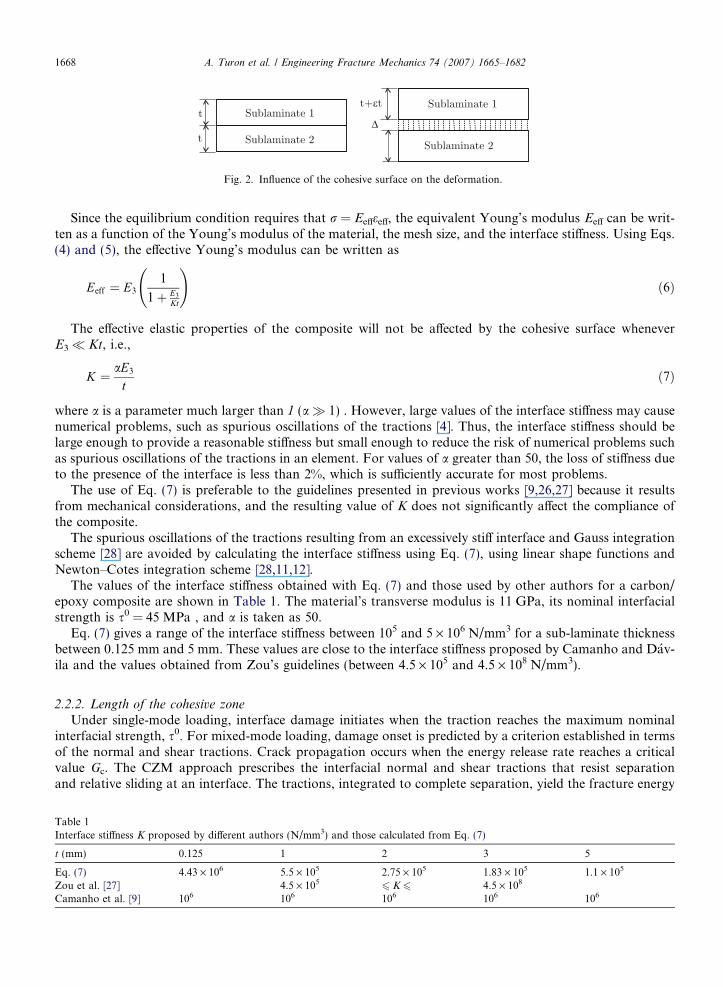
Fig. 2. Influence of the cohesive surface on the deformation.

1668 A. Turon et al. / Engineering Fracture Mechanics 74 (2007) 1665–1682

Since the equilibrium condition requires that r = Eeffeeff, the equivalent Young’s modulus Eeff can be writ-ten as a function of the Young’s modulus of the material, the mesh size, and the interface stiffness. Using Eqs.(4) and (5), the effective Young’s modulus can be written as

TableInterfa

t (mm

Eq. (7Zou etCaman

Eeff ¼ E3

1

1þ E3

Kt

!ð6Þ

The effective elastic properties of the composite will not be affected by the cohesive surface wheneverE3� Kt, i.e.,

K ¼ aE3

tð7Þ

where a is a parameter much larger than 1 (a� 1) . However, large values of the interface stiffness may causenumerical problems, such as spurious oscillations of the tractions [4]. Thus, the interface stiffness should belarge enough to provide a reasonable stiffness but small enough to reduce the risk of numerical problems suchas spurious oscillations of the tractions in an element. For values of a greater than 50, the loss of stiffness dueto the presence of the interface is less than 2%, which is sufficiently accurate for most problems.

The use of Eq. (7) is preferable to the guidelines presented in previous works [9,26,27] because it resultsfrom mechanical considerations, and the resulting value of K does not significantly affect the compliance ofthe composite.

The spurious oscillations of the tractions resulting from an excessively stiff interface and Gauss integrationscheme [28] are avoided by calculating the interface stiffness using Eq. (7), using linear shape functions andNewton–Cotes integration scheme [28,11,12].

The values of the interface stiffness obtained with Eq. (7) and those used by other authors for a carbon/epoxy composite are shown in Table 1. The material’s transverse modulus is 11 GPa, its nominal interfacialstrength is s0 = 45 MPa , and a is taken as 50.

Eq. (7) gives a range of the interface stiffness between 105 and 5 · 106 N/mm3 for a sub-laminate thicknessbetween 0.125 mm and 5 mm. These values are close to the interface stiffness proposed by Camanho and Dav-ila and the values obtained from Zou’s guidelines (between 4.5 · 105 and 4.5 · 108 N/mm3).

2.2.2. Length of the cohesive zone

Under single-mode loading, interface damage initiates when the traction reaches the maximum nominalinterfacial strength, s0. For mixed-mode loading, damage onset is predicted by a criterion established in termsof the normal and shear tractions. Crack propagation occurs when the energy release rate reaches a criticalvalue Gc. The CZM approach prescribes the interfacial normal and shear tractions that resist separationand relative sliding at an interface. The tractions, integrated to complete separation, yield the fracture energy

1ce stiffness K proposed by different authors (N/mm3) and those calculated from Eq. (7)

) 0.125 1 2 3 5

) 4.43 · 106 5.5 · 105 2.75 · 105 1.83 · 105 1.1 · 105

al. [27] 4.5 · 1056 K 6 4.5 · 108

ho et al. [9] 106 106 106 106 106

A. Turon et al. / Engineering Fracture Mechanics 74 (2007) 1665–1682 1669

release rate, Gc. The length of the cohesive zone lcz is defined as the distance from the crack tip to the pointwhere the maximum cohesive traction is attained.

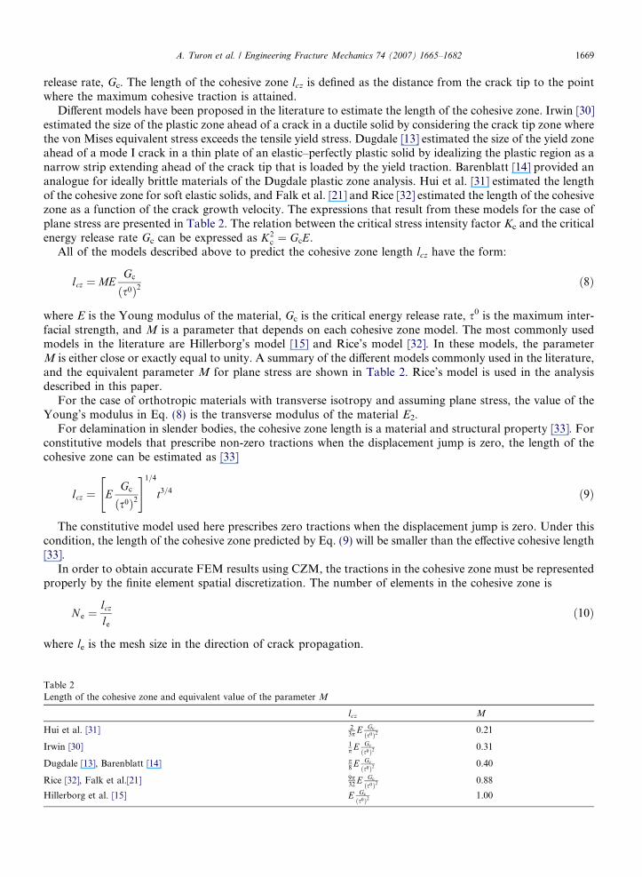
Different models have been proposed in the literature to estimate the length of the cohesive zone. Irwin [30]estimated the size of the plastic zone ahead of a crack in a ductile solid by considering the crack tip zone wherethe von Mises equivalent stress exceeds the tensile yield stress. Dugdale [13] estimated the size of the yield zoneahead of a mode I crack in a thin plate of an elastic–perfectly plastic solid by idealizing the plastic region as anarrow strip extending ahead of the crack tip that is loaded by the yield traction. Barenblatt [14] provided ananalogue for ideally brittle materials of the Dugdale plastic zone analysis. Hui et al. [31] estimated the lengthof the cohesive zone for soft elastic solids, and Falk et al. [21] and Rice [32] estimated the length of the cohesivezone as a function of the crack growth velocity. The expressions that result from these models for the case ofplane stress are presented in Table 2. The relation between the critical stress intensity factor Kc and the criticalenergy release rate Gc can be expressed as K2

c ¼ GcE.All of the models described above to predict the cohesive zone length lcz have the form:

TableLength

Hui et

Irwin [

Dugda

Rice [3

Hillerb

lcz ¼ MEGc

s0ð Þ2ð8Þ

where E is the Young modulus of the material, Gc is the critical energy release rate, s0 is the maximum inter-facial strength, and M is a parameter that depends on each cohesive zone model. The most commonly usedmodels in the literature are Hillerborg’s model [15] and Rice’s model [32]. In these models, the parameterM is either close or exactly equal to unity. A summary of the different models commonly used in the literature,and the equivalent parameter M for plane stress are shown in Table 2. Rice’s model is used in the analysisdescribed in this paper.

For the case of orthotropic materials with transverse isotropy and assuming plane stress, the value of theYoung’s modulus in Eq. (8) is the transverse modulus of the material E2.

For delamination in slender bodies, the cohesive zone length is a material and structural property [33]. Forconstitutive models that prescribe non-zero tractions when the displacement jump is zero, the length of thecohesive zone can be estimated as [33]

lcz ¼ EGc

ðs0Þ2

" #1=4

t3=4 ð9Þ

The constitutive model used here prescribes zero tractions when the displacement jump is zero. Under thiscondition, the length of the cohesive zone predicted by Eq. (9) will be smaller than the effective cohesive length[33].

In order to obtain accurate FEM results using CZM, the tractions in the cohesive zone must be representedproperly by the finite element spatial discretization. The number of elements in the cohesive zone is

N e ¼lcz

le

ð10Þ

where le is the mesh size in the direction of crack propagation.

2of the cohesive zone and equivalent value of the parameter M

lcz M

al. [31] 23p E Gc

ðs0Þ2 0.21

30] 1p E Gc

ðs0Þ2 0.31

le [13], Barenblatt [14] p8 E Gc

ðs0Þ2 0.40

2], Falk et al.[21] 9p32 E Gc

ðs0Þ2 0.88

org et al. [15] E Gc

ðs0Þ2 1.00

1670 A. Turon et al. / Engineering Fracture Mechanics 74 (2007) 1665–1682

When the cohesive zone is discretized by too few elements, the distribution of tractions ahead of the cracktip is not represented accurately. Therefore, a minimum number of elements, Ne, is needed in the cohesive zoneto get successful FEM results.

However, the minimum number of elements needed in the cohesive zone is not well established: Moes andBelytschko [34], based on the work of Carpinteri et al. [35], suggested using more than 10 elements. However,Falk et al. [21] used between 2 and 5 elements in their simulations. In the parametric study by Davila andCamanho et al. [36], the minimum element length for predicting the delamination in a double cantilever beam(DCB) specimen was 1 mm, which leads, using Eq. (8) with M = 1, to a length of the cohesive zone of3.28 mm. Therefore, three elements in the cohesive zone were sufficient to predict the propagation of dela-mination in mode I.

2.3. Guidelines for the selection of the parameters of the interface with coarser meshes

One of the drawbacks in the use of cohesive zone models is that very fine meshes are needed to assure areasonable number of elements in the cohesive zone. The length of the cohesive zone given by Eq. (8) is pro-portional to the fracture energy release rate (Gc) and to the inverse of the square of the interfacial strength s0.For typical graphite–epoxy or glass–epoxy composite materials, the length of the cohesive zone is smaller thanone or two millimeters. Therefore, according to Eq. (10), the mesh size required in order to have more thantwo elements in the cohesive zone should be smaller than half a millimeter. The computational requirementsneeded to analyze a large structure with these mesh sizes may render most practical problems intractable.

Alfano and Crisfield [8] observed that variations of the maximum interfacial strength do not have a stronginfluence in the predicted results, but that lowering the interfacial strength can improve the convergence rate ofthe solution. The result of using a lower interfacial strength is that the length of the cohesive zone and thenumber of elements in the cohesive zone increase. Therefore, the representation of the softening responseof the fracture process ahead of the crack tip is more accurate with a lower interface strength althoughthe stress distribution in the regions near the crack tip might be altered [8].

It is possible to develop a strategy to adapt the length of the cohesive zone to a given mesh size. The pro-cedure consists of determining the value s0 of the interfacial strength required for a desired number of elementsðN 0

eÞ in the cohesive zone. From Eqs. (8) and (10), the required interface strength is

s0 ¼ffiffiffiffiffiffiffiffiffiffiffiffiffiffi9pEGc

32N 0ele

sð11Þ

Finally, the interfacial strength is chosen as

T ¼ minfs0; s0g ð12Þ

The interfacial strength is computed for each loading mode by substituting the values of the fracture tough-

ness in Eq. (11) and of the ultimate traction in Eq. (12) by the values corresponding to the loading mode.The effect of a reduction of the interfacial strength is to enlarge the cohesive zone, and thus, the model is

better suited to capture the softening behaviour ahead of the crack tip. Although the stress concentrations inthe bulk material near the crack tip are less accurate when using a reduced interfacial strength value, themechanics of energy dissipation are properly captured, which ensures the proper propagation of the crackfront. Moreover, if Eq. (7) is used to compute the interface stiffness, the interface stiffness will be large enoughto assure a stiff connection between the two neighboring layers and small enough to avoid spuriousoscillations.

The strategy of lowering the interfacial strength whilst keeping the fracture toughness constant was alsoproposed by Bazant and Planas [37] in a different context. The procedure developed by Bazant and Planasis used in the numerical implementation of crack band models where the energy dissipated is a function ofthe volume of the finite element [37]. In this case, it is necessary to modify the constitutive model includinga characteristic element length to assure that the computed fracture energy is independent of the discretization.The reduction of the maximum stress is used to avoid snap-back of the modified constitutive model of largeelements.

A. Turon et al. / Engineering Fracture Mechanics 74 (2007) 1665–1682 1671

Using cohesive elements there is no need to use a characteristic element length in the constitutive model. Itis however necessary to have a sufficient number of elements in the cohesive zone to capture the correctdistribution of tractions. Therefore, the critical dimension of the finite element is along the crack propagationpath.

When using crack band models in the simulation of delamination using coarse meshes, the strength must beadjusted taking into account the dimension of the element in the direction perpendicular to the crack plane(Bazant’s model [37]), and also the dimension of the element in the crack propagation path using the methodproposed here.

3. FEM implementation

The cohesive zone model used here is based on the model that was previously proposed by the authors[11,12]. The model has been adapted to be used in 2D finite element models. A brief description of the model,with special focus on the kinematics and constitutive damage model, is presented.

3.1. Kinematics and constitutive relation of cohesive zone models

The displacement jump across the interface of the material discontinuity required in the constitutive model,suib, can be obtained as a function of the displacement of the points located on the top and bottom side of theinterface, uþi and u�i , respectively:

suit ¼ uþi � u�i ð13Þ

where u�i are the displacements with respect to the fixed Cartesian coordinate system. A co-rotational formu-lation is used in order to express the components of the displacement jumps with respect to the deformed inter-face. The coordinates �xi of the deformed interface can be written as [38]

�xi ¼ X i þ1

2uþi þ u�i� �

ð14Þ

where Xi are the coordinates of the undeformed interface.The components of the displacement jump tensor in the local coordinate system on the deformed interface,

Dm, are expressed in terms of the displacement field in global coordinates:

Dm ¼ Hmisuit ð15Þ

where Hmi is the rotation tensor.

The constitutive operator of the interface, Dji, relates the element tractions, sj, to the displacement jumps,Di:

sj ¼ DjiDi ð16Þ

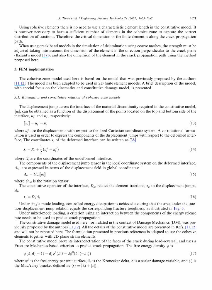
Under single-mode loading, controlled energy dissipation is achieved assuring that the area under the trac-

tion–displacement jump relation equals the corresponding fracture toughness, as illustrated in Fig. 3.Under mixed-mode loading, a criterion using an interaction between the components of the energy release

rate needs to be used to predict crack propagation.The constitutive damage model used here, formulated in the context of Damage Mechanics (DM), was pre-

viously proposed by the authors [11,12]. All the details of the constitutive model are presented in Refs. [11,12]and will not be repeated here. The formulation presented in previous references is adapted to use the cohesiveelements together with 2D plane strain elements.

The constitutive model prevents interpenetration of the faces of the crack during load-reversal, and uses aFracture Mechanics-based criterion to predict crack propagation. The free energy density w is

wðD; dÞ ¼ ð1� dÞw0ðDiÞ � dw0 d1i �D1h ið Þ ð17Þ

where w0 is the free energy per unit surface, dij is the Kronecker delta, d is a scalar damage variable, and hÆi isthe MacAuley bracket defined as hxi ¼ 1

2ðxþ jxjÞ.

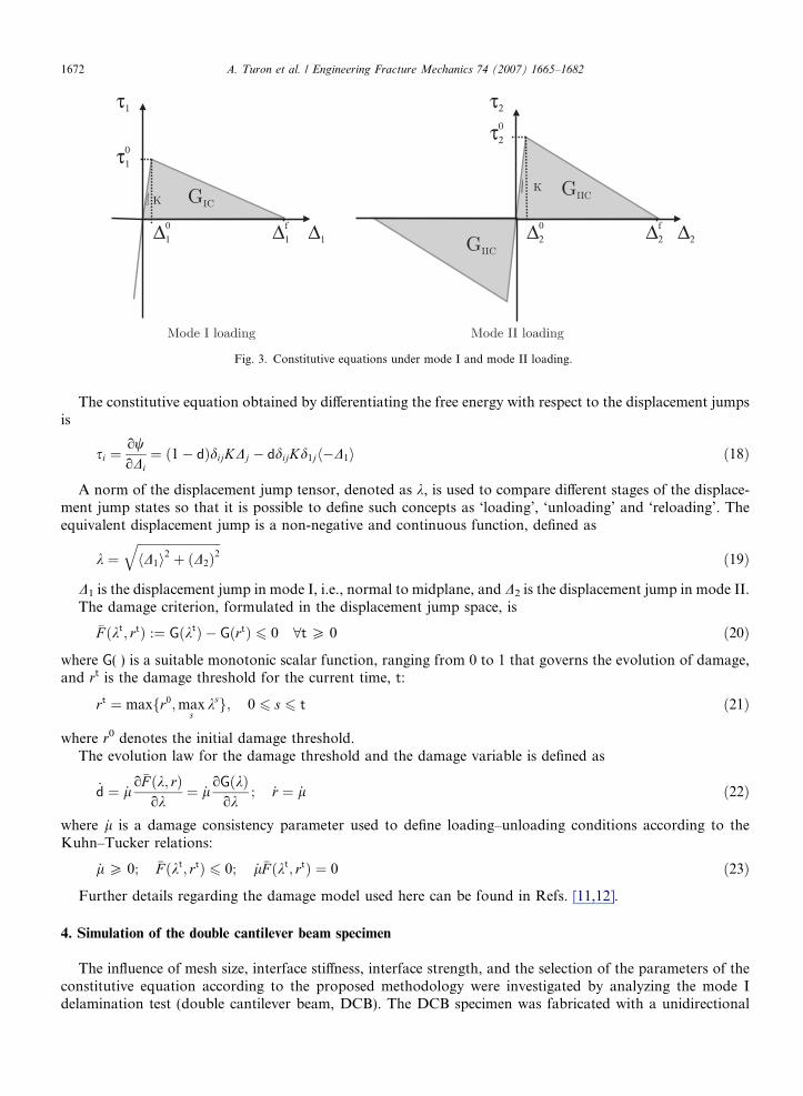
Fig. 3. Constitutive equations under mode I and mode II loading.

1672 A. Turon et al. / Engineering Fracture Mechanics 74 (2007) 1665–1682

The constitutive equation obtained by differentiating the free energy with respect to the displacement jumpsis

si ¼owoDi¼ ð1� dÞdijKDj � ddijKd1j �D1h i ð18Þ

A norm of the displacement jump tensor, denoted as k, is used to compare different stages of the displace-ment jump states so that it is possible to define such concepts as ‘loading’, ‘unloading’ and ‘reloading’. Theequivalent displacement jump is a non-negative and continuous function, defined as

k ¼ffiffiffiffiffiffiffiffiffiffiffiffiffiffiffiffiffiffiffiffiffiffiffiffiffiffiffiD1h i2 þ D2ð Þ2

qð19Þ

D1 is the displacement jump in mode I, i.e., normal to midplane, and D2 is the displacement jump in mode II.The damage criterion, formulated in the displacement jump space, is

�F ðkt; rtÞ :¼ GðktÞ � GðrtÞ 6 0 8t P 0 ð20Þ

where G(Æ) is a suitable monotonic scalar function, ranging from 0 to 1 that governs the evolution of damage,and rt is the damage threshold for the current time, t:

rt ¼ maxfr0;maxs

ksg; 0 6 s 6 t ð21Þ

where r0 denotes the initial damage threshold.The evolution law for the damage threshold and the damage variable is defined as

_d ¼ _lo�F k; rð Þ

ok¼ _l

oG kð Þok

; _r ¼ _l ð22Þ

where _l is a damage consistency parameter used to define loading–unloading conditions according to theKuhn–Tucker relations:

_l P 0; �F ðkt; rtÞ 6 0; _l�F ðkt; rtÞ ¼ 0 ð23Þ

Further details regarding the damage model used here can be found in Refs. [11,12].

4. Simulation of the double cantilever beam specimen

The influence of mesh size, interface stiffness, interface strength, and the selection of the parameters of theconstitutive equation according to the proposed methodology were investigated by analyzing the mode Idelamination test (double cantilever beam, DCB). The DCB specimen was fabricated with a unidirectional

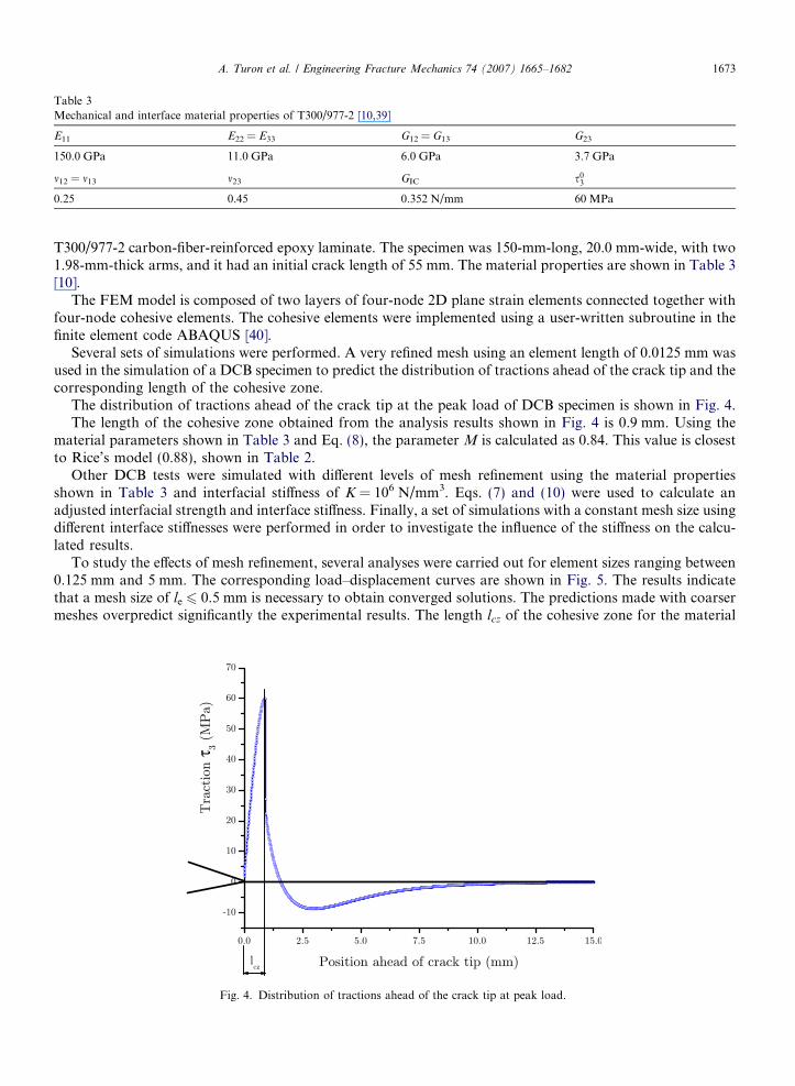
Table 3Mechanical and interface material properties of T300/977-2 [10,39]

E11 E22 = E33 G12 = G13 G23

150.0 GPa 11.0 GPa 6.0 GPa 3.7 GPa

m12 = m13 m23 GIC s03

0.25 0.45 0.352 N/mm 60 MPa

A. Turon et al. / Engineering Fracture Mechanics 74 (2007) 1665–1682 1673

T300/977-2 carbon-fiber-reinforced epoxy laminate. The specimen was 150-mm-long, 20.0 mm-wide, with two1.98-mm-thick arms, and it had an initial crack length of 55 mm. The material properties are shown in Table 3[10].

The FEM model is composed of two layers of four-node 2D plane strain elements connected together withfour-node cohesive elements. The cohesive elements were implemented using a user-written subroutine in thefinite element code ABAQUS [40].

Several sets of simulations were performed. A very refined mesh using an element length of 0.0125 mm wasused in the simulation of a DCB specimen to predict the distribution of tractions ahead of the crack tip and thecorresponding length of the cohesive zone.

The distribution of tractions ahead of the crack tip at the peak load of DCB specimen is shown in Fig. 4.The length of the cohesive zone obtained from the analysis results shown in Fig. 4 is 0.9 mm. Using the

material parameters shown in Table 3 and Eq. (8), the parameter M is calculated as 0.84. This value is closestto Rice’s model (0.88), shown in Table 2.

Other DCB tests were simulated with different levels of mesh refinement using the material propertiesshown in Table 3 and interfacial stiffness of K = 106 N/mm3. Eqs. (7) and (10) were used to calculate anadjusted interfacial strength and interface stiffness. Finally, a set of simulations with a constant mesh size usingdifferent interface stiffnesses were performed in order to investigate the influence of the stiffness on the calcu-lated results.

To study the effects of mesh refinement, several analyses were carried out for element sizes ranging between0.125 mm and 5 mm. The corresponding load–displacement curves are shown in Fig. 5. The results indicatethat a mesh size of le 6 0.5 mm is necessary to obtain converged solutions. The predictions made with coarsermeshes overpredict significantly the experimental results. The length lcz of the cohesive zone for the material

Fig. 4. Distribution of tractions ahead of the crack tip at peak load.

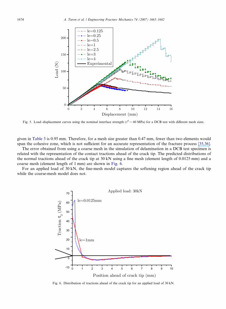
Fig. 5. Load–displacement curves using the nominal interface strength (s0 = 60 MPa) for a DCB test with different mesh sizes.

1674 A. Turon et al. / Engineering Fracture Mechanics 74 (2007) 1665–1682

given in Table 3 is 0.95 mm. Therefore, for a mesh size greater than 0.47 mm, fewer than two elements wouldspan the cohesive zone, which is not sufficient for an accurate representation of the fracture process [35,36].

The error obtained from using a coarse mesh in the simulation of delamination in a DCB test specimen isrelated with the representation of the contact tractions ahead of the crack tip. The predicted distributions ofthe normal tractions ahead of the crack tip at 30 kN using a fine mesh (element length of 0.0125 mm) and acoarse mesh (element length of 1 mm) are shown in Fig. 6.

For an applied load of 30 kN, the fine-mesh model captures the softening region ahead of the crack tipwhile the coarse-mesh model does not.

Fig. 6. Distribution of tractions ahead of the crack tip for an applied load of 30 kN.

A. Turon et al. / Engineering Fracture Mechanics 74 (2007) 1665–1682 1675

4.1. Effect of interface strength

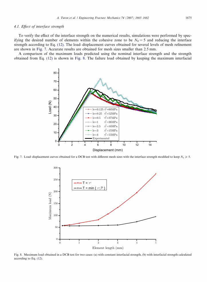
To verify the effect of the interface strength on the numerical results, simulations were performed by spec-ifying the desired number of elements within the cohesive zone to be N0 = 5 and reducing the interfacestrength according to Eq. (12). The load–displacement curves obtained for several levels of mesh refinementare shown in Fig. 7. Accurate results are obtained for mesh sizes smaller than 2.5 mm.

A comparison of the maximum loads predicted using the nominal interface strength and the strengthobtained from Eq. (12) is shown in Fig. 8. The failure load obtained by keeping the maximum interfacial

Fig. 7. Load–displacement curves obtained for a DCB test with different mesh sizes with the interface strength modified to keep Ne P 5.

Fig. 8. Maximum load obtained in a DCB test for two cases: (a) with constant interfacial strength, (b) with interfacial strength calculatedaccording to Eq. (12).

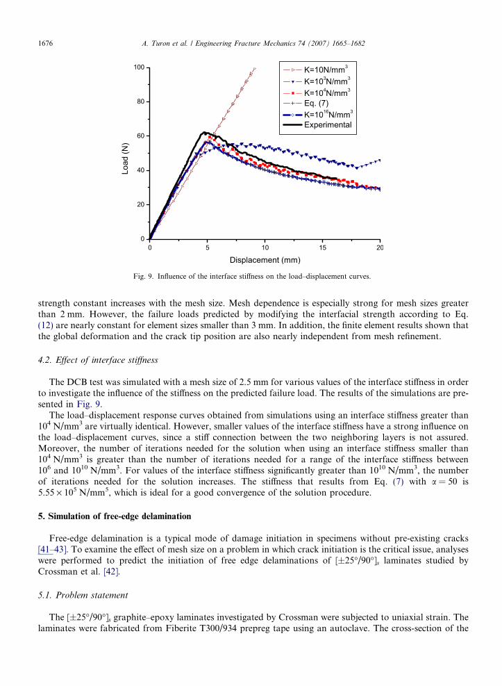
Fig. 9. Influence of the interface stiffness on the load–displacement curves.

1676 A. Turon et al. / Engineering Fracture Mechanics 74 (2007) 1665–1682

strength constant increases with the mesh size. Mesh dependence is especially strong for mesh sizes greaterthan 2 mm. However, the failure loads predicted by modifying the interfacial strength according to Eq.(12) are nearly constant for element sizes smaller than 3 mm. In addition, the finite element results shown thatthe global deformation and the crack tip position are also nearly independent from mesh refinement.

4.2. Effect of interface stiffness

The DCB test was simulated with a mesh size of 2.5 mm for various values of the interface stiffness in orderto investigate the influence of the stiffness on the predicted failure load. The results of the simulations are pre-sented in Fig. 9.

The load–displacement response curves obtained from simulations using an interface stiffness greater than104 N/mm3 are virtually identical. However, smaller values of the interface stiffness have a strong influence onthe load–displacement curves, since a stiff connection between the two neighboring layers is not assured.Moreover, the number of iterations needed for the solution when using an interface stiffness smaller than104 N/mm3 is greater than the number of iterations needed for a range of the interface stiffness between106 and 1010 N/mm3. For values of the interface stiffness significantly greater than 1010 N/mm3, the numberof iterations needed for the solution increases. The stiffness that results from Eq. (7) with a = 50 is5.55 · 105 N/mm5, which is ideal for a good convergence of the solution procedure.

5. Simulation of free-edge delamination

Free-edge delamination is a typical mode of damage initiation in specimens without pre-existing cracks[41–43]. To examine the effect of mesh size on a problem in which crack initiation is the critical issue, analyseswere performed to predict the initiation of free edge delaminations of [±25�/90�]s laminates studied byCrossman et al. [42].

5.1. Problem statement

The [±25�/90�]s graphite–epoxy laminates investigated by Crossman were subjected to uniaxial strain. Thelaminates were fabricated from Fiberite T300/934 prepreg tape using an autoclave. The cross-section of the

Fig. 10. Cross-section of the laminate.

Table 4Mechanical properties of T300/934 graphite–epoxy [41,44]

E11 E22 = E33 G12 = G13 G23 m12 = m13 m23

140.0 GPa 11.0 GPa 5.5 GPa 3.61 GPa 0.29 0.52

A. Turon et al. / Engineering Fracture Mechanics 74 (2007) 1665–1682 1677

specimen was 25.0-mm-wide and 0.792-mm-thick (see Fig. 10). No initial cracks were induced in the laminate.The material properties are shown in Table 4 [41,44].

Tensile tests were performed by applying a controlled displacement in the x-direction. Due to the stackingsequence, the through the thickness free-edge stress distribution produces high rzz in the 90� ply. Therefore,high tractions occur at the 90�/90� interface, leading to the onset of delamination at the free-edge.

5.2. Numerical predictions

A FEM model was developed using six layers of four-node generalized plane strain elements [45,46]. Thegeneralized plane strain model developed calculates the out-of-plane components of the stress tensor thatcause delamination onset. The 90�/90� interface was modeled with the four-node cohesive elements presentedin previous sections. The elastic properties of each layer were defined by means of the 3D stiffness matrix. The

Fig. 11. Load–displacement curves obtained for a free-edge test with different mesh sizes using nominal interface strength properties.

1678 A. Turon et al. / Engineering Fracture Mechanics 74 (2007) 1665–1682

cohesive elements were implemented using a user-written subroutine in the finite element code ABAQUS [40].Due to the symmetry of the laminate, only half of the cross-section was modeled.

Two sets of simulations were performed. First, tensile tests were simulated with different levels of meshrefinement. Then, Eqs. (10) and (7) were used to calculate the interface strength and the interface stiffness.

Several analyses were carried out for mesh sizes ranging between 0.05 mm and 0.5 mm. The load–displace-ment curves obtained are shown in Fig. 11. An interfacial stiffness of K = 106 N/mm3, an interface strength of51.7 MPa, a critical energy release rate of 0.175 N/mm [41], and the material properties shown in Table 4 wereused. The length of the cohesive zone obtained with these properties, using Eq. (8), is 0.63 mm. A mesh size

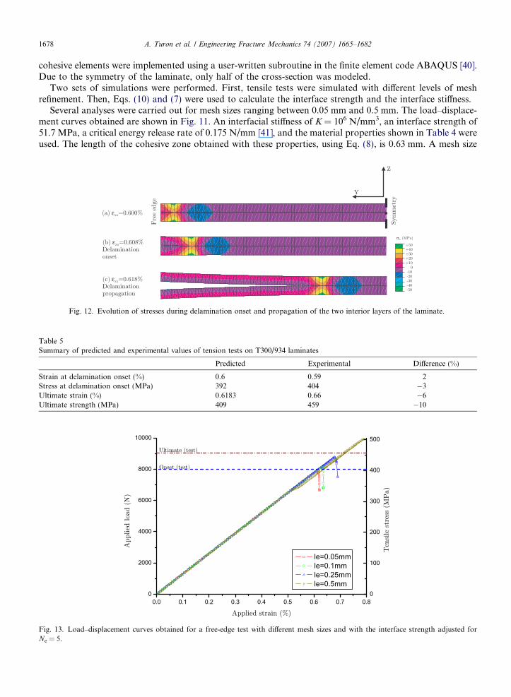
Fig. 12. Evolution of stresses during delamination onset and propagation of the two interior layers of the laminate.

Table 5Summary of predicted and experimental values of tension tests on T300/934 laminates

Predicted Experimental Difference (%)

Strain at delamination onset (%) 0.6 0.59 2Stress at delamination onset (MPa) 392 404 �3Ultimate strain (%) 0.6183 0.66 �6Ultimate strength (MPa) 409 459 �10

Fig. 13. Load–displacement curves obtained for a free-edge test with different mesh sizes and with the interface strength adjusted forNe = 5.

A. Turon et al. / Engineering Fracture Mechanics 74 (2007) 1665–1682 1679

smaller than 0.2 mm is needed in order to have three or more elements in the cohesive zone. The predictionsobtained using different levels of mesh refinement are shown in Fig. 11. Using meshes coarser than 0.2 mm, thecorrect solution is significantly overpredicted. For a mesh size equal to 0.5 mm the maximum applied load isgreater than two times the maximum load obtained with meshes smaller than 0.1 mm.

The ultimate tensile strength calculated using a mesh size of 0.1 mm is 404 MPa. Delamination onset occurswhen a point in the interface is not able to carry any traction, which changes the stress distribution. The stressdistribution of the two interior layers of the laminate in a plane perpendicular to the interface and normal tothe load direction are represented in Fig. 12 for three stages of deformation. At the first stage, before dela-mination onset, the stresses rzz near the free edge are tensile due to the mismatch effect of the Poisson ratio(red-lighter zones in Fig. 12). At delamination onset, a region of the free edge is unable to carry load and the

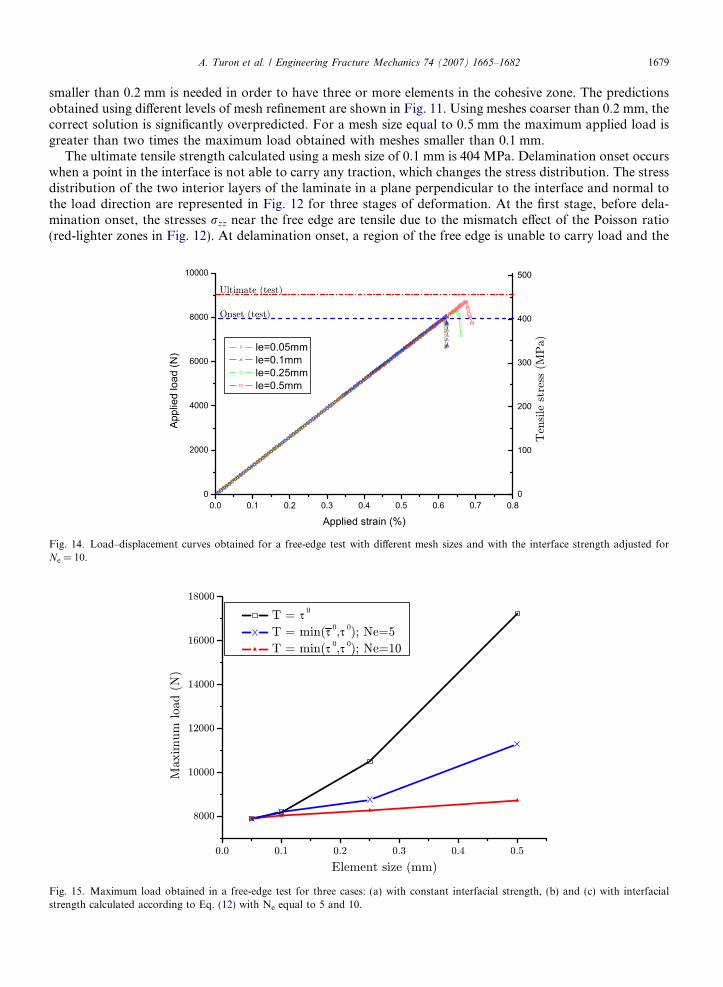
Fig. 14. Load–displacement curves obtained for a free-edge test with different mesh sizes and with the interface strength adjusted forNe = 10.

Fig. 15. Maximum load obtained in a free-edge test for three cases: (a) with constant interfacial strength, (b) and (c) with interfacialstrength calculated according to Eq. (12) with Ne equal to 5 and 10.

1680 A. Turon et al. / Engineering Fracture Mechanics 74 (2007) 1665–1682

stresses become compressive, as shown in Fig. 12b (blue-darker zones). The predicted onset of delamination isexx = 0.6%, and the corresponding stress is 392 MPa. The experimental results obtained by Crossman andWang [42] reported a delamination onset tensile stress of 409 MPa and an ultimate tensile strength of459 MPa. The predicted and experimental onset and failure stresses and strains are summarized in Table 5.Unstable delamination propagation and the corresponding structural collapse occurs at a strain of 0.6183%.

To verify the effect of interface strength on the predicted results, simulations were performed by specifyingthe desired number of elements spanning the cohesive zone to be Ne = 5 and reducing the interface strengthaccording to Eq. (12). The load–displacement curves obtained for several levels of mesh refinement are shownin Fig. 13.

A similar study of mesh size effect was repeated by selecting the desired number of elements spanning thecohesive zone to be Ne = 10. Although the results presented in Figs. 14 and 15 for Ne = 10 are more accuratethan those for Ne = 5, the improvement is insignificant when the element is smaller than 0.25 mm.

Figs. 14 and 15 show that the maximum load predicted by the numerical model converges to the same valuewhen decreasing the element length. The maximum load predicted differs 12% of the experimental value. Thisdifference can be justified by the increase of the fracture toughness associated with fiber bridging that is nottaken into account in the model.

6. Concluding remarks

An engineering solution for the simulation of delamination using coarse meshes was developed. Two newguidelines for the selection of the parameters for the constitutive equation used for the simulation of delam-ination were presented.

First, a new equation for the selection of the interface stiffness parameter K was derived. The new equationis preferable to previous guidelines because it results from mechanical considerations rather than from expe-rience. The approach provides an adequate stiffness to ensure a sufficiently stiff connection between two neigh-boring layers, while avoiding the possibility of spurious oscillations in the solution caused by overly stiffconnections.

Finally, an expression to adjust the maximum interfacial strength used in the computations with coarsemeshes was presented. It was shown that a minimum number of elements within the cohesive zone is necessaryfor accurate simulations. By reducing the maximum interfacial strength, the cohesive zone length is enlargedand the cohesive zone spans more elements. The results obtained by reducing the maximum interfacialstrength show that accurate results can be obtained with a mesh ten times coarser than by using the nominalinterface strength. The drawback in using a reduced interfacial strength value is that the stress concentrationsin the bulk material near the crack tip are less accurate.

Acknowledgement

This work has been partially funded by the Spanish government through DGICYT under contract:MAT2003-09768-C03-01. The first author would like to thank the University of Girona for the grantBR01/09.

The financial support of the Portuguese Foundation for Science and Technology (FCT) under the projectPDCTE/50354/EME/2003 is acknowledged by the third author.

References

[1] Krueger R. The virtual crack closure technique: history, approach and applications. NASA/Contractor Report-2002-211628; 2002.[2] Allix O, Ladeveze P, Corigliano A. Damage analysis of interlaminar fracture specimens. Compos Struct 1995;31:66–74.[3] Allix O, Corigliano A. Modelling and simulation of crack propagation in mixed-modes interlaminar fracture specimens. Int J Fract

1996;77:111–40.[4] Schellekens JCJ, de Borst R. A nonlinear finite-element approach for the analysis of mode-I free edge delamination in composites. Int

J Solids Struct 1993;30(9):1239–53.[5] Chaboche JL, Girard R, Schaff A. Numerical analysis of composite systems by using interphase/interface models. Comput Mech

1997;20:3–11.

A. Turon et al. / Engineering Fracture Mechanics 74 (2007) 1665–1682 1681

[6] Mi U, Crisfield MA, Davies GAO. Progressive delamination using interface elements. J Compos Mater 1998;32:1246–72.[7] Chen J, Crisfield MA, Kinloch AJ, Busso EP, Matthews FL, Qiu Y. Predicting progressive delamination of composite material

specimens via interface elements. Mech Compos Mater Struct 1999;6:301–17.[8] Alfano G, Crisfield MA. Finite element interface models for the delamination analysis of laminated composites: mechanical and

computational issues. Int J Numer Methods Engng 2001;77(2):111–70.[9] Camanho PP, Davila CG, de Moura MF. Numerical simulation of mixed-mode progressive delamination in composite materials. J

Compos Mater 2003;37(16):1415–38.[10] Goyal-Singhal V, Johnson ER, Davila CG. Irreversible constitutive law for modeling the delamination process using interfacial

surface discontinuities. Compos Struct 2004;64:91–105.[11] Turon A, Camanho PP, Costa J, Davila CG. An interface damage model for the simulation of delamination under variable-mode

ratio in composite materials. NASA/Technical Memorandum 213277; 2004.[12] Turon A, Camanho PP, Costa J, Davila CG. A damage model for the simulation of delamination under variable-mode loading. Mech

Mater 2006;38:1072–89.[13] Dugdale DS. Yielding of steel sheets containing slits. J Mech Phys Solids 1960;8:100–4.[14] Barenblatt G. The mathematical theory of equilibrium cracks in brittle fracture. Adv Appl Mech 1962;7:55–129.[15] Hillerborg A, Modeer M, Petersson PE. Analysis of crack formation and crack growth in concrete by means of fracture mechanics

and finite elements. Cement Concr Res 1976;6:773–82.[16] Tvergaard V, Hutchinson JW. The relation between crack growth resistance and fracture process parameters in elastic–plastic solids.

J Mech Phys Solids 1992;40:1377–97.[17] Cui W, Wisnom MR. A combined stress-based and fracture-mechanics-based model for predicting delamination in composites.

Composites 1993;24:467–74.[18] Needleman A. A continuum model for void nucleation by inclusion debonding. J Appl Mech 1987;54:525–32.[19] Xu X-P, Needleman A. Numerical simulations of fast crack growth in brittle solids. J Mech Phys Solids 1994;42(9):1397–434.[20] Reddy Jr ED, Mello FJ, Guess TR. Modeling the initiation and growth of delaminations in composite structures. J Compos Mater

1997;31:812–31.[21] Falk ML, Needleman A, Rice JR. A critical evaluation of cohesive zone models of dynamic fracture. J Phys IV, Proc 2001:543–50.[22] Rice JR. Dislocation nucleation from a crack tip – an analysis based on the PIERLS concept. J Mech Phys Solids 1992;40:239–71.[23] Rice JR, Beltz GE. The activation-energy for dislocation. J Mech Phys Solids 1994;42:333–60.[24] Camacho GT, Ortiz M. Computational modelling of impact damage in brittle materials. Int J Solids Struct 1996;33:2899–938.[25] Ruiz G, Pandolfi A, Ortiz M. Three-dimensional cohesive modeling of dynamic mixed-mode fracture. Int J Numer Methods Engng

2001;52:97–120.[26] Daudeville L, Allix O, Ladeveze P. Delamination analysis by damage mechanics. Some applications. Compos Engng 1995;5(1):17–24.[27] Zou Z, Reid SR, Li S, Soden PD. Modelling interlaminar and intralaminar damage in filament wound pipes under quasi-static

indentation. J Compos Mater 2002;36:477–99.[28] Schellekens J. Computational strategies for composite structures. PhD thesis, Delft University of Technology; 1992.[29] Klein PA, Foulk JW, Chen EP, Wimmer SA, Gao H. Physics-based modeling of brittle fracture: cohesive formulations and the

application of meshfree methods. Sandia Report SAND2001-8099; 2000.[30] Irwin GR. Plastic zone near a crack and fracture toughness. Proceedings of the seventh Sagamore Ordnance materials conference,

vol. IV. New York: Syracuse University; 1960. p. 63–78.[31] Hui CY, Jagota A, Bennison SJ, Londono JD. Crack blunting and the strength of soft elastic solids. Proc R Soc Lond A

2003;459:1489–516.[32] Rice JR. The mechanics of earthquake rupture. In: Dziewonski AM, Boschhi E, editors. Physics of the Earth’s interior. Proceedings

of the international school of physics ‘‘Enrico Fermi’’, Course 78, 1979. Amsterdam: Italian Physical Society/North-Holland; 1980.p. 555–649.

[33] Yang Q, Cox B. Cohesive models for damage evolution in laminated composites. Int J Fract 2005;133:107–37.[34] Moes N, Belytschko T. Extended finite element method for cohesive crack growth. Engng Fract Mech 2002;69:813–33.[35] Carpinteri A, Cornetti P, Barpi F, Valente S. Cohesive crack model description of ductile to brittle size-scale transition: dimensional

analysis vs. renormalization group theory. Engng Fract Mech 2003;70:1809–939.[36] Davila CG, Camanho PP, de Moura MFSF. Mixed-Mode decohesion elements for analyses of progressive delamination. In:

Proceedings of the 42nd AIAA/ASME/ASCE/AHS/ASC structures. Structural dynamics and materials conference, Seattle,Washington; April 16–19, 2001.

[37] Bazant ZP, Planas J. Fracture and size effect in concrete and other quasibrittle materials. Boca Raton: CRC Press; 1998.[38] Ortiz M, Pandolfi A. Finite-deformation irreversible cohesive elements for three-dimensional crack propagation analysis. Int J Numer

Methods Engng 1999;44:1267–82.[39] Morais AB, de Moura MF, Marques AT, de Castro PT. Mode-I interlaminar fracture of carbon/epoxy cross-ply composites.

Compos Sci Technol 2002;62:679–86.[40] Hibbitt, Karlsson, Sorensen. ABAQUS 6.2 User’s Manuals. Pawtucket, USA; 1996.[41] Schellekens JCJ, de Borst R. Numerical simulation of free edge delamination in graphite–epoxy laminates under uniaxial tension. In:

6th International conference on composite structures. 1991. p. 647–57.[42] Crossman FW, Wang ASD. The dependence of transverse cracking and delamination on ply thickness in graphite/epoxy laminates.

In: Reifsnider KL, editor. Damage in composite materials. ASTM STP 775. Ann Arbor (MI): American Society for Testing andMaterials; 1982. p. 118–39.

1682 A. Turon et al. / Engineering Fracture Mechanics 74 (2007) 1665–1682

[43] O’Brien TK. Characterization of delamination onset and growth in a composite laminate. In: Reifsnider KL, editor. Damage incomposite materials. ASTM STP 775. Ann Arbor (MI): American Society for Testing and Materials; 1982. p. 140–67.

[44] Wang ASD. Fracture analysis of interlaminar cracking. In: Pagano NJ, editor. Interlaminar response of composite materi-als. Amsterdam: Elsevier; 1989. p. 69–109.

[45] Li S, Lim SH. Variational principles for generalized plane strain problems and their applications. Composites A 2005;36:353–65.[46] Pipes RB, Pagano NJ. Interlaminar stresses in composite laminates under uniform axial tension. J Compos Mater 1971:538–48.