an empirical study of mala ysian firms' capital struture - CORE

---------- ------------------

AN EMPIRICAL STUDY OF MALA YSIAN FIRMS' CAPITAL STRUTURE

By

SHARIFAH RAIHAN SYED MOHD ZAIN

A thesis submitted to the University of Plymouth In partial fulfilment for the degree of

DOCTOR OF PHILOSOPHY

Accounting and Finance Group Department of Business and Management

Plymouth Business School

November 2003

Dedication

In Loving Memory, My dad ( /938-2002)

Mymom

My wonderful husband and son

And special dedication to my supervisor

AN EMPIRICAL STUDY OF MALA YSIAN FIRMS' CAPITAL STRUCTURE

SHARIFAH RAIHAN SYED MOHD ZAIN

ABSTRACT

It is sometimes purported that one of the factors affecting a firm's value is its capital structure. The event of the 1997 Asian financial crisis was expected to affect the firms' gearing level as the firms' earnings deteriorated and the capital market collapsed. The main objective of this research is to examine empirically the determinants of the capital structure of Malaysian firms. The main additional aim is to study the capital structure pattern following the 1997 financial crisis. Empirical tests were conducted on two different data sets: the first data set is the published data extracted from Datastrearn and consists of: 572 companies listed on the Kuala Lumpur Stock Exchange (KLSE) between 1994 and 2000. The second data set comprises finance managers' responses to a questionnaire survey. Chi-square, Kruskal-Wallis, ANOVA, multiple regression, stepwise regression and logistic regression were utilised to analyse the data. The multiple regression analysis was employed to find the determinants of the capital structure using various account data items provided by Datastream. The gearing differences between the two boards and within the sectors were also analysed using ANOV A and Krukal-Wall is tests. The panel data were evaluated with regard to the gearing pattern following the 1997 currency cns1s.

Overwhelming evidence on profit was found, with past profitability being the major determinant of gearing. In particular was the support for pecking order theory, in that finance managers had given internal funds the highest priority, followed by debt and equity as a last option. The statistical analysis found a strong negative correlation between liquidity and the gearing ratio for both boards, implying firms considered highly the excess current assets for funding, a conservative approach towards debt management policy. On the other hand, taxation items were not highly significant in capital structure decisions. The results indicate the existence of gearing differences between the main board and the second board gearing with high debt levels employed by second board companies. However, the second board's high gearing is dominated largely by short to medium term bank credit. Differences were also significant between different sectors of companies listed on the main board. Firms' gearing ratios increased significantly following the 1997 financial crisis, and the gearing tended to increase where the company's share prices were highly sensitive towards currency volatility. Also inflation is found to influence the changes in actual and target gearing ratios following the crisis. Recent emphasis on the development of private debt securities may affect the findings of this research in the near future.

CONTENTS

Table of Contents ............................................................................................... 1-v List of Appendices . ..... .. .. . . . . . . . . . . ....... ...... ......... .. .. . . .... .. .. . . . . . . . . .. . . ....... ................ .. . VI

List of Tables.................................................................................................. VII-IX

Table of Graphs ...................................................................................................... x List of Figures ...................................................................................................... xi List of Diagrams .. . . . . . . . .. . . . . . . . . . . . . ......... ... . . . .. . .. . . . . . ..... ... ................ ...... ... . . . . .. . . . . . . . . . . . . XI

Abbreviation ................................................................................................. XII-XIV

Acknowledgements . . . . . . . . . . .. . . . . . . . . .. . . . . . ... . . . . . . . . . . .. ...... ... . .. . . . . . . . .. .. . ....... ... . . .. .. . . . . . . . .. . . xv Declaration ..................................... .. . ...... .. . . . . . .. .......... .. . . . . . . . . . . . . .... .. . ... . . . . .. . . . . . . . . . . xv1

Chapter 1: Introduction ................................................................................... 1 1.1 - Introduction .. ........ ...... ..... ... . . . . ... . .. . . . . . . . . . . . . ......... .. . . . . ....... .. . . . . . .. ... . 1 1.2 - Research Concentration ... . ....... ... . . . . . . . . . . . . . ................. .. . . . . . . . . . . ... . .. 2 1.3 - Research Objective ..................................................................... 3 1.4 - Research Outline.......................................................................... 6

Chapter 2: Malaysian Financial Background ··························.······················ 9 2.1 - Introduction ...................................................................... ........... 9 2.2 - Geographical Background and Culture ....................................... 10 2.3- Economic Background................................................................ 12

2.3.1 -Gross Domestic Product ................................................. 12 2.3 .2 - Consumer Price Index (Inflation) ................................... 15 2.3.3- Comparison ofMalaysian Economic

Indicator and Other Nations ........................................... 17 2.4 - Financial Background ................................................................. 19

2.4.1 -The Money and Foreign Exchange Market..................... 20 2.4.2 -The Capital and Derivatives Market ............................... 21

2.4.2.1 - The Stock Market ............................................. 23 2.4.2.2 - The Private Debt Market................................... 25

2.4.2.2.1 - Overview of Bank Credit ............... 27 2.5 - Islamic Financial System ............................................................ 29 2.6 - The 1997 Financial Crisis ........................................................... 34

2.6.1 - The Impact of the Currency Crisis .................................. 36 2.6.2- The Management of the Crisis ........................................ 39

2.7- Conclusion .................................................................................. 40

Chapter 3: Literature Review .......................................................................... 43 3.1 -Introduction ................................................................................. 43 3.2- The Beginning of the Capital Structure Debate .......................... 44

3 .2.1 - The Traditional Approach to the Capital Structure ............................................................. 45

3.2.2- The New Approach to Capital Structure ......................... 47 3.2.2.1 -The Net Income and the Net

Operating Income Approach ........................... 48 3.2.2.2 - Modiagliani and Miller 1958 Model ................ 49 3.2.2.3- Empirical Evidence on MM Model ................. 51 3.2.2.4- Criticism on MM Propositions ......................... 52

3.3 -Capital Structure and Taxes ........................................................ 54 3.3.1 - Miller's Equilibrium Model ............................................ 55 3.3.2- Tax Exhaustion on Capital Structure .............................. 59 3.3.3- Tax System ..................................................................... 61 3.3.4- Malaysian Tax System .................................................... 64

3.4- Factors Determining the Capital Structure ................................. 67 3.4.1 -Firms Specific Factors .................................................... 67

3.4.1.1 -Asset Structure- Liquidity ............................... 67 3.4.1.2- Tangibility ........................................................ 70 3.4.1.3-Size ................................................................... 71 3.4.1.4- Profitability ...................................................... 74 3.4.1.5 -Pecking Order Theory ...................................... 78 3.4.1.6- Firms' Growth or Investment

Opportunities . . . . . . . . . .. . . . . . . . ............. .. . . .. . . . . . . . . . . . . . .. 80 3.4.1.7-Risk .................................................................. 82

3.4.1.7.1- Bankruptcy Risk ............................ 83 3.4. 1.7.2- Firms' Specific Risk or

Business Risk ... . . . . . . . . .. ...... .. . . . . . . . . . . . 85 3.4.1.7.3- Interest Coverage ........................... 89

3.4.1.8 -Agency Costs and Ownership .......................... 90 3.4.1.8.1 - Ownershiop of Firm in Malaysia ... 92

3.4.1.9- Disclosure ........................................................ 94 3 .4.1.1 0 - Leasing ........................................................... 96

3.4.2- Non Firms Specific Factors ............................................ 98 3.4.2.1 -Macroeconomics Variables .............................. 98

3.4.2.1.1 -Inflation .......................................... 99 3.4.2.1.2 - Interest Rate Risk ........................... I 0 I 3.4.2.1.3 -Exchange Rate Risk ....................... I 02

3 .4.2.2 - Industry ............................................................ I 05 3.4.2.3- Government Incentives .................................... 109

3.5 -Financial Crisis Literature Review ............................................. Ill 3.5.1 -The Cause of the Crisis ................................................... Ill

3.5.1.1 -Flaws in the Economic Fundamental ............... 112 3.5.1.2- Liberalisation and Moral Hazard ..................... 114 3.5.1.3 -Excessive Investment ....................................... 115 3.5.1.4- Contagion Effect Following

Regional Panic . ... ....... .. . . . . ................. .. . ... .. ....... 116 3.5.2- Crisis Effect on Gearing.................................................. 116

3.6- Islamic Financing ........................................................................ 118 3 .6.1 - Religion and Economy...................................................... 119 3.6.2- Different Opinions on Usury ........................................... 121 3.6.3 -Literature on Islamic Financing ....................................... 122

3.7-Conclusion .................................................................................. 126

Chapter 4: Data and Research Methodology . . .. . .. . . .. .. .. . . . . . ... .... .. .. . . ...... .......... 129 4.1 - Introduction ....................................................................... .......... 129 4.2 - Data Employed for the Research ............................................... 130

4.2.1 - Secondary Data from Datastream ................................... 130 4.2.2- Primary Data Using Questionnaire Survey ..................... 131

4.3 - Research Hypotheses .................................................................. 132

11

4.4 - Research Methodology ............................................................... 13 7 4.4.1 - Chi-Square ...................................................................... 138 4.4.2 - ANOV A .......................................................................... 139 4.4.3 - Multiple Regression ........................................................ 141

4.4.3.1 - Stepwise Regression ........................................ 144 4.4.3.2- Multicolinearity ................................................ 145

4.4.4 - Logistic Regression ......................................................... 145 4.5- Data ............................................................................................. 149

4.5.1 - An Overview of Datastream Data ................................... 149 4.5.1.1 -Current Ratio .................................................... 151 4.5.1.2 - Working Capital Ratio ..................................... 151 4.5.1.3 -Net Profit Margin ............................................. 152 4.5.1.4- Market to Book Value Ratio ............................ 152 4.5.1.5 - Interest Coverage Ratio .................................... 152 4.5.1.6- Tax ................................................................... !53 4.5.1.7- Depreciation to Total Assets ............................ 153 4.5.1.8 - Return on Capital Employed ............................ 154 4.5.1.9- Net Fixed Assets to Total Assets ..................... 154 4.5.1.10- Logarithm ofTotal Assets ............................. !55 4.5.1.11 -Price-Currency Sensitivity ............................. !55 4.5.1.12- Risk ................................................................ 156

4.5.2 -An Overview of Questionnaire Data .............................. 157 4.6- Overview of the Malaysian Data ................................................ 158 4. 7 - Conclusion .................................................. ...... ... ....................... 173

Chapter 5: Analysis of Malaysian Capital Structure from Published Data ............................................................................... 175

5.1 - Introduction . ................. .. .. ............ .......... ..... .. .. . . . .. . . . . . . . . ... .. ... ... . . . . I 7 5 5.2- The Datastream ........................................................................... 176 5.3 - Period of Study . . ..... ... . . . . . . .. .. . .. ..... ....... .. . . .. .. . . . . . . . . . . . . . . . .. .. . ..... ... . . . . 1 77 5.4- The Data ...................................................................................... 178 5.5- Analysis of Variance (ANOV A) ................................................. 179

5.5.1 -Introduction ..................................................................... 179 5.5.2 - ANOV A - Mean and Median Analysis ........................... 180 5.5.3 - ANOV A - Median Analysis ........................................... 186 5.5.4- Discussion ....................................................................... 187

5.6- Multiple Regressions Analysis.................................................... 190 5.6.1 - Preliminary Modelling of Multiple

Regression Analysis ....................................................... 191 5.6.2- Modelling for Multiple Regression Analysis

and Cross Sectional Result ............................................. 202 5.6.2.1 -Cross Sectional Result ..................................... 204

5.6.3 -Discussion ....................................................................... 205 5.6.3.1 - Liquidity .......................................................... 205 5.6.3.2 -Investment Opportunities .................................. 208 5.6.3.3 -Profitability ....................................................... 210 5.6.3.4- Size .................................................................... 211 5.6.3.5- Tangibility ......................................................... 213 5.6.3.6- Price-Currency Sensitivity ............................... 215 5.6.3.7- Risk (Business Risk) ........................................ 216

iii

-

5.6.4- The Difference Between Book-Value Gearing and Mixed-Value Gearing ................................ 218

5.6.5 - Panel Data ....................................................................... 221 5.6.5.1 -Introduction ...................................................... 221 5.6.5.2 -The Panel Data Analysis .................................. 223 5.6.5.3- Discussion of Panel Data Analysis .................. 223

5.7- The Results of the Hypotheses .................................................... 226 5.7.1- Hypotheses on Gearing Differences ............................... 226 5.7.2- Firms' Specific Factors Hypotheses ................................ 228

5.8 -Conclusion .................................................................................. 231

Chapter 6: Malaysian Capital Structure: Behavioral Reactions ................... 233 6.1 - Introduction ................................................................................. 233 6.2 - Pilot Study ................................................................................... 234 6.3 - Postal Surveys ............................................................................. 235

6.3.1 - Response Rate ................................................................. 236 6.3.2 -Questionnaire Analysis ................................................... 238 6.3.3 -Coding and Analysing Questionnaire ............................. 241

6.4 - Chi-Square ............................................................ ...................... 242 6.4.1 - Introduction ..................................................................... 242 6.4.2 - Chi-Square Analysis ....................................................... 243 6.4.3- Discussion of the Chi-Square Results ............................. 244

6.4.3.1 -Retention, Ordinary Shares and Total Debt ................................................. 244

6.4.3.2- Conventional Debt (Cdebt) and Islamic Debt (Idebt) .................................. 246

6.4.3.3 -Total Debt, Overdraft and Financial Lease ................................................ 249

6.5- Analysis of Variance (ANOVA) ................................................. 251 6.5.1 -Introduction ..................................................................... 251 6.5.2- Summary of the Mean Test Results ................................ 252 6.5.3- Summary of the Median Test Results ............................. 253 6.5.4- Discussion of the Mean and Median

Results for Question I .................................................... 255 6.5.5- Summary of the Mean and Median Test

Results for Questions 2 to 5 ........................ .... ...... .. .. .. .. . 260 6.5.6- Discussion of Mean and Median Test

Results for Questions 2 to 5 ............ .... .. .. .. ..................... 264 6.6 - Logistic Regression ..................................................................... 269

6.6.1 - Introduction .. ............ ...... .. .. .. .... .. .. .. ...... .. .. .. .. .. .. .... .. .. .. .. ... 269 6.6.2 - Logistic Regression Analysis .......................................... 272 6.6.3 -Modelling Results for Question I ................................... 274 6.6.4- Discussions of Question I Logistic Regressions ............ 275 6.6.5 - Modelling Results for Questions 2 to 5 .......................... 279 6.6.6 - Discussion of Questions 2 to 5 Logistic

Regression . .. . .. ............ ... . .. .. . . . . . . . . . . . . . .. .. . . .. .. . . . . . . . . . . .. .. ...... . 281 6.6.7- Modelling Results for Questions 6 to 9 .......................... 289 6.6.8 - Discussions for Questions 6 to 9

of Logistic Regression .... .... .. .. .... .. .. .. .... .... .. .. .. .. .... .. .... .. .. 291 6.7- The Results of the Hypotheses .................................................... 292

iv

6. 7.1 - The Financing Priority Hypotheses ................................ 292 6.7.2- The Firms' Financing Preference Hypotheses ................ 293 6. 7.3 - The Firms' Specific and Sensitivity Factors

Hypotheses ..................................................................... 295 6.7.4- The Financial Crisis Hypotheses .................................... 297

6.8 - Interview Survey ......................................................................... 299 6.8.1 -Interview Analysis and the Discussion ........................... 300

6.9 - Conclusion .................................................................................. 305

Chapter 7: Conclusion ...................................................................................... 309 7.1 -Introduction ................................................................................. 309 7.2- Summary of the Research Findings ............................................ 309

7.2.1 -Factor that Positively and Negatively Related to Gearing . . . . . . . . . . . . . . . . . . . . . . . . . . . . . . . . . . . . . . . . . . . . . . . . . . . . . . . . . . . . . . . . . . . . . . . 3 11

7.3 - Does Crisis Affects the Firms' Gearing?...................................... 314 7.4 - Limitations of the Research . . . . . ... .. . . . . . . .. .. . . . . . . . . . . . . . . . . ... . . . .. . . . . . . . . . . .. 316 7.5 - Future Research Suggestions ...................................................... 318

Glossary of Terms ............................................................................................. 321

Bibliography ...................................................................................................... 326

V

List of Appendices

Appendix A: Malaysian Financial Background (and Appendix A I) ............... AI

Appendix B: Datastream Codes ....................................................................... AS

Appendix C: Hypotheses 17, 18, 19, 20, 21, and 22 ........................................ A6 .

Appendix D: Computation of variables provided by Datastream for Malaysia . . . . . . . . . . . . .... ..... .. . . . .. ... .. ........ ........... .. . A 12

Appendix E: Asset Structure and Graphs for Price-Currency Sensitivity (and Appendix El).......................... Al3

Appendix F: Panel Data Correlation Matrix . . . . . . . . . . .... ... . .. . . . . ... ............ .............. A 19

Appendix G: ANOV A and Kruskal-Wall is Tables .......................................... A21

Appendix H: Logistic Regression Tables ......................................................... A24

Appendix 1: Pilot Study Questionnaire ........................................................... A30

Appendix J: Questionnaire Using Postal Mail ................................................. A33

Appendix K: Cover Letter for the Questionnaire Reminder ............................ A39

vi

List of Tables

Chapter 2: Malaysian Financial Background 9

2.1 Annual Growth Rates of Gross Domestic Product . . . . ... . . . . . . .. . . . . . . . . .. ... .. . . . 13

2.2 Consumer Price Index (CPI) Average Annual Growth Rate.................. 16

2.3 Comparison Between Malaysian 5-year GDP and CPI with Other Nations ............................................... .................... 18

2.4 Stock Market Performance Immediately Following the Crisis ............................................................................... 36

2.5 Funds Raised in the Capital Market Immediately Following the Crisis ............................................................................... 37

Chapter 5: An Analysis of Malaysian Capital Structure from Published Data

5.1 Gearing Differences Between the Main Board and the Second Board . . . . . . . . . . . . . . . . . . . . . . . . . . . . . . . . . . . . . . . . . . . . . . . . . . . . . . . . . . . . . . . . . . . . . . . . . . . . . . . . . . . 181

5.2 The Main Board and the Second Board Skewness ................................ 183

5.3 Gearing Differences Between the Main Board 6 Sectors Analyse Using Anova ............................................................................ 184

5.4 Gearing Differences Between The Main Board 6 Sectors Analyse Using Bonferroni Multiple Range Tests ................................. 185

5.5 The Main Board 6 Six Sectors Skewness .............................................. 186

5.6 Gearing Differences Between The Main Board 6 Sectors Analyse Using Kruskal-Wall is .............................................................. 187

5.7 Factors Determined the Main Board Firms' Book Value Ratio Analyse Using Multiple Regression ...................................................... 193

5.8 The Main Board Pre-Crisis Correlation Matrix ..................................... 194

5.9 The Main Board 1997 Correlation Matrix ............................................ 194

5.10 The Main Board Post-Crisis Correlation Matrix ................................... 195

5.11 Factors Determined the Main Board Firms' Book Value Ratio Analyse Using Stepwise Regression ..................................................... 195

VII

5.12 Factors Determined the Second Board Finns' Book Value Ratio Analyse Using Multiple Regression ...................................................... 196

5.13 The Second Board Pre-Crisis Correlation Matrix .. . . . . . . . . . . . .. . . . . . . . . .. ........ 197

5.14 The Second Board 1997 Correlation Matrix . . . . . . .... .. . . . . . . . . . . .. . . . . . . . .. . ... . . . . 197

5.15 The Second Board Post-Crisis Correlation Matrix ................................ 198

5.16 Factors Determined the Second Board Finns' Book Value Ratio Analyse Using Stepwise Regression ..................................................... 198

5.17a The Main Board Dependent and Independent Variables Descriptive Statistic ............................................................................... 200

5.17b The Second Board Dependent and Independent Variables Descriptive Statistics . . . . . ......... ....... .. . . . . ... . . . ........... .. . . . . . . . . . . . . .. . . . .. . . .. ........ 20 I

5.18 Factors Determined the Main Board and the Second Board Finns' Book Value Ratio Analyse Using Multiple Regression ................. ..................................... 206

5.18a The Main Board and the Second Board Average Short-term Debt ...................................................................... 207

5.19 Factors Determined the Main Board and the Second Board Finns' Mixed Value Ratio Analyse Using Multiple Regression ...................................................... 220

5.20 Factors Determined the Main Board and the Second Board Finns' Book Value and Mixed Value Ratio-Panel Data Analyse Using Multiple Regression ...................................................... 225

5.21 Gearing Differences Hypotheses Results Based on Book Value Ratios ................................................................. 227

5.22 Gearing Differences Hypotheses Results Based on Mixed Value Ratios ............................................................... 227

5.23 The Main Board Gearing Hypotheses Results ...................................... 229

5.24 The Second Board Gearing Hypotheses Results ................................... 230

5.25 The Panel Data Hypotheses Results ...................................................... 231

Chapter 6: Malaysian Capital Structure: Behavioral Reactions

6.1 The Questionnaire Survey Response Rate According to the Sectors ...................................................... ................. 238

viii

6.2 Frequency Distribution for Question 1 .................................................. 239

6.3 Frequency Distribution for Questions 2 to 5 ......................................... 240

6.4 Frequency Distribution for Questions 6 to 9 ..................... .................... 241

6.5 Chi-square Analysis .............................................................................. 243

6.6 Chi-square Analysis for Re, Os, Tdebt .................................................. 245

6.7 Chi-square Analysis ofiBL and CBL ................................................... 246

6.8 Chi-square Analysis oflbond and Cbond ............................................. 246

6.9 Chi-square Analysis ofT debt and Cdebt ............................................... 248

6.10 Chi-square Analysis ofT debt, Ov, and Flease ...................................... 250

6.11 ANOV A for Question 1 ........................................................................ 253

6.12 Kruskal-Wallis For Question 1 .............................................................. 255

6.13 ANOV A for questions 2 to 5 ................................................................. 261

6.14 Kruskal-Wall is for Questions 2 to 5 ...................................................... 264

6.15 Logistic Regression for Question 1 ....................................................... 275

6.16 Logistic Regression for Questions 2 to 5 280

6.17 Logistic Regression for Questions 6 to 9 290

6.18 The Financing Priority Hypotheses Results .......................................... 293

6.19 The Financing Preference and Firms' Specific Factors Hypotheses Results ................................................................... 294

6.20 The Financing Preference and Firms' Sensitivity Factors Hypotheses Results ................................................................... 295

6.21 The Firms' Sensitivity Factors and Firms' Specific Factors Hypotheses Results ................................................................... 296

6.22 The Firms' Sensitivity Factors and Firms' Sensitivity Factors Hypotheses Results ................................................................... 297

6.23 The Financial Crisis and Firms' Specific Factors Hypotheses Results ................................................................... 298

6.24 The Financial Crisis and Firms' Sensitivity Factors Hypotheses Results ................................................................... 299

ix

List of Graphs

Chapter 2: Malaysian Financial Background

2.2 Financing the Economy ......................................................................... 27

Chapter 4: Data and Research Methodology

4.1 Main board Firms' Gearing ................................................................... 159

4.2 Second board Firms' Gearing ................................................................ 159

4.3 Firms' Current Ratio .............................................................................. 161

4.4 Firms' Working Capital Ratio ............................................................... 161

4.5 Firms' Net Profit Margin ....................................................................... 162

4.6 Firms' Return on Capital Employed ..................................................... 162

4.7 Firms' Market to Book Value Ratio...................................................... 163

4.8 Firms' Interest Coverage Ratio ............................................................. 164

4.9 Firms' Tax Charge................................................................................. 164

4.10 Firms' Depreciation To Total Assets .................................................... 165

4.11 Firms' Net Fixed Assets to Total Assets ............................................... 166

4.12 Firms' Log(Total Assets) ...................................................................... 170

4.13 Firms' EBITDA ..................................................................................... 170

4.14 Main Board Price Sensitivity ................................................................ 172

4.15 Second Board Price Sensitivity ............................................................. 173

X

List of Figures

Chapter 3: Literature Review

3.1 Rate of Return Under Traditional View of the Capital Structure .................................................................................... 46

3.2 Firm's Value Under the Traditional View of the Capital Structure .................................................................................... 47

3.3 Cost of Capital under MM 1958 Model ............................................... . 51

3.4 Cost of Capital under MM Model with Taxes ..................................... . 55

3.5 Miller Equilibrium in the Market for Bonds ........................................ . 58


6.1 Firms' Debt to Equity Ratio Sensitivity Factors ................................... 282

List of Diagrams

Chapter 1: Introduction

1.1 Capital Structure Determinants 1: Observed Responses ........................ . 4

1.2 Capital Structure Determinants 11: Behavioral Responses ..................... . 5


6.1 An Increase in Debt to Equity Ratio ...................................................... 283

6.2 A Decrease in Debt to Equity Ratio ...................................................... 284

6.3 A Decrease in Debt to Equity Ratio ............. ................................ ......... 284

xi

Abbreviations

Abbreviation

APEC

Agcc*

Agcf*

BNM

Capu*

CBL/Cbloan*

Cbond*

Cdebt*

COMMEX

CPI

Cr

CRSP

Curr

Dep/tas

EBITDA

Flease/Fl*

Fau*

FKLI

Fod*

FTSE

GDP

Gvid*

IBL/Ibloan* -

Full word

Asia Pacific Economic Cooperation

the actual d/e ratio change following the crisis

the actual d/e ratio change following the ringgit being fixed

Bank Negara Malaysia (Central Bank of Malaysia)

capital allowances increases

Conventional bank loan

Conventional bond

Conventional debt

Commodity and Monetary Exchange of Malaysia

Consumer Price Index

Current ratio, proxy for liquidity (quick ratio)

Centre for Research in Security Prices

Currency (currency-price sensitivity)

Depreciation/total assets, proxy for tax surrogate or exhaustion

Earning before interest, taxes, depreciation and amortisation

Financial lease

Fixed assets increase

Kuala Lumpur Stock Exchange Composite Index Futures

Fixed overhead cost decrease

Financial Times Stock Exchange

Gross Domestic Product

Government incentive decreases

Islamic bank loan

xii

I bond*

ldebt*

lDS

lndu*

Infu*

In tu*

KLIA

KLIBOR

KLOFFE

KLSE

KLCI

Log(tas)

MGS

MNCs

MSC

Mtbv

Nfa/tas

Npm

OLS

Os*

PDS

Pfd*

Re*

Rdu*

RHB

Islamic bond

Islamic debt

Islamic Debt Securities

Industry average debt ratio increases

Inflation increase

Interest rates increase

Kuala Lumpur International Airport

Kuala Lumpur 3-month Interbank Offered Rates

Kuala Lumpur Options and Financial Futures Exchange

Kuala Lumpur Stock Exchange

Kuala Lumpur Composite Index

Logarithm of total assets, proxy for size

Malaysian Government Securities

Multinational Companies

Multimedia Super Corridor

Market to book value ratio, proxy for investment opportunities or growth

Net fixed assets/total assets, proxy for tangibility

Net profit margin, proxy for profitability

Ordinary Least Square

Ordinary shares

Private Debt Securities

Profit decrease

Retentions

Research and development

Rashid Hussin Berhad (cjaan)

xiii

Risk

RM

Roce

se

Tax

Tdebt*

Tie

Taxd*

Tgcc*

Tgcf*

Wcr

Standard deviation of EBITDA, proxy for business risk or operating risk

Ringgit Malaysia

Return on Capital employed, proxy for profit from investment

Securities Commission

Tax charge in percentage, proxy for tax advantage

Total debt

Time interest cover, proxy for interest cover

Corporate tax rate decreases

The target d/e ratio change following the crisis

The target d/e ratio change following the ringgit being fixed

Working capital ratio, proxy for liquidity (current ratio)

*This variable/factor begin with letter D in the thesis which stand for Dummy I or 0 in the Statgraphics statistical analysis.

XIV

ACKNOWLEDGEMENTS

Alhamdullillah, thanks to God for giving me the will to finish this thesis.

My deepest gratitude goes to my first supervisor Professor John Pointon, who had been very patient in putting up with me during the 3 and half years it took to complete the thesis. Throughout the entire duration, he had guided me with great care and had taught me various aspects of conducting research.

My thanks also go to the following people: My second supervisor, Dr. Jonathan P. Tucker for the numerous helpful comments and guidance; my husband, Mohd Nizam · Osman for being so patient reviewing and editing my work; Associate Professor Dr. Azmi bin Omar who had originally suggested the topic for my research; Associate Professor Dr. Obyathullah Ismath Bacha and Assistant Professor Dr. Ahmed Kameel Mydin Meera for their invaluable advice and suggestions.

I am also thankful to all the finance managers who have participated in the questionnaire survey and who had volunteered to be interviewed for the study. I am also indebted to Puan Rohati for assisting me in the collection of the questionnaire survey. I wish to also say a word of thanks to Zofjia, Caroline, Jock, Diana, Teresa and the rest of the members at the Plymouth Business School academic and administration unit. Not forgetting, Post Graduate Office, Technical Support Staff, Research Support Unit, Library and International Student Office who have provided some level of support to enable me to complete my thesis.

I am especially thankful to the following organisations and people and that were directly involved in the administrative aspect of my research study: the International Islamic University of Malaysia (IIUM) for the financial support, the IIUM Research Centre, IIUM Management Service Division and the IIUM Finance Unit, specifically to Puan Siti Zubaidah and Puan Suriani. My study would not be possible without the support of the following people who had been so willing to be my guarantor to secure the funding for my studies: Puan Wan Najihah Nurasyikin and Puan Asmah.

Finally, I am especially thankful and indebted to my family, my husband's family, Ahmed AI Regal, and all of my friends as well as my research colleagues for their never ending moral support and encouragement throughout the entire duration of my thesis work.

XV

AUTHOR'S DECLARATION

At no time during the registration for the degree of Doctor of Philosophy has the author been registered for any other University award.

This study was financed with the aid of the International Islamic University of Malaysia and Skim Latihan Akademik Bumiputra (SLAB).

The following activities, pertaining to the programme of related study, have been undertaken:

I

II Ill.

Signed: Date:

Attendance and participation of staff seminars, PhD Symposium during which research work was presented. Attendance at various Accounting and Finance conferences Presented research work at South West accounting group annual conference, British Accounting Association (BAA) at University of West England, Bristol, 09/09/2002.

. ........•.... ,~

..... !!f. .. ~ .. !lUt!.:~.if...~o o.3

xvi

I. I Introduction

CHAPTER I INTRODUCTION

A firm's capital structure refers to the mix of its different securities. There are many

methods which firms can use to raise its required funds, but the most basic and

important financial sources are retentions, shares and debt. The different types of

financing are also associated with different levels of costs. Capital structures research

has a long history. According to Weston (1966), capital structure is one of the first

areas to be observed and noted in the history of finance. It started in the beginning of

the 201h century due to the mergers and acquisition wave which had caused capital

structure problems in the management of finance large industrial firms. Since then,

problems associated with capital structure have been renowned in the financial history

and have undergone a great evolution along side other areas in finance.

Few other studies in finance have received as much attention as the 1958 paper by

Modigliani and Miller ("MM" hereafter). Their proposition opposes the "traditional

view" of capital structure which believes that the stockholders' wealth (value per

share) can be increased by sensible use of debt. The MM proposition, however, states

that, in the absence of taxes, the value of a firm is independent of the proportion of

debt to equity. Their first view on capital structure created an early controversy and

attracted the attention of many writers including Durand (1959), Schwartz (1959), and

Solomon (1963), who had all reviewed, criticised and argued against the MM capital

structure assumptions and proposition. The MM controversy had resulted in many

researchers agreeing that the capital structure of the firms "does matter", it does affect

the value of the firm. Since this early debate there have been a number of empirical

studies, and indeed further theoretical research (for example Miller ( 1977)). So, why

is it important to examine capital structure in the late 20th century?

1.2 Research Concentration

This study focuses on Malaysia for several reasons. Firstly, extensive areas have been

explored in the study of the capital structure in developed countries such as the UK,

US and other 07 countries during the last two decades. However, not many studies

have been conducted in the East Asian countries such as Malaysia, Indonesia and

Singapore. Although Malaysia is now considered as a newly developed nation, less

than 5 comprehensive studies on Malaysian capital structure have been published

between 1990 and 2000.

Secondly, Malaysian economic and financial systems are different from other

countries due to the uniqueness of its history and cultural background. The diversity

and complexity of the society and the economic system has resulted in the

establishment of two distinctive financial systems, conventional and Islamic financial

systems. According to the Malaysian Central Bank, although the country's stock

market has become fully developed, the private debt market is still undeveloped and,

therefore, most of the Malaysian firms are highly dependent on banks for credit.

These differences in the financial system and perhaps debt preference enable an

extension to capital structure research findings.

Thirdly, the study covers two different groups of public listed companies: the first

group of the companies are listed on the main board, while the second group is listed

on the second board. The major difference between the two boards is their paid-up

2

capital required by the Kuala Lumpur Stock Exchange (KLSE), whereby companies

need to have a higher paid-up capital to be listed at the main board. A comparative

study of these two boards comprehensively covers most of the public listed companies

in Malaysia, which makes this research distinctive and on a par with similar research.

Fourth, Malaysia has also been affected by the 1997 East Asian financial crisis which

resulted in a short recession in 1998 (BNM, 1999). The crisis began with massive

currency speculation on the Thai bhat which then spread to other countries in the

region. Despite the government's interventions to keep the ringgit safe from

depreciation, it eventually fell to a historic low of RM4.88 to the US dollar on 7

January 1998. This caused the government to introduce a drastic measure on 2"d of

September 1998 to fix the ringgit at RM3.80 to the US dollar. Malaysian firms'

market values fell to their lowest, especially those of the second board listed firms.

The KLCI index was at its highest at 1200 points in the first quarter of 1997, yet had

declined to its lowest at 286 points in the third quarter of 1998. Since then, many

studies have been conducted to understand the reasons for the currency crisis that had

eventually led to a financial crisis.

1.3 Research Objective

The centrality of this investigation addresses the following research question: What

are the determinants of capital structure of Malaysian firms? Emphasis is given to

this main objective, which takes the following into account:

I. The 1997 crisis event.

2. The differences between gearing of the mam board and the second board

companies.

3

3. The firms' financing priorities.

To achieve the objective, the study can be evaluated by examining the items in

Diagrams 1.1 and 1.2. Diagram 1 covers the published account items including

working capital ratio, market to book value ratio, return on capital employed, the

proportion of fixed assets to total assets, total assets, the sensitivity of the share prices

towards currency exchange and the volatility of the earnings. These variables are

used as proxies for liquidity, investment opportunity, profitability, tangibility, size,

price sensitivity and risk. The study focuses on the 357 companies listed on the main

board and 215 companies listed on the second board of the Kuala Lumpur Stock

Exchange (KLSE). The time frame of the study is concentrated on the following 3

periods relating to the crisis event: pre~crisis, 1997 and the post-crisis periods. Some

of the statistical tests used to analyse the data are ANOV A, Kruskal-Wall is and

multiple regression.

Diagram 1.1 Capital Structure Determinants 1: Observed Responses

IEvenij lcompanie~ IFactoljl

Liquidity

Pre-crisis

~ Growth

... Main Board Profitability

1997 Tangibility

... Second Board ~ Size

Post-crisis Price sensitivity

Risk

4

Diagram 1.2 Capital Structure Determinants II: Behavioural Responses

lt. Financing Preferenctij

I Retentions, ordinary shares and total debt Islamic financing and conventional financing Total debt, financial lease and overdraft

@. Gearing sensitivity Factors

The increase in firms' fixed assets The decrease in firms' fixed overhead costs The decrease in firms' profit The increase in firms' research & development The increase in firms' capital allowances The decrease in corporate tax rate The increase in inflation rate The increase in interest rate The decrease in government incentives The increase in industry debt average ratio

~- Target and Actual Rati()l

Due to the Crisis Due to the ringgit being fixed

!Finance Managerl

----11111>~ Priority response

!Finance Managerl

-----11111>~ Debt-equity ratio response

!Finance Managerl

.. Response to the effect of the crisis ..

Diagram 1.2 shows a brief snap-shot regarding the evaluation of capital structure

determinants, according to the behaviour of finance managers as indicated by their

response to survey questions. Three aspects of capital structure issues are reviewed:

financing preference, the sensitivity of debt to equity response due to certain factors

and the effect of the crisis on the target and actual gearing ratio. The choice of

financing includes retention, ordinary shares, total debt, Islamic debt, conventional

debt, financial lease and overdraft. The second part analyses the gearing response of

5

finance managers to the increase and decrease of certain factors: such as fixed assets,

inflation and so on. The last part reviews their actual and target gearing ratio

responses to the crisis. Chi-square, ANOVA, K.ruskal-Wallis and logistic regression

are used to test the impact of selected variables.

1.4 Research Outline

The thesis is divided into 7 chapters. Following this chapter, the next three chapters

are devoted to: the Malaysian economic background, the literature review of capital

structure and an introduction to data and the research methodology. The next two

chapters focus on: the statistical analysis of Datastream data and questionnaire survey

data. The final chapter is the conclusion.

Chapter 1 outlines the introduction to the thesis. Chapter 2 reviews the Malaysian

financial background including the national economy. General issues such as

location, population and cultural issues are briefly mentioned. The economics related

issues cover the growth rate (Gross Domestic Product), inflation and interest rates.

The financial background includes the stock market, bank credit and private debt

securities. The interest-free Islamic financial system and the event of financial crisis

are also covered in this chapter.

Chapter 3 discusses the literature review on capital structure. It discusses early

studies on capital structure, followed by different theoretical views of capital

structure: from the traditional vtew to the MM main proposition, the MM second

proposition on tax, and Miller's tax advantage to debt and various issues forwarded by

finance scholars. The review of the theories is cross referenced with the findings on

6

the capital structure empirical research. Chapter 4 describes the method of data

collection and the methodology employed to analyse those data. The Research

hypotheses are stated in detail, followed by an overview of Malaysian accounts data

in a form charts.

Chapter 5 covers the statistical analysis of the Datastream data. The data are divided

into the following three periods relating to the crisis events: before the crisis, during

the crisis and after the crisis. The differences between the gearing of the companies

listed on the main board and the second board are tested using the ANOVA and the

Kruskal-Wallis statistical tests. The same tests are used to test the differences

between the main board's six sectors. The determinants of the capital structure are

modelled using multiple regression ordinary least square (OLS). Finally, the accounts

data were "pooled" to test if the gearing has increased following the crisis. Each

statistical test is followed by analyses and discussions of the results.

Chapter 6 focuses on the data obtained from the questionnaire and interview surveys.

Chi-square, ANOVA, Kruskai-Wallis and logistic regressions are used to analyse the

data from the questionnaire survey. The questionnaire data are divided into three

parts: i) the financing preferences of the finance managers, ii) sensitivity factors

relating to debt to equity ratio and iii) the change in gearing following both the crisis

and the ringgit being fixed to the US dollar. The last part of the survey briefly

discusses the interview transcripts which had given an additional dimension to the

capital structure research in this thesis.

7

Chapter 7 is the concluding chapter for the thesis and includes a discussion of the

research findings, followed by brief sections on limitations of the study and

suggestions for further research.

8

CHAPTER2 MALA YSIAN FINANCIAL BACKGORUND

2.1 Introduction

Chapter 2 presents the Malaysian economic and financial background. The history of

the country as well as geographical and cultural background is briefly discussed. It

also includes the economic and financial background which introduces the Malaysian

growth and market performance. The chapter covers two distinct issues: the financial

crisis and the Islamic Interest Free system. The discussions in this chapter will

contribute to the understanding of the material in the later chapters concerning firms'

behaviour towards capital structure. The chapter includes: Section 2.2 which briefly

reviews the geographical and cultural background, Section 2.3 covers the economic

background and Section 2.4 discusses the financial background. Section 2.5 reviews

the Islamic Interest Free system, Section 2.6 reviews the 1997 financial crisis and

Section 2.7 concludes the chapter.

9

2.2 Geographical Background and Cultut:e .

Malaysia is positioned at the centre of Southeast Asia, between the Indian and Pacific

Oceans and lies entirely within the equatorial region characterised by a hot, wet and

humid climate and green tropical rainforests. The country comprises two regions:

West Malaysia (peninsula Malaysia) which represents the mainland of the country

and East Malaysia which is comprised of the two states of Sabah and Sarawak. Much

of Malaysia is mountanainous and sparsely inhibited, particularly in the eastern states

of Sabah and Sarawak. The country is well endowed with natural resources including

rubber, tin, palm oil, crude petroleum and natural gas.

Malaysia has always been pivotal to trade routes from India, China, the Middle East

and Europe due to its strategic location at the centre of Southeast Asia. Its warm

tropical climate and abundant natural blessings made it a congenial destination for

immigrants as early as 5,000 years ago when ancestors of the indigenous peoples

decided to settle in Malaysia. Around the first century BC, strong trading links were

established between China and India and the Malaysian State of Malacca, and these

had a major impact on the culture, language and social customs of the country.

Evidence of a Hindu/Buddhist period in the history of Malaysia can today be found in

most parts of the country. The spread of Islam by the Arab and Indian traders,

brought the Hindu/Buddhist era to an end by the 131h century. Malacca was a major

regional entry-port, where Malay, Chinese, Arab and Indian merchants traded

precious goods, in particular spices. Drawn by this rich trade, European fleets started

to arrive in 1500.

10

The arrival of the Europeans in Malaysia has brought a dramatic change to the

country. In 1511, the Portuguese arrived and colonised the Malaysian State of

Malacca. The Portuguese were in turn defeated in 1641 by the Dutch, who colonised

Malacca until the advent of the British in the 1820s. The British arrived in 1786 in

Penang and later acquired Malacca from the Dutch in exchange for the English

occupancy in Sumatera {Indonesia) in 1824. The English, through their influence and

power, began the process of political integration of the Malay States of Peninsular

Malaysia. During the English reign, a well ordered system of public administration

was established, public services were extended and large-scale rubber and tin

production was developed. The mid of the 19th to 20th centuries witnessed the arrival

of a large number of immigrants from China and India, encouraged by the British to

labour the growing tin and rubber industries. After World War 11 and the Japanese

occupation from 1941 to 1945, the British created the Malayan Union in 1946. This

was eradicated in 1948 and the Federation of Malaya emerged in its place. The

federation gained its independence from Britain on 31st August 1957. On 16th

September 1963, Malaya, Singapore, Sarawak and Sabah, joined an expanded

federation that was renamed Malaysia. On gth August 1965, economic and political

disputes led to Singapore's departure from the federation.

The current population of Malaysia is estimated at 23.3 million. The Malaysian

government envisions is to expand the national population to 70 million by the year

2020. At present, over 80 per cent of the total population reside in Peninsular

Malaysia, with more than 80 per cent of the people living in urban areas. Sabah and

Sarawak are much less densely populated than the mainland, with the majority of

people in these regions living in rural areas. The predominant ethnic groups in

I I

Malaysia are: Malays (59 per cent), Chinese (32 per cent) and Indians (8 per cent). In

addition, there are small numbers (less than 1 per cent of the total population) of

Orang Asli, the aboriginal peoples whose ancestors pre-date the arrival of the Malays

in the peninsula. The Orang Asli are comprised of a wide range of small tribal

groupings, which are mainly found scattered across the rural areas of the Peninsula.

The official language of Malaysia is Bahasa Malaysia which is derived from the

native language of the indigenous Malays. Other widely spoken languages include

English, Chinese (predominantly Cantonese and Hokkien dialect groups) and Tamil.

These four major languages are used as the medium of teaching at the primary school

level, with English as the compulsory second language for all ethnic groups in

Malaysia.

2.3 Economic Background

Since achieving its independence, Malaysia has actively pursued policies to develop

and modernise the country to reduce poverty amongst the population. Rapid

development from the 1970s onwards is most obviously seen in urban expansion and

in population growth. From an agricultural trade oriented economy, the economy has

diversified through industrialisation. By the end of the 20th century, just over 40 years

after independence, Malaysia was the world's 19th largest trading nation with its

industrial exports surpassing agricultural produce.

2.3.1 Gross Domestic Product

Malaysia is essentially a trade-oriented economy based on agriculture, however, the

attention of the authorities is increasingly focusing on industrial development. In

1957, the agriculture, forestry and fishing sector accounted for about 40 per cent of

12

the GDP and over 60 percent of total employment and export earnings (BNM, 1999).

However, the economy had become well diversified through the 1960s-1970s aiming

primarily at export diversification.

As shown in Table 2.1, the annual growth in the gross domestic product at constant

price had steadily increased from an average annual rate of 4.1 per cent in the 1950s

to 5.2 per cent in the 1960s and accelerated to 8.3 per cent in the 1970s. However, the

rate of the economic growth has slowed down considerably in the early 1980s on

account of the prolonged recession and structural problems in the domestic economy.

Table 2.1: Annual Growth Rates of Gross Domestic Product (at Constant Price)

Malaya* Malaysia 1951-1960 1961-1970

I 1.4

2 6.9

3 5.5

4 5.8

5 5.6

6 2.9 6.2

7 2.5 1.0

8 0.5 4.2

9 4.5 10.4

10 9.9 5.0

Average 4.1 5.2 Average 1996-2000

Sources: (BNM, 1994) and (BNM, 1999) *Peninsular Malaysia only

Malaysia Malaysia 1971-1980 1981-1990

10.0 6.9

9.4 6.0

11.7 6.2

8.3 7.8

0.8 -l.l

11.6 1.2

7.8 5.4

6.7 9.9

9.3 9.1

7.4 9.0

8.3 6.0

N.B. The rates are based on the real GDP (GDP are adjusted for inflation)

Malaysia 1991-2000

9.5

8.9

9.9

9.2

9.8

10.0

7.5

-7.5

5.8

8.5

7.16

4.86

N.B. GDP is the measure of the size of the economy, it measures the value of all goods and services newly produced in an economy during a specified period of time.

13

By 1987, the structure of the Malaysian economy had undergone significant changes,

with the manufacturing sector surpassing the traditional mainstay of agriculture. By

1992, the manufacturing sector accounted for nearly 30 per cent of the total GDP,

compared to 14 per cent in 1970. In contrast, the contribution of the agriculture and

mining sectors were correspondingly reduced to 16 per cent and 9 per cent of GDP,

respectively. Between 1987 and 1997, the Malaysian economy has been on a strong

recovery path, with a real GDP growth averaging at 9.8 per cent. Nevertheless, the

1997 financial crisis has brought the country's growth down to the lowest in the

history of its economy, at -7.5 per cent. The GDP recovered in 1999 and 2000 with

the rates at 5.8 and 8.5 per cent, respectively.

Besides advancing from an agricultural to industrial based economy, privatisation has

also played an important role in the growth of the economy. Since 1983, the Federal

Government has privatised a total of 179 projects and as a results a total of RM21.5

billion had been raised from the sales of equity and assets from the privatised entities

and projects. Some of many public entities that have been privatised are: railroads,

telecommunications, power generation, education and training, roads and highways

and waste disposal. Alongside with the manufacturing (industrial) and privatisation,

the services sector has also developed significantly. The new focus is on the

development of advanced communication services, financial and managerial services

and computer related services. The share of the services sector as a percentage of

GDP has increased to 51.8 per cent in 1997 compared with 45.3 per cent in 1987.

14

2.3.2 Consumer Price Index (Inflation)

As presented in Table 3.2, the average inflation of 1957 to 1970 was between 0.1 to

1.1, however, following the global oil crisis in 1973 and 1975, the inflation rate rose

to the highest at 10.5 per cent in 1973 and 17.4 per cent in 1974. The 1981 inflation

rate of 9.7 per cent was again due to the oil crisis which began in 1979 and ended in

1983. The rates were eventually averaged at 3.3 per cent throughout the 1980s.

In the last decade, Malaysia has experienced two relatively high inflation periods, the

first was in 1991-1992 and the second was in 1998 as shown in Table 3.2. The cause

of these two inflationary periods is totally different from those of the oil crises. The

pressure of the first inflationary period was realised when the annual growth rate of

CPI reached a high of 5.3 per cent in August 1991. This was largely due to an

extensive increase in domestic demand that was higher than the supply capacity.

Private consumer spending was increased by more than 14 per cent between 1988 and

1990. At the same time, private investment activities and bank liquidity were

increased substantially due to the capital inflows, and high growth of money supply

(M3). The M3 rose to a high of 20.6 per cent in 1989 but later was gradually

increased at an average of 19.5 per cent between 1989 and 1992 (see graph 1 in

Appendix A). Increase in M3 was partly due to the increase in the amount of fixed

deposits by finance companies from 64 per cent in 1989 to 76 per cent in 1993. The

high deposit rates were the main reason which attracted these finance companies.

According to Taylor (1995), the higher the supply of money in the economy, the

higher is the inflation. This is because too much money would generate excess

liquidity, which would later lead to the inflationary expectation. The supply of

money, demand aggregate and investment expansion imposed a strain on the existing

15

resources especially labour shortages and infrastructure which would later cause the

CPI to increase.

Table 2.2: Consumer Price Index (CPI)-Average Annual Growth Rate

Malaya* Malaysia Malaysia Malaysia Malaysia 1951-1960 1961-1970 1971-1980 1981-1990 1991-2000

-1.0 1.6 9.7 4.4

2 1.0 3.2 5.8 4.7

3 4.0 10.5 3.7 3.6

4 0.0 17.4 3.9 3.7

5 -1.0 4.5 0.3 3.4

6 1.0 1.0 2.6 0.7 3.5

7 5.1 5.8 4.8 0.3 2.7

8 -1.0 -0.2 4.9 2.5 5.3

9 -2.9 -0.4 3.6 2.8 2.8

10 -0.2 1.9 6.7 3.1 1.6

Average 0.4 1.1 6.0 3.3 3.57 Average

2.77 1996-2000 Sources: (BNM, 1994) and (BNM, 1999) *Peninsular Malaysia only N.B Inflation is the percentage increase from year to year in the overall price level

The second inflationary period in 1998 was different from that of 1992, whereby the

high price occurred when capacity was in substantial excess. The economic growth

rate was high at the end of 1997, while inflation recorded low rates of 2.7 per cent.

Measures have been taken by the government to address the supply constraints that

caused the 1992 inflation. Therefore, the main factor of price increases in 1998 was

not due to domestic factors, but the pressure was on excessive depreciation of the

ringgit exchange rate. This is due to the speculative attacks on the ringgit towards

mid 1997. Inflation, in terms of CPI, was at a peak of 6.2 per cent in June, 1998, and

moderated thereafter. The CPI for 1998 had risen to 5.3 per cent, the highest increase

16

since 1982 (see Table 3.2). Due to contraction on domestic demand, the country had

experienced mild inflation despite severe depression following the currency crisis.

Although it seems that depreciation of the ringgit was the main factor of the increase

in inflation, Obiyathulla (1998b) in his study of the Asian financial crisis argued that

although the government of the Asian countries has been prudent in their fiscal policy,

the M1 and M2 of those countries have grown rapidly between 1990 and 1996 as

compared to developed countries such as the US. The compounded annual growth

rates for Malaysian M1 and M2 between 1990 and 1996 were 13.7 per cent and 15.5

per cent respectively, while the US had a compounded growth rate of 4.53 and 2.14

per cent, respectively. Therefore, there may be some similarity in the increase of

inflation for 1992 and 1998, which to some extent may be due to the monetary supply.

Besides the speculation attack, the excessive money had exposed the country to

vulnerability of attaining greater inflation.

2.3.3 Comparison of Malaysian Economic Indicator with other Nations

Table 2.3 presents a comparison between Malaysian GDP and CPI with 5 other

nations. The table shows a vast difference in GDP (except for Singapore) and CPI

rates between developed and developing countries. The growth rates of the South East

Asian countries were very high before the 1997 financial crisis, however, they

dropped substantially following the crisis. On the other hand, the US and the UK

revealed low growth rates during the 5-year period. Although Singapore is

categorised as a developed country, its GDP was similar to those of the South East

Asian countries. Following the 1997 crisis, the country which was affected the most is

17

Indonesia with its GDP at a low of -13.7 per cent while Singapore was the least

affected country with 0.1 per cent GDP.

Table 2.3: Comgarison Between Mala~sian 5-~ear GDP and CPI With Other Nations

GDP ( % change year over year) CPI (% change year over year)

1995 1996 1997 1998 1999 2000 1996 1997 1998 1999 2000

!.Malaysia 10 7.3 -7.4 6.1 8.3 3.5 2.7 5.3 2.8 1.6

2. Thailand 8.6 5.9 -1.4 -10.8 4.2 4.4 5.9 5.6 8.1 0.3 1.6

3.Indonesia 8.2 7.8 4.9 -13.7 0.31 4.8 7.9 6.2 58 20.7 3.8

4. Singapore 8.0 7.6 8.5 0.1 5.9 9.9 1.4 2.0 -0.3 0.0 1.3

S.UK 2.90 2.62 3.44 2.92 2.41 3.08 -0.96 0.68 0.29 -1.86 1.37

6.US 2.7 3.6 4.4 4.3 4.1 4.1 2.9 2.3 1.5 2.2 3.4

Sources: UK-Datastream, Malaysia-Central bank of Malaysia, others-APEC Economy report 1-3 Developing countries, 4-6 Developed countries

The CPI rates of all the 3 developed countries were lower than the developing

countries. On a 5-year average, the UK had the lowest inflation rate while Indonesia

had the highest. The Indonesian inflation rate during the year of the crisis was 6.2 per

cent, and was significantly increased in 1998 to 58 per cent and dropped to 20.7 per

cent in 1999. Although Singapore's GDP was affected by the crisis, its inflation

remained low at 2 per cent in 1997 and -0.3 per cent in 1998.

Researchers have different views and findings on the relationship between growth

rates (GDP) and inflation. Studies by Wai (1959) and Bhatia (1960) have found little

evidence which indicate that inflation causes damage to the economy. Many other

studies such as J ohnson (1967) and Pazos (1972), have shown that there was no

conclusive empirical evidence to support positive or negative relationships between

18

inflation and economic growth. However, Fischer's (1991) Mundell-Tobin effect of

inflation has found that an increase in expected inflation rates could lead to a higher

income, hence resulting in economic growth. An empirical study by Zind (1993) on

83 less developed countries has found a positive relationship between money supply,

growth rates and inflation rates. In contrast, Feldstein (1983) has found that a 2 per

cent drop in inflation will raise the level of GDP by 1 percent. Consistently, studies

by Jarett and Selody (1982) on inflation in Canada have found that a 1 per cent

decline in inflation is associated with a 0.38 per cent permanent rise in productivity.

With regards to Malaysia, the first episodes of inflationary periods in 1992 occurred

when the growth rate was high, implying a positive relationship between growth and

inflation. However, there was evidence of excessive money supply during that

period. That is consistent with the Zind findings of a positive relationship between

money growth and inflation. On the other hand, the 1998 inflation rate occurred

when the GDP was negative, suggesting a negative relationship between inflation and

growth rates. This is supported by many of the negative relationship results argued

above. Therefore, there are positive and negative relationships between the

Malaysian growth rates and inflation with two different sources causing the inflation

to rise.

2.4 Financial Background

The financial system in Malaysia is comprised of the financial institutions and the

financial market. In the 1960s, the main objective of the government is to provide

sufficient infrastructure for the financial institutions, mainly commercial banking. In

the 1970s, finance companies and merchants banks were introduced. Due to the oil

19

crises in the 1970s, which damaged the Malaysian economy, much of the 1980s were

characterised by regulation and re-regulate to strengthen the financial system. The

1990s have seen many changes in the financial market with new regulations, product

innovations and technological advancements. The discussions presented in this

section will only be focusing on the financial market, which is comprised of: i) the

money & foreign exchange markets and ii) the capital and derivatives markets.

2.4.1 The Money and Foreign Exchange Market

The main difference between these two markets is that in the money market, financial

assets are traded in the domestic market, dominated by the ringgit, whereas foreign

exchange trading involves transactions in foreign currencies or against the ringgit.

Both markets are essential for the functioning of the financial institutions. Through

hedging and arbitraging activities, the foreign exchange market is able to influence

the supply and demand of funds in the money market and thus influence interest rates

in the money market. Securities traded in the money market includes treasury bills,

bankers acceptances, negotiable certificate of deposit, Cagamas notes and bonds,

Khazanah bonds and Malaysian Government Securities. The average monthly volume

of funds transacted in the money market has increased significantly from RM3.6

billion in 1981 to RM17.8 billion in 1989, to RM36 billion in 1992 and was further

increased to RMl37.5 billion in 1998 (BNM, 1994) and (BNM, 1999).

The foreign exchange market is essentially a wholesale interbank market for the sale

and purchase of foreign currencies from import and export activities, and also carries

out transactions between travellers and money changers. The Kuala Lumpur foreign

exchange market rose rapidly at an average annual rate of 25.4 per cent between 1993

20

and 1996 due to large inflows of short-term foreign funds. This is reflected in the

figures released by the Central Bank of Malaysia (1999), which indicate a significant

increase of RM356.9 billion in the annual transactions, rising from RM444.2 billion

in 1993 to RM80l.l biilion in 1996.

During the 1997 regional financial crisis, the Kuala Lumpur foreign exchange market

recorded its highest annual volume of RM1,318.2 billion for the 10-year period. This

was due to heavy speculation on the ringgit and panic selling activities in the mid-

1997. According to the central bank, the normal/usual size of transaction under

normal situation ranges between US$3 million and US$5 million, however, during the

crisis, the size of each transaction was increased to between US$50 million and

US$100 million. Some orders to buy US dollars against the ringgit reached US$200

million to US$500 million.

2.4.2 The Capital and Derivatives Market

The lengthy discussion for this section will only be focusing on the capital market as

it relates directly to the capital structure study. The derivatives market, on the other

hand, will only be reviewed briefly. Malaysia has become the fourth country in the

Asian region after Japan, Hong Kong and Singapore to introduce financial derivatives

on the 15th of December, 1995. The first product offer was the Kuala Lumpur Stock

Exchange Composite Index Futures (FKLI) followed by the Kuala Lumpur 3-month

lnterbank Offered Rate (KLIDOR). FKLI contracts were traded on the Kuala Lumpur

Options and Financial Futures Exchange (KLOFFE) and KLIDOR contracts were

traded on the Commodity and Monetary Exchange of Malaysia (COMMEX).

21

The main components of the capital markets in Malaysia are the conventional and

Islamic markets. The conventional market mainly deals with stock market for

corporate stocks and shares, and medium and long-term public and Private Debt

Securities (PDS). The Islamic market dealing, on the other hand, deals primarily with

Islamic equity securities as well as public Islamic Debt Securities (lDS). The Kuala

Lumpur Composite Index (KLCI) and Kuala Lumpur Emas Index are two major

indices for the conventional securities. On the other hand, RHB Islamic index and

KLSE Islamic index are the indices for the Islamic securities.

Both the Islamic and the conventional securities are traded in the primary and

secondary markets. The primary market offers public and private securities to the

individual and institutional investors, while the secondary market trades the existing

public and private securities. Prior to 1989, funds raised in the capital market were

generally dominated by the public sector to finance public expenditures. The

expenditure of the government was substantially reduced due to the privatisation

policies. The figures released by the Central Bank of Malaysia show that, in 1988, net

funds raised by the public sector were RM7 ,534 million compared with net funds

raised by the private sector which was RM2,811 million. However, between 1989

and 1997, the funds raised by the private sector have always been higher than those

raised by the public sector.

Fund raised from the private equity market had risen to RM 18.4 billion in 1997 from

RM0.93 billion in 1988. Meanwhile funds raised through private debt securities

(PDS) markets rose to RM16.6 billion in 1997 from RM1.9 billion in 1988 (see Table

1 in Appendix A). The funds raised were significantly reduced following the 1997

22

Asian financial crisis; however, as the economy worsened, the government had to

increase public funds to revive the economy.

2.4.2.1 The Stock Market

Part of Malaysia's success story over the last decade is due to the rapid development

of its stock market. According to the central bank of Malaysia, based on the

performance of the 1996 market turnover of RM463 billion, the KLSE ranked 13th in

the world, first in ASEAN1 and fifth in Asia (BNM, 1999). The earliest transaction in

shares in Malaysia was documented in the late 1780s as an extension to the British

corporate presence in the rubber and tin industries. However, the stock market was

formally established in 1930 as the Singapore Stockbrokers' Association, but was

later renamed the Malaya Shares Brokers Association in 1938. It was re-registered as

the Malayan Stockbrokers after the World War II and, in March 1960, the association

changed its name again to the Malayan Stock Exchange, before being later changed to

the Stock Exchange of Malaysia following the formation of Malaysia. The stock

exchange had undergone another name change to the Kuala Lumpur Stock Exchange

Berhad. However, following the full implementation of the Securities Act on 27th

December 1976, the exchange was finally changed to the Kuala Lumpur Stock

Exchange (KLSE) until the present day.

Besides the regulatory framework and structural reforms, the KLSE infrastructure has

been significantly improved through the use of information technology to enhance

trading activities. The KLSE launched its first market barometer in 1986 known as

the Kuala Lumpur Composite Index (KLCI), which is comprised of lOO well-

1 ASEAN comprises of the following tO countries in the South East Asia region: Brunei Darussalam, Cambodia, Indonesia, Laos, Malaysia, Myanmar, Philippines, Singapore, Thailand, and Vietnam.

23

established companies listed on the KLSE. Prior to the introduction of KLCI,

performance of the market could only be estimated through the New Straits Times

Industrial Index and the KLSE's own Industrial, which are not sufficient. Then, in

1988, the KLSE launched its Second Board to enable small and medium sized

companies with growth potential to be listed on the KLSE. In 1991, the KLSE

introduced the EMAS Index as another barometer of the stock market. While KLCI is

based on the stocks of lOO companies listed on the main board, the Emas index is

based on all stocks listed on the main board of the KLSE. The Securities Commission

(SC) was established in March 1993 primarily to regulate and monitor the movement

of the capital market.

The last 10 years has witnessed a tremendous increase in the number of companies

listed in the KLSE. As shown in Table 2 in Appendix A, the total number of

companies listed on both boards at the end of 1999 stood at 757. The main board

companies registered 474 companies in 1999, an increase of more than double from

295 companies registered in 1988. The second board companies had recorded an

impressive increase within a 10-year period, from 2 in 1989 to 283 in 1999. The

increase in the number of companies listed on the KLSE has also led to a

corresponding increase in total market capitalisation as shown in Table 2 in Appendix

A. Total market capitalisation was increased more than five-fold from RM98.7

billion in 1988 to RM552.7 billion in 1999.

Trading activities on the KLSE have also increased tremendously within the last 10

years. The annual trading volume has increased from 4 billion units in 1988 to 58.3

billion units in 1998 as shown in Table 2 in Appendix A, while the annual trading

24

value has increased to RM115.2 billion m 1998 compared with RM6.8 billion in

1988.

2.4.2.2 The Private Debt Market

The debt market consists of conventional and Islamic public and private debt

securities. In the mid-1980s, the Malaysian Government Securities (MGS) fully

dominated the debt market. The MGS amounted to RM48.8 billion, and accounted

for 60.2 per cent of GDP, while the PDS only amounted to RM395 million, and

accounted for 0.5 per cent of GDP. The popularity of private debt securities (PDS)

only emerged in the late 1980s, when the government reduced its borrowing activities

substantially to allow for privatisation activities. In line with new government policy

and measurement to promote private debt securities, the PDS market has achieved a

positive result both in the primary and secondary markets.

Total funds raised through private debt securities rose from RM395 million in 1987 to

RM4.1 billion in 1992 and amounted to RM80 billion in 1999 (BNM, 1994 and

1999). Trading in government securities gradually decreased from RM8 billion in

1989, to RM5.5 billion in 1992. The rapid developments are due to the funding

requirements of a privatised infrastructure and development projects, and increasing

demand from the lender to save money in the financial assets. However, due to the

crisis, many companies have faced difficulties in fulfilling their fixed interest

obligations which have resulted in the downgrading of their debt rating.

As the trend in the conventional PDS market accelerates, funds raised from the

Islamic debt market gradually increased. The Central Bank of Malaysia revealed that

25

the outstanding Islamic Debt Securities (lDS) totalled RM17.1 billion by the end June

1999. It is comprised of Islamic bonds (RM14.3 billion) and Islamic commercial

papers (RM2.8 billion) (BNM, 1999). The rapid growth of lDS is reflected in its

outstanding market share of 20.4 per cent of total public debt securities outstanding by

the end of June 1999.

Among the many incentives to promote the growth of the PDS are the following

government fiscal incentives:

• Interest income earned by individuals from corporate bonds (except convertible loan stocks) issued by public companies listed on the KLSE was exempted from income tax, with effect from January 1992;

• Interest income earned by individuals from corporate bonds (except convertible loan stock) issued by unlisted companies but rated by RAM or MARC was exempted from income tax, with effect from January 1993;

• The witholding tax rate on interest paid to non-residents was reduced from 20% to 15% with effect from October 1994; and

• Interest income earned by listed closed-end funds and unit trust funds from corporate bonds (except convertible loan stock) issued by public companies listed on the KLSE and unlisted companies but rated by RAM or MARC, was exempted from income tax, effective from January 1996.

(see BNM (1999), p.357)

The incentive and infrastructure provided by the government have resulted in a large

inflow of foreign capital into the country. Total short-term capital inflows into

Malaysia in 1993 were estimated at US$5.4 billion (RM13.9 billion). BNM (1999)

citing the survey by the International Finance Corporation on emerging stock markets

have indicated that one of the benefits for the United States-based investors to invest

in Malaysia is the advantage of tax exemption on both dividends and capital gains

taxes. The survey also confirmed the ease of entry and exit into the Malaysian capital

market, and the market was identified as having one the most liberal exchange control

systems.

26

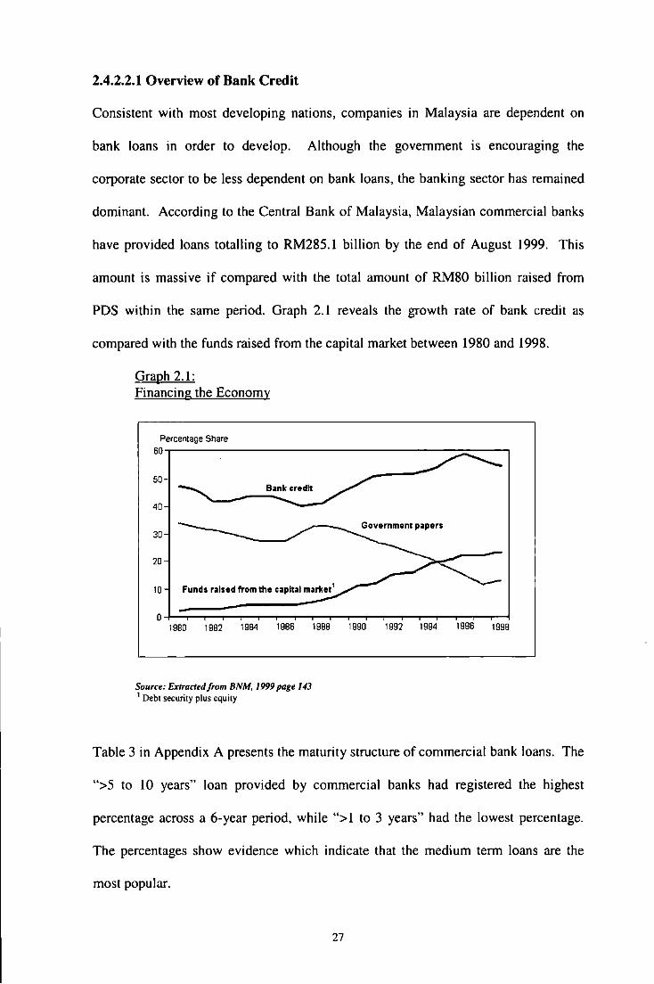
2.4.2.2.1 Overview of Bank Credit

Consistent with most developing nations, companies in Malaysia are dependent on

bank loans in order to develop. Although the government is encouraging the

corporate sector to be less dependent on bank loans, the banking sector has remained

dominant. According to the Central Bank of Malaysia, Malaysian commercial banks

have provided loans totalling to RM285.1 billion by the end of August 1999. This

amount is massive if compared with the total amount of RM80 billion raised from

PDS within the same period. Graph 2.1 reveals the growth rate of bank credit as

compared with the funds raised from the capital market between 1980 and 1998.

Graph 2.1: Financing the Economy

Percentage Share 60~--------------------------------------~----,

50

40

30

20

10

1980 1982 1984 1986 1988 1990 1992 1994 1996 1998

Source: Extracted from BNM, 1999 page 143 1 Debt security plus equity

Table 3 in Appendix A presents the maturity structure of commercial bank loans. The

">5 to 10 years" loan provided by commercial banks had registered the highest

percentage across a 6-year period, while ">l to 3 years" had the lowest percentage.

The percentages show evidence which indicate that the medium term loans are the

most popular.

27

However, the listed percentage represents the total loan amount given to the

companies as well as to the individual. The report on commercial bank loan direction

figures revealed that more than 50 per cent of the commercial bank loans are

channelled to the following sectors: manufacturing, properties and services.

Constructions and agricultural sectors are among the lowest. Following the economic

downturn in 1997, loans to the manufacturing and properties sectors have increased to

more than 80 per cent while loans to the construction sector have increased to more

than 60 per cent2.

On the other hand, figures from Datastream showed that second board companies rely

more on short-term debt rather than medium or long-term debt. Datastream classifies

short-term debt figures as borrowing repayable within 1 year (including bank

overdraft). Graph 2 in Appendix A illustrates the proportion of short-term debt to

long-term debt of companies listed on the main board and the second board. The

proportion of second board short-term debt to long-term debt is averaged at 75.36 per

cent between 1994 and 2000, while the average for the main board companies is only

39.54 per cent within the same period.

The above discussions indicate that the second board companies rely more on short-

term bank loans for financing while the main board companies tend to rely more on

medium term loans. The conclusion for the main board is based on the higher number

of companies listed at the main board and the high percentage of medium term loans

as shown in Table 3 in Appendix A. PDS may be the least preferred in terms of

gearing.

2 The figures calculated from the Table JV.7, Commercial banks :Direction of lending (BNM, 1999, p. 643)

28

2.5 Islamic Financial System

The Islamic Financial System was developed to enable Muslims to practice the

Islamic principles in accordance to the Qu'ran (Muslims' sacred book) and Traditions

(the prophet's deeds). A growing number of Muslim countries have expressed their

desire to abide to the Islamic laws (Shariah) and principles as guidance for their social

and economic welfare. Countries such as Iran, Pakistan and Sudan have converted

their entire financial systems in accordance to the Islamic principles (Middle East

Economic Digest, 1995). Nevertheless one should remember that Muslim countries

vary greatly in the degree to which they adopt the Islamic teachings. Different

religious bodies may have different opinions on the same topic because of their

adherence to different schools of jurisprudence. For instance, Malaysia appears to be

taking a liberal approach in addressing modem financial problems. The Malaysian

approach may not necessarily be accepted by other schools of jurisprudence, which

may rely more on a conservative approach.

The seriousness of adapting the Islamic laws and teachings have greatly influenced

the Malaysian society as Muslims make up over half of the total population. The

implications of Islamic principles to economic behaviour may affect the Malaysian

firms in their financing decisions as large percentage of Muslims are active believers.

One critical aspect of the teachings is the prohibition of the interest or usury.

Maintaining the principle of not charging interest is the primary task facing the

Islamic economists in a financial world where interest rates have assumed a supreme

role. However, Islamic economists have clearly explained that the prohibition of

usury is just one aspect of the economic philosophy on which Islamic banking is

29

based. Then again, interest is an important aspect for this research as capital structure

deals directly with interest.

What is interest? Economists have given different definitions of interest with each

trying to adapt their definition to their theory of justifying the payment of interest.

Samuelson (1958) states that "Interest is the price or rental of the use of money".

J.M. Keynes did not define interest, but mentioned the rate of interest as "Money rate

of interest is the percentage of excess of sum of units of money contracted for forward

deliver". The modem finance definition on interest is the excess of money paid by

the borrower to the lender over and above the principal for the use of the lender's

money over a certain period of time. While in Islam the "Traditions" (the prophet's

deeds) have made it clear that interest or usury is any increase in money or in kind

that the debtor is asked to pay over the amount originally borrowed (EI-Ashker,

1987).

Islam was not alone or even first in prohibiting the payment of interest, the lending of

money with interest have long been the subjects of religious contentions. Similar

prohibition is found in the pre-Qur'anic scriptures, at least, to the Babylon of

Hammurabi in 1775BC. The Torah instructed Jews that:

Thou shalt not lend upon interest to thy brother; interest of money, interest or victuals, interest of any thing that is lent upon interest. Unto a foreigner though mayest lend upon interest; but unto thy brother thou shalt not lend upon interest.

(Deuteronomy 23:20-21-cited in Lister (1988))

The Old Testament forbade the charging of interest between the Jews while the

mediaeval Church has strongly opposed the practice by Christians. The Christian

Church has long viewed interest-taking as a sin, and a council of bishops held in

30

France in 1312 hardened this into a threat of excommunication for those who

practiced it, or even rulers who allowed the practice of interest taking,

put usurers amid the fiery sands of the seventh circle of hell. (The Economist 1999)

A few relevant verses of The Holy Qur'an have explicitly forbade its believers from

interest taking,

and,

0 you who believe! Be afraid of Allah and give up what remains (due to you) from riba (usury) (from now onward) if you are (really) believers. And ifyou do not do it, then take a notice of war from Allah and his messenger hut if you repent, you shall have your capital sums. Deal not unjustly (asking more than your capital sums), and you shall not be dealt with unjustly (by receiving less than capital sum).

(Qur'an, 2:278-279)

0 you who believe! Eat not riba (usury) doubled and multiplied, but fear Allah that you may be successful

(Qur'an, 3:130)

Usury is committed when a lender charges more than the legal amount of interest

permitted. In practice, as the economy develops progressively through time and

technology, Muslims and Christians alike sidestepped these rules; the Jews happily

lent, at interest, to both, as their own selective prohibition allowed. Yet as late as

1571 an English law had been introduced to ban interest taking, with special penalties

for rates above 10%. The UK's usury laws were abolished in 1854, while South

Africa and parts of the United States still administer usury laws (Edwardes, 1999).

According to the Islamic teachings, financial institutions may perform most, if not all,

their functions provided that they avoid the payment and receipt of interest. This

practice already exists and is being constantly refined and modified to meet the

rapidly changing needs of ever more sophisticated businesses. The essential principle

31

of interest-free banking is profit/loss sharing. This means that both the supplier of the

capital and the borrower share the risks; both prosper when the returns are favourable

and both will suffer when the returns are low. This has resulted in what is known as

the "interest-free system".

Although interest is the main factor, the money is to be invested only in worthy

causes. This is largely equivalent to the western concept of socially responsible

investing. Further to that, there are a few other rules that are compulsory for Islamic

transaction activities such as: no profit is deemed "clean" in shariah law until zakat

(tax) is paid to the poor, orphan and the needl. The transactions have to be free

from all forbidden elements such as alcohol or gambling. Muslims are not allowed to

invest in a company dealing with any aspect of the forbidden elements.

Very few companies have practised the new interest-free system when it began in the

early eighties, as they are regarded as a strange kind of institution which functions in

unusual ways which can only be understood by certain groups of people. This

however is now beginning to change as the institution has penetrated the western

world. The evidence exists regarding two international giant banking corporations,

Citibank and Hongkong Shanghai Banking Corporation (HSBC) which penetrated the

Islamic banking world. Further to that, the Dow Jones Islamic Market Index has been

established in the US in 1999. The indexes track Shariah compliant stocks from

around the world, providing investors with comprehensive tools based on a truly

global investing perspective. Some of the companies that comply to the shariah law

3 Zakat law is very broad which provides guidelines on maturity of zakat due, amount to be paid and etc.

32

are Microsoft, Coca-Cola and BP Amoco4. In the same year, the Financial Times

Stock Exchange (FTSE) in London introduced its own Islamic indexes. Elnajjar

(2002) cited the statement of the General Council for Islamic Banks and Financial

Institutions (GCIDFD that

"The Islamic banking investment and .financial management market is growing at a rate of 15 percent per year, currently operates in 75 countries and accounts for around US$200 billion".

Four basic methods of finance are sanctioned by Islam: murabahah is a form of sale

whereby the seller expresses the cost of the sold commodity or goods that he/she has

incurred before selling it to another person by adding some profit or mark up. The

profit can be determined by mutual consent, by either a Jump sum or a pre-determined

ratio over the costs. All expenses incurred by the seller shall be in the cost price.

Therefore, murabahah is originally a form of sale, not a financing mode. However,

shariah scholars collectively allowed the use of murabahah as a mode of financing

(subject to certain conditions). The reason for the approval is based on the current

perspective of the economic set up, in which it is difficult to practice musyarakah and

mudarabah-the true mode of financing. Nowadays, murabahah is widely practised

by most of the Islamic financial institutions as a mode of short-term financing.

Second, is the mudarabah, a joint venture in which one party provides capital and

another provides expertise or labour. The profits from the venture are shared

according to an agreed ratio but losses are born entirely by the provider. According to

the Islamic literature, mudarabah was practised even before the Qur'an was revealed

and this was approved by the Prophet, as indicated by Islamic scholars (Mohamed,

4 http://www.getyourmoneyworking.com/2001/NOV/28

33

1985). An alternative is musarakah, a partnership in which all parties provide capital

and share in the profits or losses of the venture depending on the investment ratio.

These are regarded as the ethically strongest methods of finance and can be used to

invest in medium or long term projects as well as stock markets. The final option is

Ijara or leasing, which is basically the same as its conventional counterpart except

that. the price must be fixed in advance for a given period of time and must fluctuate in

accordance with changes in the interest rates. Besides establishing Islamic banking

institutions and penetrating the capital market with Islamic equity and debt securities,

Malaysia is also promoting the Islamic insurance called Takafu/.

As part of its initiative to assist in the development of Islamic debt, the government

also announced a few measures in the recent Budget 2003 (Budget Speech 2003):

• Income tax exemption on interest income for bonds and debentures • Tax deduction for lDS • Review of stamp duty on financing facilities under Islamic banking • Expenditure incurred on issuance of lDS is allowed tax deduction for 5 years

commencing from 2003.

The incentives are aimed at promoting a more resilient capital market, whilst

encouraging financing through private debt securities.

2.6 The 1997 Financial Crisis

Within the three decades of early economic development, Malaysia has witnessed at

least four economic downturns. The first is identified as "the first oil crisis", which

lasted between 1973 and 1975, for a period of two years. The second economic crisis,

identified as the "second oil crisis", began in 1979 and lasted until 1983. The third

economic crisis, identified as the "electronic or commodity crisis", lasted between

34

1985 and 1986. Finally, the fourth economic crisis, identified as the "financial or

currency crisis", lasted between 1997 and 1998.

All crises have bought the growth rate to zero or a negative percentage except for the

second oil crisis (see Table 2.1). The first and second crises were due to the oil crises.

According to Okposin and Cheng (2000), although the second oil crisis had

constrained the country, it was compensated by the profit of oil export and significant

developments in the manufacturing sectors. The massive growth of the

manufacturing sectors has not only contributed to the GDP growth, it also helps to

decrease the unemployment percentage. However, during the third crisis, the high

investments in the manufacturing sectors have caused problems to the economy. The

world growth rate has been constantly decreasing since the 1960s and 1970s. The

global decrease had affected many of the Malaysian international trading partners,

causing a low demand for electronic and commodity products.

East Asia's financial crisis began with a speculative attack on the Thai baht in May

1997, which later spread to the entire region. The ringgit came under attack as

speculators (currency traders) began placing bets on a depreciation of the ringgit in

July 1997 (see Section 2.4.1 for the amount speculated). Between June 1997 and

December 1998, the ringgit had lost close to 33.6 per cent of its value. The baht had

fallen by almost 29.4 per cent, the Philippines peso about 32.8 per cent and the

Indonesian rupiah by 70 per cent against the US dollar. The Malaysian ringgit was

pegged against the US dollar, and as a result of the peg, the domestic currency

becomes over or undervalued against other currencies as the peg currency fluctuates.

35

Overvalued currencies have encouraged imports by making them cheaper relative to

domestic prices.

2.6.1 The Impact of the Currency Crisis

The immediate impact of the currency depreciation was on the stock market. Fund

managers quickly withdraw funds from the market when speculators initiate their

attacks on the ringgit. On the other hand, local investors have taken immediate

actions of selling their securities while banks tightened their credit facilities, causing

the stock market to be illiquid and collapse.

Table 2.4: Stock Market Performance Immediately Following the Crisis

1997- 1997 Differences 2nd quarter 3rt! quarter

KLCI 1077.30 814.57 262.73 (24.76%)

EMAS Index 303.46 229.57 73.89 (24.35%)

Second Board Index 562.66 406.93 155.73 (27.68%)

Market Capitalisation (RM 744 585

159 billion) (21.37%)

Sources: BNM, Quarterly Bulletin **differences between 2nd and 3"' quarter and percentage decrease

As shown in Table 2.4, immediately following the crisis in July 1997, the KLCI, the

Emas index, the second board index and market capitalisation have declined to more

than 20 per cent from the 2"d quarter of 1997 to the 3'd quarter of 1997 (April-June

and July-September). The main index, (KLCI) further declined to 477.16 points on

12 January 1998, a decline of 41.4 per cent from the 3'd quarter of 1997. A year later,

the KLCI felt to its lowest point ever at 262.70 on 151 September 1998, a drop of 79

per cent compared with the 1997 highest performance of 1,271.57 points on 25th

February 1997. The market capitalisation declined by 53.4 per cent from RM806.8

36

billion in 1996 to RM375.8 billion in 1997 (see Table 2 in Appendix A). Based on

the market turnover in 1988, Malaysia's rank dropped to 29th in the world, second in

ASEAN and eight in Asia following the crisis (BNM, 1999).

Besides the sudden drop in the stock market, the total funds raised for new issues of

capital were also affected. Table 2.5 presents the funds raised by the private sectors

for the 2"d quarter and the 3'd quarter of 1997. Funds raised through shares issuance

dropped by 11.2 per cent while funds raised by debt securities suffered a huge drop of

48.1 per cent. Table 1 in Appendix A presents the annual figures of funds raised by

the private sectors. The total new issues of shares fell significantly from RM18,358.3

in 1997 to RM1,787.7 in 1998, a drop of 90.3 per cent. The debt securities fell by

62.8 per cent from RM16,588.4 in 1996 to RM6,175.4 in 1998.

Table 2.5: Funds Raised in the Capital Market Immediately Following the Crisis

Shares (RM mil)

Debt securities* (RMmil)

Total net fund raised (RM mil)

Sources: BNM, Quarterly Bulletm p-preliminary

1997p 2"d quarter

5,912

6183

12,094

1997p Differences** 3rd quarter

5246 666 (11.2%)

3209 2974 (48.1%)

8,454 3640 30.1%)

*Excludes debt securities issued by banking institutions and figures after minus redemption **differences between znd and 3rd quarter and percentage decrease

Due to the currency devaluation, Malaysia's foreign debt rose by 75 per cent from

RM97 billion at the end of 1996 to RM 171 billion at the end of the crisis year (see

Table 4 in Appendix A). As shown in the table, medium and long-term debt for the

private sector has increased by 88 per cent from 1996 to 1997. The short-term debt

for the private sector has increased by 36 per cent for the same period. However, the

37

private sector's short-term foreign debt was only at 6 per cent of the total external

debt compared with the medium and long term debt, which accounted for 62 per cent.

The financial institution is the main provider of funds in Malaysia. As previously

mentioned, commercial banks alone provide funds amounting to RM285.1 billion as

of June, 1999. However, the biggest problem faced by the financial institutions

following every crisis is the non-performing loans (NPL). As a result of the crisis, the

corporate sector has experienced significant loss of wealth as a result of sharp falls in

the value of their assets. Corporate incomes and cash flows also declined, causing

some corporations difficulties in servicing their debt. The situation has led to a

significant increase in the financial institutions' NPL's ratio. In November 1998, total

NPLs for commercial banks increased to RM22.7 billion (7.9 per cent of total loan)

from RM4.3 billion in 1996 (1.9 per cent of total loan). The NPLs for finance

companies rose from 4. 7 per cent of total loans by the end of 1996 to 12 per cent by

the end of 1998. On the other hand, NPLs for merchant banks increased by 13.8 per

cent in the second quarter of 1999.

The overall impact on the GDP is shown in the -7.5 per cent GDP in 1998-the lowest

in the Malaysia economic history. The real GDP began to slow down in 1997, at 7.5

per cent compared with the 1996 percentage GDP of 10. According to Okposin and

Cheng (2000), as a result of the crisis, Malaysia has lost its per capita income of

USD40 billion annually (in GDP terms) from the ringgit devaluation and US$100

billion were wiped out from the stock market. Overall, Malaysia has lost a total of

US$140 billion. Besides the reduction in GDP, the CPI rose at 6.2 per cent on an

38

annual basis in the half of 1998 compared with an average of 3.5 per cent in early

1997. Both food prices and producer price index (PPI) registered the largest increase.

2.6.2 The Management of the Currency Crisis

Following the speculative attacks on lO July, 1997, the initial response from the

authorities was to intervene in the foreign exchange market. This has resulted in the

tightening of market liquidity and a sharp rise in interest rates; the overnight (inter

bank) and 3-month rates rose to 40 per cent and 8.6 per cent from 7.5 and 7.9 per cent,

respectively. Although the increase in interest rates would support the ringgit from

further depreciation, it had an adverse effect on the real sector. To ease the liquidity

tightening and to reduce the interest rates, the Central Bank had injected money to the

banking institutions. Interest rates were reduced to their pre-crisis levels until

September 1997. Nonetheless, the action caused inflation to rise as the ringgit

depreciated further and credit grew significantly.

The interest rates had gradually risen to allow depositors to earn positive real returns.

Such a situation creates a dilemma and chaos to the authorities; if liquidity is

tightened, it will appreciate the ringgit but at the same time it will hurt the real

economic sectors as interest rates rise. While at the same time, International

Monetary Fund (IMF) advised the regional countries to mcrease interest rates.

Finally, Malaysia decided to take the strategic action of fixing the exchange rate at

RM3.80 to the US dollar on 2"d September 1998.

As a result of difficulties found by the financial institutions regarding the NPLs, the

government established the Danaharta, Corporate Debt Restructuring Committee

39

(CDCR) and Danamodal in June, July and August 1998, respectively. Danaharta was

established to purchase NPLs from the financial institutions and manage the NPLs in

order to maximise their recovery value. The CDCR function is to deal with debt of

the large corporations with the financial institutions so that the corporations will be

able to continue with their normal operations. The Danamodal is involved in the

recapitalisation of the financial institutions in which funds will be injected for smooth

running of their operations.

The other policies were to reduce current account deficits and maintaining export

competitiveness as well as monitoring the inflation. The government had also

reduced its expenditure and certain infrastructure projects had been delayed. The

budget allocations for health, education and basic amenities were maintained.

2. 7 Conclusion

Since independence in 1957, the Malaysia economy has developed and diversified~

from rubber and tin into a more broad-based and export-oriented economy focusing

on the production of a wide range of exports, namely rubber, tin, palm oil, timber,

cocoa, crude oil and increasingly manufacturing and services. The development was

initiated through the implementation of a number of medium and long-term

development plans.

As a result of the rapid development, by the early 1980s, growth was accompanied by

an increase in budget deficits and public debt. Measures were taken to reduce the

budget deficit, including open trade to expand the export base. This action has

resulted in a dramatic shift in the structure of the economy from agriculture and

40

mining to a growing reliance on manufacturing of electronics and other export-

oriented industries. Investments were also targeted at non-tradable sectors, including I

capital-intensive infrastructure and the real estate sector. Liberalisation measures were

introduced across the board and this helped improve competitiveness and

productivity.

Despite the high growth and strong economic performance, the Malaysian economy

shares the characteristics of the developing countries: it is heavily dependent on

exports and open to foreign trade. Although in the early 1990s, the government

investment strategy was successful in raising output and income, however, there were

also signs of stress as exports decelerated and a large current account deficit

developed. As shown in Table A. 21 in Appendix Al 5, the Malaysian current account

balance showed negative figures from 1990 to 1997. This eventually led to major

balance sheet weaknesses in the banking and corporate sectors, exposing the economy

to the regional crisis. The Malaysian economic vulnerabilities intensified significantly

following the crisis in mid-1997.

It started when currency traders began to speculate on the Malaysian ringgit, the

market confidence increasingly diminished, large portfolio outflows took place, and

equity and property values declined substantially. By 1998, the stock market had

fallen to its lowest level in recent history together with the rest of the region. The

contagion effects of the crisis and the associated economic contraction were far worse

than anticipated. Anticipation of further devaluation of the ringgit intensified.

Domestic imbalances shown as growth rates slowed and then turned negative in 1998.

5 Tables A.21 and A6 in Appendix AI are obtained from CD-ROM of 1996 and 2000 Annual report of the Malaysian Central Bank.

41

Nevertheless, with the policy and structural changes undertaken, Malaysia's external

vulnerability was relatively well controlled: the current account showed a large

surplus in 1998 and 1999 (see Table A.6 in Appendix A1) 5; short-term external debt

was low; and reserves have remained adequate. Progress in the restructuring of the

financial sector has also improved the capacity of banks to manage risks. Although

the government continually stresses the need to minimise the dependency on bank

loans, the banking sector has remained dominant. Given the fact that alternative

financing sources have been limited and unstable due to the crisis, this suggests that

commercial banks will continue to be the dominant financiers in the foreseeable

future. Recently, many tax incentives were legislated on the Islamic debt securities to

attract investors seeking for Islamic financing products (see Section 2.5). The lessons

learned have shown the need for Malaysia to better protect itself from future crisis.

The country is also consistently seeking for prudent macroeconomic policies to

maintain financial stability and sustainable fiscal and external positions.

42

3.1 Introduction

CHAPTER3 LITERATURE REVIEW

Chapter 3 presents the literature review on the capital structure theories and empirical

studies. The chapter begins by examining the capital structure background, followed

by the traditional and new approach to the capital structure. The theory is followed by

the empirical research on capital structure, it integrates the theory and the results from

the field research. Besides reviewing the literature on capital structure, the chapter

also analyses the literature on the financial crisis and the Islamic financing. The

chapter includes: Section 3.2 capital structure instigation, Section 3.3 capital structure

and taxation, Section 3.4 factors determining the capital structure, Section 3.5 Islamic

financing, Section 3.6 the 1997 financial crises, and Section 3.7 concludes the

chapter.

43

3.2 The Beginning of the Capital Structure Debate

A classic study on capital structure began in 1914 when Professor Arthur Stone

Dewing observed the major consolidation movement in the United States. The

merger movement was associated with the emergence of national markets after the

completion of the cross-continental railroad networks in the late 1880s. During that

time, deflation plagued the US which resulted in expansionary policy and economic

reforms through the constitutional power of Congress. The economic reforms

resulted in 305 industrials being merged in the early 1900s. However, financing these

large industrial aggregates had brought management to the capital structure problems.

This is because the consolidation itself is too large in relation to the size of the

economy. Reorganisation and consolidation development of the companies had

greatly impressed Dewing. He started his research by studying the success and the

failure of the companies prior to merging and found that the failure was due to the

management flaw in managing their financial assets and liabilities. He commented:

They failed because their earnings were inadequate for the load put upon them. If the load was especially burdensome by reason of heavy fzxed charges and unwarranted dividend payments, the failure was all the more certain. The direct cause of failures in every instance was the deflection of working capital to the payments of interest and dividends.

(Dewing (1930) cited in Weston (1966) p.24)

Therefore, the failure of the companies during that period was due to the insufficient

earning and current assets to cover both fixed charges of interest. Then, he reviewed

the financial structure of the companies and found that the choice of capital structure

was seen to be of great significance. Dewing noted that companies with smaller debt

burdens were in a stronger financial position than those with higher debt burdens. He

wrote:

44

It is largely because of these clearly recognised fluctuations of trade, that a sound financial policy dictates the use of stocks rather than bonds. And it should be remarked at this point that strength of our so-called "industrial trusts" lies partly in the fact that the majority of them were promoted without bonds. But when foolish promoters had once over-loaded a corporation with liabilities bearing fixed charges, it became the duty of the subsequent management to get along as best it could. A default in bond interest payments was very disastrous to the credit of a corporation, as well as to the market price of its securities. It was disastrous to its trade as well.

(Dewing (1930) cited in Weston (1966) p.24)

He also acknowledged the financial distress of interest default to the company, as well

as the effect on the share prices and business operation.

The study of capital structure and major financing movements by Dewing at the turn

of the century marked the beginning of the era of systematic studies in the finance

field. The problems of financial structure had prolonged to the next few decades as

the economy deteriorated in the 1920s. According to Weston (1966), between 1920-

21, and 1929-33, corporate management reacted irrationally towards debt in which

firms only employed long-term debt when absolutely necessary and sought to retire

debt as soon as possible. The aversion towards debt is due to the fear of a financial

crisis which may lead firms to financial embarrassment. The central concern of

financial management in the environment of the sharp economic crisis during that

century was to protect the firms against bankruptcy and reorganisation.

3.2.1 The Traditional Approach to the Capital Structure

According to Weston (1966), Dewing's subsequent work on capital structure have set

the pattern for what is now referred as the traditional view of the capital structure in

many of the corporate finance text books. The capital structure traditional view

advocates that with the presence of gearing, the firm's value will increase to a certain

45

level before decreasing due to the expected risk as the debt level continues to

increase. The firm's value is maximised at the point at which the cost of capital is

minimised. Figure 3.1 illustrates the traditional view of gearing, and the expected rate

of return for both the debtholders and shareholders. The line kd represents the cost of

debt, the line W ACC is the weighted average cost of capital, and the line k, is the cost

of equity.

Figure 3.1: Rate of Return Under The Traditional View of The Capital Structure

Rate of return %

~Optimal

Ke (return on equity)

W ACC (weighted average cost of capital)

Kd (return on debt)

Debt-equity ratio %

According to this view, firm moves from a zero debt position to small amounts of

debt. At this point gearing increases the shareholders' risk but does not significantly

increase the risk borne by debtholders. Similarly, k, will not rise significantly until

large amounts of debt are used. This is based on the argument that since debt is

cheaper, combining equity with reasonable amounts of debt will result in a reduction

in the firm's overall cost of capital or WACC. Therefore, the value of the firm is

maximised at the lowest level of WACC.

46

Figure 3.2: Firm's Value Under The Traditional View of The Capital Structure

Finn's value

Optimum debt/equity ratio

Debt-equity ratio %

However, when too much debt is added to the firm's capital structure, the kd will start

to rise significantly, as shown in Figure 3.1. This is because firstly, debtholders

demand a higher rate of return due to their concern over the firm's ability to generate

enough income to avoid default on the interest payments. Secondly, at high debt

levels, the cost of equity also rises quickly because high amounts of debt are

accompanied by high amounts of fixed interest payments, which may reduce the

equityholders' residual claims. This will cause the equityholders to increase their

expected return, k,, to offset the risk of gearing. The overall cost of capital of the firm

begins to rise at high levels of debt, thus decreasing the firm's value as depicted in

Figure 3.2.

3.2.2 The New Approach to Capital Structure

As finance researchers and academicians uphold to the traditional view of capital

structure, two new propositions have been forwarded in the 1950s; Durand (1952) and

Modigliani and Miller (1958). Durand presented two models, the Net Income

Approach and the Net Operating Income Approach, while Modigliani and Miller

47

(hereafter MM) proposed the capital structure irrelevancy theory. The most famous

and controversial are those of MM due to the assumption accompanying the models.

Many critics were focused on the perfect market assumption which reflects the

situation of the market with no taxes and no transaction costs.

3.2.2.1 The Net Income and The Net Operating Income Approach

Durand (1952) proposed the Net Operating Income (NOI) and the Net Income (NI)

approach of capital structure. The basis of the NOI approach is that the total value of

all debts and shares must be the same, regardless of their proportions, therefore, the

firm's value remains constant. The reason is the total value of the firm is calculated

by capitalising the net operating income (before interest) at certain rates which gives

an amount equivalent to the total amount of debt plus equity value. Durand

contrasted the NOI approach with the NI approach, which assumes that the firm's

value does not remain constant, but increases with the proportion of debt in the capital

structure. This is because the total value of the firm is based on the net income after

deducting the amount of interest in which the amount of net income will vary

according to the interest paid.

Under the NOI approach, the required rate of return, k,, increases in direct proportion

to the debt to equity ratio, whilst the weighted average cost of capital remains

constant even as the debt to equity ratio increases. The argument is that the

shareholder is asking for higher returns as the firm's financial risk mcreases.

However, the value of the firm will be the same under the NOI approach.

48

The NI approach argues that the higher the debt levels, the lower is the cost of capital.

If the cost of capital is low, the overall value of the firm will increase. This is based

on the assumption that required rate of return, k,, would remain constant. Under this

argument, the cost of capital will further decrease due to fixed cheaper cost of debt

paid and at the same time the cost of equity remains the same. Therefore, if the

operating income increases, net income will increase because the same amount of

interest will be deducted. As the net income increase is capitalised at a certain rate

(equivalent rate as k, which is assumed to be constant), it will increase the total value

of the firm.

Durand provided a formal model on the capital structure issues by showing the impact

of debt-equity preferences on the overall cost of capital, WACC. However, he

provided no evidence for either the NI or NOI methods of determining the cost of

capital. Furthermore, there were a number of ambiguities under both approaches,

such as the cost of equity remaining constant under the NI approach. In reality, it will·

be difficult for the cost of equity to remain constant as it is subjected to other factors

such as dividend policy, risk and etc.

3.2.2.2 Modigliani and Miller 1958 Model

Modigliani and Miller (MM) extended the work of Durand by providing a different

capital structure model. The paper was famously known as the "MM irrelevance

propositions". They proposed two propositions to explain their capital structure

model. Propositions I and II state;

49

Equation 3.1

X V1 ::: S 1 + D 1 = p: , for any firm j in class k (proposition I)

Equation 3.2

I 1 = pk + (pk - r) D 1 , for any firm j in class k (proposition 11) sj

Where,

V1

=Total market value of the firm

S 1

=The market value of the firm's equity

D1 =The market value of the firm's debt

X 1 =Expected average earning before interest

pk =The expected return from an identical ungeared firm (WACC)

I 1 =The expected rate of return on the stock ( Ke)

r =the risk free rate of interest (Kd)

MM explained their proposition 1:

"That is, the market value of any firm is independent of its capital structure and is given by capitalizing its expected return at the rate pk appropriate to its class."

(MM (1958), p.375)

In other words, capital structure is irrelevant, and firm's value is equal to the present

value of the free cash flow discounted at the relevant cost of capital. Accordingly,

what is important to the firm's value is the risk of its operating cash flows, the

financing decision on the cash flow is irrelevant. However, if the proposition does not

hold, arbitrage will take place and will therefore restore the stated equalities. They

demonstrated that an arbitrage opportunity exists if the market value of the geared

50

firm differs from that of an identical ungeared firm. As arbitragers exploit this

opportunity, the value of the overpriced shares will fall whereas the underpriced

shares will rise, therefore, the price would converge in equilibrium.

Figure 3.3: Cost of Capital Under MM 1958 Model

Rate of return %


WACC (cost of capital)

Kd (return on debt)

Debt to Equity ratio (%)

MM proposition II asserts that the expected return, ke, on a geared firm is a linear

function of gearing, in other words the cost of equity, (ke), increases with financial

structure and the slope being the difference between the company's WACC and kd

(pFr). By retaining capital structure as irrelevant under proposition I, proposition II

specifies what the expected return on the geared firm must be for total firm market

value to be unchanged, and for the overall cost of capital to remain constant, as debt is

added to the firm's capital structure. Figure 3.3 illustrates the Cost of Capital under

this MM proposition.

3.2.2.3 Empirical Evidence on MM Model

MM (1958) improved their propositions by providing empirical evidence based on

data studied by Alien (1954) and Smith (1955) on 43 electric and 42 oil companies,

respectively. The former used a 2-year average figure between 1947 and 1948, while

51

the latter used a one-year period of company data, 1953. Both studies were originally

designed to find the relationship between the securities return and the capital structure

of the firms. According to their proposition I, the W ACC should have the same value

regardless of the gearing, therefore, if the traditional view was upheld, the correlation

coefficient of W ACC and gearing should be negative, however, if the views proposed

by MM was right, then correlation should not be significantly different from zero.

The MM empirical evidence clearly supports their proposition which suggest

insignificant correlation between W ACC and gearing. Their empirical test on

proposition II was also proven to be correct as they found significant positive

correlation between Ke (return on equity) and gearing (debt over equity). Both results

had strengthened the irrelevance proposition that there is no correlation between the

overall cost of capital and gearing, and the cost of equity increases as debt to equity

ratio increases. The result of the study, nonetheless, is not consistent with the

traditional view of the capital structure.

3.2.2.4 Criticism of MM Propositions

Since 1958, the MM model was constructively criticised by several prominent

researchers, both theoretically and empirically. The most obvious flaw of the model

is probably its unrealistic assumptions. To arrive at their irrelevance decision, there

were a number of accompanying assumptions, either explicit or implicit, such as: the

existence of efficient capital markets; all physical assets are owned by corporations;

no corporate or personal income taxes; risk free interest rates for both lenders and

borrowers; no bankruptcy and transaction costs; and all corporations can be classified

into one of several "equivalent return classes", such that the returns on shares are

perfectly correlated with all other firms within that class.

52

Durand (1959) indicated some of the difficulties of using MM's assumptions in the

real world to support their propositions. According to him, MM restricted the

freedom of the firm to arbitrage whenever the market deviates from equilibrium but

instead allowed the investors to arbitrage without restraint. Also, MM had

underestimated the difficulty of setting up an equivalent return class. Practically, it is

impossible to postulate the existence of two or more different and independent firms

with uncertain income streams and yet be perfectly correlated indefinitely. The

concepts of an equivalent return class, derived from the ideas of static equilibrium, is

not adaptable to a highly advanced market in which stock prices fluctuate

unpredictably.

The point is further emphasised by Weston (1963) who stated that empirically that it

would be very difficult to gather a sample of corporations capable of supporting the

MM's equivalent class requirement and at the same time he questions some other

unrealistic assumptions, such as finding samples that are reasonably homogeneous in

most respects. However, Weston states that Durand's NOI approach and MM's

proposition I are logically equivalent. Both state that the value of a corporation is

determined by capitalising the firm's net operating income at the appropriate rate,

giving the total market value to which the firm's capital structure must conform.

He criticises MM's empirical studies which have failed to investigate the nature of the

relationship between gearing and other variables influencing a firm's cost of capital.

Weston then conducted an empirical test on MM's model by adding growth in

earnings per share as an additional factor, as he found this factor to be highly

correlated with the cost of capital and the cost of equity. Nevertheless, when the

53

influence of growth is isolated, leverage is found to be negatively correlated with the

cost of capital. The result explains that MM have found no correlation between the

cost of capital and the leverage, because that leverage is correlated with other

influences which change the gross relationship between cost of capital and leverage.

Taking the influence of growth on both cost of capital and the cost of equity,

Weston's evidence is consistent with the traditional approach as these variables are

highly correlated.

3.3 Capital Structure and Taxes

In 1963, Modigliani and Miller wrote "a correction" paper; whilst maintaining the

environment they introduced in 1958, but allowing for a tax benefit on debt. They did

consider tax in their 1958 proposition but their analysis was flawed. The tax shield is

simply the effective corporate tax rate multiplied by the market value of debt issued as

shown,

Equation 3.3

Value of Geared Firm= Value of Ungeared Firm+ TcD

where Tc is the corporate tax rate and D is the amount borrowed. By integrating tax

into their proposition, they discovered that gains accrue from interest deductibility and

raised questions over their previous irrelevant model. Given that interest is tax

deductible, the higher the debt, the higher is the tax shield and therefore the higher is

the firm's value. Although the equity holders demand higher returns to compensate

them for the higher risk as debt increases, the much cheaper interest after-tax

outweighed this, and thus the overall cost of capital decreases as debt is added to the

firm's capital structure as illustrated in Figure 3.4.

54

Figure 3.4: Cost of Capital under MM Model with Taxes

Rate of Return %


W ACC (cost of capital)

Kd (return on debt)

Debt-to-equity ratio

MM state that the tax shield is a valuable asset for the company. They elaborate:

since the firm's debt is fixed and permanent, the company will receive a permanent

cash flow from the tax shield. Additional borrowing decreases corporate income tax

payments and increases the cash flows available to both debtholders and stockholders,

thus increasing the firm's market value. However, the tax shield depends only on the

corporate tax rate and the ability of the firms to generate sufficient earnings to cover

interest payments. Nonetheless, in their concluding section, MM state that although

the cost of debt is cheaper, persistently seeking a maximum amount of debt in capital

structure is unnecessary, under some circumstances, and retained earnings could be

cheaper.

3.3.1 Miller's Equilibrium Model

Later in 1977, Merton Miller proposed another theory regarding the tax advantage of

debt by incorporating investors' tax rates and company tax rates into his equilibrium

model. The equation is the extension of MM 1963 model, which gave Vg = V, + T,. D

55

as discussed in Section 3.3 above. Miller arrives at the new model by adding tax

levied on investors' equity and debt income. The equation expresses the value of the

geared firm as being equal to the value of the ungeared firm plus the amount of debt

multiplied by the value of the tax shield or tax advantage to debt. The tax advantage

to debt is defined by the bracketed expression.

Equation 3.4

where,

VR = value of geared firm

v. = value of ungeared firm

D =debt of geared firm

Tr = corporation tax rate

TP, =the personal tax rate on equity income

T ptf = the personal tax rate on interest income

In the original MM (1963) analysis with only the corporate tax, the TP, = T ptf = 0, so,

if the tax on equity income is equal to the tax on debt income, the tax advantage will

only be TrD. Thus, the higher the D or more debt added into the firm's capital

structure, the higher is the value of the geared firm relative to the ungeared firm.

Intuitively, if all tax rates are disregarded, there will be no tax advantage to debt either

at corporate level or personal level. But, if TP, > Tpd, the tax advantage to debt is

higher, however, if Tp.• <T ptf, the net advantage to debt is reduced. The model's

predictions are plausible only if the effective tax rate on equity income is considerably

56

lower than the interest income, lower enough to offset the corporate interest tax

shield.

Consequently, Miller's approach suggests that debt has both tax advantages and tax

disadvantages. The tax advantages of debt are derived from the tax deductibility of

interest at the corporate level, while the tax disadvantages of debt come from the fact

that the personal taxes rates on interest income are typically higher than those rates

levied on income on capital gains derived from equity, TP_, <Tpd. Hence, the tax

advantage to debt could reduce or there will be no tax advantage to debt. The reason

for higher tax on personal interest income received from debt than the personal

income from equity (dividend plus capital gains) is mainly related to various capital

gains exemptions. With that argument, the tax advantage to debt is lower than

expected.

Although Miller have suggested that TP-' and Tpd can vary across investors, he then

simplifies his model under the general equilibrium proposition by assuming that TP_, =

0, bonds are riskless and no transaction or issue costs are involved. With the presence

of tax exempt bonds that require r0 for their return, he determined the supply and

demand of the corporate debt.

The initial suggestion is that bonds can be issued at r0 to tax exempt investors.

However, the interest rate must be higher than the r0 to attract taxable investors to

purchase bonds. The higher rate is to compensate for the taxes on interest income

levied on them, hence their demand rate of interest will be r0 /( 1-Tpd).

57

Figure 3.5 Miller Equilibrium in the Market for Bonds

Rate of Interest

B*

Quantity of bonds outstanding

As shown in Figure 3.5 the rd (B) represents the investor demand for bonds at the

low rate, r0 represents the demand of fully tax-exempt investors, as illustrated by the

flat section of the demand curve. A further increase in the curve illustrates high

demand for higher tax bracket investors in order to acquire the same return as the tax-

exempt investor. Nevertheless, companies are only willing to issue bonds

atr0 /(1-T,.), thus the equilibrium will reach B*, the point where the marginal

personal tax rate on bonds is equal to the corporate tax rate. Miller argues that given

both the marginal personal tax disadvantage of debt and firms' adjustments on the

supply side, r, (B) will override the corporate tax advantage of debt causing market

prices to move to an equilibrium. The argument supports his (and Modiagliani's)

previous irrelevancy theory, V8

= v •. Miller's model was intended to illustrate how

corporate and personal taxes could cancel out and leave firm value independent of

capital structure.

58

3.3.2 Tax Exhaustion Effect on Capital Structure

Following the Miller tax equilibrium in 1977, DeAngelo and Masulis (1980)

highlighted the issues of tax exhaustion. By using existing evidence such as the MM

1963 empirical evidence, their models produced a number of testable hypotheses.

According to them, positive non-debt tax shields substitute for debt shields and are

capable of reversing Miller's equilibrium model. Positive tax shields imply that the

expected marginal corporate tax benefits decline as debt is added to the capital

structure.

He argued that borrowing is not the only way to shield income against tax and that

firm's investment in tangible and intangible assets can be substituted for debt to

benefit from tax advantage of depreciation deductions. Not only depreciation,

investment tax credits will also reduce the tax advantage to debt. The more the firms

shield income in these ways, the lower is the expected tax shield from borrowing.

Therefore, firms will become tax exhausted if too much debt is added to the capital

structure. However, he stated that corporate tax shields are worth more to some firms

than others, and suggests that firms with many non-interest tax shields and uncertain

future prospect should borrow less than consistently profitable firms with lots of

taxable profits to shield. Firms with large accumulated tax-loss carry-forwards should

not use debt. It is worthless for firms to issue debt if the firms are unable to gain

benefit from interest tax shield.

De Angelo and Masulis ( 1980) extended their research on tax reform effect to the

firms' capital structure. According to them, US's federal income tax code on the

corporate tax rate and corporate investment tax deductions and credits have been

59

increasing significantly over the years. They reviewed the 1975 data from the US

internal revenue services (IRS) which indicate investment tax shields in the amount of

USD49.5 billion are almost the same with the interest tax shield of USD64.3 billion.

Therefore, non-debt tax shield items are as significant as the tax shield from a capital

structure perspective.

The following are empirical evidences supporting the relationship between gearing

and tax shield, gearing and non-debt tax shield.

Based on DeAngelo's and Masulis's proposition, Titman and Wessels (1988)

empirically studied the effect of non-debt tax shield on the geanng of US

manufacturing firms. The three indicators of non debt tax shield are: the ratios of

investment tax credits over total assets, depreciation over total assets, and a direct

estimate of non-debt tax shields over assets. However, no evidence was found at all

in the measurements, since all statistical results were not significant.

Rajan and Zingales (1995) included taxation reform in their study on the capital

structure of the 07 countries. They stressed the importance of cooperating the "right"

personal tax rates in computing the company tax advantage to debt. The tax

advantage to debt is studied with respect to firms' retained earning and dividend

advantage. The result showed, following the reform, that the US had the highest tax

advantage, its share of the pre-tax dollar increased from $0.26 in 1982 -1984 to $0.40

in 1989-1991. In contrast, the retained earnings attracted the least tax advantage

following the reform. Retained earnings' share declined from USD0.35 to USD0.21,

between 1982-1984 and 1989-1991, respectively. The results also indicate an

60

increase in tax advantage for Canada and the UK but not for Japan, Germany, France,

and Italy.

Booth et al. (2001) included taxation in their study on the capital structure of

developing countries. Generally, the results indicate a weak negative significant

relationship between gearing and tax across the countries except for Pakistan which

had a result indicating a highly significant negative coefficient. The results for

Malaysia are mostly insignificant except when gearing is measured by total-debt-to

total-debt-plus-equity (all book values) for the period of 1985-1987.

3.3.3 Tax System

The corporate finance literature has shown that the determination of corporate capital

structure is also dependent on corporate taxes, due to the tax-deductibility of interest

payments. However, different tax systems in different countries may have a different

effect of the tax shield on debt. Therefore, the research is more effective by looking

at the various tax systems in operation. Many hybrid tax systems are used in different

countries to meet the regional requirement. This is based on domestic environmental

factors, such as economic priorities, fiscal policy, administrative considerations,

international influence and historical development. The majority of the countries

worldwide operate their classical tax system with some modification, while others

operate various forms of an imputation tax system.

The pure classical tax system imposed a flat tax rate to pre-distributed profits. This

system allows the distribution of dividend to be taxed twice, once at the corporate

level and then again at the personal level. The result is referred to as economic

61

double taxation. The modification of a classical tax system by most of the countries is

to reduce the burden of double taxation either by imposing a different tax bracket on

distributed income (dividend) or by giving a full or partial relief to shareholders.

According to Pointon and Spratley (1988), under the full imputation system, the full

corporate tax liability is treated as an imputed tax credit to determine total personal

taxable income; where the tax credit is attached to the dividends in the personal tax

computation. The effective tax rate on the underlying profits (dividend and retention)

represents the personal tax rate on investment income. Thus, the double taxation is

eliminated and distributed profits (dividend) are subjected to taxation only once under

the imputation system. They explained that a partial imputation system operates

when the partial corporate tax liability is treated as an imputed tax credit to determine

total personal taxable income, which means credit is given under the personal tax

computation for part of the underlying corporation tax on profits paid out as

dividends. Thus, under this system, there is still some remaining corporation tax that

is imputed to shareholders.

Theories tend to favour an imputation system because, amongst others, it avoids

economic double taxation. However, the major drawback to the imputation system is

its complexity with regards to legislation, subsequent administrative burden and

compliance costs, this is costly to society. For every dollar of tax collected, these

costs can be quite significant, the result is not expended directly for consumption or

wealth generating activities. It may appear that imposing tax when a shareholder

receives a dividend is a rather simple approach and this would reduce compliance

62

costs. However, it is not the intention of this research to analyse the details of pros

and cons of these two systems.

Previous studies on tax influences on capital structure are based on the classical tax

system as most of the literature on this subject is derived from the United States,

which operates under a pure classical tax system. However, analyses by Franks and

Broyles (1979), Pointon (1981), Rutterford (1988), and Ashton (1989) have extended

the MM tax advantage models for different tax systems. Most of these researchers

conducted their study based on the UK's partial imputation system. Again, the

system aims to alleviate the double taxation of corporate profits arising under the

classical system by offering a tax credit to shareholders on receipt of a dividend for

part of the tax paid by the company.

Franks and Broyles (1979) argued that a company is considered to act as an agent for

the Inland Revenue authorities in collecting shareholder's tax; and hence the

corporate tax rate in effect "includes" the shareholder's tax at the standard rate. They

argued that the tax advantage to debt then becomes the difference between the

corporate rate and the shareholder standard rate. They concluded that, due to the

imputation system, the tax advantage is very much less in the UK.

Rutterford (1988) examined the impact of taxes on the UK, France, Germany and

Japan by extending the major tax models of optimal capital structure on all of the

following tax systems: classical, imputation and hybrid system. With the exception of

the US, the other four countries have altered their tax systems since World War 11 to

avoid double taxation under the pure classical tax system. According to her, tax

63

advantage to debt depends on both the type of tax system and tax rates imposed on the

corporation and investors. Rutterford then compared the tax advantage to debt in each

country by using a different tax system. Her findings indicate that the tax advantage

of debt is highest for the US corporations and is lowest for German and Japanese

firms, while UK and France were ranked in the middle. Surprisingly, the gearing

ratios in the UK, France, Japan and German gradually increase over time although

these countries moved further towards an imputation system.

3.3.4 Malaysian Tax System

The fiscal laws in Malaysia are based on the British system and have been developed

progressively since independence. Corporation tax has been reduced gradually over

the years from a high rate of 40 percent in 1984 to 32 per cent between 1995 and

1997, and to a low rate of 28 per cent as of 1998 to 2001 (Singh and Teoh, 2001).

Similarly, the tax rates for individuals were reduced substantially between the range

of 0 to 29 per cent in the year 2000 compared with 5 to 40 per cent in 1985. Malaysia

operates under a full imputation system where shareholders receive credit for the

income tax levied on companies, and thus ensuring that corporate profits are no longer

taxed twice as in the classical tax system. However, capital gains and interest earned

by individuals are exempted from tax, therefore, there is no personal tax rate on

investor returns.

MM's (1963) and Miller's (1977) tax proposition are remodelled using the Malaysian

full imputation system (adapted from the Pointon and Spratley ( 1988) imputation

model). The tax advantage to debt under the MM 1963 classical tax system is:

64

Referring to Equation 3.3

where:

vg = value of geared firm

V" = value of ungeared firm

D = debt of geared firm

Tc =corporation tax rate

The Miller 1977 model is represented by:

Referring to equation 3.4

where:

Tps = the personal tax rate on equity income

Tpd =the personal tax rate on interest income

Pointon and Spratley (1988) explain that (1- TP,) = ~- "'?, under the imputation 1-s

system, where,

m =the marginal rate of income tax on gross dividend income

s =the rate of imputed tax credit on gross dividends

TP, = the personal tax rate on equity income

Therefore, the tax advantage to debt for the companies tn Malaysia under the

imputation system if all profits are paid out as dividends is,

Equation 3.5

65

T pd is taken off the equation since interest income for an individual is exempted under

the Malaysian tax system (see Section 2.4.2.2 and Singh 2001). However, since there

is a full imputation, s = Tr , therefore,

Vg =Vu+D[1-{1-m)] and so, Vg =Vu+mD

This equation is applicable for firms with no capital gains induced retentions.

The scenario under the imputation tax system in Malaysia reveals that if the company

retains all the profits and the shareholders sell the shares before a dividend is paid,

this will be similar to MM's 1963 model since capital gains is exempted from tax.

Under Miller's argument,

Equation 3.6

where:

TrR = ea pi tal gains tax

Since capital gains tax (Singh, 2001 and Emst & Young, 1998) and tax on personal

interest income are exempted in Malaysia, the equation will be as follows:

VR =V" + TcD. In this instance, the valuation relationship holds for a firm with full

retentions, i.e. for a growth firm paying no dividends. Since both m and Tc are likely

to be positive under each model, Vg >Vu. Hence debt is preferred to equity and

equity retentions would normally be preferred to new issues (i.e. for tax payers).

66

3.4 Factors Determining the Capital Structure

As studies on taxes and capital allowances progress, many other factors were found as

determinants of the capital structure. The factors that influence the determination of a

firm's capital structure have been examined extensively both in theoretical and

empirical research, in particular, the corporate or firm specific factors that influence

the capital structure ratio such as earnings and assets. Perhaps the finance managers'

decision on capital structure is weighed more on these factors than the taxes and non

debt tax shield items. This chapter will be divided into two sections: i) firm specific

factors which discusses the effects of corporate specific factors on capital structure

which includes variables such as asset structure, size and growth, earnings volatility,

risk and agency costs, and ii) non firm specific factors which discusses the external

factors that may affect capital structure such as inflation, interest rates, industry norms

and government incentives.

3.4.1 Firms Specific Factors

The finance managers' decisions on capital choices are usually based on the

assessment of the firms' strengths and weaknesses. Factors such as fixed assets and

interest coverage ratios are very important in determining how much debt to acquire.

The factors include firms' liquidity, profitability, investment opportunity or firms'

growth, tangibility, size, bankruptcy risk, interest coverage, agency costs, ownership,

leasing and operational gearing.

3.4.1.1 Asset Structure- Liquidity

There are many indirect evidences indicating that the types of asset the firms hold

would determine the level of debt. There are two types of assets; current assets and

67

fixed assets. The current assets are related to the liquidity while the fixed assets are

related to tangibility. The higher the current assets, the higher is the firms' liquidity,

while the higher the firm's fixed assets, the higher is the firm's tangibility (in terms of

real assets). The next section will cover the relationship between gearing and fixed

assets. The perception on the liquidity is that the higher the current assets, the better

is the firms' position to service debt, therefore, implying a positive relationship

between liquidity and debt.

The earliest study to include the liquidity in their empirical study is by Martin and

Scott (1974). Their liquidity argument is based on Van Home's (1974) statements

that the greater the firm's projected liquidity posture, including its cash flow

generating capacity, the greater is its debt capacity. They supported the statement by

arguing that firms with high liquidity tend to issue debt rather than equity. In their

multiple discriminant analysis of 112 US firms that issued either debt or equity in

1971, they found that high liquidity firms mostly issue equity rather than debt. The

results support the notion that highly liquid firms prefer equity than debt but did not

specify any causal relationship between liquidity and equity or debt.

Stonehill et al. (1975) surveyed the debt ratio determinants of 87 manufacturing firms

in France, Japan, the Netherlands, Norway and the US over the period of 22 years

(1972-73). They found that liquidity in Norway was ranked second after the financial

risk as debt ratio determinants. They explained that the assets of the firms should be

highly liquid to secure the high proportion of the firms' short-term debt. Thus, the

evidence confirms a positive relationship between liquidity and the gearing ratio as

perceived by the Norwegian finance managers. However, liquidity is not important

68

for the other 4 countries: France, Japan, the Netherlands and the US. Although the

findings support the positive relationship between gearing and liquidity, their

statistical tests are not strong enough to support the existence of such a relationship.

Ozkan (200 1) suggests that liquidity could be related positively and negatively with

gearing. According to him, a positive relationship would derive if the firms' liquidity

is used to support the firm's short-term obligations which are interest and capital

repayments. On the other hand, firms may use the highly liquid assets to finance their

investments, which would result in a negative relationship between liquidity and

gearing. In his sample of 390 UK firms from 1984 to 1996, Ozkan found that

liquidity is highly negatively related to the firms' gearing. He further explained that

the negative effect may be due to the potential conflict between debtholders and

shareholders in which high liquidity of the firms' assets can be manipulated by

shareholders at the expense of bondholders. This is because by selling secured debt,

firms will increase the value of their equity by expropriating wealth6 from their

existing unsecured debtholders.

Generally, not many researchers would include liquidity in their capital structure

studies. With the exception of Ozkan, the other two studies mentioned previously did

not really produce conclusive evidence in relation to the association between gearing

and liquidity. Although Ozkan found a statistical relationship between liquidity and

gearing for the UK firms, the reason for such a relationship is still vague.

6 Expropriating wealth through i) investing in risky projects resulted in high discount rate, thus reduce the debt value ii) investing in risky projects and if the projects succeed, the shareholder will get higher return, but return for debtholders will remain the same, if the project fail, firm may default on both principal and interest payment.

69

3.4.1.2 Tangibility

Several theories have argued that the type of assets owned by a firm may indirectly

affect its capital structure choice. As discussed previously in section 3.4.1.1, the

higher the firm's fixed assets, the higher is the firms' tangibility. Firms with high

tangible assets such as plant and equipment may use that as the collateral for their

debt, therefore many researchers have agreed that tangibility is associated positively

with gearing. The relationships between the two variables are examined below.

Based on his study on 748 debt and equity issues made by UK quoted companies

between 1959 and 1970, Marsh (1982) argued that firms with a higher proportion of

fixed assets should employ higher long-term debt. Using the ratio of fixed assets to

total assets in his logit analysis, Marsh found evidence that the fixed asset ratio was a

significant determinant of debt issue.

Rajan and Zingales (1995) stated that firms with a large proportion of fixed assets

have sufficient collateral to reduce the agency costs of debt suffered by the lender,

and tangible assets will retain more value in the event of liquidation. Therefore, the

higher the fixed assets' proportion, the more willing the lenders would be to lend to

the firms, and the higher is the level of firms' debt. In their regression analysis on the

G7 countries, they found that gearing is positively related to tangibility in the US,

Japan, Germany and the UK using book value gearing and gearing based on market

value of equity. Tangibility is positively related to gearing for Canadian firms when

gearing is measured using book value. Consistently, a positive coefficient is realised

for Italian firms when gearing is measured using market value of equity.

70

Based on the Rajan and Zingales (1995) argument, Mansor and Mohamad (2000) in

their study on three Asian countries' capital structure proposed a positive relationship

between gearing and tangibility. Through their regression analysis, they found a

significant positive relationship for Japan and Pakistan but no statistical evidence was

found for the Malaysian firms.

Booth et al. (2001) studied the capital structures of developing countries which

includes Malaysia in their sample. They employed the data of 96 firms between the

periods of 1983 to 1990 and 1985 to 1987. Among the many variables studied are the

relationship between tangibility and firms' gearing. The tangibility is computed by

subtracting current assets from total assets and divided by total assets, while gearing is

measured by the total book debt ratio, the long-term book debt ratio and the long term

market debt ratio7. Their cross sectional regression of panel data produced mixed

results between tangibility and the different measures used. When gearing is

measured using the total book debt ratio, a negative relationship was found.

However, when gearing is measured by long term debt book ratio and the long term

market debt ratio, a positive relationship was found for the Malaysian companies.

3.4.1.3 Size

Several researchers have suggested that firm's size is positively related to firm's

gearing. The larger the firm, the higher is the gearing which is due to the firm's

capability of issuing debt. Larger firms have the advantage of using assets as

collateral to employ debt, as well as reliability not to default on the interest and

7 All measurements used book value except for the long-term market debt ratio, debt is measured using the book value while equity is measured using the market value.

71

principal payment. In contrast, a few other findings have revealed that size is

negatively related to gearing. Both positive and negative findings will be discussed.

Gupta (1969) studied the effect of size, growth and industry on the financial structure

of 173,000 US manufacturing firms over the period of 1961-1962. In his statistical

analysis, he found a negative relationship between gearing (debt-to-assets) and size

(total assets). He explained that debt had a negative relationship with size because

smaller firms would find outside equity issues very costly and therefore would be

reluctant to share ownership with new equity owners if they issued equity. Hence,

they relied heavily on debt financing more than the larger firms did. However,

according to Gupta, much of the debt was short-term, as long-term debt would be

difficult for the small companies to obtain.

Martin and Scott (1974) suggested a positive relationship between the firm's size and

its gearing. They argued that larger firms are usually older and more mature, and

therefore enjoyed a wider range of financing options. On the other hand, due to its

size, it is not easy for smaller firms to market their long-term debt. In their multiple

discriminant analysis of 112 US firms' issues (debt and equity) during 1971, they

found size to have contributed the most in differentiation between groups (debt and

equity). This indicates that larger firms are more likely to issue debt than equity. They

further explained that firms with larger assets can provide more security to the bond

buyer, thus it is easier for the larger firms to raise funds using long-term debt.

Taub (1975) studied the factors determining the firm's choice of a debt-equity ratio on

89 US firms over the period of 1960-69. He proposed a positive relationship between

72

the gearing and size of the firm. This is because larger firms have larger assets to

back them up if they were to default on the interest payment due to their generating

losses. He found evidence which supported his hypothesis of a positive relationship.

In his study of railroad companies' bankruptcy proceedings, Warner (1977) found that

the ratio of direct bankruptcy costs to the firm's market value decreases as the value of

the firm increases. The findings suggest that large firms are more diversified and less

vulnerable to bankruptcy. Hence, larger firms should be able to use more debt than

smaller firms.

Smith (1977) states that small firms pay higher costs to issue equity and debt

compared with larger firms. Therefore, they would prefer short-term debt from the

bank rather than issue long-term debt or equity. This suggests that small firms may be

more leveraged than larger firms which have the advantage of issuing equity.

Both studies by Titman and Wessels (1988) and Rajan and Zingales (1995)

hypothesised that larger firms tend to be more diversified and are less likely to fail

than smaller firms, and thus the bigger the size of the firm, the less likely is the

company to be led into bankruptcy. The arguments suggest that larger firms should

be more highly geared than the smaller firms. Rajan and Zingales found evidence of a

positive relationship for the US, Japan and Canadian firms. However, large firms in

Germany tend to associate with low gearing. Although Rajan and Zingales have found

a positive correlation between debt and size of US companies, Titman and Wessels

instead found a negative result which suggests that smaller firms use more debt than

larger firms. By citing Smith (1977), they explained that smaller firms tend to use

73

more short term financing than larger firms. The reason is due to the high transaction

cost involved if they (small firms) were to use long-term debt or equity. The

arguments are consistent with those of Gupta' s (1969) that was previously discussed.

Qaizar's (1996) study on the capital structure of middle income countries has found

that large Malaysian firms relied more on long-term debt than short-term as a ratio.

However, a study by Booth et al (2001) on developing countries' capital structure

found that size is positively related to gearing for Malaysian firms using the three

measurements (see footnote 7 for the measurements). On the other hand, Mansor and

Mohamad (2000) found weak evidence which indicates a firm's size is positively

related to gearing for Malaysian firms.

Therefore, there are positive and negative relationships between size and gearing as

found by various researchers. However, mostly positive relationships are associated

with larger firms using long-term debt and smaller firms using short-term debt for

financing. The larger the firms, the higher are the long-term debt while the smaller

the firms, the higher is the short-term debt.

3.4.1.4 Profitability

Profitability of the firms was found to have a positive and negative significant

relationship with gearing. As profit increases, one might expect the debt ratio will

decrease due to the availability of retentions for financing. On the other hand, the

higher the profit, the better is the position of the firm to meet interest payments,

therefore, encouraging more debt to be used. The literature on both positive and

negative arguments will be presented.

74

Toy et al. (1974) hypothesised that highly profitable firms, ceteris paribus, would

maintain a low gearing ratio due to their ability to finance their investments using

internal funds (retentions). They conducted a comparative study between 1966 and

1972 on 816 manufacturing firms in 5 industrialised countries. Using regression

analysis, they estimated the correlation coefficient of the firm's gearing and its

profitability. They found that profitability was significantly negatively related to the

debt ratio in the following four countries: Norway, the US, Holland, and Japan.

Although they found a negative relationship between the firm's gearing and

.profitability in France, the r-squared of 2.4 per cent is too low to have any explanatory

power to explain the relationship.

Drury and Bougen (1980) suggested a positive and negative relationship between

profitability and gearing. According to them, it is not easy for a low profit firm to get

an affordable price of debt; therefore, the firm has to settle for equity financing. On

the other hand, they argued that highly profitable firms prefer debt, which is cheaper

in order to maximise the shareholders' earnings. Their arguments implied a positive

relationship between gearing and profitability. However, they argued that a negative

relationship is possible between profitability and gearing. With high profit, it is easier

for the companies to attract investors by issuing equity due to the companies' high

retentions, hence less debt is employed. On the other hand, investors may be reluctant

to invest in a company with low profit. This leaves the company with debt as the sole

new source of financing. Both situations seem to support a negative relationship

between gearing and profitability. However, overall in their examination of 700 UK

firms over the period 1968-77 they found that high profitability firms are more likely

75

to employ low gearing ratios, which confirms a negative relationship between gearing

and profitability.

Titman and Wessels (1988) proposed a negative relationship between profitability and

gearing using the argument of the pecking order theory, as proposed by Myers (1984)

and Myers and Majluf (1984). The theory suggests that firms would prefer to use

internal rather than external funds, and if they have to use external fund, debt will be

the first choice as it is perceived safer than equity financing. In their factor analysis

of 469 US firms over the period 1974-82, they found significant evidence of a

negative relationship between profitability and gearing. They concluded that their

findings support to the Myers (1984) pecking order theory.

Rajan and Zingales (1995) suggested that firms' gearing and profitability may either

be positive or negative. They argued that although the Myers and Majluf (1984)

theorem should lead to a negative relationship, managers of highly profitable firms

may prefer to issue equity rather than debt to avoid the disciplinary role of debt

(agency conflict between owner and manager) as proposed by Jensen (1986). In their

study on the capital structure of the G7 countries, they found a very significant

negative relationship between profitability and book value gearing, market value

leverage (market value for equity only) for the US, Japan and Canada. While for the

UK, only gearing measured by the market value of equity was found to a have

negative relationship with profitability. No significant relationship was found for

Germany, France and Italy.

76

Mohamad (1995) studied the Malaysian firms' capital structure between 1986 and

1990 by analysing 108 large companies listed on the Kuala Lumpur Stock Exchange

(KLSE) using correlation and analysis of variance. He concluded that highly geared

firms are more likely to earn higher profits than the less geared firms.

Krishnan and Moyer (1996) studied capital structure determinants of large

industrialised countries and hypothesised a negative relationship between profitability

and gearing based on the pecking order theory. Using operating income to sales as a

measure of profitability, their ordinary least squares regression found that gearing is

negatively related to the firm's profit.

Booth et al. (2001) included profitability in their study on the capital structures of

developing countries. Profitability is measured by return on assets while gearing is

measured by total book debt ratio, long term book debt ratio and long term market

debt ratio (see footnote 7). Their cross sectional regression of panel data revealed a

significant negative relationship between gearing and profitability for the Malaysian

firms using all the three measurements of gearing.

There is a very strong negative relationship between profitability and the proportion

of debt in the corporate capital structure. This may be because more profitable firms

find it easier to resort to retentions rather than issue equity or debt, supporting Myers

and Majluf's (1984) theorem (see Section 3.4.1.5 below) Thus, more profitable firms

appear to prefer to finance internally, but if they do require external finance they will

chose debt so that they do not prefer to extend their equity ownership.

77

3.4.1.5 Pecking Order Theory

The profitability of finns is closely related to the pecking order theory which has been

briefly mentioned already. The most influential works in this area were those of

Myers (1984) and Myers and Majluf (1984). Pecking order theory of capital

structure states that finns have a preferred hierarchy for financing decisions. The first

preference is to use internal financing, before resorting to any other fonns of

financing. If finns had to use external funds, the preference would be to use the

following order of financing sources: debt, convertible securities, preferred stock and

common stock. According to Myers, the preference is based on the safety ranking of

the security as common stock is considered bearing the highest risk to the issuer.

However, according to Myers, the order of financing preference is not new as

Donaldson ( 1967) has observed the financing hierarchy of large companies and noted:

" management strongly favoured internal generation as a source of new funds even to the exclusion of external funds except for occasional unavoidable 'bulges' in the need for funds".

(Donaldson (1961) P.67 cited in Myers (1984))

The pecking order is derived from the Myers and Majluf (1984) asymmetric

infonnation discussion. Literally the asymmetry infonnation in capital structure is,

where there is asymmetry of infonnation, the Finn's choice of capital structure sends

signals to outside investors regarding the infonnation of insiders. This is because the

Finn's managers or insiders are assumed to have better infonnation regarding the

Finn's return or investment opportunities. Myers and Majluf (1984) proposed that

high value finns can reduce the costs of infonnational asymmetries by choosing the

external financing only if financing cannot be generated internally. If external funds

78

are required, the finns should issue debt before considering external equity. Myers

and Majluf argued that finns would attempt to set target dividend payout ratios to

ensure that the investment could be funded internally. However, finns may still issue

debt as long as it is low risk; and if the internal funds and risk free debt is exhausted,

risky debt and convertible debt would be issued before issuing new shares. Both

researchers use infonnational asymmetries to justify their financing hierarchy

approach. Therefore, the pecking order of financing hierarchy is suggested rather than

choosing the optimal capital structure.

Kester and Mansor (1993) conducted a comparative study on Malaysian capital

structure policy amongst the Chief Executive Officers (CEO) of companies listed on

the Kuala Lumpur Stock Exchange (KLSE). The study utilised Pinegar and

Wilbricht's questionnaire survey which was previously disseminated to the CEOs of

US, Hong Kong and Singapore based finns. The attitudes of the Malaysian

executives were then compared with the attitudes of their counterparts in Hong Kong,

Singapore and the United States. The previous results confinned that the CEOs of the

US companies ranked internal equity as their first choice of long-tenn financing,

followed by debt and finally common stock. Both CEOs in Hong Kong and

Singapore ranked retentions as their highest priority but the priority for debt and

common stock was different among the CEOs of these two countries. The CEOs of

Hong Kong based finns ranked common stock slightly higher than debt while the

CEOs of Singapore based finns had given mixed reactions. Although they ranked

debt ahead of new common stock sold through initial public offerings, they ranked

debt after new common stock sold through right issues.

79

A total of 361 questionnaires adapted from Pinegar and Wilbricht's methods were

sent to the CEOs of the KLSE, however only 106 completed surveys were received.

The results of the survey indicate that 77.9 per cent of the respondents preferred the

hypothesised financing hierarchy; 81 per cent selected internal equity; however,

mixed results were obtained for external financing which was similar to the Singapore

findings. They ranked new ordinary shares sold to the public after debt, while they

ranked new ordinary shares sold through rights issues ahead of debt. Therefore, the

result revealed that only US firms had followed the pecking order theory as proposed

by Myers. They explained that the reason for these differences may be due to the

undeveloped debt market in the Pacific Basin countries, especially Malaysia and

Singapore.

3.4.1.6 Firms' Growth or Investment Opportunity

A firm's opportunity to invest or a firm's growth should have some influence on its

debt to equity ratio. A few different proxies for growth and investment opportunities

have been used by researchers. Some of the proxies include the sales' growth rate,

the assets' growth rate, research and development and the market to book value ratio.

A different measure should lead to a different relationship between growth and

gearing. For example, firms with a high market value relative to their book value are

expected to a have high growth rate and are therefore capable of issuing more debt

than those with a low market to book value. This implies a positive relationship

between growth and gearing.

In the research as previously mentioned, Toy et al. (1974) also studied the growth rate

effect on the corporate debt ratio for those 5 industrialised countries in four selected

80

industries. They hypothesised that a firm with a high growth rate of assets, ceteris

paribus, should have high debt to equity ratios. Thus, assets are used as a proxy for

firms' growth in their regression modelling. Their positive hypothesis was confirmed

when they found a positive relationship between growth and the firms' gearing in

Norway, the US, Holland and Japan. However, a negative relationship was found for

France, but then, the model r-squared was too small (2.4 per cent) to draw any

conclusive evidence.

Contrary to Toy et al.'s findings, Long and Malitz (1983) found a significant negative

relationship between rates of investment in advertising and research and development

(R&D) and the level of debt. However, the findings are consistent with Bradley et

al.'s (1984) empirical results, indicating an inverse relationship between gearing and

R&D and advertising expenditure of US firms.

Consistent with Long and Malitz and Bradlet et al., Titman and Wessels (1988)

suggest a negative relationship between growth and gearing. The suggestion was

based on the proposition that the agency cost associated with high growth rate firms is

higher than that for low growth firms. This is due to equityholders' actions to invest

suboptimally to expropriate wealth from bondholders (see footnote 6). Convertible

debt may instead be used, to reduce the agency cost. Therefore, gearing is positively

related to convertible debt but is negatively related to long term debt. They noted that

growth opportunities are capital assets that add value to a firm but cannot be used as

collateral and do not provide any income from taxation. With no collateral value and

tax advantage, growth should be negatively related to gearing. In proving their

proposal, three measures of growth were used, capital expenditures over total assets,

81

the percentage change in total assets and research and development over sales.

However, their empirical tests were found to be insignificant for a growth and gearing

relationship in any of the measurements.

On the other hand, Rajan and Zingales (1995) used market to book value as a proxy

for growth opportunities. Their argument is based on Myers's (1977) suggestion that

highly geared firms are more likely to forgo any investment opportunity if they were

to use debt at present. The reason is high market to book value firms are very likely

to experience high financial distress. Therefore, firms which expect high investment

opportunities in the future should use equity at present and use debt in the future.

Higher market to book value is associated with high growth rates, therefore, less debt

should be used. This implies a negative relationship between growth and gearing.

They found evidence of a negative relationship for all the 07 countries when debt is

measured using book value of debt and market value of equity. When debt and equity

is measured using book value, the same negative results are realised for all countries,

except Japan and Italy which are not significant.

Booth et al.'s (2001) study on Malaysian companies found a positive relationship

between gearing and growth opportunities when gearing is measured by book value

equity. However, a negative relationship was found when gearing is measured using

market value of equity.

3.4.1.7 Risk

There are two types of risk generally being studied under capital structure: i)

bankruptcy risk and ii) business risk. Interest coverage and operating leverage are

82

usually used to proxy for these two risks; therefore, these subjects will be included in

the following discussion.

3.4.1.7.1 Bankruptcy Risk/Cost

Since the first observations by Dewing (1930) on bankruptcy problems, many authors

sought to determine the effect of possible bankruptcy into the capital structure model.

Firms are forced into bankruptcy on the demands of debt holders when they can no

longer meet the capital or interest payments due on debt. When bankruptcy occurs,

the assets of firms are sold and the funds are distributed among the debtholders, and

any residual of funds are distributed to the firm's equityholders. The following

literature centred on the relationship between bankruptcy risk and the capital structure

of firms, the bankruptcy cost magnitude and the trade off between bankruptcy cost

and the tax advantage to debt.

Stonehill et al (1975) studied the capital structure determinants for 87 firms and found

that financial risk ranked the most important determinant among firms in the

Netherlands, Norway and the United States, using the interest coverage ratio. Using

the same measure, Marsh (1982) found that bankruptcy risk was a significant capital

structure determinant and that those with greater bankruptcy risks were more likely to

issue equity than debt among UK companies between 1959 and 1974. By using

various earnings variances as a measure for financial distress for a sample of 1,747

US issues (public offering) since 1977, Mackie-Mason ( 1990) found that financial

distress variables were significantly negatively related to the probability of issuing

debt. Thus, there is evidence that bankruptcy does significantly influence the capital

structure.

83

In questioning the MM 1958 irrelevance proposition, Baxter (1967) argued that

excessive use of leverage can be expected to raise the firms' cost of capital, which

could increase the firm's "risk of ruin". From his study on bankruptcy statistics in the

US in 1965, he revealed that 19.9 per cent of large US bankruptcy realisation values

(exceeding $50,000) went to administrative expenses (trustee's fees, legal fees and

referee's fees). He noted that although the costs seems to be relatively small, but not

insignificant, firms suffer from financial embarrassment, i.e. poor reputation which

affects future earnings, through the loss of sales.

Warner (1977) suggested that bankruptcy costs are: i) direct which include lawyers'

and accountants' fees of other professionals, and the managerial time spent in

administering the bankruptcy, and ii) indirect which include lost sales, profits

shrink/ease and the increased difficulty of raising new funds for firms. Further to his

suggestion of direct and indirect costs, Warner (1977) provide evidence of direct

bankruptcy costs from his study on 11 US railroad firms which were in bankruptcy

proceeding between 1933 and 1955. He found that bankruptcy costs represented on

average of only 2.5 and 1 per cent of the value of the firm 3 years and 7 years prior to

bankruptcy, respectively. Although he noted that the expected cost of bankruptcy is

smaller than the tax advantage of debt during these periods, the issues of bankruptcy

costs are not to be neglected in the study of capital structure policy.

Apart from the central issue of financial magnitude, researchers such as Stiglitz

(1972) and Kraus and Litzenberger (1973) recognized the trade-off between the risk

of bankruptcy and the tax advantage to debt. Their models suggest that an optimal

84

firm-level capital structure may be reached when the marginal benefit of the tax

deduction is equivalent to the marginal costs related to the bankruptcy risk.

The first explain that as more debt is added to the capital structure, the cost of debt is

increased, however the increase in bankruptcy cost counterbalance the tax advantage

to debt. Kraus and Litzenberger (1973) noted from their model that:

"The market value of a levered firm is shown to equal the un/evered market value, plus the corporate tax rate times the market value of the firm's debt, less the complement of the corporate tax rate times the present value of the bankruptcy cos/S. ··

(Kraus and Litzenberger (1973), p.918)

Therefore, the consensus of academic opinion was that trade-off was indeed possible

between the tax advantage to debt and the costs associated with bankruptcy.

3.4.1.7.2 Firms' Specific Risk or Business Risk

In studying the firms' specific risk, two proxies or measures were involved: earnings

volatility (operating earnings or EBIT) and degree of operating leverage (fixed costs).

The volatility of the firm's earnings provides additional risks to the firms, whereby

the more uncertain the earnings are, the higher is the firm's risk. If the borrowing

firms' earnings are uncertain, the lender would perceive that as very risky to invest in.

This is due to the security of the fixed interest payment to be able to service the debt.

The risk will result in a low rating and would burden the issuer with a high yield to

compensate for the risk. Generally, the more uncertain the earnings are, the lower is

the gearing.

Operating leverage on the other hand, refers to the ability of magnifying the

uncertainty of operating income relative to the uncertainty of sales due to the added

85

fixed production costs. The financial leverage or gearing on the other hand, refers to

the ability of magnifying the uncertainty of net income due to the added fixed interest

costs. The usual perception of firms having both high operational gearing and high

financial gearing is that they are too risky due to the commitment of paying fixed

costs and fixed debt charges. Generally, the probability of default on debt is large

when operating cash flows decrease due to the fixed production costs. Therefore, the

amount of company's fixed production costs will affect the amount of gearing the

firms can afford, so the firms will be able to avoid future financial distress or

bankruptcy risk. Due to that reason, some researchers have suggested a trade off

between the degree of operating leverage and the degree of financing leverage. Based

on the discussions given above, both the earnings volatility and the degree of

operating leverage measure the same factor, i.e. the firms' business risk. The only

difference is when the earnings after tax (EAT) volatility is used, then both the fixed

production cost and the fixed interest cost will be included.

Toy et al. (1974) hypothesised that firms with relatively high earnings variability,

ceteris paribus, would settle for a low gearing ratio due to the bankruptcy risks and

debt covenants imposed by lenders. They noted that operating income (EBIT)

indicate a business risk while pre-tax earning (EBT) contain both business and

financial risk. Both earnings measurements were used because different countries

used different earnings measure. However, they found a positive relationship between

firms' earnings volatility and the gearing ratio for Holland, Japan Norway and the US.

Again, although the results indicate that France had a negative relationship between

the earnings volatility and the gearing ratio, the r-squared of 2.4 per cent was too low

to be considered for any meaningful relationship.

86

Bradley et al. (1984) empirically investigated the gearing behaviour of 851 firms

during a 20-year period. A number of factors were studied against gearing, including

earnings volatility (EBIT), non-debt tax shields and research and development. They

found a negative relationship between gearing and the firms' earnings volatility in

their ordinary least square regression.

Titman and Wessels (1988) hypothesised a negative relationship between operating

risk and gearing based on past studies. By using the standard deviation of the

percentage change in operating income in their logit analysis, they found no statistical

evidence between earnings volatility and all their gearing measurements.

Annuar and Shamser (1993) studied the relationship between earnings volatility and

gearing of 60 firms continuously traded on the Kuala Lumpur Stock Exchange

(KLSE). Two measures of gearing were used: DIE (debt divided by equity) and D/A

(debt divided by total asset). Earnings were measured using the variance of firms

earnings per share. Although a negative coefficient was realised from the regression,

the coefficients were not significant for both debt measures, suggesting no

relationship between gearing and operating risk. To further validate their results, they

conducted a causality test between earnings volatility and the gearing ratio. The

relationship between earnings volatility and the debt/equity ratio was found to be

significant. They suggested that the results are consistent with the practice of

Malaysian firms in employing debt when earnings are stable. Part of the reason is due

to the requirement of the financial institutions for firms to demonstrate stable earnings

for loan approval.

87

Dwight (1974) conducted an investigation on whether low risk firms with zero

gearing would employ more debt than high risk firms with gearing. To test such a

relationship, he developed measures of risk before and after the leverage based on

operating income (firms' risk) and market value (market risk) using a sample of 358

industrial companies between 1958 and 1965. The product moment cross-section

correlation was employed to test the correlation between risk and the level of debt

used by firms, and between the change in risk induced by leverage and the level of

risk before leverage. The correlations were approximately zero or positive. However,

he did acknowledge that his study has some conceptual and measurement flaws.

Prezas (1987) built a model to study the effects of debt on the degrees of operating

(DOL) and financial leverage (DFL). He showed that DOL could increase or decrease

with debt while DFL could increase, remain unchanged, or decrease with debt when

there is interaction between investment and financing decisions. However, the

changes in both variables are dependent on the relative size of the debt elasticities of

the investment in capital and the contribution margin (the difference between the price

and the variable costs).

Mansor and Mohamad (2000) included the degree of operating leverage (DOL) in

their study on factors influencing capital structure in Japan, Malaysia and Pakistan.

However, the result from the regression analysis on gearing and the DOL indicates no

significant relationship for all three countries. Therefore, no relationship was found

between DOL and the gearing for Japan, Pakistan and Malaysia.

88

3.4.1.7.3 Interest Coverage

The interest coverage ratio is a key credit-evaluation tool in analysing firms' credit

worthiness. Default on interest for firms with a high interest coverage ratio would

usually be low. Firms with a higher net income should have a higher interest coverage

ratio which leads to more debt being employed. In contrast, heavy use of debt would

result in a low interest coverage ratio even when the income is high. Therefore, a

balance between income and interest would result in a good ratio of interest coverage.

Firms with a high interest coverage ratio are usually given good ratings by the ratings

agency and this would result in an increase in the firms' value.

Stonehill et al. (I 975) interviewed the financial executives in four industries to study

the cross-country differences in debt ratio determinants in 5 countries: France, Japan,

the Netherlands, Norway and the United States. In France and Japan, the availability

of capital was found to be more important than any other debt determinant, while

Dutch, Norwegian and American executives rank fixed charge coverage as the most

important debt ratio determinant, reflecting their consensus towards financial risk.

These two factors outweighed other capital structure determinants, such as the tax

advantage to debt, which were included in their survey.

In a recent survey on corporate finance practice, Graham and Harvey (200 I) found

that informal criteria such as financial flexibility and credit ratings were the most

important debt policy factors. Although it was not directly related to the interest

coverage ratio, to achieve a high rating, firms have to improve their interest coverage

ratio.

89

Although the interest coverage ratio is an important consideration for debt evaluation,

not many studies in the capital structure area have included raw data of the interest

coverage ratio in their capital structure studies. Both the related studies cited above

utilised survey-based rather than companies' account data.

3.4.1.8 Ownership and Agency Costs

Jensen and Meckling (1976) defined an agency relationship as:

"A contract under which one or more persons (the principal(s)) engage another person (the agent) to perform some service on their behalf which involves delegating some decision making authority to the agent. "

(Jensen and Meckling, p.308)

In a contracting relationship among interested parties each of them can be driven by

the pursuit their own rational economic and other self interests. The owner manager

who owns less than lOO per cent of residual claims on the firm will pursue to some

extent his own goals such as maximising the level of perquisites or minimising his/her

effort searching for new profitable projects, rather than pursuing the goal of

maximizing equity holders' wealth. As the divergence between the goals of owner-

manager and the equity holder increases, the equity holder sets up monitoring

procedures and safeguards to minimise the divergence, the foresaid problem

representing an agency's cost of equity.

Agency costs may also arise between debt holders and the owner-manager or the

equity holders. The manager may raise funds using debt with the assumption to

invest in a low risk project. After the funds were raised, the manager may choose to

take the riskier projects, and has therefore essentially transferred the risk from equity

holders to the debt holders.

90

However, according to Jensen (1986), debt is an effective substitute for dividends, as

the firms would be obligated to pay fixed future cash flows (interest due). This is

because without debt, the managers of firms with substantial free cash flow might

invest in ineffective and unproductive projects rather than paying it out as dividends.

"Thus, debt reduces the agency costs of the free cash flow by reducing the cash flow available for spending at the discretion of managers."

(Jensen(1986), p.324)

A few researchers confirmed the empirical result of this agency cost effect on the firm capital structure, such as Smith and Warner (1979) and Mackie-Mason (1990). Smith and Warner (1979) studied the effect of agency's conflict on the firm's value through 87 public issues in the US, randomly selected between the period 1974-75. They noted:

90.8 per cent of bond covenants contained restrictions on the issuance of additional debt; 23.0 per cent have restrictions on dividend payment, 39.1 per cent restrict merger activities; 35.6 per cent constrained the jim1 's disposition of assets.

(Smith and Warner (1979), p.l22)

These restrictions imply that the cost of agency conflicts between debt holders and

owner-managers and shareholders of the firms must be significant.

Mackie-Mason (1990) studied the investment inefficiencies' effect on the debt to

equity choice due to the possibility of moral hazard committed by the owner manager.

One of the variables used as a moral hazard measure was the free cash flow deficit

used as a proxy for Jensen (1986). He found a negative coefficient for the cash flow

deficit variable which implies a higher probability of choosing equity. This is

consistent with Jensen's hypothesis in which firms with uncommitted cash (deficits)

are more likely to issue debt, thus reducing the moral hazard costs of leaving free cash

flows to the firm's manager. Therefore, both theory and empirical evidence show that

agency costs significantly influence the firm's choice of capital.

91

3.4.1.8.1 Ownership of Firm in Malaysia

According to the KLSE official website, companies are required to have, upon listing,

the following minimum number of public shareholders holding not less than 1,000

shares each, as follows:

RM40 million to less than RM60 million

RM60 million to less than RM.1 00 million

RM100 million and above

Source: KLSE Website, (2003)

Minimum nuiT!ber of shareholders

750

1,000

1,250

In fulfilling the public spread requirements:-

o the entire issued and paid-up capital of the company which is held by employees; and

o up to 10% of the issued and paid-up capital of the company which is held by Bumiputera investors (or 15% if the shareholder falls under certain conditios) for the purpose of compliance with the National Development Policy can make up the 25% public spread.

(KLSE Website, (2003))

Ethnic share ownership has been an issue among the Malaysian community especially

between Bumiputera and other races. During the post independence period, the

Chinese community undoubtedly has a much stronger economic capability than other

ethnic communities. Economic disparity was arguably the main factor causing racial

violence in 1969 which resulted in the establishment of the New Economic Policy

(NEP). NEP objectives include social restructuring and income redistribution. The

following discusses a few items of literature that are relevant directly or indirectly to

firms' ownership among different races and the role of government in trying to

harmonize the scenario.

92

Osman (1998) conducted a survey on investment behaviour of 477 Malaysian

investors by interviewing them in the trading galleries of stockbrocking companies.

His study revealed that almost 70 per cent of shareholders were Chinese, followed by

Malays (24 per cent) and Indians (7 per cent). Consistently, 31 years after achieving

independence, the Chinese still play a dominant role in influencing the country's

economic development.

Studies by Asmon I.E (2003) on the (ESOP) Employee Share Ownership Plan

indicate that the Malaysian government diffuses ESOP by divesting state-owned

estates to the Malay labor force, when privatizing state owned entities. Very few

Chinese have been awarded privatization projects. The Chinese, however receives

benefits in the form of their being minority partners or sub-contracters to the Malays

who have majority stakes in the businesses, as revealed by Koon (1996).

On the other hand, Koon (1996), in his study of Chinese responses to Malay

hegemony, states that successful Chinese entrepreneurs were those with powerful

Malay patrons, by which Malay partners/patrons served as sleeping partners while the

Chinese partner managed the business, the so called "Ali Baba" relationship.

According to him, the Ali Baba relationship has helped the Chinese to pass NEP

imposed hurdles and at the same time Bumiputera (Malay) has the access to Chinese

economic capability, i.e. capital and skills. The Ali Baba relationship has resulted in a

"win-win" situation between both ethnic communities in developing the country's

economy. In this regard, he states that Malays leaders have regarded Chinese

entrepreneurs as an asset rather than a liability in helping the country to develop.

93

3.4.1.9 Disclosure

From the observation of asymmetric information (signalling theory), Myers and

Majluf (1984) derived their pecking order theory. The theory (asymmetric

information) indicates that managers (insiders) know more about the companies

prospects, risk and value than do outside investors (outsiders). Firm managers or

insiders are assumed to have better information regarding the firm. Therefore, they

often used the knowledge to send signals to the investor. For example, when a

company announces an increase in regular dividend, stock prices would typically rise,

because investors would interpret the increase as a sign of management confidence in

future earnings. Changes in the capital structure policies would convey information to

the stock market about the future performance of a firm.

With high corporate disclosure, the information asymmetry will reduce and this will

enhance the transparency of information between the insiders and outsiders. A few

studies have been documented studying the relationship between information

asymmetry and capital structure; however, studies on the effect of disclosure on

capital structure have yet to be found. However, a few research studies on the effect

of disclosure on the cost of capital have been found. These studies may indirectly

support the study of disclosure and capital structure.

Diamond and Verrenchia (1991) investigated the relationship between disclosure,

liquidity and the cost of capital and suggest that reducing the asymmetry information

would reduce the cost of capital. Therefore, public disclosure of companies'

information is used as a means of changing information asymmetry. They have

concluded that revealing public information to reduce information asymmetry will

94

increase the firms' securities' liquidity, thus leading to a low cost of capital for the

firm. This is because when the investors have inside information, they would then be

willing to take a larger position in the firm and this will therefore increase the demand

for the firms' securities and raise the current share prices, thus reducing the cost of

capital.

Based on past theoretical research, Botoson (1997) presented two streams of

relationship between the cost of capital and disclosure. Firstly, the greater the

disclosure, the higher is the stock market liquidity, thus reducing the cost of equity

capital either through reduced transaction costs or increased demand for a firm's

securities. Secondly, greater disclosure reduces the non-diversifiable risk; therefore,

this reduces the cost of equity capital. She then empirically examined the association

between the level of disclosure and the cost of equity capital using the 1990 annual

reports from 122 manufacturing firms. From her regression, she found evidence

suggesting that greater disclosure is associated with a lower cost of equity capital for

the sample of companies, whose progress was monitored by only a small group of

analysts.

Botoson also cited Ahmed's (1995) working paper examining studied the association

between the level of disclosure and firm's characteristics. Ahmed found that a firm's

size, exchange listing status, audit firm's size and leverage are statistically positively

related to the level of disclosure. (No other conclusions can be drawn from Ahmed's

study since the researcher was unable to obtain a copy of the study.)

95

Most of the studies discussed above indicate a negative relationship between

disclosure and the cost of equity capital. This implies that the higher the disclosure,

the higher is the equity cost. However, no direct studies have been found on the

relationship between disclosure and the cost of debt capital. However, there is

evidence from Ahmed's study which indicates that greater disclosure will result in a

higher gearing ratio.

3.4.1.10 Leasing

Leasing has become popular in finance as a substitute for debt. Signing a contract for

a financial lease is similar to borrowing money from creditors; hence, the cash flow of

leasing and borrowing are similar. Also, tax benefits from leasing are found to be

important consideration for leases. The lessor who owns the leased assets can deduct

tax depreciation from taxable income. With the depreciation tax shields, the leasing

company which owns the equipment, can contribute some of the tax benefits to the

lessee in the form of low lease payments. Furthermore, leasing provides a few

additional advantage such as convenience, a paperless facility, cancellation options,

maintenance, low administration and transaction costs and tax advantages.

Bowman (1980) studied the relationship between capital leases and market risk (beta).

The main objective of the investigation was to find whether certain leases are

perceived to be a form of debt financing by market participant. The final list of 92

firms which had disclosed the present value of their capital lease commitments were

selected for their multiple regression model. The following independent variables:

debt to equity ratio and leases to equity ratio were regressed against the dependent

variable of market risk (beta). None of the independent variables was found to be

96

significant; furthermore, both variables were highly correlated. To eliminate the

presence of multicollinearity, two tests were conducted. Subsequently, both

independent variables were found to be significant with a positive coefficient when

regressed separately. Therefore, the higher the usage of lease financing, the higher is

the market risk; similarly, the higher the gearing, the higher is the market risk.

According to Hull and Hubbard (1980), if the lessee and lessor are in an identical tax

paying position, no benefit of leasing will materialise. However, leasing will be

valuable if only the lessor is in a tax paying position, whereby the lessor is then able

to contribute some of the benefits of the capital allowances to the lessee. However,

from their survey, Hull and Hubbard concluded that the 'cash flow related' feature is

the decisive reason for the firm's lease decision, rather than tax. They cited Fawthrop

and Terry's ( 1975) interview survey findings which indicated tax advantages of

leasing are irrelevant as indicated by the majority of the interviewees.

Drury (1989) used a questionnaire survey to study the leasing practice of the UK's

firms. Drury concluded that larger firms, highly geared firms and non-tax paying

firms were more likely to take on a leasing contract. Larger firms tend to stress the

tax advantage of leasing while smaller firms tend to stress leasing as a source of

finance.

Pointon and Welsh (1994) conducted a questionnaire survey on 400 quoted and

unquoted firms in the UK. Firstly, they studied finance leasing as displacing debt.

They hypothesised that there was a relationship between gearing and the sensitivity of

the borrowing capacity to finance a lease contract. The chi-square test was significant

97

at the 5 per cent level which indicated there was a relationship between the level of

gearing and whether finance lease contracts affects the firm's borrowing. Secondly,

they considered the importance of the taxation to potential lessees. The chi-square

result was only significant for UK quoted companies which implies that only quoted

companies consider tax as an important factor for their leasing decision.

Leasing is found to be as important as debt replacement in some of the studies

discussed above. Although leasing research emphasises taxation, mixed results were

found on the importance of taxation as a leasing determinant.

3.4.2 Non-Firm Specific Factors

The combination of the domestic economic environment, fiscal policy, and social

beliefs can contribute to the firm's behaviour in decision making. This section

discusses the external factors that may influence the firms' capital structure decision.

Factors such as macroeconomic variables, industry norms, and government fiscal

policy may have influence on a firm's gearing decision. The section includes the

literature on the influence of industry, government policy and the following three

economic variables: inflation, interest rates and exchange rates.

3.4.2.1 Macroeconomic variables

Macroeconomics is the branch of econom1cs that examines the workings and

problems of the economy as a whole. It is the study of how the economy as a whole

grows and changes over time. There has been relatively little research work which

deals specifically with the macroeconomic effects on capital structure. However,

pertinent issues dealing directly with the potential influence of individual aspect

98

within the macroeconomic environment on the capital structure determinant is

important to incorporate into this research. Further to that, evidence was found

relating the macroeconomics fundamental to the financial crisis events.

3.4.2.1.1 Inflation

Inflation is one of the most important macro economic indicators as it affects all real

variables when valued in money terms (even when their real values are unchanged).

Most researchers have agreed that inflation and the corporate debt to equity ratio are

positively correlated. Corcoran (1977), Zwick (1977) and De Angelo and Masulis

(1980) theoretically demonstrated that inflation generally leads to the increase use of

debt because the real cost of debt declines during an inflationary period. On the other

hand, Schall (1984) suggests a negative relationship between inflation and the

corporate debt to equity ratio.

Corcoran (1977) argued that an increase in inflation would cause the real cost of debt

to decline, thus encouraging more debt to be used. Corcoran's study on the US non

financial firms had found that the debt to debt plus equity ratios of those firms had

increased from 22 per cent to 42 per cent between the 1965-74, during which time

inflation had accelerated.

Zwick (1977) argued that inflation encourages firms to give priority to debt financing

if the real cost of borrowing is reduced. However, he noted that the extent to which

the decline in the real costs of borrowing is dependent on how nominal rates of

interest react. Zwick found that the higher rate of inflation between 1968 and 1974

had caused US firms to significantly increase their debt to equity ratio.

99

The level of debt however, is negatively associated with the size of depreciation,

which is consistent with the De Angelo and Masulis (1980) study. They state that

inflation reduces the real value of investment allowances, and therefore increases the

tax advantage to debt, encouraging more debt to be used in the high inflationary

period.

While most researchers have agreed that the relationship is positive, Schall (1984)

suggested a contrasting relationship between inflation and the firm's gearing. He

explained that during inflationary periods, the real stockholder after-tax return

becomes relatively higher than those of bonds. Consequently, bondholders will sell

their bonds in exchange for stocks, thus, dropping the aggregate debt ratio.

Kim and Wu (1988) reconciled the arguments by simultaneously considering the

effects of inflation on both the cost of capital and the return on debt. They explained

that inflation decreases the demand for debt if the return on debt is smaller than the

return on equity. However, the supply of debt will increase if the tax advantage to

debt is large enough to offset non-debt tax shield variables. Hence, the net effect of

supply and demand factors would determine the net effect of inflation. They

incorporated non-debt tax shield items and inflation in their regression on 1,092 US

firms' data over the period 1953 -1980. The coefficient of their regression model

suggested that a 1 per cent change in inflation leads to a 0.7 per cent change in the

corporate debt ratio. The result implies a positive relationship between gearing and

inflation.

100

Tucker (1997) hypothesised a positive relationship between inflation and gearing

based on evidence of previous majority findings. He ran time series models on the

data of four European countries to test the existence of such a relationship. Different

measures of inflation were used against the book value gearing of debt to debt plus

equity. Although the majority of the results had indicated a positive relationship,

however, all of the p-values were not significant.

Although the theory is somewhat mixed regarding the effect of inflation on firms'

gearing, the evidence appears to support a positive relationship. The effect of inflation

on the firms' capital structure may be a result of the demand and supply trade-offs as

suggested by Kim and Wu.

3.4.2.1.2 Interest Rate Risk (Volatility)

A basic notion suggests that the higher the interest rate, the higher is the cost of

capital, and therefore the less likely it is for companies to issue debt. Alternatively,

the higher the interest rate fluctuation, the higher is the risk, which can lead to high

financial distress, therefore less gearing should be employed. Both arguments imply a

negative relationship between interest rates and gearing.

Corcoran (1977) on the other hand, stated that higher interest rates may lead to higher

debt interest tax deductions stimulating a positive correlation between gearing and

interest rates. On the other hand, Marsh (1982) suggested that a company would

probably issue equity after a period of bull market performance and would probably

issue debt when interest rates are low or are expected to rise.

101

Tucker (1997) hypothesised a negative relationship between debt to debt-plus-equity

and debt interest rates in his study on European capital structure. His time series

model had produced a mixture of weak positive and negative coefficient with low r

squared. France tends to have a negative relationship for all three measurements of

short, medium and long-term interest rates. In contrast, the UK companies revealed a

positive relationship for all three measurements of interest rates. The results for

Holland and Germany are a mixture of negative and positive relationships between

debt and three measurements of interest rates. Holland has a positive short term

interest rate relationship with debt but a negative relationship is found between

gearing and medium and long-term interest rates. Germany, on the other hand, had a

negative relationship between gearing and short-term interest rate, but a positive

relationship between gearing and medium and long-term interest rate measures.

Not many studies have been conducted, however, to investigate the relationship

between gearing and interest rates. Although Tucker's (1997) investigation is the

most extensive by far, his study had produced weak significant results. However, his

results support both the Corcoran (1977) positive argument and Marsh's (1982)

negative proposal.

3.4.2.1.3 Exchange Rates Risk (Volatility)

Exchange rate refers to the rate at which the currency value of one country can be

changed for the currency value of another country, whereby the rate of exchange is

based on the demand and supply of both currencies. If the demand for the ringgit

goes up, then the price of ringgit in terms of foreign currency will rise. The

movement of funds around the world to receive the highest return creates a link

102

between the interest rates and the exchange rates. Government may raise domestic

interest rates using tight monetary policy to attract capital from abroad. Traders will

then invest more of their funds in that particular currency to increase their interest

income. The inflow of capital then creates a balance of payment surplus at the

existing exchange rate and leads to an appreciation of a flexible rate. Thus, a higher

interest rate would raise the value of the currency. Therefore, with the positive

relationship between interest rates and exchange rates, one would expect an inverse

relationship between exchange rate risk and the debt level as the interest rate rise

leads to an appreciation of the cost of capital. Thus, the higher the exchange rate

volatility, the higher is the risk and the lower is the target debt ratio.

An extensive study on the relationship between exchange rate and capital structure

was conducted by Burgrnan (1996). He examined the effect of exchange rate, political

risk and a few other variables on the capital structure of multinational companies

(MNCs), as well as domestic companies. Burgman argued that exchange rate risk

could either be positively or negatively related to the gearing level. His negative

argument suggests that the more sensitive the firm is to exchange rate volatility, the

higher is the expected bankruptcy cost which would later lead to a lower gearing ratio.

His positive argument is based on the higher economic exchange rate exposure that

eventually leads to higher gearing debt levels. This is done through exchange rate

hedging. He explained that the MNC's income from foreign affiliation is usually

denominated in foreign currency. The MNCs can hedge the exchange risk exposure

on this income by raising foreign currency denominated capital, particularly debt.

This is because debt is usually cheaper than equity in the foreign market. The

hedging should reduce the currency exposure. But this hedging is not entirely perfect,

103

some risk is left unhedged. Due to MNCs' imperfect attempts to hedge all the risks,

the residual (unhedged) exchange rate sensitivity could be argues, therefore have a

positive relationship with gearing4•

Besides hedging and foreign debt funding, he suggested several alternatives for

MNCs to mitigate the exchange rate risk exposure, by shifting production to low cost

areas, utilising transfer pricing and multilateral netting. Through the alternatives and

diversification, MNCs would be less sensitive to exchange rate volatility.

The domestic compames on the other hand, faced competition from foreign

companies in their local markets, thus exposing themselves to economic exchange

rate risk. Burgman explained that if the U.S dollar appreciates, foreign competitors in

the US will be able to reduce the price in dollars while maintaining profit in their local

currencies. If the dollar depreciates, the price of imported input for the local

companies in the US will increase.

In testing his argument, Burgman conducted regression analysis using MNC leverage

as the dependent variable, and a few other independent variables including foreign

exchange. The leverage is measured using long term debt divided by long term debt

plus market value of equity. The exchange rate measure is based on Madura's (1983),

Adler and Dumas's (1984) and Madura's (1995) research work which state that

economic exchange rate risk exposure can be measured as a slope coefficient in a

regression of company stock returns as a function of exchange rate returns. The

4 The researcher personally thinks the relationship should be negative if it is based on the residual of unhedged basis.

104

exchange rate sensitivity measure is computed as the absolute value of the b2

coefficient in the following regression:

where r; is the return on the stock of firms i, r,.., is the return on the Centre for

Research in Security Prices (CRSP) equally weighted index, and rs is the return on

the U.S.$/SDR exchange rate. The foreign exchange rates variables are highly

significant at the 99 per cent confidence level with a positive coefficient. It supports

the notion that the positive relationship between leverage and exchange rate risk could

be the evidence of MNCs' imperfect attempts to manage exchange rate risk.

3.4.2.2 Industry

There are two types of industry issues in the study of capital structures: i) industry

differences, and ii) industry norms. The first investigates whether there is any

difference between the capital structure of one industry and another. For example, the

airline industry debt level should be higher than the debt level of the food industry.

The latter investigates whether firms' debt to equity ratio decisions are based on their

peer group or in popular terms "following the leader". For example, if Sainsbury

increased their gearing ratio, will this prompt Tesco to do the same? However, both

issues are interrelated, if all firms choose to follow the industry norms, then it will

lead to gearing differences among the different industries.

Schwartz and Aronson ( 1967) studied the financial structure differences in the

following four classes of the US industries: railroads, electric and gas utilities,

mining, and industrials (manufacturing) between 1928 and 1961. They compared the

sample means using an F-ratio to test the differences within and between the means of

105

the different industry equity ratios. The differences between industries were

significant whereas the differences within the industries were not significant.

In his study of financial structure, Scott (1972) argued that firms are categorised

according to their exposure to business risk. These clusters of risk determine to which

group the firms belong in determining their capital structure ratios. In proving their

assumption that a firm's capital structure is different based on the grouping, Scott

(1972) studied 12 US industries consisting of 77 firms over the period of 1959-68.

Consistent with Schwart and Aronson, he found a similar result of differences

between the industry classes at the I per cent level of significance for each year

during that 10-year period. Scott's study was more extensive compared with that of

Schwart and Aronson who covered many industries and within a longer time period.

Scott and Martin (1975) argued that since there is no valuation formula for the firms

to determine their best ratio of gearing, the firms' finance managers should rely

instead on their analysis and judgement by examining the funding mixes of other

firms within the same industry. To study whether firms' gearing are located within

the same industry, they conducted a Kruskal-Wallis one way analysis of variance by

ranks on 277 US firms from 12 industries over the period of 1967-72. They found

industry class to be a significant determinant of the firms' financial structure.

Aggarwal (1981) studied international differences in capital structure norms. He

examined 38 industries within 500 European industrial corporations in 13 countries.

He found existence of industry effects on the capital structure. However, the results

106

indicate that the country factor is the most significant determinant of capital structure

rather than industry classification among large industrial enterprises.

Annuar and Shamser (1993) used analysis of variance to test industry differences

using a sample of60 Malaysian firms from of 1975 to 1989. Differences in industrial,

finance, properties, plantation and tin sectors gearing were analysed using debt-to

equity ratio and debt-to-assets ratio. Except for the finance sector, they found gearing

of firms to differ significantly within and between industries. Both the industrial and

finance sectors have recorded the highest gearing ratio while plantation had the

lowest. According to them, one of the reasons the plantation sector recorded the

lowest gearing ratio was due to the lack of reinvestment in this sector as the

Malaysian government is providing more support to manufacturing (industry).

The same result was found by Mohamad (1995) in his study on the capital structure of

large Malaysian companies. He found inter-industry differences among the

companies. The latest study on industry differences on Malaysian companies was

conducted by Mansor and Mohamad (2000) between 1986 and 1995. Again, they

found evidence of industry differences in the Malaysian firms' gearing ratios.

However, the differences were not consistent when different gearing measures were

used. They concluded that a lack of industry effect in Malaysian companies may be

due to the firms' heavy diversification activities.

Yam (1998) argued that firms within the same industry face similar supply and

demand conditions and experience a similar technological environment, which leads

to a similar risk exposure. Therefore, firms in the same industry should employ a

107

similar debt to equity ratio. Using analysis of variance and pairwise analysis, Yam

sought to determine the gearing differences of 18 industries' classification from listed

companies and 19 industry classifications from unlisted companies. The ANOVA

analysis revealed significant differences in the gearing of both listed and unlisted

industry classification. Their result confirms a previous study by Ariff et al. (1975-

1985) on Singapore listed companies, showing that gearing levels of Singapore listed

companies are industry-specific.

The previous literature had found significant gearing differences among industries

implying the existence of "industry norms" or following the leaders. In contrast, the

Remmers et al. (1974) and Collins and Sekely (1983) analyses on industry gearing

differences findings were either partially significant or not significant.

Based on Scott's (1972) argument of gearing being industry specific due to the

business risk clustering, Remmers et al. (1974) state that firms within the same

industry face the same environmental and economic conditions and, therefore, should

be grouped in the same business cycle. They studied Fortune 500 companies from 9

industries in the US, Norway, Japan, and Holland. They found that the debt ratio is

determined by industry differences for the Japanese and French companies, but not

for the US, Holland and Norway based companies.

In studying the country and industry effect on capital structure, Collins and Sekely

(1983) employed data of 411 firms within 9 industries in 9 countries for the period of

1979 to 1980. Although they found support for the country effect, they did not find

much support for the industry effect.

108

Therefore, the findings of industry differences that led to the industry norms are

extensive. If firms target their capital structure on the "norm" for their industry then

that may be the best level of gearing ratio. Finance managers often look for guidance

from similar firms on financial structure decisions, as they recognise that similar firms

will be exposed to similar environmental factors that may expose the firms to similar

risk. They also realised that significant departure from published industry norms will

be viewed with some suspicion by the investors. Drury and Bougen (1980) stated that

any divergence from the industry norms is viewed with some suspicion by both

lenders and investors.

3.4.2.3 Fiscal/Government Incentives

This section discusses the relationship between government incentives (policy) and

the capital structure. Certain policies and incentives will induce the finance manager

to increase or decrease the debt ratio. For example, incentives in tax, as noted in

section 2.4.2.2 for PDS and Section 2.5 lDS, would probably result in the debt ratio

rising. Besides tax, there is a number of other factors such as Central Bank

intervention on interest rates and government credit policy. To this date, it was rather

difficult to find the literature on government fiscal incentives' contribution to the

capital structure decision. However, a few studies have been conducted on the

country effect of capital structure that may include certain information related to the

fiscal policy of a certain country.

Stonehill and Stitzel (1969) presented four environmental variables which establish a

gearing country norm: tax regulations, inflation, development of the capital market

and financial institutions, and national attitude towards risk. These four variables are

109

explicitly and implicitly influenced by government policy. Tax, for example, is

definitely under government control.

Stonehill et al. (1975) in their study on corporate financial goals and debt ratio

determinants in five countries found that international factors such as government

incentives to raise funds abroad, hedging operation and repatriation of capital were

found to be important as debt determinants in France, United States and the

Netherlands.

In her study of the international capital structure puzzle, Rutterford (1988) compared

the debt to equity ratios of US, UK, France, Germany and Japan. She mentioned that

the accounting practices (such as differences in depreciation treatment) and legal

factors of regional countries affect the variances in leverage ratios. Nevertheless, she

found tax rates as not an important explanatory variable for capital structure.

Rajan and Zingales (1995) examined whether the capital structure in other countries is

related to factors similar to those that appeared to influence the capital structure of the

U.S. firms. Using different measures of gearing and narrowing down the main

differences in accounting practices, they found that firms in the UK and Germany

appeared to be substantially less leveraged than firms in other G7 countries.

According to them, this is due to the regional differences, such as the tax system,

bankruptcy laws, bank regulations, debt market development, and ownership pattern.

110

Mcclure et al. (1999) presented variables that affect a country's gearing in his study of

the capital structures of the G7 countries. Among others are: political risk and

government policies, financial institutions' policies and national cultural attitudes.

Although a number of studies on country differences have largely been found to

contribute to capital structure, however, these differences are the result of the

domestic economic behaviour which is largely influenced by government policy and

regulation. One factor that seems to be important in most of the previous literature is

tax, which is solely under the government's supervision.

3.5 Financial Crisis Literature Review

One of the objectives of this research is to examine the impact of the 1997 financial

crisis on the capital structure of the Malaysian public listed firms. However, the

discussion will begin by analysing the causes of the crisis in order to fully understand

the event relating to the crisis. Perhaps, by evaluating individual factors that

contribute to the crisis, the relationship between crisis and gearing would be more

plausible.

3.5.1 The Cause of the Crisis

Researchers are still debating the real cause of the East Asian financial crisis which

started with the speculative attack on the local currency. The question is what is so

special about the East Asian crisis? According to Radelet and Sachs (1998) the crisis

had hit one of the most rapidly growing economies in the world and it was the

sharpest crisis to hit the developing countries and which prompted for the largest

I 11

financial bailouts in history. The following are the factors considered to have caused

the crisis.

3.5.1.1 Flaws in the Economic Fundamental

Krugman' s (1979) model of Balance-of-Payments crisis suggests that when the

underlying fundamentals are inconsistent with a pegged exchange rate, this will result

in speculative attacks. A country will become vulnerable to external risk when the

economic fundamentals (budget deficit, reserve losses etc) are deteriorating. Krugman

stressed that the decline in reserves is the most important factor which has caused

governments to be helpless and are unable to defend their currency.

Otker and Pazarba~ioglu (1997) evaluated the role of macroeconomic fundamentals in

contributing pressure on six currencies within the European Exchange Rate

Mechanism (ERM) from 1979 to 1995. Their empirical study suggests that each

speculative attack is associated with deterioration in the economic fundamentals.

Factors such as widening credit policies and large government deficits appeared to

generate speculative attacks and contribute to an increase in the probability of

currency depreciation.

Contradictory to the Krugman theory and the Otker and Pazarba~ioglu investigation,

Frankel and Kose (1996) found a slightly different result in their empirical study of

currency crashes in emerging markets. They gathered data from more than 105

developing countries from 1971 to 1992 to examine the characteristics of a currency

crash. They found several common features of countries experiencing crashes; low

international reserve, low foreign direct investment (FDI) ratio, high levels of credit

112

(largely financed by commercial banks), increases in the international interest rates,

and crash currencies were overvalued in the official rate by at least 10%.

Nevertheless, they did not find current account and budget deficits to have any

significant relationship with any crisis.

Although Malaysia has an impressive growth record over the years, it shares some of

the fundamental flaws. The Malaysian International Reserve was high in 1997, but

the reserve was low in 1994-95 and negative in 1996 (see Table A.21 in Appendix

A1). Besides uncertain international reserves from year to year, Malaysia's current

account balance has appeared in deficit from 1990 to 1997 (see Table A.6 in

Appendix A1). The main factors are the large increase in private investment activities

(especially manufacturing) which led to the increase in import content which is higher

than the export content. Another factor contributing to the current account deficit was

the large service deficit. The impressive economic growth has led to distinct labour

shortages placing pressures on wages, having to rely more on foreign workers from

Indonesia, Bangladesh and the Philippines (BNM, 1999).

Obiyathulla (1998b) computed the percentage of over-or under-valuation of crisis

countries' currencies to determine the extent of exchange rate deviation from parity

by using the standard Purchasing Power Parity (PPP) equation. He found that the

ringgit was the least overvalued among the countries affected by the crisis, at 12.5 per

cent overvaluation as of December 1996 (6 months before the crisis strike). The

computed value supports the Frankel and Kose (1996) finding that crashes tend to

occur when the exchange rate shows an indication of over-valuation.

113

3.5.1.2 Liberalisation and Moral Hazard

Liberalisation of the economy is a doctrine equated with laissez-faire economics,

holding to free trade and minimum interference from the state government in

activities (Webster, 1999). Hahm and Mishkin (2000) proposed that the first run-up

to propagate a financial crisis is financial liberalisation. As a result of minimal

restriction, especially on the lending activities, foreign capital flows in rapidly hence

increasing domestic lending activities, but simultaneously exposing the country to

external vulnerability.

Poret (1998), writing for the Organisation for Economic Co-operation and

Development (OECD), states that countries which open themselves to capital inflows

would be more vulnerable to large capital outflows especially when investor

sentiment is reversed. According to him, to maximise the benefits of foreign

investment and reducing the risks associated with capital liberalisation, it is important

to have prudent macro economic policies, responsive exchange rate regimes, a robust

domestic banking system and good corporate governance.

The large capital inflow which led to over investment among foreign investors is

largely associated with moral hazard. According to the Central Bank of Malaysia

(1999), foreign financial institutions' willingness to lend large amount of funds to

local banks is due to their perceptions that the local governments would step in to bail

out local financial institutions in the event of default or crisis. Therefore, the process

of lending to domestic banks, mostly on a short-term basis, was done without the

adequate appraisal ofthe risks involved. Besides the local government, the IMF had

constantly provided balance of payments support to emerging markets.

114

Both liberalisation and moral hazard contribute to the large capital inflow into the

Malaysian capital market. Likewise, Malaysia requires huge amounts of capital

inflows to finance the investments to push for rapid growth. In portfolio investments,

foreign funds carry both price risk and exchange rate risk. This is because in order to

purchase financial instruments, fund managers must first convert their currency to

local currency. All these factors will expose the country to external vulnerability and

this will eventually lead to a crisis.

3.5.1.3 Excessive Investment

According to Miller and Luangaram (1998) in their study on the financial crisis in

East Asia, some of the factors contributing to the crisis are related to the private

sector activities, the build-up of short-term foreign liabilities (on an unhedged basis),

and the misallocation of uneconomic projects to non-productive sectors. Many

researchers agree that investments in prestigious but uneconomic projects would bring

serious imbalances to the economy.

In the case of Malaysia, prior to the crisis, the country had invested heavily on a few

large scale investments which include the construction of the state-of-the art Bukit

Jalil Sports Complex which was used for the 1998 Commonwealth Games, the

massive Kuala Lumpur International Airport (KLIA), the Petronas Twin Tower,

which is currently the tallest tower in the world, the impressive Putrajaya Government

complex and the Multimedia Super corridor (MSC-Cyber city). For example, the

KLIA was built on 10,000 hectares or 100 square kilometres of land at a cost of about

USD3.5 billion (KLIA, 2003), while the MSC is estimated to cost in the region of

USD4 billion and is built on 750 square kilometres of land (Chandler, 2003). These

115

developments have received criticisms from both local and foreign observers as a

wastage of public funds which have been implemented at an inappropriate time.

3.5.1.4 Contagion Effect Following the Regional Panic.

Since the Mexican crisis at the end of 1994, followed by speculative attacks in some

Latin American countries, there has been many studies conducted to explain why a

crisis in one country might trigger a crisis in another. These studies have been

conducted by researchers such as Gerlach and Smets (1995) and Masson (1997).

Generally, the term 'contagion' occurs when a crisis in one country triggers a similar

crisis elsewhere, due to 'panic' of losing money or perhaps psychological reasons

among investors. Many researchers have extended the idea to explain that the

elements of contagion clearly exist in East Asian countries, which started in Thailand

and eventually spread across the entire region.

3.5.2 Crisis Effect on Gearing

One of the nearest findings on gearing pattern following the crisis was by Rudolf

(1978). He studied the effect of the economic environment on balance sheet items

and concluded that, as the economy shifts from a recession into a recovery period,

firms should raise their debt. His suggestions imply an increase in the debt-to-equity

ratio following the recession. However, his empirical results on US manufacturing

firms between 1964-1974 contradict his suggestions. The results of his study instead

indicate that as the economy recovers, the amount of debt tends to decrease.

According to him, this is because firms use retained earning to replace debt during the

recovery period.

116

Pomerleano (1998) reviewed and studied the financial practices and performances of

corporations in Asian countries, Latin American and also developed countries. He

reported an increasing trend in leverage among the Asian countries from the period of

1992 to 1996. Latin America and other developed countries indicated a moderate

debt-to-equity ratio, while Thailand and Korea indicated a high debt ratio. The rest of

the countries had a moderate ratio. Besides gearing, he observed the companies'

tangible assets, liquidity, interest coverage ratio and profitability during the same

period (1992- 1996). From the corporate balance sheet performance, he concluded

that Thailand, Indonesia and Korea had a risky financial practice that made those

countries vulnerable to the financial crisis. Hong Kong, Malaysia and Taiwan, on the

other hand had shown prudent financial conducts, combine with progressive

regulatory and supervisory practices.

Schmukler and Vesperoni (2001) studied the effects of liberalisation. on the

corporates' financing choices of Argentina, Brazil, Indonesia, Malaysia, Mexico and

South Korea and concluded that profit is negatively related to long-term debt but is

positively associated with retentions. This suggests that firms tend to employ less

debt and rely more on internal funds. Financial liberalisation had a significant effect

on Latin American countries which show the decrease in gearing following financial

liberalisation. Firms trading globally in Latin America are associated with high

gearing and a longer debt maturity structure. While in Asia, firms trading globally are

associated with lower retained earnings. Also, during the crisis, the gearing ratio was

found to have increased in East Asia (Malaysia, Thailand and Indonesia) but not in

South Korea and Latin American countries.

117

Bris et al. (2002) studied the firms' gearing level in 17 countries before and after the

crisis between 1985 and 2000. They found evidence that Asian firms are more fragile

following the crisis compared with Latin America and Europe. They found that as the

profit decelerated following the crisis, the firms' gearing increases further. The

results also revealed that the firms which expect to benefit from currency depreciation

during the pre-crisis will increase their gearing ratio more than the firms which expect

to be affected by the currency depreciation.

Many studies have pointed out that when a country's economic fundamentals (budget

deficit, reserve losses etc) are deteriorating, the country will be vulnerable to

speculative attacks by foreign exchange investors. However, some studies suggest

that the Asian financial crisis was the result of unbridled growth, which lead to

unsustainable imbalances. Both factors, economic fundamentals and external factors

(speculation that led to contagion) seemed to have played a role in the 1997

Malaysian financial crisis. With the destruction in the domestic economy, firms are

expected to encounter difficulty in getting funds especially from equity financing due

to the shrinking of the market. At the same time, financial institutions would tighten

their credit facilities. Probably, the only option for the firm is to issue bonds or

convertible bonds at higher discount rates to compensate for the risk involved.

Therefore, this suggests that firms do expect to experience a high debt ratio during a

financial crisis.

3.6 Islamic Financing

Islamic financing was previously introduced in Chapter 2, under Section 2.5. Its

development is based on the Muslims' quest to rediscover the true meaning of Islam

118

and to find ways and means of translating the Islamic principles into socio-economic

reality in accordance to the Qur'an (Muslims' sacred book- Qur'an) and Traditions

(the prophet's deeds). This section covers the literature on Islamic financing based on

the views given by a number of scholars and researchers. Nevertheless, different

scholars tend to follow different religious boards, and, therefore have different

opinions on the same subject matter following their adherence to different schools of

jurisprudence. This is because the Qur'an provides a detailed code of conduct for

every individual believer. The Qur'an provides precise instructions on every facet of

everyday life such as inheritance, the conduct of business, relationship between

genders, and the consumption of food and liquid. The Traditions, on the other hand,

provide guidance for Muslims based on the deeds (speech, actions, instructions and

etc) of the Prophet Muhamad. The Prophet Muhamad was not only said to be a

messenger of God, but also played an important role as a legislator. Apart from his

wisdom in theology, he also had knowledge in trade, contract law and economic

affairs. The Prophet was raised and received some basic knowledge in business from

his uncle who was a merchant. The Prophet then married a successful business

widower, Khadijah. At a later stage in his life, the Prophet became the ruler of Madina

and it was during this time that he had adjudicated disputes in trade and commerce.

He made no distinction between theology and law or economics. Therefore, when a

certain law was applied in all fields of social relations, that is believed to be the law of

God.

3.6.1 Religion and Economy

Muslims believe Islam covers every aspect of life; therefore, there is no separation

between spiritual and physical conduct. From the Muslims' point of view, the virtue

119

of economics should be based on the principle adherence to the religious code of law.

Past historical events have revealed how the Islamic world prospered during the six

centuries after the Prophet's death when the religious fervour was at its peak.

Therefore, all Muslims believe that religion is positively related to the success of the

economy. Although this relationship may not be statistically tested in this thesis,

fundamentally, it attributes to the understanding of Muslim's priority towards the

Islamic financial system. However, not only Muslims have positive views about

religion and economy, some studies on Christianity also indicate a positive

relationship between the two variables (religion and economy).

The most famous is the work of Weber (1958) entitled; "the Protestant Ethic and the

Spirit of Capitalism". Max Weber's thesis was on the relationship between Protestant

religious ethics and economic outcomes. According to Weber, the strengths of the

Protestantism in a country was associated with the rise and success of industrial

capitalism. Since the Weber Protestant ethic and the spirit of capitalism, there have

been active debates on the impact of religion on people's economic attitudes. Many

have dismissed the importance of the belief system in keeping up with today's

technological advancement. For example, Rodinson (1974) has questioned the

principles of Islam and the way of life which mitigates the change and development of

the Muslim world.

Consistent with Weber, Wilson (1985) states that the success of Western capitalism is

attributed to the Protestant ethic, which stresses the importance of the individual and

the belief in the direct personal link with God.

120

A recent study by Guiso et al. (2003) found a positive result on the impact of religion

on people's economic attitudes. Their study utilised the World Values Surveys to

identify the relationship between intensity of religious beliefs and economic attitudes,

controlling for country-fixed effects. The economic attitude variables cover

cooperation, the government, working women, legal rules, thriftiness, and the market

economy. They found that, in general, religious beliefs are associated with "good"

economic attitudes, where "good" is defined as conducive to higher per capita income

and growth.

3.6.2 Different Opinions on Usury (Interest)

The fundamental difference between the Islamic and the conventional economic

principle is the prohibition of the usury or interest. Many studies have attempted to

distinguish between usury (riba as reveals in the Qur'an) and interest. Mohamed

(1988) states that there was an argument which suggests that riba is referred to as

usury practised by petty money-lenders and not the interest charged by conventional

banks. This suggests that no riba is involved when interest is imposed on productive

loans. Another perspective on riba was pointed out by the Pakistani Finance Minister

in 1992.

"although riba is totally prohibited in Islam, unfonunately there is no universally acceptable definition of riba in the Muslim world according to which existing financial practices can be tested on the basis of Islamic law".

(Sartaj Aziz, the Economist, 1992)

The comment was given when the Pakistani Federal Shariah court announced that

interest is riba or usury and hence is illegal. The court gave the government an

approximation of 6 months to amend all financial laws in accordance to the Islamic

Shariah. It has taken the government by surprise. However, arguments which suggest

121

that conventional interest is permissible have been rejected. The general consensus

among Muslim scholars clearly indicate that there is no difference between riba and

interest. Therefore, it is prohibited for Muslims either to take or to give interest.

Interest is prohibited primarily to prevent the financial practice which may eventually

create problems to society at large due to its injustice both to the providers and the

receivers. For instance, it is unjust for the banks to give depositors interest from their

savings if the banks had encountered losses. Consistently, it would be unjust for the

borrower to pay the lender interest if their investment did not provide any return.

Wilson (1982) agrees to the objection of interest by stating:

The objection to interest is also because of its adverse redistribution effects - not only does it make the more productive indebted to the less productive-but it can also result in the poor being indebted to the rich.

(Wilson 1982, p.109)

Due to this argument, most of the Islamic financing principles are therefore based on

profit sharing between lender and borrower, whereby both parties will bear the risk

and earn the profit. The Qur'an distinguishes between interest and trade and urges

Muslims to receive only the principal sum loaned and that principal should only be

taken back subject to the ability of the borrower to repay. The distinction between

interest and trade allows various Islamic financial instruments of "mark up" for early

payment discounts or deferred payment, trade financing commissions and leasing type

transactions that fit neatly into conventional financial instruments.

3.6.3 Literature on Islamic Financing

Although the Islamic economy has developed rapidly during the past 2 decades, when

compared with the traditional conventional economy, the Islamic economy is

122

relatively new. Therefore, at present, there are only a few studies on firms which used

the Islamic financing principles in their capital structure decision. There are even

fewer studies on the determinants of Islamic financing decisions. Substantial studies

have been conducted focusing on the features of Islamic financial institutions and the

Islamic financing features, and the issues relating to its compliance to the Islamic

Shariah law. The following are some of the literatures related to the current practice

of Islamic financing.

Although Mudarabalt and Musltarakalt (both are long-term financing types) represent

the desired forms of Islamic financing product, their current use is not significant.

According to Syedain (1989), it is estimated that between 80 per cent and 95 per cent

of Islamic businesses are based on the short-term Murabaltalt (cost-plus resale)

finance. He suggested that the Murabaltalt is in high demand among the financial

institutions because it presents the lowest risk of all the Islamic financing methods.

According to Mohamed (1988), the short-term trade financing has clearly dominated

most Islamic banks regardless of their size. His view is based on the two studies of

Islamic banks in South East Asia by Man (1988) on Bank Islam Malaysia Berhad

(BIMB) and Mastura (1988) on the Philippines Amanah Bank (PAB). Man has found

that the growth of BIMB has been remarkable with the opening of new branches and

with a higher rate of return to the depositors compared with the conventional banks.

However, 90 per cent of its deposits are short term with less than two years' maturity.

Mudarabalt and Musyarakah (long term financing), on the other hand, accounted for a

small proportion of the total investment portfolio, while Ijarah (leasing) and

Bai'muajjal (deferred payment sale) constituted a huge amount of the total investment

123

portfolio. Relatively, Mastura's study showed that PAB has also concentrated on the

short-term debt of the Murabahah transaction, rather than Mudarabah and

Musyarakah. The above arguments are consistent with Obiyathulla's (1995) study

which indicates that Islamic financing is relying more on short term debt than long

term debt. He explained that part of the Islamic banking hesitance is due to the moral

hazards that were incorporated in the long term debt feature which Obiyathulla

documented as an agency problem.

Therefore, the criticism on the Islamic financial institutions is that they failed to

promote the development of the Islamic economy by being not willing to take risks of

using long-term financing and investing in long-term projects (partnership in

Musyarakah etc.). The financial institutions defended themselves by pointing out that

since most of their liabilities are short-term (deposits), it would be imprudent to tie up

funds in medium or long-term assets (Syedain, 1989). This is because there is no

secondary market for Islamic financial instruments and it is not easy to find lenders

that are willing to operate without taking interest, therefore there is no guarantee of

extra liquidity in the event of a crisis.

However, if the long-term Islamic debt financing is widely exercised, both financing

features may lead to monopolistic behaviour. Wilson (1985) argued that banks, by

nature of their operations acquire direct financial stakes in the companies that they

support. By holding shares in many businesses through mudarabah arrangements, and

by acting as joint venture partners for many other enterprises through musharakah, the

banks could become giant conglomerates. This would reduce competition and would

124

result in one enterprise supported by the bank being given preference in matters such

as subcontracting involving another firm also supported by the bank.

As previously discussed in Section 2.6, Islamic financing features are based on profit

sharing, therefore both the lender and the borrower will have to bear the risk as well

as earn the profit. Since risk is divided equally, the risk proportion of the lender will

be minimal, one would expect less collateral is needed for the investment using

Islamic financing. UAE MONEYworks (2001) state that one of the main selling

points of the Islamic financial practices is the size of the collateral. Yet it is

concerned about the viability of the project and the profitability of the operation and

not the size of the collateral. For instance high quality projects that were rejected by

the conventional bank for lack of collateral would be financed by the Islamic banks on

a profit sharing basis. Therefore, in this situation, the Islamic financial institutions

play a major role in stimulating the economic development. However, collateral may

not be large (at least in theory) for the Islamic financing instrument such as

musyarakah as it is purely a profit based but it may be large for mudarabah financing.

Mudarabah is a partnership whereby one partner provides the funds to the other for

the purpose of investing in a commercial enterprise. Most of the Islamic bonds

issuance and equity compliance stock are based on the principle of mudarabah ..

Therefore, the collateral may contribute to the high gearing ratio if the firms were to

use certain types of Islamic financing.

Besides collateral, another issue which should be addressed is tax which is very

important under the conventional debt due to its advantage. The Islamic businesses

are subjected to Islamic tax called 'zakat'. Zakat functions totally in a different way

125

compared with the nonnal tax system in which the zakat income should be channelled

to the poor and needy. However, problems generally arise when a country does not

practice the zakat system or is solely dependent on the zakat system as a fonn of

collecting tax. Zakat is a religious obligation, therefore, Muslims who earned profit

from non-Muslim countries (without the zakat system) are required to pay nonnal tax

to the country where the business was conducted and to pay zakat elsewhere to fulfil

his religious obligations. This is a double taxation on their business income. On the

other hand, non-Muslims conducting business in Muslim countries which only abide

to the zakat system are not required to pay zakat (Wilson, 1985). In Malaysia,

companies will be able to get tax relief in the amount of zakat paid if the companies

were to pay zakat, so there is therefore, no double taxation.

There are also problems with regards to capital gains. For example, title is transferred

twice in Islamic trade financing in order to comply with the shariah law: one from

seller to the banks and then from the banks to the buyer, hence twice taxed on this

account which will diminish the profitability of the venture.

3.7 Conclusion

Although Dewing had started the work on capital structure, Miller and Modigliani

were recognised as the pioneers in moving capital structure analysis from a static

traditional view to a debatable and expendable perspective for further research. The

study on capital structure has received numerous attention since MM proposed their

irrelevancy theory. Every aspect of their 1958 model has been discussed, reviewed

and criticised.

126

There are three different views of taxation effects upon capital structure: the first is

unlimited use of debt due to the tax shields' advantage as proposed by MM 1958; the

second is the equilibrium position due to the personal income tax effect of investors;

and finally the existence of non-debt tax shield items, such as depreciation which can

cause tax exhaustion. It is very difficult to determine which views would significantly

contribute to optimal capital structure as different empirical works provide different

results due to the different data and different methods of analysis.

On the other hand, the different types of tax systems may have different effects on a

firm's capital structure in different countries. For instance, tax effects upon capital

structure of Malaysian firms will be different from that of the United States as both

countries practice different tax systems. The existence of the UK imputation

literature helps to understand the Malaysian taxation.

Following the examination of taxation and capital allowance influences on gearing,

the research was extended to many other variables that may be related to the firms'

gearing. Similar to tax, other pioneer variables were gathered from the balance sheet

and the income statement. Account items such as net income, fixed assets, total asset,

earnings volatility were found to have an effect on influencing management decisions

on capital structure. Although empirical results varied among researchers, however,

the results tend to support various theories, such as the pecking order theory.

Besides, the internal influence of balance sheet and income statement items, the

external environment has also affected firms' capital structure. The literature has

covered external factors, including macroeconomics, industry and government

127

incentives. Despite the differences between the theory and the empirical results, most

researchers are agreed on the industry differences.

Most studies on the currency crisis are focused on the domestic condition and

macroeconomic factors leading to the crisis. Besides these factors, moral hazard

perception and regional contagion also contributed to the crisis. Few studies indicate

an increase in gearing of the East Asian countries following the 1997 currency crisis.

An Islamic economy is primarily an equity-based economy as most of the financing

instruments are based on profit sharing. The emphasis on profit and loss sharing

removes the distortion of the interest-based system which guarantees a return

regardless of the efficiency of the investment. However, the trend of financing seems

to emphasise more on short-term rather than long-term financing. More research is

encouraged on the zakat and taxation effect on the capital structure of firms which

employ Islamic financing.

128

CHAPTER4 DATA AND RESEARCH METHODOLOGY

4.1 Introduction

The main purpose of chapter 4 is to introduce the data, the research hypotheses to be

tested throughout the thesis and the methodology employed to test the hypotheses.

There are two types of data collected and a few statistical techniques were applied to

test those data. The chapter discusses the methodology, explains how the data have

been retrieved, and provides on overview of the accounts data of the Malaysian

companies.

Section 4.2 describes two sets of data used in this thesis: data from Datastream and

data from the questionnaire and a brief telephone interview survey. Section 4.3

discusses the research hypotheses, the main hypotheses, and the supporting

hypotheses. Section 4.4 exammes the methodology used to test the hypotheses

throughout the empirical research. Section 4.5 describes the various data sets that was

prepared for analysis. Section 4.6 discusses the trends of the Malaysian firms' capital

structure. Finally, Section 4.7 concludes the chapter.

129

4.2 Data Employed for the Research

Both the primary and secondary data are important in any research investigation. The

primary data stress the originality of the research which has not been encountered

before, whilst the secondary data provide a more reliable and precise source for the

research investigation. There are two types of data employed in this thesis:

i) Secondary data from Datastream database on-line, and

ii) Primary data from a questionnaire survey.

4.2.1 Secondary Data from Datastream

The main advantage of using secondary data from Datastream is enormous resources

can be collected within a short period of time. In addition, they are likely to provide

higher quality than the primary data. The only disadvantage is that the service is very

costly (to the university) and riot easy to access. The secondary data has been

retrieved from Datastream on-line for windows. It is simply a program that allows

access and interaction with the Datastream International databases located in London.

Although its primary user is the broker and financial analyst, many academicians are

using it for their research due to the accuracy and extensive coverage of their

database. It is designed specifically for navigating large amounts of data from it

database. It provides data on most of the countries in the world and gives details of

many financial accounts and economics items.

The program numbers and code numbers in Datastream represent methods of

retrieving and displaying data that are available in their database. Finding these codes

and program numbers is the most difficult aspect of Datastream search. An extensive

amount of time have been spent to become familiarised with the program. Most of

130

the codes allow the users to specify precisely what they would like to obtain while the

datatypes allow the users to retrieve different types of data within one series. Tables

1 and 2 in Appendix B, show the list of program numbers, code numbers and

datatypes used to retrieve data for this research. The researcher has created some

expressions/codes using the Datastream user created program, since the standard

program is not available for Malaysian data.

The on-line databases provide information which includes company's account items,

macroeconomics variables, equity and bond market prices and many other

information. Most of the data retrieved for this research are the account items.

Datastream provides a wide range of programs that can be used to display the

accounts data of companies. Program 190V was used extensively for account data,

supported by datatypes such as MY (market value) and user created

expressions/codes. Program 900A, 900B, 100 were also used to retrieve economics

and equity related information. The data were exported to a spreadsheet for cleaning

and sorting before finally being transferred to the Statgraphics Verson 5.0. ANOVA,

Krukai-Wallis and multiple regression were used to test the Datastream data. Chapter

5 covers the analyses of Datastream data including the statistical tests and their

results.

4.2.2 Primary Data Using Questionnaire Survey

The researcher applied for a research grant at the beginning of the PhD programme

from the Research Centre oft he U lA, Malaysia. T he grant was approved with a

small amount of funds allocated for the administration of the self-administered

questionnaire survey. The advantage of using questionnaire survey is to give the

131

researcher more control over the research and allows the collection of a large amount

of data from a sizeable population at a reasonable cost. However, the biggest

problems are the low response rate, contamination (consultation with others), and

completion by unrelated people who may not be the finance manager.

Following a pilot study through email, the questionnaires were distributed by post in

April 2001 to the finance managers of the main board and the second board of the

public listed companies. The response rate for the second board was very low;

therefore, the analysis was only based on the response collected from the main board

respondents. Virtually all data collected by the questionnaires have been coded for the

computer statistical package for analysis. The statistical analyses include chi-square,

ANOVA, Kruskal-Wallis and logistic regression using spreadsheets, SPSS and

Statgraphics version 5.0. By combining the data from the survey with the data from

the questionnaire survey, the best possible results are expected to be achieved in this

research investigation. Chapter 6 of the thesis covers a detailed analysis of the

questionnaire survey.

A brief unstructured telephoned interview was conducted during the questionnaire

survey dissemination stage. The main objective of the exercise was to obtain direct

information from the finance managers regarding their capital structure decisions.

The section for the interviews will be included in chapter 6.

4.3 Research Hypotheses

The research problem that has been identified is usually analysed by formulating a

hypothesis. Silverman ( 1993) defines hypothesis as 'a testable proposition'. It is

132

regarded as a statement of an empirical relationship between a set of variables. A

statistical hypothesis is a hypothesis about the parameters of a probability distribution.

The probability distribution may be of the variables or the coefficient of relationships

between the dependent and independent variable. Statistical hypotheses are generally

investigated by specifying a null hypothesis (Ho), and an alternative hypothesis (HI)

which is simply a negation of the null hypothesis.

The main objective of the research is to find the determinants of the capital structure

of Malaysian listed companies. Therefore, all the hypotheses are related to the

factors that may possibly determine the capital structure of the firms. A total of 22

hypotheses has been listed and will be tested and discussed in Chapters 5 and 6. All

hypotheses are based on the central investigation enquiry which addresses the

following research question: What are the determinants of capital structure of

Malaysian firms? Hypotheses 18 to 22 are accompanied by supporting hypotheses

that are listed in Appendix C. The following are the list of the hypotheses:

Central Investigation Enquiry:

Question: What are the determinants of capital structure of Malaysian firms?

Associated hypotheses:

Hl: Firms' gearing vary significantly between two boards

H2: Firms' gearing vary significantly across sectors

H3: Firms' gearing is significantly related to the firms' liquidity

H4: Firms' gearing is significantly negatively related to the firms' investment opportunities

H5: Firms' gearing is significantly negatively related to the firms' profitability

133

H6: Finns' gearing is significantly positively related to the firms' tangibility

H7: Finns' gearing is significantly positively related to the firms' size

H8: Finns' gearing is significantly negatively related to the price currency sensitivity

H9: Finns' gearing is significantly negatively related to the firm's operating risk

H10: Controlling for variations in pre-specified factors (e.g. liquidity, investment opportunity, profitability, tangibility, size, price sensitivity and risk), there are gearing effects caused by the crisis (tested by dummy variables)

H11: There is an association between types of financing and the level of priority

H12: Retentions are the main financing priority

H13: Finns follow the financing hierarchy

H 14: Conventional bank loan is preferred over Islamic bank loan

H 15: Conventional debt is preferred over Isla.rilic debt

H16: Debt finance and financial leases attract equal preference

H17: Finns' financial preferences (see list 4.1 for financing preference) are significantly related to firms' specific factors (see list 4.2 for firms' specific factors)

i.e. Finns' financial preference (e.g. retention, ordinary shares, total debt, Islamic debt, conventional debt, overdraft and financial lease) are related to firms' specific factors (e.g. I iquidity, profitability, investment growth, interest coverage ratio, tax, non-debt tax shield, return on investment, tangibility, size, price sensitivity and operating risk). (see Box 1 in Appendix C for the lists of the hypotheses)

H18: Finns' financial preferences (see list 4.1 for financing preference) are significantly related to firms' sensitivity factors (see list 4.3 for firms' sensitivity factors)

i.e. Firms' financial preference (e.g. retention, ordinary shares, total debt, Islamic debt, conventional debt, overdraft and financial lease are related to firms' sensitivity factors (fixed assets increase, fixed overhead decrease, profit decrease, research and development increase, corporate tax rate decrease, capital allowances increases interest rates increase, inflation increases, government incentives decreases, industry debt average increases). (see Box 2 in Appendix C for the list of the hypotheses).

134

Hl9: Finns' sensitiVIty factors (see list 4.3 for finns' sensitivity factors) are significantly related to finns' specific factors (see list 4.3 for finns' specific factors).

i.e. Finns sensitiVIty factors (e.g. fixed assets increase, fixed overhead decreases, profit decreases, research and development increases, corporate tax rate decreases, capital allowances increases, interest rates increases, inflation increases, government incentives decreases, industry debt average increases) are related to finns specific factors (e.g. liquidity (cash), liquidity (working capital), (profitability, investment/growth, interest coverage ratio, tax, non-debt tax shield, return on investment, tangibility, size, price sensitivity and operating risk. (see Box 3 in Appendix C for the lists of the hypotheses)

H20: Finns' sensitivity factors (see list 4.3 for finns' sensitivity factors) are significantly related to other sensitivity factors (see list 4.3 for finns sensitivity factors)

i.e. Finns' sensitivity factors (e.g. fixed assets increase, fixed overhead decreases, profit decreases, research and development increases, corporate tax rate decreases, capital allowances increases, interest rates increases, inflation increases, government incentives decreases, industry debt average increases) are related to other finns' sensitivity factors (fixed assets increase, fixed overhead decreases, profit decreases, research and development increases, corporate tax rate decreases, capital allowances increases, interest rates increases, inflation increases, government incentives decreases, industry debt average increases). (see Box 4 in Appendix C for the list of the hypotheses).

H21: Financial crisis factors (see list 4.4 for financial crisis factors) are related to the finns' specific factors (see list 4.2 for finns' specific factors)

i.e. Financial crisis factors (e.g. actual and target debt to equity ratio following the crisis and following the ringgit being fixed) are related to the finns' specific factors (e.g. liquidity (cash), liquidity (working capital), (profitability, investment/growth, interest coverage ratio, tax, non-debt tax shield, returned on investment, tangibility, size, price sensitivity, operating risk). (see Box 5 in Appendix C for the lists of the hypotheses).

H22: Financial crisis factors (see list 4.4 for financial crisis factors) are related to the finns' sensitivity factors (see list 4.3 for finns' sensitivity factors).

i.e. Financial crisis factors (e.g. actual and target debt to equity ratio following the crisis and following the ringgit being fixed) are related to the finns' sensitivity factors (fixed assets increase, fixed overhead decreases, profit decreases, research and development increases, corporate tax rate decreases, capital allowances increases, interest rates increases, inflation increases, government incentives decreases, industry debt average increases). (see Box 6 Appendix C for the list of the hypotheses).

135

List 4.1: List of financing preference

Re Retention Os Ordinary shares Tdebt = Total debt Idebt Islamic debt Cdebt Conventional debt Flease = Financial lease

List 4.2: List of firms' specific factors

Cr = Wcr Npm Mktv = Tie = Tax = Dep/tas = Roce = Nfaltas

Log (tas)= Curr =

Risk =

List 4.3:

Current ratio (proxy for liquidity) Working capital ratio (proxy for liquidity) Net profit margin (proxy for profitability) Market to book value ratio (proxy for investment/growth) Interest coverage ratio Percentage tax charge Depreciation to total assets (proxy for non-debt tax shield) Returned on Capital Employed (proxy for profitability) Net fixed assets to total assets (proxy for tangibility -return on investment) Logarithm of total assets (proxy for size) Stock prices and currency correlation (proxy for price sensitivity) Standard deviation ofEbitda (proxy for risk)

List of firms' sensitivity factors

Fau Fixed assets increases (proxy for tangibility) Fod = Fixed overhead decreases (proxy for operating costs) Pfd Profit decreases Rdu Research and development increases Taxd Corporate tax rate decreases Capu = Capital allowances increases (proxy for non-debt tax shield) lntu = Interest rates increase lnfu = Inflation increases Gvid Government incentives decrease Indu = Industry debt average ratio increases

136

List 4.4: Financial crisis factors

Agcc Actual debt to equity ratio change following the crisis Tgcc Target debt to equity ratio change following the crisis Agcf Actual debt to equity ratio change following ringgit being fixed Tgcf Target debt to equity ratio change following ringgit being fixed

4.4 Research Methodology

This section introduces the empirical research methodology employed throughout the

thesis to test the hypotheses. The methodology employed have been determined from·

the review of the literature. The methodology for the data includes bivariate analysis

and multivariate analysis. For the Datastream, the bivariate analysis includes

ANOV A and multivariate includes the multiple regression analysis. The

methodology for the survey data includes bivariate and multivariate analyses. The

bivariate analysis covers the chi square test and ANOV A test while the multivariate

uses logistic regression.

The chi-square test is a hypothesis test that allows for investigation of statistical

significance in the analysis of a frequency distribution. An observed distribution of

categorical data from a sample may be compared with an expected distribution of the

goodness of fit. The ANOV A is a hypothesis testing technique to determine whether

statistically significant difft?rences on means occur between two or more groups.

Multiple regression analysis is an investigation that allows for simultaneous

investigation of the effect of two or more independent variables on a single interval

dependent variable. More comprehensive methods on data testing are presented

throughout the report.

137

4.4.1 Cbi-Square

The chi-square ( z 2) test reveals whether the collected data are close to the values

considered to be typical and generally expected (the goodness-of-fit test) and whether

two variables are related to each other (the test of independence). The data obtained

in the survey (observed frequencies) are compared with the expected data (expected

frequencies); their actual difference of observed and expected values determine the

level of significance.

Equation 4.1:

(see example, Sapsford and Jupp 1996)

where each observed frequency from the experiment is referred to by the symbol 0

and the corresponding expected frequency by the symbol E, the deviation from

perfection is expressed by (0-E), which can either be positive or negative. The

negative or positive signs are removed when each deviation is squared.

The chi-square value measures how different the set of the observed frequencies are

from the expected frequencies. If the chi-square is equal to or larger than the critical

value, the null hypothesis is therefore rejected. This means that if the differences in

the data are significant, the observed differences represent differences in the

population for the goodness-of-fit test. The test of the dependence means that the two

variables (between row and column) are independent from each other or dependent on

each other. The null hypothesis being tested is that the frequencies or proportions

found in the cells of the contingency table is what is expected to be found if there was

no association between row and column.

138

4.4.2 Analysis of Variance (ANOV A)

Analysis of variance is the statistical method used for testing the null hypothesis, that

the means of several populations are equal. ANOV A uses a single-factor, fixed effects

model to compare the effects of one factor on a continuous dependent variable. It

partitions total variability into component parts and uses variances instead of standard

deviation. In this model, each group has its own mean and values that deviate from

the mean. The total deviation of any particular data may be partitioned into between

groups and within-groups variance. The differences of the means for between-groups

imply that each group was treated differently, and the treatment will appear as a

deviation of the sample mean from the grand mean.

On the other hand, the within-groups variance describes the deviations of the data

points within each group from the sample mean. Therefore, the between-groups

variance usually represents the effects of the treatment/factor, while the within-groups

is usually referred to as a random error, as it shows the variability among subjects and

from random variation. The viability of the null hypothesis begins to diminish as the

variability attributable to the treatment exceeds the variability arising from error and

random fluctuation. Conversely, the greater the deviations of the group means from

the grand mean, the bigger are the differences between groups, the greater the size of

the between group variance, and therefore the more different the groups are from each

other. The test statistic for the ANOV A is the F ratio. It compares the variance of

between-groups and within-groups:

139

Equation 4.2: F ratio

sum of squares berween

F = Between- groups variance = Mean squareberween = deg reeof freedomberween Within- groups variance Meansquarewirhin sum of squares,..irhin

degree of freedomwirllin

(see example, Cooper and Schindler, 1999, p.493)

If the population means are equal (null hypothesis is true), there should be no

difference between the populations, and. the F ratio should be close to 1. If the

population means are not equal (null hypothesis is true), then the F ratio should be

greater than l. Therefore, the F distribution determines the size of the ratio necessary

to reject or to accept the null hypothesis based on the level of significance.

However, if the ANOV A assumption is violated, for example, the assumption that the

underlying variance of each group is equal, the Kruskal-Wallis test will then be used,

which compares medians instead of the means. According to Cooper and Schindler

(1999) the Kruskal-Wall is test is appropriate for data that are collected on an ordinal

scale or for interval data that does not meet the F-test assumption. It assumes random

selection and independence of samples, and an underlying continuous distribution.

The data are prepared by converting ratings or scores of each evaluated observations

to ranks. The ranks are then tested to decide if they are samples from the same

population.

Equation 4.3: H-test

((see, for example, Sarantakos (1993) p.403)

140

where, H = Kruskal-Wallis test statistic

N1 , I.R1 2 =number of observations & the square of the sum of the ranks for sample 1

N2 , I.R2 2

=number of observations & the square of the sum of the ranks for

sample 2

N = Number of observations in all samples

N, =K,h sample

The null hypothesis in this test asserts that there are no differences among the

samples, i.e. all the samples come from the same population. If the null hypothesis is

true, this would mean: i) there is no significant difference between the median of the

main board and the second board, and ii) there is no difference between the median of

the six sectors under main board.

Hypothesis statement for ANOV A

Null hypothesis: all population means are equal

Ho =J.11 = J.lz = ···· = J.l;

Alternative hypothesis: Not all population means are equal

H 1 =J.l1 ;t. J.l 2 and I or J.l1 ;t. j.lpand I or J.l 2 ;t. J.lp········

where, J.l is the mean of book-values ratio or the mean of mixed-values ratio.

4.4.3 Multiple Regression

Statgraphics version 5.0 was used to build the multiple regression models to examine

the twelve variables of capital structure determinants against the book-value ratios

and the mixed-value ratios. Regression analysis is one of the statistical

141

methodologies which relate a response Y to a set of independent variables y,).

x2 ... x3. The goal is to build a good model, a prediction equation relating Yto the

independent variables of xi. x2 ... x3. The model should be constructed to allow for

random error, which includes both a deterministic (xJ component and a random error

(E) component which is referred to as probabilistic model. Simple regression includes

one independent variable in the model:

Equation 4.4

Y = flo + fJ1X1 + & , (simple regression)

where,

y = is the variable to be predicted or dependent variable

{J0, {J1 =Constant, Estimation/coefficient for X1

X1 =Independent variable

& =Error

The random error will enable the researcher to estimate the magnitude of the error of

prediction when the model is used to predict some value of Y to be observed in the

future. Therefore, multiple regression models are probabilistic models that include

more than one independent variable (x).

Equation 4.5:

y = flo + {Jl X I + flz X l + ... {J n X n + & (multiple regression)

where,

y = is the variable to be predicted or dependent variable

{J0, {J1 , {J2 , fln =Constant, Estimation/coefficient for Xi' X 2 , X"

X1 , X 2 , X" =Independent variable 1, variable 2, and variable n

& =Error

142

fJ can be interpreted as the marginal effect of x on y and is a measure of how much x

influences y, hence ~ measures how much y tends to change when X is changed by

one unit. A positive fJ notes that x and y are positively correlated. The null

hypothesis for the model is that {31 = 0, i.e., that there is no relationship between they

and the x. The alternative hypothesis is that {31 * 0, i.e., that there is relationship

between they and the x. It is appropriate to have some measures of the best fitting

line of the regression model which is measured by R 2 (r-squared). It relates closely

to the correlation between the dependent and the independent variables. Thus,

R2 measures the proportion of the total variance of the dependent variable that can be

explained by the independent variables. R 2 = 0 implies a complete lack of fit of the

model to the data, and R 2 =1 implies a perfect fit, with every model passing through

every data point. Hence, the closer the value of r-squared is to 1, the better the model

fits the data. Adjusted r-squared occurs when theR 2 is adjusted to reflect the model's

goodness of fit for the population. According to Cooper and Schindler (1998) the net

effect of this adjustment is to reduce the r-squared slightly to make it comparable to

other R 2 s from the equations with a different number of independent variables. The

test statistic used to test the null hypothesis of these regressions is:

Equation 4.6:

F = SS(model)/k

SSE !(n- (k + 1))

[see, for example Mendenhall and Sincich {1989)]

where,

n = is the number of data points

k =is the number of parameters in the model not including the constant {30

143

SS( model) =Mean square for model

SSE =Mean square for error (residual)

Mendenhall and Sincich (1989) have shown that an equivalent form of equation 5.5

test statistic is:

Equation 4.7:

Therefore, the F-test statistic becomes larger as the coefficient of determination R2 s

becomes larger.

4.4.3.1 Stepwise Regression

The biggest problem in building a model to describe the dependent variable is

choosing the important independent variables to be included in the model. According

to Mendenhall and William (1989), a systematic approach to building a model with a

large number of independent variables is to use a s tepwise regression. It involves

entering the independent variables into the discriminant function one at a time, based

on the basis of their discriminating power. The single best variable is chosen first; the

initial variable is then paired with each of the other independent variables, one at a

time, and the second variable is chosen, and the process is repeated until the best

fitted model is produced. A stepwise model contains only the main effects with t-

values that are significant at the specified a level. Therefore, only several of the large

number of independent variables will remain in the model. Nevertheless, Mendenhall

and William (1989) point out that the results do not reflect the fact that all the

independent variables that have been identified in the reduced model are important for

predicting y (dependent variables). The important independent variables may have

144

been eliminated during the process. This is because this procedure only uses sample

estimates of the true model coefficients (fJ's) to select the important variables. A

large number of single f3 parameter t -test will be conducted, and the probability is

typically very high that one or more errors have been inchided or excluded; that is, the

probability of including some unimportant independent variables in the model (type I

errors) and eliminating some important ones (Type II errors).

4.4.3.2 Multicollinearity

Prior to estimating the coefficient of the model using stepwise regression, the sample

data are tested for the existence of multicollinearity among the independent variables.

Koop (2000) explains that multicollinearity exists when some or all of the explanatory

variables are highly correlated with one another. Therefore, the regression model has

difficulty in explaining which explanatory variable(s) is influencing the dependent

variable. Mendenhall and William (1989) explained that when serious

multicollinearity is present in regression analysis, it will increase the likelihood of

rounding errors in the calculations of the ~ estimates, standard errors, and others, and

hence, the results may be misleading. For each model of the multiple regressions,

Statgraphics produced a correlation matrix that shows the correlation among the

twelve independent variables. According to Koop (2000), to resolve the

multicollinearity existence, at least one of the highly correlated variables should be

removed from the regression.

4.4.4 Logistic Regression

Logistic regression is used to fit a model to binary response (Y) data, such as whether

a subject is successful or failed, increased or decreased. For each possible set of

145

values for the independent (X) variables, there is a probability (p) for a success to

occur. The linear logistic model fitted by maximum likelihood is:

Equation 4.8:

Y = f3o + f31X1 + f3zXz + ... + f3.x.

where,

y =Dependent variable or logit transformation ofP (the variable to be predicted).

{30 , /31 , /32 , f3. = Constant, Estimation/coefficient for XI' X 2 , X".

X1, X 2 , X n =Independent variable 1, variable 2, and variable n.

The logit transformation Y of a probability p of an event is the logarithm of the ratio

between the probability that the event occurs and the probability that the event does

not occur:

Y = log(p/(1- p)).

A transformation of data value is done by applying the same function to each data

value, such as by taking logarithms of the data. Therefore:

log(p /(1- p )) = f3o + f31X1 + f3zX z , ... ,+ f3.X n

(see example, Hutcheson and Sofroniou ((1999))

However, the above model does not predict a precise numerical value of a dependent

variable, but rather the probability (p) of success, the latter labelled I rather than 0.

Logit (p) is the log (to base e) of the odds or likelihood (probability) ratio that the

dependent variable is I. Whereas p can only range from 0 to I, logit (p) ranges from

negative infinity to positive infinity. On the other hand, similar to linear regression,

logistic regression gives each regressor a coefficient, 13 which measures the

regressor's independent contribution to variations in the dependent variable.

146

The fundamental equation for logistic regression suggests that with all other variables

held constant, there is a constant increase of !31 in logit (p) for every 1-unit increase in

X1 . However, because the logit transformation is non-linear, it does not mean a

constant increase in p; so the increase in p is associated with a 1-unit increase in X1

changes with the value of X1 • However, it corresponds to a constant multiplication

(by exp(l3)) of the odds that the dependent variables take the value of 1 rather than 0.

Thus, the (exp(l3)) is the effect of the independent variable on the "odds ratio" (p/(1-

p)). The measure of odds and probability provides similar information with a slight

distinction.

For instance; if there is a 50/50 chance that a firm's increase in debt is due to the

factor such as fixed assets, the probability of debt ratio increase is 0.5 whereas the

odds of debt ratio increase is 1 .0 ( 0.5/0.5). T his means that fore very firm which

increases its debt ratio, one is expected to decrease. If the probability of debt ratio

increase is 0.25, the odds of increase is 0.33 (0.25/0. 75) and for every 0.33 firm which

increases its debt ratio, one firm is expected to decrease its debt ratio. If the

probability of increasing debt ratio is 0.9, the odds of increase d/e is 9 (0.9/0.1), which

means fore very 9 firms which increase their debt ratio, 1 firm will decrease, thus

making it an odds of 9 in favour of increase. Therefore, an odds ratio of I indicates

that changes in the explanatory variable do not lead to changes in the odds of p. A

ratio of less than I indicates that the odds of p decreases as x increases, and a ratio of

greater than I indicates that the odds of p increases as x increases.

Logistic regression also tests the hypothesis that a coefficient is different from zero

(zero means that the odds ratio does not change and the probability is not affected).

147

The test that a coefficient is 0 can be based on the W aid statistic, which has a Chi

square distribution. Logistic regression uses the Chi square with their p-values to

provide the statistical significance for each estimated coefficient to test the

hypothesis. The parameters of the model are estimated using the maximum-

likelihood method that is the coefficients that make the observed results most "likely"

are selected. The logistic regression also shows the percentage deviance and the

adjusted percentage deviance. According to the Statgraphics Version 5.0 StatAdvisor,

this statistic is similar to the usual R-squared and adjusted R-squared. Therefore, the

percentage deviance is the proportion of the variance in the dependent variable which

is explained by the variance in the independent variable.

Throughout the analysis of the logistic regressiOn, the first consideration is the

percentage deviance of more than I 0 per cent followed by the significance of the

model p-value at least at 90 or 95 or 99 per cent confidence level. However, for the

discussion, the emphasis is given to the coefficient estimation or the relationship

between the factors/variables.

As noted earlier, if /31 is positive, its transformation (antilog) will be greater than 1,

and the odds ratio will increase. This increase occurs when the predicted probability

of the event's occurring increases and the predicted probability of its not occurring is

reduced. If /]1 is negative, the antilog is less than one and the odd will be decreased.

Hence, a positive coefficient increases the probability, whereas a negative value

decreases the predicted probability. If the predicted probability is greater than 0.5,

then the prediction is yes, otherwise no. A coefficient of zero equates to a value of

1.0, resulting in no change in the odds.

148

The methods utilised reflect the rich data used in this thesis and the diversity of

hypotheses to be tested. More than one statistical technique is sometimes used to test

the same hypothesis to enhance the testing procedures. Throughout the thesis, three

levels of significant statistical tests are reported at the 90 or 95 or 99 per cent

confidence level.

4.5 Data

This section introduces the data employed throughout the thesis which have been

identified from the review of the literature. Two measurements of the dependent

variables, and 12 independent variables were selected using Datastream. On the other

hand, a total of9 questions have been prepared for the questionnaire survey.

4.5.1 An Overview of Datastream Data

The data source from Datastream provides accounting data for the firms. Only firms

with at least 4 continuous time series observations between 1994 and 2 000 for the

main board and 3 time series observations between 1995 and 2000 for the second

board have been chosen fort his study. T he total number of firms chosen for this

study is 572, which is comprised of 357 from the main board and 215 from the second

board. The main difference between the two boards is the requirement of their paid

up capital to be listed on the KLSE, i.e. RM60 million for firms listed in the main

board and RM40 million for firms listed in the second board. Therefore, the main

board consists of large and mature companies, while the second board consists of

small and newly listed companies.

149

There is no common measure of capital structure that was used in most of the

literature. Different researchers and authors use different sets of capital structure

measures, based on their own argument and theoretical standpoint. However, most of

the measures would definitely serve the objective of measuring the gearing ratio.

Stonehill et al. (1975) state that corporate treasury usually prefer book values measure

over market values measure. Their findings are supported by Myers (1977), who

suggested that such measures were strongly related to the firms' "assets-in-place".

Marsh (1982) proposed the use of market values rather than book values to calculate

debt. However, he employed both methods as he found it very difficult to calculate

the market value of firms' debt. Ironically, he found similar results for both

measurements.

Titman and Wessels (1988) used both methods to measure equity and used book value

to measure debt. They argued that they did not suspect the cross-sectional differences

between the market values and book values of debt to be correlated with any of the

capital structure determinants in their study. Therefore, the use of both methods are

acceptable. One of Harris and Raviv's (1990) measurements is book value of debt to

the market value of equity plus the book value of debt. Rajan and Zingales (1994)

also used a total debt to total debt plus market value of equity.

Clearly, many authors used a book value measure for debt and either book value or

market value measure for equity. The gearing measurement in this thesis is consistent

with the Harris and Raviv (1990) and Rajan and Zingales (1994) studies: i) "Book

value ratios" for book value of debt to book value of debt plus book value of equity.

!50

ii) "Mixed value ratios" for book value of debt to book value of debt plus market

value of equity. The codes and the formulas for the dependent and independent

variables are listed in the Appendix D.

There are twelve independent variables extracted for each company under the main

board and the second board.

4.5.1.1 Current Ratio

Current ratio is defined as total cash and equivalents divided by current liabilities.

Cash and equivalents include fixed term and bank deposits, short-term

investments/trading securities, cash balances with a financial company, loans to

associates and cash assets of subsidiaries engaged in financial activities. This

attempts to measure the ability of the company to use cash, and its equivalents, to

meet the financial obligations that are due within one year. Current ratio is expected

to have a positive or a negative relationship with gearing as discussed in the literature

review.

4.5.1.2 Working Capital Ratio

Working capital ratio is defined as total current assets divided by total current

liabilities. Current assets include cash and cash equivalents, stocks, debtors and short

term investment. Attempts are made to measure the ability of the company to use

current assets to meet its financial obligations that are due within one year. Usually,

it is expected that firms with a higher liquidity ratio will be able to borrow more,

particularly short-term debt as the risk of defaulting is I ow. P ositive and negative

liquidity relationships are hypothesised, similar to the current ratio.

151

4.5.1.3 Net Profit Margin

Net profit margin is the profit after tax divided by total sales. It gives an indication of

the average profit margin achieved by a company per ringgit of sales. A lower profit

margin may indicate a decrease in profit. Maitin and Scott (1974) suggest a positive

and negative relationship between profitability and gearing. Higher profit will result

in high cash flows, therefore firms will be able to support interest payments on debt.

Alternatively, profitable firms may prefer to use the accumulated earnings for

financing as suggested by Myers (1977), therefore resulting in a negative relationship

between debt and gearing. The profitability is hypothesised to have a negative

relationship with debt.

4.5.1.4 Market to Book Value Ratio

Market to book value ratio is defined as market value divided by the equity book

value. The market to book value ratio shows the extent to which the market value of a

company exceeds the book value of equity. The ratio provides an indication of the

company's financial position as perceived by the market. The market to book value is

usually thought as a proxy for growth or investment opportunities as proposed by

Raj an and Zingales ( 1995). Firms with high investment opportunities will use debt in

the future, therefore market to book value ratio is expected to have a negative

relationship with gearing.

4.5.1.5 Interest Coverage Ratio (RICBT-reported interest cover before tax)

Time interest earned is defined as pre-tax profits plus net interest charge divided by

net interest charge. Net interest is the difference between interest paid and the interest

received. It is a measurement of the number of times a company could make its

152

interest payments with its earmngs before tax. According to Kennon (2003),

investors are usually advised not to buy the company's shares if the company has an

interest coverage ratio of under 1.5. An interest coverage ratio of below 1.0 indicates

as equal amount of earnings and the interest that firms will have to pay, suggesting

that the business is having difficulties generating the cash necessary to pay its interest

obligations. While there is no general rule, a ratio of net income to interest of 2:1 is

usually considered safe since it suggests that the debtor can earn twice as much in a

year as it can afford to pay in interest charges. Interest coverage ratio is expected to

have a positive relationship with gearing.

4.5.1.6 Tax

Tax charge is the annual differences of taxes being paid in the form of percentage.

Interest on debt is one of the many tax shields available to firms. As the corporate tax

rate is raised, firms may substitute debt for equity financing. Alternative views were

discussed in the literature reviews. This suggests that firms that are subjected to

lower corporate tax rates will employ less debt in their capital structures. Therefore it

is expected that the higher the tax rate, the higher is the debt in the company's capital

structure.

4.5.1.7 Depreciation to Total Assets

Depreciation to total assets refers to provisions for depreciation and amortisation of

tangible fixed assets divided by the total assets. It is the process by which a company

gradually records the loss in value of fixed assets. The purpose of recording

depreciation as an expense over a period of time is to spread the initial purchase price

of the fixed assets over its useful life. Depreciation to total assets is used as a proxy

!53

for allowable investment related tax shields. Depreciation would represent the best

alternative shield available and should capture any substitute effect of other tax

shields. Decreases in allowable investment-related tax shields (e.g. depreciation

deductions or investment tax credits) which reduces the real value of tax shields

should increase the amount of debt that firms employ. It has been argued that firms

with a high non-debt tax shield have lower debt ratios, (Angelo and Masulis (1980)).

4.5.1.8 Return on Capital Employed (Roce)

Return on capital employed is defined as pre tax profit plus net interest divided by

total capital employed plus short term debt, payable within a one year period. It is one

of the profitability ratios which measure the returns of a company from its capital.

The resulting percentage/ratio represents the efficiency with which capital is being

utilised to generate revenue. Profit before interest and taxes are used because Roce is

usually used to measure general management performance, while interest and taxes

are controlled externally. Capital employed is fixed assets plus current assets minus

current assets. The correlation between debt and return on capital employed can be

either negative or positive, and is similar to the argument of the net profit margin.

However, the research-hypothesised negative relationship between profit and debt is

based on the Kester and Isa (1993) findings, that Malaysian companies prefer

retentions over external financing, therefore less debt is required if the profit is high.

4.5.1.9 Net Fixed Assets to Total Assets

Net fixed assets to total assets is defined as the total tangible fixed assets, property,

plant and equipment used in the business net of accumulated depreciation and

amortisation divided by the total assets. Fixed assets are one of the most important

154

categories of loan collateral. It is commonly suggested as a variable in the trade-offs

models whereby the costs of financial distress are lower on collateralised loans.

Myers (1977) argued that assets in place increase a firm's debt capacity. Therefore,

net fixed assets are expected to have a positive coefficient in the capital gearing

model.

4.5.1.10 Logarithm of Total Assets

Total assets are the total assets employed by the company. They represent the total of

tangible and intangible fixed assets, other long-term assets, investment and the current

assets. In other words, it is the sum of current and non-current assets or total assets

employed plus current liabilities. The logarithm of total assets is used as the proxy for

size. Warner ( 1977) and Ang, et al. (1982) suggested that larger firms should be able

to borrow more because the potential bankruptcy costs value is smaller for larger

firms. Therefore, size is expected to have a positive relationship with gearing.

4.5.1.11 Price-Currency Sensitivity

One of the factors that triggered the Asian financial crisis in July 1997 is the currency

speculation that had severely affected the stock market. Price sensitivity is the

measure of how sensitive the share prices are towards ringgit movements. Datastream

produces the correlation between the two variables for the companies under the main

board and the second board. The company share prices are regressed against the

ringgit (US $ to Malaysian Ringgit, i.e. RM I = 0.26) to get the correlation coefficient

for capital structure modelling. The more sensitive the stock prices to the ringgit

movement, the more vulnerable the share price is to the currency risk. The currency

appreciates and depreciates according to economic variables, such as interest rates and

155

inflation, thus exposing the firms to risk. This suggests that firms with high price

currency sensitivity are expected to have low gearing ratios. Therefore, a negative

coefficient is hypothesised between gearing and currency correlation.

4.5.1.12 Risk (Operating Risk)

Business risk is the standard deviation of EBITDA-earning before interest and taxes

and depreciation - or operating income. For the main board, the standard deviation of

three years, two years and three years is used to represent before the crisis, during the

crisis and after the crisis, respectively (see Section 5.3 in Chapter 5 for period of

study). While for the second board, the two-year period is used to represent the three

different states. The standard deviation is used as a measure of volatility of risk.

Higher operating risk implies a higher probability of financial distress and therefore

higher bankruptcy costs. Therefore, this suggests that risk is expected to have a

negative relationship with gearing.

The focal point of the study of capital structure is to incorporate the 1997 financial

crisis event into the data. Therefore, the cross sectional data discussed previously

were divided into 3 time-periods: pre-crisis, during the crisis, and post-crisis. Any

changes in the results within those 3 periods will be analysed to determine the cause

of the change. Besides the cross sectional study, the same data were also treated as

pooled data in which dummy 0 represents the pre-crisis period and dummy 1

represents the crisis period. If the dummies were significant, the results proved that

gearing is affected by the 1997 financial crisis.

!56

4.5.2 An Overview of Questionnaire Data

As previously mentioned, the questionnaire survey consisted of 9 questions,

comprised of dependent and independent variables in the hypothesised relationships.

The gearing measurement for the questionnaire is referred to as debt to equity ratio, in

which book value of debt is divided by book value of equity. The first question

covers the financing choice and the level of preference. Questions 2 to 5 cover the

sensitivity factors and questions 6 to 9 cover the changes of gearing ratio following

the crisis.

Question l includes the priority towards retentions, ordinary shares, Islamic bond,

Islamic bank loan, conventional bond, conventional bank loan, overdraft and financial

lease. Firms are expected to follow the financing hierarchy ass uggested by M yers

(1984). Therefore, retention may be the first option, followed by debt which is the

safest form of external funding, and lastly ordinary shares. It is also expected that

conventional financing is preferred over Islamic financing. The reason is Islamic debt

is relatively new to firms in Malaysia, while conventional debt has already been

established since the establishment of the first foreign commercial bank, the Hong

Kong and Shanghai Banking Corporation in 1884 (BNM, 1994, p.l42). Debt and

financial leases are expected to have equal preferences, because both form of

financing are tax deductible in the profit and loss account, and leasing obligations

should use up debt capacity.

Questions 2 to 5 relate to the debt to equity response to the: increase in the firms'

fixed assets, decrease in the firms' profit, increase in the firms' research and

development, decrease in the corporate tax rate, increase in the capital allowances,

157

mcrease in the interest rates and inflation, decrease in government incentive and

increase in industry average debt ratio. Questions 6 to 9 cover the actual and target

gearing ratio responses following the 1997 financial crisis and following the ringgit

being fixed to the US dollar. The above factors are expected to have a significant

relationship with the variables being tested.

4.6 Overview of the Malaysian Data

This section provides evidence of Malaysian firms' capital structure from the

observation of the data extracted from Datastream. Data were extracted from

Datastream and transferred to spreadsheets to generate charts. The figures in the

graphs indicate the annual average of each item calculated by Statgraphics. The data

of the main board companies are for the period of 7 years ( 1994-2000) and 6-year

period (1995-2000) for second board listed companies. The following charts

represent both the dependent and independent variables employed in the thesis.

Graph 4.1 shows the gearing of the main board based on book value ratios and mixed

value ratios. Although the debt ratio is constantly rising from 1994 to 1999, the

figures are maintained below the 40 per cent for both assessments for the 7-year

period. It confirms the Sekely and Collins (1988) study of the low debt ratio of

Malaysian firms using the Kruskal-Wallis test. Booth et al. (2001) placed Malaysia in

the low-debt-group in their study on the capital structure of developing countries. It is

obvious that gearing based on the book value ratio is higher than that on the mixed

value ratio from 1994 to 1997, but immediately following the 1997 crisis, the mixed

value ratios rise slightly higher than the book value ratios. The crisis did not raise

the ratio of the main board companies above the 50 per cent level.

!58

Graph 4.1

Main Board Firms' Gearing

50

40

w 30 ~ + c -c 20

10 ~

0 1993 1994 1995 1996 1997 1998 1999 2000 2001

year

Graph 4.2

Second Board Firms' Gearing

100 ~------------~----~----------------~

0

1993 1994 1995 1996 1997 1998 1999 2000 2001

Year

Graph 4.2 illustrates the second board gearing based on the book value ratios and

mixed value ratios. A similar trend exists for the second board in which the book

value ratios are higher than the mixed value ratios before the crisis and substantially

increased following the 1997 financial crisis. Whether at the book value or mixed

value ratios, the second board ratios are always higher than those of the main board.

From 1994, the average book value ratios of the second board are 31 per cent as

compared to 22 per cent for the main board. In 1994, the mixed value ratio of the

main board was 11 per cent, while the second board figure was close to 20 per cent.

159

Immediately following the crisis, the main board companies were able to maintain

their gearing ratio with little increase. However, the second board mixed value

gearing surpassed its book value ratios almost double from 40 per cent in 1997 to 60

per cent in 1998 and finally to 80 per cent in 1998.

The rise in gearing using the mixed value ratios may be due to the decrease in the

market value of equity following the collapse of the Malaysian stock market. When

the market value of equity shrinks, the debt ratio will automatically rise in the

computation of the mixed value ratio. The main board equity value is not affected as

badly due to their size and stability. Small companies would probably have applied

for bank loans due to the unavailability of funds in the market as a result of the crisis,

causing the debt ratio of the second board companies to accelerate.

The first capital structure determinant extracted was liquidity, which was proxied by

current ratio (cash and equivalents) and working capital ratio (current assets). As

shown in Graphs 4.3 and 4.4, the main board liquidity ratios are always higher than

the second board ratios. The main board current ratio ratios fell to 0.5 during the

crisis, otherwise the figures are between 0.8 and 1.5. The second board ratios have

always been below 0.5 from 1994 to 2000. A similar pattern is observed for the

working capital ratio, where the average for the main board ratios was between 1.5

and 2.5 within that 7-year period. The average of the second board ratios was

between 1.0 and 1.5 from 1995 to 2000. Thus, both results illustrate that the main

board companies are in better position in terms of liquidity as compared to the second

board companies. From the figures, liquidity based on working capital ratios are in a

better position than liquidity based on the current ratio for both boards.

160

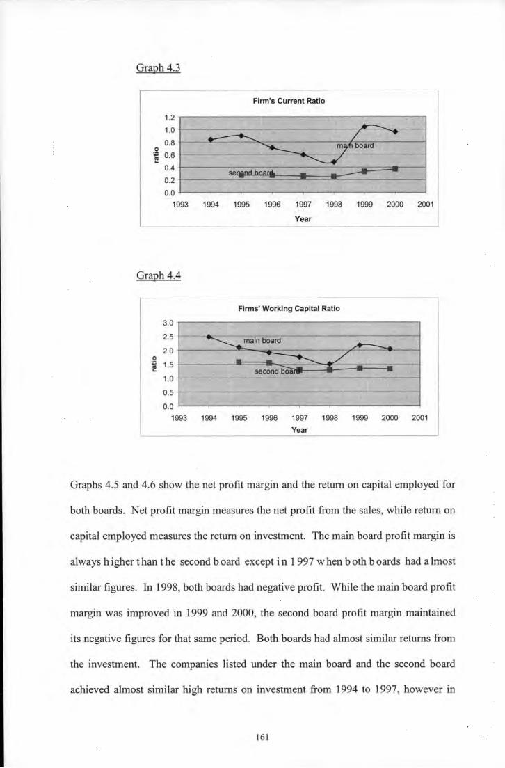
Graph 4.3

Firm's Current Ratio

1.2

1.0

0.8 0 ; 0.6 "' ..

0.4

0.2

0.0

1993 1994 1995 1996 1997 1998 1999 2000 2001

Year

Graph 4.4

Firms' Working Capital Ratio

3.0

2.5

2.0 0 ... 1.5 "' ..

~main board

~ --............ -second b"oai-= ~ - ~- ---1.0 -

0.5

0.0

1993 1994 1995 1996 1997 1998 1999 2000 2001

Year

Graphs 4.5 and 4.6 show the net profit margin and the return on capital employed for

both boards. Net profit margin measures the net profit from the sales, while return on

capital employed measures the return on investment. The main board profit margin is

always higher than the second board except in 1 997 when both boards had almost

similar figures. In 1998, both boards had negative profit. While the main board profit

margin was improved in 1999 and 2000, the second board profit margin maintained

its negative figures for that same period. Both boards had almost similar returns from

the investment. The companies listed under the main board and the second board

achieved almost similar high returns on investment from 1994 to 1997, however in

161

mid 1997 and early 1998, comparues under both boards suffered a rather high

negative return. While main board recovers from negative profit and return in mid-

1998, second board companies continued to experience negative ratios until 2000.

Graph 4.5

Firms' Net Profit Margin

80.0 T"""'~~---------=-------~~---..........-.

60.0 +-------j..._~"='L'=:.-----------:

CD E 4o.o ; 20.0 -r----.=:;;;;;::::=:;,~~----\:-------::'(Y'----~

~ ~-----~~===!~==~~~~~~~----~ &?. 0.0 + -20.0

-40.0 ..1.-.-~~~~-~~-~--~----~~

Year

Graph 4.6

Firms' Returned on Capital Employed

15.0

10.0

5.0

:8 "' ..

-10.0

-15.0

year

The market to book value ratio is the proxy for investment opportunity or growth of

the firms. As shown in Graph 4.7, the main board growth shows a fairly constant

declining trend over that 7-year period. Although the second board shows a

significant increase in growth from 1995 to 1996, it fell substantially following the

crisis in 1997. The results indicate that the share prices of the small companies are

162

very sensitive towards the economic downturn as compared with the companies on

the main board.

Graph4.7

Firms' Market to Book Value Ratio

8.4 -.......---------------------.

6.3 +----------:---""""-~--------......_----l

4.2 -l---...---:=7'~......,...~nnrl-6n)vd------------1

0.0 +-----,----.--------.----.-----,-----,----"..--r----l

-2.11

4.2 ~-----~----~-----------~

Year

Both the main board and the second board interest coverage ratio were constantly

fluctuating even before the crisis as shown in Graph 4.8. While the main board had a

negative ratio in 1994, the second board experienced a negative ratio in 1995 and

1996. Both boards had a positive ratio in 1997 and a negative ratio in 1998.

However, the ratios have been improved since 1999 especially for companies under

the second board. It is not surprising to have high fluctuation in the ratios since the

earnings fluctuate as shown in Graph 4.5, especially following the crisis.

The annual change (growth) in tax paid are almost similar for both the main board and

the second board as shown in Graph 4.9, although the second board figures indicate a

small fluctuation over the years. Both boards had a low percentage change in 1998

and 1999. This is due to the Income Tax Amendment Act (1999), relating to the

waiver of tax for income earned in 1999, and this tax-exempt income is subject to

agreement by the Inland Revenue Board. The reason behind the exemption is partly as

a fiscal incentive in respond to the crisis. However, not all companies are given the

163

exemption, it depends on the rules and conditions set by the Inland Revenue Board.

Singh and Teoh (2001) provide some details of the tax exemption for a corporation.

Graph4.8

Firms' Interest Coverage Ratio

25.0 .,----------------------.,

20.0 -1----------,------.----------....,..-t

:8 10.0 ~ 5.0 +--m,,;,-tMT2,...._ ____ ___,..,........,_=----' _ _____ ,.,..."-'-------I

0.0 -f----..,...+-----...----,--./--,.-"'&---,--~r/---..-----l

-5.d -10.0 _.__ __________________ __.

Year

Graph 4.9

Firms' Tax Charge

36.6 ..,.----------------------...,

30.5 +----------"?llk------------1 Q) E 24.4

lii 18.3 +---------;;ia~:rJV;=----'._..,~-----..,----1 u :; 12.2 ·t----------------'1..--Y--~~---l c.

6.1 -!---------------~~~~---4

0.0 -1------.----r---,------.---.......-------,----l 1993 1994 1995 1996 1997 1998 1999 2000 2001

Year

Graph 4 .1 0 s hews the depreciation to total assets of main b card and second b card

companies. Depreciation is used as a tax surrogate in this study or proxy for the non-

debt tax shield item. The main board depreciation ratios were very small and are

almost non-existent on the graph. The reason is the numerator value (Depreciation) is

very small, while the denominator values (Total assets) are very high, resulting in

0.01 to 0.02 ratios in the computation of depreciation over total assets for that 7-year

period. It reflects that large companies have large amount of assets as compared to

164

their fixed assets. The second board depreciation ratio ranges from 0.03 to 0.61 ,

considerably higher than the main board companies. However, the proportion is still

below the ratio of 1. The result is consistent with the amount of the fixed assets

owned by the companies on both boards. Graph 4.11 shows that the second board has

a high proportion of net fixed assets to total assets as compared with the main board

companies which is very small and is slightly above 0. The amount of fixed assets in

place is reflected in the computation of the depreciation ratio.

Graph 4.10

Depreciation to Total Assets

0.70

0.60

0.50

0 0.40 .. ~ 0 .30

0 .20

0.10

- -/ second board ........--.

,. ~ \ I

I \ I - I y

"' main b~ard 0.00

1993 1994 1995 1996 1997 1998 1999 2000 2001

year

Graph 4.11 depicts a higher proportion of second board net fixed assets in relation to

the total assets compared with the main board net fixed assets' proportion to total

assets. The main board had an average ratio of 0.3 from 1994 to 2000. The second

board ratio ranged from 0 .4 in 1 995 to 8 .5 in the year 2 000. G enerally, the 1 arge

companies would expect to have a larger amount of fixed assets than the small

companies. Large companies may have a higher proportion of current assets and

intangible assets than the fixed assets in the total assets ' computation.

165

Graph 4.11

Firms' Net Fixed Assets to Total Assets

10.0

8.0

.2 6.0 iii ... 4.0

2.0

0.0

1993 1994 1995 1996 1997 1998 1999 2000 2001

year

Due to the apparent differences between the two boards' net fixed assets as shown in

Graphs 4.11 , the main board net fixed assets ratio is much lower compared with the

second board net fixed assets ratio. Therefore, the nature of the assets for both boards

are further investigated. The absolute figures of current assets, fixed assets and total

assets were extracted from Datastream. The current assets and fixed assets were

summed using a formula in Excel, however these figures are different from the total

assets' figures obtained using Datastream 392 code. There are large discrepancies of

values especially for the main board. The reason is because Datastream only reported

the figures of total assets, fixed asset and current assets as indicated in the company's

annual report. A few items such as goodwill, and R&D were not available for

Malaysian companies for the researcher to access using Datastream. For the purpose

of this research, the discrepancies between total assets and current assets plus fixed

assets are referred to as investment.

The ratio of current assets, fixed assets and investment assets to total assets were then

calculated using Excel for both boards. The results are depicted in Graphs 1 and 2 in

Appendix E for both the main board and the second board, respectively. The ratio of

166

current assets to total assets ranges between 0.42 to 0.45 for the main board and 0.58

to 0.50 for the second board for the period between 1995 and 1999. On the other

hand, fixed assets to total assets varies between 0.35 to 0.36 for main board and 0.38

to 0.40 for the second board. The ratio of investments to total assets varies between

0.20 to 0.21 for the main board and 0.05 to 0.08 for the second board.

Obviously, both boards have a high ratio of current assets compared with fixed assets.

The investment assets ratio for the second board of companies are so much lower than

for the main board. A !though the differences in the fixed assets and current asset

ratios are very small, it raises the question as to why the companies hold high current

assets over fixed assets. This is because, conventionally, companies in general regard

high fixed assets as better for the company especially established companies in the

main board. Further to that, from the investors' point of view, companies with high

fixed assets tend to lower their (investors) risk of investing especially during a

liquidation. Should investment figures be considered as part of the fixed assets? If

the answer is yes, by combining the fixed assets and investments figures, this will

raise the ratio of fixed assets above the current ratio figures especially for the main

board companies.

Further to that, the 1998-2000 annual reports of 17 and 4 companies listed under main

board and second board respectively, were analysed, particularly regarding the

investment figures. The selection is based on the availability of companies' annual

reports in the KLSE web site. The second board has a lesser number as only 5

companies were selected due to the availability of these companies' annual reports on

the web site. All the 17 companies listed in the main board are individually labelled

167

as company 1, company 2 and so on, and the same process is repeated for the 5

companies listed in the second board.

Apparently, companies listed in the main board usually had three extra items on the

assets side of the balance sheet (other than the common entry of current assets,

goodwill, research and development and fixed assets). These include investments in

subsidiary companies, associate companies and other companies quoted in terms of

the shares' value.

The ratio of current assets, fixed assets and investment (the sum of 3 types of

investments) were calculated. As shown in Table I of Appendix E, the current assets

to total assets (ca/ta) of 17 companies had the highest ratio (0.384), followed by fixed

assets to total assets (fa/ta) with a ratio of 0.302. The lowest, however, is the

investment to total assets with a ratio of 0.27. To facilitate an understanding of the

high current assets' nature of the companies, various analyses were conducted on the

following current assets items: stock, trade or receivables, deposits with the financial

institutions, cash and short term investments. The ratio to total current assets of all

these 5 items were computed using Excel. As shown in Tables 2 and 3 in Appendix

E, trade and receivables had the highest ratio for both main board and second board

companies with a ratio of 0.542 and 0.41 0, respectively, representing 50 per cent of

current assets. Why do these firms have such a high amount of account receivables?

Further study may be required to answer this question. Studies by Tucker and Moore

(2000), for example, found evidence indicating that account receivables are a valuable

source of cash to pay creditors in a bankruptcy situation, and that trade creditors may

be more supportive of a liquidation compared with other creditors.

168

Three types of investment ratio to total investment ratio were also calculated. As

shown in Table 1 in Appendix E, investment in associated companies (ass/tinv) had

the highest ratio, 0.404, followed by investment in subsidiary companies (sub/tinv)

with a ratio of 0.317, while investments in other company (oinv/tinv) had generated a

ratio of0.279. Table 3 in Appendix E shows a different scenario for the second board

companies, whereby the fixed assets ratio is higher than current assets ratio whilst the

investment to total assets figures almost do not exist. As mentioned earlier in the

thesis, the companies listed under the main board are comprised of large and

established companies, therefore it was no surprise for these companies to have

subsidiaries, associates and investments in other companies. However, since only five

companies had been chosen to represent companies I isted in the second board, the

results may be biased. As a conclusion, the three types of investments are considered

asp art oft he companies assets, however, they should be considered separate from

fixed assets, as the subsidiary, associate and other company share values are subjected

to greater uncertainty.

Graph 4.12 shows that the main board companies' total assets are much higher than

the total assets of the second board companies. However, the amount of assets for

both boards is fairly constant from 1994 to 2000. The assets amounted to between 10

and 11 million each year for the second board companies and 14 to 16 million for the

main board companies. The comparisons made between Graphs 4.11 and 4.12

indicate that small companies have a relatively high level of fixed assets while large

companies have a relatively high level of current assets.

169

Graph 4.12

Firms' Log{Total Assets)

20.0 m::~in hn::~rrl

... 16.0 c: :::J 0 12.0 E CV

• • • • ·-.. • ---

!\i!_~nrl hn:~rrl ---- -- -~ 8.0 0 ... 4.0

0.0

1993 1994 1995 1996 1997 1998 1999 2000 2001

year

Graph 4.13

Earning Before Interest, taxes, Depreciation and Amortisation

60 -r-------------------------------~ 12

10 c: 50 1----g 8 :i 40 \-\-----~.L----1 6 .!: -g

..... nJ

c: 30 -1-----,~ --------\-+--+-----~ 4 5 ~ 1: 0 0

g 20 2 ~ ~ E 0 < 10 -2

0 .L..-----t----'-----~----t-----'-----1------+ -4

1994 1995 1996 1997 1998 1999 2000 Year

Earning before interest, taxes, depreciation and amortisation for both boards were

continuously fluctuating between 1994 and 2000 as shown in Graph 4.13. The gap of

the earnings between the main board and the second board is huge. The total amount

of the main board is shown in million ringgit (left y-axis) while the total amount of

the second board is shown in the thousand ringgit (right y-axis). The highest amount

of earnings achieved by the main board was in 1997 (RM56 million) while the lowest

was in 1998 (RM21 million). The highest for the second board was in 1995 in the

amount of 10 thousand ringgit while the lowest was in 1999, in the amount of-

RM2.76 thousand ringgit (-2760). The fluctuation of earnings within that 6 and 7

year period, implied great uncertainty. Therefore, both boards were exposed to

170

substantial business risk, which got worse immediately after the 1997 as firms were

exposed to macroeconomics effects.

Graph 4.14 and 4.15 depicts the relationship between share prices and the ringgit

movement from the period of 1994 to 2000. The first graph (4.14) shows high

positive correlation of ringgit and the Kuala Lumpur Composite Index (KLCI) at

0.9095 of coefficient. The ringgit in the graph is obtained from the Datastream Global

Treasury Information Service (GTIS) code of MALAYUS (US$ to Malaysian Ringgit,

i.e. RMl = 0.26 USD) from 1994-2000, using monthly frequency. It was intended to

run the correlation between ringgit and each oft he 357 companies under the main

board, however, unlike the second board, the Datastream code for all the listed

companies under main board was not valid to use with this program (correlation

program), therefore KLCI was used. KLCI is the index of weighted market

capitalisation in which current aggregate market capitalisation is divided by base

aggregate market capitalisation multiplied by 1 00 using 1977 as a base year. Graph

4.14 shows that share prices are highly positively correlated with the ringgit

movement. Therefore, if the ringgit is appreciated, the share prices will tend to go up

and vice versa.

To cover each company price-currency sensitivity, a series of Graphs fort he main

board sectors are attached to the Appendix El for the observation, Graphs 1, 2, 3, 4, 5,

6 are for the six sectors listed under main board, construction, consumer product,

industrial product, plantation, properties and services. All sectors show a high positive

correlation of share prices and the ringgit fluctuation, with 0.9477 being the highest

score for the industrial product and 0.8092 the lowest for the consumer product.

171

Therefore, it is fair to conclude that companies listed under the main board are highly

positively sensitive to the ringgit fluctuation.

Graph 4.14

Main Board Price Sensitivity

1500

1000

500

0 1999 2000

SERIES 1 KUALA LUMPUR COMPOSITE- PRICE INDEX

SERIES 2 US$ TO MALAYSIAN RINGGIT (GTIS)- EXCHANGE RATE

Correlation coefficient = 0.9095, frequency= monthly

Source: DATASTREAM

The second graph, Graph 4.15 shows the correlation between ringgit and share prices

of the companies listed under the second board. Although the share prices of the

companies listed under the second board have a positive relationship with the ringgit

movement at a 0.709 coefficient, the correlation is not as high as for the main board.

From the graph (4.15), it can be observed that the ringgit has a constant movement

from 1994 to 1997, subsequently the ringgit depreciated as well as the price index of

the second board companies in 1996 and 1997. The conclusion for the second board

is that the companies are not really sensitive toward the movement of the ringgit as

compared with companies listed on the main board, particularly when the market was

optimistic during 1996 and mid 1997.

172

Graph4.15

800

600

400

200

0

Second Board Price Sensitivity

ringgit

1994 1995 1996 1997 1998 1999 2000

SERIES 1 KUALA LUMPUR SE SECOND BOARD - PRICE INDEX

SERIES 2 US$ TO MALAYSIAN RINGGIT (GTIS)- EXCHANGE RATE

Correlation coefficient =0.7097, Frequency= monthly

Source: DATASTREAM

4. 7 Conclusion

Chapter 4 has provided a detailed discussion on the data and the methodology that

will be used in the subsequent chapter to analyse the data. The data include primary

data from a questionnaire survey and the secondary data from Datastream. The

chapter reviews each variable that is used for data extraction from Datatstream for

subsequent analyses. The formulas utilised by Datastream are appended and the

program was discussed. Each hypothesis statement is given in section 4.3. There

are 22 hypotheses to be tested.

An overview of the Malaysian data was presented in Section 4.5 in charts presentation

to give some ideas of the companies' performance based on their ratios and figures.

The graphs show that Malaysian gearing ratios gradually increased over time, the

main board companies maintain their 40 per cent or less ratios under the book value

173

and mixed value ratios' assessment. The second board gearing is always higher than

the main board; it is even higher following the 1997 financial crisis.

It is found that the main board (large companies) has high liquidity, high profitability,

but low fixed assets, low depreciation to total assets and share prices are highly

positively sensitive to the currency movement. There are a few items that experiences

gradual decline over the period of study, such as the tax ratio and the market to book

value ratio. The profitability ratios, interest coverage ratios and operating risk showed

few fluctuations, especially immediately after the 1997 financial crisis.

The second board (small companies) have high fixed assets, high depreciation and

share prices are positively correlated to the ringgit. Nevertheless, the second board

liquidity and total assets are low. Similar to the main board, the second board tax

ratio is gradually reduced over the years. However, its profitability and EBITDA are

very uncertain, as well as its market to book value ratio and interest coverage ratios.

174

CHAPTERS ANALYSIS OF MALAYSIAN CAPITAL STRUCTURE FROM

PUBLISHED DATA

5.1 Introduction

Chapter 5 includes the discussion on published data that were collected from the

online Datastream financial database. The database consists of large and accurate

information which includes account items, macro economic variables, equity and

bond prices and many other variables that will be used to support this research on

capital structure. The events of the 1997 financial crisis have been taken into

consideration in the analysis of the Datastream data. The chapter consists of the

following sections: Section 5.2 reviews the Datastream sample, Section 5.3 discusses

the period of the study, Section 5.4 provides a summary of the data analysis. Section

5.5 shows the results and analysis of the ANOV A statistical test, Section 5.6 covers

the Multiple Regression analysis, Section 5.7 focuses on the Pool Data and Section

5.8 concludes the chapter.

175

5.2 The Datastream

The data used in chapter 5 mainly comes from Datastream. The sample covers

publicly listed companies in the Kuala Lumpur Stock Exchange (KLSE). The main

board and the second board companies' financial and accounting data were extracted

from Datastream database on-line. The main difference between the two boards is on

the requirement of their paid-up capital by the Malaysian Security Commission. As of

January 200 I, the KLSE (KLSE website, 200 I) requires all companies that are listed

on the main board to have a minimum issued and paid-up capital of RM60 million

comprising of ordinary shares of RMI.OO per share. The second board listing is also

required to have a minimum issued and paid-up capital of RM40 million comprising

of ordinary shares of RMI.OO. The second board is relatively new, launched in 1988

to enable smaller companies which are viable and have strong growth potential to be

listed. Therefore, companies listed on the main board are usually large and mature

while the second board companies are smaller, immature and very volatile.

Each board is further classified by sectors, which reflect the core business of these

companies. The main board consists of six different sectors which include

construction, consumer products, industrial products, plantation, properties and

services. The second board consists of a few groups, but is treated as one sector or one

board for this thesis because there are too few companies that are listed under each

sector.

When the data were first collected in September 2000, information on more than 700

companies were available on Datastream on-line. However, a number of problems

were encountered in the attempt to extract the data from over 700 companies due to

176

the inconsistency of the listed number of companies. For example, in I990, a total of

285 companies were listed in both boards, however by 1995, the number doubled to

529 companies. Therefore, the data of the companies will only be available starting

from the year in which they were listed. Only companies that have been listed for a

minimum of 4 years or more will have their data included in this survey. A final list

of 572 companies was extracted from Datastream, in which the data of 357 companies

were obtained from the main board, while the data of 2I5 companies were obtained

from the second board of the KLSE.

5.3. Period of Study

The period of study was initially intended to be fort en years, from I 99I to 2 000.

However, due to the problems of inconsistency and insufficient data in the early

nineties, the data that were obtained from the period of I 99I to I 993 and I 991 to

I994 had to be disregarded for the main board and second board companies,

respectively. Therefore, for a 7-year period account items were gathered from 1994

to 2000 for the companies listed on the main board. For a 5-year period account items

for the companies on the second board were gathered from I995 to I999. For the

purpose of studying the effects of the 1997 financial crisis on the capital structure of

Malaysian firms', the data have been divided into the following 3 time periods: pre

crisis, crisis and post-crisis. For the main board, for a 3-year period data have been

averaged pre-crisis and post crisis, while for a 2-year period data have been averaged

for the second board pre-crisis and post crisis. Both boards used the 1997 data for the

crisis period.

177

The total number of companies and their data are constantly changing due to listing

and de-listing, therefore, it affects the consistency of the data in the spreadsheet.

Some companies that have been listed in the second board may instead be listed in the

main board after some years due to the increase in their paid-up capital. The problem

is resolved by considering the length of time they were listed under each board. For

instance, if a company was listed in the second board from 1994 to 1997 and was then

promoted to the main board in 1998 to 2000, the company will remain under the·

second board throughout the analysis. This is because the length of time the company

was listed under the second board weighed more than the time it was listed under the

main board.

5.4 The Data

The thousands of types of data that are maintained by Datastream are used through

program numbers, codes and datatypes. Account items such as financial ratio, profit

and loss and balance sheet were the main items used in the capital structure research.

Besides account items, macroeconomics items and shares prices were also collected.

The raw data collected from the Datastream were then transferred to spreadsheets. A

considerable amount of time was spent in cleaning and sorting the data to match the

rows and columns for each company. The cleaning and sorting process resulted in the

deletion of some of the companies from the spreadsheet, including any unwanted

information before finally being imported to the Statgraphics version 5.0 for statistical

analysis.

The review of the literature together with discussion held with the research supervisor

have resulted in 2 dependent and 12 independent variables being chosen for the study.

178

Most of the data collected are cross-sectional data except for the share prices and the

ringgit. The two dependent variables are the capital gearing based on the book value

ratio and the mixed value ratio. Book value ratio comprises total debt over total debt

plus book value of equity while mixed value ratio comprises total debt over total debt

plus market value of equity. Datastream defmes total debt as the sum of preference

capital, long term debt and short-term debt. A high debt simply indicates that a

company has placed a greater reliance upon debt than equity to finance its operations.

Too much debt may expose the company to uncertain future conditions which may

eventually result in the company experiencing difficulty in continuing debt finance in

the future.

5.5 Analysis of Variance (ANOV A)

5.5.1 Introduction

Analysis of variance is the statistical method used for testing the null hypothesis, that

the means of several populations are equal. ANOV A is used to test if there is any

difference between and within the means of the main board and the second board. It

is also used to test if there is any difference between the means of six sectors selected

under the main board.

The following hypotheses (HI and H2) are from Section 4.3, Chapter 4:

HI: Firms' gearing vary significantly between two boards

H2: Firms' gearing vary significantly across sectors

179

The hypotheses are adjusted in accordance with the three time periods.

Null hypotheses:

HO: There is no difference between main board and second board firms' gearing before, during and after the crisis.

HO: There are no differences between gearing ratios among firms in the same sectors on the main board before, during and after the crisis.

Alternatively Hypotheses:

H1: There is a significant difference between main board and second board firms' gearing before, during and after the crisis.

H2: Alternative hypothesis: There are significant differences between gearing ratios among firms in the same sectors on the main board before, during and after the CnSIS.

5.5.2 ANOV A- Mean and Median Analysis

As was previously explained, there is a book value ratio of debt to book value debt

plus book value of equity, and a mixed value ratio of book value debt to book value

debt plus market value equity for the statistical analyses. As shown in Table 5.1 of

the Statgraphics one-way analysis of variance, the differences between the means

were found to be significant for the book-value ratio of the pre-crisis with a p-value of

the F-test less than 0.10 (0.0867). The post-crisis book-value ratios are also

significant at the 99 per cent confidence level with a 7.32 F ratio. The 1997 book-

value ratio is statistically not significant and violates the ANOV A assumption with a

significant Cochran's statistic. Thus, based on the book value ratios, there is a

significant difference between the gearing of large and small companies at the 90 and

99 per cent confidence level before and after the crisis. As indicated by the mean

scores of both periods, the second board companies gearing is higher than the main

board gearing (29.0456 > 25.6148) during the pre-crisis and (50.9003 > 35.8393) during the

post-crisis period. The post-crisis period has given a stronger level of difference with

180

the p-value of less than 0.05. However, the standard deviation of the post crisis mean

score is so much higher than the pre-crisis period. The deviation indicates a large

deviation of certain firms from the average group gearing.

Table 5.1: Gearing Differences Between The Main Board and the Second Board Analyse Using ANOV A and Kruskal-Wall is

Book value ratios Mixed-value ratios Group

Pre- crisis 1997 Post-crisis Pre crisis 1997

Main board 25.6148 33.5908 35.8393 13.5248 27.9872

(20.1481) (35.5104) (64.216) (13.6032) (25.2012) Second- 29.0456 36.3284 50.9003 16.9983 40.0936 board (21.269) (29.8707) (64.8309) (16.4212) (30.3792) ANOVA F-ratio 2.95 0.87 7.32 5.65 24.55 Prob-value 0.0867* 0.3513 0.0070*** 0.0178 0.0000 COCHRAN'S TEST Prob-value 0.3998 0.0041 *** 0.8724 0.0045*** 0.0025*** K.RUSKAL-W ALLTS Mainboard 236.845 269.854 275.794 219.664 239.958 Second board 259.471 295.731 302.90 252.383 309.447 H-Statistic 2.7223 3.3616 3.6188 6.0365 25.531 Prob-value 0.0989* 0.0667* 0.0571 * 0.0140** 0.0000***

*, **, ***S1gruficant at the l 0, 5, and l per cent confidence level, respectively. Reported standard deviation are in parenthesis Book value ratio-book value of debt to book value of debt plus book value of equity Mixed value ratio-book value of debt to book value of debt plus market value of equity

Post crisis

36.4108 (26.631) 54.0876

(70.7932)

16.97 0.0000

0.0000***

253.907 298.580 10.4377

0.0012***

Although significant results are found for the mixed-value ratio across three periods,

Cochran's test shows a significant p-value which indicates the standard deviations are

not equal, therefore violating the ANOV A assumption that the populations should

have equal variances. For any p-value with a significant standard deviation, i.e., with

a p-value of less than 0.05 from the Cochran test, the Kruskal-Wallis test will then be

applied to validate the hypothesis based on the median. This is a one-way analysis of

variance by rank. Table 5 .1 shows both the book-valuer atios and the mixed-value

ratios, where the p-values of the Kruskal-Wallis test are less than 0.1, 0.05 or 0.01,

and are significant at the 90, 95 or 99 per cent confidence level across the three

181

periods. The null hypothesis of the Kruskal-Wallis test states that the medians of the

dependent variable within each level of factor are the same. Since all the p-values are

significant at the required level, there is a difference between the main board and the

second board companies' gearing before, during and after the crisis based on the book

value and the market value of equity. The second board median rank is always higher

than the main board median rank across the three periods. Based on the book-value

ratios, the test also revealed that the 1997 median rank of both boards was higher than

the pre-crisis values and the values of the post-crisis period were ranked even higher.

The same result is evident for the mixed-value ratio, indicating the increase in gearing

following the 1997 crisis.

It is essential to note that another important assumption of the ANOV A is that the

sample must be randomly selected from normal populations. According to the

Statgraphics statistical summary of ANOV A, the standardised skewness of the main

board and the second board is outside the range of -2 to +2 for two levels of gearing

for all periods at both gearing measurements. This indicates some significant non

normality in the data, which violates the assumption that the data come from normal

distribution. Although this has distorted the means, the distortions a re identical for

most groups. According to Roberts and Russo ( 1999), it is still meaningful to see

which means differ if the skewed data are roughly by the same degree in the same

direction. However, it is meaningless to interpret differences between the means if

some groups are skewed positively while the others are skewed negatively. Table 5.2

shows the skewness of the groups based on the previous ANOVA test showing all the

data being skewed in the same positive direction (see Table 5.1).

182

Table 5.2: The Main Board and The Second Board Skewness

Book value ratios Mixed value ratios *Pre-

1997 *Post-

cns1s cns1s

Main board 4.2232 51.2017 12.7036

Second board 2.2505 9.5136 19.7808

*The astensks refer to the test With sigruficant F-rat10 N.B. The shaded figures are therefore ignored.

Pre-1997

crisis

12.5777 5.5436

12.0208 8.1908

Book value ratio-book value of debt to book value of debt plus book value of equity Mixed value ratio-book value of debt to book value of debt plus market value of equity

Post-crisis

1.5908

2.4669

The similar tests are applied to the following different sectors on the main board:

construction, consumer products, industrial products, plantation, properties and

services. Although there are more than six sectors listed on the Kuala Lumpur Stock

Exchange, a few of the sectors are excluded due to the small number of the companies

listed in those sectors. Using a one-way analysis of variance, the differences between

the means of the six sectors are found to be significant during the pre-crisis period

using the book-value ratios. The differences are also found to be significant using the

mixed-value ratios during the 1997 and post-crisis period. The F ratio in Table 5.3

shows a p-value of less than 0.05 for the book-value ratio during the pre-crisis period

with a gearing ratio of 20 to 30 per cent among all sectors except for plantation which

had the lowest score of 12.615 per cent. The mixed value ratio of the 1997 and post-

crisis period shows a high ratio for construction, at 37.555 and 45.381 per cent

respectively, whilst the plantation is still the lowest with a score of 23.3756. Hence,

there were differences between the book-value ratios for construction, consumer

products, industrial products, plantation, properties and services during the pre-crisis

period. There were also differences of the six sectors' mixed value ratios gearing

during the 1997 and post-crisis period.

183

Table 5.3: Gearing Differences Between The Main Board 6 Sectors Analyse using ANOV A

Book-Value Ratios Mixed-Value Ratios Variables Post Pre Post

Pre crisis 1997 .. 1997 CnSIS CnSIS CnSIS

. Construe- 29.3836 39.6821 20.4669 13.2004 37.5453 45.3814 tion (14.4306) (21.087) (116.706) (8.5676) (26.8071) (25.0051)

Consumer 25.4863 30.6098 37.9246 12.2141 23.2639 30.742 Products (21.9837) (25.0994) (49.6834) (12.2884) (21.8046) (26.1153)

Industrial 28.7059 38.9093 36.9386 15.1171 26.5026 34.6435 Products (22.1687) (56.7383) (59.1739) (16.8883) (25.031) (27.1031)

12.6146 21.9126 16.745 6.5362 17.8825 23.3756 Plantation

(16.4476) (27.6052) (50.6714) (9.6406) (23.2979) (25.9291)

24.9114 28.9596 41.0588 13.2579 29.4643 40.8217 Properties

(16.4566) (17.8359) (80.3403) (9.7305) (23.6588) (23.2151)

27.5321 36.3878 43.0886 16.4619 33.1413 41.4421 Services

(20.8921) (25.3175) (32.4101) ( 15.1 046) (27.2947) (27.6282)

F-ratio 3.81 1.75 1.28 2.88 3.00 3.84

Prob-0.0023*** 0.1232 0.2719 0.0147** 0.0116** 0.0021 *** value

COCHRAN'S TEST

P-value 0.1486 0.0000*** 0.0000*** 0.0000***

*, **, *** S1gmficant at the 10, 5, and I per cent level, respectively. Reported standard deviations are in parenthesis

0.6575

Book value ratio-book value of debt to book value of debt plus book value of equity Mixed value ratio-book value of debt to book value of debt plus market value of equity

1.0

Many statisticians have suggested a follow-up test for the one-way analysis of

variance if the factors are at more than two levels. The test is intended to compare

every possible pair of means. The two common tests are Newman-Keuls and Tukey

HSD (Honestly Significant Difference). According to Roberts and Russo (1999), the

former is suitable when comparing the means of up to and including three groups

while the latter is more suitable to compare the means of a group of 5 or more. Both

tests are suitable with roughly equal sized groups, with similar variances and normally

distributed data. Due to the difference in the number of observations at each level of

the sectors, Statgraphics Version 5.0 has suggested a Bonferroni test instead of the

184

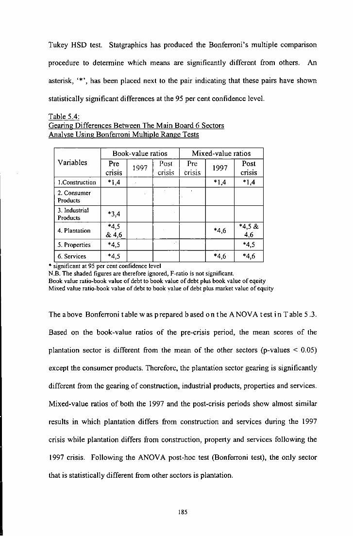
Tukey HSD test. Statgraphics has produced the Bonferroni's multiple comparison

procedure to determine which means are significantly different from others. An

asterisk, '*',has been placed next to the pair indicating that these pairs have shown

statistically significant differences at the 95 per cent confidence level.

Table 5.4: Gearing Differences Between The Main Board 6 Sectors Analyse Using Bonferroni Multiple Range Tests

Book-value ratios Mixed-value ratios Variables Pre

1997 Post Pre

1997 Post

CDSIS cnsts C.J'ISlS cnsts !.Construction *1,4 *1,4 *1,4

2. Consumer Products

3. Industrial *3,4

Products

4. Plantation *4,5

*4,6 *4,5 &

&4,6 4,6

5. Properties *4,5 *4,5

6. Services *4,5 *4,6 *4,6

* s1gmficant at 95 per cent confidence level N.B. The shaded figures are therefore ignored, F-ratio is not significant. Book value ratio-book value of debt to book value of debt plus book value of equity Mixed value ratio-book value of debt to book value of debt plus market value of equity

The above Bonferroni table was prepared based on the A NOVA test in Table 5 .3.

Based on the book-value ratios of the pre-crisis period, the mean scores of the

plantation sector is different from the mean of the other sectors (p-values < 0.05)

except the consumer products. Therefore, the plantation sector gearing is significantly

different from the gearing of construction, industrial products, properties and services.

Mixed-value ratios of both the 1997 and the post-crisis periods show almost similar

results in which plantation differs from construction and services during the 1997

crisis while plantation differs from construction, property and services following the

1997 crisis. Following the ANOV A post-hoc test (Bonferroni test), the only sector

that is statistically different from other sectors is plantation.

185

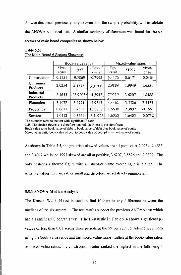
As was discussed previously, any skewness in the sample probability will invalidate

the ANOV A statistical test. A similar tendency of skewness was found for the six

sectors of main board companies as shown below.

Table 5.5: The Main Board 6 Sectors Skewness

Book-value ratios Mixed-value ratios *Pre- 1997 ' . · Pbst-' Pre-

*1997 CriSIS · ci'isis' CriSIS

Construction 0.1151 • cQ.3860 o·"94" - . .J· .. ' .;) . :1.43,76 0.6171

Consumer 2:1747

.. ... Products

2.0254 7:,9089:. .2.9889 1.9949 . ' ..

Industrial 2.4655 'i3:9205. -4.5947 7.9219 3.6207

Products .. . ,1" ... Plantation 3.4072 3.4771' -3.9517 4.4462 3.5526

Properties 0.6611 0~7388· . 18'.3237 L660S 2.3892

Services 1.0412 0.3264 3.1072' 3.6060 1.6405 The astensks refer to the test w1th s1gmficant F-rat10 N.B. The shaded figures are therefore ignored, the F-test is not significant Book value ratio-book value of debt to book value of debt plus book value of equity Mixed value ratio-book value of debt to book value of debt plus market value of equity

*Post-CriSIS

-0.0464

1.655 I

1.8488

2.3523

-0.1661

-0.0732

As shown in Table 5.5, the pre-crisis skewed values are all positive at 2.0254, 2.4655

and 3.4072 while the 1997 skewed are all at positive, 3.6207, 3.5526 and 2.3892. The

only post-crisis skewed figure with an absolute value exceeding 2 is 2.3523. The

negative values here are rather small and therefore are relatively unimportant.

5.5.3 ANOV A-Median Analysis

The Kruskai-Wallis H-test is used to find if there is any difference between the

medians of the six sectors. The test results support the previous ANOV A test which

had a significant C ochran 's test. T he H -statistic in Table 5 .4 shows significant p-

values of less than 0.01 across three periods at the 99 per cent confidence level both

using the book-value ratios and the mixed-value ratios. Either at the book-value ratios

or mixed-value ratios, the construction sector ranked the highest in the following 4

186

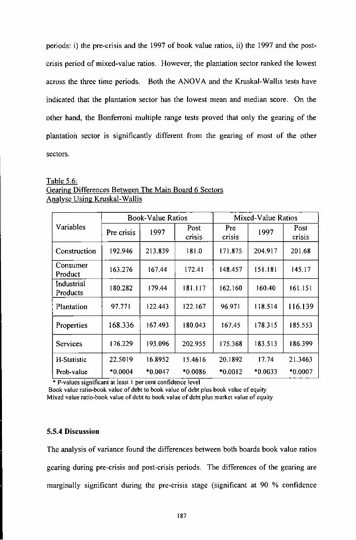
periods: i) the pre-crisis and the \997 of book value ratios, ii) the 1997 and the post-

crisis period of mixed-value ratios. However, the plantation sector ranked the lowest

across the three time periods. Both the ANOV A and the Kruskal- Wall is tests have

indicated that the plantation sector has the lowest mean and median score. On the

other hand, the Bonferroni multiple range tests proved that only the gearing of the

plantation sector is significantly different from the gearing of most of the other

sectors.

Table 5.6: Gearing Differences Between The Main Board 6 Sectors Analyse Using Kruskal-Wall is

Book-Value Ratios Mixed-Value Ratios Variables

Pre crisis 1997 Post Pre

1997 CriSIS CriSIS

Construction 192.946 213.839 181.0 171.875 204.917

Consumer 163.276 167.44 172.41 148.457 151.181

Product Industrial

180.282 179.44 181.117 162.160 160.40 Products

Plantation 97.771 122.443 122.167 96.971 118.514

Properties 168.336 167.493 180.043 167.45 178.315

Services 176.229 193.096 202.955 175.368 183.513

H-Statistic 22.5019 16.8952 15.4616 20.1892 17.74

Prob-value *0.0004 *0.0047 *0.0086 *0.0012 *0.0033

• P-values s1gmficant at least I per cent confidence level Book value ratio-book value of debt to book value of debt plus book value of equity

Mixed value ratio-book value of debt to book value of debt plus market value of equity

5.5.4 Discussion

Post crisis

201.68

145.17

161.151

116.139

185.553

186.399

21.3463

*0.0007

The analysis of variance found the differences between both boards book value ratios

gearing during pre-crisis and post-crisis periods. The differences of the gearing are

marginally significant during the pre-crisis stage (significant at 90 % confidence

187

level) but strongly significant following the cnsts (significant at 99 per cent

confidence level). Therefore, there are small differences in gearing between large and

small companies when the economy is growing but large differences are found when

the economy is in trouble.

The second board gearing ratios surpassed the main board ratios at both periods. One

of the reasons high debt ratios for small companies increased substantially following

the crisis may be due to the financial assistance in the amount of 1.5 billion ringgit

provided by the government to the financial institution to aid small and medium-sized

companies following the collapse of the financial market (BNM, 1999). Titman and

Wessels (1988) state that small firms may be more geared than large firms and may

therefore prefer to borrow short term debt (through bank loans) rather than issue

long-term debt because of the lower fixed costs associated with using short term debt.

The evidence in Graph 2 in Appendix A reveals a higher proportion of short-term debt

to long-term debt for the second board companies. The proportion had an average of

75.36 for the 7 year period (1994 to 2000). The differences in the financing practice

between large and small firms are probably reflected in the high transaction costs that

small firms face when they issue long-term debt or equity. By borrowing more short

term debt, these firms are particularly sensitive to temporary economic downturns,

which have less effect on larger firms that are less geared.

The null hypothesis of no difference between the six sectors of the main board was

rejected fori) the pre-crisis period of the book-value ratios, ii) the 1997 and the post

crisis of the mixed value ratios. The strong differences between the sectors when the

economy was stable are consistent with many studies on the industrial differences of

188

Malaysian capital structure such as Annuar and Shamser (1993) and Mohamad

(1995). The Annuar and Shamsher (1993) study of the five sectors traded under the

KLSE found that Malaysian firms' capital structure differ significantly within and

between industries. Using analysis of variance, Mohamad (1995) found that there are

significant inter-industry differences in capital structure among large Malaysian

companies.

Mansor and Mohamad's (2000) study on Malaysian firm's capital structure found that

heavy industries such as construction, chemical and electrical (industrial products)

tend to have higher debt ratios than other industries. Light industries such as food

(consumer products) and services tend to have low gearing. Their proposition on high

debt level in the heavy industries is due to the proportion of fixed assets held by this

industry as collateral for debt. However, they concluded that there was lack of

significance in industry classification between the industries due to substantial

diversification among listed firms in their activities. The results of the Bonferoni

multiple range test in Table 5.5 show that only plantation is significantly different

from the other sectors for all the three tests that are significant. Mansor and

Mohamad's argument on the lack of significance would support this finding as most

of the companies in those five sectors are linked to each other as they diversified. For

example, the parent company is listed under services while the subsidiary is listed

under construction and properties. However, that may not be the case for the

plantation sectors. Further to that, the crisis had a minor effect on the plantation

sector especially on the cost of production. The costs of imported inputs such as

fertilisers, pesticides and machinery were higher due to the depreciation of the ringgit

(BNM, 1999). However, palm oil and saw log had both benefited from the

189

depreciation of the ringgit due to the sharp increase in the export earnings because the

transaction for these two items was quoted in the US dollar. Due to that reason, the

profit of the firms related to these sectors were not as badly affected as those in the

other 5 sectors, therefore, profitable firms would require less debt for their

investments. The situation explains why the plantation had the lowest gearing

The strong differences are also consistent with the international study by Errunza

(1979), who found a strong industrial classification on the capital structure of

developing nations in Central American Common. However, the weak and no

differences between gearing are consistent with the studies conducted by Sekely and

Collins (1988), Ferri and Jones (1979) and Gupta (1969). Sekely and Collins (1988)

found little industry impact on the gearing ratios of the 9 industries in 23 countries

including Malaysia. Ferri and Jones ( 1979) concluded that the dependence between

capital structure and industry classification is weak. Gupta (1969) who studied

173,000 manufacturing companies found no significant relationship between gearing

and industry classification.

5.6 Multiple Regression Analysis

The independent and dependent variables were modelled using multiple regression

analysis to examine the influence of capital structure determinants on the gearing

ratio. In achieving the best possible model, the models were re-run for stepwise

regression and the existence of multicollinearity was validated. Section 4.4.3 in

Chapter 4 discusses the methodology employed in detail.

190

5.6.1 Preliminary Modelling of Multiple Regression Analysis

Table 5.7 illustrates the main board's first and second multiple regressions, while

Table 5.12 provides the second board's first and second multiple regressions. The

initial multiple regressions each regresses a measure of gearing against 12 variables

and is repeated for different time periods: during the pre-crisis, during 1997 and post-

CnSIS.

The main board's first multiple regression indicates r-squared o f3 0.53 %, 5 7.19%

and 33.92 % for the pre-crisis, 1997 and post crisis, respectively. Not much

difference was found for the second multiple regression of the main board's r-squared

which had a percentage of 30.37 % for the pre-crisis model, 57.05% for the 1997

model and 31.10% for the post-crisis model. The only variable that is significantly

related to gearing at the 99 per cent confidence level across three periods is Roce, for

both the first and second multiple regression. Mixed significant results were found

for other variables.

As shown in Table 5.12, the r-squared for the second board's first multiple regression

are 46.47 %, 43.10 % and 34.31 % for the pre-crisis, 1997 and the post-crisis,

respectively. During the second multiple regression, the pre-crisis had an r-squared of

43.90 % and the post crisis had an r-squared of 33.32 %. Not many variables are

significant across the three time periods except the Wcr which is significant during

the first multiple regression.

However, the results from the first multiple regression for both boards were

disregarded as some of the variables were highly correlated with one another. As

191

shown in Tables 5.8, 5.9 and 5.10 (correlation matrix ofpre-crisis of the book-value

ratios), the current ratio is highly correlated with the working capital ratio at -0.772.

Current ratios were then removed from the second multiple regression analysis across

the three time periods. Another variable to be removed from the second multiple

regression is the depreciation to total assets which is correlated at 0.509 with the

Log( total assets) during the post-crisis period.

The second multiple regression was followed by stepwise regression as shown in

Table 5.11, in which the working capital ratio (Wcr) and the return on capital

employed (Roce) were significant across the three periods. Tables 5.13, 5.14, 5.15

demonstrate the three periods' second board correlation matrices. The working

capital ratio, (Wcr) was highly correlated with the current ratio (Cr) at -0.711 during

the pre-crisis and post-crisis periods. Depreciation to total assets (Dep/Tas) was

correlated above 0.5 with net fixed assets to total assets (Nfa/Tas) and Log(total

assets) (Log(Tas)) during the pre-crisis and post-crisis periods. Eventually, both the

current ratio and the depreciation to total assets were removed from the second

multiple regression as shown in Table 4.12. Cooper and Schindler (1998) explained

that there is no definite answer on how high can the acceptable correlation be between

the independent variables. However, Statgraphics rules out any variable with a

correlation ofO.S and above as it is considered to have a presence ofmulticolleniarity.

192

Table 5.7: Factors Determined the Main Board Firms' Book Value Ratio Analyse Using Multiple Regression

First multiple regression Second multiple regression

Variables (book-value ratios) (book-value ratios)

Pre- Post-.. 1997 Pre-crisis

cnsts cnsts

Constant 30.9754 1.2817 42.6485 31.3951 (5.5473) (0.1283) (2.3700) (5.6546)

*** Cr

-0.5636 -2.4725 10.0582

(-0.7631) (-0.9220) (3.4903)

** *** *** Wcr -1.2551

-0.9545 -11.0825 -1.5496

(-2.5116) (-0.6724)

(-3.915) ( -4.883)

Npm -0.0028 -0.0055 0.0059 -0.0031 (-0.7103) (-0.6537) (0.4230) (-0.8006)

•• Mtbv 0.3868

0.8722 0.8632 0.3876

(1.3419) (2.2827)

( 1.0489) (1.3458)

* ** Tie 0.0376

0.0004 0.0193 0.0382

(1.9680) (0.0136) (0.8564)

2.0075

Tx 0.0016 0.0062 -0.0504 0.0012 (0.0327) (0.1923) (-0.6697) (0.0245)

••• Dep/tas 0.0105

627.22 -173.746 0.0105

(I.J671) (7.4909)

(-0.9298) (I.J678)

*** ••• ••• *** Roce -0.7591 -1.2662 -0.7730 -0.7604

(-7.757) (-13.885) ( -10.895) (-7.778) •• *** **

Nfa/tas -9.3014 -18.1708 2.1024

-9.4222 _ (-2.0155) (-2.7196)

(0.1704) ( -2.0445) _ ...

Log(tas) 0.4642 2.1716

0.8308 0.4542 (1.6099)

(4.9079) (1.0169) (1.5779)

Curr -5.3208 11.172 -9.2292 -5.4946

(-0.8079) (0.7301) (-0.5246) ( -0.8355)

** ** Risk 3.6566

0.3138 0.0195 3.7318

(2.2545) ( 1.0207) (0.1409)

(2.3071)

R-squared 30.53% 57.19% 33.92% 30.37%

*,**,***S1gruficant at the 10, 5, and I per cent level, respechvely. Reported !-statistics are in parenthesis

1997

2.1004 0.2112

••• -2.0762

( -2.8379)

-0.0058 ( -0.6872)

•• 0.8600

(2.2526)

-0.0004 ( -0.0 158)

0.0052 (0.1636)

*** 631.254 (7.5516) ... -1.2645

(- 13.873) ***

-18.4488 ( -2.7648)

*** 2.1415

(4.8545)

12.2906 (0.8060)

0.3250 ( 1.0582)

57.05%

Book value ratio-book value of debt to book value of debt plus book value of equity

Post-crisis

18.9544 (1.2391)

-1.4116 (-2.1517)

0.0041 (0.2940)

I.J092 ( 1.3289)

0.0229 (1.0041)

-0.0514 ( -0.6723)

*** -0.7866

(-10.911)

1.0996 (0.00975)

** 1.4555

(2.0432)

-9.2306 (-0.5161)

0.0060 (0.0424)

31.10%

Cr-current ratio, Wcr-Working capital ratio, Npm-Net profit margin, Mtbv-Market to book value ratio, Tie-Interest coverage ratio, Tx-Tax, Dep/tas-Depreciation to total assets, Roce-Return on Capital Employed, Nfa/tas-Net fixed assets to total assets, Log(tas)-Logarithm of total assets, Curr-pricecurrency sensitivity, Risk-Standard deviation of operating income.

193

Table 5.8: The Main Board Pre-crisis Correlation Matrix (see Table 5.7)

er wcr npm mtbv tie tax dep roce nfdtas Io~~ CUlT risA

er 1.000

wcr -1.77Z 1.000

npm -0111 0025 1.000

mtbv 0004 0.002 -0.013 1.000

tie 0.047 -0014-0017 0014 1.000

tax -0011 0017 0018 0.075 0.006 1.000

dep -0000 0.014 0003 0016 0.1 06 -0.009 1.000

roce -0017 0.034 -0.006 -0366-0.017 -0164 -0046 1.000

nfdtas -0034 0.140 0036 -0.050 0003 0.041 0.049 0061 1.000

lo~~ -0046 0.139 -0128 0.118 0018 -0037 0.058 0008 0.375 1.000

curr -0035 0.039 0015 -0069-0046 - 0093 0.003 0.133 -0098 -0061 1.000

risk 0.061 -0115 0018 - 0.069-0.007 0032 0.000 0149 0007 -0056-0.0161.00 Notes : current ratio was highly correlated with working capital ratio Cr-current ratio, Wcr-Working capital ratio, Npm-Net profit margin, Mtbv-Market to book value ratio, Tie-Interest coverage ratio, Tx-Tax, Dep/tas-Depreciation to total assets, Roce-Return on Capital Employed, Nfa/tas-Net fixed assets to total assets, Log(tas)-Logarithm of total assets, Curr-pricecurrency sensitivity, Risk-Standard deviation of operating income.

Table 5.9: The Main Board 1997 Correlation Matrix (see Table 5.7)

er wcr npm mtbv tie tax deptas roce nfdtas Io~~ curr riSk

er 1.000

wcr 8.857 1.000

npm -0036 0005 1.000

mtbv - 0.035 0074 0010 1.000

tie -0032 0.000 0.001 - 0.025 1.000

tax -0.031 0.027 - 0016 0.037 0.022 1.000

deptas 0.052 0.002 - 0011 - 0.010 - 0059 - 0.030 1.000

roce 0.021 -0066 - 0115 -0.090 - 0002-0107 0193 1.000

nfdtas - 0.045 0.073 0043 0.085 0.004 - 0058 -0.350 -0.040 1.000

lo~~ -0074 0158 -0095 0155 - 0150 -0061 0.381 0032 0202 1.000

curr 0.079 - 0026 - 0058 - 0057 0063 - 0.012 -0091 0.038 0.072 0074 1.000

risk 0.039 0.003 - 0.007 0.035 - 0.015 0.000 0.015 - 0.021 - 0.008 0.061 0.020 1.00 Notes: current ratio was highly correlated with working capital ratio. Cr-current ratio, Wcr-Working capital ratio, Npm-Net profit margin, Mtbv-Market to book value ratio, Tie-Interest coverage ratio, Tx-Tax, Dep/tas-Depreciation to total assets, Roce-Return on Capital Employed, Nfa/tas-Net fixed assets to total assets, Log(tas)-Logarithm of total assets, Curr-pricecurrency sensitivity, Risk-Standard deviation of operating income.

194

Table 5.10: The Main Board Post-Crisis Correlation Matrix (see Table 5.7)

er wcr npm mtbv tie tax depl tas roce nfal tas 1ogqas) curr risk

er 1.000

wcr -0.174 1.000

npm 0.061 - 0.076 1.000

mtbv '- 0.079 0.078 - 0.0 18 1.000

tie -0.030 0.015 0.008 0.000 1.000

tax · 0.013 - 0.012 - 0.058 - 0.020 - 0.00 1 1.000

depl tas - 0.027 0.048 0.1 01 0.031 0.070 0.039

roce 0.057 -0.065 -0.007 -0.110 0.017 -0.005

nfaltas -0.080 0.098 -0.031 0.013 -0.066 -0.052

1ogfas) -0.098 0.133 0.083 -0.009 0.053 0.078

Curr 0.011 -0.009 -0.011 0.125 -0.039 0.014

1.000

0.006

-0.429

0.508

0.044

1.000

0.030 1.000

0.043 0.080 1.000

0.061 0.046 0.101 1.000

risk '0.031 -0.033 0.000 -0.002 0.007 -0.050 0.011 -0.013 0.021 0.014 0.058 1.00(

Notes: Currency ratio and depreciation to total assets are found to have a high correlation with working capital ratio and total assets, respectively. er-current ratio, Wcr-Working capital ratio, Npm-Net profit margin, Mtbv-Market to book value ratio, Tie-Interest coverage ratio, Tx-Tax, Dep/tas-Depreciation to total assets, Roce-Retum on Capital Employed, Nfa/tas-Net fixed assets to total assets, Log(tas)-Logarithrn of total assets, Curr-pricecurrency sensitivity, Risk-Standard deviation of operating income.

Table 5.11: Factors Determined the Main Board Firms' Book Value Ratio Analyse Using Stepwise Regression

Variables Book Value Ratios

Pre-crisis 1997 Post -crisis

Constant 39.1595 7.2719 16.2295 (17.113) (0.8605) (1.5007)

Wcr -1.6570 -2.2013 -1.3644 ( -5 .2929)** * (-3.0506)*** (-2.1261)**

Mtbv 0.8605 (2.2729)**

Roce -0.7080 -1.2701 -0.7747 (-7.9010)*** (-14.1936)*** (-10.9111)***

Dep/tas 635.82 (7.6961)***

Nfaltas -11.7145 -18.5501 (-2.7730)*** ( -2.81 05)***

Tas 2.0587 1.5091 (4.8072)*** (2.3233)**

Curr

Risk 4.0064 (2.4778)**

R-squared 27.87% 56.70% 30.26%

*,**,***S1gmficant at the 10, 5, and I per cent level, respectively. Reported !-statistic is in parenthesis Book value ratio-book value of debt to book value of debt plus book value of equity Wcr-Working capital ratio, Mtbv-Market to book value ratio, Dep/tas-Depreciation to total assets, Roce-Retum on Capital Employed, Nfa/tas-Net fixed assets to total assets, Log(tas)-Logarithrn of total assets, Curr-price-currency sensitivity, Risk-Standard deviation of operating income

195

Table 5.12 Factors Determined the Second Board Finns' Book Value Ratio Analyse Using Multiple Regression

First multiple regression Second multiple regression

Variables (book-value ratios) (book-value ratios)

Pre-crisis 1997 Post-crisis Pre-crisis

Constant -83.0906 53.4099 134.486 -49.1478 (-3.7555) (3.9636) (3.9633) ( -3.5363) ..

Cr -3.2249 -7.5575

19.1019 (-0.5823)

(-2.0396) ( 1.6281)

*** *** *** *** Wcr -6.2520 -11.4761 -28.9204 -7.6763

(-2.844) (-5.232) (-5.1076) ( -5.042) ***

Npm 0.0471 0.0836 -0.2700

0.0527 (0.6160) (0.7635)

(-4.4137) (0.6900)

** * * Mtbv 1.0004

0.2586 -0.9796 0.8631

(2.1725) (1.1772)

(-1.7352) (1.9040)

Tie 0.0124 -0.0092 0.0583 0.0124 (0.3451) ( -0.3709) (0.3776) (0.3509)

Tax 0.1073 -0.0112 -0.0315 0.1071 (0.8957) (-0.4658) ( -0.3854) (0.9012)

Dep/tas 19.0501 -1.6644 2.7710 (1.5013) ( -1.5236) (0.2341)

*** *** Roce -0.3994

-0.5311 -0.3685 -0.4230

(-1.486) ( -5.763) (-4.137)

(-1.6205)

* Nfa/tas -0.3331 -0.0397

-2.2911 ( -0.3766) ( -0.3915)

(-1.8219) ... * *** Log(tas) 11.0512

0.1227 -5.2392 8.2255

(5.641) (0.1142)

( -1.887) (6.254)

Curr 0.0114 9.4994 15.9376 -0.0379 (0.0007) (0.6181) (0.6494) (-0.0026)

Risk 0.5655 -0.0412 -0.0143 0.6040 (0.9005) (-0.0966) (-0.2450) (0.9639)

R-squared 46.47% 43.10% 34.31% 43.90%

*,**,*** S1gruficant at the 10, 5, and I per cent level, respechvely. Reported !-statistics are in parenthesis

1997


Post-crisis

133.037

(4.00!9)

*** -21.717 (-6.306)

*** -0.2808

(-4.6123) *

-0.9701 ( -1.7149)

0.0446 (0.2887)

-0.0338 (-0.4131)

*** -0.3804 (-4.277)

** -2.1106

( -2.5631)

-5.5707 ( -2.041)

15.683 (0.6379)

-0.0143 (-0.2443)

33.32%

Cr-current ratio, Wcr-Working capital ratio, Npm-Net profit margin, Mtbv-Market to book value ratio, Tie-Interest coverage ratio, Tx-Tax, Dep/tas-Depreciation to total assets, Roce-Return on Capital Employed, Nfa/tas-Net fixed assets to total assets, Log(tas)-Logarithm of total assets, Curr-pricecurrency sensitivity, Risk-Standard deviation of operating income.

196

Table 5.13: The Second Board Pre-crisis Correlation Matrix (see Table 5.12)

er wcr npm mtbv tie tax dep roce nfd tas log(a~ CUlT risk

er 1.000

wcr -0.711 1.000

npm -0.020 -0.028 1.000

mtbv 0.072 -0.095 0.026 1.000

tie 0.166 -0.032 -0.016 0.061 1.000

tax 0.10 I -0.055 0.040 -0.022 -0.0 IS 1.000

dep -0.021 0.095 -0.040 0.109 0.019 0.019 1.000

roce -0.064 -0.113 -0.164 0.026 0.005 -0.281 0.170 1.000

nfdtas 0.058 -0.053 0.021 -0.018 0.024 -0.026 -0.768 -0.220 1.000

iog(a~ 0.089 0.006 -0.082 0.134 0.068 -0.146 0.605 0.037 -0.209 1.000

curr 0.096 -0.084 0.107 0.001 -0.058 0.071 0.148 0.122 -0.213 -0.102 1.000

risk -0.011 -0.010 0.025 -0.234 0.00 I 0.005 0.011 0.209 -0.040 -0.067 0.002 1.00 Notes: Current ratio is found to have high correlation with working capital ratio, and depreciation to total assets is found to have high correlation with net fixed assets to total assets and log (total assets). When multiple regression is run again, the net fixed assets are found to have high correlation with total assets. Cr-current ratio, W er-Working capital ratio, Npm-Net profit margin, Mtbv-Market to book value ratio, Tie-Interest coverage ratio, Tx-Tax, Dep/tas-Depreciation to total assets, Roce-Return on Capital Employed, Nfaltas-Net fixed assets to total assets, Log(tas)-Logarithrn of total assets, Curr-pricecurrency sensitivity, Risk-Standard deviation of operating income.

Table 5.14: The Second Board 1997 Correlation Matrix (see Table 5.12)

er wcr npm mtbv tie tax derftas roce nfaltas log(a-9 curr risk

er 1.000

wcr -0.471 1.000

npm 0.165 -0.178 1.000

mtbv -0.021 0.096 -0.087 1.000

tie -0.011 -0.039 -0.062 -0.013 1.000

tax -0.005 0.091 -0.019 -0.016 -0.017 1.000

derftas -0.040 0.003 -0.054 -0.222 -0.009 0.028 1.000

race -0.118 -0.042 0.060 -0.026 0.062 -0.025 0.167 1.000

nfaltas 0.010 0.100 -0.014 0.042 -0.120 0.020 -0.288 -0.023 1.000

log(a-9 -0.033 0.113 -0.040 -0.031 0.009 -0.020 0.267 0.139 0.402 1.000

curr -0.016 -0.027 0.035 0.046 -0.032 -0.209 -0.033 0.177 -0.082 -0.014 1.000

risk 0.081 -0.162 0.092 0.025 0.023 -0.036 0.005 -0.025 -0.001 0.029 -0.027 1.00 Notes: There is no correlation with absolute value greater than 0.5 (not including the constant term). Cr-current ratio, Wcr-Working capital ratio, Npm-Net profit margin, Mtbv-Market to book value ratio, Tie-Interest coverage ratio, Tx-Tax, Dep/tas-Depreciation to total assets, Roce-Return on Capital Employed, Nfaltas-Net fixed assets to total assets, Log(tas)-Logarithrn of total assets, Curr-pricecurrency sensitivity, Risk-Standard deviation of operating income.

197

Table 5.15: The Second Board Post-Crisis Correlation Matrix (see Table 5.12)

er wcr npm mtbv tie ta:r deJitas race nfaltas log(a.s) curr risk

er 1.000

wcr -0.793 1.000

npm 0.093 -0.079 1.000

mtbv -0.010 0.046 -0.025 1.000

tie 0.051 -0.027 0.047 0.019 1.000

ta:r 0.014 -0.082 0.012 0.025 0.026 1.000

deJitas -0.066 0.107 0.067 -0.002 0.015 0.014 1.000

roce 0.083 -0.157 0.133 -0.038 -0.146 -0.022 -0.009 1.000

nfa/tas 0.071 -0.051 0.068 0.013 -0.017 -0.018 -0.757 0.009 1.000

log( a.!) 0.034 0.075 -0.014 -0.031 -0.024 -0.054 0.187 0.042 0.107 1.000

curr 0.001 0.078 0.041 0.134 0.135 -0.046 0.026 -0.112 0.019 0.041 1.000

risk -0.010 0.045 -0.043 0.002 -0.003 -0.023 0.046 -0.003 -0.052 0.077 0.062 1.00(

Notes: Currency ratio is found to have a high correlation with working capital ratio, and depreciation to total assets with total assets. Cr-current ratio, Wcr-Working capital ratio, Npm-Net profit margin, Mtbv-Market to book value ratio, Tie-Interest coverage ratio, Tx-Tax, Dep/tas-Depreciation to total assets, Roce-Retum on Capital Employed, Nfa/tas-Net fixed assets to total assets, Log(tas)-Logarithm of total assets, Curr-pricecurrency sensitivity, Risk-Standard deviation of operating income.

Table 5.16: Factors Determined the Second Board Firms' Book Value Ratio Analyse Using Stepwise Regression

Variables Book Value Ratios

Pre-crisis 1997

Constant -53.0347 57.7688 (-3.9398) (18.2004)

Cr -7.9693 (-2.2084)**

Wcr -8.333 -11.398 (-5.7613)*** (-5.4808)***

Npm

Mtbv 1.0156 (2.3296)**

Roce -0.5245 (-0.5245)***

Log(tas) 8.507 ( 6.8823)** *

Curr

Risk

R-squared 41.39% 40.78%

*,**,***S1gmficant at the 10, 5, and I per cent level, respectively, Reported !-statistic are in parenthesis

Post-crisis 71.1653 (11.2048)

-20.3642 ( -6.0080)*** -0.2665 ( -4.43)***

-0.3704 (-4.1813)***

28.90%

Book value ratio-book value of debt to book value of debt plus book value of equity Wcr-Working capital ratio, Mtbv-Market to book value ratio, Dep/tas-Depreciation to total assets, Roce-Retum on Capital Employed, Nfa/tas-Net fixed assets to total assets, Log(tas)-Logarithm of total assets, Curr-price-currency sensitivity, Risk-Standard deviation of operating income.

198

Following the multicollinearity identification and stepwise regression, the following

seven independent variables were selected for capital gearing model for both boards:

working capital ratio (Wcr), market to book value ratio (mtbv), return on capital

employed (Roce), net fixed assets to total assets (Nfa/tas), total assets (log(tas)),

currency correlation (currency) and standard deviation of EBITDA(Risk).

Tables 5.17a and 5.17b present descriptive statistics of the dependent and independent

variables for 357 companies on the main board and 215 companies on the second

board across three different periods. As indicated in the tables, the mean book value

figure ranges from a low of25.69 per cent to a high of36.13 per cent based on book

value ratios for the companies in the main board. However, the mixed value measure

ranges from a low mean score of 13.59 per cent to a high score of36.71 per cent. The

second board scores for the book value ratios range from 28.71 per cent to a high of

61.09 per cent while mixed value gearing scores range from 16.97 per cent to 63.15

per cent.

As shown in the ANOV A analysis in Section 5.5.2, the average of second board

gearing is higher than the average of the main board gearing across the three periods.

The results also show a significant increase in gearing following the crisis for both

boards. The main board had a huge increase in the gearing of the mixed value ratios

during post-crisis, from 13.59 per cent to 36.71 per cent. The second board had a

huge increase during the post-crisis for both measurements, book value ratios and

mixed value ratios. The increase in mixed value ratios may be due to: the trading

losses during the crisis suffered by many companies at large, which reduces the book

value of the equity-based denominator, and a fall in share values, reducing the equity

199

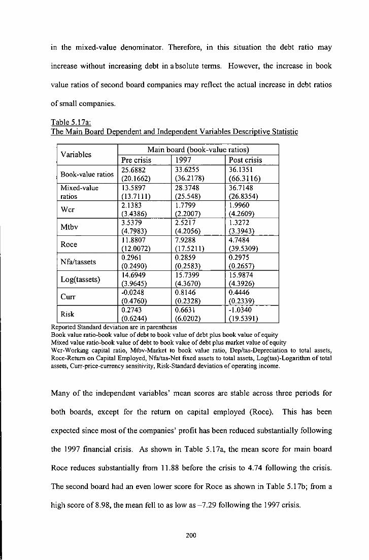
m the mixed-value denominator. Therefore, in this situation the debt ratio may

increase without increasing debt in absolute terms. However, the increase in book

value ratios of second board companies may reflect the actual increase in debt ratios

of small companies.

Table 5.17a: The Main Board Dependent and Independent Variables Descriptive Statistic

Variables Main board (book-value ratios)

Pre crisis 1997 Post crisis

Book-value ratios 25.6882 33.6255 36.1351 (20.1662) (36.2178) (66.3116)

Mixed-value 13.5897 28.3748 36.7148 ratios (13.7111) (25.548) (26.8354)

Wcr 2.1383 1.7799 1.9960 (3.4386) (2.2007) (4.2609)

Mtbv 3.5379 2.5217 1.3272 (4.7983) (4.2056) (3.3943)

Roce 11.8807 7.9288 4.7484 (12.0072) (17.5211) (39.5309)

Nfa/tassets 0.2961 0.2859 0.2975 (0.2490) (0.2583) (0.2657)

Log(tassets) 14.6949 15.7399 15.9874 (3.9645) (4.3670) (4.3926)

Curr -0.0248 0.8146 0.4446 (0.4760) (0.2328) (0.2339)

Risk 0.2743 0.6631 -1.0340 (0.6244) (6.0202) (19.5391)

Reported Standard dev1anon are m parenthesiS Book value ratio-book value of debt to book value of debt plus book value of equity Mixed value ratio-book value of debt to book value of debt plus market value of equity Wcr-Working capital ratio, Mtbv-Market to book value ratio, Dep/tas-Depreciation to total assets, Roce-Rerum on Capital Employed, Nfa/tas-Net fixed assets to total assets, Log(tas)-Logarithm of total assets, Curr-price-currency sensitivity, Risk-Standard deviation of operating income.

Many of the independent variables' mean scores are stable across three periods for

both boards, except for the return on capital employed (Roce). This has been

expected since most of the companies' profit has been reduced substantially following

the 1997 financial crisis. As shown in Table 5.17a, the mean score for main board

Roce reduces substantially from 11.88 before the crisis to 4.74 following the crisis.

The second board had an even lower score for Roce as shown in Table 5.17b; from a

high score of 8.98, the mean fell to as low as -7.29 following the 1997 crisis.

200

Table 5.17b: The Second Board Dependent and Independent Variables Descriptive Statistic

Variables Second board (book-value ratios)

Pre crisis 1997 Post crisis

Book-value ratios 28.713 41.5632 61.0884 (21.1934) (31.3983) (72.9496)

Mixed-value 16.9686 46.2281 63.1458 ratios (16.4705) (31.5758) (81.4094)

Wcr 1.2789 1.2548 1.2639

(1.0457) (0.8565) ( 1.2385)

Mtbv 4.1295 4.2398 1.6487

(3.6656) (9.6274) (5.8795)

Roce 8.9786 9.1138 -7.2941

(7.0698) (20.3516) (59.5399)

Nfa/tassets 2.3174 7.9446 1.1083

(15.8621) (40.7925) (2.8837)

Log(tassets) 10.6014 10.7234 11.0285 (1.5025) (2.1922) (1.7032)

Curr -0.0510 0.8465 0.3658 (0.2918) (0.2714) (0.1807)

Risk 0.5027 0.2003 0.3809 (2.3491) (4.3704) (10.6455)

.. Reported Standard deviatiOns are m parenthesiS Book value ratio-book value of debt to book value of debt plus book value of equity Mixed value ratio-book value of debt to book value of debt plus market value of equity Wcr-Working capital ratio, Mtbv-Market to book value ratio, Dep/tas-Depreciation to total assets, Roce-Return on Capital Employed, Nfa/tas~Net fixed assets to total assets, Log(tas)-Logarithrn of total assets, Curr-price-currency sensitivity, Risk-Standard deviation of operating income.

Wcr, Log(tas) and Risk have a stable mean across three periods for both boards.

However the standard deviation of Risk shows a very significant increase following

the crisis. Risk is formulated by standard deviation of EBITDA, a proxy for earnings

volatility. As profit (Roce) showed a significant decrease in value following the

crisis, the EBITDA would expect to suffer under the same circumstances. Therefore,

the volatility of the companies' earnings will be reflected in EBITDA's variance or

standard deviation.

There is a slight decrease in Mtbv of both boards following the crisis as this may be

due to the decrease in the market value of the equity following the crisis. Although

the main board had stable figures for Nfa/tas across three periods, the second board

201

had a very high Nfa!tas figure during 1997. However, the high figure was also

followed by a very high standard deviation. Therefore, there is high variance of

Nfa/tas in 1997. The main board and second board Curr correlation changed from a

weak negative correlation before the crisis to a high positive correlation in 1997 and

moderate positive correlation after the crisis. Graphs 4.14 and 4.15 in Chapter 4

depicts that from early 1996 towards the end of 1997, there has been small

discrepancy between stock prices and the currency movement, therefore, this resulted

in negative relationship between shares prices and the ringgit within that period.

However, when the ringgit depreciated considerably in the late 1997 and thereafter,

the stock market steadily collapsed. Eventually, the companies share prices on both

boards dropped considerably in the last quarter of 1997 resulting in high positive

correlation with the ringgit in 1997 and moderate positive correlation following the

CnSIS.

5.6.2 Modelling for Multiple Regression Analysis and Cross Sectional Result

The multiple regression models expresses the capital gearing as a linear function of

potential capital structure determinants;

Equation 5.1

GearingP"-"'''' =a+ /],Wcr + /32mtbv +/],Race+ f34 Nfa I tas + f35 Lag(tassets) +

f36 currency + /31 Risk + t:

HA :/31 > 0;/]2 > 0;/]3 < 0;/]4 > 0;/]5 > 0;/]6 < 0;/]1 < 0

Gearing 1991 =a+ f31Wcr + f32mtbv + f33 Race + /]4 Nfa I tas + f35Lag(tassets) +

/36currency + /]1 Risk + t:

HA:/],> 0;/]2 > 0;/]3 < O;fJ. > O;[J, > O;fJ. < 0;/]7 < 0

Gearing post-crisis =a+ fJ,Wcr + /]2mtbv+ /],Race+ /34 Nfa I /as+ fJ,Lag(tassets) +

f36currency + f37 Risk + t:

HA:/], >0;/]2 >0;/]3 <O;fJ. >0;/], >O;fJ. <0;/]7 <0

202

where,

Gearing precrisis , 1997 , posrcrisis = total debt as a percentage of total debt plus equity

Wcr: Working capital ratio, (current assets divided by total current liabilities)

Mtbv: Market to book value ratio, (market value divided by the equity book value)

Roce: Return on capital employed, (pre tax profit plus net interest divided by total

capital employed plus short term debt)

Nfa/tas: Net fixed assets to total assets, (fixed assets divided by the total assets)

Log (tas): Log of total assets employed by the company

Curr: Correlation coefficient ofringgit against the stock prices of the company.

Risk: The standard deviation of operating income, EBITDA

Hypothesis:

Null hypothesis(fJ=O)

Alternative hypotheses (fJ;tO)

The following hypotheses H4 to HI 0 are derived from Section 4.3 in Chapter 4:

HO: Firms' capital gearing stay the same

Alternatively,

H3: Firms' gearing is significantly related to firms' liquidity

H4: Firms' gearing is significantly negatively related to firms' growth/investment opportunities

HS: Firms' gearing is significantly negatively related to the firms' profitability

H6: Firms' gearing is significantly positively related to the firms' tangibility

H7: Firms' gearing is significantly positively related to the firms' size

H8:Firms' gearing is significantly negatively related to the price currency sensitivity

203

H9: Finns' gearing is significantly negatively related to the firm's operating risk

N.B * H4 does not state a positive and negative relationship, (see the literature review or Sections 4.5.1.1 & 4.5.1.2 in Chapter 4)

5.6.2.1 Cross Sectional Result

Table 5.18 shows the six models built using the multiple regression for both boards

across three periods of time. The models are based on the book value ratios in which

total· debt is divided by total debt plus equity. A separate discussion on the mixed

value ratios will be presented later in Section 5.6.7. Since the p-values are less than

0.01· across six models, there are statistically significant relationships between the

dependent and the independent variables at the 99 per cent confidence level. The

adjusted r-squared shows a percentage of25.95, 44.91 and 28.77 for the main board

pre-crisis, 1997 and post-crisis periods, respectively. The second board figures are

40.69 per cent during the pre-crisis, 31.20 per cent during 1997 and 23.48 per cent

during the post-crisis. Therefore, the main board 1997 model is the best fitted model

with the highest r-squared, 44.91 per cent and a 39.90 F-statistic ratio. On the other

hand, the least fitted model is the second board post-crisis period with an r-squared of

23.48 per cent and a 9.55 F-statistic ratio.

Working capital ratio (Wcr) and return on capital employed (Roce) are statistically

significant at either 95 or 99 per cent confidence level across six models with negative

coefficients. The former is the proxy for liquidity and the latter is the proxy for

profitability. The size proxy, Log(tas) shows a significant p-value with a positive sign

for all three periods of the main board, while the second board shows a shift in trend

from a positive coefficient before the crisis to a negative coefficient after the crisis.

The rest of the independent variables show mixed results.

204

The second board Nfa/tas are positively significant before and after the crisis at 95

and 90 per cent confidence level, respectively. The main board Mtbv has a positive

significant sign in 1997 and the second board Mtbv has a negative significant sign

during the post crisis period. The main board risk has a positive significant

relationship with debt before the crisis. The correlation coefficients of currency and

share prices are not significant at all across the six models. In general, it appears that

crisis does not have any effect at all on Wcr and Roce as these variables are

significantly related to debt across three periods for both boards.

Section 5.6.3 will discuss the findings of each independent variable separately. The

results are based on the pre-crisis, 1997 and post-crisis models in Table 5.18, page

199 for both the main board and the second board. The discussion will be followed

by the comparison of using gearing based on book value ratios and mixed value ratios

in Section 5.6.4. Finally, the cross sectional data were "pooled" together in Section

5.6.5 for the panel data regression. The multiple regression of the panel data is to

compare the results between gearing using cross sectional data at three different time

periods and the results of gearing using time series and cross-sectional data together.

5.6.3 Discussion

5.6.3.1 Liquidity (proxied by Working Capital Ratio, Wcr)

Working capital ratios are a proxy for liquidity. Liquidity has a negative coefficient

across three periods for both boards either at the 95 per cent or 99 per cent confidence

205

Table 5.18: Factors Determined the Main Board and the Second Board Firms' Book Value Ratio Analyse Using Multiple Regression

Main board Second board (book value ratios) (book value ratios)

Pre-crisis 1997 Post-crisis Pre-crisis

Constant 29.6893 27.0771 27.9755 -44.8696 (5.896) (3.114) . (1.860) (-3.754)

Wcr -1.5609 -3.0280 -1.5122 -6.9711 (-5.328)*** (-4.521)*** ( -2.254)** (-4.664)***

Mtbv 0.1344 0.7267 0.9691 0.3239 (0.6098) (2.0497)** (1.1269) (0.8021)

Roce -0.7566 -1.3807 -0.8334 -0.5912 (-8.212)*** (-15.311)*** (-11.265)*** (-2.545)**

Nfa/tas -6.1539 1.1007 -3.8971 0.2377 ( -1.4391) (0.1831) ( -0.3445) (2.4043)**

Log(tas) 0.6086 0.9304 1.1814 8.2917 (2.280)** (2.494)** (1.687)* (7.510)***

Curr -3.9337 19.0885 -15.6948 -1.7477 ( -0.622) (1.362) (-0.877) (-0.128)

Risk 3.5136 0.0515 -0.0007 0.7465 (2.187)** (0.215) (-0.005) (1.194)

R-squared 27.59% 46.07% 30.25% 43.96%

Adj. R-25.95% 44.91% 28.77% 40.69%

squared

F -statistic 16.77 39.90 20.38 13.44

(P- value) 0.0000 0.0000 0.0000 0.0000

Book value ratio of debt= Total debt over total debt plus book value eqmty *,**,***Significant at the 10, 5, and I per cent level, respectively. Reported t-statistic are in parenthesis

1997

60.4368 (4.495) -14.4092 (-6.576)*** 0.1095 (0.4879) -0.5813 (-5.613)*** -0.0928 (-0.8654) 0.0940 (0.091) 0.7131 (0.044)

-0.0041 (-0.008)

33.78%

31.20%

13.12

0.0000


Post-..

COSIS

146.106 (4.222) -22.2087 (-6.241)*** -1.8798 (-2.2272)** -0.3234 (-3.567)*** -1.4431 (-1.7110)* -6.1342 (-2.164)** 13.8788 (0.546) -0.0265 ( -0.436)

26.22

23.48%

9.55

0.0000

Wcr-Working capital ratio, Mtbv-Market to book value ratio, Dep/tas-Depreciation to total assets, Roce-Retum on Capital Employed, Nfa/tas-Net fixed assets to total assets, Log(tas)-Logarithm of total assets, Curr-price-currency sensitivity, Risk-Standard deviation of operating income.

level. Therefore, the more liquid the firm is, the lower is the gearing. Obviously, a

ratio of one and above is usually considered as reasonably possible in meeting current

obligations. Studies of bankruptcy have emphasised the importance of I iquidity for

immediate solvency, which suggest that the higher the liquidity, the lower is the

bankruptcy cost or financial distress. Hence, debt would be expected to rise with the

increase in liquidity, resulting in a positive coefficient. Nevertheless, an inverse

relationship is found from the regression analysis of Malaysian firms. Intuitively, if

206

short-term debt increases, ceteris paribus, the working capital ratio will decrease, and

the gearing ratio will increase. The reason is due to the presence of short-term debt in

the gearing measurement, whereby any increase in the short-term debt, ceteris

paribus, will increase the amount of gearing. Therefore, this results in a negative

relationship between gearing and the working capital ratio.

Table 5.18a shows the mean of short-term debt over a 7-year period for both boards.

The short term debt of the main board companies increased substantially from 1994 to

1997, but decreased in 1998, while second board companies' short term debt

increased throughout the whole period. Bris et al. (2002), Claessens et al. (1998) and

Pomerleano (1998) also documented the rapidly increasing short-term debt ratios in

the Asian countries from 1992 to 1996.

Table 5.18(a): The Main Board and the Second Board Average Short-term Debt

Year 1994 1995 1996 1997 1998 1999 2000

Main board 75731 144434 223048 306910 257445 261380 264552 ( 165328) (253852) (982195) ( 1.5E6) (495053) (566251) (645277)

Second board 31686 76003 118720 198429 248862 263712 266718 (119002) (338264) (607093) (I.OE6) (1.3E6) ( 1.4E6) (1.5E6) ..

Reported standard deviation IS m parenthesis

Ozkan (200 I) proposed a positive and negative relationship between gearing and

firms' liquidity. The positive stance is due to a greater ability to meet short-term debt

obligations reflected in more liquidity and a negative relationship may be due to the

reason that firms may use current assets to finance their investment, therefore less

debt is needed for the investment. Using UK companies' panel data, Ozkan found a

negative relationship between gearing and liquidity. He explained that firms with high

207

liquidity may use the assets to finance their investment. Therefore, the firm's liquidity

position should exert a negative impact on its gearing ratio.

The negative sign of liquidity is evidence of building up "financial slack" by storing

excess funds by managers until they are needed. The agency perspective would

suggest that firms should use less debt to afford more financial slack; i.e hold asset

with a low return. The argument is based on Myers and Majluf (1984) who advocate

that managers do not distribute free cash flows but rather invest them in alternative

venues. These cash flows will be retained in a form where they are readily accessible;

i.e. as cash or short-term financial assets (current assets). By doing so, the companies

ensure that they have sufficient financial slack so financing is readily available for

good investment. The suggestion is to follow the conservative style of financing,

which uses less debt and relies more on capital investment and operating decision

rather than financing. In this case, the agency costs are lower, and managers do not

feel pressurised and the potential lender perceives the company's debt as a safe

investment. The argument on financial slack supports the negative relationship

between debt and liquidity for Malaysian companies.

5.6.3.2 Investment Opportunities (proxied by Market to Book Value Ratio-Mtbv)

As suggested by Myers ( 1977), market to book value (Mtbv) is used as proxy for

investment opportunities or growth. Most of the p-values for the market to book

value are not significant except for the 1997 of the main board and post-crisis of the

second board. The 1997 main board market to book value is positively related to

gearing while the post-crisis second board is negatively related to gearing, a contrast

between the large and the small companies. Titman and Wessels' (1988) empirical

208

research found that growth is positively related to LTD/BVE {long term debt divided

by book value of equity) and negatively related to L TD/MVE (long term debt divided

by market value of equity). Thus, the findings of the main board are therefore

consistent with the findings of their book-value ratios.

On the other hand, the second board negative coefficient is consistent with Myers'

(1977) argument that highly geared firms are more likely to forgo profitable

investment opportunities; therefore, firms that expect high growth rates in the future

should use more equity to finance their projects. The negative results for the second

board are in line with his views as second board companies were highly geared

following the crisis (table 5.17b). Therefore, if the firms are forecasting a high

prospect in the near future, they will more likely use equity than debt, resulting in a

negative relationship between debt and investment opportunity.

Myers's suggestion is supported by Rajan and Zingales' (1995) empirical work on the

capital structure oft he G7 countries. A ccording to them, a negative correlation is

expected between gearing and market to book value ratio as firms with high market to

book value ratios have higher costs of financial distress. Their empirical study found

that all market to book value ratios (Mtbv) of G7 countries are negatively related to

gearing for both the debt to book value measure and the debt to market value measure.

Chung (1993) and Barclay et al. (1995) found a similar negative correlation between

growth opportunities and gearing.

Despite the controversy of the positive and negative signs of the market to book value

ratio and gearing, Kester ( 1986) did not find any support for the predicted negative

209

relationship between growth opportunities and gearing. This is similar to the other

four models in Table 5.18 (main board-pre-crisis and post-crisis, second board-pre

crisis and 1997).

5.6.3.3 Profitability (proxied by Return on Capital Employed, Roce)

A consistent negative correlation of return on capital employed (Race) is shown in

Table 5.18 for both boards before, during and after the crisis. The results of a

negative coefficient are consistent with the findings of many empirical works such as

Toy et al. (1974), Long and Malitz (1985), Kester (1986), Rajan and Zingales (1995)

and Krishnan et al. (1996). Myers (1984) suggests that most firms follow pecking

order theory in capital structure decisions in which a retention is preferred over the

use of debt and new equity. If his suggestion is right, past profits are expected to have

a negative relationship with gearing. In this sense, profitability allows the firms to use

retained earnings rather than an external source and therefore a negative association

between gearing and profitability would be expected.

A survey by Kester and Mansor (1994) on I 04 Malaysian companies found that

Malaysian finance managers preferred internal sources of funds over external funding.

Their survey outcomes are consistent with the negative coefficient found in this

research. Thus, the negative sign of Malaysian firm's profitability is consistent with

the pecking order theory forwarded by Myers (1984) and Myers and Majluf(l984).

The financial crisis would be very unlikely to have any affect on the role of

profitability in relation to gearing, since negative coefficients are realised across the

three periods. The reason may be due to the preference for retained earnings; if the

firms' past profit is already high, the firms will use the retained earnings to fmance

210

their investment during the 1997 and following the 1997 financial crisis. Another

possible explanation is that not many investments were carried out after the crisis; as a

result, the past profit will be enough to fund any profitable investment.

5.6.3.4 Size (proxied by Total Assets, Log(tas))

Log(tas) is a proxy for size as used by many past studies. A positive coefficient of

size in relation to gearing was found for the companies listed at the main board

before, during and after the crisis period at 95, 95 and 90 per cent confidence level,

respectively. For the second board, the company's size is positively related to gearing

before the crisis at 99 per cent confidence level. The results indicate no significant

relationship during the crisis and are negatively correlated at 95 per cent confidence

level after the crisis.

Martin and Scott (1974), Ferri and Jones (1979), Crutchley and Hansen (1989), Rajan

and Zingales ( 1995) found a positive relationship between capital structure and size in

their studies. Many of those studies proposed that a positive relationship exist

between gearing and size with the arguments that larger firms should be able to

borrow more due to their low financial distress and bankruptcy costs. Rajan and

Zingales (1995) argued that size may be proxy for the probability of default, where

the bigger the size, the I ower is the probability of defaulting in debt, therefore the

higher is the debt capacity. Their empirical evidence has proven that size is

positively related to gearing for US, Japan and Canada using the measure of book

value ratios and the mixed value ratios.

211

The main board results are consistent with past studies, which show that gearing will

increase with the increase in size. Therefore, the presence of the financial crisis does

not change the on-going relationship of gearing and size of the main board companies

given that the size is positively significant across the three periods. H owever, the

second board companies are mostly small and new, suggesting that the probability of

default would be higher. Therefore, this indicates a positive relationship during the

pre-crisis period whereby the smaller the size of the firm, the lower is the debt. There

is no statistical relationship derived during the 1997 as most of the companies were in

a state of uncertainty in trying to deal with the collapse of the financial market.

Following the crisis, the probability of default was expected to be higher for those

companies under the second board because they were new and immature with small

and unstable assets in place. However, Gupta (1969) argued that smaller US

manufacturing firms would find external equity very expensive and by selling shares,

they will have to share the ownership of the firms. Therefore, smaller firms would

settle for debt. But this does not explain the change in sign following the crisis.

Another possible explanation for the reverse sign is the establishment of a number of

funds by the government to the financial institutions in relation to the financial crisis

to provide credit to the priority sectors including small businesses (this was mentioned

in section 5.5.4). Funds to the amount of 1.5 billion Malaysian ringgit were allocated

to the small and medium industries (BNM, 1999). With such amount of funds, the

debt level of the smaller companies will increase regardless of the higher probability

of default. The situation is a lot better for the companies on the main board as they

are more diversified with stable assets, and are less prone to bankruptcy.

212

5.6.3.5 Tangibilty (proxied by Net Fixed Assets/Total Assets)

The proportion of net fixed assets to total assets is the proxy for tangibility. None of

the statistical tests on the main board net fixed assets to total assets proved any

significant results across the three periods. Hence, tangibility of the main board firms

does not have any effect on their gearing. Many studies, including Jensen and

Meckling (1976), Titman and Wessels (1988) and Rajan and Zingales (1995)

proposed a positive result between gearing and tangibility. The underlying reason for

hypothesising a positive relationship is that the tangible assets are easy to

collateralise, may increase the company's debt capability and at the same time will

reduce the agency's costs of debt. Graph 4.11 in chapter 4 and Table 5.17(a) show a

very low average of main board net fixed assets to total assets ratio of 0.2961, 0.2859

and 0.2975 for the pre-crisis, 1997 and post-crisis periods, respectively. With the low

figures shown and the low variation of the mean, net fixed assets may not be an

important factor with regard to gearing, and, therefore, no significant relationship

would be realised from the regression analysis.

Conversely, the second board pre-crisis and post-crisis net fixed asset ratios are

significant at the 95 and 90 per cent confidence level. The former shows a positive

relationship while the latter is negatively correlated to gearing. The pre-crisis positive

coefficient is consistent with the studies previously cited. With reference to Table

5.17 (b), the proportion of second board net fixed assets to total assets is definitely

higher than that of the main board at 2.317 4 during the pre-crisis, 7.9446 in 1997 and

1.1083 following the 1997 crisis. The firms may use net fixed assets as collateral as

suggested by previous studies discussed earlier which would have resulted m a

positive sign between the firm's gearing and tangibility before the crisis. No

213

significant results were obtained for the 1997 model. The results are almost similar to

the findings of the second board Log(tas), which indicate a significant positive

relationship before the crisis, in which no statistical evidence was found during the

crisis and a negative coefficient found after the crisis.

Meanwhile, the negative sign of the post crisis modelling asserts that the higher the

tangibility, the lower is the gearing. Titman and Wessels (1988) pointed out that the

tendency of the managers to consume more than the optimal level of perquisites may

produce the opposite relation between collateralisable capital and gearing levels. To

overcome the problem, they cited the Grossman and Hart (1982) suggestion of

increasing the debt level to increase the bankruptcy threat and thus reducing the

managers' inclination to increase their perk. Furthermore, the debt-holder will closely

monitor any excessive perquisite received by the manager.

Although their suggestions are highly viewed, the researcher feels that the negative

sign of gearing and tangibility is due to the crisis effect on the increase in the second

board book value gearing. The reason is there was a decrease in the proportion of net

fixed assets to total assets following the crisis as compared with the before the crisis

proportion (2.3174 to 1.1 083), and the book value ratio of gearing was increased

substantially following the crisis (28.713 to 61.0884). Therefore, while the firms'

net fixed assets were reducing, the firms' gearing was increasing even faster. The

increase in debt was therefore not supported by the collateral position of the company

in the crisis situation. The increase in gearing of small companies is due to the loans

provided by the financial institutions as discussed in the previous section related to

size (5.6.6.5). Therefore, in this situation, tangibility has very little influence.

214

5.6.3.6 Price-Currency Sensitivity (Curr)

Given that very few studies have established significant relationships between

economic variables and capital structure, this research attempts to discover whether

currency plays an important role in influencing the determinants of capital structure.

Furthermore, the East Asian 1997 financial crisis was initiated by the currency

speculation. However, no statistical evidence has shown any relationship between the

price sensitivity and the gearing for both the main board and the second board before,

during and after the crisis.

Although the sensitivity of the share prices and ringgit does not statistically influence

the gearing, the correlation between those two variables is probably related to the

equity which eventually may have an affect on the debt ratio, explicitly. As shown in

Table 5.17a, the main board Curr mean correlation is -0.0248 during the pre-crisis,

0.8146 during the crisis and 0.4446 after the crisis, (with an average standard

deviation of between 0.2 to 0.4 across the three periods of time.). Although the pre

crisis correlation reveals a negative correlation between share prices and the ringgit,

the correlation coefficient is too small to make any constructive conclusion on the

relationship between the two variables. However, the correlation of ringgit and share

prices was very high during the crisis. As the currency was badly depreciated in

1997, the company share prices also fell, as implied by their strong positive

correlation of 0.8146. If the funding through equity is impossible during that period,

the debt ratio will be expected to rise. However, for the firms with high past profit

(retentions), debt will not be needed for capital investment, therefore there is counter

balancing effect on the debt ratio (remain constant). While the stock market was still

low following the crisis, in September 1998, the government had taken measures to

215

fix the ringgit to the US dollar. This has resulted m the correlation to remain

moderately positive after the crisis.

Table 5.17b of the second board depicts Curr figures of -0.0510, 0.8465 and 0.3658

for before, during and after the crisis, respectively with a standard deviation of 0.2 for

all the figures. The situation is almost similar to the main board companies in which

share prices have a low negative relationship with gearing before the crisis; high

positive relationship during 1997; and moderate positive correlation after the crisis.

Although the mean of the second board and the main board are almost identical,

Graph 4.15 in Chapter 4, illustrates some large discrepancy between the ringgit and

share prices of the second board companies as compared with the main board before

the crisis period. During that optimistic period (pre-crisis), the ringgit moderately

appreciated, but the second board companies' share prices were considerably high,

thus less debt was needed for financing. On the other hand, when Malaysia was hit

with the financial crisis, the ringgit depreciated substantially and share prices of the

small second board companies fell, resulting in a positive correlation between the

ringgit and share prices. In this situation, debt will be a high priority for small

companies especially when past profit was scarcely available. The situation may

change following the ringgit being fixed to the US dollar, however debt was still

accelerating between 1998 and 2000 as shown in Graph 4.1 in Chapter 4.

5.6.3. 7 Risk (Business Risk, proxied by Standard Deviation of EBITDA)

As shown in Table 5.18, the risk is only significant for the main board companies

before the crisis with a positive coefficient at the 95 per cent confidence level.

Therefore, the business risk has no effect on the main board gearing companies during

216

and after the crisis. The risk also has no effect on second board companies before,

during and after the crisis.

The significant results of the main board pre-crisis period suggest that the higher the

risk, the higher is the gearing. T he results imply that during the p re-crisis period,

when the· market was optimistic, firms exhibiting a greater earnings volatility were

more highly geared. The findings are not consistent with many of the traditional

finance textbooks which suggest that firms with a high degree of business risks will

be associated with high financial risk, thus less capacity to borrow more. However,

the notion of an indirect relationship is consistent with a study by Bradley et al.

(1984) which found a statistically significant negative relationship between gearing

and earnings volatility. Studies by Ariff et al. (1990) on the capital structure of

Singapore firms' found a similar positive relationship between gearing and earnings

volatility. Ariff et al. ( 1990) explained that the Bradley et al (1984) findings were

based on the higher costs of financial distress, which might contribute to low gearing

if the operating income was uncertain. Singapore firms nevertheless had low

financial distress, hence providing a positive relationship between gearing and

operating risk.

By observing Table 5.17a of the main board's risk during the pre-crisis, the mean and

standard deviation of the risk are not very high, 0.2743 and 0.6244, respectively,

hence a low probability of financial distress would be expected for the Malaysian

companies. The Ariff et al. (1990) arguments would therefore support the direct

relationship of gearing and risk of the Malaysian companies when the economy is

performing well. Furthermore, the direct relationship found between gearing and risk

217

is also consistent with the study ofKim and Sorenson (1986), where their book-value

ratios and mixed-value ratios of gearing increases with the increase in operating risk.

To support their findings, they cited Myers (1977) proposition that firms with high

business risk may have a lower agency cost of debt, hence would be able to borrow

more. High variance in operating income may reduce the agency cost of debt, rather

than increase it.

5.6.4 Tbe Difference between Book-Value Gearing and Mixed-Value Gearing

Mixed-value ratios are derived from the computation of the book value of debt

divided by the book value of debt plus the market value of equity. As shown in Table

5.19, the results of the main board are not much different between book-value ratios

and mixed-value ratios except for the significant p-value of the 1997's Curr and Mtbv

negative sign. The main board's working capital ratio, return on capital employed

and logarithm of total assets are all significant across three periods of time. Similar

results were achieved for the second board; working capital ratio and return on capital

employed were both significant before, during and after the crisis. The second board

size was found to influence gearing before the crisis period; the other two periods

were not significant.

The studies by Rajan and Zingales (1995) support the similarity of the results

achieved between book-value ratios and mixed-values ratios. They studied the factors

that affected the capital structure of the G7 countries by using the book value of

equity and the market value of equity as a debt measurement. They found that all the

coefficient of the regressions retained their same expected sign using the book value

218

of gearing as when using the market value of the equity in the gearing ratio as a

dependent variable.

The 1997 market to book value (mtbv) of the main board shows a contrasting sign

between the use of the measure of book-value ratios and mixed-value ratios. The

negative relationship between debt and growth under mixed value measures are

consistent with Booth et al. (2001) findings for Malaysia and Titman and Wessels's

(1988) findings discussed previously under investment opportunity of book-value

ratios. Based on a book value weighting, the earnings are not anticipated using

accounting conventions. Based on a market value weighting, the earnmgs are

anticipated, thus firms that expect high growth rates in the future should use m ore

equity to finance their projects through retentions, resulting in a negative correlation

between investment opportunities and gearing.

Since no relationship was found when gearing was measured using the book-value

ratios (see Table 5.18), it is therefore unexpected to have a positive coefficient of the

main board Curr (price sensitivity) during the 1997 based on mixed-value ratios. The

gearing and price sensitivity positive relationship was found significant during an

uncertain and chaotic economic environment, which implies that the higher the price

sensitivity, the higher is the gearing. Therefore, gearing is proven to be affected when

the share prices and the currency are highly sensitive. The result is significant when

the mixed value ratio was used to measure the gearing. During this period, both

currency and share prices were very low due to the depreciation of the ringgit and the

deterioration of the market value of equity, resulting in a highly positive correlation

(see Graph 4.14 and Table 5.17a). In the mathematical expression, the debt ratio will

219

increase if the market value of equity falls. In reality, however, debt may be the only

option due to the falling share prices and companies' profit as a result of the crisis.

Table 5.19: Factors Determined the Main Board and the Second Board Firms' Mixed Value Ratio Analyse Using Multiple Regression

Main board Second board

Variables (Mixed-value ratios) (Mixed-value ratios)

Pre-crisis 1997 Post-

Pre-crisis CflSIS

Constant 5.9360 5.1113 10.1869 -22.8133 (1.6074) (0.6889) ( 1.3696) (~2.3744)

Wcr -0.7174 -1.9809 -1.5793 -4.627 (-3.394)*** ( -3.538)*** (-4.889)*** (-3.687)***

. 0.0159 -1.0577 0.0662 -0.4162 Mtbv (0.0961) ( -3.511 )*** (0.1575) (-1.3130)

Roce -0.3569 -0.4910 -0.1266 -0.3456 (-5.180)*** ( -6.461 )*** (-2.824)*** ( -1.898)*

Nfa/tas -1.9273 -0.7345 0.1690 0.1417 (-0.6223) ( -0.1452) (0.0309) (1.8224)*

Log(tas) 0.9049 1.5274 1.5879 4.7367 (4.687)*** (4.846)*** (4.655)*** (5.380)***

Curr -0.6164 32.0472 13.6892 16.3685 ( -0.1347) (2.6609)*** (1.5585) (1.5320)

Risk 3.4729 0.5221 -0.0593 -0.2166 (2.902)*** (2.488)** (-0.8503) ( -0.4417)

R-squared 23.22% 29.34% 17.99% 34.47%

Adj. R-21.38% 27.76% 16.18% 30.62% squared

F -statistic 12.62 18.51 9.91 8.94

(P value) 0.0000 0.0000 0.0000 0.0000 •, **,***Stgmficant at the 10, 5, and I per cent level, respectively. Reported !-statistic are in parenthesis.

1997

56.5238 4.4082 -16.1293 (-7.709)*** 0.0156 (0.0729) -0.5964 (-6.055)*** -0.0782 (-0.7645) 1.0493 1.0548 3.9673 (0.2524) -0.1785 (-0.1519)

40.82%

38.48%

17.44

0.0000

Mixed value ratio-book value of debt to book value of debt plus market value of equity

Post-CflSIS

82.5053 (2.2654) -18.9646

_(-5.068)*** -0.9786 (-1.!041) -0.6875 (-7.217)*** -0.5613 (-0.6335) 0.3044 (0.1020) -15.4736 (-0.5780) -0.0141 ( -0.2!99)

33.68%

31.18%

13.49

0.0000

Wcr-Working capital ratio, Mtbv-Market to book value ratio, Dep/tas-Depreciation to total assets, Roce-Retum on Capital Employed, Nfa/tas-Net fixed assets to total assets, Log(tas)-Logarithm of total assets, Curr-price-currency sensitivity, Risk-Standard deviation of operating income. N.B. multicollinearity of mixed value ratios are similar to book value ratio (independent variables of both measurement are similar).

The main board risk has shown a positive sign for both pre-crisis and the 1997 period

using the mixed-value ratios measurement. As previously discussed under the book-

value ratios, Kim and Sorenson's (1986) views would support the findings of a

positive coefficient between debt and risk at book-value ratios and mixed-value ratios

as they found a similar result for both measurements.

220

5.6.5 Panel Data

5.6.5.1 Introduction

A I ongitudinal or panel data is a data set that combine both time-series and cross

sectional data. The multiple regressions in Section 5.6.3 only predict using cross

sectional data for three periods of time. The process of combining cross-sectional and

time-series data to form a panel is called pooling. By pooling the data together, it is

possible to study the determinants of the firms' capital structure over a period of time.

The panel data set allows the studying of both the changes in gearing of a single firm

overtime and the variation in the gearing of m any firms at a given point in time.

There are three techniques to treat panel data using the regression analysis. The first

technique is to simply combine, or pool all the time-series and cross-section data and

then estimate the underlying model by utilising OLS (ordinary least square) method.

The second and third techniques involve a dummy (Y) that represents the value of the

dependent variable for individual i at timet. If the 1 is treated as a constant, then the

model is called a fixed effects models which includes the recognition that omitted

variables may lead to changes in the cross-section and time-series disturbances. If the

1 is treated as a random variable, then it is called a random effects model, which

improves the efficiency of the OLS (first technique) estimation process by accounting

for cross-section and time-series disturbances.

The researcher utilises the fzxed effect model which uses dummy 1 and dummy 0.

These dummy variables implicitly classified the gearing in the data set into three

different groups:

i) If D1 = 1 and D2 = 0, pre-crisis is identified;

ii) If D1 = 0 and D2 = 1, 1997 is identified;

221

iii) If D1 = 0 and D2 = 0, post-crisis is identified (default)

Multiple regression is used to predict the coefficient of the panel data. The dummies

were treated as D1 and D2 in the OLS analysis. The foil owing is the panel data

fixed effects model:

Equation 5.2:

where,

Y =represents the dependent variable

DJ>D2 =seeearlier

a 1 ,a2 =estimation I coefficient for D1 ,D2

(see, for example, Koop (2000))

a,fJJ32.f3n =Constant, estimation I coefficient for X1,X2.Xn

%1.%2,% n =Independent variables; variable l, var iable2 and variable n

E:=error

The coefficients of the dummy variables, a 1 and a 2 measure additional value

associated with gearing due to the pre-crisis and crisis period. The coefficients of the

non-dummy variables /31 and /32 are interpreted as the marginal effects of other

independent variables on gearing ( y). The m ode! with dummy variables allows for

different intercepts in the regression line, but the slope of the regression line is always

the same unless dummy and non-dummy were allow for interacting, [Koop (2002)].

The hypothesis for panel data:

HlO: Controlling for variations in pre-specified factors (e.g. liquidity, investment

opportunity, profitability, tangibility, size, price sensitivity and risk), there are

gearing effects caused by the crisis (tested by dummy variables)

222

5.6.5.2 Tbe Panel Data Analysis

Both the book-value ratios and mixed value ratios were regressed against the 7

independent variables that were previously discussed in Section 5.5. The existence of

multicollinearity was also tested. The D1 (pre-crisis) of all models were correlated

above 0.5 with the Curr (see Tables I to 4 in Appendix F). Although Statgraphics

suggests removing one of the variables, both variables are retained as the figure is still

below 0.8. Cooper and Schindler (1998) suggested removing one of the independent

variables if it was correlated at 0.8 or greater. Since the correlation of pre-crisis

dummy and Curr is less than 0.8 for the second board and the main board, the

multicollinearity is not serious, therefore, it would not mislead the results of which

explanatory variable(s) are explaining or influencing the dependent variable.

As shown in Table 5.20, both the main board book-value ratio and the mixed-value

ratio pool data models are significant at the 99 per cent confidence level. The second

board book value ratio is significant at the 99 per cent confidence level while the

mixed-value model is not significant. The main board book value ratios had the

highest r-squared with a percentage of 32.69 while the lowest is the second board

mixed value ratios with a percentage of 2.52. Although three models are significant,

only the mixed value ratios model of the main board has a significant coefficient of

D 1 (pre --crisis) and D2 (1997).

5.6.5.3 Discussion of Panel Data Analysis

The discussion will only emphasise the mixed value model since both D1 and D 2 of

this model is significant. The other independent variables under this model are

significant at least at the 90 per cent confidence level except Risk which is not

223

significant. Pre-crisis (D1 )and post-crisis (D2 ), Wcr, Roce, and Log(tas) are all

significant at 99 per cent confidence level, whilst Mtbv and Nfa/tas are both

significant at 95 per cent confidence level and finally the Curr is significant at the 90

per cent confidence level.

The pre-crisis coefficient figure of -16.7449 is lower than the crisis year (1997) with

a coefficient value of -7.2878. The coefficient figures reflect a small gearing ratio

during the pre-crisis as compared to the post-crisis. There are two different regression

lines depending on whether the gearing is predicted before the crisis or during the

crisis. If the lines were prepared for the period before and during the crisis, the

intercept for the gearing based on the 1997 dummy will be higher than the pre-crisis y

intercept. The results imply a shift in gearing ratio following the crisis. However,

since they have the same slope, the marginal effects of other independent variables are

still the same whether the gearing is predicted for the pre-crisis or in 1 997. The

second board book value model has a weak significant D 2 (1997). Therefore, if the

dummy coefficient were added to the constant, it will increase the gearing ratio during

the crisis.

224

Table 5.20: Factors Determined the Main Board and the Second Board Firms' Book Value and Mixed Value Ratio-Panel Data Analyse Using Multiple Regression

Main Board Variables Book-value Mixed-value

ratios ratios

Constant 26.7685 14.7252 (4.1986) (3.9456)

Pre-Crisis -5.2064 -16.7449 (-1.4468) (-7.971)***

1997 -1.0700 -7.2878 (-0.3586) ( -4.1989)***

Wcr -1.7498 -1.2776 ( -5.0662)*** ( -6.4815)***

Mtbv 0.5875 -0.3348 (2.0408)** ( -1.9865)**

Roce -0.9020 -0.2000 (-19.2911)*** ( -6.2532)***

Nfa/tas 0.5695 0.7281 (1.0879) (2.4453)**

Log(tas) 1.1615 1.4233 (3.4941)*** (7.3681)***

Currency -7.0667 9.6900 (-0.8289) (1.9565)*

Risk 0.0307 -0.0137 (0.3072) (-0.2394)

R-squared 32.69% 29.39%

Adj. R-squared 32.00% 28.65%

F -statistic 48.29 39.36

Prob. F-statistic 0.0000*** 0.0000***

(P value) *, **, ***Stgmficant at least at I 0%, 5% and I% respecllvely. Reported !-statistic are in the parenthesis

Second Board

Book-value Mixed-value ratios ratios 60.1785 -122.471 (4.1543) (-0.8874) -7.9807 -60.2772 ( -1.1627) (-0.9224) -7.8470 38.9653 (-1.7422)* (0.9085) -14.2213 8.2057 (-7.8103)*** (0.4680) -0.2578 0.4337 (-0.9546) (0.1695) -0.2987 -1.3320 ( -4.8845)*** ( -2.2963)** -0.1400 1.0014 (-1.0162) (0.7663) 0.1480 18.6208 (0.1258) (1.6619)* 20.4609 -249.79 (1.4985) ( -1.9247)* -0.0140 0.0604 ( -0.3160) (0.1433)

19.60% 2.5210

18.16% 0.7523

13.57 1.43

0.0000*** 0.1741

Book value ratio-book value of debt to book value of debt plus book value of equity Mixed value ratio-book value of debt to book value of debt plus market value of equity Wcr-Working capital ratio, Mtbv-Market to book value ratio, Dep/tas-Depreciation to total assets, Roce-Retum on Capital Employed, Nfa/tas-Net fixed assets to total assets, Log(tas)-Logarithm of total assets, Curr-price-currency sensitivity, Risk-Standard deviation of operating income. N.B correlation matrixes for pool data are in the Appendix F (Tables I ,2,3 and 4).

225

5. 7 The Results of the Hypotheses

This section covers the outcome of the hypotheses from the statistical tests performed

in Chapters 5. Statisticians recommend either "rejecting" or "not rejecting"

hypotheses, to avoid accepting a hypothesis that is not true. However, in this thesis

the term "accept" a hypothesis, strictly means "do not reject". The hypotheses are

accepted based on the alternative hypotheses, hence, if the alternative hypothesis is

true, the result is "accept", however, if the alternative hypothesis is not true, the result

is "reject". Alternatively, if the alternative hypothesis was false, the result is rejected.

5.7.1 Hypotheses on Gearing Differences

Two differences in gearing have been studied: i) between the main board and the

second board, ii) between six sectors listed . on the main board. There are two

hypotheses formulated to test the differences in gearing:

Hl: There is a significant difference between the main board and the second board firms' gearing in each selected time period (i.e. before, during and after the crisis)

H2: There are significant differences between the gearing ratios in different sectors on the main board in each selected time period (i.e. before, during and after the crisis)

ANOV A and the Kruskal-Wall is techniques were used to test statistically the

statement of the null hypothesis. The ANOV A is a one-way analysis of variance by

mean, while the Kruskal-Wallis is one-way analysis of variance by median ranks.

Based on the book value ratios of gearing, both hypotheses are accepted across three

time periods as shown in Table 5.21. Therefore there are differences in gearing: i)

between main and second board, ii) between six sectors at the main board. The

results are significant across three periods of time using the Kruskal-Wallis (median)

test as compared to ANOV A (mean) which is only significant before the crisis for Hl

226

and H2 and after the crisis for HI. However, at the O.OI significance level, the

ANOV A shows strong differences for HI post-crisis and H2 pre-crisis. In conclusion,

there are differences in book value gearing of the main board and the second board

and there are differences between the book value gearing of the six sectors at the main

board.

Table 5.2I: Gearing Differences Hypotheses Results (Based on Book Value Ratios)

Pre-crisis I997 Post-crisis

Accept Accept HI ANOVA AcceptKruskal-Wall is ANOVA*

Kruskal-Wallis Kruskal-Wallis

Accept Accept Accept

H2 ANOVA* Kruskal-Wallis

Kruskal-Wall is Kruskal-Wallis

All tests Sigmficant at least at 10 per cent level, • s1gmficant at I per cent level

Table 5.22: Gearing Differences Hypotheses Results (Based on Mixed Value Ratios)

Pre-crisis I997 Post-crisis

HI Accept Accept Accept Kruskai-Wallis Kruskal-Wallis* Kruskal-Wallis*

Accept Accept Accept

H2 ANOVA ANOVA* Kruskal-Wall is

Kruskal-Wall is Kruskal-Wallis All tests are sigrnficant at least at I 0 per cent level, * sigrnficant at I per cent level

Similar results have been achieved for gearing based on mixed value ratios. The

Kruskal-Wallis tests were significant for both HI and H2 across three periods of time.

The ANOV A tests were significant for H2 during I997 and post-crisis period.

Therefore, there are differences between mixed value gearing of the main board and

the second board with or without the crisis. At the 99 per cent confidence level, the

I997 and post-crisis periods have the strongest differences. There are differences

between the six sectors' mixed value gearing with or without the crisis, and the post-

227

crisis period showed the highest differences with a p-value of less than 0.01.

5.7.2 Firms' Specific Factors Hypotheses

Seven independent variables that are possibly associated with gearing were selected to

find the determinants of the capital structure of the Malaysian companies. Seven

hypotheses were prepared and multiple regression analysis was used to test the

hypotheses. The statistical tests used were identified in Sections 5.6.3 and 5.6.4. The

hypotheses were applied to both the book value gearing and the mixed value gearing.

The related discussions on each variable a rep resented in Chapter 4, Section 4 .4.1.

The following are the hypotheses related to each board for each time period:

H3: Firms' gearing is significantly related to the firms' liquidity*

H4: Firms' gearing is significantly negatively related to the firms' investment opportunities

H5: Firms' gearing is significantly negatively related to the firms' profitability

H6: Firms' gearing is significantly positively related to the firms' tangibility

H7: Firms' gearing is significantly positively related to the firms' size

H8: Firms' gearing is significantly negatively related to the currency sensitivity

H9: Firms' gearing is significantly negatively related to the firm's operating risk

N.B *the word related without the negative and positive relationship is due to both positive or negative relationships present in the arguments in the literature review

Table 5.23 illustrates the results of the hypotheses for the main board book value

ratios and the mixed value ratios based on multiple regression analysis. The

hypotheses are rejected if the alternative hypotheses are not true. The alternative

hypotheses H3, H5 and H7 have been accepted across the three periods of time based

on both measurements. The H4 and H9 of 1997 and post-crisis period book value

ratios have been rejected, and the H8 of 1997, H9 of 1997 pre-crisis and 1997 have

228

also been rejected. Therefore, the liquidity, profitability and size have a strong

influence over gearing as shown in the results. All three variables are at least

significant at 95 per cent confidence level, suggesting a strong relationship between

the variables and gearing.

Table 5.23: The Main Board Gearing Hvootheses Results

Book Value Ratios Mixed Value Ratios Pre-crisis 1997 Post-crisis Pre-crisis 1997 Post -crisis

H3 accept accept accept Accept accept accept

H4 reject reject* reject Reject accept reject


H6 reject reject reject Reject reject reject


H8 reject reject reject Reject reject* reject

H9 reject* reject reject Reject* reject* reject All tests are s1gmficant at least at I 0 per cent level, *s1gmficant at I per cent level

As shown in Table 5.24, the results for H3 and H5 of the second board are similar to

the main board, both hypotheses are accepted across three periods at both

measurements. There is a strong influence of profitability and liquidity over the

gearing of the second board companies as shown by the significance results. H7 and

H8 show a similar trend of results: the hypotheses are accepted during pre-crisis and

rejected after the crisis for book value ratios, and accept during pre-crisis for mixed

value ratios. Many of the second board alternative hypotheses were rejected as

compared with the main board. None of the hypotheses was accepted for H4, H8 and

H9.

229

Table 5.24: The Second Board Gearing Hypotheses Results

Book Value Ratios Mixed Value Ratios Pre-crisis 1997 Post-crisis Pre-crisis 1997 Post-crisis

H3 accept accept accept accept accept accept

H4 reject reject reject reject reject reject

H5 accept accept accept accept accept accept

H6 accept reject reject* accept reject reject

H7 accept reject reject* accept reject reject

H8 reject reject reject reject reject reject

H9 reject reject reject reject reject reject All tests are s1gruficant at least at I 0 per cent level, * s1gruficant at I per cent level

The panel data were discussed in Section 5.6.5. The study was looking at the time

series effect on the gearing. The following is the hypothesis for the panel data:

HIO: Controlling for variations in pre-specified factors (e.g. liquidity, investment

opportunity, profitability, tangibility, size, price sensitivity and risk), there are

gearing effects caused by the crisis (tested by dummy variables in multiple

regression)

Table 5.25 shows the results of the hypothesis of the panel data in which two models

have a significant dummy result: mixed value ratios of main board and book value

ratios of second board. However, for the second board book value ratios, only one

dummy is significant, dummy 0 which represents 1997. Based on the results, the

alternative hypothesis for the main board mixed value model is accepted and the

second board book value ratios is partially accepted or qualified, while the other two

hypotheses are rejected, the main board book value ratios and the second board mixed

value ratios.

230

Table 5.25: The Panel Data Hypotheses Results

Main board Second Board Book Mixed Book Mixed

value ratios value ratios value ratios value ratios

HlO reject Accept qualified

Reject accepted

All tests are s1gmficant at least at I 0 per cent level

5.8 Conclusion

The Kruskal-Wall is test shows significant differences between the main board and the

second board gearing ratios both at the book value ratios and mixed value ratios

across three time periods. However, the ANOV A test indicates a significant

difference between book value gearing ratios of both boards only during the pre-crisis

and post-crisis. Therefore, differences in gearing exist between the large and small

firms. The results also indicate that small firms are highly geared compared with

large firms using both measurements at three different time periods.

The Kruskal-W allis test shows a weak (90 per cent confidence level) significant

difference between median gearing of the six sectors of firms listed at the main board

using both measurements. However, the ANOV A test shows a significant difference

between mean gearing of the six sectors when using mixed value ratios measurement.

The Bonferrani test on the sector differences has revealed that out of the six sectors

tested, only plantation sector's gearing is statistically different from the gearing of

other sectors. The result also shows that construction has the highest gearing ratio at

the book value ratio and mixed value ratio while plantation has the lowest.

231

Based on the multiple regression analysis, not many differences were found between

gearing using book value and mixed value ratios. Profitability and liquidity of both

boards have the same effects on gearing across three time periods either using book

value ratios or mixed value ratios. Size on the other hand has the same positive effect

on gearing through three periods using both measurements but only for the main

board companies. For the second board companies, size has an effect on book value

gearing during the pre-crisis and the post-crisis, and when measured by mixed value

ratios, the results indicate that second board firms' size is only positively significant

during the pre-crisis period. For the rest of the independent variables, mixed results

were found.

The mixed value ratios of panel data found that profitability, liquidity and size, the

investment opportunity, tangibility and currency are related to gearing. The statistical

results of the mixed value model reveal that gearing ratio of 1997 is higher than

gearing ratio of the pre-crisis period, implying an increase in gearing due to the 1997

financial crisis. The second board book value ratio model has a significant dummy

during 1997. Therefore, gearing is shifting up during this period, but no comparison

can be made with the pre-crisis period as the dummy for that period is not significant.

The dummies of other two models of panel data are not significant, therefore, no

conclusion can be drawn from that analysis.

232

CHAPTER6 MALAYSIAN CAPITAL STRUCTURE: BEHAVIOURAL REACTIONS

6.1 Introduction

Chapter 6 mainly covers data from the questionnaire mail survey. The purpose of the

questionnaire survey is to examine the behavioural response of finance managers to

the assessment on the capital structure. It is considered appropriate for this research

to study and analyse both the secondary data from Datastream and the primary data

from the survey. A m ore constructive and comparable result will be achieved as a

result of studying two different sets of data from the same population.

A number of statistical tests have been employed on the questionnaire surveys,

consisting of the chi-square test, analysis of variance and logistic regression analysis.

The chapter is organised as follows: Section 6.2 briefly describes the pilot study,

Section 6.3 provides an overview of the questionnaire which includes the response

rate of the survey and frequency distribution of the responses provided by the

respondents. Section 6.4 and Section 6.5 each outlines a comprehensive data analysis

using chi-square and the ANOV A, respectively. Section 6.6 reviews the logistic

regression analysis while Section 6. 7 discusses the results of the hypotheses. Section

6.8 summarises the telephone interview and finally, Section 6.9 concludes the chapter.

233

6.2 Pilot Study

A pilot study is a small-scale trial before the main investigation is canied out, it is

intended to test the research instrument and avert any problems or ambiguity.

Bourque and Fielder (1995) and Saunders et al. (1997) emphasise the importance of

employing representative members of the target population in the pilot, even though

these results may not then be included in the overall findings, as they may contribute

to the necessity for changes to the main questionnaire or its administration. Sauders

et al. (1993) coded Bell's (1993) advice on the importance of the pilot test:

"however pressed for time you are, do your best to give the questionnaire a trial run as, without a trial run, you have no way of knowing that your questionnaire will succeed"

(Bell (1983, p.84 cited in Sauders (1993), p.269)

The first draft of the questionnaire was disseminated vta email to the finance

managers of the 200 companies listed under the KLSE for a pilot test. Email was

chosen as the medium of distribution for the pilot questionnaire due to its speed and

minimal cost. However, there are a few drawbacks to the method used because (i) not

all companies have their own web-site which makes it very difficult to obtain the

email addresses of the finance managers, (ii) not all finance managers have email

accounts and (iii) email is still considered as an inappropriate delivery method for

official business-related correspondence. A total of 20 valid responses were received,

representing I 0 per cent of total sample sent.

After the questionnaire had been piloted satisfactorily, it was decided to proceed with

the main survey. The main questionnaire was developed after considerable changes

and improvements have been made based on the feedback obtained from the pilot

study. Significant changes were made to the Likert scales of questions 1 and 2. The

234

response option of"During the next 12 months" and "in the longer term" for Question

I has been changed to "high, medium and low priority". For Question 2, the response

option has been changed to "Large, Medium and No Change". Question 2 has been

divided into a few sub-questions. A few additional questions were also included in

the revised version of the questionnaire. A copy of the pilot and postal survey

questionnaire are attached in Appendixes I and J.

6.3 Postal Surveys

The postal survey questionnaire was sent from the United Kingdom to the companies

listed under the main board of the KLSE in April 2001. The addresses were obtained

from the KLSE web-site which is linked to the companies' web-site. A total of 357

questionnaires were sent to the following sectors listed under the main board of the

KLSE: construction, consumer products, industrial products, trading and services,

plantation and properties. These sectors have been categorised by the KLSE and are

available online from the Datastream. The same sectors were used in chapter 5 under

the Datastream data analysis.

The questionnaire was numbered individually by hand on the top right corner. It was

intended to facilitate the counting of the questionnaire during the administration of the

survey. The respondents were requested to mail the completed questionnaire back to

the researcher in the self-addressed stamped envelope provided. This was also to

encourage a high response rate as it was felt that finance managers were more likely

to reply.

235

A few minor problems were encountered during the process of administration of the

questionnaire. These included problems with addresses of the finance managers

where in most cases, the questionnaire was sent to the secretary's office of the

companies, instead of the office of the finance managers. Considerable hours had to

be allocated to contact the companies by phone to get their correct mailing addresses.

Despite all the follow-up efforts a low response rate of 10 per cent was obtained. To

improve the rate of return and as a form of a second reminder, the questionnaire (see

Appendix K) was sent out again to the companies which have yet to return the

completed questionnaire back to the researcher. These companies have been

identified and singled out from the number on the top right corner of the

questionnaire. According to Cooper and Schindler ( 1998), follow-ups or reminders

are very successful in increasing the response rates of the questionnaire survey.

6.3.1 Response Rate

The completed survey forms were returned back to the researcher in the sealed

envelopes provided. A number of the completed survey forms received had had the

individual serial numbers intentionally removed by the respondents. Despite giving

complete assurance of confidentiality on the cover letter attached to the survey forms,

it was obvious that some finance managers had tried to avoid detection. A number of

the participants had given valuable feedback to the researcher by providing additional

comments as well as their personal business cards. Nevertheless, a majority of the

target population had satisfactorily completed and returned the questionnaire back to

the researcher.

236

Following the reminder, a total of 71 valid completed questionnaires had been

received from the sample of 357 companies listed on the main board. The

computation of the response rate differs from one statistician to another. The simplest

method of calculation is to divide the total number of respondents in the sample by

the total number of questionnaire sent. In this case, a total of 19.89 per cent has been

obtained by dividing 71 by 357. However, deVaus's (1991) approach is to subtract the

'unreachable' or 'non-response' from the total sample in the calculation. Sauders et

al. {1993) define 'unreachable' or 'non response' as refusal to respond, ineligible to

respond and cannot be contacted. Approximately 65 companies have been identified

as non-response in this survey, therefore the response rate is equivalent to 24.32 per

cent [71/(357-6S)t

The accepted percentage for the survey response varies among statisticians. Dillman

(1978) recorded a response rate of 50 to 92 percent for questionnaire survey, while

Owen and Jones ( 1990) and Cooper and Schindler (1998) considered 30 per cent

response as reasonable. However, Saunders et al. ( 1997) reviewed the latest business

survey response rates and have found rates as low as 15 to 20 percent. Therefore, a

response rate of 24.32 per cent obtained for this study is considered satisfactory when

compared with other similar studies with similar or even much lower rates. This

includes Kester and Mansor (1993), Trahan and Gitman (1995) and Graham and

Harvey (2001), whom had obtained a response rate of28.8 per cent, 12 percent and 9

per cent, respectively.

9 (total number of responses/( total number in sample-non-response))

237

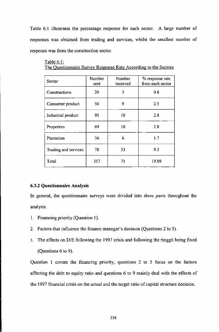
Table 6.1 illustrates the percentage response for each sector. A large number of

responses was obtained from trading and services, whilst the smallest number of

response was from the construction sector.

Table 6.1: The Questionnaire Survey Response Rate According to the Sectors

Sector Number Number % response rate

sent received from each sector

Constructions 29 3 0.8

Consumer product 50 9 2.5

Industrial product 95 10 2.8

Properties 69 10 2.8

Plantation 36 6 1.7

Trading and services 78 33 9.2

Total 357 71 19.89

6.3.2 Questionnaire Analysis

In general, the questionnaire surveys were divided into three parts throughout the

analysis.

1. Financing priority (Question 1 ).

2. Factors that influence the finance manager's decision (Questions 2 to 5).

3. The effects on DIE following the 1997 crisis and following the ringgit being fixed

(Questions 6 to 9).

Question 1 covers the financing priority, questions 2 to 5 focus on the factors

affecting the debt to equity ratio and questions 6 to 9 mainly deal with the effects of

the 1997 fmancial crisis on the actual and the target ratio of capital structure decision.

238

Tables 6.2, 6.3 and 6.4 have been prepared to show the frequency distribution for

question 1, questions 2 to 5, and questions 6 to 9, respectively. Frequencies of

individual sources were computed using SPSS version 9.0.

The frequency distribution in Table 6.2 for question 1 shows retentions as the highest

priority among firms in terms of financing preference, accumulating a total of 70.8

per cent, while preference shares obtained the lowest scores under high priority at 1.7

per cent. Under the medium priority of financing preferences, overdraft scores the

highest at 47.7 per cent while 'others' had the lowest score of 11.1 per cent. Under

the low priority column, the results were just the opposite, preference shares had the

highest score of 74.1 per cent while retention had the lowest score of 12.3 per cent.

Table 6.2: Frequency Distribution for Question 1 (in percentage)

Sources of funds High Medium Low

Total priority priority priority

Internal equity (retentions) 70.8 16.9 12.3 100

Ordinary shares 31.3 31.3 37.5 100

Preference shares 1.7 24.1 74.1 100

Islamic bonds 10 33.3 56.7 100

Conventional bonds 22.2 38.1 39.7 100

Islamic bank loan 12.1 41.4 46.6 100

Conventional bank loan 42.4 43.9 13.6 100

Overdrafts 26.2 47.7 26.2 100

Finance leases 17.5 22.8 59.6 100

Others (please specify) 55.6 11.1 33.3 100

·······························

Table 6 .3 shows the frequency distribution for questions 2 to 5 . The questions a re

related to debt to equity response due to the certain factors that may determine the

firms' capital structure. The increase in fixed assets had the highest score of 24.6 per

239

cent refening to the Large Increase in DIE column, while the significant increase in

profit shows the highest score of30.4 refening to the Large Reduction in DIE column.

As for No Change in DIE, the highest score is 88.1 per cent which is the response to

the increase in public disclosure of accounting. A significant decrease in profit scores

the highest for the Moderate Increase in DIE, accumulating a total score of 55.1 per

cent, while a significant decrease in fixed overhead costs scores the highest for

Moderate Reduction in DIE.

Table 6.3: Frequency Distribution for Questions 2 to 5 (in percentage)

Large Moderate No Moderate Large Total Questions 2 to 5 Reduction Reduction change in Increase Increase

% in DIE" in DIE DIE in D/E in DIE

A significant increase in fixed assets as a proportion of total 5.8 I 0.1 17.4 42 24.6 100 assets

A significant decrease in fixed 5.8 60.9 29 4.3 0 100 overhead costs

A significant increase in the 30.4 55.1 11.6 2.9 0 100

company's profit

A significant decrease in the 1.4 10.1 15.9 55.1 17.4 100 company's profit

A significant increase in research and development 0 1.5 63.1 33.8 1.5 100 expenditure A significant increase in public disclosure of accounting

1.5 4.5 88.1 6.0 0 100 information beyond minimum statutory requirement Annual decrease in corporate tax rate similar to those 4.3 52.2 37.7 5.8 0 100 experienced in recent years A significant increase in capital allowances on assets (for tax 5.9 50 33.8 10.3 0 100 purposes) Temporary tax losses (if

1.7 20.3 61.0 16.9 0 100 applicable)

An increase in long-term interest 2.9 7.2 31.9 43.5 14.5 100 rates by 2 percentage points

A decrease in long-term interest I 0.1 46.4 34.8 7.2 1.4 100 rates by 2 percentage points

An increase in inflation by 2 1.4 7.2 53.6 31.9 5.8 100 percentage points

A decrease in inflation by 2 2.91 35.3 57.4 4.4 5.8 100 percentage points

240

An increase in government 2.9 47.1 45.6 4.4 0 100 incentives

A decrease in government 0 5.9 55.9 38.2 0 100

incentives

An increase in industry average 0 1.5 69.7 28.8 0 100

debt ratio

A decrease in industry average 0 30.3 69.7 0 0 100 debt ratio

Table 6.4: Frequency Distribution for Questions 6 to 9 (in percentage)

Questions 6 to 9 Yes No Total

If tbe actual gearing changed due to 54 46 100 crisis

If tbe target gearing changed due to 42 58 100 crisis

If tbe actual gearing changed due to 21 79 100 ringgit being fixed

If tbe target gearing changed due to 15 85 100 ringgit being fixed

Table 6.4 shows the breakdown of scores obtained for the 'YES' and 'NO' response

to questions 6 to 9. For questions 6, 7, 8, and 9, the total percentage of respondents

answered 'YES' are 54, 42,21 and 15, respectively.

6.3.3 Coding and Analysing Questionnaire

As previously noted, a total of seventy-one valid responses have been received. The

responses were eventually coded into the spreadsheet before being transferred to the

Statgraphics version 5.0 and the Statistical Package for Social Scientists (SPSS)

version 9.0. The codes, using numbers 1 to 5 to represent the scoring scale of the

Likert Scale questions in the questionnaire. Numbers I, 2 and 3 have been used to

represent high, medium and low priority, respectively for question 1. Numbers 1, 2,

3, 4 and 5 have been used to represent "large reduction in debt to equity ratio,

241

moderate reduction in debt to equity ratio, no change in debt to equity ratio, moderate

increase in debt to equity ratio, and large increase in debt to equity ratio,

respectively. Questions which have not been answered were considered missing and

were coded as 9 in SPSS and left blank in Statgraphics.

The coding were later changed again to dummy 1 for high priority and dummy 0 for

low priority, and dummy 1 for the increase in debt-equity ratio and dummy 0 for the

decrease in debt-equity ratio. F or then eutral response (medium and no change in

die), each neutral Likert category has been allocated optimally into dichotomous

groups to avoid small responses. For example, the medium priority response to

question 1 is 1 6.9 percent, it was allocated to dummy 0 as the total of dummy 0

allocation is very small. This means that retentions were classified simply as high

priority or not. A similar approach was used for questions 2 to 5, where large and

moderate increases in debt were coded as 1, and large and medium reduction in debt

were coded as 0. The re-coded is relevant for the ANOV A analysis and logistic

regression in Sections 6.5 and 6.6.

6.4 Chi-square

6.4.1 Introduction

As previously reviewed in Section 4.4.1 in Chapter 4, the chi-square value measures

how different the set of the observed frequencies are from the expected frequencies.

Thus, the test is based on the differences between the actual observed frequencies and

the frequencies which would be expected if the null hypothesis was true. The chi

square test is used only to test question 1 of the questionnaire to find the association

between the financing type and the financing priority.

242

The alternative hypotheses, Hll to H16 are from Section 4.3, Chapter 4.

Hll: There is an association between types of financing and the level of priority

H12: Retentions are the main financing priority

H13: Firms follow the financing hierarchy

Hl4: Conventional bank loan is preferred over Islamic bank loan

H15: Conventional bond is preferred over Islamic bond

H16: Debt finance and financial leases attract equal preference

6.4.2 Chi-square Analysis

The results in Table 6.5 are comprised of two outputs: calculations using Microsoft

Excel (spreadsheet) and S tatgraphics version 5.0. Both methods have obtained the

same values of chi-square, however, only Excel provides the critical value figures

while Statgraphics provides the p-value. With the only exception of lbond versus

Cbond, most of the p-value results are significant, which suggest that the null

hypothesis can be rejected due to no association between types of financing and the

levels of priority.

Table 6.5: Chi-square Analysis

Sources Chi Degree of *Critical

P-value square freedom value

Re * Os * Tdebt 49.73 4 9.49@5% 0.0000

Os* Tdebt 8.99 2 5.99@5% 0.0112

Idebt * Cdebt 14.49 2 5.99@5% 0.0007

Ibloan *Cbloan 21.65 2 5.99@5% 0.0000

Ibond *Cbond 4.87 2 5.99@5% 0.0878

Tdebt, Ov and 22.38 4 9.49@5% 0.0002

Flease p-value s1gruficant at least at 95 % or more level * spreadsheet calculation is shown in the discussion Re-retentions, Os-Ordinary shares, Tdebt-total debt, Idebt-Islamic Debt, Cdent-Conventional debt, Ibloan-Islamic bank loan, Cbloan-Conventional bank loan, Ibond-Islamic bond, CbondConventional bond, Qv-Overdraft, Flease-financiallease

243

6.4.3 Discussion of the Chi-Square Results

6.4.3.1 Retentions (Re), Ordinary Shares (Os) and Total Debt (Tdebt)

The chi-square calculation value between the retentions, ordinary shares (Os), total

debt (Tdebt) and the three level of financing priority is 49.73. The p-value result of

0.0000 suggests that the result is significant at the 99 per cent confidence level. This

shows that there is an association between the three types of financing and the three

levels of priority.

From the observed and expected value figures in Table 6.6, it is obvious that retention

obtained the highest observed (0) value of 46 at the high priority. This figure is

significantly higher than the high priority expected (E) figure of 25.54. On the other

hand, the observed (0) figures for the ordinary shares and total debt are lower than the

expected (E) figures (20 < 25.14 and 11 < 26.3214), respectively at the high priority.

However, when compared between the observed (0) and expected figures at medium

priority, only debt observed (0) figures exceed its expected value (38 > 23.59), hence

debt is preferred over ordinary shares. However, at the low priority, ordinary shares'

observed and expected figure difference of 8 is higher compared with the total debt

difference of 1. The observed results show that companies prefer retention at high

priority, debt at medium priority and ordinary shares at low priority.

The result is consistent with Myers (1984) pecking order theory that firms follow a

certain hierarchy when acquiring funds. According to him, retentions are the first

choice, followed by debt and ordinary shares as the last option. Myers explains that

most profitable firms generally borrow less as they do not need external financing as

retentions will be sufficient for any financing need to fund new projects. If the

244

retentions are not available, the finns will seek funds in order of the riskiness, thus

debt will be issued before ordinary shares.

However, the result is not consistent with the Kester's and Mansor's (1993) survey of

Ma1aysian companies' financing hierarchy. Their survey showed that finance

managers select retentions as their first choice, followed by ordinary shares and debt.

The differences between the findings may be due to the differences in the periods of

the survey. Their study was conducted in 1993 while the survey for this research was

distributed in A pri1 2 001. T he result i s despite the fact that the M a1aysian c apita1

market has developed significantly and has undergone considerable changes within

that 8-year period.

Table 6.6: Chi-sguare Analysis for Retention (Re), Ordinary shares (Os) and Total debt (Tdebt)

observed(O) Re Os Tdebt Total Expected(E) High 46 20 11 77 25.536 25.143 26.321 Medium 11 20 38 69 22.883 22.531 23.587 Low 8 24 18 50 16.582 16.327 17.092 Total 65 64 67 196 Missing 6 7 4 17 Grand total 71 71 71 213 (O-E)"2/E

16.400 1.052 8.918 6.171 0.284 8.808 4.441 3.607 0.048

Re: retention Os: ordinary shares Chi square 49.729 Tdebt: total debt Df(3-1 )(3-1 ) 4

Critical Value 9.49 @5%

245

6.4.3.2 Conventional Debt (Cdebt) and Islamic Debt (ldebt)

Tables 6.7 and 6.8 show the analysis of bank loan and bond pertaining to the Islamic

and conventional financing type. As shown in Table 6 .5, Islamic and conventional

bank loans are associated at the 99 per cent confidence level. However, there is no

association between Islamic and conventional bonds as the p-value is larger than 0.05

(Table 6.5) and the chi-square value is smaller than the critical value (Table 6.8).

Table 6.7: Chi-sguare Analysis of Islamic Bank Loan (IBL) and Conventional Bank Loan (CBL)

Observed{ G) IBL CBL Total Expected{E) High 7 28 35 16.371 18.629 Medium 24 29 53 24.790 28.210 Low 27 9 36 16.839 19.161 Total 58 66 124 Missing 13 5 18 {O-E)"2/E Grand total 71 71 142 5.364 4.714

0.025 0.022 6.132 5.389

Chi Square 21.646 IBL: Islamic Bank Loan Df{column-1 )*{row-1) CBL: Conventional Bank Loan Df={2-1 )*{3-1) 2

Critical value 5.99@5%

Table 6.8: Chi-sguare Analysis for Islamic Bond (lbond) and Conventional Bond (Cbond)

Observed{ G) IB CB Total Expected{E) High 6 14 20 9.756 10.244 Medium 20 24 44 21.463 22.537 Low 34 25 59 28.780 30.220 Total 60 63 123 Missing 11 8 19 {O-E)"2/E Grand total 71 71 142 1.4461 1.3772

0.0998 0.0950 0.9466 0.9015

Chi Square 4.8662 IB: Islamic Bond (!bond) Df{column-1 )*{row-1) CB: Conventional Bond Df={2-1 )*{3-1) 2

{Cbond) Critical value 5.99@5%

246

The conventional bank loan is preferred over Islamic bank loan both at high priority

and medium priority. As shown in Table 6.7, the observed figure of conventional

bank loan is higher than the expected figure, (28 > 18.629) at high priority and (29 >

28.21) at the medium priority. Conversely, at I ow priority, the observed figure of

Islamic bank loan is so much higher than the expected figure (27 > 16.82), and both

high priority and medium priority observed figure of Islamic bank loan are lower than

their expected figures. Therefore, the firms have given the highest priority to the

conventional bank loan and lowest priority to the Islamic bank loan.

To conclude the preference of conventional and Islamic securities, the following two

new variables have been created: the total conventional debt financing and total

Islamic debt financing. This was done by observing the responses of conventional and

Islamic bond and bank loans provided by the respondents. The total of both Islamic

and conventional financing are tested using chi-square.

The chi-square test for total Islamic debt (Islamic bond plus Islamic bank loan) and

the total conventional debt (conventional bank loan plus conventional bond) is

significant at the 99 per cent confidence level. Therefore, there is an association

between both types of financing and the level of priority. As shown in Table 6.9,

conventional debt is preferred over Islamic debt as the observed value is higher than

the expected value (7 > 5.2), however the observed figure of 7 is too small to be

considered as a high priority choice.

At medium priority, the conventional debt is again preferred over Islamic debt with

the observed figure being higher than the expected figure (42 > 33.26) while the

247

expected figure for Islamic debt (I debt) is higher than the observed figure of 2 2 <

30.74. At low priority, the Islamic debt is preferred over the conventional debt.

Based on the observation of observed and expected figures of high, medium and low

priority, the Malaysian companies have given highest priority to the conventional debt

and lowest priority to the Islamic debt.

Table 6.9: Chi-sguare Analysis of Total Islamic Debt (!debt) and Total Conventional Debt (Cdebt)

ObseiVed(O) I debt Cdebt Total Expected{ E)

High 3 7 10 4.803 5.197

Medium 22 42 64 30.740 33.260

Low 36 17 53 25.457 27.543

Total 61 66 127

Missing 10 5 15 {0-E)A2/E

Grand total 71 71 142 0.677 0.626

2.485 2.297 4.367 4.036

Chi Square 14.487 !debt: Islamic debt Df{column-1 )*{row-1) Cdebt: Conventional debt Df={2-1 )*{3-1) 2

Critical value 5.99@5%

It has been expected for firms to prefer conventional debt over Islamic debt due to the

unfamiliarity of many companies with the Islamic financing products because Islamic

financing is relatively new. Furthermore, many researchers have constructively

criticised many Islamic financing products in Malaysia which have been derived

from conventional products but with a few adjustments to comply with the Islamic

syariah ( law)10. T his practice has been strongly criticised by A hmad (1992) as he

considers this as merely renaming the interest. These adjustments have revealed

many weaknesses such as relying on secondary modes (short-term) of financing such

10 This seems to be general feeling and was expressed by Rodney Wilson September 1996, in the following words " Often it has been a case of adapting and modifying conventional instruments so that they can be seen to be Islamically legitimate". Cited from Tlemsani and Mathews (2003), p.4.

248

as murabahah, Baithamal ajil and leasing as discussed by Obiyathulla (1995). The

reason is to reduce risk of enterprise failure and moral hazards if they were to use long

term fmancing modes such as musharakah and mudarabah.

AI H arran ( 1995) documented that m udarabah financing represents I ess than 1 per

cent of the Bank Islam Malaysia Berhad (BIMB) total loan throughout the 1985-1991

period, while Musyarakah shows a rate ranging from 0.01 to 2.2 per cent. According

to AI Harran, some of the customers of BIMB had been cheated because these

customers (borrowers) did not declare their profit and they also lack the ability to

understand the projects to finance 11.

Whilst Obiyathulla (1995) argues on the features of mudarabah and musharakah

contract in which the borrowers have nothing to lose if they take unprofitable projects,

because the lenders will bear all the costs. This phenomenon called 'moral hazard'

where the borrowers (firms) have an incentive to switch to riskier projects that may

either give high returns or may be unprofitable after receiving their loans. The reason

is because the creditors do not share (beyond interest and principal payments) the

returns from highly successful projects. This situation will result in the reluctance of

the lender to provide long term financing modes.

6.4.3.3 Total Debt, Overdraft and Financial Lease

The null hypothesis of no association between the above three types of financing and

the level of priority is rejected, as the chi-square value is larger than the critical value

11 Mudarabah for example; is a profit sharing partnership whereby the lender (fust partner) is the sole provider of the fund and the borrower (the other partner) who is exclusively responsible for management and investment of the fund provided.

249

(22.384 > 9.49) and the test is significant at the 99 per cent confidence level. Table

6.10 shows that at high priority, overdraft is preferred over the other two methods of

financing with the observed value is higher than the expected value (17 > 13.069).

Table 6.10: Chi-sguare Analysis of Total Debt (Tdebt), Overdraft (OV) and Financial Lease (Flease)

0 bserved(O) Tdebt ov Flease Total Expected(E) High 11 17 10 38 13.4 71 13.069 11.460 Medium 38 31 13 82 29.069 28.201 24.730 Low 18 17 34 69 24.460 23.730 20.810

Total 67 65 57 189 Missing 4 6 14 24 Grand total 71 71 71 213 (O-E)112/E

0.453 1.183 0.186 2.744 0.278 5.564 1.706 1.909 8.361

Tdebt: total debt OV: overdraft Chi square 22.384 Flease: Financial Df(3-1 )(3-1 ) 4 lease

Critical Value 9.49 @5%

At medium priority, both debt and overdraft observed figures are higher than the

expected figures, (38 > 29.069,31 > 28.201), the difference of observed and expected

value of total debt is higher than the overdraft difference, thus, debt is preferred over

overdraft. At low priority, only financial lease observed figure is higher than

expected figure, 34 > 20.810, hence fmancial lease is preferred over debt and

overdraft. Therefore, overdrafts would be the first choice of financing, followed by

debt and the financial lease as the least preferred method of financing.

The long term debt market, especially for bonds is still new in Malaysia, therefore a

bank loan is still favourable over any other types of debt financing. Graph 2.1 from

Chapter 2 illustrates the financing tendency of Malaysian firms in which bank credit

250

scores the highest. Furthennore, finns prefer short-tenn debt because its transaction

cost is lower than the long tenn debt and equity (Titrnan and Wessels (1988)).

6.5 Analysis of Variance (ANOV A)

6.5.1 Introduction

ANOV A test has been described thoroughly in Section 4 .4.2 in Chapter 4 and has

been used for the Datastream data analysis in Section 5.5. The same test is used to

test the questionnaire survey data in this section. The test is between the continuous

data from Datastream and dichotomous data from the postal survey. The continuous

data were the account data averaged for seven years and dichotomous data was

between dummy 1 and dummy 0. Tables 1 and 2 in Appendix G, show the results of

the ANOVA test and Cochran test for question 1 (financing priority) and 12

independent variables from Datastream. While Tables 4 and 5 in Appendix G shows

the results of the ANOV A test and Cochran test for questions 2 to 5 on the postal

survey and the 12 independent variables from Datastream.

The means core o fm any variables are significantly different fort he A NOVA test,

however the same variables had a significant Cochran's test (standard deviation).

Therefore, the results have to be disregarded for discussion and instead, had to rely on

the Kruskai-Wallis test. Tables 3 and 6 in Appendix G show the results of the

Kruskal-Wallis tests for question 1 and questions 2 to 5, respectively.

The alternative hypotheses (H17 and H19) are from Section 4.3, Chapter 4.

Null hypothesis: 11 = 11

Alternative hypothesis: 11 * 11

251

Alternatively,

Null hypotheses

HO: Firms' financial preferences (see list 4.1 for financing preference) are not related to firms' specific factors (see list 4.2 for firms' specific factors)

HO: Firms' sensitivity factors (see list 4.3 for firms' sensitivity factors) are not related to firms' specific factors (see list 4.3 for firms' specific factors)

Alternative hypotheses

H17: Firms' financial preferences (see list 4.1 for financing preference) are related to firms' specific factors (see list 4.2 for firms' specific factors)

i.e. Firms financial preferences (e.g. retention, ordinary shares, total debt, Islamic debt, conventional debt, overdraft and financial lease are related to firms' specific factors (e.g. liquidity, profitability, investment growth, interest coverage ratio, tax, non-debt tax shield, returned on investment, tangibility, size, price sensitivity and operating risk). (see Box 1 in Appendix C for the list of the hypotheses)

H19: Firms' sensitivity factors (see list 4.3 for firms' sensitivity factors) are related to firms' specific factors (see list 4.3 for firms' specific factors)

i.e. Firms' sensitivity factors (e.g. fixed assets increase, fixed overhead decreases, profit decreases, research and development increases, corporate tax rate decreases, capital allowances increase, interest rates increase, inflation increases, government incentives decrease, industry debt average increases) are related to firms specific factors (e.g. liquidity (cash), liquidity (working capital), (profitability, investment/growth, interest coverage ratio, tax, non-debt tax shield, returned on investment, tangibility, size, price sensitivity and operating risk. (See Box 2 in Appendix C for the list of the hypotheses)

6.5.2 Summary of the Mean Test Results

Table 6.11 summarises the results of Table 1 in Appendix G which shows only the

significant mean results for question 1. The mean results are between Dos and the

log(tas) which are significant at the 95 per cent confidence level with a p-value of

0.0111. The 0 dummy which represents a low priority of ordinary shares (Dos) has a

mean of 15.1614 whilst dummy 1 which represents high priority of ordinary shares

252

has a mean of 12.7854. This implies that smaller companies have a high priority for

ordinary shares, while bigger companies have a low priority for ordinary shares.

Table 6.11: ANOV A for Question 1

Factors Log(tas)

Variables 0 15.161**

Dos -I 12.785

(dummy 0-low pnonty, dummy l-h1gh pnonty) •, **,***Significant at least at 10%, 5% and I %level critical values Log(tas)-Logarithm of total assets, Dos-dummy for Ordinary shares

6.5.3 Summary of Median Test Results

Table 6.12 shows the results of the Kruskal-Wallis median test on the responses

obtained from question 1 (the financing preferences) and the Datastream data of

capital structure determinants. The median scores of many Datastream capital

structure determinants are significantly different from the financing priority,

especially Mtbv, Dep/tas and Nfaltas.

The Wcr and Idebt median test is significant at the 99 per cent confidence level. The

mean for Wcr dummy 0 is 32.543 while the figure for dummy 1 is 24.870. Therefore,

this shows that low liquid firms prefer Islamic debt as compared to highly liquid

firms. Npm is significantly different from Dos, in which the mean score of dummy 0

is higher than dummy 1; 36.000 > 27.316; thus, firms with high profit margin tend to

give low priority to ordinary shares.

Mtbv, proxy for investment opportunity or growth are significantly related to Dtdebt,

Didebt, Dcdebt, related to all types of debt financing. Table 6.12 reveals that dummy

0 figures are higher than dummy 1. Thus, low investment growth firms give high

253

priority to total debt, Islamic debt, and conventional debt. The !debt is also related to

the tax in which the dummy 0 of both types of financing are lower than dummy 1;

27.361 < 35.208 for Islamic debt. Therefore, high tax bracket firms prefer Islamic

debt.

The Dep/tas is related to the Dos, Dtdebt, Didebt, and Dfl. The two types of debt

have achieved the same results, whereby the median rank for dummy 0 is higher than

dummy 1. Hence, this implies that firms with low non-debt tax shield give high

priority to the total debt and Islamic debt. However, firms with high non-debt tax

shield give high priority to ordinary shares and financial lease. The dummy 0 results

of both ordinary shares and financial lease are lower than dummy 1; 26.583 < 36.050

for ordinary shares and 25.029 < 34.870 for financial lease.

The median rank of dummy 0 is higher than the dummy 1 for Nfaltas and Didebt.

This suggests that low tangibility firms prefer Islamic debt. Nevertheless, firms with

high tangibility have given high priority to ordinary shares and financial lease as

shown by the dummy figures. Log(tas) is related to Dos, with a median rank of

38.737 ford ummy 0 and 2 3.243 ford ummy 1, suggesting that, smaller firms give

high priority to ordinary shares.

The risk is significant with Dos and the Dcdebt at 90 and 95 per cent confidence level

with median rank dummy 1 is higher than dummy 0 for ordinary shares (26.688 <

35.269) and dummy 0 is higher than dummy 1 for the conventional debt (42.177 >

29.000). Therefore, high-risk firms prefer ordinary shares while low-risk firms prefer

conventional debt.

254

Table 6.12: K.ruskal-Wall is for Question I

Variables Wcr Npm Mtbv Tax Dep/tas Nfa/tas Tas Risk

Factor * ** * *** *

Dos 0 36.000 26.583 27.458 38.737 26.688

1 27.316 36.050 35.525 23.243 35.269

** •• Dtdebt

0 40.912 42.778

1 29.457 30.021 * *** * *** ***

Didebt 0 32.543 34.214 27.361 36.111 37.056 1 24.870 22.326 35.208 22.083 20.667

* **

Dcdebt 0 38.719 42.177

1 29.713 29.000 ** **

Dfl 0 25.029 24.941

1 34.870 35.000 (dummy 0-low pnonty, dummy l-h1gh pnonty) *, **, ***Significant at least at I 0%, 5% and I % level critical values Wcr-Working capital ratio, Npm-Net profit margin, Mtbv-Market to book value ratio, Tx-Tax, Dep/tasDepreciation to total assets, Nfa/tas-Net fixed assets to total assets, Tas-Logarithm of total assets, Risk-Standard deviation of operating income. Os-Ordinary shares, Tdebt-total debt, Idebt-Islamic Debt, Cdebt-Conventional debt, Flease-financiallease N.B. Some factors in the above Table beginning with tbe letter D represent the Dummy

6.5.4 Discussion of the Mean and Median Test Result for Question 1

Tables 6.11 and 6.12 along with the previous summary illustrate the behaviour of the

Malaysian firms with regards to their financing preferences and factors that determine

their choice of financing. Low liquid firms have given high priority to Islamic debt,

implying that firms with either high current liability or low current assets tend to

choose Islamic debt for financing. The results are consistent with the results from the

previous chapter using multiple regression analysis in which a negative coefficient

was found between liquidity and gearing, although the gearing in Chapter 5 does not

specifically refers to Islamic debt. As the liquidity position declines, firms may need

higher amount of short-term debt to support their high current liability or to improve

their current assets. By using Islamic debt financing to finance their liquidity, firms

reduce the interest rates variation risk by using short term Islamic debt. Sudin (2003)

255

in his comparative study of Islamic banking practices in 11 countries has found that

Bank Islam Malaysia Berhad (BIMB) has the highest percentage of bai bithaman ajil

(short-term financing), which was 68 per cent of total financing. While musyarakah

(long-term financing) represents only 2 per cent of total financing.

Firms with a low market to book value ratio gave high priority to all types of debts

financing including total debt, Islamic debt, and conventional debt. As was

previously discussed in chapter 4, the market to book value ratio is a proxy for

investment opportunities or growth for the firms, thus implying that high growth firms

consider debt as low priority for financing and vice versa. The results implied a

negative relationship between debt and growth opportunity, consistent with the Myers

(1977) and Rajan and Zingales (1995) discussions presented in the previous chapter.

Their main reason is that firms with a high growth rate will forgo profitable projects

in the future i f they choose to continue using debt (either types o f debt would not

make any difference in this relationship).

Tax is positively related to the Islamic debt whereby high tax shield firms give high

priority to the Islamic debt at the 99 per cent confidence level. There are many

theories and studies of the relationship between debt and taxes because of the tax

advantage on debt due to the interest deductibility. It is expected that high tax rates

will result in a low cost of debt and hence more debt can be used, resulting in a

positive relationship between tax and gearing. The positive results of debt and tax is

consistent with MM (1963) proportion of tax advantage of debt and the positive result

of tax and debt is consistent with the Rajan and Zingales (1995) findings of the G7

countries capital structure. The findings are however not consistent with the Booth et

256

al. (2001) findings on Malaysian firms in which they found a negative relationship

between tax and gearing. However, their study did not utilise survey-based data and

did not specifically referred to Islamic debt.

Although the proposition by MM (1963) and the Rajan and Zingales (1995) study

support the above findings, their studies were not specifically related to Islamic

financing. Under the conventional system, interest is the main issue and tax

advantage of debt is due to the interest deductibility. In the Islamic financial system,

interest is prohibited, therefore, the question arises as to why tax is positively related

to Islamic debt in the absence of interest? As being noted previously, interest is

prohibited, therefore, interest is effectively replaced by either dividend or profit in the

financing transaction to comply with Shariah law. A transaction to provide Islamic

debt financing to a company is through the sale or leaseback method, by which a

company requiring financing sells some or all of its tangible or intangible assets to the

financier who in turn leases them back to the company for periodic rental payments.

The purchased assets would be recognised in full based on the cash price and the

mark-up portion of each instalment paid would be documented as accrued expenses.

Thus, the mark-up portion of each instalment paid would be debited to profit and loss

as expenses and credited to the accrued expenses on each due date. Therefore, the

expenses are taxable in the financial statement similar to the costs of the conventional

fixed interest. Hence, the higher the tax rate the higher is the advantage to use either

conventional or Islamic debt.

On the other hand, the high Dep/tas (depreciation to total assets, proxy for non-debt

tax shields) firms give a low priority to the total debt and Islamic debt but high

257

priority to the ordinary shares and financial lease. The negative relationship between

non-debt tax shield and debt were consistent with the empirical findings of Titman

and W esse Is ( 1988) on 469 firms in the USA. The argument of non-debt tax shields

were put forward by DeAngelo and Masulis (1980). They argued that tax deductions

for depreciation and investment tax credits are substitutes for the tax benefits of debt

financing. Therefore, firms with high non-debt tax shields relative to their expected

cash flow will use less debt in their capital structure. The low debt priority given by

the high non-debt tax shield firms, ·obtained from the K ruskal-Wallis test. The test

results support the DeAngelo and Masulis (1988) proposition.

The results show that high non-debt tax shield firms are more likely to give high

priority to the ordinary shares and financial lease. Firms will tend to use ordinary

shares for external fmancing if financing using debt was not giving any advantage to

firms with a high non-debt tax shield. High non-debt tax shield firms have given high

priority to the fmancial lease, which may be due to the generous benefit from

depreciation and investment allowances that the borrowers (lessor) of the fund

effectively pass on to the lessees on the form of a reduced leasing rental.

High tangible asset fiims have given a high priority to ordinary shares and financial

lease and a low priority to the Islamic debt. The basic conception in the study of

capital structure suggests that firms with high fixed assets will be able to use the

tangible assets as collateral for debt, hence the higher the tangibility, the higher is the

debt. It is not surprising for the high fixed asset firms to give high priority to financial

lease, as most of the leases need collateral.

258

However the results of the negative relationship between tangibility and Islamic debt

is the opposite of that positive basic assumption between debt and tangibility.

Tangibility is derived from high fixed assets over the total assets, if the tangibility is

low, perhaps the current assets is high12• Since there is evidence that short term

Islamic financing is more favourable than long term among the companies that use

Islamic financing, the high current assets is important to support the short term fixed

costs. However, if the firms use long term debt rather than short term Islamic debt,

the reason for the negative relationship may be due to the feature of Islamic debt

itself. This was noted in Section 3.6 in Chapter 3 and Section 6.4.3.2 in this chapter

which imply collateral is less needed for long term Islamic debt concern.

Nevertheless, for instance for mudharabah long term financing, a collateral may be

added to be used only in case of loss resulting from Mudhareb's (borrower)

negligence or violation of conditions of contract (Kahf, 1999).

Both the mean and median tests confirmed that smaller firms have given high priority

to the ordinary shares and larger firms have given low priority to the ordinary shares.

There are a few reasons fors mall firms to use ordinary shares rather than debt: i)

smaller firms are very fragile and are constantly exposed to the business and market

risk. T herefore, it is not a good option fors mall firms to employ debt, as debt is

always associated with high financial distress, while equity financing does not

increase the probability of financial distress. ii) with low asset position, smaller

companies will not be able to use it as a collateral for debt whilst equity finance does

not require the firms to post collateral, i ii) shareholders do not share in the upside

12 tangibility=fixed assets/total assets, :. tangibility= (total assets-current assets)rfotal assets= 1-( current assetsrr otal assets).

259

returns of the firms profit, therefore giving the small firms the chance to use the profit

for capital investments or any other purpose.

Hi&!:! risk firms have given high priority to ordinary shares while low risk firms have

given a high priority to conventional debt. As previously mentioned, equity

financing does not increase the probability of financial distress, therefore it is wise for

the high risk firms to use ordinary shares for financing as debt will add the distress to

the firms and this will make it more risky. On the other hand,. low risk firms will be

able to cope with additional risk by adding more debt. Bradley et al. (1984) support

the findings of a negative relationship between gearing and risk. According to them,

if the operating income is uncertain, the firms will avoid debt due to a perceived high

cost of financial distress and vice versa.

6.5.5 Summary of the Mean and Median Test Results for Questions 2 to 5

Table 6.13 summarises the results of the ANOV A test for questions 2 to 5 which is

significant at least at the 90 per cent confidence level. It summarises the results of the

ANOVA test from Table 4 in Appendix G. The first significant figures are Dfau and

Tie. The 0 dummy shows a mean of -12.2791 for the Tie while dummy 1 shows a

mean of 4.8398. Thus, companies with high interest coverage will increase their debt

ratio if the fixed assets are increased while companies with negative interest coverage

ratio (i.e. caused by losses) will decrease their debt ratio if the fixed assets are

increased.

A significant result was also found for the Tie and Dintu. The dummy 1 had a mean

score of 4.5285 and dummy 0 had a mean score of -8.7775. The results imply that

260

when interest rates are increased by 2 percentage points, the companies with high

coverage ratio will increase their debt ratio while companies with a low negative

coverage ratio (i.e. caused by losses) will reduce their debt ratio.

Table 6.13: ANOV A for Questions 2 to 5

Variables Tie Roce Tas Factor

Dfau 0 -12.279** 0

1 4.840

Din tu 0 -8.778* 1 4.529

Dinfu 0 6.278* 1 11.90 I

Dgvid 0 14.536* 1 12.934

(dummy 0-large reductiOn m debt ratio, dummy !-large mcrease m debt ratio) *,**,***Significant at least at 10%, 5% and I %level critical values

Tie-Interest coverage ratio, Roce-Return on Capital Employed, Tas-Logarithm of total assets, Fau-Fixed assets increase, Intu-Interest rates increase, Infu-Inflation increase, GvidGovernment incentive increases N.B. Some factors in the above Table beginning with the letter D represent the Dummy

The third significant result is between Roce and Dinfu. The dummy 0 shows Roce's

mean score of 6.2779 while the dummy I shows Roce's mean score of 11.9008.

Thus, during a high inflation period, companies with a high return on capital

employed will increase their debt ratio while the companies with low return on capital

employed will decrease their debt ratio. Since it has already been demonstrated that

Malaysian companies prefer retention over debt, it is expected that a high return on

capital employed may suggest a potentially high retention ratio, thus using less debt.

This suggests that the firms are following the pecking order hierarchy. However, the

added dimension here is that if inflation becomes high, the pecking order theory may

change.

261

The fmal significant result of the mean test is the Log(tas) (proxy for size) and the

Dgvid. The results are significant at the 90 per cent confidence level. A mean score

of 14.5361 was found for dummy 0 and a mean score of 12.934 was found for dummy

I. Therefore, when government incentives are low, larger companies will reduce their

debt ratio while smaller companies will increase their debt ratio.

Table 6.14 demonstrates the results oft he Kruskal-Wallis test for questions 2 to 5

which are significant at the 99, 95 or 90 per cent confidence level. It summarises the

result of the Kruskal-Wallis test from Table 6, Appendix G. The figures in the first

row are the significant results for Dfau and the Risk at the 90 per cent confidence

level. The median rank ofO dummy figure is lower than the dummy 1 figure, 28.34 <

36.77, therefore, high risk firms will increase their debt ratio if their fixed assets are

increased.

The Dpfd and the Cr are significant at the 95 per cent confidence level, indicating

dummy 0 median rank is higher than dummy 1, 43.18 > 31.12. Thus, low liquidity

firms will increase their debt ratio if there is a decrease in the firm's profit. The

Dcapu and Risk are significant at the 90 per cent confidence level. The Dcapu

dummy 0 median rank figure is higher than dummy 1 figure, 37.42 > 28.50,

suggesting that low risk firms will increase their debt ratio if the firms non-debt tax

shield increases.

Both Cr and Wcr are significant with Dintu (interest rate increase) at the 99 and 90

per cent confidence level. Both liquidity measures have lower median rank at dummy

0 than dummy 1; 29.11 < 42.20 for current ratio, and 30.04 < 38.50 for working

262

capital ratio. Hence, with the increase in interest rates, low liquid firms will increase

their debt ratio.

The Dinfu are related to Roce and Curr. Both Roce and Curr have a high median rank

at dummy 1 than dummy 0; 30.52 < 40.92 for Roce and 29.39 < 37.36 for Curr.

Hence, if the inflation increases, the high roce firms will increase their debt level.

Apart from high Roce's firms, firms which are sensitive to the currency movement

will also increase their debt ratio if the inflation is increased.

Many factors are related to the Dgvid at the 90, 95 or 99 per cent confidence level.

The factors are Npm, Tax, Nfaltas, Log(Tas) and the Risk . The factors with higher

median rank at dummy1 as compared to dummy 0 are Tax (30.43 < 40), Nfa/Tas

(30.98 < 39.08), and Risk (28.57 < 41.58). Therefore, with the decrease in

government incentives, the firms with high tax bracket, high proportion of fixed assets

and high risk will increase their debt ratio. The factors with higher dummy 0 than

dummy 1 are Npm/Tas (26.27 < 35.07), and Log(Tas) (24.78 < 34.05). Thus, with

the decrease in government incentives, small and low profit margin firms will

increase their debt level.

The Dindu is related to Cr, Dep/tas and Log(Tas). The median rank of Cr and

Dep/tas dummy 0 is higher than dummy 1; (35.58 > 26.76) for current ratio, and

(35.52 > 26.90) for Dep/tas, while Tas dummy 0 is lower than dummy 1 (26.76 <

36.12). Therefore, with the increase in industry debt level, high liquidity firms and

high non-debt tax shield firms will decrease their debt ratio, and large firms will

increase their debt ratio.

263

-------

Table 6.14: Kruskal Wallis for Questions 2 to 5

Variables Cr Wcr Npm Tax

Dep Roce

Nfa Factor tas tas

Dfau 0

1 **

Dpfd 0 43.18 1 31.13

Dcapu 0

1 *** *

Din tu 0 42.20 38.50 1 29.11 30.04

** Dinfu

0 30.52 1 40.92

* * * Dgvid

0 35.07 30.43 30.98 1 26.27 40.00 39.08

* * Dindu

0 35.58 35.52 1 26.76 26.90

(dummy 0-large reductiOn m debt ratio, dummy !-large mcrease m debt ratiO) *,**,***Significant at least at 10%, S% and I% level critical values

Log Curr Risk

(Tas)

* 28.34 36.77

* 37.42 28.50

* 29.39 37.36

** *** 34.05 28.57 24.78 41.58 * 26.76 36.12

Cr-current ratio, Wcr-Working capital ratio, Npm-Net profit margin, Tax-Tax, Dep/tas-Depreciation to total assets, Roce-Return on Capital Employed, Nfa/tas-Net fixed assets to total assets, Log(tas)Logarithm of total assets, Curr-price-currency sensitivity, Risk-Standard deviation of operating income. Fau-Fixed assets increases, Pfd-profit decreases, Capu-capital allowances increases, lntu-interest rates increases, Infu-inflation increases, Gvid-Govemment incentives decreases, lndu-lndustry average debt ratio increases N.B. Some factors in the above Table beginning with the letter D represent the Dummy

6.5.6 Discussion of Mean and Median Test Results for Questions 2 to 5

The negative interest coverage ratio mean score of -12.279 implies that the firms

incurred losses while the positive interest coverage ratio mean score of 4.840 suggests

that the firms are making profit. The increase in fixed assets will increase the firms'

collateral position, therefore, profitable firms (positive interest cover) tend to use

more debt as they can cover the interest payment and secured the debt using fixed

assets. On the other hand, firms which incurred losses (negative interest cover) will

264

use less debt, as it is too risky to use more debt even with the increase in fixed assets

as collateral. The collateral may not be sufficient to cover the risk of income losses.

The Kruskal-Wallis test reveals that high risk firms tend to increase their debt ratio

when the firms' fixed assets are increased. With the increase in the fixed assets as

collateral, firms will be inclined to increase their debt ratio even when the operating

income is uncertain. The positive relationship between gearing and risk was also

found in the regression analysis in Chapter 5, the results therefore support the median

test result that high risk firms use more debt.

The median test for profit decreases (Dpfd) and current ratio (Cr) is significantly

different at the 95 per cent confidence level. It suggests that low liquid firms will

increase their debt ratio when the firms profit decreases, suggesting a negative

relationship between liquidity and debt ratio. The results are consistent with the

analysis of the regression results presented in chapter 5, which suggest that liquidity

are negatively related to gearing across three periods. Although the liquidity analysis

presented in chapter 5 was without the influence of profitability, the same negative

coefficient results were found for the profit (measured by returned on capital

employed), before, during and after the crisis. Hence, this supports the median test

where low liquid firms will increase their debt ratio when the firms' profit decreases.

A weak significant result was found between the increase of capital allowances

(Dcapu-proxy for non-debt tax shields) and the Risk. This implies that the less risky

firms will tend to increase their debt ratio if their non-debt tax shields increases. The

findings in Section 6.5.4 have indicated that high non-debt tax shield firms have given

low priority to the debt financing. Although the findings in Section 6.5.4 is consistent

265

with the DeAngelo and Masulis (1980) argument, but the result in this section is

conflicting because the firms with high non-debt tax shield tend increase their debt to

equity ratio. The decision to increase debt maybe influenced by the low operating

risk rather than the increase in non-debt tax shield. The low earnings variability

averts firms from financial constraints and the risk of bankruptcy. A negative

relationship between debt and risk is consistent with Taub (1975) empirical work on

the US firms between 1960 and 1969. Therefore, low risk firms will increase their

debt to equity ratio despite the increase in non-debt tax shield.

The increase in interest rates by two percentage points (Dintu) is significant with the

mean of interest coverage ratio (Tie), the median of current ratio (Cr) and working

capital ratio (Wcr). The mean of interest coverage ratio scored a negative result for

dummy 0 (-8.778) and a positive result for dummy 1 (4.529). It implies that firms

experiencing losses will use less debt while firms making profit will use more debt.

The increase in interest rates will result in greater interest payments on variable rate

debt and on new fixed rate of debt finance, however, this is not applicable to firms

which are making profit as they can quite easily absorb the debt interest. However,

the increase in interest rates will accelerate losses even more for firms already

experiencing losses. This is because the profit margin is shrinking due to the high

selling price to cover the financial cost, forcing firms to react by reducing the gearing

ratio. The results also show that low liquid firms use more debt when the interest rates

are increased by two percentage points. Firms may increase debt to equity ratio to

finance current assets, therefore increasing the firms' liquidity. The negative

relationship between debt and liquidity was found in the discussion on regression

analysis presented in chapter 5 across three periods for the companies listed under the

266

mam and second board of the KLSE. Thus, the results remain the same with or

without the increase in interest rates.

Both the mean and median test results are found to be significant for the increase in

inflation (Dintu) and return on capital employed (Roce) at the 90 and 95 per cent

confidence level, respectively. With the increase in inflation, the firms would expect

to reduce their debt ratio as the cost associated with issuing debt will be very high,

suggesting a negative relationship between. debt and inflation. Instead, the opposite

was found, as this may be due to the high profit (Roce) of the firm. High profit firms

would be able to cope with the increase in cost of fmancing because the profit will

absorb the cost, thus enabling the firms to use more debt. The results also revealed a

positive relationship between price sensitivity (Curr) and debt when inflation rises by

two percentage points (Dintu). As illustrates in Graph 4.14, share prices and currency

are positively correlated, therefore, as the currency depreciates, stock prices will

depreciate too, forcing firms to use debt for financing. Therefore, as the inflation

increases, debt will be the only option for highly sensitive firms. Thus, as the inflation

rises, firms with high Roce (return on capital employed) and with stock pnces

sensitive to currency movements will increase their debt ratio accordingly.

The net profit margin (Npm), tax, net fixed assets to total assets (Nfa/tas), total assets

(Log(tas)) and operating risk (Risk) are all significantly related to the decrease in

government incentives (Dgvid). Martin and Scott (1974) argued that greater

profitability creates a higher cash flow which will enable firms to use more debt.

However, firms with low profit margin should use less debt because there is the

possibility that the firms may not be able to cover the interest especially when the

267

government decreases its incentives. On the other hand, high tax shield firms have

the capacity to increase their debt ratio even with minimal aid from the government.

This may be due to the advantage of tax shields surpassing the government incentives.

High tangibility firms use more debt even with less incentive from the government.

Studies by Rajan and Zingales (1994) found a positive relationship between

tangibility and gearing for US, Japan, Germany and Canada. Firms with high

collateral require less incentives and the decrease in government incentives will not

affect the firms' financing decision.

Smaller firms and high risk firms will increase their debt ratio despite the decrease of

incentive from the government. The researcher had expected a decrease in debt ratio

for the smaller and riskier firms especially with the decreased in the government

incentives. This is because smaller firms usually have high risk due to their price and

earnings fluctuation and little assets as a back up in the event of liquidation.

Therefore smaller firms and high risk firms may not be able to cover the interest and

may eventually require more incentives in order to use debt in their financing.

However, as previously found in Section 5.5.4 in Chapter 5, smaller firms prefer to

use short term debt especially bank loans because it costs more for smaller firms to

raise funds using equity or long term debt as compared to larger firms. Therefore, if

there was no other option for the firms to acquire the fund, it is possible for these

firms to continue to seek more short-term loan from the bank even with less

incentives from the government.

The current ratio (Cr), depreciation to total assets (Dep/tas-proxy for non debt tax

shield) and size (Log(Tas) are all significant at the 90 per cent confidence level when

268

the industry average debt ratio increases (Dindu). Low liquid firms choose to reduce

their debt ratio as the industry debt ratio increases, suggesting a positive relationship

between liquidity and debt ratio when the industry debt average ratio increases. The

results are inconsistent with the previous findings in chapter 4 which show that

liquidity had a negative relationship with gearing. If the firms liquidity ratio is related

negatively with the firms financial distress (see 5.6.3.1 in Chapter 5), even if other

firms in the industry increase their debt ratio, it is still sensible for the firms to

decrease their debt ratio when the firms liquidity are low.

On the hand, low non-debt tax shield firms will increase their debt ratio as the

industry average increases. The negative relationship between non-debt tax shield

and debt have been mentioned earlier, when discussing the arguments presented by

De Angelo and Masulis (1980) on tax advantage of debt and how it would be

exhausted with the increase in non-debt tax shield items. With the increase in

industry average ratio, low non-debt tax shield firms will be more inclined to use debt

in their capital structure. Finally, larger firms will increase their debt ratio as the

industry average increases. It is expected that large firms will increase their debt ratio

especially when the industry debt ratio increases. A positive relationship between

debt and size has been previously found in Chapter 5 and is supported by many

studies as indicated in the literature review.

6.6 Logistic Regression

6.6.1 Introduction

Logistic regression techniques are similar to the ordinary linear models that were

previously discussed in Chapter 5. However, a limitation of ordinary linear models is

269

the requirement that the dependent variables are continuous data rather than reflect

categorical data. A range of techniques have been developed for analysing data with

categorical dependent variables, fori nstance: discriminant analysis, p rob it analysis,

loglinear regression and logistic regression. As noted from the previous ANOV A test,

most of the debt to equity response using Likert scales from the survey data have been

converted to the dichotomous data or dummy 0 and dummy I. Therefore, the same

categorical data is used for the logistic regression analysis. A Detail discussion on

methodology for logistic regression is presented in Chapter 4.4.4.

The hypotheses is from Section 4.3, Chapter 4, HI7 to H22

Hypothesis:

Null hypothesis(fJ=O)

Alternative hypothesis (fJ.=O)

Alternatively,

Null Hypotheses:

HI7: Firms' financial preferences (see list 4.1 for financing preferences) are not significantly related to firms' specific factors (see list 4.2 for firms' specific factors)

HIS: Firms' financial preferences (see list 4.1 for fmancing preferences) are not significantly related to firms' sensitivity factors (see list 4.3 for firms' sensitivity factors)

HI9: Firms' sensitivity factors (see list 4.3 for firms' sensitlVlty factors) are not significantly related to firms' specific factors (see list 4.2 for firms' specific factors)

H20: Firms' sensitivity factors (see list 4.3 for firms' sens1t1v1ty factors) are not significantly related to other firms' sensitivity factors (see list 4.3 for firms' sensitivity factors)

270

H21: Financial crisis factors (see list 4.4 for financial crisis factors) are not significantly related to the firms' specific factors (see list 4.2 for firms' specific factors)

H22: Financial crisis factors (see list 4.4 for financial crisis factors) are not significantly related to the firms' sensitivity factors (see list 4.3 for firms' sensitivity factors).

Alternative hypotheses:

H17: Firms' financial preferences (see list 4.1 for financing preferences) are significantly related to firms' specific factors (see list 4.2 for firms' specific factors)

i.e. Firms' fmancial preferences (e.g. retention, ordinary shares, total debt, Islamic debt, conventional debt, overdraft and financial lease a re significantly related to firms' specific factors (e.g. liquidity, profitability, investment growth, interest coverage ratio, tax, non-debt tax shield, return on investment, tangibility, size, price sensitivity and operating risk). (see Box 1 in Appendix C for the lists of the hypotheses).

H18: Firms' financial preferences (see list 4.1 for financing preferences) are significantly related to firms' sensitivity factors (see list 4.3 for firms' sensitivity factors)

i.e. Firms' financial preferences (e.g. retention, ordinary shares, total debt, Islamic debt, conventional debt, overdraft and financial lease are significantly related to firms' sensitivity factors (fixed assets increase, fixed overhead decreases, profit decreases, research and development increases, corporate tax rate decreases, capital allowances increases, interest rates increases, inflation increases, government incentives decreases, industry debt average increases). (see Box 2 in Appendix C for the list of the hypotheses).

H19: Firms' sensthvtty factors (see list 4.3 for firms' sensttiVIty factors) are significantly related to firms' specific factors (see list 4.3 for firms' specific factors)

i.e. Firms' sensthvtty factors (e.g. fixed assets increase, fixed overhead decreases, profit decreases, research and development increases, corporate tax rate decreases, capital allowances increases, interest rates increases, inflation increases, government incentives decreases, industry debt average increases) are significantly related to firms specific factors (e.g. liquidity (cash), liquidity (working capital), (profitability, investment/growth, interest coverage ratio, tax, non-debt tax shield, return on investment, tangibility, size, price sensitivity and operating risk. (see Box 3 in Appendix C for the list of the hypotheses).

271

H20: Firms' sensitiVIty factors (see list 4.3 for firms' sensitiVIty factors) are significantly related to other sensitivity factors (see list 4.3 for firms' sensitivity factors)

i.e. Firms' sensitiVIty factors (e.g. fixed assets increase, fixed overhead decreases, profit decreases, research and development increases, corporate tax rate decreases, capital allowances increases, interest rates increases, inflation increases, government incentives decreases, industry debt average increases) are significantly related to other firms' sensitivity factors (fixed assets increase, fixed overhead decreases, profit decreases, research and development increases, corporate tax rate decreases, capital allowances increases, interest rates increases, inflation increases, government incentives decreases, industry debt average increases). (see Box 4 in Appendix C for the list of the hypotheses).

H21: Financial crisis factors (see list 4.4 for financial crisis factors) are significantly related to the firms' specific factors (see list 4.2 for firms' specific factors)

i.e. Financial crisis factors (e.g. actual and target debt to equity ratio following the crisis and following the ringgit being fixed) are significantly related to the firms' specific factors (e.g. liquidity (cash), liquidity (working capital), (profitability, investment/growth, interest coverage ratio, tax, non-debt tax shield, returned on investment, tangibility, size, price sensitivity, operating risk). (see Box 5 in Appendix C for the list of the hypotheses).

H22: Financial crisis factors (see list 4.4 for financial crisis factors) are significantly related to the firms' sensitivity factors (see list 4.3 for firms' sensitivity factors).

i.e. Financial crisis factors (e.g. actual and target debt to equity ratio following the crisis and following the ringgit being fixed) are related to the firms' sensitivity factors (fixed assets increase, fixed overhead decreases, profit decreases, research and development increases, corporate tax rate decreases, capital allowances increases, interest rates increases, inflation increases, government incentives decreases, industry debt average increases). (see Box 6 in Appendix C for the list of the hypotheses).

6.6.2 Logistic Regression Analysis

Based on the questionnaire survey, analyses for logistic regressions were divided into

three parts:

1. Financing priority (Question 1 ).

2. Factors that influence the finance manager's decision (Questions 2 to 5).

272

3. The effects on DIE following the 1997 crisis and following the ringgit being fixed

(Questions 6 to 9).

The three parts were considered as dependent and independent variables,

interchangeably. The data from the Datastream were included in the analysis as the

continuous independent variables.

As previously mentioned, the questionnaire survey data were changed to dummy 0

and dummy 1, given that logistic regression involves categorical data. Dummy 1

represents the high priority for financing type for question 1, the large and moderate

increase in debt to equity ratio for questions 2 to 5 and the "YES" answer to questions

6 to 9. Dummy 0 represents low priority for question 1, the large and moderate

decrease of debt to equity ratio for questions 2 to 5 and the "NO" answer to questions

6 to 9.

Every model of logistic regressiOn consists of a large number of independent

variables. All three parts of the survey regression were regressed against a total of 17

independent variables, comprising of 7 continuous independent variables and 10

categorical independent variables. Due to a large number of independent variables,

stepwise regression was used following the logistic regression result, and at the same

time, a correlation matrix was produced for the purpose of checking the existence of

multicollinearity among the independent variables. Based on the stepwise regression

and correlation matrix output for multicollinearity, more concise and simple models

were produced.

273

The results for logistic regression for all three parts are shown in Appendix H, Tables

7, 9 and 11, while the results for stepwise logistic regression are shown in Appendix

H, tables 8, I 0, and 12. Tables 6.15, 6.16 and 6.17 were produced as a result of

simplifying the stepwise regression tables in the appendix. All tables show the cm

square figures and the p-values, the estimation of the coefficient (in the parenthesis),

the model's p-value, percentage deviance and the adjusted percentage deviance.

6.6.3. Modelling Result for Question 1

Table 6.15 shows the more simplified results of logistic regression modelling taken

from Table 8 in Appendix H. The table illustrates: (i) the models' deviance

percentage which ranges from 10.91 per cent to 32.40 per cent, (ii) the models' p

values which are all significant at the 99 per cent confidence level, (iii) the variables

Chi square figures with its significance level (asterisk), and (iv) the coefficient

between the independent and dependent variables (figure in the parenthesis).

The first model is the dummy for the ordinary shares (Dos) related to three variables

at the 99 per cent confidence level with 25.76 per cent of percentage deviance. The

variables are Roce, Dcapu and Dindu. Return on capital employed (Roce) is

negatively related to the priority of the ordinary shares, while the increase in the

capital allowances (Dcapu- non debt tax shields) and the increase in industry debt to

equity average ratio ( Dindu) have a positive effects on the priority oft he ordinary

shares.

The second m ode I shows a negative relationship between the D tdebt and the D pfd

with a 95 per cent confidence level and 10.91 percent of deviance. The third model

shows the largest percentage deviance which is 32.40 per cent with negative

274

coefficients between Didebt and Dintu, and Didebt and Dindu. The last model shows

a positive coefficient between Dcdebt and Curr as well as a negative coefficient

between Dcdebt and Dpfd. The model percentage deviance is 17.82 per cent.

Table 6.15: Logistic Regression for Question 1

Dos Dtdebt Didebt

Constant (-1.320) (1.139) (1.266)

Roce 7.730*** (-0.136)

Curr

Dpfd=O 6.709** (-1.727)

Dcapu=O 11.573***

(2.438)

Dintu=O 4.777** (-2.261)

Dindu=O 6.853*** 7.720*** (2.237) (-2.524)

Analysis of deviance Model p-

0.0000 0.010 0.001 value %of

25.76% 10.91% 32.40% deviance

.. *, **, ***S1gruficant at least at 10%, 5% and I %level cnttcal values The value in the parenthesis is the coefficient of the parameter

Dcdebt

(-0.360)

4.564** (2.622)

7.186*** (-1.914)

0.0061

17.82%

Os-Ordinary shares, Tdebt-total debt, ldebt-Islamic Debt, Cdebt-Conventional debt Roce-Return on Capital Employed, Curr-price-currency sensitivity, Pfd-profit decreases, Capu-capital allowances increases, Intu-interest rates increases, Indu-Industry average debt ratio increases N.B. Some factors in the above Table beginning with the letter D represent the Dummy

6.6.4 Discussion of Question 1 Logistic Regression

All three independent variables (Roce, Dcapu and Dindu) under the first model (Dos)

show a very strong significant relationship with all the p-values significant at the 99

per cent confidence level. The negative coefficient of return on capital employed

suggests a negative profit that results in high priority to ordinary shares. In contrast, a

positive Roce would result in a low probability to ordinary shares. If the profit was

positive or high, the firms would prefer to use retention over external financing such

275

as debt and ordinary shares as suggested by Myers (1984). However, a low profit

would result in low retentions for the firms. Without the internal fund, the companies

will therefore opt for external financing, in this instance it is the ordinary shares.

Study by Kester and Mansor (1993) on Malaysian companies showed that Malaysian

firms prefer retentions as a first financing choice, followed by ordinary shares and

debt as a last option. The findings therefore support the discussion on high priority to

ordinary shares due to the insufficiency of internal funds.

For the second variable there is a positive relationship between (i) the debt to equity

response to the increase in capital allowances and (ii) the priority of the ordinary

shares. The result suggests that any increase in non-debt tax shield would lead to a

lower debt ratio (as indicated by the predominance of a zero dummy) and therefore

would result in a high priority to the ordinary shares due to their positive relationship.

The result is consistent with the De Angelo and Masulis (1980) argument that high

non-debt tax shield firms should reduce debt as the tax shield of debt is diminishing.

In this instance, ordinary shares will be at a high priority to meet the financing needs.

The same positive sign was depicted for the relationship between the priority of the

ordinary shares (Dos) and the debt to equity ratio response to the increase in industry

debt to equity average ratio (Dindu). The relationship suggests that the companies

that decide to decrease their debt ratio as the industry average debt ratio increases will

give a high priority to ordinary shares. A large number of respondents, totalling 71.21

per cent, have chosen to decrease their debt ratio if the industry debt ratio increases.

Therefore, as the industry debt ratio increases, firms would decrease their debt ratio

and choose the ordinary shares for financing.

276

A negative relationship was found between the priority of the total debt (Dtdebt) and

the debt to equity response to any decrease in the firms' profit (Dpfd). This

relationship suggests that as the profit decreases, firms which choose to decrease their

debt ratio will therefore have a low priority to the total debt. On the other hand, firms

which choose to increase their debt ratio as the profit decreases will give a high

priority to the total debt ratio. The results of the completed questionnaire collected for

this study show that a total of 72.46 per cent of respondents have indicated that they

would increase their debt ratio if the profit were to decrease, which therefore supports

the negative relationship found for this model. The findings were consistent with

most of the previous tests in this thesis which show that high profit firms would prefer

a retention while low profit firms would prefer external financing such as ordinary

shares or debt. In this case, debt is preferred, consistent with the argument of

financing hierarchy given by Myers (1984).

The Islamic debt priority is negatively associated with the debt to equity response to

the increase in interest rates (Dintu) and debt to equity response to the increase in the

industry average debt ratio (Dindu). This implies that as interest rates increase, firms

which reduce their debt ratio will give low a priority to the Islamic debt. However, if

these firms choose to increase the debt ratio when interest rates increases by two

percentage points, a high priority is given to the Islamic debt. A majority of the firms

choose to increase their debt ratio if the interest rates rise, therefore a high priority is

given to the Islamic debt for this analysis. This may be due to the interest rates

variation that does not directly affect the Islamic debt as much as it affects the

conventional debt. This is because the Islamic debt is based on the interest free

277

---------------- --

I,

economic system. Therefore, it is comprehensible if the finance managers of the

firms choose to ignore the impact ofthe rise of the interest rates on the cost of debt.

A negative coefficient was found between Islamic debt and the debt to equity

response to an increase in the industry average debt ratio. With a negative coefficient

found, firms which choose to decrease their debt due to the increase in industry

average debt ratio will give a low priority to the Islamic debt. As mentioned earlier,

the majority response of the survey choose to decrease the firms' debt to equity ratio

if the industry debt ratio increases, therefore, the majority firms' action will lead to a

low priority on Islamic debt should the industry debt ratio increases.

There is a positive relationship between the conventional debt propensity (Dcdebt)

and stock price sensitivity to currency movements (Curr). The firms with stock prices

highly positively correlated with the ringgit have given a high priority to the

conventional debt. The strong ringgit usually leads to high stock prices in a stable

market. When the stock prices are high, the interest rates are usually low, partly

because moderate and low interest rates generally boost stock prices up. From the

perspective of firms, lower interest rates would reduce the cost of capital for capital

investment, hence the companies can take advantage of cheaper cost of capital by

issuing debt. Therefore, the ups and downs of the ringgit and stock prices are one of

the factors considered by firms to determine their debt priority. The test confirms that

the firms will give high priority to the conventional debt if the stock prices and the

ringgit are highly correlated (positively correlated).

278

The final significant relationship is a negative relationship between the conventional

debt (Dcdebt) and profit decreases (Dpfd). A similar result was previously found

between profit decreases (Dpfd) and the total debt (Dtdebt). Therefore, a similar

conclusion can be made for this relationship, where the majority of the firms will

choose to increase their debt ratio as the profit decreases and the firms will also give

high priority to the conventional debt.

6.6.5 Modelling Results for Questions 2 to 5

Table 6.16 shows the coefficients of the logistic regression modelling for questions 2

to 5, summarising the results of the stepwise logistic regression of Table BlO in

Appendix H. The p-values of all the models are significant at the 99 per cent

significant level and the percentage deviance ranges from 10.79 to 35.66 per cent.

The first model, Dfod (dummy for the increase in fixed overhead) is positively related

to Drdu (dummy for the increase research and development). Dpfd (dummy for the

decrease in profit) is negatively related to Dintu (dummy for interest rates increase).

Drdu (dummy for the increase in research and development) is positively related to

Dfod (dummy for the decrease in fixed overhead costs).

Dcapu (dummy for the increase in non debt tax shields) is positively related to Dfau

(dummy for the increase in fixed assets but negatively related to Dtaxd (dummy for

the decrease in annual corporate tax). Dtaxd (dummy for the decrease in annual

corporate tax) is negatively related to Dcapu (dummy for the non debt tax shields) but

positively related to Dinfu (dummy for the increase in inflation rates).

279

Table 6.16: Logistic Regression for Questions 2 to 5

Dfod Dpfd Drdu Dcapu Dtaxd Din tu

Constant (-16.57) (1.75) (-16.57) (0.682) (0.295) ( -0.04)

Roce

Nfa/tas

Log(tas)

** Dfau=O 4.663

(1.780) ***

Dfod=O 9.885 (16.20)

•• Dpfd=O 6.475

(-1.75) •••

Drdu=O 9.885 (15.83)

*** •• Dtaxd=O 20.666 5.025

(-3.18) (1.408) ***

Dcapu=O 15.333 (-2.72)

•• Dintu=O 6.593

( -1.66) ••

Dinfu=O 5.410 (1.799)

Dindu

Analysis ofDev:iance

p-va1ue 0.002 0 .010 0.002 0.000 0.000 0.003

% 18.76 10.79 15.77 34.90 35.66 16.84 deviance

. . *, **, ***S1gruficant at least at 10%, 5% and 1 % level cnncal values The value in the parenthesis is the coefficient of the parameter.

Dinfu Dgvid Dindu

( -1.26) (4.539) (-4.75)

*** *** 7.293 8.018

(0.115) (-0.13) **

4.200 (3.098)

*** ••• 7.484 10.429 ( -0.34) (0.353)

** *** 4.767 7.205 (-2.01) (-3.08)

• •• 7.747

(2.152) ••• 8.667 (2.338)

•• 6.161 (-2.03)

*** 12.244 ( -3.48)

0.000 0.000 0.000

37.56 37.93 34.49

Fau-Fixed assets increase, Fod-Fixed overhead decreases, Pfd-Profit decreases, Rdu-Research and development increases, Taxd-Corporate tax rate decreases, Capu-capital allowances increases, Intuinterest rates increases, lnfu-inflation increases, Gvid-govemment incentives decreases, Indu-industry debt average increases, Roce-Return on capital employed, Nfa/tas-Net Fixed Assets to total assets, Log(tas)-Logarithm of total assets N.B. Some factors in the above Table beginning with the letter D represent the Dummy

280

Dintu (dummy for the increase in interest rates) is negatively related to Dpfd {dummy

for the decrease in profit) but positively related to Dtaxd (dummy for the decrease in

annual corporate tax). Dinfu (dummy for the increase in inflation rates) is positively

related to Roce (return on capital employed), Nfa/tas (net fixed assets to total assets),

and Dtaxd (dummy for the decrease in annual corporate tax) but negatively related to

Dindu (dummy for the increase in industry die ratio). Dgvid (dummy for the decrease

in government incentives) is negatively related to Log(tas), Dpfd, and Dindu but

positively related to Dcapu. Dindu is negatively related to Roce and Dpfd but

positively related to Log(tas).

6.6.6. Discussion of Questions 2 to 5 Logistic Regression

Due to the complexity of Table 6.16, a diagram on firms' debt to equity ratio

sensitivity factors (figure 6.1) has been created to provide a simplified explanation on

the relationship between the dependent and the independent variables. The diagram in

Figure 6.1 illustrates all positive and negative relationships that are depicted from

Table 6.16. For the dummy variable regressed against another dummy variable, the

positive regression coefficient implies an uncertain effect on debt to equity ratio. The

reason for this can be explained by a simple illustration.

Suppose there is a positive relationship between (i) the (zero) dummy for capital

allowance increases (Dcapu) being associated with a reduction in the debt-equity

ratio, and (ii) the dummy for the fixed assets increases (Dfau) being associated with

an increase in the debt-equity ratio. The combined outcome may be an overall

increase or decrease in the debt-equity ratio.

281

Figure 6.1 Firms' Debt to Equity Ratio Sensitivity Factors

s+----e ------·s I

8 +----~----+ 9 \

Negative coefficient Positive coefficient

_____. From X (independent) toY (dependent) ......_. Both Direction

liD~ Dummy 1> 55 per cent @XID Dummy 0 > 55 per cent

282

In the event when the debt ratio of the dependent and independent variable contradict

each other, they are omitted from the discussion. The reason for the contradiction is

because Statgraphics has chosen dummy 0 for the x variable and dummy I for the Y

log probability. Nonetheless, the end results of the negative relationship show either

an increase or decrease in debt ratios for both sides of dependent and independent

variables. Following the findings of negative and positive relationship between the

factors, diagrams 6.1, 6.2 and 6.3 were prepared on the basis of a negative

relationship found and are based on the frequency responses of more than 55 per cent

for dummy I and less than 55 per cent for dummy 0.

Diagrams 6.1, 6.2 and 6.3 were prepared on the basis of a negative relationship

coefficient as previously described, and are based on the frequency responses of more

than 55 per cent for dummy l and less than 55 per cent for dummy 0.

Diagram 6.1: An Increase in Debt to Equity Ratio

The above diagram shows the negative relationship between the debt to equity

response to the decrease of the firms' profitability and the debt to equity response to

the increase in the interest rates. Both directions for both factors are significant as

either dependent or independent variables. The debt ratio tends to increase as the

interest rates increases as indicated by the majority response of the Dintu, and as a

result of negative regression coefficient, and the choice of a 0 dummy rather than a

dummy of l for X variable, the debt ratios will increase as the profit decreases. Since

both directions have negative coefficients and both variables have a majority response

283

to increase the debt to equity ratio, it suggests a consistent relationship of debt to

equity ratio for Dintu and Dpfd. Therefore, as the profit decreases and the interest

rates are increased by two percentage points, the firms will increase their gearing

ratio.

The profitability is related to the pecking order theory in which low profitability firms

were forced to seek external financing, preferably debt, followed by equity.

Therefore, the result is consistent with the pecking order which suggests that as the

profit decreases, the firms will increase their debt ratio. In general, the firms will

reduce their debt ratio as the interest rates rise; this is due to the high cost of debt

associated with the increase in interest rates. Therefore, the results above are very

unexpected, and may suggest that as the firms are faced with financial difficulty, they

will increase the borrowing ratio to pay the interest.

Diagram 6.2 & 6.3: A Decrease in Debt to Equity Ratio

Diagram 6.2

Diagram 6.3

Diagrams 6.2 & 6.3 illustrate negative relationships between the independent and

dependent variables. It is similar to diagram 6.1 except under each variable scenario

for these two diagrams, more than 55 per cent of the respondents choose to decrease

284

their companies' debt ratio. The arrows from left to right in Diagram 6.2 represent the

direction of x (independent variable) to y (dependent variable) for Dindu, Dinfu and

Dgvid. While the arrow in Diagram 6.3 shows the direction from x to y,

interchangeably.

Diagram 6.2 includes Dindu, Dinfu and Dgvid, all three with a response of debt

decreases due to the increase in industry debt ratio, inflation rates and decrease in

government incentive. The decrease in debt ratio due to the increase in the industry

average debt ratio is contradictory to many previous notations of industry norm and

debt. Although researchers such as Scwartz and Aronson (1976) and Scott and Martin

(1975) had put forward a positive relationship between debt and industry average

capital structure, Stonehill et al. ( 197 5) did not find industry norms to be an important

debt ratio determinants in their survey of manufacturing companies in 5 countries.

Although most of the results reported the existence and non-existence of the industry

norms, the results did not conclude a direct relationship between debt and the industry

norm itself.

The increase in inflation causes firms to decrease their debt ratio, showing a

macroeconomics risk leading to a more prudent debt ratio. As the inflation

accelerates, the interest rates will rise, causing a high cost of debt, hence resulting in

firms reducing their debt ratio. The findings confirmed Schall's (1984) argument that

in an inflationary environment, investors will sell debt in exchange for equity because

the real after tax return on equity becomes relatively higher than the return on debt.

However, studies by Zwick (1977) and Corcoran (1977) on the relationship between

285

inflation and capital structure found that firms tend to increase their debt to equity

ratio during which time inflation accelerated.

A decrease in government incentives will result in a decrease in the debt to equity

ratio according to the responses. As expected, the firms will reduce their debt level if

the government reduces its incentives. The Malaysian government provides many

fiscal incentives in order to enhance the growth of PDS (private debt securities) to

both lender and borrower as was discussed in Section 2.4.2.2 in Chapter 2. Besides

tax exemption to the lender and cost reduction for the borrower side before the 1997

financial crisis, following the 1997 financial crisis, the government also established

the "Danabarta" and "Danamodal". The "Danaharta" was established to purchase

NPLs (non performing loans) from banking institutions and to manage these NPLs to

maximise their recovery value. The "Danamodal" was established to facilitate the re

capitalisation of banking institutions by providing capital into viable banking

institution ( BNM, 1 999). If firms a re deprived of all oft hese incentives, it is then

sensible for the companies to reduce their debt ratio because it would otherwise be

difficult for the companies to acquire loans or to issue debt.

Diagram 6.3 presents the Dcapu and Taxd, both variables representing the increase in

firms' non-debt tax shield and the decrease in corporate annual tax rates. The higher

the capital allowances and the decrease in tax rates, the lower is the debt to equity

ratio according to the results. The findings on the increase in capital allowances

leading to a decrease in debt ratio are consistent with the non-debt tax shield views on

capital structure. The argument is that as the non-debt tax shield items increase, it

reduces or eliminates the tax advantage of debt, therefore, causing the advantage of

286

using debt because of tax to decrease. The findings are supported by the De Angelo

and Masulis ( 1980) proposition that the greater the level of non-debt tax shields of a

firm, the lower is the gearing ratio.

Tax is the most debatable item for reducing the cost of debt, due to the interest

deductibility. Although the tax advantage may be significantly less than that

proposed by the MM (1963), it would still be expected that an increase in any tax

advantage would increase the debt ratio of the firm. King (1977), Norton (1991) and

Raj an and Zingales ( 1994) have found evidence to support this important relationship.

Therefore, a constant decrease in the corporate tax in Malaysia would result in firms

decreasing their debt ratio as found in this research.

As shown in Figure 6.1, the logistic regression analysis have found three Datastream

data of the capital structure determinants (x variables) affecting the y probability of

the dummy variable. Roce has a positive relationship with Dinfu and a negative

relationship with Dindu. While Log(tas) is positively related to Dindu and negatively

related to Dgvid, the Nfa/tas is positively related to Dinfu. Datastream variables do

not in themselves imply a gearing response, while the survey dummy variables which

came from questions phrased in such a way that a gearing response was noted.

There is a positive relationship between Roce and the Dinfu. Therefore, profitable

firms will increase their debt to equity ratio if inflation is increased. Previously, profit

was found to have negative association with gearing (see 5.6.6.3), thus a contrasting

relationship is found in the present of inflation. However, Martin and Scott (1974)

and Drury and Bougen (1980) argued that profitability may be positively related to

287

debt over equity. According to them, profitable firms create a higher cash flow which

should support more fixed-interest of debt, while low profitable firms may find it

difficult to obtain debt capital compared with equity. Therefore, although inflation is

increased, profitable firms would still increase their debt to equity ratios.

On the other hand, Roce has a negative relationship with Dindu. Any increase in

profitability will decrease the debt to equity response to Dindu, implying a decrease in

the debt ratio. The findings of a negative correlation between debt and profit are

supported by the previous suggestion that high profit firms usually use less debt. The

negative relationship with the presence of industry norms here is consistent with the

previous suggestion.

Log(tas) is negatively related to the Dgvid. Therefore, any reductions in government

incentives would be associated with larger firms decreasing their debt ratio or smaller

firms increasing their debt ratio. The negative relationship between size and debt

ratio is unexpected as size is usually positively correlated with gearing. The previous

multiple regression analysis in Chapter 5 found positive results and have proven its

consistency with a few past empirical studies such as by Rajan and Zingales (1994)

and Titman and Wessels (1988). However, Gupta (1969) found evidence of a negative

relationship between debt and firm size in his study on 173,000 US manufacturing

firms. According to him, smaller firms would find external outside equity issues very

costly and thus would be reluctant to share ownership with new equity owners, and

therefore would tend to use more debt than the I arger firms. With the decline in

government incentives, larger firms would use less debt while smaller firms will use

288

more debt. Therefore, incentives are important to large firms but not as important to

small firms.

Size is also positively related to Dindu, so, larger firms are likely to increase their

debt to equity ratio as the industry debt ratio increases. Therefore size is positively

related to debt, confirming many previous findings which found that the bigger the

size, the higher is the debt. Since a similar positive argument relates to industry

norms and debt-equity ratio, industry capital structure should have a significant

impact upon individual firm's capital structure. D rury and B ougen ( 1980) suggest

that any deviation from the industry average ratio would be regarded as suspicious by

investors and lenders. Further to that, Scott and Martin (1975) argued that the finance

managers' judgement on the capital structure decision will improve by examining the

funding mixes of other firms in the same industry.

A positive result was obtained for the Nfa/tas and Dinfu, whereby any increase in

tangibility will increase debt ratio as inflation increases. This is because tangibility

increases the firm collateral position to obtain more debt for financing although the

general notion is that when the inflation rate increases, the debt ratio would decrease.

With the increase in interest rates due to the increase in inflation, the required return

for the investment is higher and at the same time the collateral secures the lender's

investment with the firms.

6.6. 7 Modelling Result for Questions 6 to 9

Table 6.17 summarise the stepwise regression of Table 12, and Appendix H. It shows

the coefficient results for questions 6 to 9 on the logistic regression modelling. All

289

models are significant at the 99 per cent confidence level. The highest percentage

deviance is 61.63 per cent while the lowest is 13.12 per cent. All dependent variables

are related to the events of the 1997 financial crisis. Two issues are involved in this

instance: whether actual and target debt to equity ratio has been changed following

the 1997 crisis and following the ringgit being fixed.

Table 6.17: Logistic Regression for Questions 6 to 9

Dagcc Dtgcc Dagcf

Constant ( 1.674) (0.773) (-0.318)

Roce

Risk

Din tu

Dinfu 12.980*** 8.927*** 9.345*** ( -2.367) ( -1.829) (-2.356)

Analysis of Deviance

p-value 0.003 0.0028 0.0022

% 19.16% 13.12% 18.67% Deviance

0 0

*, **, ***Stgruficant at least at 10%, 5% and I %level cnllcal values The value in the parenthesis are the coefficient of the parameter. Dagcc- dummy if the actual die ratio changed following the crisis Dtgc- dummy if the target die ratio changed following the crisis

Dtgcf

( -3. 783)

5.028** (0.197)

8.289*** (3.691)

14.780*** ( -52.496)

10.041 *** (-4.856)

0.0000

61.63%

Dagcf- dummy if the actual die ratio changed following the ringgit being fixed Dtgcf- dummy if the target die ratio changed following the ringgit being fixed lntu-interest rates increases, Infu-inflation increases, Roce-Return on capital employed, Risk-Standard deviation of operating income N.B. Some factors in the above Table beginning with the letter D represent the Dummy

Dagcc is the dummy if the actual die ratio has been changed following the crisis. Dtgc

is the dummy if the target die ratio has been changed following the crisis. Dagcf is the

dummy if the actual die ratio has been changed following the ringgit being fixed and

Dtgcf is the dummy if the target die ratio has been changed following the ringgit

being fixed. Dagcc, Dtgcc and Dagcf are negatively related to Dinfu. Dtgcf is

positively related to roce and risk but negatively related to Dintu and Dinfu

290

6.6.8 Discussion for Questions 6 to 9 of Logistic Regression

Negative coefficients were found between Dinfu and all the four dependent variables.

As the inflation increases, the debt to equity ratio decreases as chosen by the 0

dummy. As implied by the negative relationship, any increase in the inflation will

cause no effect on the actual and target gearing ratio following the crisis and

following the ringgit being fixed to the US dollar. However, if the dummy 1 was

chosen, the debt ratio will increase due to the increase in inflation, resulting in

companies having to change their actual and target debt ratio following the 1997

financial crisis and following the ringgit being fixed. However, the majority of the

respondents had chosen to decrease their debt ratio if the inflation is increased by two

percentage points, suggesting that debt ratio is expected to decrease when the inflation

is increased. Thus, the actual and target gearing ratio would be less likely to have

any effect from the financial crisis and the fixed ringgit.

The last model is related to roce, risk and Dintu at the 95 or 99 per cent confidence

level. The positive coefficient was shown by roce, where any increase in roce or

profitability will increase the likelihood of firms changing their target gearing ratio

following the ringgit being fixed to the US dollar. A similar conclusion was achieved

for the risk, which suggests that any increase in business risk will encourage the firms

to change their target gearing ratio following the ringgit being fixed to the US dollar.

The final variable is between the Dintu and the Dtgcf, where any increase in interest

rates will have no effect on target gearing ratio if the dummy 0 is chosen for the

Dintu. Nevertheless, if dummy 1 was chosen, any increase in interest rates will cause

a change in the firm's target gearing ratio following the ringgit being fixed to the US

291

dollar. The majority of the responses obtained suggest that firms will increase their

debt to equity ratio if the interest rates were increased by two percentage points.

Therefore, if the interest rates were increased, firms' target gearing ratio will be

affected following the ringgit being fixed.

6. 7 The Results of the Hypotheses

6. 7.1 The Financing Priority Hypotheses

The hypotheses in this section are used to test the association between financing

preferences and the level of priority. The financing types include: retention, ordinary

shares, total debt, total Islamic debt, total conventional debt, Islamic bond,

conventional bond, Islamic bank loan, conventional bank loan, overdraft and financial

lease. The statements for the hypothesis are based on the discussion in Chapter 4,

Section 4.4.2. All hypotheses are tested using chi-square, and are presented in

Section 6.4. The following are the alternative hypothesis statements:

H 11: There is an association between types of financing and the level of priority

H 12: Retentions are the main financing priority

Hl3: Firms follow the financing hierarchy

H 14: Conventional bank loan is preferred over Islamic bank loan

H 15: Conventional bond is preferred over Islamic bond

H 16: Debt finances and financial leases attract equal preference

Table 6.18 reveals that all alternative hypotheses are accepted except for H 15 and

H 16 which were both rejected. There is no association between the preference of

Islamic bond and the conventional bond, and debt finances and financial leases do not

attract equal preference.

292

Table 6.18: The Financing Priority Hypotheses Results

Hypotheses Alternative hypothesis Test

Hll accept Chi-square

Hl2 accept Chi-square

Hl3 accept Chi-square

H14 accept Chi-square

HIS reject Chi-square

Hl6 reject Chi-square

6.7.2 The Firms' Financing Preference Hypotheses

This section discusses the hypothesis statements of factors affecting the financing

preference. There are two factors tested against the financing preference: the firms

specified factors (Datastream data) and the firms' sensitivity factors (survey data).

The ANOV A, Kruskal-Wall is and logistic regression were used to test the

hypotheses. Detail tests were performed and are presented in Sections 6.5.2 and

6.6.3. Hypotheses 17 represent the financing preferences, followed by hypotheses 18.

Hypotheses 17

Hl7: Firms' financial preferences (see list 4.1 for financing preference) are significantly related to firms' specific factors (see I ist 4.2 for firms specific factors)

i.e. Firms' financial preferences (e.g. retention, ordinary shares, total debt, Islamic debt, conventional debt, overdraft and financial lease are significantly related to the firms' specific factors (e.g. liquidity, profitability, investment growth, interest coverage ratio, tax, non-debt tax shield, return on investment, tangibility, size, price sensitivity and operating risk). (see Box 1 in Appendix C for the lists of the hypotheses)

Table 6.19 shows the results of hypotheses 17. Three different tests were used to test

these hypotheses. For retentions and overdraft, Hypotheses 17 is rejected, since no

significant firms specific factors are related to it. However, for ordinary shares, total

293

debt, Islamic debt, conventional debt, and financial lease, there are some significant

firms specific factors, therefore hypotheses 17 are partially accepted.

Table 6.19 The Financing Preferences and Firms' Specific Factors Hypotheses Results

Financial Significant firm's specific factors

preference

Retentions None

Ordinary shares Profitability (k), non-debt tax shields (k), return on investment (1), tangibility (k)size (a, k)

Total debt Investment opportunity (k), non-debt tax shields (k)

Islamic debt Liquidity (k), investment opportunity (k), tax (k), non debt tax shield (k), tangibility (k)

Conventional Investment opportunity (k), price sensitivity(!), risk (k) debt

Financial lease Non-debt tax shield (k), tangibility (k)

Overdraft None ..

a- ANOVA. k- Kruskai-Walhs. 1- Logzstzc regresswn

A similar conclusion is applied to Table 6.20 for H18, for retention, financial lease

and overdraft. The hypothesis was rejected, because there is no significant firms'

sensitivity factors related to it. However, some firms' sensitivity factors of

hypotheses 18 are significantly related to ordinary shares, total debt, Islamic debt and

conventional debt, hence hypotheses 18 is partially accepted for theses factors.

Hypotheses 18

HIS: Firms' financial preferences (see list 4.1 for financing preferences) are related to firms' sensitivity factors (see list 4.3 for firms' sensitivity factors)

i.e. Firms' financial preferences (e.g. retention, ordinary shares, total debt, Islamic debt, conventional debt, overdraft and financial lease are significantly related to the firms' sensitivity factors (fixed assets increase, fixed overhead decreases, profit decreases, research and development increases, corporate tax rate decreases, capital allowances increases, interest rates increases, inflation increases, government incentives decreases, industry debt average increases). (see Box 2 in Appendix C for the list of the hypotheses).

294

Table 6.20 The Financing Preferences and Firms' Sensitivity Factors Hvootheses Results

Financial Significant firm's sensitivity factors preference

Retentions None

Ordinary shares Capu ({), lndu(f)

Total debt Pfd(f)

Islamic debt Intu (I), Indu(f)

Conventional Pfd(l)

debt

Financial lease None

Overdraft None ..

a- A NOVA, k- Kruskal-Wa/hs. 1- Log1st1C regresswn

6. 7.3 The Firms' Specific and Sensitivity Factors Hypotheses

The following two hypotheses are related to firms' specific factors and firms'

sensitivity factors: Hl9 and H20. Both hypothesis tests are presented in Sections

6.5.5 and 6 .6.5. Section 6 .6.5 details the A NOVA and Kruskai-Wallis test for the

related hypotheses while section 6.6.5 performed the logistic regression analysis.

The following are the firm's specific factors and sensitivity factors hypotheses:

Hypotheses 19

H 19: Firms' sensitivity factors (see list 4.3 for firms' sensitivity factors) are related to firms' specific factors (see list 4.3 for firms' specific factors)

i.e. Firms' sensitivity factors (e.g. fixed assets increase, fixed overhead decreases, profit decreases, research and development increases, corporate tax rate decreases, capital allowances increases, interest rates increases, inflation increases, government incentives decreases, industry debt average increases) are significantly related to firms' specific factors (e.g. liquidity (cash), liquidity (working capital), (profitability, investment/growth, interest coverage ratio, tax, non-debt tax shield, return on investment, tangibility, size, price sensitivity, operating risk are related to debt to equity response due to the firms). (see Box 3 in Appendix C for the lists of the hypotheses)

295

Table 6.21 reveals the results ofhypotheses 19, which indicate that none of the firms'

specific factors are significantly related to the Fod (Debt-equity response to fixed

overhead decreases), Rdu (Debt-equity response to research development increases)

and Taxd (Debt-equity response to the corporate tax decreases). Therefore,

Hypotheses 19 for Fod, Rdu and Taxd are rejected.

Table 6.21: The Firms' Sensitivity Factors and Firms Specific Factors Hypotheses Results

firm's sensitivity Significant Firms' Specific Factors

factors

Fau Interest coverage ratio (a), Risk (k)

Fod None

Pfd Liquidity, Cr (k),

Rdu None

Taxd None

Capu Risk (k)

In tu Interest coverage ratio (a), liquidity, Cr imd Wcr (k),

lnfu Profitability (a), Profitability (k. f), Price sensitivity (k), tangibility (f)

Gvid Size (a), profitability (k), Tax (k), Tangibility (k), size (k. f), Risk (k)

Indu Liquidity Cr (k), Non-debt tax shield (k), size (k. f), profitability (I)

a- ANOVA, k- K.ruskal-Walhs, 1- Logistic regressiOn

On the other hand, hypotheses 19 for Fau, Pfd, Capu, lntu, lnfu, Gvid and lndu are

partially accepted because some of the firms' specific factors are significantly related

to those variables.

The following hypotheses are between the firms' sensitivity factors and "other" firms'

sensitivity factors.

Hypotheses 20

H20: Firms' sensitivity factors (see list 4.3 for firms' sensitivity factors) are related to other sensitivity factors (see list 4.3 for firms sensitivity factors)

296

i.e Finns' sensitivity factors (e.g. fixed assets increase, fixed overhead decreases, profit decreases, research and development increases, corporate tax rate decreases, capital allowances increases, interest rates increases, inflation increases, government incentives decreases, industry debt average increases) are significantly related to other sensitivity factors (fixed assets increase, fixed overhead decreases, profit decreases, research and development increases, corporate tax rate decreases, capital allowances increases, interest rates increases, inflation increases, government incentives decreases, industry debt average increases). (see Box 4 in Appendix C for the list of the hypotheses).

Table 6.22: Finns' Sensitivity Factors and Finns Sensitivity Factors Hypotheses Results

Finns' sensitivity Significant firms' sensitivity factors factors

Fau None

Fod Rdu (f)

Pfd Intu (f)

Rdu Fod(f)

Taxd Capu, Infu (f)

Capu Fau, Taxd (f)

In tu Pfd, Taxd (f)

Infu Taxd, Indu (f)

Gvid Pfd, Capu, Infu (f)

Indu Pfd (f) ..

a- ANOVA, k- Kruskal-Walhs, 1- Logistic RegressiOn

As illustrated in Table 6.22, hypotheses 20 indicate that all firms' sensitivity factors

are partially accepted except for Fau. Some of the firms' sensitivity factors are

significantly related to the other firms' sensitivity factors. The related factors are

Fod, Pfd, Rdu, Capu, Taxd, In tu, Infu, Gvid, and Indu. Since none of the factors are

significantly related to Fau, the alternative hypotheses are rejected.

6.7.4 Tbe Financial Crisis Hypotheses

The following two hypotheses are related to financial crisis: hypotheses 21 and 22.

The first hypothesis relates the firms' specific factors to gearing while the second

297

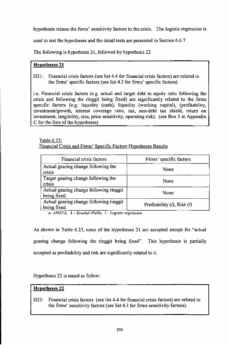
hypothesis relates the finns' sensitivity factors to the crisis. The logistic regression is

used to test the hypotheses and the detail tests are presented in Section 6.6. 7.

The following is hypothesis 21, followed by hypothesis 22.

Hypotheses 21

H21: Financial crisis factors (see list 4.4 for financial crisis factors) are related to the finns' specific factors (see list 4.2 for finns' specific factors)

i.e. Financial crisis factors (e.g. actual and target debt to equity ratio following the crisis and following the ringgit being fixed) are significantly related to the finns specific factors (e.g. liquidity (cash), liquidity (working capital), (profitability, investment/growth, interest coverage ratio, tax, non-debt tax shield, return on investment, tangibility, size, price sensitivity, operating risk). (see Box 5 in Appendix C for the lists of the hypotheses)

Table 6.23: Financial Crisis and Finns' Specific Factors Hypotheses Results

Financial crisis factors Finns' specific factors

Actual gearing change following the None

CnSIS

Target gearing change following the None

CnSIS

Actual gearing change following ringgit None

being fixed Actual gearing change following ringgit

Profitability([), Risk (f) being fixed

a- ANO VA, k- Kmskal- Wallts, 1- Logtsttc regresswn

As shown in Table 6.23, none of the hypotheses 21 are accepted except for "actual

gearing change following the ringgit being fixed". This hypothesis is partially

accepted as profitability and risk are significantly related to it.

Hypothesis 22 is stated as follow:

Hypotheses 22

H22: Financial crisis factors (see list 4.4 for financial crisis factors) are related to the finns' sensitivity factors (see list 4.3 for finns sensitivity factors).

298

i.e. Financial crisis factors (e.g. actual and target debt to equity ratio following the crisis and following the ringgit being fixed) are significantly related to the firms sensitivity factors (fixed assets increase, fixed overhead decreases, profit decreases, research and development increases, corporate tax rate decreases, capital allowances increases, interest rates increases, inflation increases, government incentives decreases, industry debt average increases). (see Box 6 in Appendix C for the list of the hypotheses).

The results in Table 6.24 reveal that all hypotheses related to the financial crisis are

partially accepted because lnfu is the firms' only sensitivity factors that is

significantly related to the financial crisis factors.

Table 6.24: Financial Crisis and Firms' Sensitivity Factors Hypotheses Results

Financial crisis factors Significant firms' sensitivity factors

Actual gearing change following the lnfu (/)

CnSIS

Target gearing change following the Infu (/)

crisis Actual gearing change following

lnfu (/) currency being fixed to the US Dollar Actual gearing change following

Infu (/) currency being fixed to the US Dollar

.. a- ANOVA. k- Kruskal-Walhs. 1- Log1st1c regresswn

6.8 Interview Survey

According to Kahn and Cannel (1957), an interview is a purposeful discussion

between two or more people. It can help gather valid and reliable data that are

relevant to the research questions and objective. Due to the short duration of the field

study (3 months), the researcher had decided to conduct telephone interviews. It was

conducted as an alternative to the face-to-face interviews because the majority of the

field research time was spent on the process of collecting questionnaire data, i.e.,

sending reminders to the finance managers, calling the companies to get the correct

mailing address for the questionnaire and etc.

299

Due to its informality, the interview was classified as semi-structured interview. For

this study, the researcher had a list of thematic questions to enable the finance

managers to provide their personal and professional opinions and views in the areas of

capital structure. The telephone interviews which each lasted between 30 minutes to

one hour, were conducted in July 2001 with 8 finance managers from 5 main board

and 3 second board listed companies.

Due to the informal nature of the phone interviews, the discussions were generated

based on the flow of conversation and therefore differed substantially among the 8

telephone interviewees. The advantage of the interviews is to give the finance

managers the freedom to express themselves without having to write their thoughts on

the paper. The opinions and views of the interviewees were recorded by note taking.

To upheld confidentiality, the researcher has assured the phone interviewees that their

personal information will not be mentioned in the thesis. Therefore, when discussing

the information obtained from the phone interviews, the interviewees will instead be

referred to as Interviewee 1, Interviewee 2 and so on.

6.8.1 Interview Analysis and the Discussion

The following are the four questions that were asked during the phone interviews:

1. Does your company have target debt to equity ratio?

2. How do you measure debt to equity ratio?

3. What are the main factors considered in gearing/leverage decision?

4. How did the financial crisis affect your company?

300

The discussions in this section mostly focus on the infonnation obtained from the

phone interviews and are cross-referenced with a few comments that were received

from the questionnaire survey. The discussions generated from the phone interviews

show that 4 out of the eight companies had a target debt to equity ratio. These four

established finns are main board listed companies. The finn of Interviewee 2 has a

ratio of 30:70 of internal and external funding rate with a debt ,to equity ratio of 1:1.

Two other companies had maintained an internal and external ratio of 40:60, of which

the ratio of debt to equity is maintained at 1:1. Interviewee 6 had a conservative

approach of debt, with the internal and external ratio of 50:50, in which 10 per cent of

external financing is debt and 90 per cent is equity. According to the finance

manager, due to the interest incurred on debt, the finn is obligated to pay fixed

interest payment and may be subjected to financial distress if the obligations are not

fulfilled.

"Using debt will put this firm at risk especially when the firm's profit is low, we are obligated to pay the interest and we do have many other obligations".

(Interviewee 6)

On the contrary, the company affiliated with Interviewee 5 does not have target debt

to equity ratio and had maintained that the company does not use debt at all because

the company is always in a surplus situation. Therefore any short-tenn project is

financed using profit while long-tenn project would only require external equity.

Although equity has a high risk, it is however regarded as safer by Interviewees 6 and

5 as there is no risk of bankruptcy when using equity since they are not subjected to

financial distress.

301

In response to interview question 2 on the measurement of debt to equity ratio, none

of the four firms had indicated having any specific formula or computation to measure

their ratio. However, one of the managers specified that the ratio that they used is

based on the effective cost of capital. According to that manager, the company would

settle for the lowest financing costs for any project as a determinant of the financing

sources and gearing ratio. On the other hand, the key factor for debt to equity ratio

determinants for the company affiliated with Interviewee 2 is to observe the interest

coverage ratios. According to the manager, the higher the interest coverage ratio, the

better it is for the firm. One of the reasons to consider interest coverage ratio is due to

the private debt securities rating by Rating Agency Malaysia (RAM). One of the

rating criteria outlined by RAM for the independent power producers is as follow:

"Cash generating ability to cover debt-servicing obligations is of the rating methodology"

(RAM (2002)).

Therefore, interest coverage ratio is very important for utility companies for debt to

equity ratio determinants.

In response to interview question 3, five of the interviewees had mentioned collateral

as the most important aspect of getting loans from banks.

"The higher the value of your collateral, the faster and the bigger the amount of cheque the bank will produce"

(Interviewee 3)

However, according to one of the interviewees, although the banks reqmre the

collateral as part of the security arrangement, they do take into considerations other

factors such as the firms' profit. Interviewees 7 and 8 had given a very interesting

point regarding the title 13 of the company's board of directors do account for the

13 The title of Tan Sri, Datuk and others are given by Royal Figure or the states ruler (equivalent to the title of Sir)

302

credit assessments. The higher the title of the firm's board of directors, the more

considerate the banks would be towards credit approval.

In response to the last question, the gearing of only two companies were directly

affected by the crisis while the other five were indirectly affected due to weak

performance of the stock market which had reduced the market value of their equity.

According to Interviewee 8, the equity market was really low due to the crisis,

causing top management to change their gearing decision accordingly, based on the

development of the market. Interview 8 also said that while the company's profit was

deteriorating, the share prices also fell and at the same time, the financial institutions

tightened their credit. The company would therefore have to seriously consider these

factors in deciding their fmancing sources to minimise the company's cost of capital.

Interviewee 5 who had previously stated that the company did not intend to use debt

is now considering using debt for financing if the market does not recover soon

because the company's profit is gradually falling due to the low sales volume. The

finance manager specified that their previous policy on financing was to use profit for

short-term projects and to issue shares for long-term projects. However, the manager

explained that it is not advisable to raise funds through external equity to finance any

investment following the crisis. The financial crisis may have changed their financing

policy, which left with the option of using debt for both short-term and long-term

financing. The company did use debt in 2002, as shown in their financial statement of

the 2002 armual report.

303

The final response on the financial crisis was based on the feedback obtained from

interviewee 8, who was the finance manager of a small listed company on the second

board. The crisis and the contraction of the economy had caused the company to

experience severe financial difficulties, therefore forcing the company to be

dependent on the government's assistance through financial a id and fiscal policies.

Bank Negara indicated that the financial crisis had caused a significant increase in the

number of business closures and cases of companies filing for court-sanctioned

restraining orders from their creditors (BNM, 1999).

One of the questionnaire respondents had written the following comments on the

questionnaire, suggesting that the actual and target gearing of the company has

changed following the financial crisis:

"Prior to the depreciation of RM against foreign currencies, the DIE ratio was I: 1. The impact of the depreciation which reduced the value of the ringgit against other currencies by about 50 per cent, had led to an increase in DIE ratio by about 62-64 per cent of debt at the end of August, 1998 which was in foreign currencies".

The above quote implies an increase in gearing following the ringgit depreciation due

to the debt denominated in the US dollar and the Japanese Yen. In response to the

currency depreciation, the company has changed the foreign debt policy ratio of 62:38

percent of foreign to local debt on 31st August 1998 to a ratio of 50:50 per cent on 31 51

August 2001. Therefore, the use of foreign denominated debt has been reduced. One

of the reasons of reducing debt denominated in foreign currencies is to minimize

future fixed interest rates which m ay create future problems for the firms (i.e., the

firm will have to pay the interest due in the Malaysian ringgit).

304

6.9 Conclusion

The chi-square test proves that majority of the companies have given high priority to

retentions, however, none of the ANOV A and Kruskal-Wallis test on retention give

any significant result between and any other factors or variables in the analysis.

Therefore, with the exception of the high priority given to retentions, no other

conclusions can be drawn on retentions.

Based on the chi-square analysis, ordinary shares are the last priority chosen by firms

listed under the main board. Nevertheless, the Kruskal-Wall is test have shown that

firms with high tax surrogate (Dep/tas), high tangibility and high risk have given high

priority to ordinary shares, while firms with low profit (Npm) and small in size have

given low priority to ordinary shares. The ANOV A test has revealed similar results

indicating that small size firms give low priority to the ordinary shares. The logistic

regression modelling shows that the decrease in non-debt tax shield and industry

average ratio are positively related to ordinary shares while profitability (Roce) is

negatively related to ordinary shares.

The chi-square test proves that firms have g1ven medium priority to the debt

financing. On the other hand, the Kruskal-Wallis assessments have shown that low

growth and low non-debt tax shield firms have given low priority to debt. Logistic

regression, however, shows that the increase in debt to equity ratio due to the response

of the profit decreases (Pfd) has resulted in high priority given to the total debt

financing.

305

The chi-square analysis clearly shows that a 11 types of conventional debt are given

higher priority over Islamic debt. The Kruskal-Wallis test shows that firms with high

price-currency sensitivity have given high priority to conventional debt; however,

high-risk and high investment opportunity firms have given low priority to the

conventional debt. Nevertheless, logistic regression shows that the increase in debt

to equity ratio, due to the response of a profit decrease (Pfd) has resulted in high

priority given to the conventional debt financing.

On the contrary, liquidity, investment opportunity, non-debt tax shield, and tangibility

are negatively related to Islamic debt using the median test, but the same test has

resulted in a positive relationship between tax and Islamic financing. Based on the

logistic regression, however, an increase in the debt to equity ratio due to the response

of an interest rate increase has resulted in high priority given to the Islamic debt, but

the decrease in debt to equity ratio, due to the response of the increase in the industry

average debt ratio, has given low priority to the Islamic debt.

The ANOV A, Kruskal-Wall is and logistic regression analyses have found that with an

increase in inflation, high profit firms are likely to increase their debt to equity ratio.

The Kruskal-Wallis and logistic regression have also proven on increase in the

industry average debt ratio has resulted in large firms increasing their debt to equity

ratio. The Kruskal-Wallis median test has found that despite low incentives given by

the government, firms with high tangibility, high risk and high tax brackets will

increase their debt to equity ratio. The same test has proven that with the increase in

fixed assets, high risk firms will increase their debt to equity ratio. Finally, both the

Kruskal-Wallis and the logistic regression show on the increase of two percentage

306

points m inflation would result in firms with high tangibility, price-currency

sensitivity and high profit increasing their debt to equity ratio.

All three tests have confirmed that with a decrease in government incentives will

result in larger firms decreasing their debt to equity ratio. Highly liquid firms will

decrease their debt to equity ratio if interest rates a re increased by two percentage

points, as shown by the K.ruskal-Wall is median test. The same test verifies that highly

liquid firms tend to decrease their debt to equity ratio with a decrease in profit and an

increase in the industry average debt ratio. With the decrease in government

incentives, the median test shows that high profit margin firms will decrease their

debt-equity ratio, while logistic regression confirms that an increase in inflation and

lack of government incentive will result in firms having to decrease their debt to

equity ratio. Using the ANOV A, the result shows that low profit firms will decrease

their debt to equity ratio if interest rates are increased or even if the firms' fixed assets

are increased. However, the logistic regression has shown that highly profitable firms

will decrease their debt to equity ratio if the industry average debt ratio is increased.

The same result was achieved for high non-debt tax shield firms which indicate that

these firms would decrease their debt ratio should the industry average debt ratio be

increased.

The test has revealed that the increase in inflation will not have any effect on the firms

actual and target gearing ratio following the 1997 financial crisis and the ringgit being

fixed. However, a high return on investment and increase in risk has influenced firms

to change their target debt to equity ratio following the ringgit being fixed to the US

dollar.

307

The interview summary shows that only large and established companies have target

debt to equity ratios. Although their debt to equity ratios vary, the companies

maintained a debt ratio of less than 50 per cent. Between 30 to 50 per cent of the

funding was targeted from internal funds. Many companies consider fixed assets as

the most important factor in debt determination, while others refer to interest coverage

ratio and the influence of the board of directors. Most of the interviewees agreed that

the crisis did affect their capital structure either implicitly or explicitly. The

companies which had debt denominated in foreign currencies would experience a

direct effect of the crisis on their capital structure. However, the crisis had an effect

indirectly on the balance sheets of some of the companies through decline profitability

and financial distress.

The interviewees had different perceptions towards the crisis. The finance managers

of the companies in the main board tended to emphasise changing their debt

management policy, while the finance managers of the second board companies

stressed the damaging extent of the crisis and feared that their companies may not

survive. However, since only 8 respondents had participated in the phone interviews,

the number is too small to represent the views of the entire population of the

companies listed in the KLSE.

308

7.1 Introduction

CHAPTER 7 CONCLUSION

Chapter 7 discusses the overall findings of the research study which include the

review of gearing differences between the main board and the second board

companies, the finance managers financing preference, and finally factors which are

positively or negatively related to debt. A short discussion on the effects of the crisis

on gearing is also included. The discussions on the limitations and recommendations

for further research conclude the thesis. The chapter is comprised of the following

sections: Section 7.2 summarises the research findings, Section 7.3 discusses the crisis

effect on the firms' gearing, Section 7.4 states the limitations of the research and

Section 7.5 provides a direction for further research.

7.2 Summary of the Research Findings

The ANOV A and the Kruskal-Wall is have shown that there are differences between

the main board and the second board companies' gearing using book value ratios and

mixed value gearing across three time periods. The observations of the mean scores

and median ranks have indicated evidence that the gearing ratio for both boards

gradually increases from the pre-crisis to post-crisis period. The figures were even

higher when measured by the mixed value ratio. The ANOV A and the Kruskal-

Wallis results are furthers upported by the multiple regression results on the panel

data. The mixed value model of the panel data have statistically proven that the main

board companies gearing are increased following the crisis.

309

The similar tests have proven that there are statistical differences between the book

value gearing of the main board's six sectors, the differences are highly significant

during the pre-crisis. The mean scores reveal that except for plantation, the gearing of

the other five sectors have increased even more following the crisis. The Bonferroni

mean test also reveals that the gearing of the plantation sector is the only sector that is

statistically different from all the other sectors. The evidence shows that the

plantation sector had gained from the depreciation of the ringgit as the profit from the

exported commodities was quoted in US dollars. Due to this reason, the profit of the

firms related to these sectors were not as badly affected as those in the other 5 sectors,

therefore, less debt is required for the investment. The situation explains why the

plantation had the lowest gearing before and after the crisis.

The chi-square result has statistically proven that there is an association between the

financing preference and the priority preference. T he retention is regarded as the

highest priority, followed by debt and ordinary shares as a last option. This shows

that Malaysian firms follow the financing hierarchy as suggested by Myers' pecking

order theory. Consistently, studies by the Malaysian Central Bank on sources of

finance of industrialisation in Malaysia between 1994 and 1996 have found that 48.8

per cent of companies' financing are realised from internal funds, 37.3 from debt and

13.9 from external equity (BNM, 1996).

The same test shows that conventional debt is preferred over Islamic debt. Clearly the

Islamic financing is the least preferred financing compared with conventional

financing. Putting aside all the comments that were noted in the earlier discussions in

Chapter 6 on the current practice of the Islamic financing, is it possible for the interest

310

free economic system to replace the interest based system in Malaysia? The

Malaysian economy develops and progresses based on a very complex cultural

background due its multiracial society. The significant developments on the "interest

free economic system" in Malaysia are due to the strong commitment from the

Muslim community, which represents the majority population of the country. There

are few evidences showing that the user of Islamic financing did not suffer the impact

of the high interest rates following the crisis. The positive effects of the crisis to the

Islamic financing participants would encourage further use of Islamic financing in the

future. However, it would be difficult to predict the changes in the future economy as

any changes in world economy would have an effect on the local economy. At

present, both systems allow the community to choose the ideal methods in accordance

to their needs and religious belief.

7.2.1 Factors That Positively and Negatively Related to Gearing

The statistical analyses have indicated that a few factors are positively and negatively

related to gearing. Size were found positively related to the main board and the

second board gearing measured by book value ratios and mixed value ratios.

Therefore, the larger the size of the firms, the higher is the gearing ratio of that

particular firm. On the other hand, tangibility was found to have a significant positive

relationship with the gearing for the companies listed at the second board. However,

no relationship is found between the tangibility and the gearing o fthe main board

companies. Tangibility is therefore very important for the small companies compared

with large companies with regard to debt financing. The other variable to have a

positive influence on gearing is risk. However, only firms listed on the main board

have a positive significant risk influence on their book value gearing ratio. Therefore,

311

the higher the risk of the large firms, the higher is the gearing. The price sensitivity or

the correlation between companies' share prices and the ringgit movement shows a

significant positive result, when the gearing is measured using mixed value ratios.

The falling of share prices due to the ringgit depreciation has reduced the market

value of equity, thus, increasing the debt ratio of the firms.

Firms' gearing based on the book value ratios and the mixed value ratios are found to

be highly negatively related top rofit. Besides the findings o fn egative relationship

between profitability and gearing using firms' account data, a few other evidences

show that Malaysian firms prefer internal funds over external funds. The response of

the finance managers shows that retentions are their highest priority compared with

debt and equity. Further to these findings, target gearing ratios of internal to external

funds were from 30 to 50 per cent, as indicated by the finance managers during the

interviews. This implies an emphasis on a high ratio of internal funds over debt and

external equity mixture. The overwhelming evidence indicates that less debt is

required if the firms' profit is high, resulting in a negative relationship between profit

and gearing.

Besides profitability, liquidity was also found to have a negative relationship with the

book value ratios and the mixed value ratios gearing. The negative relationship

between liquidity and gearing are related to the "financial slack", whereby firms with

a conservative approach to debt will ensure that they have sufficient readily available

current assets for financing investment, resulting in a negative relationship between

liquidity and debt.

312

Other than the above individual factors relating to the gearing ratio, there are a few

additional combining factors causing the gearing ratio to increase or decrease. This

conclusion is drawn based on the combination of i) the firms' account data obtained

from Datastream and ii) the finance managers' response obtained from the

questionnaire.

As discussed above, size is positively related to debt, it is also found that larger firms

would increase their debt-equity ratio if the industry average debt ratio increases.

However, larger firms tend to decrease their ratios if the government incentives are

reduced. High tangibility firms are found to have a positive relationship with gearing

even if the government reduces its incentives or when the inflation rises.

The statistical analysis also reveals that high risk firms tend to increase their debt to

equity ratio if the firms' fixed assets are increased or even when the government

incentives are reduced. However, high risk firms will reduce their debt to equity ratio

if the non-debt tax shield is reduced. On the other hand, firms with high price

currency sensitivity will increase their debt to equity ratio when inflation rises.

Profitability, as previously mentioned, having a negative relationship with gearing,

would imply profitable firms using less debt. However, it is also found that an

increase in inflation would result in profitable firms using use more debt. The test

also reveals that low interest coverage firms use less debt even if the firms' fixed

assets a re i ncreased or when interest rates a re increased. Low interest coverage i s

associated with low profit; in other words, low profit firms use less debt if interest

313

rates are increased. The low profit firms would even reduce their debt to equity ratio

although the fixed assets are increased to back the debt.

Liquidity is negatively associated with gearing: the combined data revealed that

highly liquid firms will decrease their debt to equity ratio when interest rates are

increased, when the profit is decreased and even when the industry average debt ratio

is increased.

7.3 Does the Crisis Affect the Firms' Gearing?

Section 7.2 discusses the significant differences between the gearing of the main

board and second board companies. Although the analysis of the mean has shown a

substantial increase in the gearing ratios from the pre-crisis to the post crisis, the

AN OVA and theKruskal-Wall is methods only test the difference between the gearing

of companies on the main board and second board one period at a time. The panel

data regression is the only statistical test that indicates the increase in gearing

following the crisis. The result shows a significant increase in mixed value ratios of

panel data from pre-crisis to 1997. Therefore, the gearing has increased following the

cns1s.

Although a few studies have categorised Malaysia under the low-debt country group,

gearing has increased over the last few years, even before the 1997 crisis. A study by

Claessens et al. (1998) has indicated a significant increase in Malaysia's annual

gearing ratio from 1988 to 1996. Therefore, any increase in gearing following the

crisis may be due to either one of the following reasons: a general trend of increasing

the debt ratio, or firms do indeed employ more debt due to the crisis.

314

If the increase in gearing is due to the cns1s, the following are a few possible

explanations for the increase in gearing ratio following the crisis; i) it could partly be

just an accounting entry of accumulated losses resulting in a low book value of

equity; ii) as the share prices fell due to the crisis, the market value of the equity was

also reduced, causing the debt ratio to increase; iii) in reality, following the crisis, the

only choice for financing is to use debt if the firms' shares and retentions are

unavailable. Graph 3 in Appendix A shows and increase in private debt securities

issuance over the equity issuance following the 1997 financial crisis in Malaysia.

Immediately following the crisis, both capital sources issued by corporations were

very low as indicated in the graph for the year 1998, however, debt issuance surpassed

the equity issuance during that year and the subsequent years (compared with 1996

and 1997 proportions). The evidence supports the third explanation for the scarce

equity sources due to the crisis.

The statistical analyses have found a number of factors associated with the crisis. The

high risk and profitable firms were found to change their target gearing ratio

following the ringgit being fixed to the US dollar. The conducted test also found that

managers will change the actual and target gearing ratio following the crisis and

following the ringgit being fixed to the US dollar if inflation rises. The multiple

regression tests of three different periods found certain factors such as investment

opportunity, tangibility and size (for second board) has changed from positive to

negative, and vice versa from one period to another. Therefore, the crisis may have

had some impact, perhaps more pronouncedly upon opportunities. Companies which

employed foreign denominated debt were found to change their debt policy by

315

reducing their foreign denominated debt to avoid pa)'lng a high fixed cost m

depreciated ringgit when the interest is due.

7.4 Limitations of tbe Research

There are inevitable limitations and weaknesses associated with some aspects of the

research, such as the way in which the research was designed. There are also some

external factors which may have influenced the way in which the research was

conducted. Some of the limitations of the project are described below.

The comparability of results between Malaysia and the USIUK firms is probably not

fully valid. This is because Malaysian firms are categorised under the developing

country as compared to the US and UK firms which are categorised under developed

countries. There is a huge difference between the economic and political aspects of

developing and developed countries.

Other limitations include the inconsistency of the firms' data in Datastream whereby a

substantial number of data were not available in certain years within the period of

study. Therefore, many companies have to be excluded from the study. This had

significantly reduced the number in the research sample, especially for the second

board companies. Further to that, many companies' data had to be disregarded due to

extreme figures ( outliers ).

Another limitation to the study worth mentioning is time. Although it was felt that

time was managed and spent effectively during the process of conducting the

re~earch, a number of barriers had prevented the researcher from being able to fully

316

concentrate on the research. A large amount of time was spent in sorting and cleaning

the data obtained from the Datastream.

The method of collecting data is another aspect of the study which had caused some

problems for the researcher. For example, the process of disseminating the research

questionnaire to the finance managers had resulted in a large number of the

questionnaires having been sent by mistake to the company's secretary, instead of to

the finance managers. This is primarily due to the inability of the researcher to obtain

the full mailing address of the finance managers. Due to the time constraints of the

field research, the researcher had to cancel face to face interviews to accommodate for

the time spent in having to contact the companies for the correct mailing address. The

reason is the researcher only had 3 months to collect the completed questionnaire, to

interview the finance managers, to collect relevant research materials from various

libraries and government institution such as The Central Bank of Malaysia before

departure back to the UK.

It is also worth mentioning that smce this research study was predominantly

conducted in the United Kingdom, it was rather difficult for the researcher to obtain

further useful information relating to this research such as on Malaysian taxation,

Islamic Banking Act and the latest economic development report. Some of these

problems have been minimised through kind assistance from friends and family

members in Malaysia.

317

7.5 Future Research Suggestions

Although this research can be considered a comprehensive study on the capital

structure of Malaysian firms, the findings have introduced a number of areas which

could be further explored in future research. This study has also revealed that there

are numerous avenues to be studied on the Malaysian capital structure by future

researchers.

There are a few other factors that may have influenced the gearing of Malaysian firms

that are not included in this thesis such as agency conflict, bankruptcy cost,

asymmetric information and dividend policy. The Malaysian markets have

overwhelming preferences for callable or bond with warrants and convertible

securities (see Table I in Appendix A for the 1996 and 1997 figures), therefore

further studies on these areas are highly recommended. Further to that, a few other

factors that related to the crisis may be encompassed in the model, to extend the scope

of the study on the crisis effects on gearing to include economic factors such as

money growth (M1, M2 and M3), foreign direct investment and foreign denominated

debt.

Another consideration is to use different measurements for the gearing. As indicated

in the results of the study, Malaysian companies prefer medium sized debt. Instead of

using the total debt (short-term plus long-term debt) to measure gearing, it may be

worth using short-term debt or medium-term debtor I ong-term debt. S ome oft he

gearing measurements that have been used by previous researchers are: the ratio of

long term debt over total debt, the ratio of short term over total debt and income

gearing. Titman and Wessels (1988) have used long term debt, short-term debt and

318

convertible debt over book value and market value of equity in their capital structure

studies.

A few other methodologies may also be used to study the time series effect on gearing

such as the regression with time lags. As to the questionnaire survey, different

methods such as the Mann-Whitney U test may contribute to slightly different

findings on the survey.

Further analyses on the financing are also recommended because there are many

related issues which are rather vague and would require extensive analysis in the area.

Islamic banking has emerged as a new market in the international financial scene side

by side with the conventional system. The Central Bank of Malaysia has reported that

there are about 177 Islamic financial institutions operating around the world,

managing assets estimated at US$90 billion. As for Malaysia, the total assets of the

Islamic banking system, as at the end of 1999, stood at RM34.1 billion while deposits

and financing amounted to RM26.1 billion and RM 11.7 billion respectively. Another

major development is the establishment of the Islamic money market in 1994 with

one of the functions being the trading ofl slamic financial instruments. With such

development, future research in this area is highly recommended.

Besides questionnaire survey and interview, small scale case studies may be

appropriate to get direct results from companies. Very few studies on the capital

structure area have been conducted using the case study approach. By focusing on a

few companies, the researcher will gain a rich understanding of the context of the

research and its research process. The case study approach also has the ability to

319

generate answers to specific questions, such as what and why and how. According to

Emory and Cooper (1991), a simple, well-constructed case study can enable a

researcher to challenge an existing theory and provide a source of new hypotheses.

Another potential suggestion is to conclude comparative study of the effects of the

financial crisis on the firms' gearingin other countries that were affected by the crisis.

The study may be extended to include South East Asian countries such as Thailand,

Indonesia, Singapore and even Hong Kong and South Korea for gearing comparisons.

Similar to Malaysia, not many studies on capital structure have been conducted on

those countries. Therefore, not only the crisis effects on gearing are recommended

but many other capital structure related issues may also be explored for comparative

study.

320

GLOSSARY OF TERMS1

Arbitrage Purchase of one security and simultaneous sale of another to give a risk-free profit.

Adjusted R-Squared A statistic that is suitable for comparing models that have different numbers of independent variables; indicates the percentage of variability for which the model accounts.

Bai al Salam Contract of sale of goods, where the price is paid in advance before the goods are delivered.

Bai bithaman ajil (Bai' muajjal) This contract refers to the sale of goods on a deferred payment basis. Equipment or goods (the assets) requested by the client are bought by the bank, which subsequently sells the goods to the client at an a greed price (the sale price), which includes the bank's mark-up (profit). The client may be allowed to settle payment by installments within a pre-agreed period, or in a lump sum. Similar to the murabahah contract, this is also a credit sale.

Balance of Payments The record of all the transactions between a country and the rest of the world; it includes information on the value of trade in goods and services as well as transfer payments.

Bhat The unit of currency of Thailand

Cagamas The securitisation process of mortgage by the National Mortgage Corporation known as Cagamas Berhad. In the securitisation process, Cagamas purchases loans from major primary lenders such as banks, insurance companies and pension funds. The purchase is funded through the issuance of Cagamas debt securities. Cagamas, therefore, converts a long-term illiquid asset (example property loans) into liquid debt securities which can be traded in the secondary market. This process enables investors to earn an income from Cagamas debt securities which is basically derived from the interest paid by borrowers on their loans.

Ceteris Paribus All other things being equal; refers to holding all other variables constant or keeping all other things the same when one variable is change

Correlations A measurement of the strength of the linear relationship between random variables.

1 The glossary of terms extracted from: BNM (1999), Taylor (1995), Brealey et al.(2000) and Statgraphics (2000).

321

Correlation Matrix A table of the Pearson correlation coefficients for the estimated coefficients m a model.

Consumer Price Index (CPI) A price index equals to the current price of a fixed market basket of consumer goods and services in a base year.

Current Account Balance The value of export minus the value of imports plus net factor income from abroad plus net transfer from abroad

Danaharta Main function is to purchase NPLs from the financial institutions and manage the NPLs in order to maximise their recovery value.

Danamodal Main function is to re-capitalise the financial institution by injecting funds to enable them to operate efficiently.

Developing Country A country that is poor by world standards in terms of real GDP per capita.

Gearing Leverage: Use of debt to increase the expected return on equity.

Gross Domestic Product (GDP) The measure of the size of the economy, it measures the value of all goods and services newly produced in an economy during a specified period of time.

Hedging Buying one security and selling another in order to reduce risk

Ijara A contract under which a bank buys and leases out for a rental fee equipment required by its client. The duration of the lease and rental fees are agreed in advance. Ownership of the equipment remains in the hands of the bank. The contract is a classical Islamic financial one, now in increasing use worldwide.

Imputation Tax System Arrangement by which investors who received a dividend also receive a tax credit for corporate taxes that the firm has paid.

Inflation An increase in the overall price level

Inflation rate The percentage increase in the overall price level over a given period of time.

322

International Monetary Fund (IMF) An international agency, established after World War Il, designed to help countries with balance of payments problems and to ensure the smooth functioning of the international monetary system.

Keynesian A thought concern with pursuing demand -side macroeconomic policies, primarily fiscal policies to reduce unemployment and encourage economic growth. Shaped by the Great Depression and the work of John Maynard Keynes.

Khazanah Bonds Treasury Bonds

Lessee User of leased assets

Lessor Owner of a leased asset

Moral Hazard The risk that the existence of a contract will change the behaviour of one or both parties in accordance to the contract; e.g., an insured firm may take fire precautions lightly.

Mudarabah (Trust Financing) This is an agreement made between two parties: one which provides 100 per cent of the capital for the project and another party known as a mudarib, who manages the project using his/her entrepreneurial skills. Profit arising from the project are distributed according to a pre-determined ratio. Any losses accruing are borne by the provider of capital. The provider of capital has no control over the management of the project.

Murabahah (cost-plus financing) This is a contract sale between the bank and its client for the sale of goods at a price which includes a profit margin agreed by both parties. As a financing technique it involves the purchase of goods by the bank as requested by its client. The goods are sold to the client with a mark-up. Repayment, usually in instalments, is specified in the contract.

Musharaka (partnership financing) This Islamic financing technique involves a partnership between two parties, both providing capital towards the financing of a project. Both parties share a pre-agreed ratio, and losses are shared on the basis of equity participation. Management of the project may be carried out by both the parties or by just one party. This is very flexible partnership arrangement where the sharing of the profits and management can be negotiated and pre-agreed by all parties.

Ml Currency in circulation and demand deposits of the private sectors

323

M2 Ml plus fixed and saving deposits of the private sector placed with BNM and commercial banks, net negotiable instruments of deposit issued by the banks and repurchase agreements (repos) done by banks.

M3 Currency in circulation plus all private sector deposits (including repos) with BNM, commercial banks (including Bank Islam), finance companies, merchant banks and discount houses; excludes placements among these financial institutions.

Negatively Related A situation in which an increase in one variable is associated with a decrease in another variable; also called inverse related.

Positively Related A situation in which an increase in one variable is associated with an increase in another variable; also called directly related.

Private Debt Securities All types of debt issued by corporations

Public Debt Securities All types of debt issued by government

Purchasing Power Parity The theory that exchange rates are determined in such a way that the prices of goods in different countries is the same when measured in the same currency (Taylor, (1995), p.1047)

Repo Repurchase agreement-Purchase of treasury securities from a security dealers with an agreement that the dealer will repurchase them at a specific price.

Rib a Literally, an increase or addition. Technically it denotes, in loan transaction, any increase or advantage obtained by the lender as a condition of the loan. In a commodity exchange it denotes any disparity in the quantity or time of delivery.

Ringgit The unit of currency of Malaysia

Shariah Islamic canon law derived from three sources- The Qur'an, the Hadith (sayings of Prophet Muhamrnad) and the Sunnah (practice and the traditions of the Prophet Muhamad).

Skewness A value used to measure the symmetry or shape of the data

324

Tax Bracket A range of taxable income that is taxed at the same rate

Trade Credit Account receivable

Zakat (tax) There are two types of zakat: i) zakat al-fitr, which is payable by every Muslim who are able to pay at the end of Ramadhan (the month of fasting). ii) zakat al maal is an annual levy on the wealth of a Muslim (above a certain level). The rate paid differs according to the type of property owned. This tax is earmarked, among others, for the poor and needy.

325

BIBLIOGRAPHY

Aggarwal, R. (1981), "International Differences in Capital Structure Norms: An Empirical Study of Large European Companies", Management International Review, Vol. 21, Issue 1, p. 75-88.

Ahamad, S. (1992), Towards Interest-Free Banking~ New Delhi: International Islamic Publishers.

Ahmed, K. ( 1995), The effect of Corporate Characteristics on Disclosure Quality in Corporate Annual Reports: A Meta-Analysis. Working Paper, Victoria University of Wellington, New Zealand. In: Botoson C. A. (1997) "Disclosure Level and the Cost of Equity Capital", The Accounting Review, Vol. 72, No.3 (July), p. 3 23-349.

Al-Harran, S. (1995), Time for Long Term Islamic Financing. In: Al-Harran S. (1995) Leading Issues in Islamic Banking and Finance. Malaysia: Pelanduk Publication, p. 31.

Al-Harran, S. (1995), "Proposal for an Integrated ·Marketing Model of M usharakah Financing to Help Disadvantage Fishing People in Malaysia". Available from: http:/ /islamic-finance. neUislamic-microfinance/harran6. html [ Accessed 10 Dec 2002]

Alien, F .B. ( 1954), "Does Going into Debt Lower the ' Cost of Capital?", Analysts Journa/1 Vol. 10 (August), p. 57-61.

Ang, J.S., Chua, J.H. and McConnell, J.J. (1982), "The Administrative Costs of Corporate Bankruptcy: A Note", Journal of Finance, Vol.3 7, p. 219-226.

Annuar, M.N. and Shamser, M., (1993), "An Empirical Study of the Capital Structure ofMalaysian Listed Firms", Capital Market Review 1, p. 96-108.

Ariff, M., Lim, S.L. and Johnson, L.W. (1988), "An Empirical Study of the Capital Structure of Firms", Singapore Management Review, 11(2), p. 1-9. In: Ariff, M., and Johnson L. W. (1990) Securities Markets and Stock Pricing, Longman.

Ashton, D.J. (1989), "Textbook Formulae and UK Taxation: Modigliani and Miller Revisited", Accounting and Business Research, Vol. 19, No. 75, p. 207-12.

Asmon I.R (2003) "The Employee Share Ownership Plan (ESOP)". Available from: Http://www.Thehope.org/esop.htm#IV [Accessed 4 September 2003].

Barclay, M.J., and Smith C.W. (1995), "The Maturity Structure of Corporate Debt", Journal of Finance, Vol. 50, (June), p. 609-632.

Baxter, N.D (1967), "Leverage. Risk of Ruin and the Cost of Capital", Journal of Finance, Vol. 22, p. 395-403.

326

Bell, J. (1993), Doing Your Research Project. 2"d Ed. Buckingham: Open University Press. In: Sauders, M., Lewis, P. and Thornhill, A. (1997), Research Methods for Business Students. London: Financial Times, Pitman Publishing.

Bhatia, R.J. (1960), Inflation, Deflation, and Economic Development. IMF Staff Papers, Vol. 8, No. 1, p. 101-114.

BNM 1 (1994), Money and Banking in Malaysia. 4th Ed. Kuala Lumpur: The Economics Department, Bank Negara Malaysia (BNM).

BNM 1 (1996-2000), Bank Negara Malaysia 1996-2000 Annual Report. [CD ROM]. Bank Negara Malaysia (BNM).

BNM 1 (1999), The Central Bank and the Financial System in Malaysia-A Decade of Change. 1st ed. Kuala Lumpur: Bank Negara Malaysia (BNM).

BNM 1 (1997), Quarterly Bulletin. Kuala Lumpur: Bank Negara Malaysia (BNM), 1st quarter 1997, Vo.l2, No.l.

BNM 1 (1997), Quarterly Bulletin. Kuala Lurnpur: Bank Negara Malaysia (BNM), 2"d quarter 1997, Vo.l2, No.2.

BNM 1 (1997), Quarterly Bulletin. Kuala Lumpur: Bank Negara Malaysia (BNM), 3'd quarter 1997, Vo.l2, No.3.

BNM 1 (2000), "Quarterly Bulletin" Kuala Lurnpur: Bank Negara Malaysia (BNM), 1st quarter 2000, Vo.15, No. I.

BNM 1 (2000), "Quarterly Bulletin" Kuala Lumpur: Bank Negara Malaysia (BNM), 2"d quarter 2000, Vo.15, No.2.

BNM 1 (2000), "Quarterly Bulletin" Kuala Lumpur: Bank Negara Malaysia (BNM), 3'd quarter 2000, Vo.15, No.3.

BNM 1 (2000), "Quarterly Bulletin" Kuala Lurnpur: Bank Negara Malaysia (BNM), 4th quarter 2000, Vo.15, No.4.

Booth, L., Aivazian, V., Demirguc-Kunt, A and Maksimovic, V (2001), "Capital Structures in Developing Countries", The Journal of Finance, Vol. LVI, No.l, (February), p. 87-130.

Botoson C. A. (1997), "Disclosure Level and the Cost of Equity Capital", The Accounting Review, Vol. 72, No. 3 (July) p. 323-349.

Bourque, L.B. and Fielder, E.P. (1995) How to Conduct Self-Administered and Mail Surveys. London: Sage.

1 BNM-Bank Negara Malaysia or Central Bank of Malaysia

327

Bowman, R. G. (1980), "The debt Equivalence of Leases: An Empirical Investigation", The Accounting Review, Vol. LV, No. 2 (April) p. 237-253.

Bradley, M., Jarrel, A .G., and Kim, E.H. ( 1984), "On the Existence of an Optimal Capital Structure: Theory and Evidence", Journal of Finance, Vol. 39, No. 3 (July), p. 857-880.

Brealey, R.A and Myers, S. (1984), Principles of Corporate Finance. 2"d ed. USA: McGraw-Hill.

Brealey, R.A. and Myer, S. (2000), Principles of Corporate Finance. 6th ed. USA: Irwin McGraw-Hill.

Brealey, R.A. and Myers, S.C. and Marcus, A.J (1999), Fundamentals of Corporate Finance, 2"d ed. USA: Irwin!McGraw-Hill

Bris, ·A. Koskinen, Y. and Pons, V. (2002), Corporate Financial Policies and Performance Around Currency Crises. Yale ICF Working Paper, No.00-61, (6 June), p.1-33

Burgman, T. A. (1996), "An Empirical Examination of Multinational Corporate Capital Structure", Journal of International Business Studies, 3'd quarter, p. 553-570.

Chandler, C. (2003), "Coping With China", Fortune.com-Magazine". Available from: http://www.fortune.com/fortune/articles/O, 15114.408670-2,00.html. [Accessed 4 Apr 2003].

Chung, K.H. ( 1993), "Asset Characteristics and Corporate Debt Policy: An Empirical Test", Journal of Business Finance & Accounting, Vol. 20, No.1 (January), p. 83-98.

Claessens, S., Simeon, D., and Larry, L. (1998), East Asian Corporate: Growth, Financing and Risks Over the Last Decade. World Bank: Working Paper.

Collins J.M., and Sekely, S (1983), "The Relationship of Headquarters Country and Industry Classification to Financial Structure". Financial Management, (Autumn), p. 45-51.

Cooper, D. and Schindler, P. (1998), Business Research Methods. 6th ed. Singapore: McGraw Hill International Editions.

Corcoran, P. (1977), "Inflation, Taxes, and Corporate Investment Incentives". Federal Reserve Bank of New York Quarterly Review, Vol. 2, p. 1-9.

Cordes, J.J. and Sheffrin, S.M. (1983), "Estimating the Tax Advantage of Corporate Debt", Journal of Finance, Vol. 32 (March), p. 95-105.

Corsetti, G., Paolo, P. and Nouriel, R. (1999), "Paper tigers? A model of the Asian Crisis", European Economic Review, Vol. 43, p. 1211-36.

328

Crutchley, C. E. & Robert S. H. (1989), "A Test of the Agency Theory of Managerial Ownership, Corporate Leverage, and Corporate Dividends", Financial Management, Vol. 18, No. 4 (Winter), p. 36-46.

DeAngelo, H. and Masulis, R.W. (1980), "Optimal Capital Structure Under Corporate and Personal Taxation". Journal of Financial Economics, Vol. 18, p. 3-29.

deVaus, D.A. (1991) Surveys in Social Research. 3'd ed. London: UCL Press and Alien & Unwin. In: Sauders, M., Lewis, P. and Thomhill, A. (1997), Research Methods for Business Students. London: Financial Times, Pitman Publsihing, p. 130.

Dewing, A. S. (1930), Corporate Promotions and Reorganizations. Cambridge, Mass: Havard Univesity Press. In: Weston, J.F. (1966), The Scope and Methodology of Finance-Foundation of Finance Series. New Jersey, USA: Prentice Hall.

Diamond, D.W. and Verrecchia, R. E. (1991), "Disclosure, Liquidity, and the Cost of Capital", The Journal of Finance, Vol. 46, No. 4 (September), p.1325-1359.

Dillman, D.A. (1978), Mail and Telephone Surveys: The Total Design Methods. New York: Wiley. In: Sauders, M., Lewis, P. and Thomhill, A. (1997). Research Methods for Business Students. London: Financial Times, Pitrnan Publsihing, p.l31.

Donaldson, G. (1961 ), "Corporate Debt Capacity: A Study of Corporate Debt Policy and the Determination of Corporate Debt Capacity", Harvard Business School, Division of Research. In: Myers, S.C. (1984). "The Capital Structure Puzzle". Journal of Finance, Vol. 39 (July), p. 575-92.

Drury, C. (1989), "A Survey ofUK Leasing Practice", Management Accounting, Vol. 67, No. 4 (April), p. 40-43.

Drury, J. and Bougen, P. (1980), "UK gearing levels: An investigation", Accountancy, Vo1.91, Issue 1043, (July), p. 103-106.

Durand, D. (1952), Cost of Debt and Equity Funds for Business: Trends and Problems of Measurement. Paper presented at a conference on Research in Business Finance, New York: National Bureau of Economic Research. In: Archer and D'Arnbrosio (1967).

Economist (1992), "Islam's Interest", Vol. 322, Issue 7742, p. 33-35. Available from: EBSCO Research Database, http://search.global.epnet.com. [Accessed 20 March 2003)

Economist (1999), "Damned Usurers", Vol. 353, Issues 8151, p. 90. Available from: http://infotrac.galegroup.com/itweb/plymouth. [Accessed 15 August 2000]

Edwards, W. (1999), "Islamic Banking", Princeton Economics Journal, Princeton Economics International, USA, 151 quarter.

329

El-Ashker, A. (1987), The Islamic Business Enterprise. London: Croom Helm, p.39.

Elnajjar, G. (2002), http://usinfo.state.gov/usa/islam. [Accessed 03 Oct 2002].

Emory, C. and Cooper, D. (1991), Business Research Methods. 41h ed. Homewood,

Illinois: Richard D. Irwin.

Emst & Young (1997), 1998 World Wide Executive Tax Guide. Emst & Young International, Ltd., p. 324.

Errunza, V.R., (1979), "Determinants of Financial Structure in the Central American Common Market", Financial Management, 8(3), p. 72-77.

Feldstein, M. (1983), Inflation, Tax Rules and Capital Formation. Chicago: University of Chicago Press.

Ferri, M .G. and Jones, W.H. ( 1979), "Determinants ofF inancial Structure: A New Methodological Approach", Journal of Finance, Vol. 34 (June), p. 631-44.

Fischer, A. (1991), "Growth, Macroeconomic and Development". NBER Macroeconomic Annual, Vol. 6, p. 3259-364.

Franks, J.R. and Broyles, J.E. (1979), Modern Managerial Finance. Chichester: John Wiley and Sons.

Frankel, J. A., and Kose, A. R. (1996), "Currency Crashes in Emerging Markets: An Empirical Treatment", Journal of International Economics, 41, p. 351-366.

Gerlach, S. and Smets, F. (1995), "Contagion Speculative Attacks", European Journal of Political Economy, Vol. 11, p. 45-63.

Graham, J. R., and Harvey, C. R. (2001), "The Theory and Practice of Corporate Finance: Evidence from the Field", Journal of Financial Economics, Vol. 60, p.l87-243.

Grossman, S. and Hart, 0. (1982), "Corporate Financial Structure and Managerial Incentives". In: Titman, S. and Wessels, R. (1988), "The Determinants of Capital Structure Choice", The Journal of Finance, Vol. 43, No. 1 (March).

Guioso, L., Sapienza, P., Zingales, L. (2003), "People's Opium, Religion and Economics Attitudes", Journal of Monetary Economics, Vol. 51, No.l (January), p. 225-283.

Gupta, M.C. (1969), "The Effect of Size, Growth, and Industry on the Financial Structure of Manufacturing Companies", Journal of Finance, Vol. 24 (June), p.517-29.

Hahn, J. and Mishkin, F.S. (2000), "The Korean financial crisis: An asymmetric information perspective", Emerging Market Review, Vol. 1, p. 21-52.

330

Hamada, R.R. (1972), "The Effect of the Fim1's Capital Structure on the Systematic Risk of Common Stock", Journal of Finance, Vol. 27, p. 435-52.

Harris, M. and Raviv, A (1991), "The theory of Capital Structure", Journal of Finance, Vol. 46, No. 1 (March), p. 297-355.

Haugen, R.A. and Senbet, L.W. (1984), Bankruptcy and Agency Costs: Their Significance to the Theory of Optimal Capital Structure. Paper presented to the European Finance Association, p.1-21.

Hull, J.C. and Hubbard, G.L., (1980), "Lease Evaluation in The UK: Current Theory and Practice", Journal of Business Finance & Accounting 7, 4, p. 619-637.

Huffman S. P., (1989), "The Impact of the Degree of Operating and Financial Leverage on the Systematic Risk of Common Stocks: Another Look", Quarterly Journal of Business and Economics, Vol. 28 Issue 1, (Winter), p. 83-105.

Hutcheson, G. and Sofroniou, N. (1999), The Multivariate Social Scientist. London: SAGE Publications.

Jarett, P. and Selody, J. (1982), "The Production-Inflation Nexus in Canada, 1963-1979", The Review of Economics and Statistics, Vol. 56, No. 3.

Jensen, M.C. (1986), "Agency Costs of Free Cash Flow, Corporate Finance, and Takeovers", The American Economic Review: Papers and Proceedings of the Ninety-Eighth Annual Meeting of the A.E.A (May).

Jensen, M.C., and Meckling, W.H. (1976), "Theory of the Firm: Managerial Behaviour, Agency Costs and Ownership Structure", Journal of Financial Economics, Vol. 3 (October), p.J05-360.

Johnson, H.G. (1967), Is Inflation a Retarding Factor in Economic Growth? In: Krivine, D. (Eds.), Fiscal and Monetary Problems in Development in States. New York: Praeger.

Kahf, M. (1999), "Samples of Islamic Financing Contracts". Available from: http://www.kahf.net. [Accessed 20 Jan 2003]

Kahn, R. and Cannell, C. (1957), The Dynamics of Interviewing. New York and Chichester: John Wiley. In: Sauders, M., Lewis, P. and Thomhill, A. (1997), Research Methods for Business Students. London: Financial Times, Pitman Publishing, p.210.

Kennon, J. (2003), "Interest Coverage Ratio - Analyzing an Income Statement". Available from: http://beginnersinvest.about.com/library/lessons/b 1-interestcoverageratio.htrn. [Accessed 23 Dec 2002]

331

Kester, W. C. (1986), Capital and Ownership Structw·e: A Comparison of United States and Japanese Manufacturing Corporations. Financial Management, Vol. 15, Issue I (Spring), p. 5-16

Kester, G. W. and Mansor M. I. (1993), "Capital Structure Policy in Malaysia: A Comparative analysis", Capital Market Review, Vol. 2, No. 2, p. 96-108.

Kim, H., Lewellyn, W. and McConnell, J. (1979), "Financial Leverage Clienteles: Theory and Evidence", Journal of Financial Economics, Vol. 7, p. 83-109.

Kim, M.K. and Wu, C. (1988), "Effects of Inflation on Capital Structure", The Financial Review, Vol. 23, No. 2 (May), p. 183-200.

Kim, W. S., and Sorenson E.H. (1986), "Evidence on the Impact of the Agency Costs of Debt on Corporate Debt Policy", Journal of Financial and Quantitative Analysis, Vol. 21, No.2 (June), p. 131-145.

King, M. (1977), Public Policy and the Corporation. London: Chapman and Hall.

KLIA (2003), "Fantastic Facts". Available from: http ://www.klia.com.my/index .php?Websitedld= 13&ch=8&pg=81 &ac=6. [Accessed 11 Apr 2003]

KLSE (2001), "Listing Requirements". Available from: http://www.klse.com/mywebsitellisting/lstregs.htm [Accessed 24 Apr 2001]

KLSE (2001),"Total Number of Listed Companies". Available from http://www.klse.com.mv/website/listing/totallc.htm [Accessed 24 Apr 2001]

KLSE (2003) "Listing Requirements Summary". Available from http://www.klse.com.my/website/listing/listingregssum.htm [Accesed 26 August 2003]

Koon H. P. (1996), "Chinese Responses to Malay Hegemony in Peninsular Malaysia 1957-96", Southeast Asian Studies, Vol. 34, No.3, December, p. 32-55.

Koop, G. (2000), Analysis of Economic Data. England: John Wiley & Sons, Ltd.

Krishnan, V.S. and Moyer, R. C. (1996), "Determinants of Capital Structure: An Empirical Analysis of Firms In Industrialized Countries", Managerial Finance, Vol. 22, No.2, p. 39-55.

Krugman, P . ( 1979), "A M ode I of Balance-of-Payment Crises", Journal of Money, Credit, and Banking, Vol. 11, p. 311-25

Krugman, P. (1999), "Balance Sheets, the Transfer Problem, and Financial Crisis". In Isard, P., Razin, A., Rose, A. (Eds.), International-Finance and Financial Crisis, Essays in honor ofRobert P. Flood.

332

Le land, H. and Pyle, D. ( 1977), "Informational Asymmetry, Financial Structure and Financial Intermediation", Journal of Finance, Vol. 32 (May), p. 371-87.

Lister, R.J. (1988), "Interest, Morality, Orthodoxy, Gambling and Karim", Journal of Business Finance and Accounting, Vol. 15, No. 4 (Winter), p. 585-596.

Long, M.S. and Malitz, E.B. (1985), Investment Patterns and Financial Leverage. In: B. Friedman (Eds.), Corporate Capital Structures in the United States. Chicago: University of Chicago Press.

Long, M.S. and Malitz, LB. (1983), Investment Patterns and Financial Leverage. National Bureau of Economic Research Working Paper No. 1145 (June 1983). In: Tucker, J.P. (1994), "European Capital Structure and The Macroeconomic, Corporate and Taxation Environments", Thesis (PhD). University of Plymouth

Mackie-Mason J. K. (1990) Do Taxes Affect Corporate Financing Decisions?", The Journal of Finance, Vol XLV, No. 5, December.

Man, Z. (1988), Islamic Banking: the Malaysian Experience. In: Mohamed, A. (1988), "Islamic Banking", Asian-Pacific Economic Literature, Vol. 12, No. 2, p. 42-62.

Mansor, I and Mohamad, M. (2000), Factors Influencing Capital Structure in Three Asian Countries: Japan, Malaysia and Pakistan. Paper presented at the 4th David Finch Lecture, The University of Melbourne, Australia 5-7 July.

Mastura, M. 0. (1988), Islamic Banking: The Philippine Experience. In: Mohamed Ariff, (1988) "Islamic Banking". Asian-Pacific Economic Literature, Vol. 12, No. 2, p. 42-62.

Marsh, P. (1982). "The Choice Between Equity and Debt: An Empirical Study", Journal of Finance (March), p. 121-44.

Martin, J.D. and Scott, D.F. (1974), "A Discriminant Analysis of the Corporate Debt Equity Decision", Financial Management (Winter), p. 71-79.

Masson, P. (1998), Monsoonal Effects, Spillovers and Jumps Between Multiple Equilibria. International Monetary Fund Working Paper (September).

Masulis, R. W. (1980), "The Effects of Capital Structure Change on Security Prices", Journal of Financial Economics, Vol. 8, p.l39-78.

Masulis, R.W. (1983), "The Impact of Capital Structure Change on Firm Value", Journal of Finance, Vol. 38 (March), p.107-26.

McClure, K.G., Clayton, R. And Hofler, R.A. (1999), "International Capital Structure Differences Among the G7 Nations: A Current Empirical View", The European Journal of Finance, Vol. 5, p. 141-164.

333

Mendenhall, W. and Sincich, T. (1989), A Second Course in {Jusiness Statistics: Regression Analysis. CA: Dellen Publishing Company, A division of Macmillan.

Middle East Economic Digest (1995), "Interest Grows in Bid to Defy Convention", Vol.39, No. 25 (June 23), p. 26-28. Available from: http://www. infotrac. galegroup.com/itweb/plymouth. [ Accessed 15 August 2000]

Miller, M. ( 1977), "Debt and Taxes", Journal of Finance, Vol. 32, No. 2, p. 261-75.

Miller, M. and Luangaram, P. (1998), Financial Crisis in East Asia: Bank Runs, Asset Bubbles and Antidotes. Center for the Study of Globalization and Regionalization (CSGR) working paper No.ll/98 (July).

Miller, M. and Modigliani, F. (1966), "Some Estimates of the Cost of Capital to the Electric Utility Industry, 1954-57", American Economic Review, Vol. 56, p. 333-391.

Modigliani, F. and Miller, M. (1958), "The Cost of Capital, Corporation Finance and the Theory of Investment", American Economic Review, Vol. 48, No. 3, p. 261-297.

Modigliani, F. and Miller, M. (1963), "Corporation Income Taxes and the Cost of Capital: A Correction", American Economic Review, Vol. 53! p. 433-43.

Mohamed Ariff, (1988), "Islamic Banking". Asian-Pacific Economic Literature, Vol. 12, No. 2, p. 42-62.

Mohamad, H. M. (1995), Capital Structure in Large Malaysian Companies. Management International Review, Special Issue 1995/2, p. 119-130.

Myers, S.C. (1977), "Determinants of Corporate Borrowing", Journal of Financial Economics, Vol. 5, p. 147-75.

---~ (1984), "The Capital Structure Puzzle", Journal of Finance, Vol. 39, (July), p. 575-92.

Myers, S.C. and Majluf, N.S. (1984), "Stock Issues and Investment Policy when Firms have information that Investors do no have", Journal of Financial Economics, Vol. 12, p. 187-221.

Norton, E. (1991), "Factors Affecting Capital Structure Decisions", The Financial Review, Vol. 26, No. 3, (August), p. 431-446.

Obiyathulla I. B. ( 1995), "Conventional Versus Mudarabah Financing: An Agency Cost Perspective", Journal of Islamic Economics, Petaling Jaya, Malaysia: International Islamic University Press, Vol. 4, No. 1&2, (July).

334

------, (1998a), Malaysia: From Currency to Banking Crisis. Paper presented at the 23rd Federation of ASEAN Economics Associations (F AEA) Conference, Kuala Lumpur, 13-17 October.

____ ( 1998b ), The Asian Currency Crisis- A Fa it Accompli". U npublished Manuscript.

OECD (1989), Economies in Transition: Structural adjustment in OECD Countries. Paris: OECD.

Okposin, S.B. and Cheng M. Y. (2000), Economic Crises in Malaysia: Causes & Policy Prescriptions. Malaysia: Pelanduk Publication.

Osman Md. Zain (1988), "The Study of the Extent of Knowledge and Usage of lnvestemnt Technique on the KLSE Individual Investors (translated)", Jurnal Pengurusan, University Kebangsaan Malaysia, Vol. 6&7, p. 21-34. In Mansor Md Isa and Kok Kim Lian (2002), "Investment Analysis in the Malaysian Securities market", Research Institute of Investment Analysts Malaysia (RIIAM), p. 381-393.

Otker, i. and Pazarba~ioglu (1997), "Speculative Attacks and Macroeconomic Fundamentals: Evidence from Some European Currencies", European Economic Review, Vol. 41, p. 847-860.

Owen, F. and Jones, R (1991), Statistics. 3rd ed. London: Pitman Publishing. In: Sauders, M., Lewis, P. and Thomhill, A. (1997). Research Methods for Business Students. London: Financial Times, Pitman Publsihing, p.131.

Ozkan, A., (2001), "Determinants of Capital Structure and Adjustment to Long Run Target: Evidence from UK Company Panel Data", Journal of Business Finance & Accounting, Vol. 28, (January/March), p. 175-198.

Pazos, F. (1972), Chronic Inflation in Latin America. New York: Praeger.

Pointon, J. (1981), "Optimal Capital Structure under the Imputation System", Accounting and Business Research, Vol. 11, No. 43, p. 217-226.

Pointon, J. and Spratley, D. (1988), "Principles of Business Taxation" Oxford University Press

Pointon, J. and Welsh, E. (1994), "UK Taxation and Finance Leasing", In: Pointon, 1 (1994), Issues in Business Taxation. Aldershot, England: Avebury, p. 23-41.

Pointon, J., Farrar, S. and Tucker, J. ( 1996), "European Taxation and Capital Investment" European Journal of Finance, Vol. 2, No. 1 (March), p. 57-77.

Qaizar, H. (1996), "Capital Structures in Middle-Income Countries: A Study of Indonesia and Malaysia", In: Doukas, J and Lang, L (1996), Research in International Business and Finance. Connecticut: Jai Press Inc., p. 361-400

335

Pomerleano, M. (1998), "The East Asian Crisis and Corporate Finances. The Untold Micro Story", Emerging Market Quarterly, Vol. 2, No. 4, p. 14-27

Poret, Pierre (1998), Liberalizing Capital Flows: Lessons From Asia. Writing for OECD Observer, No. 214.

Prezas, A. P., (1987), "Effects of Debt on the Degree of Operating and Financial Leverage", Financial Management, Vol. 16, No. 2 (Summer), p. 39-53.

The Qur'an "Interpretation of the Meanings of the Noble Qur'an in the English Language" Translated by Muhammad, T. A. and Muhammad, M. K. (1993), Riyadh: Maktba Dar-Us-Salam, p.72 & 106.

Radelet, S. and Sachs, 1. ( 1998), "The Onset of the East Asian Financial Crisis", mirneo, Harvard Institute for International Development, (March).

Rajan, R.G. and Zingales, L. (1995), "What Do We Know About Capital Structure? Some Evidence From International Data", The Journal of Finance, Vol. 50, No. 5 (December), p. 1421-60.

RAM2 (2002), "Rating Methodology - Independent Power Producers ("IPPs")". Available from: http://www.ram.com.my/article.cfrn?id=42. [Accessed 20 Dec 2002]

Remmers, L., Stonehill, A., Wright, R., and Beekhuisen, T. (1974), "Industry and Size as Debt Ratio Determinants in Manufacturing Internationally", Financial Management, Vol. 3, p. 24-32.

Robert, M. 1. and Russo, R. (1999), Student's Guide to Analysis of Variance. USA: Routledge.

Rodinson, M. (1974), Islam and Capitalism. Harmondsworth: Penguin.

Rudolph, P.M. (1978), "The Impact of Price Expectations and Business Conditions on the Balance Sheet Structure Firms". Review of Business and Economic Research, (Fall), p. 61-73.

Rutterford, 1. (1988), "An International Perspective on the Capital Structure Puzzle". In: New Developments in International Finance, Stem, J.M. and Chew, D.H. (Eds.), Blackwell, p. 194-208.

Samuelson, P.A. (1958), "An Exact Consumption-Loan Model of Interest With or Without the Social Contrivance of Money", Journal of P o/itical Economy, Vol. 66, (December), p. 467-482.

Sapsford, R. and Jupp, V. (1996), Data Collection and Analysis. London: SAGE Publications

2 RAM (rating agency Malaysia)

.. 336

Sm~ders, M., Lewis, P. and Thornhill, A. (1997), Research Methods for Business Students. London: Financial Times, Pitman Publsihing.

Schall, L.D. (1984), "Taxes, Inflation and Corporate Financial Policy", Journal of Finance, Vol. 39, (March), p.1 05-126.

Schmukler, S. and Vesperoni, E. (2001), Globalisation and Firms' Financing Choices: Evidence from Emerging Economies. The World Bank and IMF working paper, (1 0 January).

Schwartz, E. (1959), "Theory of the Capital Structure of the Firm", Journal of Finance, Vol. 12, Issue 1, p.18-40.

Schwartz, E. and Aronson, J.R. (1967), "Some Surrogate Evidence in Support of the Concept of Optimal Capital Structure", Journal of Finance, Vol. 22 (March), p. 10-19.

Scott, D.F. (1972), "Evidence on the Importance of Financial Structure", Financial Management, (Summer), p. 45-50.

Scott, D.F. and Martin, J.D. (1975), "Industry Influence on Financial Structure", Financial Management, Vol. 4, (Spring), p. 67-73.

Sekely, W.S. and Collins, J.M. (1988), "Cultural Influences on International Capital Structure", Journal of International Business Studies, Vol. 19, No. 1, p.87-100.

Silverman, D. (1993), Interpreting Qualitative Data. London: SAGE.

Singh, V. and Teoh B.K. (2001), Malaysian Master Tax Guide. 181h ed. Singapore:

CCH Asia Pte. Ltd., p.656, ~1936.

Smith, R. {1955), Cost of Capital in the Oil Industry. Carnegie Institute of Technology, Pittsburgh. In: Modigliani, F. and Miller, M. {1958), "The Cost of Capital, Corporation Finance and the Theory of Investment", American Economic Review, Vol. 48, No. 3, p. 261-297.

Smith, C. (1977), Alternative Methods for Raising Capital: Rights versus Underwritten Offerings. Journal of Financial Economics 5, (Dec 1977), p.273-307. In: Titman, S. and Wessels, R. ( 1988), "The Determinants of Capital Structure Choice", The Journal of Finance, Vol. 43, No. 1 (March), p. 1-19

Smith C.W. and Warner J.B. (1979), "On Financial Contracting: An Analysis of Bond Covenants", Journal of Financial Economics, p. 117-161.

Solomon, E. (1963), "Leverage and the Cost of Capital", The Journal of Finance, Vol. 18, No.2 (May) p. 273-279.

Statgraphics (2000), Statgraphics 5 Plus. USA: A Manugistic Product (User Manual).

337

Stonehill, A. and Stitzel, (1969), "Financial Structure and Multinational Corporations", California Management Review, Vol. 12, No. 1, p. 91-95.

Stonehill, A., Beekhuisen, T., Wright, R., Remrners, L., Toy, N. Pares, A., Shapiro, A., Egan, D. and Bates, T.. (1975), "Financial Goals and Debt Ratio Determinants: A Survey of Practice in Five Countries", Financial Management, (Autumn), p. 27-41.

Sudin, H., (2000), "A comparative Study of Islamic Banking Practices". Islamic Economics Magazine, No. 10. Available from: http://www.kaau.edu.sa/CENTERS/SPC?page-092.htm. [Accessed 22 Jan 2003]

Syeidan, H (1989), "Counting on the Qur'an", Management Today, p.l 04 (5). Available from: http://web6.infotrac ... ./purl=rcl EBA 0 A7474293&dvn=25!ar frntsw aep= plymouth [Accessed 15 August 2000]

Taub, A.J. (1975), "Determinants of the Firm's Capital Structure", The Review of Economics and Statistics. Vol. 57, No. 4, (November), p. 410-416.

Taylor, J. (1995), Economics. USA: Houghton Mifflin Company.

Titman, S. and Wessels, R. ( 1988), "The Determinants of Capital Structure Choice", The Journal of Finance, Vol. 43, No. 1 (March), p. 1-19.

Tlemsani, I. and Matthews, R. (2003), "Ethical Banking: the Islamic View". Available from: http:/ /Business.king.ac. uk/researchlintbus/ethbank.pdf [Accessed 12 Jan 2003]

Tucker, J.P. (1994), European Capital Structure and The Macroeconomic, Corporate and Taxation Environments Thesis (PhD). University ofP1ymouth

(1997) The Impact of the Macroeconomic Environment Upon the European Corporate Capital Structure. In: Atrill, P. and Lind1ey, L. (1997) Issues in Accounting and Finance. England: Ashgate Publishing Ltd. p. 283-305.

Tucker J.W. and Moore, W.T. (2000) "Accounts Receivable, trade debt and Reorganization" Journal of Financial and Strategic Decisions, Vol. 13, No. 2 p. 39-43.

Toy, N., Stonehill, A., Remrners, L., Wright, R. and Beekhuisen, T. (1974), "A Comparative International Study of Growth, Profitability, and Risk as Determinants of Corporate Debt Ratios in the Manufacturing Sector", Journal of Financial and Quantitative Analysis, (November), p. 875-886.

338

Traham, 'E. A. and Gitman, L.J. (1995), "Bridging the theory-practice gap in Corporate Financial Officers", Quarterly Review of Economics and Finance, 35, p. 73-87. In: Graham, J. R., and Harvey, C. R. {2001), "The Theory and Practice of Corporate Finance: Evidence from the Field", Journal of Financial Economics, Vol. 60, p. 187-243.

UAE MONEY works Magazine (2001), "Islamic Finance: The Inside Story". Available from: http://www.getyourmonevworking.com/200 I /NO V /28 [Accessed 20 Jan 2002]

Van Home, J.C. (1974), Financial Management and Policy, 3'd Ed. New Jersey, Englewood Cliffs: Prentice-Hall Inc.

Wai, U.T. (1959), The Relationship Between Inflation and economic Development: A Statistical Inductive Study. IMF staff Papers, 7(2), p. 302-317.

Warner, J. (1977), "Bankruptcy Costs: Some Evidence", Journal of Finance. Vol. 32, p. 37-47.

Weber (1958), The Protestant Sects and the Spirit of Capitalism. Essays in Sociology edited by Hans H. G. and Mills C. W., Oxford University Press, p. 302-322.

Webster (1999), The New International Webster 's Comprehensive Dictionary of the English Language. 1999 ed. USA: Trident Press International. p. 734.

Weston, J.F. ( 1963), "AT est of Cost o fC apital Propositions", Southern Economic Journal, Vol. 30, No. 2. In: Archer and D' Ambrosio (1967), p. 105-12.

---.,--- (1966), The Scope and Methodology of Finance-Foundation of Finance Series. New Jersey, USA: Prentice Hall.

Wilson, R. (1982), Economic Change and Re-Interpretation of Islamic Social Value, text on the 9th Annual Conference of the Society, University of Lancaster 11-14 Jul. In: British Society for Middle Eastern Studies Bulletin (1982), p. 107-113.

(1985), Islamic Business: Theory and Practice. The Economist Intelligence Unit (EnJ), London: Special Report.

Yam, W.L., (1998), "Industry Influence on Capital Structure of the Firm: The Singapore Evidence", Accounting and Business Review, Vol. 5, No. 1 (January), p. 51-61.

Zind, R.G. (1993), Inflation and Growth m the LDCs, The Economics Studies Quarterly, (June), p. 108-115

Zwick, B. (1977), "The Market for Corporate Bonds", Federal Reserve Bank of New York, Quarterly Review, Vol. 2, p. 27-36.

339

APPENDIX A

Table 1: Net Fund Raised by the Private Sector (RM million)

1988 1996 1997 1998 1999

1. Shares

Ordinary shares 6,096

Initial public offers 169.0 4,099.2 4,781.0 684.6 -

Right Issues 668.0 5,268.5 8,524.9 722.0 -

Private Placements - 4,554.4 3,233.6 320.1 -

Special issues 94.2 2,002.3 1,818.8 61.0 -

Preference shares - - - - -

Total new issues of 931.2 15,924.4 18,358.3 1,787.7 6,096

shares

2. Debt Securities

Straight Bonds 559 2,675.4 4,209.0 10,238.0 18,182

Bonds with 5,563.7 2,950.3 150.0 947

Warrants -Convertible Bonds 121.7 1,794.6 2,018.9 98.8 1,269

Islamic Bonds - 2,350.0 5,249.7 345.0 1,734

Cagamas Bond 1,200 4,665.0 5,169.0 3,320.0 4,425 .

Total New Issues of 1,880.7 17,048.7 19,596.9 14,151.8 26,557

debt Securities

Less: redemptions .

Private debt 1,765.0 1,368.5 2,964.4 6,280

Securities* -

Cagamas Bonds** - 750 1,640.0 5,012.0 6,470

Net Issue of Debt 1,880.7 14,533.7 16,588.4 6,175.4 13,807

Securities

Net fund Raised By 2,811.9 30,458.1 34,946.7 7,963.1 19,904

Private Sector Source: BNM, 1999 except for the year 1999 which extracted from CD ROM ofBNM 2000 Annual Report +Excludes bonds issued by the banking institutions * Includes all straight bonds, **issued by the National Mortgage Corporation-to promote the secondary mortgage market in Malaysia.

AI

Table 2: KLSE Selected Indicators

1988 1996

Prices Indices

Composite 357.4 1,238.0

Emas '98.9 347.7

Second Board - 576.3

Total Turnover

Volume (billion units) 4.0 66.5

RM (billion) 6.8 463.3

Market Capjtalisation Main Board 98c7 746.0 Second Board* - 60.8

Total (RM billion) 98.7 806.8

Number of Companies listed Main Board 295 413

Second Board - 208

Total 295 621

*starts m 1989 With two comparues hsted

Table 3: Commercial Banks: Terms Loan by Maturity

As at end of 1994 1995 Up to 1 year 14.5 13.4 > 1 to 3 years 9.2 10.2 > 3 to 5 years 12.7 12.1 > 5 to 10 years 26.6 26.7 >10 to 15 years 20.7 21.1 > 15 years 16.3 16.5 Total% 100.0 100.0 Total value

68,623.8 84,472.5 (RM Million)

Sources: The Central Bank of Malays1a ( 1999) N .B The figures are as a percentage of total loan *as at end of June

1996 14.7 9.6 11.8 26.7 21.1 16.2

100.0

104,863.1

A2

1997 1998 1999

594.4 586.1 812.3

151.2 146.9 206.4

162.9 158.4 180.6

72.8 58.3 90.1

408.6 115.2 199.6

375.8 353.4 527.6 21.6 21.1 25.1

375.8 374.5 552.7

444 454 474

264 282 283

708 736 757

1997 1998 1999* 13.6 11.5 12.0 11.1 10.6 9.5 12.1 13.2 13.3 27.2 27.7 26.6 19.4 20.4 20 16.6 16.7 18.6

100.0 100.0 100.0

108,785.6 118,351.3 128,225.1

Table 4: Malaysian Foreign Debt (RM million)

1996 1997 1998

Medium to Long-term debt

Federal Government 10,470 12,952 14,924

Private Sector 32,973 62,081 62,717

Others (NFPEs) 29,239 52,467 53,232

Short-term debt

Banking 17,053 32,276 20,339

Non bank Private 8,098 10,981 11 ,810

Sector

Total 97,833 170,757 163,022

Sources: Bank Negara Malaysta

Graph 1: Annual Percentage Growth ofM3

Annual percent gf"OII\fttl of M3 35~-------------------------------------------,

30

25

20

IS

10

s

0;---~--~--r---r---r---.-~~-,--~--~----~

1988 1989 1990 1991 1992 1993 1994 1995 1996 1997 1998 1999

Source: BNM, 1999, page 140

A3

Graph 2: The Short-Term Debt to Long-Term Debt Ratio

Short-term to Long-term Debt Ratio

100.00

-80.00 - --lP Cl .l! 60.00

... -- second board ---c: lP u 40.00 Cii a.

.... .... ... main .... .....

20.00 ~-- .... 0 .00

1993 1994 1995 1996 1997 1998 1999 2000 2001

Year

Graph 3: Fund Raised by the Private Sector in the Capital Market

RM million

40,000

3 5,000

30,000

25,000

20,000

1 5,000

10,000

5,000

0 1996 1997

• Bond Market

Source: (BNM, 2000) CDROM

1998 1999 2000

Equity Market

A4

APPENDIX At

Toble A.21 Balance of Payments

1992 1993

+ Net +

RM million

Merchandise blilance (f.o.b.)1 Freight and insurance Other transportation Travel

Investment income2 Government transaction n.i.c.J Other services Services balance

Balance on goods and services

Transfers (net)

Balance on current aCcount

100,910 1,860

2,741 5,166

3,709 277

3,589 17,342

118,252

753 ·----~-~-- -

l li9,005 ~~- -------·-- ---~---!-----

OfficiaJiong-tenn capitaJ4 Federal Government

Market loans Project loans

Suppliers' credit NFPEs

Guaranteed

Non-guamnteed OthersS

Corporate investment

Balance on long.:.tcrm ._capital .. , 1

734

0 734

0 2,901

752 2,149

92,301 8,609

6,125 -4,265

3,096 -355

4,509 657

11,629 -7,920

223 54

6,328 -2,739

31,910 -14,568

.124,211 -5,959

416 337 ·------------ --------·-.

1·24,627

~;904 '2,859

91,8 127

2,512 1,1,25

1.387

-5;622

,2;876

·'·3;170 .i,859

-184 -127

389 ·373 762 ,95

13,204 1o,3is

- . - --·-· -- ··"'----···~-- __ .. _ ------~- -·~ ----. - _________ ,. Basic balance . , 4,'fo6

18,383 110,152 1,927 6,817

2,876 3,072

5.638 4,732 4,714 12,888

302 374 6,851 11,095

22,308 38,978

140,691 149,130

1,207 694 -------.---------~- --··· ·-

149;824

1.220 4,354

708 2,532

512 1,710

0 112 6,682 2,4os

654 1,000 6,028 1.405

Net

8,231

-4,890 -196

906

·8,174 -72

-4,244

-16,670

-8,439

513

-7,926

979 -3',134

·1,824 -1,198

-112 4,277 -346

4,623 -164

12,885 13,864

5,938 ~~~-r--~~~~~ ·--------··-------·----

Private short-term capital (net) 11,957 Commercial banks6 9,249 Others7 f 2,708

Errors & omissions i 81 1

-- _____ , __________________ L_ ________________ .,._ ------ ---,:---· ~-----~--- -------- --- --------·--

Overall bolancc (surplus +/deficit-)----~- ______ -~------ 16,744 I -------------------

Allocation of SDRs 0 I

IMF resources -------··

Net change in international reserves of Bank Negara MalaySiaS SDR holdings

IMF reserve position . Gold and foreign exchange

-~--+-- ---------------0

I ---- --·---·r ---------

-16,744

275 1

Ji

-148

--~-'-----------·-1_6,_87_1_1__ ______ __

Adjusled for valuation and coverage to the balance ofpaymenlS ~asis. Imports include military goods which is not included in trade data.

13,931 10,875 3.056 9,370

29,239

0 0

-29,239 -31

9 -29,217

Include undistributed earnings of foreign direct-investment companies. The counterpart of these earnings is shown as an inflow of direct reinvestment capital under "Corporate

investment''.

Include tronsactions of foreign militaiy and diploril*ic-"establishments.

4 Prior to 1996. data on external borrowings ofNfPEs:diiTers- from data shown in tlle-Extemal Debt table. Data sho\\11 here reflects the preliminary data published by the

Department of SID.tistics.

Refer to changes in overseas a<>.~ets of the Government and statutory authorities and subscriptions to international institutions and international commodity arrungements.

Refer to the change in net external assetsl1iabilities ..

Refer to the change in net external assetslliabilities of fimmce companies, men:hnnt banks and other identified flnnnciill tmnsactions.

Accumulation of reserves is indicated as a minus(·) sign.

Source: Department of Statistics and Bank Negara Malaysia. -------------------

148,506

2,054

3,681

8,835

5,745

316

I 0,692

31,323

179,829

1,079

180,908

1,293

776

517

0 8,659

1,829

6,830

1994

143,945

9,421

3,240

5,232

15,214

352

14,889

48,348

192,293

691

192,984

6,050

5,104 946

0 3,286

1,842

1,444

-----------

Net

4,561

-7,367

441

3,603

-9,469

-36

-4,197

-17,025

-12,464

388

-12,076

480 -4,757

-4,328

-429

0

5,373

-13

5,38~

"136 11,394

11,874

+

179,491

2,552

4,443

9,939

6,259

319

12,191

35,703

215,194

1995

RM million

179,258

11,580

3.697

5,796

16,821

342

16,508

54,744

234;002

Net

233

-9,028

746

4,143

-10,562

-23

-4,317

-19,041

-18,808

I' I '

+

192,586

2,873

5.619

11,381

6,266

321

17,140

43,600

236;186

--------

1996

183,957

11,371

3,915

6,525

17,872

333

22,350

62,366

246,323

Net

8,629

-8,498

1,704

4,856

-11,606

-12

-5,210

-18,766

-10,137

826 118 1,827 4,667 -2.840

. ' ·-----+ -·--·------.. ------·--··----· 234,828 -18,690 238,013 250;990 -12,977 r--. -· ---·-------- -

442 2,077

0 1,101

442 976

0 0 11,310 3,853

1;824 1,183

9,486 2,670

5,834

-1,635

-1,101

-534

0 7,457

641

6,816

12

1.0;347

16,181

., 7~:-

1

342

407 I 0

8,128

589

7,539

2,926

1;016

1,910

0

5i284

2,375

2,909

721 -2,177

-674

-1,503

0

2,844

-1,786

406.30 S4

11;2]0

u;99't - --- -~ -- . ·----------------,----- ----- ----- --------- --- -

------ ---·-----

-202 I - .------ -- ---- -· ----

-8,485 I -13.306 1

4,821

425

-8.262 ' - -- - _J o I 0

8,262

-23

-184

8,469

-2,509 -986

2,412 I 11.201 I

229 1 8,562

2, 183 ! 2,639

-4,306 I -3,97o ______ !_ ___ --------------

1

-4,40: i

4,40: ,_ -

.l

i 5,145

-41

-701

--- L ------

6,245

0

0

-6,245

-37

-15

-6,193

-----------------------------------

•

•

Table A.6 Balance of Payments

1997 1998

Item + - Net + - Net

RM million

Merchandise account (f.o.b.)' 217,713 207,439 10,274 281,669 212,453 69,216 Trade account 220,891 220,936 -45 286,563 228,124 58,439

Balance on services 51,526 74,321 -22,795 51,555 73,794 -22,239 Freight and insurance 3,297 12,377 -9,080 4,161 12,609 -8,448 Other transportation 6,249 4,579 1,670 6,782 5,062 1,720 Travel and education 10,523 7,286 3,237 9,342 7,004 2,338 Investment income' 6,443 21,082 -14,639 5,308 20,125 -14,817 Government transactions n.i.e.' 321 458 -137 338 567 -229 Other services 24,693 28,539 -3,846 25,624 28,427 -2,803

Balance on goods and services 269,239 281,760 -12,521 333,224 286,247 46,977

Unrequited transfers 2,781 6,957 -4,176 2,975 12,558 -9,583

Balance on current account 272,020 288,717 -16,697 336,199 298,805 37,394 %of GNP -6.3 13.9

Official long-term capital 4,645 2,137 Federal Government 462 2,145 -1,683 4,001 2,182 1,819

Market loans 0 697 -697 2,435 1,324 1,111 Project loans 462 1,448 -986 1,566 858 708

Non-financial public entreprises 9,372 3,006 6,366 4,705 4,344 361 Other assets and liabilities• -38 -43

Private long-term capital 14,450 8,490

Balance on long-term capital 19,095 10,627

Basic balance 2,398 48,021

Private short-term capital (net) -12,913 -20,633 Errors and omissions -377 12,913

of which Exchanges revaluation gains/loss - 24,542

Overall balance (surplus + / deficit -) -10,892 40,301

Bank Negara Malaysia international reserves, net (RM million) 59,123' 99,424'

Bank Negara Malaysia international reserves, net (US$ million] 21,704 26,164

Reserves as months of retained imports 3.4 5.7 .

Adjusted for valuation and coverage to the balance of payments bilsis. Imports include military goods which are not included in trade data.

2 Include undistributed earnings of foreign direct investment companies. The counterpart of these earnings is shown as an inflow of direct reinvestment capital under "Private long-term capital~

1 Include transactions of foreign military and diplomatic establishments. Refer to changes in overseas assets of the Government and statutory authorities and subscriptions to international institutions and commodity arrangements.

e Estimate

Source: Department of Statistics, Malaysia and Bank Negara Malaysia

1999 2000c' 2001f

+ Net + Net + Net

RMmillion · ·

318,946 232,411 86,535 372,778 293,256 79,522 389,170 318,005 71 '164 321,560 248,477 73,083 373,307 . 312,427 60,880 391,519 338,664 52,855

53,250 85,384 -32,134 60,721 101,345 -40,624 63,253 104,591 -41,338 4,964 14,402 -9,438 5,698 ]8,548 -12,850 6,480 19,986 -13,506 6,695 4,816 1,879 7,901 5,913· 1,988 8,752 6,287 2,465

13,634 7,499 6,134 1.7,716 7,978 9,738 18,408 8,166 10,241 6,385 26,660. . -20,275 6,907 34,892 -27,985 7,181 35,401 -28,221

349 396 - .-47 363 384 -21 381 407 -26 21,223 31,611. -10,388 22,136 33,629 -11,493 22,052 34,344 -12,292

..

372,196 317,795 54,401 . 433,499 394,601' 38;898 452,423 422,597 29,826

3,148 9,647 _-6;499 ''3,229 10,964 -7,735 3,440 11,200 -7,760 -

375,344 327,442 47,902 436,728 405,565 31 '163 455,863 433,796 22,066 17.1 10.0 6.8

6;697 c 3,961 5,743 4,763 1,841 2:922 4.767 3,902 865 6,105 782 5,323 4,164 1,108 3,056 4,381 3,267 1,114 5,115 212 4,903

599 733 -134 '; 386 635 -249 990 570 420 6,080 2,230 3,850 6,933 3,782 3,151 5,580 5,108 472

-75 -55 -52

5,901 7,510 5,895

12,598 11,4 71 11,638

60,500 42,634 33;(04

-37,750 ,. -36,000 -4,931 -10,337

-1,345 -5,335

17·,819 .. : . ; -3,703 .

·- " . '

1H;244' 113,541'

t•'-

·30,854 ,.

29,879 ,, .. 5.9 4.5

.. ~ In 1997, the foreigO exchange gaih on the balance sheet date was hOt rfcrignised in the Bank's account-in View_Olvciiatilfty of the

exchange rate during the year. ij Arising from the-fiXing of the ringgit/US dollar exchange rate-in September 1998, all assets-and liabilities in foreign currencies have

been revalued into rin9git at rates of exchange ruling on ihe balance sheet date and the gain/loss has been reflected accordingly in the Bank's current year account.

e Estimate Forecast

Source :Department· of Statistics, Malaysia and Bank Negara Malaysia

I

!

I

I I I r

I I I I i

I I

I I

I

J I

I

I I

APPENDIXB

Table 1: Datastream codes the main board and second board listed companies

Datastream codes Main board sectors

LKLSECON Construction

LKLSECOP Consumer product

LKLSEINP Industrial product

LKLSEPLN Plantation

LKLSEPRP Property LKLSETAS Services and trading

Datastream codes Second board LKLSE2BD Second board

Table 2: Datastream program types used and datatypes

Usinl!. Prol!.ram 190V Explanation Item number: 731 Capital gearing(%)- book value ratios oo((306+ 130 1}1130 I+ 306+ 305)) *oo((306+ 1301)/(1301 +306+ MY)

Capital gearing (%) - mixed value ratios

743 Current ratio 741 Working capital ratio 717 Net profit margin *D030(MV/305) Market to book value ratio 1503 Reported Interest cover before tax *D018 ~154-623)/!54)*100 % change in tax charge 707 Returned on Capital employed 136 Depreciation 339 Total net fiXed assets 392 Total assets 1502 Earning before interest, tax, depreciation and

amortisation

*expressions are created using the item numbers in the parentheses. oo 130 I= loan term debt+ short term debt, 306 =preference capital

305 =book value of equity, MV= market value of equity !54 = pre-tax profit, 623 =Associates after tax profit

A5

APPENDIXC

Box 1

Hypotheses 17

H17: Finns' financial preference (see list 4.1 for financing preference) are significantly related to firms' specific factors (see I ist 4 .2 for firms specific factors)

i.e. Finns' financial preferences (e.g. retention, ordinary shares, total debt, islarnic debt, conventional debt, overdraft and financial lease are related to firms' specific factors (e.g. liquidity, profitability, investment growth, interest coverage ratio, tax, non-debt tax shield, returned on investment, tangibility, size, price sensitivity and operating risk).

H 17 .A. Finns' financial preference are significantly related to liquidity (current ratio)

H17.B. Finns' financial preference are related significantly to liquidity (working capital ratio)

H17.C. Finns' financial preference are significantly related to profitability

H17.D. Finns' financial preference are significantly related to investment/growth

H17.E. Finns' financial preference are significantly related to interest coverage ratio

H17.F. Finn' financial preference are significantly related to tax

H17.G. Finns' financial preference are significantly related to non-debt tax shield

H17.H. Finns' financial preference are significantly related to return on investment

H17.1. Finns' financial preference are significantly related to tangibility

H17.J. Finns' financial preference are significantly related to size

Hl7.K. Finns' financial preference are significantly related to price sensitivity

H17.L. Finns' financial preference are significantly related to operating risk

A6

Box2

Hypotheses 18

Hl8: Firms' financial preference (see list 4.1 for financing preference) are significantly related to firms' sensitivity factors (see list 4.3 for firms' sensitivity factors)

i.e. Firms' financial preferences (e.g. retention, ordinary shares, total debt, islamic debt, conventional debt, overdraft and financial lease are significantly related to firms' sensitivity factors (fixed assets increase, fixed overhead decreases, profit decreases, research and development increases, corporate tax rate decreases, capital allowances increases, interest rates increases, inflation increases, government incentives decreases, industry debt average increases).

Hl8.A Firms' financial preference are significantly related to the response of debtequity ratio due to the increase in the firms' fixed assets.

Hl8.B Firms' financial preference are significantly related to the debt to equity response due to the decrease in firms' operating costs

Hl8.C Firms' financial preference are significantly related to the debt-equity response due to the decrease in firms' profit

Hl8.D Firms' financial preference are significantly related to the debt-equity response due to the increase in firms' research and development

Hl8.E. Firms' financial preference are significantly related to the debt-equity response due to the decrease of corporate tax

Hl8.F. Firms' financial preference are significantly related to the debt to equity response due to the increase in firms' corporate allowances

Hl8.G. Firms' financial preference are significantly related to the debt to equity response due to the increase in interest rates by two percentage points.

Hl8.H. Firms' financial preference are significantly related to debt to equity response due to the increase in inflation by two percentage points

Hl8.1. Firms' financial preference are significantly related to the debt to equity response due to the decrease in government incentive

Hl8.J. Firms' financial preference are significantly related to the debt to equity response due to the increase in industry debt average ratio

A7

Box3

Hypotheses 19

Hl9: Firms' sensitivity factors (see list 4.3 for firms' sensitlVlty factors) are significantly related to firms' specific factors (see list 4.3 for firms' specific factors)

i.e. Firms' sensitivity factors (e.g. fixed assets increase, fixed overhead decreases, profit decreases, research and development increases, corporate tax rate decreases, capital allowances increases, interest rates increases, inflation increases, government incentives decreases, industry debt average increases) are significantly related to firms' specific factors (e.g. liquidity (cash), liquidity (working capital), (profitability, investment/growth, interest coverage ratio, tax, non-debt tax shield, returned on investment, tangibility, size, price sensitivity, operating risk are related to debt to equity response due to the firms).

Hl9.A Firms' sensitivity factors are significantly related to liquidity (current ratio)

Hl9.B Firms' sensitivity factors are significantly related to liquidity (working capital ratio)

Hl9.C Firms' sensitivity factors are significantly related to profitability

Hl9.D Firms' sensitivity factors are significantly related to investment/growth

Hl9.E. Firms' sensitivity factors are significantly related to interest coverage ratio

Hl9.F. Firms' sensitivity factors are significantly related to tax

Hl9.G. Firms' sensitivity factors are significantly related to non-debt tax shield

Hl9.H. Firms' sensitivity factors are significantly related to return on investment

Hl9.I. Firms' sensitivity factors are significantly related to tangibility

Hl9.J. Firms' sensitivity factors are significantly related to size

Hl9.K. Firms' sensitivity factors are significantly related to price sensitivity

Hl9.L. Firms' sensitivity factors are significantly related to operating risk

A8

Box4

Hypotheses 20

H20: Finns' sensitivity factors (see list 4.3 for finns' sensitiVIty factors) are significantly related to other sensitivity factors (see list 4.3 for finns sensitivity factors)

i.e Finns' sensitivity factors (e.g. fixed assets increase, fixed overhead decreases, profit decreases, research and development increases, corporate tax rate decreases, capital allowances increases, interest rates increases, inflation increases, government incentives decreases, industry debt average increases) are significantly related to other sensitivity factors (fixed assets increase, fixed overhead decreases, profit decreases, research and development increases, corporate tax rate decreases, capital allowances increases, interest rates increases, inflation increases, government incentives decreases, industry debt average increases).

H20.A Finns' sensitivity factors are significantly related tot he response of debtequity ratio due to the increase in the finns' fixed assets.

H20.B Finns' sensitivity factors are significantly related to the debt to equity response due to the decrease in finns' operating costs

H20.C Finns' sensitivity factors are significantly related to the debt-equity response due to the decrease in finns' profit

H20.D Finns' sensitivity factors are significantly related to the debt-equity response due to the increase in finns' research and development

H20.E. Finns' sensitivity factors are significantly related to the debt-equity response due to the decrease of corporate tax

H20.F. Finns' sensitivity factors are significantly related to the debt to equity response due to the increase in finns' corporate allowances

H20.G. Finns' sensitivity factors are significantly related to the debt to equity response due to the increase in interest rates by two percentage points.

H20.H. Finns' sensitivity factors are significantly related to debt to equity response due to the increase in inflation by two percentage points

H20.1. Finns' sensitivity factors are significantly related to the debt to equity response due to the decrease in government incentive

H20.J. Finns' sensitivity factors are significantly related to debt to equity response due to the increase in industry debt average ratio.

A9

Box 5

Hypotheses 21

H21: Financial crisis factors (see list 4.4 for financial crisis factors) are significantly related to the firms' specific factors (see list 4.2 for firms' specific factors)

i.e. Financial crisis factors (e.g. actual and target debt to equity ratio following the crisis and following the ringgit being fixed) are significantly related to the firms specific factors (e.g. liquidity (cash), liquidity (working capital), (profitability, investment/growth, interest coverage ratio, tax, non-debt tax shield, returned on investment, tangibility, size, price sensitivity, operating risk).

H2l.A. Financial crisis factors are significantly related to liquidity (current ratio)

H2l.B. Financial crisis factors are significantly related to liquidity (working capital ratio)

H2l.C. · Financial crisis factors are significantly related to profitability

H2l.D. Financial crisis factors are significantly related to investment/growth

H2l.E. Financial crisis factors are significantly related to interest coverage ratio

H2l.F. Financial crisis factors are significantly related to tax

H2l.G. Financial crisis factors are significantly related to non-debt tax shield

H2l.H. Financial crisis factors are significantly related to return on investment

H21.1. Financial crisis factors are significantly related to tangibility

H2l.J. Financial crisis factors are significantly related to size

H2l.K. Financial crisis factors preference are significantly related to price sensitivity

H2l.L. Financial crisis factors are significantly related to operating risk

AIO

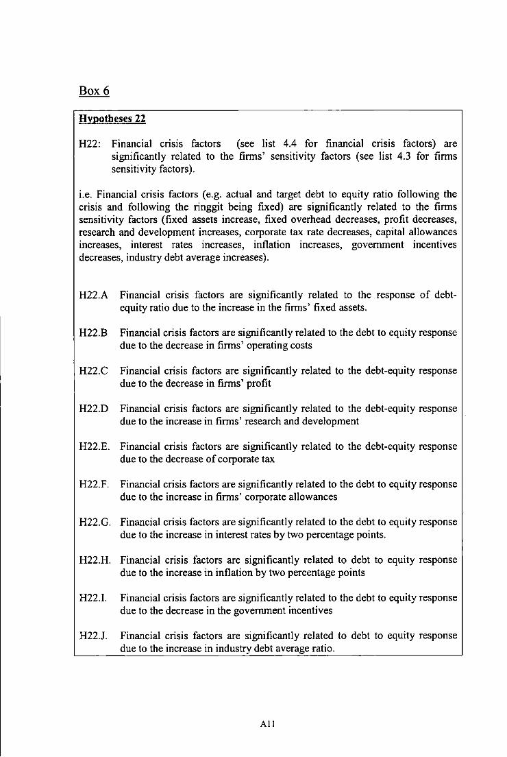
Box6

Hypotheses 22

H22: Financial crisis factors (see list 4.4 for financial crisis factors) are significantly related to the firms' sensitivity factors (see list 4.3 for firms sensitivity factors).

i.e. Financial crisis factors (e.g. actual and target debt to equity ratio following the crisis and following the ringgit being fixed) are significantly related to the firms sensitivity factors (fixed assets increase, fixed overhead decreases, profit decreases, research and development increases, corporate tax rate decreases, capital allowances increases, interest rates increases, inflation increases, government incentives decreases, industry debt average increases).

H22.A Financial crisis factors are significantly related to the response of debtequity ratio due to the increase in the firms' fixed assets.

H22.B Financial crisis factors are significantly related to the debt to equity response due to the decrease in firms' operating costs

H22.C Financial crisis factors are significantly related to the debt-equity response due to the decrease in fmns' profit

H22.D Financial crisis factors are significantly related to the debt-equity response due to the increase in firms' research and development

H22.E. Financial crisis factors are significantly related to the debt-equity response due to the decrease of corporate tax

H22.F. Financial crisis factors are significantly related to the debt to equity response due to the increase in firms' corporate allowances

H22.G. Financial crisis factors are significantly related to the debt to equity response due to the increase in interest rates by two percentage points.

H22.H. Financial crisis factors are significantly related to debt to equity response due to the increase in inflation by two percentage points

H22.I. Financial crisis factors are significantly related to the debt to equity response due to the decrease in the government incentives

H22.J. Financial crisis factors are significantly related to debt to equity response due to the increase in industry debt average ratio.

All

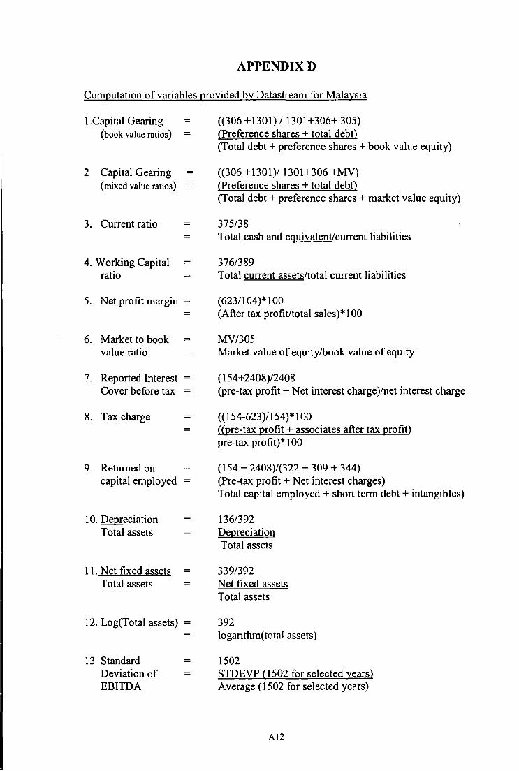
APPENDIXD

Computation of variables provided by Datastream for Malaysia

!.Capital Gearing (book value ratios) =

2 Capital Gearing (mixed value ratios) =

3. Current ratio

4. Working Capital =

ratio =

5. Net profit margin =

6. Market to book value ratio

7. Reported Interest Cover before tax

8. Tax charge

9. Returned on capital employed

10. Depreciation Total assets

11. Net fixed assets Total assets

= =

=

=

((306 + 1301) I 1301 + 306+ 305) (Preference shares + total debt) (Total debt+ preference shares + book value equity)

((306 +1301)/ 1301 +306 +MY) (Preference shares + total debt) (Total debt+ preference shares + market value equity)

375/38 Total cash and equivalent/current liabilities

376/389 Total current assets/total current liabilities

(6231104)*100 (After tax profit/total sales)* 100

MV/305 Market value of equity/book value of equity

( 154+ 2408)/2408 (pre-tax profit+ Net interest charge)/net interest charge

((154-623)/154)* 100 ((pre-tax profit + associates after tax profit) pre-tax profit)* 100

(154 + 2408)/(322 + 309 + 344) (Pre-tax profit+ Net interest charges) Total capital employed+ short term debt+ intangibles)

136/392 Depreciation Total assets

339/392 Net fixed assets Total assets

12. Log(Total assets) 392

13 Standard Deviation of EBITDA

= =

logarithm(total assets)

1502 STDEVP (1502 for selected years) Average ( 1502 for selected years)

Al2

APPENDIXE

Graph 1: Main Board Assets Structure

Main Board Asset Structure

0.50

0.40 0

0.30 .. • CG 0.20 a::

0.10

0.00

1994 1995

CA-T A= Current Assets ffotal Assets FA-T A = Fixed Assets ffotal Assets lnv-TA = lnvestmentsffotal assests

Graph 2:

•

1996

Second Board Asset Structure

CA-TA

• • • FA-TA

..... lnv-TA

1997 1998 1999 2000

Year

Second Board Asset Structure

0 .70 0 .60

~

0 .50 \...~·111

0 0.40 ... "' 0 .30 0:::

-- - - Fa-Ta

0 .20 0 .10 0 .00 Tnv-T.

' '

1994 1995 1996 1997 1998 1999 2000

Year

CA-T A = Current Assets ffotal Assets FA-T A = Fixed Assets ffotal Assets Inv-TA = Jnvestmentsrrotal assests

Al3

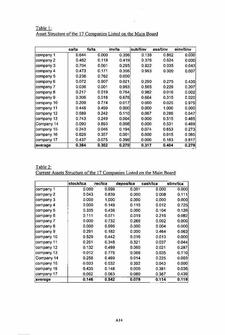
Table 1: Asset Structure ofthe 17 Companies Listed on the Main Board

ca/ta fa/ta inv/ta sub/tinv ass/tinv oinv/tinv company 1 0.644 0.000 0.356 0.138 0.862 0.000 company 2 0.462 0.119 0.419 0.376 0.624 0.000 company 3 0.704 0.001 0.295 0.922 0.035 0.043 company 4 0.473 0.171 0.356 0.993 0.000 0.007 company 5 0.238 0.762 0.000 company 6 0.072 0.907 0.021 0.290 0.275 0.435 company 7 0.036 0.001 0.963 0.565 0.229 0.207 company 8 0.217 0.019 0.764 0.982 0.016 0.002 company 9 0.306 0.018 0.676 0.664 0.315 0.020 company 10 0.209 0.774 0.017 0.000 0.025 0.975 company 11 0.446 0.499 0.000 0.000 1.000 0.000 company 12 0.589 0.242 0.110 0.067 0.286 0.647 company 13 0.743 0.249 0.004 0.000 0.515 0.485 Company 14 0.090 0.893 0.008 0.000 0.531 0.469 company 15 0.243 0.046 0.194 0.074 0.653 0.273 company 16 0.626 0.357 0.001 0.000 0.915 0.085 company 17 0.437 0.075 0.399 0.000 0.183 0.817 average 0.384 0.302 0.270 0.317 0.404 0.279

Table 2: Current Assets Structure of the 17 Companies Listed on the Main Board

stock/tea rec/tca depos/tca cash/tea stinv/tca company 1 0.000 0.999 0.001 0.000 0.000 company 2 0.043 0.839 0.000 0.008 0.111 company 3 0.000 1.000 0.000 0.000 0.000 company 4 0.000 0.149 0.115 0.012 0.725 company 5 0.335 0.436 0.000 0.104 0.126 company 6 0.111 0.571 0.019 0.216 0.082 company 7 0.000 0.732 0.266 0.002 0.000 company 8 0.000 0.996 0.000 0.004 0.000 company 9 0.291 0.182 0.000 0.464 0.063 company 10 0.529 0.442 0.016 0.013 0.000 company 11 0.251 0.348 0.321 0.037 0.044 company 12 0.132 0.499 0.060 0.021 0.287 company 13 0.012 0.776 0.066 0.035 0.110 Company 14 0.258 0.499 0.014 0.225 0.003 company 15 0.033 0.532 0.392 0.043 0.000 company 16 0.435 0.148 0.000 0.381 0.036 company 17 0.052 0.063 0.080 0.367 0.439 average 0.146 0.542 0.079 0.114 0.119

Al4

Table 3: Asset Structure of the 5 Companies Listed on the Second Board

calta fa/ta inv/ta sub/tinv asso/tinv oinv/tinv Company 1 0.268 0.732 0.000 Company 2 0.268 0.732 0.000 1.000 0.000 0.000 Company 3 0.214 0.786 0.000 Company4 0.674 0.024 0.302 1.000 0.000 0.000 Company5 0.242 0.736 0.022 0.000 0.000 1.000.

average 0.333 0.602 0.065 0.667 0.000 0.333

stock/tea rec/tca depos/tca cash/tea stinv/tca Company 1 0.473 0.416 0.031 0.005 0.075 Company2 0.473 0.416 0.031 0.005 0.075 Company3 0.345 0.224 0.000 0.431 0.000 Company4 0.000 0.995 0.000 0.005 0.000 Company 5 0.000 0.002 0.007 0.000 0.990 average 0.258 0.410 0.014 0.089 0.228

AIS

APPENDIX El

Graph 1: Main Board Construction Sector (Price-Currency) Sensitivity

600

400

200

0

Source· OATASTREAM

Graph 2:

PRICE SENSITIVITY

SERIES 1 KUALA LUMPUR SE CONSTRUCTION - PRICE INDEX SERIES 2 US$ TO MALAYSIAN RINGGIT (GTIS)- EXCHANGE RATE CORRELATION COEFF=0.9211 FREQUENCY=MONTHL Y

Main Board Consumer Products Sector (Price-Currency Sensitivity)

300

200

100

0

~· DATAST~

PRICE SENSITIVITY

1994 1995 1996 1997 1998

SERIES 1 KUALA LUMPUR SE CONSUMER PROD. - PRICE INDEX SERIES 2 US$ TO MALAYSIAN RINGGIT (GTIS) - EXCHANGE RATE CORRELATION COEFF=0.8092 FREQUENCY=MONTHL Y

Al6

1999 2000

Graph 3: Main Board Industrial Product (Price-Currency Sensitivity)

250

200

150

100

50

0

PRICE SENSITIVITY

1994 1995 1996 1997 1998

SERIES 1 KUALA LUMPUR SE INDUSTRIAL PROD. • PRICE INDEX SERIES 2 US$ TO MALAYSIAN RINGGIT (GTIS) · EXCHANGE RATE

CORRELATION COEFF=0.9477 FREQUENCY=MONTHL Y

Source. OATASTREAM

Graph4: Main Board Plantation Sector (Price-Currency Sensitivity)

PRICE SENSITIVITY

4000 ringgit

3000

2000

1000

- SERIES 1 KUALA LUMPUR SE PLANTATIONS· PRICE INDEX - SERIES 2 US$ TO MALAYSIAN RINGGIT (GTIS) · EXCHANGE RATE

CORRELATION COEFF=0.8947 FREQUENCY=MONTHL Y

Source: OATASTREAM

AJ7

1999 2000

2000

Graph 5: Main Board Properties Sector (Price-Currency Sensitivity)

4000

3000

2000

1000

0

Source. DATASTREAM

Graph 6:

PRICE SENSITIVITY

price index

1994 1995 1996 1997 1998

SERIES 1 KUALA LUMPUR SE PROPERTIES- PRICE INDEX SERIES 2 US$ TO MALAYSIAN RINGGIT (GTIS)- EXCHANGE RATE CORRELATION COEFF=0.9460 FREQUENCY=MONTHL Y

1999

Main Board Services Sector (Price Sensitivity)

250

200

150

100

50

0

Source: DATASTREAM

PRICE SENSITIVITY

price index

1994 1995 1996 1997 1998 1999

SERIES 1 KUALA LUMPUR SE TRADE & SERVICE - PRICE INDEX SERIES 2 US$ TO MALAYSIAN RINGGIT (GTIS)- EXCHANGE RATE CORRELATION COEFF=0.8988 FREQUENCY=MONTHL Y

Al8

2000

2000

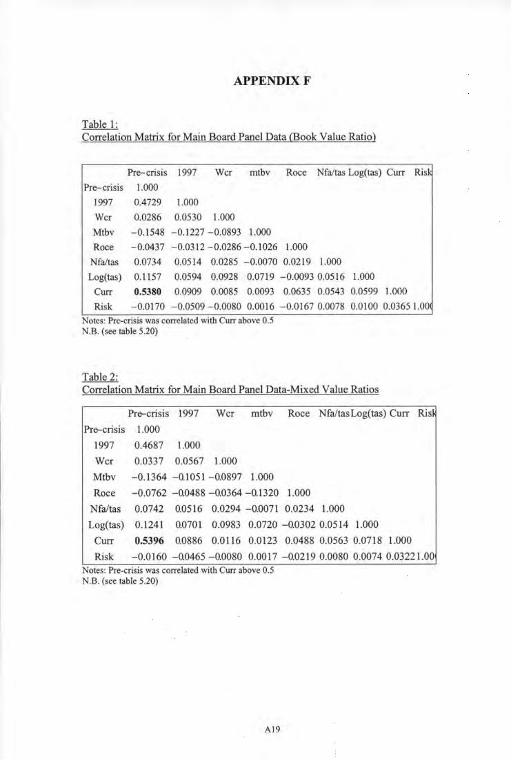
APPENDIXF

Table 1: Correlation Matrix for Main Board Panel Data (Book Value Ratio)

Pre-crisis 1997 Wcr mtbv Roce Nfa/tas Log(tas) Curr Ris~

Pre-crisis 1.000

1997 0.4729 1.000

Wcr 0.0286 0.0530 1.000

Mtbv -0.1548 -0.1227 -0.0893 1.000

Roce -0.0437 -0.0312 -0.0286 -0.1026 1.000

Nfa/tas 0.0734 0.0514 0.0285 -0.0070 0.0219 1.000

Log(tas) 0.1157 0.0594 0.0928 0.0719 -0.0093 0.0516 1.000

Curr 0.5380 0.0909 0.0085 0.0093 0.0635 0.0543 0.0599 1.000

Risk -0.0170 - 0.0509 - 0.0080 0.0016 - 0.0167 0.0078 0.0100 0.0365 1.00 Notes: Pre-crisis was correlated with Curr above 0.5 N.B. (see table 5.20)

Table 2: Correlation Matrix for Main Board Panel Data-Mixed Value Ratios

Pre-crisis 1997 Wcr mtbv Roce Nfa/tasLog(tas) Curr Ris~

Pre-crisis 1.000

1997 0.4687 1.000

Wcr 0.0337 0.0567 1.000

Mtbv -0.1364 -0.1051 -0.0897 1.000

Roce -0.0762 -0.0488 -0.0364 -0.1320 1.000

Nfa/tas 0.0742 0.0516 0.0294 -0.0071 0.0234 1.000

Log(tas) 0.1241 0.0701 0.0983 0.0720 -0.0302 0.0514 1.000

Curr 0.5396 0.0886 0.0116 0.0123 0.0488 0.0563 0.0718 1.000

Risk -0.0160 -0.0465-0.0080 0.0017 -0.0219 0.0080 0.0074 0.03221.00 Notes: Pre-crisis was correlated with Curr above 0.5 N.B. (see table 5.20)

Al9

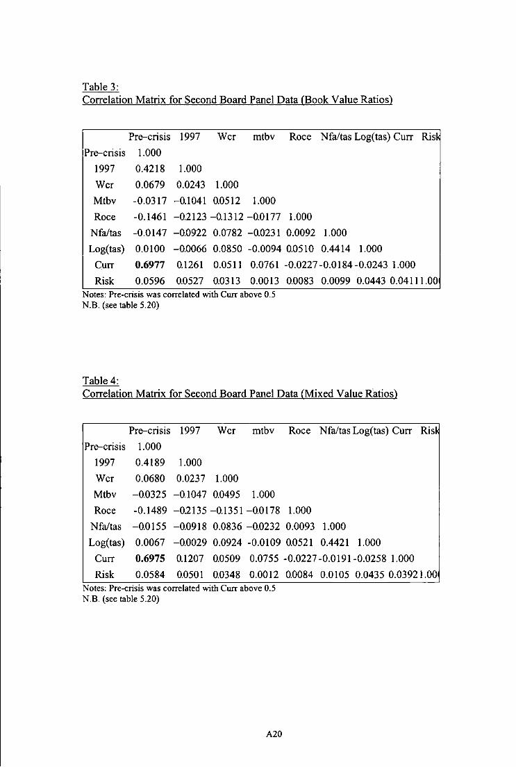
Table 3: Correlation Matrix for Second Board Panel Data (Book Value Ratios)


Pre-crisis 1.000

1997 0.4218 1.000

Wcr 0.0679 0.0243 1.000

Mtbv -0.0317 -0.1041 0.0512 1.000

Roce -0.1461 -0.2123 -0.1312-0.0177 1.000

Nfa/tas -0.0147 -0.0922 0.0782 -0.0231 0.0092 1.000

Log(tas) 0.0100 -0.0066 0.0850 -0.0094 0.0510 0.4414 1.000

Curr 0.6977 0.1261 0.0511 0.0761 -0.0227-0.0184-0.0243 1.000

Risk 0.0596 0.0527 0.0313 0.0013 0.0083 0.0099 0.0443 0.04111.00 Notes: Pre-crisis was correlated with Curr above 0.5 N.B. (see table 5.20)

Table 4: Correlation Matrix for Second Board Panel Data (Mixed Value Ratios)


Pre-crisis 1.000

1997 0.4189 1.000

Wcr 0.0680 0.0237 1.000

Mtbv -0.0325 -0.1047 0.0495 1.000

Roce -0.1489 -0.2135 -0.1351 -0.0178 1.000

Nfa/tas -0.0155 -0.0918 0.0836 -0.0232 0.0093 1.000

Log(tas) 0.0067 -0.0029 0.0924 -0.0109 0.0521 0.4421 1.000

Curr 0.6975 0.1207 0.0509 0.0755 -0.0227-0.0191-0.0258 1.000

Risk 0.0584 0.0501 0.0348 0.0012 0.0084 0.0105 0.0435 0.03921.00 Notes: Pre-crisis was correlated with Curr above 0.5 N. B. (see table 5.20)

A20

APPENDIXG

Table I: ANOV A- Question 1

Variable De Nfa Log

Cr Wcr Npm Mtbv Tie Tax g Roce Factor tas (tas)

tas

Re

Os (**) **

Tdebt

I debt (*) (***)

Cdebt

lbond (**) (***)

Cbond (**)

lbl (*)

Cbl (**)

Fl (*"') (**)

ov (*) . . ..

The astensks m parentheSIS md1cate the cochran 's test of standard dev1at10n IS s1gruficant *,**,***Significant at least at 10%,5% and 1% level critical values

Table 2: Cochran's Test (Standard Deviation Test) of Question 1

Variables Cr Wcr

Np Mtbv Tie Tax

Dep Roce

Nfa/ Tas

Factor m tas !aS

Dre *** ** *"'* **

Dos *** *** *** *** ** ***

Dtdebt ** *** ** *** ***

Didebt •• *** *** *** ***

Dcdebt *** ** ** *** ***

Dibond * *** *** * *** ***

Dcbond *** *** *** **

Dibl * ....... *"'* ** ***

Dcbl *** ** *** *** ** *** ***

Dfl ** *** *** *** ** *"'*

OV ** * ..

*,**,***S1grnficant at least at 10%,5% and !%level cntlcal value

A21

CUIT risk

(*)

c Risk

ur

***

***

***

**

***

***

***

***

***

**

** **

Table 3: Kruskal-Wall is - Question 1

Variable Cr Wcr Npm Mtbv Tie Tax

Dep Roce

Nfa Tas

Factor tas tas

Re

*** Os * ** *

Tdebt ** **

** Idebt * *** * ***

*

Cdebt *

** Ibond ** *** ** **

"' *

Cbond * * *** **

Ibl ** *"' ** Cbl *"'

Fl ** *"'

.. *, **, ***S1gruficant at least at 10%, 5% and I %level cnlical values

Table 4: ANOV A-Questions 2-5


Dep Roce

Nfa Tas

Factor tas tas

Dfau **

Dfod (*)

Dpfd

Drdu ("')

Dtaxd

Dcapu

Din tu (**) "'

Dinfu *

Dgvid *

Dindu ("') (*"') ..

The astensk m parenthesis md1cate the cochran 's test of standard dev1anon IS sigruficant *, **, ***Significant at least at I 0%, 5% and I % level critical values

A22

curr risk

*

*"'

curr risk

(*) (**)

(*)

(**)

Table 5: Cochran's Test (Standard Deviation) of Questions 2-5

Variables Cr Wcr Npm Mtbv Tie Tax

Dep Roce

Nfa Tas R

Factor tas tas

Dfau ** * *** *** *** ***

Dfod *** ** *** *** *** ***

Dpfu * *** *** ***

Drdu *** * ** ** *** *** *** **

Dcapu *** *** *** *** ** *** *** "' Dtaxd * * *** *** *** * ***

Din tu ** *** *** ** *** * ***

Dinfu ** *** *** *** *** * *** *

Dgvid *** *** *** *** * *** *** *

Dindu *** ** *** *** *** ••• * *** ..

*,**,***Stgmficant at least at 10%,5% and 1% level cnt1eal value

Table 6: Kruskal-Wallis (Median Test) Questions 2-5


Dep Roce Nfa Tas risk curr

Factor tas tas

Dfau *

Dfod

Dpfd **

Drdu

Dcapu *

Dtaxd

Din tu *** • Dinfu ** *

Dgvid * * • ** ***

Dindu * • * .. *, **, ***Stgruficant at least at 10%, 5% and I %level cnncal values

A23

APPENDIXH

Table 7: Logistic Regression (Question 1)

Dre Dos Dtdebt Didebt

Constant (3.3721) (7.176) (-4.681) (21.298)

Wcr 0.094 3.029* 0.118 11.558*** (0.11 I) (3.363) (0.152) (-15.51 I)

Mtbv 1.974 60.595*** 0.022 18.075***

(-0.299) (0.834) (-0.024) (-16.184)

Roce 0.215 24.134*** 0.15 -0.188 (-0.035) (-0.873) (-0.008) (-0.015)

N fa/tassets 0.009 60.595*** 0.359 0.684 (-0.157) (2.711) (0.664) ( -4.250)

Log(tas) 0.510 7.471 *** 0.000 57.927***

(0.11)) (-0.958) (0.002) ( 1.936)

Curr 0.791 60.600*** 4.981'"* 21.414*** (-2.673) (4.284) (4.322) (41.23)

Risk 0.002 0.117 0.227 -0.006 (0.016) (0.164) (0.154) (-0.288)

Dfau 0.821 3.119* 2.734* 13.057

(0.979) (3.643) (1.917) (31.6)

Dfod 0.151 0.072 0.157 -0.176 (-0.584) (-0.647) (-0.452) (4.865)

Dpfd 0.325 0.507 9.628*** 21.504**'" (0.655) (1.480) (-3.135) (-37.90)

Drdu 0.816 0.150 1.169 0.579 (1.054) (0.651) (-1.141) (-6.193)

Dtaxd 0.265 -0.150 0.661 17.215*** (0.560) (-5.501) (1.040) ( -12.070)

Dcapu 1.317 19.302'"** 1.292 0.063 (-1.437) (11.049) (1.460) (-18.235)

Din tu 0.036 60.600*** 0.174 20.475***

(0.192) (1.041) (-0.427) (9.768)

Dinfu 0.219 60.600*** 1.547 0.603 (-0.692) (-7.734) (1.923) (7.665)

Dgvid 2.475 60.600*** 1.011 12.796*** (-1.949) ( -2.304) (1.180) (-36.96)

Dindu 0.548 60.600*** 0.033

Linear (0.992) (4.733) (0.244)

Analysis of deviance

Model 0.849 0.0000 0.2980 0.0001

p-value 0

%Deviance 21.57 90.47% 31.78% 99.35%

%

Adjusted% 0 32.78% 0 25.61% ..

*, **, ***S•gruficant at least at 10%, 5% and I %level cnucal values The value in the parenthesis is the coefficient of the parameter.

A24

Dcdebt Dfl Ov

(-10.895) (18.519) (-12.956)

0.045 28.985*** 0.000 (0.124) (-2.558) (-0.023) 0.113 -2.466 0.998

(-0.063) ( -1.666) (0.700) 0.083 26.325*** 0.187

(0.022) (0.569) (-0.046) 4.386** 8.724** 0.658 (6.659) (9.961) (-1.112) 1.324 24.865*** 0.779

(0.236) (-3.275) (0.164) 6.628 5.156** 1.090

(5.427) (I 5.036) (2.95)

0.001 -1.843 6.556** (0.026) (-3.Q92) (1.869)

0.723 11.592*** 0.160 (0.991) (2.943) (-0.597)

0.395 0.688 1.353 (-1.060) (4.633) (1.978)

11.668*** 8.341*** 0.000 (-4.165) (-10.665) (-0.022)

0.000 1.677 0.223 (-0.029) (4.216) (0.675)

2.609 -1.797 0.343 (1.975) (-9.550) (1.620)

1.781 -2.119 1.329 (2.235) (12.081) (2.468)

0.669 2.293 6.302** ( -0.944) (-12.512) (-4.311)

1.095 11.720 2.203 (1.942) (-3.225) (2.856)

0.356 25.504*** 7.021 *** (0.804) (20.340) (4.758)

0.807 0.523 1.202 (1.501) (3.023) 1.841)

0.1385 0.0000 0.080

40.77% 92.36% 44.80%

0 29.60% 0

Table 8 : Stepwise Logistic Regression (Question 1)

Dre Dos Dtdebt Didebt

Constant (-1.320) ( 1.139) (1.266)

Wcr

Mtbv

Roce 7.730*'"* ( -0.136)

Nfa/tassets

Log(tas)

Curr

Risk

Dfau

Dfod

Dpfd 6.709** (-1.727)

Drdu

Dtaxd

11.573** Dcapu •

(2.438)

Din tu 4.777** (-2.261)

Dinfu

Dgvid

Dindu 6.853*** 7.720*** (2.237) (-2.524)


Model p-value 0.0000 0.010 0.0012

%deviance 25.76% 10.91% 32.40%

Adjusted% 14.68% 4.40% 19.23% ..

*, ••, ***Stgmficant at least at 10%, 5% and I %level cnucal values The value in the parenthesis is the coefficient of the parameter.

A25

De debt dfl Qv

(-0.360)

4.564** (2.622)

7.186*** (-1.914)

0.0060

17.82

7.34%

Table 9: Logistic Regression (Questions 2 to 5)

Dfau Dfod Dpfd Drdu Dtaxd Dcapu

Constant (-1.83) (0.0) (8.71) (-28.9) (1.79) (5.59)

Wcr 1.38 -52.48 0.47 0.54 0.87 4.62•• (0.39) (0.0) (-0.21) (0.64) (-0.34) (1.26)

Mtbv 0.22 -37.25 0.18 2.34 1.08 0.26 (0.12) (0.0) (0.06) (-0.48) (0.19) (0.07)

Roce 0.01 -51.95 0.10 7.3••• 0.78 5.56° 0

(-0.01) (0.0) (-0.02) (-0.46) (0.06) (0.28)

Nfa/tas 1.03 -57.63 0.08 5.01° 0 0.14 3.92° 0

( 1.91) (0.0) (-0.42) ( -5.39) (0.71) (6.48)

Log(tas) 0.02 -53.44 0.11 3.51° 0.02 4.21° 0

( -0.02) (0.0) (0.05) (0.97) (-0.02) (-0.66)

Curr 4.36° 0 0.0 2.37 14.3••• 0.01 5.09•• (3.68) (0.0) ( -3.52) (-24.31) (-0.28) (9.17)

Risk 1.51 -46.67 0.23 3.20° 0.63 3.05°

(0.88) (0.0) (0.12) ( -4.05) (-0.22) (-2.78)

Dfau Linear -68.14 0.68 1.13 2.37 11.3••• (0.0) (-0.81) (2.43) (-1.98) (8.23)

Dfod 1.44 Linear 1.68 23.9°00 0.03 7.6••• (- 1.78) (I. 77) (49.44) (-0.34) (-6.81)

Dpfd 0.45 -51.24

Linear 4.27•• 0.37 1.30

( -0. 72) (0.0) (5.98) (0.69) (-2.52)

Drdu 0.20 -44.51 0.01 0.46 0.05

(0.53) (0.0) (-0.13) Linear

(-0.97) (0.27)

Dtaxd 4.o8•• -68.96 0.01 3.30

Linear 15.6···

( -3.02) (0.0) (0.11) (-5.08) (-9.44)

Dcapu 9.1t••• -51.92 3.57* 1.19 8.6•••

Linear (3.97) (0.0) (-2. 76) (2.58) (-3.65)

Din tu 0.92 -45.43 3.os• 8.46 1.80 -0.12

( -1.15) (0.0) ( -1.69) (-5.15) (1.44) (1.88)

Dinfu 0.13 -43.36 0.62 6.64 3.08 0.55

(0.44) (0.0) (-1.19) (-5.79) (2.86) ( 1.40)

Dgvid 0.08 -47.88 3.33° 5.70 0.86 2.29

(0.33) (0.0) (-2.20) (-8.02) (1.16) (2.39)

Dindu 0.44 -46.18 1.43 0.09 0.76 3.63•

(-0.97) (0.0) ( -2.05) (0.55) (-1.52) ( -6.9)


p-value 0.386 1.000 0.185 0.001 0.005 0.001 %

27.11 -31.55 34.11 61.64 49.80 69.33 deviance Adjusted

0.0 0.0 0.0 7.40 0.69 19.76 %

.. •, ••, ***S•gruficant at least at 10%, 5% and I% level cntlcal values The value in the parenthesis is the coefficient of the parameter.

A26

Din tu Dinfu Dgvid Dindu

(3.33) ( 11.62) ( 1.33) (-17.3)

1.16 2.02 3.50 -3.20 (0.48) ( -2.02) (-1.36) (-0.17)

0.90 0.39 49••• 0.20 (0.12) ( -0.38) (0.39) ( -0.36)

1.33 10.4°00 49••• 2o••• (0.06) (0.32) (0.18) (-0.81)

1.54 2.51 0.03 9.7••• ( 1.38) (2.19) (-0.17) ( -4.78)

0.95 0.86 8.3••• 11··· (-0.16) ( -0.29) (-0.53) ( 1.30)

0.08 0.49 8.9••• -3.24 (0.44) (1.96) (7.76) (6.65)

3.39° 6.9••• 12.4 25••• (-0.41) ( -0.85) (4.64) ( 1.59)

0.36 0.00 0.02 -3.28 (-0.56) (-0.02) (0.30) ( 1.25)

1.44 6.9••• 3.11° 0.31 (-1.43) (-4.72) (-2.92) (0.93)

3.84° 0 0.10 6.9••• -3.01 (-1.83) (0.58) (-3.55) (-7.54)

2.37 3.93° 0 49°00 2.63 (-1.47) (-3.65) (-3.60) (4.02)

4.52° 0 2.53 1.79 0.04 (2.20) (3.45) (1.84) (0.10)

0.19 0.00 49°* 0 -0.16 (-0.54) (0.00) (2.53) (1.12)

Linear 0.57 0.07 -3.17 ( 1.19) (0.17) (-1.88)

0.48 Linear 0.40 19°00

(0.76) (-0.84) (-13.3)

0.44 0.51 Linear 0.72 (-0.64) (-1.20) (4.37)

1.30 5.23°0 -0.07 Linear (-1.61) (-5.24) (0.49)

0.133 0.000 0.000 0.000

32.38 64.18 69.79 90.44

0.0 12.98 19.81 31.10

Table 10: Stepwise Logistic Regression (Questions 2 to 5)

dfau Dfod Dpfd drdu dcapu dtaxd

Wcr

Mtbv

Roce

Nfaltas

Log(tas)

cuir

Risk

Dfau 4.66** (1.780)

Dfod 9.89••• (16.20)

Dpfd

Drdu 9.89*** (15.83)

Dtaxd 20.7••• (-3.18)

Dcapu 15.3* .. (-2.72)

Din tu 6.59** ( -1.66)

Dinfu 5.41** (1.799)

Dgvid

Dindu

Analxsis of deviance

p-value 0.002 0.010 0.002 0.000 0.000 %deviance 18.76 10.79 15.77 34.90 35.66 Adjusted% 11.17 4.24 9.39 26.15 26.99

.. *, **, ***S1gruficant at least at I 0%, 5% and I % level cntlcal values The value in the parenthesis is the coefficient of the parameter.

A27

din tu

6.48** (-1.75)

5.025** (1.408)

0.003 16.84 8.14

dinfu dgvid dindu

7.29··· 8.02··· (0.115) (~.13)

4.2o•• (3.10)

7.48••• 10.4 ... (~.34) (0.353)

4.77** 7.21··· (-2.01) (-3.08)

1.1s••• (2.152)

8.67••• (2.34)

6.16** (-2.03)

12.2··· (-3.48)

0.000 0.000 0.000 37.56 37.93 34.49 22.50 23.23 20.53

Table 11: Logistic Regression (Questions 6 to 9)

Dagcc Dtgcc Dagcf

Constant (1.799) (7.254) (2.906)

Wcr 6.819*** 2.482 0.003 (-1.197) (-0.732) (-0.064)

Mtbv 0.207 1.180 1.576

(0.150) (-0.169) (-1.067)

Roce 3.666 0.053 0.229

(0.144) (0.014) (0.076)

Nfaltas 0.267 2.185 0.195

(0.968) (1.606) (0.770)

Log(tas) 1.058 4.417** 0.919

(-0.205) (0.370) (0.323)

Curr 0.665 0.277 0.021

(1.721) (-0.881) (-1.007)

Risk 0.986 1.100 2.051

(0.332) (-0.270) ( -1.990)

Dfau 0.441 1.194 0.119

(-0.742) (1.024) (0.811)

Dfod 0.001 0.037 0.010

(-0.051) (0.220) (-0.212)

Dpfd 1.431 1.504 1.430

( -1.596) (-1.334) (2.671)

Drdu 0.612 0.492 0.026

(-1.064) (0.747) (0.321)

Dtaxd 1.261 0.091 0.160

(1.918) (-0.341) (-1.321)

Dcapu 0.008 0.652 1.757

(0.162) ( 1.0 12) (-4.357)

Din tu 1.747 0.081 1.695

(-1.761) (0.267) (-2.828)

Dinfu 2.583 3.441* 6.456**

(-2.406) (-2.045) (-5.793)

Dgvid 11.122*** 0.649 5.937**

(4.620) (0.910) (-5.254)

Dindu 0.036 1.003 1.049

(0.331) (-1.466) (1.914)


p-value 0.0070 0.2130 0.0475 % 51.07% 31.32% 55.53% deviance

Adj.% 0% 0% 0% ..

*, **, ***S1gruficant at least at 10%, 5% and I %level cnllcal values The value in the parenthesis is the coefficient of the parameter.

A28

Dtgcf

(27.55)

23.517*** (2.818)

15.177*** (-0.043)

0.225 (0.079)

0.300 (1.286)

15.712 ... (0.202)

64.360*** (-26.793)

15.245*** (0.598)

-0.881 (-2.600)

23.495*** (-3.248)

23.882*** (1.510)

-0.075 ( -2.750)

23.489*** (-5.536)

16.187*** (-2.538)

13.320*** (-6.591)

-1.000 (-13.716)

-2.684 ( -9.042)

15.266*** ( -0.40 I)

0.0018

88.73%

6.85%

Table 12: Stepwise Logistic Regression (Questions 6-9)

Dagcc Dtgcc Dagcf

Constant (1.674) (0.773) (-0.318)

Wcr

Mtbv

Roce

Nfa/tas

Log(tas)

Curr

Risk

Dfau

Dfod

Dpfd

Drdu

Dtaxd

Dcapu

Din tu

Dinfu 12.980*** 8.927••• 9.345*** (-2.367) ( -1.829) (-2.356)

Dgvid

Dindu


p-value 0.003 0.0028 0.0022 %

19.16% 13.12% 18.67% deviance

Adj.% 13.26% 7.24% 10.68% ..

•, ••, •••s1gruficant at least at I 0%, 5% and I % level cntlcal values The value in the parenthesis is the coefficient of the parameter. Dagcc - dummy if the actual die ratio change following the crisis Dtgc - dummy if the target die ratio change following the crisis

Dtgcf

( -3. 783)

5.028** _(0.197)_

8.289*** (3.691)

14.780••• (-52.496) 10.041*** (-4.856)

0.0000

61.63%

38.89%

Dagcf- dummy if the actual die ratio change following the ringgit being fixed Dtgcf- dummy if the target die ratio change following the ringgit being fixed.

A29

APPENDIX I

PILOT STUDY QUESTIONNAIRE

Sharifah Raihan Syed Mohd Zain Research Office Plymouth Business School University of Plymouth Plymouth PL4 8DW United Kingdom

Dear Sir/Madam,

Re: Questionnaires Survey for PhD Research

I am currently pursuing a PhD degree at the University of Plymouth, in the United Kingdom. As part of this research exercise, I am conducting a short questionnaire survey on the topic of the capital structure ofMalaysian companies. I would

. appreciate very much if you could spend a few minutes to read the term of reference and complete the questionnaire survey.

Please be advised that information gathered in this survey will be treated with the strictest confidence and will only be used for the purpose of this research study. Names of individual people or companies will not be revealed in the dissemination of this research. An executive summary of results will be sent to participants.

Thank you in anticipation your reply.

Yours sincerely,

(Sharifah Raihan Syed Mohd Zain)

Instructions on bow to complete tbe questionnaire:

1. Please double click on the attachment file below, complete the questionnaire, SAVE IT. Please email the SAVED attachment file (completed questionnaire) back to me. OR

2. Please print the attachment file, complete the questionnaire and mail it through regular mail (post office) using the above address.

Thank you.

A30

Tenus of Reference

As you will no doubt already know, capital structure refers to the appropriate mix of debt and equity of a finn. This is usually measured by the ratio of debt to equity or the ratio of debt to total assets, using book or market values. The factors that influence the detennination of a finn's capital structure have been examined extensively both in theoretical and empirical research. However, most of the studies are centred on countries such as the United States, United Kingdom and Japan. Therefore, this research is very important for Malaysian companies, as very little research has been conducted in this area.

Questionnaire

I. Please indicate how you intend your long-tenn capital projects to be financed? (please indicate the percentage of financing)

Source of finance During the next 12 In the longer-term months(%) (%)

Internal equity (retentions)

Ordinary shares

Preference shares

Islamic bonds

Conventional bonds

Islamic bank loan


Overdrafts

Other(please specify)

2. Please indicate the extent to which the following factors are important in the detennination of the finn's capital structure (debt as a proportion of total longtenn financing). Please indicate ("X") to important factors only.

Factors During tbe next In tbe longer

12 months term

Level of fixed overheads

Ratio of fixed assets to total assets

Total assets employed

An increase in your company's profit

A31

Reductions in corporate tax rate

Capital allowances on assets (for tax purposes)

Research and development expenditure

Inflation

Interest rates

Exchange rates

Views of market commentators

The use ofusury(RIBA)/interest rates

Mix of short and long-term debt

Degree of political risk exposure

Government incentives (e.g. subsidiaries)

Following the industry norm

Lease as a substitute for debt

Mergers, acquisitions and divestments

Debt as a substitute for equity to avoid equity dilution

Public disclosure of accounting information beyond minimum statutory requirement

4. Would it be possible to have a fonnal interview about this survey in the future? (between July 2001 to October 2001), please indicate ("X").

I Yes I

The following infonnation is optional:

Your name: Your position: Your company:

A32

APPENDIXJ

QUESTIONNAIRE USING POSTAL MAIL

Finance Manager,

Address

24/04/2001

Dear Sir/Madam,

Re: Questionnaire Survey for Ph.D. Research

I am currently pursuing a Ph.D. Degree at the University of Plymouth, in the United Kingdom. As part of this research, I am conducting a questionnaire survey on the capital structure of Malaysian companies. I would very much appreciate if you could spend a few minutes to read the terms of reference and complete the questionnaire attached.

Please be advised that information gathered in this survey will be treated with the strictest confidence and will only be used for the purpose of this research study. Names ofindividual persons or companies will not be revealed in the dissemination of this research. An executive summary of results will be sent to respondents.

Thank you in anticipation of your reply.

Yours sincerely,

Sharifah Raihan Syed Mohd Zain

Research Office Plymouth Business School University of Plymouth Plymouth PL4 8AA United Kingdom

Email: [email protected], [email protected]

A33

Terms of Reference

As you will no doubt already know, capital structure refers to the appropriate mix of debt and equity of a firm. This is usually measured by the ratio of debt to equity or the ratio of debt to total assets, using book or market values. The factors that influence the determination of a firm's capital structure have been examined extensively both in theoretical and empirical research. However, most of the studies are centred on countries such as the United States, the United Kingdom and Japan. Therefore, this research is very important for Malaysian companies, as very little research has been conducted in this area.

1. Please indicate your firm's priorities in raising additional funds to finance new investment. (Please tick the appropriate box, where applicable).

Sources of funds High Medium Low

priority priority priority

Internal equity (retentions)

Ordinary shares

Preference shares

Islamic bonds

Conventional bonds

Islamic bank loan


Overdrafts

Finance leases

Other (please specify)

·······························

A34

2. Please indicate the likely impact of the following company factors upon your firm's leverage (i.e. debt-to-equity) ratio. (Please tick the appropriate box).

Large Moderate No change

Moderate Large Company's factors Reduction Reduction

in DIE Increase in Increase in

in DIE* in DIE DIE DIE

A significant increase in fixed assets as a proportion of total assets

A significant decrease in fixed overhead costs

A significant increase in the company's profit

A significant decrease in the company's profit

A significant increase in research and development expenditure

A significant increase in public disclosure of accounting information beyond minimum statutory requirement

* DIE = debt/eqUity ratio (book value of debt/book value of eqUity)

3. Please indicate the likely impact of the following tax factors upon your firm's leverage (i.e. debt-to-equity) ratio. (Please tick the appropriate box).


Moderate Large Tax factors Reduction Reduction Increase in Increase in

in DIE* in DIE in DIE DIE DIE

Annual decrease in corporate tax rate similar to those experienced in recent years

A significant increase in capital allowances on assets (for tax purposes)

Temporary tax losses (if applicable)

* DIE- debt/eqUity ratio (book value of debt/book value of eqUity)

A35

4. Please indicate the likely impact of the following macroeconomic factors upon your firm's leverage (i.e. debt-to-equity) ratio. (Please tick the appropriate box).

Large Moderate No change Moderate Large Macroeconomic factors Reduction Reduction Increase in Increase in

in DIE* in DIE in DIE DIE DIE

An increase in long-term interest rates by 2 percentage points

A decrease in long-term interest rates by 2 percentage points

An increase in inflation by 2 percentage points

A decrease in inflation by 2 percentage points

• DIE = debt/eqmty ratto (book value of debt/book value of equtty)

5. Please indicate the likely impact of the following specific factors upon your firm's leverage (i.e. debt-to-equity) ratio. (Please tick the appropriate box).

Large Moderate No change Moderate Large Specific factors Reduction Reduction in DIE Increase in Increase in

in DIE* in DIE DIE DIE

An increase in government incentives

A decrease in government incentives

An increase in industry average debt ratio

A decrease in industry average debt ratio

* DIE = debtlequtty ratto (book value of debt/book value of eqmty)

6. Please indicate whether your firm's ACTUAL leverage ratio (book value of debt/book value of equity) changed directly following the 1997 currency crisis. (Please tick the appropriate box).

yes no

A36

If yes, please indicate the impact. (Please tick the appropriate box).


Moderate Large Reduction Reduction Increase in Increase in

in DiP in DiE in DIE

DIE DIE

*DIE =debt/eqUity ratio (book value of debt/book value of equity)

7. Please indicate whether your firm's TARGET leverage ratio (book value of debt/book value of equity) changed immediately following the currency crisis. (Please tick the appropriate box).

yes no




in DIE* in DiE in DIE

DIE DiE

*DIE =debt/eqUity ratio (book value of debt/book value of equity)

8. Please indicate whether your firm's ACTUAL leverage ratio (book value of equity/book value of debt) changed as a result of the ringgit being fixed to the US dollar. (Please tick the appropriate box).

yes no




in DIE* in DIE in DIE

DIE DIE

*DIE - debt/equtty ratio (book value of debt/book value of equity)

9. If you have aT ARGET leverage ratio, please indicate whether your firm's TARGET changed as a result of the ringgit being fixed to the US dollar. (Please tick the appropriate box).

yes no

A37




in DIE* in DIE in DIE

DIE D/E

*DIE = debt/eqmty ratto (book value of debt/book value of equity)

10. Would you agree to a brief informal interview on this subject if requested? (Please tick the appropriate box).

yes no

Please provide the following information (optional):

Name of Respondent:

Position:

Company's Name and address:

Telephone and Fax number:

Email address:

THANK YOU FOR YOUR CO-OPERATION

PLEASE RETURN THE COMPLETED QUESTIONNAIRE USING THE ENCLOSED SELF ADDRESSED ENVELOPE

A38

APPENDIXK

COVER LETTER FOR THE QUESTIONNAIRE REMINDER

Finance Manager, Address

15/08/2001

Dear Sir/Madam,

Re: A Kind Reminder for Ph.D. Research Questionnaire Survey

I am writing to kindly inquire if you have received a copy of the questionniare which I sent from the United Kingdom in May 2001. This questionnaire is crucial and very important for my Ph.D. study. Without your assistant in this matter, my analysis in this field of study will not be complete.

Please be advised that information gathered in this survey will be treated with the strictest confidence and will only be used for the purpose of this research study. Names of individual persons or companies will not be revealed in the dissemination of this research. An executive summary of results will be sent to respondents.

If you have not completed the questionnaire, I am attaching a second copy for your convenience. However, if you have already completed and sent the questionnaire to me, please kindly ignore this letter.

Your kind assistance and attention in this matter is very much appreciated.

Thank you.

Yours sincerely,

Sharifah Raihan Syed Mohd Zain Department of Business Administration KENMS,IIUM Jalan Gombak 53100 Kuala Lumpur Malaysia

Email: [email protected], [email protected]

A39

COPYRIGHT STATEMENT

This copy of the thesis has been supplied on condition that anyone who consults it is understood to recognise that its copyright rests with its author and that no quotation from the thesis and no information derived from it may be published without the author's prior consent.

an empirical study of mala ysian firms' capital struture - CORE

Documents

Transcript of an empirical study of mala ysian firms' capital struture - CORE