An Empirical Study ofConstraint Logic Programming

andAnswer Set Programming

Solutions of Combinatorial Problems∗

Agostino Dovier† Andrea Formisano‡ Enrico Pontelli§

Abstract

This paper presents experimental comparisons between the declarative encod-ings of various computationally hard problems in bothAnswer Set Programming(ASP)and Constraint Logic Programming over finite domains (CLP(FD)). Theobjective is to investigate how the solvers in the two domains respond to differ-ent problems, highlighting strengths and weaknesses of their implementations andsuggesting criteria for choosing one approach versus the other. Ultimately, thework in this paper is expected to lay the foundations for transfer of technologybetween the two domains, e.g., suggesting ways to use CLP(FD) in the executionof ASP.

Keywords. Declarative Programming, Constraint Logic Programming, An-swer Set Programming, Solvers, Benchmarking.

1 Introduction

The objective of this work is to experimentally compare the use of two distinct logic-based paradigms, traditionally recognized as excellent tools to tackle computationallyhard problems. The two paradigms considered areAnswer Set Programming (ASP)[2]andConstraint Logic Programming over Finite Domains (CLP(FD)) [27]. The moti-vation for this investigation arises from the successful use of both paradigms in dealingwith various classes of combinatorial problems, and the need to better understand theirrespective strengths and weaknesses. Ultimately, we hope this work will indicate meth-ods for integration and cooperation between the two paradigms (e.g., along the lines of[10, 11]).

∗A preliminary version of this paper appeared in the Proceedings of the International Conference onLogic Programming, LNCS 3668, pp. 67–82, Springer Verlag, 2005.

†Univ. di Udine, Dip. di Matematica e Informatica.dovier@dimi.uniud.it‡Univ. di L’Aquila, Dip. di Informatica.formisano@di.univaq.it§New Mexico State University, Dept. Computer Science.epontell@cs.nmsu.edu

1

It is well-known [2, 25] that, given a propositional normal logic programP , de-ciding whetherP admits ananswer set[15] is an NP-complete problem. As a con-sequence, any NP-complete problem can be encoded as a propositional normal logicprogram under answer set semantics. Answer-set solvers [36] are programs designedto compute the answer sets of normal logic programs. These tools can be seen as the-orem provers, or model builders, enhanced with several built-in heuristics to guide theexploration of the search space. Most ASP solvers rely on variations of the Davis-Putnam-Logemann-Loveland procedure [6, 7] in their computations. Such solvers areoften equipped with a front-end that transforms a collection of non-propositional nor-mal logic programming clauses (with limited use of functionsymbols) to afinite setof ground instances of such clauses. Some solvers provide also syntactic extensions tofacilitate program development—e.g., limited forms of aggregation [31]—and classesof optimization statements, used to select answer sets that maximize or minimize anobjective function dependent on the content of the answer set.

An alternative framework, frequently adopted to handle NP-complete problems, isConstraint Logic Programming over Finite Domains[19, 27]. In this context, a finitedomain of objects (typically integers) is associated to each variable in the problemspecification, and the constraints are literals of the formss = t, s 6= t, s < t, s ≤ t, etc.,wheres andt are arithmetic expressions. This type of framework supports the naturaland declarative encoding of search strategies and NP-complete problems. Indeed, arich literature has been developed presenting applications of CLP(FD) to a variety ofsearch and optimization problems [27].

In this paper, we report the outcome of a study aimed at comparing these two declar-ative approaches in solving combinatorial problems. We address a set of computation-ally hard problems—in particular, we mostly consider decision problems known to beNP-complete. We formalize each problem, both in CLP(FD) andin ASP, by takingadvantage of the specific features available in each logicalframework, attempting toencode the various problems in themost declarativeway possible. In particular, weadopt aconstraint-and-generatestrategy [27] for the construction of the CLP(FD) pro-grams, while in ASP we exploit the naturalgenerate-and-testapproach [2]. Wheneverpossible, we make use of encodings of these problems that have been presented andwidely accepted in the literature.

With this work we intend to develop a bridge between these twologic-based frame-works, in order to emphasize the strengths of each approach,and in favor of potentialcross-fertilizations. This study also complements the system benchmarking studies,recently published for both CLP(FD) systems [13, 34] and ASPsolvers [1, 24, 21, 18].

2 Brief Overview of the Computational Models

2.1 Constraint Logic Programming over Finite Domains

Constraint logic programming (briefly, CLP) [19] is a programming paradigm that isparticularly well suited for encoding combinatorial optimization problems. CLP nat-urally merges two declarative paradigms: constraint solving and logic programming.

2

Let Σ be a logic language signatureΣ = 〈F ,V , Π ∪ΠC〉, where

• F is a finite set of function and constant symbols

• V is a denumerable collection of variables

• Π ∪ΠC is a finite set of predicate symbols, whereΠ andΠC are disjoint sets.

A constraintis a first-order formula over〈F ,V , ΠC〉. Typically, constraints are con-junctions of literals, e.g.,0 < X, X < 3, X + Y 6= 4. Following the traditional logicprogramming notation, a comma indicates a conjunction, capital letters denote vari-ables, and the symbol:− denotes the implication←. CLP lets a programmer usedifferent classes of constraints and domains to encode problems. For combinatorialproblems, it is common to usefinite domain constraints, namely arithmetic constraintsbetween arithmetic expressions, where each variable is associated to a finite domain ofpossible values. In this case the interpretation of variables, expressions, and constraintsis overZ.

A CLP program overΣ is a finite set of rules of the form

p(s1, . . . , sn) :− C, q1(t11, . . . , t

1n1

), . . . , qm(tm1 , . . . , tmnm)

whereC is a constraint,si and tij are(F ,V)-terms, andp, q1, . . . , qm are predicatesymbols ofΠ. Observe that a CLP program without constraints is in fact a Prologprogram.

In contrast to classic generate-and-test approach of logicprogramming, CLP usu-ally uses aconstrain-and-generatetechnique in which an initial deterministic phaseimposes a number of constraints, then a non-deterministic phase generates/explores thesolution space. In theconstraint phase, in particular, a finite domain of values is as-signed to each of the variables. For instance, the constraint domain([A,B,C],1,5)

assigns the set of admissible values{1,2,3,4,5 } to the variablesA, B, andC. Thebuilt-in predicatelabeling implements the solution search process. Each time a vari-able is assigned a value, a deterministic propagation stageis executed, pruning the setof values to be attempted for the other variables. Various options (affecting, for in-stance, the variable selection criteria, the ordering of the attempted values, etc.) canbe used to guide the search. The main structure of a program using this programmingstyle is the following:

solve_problem(X1,...,Xn) :-constraint(X1,...,Xn),labeling([options], X1,...,Xn).

A CLP(FD) system executes program according togoals provided by the user,where a goal is a conjunction of literals. Given a programP and a goala1, . . . , ak,the program will determine the instantiationsσ of the variables in the goal such that∀(a1, . . . , ak)σ is a logical consequence ofP .

2.2 Answer Set Programming

Answer Set Programming is a logic programming paradigm thathas its foundations intraditional logic programming under answer set semantics [15].

3

Let us consider a logic language signatureΣ = 〈F ,V , Π〉, where

• F is a finite set of constant symbols

• V is a denumerable collection of variables

• Π is a finite set of predicate symbols

The set oftermsis F ∪ V , and an atom is a formula of the typep(t1, . . . , tk), wherep ∈ Π andt1, . . . , tk are terms.

An ASP program is a finite collection of rules, where rules areof the form

h :− a1, . . . , am, not b1, . . . , not bn

whereh, a1, . . . , am, b1, . . . , bn are atoms. Each program is viewed as a syntactic sugarrepresenting the set ofground instancesof its rules, where the ground instances of arule are obtained by consistently replacing the variables in the rule with elements ofF .A special type of rules are the so calledconstraints—rules with an empty head; in thiscase, the head of the rule is implicitly assumed to befalse.

Given a ground programP , the answer set semantics characterizes the semanticsof P in terms of a collection of minimal models (calledanswer sets). A set of groundatomsM is an answer set ifM is the unique minimal model of the programPM ,obtained as

PM =

{

h :− a1, . . . , akh :− a1, . . . , ak, not b1, . . . , not bh ∈ P,

{b1, . . . , bh} ∩M = ∅

}

In ASP, each problem is modeled as a collection of rules, in such a way that the solu-tions to the problem correspond one-to-one to the answer sets of the program. AnASPSolveris a program that computes all the answer sets of a given ASP program.

Systems like SMODELS have extended the syntax of ASP to allow more expressiveconstructs, such as:

• domain declarations:these are atoms of the form

p(v1..v2)

wherev1 ≤ v2 are integers; these are short forms for the collection of facts:

p(v1). p(v1 + 1). . . . p(v2).

• cardinality constraint atoms:these are atoms of the form

L{p1, . . . , pk, not q1, . . . , not qh}U

wherep1, . . . , pk, q1, . . . , qh are atoms andL ≤ U are integers; the atom issatisfied by a set of atomsM if

L ≤ |({p1, . . . , pk} ∩M) ∪ ({q1, . . . , qh} \M)| ≤ U

4

• weight constraint atoms:these are similar to cardinality atoms, but where ex-plicit weights are attached to the elements, i.e.,

L[p1 = w1, . . . , pk = wk, not q1 = v1, . . . , not qh = wh]U

The atom is satisfied byM if

L ≤∑

pi∈M

wi +∑

qi 6∈M

vi ≤ U

Both constructs can also includeconditional atomsof the formp(X) : q(X) —theseplay the same role as intensional set constructors. For example,L{p(X) : q(X)}U istreated asL{p(a1), . . . , p(ak)}U if a1, . . . , ak are the values for whichq is true.

3 The Experimental Framework

The experimental studies reported in this paper have been mainly conducted usingtwo CLP(FD) implementations and two ASP solvers. The CLP(FD) programs havebeen designed for execution by SICStus Prolog 3.11.2 (usingthe libraryclpfd ) andGNU-Prolog 1.2.16—though the code is general enough to be used on other platforms,such as B-Prolog and ECLiPSe, with minimal syntactic adjustments [37]. The ASPprograms have been designed to be processed bylparse, the grounding preprocessoradopted by both the SMODELS (version 2.28) and the CMODELS (version 3.03) sys-tems [36]. The CMODELS system makes use of a SAT solver to compute answer sets—in our experiments we used both the default SAT solver, mChaff [28], and Simo [17].Some experiments have been performed using the SAT solvers zChaff and RelSat. Wedo not report here results concerning them—the interested reader is referred to [9] forsuch results.

SAT-based ASP solvers, such as CMODELS, take advantage of thetightnessofthe ASP programs [20]. In presence of non-tight programs, CMODELS is forced torepeatedly call the SAT solver in order to reach a solution. This is done to discardthose models of the program that are not answer sets, trying to avoid the introductionof a potentially exponential number ofloop formulae[23].

We focused on well-known computationally-hard problems. Among them: Graphk-coloring (Section 4), Hamiltonian circuit (Section 5), Schur numbers (Section 6),protein structure prediction in a 2D lattice [3] (Section 7), planning in a block world(Section 8), generalized Knapsack (Section 9), and code design (Section 10). Whilesome of the programs have been drawn from the best proposals appeared in the liter-ature, others are novel solutions, developed by the authorsfor this project—e.g., thisis the case for the ASP implementation of the protein structure prediction problem andthe planning implementation in CLP(FD).

3.1 Basic Encoding Schema

In most of the problems considered, we look for (the existence of) a functionf , froma set ofN elements to a set ofK elements, fulfilling a collection of constraints that

5

characterize the solutions of the problem. To fix the ideas, let us assume that the domainof f is the set{1, . . . , N} while the range is the set{1, . . . , K}.

In CLP(FD), problems of this kind are typically encoded by introducing a listVars

of N variables. The domain of each variable is expressed by a built-in predicate (e.g.,domain(Vars,1,K) in SICStus). Further constraints are imposed onVars depend-ing on the specific problem at hand. The resolution of such constraint-satisfactionproblem is then delegated to alabelingprocedure, which explores the possible value-assignments forVars , through some form of search space exploration (e.g., chrono-logical backtracking).

Alternative search strategies can be typically selected bythe user, via appropriatedeclarations. In most of the experiments we conducted, we made use of thefirst-fail

strategy, i.e., the strategy that selects first the variables with the smallest domain—asit often leads to search trees with smaller degrees in the higher levels. In the Schurproblem, discussed in Section 6, we report also results obtained with theleftmost

strategy—i.e., select the leftmost uninstantiated variable from the list of problem vari-ables. Each solution corresponds to an admissible functionf . More specifically, foranyi = 1, . . . , n, f(i) = j holds if and only if thej is assigned to theith variable inVars .

The encoding style exploited in ASP is quite different. The functionf is repre-sented by a (binary) predicatepred f that has to be defined so thatpred f(i,j)holds if and only iff(i) = j. Thus, a general form of this ASP-encoding is:

domain(1..n).range(1..k).1 { pred_f(X,Y) : range(Y) } 1 :- domain(X).

Other rules and constraints must be added to properly definepred f .We will stay as close as possible to this high-level encodingschema in all the prob-

lems we present in this paper.

In the remaining sections, we describe the solutions of the various problems andreport the results from the experiments. All the timing results, expressed in seconds,have been obtained by measuring only the CPU usage time needed for computing thefirst solution, if any—thus, we ignore the time spent in reading the input, as well asthe time spent to ground the program, in the case of the ASP solvers. We separatelyreport the time needed bylparseto ground the programs. We used theruntime optionto measure the time in CLP(FD), that does not account for the time spent in garbagecollection and system calls. All tests have been performed on a PC (P4 processor2.8 GHz and 512 MB RAM memory) running Linux kernel 2.6.3. Thecode of thevarious benchmarks and the complete results are reported in[9].

4 k-Coloring

Thek-coloring problem computes the coloring of a graph usingk colors. The mainsource of case studies adopted in our experiments is the“Graph Coloring and its Gen-eralizations” [39] repository, which provides a rich collection of instances, mainly

6

aimed at benchmarking algorithms and approaches to graph problems. Let us describethe two formalizations ofk-coloring.

CLP(FD) Encoding

In this formulation, we assume that the input graph is represented by a single fact ofthe form graph([1,2,3],[[1,2],[1,3],[2,3]]) , where the first argument rep-resents the list of nodes, while the second argument is the list of edges. The followingis a possible constrain-and-generate CLP(FD)-encoding ofk-coloring:

(1) coloring(K, Vars) :-(2) graph(Nodes, Edges),length(Nodes,N),(3) length(Vars,N),(4) domain(Vars, 1, K),(5) constraints(Edges, Nodes, Vars),(6) labeling([ff], Vars).(7) constraints([],_,_).(8) constraints([[A,B]|R], Nodes, Vars) :-(9) nth(IdfA,Nodes,A),nth(IdfA,Vars,ColA),

(10) nth(IdfB,Nodes,B),nth(IdfB,Vars,ColB),(11) ColA #\= ColB,(12) constraints(R, Nodes, Vars).

In this program,Vars is a list of variables[C1,...,CN] where, for each nodeiwe introduce a color variableColi in the range1...K . Lines (3)–(5) implement theencoding schema discussed in Section 3.1. The predicateconstraints imposes dis-equality constraints between variables related to adjacent nodes (line (11)). The tradi-tional list predicatenth finds the positions of nodesA andB in the input list ofNodes

and then retrieves the corresponding variables in the listVars (lines (9)–(10)). Weused theff option of labeling , as it offered the best results for this problem.

ASP Encoding

In the ASP encoding of thek-coloring problem, we adopt a different representation ofthe graphs. Nodes are represented by factsnode(V) , for each nodeV—as this allowsa compact declaration of the nodes using the interval notation (e.g.,node(1..138) ).Edges are also encoded as facts, e.g.:

edge(1,36). edge(2,45). edge(138,36).A natural ASP encoding of thek-coloring problem is:

(1) col(1..k).(2) 1 {color(X,C):col(C)} 1 :- node(X).(3) :- edge(X,Y), col(C), color(X,C), color(Y,C).

Rule (1) states that there arek colors (k is a constant to be initialized in the groundingstage). The ASP rule (2) states that each node has exactly onecolor. These two linescontain the encoding schema discussed in Section 3.1. The constraint in line (3) assertsthat two adjacent nodes cannot have the same color. Note that, by using domain re-stricted variables (ranging over all nodes), a single ASP-constraint suffices to state thisproperty for all edges. The same property is described by thepredicatedifferent in

7

the CLP(FD) code, but in that case a recursive definition is required. This fact shows acommon situation that will be observed again in the following sections: ASP permits asignificantly more compact encoding of the problem w.r.t. CLP(FD).

Results

We tested the above programs on more than one hundred instances drawn from [39].Such instances belong to various classes of graphs from different sources in the lit-erature. Table 1 shows an excerpt of the results we obtained for k-coloring withk = 3, 4, 5. The columns report the time (in seconds) spent by the various systems weused (the first column of each block indicates whether a solution exists for the probleminstance). For the CLP(FD) solvers, we report only the results obtained with SICStusProlog, because GNU-Prolog was unable to solve most of the instances (except for thesmallest ones) within a reasonable amount of time. In our result tables, we will use “–”to denote the lack of answer within a given time period, while“?” indicates that noneof the solvers gave an answer. As we can observe from the table, CMODELS outper-forms both SMODELS and CLP(FD) in most of the tests (with very few exceptions, e.g.,mulsol ). In particular, CMODELS is capable of completing some benchmarks that theother solvers fail to complete. In most cases, the time for the program grounding isnegligible w.r.t. the time for the computation of the answersets.

A particular class of graph coloring problems listed in [39]originates from encod-ing a generalized form of theN -queens problem. Graphs for theM -N -queen problemsare obtained as follows. The nodes correspond to the cells ofaN×N chess-board. Twonodesu andv are connected by an (undirected) edge if a queen in the cellu attacks thecell v. Solving theM -N -queens problem consists of determining whether or not suchgraph isM -colorable. In the particular case whereM = N , this is equivalent to findingN independent solutions to the classicalN -queens problem. Observe that, forM < N

the graph cannot be colored. We run a number of tests on this specific class of graphs.Table 2 lists the results obtained forN = 5, . . . , 11 andM = N − 1, N, N + 1. Forthe sake of completeness, we also experimented, on these instances, using the libraryugraphs of SICStus Prolog (a library independent from the libraryclpfd ), wherethe coloring/3 predicate is provided as a built-in feature.ugraphs is slower thanCLP(FD) for small instances, however, it finds solutions in acceptable time for somelarger instances, whereas CLP(FD) times out.

5 Hamiltonian Circuit

The Hamiltonian circuit problem deals with establishing whether a directed graph ad-mits a cycle which visits once each node in the graph. The graph representationsadopted are the same as in the previous section, with the restriction that graph nodesare1..N (needed to correctly use the built-in predicatecircuit of SICStus Prolog).

CLP(FD) Encoding

A possible CLP(FD) encoding is the following:

8

Instance 3-colorability 4-colorability 5-colorabilityGraph V×E lparse SMODELS CMODELS CLP(FD) lparse SMODELS CMODELS CLP(FD) lparse SMODELS CMODELS CLP(FD)

mChaff Simo SICStus mChaff Simo SICStus mChaff Simo SICStus

1-FullIns 5 282×3247 N 0.11 1.06 0.15 0.12 0.10 N 0.13 – 0.23 0.22 2.90 N 0.16 – 107.78 48.93 –4-FullIns 4 690×6650 N 0.24 0.94 0.29 0.25 0.46 N 0.29 2.20 0.35 0.32 1.98 N 0.34 10.02 0.42 0.39 –5-FullIns 4 1085×11395 N 0.42 1.72 0.47 0.42 1.26 N 0.51 4.67 0.57 0.53 3.58 N 0.60 23.79 0.70 0.66 –3-FullIns 5 2030×33751 N 1.18 5.92 1.23 1.18 7.24 N 1.42 21.31 1.51 1.47 13.69 N 1.67 – 1.96 2.04 –4-FullIns 5 4146×77305 N 2.76 15.11 2.69 2.69 33.44 N 3.35 69.30 3.37 3.38 42.53 N 3.95 414.93 4.19 4.13 –3-Insertions3 56×110 N <0.01 4.28 4.16 7.59 1281.18 Y 0.01 0.03 0.04 0.01 <0.01 Y 0.01 0.04 0.04 0.01 <0.014-Insertions3 79×156 N 0.01 328.25 1772.14 1481.27 – Y 0.01 0.05 0.04 0.01 <0.01 Y 0.01 0.06 0.05 0.02 <0.012-Insertions4 149×541 N 0.02 1.20 0.15 1.08 2.04 ? 0.02 – – – – Y 0.03 0.25 0.07 0.04 0.014-Insertions4 475×1795 N 0.08 – 1443.33 1468.91 – ? 0.09 – – – – Y 0.11 3.402 0.32 0.35 –2-Insertions5 597×3936 N 0.15 45.08 0.50 2.62 6.97 ? 0.18 – – – – ? 0.22 – – – –DSJR500.1 500×3555 N 0.13 0.53 0.18 0.15 0.18 N 0.16 2.78 0.21 0.19 0.18 N 0.19 – 0.26 0.23 0.19DSJC500.1 500×12458 N 0.42 2.19 0.45 0.42 0.64 N 0.51 12.30 0.57 0.57 0.76 N 0.61 – 6.21 120.47 46.55DSJR500.5 500×58862 N 1.87 25.76 1.81 1.78 2.97 N 2.28 175.63 2.26 2.19 2.98 N 2.69 971.46 2.71 2.68 3.09DSJC500.5 500×62624 N 2.02 28.29 1.92 1.92 3.15 N 2.45 376.35 2.36 2.37 3.19 N 2.80 – 2.84 2.99 3.47DSJR500.1c 500×121275 N 3.81 84.19 3.66 3.68 6.07 N 4.71 1083.17 4.54 4.59 6.18 N 5.51 – 5.50 5.53 6.19DSJC500.9 500×224874 N 3.57 74.44 3.39 3.42 5.67 N 4.35 543.02 4.29 4.32 5.67 N 5.12 – 5.09 5.05 5.77DSJC1000.1 1000×49629 N 1.61 12.99 1.61 1.62 5.01 N 1.97 241.43 2.02 2.23 5.06 N 2.32 – 3.61 98.85 –flat300 20 0 300×21375 N 0.67 6.39 0.68 0.66 0.63 N 0.82 86.91 0.84 0.82 0.64 N 0.97 1555.37 1.08 1.03 0.69flat300 26 0 300×21633 N 0.67 6.45 0.70 0.66 0.65 N 0.83 131.91 0.87 0.84 0.67 N 0.99 – 1.13 1.15 0.69flat300 28 0 300×21695 N 0.67 6.51 0.70 0.68 0.65 N 0.83 34.76 0.86 0.83 0.69 N 0.98 322.99 1.02 1.01 0.67fpsol2.i.1 496×11654 N 0.39 2.75 0.41 0.37 0.77 N 0.48 24.98 0.52 0.48 0.77 N 0.57 205.12 0.61 0.57 0.84fpsol2.i.2 451×8691 N 0.28 1.92 0.33 0.29 0.53 N 0.35 16.66 0.40 0.37 0.54 N 0.41 279.96 0.52 0.46 0.55fpsol2.i.3 425×8688 N 0.28 1.91 0.32 0.29 0.5 N 0.34 16.63 0.40 0.36 0.51 N 0.40 277.91 0.49 0.46 0.51gen200p0.9 44 200×17910 N 0.56 5.53 0.57 0.55 0.36 N 0.68 30.87 0.70 0.68 0.36 N 0.79 306.81 0.84 0.82 0.38gen200p0.9 55 200×17910 N 0.56 5.54 0.57 0.54 0.36 N 0.68 39.56 0.71 0.68 0.36 N 0.79 287.14 0.85 0.81 0.38gen400p0.9 55 400×71820 N 2.27 38.91 2.19 2.18 2.88 N 2.81 656.07 2.68 2.69 2.89 N 3.23 – 3.24 3.22 2.93gen400p0.9 65 400×71820 N 2.27 39.02 2.16 2.15 2.88 N 2.76 275.33 2.67 2.66 2.87 N 3.24 1563.52 3.22 3.23 2.92gen400p0.9 75 400×71820 N 2.26 38.87 2.17 2.15 2.88 N 2.76 270.12 2.70 2.71 2.89 N 3.25 1608.19 3.22 3.19 2.94inithx.i.1 864×18707 N 0.62 4.92 0.65 0.65 2.28 N 0.76 57.15 0.81 0.78 2.29 N 0.89 415.41 1.00 0.93 2.32inithx.i.2 645×13979 N 0.47 3.50 0.50 0.46 1.28 N 0.56 34.19 0.63 0.59 1.28 N 0.67 268.87 0.83 0.73 1.31inithx.i.3 621×13969 N 0.46 3.50 0.50 0.52 1.22 N 0.55 34.14 0.64 0.58 1.24 N 0.66 268.36 0.80 0.73 1.26le4505a 450×5714 N 0.20 0.85 0.24 0.21 0.26 N 0.25 9.06 0.29 0.27 0.28 Y 0.28 190.38 12.30 1.99 5.29le4505b 450×5734 N 0.20 0.85 0.24 0.20 0.29 N 0.24 7.77 0.29 0.27 0.3 Y 0.28 – 0.98 12.47 0.48le4505c 450×9803 N 0.32 1.64 0.37 0.33 0.44 N 0.39 9.98 0.46 0.45 0.44 Y 0.46 217.77 0.70 0.58 0.03le4505d 450×9757 N 0.32 1.64 0.36 0.33 0.44 N 0.39 10.29 0.44 0.42 0.47 Y 0.46 530.63 0.60 0.51 0.08mulsol.i.1 197×3925 N 0.13 0.58 0.17 0.12 0.10 N 0.16 2.80 0.20 0.16 0.10 N 0.19 19.07 0.24 0.19 0.11mulsol.i.2 188×3885 N 0.12 0.57 0.17 0.13 0.10 N 0.15 2.83 0.20 0.16 0.09 N 0.18 31.25 0.24 0.19 0.11mulsol.i.3 184×3916 N 0.13 0.58 0.16 0.12 0.09 N 0.15 2.86 0.20 0.16 0.10 N 0.18 31.93 0.25 0.20 0.10mulsol.i.4 185×3946 N 0.12 0.58 0.17 0.13 0.10 N 0.15 2.92 0.20 0.17 0.10 N 0.19 32.83 0.25 0.20 0.11mulsol.i.5 186×3973 N 0.13 0.59 0.17 0.13 0.10 N 0.15 2.93 0.20 0.16 0.09 N 0.18 33.02 0.26 0.20 0.11wap05a 905×43081 N 1.39 11.39 1.38 1.36 2.96 N 1.69 62.81 1.73 1.70 2.96 N 2.00 949.66 2.07 2.05 2.96wap06a 947×43571 N 1.38 11.63 1.42 1.40 3.25 N 1.70 62.70 1.75 1.70 3.24 N 2.01 1326.84 2.13 2.10 3.26wap07a 1809×103368 N 3.39 31.98 3.28 3.31 15.14 N 4.13 191.06 4.12 4.09 15.14 N 4.87 – 4.99 5.05 15.19wap08a 1870×104176 N 3.48 32.07 3.31 3.32 16.17 N 4.25 192.54 4.15 4.19 16.22 N 5.02 – 5.08 5.00 16.18

Table 1:Graphk-coloring (30 minutes time limit)

9

Instance Solvability for M = N − 1 Solvability forM = N Solvability for M = N + 1

N V × E SM

OD

EL

S

CM

OD

EL

S

mC

haff

SIC

Stu

sC

LP

(FD

)

SIC

Stu

sug

raph

s

SM

OD

EL

S

CM

OD

EL

S

mC

haff

SIC

Stu

sC

LP

(FD

)

SIC

Stu

sug

raph

s

SM

OD

EL

S

CM

OD

EL

S

mC

haff

SIC

Stu

sC

LP

(FD

)

SIC

Stu

sug

raph

s

5 25×320 N 0.06 0.07 0.01 <0.01 Y 0.06 0.07 <0.01 <0.01 Y 0.07 0.08 <0.01 <0.016 36×580 N 1.00 0.11 0.01 <0.01 N 63.80 198.65 1.33 0.02 Y 0.66 0.19 <0.01 0.167 49×952 N 341.17 0.20 0.02 0.03 Y 1.95 0.18 <0.01 0.29 Y 0.54 14.08 0.02 0.358 64×1456 N – 0.42 0.16 0.89 N – – – 224.11 Y 116.50 1.28 1.04 –9 81×2112 N – 0.85 1.37 106.64 ? – – – – Y – – 138.85 131.2710 100×2940 N – 3.63 14.53 – ? – – – – ? – – – –11 121×3960 N – 10.62 148.74 – ? – – – – ? – – – –

Table 2: TheM -N -Queens problem (10 minutes time limit)

(1) hc(Path) :-(2) graph(Nodes, Edges),length(Nodes, N),(3) length(Path, N),(4) set_domains(Path, 1, Edges),(5) circuit(Path),(6) labeling([ff], Path).(7) set_domains([], _, _ ).(8) set_domains([X_I | Path], I, Edges) :-(9) findall(Z, member([I,Z], Edges), [S|Ucc]),

(10) convert([S|Ucc],Domain),(11) X_I in Domain,(12) I1 is I+1, set_domains(Path, I1, Edges).(13) convert([A],{A}) .(14) convert([A|R],{A} \/ S) :- convert(R,S).

In this case, we generate a listPath of Nvariables (line (3)). The expected value ofvariableXI is the successor of the nodeI in the Hamilton circuit. Therefore, its domainis the set of all nodesZ that can be reached from nodeI with an edge〈XI , Z〉. The listof these nodes is computed in line (9). It is then converted ina suitable representationfor clpfd (using the predicateconvert , defined in lines (13) and (14)). The domainfor XI is established in line (11). Just a remark on the requirementof non-empty listof successors in line (9): if a node has no successors there cannot be any Hamiltoniancircuits, and thushc will fail. On the other hand, thein built-in of line (11) requires anon-empty set on the right-hand side to be well-typed.

We use the built-in predicatecircuit , provided byclpfd in SICStus. In the literalcircuit(Path) , thePath is the above mentioned list of finite domain variables. Thegoalcircuit ([X1, . . . , Xn]) constrains the variables so that the set of edges〈1, X1〉,〈2, X2〉, . . . , 〈n, Xn〉 represents an Hamiltonian circuit.

ASP Encoding

The ASP program for Hamiltonian circuit has been drawn from the ASP literature [26]:

(1) 1 {hc(X,Y) : edge(X,Y)} 1 :- node(X).(2) 1 {hc(Z,X) : edge(Z,X)} 1 :- node(X).(3) reachable(X) :- node(X), hc(1,X).

10

Hamiltonian?Instance nodes×edges lparse SMODELS CMODELS SICStus

mChaff Simo

hc1 200×1250 Y 0.46 3.01 37.60 14.30 0.33hc2 200×1250 Y 0.44 3.03 1390.15 3.48 0.35hc3 200×1250 Y 0.45 3.06 20.08 6.52 0.31hc4 200×1250 Y 0.45 3.02 92.99 6.54 0.33hc5 200×1250 N 0.44 1.45 0.22 0.21 0.24hc6 200×1250 N 0.45 1.46 0.21 0.21 0.10hc7 200×1250 N 0.45 1.46 0.21 0.21 0.24hc8 200×1250 N 0.45 1.46 0.21 0.21 0.23

np10c 10×90 Y <0.01 0.01 0.04 0.01 <0.01np20c 20×380 Y 0.01 0.07 0.81 0.05 0.01np30c 30×870 Y 0.03 0.26 0.26 0.20 0.01np40c 40×1560 Y 0.07 0.84 4.35 0.68 0.02np50c 50×2450 Y 0.11 2.69 117.77 1.55 0.03np60c 60×3540 Y 0.17 7.34 24.72 5.54 0.04np70c 70×4830 Y 0.25 15.58 9.46 7.46 0.07np80c 80×6320 Y 0.34 27.88 12.53 12.60 0.10np90c 90×8010 Y 0.45 46.07 127.31 42.32 0.142xp30 60×316 N 0.04 0.14 0.02 0.02 0.01

2xp30.1 60×318 Y 0.04 0.19 4.59 377.09 0.032xp30.2 60×318 Y 0.04 7931.75 2.68 3.90 5.422xp30.3 60×318 Y 0.04 7910.75 2.69 3.87 5.392xp30.4 60×318 N 0.04 – 5692.11 – –4xp20 80×392 N 0.07 0.24 0.04 0.04 0.04

4xp20.1 80×395 N 0.07 – 1.48 36.36 0.034xp20.2 80×396 Y 0.07 0.37 3.32 3.42 0.054xp20.3 80×396 N 0.07 0.24 2.62 51.45 –

Table 3: Hamiltonian circuit (180 minutes time limit)

(4) reachable(Y) :- node(X), node(Y), reachable(X), hc(X, Y).(5) :- not reachable(X), node(X).

The description of the search space is given by rules (1) and (2): for each nodeX, exactly one outgoing edge〈 X,Y 〉 and one incoming edge〈 Z,X 〉 belong to thecircuit (represented by the predicatehc ). Rules (3) and (4) define the transitive closureof the relationhc starting from node number1. The “test” phase is expressed by theASP-constraint (5), which weeds out the answer sets that do not represent solutions tothe problem. Also in this case, the ASP approach permits a more compact encoding(even if in CLP(FD) we exploit the built-inscircuit andfindall ).

Results

Most of the problem instances have been taken from the benchmarks used to com-pare ASP solvers [24]. Graphshc1 –hc8 are drawn fromwww.cs.uky.edu/ai/

benchmark-suite/hamiltonian-cycle.html . All other graphs are chosen fromassat.cs.ust.hk/Assat-2.0/hc-2.0.html . The graphsnpnc are complete di-rected graphs withn nodes and one edge〈u, v〉 for each pair of distinct nodes. Theinstances2xp30 (resp., 4xp20) are obtained by joining 2 (resp., 4) copies ofthe graphp30 (resp.,p20 ) plus 2 (resp., 3–4) new edges. Graphsp20 andp30 are graphs pro-vided in the SMODELS’ distribution [36]. Table 3 reports the experimental results.

Note that the ASP encoding we used originates non-tight programs. Hence, asexpected, the performances of SMODELS and CMODELS are closer than in the otherproblems (which, actually, involve tight programs) SMODELS performs well in various

11

instances, outperforming CMODELS in the relatively smaller instances of thehc graphsand in most of thenp graphs. SICStus outperforms the ASP solvers in most of thecases.

6 Schur Numbers

A setS ⊆ N is sum-freeif the intersection ofS and the setS + S = {x + y : x ∈S, y ∈ S} is empty. TheSchur numberS(P ) is the largest integern for which theinterval [1..n] can be partitioned inP sum-free sets. For instance,{1, 2, 3, 4} can bepartitioned inS1 = {1, 4} andS2 = {2, 3}. Observe that the setsS1 + S1 = {2, 5, 8}andS2 + S2 = {4, 5, 6} are sum-free. The set{1, 2, 3, 4, 5}, instead, originates atleast 3 sum-free subsets, thus,S(2) = 4. It should be noted that, so far, only 4 Schurnumbers have been computed, i.e.,S(1) = 1, S(2) = 4, S(3) = 13, andS(4) = 44.The best known bound forS(5) is 160 ≤ S(5) ≤ 315 [35]. We focus on the decisionproblem: isS(P ) ≥ N? Namely, we look for a functionB : [1..N ] −→ [1..P ] suchthat: (∀I ∈ [1..N ])(∀J ∈ [I, . . . , N ])(B(I) = B(J)→ B(I + J) 6= B(I)).

CLP(FD) Encoding

The encoding of this problem in CLP(FD) makes use of a list of constrained variablesList = [B1,...,BN] , each having the domain1,...,P .

(1) schur(N,P) :-(2) length(List,N),(3) domain(List,1,P),(4) constraints(List,N),(5) labeling([ff],List). %%% labeling([leftmost],List) .(6) constraints(List, N) :-(7) List=[1,2|_],(8) recursion(List,1,1,N).(9) recursion(_,I,_,N):- I>N, !.

(10) recursion(List,I,J,N):-(11) I+J>N, !,(12) I1 is I+1, recursion(List,I1,1,N).(13) recursion(List,I,J,N):-(14) I>J, !,(15) J1 is J+1, recursion(List,I,J1,N).(16) recursion(List,I,J,N):-(17) K is I+J, J1 is J+1,(18) nth(I,List,BI), nth(J,List,BJ), nth(K,List,BK),(19) (BI #= BJ) #=> (BK #\= BI),(20) recursion(List,I,J1,N).

Each variableBi in List can assume values in1..P (line (3)). Its value identifies theblock of the partitioni belongs to. The predicaterecursion states that for allI andJ ,with 1≤ I ≤ J ≤N, the numbersI , J andI+J must not be all in the same block. Line(7) setsB1 = 1 andB2 = 2 to remove some simple symmetries; this is required to al-low for a fair comparison w.r.t. the ASP solution, that imposes an analogous constraint

12

Instance is Schur(P ) ≥ N?〈P, N〉 lparse SMODELS CMODELS SICStus GNU-Prolog

mChaff Simo first-fail leftmost first-fail leftmost first-fail leftmost

+ (7) + (7) + (7) + (7)

〈4, 43〉 Y 0.06 0.27 0.25 1.59 2.49 0.04 2.78 0.03 0.31 <0.01〈4, 44〉 Y 0.06 0.29 3.37 3.50 4.14 20.84 4.44 20.72 0.56 0.97〈4, 45〉 N 0.06 510.01 892.54 299.33 – – – 1204.86 – 53.04〈4, 46〉 N 0.07 561.80 813.73 196.47 – – – 1340.64 – 54.58〈4, 47〉 N 0.07 767.80 791.37 295.70 – – – 1473.02 – 56.16〈4, 48〉 N 0.07 978.84 805.69 312.28 – – – 1565.28 – 57.11〈4, 49〉 N 0.07 1258.57 679.20 216.00 – – – 1698.08 – 58.42〈5, 109〉 Y 0.47 – 14.05 0.90 0.46 0.18 0.43 0.13 0.05 0.05〈5, 110〉 Y 0.48 – 33.29 0.84 54.75 0.16 55.08 0.14 5.78 0.05〈5, 111〉 Y 0.48 – 0.53 14.69 57.14 0.14 57.19 0.16 5.80 0.05〈5, 112〉 Y 0.50 – 0.55 0.73 58.46 0.18 58.56 0.16 5.73 0.05〈5, 113〉 Y 0.51 – 0.55 0.85 207.80 0.19 207.98 0.16 3.79 0.05〈5, 114〉 Y 0.52 – 11.75 0.77 1037.88 0.16 1038.86 0.16 3.93 0.05〈5, 115〉 Y 0.52 – 82.48 1.22 1074.24 8.53 1076.42 8.63 4.27 0.51〈5, 116〉 Y 0.53 – 60.47 1.06 1110.47 8.88 1116.71 8.92 4.44 0.51〈5, 117〉 Y 0.54 – 762.91 0.81 1149.36 9,62 1156.06 9.74 2.62 0.56〈5, 118〉 Y 0.55 – 21.84 5.17 1192.68 10.16 1197.82 10.19 4.68 0.56〈5, 119〉 Y 0.57 – – 8.44 1233.69 66.75 1239.31 66.95 5.19 3.59

Table 4: Schur numbers (30 minutes time limit)

(see lines (4) and (5) in the ASP-encoding of this problem).

ASP Encoding

The above mentioned functionB is implemented by a predicateinpart(X,P) , whichrepresents the fact that the numberX is assigned to the blockP of the partition:

(1) number(1..n).(2) part(1..p).(3) 1 { inpart(X,P) : part(P) } 1 :- number(X).(4) :- number(X;Y), part(P), X<=Y,

inpart(X,P), inpart(Y,P), inpart(X+Y,P).(5) :- number(X), part(P;P1), inpart(X,P), P1<P, not used( X,P1).(6) used(X,P) :- number(X;Y), part(P), Y<X, inpart(Y,P).

The declarative formalization of the problem is composed ofrules (1) to (4). Rule(3) states thatinpart is a function from numbers to blocks of the partition. The ASP-constraint (4) states that, for anyX andY, the three numbersX, Y, andX+Ycannot belongto the same block. It is also customary to add the constraints(5) and (6), that removesymmetries, by selecting, for each number, the free block with the lowest index.

Results

Table 4 reports the execution time results for different instances of the problem. Thesecond column indicates whether the answer to the test is positive or negative. ForCLP(FD), we report results using bothleftmost and first-fail labeling strate-gies; we also provide results with and without the constraint of line (7). The leftmoststrategy, along with constraint (7), allows the CLP(FD) solvers to handle all instancesof the problem (while the first-fail strategy is unable to handle the cases with a negative

13

7 8 9 10 117

8

9

10

11

-

-1

-

-1-

-1u

u

r u

u

u r

u

7 8 9 10 117

8

9

10

11

-

-1u

u

r

u u

u

r

u

u stands forhr stands forp

Value: -3 Value: -1

Figure 1: Two foldings forS = hhphhhph (n = 8). The leftmost one is minimal.

answer)—it appears that in this problem the solution lies towards the left part of thetree. Observe that GNU-Prolog significantly outperforms all other solvers.

7 Protein Structure Prediction

The problem we study is an abstraction of the protein structure prediction problem.In the 2D HP-protein structure prediction problem[3], given a protein sequence, weseparate the amino acids in two classes,h (hydrophobic) andp (polar, or hydrophilic),and we try to determine a folding of the sequence in the 2D square lattice space suchthat most HH pairs are neighboring. More precisely, given a sequenceS = s1 · · · sn,with si ∈ {h, p}, the2D, HP-protein structure prediction problem[3] is the problemof finding a mapping (folding) ω : {1, . . . , n} −→ N

2 such that

(∀i ∈ [1, n− 1]})next(ω(i), ω(i + 1)) and (∀i, j ∈ [1, n])(i 6= j → ω(i) 6= ω(j))

and minimizing the energy:∑

1 ≤ i ≤ n − 2

i + 2 ≤ j ≤ n

Pot(si, sj) · next(ω(i), ω(j))

wherePot(si, sj) ∈ {0,−1} andPot = −1 if and only if si = sj = h. The conditionnext(〈X1, Y1〉, 〈X2, Y2〉) holds between two adjacent positions of a given lattice if andonly if |X1−X2|+ |Y1−Y2| = 1. Without loss of generality, we setω(1) = 〈n, n〉 andω(2) = 〈n, n+1〉, to remove some symmetries in the solution space. To furtherreducethe solution space, we imposed the heuristics constraintsXi, Yi ∈ [n−√n, n +

√n].

Intuitively, we look for a self-avoiding walk that maximizes the number of contactsbetween occurrences of objects (amino acids) of kindh (see Figure 1). Contiguousoccurrences ofh in the input sequenceS contribute in the same way to the energy as-sociated to each spatial conformation and, thus, they are not considered in the objectivefunction. Note that two objects can be in contact only if theyare at an odd distancein the sequence (odd propertyof the lattice). This problem is a version of the proteinstructure prediction problem, whose decision problem is known to be NP-complete [4].

CLP(FD) Encoding

A complete CLP(FD) encoding of this problem (following the general design pre-sented in [3]) is presented below. Lines (1)–(3) drive the basic constraint-and-generate

14

scheme. The predicateconstrain introduces the list of unknown variables (lines (5)–(6)), set their domains (lines (7)–(8)) and call the other constraints predicates. Thepredicatestarting points (line (13)) sets the two initial points to be〈N, N〉 and〈N, N + 1〉. The predicateavoid self loops (line (14)) forces all points〈Xi, Yi〉and 〈Xj , Yj〉, with i 6= j to be different. This is stated, for each pair, by a uniqueinteger constraint:kXi + Yi 6= kXj + Yj , wherek can be any number sufficientlylarger thanN (we used 100 in line (19)). The predicatenext constraints statesthat abs(Xi − Xi+1) + abs(Yi − Yi+1) = 1 for all i = 1, .., N − 1 (lines (26)–(28)). The predicateenergy constraints adds the energy contribution of every pair〈Xi, Yi〉 and〈Xj , Yj〉, with j > i + 1. This contribution is always0 but in the casesi = sj = h andabs(Xi −Xj) + abs(Yi − Yj) = 1 (lines (41)–(46)).

(1) pf(Primary, Tertiary) :-(2) constrain(Primary,Tertiary,Energy),(3) labeling([ff,minimize(Energy)],Tertiary).(4) constrain(Primary,Tertiary,Energy) :-(5) length(Primary,N),(6) M is 2 * N,length(Tertiary,M),(7) Min is N-integer(sqrt(N)), Max is N+integer(sqrt(N)),(8) domain(Tertiary,Min,Max),(9) starting_point(Tertiary,N),

(10) avoid_self_loops(Tertiary),(11) next_constraints(Tertiary),(12) energy_constraint(Primary,Tertiary,Energy).(13) starting_point([N,N,N,N1|_],N) :- N1 is N+1.(14) avoid_self_loops(Tertiary):-(15) positions_to_integers(Tertiary, ListaInteri),(16) all_different(ListaInteri).(17) positions_to_integers([],[]).(18) positions_to_integers([X,Y|R], [I|S]):-(19) I #= X * 100+Y,(20) positions_to_integers(R,S).(21) next_constraints([_,_]).(22) next_constraints([X1,Y1,X2,Y2|C]) :-(23) next(X1,Y1,X2,Y2),(24) next_constraints([X2,Y2|C]).(25) next(X1,Y1,X2,Y2):-(26) domain([Dx,Dy],0,1),(27) Dx #= abs(X1-X2), Dy #= abs(Y1-Y2),(28) Dx+Dy #= 1.(29) energy_constraint([_],_,0).(30) energy_constraint([A,B|Primary],[XA,YA,XB,YB|Te rtiary],E) :-(31) energy_contrib(0,A,XA,YA,Primary,Tertiary,E1),(32) energy_constraint([B|Primary],[XB,YB|Tertiary], E2),(33) E #= E1+E2.(34) energy_contrib(_,_,_,_,[],[],0).(35) energy_contrib(0,A,XA,YA,[_|Primary],[_,_|Terti ary],E):-(36) energy_contrib(1,A,XA,YA,Primary,Tertiary,E).(37) energy_contrib(1,A,XA,YA,[B|Primary],[XB,YB|Ter tiary],E):-(38) energy(A,XA,YA,B,XB,YB,C), E #= E1+C,

15

(39) energy_contrib(0,A,XA,YA,Primary,Tertiary,E1).(40) energy(h,XA,YA,h,XB,YB,C) :-(41) DX #= abs(XA-XB), DY #= abs(YA-YB),(42) C in {0,-1},(43) 1 #= DX+DY #<=> C #= -1.(44) energy(h,_,_,p,_,_,0).(45) energy(p,_,_,h,_,_,0).(46) energy(p,_,_,p,_,_,0).

A refinement of this encoding (in 3D, inside a realistic lattice, and with a morecomplex energy function) has been used to predict the spatial shape of real proteins [5].

ASP Encoding

As far as we know, there are no ASP formulations of this problem available in the liter-ature. A specific instance of the problem is represented by a set of facts, describing thesequence of amino acids. For instance, the protein denoted by hpphpphpph ((hpp )3h,for short) is described as:

prot(1,h). prot(2,p). prot(3,p). prot(4,h). prot(5,p).prot(6,p). prot(7,h). prot(8,p). prot(9,p). prot(10,h).

The ASP code is as follows:

(1) size(10). %%% size(N) where N is input length(2) range(7..13). %%% [ N-sqrt{N}, N+sqrt{N} ](3) sol(1,N,N) :- size(N).(4) sol(2,N,N+1) :- size(N).(5) 1 { sol(I,X,Y) : range(X;Y) } 1 :- prot(I,Amino).(6) :- prot(I1,A1), prot(I2,A2), I1<I2,

sol(I1,X,Y), sol(I2,X,Y), range(X;Y).(7) :- prot(I1,A1), prot(I2,A2), I2>1,

I1==I2-1, not next(I1,I2).(8) next(I1,I2) :- prot(I1,A1), prot(I2,A2), I1<I2,

sol(I1,X1,Y1), sol(I2,X2,Y2), range(X1;Y1;X2;Y2),1==abs(Y1-Y2)+abs(X2-X1).

(9) energy_pair(I1,I2) :- prot(I1,h), prot(I2,h),next(I1,I2), I1+2<I2, 1==(I2-I1) mod 2.

(10) maximize{ energy_pair(I1,I2) : prot(I1,h): prot(I2, h) }.

Rules (1) and (2), together with the predicateprot , define the domains. Rule (5) im-plements the “generate” phase: it states that each amino acid occupies exactly oneposition. Rules (3) and (4) fix the positions of the two initial amino acids (they elimi-nate some symmetric solutions). The ASP-constraints (6) and (7) state that there are noself-loops and that two contiguous amino acids must satisfythe next property. Rule(8) defines thenext relation, also including the odd property of the lattice. The objec-tive function is defined by Rule (9), which determines the energy contribution of theamino acids, and rule (10), that searches for answer sets maximizing the energy. Forthe decision version of the problem, ifen is the desired energy value, then the assertion(10) is replaced by(10’) en { energy pair(I1,I2) : prot(I1,h) : prot(I2,h) }.

16

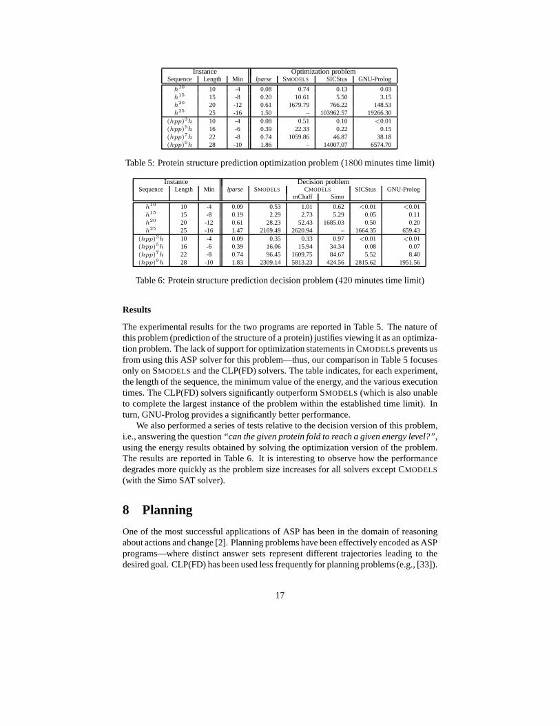
Instance Optimization problemSequence Length Min lparse SMODELS SICStus GNU-Prolog

h10 10 -4 0.08 0.74 0.13 0.03h15 15 -8 0.20 10.61 5.50 3.15h20 20 -12 0.61 1679.79 766.22 148.53h25 25 -16 1.50 – 103962.57 19266.30

(hpp)3h 10 -4 0.08 0.51 0.10 <0.01(hpp)5h 16 -6 0.39 22.33 0.22 0.15(hpp)7h 22 -8 0.74 1059.86 46.87 38.18(hpp)9h 28 -10 1.86 – 14007.07 6574.70

Table 5: Protein structure prediction optimization problem (1800 minutes time limit)

Instance Decision problemSequence Length Min lparse SMODELS CMODELS SICStus GNU-Prolog

mChaff Simo

h10 10 -4 0.09 0.53 1.01 0.62 <0.01 <0.01h15 15 -8 0.19 2.29 2.73 5.29 0.05 0.11h20 20 -12 0.61 28.23 52.43 1685.03 0.50 0.20h25 25 -16 1.47 2169.49 2620.94 – 1664.35 659.43

(hpp)3h 10 -4 0.09 0.35 0.33 0.97 <0.01 <0.01(hpp)5h 16 -6 0.39 16.06 15.94 34.34 0.08 0.07(hpp)7h 22 -8 0.74 96.45 1609.75 84.67 5.52 8.40(hpp)9h 28 -10 1.83 2309.14 5813.23 424.56 2815.62 1951.56

Table 6: Protein structure prediction decision problem (420 minutes time limit)

Results

The experimental results for the two programs are reported in Table 5. The nature ofthis problem (prediction of the structure of a protein) justifies viewing it as an optimiza-tion problem. The lack of support for optimization statements in CMODELS prevents usfrom using this ASP solver for this problem—thus, our comparison in Table 5 focusesonly on SMODELS and the CLP(FD) solvers. The table indicates, for each experiment,the length of the sequence, the minimum value of the energy, and the various executiontimes. The CLP(FD) solvers significantly outperform SMODELS (which is also unableto complete the largest instance of the problem within the established time limit). Inturn, GNU-Prolog provides a significantly better performance.

We also performed a series of tests relative to the decision version of this problem,i.e., answering the question“can the given protein fold to reach a given energy level?”,using the energy results obtained by solving the optimization version of the problem.The results are reported in Table 6. It is interesting to observe how the performancedegrades more quickly as the problem size increases for all solvers except CMODELS

(with the Simo SAT solver).

8 Planning

One of the most successful applications of ASP has been in thedomain of reasoningabout actions and change [2]. Planning problems have been effectively encoded as ASPprograms—where distinct answer sets represent different trajectories leading to thedesired goal. CLP(FD) has been used less frequently for planning problems (e.g., [33]).

17

A planning problem is based on the notions ofState —i.e., a representation of therelevant components of the world—andActions —that affect the state of the world,and thus allow the transition from a state to another. Each state is described by thetruth value assigned to a given collection of atomic formulae (calledfluents). Planningdomains can be effectively described using high-levelaction description languages,e.g., the languagesA andB [16]. In our experiments, we use a slight variation ofB,based on a syntax similar to the one used in [32]. Anaction theoryis a specification ofa planning problem using the action language.

Let us review the structure of the action descriptions used in our tests. An as-sertion of the kindfluent(f) declares thatf is a fluent. Fluent literals are con-structed from fluents and their negations (denoted bymneg(f) ). Declarations of theform action(a) are used to describe the possible actions (in this case,a). The lan-guageB allows one to specify an action theory relating actions, states, and fluents usingpredicates of the following forms (where[list-of-preconditions] denotes a listof fluent literals):

• executable(a, [list-of-preconditions]) asserting that the given pre-conditions have to be satisfied in the current state in order for the actiona to beexecutable.

• causes(a, f, [list-of-preconditions]) encodes a dynamic causal law,describing the effect (the fluent literalf ) of the execution of actiona in a statesatisfying the given preconditions.

• caused([list-of-preconditions], f) describes a static causal law—i.e., the fact that the fluent literalf is true in a state satisfying the given pre-conditions.

A specific instance of a planning problem contains also a description of the initial stateand of the desired goal:

• initially(f) asserts that the fluent literalf is true in the initial state. In ourexamples, we assume complete initial states (i.e., we have knowledge of thetruth value of each fluent in the initial state).

• goal(f) asserts that the goal requires the fluent literalf to hold in the finalstate.

Our approach assumes that the length of the desired plan is given; we also disallow par-allel actions. In the following, we describe how to solve a planning problem specifiedin this action language, using CLP(FD) and ASP solvers.

As an example of the planning problems we experimented with,we describe aplanning problem in the block world domain withN blocks (blocks1, . . . , N ). In theinitial state, the blocks are arranged in a single stack, in increasing order, i.e., block 1 ison the table, block 2 is on top of block 1, etc. BlockN is on top of the stack. In thegoalstate, there must be two stacks, composed of the blocks with odd andeven numbers,respectively. In both stacks the blocks are arranged in increasing order, i.e., blocks 1and 2 are on the table and blocksN − 1 andN are on top of the respective stacks.The planning problem consists of finding a sequence ofT actions (plan) to reach thegoal state, starting from the initial state. An additional restriction must be met: in each

18

state at most three blocks can lie on the table. The followingis the specification of aninstance of the planning problem withN = 5 using the proposed action language.

(1) blk(1). blk(2). blk(3). blk(4). blk(5).(2) fluent(on_table(X)):- blk(X).(3) fluent(clear(X)):- blk(X).(4) fluent(on(X,Y)):- blk(X), blk(Y), neq(X,Y).(5) fluent(space_on_table).(6) action(move(X,Y)):- blk(X), blk(Y), neq(X,Y).(7) action(to_table(X)):- blk(X).(8) initially(clear(5)).(9) initially(mneg(clear(X))) :- blk(X), X<5.

(10) initially(on_table(1)).(11) initially(mneg(on_table(X))) :- blk(X), X>1.(12) initially(space_on_table).(13) initially(on(X,Y)) :- blk(X), blk(Y), Y<5, X is Y+1.(14) initially(mneg(on(X,Y))):- blk(X), blk(Y), X<Y.(15) initially(mneg(on(X,Y))) :- blk(X), blk(Y), Y<5,

neq(Y,X), P is Y+1, neq(X,P).(16) goal(on(X,Y)) :- blk(X), blk(Y), Y<4, X is Y+2.(17) goal(on_table(1)).(18) goal(on_table(2)).(19) goal(space_on_table).(20) causes(move(X,Y),clear(Z),[on(X,Z)]):- blk(X), bl k(Y), blk(Z),

action(move(X,Y)),neq(X,Z),neq(Y,Z).(21) causes(move(X,Y),on(X,Y),[]):- blk(X), blk(Y), act ion(move(X,Y)).(22) causes(move(X,Y),mneg(on(X,Z)),[on(X,Z)]):- blk( X), blk(Y), blk(Z),

action(move(X,Y)),neq(Y,Z).(23) causes(move(X,Y),space_on_table,[on_table(X)]): - blk(X), blk(Y),

action(move(X,Y)).(24) causes(to_table(X),on_table(X),[]):- blk(X), acti on(to_table(X)).(25) causes(to_table(X),clear(Y),[on(X,Y)]):- blk(X), blk(Y),

neq(X,Y), action(to_table(X)).(26) causes(to_table(X),mneg(space_on_table),[on_tab le(Y),on_table(Z)]):-

blk(X), blk(Y), blk(Z), neq(X,Y), neq(Y,Z), neq(X,Z),action(to_table(X)).

(27) executable(move(X,Y),[clear(X),clear(Y)]) :- blk( X), blk(Y),action(move(X,Y)).

(28) executable(to_table(X),[clear(X),mneg(on_table( X)),space_on_table]):-blk(X), action(to_table(X)).

(29) caused([on(X,Y)],mneg(clear(Y))) :- blk(X), blk(Y) , neq(X,Y).(30) caused([clear(Y)],mneg(on(X,Y))) :- blk(X), blk(Y) , neq(X,Y).(31) caused([on(X,Y)],mneg(on_table(X))) :- blk(X), blk (Y), neq(X,Y).(32) caused([on_table(X)],mneg(on(X,Y))) :- blk(X), blk (Y), neq(X,Y).(33) caused([on(X,Y)],mneg(on(Y,X))) :- blk(X), blk(Y), neq(X,Y).

In this specification, the blocks are defined in line (1). Lines (2)–(5) define thefluents of the problem. A block may lie on the table or on top of another block (fluenton(X,Y) ). A block may be clear (if no other block is on top of it) or not.There may bespace on the table for other blocks (fluentspace on table ). There are two possiblemoves (lines (6)–(7)). The initial state and the goal state are described in lines (8)–(15)and (16)–(19), respectively. Thecauses rules (lines (20)–(26)) assert the effect ofmoves on the fluents. Executability predicates (lines (27)–(28)) impose that one canmove a blockX on top of another blockY only if both are clear. On the other hand,X

can be moved to the table only if there is free space (i.e., there are at most two blocks

19

lying on the table). Thecaused assertions (lines (29)–(33)) are easy to understand.

In the following we describe two ways of solving planning problems specified inthe proposed action language, using a CLP(FD) solver and an ASP solver. More specif-ically, regarding CLP(FD), we report a program that directly processes an action the-ory specification. Concerning the ASP solution, we developed a translator, writtenin Prolog, that, given an action theory specification, produces a suitable input file forlparse—the translation process follows the general guidelines highlighted, for exam-ple, in [32, 14].

CLP(FD)

Our CLP(FD) encoding of a planning problem uses the following representation. Aplan withN states,p different fluents, andm possible actions is represented by:

• A list States of N lists ofp termsfluent(fluent name, Bool var) . Thevariable of theith term in thejth list is 1 if and only if theith fluent holds inthejth state. E.g., withN = 3 and fluentsf , g, andh, we have:

States = [[fluent(f,X_f_1),fluent(g,X_g_1),fluent(h,X _h_1)],[fluent(f,X_f_2),fluent(g,X_g_2),fluent(h,X_h_2)],[fluent(f,X_f_3),fluent(g,X_g_3),fluent(h,X_h_3)]]

• A list ActionsOcc of N−1 lists ofm termsaction(action name,Bool var) .The variable of theith term of thejth list is 1 if and only if theith action occursduring the transition from statei to statei + 1. E.g., withN = 3 and actionsaandb, we have:

ActionsOcc = [[action(a,X_a_1),action(b,X_b_1)],[action(a,X_a_2),action(b,X_b_2)]]

The CLP program listed below takes an action language specification as input andsearches for a plan. In particular, lines (2) and (3) collectthe lists of fluents (Lf ) andactions (La), the description of the initial (Init ) and the final (Goal ) states. Lines(4) and (5) define the listsStates andActionsOcc , as explained above. The pred-icates in lines (6) and (7) handle the knowledge about the initial and the goal states,respectively. Lines (8) and (9) impose the constraints on state transitions and actionexecutability. Line (10) gathers all variables denoting action occurrences, in prepara-tion for the labeling phase (line (11)). Note that the labeling is focused on the selectionof the action to be executed at each time step. The clauses in lines (12)–(36) define thepredicates used in lines (4)–(7).

(1) main(N,ACTIONSOCC,STATES):-(2) setof(F,fluent(F),Lf), setof(A,action(A),La),(3) setof(F,initially(F),Init), setof(F,goal(F),Goal) ,(4) make_states(N,Lf,STATES),(5) make_action_occurrences(N,La,ACTIONSOCC),(6) set_initial(Init,STATES),(7) set_goal(Goal,STATES),(8) set_transitions(ACTIONSOCC,STATES),

20

FromSt'

&

$

%

vIV1

vIVp

ToSt'

&

$

%

vEV1

vEVp

-V A1

-V Am

∑m

i=1 V Ai = 1

Figure 2: Action constraints (see proceduresset transitions —build sum prod )

(9) set_executability(ACTIONSOCC,STATES),(10) get_all_actions(ACTIONSOCC,AllActions),(11) labeling([ff],AllActions).(12) make_states(0,_,[]).(13) make_states(N,List,[S|STATES]) :-(14) N1 is N-1, make_states(N1,List,STATES),(15) make_one_state(List,S).(16) make_one_state([],[]).(17) make_one_state([F|Fluents],[fluent(F,VarF)|VarF luents]) :-(18) make_one_state(Fluents,VarFluents), VarF in 0..1.(19) make_action_occurrences(1,_,[]).(20) make_action_occurrences(N,List,[Act|ActionsOcc] ) :-(21) N1 is N-1, make_action_occurrences(N1,List,Actions Occ),(22) make_one_action_occurrences(List,Act),(23) get_action_list(Act,AList), sum(AList,#=,1).(24) make_one_action_occurrences([],[]).(25) make_one_action_occurrences([A|Actions],[action (A,OccA)|OccActs]) :-(26) make_one_action_occurrences(Actions,OccActs), Oc cA in 0..1.(27) set_initial(List,[InitialState|_]) :-(28) set_state(List,InitialState).(29) set_goal(List,States) :-(30) last(States,FinalState),(31) set_state(List,FinalState).(32) set_state([],_).(33) set_state([Fluent|Rest],State) :-(34) (Fluent=mneg(F),!,member(fluent(F,0),State);(35) member(fluent(Fluent,1),State)),(36) set_state(Rest,State).(37) %...continued

The core of the constraint phase is carried out by the predicatesset transitions

and set executability (lines (8)–(9)). In particular, lines (37)–(44) recursivelydefine the predicateset transitions , which ultimately relies onset one fluent

to constrain all boolean variables related to each possiblefluent in each possible statetransition (i.e., action execution).

Let us consider a state transition from stateFromSt to stateToSt , as depicted inFigure 2, where we assume that there arep fluents1, . . . , p involved. As mentioned,two boolean variablesIVi andEVi (for i = 1, . . . , p) denote whether the fluenti holdsin FromSt and inToSt , respectively. Let the variableV Aj , (j = 1, . . . , m) denotewhether the actionj occurs in such a state transition. In this situation, let us considera generic call (line (43)) of the predicateset one fluent (defined in line (45)). For

21

a given fluentFl , the predicateset one fluent collects the listPos (resp. Neg) ofpairs[Action,Preconditions] such thatAction makesFl true (resp. false) in thestate transition (cf. line (46)). Similarly, it handles thestatic causal laws (caused asser-tions), by collecting the lists of conditions that affect the truth value ofFl (cf. StatPos

andStatNeg , in line (49)). The CLP variables involved are then constrained by theproceduresbuild sum prod (lines (47)–(48)) andbuild sum stat (lines (50)–(51)).Finally, all variables related to introductions (resp. removals) of fluents are collectedin Pos Fl (resp. Neg Fl ). Their sums are collected in variablesPsum andNsum, re-spectively. Further constraints inbuild sum prod andbuild sum stat ensure thatthey are both greater than zero. Moreover, we take care of theinertia law in line (56):if none of the actions affectFl , thenEV = IV .

Let us focus on the predicatebuild sum prod . For the sake of simplicity, let us as-sume that it is called withMode == p (cf. line (47)). The predicatebuild sum prod

recursively processes a list of pairs[Action,Preconditions] . For each actionAj ,if Aj occurs and all of its preconditions (Prec ) hold, then there is an action effect(Flag = 1 , line (62)). Moreover, the constraintMode == p -> EV #>= Flag inline (63), imposes that, if an actionAj occurs in a state transition (i.e., the correspond-ing boolean variableVA j is 1), and such action makes a fluent true, then the booleanvariableEV associated to it has to be 1. Analogous constraints are imposed in the caseMode == n, corresponding to the handling of actions that make a given fluent false(called in line (48)).

The modus operandi for imposing the executability conditions for actions is simi-lar. Through the predicateset executability (defined in line (72)), all the precon-ditions of each action (cf.Cs in line (82)) are considered. Any boolean variable relatedto the occurrence of such action in a state transition is constrained with respect to thevalues of all variables inCs (which denote the truth value of the fluents involved in thepreconditions).

(37) set_transitions(_Occurrences,[_States]) :- !.(38) set_transitions([O|Occurrences],[S1,S2|Rest]) :-(39) set_transition(O,S1,S2,S1,S2),(40) set_transitions(Occurrences,[S2|Rest]).(41) set_transition(_Occ,[],[],_,_).(42) set_transition(Occ,[fluent(F,IV)|R1],[fluent(F, EV)|R2],FromSt,ToSt):-(43) set_one_fluent(F,IV,EV,Occ,FromSt,ToSt),(44) set_transition(Occ,R1,R2,FromSt,ToSt).(45) set_one_fluent(Fl,IV,EV,Occurrence,FromSt,ToSt) :-(46) findall([X,L],causes(X,Fl,L),Pos),findall([Y,M] ,causes(Y,mneg(Fl),M),Neg),(47) build_sum_prod(Pos,nOccurrence,FromSt,PFormula, EV,p),(48) build_sum_prod(Neg,Occurrence,FromSt,NFormula,E V,n),(49) findall(P,caused(P,Fl),StatPos),findall(N,cause d(N,mneg(Fl)),StatNeg),(50) build_sum_stat(StatPos,ToSt,PStatPos,EV,p),(51) build_sum_stat(StatNeg,ToSt,PStatNeg,EV,n),(52) append(PFormula,PStatPos,Pos_Fl),(53) append(NFormula,PStatNeg,Neg_Fl),(54) sum(Pos_Fl,#=,Psum),(55) sum(Neg_Fl,#=,Nsum),(56) EV #<=> ((Psum + IV - IV * Nsum) #> 0).(57) build_sum_prod([],_,_,[],_,_).(58) build_sum_prod([[Action,Prec]|Rest],Occurrence, State,[Flag|PF1],EV,Mode):-(59) get_precondition_vars(Prec,State,ListPV),

22

(60) length(Prec,NPrec), sum(ListPV,#=,SumPrec),(61) member(action(Action,VA),Occurrence),(62) (VA #= 1 #/\ (SumPrec #= NPrec)) #<=> Flag,(63) (Mode == p -> EV #>= Flag; Mode == n -> EV #=< 1-Flag),(64) build_sum_prod(Rest,Occurrence,State,PF1,EV,Mod e).(65) build_sum_stat([],_,[],_,_).(66) build_sum_stat([Cond|Others],State,[Flag|Fo],EV ,Mode) :-(67) get_precondition_vars(Cond,State,List),(68) length(List,NL), sum(List,#=,Result),(69) Flag #<=> (Result #= NL),(70) (Mode == p -> EV #>= Flag; Mode == n -> EV #=< 1-Flag),(71) build_sum_stat(Others,State,Fo,EV,Mode).(72) set_executability(ActionsOcc,States) :-(73) setof([Act,C],executable(Act,C),Conds),(74) set_executability1(ActionsOcc,States,Conds).(75) set_executability1([],[_],_).(76) set_executability1([AStep|ARest],[State|States] ,Conds) :-(77) set_executability_sub(AStep,State,Conds),(78) set_executability1(ARest,States,Conds).(79) set_executability_sub(_Step,_State,[]).(80) set_executability_sub(Step,State,[[Act,C]|CA]) : -(81) member(action(Act,VA),Step),(82) get_precondition_vars(C,State,Cs),(83) length(Cs,NCs), sum(Cs,#=,Temporary),(84) VA #=1 #=> Temporary #= NCs,(85) set_executability_sub(Step,State,CA).(86) get_precondition_vars([],_,[]).(87) get_precondition_vars([P1|Rest],State,[F|LR]) :-(88) get_precondition_vars(Rest,State,LR),(89) (P1 = mneg(FN),!, member(fluent(FN,A),State), F #= 1- A;(90) member(fluent(P1,F),State)).(91) get_all_actions([],[]).(92) get_all_actions([A|B],List) :-(93) get_action_list(A,List1),get_all_actions(B,List 2),(94) append(List1,List2,List).(95) get_action_list([],[]).(96) get_action_list([action(_,V)|Rest],[V|MRest]) :-(97) get_action_list(Rest,MRest).

ASP

There are several ways to encode a block world in ASP (e.g., [22, 2]). As mentioned,we developed a translator from our action description language tolparse’s syntax. Sucha translation is quite simple and we do not report its products. It suffices to say thatmuch of the translation amounts to syntactical rewriting ofthe action theory specifica-tion to suitable ASP rules. The translator can be found in [9], together with the actiontheory specifications we used.

Results

Table 7 reports the execution times from the three systems, for different numbers ofblocks and plan lengths (i.e., the number of moves). We also experimented with avariant of the problem described above, where a further constraint is imposed: noblockx can be placed on top of another blocky if y ≥ x. This constraint can be easily

23

Instance (using(6) ) Plan lparse SMODELS CMODELS SICStusBlocks Length exists mChaff Simo

5 5 N 2.31 0.14 0.02 0.02 0.205 6 N 2.29 0.17 0.11 0.06 0.115 7 Y 2.34 0.21 0.12 0.10 0.086 7 N 7.64 0.32 0.16 0.13 0.316 8 N 7.65 0.37 0.19 0.15 1.706 9 Y 7.69 0.55 0.27 0.43 0.997 9 N 22.96 0.64 0.32 0.27 6.237 10 N 23.06 0.75 0.39 0.32 38.247 11 Y 23.10 2.15 0.57 1.35 17.408 11 N 36.71 1.18 0.63 0.53 154.968 12 N 36.81 1.92 0.74 0.62 948.318 13 Y 37.10 7.98 2.14 10.36 422.519 13 N 98.69 2.25 1.09 0.93 –9 14 N 98.45 5.99 1.46 1.13 –9 15 Y 100.01 433.28 4.16 23.07 –

Instance (using(6’) ) Plan lparse SMODELS CMODELS SICStusBlocks Length exists mChaff Simo

4 4 N 0.40 0.05 <0.01 <0.01 0.084 5 N 0.41 0.06 0.06 0.02 0.014 6 Y 0.42 0.06 0.06 0.02 0.015 11 N 1.67 0.35 0.18 0.33 2.175 12 N 1.68 0.59 0.26 0.64 5.925 13 Y 1.68 0.75 0.28 0.50 8.076 25 N 3.38 – 685.43 – –6 26 N 3.38 – 1173.55 – –6 27 Y 3.41 – 1181.99 – –

Table 7: Planning in blocks world (20 minutes time limit)

modeled in the action language, by replacing line(6) of the action theory specificationseen above, with the following one:

(6’) action(move(X,Y)):- blk(X), blk(Y), X>Y.

The results reported in Table 7 show that the ASP solvers can solve the instances(save for the easiest ones) more quickly than CLP(FD). Notice that, the CLP(FD) so-lution is general and applicable to every action theory described in the proposed actionlanguage. We have also tested it on planning problems for elevators, obtaining similarresults. Observe also that, in CLP(FD), a price is paid in making use of a declara-tive translation from a generic action theory to constraints; for example, a manual andad-hoc encoding of the same planning problem presented here(using rule(6’) ) for5 blocks and 13 actions founds the solution in 2ms (see [9] forthis code and relatedrunning times). We expect similar improvements also from anad-hoc encoding ofplanning problems using ASP. Let us observe that in this problem, the time spent bylparse is not completely negligible: this is also due to the size of the file generated.

9 Knapsack

In this section, we discuss a generalization of the knapsackproblem. Let us considern types of objects, and each object of typei has sizewi and costci. We wish to filla knapsack withX1 objects of type1, X2 objects of type2, and so on, in such a way

24

that:n

∑

i=1

Xiwi ≤ max size andn

∑

i=1

Xici ≥ min profit. (*)

wheremax size is the capacity of the knapsack andmin profit is the minimumprofit required.

CLP(FD) Encoding

We represent the types of objects using two lists, containing the size and cost of eachtype of object. For instance:

objects([2,4, 8,16,32,64,128,256,512,1024],[2,5,11,23,47,95,191,383,767,1535]).

The encoding of the problem in CLP(FD) is as follows:

(1) knapsack(Max_Size,Min_Profit) :-(2) objects(Sizes,Costs), length(Sizes,N),(3) length(Vars,N),(4) domain(Vars,0,Max_Size),(5) scalar_product(Sizes,Vars,#=<,Max_Size),(6) scalar_product(Costs,Vars,#>=,Min_Profit),(7) labeling([ff],Vars).

Line (2) retrieves the input data and computes its lengthN. Lines (3) and (4) introducethe list of variables and fix their domains. Lines (5) and (6) encode the constraint (*).This is accomplished by using the built-in predicate

scalar product([c 1,...,c n], [V 1,...,V n], op, Value).

Such predicate imposes the constraint:c1V1+· · ·+cnVn op Value whereop is a bi-nary, finite-domain predicate such as#=<, #>=, #=, etc.1

ASP Encoding

Each instance of the knapsack problem is represented in ASP by a collection of factsof the formitem(Item,Weight,Cost) , e.g.,

item(1,2,2). item(2,4,5). item(3,8,11). item(4,16,23).item(5,32,47). item(6,64,95). item(7,128,191). item(8, 256,383).item(9,512,767). item(10,1024,1535).

The knapsack problem can be encoded as follows:

(1) occs(0..max_size).(2) item_occs(I,Item_Occurences,W,C) :-

item(I,W,C), occs(O), Item_Occurences = O/W.(3) 1{in_sack(I,IO,W,C):item_occs(I,IO,W,C)}1 :- item( I,W,C).(4) cond_cost :-

min_profit [in_sack(I,IO,W,C):item_occs(I,IO,W,C) = IO * C].

1The built-in predicateknapsack , available in SICStus Prolog, is a special case ofscalar productwhere the third argument is the equality constraint.

25

Instance max size min profit Answer lparse SMODELS SICStus GNU-Prolog

k1 255 374 Y 0.01 0.04 0.02 <0.01k2 255 375 N <0.01 3.08 0.03 <0.01k3 511 757 Y 0.01 0.12 0.36 0.08k4 511 758 N 0.02 130.82 0.36 0.08k5 1023 1524 Y 0.03 0.49 8.81 1.92k6 1023 1525 N 0.03 – 8.75 1.87k7 2047 3059 Y 0.07 1.84 368.50 80.68k8 2047 3060 N 0.08 – 366.79 80.40

Table 8: Knapsack instances (30 minute time limit)

(5) :- not cond_cost.(6) cond_weight :-

[in_sack(I,IO,W,C):item_occs(I,IO,W,C) = IO * W] max_size.(7) :- not cond_weight.

Fact (1) fixes the domain for the occurrences of items in the knapsack. Rule (2)fixes the possible occurrences for each item in the knapsack.Rule (3) states that,for each type of objectsI , there is only one factin sack(I,IO,W,C) in the an-swer set, representing the number of objects of typeI in the knapsack. Notice that,in CLP(FD), the same effect is obtained by bound-consistency. Rules (4)–(7) imposethe constraints about minimum profit and maximum size. The two constantsmax size

andmin profit must be provided tolparseduring grounding.

Results

Table 8 reports some of the results we obtained with different solvers. Notice thatCMODELS seems unable to properly deal with this encoding: for all theinstances weexperimented with (except the smallest ones, involving at most five types of objects),the corresponding process was terminated by the O.S. The reason for this could befound by observing that the run-time images of such processes grew very large in size(up to several GBs, in some instances). We have also experimented with an alternativeencoding of this problem, which useslparse’s #weight declarations, but the encodingpresented here turned out to be faster and less sensible to the numbers sizes.

The results denote a fairly irregular behavior. SMODELS has a good performancefor those instances that have a solution, while it is significantly slower than the CLP(FD)solvers for instances that require the full exploration of the search space. Also in thiscase, SICStus is outperformed by GNU-Prolog.

10 Codes

In this section we face the problem of finding binary codes ofN -elements. Let us recallsome standard information-theory notions. Given twoN -bit vectorsu = u1u2 . . . uN

andv = v1v2 . . . vN , their Hamming distanceis defined asdH(u, v) =∑N

i=1 |ui −vi|. A codeC(N, D) is a subset of{0, 1}N such that for all wordsu, v ∈ C(N, D),with u 6= v, it holds thatdH(u, v) ≥ D. Without loss of generality, we can assume(0, 0, . . . , 0) ∈ C(N, D).

26

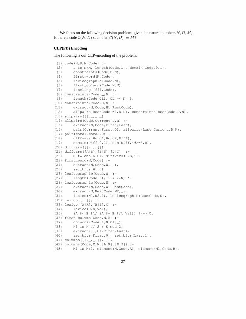
We focus on the following decision problem: given the natural numbersN, D, M ,is there a codeC(N, D) such that|C(N, D)| = M?

CLP(FD) Encoding

The following is our CLP-encoding of the problem:

(1) code(N,D,M,Code) :-(2) L is N * M, length(Code,L), domain(Code,0,1),(3) constraints(Code,D,N),(4) first_word(N,Code),(5) lexicographic(Code,N),(6) first_column(Code,N,M),(7) labeling([ff],Code).(8) constraints(Code,_,N) :-(9) length(Code,CL), CL =< N, !.

(10) constraints(Code,D,N) :-(11) extract(N,Code,W1,RestCode),(12) allpairs(RestCode,W1,D,N), constraints(RestCode, D,N).(13) allpairs([],_,_,_).(14) allpairs(Code,Current,D,N) :-(15) extract(N,Code,First,Last),(16) pair(Current,First,D), allpairs(Last,Current,D,N ).(17) pair(Word1,Word2,D) :-(18) diffvars(Word1,Word2,Diff),(19) domain(Diff,0,1), sum(Diff,’#>=’,D).(20) diffvars([],[],[]).(21) diffvars([A|R],[B|S],[D|T]) :-(22) D #= abs(A-B), diffvars(R,S,T).(23) first_word(N,Code) :-(24) extract(N,Code,W1,_),(25) set_bits(W1,0).(26) lexicographic(Code,N) :-(27) length(Code,L), L < 2 * N, !.(28) lexicographic(Code,N) :-(29) extract(N,Code,W1,RestCode),(30) extract(N,RestCode,W2,_),(31) lexico(W1,W2,1), lexicographic(RestCode,N).(32) lexico([],[],1).(33) lexico([A|R],[B|S],C) :-(34) lexico(R,S,Val),(35) (A #< B #\/ (A #= B #/\ Val)) #<=> C.(36) first_column(Code,N,K) :-(37) columns(Code,1,N,C1,_),(38) K1 is K // 2 + K mod 2,(39) extract(K1,C1,First,Last),(40) set_bits(First,0), set_bits(Last,1).(41) columns([],_,_,[],[]).(42) columns(Code,M,N,[A|R],[B|S]) :-(43) M1 is M+1, element(M,Code,A), element(M1,Code,B),

27

Exists code?Input lparse SMODELS CMODELS SICStus GNU-Prolog

(n, d, k) mChaff Simo(a) (b) (a) (b) (a) (b) (a) (b) (c) (d) (a) (b) (c) (d)

(6,3,8) Y <0.01 0.02 0.02 0.08 0.10 0.05 0.08 <0.01 0.01 <0.01 <0.01 <0.01 <0.01 <0.01 <0.01(6,3,9) N <0.01 0.02 0.02 0.13 0.20 0.13 0.18 573.46 0.08 2.26 0.01 54.04 0.01 0.24 <0.01(7,3,16) Y 0.01 0.09 0.09 1.19 2.05 2.83 9.40 0.04 0.01 0.01 0.02 <0.01 <0.01 <0.01 <0.01(7,3,17) N 0.01 6.11 6.92 2.74 7.36 17.51 20.97 – 865.50 – 3.30 – 118.81 – 0.42(8,3,20) Y 0.04 0.22 224.37 7.75 1188.34223.91 – – – – – – – – –(8,3,21) ? 0.04 – – – – – – – – – – – – – –(8,5,4) Y 0.07 0.11 0.11 0.10 0.12 0.07 0.10 <0.01 <0.01 0.01 <0.01 <0.01 <0.01 <0.01 <0.01(8,5,5) N 0.07 0.40 0.41 0.36 0.51 0.42 0.78 3.90 0.02 0.42 0.01 0.41 <0.01 0.04 <0.01(9,3,32) Y 0.10 0.38 626.18 16.90 10.24 – – 0.65 0.34 0.09 0.07 0.11 0.04 0.03 <0.01(9,3,33) Y 0.10 388.80 – 6.71 11.86 – – – – – – – – – 1931.52(9,5,6) Y 0.31 24.33 24.64 0.49 0.46 2.25 4.04 0.02 <0.01 0.01 0.01 <0.01 <0.01 <0.01 <0.01(9,5,7) N 0.31 80.15 81.44 124.48 144.39 267.00 372.06 – 7.79 252.95 1.70 – 1.10 38.99 0.20

(10,5,12)Y 1.24 – – 82.85 205.45 – – 792.78 0.04 14.87 0.03 89.76 <0.01 2.50 <0.01(10,5,13)N 1.24 – – – – – – – – – 374.39 – – – 43.28

Table 9: The codes problem (30 minutes time limit)

(44) extract(N,Code,_,RestCode), columns(RestCode,M,N ,R,S).(45) extract(N,Code,First,Last) :-(46) length(First,N), append(First,Last,Code).(47) set_bits([],_).(48) set_bits([N|R],N) :- set_bits(R,N).

Line (2) introducesM×N binary variables, i.e.,N of them for each word. The pred-icateconstraint (line (3)) introduces the distance constraints among words. Eachpair of words is selected in lines (8)–(16), using a recursive procedure. For each pair ofwords, the listDiff of difference variables is generated (lines (17)–(19)), and the num-ber of difference variables that are different from 0 is set to be at leastD in line (19). Theauxiliary predicateextract(N,List, First,Last) , defined in lines (45)–(46), isused to split a listList into a prefixFirst of Nelements and the remaining partLast .We employ three simple constraint optimizations:

• The predicatefirst word sets the first word to be(0, 0, . . . , 0).• The predicatefirst column requires the first half of the words to start with 0

and the remaining ones with 1.• The predicatelexicographic requires that the code is computed using lexi-

cographic ordering among tuples, to reduce the number of symmetries.

Lexicographic ordering is imposed by using reified constraints (line (35)). We alsoexperimented with imposing lexicographic ordering by using a binary/decimal conver-sion (i.e.,(Xn−1, Xn−2, . . . , X1, X0) is considered as2n−1Xn−1+2n−2Xn−2+· · ·+21X1 +X0 and those values are constrained to be strictly increasing), but the resultingsolution provided slightly worse performance.

ASP Encoding

The key idea in obtaining an ASP-encoding of the problem is that a wordu belongs tothe code if (and only if) all other words of distance less thand from u do not belong tothe code (an analogous encoding is used in [31]). For instance, forn = 4, d = 3 the

28

following program can answer the question|C(n, d)| = m? for anym:

(1) bit(0). bit(1).(2) word(0, 0, 0, 0).(3) word(Var4,Var3,Var2,Var1) :-(4) not word(Var4,Var3,Var6,Var5),(5) not word(Var4,Var7,Var2,Var5),(6) not word(Var8,Var3,Var2,Var5),(7) not word(Var4,Var7,Var6,Var1),(8) not word(Var8,Var3,Var6,Var1),(9) not word(Var8,Var7,Var2,Var1),

(10) not word(Var4,Var3,Var2,Var5),(11) not word(Var4,Var3,Var6,Var1),(12) not word(Var4,Var7,Var2,Var1),(13) not word(Var8,Var3,Var2,Var1),(14) bit(Var4),bit(Var8),Var4 != Var8 ,(15) bit(Var3),bit(Var7),Var3 != Var7 ,(16) bit(Var2),bit(Var6),Var2 != Var6 ,(17) bit(Var1),bit(Var5),Var1 != Var5.(18) :- (m/2+(m mod 2)+1) {

word(0,Var8,Var7,Var6,Var5,Var4,Var3,Var2,Var1) :bit(Var8;Var7;Var6;Var5;Var4;Var3;Var2;Var1)} m.

(19) :- (m/2+1) {word(1,Var8,Var7,Var6,Var5,Var4,Var3, Var2,Var1) :bit(Var8;Var7;Var6;Var5;Var4;Var3;Var2;Var1)} m.

(20) solutions :- m {word(Var4,Var3,Var2,Var1) :bit( Var4;Var3;Var2;Var1)} m.

(21) :- not solutions.

We uniformly generate programs of this form, for various values ofn andd, bymeans of a Prolog program—such Prolog program that can be found in [9]. Let usdescribe the above ASP program. The domains are set in line (1). The fact (2) imposesthat (0, 0, . . . , 0) belongs to the code (similarly to what done in CLP(FD)). The rulesin lines (3)-(17) impose the constraints on the distance among words. Let us observethat the number of atoms of the formnot word(...) depends onNandD. In general,

their number is∑D−1

i=1

(n

i

)

. For the particular case at hand, lines (4)–(9) handle tuples

of distance 2, while lines (10)–(13) are related to tuples ofdistance 1. The constraints(18)–(19) impose that half of the words begin with 0. Ifmis odd, the number of wordsstarting with 0 is greater than those starting with 1. Lines (20) and (21) requiremwordsin the solution, wheremis a constant to be supplied at grounding time.

Results

The results are reported in Table 9; the table describes fourclasses of experiments,depending on which of the three constraints mentioned abovehave been allowed in theprogram. In particular,

(a) the word(0, 0, . . . , 0) is forced to belongs to the code;(b) as (a) and half of the words must begin with 0;

29

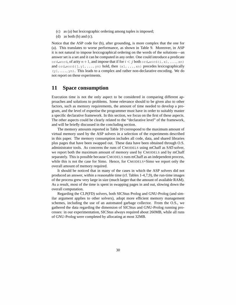
(c) as (a) but lexicographic ordering among tuples is imposed;(d) as both (b) and (c).

Notice that the ASP code for (b), after grounding, is more complex that the one for(a). This translates to worse performance, as shown in Table9. Moreover, in ASPit is not natural to impose lexicographical ordering on the words of the solutions—ananswer set is a set and it can be computed in any order. One could introduce a predicateord word , of arityn+1, and impose that if fori < j bothord word(i,x1,...,xn)

andord word(j,y1,...,yn) hold, then(x1,...,xn) precedes lexicographically(y1,...,yn) . This leads to a complex and rather non-declarative encoding. We donot report on these experiments.

11 Space consumption

Execution time is not the only aspect to be considered in comparing different ap-proaches and solutions to problems. Some relevance should to be given also to otherfactors, such as memory requirements, the amount of time needed to develop a pro-gram, and the level of expertise the programmer must have in order to suitably mastera specific declarative framework. In this section, we focus on the first of these aspects.The other aspects could be clearly related to the “declarative level” of the framework,and will be briefly discussed in the concluding section.

The memory amounts reported in Table 10 correspond to the maximum amount ofvirtual memory used by the ASP solvers in a selection of the experiments describedin this paper. The memory consumption includes all code, data, and shared librariesplus pages that have been swapped out. These data have been obtained through O.S.administrator tools. As concerns the runs of CMODELS using mChaff as SAT-solver,we report both the maximum amount of memory used by CMODELS and by mChaffseparately. This is possible because CMODELS runs mChaff as an independent process,while this is not the case for Simo. Hence, for CMODELS+Simo we report only theoverall amount of memory required.

It should be noticed that in many of the cases in which the ASP solvers did notproduced an answer, within a reasonable time (cf. Tables 1-4,7,9), the run-time imagesof the process grew very large in size (much larger that the amount of available RAM).As a result, most of the time is spent in swapping pages in and out, slowing down theoverall computation.

Regarding the CLP(FD) solvers, both SICStus Prolog and GNU-Prolog (and sim-ilar argument applies to other solvers), adopt more efficient memory managementschemes, including the use of an automated garbage collector. From the O.S., wegathered the data regarding the dimension of SICStus and GNU-Prolog running pro-cesses: in our experimentation, SICStus always required about 260MB, while all runsof GNU-Prolog were completed by allocating at most 32MB.

30

Instance SMODELS CMODELS

mChaff Simo

4-FullIns 5 49 70 (38) 1033-Insertions3 27 3 (4) 14DSJR500.5 34 48 (23) 71DSJC500.5 36 51 (24) 75gen400p0.9 55 41 57 (34) 86gen400p0.9 65 41 57 (30) 85

3-co

lorin

g

wap05a 26 37 (20) 55wap06a 27 38 (18) 55wap07a 59 84 (38) 122wap08a 60 85 (41) 1233-FullIns 5 27 38 (21) 574-FullIns 5 58 83 (40) 121DSJR500.5 41 55 (32) 81DSJC500.5 43 59 (29) 86gen400p0.9 55 49 67 (31) 97gen400p0.9 65 49 67 (35) 97

4-co

lorin

g

wap05a 31 43 (18) 63wap06a 31 44 (25) 64wap07a 71 98 (61) 141wap08a 71 99 (61) 143DSJR500.5 47 63 (34) 92DSJC500.5 50 67 (36) 98gen400p0.9 55 56 76 (45) 108gen400p0.9 65 56 76 (45) 108wap05a 36 49 (31) 72

5-co

lorin

g

wap06a 36 50 (29) 73wap07a 82 109 (64) 162wap08a 82 110 (65) 163〈4, 45〉 4 4 (76) 143〈4, 46〉 4 4 (73) 122〈4, 47〉 4 4 (70) 141

Sch

ur

〈4, 48〉 4 4 (70) 145〈4, 49〉 4 4 (87) 125

Instance SMODELS CMODELS

mChaff Simo

M = N = 6 3 4 (36) 40M = 6, N = 7 3 4 (3) 6

Que

ens

M = 9, N = 8 4 6 (8) –hc1 12 23 (15) 26hc2 12 158 (100) 26hc3 12 20 (13) 26hc4 12 24 (23) 26np50c 4 43 (47) 28np60c 4 35 (30) 45

Ha

milt

onia

n

np70c 5 45 (41) 70np80c 6 64 (56) 98np90c 7 102 (86) 145E(h15) 5 13 (17) 27E(h20) 11 37 (114) 229E(h25) 22 90 (433) –E((hpp)5h) 8 23 (31) 68E((hpp)7h) 12 41 (217) 112

HP

-De

cisi

on

E((hpp)9h) 26 30 (438) 295〈7, 9〉 6 10 (7) 14〈7, 10〉 6 11 (7) 16〈7, 11〉 7 12 (9) 19〈8, 11〉 8 16 (11) 24

Pla

nnin

g

〈8, 12〉 9 18 (12) 27〈8, 13〉 9 20 (16) 35(7,3,17)(a) 3 6 (8) 23(7,3,17)(b) 3 9 (9) 21(8,3,20)(a) 3 12 (15) 94(8,3,20)(b) 3 19 (170) –

Cod

es

(9,5,6)(a) 3 10 (8) 17(9,5,6)(b) 3 13 (10) 23(9,5,7)(a) 3 11 (39) 64(9,5,7)(b) 3 14 (42) 74

Table 10: Space consumption of ASP solvers (MBs)

12 Discussion

We tested the CLP(FD) and ASP codes for various combinatorial problems. In the Ta-bles 1–9 we reported the running times (in seconds) of the solutions to these problemson different problem instances, while in Section 11 we gathered an excerpt of the dataregarding memory consumption. Let us try to analyze these results.

12.1 Comparing CLP(FD) and ASP

First of all, it is clear that ASP provides a more compact, andprobably more declar-ative, encoding. In particular, the use of grounding and domain-restricted variablesallows ASP programmers to avoid the explicit use of recursion in most situations. Ingeneral, in designing the CLP(FD) code, the programmer cannot easily ignore the spe-cific inference strategy adopted by the CLP(FD) engine. The fact that CLP(FD) adoptsa top-down, depth-first strategy affects the programmer’s choices in encoding the algo-rithms. As a result, the amount of effort required to acquiregood programming skills inthe two paradigms is very different. Indeed, teaching experiences with undergraduatestudents confirm that ASP is easier to learn, especially without previous knowledge of

31

declarative programming.On the other hand, it is reasonable that deeper understanding of specific “non-

declarative” aspects of the CLP(FD) framework allows the programmer to developmore efficient, albeit more complex, solutions. The problemof code generation (Sec-tion 10) is paradigmatic: the more the CLP(FD) solution is refined (by introducingfurther heuristics) the faster is the execution. Conversely, attempts to surrogate thesame heuristics in the profoundly declarative framework ofASP yielded (in our exper-iments) unsatisfactory results.

As far as running times are concerned, CLP(FD), in most of thecases, wins thecomparison vs. SMODELS. In a few cases, the running times are comparable, but inmost of the cases CLP(FD) runs significantly faster. Nevertheless, there are cases (e.g.,the code-generation problem) in which CLP(FD) fails in solving instances that arerelatively easy for the ASP solvers. Observe also that CMODELS is, in most of theproblems, faster than SMODELS; part of this can be justified by the fact that the pro-grams we are using are mostly tight [12], and by the high speedof the underlying SATsolver used by CMODELS.

The comparison between CLP(FD) and CMODELS is more interesting. In thek-coloring andN -M -queens cases, running times are comparable. In some of the classesof graphs, CMODELS performs slightly better on all instances. More in general,when-ever the instances of a single class are considered, one of the two systems tends toalways outperform the other. This indicates that the behavior of the solver is signifi-cantly affected by the nature of the specific problem instances considered (recall thateach class of graphs comes from encodings of instances of different problems [39]).

As one may expect, the bottom-up search strategy of ASP is less sensitive to thepresence of solutions w.r.t. the top down search strategy ofCLP(FD). As a matter offact, CLP(FD) typically runs faster than CMODELS when a solution exists. Moreover,CLP(FD) behaves better on small graphs.

For the Hamiltonian circuit problem, CLP(FD) runs significantly faster—we be-lieve this is due to the use of the built-in global constraintcircuit , which guaranteesexcellent constraint propagation. In this case, only in absence of solutions the run-ning times are comparable—i.e., when the two approaches areforced to traverse thecomplete search tree.

A similar situation arises in computing Schur numbers. Whenthe solution existsCLP(FD) performs better. On the other hand, whenever there is no solution, runningtimes are favorable to CMODELS. The performance of CMODELS does not seem tobe significantly affected by the growth in the size of the problem instance, as clearlyhappens for CLP(FD). The same behavior of CMODELS can be also observed in othersituations (see the Hamiltonian circuit problem). In thesecases, the time spent byCMODELS to obtain a solution does not appear to be directly related tothe raw dimen-sion of the problem instance. Initial experiments reveal that this phenomenon ariseseven when different SAT-solvers are employed. Further studies are needed to betterunderstand to which extent the intrinsic structure of an instance biases CMODELS’ be-havior, in particular the way in which CMODELS’ engine translates an ASP programinto a SAT-instance. A further challenging theme for futureresearch is to understandhow such intrinsic structure of a problem could be exploitedin order to better drive theinteraction with the SAT-solver (especially for non-tightproblems).

32

Coloring Hamilton Schur PF Planning Knapsack CodesCLP(FD) + ++ + + - + +

ASP CMODELS ++ + + - + - +

Table 11: Schematic results’ analysis for execution time. +(-) means that the formalismis (not) applicable. ++ that it is the best when the two formalisms are applicable.

Regarding the protein folding problem, CLP(FD) solves the optimization problemsmuch faster than ASP. In the decision version, times are quite close. Also in this case,however, the ASP code appears to be simpler and more compact than the CLP(FD) one.

For the planning problem, we observe that SMODELS has running times higher butusually comparable with CMODELS. The CLP(FD) approach, although correct, seemsless suitable to this problem, especially when the size of the instance grows.

For the Knapsack problem, CMODELS is not applicable. CLP(FD) runs definitivelyfaster than SMODELS; furthermore, SMODELS becomes inapplicable for large probleminstances.

Table 12.1 intuitively summarizes our observations drawn from the different bench-marks. From this experience we can draw some concrete indications that can be takeninto account when choosing a paradigm to tackle a problem. Wecan summarize themain points as follows:

• graph-based problems have nice and compact encodings in ASP, and the perfor-mance of the ASP solutions is acceptable and scalable;• problems requiring more intense use of arithmetic and/or numbers are declara-

tively and efficiently handled by CLP(FD);• for problems with no arithmetic, the exponential growth w.r.t. the input size is

less of an issue for ASP.

A comparison between CLP(FD) implementations is outside the scope of this paper(see, e.g., [13, 34, 8]). Nevertheless, we tested the CLP(FD) programs using SICStusProlog, B-Prolog, ECLiPSe, and GNU-Prolog [37]. As far as running times are con-cerned, such partial experimentation indicates that B-Prolog and SICStus Prolog havecomparable behavior (with B-Prolog being a bit faster), GNU-Prolog is the fastest, andECLiPSe is the slowest.

In our experiments, we have isolated the grounding phase from the answer set com-putation timings, and reported them separately. Nevertheless, in our tests, the timespent in grounding is often negligible (see the case of planning in Section 8 for theunique exception) w.r.t. SMODELS/CMODELS running time, save for the easier in-stances. Regarding the use of different SAT-solvers with CMODELS (we also testedzChaff and RelSat), as one can expect (see, e.g., [17]) the choice of the SAT solveraffects performance, but there is not a definite winner.

12.2 ASP vs. SAT

As mentioned, our experiments suggest that the greater efficiency of CMODELS, withrespect to SMODELS, originates from the high speed of the underlying SAT solvers. In

33

Instance CMODELS Sat solverGraph Colors mChaff Simo zChaff mChaff Simo zChaff

3-FullIns 5 3 1.23 1.18 1.17 1.04 0.08 0.014-FullIns 5 3 2.69 2.69 2.65 2.41 0.28 0.022-Insertions4 3 0.15 1.08 0.13 0.13 59.54 0.082-Insertions5 3 0.50 2.62 0.69 0.33 – 0.183-Insertions3 3 4.16 7.59 2.64 5.22 61.67 –4-Insertions3 3 1772.14 1481.27 213.22 – – –4-Insertions4 3 1443.33 1468.91 – 876.77 – –DSJR500.5 3 1.81 1.78 1.78 1.60 0.01 0.01DSJC500.5 3 1.92 1.92 1.87 1.70 0.01 0.01gen400p0.9 55 3 2.19 2.18 2.15 1.91 0.01 0.01gen400p0.9 65 3 3.16 2.15 2.17 1.92 0.01 0.01le450 5a 3 0.24 0.21 0.20 0.17 0.01 <0.01le450 5b 3 0.24 0.20 0.20 0.17 <0.01 <0.01le450 5c 3 0.37 0.33 0.34 0.28 <0.01 <0.01le450 5d 3 0.36 0.33 0.33 0.27 <0.01 <0.01wap05a 3 1.38 1.36 1.36 1.27 <0.01 0.01wap06a 3 1.42 1.40 1.34 1.27 <0.01 0.01wap07a 3 3.28 3.31 3.28 3.04 0.01 0.01wap08a 3 3.31 3.32 3.32 3.07 0.01 0.013-FullIns 5 4 1.51 1.47 1.47 1.48 0.25 0.034-FullIns 5 4 3.37 3.38 3.33 3.41 0.31 0.062-Insertions4 4 – – – – – –2-Insertions5 4 – – – – – –3-Insertions3 4 0.04 0.01 0.01 0.01 <0.01 <0.014-Insertions3 4 0.04 0.01 0.01 0.01 <0.01 <0.014-Insertions4 4 – – – – – –DSJR500.5 4 2.26 2.19 2.19 2.17 0.10 0.02DSJC500.5 4 2.36 2.37 2.29 2.30 0.34 0.02gen400p0.9 55 4 2.68 2.69 2.66 2.66 0.05 0.02gen400p0.9 65 4 2.67 2.66 2.67 2.65 0.06 0.02le450 5a 4 0.29 0.27 0.26 0.24 1.50 <0.01le450 5b 4 0.29 0.27 0.26 0.24 1.33 0.01le450 5c 4 0.46 0.45 0.42 0.40 1.67 0.01le450 5d 4 0.44 0.42 0.42 0.39 8.60 0.01wap05a 4 1.73 1.70 1.71 1.71 0.08 0.01wap06a 4 1.75 1.70 1.71 1.74 0.10 0.01wap07a 4 4.12 4.09 4.08 4.08 0.22 0.02wap08a 4 4.15 4.19 4.15 4.14 0.24 0.023-FullIns 5 5 1.69 2.04 1.91 1.97 442.03 0.134-FullIns 5 5 4.19 4.13 4.11 4.58 1.16 0.182-Insertions4 5 0.07 0.04 0.04 0.04 <0.01 <0.012-Insertions5 5 – – – – – –3-Insertions3 5 0.04 0.01 0.01 0.01 <0.01 <0.014-Insertions3 5 0.05 0.02 0.01 0.01 <0.01 <0.014-Insertions4 5 0.32 0.35 0.15 0.14 <0.01 <0.01DSJR500.5 5 2.71 2.68 2.65 2.79 5.36 0.06DSJC500.5 5 2.84 2.99 2.84 2.96 1567.77 0.07gen400p0.9 55 5 3.24 3.22 3.18 3.40 1.70 0.05gen400p0.9 65 5 3.22 3.23 3.17 3.37 1.89 0.06le450 5a 5 12.30 1.99 – 0.90 – 0.28le450 5b 5 0.98 12.47 – 2.66 – –le450 5c 5 0.70 0.58 0.51 0.52 – 0.01le450 5d 5 0.60 0.51 – 0.59 1021.36 0.30wap05a 5 2.07 2.05 2.04 2.17 1.13 0.04wap06a 5 2.13 2.10 2.09 2.22 2.56 0.05wap07a 5 4.99 5.05 4.92 5.21 13.90 0.07wap08a 5 5.08 5.00 4.97 5.29 12.21 0.11

Table 12:Graphk-coloring: ASP vs SAT (30 minutes time limit)

34

view of this fact, one could wonder whether it is better to solve an instance of a hardcombinatorial problem by using a SAT-based ASP solver or by directly employing astand-alone SAT solver. The two alternatives require different approaches in modelingthe problem, and different amounts of effort in encoding theproblem. A comparisonbetween SAT and ASP solvers is important, but goes beyond thescope of this arti-cle. Nevertheless, we made a first step in this direction by comparing the behaviorof CMODELS with the stand-alone implementations of the same SAT solvers it uses,namely zChaff, Simo, and mChaff [38].

The experiments we performed make use of a selection of instances of two specificproblems, namely graphk-coloring and Hamiltonian circuit. A motivation for thischoice is that, in our encodings, such problems lead to tightand non-tight programs,respectively. The instances to be processed by the SAT solvers have been encoded inthe DIMACS format, and generated by applying two well-knowntranslations of Graphcoloring (e.g., [30]—Section 1.1) and Hamiltonian circuit(e.g., [29]—Example 8.1)instances to SAT.

As shown in Tables 12 and 13, the tightness of programs significantly affects thebehavior of the solvers. On one hand, whenever a tight instance is tackled, it is oftenthe case that the SAT solvers outperform CMODELS. On the other hand, very oftennon-tight programs are efficiently solved by the ASP solver while all SAT solvers fail.

Such failures are a direct consequence of the growth in the size of the run-timeimage of the processes. We have already observed how this phenomenon also affectsCMODELS when processing the instances of the Knapsack problem (see Section 9),which actually involves tight instances.

The better behavior of CMODELS in dealing with non-tight programs could be intu-itively explained by observing that, while a SAT solver tries to solve the entire instance,CMODELS exploits a SAT solver to drive the construction of the answersets throughthe discovery of loop formulae. This use of a SAT solver usually involves smaller SATinstances.

13 Conclusions

In this paper, we described an experimental study aimed at comparing the performanceof CLP(FD) and ASP on various classes of combinatorial problems. The aim of thestudy is to provide a better understanding of what makes one paradigm more suit-able than the other in solving combinatorial problems. We provided what we feelare the most natural and declarative encodings of the various problems in the differ-ent paradigms, and we analyzed the performance figures obtained by running suchinstances through different CLP(FD) and ASP solvers.

In the future, we plan to extend our analysis to other problems and to other con-straint solvers (e.g., ILOG) and ASP solvers (e.g., ASSAT, aspps, DLV). We are inter-ested in answering the following questions:• Is it possible to formalize the domain and problem characteristics and employ

this to choose which paradigm to use?• Is it possible to introduce strategies to split problem components and map them

to cooperating solvers (using the best solver for each part of the problem)?

35

Instance CMODELS Sat solverGraph mChaff Simo zChaff mChaff Simo zChaff

hc1 37.60 (56) 14.30 (33) 5.53 (10) – – –hc2 1390.15 (681) 3.48 (5) 3.25 (5) – – –hc3 20.08 (33) 6.52 (14) 10.71 (25) – – –hc4 92.99 (117) 6.54 (13) 4.11 (8) – – –hc5 0.22 (0) 0.21 (0) 0.21 (0) 123.21 – 0.60hc6 0.21 (0) 0.21 (0) 0.21 (0) 123.52 – 0.58hc7 0.21 (0) 0.21 (0) 0.21 (0) 123.32 – 0.45hc8 0.21 (0) 0.21 (0) 0.21 (0) 123.69 – 0.44np10c 0.04 (0) 0.01 (4) 0.01 (4) <0.01 0.01 <0.01np20c 0.81 (17) 0.05 (11) 0.07 (9) 0.04 – <0.01np30c 0.26 (1) 0.20 (24) 0.27 (14) 0.12 – <0.01np40c 4.35 (14) 0.68 (37) 0.76 (19) – – <0.01np50c 117.77 (115) 1.55 (51) 1.72 (24) – – <0.01np60c 24.72 (27) 5.54 (136) 3.77 (29) – – 0.01np70c 9.46 (7) 7.46 (118) 5.91 (34) – – 0.01np80c 12.53 (6) 12.60 (152) 9.20 (39) – – 0.01np90c 127.31 (43) 42.32 (411) 14.24 (44) – – 0.012xp30 0.02 (0) 0.02 (0) 0.02 (0) – 7309.64 –2xp30.1 4.59 (51) 377.09 (127) 371.81 (23) – – –2xp30.2 2.68 (43) 3.90 (251) 21.47 (50) – – –2xp30.3 2.69 (43) 3.87 (251) 21.49 (50) – – –2xp30.4 5692.11 (26) – 553.54 (44) – – –4xp20 0.04 (0) 0.04 (0) 0.04 (0) 3008.58 – –4xp20.1 1.48 (1) 36.36 (1) 3.56 (1) 4754.89 – –4xp20.2 3.32 (43) 3.42 (108) 7.43 (99) – – –4xp20.3 2.62 (5) 51.45 (12) 1.46 (10) – – –

Table 13:Hamiltonian circuit: ASP vs SAT (180 minutes time limit)

In particular, we are interested in identifying those contexts where the ASP solversperform significantly better than CLP(FD). It seems reasonable to expect this behavior,for instance, whenever incomplete information comes into play.

Acknowledgments

We thank Yuliya Lierler, Marco Maratea, Tran Cao Son, and Neng-Fa Zhou for usefuldiscussions on the topics of this paper. This work is partially supported by MIUR-PRINproject n.2005-015491, GNCS2005 project on constraints and their applications, andby NSF grants CNS-0220590, CNS-0454066, and HRD-0420407.

References

[1] C. Anger, T. Schaub, and M. Truszczynski. ASPARAGUS – the Dagstuhl Initia-tive. ALP Newsletter, 17(3), 2004.

[2] C. Baral. Knowledge representation, reasoning and declarative problem solving.Cambridge University Press, 2003.

36

[3] P. Clote and R. Backofen.Computational Molecular Biology. Wiley & Sons,2001.

[4] P. Crescenzi, D. Goldman, C. H. Papadimitriou, A. Piccolboni, and M. Yan-nakakis. On the complexity of protein folding.J. of Computational Biology,5(3):423–466, 1998.

[5] A. Dal Palu, A. Dovier, and F. Fogolari. Constraint logic programming approachto protein structure prediction.BMC Bioinformatics, 5(186):1–12, 2004.

[6] M. Davis, G. Logemann, and D. Loveland. A Machine Programfor TheoremProving.Communications of the ACM, 5(7):394–397, 1962.

[7] M. Davis and H. Putnam. A Computing Procedure for Quantification Theory.J. of the ACM, 7(3):201–215, 1960.

[8] D. Diaz and P. Codognet. Design and Implementation of theGNU-Prolog System.J. of Functional and Logic Programming, 2001(6), 2001.

[9] A. Dovier, A. Formisano, and E. Pontelli. A comparison ofCLP(FD) andASP in tackling hard combinatorial problems. Web site:www.di.univaq.it/

˜ formisano/CLPASP .

[10] I. Elkabani, E. Pontelli, and T. C. Son. Smodels with CLPand Its Applications:A Simple and Effective Approach to Aggregates in ASP. In Proc. of ICLP04,Springer Verlag, pp. 73–89, 2004.

[11] O. Elkhatib, E. Pontelli, and T. C. Son. A Tool for Reasoning about Answer Setsin Prolog. In Proc. ofPADL, Springer Verlag, pp. 148–162, 2004.

[12] E. Erdem and V. Lifschitz. Tight Logic Programs.TPLP, 3:499-518, 2003.

[13] A. J. Fernandez and P. M. Hill. A Comparative Study of 8 Constraint Program-ming Languages Over the Boolean and Finite Domains.Constraints, 5(3):275–301, 2000.

[14] M. Gelfond. Representing Knowledge in A-Prolog. InComputational Logic:Logic Programming and Beyond, Springer Verlag, pp. 413–451, 2002.

[15] M. Gelfond and V. Lifschitz. The Stable Model Semanticsfor Logic Program-ming. In Proc. ofICLP88, pp. 1070–1080, MIT Press, 1988.

[16] M. Gelfond and V. Lifschitz. Action Languages.Electron. Trans. Artif. Intell.,2:193–210, 1998.

[17] E. Giunchiglia, Y. Lierler, and M. Maratea. SAT-Based Answer Set Programming.In Proc. ofAAAI’04, pp. 61–66, AAAI/Mit Press, 2004.

[18] E. Giunchiglia, Y. Lierler, and M. Maratea. Answer Set Programming based onPropositional Satisfiability.J. Automated Reasoning, to appear, Kluwer, 2006.

37

[19] J. Jaffar and M. J. Maher. Constraint Logic Programming: A Survey.J. of LogicProgramming, 19/20:503–581, 1994.

[20] J. Lee and V. Lifschitz. Loop formulas for disjunctive logic programs In Proc. ofICLP03, pp. 451–465, 2003.

[21] Y. Lierler and M. Maratea. CMODELS-2: SAT-based Answer Set Solver En-hanced to Non-tight Programs. In Proc. ofLPNMR04, pp. 346–350. SpringerVerlag, 2004.

[22] V. Lifschitz. Answer Set Planning. In Proc. ofICLP99, MIT Press, pp. 23–37,1999.

[23] V. Lifschitz and A. Razborov. Why are there so many loop formulas? ACMTransactions on Computational Logic, 7(2):261–268, 2006.

[24] F. Lin and Y. Zhao. ASSAT: Computing Answer Sets of A Logic Program BySAT Solvers. InAAAI’02, pp. 112–117. AAAI/MIT Press, 2002.

[25] V. W. Marek and M. Truszczynski. Autoepistemic Logic.J. of the ACM,38(3):588–619, 1991.

[26] V. W. Marek and M. Truszczynski. Stable models and an alternative logic pro-gramming paradigm.The Logic Programming Paradigm, pp. 375–398. SpringerVerlag, 1999.

[27] K. Marriott and P. J. Stuckey.Programming with Constraints. MIT Press, 1998.

[28] M. W. Moskewicz, C. F. Madigan, Y. Zhao, L. Zhang, and S. Malik. Chaff:Engineering an Efficient SAT Solver. In Proc. ofDesign Automation Conference,ACM Press, pp. 530–535, 2001.

[29] C. H. Papadimitriou.Computational Complexity. Addison Wesley, 1994.

[30] S. D. Prestwich. Local Search on SAT-encoded ColouringProblems. In Proc. ofSAT 2003, 6th International Conference, LNCS 2919, pp. 105–119, 2003.

[31] P. Simons. Extending and Implementing the Stable ModelSemantics. Doctoraldissertation. Report 58, Helsinki University of Technology, 2000.

[32] T. C. Son, C. Baral, and S. McIlraith. Planning with different forms of domain-dependent control knowledge — an answer set programming approach. In Proc.of LPNMR01, Springer Verlag, pp. 226–239, 2001.

[33] M. Thielscher. Reasoning about Actions with CHRs and Finite Domain Con-straints. In Proc. ofICLP02, LNCS 2401, pp. 70–84, 2002.

[34] M. Wallace, J. Schimpf, K. Shen, and W. Harvey. On Benchmarking ConstraintLogic Programming Platforms.Constraints, 9(1):5–34, 2004.

[35] E. W. Weisstein.Schur Number. From MathWorld–A Wolfram Web Resource.mathworld.wolfram.com/SchurNumber.html .

38

[36] Web references for some ASP solvers. ASSAT:assat.cs.ust.hk .CCalc: www.cs.utexas.edu/users/tag/cc . Cmodels: www.cs.utexas.

edu/users/tag/cmodels . DeReS and aspps:www.cs.uky.edu/ai .DLV: www.dbai.tuwien.ac.at/proj/dlv . SMODELS: www.tcs.hut.fi/

Software/smodels .

[37] Web references for some CLP(FD) implementations. SICStus Pro-log: www.sics.se/isl/sicstuswww/site/index.html . B-Prolog: www.

probp.com . ECLiPSe: eclipse.crosscoreoptimization.com . GNU-Prolog:pauillac.inria.fr/ ˜ diaz/gnu-prolog .

[38] Web references for some SAT solvers. mChaff and zChaff:www.princeton.

edu/ ˜ chaff/software.html . Simo: www.star.dist.unige.it/ ˜ sim/

simo/ .

[39] Web site of COLOR02/03/04: Graph Coloring and its Applications:mat.gsia.

cmu.edu/COLORING03 .

39