Constraint Programming based Local Search for the Vehicle ...

Constraint Programming basedLocal Search for the Vehicle Routing

Problem with Time Windows

Master Thesis of

Joan Sala Reixach

At the Department of InformaticsInstitute of Theoretical Computer Science

Reviewers: Prof. Dr. Dorothea WagnerProf. Dr. Peter Sanders

Advisors: Anne Meyer (FZI, LSE Furmans)Julian Dibbelt (KIT, ITI Wagner)

Time Period: 1st April 2012 – 30th September 2012

KIT – University of the State of Baden-Wuerttemberg and National Laboratory of the Helmholtz Association www.kit.edu

Statement of Authorship

I hereby declare that this document has been composed by myself and describes my ownwork, unless otherwise acknowledged in the text.

Karlsruhe, September 30, 2012

iii

Abstract

Vehicle Routing is a problem of extreme variance and at the same time, of extremeimportance to companies around the world. Extensive work has been done on findingmethods to solve it in an efficient way that provides a solution of good quality.

This project focuses especially on the Vehicle Routing Problem with Time Windows.It explores and tests a method based on a Constraint Programming formulation ofthe problem, and it implements a local search method with the power of makingvery powerful moves: Large Neighbourhood Search. Large Neighbourhood Searchremoves big sets of customers from the solutions (up to around 30% of the customers)and tries to reinsert them. Those powerful moves help solving one of the biggestproblems of local search methods: Escaping local minima.

We first explore a basic path formulation of the model, as well as some alternativeformulations. We implement a first basic version of a Large Neighbourhood Searchengine and try to improve it through the exploration of different options for all thedecisions that must be taken when designing such an engine. Concretely, the maindecisions to take are about how to design the methods to remove customers fromthe solution and the methods to reinsert them back into the solution, desirably in abetter way.

The methods are then tested using a set of benchmark problems. The results ob-tained are then compared to the best known solutions for these benchmarks, as wellas to the results obtained by other authors that have done work regarding the VehicleRouting Problem with Time Windows.

Deutsche Zusammenfassung

Dieses Projekt beschaftigt sich mit dem Vehicle Routing Problem. Diese Problemesind extrem unterschiedlich und ahnlich nur in ihren Grundbegriffen. Das Problemist aber sehr wichtig fur Firmen, die im Logistikbereich arbeiten.

Dieses Projekt konzentriert sich vor allem auf das Vehicle Routing Problem mit TimeWindows. Es erforscht und testet eine Methode basierend auf einer Constraint-Programming Formulierung des Problems, und es setzt eine lokale Suchmethodeein, mit der Fahigkeit, große Teilen der Losung zu andern: Large NeighbourhoodSearch. Diese Methode loscht eine große Menge von Kunden aus den Losungen (bisetwa 30 % der Kunden) und versucht, sie besser wieder einzufugen. Diese machtigenMoves helfen bei der Losung eines der großten Probleme der lokalen Suchmethoden:Lokalen Minima zu entkommen.

Zuerst exploriert die Arbeit die elementare Path-Formulierung des Modells, sowieeinige alternative Formulierungen. Wir implementieren eine erste Basisversion einergroßen Nachbarschaftssuche. Wir versuchen danach diese Basisversion zu verbesserndurch die Erforschung der verschiedenen Optionen fur alle Entscheidungen, die sichprasentieren bei der Gestaltung der Suche. Konkret sind die wichtigsten Entschei-dungen zu treffen, wie die Kunden geloscht werden und wie die geloschten Kundenwieder in die Losung eingefugt werden.

Die Methoden werden dann unter Verwendung eines anerkannten Benchmarks getestet.Die erhaltenen Ergebnisse werden dann zu den besten bekannten Losungen fur dieseBenchmarks sowie zu Ergebnissen von anderen Autoren verglichen.

v

Contents

1 Introduction 11.1 Related Work . . . . . . . . . . . . . . . . . . . . . . . . . . . . . . . . . . . 11.2 Contributions . . . . . . . . . . . . . . . . . . . . . . . . . . . . . . . . . . . 21.3 Summary . . . . . . . . . . . . . . . . . . . . . . . . . . . . . . . . . . . . . 2

2 Preliminaries 32.1 The Vehicle Routing Problem . . . . . . . . . . . . . . . . . . . . . . . . . . 32.2 Constraint Programming . . . . . . . . . . . . . . . . . . . . . . . . . . . . . 42.3 Gecode . . . . . . . . . . . . . . . . . . . . . . . . . . . . . . . . . . . . . . 4

2.3.1 Modelling . . . . . . . . . . . . . . . . . . . . . . . . . . . . . . . . . 52.3.1.1 Gecode Variables . . . . . . . . . . . . . . . . . . . . . . . . 5

2.3.2 Propagation . . . . . . . . . . . . . . . . . . . . . . . . . . . . . . . . 52.3.3 Branching . . . . . . . . . . . . . . . . . . . . . . . . . . . . . . . . . 62.3.4 Search Engines . . . . . . . . . . . . . . . . . . . . . . . . . . . . . . 6

2.4 Large Neighbourhood Search . . . . . . . . . . . . . . . . . . . . . . . . . . 7

3 The Model 93.1 The Path Model . . . . . . . . . . . . . . . . . . . . . . . . . . . . . . . . . 93.2 The Set Model . . . . . . . . . . . . . . . . . . . . . . . . . . . . . . . . . . 103.3 Propagation . . . . . . . . . . . . . . . . . . . . . . . . . . . . . . . . . . . . 11

3.3.1 The NoCycle Propagator . . . . . . . . . . . . . . . . . . . . . . . . 123.4 Branching . . . . . . . . . . . . . . . . . . . . . . . . . . . . . . . . . . . . . 12

3.4.1 Selecting a variable . . . . . . . . . . . . . . . . . . . . . . . . . . . . 123.4.2 Selecting the value . . . . . . . . . . . . . . . . . . . . . . . . . . . . 13

3.4.2.1 The minimum distance brancher . . . . . . . . . . . . . . . 133.4.2.2 The time brancher . . . . . . . . . . . . . . . . . . . . . . . 13

4 The Search Engine 154.1 General Algorithm . . . . . . . . . . . . . . . . . . . . . . . . . . . . . . . . 154.2 Construction Heuristic . . . . . . . . . . . . . . . . . . . . . . . . . . . . . . 164.3 Improvement Heuristic . . . . . . . . . . . . . . . . . . . . . . . . . . . . . . 16

4.3.1 Relaxation . . . . . . . . . . . . . . . . . . . . . . . . . . . . . . . . 174.3.1.1 Neighbourhood Size . . . . . . . . . . . . . . . . . . . . . . 174.3.1.2 Relatedness Function . . . . . . . . . . . . . . . . . . . . . 17

4.3.2 Reinsertion . . . . . . . . . . . . . . . . . . . . . . . . . . . . . . . . 184.3.2.1 Limited Discrepancy Search . . . . . . . . . . . . . . . . . 184.3.2.2 General Algorithm . . . . . . . . . . . . . . . . . . . . . . . 184.3.2.3 Fixing Clients . . . . . . . . . . . . . . . . . . . . . . . . . 204.3.2.4 Costumers Left Free . . . . . . . . . . . . . . . . . . . . . . 214.3.2.5 Time Limit on Reinsertion . . . . . . . . . . . . . . . . . . 244.3.2.6 First-Found, all-solutions . . . . . . . . . . . . . . . . . . . 24

4.3.3 Objective Function . . . . . . . . . . . . . . . . . . . . . . . . . . . . 25

vii

Contents

4.3.4 Implementation in Gecode . . . . . . . . . . . . . . . . . . . . . . . . 25

5 Evaluation 275.1 Propagators and Branchers . . . . . . . . . . . . . . . . . . . . . . . . . . . 29

5.1.1 NoCycle Propagator . . . . . . . . . . . . . . . . . . . . . . . . . . . 295.1.2 Branchers . . . . . . . . . . . . . . . . . . . . . . . . . . . . . . . . . 30

5.2 Construction Heuristics . . . . . . . . . . . . . . . . . . . . . . . . . . . . . 315.3 Improvement Heuristics . . . . . . . . . . . . . . . . . . . . . . . . . . . . . 32

5.3.1 Reinsertion . . . . . . . . . . . . . . . . . . . . . . . . . . . . . . . . 325.3.2 Heuristics for Insertion Sequence . . . . . . . . . . . . . . . . . . . . 345.3.3 Inserting Variables when Only One Position is Left . . . . . . . . . . 355.3.4 Time Limit on Reinsertion . . . . . . . . . . . . . . . . . . . . . . . 365.3.5 Stopping Search When a Solution is Found . . . . . . . . . . . . . . 37

5.4 Relatedness Function . . . . . . . . . . . . . . . . . . . . . . . . . . . . . . . 385.5 Parameters . . . . . . . . . . . . . . . . . . . . . . . . . . . . . . . . . . . . 39

5.5.1 Discrepancies . . . . . . . . . . . . . . . . . . . . . . . . . . . . . . . 405.5.2 Attempts . . . . . . . . . . . . . . . . . . . . . . . . . . . . . . . . . 415.5.3 Determinism . . . . . . . . . . . . . . . . . . . . . . . . . . . . . . . 415.5.4 Overall . . . . . . . . . . . . . . . . . . . . . . . . . . . . . . . . . . 41

5.6 Objective Function . . . . . . . . . . . . . . . . . . . . . . . . . . . . . . . . 435.7 Best Found Configurations . . . . . . . . . . . . . . . . . . . . . . . . . . . . 435.8 Robustness of the Solution . . . . . . . . . . . . . . . . . . . . . . . . . . . . 465.9 Improvement over Time . . . . . . . . . . . . . . . . . . . . . . . . . . . . . 46

6 Conclusion 49

Bibliography 51

viii

1. Introduction

Vehicle routing is a key problem to management of goods distribution and has become oneof the most important areas for improvement for companies around the world, and onewhich must be systematically solved. In the industrial practice, vehicle routing problemsare extremely different and they share only a common basis. This high variability comesfrom the different requisites and constraints that each company will provide for the prob-lem, and in it resides the complexity of solving these problems. Therefore it is interestingto find a method that allows us to be able to easily model constraints, as well as being ableto modify them easily without the need of major changes. Its flexibility to add new con-straints or modify existing ones is what makes Constraint Programming (see [RVBW06])so useful for this problem.

We provide extensive evaluation on a suite of well-known test instances, namely theSolomon instances designed in [Sol87]. Solomon instances are sets of benchmark Vehi-cle Routing problems, which present different scenarios. There are sets with the customersdistributed randomly, and sets of problems with clustered clients. Vehicle capacity, as wellas the time windows of the customers also vary. With them, the best solution found sofar for each of them is also provided. These instances are very useful for the testing ofapplications for the Vehicle Routing Problem.

1.1 Related Work

Extensive work has been done around the vehicle routing problem, as summarized in [Lap09].A wide variety of exact algorithms have been developed, including branch and bound, dy-namic programming, set partition and flow algorithms. However, these exact methodshave proved unfeasible for problems bigger than 100 nodes. To try and solve bigger prob-lems many heuristic methods have been introduced, one of the most popular being theSavings method proposed by Clarke and Wright in 1964 in [CW64]. The Savings methodstarts with an initial solution tries to merge two routes at each iteration until it is notpossible to merge routes anymore. Set Partitioning heuristics [GM74], try to solve the setpartitioning formulation with a subset of promising vehicle routes. Generalized assignment(GAP) approaches were intorduced in [FJ81]. These methods try to locate a given numberof seeds and cluster the visits around those, then solve TSP for each cluster.

Further research has been done in the line of metaheuristics. These methods start withan initial solution and try to improve it according to some criteria by applying changes

1

1. Introduction

to it. Many Local Search methods have been applied to vehicle routing problems. Localsearch methods differ mainly in how the neighbourhood is defined. Basic methods havebeen applied to the Vehicle Routing Problem, like Tabu Search in [GLS96, BGG+97] andSimmulated Annealing in [DS90, Due93] Other methods have been explored like VariableNeighborhood Search in [MH97] or Very Large Neighborhood Search in [EOSF06]. Pop-ulation methods like Genetic algorithms (proposed by [HM91]) have also been proposedand can be combined with local search methods. Some research has also been made inhow to include neural networks to provide learning mechanisms that can learn from ex-perience and incrementally adjust their weights in an iterative fashion. This concept hasbeen however found to be hardly able to be applied to VRP.

1.2 Contributions

This project focusses in a combinations of constraint programming and local search meth-ods, which leads to the Large Neighbourhood Search. This method consists of removinga set of visits from a current feasible solution and re-inserting them in an optimal or atleast better way with the help of Constraint Programming, which is used to maintain thedomains of this variables through propagation rules. This allows both the high explorationfrom local search methods and the propagation of constraint programming methods to beused.

The main aim of this project is to further examine the constraint programming based largeneighbourhood search introduced by Paul Shaw in 1998 [Sha98]. In particular, we want tofind better lower bounds for the solutions, determine meaningful strategies for the largeneighbourhood search—selection of clients and reinsertion, as well as design experimentsfor performance measuring with respect to the instances known from the literature. Firstof all a basic version of the Constraint Programming based Large Neighbourhood Searchmethod will be implemented in Gecode (see [STL11]). This will serve as the starting pointfrom which further work will be done to improve the methods that form engine and willserve as a base to test whether the proposed new methods actually perform better.

The main side of the project results serve as a test method for the Large NeighbourhoodSearch method, as well as the adequacy of using Constraint Programming to solve VehicleRouting problems. It also aims to test the flexibility of Constraint Programming to easilyadapt to the introduction of new side constraints.

1.3 Summary

The concepts in the project will be presented in the following order:

• Chapter 2 reviews the basic concepts that will be used throughout the project.This consists of the description of the Vehicle Routing Problem, and key conceptsabout Constraint Programming and Large Neighbourhood Search.

• Chapter 3 describes the problem modelling—the formulation of the Vehicle RoutingProblem in terms of Constraint Programming, as well as alternative formulations.

• Chapter 4 describes the search engine that implements Large Neighbourhood Searchand details the various methods that have been implemented and tested.

• Finally, Chapter 5 exposes the tests that have been run and the results obtained.

• Chapter 6 presents the conclusions of the work.

2

2. Preliminaries

This chapter serves as an introduction to the project by defining and laying out the mainconcepts that we will work with. First we provide a formal definition of the Vehicle Rout-ing Problem with Time Windows. Then we review Constraint Programming and LargeNeighbourhood Search, laying out the main aspects and advantages of those methods. Wealso provide an introduction to the C++ framework that we used to implement the system,Gecode. We explain how it works generally as well as which are its main components andoperations.

2.1 The Vehicle Routing Problem

The Vehicle Routing Problem (VRP) is a generalization of the famous travelling salesmanproblem (TSP). Whereas in the TSP we only have one vehicle to visit all the customers,VRP generalizes to a fleet of multiple vehicles. The VRP is precisely the problem offinding a set of routes to visit a set of customers exactly once with the available vehicles,and considering restrictions like vehicle capacity. We want to find a solution that is optimalaccording to some criteria. Usual optimization criteria are the minimization of the travelleddistance or travel time, and number of vehicles required to visit all the customers. Theproblem can be further complicated with the addition of the time period during whicha costumer can be visited. This time interval is called a time window and the resultingproblem, a VRPTW. We define a Vehicle Routing Problem with Time Windows as:

• The set of n customers that must be visited, coupled with their coordinates [xi, yi],for i = 1..n.

• The amount ri of goods requested by each customer i.

• The time window [ai, bi] for each customer indicating in which period of time thecostumer i can be visited.

• The set of m vehicles, the vehicle fleet. In the case of a homogeneous fleets, it consistsof a single value indicating how many vehicles are available.

• The vehicle capacity Qj , for j = 1..m. If the fleet is homogeneous all vehicles havethe same capacity and thus a single value Q is given for all vehicles.

• The depot coordinates [xd, yd], where all vehicles start and must end their tours.

3

2. Preliminaries

The problem is extremely variable and flexible, allowing to add a wide variety of sideconstraints. This will almost always happen in real life, as each company or situationasks for their own side constraints or the exact optimization criteria that will fit its needs.There are also several variants of the problem that arise from the depot, including problemswith multiple depots, problems which don’t require vehicles to return to the depot andproblems where the picking up of goods is done through the route (pick-up and delivery).

2.2 Constraint Programming

Constraint programming is a declarative paradigm that, unlike imperative languages, doesnot specify the exact step sequence to find the solution. Constraint programming limitsthe programming process to a generation of constraints [Apt03]. These constraints de-scribe a solution by specifying the requirements it must meet. As the step sequence toexecute is not determined, constraint programming subsequently has to use the specifiedproperties of a solution to find it. It makes use of domain variables representing the rangeof values the variable can take. Those domain variables are reduced according to the con-straints during computation, pruning the space and guiding the search. It provides easyuse for both mathematical constraints (e.g. X > Y), or more complex symbolic constraintsthat describe non-mathematical relations between constraints (e.g. all-different constraint,which applied to a vector will make sure all the variables in that vector take different val-ues). These symbolic constraints allow for precise modelling for the problems [FLM02].When all the variables are assigned to one value, a solution is found. If on the contrary thedomain of any variable becomes empty, the model is failed. If there are still variables withmore than one possible value, then we need to keep exploring the search space accordingto some search strategy.

Standard search methods that perform complete search on the whole space are usuallyunable to find a solution in a short time period, and have the big problem of local minima.To try and escape those minima and find solutions in shorter times, it is interesting to usesome heuristic or meta-heuristic to guide the search. Iterative small improvements doneby small changes in the current solution, usually have success in these problems [BFS+00].Constraint programming provides a very rich language to model the problem, both forusual arithmetic and logical operators as well as complex constraints, for example theall-different constraint. Constraint programming also allows for great flexibility to theinsertion of different side constraints to a basic model, and this is precisely what makes ita very adequate tool for vehicle routing problems, as those are usually very variable in thesense that each of them incorporates different side constraints to the basic model.

2.3 Gecode

Gecode [STL11] is a C++ software library for the development of constraint programmingapplications, distributed as free software under the MIT license. Despite being a maturetool, still a lot of acting development and improving is being done to provide with morereliable tools. It is open source, as all the code is available, and has a detailed and extensivedocumentation. It also comes with an interactive graphical debugging tool, Gist, which isuseful when testing applications. Gecode provides a lot of options to the developer, as itallows the programming of new variables, propagators, branching strategies and even thesearch engine itself. This feature makes possible to develop elements specifically designedfor our own problem.

Models are implemented in Gecode using spaces. Spaces are the basic Gecode objects,which contain variables, propagators and branchings. Propagators implement constraintsand branchings describe the search tree. To implement a Gecode model, one needs to start

4

2.3. Gecode

by creating a space and defining the variables we want to assign values to. Next step isspecifying the constraints that the variable values need to satisfy. Gecode offers a rich setof propagators that can be easily posted to the model using its constraint post function.Those propagators implement a variety general of constraints, however it is interesting todesign one’s own propagators to post constraints specific to our own problem. Finally,the branchings define the shape of the search tree, and are implemented by branchers.Branchers take a space and create a choice, which consists of a number of alternatives tobe explored. Gecode provides basic Depth-first search and Branch-and-bound engines, butagain it will be interesting to implement our own branchings to meet the specific needs ofour problem.

2.3.1 Modelling

The model is implemented following C++’s object orientation philosophy, and thus willbe a subclass of the class Space which implements all spaces, and will inherit from it.Posting variables is simple, as Gecode provides operations for creation, access and updateof integer, boolean and set variables, as well as arrays of said variables. These variables willlater be constrained through the posting of constraints, and modified through constraintpropagation and branching. Aside from the model itself, our space will need to implementa cost function that defines how good a solution is if we want to use Branch-and-boundsearch. Besides, a copy creator and a copy function are needed for the search engines towork.

2.3.1.1 Gecode Variables

The variables used in Gecode are not like usual C++ variables. While the last containonly the value of the variable, Gecode variables contain the set of possible values that thevariable can still take. When constraint propagation occurs, the domains of these variableswill reduced through the removal of the values that are no longer permitted for each one.Gecode variables can be maintained in three consistency levels [STL11]:

• Value consistency. Maintains the whole set of possible values for a variable andperforms value propagation. Gecode will wait until a variable is assigned and thenremove all the values that are not consistent with this assignment from the domainsof the other variables.

• Domain consistency. Like value consistency, it maintains the whole set of possiblevalues for a variable but will always keep this set consistent with the domains of theother variables.

• Bounds consistency. Only the lower and upper bound for the variable are main-tained, giving a range of possible values from min to max.

2.3.2 Propagation

Propagators implement constraints by removing values from the variable domains that areno longer permitted, because they are in conflict with a constraint. As variables do notoffer operations for modification—only for access—, propagators work with variable viewsinstead, which serve as an interface to access modify the values of the variables. When apropagator is created, it will subscribe to some views, and will go from idle to scheduledfor execution as soon as that view is modified—that is, some of its values are removed.When the status() function of a space is called, it will execute one of the propagators thatare scheduled for execution. If no more propagators are scheduled—no more propagationcan be done, then we call the space stable. When a propagator is executed, values will beremoved from the views. This can cause in turn to schedule more propagators. Besides

5

2. Preliminaries

propagating the constraints, the propagators will also report about the propagation done,reporting one of the following outcomes:

• SS FAILED. A propagator will report failure if the constraint they implement isnot satisfiable anymore with the current assignment of variables.

• ES FIX. The propagator is at a fixpoint. We say a propagator is at a fixpoint if itcannot remove any more values from any of its views.

• ES NOFIX. Propagation was successful but the propagator is not at a fixpoint.

• ES SUBSUMED. The constraint the propagator implements is guaranteed to besatisfied from this point. The propagator can thus be disposed of. A propagatormust report subsumption at latest when all of its views are assigned.

2.3.3 Branching

Branchers are used in modelling to determine the shape of the search tree. Spaces havea list of branchers available in a queue. Branchers will be executed following that queueorder. The first brancher in the queue is called the current brancher. Three functions arebasic to the implementation of branchers—these are actually virtual functions that will beused by the search engine—.

• status() tests whether the current brancher has anything left to do, for example ifthere are unassigned views on which to branch.

• choice() will create a choice with a number of alternatives, which describe to thesearch engine how to branch. It should be space independent and not contain anyinformation about the space so it can be used with different spaces.

• commit() will commit to one of the previously created alternatives, typically mod-ifying views as defined by the choice.

We will understand the use of these functions when looking at how search engines work.

2.3.4 Search Engines

Search in Gecode is based on spaces. Spaces have to implement the same three functionsas branchers: status(), choice() and commit(). When an engine wants to determine if aSpace is failed, it will call its status() function, that will trigger constraint propagation andcheck the result of the process. If the space is failed, it will return SSFAILED. Otherwisethe search engine will check the status of the current brancher. If it returns false, theengine will jump to the next brancher in the queue. When one of them returns true,the status() function of the Space will return SSBRANCH, indicating that branching isrequired. If all the branchers in the queue return false, then it means that any of thebranchers has any work left to do and thus the engine will conclude that the space issolved. If branching is required, the engine will call the choice() function of the space.This function will in turn call the choice() function of the current brancher, which willcompute a choice with a number of alternatives and return it back to the engine. Once thischoice has been computed, the engine can use the commit() function of the space. Thisfunction will commit the space to one of its alternatives by calling the commit() memberof the brancher that has generated the choice.

Besides, the space has to provide a method for cloning during search. This is used to allowthe engine to backtrack. When branching is needed, the engine will always create a clonebefore commiting to one of the alternatives. This clone of the space can be used if in thefuture it needs to backtrack and commit to a different alternative, as it is a copy of theexact state of the space at that point in the search.

6

2.4. Large Neighbourhood Search

Finally, a cost function is also needed to guide the search. Gecode needs a way of deter-mining whether a solution is better than another. When this is required, the cost functionwill be called to evaluate the current quality of the space.

2.4 Large Neighbourhood Search

Large Neighbourhood Search (LNS) is a term first coined in [Sha97, Sha98]. It is a form oflocal search enhanced by constraint programming techniques, following a tree-based localsearch. Constraint Programming makes it easy to maintain the domains of the variablesand can be easily used to evaluate the legality and cost of moves [Sha11]. It tries totake advantage both from the high exploration capacity of local search methods and theflexibility of constraint programming methods. Each move in the search is defined by theremoval and re-insertion of a set of costumer visits. LNS is a process of continual relaxationand re-optimization, which at each step, will remove a set of customers and try to re-insertthem in a better way. As the neighbourhood of a solution is defined by the set of all othersolutions that can be reached using those relax and reinsert methods, the neighbourhoodof a solution is implicitly defined by the relaxation and reinsertion methods.

• Relaxation A method must be designed to destroy the current solution by removinga set of customers from it. It is interesting to remove a set of customers that are insome way related, for example because they are geographically close or in the sametour. For this reason, a function that measures relatedness between customers isneeded. This method is very important, as it will in a strong way determine whetherLNS is or is not successful. We don’t want to choose variables that are likely tomaintain the same value when reinserted, but variables that give way to betteralternatives and improvement. Another point to consider is how many customers toremove, that is, the neighbourhood size. It is usually a good strategy to start withneighbourhood size of 1, and increase it when the search cannot improve the currentsolution any more, or when the search does a given number of consecutive moveswithout improvement. The neighbourhood size will keep increasing until some fixedlimit is reached.

• Reinsertion Once the solution has been destroyed according to the relaxationmethod he following problem to solve is where to reinsert the customers we haveremoved. For this we will use constraint programming and metaheuristics. Therelaxed visits are the constrained variables, maintained through propagation rulesthat also maintain capacity and time constraints along a route. A simple branch andbound method can be used to find the minimum cost insertion place for the relaxedcustomers, but this can take a long time in some cases. Limited Discrepancy Search(LDS) tries to avoid this by reducing the size of the search tree. This is done byallowing the removed customers only to be inserted in their n-best positions, being nthe number of discrepancies. A strategy is also needed to choose the order in whichthe customers will be inserted.

One of the main advantages of LNS is that it doesn’t suffer as much from local minimaas traditional local search methods do. These methods only perform small changes to thecurrent solution, and because of that suffer greatly from the problem of escaping localminima. We call this method large neighbourhood search because it can remove a bigset of customers—up to 30% of the customers in the current solution. Removing such abig set of customers provides the engine a very big neighbourhood to explore, and hasthe potential to perform powerful moves, changing big parts of a solution. The method isable to perform far-reaching changes that allow the search to move out of local minima.The moves allowed by Large Neighbourhood Search are so powerful that it usually doesn’t

7

2. Preliminaries

need any other local minima escaping technique [Sha97]. Those powerful and far-reachingmoves also help better handling side constraints, as they can drive the search over barriersin the search space created by side constraints. Cost differences are just a hint to thesearch and thus can be simple functions related to distance. The cost of solutions helpsevaluate new found solutions, which will be accepted only if their cost is lower than thecost of the best found solution so far.

8

3. The Model

In this chapter we review two models proposed by [KS06] for the Vehicle Routing Problemwith Time Windows. We also want to study the implementation of custom propagatorsand branchers.

3.1 The Path Model

First constraint programming approaches for the TSP were described by [CL97, PGPR98],using path constraints to model the routing. This formulation is adapted to the VRP byintroducing the multiple-vehicle concept in [BFS+00, KPS00]. It is further developed andexplored in [KS06]. It maintains a variable pi for each customer i that represents thevisit that goes immediately before it. We call the vector p formed by these variables thepredecessor vector. Similarly, a successor vector s is maintained, the variables si of whichindicate the visit that is performed immediately after costumer i. The maintenance ofthose vectors is redundant, because s is implicitly defined by the values of p through thecoherence constraints 3.1. However, maintaining both helps to propagate the constraintsquicker. Two special visits fj , lj are introduced for each vehicle j. These visits representthe first and last visits of each vehicle to the depot. We will refer to the sets of the first andlast visits as F and L respectively. We will refer to the set of all visits as V . Additionally,two variable vectors are used to maintain time windows and capacity along the tours, wecall these vectors t and q. For each visit, ti represents the time the service at visit i starts,while qi represents the load of the vehicle after the visit i has been performed. Finally avector v is maintained, each variable vi of which indicates the vehicle that visits costumeri.

All-different constraint ensures that all values of p and s must be different from eachother. This is needed to guarantee that all the clients are visited exactly once.

pi 6= pj , ∀i, j ∈ V ∧ i < j

Coherence constraints enforce that the predecessor and successor variable vectors areconsistent with one another. For convention, we will say that the last visit of a vehicle hasthe first visit of the vehicle as successor, consequently the first visit will have the last visitof its tour as predecessor.

spi = i, ∀i ∈ V, psi = i, ∀i ∈ V

9

3. The Model

Vehicle constraints indicate that all variables must be visited by the same vehicle astheir predecessor. Each first visit fj ∈ F and last visit lj ∈ L will be assigned theirrespective vehicle j when setting up the model.

vi = vpi , ∀i ∈ V, vi = vsi , ∀i ∈ V

Capacity constraints make sure the vehicle capacity is not exceeded. We first needthe constraints which will maintain the values of the quantity of goods being carriedby a vehicle. For these quantities, we only need to maintain bounds consistency (seesection 2.3.1.1). The load of a vehicle j after performing visit i will be equal to the loadqpi after visiting the previous customer in the tour plus the demand ri of the currentcustomer.

qi = qpi + ri, ∀i ∈ V − F, qi = qsi − rsi , ∀i ∈ V − L

Then we need, for each visit, to make sure the vehicle load does not exceed the vehiclecapacity Q, assuming a homogeneous fleet where all vehicles have the same capacity.

qi ≤ Q ∀i ∈ V

Time constraints make sure the planned tour meets the time window constraints forall the costumers. Recall ti represents the time at which visit i starts. Then we havethat the start of service for client i is the start of service for the predecessor tpi , plus theservice time for pi and travel time between the costumers dist(i, pi). We define Tpi,i =servicetimei + distancepi,i. In the same manner as with capacity, we need only maintainconsistency bounds for the time values along vehicle routes. For the start of service, waitingis usually allowed, for this reason an inequality is maintained instead of an exact equality.

ti ≥ tpi + Tpi,i ∀i ∈ V − F, ti ≤ tsi − Ti,si ∀i ∈ V − L

Finally we have to constraint that the start of service for each costumer i fits its timewindow [ai, bi].

ai ≤ ti ≤ bi

3.2 The Set Model

The set model described in [PGPR98] presents an alternative to the above described pathformulation 3.1 for the TSP problem. The model can be easily extended to make it ap-plicable to the VRP [KS06]. The authors of [PGPR98] report that the model for theTSP resulted in increased propagation by eliminating certain arcs from consideration orenforcing that certain costumers must be visited by different vehicles. Instead of maintain-ing only a predecessor and successor vector, two sets of visits Ai and Bi are maintainedfor each client. Those sets represent the visits that come before and after the costumerrespectively. The model is defined through the constraints:

• For every costumer i, the intersection of its respective sets Ai and Bi must be empty.This is, any other visit can come either before or after costumer i, but can not comeboth before and after. This constraint helps forbid cycles in tours.

Bi ∩Ai = ∅

• If customer j comes after customer i, then customer i must come before customer j.

j ∈ Ai ⇔ i ∈ Bj

• If the direct successor of customer i is customer j, then the set of visits that comeafter i must be exactly the set of visits that come after j plus the same node j.

si = j ⇔ Ai = Aj ∪ { j }

10

3.3. Propagation

• The transitive property that if a customer j comes after i, and in turn a costumer lcomes after j, then necessarily customer l comes after customer i.

j ∈ Ai ∧ l ∈ Aj ⇒ l ∈ Ai

• For two customers i, j, the customer j must either come before or after i in the sametour, or they are in a different tour—served by different vehicles.

vi 6= vj ∨ j ∈ Bi ∨ j ∈ Ai

• If other visits come between i and j, then j can’t be the direct successor of i.

Ai ∩Bj 6= ∅ ⇒ si = j

• These constraints enforce time window constraints by stating that there must be acertain time gap in between two visits when they are ordered in some way in thesame tour.

j ∈ Ai ⇒ tj ≥ ti + τi,j

j ∈ Bi ⇒ tj ≤ ti − τj,i

• Additionally to these constraints described by the authors, we also need similarconstraints for the vehicle capacity.

j ∈ Ai ⇒ qj ≥ qi + rj

j ∈ Bi ⇒ qj ≤ qi − rj

Despite the good results described in [PGPR98] for the TSP, which described increasedpropagation in the model, we have found that when applied to VRPTW, the model growsexponentially in size due to the multiple alternatives caused by multiple vehicles. The factthat the variable domain is a large set (all subsets from 0..n) causes it to run very slowly,while the quality of the solution found remains the same. To understand this we need tothink about the sets that are being maintained for each variable, Ai and Bi. In the TSP,all the visits are either contained in Ai or in Bi, meaning one of this sets is completelydefined by the other set, and for this reason we only have to branch on one of the sets. Onthe VRP, there is a third possibility: according to constraint e, a visit can either be in Ai,Bi, or visited by another vehicle. In the TSP problem, it is enough to maintain the set Ai

for each visit, while in the VRP we need to maintain both Ai and Bi for each visit. Also,in TSP the domain of the A sets is much smaller, as it is strongly constrained by the factthat visits must be either in A or B, while in VRP those domains are very large due tothe possibility of being visited by another vehicle. A number of preliminary tests were runon Solomon instances, mostly resulting in ”heap memory exhausted” exceptions. Hence,from here on we only consider and work with the path formulation described in 3.1.

3.3 Propagation

Recall that propagators serve as implementation of the constraints 2.3.2. Propagation inGecode occurs when the status() function of a space is called. This happens when thedomain of any variable is modified, and all the constrained values that are affected bythis modification will be updated—this is what we call propagation. Although Gecodeprovides many available propagators that implement a wide variety of constraints, it canbe useful to implement custom own propagators for specific constraints.

11

3. The Model

3.3.1 The NoCycle Propagator

This efficient constraint for avoiding cycles was first introduced in [CL97, PGPR98]. Foreach variable, we maintain a pair [bi, ei] representing the nodes at the beginning and atthe end of the corresponding chain respectively. A propagation rule enforces that thesuccessor of a variable cannot be the node at the beginning of the same chain, forbiddingcycles. This constraint is not applied to last visits, which have first visits as successors.Cycles in tours are already forbidden by various constraints. The most obvious is theall-different constraint placed on the successor vector s. If there was a cycle, then for somevariables j and k, sj = sk, directly violating the constraint. Capacity and time windowconstraints also guarantee that no cycles can happen, as the inequations maintained wouldcontradict each other. Despite cycles being already forbidden, adding this propagator willhelp propagate faster.

ut we want to use it for better and quicker propagation. The idea is to fail nodes quickerand be able to explore more nodes in a shorter time.

As far as problems with a very clustered set of costumers is concerned, very similar computetimes are required to find a solution. This problems however are normally easy and quickto solve. In all of the more complicated problems though, the model performs faster withthe noCycle propagator, especially in problems with wide time windows. The reason forthis is that in problems with small time windows, much of the constraint propagation andvariable domain restrictions come from the said time windows. The wider time windowsare, the less restricted the variable domains are and thus there is more room for the systemto make a choice that violates the noCycle constraint.

3.4 Branching

2.3.3 Branchings determine the shape of the search tree by providing the search enginewith a choice, which will keep reducing the domains of the variables and try to assign thema value. Branching occurs in two steps:

• Select a variable. We first need to choose one of the unassigned values to whichwe will try to assign a value. At its simplest it can just be the first unassigned value,but other strategies make sense like choosing to first assign the most constrainedvariable.

• Select a value. The next step is to determine which value to assign to the variablewe have chosen. Again, we can choose one of the permitted values in the variable’sdomain at random, but we can also use information we have about the problem tomake a better choice.

In the presented model, we branch on the p vector, that is, on the predecessor variables.This means we will try to assign a value to each one of the variables in p. If we can dothis, then we have a solution and the other vectors s and v are implicitly defined by thevalues in p.

3.4.1 Selecting a variable

From the start, two options have been considered within the default branchings thatGecode offers:

• INT VAR NONE. This default brancher will simply assign a value to the firstunassigned value that it encounters, without taking into account the variables as-signed so far nor the domains of the remaining variables.

12

3.4. Branching

• INT VAR MIN SIZE. This brancher will take into account the domains of thevariables that have not yet been assigned. It will search for the variable with thesmallest domain size, that is the most constrained variable so far. The idea is to as-sign the most constrained variables first to prevent states without possible solutions.

This strategies make sense each one in their own scenario (see section 4. Evaluation)and for this reason it has not been modified nor has the need to implement new selectionmethods arisen.

3.4.2 Selecting the value

The default brancher provided by Gecode assigns the minimum value from the domain tothe variable. This doesn’t make much sense when treating with vehicle routing problems,so it is desirable to design a better way to assign a value. Two new branchers wereimplemented, the minimum distance brancher and the time brancher.

3.4.2.1 The minimum distance brancher

Once a variable has been selected, this brancher will consider the distance between thenode and all the possible domain values to assign the node with the minimum distance asthe predecessor. The calculation of this minimum distance poses obviously an overhead inthe brancher every time a new choice has to be computed, resulting in longer computationtimes. However, preliminary experiments show that the quality of the solution found ismuch better, making for a good trade-off between computation time and solution quality.This strategy works with similar results independently of the strategy used to select thevariable.

3.4.2.2 The time brancher

Another idea when assigning a value to a variable is to assign as a successor to a variablethe node with the smallest time window. We understand that the smaller the late windowvalue is the more likely it is that this node will need to be visited first. The idea is to visitfirst the nodes that are more urgent. The interesting thing about it is to avoid makingassignations to variables that will inevitably lead to failed nodes, to find solutions in asmaller computation time. As it doesn’t take into account any distances, the quality ofthe solution is expected to go down. However, the idea is to combine this brancher with theminimum distance brancher described above to find a good balance between computationtime and solution quality. However, as preliminary tests showed this brancher alone didn’tpresent good results, we didn’t explore this option further.

13

4. The Search Engine

Gecode provides already built engines for Depth-First Search and Branch-and-Boundsearch. We are however interested in Large Neighbourhood Search, and so we want todesign a new Gecode search engine that implements it. Various decisions over all theavailable options must be taken when designing the engine. First of all, we need a con-struction heuristic that will be used to determine an initial solution from which to startthe search. We need to define an improvement heuristic that will determine how LargeNeighbourhood Search is performed. This improvement heuristic will be basically definedthrough the relaxation and reinsertion methods—that is, how the solution will be de-stroyed and rebuilt. As for the relaxation method, the main decision will be how to choosethe customers to remove, the reinsertion process will determine how those removed clientsare inserted. As the whole process of choosing a neighbourhood, destroying the solutionand reinserting the removed clients is not exactly described in [Sha98] we want to explorevarious options and decisions that present themselves when designing the search engine.

4.1 General Algorithm

We present the general algorithm for Large Neighbourhood Search (Algorithm 4.1), basedon [PR10]. A variable xB is maintained throughout the algorithm, it is the best solutionfound until the current time. The algorithm receives an instance problem from the entryand searches for an initial solution using the construction heuristics. This solution is usedas first best found solution. Then it enters the loop, the first thing it does is a copy x of thecurrent best solution. The following steps are destroying it using the function destroy(x)and rebuilding it using the function rebuild(xD). Once the solution has been rebuilt, wehave to see whether we accept the new solution or not. Typically, we will accept anyvalid solution the cost of which is lower than the current best solution. That is, we willaccept any valid solution that improves the current solution. In this case, the variable xB

is updated to the new found solution. When the neighbourhood size becomes too big, it istoo expensive to determine that we are truly at a local minima, and thus some other stopcondition must be placed on the search [KPS98]. This condition is usually a time limitthat accounts for how long the user is disposed to wait to find a solution. In our case a

15


time limit of 900 seconds will be placed on the whole search to receive an answer. It willnaturally end sooner if the whole search space until a neighbourhood size of 30 is explored.

Algorithm 4.1: General algorithm for the Large Neighbourhood Search.

Input instance problem initSol = find initial solution(problem) xB = initSol ;1

while stop criterion not met do2

x = xB ;3

xD = destroy(x) ;4

xR = rebuild(xD) ;5

if accept solution(xR) then6

xB = xR ;7

return xB8

4.2 Construction Heuristic

The first step is to determine the initial solution. It is important to choose how the startsolution will be determined because it is the starting point from where to perform LargeNeighbourhood Search. Various methods have been tested to evaluate various ways toobtain an initial solution.

• Using one of the default engines. We can use the default Branch and Bound orDepth-First Search engines, combined with our custom brancher (see section 3.4.2.1),to determine an initial solution. The solution obtained by this method is usually ofa good quality. However, the BAB and DFS engines can take a very long time tofind an initial solution, especially for instances with wide time windows, sometimeseven exceeding the total time limit set for the whole search. The quality of the initialsolution rarely pays off for this high temporal cost.

• Start with one tour per vehicle. A very simple option is to start with a vehicleper client [Sha98]. For the Solomon instances, this means we start with 100 vehicles.Although the quality of this initial solution is obviously as poor as it can be, thesolution is very quickly improved to one of similar quality as the one found with theBAB engine. This quick improvement is possible thanks to the low cost of moveswhen only a single client is removed, allowing to perform a long series of successfulmoves in little time.

• Savings method. A third alternative is the savings method [CW64]. It also startswith one tour per client, but the idea is to use the savings method before runningLNS to try and start from a better start point. The method computes the cost forevery pair of nodes, in this case the distance and ranks them accordingly, from lowestto highest cost. It does then iteratively try to link the cheapest pair of clients untilno more moves are possible. This method improves the solution in a relatively lowtime, but no big differences can be observed with respect to starting LNS right afterassigning one tour per client.

4.3 Improvement Heuristic

After finding a first solution, the next step is to improve this solution. We will do this byiteratively removing sets of customers and trying to reinsert them in the solution.

16

4.3. Improvement Heuristic

4.3.1 Relaxation

The next step is to determine how we will destroy the current solution. To do that wewant to remove a set of clients from the solution. The most important decision in this stepis deciding which clients to remove, and the relaxation method will be implicitly definedby the function that makes this choice. The most basic method is to remove a set of clientschosen at random, but this doesn’t make any use of the information we have about theproblem or the state of the current solution. Using these informations, we ideally want thecostumers that we choose to remove to be maximally related according to some relatednessmeasure, to avoid removing sets of clients that are very likely to be reinserted in the samepositions, leading to no improvement in the solution. The main part of designing therelaxation method consists in defining said relatedness measure.

4.3.1.1 Neighbourhood Size

Another important question that arises is how many clients to remove from the solution.It is best to remove a set of costumers as small as possible, as their reinsertion stepis very cheap, but we also want to remove sets of clients big enough as to allow largeparts of the solution to be changed and make it easier to escape local minima. Thereforewe will start removing a single client and increase the neighbourhood size once no moreimprovements have been found after a certain number of failed attempts. A parameterwill indicate how many consecutive failed attempts will be performed before jumping tothe next neighbourhood size. The higher this number is, the more stubbornly will theengine try to find a solution in a given neighbourhood size before increasing the numberof clients to remove.

4.3.1.2 Relatedness Function

As said in section 4.3.1 we want to remove clients that are maximally related to each other.The set of customers to be removed from the current solution is implicitly determined bythe relatedness function. A very basic method that considers relatedness is to choose arandom seed node and remove the set of visits that are closer geographically. A betteroption suggested in [Sha98] is to consider also whether the visits are or not on the sametour as the seed node. This helps by optimization of the number of vehicles used, as toreduce the number of vehicles we need to relax all the visits on one tour so that they canbe re-inserted somewhere else.

rel(i, j) = 1dist(i,j)+v(i,j)

Where dist(i, j) is the distance between the nodes normalized in the range [0..1) andv(i, j) = 0 if the clients are in the same tour and v(i, j) = 1 otherwise.

This function will always attempt to remove first all the clients in the tour, as theirrelatedness will always be higher than those in other tours. This is important for vehicleoptimization, as reducing the number of vehicles used requires the removal of entire tours.

Determinism

A determinism parameter is used to introduce a certain degree of randomness to thealgorithm. This randomness is used when removing clients and it will cause the engineto take not always the most related client to the seed node. It indicates how strongly theengine relies in the relatedness function. With determinism = 0, relatedness is completelyignored and the nodes to remove are randomly selected. With determinism = ∞, thealgorithm takes always the most related client. The importance of this factor lies in

17


the fact that if we rely entirely on the relatedness function, it is pointless to performmore attempts than the total number of clients, as the removal of a given seed client willalways result in the removal of the same neighbourhood and perform the same reinsertionattempts. By introducing a certain randomness we allow that different attempts, evenwith the same seed node, result in slightly different neighbourhoods.

4.3.2 Reinsertion

Once the solution has been destroyed, the next step is to try and reinsert those clientsin the solution, hopefully in a better way that improves the quality of the solution. Itis possible to use the default branchers or the custom ones described in section 3.4.2.1to explore the whole search tree of the destroyed solution, that is, consider every singleinsertion position for each one of the removed customers with hopes of finding a bettersolution. However, although for some reinsertion steps, especially with neighbourhoods ofsmall size, the engine can quickly find out a solution or determine that no better solutionexists, in other occasions exploring the whole search tree of the destroyed solution can takea very long time. As a great number of reinsertions are made during the whole process,we wish that this step is as fast as possible, and a high overhead on this process canlead to very high computation times. The alternative to try and compute this reinsertionstep faster, is to not explore the whole search tree but only a part of it. If we can finda way to explore only the best branches of the search tree, then we will quickly find outwhether there is a solution that improves our current best or not. For this we will useLimited Discrepancy Search introduced in [HG95]. It is also important to choose a way todetermine in which order will the customers be reinserted. As for the reinsertion method,a series of different strategies have been implemented and tested to the effect of finding theoptimal way to reinsert the removed nodes. The main reinsertion variants revolve aroundfixing or not fixing the customers when they are inserted. Fixing them will mean that,when inserting customer j after customer i, we will unequivocally set pj = i and si = j.The alternative is not to set this and keep the domains bigger to allow other insertions tobe made between those nodes.

4.3.2.1 Limited Discrepancy Search

The idea behind LDS (see [HG95]) is to explore only the best possible insertion positionsfor the removed customers, assuming that, if there is a better solution to be found withinthe search tree, it will be one involving those values for the removed costumers. We willexplore only the d best insertion points for the nodes, being d the number of discrepan-cies. We call a discrepancy the insertion of a removed visit in its second best position.We consider two discrepancies either the insertion of a visit in its third best position orthe insertion of two visits in their second best position. The parameter d indicates howstubbornly the engine will try to find a new solution within a given neighbourhood. Themore discrepancies we allow, the longer the engine will try to find a better solution byinserting the removed costumers in different positions, even when they are not the bestpositions for those customers.

4.3.2.2 General Algorithm

We present the general algorithm for the reinsertion process based on [Sha98], using Lim-ited Discrepancy Search. It is implemented with a recursive function (see Algorithm 4.2).The algorithm receives the current solution, the number of discrepancies parameter anda vector that contains the customers that are yet to be inserted. On the first call, theseare precisely the destroyed solution and the set of removed customers. First of all, thealgorithm checks whether there are still customers to be reinserted. If this is not the case,

18


then it means we have effectively reinserted all the customers and thus have a solution.If it is better than the best found so far, we will accept it. If there are still customersto insert, the algorithm chooses one of the removed customers to be inserted using theinsertion order heuristic, and computes the allowed insertion points for that customer andranks from lower to higher cost. Then it tries, while there are still valid insertion pointsand we haven’t used all the allowed discrepancies, to insert the chosen customer in the nextbest position, and recursively call the function to try and insert the remaining customers.Before inserting, a clone of the current solution is done so that we can backtrack to it afterthe reinsertion process, in the case that it has not produced a better solution.

Algorithm 4.2: General algorithm for the reinsertion step.

Input current solution x, number of discrepancies d, removed clients removed ;1

if |removed| = 0 then2

if cost(x) < cost(xB then3

xB = x ;4

else5

toInsert = choose customer to insert(removed) ;6

insertionPoints = calculate and rank insertion points(toInsert) ;7

i = 0 ;8

for p in insertionPoints and i <= d do9

xC = clone(x) ;10

insert(x, toInsert, p) ;11

reinsert(x, removed-toInsert, d-i) ;12

x = xC ;13

i = i+1; ;14

Choosing Which Customer to Insert

We have to reinsert all the clients back in the destroyed solution. The order of insertion ofthese customers is of big importance, as every insertion affects the domains of all the othervariables. To choose which variable we will assign first, we have considered two heuristics,the most-constrained heuristic and the farthest insertion heuristic:

• Most-Constrained heuristic. Consists in assigning a value first to those variableswith less possible options available, to try and avoid that their domains becomeempty and fail the model.

• Farthest insertion heuristic. For each removed client, we consider the set of itsinsertion points as the set of nodes after which the removed client can be inserted.The cost of each insertion point is defined as the increase in distance when insertingthe removed node. We choose as the variable to insert the one for which the cheapestinsertion point is largest. The basis for this is to minimize the maximum cost byinserting first the node with largest distance increases, for inserting it at the endcould cause the total cost to increase highly.

Inserting Variables when Only One Position is Left As an optimization for theFarthest Insertion heuristic, as soon as one of the customers yet to be reinserted is leftwith only one possible value in its domain, it is immediately inserted in that point—note that the Most Constrained heuristic does that implicitly. This can hopefully avoidthe failing of a state due to the domain of this variable becoming empty and increaseefficiency resulting in the exploration of larger neighbourhoods in less time. This aims tocombine the good parts of both methods: Using information about the problem provided

19


through the Farthest Insertion heuristic and avoiding explorations that will most likelylead to empty domains through inserting variables when only one position is left. Anotherway to see it is as using the Most Constrained heuristic only if the domain of a variablehas only one value, and using the Farthest Insertion heuristic otherwise.

4.3.2.3 Fixing Clients

In this versions, when an insertion point is decided for a client, the predecessor variablefor this client is fixed to be equal to the client after which it is inserted. This meansthat if customer j is inserted after customer i, then pj = j and si = j. This method isvery simple, as it allows us to use Gecode both for solution checking as well as constraintpropagation. The main issue with this version is that, after this insertion, no more nodescan be inserted between the nodes i and j. This is so because domains in Gecode cannever become bigger, meaning that once an assignment has been made, it is not reversibleand that customer j will always have the customer i as predecessor, unless we decide thesearch has failed and we decide to backtrack. An alternative to these methods is presentedin the next section which aims to solve this problem. Another question is what to do withthe clients that we don’t remove: we can either leave them fixed or allow removed clientsto be inserted between them:

Fixing the non-removed clients

The first option implies that we will only allow to change the part of the solution that wehave destroyed, re-organizing those clients in the same tour or moving them to other toursnext to other removed clients, while the rest of the solution will remain exactly the same(see Figure 4.1). The main advantage of having everything fixed is that it is much fasterto explore the neighbourhoods due to them being much smaller, unfortunately this verysame fact also causes that some solutions that would be possible are passed away and notfound.

A

B

C

F L

P

Q

dom(p[C]) = P

dom(p[Q]) = A,C,F,L,P

dom(p[P]) = B

dom(p[B]) = A

dom(p[A]) = F

dom(p[F]) = L dom(p[L]) = C

Depot

Figure 4.1: Domains of the clients after reinserting the client P in the tour in the all nodesfixed version.

Allowing clients to be inserted anywhere

The second option allows for clients to be reinserted anywhere in the solution. All non-removed nodes here have as predecessor variable’s domain the set of removed costumersplus their predecessor in the current solution. When a node is inserted its predecessor will

20


be automatically removed from the domains of the other clients, as per the all-differentconstraint (see Figure 4.2). Obviously the neighbourhood is here bigger, and althoughit will take longer to explore the removed neighbourhoods, there is the hope that bettersolutions will be found. The method still suffers from the fact that no nodes can be furtherinserted before the node that we have just inserted, which limits the search options.

A

B

C

F L

P

Q

dom(p[C]) = P,Q

dom(p[Q]) = A,C,F,L,P

dom(p[P]) = B

dom(p[B]) = A,Q

dom(p[A]) = F,Q

dom(p[F]) = L dom(p[L]) = C,Q

Depot

Figure 4.2: Domains of the clients after reinserting the client P in the tour in the versionallowing clients to be inserted everywhere.

4.3.2.4 Costumers Left Free

The idea behind this method is to allow removed clients to be inserted after any of the non-removed nodes. To allow this, no node link can be fixed until the end, because this wouldcause the model to always fail when only one removed client is left, as the domain of thepredecessor for this client is empty. This is because due to the all-different constraint, allpi variables must be different, and at the same time a node can’t have itself as predecessor.The insertion of nodes will be done instead by adjusting the domains of the nodes accordingto the insertion. A solution is found when all the removed nodes have been successfullyreinserted. If the domain of any variable becomes empty during the process, the status()function of the model will report that it has been failed.

As this method requires the shrinking of domains and propagation of some constraints tobe done manually, which leaves the Constraint Programming environment almost only asa solution checker, used to determine whether a model can still be further explored, hasbeen failed or is already a solution.

Passive Representation

In this method, instead of inserting clients directly to the model, the domains of the vari-ables will be manually updated to be consistent with the current state of the solution.The model now only contains a set of constrained variables with their corresponding do-mains for predecessor and successor variables. As we want to keep the options open forthe removed customers to be inserted anywhere, even the variables that have already beenassigned a predecessor will have not only that predecessor in their domain, but also othercustomers that are yet to be inserted—those could come in between that variable andits current predecessor. Because of that, the model loses the information about whichcustomers are actually assigned together in the current solution. To avoid losing this in-formation, a passive representation will be maintained to describe the actual state of the

21


solution. It consists of two additional vectors. These vectors represent how would the pre-decessor and successor vectors be in the original model if the customers actually insertedin the solution. When costumers are removed, this passive representation represents thetours that the the non-removed customers form. When customers are inserted, the vectorsare updated to include that customer in the corresponding tour.

Domain Adjusting

This method is based on adjusting the domains of the variables to make them consistentwith the actual state of the model. This has to be done both when destroying the currentsolution—as the removal of variables changes variable domains, and as well when insertingclients, as this will make the set of possible values left smaller.

Removing Clients from the Current Solution When we have a valid solution, allthe pi and si variables are set and this means the domain of each of these variables has oneand only one value. After removing clients, there will be many values again open for thosedomains. As the domains of the variables can never become bigger in Gecode, we willpart from an empty model, completely unrestricted, and set the domains of the variablesaccording to the removed clients Figure 4.3. For this task there are three kinds of clients:

• The first visits. Those visits representing the starting point at depot will alwayshave the corresponding last visits as their predecessor. This is enforced throughconstraints in the model so no further work must be done for those clients.

• The removed clients. These are the clients whose domain becomes bigger. Thedomain for their predecessor variables will include virtually all the non-removedclients. This is, they can be inserted after any of the clients that have not beenremoved as long as they are not forbidden by time windows or capacity constraints.The rest of the removed clients must also be included in the domain, because althoughthey will not be considered as insertion points while they remain free, they couldbe once if they are inserted before the current node, as explained in the followingsection.

• The non-removed clients. The predecessor variable for these clients can take anyof the removed clients yet to be inserted plus their predecessor in the current solution,that is, they can either keep their current predecessor or get one of the removed clientsinserted before them—again, unless time windows or capacity constraints forbid it.

Reinserting Removed Nodes in the Model Each time a removed node is inserted,the domains of most of the rest of variables will be shrunk Figure 4.4. Again, the firstvisits don’t require any treatment, they keep the corresponding last visit as predecessor.There are four different cases that must be considered when inserting a node:

• The inserted node. The inserted node becomes a completely normal non-removednode when inserted and will be treated as such from here on. This means that thedomain for this node will be, as for all the other non-removed nodes, the currentpredecessor in the solution plus the nodes that are still free. This translates inremoving all the non-removed nodes from the domain of this client except for theone after which it has been inserted.

• The successor of the inserted node. The old predecessor for this node is not avalid option anymore, as a node has been inserted in between and this node is nowthe current predecessor. As it was already in the domain of that variable, the onlything that must be done is remove the old predecessor which is not valid anymorefrom its domain.

22


A

B

C

F L

P

Q

dom(p[C]) = B,P,Q

dom(p[Q]) = A,B,C,F,L,P

dom(p[P]) = A,B,C,F,L,Q

dom(p[B]) = A,P,Q

dom(p[A]) = F,P,Q

dom(p[F]) = L dom(p[L]) = C,P,Q

Depot

Figure 4.3: Domains of the clients after removing the nodes P and Q from the tour.

A

B

C

F L

P

Q

dom(p[C]) = P,Q

dom(p[Q]) = A,B,C,F,L,P

dom(p[P]) = B,Q

dom(p[B]) = A,Q

dom(p[A]) = F,Q

dom(p[F]) = L dom(p[L]) = C,Q

Depot

Figure 4.4: Domains of the clients after reinserting P back in the tour.

• The rest of non-removed clients. Those nodes can no longer have the insertednode as their predecessor because this node is no longer free. The inserted nodemust thus be removed from their domains.

• The nodes that remain free. Nothing must be done for the nodes that are yet tobe inserted. They keep all the options open, including all the non-removed clients,the removed ones and the inserted node as well.

Constraint Propagation

We need to remember that constraint propagation in Gecode happens when the status()function of the space is called. When a variable is assigned, the domains of all the othervariables will be reduced according to that assignment. Due to the variables not beingfixed in this version, the status() function cannot perform propagation on the time andcapacity vectors for that assignment, because although the customer has been assigned apredecessor in the passive representation, the domain of this variable in the active modelcan still contain other values. As we want to keep them coherent with the current state ofthe solution that we have in the passive representation, constraint propagation for thosevariables must be performed by hand. In practice, this means that when a node is inserted

23


in a tour, the time window and capacity variables must be updated for the nodes in thesame tour Figure 4.5. Always starting from the inserted node until we reach the depot,we need to do two kinds of propagation:

• Forwards Propagation. The minimum values for t and q must be updated forall the nodes that come after the inserted client, as they are no longer valid. Thismeans that the insertion of a node before them will most probably cause the startof service for those clients to start later.

• Backwards Propagation. In the same manner, maximum values for the nodesthat come before the inserted client must be updated. The insertion of a client afterthose visits means that the service time for visits before will be constrained to startsooner.

A

B

C

F L

P

Q

Depot

tP ≥ min(tB) + distB,P + servicetimeBqP >= min(qB) + requestP

tB ≤ max(tP ) − distB,P − servicetimeBqB ≤ max(qP ) − requestP

tC ≥ min(tP ) + distP,C + servicetimeCqC >= min(qP ) + requestC

tL ≥ min(tC ) + distC,L + stCqL >= min(qC ) + requestL

tP ≤ max(tC ) − distP,C − servicetimePqP ≤ max(qC ) − requestC

tA ≤ max(tB) − distA,B − servicetimeAqA ≤ max(qB) − requestB

tF ≤ max(tA) − distF,A − servicetimeFqF ≤ max(qA) − requestA

Figure 4.5: Forwards and backwards propagation of the time windows and capacity con-straints after reinserting node P in the tour.

Finally, we also have to take this into account when destroying the solution, and propagatethis constraints after the removal of clients. It is done in the exact same way as for theinserted clients, but it must be done for all tours where clients have been removed from.For simplicity the constraints are propagated forwards from the first to the last node andsimilarly backwards from the last to the first node.

4.3.2.5 Time Limit on Reinsertion

Observing the results of each iteration, one can see that most of the iterations where asolution is found, this solution is found quickly. In other words, it can be seen that mostof the reinsertion iterations that take long time don’t end up in the finding of a bettersolution, while on the contrary in most of the iterations where new solutions are foundthe reinsertion time is relatively low. Based on this observation a time limit can be placedon each iteration to avoid long reinsertion steps that most likely won’t find any bettersolution.

4.3.2.6 First-Found, all-solutions

Another decision to take is whether to consider the first solution found or keep searchingfor better ones. Finding all the solutions does not seem a good option, as when a bettersolution is found it is unlikely to become any better by finding more solutions due to our

24


LDS engine inserting the clients in their best positions. It does seem clear then that wewill halt when a solution is found. We have however two options:

• Stop when a solution better than the current best solution is found.

• Stop when a solution is found, be it better or not than the current best solution.It can be similarly argumented that the first solution found is most likely to be thebest we will find in during that reinsertion iteration.

4.3.3 Objective Function

The search in Gecode needs an objective function or cost function that returns the costassociated with the current solution. This function will help decide whether a solutionfound is better or not than the current best solution. As an important part of our problemis to optimize the number of vehicles used, using the distance travelled is not enough,and a high penalty for each vehicle used is added to the cost function besides distancetravelled. In addition to providing better guidance for the search, it allows small increasesin the total distance travelled if this means using less vehicles. As we never accept worsesolutions, this would never be possible if the cost function only takes the distance intoaccount, but with this penalty per vehicle, even if the distance goes slightly up, the totalvalue of the objective function decreases, making this move possible.

4.3.4 Implementation in Gecode

Gecode doesn’t provide a way to unassign values, because this is a really complex problemthat doesn’t only involve the value itself but the propagation of all the constraints and rulesthat come with this assignment. Relaxing visits in Gecode thus involves creating a newunconstrained model and adjusting the domains of the non-relaxed variables to take thecorresponding allowed values. Reinsertions will always be done on a clone of the currentSpace. In case backtracking is needed because the reinsertion we tried did not work andwe need to try another choice, then we still have the original state of the model at thatpoint. This need to constantly clone the current state of the model before each reinsertioncauses this clone operation to be one of the most time consuming in the whole process,taking up to around half the execution time.

25

5. Evaluation

The objective of this section is to analyse the data obtained from the run tests to evaluatethe performance of each method and understand why some methods perform better thanothers. First of all we will quickly evaluate and review the NoCycle propagator from 3.3.1and the Minimum Distance brancher from 3.4.2.1. Then we will proceed to analyse theLNS engine. The construction heuristics will be evaluated to see if starting with thesavings method is useful. As for the improvement heuristics, we will present a numberof tests regarding the three main reinsertion methods and the farthest insertion heuristic.Relaxation will be analysed based on tests on the relatedness function. Many tests havebeen also run to determine the effect the main parameters in search have—number ofdiscrepancies, attempts and determinism. Finally, we will test other options like insertinga variable immediately when only one client is left, objective function and stopping searchwhen the first solution is found.

Environment

We compiled the programs using GCC v4.5.0 with full optimization—using the flag -O3.All tests have been run on one core of a 4x12-core AMD Opteron Processor 6172 machineclocked at 2.6 GHz, running Linux Suse 2.6.34. It has 128 KiB L1 cache (per core), 512 KiBL2 cache (per core), 12 MiB L3 cache (per socket) and a total of 256 GiB RAM.

Inputs

To test the implemented models, the Solomon benchmark instances [Sol87] have been used.These are problems for which best-known solutions are provided. The instances can bedivided using two criteria: The geographic distribution of the customers and the vehiclecapacity.

Regarding the distribution of the clients we have three kinds of instances:

• The C instances. These instances present a set of clustered customers (see Fig-ure 5.1). Given the clustered distribution, these problems are usually easy to solvewith an optimal number of vehicles.

• The R instances. These instances have a set of customers that are randomlydistributed (see Figure 5.2).

• The RC instances. These instances have a mix of clustered and randomly dis-tributed clients (see Figure 5.3). They are a mix of the C and R instances.

27

5. Evaluation

All the instances in each of these sets presents the exact same distribution of customers.In each set, the instances are divided in groups of four—that is 101..104, 105..108, etc.,except for c109 that is left alone. Within each group, time windows widen progressively,with the first in the group having very narrow time windows and the last in the grouphaving very wide time windows—in some cases almost no time window restrictions.

●●

●●

●

●

●●●

●

●

●

●

●

●

●

●●

●

●●●

●

●●

●

●

●

●

●

●

●●

●

●

●

●●

●

●●●

●

●●●

●

●

●

●●

●

●

●

●

●

●

●

●

●

●

●

●

●

●

●

●

●

●

●

●

● ●

●

●

●

●

●

●

●

●

●●

●●

●●

●●

●

●

●●

●●●

●

●

●

●

X

Figure 5.1: Distribution of clustered customers found in the C-Type instances. The pointmarked with a cross represents the depot.

●

●

●

●

● ●

●

●

●●

●

●

●

●

●

●

●

●

●

●

●

●

●

●

●

●

●

●

●

●

●

●

●

●

●

●

●

●

●

●

●

●

●

●

●

●

●

●

●

●

●

●

●

●

●

●●

●

●

●

●

●

●

● ●

●

●

●

●

●

●

●●

●

●

●●

●

●

●

●

●

●

●

●

● ●

●

●

●

●

●

●

●

●

●

●●

●

●

X

Figure 5.2: Distribution of randomly placed customers found in the R-Type instances. Thecross is marked with a red point.

With respect to tour length we have two kinds of instances:

• C1, R1, RC1 instances. The vehicle capacity for this instances is relativelylow, resulting in a relatively high number of tours of short length, as the capacityconstraints do not allow the tours to become much longer.

• C2, R2, RC2 instances. This instances have a high vehicle capacity, which allowsthe tours to be very long. These instances usually can be solved with 2-3 vehiclesthat do a very long tour.

28

5.1. Propagators and Branchers

●

●

●

●

●

●●

●

●

●●

●

●

●

●●

●

●

●

●

●

●

●

●

●

●

●

●

●

●

●

●

●

●

●●

●●●

●

●

●

●

●●●

●

●

●

●

●

●

●

●●

●

●

●

●

●

●

●

●

●

●

●

●

●

●

●

●

●

●

●

●

●

●

●

●

●

●

●

●●

●●●

●

●

●

●●

●

●

●

●

●

●

●

●

X

Figure 5.3: Mixed distribution of clustered and randomly placed customers found in theRC-Type instances. The point marked with a cross represents the depot.

This evaluational chapter of the project focuses on the C1, R1 and RC1 instances, as theyare the ones that are suitable to be effectively solved by Large Neighbourhood Searchmethods. The C2, R2 and RC2 are usually solved with three or four vehicles, each ofwhich has a length of about 25 customers. This means that to remove a whole tour weneed to remove a very large set of customers. As vehicle optimization usually requiresthe removal of two or even three complete tours, that would mean removing around 50 or60 customers, which is more than half of the solution. The LNS engine proposed gets toremove only a 30% of the customers, which is already a large number.

Methodology

As our algorithm has a part of randomness, for each instance ten runs of the program havebeen executed in parallel with different random seeds. The best solution obtained fromthe ten runs has been taken to analyse. A time limit of 900 seconds has been placed onthose tests, unless specified otherwise. In most of the tests we left the C-Type instancesout of the analysis, the fact is that these problems are the easiest kind and most methodsalways find the optimal solution, at least in number of vehicles, and with results in termsof distance varying only very slightly. This fact causes the analysis of this data not tobring a lot of insight into the performance of the methods.

5.1 Propagators and Branchers

Although our custom brancher and propagator are not finally used in our final LargeNeighbourhood Search engine, it is interesting to quickly test their performance on aBranch and Bound or Depth-First Search engine. We first present the results for theNoCycle propagator. Secondly, we analyse the in-built variable selection methods providedby Gecode, and finally we evaluate our custom brancher, the distance brancher.

5.1.1 NoCycle Propagator

The NoCycle propagator forbids cycles within a chain of customers. It aims to increasepropagation and speed up the process of finding an initial solution. Tests have been runto find out whether it really accomplishes this objective, as well as running an analysison propagation data to see how this affects search. As evidenced by Table 5.1, using the

29

5. Evaluation

propagator results in increased propagation. Around 90% more fails occur when usingthe nocycle propagator, which means spaces are failed before. This results in avoidinga lot of useless search. It is also evidenced by the number of nodes explored. Around75% more nodes are explored in less time when using the nocycle propagator. For theC-Type instances this doesn’t result in a tangible win in terms of computation time, asthese problems are easy to solve and an initial solution is very quickly found. On the Rand RC instances though, the computation time for the initial solution is reduced almosta 15%.

Table 5.1: Table showing execution times, fails and nodes explored, as well as win percent-ages when using the nocycle propagator.

C-Type R/RC-Type

Average Time 0.32 0.41Average Fails 9.71 16.95Average Nodes Eplored 144.41 158.89Average Time (NoCycle) 0.32 0.35Average Fails (NoCycle) 269.18 297.34Average Nodes Explored (NoCycle) 663.35 719.68

%Time Win 0,91 14.49%Fail increase 96.39 94.30%Nodes explored increase 78.23 77.92

5.1.2 Branchers

Recall that branching in Gecode has two steps: Selecting a variable and selecting a value(see section 2.3.3). A new brancher has been implemented to improve the default branch-ers that use no information about the problem. It uses information about the problem,concretely the distance between nodes, to assign a value to a variable, and uses the built-instrategies for variable selection.

Selecting the Variable

We have two already built-in options for variable selection:

• INT VAR NONE. Assign a value to the first unassigned variable.

• INT MIN SIZE. Assign a value to the variable with smallest domain—that is,most constrained variable.

Although it could initially seem that assigning first to the variable with the smallestdomain would yield the best results, this is not always the case. For problems with a bigfleet available, it is much better to assign a value to the first unassigned variable first.This is due to the fact that the problem is much less constrained and because of that,the domains of the variables remain considerably big. On the other hand, with problemswith a narrow number of vehicles where the variables are much more constrained, thedomain of the variables are quickly reduced, leading to more failings of the space. Forethese problems, it is much better to choose the most constrained variable to minimize thisfailing. Using this method, a solution is found faster. On these problems, assigning thefirst unassigned variable performs poorly.

Preliminary tests have shown that using the most constrained selection when the numberof vehicles is very restricted is not a good idea, even failing to find solutions for some of

30

5.2. Construction Heuristics

the C-Type instances. When the number of vehicles is not that restricted, as is the caseof the Solomon instances, using first unassigned variable performs really good for C-Typeinstances. This is again, because those instances are easy. Using most constrained variabletakes longer to find a solution, and even fails to find one in the time limit placed for theinstance c103. However, when moving to more complicated problems, namely R-Type andRC-Type, the first unassigned method fails to find a solution for 55% of the instances onthe placed time limit, while using the most constrained only fails in 25% of the instances,namely those with very wide time windows.

Selecting the Value: Distance Brancher

The distance brancher aims to reduce total distance values by always assigning as a pre-decessor for a customer, the customer that is geographically closer. Tests have been runto see if this is accomplished and which impact does that have on computation time. Weshow analysis based on those instances for which an initial solution could be determinedwithin the 900 seconds time limit for both methods. There were a series of instances withwide time windows for which both methods failed to find a solution, and other when onlyone of them could—. For those instances that both methods could solve, tests result inthe whole computation being made around 80% faster. The solution quality in terms ofdistance improves—that is total travelled distance goes down, around 44%.

5.2 Construction Heuristics

We want to determine which of the options we have to obtain the initial solution is better:Using one of the default engines, starting with the savings method or starting directly withone vehicle per customer. Preliminary tests have shown that it is not viable to find aninitial solution with the default engines 5.1.2, as for problems with very wide time windowsit can take more than the 15 minutes placed as time limit for the whole search only to findthat initial solution.

Having discarded the default engines option, it remains to see if the savings method addsany benefit with respect to searching directly with LNS after starting with one tour pervehicle. As can be seen in Table 5.2, the results are very similar for most instances.However, in some cases using the savings method before launching LNS results in bettersolutions (r110, r111, rc107), using one vehicle less, and it only performs worse for theinstance r106 (one vehicle more). Although there is not a big difference between the twomethods, applying the savings method seems to help with some instances, and the biggestdownside it presents is a low increase of travelled distance on most instances.

The fact that both methods perform so similarly is because when starting with a vehicleper customer, the search engine does moves that are very similar to the savings method.Recall that at the start of LNS the neighbourhood size is one, meaning only one singleclient is removed (see section 4.3.1.1). While the savings method will always take one ofthe customers that is still alone in a tour and try to insert it in another tours, LNS selectsa customer randomly and as such can choose a customer that is already together withother customers in the same tour. However, removing a costumer that is already coupledwith another one will never result in opening a new tour due to the vehicle penalty causingthe objective function to rise greatly. On the other hand, when removing a customer thatis alone in a tour, we will always put it together with other nodes—as long as capacityand time window constraints allow it, due to the objective function now sinking wheneliminating a vehicle. Finally, as the lowest tested number of attempts is 250, even withthe randomness factor we can be almost sure that all nodes will be chosen at some point,and so they will be placed within other tours. All together, we could say that, in the firststep where the neighbourhood size is one, the LNS engine does perform in a very similar

31

5. Evaluation

Table 5.2: Comparative of the performance on distance and number of vehicles startingwith one vehicle per tour (init) and for the savings method.

Instance Vehicles (init) Distance (init) Vehicles (savings) Distance (savings)

r101 20 1695.79 20 1684.59r102 19 1529.07 19 1520.44r103 14 1265.32 14 1277.91r104 11 1062.91 11 1042.70r105 16 1403.68 16 1405.82r106 13 1289.56 14 1281.91r107 12 1116.89 12 1123.89r108 11 994.33 11 1006.51r109 14 1233.84 14 1239.85r110 13 1146.32 12 1139.32r111 13 1104.25 12 1103.78r112 11 989.92 11 1048.89rc101 17 1711.34 17 1709.37rc102 15 1547.61 15 1553.86rc103 13 1354.11 13 1402.81rc104 11 1194.70 11 1303.46rc105 16 1598.80 16 1584.40rc106 14 1468.65 14 1524.74rc107 13 1303.16 12 1309.16rc108 12 1222.51 12 1220.08

Sum 278 26232.76 276 26483.49

way to the savings method. We can see that in the time the savings method takes to findthe initial solution, the search engine reaches a solution of even a better quality by makinglots of moves removing only one customer, as shown in Table 5.4 . However in the threementioned instances the savings method performs better, which indicates that in thosevery concrete cases the pairings the savings method does provide a better basis for furtheroptimization.

5.3 Improvement Heuristics

This section aims to analyse the performance of the different improvement heuristics andexplore all the options and parameters that are involved in the process. First of all weevaluate the three main insertion methods and the heuristics for choosing the node toreinsert. We also develop the question of when should the reinsertion process be stopped,for example by accepting the first found solution or placing a time limit on reinsertion.Secondly we evaluate the relatedness functions, and its effectiveness in comparison torandom selection of clients. Finally we evaluate various values for the main parameters ofthe search engine.

5.3.1 Reinsertion

The objective of this section is to evaluate the performance of the three main reinsertionmethods, summarized in Table 5.3. First of all, we want to compare the two methods thatfix customers when reinserting them. These are the Fixed and Partially Fixed methods.

32

5.3. Improvement Heuristics

0 100 200 300 400 500 600 700

2040

6080

100

Time

Veh

icle

s

●

Figure 5.4: Evolution of the number of vehicles starting directly with LNS. The pointrepresents the initial solution obtained by the savings method.

By comparing those methods we want to find out which impact has fixing all the non-removed customers with respect to leaving them open. Secondly, we want to see howimportant is the problem of not allowing further insertions before reinserted nodes, andwhether the Costumers Left Free method—which solves this problem, performs better.

Table 5.3: Summary of the three reinsertion methods classified by whether removed cus-tomers are fixed upon reinsertion and by whether the rest of the non-removednodes are fixed.

Fix removed clients upon reinsertion?YES NO

Non-removed clients fixed?YES Fixed Method (Fix) -NO Partially Fixed Method (PF) Clients Left Free Method (CLF)

Within the two methods fixing the costumers when they are inserted (see section 4.3.2.3),the one that also fixes the non-removed costumers performs better as can bee seen in Ta-ble 5.4. Not fixing the non-removed costumers provides a larger neighbourhood to explore.Although a larger neighbourhood allows the engine to explore more options to find solu-tions, it also takes more time to be completely explored, because more reinsertions andbacktracks have to be done, each of them involving a clone operation (see section 4.3.4).The Customers Left Free method does not fix anything, allowing free customers to be

33

5. Evaluation

Table 5.4: Comparative of the results obtained with the three reinsertion methods: ClientsLeft Free (CLF), Only fixing the reinserted costumers (Partially Fixed, PF) andEverything Fixed (fix).

Instance Veh. (CLF) Dist (CLF) Veh. (PF) Dist (PF) Veh. (Fix) Dist (Fix)

r101 20 1695.79 22 1764.76 22 1764.25r102 19 1529.07 20 1608.47 20 1542.66r103 14 1265.32 16 1358.48 17 1346.82r104 11 1062.91 13 1166.12 14 1126.54r105 16 1403.68 18 1547.00 19 1506.38r106 13 1289.56 16 1390.05 17 1370.58r107 12 1116.89 14 1205.06 14 1180.66r108 11 994.33 12 1063.71 13 1072.42r109 14 1233.84 16 1350.24 16 1271.52r110 13 1146.32 15 1303.54 15 1245.88r111 13 1104.25 15 1286.18 15 1235.94r112 11 989.92 15 1237.87 14 1098.97rc101 17 1711.34 19 1881.81 19 1901.39rc102 15 1547.61 19 1929.07 18 1690.82rc103 13 1354.11 17 1624.49 15 1473.92rc104 11 1194.70 14 1568.24 14 1401.39rc105 16 1598.80 20 1966.50 18 1738.78rc106 14 1468.65 17 1751.27 17 1569.44rc107 13 1303.16 15 1488.59 16 1504.73rc108 12 1222.51 16 1533.95 15 1398.83

Sum 278 26232.76 329 30025.40 328 28441.92

reinserted anywhere in the current solution. This provides a much bigger neighbourhoodfor the engine as the nodes can be inserted in a much bigger set of positions, and althoughit also becomes a bit slower because of the increase of size in the neighbourhoods, muchbetter solutions are found, as can be seen in Table 5.4. As seen in the table, the resultsobtained by this method are clearly better for all instances, both in vehicles and distance.

The fact that the Customers Left Free method performs so much better demonstrates howbig a problem fixing the customers upon insertion is: It greatly reduces the neighbourhoodcausing the engine to miss a lot of choices that could potentially lead to better solutions.The better performance of the Partially Fixed Method with respect to the Fixed Methodindicates that a big neighbourhood to explore is useless if the neighbourhood isn’t properlychosen. This method does provide a bigger search tree, but the big problem it has makes ituseless, because the values we want to find are most likely left out because of this problem.The only thing it accomplishes is wasting more time exploring a bigger search tree thatwon’t lead to any better solution.

5.3.2 Heuristics for Insertion Sequence

Another decision that can be important when reinserting clients is the choice of which clientto reinsert first. Two options have been presented (see section 4.3.2.1). Tests have beenrun to determine which of them yields the best results. Although the Farthest InsertionHeuristic performs better on the instance r103, the Most Constrained Heuristic does givebetter results in almost all the RC-Type instances—concretely for the rc101, rc105, rc106,rc107 and rc108 (see Table 5.5). The better performance of the Most Constrained Heuristiccan come from the fact that a lot of searches that end up with a failed spaced are avoided.

34


Inserting first the variables with less possible values attempts to minimize the risk of thedomain of a variable becoming empty. Avoiding the search of those neighbourhoods thatwill end up in a fail is important because it increases the speed of the reinsertion processand can take the engine to bigger neighbourhoods within the placed time limit. Theseresults indicate that it is important to try and minimize distance travelled, but it is alsoimportant to guide search but taking the current domains into the variables into account.

Table 5.5: Results for the Farthest Insertion Heuristic (FI) and the Most ConstrainedHeuristic (MC)

Instance Vehicles (FI) Distance (FI) Vehicles (MC) Distance (MC)

r101 20 1695.79 20 1680.45r102 19 1529.07 19 1520.05r103 14 1265.32 15 1243.72r104 11 1062.91 11 1058.80r105 16 1403.68 16 1400.01r106 13 1289.56 13 1305.13r107 12 1116.89 12 1125.59r108 11 994.33 11 976.78r109 14 1233.84 14 1241.51r110 13 1146.32 14 1241.51r111 13 1104.25 12 1093.04r112 11 989.92 11 988.96rc101 17 1711.34 16 1706.99rc102 15 1547.61 15 1534.57rc103 13 1354.11 13 1353.73rc104 11 1194.70 11 1183.79rc105 16 1598.80 15 1619.02rc106 14 1468.65 13 1469.65rc107 13 1303.16 12 1274.19rc108 12 1222.51 11 1163.03

Sum 278 26232.76 274 26180.52

The fact that the Most Constrained heuristic works better than the Farthest Insertionheuristic comes from the fact that it avoids failing of spaces sooner. However, it is inter-esting to compare these results with those obtained when variables with only one validinsertion point left are immediately inserted (see Table 5.6).

5.3.3 Inserting Variables when Only One Position is Left

We want to see if inserting variables immediately if at some point they are left with onepossible value 4.3.2.2 has any influence on both the solution quality and computationtime. It can be seen in Table 5.6 inserting variables when only one position is left resultsin better vehicle optimization for some instances, specifically r102, r109, r111, rc107 andrc108. It also performs better on distance for most of the instances. Inserting variableswhen only one value is left in their domain avoids many useless explorations that willend in failed spaces, greatly accelerating the search and allowing the engine to explorebigger neighbourhoods in less time. This is reflected in the neighbourhood size reachedwithin the 900 time limit, which is greater in all instances. This is especially importantfor instances with wide time windows. These instances are much less constrained and thus

35

5. Evaluation

reinsertion takes longer, as many possibilities are available and must be explored. Due tothis extra cost on reinsertion, for some of the instances the engine only reaches a very smallneighbourhood size—for example for the instance r104, it only reaches neighbourhood sizeof 8 removed customers. On the other hand, by inserting the customers when they haveonly a single allowed value brings the engine to reach neighbourhood size of 14 removedcustomers. Getting to remove bigger sets of customers is important because it allowschanging bigger parts of the solution, which is important to escape local minima (seesection 2.4).

Table 5.6: Results on distance for the plain Farthest Insertion heuristic (FI) and the Far-thest Insertion heuristic with immediate insertion of variables with only oneposition left (FI-INS) , as well as neighbourhood size reached.

Instance Veh. (FI) Dist (FI) Veh. (FI-INS) Dist (FI-INS) NSize (FI) NSize (FI-INS)

r101 20 1695.79 20 1682.16 30 30r102 19 1529.07 18 1556.08 30 30r103 14 1265.32 14 1285.53 24 30r104 11 1062.91 11 1071.13 11 13r105 16 1403.68 16 1403.62 30 30r106 13 1289.56 13 1302.59 22 30r107 12 1116.89 12 1147.18 18 28r108 11 994.33 11 990.75 11 17r109 14 1233.84 13 1199.86 23 29r110 13 1146.32 13 1162.69 19 22r111 13 1104.25 12 1099.56 24 26r112 11 989.92 11 994.25 10 16rc101 17 1711.34 17 1708.74 30 30rc102 15 1547.61 15 1551.35 30 30rc103 13 1354.11 13 1345.78 21 19rc104 11 1194.70 11 1166.51 8 14rc105 16 1598.80 16 1591.16 30 30rc106 14 1468.65 14 1496.01 24 29rc107 13 1303.16 12 1295.62 18 26rc108 12 1222.51 11 1198.44 12 16

Sum 278 26232.76 273 26249.01 425 495

It is also interesting to compare these results obtained with the Farthest Insertion Heuristicagainst the ones obtained with the Most Constrained heuristic (see Table 5.5). With thisoptimization, the Farthest Insertion heuristic gives distances slightly higher, but performsbetter in number of vehicles on 20% of the instances (r102, r109, r111, rc107, rc108),so inserting variables immediately when only one insertion point is left indeed succeedsin bringing some of the advantage of the most Constrained Heuristic into the FarthestInsertion heuristic.

5.3.4 Time Limit on Reinsertion

As solutions are usually found relatively quick within a neighbourhood, we want to see ifplacing a 20 second time limit on the reinsertion step 4.3.2.5 accelerates the whole search,allowing the engine to reach bigger a neighbourhood size faster. We also want to see ifcutting the search at this point has any significant effect on the solution quality becauseit will prevent the engine from finding a better solution, or on the contrary it is safe toassume that from there on no better solutions will be found in the search. We can see

36


that the results obtained are better for many instances in Table 5.7, namely r102, r109,r111, rc103, rc107 and rc108. Only for the instance rc106 the number of vehicles goesup. The reason for it performing better for many instances is that due to the reinsertionprocess being accelerated, we get to remove bigger sets of clients—that is, we get to explorebigger neighbourhoods. Removing big sets of customers is a requirement regarding vehicleoptimization, as this allows the engine to perform more powerful moves, which favoursescaping from local minima.

Table 5.7: Comparative of the results obtained by placing a time limit on the reinsertionstep against the ones obtained by not doing so.

Instance Veh. Dist Veh. (Inslimit) Dist (Inslimit) NSize NSize (Inslimit)

r101 20 1695.79 20 1682.16 30 30r102 19 1529.07 18 1556.08 30 30r103 14 1265.32 14 1285.53 24 26r104 11 1062.91 11 1067.69 11 19r105 16 1403.68 16 1403.62 30 30r106 13 1289.56 13 1302.59 22 30r107 12 1116.89 12 1124.46 18 26r108 11 994.33 11 990.75 11 14r109 14 1233.84 13 1199.86 23 30r110 13 1146.32 13 1162.69 19 24r111 13 1104.25 12 1108.79 24 23r112 11 989.92 11 994.25 10 14rc101 17 1711.34 17 1708.74 30 30rc102 15 1547.61 15 1547.20 30 27rc103 13 1354.11 12 1357.21 21 27rc104 11 1194.70 11 1223.04 8 13rc105 16 1598.80 16 1615.90 30 30rc106 14 1468.65 15 1500.46 24 29rc107 13 1303.16 12 1311.02 18 23rc108 12 1222.51 11 1199.34 12 16

Sum 278 26232.76 273 26341.38 425 491

5.3.5 Stopping Search When a Solution is Found

We want to test when should the reinsertion step be stopped. Preliminary tests haveshown that exploring the whole neighbourhood even when a solution that is better thanthe current best found solution is not worth it, as it takes a lot of time to explore neigh-bourhoods for which already a better solution has been found. Based on 4.3.2.6 we nowwant to test if it is safe to assume the first solution found will be the best, stopping searchin the current neighbourhood even if this first found solution is not as good as our currentbest solution, or if contrarily we should keep searching for better solutions.

The results in Table 5.8 show that it is better to keep searching for a solution that is betterthan the current best. Doing so yields better results for some of the instances (r102, r109,r110, r111, rc107).

To understand what is happening we have to look at the evolution of the number ofvehicles through time. As can be seen in the Figure 5.5, at the beginning both strategiespresent almost the same results, going exponentially down. This is because the initialsolution with one vehicle per tour is of very poor quality, and as a almost any solutions

37

5. Evaluation

Table 5.8: Results for the both strategies, stopping when a solution is found (FF), orstopping when a solution better than the current one is found (FB).

Instance Distance FF Vehicles FF Distance FB Vehicles FB

r101 1695.79 20 1703.19 20r102 1529.07 19 1556.08 18r103 1265.32 14 1285.53 14r104 1062.91 11 1067.69 11r105 1403.68 16 1403.62 16r106 1289.56 13 1302.59 13r107 1116.89 12 1124.46 12r108 994.33 11 990.75 11r109 1233.84 14 1199.86 13r110 1146.32 13 1164.06 13r111 1104.25 13 1099.56 12r112 989.92 11 994.25 11rc101 1711.34 17 1708.74 17rc102 1547.61 15 1613.88 15rc103 1354.11 13 1345.78 13rc104 1194.70 11 1166.51 11rc105 1598.80 16 1612.75 16rc106 1468.65 14 1496.01 14rc107 1303.16 13 1295.62 12rc108 1222.51 12 1198.44 11

Sum 26232.76 278 26329.37 273

that are found will also be better than the current one. Note that if the first solutionfound within a neighbourhood is better than the current one, then both methods behaveexactly the same. However, as the solution gets better, its more difficult to found a bettersolution. The assumption that the best solution will always be the first found—or at leastmost times, is incorrect, as evidenced by the fact that although both methods do similarlythrough time, by searching for a solution that improves the current best the engine findsone last solution at the end that the other strategy fails to find. This means that there arebetter solutions hidden deeper in the search tree that will be found only if it is explored.Although exploring deeper into the tree means using more discrepancies or the removedcustomers and consequently inserting more nodes in locally less optimal positions, it canhappen that the overall solution becomes better. It is worth being explored, as otherwisethis new improvement in the solution is skipped by the engine.

5.4 Relatedness Function

In this section we want test the various ways of choosing the clients to remove. First ofall we want to evaluate if the concept of using relatedness between customers is indeedbetter than choosing clients to be removed at random. Table 5.9 shows that randomselection of customers performs poorly in comparison with the relatedness functions, bothin number of vehicles and distance. This confirms that indeed using the information wehave available about the problem and current state of the solution by removing relatedclients is important.

38

5.5. Parameters

0 1000 2000 3000 4000

2040

6080

100

Iterations

Veh

icle

sStop at First BetterStop at First Found

Figure 5.5: Evolution of the number of vehicles using the both strategies.

Secondly, we want to compare the suggested relatedness function 4.3.1.2 to a simple func-tion that only considers geographic closeness. Our relatedness functions perform verysimilarly regarding distance, but there are some differences regarding number of vehi-cles 5.9. While the only geographically related function performs slightly better on a fewinstances (r102, r109, r111, rc108), it also performs slightly worse on some others (r103,r106, rc107), and much worse on some others (rc102, rc103) where the solution obtainedis up to 4 vehicles over the solution found with the same tour relatedness function. Thisindicates that while both relatedness functions seem to perform similarly on some of theinstances, there are other instances where it is indeed required to remove entire tours tosuccessfully optimize the number of vehicles. Those are the instances where using ourrelatedness function really performs much better than the only geographically related.

5.5 Parameters

In these section we want to test the three main parameters of our search engine: Numberof discrepancies, number of attempts and determinism. We first make an analysis ofeach parameter on its own to understand how the search is affected by each of thoseparameter variations, and then we have an global overview of the results obtained withvarious combinations of the parameters.

39

5. Evaluation

Table 5.9: Table showing a comparative of the results obtained removing a set of clientsat random (RDM), using a geographically-close relatedness mesure (GEO) andusing a geographic and same tour relatedness function (Tour).

Instance Veh. (RDM) Dist (RDM) Veh. (GEO) Dist (GEO) Veh. (TOUR) Dist (TOUR)r101 20 1688.52 20 1659.69 20 1695.79r102 20 1568.67 18 1546.79 19 1529.07r103 16 1312.34 15 1264.12 14 1265.32r104 13 1086.99 11 1070.10 11 1062.91r105 18 1470.34 16 1410.20 16 1403.68r106 16 1360.65 14 1276.95 13 1289.56r107 13 1149.53 12 1128.71 12 1116.89r108 15 1175.51 11 983.12 11 994.33r109 15 1287.92 13 1236.46 14 1233.84r110 13 1158.45 13 1139.38 13 1146.32r111 13 1261.94 12 1189.23 13 1104.25r112 13 1092.31 11 998.22 11 989.92rc101 19 1765.28 17 1690.12 17 1711.34rc102 17 1637.01 17 1690.12 15 1547.61rc103 13 1400.84 17 1690.12 13 1354.11rc104 13 1335.27 11 1192.47 11 1194.70rc105 16 1594.54 16 1579.12 16 1598.80rc106 16 1540.73 14 1448.55 14 1468.65rc107 14 1422.15 14 1448.55 13 1303.16rc108 13 1342.75 11 1176.85 12 1222.51

Sum 306 27651.74 283 26818.87 278 26232.76

5.5.1 Discrepancies

Discrepancies indicate how stubbornly the engine will try to find a solution within theneighbourhood of a removed solution. A number of discrepancies that is too low will causethe engine to discard neighbourhoods very soon when a solution might still be there to find,while a number of discrepancies that is too high will cause the engine to keep exploring thesearch tree for solutions where none is to be found, trying values for the removed customersthat are far from optimal. This is the most important parameter of the three and it hasa strong influence on how the engine performs, as it determines how the neighbourhoodsare explored. Adjusting the number of discrepancies is thus very important. We haverun tests for values of 2, 3, 5, 10, 15 and 20 discrepancies. To perform those tests, wehave fixed the other parameters at D = 15 and a = 250. The obtained results are shownin Table 5.10. The best results are obtained with d = 10 and d = 15. While d = 10has slightly worse results in number of vehicles, d = 15 presents higher travelled distancevalues. Results slightly worse in both distance and number of vehicles are obtained withd = 3 and d = 5, which perform very similarly compared to each other. d = 2 is clearlyan insufficient number of discrepancies, as the results obtained are significantly worse, andalthough we can almost always explore until neighbourhoods of 30 removed costumers asthe reinsertion is very cheap, we don’t explore deep enough in each of them to find goodsolutions. On the contrary, for d = 20 the results go worse again with respect to d = 10 ord = 15. The number of discrepancies is too high and exploration of a neighbourhood takesa very long time. For this reason, we don’t reach big neighbourhoods—for some instanceswith wide time windows, the engine only reaches neighbourhood size of five or six, whichis clearly insufficient.

40

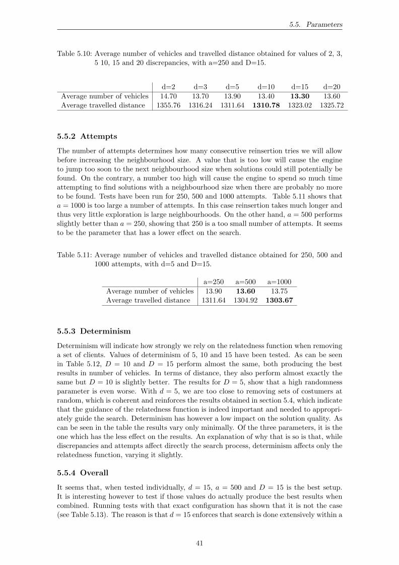
5.5. Parameters

Table 5.10: Average number of vehicles and travelled distance obtained for values of 2, 3,5 10, 15 and 20 discrepancies, with a=250 and D=15.

d=2 d=3 d=5 d=10 d=15 d=20

Average number of vehicles 14.70 13.70 13.90 13.40 13.30 13.60Average travelled distance 1355.76 1316.24 1311.64 1310.78 1323.02 1325.72

5.5.2 Attempts

The number of attempts determines how many consecutive reinsertion tries we will allowbefore increasing the neighbourhood size. A value that is too low will cause the engineto jump too soon to the next neighbourhood size when solutions could still potentially befound. On the contrary, a number too high will cause the engine to spend so much timeattempting to find solutions with a neighbourhood size when there are probably no moreto be found. Tests have been run for 250, 500 and 1000 attempts. Table 5.11 shows thata = 1000 is too large a number of attempts. In this case reinsertion takes much longer andthus very little exploration is large neighbourhoods. On the other hand, a = 500 performsslightly better than a = 250, showing that 250 is a too small number of attempts. It seemsto be the parameter that has a lower effect on the search.

Table 5.11: Average number of vehicles and travelled distance obtained for 250, 500 and1000 attempts, with d=5 and D=15.

a=250 a=500 a=1000

Average number of vehicles 13.90 13.60 13.75Average travelled distance 1311.64 1304.92 1303.67

5.5.3 Determinism

Determinism will indicate how strongly we rely on the relatedness function when removinga set of clients. Values of determinism of 5, 10 and 15 have been tested. As can be seenin Table 5.12, D = 10 and D = 15 perform almost the same, both producing the bestresults in number of vehicles. In terms of distance, they also perform almost exactly thesame but D = 10 is slightly better. The results for D = 5, show that a high randomnessparameter is even worse. With d = 5, we are too close to removing sets of costumers atrandom, which is coherent and reinforces the results obtained in section 5.4, which indicatethat the guidance of the relatedness function is indeed important and needed to appropri-ately guide the search. Determinism has however a low impact on the solution quality. Ascan be seen in the table the results vary only minimally. Of the three parameters, it is theone which has the less effect on the results. An explanation of why that is so is that, whilediscrepancies and attempts affect directly the search process, determinism affects only therelatedness function, varying it slightly.

5.5.4 Overall

It seems that, when tested individually, d = 15, a = 500 and D = 15 is the best setup.It is interesting however to test if those values do actually produce the best results whencombined. Running tests with that exact configuration has shown that it is not the case(see Table 5.13). The reason is that d = 15 enforces that search is done extensively within a

41

5. Evaluation

Table 5.12: Average number of vehicles and travelled distance obtained for values of de-terminism of 5, 10 and 15, with d=5 and a=250.

D=5 D=10 D=15

Average number of vehicles 14.00 13.90 13.90Average distance travelled 1308.61 1311.14 1311.64

given neighbourhood, while a = 500 enforces that many attempts are done before increas-ing the neighbourhood size. As discrepancies were tested with a low value of attempts, wecould afford using a high number of discrepancies. Similarly, attempts were tested with alow number of discrepancies, allowing us to afford a relatively high number of attempts.However, when a high number of discrepancies and a high number of attempts are com-bined, these configurations slow up the whole reinsertion process significantly, resultingin the engine not getting to explore neighbourhoods big enough—to around five or sixremoved customers, which is of course insufficient. In addition, while for configurationsthat are less search-extensive we can see that the last solution the engine finds is foundrelatively soon, with this configuration the engine keeps finding solutions up to the verytime limit that is placed on the search. This is again caused by the fact that the enginecan only get to remove small sets of customers and has not yet got to explore the biggerneighbourhoods. The fact that new solutions are found towards the end of the test hintthat there are still more solutions to be found and that, with more time, they would endup finding a better solution. This hypothesis is explored in section 5.9. However, in thissection we want to determine which are the best parameters for our current time limit of900 seconds.

To find out the best configuration we want to test various combinations of values. Wehave taken the best values for discrepancies d = 5, 10, 15, the number of attempts a =250, 500, 1000. While discrepancies and number of attempts are strongly related as theyaffect the reinsertion step directly, determinism only affects the relatedness function andseems to have a small impact on the solution, as D = 10 and D = 15 perform so similarly.He have assumed then that D = 10 is the best value for determinism independentlyof the number of discrepancies and attemtps. We have run tests for the chosen values ofdiscrepancies and attempts with determinism fixed at D = 10. Table 5.13 shows the resultsobtained with D = 10. The best results are produced with d = 10, with both a = 250 anda = 500 producing the best value for number of vehicles, and a = 500 performing the bestresult in terms of distance. Both configurations of d = 10, a = 1000 and d = 15, a = 250perform almost as good as d = 10, a = 500, only slightly worse. For bigger values of awith d = 15, exploration is increased too much and the results we obtain begin worse asthe number of attempts increases. Similarly, for d = 5 too little exploration is done, alsoresulting in worse values. But here, the results get worse as we decrease the number ofattempts, as this reduces even more the exploration done.

If we compare the results obtained with the combination d = 10, a = 500, D = 10 with theones that we obtained with d = 15, a = 250, D = 15 from the former tests (see Table 5.10),we can see that they are slightly worse. This fact hints that, although D = 10 performsslightly better in the concrete case of d = 5, a = 250, assuming that it is always the bestchoice is not right and that D = 15 is actually a better value. We have thus repeated thetests for the chosen values of discrepancies and attempts, now with determinism fixed atD = 15. In the results presented in 5.14 we can see that the results obtained are worsein some cases. Those are cases with a low number of discrepancies or a high numberof attempts. However, with those configurations that also obtained the best values for

42

5.6. Objective Function

Table 5.13: Results obtained for distance (right) and number of vehicles (left), with var-ious configurations for discrepancies and attempts, with the fixed value fordeterminism of D = 10.

a=250 a=500 a=1000

d=5 1311.14 13.9 1304.31 13.65 1294.6 13.55d=10 1306.76 13.4 1293.64 13.4 1301.72 13.45d=15 1318.66 13.45 1308.62 13.6 1314.10 13.7

D = 10, the results improve with respect to the tests previously made with D = 10. Thebest results are obtained with d = 10, a = 500, having the best score in number of vehicles.The configuration d = 15, a = 250 performs the same in number of vehicles, but is slightlyworse in distance.

Table 5.14: Results obtained for distance (right) and number of vehicles (left), with var-ious configurations for discrepancies and attempts, with the fixed value fordeterminism of D = 15.

a=250 a=500 a=100

d=5 1311.64 13.9 1304.92 13.6 1303.69 13.75d=10 1310.79 13.4 1313.39 13.3 1301.87 13.65d=15 1323.03 13.3 1305.54 13.65 1316.02 13.75

Based on this analysis, we conclude that the best parameter combination with the currenttime limit of 900 seconds is d = 10, a = 500 and D = 10.

5.6 Objective Function

The objective of this section is to see whether our objective function 4.3.3 really allowsthe travelled distance value to become slightly worse if that implies an improvement in thenumber of vehicles. A penalty of 1000 has been used for each vehicle used, as suggestedin [Sha98]. It is a high penalty in the sense that it means we allow the distance to get up to1000 units worse if this means optimizing a vehicle. This, despite the increase in distance,still causes the overall objective function to go down. As an example the evolution of thevalues for distance and number of vehicles for the instance r106 are presented. We canclearly observe in Figure 5.6, that near iteration 5000, the travelled distance goes a bitup exactly at the point where the number of used vehicles is improved. At this point,our objective function serves its purpose and accepts a solution with a higher distance,prioritizing the optimization of the number of vehicles.

5.7 Best Found Configurations

After testing all the combinations and options presented, we want to see if all the con-figurations that were optimal locally also produce the best results when combined. As asummary, these are exactly the options that have performed best in each case: An initialsolution with the savings method. For the relaxation step, the geographic and same tourrelatedness measure has been taken. For the reinsertion, the Customers Left Free methodwith the Farthest Insertion Heuristic, with the optimization of inserting variables imme-diately when they only have one insertion point. A 20 second time limit has been placed

43

5. Evaluation

1000 2000 3000 4000 5000

1300

1400

1500

1600

1700

1800

Iterations

Dis

tanc

e

1520

2530

Veh

icle

s

DistanceVehicles

Figure 5.6: Evolution of the travelled distance and number of vehicles over iterations forthe r106 instance.

on the reinsertion step. The search is stopped when a solution that is better than thecurrent best is found. The parameter values have been set at d = 10, a = 500 and D = 15.The combination of those methods should result in better results than the ones obtaineduntil here, or in the worst case, results that are equally good. After running a completetest with this configuration, we see that it doesn’t provide the best results. That wouldindicate that one or more of the tested options perform good when tested individually butdon’t work well with the others.

Time Limit on Reinsertion. Tests have been run without the insertion time limit forthe configuration described above. Preliminary tests show that this option was indeed theone that caused the whole configuration to perform worse, as the engine performs now veryequally than the previously tested methods. The reason that time limit on reinsertion doesnot work properly now is that we now use parameters of d = 10, a = 500, while the insertiontime limit had been tested with lower values of d = 5, a = 250. More discrepancies indicatethat more search will be done within each neighbourhood. This increase in the search spacealso implies an increase on the time each reinsertion step takes. Placing this time limiton the reinsertion step with a higher number of discrepancies prevents the engine fromexploring the whole neighbourhood that results from that number of discrepancies. Thus,the insertion time limit should not be used when allowing a higher number of discrepancies,or in any case, a higher time limit should be placed.

44

5.7. Best Found Configurations

Savings method for the Initial Solution. As the savings method seem to perform verysimilar to starting directly with one vehicle per customer, the results differencing only invery few instances, we have also run tests without using it. The results indicate that itis indeed, with this configuration, better to start directly with one vehicle per customerinstead of using the savings method.

Table 5.15 shows the results obtained by this configuration but starting with one vehicleper customer and not placing the time limit on reinsertion. We can see the results arenow very similar to the ones obtained in the previous analysis, with some instances evenperforming better (r102).

Table 5.15: Results obtained with the best configuration for the engine. We also reportthe neighbourhood size reached (NSize Reached) before the time limit of 900seconds.

Instance Vehicles Distance NSize Reached

r101 19 1691.23 13r102 17 1527.86 8r103 14 1285.47 7r104 11 1071.80 7r105 15 1447.05 14r106 13 1286.64 9r107 12 1128.47 7r108 11 1003.51 6r109 13 1207.69 11r110 12 1145.83 9r111 12 1095.10 7r112 11 1022.09 5rc101 16 1678.98 9rc102 14 1548.73 10rc103 12 1339.68 8rc104 11 1200.77 5rc105 15 1591.66 12rc106 14 1427.90 8rc107 12 1305.01 6rc108 12 1204.81 6

From this analysis we conclude that the best configuration for the engine is the following:

• The initial solution will constructed assigning one vehicle to each customer.

• Relaxation will make use of the relatedness function that considers geographicrelation as well as whether the customers are currently on the same tour.

• Reinsertion will be done with the Customers Left Free method.

• As insertion order heuristic we will take the Farthest Insertion heuristic, withthe optimization of inserting a variable immediately when it only has one insertionpoint left.

• No time limit will be placed on the reinsertion step.

• We stop the search after we found a solution that is better than the best foundsolution so far.

45

5. Evaluation

• Parameter Configuration. We take the best found values of bf d = 10, a = 500and D = 15.

5.8 Robustness of the Solution

Finally we want to analyse how robust is the solution. All the tests have been run tentimes with different random seeds. We want to see how big a part this randomness factorhas, and see if the other solutions found differ a lot from the best found one. We havecomputed the standard deviation for the 10 tests corresponding to the results in Table 5.15.The results for the standard deviation are shown in Table 5.16. The results show that thesolution is robust in number of vehicles, for which the standard deviation is less than onefor all instances. In terms of distance, it is also robust in most of the instances, althoughsome of them present a relatively high deviation of around 20% of their distance value.

Table 5.16: Average solution quality, in number of vehicles and distance, found by the tenruns of our engine, as well as the standard deviation.

Instance Avg. Vehicles Avg. Distance StDev (Vehicles) StDev (Distance)

r101 19.90 1684.73 0.32 16.31r102 18.70 1531.56 0.67 7.21r103 18.70 1531.56 0.67 13.54r104 12.10 1083.21 0.57 30.69r105 16.00 1423.47 0.47 23.55r106 14.10 1299.31 0.57 21.08r107 12.90 1145.60 0.32 22.08r108 11.10 1022.27 0.32 16.39r109 13.90 1231.39 0.57 26.05r110 13.10 1166.16 0.57 14.24r111 12.90 1130.88 0.74 17.68r112 11.90 1046.14 0.57 25.02

rc101 16.50 1695.98 0.53 15.69rc102 14.90 1557.89 0.32 23.08rc103 12.90 1367.07 0.57 15.25rc104 11.80 1250.99 0.42 25.74rc105 16.00 1609.37 0.47 17.50rc106 14.40 1477.63 0.70 30.02rc107 12.60 1327.21 0.52 23.96rc108 12.50 1276.23 0.53 48.21

5.9 Improvement over Time

We want to see how the solution evolves with more computation time. Especially, sincewe have a relatively high number of discrepancies and attempts (d = 10, a = 500) andthis causes the engine not to reach very big neighbourhoods, as evidenced in Table 5.15.We want to see if giving the engine more time to explore those neighbourhoods results inbetter solutions for the problems.

We have run test with a half an hour limit (1800 seconds) and one hour limits (3600seconds) to see if the solution really improves with more computation time. The resultsobtained for a half an hour time limit are shown in Table 5.17. While distance is improved

46

5.9. Improvement over Time

for almost all instances, there isn’t a big influence in the number of vehicles used whengiving the engine more computation time. By giving the engine half an hour, we improvea vehicle for instances r109 and rc108, and by giving it a whole hour we further improvea vehicle for instance r107. What can be observed is that the solution is more robust,meaning that from the 10 executions with different random seeds, most of them find thatbest solution but fail to further improve it.

Table 5.17: Results obtained with the 900 seconds time limit compared to the resultsobtained with 1800 seconds and 3600 seconds.

Instance Vehicles (900) Dist (900) Vehicles (1800) Dist (1800) Vehicles (3600) Dist (3600)

r101 19 1691.23 19 1691.23 19 1691.23r102 17 1527.86 17 1518.67 17 1518.67r103 14 1285.47 14 1268.52 14 1263.02r104 11 1071.80 11 1031.55 11 1025.78r105 15 1447.05 15 1447.05 15 1447.05r106 13 1286.64 13 1322.07 13 1279.06r107 12 1128.47 12 1111.10 11 1121.26r108 11 1003.51 11 1002.58 11 988.68r109 13 1207.69 12 1215.43 12 1215.43r110 12 1145.83 12 1133.24 12 1132.59r111 12 1095.10 12 1083.52 12 1083.52r112 11 1022.09 11 1004.04 11 999.91

rc101 16 1678.98 16 1678.98 16 1678.98rc102 14 1548.73 14 1545.67 14 1538.11rc103 12 1339.68 12 1339.68 12 1331.30rc104 11 1200.77 11 1184.38 11 1175.39rc105 15 1591.66 15 1591.66 15 1591.66rc106 14 1427.90 13 1432.01 13 1432.01rc107 12 1305.01 12 1249.82 12 1249.82rc108 12 1204.81 11 1175.42 11 1161.32

47

6. Conclusion

To conclude, a test for our methods with the combination of each best performing part iscompared to the results exposed in [Sha98]. We have used the best configuration found insection 5.7. As an initial solution, we use the one obtained by initially assigning one vehicleper customer. For the relaxation step, we use the relatedness function that considers bothgeographic closeness and whether or not the customers are in the same tour. As forreinsertion, we use the Customers Left Free method combined with the Farthest Insertionheuristic—but inserting variables immediately if only one value is left in their domain. Notime limit is placed on the reinsertion step, but we will stop it once a solution that is betterthan the current best solution is found. The parameters have been set at d = 10, a = 500and D = 15.

As can be observed in table Table 6.1, while the results obtained in distance travelled arevery similar, in most instances we are one or two vehicles over the solution the authorsreported. Concretely, for all the C-Instances the optimal number of vehicles has beenfound. For the other instances, we have found the optimal solution for 10% of the instances(r101, r102). In 40% of the instances, we are 1 vehicle above and in the remaining 50%of the instances the results obtained use 2 vehicles more than the ones reported by theauthors. In terms of distance, the results obtained are almost optimal, being 1.93% abovefor the C-Type instances and 3.39% above for the rest of the instances. It should be notedthat in some cases where we obtain better results in distance this can come from the factthat our computation is done with integer variables, which could lead to some solutionbeing accepted when it wouldn’t be if computing with the decimal numbers.

The fact that the solutions obtained are not exactly optimal can come from the fact thatthe authors of [Sha98] do not describe exactly neither how the neighbourhoods are chosenand not many details about the implementation are given, which can have led to somemisinterpretation from our part. Parameter analysis however provides a bit of insightregarding where the problem might be. Especially interesting is the observation that weobtain the best results for d = 10, 15 discrepancies while the authors obtain them ford = 5, 10. This means that we need more discrepancies to find a solution which impliesthat we need to try more insertion points to find it. This in turn means that the insertionpoints we calculate for each customer to insert are not the same as the authors’. Probablythe problem lies within deciding which insertion points are candidates for reinsertion, andin which order those insertion points will be tried.

Although we were not able to perfectly reproduce the results of [Sha98], we could verify thatConstraint Programming is indeed an effective way of solving Vehicle Routing Problems,

49

6. Conclusion

Table 6.1: Comparison of our best found solutions against the best found solutions theauthors reported.

Instance Vehicles Shaw Distance Shaw Vehicles Distance

c101 10 828.94 10 828.94c102 10 828.94 10 829.70c103 10 828.06 10 882.13c104 10 824.78 10 836.06c105 10 828.94 10 828.94c106 10 828.94 10 829.70c107 10 828.94 10 829.70c108 10 828.94 10 859.76c109 10 828.94 10 869.12r101 19 1650.80 19 1691.23r102 17 1486.12 17 1527.86r103 13 1292.68 14 1285.47r104 9 1007.31 11 1071.80r105 14 1377.11 15 1447.05r106 12 1252.03 13 1286.64r107 10 1104.66 12 1128.47r108 9 963.99 11 1003.51r109 11 1197.42 13 1207.69r110 10 1135.07 12 1145.83r111 10 1096.73 12 1095.10r112 10 953.63 11 1022.09rc101 14 1696.95 16 1678.98rc102 12 1554.75 14 1548.73rc103 11 1261.67 12 1339.68rc104 10 1135.48 11 1200.77rc105 14 1540.18 15 1591.66rc106 12 1376.26 14 1427.90rc107 11 1230.48 12 1305.01rc108 10 1139.82 12 1204.81

as the solutions obtained are very little over the optimal. The ease with which new sideconstraints can be added greatly outweighs the somewhat less optimization performance.To add side constraints to the system, only the specification of the requirements thesolution has to meet has to be modified. This is done by adding the new constraints tothe model. Most constraints can be posted using the implemented propagators Gecodeprovides, but in the worst case all that must be done is implement a custom propagator.The important thing is that to add new side constraints, nothing from the engine has tobe modified—the engine remains exactly the same.

Future work should further consider strategies for the reinsertion step, especially for thedefinition and choice of the insertion points for the customers, as well as possibly theorder in which clients are inserted. Other relatedness functions and other reinsertionmethods should not be discarded though, as it could be that better options exist. Itshould also concentrate on an in-detail evaluation of the impact of real-world constraintson the performance of the search engine.

50

Bibliography

[Apt03] K.R. Apt. Principles of constraint programming. Cambridge University Press,2003.

[BFS+00] B.D. Backer, V. Furnon, P. Shaw, P. Kilby, and P. Prosser. Solving vehiclerouting problems using constraint programming and metaheuristics. Journalof Heuristics, 6(4):501–523, 2000.

[BGG+97] P. Badeau, F. Guertin, M. Gendreau, J.Y. Potvin, and E. Taillard. A paral-lel tabu search heuristic for the vehicle routing problem with time windows.Transportation Research Part C: Emerging Technologies, 5(2):109–122, 1997.

[CL97] Y. Caseau and F. Laburthe. Solving small tsps with constraints. In Interna-tional Conference on Logic Programming, pages 316–330, 1997.

[CW64] G. Clarke and JW Wright. Scheduling of vehicles from a central depot to anumber of delivery points. Operations research, pages 568–581, 1964.

[DS90] G. Dueck and T. Scheuer. Threshold accepting: a general purpose optimizationalgorithm appearing superior to simulated annealing. Journal of computationalphysics, 90(1):161–175, 1990.

[Due93] G. Dueck. New optimization heuristics. Journal of computational physics,104(1):86–92, 1993.

[EOSF06] O. Ergun, J.B. Orlin, and A. Steele-Feldman. Creating very large scale neigh-borhoods out of smaller ones by compounding moves. Journal of Heuristics,12(1):115–140, 2006.

[FJ81] M.L. Fisher and R. Jaikumar. A generalized assignment heuristic for vehiclerouting. Networks, 11(2):109–124, 1981.

[FLM02] F. Focacci, A. Lodi, and M. Milano. Embedding relaxations in global con-straints for solving tsp and tsptw. Annals of Mathematics and Artificial Intel-ligence, 34(4):291–311, 2002.

[GLS96] M. Gendreau, G. Laporte, and R. Seguin. A tabu search heuristic for thevehicle routing problem with stochastic demands and customers. OperationsResearch, 44(3):469–477, 1996.

[GM74] B.E. Gillett and L.R. Miller. A heuristic algorithm for the vehicle-dispatchproblem. Operations research, 22(2):340–349, 1974.

[HG95] W.D. Harvey and M.L. Ginsberg. Limited discrepancy search. In Interna-tional Joint Conference on Artificial Intelligence, volume 14, pages 607–615.LAWRENCE ERLBAUM ASSOCIATES LTD, 1995.

[HM91] J.H. Holland and J.H. Miller. Artificial adaptive agents in economic theory.The American Economic Review, 81(2):365–370, 1991.

51

Bibliography

[KPS98] P. Kilby, P. Prosser, and P. Shaw. Apes report apes-01-1998. 1998.

[KPS00] P. Kilby, P. Prosser, and P. Shaw. A comparison of traditional and constraint-based heuristic methods on vehicle routing problems with side constraints.Constraints, 5(4):389–414, 2000.

[KS06] P. Kilby and P. Shaw. Vehicle routing. Foundations of Artificial Intelligence,2:801–836, 2006.

[Lap09] Gilbert Laporte. Fifty years of vehicle routing. Transportation Science,43(4):408–416, November 2009.

[MH97] N. Mladenovic and P. Hansen. Variable neighborhood search. Computers &Operations Research, 24(11):1097–1100, 1997.

[PGPR98] G. Pesant, M. Gendreau, J.Y. Potvin, and J.M. Rousseau. An exact constraintlogic programming algorithm for the traveling salesman problem with timewindows. Transportation Science, 32(1):12–29, 1998.

[PR10] D. Pisinger and S. Ropke. Large neighborhood search. Handbook of meta-heuristics, pages 399–419, 2010.

[RVBW06] F. Rossi, P. Van Beek, and T. Walsh. Handbook of constraint programming,volume 2. Elsevier Science, 2006.

[Sha97] P. Shaw. A new local search algorithm providing high quality solutions tovehicle routing problems. Department of Computer Sciences, University ofStrathclyde, Glasgow, Scottland, Tech. Rep, APES group, 1997.

[Sha98] Paul Shaw. Using constraint programming and local search methods to solvevehicle routing problems. In Michael Maher and Jean-Francois Puget, editors,Principles and Practice of Constraint Programming – CP98, volume 1520 ofLecture Notes in Computer Science, pages 417–431. Springer Berlin / Heidel-berg, 1998.

[Sha11] P. Shaw. Constraint programming and local search hybrids. Hybrid Optimiza-tion, pages 271–303, 2011.

[Sol87] M.M. Solomon. Algorithms for the vehicle routing and scheduling problemswith time window constraints. Operations research, 35(2):254–265, 1987.

[STL11] C. Schulte, G. Tack, and M.Z. Lagerkvist. Modeling and programming withgecode, 2011.

52

Constraint Programming based Local Search for the Vehicle ...

Documents

Transcript of Constraint Programming based Local Search for the Vehicle ...