A Systematic Approach to MDD-Based

Constraint Programming

Samid Hoda, Willem-Jan van Hoeve, and J. N. Hooker

Tepper School of Business, Carnegie Mellon University5000 Forbes Avenue, Pittsburgh, PA 15213, U.S.A.

shoda,vanhoeve@andrew.cmu.edu, john@hooker.tepper.cmu.edu

Abstract. Fixed-width MDDs were introduced recently as a more re-fined alternative for the domain store to represent partial solutions toCSPs. In this work, we present a systematic approach to MDD-basedconstraint programming. First, we introduce a generic scheme for con-straint propagation in MDDs. We show that all previously known prop-agation algorithms for MDDs can be expressed using this scheme. More-over, we use the scheme to produce algorithms for a number of otherconstraints, including Among, Element, and unary resource constraints.Finally, we discuss an implementation of our MDD-based CP solver, andprovide experimental evidence of the benefits of MDD-based constraintprogramming.

1 Introduction

The domain store is a fundamental tool for constraint programming (CP), be-cause it propagates the results of individual constraint processing. It allows thereduced domains obtained for one constraint to be passed to the next constraintfor further filtering. A weakness of the domain store, however, is that it trans-mits a limited amount of information. It accounts for no interaction among thevariables, because any solution in the Cartesian product of the current domainsis consistent with it. This restricts the ability of the domain store to pool theresults of processing individual constraints and provide a global view of theproblem.

To address this shortcoming, Andersen, Hadzic, Hooker, and Tiedemann [1]proposed replacing the domain store with a richer data structure, namely a mul-tivalued decision diagram (MDD). In their approach, domain filtering algorithmsare replaced or augmented by algorithms that refine and update the MDD toreflect each constraint. It was found that MDD-based propagation can lead tosubstantial speedups in the solution of multiple AllDifferent constraints. Theidea was extended to equality constraints by Hadzic et al. [4]. A unified node-splitting scheme for refining the MDD was proposed by Hadzic et al. [3] andapplied to certain configuration problems. For this reason, we will mainly focuson filtering algorithms in this work.

MDDs have been applied before in CP. For example, in [6] and [2] MDDs areapplied to perform inferences (domain filtering) based on individual constraints.

2

In [5], this is taken one step further, by passing structural information from oneconstraint to the next. The key difference is that in these approaches, an MDDis built and maintained for each individual constraint, whereas in MDD-basedconstraint programming, the MDD is the information that is passed from oneconstraint to the next. In other words, multiple constraints process the sameMDD, instead of each constraint processing its individual MDD.

The contributions of this work are threefold. First, we introduce a systematicscheme for constraint propagation in MDDs, and we show that all previouslyproposed filtering algorithms for MDD-based CP can be viewed as instantiationsof our scheme. Second, we apply our scheme to introduce new filtering algorithmsfor other constraints; we present such algorithms for the Among, Element, andunary resource constraints as an illustration of the versatility of the approach.Third, we present computational results for the first pure MDD-based CP solver,showing that i) this approach can scale up to realistic problem sizes, and ii)enormous savings (in terms of time as well as search tree size) can be realizedwhen compared to solvers relying on the traditional domain store.

The remainder of the paper is organized as follows. In Section 2 we providethe necessary background on MDDs and MDD-based constraint programming.In Section 3 we present and discuss a systematic scheme for constraint propaga-tion in MDDs. We apply our scheme to a variety of constraints in Section 4. InSection 5 we provide a brief description of our MDD-based constraint program-ming system. Experimental results using this system are reported in Section 6.Finally, we conclude in Section 7.

2 MDDs and MDD-Based Constraint Solving

In this work, an ordered Multivalued Decision Diagram (MDD) is a directedacyclic graph whose nodes are partitioned into n (possibly empty) subsets orlayers L1, . . . , Ln+1, where the layers L1, . . . , Ln correspond respectively to vari-ables x1, . . . , xn. L1 contains a single top node T, and Ln+1 contains two bottomnodes 0 and 1. The width of the MDD is the maximum number of nodes ina layer, or maxn

i=1{|Li|}. In MDD-based CP, the MDDs typically have a givenfixed maximum width.

All edges of the MDD are directed from an upper to a lower layer; that is,from a node in some Li to a node in some Lj with i < j. For our purposes it isconvenient to assume (without loss of generality) that each edge connects twoadjacent layers. Let L(s) denote the layer of the node s, and var(s) the variableassociated with L(s). Each edge out of layer i is labeled with an element of thedomain D(xi) of xi. The set E(s, t) of edges from node s to node t may containmultiple edges, and we denote each with its label. Let Ein(s) denote the set ofedges coming into s, and Eout(s) the set of edges leaving s. For an edge e, tail(e)is the tail of e and head(e) the head.

An edge with label v leaving a node in layer i represents an assignmentxi = v. Each path in the MDD from T to 0 or 1 can be denoted by the edgelabels v1, . . . , vn on the path and is identified with the assignment (x1, . . . , xn) =

3

x1

x2

x3

{0,1}

{0,1,2}

{1,2} {1,2}

{1}

{0,1,2}{0,1,2}

{0} {1}

{1,2}{1,2}

{1,2}

{0}{1}

{0}

{2}{2}

{1}

{0}{1}

{0}

{2} {2}

{2}{1,2} {1} {1}

{1}

{0}{1}

{0}

{2}

{1}{2}{2}

(a) (b) (c) (d) (e)

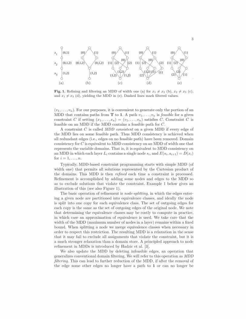
Fig. 1. Refining and filtering an MDD of width one (a) for x1 6= x2 (b), x2 6= x3 (c),and x1 6= x3 (d), yielding the MDD in (e). Dashed lines mark filtered values.

(v1, . . . , vn). For our purposes, it is convenient to generate only the portion of anMDD that contains paths from T to 1. A path v1, . . . , vn is feasible for a givenconstraint C if setting (x1, . . . , xn) = (v1, . . . , vn) satisfies C. Constraint C isfeasible on an MDD if the MDD contains a feasible path for C.

A constraint C is called MDD consistent on a given MDD if every edge ofthe MDD lies on some feasible path. Thus MDD consistency is achieved whenall redundant edges (i.e., edges on no feasible path) have been removed. Domainconsistency for C is equivalent to MDD consistency on an MDD of width one thatrepresents the variable domains. That is, it is equivalent to MDD consistency onan MDD in which each layer Li contains a single node si, and E(si, si+1) = D(xi)for i = 1, . . . , n.

Typically, MDD-based constraint programming starts with simple MDD (ofwidth one) that permits all solutions represented by the Cartesian product ofthe domains. This MDD is then refined each time a constraint is processed.Refinement is accomplished by adding some nodes and edges to the MDD soas to exclude solutions that violate the constraint. Example 1 below gives anillustration of this (see also Figure 1).

The basic operation of refinement is node-splitting, in which the edges enter-ing a given node are partitioned into equivalence classes, and ideally the nodeis split into one copy for each equivalence class. The set of outgoing edges foreach copy is the same as the set of outgoing edges of the original node. We notethat determining the equivalence classes may be costly to compute in practice,in which case an approximation of equivalence is used. We take care that thewidth of the MDD (maximum number of nodes in a layer) remains within a fixedbound. When splitting a node we merge equivalence classes when necessary inorder to respect this restriction. The resulting MDD is a relaxation in the sensethat it may fail to exclude all assignments that violate the constraint, but it isa much stronger relaxation than a domain store. A principled approach to noderefinement in MDDs is introduced by Hadzic et al. [3].

We also update the MDD by deleting infeasible edges, an operation thatgeneralizes conventional domain filtering. We will refer to this operation as MDDfiltering. This can lead to further reduction of the MDD, if after the removal ofthe edge some other edges no longer have a path to 1 or can no longer be

4

reached by a path from the root. An MDD-based constraint solver is based onpropagation and search just as traditional CSP solvers, but the domain filteringprocess at each node of the search tree is replaced (or supplemented) by an MDDrefinement and filtering process.

Example 1. Consider a CSP with variables x1 ∈ {0, 1}, x2 ∈ {0, 1, 2}, and x3 ∈{1, 2}, and constraints x1 6= x2, x2 6= x3, and x1 6= x3. All domain values aredomain consistent (even if we were to apply the AllDifferent propagator onthe conjunction of the constraints), and the domain store defines the relaxation{0, 1} × {0, 1, 2} × {1, 2}, which includes infeasible solutions such as (1, 1, 1).

The MDD-based approach starts with the MDD of width one in Figure 1(a),in which multiple arcs are represented by a set of corresponding domain values forclarity. We refine and filter each constraint separately. Starting with x1 6= x2,we refine the MDD by splitting the node at layer 2, resulting in Figure 1(b).This allows us to filter two domain values, based on x1 6= x2, as indicated in thefigure. In Figure 1(c) and (d) we refine and filter the MDD for the constraintsx2 6= x3 and x1 6= x3 respectively, until we reach the MDD in Figure 1(e). ThisMDD represents all three solutions to the problem, and provides a much tighterrelaxation than the domain store.

3 A Systematic Scheme for MDD Propagation

In the literature, MDD propagation algorithms (in the sense of Section 2) havebeen proposed for the following three constraint types: (one-sided) inequalityconstraints [1], AllDifferent [1], and equality constraints [3]. The reasoningused for designing propagation algorithms for each of these constraints seemedto be ad-hoc. In this section we will present and analyze a systematic schemefor designing MDD propagation algorithms. In the following section we use thisprocedure to express the existing MDD propagation algorithms and introducenew algorithms for the Among, Element, and unary resource constraints.

3.1 The General Scheme

Our scheme is based on the idea of ‘local information’ I(s) stored for each con-straint at each node s. We will show that all MDD propagation schemes so farintroduced, and others as well, can be viewed as based on local information.The precise nature of the local information depends on the propagation scheme,which is characterized in part by what kind of local information is required toapply it.

More precisely, the decision as to whether to delete an edge in E(s, t) isbased solely on I(s) and I(t)—that is, on local information stored at either endof the edge. Furthermore, the local information can be accumulated by a singletop-down pass and a single bottom-up pass through the MDD.

It is convenient to regard I(s) as a pair (I↓(s), I↑(s)) consisting of the infor-mation I↓(s) accumulated during the top-down pass, and the information I↑(s)

5

accumulated during the bottom-up pass. I↓(s) and I↑(s) can take several forms,such as a set of domain values or parameters related to the constraint, or a tupleof such sets. What is common to all the schemes is that I↓(s) is computed solelyon the basis of local information at the opposite end of edges coming into s, andI↑(s) on the basis of local information at the opposite end of edges leaving s.

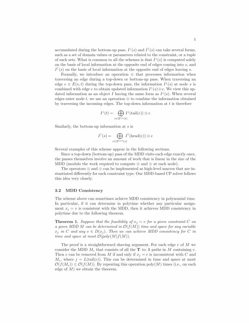
Formally, we introduce an operation ⊗ that processes information whentraversing an edge during a top-down or bottom-up pass. When traversing anedge e ∈ E(s, t) during the top-down pass, the information I↓(s) at node s iscombined with edge e to obtain updated information I↓(s)⊗e. We view this up-dated information as an object I having the same form as I↓(s). When severaledges enter node t, we use an operation ⊕ to combine the information obtainedby traversing the incoming edges. The top-down information at t is therefore

I↓(t) =⊕

e∈Ein(t)

I↓(tail(e)) ⊗ e

Similarly, the bottom-up information at s is

I↑(s) =⊕

e∈Eout(s)

I↑(head(e)) ⊗ e

Several examples of this scheme appear in the following sections.Since a top-down (bottom-up) pass of the MDD visits each edge exactly once,

the passes themselves involve an amount of work that is linear in the size of theMDD (modulo the work required to compute ⊕ and ⊗ at each node).

The operators ⊗ and ⊕ can be implemented as high-level macros that are in-stantiated differently for each constraint type. Our MDD-based CP solver followsthis idea very closely.

3.2 MDD Consistency

The scheme above can sometimes achieve MDD consistency in polynomial time.In particular, if it can determine in polytime whether any particular assign-ment xj = v is consistent with the MDD, then it achieves MDD consistency inpolytime due to the following theorem.

Theorem 1. Suppose that the feasibility of xj = v for a given constraint C ona given MDD M can be determined in O(f(M)) time and space for any variablexj in C and any v ∈ D(xj). Then we can achieve MDD consistency for C intime and space at most O(poly(M)f(M)).

The proof is a straightforward shaving argument. For each edge e of M weconsider the MDD Me that consists of all the T–to–1 paths in M containing e.Then e can be removed from M if and only if xj = e is inconsistent with C andMe, where j = L(tail(e)). This can be determined in time and space at mostO(f(Me)) ≤ O(f(M)). By repeating this operation poly(M) times (i.e., on eachedge of M) we obtain the theorem.

6

To establish MDD consistency, the goal is to efficiently compute informationthat is strong enough to apply Theorem 1. In the sequel, we will see that this canbe done for inequality constraints and Among constraints in polynomial time, andin pseudo-polynomial time for two-sided inequality constraints. Furthermore, wehave the following result.

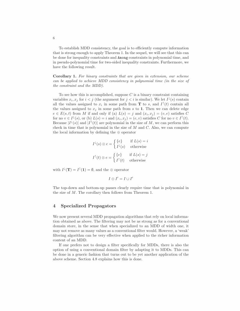
Corollary 1. For binary constraints that are given in extension, our schemecan be applied to achieve MDD consistency in polynomial time (in the size ofthe constraint and the MDD).

To see how this is accomplished, suppose C is a binary constraint containingvariables xi, xj for i < j (the argument for j < i is similar). We let I↓(s) containall the values assigned to xi in some path from T to s, and I↑(t) contain allthe values assigned to xj in some path from s to 1. Then we can delete edgee ∈ E(s, t) from M if and only if (a) L(s) = j and (xi, xj) = (v, e) satisfies C

for no v ∈ I↓(s), or (b) L(s) = i and (xi, xj) = (e, v) satisfies C for no v ∈ I↑(t).Because |I↓(s)| and |I↑(t)| are polynomial in the size of M , we can perform thischeck in time that is polynomial in the size of M and C. Also, we can computethe local information by defining the ⊕ operator

I↓(s) ⊗ e =

{

{e} if L(s) = i

I↓(s) otherwise

I↑(t) ⊗ e =

{

{e} if L(s) = j

I↑(t) otherwise

with I↓(T) = I↑(1) = ∅, and the ⊕ operator

I ⊕ I ′ = I ∪ I ′

The top-down and bottom-up passes clearly require time that is polynomial inthe size of M . The corollary then follows from Theorem 1.

4 Specialized Propagators

We now present several MDD propagation algorithms that rely on local informa-tion obtained as above. The filtering may not be as strong as for a conventionaldomain store, in the sense that when specialized to an MDD of width one, itmay not remove as many values as a conventional filter would. However, a ‘weak’filtering algorithm can be very effective when applied to the richer informationcontent of an MDD.

If one prefers not to design a filter specifically for MDDs, there is also theoption of using a conventional domain filter by adapting it to MDDs. This canbe done in a generic fashion that turns out to be yet another application of theabove scheme. Section 4.8 explains how this is done.

7

4.1 Equality and Not-Equal Constraints

We first illustrate MDD propagation of the constraints xi = xj and xi 6= xj .Because these are binary constraints, by Corollary 1 the scheme presented inSection 3.2 achieves MDD consistency in polytime. If we compute I↓ as describedin that section, we can achieve MDD consistency for xi = xj by deleting an edgee ∈ E(s, t) whenever (a) L(s) = j and e 6∈ I↓(s) or (b) L(s) = i and e 6∈ I↑(t). Wecan achieve MDD consistency for xi 6= xj by deleting e whenever (a) L(s) = j

and I↓(s) = {e} or (b) L(s) = i and I↑(t) = {e}.We note that this scheme generalizes directly to propagating fi(xi) = fj(xj)

and fi(xi) 6= fj(xj) for functions fi and fj . The scheme can also be appliedto constraints xi < xj . However, in this case we only need to maintain boundinformation instead of sets of domain values, which leads to an even more efficientimplementation.

4.2 Propagating Linear Inequalities

We next focus on the filtering algorithm for general inequalities, as proposedin [1]. That is, we want to propagate an inequality over a separable function ofthe form:

∑

j∈J

fj(xj) ≤ b (1)

We can propagate such constraint on an MDD by performing shortest-path com-putations.

Recall that each edge e ∈ E(s, t) is identified with a value assigned to var(s).Supposing that var(s) = xj , we let the length of edge e be fj(e) when j ∈ J andzero otherwise. Thus the length of a T–to–1 path is the left-hand side of (1).

We let I↓(s) be the length of a shortest path from T to s, and I↑(s) thelength of a shortest path from s to 1. Then we delete an edge e ∈ E(s, t) whenL(s) ∈ J and every path through e is longer than b; that is,

I↓(s) + fL(s)(e) + I↑(t) > b

It is easy to compute local information in the form of shortest path lengths,because we can define for e ∈ E(s, t)

I↓(s) ⊗ e =

{

I↓(s) + fL(s)(e) if L(s) ∈ J

I↓(s) otherwise

I↑(t) ⊗ e =

{

I↑(t) + fL(s)(e) if L(s) ∈ J

I↑(t) otherwise

with I↓(T) = I↑(1) = 0. We also define

I ⊕ I ′ = min{I, I ′}

This inequality propagator achieves MDD consistency as an edge e is alwaysremoved unless there exists a feasible solution to the inequality that supportsit [1].

8

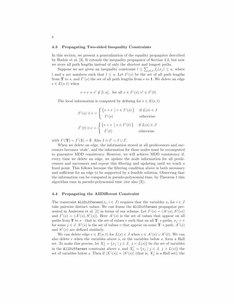
4.3 Propagating Two-sided Inequality Constraints

In this section, we present a generalization of the equality propagator describedby Hadzic et al. [3]. It extends the inequality propagator of Section 4.2, but nowwe store all path lengths instead of only the shortest and longest paths.

Suppose we are given an inequality constraint l ≤∑

j∈J fj(xj) ≤ u, where

l and u are numbers such that l ≤ u. Let I↓(s) be the set of all path lengthsfrom T to s, and I↑(s) the set of all path lengths from s to 1. We delete an edgee ∈ E(s, t) when

v + e + v′ 6∈ [l, u], for all v ∈ I↓(s), v′ ∈ I↑(t)

The local information is computed by defining for e ∈ E(s, t)

I↓(s) ⊗ e =

{{

v + e∣

∣ v ∈ I↓(s)}

if L(s) ∈ J

I↓(s) otherwise

I↑(t) ⊗ e =

{

{

v + e∣

∣ v ∈ I↑(t)}

if L(s) ∈ J

I↑(t) otherwise

with I↓(T) = I↑(1) = ∅. Also I ⊕ I ′ = I ∪ I ′.When we delete an edge, the information stored at all predecessors and suc-

cessors becomes ‘stale’, and the information for these nodes must be recomputedto guarantee MDD consistency. However, we will achieve MDD consistency if,every time we delete an edge, we update the node information for all prede-cessors and successors and repeat this filtering and updating until we reach afixed point. This follows because the filtering condition above is both necessaryand sufficient for an edge to be supported by a feasible solution. Observing thatthe information can be computed in pseudo-polynomial time, by Theorem 1 thisalgorithm runs in pseudo-polynomial time (see also [3]).

4.4 Propagating the AllDifferent Constraint

The constraint AllDifferent(xi, i ∈ J) requires that the variables xi for i ∈ J

take pairwise distinct values. We can frame the AllDifferent propagator pre-sented in Andersen et al. [1] in terms of our scheme. Let I↓(s) = (A↓(s), S↓(s))and I↑(s) = (A↑(s), S↑(s)). Here A↓(s) is the set of values that appear on allpaths from T to s—that is, the set of values v such that on all T–s paths, xj = v

for some j ∈ J . S↓(s) is the set of values v that appear on some T–s path. A↑(s)and S↑(s) are defined similarly.

We can delete edge e ∈ E(s, t) for L(s) ∈ J when e ∈ A↓(s) ∪ A↑(t). We canalso delete e when the variables above s, or the variables below s, form a Hallset. To make this precise, let X↓

s = {xj | j ∈ J, j < L(s)} be the set of variables

in the AllDifferent constraint above s, and X↑t = {xj | j ∈ J, j > L(s)} the

set of variables below s. Then if |X↓(s)| = |S↓(s)| (that is, X↓s is a Hall set), the

9

values in S↓(s) cannot be assigned to any variable not in X↓(s). So we delete e

if e ∈ S↓(s). Similarly, if X↑(t) is a Hall set, we delete e if e ∈ S↑(t).Finally, we compute the local information by defining for e ∈ E(s, t)

I↓(s) ⊗ e =

{

I↓(s) ∪ ({e}, {e}), if L(s) ∈ J

I↓(s), otherwise

I↑(t) ⊗ e =

{

I↑(t) ∪ ({e}, {e}), if L(s) ∈ J

I↑(t), otherwise

where the unions are taken componentwise and I↓(T) = I↑(1) = (∅, ∅). Also wedefine

I ⊕ I ′ = (A ∩ A′, S ∪ S′).

4.5 Propagating the Among Constraint

The Among constraint restricts the number of variables that can be assigned avalue from a specific subset of domain values. Formally, if X = (x1, . . . , xq) isa sequence of variables, S a set of domain values, and ℓ, u, q are constants with0 ≤ ℓ ≤ u ≤ q, then Among(X, S, ℓ, u) requires that

ℓ ≤ |{i ∈ {1, . . . , q} | vi ∈ S}| ≤ u

We can reduce propagating Among(X, S, ℓ, u) to propagating a two-sided sep-arable inequality constraint,

ℓ ≤∑

xi∈X

fi(xi) ≤ u,

where

fi(v) =

{

1, if v ∈ S

0, otherwise.

Because each fi(·) ∈ {0, 1}, we can compute the information in polynomialtime, and by Theorem 1 MDD consistency can be achieved in polynomial timefor Among constraints.

However, this filtering is too slow in practice. Instead, we propose to propa-gate bounds information instead. That is, we can use the inequality propagatorfor the pair of inequalities separately, and reason on the shortest and longestpath lengths, as in Section 4.2.

4.6 Propagating the Element Constraint

We next consider constraints of the form Element(xi, (a1, . . . , am), xj), wherethe ak are constants. This means that the variable xj must take the xth

i valuein the list (a1, . . . , am); that is, xj = axi

.Because this is a binary constraint, we can achieve MDD consistency in

polytime by defining I↓(s), I↑(t) as in the proof of Corollary 1. Supposing thati < j, we delete an edge e ∈ E(s, t) when (a) L(s) = j and e = ak for nok ∈ I↓(s), or (b) L(s) = i and ae 6∈ I↑(t).

10

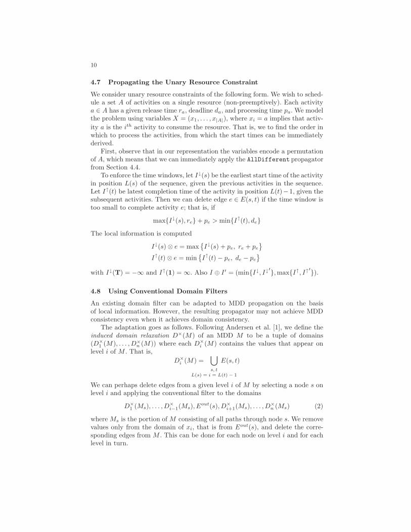
4.7 Propagating the Unary Resource Constraint

We consider unary resource constraints of the following form. We wish to sched-ule a set A of activities on a single resource (non-preemptively). Each activitya ∈ A has a given release time ra, deadline da, and processing time pa. We modelthe problem using variables X = (x1, . . . , x|A|), where xi = a implies that activ-

ity a is the ith activity to consume the resource. That is, we to find the order inwhich to process the activities, from which the start times can be immediatelyderived.

First, observe that in our representation the variables encode a permutationof A, which means that we can immediately apply the AllDifferent propagatorfrom Section 4.4.

To enforce the time windows, let I↓(s) be the earliest start time of the activityin position L(s) of the sequence, given the previous activities in the sequence.Let I↑(t) be latest completion time of the activity in position L(t)−1, given thesubsequent activities. Then we can delete edge e ∈ E(s, t) if the time window istoo small to complete activity e; that is, if

max{I↓(s), re} + pe > min{I↑(t), de}

The local information is computed

I↓(s) ⊗ e = max{

I↓(s) + pe, re + pe

}

I↑(t) ⊗ e = min{

I↑(t) − pe, de − pe

}

with I↓(T) = −∞ and I↑(1) = ∞. Also I ⊕ I ′ = (min{I↓, I↓′}, max{I↑, I↑

′}).

4.8 Using Conventional Domain Filters

An existing domain filter can be adapted to MDD propagation on the basisof local information. However, the resulting propagator may not achieve MDDconsistency even when it achieves domain consistency.

The adaptation goes as follows. Following Andersen et al. [1], we define theinduced domain relaxation D×(M) of an MDD M to be a tuple of domains(D×

1 (M), . . . , D×n (M)) where each D×

i (M) contains the values that appear onlevel i of M . That is,

D×i (M) =

⋃

s, tL(s) = i = L(t) − 1

E(s, t)

We can perhaps delete edges from a given level i of M by selecting a node s onlevel i and applying the conventional filter to the domains

D×1 (Ms), . . . , D

×i−1(Ms), E

out(s), D×i+1(Ms), . . . , D

×n (Ms) (2)

where Ms is the portion of M consisting of all paths through node s. We removevalues only from the domain of xi, that is from Eout(s), and delete the corre-sponding edges from M . This can be done for each node on level i and for eachlevel in turn.

11

To compute D×(Ms), we can regard it as local information I↓(s) (bottom-upinformation I↑(s) is not needed). Then for e ∈ E(s, t)

I↓(s) ⊗ e = I↓(s) ∪ (∅, . . . , ∅, {e}, ∅, . . . , ∅)

where {e} is component L(s) of the vector, and the union is taken component-wise. Also I ⊕ I ′ = I ∪ I ′.

This leads to the following lemma.

Lemma 1. The induced domain relaxation D×(Ms) can be computed for allnodes s of a given MDD M in polynomial time (in the size of the MDD).

Again following Andersen et al. [1], we can strengthen the filtering by notingwhich values can be deleted from the domains D×

j (Ms) for j 6= i when (2) is

filtered. If v can be deleted from D×j (Ms), we place the nogood xj 6= v on each

edge in Eout(s). Then we move the nogoods on level i toward level j. If j > i,for example, we filter (2) for each node on level i and then note which nodes onlevel i + 1 have the property that all incoming edges have the nogood xj 6= v.These nodes propagate the nogood to all their outgoing edges, and so forth untillevel j is reached, where all edges with nogood xj 6= v and label v are deleted.

5 Implementation Issues

We have implemented a C++ system for MDD-Based Constraint Programming.For a detailed description of the system, we refer to [7]. We next highlight someof the most important design decisions we have made.

Even though MDDs can grow exponentially large to represent a given con-straint perfectly, the basis of MDD-based constraint programming is to controlthe size of the MDD by specifying a maximum width k. A MDD of width one isequivalent to the conventional domain store, while increasing values of k allowthe MDD to converge to a perfect representation of the solution space. An MDDon n variables therefore contains O(nk) nodes. Furthermore, by aggregating thedomain values corresponding to multiple (parallel) edges between two nodes, theMDD contains O(nk2) edges. Therefore, for fixed k, all bottom-up and top-downpasses take linear time.

In our system, we do not propagate the constraints until a fixed point. In-stead, by default we allocate one bottom-up and top-down pass to each con-straint. The bottom-up pass is used to compute the information I↑. The top-down pass processes the MDD a layer at a time, in which we first compute I↓,then refine the nodes in the layer, and finally apply the filtering conditions basedon I↑ and I↓.

Our outer search procedure is currently implemented using a priority queue,in which the search nodes are inserted with a specific weight. This allows to easilyencode depth-first search or best-first search procedures. Each search tree nodecontains a copy of the MDD of its parent, together with the associated branch-ing decision. When applying a depth-first search strategy, the total amount of

12

space required to store all MDDs is polynomial, namely O(n2k2). We note that‘recomputation’ strategies that are common in conventional CP systems, cannotbe easily applied in this context, because the MDD may change from parent tochild node, due to the node refinement procedure.

6 Experimental Results

In this section, we provide detailed experimental evidence to support the claimthat MDD-based constraint programming can be a viable alternative to con-straint programming based on the domain store. All the experiments are per-formed using a 2.33GHz Intel Xeon machine with 8GB memory, using our MDD-based CP solver. For comparison reasons, our solver applies a depth-first search,using a static lexicographic-first variable selection heuristic, and a minimum-value-first value selection heuristic. We vary the maximum width of the MDD,while keeping all other settings the same.

Multiple Among Constraints We first present experiments on problemsconsisting of multiple Among constraints. Each instance contains 50 (binary)variables, and each Among constraint consists of 5 variables chosen at random,from a normal distribution with a uniform-random mean (from [1..50]) and stan-dard deviation σ = 2.5, modulo 50. As a result, for these Among constraints thevariable indices are near-consecutive, a pattern encountered in many practicalsituations. Each Among has a fixed lower bound of 2 and upper bound of 3, spec-ifying the number of variables that can take value 1. In our experiments we varythe number of Among constraints (from 5 to 200, by steps of 5) in each instance,and we generate 100 instances for each number. We note that these instancesexhibit a sharp feasibility phase transition, with a corresponding hardness peak,as the number of constraints increases. We have experimented with several otherparameter settings, and we note that the reported results are representative forthe other parameter settings; see Hoda [7] for more details.

In Figure 2, we provide a scatter plot of the running times for width 1 versuswidth 4, 8 , and 16, for all instances. Note that this is a log-log plot. Points on thediagonal represent instances for which the running times, respectively numberof backtracks, are equal. For points below the diagonal, width 4, 8, or 16 has asmaller search tree, respectively is faster, than width 1, and the opposite holdsfor points above the diagonal.

We can observe that width 4 already consistently outperforms the domainstore, in some cases up to six orders of magnitude in terms of search tree size(backtracks), and up to four orders of magnitude in terms of computation time.For width 8, this behavior is even more consistent, and for width 16, all instancescan be solved in under 10 seconds, while the domain store needs hundreds orthousands of seconds for several of these instances.

Nurse Rostering Instances We next conduct experiments on a set of in-stances inspired by nurse rostering problems, taken from [8]. The instances areof three different classes, and combine constraints on the minimum and maxi-mum number of working days for sequences of consecutive days of given lengths.

13

backtracks time

100

101

102

103

104

105

106

107

100 101 102 103 104 105 106 107

back

trac

ks w

idth

4

backtracks width 1

10-2

10-1

100

101

102

103

104

10-2 10-1 100 101 102 103 104

time

wid

th 4

(s)

time width 1 (s)

100

101

102

103

104

105

106

107

100 101 102 103 104 105 106 107

back

trac

ks w

idth

8

backtracks width 1

10-2

10-1

100

101

102

103

104

10-2 10-1 100 101 102 103 104

time

wid

th 8

(s)

time width 1 (s)

100

101

102

103

104

105

106

107

100 101 102 103 104 105 106 107

back

trac

ks w

idth

16

backtracks width 1

10-2

10-1

100

101

102

103

104

10-2 10-1 100 101 102 103 104

time

wid

th 1

6 (s

)

time width 1 (s)

Fig. 2. Scatter plots comparing width 1 versus width 4, 8, and 16 (from top to bottom)in terms of backtracks (left) and computation time in seconds (right) on multiple Amongproblems.

That is, class C-I demands to work at most 6 out of each 8 consecutive days(max6/8) and at least 22 out of every 30 consecutive days (min22/30). For classC-II these numbers are max6/9 and min20/30, and for class C-III these numbersare max7/9 and min22/30. In addition, all classes require to work between 4 and5 days per calendar week. The planning horizon ranges from 40 to 80 days.

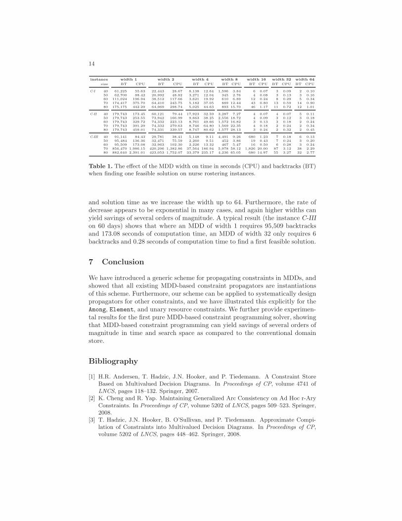
The results are presented in Table 1. We report the total number of back-tracks upon failure (BT) and computation time in seconds (CPU) needed by ourMDD solver for finding a first feasible solution, using widths 1, 2, 4, 8, 16, 32,and 64. Again, the MDD of width 1 corresponds to a domain store. For all prob-lem classes we observe a nearly monotonically decreasing sequence of backtracks

14

instance width 1 width 2 width 4 width 8 width 16 width 32 width 64

size BT CPU BT CPU BT CPU BT CPU BT CPU BT CPU BT CPU

C-I 40 61,225 55.63 22,443 28.67 8,138 12.64 1,596 3.84 6 0.07 3 0.09 2 0.10

50 62,700 88.42 20,992 48.82 3,271 12.04 345 2.76 4 0.08 3 0.13 3 0.16

60 111,024 196.94 38,512 117.66 3,621 19.92 610 6.89 12 0.24 8 0.29 5 0.34

70 174,417 375.70 64,410 243.75 5,182 37.05 889 12.44 43 0.80 13 0.59 14 0.90

80 175,175 442.29 64,969 298.74 5,025 44.63 893 15.70 46 1.17 11 0.72 12 1.01

C-II 40 179,743 173.45 60,121 79.44 17,923 32.59 3,287 7.27 4 0.07 4 0.07 5 0.11

50 179,743 253.55 73,942 166.99 9,663 38.25 2,556 18.72 4 0.09 3 0.12 3 0.18

60 179,743 329.72 74,332 223.13 8,761 49.66 1,572 16.82 3 0.13 3 0.18 2 0.24

70 179,743 391.29 74,332 279.63 8,746 64.80 1,569 22.35 4 0.18 2 0.24 2 0.34

80 179,743 459.01 74,331 339.57 8,747 80.62 1,577 28.13 3 0.24 2 0.32 2 0.45

C-III 40 91,141 84.43 29,781 38.41 5,148 9.11 4,491 9.26 680 1.23 7 0.18 6 0.13

50 95,484 136.36 32,471 75.59 2,260 9.51 452 3.86 19 0.43 7 0.24 3 0.20

60 95,509 173.08 32,963 102.30 2,226 13.32 467 5.47 16 0.50 6 0.28 3 0.24

70 856,470 1,986.15 420,296 1,382.86 37,564 186.94 5,978 58.12 1,826 20.00 87 3.12 38 2.29

80 882,640 2,391.01 423,053 1,752.07 33,379 235.17 4,236 65.05 680 14.97 55 3.27 32 2.77

Table 1. The effect of the MDD width on time in seconds (CPU) and backtracks (BT)when finding one feasible solution on nurse rostering instances.

and solution time as we increase the width up to 64. Furthermore, the rate ofdecrease appears to be exponential in many cases, and again higher widths canyield savings of several orders of magnitude. A typical result (the instance C-IIIon 60 days) shows that where an MDD of width 1 requires 95,509 backtracksand 173.08 seconds of computation time, an MDD of width 32 only requires 6backtracks and 0.28 seconds of computation time to find a first feasible solution.

7 Conclusion

We have introduced a generic scheme for propagating constraints in MDDs, andshowed that all existing MDD-based constraint propagators are instantiationsof this scheme. Furthermore, our scheme can be applied to systematically designpropagators for other constraints, and we have illustrated this explicitly for theAmong, Element, and unary resource constraints. We further provide experimen-tal results for the first pure MDD-based constraint programming solver, showingthat MDD-based constraint programming can yield savings of several orders ofmagnitude in time and search space as compared to the conventional domainstore.

Bibliography

[1] H.R. Andersen, T. Hadzic, J.N. Hooker, and P. Tiedemann. A Constraint StoreBased on Multivalued Decision Diagrams. In Proceedings of CP, volume 4741 ofLNCS, pages 118–132. Springer, 2007.

[2] K. Cheng and R. Yap. Maintaining Generalized Arc Consistency on Ad Hoc r-AryConstraints. In Proceedings of CP, volume 5202 of LNCS, pages 509–523. Springer,2008.

[3] T. Hadzic, J.N. Hooker, B. O’Sullivan, and P. Tiedemann. Approximate Compi-lation of Constraints into Multivalued Decision Diagrams. In Proceedings of CP,volume 5202 of LNCS, pages 448–462. Springer, 2008.

15

[4] T. Hadzic, J.N. Hooker, and P. Tiedemann. Propagating Separable Equalities inan MDD Store. In Proceedings of CPAIOR, volume 5015 of LNCS, pages 318–322.Springer, 2008.

[5] T. Hadzic, E. O’Mahony, B. O’Sullivan, and M. Sellmann. Enhanced Inference forthe Market Split Problem. In Proceedings of ICTAI, pages 716–723. IEEE, 2009.

[6] P. Hawkins, V. Lagoon, and P.J. Stuckey. Solving Set Constraint SatisfactionProblems Using ROBDDs. JAIR, 24(1):109–156, 2005.

[7] S. Hoda. Essays on Equilibrium Computation, MDD-based Constraint Programming

and Scheduling. PhD thesis, Carnegie Mellon University, 2010.[8] W.-J. van Hoeve, G. Pesant, L.-M. Rousseau, and A. Sabharwal. New Filtering

Algorithms for Combinations of Among Constraints. Constraints, 14:273–292, 2009.