A Graphical Realization of the Dynamic Programming

Method for Solving NP -Hard Combinatorial Problems

Alexander A. Lazarev

Institute of Control Sciences of the Russian Academy of Sciences,Profsoyuznaya st. 65, 117997 Moscow, Russia,

email: jobmath@mail.ru

Frank Werner

Fakultat fur Mathematik, Otto-von-Guericke-Universitat Magdeburg,PSF 4120, 39016 Magdeburg, Germany,

email: frank.werner@mathematik.uni-magdeburg.de

September 4, 2008, revised: November 27, 2008

Abstract

In this paper we consider a graphical realization of dynamic pro-gramming. The concept is discussed on the partition and knapsackproblems. In contrast to dynamic programming, the new algorithmcan also treat problems with non-integer data without necessary trans-formations of the corresponding problem. We compare the proposedmethod with existing algorithms for these problems on small-size in-stances of the partition problem with n ≤ 10 numbers. For almost allinstances, the new algorithm considers on average substantially less”stages” than the dynamic programming algorithm.

Keywords: Dynamic programming, exact algorithm, graphical algorithm,partition problem, knapsack problem

1 INTRODUCTION

Dynamic programming is a general optimization technique developed by Bell-man. It can be considered as a recursive optimization procedure which inter-prets the optimization problem as a multi-stage decision process. This meansthat the problem is decomposed into a number of stages. At each stage, adecision has to be made which has an impact on the decision to be made

1

in later stages. By means of Bellman’s optimization principle [1], a recur-sive equation is set up which describes the optimal criterion value at a givenstage in terms of the optimal criterion values of the previously consideredstage. Bellman’s optimality principle can be briefly formulated as follows:Starting from any current stage, an optimal policy for the subsequent stagesis independent of the policy adopted in the previous stages. In the case of acombinatorial problem, at some stage α sets of a particular size α are consid-ered. To determine the optimal criterion value for a particular subset of sizeα, one has to know the optimal values for all necessary subsets of size α− 1.If the problem includes n elements, the number of subsets to be consideredis equal to O(2n). Therefore, dynamic programming usually results in anexponential complexity. However, if the problem considered is NP -hard inthe ordinary sense, it is possible to derive pseudopolynomial algorithms. Theapplication of dynamic programming requires special separability properties.

In this paper, we give a graphical realization of the dynamic programmingmethod which is based on a property originally given for the single machinetotal tardiness problem by Lazarev and Werner (see [2], Property B-1). Thisapproach can be considered as a generalization of dynamic programming.The new approach often reduces the number of ”states” to be consideredin each stage. Moreover, in contrast to dynamic programming, it can alsotreat problems with non-integer data without necessary transformations ofthe corresponding problem. However, the complexity remains the same asfor a problem with integer data in terms of the ”states” to be considered.

In the following, we consider the partition and knapsack problems forillustrating the graphical approach. Both these combinatorial optimizationproblems are NP -hard in the ordinary sense (see, e.g. [3, 4, 5, 6]). Here, weconsider the following formulations of these problems.

Partition problem: Given is an ordered set B = {b1, b2, . . . , bn} of n pos-itive numbers with b1 ≥ b2 ≥ . . . ≥ bn. We wish to determine a partition ofthe set B into two subsets B1 and B2 such that∣∣∣∣∣∣

∑bi∈B1

bi −∑

bi∈B2

bi

∣∣∣∣∣∣ → min, (1)

where B1 ∪ B2 = B and B1 ∩ B2 = �.

One-dimensional knapsack problem: One wishes to fill a knapsack of ca-

2

pacity A with items having the largest possible total utility. If any item canbe put at most once into the knapsack, we get the binary or 0 − 1 knap-sack problem. This problem can be written as the following integer linearprogramming problem:⎧⎪⎪⎪⎪⎪⎪⎪⎪⎪⎪⎪⎪⎨

⎪⎪⎪⎪⎪⎪⎪⎪⎪⎪⎪⎪⎩

f(x) =n∑

i=1

cixi → max

n∑i=1

aixi ≤ A;

0 < ci, 0 < ai ≤ A, i = 1, 2, . . . , n;

n∑i=1

ai > A;

xi ∈ {0, 1}, i = 1, 2, . . . , n.

(2)

Here, ci gives the utility and ai the required capacity of item i, i =1, 2, . . . , n. The variable xi characterizes whether item i is put into the knap-sack or not.

We note that problems (1) and (2) are equivalent if

ci = ai = bi for i = 1, 2, . . . , n and A =1

2

n∑j=1

bj .

For the application of the graphical algorithm, the problem data may bearbitrary non-negative real numbers.

This paper is organized as follows. In Section 2, we consider the partitionproblem. First we explain the concept of the graphical algorithm for thisproblem. Then we describe in Subsection 2.2 how the number of intervals(or points) to be considered by the graphical algorithm can be reduced. Thealgorithm is illustrated by an example in Subsection 2.3. Then we prove theoptimality of the given algorithm and discuss some complexity aspects inSubsection 2.4. Computational results for small-size instances are given inSubsection 2.5. In Section 3, we consider the knapsack problem. In Subsec-tion 3.1, a brief illustration of the application of dynamic programming tothe knapsack problem is given. In Subsection 3.2, the graphical algorithm isapplied to the knapsack problem. An illustrative example for the graphicalalgorithm is given in Subsection 3.3. Some complexity aspects are discussedin Subsection 3.4. Finally, we give some concluding remarks in Section 4.

3

2 PARTITION PROBLEM

2.1 Graphical algorithm

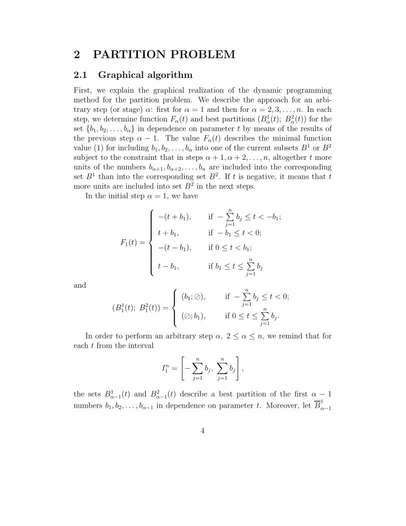
First, we explain the graphical realization of the dynamic programmingmethod for the partition problem. We describe the approach for an arbi-trary step (or stage) α: first for α = 1 and then for α = 2, 3, . . . , n. In eachstep, we determine function Fα(t) and best partitions (B1

α(t); B2α(t)) for the

set {b1, b2, . . . , bα} in dependence on parameter t by means of the results ofthe previous step α − 1. The value Fα(t) describes the minimal functionvalue (1) for including b1, b2, . . . , bα into one of the current subsets B1 or B2

subject to the constraint that in steps α + 1, α + 2, . . . , n, altogether t moreunits of the numbers bα+1, bα+2, . . . , bn are included into the correspondingset B1 than into the corresponding set B2. If t is negative, it means that tmore units are included into set B2 in the next steps.

In the initial step α = 1, we have

F1(t) =

⎧⎪⎪⎪⎪⎪⎪⎪⎪⎨⎪⎪⎪⎪⎪⎪⎪⎪⎩

−(t + b1), if −n∑

j=1

bj ≤ t < −b1;

t + b1, if − b1 ≤ t < 0;

−(t − b1), if 0 ≤ t < b1;

t − b1, if b1 ≤ t ≤n∑

j=1

bj

and

(B11(t); B2

1(t)) =

⎧⎪⎪⎨⎪⎪⎩

(b1;�), if −n∑

j=1

bj ≤ t < 0;

(�; b1), if 0 ≤ t ≤n∑

j=1

bj .

In order to perform an arbitrary step α, 2 ≤ α ≤ n, we remind that foreach t from the interval

In1 =

[−

n∑j=1

bj ,

n∑j=1

bj

],

the sets B1α−1(t) and B2

α−1(t) describe a best partition of the first α − 1

numbers b1, b2, . . . , bα−1 in dependence on parameter t. Moreover, let B1

α−1

4

and B2

α−1 describe an arbitrary but fixed partition of the first α−1 numbers.Thus, in step α − 1, we have

B1α−1(t) ∪ B2

α−1(t) = {b1, b2, . . . , bα−1} = B1

α−1 ∪ B2

α−1 for all t ∈ In1 .

Moreover, from step α − 1, we know the function values

Fα−1(t) =

∣∣∣∣∣∣∑

bj∈B1α−1(t)

bj + t −∑

bj∈B2α−1(t)

bj

∣∣∣∣∣∣ .Function Fα−1(t) is piecewise-linear and, as we see later, it suffices to storethose break points which are a local minimum of this function:

tα−11 , tα−1

2 , . . . , tα−1mα−1

.

We give a more detailed discussion later when speaking about the propertiesof function Fα(t) determined in step α.

In step α, 2 ≤ α ≤ n, the current number bα is included into one of

the sets B1

α−1 or B2

α−1. To this end, the algorithm considers the followingfunctions:

F 1α(t) =

∣∣∣∣∣ ∑bj∈B1

α−1(t+bα)

bj + t + bα − ∑bj∈B2

α−1(t+bα)

bj

∣∣∣∣∣ ,

F 2α(t) =

∣∣∣∣∣ ∑bj∈B1

α−1(t−bα)

bj + t − bα − ∑bj∈B2

α−1(t−bα)

bj

∣∣∣∣∣ .

Then, we construct function

Fα(t) = min {F 1α(t), F 2

α(t)}= min

{Fα−1(t + bα), Fα−1(t − bα)

},

for t ∈ In1 . Notice that we have shifted function Fα−1(t) to the left and to

the right, respectively, by bα units.Next, we determine B1

α(t) and B2α(t) according to the best inclusion of

number bα into one of the possible sets. More precisely, for t ∈ In1 , if F 1

α(t) ≤F 2

α(t), then

B1α(t) = B1

α−1(t + bα) ∪ {bα} and B2α(t) = B2

α−1(t + bα)

5

(i.e. bα is included into the first set), otherwise

B1α(t) = B1

α−1(t − bα) and B2α(t) = B2

α−1(t − bα) ∪ {bα}(i.e. bα is included into the second set). This is analogue to the classicaldynamic programming algorithm.

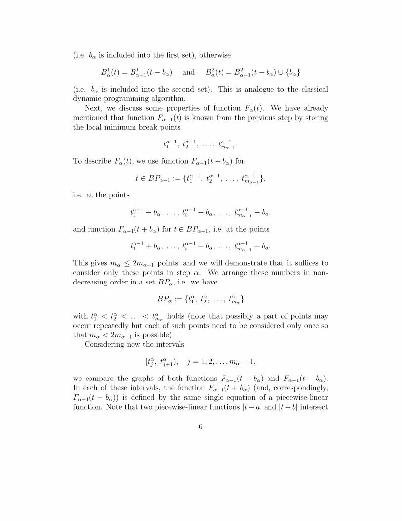
Next, we discuss some properties of function Fα(t). We have alreadymentioned that function Fα−1(t) is known from the previous step by storingthe local minimum break points

tα−11 , tα−1

2 , . . . , tα−1mα−1

.

To describe Fα(t), we use function Fα−1(t − bα) for

t ∈ BPα−1 := {tα−11 , tα−1

2 , . . . , tα−1mα−1

},i.e. at the points

tα−11 − bα, . . . , tα−1

i − bα, . . . , tα−1mα−1

− bα,

and function Fα−1(t + bα) for t ∈ BPα−1, i.e. at the points

tα−11 + bα, . . . , tα−1

i + bα, . . . , tα−1mα−1

+ bα.

This gives mα ≤ 2mα−1 points, and we will demonstrate that it suffices toconsider only these points in step α. We arrange these numbers in non-decreasing order in a set BPα, i.e. we have

BPα := {tα1 , tα2 , . . . , tαmα}

with tα1 < tα2 < . . . < tαmαholds (note that possibly a part of points may

occur repeatedly but each of such points need to be considered only once sothat mα < 2mα−1 is possible).

Considering now the intervals

[tαj , tαj+1), j = 1, 2, . . . , mα − 1,

we compare the graphs of both functions Fα−1(t + bα) and Fα−1(t − bα).In each of these intervals, the function Fα−1(t + bα) (and, correspondingly,Fα−1(t − bα)) is defined by the same single equation of a piecewise-linearfunction. Note that two piecewise-linear functions |t−a| and |t− b| intersect

6

(or coincide) in this interval at most at one point. Moreover, the piecewise-linear function Fα(t) obeys the equation Fα(t) = |t − tαi | in the interval[

tαi +tαi−1 − tαi

2, tαi +

tαi+1 − tαi2

), i = 2, 3, . . . , mα − 1,

i.e. its graph touches the t-axis at the point tαi . This means that thesebreak points are local minimum points (in the following denoted as min-break points) and also the zeroes of function Fα(t). As a consequence fromthe above discussion, function Fα(t) consists of segments having alternatelythe slopes −1 and +1.

Moreover, the same fixed partition(B

1

α; B2

α

)is chosen for all t from the

whole interval [tαi +

tαi−1 − tαi2

, tαi +tαi+1 − tαi

2

),

that is, we have

Bkα(t′) = Bk

α(t′′) for all t′, t′′ ∈[tαi +

tαi−1 − tαi2

, tαi +tαi+1 − tαi

2

)

for k = 1, 2 and i = 2, 3, . . . , mα − 1. The local maximum break pointsof function Fα(t) characterize the values of parameter t, where the chosen

partition (B1

α; B2

α) may change (notice that function Fα(t) has alternatelylocal minimum and local maximum break points).

Thus, it suffices to store the min-break points of function Fα(t)

tα1 , tα2 , . . . , tαmα,

together with the corresponding best partial partitions in a tabular form, i.e.mα ≤ 2 · mα−1 points are considered in step α.

Finally, the partition (B1n(0); B2

n(0)) obtained in the last step α = n isan optimal solution of the problem. The optimal objective function value isequal to Fn(0).

2.2 Reduction of the Considered Intervals

Next, we describe how the intervals (and points) to be considered can bereduced. We remind that the numbers in set B are arranged in non-increasing

7

order: b1 ≥ b2 ≥ . . . ≥ bn. Moreover, without loss of generality, we assumein the rest of Section 2 that

b1 <

n∑j=2

bj

(otherwise, we have a trivial case and B1 = {b1} and B2 = {b2, b3, . . . , bn} isobviously an optimal solution).

Since in step n, one has to calculate the value of the objective functionand to determine the corresponding partition only at point t = 0, it sufficesto calculate in step n − 1 the function values Fn−1(t) only at the pointst ∈ In

n = [−bn, bn]. Similarly, in step n − 2, it suffices to calculate thefunction values Fn−2(t) in the interval In

n−1 = [−bn − bn−1, bn + bn−1], and soon. Consequently, it suffices to consider in step α only the interval

Inα+1 =

[−

n∑j=α+1

bj ,

n∑j=α+1

bj

].

instead of the interval

In1 =

[−

n∑j=1

bj ,n∑

j=1

bj

].

If one takes into account that Fα(t), α = 1, 2, . . . , n, is an even function,it suffices to store only half of the min-break points and the correspondingbest partitions in a table for a practical realization of the algorithm.

2.3 Example

Let us consider an example with n = 4 and B = {100, 70, 50, 20}. Note thatthe numbers are given in non-increasing order.

Step 1. We make the arrangement for b1 = 100. We have to consider the

two points 0− 100 and 0 + 100. Due ton∑

j=1

bj = 240, the function values are

compared for the three intervals [−240,−100), [−100, 100), and [100, 240].Taking into account the described reduction of the intervals, it suffices toconsider only the intervals [−140,−100), [−100, 100) and [100, 140] due to4∑

j=2

bj = 140.

8

Figure 1: Function values F1(t).

For the interval [−140, 0), we get the optimal partition B11(t) = {b1},

B21(t) = �; and for the interval [0, 140], we get the optimal partition B1

1(t) =�, B2

1(t) = {b1}, i.e. in the max-break point t = 0 the optimal partitionchanges. The results of the calculations and function F1(t) are shown in Fig.1. The following information is stored:

t −100 100(B1

1(t); B21(t)) (b1;�) (�; b1)

Remember that it suffices to store only ”half” of the table and thus, onecolumn can be dropped.

Step 2. We make the arrangement for b2 = 70. We have to consider thefour points −100 − 70 = −170, −100 + 70 = −30, 100 − 70 = 30 and100 + 70 = 170. Thus, in our calculations we have to take into account thefive intervals [−240,−170), [−170,−30), [−30, 30), [30, 170) and [170, 240].Again, due to the reduction of the intervals it suffices to consider only three

intervals: [−70,−30), [−30, 30), and [30, 70] due to4∑

j=3

bj = 70. Now we get

the optimal partition B12(t) = {b1}, B2

2(t) = {b2} for all t from the interval[−70, 0) and the optimal partition B1

2(t) = {b2}, B22(t) = {b1} for all t

from the interval [0, 70]. In fact, we do not consider the whole intervals, butimmediately construct the function F2(t) by including the points t = −30and t = 30 and their corresponding partitions into the table. The partitions

9

Figure 2: Transformation of the function F1(t).

Figure 3: Function F2(t).

B12(t) = {b1}, B2

2(t) = {b2} and B12(t) = {b2}, B2

2(t) = {b1} correspondto the points t = −30 and t = 30, respectively. Fig. 2 illustrates thetransformation of function F1(t) to the functions F 1

2 (t) and F 22 (t).

The results of the calculations and function F2(t) are shown in Fig. 3(for a better illustration, we given function F2(t) not only for the interval[−70, 70] but for a larger interval including all min-break points). To executethe next step, it suffices to store the information only at the point t = 30(note that point t = −30 can be disregarded):

t 30(B1

2(t); B22(t)) (b2; b1)

Step 3. We make the arrangement for the number b3 = 50. We have to

10

Figure 4: Function F3(t).

consider the four points −30− 50 = −80, −30 +50 = 20, 30− 50 = −20 and30 + 50 = 80. Due to the possible interval reduction, it suffices to consider

only one interval: [−20, 20] due to4∑

j=4

bj = 20. The results of the calculations

and function F3(t) are given in Fig. 4. The following information is storedfor the point t = 20 (point t = −20 can be disregarded):

t 20(B1

3(t); B23(t)) (b1; b2, b3)

We have again only one max-break point t = 0 in the interval [−20, 20].

Step 4. We obtain the two optimal ”symmetric” solutions: B14(0) =

{b1, b4} = {100, 20}, B24(0) = {b2, b3} = {70, 50} and B1

4(0) = {b2, b3} ={70, 50}, B2

4(0) = {b1, b4} = {100, 20}.

Thus, we have considered 2 (t = −100 and t = 100) + 2 (t = −30 andt = 30) + 2 (t = −20 and t = 20) + 1 (t = 0) = 7 points (using that functionsFα(t) are even, we can disregard 3 points whereas the dynamic programmingalgorithm [1] (with a reduction of intervals) would require 281+141+41+1 =464 points. The best known exact partition algorithm Balsub [6, p.83] requiresO(nbmax) operations and finds a solution with 2 · (n/2) · (bmax + 1) = 404operations, where bmax = max1≤i≤n {bi} = 100.

11

2.4 Proof of Optimality and Some Complexity Aspects

First, we prove that the graphical algorithm finds an optimal solution.

Theorem 1 In step α = n, the graphical algorithm determines an optimalpartition B1

n(0) and B2n(0).

Proof. We show that the algorithm determines an optimal partition B1α(t)

and B2α(t) for the subset {b1, b2, . . . , bα} for each point

t ∈ Inα+1 =

[−

n∑j=α+1

bj ,n∑

j=α+1

bj

]

in each step α = 1, 2, . . . , n. For α = n, we define Inn+1 := {0}. The proof is

done by induction.(1) Obviously, in step α = 1 we get the optimal partition B1

1(t) and B21(t)

for each point

t ∈ In2 =

[−

n∑j=2

bj ,

n∑j=2

bj

].

(2) Let us assume that in step α − 1, 2 ≤ α ≤ n, we have found someoptimal partition B1

α−1(t) and B2α−1(t) for each point

t ∈ Inα =

[−

n∑j=α

bj ,n∑

j=α

bj

].

(3) We show that in step α, the algorithm also provides an optimal par-tition B1

α(t) and B2α(t) for each point

t ∈ Inα+1 =

[−

n∑j=α+1

bj ,n∑

j=α+1

bj

].

Let us assume the opposite, i.e. for some point t ∈ Inα+1, the algorithm

has constructed two partitions(B1

α−1(t + bα) ∪ {bα}; B2α−1(t + bα)

)and (

B1α−1(t − bα); B2

α−1(t − bα) ∪ {bα})

12

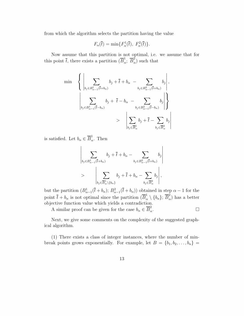
from which the algorithm selects the partition having the value

Fα(t) = min{F 1α(t), F 2

α(t)}.

Now assume that this partition is not optimal, i.e. we assume that for

this point t, there exists a partition (B1

α; B2

α) such that

min

⎧⎨⎩

∣∣∣∣∣∣∑

bj∈B1α−1(t+bα)

bj + t + bα −∑

bj∈B2α−1(t+bα)

bj

∣∣∣∣∣∣ ,∣∣∣∣∣∣∑

bj∈B1α−1(t−bα)

bj + t − bα −∑

bj∈B2α−1(t−bα)

bj

∣∣∣∣∣∣⎫⎬⎭

>

∣∣∣∣∣∣∑

bj∈B1α

bj + t −∑

bj∈B2α

bj

∣∣∣∣∣∣is satisfied. Let bα ∈ B

1

α. Then∣∣∣∣∣∣∑

bj∈B1α−1(t+bα)

bj + t + bα −∑

bj∈B2α−1(t+bα)

bj

∣∣∣∣∣∣>

∣∣∣∣∣∣∑

bj∈B1α\{bα}

bj + t + bα −∑

bj∈B2α

bj

∣∣∣∣∣∣ ,

but the partition (B1α−1(t + bα); B2

α−1(t + bα)) obtained in step α− 1 for the

point t + bα is not optimal since the partition (B1

α \ {bα}; B2

α) has a betterobjective function value which yields a contradiction.

A similar proof can be given for the case bα ∈ B2

α. �

Next, we give some comments on the complexity of the suggested graph-ical algorithm.

(1) There exists a class of integer instances, where the number of min-break points grows exponentially. For example, let B = {b1, b2, . . . , bn} =

13

{M, M − 1, M − 2, . . . , 1, 1, . . . , 1}, where M > 0 is a sufficiently large num-ber and there are M(M + 1)/2+1 numbers 1 contained in set B, that is, wehave n = M + M(M + 1)/2. The complexity of the graphical algorithm forthis instance is O(2M).

(2) There exists a class of non-integer instances B = {b1, b2, . . . , bn},where the number of min-break points grows exponentially, too. For exam-ple, if there exists no set of numbers λi = ±1, i = 1, 2, . . . , n, such thatλ1b1 + . . . + λnbn = 0 holds, then the number of min-break points in thisexample grows as O(2n).

Next, we briefly discuss the situation when the problem data are changedas follows. We consider an instance with b′j = Kbj + εj , where |εj| K, j = 1, 2, . . . , n, and K > 0 is a sufficiently large constant. In this case,the complexity of the dynamic programming algorithm is O(Kn

∑bj). For

the Balsub algorithm with a complexity of O(nbmax), this ”scaling” also leadsto an increase in the complexity by factor K. However, the complexity of thegraphical algorithm remains the same. In general, the graphical algorithmdetermines an optimal solution with the same number of operations for allpoints of some cone in the n-dimensional space, provided that the parametersof the instance are represented as a point (b1, b2, . . . , bn) in the n-dimensionalspace.

2.5 Computational Results

Two algorithms described in [6] (namely the standard dynamic program-ming algorithm and the Balsub algorithm) have been compared with theabove graphical algorithm. The complexity of the dynamic programmingalgorithm is determined by the total number of states to be considered. For

the graphical algorithm, the complexity is determined by the numbern∑

α=1

mα

of min-break points that have to be stored. In the following, we always givethe total numbers of min-break points obtained within the interval In

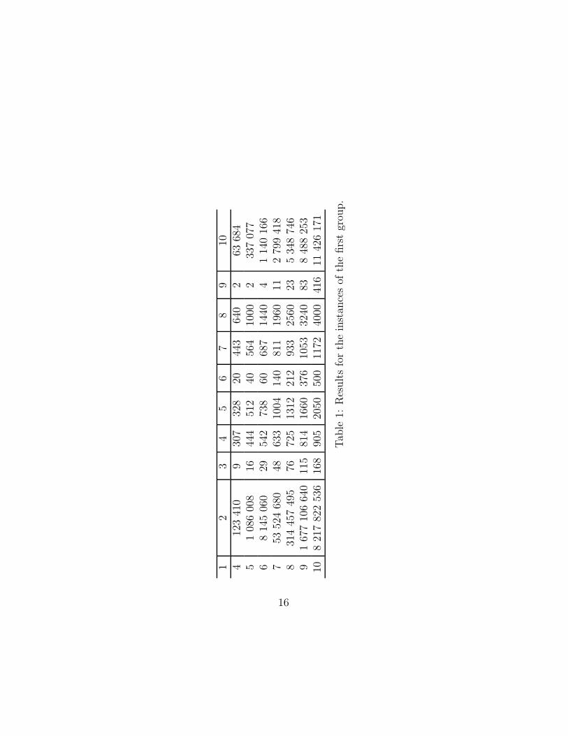
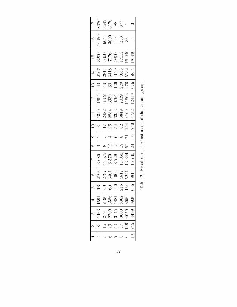
1 (i.e.without a reduction of the intervals). Notice that, using the reduction ofintervals described in Subsection 2.2, these numbers and thus the complexitywill even reduce further. We have run two groups of experiments. Results ofthe experiments are presented in Tables 1 and 2.

In the first group, we have generated instances for n = 4, 5, . . . , 10,

14

where all integer values of the data of the problem satisfy the inequalities40 ≥ b1 ≥ b2 ≥ . . . ≥ bn ≥ 1. The results obtained are given in Table 1,where the first column shows the value of n, the second column gives thetotal number of instances solved for the particular value of n (this numberis equal to the number of possibilities of choosing n numbers simultaneouslyfrom bmax +n−1 numbers, where bmax = 40). Columns three to five give theaverage complexity of the graphical, the Balsub and the dynamic program-ming algorithms, respectively. Columns six to eight present the maximalcomplexity of the graphical, the Balsub and the dynamic programming al-gorithms, respectively. The ninth column gives the number of instances forwhich the complexity of the Balsub algorithm is smaller than that of thegraphical algorithm, and the tenth column gives the number of instancesfor which the complexity of the dynamic programming algorithm is smallerthan that of the Balsub algorithm. For all instances, the complexity of thegraphical algorithm is essentially smaller than the complexity of the dynamicprogramming algorithm.

In the second part of experiments, we generated for n = 4, 5, . . . , 10groups of 20000 instances with uniformly chosen numbers bi ∈ [1, 200], i =1, 2, . . . , n. Then 1000 · n instances {b′1, b′2, . . . , b′n} were solved for each in-stance in the n-dimensional space in the neighborhood of point (b1, b2, . . . , bn)such that each component can differ by at most r = 100 + n so that

bi − (100 + n) ≤ b′i ≤ bi + (100 + n), i = 1, 2, . . . , n.

If an instance with a large number of min-break points (which characterizesthe complexity of the graphical algorithm) to be considered occurs in theneighborhood of the current instance data, then we ”pass to this instance”and find an instance with a large complexity of the algorithm in the newneighborhood of this instance. The process stops when one fails to find”more difficult instances” in the neighborhood. The results obtained aregiven in Table 2.

Column one gives the value of n, columns two to four give the averagecomplexity of the graphical, Balsub, and the dynamic programming algo-rithms, respectively, for the ”initial instance”. Columns five to seven presentthe maximal complexity of the algorithm for the ”initial instance”. Columnseight and nine present the maximal and average numbers of passages fromthe ”initial to the final instance” in the graphical algorithm. Columns ten

15

12

34

56

78

910

412

341

09

307

328

2044

364

02

6368

45

108

600

816

444

512

4056

410

002

337

077

68

145

060

2954

273

860

687

1440

41

140

166

753

524

680

4863

310

0414

081

119

6011

279

941

88

314

457

495

7672

513

1221

293

325

6023

534

874

69

167

710

664

011

581

416

6037

610

5332

4083

848

825

310

821

782

253

616

890

520

5050

011

7240

0041

611

426

171

Tab

le1:

Res

ult

sfo

rth

ein

stan

ces

ofth

efirs

tgr

oup.

16

12

34

56

78

910

1112

1314

1516

174

814

6315

9116

2196

308

04

26

1310

1604

2022

0732

0010

504

8970

516

2191

2490

4027

9744

675

83

1724

8231

0240

2811

5000

6641

3642

629

2700

3586

6034

016

570

124

2628

8439

3260

3418

7176

3000

3170

750

3145

4881

140

4006

872

915

654

3353

6794

136

4029

9800

1101

888

8736

0063

6221

646

1711

056

198

8238

4970

3922

046

4512

112

333

377

914

940

5080

5946

452

4113

644

5221

144

4109

1180

347

652

3216

200

861

1024

544

9999

3065

658

1516

730

2410

240

4732

1241

067

658

5418

840

183

Tab

le2:

Res

ult

sfo

rth

ein

stan

ces

ofth

ese

cond

grou

p.

17

to twelve show the average complexity of the algorithms under considera-tion at the ”final instances”. Columns thirteen to fifteen show the maximalcomplexity of the algorithms considered at the ”final instances”. Finally,columns sixteen and seventeen give the numbers of instances for which thecomplexity of the dynamic programming algorithm is smaller than that ofthe Balsub algorithm at the initial and final instances, respectively.

Among all ”initial” and ”final” instances, there were only 38 instanceswith n = 4 and two instances with n = 5 among the ”final” instances, wherethe graphical algorithm had to consider more states (i.e. min-break points)than the Balsub algorithm.

3 KNAPSACK PROBLEM

Recall that in the binary knapsack problem we are given a knapsack withcapacity A and n items i = 1, 2, . . . , n with utility values ci and weights ai:⎧⎪⎪⎪⎪⎪⎪⎪⎪⎪⎪⎪⎪⎨

⎪⎪⎪⎪⎪⎪⎪⎪⎪⎪⎪⎪⎩

f(x) =n∑

i=1

cixi → max

n∑i=1

aixi ≤ A;

0 < ci, 0 < ai ≤ A, i = 1, 2, . . . , n;

n∑i=1

ai > A;

xi ∈ {0, 1}, i = 1, 2, . . . , n.

The variable xi characterizes whether item i is put into the knapsack or not.

3.1 Illustration of Dynamic Programming

The dynamic programming algorithm based on Bellman’s optimality princi-ple [1, 5] is considered to be the most efficient one. It is assumed that allparameters are integer: A; ai ∈ Z+, i = 1, 2, . . . , n. In step α, α = 1, 2, . . . , n,the function values

gα(t) = maxxα∈{0,1}

{cαxα + gα−1(t − aαxα)

}, aαxα ≤ t ≤ A,

18

t g1(t) x(t) g2(t) x(t) g3(t) x(t) g4(t) x(t)0 0 (0,,,) 0 (0,0,,) 0 (0,0,0,) 0 (0,0,0,0)1 0 (0,,,) 0 (0,0,,) 0 (0,0,0,) 0 (0,0,0,0)2 5 (1,,,) 5 (1,0,,) 5 (1,0,0,) 5 (1,0,0,0)3 5 (1,,,) 7 (0,1,,) 7 (0,1,0,) 7 (0,1,0,0)4 5 (1,,,) 7 (0,1,,) 7 (0,1,0,) 7 (0,1,0,0)5 5 (1,,,) 12 (1,1,,) 12 (1,1,0,) 12 (1,1,0,0)6 5 (1,,,) 12 (1,1,,) 12 (1,1,0,) 12 (1,1,0,0)7 5 (1,,,) 12 (1,1,,) 12 (1,1,0,) 12 (1,1,0,0)8 5 (1,,,) 12 (1,1,,) 13 (0,1,1,) 13 (0,1,1,0)9 5 (1,,,) 12 (1,1,,) 13 (0,1,1,) 13 (0,1,1,0)

Table 3: Application of the dynamic programming algorithm

are calculated for each integer point (i.e. ”state”) 0 ≤ t ≤ A. Here, we haveg0(t) = 0 for all integers t with 0 ≤ t ≤ A. For each point t, a correspondingbest (partial) solution (x1(t), x2(t), . . . , xα(t)) is stored.

The algorithm is illustrated by the example from [7, p.125 − 129]:⎧⎪⎨⎪⎩

f(x) = 5x1 + 7x2 + 6x3 + 3x4 → max

2x1 + 3x2 + 5x3 + 7x4 ≤ 9;

xi ∈ {0, 1} , i = 1, . . . , 4.

(3)

The results with the dynamic programming algorithm are summarized inTable 3. Therefore, for t = 9, we get the optimal solution

x(13) = (x1(13), x2(13), x3(13), x4(13)) = (0, 1, 1, 0)

and the corresponding optimal objective function value g4(9) = 13. Thecomplexity of the algorithm is O(nA).

3.2 Graphical Approach

We describe the modifications of the graphical algorithm. In an arbitrary stepα, 2 ≤ α ≤ n, function gα(t) is now defined for all real t with 0 ≤ t ≤ A.In particular, gα(t) is a step function, i.e. it is a discontinuous function with

19

jumps. We assume that the function values gα−1(tj) = fj, j = 1, 2, . . . , mα−1

are known from the previous step α − 1. Here, t1 is the left boundary pointto be considered and t2, t3, . . . , tmα−1 are the jump points of function gα−1(t)from the interval [0, A]. These function values can be stored in a tabularform as follows:

t t1 t2 . . . tmα−1

g(t) f1 f2 . . . fmα−1

As a consequence, for t ∈ [tj , tj+1), we have gα−1(t) = fj for all j =1, 2, . . . , mα−1 − 1. Note that t1 = 0 and f1 = 0 for all α = 1, 2, . . . , n.In the initial step α = 1, we get

g1(t) =

{0, if 0 ≤ t < a1,c1, if a1 ≤ t ≤ A.

Similarly to dynamic programming, function gα(t) can be obtained fromfunction gα−1(t) in the following way:

g1(t) = gα−1(t);

g2(t) =

{g1(t), if 0 ≤ t < aα,cα + gα−1(t − aα), if aα ≤ t ≤ A.

Thengα(t) = max{g1(t), g2(t)}

and for the corresponding solution component, we get

xα(t) =

{1, if g2(t) > g1(t),0, otherwise .

In the last step (α = n), we have an optimal solution of the problem foreach point t ∈ R with 0 ≤ t ≤ A:

x(t) = (x1(t), x2(t), . . . , xn(t)).

Consider an arbitrary step α with 2 ≤ α ≤ n, The graph of g2(t) canbe constructed from the graph of gα−1(t) by an ”upward” shift by cα and a”right” shift by aα. Function g2(t) can be stored in a tabular form as follows:

20

t t1 + aα t2 + aα . . . tmα−1+aα

g(t) f1 + cα f2 + cα . . . fmα−1+cα

The graph of function g1(t) corresponds to that of gα−1(t). Consequently,in order to construct

gα(t) = max {g1(t), g2(t)},

one has to consider at most 2mα−1 points (intervals) obtained by means ofthe points chosen from the set

{t1, t2, . . . , tmα−1 , t1 + aα, t2 + aα, . . . , tmα−1 + aα}

belonging to the interval [0, A]. The number of points does not exceed A foraj ∈ Z+, j = 1, 2, . . . , n. For the integer example, the number of intervalsconsidered by the graphical algorithm in step α, therefore, does not exceedmin{O(nA), O(nfmax)}, where fmax = max

1≤i≤mα

{fi}. Thus, the worst case

complexity is the same as for the dynamic programming algorithm.

3.3 Example

We use again instance (3) to illustrate the graphical algorithm by an example.

Step 1. As the result, we get the following table:

t 0 2g1(t) 0 5x(t) (0, , , ) (1, , , )

Step 2. Due to a2 = 3, one has to consider the intervals obtained fromthe boundary points 0, 2, 0 + 3, 2 + 3 in order to construct the function g2(t).The dashed lines in Fig. 5 give function g2(t). As the result, we get:

t 0 2 3 5g2(t) 0 5 7 12x(t) (0, 0, , ) (1, 0, , ) (0, 1, , ) (1, 1, , )

Step 3. To construct function g3(t), one has to consider the intervalsobtained from the boundary points 0, 2, 3, 5, 0 + 5, 2 + 5, 3 + 5 due to a3 = 5.

21

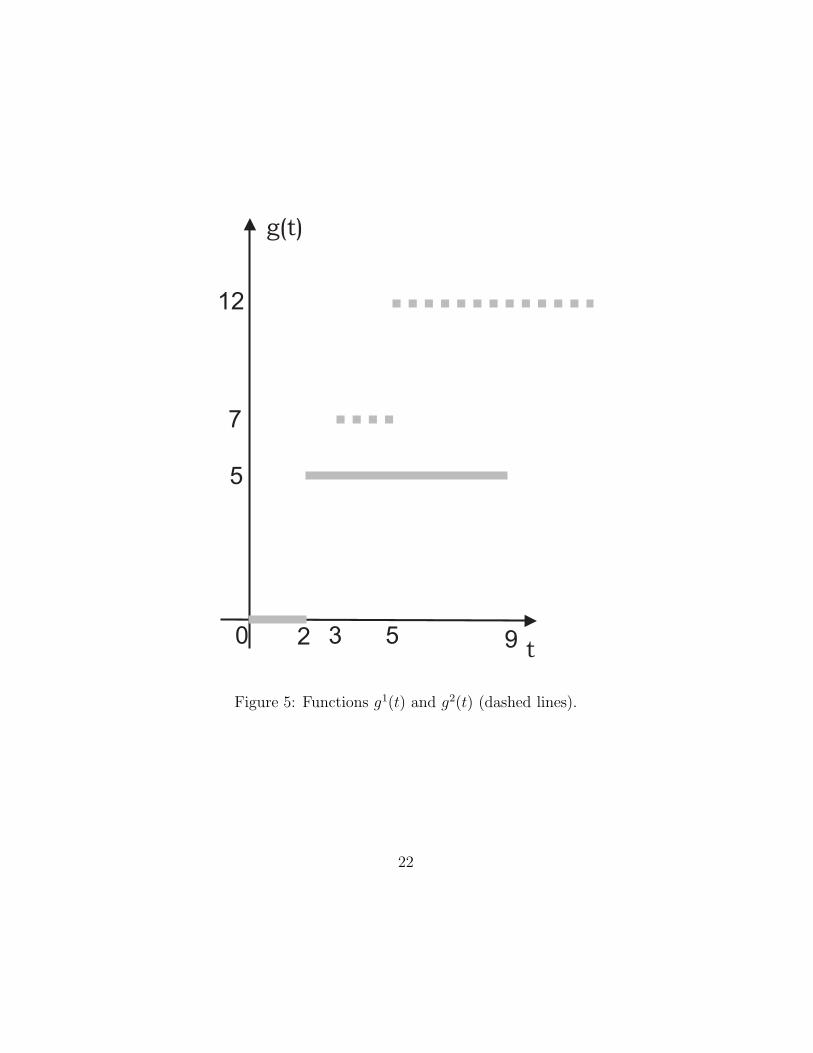
Figure 5: Functions g1(t) and g2(t) (dashed lines).

22

Figure 6: Function g3(t).

23

The point 5+5 > 9 need not to be considered. The results of the calculationsand function g3(t) are shown in Fig. 6. Several fragments g2(t) (shown bythe bright line) are ”absorbed” and do not influence the values g3(t). In thethird step of the algorithm, we obtain the following results:

t 0 2 3 5 8g3(t) 0 5 7 12 13x(t) (0, 0, 0, ) (1, 0, 0, ) (0, 1, 0, ) (1, 1, 0, ) (0, 1, 1, )

Step 4. The results of the calculations and the objective function g4(t)are depicted in Fig. 7. One has to consider the intervals resulting from theboundary points 0, 2, 3, 5, 8, 0 + 7, 2 + 7 in order to construct function g4(t).The points 3 + 7, 5 + 7, 8 + 7 need not to be considered since they are largerthan A = 9. Therefore, it suffices to consider five points. As the result, weobtain the following table:

t 0 2 3 5 8g4(t) 0 5 7 12 13x(t) (0, 0, 0, 0) (1, 0, 0, 0) (0, 1, 0, 0) (1, 1, 0, 0) (0, 1, 1, 0)

3.4 Some Complexity Aspects of the GraphicalAlgorithm

The complexity of the graphical algorithm for solving the knapsack problem

is determined by the total number of jump pointsn∑

α=1

mα−n to be considered.

Notice that there are mα−1 jump points and the left boundary point in eachstep α.

For the example presented in Subsection 3.3, the graphical algorithmstored 12 jump points: 1 in the first step (t = 2), 3 in the second step (t =2, 3, 5), 4 in the third step (t = 2, 3, 5, 8), and 4 in the last step (t = 2, 3, 5, 8),too. In contrast, the dynamic programming algorithm would consider 4×9 =36 points. Consequently, for the example at hand the number of requiredsteps is substantially reduced.

One can see that for the example considered in Subsection 3.3, in steps3 and 4 the number of intervals to be considered is not doubled. One canconjecture that the average number of necessary operations of the graphi-cal algorithm (i.e. total number of jump points) will be polynomial for asubstantial number of instances.

24

Figure 7: Function g4(t).

25

To minimize the number of new intervals to be considered in each stepα, the source data must be ordered such that

c1

a1≥ c2

a2≥ . . . ≥ cn

an.

In this case, the functions g2(t) will be ”absorbed” more effectively.Moreover, the graphical algorithm takes the specific properties of the

problem indirectly into account. The dynamic programming algorithm dis-regards the fact that the least preferable item in the above example is thatwith number 4 (see the quotient c4/a4). In the graphical algorithm, one cansee that function g2(t) does not affect g4(t) in step 4. Thus, heuristic con-siderations can be taken into account and may reduce the complexity of thealgorithm.

Moreover, we also note that for ci = 2, i = 1, 2, . . . , n, and n ≥ 4, theexample from [4, 8] ⎧⎪⎪⎨

⎪⎪⎩n∑

i=1

cixi → max

n∑i=1

2xi ≤ 2[

n2

]+ 1

(4)

can be solved by the graphical approach in O(n) operations. In the generalcase, i.e. for arbitrary ci, i = 1, 2, . . . , n, the proposed algorithm solvesexample (4) with O(n logn) operations. An algorithm based on the branchand bound method needs O( 2n√

n) operations to solve this example, when

ci = 2 for all i = 1, . . . , n.

4 CONCLUSIONS

The concept of the graphical approach is a natural generalization of thedynamic programming method. This algorithm can also treat instances withnon-integer data without increasing the number of required operations (interms of min-break of jump points to be considered). For small-size problems,it turned out to be superior to the standard algorithms in terms of the averageand maximum complexity, i.e. the average and maximal number of ”states”(break points for the partition problem and jump points for the knapsackproblem) to be considered.

26

Note that the complexity of the graphical algorithm is the same for thefollowing instances of the partition problem with n = 3: {1, 3, 2}; {1, 100, 99}and {10−6, 1, 1−10−6}. In contrast, the complexity of the dynamic program-ming algorithm strongly differs for the above small instances. In particular,the third instance requires a scaling of the data since integer ”states” areconsidered. However, this considerably increases the complexity.

For further research, it will be interesting to compare the graphical algo-rithm with the existing dynamic programming-based algorithms on bench-mark problems with larger size. In addition, a comparison with branch andbound algorithms is of interest, too. More precisely, one can compare thenumber of nodes of the branching tree with the number of points to be con-sidered by the graphical algorithm.

Acknowledgments

This work has been supported by DAAD (Deutscher Akademischer Aus-tauschdienst: A/08/08679, Ref. 325). The authors would like to thank Dr.E.R. Gafarov for valuable discussions of the results obtained.

References

[1] Bellman, R., Dynamic Programming, Princeton: Princeton Univ. Press,1957.

[2] Lazarev, A. and Werner, F., Algorithms for Special Cases of the SingleMachine Total Tardiness Problem and an Application to the Even-OddPartition Problem (to appear in Mathematical and Computer Modelling,2009, doi:10.1016/j.mcm.2009.01.003).

[3] Korbut A.A., Finkelstein, J.J., Discrete Programming, Moscow: Nauka,1969 (in Russian). (In German: Korbut A.A., Finkelstein, J.J., DiscreteOptimierung, Berlin: Akademia-Verlag, 1971.)

[4] Finkelstein, J.J., Approximative Methods and Applied Problems of Dis-crete Programming, Moscow: Nauka, 1976 (in Russian).

[5] Papadimitrou, Ch. and Steiglitz, K., Combinatorial Optimization: Al-gorithms and Complexity, Englewood Cliffs: Prentice Hall, 1982.

27

[6] Keller, H., Pferschy, U. and Pisinger, D., Knapsack Problems, New York:Springer, 2004.

[7] Sigal, I.Kh. and Ivanova, A.P., Introduction to Applied Discrete Pro-gramming, Moscow: Fizmatlit, 2007 (in Russian).

[8] Moiseev, N.N. (Ed.), State-of-the-Art of the Operations Research The-ory, Moscow: Nauka, 1979 (in Russian).

28