An empirical analysis of joint decisions on labour supply and welfare participation
22
An Empirical Analysis of Joint Decisions on Labor Supply and Welfare Participation Gi Kang, Sonya K. Huffman, and Helen H. Jensen Working Paper 04-WP 361 May 2004 Center for Agricultural and Rural Development Iowa State University Ames, Iowa 50011-1070 www.card.iastate.edu This research was conducted while Gi Kang, an associate professor at Cheju National University, China, was visiting at Iowa State University. Sonya Huffman is adjunct assistant professor in the Department of Economics and Helen Jensen is professor of economics and head of the Food and Nutrition Policy Division in the Center for Agricultural and Rural Development at Iowa State University. The authors acknowledge helpful comments and suggestions from Peter Orazem. The Economic Research Service, United States Department of Agriculture, provided partial funding support for the research. This publication is available online on the CARD Web site: www.card.iastate.edu. Permission is granted to reproduce this information with appropriate attribution to the authors and the Center for Agricultural and Rural Development, Iowa State University, Ames, Iowa 50011-1070. For questions or comments about the contents of this paper, please contact Helen Jensen, 578E Heady Hall, Iowa State University, Ames, IA 50011-1070; Ph: 515-294-6253; Fax: 515-294-6336; E-mail: [email protected]. The U.S. Department of Agriculture (USDA) prohibits discrimination in all its programs and activities on the basis of race, color, national origin, gender, religion, age, disability, political beliefs, sexual orientation, and marital or family status. (Not all prohibited bases apply to all programs.) Persons with disabilities who require alternative means for communication of program information (Braille, large print, audiotape, etc.) should contact USDA’s TARGET Center at (202) 720-2600 (voice and TDD). To file a complaint of discrimination, write USDA, Director, Office of Civil Rights, Room 326-W, Whitten Building, 14th and Independence Avenue, SW, Washington, DC 20250-9410 or call (202) 720-5964 (voice and TDD). USDA is an equal opportunity provider and employer. Iowa State University does not discriminate on the basis of race, color, age, religion, national origin, sexual orientation, sex, marital status, disability, or status as a U.S. Vietnam Era Veteran. Any persons having inquiries concerning this may contact the Director of Equal Opportunity and Diversity, 1350 Beardshear Hall, 515-294-7612.
Transcript of An empirical analysis of joint decisions on labour supply and welfare participation
An Empirical Analysis of Joint Decisions on Labor Supply and Welfare Participation
Gi Kang, Sonya K. Huffman, and Helen H. Jensen
Working Paper 04-WP 361 May 2004
Center for Agricultural and Rural Development Iowa State University
Ames, Iowa 50011-1070 www.card.iastate.edu
This research was conducted while Gi Kang, an associate professor at Cheju National University, China, was visiting at Iowa State University. Sonya Huffman is adjunct assistant professor in the Department of Economics and Helen Jensen is professor of economics and head of the Food and Nutrition Policy Division in the Center for Agricultural and Rural Development at Iowa State University. The authors acknowledge helpful comments and suggestions from Peter Orazem. The Economic Research Service, United States Department of Agriculture, provided partial funding support for the research. This publication is available online on the CARD Web site: www.card.iastate.edu. Permission is granted to reproduce this information with appropriate attribution to the authors and the Center for Agricultural and Rural Development, Iowa State University, Ames, Iowa 50011-1070. For questions or comments about the contents of this paper, please contact Helen Jensen, 578E Heady Hall, Iowa State University, Ames, IA 50011-1070; Ph: 515-294-6253; Fax: 515-294-6336; E-mail: [email protected]. The U.S. Department of Agriculture (USDA) prohibits discrimination in all its programs and activities on the basis of race, color, national origin, gender, religion, age, disability, political beliefs, sexual orientation, and marital or family status. (Not all prohibited bases apply to all programs.) Persons with disabilities who require alternative means for communication of program information (Braille, large print, audiotape, etc.) should contact USDA’s TARGET Center at (202) 720-2600 (voice and TDD). To file a complaint of discrimination, write USDA, Director, Office of Civil Rights, Room 326-W, Whitten Building, 14th and Independence Avenue, SW, Washington, DC 20250-9410 or call (202) 720-5964 (voice and TDD). USDA is an equal opportunity provider and employer. Iowa State University does not discriminate on the basis of race, color, age, religion, national origin, sexual orientation, sex, marital status, disability, or status as a U.S. Vietnam Era Veteran. Any persons having inquiries concerning this may contact the Director of Equal Opportunity and Diversity, 1350 Beardshear Hall, 515-294-7612.

Abstract
Economic and welfare program factors affect the well-being of low-income families
and their labor supply decisions. This study uses data from the U.S. Survey of Income
and Program Participation. A nested logit model is estimated to explain the joint
decisions to participate in Temporary Assistance for Needy Families (TANF) and the
labor market for the population of families potentially eligible for TANF. The empirical
findings indicate that higher wages increase labor and decrease welfare program
participation; an increase in nonlabor income decreases both labor market and welfare
participation.
Keywords: labor supply, low income, welfare program, welfare reform.
AN EMPIRICAL ANALYSIS OF JOINT DECISIONS ON LABOR SUPPLY AND WELFARE PARTICIPATION
Introduction Between 1965 and 1985 the United States experienced a large increase in the
caseload of welfare programs. There are many explanations for the high caseload level,
and these include long-term welfare dependency and work disincentives. In response,
recent state and federal welfare reforms have been designed to increase work
participation among welfare recipients. The Personal Responsibility and Work
Opportunity Reconciliation Act (PRWORA) enacted in 1996 brought major changes in
the scope, structure, and impact of programs targeted to the low-income population,
including Aid to Families with Dependent Children (AFDC), the Food Stamp Program,
Medicaid, Supplemental Security Income (SSI), child welfare, and child support.
Following the introduction of PRWORA, the number of welfare recipients declined
across the nation. Both the reforms introduced through PRWORA and America’s
growing economy contributed to the declining welfare rolls.
Linkages among social assistance programs have significant effects on the behavior
of low-income individuals and families. This study examines the effects of cash transfers
on labor supply and welfare participation decisions in order to better understand factors
affecting welfare program and labor market activities of the poor. Many researchers have
analyzed the effects of government transfer programs on labor supply decisions among
the low-income population (see Moffitt 1992). Much of the empirical work provides
insights on how welfare transfers affect labor supply decisions of low-income families
and has focused on either females or married couples.
For example, Keane and Moffitt (1998) use a structural model to examine work and
multiple welfare program participation decisions among families headed by single adult
females. Hagstrom (1996) examines the effect of the Food Stamp Program on intra-
family labor supply and program participation decisions. Married couples simultaneously

2 / Kang, Huffman, and Jensen
choose the labor supply of the husband and wife and whether to participate in the Food
Stamp Program. Hagstrom estimates a nested multinomial logit model and uses data from
the Survey of Income and Program Participation (SIPP). He found smaller labor supply
effects for married couples to changes in the food stamp benefit compared with those of
single parents. He also found program participation by married couples to be responsive
to changes in food stamp benefits.
The purpose of this paper is to examine the effect of the 1996 welfare reforms on
the labor supply decisions of low-income families. There are three types of families:
two-parent families, male-headed families, and female-headed families. The core of the
transfer system for the low-income population of the nonelderly and nondisabled
includes AFDC (now Temporary Assistance to Needy Families [TANF]), the Food
Stamp Program, Medicaid, and public housing. Among these, the TANF program is the
most widely known cash transfer program for the poor. This study uses data from the
SIPP to analyze labor market and TANF participation decisions among all low-wealth
families in the United States. A static model of family behavior is developed in which
work and program participation is chosen to maximize a family utility function given
resource constraints. The model is used to explain the joint decision to participate in
TANF and the labor market for the population of families eligible for TANF. The paper
provides two approaches to explaining joint decisions of families. First, we estimate a
bivariate probit model of participation in the labor force and TANF program. Second,
we estimate a nested logit model that incorporates simultaneous decisions on labor
market and TANF participation.
TANF Program The PRWORA gives the states a fundamental role in assisting poor families. Under
TANF, the eligibility rules and benefits differ across states. To be eligible for TANF, an
applicant family must pass both nonfinancial tests based on the demographic
characteristics of the family and its members and financial tests based on the family’s
income and asset holdings. At the most basic level of nonfinancial tests, the family must
include a child or, in some states, a pregnant woman. If the head of the family is a
An Empirical Analysis of Joint Decisions on Labor Supply and Welfare Participation / 3
teenager, she may or may not be eligible to receive a benefit on her own. In most states,
she is eligible only if she is living with her parents.
The financial tests require that an applicant family must have sufficiently low
income and asset levels. The asset limits that states have adopted under TANF differ
greatly by state. Thirty-nine states have increased the asset limit for recipients above the
$1,000 limit allowed under AFDC. Twenty-two states allow recipients to accumulate
additional savings in a restricted savings account set aside for a specific purpose allowed
by the state. If the family’s total assets exceed the amounts determined by the state, the
family is ineligible for TANF.
Once the family has passed the state’s asset tests, its available income is computed
for eligibility purposes. States use the total gross income calculated from the unit’s
earned and unearned income as a starting point for income eligibility tests (Rowe 2000).
Many states now impose just one income test on applicants; however, others use a
combination of a gross income test, gross earnings test, and/or net income test. Net
income tests require that net family income not exceed a maximum benefit level that
varies by family size and state of residence. Net income is calculated by subtracting the
state’s earned income disregards from the unit’s gross earned income and then adding to
this amount the unit’s unearned income. The net income is then compared to an income
standard determined by the state. If the net income is less than the standard, then a benefit
is calculated.
Although states use many different formulas to determine net income, there are
general rules that most states apply. All but two states allow recipients to disregard a
portion of their earned income before benefit computation and vary the units’ benefits by
income. In more straightforward calculations, net income is subtracted from a state-
determined standard, the so-called payment standard, which varies by family size. The
benefit paid is the difference.
Theoretical and Empirical Model
Theoretical Model The family head is assumed to choose labor supply and welfare (here, TANF)
participation simultaneously to maximize the family’s utility subject to its budget
4 / Kang, Huffman, and Jensen
constraint. Assume that a family’s utility is a function of leisure time and disposable
income and is represented by
),,( δYHUU = (1)
where H is monthly hours of work supplied by family, Y is monthly disposable income,
and δ represents preferences for receiving a TANF benefit. Monthly disposable income
may be written as the following budget constraint:
]),([),( CNHBPNwHPHY TT −++= (2)
where w is the hourly wage rate, N is nonlabor income, TP is defined to be an indicator
equal to 1 if the family head participates in the TANF program and 0 otherwise, )(⋅B is
the TANF benefit given the family’s labor supply, and C is the monetary cost of
participating in the TANF program. The family head is assumed to simultaneously
choose H and TP that maximizes his or her utility given in equation (1) subject to the
budget constraint given in equation (2). That is, the family head chooses the (H, TP )
combination that gives the greatest indirect utility.
Participation in the welfare program is not costless. There are costs associated with
the application process and with application itself. The costs include the transportation
and time costs of applying for the program and some compliance costs while
participating. These costs vary by individual family and by location. However, there are
benefits with TANF participation. A family with no income is eligible to receive the
maximum TANF grant. For a family with income, the TANF benefits are calculated as
the difference between the maximum benefit and net family income. The TANF benefits
are calculated according to the following formula:
]}))(([,min{ CCBRRHEwHNGPB TT −−+−= if wH + N < 1.85L (3)
where TB is the monthly TANF benefit, P is the maximum permitted payment in the
state, TG is the maximum amount paid or pay standard, )(⋅E is the earnings disregard,
BRR is the benefit reduction rate, CC is child care deductions, and L is living costs. The
variables P, TG , L, E, and BRR vary by state and family size.
An Empirical Analysis of Joint Decisions on Labor Supply and Welfare Participation / 5
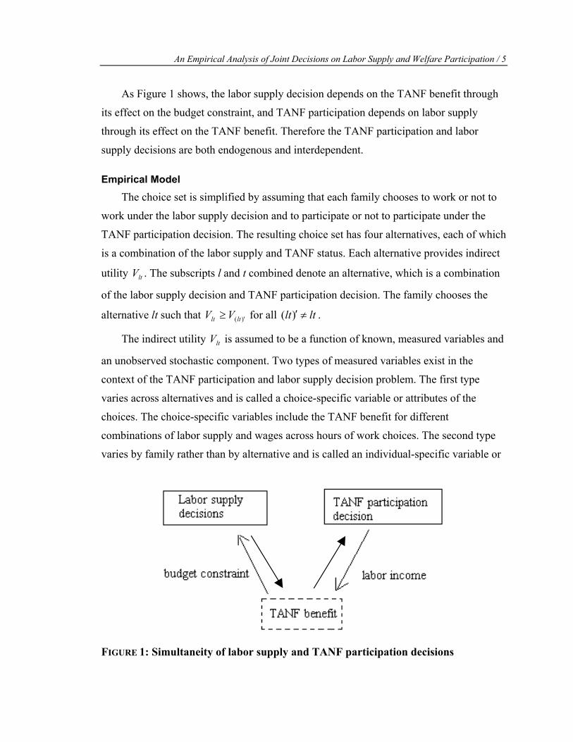
As Figure 1 shows, the labor supply decision depends on the TANF benefit through
its effect on the budget constraint, and TANF participation depends on labor supply
through its effect on the TANF benefit. Therefore the TANF participation and labor
supply decisions are both endogenous and interdependent.
Empirical Model The choice set is simplified by assuming that each family chooses to work or not to
work under the labor supply decision and to participate or not to participate under the
TANF participation decision. The resulting choice set has four alternatives, each of which
is a combination of the labor supply and TANF status. Each alternative provides indirect
utility ltV . The subscripts l and t combined denote an alternative, which is a combination
of the labor supply decision and TANF participation decision. The family chooses the
alternative lt such that )'(ltlt VV ≥ for all ( )lt lt′ ≠ .
The indirect utility ltV is assumed to be a function of known, measured variables and
an unobserved stochastic component. Two types of measured variables exist in the
context of the TANF participation and labor supply decision problem. The first type
varies across alternatives and is called a choice-specific variable or attributes of the
choices. The choice-specific variables include the TANF benefit for different
combinations of labor supply and wages across hours of work choices. The second type
varies by family rather than by alternative and is called an individual-specific variable or
FIGURE 1: Simultaneity of labor supply and TANF participation decisions
6 / Kang, Huffman, and Jensen
characteristics of the individual. The individual-specific variables include information on
the family head’s age, education, marital status, number of children, and so forth.
The stochastic error component captures the effect of unmeasured variables and
unobserved differences in preferences across families. Given the form of utility function
and the probability distribution of the stochastic term, the probability that the family will
choose alternative wt can be written ]Pr[Pr )'(ltltlt VV ≥= , for all ( )lt lt′ ≠ .
Model I: Bivariate Probit Model Several models are available for estimating the described random utility model based
on different assumptions about the stochastic component of indirect utility function, ltV
(Green).1 One model for incorporating simultaneous decisions on labor market and
TANF participation is a bivariate probit model. Define PL and PT as participation in the
labor market and the TANF program, respectively. All families are then classified into
four mutually exclusive regimes based on the discrete choice outcome on PL and PT:
R1: PL = PT = 1 (those who participate in the labor market and TANF)
R2: PL =1 and PT = 0 (those who participate in the labor market but not in TANF)
R3: PL = 0 and PT = 1 (those who participate in TANF but not in the labor market)
R4: PL = PT = 0 (those who do not participate in the labor market or TANF)
All observations have a nonzero probability of being assigned to one of four regimes.
This probability can be evaluated with the following bivariate probability statements:
M11≡P(R1)=P(PL = 1,PT = 1)=P[PL*=θL′ ZL+µL>0, PT
*=θT′ ZT+µT>0] (4)
M10≡P(R2)=P(PL = 1,PT = 0)=P[PL*=θL′ ZL+µL>0, PT
*=θT′ ZT+µT≤0] (5)
M01≡P(R3)=P(PL = 0,PT = 1)=P[PL*=θL′ ZL+µL≤0, PT
*=θT′ ZT+µT>0] (6)
M00≡P(R4)=P(PL = 0,PT = 0)=P[PL*=θL′ ZL+µL≤0, PT
*=θT′ ZT+µT≤0] (7)
Although PL* and PT
* are unobservable variables, we can observe the dummy
variables PL and PT such that PL=1 if PL*>0 and PL=0 otherwise, and PT=1 if PT>0 and
PT=0 otherwise. Define ZL and ZT as vectors of exogenous variables, θL and θT as
parameter vectors, and µL and µT as disturbance terms. Maximum-likelihood estimation
An Empirical Analysis of Joint Decisions on Labor Supply and Welfare Participation / 7
of bivariate probit regressions are used to estimate θL and θT. These estimates are used to
calculate the probabilities of statements (4)-(7).
The empirical specification of the human-capital based wage equation is
wYXWLn εβββ +++= 210)( (8)
where X is a vector of exogenous variables including education, marital status, gender,
race, and metro/nonmetro location of the family head; Y is a vector of other exogenous
variables, including local unemployment rate, experience, and an interaction term
between experience and education; and wε is a normal random error. The wage equation
also needs to be corrected for potential selection bias.
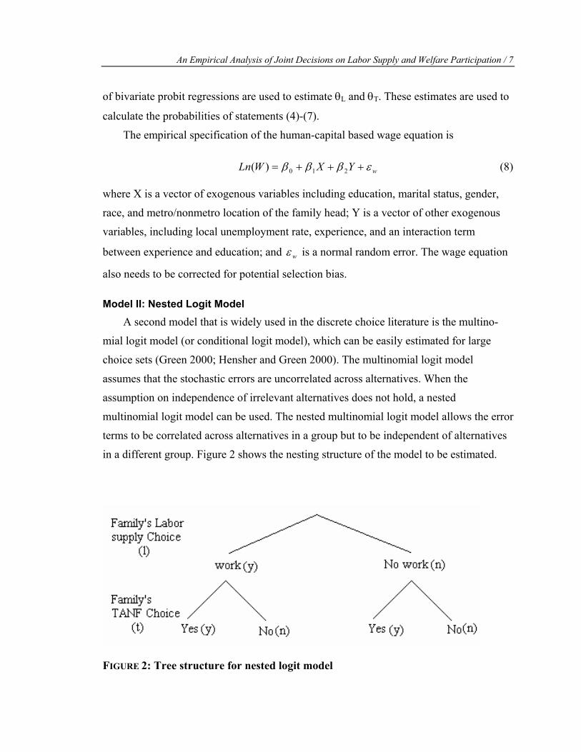
Model II: Nested Logit Model A second model that is widely used in the discrete choice literature is the multino-
mial logit model (or conditional logit model), which can be easily estimated for large
choice sets (Green 2000; Hensher and Green 2000). The multinomial logit model
assumes that the stochastic errors are uncorrelated across alternatives. When the
assumption on independence of irrelevant alternatives does not hold, a nested
multinomial logit model can be used. The nested multinomial logit model allows the error
terms to be correlated across alternatives in a group but to be independent of alternatives
in a different group. Figure 2 shows the nesting structure of the model to be estimated.
FIGURE 2: Tree structure for nested logit model
8 / Kang, Huffman, and Jensen
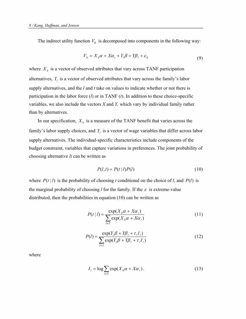
The indirect utility function ltV is decomposed into components in the following way:
ltlltltlt YYXXV εββαα ++++= (9)
where ltX is a vector of observed attributes that vary across TANF participation
alternatives, lY is a vector of observed attributes that vary across the family’s labor
supply alternatives, and the l and t take on values to indicate whether or not there is
participation in the labor force (l) or in TANF (t). In addition to these choice-specific
variables, we also include the vectors X and Y, which vary by individual family rather
than by alternatives.
In our specification, ltX is a measure of the TANF benefit that varies across the
family’s labor supply choices, and lY is a vector of wage variables that differ across labor
supply alternatives. The individual-specific characteristics include components of the
budget constraint, variables that capture variations in preferences. The joint probability of
choosing alternative lt can be written as
)()|(),( lPltPtlP = (10)
where )|( ltP is the probability of choosing t conditional on the choice of l, and )(lP is
the marginal probability of choosing l for the family. If the ε is extreme-value
distributed, then the probabilities in equation (10) can be written as
∑∈
++
=
Tttlt
tlt
XXXX
ltP
')exp(
)exp()|(
αααα
(11)
∑∈
++++
=
Llllll
llll
IYYIYY
lP
')exp(
)exp()(
τββτββ
(12)
where
∑∈
+=Tt
tltl XXI'
)exp(log αα . (13)
An Empirical Analysis of Joint Decisions on Labor Supply and Welfare Participation / 9
The term lI is the inclusive value in the labor supply equation and can be interpreted
as a measure of the sum of the utility for choice t given choice of l. The “nested logit”
aspect of the model arises when the coefficients of the inclusive values lτ differ from 1.
To be consistent with the random utility model, the utility function for the four
alternatives can be specified in the following way:
, , , , , ,
, , , ,
( ) ( ) ( )
( ) ( )yy yy b yy r W l W t M l M t C l C t
N l N t U l U t yy
V B BRR W M C
N U
= + + + + + + + +
+ + + + +
α β β γ γ γ γ γ γ
γ γ γ γ ε
ynlUlNlClMlWrynbynyn UNCMWBRRBV εγγγγγββα ++++++++= ,,,,, nytUtNtCtMtWrnybnyny UNCMWBRRBV εγγγγγββα +++++++++= ,,,,, nnrnnbnn BRRBV εββ ++= (14)
where ltB is the pay standard, BRR is the benefit reduction rate,2 W is the predicted wage,
M is a family head’s gender, C is the number of children in the family, N is nonlabor
income to the family, and U is the state unemployment rate.
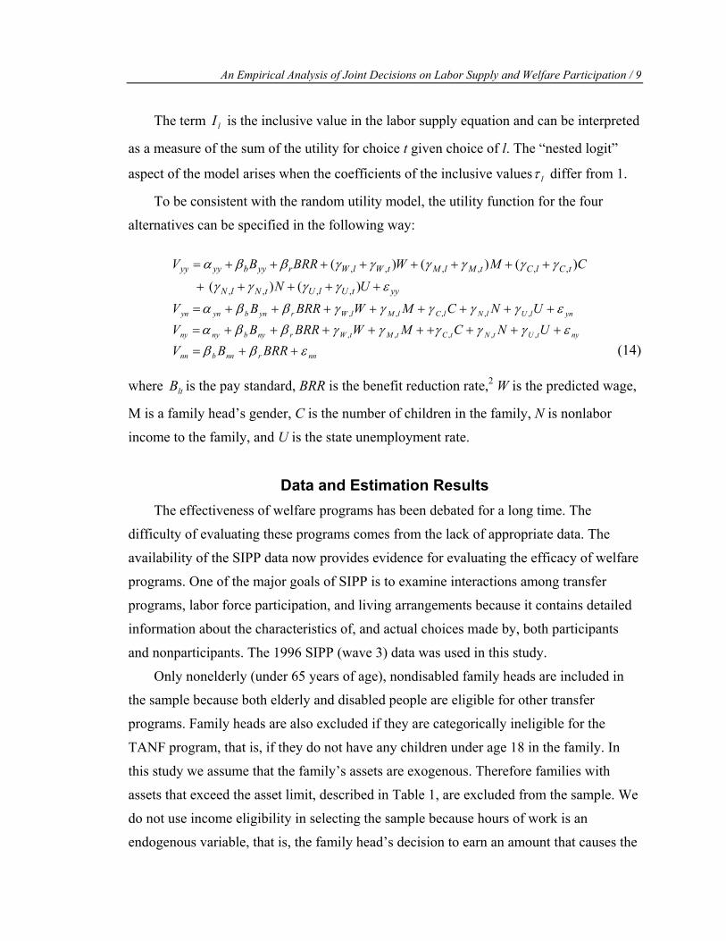
Data and Estimation Results The effectiveness of welfare programs has been debated for a long time. The
difficulty of evaluating these programs comes from the lack of appropriate data. The
availability of the SIPP data now provides evidence for evaluating the efficacy of welfare
programs. One of the major goals of SIPP is to examine interactions among transfer
programs, labor force participation, and living arrangements because it contains detailed
information about the characteristics of, and actual choices made by, both participants
and nonparticipants. The 1996 SIPP (wave 3) data was used in this study.
Only nonelderly (under 65 years of age), nondisabled family heads are included in
the sample because both elderly and disabled people are eligible for other transfer
programs. Family heads are also excluded if they are categorically ineligible for the
TANF program, that is, if they do not have any children under age 18 in the family. In
this study we assume that the family’s assets are exogenous. Therefore families with
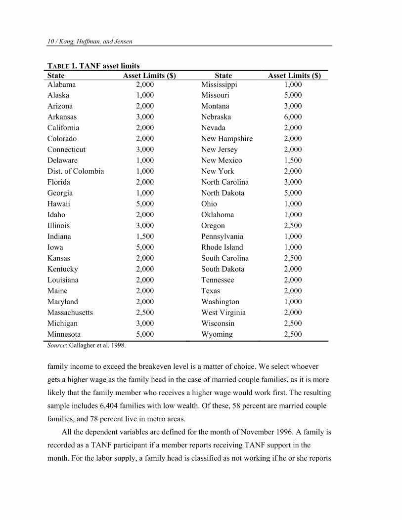
assets that exceed the asset limit, described in Table 1, are excluded from the sample. We
do not use income eligibility in selecting the sample because hours of work is an
endogenous variable, that is, the family head’s decision to earn an amount that causes the
10 / Kang, Huffman, and Jensen
TABLE 1. TANF asset limits State Asset Limits ($) State Asset Limits ($) Alabama 2,000 Mississippi 1,000 Alaska 1,000 Missouri 5,000
Arizona 2,000 Montana 3,000 Arkansas 3,000 Nebraska 6,000
California 2,000 Nevada 2,000 Colorado 2,000 New Hampshire 2,000 Connecticut 3,000 New Jersey 2,000 Delaware 1,000 New Mexico 1,500 Dist. of Colombia 1,000 New York 2,000 Florida 2,000 North Carolina 3,000 Georgia 1,000 North Dakota 5,000 Hawaii 5,000 Ohio 1,000 Idaho 2,000 Oklahoma 1,000 Illinois 3,000 Oregon 2,500 Indiana 1,500 Pennsylvania 1,000 Iowa 5,000 Rhode Island 1,000 Kansas 2,000 South Carolina 2,500 Kentucky 2,000 South Dakota 2,000 Louisiana 2,000 Tennessee 2,000 Maine 2,000 Texas 2,000 Maryland 2,000 Washington 1,000 Massachusetts 2,500 West Virginia 2,000 Michigan 3,000 Wisconsin 2,500 Minnesota 5,000 Wyoming 2,500 Source: Gallagher et al. 1998.
family income to exceed the breakeven level is a matter of choice. We select whoever
gets a higher wage as the family head in the case of married couple families, as it is more
likely that the family member who receives a higher wage would work first. The resulting
sample includes 6,404 families with low wealth. Of these, 58 percent are married couple
families, and 78 percent live in metro areas.
All the dependent variables are defined for the month of November 1996. A family is
recorded as a TANF participant if a member reports receiving TANF support in the
month. For the labor supply, a family head is classified as not working if he or she reports
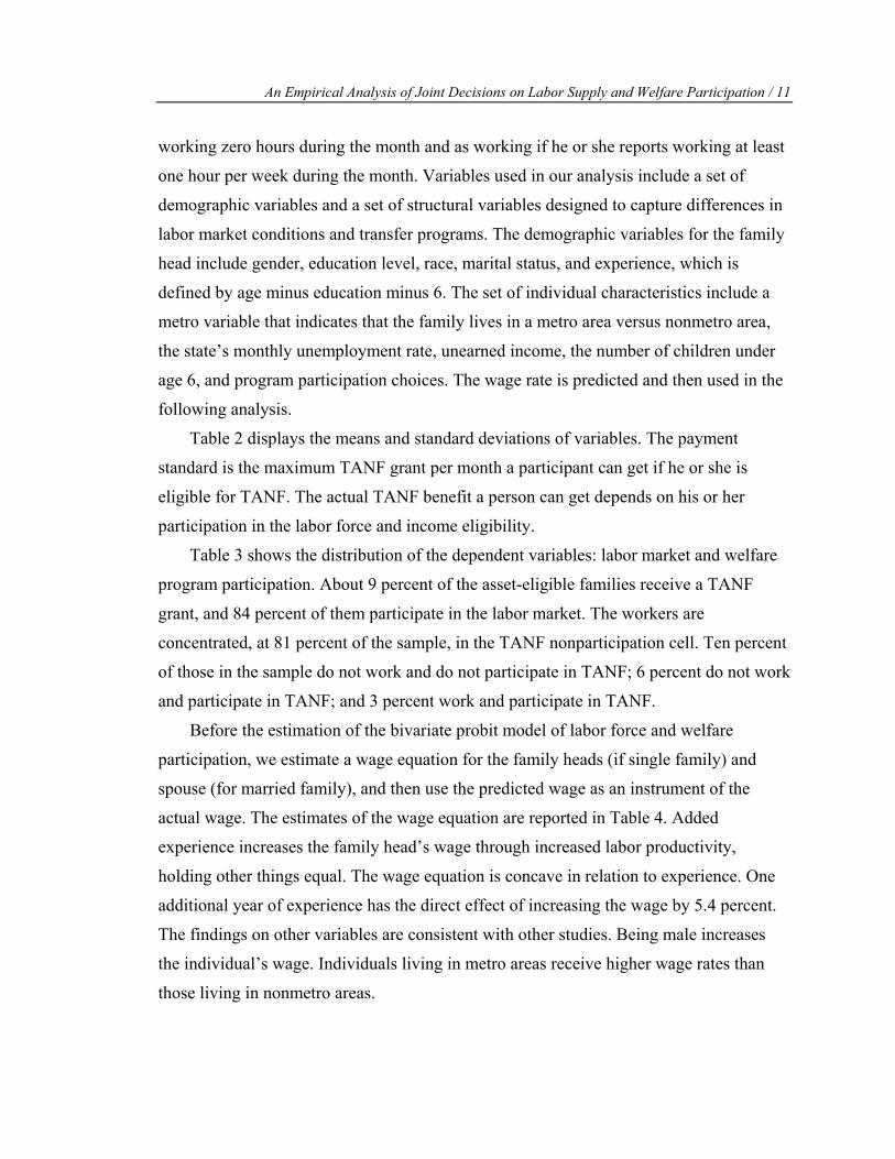
An Empirical Analysis of Joint Decisions on Labor Supply and Welfare Participation / 11
working zero hours during the month and as working if he or she reports working at least
one hour per week during the month. Variables used in our analysis include a set of
demographic variables and a set of structural variables designed to capture differences in
labor market conditions and transfer programs. The demographic variables for the family
head include gender, education level, race, marital status, and experience, which is
defined by age minus education minus 6. The set of individual characteristics include a
metro variable that indicates that the family lives in a metro area versus nonmetro area,
the state’s monthly unemployment rate, unearned income, the number of children under
age 6, and program participation choices. The wage rate is predicted and then used in the
following analysis.
Table 2 displays the means and standard deviations of variables. The payment
standard is the maximum TANF grant per month a participant can get if he or she is
eligible for TANF. The actual TANF benefit a person can get depends on his or her
participation in the labor force and income eligibility.
Table 3 shows the distribution of the dependent variables: labor market and welfare
program participation. About 9 percent of the asset-eligible families receive a TANF
grant, and 84 percent of them participate in the labor market. The workers are
concentrated, at 81 percent of the sample, in the TANF nonparticipation cell. Ten percent
of those in the sample do not work and do not participate in TANF; 6 percent do not work
and participate in TANF; and 3 percent work and participate in TANF.
Before the estimation of the bivariate probit model of labor force and welfare
participation, we estimate a wage equation for the family heads (if single family) and
spouse (for married family), and then use the predicted wage as an instrument of the
actual wage. The estimates of the wage equation are reported in Table 4. Added
experience increases the family head’s wage through increased labor productivity,
holding other things equal. The wage equation is concave in relation to experience. One
additional year of experience has the direct effect of increasing the wage by 5.4 percent.
The findings on other variables are consistent with other studies. Being male increases
the individual’s wage. Individuals living in metro areas receive higher wage rates than
those living in nonmetro areas.

12 / Kang, Huffman, and Jensen
TABLE 2. Definitions, mean, and standard deviations of variables (N=6,404)
Variable Mean (Std. deviation) Definition
Age 36.09 (8.74) Age of family head Education 12.25 (2.66) Years of schooling of family head Male 0.45 (0.5) Dichotomous variable equal to 1 if
family head is male Married 0.58 (0.49) Dichotomous variable equal to 1 if
family head is married White 0.75 (0.43) Dichotomous variable equal to 1 if
family head is white Metro 0.78 (0.41) Dichotomous variable equal to 1 if
family head lives in metro Kids6 0.71 (0.83) Number of children under 6 Experience 18.26 (9.05) Age-Education-6 Unemployment rate 5.25 (1.05) Local state unemployment rate (%) Nonlabor income 128.68 (344.06) Family nonlabor income per month ($) Wage 9.46 (1.99) Predicted hourly wage ($) Payment standard 445.00 (213.00) Maximum TANF grant per month
given participation ($) BRR 0.53 (0.18) The benefit reduction rate is the rate at
which additional dollars of earned income reduce the amount transferred
Labor force participation
0.84 (0.37) Dichotomous variable equal to 1 if family head works
TANF participation 0.09 (0.29) Dichotomous variable equal to 1 if family head participates in TANF
TABLE 3. Distribution of the sample by labor supply and welfare participation Welfare Program (TANF) Participation No participation All Work 199 3% 5,165 81% 5,364 84%
Not work 397 6% 643 10% 1,040 16%
All 596 9% 5,808 91% 6,404 100%
An Empirical Analysis of Joint Decisions on Labor Supply and Welfare Participation / 13
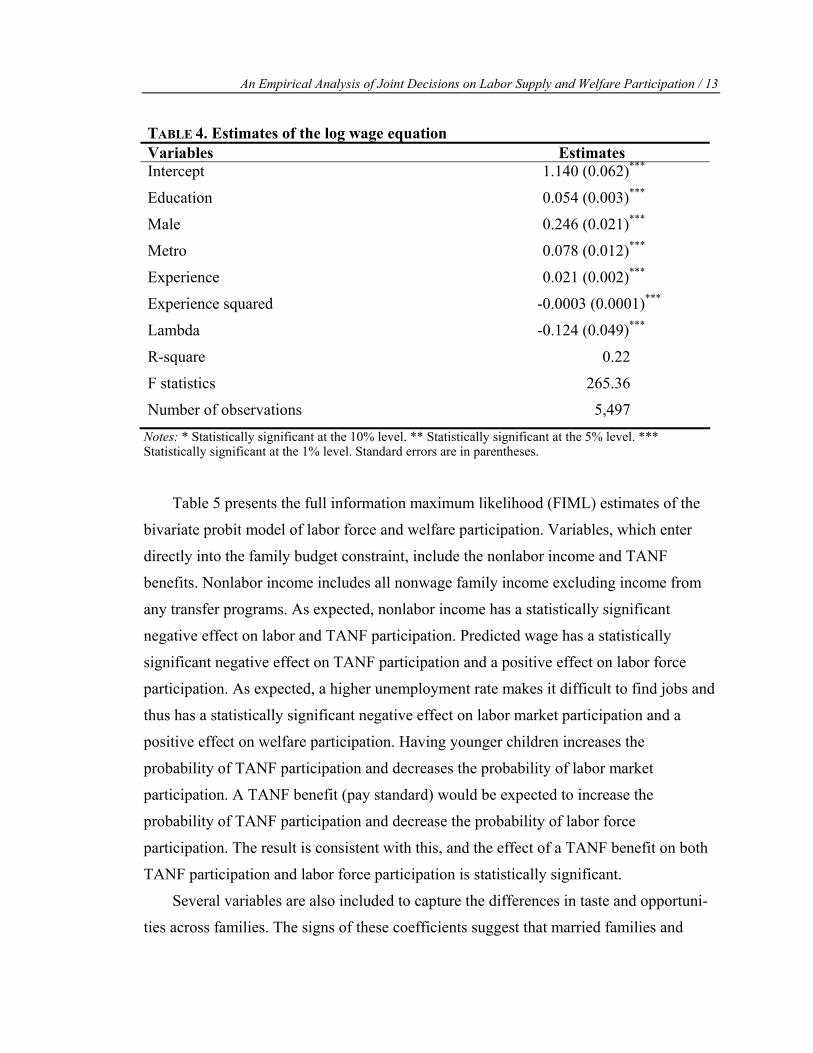
TABLE 4. Estimates of the log wage equation Variables Estimates Intercept 1.140 (0.062)***
Education 0.054 (0.003)***
Male 0.246 (0.021)***
Metro 0.078 (0.012)***
Experience 0.021 (0.002)***
Experience squared -0.0003 (0.0001)***
Lambda -0.124 (0.049)***
R-square 0.22
F statistics 265.36
Number of observations 5,497 Notes: * Statistically significant at the 10% level. ** Statistically significant at the 5% level. *** Statistically significant at the 1% level. Standard errors are in parentheses.
Table 5 presents the full information maximum likelihood (FIML) estimates of the
bivariate probit model of labor force and welfare participation. Variables, which enter
directly into the family budget constraint, include the nonlabor income and TANF
benefits. Nonlabor income includes all nonwage family income excluding income from
any transfer programs. As expected, nonlabor income has a statistically significant
negative effect on labor and TANF participation. Predicted wage has a statistically
significant negative effect on TANF participation and a positive effect on labor force
participation. As expected, a higher unemployment rate makes it difficult to find jobs and
thus has a statistically significant negative effect on labor market participation and a
positive effect on welfare participation. Having younger children increases the
probability of TANF participation and decreases the probability of labor market
participation. A TANF benefit (pay standard) would be expected to increase the
probability of TANF participation and decrease the probability of labor force
participation. The result is consistent with this, and the effect of a TANF benefit on both
TANF participation and labor force participation is statistically significant.
Several variables are also included to capture the differences in taste and opportuni-
ties across families. The signs of these coefficients suggest that married families and
14 / Kang, Huffman, and Jensen
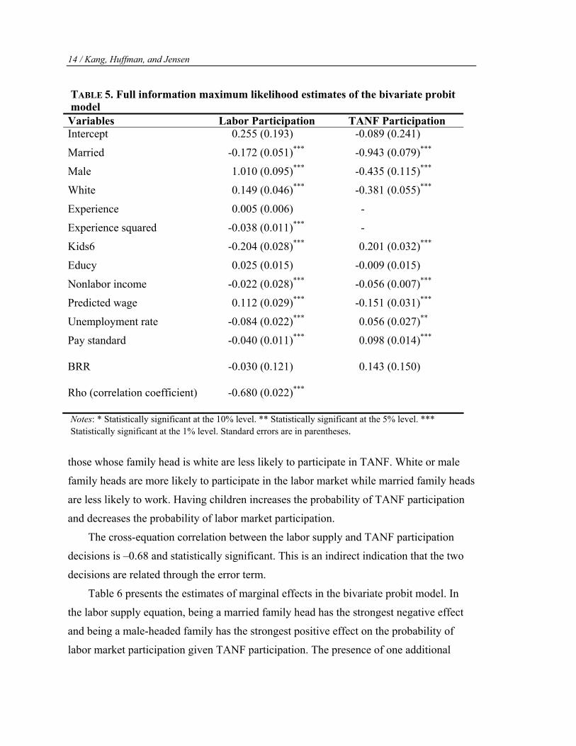
TABLE 5. Full information maximum likelihood estimates of the bivariate probit model Variables Labor Participation TANF Participation Intercept 0.255 (0.193) -0.089 (0.241)
Married -0.172 (0.051)*** -0.943 (0.079)***
Male 1.010 (0.095)*** -0.435 (0.115)***
White 0.149 (0.046)*** -0.381 (0.055)***
Experience 0.005 (0.006) -
Experience squared -0.038 (0.011)*** -
Kids6 -0.204 (0.028)*** 0.201 (0.032)***
Educy 0.025 (0.015) -0.009 (0.015)
Nonlabor income -0.022 (0.028)*** -0.056 (0.007)***
Predicted wage 0.112 (0.029)*** -0.151 (0.031)***
Unemployment rate -0.084 (0.022)*** 0.056 (0.027)**
Pay standard -0.040 (0.011)*** 0.098 (0.014)***
BRR -0.030 (0.121) 0.143 (0.150)
Rho (correlation coefficient) -0.680 (0.022)***
Notes: * Statistically significant at the 10% level. ** Statistically significant at the 5% level. *** Statistically significant at the 1% level. Standard errors are in parentheses.
those whose family head is white are less likely to participate in TANF. White or male
family heads are more likely to participate in the labor market while married family heads
are less likely to work. Having children increases the probability of TANF participation
and decreases the probability of labor market participation.
The cross-equation correlation between the labor supply and TANF participation
decisions is –0.68 and statistically significant. This is an indirect indication that the two
decisions are related through the error term.
Table 6 presents the estimates of marginal effects in the bivariate probit model. In
the labor supply equation, being a married family head has the strongest negative effect
and being a male-headed family has the strongest positive effect on the probability of
labor market participation given TANF participation. The presence of one additional
An Empirical Analysis of Joint Decisions on Labor Supply and Welfare Participation / 15
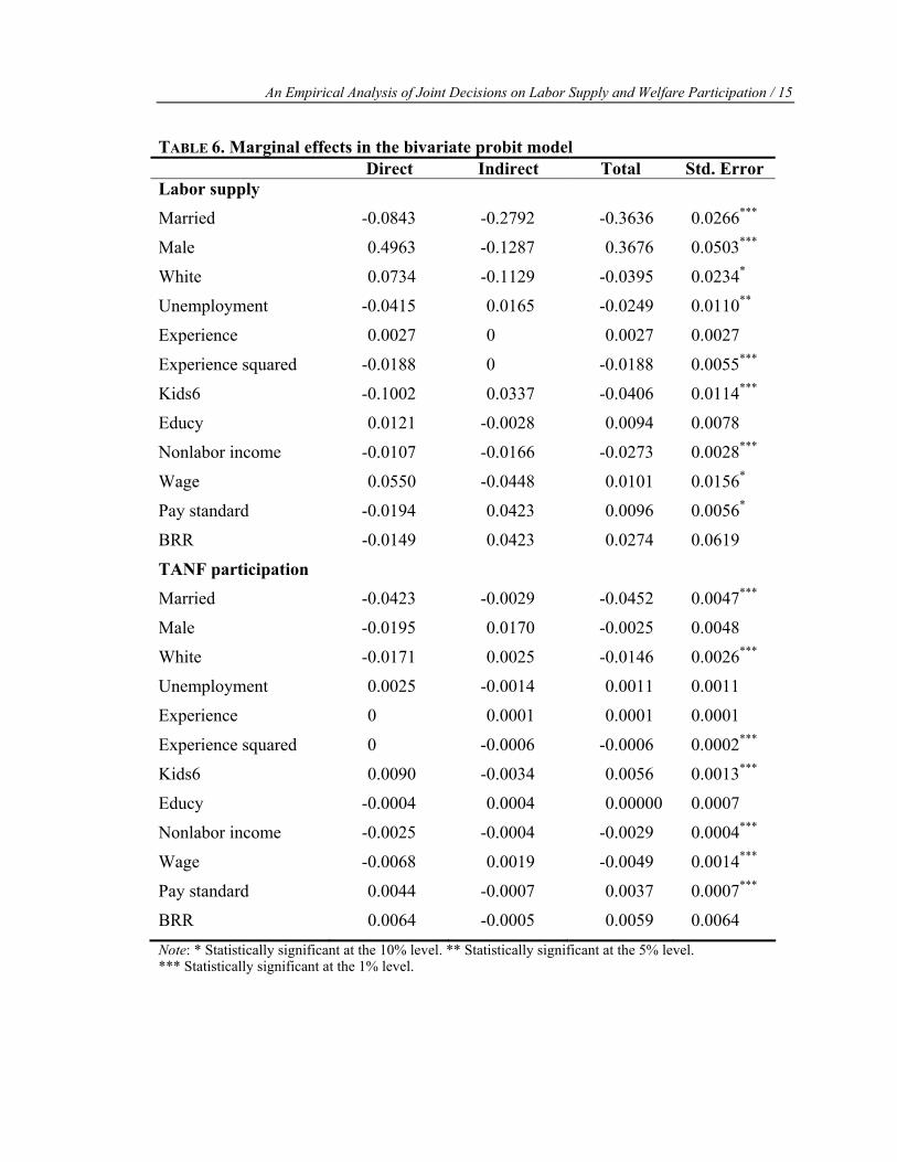
TABLE 6. Marginal effects in the bivariate probit model Direct Indirect Total Std. Error Labor supply
Married
-0.0843
-0.2792
-0.3636
0.0266***
Male 0.4963 -0.1287 0.3676 0.0503***
White 0.0734 -0.1129 -0.0395 0.0234*
Unemployment -0.0415 0.0165 -0.0249 0.0110**
Experience 0.0027 0 0.0027 0.0027
Experience squared -0.0188 0 -0.0188 0.0055***
Kids6 -0.1002 0.0337 -0.0406 0.0114***
Educy 0.0121 -0.0028 0.0094 0.0078
Nonlabor income -0.0107 -0.0166 -0.0273 0.0028***
Wage 0.0550 -0.0448 0.0101 0.0156*
Pay standard -0.0194 0.0423 0.0096 0.0056*
BRR -0.0149 0.0423 0.0274 0.0619
TANF participation
Married
-0.0423
-0.0029
-0.0452
0.0047***
Male -0.0195 0.0170 -0.0025 0.0048
White -0.0171 0.0025 -0.0146 0.0026***
Unemployment 0.0025 -0.0014 0.0011 0.0011
Experience 0 0.0001 0.0001 0.0001
Experience squared 0 -0.0006 -0.0006 0.0002***
Kids6 0.0090 -0.0034 0.0056 0.0013***
Educy -0.0004 0.0004 0.00000 0.0007
Nonlabor income -0.0025 -0.0004 -0.0029 0.0004***
Wage -0.0068 0.0019 -0.0049 0.0014***
Pay standard 0.0044 -0.0007 0.0037 0.0007***
BRR 0.0064 -0.0005 0.0059 0.0064
Note: * Statistically significant at the 10% level. ** Statistically significant at the 5% level. *** Statistically significant at the 1% level.

16 / Kang, Huffman, and Jensen
child under age 6 would decrease the probability of working by 4 percent. Nonlabor
income has a significant negative effect and wages have a significant positive effect on
the probability of working; both nonlabor income and wages have statistically significant
negative effects on the probability of welfare participation. In the TANF participation
equation, most variables seem to have relatively smaller effects on the probability of
TANF participation given labor market participation. This implies that if family heads
work, it makes relatively less difference whether or not they participate in TANF.
The FIML estimates of the nested logit model are presented in Table 7. The
estimated coefficients are interpreted with respect to the “no labor–no TANF
TABLE 7. Full information maximum likelihood estimates of nested logit model Coefficients Estimates
αyy 2.818 (10.894)
αyn 3.687 (10.875)
αny 1.187 (0.424)***
βb 0.040 (0.034)
βr 0.001 (0.003)
γW,l 0.060 (0.189)
γW,t -0.263 (0.036)***
γM,l 0.891 (2.651)
γM,t -1.481 (0.191)***
γC,l 0.035 (0.136)
γC,t 0.271 (0.049)***
γN,l -0.115 (0.333)
γN,t -0.117 (0.017)***
γU,l -0.099 (0.311)
γU,t 0.065 (0.039)*
IVwork 0.853 (2.486)
IVno work 3.260 (0.772)***
Log likelihood -3707.024 Notes: * Statistically significant at the 10% level. ** Statistically significant at the 5% level. *** Statistically significant at the 1% level. Standard errors are in parentheses.
An Empirical Analysis of Joint Decisions on Labor Supply and Welfare Participation / 17
participation” category. Higher wages lead to less participation in TANF (γW,t) and, although not statistically significant, make family heads work more (γW,l). The coefficients on TANF benefits (βb) and BRR (βr) are not statistically significant. Male family heads tend to work more (γM,l) and participate less in TANF (γM,t). Families with more young children (under age 6) participate more in TANF(γC,t). Family heads with more unearned income participate less in TANF (γN,t) and, although not statistically significant, tend to work less (γN,l). The unemployment rate has a positive and statistically significant effect on the probability of TANF participation (γU,t).
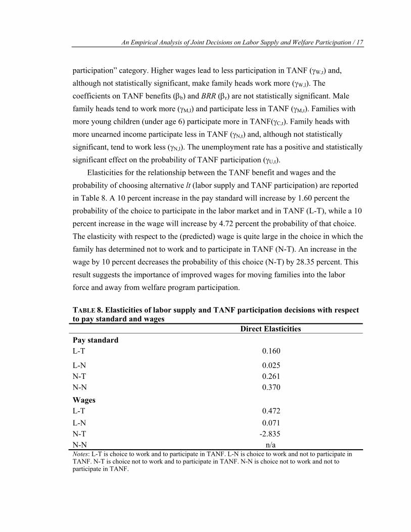
Elasticities for the relationship between the TANF benefit and wages and the probability of choosing alternative lt (labor supply and TANF participation) are reported in Table 8. A 10 percent increase in the pay standard will increase by 1.60 percent the probability of the choice to participate in the labor market and in TANF (L-T), while a 10 percent increase in the wage will increase by 4.72 percent the probability of that choice. The elasticity with respect to the (predicted) wage is quite large in the choice in which the family has determined not to work and to participate in TANF (N-T). An increase in the wage by 10 percent decreases the probability of this choice (N-T) by 28.35 percent. This result suggests the importance of improved wages for moving families into the labor force and away from welfare program participation.
TABLE 8. Elasticities of labor supply and TANF participation decisions with respect to pay standard and wages Direct Elasticities Pay standard L-T
0.160
L-N 0.025 N-T 0.261 N-N 0.370 Wages L-T
0.472
L-N 0.071 N-T -2.835 N-N n/a Notes: L-T is choice to work and to participate in TANF. L-N is choice to work and not to participate in TANF. N-T is choice not to work and to participate in TANF. N-N is choice not to work and not to participate in TANF.
18 / Kang, Huffman, and Jensen
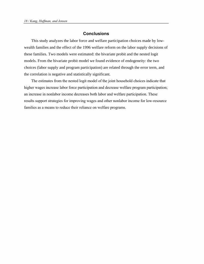
Conclusions This study analyzes the labor force and welfare participation choices made by low-
wealth families and the effect of the 1996 welfare reform on the labor supply decisions of
these families. Two models were estimated: the bivariate probit and the nested logit
models. From the bivariate probit model we found evidence of endogeneity: the two
choices (labor supply and program participation) are related through the error term, and
the correlation is negative and statistically significant.
The estimates from the nested logit model of the joint household choices indicate that
higher wages increase labor force participation and decrease welfare program participation;
an increase in nonlabor income decreases both labor and welfare participation. These
results support strategies for improving wages and other nonlabor income for low-resource
families as a means to reduce their reliance on welfare programs.
Endnotes
1. Maddala (1983) presents an extensive discussion of limited-dependent and
qualitative-variable models in econometrics.
2. The term ltB is the maximum TANF grant per month; BRR is the benefit reduction
rate, the rate at which additional dollars of earned income reduce the TANF benefit.
References
Gallagher, J., M. Gallagher, K. Perese, S. Schreiber, and K. Watson. 1998. “One Year After Welfare Reform: A Description of State Temporary Assistance for Needy Families (TANF) Decisions as of October 1997.” Research Report #307472. The Urban Institute, Washington, DC. May.
Green, W. 2000. Econometric Analysis, 4th ed. Englewood Cliffs, NJ: Prentice-Hall.
Hagstrom, P. 1996. “The Food Stamp Participation and Labor Supply of Married Couples: An Empirical Analysis of Joint Decisions.” Journal of Human Resources 31(2, Spring): 383-403.
Hensher, D., and W. Green. 2000. “Specification and Estimation of the Nested Logit Model: Alternative Normalisations.” Mimeo. February.
Keane, M., and R. Moffitt. 1998. “A Structural Model of Multiple Program Participation and Labor Supply.” International Economic Review 39(3): 553-89.
Maddala, G.S. 1983. Limited-Dependent and Qualitative Variables in Econometrics. Cambridge: Cambridge University Press.
Moffitt R. 1992. Incentive Effects of the U.S. Welfare System: A Review.” Journal of Economic Literature 30(March): 1-61.
Rowe, G. 2000. “State TANF Policies as of July 1999.” In Welfare Rules Databook. The Urban Institute, Washington, DC. November.