1

AN AUTOMATED WIRELESS FIXED-ACCESS NETWORKS ANTENNA POSITIONING ALGORITHM

Boaz Ben-Moshe, Yehuda Ben-Shimol, Yoav Ben-Yehezkel, Amit Dvir, Michael Segal Communication System Engineering Department & Computer Science Department

Ben-Gurion University Beer-Sheva, Israel

ABSTRACT This article addresses a real-life problem - obtaining communication links between multiple base station sites, by positioning a minimal set of fixed-access relay antenna sites on a given terrain. Reducing the number of antennas is critical, since the cost of their installation and maintenance is substantial. Despite the significant cost saving by eliminating even a single site, a hardly optimal manual approach is employed due to the computation complexity of the problem (Max-SNP-hard, as we prove in Section 3). In this paper we suggest several alternative automated heuristics, relying on terrain preprocessing to find educated potential points for positioning relay stations, then finding all the shortest paths for a Point-To-Point (P2P) case, and finally, expanding this model to support connectivity between multiple (more than 2) base station sites. We conducted a large-scale experiment consisting of running approximately 7,000 different scenarios. We isolated and displayed the experiment factors, which we have found to affect the standard deviation between heuristics, we compared between the suggested heuristics and we show that in this experiment the saving potential grows when more base stations are required to be interconnected. In addition, using an application we developed that allows manual positioning of relay stations on a map, we compared our suggested heuristics results to the best results obtained by human experts on a small subset of the experiment scenarios. Our studies indicate that for small networks (e.g. connecting 10 base stations), the results obtained by human experts are sufficient although rarely exceed our automated alternatives. However, the process of obtaining these results in comparison to automated heuristics is much longer. In addition, when more base station sites should be interconnected, the human approach is easily outperformed by our heuristics, both in terms of better results (fewer antennas) and in significant shorter calculation time.

1. INTRODUCTION

Background In Fixed-Access Networks (FAN), there is no need for continuous coverage of a given area. Each base station antenna serves its local potential subscribers. However, in this article we do not study the problem of serving clients, we are interested only in interconnecting base stations located in remote cities or villages using a minimal set of relay stations. The relay station antennas used to connect base stations are typically microwave Point-To-Point (P2P).

General Problem Definition Connecting Multiple fixed access Base Stations (CMBS) – Given a terrain T and a set of Base Stations (BS), connect all BS in that set using the smallest set of Relay Stations (RS). An RS can connect any number of BS/RS. BS can also serve as RS.

Related Work and Existing Solutions Some solutions for automation of antenna-positioning problems in cellular networks were suggested[3-7]. In addition, the CMBS problem is often raised in the context of minimizing the number of BS that can serve all (or most of) the network clients [17]. Solutions to the problem of serving a maximum surface of a geographical area with a minimum number of Base Transceiver Stations (BTS) were also given [16]. Most of our suggested heuristics are based on variations of minimal spanning trees, and on shortest paths, these methods have been studied extensively in the context of facility location problems [12-15]. We suggest two other heuristics based on a new grading scheme defined specifically for solving the CMBS problem. The CMBS problem resembles the Steiner Tree Problem that was thoroughly studied [18]. The analogous problem in this paper was to minimize the total number of Steiner nodes used to solve a Steiner Tree Problem. To the best of our knowledge there are no previous studies on the CMBS problem as defined above. Solutions to problems of antenna positioning of FAN networks are usually semi-automated. A professional RF engineer or a geographer, experienced in the essentials of FAN installation, suggests an antenna-positioning strategy. Interconnecting microwave antennas (as done in this work) requires both Line Of Sight (LOS) and a distance limit between any two antennas. Connecting different antenna types may even work when LOS is broken, although path loss increases significantly [9].

2

Our Contribution Human strategies usually achieve good results for small FANs, but as the quantity of base stations increases, human approach is less efficient, more confusing and far more time consuming. The goal of this research is to establish a fully-automated wireless FAN antenna positioning algorithm, that will outperform human approaches, in terms of both selecting fewer RS antennas, and achieving this strategy in a much shorter time. Base stations solutions (of equal size) that serve the same number of subscribers may still be subjected to a significant difference from their CMBS point of view (number of relay stations). Therefore, we believe that CMBS algorithms should be used as complementary objectives of GIS-RF applications [1,2]. Usually, these applications focus on optimization algorithms that attempt to minimize the number of base station antennas while providing service to the subscribers. However, interconnecting base station antenna sites directly or through a minimum set of relay stations is not dealt with at all using these applications. From the theoretical aspect we show that the CMBS problem is ‘set-cover’ hard to approximate. Section 2 presents a solution for connecting two BS antenna sites using the smallest set of RS; Section 3 proves the NP-hardness of the CMBS problem and is also dedicated to heuristics that connect multiple (more than two) BS, as well as to some examples of the CMBS solver application we developed; Section 4 provides details of the large scale experiment we conducted and finally, Section 5 discusses our recommendations for future work.

2. POINT-TO-POINT (P2P) CASE

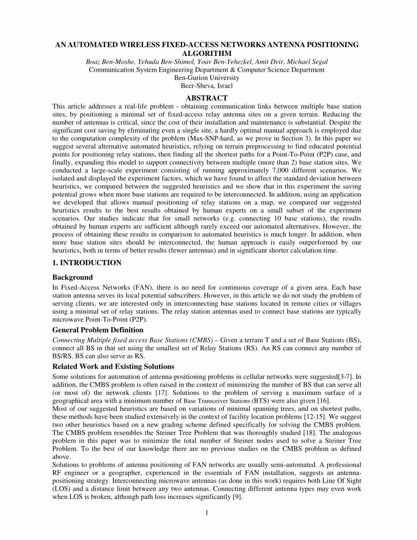
P2P Case Definition Given a terrain T and exactly 2 Base Stations (BS), connect these BS using the smallest set of Relay Stations (RS). An RS can connect any number of BS/RS. BS can also serve as RS. Terrain Preprocessing Since the proportion of the terrain models in our problem is huge (hundreds of square km), it is necessary to preprocess it in order to reduce the input size by an order of magnitude, before applying various facility location algorithms on it. To analyze whether two antennas, positioned on two arbitrary points on the map can communicate directly, it is required to calculate the accumulated path-loss between these two points and to compare it with the sensitivity threshold of the receiver. Calculating all pairs of points on a large-scale map is unfeasible. Therefore, we applied a preprocessing algorithm that attempted to preserve the LOS property between potential antenna locations (usually positioned on top of hills or high dominating places). We used a Digital Elevation Map (DEM) format, representing the map as an elevation function of x,y coordinates - z(x,y). Finding Potential Relay Station Positions: We used two methods for finding potential RS positions. The first method was to place a network of NxN grids on the map (where N is a user-defined parameter). From each NxN square, the two highest grid points among all NxN points in that square are selected as potential antenna positioning candidates. The second method is based on a variation of using the map as an input for the convex hull[8] algorithm. When a map serves as an input to a convex hull algorithm, the outcome consists of non-relevant facets below the surface. To solve this, we padded the map margins with elevations that are far lower than all the points in the map. This ensured only one facet below the surface of the convex hull. This output is much easier to correct than the convex hull algorithm outputs after running them on the unpadded map. The additional potential RS positions were obtained from the list of coordinates of the convex hull nodes. We removed the map padding as well as all the convex hull outputs on the lowermost facet (the single facet below the surface) and display the convex hull facets on the map in Figure 1.

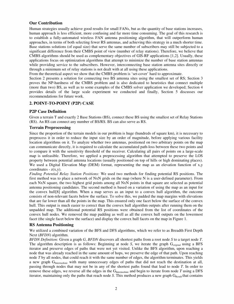
RS Antenna Positioning We utilized a combined variation of the BFS and DFS algorithms, which we refer to as Breadth First Depth Next (BFDN) algorithm. BFDN Definition: Given a graph G, BFDN discovers all shortest paths from a root node S to a target node T. The algorithm description is as follows: Beginning at node S, we iterate the graph Goriginal using a BFS iterator and preserve edges of paths that were not yet visited. Unlike the BFS algorithm, upon reaching a node that was already reached in the same amount of hops, we preserve the edge of that path. Upon reaching node T by all nodes, that could reach it with the same number of edges, the algorithm terminates. This yields a new graph GIntermediate with many unnecessary edges of paths that did not reach the destination at all, passing through nodes that may not be in any of the shortest paths found that lead to node T. In order to remove these edges, we reverse all the edges in the GIntermediate and begin to iterate from node T using a DFS iterator, maintaining only the paths that reach node S. This method produces a new graph GResult that contains

3

all shortest paths from node T to node S. Reversing all the edges again yields the required solution. An example to the BDFN algorithm is given in Figure 2. RS Antenna Positioning Algorithm: From the set of potential RS positions (convex hull and local peaks coordinates as explained above) as well as the source BSS and target BST coordinates, we constructed a Visibility Graph (VG) using the condition dictated by the narrow beam microwave nature of the antennas. Two nodes on VG are connected if and only if their Euclidean distance is smaller than a given threshold and they maintain LOS. We performed the BFDN algorithm on VG, finding all shortest path coordinates on the map from BSS to BST. All the shortest paths are given as a suitable alternative solution to select from, since when testing these paths in the field, additional constraints, such as restricted military zones, deep water reservoirs, swamps, etc., which cannot be used or are impractical for antenna positioning, are posed.

Figure 1. Convex hull variation output on a map (after removing the single facet below the surface)

�

� � � �

�

� �

�

� � � �

�

�

�

� � � �

�

� �

��������������

������������

� ��� � �������

� ��� ������ ������

� ��� � �����

Figure 2. Example to the BFDN algorithm

Discussion and Implementation Remarks on the P2P Case: Terrain Preprocessing: We wish to note that this solution does not require reevaluation of the convex hull variation algorithm on the same map, to enable connection between two new BS sites. This fact, allowed us to perform the convex hull variation once for each map, and to introduce the convex hull points as integral “implanted” candidate points in the input for the calculation of the CMBS problem. We also wish to note that although the method we suggested for finding potential RS positions using the NxN grids seems somewhat trivial, its strength is in its simplicity and its short run-time (which was an dominant factor in this research). BDFN: BFDN serves as a basis to solve the CMBS problem in many of our later proposed heuristics.

3. ESTABLISHING COMMUNICATION LINKS AMONG MULTIPLE BASE STATIONS In this section we present several heuristics we implemented in an attempt to resolve the CMBS problem. We first provide a formal reduction from the CMBS problem to the general set cover problem. This reduction shows that the CMBS problem is ‘set cover hard’. Then, we present several heuristics (approximation algorithms) for solving the CMBS problem, and present solutions to one scenario using the application we developed.

4

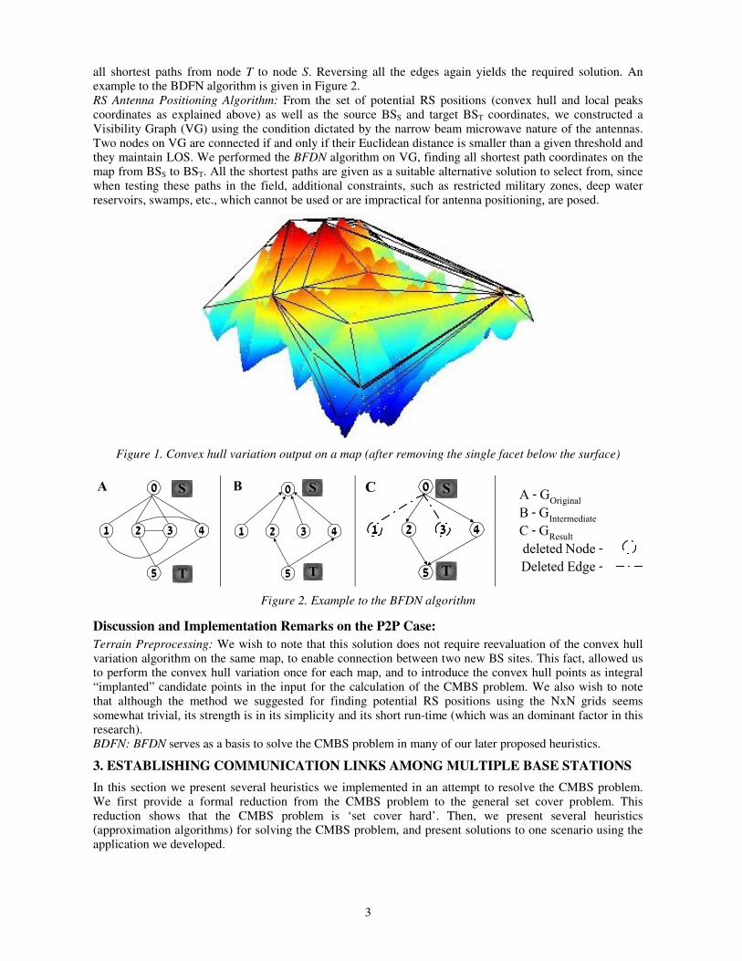
NP-Completeness (Max SNP-hard) Proof The CMBS problem, as we show below, is an optimization problem which has no constant approximation factor, i.e. for any suggested algorithm (A) solving the CMBS problem and a constant number C – there is always an input for which the ratio between the size of the solution (given by the algorithm A) and the size of the optimal solution is bigger than C. Informally, we show that any instance of the set cover problem can be reduced to an instance of the CMBS problem such that an optimal solution for the CMBS problems implies an optimal solution for the set cover problem, furthermore, every approximation for CMBS problem implies the same approximation for the set cover problem. The general set-cover problem is defined as follows: let S be set of all integers from 1 to n, let S*={s1,…,sm} be a set of (m) subsets of S. Our goal is to find the smallest subset of S* such that its union is S. The k-set cover problem is a set-cover problem for which the size of the maximal set in S* is bounded by k. The k-set cover problem is known to be NP complete for k��3 [10], and unapproximatable within (1-�) ln(k) for any fixed �>0 – i.e. MAX SNP-hard [11] (assuming P is not NP). Lemma: The CMBS problem can be reduced from the set-cover problem using a ‘gap-preserving’ reduction that preserves the approximation ratio (using visibility over the terrain as a connection condition). Proof: Given an instance of the set cover problem, which includes a set S=[1…n] (all integers from 1 to n), and a collections of subsets s1,…,sm of S, We first locate the set S and the subsets s1,…,sk on a flat rectangular grid terrain (see Figure 3) and draw a segment from each set si to all its members (in S), then we locate a thick wall which has only thin ‘cracks’, so that the segments can go through (but no further visibility will be created). Finally we partition the points in S so that no two points could directly see each other (note: all the vertices s1,…,sk can see each other).

Figure 3. NP-hardness (no constant factor approximation) reduction from the set cover problem

Any valid solution to the CMBS problem implies a valid solution to the original set cover problem, moreover any subset of s1,…,sm which does not connect all S (not a valid CMBS solution), also does not cover all S. To conclude, if there was an algorithm, which has a constant factor approximation for the CMBS problem, it could have been used to compute a constant factor approximation to the set-cover problem – contradiction. Theorem: the CMBS problem is MAX-SNP-hard, and therefore cannot have an approximation ratio better than O(1)ln(k) (where k is the maxima over the size of subsets s1,…,sm). Namely, the CMBS is set-cover hard.

Heuristics for the CMBS problem In order to solve the CMBS problem we first compute a finite set of potential RS positions. This set consists of the BS coordinates, the coordinates obtained by the local peaks analysis and the convex hull coordinates calculated for each map. We compute the Visibility Graph (VG) on this set, as described in Section 2. Henceforth, we will address the CMBS problem in terms of graph theory; select the smallest RS subset (SRS), such that all BS produce a single connected component using the vertices of SRS [18].

Minimal Spanning Tree (MST) Heuristics The first class of heuristics we developed and tested was based on MST like algorithms. In some of these heuristics we calculate on VG all the shortest paths of potential RS between any two BS using BFDN (presented in Section 2), as a basis for our solution. Trivial Minimal Spanning Tree (T-MST): We use T-MST as a fast upper-bound approximation for the number (not positions) of RS required to solve the CMBS problem. We begin with the minimal shortest path

5

distance (in terms of RS hops) among any two BS. Then, we compute which BS has the shortest path to any of the already connected BS nodes, and add that distance to the total sum of the distances until all BS nodes are connected. The result is an upper bound for the number of required RS, because the summing of distances includes RS positioned on more than one of the shortest paths more than once. We frequently use this approximation in the positioning heuristics below as a grading mechanism enabling to compare the effectiveness of several possible solutions. We also use the fact that this is an upper bound in Section 4, where we perform comparison between heuristics using T-MST as one of the normalizing factors. Simple Minimal Spanning Tree (S-MST): S-MST heuristic is the first heuristic that allows to actually position RS antennas on the given terrain. The S-MST has three variations:

1. First, we select a predefined initial BS to begin with. Then we calculate the shortest path to its nearest neighbor. If several such paths are available, we pick the first one on the list. In each step henceforth, we connect the first BS closest to the already connected component (any already connected RS or BS).

2. Essentially, this variation is the same as described above. However, instead of predefining the initial BS, we select it randomly. In addition, if more than one shortest path to the closest connected component exist, we randomly select one of these shortest paths (instead of selecting the first one on the list).

3. This variation resembles the second variation, however, rather than connecting the entire shortest path to the connected component, we add only a single RS to the solution, until all BS are connected.

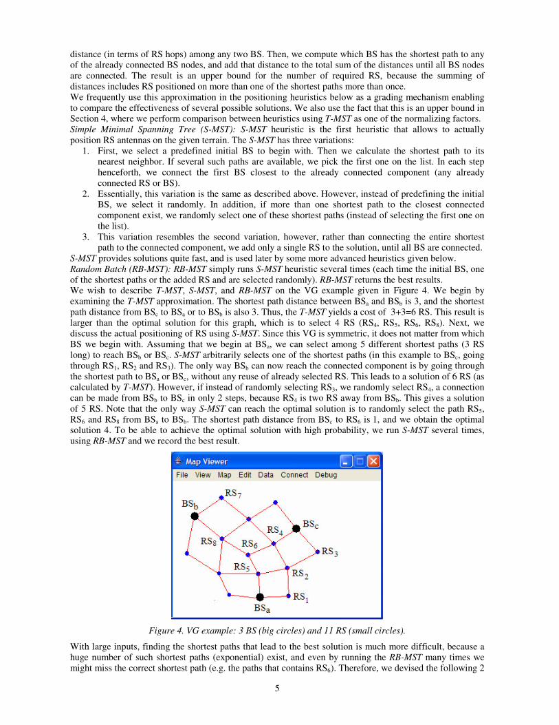
S-MST provides solutions quite fast, and is used later by some more advanced heuristics given below. Random Batch (RB-MST): RB-MST simply runs S-MST heuristic several times (each time the initial BS, one of the shortest paths or the added RS and are selected randomly). RB-MST returns the best results. We wish to describe T-MST, S-MST, and RB-MST on the VG example given in Figure 4. We begin by examining the T-MST approximation. The shortest path distance between BSa and BSb is 3, and the shortest path distance from BSc to BSa or to BSb is also 3. Thus, the T-MST yields a cost of 3+3=6 RS. This result is larger than the optimal solution for this graph, which is to select 4 RS (RS4, RS5, RS6, RS8). Next, we discuss the actual positioning of RS using S-MST. Since this VG is symmetric, it does not matter from which BS we begin with. Assuming that we begin at BSa, we can select among 5 different shortest paths (3 RS long) to reach BSb or BSc. S-MST arbitrarily selects one of the shortest paths (in this example to BSc, going through RS1, RS2 and RS3). The only way BSb can now reach the connected component is by going through the shortest path to BSa or BSc, without any reuse of already selected RS. This leads to a solution of 6 RS (as calculated by T-MST). However, if instead of randomly selecting RS3, we randomly select RS4, a connection can be made from BSb to BSc in only 2 steps, because RS4 is two RS away from BSb. This gives a solution of 5 RS. Note that the only way S-MST can reach the optimal solution is to randomly select the path RS5, RS6 and RS8 from BSa to BSb. The shortest path distance from BSc to RS6 is 1, and we obtain the optimal solution 4. To be able to achieve the optimal solution with high probability, we run S-MST several times, using RB-MST and we record the best result.

Figure 4. VG example: 3 BS (big circles) and 11 RS (small circles).

With large inputs, finding the shortest paths that lead to the best solution is much more difficult, because a huge number of such shortest paths (exponential) exist, and even by running the RB-MST many times we might miss the correct shortest path (e.g. the paths that contains RS6). Therefore, we devised the following 2

6

heuristics. To understand these heuristics, we must first explain the notion of RS-min-cut set. Given 2 nodes A, B (on VG) and all the shortest paths between them sp(A,B). The RS-min-cut set of VG refers to the smallest set of RS nodes on sp(A,B), which all have the same distance to A (and to B). Greedy Improvement (GI-MST): Our primitive version of GI-MST stated that we begin at a random base station (e.g. BSa) and find all the shortest paths to its nearest base station (e.g. BSb) using the BFDN algorithm. Now, we iterate through these shortest paths, one at a time, and grade these paths pretending that all the RS on that path are BS. The greedy grading function can be the number of required RS by using T-MST, S-MST or a combination of both of them. The path with the highest grade is selected. However, the number of shortest paths can be large, and we wish to reduce the number of grade recalculations. Therefore, we implemented another shorter version of GI-MST. In this implementation, we recalculated the grading function only on the RS-min-cut set between any two BS on VG. Greedy & Random (GR-MST): GR-MST runs GI-MST several times, selecting the GI-MST parameters at random. The initial BS, which RS-min-cut set to select if there are several of the same size, the BS destination to apply GI-MST if several shortest paths reach more than one BS, serve as examples to the random selection we can make. In general, whenever a selection is made, it is done randomly. GR-MST returns the best results. The implications of GI-MST and GR-MST are demonstrated in Figure 4. Assuming that we begin at BSa, there are 5 shortest paths to BSb. The RS-min-cut set size is 2, resulting from any set of nodes whose distance to the BS is the same. We select the first RS-min-cut set (RS5 and the one on its left). Then, we pretend that RS5 is a BS, and recalculate T-MST. We get 4 as the T-MST result, whereas recalculating the RS left to RS5, yields 5. Note, that if we use S-MST instead of T-MST, the result would have been optimal. Figure 4 also enables to examine the set of random selections GR-MST makes. For example, we can begin at any of the 3 BS. There are 5 shortest paths from BSa to BSb, but also to BSc. There are 3 RS-min-cut sets of size 2 on any selected shortest path. We do not obtain better results, but for larger and non-symmetrical inputs, GR-MST occasionally produces better results than GI-MST.

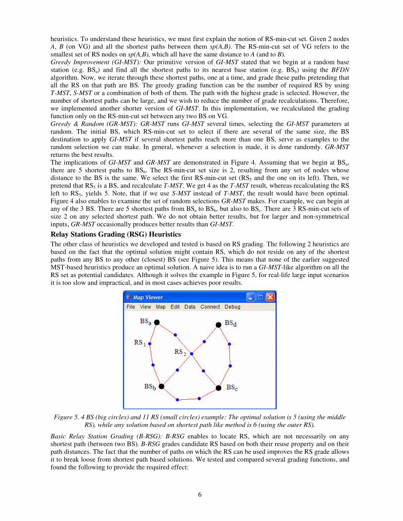
Relay Stations Grading (RSG) Heuristics The other class of heuristics we developed and tested is based on RS grading. The following 2 heuristics are based on the fact that the optimal solution might contain RS, which do not reside on any of the shortest paths from any BS to any other (closest) BS (see Figure 5). This means that none of the earlier suggested MST-based heuristics produce an optimal solution. A naive idea is to run a GI-MST-like algorithm on all the RS set as potential candidates. Although it solves the example in Figure 5, for real-life large input scenarios it is too slow and impractical, and in most cases achieves poor results.

Figure 5. 4 BS (big circles) and 11 RS (small circles) example: The optimal solution is 5 (using the middle

RS), while any solution based on shortest path like method is 6 (using the outer RS).

Basic Relay Station Grading (B-RSG): B-RSG enables to locate RS, which are not necessarily on any shortest path (between two BS). B-RSG grades candidate RS based on both their reuse property and on their path distances. The fact that the number of paths on which the RS can be used improves the RS grade allows it to break loose from shortest path based solutions. We tested and compared several grading functions, and found the following to provide the required effect:

7

For each base station BSi , or set of BS, which are directly connected (without using unselected-RS), find the closest BS’, denoted by d1=d(BSi ,BS’), where d is the link distance in terms of RS hops. For each RS, such that d(RS,BSi )��d(BSi ,BS’), we find the closest BS’’ (excluding BSi ). Denote d2=d(RS,BSi)+1 and d3=d(RS,BS’’). The grade for the RS using BSi is given by the expression: g(RS,BSi)=f(d1,d2,d3), where f(d1,d2,d3) is calculated as follows: � �c321321 ddd)d,d,d(f �� , where 1<c<2. The total grade of RS is:

g(RS)=�

n

1ii )BS,RS(g , where n is the number of BS connected components.

A justification for this grading function is that RS on shortest paths are graded 1, because d2+d3=d1, and the grade of an RS not on shortest paths is lower. However, if an arbitrary RS that is not on the shortest path but can be reused more than another RS’, which resides on shortest paths, then the sum of all RS grades over all the BS on its connected component may increase its grade to be greater than the grade of RS’. The B-RSG algorithm works as follows:

1. While all BS are not yet connected: 1.1 Initialize the grades of all RS. 1.2 Grade all RS (according to the grading method suggested above) 1.3 Locate the best-graded RS and select it as an RS for the solution. 1.4 In the next iteration, connect the stations that were directly connected to the best-graded RS 1.5 Return to 1.

For example, in Figure 5, we begin at BSa with d1=d(BSa,BSb)=2. Next, we grade all the RS that are no more than 2 hops away from BSa. We shall only give the grading example for RS1 and RS2: d2=d(RS1,BSa)+1=1 and d3=d(RS1,BSb)=1, f(d1,d2,d3)=2/(1+1)=1 (assuming that c=1). When we begin at BSa and grade RS2, we need to calculate d2=d(RS2,BSa)+1=2 and d3=d(BSa,RS2)=1, thus the grade of RS2 is equal to 2/3. The grade of RS1 increases when we begin at BSb, thus the final grade of RS1 is 1+1=2. However, RS2 is graded 3 more times, each time its grade increases by another 2/3. Therefore, the final grade of RS2 is 8/3, which is more than any RS on shortest paths. We position RS2 in the B-RSG solution. In the next iteration we connect all the RS that were connected to RS2 directly, and restart the grading iteration. Upon completion of this algorithm the optimal path is reached. It should be noted that B-RSG usually selects RS lying on shortest paths, in which case it does not improve the MST-based heuristics (but rather produce similar results). In addition, B-RSG run-time is longer than MST-based heuristics. However, B-RSG is exceptionally useful in the rare situations where a solution can be found on none of shortest paths. Hybrid-RSG Heuristic (H-RSG): H-RSG combines both B-RSG and GI-MST heuristics. It is based on the idea that the B-RSG can serve as a filtering mechanism to select a relatively small and meaningful set of candidates (e.g. the RS whose grade is greater than a given percentage of the highest grade). Then, the GI-MST is applied on that small set of RS candidates. Both grades are weighted and the RS with the highest weighted grade is marked as an RS in the solution. This grading method is repeated and terminates when all BS are connected. As with other random based heuristics, this heuristic also runs several times and returns the best results. We encountered some interesting cases in which more than one RS receives the same weighted grade. In such cases, we use a partial version of the algorithm referred to in the literature as the “Branch & Bound” method [19]. We memorize the current positioning strategy, one of the RS is selected and the algorithm persists. Upon reaching a solution, the memorized positioning strategy is restored, and the algorithm persists after selecting the other RS. It should be emphasized that unlike the GI-MST heuristic, where the candidates are always lying on a shortest path between two BS, using H-RBG implies that GI-MST may be given some RS candidates that do not reside on any of the shortest paths. This heuristic proved to be the most prominent and often selected the best results (in 81% of the run scenario H-RSG produced the lowest results, and in 54% it was the only heuristic to achieve the best results).

CMBS problem solver application examples Following is a brief overview of the map viewer and CMBS problem solving application we developed. Our application enables users to locate RS on their own, since a large portion of the actual CMBS problems are still solved manually. We have solved a small subset of the CMBS scenarios manually, only to find out that in most cases the suggested automatic heuristics achieved better results, and took only a few seconds of calculation to obtain results. Moreover, for large CMBS problems, with more than 10 BS and more than several hundreds of possible RS positions, the performance of the automatic heuristics (mainly H-RSG) obtained better solutions than all manual solutions suggested by human experts. Our application is capable of loading and displaying DEM and defining BS and possible RS positions (each with parameters of height

8

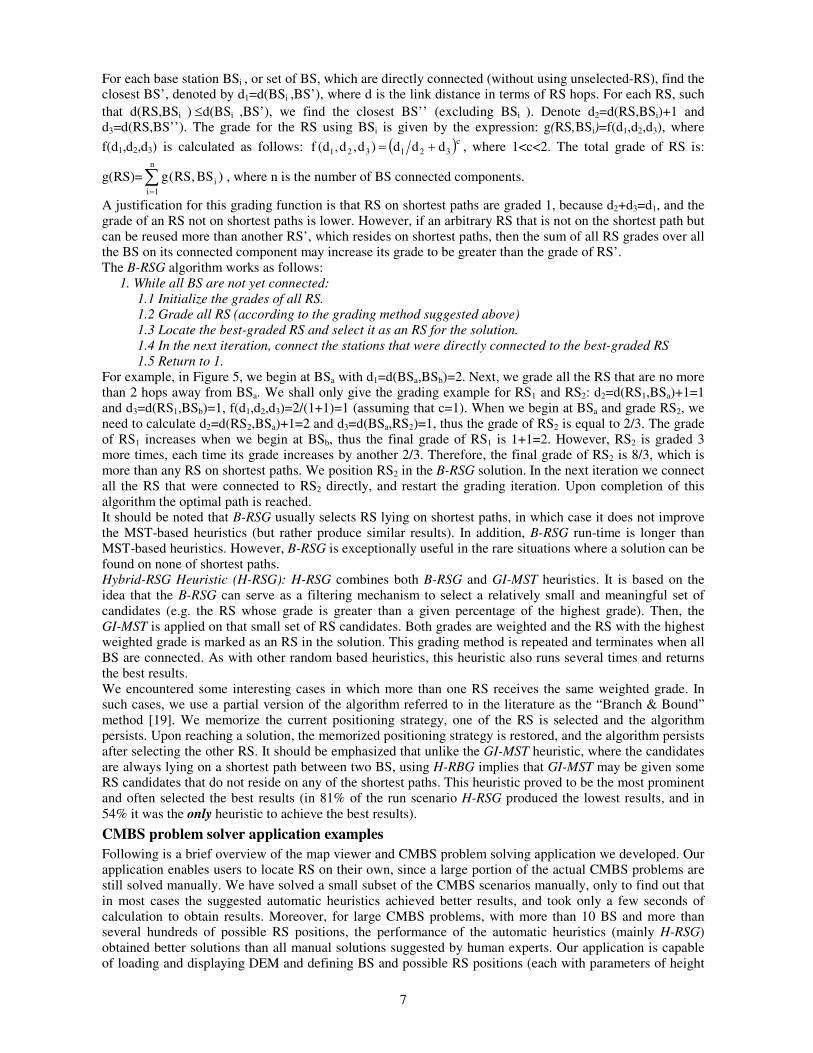
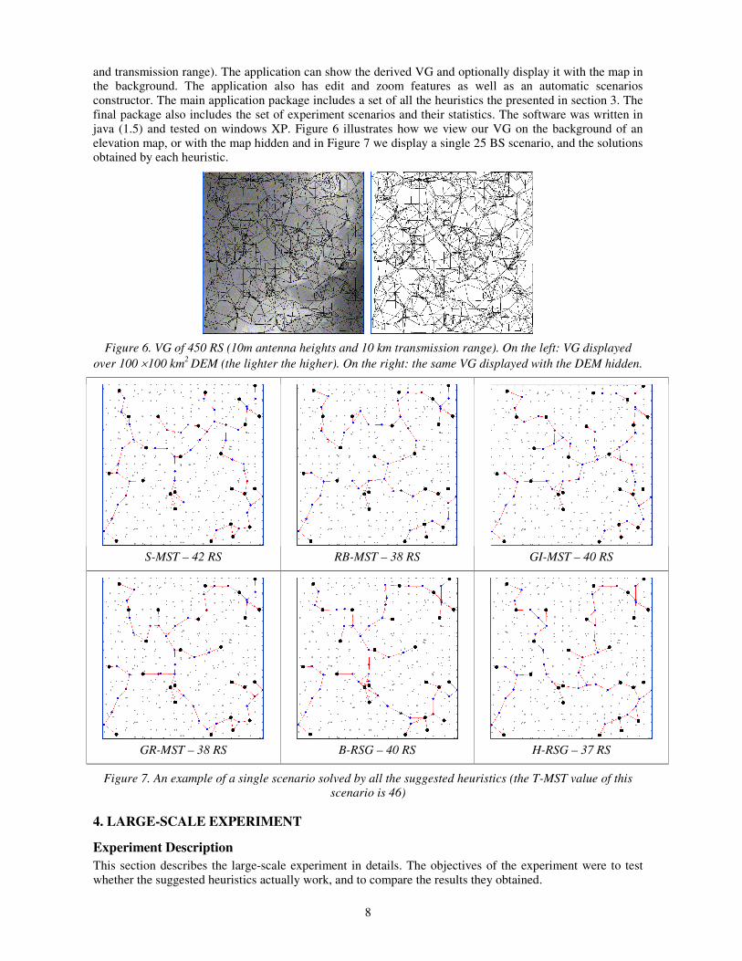
and transmission range). The application can show the derived VG and optionally display it with the map in the background. The application also has edit and zoom features as well as an automatic scenarios constructor. The main application package includes a set of all the heuristics the presented in section 3. The final package also includes the set of experiment scenarios and their statistics. The software was written in java (1.5) and tested on windows XP. Figure 6 illustrates how we view our VG on the background of an elevation map, or with the map hidden and in Figure 7 we display a single 25 BS scenario, and the solutions obtained by each heuristic.

Figure 6. VG of 450 RS (10m antenna heights and 10 km transmission range). On the left: VG displayed

over 100�100 km2 DEM (the lighter the higher). On the right: the same VG displayed with the DEM hidden.

S-MST – 42 RS RB-MST – 38 RS GI-MST – 40 RS

GR-MST – 38 RS B-RSG – 40 RS H-RSG – 37 RS

Figure 7. An example of a single scenario solved by all the suggested heuristics (the T-MST value of this scenario is 46)

4. LARGE-SCALE EXPERIMENT

Experiment Description This section describes the large-scale experiment in details. The objectives of the experiment were to test whether the suggested heuristics actually work, and to compare the results they obtained.

9

We defined an experiment scenario by a vector of one permutation of the parameters specified in Table 1 (e.g. map#2, Selecting positions for 10 BS, with all antennas height = 30m, and transmission ranges = 10km, with 1,000 potential RS). We tested many different possible sets of scenarios, and the experiment consisted of a total of approximately 7,000 scenarios (about one quarter of the possible permutations) using all the heuristics detailed in Section 3. We neglected the non-realistic cases, such as: long ranged antennas used with many RS, or short ranged antennas with few potential RS. We selected 17 high-resolution elevation maps (100�100 km2), each representing a different type of terrain: flat, hills, dunes, mountains, lakes, etc. We positioned the selected number of BS on the map either by selecting a subset of the potential RS (which is a reasonable strategy, because BS are usually positioned on high topology points) or randomly. For each permutation of the parameters (i.e number of BS, number of potential RS, antenna heights and transmission ranges) we tested 10 different positions for BS.

Parameter Permutations Maps 17

Total BS on a map (10/25/50/100 BS) 4

Number of BS positions for each parameter vector 10

Antenna Heights (10/20/30/50 m) 4

Transmission ranges (5/10/20 km) 3

Potential relay stations (500, 1000, 2500, 100000 relays) 4

Table 1. List of Tested Parameters in the Large-Scale Experiment

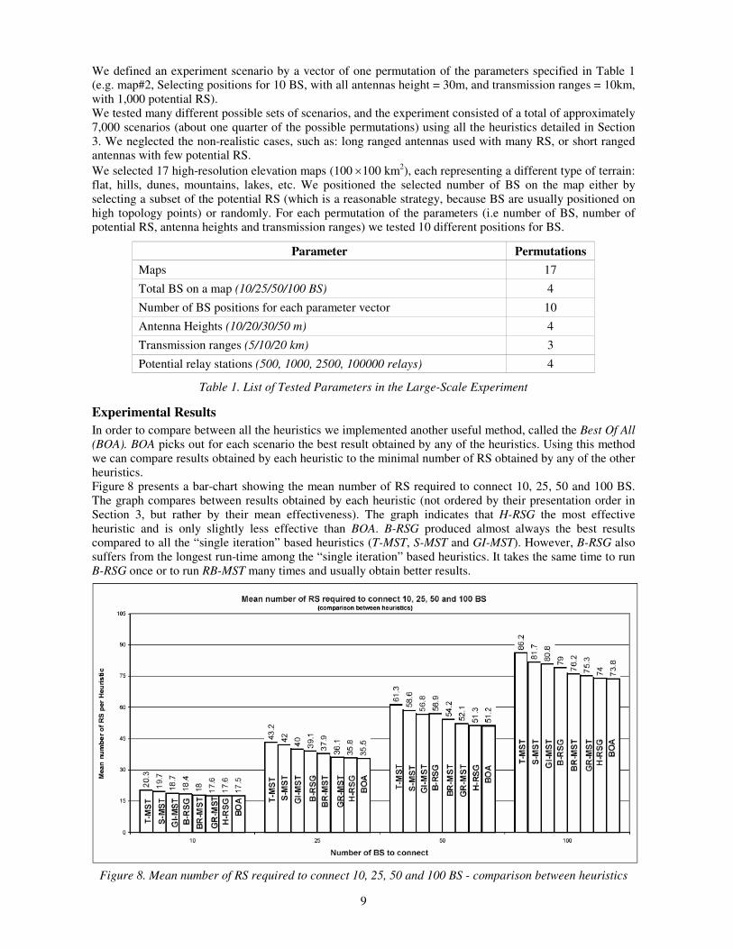
Experimental Results In order to compare between all the heuristics we implemented another useful method, called the Best Of All (BOA). BOA picks out for each scenario the best result obtained by any of the heuristics. Using this method we can compare results obtained by each heuristic to the minimal number of RS obtained by any of the other heuristics. Figure 8 presents a bar-chart showing the mean number of RS required to connect 10, 25, 50 and 100 BS. The graph compares between results obtained by each heuristic (not ordered by their presentation order in Section 3, but rather by their mean effectiveness). The graph indicates that H-RSG the most effective heuristic and is only slightly less effective than BOA. B-RSG produced almost always the best results compared to all the “single iteration” based heuristics (T-MST, S-MST and GI-MST). However, B-RSG also suffers from the longest run-time among the “single iteration” based heuristics. It takes the same time to run B-RSG once or to run RB-MST many times and usually obtain better results.

Figure 8. Mean number of RS required to connect 10, 25, 50 and 100 BS - comparison between heuristics

10

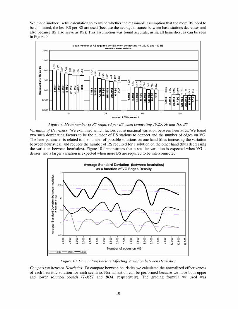
We made another useful calculation to examine whether the reasonable assumption that the more BS need to be connected, the less RS per BS are used (because the average distance between base stations decreases and also because BS also serve as RS). This assumption was found accurate, using all heuristics, as can be seen in Figure 9.

Figure 9. Mean number of RS required per BS when connecting 10,25, 50 and 100 BS

Variation of Heuristics: We examined which factors cause maximal variation between heuristics. We found two such dominating factors to be the number of BS stations to connect and the number of edges on VG. The later parameter is related to the number of possible solutions on one hand (thus increasing the variation between heuristics), and reduces the number of RS required for a solution on the other hand (thus decreasing the variation between heuristics). Figure 10 demonstrates that a smaller variation is expected when VG is denser, and a larger variation is expected when more BS are required to be interconnected.

Figure 10. Dominating Factors Affecting Variation between Heuristics

Comparison between Heuristics: To compare between heuristics we calculated the normalized effectiveness of each heuristic solution for each scenario. Normalization can be performed because we have both upper and lower solution bounds (T-MST and BOA, respectively). The grading formula we used was

11

���

���

�

���

��)BOA(RS)MSTT(RS

)BOA(RS)h(RS1)h(Grade , where h denotes a heuristic and RS(x) denotes the number of

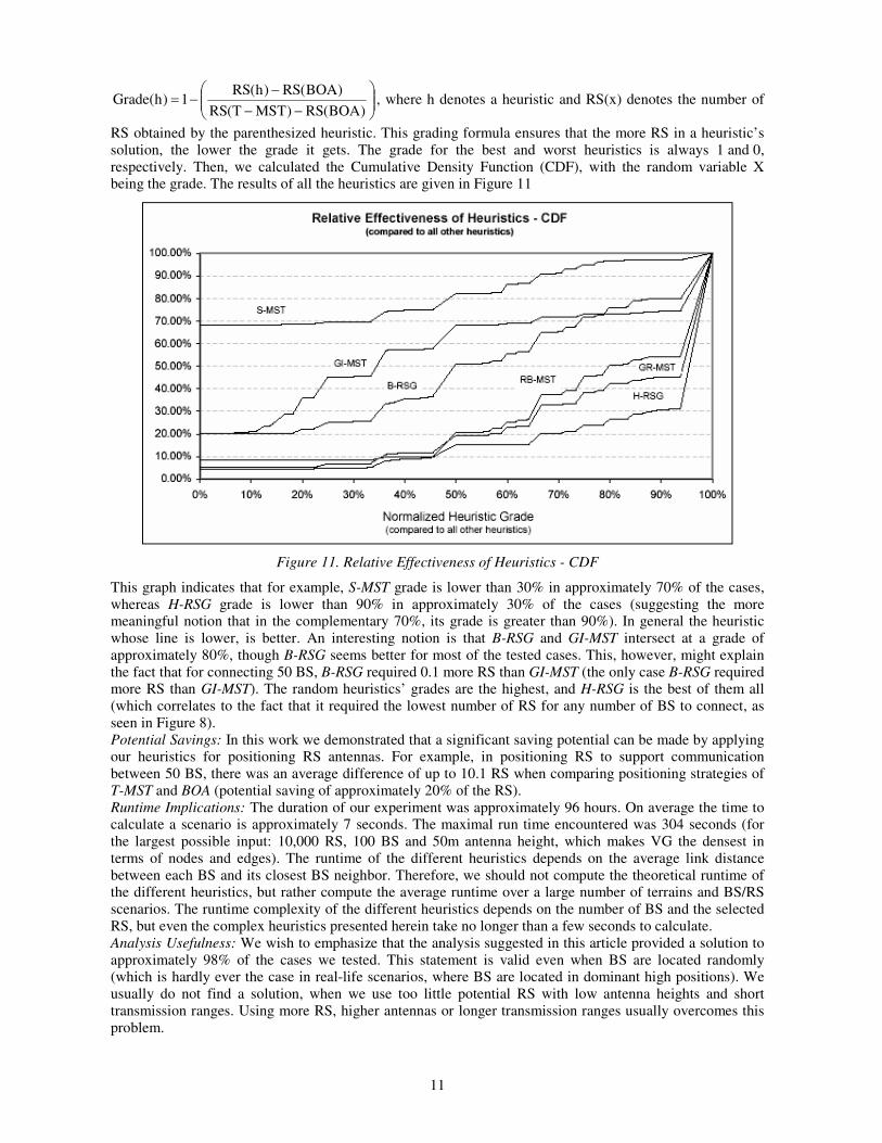
RS obtained by the parenthesized heuristic. This grading formula ensures that the more RS in a heuristic’s solution, the lower the grade it gets. The grade for the best and worst heuristics is always 1 and 0, respectively. Then, we calculated the Cumulative Density Function (CDF), with the random variable X being the grade. The results of all the heuristics are given in Figure 11

Figure 11. Relative Effectiveness of Heuristics - CDF

This graph indicates that for example, S-MST grade is lower than 30% in approximately 70% of the cases, whereas H-RSG grade is lower than 90% in approximately 30% of the cases (suggesting the more meaningful notion that in the complementary 70%, its grade is greater than 90%). In general the heuristic whose line is lower, is better. An interesting notion is that B-RSG and GI-MST intersect at a grade of approximately 80%, though B-RSG seems better for most of the tested cases. This, however, might explain the fact that for connecting 50 BS, B-RSG required 0.1 more RS than GI-MST (the only case B-RSG required more RS than GI-MST). The random heuristics’ grades are the highest, and H-RSG is the best of them all (which correlates to the fact that it required the lowest number of RS for any number of BS to connect, as seen in Figure 8). Potential Savings: In this work we demonstrated that a significant saving potential can be made by applying our heuristics for positioning RS antennas. For example, in positioning RS to support communication between 50 BS, there was an average difference of up to 10.1 RS when comparing positioning strategies of T-MST and BOA (potential saving of approximately 20% of the RS). Runtime Implications: The duration of our experiment was approximately 96 hours. On average the time to calculate a scenario is approximately 7 seconds. The maximal run time encountered was 304 seconds (for the largest possible input: 10,000 RS, 100 BS and 50m antenna height, which makes VG the densest in terms of nodes and edges). The runtime of the different heuristics depends on the average link distance between each BS and its closest BS neighbor. Therefore, we should not compute the theoretical runtime of the different heuristics, but rather compute the average runtime over a large number of terrains and BS/RS scenarios. The runtime complexity of the different heuristics depends on the number of BS and the selected RS, but even the complex heuristics presented herein take no longer than a few seconds to calculate. Analysis Usefulness: We wish to emphasize that the analysis suggested in this article provided a solution to approximately 98% of the cases we tested. This statement is valid even when BS are located randomly (which is hardly ever the case in real-life scenarios, where BS are located in dominant high positions). We usually do not find a solution, when we use too little potential RS with low antenna heights and short transmission ranges. Using more RS, higher antennas or longer transmission ranges usually overcomes this problem.

12

5. FUTURE WORK Further research may include additional heuristics and fine-tuning to the ones suggested here, or generalizing the CMBS problem to a weighted CMBS problem, in which the objective function is weighted, subject to the same constraint of connecting all BS seems as a good direction for research. One obvious application for this generalization is to solve the CMBS problem while minimizing the installation cost, for example by assuming different costs to different RS types. We also think that the algorithm for selection of potential RS antenna positioning can be improved in terms of runtime complexity and approximation factor. Another aspect of the CMBS problem is to compute a lower bound for a given input by employing continuous linear programming based methods.

ACKNOLEGMENTS The authors wish to thank Irena Rabaev who helped implement the CMBS algorithms, Paz Carmi for the helpful discussions, and Nili Ben-Yehezkel for her patience and long hours of editing and proof reading.

BIBLIOGRAPHY [1] http://www.schema.com/ [2] http://www.hexagonltd.com/ [3] Vasquez M. and Hao J.K., “A Heuristic Approach for Antenna Positioning in Cellular Networks,”

Journal of Heuristics, 7(5): pp. 443-472, 2001 [4] Anderson H.R. and McGeehan J.P., “Optimizing Microcell Base Station Locations Using Simulated

Annealing Techniques,” Proc. of the IEEE Vehicular Technology Conference, pp. 858-862, 1994. [5] Tutschku K., “Demand-based Radio Network Planning of Cellular Mobile Communication System,”

Infocom 98 Conference, San Francisco, USA, 1998. [6] Sherali H.D., Pendyala C.M. and Rappaport T.S., “Optimal Location of Transmitters for Micro-Cellular

Radio Communication System Design,” IEEE Journal on Selected Areas in Communications, 14(4): pp. 662-673, 1996.

[7] Hao J.K., Dorne R. and Galinier P., “Tabu Search for Frequency Assignement in Mobile Radio Networks,” Journal of Heuristics, 4 (1): pp. 47-62, 1998.

[8] The QConvex user manual available at http://www.qhull.org/ [9] Blaunstein N., “Radio Propagation in Cellular Networks,” Artech House, 1999. [10] Karp R.M., “Reducibility among combinatorial problems,” Complexity of Computer Computations (R.

E. Miller and J. W. Thatcher, eds.), Plenum Press, New York, pp. 85-103, 1972. [11] Feige U., “A threshold of ln n for approximating set cover (preliminary version),” Proceedings of the

twenty-eighth annual ACM symposium on Theory of computing, pp. 314-318, 1996. [12] Mitchell J.S.B., “Geometric shortest paths and network optimization,” J.-R. Sack and J. Urrutia,

editors, Handbook of Computational Geometry, 1998. [13] Agarwal P.K., Har-Peled S., Sharir, M. and Varadarajan K.R., “Approximate Shortest Paths on a

Convex Polytope in Three Dimensions,” J. ACM, (44): pp. 567-584, 1997. [14] Har-Peled S., “Constructing approximate shortest path maps in three dimensions,” SIAM J. Comput., (28),

pp. 1182—1197, 1999. [15] Tan X., “Approximation algorithms for the watchman route and zookeeper's problems,” J. Discrete Appl.

Math., (136): pp. 363—376, 2004. [16] P. Calegari, F. Guidec, P. Kuonen and F. Nielsen, “Combinatorial optimization algorithms for radio

network planning,” Theoretical Computer Science (263), pp. 235-245, 2001. [17] Ben-Moshe B., “Geometric Facility Location Optimization”, PhD thesis (chapter 7), 2004. [18] Hwang F.K., Richards D.S. and Winter P., “The Steiner tree problem,” Elsevier, pp. 93−202, 1992. [19] Efroymson, M.A. and Ray T.L. “A branch and bound algorithm for plant location”. Operations

Research, 14, 361-368, 1966.