AN APPLICATION OF 3D LOGICAL STRUCTURE IN A DHT ...
281
AN APPLICATION OF 3D LOGICAL STRUCTURE IN A DHT PARADIGM FOR EFFICIENT COMMUNICATION IN MANETS SHAHBAZ AKHTAR ABID THESIS SUBMITTED IN FULFILMENT OF THE REQUIREMENTS FOR THE DEGREE OF DOCTOR OF PHILOSOPHY FACULTY OF COMPUTER SCIENCE AND INFORMATION TECHNOLOGY UNIVERSITY OF MALAYA KUALA LUMPUR 2014
-
Upload
khangminh22 -
Category
Documents
-
view
2 -
download
0
Transcript of AN APPLICATION OF 3D LOGICAL STRUCTURE IN A DHT ...

AN APPLICATION OF 3D LOGICAL STRUCTURE
IN A DHT PARADIGM FOR
EFFICIENT COMMUNICATION IN MANETS
SHAHBAZ AKHTAR ABID
THESIS SUBMITTED IN FULFILMENT
OF THE REQUIREMENTS
FOR THE DEGREE OF DOCTOR OF PHILOSOPHY
FACULTY OF COMPUTER SCIENCE AND
INFORMATION TECHNOLOGY
UNIVERSITY OF MALAYA
KUALA LUMPUR
2014

Dedication
This thesis is dedicated to my father whose will, support, and prayers drives me through all the way to
make this dream a reality and my mother whose prayers have always been a source of my success.

UNIVERSITI MALAYA
ORIGINAL LITERARY WORK DECLARATION
Name of Candidate: Shahbaz Akhtar Abid (I.C/Passport No: ) AM1079722
Registration/Matric No: WHA110020
Name of Degree: Doctor of Philosophy
Title of Project Paper/Research Report/Dissertation/Thesis (“this Work”): An Application of 3D Logical Structure
in a DHT Paradigm for Efficient Communication in MANETs
Field of Study: Computer Science
I do solemnly and sincerely declare that:
(1) I am the sole author/writer of this Work;
(2) This Work is original;
(3) Any use of any work in which copyright exists was done by way of fair dealing and for permitted
purposes and any excerpt or extract from, or reference to or reproduction of any copyright work
has been disclosed expressly and sufficiently and the title of the Work and its authorship have been
acknowledged in this Work;
(4) I do not have any actual knowledge nor do I ought reasonably to know that the making of this
work constitutes an infringement of any copyright work;
(5) I hereby assign all and every rights in the copyright to this Work to the University of Malaya
(“UM”), who henceforth shall be owner of the copyright in this Work and that any reproduction or
use in any form or by any means whatsoever is prohibited without the written consent of UM
having been first had and obtained;

(6) I am fully aware that if in the course of making this Work I have infringed any copyright whether
intentionally or otherwise, I may be subject to legal action or any other action as may be
determined by UM.
Candidate’s Signature Date
Subscribed and solemnly declared before,
Witness’s Signature Date
Name: Mazliza Binti Othman
Designation: Senior Lecturer

Abstract
In the last few years, Distributed Hash Table (DHT) has come forth as a useful additional technique to
the design and specification of spontaneous and self-organized networks. Researchers have exploited its
strengths by implementing it at the network layer and developing scalable routing protocols for mobile
adhoc networks (MANETs). This study investigates the features, strengths and weaknesses of existing
DHT-based routing protocols and identifies key research challenges that are vital to address, namely the
mismatch problem, merging of logical networks, and resilience of logical structure.
This thesis proposes a novel three-dimensional DHT-based routing protocol, named 3D-RP, which
exploits a 3D logical space that takes into account the physical intra-neighbor relationships of a node
and exploits a 3D structure to interpret that relationship. The three- dimensional logical space (3D-LS)
gives a node the liberty to exactly interpret the physical relationship of nodes in the three-dimensional
logical structure (3D-LIS), which helps to avoid the mismatch problem.
This work also addresses the mismatch problem between the overlay network and the physical network
in P2P protocols over MANET that works at the application layer. Moreover, this study presents a novel
protocol for content sharing in P2P over MANET that is a variation of 3D-RP and exploits a 3-
dimensional overlay and 3D space at the application layer to avoid the mismatch problem in P2P over
MANETs.
The inefficiency of merging logical networks is addressed with the proposed leader-based approach
(LA), which detects and merges DHT-based logical networks. LA is embedded in 3D-RP and MDART
to compare their performance when merging two logical networks.
3D-RP and LA are compared with the existing schemes on the basis of path-stretch ratio, end-to-end
delay, packet delivery ratio, false negative ratio, loss ratio, and routing overhead. Simulation results
show that the proposed protocols effectively handle the mismatch problem, merging of logical networks,
and resilience of the logical structure.

Abstrak
Dalam beberapa tahun kebelakangan ini, Jadual Cincang Teragih (DHT) telah tampil sebagai teknik
tambahan yang berguna untuk mereka bentuk dan spesifikasi rangkaian spontan dan rancang-kendiri.
Para penyelidik telah menggunakan kekuatannya dengan melaksanakannya pada lapisan rangkaian dan
untuk membangunkan protokol penghalaan berskala untuk rangkaian adhoc kembara (MANETs).
Kajian ini menyiasat ciri-ciri, kekuatan dan kelemahan protokol penghalaan berasaskan DHT yang sedia
ada dan mengenal pasti cabaran utama penyelidikan yang penting untuk ditangani, iaitu masalah tidak
cocok, penggabungan rangkaian logikal, dan daya tahan struktur logikal.
Tesis ini mencadangkan protokol penghalaan baru tiga dimensi yang berasaskan DHT, dinamakan 3D-
RP, yang mengeksploitasi ruang logikal 3D dengan mengambil kira hubungan fizikal antara jiran bagi
suatu nod dan mengeksploitasi struktur 3D untuk mentafsir hubungan tersebut. Ruang logikal tiga
dimensi (3D-LS) memberikan nod kebebasan untuk menafsir hubungan fizikal nod dalam struktur
logikal tiga dimensi (3D-LIS) dengan tepat, yang mana ini membantu untuk mengelakkan masalah tidak
cocok.
Kajian ini juga menangani masalah tidak cocok antara rangkaian penindisan atas dan rangkaian fizikal
dalam protokol P2P atas MANET pada lapisan aplikasi. Selain itu, kajian ini membentangkan protokol
baru untuk perkongsian kandungan dalam P2P atas MANET yang merupakan variasi 3D-RP dan
mengeksploitasi penindisan atas 3-dimensi dan ruang 3D di peringkat aplikasi untuk mengelakkan
masalah tidak cocok dalam P2P atas MANET.
Ketidakcekapan penggabungan rangkaian logikal ditangani dengan pendekatan berasaskan pemimpin
(LA), yang mengesan dan menggabungkan rangkaian logikal berasaskan DHT. LA ditanam dalam 3D-
RP dan MDART untuk membandingkan prestasi mereka apabila menggabungkan dua rangkaian logikal.
3D-RP dan LA dibandingkan dengan skema sedia ada berdasarkan nisbah rentangan-laluan, lengah
hujung ke hujung, nisbah penghantaran bingkisan, nisbah negatif palsu, nisbah hilang, dan overhed
penghalaan. Keputusan simulasi menunjukkan bahawa protokol yang dicadangkan berkesan dalam
menangani masalah tidak cocok, penggabungan rangkaian logikal dan daya tahan struktur logikal.

Acknowledgement
Allah, the most beneficient, the most compassionate and merciful whose benevolence and blessings
enabled me to accomplish this task.
I would like to express heartfelt gratitude to my supervisors Dr. Mazliza Othman and Dr. Nadir Shah
(from COMSATS Institute of Information Technology, WahCantt). Their vision, expertise, support,
attention, and hard work guided me to the successful completion of this thesis. I am thankful to their
consistent efforts and true desire to keep me on track.
I express my heartfelt gratitude to my parents (Akhtar Ali Abid and Perveen Akhtar), my teacher Qari
Muhammad Siddique, my brothers Sheraz Akhtar and Dr. Faraz Akhtar , and especially my wife (Amna
Akhtar) and my daughter (Zaynah Akhtar) for their love, prayers, moral support, encouragements, and
sincere wishes for the completion of my work.
I am deeply indebted to my friends Rao Muhammad Adeel Nawab and Osama Fuad Akasha Sabir
whose guidance, suggestions, and encouragements remained continual source of inspiration for me
throughout the course of study.
I am grateful to University of Malaya (UM) for providing us a tremendous opportunity, guidance, and
continuous motivational, financial, and technical support. I am thankful to CIIT for providing us a
plateform to get this opportunity.
Thanks are in order for Faheem Khan, Jawad Shafi, Muhammad Omer Yaqoob, Rab Nawaz Jadoon,
Touseef Tahir, Muhammad Nasir Khan, Tayyab Chaudhary, Ahmed Kareem, Atta ur Rehman Khan,
and Irum Inayat whose decorousness, continuous tangible, moral support and willingness to help me,

especially in early stages, made this work possible. I wish them happiness and success throughout their
life.

List of Publications
1. ABID, S. A., OTHMAN, M. & SHAH, N. 2014. A Survey on DHT-Based Routing for Large-
Scale Mobile Ad Hoc Networks. ACM Comput. Surv., 47, 1-46.
2. ABID, S. A., OTHMAN, M. & SHAH, N. 2014. 3D P2P overlay over MANETs. Computer
Networks, 64, 89-111.
3. ABID, S. A., OTHMAN, M. & SHAH, N. 2014. 3D-RP: A DHT-based Routing Protocol for
MANETs. Computer Journal, Accepted for publication. DOI:10.1093/comjnl/bxu004
4. ABID, S. A., OTHMAN, M. & SHAH, N. 2013. Exploiting 3D Structure for Scalable Routing in
MANETs. Communications Letters, IEEE, 17, 2056-2059.

Table of Content
1 Introduction ........................................................................................................................................................1
1.1 Problem Statement ......................................................................................................................................2
1.2 Objectives of Study ....................................................................................................................................4
1.3 Hypothesis ..................................................................................................................................................5
1.4 Thesis Outline .............................................................................................................................................5
2 Dynamic Addressing, Location Services, and Routing using DHTs in MANETs .............................................7
2.1 Distributed Hash Tables (DHTs) and DHT-based Logical Identifier Strucure (LIS) ................................8
2.2 DHT-based Routing in MANETs ...............................................................................................................9
2.2.1 LID Addressing ................................................................................................................................10
2.2.2 Lookup ..............................................................................................................................................10
2.2.3 Routing .............................................................................................................................................11
2.3 Classification of dht-based routing protocols ...........................................................................................12
2.3.1 DHT-based Overlay Deployment Protocols .....................................................................................13
2.3.2 DHT Paradigm for Large Scale Routing ..........................................................................................16
2.3.2.1 DHT for Addressing in MANET ..................................................................................................20
2.3.2.2 DHT for Routing in MANET .......................................................................................................24
2.3.3 Challenges and Requirements to Develop DHT-based Large Scale Routing Protocols for MANETs
45
2.3.3.1 Mismatch between Logical and Physical Topologies ..................................................................45
2.3.3.2 High Maintenance Overhead ........................................................................................................49
2.3.3.3 Selection of LIS Structure ............................................................................................................50
2.3.3.4 Address Space Utilization ............................................................................................................52
2.3.3.5 Partitioning and Merging ..............................................................................................................52
2.3.4 Analysis of the Existing DHT-based Paradigms for Large scale Routing .......................................54
2.4 conclusions ...............................................................................................................................................57
3 3D-RP: A DHT-based Routing Protocol for MANETs ...................................................................................60
3.1 Introduction ..............................................................................................................................................60
3.2 System Model ...........................................................................................................................................64
3.3 Joining Operations ....................................................................................................................................66
3.3.1 LID Computation ..............................................................................................................................66
3.3.2 Anchor Node Computation ...............................................................................................................78

3.4 Greedy Logical Routing Algorithm ..........................................................................................................81
3.5 Node dynamics and failures .....................................................................................................................84
3.6 Performance Analysis ...............................................................................................................................86
3.6.1 Quality of Routing Paths ..................................................................................................................89
3.6.2 Impact of Traffic Load .....................................................................................................................93
3.6.3 Impact of Network Size ..................................................................................................................102
3.7 Conclusion ..............................................................................................................................................113
4 Merging of DHT-based Logical Networks in MANETs ................................................................................114
4.1 Merging of DHT-based Logical Identifier Structures in MANETs .......................................................115
4.2 Merging detection ...................................................................................................................................118
4.2.1 Leader-based Approach (LA) to Detect Two Distinct Networks ...................................................119
4.3 Merging Process .....................................................................................................................................120
4.4 Merging in DHT-based Logical Identifier Structures ............................................................................121
4.4.1 Node Joining Algorithms................................................................................................................122
4.4.2 Resilience of the LIS ......................................................................................................................122
4.4.3 Logical network merger case-study: MDART ...............................................................................124
4.4.4 Analysis of Merging in DHT-based Routings ................................................................................129
4.5 3D-based LIS ..........................................................................................................................................131
4.5.1 Logical network merger case-study: 3D-RP...................................................................................132
4.6 Performance Analysis .............................................................................................................................137
4.6.1 Quality of Routing Paths ................................................................................................................139
4.6.2 Impact of network size ...................................................................................................................143
(a) End-to-End delay ................................................................................................................................143
(b) Packet Delivery Ratio .........................................................................................................................150
(c) Routing Overhead ...............................................................................................................................157
(d) False negative (FN) ratio ....................................................................................................................164
4.7 Conclusion ..............................................................................................................................................171
5 3D P2P Overlay over MANETs .....................................................................................................................173
5.1 Introduction ............................................................................................................................................173
5.2 3D Overlay Protocol (3DO) ...................................................................................................................180
5.2.1 Peer Join .........................................................................................................................................181
5.2.2 Update.............................................................................................................................................192

5.3 Primary Anchor Peer Computation and File Index Information storage ................................................193
5.4 File discovery .........................................................................................................................................196
5.5 Replication Strategy ...............................................................................................................................199
5.6 Performance Evaluation of 3DO ............................................................................................................200
5.6.1 Routing Overhead ...........................................................................................................................202
5.6.2 Average File Discovery Delay .......................................................................................................210
5.6.3 False-negative (FN) ratio ................................................................................................................219
5.6.4 Path-Stretch Ratio ...........................................................................................................................228
5.7 Conclusions ............................................................................................................................................237
6 Modelling and Analysis using formal methods ..............................................................................................239
6.1 High Level Petri Nets .............................................................................................................................239
6.2 SMT-Lib and Z3 .....................................................................................................................................239
6.3 Formal Analysis and Verification...........................................................................................................240
6.4 Verification Property ..............................................................................................................................244
7 Conclusion ......................................................................................................................................................245
7.1 SIGNIFICANCE OF CONTRIBUTIONs ..............................................................................................245
7.2 Future Trends and DHT-based routing ...................................................................................................246
7.2.1 Content Centric Networking (CCN) ...............................................................................................247
7.2.2 Device-to-Device (D2D) Communication ......................................................................................247
7.2.2.1 Multi-hops D2D communication ................................................................................................248
7.2.3 Integrated MANET and Internet .....................................................................................................249
7.2.4 Internet of Things (IoT) ..................................................................................................................250
7.2.5 Machine-to-Machine (M2M) Communications .............................................................................251

List of Figures
Figure 2.1: An example of DHT-based routing ........................................................................................................11
Figure 2.2: Overlay Network over Physical Network ..............................................................................................12
Figure 2.3: Classification of DHT based routing Protocols .....................................................................................20
Figure 2.4: Relationship between Virtual Ring and Physical Topology ..................................................................22
Figure 2.5: Hypercube with d=4 (curtesy from (Alvarez-Hamelin et al., 2006)) .....................................................28
Figure 2.6: Spontaneous Network: physical position of nodes (Curtesy from (Alvarez-Hamelin et al., 2006)) .....29
Figure 2.7: DART Logical Address Tree and Corresponding Physical Network ....................................................31
Figure 2.8: Node(0.0) sends a packet towards node(0.51). The solid line represents a logical cord. The solid
arrows show the route of the packet. A dead end is detected as node 0.47 fails. The dashed arrows represent the
NP packet to find an alternative route. The dotted arrow is the NBP to avoid loops. Nodes use greedy forwarding
to send packet toward the destination node 0.51. .....................................................................................................36
Figure 2.9: N sends data to node K. Node C acts as the anchor for K. ....................................................................38
Figure 2.10: An example of path-stretch penalty caused by uncorrelated Logical Address Space and Physical
Network ....................................................................................................................................................................47
Figure 2.11: Mismatch problem - a VCP example: dashed lines is cord maintained by the VCP protocol. ...........49
Figure 3.1: 3D Logical Identifier Structure. .............................................................................................................65
Figure 3.2: The joining process. Solid lines represent the local LIS of a node. Dashed lines are the physical links
between nodes in the PT ...........................................................................................................................................69
Figure 3.3: Flow chart of Joining Algorithm ............................................................................................................76
Figure 3.4 : A logical view of the physical arrangement of nodes in the local 3D-LIS of node i and p maintained
by 3D-RP ..................................................................................................................................................................77
Figure 3.5: Illustrates the example of the following processes: i) Anchor node (AN) computation; ii) Greedy LID-
based Routing ...........................................................................................................................................................80
Figure 3.6: Routing Table of node i with LID {1|1|1}-0 ..........................................................................................83
Figure 3.7: Examples of node dynamics and failures: a) Node u and node l acquire a new LID on repositioning; b)
An intermediate node fails and the selection of an alternative route is initiated while sending a packet to node u .86
Figure 3.8: Path-stretch ratio as a function of network size .....................................................................................90
Figure 3.9: Average end-to-end delay as a function of traffic load ..........................................................................94

Figure 3.10: Loss ratio as a function of traffic load .................................................................................................97
Figure 3.11: Routing Overhead as a function of traffic load ....................................................................................99
Figure 3.12: Percentage of improvement provided by 3D-RP over MDART as a function of traffic load ...........100
Figure 3.13: Average End-to-End delay as a function of the node number ...........................................................103
Figure 3.14: : Packet delivery ratio as a function of the node number ...................................................................105
Figure 3.15: Percentage of MAC collisions per data packet sent as a function of the node number .....................108
Figure 3.16: Routing overhead as a function of the node number ..........................................................................110
Figure 3.17: Percentage of improvement provided by 3D-RP over MDART as a function of the node number ..111
Figure 4.1: A partitioned network into two disconnected topologies .....................................................................116
Figure 4.2: Merging of two logical networks using MDART ................................................................................127
Figure 4.3: Merging of two logical networks using 3D-RP ...................................................................................135
Figure 4.4: Routing Tables for node i, q, p, s .........................................................................................................137
Figure 4.5: Path-stretch ratio as a function of the network size .............................................................................140
Figure 4.6: End-to-End delay as a function of network size with varying node speed ..........................................145
Figure 4.7: Packet Delivery Ratio as a function of network size with varying node speed ...................................152
Figure 4.8: Routing Overhead as function of network size with varying node speed ............................................158
Figure 4.9: False negative ratio with respect to network size with varying node speed ........................................165
Figure 4.10: Percentage of improvement provided by LA-3D-RP over LA-MDART as a function of the node
number at various node speed ................................................................................................................................170
Figure 5.1: The peer-joining process. The dashed lines are the physical links between neighboring peers in the
physical network. ....................................................................................................................................................186
Figure 5.2: Flow chart of Peer Joining Algorithm ..................................................................................................190
Figure 5.3: A logical view of the physical arrangement of neighboring peers in the local 3D-Overlay of peer Pi
maintained by the 3DO. ..........................................................................................................................................192
Figure 5.4: Peer-routing table for peers Pj, Ps, and Pu ............................................................................................195
Figure 5.5: File’s index information storage, lookup, and retrieval process in 3DO. The overlay network on left
side shows the arrangement of peers in 3D-Overlay. The physical network on the right describes the physical
arrangement of nodes in the P2P network. .............................................................................................................198

Figure 5.6: Routing Overhead as a function of peers ratio .....................................................................................204
Figure 5.7: Average file discovery delay as a function of peers ratio ....................................................................213
Figure 5.8: False negative ratio as a function of peers ratio ...................................................................................222
Figure 5.9: Path-stretch ratio as a function of peers ratio .......................................................................................230
Figure 5.10: Percentage improvement with respect to MA-SP2P at node speeds 0.5m/s, 1m/s, 1.5m/s, 2m/s ......237
Figure 6.1: HLPN model for 3DO. .........................................................................................................................241
Figure 7.1: An example scenario for underlay D2D single-hop (S to D1) and multi-hops (S to D2)
communication. ......................................................................................................................................................249
Figure 7.2: Possible use of MANETs in 4G networks (Ding, 2008) ......................................................................250

List of Tables
Table 2.1: Definitions of important terms related to DHT-based Routing in MANETs ............................................8
Table 2.2: Classification of DHT-based routing protocols based on how they use DHT ........................................19
Table 2.3: Summarized features of DHT-based protocols for scalable routing in MANETs .................................42
Table 3.1: List of dim values ....................................................................................................................................68
Table 3.2: Simulation Parameters .............................................................................................................................87
Table 3.3: Summary of data analysis of the path-stretch ratio for 3D-RP and MDART using ANOVA Two-Factor
with replication .........................................................................................................................................................92
Table 3.4: Results: pairwise data analysis of path-stretch ratio at each network size for 3D-RP and MDART using
ANOVA Two-Factor With Replication ...................................................................................................................92
Table 3.5: Summary of data analysis of the end-to-end delay for 3D-RP and MDART using ANOVA Two-Factor
with replication .........................................................................................................................................................95
Table 3.6: Results: pairwise data analysis of end-to-end delay at each network size for 3D-RP and MDART using
ANOVA Two-Factor With Replication ...................................................................................................................96
Table 3.7: Summary of data analysis of the loss ratio for 3D-RP and MDART using ANOVA Two-Factor with
replication .................................................................................................................................................................97
Table 3.8: Results: pairwise data analysis of the loss ratio at each network size for 3D-RP and MDART using
ANOVA Two-Factor With Replication ...................................................................................................................98
Table 3.9: Summary of data analysis of the routing overhead for 3D-RP and MDART using ANOVA Two-Factor
with replication .......................................................................................................................................................100
Table 3.10: Results: pairwise data analysis of routing overhead at each network size for 3D-RP and MDART
using ANOVA Two-Factor With Replication ........................................................................................................101
Table 3.11: Summary of data analysis of the end-to-end delay for 3D-RP and MDART using ANOVA Two-
Factor with replication ............................................................................................................................................104
Table 3.12: Results: pairwise data analysis of end-to-end delay at each network size for 3D-RP and MDART
using ANOVA Two-Factor With Replication ........................................................................................................104
Table 3.13: Summary of data analysis of the packet delivery ratio for 3D-RP and MDART using ANOVA Two-
Factor with replication ............................................................................................................................................106
Table 3.14: Results: pairwise data analysis of the packet delivery ratio at each network size for 3D-RP and
MDART using ANOVA Two-Factor With Replication ........................................................................................107

Table 3.15: Summary of data analysis of the percentage of MAC collision per data packet for 3D-RP and
MDART using ANOVA Two-Factor with replication ...........................................................................................109
Table 3.16: Results: pairwise data analysis of the percentage of MAC collisions per data packet at each network
size for 3D-RP and MDART using ANOVA Two-Factor With Replication .........................................................109
Table 3.17: Summary of data analysis of routing overhead for 3D-RP and MDART using ANOVA Two-Factor
with replication .......................................................................................................................................................112
Table 3.18: Results: pairwise data analysis of routing overhead at each network size for 3D-RP and MDART
using ANOVA Two-Factor With Replication ........................................................................................................112
Table 4.1: Simulation Parameters ...........................................................................................................................139
Table 4.2: Summary of data analysis of the path-stretch Ratio for LA-3D-RP and LA-MDART using ANOVA
Two-Factor with replication ...................................................................................................................................141
Table 4.3: Results: pairwise data analysis of the path-stretch ratio at each network size for LA-3D-RP and LA-
MDART using ANOVA Two-Factor With Replication ........................................................................................142
Table 4.4: Summary of data analysis of End-to-End Delay for LA-3D-RP and LA-MDART at node speed 1m/s
using ANOVA Two-Factor with replication ..........................................................................................................146
Table 4.5: Summary of data analysis of End-to-End Delay for LA-3D-RP and LA-MDART at node speed 1.5m/s
using ANOVA Two-Factor with replication ..........................................................................................................147
Table 4.6: Summary of data analysis of End-to-End Delay for LA-3D-RP and LA-MDART at node speed 2m/s
using ANOVA Two-Factor with replication ..........................................................................................................147
Table 4.7: Results: pairwise data analysis of the End-to-End Delay at node speed 1m/s for LA-3D-RP and LA-
MDART using ANOVA Two-Factor with Replication .........................................................................................148
Table 4.8: Results: pairwise data analysis of the End-to-End Delay at node speed 1.5m/s for LA-3D-RP and LA-
MDART using ANOVA Two-Factor with Replication .........................................................................................149
Table 4.9: Results: pairwise data analysis of the End-to-End Delay at node speed 2m/s for LA-3D-RP and LA-
MDART using ANOVA Two-Factor with Replication .........................................................................................150
Table 4.10: Summary of data analysis of the Packet Delivery Ratio for LA-3D-RP and LA-MDART at node
speed 1m/s using ANOVA Two-Factor with replication .......................................................................................153
Table 4.11: Summary of data analysis of the Packet Delivery Ratio for LA-3D-RP and LA-MDART at node
speed 1.5m/s using ANOVA Two-Factor with replication ....................................................................................153
Table 4.12: Summary of data analysis of the Packet Delivery Ratio for LA-3D-RP and LA-MDART at node
speed 2m/s using ANOVA Two-Factor with replication .......................................................................................154

Table 4.13: Results: pairwise data analysis of the Packet Delivery Ratio at node speed 1m/s for LA-3D-RP and
LA-MDART using ANOVA Two-Factor with Replication ...................................................................................154
Table 4.14: Results: pairwise data analysis of the Packet Delivery Ratio at node speed 1.5m/s for LA-3D-RP and
LA-MDART using ANOVA Two-Factor with Replication ..................................................................................155
Table 4.15: Results: pairwise data analysis of the Packet Delivery Ratio at node speed 2m/s for LA-3D-RP and
LA-MDART using ANOVA Two-Factor with Replication ...................................................................................156
Table 4.16: Summary of data analysis of Routing Overhead for LA-3D-RP and LA-MDART at node speed 1m/s
using ANOVA Two-Factor with replication ..........................................................................................................159
Table 4.17: Summary of data analysis of Routing Overhead for LA-3D-RP and LA-MDART at node speed
1.5m/s using ANOVA Two-Factor with replication ..............................................................................................160
Table 4.18: Summary of data analysis of Routing Overhead for LA-3D-RP and LA-MDART at node speed 2m/s
using ANOVA Two-Factor with replication ..........................................................................................................160
Table 4.19: Results: pairwise data analysis of Routing Overhead at node speed 1m/s for LA-3D-RP and LA-
MDART using ANOVA Two-Factor with Replication .........................................................................................161
Table 4.20: Results: pairwise data analysis of Routing Overhead at node speed 1.5m/s for LA-3D-RP and LA-
MDART using ANOVA Two-Factor with Replication .........................................................................................162
Table 4.21: Results: pairwise data analysis of Routing Overhead at node speed 2m/s for LA-3D-RP and LA-
MDART using ANOVA Two-Factor with Replication .........................................................................................163
Table 4.22: Summary of data analysis of the FN Ratio for LA-3D-RP and LA-MDART at node speed 1m/s using
ANOVA Two-Factor with replication ....................................................................................................................165
Table 4.23: Summary of data analysis of the FN Ratio for LA-3D-RP and LA-MDART at node speed 1.5m/s
using ANOVA Two-Factor with replication ..........................................................................................................166
Table 4.24: Summary of data analysis of the FN Ratio for LA-3D-RP and LA-MDART at node speed 2m/s using
ANOVA Two-Factor with replication ....................................................................................................................166
Table 4.25: Results: pairwise data analysis of the FN Ratio at node speed 1m/s for LA-3D-RP and LA-MDART
using ANOVA Two-Factor with Replication .........................................................................................................167
Table 4.26: Results: pairwise data analysis of the FN Ratio at node speed 1.5m/s for LA-3D-RP and LA-MDART
using ANOVA Two-Factor with Replication .........................................................................................................168
Table 4.27: Results: pairwise data analysis of the FN Ratio at node speed 2m/s for LA-3D-RP and LA-MDART
using ANOVA Two-Factor with Replication .........................................................................................................169
Table 5.1: Simulation Parameters ...........................................................................................................................202

Table 5.2: : Summary of data analysis of Routing Overhead for 3DO and MA- SP2P at node speed 0.5m/s using
ANOVA Two-Factor with replication ....................................................................................................................206
Table 5.3: Summary of data analysis of Routing Overhead for 3DO and MA- SP2P at node speed 1m/s using
ANOVA Two-Factor with replication ....................................................................................................................206
Table 5.4: Summary of data analysis of Routing Overhead for 3DO and MA- SP2P at node speed 1.5m/s using
ANOVA Two-Factor with replication ....................................................................................................................207
Table 5.5: Summary of data analysis of Routing Overhead for 3DO and MA- SP2P at node speed 2m/s using
ANOVA Two-Factor with replication ....................................................................................................................207
Table 5.6: Results: pairwise data analysis of Routing Overhead at node speed 0.5m/s for 3DO and MA-SP2P
using ANOVA Two-Factor with Replication .........................................................................................................208
Table 5.7: Results: pairwise data analysis of Routing Overhead at node speed 1m/s for 3DO and MA-SP2P using
ANOVA Two-Factor with Replication ..................................................................................................................208
Table 5.8: Results: pairwise data analysis of Routing Overhead at node speed 1.5m/s for 3DO and MA-SP2P
using ANOVA Two-Factor with Replication .........................................................................................................209
Table 5.9: Results: pairwise data analysis of Routing Overhead at node speed 2m/s for 3DO and MA-SP2P using
ANOVA Two-Factor with Replication ..................................................................................................................209
Table 5.10: : Summary of data analysis of File Discovery Delay for 3DO and MA- SP2P at node speed 0.5m/s
using ANOVA Two-Factor with replication ..........................................................................................................215
Table 5.11: Summary of data analysis of File Discovery Delay for 3DO and MA- SP2P at node speed 1m/s using
ANOVA Two-Factor with replication ....................................................................................................................215
Table 5.12: Summary of data analysis of File Discovery Delay for 3DO and MA- SP2P at node speed 1.5m/s
using ANOVA Two-Factor with replication ..........................................................................................................216
Table 5.13: Summary of data analysis of File Discovery Delay for 3DO and MA- SP2P at node speed 2m/s using
ANOVA Two-Factor with replication ....................................................................................................................216
Table 5.14: Results: pairwise data analysis of File Discovery Delay at node speed 0.5m/s for 3DO and MA-SP2P
using ANOVA Two-Factor with Replication .........................................................................................................217
Table 5.15: Results: pairwise data analysis of File Discovery Delay at node speed 1m/s for 3DO and MA-SP2P
using ANOVA Two-Factor with Replication .........................................................................................................217
Table 5.16: Results: pairwise data analysis of File Discovery Delay at node speed 1.5m/s for 3DO and MA-SP2P
using ANOVA Two-Factor with Replication .........................................................................................................218
Table 5.17: Results: pairwise data analysis of File Discovery Delay at node speed 2m/s for 3DO and MA-SP2P
using ANOVA Two-Factor with Replication .........................................................................................................218

Table 5.18: : Summary of data analysis of False Negative Ratio for 3DO and MA- SP2P at node speed 0.5m/s
using ANOVA Two-Factor with replication ..........................................................................................................223
Table 5.19: Summary of data analysis of False Negative Ratio for 3DO and MA- SP2P at node speed 1m/s using
ANOVA Two-Factor with replication ....................................................................................................................223
Table 5.20: Summary of data analysis of False Negative Ratio for 3DO and MA- SP2P at node speed 1.5m/s
using ANOVA Two-Factor with replication ..........................................................................................................224
Table 5.21: Summary of data analysis of False Negative Ratio for 3DO and MA- SP2P at node speed 2m/s using
ANOVA Two-Factor with replication ....................................................................................................................224
Table 5.22: Results: pairwise data analysis of False Negative Ratio at node speed 0.5m/s for 3DO and MA-SP2P
using ANOVA Two-Factor with Replication .........................................................................................................225
Table 5.23: Results: pairwise data analysis of False Negative Ratio at node speed 1m/s for 3DO and MA-SP2P
using ANOVA Two-Factor with Replication .........................................................................................................225
Table 5.24: Table 5.6: Results: pairwise data analysis of False Negative Ratio at node speed 1.5m/s for 3DO and
MA-SP2P using ANOVA Two-Factor with Replication .......................................................................................226
Table 5.25: Results: pairwise data analysis of False Negative Ratio at node speed 2m/s for 3DO and MA-SP2P
using ANOVA Two-Factor with Replication .........................................................................................................226
Table 5.26: : Summary of data analysis of Path-stretch ratio for 3DO and MA- SP2P at node speed 0.5m/s using
ANOVA Two-Factor with replication ....................................................................................................................231
Table 5.27: Summary of data analysis of Path-stretch ratio for 3DO and MA- SP2P at node speed 1m/s using
ANOVA Two-Factor with replication ....................................................................................................................232
Table 5.28: Summary of data analysis of Path-stretch ratio for 3DO and MA- SP2P at node speed 1.5m/s using
ANOVA Two-Factor with replication ....................................................................................................................232
Table 5.29: Summary of data analysis of Path-stretch ratio for 3DO and MA- SP2P at node speed 2m/s using
ANOVA Two-Factor with replication ....................................................................................................................233
Table 5.30: Results: pairwise data analysis of Path-stretch ratio at node speed 0.5m/s for 3DO and MA-SP2P
using ANOVA Two-Factor with Replication .........................................................................................................233
Table 5.31: Results: pairwise data analysis of Path-stretch ratio at node speed 1m/s for 3DO and MA-SP2P using
ANOVA Two-Factor with Replication ..................................................................................................................234
Table 5.32: Table 5.6: Results: pairwise data analysis of Path-stretch ratio at node speed 1.5m/s for 3DO and MA-
SP2P using ANOVA Two-Factor with Replication ...............................................................................................234
Table 5.33: Results: pairwise data analysis of Path-stretch ratio at node speed 2m/s for 3DO and MA-SP2P using
ANOVA Two-Factor with Replication ..................................................................................................................235

Table 6.1: Data types for the HLPN model. ...........................................................................................................241
Table 6.2: Places and mappings used in the HLPN model. ....................................................................................242

1
1 INTRODUCTION
Mobile and wireless technology has achieved great progress in recent years. A majority of people use
cell phones, PDAs, laptops and other handheld devices. Today’s cell phones, PDAs and other handheld
devices have larger memory, higher processing capability and richer functionalities. The user can store
more audio, video, text and image data on these devices. There is an increasing need to exchange
information easily without using the conventional wired communication. The following are possible
scenarios where users require information exchange:
Participants may need to exchange information in universities, campuses and classes to share
notes, lectures, presentation slides, assignments, meetings, events and other activities,
People related to disaster recovery teams in a disaster hit area, e.g. flooding, earthquake, typhoon
etc., can communicate with each other to locate the survivors, a patient may want to find the
nearest available healthcare provider and/or a rescue person,
Protestors can share messages in areas where regular communication is sabotaged or disabled by
terrorists or the government,
Commuters may need to know traffic information, taxi cab network or weather information,
People in trade fairs, airports, railway stations, shopping malls, stadiums, conference can share
any type of information with each other.
Under these circumstances, users would be able to share information quickly and more efficiently using
a mobile ad hoc network (MANET), which would be a part of the future communication network, where
people govern the communication. There are a number of design issues that are pertinent to address in

2
order to support the deployment of MANET, namely scalability, adaptability, node mobility,
infrastructureless nature, spontaneous networking, decentralized communications, limited radio range,
energy-constrained operation and dynamic topology. In this context, routing in MANETs, which is
intended to support a large number of users, is a challenging task specifically because of its dynamic
topology, decentralization and infrastructureless nature.
The challenge is to design a scalable routing protocol for MANETs that can support communication
among a large number of nodes and performs efficiently in a dynamic environment. In the past, many
approaches and protocols have been proposed to overcome the challenges in MANETs like bandwidth
optimization, network configuration, node discovery, topology maintenance and ad hoc addressing.
There are multiple standardization efforts within the Internet Engineering Task Force and the Internet
Research Task Force, as well as academic and industrial projects. These efforts have produced several
routing protocols able to perform very well in small networks. However, it has been proven that the
overhead incurred to provide network connectivity increases quickly with the number of nodes that it
eventually consumes all of the available bandwidth even in networks of moderate size (Eriksson et al.,
2007, Caleffi and Paura, 2011).
1.1 PROBLEM STATEMENT
A trivial solution to this problem is to arbitrarily consider only small networks, but the application
scenarios given above may involve interconnecting hundreds of users. Therefore, our focus is to propose
a network layer routing protocol for MANETs by utilizing the functionality of Distributed Hash Tables
(DHTs). DHTs provides a diverse set of functionalities, like information distribution, location service
and location-independent identity, with which various self-organized applications can be built (Caleffi
and Paura, 2011, Eriksson et al., 2007, Caesar et al., 2006, Baccelli and Schiller, 2008, Garcia-Luna-

3
Aceves and Sampath, 2009, Sampath and Garcia-Luna-Aceves, 2009, Awad et al., 2008, Awad et al.,
2011, Zhao et al., 2009, Jain et al., 2011, Lu et al., 2008, Alvarez-Hamelin et al., 2006, Chen and
Morris, 2002, Viana et al., 2004, Sabeur et al., 2007, Jha et al., 2008). The deployment of DHT at the
network layer for routing in MANETs gives rise to a few new challenges that are imperative to address
in order to make DHT-based routing protocols more scalable. This thesis identifies the following issues
that must be considered when designing a DHT-based routing protocol.
A mismatch between physical and logical topologies occurs when a node’s physical neighbors
are not its logical neighbors, resulting in longer routes, high path-stretch ratio, larger end-to-end
delay and increased traffic overhead.
The intra-neighbor relationship and connecting order of the logical identifier structure directly
affects the assignment of logical identifier to nodes and the number of logical neighbors of a
node. The resilience of the logical identifier structure in terms of route selection depends upon
the connecting order and the interpretation of neighbor relationships in terms of logical identifier.
Lack of resilience of logical identifier structure results in a nonconsecutive LID assignment that
reduces route resilience and amplifies the mismatch between physical and logical topologies.
The merging of logical networks that occurs due to nodes' limited transmission range and node
mobility is crucial and results in address duplication and loss of information. When nodes from
two different physical networks come within transmission range of each other and connect at the
physical level, the logical networks remain disconnected even though they are now connected at
the physical level. The detection of the other logical network in DHT-based routing protocols is
crucial in order to smoothly conduct the merging process and avoids the address duplication and
loss of information.

4
Efficient utilization of the logical identifier space is one of the major concerns in the design of a
large scale, DHT-based routing protocol. Unequal distribution of the logical identifier space
creates critical nodes in the network whose failure causes extensive loss of information.
These issues are elaborated in Chapter 2.
1.2 OBJECTIVES OF STUDY
The objectives of this study are:
i) To design and develop a DHT-based scalable routing protocol for MANETs that supports
hundreds of nodes and provides efficient data transmission, in terms of throughput and delay,
without flooding the network. This protocol maintains and utilizes only local logical neighbor
information to communicate on both the control and data planes.
ii) To design a 3D logical identifier structure that fulfills the following requirements:
o The neighbor nodes in the logical identifier structure should also be adjacent in the
physical topology that helps to avoid the mismatch problem.
o A node in the logical identifier structure should be logically closest to all of its physically
adjacent nodes to help to find the shortest route between any two nodes.
o Evenly distributes the load, in terms of address information about other nodes,
maintained at each node and provide multiple routes by utilizing the logical identifier
space efficiently.
o A node should control the overhead in terms of messages by carefully involving the DHT
maintenance procedures.
o Easily merge partitioned networks with minimum overhead in terms of messages and
packet loss on both control and data planes.

5
iii) To design and develop a P2P Overlay routing protocol for MANETs that uses a 3D
overlay/logical identifier structure at the application layer and provides efficient content sharing
by minimizing the mismatch between problem at application layer.
iv) To perform a rigorous numerical and statistical analysis of the proposed protocols in order to
check their effectiveness.
1.3 HYPOTHESIS
It is expected that the proposed protocol is able to:
Minimize the path stretch ratio to eliminate unnecessary long routes between any two nodes due
to the mismatch between logical identifier structure and physical network.
Reduce the routing overhead on both the control and data planes by restricting communications
to local nodes only. This reduces unnecessary bandwidth utilization that directly affects the
throughput of the network.
Provide route flexibility by maintaining a logical identifier structure that provides more than one
route between any two nodes, which would make the network resilient towards node
mobility/failures while reducing end-to-end delay, increasing network throughput and avoid
network partitioning.
1.4 THESIS OUTLINE
The rest of the thesis is organized as follows. Chapter 2 discusses in detail the basic concepts, taxonomy,
existing literature and their comparison, and challenges related to DHT-based routing in MANETs. The
methodology adopted to handle the mismatch problem is discussed in detail in Chapter 3. Chapter 4
covers the proposed leader-based approach to address network merging in DHT-based routing protocols
for MANETs. Chapter 5 presents a variation of 3D-RP, i.e., 3DO, which is designed to handle the

6
mismatch problem in P2P overlays over MANETs. Chapter 6 presents the verification and modeling of
3DO using formal methods. Chapter 7 concludes the thesis.

7
2 DYNAMIC ADDRESSING, LOCATION SERVICES, AND
ROUTING USING DHTS IN MANETS
In a MANET, the identity and location of nodes are considered separately because nodes are mobile and
the network topology continuously changes. In traditional routing protocols for MANETs, the IP address
is used to identify a node in the network and for routing. Therefore, the node identity is equal to the
routing address of the node (static addressing). This assumption is invalid for MANETs because of the
frequent network addressing updates caused by node mobility. In MANETs, the node should have a
logical identifier that reflects its relative position with respect to its neighbors (dynamic addressing)
(Caleffi et al., 2007, Eriksson et al., 2007).
In this context, providing a scalable location service in a situation where there is a relationship between
the location and identity of a node is a challenging task. In order to achieve this goal, for the past few
years, researchers have focused on utilizing a Distributed Hash Tables (DHTs) as a scalable substrate in
order to provide a diverse set of functionalities, like information distribution, location service and
location-independent identity, with which various self-organized applications can be built (Caleffi and
Paura, 2011, Eriksson et al., 2007, Caesar et al., 2006, Baccelli and Schiller, 2008, Garcia-Luna-Aceves
and Sampath, 2009, Sampath and Garcia-Luna-Aceves, 2009, Awad et al., 2008, Awad et al., 2011,
Zhao et al., 2009, Jain et al., 2011, Lu et al., 2008, Alvarez-Hamelin et al., 2006, Chen and Morris,
2002, Viana et al., 2004, Sabeur et al., 2007, Jha et al., 2008).
In dynamic address based routing, when a source node wants to communicate with a destination node,
the only information it has is the destination’s IP address. The location service is responsible for
translating this IP address into a logical identifier of the destination node. An example is the DNS in the
Internet, which receives a name (e.g., a URL) and gives the corresponding IP address. Nevertheless,

8
DNS relies upon a hierarchy of authoritative servers distributed over the Internet. DHT provides a
scalable way to decouple node logical identifier from its IP address and facilitate general mapping
between them.
2.1 DISTRIBUTED HASH TABLES (DHTs) AND DHT-BASED LOGICAL
IDENTIFIER STRUCURE (LIS)
DHT supports a scalable and unified platform for managing application data. It supports logical
identifier-based indirect routing and location framework (Eriksson et al., 2007). Moreover, it offers a
simple application programming interface for designing a protocol that can be used for a variety of
applications (Eriksson et al., 2007, Baccelli and Schiller, 2008). Table 2.1 lists the definition of
important terms to clarify the concepts related to DHT-based routing.
Table 2.1: Definitions of important terms related to DHT-based Routing in MANETs
Anchor Node (AN) A node that holds the mapping information of other nodes with respect
to its logical identifier space portion (LSP). Any node in the logical
network can act as an Anchor Node.
Logical Identifier
(LID)
It is a unique ID that identifies a node in the Logical Identifier Structure
(LIS) and it describes the relative position of the node in the LIS.
Logical Identifier
Space (LS)
An address space from which each node gets its LID. For example, in
VCP (Awad et al., 2011) the address space is [0-1], which means each
node gets a LID between 0 and 1.
Logical Identifier
Structure (LIS)
A structure that arranges nodes according to their LID is called Logical
Identifier Structure, e.g. a cord (Awad et al., 2011) and a ring (Caesar et
al., 2006).
Logical Network (LN) The interconnection of nodes based on their LIDs is called Logical
Network.
LS Portion (LSP) Each node in the LN has a disjoint subset of the whole LS, which
termed the LS Portion of that node.
Universal Identifier
(UID)
It refers to an identifier of a node that is unique and remains the same
throughout the network lifetime. It could be the IP or MAC address of a
node.

9
DHT maps application data/values to keys, which are m-bit identifiers drawn from the LS. A node
participating in DHT is assigned a UID and a LID. The LID is drawn from the same LS (Shah et al.,
2012). Each node has a disjoint subset of the whole LS, called LSP, which is used to store the database
of keys of application data/values to resolve address resolution queries. A data item itself or its index
information is stored at node P if the key of the data item falls in the LSP of P. DHTs provide two-
methods, namely Insert(k,v) and Lookup(k), where k and v represent the key and its value, respectively.
A DHT scheme defines how the LIS is fabricated (i.e., it defines the LID addressing of nodes), how
node state is maintained (i.e., lookup procedure) and how communications between nodes is carried out
in LN (i.e., routing).
2.2 DHT-BASED ROUTING IN MANETS
In DHT-based routing, a logical network (LN) is built up over the physical network in which each node
is assigned a logical identifier (LID), which is obtained from a pre-defined logical identifier space (LS).
The nodes in LN are arranged according to their LID in a structure, referred to as Logical identifier
structure (LIS). The routing is performed based on LID rather than IP or MAC address (UID) of a node.
Figure 2.1 illustrates an example of the basic concepts related to DHT-based addressing, look-up and
routing. The range of the LS is {0-2m}, where m=3. The letters a, b, c…refers to the UID of nodes, while
the numbers 1, 2, 3… refers to the LID of nodes. The nodes are arranged in a ring shaped LN in an
increasing order of their LIDs. Each node maintains its 1-hop logical neighbors (Lnbr) in the ring, i.e., its
predecessor and successor nodes and physical neighbors to perform routing on both control and data
planes. A greedy routing approach is adopted in which a neighbor with the closest LID compared to the
destination node’s LID becomes the next hop towards the destination node. A physical network of six
nodes with its corresponding ring-LN is illustrated in Figure 2.1.

10
Below is an explanation of the operations in a logical network.
2.2.1 LID Addressing
To join a network, a node is assigned a LID either by hashing the UID of the node, or based on the LIDs
of its neighbor nodes. For example, a node with UID f gets its LID 5 from its logical neighbor node e
with LID 4 and corresponding LSP (5-6) that is a subset of the whole LS as shown in Figure 2.1(a).
2.2.2 Lookup
After computing its LID, a node computes its anchor node (AN) in order to store its own mapping
information. For this purpose, a consistent hashing function, e.g., SHA-1, is used that takes the UID of
the joining node as input and generates a hashed value h(v) within the range of LS. LIDs of nodes and
h(v) are drawn from the same logical identifier space (LS). A node whose LID is closest to the h(v)
becomes the AN for the joining node. Referring to Figure 2.1(b), node 5 computes the LID of its AN by
applying the hash function on its UID as hash {f} = 2.3. The resulting hashed value (2.3) is closest to
node with LID 2 and also falls in its LSP, which is 2-3. This means that node 2 acts as an anchor for
node 5. So, node 5 then stores its mapping information (LID, UID and LSP) at node 2. For this purpose,
node 5 selects one of its logical and physical neighbors with LID closest to the hashed value, i.e, 2.3.
Similarly, each intermediate hop repeats the same process until the mapping information arrives at node
2 as shown by the dot-dashed arrows in Figure 2.1(b).
Let's say, node 0 wants to send a data packet to node 5. The first step is then to locate the AN of node 5
by applying a hash {f}, which results clearly in hashed value, i.e., 2.3, that is closest to node with LID 2.
A request query is then routed towards node 2 as shown by the dashed arrows in Figure 2.1(b). Node 2
responds with the reply containing the mapping information (i.e., LID and LSP) of node 5 (see dotted

11
arrows in Figure 2.1(b)), which allows node 0 to communicate directly with node 5 as shown in Figure
2.1(c).
Figure 2.1: An example of DHT-based routing
2.2.3 Routing
To route a data packet to any destination, a source node forwards the data packet to one of its next hops,
which has the closest LID to that of the destination LID in the packet. This process repeats until the data
packet arrives at the destination node. The route traversed by a data packet from node 0 to node 5 using
its LID and LSP is given by the solid arrows in Figure 2.1(c).
A LIS/overlay/LN is a layer on top of the physical network (PN) . Therefore, a direct link between two
nodes in the LIS may span multi-hops in the PN (PhD Thesis: Shah, 2011), as shown in Figure 2.2. Each

12
node stores information about a certain number of logical neighbors, depending on the specification of
the routing algorithm, and employs a deterministic algorithm to route the query for key k from the
requesting node to the destination node. This lookup is achieved in O(f(n)) logical hops where f(n) is a
function of the number of neighbors a node has in the LIS.
Figure 2.2: Overlay Network over Physical Network
Now that we have introduced the basic terms and concepts of DHT-based routing and location services,
the following sections describes in detail the classification, features, and potential challenges of DHT-
based routing protocols, followed by a critique of the existing work.
2.3 CLASSIFICATION OF DHT-BASED ROUTING PROTOCOLS
The DHT-based approaches were initially proposed to work at the application layer for peer-to-peer
(P2P) overlay over the Internet. Later on, researchers have exploited these protocols to work with
MANETs, which have a totally different network architecture compared to the Internet. DHT-based LIS
is investigated for MANETs in two ways:
(i) Due to advances in wireless and mobile technology, P2P overlays can also be deployed over
MANETs and several approaches have been proposed to do so – we call these approaches DHT-

13
based overlay-deployment protocols. These approaches are designed to work at the application
layer and rely on the underlying routing protocol at the network layer. An overview of these
approaches is given in Section 2.3.1.
(ii) Both DHT-based P2P overlay and MANET share common characteristics such as self-
organization, decentralized architecture, and dynamic topology. There is a synergy between P2P
overlays and MANET (Hu et al., 2003), which can be exploited for large scale routing. In the
past few years, DHT-based overlays have been adopted for large scale MANET routing
protocols by directly implementing DHT at the network layer (Caleffi and Paura, 2011, Eriksson
et al., 2007, Caesar et al., 2006, Baccelli and Schiller, 2008, Garcia-Luna-Aceves and Sampath,
2009, Sampath and Garcia-Luna-Aceves, 2009, Awad et al., 2008, Awad et al., 2011, Zhao et al.,
2009, Jain et al., 2011, Lu et al., 2008, Alvarez-Hamelin et al., 2006, Chen and Morris, 2002,
Viana et al., 2004, Sabeur et al., 2007, Jha et al., 2008). We name these approaches DHT-based
paradigm for large scale routing. An overview of these approaches is presented in Section 2.3.2.
2.3.1 DHT-based Overlay Deployment Protocols
Several schemes have been proposed for P2P networks over MANET (Oliveira et al., 2005, da Hora et
al., 2009, Kummer et al., 2006, Li et al., 2006, Hwang and Hoh, 2009, Sözer et al., 2009, Lee et al.,
2008, Shin and Arbaugh, 2009, Shah and Qian, 2010c, Macedo et al., 2011, Liang et al., 2011, Lee et al.,
2013, Shah et al., 2012, Shen et al., 2013, Fanelli et al., 2013, Li et al., 2013, Kuo et al., Papapetrou et
al., 2012, Conti et al., 2005, Ratnasamy et al., 2001, Hu et al., 2003, Jung et al., 2007, Zahn and Schiller,
2005, Pucha et al., 2004). A P2P network is a robust, distributed and fault tolerant network structure for
sharing resources. Below is a description of a few schemes for DHT-based overlay over MANETs that
have been proposed recently.

14
Ekta (Pucha et al., 2004) integrates the functionality of the DHT protocol operating in a logical
namespace with an underlying MANET routing protocol operating in a physical namespace. However,
the protocol does not consider the hop count between nodes in the physical network, which causes
undesirable long end-to-end latency. Another approach by (da Hora et al., 2009) to improve the
performance of Chord (Stoica et al., 2003) over MANET uses redundant transmissions of the file-lookup
query to avoid frequent loss of query packets due to packet collision. This approach suffers from a large
file retrieval delay. Also, it does not attempt to construct an overlay that matches the physical network
and may perform poorly in MANET.
Similarly, (Sözer et al., 2009) use DHT and the topology-based tree-structure to store the file index and
the routing information, and unify the lookup and routing functionalities. The limitation of this scheme
is that peers (nodes that are participating in P2P overlay) cannot communicate if they are separated by
some intermediate non-peer(s) (nodes other than peers in P2P overlay), resulting in P2P network
partition. A network partition may also occur at the overlay layer if two peers do not have a parent-child
relationship even though they are within communication range in the physical network.
(Shin and Arbaugh, 2009) take a different approach by proposing the Ring Interval Graph Search
(RIGS) that is suitable for static scenarios. RIGS is not a distributed approach as it requires the topology
information of the entire network to construct the spanning tree containing all peers in the physical
network for building up RIGS.
Later, (Shah and Qian, 2010c) introduce a root-peer in the P2P network. In this approach, each peer
stores a disjoint portion of the ID space such that the peer closer to the root-peer has a lower portion of
the ID space. This scheme introduces heavy traffic overhead in exchanging information when the node’s
distance to the root-peer changes. Furthermore, (Zahn and Schiller, 2005) provide an explicit
consideration of locality by arranging nodes that have a common logical ID prefix in the same cluster so

15
that they are likely to be physically close. This approach of clustering also helps to reduce control
overhead. They use AODV as the underlying protocol and modified it from network-wide broadcast to
cluster-wide broadcast. By meeting these requirements, packets take a shorter route in the overlay
network as well as in the physical network.
A more recent approach, named MA-SP2P, to P2P overlay proposed by (Shah et al., 2012) that focus
mainly on the locality of the node and ensuring that neighbors in the logical network are physically
close. Moreover, the LS portions of each directly connected neighboring peers should be consecutive in
the overlay. The distribution of LS ensures that physically adjacent peers are also close to each other in
the overlay topology.
From the above discussion, we identify that the main problems in applying DHT-based P2P overlays in
MANETs are:
i) lack of explicit consideration of locality;
ii) frequent route breaks caused by node mobility and superfluous application level routing due
to broadcast in the underlying routing protocols;
iii) high maintenance overhead incurred by maintaining the DHT routing structures; and
iv) a need for an explicit mechanism to detect the merging of P2P overlays at the application
layer (Shah and Qian, 2010b, Shah and Qian, 2010a).
Researchers also try to apply the DHT-based overlay-deployment protocols directly at the network layer.
Unfortunately, those protocols are designed for the application layer and cannot be used directly at the
network layer for routing because they assume that reachability of nodes in the underlying network
through the routing protocol. Also, these protocols do not consider network topology changes in the
underlying network.

16
2.3.2 DHT Paradigm for Large Scale Routing
DHT distributes the LS and node location information throughout the network by providing a mapping
mechanism that decouples the identification of a node from its location. This characteristic motivates the
research community to use DHT to devise large scale routing protocols that can be used directly at the
network layer. DHT at the network layer are used in three ways:
DHT for Addressing: Each node is assigned a unique LID from the LS, which is used for
routing in LN. The LID could be location dependent (the LID changes with the location of a
node and shows its relative position in the LIS; termed as locators (Sampath and Garcia-Luna-
Aceves, 2009) or location independent (the LID does not change with the location of the node
and is retained for the entire network lifetime; termed fixed LIDs (Caesar et al., 2006). LID can
be assigned to a node either by hashing its UID from LS (e.g., VRR (Caesar et al., 2006) or on
the basis of LIDs of its neighbor nodes ( e.g., VCP (Awad et al., 2008)).
DHT as a Location Service: DHT can be used to provide a location service to look up the
location or mapping information of a node. It provides a distributed location structure to
maintain the mapping information of nodes (Viana et al., 2005). After a node is assigned
coordinates using either GPS or GPS-free positioning system (Caruso et al., 2005), it advertises
its mapping information (i.e., both coordinates and IP) to its AN. For instance, in (Hubaux et al.,
2001, SJ et al., 2000, Xue et al., 2001), DHT is used only for location services.
DHT for Routing: DHT can also be used to disseminate information (data packets, control
packets and mapping advertisements) in LN at both the control and data planes. The routing
decisions are made in two ways:

17
o Logical information: The packet forwarding is decided by utilizing only logical
neighbors of the node in the LN. The number of logical neighbors depends on the
connection order of the LIS. A node determines the next hop among its logical neighbors
on the basis of the LIDs of its logical neighbors (1-hop/2-hop). For example, in (Awad et
al., 2008, Eriksson et al., 2007, Garcia-Luna-Aceves and Sampath, 2009, Sampath and
Garcia-Luna-Aceves, 2009), the routing decision for a packet is made by utilizing only a
node’s logical neighbor information.
o Logical and physical information: The routing decision for a packet utilizes logical
neighbor information as well as physical neighbor information of the node. Here, the
physical neighbor information comprises of LIDs and LSPs of physical neighbors that are
not adjacent to the node in LIS or that are not logically linked in the LIS. A node
determines the next hop of a packet based on the LID of both its logical and physical
neighbor nodes (1-hop/2-hop). For example, in (Awad et al., 2008, Awad et al., 2011),
the routing decision is made at the node by considering both its logical and physical
neighbor information.
Table 2.2 summarizes how different protocols use DHT at the network layer in the ways mentioned
above.
DHT-based protocols that are mainly designed to work at the network layer in MANETs can be further
classified into three categories based on how they implement DHT as described in Table 2. First, DHT
is used for addressing and routing without using lookup services (Caesar et al., 2006, Zhao et al., 2009),
referred as DHT-like protocols (see Section 2.3.2.1). Second, DHT is used only for lookup services
(Hubaux et al., 2001, SJ et al., 2000, Xue et al., 2001). In these protocols, the node addressing is
performed by using either geographical means via GPS or any other position assignment mechanism

18
(Caruso et al., 2005) and DHT provides a distributed location structure to maintain the mapping
information of nodes. Third, DHTs define the addressing and routing mechanism in addition to location
services (Caleffi and Paura, 2011, Eriksson et al., 2007, Baccelli and Schiller, 2008, Garcia-Luna-
Aceves and Sampath, 2009, Sampath and Garcia-Luna-Aceves, 2009, Awad et al., 2008, Awad et al.,
2011, Zhao et al., 2009, Jain et al., 2011, Lu et al., 2008, Alvarez-Hamelin et al., 2006, Chen and
Morris, 2002, Viana et al., 2004, Sabeur et al., 2007, Jha et al., 2008) (see Section 2.3.2.2).

19
Table 2.2: Classification of DHT-based routing protocols based on how they use DHT
DHT at
network
layer
Protocols
DHT for Addressing
DHT as a
Location
Service
DHT for Routing
Fixed LIDs Locator Logical
Neighbor
Info.
Logical +
Physical
Neighbor Info. By
hashing
Via
Logical
Neighbors
By
hashing
Via
Logical
Neighbors
L+ (Chen
and Morris,
2002)
- - - -
Tribe (Viana
et al., 2004) - - - -
DFH
(Alvarez-
Hamelin et
al., 2006)
- - - -
VRR (Caesar
et al., 2006) - - - - -
DART
(Eriksson et
al., 2007)
- - - -
ATR (Caleffi
et al., 2007,
Caleffi and
Paura, 2011)
- - - -
VCP (Awad
et al., 2008,
Awad et al.,
2011)
- - - -
EMP (Jha et
al., 2008) - - - -
AIR (Garcia-
Luna-Aceves
and
Sampath,
2009,
Sampath and
Garcia-Luna-
Aceves, 2009)
- - - -
KDSR (Zhao
et al., 2009) - - - - -
VIRO (Jain
et al., 2011,
Lu et al.,
2008)
- - - -
In this thesis, our focus is mainly on the protocols that are related to the first and third categories
because the challenges discussed in the Section 2.3.3 are related to the protocols that fall into these two
categories. The protocols related to the second category do not maintain LIS and do not assign LIDs to

20
nodes from the LS. In this category, the addressing and location services are completely independent.
Moreover, the routing decisions are performed at the node based on the addresses (geographic
coordinates) obtained by GPS or any other positioning system. Such protocols only utilize DHT to
locate the geographic coordinates of the destination in the network. Figure 2.3 shows the detailed
classification of DHT-based routing protocols.
The following Section 2.3.2.1 and Section 2.3.2.2 describes in detail the working, features, and
shortcomings of protocols that utilizes DHT for addressing and DHT for routing, respectively.
Figure 2.3: Classification of DHT based routing Protocols
2.3.2.1 DHT for Addressing in MANET
In this section, we elaborate on routing protocols that perform routing by exploiting the logical
identifiers of nodes assigned using DHT-based LS. These protocols do not use DHT-based location
services.
(Caesar et al., 2006) propose a DHT-based Virtual Ring Routing (VRR) protocol for MANETs. It is a
proactive unicast routing protocol. The proposed scheme organizes the nodes into a virtual ring (LIS) in
increasing order of their LIDs. Each node maintains information about r/2 logical neighbors on each side

21
of the ring (clockwise and anti-clockwise) in a virtual neighbor set (vset), where r represents the
cardinality of the vset and the value of r depends on the number of bits assigned to the LID.
Each node also maintains a physical neighbor set (pset), which consists of neighbors that are physically
close. The link quality at the node towards these physical neighbors must be above a certain threshold
value. Each node keeps track of all vset-paths to its logical neighbors, including the node itself. The
routing table complexity of VRR is O(r*p), where r is the number of virtual paths and p is the average
virtual path length. Figure 2.4 shows the vset with 12-bit identifier (8F6) in radix 16, where r is 4. It also
illustrates the mapping of nodes in the virtual ring to their corresponding location in the physical
topology (PT). A node's routing table entry consists of LIDs of the endpoints of the path, the LID of the
physical neighbor that could be used as the next hop towards each endpoint and the identifier of each
vset-path.
A newly joining node first initializes its pset and vset by using its physical neighbors as proxies to
forward messages. Forwarding in VRR is simple as the next hop is the one with the numerically closest
LID to the destination node’s LID. VRR employs a DHT-based randomly hashed LID assignment that
produces LIS, which is completely independent of the physical network. Forwarding in VRR is based on
the logical distance to the LID of the destination, incurring a path-stretch penalty (which is unbounded
in the worst case). VRR detects both node and path failures using only direct communication between
physical neighbors.

22
Figure 2.4: Relationship between Virtual Ring and Physical Topology
VRR also introduces a symmetric failure detection procedure, which ensures that if node n1 marks a
neighbor node n2 as faulty, node n2 would also mark node n1 as faulty. The link/node failures and node
dynamics (node joining/leaving and its movement in the network) in VRR might induce a network-wide
effect, as two logically close nodes may be far away in the underlying physical network. The VRR
scheme partially addresses partitioning and merging of the ring structures due to link/node failure. The
merging of two disconnected topologies (rings) after coming into each other’s transmission range is
achieved by selecting one node as a representative of each ring that has an LID close to zero. Each node
maintains a route to these representatives. Also, each node keeps the LID of the representative in its vset
by exchanging the setup messages. The routes to the representative nodes ensure that the messages can
be routed to other ring partition. The protocol achieves a routing complexity of O(log n) for n number of
nodes.

23
In VRR, adjacent neighbors in the virtual ring (LIS) might not be physically close in PT because the
LIDs are assigned to nodes without taking the physical topology into account, which leads to a
mismatch between the logical and physical network (see Case 1 in Section 2.3.3.1). Moreover, because a
node maintains its physical neighbors along with its logical neighbors, it might also result in long routes,
high traffic overhead, and large end-to-end delay (see Case 2 in Section 2.3.3.1). The routing table
overhead might be significant because a node maintains all routes to its logical and physical neighbors.
Additionally, a node in VRR also maintains routes to destinations for which it is an intermediate node. It
also suffers from the partitioning and merging problem that is partially addressed. VRR does not support
high node mobility because it produces significant routing overhead in this situation.
A different approach to P2P overlay is taken by (Zhao et al., 2009), called Kademlia-based Dynamic
Source Routing (KDSR) that integrates the functionality of both Kademlia (Maymounkov and Mazieres,
2002) and Dynamic Source Routing (DSR) (Johnson et al., 2007) at the network layer. KDSR is a
reactive routing protocol that provides an efficient indirect routing primitive in MANETs. It employs a
DHT-based randomly hashed LID assignment that produces LIS and LS that are completely independent
of the underlying network topology. Nodes in KDSR store the contact information to each other using k-
buckets. Each node keeps a list of k-buckets for nodes of distance between 2i and 2
i+1from itself, where
0 ≤ i ≤ 160. To obtain information about logical neighbors, each newly joining node sends a packet to
its own LID using non propagating route request. The distance between any two nodes is defined by the
bitwise XOR of their LIDs. Each entry in the k-bucket stores a vector of source routes to reach the
destination. KDSR not only uses explicit route discovery, but also relies on the implicit route discovery
by snooping and overhearing packets in order to find the freshest route to the destination node. KDSR
uses the least recently discovered replacement algorithm to update k-buckets.

24
To route a packet from the source node n1 to the destination node n2, node n1 generates the LID of node
n2 by hashing n2’s UID and sends the packet by using the XOR-based routing algorithm. Forwarding in
KDSR is based on XOR distance to the LID of the destination, which might incur high path-stretch
penalty in the worst case. KDSR maintains a route cache, created by using the node’s k-bucket, in order
to find direct routes to the destination before executing the XOR-based routing algorithm. To minimize
the route discovery overhead, KDSR uses a non-propagating route request, whose hop limit is 1, if an
intermediate node does not find any node to progress in the LS. The basic aim of sending the non-
propagating route request is to determine whether the destination node is currently a neighbor of the
initiator, or if any of its neighbors has a direct source route, or if there is a closer k-bucket entry for the
destination node. KDSR inherits all the route maintenance features of DSR. In case of a link failure, the
node attempts one of the following two options before dropping the packet. The first option is the node
finds an alternative route from its route cache for the destination. The other option is it sends the packet
to the next logical hop using XOR distance.
KDSR might introduce extensive traffic overhead in case of link/node failures and node dynamics
because two logically close nodes may be far away in the underlying physical network, resulting in
unbounded path-stretch penalty in the worst case. It combines the features of traditional routing
protocols with DHT to improve performance in terms of short routes. However, KDSR also inherit the
limitations of traditional routing protocol as discussed above.
2.3.2.2 DHT for Routing in MANET
In this section, we discuss in detail routing protocols that use DHT-based LS to address nodes, provide
location services, and perform routing in the network based on the logical identifiers assigned to nodes
from the same LS.
25
(Chen and Morris, 2002) propose a proactive routing algorithm, named L+, which is designed to
enhance the original Landmark system proposed in (Tsuchiya, 1988). L+ uses DHT to implement the
location service, landmark hierarchy and routing algorithm to achieve scalability and support node
mobility. Each node has a UID and LID that are used for routing. The node’s LID is a concatenation of
the node’s identifier, followed by its ancestor’s LIDs, until the root node LID is reached in the logical
identifier space. L+ nodes are arranged in a tree-based LIS and the LID of a node describes its relative
position in the LIS. The leaves of the tree are called level 0 landmarks. Every node starts out as level 0
landmark.
Each level i landmark (L+ logical nodes at level i of the hierarchy) picks the nearest upper level i+1
landmark as its parent within a radius of ri hops, where the radius at level 0 is 2, i.e., r0 and it doubles
every level. If no such landmark node is available, level i landmark increases its landmark level by one,
i.e., level i landmark is moved to level i+1. Similarly, level i landmark decrements its level by one
when all level i-1 landmarks can be covered by another level i landmark. A landmark node keeps
information about nodes that are 2ri hops away from it for level i landmark.
Each L+ node keeps multiple ANs at exponentially increasing distances. A node sends update
information to each level i landmark whose address is numerically closest to its hashed UID value.
Then, the level i landmark sends the update information to its child nodes that are at level i-1 downward
in the hierarchy, and this process continues until the information reaches the leaf nodes. To deliver a
packet to a destination node n2, the source node n1 takes the following steps. First, node n1 applies a
hash function on node n2’s UID. This gives the AN address where the LID of node n2 is stored. Second,
node n1 forwards the query to the AN. Third, the AN returns the LID of node n2 to node n1. Finally,
node n1 sends the packet to node n2 based on n2’s LID.

26
In addition to the shortest path to the destination node, each node keeps information about all other paths
with distance one-hop more than the shortest one. To forward a packet to the destination, the node looks
for each component of the destination’s LID in its own routing table. While scanning the LID from left
to right, the leftmost entry (lowest level) is used if it corresponds to a valid node in the structure.
Otherwise, the second entry (component) of the LID is used. If a routing failure also occurs when using
the second entry, the packet is dropped. The per node communication cost is O(log n), where n number
of nodes.
L+ is limited by the hierarchical tree structure as there exists only one path between any two nodes,
which may degrade performance in terms of path length, traffic concentration, and resilience to failures.
L+ focuses primarily on the design of scale-free systems. Thus, node mobility may result in lower
throughput, extensive traffic overhead, or lost of system stability.
(Viana et al., 2004) propose Tribe, a DHT-based proactive protocol for scalable unicast routing in
MANET. In Tribe, each node holds the LSP such that physically close nodes in the network also
manage consecutive LSPs in the LS. By doing so, the logically close nodes would also be physically
close, thus reducing control traffic by avoiding the mismatch problem (Shah et al., 2012). Each node has
a global UID, its AN’s LID, and its own LID that describes its relative position in the LIS. LID is an m-
bit identifier drawn from the same LS. Each node keeps information about its 1-hop logical neighbors.
A new node joins the network by broadcasting a request packet to its 1-hop physical neighbors. These
physical neighbors reply by sending their LSPs along with other information to the new node. Then, the
new node sends a joining request packet to a neighbor with the largest LSP. On receipt of a joining
request, the neighbor node splits its LSP into half and assigns the upper half portion to the new node.
The Tribe scheme follows a tree-like LIS in which descendants of a node n1 have LSPs that are subset
of n1’s LSP. The routing table complexity of Tribe is O(k), where k is the number of 1-hop neighbors.

27
Each node maintains one or more ANs to store its mapping/index information. To find the LID of node
n2, node n1 applies the hash function on node n2’s UID. This gives AN’s LID for node n2. Node n1
forwards the query to AN, which then returns the LID of node n2 to node n1. Node n1 sends the data
packet to node n2 by forwarding to one of its 1-hop logical neighbors whose LID is close to node n2’s
LID. These logical neighbors of the node n1 can be one of its children or its parent, or the nodes in
different sub trees of the LIS. The forwarding preference among these logical neighbors at node n1 is as
follows.
First, node n1 examines if the LID of node n2 corresponds to one of its children. If so, node n1 forwards
the packet to one of its children that is closest to the LID of node n2. But, if the LID of n2 corresponds
to a neighbor of node n1 in a different sub-tree, node n1 forwards the packet to a neighbor with LID
closest to n2’s LID. If both fail, node n1 forwards the packet to its parent. The protocol has the routing
complexity of O(log n) for n number of nodes in the network.
Tribe may suffer from longer routes and critical node problem due to the inherent parent-child
relationship. This problem is exacerbated if the parent-child address space portions are not contiguous.
Moreover, Tribe uses flooding to find a node with a contiguous portion of LS to that of the leaving node,
which could produce extensive routing overhead in both the control and data planes. Furthermore, Tribe
clones addresses, which is unsuitable for networks with high mobility because it may lead to extensive
routing overhead. Tribe is more suitable for MANETs with low mobility and churn rate.
(Alvarez-Hamelin et al., 2006) propose a DHT-based protocol, referred to as DFH, for unicast routing in
MANET based on a hypercube structure in order to increase the number of multiple paths between two
nodes. The protocol can work in either proactive mode or reactive mode. Each node has a unique
identifier UID and a d-bit LID in binary form, where d is the dimensions of the hypercube. The total
number of nodes supported in the network is 2d for d-dimensional hypercube. A node n1 is logically

28
connected to all nodes whose LIDs differ only in one dimension from that of node n1, e.g., a node with
LID 0000 is linked to nodes with LIDs 0100, 0010, 0001, and 1000 as shown in Figure 2.5.
Figure 2.5: Hypercube with d=4 (curtesy from (Alvarez-Hamelin et al., 2006))
A newly joining node broadcasts a request packet to its 1-hop physical neighbors to get their LIDs.
Based on these LIDs, the joining node computes its own LID such that its LID is close to the LIDs of its
physical neighbors this minimizes the mismatch between physical and logical topologies. The newly
joining node finds its AN by applying the hash function on its UID. Then, the joining node stores its
LID and its corresponding LSP at the AN.
In addition to LID, a node also gets a Secondary Logical Identifier (SLID) if some of its physical
neighbors are not adjacent in the LIS, so that a mismatch between LIS and PT can be reduced. The
routing table complexity is O(d+s), where d is the dimension of the hypercube and s is the number of
non-adjacent nodes. The LSP of a node is determined by taking the logical AND of its LID and the mask
(represented by the number of 1’s from left side). The hypercube is said to be incomplete if a node in the
LIS (hypercube) is not logically connected to all of its physical neighbors, which can lead to a mismatch
problem between physical and logical topologies. The protocol has partially addressed the mismatch

29
between LIS and PT by assigning SLID to a node when some of its physical neighbors are logically non-
adjacent.
The lookup process for AN is similar to the routing of a packet towards the destination node except that
in the routing process, the destination’s SLID cannot be used. But in lookup process, both LID and SLID
of AN can be used as AN’s identifier. Let’s take Figure 2.6 as an example. Node n1 with LID 0110m3
wants to get the mapping information of node n2 with LID 1011m3. By applying a hash function on the
UID of node n2, node n1 gets the LID of node n2’s AN, say for example, hash(n2’s UID) =1101m2.
The hashed value 1101 is not managed by node n1 with LID 0110m3 as shown in Figure 2.6, so it
forwards the request packet to one of its neighbors as follows. The first entry in the routing table of node
n1( 0110m3) is 1100m2 1111m4, as shown in Figure 2.6, and this entry matches with 1101 because
both have 11 as their most significant bits.
Figure 2.6: Spontaneous Network: physical position of nodes (Curtesy from (Alvarez-Hamelin et al., 2006))
Therefore, node n1(0110m3) forwards the request packet to node with LID 1111m4. After receiving the
request packet, the node with LID 1111m4 examines the first entry in its routing, i.e., 0000m1

30
0111m2 and finds that this entry does not match with 1101 (the LID in the request packet). Then, the
node with LID 1111m4 examines the second entry (i.e., 0000m01110m4) in its routing table, which is
the default routing entry. Therefore, the request packet at the node with LID 1111m4 is forwarded to
node with LID 1110m4. This procedure is repeated at every node along the path until the request packet
reaches the node with LID 1100m3 that holds the address 1101 in its LSP. Therefore, node with LID
1100m3 sends a reply packet to node n1(0110m3) in response to the request packet in order to provide
the LID of node n2, i.e., 1011m3. After receiving node n2’s LID, node n1 can directly communicate
with node n2 using n2’s LID.
In order to ensure connectivity between two nodes, DFH partially overcomes the mismatch problem by
assigning multiple coordinates to a node in order to provide better adjacency among nodes. But,
maintaining physical neighbors at a node by using secondary LIDs might lead to long routes, redundant
traffic, and high path-stretch (see Case 2 in Section 2.3.3.1). Moreover, it does not consider intra-
neighbor relationships (like adjacent/nonadjacent neighbors, common neighbors etc.) and places
neighbors of a node in different dimensions of that node, resulting in non consecutive LIDs that might
lead to long routes. DFH does not evenly distribute LS among all nodes. Hence, there is a possibility of
extensive information loss in case a critical node fails. The protocol is more suitable for networks with
low churn rates and node mobility.
(Eriksson et al., 2007) propose DART, a dynamic address unicast routing protocol to deal with the
routing scalability issue in MANETs. The main idea is to use dynamic addressing instead of static or flat
addressing, which is one of the basic hindrances in achieving routing scalability. DART is an attempt to
handle the challenges of dynamic address allocation and address lookup by using DHT. Each node has a
UID and an L-bit LID. The LID of a node reflects the relative position of the node with respect to its
neighbors in the logical network. This means that nodes that are close in the physical network topology

31
share a common LID prefix by forming a sub graph in the network topology. DART arranges LIDs in
the form of a binary tree with L+1 levels. A leaf of the tree represents the nodes and their LIDs in the
LIS. Each inner node in the tree represents a sub tree that consists of nodes whose LIDs share a common
prefix with the inner node. These nodes form a sub graph in the network topology as shown in Figure
2.7. The level K sub tree shares the prefix of (L-K) bits among the nodes. For example, in the 3-bit LS,
the level-1 sub tree can only consist of two nodes, which share the (L-1) prefix (e.g., 3-1=2 as L=3 in
Figure 2.7). Two nodes with a longest common prefix would have a shorter physical distance between
them in the physical network.
Figure 2.7: DART Logical Address Tree and Corresponding Physical Network
DART proactively maintains routing information and incurs O(log n) routing table complexity for n
number of nodes in the network. The newly joining node gets the unoccupied LID based on the largest
set of available LIDs among its physical neighbors. Then, the new node applies a hash function on its

32
UID and stores its LID on the node with LID close to the hashed value of the node’s UID. The node that
keeps the mapping information acts as AN for the corresponding node. To send a packet to a destination
node n2, the source node n1 gets n2’s AN by applying the hash function to n2’s UID, which gives AN’s
LID. Then, node n1 sends a request packet to AN in order to get n2’s LID. This request packet is
forwarded in the network as follows.
Node n1 finds the entry in its routing table that has the longest prefix match with AN’s LID. If this entry
points to one of node n1’s sibling tree, node n1 forwards the request to the node in that sibling tree. In
this routing process, a packet may visit a sub-tree more than once, which could lead to looping.
However, DART avoids looping by restricting the forwarding of packets as follows. Each node
maintains a route login, where a bit k is used to ensure that the route update arrives at the node via level-
k sibling. This routing procedure is repeated at each intermediate node until the request packet reaches
the AN. After receiving the request packet, AN sends a reply packet to the requesting node n1,
containing n2’s LID along with other information. The reply packet is forwarded to node n1 in the same
way the request packet is routed from node n1 to n2’s AN. After getting node n2’s LID, node n1 can
send data packets to n2 according to DART routing.
The limitation of DART is its low fault tolerance because only one path is maintained between a node
and its siblings, which degrades resilience to failures. This scheme could be vulnerable if either the next
hop towards the destination fails or the network is partitioned. The tree-based LIS in DART suffers from
a single point of failure and congestion due to the presence of critical nodes. DART, like L+, focuses
primarily on the design of scale-free systems. Thus, node mobility in these approaches may result in
lower throughput, extensive traffic overhead, or lost of system stability.

33
To overcome the limitations of DART, (Caleffi and Paura, 2011) propose a DHT-based hierarchical
multi-path routing protocol, named Augmented Tree-based Routing (ATR). ATR exploits augmented
tree-based address space structure to achieve scalability, to gain resilience against node churn/mobility,
and to avoid link congestion/instability in MANETs. Unlike DART, ATR proactively maintains all
possible routes via its next hop neighbor nodes to reach a destination node in the sibling tree without
incurring any additional communication or coordination overhead. In DART, a newly joining node
obtains a LID from one of its physical neighbors with the largest unused LSP. This process could result
in invalid address assignment and slower convergence (Caleffi et al., 2007). However, in ATR, if a new
node gets an invalid LID from its neighbor because the neighbor’s routing table is not updated, the new
node examines its other physical neighbors to obtain a valid LID. Furthermore, ATR uses a caching
technique to minimize the traffic overhead associated with the node lookup. This cache mechanism also
provides fault tolerance to ATR’s routing process.
Each node in ATR keeps a subset of pairs in the form of (identifier (UID), network address (LID)) that
is assigned to the node based on the hash function. Suppose that node n2 with UID id2 joins the network
and picks up the LID add2. Then, node n2 sends a Network Address Update (NAUP) packet to its AN
whose LID is equal to the hashed value of n2’s id2, e.g., the LID of AN is add3=hash(n2’s id2). ATR
adopts the unicast routing procedure of DART in addition to multi-path routing and caching mechanism.
While forwarding the NAUP packet towards AN with LID add3, every intermediate node along the path
also caches the pair <id2, add2> of node n2. In case AN with LID add3 does not exist in the network,
the NAUP packet is routed to a node with a LID that is at least greater than add3.
Similarly, to send a data packet to the destination node n2, the sending node n1 applies a hash function
to id2 and gets the LID of n2’s AN (say add3). Node n1 sends a Network Address Request (NARQ)
packet to n2’s AN to get the LID of node n2. Here, the routing of NARQ is similar to the routing of

34
NAUP. The AN returns the LID add2 of node n2 in the reply to NARQ from node n1. Node n1 then
forwards the data packet to node n2 based on its LID add2. If node n1 gets multiple paths towards node
n2, it selects the shortest one in terms of the number of hops. In case of a route failure, node n1 resends
the data packet through an alternative shortest path.
In ATR, despite maintaining all routes towards a destination, the LIS does not ensure adjacency of
neighbors between LIS and PT. ATR does not consider intra-neighbor relationships, like adjacent/
nonadjacent neighbors and common neighbor, when assigning LID to nodes, resulting in nonconsecutive
LID assignment to physically adjacent nodes that might cause long routes, high-path stretch when
routing a packet (see Case 1 and Case 2 in Section 2.3.3.1). Moreover, the connecting order of the tree-
based LIS in MDART is inherently inflexible and does not allow assignment of consecutive LIDs to all
physically adjacent nodes (see Section 2.3.3.3).
(Baccelli and Schiller, 2008) propose a hybrid protocol called DHT-OLSR that maintains a regular
OLSR (Clausen et al., 2003) routing table along with DHT support that enables DHT-OLSR to provide
an efficient and low delay unicast routing. In DHT-OLSR, each node runs OLSR locally within a
cluster, which confines the signaling of nodes to a local scope by limiting the TTL of Topology Control
packet to two hops. This effectively places each node at the center of its own OLSR cell/cluster with a
diameter of four hops. To send a packet, a node first examines the route for the destination in its OLSR
routing table. If the route is available, the node sends the packet according to OLSR routing. Otherwise,
the node switches to DHT-based routing, which is based on a modified MADpastry (Zahn and Schiller,
2005, Zahn and Schiller, 2006). In this mode of routing, the packet is routed based on the node LID
drawn from the MADpastry’s LS instead of UID. DHT-OLSR uses a unicast scheme to resolve node
addresses to their corresponding LIDs as follows.

35
Each node gets its AN’s LID by applying a hash function on its UID and it sends its mapping
information to its AN. In this way, DHT-OLSR reduces routing overhead compared to pure OLSR
routing. DHT-OLSR has two limitations. First, DHT-OLSR does not address the mismatch between LIS
and PN that results in path-stretch penalty. Second, DHT-OLSR does not consider the node churns that
is common in every network.
DHT-OLSR combines the features of a traditional routing protocol with DHT to improve performance
for short routes. However, DHT-OLSR also inherits the limitations of traditional routing protocol. It
may introduce extensive traffic overhead in case of link/node failures and node dynamics because two
logically close nodes may be far away in the underlying physical network, resulting in unbounded path-
stretch penalty in the worst case.
(Awad et al., 2011) propose the Virtual Cord Protocol (VCP) in an attempt to achieve routing scalability
in MANETs. In VCP, nodes are organized into a cord structure with respect to their LID in the logical
identifier space (LS), i.e., [0-1]. Each node has a UID and a LID. The LID describes the relative position
of the node in the cord structure. In addition to its 1-hop logical neighbors, each node proactively keeps
information of its 1-hop physical neighbors. Hence, the routing table size is O(k), where k is the sum of
its logical and 1-hop physical neighbors.
A newly joining node gets its LID based on the LIDs of its 1-hop physical neighbors. If a new node has
two 1-hop physical neighbors that are logically adjacent in the cord structure (i.e. these two physical
neighbors have adjacent LIDs), it gets the LID that is in between the LIDs of these two physical
neighbors. If the new node has only one 1-hop physical neighbor, it gets the LID between the LIDs of
the physical neighbor and a virtual node that is created by its physical neighbor.
A node forwards the packet to one of its next-hop neighbors with the closest LID to the destination
node’s LID among the node’s logical predecessor and successor, and the node’s 1-hop physical

36
neighbors. In case of link failure to the next hop at an intermediate node, the packet is dropped if the
next hop is the final destination. Otherwise, the intermediate node creates a No-path interval (NP-I),
consisting of LIDs that the failed node was responsible for and sends a no path (NP) packet containing
NP-I to another active node among its neighbors as shown in Figure 2.8. Each node receiving a NP-I
either forwards it to the destination by using a greedy approach or continues to send NP to another active
node in its neighbors. If a node receives a duplicate NP, it sends a no path back (NPB) packet to avoid
loops.
In order to improve the reliability of VCP in case of node or link failure, the scheme uses integrated
replication strategies. In this approach, VCP exploits the virtual cord to place the replicas at a few
logical neighbors along the cord in both directions, which would produce traffic overhead that is twice
the number of neighbors to create and manage replicas.
Figure 2.8: Node(0.0) sends a packet towards node(0.51). The solid line represents a logical cord. The
solid arrows show the route of the packet. A dead end is detected as node 0.47 fails. The dashed arrows
represent the NP packet to find an alternative route. The dotted arrow is the NBP to avoid loops. Nodes
use greedy forwarding to send packet toward the destination node 0.51.

37
The limitation of VCP is its low fault tolerance. A node failure could split a cord into two disconnected
logical partitions, resulting in packet loss and increased end-to-end delay. The protocol maintains both
logical neighbor and local physical neighbor information in order to find shorter routes, which leads to
long routes, high traffic overhead, and larger end-to-end delay (see Case 2 in Section 2.3.3.1). Moreover,
the cord-based LIS maintained by VCP to logically arrange nodes is inflexible due to its connection
order (see Section 2.3.3.3). VCP is unsuitable for networks with high churn rates and high node
mobility.
(Sampath and Garcia-Luna-Aceves, 2009, Garcia-Luna-Aceves and Sampath, 2009) propose an
approach called Automatic Incremental Routing (AIR), which is a DHT-based proactive approach for
both unicast and multicast routing in MANETs. This scheme focuses on two major routing issues,
namely flooding and scalability. Each node has a UID and gets its LID in such a way that the nodes in
the logical network form a Labeled Directed Acyclic Graph (LDAG). This LDAG structure is built with
reference to a designated node, called the root node. The LID of a node shows its relative position with
respect to the root node in the LDAG structure. LDAG is established by periodically exchanging hello
packets among the nodes, which are propagated in a breadth-first manner from the root node.
Each node maintains information of its 1-hop and 2-hop logical neighbors in two separate tables. After
getting a LID, a node computes the LID of its AN by applying a hash function on its UID. To store LID
at its AN, the node forwards a request packet to one of its neighbor nodes up to two hops away whose
LID has the closest prefix matching to the LID of the AN. This routing procedure is repeated at each
intermediate node until the request packet reaches the AN. Figure 2.9 illustrates the lookup and routing
procedures using AIR.

38
Figure 2.9: N sends data to node K. Node C acts as the anchor for K.
AIR and PROSE rely on tree-based logical identifier structure that keeps only one path between a node
and its siblings. The failure of a next hop towards a sibling node would break the connectivity, leaving
the destination set of nodes in the sibling tree disconnected from the forwarding node. Also, the failure
of a critical node might cause the re-assignment of all the siblings, thus, increasing the traffic overhead.
One of the requirements for any DHT-based routing is that LS resulted from a DHT function mappings
should be fixed and static. PROSE and AIR do not assume fixed and static LS.
(Jha et al., 2008) proposed a DHT-based unicast routing protocol called Enhanced Mobile Party (EMP).
EMP improves the mobile party (MP) protocol (Sabeur et al., 2007) by an enhanced scheme for
maintaining LIDs when a node joins or leaves a network. Similar to MP, the nodes are arranged in a
logical tree structure in EMP. Each node has a UID and a LID, which is based on its parent’s LID. Each
node proactively updates its routing table and maintains only information about its 1-hop logical
neighbors. EMP incurs routing table complexity of O(k), where k is the number of its 1-hop logical
neighbors. Each node is responsible for a portion of the LS depending on its LID. An LID is a k-digit
decimal number (ak-1. . . a0). The first node in the network is called the root-node and it gets LID 00….0.

39
The 1-hop neighbors of the root node are referred as level-1 nodes and they are assigned LIDs by
flipping the first digit of the root-node’s LID, i.e., their LIDs would be 100..0 to 900..0. In the same
way, the level-1 nodes assign the LID to their child nodes by flipping the second leftmost digit in the LS,
i.e., LIDs 110..0 to 990…0 would be assigned to their child nodes. These child nodes are called level 2
of the LS. In this way, all the nodes are arranged in the LIS.
EMP supports unicast routing. To forward a packet, the node searches the list of its 1-hop neighbors to
find a node whose LID shares the longest prefix to the LID of the destination node in the packet. If the
node succeeds, the packet is forwarded to that 1-hop neighbor. Otherwise, the node forwards the packet
to its parent node. When the parent of a node in EMP is lost or fails, the node gets a new LID from one
of the available 1-hop neighbors in the network. If its parent’s LID changes, the child nodes’ LID also
change.
EMP uses a tree-based structure and is vulnerable to network partition and extensive information loss in
case of critical node failure, which would affect the network throughput and end-to-end delay. Also, it
does not provide any explicit mechanism for avoiding loops and keeps only the shortest routes to its
neighbors.
(Jain et al., 2011) proposed a scalable DHT-based unicast routing algorithm, named virtual identifier
routing paradigm (VIRO). The idea is to introduce a topology-aware structured virtual id (Vid) space to
which both the UIDs as well as higher layer addresses/names of the nodes are mapped. This is an
attempt to eliminate flooding at both the data and control planes. The proposed scheme consists of three
major phases: LID assignment, VIRO routing, and LID lookup and forwarding.
The LID of a node can be assigned either in a centralized (top-down) or distributed (bottom-up) fashion.
The LIS forms a Kademlia (Maymounkov and Mazieres, 2002) binary tree . A node’s LID is a L-bit
identifier that is based on its distance from the root node. The LIDs are arranged in a logical tree

40
structure with L levels for L-bit identifier. In VIRO, the leaves of the tree represent the nodes and their
LIDs. The LIDs are assigned to nodes according to the following two criteria. First, if two nodes are
close in the LS, then they would also be close in the physical topology. Second, there should be at least
one node in a sub-tree that has a link to a node in the other sub-tree. To join the network, a node gets its
LID based on the physical neighbor’s LID. For L-bit LID, each node has a routing table of L entries.
Hence, the routing table size is O(log n), where n is the number of nodes in the network.
VIRO proactively builds its routing tables by discovering nodes at each level. It avoids loops by
selecting a gateway at each level. It handles node failures using a withdraw update mechanism in which
a node adjacent to the failed node, say the gateway, notifies the appropriate rendezvous point(s) by
withdrawing its previously published connectivity information. Upon receiving the withdraw
notification, the rendezvous point notifies all nodes in the affected sub-tree about the gateway failure
and suggests an alternative gateway. If the rendezvous node fails, a neighboring node would take over
and serves as a new rendezvous node.
The VIRO protocol is designed to work in static networks or networks with low mobility of only end
nodes. The tree-based LIS in VIRO may suffer from extensive information loss and network partitioning
in case of critical node failure, leaving a set of nodes disconnected. This protocol does not address the
network partitioning and merging problem, which may make the network vulnerable to node churns and
critical node failures, thus affecting network throughput and end-to-end delay.
In a nutshell, in this section we discuss in detail the basic concepts related to DHT-based routing and
classify these protocols into two major categories, namely DHT-based overlay deployment approaches
and DHT-paradigms for large scale routing in MANETs, followed by an explanation of the criteria that
distinguish them. We also classify the DHT paradigms for large scale routing in MANETs into three
categories and elaborate on the routing protocols related to these. Lastly, the features of the discussed

41
protocols are summarized in Table 2.3, where each protocol is analyzed against important metrics that
would be helpful to people working in this area. The following section describes the challenges that are
critical to address in order to design a DHT-based large scale routing in MANETs.

42
Table 2.3: Summarized features of DHT-based protocols for scalable routing in MANETs
Protocols
Metric
L+ Tribe DFH] VRR DART ATR VCP EMP AIR KDSR VIRO
Routing Philosophy
(reactive, proactive, on
demand)
Proactive Proactive Proactive/
Reactive
Proactive Proactive Proactive Proactive Proactive Proactive Reactive Proactive
Routing Metric Beside
Shortest path
keeps other
routes
Shortest
path
Keeps all
possible
routes
Shortest
Path
Shortest
path
Keeps all
possible
routes
Shortest path Shortest
path
Shortest path
based prefix
label
matching
Shortest path Shortest path
Scalable Partially Yes Partially Partially Yes Partially Yes Partially Partially No Yes
Routing Table size for
n number of nodes in
the network
O(log n) O(k), where
k is the
number of
immediate
neighbors of
a node
O(d+s),
where d is the
dimensions of
the hypercube
and s is
number of
non-adjacent
nodes
O(rp),
where r is
the
number of
virtual
paths and
p is the
average
path
length
O(log n) O(n) O(k), where k is
the number of one
hop (logical +
physical )
neighbors.
O(k), where
k is the
number of
one-hop
logical
neighbors.
O(log n) O(log n) O(log n)
Control Overhead Medium Medium Medium High High High Medium Medium Medium Medium Medium
Routing Stretch/Path-
Stretch penelty1
Medium High Medium High High Medium High High Medium Medium High
Logical Structure Tree-like Tree-like Hyper-cube Ring Tree Tree Cord Tree Tree XOR based
Tree
Tree
DHT based Yes Yes Yes DHT-like Yes Yes Yes Yes Yes DHT-Like Yes
Routing-Table
Information scope3
2rl No of
hops where
value of r is 2
for l=0.
One-hop
Neighbors
One-hop
neighbors
(r/2
neighbors
clockwise
and anti-
clockwise
in a ring,
where r is
the virtual
neighbor
set) + one
One Hop
Neighbors
Multi-hop
neighbors
One-hop logical
and physical
neighbors
One hop
neighbors
Two-hop
logical
neighbor
information
Nodes of
XOR
distance b/w
2i and 2i+1
0<=i<=160
One-hop
neighbors

43
Protocols
Metric
L+ Tribe DFH] VRR DART ATR VCP EMP AIR KDSR VIRO
hop
physical
neighbors
Mobility Support Low Low Yes Low Yes Yes Yes Yes Yes Low No (only for
host nodes)
Network Merging
detection
No No No Partially Partially No Partially No No No No
Considering Physical
Topology / New or
Extension
No/Extension
of Landmark
Routing
System
Yes/ New Yes/ New No/New Yes/ New Yes/
Extension
of DART
Yes/New No/
Extension of
MP
Yes/ New Yes/
Extension of
DSR with
Kademlia
Yes/New
Routing forwarding
based on
Logical
neighbors
Logical
neighbors
Logical +
physical
neighbors
Logical
+Physical
neighbors
Logical
neighbors
Logical
neighbors
Logical +
physical
neighbors
Logical
neighbors
Logical
neighbors
Logical
neighbors
Logical+
Physical
neighbors
Routing Complexity
for n number of nodes
O (log n) O(log n) N/A O(log n) O(log2n) N/A O(log n) N/A O(log n) O(log n) O(log n)
Support(Unicast/
Multicast)
Unicast Unicast Unicast Unicast Unicast Unicast Unicast Unicast Unicast and
Multicast
Unicast Unicast
Loop Avoidance
Addressed(Yes/No)
No No N/A Yes Yes Yes Yes No N/A N/A Yes
Multipath
Support(Yes/No)
Yes No Yes Yes No Yes Yes No Yes Yes Yes
Flood Control (Yes/No) Yes Yes Yes Yes Yes Yes Yes Yes Yes Yes Yes
Overall Complexity2
(High/Medium/Low)
High Medium High High Medium High Medium Medium Medium Medium Medium
Single point failure Yes Yes Yes No Yes Yes No Yes Yes Yes Yes
Duplicate logical ID
existence
N/A No N/A No Yes Yes No No Yes N/A N/A
1. Routing Stretch (RS) or Path-stretch penalty: The ratio between the length of path traversed by a routing algorithm and the shortest path available in the
network (Awad et al., 2011). We consider the routing stretch in the worst case. Scale: It is the shortest if RS=1. It is low if 1 < RS ≤ 1.25. It is medium if 1.25 < RS
≤ 1.5. It is high if RS > 1.5.
2. Overall Complexity: We consider the overall complexity in terms of routing information dissemination, route updating, routing table size, and routing overhead in
case of link failure.

44
3. Routing Table Information Scope: It refers to the extent of information a node keeps about its neighbors in its routing table. The scope could be 1-hop, 2- hop, or
according to the protocol specification. A node uses this information to select the next hop in order to forward the packet towards the destination.

2.3.3 Challenges and Requirements to Develop DHT-based Large Scale Routing Protocols
for MANETs
Now that we have introduced the detailed classification, working, and features of DHT-based
paradigms for large scale routing, in this section we describe the challenges that are critical to
address in order to design a scalable DHT-based routing protocol in MANETs.
2.3.3.1 Mismatch between Logical and Physical Topologies
In DHT-based LIS, each node is assigned an LID from the LS and is responsible for maintaining
a disjoint portion of the LS, i.e., LSP. Also, the node maintains a connection to each neighbor
that has an LID close to its own LID. These neighbors are called logical neighbors of the node
and can be different from its physical neighbors. The LIS in Figure 2.10(a) and Figure 2.10(b)
describes the logical interpretation of physical topology illustrated in Figure 2.10(c). We assume
that each node in LIS maintains information about 1-hop logical neighbors. The mismatch
between logical and physical topologies, also known as mismatch/ill-match problem, can be
analyzed in the following two ways.
Case 1: A node’s logical neighbors may not be its physical neighbors, resulting in an ill-
match between the LIS and physical topology (PT) (Baccelli and Schiller, 2008, Shah et al.,
2012). It has a more negative impact in MANETs, especially when LIS is implemented directly
at the network layer. Figure 2.10 illustrates the ill-match problem between LIS and PT, which
causes redundant traffic and high lookup latency.
Figure 2.10(a) and Figure 2.10(c) show that the 1-hop neighbors of node 1 in the LIS, i.e., node 2
and node 10, are not its adjacent neighbors in the PT (the physical neighbors of node 1 are node
4 and node 9). This results in a mismatch between LIS and PT. Suppose node 1 initiates a query
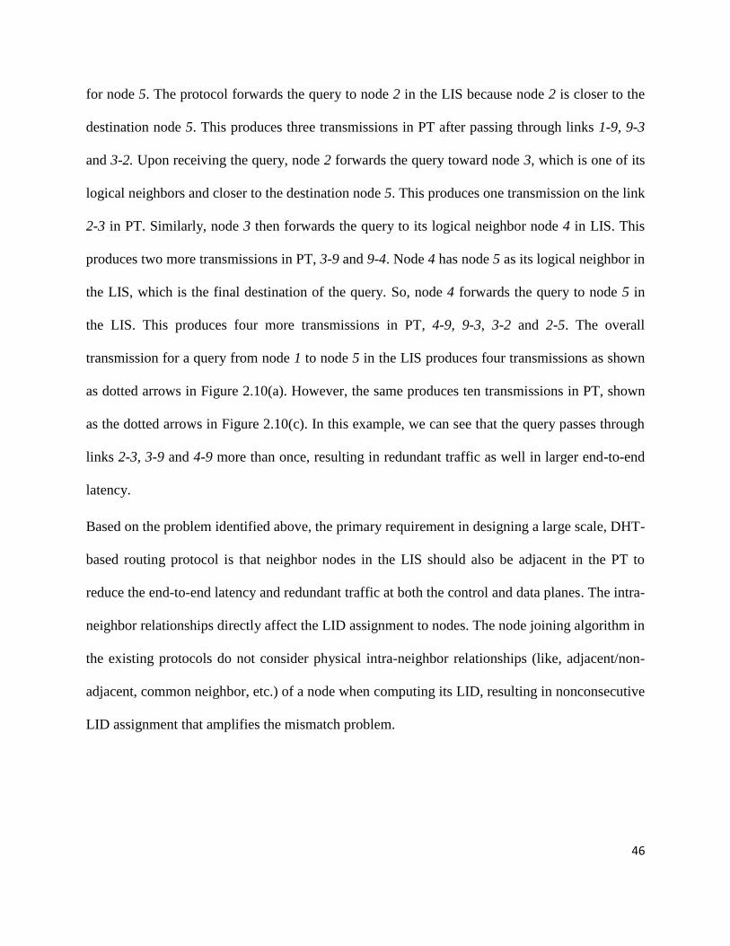
46
for node 5. The protocol forwards the query to node 2 in the LIS because node 2 is closer to the
destination node 5. This produces three transmissions in PT after passing through links 1-9, 9-3
and 3-2. Upon receiving the query, node 2 forwards the query toward node 3, which is one of its
logical neighbors and closer to the destination node 5. This produces one transmission on the link
2-3 in PT. Similarly, node 3 then forwards the query to its logical neighbor node 4 in LIS. This
produces two more transmissions in PT, 3-9 and 9-4. Node 4 has node 5 as its logical neighbor in
the LIS, which is the final destination of the query. So, node 4 forwards the query to node 5 in
the LIS. This produces four more transmissions in PT, 4-9, 9-3, 3-2 and 2-5. The overall
transmission for a query from node 1 to node 5 in the LIS produces four transmissions as shown
as dotted arrows in Figure 2.10(a). However, the same produces ten transmissions in PT, shown
as the dotted arrows in Figure 2.10(c). In this example, we can see that the query passes through
links 2-3, 3-9 and 4-9 more than once, resulting in redundant traffic as well in larger end-to-end
latency.
Based on the problem identified above, the primary requirement in designing a large scale, DHT-
based routing protocol is that neighbor nodes in the LIS should also be adjacent in the PT to
reduce the end-to-end latency and redundant traffic at both the control and data planes. The intra-
neighbor relationships directly affect the LID assignment to nodes. The node joining algorithm in
the existing protocols do not consider physical intra-neighbor relationships (like, adjacent/non-
adjacent, common neighbor, etc.) of a node when computing its LID, resulting in nonconsecutive
LID assignment that amplifies the mismatch problem.

47
Figure 2.10: An example of path-stretch penalty caused by uncorrelated Logical Address
Space and Physical Network
Case 2: A few approaches (Viana et al., 2004, Caesar et al., 2006, Awad et al., 2008,
Awad et al., 2011) maintain a node’s adjacent neighbors in PT along with its logical adjacent
neighbors in LIS in an attempt to avoid the mismatch problem in Case 1. This approach is also
not effective in completely an avoiding ill-match between the LIS and PT as shown in Figure
2.10(b). For example, node 2 initiates a query towards node 9. Node 2 has nodes 1 and 3 as
logical neighbors in the LIS, while its physical neighbors are node 3 and node 8 as shown in
Figure 2.10(b) and Figure 2.10(c), respectively. Node 2 selects node 8 as its next hop toward
destination node 9 among its physical and logical neighbors (i.e., nodes 1, 3, 8) because node 8 is
numerically closest to node 9 by using the greedy routing approach. This moves the query away
from node 9 in PT by generating one transmission. After receiving the query, node 8 forwards
the query towards node 9 because it is the closest among the logical and physical neighbors of
node 8. This further produces three transmissions in the PT, on links 8-2, 2-3, and 3-9, shown as
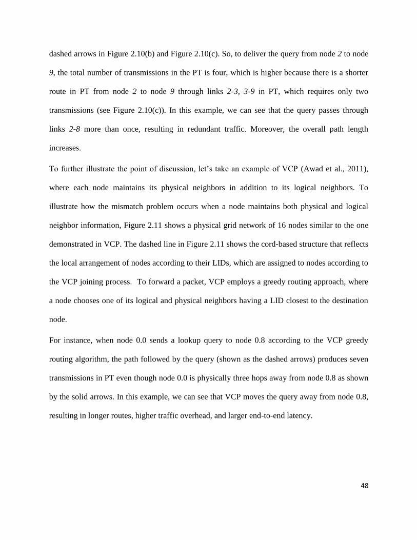
48
dashed arrows in Figure 2.10(b) and Figure 2.10(c). So, to deliver the query from node 2 to node
9, the total number of transmissions in the PT is four, which is higher because there is a shorter
route in PT from node 2 to node 9 through links 2-3, 3-9 in PT, which requires only two
transmissions (see Figure 2.10(c)). In this example, we can see that the query passes through
links 2-8 more than once, resulting in redundant traffic. Moreover, the overall path length
increases.
To further illustrate the point of discussion, let’s take an example of VCP (Awad et al., 2011),
where each node maintains its physical neighbors in addition to its logical neighbors. To
illustrate how the mismatch problem occurs when a node maintains both physical and logical
neighbor information, Figure 2.11 shows a physical grid network of 16 nodes similar to the one
demonstrated in VCP. The dashed line in Figure 2.11 shows the cord-based structure that reflects
the local arrangement of nodes according to their LIDs, which are assigned to nodes according to
the VCP joining process. To forward a packet, VCP employs a greedy routing approach, where
a node chooses one of its logical and physical neighbors having a LID closest to the destination
node.
For instance, when node 0.0 sends a lookup query to node 0.8 according to the VCP greedy
routing algorithm, the path followed by the query (shown as the dashed arrows) produces seven
transmissions in PT even though node 0.0 is physically three hops away from node 0.8 as shown
by the solid arrows. In this example, we can see that VCP moves the query away from node 0.8,
resulting in longer routes, higher traffic overhead, and larger end-to-end latency.

49
Figure 2.11: Mismatch problem - a VCP example: dashed lines is cord maintained by the VCP protocol.
In spite of maintaining both physical and logical neighbor information, VCP suffers from the
mismatch problem because its joining algorithm does not consider all relationships between
nodes. Moreover, the structure used to logically arrange nodes is inflexible and unable to assign
a consecutive LID to a node with respect to its all physically adjacent neighbors.
Based on the problem identified above, the second requirement in designing a large scale,
DHT-based routing protocol is that a node in LIS should be logically close to all its physically
adjacent nodes. This reduces the number of transmissions when forwarding a query/packet to a
destination, thus, reducing both end-to-end latency and redundant traffic at the control and data
planes.
2.3.3.2 High Maintenance Overhead
The DHT maintenance procedure ensures routing convergence and efficiency in terms of the
number of hops in LIS. As network topology continuously changes in MANETs, each node
periodically runs some procedures to ensure consistent and up-to-date information in its routing
table. Each operation may require a route discovery. The traffic overhead incurred by such
procedures is high for bandwidth constrained networks like MANETs. For reactive routing

50
protocols, the overhead is up to O(n), where n is the number of nodes in the network (Shen et al.,
2010).
Proactive routing requires periodic flooding of topology control messages, which is particularly
costly in MANETs. It is also difficult to achieve convergence in MANETs as frequent topology
changes may trigger multiple route discoveries. Furthermore, the ill-match between LIS and PT
would worsen this issue because more bandwidth would be consumed in obtaining routes that are
unnecessarily long. The situation could be even worse than simple flooding in resolving requests
for data items.
In order to overcome this problem, the third requirement for designing a large scale, DHT-based
routing protocol is that a node should control the traffic overhead by carefully calling the DHT
maintenance procedures to reduce redundant traffic at both the control and data planes.
2.3.3.3 Selection of LIS Structure
The structure interconnecting the nodes in the LS is another challenge to the performance of a
DHT-based routing protocol in MANETs. Different protocols have used different structures,
such as cord (Awad et al., 2011), ring (Caesar et al., 2006), hypercube (Alvarez-Hamelin et al.,
2006), and binary tree (Eriksson et al., 2007, Caleffi and Paura, 2011) to organize nodes in the
LS.
The connecting order of the LIS directly affects the number of logical neighbors in the LIS. All
existing proposals use LISs that are constrained by their connecting order. For instance, in a ring-
based (Caesar et al., 2006) and cord-based LIS (Awad et al., 2011) structure, a node can logically
connect to maximum two adjacent 1-hop neighbors, i.e., its successor and predecessor, and
maintain consecutive LIDs only with them. In case a node has more than two physically adjacent

51
neighbors, then these structures would not allow the node to assign consecutive LIDs or
contiguous logical address space.
The resilience of a protocol in terms of route selection strongly depends on the shape of LIS and
there is always a tradeoff between robustness and complexity in choosing the LIS (Gummadi et
al., 2003). The connecting order of the existing LISs do not allow a node to consider all of its
physically adjacent neighbors as a next hop when forwarding a packet, therefore, these LISs are
inflexible/inefficient in providing an alternative route in case an intermediate node fails/moves.
For example, tree, ring and cord structures are less complex and easy to maintain. Unfortunately,
these structures offer low flexibility in route selection that directly degrades the routing
performance and eventually results in poor resilience towards link failures and node mobility
(Alvarez-Hamelin et al., 2006). Moreover, the parent-child relationship in a tree structure
inherently suffers from longer routes and the parent node is responsible for maintaining most of
the information. This makes the network more centralized.
On the other hand, using multidimensional Cartesian Space structures, such as a sphere or
hypercube, for LS can enhance the resilience towards node failure and node mobility, which
provides more flexibility in route selection (Viana et al., 2005). These structures also help in
even distribution of the LS among nodes, resulting in a balanced traffic at each node and
inefficient bandwidth utilization. Moreover, this type of structure provides a means to map the
PT to LIS in such a way that the logical distance between two nodes is close to their physical
distance, resulting in shorter forwarding routes between the nodes.
Therefore, the fourth requirement for designing a large scale, DHT-based routing protocol is that
the LS structure selection should support flexible route selection. This is an important issue

52
because it directly affects routing performance in terms of path length, traffic concentration and
resilience to link failure.
2.3.3.4 Address Space Utilization
Efficient utilization of the LS is one of the major concerns in the design of a large scale, DHT-
based routing protocol. The LS should be evenly distributed among all nodes in the LIS. As
mentioned in Section 2.1, each node in the LIS holds a portion of the whole LS and stores
information about other nodes or data. The LSP allocated to each node should be equal in
capacity so that it results in relatively equal handling of information on each node. This implies
that the load to each node should be distributed evenly and each node has an equal opportunity to
store information. The benefit of maintaining such a structure is that minimum information has
to be transferred in case a node leaves the network, which might directly affect the traffic
overhead at both the control and data planes. Also, the traffic overhead can be reduced by
effective replication or caching schemes, which are vital for any DHT-based routing schemes.
One more element that plays a vital role in distributing the LS is the shape of the LIS.
2.3.3.5 Partitioning and Merging
The limited transmission range of nodes and their mobility can cause both network partitioning
and network merging in MANETs. Network partitioning is the breakdown of a connected
topology into two or more disconnected parts (Abid et al., 2014a). A node in one partition cannot
access a node in another partition. Network merging is the merging of two or more disconnected
topologies into one topology after nodes come into transmission range of each other.
In DHT-based protocols, nodes are arranged in a tree, cord or ring, where paths are limited by
some hierarchical structure that allows only one path between any two nodes, resulting in low

53
flexibility when selecting routes – this is unlike the greater flexibility offered by the multi-
dimensional approaches. There is a higher chance of LIS partitioning, which directly depends on
the structure of the LS. As discussed before, if the structure is resilient in terms of route selection
because it maintains multiple routes to a node, it would avoid unnecessary route discovery/
recovery. If a route to a node is lost due to network partitioning, another route to the node can be
utilized provided the node is accessible in the network. Similarly, when two physical networks
merge, then their LIS would be disjointed (Shah and Qian, 2010b, Shah and Qian, 2010a). To
detect this situation and merge the LNs, a DHT-based protocol should support seamless merging
of LIS, which is a great challenge. Most protocols discussed in Section 2.3.2.1 and Section
2.3.2.2 have not addressed the merging of partitioned networks, which is a major concern,
especially in DHT-based LIS.
In summary, below are six requirements that must be fulfilled in order to design a scalable DHT-
based routing protocol:
The neighbor nodes in the LIS should also be adjacent in the PT.
A node in LIS should be close to all its physically adjacent nodes.
The DHT maintenance procedures should incur minimal traffic overhead.
The LS structure selection should support flexible route selection.
The LS should be evenly distributed among all the nodes in LIS.
The protocol should address the issue of merging partitioned network.
These challenges are matters of great concern and affect the overall route resilience, end-to-end
latency, traffic overhead, network throughput, and path-stretch penalty. The existing work
discussed in Section 2.3.2.1 and Section 2.3.2.2 fails to overcome these challenges and suffers

54
from major problems that are yet to be addressed in order to obtain the optimal network
performance.
2.3.4 Analysis of the Existing DHT-based Paradigms for Large scale Routing
We end Section 2.3.3 with a summary of the main design issues discussed above: mismatch
problem, selection of LS structure, address space utilization and the handling of network
partitioning and merging.
The mismatch problem is important to consider in the deployment of DHT at the network layer
in MANETs because it affects performance in terms of path-stretch and end-to-end delay. All
protocols discussed above suffer from this problem. Some attempt to resolve the issue by
maintaining the physical neighbors of a node in addition to its logical neighbors, but it results in
a high path-stretch penalty and larger end-to-end delay.
VRR, ATR, DART, DHT-OLSR, VCP, AIR, KDSR, L+, Tribe, DFH, and EMP suffer from the
mismatch problem discussed in Case 1 and Case 2 of Section 2.3.3.1. The address assignment
mechanism of these protocols does not ensure contiguity among the neighbor’s identifier space
portions (LSPs) nor the adjacency of neighbors in LIS and PT. This makes them vulnerable to
high path-stretch penalty, which in turn, produces larger end-to-end delay.
DFH and VCP try to address the mismatch problem in Case 1 described in Section 2.3.3.1, by
maintaining information about both the physical and logical neighbors. Unfortunately, this also
leads to the mismatch problem in Case 2 described in Section 2.3.3.1.
We have carefully analyzed the mismatch problem and proffer that an optimal solution to the
mismatch problem would only be possible if the physical proximity of nodes is interpreted
exactly into the LIS and all physically close nodes are assigned LIDs that reflect their proximity.

55
The second issue identified is the shape of the LS structure, which plays a vital role in avoiding a
high path-stretch penalty caused by the mismatch problem and in maintaining multiple routes to
the destination. Several protocols discussed in Section 2.3.2.1 and Section 2.3.2.2 exploit
different structures to arrange nodes according to their LIDs. Routing paths in tree-based, cord-
based and ring-based structures are constrained by the connection order of the nodes that result
in low flexibility when selecting a route towards a destination. Also, these structures are not
flexible in fulfilling the conditions to avoid the mismatch between LIS and PT, which in turn,
leads to high path-stretch penalty. This problem is aggravated in case of node/link failure.
The LIS in DART, AIR, L+, Tribe, and EMP maintains only one path between any two nodes,
which may degrade performance in terms of path length, traffic concentration, and resilience to
failures. The LIS in VCP and VRR can only interpret the relationship of a node with up to two
adjacent physical neighbors. These structures are inflexible when interpreting the physical
relationship of a node in the LIS if the node has more than two physical neighbors.
DFH takes a different approach by using a hypercube to provide greater flexibility in route
selection in order to enhance the resilience towards node failure and node mobility. The
hypercube structure partially overcomes the mismatch problem by assigning multiple coordinates
to a node in order to provide better adjacency with its physical neighbors. The drawback of this
approach is that in a dense network, the number of connections per node could be high and may
lead to Case 1 (see Section 2.3.3.1) because the hypercube dimensions are fixed and must be
defined at startup time. Also, maintaining information about physical neighbors by using
secondary LIDs might lead to Case 2 described in Section 2.3.3.1. Moreover, DFH places each
neighbor in a different dimension of a node and does not consider physical intra-neighbor
relationships (adjacent/nonadjacent neighbor, common neighbor, etc.) between neighbors when

56
assigning LIDs to nodes that results nonconsecutive LID assignment, which might leads to long
routes, high path-stretch ratio. Another drawback is the addressing and location services of a
hypercube are more complex compared to a tree-based, cord-based, and ring-based structure.
The third important issue to consider is the address space utilization when allocating addresses
and distributing LS among nodes in MANETs. The aim of distributing LS evenly or assigning
LSPs in equal capacity to nodes is so that each node has an equal opportunity to store any
information about other nodes or data, resulting in a balanced load. The benefit of maintaining
such a structure is that minimal information has to be transferred in case a node leaves the
network. The amount of information transferred may directly affect information loss and traffic
overhead at both the control and data planes. Almost all protocols discussed in Section 2.3.2.1
and Section 2.3.2.2 have partially succeeded in their attempt to distribute the LS space evenly
among nodes because they are either constrained by the LS structure or the addressing strategy
adopted to allocate the addresses to nodes.
In VCP, the creation of virtual nodes hampers equal distribution of LS among all nodes, which
may lead to extensive information loss and high traffic overhead in case of node failure. Also, in
PROSE and AIR, the dual LID assignment when a root node moves or fails is similar to that of
Tribe. The solution given in PROSE and AIR is not optimal as it may cause uneven utilization of
LS and increase the number of nodes with dual LIDs. If there is no suitable node to hold the root/
parent node’s LID, it may result in the reassignment of LIDs for the whole sub-tree. Similarly,
the LS structure in ATR, DART, KDSR, L+, EMP, VIRO and DHT-OLSR hampers equal
distribution of LS among all nodes. DFH's approach of maintaining physical neighbors
information by using secondary LIDs leads to an uneven distribution of LS among all nodes,
hence, the possibility of extensive information loss in case a critical node fails.

57
Lastly, the network partitioning and merging issue is an open challenge. It is caused by either
limited transmission range of nodes or node mobility. The logical partitioning and merging
highly depends on the flexibility of the LS structure.
In ATR, DART, AIR, L+, Tribe and EMP, paths are constrained by their tree-based logical
identifier structure that allows only one path between any two nodes. This may result in the
partitioning of a sub-tree when a parent fails – this is unlike the greater flexibility offered by the
multi-dimensional approaches. Compared to tree-based routings, though VRR and VCP have
partially addressed the network partitioning and merging of a network, they do not provide a
comprehensive and viable solution. None of the protocols discussed in Section 2.3.2.1 and
Section 2.3.2.2 have addressed the network partitioning and merging that may cause extensive
information loss and communication disruption between two disconnected physical topologies.
In a nutshell, in this section we discuss in detail the potential challenges and pinpoint the key
requirements as a guideline for researchers who intend to design a DHT-based routing protocol.
Furthermore, we give a critique of the existing work in the light of the challenges discussed in
this section.
2.4 CONCLUSIONS
One of the basic design issues in implementing large scale MANETs is scalability, which is
heavily influenced by the routing protocol. Instead of modifying or optimizing the traditional
routing protocols for MANETs, the DHT or DHT-like technologies can be used for routing in
MANETs. Maintaining a DHT-based structure for a highly dynamic MANET environment has
introduced a number of new research issues. This chapter highlights some major challenges that

58
are raised by direct adoption of DHT-based or DHT-like strategies for implementing the logical
identifier space at the network layer (Abid et al., 2014b).
We classify the existing DHT-based protocols into three major categories: DHT for location
services, DHT for addressing and routing, and DHT for addressing, routing and location
services. In the first category, the DHT-based location service is coupled with a geographic
addressing space defined by some positioning system. The protocol defines addressing and
routing by utilizing the geographic addressing space, while the distribution of the node location
information is based on DHT.
In the second category, the protocol deploys a DHT-based structure that is used only for
addressing and routing. Nodes have fixed LIDs throughout the network lifetime and routing is
performed based on the LIDs. This category does not use DHT-based location service.
In the third category, a DHT-based structure is used for location services in addition to
addressing and routing. Contrary to the first and second categories, the location services, routing,
and addressing are dependent on each other and any changes in one aspect would influence the
others.
We review the existing approaches related to DHT-based routing paradigm for MANETs by
comparing the performance of different protocols against various parameters. We then identify
the shortcomings of these protocols in the light of critical challenges discussed in Section 2.3.3.
The requirements summarized in Section 2.3.3 are vital to the optimal design of a scalable DHT-
based routing protocol in MANETs. By carefully analyzing the addressing schemes and LIS
structures offered by different DHT-based protocols, we conclude that there are two major
correlated issues that require immediate attention, namely the mismatch problem and the
selection of the LS structure, which directly or indirectly cause immense overhead, unequal LS

59
utilization, and network partitioning. An optimal solution to the mismatch problem would only
be possible if:
i) the physical relationship of nodes is mapped exactly into the LIS;
ii) a node takes into account the physical intra-neighbor relationship before computing
its LID; and
iii) all physically close nodes are assigned LIDs that reflect their physical proximity. This
can only be accomplished if the LIS is flexible.

60
3 3D-RP: A DHT-BASED ROUTING PROTOCOL FOR
MANETS
This chapter presents a novel routing protocol for mobile ad hoc networks (MANETs), which
uses both a distribute hash table (DHT) and a location-based addressing scheme in order to
ensure a scalable routing service. The protocol, named 3D- Routing Protocol (3D-RP), can be
used with any link layer technology, but in this study, we consider an implementation based on
IEEE 802.11 technology. Its performance has been evaluated by means of numerical simulations
across several scenarios and workloads. The results show that 3D-RP outperforms traditional
DHT-based routing protocol as the number of nodes grows, ensuring satisfactory performance
for large networks operating in the presence of high data rate and moderate node mobility.
3.1 Introduction
In the last ten years, ad hoc technologies have grown tremendously. There are a variety of
MANET applications with practical implications and potential advantages (Reporter, 2011,
EmDiv, 2011, H. Mehendale, 2011, Distl et al., 2010). As the demand for sharing data among
users in a local area is increasing (ofcom, 2013), MANET applications would be required to
support a large number of users, which is only possible if the core routing protocol is scalable.
However, most existing protocols, regardless of whether they are reactive, proactive, or hybrid,
do not scale efficiently as the number of nodes grows (Broch et al., 1998, Tseng et al., 2002)
mainly because they were designed for wired networks. The network-wide flooding in traditional
routings that is adopted by MANET is the key factor that limits their scalability (Caleffi and
Paura, 2011, Eriksson et al., 2007, Awad et al., 2008, Garcia-Luna-Aceves and Sampath, 2009,

61
Chen and Morris, 2002). It would be possible to support a large network (in terms of number of
nodes) if we could eliminate or avoid network-wide flooding.
The research community has been using a distributed hash table (DHT) structure as a scalable
substrate in order to provide a diverse set of functionalities, like information distribution,
location service and location-independent identity (Frey, 2004, Das et al., 2008), in various self-
organized applications or systems in the Internet. It has come forth as a useful additional
technique to the design and specification of spontaneous, self-organizing networks. The basic
aim of these approaches is to address the scalability issues in MANETs by eliminating network-
wide flooding.
In DHT-based routing, a node has a unique logical identifier (LID) in addition to its public
identifier (UID), i.e., IP or MAC address. The LID describes the relative position of the node in
the logical network. The LID for a node is computed either by applying a hash function on the
node’s UID (Caesar et al., 2006) or based on LIDs of its physical neighbors (Caleffi and Paura,
2011, Eriksson et al., 2007, Awad et al., 2008, Garcia-Luna-Aceves and Sampath, 2009, Chen
and Morris, 2002, Awad et al., 2011, Sampath and Garcia-Luna-Aceves, 2009, Jain et al., 2011,
Alvarez-Hamelin et al., 2006, Abid et al., 2013, Abid et al., 2014c). The hashed values are drawn
from a pre-defined logical identifier space (LS). The node is linked with other nodes that have
LIDs closer to its LID, i.e. the nodes are connected with each other based on their LIDs,
following a ring (Caesar et al., 2006), tree (Caleffi and Paura, 2011, Eriksson et al., 2007,
Garcia-Luna-Aceves and Sampath, 2009, Sampath and Garcia-Luna-Aceves, 2009, Jain et al.,
2011, Sabeur et al., 2007, Jha et al., 2008, Viana et al., 2004), cord (Awad et al., 2008, Awad et
al., 2011), or other multidimensional structures (Alvarez-Hamelin et al., 2006, Abid et al., 2013).

62
Thus, a LIS is built over the physical network (PN). A node in LIS maintains its 1-hop/2-hop
logical neighbor (Lnbr), which may be different from its physical neighbors in the PN. Packet
routing is performed based on a node’s LID rather than its UID of a node.
The deployment of DHT at the network layer in MANETs gives rise to a few new challenges
that are imperative to address in order to make DHT-based routing protocols more scalable. We
identified two correlated issues that must be considered when designing DHT-based routing
protocol, namely the mismatch problem and resilience of the logical identifier structure, which
degrade the efficiency of the DHT-based routing protocols in terms of path stretch ratio (the ratio
between the length of the path traversed by a routing algorithm to the shortest path available in
the network), long routes, and high end-to-end delay (Shah et al., 2012). These problems need
immediate attention and require an optimal solution. The mismatch problem arises when:
i) neighbor nodes in the LIS are not adjacent in the PN;
ii) a node in LIS is not logically close to all its physically adjacent nodes (see Section
2.3.3 for details). In order to avoid this problem, a LIS should be flexible to
incorporate the physical relationship of nodes in terms of LIDs.
In this chapter, we propose a novel DHT-based routing protocol for MANETs, named 3-
dimensional routing protocol (3D-RP), by focusing our attention on the mismatch problem and
resilience of the LIS. 3D-RP exploits a 3-dimensional logical identifier structure (3D-LIS) that
interprets the physical relationship of nodes in a 3-dimensional logical identifier space (3D-LS).
The 3D-LS gives a node the liberty to exactly interpret the physical relationship of nodes in the
3D-LIS. To the best of our knowledge, 3D-RP is the first DHT-based routing protocol that

63
attempts to exploit a 3D structure to assign three dimensional LIDs to nodes. None of the
existing DHT-based protocols (Caleffi and Paura, 2011, Eriksson et al., 2007, Caesar et al., 2006,
Baccelli and Schiller, 2008, Garcia-Luna-Aceves and Sampath, 2009, Sampath and Garcia-Luna-
Aceves, 2009, Awad et al., 2008, Awad et al., 2011, Zhao et al., 2009, Jain et al., 2011, Lu et al.,
2008, Alvarez-Hamelin et al., 2006, Chen and Morris, 2002, Viana et al., 2004, Sabeur et al.,
2007, Jha et al., 2008) have used a 3D structure to map the physical proximity of nodes. Each
node in 3D-RP considers the neighbor relationships (intra-neighbor, adjacent/ nonadjacent
neighbor, and common neighbor) when computing its LID, which helps to exactly map the
physical proximity of nodes in the LIS. These relationships are crucial when calculating the
relative position of a node in order to optimally address the mismatch problem. None of the
existing DHT-based protocols have considered these relationships. We further propose the use of
Shepard’s interpolation method (Shepard, 1968) in 3D to compute the LID of a node relative to
its 1-hop neighbors.
In summary, 3D-RP is designed to achieve the following criteria:
i) The neighbor nodes in the LIS should be adjacent in the physical topology in order to
avoid long routes,
ii) A node in LIS should be logically close to all its physically adjacent nodes in order to
avoid redundant traffic,
iii) The protocol should require only local information to perform routing and maintain
the LIS in order to reduce routing overhead,

64
iv) The LIS should be flexible in selecting routes to a node in order to gain resilience
against node/link failures and provide multi-path routing,
v) The protocol should adapt to node mobility.
3.2 System Model
3D-RP resorts to a network-layer architecture in which each node has a permanent UID, which
identifies the node in the network, and a transient logical identifier that reflects the node’s
relative location in the logical identifier structure.
An optimal solution to the mismatch problem would only be possible if the physical relationship
of nodes is interpreted exactly into the LIS by assigning LID to a node such that the node's LID
is logically close to the LIDs of all its physically close nodes, i.e., the LIDs of nodes reflect their
physical proximity in the LIS. To achieve this goal, each node in 3D-RP computes a LID in the
form of three ordered tuple {x|y|z}, where each tuple is an M-bit identifier calculated from a pre-
determined 3D-LS. The 3D-LS ranges from for each axis, i.e., x, y, and z. The
protocol uses 1-hop hello messages to maintain the 3D-LIS, i.e., it relies on local information.
Each node periodically transmits a hello message that contains the LID, UID (i.e., IP address),
LSP, and its logical 1-hop neighbor information corresponding to its local 3D-LIS. In addition to
LID at each node, a dimension parameter (dim) is maintained to group nodes with respect to
different dimensions, which is helpful while routing packets. The basic idea is that each node
envisions its neighbors in a 3D rectangular coordinate system, i.e, a local 3D-LIS consists of
three planes that divide the space into six dimensions and eight octants as shown in . Each node

65
acts as the origin of its local 3D-LIS. In the local-3D LIS of a node, each neighbor obtains its
LID that reflects its relationship with its other neighbors.
Figure 3.1: 3D Logical Identifier Structure.
The basic motivation behind using 3D-LIS and decision choices are explained in Cases 1-4 (see
Section 3.3.1), which is to logically interpret the physical intra-neighbor relationship of a node.
For instance, N represents the set of nodes in the network and m N, Tm as a set of 1-hop
neighbors of node m. If nodes p, q Tm and there is no link in the physical network between
nodes p and q, then it means p and q lie in a different dimensions from node m. Therefore, both
nodes p and q obtain their LIDs corresponding to two different dimensions of the local 3D-LIS
of node m.
+Y
+X
+Z
IV
I
II
III
V
VI
VII
VIII
I, II,.., VIII are Octants
Y-dimension
-Y
-Z
-X
X-dimension
Z-dimension
Y-Plane
Z-Plane
X-Plane
Origin

66
We assume that each node in the network computes the distance between itself and its neighbor
nodes using Received Signal Strength (RSS) method (Shah and Qian, 2009). Weights are
assigned to each link providing connectivity to its neighbors on the basis of their distances using
an inverse distance function given in Eq(1). The detail of each 3D-RP component is presented in
the following subsections.
Wpm =
(1)
where, Wpm is the weight assigned to the link between a newly joining node Np and its
neighbor node Nm, d is the distance in meters measured using RSS between Np and Nm, and
k is a positive real number, called the power parameter whose value is assumed to be 2.
Greater values of k assign greater influence to nodes closest to the joining node. Here, the
weight decreases as distance in meters increases from the joining node.
3.3 Joining Operations
To join the network, a node is required to listen for a certain waiting time, Tw, to receive hello
message(s) from an existing node, referred to as the base node for the joining node. The LID of a
joining node is calculated during this phase. Based on the information in the hello message(s), a
node calculates its LID and updates its routing table. The joining operation consists of two
phases: LID computation and anchor node computation, as explained below.
3.3.1 LID Computation
After a waiting time, the joining node computes its LID based on one of the following cases:

67
(i) If a joining node does not receive any hello message, it assumes it is the first node
and automatically assigns itself the LID {1|1|1}-0.
(ii) If the joining node receives at least one hello message, it computes its LID with
respect to its physical neighbor(s) using the heuristics explained in Case 1 to Case 4
below. Assume node i is the first node in the network with LID {1|1|1}-0.
Case 1: If node p joins and finds node i as its only neighbor, node p calculates its distance from
node i and checks node i’s neighbors information received in the hello message. If node i does
not have any neighbor except p, node p selects the first available dimension of node i (say, + x-
dimension) out of the six dimensions along the positive and negative axis in the local 3D-LIS of
node i and calculates its LIDp using the following formula: {
)| | }, where Tix,
Tiy, and Tiz are the three tuple of the LIDi of node i, and LSPix+ is the maximum range of node i’s
LSP in positive x-dimension. By using this formula, node p obtains ¾ of node i’s LSPix+. The
purpose here is to give more LSP to the corner nodes so that they can accommodate new nodes
in the future. Furthermore, node p sets its dimension parameter to 1 as LIDp belongs to the
positive x-dimension.
Algorithm 1: Handling hello messages
Requirement: Locally stored state of all neighbors in neighbor table (NT) of node N
1: Receive neighbor information from node Ni
2: if Ni NT then
3: NT ← Ni NT
4: else
5: Update Ni

68
6: end if
Table 3.1: List of dim values
dim Axis
1 +X
2 -X
3 +Y
4 -Y
5 +Z
6 -Z
Similarly, the joining process of nodes h and s along with their LIDs are shown in 3.2(a). Nodes
h and s compute their LIDh and LIDs corresponding to negative x-dimension and positive y-
dimension by using the following formula: {
)| | } and { |
| },
respectively, where LSPix- is the maximum range of the LSP for node i in the negative x-
dimension and LSPiy+ is the maximum range of LSP for node i in positive y-dimension. Nodes h
and s set their dim value to 2 and 3, respectively. 3.2(a) illustrates the joining of node p, h, and s.
The basic motivation for the decision choices made in Case 1 is to map the physical intra-
neighbor relationship of a node in the 3D-LIS. If two neighbors of a node are not in transmission
range of each other, it means they exist physically in two different dimensions from the node. In
such scenarios, 3D-RP is capable of assigning LIDs in the LIS that reflects the physical intra-
neighbor relationship of nodes.

69
Figure 3.2: The joining process. Solid lines represent the local LIS of a node. Dashed lines are the
physical links between nodes in the PT
Algorithm 2: Joining Operation (Case1)
Required: Information related to neighbor Ni is stored in neighbor table (NT) of Nj and
distance to Ni is measured using RSS at joining node Nj.
1: if Ni NT : (Nm Nbr(Ni)) != Nj then
2: dimj ← NextAvailableDim(Nm, Ni)
4: else
5: dimj ← first(dimi)
6: end if
7: LIDj ← ComputeLID(Ni, dimj)
+X
1024
102
4
1024
-1024
-1024
-1024
IV
II
III
V
VI
VII
VIII
i
p{256|1|1}-1
{1|1|1}-0 I
h
{-256|1|1}-2
s
{1|256|1}-3
-X
-Y
+Y
-Z
+Z
+X
1024
1024
1024
-1024
-1024
-1024
i
p
{256|1|1}-1
{1|1|1}-0q
-X
-Y
+Y
-Z
+Z
{100|-100|100}-1
dqi
dqpr
{100|100|100}-1
+X
1024
1024
1024
-1024
-1024
-1024
{256|1|1}-1
{1|256|1}-3
-X
-Y
+Y
-Z
+Z
dqidqp
p
{257|257|1}-1q
i
+X
1024
10241024
-1024
-1024
-1024
i{1|1|1}-0
k
{-150|50|60}-2
-X
-Y
+Y
-Z
+Z {-256|1|1}-2
dqk
p
{100|100|100}-1
qdqi
dqp
I, II, III… are
Octants(a) (b)
(c) (d)
Case 1 Case 2
Case 3 Case 4
dsidpi
dhi

70
NextAvailableDim(Nm, Ni)
1: if rootNode(Ni) == true then ** the node with LID {1|1|1}-0 is the root node
2: if getDim(Nm) == ‘1’ then ** 1,2,3,4,5,6 refers to six dimensions (+x,-x,+y,-y,+z,-z) of local 3D-LIS
3: return ‘2’
4: else
5: return ‘1’
6: end if
7: else rootNode(Ni) == flase then ** T is the corresponding tuples of LIDs of nodes in x, y, z
dimensions.
8: if Tmx > Tix and Tmy == Tiy and Tmz == Tiz then
9: Nm ‘1’
10: return ‘2’
11: else if Tmx < Tix and Tmy == Tiy and Tmz == Tiz then
12: Nm ‘2’
13: return ‘1’
14: else if Tmx == Tix and Tmy > Tiy and Tmz == Tiz then
15: Nm ‘3’
16: return ‘1’
17: else if Tmx == Tix and Tmy < Tiy and Tmz == Tiz then
18: Nm ‘4’
19: return ‘1’
20: else if Tmx == Tix and Tmy == Tiy and Tmz > Tiz then
21: Nm ‘5’
22: return ‘1’
23: else if Tmx == Tix and Tmy == Tiy and Tmz < Tiz then

71
24: Nm ‘2’
25: return ‘1’
26: end if
27: end if
Case 2: If node q joins the network as shown in 3.2(b) and has access only to nodes i and p that
are adjacent, then node q first calculates the distances dqi and dqp and checks for common
neighbors between i and p.
(i) If there is no common neighbor, node q checks their collinear inequality (i.e., diq + dqp
>dip, dip + diq>dqp, and dqp + dip>diq). If nodes i, p, and q are collinear, node q calculates
LIDq by using Eq (2).
LIDm = { ∑
∑
|∑
∑
| ∑
∑
} (2)
where, m is the newly joining node and n≥2 are 1-hop neighbors of m; Wmk and Wmj are
the weights assigned by m to its neighbor nodes k and j, respectively, using inverse
distance function; and Tkx, Tky, and Tkz are the corresponding tuples k’s LID in x, y, and z
dimensions.
If node q is not collinear to i and p, then node q finds an available common octant between i and
p, and calculates LIDq corresponding to a common octant using Eq(2). Furthermore, node q sets
the signs of each tuple according to the sign dimensions of an available common octant between
nodes i and p.

72
(ii) If there is a common neighbor node (say, node r) between i and p, node q finds the next
available common octant between node i and p, and calculates LIDq corresponding to the
dimensions of that common octant using Eq(2).
Algorithm 3: Joining Operation (Case 2 and Case 3)
Required: Information related to neighbors Ni, Np is stored in neighbor table (NT) of Nj
and distance to Ni and Np is measured using RSS at joining node Nj.
1: if Ni,Np NT : Np Nbr(Ni) and Ni Nbr(Np) then
2: octj ← first(octip)
3: if Nc Nbr(Ni) and Nbr(Np) then ** Nc refers to any common neighbor other than Nj
4: octj ← NextCommonOctant(Nc,Ni,Np)
5: else
6: if Collinear(Nj,Ni,Np) == true then
7: LIDj ← ComputeLID(Ni,Np)
8: return
9: else
10: LIDj ← ComputeLID(Ni,Np, octj)
11: return
12: end if
13: end if
14: else if Ni,Np NT : Np Nbr(Ni) and Ni Nbr(Np) then
15: Nbr_adj ← false
16: if Nc Nbr(Ni) and Nbr(Np) then
17: LIDj ← Compute(Ni,Np, Nbr_adj)
18: else

73
19: if Collinear(Nj,Ni,Np) == true then
20: LIDj ← ComputeLID(Ni,Np)
21: Return
22: else
23: switch to Case 1(Compute LIDj using the available dimension of either Ni or Np)
24: end if
25: end if
26: end if
The decision choices made in Case 2 is to address a node’s physical adjacency to its neighbors
and to assign a relative LID to the node with respect to its adjacent neighbors. To get the exact
relative position of the node, the proposed scheme exploits the Shepard’s interpolation method to
assign LID to a newly joining node with respect to its discrete set of neighbors. This is an
attempt to exactly map the relative position of a node in 3D-LIS with respect to its neighbors in
the physical topology.
Case 3: Suppose node q joins and has access only to nodes i and p that are not adjacent to each
other as shown in 3.2(c). After calculating its distance, i.e., dqi and dqp, node q checks for
common neighbors between i and p.
(i) If there is no common neighbor and q is collinear with i and p, then node q calculates
LIDq by using Eq (2). If there exists a common neighbor (say, node r), between i and p,
then node q computes LIDq simply by adding each tuple of node i and p using Eq(3):

74
LIDm = { ∑ |∑
| ∑
} (3)
where, m is a newly joining node and n≥2 are 1-hop neighbors of m; Tkx, Tky, Tkz are tuples of
nonadjacent neighbors corresponding to each dimension.
(ii) If there is no common neighbor and q is not collinear with i and p, then node q calculates
LIDq by using the available dimension of either node i or node p, depending on two
parameters: a) a neighbor node that is closer in terms of distance; b) a neighbor node that
has more available dimensions.
The decision made in Case 3 addresses the physical non-adjacency of neighbors and assigns a
relative LID to the joining node in 3D-LIS with respect to its non-adjacent neighbors. 3D-RP
also exploits the information about a common neighbor between two non-adjacent neighbors
before assigning a LID to a joining node. If a common neighbor exists, it shows some kind of
relationship between these two non-adjacent neighbors. 3D-RP uses this relationship to assign a
relative position in the LIS to a joining node in order to minimize the path-stretch caused by the
mismatch problem.
Algorithm 4: Joining Operation (Case 4)
Required: Information related to neighbors Ni, Np, and Nq is stored in neighbor table (NT)
of Nj and distance to Ni, Np, and Nq is measured using RSS at joining node Nj.
1: NbrCommon← false
2: if Ni,Np,Nq NT : Np Nbr(Ni),Nbr(Nq) and Ni Nbr(Np),Nbr(Nq) and Nq Nbr(Ni),Nbr(Np)
3: then
4: LIDj ← ComputeLID(Ni,Np,Nq)
5: return

75
6: else if Ni Nbr(Np),Nbr(Nq) and Np Nbr(Nq)) and Nq Nbr(Np) or Np Nbr(Ni),Nbr(Nq)
7: and Ni Nbr(Nq) and Nq Nbr(Ni) or Nq Nbr(Np),Nbr(Ni) and Np Nbr(Ni)) and Ni
8: Nbr(Np) then
9: NbrCommon← true
10: LIDj ← ComputeLID(Ni,Np,Nq)
11: return
12:else
13: LIDj ← ComputeLID(Ni,Np,Nq, NbrCommon)
14:end if
Case 4: If node q joins the network and receives hello messages from nodes i, p, and k as shown
in 3.2 (d), then it is either of the following cases.
(i) If i, p and k are adjacent, then node q calculates LIDq by using Eq (2).
(ii) If there exists two nodes, p and k, which are non-adjacent, node q checks for a
common neighbor between p and k. If node i is a common neighbor to p and k,
q computes LIDq using Eq (2). If there is either a common neighbor other than
nodes i, p, or k, or there is no common neighbor, node q calculates LIDq using
Eq(3).
The flow chart in Figure 3.3 summarizes the joining algorithm. In addition to calculating its LID,
each joining node in Cases 1 to 4 sets its dim value by checking the dim value of its base node(s).
The term ‘base node’ refers to nodes that are involved in the computation of the new node's LID.
If base nodes are in the same dimension, the joining node sets its dim value to that of its base

76
nodes. If the base nodes have different dim values, the joining node sets its dim value to the dim
value of a base node that is closer in terms of distance.
Figure 3.3: Flow chart of Joining Algorithm
Figure 3.4 illustrates the local 3D-LIS of node i built according to 3D-RP after the joining
process is completed. This is helpful in visualizing the arrangements of nodes according to their
LIDs in the 3D-LIS. The dotted lines are the physical links between the nodes. The dashed lines
are the three planes of the local 3D-LIS of node i. The alphabets represent the IP addresses of the

77
nodes while roman numeric represents the eight octants of the node i’s 3D-LIS. Figure 3.4
describes the logical mapping of the physical relationships of node i with its 1-hop neighbors
shown in Figure 3.5. This relationship is expressed in terms of LIDs and logical dimensions of
nodes in node i’s 3D-LIS, which allows the nodes to calculate their LID such that the physically
close nodes have close LIDs. Figure 3.4 and Figure 3.5 show that 3D-RP exactly maps the
physical intra-neighbors relationship of node i with its 1-hop neighbors in terms of their LIDs.
The neighbors of node i in the 3D-LIS are adjacent in the PT and node i in its local 3D-LIS is
logically close to all its physically adjacent neighbors, which would avoid long routes and
redundant traffic overhead, and decrease the end-to-end delay. Similarly, other nodes in the
network built their local 3D-LIS by arranging their 1-hop neighbor nodes according to their
LIDs, which are computed by 3D-RP.
Figure 3.4 : A logical view of the physical arrangement of nodes in the local 3D-LIS of node i and p
maintained by 3D-RP
+Y
+X
+Z1024
1024
1024
-1024
-1024
-1024
II
III
V
VIVII
VIII
I, II,.., VIII are Octantsiq
p
j
d(qi)
d(pi)
d(hi)
d(ji)
d(ti)d(si)
d(tj)
d(jh)
d(tp)d(qp) {1|256|1}-3
{256|1|1}-1
{-256| 1 | 1}-2
{100|-100|100}-1 {1|1|1}-0
{100|100|100}-1
h
ts
I-Y
-X
-Z
IVAlphabets are IP
Addresses
Address format
{tuple 1|tuple2|tuple3}-dimension parameter
{-150|50|60}-2

78
In addition, the 3D-LIS is resilient against node/link failures and facilitates multi-path routing
because each node maintains all its physically adjacent neighbors to leverage an alternative route
if the next hop towards the destination fails/moves. Figure 3.6 illustrates the routing table
information of node i, which describes how a node maintains information about its local
neighbors and neighbors of neighbors.
3.3.2 Anchor Node Computation
In DHT-based routing, a source node needs the LID of the destination to forward a packet.
Therefore, each node stores its LID-IP pair (referred to as mapping information) on a node called
an anchor node (AN). The AN for a node f stores f's mapping information. A node can act as an
AN for multiple nodes.
After computing its LID, each node performs two major operations:
i) It retrieves and stores the mapping information about nodes with LIDs closest to its
LID and acts as the primary anchor node (PAN) for those nodes;
ii) It computes the LID of its PAN in order to store its own mapping information.
For this purpose, a consistent hashing function, e.g., SHA-1, is used that takes the UID of the
joining node as input and generates a hashed value (h(v)-dim) within the range of LS. LIDs of
nodes and h(v)-dim are drawn from the same logical identifier space (LS). A node whose LID is
closest to the h(v)-dim becomes the PAN for the joining node. To route a message with
destination address h(v)-dim, each node uses information about its 1-hop logical neighbors (Lnbr)
and forwards the query to one of its Lnbr that has the same dimension parameter to that of h(v)-

79
dim and offers the closest position in every tuple of its LID with respect to h(v)-dim, i.e., with
least sum of difference (LSD) to the h(v)-dim. This is achieved simply by computing the sum of
difference (SD) of each tuple of the Lnbr’s LID with the corresponding tuple of h (v)-dim using
Eq(4) and then selecting Lnbr as a next hop with the LSD to the h(v)-dim using Eq(5) :
( – ) ( – ) ( – ) (4)
(5)
where, SDnbr is sum of the difference of each tuple of nbr’s LID to the corresponding
tuple of the destination’s LID or hashed value; Tnbrx, Tnbry, Tnbrz are three tuples of nbr’s
LID; and Tdx, Tdy, Tdz are three tuples of destination’s LID or hashed value; LSDnbr is the
least sum of the difference of nbr, and Lnbr are 1-hop neighbors.
If such a neighbor does not exist, the node simply forwards the message to its base node. For
example, in Figure 3.5, in order to store its mapping information, node f with LID {-256|-448|1}-
2 computes the hash value by applying a hash function on its UID, i.e. hash(f) = {50|-250|1}-1,
and forwards the store-mapping information (SMI) message to the PAN as follows. Because
none of node f’s 1-hop neighbors is in dimension 1 (i.e., the hashed value), node f forwards the
query to its base node h with LID {-256|1|1}-2. Node h also does not have any 1-hop neighbor in
dimension 1, therefore, it forwards the query to node i with LID {1|1|1}-0, shown by solid
arrows in Figure 3.5. Node i has three neighbors q, t, and p with the same dim value to the
hashed value, i.e., dim=1. Node i calculates the sum of difference of nodes using Eq(4) as
follows:

80
SDq = {|100-(50)|=50} + {|-100-(-250)|=150} + {|100-1|=99}→{50+150+99}→{299}
SDt = {|100-(50)|=50} + {|100-(-250)|=350} + {|100-1|=99}→{|50+350|+99}→{499}
SDp = {|256-(50)| =206} + {|1-(-250)|=251} + {|1-1|=0}→{206+251+0}→{457}
Figure 3.5: Illustrates the example of the following processes: i) Anchor node (AN) computation; ii)
Greedy LID-based Routing
Node i then compares the sum of difference of each of its 1-hop neighbors with its own, i.e., SDi
= {|1-50|=49}+{|1-(-250)|=251}+{1-1=0}→{49+251+0}→{300}. Node i then forwards the SMI
towards node q, which has the least sum of difference to the hashed value, i.e., LSDnbr = {299}
using Eq (5). Finally, node q forwards the query to node l with SDl = {|100-50|=50}+{|-331-(-
250)|=81}+{|100-1|=99}→{50+81+99 → {230}, which is the closest to the hashed value {50|-

81
250|1}-1. Thus, node l acts as a PAN for node f. Moreover, node l selects node q from its 1-hop
neighbors, with LID second closest to the hashed value as secondary anchor node (SAN) and
replicates the mapping information at node q. The SAN becomes active in case PAN fails or
moves.
3.4 Greedy Logical Routing Algorithm
To send a data packet to node f, source node m (refer to Figure 3.5) retrieves f's mapping
information from f's PAN. To do so, node m applies the same hashing function on f's UID, i.e.,
hash(f)={50}|-250|1}-1, and sends an ID request message (IRQST) with the destination address
{50|-250|1}-1 for f's mapping information in the same way that the SMI message is routed to the
PAN. Node l with LID {100|-331|100}-1 is the closest to the hashed value {50|-250|1}-1 and acts
as f’s PAN as shown in Figure 3.5. Therefore, node l receives the IRQST. Upon receiving
IRQST, node l replies by sending an ID response message (IRSP) to node m containing the LID
of node f or null value in case node f is not available in the network. The IRSP is routed to node
m using m’s LID in the same way that a SMI message is routed to the PAN. On receiving node f's
LID, node m now sends the data packet towards the destination node based on node f’s LID.
Node m checks its 1-hop logical neighbors, i.e., node r {448|1|1}-1 and node g {256|448|1}-1 as
shown in Figure 3.5. Both node r and node g are base nodes of node m and are in different
dimensions to the destination node f. Node m sends the packet to one of its base nodes with the
LSD to node f. Node m computes the sum of difference of each tuple of node r, i.e., SDr = {|448-
(-256)|=704} + {|1-(-448)|= 449} + {|1-1|=0}→ {704+449+0}→{1153} and node g, i.e., SDg =
{|256 - (-256)| = 512} + {|448- (-448)|=896} + {|1-1|=0}→{512+896+0}→{1408} with the
corresponding tuple of node f’s LID by using Eq(4). So, node r has the least sum of difference to

82
node f’s LID and becomes the next hop. In case the sum of difference is the same, node m would
select one that is closer in terms of distance. Node r then forwards the data packet using the same
approach to its neighbor node p with LID {256|1|1}-1.
Algorithm 5. Greedy forwarding algorithm
Require: Received data packet P for destination logical identifier LIDdest and information
related to all local neighbors is stored in the neighbor table (NT)
1: if dimself == dimdest then
2: flag ← true, SDself ← SumDiff(LIDself, LIDdest)
3: end if
4: Select Ni NT such that Nj NT, i j : SDi ← SumDiff(LIDi, LIDdest) < SDj ←
SumDiff(LIDj, LIDdest)
5: if flag == true and SDself < SDi then
6: store data
7: else
8: send P to Ni
9: end if
Node p has four 1-hop neighbors, namely q, i, t, and g, with the same dim value to the hashed
value, i.e., dim=1. Node p uses Eq(4) to calculate the sum of difference of its neighbor nodes,
i.e., SDq = {803}, SDi = {706}, SDt = {1003}, and SDg = {1408}. Node p then sends the data
packet to node i with LID {1|1|1}-0 and LSDi = {706} as shown in Figure 3.5. The routing table
maintained by node i is shown in Figure 3.6. Node i has two 1-hop logical neighbors, namely
node h with LID {-256|1|1}-2 and node j with LID {-150|-50|60}-2, in the same dimension with
node f. Node i uses Eq(4) to calculate the sum of difference of node h, i.e., SDh = {449} and node

83
j, i.e., SDj = {663}. Node i then sends the packet to node h that has LSDh = {449}. Finally, node h
forwards the data packet to the destination node f.
While forwarding a packet, in case a node does not have any other neighbor to forward the
packet to or the link to the next hop breaks, then the node sets the no_Further_Progress bit ON
and returns the message to the previous hop, which in turn, attempts to find an alternative route
towards the destination. After receiving the message with no_Further_Progress bit ON, the node
updates its routing table for that neighbor, sets the no_Further_Progress bit OFF, and checks its
neighbor table to find the next closest neighbor to the destination. Figure 3.7(b) shows an
intermediate node n fails and node g finds an alternative local neighbor node p to send a packet
towards destination node u. Our proposed greedy logical routing algorithm provides a way to
find alternative routes to each destination and avoids dead ends. In addition, it helps to find
optimal routes towards the destination.
Figure 3.6: Routing Table of node i with LID {1|1|1}-0
Dimension
IDNext Hop
Distance
(m)
Cost
(in
hops)
Is Base1-hop neighbors
of Neighbor
Cost
(in
hops)
Is Base of
Neighbor
1
{100|100|100}-1 21 1 No {-150|50|60}-2
{256|1|1}-1
2
2
No
Yes
{256|1|1}-1 37 1 No {448|1|1}-1
{256|448|1}-1
{100|-100|100}-1
{100|100|100}-1
2
2
2
2
No
No
No
No
{100|-100|100}-1 21 1 No {100|-331|100}-1
{256|1|1}-1
2
2
No
Yes
2
{-256|1|1}-2 30 1 No {-256|-448|1}-2
{-150|50|60}-2
2
2
No
No
{-150|50|60}-2 32 1 No {256|1|1}-1
{100|100|100}-1
2
2 Yes
*{100|100|100}-1
{-150|50|60}-2
21 1 No {-150|50|60}-2
{256|1|1}-1
2
2
No
No
3 {1|256|1}-3 38 1 No - - -

84
3.5 Node dynamics and failures
3D-RP offers greater flexibility in route selection because it exploits a 3D-LIS that optimally
interprets the physical relationships of a node with its neighbors in LS. In other words, a node in
LS is logically close to all its physically adjacent nodes. This provides a node the liberty to select
an alternative path in case the next hop towards the destination node fails/moves. This flexibility
in selecting routes enhances the reliability of 3D-RP in terms of the packet delivery ratio and
reduces the traffic overhead, especially when there is a link/node failure. The condition discussed
above is very difficult to achieve in the existing schemes that use tree, cord, and ring-based LS
because of the connecting order of nodes. The LISs of existing DHT-based routing protocols do
not allow a node to use all its physical neighbors as its next logical hop. So, in case of node/link
failure at an intermediate node: i) it increases the chances of dead ends that occurs when a packet
falls into the local minimum using greedy forwarding; ii) the intermediate node either drops the
packet or returns the packet to the source, which would increase the routing overhead and the
number of intransit packet, resulting in contention that causes congestion.
Since nodes continuously move in a MANET, the network topology changes continuously. 3D-
RP allows a node to compute its new LID when its physical neighbors change due to node
failure/mobility. When a node does not receive hello messages from a neighbor, the node
assumes that the neighbor has either failed or moved out of its transmission range. After
detecting this, a timer Tfail is maintained at the node, similar to the one used in (Garcia-Luna-
Aceves and Sampath, 2009) that waits for a specific period of time to allow the neighbor to
reconnect with the node. When this timer expires, the node calculates a new LID if it no longer
connects to any of its neighbor nodes. After computing a new LID, the node maintains its old

85
LID for a certain interval, named old_LID_Timer, to avoid in transit packet drops. For example,
in Figure 3.7(a), nodes u and l relocate, causing a link break with their base nodes. Further, nodes
u and l trigger the joining operation and re-calculates their LIDs upon joining nodes n and r,
respectively. The failure of a node can be one of the following three cases.

86
Figure 3.7: Examples of node dynamics and failures: a) Node u and node l acquire a new LID on
repositioning; b) An intermediate node fails and the selection of an alternative route is initiated
while sending a packet to node u
Case 1: If the anchor node, i.e. PAN fails/moves, then the SAN becomes the PAN.
Case 2: If an intermediate node p fails, i.e., it is no longer connected to its base node i, then this
scenario is handled as follows. Each node in 3D-RP also keeps track of neighbor nodes that share
its base node. If node p is no longer connected to its base node i, node p looks up its neighbor
table to find a common neighbor in the same dimension with node p and closest to the base node.
If it finds a common neighbor, for instance node t, node p retains its LID and node t becomes its
base node. If there is a common neighbor but in a different dimension from node p, node p
calculates its new LIDp by checking the available dimensions of that common neighbor.
Case 3: In case a node has multiple base nodes and one of its base nodes fails, it initiates a
joining process and calculates its new LID using its other base node(s).
3.6 Performance Analysis
To analyze the performance of 3D-RP, we implemented it in NS-2 (version 2.35) (Fall and
Varadhan, 2005), which is an open source discrete event network simulator. We adopted the
standard values for both the physical and the link layers to simulate IEEE 802.11 with Two-Ray
Ground as the propagation model. The key objective is to rely on a contention-based MAC
protocol that is best suited for distributed and self-organizing routing protocols. To generate
mobile topologies, we adopt the Random Way-Point as the mobility model. The mobility
parameters have been set to simulate moderate mobility, specifically, the speed values are
uniformly taken in the [1m/s, 5m/s] range. The simulation parameters are given in Table 3.2. The

87
data traffic is modeled as CBR flows over UDP protocol and Random Traffic Model is used as
data pattern. We do not adopt TCP as the transport protocol to avoid the elasticity effects of TCP
flow control on routing performances (Holland and Vaidya, 1999). The global load offered is
kept constant at 64 pkts/sec, in order to avoid running out of capacity due to multi-hop approach.
Moreover, the main objective is to analyse the effectiveness of the protocols against the
mismatch problem rather than the traffic load. So, in order to avoid the performance degradation
of the protocols due to traffic load, we kept the low traffic rate at the sources.
Table 3.2: Simulation Parameters
Input Parameters Value
Number of Nodes
Transmission range
25-400
50m
Playground Size 1000*1000m
Data Rate 1 to 400pps
Simulation Time 500sec
Start of Data Transmission 70,300
End of Data Transmission 250,499
Node Speed 1 to 5 m/s
Start of Node Failure
Mobility Model
Radio Propagation Model
100 sec
Random Way-point
TwoRayGround Model
Traffic Model Random Traffic pattern
We analyze different aspects by varying several parameter values that affect the performance of
the protocol and compare 3D-RP with MDART (Caleffi and Paura, 2011), which is a
competitive approach in the category of DHT-based scalable routing in MANETs. MDART is an

88
enhancement of DART(Eriksson et al., 2007) and allows multipath to the destination. MDART
proves to be a better protocol than DART and other conventional state-of-the-art reactive and
proactive routing protocols (Caleffi and Paura, 2011). We assume connected network topology
both for MDART and our protocol.
For performance comparison, we choose the following parameters with varying data rates and
network size.
Path-stretch ratio: It is the ratio between the length of the path traversed by a routing
algorithm to the shortest path available in the network. It describes the ability of the
protocol to find the shortest possible route towards a destination in the network. The
path-stretch ratio equals to 1 means that the protocol observes the shortest route.
Packet-delivery ratio: It is a ratio of the total number of packets received at the
destination to the total number of packets sent by the source. It shows the capability of
the protocol to successfully deliver data packets to the destination. It is also referred to as
loss ratio.
End-to-end delay: It is the average time taken by the data packet to arrive at the
destination. It includes the route discovery delay and queuing delay.
Routing overhead: It measures the total control overhead packets incurred by the
protocol to perform routing of data packets.
% MAC-layer collision per packet sent: It measures the impact of the overall traffic load.

89
All results discussed in the following sections are shown as box plots. For each data set, a box is
drawn from the first quartile to the third quartile, and the median is marked with a thick line.
Additional whiskers extend from the edges of the box toward the minimum and maximum of the
data set. Additionally, the mean value is depicted in the form of a small diamond for MDART
and a triangle for 3D-RP. We perform ten runs for each scenario.
Data analysis is performed using SPSS (version 21) to measure the significance of the results
with respect to network size and data rate. We applied the analysis of variance (ANOVA) test on
our data. ANOVA is used to analyze the differences between group means and their associated
procedures (such as variation among and between groups). In order to analyze the significance of
our data with respect to protocol and network size, two way ANOVA test is applied to the data
because the data is comprised of two independent factors, i.e., protocols and network size, and
one dependent factor that could be any one of these, i.e., end-to-end delay, packet delivery ratio,
loss ratio, % MAC collisions per data packet, and routing overhead. We use = 0.05, which
shows 95% confidence interval.
3.6.1 Quality of Routing Paths
In this section, the experiments are performed to check the quality of routing paths in terms of
the number of hops. The path-stretch ratio is calculated to compare the length of the routing
paths in logical network and physical network. The parameter is very important to compare the
effect of the mismatch problem between 3D-RP and MDART.
Figure 3.8 plots the average path-stretch ratio against network size to compare MDART to 3D-
RP. In 3D-RP, the average path-stretch ratio is lower compared to MDART for all network sizes.
The path-stretch ratio of 3D-RP stays slightly above the shortest path, but this increase is

90
reasonable and the mean value stays below 1.2. The slight increase of path-stretch ratio in 3D-RP
is because when a new node, for instance P, comes in contact with two non-adjacent neighbors
(say, P1, and P2) with different dim values and there is no common neighbor, then the new node
P would get an LID using available dimensions of either P1 or P2, depending on which one is
closer in terms of distance. So, in this case, the LID of the new node P would only show its
relative position in the 3D-LIS with respect to that neighbor from which it gets its LID. This can
cause a slight mismatch problem in 3D-RP. However, this situation occurs less frequently in 3D-
RP and its impact is less serious as shown by the simulation results.
Reducing the path-stretch ratio improves network performance by reducing redundant
transmissions in the network. For example, for 1 vs 1.4 ratio, if the shortest available path is 6
hops, then 1:1.4 would be equivalent to 6:8.4. This means that the path with the path - stretch
value 1.4 is almost 3 hops longer. This is equivalent to 3 extra transmissions in the network,
which in turn, increases end-to-end delay and routing overhead.
Figure 3.8: Path-stretch ratio as a function of network size
1
1.2
1.4
1.6
1.8
25 50 100 150 200 400
Pa
th-S
tretc
h R
ati
o
Network Size (nodes)
MDART
3D-RP

91
Figure 3.8 shows that 3D-RP has a lower path-stretch ratio compared to MDART, which means
that 3D-RP is more capable of selecting an optimal path. 3D-RP improves the path-stretch ratio
between 20%-25%. The path-stretch ratio of MDART is higher for all network sizes compared to
3D-RP. The path-stretch ratio in MDART increases up to 1.4 because it uses a tree-based LIS to
map the physical network, resulting in the mismatch problem. As discussed in Section 2.3.3.3,
the tree-based LIS ensures neither adjacency of all physically adjacent neighbors in LIS nor the
intra-neighbor relationship of nodes, making it impossible to assign consecutive LIDs to all
physical adjacent neighbors of a node. Therefore, messages may be routed through many
unnecessary nodes.
3D-RP reduces the number of redundant transmissions that decreases the end-to-end delay, loss
ratio, and routing overhead, which in turn, reduces energy consumption and increases network
longevity. When the number of transmissions in a MANET decreases, then packet collision
probability at the MAC layer also decreases, leading to more reliable transmissions. Thus, our
approach also results in more reliable transmissions at the MAC layer by reducing the number of
redundant transmissions compared to MDART.
Let us establish our null hypothesis to test the impact of network size on the path-stretch ratio
obtained for MDART and 3D-RP:
Ho : 3D-RP does not significantly reduce the path-stretch ratio compared to MDART.

92
Table 3.3: Summary of data analysis of the path-stretch ratio for 3D-RP and MDART using
ANOVA Two-Factor with replication
The results of the Two-way ANOVA with replication (Table 3.3) shows that p < 0.05, which
leads to the rejection of Ho. This shows that 3D-RP is statistically significant in terms of
reducing path-stretch compared to MDART.
Table 3.4: Results: pairwise data analysis of path-stretch ratio at each network size for 3D-RP and
MDART using ANOVA Two-Factor With Replication

93
Table 3.4 illustrates the pairwise comparisons of 3D-RP and MDART in terms of path-stretch
ratio for each network size. Table 3.4 shows that 3D-RP significantly improves path-stretch ratio
over MDART for all the network sizes. This shows the 3D structure is efficient in reducing the
mismatch problem. It allows a node to logically reflect its physical proximity, which results in
short routes towards the destination node. The results show that 3D-RP is more scalable for large
networks.
3.6.2 Impact of Traffic Load
In this section, the experiments are performed to check the viability of the 3D-RP under various
traffic loads and compared with MDART. End-to-end delay, loss ratio, and routing overhead are
monitored under different traffic loads to compare 3D-RP and MDART. The network size is kept
at 100 nodes and the data rate is varied from 1 to 400 pkts/sec. The simulation results show that
3D-RP outperforms MDART and scales better in terms of data load. Moreover, the results show
that MDART exhibits detrimental behavior at high traffic load.
(a) End-to-end Delay: 3D-RP is largely unaffected by data load, as shown by the end-to-end
delay and packet delivery results in Figure 3.9 and Figure 3.10, respectively. The slight increase
in the end-to-end delay incurred by 3D-RP, especially for data rate of 100 pkts/s and above, is
because the packets are delayed in the queue due to MAC layer congestion. The impact of the
congestion on 3D-RP is less severe compared to MDART. This behavior is reasonable given that
3D-RP introduces low path stretch ratio.

94
Figure 3.9: Average end-to-end delay as a function of traffic load
On the contrary, MDART is seriously affected in terms of end-to-end delay and loss ratio as the
data rate increases, which means MDART scales poorly. MDART’s tree-based hierarchical
nature results in high path-stretch, is inefficient against mobility and is a potential source of path
length inefficiency. For the same reason, the alternative routes provided by MDART are not
optimal, causing an increase in the number of intransit packets that leads to network congestion,
especially at high data rate.
Figure 3.12 shows that the improvement in end-to-end delay is between 47%-51% for data rate 1
pkts/s to 16 pkts/s. The improvement drops by almost half to 28% and 39% for data rate 32
pkts/s and 64 pkts/s, respectively. For data rate 100 pkts/s and above, the improvement is
between 41%-51%. The overall result proves that 3D-RP resolves the mismatch problem
effectively.
The following is the null hypothesis to test the impact of data rate and protocols on end-to-end
delay:
0
0.1
0.2
0.3
0.4
0.5
0.6
0.7
1 2 4 8 16 32 64 100 128 200 400
En
d-t
o-E
nd
Dela
y (
sec)
Data Rate (packets/sec)
MDART
3D-RP

95
Ho : 3D-RP does not significantly reduce end-to-end delay compared over MDART.
Table 3.5: Summary of data analysis of the end-to-end delay for 3D-RP and MDART using
ANOVA Two-Factor with replication
The result of the Two-way ANOVA test (Table 3.5) shows that p < 0.05, which leads to the
rejection of Ho. This shows that 3D-RP is statistically significant in terms of reducing end-to-end
delay compared to MDART.
Table 3.6 shows the pairwise comparisons of 3D-RP and MDART in terms of end-to-end delay
for each data rate. The result shows that 3D-RP significantly reduces end-to-end delay for data
rates greater than 100 pkts/sec, which means 3D-RP is more scalable than MDART for high data
rates. For data rates 1 to 100 pkts/sec, p > 0.05, meaning that 3D-RP performs better than
MDART in terms of end-to-end delay, but the mean difference of the two protocols is not
significant.

96
Table 3.6: Results: pairwise data analysis of end-to-end delay at each network size for 3D-RP and
MDART using ANOVA Two-Factor With Replication
(b) Loss Ratio: 3D-RP outperforms MDART for every data rate in terms of packet delivery
ratio as shown in Figure 3.10. The impact of increasing traffic load on 3D-RP is low compared
to MDART. For 3D-RP, the loss ratio is zero for data rate 1 pkts/s to 32 pkts/s (the loss ratio
improvement is at most 10%). Figure 3.12 shows that starting from 64 pkts/s, a big improvement
in the loss ratio is observed, i.e., between 24%- 59%. 3D-RP performs better than MDART even
at high data rates, which proves that it is more scalable and reliable than MDART.

97
Figure 3.10: Loss ratio as a function of traffic load
Table 3.7: Summary of data analysis of the loss ratio for 3D-RP and MDART using ANOVA Two-
Factor with replication
Below is the null hypothesis to test the impact of data rate and protocols on loss ratio:
Ho : 3D-RP dose not significantly reduce the loss ratio compared to MDART.
Table 3.7 shows the results of applying the Two-way ANOVA with replication.
0
0.2
0.4
0.6
0.8
1
1 2 4 8 16 32 64 100 128 200 400
Lo
ss R
ati
o
Data Rate (packets/sec)
MDART
3D-RP

98
Table 3.8: Results: pairwise data analysis of the loss ratio at each network size for 3D-RP and
MDART using ANOVA Two-Factor With Replication
The result of the Two-way ANOVA test (Table 3.7) shows that p < 0.05, which leads to the
rejection of Ho. This shows that 3D-RP is statistically significant in terms of reducing the loss
ratio compared to MDART.
Table 3.8 shows the pairwise comparison of 3D-RP and MDART in terms of the loss ratio for
each data rate. The result shows that 3D-RP significantly reduces the loss ratio for each data
rates greater than 2 pkts/sec, which means 3D-RP is more scalable than MDART for high data

99
rates. For data rates 1 pkts/sec, p > 0.05, meaning that 3D-RP performs better than MDART in
terms of loss ratio, but the mean difference of the two protocols is not significant.
(c) Routing Overhead: Figure 3.11 compares the performance of 3D-RP and MDART in
terms of routing overhead. Figure 3.12 shows that 3D-RP reduces the routing overhead between
26%-34% for data rate 128 pkts/s and below. For data rate 200 pkts/s and above, the
improvement is between 40%-50%. This proves the effectiveness of 3D-RP in reducing the
routing overhead.
Figure 3.11: Routing Overhead as a function of traffic load
0
50
100
150
200
250
300
350
400
1 2 4 8 16 32 64 100 128 200 400
Ro
uti
ng
Ov
erh
ea
d-N
um
ber
of
pa
ck
ets
(1
03)
Data Rate (packets/sec)
MDART
3D-RP

100
Figure 3.12: Percentage of improvement provided by 3D-RP over MDART as a function of traffic
load
Table 3.9: Summary of data analysis of the routing overhead for 3D-RP and MDART using
ANOVA Two-Factor with replication
The following is the null hypothesis to test the impact of data rate and protocols on routing
overhead:
Ho : 3D-RP does not significantly reduce routing overhead compared to MDART.
0
10
20
30
40
50
60
70
1 2 4 8 16 32 64 100 128 200 400
% I
mp
ro
vem
en
t w
.r.t
MD
AR
T
Data Rate (pkts/sec)
End-to-End Delay
Loss Ratio
Routing Overhead

101
Table 3.9 shows the results of applying the Two-way ANOVA with replication.
The result of the Two-way ANOVA test (Table 3.9) shows that p < 0.05, which leads to the
rejection of Ho. This shows that 3D-RP is statistically significant in terms of reducing the routing
overhead compared to MDART.
Table 3.10: Results: pairwise data analysis of routing overhead at each network size for 3D-RP and
MDART using ANOVA Two-Factor With Replication

102
Table 3.10 shows the pairwise comparisons of 3D-RP and MDART in terms of path-stretch ratio
for each network size. Table 3.10 shows that 3D-RP significantly improves the path-stretch ratio
over MDART for all the network sizes.
3.6.3 Impact of Network Size
In this section, the behavior of 3D-RP and MDART are analyzed against various network sizes.
The main objective of the experiments is to compare the scalability of 3D-RP and MDART in
terms of network size.
In order to analyze the behavior of 3D-RP with respect to network size, we conduct experiments
by varying the number of nodes from 25 to 400 while maintaining the data rate at 64 pkts/s. The
data rate is kept low in order to reduce the impact of traffic load on the protocol’s performance.
The simulation results show that 3D-RP is consistent in improving performance over MDART.
(a) End-to-end Delay: Figure 3.13 shows that 3D-RP scales better than MDART in terms of
end-to-end delay as the network size increases. As shown in Figure 3.17, the end-to-end delay
improvement over MDART is between 24% to 56%. Please note that MDART, which is an
enhancement of DART (Eriksson et al., 2007), is designed to provide a reliable path in order to
enhance throughput rather than minimize the hop count. MDART’s inflexible structure results in
longer routes and larger end-to-end delay.
Unlike MDART, 3D-RP is designed to provide a reliable path that enhances its throughput.
Furthermore, the arrangement of nodes in the 3D-hierarchical structure and the addressing
scheme supplements to minimize the number of hops between nodes and provide an alternative
route in case of intermediate node fail/move. 3D-RP performs better and provides near optimal

103
routes towards the destination, which decreases the end-to-end delay and increases packet
delivery ratio as shown in Figure 3.13 and Figure 3.14, respectively.
Figure 3.13: Average End-to-End delay as a function of the node number
Below is the null hypothesis to test the impact of network size and protocols on end-to-end
delay:
Ho : 3D-RP does not significantly reduce end-to-end delay compared to MDART.
Table 3.11 shows the result of applying the Two-way ANOVA with replication.
The result of the Two-way ANOVA test (Table 3.11) shows that p < 0.05, which leads to the
rejection of Ho. This shows that 3D-RP is statistically significant in terms of reducing end-to-end
delay compared to MDART.
0
0.01
0.02
0.03
0.04
25 50 100 150 200 400
En
d-t
o-E
nd
dela
y (
sec)
Network Size (nodes)
MDART
3D-RP

104
Table 3.11: Summary of data analysis of the end-to-end delay for 3D-RP and MDART using
ANOVA Two-Factor with replication
Table 3.12: Results: pairwise data analysis of end-to-end delay at each network size for 3D-RP and
MDART using ANOVA Two-Factor With Replication
Table 3.12 shows the pairwise comparisons of 3D-RP and MDART for each network size. The
result shows that 3D-RP significantly reduces end-to-end delay for each network size. 3D-RP

105
scales better than MDART as the network size increases. The result confirms the efficiency of
the technique adopted in 3D-RP to avoid the mismatch problem.
(b) Packet Delivery Ratio: The effect of increasing network size on the packet delivery ratio
is less detrimental on 3D-RP compared to MDART as shown in Figure 3.14. This is important
because it proves the effectiveness and capability of 3D-RP in delivering packets in large
networks with relatively high data traffic. On the contrary, MDART’s performance degrades as
the number of nodes increases (see Figure 3.14). The packet delivery ratio improvement over
MDART is between 30% to 46% as shown in Figure 3.17.
Figure 3.14: : Packet delivery ratio as a function of the node number
0
20
40
60
80
100
25 50 100 150 200 400
Pa
ck
et
Deli
very
Ra
tio
Network Size (nodes)
MDART
3D-RP

106
Table 3.13: Summary of data analysis of the packet delivery ratio for 3D-RP and MDART using
ANOVA Two-Factor with replication
The following is the null hypothesis to test the impact of network size and protocols on packet
delivery ratio:
Ho : 3D-RP does not significantly improve the packet delivery ratio compared to MDART.
Table 3.13 shows the result of applying the Two-way ANOVA with replication.
The result of the Two-way ANOVA test (Table 3.13) shows that p < 0.05, which leads to the
rejection of Ho. This shows that 3D-RP is statistically significant in terms of improving packet
delivery ratio compared to MDART. This proves the reliability of the route selection in 3D-RP,
which is due to its flexible 3D structure that provides multiple routes towards the destination
node. Moreover, the replication strategy used in 3D-RP efficiently reduces the packet loss in case
an anchor node moves/fails.
Table 3.14 shows the pairwise comparisons of 3D-RP and MDART for each network size. The
result shows that 3D-RP significantly improves the packet delivery ratio for each network size,

107
which shows the effectiveness of the technique adopted in 3D-RP that reduces the routing
overhead by avoiding the mismatch problem, resulting in an increased packet delivery ratio.
Table 3.14: Results: pairwise data analysis of the packet delivery ratio at each network size for 3D-
RP and MDART using ANOVA Two-Factor With Replication
Table 3.14 shows the pairwise comparisons of 3D-RP and MDART for each network size. The
result shows that 3D-RP significantly improves the packet delivery ratio for each network size,
which shows the effectiveness of the technique adopted in 3D-RP that reduces the routing
overhead by avoiding the mismatch problem, resulting in an increased packet delivery ratio.
(d) MAC Collisions per Data Packet: An important metric for analyzing MANET routing
protocols is the number of MAC layer collisions per packet sent, which measures the overall
network load. Figure 3.15 compares the percentage of MAC collisions per data packet for 3D-RP

108
and MDART while Figure 3.17 shows that the percentage of collision for 3D-RP is 8% to 27%
lower than MDART.
Figure 3.15: Percentage of MAC collisions per data packet sent as a function of the node number
Below is the null hypothesis to test the impact of network size and protocols on % MAC
collisions per data packet:
Ho : 3D-RP does not significantly reduce the percentage of MAC collisions per data packet
compared to MDART.
Table 3.15 shows the result of applying the Two-way ANOVA with replication.
The result of the Two-way ANOVA test (Table 3.15) shows that p < 0.05, which leads to the
rejection of Ho. This shows that 3D-RP is statistically significant in terms of reducing the MAC
collisions per data packet compared to MDART. 3D-RP is designed to avoid the mismatch
problem that reduces the number of transmissions in the network. The net effect of this reduces
congestion, resulting in less packet collisions.
0
10
20
30
40
50
60
25 50 100 150 200 400% M
AC
co
llis
ion
s p
er p
ack
et
sen
t
Network Size (nodes)
MDART
3D-RP

109
Table 3.15: Summary of data analysis of the percentage of MAC collision per data packet for 3D-
RP and MDART using ANOVA Two-Factor with replication
Table 3.16: Results: pairwise data analysis of the percentage of MAC collisions per data packet at
each network size for 3D-RP and MDART using ANOVA Two-Factor With Replication

110
Table 3.16 shows the pairwise comparisons of 3D-RP and MDART for each network size. The
result shows that MAC collisions per data packet are significantly less in 3D-RP for each
network size compared to MDART.
(c) Routing Overhead: Lastly, both 3D-RP and M-DART exhibit high routing overhead
because their routing update packets are of fixed size regardless of the network size (see Figure
3.16). However, the replication strategy used by 3D-RP in case the primary anchor node
moves/fails effectively reduces the overhead between 13% to 24%.
Figure 3.16: Routing overhead as a function of the node number
40
60
80
100
120
25 50 100 150 200 400
Ro
uti
ng
Ov
erh
ea
d-N
um
ber
of
pa
ck
ets
(1
03)
Network Size (nodes)
MDART
3D-RP

111
Figure 3.17: Percentage of improvement provided by 3D-RP over MDART as a function of the
node number
The following is the null hypothesis to test the impact of network size and protocols on routing
overhead:
Ho : 3D-RP does not significantly reduce routing overhead compared to MDART.
Table 3.17 shows the result of applying the Two-way ANOVA with replication.
The result of the Two-way ANOVA test (Table 3.17) shows that p < 0.05, which leads to the
rejection of Ho. This shows that 3D-RP is statistically significant in terms of reducing routing
overhead compared to MDART. As shown in Figure 3.8, the path-stretch ratio of 3D-RP is lower
compared to MDART, which means 3D-RP is more efficient in selecting that reduce the end-to-
end delay and routing overhead.
Table 3.18 shows the pairwise comparisons of 3D-RP and MDART for each network size. The
result shows that MAC collisions per data packet are significantly less in 3D-RP for each
0
10
20
30
40
50
60
25 50 100 150 200 400
% I
mp
ro
vem
en
t w
.r.t
MD
AR
T
Netwrok Size (nodes)
End-to-End Delay
Packet Delivery Ratio
% MAC Collisions per data
packet sent
Routing Overhead

112
network size compared to MDART. The result shows that 3D-RP significantly reduces routing
overhead for each network size.
Table 3.17: Summary of data analysis of routing overhead for 3D-RP and MDART using ANOVA
Two-Factor with replication
Table 3.18: Results: pairwise data analysis of routing overhead at each network size for 3D-RP and
MDART using ANOVA Two-Factor With Replication

113
3.7 Conclusion
Two crucial issues to address for DHT-based routing protocols in MANETs are the mismatch
problem and the resilience of the logical structure. This chapter proposes a DHT-based routing
protocol, named 3D-RP, which takes into account the physical intra-neighbor relationship of a
node by exploiting a 3D-LIS, which is also utilized to achieve resilience against node
mobility/failure in MANETs.
Simulation results show that 3D-RP scales well as the network size increases. Compared to
MDART, 3D-RP reduces the end-to-end delay between 24% to 56% and increases the packet
delivery ratio between 30% to 46%. In addition, 3D-RP incurs lower routing overhead and path-
stretch ratio, which makes it attractive for large scale MANETs. Also, 3D-RP has higher packet
delivery ratios and shorter end-to-end delay than MDART even at high data rate. 3D-RP reduces
the end-to-end delay from 28% to 53% over MDART. For data rates 64 pkts/s and above, 3D-
RP improves the loss ratio between 24% to 59%.
In conclusion, the simulation results show that 3D-RP has successfully addressed the mismatch
problem and is a resilient logical structure. In the next chapter, we intend to extend our work to
handle network partitioning and merging.
114
4 MERGING OF DHT-BASED LOGICAL NETWORKS IN
MANETS
The existing DHT-based approaches for routing in MANETs do not consider the merging of
logical networks that occurs due to nodes' limited transmission range and node mobility. This
chapter discusses the impact of the mismatch problem when merging two logical networks and
how the shape of the logical structure plays a key role in the merging of logical networks. A
leader based-approach (LA) is proposed to detect and merge two distinct logical networks. The
LA is embedded with 3D-RP, referred as LA-3D-RP, to prove the resilience of the 3D structure
when merging two logical networks. The performances have been evaluated by means of
numerical simulations across several scenarios and node speeds. The results show that LA-3D-
RP reduces the impact of the mismatch problem when merging logical networks compared to the
traditional DHT-based routing protocol.
In this chapter, we propose a novel approach, named leader-based approach (LA), to detect and
merge two logical networks. LA is designed to work with 3D-RP to reduce the impact of the
mismatch problem when merging two logical networks. This chapter addresses the following
challenges:
i) Partitioning and merging of the logical networks and the impact of mismatch problem
when merging two logical networks is explained in detail. To the best of our
knowledge, this is the first attempt to discuss the challenges and issues related to the
merging of two DHT-based logical networks over physical networks;

115
ii) LA is embedded in 3D-RP and MDART to compare their performance ability to
resolve the mismatch problem when merging two logical networks. How the 3D
structure leverages the merging of two logical networks is explained in detail.
iii) The Merging process is based on the merging strategy discussed in (Datta and Aberer,
2006), which is simple to execute;
iv) A comprehensive analysis of how the node joining algorithm and LIS structure
affects the performance of a DHT-based routing protocol when merging two logical
networks is discussed.
In DHT-based routing protocols, when the nodes from two different physical networks come
within transmission range of each other and connect at the physical level, the logical networks
remain disconnected even though they are now connected at the physical level. The detection of
the other logical network in DHT-based routing protocols is crucial in order to smoothly conduct
the merging process and avoids address duplication. When nodes in two logical networks come
within transmission range of each other, it might be possible that the nodes are assigned
duplicate LIDs, because in DHT-based logical network, each node computes its LID from a
predefined LS. The following section proposes an approach to overcome this problem.
4.1 Merging of DHT-based Logical Identifier Structures in MANETs
Due to the self-organizing nature, limited transmission range, and node mobility in MANETs,
network partitioning and merging can occur frequently. Network partitioning is the breakdown
of a connected topology into two or more disconnected parts (Shah and Qian, 2010b, Shah and
Qian, 2010a). A node in one partition cannot access a node in another partition. For instance, the

116
network breaks into two partitions PN-1 and PN-2 as shown in Figure 4.1(a). On the other hand,
network merging happens when two or more disconnected networks joins to form one network
because nodes in these networks come within transmission range of each other. For instance, the
two network partitions PN-1 and PN-2 are merged into a single network as shown in Figure
4.1(b).
In DHT-based protocols, when two physical networks merge, the logical networks over these
two physical networks would remain disconnected. So, in these protocols, network merging can
be viewed at two levels, i.e., logical level and physical level. To handle network merging at the
logical level, the two main concerns are:
i) To detect the occurrence of the new logical network, i.e, merging detection;
ii) To merge the two logical networks, i.e., merging process.
Figure 4.1: A partitioned network into two disconnected topologies

117
The routing and merging overhead in DHT-based routing protocols strongly depends on the node
joining algorithm and arrangement of nodes in the LIS, i.e., the shape of the LIS. The existing
DHT-based protocols (Caleffi and Paura, 2011, Eriksson et al., 2007, Caesar et al., 2006,
Baccelli and Schiller, 2008, Garcia-Luna-Aceves and Sampath, 2009, Sampath and Garcia-Luna-
Aceves, 2009, Awad et al., 2008, Awad et al., 2011, Zhao et al., 2009, Jain et al., 2011, Lu et al.,
2008, Alvarez-Hamelin et al., 2006, Chen and Morris, 2002, Viana et al., 2004, Sabeur et al.,
2007, Jha et al., 2008, Abid et al., 2013) have used different node joining algorithms and LISs in
order to assign LIDs to nodes and arrange nodes according to their LIDs but none is able to
exactly map the physical proximity of nodes in the LIS. Moreover, none of these discuss and
analyze the consequences of merging two LISs, which is very crucial. When two disconnected
networks come within transmission range of each other, it may be possible that the nodes are
assigned duplicate LIDs that causes address conflicts (Zhou et al., 2003, Datta and Aberer, 2006)
because in DHT-based routing protocols:
i) LIDs are computed from a predefined LS;
ii) the forwarding of packets on both control and data planes is performed using LIDs of
nodes rather UIDs. Figure 4.1 illustrates the basic concepts related to merging in
DHT-based Logical identifier Structures.
Figure 4.1(a) shows two physical networks, PN1and PN2, which are ring-based logical networks,
LIS-1and LIS-2, respectively, over the physical networks. Suppose, nodes from PN1 and PN2
come within transmission range of each other and connect at the physical level as shown in
Figure 4.1(b). The logical networks (LIS-1and LIS-2) remain disconnected, as shown in the
Figure 4.1(b), even though they are now connected at the physical level. Merging the logical

118
networks is very crucial in DHT-based routings because the routing of data is based on the LID
and the LIS of the protocol.
The inability to merge the logical networks gives rise to the following challenges:
i) How to detect the occurrence of two or more logical networks (merging detection);
ii) How to handle the merging of the two or more logical networks when the nodes in the
physical network come within the transmission range of each other (merging
process);
iii) How to maintain the resilience of the LIS and the node joining process when merging
two or more logical networks.
4.2 Merging detection
The detection of the other logical network is crucial in order to smoothly conduct the merging
process and avoids address duplication. When nodes in two logical networks come within
transmission range of each other, it might be possible that the nodes are assigned duplicate LIDs,
because in DHT-based logical network, each node computes its LID from a predefined LS.
For example, let node q belong to a network N1 and node p belongs to another network N2, and
N1 and N2 are partitioned. Because they are partitioned and have the same LS range, the nodes
in each network gets LIDs that are independent of the other network. Let's say after some time,
node q detects that node p has come into its transmission range. If there is no mechanism to
identify the logical network of node p, node q considers node p as either a new node that joins its
network or an existing node that moves from one location to another in its network. In this case,
node q simply invokes the joining process and assigns an LID to node p according to N1’s LS,

119
independent of N2’s LS. This may result in node p getting a LID that is already assigned to a
node in N2, which leads to duplicate LID assignment and address conflicts. The address conflict
can lead to misrouting when forwarding packets at both the control and data planes. In order to
address this problem, we propose a novel strategy to detect and identify nodes belonging to
different logical networks when they come within transmission range of each other.
4.2.1 Leader-based Approach (LA) to Detect Two Distinct Networks
We propose a leader-based approach (LA) to detect two disconnected logical networks. In LA,
one node is elected as a leader for the logical network. The leader periodically broadcasts a keep-
alive message (KLIVE) to its 1-hop neighbors to indicate its presence. KLIVE contains the
leader ID, which consists of its UID and LID. In case the leader ID changes, 1-hop neighbors of
the leader forwards the new leader ID to all nodes of the network by piggybacking it in the hello
messages. The leader of the logical network is elected and maintained as follows:
The first node joining the logical network becomes the leader. When a leader in the
logical network disconnects, a new leader is elected as follows.
When a node i does not receive the KLIVE from the leader, it waits for a random time.
After the waiting time expires, node i sends a 1-hop broadcast message, termed leader-
elect packet (LEPKT), in the logical network. LEPKT from node i contains the
disconnected leader ID. A node with the lowest UID is elected as a new leader. The
disconnection of a leader may be either due to node mobility or it has left the logical
network/switched off.
In LA, the merging detection process is simple and based on the leader ID of the logical network.
When a node q receives a KLIVE message that contains a different leader ID, node q detects that

120
there exists another logical network to which it is not connected to at the logical level, but it can
access nodes related to the other logical network in the physical network. In this case, node q
invokes the merging process. To differentiate between the new leader ID and the leader ID of the
other logical network, whenever a leader ID changes, the hello message carries a new leader ID
along with the old leader ID. When q receives the hello message, it matches its old leader ID
with the old leader ID in the hello message to verify that the message is from its own network
and then updates its leader ID with the new one. If the hello message contains a leader ID that is
different from the q’s old leader ID, then it means it is a leader ID of the other network.
4.3 Merging Process
Upon detecting the existence of another logical network, node q invokes the merging process.
The merging process is simple and based on the merging strategy discussed in (Datta and Aberer,
2006). In the merging process, each node from one logical network joins the other logical
network. Nodes in a network with a lower leader ID invokes the merging operation by
broadcasting to its 1-hop neighbors the merging request message (MRQST) and replacing the
leader of the other logical network with its leader. Node q waits for a random time Thd before
invoking the merging process, where Thd is an order of q’s hop distance from the leader of the
new logical network. The Thd is maintained to check if any other node that is closer to the leader
of the new logical network has intiate the merging process or not. Node q discards the MRQST
received from any other node in the logical network if the other node is at a greater distance from
the leader of the new logical network compared to node q. Suppose node q receives MRQST
from node p, which is at a greater hop distance from the leader of the new logical network than
node q, then node q discards node p’s MRQST. After the random waiting time expires, node q

121
broadcasts MRQST to its 1-hop neighbors. MRQST from node q contains q’s leader ID, leader
ID of the new logical network and q’s distance to the leader of the new logical network. Upon
receiving MRQST from node q, the receiving node r responds to the MRQST as follows.
If r’s leader ID is same as q’s leader ID, r discards the MRQST.
Otherwise, node r first re-computes its LID and then changes its leader ID to q’s leader
ID. In addition, node r sends the merging reply message (MRPLY) to q and forwards the
MRQST to its 1-hop logical neighbors.
After merging with the new logical network, the leader of q’s logical network announces the
change of leader in the logical network so that all nodes have the same leader ID after the
merging process is completed. This is done by piggybacking the leader ID in its hello message.
4.4 Merging in DHT-based Logical Identifier Structures
Existing DHT-based routing (Caleffi and Paura, 2011, Eriksson et al., 2007, Caesar et al., 2006,
Baccelli and Schiller, 2008, Garcia-Luna-Aceves and Sampath, 2009, Sampath and Garcia-Luna-
Aceves, 2009, Awad et al., 2008, Awad et al., 2011, Zhao et al., 2009, Jain et al., 2011, Lu et al.,
2008, Alvarez-Hamelin et al., 2006, Chen and Morris, 2002, Viana et al., 2004, Sabeur et al.,
2007, Jha et al., 2008, Abid et al., 2013) differs in many ways, but one of the fundamental
distinctions between them is the shape of the LIS. The resilience of a DHT-based routing
protocol strongly depends on its LS structure. When merging two logical networks, two factors
play a vital role that affects the performance of the routing protocol: the node joining algorithm
and the shape of the LIS. These are the same factors that are responsible for the mismatch
problem and affects the resilience of the LIS in terms of route concentration as discussed in

122
Chapter 2. So, it can be inferred that the mismatch problem would be aggravated when two
disconnected networks merge.
4.4.1 Node Joining Algorithms
When nodes from two networks are in the transmission range of each other, a node in the logical
network with a lower leader ID invokes the merging process. In the merging process, each node
from one network joins the other network. During this process, each node re-computes its LID. If
the node joining algorithm of a DHT-based protocol does not satisfy the requirements that are
necessary to reflect the physical proximity of a node in the LIS, it might be possible that a node’s
logical neighbor in the LIS may not be its physical neighbors in the physical network as
discussed in Chapter 2. This would aggravate the mismatch problem when a node from one
logical network joins another logical network during the merging process. So, it is crucial that a
node joining algorithm of a DHT-based protocol computes a node’s LID so that:
i) It reflects the physical proximity of that node with respect to its neighbor nodes in the
LIS;
ii) Neighbor nodes in the LIS should also be adjacent in physical network.
Otherwise, the merging process would result in a logical network in which the routing of packets
between nodes increases the redundant traffic, routing overhead, path-stretch ratio, and end-to-
end delay extensively.
4.4.2 Resilience of the LIS
The resilience of the LIS depends on the connecting order of the structure and it plays a key role
in conducting a smooth merging of two logical networks. When a node invokes a node joining

123
algorithm during the merging process, the flexible connection order of the LIS would leverage
the algorithm to assign a LID to the node that reflects its relationship with its 1- hop neighbors in
the new logical network. For example, in the tree-based LIS (Caleffi and Paura, 2011, Eriksson
et al., 2007, Garcia-Luna-Aceves and Sampath, 2009, Sampath and Garcia-Luna-Aceves, 2009,
Jain et al., 2011, Sabeur et al., 2007, Jha et al., 2008, Viana et al., 2004), a node i can have two
logical neighbors, i.e, its child nodes, and can only maintain consecutive LIDs with these two
neighbors. In case a node q from a different logical network joins the new logical network
through node i, node q would get a non consecutive LID in a different sibling tree to that of node
i (Caleffi and Paura, 2011). After the merging process is completed, this results in a logical
network that does not reflect the physical proximity of a node with respect to its neighbor nodes,
resulting in long routes and high path-stretch when routing packets. Moreover, the routing paths
in tree-based LIS are limited by its hierarchical nature, i.e., there exists only one logical path
between any two nodes via its parent node. This results in low flexibility in route selection
towards a destination.
Similarly, both cord-based (Awad et al., 2008, Awad et al., 2011), ring and ring-based (Caesar et
al., 2006) structures are also inflexible and constrained by their connecting order. In order to find
short routes, nodes maintain their physical neighbors in addition to logical neighbors
(predecessor and successor nodes), which results in a mismatch problem because these physical
neighbors are not close in LIS. The inflexibility of these structures makes them incapable of
logically mapping the physical relationship of a node with its neighbors and conducting a smooth
merging of two logical networks.

124
As a case study, we evaluate the node joining algorithm and the tree-based LIS in MDART, with
respect to merging two logical networks by using the proposed LA. MDART is a competitive
approach in the category of DHT-based scalable routing in MANETs.
4.4.3 Logical network merger case-study: MDART
MDART is a DHT-based hierarchical multi-path routing protocol. MDART exploits augmented
tree-based address space to achieve scalability, gain resilience against node churn/mobility, and
avoid link congestion/instability in MANETs. MDART proactively maintains all possible routes
via its next hop neighbor nodes to reach a destination node in the sibling tree. Each node has a
UID and a L-bit LID. The LID of a node reflects the relative position of the node with respect to
its neighbors in the logical network. MDART arranges LIDs in the form of a binary tree with
L+1 levels. A leaf of the tree represents the nodes and their LIDs in the LIS. Each inner node in
the tree represents a sub tree that consists of nodes whose LIDs share a common prefix with the
inner node. These nodes form a sub graph in the network topology.
The Path Discovery Process updates the routing table of each node based on the routing update
sent in the hello packets by neighbor nodes. The routing update includes 1-hop neighbor
information, which consists of LID, UID (IP address) and cost. This routing update advices
neighbor nodes about which destination siblings the sending node could forward packets to, but
it does not provide information about the specific path the packets will be forwarded along.
MDART stores all the available paths that the node could find towards the same sibling.
Figure 4.2 describes the merging process of two tree-based LISs, where nodes are assigned LIDs
according to MDART protocol. Suppose two logical networks, LIS-1 and LIS-2, are allocated 3-
bit logical address space each, which corresponds to physical network 1 and Physical Network 2,

125
respectively, as shown in Figure 4.2(a). A node gets a LID from a sub-tree for which no entry
exists or a sub-tree with the largest unoccupied address block in a given neighbor’s routing table.
Node 1 and node 5 are the leader nodes of their corresponding logical networks, i.e., LIS-1 and
LIS-2, respectively. The numbers 1, 2, 3,… refers to the UID of nodes and 000, 001, … refers to
the LID of nodes in the tree-based LIS.

126

127
Figure 4.2: Merging of two logical networks using MDART
Node 4 with LID 100 in LIS-1 detects that there exists another network, LIS-2. Node 4 can
access node 5 with LID 000 of LIS-2 in the physical network but is not connected at the logical
network as shown in Figure 4.2(a). Node 4 of LIS-1 invokes the merging process by sending a
merging request message (MRQST) to node 5 of LIS-2. On receiving the MRQST, node 5 first
changes its leader ID to node 4’s leader ID, i.e., node 1 with LID 000. Node 5 then re-computes
its LID and obtains 011 as its new LID in LIS-1 according to the MDART’s node joining
algorithm. Next, node 5 with new LID 011 sends a merging reply message (MRPLY) to node 4
of LIS-1. In the mean time, node 5 also maintains its connectivity in LIS-2, acting as a BRIDGE
node between LIS-1 and LIS-2 as shown by the large-dashed line in Figure 4.2(b).

128
After joining LIS-1, node 5 with LID 011 informs its one hop neighbors, i.e., node 6 with LID
010, of the merger by forwarding the MRQST so that it can join LIS-1. Upon receiving the
MRQST, node 6 repeats the same process that node 5 performed when joining LIS-1 and re-
computes its LID. The new LID for node 6 in LIS-1 is 101 assigned through its neighbor node 5
as shown in Figure 4.2(c). Receiving the information that its direct neighbors have joined the
LIS-1, node 5 leaves LIS-2 and changes its state of BRIDGE to an ordinary node. After
obtaining a new LID, node 6 maintains its connectivity in LIS-2 and acts as a BRIDGE between
the two logical networks in case they have any direct neighbors. Similarly, node 7 with LID 100
and node 8 with 110 joins the LIS-1 and obtains a new LID 001 and 111, respectively, as shown
in Figure 4.2(c).
Figure 4.2(d) shows that after completing the merging process in MDART:
i) the neighbor nodes in LIS-1 are not adjacent in PN-1; and
ii) a node in LIS-1 is not logically close to its all physically adjacent nodes.
LIS-1 in Figure 4.2(c) does not fulfill the basic requirements to avoid the mismatch problem.
This shows that MDART is unable to maintain the physical proximity of nodes in terms of LIDs
in the logical network after merging, which would result in redundant traffic and increase the
path length when routing packets from a source node to a destination node. The routing tables in
Figure 4.2(c) are built according to MDART path discovery process, where each node maintains
all possible routes to its siblings.
Suppose node 6 with LID 101 initiates a query destined for node 3 with LID 110. Node 6 checks
the related entries in the level-1 sibling [11X] as shown in the routing table of node 6 (see Figure

129
4.2(c)). There is one entry in the routing table, so node 6 forwards the query towards node 7 with
LID 001, which actually moves the query away from destination node 3 in the physical network
as shown by solid arrows in Figure 4.2(c). Node 7 then forwards the query towards node 8 with
LID 111, which moves the query further away from node 3. Node 8 returns the query towards
node 7, generating a redundant transmission. Similarly, node 7 forwards the query towards node
6, resulting in one more redundant transmission. It can be seen from Figure 4.2(c) that the path
followed by the query (shown as the solid arrows) produces seven transmissions in PT even
though destination node 3 is physically three hops away from the source node 6 as shown by the
dashed arrows in Figure 4.2(c).
MDART moves the query away from node 3, resulting in longer routes, increased path-stretch,
higher routing overhead, and larger end-to-end latency. This shows that MDART’s joining
algorithm and tree-based LIS fails to logically interpret the physical proximity of a node in the
LIS, which is aggravated after merging the two networks. This is because the merging process
depends on the node joining algorithm and the shape of the LIS. It can be inferred that
MDART’s node joining algorithm and tree-based LIS are unsuitable for the smooth merging of
two logical networks.
4.4.4 Analysis of Merging in DHT-based Routings
In DHT-based LIS, it is crucial to compute a LID that reflects a node’s physical proximity to its
neighbors and the LIS should take into account the physical intra-neighbor relationship of a
node. The intra-neighbor relationship and connecting order of the LIS directly affects the LID
assignment to nodes and the number of logical neighbors in the LIS, which are crucial when
joining two logical networks.
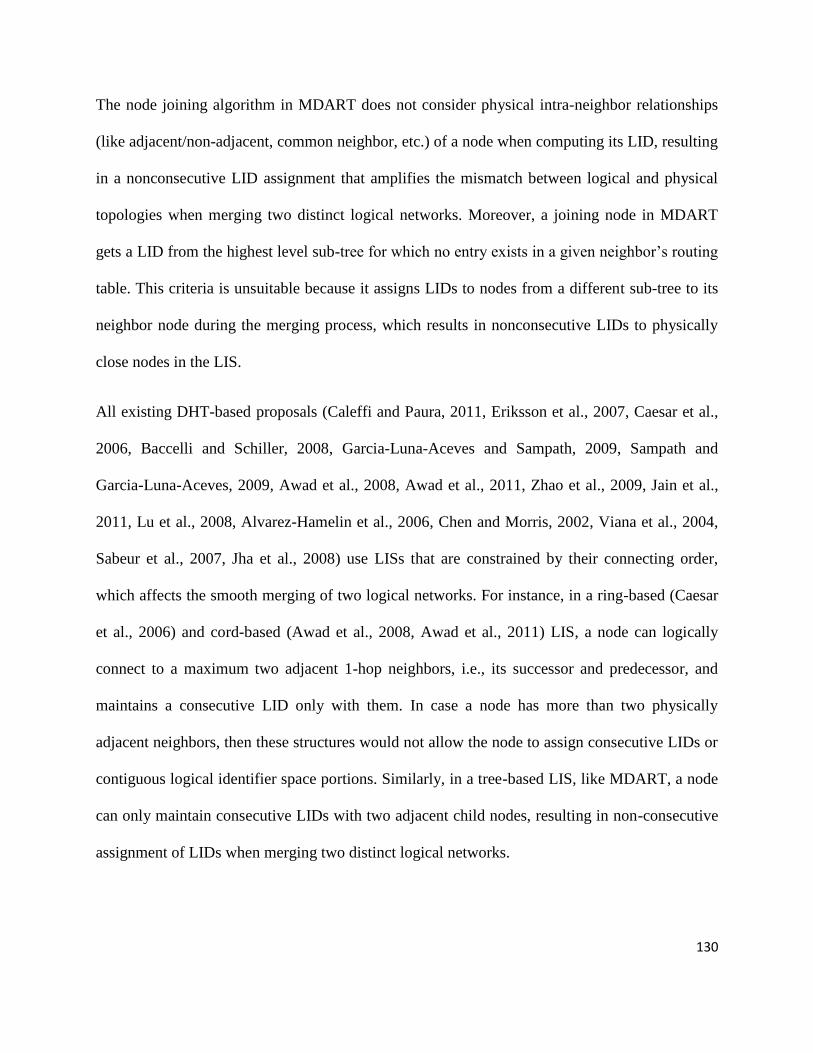
130
The node joining algorithm in MDART does not consider physical intra-neighbor relationships
(like adjacent/non-adjacent, common neighbor, etc.) of a node when computing its LID, resulting
in a nonconsecutive LID assignment that amplifies the mismatch between logical and physical
topologies when merging two distinct logical networks. Moreover, a joining node in MDART
gets a LID from the highest level sub-tree for which no entry exists in a given neighbor’s routing
table. This criteria is unsuitable because it assigns LIDs to nodes from a different sub-tree to its
neighbor node during the merging process, which results in nonconsecutive LIDs to physically
close nodes in the LIS.
All existing DHT-based proposals (Caleffi and Paura, 2011, Eriksson et al., 2007, Caesar et al.,
2006, Baccelli and Schiller, 2008, Garcia-Luna-Aceves and Sampath, 2009, Sampath and
Garcia-Luna-Aceves, 2009, Awad et al., 2008, Awad et al., 2011, Zhao et al., 2009, Jain et al.,
2011, Lu et al., 2008, Alvarez-Hamelin et al., 2006, Chen and Morris, 2002, Viana et al., 2004,
Sabeur et al., 2007, Jha et al., 2008) use LISs that are constrained by their connecting order,
which affects the smooth merging of two logical networks. For instance, in a ring-based (Caesar
et al., 2006) and cord-based (Awad et al., 2008, Awad et al., 2011) LIS, a node can logically
connect to a maximum two adjacent 1-hop neighbors, i.e., its successor and predecessor, and
maintains a consecutive LID only with them. In case a node has more than two physically
adjacent neighbors, then these structures would not allow the node to assign consecutive LIDs or
contiguous logical identifier space portions. Similarly, in a tree-based LIS, like MDART, a node
can only maintain consecutive LIDs with two adjacent child nodes, resulting in non-consecutive
assignment of LIDs when merging two distinct logical networks.

131
We have shown how the mismatch problem between physical and logical networks is aggravated
when merging two logical networks. If we observe the LIS in MDART after the merging process
is completed (Figure 4.2(c)), the tree-based LIS does not reflect the physical proximity of nodes.
The resultant effect can be seen when routing a packet from a source to a destination node. As
routing is performed using LIDs, a direct link between two nodes in the LIS may span multi-
hops in the physical network, resulting in redundant traffic and increased end-to end delay.
In the next section, we explain how 3D-LIS proposed in 3D-RP (see Chapter 3) is efficient in
merging two logical networks.
4.5 3D-BASED LIS
3D-LIS is a multidimensional Cartesian Space, which leverages each node in the network to
compute its LID that exactly reflects the physical proximity of the node to optimally address the
mismatch problem. Moreover, the 3D-structure is not constrained by the connecting order, unlike
the LISs discussed in Chapter 2, which helps to smoothly conduct the merging process without
disturbing the consecutiveness of LIDs. In 3D-LIS, each node considers the neighbor
relationships, like intra-neighbor, adjacent/nonadjacent neighbor, and common neighbor, when
computing its LID, which helps to exactly map the physical proximity of nodes in the LIS. These
relationships are crucial when calculating the relative position of a node. For instance, if a node
p has three neighbors (say p1, p2, and p3) and p1, p2, and p3 are not within the transmission
range of each other, then we assume that these neighbors exist physically in three different
dimensions of node P. 3D-LIS is flexible in assigning LIDs to nodes in such scenarios.

132
4.5.1 Logical network merger case-study: 3D-RP
We use an example to illustrate how the node joining algorithms and 3D-LIS proposed in 3D-RP
are more resilient and flexible in merging two logical networks compared to MDART’s node
joining algorithms and LISs.
Figure 4.3 shows the merging process of two 3D-LISs, i.e., LIS-1 and LIS-2, in which nodes are
assigned LIDs according to the algorithm described in Chapter 3. Suppose the corresponding
physical networks of LIS-1 and LIS-2 are PN-1and PN-2, respectively, as shown in Figure
4.3(a). The 3D-LS ranges from 1 to ± 210
for each axis, i.e., x, y, and z. Node i and node s are
leader nodes of LIS-1 and LIS-2, respectively. The alphabets i, p, q,… refers to the UID of nodes
and {1|1|1}-0, {256|1|1}-2, … refers to the LID of nodes.
Node i with LID {1|1|1}-0 in LIS-1 detects that there exists another logical network, LIS-2. Node
i of LIS-1 can access node s with LID {1|1|1}-0 of LIS-2 in the physical network but is not
connected with LIS-2 as shown in Figure 4.3(a). Node i of LIS-1 invokes the merging process by
sending a merging request message (MRQST) to node s of LIS-2. On receiving the MRQST,
node s first changes its leader ID to node i’s leader ID, i.e., node i’s UID and re-computes its
LID, i.e., {1|256|1}-3 in LIS-1 by selecting the available dimension of node i as discussed in
Case 1 of the proposed node joining algorithm (see Section 3.2 for details). Next, node s with
new LID {1|256|1}-3 sends a merging reply message (MRPLY) to node i of LIS-1.
In the mean time, node s also maintains its connectivity in LIS-2, acting as a BRIDGE node
between LIS-1 and LIS-2, as shown by the big-dashed line in Figure 4.3(b).

133
After joining LIS-1, node s informs its one-hop neighbours, i.e. node u with LID {256|1|1}-1 and
node t with LID {-256|1|1}-2, of the merger by forwarding the MRQST to them so that they can
join LIS-1. Upon receiving the MRQST, nodes u and t repeat the same process that node s
performed when joining the LIS-1 and re-compute their LIDs. The new LIDs for node u and
node r are {1|448|1}-3 and {448|256|1}-3, respectively, chosen by selecting the available
dimensions of node s as shown in Figure 4.3(c). Receiving the information that its direct
neighbors have joined LIS-1, node s with LID {1|256|1}-3 leaves LIS-2 and changes its state
from BRIDGE to a common node. After computing their LIDs, node u and node t maintain their
connectivity with LIS-1 and acts as BRIDGE between the two logical networks in case they have
any direct neighbors.
Figure 4.3(c) shows that after completing the merging process in 3D-LIS:
i) the neighbor nodes in LIS-1 are also adjacent in PN-1;
ii) a node in LIS-1 is logically close to all its physically adjacent nodes.
These are the basic requirements to avoid the mismatch between logical and physical networks.
This shows that 3D-RP successfully maintains the physical proximity of nodes in terms of LIDs
even after merging two 3D-LISs. The routing tables in Figure 4.4 are built according to 3D-RP’s
path discovery process, where each node maintains information about all its 1-hop neighbors and
neighborhood of 1-hop neighbors.

134
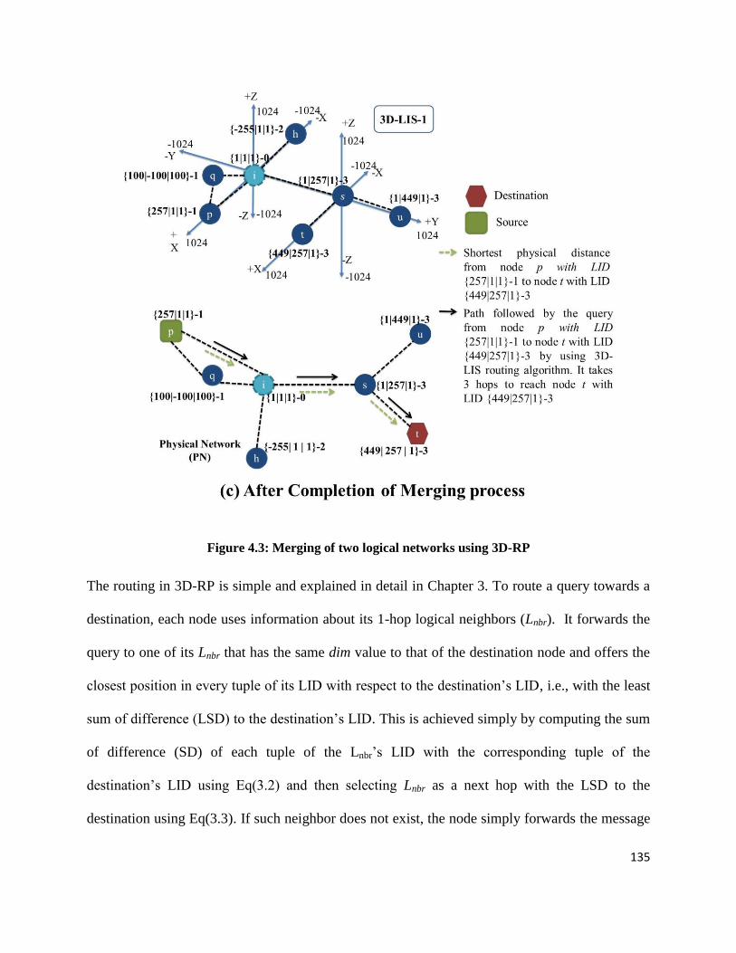
135
Figure 4.3: Merging of two logical networks using 3D-RP
The routing in 3D-RP is simple and explained in detail in Chapter 3. To route a query towards a
destination, each node uses information about its 1-hop logical neighbors (Lnbr). It forwards the
query to one of its Lnbr that has the same dim value to that of the destination node and offers the
closest position in every tuple of its LID with respect to the destination’s LID, i.e., with the least
sum of difference (LSD) to the destination’s LID. This is achieved simply by computing the sum
of difference (SD) of each tuple of the Lnbr’s LID with the corresponding tuple of the
destination’s LID using Eq(3.2) and then selecting Lnbr as a next hop with the LSD to the
destination using Eq(3.3). If such neighbor does not exist, the node simply forwards the message

136
to its base node. If there are multiple base nodes, the node selects the one that offers the closest
position in every tuple of its LID with respect to the destination’s LID.
Suppose node p with LID {256|1|1}-1} initiates a query destined for node t with LID
{448|256|1}-3 as shown in Figure 4.3(c). Node p checks its 1-hop logical neighbors, i.e., node i
{1|1|1}-0 and node q {100|-100|100}-1, in its routing table as shown in Figure 4.4. Both node i
and node q are in different dimensions to that of the destination node t, i.e., dim=3. Node m
sends the packet to its base node i, which becomes the next hop. Node i then checks 1-hop
logical neighbors in its routing table as shown in Figure 4.4 and finds node s with LID {1|256|1}-
3 that has the same dim value as that of the destination node t. Node i calculates the sum of
difference, i.e., SDs = {|1-448|=447}+{|256-256|=0}+{1-1=0}→{447+0+0}→{447} of its
neighbor node s with respect to the destination node q to see if node s is the destination node.
SDs = {447}≠ 0, which means that node s is not the destination node but is near the destination
node t. So, node i forwards the query towards node s. Node s has two 1-hop neighbors, i.e., node
u and node t with the same dim value to the destination node. Node s calculates the sum of the
difference of its neighbor nodes, i.e., SDu = {|1-448|=447} + {|448-256|=192} + {1-1=
0}→{447+192+0}→{639}and SDt = {|448-448|=0}+{|256-256|=0}+ {1-1=0}→{0+0+0}→{0},
using Eq(3.2). Node s then sends the data packet to node t with LID {448|256|1}-3, which is the
destination node with LSDt = {0} as shown in Figure 4.3(c).
In the above example, we observe that 3D-LIS takes the shortest route in the logical network,
i.e., p→i, i→s, s→t (3 hops) towards the destination node t as shown in Figure 4.3(c). The
shortest route between node p and node t in the physical network is also 3 hops.

137
Figure 4.4: Routing Tables for node i, q, p, s
This proves that the proposed node joining algorithm and 3D structure proposed in 3D-LIS is
more resilient than the existing DHT-based protocols. The node joining algorithm and 3D
structure are more capable of smoothly merging two logical networks compared to MDART.
4.6 Performance Analysis
To analyze the performance of 3D-LIS when merging two logical networks, we implemented it
in NS-2 (version 2.35) (Fall and Varadhan, 2005), which is an open source discrete event

138
network simulator. We adopted the standard values for both the physical and link layers to
simulate IEEE 802.11 with Two-Ray Ground as the propagation model. The key objective is to
rely on a contention-based MAC protocol that is best suited for distributed and self-organizing
routing protocols. To generate mobile topologies, we adopt the Random Way-Point as the
mobility model. The mobility parameters have been set to simulate moderate mobility,
specifically, the speed values are uniformly taken in the [1 m/s, 2 m/s] range. The simulation
parameters are given in Table 4.1. The data traffic is modeled as CBR flows over UDP protocol
and Random Traffic Model is used as data pattern. We do not adopt TCP as the transport
protocol to avoid the elasticity effects of TCP flow control on routing performances (Holland and
Vaidya, 2002). The global load offered is kept constant at 100 pkts/sec in order to avoid running
out of capacity due to multi-hop approach.
We embed the proposed leader-based based approach (LA) to detect and merge two logical
networks in 3D-RP and MDART protocols to analyze different aspects by varying several
parameter values that affect the performance of these protocols and compare LA-3D-RP with
LA-MDART.
The same parameters explained in Section 3.6 are used to evaluate the performance of LA-
MDART and LA-3D-RP, namely path-stretch ratio, packet delivery ratio, end-to-end delay, and
routing overhead, an additional parameter is false negative (FN) ratio (%), which is the ratio
between the number of unresolved lookup queries for the destination that exist in physically
connected network to the total number of initial lookup queries.
We perform ten experiments for each scenario. The upper and lower bars in the graphs show the
margin of error to the mean estimates at 95% confidence interval.

139
Table 4.1: Simulation Parameters
Input Parameters Value
Number of Nodes
Transmission range
25-400
50m
Playground Size 1000*1000m
Data Rate 100pps
Simulation Time 500sec
Start of Data Transmission 70,300
End of Data Transmission 250,499
Node Speed 1 to 2 m/s
Start of Node Failure
Mobility Model
Radio Propagation Model
100 sec
Random Way-point
TwoRayGround Model
Traffic Model Random Traffic pattern
4.6.1 Quality of Routing Paths
Figure 4.5 plots the average path-stretch ratio against network size to compare LA-MDART to
LA-3D-RP, which shows the path-stretch ratio of LA-3D-RP is lower compared to LA-MDART
for all network sizes. LA-3D-RP improves the path-stretch ratio between 25%-27%. The path-
stretch ratio of LA-3D-RP stays slightly above the shortest path, but the mean value stays below
1.2. The slight increase of path-stretch ratio in LA-3D-RP is because when a new node, for
instance P, comes in contact with two non-adjacent neighbors (say, P1, P2) with different dim
values and there is no common neighbor, then the new node P would get an LID using available
dimensions of either P1 or P2, depending on which one is closer in terms of distance. So, in this

140
case, the LID of the new node P would only show its relative position in the 3D-LIS with respect
to that neighbor from which it gets its LID. This can cause a slight mismatch problem in LA-3D-
RP when merging two logical networks. However, this situation occurs less frequently in LA-
3D-RP and its impact is less serious as shown by the simulation results.
Figure 4.5: Path-stretch ratio as a function of the network size
Figure 4.5 shows that LA-3D-RP has a lower path-stretch ratio compared to LA-MDART, which
means that LA-3D-RP is more capable of selecting an optimal path even after merging two
logical networks. The path-stretch ratio in LA-MDART increases up to 1.4 because it uses a tree-
based LIS to map the physical network, resulting in the mismatch problem. As discussed in
Section 4.4.2, the tree-based LIS ensures neither adjacency of all physically adjacent neighbors
in LIS nor the intra-neighbor relationship of nodes. This makes it impossible to assign
consecutive LIDs to all physically adjacent neighbors of a node when merging two distinct
logical networks. Therefore, messages may be routed through many unnecessary nodes.
1
1.2
1.4
1.6
0 50 100 150 200 250 300 350 400
Pa
th-s
tretc
h r
ati
o
Network Size (nodes)
LA-MDART
LA-3D-RP
141
LA-3D-RP reduces the number of redundant transmissions that decreases the end-to-end delay,
loss ratio, and routing overhead, which in turn, reduces energy consumption and increases
network longevity. When the number of transmissions in a MANET decreases, packet collision
probability at the MAC layer also decreases, leading to more reliable transmissions. Thus, our
approach also results in more reliable transmissions at the MAC layer by reducing the number of
redundant transmissions compared to LA-MDART.
Below is the null hypothesis to test the impact of network size and protocols on path-stretch
ratio:
Ho: LA-3D-RP does not significantly reduce the path-stretch ratio compared to LA-MDART.
Table 4.2 shows the result of applying the Two-way ANOVA with replication.
Table 4.2: Summary of data analysis of the path-stretch Ratio for LA-3D-RP and LA-MDART
using ANOVA Two-Factor with replication
The results of the Two-way ANOVA with replication (Table 4.2) shows that p < 0.05, which
leads to the rejection of Ho. This shows that LA-3D-RP is statistically significant in terms of

142
reducing path-stretch ratio compared to LA-MDART and that LA-3D-RP is effective in reducing
the impact of the mismatch problem when merging two logical networks. The notion of
involving intra-neighbor relationships of a node while calculating LID ensures the physical
proximity of nodes in the logical network that leads to optimal routes towards destination nodes,
resulting in reduced path-stretch ratio in case of LA-3D-RP.
Table 4.3: Results: pairwise data analysis of the path-stretch ratio at each network size for LA-3D-
RP and LA-MDART using ANOVA Two-Factor With Replication
Table 4.3 shows the pairwise comparisons of LA-3D-RP and LA-MDART for each network
size. Table 4.3 shows that LA-3D-RP significantly improves the path-stretch ratio over LA-

143
MDART for each network size when merging two logical networks. The result confirms that 3D
structure is efficient in merging logical networks and the methodology adopted in LA-3D-RP is
effective in reducing the impact of the mismatch problem when merging two logical networks.
4.6.2 Impact of network size
In order to analyze the behavior of LA-3D-RP with respect to network size, we conduct
experiments by varying the number of nodes from 25 to 400 while maintaining the data rate at
100 pkts/s. The data rate of 100 pkts/sec is selected because both LA-3D-RP and LA-MDART
performs better at this rate. It has been observed that MDART is vulnerable to high data rates as
shown in Section 3.6.2 The simulation results show that 3D-RP is consistent in improving
performance over LA-MDART.
(a) End-to-End delay
Figure 4.6 shows that LA-3D-RP scales better than LA-MDART in terms of end-to-end delay as
the network size increases. Please note that LA-MDART, which is an enhancement of DART, is
designed to provide a reliable path in order to enhance throughput rather than minimize the hop
count. LA-MDART’s inflexible structure that results in longer routes and larger end-to-end delay
when merging two logical networks.
Unlike LA-MDART, LA-3D-RP is designed to provide a reliable path that enhances its
throughput. Furthermore, the arrangement of nodes in the 3D structure and the joining scheme
supplements to minimize the number of hops between nodes, provide an alternative route in case
of intermediate node fail/move, and effective for smooth merging of two logical networks. LA-
3D-RP performs better and provides near optimal routes towards the destination, which

144
decreases the end-to-end delay and increases packet delivery ratio as shown in Figure 4.6 and
Figure 4.7, respectively.
0
0.01
0.02
0.03
0.04
0.05
0.06
0.07
0 50 100 150 200 250 300 350 400
En
d-t
o-E
nd
Dela
y (
s)
Network Size (nodes)
LA-MDART
LA-3D-RP
(a) Node Speed 1m/s
0
0.01
0.02
0.03
0.04
0.05
0.06
0.07
0 50 100 150 200 250 300 350 400
En
d-t
o-E
nd
Dela
y (
s)
Network Size (nodes)
LA-MDART
LA-3D-RP
(b) Node Speed 1.5m/s

145
Figure 4.6: End-to-End delay as a function of network size with varying node speed
As shown in Figure 4.10, the end-to-end delay improvement of LA-3D-RP over MDART with
respect to increase in network size is between 11% to 46%. This shows the LA-3D-RP is more
consistent and reliable approach for relatively large networks compared to LA-MDART.
Figure 4.6 also shows that end-to-end delay of LA-3D-RP increases as the node speed increases,
but the net effect is less compared to LA-MDART. Because the network topology changes
frequently as the node speed increases, it produces more routing traffic in the network by
executing more frequently the recovery and logical network merging operations, which effects
the end-to end delay for both protocols. Figure 4.6 indicates that the end-to-end delay of LA-3D-
RP is less than LA-MDART. LA-MDART’s inflexible tree-based structure fails to maintain
consecutive LIDs between adjacent neighbors of a node, resulting in long routes and larger end-
to end delay. Figure 4.10 shows that the end-to-end delay improvement over MDART decreases
with the increase in node speed but still the improvement is significant, especially, with an
increasing network size, which shows the effectiveness of the LA-3D-RP in mobile scenarios
compared to LA-MDART.
0
0.01
0.02
0.03
0.04
0.05
0.06
0.07
0 50 100 150 200 250 300 350 400
En
d-t
o-E
nd
Dela
y (
s)
Network Size (nodes)
LA-MDART
LA-3D-RP
(c) Node Speed 2m/s

146
The following is null hypothesis to test the impact of network size and protocols on end-to-end
delay at node speed 1 m/s, 1.5m/s, and 2 m/s:
Ho : LA-3D-RP does not significantly reduce on end-to-end delay compared to LA-MDART at
node speeds of 1m/s, 1.5m/s, and 2m/s.
Table 4.4, Table 4.5, Table 4.6, Table 4.7 show the result of applying the Two-way ANOVA
with replication.
The result of the Two-way ANOVA test (Table 4.4, Table 4.5 and Table 4.6) shows that p < 0.05
for data at node speeds 1m/s, 1.5 m/s, and 2m/s, which leads to the rejection of Ho. This shows
that LA-3D-RP is statistically significant in terms of reducing end-to-end delay compared to LA-
MDART. Thanks to the efficient 3D structure and node joining algorithm of LA-3D-RP that not
only ensure the physical proximity of nodes in the logical network that leads to optimal routes
towards destination nodes, but also effective in merging two logical networks.
Table 4.4: Summary of data analysis of End-to-End Delay for LA-3D-RP and LA-MDART at node
speed 1m/s using ANOVA Two-Factor with replication

147
Table 4.5: Summary of data analysis of End-to-End Delay for LA-3D-RP and LA-MDART at node
speed 1.5m/s using ANOVA Two-Factor with replication
Table 4.6: Summary of data analysis of End-to-End Delay for LA-3D-RP and LA-MDART at node
speed 2m/s using ANOVA Two-Factor with replication
Table 4.7, Table 4.8, and Table 4.9 show the pairwise comparisons of LA-3D-RP and LA-
MDART for each network size at node speed of 1 m/s, 1.5 m/s, and 2 m/s, respectively. The
results show that LA-3D-RP significantly reduces end-to-end delay for each network size when

148
merging two logical networks. When the network size increases, LA-3D-RP shows more
promising behavior compared to MDART. The results confirm that 3D structure is efficient in
merging logical networks and the technique adopted in LA-3D-RP is effective in reducing the
impact of the mismatch problem when merging two logical networks.
Table 4.7: Results: pairwise data analysis of the End-to-End Delay at node speed 1m/s for LA-3D-
RP and LA-MDART using ANOVA Two-Factor with Replication

149
Table 4.8: Results: pairwise data analysis of the End-to-End Delay at node speed 1.5m/s for LA-3D-
RP and LA-MDART using ANOVA Two-Factor with Replication

150
Table 4.9: Results: pairwise data analysis of the End-to-End Delay at node speed 2m/s for LA-3D-
RP and LA-MDART using ANOVA Two-Factor with Replication
(b) Packet Delivery Ratio
Figure 4.7 shows that the effect of increasing network size on the packet delivery ratio is less on
LA-3D-RP compared to LA-MDART. This is important because it proves the effectiveness and
capability of LA-3D-RP in delivering packets in large networks with relatively high data traffic.
On the contrary, LA-MDART’s performance degrades as the number of nodes increases (see
Figure 4.7). Figure 4.10 shows that the packet delivery ratio improvement of LA-3D-RP over
LA-MDART is between 6% to 29% for different network sizes and node speeds.

151
0
20
40
60
80
100
0 50 100 150 200 250 300 350 400
Pa
ck
et
Deli
very
Ra
tio
Network Size (nodes)
LA-MDART
LA-3D-RP
(a) Node Speed 1m/s
0
20
40
60
80
100
0 50 100 150 200 250 300 350 400
Pa
ck
et
Deli
very
Ra
tio
Network Size (nodes)
LA-MDART
LA-3D-RP
(b) Node Speed 1.5m/s
0
20
40
60
80
100
0 50 100 150 200 250 300 350 400
Pa
ck
et
deli
very
Ra
tio
Network Size (nodes)
LA-MDART
LA-3D-RP
(c) Node Speed 2m/s

152
Figure 4.7: Packet Delivery Ratio as a function of network size with varying node speed
Figure 4.7 also illustrates that varying node speeds affects the performance of both protocols, but
the net effect of increasing the node speed on the packet delivery ratio is lower in LA-3D-RP
compared to LA-MDART. With the increase in node speed, the network topology changes more
frequently, resulting in increasing routing overhead due to frequent execution of recovery and
logical network merging operations. This causes the packets to be delayed in the queue due to
MAC layer congestion, resulting in packet drops. The effect of the congestion on LA-3D-RP is
lower compared to LA-MDART. This behavior is reasonable given that LA-3D-RP introduces
low path stretch ratio. On the contrary, LA-MDART’s tree-based hierarchical nature results in
high path-stretch, is inefficient against mobility and is a potential source of path length
inefficiency. For the same reason, the alternative routes provided by MDART are not optimal,
causing an increase in the number of in transit packets that leads to network congestion,
especially at a relatively high data rate. The overall result proves that LA-3D-RP resolves the
mismatch problem effectively when merging two logical networks.
Below is the null hypothesis to test the impact of network size and protocols on the packet
delivery ratio at node speeds 1 m/s, 1.5m/s, and 2 m/s:
Ho: LA-3D-RP does not significantly improve the packet delivery ratio compared to LA-
MDART at node speeds 1m/s, 1.5m/s, and 2m/s.
Table 4.10, Table 4.11, and Table 4.12 show the results of applying the Two-way ANOVA with
replication on data about the packet delivery ratio at node speeds 1m/s, 1.5m/s, and 2m/s.

153
Table 4.10: Summary of data analysis of the Packet Delivery Ratio for LA-3D-RP and LA-MDART
at node speed 1m/s using ANOVA Two-Factor with replication
Table 4.11: Summary of data analysis of the Packet Delivery Ratio for LA-3D-RP and LA-MDART
at node speed 1.5m/s using ANOVA Two-Factor with replication

154
Table 4.12: Summary of data analysis of the Packet Delivery Ratio for LA-3D-RP and LA-MDART
at node speed 2m/s using ANOVA Two-Factor with replication
Table 4.13: Results: pairwise data analysis of the Packet Delivery Ratio at node speed 1m/s for LA-
3D-RP and LA-MDART using ANOVA Two-Factor with Replication

155
The results of the Two-way ANOVA test (Table 4.10, Table 4.11, and Table 4.12) show that p <
0.05, which leads to the rejection of Ho. This shows that LA-3D-RP is statistically significant in
terms of improving the packet delivery ratios compared to LA-MDART and that LA-3D-RP is
less affected in terms of the packet delivery ratio when merging logical networks. This also
shows that LA-3D-RP is efficient in selecting routes that reduces the end-to-end delay, which in
turn decreases congestion and increases the packet delivery ratio. 3D structure is flexible in
providing multiple routes towards the destination node that increases the packet delivery ratio of
LA-3D-RP. Moreover, the replication strategy used in 3D-RP efficiently reduces the packet loss
in case anchor node moves/fails.
Table 4.14: Results: pairwise data analysis of the Packet Delivery Ratio at node speed 1.5m/s for
LA-3D-RP and LA-MDART using ANOVA Two-Factor with Replication

156
Table 4.13, Table 4.14, and Table 4.15 show the pairwise comparisons of LA-3D-RP and LA-
MDART in terms of the packet delivery ratio for each network size at node speed of 1 m/s, 1.5
m/s, and 2 m/s, respectively.The results show that LA-3D-RP shows significant improvement
over LA-MDART in terms of the packet delivery ratio for each network size when merging two
logical networks. When the network size increases LA-3D-RP shows more promising behavior
compared to MDART. The results confirm that the 3D structure is efficient in merging logical
networks and the technique adopted in LA-3D-RP is effective in reducing the impact of the
mismatch problem when merging two logical networks.
Table 4.15: Results: pairwise data analysis of the Packet Delivery Ratio at node speed 2m/s for LA-
3D-RP and LA-MDART using ANOVA Two-Factor with Replication
157
(c) Routing Overhead
Figure 4.8 shows that both LA-3D-RP and LA-MDART exhibit high routing overhead because
their routing update packets are of fixed size regardless of the network size. Moreover, the
reassignment of LIDs to one partition when merging two logical networks increase the overhead
in both protocols as shown in Figure 4.8. However, the replication strategy (see Chapter 3 for
detail) used by LA-3D-RP in case the anchor node moves/fails, effectively reduces the overhead
between 13% to 30% as shown in Figure 4.10. Moreover, the flexible 3D structure assists the
smooth merging of two distinct logical networks that further reduces the overhead in LA-3D-RP.
Figure 4.8 also illustrates the effect of increase in node speed. As the node speed increases, the
network topology changes frequently and produces more routing traffic in the network by
executing more frequently the recovery, reassignment of LIDs, displacement of anchor nodes,
storing mapping information at anchor nodes. The routing overhead of LA-3D-RP increases with
the increase in speed, but the net effect is lower compared to LA-MDART. LA-3D-RP employs
an effective replication strategy at anchor nodes for storing mapping information, which is
effective in case anchor node moves or fails. Moreover, LA-3D-RP’s resilient 3D structure is
effective in smooth merging and routing of data packets from source to destination compared to
LA-MDART.

158
Figure 4.8: Routing Overhead as function of network size with varying node speed
0
50
100
150
200
250
300
350
400
450
0 50 100 150 200 250 300 350 400
Ro
uti
ng
Ov
erh
ea
d (
10
3)
in
pa
ck
ets
Network Nodes (nodes)
LA-MDART
LA-3D-RP
(a) Node Speed 1m/s
0
50
100
150
200
250
300
350
400
450
0 50 100 150 200 250 300 350 400
Ro
uti
ng
Ov
erh
ea
d (
10
3)
in p
ack
ets
Network Size (nodes)
LA-MDART
LA-3D-RP
(b) Node Speed 1.5m/s
0
50
100
150
200
250
300
350
400
450
0 50 100 150 200 250 300 350 400
Ro
uti
ng
Ov
erh
ea
d (
10
3)
in p
ack
ets
Network Size (nodes)
LA-MDART
LA-3D-RP
(c) Node Speed 2m/s

159
The following id the null hypothesis to test the impact of network size and protocols on routing
overhead at node speed 1 m/s, 1.5m/s, and 2 m/s:
Ho: LA-3D-RP does not significantly reduce routing overhead compared to LA-MDART at node
speeds of 1m/s, 1.5m/s, and 2m/s.
Table 4.16, Table 4.17, and Table 4.18 show the results of applying the Two-way ANOVA with
replication on data about routing overhead at node speeds 1m/s, 1.5m/s, and 2m/s.
Table 4.16: Summary of data analysis of Routing Overhead for LA-3D-RP and LA-MDART at
node speed 1m/s using ANOVA Two-Factor with replication
The results of the Two-way ANOVA test (Table 4.16, Table 4.17, and Table 4.18) show that p <
0.05, which leads to the rejection of Ho. This shows that LA-3D-RP is statistically significant in
terms of reducing routing overhead compared to LA-MDART. This shows that LA-3D-RP is less
affected in terms of routing overhead when merging logical networks and shows significant
improvement over LA-MDART.

160
Table 4.17: Summary of data analysis of Routing Overhead for LA-3D-RP and LA-MDART at
node speed 1.5m/s using ANOVA Two-Factor with replication
Table 4.18: Summary of data analysis of Routing Overhead for LA-3D-RP and LA-MDART at
node speed 2m/s using ANOVA Two-Factor with replication

161
Table 4.19: Results: pairwise data analysis of Routing Overhead at node speed 1m/s for LA-3D-RP
and LA-MDART using ANOVA Two-Factor with Replication
The inflexible tree structure of LA-MDART does not ensure the physical proximity of nodes
when merging two logical networks. This aggravates the mismatch problem and increases
routing overhead when routing packets towards destination node. On the other hand, LA-3D-RP
employs a 3D structure that reduces overhead when merging two logical networks, but also
efficiently reduces the impact of mismatch problem after merging of logical networks. The
analysis above shows the improvement in routing overhead using LA-3D-RP is significant
compared to LA-MDART.

162
Table 4.20: Results: pairwise data analysis of Routing Overhead at node speed 1.5m/s for LA-3D-
RP and LA-MDART using ANOVA Two-Factor with Replication
The inflexible tree structure of LA-MDART does not ensure the physical proximity of nodes
when merging two logical networks. This aggravates the mismatch problem and increases
routing overhead when routing packets towards destination node. On the other hand, LA-3D-RP
employs a 3D structure that reduces overhead when merging two logical networks, but also
efficiently reduces the impact of mismatch problem after merging of logical networks. The
analysis above shows the improvement in routing overhead using LA-3D-RP is significant
compared to LA-MDART.

163
Table 4.20, and Table 4.21 show the pairwise comparisons of LA-3D-RP and LA-MDART in
terms of routing overhead for each network size at node speed of 1 m/s, 1.5 m/s, and 2 m/s,
respectively. The results show that LA-3D-RP significantly reduces routing overhead compared
to LA-MDART for each network size when merging two logical networks. The results confirm
that 3D structure is efficient in merging logical networks and the technique adopted in LA-3D-
RP is effective in reducing the impact of the mismatch problem when merging two logical
networks..
Table 4.21: Results: pairwise data analysis of Routing Overhead at node speed 2m/s for LA-3D-RP
and LA-MDART using ANOVA Two-Factor with Replication

164
(d) False negative (FN) ratio
Figure 4.9 shows that the FN ratio of LA-3D-RP and LA-MDART increases as the network size
increases and/or varying nodes’ speed because the routing traffic of both increases with
increasing network size and/or node speed. This leads to more packet collisions in the network,
resulting in an increased FN ratio. The FN ratio of LA-3D-RP is 24%-65% less compared to LA-
MDART under various node speeds because LA-MDART incurs a higher routing overhead than
LA-3D-RP, which leads to more packet collisions in the network.
0
5
10
15
20
25
30
35
40
25 50 100 150 200 250 300 350 400
Ra
tio
of
FN
(%)
Network Size (nodes)
LA-MDART
LA-3D-RP
(a) Node Speed 1m/s
0
5
10
15
20
25
30
35
40
25 50 100 150 200 250 300 350 400
Ra
tio
of
FN
(%)
Network Size (nodes)
LA-MDART
LA-3D-RP
(b) Node Speed 1.5m/s

165
Figure 4.9: False negative ratio with respect to network size with varying node speed
Below is the null hypothesis to test the impact of network size and protocols on FN ratio at node
speed 1 m/s, 1.5m/s, and 2 m/s:
Ho: LA-3D-RP does not significantly reduces the FN ratio compared to LA-MDART at node
speeds 1m/s, 1.5m/s, and 2m/s.
Table 4.22: Summary of data analysis of the FN Ratio for LA-3D-RP and LA-MDART at node
speed 1m/s using ANOVA Two-Factor with replication
0
5
10
15
20
25
30
35
40
25 50 100 150 200 250 300 350 400
Ra
tio
of
FN
(%
)
Network Size (nodes)
LA-MDART
LA-3D-RP
(c) Node Speed 2m/s

166
Table 4.23: Summary of data analysis of the FN Ratio for LA-3D-RP and LA-MDART at node
speed 1.5m/s using ANOVA Two-Factor with replication
Table 4.24: Summary of data analysis of the FN Ratio for LA-3D-RP and LA-MDART at node
speed 2m/s using ANOVA Two-Factor with replication

167
Table 4.25: Results: pairwise data analysis of the FN Ratio at node speed 1m/s for LA-3D-RP and
LA-MDART using ANOVA Two-Factor with Replication
Table 4.22, Table 4.23, and Table 4.24 show the results of applying the Two-way ANOVA with
replication on data about the FN ratio for LA-3D-RP and LA-MDART at node speeds 1m/s,
1.5m/s, and 2m/s.

168
Table 4.26: Results: pairwise data analysis of the FN Ratio at node speed 1.5m/s for LA-3D-RP and
LA-MDART using ANOVA Two-Factor with Replication
The results of the Two-way ANOVA test (Table 4.22, Table 4.23, and Table 4.24) show that p <
0.05, which leads to the rejection of Ho. This shows that LA-3D-RP is statistically significant in
terms of reducing FN ratio compared to LA-MDART. LA-3D-RP is less affected in terms of
routing overhead when merging logical network and difference of the number of lookup queries
that reaches the destination is significant in LA-3D-RP compared to LA-MDART. This confirms
the results related to the high packet delivery ratio of LA-3D-RP compared to LA-MDART.
Table 4.27, Table 4.25, Table 4.26 show the pairwise comparisons of LA-3D-RP and LA-
MDART in terms of FN ratio for each network size at node speeds 1 m/s, 1.5 m/s, and 2 m/s,

169
respectively. The results show that LA-3D-RP significantly improves the FN ratio over LA-
MDART when merging two logical networks.
Table 4.27: Results: pairwise data analysis of the FN Ratio at node speed 2m/s for LA-3D-RP and
LA-MDART using ANOVA Two-Factor with Replication

170
Figure 4.10: Percentage of improvement provided by LA-3D-RP over LA-MDART as a function of
the node number at various node speed
0
10
20
30
40
50
60
25 50 100 150 200 250 300 350 400
% I
mp
ro
vem
en
t w
.r.t
LA
-
MD
AR
T a
t N
od
e S
peed
of
1m
/s
Network Size
PDR
E2E
OV
(a)
0
10
20
30
40
50
60
25 50 100 150 200 250 300 350 400
% I
mp
ro
vem
en
t w
.r.t
LA
-
MD
AR
T a
t N
od
e S
peed
of
1.5
m/s
Network Size
PDR
E2E
OV
(b)
0
10
20
30
40
50
60
25 50 100 150 200 250 300 350 400
% I
mp
ro
vem
en
t w
.r.t
LA
-
MD
AR
T a
t N
od
e S
peed
of
2
m/s
Network Size
PDR
E2E
OV
(c)

171
4.7 CONCLUSION
Physical network partitioning and merging in MANETs may occur due to limited transmission
range and mobility of nodes. This partitioning and merging leads to logical network partitioning
and merging in DHT-based routing protocols. Two crucial issues to address for DHT-based
routing protocols in MANETs are the mismatch problem and the resilience of the logical
structure that aggravates when merging two distinct logical networks.
This chapter comprehensively discusses the challenges and issues related to the merging of two
DHT-based logical networks and proposes a leader-based approach to detect and merge the
logical networks. Moreover, the leader-based approach is embedded in 3D-RP and MDART to
compare their performance in resolving the mismatch problem, especially when merging logical
networks.
Simulation results show that LA-3D-RP scales well as the network size increases and is effective
in merging logical networks. Compared to LA-MDART, LA-3D-RP reduces the end-to-end
delay between 11% to 46% and increases the packet delivery ratio between 6% to 29%. In
addition, LA-3D-RP incurs lower routing overhead, false negative ratio, and path-stretch ratio,
which makes it attractive for large scale MANETs. Compared to LA-MDART, LA-3D-RP
reduces routing overhead between 13% to 30% and improves the path-stretch ratio between 25%
to 27%.
In conclusion, the simulation results show that LA-3D-RP has successfully addressed the
mismatch problem and is a resilient logical structure to smoothly merge two logical networks.

172
We intend to extend our work to provide an analytical comparison of our approach compared to
MDART.

173
5 3D P2P OVERLAY OVER MANETS
This chapter presents a new content sharing protocol for peer-to-peer (P2P) overlay networks
over MANETs, which is inspired from 3D-RP (see Chapter 3 for detail) and uses both a
distribute hash table (DHT) and a location-based addressing scheme in order to assure a scalable
content sharing protocol for peer-to-peer (P2P) overlays over MANETs. The protocol, referred to
as 3D overlay protocol (3DO)(Abid et al., 2014a), works at the application layer and assumes
OLSR as an underlying routing agent at the network layer, similar to the one in MANET
adaptive structure for peer-to-peer networks (MA-SP2P) (Shah et al., 2012) because we want to
see only the impact of mismatch between the overlay and the physical topologies. Moreover,
OLSR is proactive in nature and routes towards next hop peers are immediately available. The
performance is evaluated by means of numerical simulations across several scenarios. The
results show that 3DO outperforms traditional P2P overlay protocol whenever the peer ratio and
node speed increases, assuring satisfactory performances also for large networks operating in the
presence of high data rate and moderate node mobility.
5.1 INTRODUCTION
P2P computing refers to a technology that enables two or more peers to collaborate
spontaneously in an overlay network by using appropriate information and communication
systems without the necessity for central coordination (Castro et al., 2010). A P2P overlay
network is a robust, distributed and fault-tolerant network architecture for sharing resources like
CPU, memory and files.
The P2P overlay network approaches were initially proposed to work at the application layer for
P2P overlay over the Internet (Stoica et al., 2003, Rowstron and Druschel, 2001, Pourebrahimi et
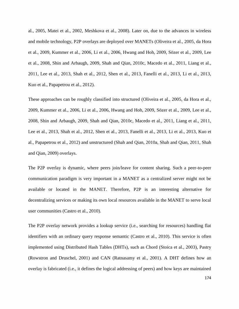
174
al., 2005, Matei et al., 2002, Meshkova et al., 2008). Later on, due to the advances in wireless
and mobile technology, P2P overlays are deployed over MANETs (Oliveira et al., 2005, da Hora
et al., 2009, Kummer et al., 2006, Li et al., 2006, Hwang and Hoh, 2009, Sözer et al., 2009, Lee
et al., 2008, Shin and Arbaugh, 2009, Shah and Qian, 2010c, Macedo et al., 2011, Liang et al.,
2011, Lee et al., 2013, Shah et al., 2012, Shen et al., 2013, Fanelli et al., 2013, Li et al., 2013,
Kuo et al., Papapetrou et al., 2012).
These approaches can be roughly classified into structured (Oliveira et al., 2005, da Hora et al.,
2009, Kummer et al., 2006, Li et al., 2006, Hwang and Hoh, 2009, Sözer et al., 2009, Lee et al.,
2008, Shin and Arbaugh, 2009, Shah and Qian, 2010c, Macedo et al., 2011, Liang et al., 2011,
Lee et al., 2013, Shah et al., 2012, Shen et al., 2013, Fanelli et al., 2013, Li et al., 2013, Kuo et
al., Papapetrou et al., 2012) and unstructured (Shah and Qian, 2010a, Shah and Qian, 2011, Shah
and Qian, 2009) overlays.
The P2P overlay is dynamic, where peers join/leave for content sharing. Such a peer-to-peer
communication paradigm is very important in a MANET as a centralized server might not be
available or located in the MANET. Therefore, P2P is an interesting alternative for
decentralizing services or making its own local resources available in the MANET to serve local
user communities (Castro et al., 2010).
The P2P overlay network provides a lookup service (i.e., searching for resources) handling flat
identifiers with an ordinary query response semantic (Castro et al., 2010). This service is often
implemented using Distributed Hash Tables (DHTs), such as Chord (Stoica et al., 2003), Pastry
(Rowstron and Druschel, 2001) and CAN (Ratnasamy et al., 2001). A DHT defines how an
overlay is fabricated (i.e., it defines the logical addressing of peers) and how keys are maintained

175
(i.e., lookup procedure). It maps application data/ values to keys that are m-bit identifiers drawn
from the logical identifier space.
There are various P2P application scenarios, where a P2P overlay over MANETs can be used to
share resources. Possible resource sharing application scenarios can be found at airport lounges,
music concerts, bus stops, railway stations, university campus, cafeterias, etc.
In this chapter, we consider a scenario of structured P2P overlay over a MANET, where not all
nodes share and access files, i.e., some nodes are peers and others are non-peers. A peer node is a
member of the P2P overlay network that shares and/or accesses a resource (e.g., a video file)
while a non-peer node does not. The P2P overlay network works at the application layer and
assumes that routing at the network layer is provided by an underlying routing protocol.
Recently, several schemes have been proposed for structured P2P networks over a MANET
(Oliveira et al., 2005, da Hora et al., 2009, Kummer et al., 2006, Li et al., 2006, Hwang and Hoh,
2009, Sözer et al., 2009, Lee et al., 2008, Shin and Arbaugh, 2009, Shah and Qian, 2010c,
Macedo et al., 2011, Liang et al., 2011, Lee et al., 2013, Shah et al., 2012, Shen et al., 2013,
Fanelli et al., 2013, Li et al., 2013, Kuo et al., Papapetrou et al., 2012). Constructing a structured
P2P overlay over MANET gives rise to some challenges that are imperative to address in order
to make the P2P protocol robust and scalable. The issues that must be considered when designing
a structured P2P overlay over MANET is similar to when designing 3D-RP, namely the
mismatch between the overlay and the physical network, and the resilience of the overlay
structure. These issues need immediate attention and affect the performance of the structured
P2P overlay over MANET in terms of path-stretch ratio, long routes, and file discovery delay.

176
In this chapter, we propose a novel protocol for constructing a structured P2P overlay over
MANETs that exploits a 3-dimensional overlay structure (3D-Overlay), named the 3-
dimensional overlay protocol (3DO), to arrange peers in an overlay that interprets the physical
relationship of peers in a 3-dimensional logical space (3D-LID space). The 3D-LID space gives a
peer the liberty to exactly interpret the physical relationship of peers in the 3D-Overlay.
3DO differs from the work in Chapter 3 in the following ways:
Both 3DO and 3D-RP are proposed to handle the mismatch problem, but they are
conceptually different and are designed to work at different layers. 3DO is a content
sharing protocol designed to work at the application layer for content sharing in P2P over
MANETs (P2P over MANET is separate domain) whereas 3D-RP is a routing protocol
that is designed to work at the network layer for routing packets.
3DO uses OLSR as an underlying routing protocol for routing packets at both control and
data planes because 3DO is designed for content sharing at the application layer and is
unable to find routes towards destination peers. On the other hand, 3D-RP is
implemented directly at the network layer for routing of packets and has nothing to do
with the content sharing at the application layer.
When a logical network is maintained over a physical network for routing at the network
layer, the mismatch problem occurs between logical and physical network. The same
mismatch problem arises when a structured overlay is maintained at the application layer.
3DO arranges peers in a 3D overlay structure. We tackled the same problem that arises at
the two conceptually different types of networks.

177
The methodology used to handle the mismatch problem in P2P overlay at the application
layer is different from the one in 3D-RP as follows:
o In 3D-RP, the distance between a node and its 1-hop neighbor node is calculated
using RSS. In 3DO, the distance between two logically linked neighbor peers is the
number of hops between the peers, which is obtained using the underlying routing
protocol, i.e., OLSR. Distance calculation using RSS is not possible in P2P overlay
because peers may be multi-hops away from each other.
o In 3D-RP, all nodes in the physical network compute a logical identifier and are part
of the 3D logical network. In 3DO, only peers obtain logical identifiers and become a
part of the 3D P2P overlay. The non-peers: i) do not possess any logical ID; ii) do not
maintain index information of files; and iii) are not part of a 3D overlay.
o In 3D-RP, each node joins the 3D logical network upon receiving at least one hello
message from its 1-hop logical neighbor nodes. In 3DO, a join request message and
join reply message are used by a peer to join a 3D Overlay (see Section 5.2.1 for
detail).
o In 3D-RP, each node N stores its mapping information (its LID and UID) at another
node Q, which acts as an anchor node for N. Therefore, in 3D-RP, each node has only
one anchor node. However, in 3DO, after establishing the overlay network at the
application layer, each peer obtains the index information of its shared files by
applying a hash function over each shared file. Then, a peer stores the index
information of its shared file at a peer that has the closest LID to that of the hashed

178
value. Therefore, a peer may share several files and each of these files may have
different hashed values that are stored at different peers. Therefore, in 3DO, a peer
can have multiple anchor peers, where its shared files are stored.
o In 3D-RP, after getting the mapping information from the anchor node, a source node
sends the packet to the destination node using the DHT-based routing (3D algorithm).
In this 3D-RO, after getting the index information of a file from the anchor peer, the
source peer retrieves the file from the destination peer using OLSR.
o In 3D-RP, if a node n1 wants to send a packet to another node n2, n1 selects one of its
1-hop neighbor nodes that is logically close to the destination node n2 as the next
hop. In 3DO, if a peer p1 wants to access a data item C, and C resides at peer p2 in
the network, then the underlying protocol, i.e., OLSR, provides the route from p1 to
p2 at the network layer.
o In 3D-RP, the simulation results are compared with MDART, which is a DHT-based
routing protocol for MANETs and operates at the network layer. 3DO is compared
with MA-SP2P, which is designed for content sharing at the overlay (application)
layer for P2P overlay over MANETs (see Chapter 6 for detail).
The above comparison would be helpful to understand the difference between the two protocols.
In summary, 3DO is designed to achieve the following requirements:
i) To avoid long routes, the neighboring peers in an overlay should also be adjacent in
the physical network in order to reduce control traffic and lookup latency in the
network, as discussed in (Shin and Arbaugh, 2009, Shah and Qian, 2010c);

179
ii) To avoid redundant traffic, a peer in an overlay should be logically close to all its
physically adjacent peers. This allows a lookup query from the peer to always be
forwarded closer to the destination peer in both the physical network and the overlay
network. The lookup query, therefore, observes a short route in the physical network
that speeds up the lookup process and reduces the routing traffic;
iii) The file should be retrieved from the source peer (the peer with the actual data item)
by the requesting peer via the shortest physical route in the network;
iv) The protocol should adapt to node mobility. When the connectivity among the peers
changes in the physical network due to node mobility, the overlay network should be
updated accordingly;
v) The system should be adaptive to network churn. When a peer joins or leaves the P2P
network, the P2P overlay should update itself accordingly;
vi) The system should be distributed in nature in the following sense. First, a system
operation should be carried out locally so that the operation has the minimum global
effect on the network. Second, the system operation should require local information
rather than global information about the network.
In the following section, the motivation behind the proposed 3D-structure and the detail of the
proposed 3D Overlay (3DO) over MANETs are explained.

180
5.2 3D Overlay Protocol (3DO)
3DO resorts to an application layer architecture, where each peer has a permanent UID (e.g., IP
address/MAC address) that identifies the peer in the physical network, and a transient logical
identifier that reflects the peer’s relative location with respect to its neighboring peers in the 3D-
Overlay.
The distance information between two peers is obtained from OLSR. Weights are assigned to
each link using the inverse distance function providing connectivity to its neighboring peers on
the basis of their distances. In our system, a peer builds the minimum spanning tree (MST) and
assigns LIDs to peers by using local neighboring peers information that makes our protocol
distributive in nature.
Algorithm 1: Handling of JQRST and JRPLY()
1: Joining peer P Broadcast JQRST using ERS
2: if receive JRPLY then
3: store neighbor peer info in NTp
4: end if
5: if Tw expires then
6: if NTp ≠ null then
7: set X1 = { Select Px1 NTp such that Px1 is a logical neighbor peer of P, which
is either 1-hop or 2-hop away }
8: set X2 = {Select Px2 NTp is a 1-hop logical neighbor peer of P}
9: Build a connected weighted undirected graph of P and Px1 X1
{/*Weight are based on hop distance between P and Px1 in the physical network
and calculated using Eq. 1*/}
10: Execute the MST algorithm with P as a source vertex
11: set Y = { Py : Py is a directly connected neighbor of P in MST}
12: set Z = { select Pw | Pw Y and Pw X2}
13: send Cprob towards Pw Z
14: remove all Pd NTp | Pd X2 and - Pd Y
15: call LIDComputation()
16: else
17: set LIDp = {1|1|1}-0
18: end if
19:end if

181
The detail of each component of the 3DO is presented in the following subsections.
5.2.1 Peer Join
To join the P2P network, a peer Pj broadcasts a join request message (JRQST) in the network
using the expanded ring search (ERS) algorithm (Hassan and Jha, 2004) in order to find the peers
that are physically adjacent to itself in the network. To join the network, a peer is required to
listen for a certain waiting time, Tw, to receive a join-reply message (JRPLY) from an existing
peer corresponding to the JQRST. A peer node sends the JRPLY to Pj upon receiving JRQST.
The JRPLY from peer P contains P’s LID, its directly connected neighboring peers along with
their distances to P. Algorithm 1 illustrates the handling of JRQST and JRPLY. Upon receiving
JRPLY, Pj stores the information in the JRPLY message in its peer-routing table. Then, Pj builds
a weighted undirected connected graph consisting of itself, its directly connected neighboring
peers and its 2-hop neighboring peers, i.e., neighboring peers of Pj’s directly connected peers.
The weight of the link in the graph between two logically linked peers is obtained by taking the
inverse of the distance (in term of number of hops) between them in the physical network. The
distance information is obtained from the underlying routing agent, i.e., OLSR, by using the
cross-layer mechanism and its peer-routing table. Using this graph, the joining peer Pj executes
the MST with itself as the source vertex. Pj stores a peer as its directly connected neighboring
peer if that peer is directly adjacent in MST and has not been selected previously as a directly
connected neighboring peer. Pj removes a peer from the directly connected neighboring peer list
if that peer is no longer adjacent in its MST. This is done in order to obtain the physically closest
peers in the network, achieving requirement (i) in Section 5.1.

182
A non-peer node simply forwards the JRQST to another node when receiving it, provided the
time-to-live (TTL) value of the JRQST message has not expired. Pj stops sending JRQST when
Tw reaches the maximum threshold.
After Tw expires, the joining peer computes its LID based on one of the following cases:
If the joining peer does not receive any JRPLY, it assumes that there is no online peer in
the P2P network, so it automatically assigns itself the LID {1|1|1}-0.
If the joining peer receives at least one JRPLY, it computes its LID with respect to its
physical adjacent neighboring peer(s) using the heuristics explained in Case 1 to Case 4
below, achieving requirement (ii) in Section 5.1. Assume node Pi is the existing peer in
the P2P network with LID {1|1|1}-0.
(a) Case 1: If peer Pj joins and finds Pi as its only neighboring peer, Pj obtains its distance in
hops to Pi from its routing agent and checks Pi’s neighboring peers information received in
JRPLY. If Pi does not have any neighbor except Pj, peer Pj selects the first available dimension
of peer Pi (say, +x-dimension) out of the six dimensions along the positive and negative axes in
the local 3D-Overlay of Pi and calculates its LIDj using the following formula: {
)| | }, where Tix, Tiy, and Tiz are the three tuple of the LIDi of peer Pi, and LSPix+ is
the maximum range of peer Pi’s LID space portion in the positive x-dimension. By using this
formula, peer Pj obtains ¾ of peer Pi’s LSPix+. The purpose here is to give a greater LID space
portion to the corner peers so that they can accommodate new peers in the future. After obtaining
its LIDj, node Pj sets its dimension parameter to 1 as LIDj belongs to the positive x-dimension.
Algorithm 2 illustrates the computation of LID in Case 1.

183
Using a similar procedure, the joining process of peers Ph and Ps along with their LIDs are
shown in Figure 5.1. Peers Ph and Ps compute their LIDh and LIDs corresponding to negative x-
dimension and the positive y-dimension by using the following formula: {
)| | }
and { |
| }, respectively, where LSPix- is the maximum range of the LSP for
peer Pi in the negative x-dimension and LSPiy+ is the maximum range of LSP for peer Pi in
positive y-dimension. Moreover, peers Ph and Ps set their dim value to 2 and 3, respectively.
Figure 5.1 illustrates the joining of peers Pj, Ph, and Ps.
The basic motivation for the decision choices made in Case 1 is to map the physical intra-
neighbor relationship of a peer in the 3D-Overlay. If two neighboring peers are not directly
linked logically to each other, it means these two neighboring peers exist physically in two
different dimensions of the peer. In such scenarios, 3DO is capable of assigning LIDs to peers in
the overlay that reflects the physical intra-neighbor relationship of peers.
(b) Case 2: If peer Pr joins the overlay, as shown in the Figure 5.1, and receives JRPLY from
two peers Pi and Pj, and both Pi and Pj are logically adjacent in the overlay network, then peer
Pr first obtains the distances dqi and dqj in number of hops using its routing agent. Pr assigns
weights to each of these links using a simple inverse distance weighting function,
Algorithm 2: LIDComputation() (Case1)
Required: Information related to neighbor peer Pi is stored in P’s peer-neighbor table (NTp) and
hop distance to Pi is obtained using routing agent, i.e., OLSR at joining peer P.
1: if Pi NTp : (Pm Nbr(Pi)) != Pj then
2: dimp ← NextAvailableDim(Pm, Pi)
4: else
5: dimp ← first(dim(Pi))
6: end if
7: LIDp ← ComputeLID(Pi, dimp)

184
Wmk=
(1)
where Wmk is the weight assigned to the link between a newly joining peer Pm and its
neighboring peer Pk, d is the distance in hops between Pm and Pk, and p is a positive real
number, called the power parameter, whose value is assumed to be 2 because greater
values of p assign greater influence to peers closest to the joining peer.
Here, the weight decreases as the distance in hops increases from the joining peer. After
assigning weights to its neighboring peers, Pr checks for a common neighboring peer between Pi
and Pj.
LIDm = { ∑
∑
|∑
∑
| ∑
∑
} (2)
where m is the newly joining peer and Pnbr≥ 2 are 1-hop neighboring peers of m, Wmk and Wmj
are the weights assigned by m to its neighboring peers Pk and Pj, respectively, using the inverse
distance function, and Tkx, Tky, and Tkz are the corresponding tuples Pk’s LID in the x, y and z
dimensions.
(i) If there is no common peer between Pi and Pj in the overlay, Pr finds an available
common octant between Pi and Pj, and computes LIDr corresponding to a common
octant using Eq(2). Furthermore, Pr sets the signs of each tuple according to the sign
dimensions of an available common octant between peers Pi and Pj.
(ii) If a common neighboring peer exists (say, peer Pq) between Pi and Pj in the overlay,
Pr finds the next available common octant between Pi and Pj, and calculates LIDr

185
corresponding to the dimensions of that common octant using Eq(2). Algorithm 3
illustrates the computation of LID in Case 2 and Case 3.
Algorithm 3: LID Computation() (Case 2 and Case 3)
Required: Information related to neighbors Pi, Pq is stored in P’s peer-neighbor table (NTp) and
hop distance to Pi and Pq is obtained using routing agent, i.e., OLSR at joining peer P.
1: if Pi,Pq NTp : Pp Nbr(Pi) and Pi Nbr(Pq) then
2: octp ← first(octiq)
3: if Pc Nbr(Pi) and Nbr(Pq) then /* Pc refers to any common neighbor peer other than P
4: octp ← NextCommonOctant(Pc,Pi,Pq)
5: else
6: octp ← FirstCommonOctant(Pi,Pq)
7: end if
8: else if Pi,Pq NTp : Pq Nbr(Pi) and Pi Nbr(Pq) then
9: Peer_adj ← false
10: if Pc Nbr(Pi) and Pc Nbr(Pq) where Pc ≠ P then
11: LIDj ← Compute(Pi,Pq,Peer_adj) /* using Eq. 3
12: else
13: Pflag = null
15: if hopDist(Pi, P) < hopDist(Pq, P) then
16: dimp ← NextAvailableDim(Pi)
17: Pflag = Pi
18: else if hopDist(Pi, P) > hopDist(Pq, P) then
19: dimp ← NextAvailableDim(Pq)
21: Pflag = Pq
22: else
23: if (CountAvaialbleDim(Pi) > CountAvailableDim(Pj) then
24: dimp ← NextAvailableDim(Pi)
25: Pflag = Pi
26: else
27: dimp ← NextAvailableDim(Pq)
28: Pflag = Pj
29: end if
30: LIDp ← ComputeLID(Pfalg, dimp)
31: end if
32: end if
33: end if

186
Figure 5.1: The peer-joining process. The dashed lines are the physical links between neighboring peers
in the physical network.

187
The decision choices made in Case 2 is to address a peer’s physical adjacency to its neighboring
peers and to assign a relative LID to the peer with respect to its adjacent neighboring peers. To
obtain the exact relative position of the peer, 3DO exploits Shepard’s interpolation method to
assign LID to a newly joining peer with respect to its discrete set of neighboring peers. This is an
attempt to exactly map the relative position of a peer in the overlay network with respect to its
neighboring peers in the physical network.
LIDm = {∑ |∑
| ∑
} (3)
where, m is a newly joining peer and p≥2 are 1-hop neighboring peers of m. Tkx, Tky, Tkz
are tuples of non-adjacent neighboring peers corresponding to each dimension.
(c) Case 3: Suppose peer Pp joins and has access only to peer Pr and Ps, which are not adjacent
to each other in the overlay network as shown in Figure 5.1. Pp first calculates its distance, i.e.,
dpr and dqs in number of hops using the routing agent and assigns weights to each link using
Eq(1). Then, peerPp checks for common neighboring peers between Pr and Ps in the overlay.
(i) If a common neighboring peer exists (say, node Pi) between Pr and Ps, then Pp computes
LIDp simply by adding each tuple of peer Pr and Ps using Eq(3).
(ii) If there is no common neighboring peer, then Pp calculates LIDp by using the available
dimension of either Pr or Ps depending on two parameters: a) a neighboring peer that is
closer in terms of distance, i.e., number of hops, and b) a neighboring peer that has more
available dimensions. Algorithm 3 is used to get a relative position with respect to non
adjacent neighboring peers in Case 3.

188
The decision made in Case 3 addresses the physical non-adjacency of neighboring peers and to
assign relative LID to the joining peer in the 3D-Overlay with respect to its non-adjacent
neighboring peers. 3DO also exploits the information about a common neighboring peer
between two non-adjacent neighboring peers before assigning a LID to a joining peer. If a
common neighboring peer exists, it shows some kind of relationship between these two non-
adjacent neighboring peers. 3DO uses this relationship to assign a relative position in the overlay
to a joining peer in order to minimize the path-stretch caused by the mismatch between the
overlay network and the physical network as explained in Section 2.3.3.
(d) Case 4: If Pc joins the P2P network and receives JRPLY messages from peers Pi, Pq and Ph
as shown in Case 4 of Figure 5.1, then either of the following cases holds.
(i) If Pi, Pq, and Ph are adjacent, then Pc calculates LIDc by using Eq (2).
Algorithm 4: LID Computation() Case 4
Required: Information related to neighbors Pi, Pq, and Ph is stored in P’s peer-neighbor table
(NTp) and hop distance to Pi, Pq, and Ph is obtained using routing agent, i.e., OLSR at joining peer
P.
1: PeerCommon← false
2: if Pi,Pq,Ph NTp : Pq Nbr(Pi),Nbr(Ph) and Pi Nbr(Pq),Nbr(Ph) and Ph Nbr(Pi),Nbr(Pq)
then
3: LIDp ← ComputeLID(Pi,Pq,Ph)
4: return
5: else if Pi Nbr(Pq),Nbr(Ph) and Pq Nbr(Ph)) and Ph Nbr(Pq) or Pq Nbr(Pi),Nbr(Ph)
and Pi Nbr(Ph) and Ph Nbr(Pi) or Ph Nbr(Pq),Nbr(Pi) and Pq Nbr(Pi)) and Pi
Nbr(Pp) then
6: PeerCommon← true
7: LIDp ← ComputeLID(Pi,Pq,Ph) /* using Eq. 2
8: return
9: else
10: LIDp ← ComputeLID(Pi,Pq,Ph, PeerCommon) /* using Eq. 3
11:end if

189
(ii) If there exists two non-adjacent peers Pq and Ph, then Pc checks for a common
neighboring peer between Pq and Ph. If node Pi is a common neighboring peer to Pq
and Ph, Pc computes LIDc using Eq (2). If there exists either a common neighboring
peer other than Pi, Pq, or Ph or there is no common neighboring peer, Pc calculates
LIDc using Eq(3). Algorithm 4 illustrates the computation of LID in Case 4.
The sequence diagram in Figure 5.2 summarizes the peer joining algorithm. In addition to
calculating its LID, each joining peer in Cases 1 to 4 sets its dim value by checking the dim value
of its base peer(s). The term ‘base peer’ refers to peers that are involved in the computation of
the joining peer's LID. If the base peers are in the same dimension, the joining peer sets its dim
value to that of its base peers. If the base peers have different dim values, the joining peer sets its
dim value to the dim value of a base peer that is closer in terms of distance.
After computing its LID, a joining peer P sends a connection-probe message (CProb) to each of
its base peers, containing P’s computed LID, the list of P’s directly connected neighboring peers
and their distances from P. When a base peer receives a CProb, it stores the information of
CProb in its peer routing table and sends a connection-reply probe message (CRProb) to P. Any
change to the peer-routing table at a peer triggers an information update to its directly connected
neighboring peers.
After joining the P2P network, P computes the ID of its shared files by applying the hash
function. Then P stores the index information of the shared files similar to the way in which a
lookup query is forwarded, which is discussed in detail in Section 5.4.

190
Figure 5.2: Flow chart of Peer Joining Algorithm
Figure 5.3 illustrates the local view of the 3D-Overlay of peer Pi and its neighboring peers in the
P2P network that is built according to the joining process of 3DO. Figure 5.3 is helpful in
visualizing the arrangement of peers according to their LIDs in the 3D-Overlay. The dotted lines
are the physical links between the peers. The dashed lines are the three planes of the local 3D-
JRPLY from the existing
peers ?
(After waiting time
Expire)
Joining
Peer
No
Yes
Is a Root Peer and gets
LID {1|1|1}-0
Obtain hop Distance using
OLSR routing tables and
assign weights using Eq .1
Count
Neighbor
Peers ?
NbrPeer_count =1
Check any
Neighbor
peer of
Neighbor
peer?
Yes
No
Calculate LID using next
available dimension
Calculate LID using
first available dimension
NbrPeer_count =3
Adjacent
Neighbor
peers?
Yes
Any
common
neighbor
peer among
neighbor
peers?
No
Calculate LID using
Eq. (2)
Yes
Calculate LID using next
available common octantNo
Any
common
neighbor
peer among
neighbor
peers?
Calculate LID by
using Eq. (3)
All
adjacent
neighbor
peers?
Yes
Check if a
neighbor
peer is
adjacent to
other?
No
Yes
No
Case 1
Case 2
Case 3
Case 4
Nb
rPeer_
cou
nt
=2
Broadcast JQRST using
ERS.
Build weighted undirected
graph and execute MST
Calculate LID using Eq.
(3)
Send Cprob
message to base
peers’
Calculate LID using first
available common octant
Select neighbor peer: i)
closer in hop distance; ii)
has more available dim
Yes
No

191
Overlay of Pi. The alphabets represent the IP addresses of the peers while roman numerals
represent the eight octants of Pi’s 3D-Overlay.
Figure 5.3 shows the logical mapping of the physical relationships of Pi with its 1-hop
neighboring peers shown in Figure 5.1. This relationship is expressed in terms of LIDs and
logical dimensions of nodes in peer Pi’s 3D-Overlay that allows the peers to calculate their LIDs
such that the physically close peers have close LIDs. It can be seen from Figure 5.1 and Figure
5.3 that 3DO exactly maps the physical intra-neighbors relationship of peer Pi with its 1-hop
neighboring peers in terms of their LIDs. The neighboring peers of Pi in the overlay network are
adjacent in the physical network and peer Pi in its local 3D-Overlay is logically close to all its
physically adjacent neighboring peers. This avoids long routes and redundant traffic overhead,
and decreases the end-to-end delay caused by the mismatch between the overlay and the physical
network discussed in Section 2.3.3. Other peers in the P2P network build their local 3D-Overlay
in the same way by arranging their 1-hop neighboring peers according to their LIDs computed by
3DO.
In addition, 3DO is resilient against peer/link failures and facilitates multipath routing because
each peer maintains all its physically adjacent neighboring peers to leverage an alternative route
if the next peer towards the destination peer fails/moves.
In 3DO, we assume that a peer P does not inform any of its neighboring peers before leaving the
network. In this case, the index information of files at P can be retrieved from the secondary
anchor peer (see Section 5.5 for detail), but the shared files that are stored at P are lost. This
problem can be handled by replicating the shared files at one of a peer’s logical neighbor of its
local 3D-overlay. We would like to handle this problem as a future work.

192
Figure 5.3: A logical view of the physical arrangement of neighboring peers in the local 3D-
Overlay of peer Pi maintained by the 3DO.
5.2.2 Update
In 3DO, each peer periodically exchanges probe messages with its directly connected
neighboring peers to update and maintain connectivity. For two logically linked peers, the peer
with the lower peer ID initiates the sending of the probe message to maintain the link. This rule
avoids redundant probe message transmissions. The probe message of a peer P contains its LID
in the form of a three-tuple and P’s directly connected neighboring peers along with their
distances from P. When P does not receive any probe message from a base peer P1 before the
time expires, P assumes that P1 has either failed or moved out of its transmission range. After
detecting this, P sets a timer Tfail to wait for a specific period of time to allow P1 to reconnect
with P. When this timer expires, P computes a new LID if it no longer connects to any of its base
peers. For this purpose, it builds the MST consisting of itself as the source vertex, its directly

193
connected neighboring peers and its 2-hop away neighboring peers, i.e., neighboring peers of P’s
directly connected peers. Then, it computes a new LID based on the updated list of the directly
connected peers. 3DO attempts to maintain the overlay closer to the physical network when the
physical network changes due to node mobility. Therefore, requirement (iv) in Section 5.1 is
satisfied.
Each peer in the P2P network also periodically refreshes its shared files index information by
sending probe messages to the corresponding peers, i.e., anchor nodes. Similarly, if P does not
receive a probe message of the index information of one of its stored files and the lifetime of the
index information expires, P removes that index information from its LID space portion.
5.3 Primary Anchor Peer Computation and File Index Information storage
After computing its LID, each peer performs two operations:
i) it retrieves from its neighboring peers the index information about files with keys
closest to its LID and acts as the primary anchor peer (PAP) for these files, and
ii) it computes the keys for its stored files and sends the index information of these files
to their respective PAPs.
To send the file f’s index information (i.e., P’s LID, file’s key) to some other peer in the P2P
network that would later act as a PAP for the files stored at peer P, peer P applies the hash
function to file f and generates a key k whose value is within the range of the LID space. The
LIDs of peers in the P2P network and the key k are drawn from the same LID space. Therefore,
the key k is in the form of an ordered three tuple, where each tuple is within the specified range
of the LID space on each axis.

194
After computing the file key k, the peer P builds the file-index information store (FIS) message
for the key k. The FIS contains P’s LID, and UID and the key k. A peer whose LID is closest to k
stores the index information of that file. To route the FIS message with destination address k,
each peer uses information about its 1-hop logical neighboring peers (Pnbr) and neighboring peers
of Pnbr (Pnbr→nbr) received in the probe messages. The FIS is forwarded to one of its Pnbr or
Pnbr→nbr that has the same dimension parameter as that of k and offers the closest position in
every tuple of its LID with respect to k, i.e., with the least sum of difference (LSD) to k. This is
achieved simply by computing the sum of difference (SD) of each tuple of Pnbr or Pnbr→nbr with
the corresponding tuple of k using Eq(4), and then selecting one of them as a next hop with the
LSD to the k using Eq(5). Algorithm 5 illustrates the handling of FIS message.
If such a neighbor does not exist, the peer simply forwards the FIS to its base peer. If P has the
LSD, then P examines its peer-routing table for index information that matches k. Otherwise, P
forwards the FIS to one of its neighboring peers that has the least SD. This process is repeated at
each peer until the FIS arrives at the peer closest to the key k (PAP for the key k).
Algorithm 5. File information Storage ()
Require: Received FIS message (M) for File’s key k at peer P (LIDp and UIDp) and Information
related to all local neighbor peers is stored in the peer-neighbor table (NTp)
1: if dimp == dimk then
2: flag ← true, SDp ← SumDiff(LIDp, k)
3: end if
4: Select Pi NTp such that Pj NTp, i j : SDi ← SumDiff(LIDi, k) < SDj ← SumDiff(LIDj, k)
5: if flag == true and SDp < SDi then
6: store File’s location information in FIS
7: else
8: send M to Pi
9: end if

195
For example, Pu in Figure 5.5 applies a hash function over file f and generates a key k , i.e., hash
(f) = k ={420|100|14}-3. Pu then builds the FIS message for the file f’s key k. In order to forward
the FIS, peer Pu first checks its 1-hop logical neighboring peers (Pu-nbr), i.e., peer Ps{1|257|1}-3
and its neighbors of neighboring peer (Pu-nbr→nbr), i.e., Pt with LIDt{513|257|1}-3 in its peer-
routing table as shown in Figure 5.4. Both the neighboring peers,Ps and Pt, have the same dim
value as that of the key k. Peer Pu then calculates the sum of difference of its neighboring peers
Ps and Pt using Eq(3), i.e., SDs = {|1-420|=419}+{|257-100|=157} + {1-14=13} → {419+157+
13}→{589} and SDt= {|513-420|=93} + {|257-100|=157} + {1-14=13} → {93+157+13}→
{263}, respectively, with respect to the key k, i.e., {420|100|14}-3. Pu then sends the FIS as
shown in Figure 5.5 to peer Pt having the least SD, i.e., 263 to the key k. Upon receiving the FIS,
Pt finds itself closest to k and stores the file f’s index information received in FIS.
Figure 5.4: Peer-routing table for peers Pj, Ps, and Pu
Dimension
IDNext Hop Cost
Is Base
Peer
1-hop neighbors
of Neighbor
Cost to 1-hop
Neighbor
Is Base Peer
of Neighbor
0
{1|1|1}-0 2 Yes {65|-65|65}-1
{64|64|64}-1
{-255|1|1}-2
{1|257|1}-3
3
4
4
4
No
No
No
No
1{65|-65|65}-1
{64|64|64}-1
2
2
No
No
{1|1|1}-0
{1|1|1}-0
3
3
Yes
Yes
Routing Table of Node ‘Pj’ with LID {257|1|1}-1
Dimension
IDNext Hop Cost
Is Base
Peer
1-hop neighbors
of Neighbor
Cost to 1-hop
Neighbor
Is Base Peer
of Neighbor
0
{1|1|1}-0 2 Yes {65|-65|65}-1
{64|64|64}-1
{-255|1|1}-2
{257|1|1}-1
3
4
4
4
No
No
No
No
3{1|513|1}-3
{513|257|1}-3
2
2
No
No
-
-
-
-
-
-
Routing Table of Node ‘Ps’ with LID {1|257|1}-3
Dimension
IDNext Hop Cost
Is Base
Peer
1-hop neighbors of
Neighbor
Cost to 1-hop
Neighbor
Is Base Peer
of Neighbor
0 - - - - - -
3{1|257|1}-3 2 Yes {513|257|1}-3
{1|1|1}-0
4
4
No
Yes
Routing Table of Node ‘Pu’ with LID {1|513|1}-3

196
5.4 File discovery
To retrieve a file f, P applies the hash function to f, producing a key k within the range of the LID
space. After obtaining the key k, peer P builds the file-lookup query (FLQ) for the key k. FLQ
contains the requesting peer’s LID and UID, and the key k. A peer whose LID is closest to k is
responsible for k. To route FLQ with destination address k, each peer (similar to the routing of
FIS) uses information about its Pnbr and Pnbr→nbr that is received in the probe messages. The peer
forwards the FLQ to one of its peers Pnbr or Pnbr→nbr that has the same dim value to that of k and
offers the closest position in every tuple of its LID with respect to k, i.e., with the least sum of
difference (LSD) to key k.
( – ) ( – ) ( – ) (4)
(5)
where, SDnbr is the sum of difference of each element of Lnbr’s LID to the corresponding
element of k or hashed value; Tnbrx, Tnbry, Tnbrz are three tuples of Lnbr’s LID, and Tkx, Tky,
Tkz are three tuples of k or hashed value; LSDnbr is the least sum of difference of Lnbr, and
Lnbr are Pnbr and Pnbr→nbr.
When the anchor peer responsible for the key k receives the FLQ, it sends the file-lookup reply
message (FLR) to the requesting peer. FLR contains either the index information of file f or a
NULL value in case there is no index information of file f at that peer. To limit the lifetime, the
FLQ is associated with a TTL value. Receiving the index information for file f, the requesting
peer retrieves the file directly from the source peer by sending a file retrieval (FR) message via a
short route in the physical network using the underlying routing due to the proactive nature of

197
OLSR. This satisfies requirement (iii) mentioned in Section 5.1. Algorithm 6 illustrates the
handling of FLQ message during the file discovery process. For the sake of simplicity, a
scheduling algorithm similar to (Shah and Qian, 2010c) can be used to retrieve the file in blocks.
Since a peer in our system has the information up to its 2 hop away neighboring peers, the
lookup query moves two hops towards the destination peer. Therefore, in our system, a lookup
query for the data item of the key k can be resolved in O([p/2]) time, where p is the number of
peers in the P2P network. However, this does not mean that 3DO has a longer lookup delay than
Chord, as Chord with a finger table can resolve a lookup query in (log p)/2 on average, where p
is the number of peers in the P2P network. But, this is the hop-cost of resolving a lookup query
in the overlay network. If the overlay network does not match the underlying physical network as
is the case with Chord, the real cost in the physical network might be much higher.

198
Figure 5.5: File’s index information storage, lookup, and retrieval process in 3DO. The overlay
network on left side shows the arrangement of peers in 3D-Overlay. The physical network on the
right describes the physical arrangement of nodes in the P2P network.
For example, peer Pj with LID {257|1|1}-1} initiates a file-lookup query (FLQ) for the key k =
{420|100|14}-3. Pj first checks its 1-hop logical neighboring peers (Pj-nbr), i.e., peer Pi{1|1|1}-0
and peer Pq{65|-65|65}-1 and their neighboring peers (Pj-nbr→nbr), i.e., Ps{1|257|1}-3 and peer
Ph{-255|1|1}-2, in its peer-routing table as shown in Figure 5.4. Pj checks the dim value and
calculates the sum of difference of Pj-nbr and Pj-nbr→nbr. Peer Ps has the same dim value as that of
key k, i.e., dim=3. So, Pj forwards the FLQ for k towards peer Ps as shown in Figure 5.5. Ps then
checks its Ps-nbr and Ps-nbr→nbr in its peer-routing table as shown in Figure 5.4.
Ps has two Ps-nbr, i.e., Pt{513|257|1}-3 and Pu{1|513|1}-3, with the same dim value as that of key
k. Peer Ps then calculates the sum of differences using Eq(3), i.e.,SDt= {|513-420|=93}+ {|257-
100| = 157}+{14-1=13}→{93+157+13}→{263} and SDu= {|1-420|=419}+{|513-100| =413} +
{1-14= 13}→{419+413+13}→{845} of its neighboring peers Pt and Pu, respectively, with
respect to the key k, i.e., {420|100|14}-3. Ps finds the LSD using Eq(4). Ps sends the FLQ
towards the Pt that has the least SD, i.e., 263.
Pt then checks its file index table to search for the index information of the file against the
corresponding key k. Pt then sends the FLR containing the required file index information
towards Pj. Upon receiving the file index information, Pj can then communicate directly with the
source peer Pu that holds the corresponding file. For this purpose, Pj sends the FR towards Pu to
retrieve file f as shown in the Figure 5.5.

199
In the above example, we observe that FLQ observes the shortest route in the overlay network
without generating any redundant traffic in the physical network. Moreover, we observe that the
intra-neighbor relationships with peers in the overlay network is the same as that of the physical
network that satisfies the conditions to avoid the mismatch between overlay network and the
physical network.
5.5 Replication Strategy
3DO adopts a simple replication strategy to avoid the loss of file’s index information in case the
primary anchor peer (PAP) moves or fails. As mentioned above, the PAP is the peer whose LID
is closest to the file f’s key k. After receiving the file f’s index information, the PAP selects a
peer from its 1-hop neighboring peers with LID second closest to k as a secondary anchor peer
(SAP) and replicates the index information of files at the SAP. The SAP becomes active in case
the PAP fails or moves.
Algorithm 6. File Discovery ()
Require: File name (f) and Information related to all local neighbor peers is stored in the peer-
neighbor table (NTp) of P.
1: hash (f) = k /* k is the form of ordered three tuple with a random dim value. Each tuple of k is
drawn from the same LID space, i.e., used to assign LIDs to peers.
2: bulid FLQ for k
3: if dimp == dimk then
4: flag ← true, SDp ← SumDiff(LIDp, k)
5: end if
6: Select Pi NTp such that Pj NTp, i j : SDi ← SumDiff(LIDi, k) < SDj ← SumDiff(LIDj, k)
7: if flag == true and SDp < SDi then
8: get File with key k
9: else
10: send FLQ to Pi
11: end if
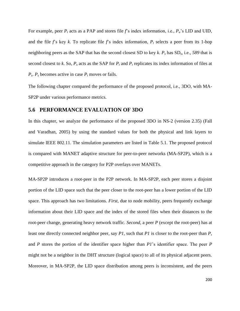
200
For example, peer Pt acts as a PAP and stores file f’s index information, i.e., Pu’s LID and UID,
and the file f’s key k. To replicate file f’s index information, Pt selects a peer from its 1-hop
neighboring peers as the SAP that has the second closest SD to key k. Ps has SDs, i.e., 589 that is
second closest to k. So, Ps acts as the SAP for Pt and Pt replicates its index information of files at
Ps. Ps becomes active in case Pt moves or fails.
The following chapter compared the performance of the proposed protocol, i.e., 3DO, with MA-
SP2P under various performance metrics.
5.6 PERFORMANCE EVALUATION OF 3DO
In this chapter, we analyze the performance of the proposed 3DO in NS-2 (version 2.35) (Fall
and Varadhan, 2005) by using the standard values for both the physical and link layers to
simulate IEEE 802.11. The simulation parameters are listed in Table 5.1. The proposed protocol
is compared with MANET adaptive structure for peer-to-peer networks (MA-SP2P), which is a
competitive approach in the category for P2P overlays over MANETs.
MA-SP2P introduces a root-peer in the P2P network. In MA-SP2P, each peer stores a disjoint
portion of the LID space such that the peer closer to the root-peer has a lower portion of the LID
space. This approach has two limitations. First, due to node mobility, peers frequently exchange
information about their LID space and the index of the stored files when their distances to the
root-peer change, generating heavy network traffic. Second, a peer P (except the root-peer) has at
least one directly connected neighbor peer, say P1, such that P1 is closer to the root-peer than P,
and P stores the portion of the identifier space higher than P1’s identifier space. The peer P
might not be a neighbor in the DHT structure (logical space) to all of its physical adjacent peers.
Moreover, in MA-SP2P, the LID space distribution among peers is inconsistent, and the peers

201
are not placed in a proper structure (like ring, chord, two-dimensional spaces, etc.) for the
overlay network. This approach does not logically interpret the physical intra-neighbor
relationship of a peer with respect to its neighboring peers.
We use OLSR as the underlying routing protocol in 3DO. The mobility scenarios are created
according to the Random Way Point mobility model using Bonnmotion2 to ensure that the
physical network is connected. The peers share ten unique files. File discovery is randomly
initiated for 100 random files by the peers in the network. We study the performance of overlay
maintenance and file discovery by varying several parameters, including the peers ratio. The
peers ratio is defined as the ratio of the number of peers in the P2P overlay network to the total
number of nodes in the physical network. We performed ten runs per scenario. The upper and
lower bars in the graphs show the margin of error of the mean estimates at 95% confidence
interval.
For performance comparison, we choose the following parameters with varying network size.
Path-stretch ratio (as defined in Section 3.6).
Average file discovery delay: The average time elapsed from the moment a file-look-up
query is issued to the moment the first reply is received.
Routing overhead: The total number of control overhead packets used by the protocol to
perform routing of query data packets.
False-negative (FN) ratio (%): The ratio between the number of unresolved lookup queries for
the destination in the physically connected network to the total number of initiated lookup
queries.

202
Table 5.1: Simulation Parameters
Input Parameters Value
Transmission range 50m
Playground Size [1000*1000m]
Data Rate [100pps]
Simulation Time 500sec
Start of Data Transmission [70,300]
End of Data Transmission [250,499]
Node Speed [0.5m/s to 2 m/s]
Start of Node Failure
Mobility Model
Radio Propagation Model
100 sec
Random Way-point
TwoRayGround Model
Traffic Model
No. of file retries
Random Traffic pattern
2
A key difference between MANETs and fixed networks is node mobility that require routes to be
constantly updated. The same is true for queries in P2P overlay networks that expect the
destination to be reached at a given time. We evaluated the impact of the physical topology
changes in 3DO and MA-SP2P. We studied the mobility by varying the average node speed from
0.5 m/s, to 1.0 m/s, to 1.5 m/s, to 2.0 m/s.
5.6.1 Routing Overhead
In this section, the behavior of 3DO and MA-SP2P is analyzed in terms of routing overhead
against various peer ratios and node speed. The main objective of the experiments is to compare
the scalability of 3DO and MA-SP2P in terms of traffic overhead.

203
The frequent change in network topology due to the increase in node speed produces more traffic
when the overlay topology is readjusted to match the physical topology. Peers out of range or
broken routes increase the routing overhead. The effect of increasing node speed on the routing
overhead is more detrimental on MA-SP2P compared to 3DO as shown in Figure 5.6. The
percentage improvement of 3DO over MA-SP2P in terms of the routing overhead is 17% to 47%
for various node speeds as shown in Figure 5.10. This is due to the inflexible tree-like structure
used to distribute the LID space portion between peers.
In MA-SP2P, a parent peer retrieves the LID space portion of its child peer in case the child peer
moves to some other place, generating extensive traffic overhead. However, in 3DO, the LID
space portion of each peer is implicit and does not require any explicit mechanism to retrieve the
LID space portion in case a peer moves. Moreover, the replication strategy used by 3DO, in case
the primary anchor peer moves/fails, effectively reduces the routing overhead, especially when
the node speed increases. The percentage improvement is between 17% to 47% with respect to
the increase in the node speed, which illustrates the effectiveness of the proposed protocol with
respect to the increasing speed.
Maximum Speed 0.5 m/s
0
50
100
150
200
250
300
350
400
450
5 10 20 30 40 50
Ro
uti
ng
Ov
erh
ead
(10
3)
pack
ets
Peer Ratio (%)
MA-SP2P
3DO
(a)
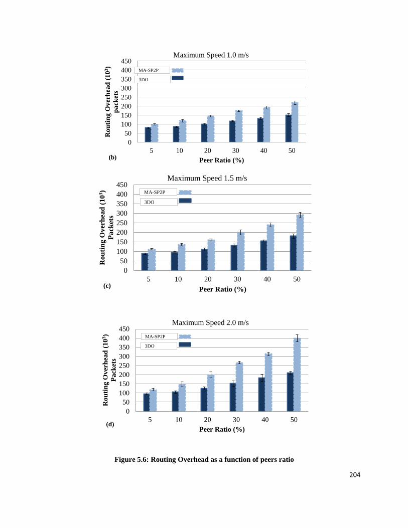
204
Figure 5.6: Routing Overhead as a function of peers ratio
Maximum Speed 1.0 m/s
0
50
100
150
200
250
300
350
400
450
5 10 20 30 40 50
Ro
uti
ng
Ov
erh
ead
(1
03)
pa
cket
s
Peer Ratio (%)(b)
MA-SP2P
3DO
Maximum Speed 1.5 m/s
0
50
100
150
200
250
300
350
400
450
5 10 20 30 40 50
Ro
uti
ng
Ov
erh
ead
(1
03)
Pa
cket
s
Peer Ratio (%)(c)
MA-SP2P
3DO
Maximum Speed 2.0 m/s
0
50
100
150
200
250
300
350
400
450
5 10 20 30 40 50
Ro
uti
ng
Ov
erh
ead
(1
03)
Pa
cket
s
Peer Ratio (%)(d)
MA-SP2P
3DO

205
Figure 5.6 shows that the routing overhead for 3DO compared to MA-SP2P against various peer
ratios decreases 17% to 33%, 19% to 32%, 19% to 38%, and 18% to 47% at node speed 0.5m/s,
1m/s, 1.5m/s, and 2m/s, respectively for the following two reasons. First, increasing the number
of peers in the network introduces more traffic in maintaining connectivity among the peers.
Second, more traffic is generated to maintain the index information at the peers when the number
of peers increases. Figure 5.6 shows that 3DO improves the routing overhead up to 47% as
shown in Figure 5.10 because 3DO builds and maintains an overlay that better matches the
physical network, eliminating redundant long links. Moreover, it introduces the replication
strategy in case the anchor peer moves/fails, which effectively reduces the overhead.
On the other hand, MA-SP2P peers frequently exchange information about their LID space
portion and the index of the stored files when their distance to the root-peer changes due to node
mobility, resulting in heavy network traffic. Moreover, a peer P (except the root-peer) has at least
one directly connected neighboring peer, say P1, such that P1 is closer to the root-peer than P
and P stores the portion of the identifier space higher than P1’s identifier space. Peer P might not
be a neighbor in the overlay network to all of its physical adjacent peers, resulting in an
mismatch between the overlay and the physical network.
The following is the null hypothesis to test the impact of peer ratio and protocols on routing
overhead at node speed 0.5 m/s, 1 m/s, 1.5m/s, and 2 m/s:
Ho: 3DO does not significantly reduce routing overhead compared to MA-SP2P at node speeds
of 0.5m/s, 1m/s, 1.5m/s, and 2m/s.

206
Table 5.2, Table 5.3, Table 5.4, and Table 5.5 show the results of applying the Two-way
ANOVA with replication on data about routing overhead at node speeds 0.5m/s, 1m/s, 1.5m/s,
and 2m/s, respectively.
Table 5.2: : Summary of data analysis of Routing Overhead for 3DO and MA- SP2P at node speed
0.5m/s using ANOVA Two-Factor with replication
Table 5.3: Summary of data analysis of Routing Overhead for 3DO and MA- SP2P at node speed
1m/s using ANOVA Two-Factor with replication

207
Table 5.4: Summary of data analysis of Routing Overhead for 3DO and MA- SP2P at node speed
1.5m/s using ANOVA Two-Factor with replication
Table 5.5: Summary of data analysis of Routing Overhead for 3DO and MA- SP2P at node speed
2m/s using ANOVA Two-Factor with replication

208
Table 5.6: Results: pairwise data analysis of Routing Overhead at node speed 0.5m/s for 3DO and
MA-SP2P using ANOVA Two-Factor with Replication
Table 5.7: Results: pairwise data analysis of Routing Overhead at node speed 1m/s for 3DO and
MA-SP2P using ANOVA Two-Factor with Replication

209
Table 5.8: Results: pairwise data analysis of Routing Overhead at node speed 1.5m/s for 3DO and
MA-SP2P using ANOVA Two-Factor with Replication
Table 5.9: Results: pairwise data analysis of Routing Overhead at node speed 2m/s for 3DO and
MA-SP2P using ANOVA Two-Factor with Replication

210
The results of the Two-way ANOVA test (Table 5.2, Table 5.3, Table 5.4, and Table 5.5) show
that p < 0.05, which leads to the rejection of Ho. This shows that 3DO is statistically significant
in terms of reducing routing overhead compared to MA-SP2P. 3DO is less affected in terms of
routing overhead and builds 3D-Overlay that better matches to the physical network and
efficiently reduces the impact of mismatch problem, eliminating redundant long links. On the
other hand, the inflexible tree-like structure of MA-SP2P that is used to distribute the LSP does
not ensure the physical proximity of nodes. This aggravates the mismatch problem and increases
routing overhead when routing packets towards a destination node.
Unlike MA-SP2P, 3DO does not maintain any explicit mechanism to retrieve the LSP in case a
peer moves/fails, which reduces overhead. Moreover, the 3DO’s replication strategy effectively
reduces the overhead in case a primary anchor node moves/fails. MA-SP2P does not employ any
replication strategy. The analysis above shows the improvement in routing overhead using 3DO
is significant compared to MA-SP2P.
Table 5.6, Table 5.7, Table 5.8, and Table 5.9 show the pairwise comparisons of 3DO and MA-
SP2P in terms of routing overhead for each peer ratio at node speed of 0.5 m/s, 1 m/s, 1.5 m/s,
and 2 m/s, respectively. The results show that 3DO significantly reduces routing overhead
compared to MA-SP2P for each peer ratio. The results confirm that 3D structure and the
technique adopted in 3DO is efficient in reducing the impact of mismatch problem.
5.6.2 Average File Discovery Delay
In this section, the experiments are performed to check the quality of routing paths in terms of
the file discovery delay. The file discovery delay is calculated to compare the time required to

211
access the file in the physical network. This performance metric is very important to see the
effect of the mismatch problem between 3DO and MA-SP2P.
Figure 5.7 illustrates the average file discovery delay for MA-SP2P and 3DO when the peer ratio
and node speed are increased. The increase in peer ratio and frequent change of network
topology causes heavier routing traffic and more contention in the network. Figure 5.7 shows
that the average file discovery delay for MA-SP2P compared to 3DO against various peer ratios
increases 43% to 54%, 35% to 48%, 30% to 42%, and 31% to 43% at node speed 0.5m/s, 1m/s,
1.5m/s, and 2m/s, respectively. MA-SP2P has larger average file discovery delay compared to
3DO because:
i) MA-SP2P has a higher false-negative ratio than 3DO, which shows that in MA-SP2P,
some accesses to files never happen because of the false-negative results in locating
the file;
ii) The resulting topological mismatch between the overlay and the physical network due
to its tree-based overlay network prevents MA-SP2P from being efficient in the file
lookup process;
iii) The LID space distribution among the peers is inconsistent in MA-SP2P and the peers
are not placed in a proper overlay structure (like ring, chord, multi-dimensional
spaces, etc.), which causes the file-lookup query to experience 30% to 54% larger
delay in the physical network as shown in Figure 5.10;

212
Maximum Speed 0.5 m/s
0
50
100
150
200
250
300
350
400
450
5 10 20 30 40 50
Fil
e D
isco
ver
y d
ela
y
(mil
lise
con
ds)
Peer Ratio (%)(a)
MA-SP2P
3DO
Maximum Speed 1.0 m/s
0
50
100
150
200
250
300
350
400
450
5 10 20 30 40 50
Fil
e D
isco
ver
y d
elay
(mil
lise
con
ds)
Peer Ratio (%)(b)
MA-SP2P
3DO
Maximum Speed 1.5 m/s
0
50
100
150
200
250
300
350
400
450
5 10 20 30 40 50
Fil
e D
isco
ver
y d
ela
y
(mil
lise
con
ds)
Peer Ratio (%)(c)
MA-SP2P
3DO

213
Figure 5.7: Average file discovery delay as a function of peers ratio
In MA-SP2P, a peer shares a consecutive LID space portion with all of its neighboring peers. A
parent peer retrieves the LID space portion of its child peer in case the child peer moves to some
other place, introducing 17% to 47% extra traffic overhead in the network as shown in Figure
5.10. Figure 5.7(d) illustrates that the effect of this increases with the increase in node speed.
In 3DO:
i) The 3D-Overlay avoids the topological mismatch between the overlay and the
physical network due to its flexible 3D structure and design choices when assigning
LID to a peer, resulting in an efficient file lookup process as illustrated in Figure 5.7.
As shown in Figure 5.7 and Figure 5.10, the file discovery delay improvement of
3DO over MA-SP2P with respect to increase in peer ratio and various node speeds is
31% to 53%. The false-negative ratio in 3DO is lower, which ensures maximum
accesses to the files and confirms the results in Figure 5.7.
Maximum Speed 2.0 m/s
0
50
100
150
200
250
300
350
400
450
5 10 20 30 40 50
Fil
e D
isco
ver
y d
ela
y
(mil
lise
con
ds)
Peer Ratio (%)(d)
MA-SP2P
3DO

214
ii) A peer P in the 3D-Overlay maintains its adjacent/non-adjacent, common neighbor,
and intra-neighbor relationships with its neighboring peers by assigning different
LIDs and utilizing the 3D-Overlay. Consequently, in 3DO, a file-lookup query from a
peer is always forwarded closer to the destination peer in both the overlay and the
physical network and experiences 10% to 36% shorter route to the destination peer,
which reduces the lookup delay.
iii) The LID space portion recovery in 3DO is implicit because the LID of a peer
determines the index information to be stored at the peer. No explicit recovery
mechanism is used in 3DO for the retrieval of the LID space portion, which reduces
the control overhead, resulting in low file discovery delay. The percentage
improvement of 3DO over MA-SP2P in terms of the file discovery delay is 31% to
42% at the a node speed of 2 m/s as shown in Figure 5.7(d) and Figure 5.10(d)
compared to the file discovery delay of 43% to 54% at a node speed of 0.5 m/s as
shown in Figure 10(a) and Figure 5.10(a), which establishes the efficiency of 3DO
with increasing node speed and peer ratio.
Below is the null hypothesis to test the impact of peer ratio and protocols on file discovery delay
at node speed 0.5 m/s, 1 m/s, 1.5m/s, and 2 m/s:
Ho: 3DO does not significantly reduce the file discovery delay compared to MA-SP2P at node
speeds of 0.5m/s, 1m/s, 1.5m/s, and 2m/s.

215
Table 5.10, Table 5.11, Table 5.12, and Table 5.13 show the results of applying the Two-way
ANOVA with replication on data about file discovery delay at node speeds 0.5m/s, 1m/s, 1.5m/s,
and 2m/s, respectively.
Table 5.10: : Summary of data analysis of File Discovery Delay for 3DO and MA- SP2P at node
speed 0.5m/s using ANOVA Two-Factor with replication
Table 5.11: Summary of data analysis of File Discovery Delay for 3DO and MA- SP2P at node
speed 1m/s using ANOVA Two-Factor with replication

216
Table 5.12: Summary of data analysis of File Discovery Delay for 3DO and MA- SP2P at node
speed 1.5m/s using ANOVA Two-Factor with replication
Table 5.13: Summary of data analysis of File Discovery Delay for 3DO and MA- SP2P at node
speed 2m/s using ANOVA Two-Factor with replication

217
Table 5.14: Results: pairwise data analysis of File Discovery Delay at node speed 0.5m/s for 3DO
and MA-SP2P using ANOVA Two-Factor with Replication
Table 5.15: Results: pairwise data analysis of File Discovery Delay at node speed 1m/s for 3DO and
MA-SP2P using ANOVA Two-Factor with Replication

218
Table 5.16: Results: pairwise data analysis of File Discovery Delay at node speed 1.5m/s for 3DO
and MA-SP2P using ANOVA Two-Factor with Replication
Table 5.17: Results: pairwise data analysis of File Discovery Delay at node speed 2m/s for 3DO and
MA-SP2P using ANOVA Two-Factor with Replication

219
The results of the Two-way ANOVA test (Table 5.10, Table 5.11, Table 5.12, and Table 5.13)
show that p < 0.05, which leads to the rejection of Ho. This shows that 3DO is statistically
significant in terms of reducing file discovery delay compared to MA-SP2P. 3DO is less affected
in terms of file discovery delay and the 3D-Overlay ensures the physical proximity of peers in
the overlay network that leads to optimal routes towards destination peers, thus reducing file
discovery delay.
Table 5.14, Table 5.15, Table 5.16, and Table 5.17 show the pairwise comparisons of 3DO and
MA-SP2P in terms of file discovery delay for each peer ratio at node speed of 0.5 m/s, 1 m/s, 1.5
m/s, and 2 m/s, respectively. When the peer ratio increases, 3DO shows more promising
behavior compared to MA-SP2P. The results show that 3DO significantly reduces file discovery
delay compared to MA-SP2P for each peer ratio. The results confirm that the 3D structure and
technique adopted by 3DO is efficient in reducing the impact of mismatch problem.
5.6.3 False-negative (FN) ratio
In this section, the behavior of 3DO and MA-SP2P is analyzed in terms of false-negative ratio
against various peer ratios and node speed. The main objective of the experiments is to compare
the number of unresolved lookup queries for the destination in the physically connected network
to the total number of initiated lookup queries.
Figure 5.8 illustrates the false-negative (FN) ratio for MA-SP2P and 3DO when the peer ratio
and node speed are increased. The effect of increasing the peer ratio on the FN ratio is more
detrimental on MA-SP2P compared to 3DO as shown in Figure 5.8. The FN ratio for MA-SP2P
compared to 3DO against various peer ratios increases 49% to 59%, 47% to 59%, 45% to 48%,
and 40% to 55% at node speed 0.5m/s, 1m/s, 1.5m/s, and 2m/s, respectively. Increasing the peer
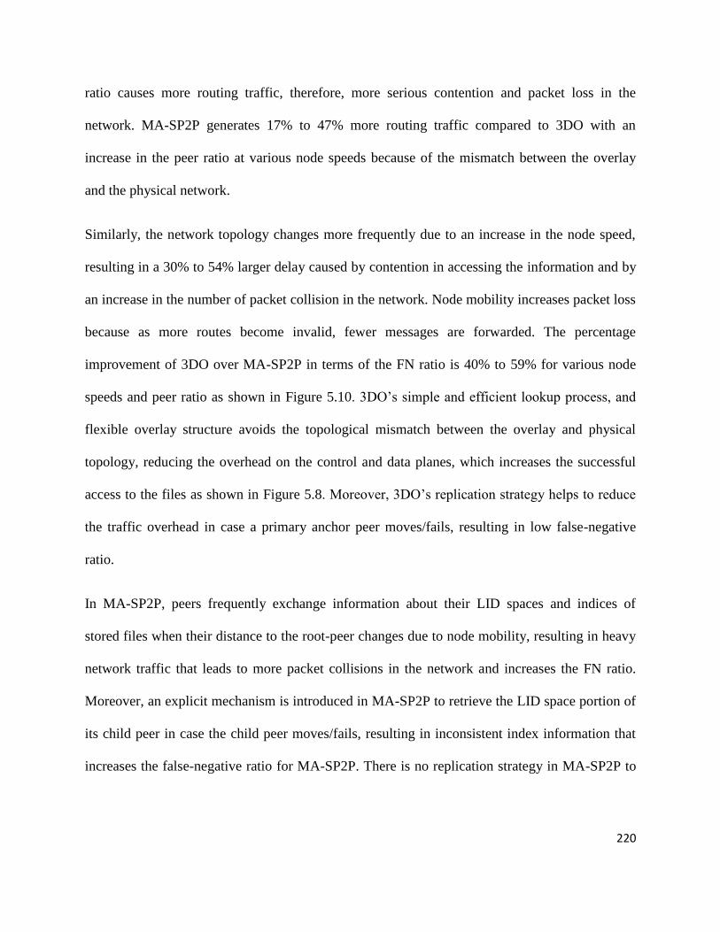
220
ratio causes more routing traffic, therefore, more serious contention and packet loss in the
network. MA-SP2P generates 17% to 47% more routing traffic compared to 3DO with an
increase in the peer ratio at various node speeds because of the mismatch between the overlay
and the physical network.
Similarly, the network topology changes more frequently due to an increase in the node speed,
resulting in a 30% to 54% larger delay caused by contention in accessing the information and by
an increase in the number of packet collision in the network. Node mobility increases packet loss
because as more routes become invalid, fewer messages are forwarded. The percentage
improvement of 3DO over MA-SP2P in terms of the FN ratio is 40% to 59% for various node
speeds and peer ratio as shown in Figure 5.10. 3DO’s simple and efficient lookup process, and
flexible overlay structure avoids the topological mismatch between the overlay and physical
topology, reducing the overhead on the control and data planes, which increases the successful
access to the files as shown in Figure 5.8. Moreover, 3DO’s replication strategy helps to reduce
the traffic overhead in case a primary anchor peer moves/fails, resulting in low false-negative
ratio.
In MA-SP2P, peers frequently exchange information about their LID spaces and indices of
stored files when their distance to the root-peer changes due to node mobility, resulting in heavy
network traffic that leads to more packet collisions in the network and increases the FN ratio.
Moreover, an explicit mechanism is introduced in MA-SP2P to retrieve the LID space portion of
its child peer in case the child peer moves/fails, resulting in inconsistent index information that
increases the false-negative ratio for MA-SP2P. There is no replication strategy in MA-SP2P to

221
provide consistent and up-to-date index information about files in case a primary anchor peer
moves/fails.
Maximum Speed 0.5 m/s
0
10
20
30
40
50
60
5 10 20 30 40 50
Fa
lse-
neg
ati
ve
rati
o(%
)
Peer Ratio (%)(a)
MA-SP2P
3DO
Maximum Speed 1.0 m/s
0
10
20
30
40
50
60
5 10 20 30 40 50
Fa
lse-
neg
ati
ve
rati
o(%
)
Peer Ratio (%)(b)
MA-SP2P
3DO
Maximum Speed 1.5 m/s
0
10
20
30
40
50
60
5 10 20 30 40 50
Fa
lse-
neg
ati
ve
rati
o(%
)
Peer Ratio (%)(c)
MA-SP2P
3DO

222
Figure 5.8: False negative ratio as a function of peers ratio
The following is the null hypothesis to test the impact of peer ratio and protocols on the FN ratio
at node speed 0.5 m/s, 1 m/s, 1.5m/s, and 2 m/s:
Ho: 3DO does not significantly reduce the FN ratio compared to MA-SP2P at node speeds of
0.5m/s, 1m/s, 1.5m/s, and 2m/s.
Table 5.18, Table 5.19, Table 5.20, and Table 5.21 show the results of applying the Two-way
ANOVA with replication on data about FN ratio at node speeds 0.5m/s, 1m/s, 1.5m/s, and 2m/s,
respectively.
Maximum Speed 2.0 m/s
0
10
20
30
40
50
60
5 10 20 30 40 50
Fa
lse-
neg
ati
ve
rati
o(%
)
Peer Ratio (%)
MA-SP2P
3DO
(d)

223
Table 5.18: : Summary of data analysis of False Negative Ratio for 3DO and MA- SP2P at node
speed 0.5m/s using ANOVA Two-Factor with replication
Table 5.19: Summary of data analysis of False Negative Ratio for 3DO and MA- SP2P at node
speed 1m/s using ANOVA Two-Factor with replication

224
Table 5.20: Summary of data analysis of False Negative Ratio for 3DO and MA- SP2P at node
speed 1.5m/s using ANOVA Two-Factor with replication
Table 5.21: Summary of data analysis of False Negative Ratio for 3DO and MA- SP2P at node
speed 2m/s using ANOVA Two-Factor with replication

225
Table 5.22: Results: pairwise data analysis of False Negative Ratio at node speed 0.5m/s for 3DO
and MA-SP2P using ANOVA Two-Factor with Replication
Table 5.23: Results: pairwise data analysis of False Negative Ratio at node speed 1m/s for 3DO and
MA-SP2P using ANOVA Two-Factor with Replication
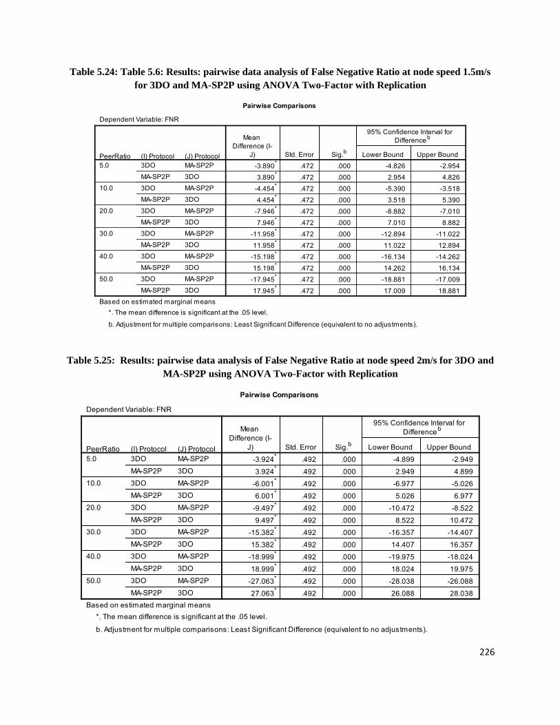
226
Table 5.24: Table 5.6: Results: pairwise data analysis of False Negative Ratio at node speed 1.5m/s
for 3DO and MA-SP2P using ANOVA Two-Factor with Replication
Table 5.25: Results: pairwise data analysis of False Negative Ratio at node speed 2m/s for 3DO and
MA-SP2P using ANOVA Two-Factor with Replication

227
The results of the Two-way ANOVA test (Table 5.18, Table 5.19, Table 5.20, and Table 5.21)
show that p < 0.05, which leads to the rejection of Ho. This shows that 3DO is statistically
significant in terms of reducing FN ratio compared to MA-SP2P. 3DO is less affected by node
mobility in terms of FN ratio and an increase in peer ratio. 3DO reduces packet loss due to node
mobility with its effective replication strategy, where a secondary anchor node implicitly
replaces a primary anchor node in case the primary anchor node moves/fails. This helps to
reduce the traffic overhead, resulting in low false-negative ratio. Moreover, the efficient peer
joining algorithm and flexible overlay structure of 3DO avoids the topological mismatch
between the overlay and the physical topology, reducing overhead at both the control and data
planes, which increases the successful access to the files.
On the other hand, the inflexible tree-like structure of MA-SP2P that is used to distribute the
LSP does not ensure the physical proximity of nodes. This aggravates the mismatch problem and
increases routing overhead when routing packets towards a destination node, resulting in packet
collisions, which decreases successful access to the files. The analysis above shows the
improvement in FN ratio using 3DO is significant compared to MA-SP2P.
Table 5.22, Table 5.23, Table 5.24, and Table 5.25 show the pairwise comparisons of 3DO and
MA-SP2P in terms of FN ratio for each peer ratio at node speed of 0.5 m/s, 1 m/s, 1.5 m/s, and 2
m/s, respectively. The results show that 3DO significantly reduces FN ratio compared to MA-
SP2P for each peer ratio. The results confirm that 3D structure and the technique adopted in 3DO
is efficient in reducing the impact of mismatch problem.

228
5.6.4 Path-Stretch Ratio
In this section, the experiments are performed to check the quality of routing paths in terms of
the number of hops. The path-stretch ratio is calculated to compare the length of the routing
paths in logical network and physical network. This performance metric is very important to see
the effect of the mismatch problem between 3D-RP and MDART. Reducing the path-stretch
ratio improves the network performance by reducing redundant transmissions in the network.
Figure 5.9 plots the path-stretch ratio of MA-SP2P and 3DO against the peer ratio. In 3DO, the
average path-stretch ratio is lower compared to MA-SP2P and stays slightly above the shortest
path, but the mean value stays below 1.25. As shown in Figure 5.9 and Figure 5.10, the path-
stretch ratio improvement of 3DO over MA-SP2P with respect to increase in peer ratio and
various node speeds is 11% to 36%.
The slight increase of path-stretch ratio in 3DO results when a joining peer, for instance P,
comes in contact with two non-adjacent neighboring peers (say, P1, P2) with different dim
values and there is no common neighboring peer. P would then get an LID using the available
dimensions of either P1 or P2, depending on which one is closer in terms of hop distance. In this
case, the LID of P would show only its relative position in the 3D-Overlay with respect to that
neighboring peer from which it gets its LID, causing a slight mismatch problem in 3DO.
However, this situation occurs less frequently in 3DO and its impact is less severe as shown by
the simulation results in Figure 5.9.

229
Maximum Speed 0.5 m/s
1
1.2
1.4
1.6
1.8
5 10 20 30 40 50
Pa
th-s
tret
ch r
ati
o
Peer Ratio (%)
MA-SP2P
3DO
(a)
Maximum Speed 1.0 m/s
1
1.2
1.4
1.6
1.8
5 10 20 30 40 50
Pa
th-s
tret
ch r
ati
o
Peer Ratio (%)(b)
MA-SP2P
3DO
Maximum Speed 1.5 m/s
1
1.2
1.4
1.6
1.8
5 10 20 30 40 50
Pa
th-s
tret
ch r
ati
o
Peer Ratio (%)(c)
MA-SP2P
3DO

230
Figure 5.9: Path-stretch ratio as a function of peers ratio
The path-stretch ratio of MA-SP2P, as shown in Figure 5.9, is 11% to 36% higher compared to
3DO because of the tree-based structure of MA-SP2P. On the other hand, the 3D-overlay exactly
maps the physical intra-neighbors relationship of peers with its 1-hop neighboring peers in terms
of their LIDs. Moreover, it ensures:
i) The neighboring peers of a peer in the overlay network are adjacent in the physical
network;
ii) A peer in its local 3D-Overlay is logically close to all its physically adjacent
neighboring peers.
This avoids long routes and redundant traffic overhead and decreases the end-to-end delay,
which establishes the results reported in Figure 5.9.
The path-stretch of MA-SP2P increases 10% to 20%, 13% to 21%, 13% to 26%, 19% to 36%
more compared to 3DO as node speed is varied from 0.5m/s, 1m/s, 1.5m/s to 2m/s, respectively,
which caused the topology of MA-SP2P to scale up and the path length between the requesting
Maximum Speed 2.0 m/s
1
1.2
1.4
1.6
1.8
5 10 20 30 40 50
Pa
th-s
tret
ch R
ati
o
Peer Ratio (%)(d)
MA-SP2P
3DO

231
peer and the source peer also increases. Figure 5.9 shows that the average path-stretch of 3DO is
slightly affected by the peers ratio and the value does not always equal to one, which means that
sometimes the path between the requesting peer and the source peer is not the shortest in the
physical network. In our view, this is due to the multi-point relay (MPR) selection in the OLSR
routing.
Below is the null hypothesis to test the impact of peer ratio and protocols on the path-stretch
ratio at node speed 0.5 m/s, 1 m/s, 1.5m/s, and 2 m/s:
Ho: 3DO does not significantly reduce the path-stretch ratio compared to MA-SP2P at node
speeds of 0.5m/s, 1m/s, 1.5m/s, and 2m/s.
Table 5.26, Table 5.27, Table 5.28, and Table 5.29 show the results of applying the Two-way
ANOVA with replication on data about path-stretch ratio at node speeds 0.5m/s, 1m/s, 1.5m/s,
and 2m/s, respectively.
Table 5.26: : Summary of data analysis of Path-stretch ratio for 3DO and MA- SP2P at node
speed 0.5m/s using ANOVA Two-Factor with replication

232
Table 5.27: Summary of data analysis of Path-stretch ratio for 3DO and MA- SP2P at node speed
1m/s using ANOVA Two-Factor with replication
Table 5.28: Summary of data analysis of Path-stretch ratio for 3DO and MA- SP2P at node speed
1.5m/s using ANOVA Two-Factor with replication

233
Table 5.29: Summary of data analysis of Path-stretch ratio for 3DO and MA- SP2P at node speed
2m/s using ANOVA Two-Factor with replication
Table 5.30: Results: pairwise data analysis of Path-stretch ratio at node speed 0.5m/s for 3DO and
MA-SP2P using ANOVA Two-Factor with Replication

234
Table 5.31: Results: pairwise data analysis of Path-stretch ratio at node speed 1m/s for 3DO and
MA-SP2P using ANOVA Two-Factor with Replication
Table 5.32: Table 5.6: Results: pairwise data analysis of Path-stretch ratio at node speed 1.5m/s
for 3DO and MA-SP2P using ANOVA Two-Factor with Replication

235
Table 5.33: Results: pairwise data analysis of Path-stretch ratio at node speed 2m/s for 3DO and
MA-SP2P using ANOVA Two-Factor with Replication
The results of the Two-way ANOVA test (Table 5.26, Table 5.27, Table 5.28, and Table 5.29)
show that p < 0.05, which leads to the rejection of Ho. This shows that 3DO is statistically
significant in terms of reducing path-stretch ratio compared to MA-SP2P and that 3DO is
effective in reducing the impact of the mismatch problem between the overlay and the physical
network. The notion of involving intra-neighbor peer relationships while calculating its LID
ensures the physical proximity of nodes in the logical network that leads to optimal routes
towards destination nodes, resulting in reduced path-stretch ratio in case of 3DO.
On the other hand, the inflexible tree-like structure of MA-SP2P that is used to distribute the
LSP does not ensure the physical proximity of nodes. This aggravates the mismatch problem and

236
increases the path stretch ratio when routing packets towards destination node, resulting in
redundant traffic that causes packet collisions and decreases the successful access to the files.
Table 5.30, Table 5.31, Table 5.32, and Table 5.33 show the pairwise comparisons of 3DO and
MA-SP2P in terms of path stretch ratio for various peer ratio at node speed of 0.5 m/s, 1 m/s, 1.5
m/s, and 2 m/s, respectively. The results show that 3DO significantly reduces path stretch ratio
compared to MA-SP2P for each peer ratio. The results confirm that 3D structure and the
technique adopted in 3DO is efficient in reducing the impact of mismatch problem.
0
10
20
30
40
50
60
70
5 10 20 30 40 50
% I
mp
rov
emen
t w
.r.t
MA
-
SP
2P
at
No
de
Sp
eed
of
0.5
m/s
Peer Ratio (%)
FDD
FN
RO
PSR
(a)
0
10
20
30
40
50
60
70
5 10 20 30 40 50% I
mp
rov
emen
t w
.r.t
MA
-
SP
2P
at
No
de
Sp
eed
of
1m
/s
Peer Ratio (%)
FDD
FN
RO
PSR
(b)

237
Figure 5.10: Percentage improvement with respect to MA-SP2P at node speeds 0.5m/s, 1m/s, 1.5m/s, 2m/s
5.7 Conclusions
This chapter presents a 3-dimensional overlay for P2P over MANETs called 3DO. Our approach
constructs an efficient 3D-Overlay over MANET with a topology matching the physical
network. Using this structure of interconnection among peers, we design a new overlay routing
algorithm to distribute, manage, and share file information among the peers. 3DO takes into
account the physical intra-neighbor peer relationship of a peer by exploiting a 3D-Overlay. A
0
10
20
30
40
50
60
5 10 20 30 40 50
% I
mp
rov
emen
t w
.r.t
MA
-
SP
2P
at
No
de
Sp
eed
of
1.5
m/s
Peer Ratio (%)
FDD
FN
RO
PSR
(c)
0
10
20
30
40
50
60
5 10 20 30 40 50
% I
mp
rov
emen
t w
.r.t
MA
-
SP
2P
at
No
de
Sp
eed
of
2m
/s
Peer Ratio (%)
FDD
FN
RO
PSR
(d)

238
performance analysis has been conducted using scenarios with relatively high peer ratio and low
node speed. The performance analysis of 3DO and MA-SP2P with a relatively high peer ratio
and low node speed show that our approach outperforms MA-SP2P in terms of routing overhead,
average file-discovery delay, false-negative ratio, and average path-stretch ratio and proves to be
effective in avoiding mismatch between the overlay network and the physical network.

239
6 MODELLING AND ANALYSIS USING FORMAL METHODS
In this chapter, we use high-level Petri nets to model and verify the working of 3D-RP. We
briefly describe HLPN, SMT-Lib, and Z3 below for better understanding for the reader.
6.1 High Level Petri Nets
Petri nets model the system graphically and mathematically, and can be applied to a range of
systems that are distributed, parallel, concurrent, non-deterministic, stochastic, or asynchronous
(Murata, 1989). We use a variant of conventional Petri net called high-level Petri nets (HLPN).
Definition 1 (HLPN) (Murata, 1989): A HLPN is a 7-tuple , where a set
of places is denoted by P. T refers to the set of transitions such that . F denotes a flow
relation such that . maps places P to data types. R is a set of rules for
transitions. L is a set of labels of F and M0 represents the initial marking. ( ) provides
information about the structure of the net and ( ) provides static semantics, which means
that the information does not change in the system.
In HLPN, places can have tokens of different types, and can be a cross product of two or more
types. The pre-conditions must hold for any transition to be enabled. Moreover, the variables
from the incoming flows are used to enable a certain transition. Similarly, the post-conditions use
variables from outgoing flows for transition firing.
6.2 SMT-Lib and Z3
SMT-Lib is used for checking the satisfiability of formulae over the theories under consideration
(de Moura and Bjørner, 2009). SMT-Lib provides a common input platform and benchmarking

240
framework that helps in the evaluation of a systems. SMT has been used in many fields including
deductive software verification. We use the Z3 solver of SMT-Lib, which is a theorem prover
developed at Microsoft Research. Z3 is an automated satisfiability checker, which also
determines whether the set of formulas is satisfiable in the built-in theories of SMT-Lib. Readers
are encouraged to read (Malik et al., 2012) for use of SMT-Lib in the verification process.
6.3 Formal Analysis and Verification
The verification process checks for the correctness of the system. Bounded model checking
verifies whether for any input parameters, the system terminates in a finite number of states. In
bounded model checking:
(a) a description of the system states properties or rules of the system,
(b) the system is represented by a model,
(c) a verification tool is used to check whether or not the model satisfies the specified
properties.
In this chapter, we use bounded model checking to verify 3DO. The HLPN model for 3DO is
shown in Figure 6.1.

241
Figure 6.1: HLPN model for 3DO.
The first step in the development of the Petri net model is to identify data types, places and
mappings of data types to places. Data types and mappings are shown in Table 6.1 and Table 6.2,
respectively. In the HLPN model, all the rectangular solid black boxes are transitions and belong
to set T. The circles are places and belong to set P.
Table 6.1: Data types for the HLPN model.
X1
CL_
C
SR
X2
X7
X13
X6
Anchor
X8
X11
LPA
X17
X6
JRQ
ST
LIDs
X4
X4
X12
X9
SHA
CL
X2
PeerX3
LID-UID
JPH
PUID
PS-AP
LID-SHA
X17
X16X16
SPS
X18
send
LID
X14X14
X5
X10
X15
Data Type Description
LID A number representing the logical ID of a peer.
PList A list containing the LID of neighboring peers and the LIDs of neighboring
peers of a neighboring peer.
IP A number representing the IP address of a peer.
Hvalue A string representing the hash value
L1 The LID of a joining peer.
L2 The LID of primary anchor peer.
L3 The LID of secondary anchor peer.
HSA The hash value of the LID of anchor peer.
M A string representing the message to be sent

242
Table 6.1 describes the data types and their definitions for 3DO. These data types are used in the
HPLN of 3DO. Table 6.2 is a mapping table for the HPLN model of 3DO. It describes the places
and their corresponding mappings.
Table 6.2: Places and mappings used in the HLPN model.
The working of 3DO is discussed in Section 5.2. In this section, we define the formulas/rules
that maps to transitions. The system starts with a joining peer sending a JRQST message and
looking for neighboring peers, if any exist. The following formula maps to the aforesaid
transition:
}{
|,,)_(
23
'
3
332211
xXX
XxXxXxCCLR
(1)
After analyzing the response(s) from the neighboring peers, the joining peer determines and
sets its LID according to the peer joining process explained in Section 5.2.1. The mathematical
rule for the transition LIDs is as follows:
Place Mapping
(CL) ℙ(PList)
(Peer) ℙ(PList×LID )
(LID-UID) ℙ (LID×UID)
(PUID) ℙ (UID)
(JPH) ℙ (Hvalue)
(PS-AP) ℙ (L1×L2×L3×Hvalue×UID)
(LID) ℙ (LID)
(LID-SHA) ℙ (LID×HSA)
(Send) ℙ (M×UID)

243
]}2[{]}2[],1[{
():]2[]1[
]}2[],1[{
():]2[]1[
|,)(
45
'
5444
'
4
44
444
'
4
44
5544
xXXxxXX
SetLIDxNULLx
xxXX
RootLIDxNULLx
XxXxLIDsR
(2)
The selection of a primary anchor peer requires the generation of the hash value of the peer’s
UID. The following transition and rule illustrate the process:
}{
])2[(:
|,)(
77
'
7
67
7766
xXX
xHshx
XxXxSHAR
(3)
The logical and physical addresses are placed at LID-IP by the transition LPA for model
checking purposes. The rule over transition LPA highlights the process is the following:
]}2[],1[{
:]2[]2[:]1[
|,,)(
999
'
9
10989
10109988
xxXX
xxxx
XxXxXxLPAR
(4)
The process of anchor peer selection (primary and secondary) is represented by the following
transition and associated formula:
]}5[],4[],3[],2[],1[{
]2[:]5[:]4[]1[:]1[
|,,)(
131313131313
'
13
121311131213
131312121111
xxxxxXX
xxxxxx
XxXxXxAnchorR
(5)
Before sending any message, the peer requests the LID of the destination peer from the
destination’s primary anchor peer as described in the routing process that is explained earlier in
Sections 5.3 and 5.4. The procedure is captured by the following rule:

244
]}2[],1[{
)(:]2[:]1[
|,)(
151515
'
15
14151415
15151414
xxXX
xhashxxx
XxXxSRR
(6)
At the end, a peer acquires the corresponding LID-IP pair of the destination peer and sends
the file retrieval message to the received LID of the destination peer. The procedure is
represented by the following rule:
]}3[],1[{
]5[]2[]1[]1[:]1[
|,,)(
181818
'
18
1718171617
181817171616
xxXX
xxxxx
XxXxXxSPSR
(7)
6.4 Verification Property
The aim of this verification is to ensure that 3DO works according to the specifications and
produces correct results. The following properties are verified:
The LIDs calculated by the peers are according to the specifications and peers place
themselves in the dimension according to the process.
Requests for the LID of a destination peer are sent to the proper primary anchor peer and
the primary anchor peer returns a valid and corresponding LID according to the received
UID.
The above model is translated to SMT-Lib and verified using the Z3 solver. The solver showed
that the model executes according to the specified properties. The Z3 solver took 0.05 seconds to
execute 3DO.

245
7 CONCLUSION
In this thesis, the adoption of the 3D logical structure in DHT-based routing paradigm to achieve
a scalable network layer for MANETs has been proposed. One of the basic design issues in
implementing large scale MANETs is scalability, which is heavily influenced by the routing
protocol. Instead of modifying or optimizing the traditional routing protocols for MANETs, the
DHT-based approaches can be used for routing in MANETs.
Maintaining a DHT-based structure for a dynamic MANET environment has introduced a
number of new research issues. This thesis highlights the major challenges that arise from direct
adoption of DHT-based strategies for implementing the logical identifier space at the network
layer. By carefully analyzing the addressing schemes and LIS structures offered by different
DHT-based protocols, we conclude that there are two major correlated issues, namely the
mismatch problem and the selection of the LS structure, which degrade the efficiency of the
DHT-based routing protocols in terms of path stretch ratio, long routes, high end-to-end delay,
and cause immense overhead, unequal LS utilization, and network partitioning.
7.1 SIGNIFICANCE OF CONTRIBUTIONS
This thesis makes three important contributions. Firstly, a DHT-based routing protocol for
MANETs, named 3D-RP, is proposed by focusing our attention on the mismatch problem and
resilience of the LIS. The 3D-LIS and node joining algorithm in 3D-RP give a node the liberty to
exactly interpret its physical neighbor relationships in the 3D-LIS, thus limiting the impact of the
mismatch problem, which reduces the path-stretch ratio, end-to-end delay, and routing overhead
introduced in the network. Simulation results and performance comparisons with existing

246
protocol substantiate the effectiveness of the proposed protocol for large MANETs operating in
presence of moderate mobility.
Secondly, some features of 3D-RP are exploited to design a new content sharing protocol, named
3DO, for P2P overlay networks over MANETs that handles the same problem at application
layer in P2P networks. 3DO allows the establishment of a P2P overlay network in which the
logical proximity agrees with the physical one, limiting the message overhead and avoiding the
redundancy of messages. The simulation results substantiate the effectiveness of such a system
across different environmental conditions.
Finally, 3D-RP is extended with a novel leader-based approach, referred to as LA-3D-RP, to
detect and merge distinct DHT-based logical networks. Physical network partitioning and
merging in MANETs leads to logical network partitioning and merging in DHT-based routing
protocols. The mismatch problem is aggravated when merging two logical networks. Simulation
results and performance comparisons with existing protocol prove that LA-3D-RP addresses the
inefficiency of merging logical networks successfully.
7.2 FUTURE TRENDS AND DHT-BASED ROUTING
Based on the above results, the suggestions for future work includes replication/replica
management strategy that would avoid extensive information loss and communication disruption
when network partitioning occurs. Moreover, future work could include the scenarios with sparse
peers and high node speed to investigate the applicability of our approach. Support towards high
mobility in a DHT-based structured P2P overlay over a MANET is itself a major challenge,
which needs immediate attention. 3D-RP and 3DO do not support network with high mobility.
An analytical comparison of our approach with other approaches will also be conducted in our
247
future work. We also plan to address other issues such as load balancing, P2P network partition,
user anonymity, and free-riding in our future research.
Here, we discuss some of the emerging fields of research and the applicability of DHT-based
lookups and routings in these fields.
7.2.1 Content Centric Networking (CCN)
Recently, a content centric networking (CCN) paradigm, which is promising not only for the
Internet but also for MANETs, has emerged as a hot research topic. CCN is based on named data
rather than host identifiers (UID) for routing (Jacobson et al., 2009, Liu et al., 2012, Oh et al.,
2010). It is capable of accessing and retrieving content by name. It decouples content from its
producer/source/owner at the network layer. CCN is effective for disruption tolerant networks
and avoids dependency on end-to-end connectivity. However, it might suffer from scalability and
efficiency challenges in global deployments (Liu et al., 2012). In such scenarios, a DHT structure
may be used to achieve scalability in CCN for both Internet and MANET because DHT provides
not only location-independent identity, but it also provides a scalable substrate to manage
contents and distribute information in the network.
7.2.2 Device-to-Device (D2D) Communication
D2D communication is a technology component that allows transmitting data signals between
user equipment over a direct link using the cellular resources, thus bypassing the base station
(Doppler et al., 2009, Lin et al., 2013) (Song et al., 2013). D2D introduces new opportunities for
proximity based commercial services, particularly social network applications for LTE-A. D2D
users communicate directly while remaining controlled under the BS. Spectrum sharing between
D2D users and BS controlled users is one of the key challenges. D2D is classified into: i) in-band

248
in which D2D uses the cellular frequency band; ii) out-band in which D2D uses the other
frequency band, like 2.4 GHz ISM band (Lin et al., 2013). The in-band is further classified into:
i) overlay D2D in which both D2D and cellular transmitters use a statistically unrelated
frequency band; ii) underlay D2D in which both cellular and D2D transmitter access the
frequency band in an opportunistic manner (Lin et al., 2013). Communication in D2D underlay
can be in a single-hop or multi-hops, depending upon the location of the destination and
transmission power of the source device.
7.2.2.1 Multi-hops D2D communication
Sometime the single-hop D2D communication is not possible. For instance, the source node S
does not have sufficient transmission power to reach the destination node D2 (Kaufman et al.,
2013, Lin et al., 2013) as shown in Figure 7.1. In this case, S uses multi-hop communication by
using intermediate nodes as relays to reach D2. (Kaufman et al., 2013) uses Dynamic Source
Routing (DSR) (Johnson et al., 2007) protocol as underlying for multi-hops D2D
communication.
The DSR protocol is based on flooding mechanism that increases routing overhead and
interference and limits the scalability of the network; therefore, it is not an efficient approach to
use it for multi-hop D2D communication. DHT-based routing protocols are more scalable than
tradition routings (e.g., DSR) (Caleffi and Paura, 2011, Garcia-Luna-Aceves and Sampath, 2009,
Sampath and Garcia-Luna-Aceves, 2009, Eriksson et al., 2007). Deploying a DHT-based routing
for underlying multi-hops D2D communication would reduce both the routing overhead and
interference. Moreover, a DHT-based routing protocol would facilitate a large number of devices

249
to communicate in D2D multi-hops mode and allows a source node to communicate with the
destination node at a larger hop distance, in turn, increases the network scalability and longevity.
Figure 7.1: An example scenario for underlay D2D single-hop (S to D1) and multi-hops (S to D2)
communication.
7.2.3 Integrated MANET and Internet
In recent years, cellular networks are used not only for voice communications, but also for data
communication (Internet access). A mobile user needs data communication mainly for content-
sharing, emails, staying connected to social-networks (like Facebook), etc. Fourth-generation
(4G) wireless system connects mobile users to the Internet through heterogeneous connecting
technologies (e.g. Cellular, wireless LAN, mobile ad hoc network (MANETs) etc.) (Al Shidhani
and Leung, 2010, Cavalcanti et al., 2005, Ding, 2008). This raises several challenges in order to
integrate these heterogeneous networks (Ding, 2008). One can find several advantages of the
integrated MANETs and Internet. First, it would extend the coverage of infrastructure based
wireless networks (e.g. Cellular network) as shown in Figure 7.2. Second, a mobile user in the

250
MANET can access the Internet via another user connected to the Internet (King, 2011). Third, it
can avoid the dead-zone. Supporting a large MANET integrated into Internet requires the
underlying routing protocol for MANET to be scalable. The existing traditional routing protocols
for MANETs are not scalable because these protocols are based on flooding mechanism (Caleffi
and Paura, 2011, Garcia-Luna-Aceves and Sampath, 2009, Sampath and Garcia-Luna-Aceves,
2009, Eriksson et al., 2007). Therefore, deploying a DHT-based routing protocols would make
MANETs more scalable (Eriksson et al., 2007, Jain et al., 2011), which in turn would allow a
larger disconnected community to be connected with Internet (King, 2011).
Figure 7.2: Possible use of MANETs in 4G networks (Ding, 2008)
7.2.4 Internet of Things (IoT)
IoT refers to a smart world of identifiable objects, such as devices, sensors, actuators, and mobile
phones with ubiquitous computing and networking and cooperating with their neighboring
objects to provide value added services (Atzori et al., 2010, Chilamkurti et al., 2013). Scalability
in IoT is one of the core issues of concern. Scalable identification, naming, name resolution, and

251
addressing space and structure due to the sheer size of the resulting system and scalable data
communication and networking due to the high level of interconnection among a large number
IoT refers to a smart world of identifiable objects, such as devices, sensors, actuators, and
mobile phones with ubiquitous computing and networking and cooperating with their
neighboring objects to provide value added services (Atzori et al., 2010, Chilamkurti et al.,
2013). Scalability in IoT is one of the core issues of concern.
Scalable identification, naming, name resolution, and addressing space and structure due to the
sheer size of the resulting system and scalable data communication and networking due to the
high level of interconnection among a large number of objects are a few major concerns related
to scalability in IoT (Chaouchi et al., 2013, Miorandi et al., 2012). The analysis and design of
IoT cannot overlook aspects related to networking technologies such as routing protocols, flow
control robustness, and synchronization.
The distributed implementation of routing protocols is a key issue for any networked systems
and for IoT in particular (Chaouchi et al., 2013). DHT-based lookup and routing technologies
can be adopted for proximity communications whenever possible in case of large deployments in
IOT.
7.2.5 Machine-to-Machine (M2M) Communications
M2M communications refers to data communication between autonomous machines without
human intervention (Antón-Haro et al., 2013). These machines could be smart sensors, mobile
devices, or computers that can communicate autonomously using different network technologies,
like Zigbee, Bluetooth, and Wi-Fi to wide area network such as wired. IoT concepts can be seen
as a superset of functionalities necessary to the design of M2M as IoT involves different other

252
technologies such as nanotechnology, robotics, artificial intelligence, etc. (Bourgeau et al.,
2013). M2M traffic raises a wide range of requirements on mobility, latency, reliability, security,
and power consumption.
Extensive communication overhead depletes energy resources of machines. This can be reduced
by carefully applying algorithmic and distributed computing techniques to design efficient
communication protocols, e.g., routing protocols (Chang et al., 2011, Lu et al., 2011). DHT-
based lookup and routing technologies can be adopted for energy efficient communications in
case of an increase in data volumes and number of connections due to large deployments in
M2M.

253
References
ABID, S., OTHMAN, M. & SHAH, N. 2014a. 3D P2P overlay over MANETs. Computer Networks, 64,
89-111.
ABID, S. A., OTHMAN, M. & SHAH, N. 2013. Exploiting 3D Structure for Scalable Routing in
MANETs. Communications Letters, IEEE, 17, 2056-2059.
ABID, S. A., OTHMAN, M. & SHAH, N. 2014b. A Survey on DHT-Based Routing for Large-Scale
Mobile Ad Hoc Networks. ACM Comput. Surv., 47, 1-46.
ABID, S. A., OTHMAN, M., SHAH, N., ALI, M. & KHAN, A. R. 2014c. 3D-RP: A DHT-Based
Routing Protocol for MANETs. The Computer Journal.
AL SHIDHANI, A. & LEUNG, V. Secure and efficient multi-hop mobile IP registration scheme for
MANET-Internet integrated architecture. Wireless Communications and Networking Conference
(WCNC), 2010 IEEE, 2010. IEEE, 1-6.
ALVAREZ-HAMELIN, J. I., VIANA, A. C. & DE AMORIM, M. D. 2006. DHT-based functionalities
using hypercubes. Ad-Hoc Networking. Springer.
ANTÓN-HARO, C., LESTABLE, T., LIN, Y., NIKAEIN, N., WATTEYNE, T. & ALONSO-ZARATE,
J. 2013. Machine-to-machine: an emerging communication paradigm. Transactions on Emerging
Telecommunications Technologies, 24, 353-354.
ATZORI, L., IERA, A. & MORABITO, G. 2010. The internet of things: A survey. Computer Networks,
54, 2787-2805.
AWAD, A., GERMAN, R. & DRESSLER, F. 2011. Exploiting virtual coordinates for improved routing
performance in sensor networks. Mobile Computing, IEEE Transactions on, 10, 1214-1226.
AWAD, A., SOMMER, C., GERMAN, R. & DRESSLER, F. Virtual Cord Protocol (VCP): A flexible
DHT-like routing service for sensor networks. Mobile Ad Hoc and Sensor Systems, 2008. MASS
2008. 5th IEEE International Conference on, 2008. IEEE, 133-142.
BACCELLI, E. & SCHILLER, J. Towards scalable manets. ITS Telecommunications, 2008. ITST 2008.
8th International Conference on, 2008. IEEE, 133-138.
BOURGEAU, T., CHAOUCHI, H. & KIRCI, P. 2013. Machine-to-machine communications. In:
NAVEEN CHILAMKURTI, S. Z., HAKIMA CHAOUCHI (ed.) Next-Generation Wireless
Technologies. Springer.
BROCH, J., MALTZ, D. A., JOHNSON, D. B., HU, Y.-C. & JETCHEVA, J. A performance comparison
of multi-hop wireless ad hoc network routing protocols. Proceedings of the 4th annual
ACM/IEEE international conference on Mobile computing and networking, 1998. ACM, 85-97.
254
CAESAR, M., CASTRO, M., NIGHTINGALE, E. B., O'SHEA, G. & ROWSTRON, A. Virtual ring
routing: network routing inspired by DHTs. ACM SIGCOMM Computer Communication
Review, 2006. ACM, 351-362.
CALEFFI, M., FERRAIUOLO, G. & PAURA, L. Augmented tree-based routing protocol for scalable ad
hoc networks. Mobile Adhoc and Sensor Systems, 2007. MASS 2007. IEEE Internatonal
Conference on, 2007. IEEE, 1-6.
CALEFFI, M. & PAURA, L. 2011. M‐DART: multi‐path dynamic address routing. Wireless
Communications and Mobile Computing, 11, 392-409.
CARUSO, A., CHESSA, S., DE, S. & URPI, A. GPS free coordinate assignment and routing in wireless
sensor networks. INFOCOM 2005. 24th Annual Joint Conference of the IEEE Computer and
Communications Societies. Proceedings IEEE, 2005. IEEE, 150-160.
CASTRO, M. C., KASSLER, A. J., CHIASSERINI, C.-F., CASETTI, C. & KORPEOGLU, I. 2010.
Peer-to-Peer overlay in mobile ad-hoc networks. Handbook of Peer-to-Peer networking.
Springer.
CAVALCANTI, D., AGRAWAL, D., CORDEIRO, C., XIE, B. & KUMAR, A. 2005. Issues in
integrating cellular networks WLANs, AND MANETs: a futuristic heterogeneous wireless
network. Wireless Communications, IEEE, 12, 30-41.
CHANG, K., SOONG, A., TSENG, M. & XIANG, Z. 2011. Global wireless machine-to-machine
standardization. Internet Computing, IEEE, 15, 64-69.
CHAOUCHI, H., BOURGEAU, T. & KIRCI, P. 2013. Internet of things: from real to virtual world. In:
NAVEEN CHILAMKURTI, S. Z., HAKIMA CHAOUCHI (ed.) Next-Generation Wireless
Technologies. Springer.
CHEN, B. & MORRIS, R. 2002. L: Scalable Landmark Routing and Address Lookup for Multi-hop
Wireless Networks. Tech. Rep. MIT-LCS-TR-837, MIT.
CHILAMKURTI, N. K., ZEADALLY, S. & CHAOUCHI, H. 2013. Next-generation wireless
technologies: 4G and beyond, Sringer.
CLAUSEN, T., JACQUET, P., ADJIH, C., LAOUITI, A., MINET, P., MUHLETHALER, P.,
QAYYUM, A. & VIENNOT, L. 2003. Optimized link state routing protocol (OLSR).
CONTI, M., GREGORI, E. & TURI, G. A cross-layer optimization of gnutella for mobile ad hoc
networks. Proceedings of the 6th ACM international symposium on Mobile ad hoc networking
and computing, 2005. ACM, 343-354.
DA HORA, D. N., MACEDO, D. F., OLIVEIRA, L. B., SIQUEIRA, I. G., LOUREIRO, A. A.,
NOGUEIRA, J. M. & PUJOLLE, G. 2009. Enhancing peer-to-peer content discovery techniques
over mobile ad hoc networks. Computer Communications, 32, 1445-1459.

255
DAS, S. M., PUCHA, H. & HU, Y. C. 2008. Distributed hashing for scalable multicast in wireless ad hoc
networks. Parallel and Distributed Systems, IEEE Transactions on, 19, 347-362.
DATTA, A. & ABERER, K. 2006. The challenges of merging two similar structured overlays: A tale of
two networks. Self-Organizing Systems. Springer.
DE MOURA, L. & BJØRNER, N. 2009. Satisfiability modulo theories: An appetizer. Formal Methods:
Foundations and Applications. Springer.
DING, S. 2008. A survey on integrating MANETs with the Internet: Challenges and designs. Computer
Communications, 31, 3537-3551.
DISTL, B., CSUCS, G., TRIFUNOVIC, S., LEGENDRE, F. & ANASTASIADES, C. Extending the
reach of online social networks to opportunistic networks with PodNet. Proceedings of the
Second International Workshop on Mobile Opportunistic Networking, 2010. ACM, 179-181.
DOPPLER, K., RINNE, M., WIJTING, C., RIBEIRO, C. & HUGL, K. 2009. Device-to-device
communication as an underlay to LTE-advanced networks. Communications Magazine, IEEE, 47,
42-49.
EMDIV. 2011. Mobiles become emergency data net [Online]. Portal EmDiv. Available:
http://emdiv.com.br/en/world/technology/33052-mobiles-become-emergency-data-net.html.
ERIKSSON, J., FALOUTSOS, M. & KRISHNAMURTHY, S. V. 2007. DART: dynamic address routing
for scalable ad hoc and mesh networks. Networking, IEEE/ACM Transactions on, 15, 119-132.
FALL, K. & VARADHAN, K. 2005. The ns Manual (formerly ns Notes and Documentation). The VINT
project, 47.
FANELLI, M., FOSCHINI, L., CORRADI, A. & BOUKERCHE, A. 2013. Self-Adaptive Context Data
Distribution with Quality Guarantees in Mobile P2P Networks. Selected Areas in
Communications, IEEE Journal on, 31, 115-131.
FREY, H. 2004. Scalable geographic routing algorithms for wireless ad hoc networks. Network, IEEE,
18, 18-22.
GARCIA-LUNA-ACEVES, J. & SAMPATH, D. Scalable integrated routing using prefix labels and
distributed hash tables for MANETs. Mobile Adhoc and Sensor Systems, 2009. MASS'09. IEEE
6th International Conference on, 2009. IEEE, 188-198.
GUMMADI, K., GUMMADI, R., GRIBBLE, S., RATNASAMY, S., SHENKER, S. & STOICA, I. The
impact of DHT routing geometry on resilience and proximity. Proceedings of the 2003
conference on Applications, technologies, architectures, and protocols for computer
communications, 2003. ACM, 381-394.
H. MEHENDALE, A. P., AND DR. S. VEMPALA. 2011. LifeNet [Online]. LifeNet Organization.
Available: http://thelifenetwork.org/about.html.

256
HASSAN, J. & JHA, S. Optimising expanding ring search for multi-hop wireless networks. Global
Telecommunications Conference, 2004. GLOBECOM'04. IEEE, 29 Nov to Dec 3 2004 Texas,
USA. IEEE, 1061-1065.
HOLLAND, G. & VAIDYA, N. Analysis of TCP performance over mobile ad hoc networks.
Proceedings of the 5th annual ACM/IEEE international conference on Mobile computing and
networking, 1999. ACM, 219-230.
HOLLAND, G. & VAIDYA, N. 2002. Analysis of TCP performance over mobile ad hoc networks.
Wireless Networks, 8, 275-288.
HU, Y. C., DAS, S. M. & PUCHA, H. Exploiting the Synergy between Peer-to-Peer and Mobile Ad Hoc
Networks. HotOS, 2003. 37-42.
HUBAUX, J.-P., GROSS, T., LE BOUDEC, J.-Y. & VETTERLI, M. 2001. Toward self-organized
mobile ad hoc networks: The Terminodes Project. Communications Magazine, IEEE, 39, 118-
124.
HWANG, R.-H. & HOH, C.-C. 2009. Cross-layer design of P2P file sharing over mobile ad hoc
networks. Telecommunication Systems, 42, 47-61.
JACOBSON, V., SMETTERS, D. K., THORNTON, J. D., PLASS, M. F., BRIGGS, N. H. &
BRAYNARD, R. L. Networking named content. Proceedings of the 5th international conference
on Emerging networking experiments and technologies, 2009. ACM, 1-12.
JAIN, S., CHEN, Y. & ZHANG, Z.-L. Viro: A scalable, robust and namespace independent virtual id
routing for future networks. INFOCOM, 2011 Proceedings IEEE, 2011. IEEE, 2381-2389.
JHA, S. C., JOUABER, B. & AHMED, K. M. Dynamic-address-allocation based scalable routing
protocol in context of node mobility. Wireless Hive Networks Conference, 2008. WHNC 2008.
IEEE, 2008. IEEE, 1-6.
JOHNSON, D., HU, Y. & MALTZ, D. 2007. The dynamic source routing protocol (DSR) for mobile ad
hoc networks for IPv4. RFC4728, 2-100.
JUNG, S., LEE, U., CHANG, A., CHO, D.-K. & GERLA, M. 2007. Bluetorrent: Cooperative content
sharing for bluetooth users. Pervasive and Mobile Computing, 3, 609-634.
KAUFMAN, B., LILLEBERG, J. & AAZHANG, B. 2013. Spectrum Sharing Scheme Between Cellular
Users and Ad-hoc Device-to-Device Users. Wireless Communications, IEEE Transactions on, 12,
1038-1049.
KING, R. S. 2011. Building a Subversive Grassroots Network [Online]. IEEE Spectrum. Available:
http://spectrum.ieee.org/telecom/internet/building-a-subversive-grassroots-network.

257
KUMMER, R., KROPF, P. & FELBER, P. 2006. Distributed lookup in structured peer-to-peer ad-hoc
networks. On the Move to Meaningful Internet Systems 2006: CoopIS, DOA, GADA, and
ODBASE. Springer.
KUO, J.-L., SHIH, C.-H., HO, C.-Y. & CHEN, Y.-C. A cross-layer middleware for context-aware
cooperative application on mobile ad hoc peer-to-peer network. Journal of Systems and Software,
accepted for publication.
LEE, S. B., WONG, S. H. Y., LEE, K. W. & LU, S. 2013. Content management in a mobile ad hoc
network: beyond opportunistic strategy. International Journal of Communication Networks and
Distributed Systems, 10, 123-145.
LEE, U., PARK, J.-S., LEE, S.-H., RO, W. W., PAU, G. & GERLA, M. 2008. Efficient peer-to-peer file
sharing using network coding in manet. Communications and Networks, Journal of, 10, 422-429.
LI, H., BOK, K. & YOO, J. 2013. Mobile P2P Social Network Using Location and Profile. In: HAN, Y.-
H., PARK, D.-S., JIA, W. & YEO, S.-S. (eds.) Ubiquitous Information Technologies and
Applications. Springer Netherlands.
LI, M., CHEN, E. & SHEU, P. C. 2006. A chord-based novel mobile peer-to-peer file sharing protocol.
Frontiers of WWW Research and Development-APWeb 2006. Springer.
LIANG, J.-C., CHEN, J.-C. & ZHANG, T. 2011. An adaptive low-overhead resource discovery protocol
for mobile ad-hoc networks. Wireless Networks, 17, 437-452.
LIN, X., ANDREWS, J. G. & GHOSH, A. 2013. A Comprehensive Framework for Device-to-Device
Communications in Cellular Networks. arXiv preprint arXiv:1305.4219.
LIU, H., DE FOY, X. & ZHANG, D. A multi-level dht routing framework with aggregation. Proceedings
of the second edition of the ICN workshop on Information-centric networking, 2012. ACM, 43-
48.
LU, G.-H., JAIN, S., CHEN, S. & ZHANG, Z.-L. Virtual id routing: a scalable routing framework with
support for mobility and routing efficiency. Proceedings of the 3rd international workshop on
Mobility in the evolving internet architecture, 2008. ACM, 79-84.
LU, R., LI, X., LIANG, X., SHEN, X. & LIN, X. 2011. GRS: The green, reliability, and security of
emerging machine to machine communications. Communications Magazine, IEEE, 49, 28-35.
MACEDO, D. F., DOS SANTOS, A. L., NOGUEIRA, J. M. & PUJOLLE, G. 2011. Fuzzy-based load
self-configuration in mobile P2P services. Computer Networks, 55, 1834-1848.
MALIK, S. U. R., SRINIVASAN, S. K., KHAN, S. U. & WANG, L. A Methodology for OSPF Routing
Protocol Verification. 12th Intlernational Conference on Scalable Computing and
Communications (ScalCom), China, 2012.

258
MATEI, R., IAMNITCHI, A. & FOSTER, I. 2002. Mapping the Gnutella network. Internet Computing,
IEEE, 6, 50-57.
MAYMOUNKOV, P. & MAZIERES, D. 2002. Kademlia: A peer-to-peer information system based on
the xor metric. Peer-to-Peer Systems. Springer.
MESHKOVA, E., RIIHIJÄRVI, J., PETROVA, M. & MÄHÖNEN, P. 2008. A survey on resource
discovery mechanisms, peer-to-peer and service discovery frameworks. Computer Networks, 52,
2097-2128.
MIORANDI, D., SICARI, S., DE PELLEGRINI, F. & CHLAMTAC, I. 2012. Internet of things: Vision,
applications and research challenges. Ad Hoc Networks, 10, 1497-1516.
MURATA, T. 1989. Petri nets: Properties, analysis and applications. Proceedings of the IEEE, 77, 541-
580.
OFCOM. 2013. The future role of spectrum sharing for mobile and wireless data services [Online].
ofcom Organization. Available: http://stakeholders.ofcom.org.uk/binaries/consultations/spectrum-
sharing/summary/Spectrum_Sharing.pdf.
OH, S. Y., LAU, D. & GERLA, M. Content Centric Networking in tactical and emergency MANETs.
Wireless Days (WD), 2010 IFIP, 20-22 Oct. 2010 2010 Venice, Italy. IEEE, 1-5.
OLIVEIRA, L. B., SIQUEIRA, I. G. & LOUREIRO, A. A. 2005. On the performance of ad hoc routing
protocols under a peer-to-peer application. Journal of Parallel and Distributed Computing, 65,
1337-1347.
PAPAPETROU, E., VASSILIADIS, P., ROVA, E. & ZARRAS, A. 2012. Cross-layer routing for peer
database querying over mobile ad hoc networks. Computer Networks, 56, 504-520.
POUREBRAHIMI, B., BERTELS, K. & VASSILIADIS, S. A survey of peer-to-peer networks.
Proceedings of the 16th Annual Workshop on Circuits, Systems and Signal Processing, ProRisc,
2005. Citeseer.
PUCHA, H., DAS, S. M. & HU, Y. C. Ekta: An efficient dht substrate for distributed applications in
mobile ad hoc networks. Mobile Computing Systems and Applications, 2004. WMCSA 2004.
Sixth IEEE Workshop on, 2004. IEEE, 163-173.
RATNASAMY, S., FRANCIS, P., HANDLEY, M., KARP, R. & SHENKER, S. 2001. A scalable
content-addressable network, ACM.
REPORTER, D. M. 2011. Mobile phones could soon be helping in the aftermath of disasters by becoming
an ad-hoc message passing network [Online]. London: Mail Online Available:
http://www.dailymail.co.uk/sciencetech/article-2024585/Mobile-phones-used-disasters-pass-
emergency-messages.html.

259
ROWSTRON, A. & DRUSCHEL, P. Pastry: Scalable, decentralized object location, and routing for
large-scale peer-to-peer systems. Middleware 2001, 2001. Springer, 329-350.
SABEUR, M., AL SUKKAR, G., JOUABER, B., ZEGHLACHE, D. & AFIFI, H. Mobile party: A
mobility management solution for wireless mesh network. Wireless and Mobile Computing,
Networking and Communications, 2007. WiMOB 2007. Third IEEE International Conference on,
2007. IEEE, 45-45.
SAMPATH, D. & GARCIA-LUNA-ACEVES, J. Prose: scalable routing in manets using prefix labels
and distributed hashing. Sensor, Mesh and Ad Hoc Communications and Networks, 2009.
SECON'09. 6th Annual IEEE Communications Society Conference on, 2009. IEEE, 1-9.
SHAH, N. 2011. Efficient Overlay Routing for Peer to Peer Network over Mobile Ad Hoc Network. PhD
Thesis, Beihang University.
SHAH, N. & QIAN, D. Context-aware routing for peer-to-peer network on MANETs. Networking,
Architecture, and Storage, 2009. NAS 2009. IEEE International Conference on, 2009. IEEE, 135-
139.
SHAH, N. & QIAN, D. Cross-Layer Design for Merging of Unstructured P2P Networks over MANET.
Ubiquitous Information Technologies and Applications (CUTE), 2010 Proceedings of the 5th
International Conference on, 2010a. IEEE, 1-7.
SHAH, N. & QIAN, D. Cross-Layer Design to Merge Structured P2P Networks over MANET. Parallel
and Distributed Systems (ICPADS), 2010 IEEE 16th International Conference on, 2010b. IEEE,
851-856.
SHAH, N. & QIAN, D. An efficient structured P2P overlay over MANET. Proceedings of the Ninth
ACM International Workshop on Data Engineering for Wireless and Mobile Access, 2010c.
ACM, 57-64.
SHAH, N. & QIAN, D. An efficient unstructured p2p overlay over manet using underlying proactive
routing. Mobile Ad-hoc and Sensor Networks (MSN), 2011 Seventh International Conference
on, 2011. IEEE, 248-255.
SHAH, N., QIAN, D. & WANG, R. 2012. MANET adaptive structured P2P overlay. Peer-to-Peer
Networking and Applications, 5, 143-160.
SHEN, H., LI, Z. & CHEN, K. 2013. A Scalable and Mobility-Resilient Data Search System for Large-
Scale Mobile Wireless Networks. Parallel and Distributed Systems, IEEE Transactions on,
accepted for publication.
SHEN, X., YU, H., BUFORD, J. & AKON, M. 2010. Handbook of peer-to-peer networking, Springer
Heidelberg.
SHEPARD, D. A two-dimensional interpolation function for irregularly-spaced data. Proceedings of the
1968 23rd ACM national conference, 1968. ACM, 517-524.

260
SHIN, M. & ARBAUGH, W. A. 2009. Efficient Peer-to-Peer Lookup in Multi-hop Wireless Networks.
TIIS, 3, 5-25.
SJ, J. L. J. J. D., DE COUTO DAVID, R. K. & MORRIS, R. 2000. A scalable location service for
geographic ad hoc routing.
SONG, L., HAN, Z. & XU, C. 2013. Resource Management for Device-to-Device Underlay
Communication, Springer Publishing Company, Incorporated.
SÖZER, H., TEKKALMAZ, M. & KORPEOGLU, I. 2009. A peer-to-peer file search and download
protocol for wireless ad-hoc networks. Computer Communications, 32, 41-50.
STOICA, I., MORRIS, R., LIBEN-NOWELL, D., KARGER, D. R., KAASHOEK, M. F., DABEK, F. &
BALAKRISHNAN, H. 2003. Chord: a scalable peer-to-peer lookup protocol for Internet
applications. Networking, IEEE/ACM Transactions on, 11, 17-32.
TSENG, Y.-C., NI, S.-Y., CHEN, Y.-S. & SHEU, J.-P. 2002. The broadcast storm problem in a mobile
ad hoc network. Wireless networks, 8, 153-167.
TSUCHIYA, P. F. The Landmark Hierarchy: A new hierarchy for routing in very large networks. ACM
SIGCOMM Computer Communication Review, 1988. ACM, 35-42.
VIANA, A. C., DE AMORIM, M. D., FDIDA, S. & DE REZENDE, J. F. 2004. An underlay strategy for
indirect routing. Wireless Networks, 10, 747-758.
VIANA, A. C., DE AMORIM, M. D., FDIDA, S. & DE REZENDE, J. F. 2005. Self-organization in
spontaneous networks: the approach of DHT-based routing protocols. Ad Hoc Networks, 3, 589-
606.
XUE, Y., LI, B. & NAHRSTEDT, K. A scalable location management scheme in mobile ad-hoc
networks. Local Computer Networks, 2001. Proceedings. LCN 2001. 26th Annual IEEE
Conference on, 2001. IEEE, 102-111.
ZAHN, T. & SCHILLER, J. MADPastry: A DHT substrate for practicably sized MANETs. Proc. of
ASWN, 2005.
ZAHN, T. & SCHILLER, J. DHT-based unicast for mobile ad hoc networks. Pervasive Computing and
Communications Workshops, 2006. PerCom Workshops 2006. Fourth Annual IEEE International
Conference on, 2006. IEEE, 5 pp.-183.
ZHAO, B., WEN, Y. & ZHAO, H. KDSR: An Efficient DHT-based Routing Protocol for Mobile Ad Hoc
Networks. Hybrid Intelligent Systems, 2009. HIS'09. Ninth International Conference on, 2009.
IEEE, 245-249.
ZHOU, H., NI, L. M. & MUTKA, M. W. 2003. Prophet address allocation for large scale MANETs. Ad
Hoc Networks, 1, 423-434.