HAL Id: tel-01947309https://tel.archives-ouvertes.fr/tel-01947309

Submitted on 6 Dec 2018

HAL is a multi-disciplinary open accessarchive for the deposit and dissemination of sci-entific research documents, whether they are pub-lished or not. The documents may come fromteaching and research institutions in France orabroad, or from public or private research centers.

L’archive ouverte pluridisciplinaire HAL, estdestinée au dépôt et à la diffusion de documentsscientifiques de niveau recherche, publiés ou non,émanant des établissements d’enseignement et derecherche français ou étrangers, des laboratoirespublics ou privés.

Authoring interactive media : a logical & temporalapproach

Jean-Michael Celerier

To cite this version:Jean-Michael Celerier. Authoring interactive media : a logical & temporal approach. Computationand Language [cs.CL]. Université de Bordeaux, 2018. English. �NNT : 2018BORD0037�. �tel-01947309�

THÈSE DE DOCTORATDEl’UNIVERSITÉ DE BORDEAUX

École doctorale Mathématiques et Informatique

Présentée par

Jean-Michaël CELERIER

Pour obtenir le grade de

DOCTEUR de l’UNIVERSITÉ DE BORDEAUX

Spécialité

Informatique

Sujet de la thèse :

Une approche logico-temporelle pour la création demédias interactifs

soutenue le 29 mars 2018

devant le jury composé de :

Mme. Nadine Couture PrésidenteM. Jean Bresson RapporteurM. Stéphane Natkin RapporteurMme. Myriam Desainte-Catherine Directrice de thèseM. Jean-Michel Couturier ExaminateurM. Miller Puckette Examinateur

Résumé

La question de la conception de médias interactifs s’est posée dès l’apparition d’ordinateursayant des capacités audio-visuelles. Un thème récurrent est la question de la spécification tem-porelle d’objets multimédia interactifs : comment peut-on créer des présentations multimédiadont le déroulé prend en compte des événements extérieurs au système.

Ce problème rejoint un autre champ d’application, qui est celui de la musique et plus spéci-fiquement des partitions interactives : des pièces musicales dont l’interprétation pourra varierdans le temps en fonction d’indications données par la partition. Dans les deux cas, il est néces-saire de spécifier les médias et données musicales qui seront orchestrées par le système. C’est lesujet de la première partie de cette thèse, qui présente un modèle adapté pour la conceptiond’applications multimédia permettant de répondre à des problématiques d’accès réparti et decontrôle à distance, ainsi que de documentation.

Une fois ce modèle défini, on construit en s’inspirant des systèmes à flots de donnée courantsdans les environnements adaptés à la musique en temps réel un environnement de calcul permet-tant de contrôler les paramètres des applications définies précédemment, ainsi que de générerdes entrées et sorties sous forme audio-visuelle. En particulier, une notion d’environnement per-manent dans ce modèle de données est introduite. Elle simplifie certains cas d’usages courantsen informatique musicale, et améliore les performances par rapport à une solution uniquementbasée sur de la communication entre nœuds explicites du système. Enfin, une structure degraphe temporel est introduite : elle permet de définir les parties du graphe de données qui vontêtre actives à un instant donné d’une partition interactive. En particulier, les connections entreobjets du graphe de données sont étudiées dans le cadre de déroulements synchrones et différés.

Un langage d’édition visuel est introduit pour l’écriture de scénarios dans unmodèle graphiqueréunissant les éléments introduits précédemment. La structure temporelle est par la suite étudiéesous l’axe de la répartition. On montre notamment qu’il est possible d’acquérir un pouvoirexpressif supplémentaire en supposant une exécution concurrente de certains objets de lastructure temporelle.

Enfin, on présente comment le système permet de recréer nombre de systèmes musicauxexistants : séquenceurs, live-loopers, et patchers, ainsi que les nouveaux types de comportementsmultimédias rendus possibles.

i

Abstract

Interactive media design is a field which has been researched as soon as computers startedshowing audio-visual capabilities. A common research theme is the temporal specification ofinteractive media objects : how is it possible to create multimedia presentations whose scheduletakes into account events external to the system. This problem is shared with another researchfield, which is interactive music and more precisely interactive scores. That is, musical workswhose performance will evolve in time according to a given score.

In both cases, it is necessary to specify the medias and musical data orchestrated by the system :this is the subject of the first part of this thesis, which presents a model tailored for the design ofmultimedia applications. This model allows to simplify distributed access and remote controlquestions, and solves documentation-related problems.

Once this model has been defined, we construct by inspiration with well-known data-flowsystems used in music programming, a computation structure able to control and orchestratethe applications defined previously, as well as handling audio-visual data input and output.Specifically, a notion of permanent environment is introduced in the data-flow model : itsimplifiesmultiple use cases commonwhen authoring interactivemedia andmusic, and improvesperformance when comparing to a purely node-based approach. Finally, a temporal treestructure is presented : it allows to score parts of the data graph in time. Especially, nodes of thedata graph are studied in the context of both synchronous and delayed cases.

A visual edition language is introduced to allow for authoring of interactive scores in agraphical model which unites the previously introduced elements. The temporal structure isthen studied from the distribution point of view : we show in particular that it is possible toearn an additional expressive power by supposing a concurrent execution of specific objects ofthe temporal structure.

Finally, we expose how the system is able to recreate multiple existing media systems :sequencers, live-loopers, patchers, as well as new multimedia behaviours.

ii

Remerciements

Cette thèse n’aurait été possible sans le concours et la dédication des personnes m’ayantentouré durant son déroulement. Je tiens à remercier avant tout mes directeurs Myriam etJean-Michel, qui m’ont soutenu de tous leurs moyens pour l’avancée de cette recherche, et dansles développements que j’ai voulu entreprendre ; la création de ce logiciel m’a permis de réaliserdes idées qui me tenaient à cœur depuis fort longtemps, et de m’intégrer à la fois aux mondes dela recherche en informatique, de la création artistique, et du développement.

Merci bien sûr à Blue Yeti et aux amis du SCRIME qui m’ont accueilli, épaulé, nourriet même parfois logé ! Magnolya, Annick, Pierre, Thibaud, Gyorgy, Pierrick, Laurent, Julia,Raphaël, vous êtes super.

Merci à vous tous, stagiaires et groupes de projets s’étant plongés dans le monde ténébreuxdu développement en C++ à mes côtés : Lucile, Maxime, Éric, Nicolas, Kinda et tant d’autres,vous avez été particulièrement courageux.

Ma chère famille n’a eu de cesse de se démener pour m’offrir un environnement amène à laconcentration et au travail, sans jamais remettre en cause mes choix : papa, maman, Raphaëlle,je vous aime fort.

Mes amis, mes proches, Julien, Himito, Bazire, Nicolas, Pierre, Émilien, Pierre-Marie, Éric,Simon, Quentin, et tous ceux que j’oublie : merci pour votre soutien, votre aide, votre patience,mais aussi vos relectures et vos hébergements de dernière minute en cas de conférence !

Et vous ! La fine équipe d’OSSIA et des projets alentours, Pascal, Théo, Julien, Renaud,Antoine, Mathieu, François, Clément, Jaime. Travailler avec vous a été un plaisir du début à lafin, et certainement une des expériences les plus enrichissantes que j’ai pu avoir – 10

10would do

again.Enfin, Akané, tu as été là chaque jour de cette thèse, m’as supporté quand je me couchais tard

le soir et levais tôt le matin, m’as encouragé dans les moments les plus durs : peu auraient eu cecourage. Merci pour chaque instant avec toi, qui m’a permis d’avancer et de repartir quand çan’allait pas. Je t’aime.

iii

Résumé français

Cette thèse CIFRE a pour ambition de répondre à des questions courantes lors de la créationde médias interactifs, principalement dans un contexte artistique et musical, mais sans restrictionà un domaine particulier. La présentation de cette thèse est déroulée en trois parties :

• La première partie introduit les problématiques, présente l’état de l’art et les objectifs derecherche en se comparant d’une part à des modèles existants et d’autre part en prenanten compte les notions issues de la recherche en créativité. On s’intéresse notamment auxméthodes de conception de logiciels auteur telles que la créativité de ses utilisateurs soitmaximisée, en se basant sur les travaux de Eaglestone [1], Turner [2] et Resnick [3].

• La seconde partie présente le modèle proposé pour l’exécution des partitions interactives,et détaille l’implémentation du logiciel auteur.

• La troisième partie présente les applications de ce modèle à des cas d’usage réels.

Une des problématiques principales de ce travail est celle du lien entre l’écoulement du tempset l’exécution de programmes : comment peut-on modéliser efficacement un programme dontle comportement évolue au cours du temps, en fonction d’interactions extérieures prévues parl’auteur de ce même programme. Pour y répondre, on choisit de se baser sur la théorie despartitions interactives (Interactive Scores), développée par Myriam Desainte-Catherine [4],Antoine Allombert [5], Mauricio Toro [6], Jaime Arias [7], que l’on rapproche du domainedes applications multimédia interactives (interactive media). Le Chapitre 2 présente les modèlesexistants en détail, non seulement pour les partitions interactives, mais pour les thèmes plusgénéraux du multimédia interactif et de la création musicale assistée par ordinateur.

Un des points centraux de cette thèse est l’introduction de calculs dans les partitions interac-tives : on donne une sémantique synchrone pour l’exécution de processus temporels produisantdes résultats réutilisés par d’autres processus. Ce cadre ajoute une difficulté par rapport à desmodèles d’exécution classiques : on cherche à réaliser une exécution cohérente même quandtous les nœuds de calcul ne sont pas actifs. Pour ce faire, plusieurs outils sont proposés auxauteurs ; ces outils sont décrits tout au long de cette thèse.

On propose d’abord de modéliser les applications interactives existantes sous forme d’arbre deparamètres associés à des méta-données spécifiques au domaine visé, présentées en détail dansle Chapitre 4. Ce modèle permet d’avoir une vision simple de systèmes répartis, avec différentslogiciels spécialisés sur différentes machines (pour le son, la vidéo, la lumière, …). On définitnotamment la notion de périphérique arborescent (Définition 4) qui associe à un protocole decommunication un arbre de données répliquant l’état d’un périphérique ou logiciel réel. Onassocie en particulier aux nœuds du périphérique un domaine de définition et un comportementaux bornes de ce domaine, ainsi qu’un système d’unités permettant de prendre en compte les casusuels nécessaires aux pratiques multimédia, tels que l’encodage des couleurs, la représentationdu volume sonore, ou les positions cartésiennes ou polaires.

Les opérations définies sur cet arbre sont présentées en Section 4.2 : lire et écrire des donnéesdepuis cet arbre de manière synchrone ou asynchrone, ainsi qu’être notifié lors d’un changement,qu’il ait lieu de manière locale ou distante. Enfin, plusieurs protocoles supportant ces opérations,dont un implémenté en partie durant cette thèse, OSCQuery, sont présentés.

iv

Récupération de l’environnement

Exécution du graphe temporel

Exécution du graphe de données

Écriture de l’environnement

Tick racine

Monde extérieurAudio,OSC,

MIDI, …

Fig. 1. : Schéma général d’exécution.

On introduit par la suite dans le Chapitre 5 un modèle pour l’exécution de calculs apte àêtre utilisé pour des applications basées sur l’évolution de temps. Ce modèle se base sur lesgraphes à flots de données. On introduit une notion d’activation sur les nœuds du graphe, afinde pouvoir considérer le cas ou certains nœuds du graphe ne sont pas actifs - une métaphoreutilisée est celle du pédalier de guitare dans lequel toutes les pédales ne sont pas forcément activesen même temps, mais ou le signal continue de s’écouler de la guitare jusqu’à l’amplificateur. Laspécification du fonctionnement de ce graphe se base en partie sur les travaux de Arumi [8] etdu projet Jamoma AudioGraph [9].

On introduit deux élements :• Un environnement avec lequel on spécifie la manière dont les nœuds lisent et écrivent

des données dans les arbres de périphériques décrits au Chapitre 4. Cet environnementest présenté en Section 5.3.

• Différents types de connections entre nœuds qui permettent de gérer différents cas d’exé-cution : les connections directes et délayées, ainsi que glouttones et strictes. Ces typessont décrits en Définition 20.

Plusieurs sémantiques d’exécution possibles sont discutées : on propose des méthodes para-métrisées pouvant répondre à différents ensembles de besoins, en particulier par rapport auxméthodes d’ordonnancement possibles, ainsi que de fusion des messages envoyés.

Une fois ce graphe de données défini, on construit dans le Chapitre 6 un modèle pour laspécification temporelle de l’exécution de processus, qui va définir à quels instants les nœuds dugraphe de données sont actifs ou non. Ce modèle est basé sur deux éléments qui permettent dedéfinir d’une part une hiérarchie de processus à exécuter et d’autre part une structure temporelle :les intervalles temporels (time intervals) peuvent contenir des processus (processes), et sont débutéset terminés par des conditions instantanées (instantaneous condition), elles-mêmes portées par desconditions temporelles (temporal condition).

Une forme simple d’expressions booléennes entre paramètres des arbres de périphériques, mu-nie d’un opérateur supplémentaire permettant d’être notifié en cas de réception asynchrone d’unmessage, est présentée en Section 6.1 : ces expressions sont celles qui servent au déclenchementet à la vérification des conditions temporelles et instantanées.

Deux processus particuliers sont introduits :

v

• Le scénario est un graphe dirigé acyclique d’éléments temporels : il contient un graphedont les nœuds sont les nœuds temporels et les arêtes sont les intervalles temporels.

• La boucle permet de répéter un intervalle un nombre arbitraire de fois.Un intervalle peut contenir un nombre arbitraire de processus, dont les scénarios et boucles,ce qui permet une hiérarchie arbitraire de processus. Les algorithmes d’exécution de ces deuxprocessus sont donnés en annexes A et B.

On considère ensuite la combinaison du graphe temporel du Chapitre 6 et du graphe de don-nées du Chapitre 5 : adjointe à plusieurs fonctions permettant la paramétrisation de l’exécution,cela permet de définir la notion de partition interactive computationnelle, dans le Chapitre 7.Notamment, chaque processus et chaque intervalle du graphe temporel est associé à un nœuddu graphe de données. On montre en particulier dans ce chapitre la manière dont le modèlepeut être utilisé pour implémenter un mixage audio hiérarchique, en créant automatiquementdes connections dans le graphe de données à partir de la position hiérarchique des processus.

La figure Figure 7.2, reproduite en Figure 1, présente le fonctionnement général du système.Une fois le modèle défini, on s’intéresse à une forme de syntaxe visuelle pour la création

de telles partitions : un des objectifs initiaux est en effet de simplifier l’écriture de contenuinteractif, on cherche donc une forme adaptée.

La figure Figure 7.6, reproduite en Figure 2, présente les éléments principaux de cette syntaxesur un scénario d’example.

On propose par la suite dans le Chapitre 9 une extension à ce modèle, pour la définition descénarios répartis : on cherche à exprimer des scénarios pour lesquels certaines parties doivents’exécuter sur différentes machines, en parallèle comme en série. On introduit plusieurs notions :celle de document, courante dans les systèmes de création distribués, ainsi que celles de clients etde groupes de clients. Les clients font parties de groupes, et les objets du document sont annotésavec des groupes et des indications de répartition. Ces annotations permettent de choisir le degréde synchronisation désiré et de réaliser des compromis entre les besoins de synchronisation et delatence.

L’implémentation principale de l’environnement est présentée dans le Chapitre 10. Elle estréalisée sous la forme de deux logiciels libres :

• libossia1 est un ensemble de bibliothèques (écrit en C++) permettant la communicationréseau et implémentant les algorithmes d’exécution des structures de graphe temporel etde données. Des portages de libossia ont été réalisés dans la majorité des environnementsde code créatif (creative coding) : Max/MSP, PureData, SuperCollider, etc.

• ossia score2 est l’environnement graphique (écrit en C++ avec Qt), dans lequel les do-cuments sont créés. Il est basé sur une architecture en plug-ins qui permet d’étendrefacilement le logiciel avec de nouveaux processus et protocoles par exemple. Une capturede l’écran de ossia score est montrée en Figure 3.

Les caractéristiques de performance des différentes méthodes proposées dans la secondepartie de cette thèse sont fournies en Section 10.4. En particulier, on notera l’analyse de ladurée moyenne d’un tic d’exécution, ainsi que de la jigue en Section 10.4.6, qui montrentque le logiciel est apte à fonctionner avec des échéances d’exécution (deadlines) de l’ordre de50 microsecondes, sur un système d’exploitation non-temps réel (Linux) avec des scénariossimples.

On présente une discussion ainsi que diverses applications du système dans le Chapitre 11 :

1https ://github.com/OSSIA/libossia2https ://github.com/OSSIA/score

vi

Direction du flot du temps

Point d'interaction

État

Condition

Synchronisation temporelle (TC)

Intervalle temporel

A

B

C

D

E

F

H

G

Fig. 2.: Présentation du langage visuel proposé. Une ligne horizontale remplie signifie que letemps ne peut pas être interrompu, tandis qu’une ligne horizontale en pointillé signifieque l’exécution peut être interrompue à cet endroit pour passer à la suite de l’exécution dela partition en réponse à un évènement extérieur. L’exécution se déroule sur cet exemplecomme suit : l’intervalle A s’exécute pour une durée fixée. Lorsqu’il se termine, unecondition est évaluée : si elle est fausse, la branche qui commence par B ne s’exécuterapas. Sinon, après un certain temps, le flot du temps dans B atteint une zone flexiblecentrée sur un point d’interaction. Si une interaction a lieu, B s’arrête et D démarre.S’il n’y en a pas, D démarre lorsque la borne max de B est atteinte. Tout comme à lasuite de A, une condition va permettre ou non l’exécution de G. Dans tous les cas, C adémarré son exécution à la suite de A. C attend une interaction, sans temps d’expiration.Si l’interaction a lieu, les deux conditions instantanées qui suivent C sont évaluées : lavaleur de vérité de chacune décidera de l’exécution de E et F .

vii

Fig. 3.: Un exemple de partition dans ossia score. Le panneau de gauche montre l’arbre des para-mètres externes. La partie centrale est la partition actuellement ouverte. Le panneau dedroit est un inspecteur qui montre des informations sur l’objet actuellement sélectionné.

• On compare d’abord le modèle à d’autres modèles couramment utilisés dans les systèmesde média interactif : relations de Allen, système MADEUS, systèmes basés sur des graphessérie-parallèle. On discute aussi de points non abordés dans la présentation du modèle :en particulier, la gestion du changement de vitesse d’exécution à la volée.

• La Section 11.4 montre que le modèle proposé permet de réimplémenter la plupart desmodèles existants dans les logiciels de musique courants (tels que séquenceur multi-piste, lecteur de boucle ou patcher), et présente de plus de nouvelles applications possiblesémergeant des combinaisons entre paradigmes de création interactive que le logiciel offre.

• La Section 11.5 présente des scénarios, spectacles, et installations réalisés par différentsartistes avec les multiples versions de l’environnement logiciel qui ont été développées aucours de cette thèse.

Enfin, on conclut en ouvrant plusieurs perspectives sur des évolutions de cet environnement :la possibilité d’un langage textuel pour l’écriture de scénarios, ainsi que la possibilité d’étendrele mécanisme de répartition à l’exécution du graphe de données en plus du graphe temporel.

viii

Contents

I. Introduction 2

1. Introduction 41.1. Motivation and position . . . . . . . . . . . . . . . . . . . . . . . . . . . . . 41.2. Problem space . . . . . . . . . . . . . . . . . . . . . . . . . . . . . . . . . . 61.3. Methodology and approach . . . . . . . . . . . . . . . . . . . . . . . . . . . 101.4. Contributions . . . . . . . . . . . . . . . . . . . . . . . . . . . . . . . . . . 111.5. Organization . . . . . . . . . . . . . . . . . . . . . . . . . . . . . . . . . . . 121.6. Publications . . . . . . . . . . . . . . . . . . . . . . . . . . . . . . . . . . . 13

2. State of the art 162.1. Interactive multimedia . . . . . . . . . . . . . . . . . . . . . . . . . . . . . . 162.2. Modelling multimedia software . . . . . . . . . . . . . . . . . . . . . . . . . 192.3. Reactive systems . . . . . . . . . . . . . . . . . . . . . . . . . . . . . . . . . 212.4. Music environments . . . . . . . . . . . . . . . . . . . . . . . . . . . . . . . 232.5. Distributed multimedia . . . . . . . . . . . . . . . . . . . . . . . . . . . . . 302.6. Interactive scores . . . . . . . . . . . . . . . . . . . . . . . . . . . . . . . . 322.7. Conclusion . . . . . . . . . . . . . . . . . . . . . . . . . . . . . . . . . . . 35

3. Goals and objectives 363.1. Introduction . . . . . . . . . . . . . . . . . . . . . . . . . . . . . . . . . . . 363.2. Context and discussion . . . . . . . . . . . . . . . . . . . . . . . . . . . . . 363.3. Targeted behaviours . . . . . . . . . . . . . . . . . . . . . . . . . . . . . . . 413.4. Introductive example . . . . . . . . . . . . . . . . . . . . . . . . . . . . . . 473.5. Problem exposition and goals . . . . . . . . . . . . . . . . . . . . . . . . . . 503.6. Conclusion . . . . . . . . . . . . . . . . . . . . . . . . . . . . . . . . . . . 51

II. A model for temporal interactive media 53

4. Models and control of interactive media 564.1. Data and environment . . . . . . . . . . . . . . . . . . . . . . . . . . . . . . 564.2. Device tree: operations, considerations and usage . . . . . . . . . . . . . . . . 624.3. Conclusion . . . . . . . . . . . . . . . . . . . . . . . . . . . . . . . . . . . 65

5. Data graph 665.1. Introduction . . . . . . . . . . . . . . . . . . . . . . . . . . . . . . . . . . . 665.2. Durations and tokens . . . . . . . . . . . . . . . . . . . . . . . . . . . . . . 695.3. Environment . . . . . . . . . . . . . . . . . . . . . . . . . . . . . . . . . . . 705.4. Graph structure . . . . . . . . . . . . . . . . . . . . . . . . . . . . . . . . . 715.5. Graph execution . . . . . . . . . . . . . . . . . . . . . . . . . . . . . . . . . 785.6. Closing words . . . . . . . . . . . . . . . . . . . . . . . . . . . . . . . . . . 90

x

Contents

6. Temporal process tree 926.1. Conditions and expressions . . . . . . . . . . . . . . . . . . . . . . . . . . . 926.2. Temporal objects . . . . . . . . . . . . . . . . . . . . . . . . . . . . . . . . 946.3. Temporal graph: scenario . . . . . . . . . . . . . . . . . . . . . . . . . . . . 966.4. Loop . . . . . . . . . . . . . . . . . . . . . . . . . . . . . . . . . . . . . . . 1006.5. Conclusion . . . . . . . . . . . . . . . . . . . . . . . . . . . . . . . . . . . 101

7. Combining temporal tree and data graph 1047.1. Relationships between temporal process tree and data graph . . . . . . . . . . 1047.2. Hierarchical audio mixing . . . . . . . . . . . . . . . . . . . . . . . . . . . . 1057.3. Automatic dependency connections according to the score process order . . . 1067.4. Main tick algorithm . . . . . . . . . . . . . . . . . . . . . . . . . . . . . . . 1077.5. Execution behaviour . . . . . . . . . . . . . . . . . . . . . . . . . . . . . . . 1077.6. Conclusion . . . . . . . . . . . . . . . . . . . . . . . . . . . . . . . . . . . 111

III.Leveraging the model 112

8. Interaction language 1168.1. A visual language . . . . . . . . . . . . . . . . . . . . . . . . . . . . . . . . 1168.2. Editing . . . . . . . . . . . . . . . . . . . . . . . . . . . . . . . . . . . . . . 1238.3. Representing execution . . . . . . . . . . . . . . . . . . . . . . . . . . . . . 1288.4. Execution offset . . . . . . . . . . . . . . . . . . . . . . . . . . . . . . . . . 1288.5. Reactive edition mechanism and live-coding . . . . . . . . . . . . . . . . . . 1308.6. Conclusion . . . . . . . . . . . . . . . . . . . . . . . . . . . . . . . . . . . 133

9. Distribution considerations 1369.1. Introduction . . . . . . . . . . . . . . . . . . . . . . . . . . . . . . . . . . . 1369.2. Approach . . . . . . . . . . . . . . . . . . . . . . . . . . . . . . . . . . . . 1369.3. Distributed execution description . . . . . . . . . . . . . . . . . . . . . . . . 1389.4. Semantics . . . . . . . . . . . . . . . . . . . . . . . . . . . . . . . . . . . . 1439.5. Conclusion . . . . . . . . . . . . . . . . . . . . . . . . . . . . . . . . . . . 145

IV. Implementation and practical applications 147

10. Implementation 15010.1. libossia: general software design . . . . . . . . . . . . . . . . . . . . . . . . . 15110.2. ossia score, the user interface . . . . . . . . . . . . . . . . . . . . . . . . . . 16610.3. Extensibility and node authoring . . . . . . . . . . . . . . . . . . . . . . . . 17010.4. Performance considerations . . . . . . . . . . . . . . . . . . . . . . . . . . . 17310.5. Conclusion . . . . . . . . . . . . . . . . . . . . . . . . . . . . . . . . . . . 183

11.Discussion on the model 18411.1. Execution speed management . . . . . . . . . . . . . . . . . . . . . . . . . . 18411.2. Comparison with existing models . . . . . . . . . . . . . . . . . . . . . . . . 18611.3. Potentially incoherent programs and their solutions . . . . . . . . . . . . . . 188

xi

Contents

11.4. Toolbox and common patterns . . . . . . . . . . . . . . . . . . . . . . . . . 19011.5. Applications . . . . . . . . . . . . . . . . . . . . . . . . . . . . . . . . . . . 19911.6. Conclusion . . . . . . . . . . . . . . . . . . . . . . . . . . . . . . . . . . . 209

V. Conclusion 210

12.Concluding remarks 21212.1. Perspective: a declarative language for authoring . . . . . . . . . . . . . . . . 21312.2. Perspective: distribution of the data graph . . . . . . . . . . . . . . . . . . . . 21312.3. Perspective: abstractions in the environment . . . . . . . . . . . . . . . . . . 21312.4. Perspective: scoping . . . . . . . . . . . . . . . . . . . . . . . . . . . . . . . 21412.5. Perspective: spatial representation and reasoning . . . . . . . . . . . . . . . . 21412.6. Perspective: formal usability studies . . . . . . . . . . . . . . . . . . . . . . . 21412.7. Perspective: real-time transport . . . . . . . . . . . . . . . . . . . . . . . . . 214

Glossary 216

Bibliography 220

Appendices 234

A. Scenario execution algorithm 236A.1. Utilities . . . . . . . . . . . . . . . . . . . . . . . . . . . . . . . . . . . . . 236A.2. Execution of temporal conditions . . . . . . . . . . . . . . . . . . . . . . . . 238A.3. Main execution algorithm . . . . . . . . . . . . . . . . . . . . . . . . . . . . 240

B. Loop execution algorithm 244B.1. Loop execution in the non-interactive case . . . . . . . . . . . . . . . . . . . 244B.2. Loop execution in the interactive case . . . . . . . . . . . . . . . . . . . . . 245

C. Minuit grammar 248

D. Expression grammar 250

E. Device statistics 252

F. Score statistics 256

xii

Part I.

Introduction

2

1Introduction

1.1. Motivation and position

This thesis presents a model and an implementation for the authoring of interactive multimediaapplications. This will cover the modelling of individual multimedia content-producing andinteractive software, such as video or music players. The resulting model is to be used uniformlywhether over the network or locally. The question of time will be asked: time is an integralpart of most multimedia processes and work, but authoring in the time domain is still a hardproblem when interactivity is involved. The main question asked is: how to model multimediaapplications where the time is not fixed by an author before performance and execution, butdepends upon interactive actions of the users of the application. In the context of this thesis,author will refer to the designers, creators, and developers of interactive artworks. This implieslatency and performance guarantees for applications with strict small-scale time requirements,such as virtual music instruments: else, the model may fall short of any possibility of real worldusage; its adequacy will be covered with regards to these metrics. Finally, the work will beexpanded to consider not only multiple applications communicating over the network, but thepossibilities offered by a single program explicitly designed to perform on multiple computers ata time, and the additional authoring perspectives that this opens.

The context of this CIFRE1 thesis is the research which has occurred at the LaBRI andSCRIME since 1997 on ISs2, and its implications for the development of interactive software atthe company Blue Yeti. Starting points for this research are the ISs model proposed by Desainte-Catherine and Allombert in [10] and evolved in many ways, the research done in the Jamomaproject [9, 11, 12], and the french research projects Virage3 [13] and OSSIA4. Virage was bornout of a study about tools and practices for sound in live performance. It extended this studytowards the search for common tooling in live shows, not only for sound but also light, videoand other controls common in performing arts. Its main realisation is a set of specifications forthe development of control and authoring interfaces of multimedia content in the context ofartistic creation and museography. OSSIA was a follow-up project which tried to formalizeprecisely a question raised during Virage: how to organize a score orchestrating different kindsof multimedia elements in time. The main research axis was the notion of temporal constraint:how are they defined, how can they be authored intuitively. An important part of OSSIA wasthe specification of looping and branching behaviours in interactive scores.

1French Ph.D. agreement between a company and a research laboratory.2Interactive Score.3www.gmea.net/Plateforme-VIRAGE4http://ossia.gmea.net/

4

1.1. Motivation and position

ISs are a tool for temporal layout: they allow writing scores such as “Play a sound for fiveseconds, then, if I press this button, play this other sound and shut down the lights on a spanof two seconds”. That is, in ISs, the author deliberately allows for variations of a given part ofthe score, for instance at the note level where onsets and durations can vary, or at the scope ofgreater musical phrases. This can be likened to the concepts of ossias1 and fermatas2 in Westernmusic notation. The three central questions relative to ISs are: “How does one write an IS”,“How are such scores performed”, and “How can such scores be checked for inconsistencies”.The majority of existing literature on the subject covers the two last points. In this work, wewill instead focus on the two first points: in particular, we believe that current IS models havefell short of providing an acceptable experience for the authoring process, which leads to a lackof a sufficient IS corpus on which formal verifications could then be applied, as well as relevantexperience that could be gained from study of their currently scarce usage.

In order to improve on this state of affairs, this work takes cues from studies originating inthe creativity research community. Part of this research community’s focus is for instance onwhat makes for an efficient creative environment and workspace for designers. We will considerthese ideas in order to provide a new environment for the authoring of ISs, and by extension ofmultimedia applications.

While the temporal aspect will be fundamental in this work, we will also show that ISs canbe a suitable model for embedding computations within the score itself, which leads to datarelationship between elements of the score and enables extended authoring possibilities. Theproposed IS model will be able to perform autonomously: previous research generally assumedcooperation with other software in order to enable multimedia data inputs and outputs sinceonly control of external software and hardware was covered. Finally, an overarching goal ofthis research is to provide a baseline platform for further research on the possibilities of ISs formusic and multimedia. This implies to take into account the extensibility problem: how canthe IS model allow for introduction of new concepts in the scores themselves. In particular,we believe that a viable long-term approach for IS research lies in the divergent-convergentapproach often cited in engineering and design research [14]. This work will take the point ofview of a research on the design space of interactive media authoring environments and providean open and extensible implementation of the models described thereafter; future works wouldthen focus on a restriction of part of this thesis, for instance for the sake of formal verification ofspecific cases that would have been found to be worthy of interest by authors, composers, andmore generally users of this model.

Score is generally understood as a musical term, and this work heavily takes its root in themusical and more generally creative and artistic domain. Yet, we strive for generality: musicallyrelevant questions and concepts, such as pitch or polyphony will not be considered directly. Weinstead try to provide a general organization of processes that may occur during a given span oftime. These processes could very well be the assembly line of a factory, stage plays, or museuminstallations; various examples will be presented. Still, existing research in computer music willserve as a basis for a large part of the work.

1In music, a section which can be played in place of another.2In music, an indication that a particular note may be played for a longer duration than the one written on the

sheet.

5

1. Introduction

Figure 1.1.: A fermata is present on the last note of the bar.

Figure 1.2.: An ossia is possible for the second bar.

1.2. Problem space

This section explores the various artistic endeavours that led to IS models: specific elementsof Western music notation, conditional music scores, and more general interactive artisticinstallations.

Before the advent of computing, writing scores containing informations of transport wasalready possible: in Western sheet music, manifestations of this are the D. S. Al Coda, D. S. AlFine, Da Capo, and repetition sign. There is however no choice left for the performer.

A case with more freedom for the performer is the fermata, shown in fig. 1.1. It allows for theduration of a musical note to be chosen during the interpretation of the musical piece: the scoremoves from purely static to interactive, since there can be multiple interpretations of the lengthswritten in the sheet. Likewise, an ossia allows the performer to choose an alternative part to playduring one or more bars; an example of notation is given in fig. 1.2.

Finally, improvisational parts have been in common usage in jazz sheet music – the musicianhas freedom of interpretation during a few bars – or even a whole piece. An example ofimprovisational notation is given in fig. 1.3.

1.2.1. Conditional works of art

Interactivity in music, and more generally in arts has been covered by Umberto Eco in [15]:a strong difference between recent open works and previous forms of art is that these worksactively encourage the performer to act not only on individual parameters, but on the structureof the work itself. A way to enable this is to enumerate the possible cases that the performerwill encounter, and let him choose amongst them.

Figure 1.3.: The performer should improvise during the second bar.

6

1.2. Problem space

Figure 1.4.: Fragments B2, C1, C3 of Klavierstücke XI, Karlheinz Stockhausen.1

Some of the most interesting cases happen in more recent times, with the advent of composerstrying to push the boundaries of the composition techniques. John Cage’s Two (1987), is a suiteof phrases augmented with flexible timing marked with brackets. The brackets are of the form:2′00′′ ↔ 2′45′′ and are indicated at the top of each sequence.

Each part has ten time brackets, nine which are flexible with respect to beginning and ending,and one, the eighth, which is fixed. No sound is to be repeated within a bracket.

(Two, John Cage)

Branching scores can be found in Boulez’s Third sonata for Piano (1955–57) or in Boucourech-liev’s Archipels (1967-70) where the interpreter is left to decide which paths to follow at severalpoints of bifurcation along the score. This principle is pushed even further in the polyvalentforms found in Stockhausen’s Klavierstücke XI (1957) where different parts can be linked to eachother to create a unique combination at each interpretation. Some of these compositions havealready been implemented in computers, however it was generally done in a case-by-case basis,for instance using specific Max/MSP patches that are only suitable for a single composition. Theuse of patches to record and preserve complex interactive musical pieces is described in [16].

In particular, we note the following quotes related to the design and performance of condi-tional and open works:

The role of the composer here is not one of setting a mechanism and watching it run, but one ofsetting the conditions that will allow him or her to perform musical actions.

(Horacio Vaggione [18])

1©1957 by Universal Edition (London) Ltd., London/UE 12654. Retrieved from [17].

7

1. Introduction

1.2.2. Interactivity

This work is heavily rooted in the notion of reactivity and further, interactivity. Traditional mediaforms such as paintings, TV or sculpture are entirely passive: we are interested in dynamicityand motion instead. In [19], the question of interactivity in the context of artistic performancein the digital age is addressed as the author states that interactivity is not a “feature” that aperformance may have, but instead a discrete spectrum in which the user interaction with thework is involved. The proposed hierarchical levels of interactivity are:

• Navigation: the audience can explore the work: a static virtual reality environment canfor instance enter this category, or simply pressing “next” on a web page to go to the nextpart. This can be known as “interactive cinema”: freedom but only in predeterminedpaths.

• Participation: the audience can have an influence in the work which other audiencememberswill be subjected to. This can be done by leavingmarks on thework. An exampleof participation is the introduction of voting in interactive cinema when experiencedby multiple persons. This has been in part formalized by Krueger’s notion of reactiveenvironments:

The environments described suggest a new art medium based on a commitment to real-timeinteraction between men and machines. The medium is comprised of sensing, display andcontrol systems. It accepts inputs from or about the participant and then outputs in a wayhe can recognize as corresponding to his behaviour. The relationship between inputs andoutputs is arbitrary and variable, allowing the artist to intervene between the participant’saction and the results perceived.

(Responsive Environments [20], Myron Krueger)

• Conversation: the audience can have a meaningful request-response-like interaction withthe work; behaviours can emerge from participation from audience members. This canbe likened to the interactions between musicians in live improvisation performances.

• Collaboration: the audience can have an influence on the work of art’s meaning; it is notrestricted to a pre-programmed “interaction loop”. It also covers for instance collaborativeperformances between musicians that would take place over internet.

Interactive pieces can also be extended towards full audio-visual experiences, in the caseof artistic installations, exhibitions and experimental video games. Multiple case studies ofinteractive installations involving conditional constraints (Concert Prolongé, Mariona, The Priest,Le promeneur écoutant) were conducted during the OSSIA project. Concert Prolongé offers anindividual listening experience, controllable on a touch screen where the user can choosebetween different “virtual rooms” and listen to a distinct musical piece in each room, whilecontinuously moving his virtual listening point – thus making him aware of the importanceof the room acoustics in the listening experience. Mariona[6, section 7.5.3] is an interactivepedagogic installation relying on automatic choices made by the computer, in response to theusers behaviours. This installation relies on a hierarchical scenarisation, in order to coordinateseveral competing subroutines. The Priest is an interactive system where a mapping occursbetween the position of a person in a room, and the gaze of a virtual priest. Le promeneur écoutant1

is a stand-alone interactive sound installation designed as a video game with different levels ofexploration, mainly through auditory means.

1http://goo.gl/et4yPd

8

1.2. Problem space

1.2.3. Interactive scores

The theory of ISs addresses the writing and execution of temporal constraints between musicalobjects, with the ability to describe the use of interactivity in the scores.

Interactive scores, as presented in [21], allow a composer to write musical scores hierarchicallyand introduce interactivity by setting interaction points. This enables different executions of thesame score to be performed, while maintaining a global consistency by the use of constraints oneither the values of the controlled parameters, or the time at which they must occur.

In particular, an IS allows the author to specify all the choices that a performer may be ableto take. In our case, the choices might involve multiple people at the same time (for instancemultiple dancers each with his position mapped and used as a parameter), and lead to completelydifferent results.

[...] the score is a restricted space of potential realizations, delimited by the indications of thecomposer. Under this approach, any one interpretation can be considered as an exploration ofthis space.

(Desainte-Catherine et al. in [4])

1.2.4. Multimedia authoring and interactive works of art

We must note a few differences with the general research topics in the fields of interactivemultimedia presentations and interactive scores and more generally interactive art. First, inter-active multimedia generally focuses on both temporal and spatial relationships of objects, whileresearch in the field of interactive art is nearly always focused on temporal relationships. Inparticular, visual requirements in the field of interactive arts are quite often driven by proceduralgeneration or mutation of graphics, instead of a layout of graphical objects such as images orvideos: a corpus of such artworks is provided in [22]. There are still sometimes recognizablespatial features, but they end up being emergent features of such works instead of authoringmeans. In this work, we will only consider the temporal dimension.

Another difference is that in artistic fields, the boundary between the artistic object, and themeans of creation is sometimes blurry. Even though specific and generally non-interaction-oriented art aesthetics such as vaporwave1 may sometimes leverage the use of traditional WIMP2

interfaces as an ironic critic and a nostalgia for earlier periods of the digital age [23], authoringsoftware such as the ones provided in multimedia authoring are scarcely the center or even theperiphery of the performance itself, while manipulation of specific interactive art authoringsoftware can sometimes be part of the performance itself, for instance in the field of live-coding [24, 25].

In [26], Meikle assesses the current state of interactive music making tools adapted to themainstream audience. In particular, he notes that since the last decade, the rise of touchscreendevices has led to a reinvigorated interactive music software and hardware market, as well as thecurrent musical trends:

1An artistic style rooted in post-modern aesthetics, characterized by its use of 1990 to 2000 computer interfacesas an art medium as well as japanese pop music sampling

2Windows, Icons, Menus, Pointer, a standard method for human-machine interface design.

9

1. Introduction

Although experimental interactive audiovisual installations are still relatively commonplacenowadays, it is the rise in popularity in recent years of popular electronic music that has beenthe driving force behind the transition of HCI in music into mainstream popular culture.

(George Meikle in [26])

Overall, the literature review conducted has shown that even though some differences existin terms of relationship between the author and the software, the underlying models used aregenerally similar between interactive scores and interactivemultimedia applications. Research onthe interactive media fields however generally focus more on the overall synchronisation of mediaobjects, and less on the methods necessary to achieve precise, sample-based synchronisationnecessary for musical performance; research on spatial knowledge and constraints is sometimesconsidered in the field of interactive art, but is not as prevalent as it is in interactive media.

1.3. Methodology and approach

The main context in which this research did take place is the crossroads between art and science:the research process was heavily intertwined with discussion and feedback with and from artistsand members of the creative community.

In particular, the work will refer to the notion of creative environments. This refers to softwareenvironments commonly used by artists to produce interactive digital artworks: Max/MSP,openFrameworks, Processing, Pure Data to name a few.

In particular, themain practical outcome of this work is a visual DSL1 tailored for the authoringof multimedia interactive scores. The software ossia score provides a working implementationof this DSL, used by multiple artists during the course of the thesis.

As was noted by Spinellis in [27], it is important for the design process to keep the domainexperts as close as possible from the design process of the language: in the present case, theseexperts are the artists, scenographers, multimedia authors and composers such as live-codersand creative coders, or more generally “New Media” artists.

A tight feedback loop was ensured through:• Regular meetings and artistic residencies of such authors, generally lasting up to a week,

multiple times per year.• Regular communication through internet communication: in particular, a software

development pipeline had been put in place to enable users to receive updates as soon asthe software was modified, which enabled constructive feedback and external assessmentof the model evolutions regularly.

In practice, this led to almost 1402 distinct iterations of the main visual environment overthe course of three years. This has implications in the evaluation of the work: multiple of theconcrete applications and artistic productions presented in the last part of this thesis used in-progress implementations; two of them are using the exact model described in this document.Likewise, papers published at multiple points during this thesis represent intermediary states ofthis research and visual and execution models that were since reconsidered [28–30].

We can relate the following quote which follows an external assessment of a meeting withparticipants of the project:

1Domain-Specific Language.2https://github.com/OSSIA/score/releases

10

1.4. Contributions

This work methodology, which empirically links in a tight loop experimentation to designand development, is however not without difficulty in practice. Professional show designersindeed cannot implement a work until the software has been developed, but the developmentcan only happen following existing specifications, which are defined through speculation andextrapolation from situations lived by the professionals; however, the concrete cases, originatingfrom artistic practice, regularly question the model and change the specifications. The work ofscientists, whose formalisation models are regularly questioned and reevaluated, as well as ofengineers, used to well-defined specifications, is hence challenged, even chaotic. It happenedthat the software had to be rewritten: since the beginning of Virage, there has been four distinctversions, and the sight of its completion is still not reached at the end of the OSSIA project.

Cette méthodologie de travail, qui noue empiriquement en une boucle serrée l’expérimentation à laconception et au développement, n’est toutefois pas sans difficultés dans les faits. Les professionnelsdu spectacle ne peuvent en effet réaliser un chantier qu’à partir du moment où le logiciel a étédéveloppé, mais le développement ne peut se faire que suivant un cahier des charges, lequel estdéfini de façon spéculative et par extrapolations à partir de situations vécues par les professionnels;or, les cas concrets, surgis des pratiques artistiques, viennent régulièrement remettre en question lemodèle et modifier le cahier des charges. Le travail aussi bien des scientifiques, dont les modèles deformalisation se trouvent régulièrement remis en question, que des ingénieurs, habitués à des cahiersdes charges bien définis, s’en trouve ainsi bousculé, voire chaotique. Il est arrivé que le logiciel doiveêtre repris à zéro: depuis le début de Virage, il y en a eu quatre versions différentes, et l’horizon desa finalisation n’est, à la fin du projet OSSIA, toujours pas atteint.

(Mireille Losco-Lena in [31])

The approach, differs fundamentally with previous works on interactive scores: the core ofthis thesis is not about providing an infallible formal model, but rather, given the expectation ofartists and authors, assume that compromises are sometimes possible between correctness andother requirements of the authors.

1.4. Contributions

This works aims to provide a complete workflow and model for the interactive multimediaapplication creation chain, starting from the architecture of independent multimedia applicationsand going to the specification of their behaviour in time and over the network.

The main contribution is the description of a semantic to associate reactive multimediaprocessing with interactive scores.

This semantic is twofold: the data flow is separated from the temporal control flow. Aparticular combination and restriction of these two structures is proposed to simplify authoring.It can then be leveraged in a proposed visual language.

The temporal control flow is applied to the distribution of the execution of interactive scoresacross multiple computers: in particular, we are interested in the gain in expressive power that adistributed execution can bring to the temporal structure.

An over-arching goal of this work is to lay the ground for an easily extensible environmentwhich would serve as a base for further research. This has implications in terms of modelling:the proposed model must be tolerant to modifications and extensions.

11

1. Introduction

1.5. Organization

The chapters of the work can be read in linear order, however, skimming through Chapter 8before reading Chapters 5, 6, 7 can be useful to form mental images of the resulting work.

Chapter 1 introduces the domain and problem space.

Chapter 2 presents existing solutions for interactive media scores.

Chapter 3 exposes the objectives and goals for this thesis, in reference to current and previousartistic and research works. This chapter ends the first part.

Chapter 4 proposes a homogeneous model for networked creative multimedia applications.The model is used to structure such applications in the context of common creativeenvironments. This chapter defines the scope of the work: which software are to becontrolled, and in which ways.

Chapter 5 introduces a data model for ISs: how can scores and parts of scores produce mean-ingful inputs and outputs, such as sounds, visuals or network message for controlling theapplications presented in the previous chapter.

Chapter 6 introduces a temporal model for ISs: how can the previous data model be orches-trated in time, how is time represented within the system, and how can a composer orauthor create interactive works with multiple competing time-lines, conditions and loops.

Chapter 7 showcases a specific union of the two previous models. The model resulting of thisunion aims to simplify authoring of the scores. In particular, this model is the one usedduring the execution of scores by the ossia score software.

Chapter 8 transposes the model of Chapter 7 to a visual syntax, which is used by the authorsduring edition in the ossia score software.

Chapter 9 presents distributed extensions to the theory of interactive scores: how can thetemporal model of Chapter 6 be extended to work in a distributed fashion, and whatexpressive power can be added this way. This concludes the second part.

Chapter 10 discusses the software implementation of the various models established in thesecond part. In particular, the possible pathways for extending the system are presented.The performance characteristics of various parts of the system are benchmarked.

Chapter 11 discusses the shortcomings and remaining questions about the presented models.It also introduces specific patterns useful for the design of multimedia software in thevisual language. In particular, this chapter covers how common multimedia softwareparadigms such as audio sequencing and live-looping can be recreated with minimaladded complexity in the present environment, and how these patterns can be extendedin ways impossible in the environments they originate from. In addition, applications ofthe current work are covered, such as musical creations or interactive installations createdduring this thesis by associate artists.

12

1.6. Publications

1.6. Publications

1.6.1. Journal publications

Arias, J., Celerier, J.-M. & Desainte-Catherine, M. Authoring and Automatic Verificationof Interactive Multimedia Scores. Journal of New Music Research 46, 15–33 (1 2016)

1.6.2. International conferences

Celerier, J.-M., Baltazar, P., Bossut, C., Vuaille, N., Couturier, J.-M., et al. OSSIA: Towardsa Unified Interface for Scoring Time and Interaction in Proceedings of the International Conference onTechnologies for Music Notation and Representation (TENOR) (Paris, France, 2015)

Celerier, J.-M., Desainte-Catherine, M. & Couturier, J.-M. Rethinking the Audio Workstation:Tree-based Sequencing with i-score and the LibAudioStream in Proceedings of the Sound and MusicComputing Conference (SMC) (Hamburg, Germany, 2016)

Celerier, J.-M., Desainte-Catherine, M. & Couturier, J.-M. Graphical Temporal StructuredProgramming for Interactive Music in Proceedings of the International Computer Music Conference (ICMC)(Utrecht, The Netherlands, 2016)

Celerier, J.-M., Desainte-Catherine, M. & Couturier, J.-M. Extending Dataflow with TemporalGraphs in Proceedings of the International Computer Music Conference (ICMC) (Shanghai, China,2017)

1.6.3. National conferences with review committee

Celerier, J.-M., Desainte-Catherine, M. & Couturier, J.-M. Outils d’écriture spatiale pour lespartitions interactives in Proceedings of the Journées d’Informatique Musicale (JIM) (Albi, France, 2016)

De La Hogue, T., Celerier, J.-M. & Baltazar, P. Présentation D’un Formalisme Graphique PourL’écriture De Scénarios Interactifs in Proceedings of the Journées d’Informatique Musicale (JIM) (Albi,France, 2016)

Celerier, J.-M., Desainte-Catherine, M. & Couturier, J.-M. Exécution Répartie De ScénariosInteractifs in Proceedings of the Journées d’Informatique Musicale (JIM) (Paris, France, 2017)

1.6.4. National conferences without review committee

Celerier, J.-M. Leveraging Domain-specific Languages in an Interactive Score System in Proceedings ofthe Acoustical Society of Japan Regular Meeting (JSSA) (Tokyo, Japan, 2018)

1.6.5. Publications using this work as part of another research

Arias, J., Desainte-Catherine, M. & Dubnov, S. Automatic Construction of Interactive MachineImprovisation Scenarios from Audio Recordings in Proceedings of the International Workshop on MusicalMetacreation (MUME) (Paris, France, 2016)

13

1. Introduction

Miranda, E., Antoine, A., Celerier, J.-M. & Desainte-Catherine, M. i-Berlioz: InteractiveComputer-Aided Orchestration with Temporal Control in Proceedings of the International Conference onNew Music Concepts (ICNMC) (Turin, Italy, 2018)

Antoine, A., Miranda, E., Celerier, J.-M. & Desainte-Catherine, M. Generating OrchestralSequences with Timbral Descriptors in Proceedings of the Timbre Conference (Montréal, Canada, 2018)

14

2State of the art

We present in this chapter existing works and methods in the literature for the authoring,modelling, and interpretation of interactive music, media and art. A first overview of the field ofinteractive multimedia systems is given in Section 2.1. Then, common approaches for modellingsuch systems, are presented in Section 2.2. Formal models for reactive systems are exposedin Section 2.3. Section 2.4 gives an overview of music authoring environments, whether theytarget real-time music performance or not. The distributed aspects of multimedia authoringand execution are considered in Section 2.5. Finally, existing approaches for interactive scoresare discussed in Section 2.6.

2.1. Interactive multimedia

Interactive multimedia systems, sometimes called interactive multimedia presentations in theliterature are generally defined as multimedia systems with temporal and spatial flexibility:

[...] system or application supporting the integrated processing of several types of objects orinformation, being at least one of them time-dependent.

(A media synchronisation survey:Reference model, specification, and case studies, Gerold Blakowski, Ralf Steinmetz [41])

Amajor part of interactivemultimedia is temporal reasoning: how to describe the relationshipsbetween different media elements in time. We will provide a short overview of the mostcommon models for this. Then, we will discuss multimedia approaches that have been proposedand accepted as international standards and data formats: they implement most of the points onwhich there is a strong consensus in the multimedia research community.

Finally, we will discuss important works in the interactive multimedia field. Note that alarge part of interactive multimedia research is done on the notion of media files, encoding andnetwork transport; this is outside the scope of this work and will not be discussed.

2.1.1. Temporal reasoning

Allen introduced in 1983 a temporal interval algebra [42], used for reasoning on temporalknowledge. It is based on a set of relations:

• X before Y (Abbr. X < Y): X finishes at some point in time before Y.• Xmeets Y (Abbr. XmY): the end of X coincides with the start of Y.• X overlaps Y (Abbr. X o Y): X starts before Y and ends during Y.• X starts Y (Abbr. X s Y): the start of X coincides with the start of Y, Y ends before X.• X during Y (Abbr. X d Y): X is entirely contained in Y.

16

2.1. Interactive multimedia

• X finishes Y (Abbr. X f Y): the end of X coincides with the end of Y, Y starts after X.• X equals Y (Abbr. X = Y): the intervals start and end at the same time.

The relations before, meets, overlaps, starts, during and finishes all have inverses: forinstance, the inverse of X before Y is Y after X.

This algebra is able to express formally situations such as: “Simon reads Haskell papers duringhis lunch. Once his lunch is finished, he walks to the laboratory and calls his friend on thephone as he starts walking.”.

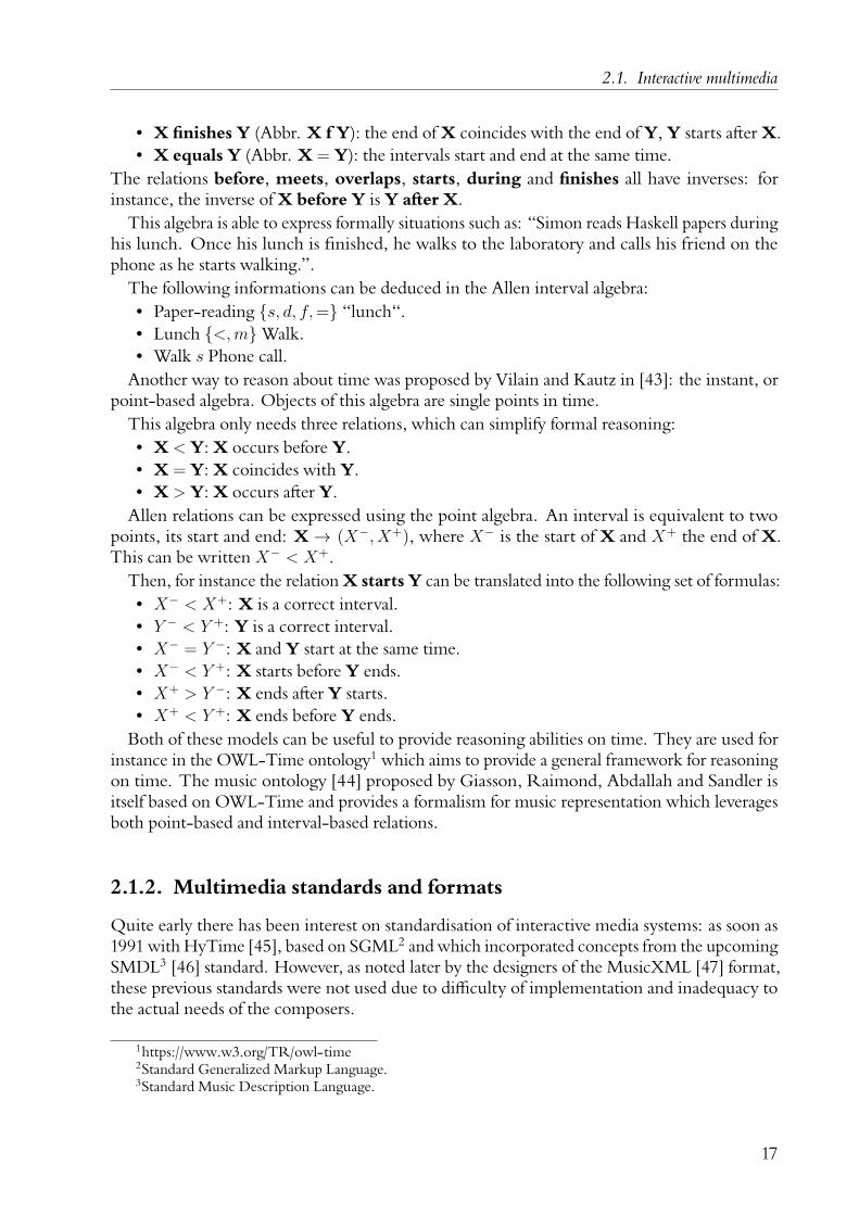
The following informations can be deduced in the Allen interval algebra:• Paper-reading {s, d, f,=} “lunch“.• Lunch {<,m}Walk.• Walk s Phone call.Another way to reason about time was proposed by Vilain and Kautz in [43]: the instant, or

point-based algebra. Objects of this algebra are single points in time.This algebra only needs three relations, which can simplify formal reasoning:• X < Y: X occurs before Y.• X = Y: X coincides with Y.• X > Y: X occurs after Y.Allen relations can be expressed using the point algebra. An interval is equivalent to two

points, its start and end: X→ (X−, X+), where X− is the start of X and X+ the end of X.This can be written X− < X+.

Then, for instance the relation X starts Y can be translated into the following set of formulas:• X− < X+: X is a correct interval.• Y − < Y +: Y is a correct interval.• X− = Y −: X and Y start at the same time.• X− < Y +: X starts before Y ends.• X+ > Y −: X ends after Y starts.• X+ < Y +: X ends before Y ends.Both of these models can be useful to provide reasoning abilities on time. They are used for

instance in the OWL-Time ontology1 which aims to provide a general framework for reasoningon time. The music ontology [44] proposed by Giasson, Raimond, Abdallah and Sandler isitself based on OWL-Time and provides a formalism for music representation which leveragesboth point-based and interval-based relations.

2.1.2. Multimedia standards and formats

Quite early there has been interest on standardisation of interactive media systems: as soon as1991 with HyTime [45], based on SGML2 and which incorporated concepts from the upcomingSMDL3 [46] standard. However, as noted later by the designers of the MusicXML [47] format,these previous standards were not used due to difficulty of implementation and inadequacy tothe actual needs of the composers.

1https://www.w3.org/TR/owl-time2Standard Generalized Markup Language.3Standard Music Description Language.

17

2. State of the art

More recently, the SMIL1 model [48] for interactive multimedia applications has beenintroduced: it is an “XML-based language that allows authors to write interactive multimediapresentations”, generally used in a web context due to the presence of hyperlinks in the structureof SMIL documents. Media objects are represented in a graph structure. Temporal propertiescan be associated to objects: start and end time, duration, and other properties are available.SMIL has been modelled by Petri nets by Chung in [49].

The MPEG-4 standard provides some ways to embed interactivity in an MPEG stream [50].A hierarchical structuring based on SMIL is used: the features are similar, but the XML2 syntaxused changes. A novel point of this standard is the adaptation of video encoding and decodingwith regards to the video layers that are shown. Interaction can be specified through eitherECMAScript scripts or the MPEG-J Java API3 and related applets – MPEGlets – which can bebroadcast as part of the MPEG-4 stream.

2.1.3. Interactive multimedia systems

Interest in modelling such systems has been constant over the years. Ackermann in [51] proposesa separation of hierarchical media systems, time-line based media systems and language-basedmedia systems. Hierarchical systems work by representing media constructions as a tree of mediaobjects. For instance, if a sound starts during another sound, it will be nested hierarchicallyduring the longer sound. Time-line based systems provide a temporal axis which maps generallylinearly to the passing of time. Objects are put by the authors on this time-line: their positiondefines at which point in time they will start. Finally, language systems are any kind of domain-specific language used for the specification of temporal media: this can be for instance commandlanguages or declarative languages. The system proposed by Ackermann aims to combine thehierarchical and time-line model: he proposes an object-oriented approach to the modelling ofsuch systems, by representing media composition by nestable time-lines. Execution occurs byregular sending of messages to objects. Every data-producing process interacts independentlywith the audio or video subsystems in ways hidden by encapsulation.

Hirzalla proposes in [52] a system of branching time-lines: that is, a condition will determineat a given time whether a set of time-lines will execute.

Song et al. in [53] and Vazirgiannis et al. in [54] both model the temporal constraints by asystem inspired from Allen relations [42]. Multiple other authors follow this approach. A recentsurvey [55] identified more than 400 papers covering the notion of interactive multimedia, mostof them providing some means to solve the temporal constraint problems.

The Madeus system for interactive media presentation has been introduced by Layaïdain his thesis [56]. It is based on a set of relations between temporal objects: Parmin(A,B),Parmax(A,B), Parmaster(A,B). In Parmin, two elements start at the same time. The endof the first element happening causes the second element to end, too. Parmax is similar: theconstruction stops when the longest element stops. Parmaster stops whenA stops: B is dominatedby A.

1Synchronized Multimedia Integration Language.2eXtensible Markup Language.3Application Programming Interface.

18

2.2. Modelling multimedia software

Improvements for the distribution of Madeus documents have been studied by Loay in [57]:in particular, he considers the problems due to network synchronisation with remote mediasources. In addition, web technologies such as HTTP1 and RTSP2 are presented as a viablepresentation layer for Madeus documents. Madeus has been linked to SMIL by an XSLT3

translation provided by Villard in his thesis [58]. Tardif [59] focuses on the authoring part ofMadeus and multimedia documents.

A special case of interactive media thoroughly studied in scientific literature is the hypervideo:a video which is not structured linearly and for whom the viewer can change the general courseof the movie during the playback, generally through choice mechanisms. A hypervideo maynot necessarily be a single video file: hypervideos are commonly arranged as graphs of such files.They can harbour additional media content, such as images or texts.

2.2. Modelling multimedia software

This section exposes the software architecture models and patterns commonly used to writemultimedia and more generally art-related software.

2.2.1. Hierarchical entity models

A simple model often used in graphical environments is a hierarchical one: entities manipulatedby the author are encapsulated recursively. Some environments provide implicit hierarchization.For instance, patchers such as Max/MSP and Pure Data are hierarchic in nature: patches cancontain sub-patches. Other environments provide explicit hierarchization, through a tree ofobjects that can be dragged and dropped: this is the case of the Unity3D environment. Exampleof both cases are given in fig. 2.1.

2.2.2. Object-oriented models

More complex graphical applications written in programming languages such as Java, C++ ,SmallTalk, often use the MVC4 pattern. It covers mainly the relationship with the Model,which contains the data on which the software operates, and the View, which allows interactionfrom external sources, generally user interface widgets. Multiple variants exist, such as Model-View-Presenter (MVP) or Model-View-View Model (MVVM) which provide different ways ofcommunicating information between the model and the view, or the external interactions andthe model. While this pattern is most often used as part of the design of authoring applicationsthemselves, it has also been used in environments themselves embedded in authoring environ-ments: for instance in the Jamoma [60] framework in particular as a set of Max/MSP objects,and for the design of web-based audio applications by Taylor in [61].

An example of distributed object-oriented system with a similar approach is D-Bus [62].D-Bus is a successor to distributed object models such as ORB5, CORBA6, DCOP7.

1Hyper-Text Transfer Protocol.2Real-Time Streaming Protocol.3eXtensible Stylesheet Language Transformations.4Model-View-Controller.5Object Request Broker.6Common Object Request Broker Architecture.7Desktop COmmunication Protocol.

19

2. State of the art

(a) Hierarchical object inspector fora small application in Unity3D.

(b) Hierarchical patch organization in Pure-Data.

Figure 2.1.: Hierarchical models of multimedia applications.

In its case, interfaces have to be first declared in some way. The most common approachesfor the declaration of D-bus interfaces, in XML format, are either writing them manually orleveraging reflection and code analysis to generate it automatically from code written in Java,C++ , etc. Then, instances of given objects in these languages are bound to such interfaces; thiscan be again a semi-automatic or manual process depending on the environment used.

The D-bus concepts are instantiated inside two namespaces:• The interface namespace: for instance org.myapp.synth would point to the declaration

an interface with the parameters of a synthesizer.• The object namespace: for instance /org/myapp/synth would be the actual path to an

instance of this synthesizer.While this approach allows a better separation of concern, since interfaces can be defined

externally, it also leads to a duplication of concepts, and an increased workload for the softwareauthor.

20

2.3. Reactive systems

2.3. Reactive systems

Reactive systems are systems which continuously transforms the input from an external envi-ronment into an output. Research on reactive systems takes its roots in research on concurrentprocessing. Part of this research considers the fundamental computational models: we note forinstance Petri nets as a classical tool used when modelling computing systems [63], includingreactive ones. Other aspects of the research on reactive systems are the design of convenientprogramming language to specify reactive programs. This generally implies that the languagemust have some built-in notion of time management. For instance, PEARL90 [64]1 providestemporal primitives allowing for instance to perform loops at a given rate for a given amount oftime. We present here an overview of various techniques used when modelling such systems.

2.3.1. Data-flow graphs

First researches on data-flow models date back to the late 1960, and are originally concernedwith computer architecture – at this point, data-flow programming is as much a hardware thana software concept. Dennis introduces in [65] one of the first formalisation of a programminglanguage based on data-flow graphs.

In a data flow representation, execution of a test or operation is enabled by availability of therequired values. The completion of one operation or test makes the resulting value or decisionavailable to the elements of the program whose execution depends on them.

(First Version of a Data Flow Procedure Language, Jack B. Dennis [65])

The amount of research on this field has led to various definitions of data-flow graphs andprograms, sometimes incompatible [66]. Kahn process networks (KPNs) [67] are directedgraphs which model concurrent processes (the vertices) communicating with infinite FIFOs2

(the edges). Processes can write to the FIFOs without blocking, but will block when reading.Synchronous data-flow graphs extends Kahn process networks by adding an upper bound on

the number of tokens in queues. This allows to compute a deterministic schedule statically andthus enables the program to run with static memory allocations. Other extensions of data-flowgraph exist: for instance cycle-static data-flow. Most of the extensions aim to trade some of thegenerality of DFGs3 against stronger execution guarantees.

Dynamicity in DFGs is generally separated in two independent aspects: dynamicity of thedata, and of the topology. The first relates to the variability on the streams of tokens, while thesecond is about changes to the structure of the graph. Boolean parametric data-flows [68] havebeen proposed to solve dynamicity of topology, by introducing conditionals at the edges.

Specific implementation aspects of data-flow systems are discussed in the Handbook of SignalProcessing Systems [69].

1Not to be mistaken with the Perl language commonly used for text processing.2First-In First-Out, a common model for data exchange.3Data-flow Graph.

21

2. State of the art

2.3.2. Functional Reactive Programming

Research in functional programming, inspired by Backus’s work on denotational functionallanguages [70], has led to modelling reactive systems in a pure functional way. A reactivesystem is in this context defined as a function that takes signals as inputs and returns signals asoutputs. Signals are defined as functions taking the time as input, and returning a value of atype relevant for the application – for instance a floating-point number. This approach has beentitled Functional Reactive Programming [71], and has been applied to various fields such asanimation or robot control [72] through domain-specific languages embedded in Haskell.

2.3.3. Synchronous programming languages

Synchronous programming languages admit the synchrony hypothesis, useful in a reactivecontext. It assumes that computations can be divided in small steps, called reactions. Thesereactions are assumed to be instantaneous. Inputs and outputs to reactions are given a coherentlogical date, instead of a physical time:

In practice, the synchrony hypothesis is the assumption that the program reacts rapidly enoughto perceive all the external events in suitable order.

(Synchronous programming of reactive systems, Nicolas Hawlbachs [73])

Multiple programming languages allow expressing synchronous data-flows, due to theiruse in real-time safety critical systems: ESTEREL, LUSTRE [74], Signal [73, 75], and morerecently Lucid Synchrone and ReactiveML are all languages based on these core principles.Some, such as ESTEREL, use an imperative programming paradigm, while others, such asLUSTRE and Signal, are based on a declarative programming paradigm. Lucid Synchrone andReactiveML are embedded in the OCaml functional programming language. Céu has recentlybeen introduced as a synchronous data-flow language with temporal operators, and applicationsto multimedia [76].

2.3.4. Scheduling in multimedia reactive systems

A large majority of reactive multimedia software is based on data-flow principles [8]: domain-specific unit generators such as sound generators, video effects are connected together in a DFG.For instance, for low-level audio engines, one of the predominant methods is the audio-graph.Prime examples are Jamoma AudioGraph [9] and Integra Framework [77]. Audio processing isthought of as a graph of audio nodes, where the output of a node can go to the input of one ormultiple other nodes. Audio workstations such as Magix Samplitude (with the flexible plug-inrouting) and Apple Logic Pro (with the Environment) provide access to the underlying audiograph.

A common approach in real-time interactive environments based on data-flow graphs isto pre-perform a topological sort of the nodes and then execute the nodes in the said order:this approach is for instance used as part of the Antescofo reactive loop [78], in Dannenberg’sAura system [79], in Pure Data and others. Donat-Bouillud gives in [80] an overview of thescheduling algorithms for other common real-time interactive music environments.

22

2.4. Music environments

Orlarey and Letz, in [81], give simple steps in order to enable parallelism for dependencygraphs of audio nodes, by adding counters to the input of nodes and distributing parallelizablenodes over multiple cores. Another approach for parallelization is proposed by Sadek in [82],which looks for whole chains in the execution graph and schedules them in different workerthreads.

Some environments allow cycles by delaying data in a circular execution by one clock cycle:this is the approach that can be taken in the LUSTRE language [74] with the operator pre.

2.4. Music environments

Multiple authors provide overviews of music creation environments. Möllenkamp presentsin [83] the common paradigms used when creating music on a computer: score-based withMUSIC and Csound [84], patch-based with Max/MSP or Pure Data [85], programming-basedwith SuperCollider [86] and many of the other music-oriented programming languages, trackerssuch as FastTracker which were used to program the music in early console-based video games,and multitrack-like such as Steinberg Cubase, Avid Pro Tools. He gives their own category toAbleton Live and Bitwig Studio thanks to their ability to compose clips of sound interactively.Another extensive overview covering the particular subject of musical notation is given by Fober,Bresson, Couprie, and Geslin in [87].

We chose here to compare the existing environments for music creation, composition, andperformance in a scale that goes from purely textual like most programming environments, topurely graphic like traditional sheet music or audio sequencers.

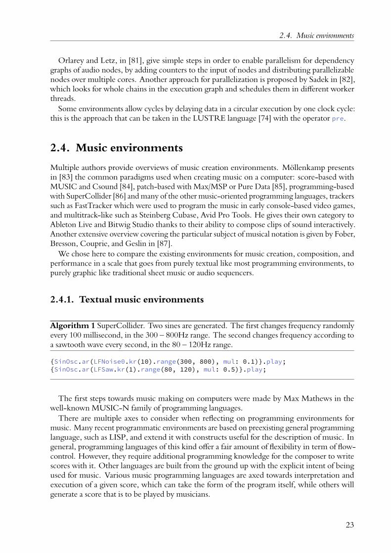
2.4.1. Textual music environments

Algorithm 1 SuperCollider. Two sines are generated. The first changes frequency randomlyevery 100 millisecond, in the 300 – 800Hz range. The second changes frequency according toa sawtooth wave every second, in the 80 – 120Hz range.

{SinOsc.ar(LFNoise0.kr(10).range(300, 800), mul: 0.1)}.play;{SinOsc.ar(LFSaw.kr(1).range(80, 120), mul: 0.5)}.play;

The first steps towards music making on computers were made by Max Mathews in thewell-known MUSIC-N family of programming languages.

There are multiple axes to consider when reflecting on programming environments formusic. Many recent programmatic environments are based on preexisting general programminglanguage, such as LISP, and extend it with constructs useful for the description of music. Ingeneral, programming languages of this kind offer a fair amount of flexibility in term of flow-control. However, they require additional programming knowledge for the composer to writescores with it. Other languages are built from the ground up with the explicit intent of beingused for music. Various music programming languages are axed towards interpretation andexecution of a given score, which can take the form of the program itself, while others willgenerate a score that is to be played by musicians.

23

2. State of the art

Algorithm 2 Antescofo. A first quarter note, labeled “NoteA” is played. Then, a chord isplayed for a half note. Finally, another note “NoteB” is played, and execution jumps back to“NoteA”.

BPM 120NOTE C4 1 NoteACHORD (A4 G4) 2NOTE A4 1 NoteB @jump NoteA

Algorithm 3 ChucK. Two sines are generated. One changes frequency every 50ms, the otherevery 100ms.

SinOsc lo => Gain lo_g => dac;SinOsc hi => Gain hi_g => dac;0.5 => lo_g.gain;0.2 => hi_g.gain;while(true) {

50::ms => now;Std.rand2f(80.0, 120.0) => lo.freq;50::ms => now;Std.rand2f(80.0, 120.0) => lo.freq;Std.rand2f(300.0, 800.0) => hi.freq;

}

Abjad [88], based on Python and Lilypond, is a music typesetting software which uses aTEX-like syntax. Csound [89] and CommonMusic [90] are score interpreters. Csound is itsown language, descended from the MUSIC-N languages, while CommonMusic is based onLISP.

SuperCollider is a SmallTalk-inspired language and networked execution environment [86]specialized for audio synthesis, as well as live and algorithmic sound composition. An exampleis given in Algorithm 1.

Antescofo is a programming language tailored for score following [91]. An example of trivialscore in Antescofo is given in Algorithm 2. The main difference with other score followingsystems is its anticipatory nature: it couples the result of multiple estimation agents whichoperate probabilistically on both audio data, and evenemential data. Actions and variations ofthe position in the score are enacted according to these estimations. The scheduling strategies,along with an overview of the system, are described in [92].

ChucK [93] is a programming language specialized for music, presented by its author GeWang as a “Strongly-timed, Concurrent, and On-the-fly Music Programming Language”. Itis sample-accurate and allows combining audio-rate and control-rate signals uniformly. Anexample is given in Algorithm 3.

Recent advances byDonat-Bouillud lead towards the use of dependent typing in theAntescofolanguage to enable verifications on buffer sizes for multi-rate schedulings [94], following theintroduction of signal processing in the system [78].

24

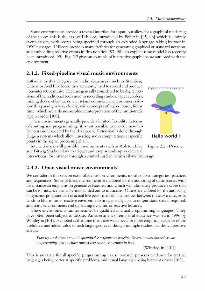
2.4. Music environments

Some environments provide a textual interface for input, but allow for a graphical renderingof the score: this is the case of INscore, introduced by Fober in [95, 96] which is entirelyevent-driven, with scores being specified through an extended language taking its root inOSC messages. INScore provides many facilities for generating graphical or standard notation,and embedding reactive events in this notation [97, 98]; an explicit time model has recentlybeen introduced [99]. Fig. 2.2 gives an example of interactive graphic score authored with theenvironment.

2.4.2. Fixed-pipeline visual music environments

Figure 2.2.: INscore.

Software in this category are audio sequencers such as SteinbergCubase or Avid Pro Tools: they are mostly used to record and producenon-interactive music. They are generally considered to be digital ver-sions of the traditional tools used in recording studios: tape recorders,mixing desks, effect racks, etc. Many commercial environments fol-low this paradigm very closely, with concepts of tracks, buses, lineartime, which are a skeuomorphic reinterpretation of the multi-tracktape recorder [100].

These environments generally provide a limited flexibility in termsof routing and programming: it is not possible to provide new be-haviours not expected by the developers. Extension is done throughplug-in systems which allow inserting audio computations at specificpoints in the signal processing chain.

Interactivity is still possible: environments such as Ableton Liveand Bitwig Studio allow to trigger and loop sounds upon externalinteractions, for instance through a control surface, which allows live usage.

2.4.3. Open visual music environments

We consider in this section extensible music environments, mostly of two categories: patchersand sequencers. Some of these environments are tailored for the authoring of static scores, withfor instance an emphasis on generative features, and which will ultimately produce a score thatcan be for instance printable and handed out to musicians. Others are tailored for the authoringof dynamic programs part of actual live performance. The frontier between these two categoriestends to blur in time: reactive environments are generally able to output static data if required,and static environments end up adding dynamic or reactive features.

These environments can sometimes be qualified as visual programming languages. Theyhave often been subject to debate. An assessment of empirical evidence was led in 1996 byWhitley in [101]. He noted at that time that there was a need for more empirical evidence of theusefulness and added value of such languages, even though multiple studies had shown positiveeffects:

Properly-used visuals result in quantifiable performance benefits. Several studies showed visualsoutperforming text in either time or correctness, sometimes in both.

(Whitley, in [101])

This is not true for all specific programming cases: research presents evidence for textuallanguages being better at specific problems, and visual languages being better at others [102].

25

2. State of the art

Figure 2.3.: Patchs and Maquette in the OpenMusic environment.

2.4.3.1. Patchers

A common pattern for visual programming environments for music is the patcher. Well-known patchers oriented towards real-time music use are Max/MSP [103] and Pure Data [85].The underlying model for patchers is based on data-flow programming: the patch representsan invariant computation which processes audio and control signals. This results in greaterexpressive power than fixed-pipeline software. In each case, it is possible to work purelygraphically. Flow control is often possible, and implemented as a block that acts on this data([expr] in Pure Data or Max/MSP, [conditional] and [omif] in OpenMusic, forinstance). These software all allow to use a textual programming language to extend thecapabilities or express some ideas more easily.

OpenMusic [104, 105] is a visual environment shown in part in fig. 2.3 where music iswritten by functional composition. It is the continuation of the PatchWork [106] environment,itself a patch-based computer-aided composition system based on a LISP variant.

Of particular interest is the Maquette: a specific object which allows laying out generativepatches in time and compose them functionally.

Timed sequences specify temporal organization of musical objects [107]; visual editors areprovided for various kinds of sequences. While OpenMusic used to be purely compositional, arecent extension has allowed OpenMusic to be used as a reactive system [108]. Denotationalsemantics have been provided for the visual language.

PWGL [109] is another descendant of PatchWork, based on CommonLisp, which featuresa reworked user interface design. Like OpenMusic, execution in a PWGL environment isdemand-driven: that is, the author requests the execution of a particular node of a program,which produces an output by recalling the dependent expressions recursively.

We can note in particular for PWGL the Expressive Notation Package [110]: a set of objectstailored for the creation of custom graphical notations for music.

26

2.4. Music environments

Scores in patchersSome of these graphic environments allow compositions of scores without the need to typecommands, with end results much closer to traditional scores that the default objects providedwith the patchers. Elements of these scores can sometimes interact reactively with the rest ofthe environment: they are not necessarily static. For instance, multiple Max/MSP externals,Bach for Max/MSP [111, 112], note~1, rs.delos2 and MaxScore [113] allow scoring in a pianoroll, time-line, or sheet music from within Max. They are geared towards traditional, linearmusic-making, but it is possible to construct non-linear interactive song by combining multipleinstances, or sending messages to the externals from the outside.

The Bach library for Max [112] allows to define temporal variations of parameters during theplaying of a note by with the mechanism of slots. The processes controlled by such parametersare then available to use in the Max patch.

PureData has been proposed as a free-form score language by Puckette in [114].The Max for Live extension to Ableton Live allows to embed Max patches in the Ableton

Live sequencer. Through the API provided, one can control the execution of various elementsof the sequencer in Max; automations in Live can also be used to send data to Max patches at agiven time. This allows in some way to create Live scores which embed explicit programmaticelements.

Amethod for dynamic patching ofMax abstractions based onCommonLisp has been proposedby Thomas Hummel [115] to reduce resource usage by enabling and disabling sub-patches atdifferent points in the execution of a program.

2.4.3.2. Sequencers

Sequencers, unlike patchers, provide a visual depiction of time in their user interface, generallyin the horizontal axis. They allow to layout media processes in time visually: sound files, au-tomations…Unlike fixed-pipeline sequencers discussed earlier, we consider here sequencerswhich allow some kind of extensibility: they are generally integrated with programming lan-guages which allows to script part of the sequences instead of enforcing graphical interaction.

AscoGraph is a user interface (fig. 2.4a) for Antescofo. It binds the score specificationlanguage with a sequence-based visual representation, in order to help composers to introducetheir scores in the system [116].

IanniX (fig. 2.4b) is a score control system created by Coduys [117] based on the musicalideas of Iannis Xenakis, and in particular its work on UPIC.

It has strong ties with the notion of graphical score: the elements of the score in IanniX aregeometrical entities such as circles, lines…These elements act as individual time-lines which cansend commands through the network, according to the position of play-heads on their shape.

1http://www.noteformax.net2http://arts.lu/roby/index.php/site/maxmsp/rs_delos

27

2. State of the art

(a) AscoGraph.

(b) IanniX.

(c) Kyma. (d) Elody.

(e) Integra Live.

Figure 2.4.: Various software which can provide elements of the sequencer paradigm.

28

2.4. Music environments

Integra Live is a visual modular environment for sound and music composition, based inpart on Pure Data [77]. It combines a track-based metaphor with advanced routing capabilities:parameters can interact across tracks and are not restrained to external control sources as theycommonly are in simpler audio sequencers. A screen capture of the environment is givenin Fig. 2.4e. The center part of the software contains the tracks with various sequences andautomations inside clips and scenes. The right panel is a library. The bottom panel allows tochange routings and parameters inside each clip.

Drile [118] is a virtual reality music creation software package. Loops are manipulatedand bound together in sequences in a virtual reality 3D environment, through instrumentalinteraction. Hierarchy is achieved by representing the musical loops in a tree structure: thetechnique is called HLL1.

Elody [119] is a visual language for music composition taking its roots from λ-calculus. Inparticular, the environment allows positioning functions which will handle events at specificpoints in a time-line. It has been extended with real-time streams by Letz [120], which allowsthe environment to be used in live settings. Elody is visible in Fig. 2.4d.

Kyma is a hybrid software and hardware environment for sound composition [121], shownin Fig. 2.4c. It offers multiple pre-built facilities for sound creation such as multi-dimensionalpreset interpolation, sound composition by addition and mutation, or sequential and parallelsound composition on a time-line. Kyma has basis in object-oriented programming theory,its first versions being entirely reliant on SmallTalk-80. The main entity of Kyma is the SoundObject: a DAG2 of individual computations or media files. A vast library of Sound Objects isprovided, in order to make the environment able to support multi-paradigm composition: withan instrument-score split à la Csound, with time-lines and virtual tape decks, or with traditionalnotation.

2.4.3.3. Live-coding and performance tools

Live-coding is a creative technique which appeared along the use of computers in artisticcreations: in this case, the performer at the center of the stage is a programmer, who createsmedia associations generally in specially tailored programming languages. As an example, wecan take Thor Magnusson’s seminal work on the interaction of scores and live code: [24]. Wenote in particular the Threnoscope from the same author, an innovative pattern-based live-coding environment allowing the musician to dispose bricks of code in a looping sequencer [25].A screen shot is provided in fig. 2.5.

AudioMulch is an environment for live music performance, which also provides presetspace exploration thanks to the Metasurface concept [122]. Cantabile Performer3 is also anenvironment geared towards live performance, with the ability to trigger sounds, and a temporalordering. It is closer to the cue metaphor than the sequencer metaphor.

1Hierarchical Live-Looping.2Directed Acylic Graph.3https://www.cantabilesoftware.com/

29

2. State of the art

Figure 2.5.: The Threnoscope. The left, circular part is the score: blocks indicate which codewill be running; polyphony is supported. The right part allows the live-coder toinput the programs that will run during a block.

2.5. Distributed multimedia

There are several families of software and tools that provide networking formultimedia authoring,and in particular music production. We distinguish low-level methods to synchronise audiostreams across multiple machines, applications that enable collaboration when authoring mediaart, and applications for distributed musical performance. Then, we discuss of the link betweentemporal relationships and distribution: clocks.

2.5.1. Distributed applications

For audio synchronisation, we mainly note the multiple incarnations of the NetJack server [123]which aim to make accessible the elements of a Jack connection bay on several machines. Theseare master-slave Jack extensions that allow one machine to send one audio or MIDI stream toanother by connecting a virtual cable. Carôt presents in [124] a more complete census of thesound servers adapted to the distributed musical game.

Different software allowing collaborative, desynchronised authoring, are presented in theliterature or as commercial offerings: Ohm Studio [125] takes the principle of traditionalsequencers and allows a sharing of documents to several users, on the internet. Splice [126]follows the same principle, but is oriented towards the community of beat-makers.

30

2.5. Distributed multimedia

Finally, there is a large family of tools geared towards real-time music improvisation [127].These include NINJAM1 and eJamming2.

The OSC protocol [128] is commonly used to communicate between different parts ofdistributed music applications; while the protocol itself does not specify a transport mechanism,most implementations leverage an UDP3 transport.

Mobile and web applications are being increasingly used to create music, but they are oftenembedded in a bigger score or framework and act more as an instrument than in other systems.An interesting example of a web-based live sequencer is JamOn [129] which allows multipleusers to collaboratively and interactively author music by drawing within a web page interface.A deeper overview of the collaborative music authoring environments is given in [130].

2.5.2. Clocks

Due to the temporal nature of the distribution problem discussed earlier, we are interested inpossible mechanisms for time management between several machines.

The literature on distributed systems distinguishes several families of clocks:• Physical: they mark the progress of time in the material world.• Logical: they mark the advancement of time in the steps of a distributed algorithm, so no

relation with time in seconds.• Hybrid clocks have recently been introduced to reconcile these two families.The two main methods for synchronising physical clocks are NTP4 [131] and PTP5 [132].

NTP is available on many platforms and allows in practice to achieve a synchronisation accuracyof a few milliseconds on the internet. PTP is more accurate and promises near-microsecondaccuracy. However, this depends on the accuracy with which the packages are timestamped andthus the quality of the implementation of the PTP clock. In practice, the interest of PTP willbe more pronounced when dedicated and expensive hardware (Grand Master Clock) is availableto stamp the packages.

A monotonous clock has the characteristic of always progressing forward. Physical clocksare not monotonous6 and thus cannot be used for stamping. Logical clocks were introducedby Lamport into [133] to provide formal reasoning and verification possibilities over the flowof time in distributed systems: they give a partial order between the messages exchanged in adistributed system.

Solutions exist to maintain a link between logical and physical clocks. For example, Googleintroduced TrueTime as part of the distributed Spanner [134] database. TrueTime works withintervals rather than precise dates, and requires synchronisation of physical clocks.

The hybrid [135] logical clocks offer guarantees of causality on a physical clock close to theprecision of NTP, with a granularity close to the microsecond.

1http://ninjam.com2http://www.ejamming.com/3User Datagram Protocol.4Network Time Protocol.5Precision Time Protocol.6For instance, the hardware clocks shipped with most computers drift when temperature varies – sometimes

by up to a second per day. Internet clock synchronization can remedy to this, but may cause the computer time togo backwards upon resynchronization. Some measurements on such clocks are provided here: switchdoc.com/2014/12/benchmarks-realtime-clocks-ds3231-pcf8563-mcp79400-ds1307

31

2. State of the art

Finally, for musicians, clocks based not on a time in seconds, but on a musical time have beenpresented recently. They make sure that several machines will play on the same beat. This isthe case for example with Ableton Link1. Note also the Global Metronome [136], which usesRaspberry Pi and a GPS connection to offer this kind of synchronisation.

2.6. Interactive scores

This section will present the formal models that were used in different families of interactivescores, as well as the resulting software allowing to use and execute these models graphically.

2.6.1. Models

Previous work on the subject of interactive scores did take place in part at the LaBRI with thework of Jaime Arias, Mauricio Toro and Antoine Allombert, that attempts both to formalizethe composition semantics and to provide ways for real-time performance of ISs. In order togive a formal foundation for interactive scores, and allow proofs and verification of temporalproperties on the scores, multiple formalisms were researched for ISs. They focus mainly onthe temporal semantics ([5–7]).

2.6.1.1. Petri nets

Petri nets have been proposed as a model for music representation as soon as 1986 with thework of Camurri and Haus [137]. A prominent idea in the field is the use of Petri nets in orderto model ISs, by focusing on agogic variations. The methodology followed by Allombert wasto define basic nets for each Allen relation [42], and then to apply a transformation algorithm,described in [5, section 9.2].

Coloured Petri nets were also used to model complex data processing in ISs [138], in orderto allow the description and execution of sound processes to occur directly in the score.

In [139], Barate et al. extends P-Timed Petri nets with real-time alteration semantics, whichpermits the score to change in real-time without loosing consistency.

2.6.1.2. Temporal Concurrent Constraint Programming

Since the ISs can be expressed in terms of constraints (A is after B), one of the recurrent ideas fortheir formalisation was to use TCC2 and more particularly NTCC3, since it allows constraintsolving. This approach was studied by Antoine Allombert [140] and Mauricio Toro [6, 141].

2.6.1.3. Reactive programming languages

Due to the static nature of models involving Petri nets and temporal constraints, a domain-specific language, ReactiveIS[142], was conceived in order to give dynamic properties to ISs.An operational semantic is defined using the synchronous paradigm, to allow both static anddynamic analysis of the ISs. This also allows composers to easily describe parts of their scorethat cannot be efficiently represented visually.

1https://www.ableton.com/en/link/2Temporal Concurrent Constraints.3Non-deterministic Temporal Concurrent Constraints.

32

2.6. Interactive scores

2.6.1.4. Timed Automata

Another model of ISs using the extended timed automata of UPPAAL has been developed byArias [143]. Timed Automata allow to describe both logical and temporal properties of ISs.Moreover, the shared variables provided by UPPAAL allow to model the conditionals. Theyare also used for hardware synthesis [144]. Real-time execution semantics are implementedwith this method; however, it does not cover loops.

2.6.2. Software implementations

The models described before were often subject to validation through implementation; some-times as prototypes and proofs of concept, and sometimes as software actually used in an artisticsetting.

2.6.2.1. Boxes

Figure 2.6.: Boxes. Screenshot taken from [145].

Boxes [146] is a software allowing free-form hierarchical composition of sounds in time.Constraints based on Allen relations can be added between boxes. It has two particularities notfound in any of its successors:

• A given composition (hierarchical object) can be referenced multiple times in a givenscore, which makes the hierarchy a DAG instead of a tree.

• Sounds are based on an additive spectral synthesis model, which allows re-scaling andstretching without audio artefacts.

It is shown in fig. 2.6.

2.6.2.2. Virage and i-score

Virage (shown in fig. 2.7), and i-score 0.1 and 0.2 (shown in fig. 2.8) are software whichimplement various stages of the research of Allombert as described in [5]. They are successorsof Boxes [145]. The main novel point is the introduction of interactivity in the scores, with thenotion of interaction point: some parts of the score can wait for an external event to happenbefore resuming their execution.

33

2. State of the art

Figure 2.7.: Virage. At the left, a mock-up. At the right, a screenshot. Images taken from [13].

In i-score, when a score is played, it is compiled into a HTSPN1 which is in turn executedusing a Petri net simulator. The visual model is based on two basic elements: boxes andrelationships between boxes. Boxes can contain either automation curves or other boxes.Interaction points can be put at the beginning and end of boxes. This introduces a graphicalcoupling between data and conditions: there has to be an automation curve in order to haveinteractions in the score, which led composers to create extremely small boxes only to be ableto use interaction points.

Figure 2.8.: An extract of score in i-score 0.2.

1Hierarchical Time Stream Petri Net.

34

2.7. Conclusion

2.7. Conclusion

This section presented an overview of the various fields related to this thesis: the modelling anddescription of existing multimedia software is one of the first questions we must ask. Multiplemodels are provided in the literature: for instance object-oriented, hierarchic, with denotationalor operational semantics. Various music and art systems are presented, most with specificinteraction paradigm tailored to artistic use cases. We note specifically Antescofo, Kyma andIanniX, whose models and implementations aim to solve problems akin to those presentedin this document. The discussion on distributed media in Section 2.5 serves as a preliminaryintroduction to the concepts used in Chapter 9. Finally, Section 2.6 provides an history of theresearch on which the proposed system is rooted.

35

3Goals and objectives

3.1. Introduction

Following the state of the art, we can state that ISs and more generally real-time media authoringtools present in the literature tend to exhibit common characteristics:

• A hierarchical arrangement of time and structured temporal relationships between objects,often following Allen relations.

• A hierarchical arrangement of logical relations between objects, as seen in Boxes, Virage,i-score.

• A codification of interaction and variable, non-linear time.• Conditional relationships between elements of the structure.• Looping.• Communication with inputs and outputs: sound cards, MIDI1 or OSC2 devices, …This works aims to construct a new interactive score model offering these characteristics,

and the associated score creation tool in a way that will foster creativity and enable, if not newdesigns, at least simplifications on common patterns used by artistic multimedia applicationauthors. The following chapter presents various ideas that will be considered during this thesis,whenever design choices and questions arise: this chapter helps us define the goals and thedesign space for the authoring environment we seek to provide.

3.2. Context and discussion

3.2.1. Common definitions

Note that scientific literature provides multiple different and sometimes incompatible definitionsfor DFGs and surrounding concepts. We give here the simplest definition that allows anunderstanding of the problem of this thesis.

Definition 1 (Graphs)An undirected graph G is a pair (V,E), with V a set of vertices and E a set of edges. An edge is a set oftwo vertices V1, V2 both in V .

A directed graph G is a pair (V,E), with V a set vertices and E a set of edges. An edge is a pair of twovertices (V1, V2) both in V ; in this case, V2 is a successor of V1.

A path is a sequence of adjacent edges: (Vi, Vj), (Vj, Vk), (Vk, Vl), ...

1Musical Instrument Digital Interface.2Open Sound Control.

36

3.2. Context and discussion

A directed acyclic graph is a directed finite graph which admits a maximum path length: all paths arefinite.

Definition 2 (Data-flow graph)A DFG is a directed graph which models data relationships between operations. Vertices of the graph areassociated with input and output ports; edges are pairs of ports instead of pairs of vertices.

Vertices, also called actors in this context, model a mechanism which consumes data from their input portsand produce data in their output ports.

Edges, also called channels in this context, model a mechanism which carries data from the output of avertex to the input of another vertex.

Execution of an actor is called firing.The data produced by actors is called token.

Definition 3 (Tick)In real-time synchronous systems, a tick is the amount of time in which a program ran periodically mustexecute.

In artistic contexts, soft real-time is achieved if the duration of a tick is consistently shorterthan the minimal duration perceived by a human. This allows for instance to apply effects tomusical instruments without creating a delay for the performer.

3.2.2. On creativity

Even at the modelling stage, it is necessary to keep in mind the objective of enabling usageby creators, artists, and more generally people in a creative mindset. In particular, we useas a reference some design principles proposed by Resnick et al. in [3], given the focus oncomposition tools – taken in this case at the raw meaning of “composing objects together”:

• Support Exploration: it must be easy to try, fail, retry different possibilities, as well as beexplicit in the possible capabilities of the environment.

• Low Threshold, High Ceiling, and Wide Walls: the environment must be easy to use forbeginners, not limiting for expert users, and suggest the idea of exploration, for instanceby providing a blank canvas.

• Support Collaboration: the environment must support multiple persons working on thedocuments written in it.

• SupportOpen Interchange: the environmentmust be compatiblewith other environmentsin similar domains.

• Make It As Simple As Possible – and Maybe Even Simpler: it is allowed to add limitations,if it is done to simplify some cases.

• Choose Black Boxes Carefully: when designing programming languages, the primitiveelements of the language must be specified with consideration of the design space thatshould be allowed for authors, and adequate abstraction levels must be provided.

• Balance user suggestions, with observation and participatory processes: users sometimesoffer ideas according to their perceived problems, which may or may not match actualscientific observation.

Likewise, Turner et al. in [2] run a study of digital art pieces, their design, and the design ofthe tools used to create the pieces. In particular, how immersive a tool is, how easily it permitshierarchisation of objects of the composition, how clear is the visualization of the objects usedduring creation are all identified as key elements of the creative software design.

37

3. Goals and objectives

Eaglestone et al. present in [1] the results of a study on the electro-acoustic music composer’srelationship to the software they use, and its impact on creativity. In particular, they noted that“All composers involved within the observations elected to work with multiple applications.”,in agreement with previous studies on the same subject.

Finally, the end goal of creativity is to improve problem-solving for users of an environment:in particular, we aim to provide a visual programming environment. The field of visual pro-gramming languages has provided multiple studies [101, 102] providing partial verification ofthe Gilmore-Green match-mismatch hypothesis: “problem-solving performance depends uponwhether the structure of a problem is matched by the structure of a notation.”.

3.2.3. On models and verifications

The end goal of this work is to provide a model suited for real-time usage, and a correspondingimplementation. The model is given in the OCaml [147] language, which we intentionallyrestrict to pure functions and strictly functional semantics in order to give simpler grounds for aformal assessment of the method presented. In particular, we take care of staying within thebounds of the OCamllight system for which a complete formal semantics exists [148] and hasbeen verified with the help of the HOL-4[149] proof assistant. This is done in order to leaveopen the possibility of a complete formal verification of the system proposed here at a later time,without requiring a rewrite in a sound environment.

This is in contrast with previous work on the subject of interactive scores such as mentionedin Section 2.6, which focused on operational semantics through translation to intermediatemodels such as Petri nets, time automatas, or concurrent constraint networks.

The reasons for this are twofold:• This keeps more proximity between the visual language and the objects of the model,

and reduces the number of concepts required to describe it. The objects we use in themodel of execution are almost exactly the objects used by the composer for authoring. Forinstance, in the method proposed by Allombert [5], the score is written by the composerin a visual language, which is then translated to Petri nets; the nets are then executed withan interpreter.

• This simplifies the description of general graph-like structures, and allows for fasteriteration. This point is particularly important: as mentioned before, the conception of asystem tailored for creation requires many iterations, generally involving back-and-forthin semantics and even kind of objects, as well as frequent refactoring; a textual languagefor which well-tested compilers and toolchains exist helps to reduce the cost of eachiteration greatly in contrast with for instance Petri net models.

We however loose the possibility to apply common tools used for instance for constraint orsoundness verification directly. This does not mean that verification is impossible. For instance,we give in [32] a method to transcribe a part of this work – the temporal model – to the timeautomata model proposed by Arias. This translation is then used to verify properties with CTL1

formulas in the UPPAAL model checker [150] as an offline step. For instance, formulas such as:∀ ⋄ sound1.finished ∧ clock < 30000 can be checked to ensure that a given sound of the scoreguarantees termination before a certain amount of time (in this case 30000ms).

It is also important to note a few differences between the OCaml model and the C++ imple-mentation (the latter described with more details in Chapter 10):

1Computational Tree Logic.

38

3.2. Context and discussion

• The model uses closed polymorphism to enumerate a small set of unit generators [151] ofthe system. The C++ implementation uses open polymorphism through inheritance, asthis is the standard way to provide extensibility to object-oriented systems.

• Due to the real-time requirements of the software, we have to take specific care ofminimizing memory allocations and system calls during execution, due to the design ofcurrent desktop operating systems [152]. This implies for instance that most allocationswill be cached and reused. Translating this to the functional model would blurry itsdefinition without helping the cause of the temporal semantics. To achieve this, theC++ algorithms are not pure and most structures are mutable.In particular, we take care in the model to separate the immutable structure of the entitieswe work with, and the state that will variate in time; the C++ implementation merges both,to allow for better cache behaviour: structural and variable data relating to the same objectsare generally related enough that being physically close in computer memory can provideimportant performance benefits. Sadek in particular identifies in [82] the importanceof cache in audio applications by showing that increasing the number of threads in amulti-threaded data-flow paradigm can cause buffer underruns to happen faster due tothe decreased cache efficiency. This leads to more audio clicks, an undesirable behaviour;this was corroborated by Orlarey and Letz while providing a method to parallelize Faustcode with OpenMP in [81].

3.2.4. On authoring and interaction

The system presented here is meant to be used directly by authors and creators of multimediaworks; wemust question its position in relationshipwith other creation tools thatwerementionedin Chapter 2.

At a purely technical level, we wish to provide the same expressive power than commonmultimedia creation software: Max/MSP, Pure Data, SuperCollider …At the very least, enoughextension points must be provided to enable general computations on different multimedia datatypes in the system.

We also have to take into account the temporal nature of the programs we want to author,and the constraints that this implies in terms of user interaction, as well as the possibilities thatthis opens. Bailey states in [153] the following about multimedia authoring applications whichuses a synchronisation model, in reference to the work of Gross and Do related to pen-baseddesign process:

Synchronisation models provide inadequate support for modelling innovative user interaction,which is required for an innovative multimedia application. Also, in order for a specificationto be executable, it must be both precise and complete. However, early in the design process, adesigner needs to be ambiguous, imprecise, and vague.

(Ambiguous Intentions:A Paper-like Interface for Creative Design [154] Mark D. Gross, Ellen Yi-Luen Do)

The present model shall then be able to cater to both aspects of the problem: enabling authors toproduce behaviour without requiring an over-specification of their design, while still enforcingrigorous semantics.

39

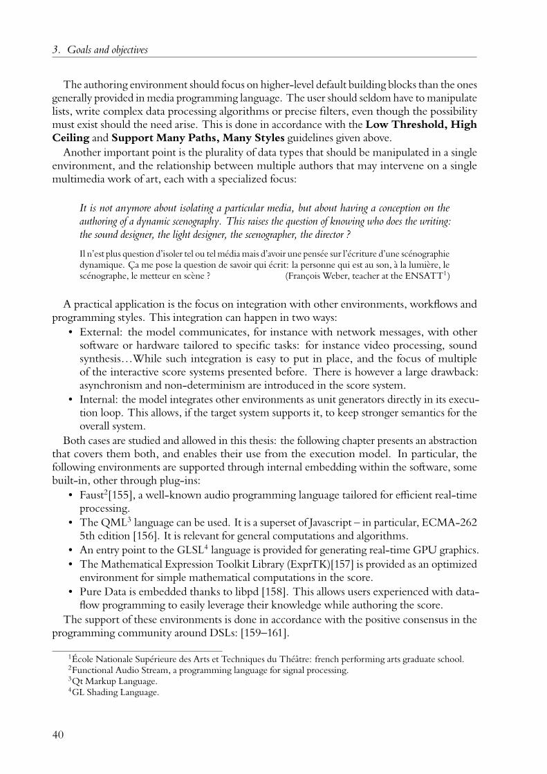
3. Goals and objectives

The authoring environment should focus on higher-level default building blocks than the onesgenerally provided in media programming language. The user should seldom have to manipulatelists, write complex data processing algorithms or precise filters, even though the possibilitymust exist should the need arise. This is done in accordance with the Low Threshold, HighCeiling and Support Many Paths, Many Styles guidelines given above.

Another important point is the plurality of data types that should be manipulated in a singleenvironment, and the relationship between multiple authors that may intervene on a singlemultimedia work of art, each with a specialized focus:

It is not anymore about isolating a particular media, but about having a conception on theauthoring of a dynamic scenography. This raises the question of knowing who does the writing:the sound designer, the light designer, the scenographer, the director ?

Il n’est plus question d’isoler tel ou tel médiamais d’avoir une pensée sur l’écriture d’une scénographiedynamique. Ça me pose la question de savoir qui écrit: la personne qui est au son, à la lumière, lescénographe, le metteur en scène ? (François Weber, teacher at the ENSATT1)

A practical application is the focus on integration with other environments, workflows andprogramming styles. This integration can happen in two ways:

• External: the model communicates, for instance with network messages, with othersoftware or hardware tailored to specific tasks: for instance video processing, soundsynthesis…While such integration is easy to put in place, and the focus of multipleof the interactive score systems presented before. There is however a large drawback:asynchronism and non-determinism are introduced in the score system.

• Internal: the model integrates other environments as unit generators directly in its execu-tion loop. This allows, if the target system supports it, to keep stronger semantics for theoverall system.

Both cases are studied and allowed in this thesis: the following chapter presents an abstractionthat covers them both, and enables their use from the execution model. In particular, thefollowing environments are supported through internal embedding within the software, somebuilt-in, other through plug-ins:

• Faust2[155], a well-known audio programming language tailored for efficient real-timeprocessing.

• The QML3 language can be used. It is a superset of Javascript – in particular, ECMA-2625th edition [156]. It is relevant for general computations and algorithms.

• An entry point to the GLSL4 language is provided for generating real-time GPU graphics.• The Mathematical Expression Toolkit Library (ExprTK)[157] is provided as an optimized

environment for simple mathematical computations in the score.• Pure Data is embedded thanks to libpd [158]. This allows users experienced with data-

flow programming to easily leverage their knowledge while authoring the score.The support of these environments is done in accordance with the positive consensus in the

programming community around DSLs: [159–161].

1École Nationale Supérieure des Arts et Techniques du Théâtre: french performing arts graduate school.2Functional Audio Stream, a programming language for signal processing.3Qt Markup Language.4GL Shading Language.

40

3.3. Targeted behaviours

For many applications, however, there are more natural ways to express the solution to a problemthan those afforded by general purpose programming languages. [...] With an appropriateDSL, one can develop complete application programs for a domain more quickly and moreeffectively than with a general purpose language.

(Domain Specific Languages, Paul Hudak [159])

In particular, media applications themselves cover various domains, such as audio processingor graphics; we assert that providing a wealth of specific languages adapted to each task, andorchestrating them from a host environment is a necessary pathway to efficient intermediaauthoring.

3.3. Targeted behaviours

A study of the field shows that there are common expectations on multimedia and especiallyaudio software. We consider four categories of specifications:

• The creative environment specification, which is about the interaction of the author withthe software: how the software can help the author to produce relevant scores.

• Technical specifications are about the precise behaviour in terms of performance to enableusage in a real-time reactive context.

• Distribution specification is about the interaction of the environment in a setting withmultiple processes or computers.

• Model specification is about the representation of concepts general enough to cater to theneeds of the previous categories.

Some of these expectations will serve as explicit goals that the implementation should be ableto meet to be relevant; others are more general guideline principles that are used whenever achoice is possible between different possibilities for the model. Most of these goals are relatedto more precise requirements that were put in place during the OSSIA and Virage researchprojects.

3.3.1. A system for creativity

3.3.1.1. Intention before correctness

In the field of temporal interval and multimedia object layout, it is commonplace to leverageconstraint resolution systems [53, 141] in order to enforce valid temporal intervals betweenobjects. These constraint systems would enforce that the constraints put by authors in such en-vironments were respected, generally by moving the position of objects to satisfy the constraintsin real-time. However, it has appeared when exchanging with users of such environments thatthis was not a desirable behaviour for authoring – at least, not if enforced: this can cause precisearrangements of temporal objects to break due to underspecification by the author. A possiblesolution would be to put more constraints, but this would then often break the creative flowof the author for the sake of protecting the work from the very algorithm that is supposed tohelp it. Besides, while it makes sense for the final resulting program at the end of the authoringprocess, during this same process, it is generally impossible to enforce permanent coherence.That is, even if generally the author wants to go from one coherent program to another coherentprogram after an edition, the shortest path between these two programs is not always a coherentprogram itself. A practical example is textual programming: generally, most the program text

41

3. Goals and objectives

between two keystrokes will not even respect the language syntax, but these steps are necessaryto go from one valid program to another. This also apply to visual languages, especially thosewith constraints: it can sometimes be easier to temporarily have an invalid constraint whichwill be made valid soon afterwards, than enforce validity at every program state change whichwould prevent many edits to be made.

Hence, we believe that the model should primarily respect the intention of the composer,even at the cost of producing incorrect or temporally incoherent behaviours at some pointduring execution: it is always possible to add off-line or explicit on-line verification passes later,but these must not be a hindrance to the author during the creation of artistic works.

3.3.1.2. Freedom of extensibility

Generally, we do not wish to impose constraints on the extensible parts of the system: that is, asfar as possible creative freedom is encouraged, even at the expense of program safety.

This stems from a simple observation: as soon as external code is allowed in the system, inlanguages without strong temporal and spatial bounding guarantees, such as dependently-typedprogramming languages (for instance, McCarthy provided library-level solutions in the Coqproof assistant [162] to enforce bounds on temporal complexity [163]), it becomes extremelyhard to guarantee program behaviour. But, as mentioned before, extensibility is a main tenantof creative authoring environments. Hence, we make the choice of not imposing artificialrestrictions on the system which we would not technically be able to enforce.

3.3.1.3. Visual interaction

We want to provide a well-defined visual language to interact with the model. It is clear from [2]and [3] that most creative types are better able to express themselves in visual environments. Amajor reason for this is the discoverability and explorability of such environments, in contrastwith textual languages which require a learning step. This has also been verified by Stowell andMcLean in [164] in which the importance of a visual language as primary syntax is noted in thecontext of live audio performance.

3.3.1.4. Live-coding

Live-coding has been briefly introduced in Section 2.4.3.3. The model should be amenableto live-coding and reactive editing without limitations: the environment must allow changesduring the execution to adapt to live performance conditions. This necessity has been madeexplicit during seminars with practitioners from the scenic arts field: however good and completethe specification of the score may be beforehand, there must always be a way to take care ofunattended events. In particular, the user must not be stuck or loose time during a criticalmoment of the performance because of a constraint that may have been placed on the scoreduring the main composition process.

42

3.3. Targeted behaviours

3.3.1.5. Freedom of data production

The model should guarantee the ability to produce large amounts of data in a short period.This is one of the most problematic choices we are to make: in practice, this means that thesynchronous hypothesis as generally used in synchronous data-flow systems cannot be formallyaccepted in our case, as it requires a bounded number of tokens in a given logical time unit tobe valid.

The main reason for this is to allow for specific kinds of music piece which rely on arbitrarilyhigh number of messages occurring at the same time: for instance, we can refer to so-called“black MIDI” musical pieces for which a compositional goal is to fit the maximal possiblenumber of MIDI notes that a computer may play in a song. Fig. 3.1 showcases this. A currentrecord is more than 688 million notes in a 5:40 span which amounts to an average of 2.26million notes per second, or 15601 notes per audio sample at a standard sample rate of 44.1kHz.

Likewise, in [165], Coleman experiments musical composition with large-scale replication ofmusical entities in order to study the timbral properties of such sounds: in practice, this leads tosongs with millions of duplicated and separately time-shifted audio tracks such as the author’s amultitude, before creation1.

Of course, it is impossible to guarantee real-time behaviour in such cases, but we do not wishto restrict their expression; a similar design choice has been expressed made by Bresson andGiavitto in the design of the reactive extension to OpenMusic [108].

Figure 3.1.: An extract rendition of a black MIDI song.

Another aspect is the magnitude bounding of values, generally done for safety of the executionof programs. Artistic creations sometimes rely on overdriving the “safe” set of values [166]:

As I began to play with the code, setting weird numbers in the functions, I found a way ofgenerating leaves by really upping the number of iterations and using a couple of conditionalstatements [...]

(Processing – Creative Coding and Computational Art, Ira Greenberg)

Other examples could be going beyond the Nyquist frequency2 in a digital oscillator to getan aliasing effect:

kernel_panic is a fixed-format work that explores the use digital audio artifacts as musicalmaterial: The byproducts of aliasing, quantization noise, and clipping are liberated to theforefront of the composition process [...] (kernel_panic, Jerod Sommerfeldt)

Hence no restrictions shall be enforced, though value bounding should be available for themajority of .

1https://soundcloud.com/christopher-coleman-603014064/a-multitude-before-creation2Half the sampling frequency of a signal per the Nyquist-Shannon theorem.

43

3. Goals and objectives

3.3.1.6. Edition and execution

We must take care to separate clearly the authoring time needs, and the execution time needs.In [4], Desainte-Catherine et al. distinguishes between environments catering to either needs,as writing-oriented for the first ones, and performance-oriented for the second ones, and mentionsthe need for a convergence of both approaches. However, it is important to consider thatdifferent needs arise in both cases, for instance in terms of verification: while in multimediaauthoring environments the authors can generally insert temporal constraints between elements,as mentioned before, there may be cases during the edition where these constraints should notbe enforced: else it would be either impossible or at least tedious to write scores.

3.3.1.7. Integration

As mentioned before, we want to be able to do both internal and external integration of multi-media software. In particular, the programs and media scores authored should stay independentof the actual external software: it should be possible for instance to replace an instance of Max-based sound synthesis with an equivalent sound synthesis built in SuperCollider without needingto change the score. The motivation for this is mainly platform independence: it is nowadayscommon to run media software on multiple platforms, some being traditional desktop systems,and others being embedded boards which run specialized operating systems. Porting to suchplatforms should not require more work than ensuring that every generator is available, and ifone is not, that there is a way to replace it easily.

3.3.2. An efficient environment

We use an integral logical time, based on a multiple of the media streams part of the score toensure no loss of precision.

Audio must be buffered, and execution must happens on regular ticks whose physical durationmatches the logical duration in samples of this buffer: this is in adequacy with how current audiohardware and middleware operate [167–170]. This method, generally named pull or buffer-synchronous in the literature, is necessary in order to provide the lowest achievable latency oncommon operating systems. The buffer size may not always be a constant.

In particular, in the context of this thesis, we call audio sample the individual data pointand audio buffer a sequence of audio samples.

A common method in creative environments is to have two rates: one for control signals,which can be once per buffer with the value of parameters being set by events at the beginning ofthe execution, and one for audio signals [89, 103]. We wish to provide a more general multi-rateenabled behaviour:

3.3.2.1. Sample-accuracy

Sound generation and control must be sample-accurate. Sample-accuracy is generally meantas the possibility for the composer to describe events occurring at the level of a single audio-frame [93]. That is, an event happening at a given time position must have repercussions exactlyat this logical time in following processes or unit generators. It does not mean that every processmust generate data at each individual audio sample, though: this would be costly in performancewhile not necessarily improving perceptual cues.

44

3.3. Targeted behaviours

3.3.2.2. Liveness

No deadlocks must happen: the multimedia scenarios must never find themselves in a configu-ration where the execution would be stuck with no possibility of forward progress. In particular,this means that we have to handle cases where deadlocks would happen due to invalid tem-poral intervals, as mentioned previously. A first solution is to make impossible the creationof obviously invalid constructions: for instance, A occurs before B and B occurs before A. Asecond solution is to have well-defined backup strategies to use whenever a constraint cannot besatisfied at run-time. These strategies can then be given under the form of hints by interactivescore authors.

3.3.3. A general model

The model should not come with strong limits on temporal dispositions of objects. For instance,the model for time conditional-branching scores described by Toro in [6] does not supportmultiple interactive musical structures starting at the same logical time. We want to preservethe freedom of the author to dispose temporal objects as arbitrarily as possible.

3.3.3.1. Hierarchisation

The model should be hierarchical: this has been noted as a defining feature of creative environ-ments [2]. We also refer to the work done by Berthaut in [118] which focus on the notion ofHLL. Interesting points of HLL noted by the author are the ability to choose the complexitylevel at which one wants to operate during playing, adaptability to different levels of experience,and easier collaboration due to the ability to work on different independent nodes of the tree.

3.3.3.2. Multi-scale data

In relationship with the hierarchy, the model should support multi-scale control on the data.That is, media data can generally be studied at the macroscopic, sometimes semantic scale: forinstance, a sequence of audio clips, musical notes, and abstract description of processes such as amusical accelerando. They can also be studied at the microscopic scale: for instance the individualaudio sample. Vaggione notes the following in [18]:

By using an increasingly sophisticated palette of signal processing tools, composers are nowintervening not only at the macro-time domain (which can be defined as the time domainstanding above the level of the “note”), but they are also intervening at the micro-time domain(which can be defined as the time domain standing within the “note”)

(Horacio Vaggione [18])

3.3.4. Relative conception of time

While music composition environments such as audio sequencers generally adopt an absoluteview of time, in the context of interactive media and interactive scores “temporal objects” mustnecessarily be laid out relatively to each other at least at the authoring phase, since anything thatwould follow an interactive event cannot be given an a priori date. Methods to represent relativetemporal intervals generally relate to Allen [42]’s work on temporal knowledge.

45

3. Goals and objectives

However, while Allen intervals are indubitably useful to perform an a posteriori analysis andreasoning of an existing work, we believe that they do not map to the state of mind of authorsduring the authoring process. Vazirgiannis notes in [54] in particular, that while they are usefulas a tool to model time as a relative notion between objects, they are not immediately practicalfor multimedia applications:

Multimedia applications demand that a relationship doesn’t change when the duration changes.The descriptive character of Allen’s relations doesn’t convey the cause and result in a relationship.

(Vazirgiannis et al. in [54])

That is, Allen relations are able to state A meets B and C overlaps A and B. However, in thecase of interactivity, if A becomes longer or shorter during the execution, Allen relations bythemselves provides no ways to ensure that A will still be meeting B: it is necessary to add amodel on top of it, very often under the form of temporal constraints networks.

3.3.5. A distributed system

Distribution covers the ability of the system to be used over multiple processes or computers.We consider the questions of distributed authoring and distributed performance separately.

3.3.5.1. Distribution of tools

The Virage and OSSIA research projects have put in evidence the need for interoperabilityof tools in a creative setting. For a new musical or media application to be relevant for artistsand creators, it should be able to exchange informations with the existing set-ups. This canbe as simple as receiving “play”, or “stop” messages to control playback for instance, but alsocover deeper temporal synchronisation or network communication with common software andhardware.

This is enabled by the use of common protocols in the field of media arts: MIDI, OSC,DMX1 to name a few.

3.3.5.2. Distributed authoring

While research on distributed authoring systems – sometimes called collaborative edition –started multiple decades ago, it is with the rise of web applications that such features have becomemainstream. These systems allow multiple users to edit concurrently a single document, whilemaintaining consistency of the document: for instance, two users editing a text document ora spreadsheet online. There are two main approaches to distributed authoring: operationaltransformation and conflict-free replicated data types. Operational transformation relies onthe idea that the various clients will perform edition actions on their document, and broadcasttheir changes through command sent to other networked instances editing the document.The instances receiving the messages will then adapt the received command in order to keepconsistency with its current internal state. Conflict-free replicated data types [171] covers aspecific kind of data structures which support concurrent non-blocking operations natively.Each computer applies the local and remote operations indiscriminately; for each data structure

1Digital Multiplexing.

46

3.4. Introductive example

a merging algorithm between two concurrent instances is defined. For instance, grow-onlycounters are counters where the only possible operations is to increment it. Merging the stateacross multiple replicated instances is done by taking the max of the counter. The system isthen able to converge towards a consistent state over time – this is sometimes called eventualconsistency.

Hence, distributed authoring is a problem well-covered in the literature: it is generally possibleto take most GUI authoring systems and transform them to enable collaboration. We will notconsider it further in this document.

3.3.5.3. Distributed performance

A less covered question is its of distributed performance and execution, in particular in thecontext of reactive systems. In particular, what are the cues that can be provided by the author toenable distribution of some parts of an interactive work, and how can interactivity, for instancewith sensors and other parts, can be defined across multiple machines, each with their distinctphysical inputs and outputs.

Supporting distributed performance natively can have multiple advantages in the context ofinteractive media: in contrast with approaches where a root instance sends messages to all theclients for each change of parameter in time, we can instead consider the case where the scoreis known beforehand to each instance and as such can be executed with only the exchange ofrequired temporal synchronisation messages, plus any message necessary for the actual score.This frees network bandwidth, which can be relevant for small, embedded systems nowadayscommonly used in interactive art. For instance, multiple works by the artists Les Baltazarsleverage Raspberry Pi Zero; benchmarks have shown that network performance of these devicescould be estimated at between 50Mbit s−1 and 100Mbit s−1; if data transfer such as real-timesound or video is necessary as part of the work, we should strive to minimize the overhead ofother parts of the system. In addition, this reduces common undesirable behaviours such asnetwork jitter or packet loss.

Applications can range from simple synchronous playback of media between multiple com-puters, for instance to enable synchronised video walls, or native support of redundancy for thesystem: should a computer crash during performance, a backup one should be able to carry onwith the performance. In particular, for performance involving multiple machines in a singlelocation, it is important for delays between the outputs of the machines to be minimized.

3.4. Introductive example

Let us first present a small example of the meaning of these various concepts, and how theconstruction we provide maps to them. This example uses the constructions that will bepresented throughout this document. It is useful as a medium to keep in mind the kind ofbehaviours that we expect to be able to easily construct by the end of this thesis. An example oforganization of the objects will be introduced.

We will consider a small score which operates on two output parameters:• The first is an external control: for instance, the intensity of a light.• The second is a sound output.The score is described as follows:

47

3. Goals and objectives

• For five seconds, an automation1 curve produces a value at regular intervals. The curveitself is shorter than five seconds: it is looped periodically.

• If an external toggle was enabled when the score started, this value should be transformedthrough an easing function2 before being sent to the light intensity parameter controlledby an external software. Else, it should be sent directly to this parameter, without takingthe mapping into account.

• After these five seconds, a five-second sound starts playing.• At some point in the score, upon the triggering of a physical switch, an audio filter id

applied to the sound. If the switch does not trigger, the effect eventually starts at 7 seconds.• When the sound stops, the effect stops, too.This score can be seen under multiple aspects.

3.4.1. Data aspect

The aspect the reader of this document will certainly be most familiar with is the data-flow.Fig. 3.2 is a simple representation of a meaningful data-flow extracted from the description of

the score, which does not cover the temporal aspects: all the possible relationships are presented.

Autom.

Mapping

Sound

Effect

/light/intens Sound card

Figure 3.2.: A simple data-flow which could match the description of the score of Section 3.4.

3.4.2. Hierarchical aspect

Note that the previous graph does not mention in any way time or hierarchical relationshipsbetween its objects. Yet, the temporal behaviours described implicitly reference a hierarchisationof objects: in particular, the unit generators are expected to run for a given duration. A simpleway to achieve this is to consider that durations are modelled by an explicit domain object, andnest unit generators under these objects. This method will be developed in Chapter 6; for nowit is enough to say that these objects will be named interval; an example of such a hierarchicallayout is given in Fig. 3.3.

Then, we need to consider the temporal layout of such intervals. In previous literature, thislayout what was generally defined as the notion of interactive score. In our case, we will give adifferent definition of interactive scores, which takes the data semantics into account.

As such, this temporal layout will be modelled by an object named scenario. Likewise, alooping behaviour was mentioned: another object will serve to model such loops.

1Term used to denote the variation of a parameter over time following a given curve.2Specific mathematical functions often used in artistic applications for transitions and smooth movement of

objects. See http://easings.net for a list.

48

3.4. Introductive example

interval

scenario

interval I5

effect

interval I4

sound

interval I3interval I2

loop

interval

automation

interval I1

mapping

Figure 3.3.: A hierarchical tree which is used to associate durations to the elements of the scoreof Section 3.4 by nesting them.

3.4.3. Temporal aspect

We now have to introduce the interactivity and durations mentioned in the score.

This is done by laying out the intervals in a graph-like structure which will be explained indetail in Chapter 6. In a few words, in addition to the interval, we introduce two objects: oneto handle temporal conditions (TC) such as when …then …, and another to handle logical,instantaneous conditions (IC) such as if …then ….

We will show that introducing these two kinds of condition as vertices of the graph whoseedges are intervals of a single hierarchical level is enough to allow the specification and authoringof a large panel of interactive media. An example of such a graph is given in Fig. 3.4.

TC1 TC2

TC3

TC4

IC1 I1 IC2 I4

IC3 I2 IC5

I3 IC4 I5

Figure 3.4.: An approximation of temporal graph for the score discussed in this section: elementswill be scheduled in the order given by a visitation of this graph.

49

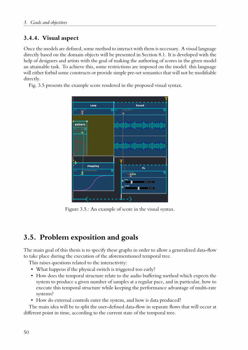
3. Goals and objectives

3.4.4. Visual aspect

Once the models are defined, some method to interact with them is necessary. A visual languagedirectly based on the domain objects will be presented in Section 8.1. It is developed with thehelp of designers and artists with the goal of making the authoring of scores in the given modelan attainable task. To achieve this, some restrictions are imposed on the model: this languagewill either forbid some constructs or provide simple pre-set semantics that will not be modifiabledirectly.

Fig. 3.5 presents the example score rendered in the proposed visual syntax.

Figure 3.5.: An example of score in the visual syntax.

3.5. Problem exposition and goals

The main goal of this thesis is to specify these graphs in order to allow a generalized data-flowto take place during the execution of the aforementioned temporal tree.

This raises questions related to the interactivity:• What happens if the physical switch is triggered too early?• How does the temporal structure relate to the audio buffering method which expects the

system to produce a given number of samples at a regular pace, and in particular, how toexecute this temporal structure while keeping the performance advantage of multi-ratesystems?

• How do external controls enter the system, and how is data produced?The main idea will be to split the user-defined data-flow in separate flows that will occur at

different point in time, according to the current state of the temporal tree.

50

3.6. Conclusion

In particular, we show in Fig. 3.6 and Fig. 3.7 the cases that can occur according to the dateof triggering of the external switch. Each cell of the table shows the data-flow associated to aparticular logical tick, which is defined by the intervals running during that tick.

Note that for instance some ticks contain sets of intervals that are in sequence; it can legit-imately be asked why objects arranged in sequence would be active at the same time. Therationale for this behaviour will be explained in Chapter 5.

In addition to these cases, we must also take into account the possibility of the toggle notbeing toggled, which would cause the mapping unit generator to be absent of the data-flow andthe automation to output directly to the OSC address /light/intens. This is the central point:how to handle data-flow with dynamically enabled nodes in the context of interactive scores.

3.5.1. A software

The ideas and models of this thesis are implemented in the free and open-source software ossiascore. This software is developed and promoted by a community of users and artists, many ofwhom have provided a lot of input, ideas (and, most of all, bug reports!).

A particular care has been given in ensuring that the implementation works on commonoperating systems on a wide range of hardware. User experience has been verified to be sufficientto allow a practitioner without programming experience to learn to use it autonomously.Chapter 10 details the software environment.

3.5.2. A research environment

An additional objective is the creation of a new research platform for interactive scores: thismeans that the software and model must be easily extensible to allow for experiments to takeplace within its bounds. Two categories of research can be explored: the various approachesfor the continuous redefinition of interactive scores themselves, and the extensions that ISs canbring to other models or paradigms. The first thematic for instance would be about comparisonbetweenmultiple semantics for data execution in the score, such as synchronous or asynchronous:hence, the environment must allow for instance to swap different execution engines. The secondis about the use of interactive scores as a support for a specific musical or artistic work: thepresent work has been for instance used by Arias and Dubnov in [38] to construct a musicalenvironment adapted to improvisation by segmenting pre-recorded audio phrases, to allowconstrained improvisation according to high-level musical structures. Likewise, Miranda andAntoine used it in [39, 40] in order to generate orchestrated musical phrases according to timbredirectives, such as “bright violins” or “cellos from warm to dull in five seconds” as a tool fortimbre-based compositions.

3.6. Conclusion

This section presented the various goals and design questions that we have to ask before in-troducing a model for interactivity. These goals were evaluated during the thesis, throughcommunication with authors and analysis of existing works of art and media installations. Inparticular, we insist on the importance of enhancing, or at least not harming, the creative andartistic process: authoring tools in the field of interactive arts should not put themselves in theway of creation.

51

3. Goals and objectives

I1 ∧ I2 I1 ∧ I2 ∧ I4 I4 I4 ∧ I5

Autom.

Mapping

/light/intens

Autom.

Mapping

Sound

/light/intens Sound card

Sound

Sound card

Sound

Effect

Sound card

Figure 3.6.: Possible valid data graph states if TC2 occurs before TC3.

I1 ∧ I2 I1 ∧ I2 ∧ I5 I1 ∧ I2 ∧ I4 ∧ I5 I4 ∧ I5

Autom.

Mapping

/light/intens

Autom.

Mapping Effect

?

/light/intens Sound card

Autom.

Mapping

Sound

Effect

/light/intens Sound card

Sound

Effect

Sound card

Figure 3.7.: Possible valid data graph states if TC2 occurs after TC3.

52

Part II.

A model for temporal interactive media

53

The goal of this part is to associate traditional DFGs with temporal semantics tailored forinteractive execution. In terms of model, three structures are presented in the following order:

• Chapter 4 presents a model to architect and structure multimedia software able to com-municate over the network.

• Chapter 5 uses this model as a foundation upon which a data graph expressing datarelationships between objects of the score is built. In particular, in contrast with otherflow-based approaches for media authoring, an explicit environment notion is introduced.

• Chapter 6 introduces a temporal tree which orchestrates the data relationships in time.• Finally, the data graph and temporal tree are combined in Chapter 7. The resulting object

of this combination is the embodiment of the notion of computational interactive score.The temporal tree allows three things:• Embedding interaction choices in the time-line.• Arbitrary hierarchy.• Merging of loop-based and timeline-based control: we show later in Section 11.4 that

this is enough to allow both time-based and loop-based behaviours to co-exist in a singlestructure and user interface, unlike existing approaches which splits those in two mostlydistinct domains. This enables a large array of possible intermediary behaviours.

We give here for the sake of reference a short overview of the resulting overall executionmethod: At each tick, the temporal tree runs as described in Chapter 6. This produces tokensin the DFG nodes. Once tokens have been produced for every temporal structure, the datagraph runs as described in Chapter 5. Graph nodes which did not receive any token for a giventick will not be executed.

To accommodate for the temporal semantics, data semantics are extended with:• The ability to specify input and output addresses to ports. This allows nodes to read and

write directly from the global environment, in a specified way and can be used to leveragetype information associated with the parameters.

• Special connection types between edges to leverage the fact that not all nodes may berunning at the same time.

When the graph runs, nodes read and write from their input and output ports; relevantvalues are then copied in other ports or in the environment by the supervising algorithm. Theenvironment is separated in two parts: a local part which can serve to reuse the result of givencomputations in further node executions, and a global part which maps to messages sent toexternal devices.

54

4Models and control of interactive media

The goal of this chapter is to present a model for the authoring and execution of ISs, as describedin Section 1.2.3.

It is important to note that there are two levels of distribution addressed in this work. Thepresent chapter covers distribution of a general artistic system (for instance, a specific work of art)over multiple software and hardware, each specialized for different tasks. For instance, a softwareproduces sounds while another produces visuals; a third software receives inputs from a MIDIcontroller and dispatches them to the two previous ones over the network. These programscould be preexisting environments, such as Max/MSP or VDMX, but also new environmentscreated by the authors specifically for a given work of art. This only requires individual messagesexchange: for instance, “set the video background colour to blue on software X”.

Chapter 9 proposes another distinct form of distribution: the distribution of the executionmodel of a single software over multiple computers. That is, specific parts of the control flow ofa single program are deported to other machines according to rules that will be presented.

4.1. Data and environment

In order to be able to control a given piece of software or hardware, it is necessary to have amodel of it. Given the focus on artistic applications, the model that we propose has specificitiestailored to this particular kind of work.

Then, we present how this model is mapped to actual applications and hardware, eitherpreexisting or future ones, and how it allows to orchestrate them through the network. Fromnow on, we will refer to the model of such an application, either hardware or software, as adevice.

We are interested in the control of specific parameters: for instance, the cut-off of a filter in asynthesizer, the colour and intensity of a projector, the welcome text displayed in a software. Adevice can communicate through various protocols: one of the most common in this field isOSC[128]. Section 10.1.6.2 has a quick reminder on the OSC protocol. Following the OSCspecification, we consider a device to be a tree of addressable parameters:

Definition 4 (Device Tree) A device tree is a n-ary tree of nodes, associated with a communicationprotocol: Device = Protocol×Node.

The definition for nodes is given in Definition 12. For now, we simply consider labelled nodes,as in fig. 4.1. Such nodes can optionally be associated to a parameter, and various metadataproperties which will be described afterwards. Protocols will not be defined explicitly: anoverview of the various supported protocols are presented at the end of this chapter.

It is possible to refer to a node of this tree by its path: /sound/lopass, which implies thatchildren nodes of a given node may not share the same name.

56

4.1. Data and environment

video

filebrightnesshue

sound

gainlopassfreq

Figure 4.1.: An example of tree for a simple media application.

Definition 5 (Device Tree Path) A path of a nodeN in a device tree is the sequence of node labels inthe path going from the root of the tree to N . A mapping exists from node paths to character strings: the labelsare concatenated with the / character. By convention, the path of the root of a device tree is the / character.

A node has attached data and optional metadata. The most important is the value; this chapterdescribes the meta-data and the operations such metadata enable. We call these metadataattributes.

4.1.1. Data types

We choose a limited set of data types relevant to media software authoring. This set is inspiredfrom real-world usages and protocols such as OSC, MIDI, DMX.

Definition 6 (Data types)

Float : 32-bit floating-pointInt : 32-bit signed integer

Vec2f : Float2

Vec3f : Float3

Vec4f : Float4

Impulse : No data, just a signalBool : Boolean valueString : Null-terminated character stringChar : ASCII characterNothing : No value

Nodes may carry an associated parameter, which contains a value and value-related attributes.Values can be sent and received through this parameter, between multiple software.

4.1.2. Value

Let T list be a list of elements of type T. The value is defined as a union of fundamental types.

57

4. Models and control of interactive media

Definition 7 (Value)

Value = Float | Int| Impulse | Bool| String | Char| Vec2f | Vec3f | Vec4f | Value list| Nothing

Some remarks on the choices of types:• 32-bit types are used instead of 64-bit for two reasons: most OSC-compliant software

currently expect 32-bit values, and higher precision is generally useful to prevent precisionloss when doing computations, while these data types are the ones used at the boundariesof the system. Instead, using 32-bit types reduces network bandwidth usage.

• One can remark that the Vec2f,Vec3f,Vec4f are redundant with Value list if the listhas 2, 3, or 4 floats. In practice, offering specific fixed-length types is useful for data typescommonly used in creative fields: coordinates (x, y, z), colours (r, g, b, a), etc. This canalso serve as a way to limit dynamic memory allocations, which can negatively impactlatency in real-time applications [172]. For the sake of simplicity, we will from now onjust refer to these three types as VecNf.

4.1.3. Domain

It is uncommon for a given problem domain to accept unbounded inputs. For instance, thefrequency of an audio filter will generally be in the human audible range. The intensity of alight will be given between zero and one and then translated in hardware to the real scale. Assuch, we associate domain-related attributes to the parameter.

Definition 8 (Range)

Option T = Some T | NothingRange T = Option T ×Option T × Set TRange String = Set TRange Impulse = ∅Range VecNf = Option Float N ×Option Float N

Range Value list = Option Value list×Option Value list

Definition 9 (Domain)

Domain = Range Float | Range Int | Range Char| Range String| Range Vecf| Range Value list| Range Impulse

The common numeric types such as Int,Float use a generic domain with a minimum, amaximum and a set of values.

The filtering of a value through the domain operates as follows:

58

4.1. Data and environment

1. If the set of values isn’t empty, the value is allowed to pass if it is contained in a set.2. Else, a bounding algorithm is applied to bound the value between the min and max.Multiple bounding algorithms are possible for number-like values; they can be useful to keep

the value in a given range while loosing less information than a simple clipping.Examples are given for x ∈ [−4; 4],min = −1,max = 1:• No bounding: the domain is only indicative; the filter is the identity function.• Clipping:

clip(x,min,max) =

⎧⎪⎨⎪⎩x, if min ≤ x ≤ max

min, if x ≤ min

max otherwise

−4 −3 −2 −1 0 1 2 3 4

−10

1

Figure 4.2.: Clip bounding mode.

• Wrapping: the value wraps around the domain. Only defined when both min and maxare set. x fmod y is the floating-point modulo of x relative to y, x frem y is the floating-point remainder of x relative to y and d = |min−max|:

wrap(x,min,max) =

⎧⎪⎨⎪⎩x, if min ≤ x ≤ max

min+ (x−min fmod d), if x ≥ max

max− (min− x fmod d), otherwise

−4 −3 −2 −1 0 1 2 3 4

−10

1

Figure 4.3.: Wrap bounding mode.

• Folding: the value goes back in the opposite direction if it goes beyond a bound. Onlydefined when both min and max are set.

fold(x,min,max) =

{x, if min ≤ x ≤ max

min+ |(x−min frem 2d)|, otherwise

Array-like values behave similarly, but can be filtered on a per-value fashion.Values ought to be filtered both according to a range and temporally: another attribute, the

repetition filter, filters a new value if it did not change from the current value of the parameter.

59

4. Models and control of interactive media

−4 −3 −2 −1 0 1 2 3 4

−10

1

Figure 4.4.: Fold bounding mode.

4.1.4. Dataspaces

A last attribute is associated to parameters: the semantic category they pertain to. This categoryis called unit.

For instance, the frequency of an oscillator is controlled in hertz, the colour of a projectorwith a RGB1 triplet.

Definition 10 (Unit) An unit is an attribute associating a semantic meaning to a value.

Definition 11 (Dataspace) A dataspace is a set of units convertible between each other.

Units are not necessarily those of the international unit system. Dataspaces are similar to thenotion of physical quantities, but they can have an abstract meaning instead of a physical one.

Note that dataspaces and domains are dissociated: a value may go beyond the physicalboundaries generally associated with the dataspace. For instance, the domain of an angle isgenerally in the [0; 2π[ range, but going beyond 2π can mean that multiple turns are made –remember in particular the examples of Section 3.3.1.5.

A given dataspace is defined as a union of units:

Color = ARGB | RGBA | BGR | ...

Each dataspace have a neutral unit, which can be considered the default unit for this dataspace.These units are chosen according to their prevalence in artistic and creative environments.Conversions to other units in a given dataspace are done by converting from and to this unit.

Each unit has an associated storage format. For instance:

Type ARGB = Vec4fType BGR = Vec3f

Type Degree = Float

Hence, any given unit consists in a pair of functions:

Unit = FromNeutral× ToNeutral

Where, given an unit T and a neutral unit N :

FromNeutral : Type N → Type TToNeutral : Type T → Type N

1Red-Green-Blue.

60

4.1. Data and environment

For instance, the ARGB1 colour format is the neutral for the colour dataspace. The BGR2

colour format is defined as:

BGR = argb→ (argb[3], argb[2], argb[1]),

bgr → (1.0, bgr[2], bgr[1], bgr[0])

Converting from BGR to RGB means that the conversion goes from BGR to ARGB toRGB. This method is chosen in opposition to writing all the possible conversions separatelyas this would mean P

|Units|2 conversion functions to write instead of 2(|Units| − 1)1. However,

a drawback exists: for conversions involving more complex floating-point arithmetic, someprecision may be lost in the process.

4.1.5. Parameter

The parameter is a product of the attributes defined previously. Coherence between theattributes is kept by converting the relevant types in a best-effort fashion.

This is needed because the framework is meant to be used in a dynamic context: for instance,themeaning and semantics of a given parametermay change for an author during the compositionprocess; hence mutating operations have to be provided to allow for live experimentation.

For instance, changing the unit of a parameter from “RGB colour”to “ARGB colour”,implies that the value representation format may change too, from Vec3f to Vec4f. In thiscase, the type of the domain would be changed to match the new type of the value.

4.1.6. Node

Nodes of the tree mentioned earlier can now be defined. A node identifies an element of thesoftware we aim to model; it is given a human-readable name. Using names for identifiers in thisfashion has the advantage of enabling pattern-matching-like behaviour, and keeping a simplecompatibility with OSC. Another requirement is being able to add any kind of user-relevantmeta-data to a given node: for instance, descriptions, tags, etc. This attribute is encoded in adictionary Dict String Any which allows storing where Any is a value of unspecified type;that is, the type of a value is erased from the type system and stored at run-time instead.

Hence, we get the definition of a node:

Definition 12 A node is a labeled n-ary tree, where nodes may be associated with a set of fixed attributesand a set of variable attributes.

Node = String×Option Parameter ×Dict String Any ×Node list

1Alpha-Red-Green-Blue.2Blue-Green-Red.1That is, given 47 distinct units, it means 2162 distinct conversion functions instead of 92.

61

4. Models and control of interactive media

4.1.7. On Any

A relevant question is: why leverage type erasure for some attributes when stronger typing isavailable ? The reasoning is that this can be used as a prototyping tool for future requirements.New attributes can be added without modification of the object’s data structures, in order toallow testing of their use-case by users of the system, without requiring harder code changesteps. Then, if the utility of an attribute is proven after practical experience with it, it can bemigrated to the stronger typed definitions provided, which will also have the benefit of increasedperformance due to fewer indirections required to access the data.

4.2. Device tree: operations, considerations and usage

4.2.1. Operations on a device tree

The simplest operations we can have on a node are the usual ones for a tree: adding and removingchildren.

Standard reading operations are available on parameters of the tree:

• get: parameter -> value: retrieve the current value stored for a parameter. It is unde-fined whether the value is the latest being applied in practice in the remote device.

• pull: parameter -> value: retrieve the current value stored for a parameter, with asynchronous request to the remote end: the value returned is guaranteed to be at least asrecent as the one present on the remote end when the request was made.

• pull_async: parameter -> value future: retrieve the current value stored for a pa-rameter, under the form of a future1: the remote end will reply asynchronously; thefuture object can then be queried for the replied value at a later time, without blockingthe control flow of the program.

• request: parameter -> unit: requests the remote end to send a message with its cur-rent value to the local end; no guarantee is provided.

These four actions allow to adapt the implementation of multimedia software to the differentlatency and performance compromises that they may require. The default recommendation isto use pull, which provides the strongest correctness guarantees.

Likewise, writing is possible in different ways:

• set: update the local copy of the value.• push: update the local and the remote copy of the value.

Finally, it is possible to request notifications on value changes:

• add_callback: parameter -> (value -> unit) -> callback_index: a function isregistered in the parameter, and will be called whenever it is updated.

• remove_callback: parameter -> callback_index -> unit: unregister a previouslyregistered function.

1In programming, a future is a way to encode the result of an asynchronous computation: when the computationis done, the future can be used to perform an action on its result.

62

4.2. Device tree: operations, considerations and usage

Using these functions allows multimedia software to be built in an event-driven fashion.This is the mechanism upon which the request function is built: the requested value will benotified to all the callbacks when it is received. The support for notification is specific to eachprotocol implementation. This can provide optimization opportunities: a protocol can forinstance enable data transfer only for listened parameters1.

4.2.2. Applications with multiple devices

We may have more than a single device considered in a given multimedia software. Considerfor instance a musical instrument which would accept OSC inputs from the network and sendMIDI outputs to sound hardware. The following convention is put in place: every device willhave an identifier – such as myDevice – and prefix the addresses. An actual address would thenbe myDevice:/my/address: this allows preventing ambiguities in the software and to makepossible unique determination of multiple identical devices across a single software.

Unless it is necessary, in this document, we will omit the device part since there will generallybe no ambiguity.

4.2.3. Patterns and accessors

The OSC protocol supports some form of pattern-matching of addresses, through a patternlanguage similar to XPath3 traditionally used to represent paths in XML documents. That is, asingle OSC address pattern can refer to multiple addresses: /a*/ refers to all the addresses of aserver with a single fragment beginning with an “a”, so /ami, /a.a.aaa would match, but not/ami/b. This can apply as well to nodes of our tree, since we follow the same structure.

We also extend this notion with the idea of accessors: it is very common for array-likeparameters to require the ability to access a single value of the parameter: for instance, 4 inthe [3, 6, 4, 5]. No explicit way is provided in the OSC protocol to handle this: it is theresponsibility of the software to implement array access. We believe that a unified solutionshould be provided for this, and propose the following grammar for accessing array elements:

array-accessor := `[ `0' .. `9' , { `0' .. `9' }, `]`;array-accessors := array-accessor, { array-accessor };

(* as defined earlier: *)dataspace := 'color' || 'distance' || ...;(* valid units for each dataspace *)unit := 'rgb' | 'xyz' | ...;(* valid accessors for each unit *)unit-accessor := 'x' | 'y' | 'z' | 'r' | 'g' | 'b' | ...;

(* e.g. color.rgb or color.rgb.r; we make a precomputed tablewith only the valid combinations. *)

unit-qualifier: dataspace, '.', unit, ('.', unit-accessor)?;

osc-accessor := osc-address, `@', array-accessors | unit-qualifier;

1This is the case for the OSCQuery2 protocol presented in Section 10.1.6.4; in contrast, the MIDI protocolalways transfers every message.

3An expression language used to locate objects in a XML document.

63

4. Models and control of interactive media

(a) The definition of a synthesizer band in aPureData abstraction (sine).

(b) The definition of the whole synthesizer.

synth

lopass

freq

sin.2

gainfreq

sin.1

gainfreq

sin.0

gainfreq

(c) The equivalent tree.

Figure 4.5.: The tree of a simple device.

This covers three things:• Simple array access: taking the nth element of a zero-indexed array or matrix: given

an address of typetag [[fff][fff][fff]], /a@[1][2] for instance would yield the sixthfloat value in the message order.

• Unit conversion: taking a value and getting it in another unit of the same dataspace: forinstance, given an address /a in the RGB colour space, /a@[color.lab] gives the samevalue converted in the La∗b∗ colour space.

• Unit conversion and array access: it is also possible to access a single component of amulti-dimensional unit: /a@[color.rgb.r] gives the red colour component of the value.This is equivalent to /a@[0] if /a is in the RGB colour space or /a@[1] if in the ARGBcolour space, providing a simple example of how this can reduce the mental hurdles ofthe author who often works with this kind of data.

Accessing an undefined value, is implementation-defined to leave open the door to performance-optimized implementations tailored for small devices: OSC is often used on microcontrollers,for instance, where bound checks can have a measurable cost. In our implementation, an out-of-bound access or an impossible conversion such as a frequency to a 2d position, yields a valueof the Nothing type; others could for instance throw an exception.

4.2.4. On instances

A common use case must be considered: node duplication. For instance, a simple polyphonicsynthesizer can be modelled by nodes for each sine, with gain and frequency child parameters.

When the software author wants to add more bands, he would simply duplicate the objectscorresponding to the existing bands and set new parameters on them.

64

4.3. Conclusion

Since the name of a node serves for its identification, when duplicating a part of the tree, weensure that if the requested name is already used we create or increment an identifier.

The syntax for the names given in regular expression format is:

\[a-zA-Z0-9.\]+(.[a-zA-Z0-9])?

where the first part is the root object and the second part the instance identifier.We extend the pattern-matching features of OSC with a special case for instances: The

character ! allows to select all the instances of an object.For instance, in fig. 4.5, the expression /synth/sin!/gain refers to /synth/sin.0/gain,

/synth/sin.1/gain, /synth/sin.2/gain.

4.3. Conclusion

In this chapter, we presented an application model which allows both the reflection of current,existing media software and network APIs, and the easy authoring of new applications, basedon OSC-like semantics. Unlike existing RPC1 approaches such as D-Bus, it aims to be usedboth in a local software, to refer and control to different parts of a creative application easily, andremotely, where it can be used to interact with other software.

This application model is implemented on multiple creative environments, which allows themto interoperate easily. The implementation is detailed in Section 10.1. Attributes of objects aretailored for multimedia creation; in particular, the set of attributes associated to objects is split ina constant part which can always be expected and allows for better performance, and a variablepart which allows for further extensions of the model in the case of new artistic needs. Protocolsfor querying the state of the model are discussed: in particular, the OSCQuery protocol, isshown as viable for the required use-case.

In addition, we note that this model is useful for the documentation of media applications:the device tree provides an abstract specification of such an application, which could then beused for recreation of equivalents or re-implementations due to future hardware or softwarelimitations such as operating system incompatibilities.

A point not considered in this chapter is the temporal semantics: for instance, OSC allowsto associate time-tags to messages, in order to specify at which date they may occur: furtherdevelopments would include these in the model. Another concern not discussed here is thedynamicity of the system: to what extent can the model be extended at run-time while main-taining coherency in the network.

1Remote Procedure Calls: environments able to provide function or method calls across processes or networks.

65

5Data graph

5.1. Introduction

In this chapter, we will introduce the necessary elements that will be used to perform computa-tions and generate data in interactive scores. In particular, we try to provide execution semanticsable to take into account dynamic activation of nodes. That is, we must not assume that at agiven point during the execution of a score, all the nodes of the graph provided by the authorwill be active: some may not have started playing yet, for instance. In addition, as explained be-fore, the programs in the given model are meant to be executed in heterogeneous environments.Some computations can take place locally, in the course of a single tick, while others can takeplace in different programs, sometimes in different computers altogether. To simplify authoring,the solution must strive to make both intra-process and inter-process communication seamlessfrom the point of view of the software user.

We argue that in some cases, it can be meaningful in terms of authoring behaviour toacknowledge that some circumstances can cause a unit generator from a DFG to not execute,while still keeping following nodes executing. A common musical occurrence of this case isthe guitar pedalboard: it is part of the normal flow that some pedals may become enabled atsome time and not at another. As an example, take Fig. 5.1: it is not unthinkable to assume thatthe patch would still be useful musical material if the [lop~] low-pass filter, or the followingreverb [rev1~] was to be temporarily disabled. In this case, we would still want sound to flowthrough the soundcard by the [dac~] objects. However, this case is much less convincing forthe [mtof] object, which converts values in the MIDI range into the corresponding frequencyin Hz, or for the [osc~] object which converts this frequency into a corresponding sine wave.

Hence, we need a way to specify that some dependencies between nodes are critical toconserve a correct behaviour, while some others can be bypassed.

Figure 5.1.: A Pure Data patch which generates a sine and filters it.

While in the guitar pedalboard case this effect can be implemented by a simple bypass at theunit generator level, we show that we can achieve more general dynamic behaviours withoutabandoning safety and reasoning abilities on the program, through the introduction of twoelements:

66

5.1. Introduction

• An environment in which unit generators will be able to read from and write to.• Qualifiers on connections between ports of the unit generators.This chapter is structured as follows: we first introduce an environment which will store

values used for local computations between unit generators, and communicate with the outsideworld. Then, we present the design of the data graph we use: how ports, connections, andnodes are defined; the notion of node activation is introduced. New attributes are applied onconnections, in order to specify the inter-node behaviour in cases where all the unit generatorsare not active. The notion of scope in context of the environment is discussed. Finally, theoverall scheduling and execution semantics are provided: in particular, multiple executionsemantics are discussed, relative to the level of dynamicity acceptable in the system.

Some ideas presented in this chapter have been published in [34]. In particular, we will keepthe same introducing example and motivation: we consider two unit generators f1 and f2. Bothexecute for a finite amount of time, but the order in which they execute is not defined: forinstance, we can consider the execution traces in fig. 5.3a and fig. 5.3b. The data relationshipsbetween the unit generators are also left undefined – the possibilities are showcased in fig. 5.2.

f1 f2

(a)

f1 f2

(b)

f1 f2

(c)

Figure 5.2.: Possible data-flows between f1 and f2 when no specification is provided.

f1

f2t0 t1 t2

(a) A possible trace ofexecution for f1and f2.

f1

f2t0 t1 t2

(b) Another trace of ex-ecution.

Figure 5.3.: Activation traces.

5.1.1. On design choices

The overview conducted by Arumi et al. in [8] provides many insights for the design of a data-flow system for music. This work provides insights about common data-flow patterns found inmusic software, and more importantly what are benefits and drawbacks of each of these patternsand design choices: operating in pull mode or push mode, separating hot and cold inlets1 andoutlets2, monitoring the content of such ports without too much negative performance impact,etc.

1Input ports of a node in a data graph.2Output ports of a node in a data graph.

67

5. Data graph

In this work, we strive to restrict the design to the minimal concepts able to make it viablefor the intended usage: as such, some of these common patterns are not considered directly. Inparticular, it is important to note that the goal of this data-flow system is only to be supportive ofthe temporal structure presented in the next chapter: as such, the software should stay open toalternative designs and behaviours for data processing, as long as they respect the same guaranteesfor inactivity of unit generators.

In particular, for the sake of simplicity, we choose to operate in pushmode at the unit generatorgranularity: unit generators will write to buffers that are copied to the input of the successorunit generators. Remember that the root tick operates in pull mode: the push mode mentionedhere is only used inside the tick. While this has an impact on performance, Section 10.4 willshow that the implementation is competitive with other data-flow audio frameworks. Bothinlets and outlets are passive: no processing occur in any other place than the main function ofeach unit generator. The graph is responsible from copying data from the environment to thenodes, between nodes, and from nodes to the environment.

This work also acknowledges concepts introduced by the Jamoma project, with the JamomaAudio Graph Layer [9, 12]: in particular, contrarily to other patching environments, the authorsassert that “connections between objects must be capable of delivering multiple channels ofaudio” and make a convincing case of the simplification this enables, as shown in Fig. 5.4.

(a) Single-channel ports.

(b) Multi-channel ports using Jamoma ob-jects.

Figure 5.4.: Comparison between the same audio graph with single-channel and multi-channelports and connections.

5.1.2. General execution method

As mentioned before, we aim to leverage a common method in media and particularly audioenvironments: callback-driven execution (sometimes also called pull mode by opposition with apush mode where data has to be read and written regularly to the output devices). The entireexecution must happen in a callback requested by the sound card driver; the contract is thatthe application will write data corresponding to the amount of time requested by the driver,generally counted in terms of audio samples There is no guarantee that the number of requestedaudio samples will be a constant across different ticks.

68

5.2. Durations and tokens

Doing so allows to provide low to very low latency guarantees: with specialized audiohardware, it is possible to reach minimal latencies smaller than five milliseconds. The onus isthen put on the application to perform all the relevant computations in the given time span.

Some specific platforms allow for even better performance through this paradigm: Moro et al.showcase in [173] the use of Pure Data in the Bela embedded board, which allows for latenciessmaller than a millisecond; such low latencies can be necessary for applications requiring tightfeedback loops such as specific human-machine interfaces for musical expression.

It is always possible in such cases to simplify the semantic by treating each sample individuallyand running the whole execution algorithm on it. This would often be wasteful on resources:many algorithms are able to produce data for longer periods with no difference on their output.But the performance cost of running a complete execution algorithm for each time unit can bewasteful. A classical example is playing a sound file: it is always possible to write all the requestedsamples in one go, instead of writing them one by one. In particular, with current compilersand processors, this provides an important advantage: when copying more than one sample,it will generally be possible, either to auto-vectorize1 if the number of elements is a knowncompile-time constant, or if it is not possible, to call specialized implementations at run-time.Even if auto-vectorization is not possible, cache effects remain: there is a lower chance of cachemisses if a unit generator is able to compute successive samples one after each other; cache missescan incur strong run-time penalties3.

In this work, since we aim for real-time performance, it is only normal that we try to takeadvantage of longer buffers, and try to run the processing steps as scarcely as possible, withoutsacrificing more accuracy than acceptable in the computations.

Definition 13 (Root tick) A root tick is a complete execution step of an interactive score.

Since the audio hardware will generally be the driver of all following operations, this executionstep will have to happen during the time left by an audio callback.

5.2. Durations and tokens

Since the work is predominantly concerned with time intervals and temporal processes, it isnecessary to define relevant data types which will be useful for the execution:

Definition 14 (Duration and position)

type duration = int;;type position = float;;

During a tick, unit generators will be requested data for specific time spans. We call thisrequest a token request:

Definition 15 (Token request)

1Auto-vectorization [174] is the process by which a compiler will produce SIMD2 instructions from a scalardefinition of a given computation. For instance, a loop which adds 1 to every element of an array could be compiledwith instructions allowing to process the array 8 elements at a time.

3Some figures for a contemporary Intel processor are given here: https://www.7-cpu.com/cpu/Haswell.html

69

5. Data graph

type token_request = {token_date: duration;position: position;offset: duration;

};;

token_date is the date that an object reaches at the end of a request. position is the positionin the execution of the object relative to its parent in the temporal tree. The reason for theposition will be explained in Chapter 7. offset is the index, relative to the beginning of thecurrent root tick, at which the first data must be written for this tick, if any.

5.3. Environment

We use the data structures presented in Chapter 4 as a base for an environment: in particular,parameters and values. Keys in the environments are paths to parameters of a device tree, similarto OSC paths: /sound/lopass. From now on, we will be able to refer to such addresses asvariables.

The environment is twofold:• A global part refers to the external devices and outside world. As far as possible, it always

represents the state of the outside world: if a physical slider moves, the environmentshould reflect the change in value as quickly and accurately as possible in order to allowfor reactions in the score.

• A local part will be used as a store for intermediary computations during an execution tick.In particular, this local part will not be subject to any external influence, which allowsbetter reasoning on the program behaviour.

Note that we are considering not only fixed values, generally called controls, but also messages.It would be unwieldy to represent a MIDI message as a variable of the environment since there isno guarantee that a single message would happen, and considering that we wish not to lose anymessage that may have been received by the system. Likewise, the Impulse data type presentedearlier is not useful if we consider only a variable with a value of such type; we are interested inthe happening of such events.

To reconcile this with the notion of environment, we define the value associated to a parameterin the environment at a given tick as a time-stamped list of values. We keep track of twotimestamps: a temporal one which corresponds to a date relative to the beginning of thecurrent root tick, and a logical one which is a message index. Different unit generators caninsert messages at any temporal index during their executions. However, message indices arehandled by the system to ensure that every message happens can happen in the order of unitgenerator execution if necessary. An example is given in fig. 5.5.

Definition 16 (Environment)

type environment = {local: (string * ((value * int * int) list)) list;global: (string * ((value * int * int) list)) list

};;

At the beginning of a root tick, the local environment is empty, and the global environmentcontains the list of messages which were received since the beginning of the previous tick.

70

5.4. Graph structure

(a, 0, 1) (b, 3, 0)

(c, 3, 2)

(d, 2, 0) (e, 4, 1)

(f, 4, 2)

Figure 5.5.: Messages with their timestamps, across two root ticks of 5 time units each. Theyare written (x, y, z) with x the message, y the time stamp, z the message index.

At the end of the tick, some data may have been written in the local environment: it is thenmerged and written to the global environment. We call this operation commit. Its semanticswill be given in Section 5.5.4.2.

Specific functions are provided to read andwrite the global environment; their implementationcaters to each protocol supported. We will assume the existence of the following functions:

let push_global key value = (* ... *);;let pull_global key : value = (* ... *);;

push_globalwill send networkmessages,MIDImessages, commit audio data to the soundcard-provided buffer…pull_global will read the current running value of a parameter in the devicetree. In particular, pull_global is used if a value is needed but no message has been receivedrecently.

Even though this can make reasoning on programs harder, the implementation keeps thepossibility for unit generators to write to the global environment at any time, even in the midstof a tick: this can be useful for any kind of emergency stop message.

5.4. Graph structure

In this section, we present the graph structure we use. This structure will operate on theenvironment introduced previously. It can be defined as a task graph: each execution of a nodecorresponds to a task that must be run after the nodes it depends upon have executed. Objectsare identified in the graph by unique integers. For instance:

Definition 17 (Identifiers)

type edgeId = EdgeId of int;;type portId = PortId of int;;type nodeId = NodeId of int;;

5.4.1. Ports

A defining feature of common unit generators in media applications is the multiplicity of inputand output ports: a synthesizer might be built upon multiple parallel oscillators, the frequencyof each defined by the value in a different port.

71

5. Data graph

Ports are defined with a unique identifier, an optional address, ingoing or outgoing edgesand a scoping information. The use of this scoping information is explained in Section 5.4.4.We separate the constant part of ports and the variable part: port is constant during a normalexecution, while port_state will change at each tick.

Definition 18 (Scope)

type scope = None | Local | Global | Default;;

Definition 19 (Port)

type port = {portId: portId;portAddr: string option;portEdges: edgeId list;portScope: scope;

};;

type port_state = {values: (value * int) list

};;

We contrast this with other approaches, where objects of the model are themselves addressed,either at a low level – e.g. with pointers in some programming languages – or a high level withobjects being themselves part of an object tree itself discoverable and addressable through remoteprocedure call protocols or the device tree presented in the previous chapter.

In systems such as Duration1, attributes of the object model itself are encoded by fixed OSCaddresses. For instance, setting an attribute of a track in Duration is done with the followingOSC message:

/duration/valuerange "my track" -1. 1.

In our case, we want the model and data-flow to be freely definable by the author. Thisprovides multiple benefits:

• Apply a single address to a group of ports: ifmany unit generator share a tempo information,there can be a single “truth source” for this value.

• Leverage pattern matching to receive inputs from multiple addresses in a single port: thisenables to react to a class of events easily.

The data copying method from ports and to ports depends on the presence of an addressand edges. Ports can have multiple inputs. The order in which values are copied to the inputsdepends in part on the order of execution of the nodes. In Section 5.5, we discuss how thisorder can be assured to be deterministic.

5.4.2. Pattern matching

Section 4.1.6 mentions the notion of OSC pattern. Instead of accepting data from a singlesource, a port can specify an input pattern such as:/foo.*/bar/b[a-zA-Z], as proposed in the OSC specification.

1https://github.com/YCAMInterlab/Duration

72

5.4. Graph structure

Upon execution, the input stream of the port would contain the list of values correspondingto the matching addresses.

Given a global environment with the variables:/foo/bar/ba 1.0/foo.1/bob/bu 2.0/foo.2/bar/be -1.0/foo.42/bar/bo -3.0

Such a pattern would yield the values −1.0 and −3.0 at the input of the port matching thepattern. These values can be combined by an optional merging step: for instance by keepingonly the latest one.

Writing to the environment supports expression of pattern-matched nodes. Patterns areresolved immediately on insertion: that is, the environment itself does not store a single messagewith the generic pattern, but distinct messages for every node existing in the tree that matchesthe message.

While this seems wasteful in terms of memory usage, it also reduces search complexity whenlooking for a value in the environment: if the pattern was stored as-is, it would be necessary tocheck most patterns when looking for a specific value; in contrast, storing directly each address-value pair allows using simple hash maps when looking for the value of a given address whichgreatly reduces average time complexity which is the main parameter we are optimising for.

Another advantage of this approach is that it eliminates the double-pattern problem. Forinstance, given a unit generator writing to the pattern /foo/ba*r and another that reads fromthe pattern /f??/b?dr, ensuring an exchange of value if the patterns match ends up beingan expensive problem: it can be likened to the question of regular expression intersection,with exponential lower bounds in spatial complexity for the size of the intersecting expressionprovided by Goulad et al. in [175].

5.4.3. Connections

We are interested in the relationships between unit generators of the DFG when they producecompatible values, whether explicitly through cables or implicitly through addresses. In par-ticular, we must take into account deactivated unit generators to be able to provide temporalsemantics, as explained in Section 3.5. Given a node of the DFG executing and producingvalues, we must define which following nodes, if any, will receive the values and when will theyexecute.

We introduce specific connection types, to cater with the use in interactive scores. Theserelationships are expressed between ports of two nodes of the data graph.

We propose two attributes on the connections, defined more precisely thereafter:• Strictness of the relationship: a strict relationship implies a strong dependency between

two ports. That is, if an inlet engaged in a strict relationship with an outlet, and the nodeof the outlet is disabled in the current tick, then the node of the inlet is also disabled. Incontrast, a relaxed relationship implies that one of the nodes can not run and the programstill be valid.

• Buffered and unbuffered relationship: if two ports are connected by an unbuffered rela-tionship, all the tokens produced by the outlet should be consumed by the inlet in thissame tick; if they are not, they are lost at the end of the tick. If the relationship is buffered,the inlet can consume tokens that were produced in the past.

73

5. Data graph

Connections have the following definition:

Definition 20 (Connections)type edgeType =

Relaxed| Strict| BufferedRelaxed of (value * int) list list| BufferedStrict of (value * int) list list| Dependency

;;type edge = {

edgeId: edgeId;source: portId;sink: portId;edgeType: edgeType;

};;

5.4.3.1. Connection as an access control

Strict connection In a given tick, an execution of a node engaged in a strict relationshipwith another node depends on the other node being active.

Consider the case in fig. 5.3a where f1 and f2 both read from a and write to a where a is anaddress of the environment. We use the DFG given in fig. 5.2a.

We consider a simplified case to explain the general desired behaviour with the followingfunction definitions:

• commit(a, x, e) writes a value x to the address a in the local scope of the environmente. In the general case, committing does not simply mean that the value replaces theexisting value in the environment: remember that we store a timestamped list of valuesas per Definition 16. Various methods of commit which leverage this list are discussedin Section 5.5.4.2. In this example, however, we assume a simple replacement.

• pull(x, e) the function that reads the value of the address x from the environment e.The local environment, by the end of each logical tick, should be defined as:• During t0: ∅.• During t1: commit(a, (f2 ◦ f1)(pull(a, e)), e).• During t2: ∅.

Relaxed connection An execution of a node will happen even if the nodes it is connectedto through relaxed relationships are not active. Instead, data will be read and written from theenvironment if an address has been given to the port.

• t0: commit(a, f1(pull(a, e)), e).• t1: commit(a, f2(f1(pull(a, e)), e).• t2: commit(a, f2(pull(a, e)), e).In the explicit case, the output of f1 goes to the input of f2 through a cable. If an address has

been specified for each port in addition to the explicit connection:• If f1 is not active, f2 reads from the local scope instead, or the global scope if the required

address is not available.• If f2 is not active, f1 writes to the local scope instead.Such a behaviour is conceptually similar to a guitarist’s pedal board: not all pedals will always

be active, but we want the signal to keep flowing even if a pedal is disabled.

74

5.4. Graph structure

No connection Even if there is no direct connection, we still have to handle the case wherea node writes from an address in the environment and another reads from this same address.

In this case, the expected behaviour would be:• t0: commit(a, f1(pull(a, e)), e).• t1: commit(a, f2(pull(a, commit(a, f1(pull(a, e)))))).• t2: commit(a, f2(pull(a, e)), e).That is, f2 would read from the value that was written in the environment instead of directly

from f1. Note however that there is a possibility for this value to be replaced with anotherwhich came from an external source between the two ticks. If it is not desirable, the authoralways has the possibility to create a custom local variable not linked to any external source.

Hence, this makes apparent that even if the composer did not create an explicit connectionbetween two unit generators, we have to consider implicit data dependencies between ports,which will have implications on the scheduling algorithm.

5.4.3.2. Connection as a buffering tool

A connection between an outlet and an inlet can be delayed through buffering in a FIFO queue.There are two possibilities for the semantics of this connection:• Readers of the buffer always start from the same point: the beginning of the previous

function in the callback chain. The frame pointer would be located in each delayedconnection, and would not be shared between processes.

• Readers of the buffer continue from the latest read position. The frame pointer would belocated in the source port, and would be shared across all processes reading from it.This behaviour can be useful when multiple functions should apply successively to a singlebuffer, as in fig. 5.7. However, it would also create concurrent accesses problems if twonodes happened to read an output at the same time.

Arumi discusses in [8] the advantages and drawbacks of storing tokens at the output or inputports. In our case, however, since there can be multiple output nodes, the tokens are storedinside the cable structure.

If we have a delay connection from f1 to f2, the first call to f2 will use the values that wereproduced during the first tick during which f1 ran. Note that the output of actual messages isnot necessary: the only necessity is that the source node used to execute: it can be necessary tobe able to react to silence or lack of messages while still knowing that the overall process wasexecuting.

The strictness level is also defined for the delayed connection. In the strict case, a node willonly be able to execute if the source has produced enough tokens; else it is disabled.

That is, in fig. 5.6, f2 would only execute during t1.Finally, note that the current implementation is unbounded. Given two arbitrary nodes

whose start and end depend on an interaction, it is not possible to know when the sink nodewill start executing and thus emptying the FIFO queue, if ever. It is necessary to store all themessages in case of the interaction happening. It is then the responsibility of the author toensure that memory will be sufficient for his use case. However, if temporal constraints areintroduced between the nodes, giving an upper bound on the number of messages producedwill become possible.

75

5. Data graph

f1

f2

t0 t1 t2

Figure 5.6.: Another execution trace. f2’s input corresponds to f1’s output, delayed: this createsa causality problem.

f1

f2 f3 f4

Figure 5.7.: f2, f3 and f4 read from f1 with a delayed connection.

5.4.4. Scopes

It is possible to link the previous behaviours to the notion of scope in textual programminglanguages. In traditional data-flow programming, there is no notion of variable scope: inputsand outputs represented by the model are entirely driven by the connections between nodes.In the present case, the presence of the environment means that reading and writing valuesto variables follows rules similar to the ones that govern reading and writing to variables incommon imperative programming languages such as C or Java.

During a tick, ports have access to three sets of values, corresponding to scopes:• Global scope: The values that were in the environment at the beginning of the tick.

These values are accessible for reading to every node, at every moment of the tick.• Local scope: The values produced by previous output ports in the data-flow under

relevant conditions explained before.• Connection scope: the explicit scope between two ports; the data flowing from one

output port can only go to input ports it is connected to.With this in mind, we can define the scope attribute of ports seen earlier.

5.4.4.1. Default scoping mechanism

Remember that the model is restricted to using the variables defined in the device tree. Thisimplies that for every value in the local scope, the key of this value also exists in global scope.This allows us to enable the following default resolution behaviour:

• If it is not possible to read from a connection, the value will be read from an address, ifgiven.

• When reading from an address, if the address is not available in the local scope, it will beread in the global scope.

The first case only happens for relaxed connections: if the connection was strict, the readingnode would be disabled and thus would not be reading.

76

5.4. Graph structure

Strict Relaxed

Immediate If a node is not active, the other is dis-abled. Else, the data is copied directlyfrom one to another.

A node can execute even if the other isdisabled. If an outlet does not have anyoutgoing edges, or at least one outgo-ing node is disabled, then the value iswritten to the environment. If an in-let does not have any ingoing edges, orat least one ingoing node is disabled,then the value is copied from the envi-ronment.

Buffered The inlet receives tokens as long asthere are tokens in the buffer. Whenthere are not anymore, its node is dis-abled.

The inlet keeps executing even whenthere is no data in the buffer.

Table 5.1.: Summary of the proposed connection semantics.

Writing by default operates in the other direction: if possible, data is written through aconnection, else it is written to the local scope, in order to constrain scope as much as possible.This is done in adequacy with the current principles of scope limiting in software design [176–178].

5.4.4.2. Explicit scoping

The three other cases of scoping simply sets an explicit scope to which data can be written to:• None: the data can only be read and written in other connections.• Local: the data can only be read and written in the local scope.• Global: the data can only be read and written in the global scope.Finally, note that the set of parameters available in the environment is supposed fixed before

the beginning of the execution: all the possible variables are known beforehand and available inthe global scope. If a user of the system specifies a non-existing address, it should be treatedequivalently as the absence of address.

5.4.5. Graph nodes

Now that ports, connections and scopes are specified, we can precise the type of the graph nodes(unit generators). This is the final step leading to the description of the execution algorithms.

The definition is twofold: grNode is the static, immutable part of the node:

Definition 21 (Graph node)

type graph_node = {nodeId: nodeId;run: graph_node -> graph_state -> token_request -> environment ->

(node_state * ((portId * port_state) list) * environment);inlets: graph_node -> graph_state -> port list;outlets: graph_node -> graph_state -> port list;

};;

77

5. Data graph

dataNode is the implementation-specific state of each node, which we will not consider infurther detail:

Definition 22 (Graph node data)

type dataNode =Automation of automation

| Sound of sound| Mapping of mapping| Passthrough of passthrough| ...;;

grNodeState is the part which will vary at each tick:

Definition 23 (Graph node state)

type node_state = {executed: bool;prevDate: duration;tokens: token_request list;data: node_data;

};;

executed serves as a flag to indicate that the node has already been executed during a tick.prevDate holds the date at which the object currently is, before executing the following tick.tokens holds the successive date spans that a node must execute in the current root tick.

We introduce two additional “tick levels” in addition to the root tick mentioned before:• A sub-tick is the execution of a node for a single token. Its specific algorithm depends on

each node’s specific type.• A base tick is the execution of all ticks of a node.Note that “tokens” as used here bear no relationship to the notion of “token” in other data-

flow environments where “token” is generally used to mean the values exchanged betweennodes during execution.

5.5. Graph execution

We can now consider the scheduling question: how to decide in which order should the nodesexecute.

Some environments, mentioned in Section 2.3.4, separate scheduling for event-like data andstream-like data such as audio signals. In our case we are interested in giving the simplest seman-tics on which temporal behaviours can be built upon, hence we consider a single scheduling forthe whole graph. In addition, this lessens the hurdles in obtaining sample-accurate behaviours.

A graph admits a topological sort only if directed and acyclic: while the directed constraintis natural for data dependency graph, since data-flows from one node to another, acyclicity ismore constraining. For the same simplicity reasons as stated above, we only consider the acycliccase. The authoring environment must then ensure that no cycle can be created.

78

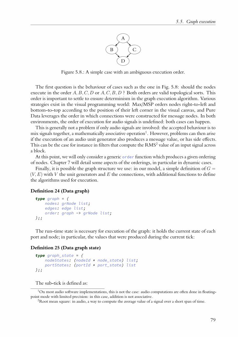
5.5. Graph execution

A

B C

D

Figure 5.8.: A simple case with an ambiguous execution order.

The first question is the behaviour of cases such as the one in Fig. 5.8: should the nodesexecute in the order A,B,C,D or A,C,B,D ? Both orders are valid topological sorts. Thisorder is important to settle to ensure determinism in the graph execution algorithm. Variousstrategies exist in the visual programming world: Max/MSP orders nodes right-to-left andbottom-to-top according to the position of their left corner in the visual canvas, and PureData leverages the order in which connections were constructed for message nodes. In bothenvironments, the order of execution for audio signals is undefined: both cases can happen.

This is generally not a problem if only audio signals are involved: the accepted behaviour is tomix signals together, a mathematically associative operation1. However, problems can then ariseif the execution of an audio unit generator also produces a message value, or has side effects.This can be the case for instance in filters that compute the RMS2 value of an input signal acrossa block.

At this point, we will only consider a generic order function which produces a given orderingof nodes. Chapter 7 will detail some aspects of the orderings, in particular in dynamic cases.

Finally, it is possible the graph structure we use: in our model, a simple definition of G =(V,E) with V the unit generators and E the connections, with additional functions to definethe algorithms used for execution.

Definition 24 (Data graph)

type graph = {nodes: grNode list;edges: edge list;order: graph -> grNode list;

};;

The run-time state is necessary for execution of the graph: it holds the current state of eachport and node; in particular, the values that were produced during the current tick:

Definition 25 (Data graph state)

type graph_state = {nodeStates: (nodeId * node_state) list;portStates: (portId * port_state) list

};;

The sub-tick is defined as:

1On most audio software implementations, this is not the case: audio computations are often done in floating-point mode with limited precision: in this case, addition is not associative.

2Root mean square: in audio, a way to compute the average value of a signal over a short span of time.

79

5. Data graph

let exec_node(g:graph) (gs:graph_state)(n:graph_node) (ns:node_state)(token:token_request) (e:environment) =

let (ns, plist, e) = n.run n gs token e in({ nodeStates = list_assoc_replace gs.nodeStates n.nodeId {

ns withexecuted = true;prevDate = token.tokenDate;data = ns.data;

};portStates = list_assoc_merge gs.portStates plist

}, e);;

That is, the specific execution algorithm of the node is called and transforms the currentgraph state with a new inner state and new port states.

Executing a node during a root tick means that it will be executed for every token requestregistered for it. Reasons for this are given in Chapter 6. The main point is to enable:

• Sample-accurate execution: there has to be a way to tell musical objects to render datafrom t = 17 to t = 23 in time units.

• Temporal looping when the size of a loop is smaller than the duration of a root tick: ifa looped sound lasts for 10 time units, and the root tick duration is 512 time units, theexecution has to repeat multiple times.

With this in hand, we can define the base tick algorithm:

let base_tick (cur_node:graph_node) (graph:graph) (gs:graph_state) (e:environment) =

let rec exec g gs n tokens e =match tokens with

| [] -> (gs, e)| token::t -> let (gs, e) = (exec_node g gs n (List.assoc n.nodeId gs.

nodeStates) token e)in exec g gs n t e

inlet (gs, e) = exec graph (init_node cur_node graph gs e) cur_node

(List.assoc cur_node.nodeId gs.nodeStates).tokense in

teardown_node cur_node graph gs e;;

And the init and teardown functions, which copy the data to the node and from the nodeto the environment:

let init_node (n:grNode) (g:graph) (gs:graph_state) (e:environment) =let rec init_inlets inlets gs =

match inlets with| [] -> gs| h::t -> setup_inlets t (init_inlet h g gs e)

inlet gs = clear_outlets (n.outlets n gs) gs insetup_inlets (n.inlets n gs) gs

;;

80

5.5. Graph execution

let teardown_node (n:grNode) (g:graph) (gs:graph_state) (e:environment) =let rec write_outlets outlets gs =

match outlets with| [] -> gs| h::t -> write_outlets (write_outlet h g gs e)

inlet gs = clear_inlets (n.inlets n gs) gs inwrite_outlets (n.inlets n gs) gs

;;

These functions clears the data in inlets and outlets from previous ticks.

let rec clear_ports ports gs =match ports with| [] -> gs| h::t -> clear_ports t (clear_port h gs)

;;

let clear_port (p:port) (gs:graph_state) ={ gs with

port_state = list_assoc_replace gs.port_state p.portId (p.portId, [])};;

let init_inlet (p:port) g gs (e:environment) =match p.portEdges with(* no edges: read from the env *)| [] -> let pv = match p.portAddr with

| None -> None| Some str -> Some (pull str e)in

replace_value p gs pv(* edges: read from them *)| _ -> replace_value p gs (List.fold_left (aggregate_data g gs) None (get_edges p.portEdges g) )

;;

let write_outlet p (g:graph) (gs:graph_state) (e:environment) =let has_targets = (p.portEdges = []) inlet all_targets_disabled =

has_targets &&List.for_all (fun x -> in_port_disabled x g gs) p.portEdges in

if(not has_targets || all_targets_disabled) then(gs, write_port_env p gs e)

else(write_port_edges p gs, e)

;;

Assuming a static scheduling of nodes given as a list of nodes in dependency order, we cangive a first example of a trivial root tick function, which assumes that all nodes are active:

let root_tick_static (g:graph) (gs:graph_state) (e:environment) =let rec impl nodes gs e =

81

5. Data graph

match nodes with| [] -> e| h::t -> let (gs, e) = base_tick h g gs e in

impl t gs ein impl (g.order g.nodes) gs e

;;

5.5.1. Execution from the point of view of a graph node

1 2 3 4 5

Figure 5.9.: A visual representation of the token requests for a node.

We also have to consider what happens from inside a unit generator implementation: what isthe programming contract that node developers must respect to provide adequate behaviour.An important design choice is to leave open possibilities for inaccurate execution. The reasonsfor this are twofold:

• Some particular unit generators may be unable to conform to strong timing requirements,because they can only work with a fixed tick-rate or do not support timing of inputmessages, yet still provide artistic value: a pathway to integration in the system should beprovided.

• In some cases, performance requirements may dwarf precision requirements. For instance,if a score’s sole point is to send OSC messages over UDP, most of the time spent ensuringsample-accurate positioning of messages will be potentially lost due to the weak guaranteesprovided by the protocol.

Remember that a graph node’s execution function has for type:

graph_node -> graph_state -> token_request -> environment-> (node_state * ((portId * port_state) list) * environment)

Each node has a certain number of inlets and outlets registered with them: these are stored inthe graph_state in the present model. The general objective in the run function is readingfrom inlets and writing to outlets, in adequacy with the timing information given in thetoken_request. A node is free not to write anything, or write as many values as it wants to theoutput port, in order to follow the principles of Section 3.3 and especially 3.3.1.5: some artisticdemeanors may require unbounded token production.

Written values are time-stamped in zero-indexed time units and are relative to the beginningof the current root tick. The first timestamp must be at least at the offset provided in thetoken_request structure. The last timestamp must be strictly inferior to this offset plus thedate minus the previous date. These restrictions hold not only for a single token request, butfor the sum of all requested tokens for a node in a given root tick; the temporal tree will inparticular preserve this guarantee. Fig. 5.9 shows a valid example.

That is, given a prevDate of 12, and a token request such as {tokenDate = 17; offset =35}, the values produced by the node must have a minimal timestamp of 35, and a maximaltimestamp of 35 + 17− 12− 1 = 39.

82

5.5. Graph execution

A more complete example is given in Fig. 5.9. The root tick duration is 5 samples: three ofsuch ticks are represented. At the beginning of the execution, the prevDate of the node is atzero. We ignore the position for now. The first token is: {date: 2; offset: 3}; during theexecution of this token, values can be produced for timestamps 3 and 4. The second token is:{date: 7; offset: 0} and prevDate is set to 2. The third token is: {date: 0; offset: 2}:no production of data should take place. The fourth token is {date: 1; offset: 2} and thefifth token is {date: 3; offset: 3}.

In addition, if we wanted to be able to satisfy the synchronous hypothesis, we would haveto bound the number of tokens produced, for instance at tokenDate - date; this is not donehere for reasons explained earlier. Note also that tokenDate - date may be negative: in thiscase no data shall be produced.

In practice, this means that multi-rate data production is possible: one data node may producefor instance values for every time unit, while another may produce once every N time units withN greater than the root tick buffer size. The common case of control-signal separation, wherecontrol events happens once per root tick, and signal production happens for every time unit,can be approximated by limiting the production of non-audio data to 1 value per token request:in the case where the token request implies a duration of the length of the root tick – which isby far the most common case as will be evidenced later – it is exactly the same. While it is up toeach node to provide an implementation that corresponds to the desired behaviour, Section 10.3will present a method to enable the node developer to simplify the choice between differentbehaviours without requiring rewrites: for instance, running at each time unit, running onceper buffer, running at a defined fixed rate, …

5.5.2. On sample accuracy and precision

Note that as-is, given root_tick_static we can respect sample-accurate behaviours: nodescan produce tokens at a given time-stamp and subsequent nodes will be able to apply the effectof this token starting from this sample.

However, operating in a buffer-synchronous manner has temporal implications on the pre-cision of processing: the value of a signal can still be affected by the duration of a buffer. Inpractice, it is common in node implementations in data-flow languages to produce data at mostonce per run call; for instance in the case of automation curves, low-frequency oscillators ornoise generators. An example is the use of the environment. Consider for instance the graphin Fig. 5.10: assuming that A produces one output value per input value, precision of executionwould be maximized if the execution was run at a tick rate of 1. Suppose that execution is runat a tick rate greater than 1: A runs with a request of N > 1 samples. The value of /address isset at timestamp 0 at A’s inlet, and A produces a value at the same time-stamp, which is thencommitted to the environment. The next time A runs will be at least 2 units after the beginningof its previous token: at least one time-stamp is missed.

There are multiple ways to get closer to ideal precision:

A/address /address

Figure 5.10.: A problematic graph when trying to be sample accurate.

83

5. Data graph

• Fixing t = 1 as the root tick buffer size: at most token requests of duration 1 will beproduced. This is the only way to achieve a perfectly precise rendering given a lack ofcontrol on external nodes.

• A possibility which optimizes for the case where nodes produce one value per tick is asfollows: data production will occur at the greatest common divisor of the token requeststhat occur in the graph. Given a set of nodes, we enumerate all the token requests andstore the beginning and ending of each relative to the root tick duration in a set. Then,for each node, the token requests are split for each value in the set. Finally, the graphexecutes for one complete tick for each interval in the set. This ensures that if a nodeproduces a value for 1 sample, all the other nodes will be able to react to the productionof this value. An example of this process is given in Fig. 5.11.

Overall, we establish that once we step out of the “tick for every sample” ideal case, someprecision is sacrificed: every choice other than this one given black-box unit generators willcome with trade-offs that must be handled in some way; in particular, different environmentscatering to specific media practices may focus on different sides of the scale.

A1 A2

B1 C1

A1 A2 A3 A4

B1 B2 C1

Figure 5.11.: Splitting tokens and running individual parts, assuming a root tick of 10 time units.A,B,C are nodes: Ki means the ith token request of node K. Ticks of the wholeexecution graph are represented by the black underline under individual bins.

5.5.3. Scheduling methods

5.5.3.1. Graph ordering and messages

The main question in this work is the relationship of node ordering and messages exchangedthrough the local state: we also want operations that uses the state to be deterministic to enableauthors to reason about their work.

The simplest case would be to ignore values exchanged through the environment altogetherand only consider the explicit connections made by the author. In particular, note that aconnection case was not discussed: the Dependency case, which allows to introduce an explicitdependency between two nodes without requiring any data transfer between either. By usingthis special edge, it is always possible to get a unique total order between nodes if necessary by

84

5.5. Graph execution

introducing new edges until the graph admits an Hamiltonian path [179], without changing thedata semantics of the program. This way, a path exists to allow the author to get deterministicbehaviour. However, in many cases, introducing enough edges to ensure a unique order wouldbe relatively tedious; besides, indeterminacy at the graph edge level means that determinacy canbe inserted through other means which can improve expressive capabilities of the environment.

Hence, we have to provide a method to order nodes relative to these messages. We will onlyconsider messages written to the local state. Messages written to the global state directly are notconsidered as part of the normal program flow but are intended for specific cases where sendinga message as soon as possible is critical.

We will consider two cases:

• The first case is the dynamic address case: here, we do not assume that nodes restrictthemselves to writing to their output ports; they can instead directly write to the localenvironment.

• The second case is the static case: the inputs and outputs of each node is fixed to specificaddresses. In this case, exec_node becomes:

let exec_node_static(g:graph) (gs:graph_state)(n:graph_node) (ns:node_state)(token:token_request) (e:environment) =

let (ns, plist, { global = g }) = n.run n gs token e in({ nodeStates = list_assoc_replace gs.nodeStates n.nodeId {

ns withexecuted = true;prevDate = token.tokenDate;data = ns.data;

};portStates = list_assoc_merge gs.portStates plist

}, { local = e.local; global = g });;

In the dynamic case, scheduling will have to occur at each tick, since a given node could writeto any number of different addresses during its execution. In the static case, we can insteadperform scheduling beforehand, which leaves more time for running actual processes duringthe tick.

It is generally hard to infer an order. Consider for instance the graph in Fig. 5.12: Hence

A B

/a

/b

/b

/a

Figure 5.12.: A graph with messages but no apparent unique schedule: the author has to provideadditional information to ensure deterministic operation.

85

5. Data graph

the presence of heuristics: object creation order, visual position, …However, we argue thatan assumption can be made on the order of operations: if a node A reads from an address x,and another node B writes to this address x, we assert that in the context of media authoring,the desired order of execution is generally B;A. We will show that in concert with a basicstructuring of certain graph nodes presented in Chapter 7, this allows to author meaningfulmultimedia pieces with only a small number of connections explicitly specified by the composer.

5.5.3.2. Ordering strategies

In the literature, multiple possibilities for ordering nodes in DFGs are provided. Some environ-ments leverage the object creation order, while some others rely on the visual position of objectsin a canvas: bottom-left to top-right for instance. In addition, the current approach allows toleverage the execution time of objects to define an order. That is, if the absolute start date ofan object A is before the absolute start date of an object B, then A will execute before B in agiven tick. This is only possible with a dynamic schedule, since the order would be updated atrun-time.

The current implementation relies by default on the creation order of objects to settle exe-cution, with a hook to introduce any other ordering strategy; three other strategies are in themidst of implementation. The proposed temporal execution, as well as two static strategies: onewhich considers first the static X position of objects in a visual canvas, then their Y position(X going from left to right and Y from top to bottom), and a similar one which considers thereverse order: Y then X.

5.5.3.3. Dynamic scheduling

In this case, we do not know on which addresses each graph node will write to in the local state.Hence, we have to run a scheduling pass at each tick to be able to provide an order. This canopen interesting creative possibilities: for instance, it allows to write a node which would outputon a random parameter amongst a set of parameters, or to have effects which would run beforeor after each other in different ticks.

We give hereafter the complete base_tick algorithm for the dynamic case.

let rec base_tick graph gs nodes (e:environment) =match nodes with| [ ] -> (gs, e);| _ ->

(* look for all the nodes that can be executed at this point *)let next_nodes = List.filter can_execute nodes in

(* order them and run the first one *)let next_nodes = List.sort (nodes_sort next_nodes) next_nodes inmatch next_nodes with| [ ] -> (gs, e);| cur_node::q ->

let (gs, e) = tick_node cur_node graph gs e in

(* repeat on the updated graph, with the remaining nodes *)sub_tick

graphgs

86

5.5. Graph execution

(remove_node next_nodes cur_node.nodeId)e;;

5.5.3.4. Static scheduling

In this case, we know the addresses that each node reads from and writes to. This enablesthe following general strategy: let connect G n1 n2 the function that creates a dependencyconnection between the vertices n1 and n2 of the graph G:

Algorithm 4 Adding connections between nodes.V ←sorted(G.nodes)for i ∈ [0; |V |[ do

for j ∈]i; |V |[ doif No path exists in G between i and j or j and i then

if A connection is possible from i to j thenconnect(G, i, j)

else if A connection is possible from j to i thenconnect(G, j, i)

end ifend if

end forend for

There are two ways to perform this algorithm; their performance on various graphs iscompared in Section 10.4:

• The first one is to do either a breadth-first or depth-first search every time to look for apath in the graph: the overall worst-case time complexity is O(|V |2 ∗ (|V |+ |E|)).

• The second is to compute the transitive closure of the graph at the beginning, and aftereach insertion. We recall that the transitive closure of a graph G = (V,E) is the graphG′ = (V,E ′) where E ′ contains an edge e between two nodes v1, v2 of V iff there isa path from v1 to v2 in G. This generally makes possible to retrieve in constant timethe existence of a path between two nodes in G; however, we need to recompute thetransitive closure after every connection which can be reduced to the quadratic matrixmultiplication problem [180].

5.5.4. Operations and combinations

5.5.4.1. Value combination

Any value combination method has to be considered in function of the data type. As mentionedbefore, if we are considering audio data, it is quite common to use sample-by-sample additionas a combination function.

However, we have to consider other data types: in particular, individual control-like values.We propose three different merging methods, which can be applied in inlets and outlets:

• Appending: New values are listed after the previous ones in the data list. Some OSCapplications may require for instance that the same message be sent multiple times. Thisis the default case.

87

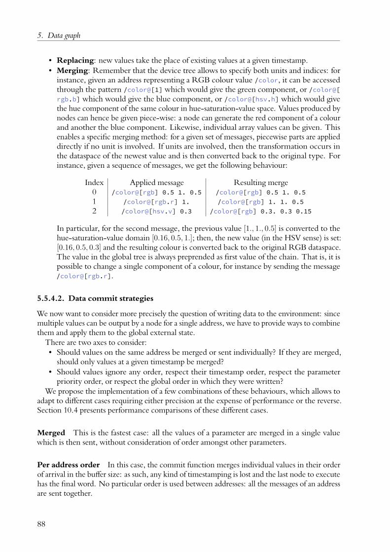
5. Data graph

• Replacing: new values take the place of existing values at a given timestamp.• Merging: Remember that the device tree allows to specify both units and indices: for

instance, given an address representing a RGB colour value /color, it can be accessedthrough the pattern /color@[1] which would give the green component, or /color@[rgb.b] which would give the blue component, or /color@[hsv.h] which would givethe hue component of the same colour in hue-saturation-value space. Values produced bynodes can hence be given piece-wise: a node can generate the red component of a colourand another the blue component. Likewise, individual array values can be given. Thisenables a specific merging method: for a given set of messages, piecewise parts are applieddirectly if no unit is involved. If units are involved, then the transformation occurs inthe dataspace of the newest value and is then converted back to the original type. Forinstance, given a sequence of messages, we get the following behaviour:

Index Applied message Resulting merge0 /color@[rgb] 0.5 1. 0.5 /color@[rgb] 0.5 1. 0.51 /color@[rgb.r] 1. /color@[rgb] 1. 1. 0.52 /color@[hsv.v] 0.3 /color@[rgb] 0.3. 0.3 0.15

In particular, for the second message, the previous value [1., 1., 0.5] is converted to thehue-saturation-value domain [0.16, 0.5, 1.]; then, the new value (in the HSV sense) is set:[0.16, 0.5, 0.3] and the resulting colour is converted back to the original RGB dataspace.The value in the global tree is always preprended as first value of the chain. That is, it ispossible to change a single component of a colour, for instance by sending the message/color@[rgb.r].

5.5.4.2. Data commit strategies

We now want to consider more precisely the question of writing data to the environment: sincemultiple values can be output by a node for a single address, we have to provide ways to combinethem and apply them to the global external state.

There are two axes to consider:• Should values on the same address be merged or sent individually? If they are merged,

should only values at a given timestamp be merged?• Should values ignore any order, respect their timestamp order, respect the parameter

priority order, or respect the global order in which they were written?We propose the implementation of a few combinations of these behaviours, which allows to

adapt to different cases requiring either precision at the expense of performance or the reverse.Section 10.4 presents performance comparisons of these different cases.

Merged This is the fastest case: all the values of a parameter are merged in a single valuewhich is then sent, without consideration of order amongst other parameters.

Per address order In this case, the commit function merges individual values in their orderof arrival in the buffer size: as such, any kind of timestamping is lost and the last node to executehas the final word. No particular order is used between addresses: all the messages of an addressare sent together.

88

5.5. Graph execution

Priority order This case is the same as before, but we additionally leverage the priorityattribute set by the author on specific device tree parameters, and described in Table 10.1: thehighest the priority on a parameter, the soonest a message should be sent. Since the attributesof a parameter are immutable and all parameters are known, the sort can be executed only once.

Global order We want to ensure a possibility to send messages to the global environment inthe exact order in which they were produced by the data graph, to preserve causality, while stillallowing merging to take place. In particular, messages are globally sorted in lexicographicalorder across the pair P = (Tl, Tg) where Tg is the global message index and Tl is the timestampof the message: this ensures that messages are sent first by order of their timestamps, and thenin a first-to-last fashion if there is an ambiguity.

However, it is necessary to be aware that the protocols used underneath message sending,like UDP which is commonly used in OSC protocol implementations, might not always havestrong timing and ordering guarantees.

5.5.5. Overall tick description

Finally, we can give a general graph tick algorithm, which will execute all the enabled nodesduring a root tick.

5.5.5.1. Dynamic case

let graph_tick graph gs e =

(* we mark the nodes which had tokens posted to as enabled *)let gs = disable_strict_nodes (get_enabled_nodes graph gs) gs inlet enabled_nodes = (get_enabled_nodes graph gs) inlet sorted_nodes = topo_sort graph inlet filtered_nodes = List.filter (fun n -> (List.mem n enabled_nodes))sorted_nodes in

(* we have a set of nodes that we now run: *)let (gs, e) = base_tick graph gs filtered_nodes e in

(* once all the nodes are ran, remove their tokens *)(clear_tokens gs, e);;

5.5.5.2. Static case

let graph_tick graph gs e =

(* we mark the nodes which had tokens posted to as enabled *)let gs = disable_strict_nodes (get_enabled_nodes graph gs) gs in

(* we have a set of nodes that we now run: *)let (gs, e) = base_tick_static graph gs e in

(* once all the nodes are ran, remove their tokens *)(clear_tokens gs, e);;

89

5. Data graph

5.6. Closing words

We have presented in this chapter an exploration of the design space of data-flow methodsto cater to interactive score execution. Research that led to the current definition has beenpublished in [34]. The specificity of such scores is that parts of the scores will run at unknowndates: in particular, the order in which media processes run must be assumed to be undefined.There are implications for the execution of unit generators: not all nodes of DFGs defined bythe author will be active at the same time, even though data dependencies may exist. Hence,we introduce two notions: an environment, in which nodes can read and write in addition ofthe usual connections of DFGs, and attributes on connections. These attributes specify thedependencies and temporal relationships between the nodes: strict or relaxed, and immediateor buffered. Various scheduling cases are considered, function of the desired attributes anddynamicity of the system. Finally, we consider different possibilities for the reading and writingof data values, which have implications on the correctness and the performance of the overallsystem. The various possibilities are represented in fig. 5.13 for the sake of clarity.

Without considering the next chapter which introduces temporal semantics on top of thisstructure, the concepts introduced in this chapter can already be useful: in particular, thisexecution model allows to treat indifferently remote and local values from within a program; itmakes trivial the creation of network-aware media applications, such as synthesizers, or videoplayers. Such an example is given in Section 10.1.8.

It is important to note that this chapter is mainly used as support for the following chapters: inparticular, there is no doubt that other execution semantics with relaxed accuracy requirements,for instance with more asynchronous behaviours, would be viable for at least a large panelof media works: future research on this topic should strive to extend the range of data-flowmethods compatible with the execution of interactive scores.

Finally, the various possibilities for the execution are presented as global choices which wouldimpact the whole execution. Further work should be done in order to relax this requirement: forinstance by making specific choices at the node level instead of the graph level, and potentiallygrouping nodes in sets of shared behaviours.

90

5.6. Closing words

Static Dynamic

None BFS TC

Creation XY YX Temporal

Append Replace Merge

Default Merged Ordered Priorized

METHOD

SCHEDULE

ORDER

MERGE

COMMIT

Figure 5.13.: Overall design and possible steps of the data execution engine: first the generalexecution method must be chosen, then schedule can be setup using breadth-firstsearch or transitive closure for the static case; in addition, the dynamic algorithmcan use the temporal execution order since it is known only at run-time. Finally,the methods used to write to nodes and to the local environment, and the finalcommit to the global environment are chosen.

91

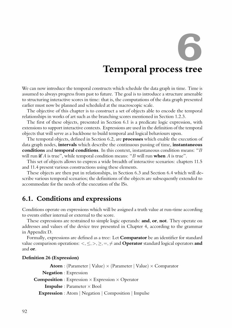
6Temporal process tree

We can now introduce the temporal constructs which schedule the data graph in time. Time isassumed to always progress from past to future. The goal is to introduce a structure amenableto structuring interactive scores in time: that is, the computations of the data graph presentedearlier must now be planned and scheduled at the macroscopic scale.

The objective of this chapter is to construct a set of objects able to encode the temporalrelationships in works of art such as the branching scores mentioned in Section 1.2.3.

The first of these objects, presented in Section 6.1 is a predicate logic expression, withextensions to support interactive contexts. Expressions are used in the definition of the temporalobjects that will serve as a backbone to build temporal and logical behaviours upon.

The temporal objects, defined in Section 6.2, are processes which enable the execution ofdata graph nodes, intervals which describe the continuous passing of time, instantaneousconditions and temporal conditions. In this context, instantaneous condition means: “Bwill run if A is true”, while temporal condition means: “B will run when A is true”.

This set of objects allows to express a wide breadth of interactive scenarios: chapters 11.5and 11.4 present various constructions using these elements.

These objects are then put in relationships, in Section 6.3 and Section 6.4 which will de-scribe various temporal scenarios; the definitions of the objects are subsequently extended toaccommodate for the needs of the execution of the ISs.

6.1. Conditions and expressions

Conditions operate on expressions which will be assigned a truth value at run-time accordingto events either internal or external to the score.

These expressions are restrained to simple logic operands: and, or, not. They operate onaddresses and values of the device tree presented in Chapter 4, according to the grammarin Appendix D.

Formally, expressions are defined as a tree: Let Comparator be an identifier for standardvalue comparison operations: <,≤, >,≥,=, ̸= and Operator standard logical operators andand or.

Definition 26 (Expression)

Atom : (Parameter | Value)× (Parameter | Value)×ComparatorNegation : Expression

Composition : Expression× Expression×OperatorImpulse : Parameter× Bool

Expression : Atom | Negation | Composition | Impulse

92

6.1. Conditions and expressions

Two operations are defined on expressions and the data types that compose them:• update : Expression×Environment→ Expression. Used to reset any internal state and

query up-to-date values for the expressions. For instance, update on an Atom fetches ifpossible new values for the parameters from the global environment.Precisely:⎧⎪⎪⎪⎪⎪⎪⎪⎪⎪⎪⎪⎪⎪⎪⎪⎪⎪⎪⎨⎪⎪⎪⎪⎪⎪⎪⎪⎪⎪⎪⎪⎪⎪⎪⎪⎪⎪⎩

update : Composition→ Composition(e1, e2, o) ↦→ (update e1,update e2, o)

update : Negation→ Negatione1 ↦→ update e1

update : Atom→ Atom⎧⎪⎨⎪⎩(parameter p1, parameter p2, o) ↦→ (pull p1, pull p2, o)(parameter p1, value v2, o) ↦→ (pull p1, v2, o). . .

update : Impulse→ Impulse(p, b) ↦→ (p, false)

• evaluate : Expression → Bool. Performs the actual logical expression evaluation, ac-cording to the expected logical rules.

• An atom is a comparison between two parameters, a parameter and a value, or two values.• Negations and compositions are the traditional predicate logic building blocks.• A specific operator, “impulse”, is introduced: it allows to decide whether a value was

received.Appendix D gives the complete grammar for expressions. For instance, checks on the arrival

of a specific network message, or checks on a remote or local address’s value with a specificexpression, can be expressed with the following syntax:

• For parameters that can have a value, there can be comparisons between the values. Forinstance:

{ dev:/some/parameter > 35 } && {{ dev:/other/parameter != "a string" } ||{ dev:/last/parameter == true }

}

• Parameters can be compared between themselves:

dev:/some/parameter > other:/another

• Value-less parameters (akin to bangs in Pure Data) can also be used as triggers for theevaluation of expressions. In this mode, logical operators have a different meaning. Forinstance:

impulse( /some/bang ) && !impulse( /another/bang )

will trigger if:– /some/bang is received, and– /another/bang is not received within the synchronisation interval.

93

6. Temporal process tree

• This is not to be confused with the comparison with boolean values:

{ /a/val == true } && { /another/val == false }

which will trigger when the parameters will both be set (not necessarily at the same time)to the required values.

6.2. Temporal objects

Existing work on interactive scores makes apparent the need for two kinds of conditionalstructures:

• Temporal conditions: the author must be able to write “When a condition becomestrue, then something happens”. It is equivalent to saying “Something happens until acondition becomes true” (and different from the when construct in the reactive languageLustre which does sample a signal every time a condition is true.).

• Logical conditions: the author must be able to write “If a condition becomes true, thensomething happens”.

The first case can easily be unbounded and allow infinite processes to occur, by using always-false conditions.

In our case, a happening is defined as a temporal execution step of a musical, artistic, or moregenerally computational process. That is, the playback of a part of a sound file can be a happening,just like the emission of a single network message.

These structures are meshed together with temporal intervals. Execution of artistic processeshappen during the execution of such intervals.

6.2.1. Processes

Processes are the principal link with unit generators in the temporal tree, and the main exten-sion point of the temporal tree. Some processes are built-in: in particular, the layouts of objectsdescribed in this chapter are themselves processes. This enables nesting of temporal objectsin a simple manner. The general function of processes will be to add token requests to nodesof the data graph, and to execute temporal behaviours. procId identifies the process uniquely.nodeId refers to a data graph node. impl holds data relevant to the specific implementation of agiven process. start, stop, tick are three functions which define the execution of a process:in particular, tick will advance the time inside this process and return a function which will beapplied to the data graph state.

The relationship with the data graph will be explained more in detail in the following chapter.For now we simply give the following definition:

Definition 27 (Process)

type processImpl =Scenario of scenario | Loop of loop | DefaultProcess

;;type processId = int;;type process = {

94

6.2. Temporal objects

procId: processId;procNode: nodeId;impl: processImpl;start: process -> score_state -> score_state;stop: process -> score_state -> score_state;tick: process -> duration -> duration -> position -> duration ->score_state

-> ((graph_state -> graph_state) * score_state)};;

6.2.2. Interval

Intervals express the passing of time, for a given duration. This duration may or may not befinite; it may also vary between different executions of a score.

A duration is defined as a strictly positive integer. An interval is at its core a set of durations:a min, an optional max, a default duration and the current position, part of the score_statestructure which will be presented thereafter. A similar set of durations have been proposed inthe elastic time model proposed by Sung [53]: a min, a max, and a length at rest called by theauthors “most desirable play length”. The lack of max means infinity; conversely, an interval issaid to be fixed when its min equals its max.

The interval is defined as:

Definition 28 (Interval)

type interval = {itvId: intervalId;itvNode: nodeId;minDuration: duration;maxDuration: duration option;nominalDuration: duration;processes: process list

};;

An interval is uniquely identified across the score with itvId, and is associated to a data graphnode with itvNode.

For the sake of clarity, two hierarchical notions are defined:

Definition 29 (Parent interval)A process admits a unique parent interval which is the interval carrying it in its process list.

Definition 30 (Parent process)An interval admits at most a unique parent process.

Position of the execution in processes is defined as current datenominal duration ; their date is the same as their

parent interval date. In Section 8.1, this allows to provide a simple mapping between the visualposition of execution and the actual computation taking place.

95

6. Temporal process tree

6.2.3. Instantaneous condition

Instantaneous conditions (ICs) serve to enable or disable intervals according to an expression,given in the expression language seen in Section 6.1. They are defined as follows:

Definition 31 (Instantaneous condition)

type condition = {icId: instCondId;condExpr: expression;previousItv: intervalId list;nextItv: intervalId list;

}

ICs are preceded and followed by intervals (previousItv, nextItv).In addition, IC are associated with a running status which will change during the execution:

Definition 32 (Execution status)

type status = Waiting | Pending | Happened | Disposed;;

ICs are disabled, or disposed, either when they are false or when they are preceded by anon-null number of intervals, all of them already disabled through other conditions. This willpropagate to the following intervals and conditions: entire branches of the score can be disabled.

They can be linked in literature to concepts such as Hirzalla’s branching choices [52]: howeverin our case we allow multiple concurrent choices to execute at the same time, which enables aneasy way to control and limit concurrent processes.

6.2.4. Temporal conditions

Temporal conditions (TCs) are used to synchronise starts and ends of intervals, while allowingimplementation of behaviours such as: “start part B when the fader is at 0”. Each TC carriesa condition of execution. The default condition is simply Atom true true (==). They areassociated to a list of ICs.

Definition 33 (Temporal condition)

type temporalCondition = {tcId: tempCondId;syncExpr: expression;conds: condition list

}

6.3. Temporal graph: scenario

Consider a DAG whose vertices are instantaneous conditions and edges are intervals, S = (I, C).Such DAG, associated with a specific execution semantic, is called a scenario.

Scenarios allow to organize the temporal elements in time. They follow these basic rules:

96

6.3. Temporal graph: scenario

• A scenario begins with a TC.• There can be multiple interval explicitly synchronised by a single TC.• An interval is always started by an IC and finished by another, distinct IC.• The direction of execution follows the flow of time, starting from the first TC.During the authoring step, these rules, as well as acyclicity of the scenario graph, are enforced

thanks to the visual syntax presented later, in Section 8.1.ICs and intervals are chained sequentially. Multiple intervals can span from a single IC and

finish on a single IC, as shown in fig. 8.4. This allows different processes to start and/or stop ina synchronised manner.

Definition 34 (Scenario)

type scenario = {intervals: interval list;triggers: temporalCondition list;

};;

We introduce a type which will keep the variable part of a temporal tree: the current durationof each interval, the status of each condition.

Definition 35 (Temporal graph state)

type score_state = {itv_dates: (intervalId * duration) list;ic_statuses: (instCondId * status) list;rootTCs: (processId * tempCondId list) list;scoreEnv: environment};;

6.3.1. Execution of scenarios

The central point in the execution of scenarios is the execution of the temporal conditions.The overall progression of the execution algorithm is as follows:1. Check for any root of the scenario that may start; try to process them.2. Increase the date of every running time interval up to their max (if any), in the capacity

allowed by the remaining time in the tick.3. Check for finished temporal conditions, process them, and potentially propagate remain-

ing parts of the tick to following time intervals.4. Return to step 2. as long as any time interval can execute.Finally, note that scenarios themselves are processes: this allows a simple implementation

of hierarchy in the temporal tree since processes are nested in intervals, themselves parts ofscenarios.

6.3.2. Execution of a temporal condition

First, let us define the following concepts for instantaneous conditions:

97

6. Temporal process tree

Definition 36 (Execution area) An instantaneous condition I is said to be in its execution area if forall previous non-disabled time intervals of I, the date of the interval is in the range defined by the min andmax durations of the interval. If I does not have previous intervals, it is always in its execution area.

A temporal condition T is said to be in its execution area if all its associated instantaneous conditions arein their execution area.

ICs can be in different states:• Waiting: the execution area has not been reached yet.• Pending: the execution area has been reached.• Happened: has been executed successfully.• Disposed: has not been executed due to a false condition.The effective range of time for the execution of ICs and TCs is only known until run-time:

even though min and max durations themselves cannot vary, the start date of an interval can varysince it may follow an already interactive TC. For the TC to enter its execution range, all theintervals that finish on the ICs in the TC must lie between their minimal and maximal duration.The evaluation of a TC’s expression is performed at each tick, as soon as all instantaneousconditions are pending.

IC are evaluated by TCs when their parent TC is triggered. The triggering of a TC canoccur in two ways: either when its expression becomes true, or when any previous non-disabledinterval reaches its max duration.

A IC is executed when its expression evaluates to true upon evaluation. Executing an ICmeans checking its expression.

• If it is true: the previous intervals are stopped, the next intervals are started, and it ismarked as happened.

• Else, the previous intervals are stopped, and it is marked as disposed.Branching occurs when, at a single point in the score, multiple intervals follow a TC. In

particular, if the intervals are on distinct ICs, different executions can happen according to theexpression evaluation, which leads the scenario to distinct states. For example, the classic if- then - else construct can be implemented by having two ICs with opposite conditions – anexample in the visual language is given in Section 11.4.2.1. It is also possible to consider othercases: for instance, there could be a set of conditions that would lead to either both interval, orno interval executed. Multiple intervals can follow from a same single condition.

Convergence occurs when parts of a scenario that previously branched are synchronised.

6.3.2.1. A special case for interactivity

We separate two cases: interactive and fixed.• A TC is said to be fixed when its expression equals the default expression, which evaluates

to true.• A TC is said to be interactive case when any other expression is used.

During the execution of an interactive TC, a delay of one tick is introduced if its execution is notdue to a max bound being reached. This is to prevent automatic triggering of a whole sequenceof TCs which would share the same expression, which was a pattern used by authors whencreating scores with the model. The reasoning is that for authors, a TC embodies the notionof interaction. Such interactions generally occur at human time scales, such as triggering asensor or pressing a button. Having multiple subsequent parts of the score trigger due to a singleinteraction then does not map to the physical reality of the score’s surrounding environment.

98

6.3. Temporal graph: scenario

6.3.3. Execution of a single interval

Algorithm 5 Executing intervals.

let scenario_run_intervalscenario overticks tick offset interval (state:score_state) =

let end_TC = find_end_TC interval scenario inlet interval_date = (List.assoc interval.itvId state.itv_dates) in

match interval.maxDuration with(* if there is no max, we can go to the whole length of the tick *)| None -> (tick_interval interval tick offset state, overticks)

(* if there is a max, we have to stop at the max and save the remainings*)| Some maxdur ->

let actual_tick = min tick (maxdur - interval_date) inlet tick_res = tick_interval interval actual_tick offset state inlet overtick = tick - (maxdur - interval_date) in

(* find if there was already over-ticks recorded for this TC, and if so, update them *)

match List.assoc_opt end_TC.tcId overticks with| None -> (tick_res, (end_TC.tcId, (overtick, overtick))::overticks)| Some (min_ot, max_ot) ->

let new_overtick = (min overtick min_ot, max overtick max_ot) in(tick_res, list_assoc_replace overticks end_TC.tcId new_overtick)

Algorithm 5 presents the execution of a given interval. tick_interval exposes the relation-ship between the temporal and the data graph; it will be presented on the following chapter.Algorithm 6 presents the starting of an interval: tokens are requested when they start in orderto allow the data node to perform an initialization routine if necessary, or to send a message onstart.

6.3.4. General execution algorithm

The complete execution algorithm is given in Appendix A; an overview follows. The algorithmworks by propagating the time across the intervals, and keeping in memory for each interval ofhow much it goes past its max duration. Then, at every TC, we devise of how much the timemust go forward past it. If there is a single interval before the TC, this amount is simply theduration that went past the max bound of the interval.

When there are multiple interval, there are possibilities of conflict: one interval may onlygo past two time units after the TC, while another might go ten time units past the TC. Inaccordance with the liveness principle discussed earlier, we choose to advance the time of themaximal duration recorded that goes past an individual TC. This allows branches withoutinteractivity (that is, whose TCs and ICs have default true conditions) to execute at the expectedrate. Consider the scenario which consists of: a starting IC, followed by two “branches” ofintervals. The first (top) branch consists of a sequence of N intervals Ti with minimal durationTmin and maximal duration Tmax. The second (bottom) branch consists of a sequence of Nintervals Bi with minimal duration and maximal duration equal to Bnom where Tmin < Bnom <

99

6. Temporal process tree

Algorithm 6 Starting intervals.

let start_interval itv (state:score_state) =let rec start_processes procs funs (state:score_state) =match procs with| [] -> (funs, (state:score_state))| proc::t -> let (state, nf) = start_process proc state in

start_processes t (funs@[nf]) statein

let (funs, state) = start_processes itv.processes [] state in({ state with itv_dates = list_assoc_replace state.itv_dates itv.itvId 0 },(funs @ [ add_tick_to_node itv.itvNode (make_token 0 0. 0) ])

);;

Tmax. For each index i, the intervals Ti and Bi share the same start and end TC. The TCexpressions for all but the starting one are set to false: they will only trigger whenever a max isreached. If after each TC, the time was advanced by any duration smaller than the max, thenexecuting a tick of a duration of N ∗Bnom would not be enough to reach the end of BN , thus atleast a maximal constraint of a Bi would be broken.

The execution begins by checking for waiting TCs: in particular, the root of the scenariomust be checked in the case where it waits for an event to happen before starting the execution1.If the TC executes and has happened, then for ICs whose expressions evaluated to true, if theyare followed by intervals, these intervals are started (Algorithm 6) and put in the running set inthe scenario execution state. Then, for every running interval in the execution state, the wholeduration of the requested tick duration is applied, according to the algorithm in Algorithm 5. Ifthe duration is greater than what the interval can accept, the remaining part is added to a setwhich associates it to the TC at the end of the interval.

The execution then consists in a loop: as long as there are remaining time units to consumein the over-tick set, they are applied to the following intervals. We have two cases to consider:

• The interval has a fixed duration: either the remaining time units are smaller or equal thanthe remaining duration for this interval, and all the remaining time units are consumedfor this branch, or the remaining time units are greater than the remaining duration forthis interval, and smaller time units are inserted in the set.

• The interval has an infinite duration: all the remaining time units in this branch areconsumed and no time units are inserted in the set.

Since the maximum time unit requested is strictly decreasing in time, the execution loopeventually terminates.

6.4. Loop

The first idea for loops would be to create a cycle in the scenario graph presented earlier.However, acyclicity of this graph is a desirable property: this allows to keep the complexity ofgraph traversal operations used lower, which matters in a real-time execution context.

1In the implementation, this has been extended to work for an arbitrary number of root TCs: this allows tobuild the score from many interactively triggered sub-scores easily, but will not be covered here.

100

6.5. Conclusion

6.4.1. Definition

The loop is modeled as its own process with simpler semantics than the scenario’s: a singleinterval will loop. Since intervals can contain other processes, we can still encounter complexmusical behaviour in it: whole scenarios and furthermore any hierarchic construction can loop.

Definition 37 (Loop)

type loop = {pattern: interval;startTC: temporalCondition;endTC: temporalCondition;

};;

At each tick of the loop, the interval is itself executed. If either of the temporal conditionsis interactive, we follow the same process than for the scenario: we wait until the next tick toperform the triggering instead of doing it immediately. Else, further tokens are added to theinterval and its child processes, starting from zero. An example of this process is given in fig. 7.5.

Null loop pattern durations are prevented since the duration of intervals is non-null: else,any tick operation would cause an infinite loop since there would never be any progression inthe loop.

Whenever the first IC is disposed, or the second IC is either happened or disposed, the statusof events and intervals is reset and execution stops for this process. This means in particular thata loop whose first IC’s expression evaluates to false is re-checked the next time the process runs.

6.4.2. Execution algorithm

The execution algorithm for the loop is separated in two cases: the first is the case of a loop withno interactive behaviour. That is, the temporal and instantaneous condition at the beginningand the end of the loop have only trivial true expressions. In this case, the algorithm given inAnnex B.1 is used: we can reach a sample-accurate looping of the datas in the interval.

In the other case, a more general algorithm which checks the conditions and interactions isused, given in Annex B.2. In this case, the technique of delaying by one tick is also used.

This separation is also done for efficiency concerns: checking conditions has a small but non-negligible cost, and we want the loop to be able to function at very high rates, up to looping onlya few samples of audio data. Hence, the common fast path of no conditions is more optimized.

6.5. Conclusion

We provide in this chapter a structural definition of temporal relationships in interactive scores.The current definition has been reached after multiple evolution steps, showcased in [28, 32,33]. That is, scores are represented as graphs of objects. Time can be thought of as flowingthrough the edges at a rate imposed hierarchically, the root rate being imposed by the durationof the root tick. Edges of this graph decide of the execution of the following parts according to

101

6. Temporal process tree

instantaneous conditions. Multiple edges can be synchronised with temporal conditions. Theseconditions are triggered whenever a boolean expression becomes true. Two particular layoutsare considered: the scenario, which is a general structure allowing to represent various temporalrelationships between objects, and the loop, which is a fixed structure which allows a part of ascore to repeat itself in time.

102

7Combining temporal tree and data

graph

This chapter presents the relationship between the temporal and data graph presented earlier.The system consisting in these two graphs and the relation is the model which is proposed to beused by authors.

In order to simplify interaction with and usage of the model, the number of objects withwhich the author creates the score is limited: this is presented in Section 7.1. A contribution isdeduced in Section 7.2 from this limitation: the model can be used as a hierarchical mixingenvironment with simple set-up steps.

Then, the overall execution algorithm tying both graphs and the external environment ispresented in Section 7.4. Finally, Section 7.5 presents some applied examples of simple programsbased on the model.

7.1. Relationships between temporal process tree anddata graph

Specific objects of the temporal tree are associated with nodes of the data graph. Duringthe execution, as a first step, objects of the temporal tree will add token requests (definedin Definition 15) to nodes of the data graph, according to their current state and date. Multipleobjects of the temporal tree relate to data graph nodes:

• Every time process is associated to a data node.• Every interval is associated to a data node. Some optimization opportunities exist, if the

interval does not carry any time processes and is not connected to any object.In particular, we consider two structural objects:• The forwarding data node, defined as the node which copies data from its input ports to

its output ports untouched.• The default time process, which adds a token request to the data node it is associated with

in its execution function.The forwarding data node is used in intervals, in the scenario process and in the loop process.The default time process is used for most processes: it merely adds a token request to the

matching data node, at the requested time. This will have the effect of enabling the data nodeand having it run for the second part of the execution tick; most audio filters or generatorsfor instance do not need any particular processing besides this. Likewise, if an interval is notrunning, either because it did not start yet or already stopped, its data node as well as the datanode of its processes will be disabled and will not take part in data production for this tick.

104

7.2. Hierarchical audio mixing

In the model, the elements of the temporal tree will return a list of functions when exe-cuted, each of the form graph_state -> graph_state. The main function used at this step isadd_tick_to_node, which simply appends a token request for a given node in graph_state.Algorithm 7 presents its usage from the function which performs execution of intervals.

Algorithm 7 This function is the main step of the execution of an interval: it advances thetime, computes a token request, and adds ticks to relevant nodes.

let tick_interval (itv:interval) t offset (state:score_state) =let (cur_date:duration) = (get_date itv state.itv_dates) inlet new_date = (cur_date + (truncate (ceil (float t) *. itv.speed))) inlet new_pos = (float new_date /. float itv.nominalDuration) inlet tp = tick_process cur_date new_date new_pos offset inlet rec exec_processes procs funs state =

match procs with| [] -> (funs, state)| proc::t -> let (nf, ns) = tp state proc in

exec_processes t (funs@[nf]) nsin

(* execute all the processes *)let (funs, state) = exec_processes itv.processes [] state in

(* execute the interval itself *)({ state with itv_dates = (set_date itv new_date state.itv_dates) },(funs @ [ add_tick_to_node itv.itvNode (make_token new_date new_pos offset) ]))

;;

7.2. Hierarchical audio mixing

In order to simplify authoring further, optional default connections are introduced betweenelements. As explained in Section 3.3.3.1, an objective of this work is to provide a hierarchicalorganization of the audio flow graph, without requiring excessive manual intervention from thecomposer. Simple cases, such as playing a sound file, should work as effortlessly as possible inorder to respect the Low Threshold, High Ceiling, and Wide Walls principle; yet the author muststill be able to perform more complex mixing operations.

As per definitions 29 and 30, both scenario and loop processes have child intervals, andintervals have child processes. This forms a hierarchy between these two families of objects.

Definition 38 (Root interval)The root of an interactive score is an interval, called root interval.

Audio connections are automatically created in the following cases:• Remember that intervals are associated to a forwarding data node: a relationship is created

between each interval data node audio output port and its parent process’ audio inputport. The forwarding data node is given an audio input and output; these are chainedtowards the root interval .

105

7. Combining temporal tree and data graph

• Between each audio output port of each time process marked with a special propagateattribute, and the audio input port of their parent interval. The audio output of thescenario and the loop is marked with this attribute.

By default, the audio output of the root interval is associated to the address corresponding tothe main output of the sound card in a device representing the sound card. Multiple intervalswith each a sound file process will play together withtout the need to add explicit cables.

This can be done because there is a commonly accepted combination function betweenmultiple signals of audio type: summing them. The sum can then be used in effect buses forinstance, in order to share CPU-consuming effect processing such as reverberation for multiplesound processes. Likewise, for the MIDI data type, it would be meaningful to combine messagestogether in a list. However, for other data types, such as the various network messages, there isno particular way to combine them through a single port, hence this is not done; messages willbe lost if a value outlet has neither address nor outgoing connections.

Relevant audio processes are marked as such by default:• Sound files.• Audio effect and various audio generators.

This is however optional and can be changed in the score for each output port.Fig. 7.1 shows how audio mixing does happen in the tree presented at the end of Section 3.4

interval

scenario

interval I5

effect

interval I4

sound

interval I3interval I2

loop

interval

automation

interval I1

mapping

Figure 7.1.: Hierarchical tree: coloured edges indicate that an automatic connection is createdbetween the associated nodes of the data graph.

7.3. Automatic dependency connections according to thescore process order

It is possible to give an ordering of the nodes of the data graph according to the temporal objects,by creating dependency connections between relevant data nodes. This way, even without anyexplicit data connection, the execution will still happen in a definite order.

The proposed order is:• In an interval, every process’s node depends on the previous one in the order of the list

held by the interval.• In a scenario or a loop, every interval depends on its parent process; no new connection

needs to be introduced there since there is already a data connection.

106

7.4. Main tick algorithm

Env. fetch

Temporal execution

Data execution

Env. commit

Root tick

Externalworld

Audio,OSC,

MIDI, …

Figure 7.2.: Overall execution schema.

• The nodes of the intervals before and after ICs are chained by dependency relationshipsin the temporal order.

This leaves one possible indeterminacy question open: the order of multiple intervals in ascenario. One possibility is to leverage additional static information provided by the author inthe visual language such as the position of objects; the default would just be the object creationorder, since intervals are stored in a list.

7.4. Main tick algorithm

We give in Algorithm 8 the main algorithm which drives the execution of the graphs definedpreviously. The root of a temporal score is by convention a single interval.

The general behaviour is easily described:

1. Retrieve the current data from the external global state.2. Run the temporal tree tick: the time is advanced in the root interval, and recursively in

its child processes. Functions modifying the graph state are gathered and applied: tokenrequests are written in various data nodes.

3. Run the data graph tick, with one of the methods chosen as mentioned in Section 5.6.4. Write the local state to the external global state.

It is represented in fig. 7.2.

7.5. Execution behaviour

In this section, we present more precisely the application of the execution algorithm on explicitdata buffers.

107

7. Combining temporal tree and data graph

Algorithm 8 Example of a main tick algorithm which binds together data graph and temporaltree. The environment provides multiple functions similar to this one, which allow to use thevarious behaviours described in this document by changing the functions used to tick the datagraph nodes.

let main_loop root graph durationgranularity (state:score_state)ext_events ext_modifications =

let total_dur = duration inlet rec main_loop_rec root graph

remaining old_remaining granularity(state:score_state) (gs:graph_state) funs =

if remaining > 0then

(let elapsed = total_dur - remaining inlet old_elapsed = total_dur - old_remaining inlet (root,graph,state) =

ext_modifications root graph state old_elapsed elapsedinlet (state, new_funs) =

tick_interval root granularity 0 stateinlet gs = add_missing graph gs inlet (gs, e) =

tick_graph_topo graph (update_graph (funs@new_funs) gs) state.scoreEnv

inlet state = {

state withscoreEnv =

(update (commit e) ext_events old_elapsed elapsed);listeners =

(update_listeners state.listeners e.local ext_eventsold_elapsed elapsed)

} inmain_loop_rec root graph (remaining - granularity)

old_remaining granularity state gs [])

else(root, graph, state)

inlet (state, funs) = start_interval root state inlet gs = { node_state = []; port_state = [] } inmain_loop_rec root graph duration duration granularity state gs funs

;;

108

7.5. Execution behaviour

7.5.1. Fixed case

We consider the following score, in Fig. 7.3: an automation runs for 13 time units. Concurrently,a sound runs for 7 time units, and is followed by another sound which runs for 8 time units.The root tick duration is five time units. Table 7.1 presents the token requests (Definition 15)put in each data node for successive ticks, under the form (previous date→ current date, offset).

Automation curve

Sound 1 Sound 2

Figure 7.3.: A score. The small bins represent individual audio samples; the bigger bins representthe tick rate of the sound card. For the sake of the example, one can assume that theautomation curve is used to control the output volume of the englobing scenario,not represented here.

Start Tick 1 Tick 2 Tick 3Automation (0→ 0, 0)Sound 1 (0→ 0, 0) (0→ 5, 0) (5→ 7, 0)Sound 2 (0→ 3, 2) (3→ 8, 0)Scenario (0→ 0, 0) (0→ 5, 0) (5→ 10, 0) (10→ 15, 0)

Table 7.1.: Value of token requests for the scenario 7.3.

7.5.2. Interactive case

In this case, we consider a score similar to the previous: however, the time between the twosounds is not fixed and can be interrupted by an external event such as an OSC message. Inthis case, the second sound will only start at the beginning of the next tick, at t = 10, for thereasons explained in Section 6.3.2.1.

Sound 1 Sound 2

An external event happens

Figure 7.4.: A scenario with an interaction.

109

7. Combining temporal tree and data graph

Start Tick 1 Tick 2 Tick 3Sound 1 (0→ 0, 0) (0→ 5, 0) (5→ 10, 0)Sound 2 (0→ 5, 0)Scenario (0→ 0, 0) (0→ 5, 0) (5→ 10, 0) (10→ 15, 0)

Table 7.2.: Value of token requests for the scenario 7.4.

7.5.3. Loop example

This example presents the execution in the case of a non-interactive loop: that is, a loop with afixed duration and no conditions.

Loop

Loop pattern (sound) Repetition

Figure 7.5.: A loop containing a sound.

Start Tick 1 Tick 2 Tick 3Pattern (0→ 0, 0) (0→ 5, 0) (5→ 7, 0), (0→ 3, 2) (3→ 7, 0), (0→ 1, 4)Loop (0→ 0, 0) (0→ 5, 0) (5→ 10, 0) (10→ 15, 0)

Table 7.3.: Value of token requests for the scenario 7.5.

7.5.4. Well-formed score

It is now possible to define completely the central object of this thesis: interactive scores.

Definition 39 (Computational interactive score)A computational interactive score is defined as the combination of:

• An environment E.• A process and interval hierarchy with a root interval: P .• An acyclic data graph: G. A bijective function associates nodes of G to processes and intervals of P .• fSplit which provides an optional resampling of a computation tick.• fOrder which handles the execution order of nodes in case of ambiguity.• fSchedule which schedules the data graph statically or dynamically.• fMerge which combines inputs of data graph nodes.• fCommit which writes the local environment, into the global environment.

110

7.6. Conclusion

7.6. Conclusion

This chapter introduces the relationships between the temporal and data graph: how thetemporal controls will define which computations will be running at each tick. These particularrelationships represent the model with which the author will interact: only one graph-likestructure has to be edited, which in turn produces elements of both the temporal and the datamodel.

Objects of the temporal tree are associated with objects of the data graph: this reduces thenumber of concepts required during the authoring phase in the most common cases. In addition,the system aims to provide a simple implementation of the notion of hierarchical mixing: theprovided method, following research presented in [29], allows to enable this behaviour easily.Section 11.4.1 will in particular present how this facilitates the recreation of common audiosoftware paradigms.

In terms of perspectives, a point important in music environments has not been covered: itsometimes happens in the authoring of interactive scores that one wants a behaviour to last a tadlonger than the actual duration given in the score, because somemusical processes may have somekind of post-end fade-out and would not produce aesthetically pleasant results when stoppeddirectly as would happen right now. While a solution is proposed in Section 11.4.2.7 usingan explicit construction of the elements of the model, we could also consider the propositionof Dannenberg in the Nyquist language [181], where it is possible to declare a post-executionduration directly in musical processes: notes can have “logical stop times” and “termination”;while subsequent processes can begin after the logical stop times, sound keeps being produceduntil termination.

111

Part III.

Leveraging the model

112

This part presents two extensions of the model: the first one, in Chapter 8, is a visual syntaxwhich allows efficient authoring of interactive scores.

The interactive musical score examples discussed in Chapter 1 operate at a macroscopic level:the choices of the performer generally concerns sections, but at the phrase level, these are oftentraditional scores, as can be seen from an excerpt from Klavierstücke XI in fig. 1.4. However, thecase of a single note which would last longer depending on a given condition can also happen.

The main problem is that there is generally no specific symbol to indicate conditional execu-tion; instead, the explanation is part of the description of the musical piece. Hence, we have todevise a graphical notation simple enough and yet able to convey easily these different levels ofconditions.

These conditions operate on a span of time, which can range from instantaneous, like in theStockhausen piece, where the performer has to choose his next phrase at the end of the one heis currently playing, to indeterminate, in the case of a perpetual artistic installation waiting forthe next visitor. A single symbol might then not be enough to convey the whole meaning, andmultiple symbols would be necessary to explain the articulation of the time in the musical piece.

Given the model defined in Part II, it is only natural to map its elements, TC, IC, intervals,to a visual language that will be used by authors for the creation process. A short referenceexample covering all the syntax elements of this language is presented in fig. 7.6. This visuallanguage contains primitives tailored for the authoring of open works discussed earlier andtranslates almost directly to the models exposed previously: some abstractions are introduced,over specific arrangements of objects in our model, to cover common artistic use cases.

We then consider in Chapter 9 the question of distribution of the scores: in particular, whatcan be gained from the execution of such scores in multiple computers. Only the distribution ofthe temporal tree will be covered: data generation is currently considered local to each computer,and media data has to be exchanged explicitly between computers through usual means such asnetwork messages.

We study different cases for the execution of processes: can a same process be run in parallelby different machines, and what can it bring to the author that is not possible to do easily with ascore running on a single computer. Conversely, is it possible to write a single score that wouldenable multiple computers to run different parts: the main use case is for instance to have onemachine run a kind of media such as video, and another a different kind of media, such as audio,while keeping the objects synchronised.

We also consider the different kinds of synchronisation between computers during thetemporality of a score: how can multiple distinct computers synchronise and desynchronise atdifferent points of the score, as to provide each a different interpretation of this part, just likemultiple musicians will perform the same part in different ways.

The questions raised in the context of open works must be re-evaluated: for instance, whatdoes it mean for a score to be branching, if multiple instances of this score take different branchesat a single point in time.

In practice, this chapter introduces distribution annotations that are explicitly added by thecomposer on some parts of the score, and a notion of machine group, which abstracts overindividual computers and allows the composer to author his work without requiring all thecomputers of the score to be connected. A translation of these annotations into the primitivesof the temporal model introduced earlier is given.

113

Direction of the flow of time

Trigger

State

Condition

Time Sync (TC)

Temporal interval

A

B

C

D

E

F

H

G

Figure 7.6.: Showcase of the proposed temporal syntax. A full horizontal line means that thetime must not be interrupted, while a dashed horizontal line means that the time ofthe interval can be interrupted to continue to the next part of the score accordingto an external event. Execution occurs as follows: the interval A runs for a fixedduration. When it ends, an IC is evaluated: if it is false, the branch which containsB will not run. Else, after some time, the flow of time in B reaches a flexible areacentered on an interaction point, also called a TC. If an interaction happens, Bstops and D starts. If there is none, D starts when the max bound of B is reachedby the flow of time in B. Just like after A, an instantaneous condition will makeG execute or not execute. In all cases, C started executing after A. C expects aninteraction, without time-outs. If the interaction happens, the two instantaneousconditions which follow C are evaluated: the truth value of each will decide of theexecution of E and F .

114

8Interaction language

8.1. A visual language

This chapter presents the mapping from the temporal and data graph objects to the visuallanguage that will serve as a main gateway to authoring scores with the model: this is thecentral part of the ossia score software. The visual language closely follows the fused modeldescribed in Chapter 7: items and entities of the visual language are arranged in a similar graph-like fashion and map and even directly to the model objects. It is mainly the result of a collegialdecision process, involving multiple iterations with users and contributors to the software.

The main focus of the visual language is on the temporal design aspect. Structures andelements used by the interactive score author are those of the temporal tree in Chapter 6:intervals, processes, etc.

We will first present these elements, and then describe the rules used by the authoringinterface to allow for an efficient compositional process.

8.1.1. General considerations

The set of graphical elements presented here are called the Ossia graphical formalism, in referenceto the research project in which they were devised.

Data-flow features only appear at a small scale: it is possible to draw connections betweenoutputs and inputs of processes, and give addresses to ports.

8.1.1.1. Introduction of the state

A new element is introduced, which abstracts a specific case of the model: the state1. A state isthe score element used to model a punctual element in time: for instance, the onset of a note. Itcorresponds to an interval of duration 1: in the visual model in particular it is represented as adot. Like intervals, states can carry processes; in addition, specific edition features are providedto simplify a common authoring task: sending a message or a set of messages at a single point intime. However, due to ergonomic reasons, processes in states cannot be connected to othersthrough cables and have to use addresses: representing the ports for each state in the interfacewould introduce too much visual complexity. For instance, the Nebula score provided by anassociate artist, Pascal Baltazar, contains 365 states over the course of a 27-minutes score. Thisscore will be discussed in more details in Section 11.5.2.

1In the visual model, an object which represents a set of instantaneous actions to be executed by the score at agiven point in time..

116

8.1. A visual language

8.1.1.2. Relationships between elements of the visual model

In the visual model, the temporal tree has a specificity with regards to the version describedearlier: instead of a chaining of IC and interval, the visual chaining is done between IC, states,and interval. That is, every interval is preceded and followed by exactly a single state; the ICholds a list of such states. When translating the visual model to the execution model, states areput in parallel with their following visual interval.

Finally, remember that Chapter 7 introduced a possibility of automatic dependency connec-tion between objects. If these automatic dependencies are used, in addition, previous intervalswill have a connection from their start state and to their end state. This way, in a tick, theprevious state is always executed before and the following state is always executed after in thedata graph: this allows to preserve a coherent intra-tick ordering between objects since thisguarantees that the states’ processes will produce data before the interval starts, while enforcingthat this data pertains to the same time units.

States have an impact on the loop model. Instead of a single interval being looped, there arenow three: the main interval, one that runs for one time unit at the beginning, and one thatruns for one time unit at the end. The visual language restricts states to non-audio processes:only messages can be sent. It is then possible to consider states as punctual objects, for whichthe values produced are messages without duration, and which are executed just before the firstlogical time unit (or just after the end of the last time unit of the main interval).

In certain cases, the splitting of the tick in sub-ticks exposed in Section 5.5.2 is necessaryto have correct execution semantics: given a loop beginning and ending with states Sb andSe, and an interval I, if the duration of the interval is smaller than the root tick duration, andthere is no interaction, the basic algorithm would mean that the states would execute beforethe interval multiple times. Given a root tick duration of N time units, and the duration TI

for I, the nodes would execute in the following order: NTI× Sb;

NTI× I; N

TI× Se, instead of the

expected NTI× (Sb; I;Se) where x; y means that x executes before y and x × y means that y

executes x times.TC and IC are represented in different ways according to the condition they carry: in

particular, the default case of a true condition is made less explicit in comparison to the casewhere an expression has been given by the composer.

8.1.1.3. Scratch space

The visual model allows for sub-scores not tied to the root score: they can serve as a scratchspace, which is an often discussed property of creative authoring environments. The importanceof such scratch spaces in creative endeavours has been studied for instance by Karlesky in [182]in the context of tangible interaction, and at a large visual scale with two projectors, one usingas a scratch buffer in [183]. Especially relevant to the work is the use of a sandbox, a similarconcept to the scratch space, in the DEMAIS system [153] for multimedia authoring.

In the present case, we choose to not dissociate the scratch space from the working space:what defines the appartenance of an object to the scratch part is whether it is connected to theroot of the scenario graph or not. In particular, this makes the central design area a free designspace where ideas can be “doodled” in some part and easily introduced and removed from thescore, for instance for testing different behaviours during execution.

117

8. Interaction language

Figure 8.1.: A screenshot of the previous graphical model of i-score, in the 0.2 version.

8.1.1.4. Differences with previous instalments of score

In contrast with the previous approach, implemented in the software i-score 0.2 (fig. 8.1), notethat by virtue of sharing a close proximity with the model presented earlier, the visual modelends up being simplified: in particular, it is now possible to have processes which exactly followeach other, in a sample-accurate way. Previous versions worked by separating boxes whichcontained processes (mainly automation curves) by constraints instead.

8.1.1.5. Graphical elements

We can now consider the various elements that constitute the visual syntax of scores writtenin the model. Part of the iconography, the general design, and colours were provided byprofessional designers of Blue Yeti. They were discussed and reworked in a feedback loop withartists and users of the software.

An important point is to enable the notation to be used easily on physical medium such aspen and paper, to improve the creative design process. As such, shapes are restricted to simplelines, dots, and very few special symbols.

This is also one of the points noted as part of the research project of the Music NotationModernization Association and its follow up, the Music Notation Project1.

Scenario vertices: temporal and instantaneous conditions Both TC and IC are verticalline: an IC spans at most a TC vertically. A state is a dot on an IC. If there is a condition otherthan the default on the TC, a small arrow in T -shape indicates it. This case is named a trigger2

in the software. TCs themselves are named time syncs.If there is a condition other than the default on the IC, or the user has explicitly modified it, a

surrounding C indicates it. This case is named a condition3 in the visual syntax; ICs themselvesare named events.

These elements are presented in fig. 8.2.

1http://musicnotation.org/systems/criteria/2In the visual model, an object which represents a temporal condition with an active expression.3In the visual model, an object which represents an instantaneous condition with an active expression.

118

8.1. A visual language

(a) A single, empty state. The IC and TC arenot shown since they are behind: they arescaled to the height of states on it.

(b) A single state which contains data: processesor messages.

(c) The vertical elements of the modelrepresented in the software. TCare represented by a gray dash; theTC goes from the bottom to thetop of the vertical element, but hasthe lowest z-position. The IC arerepresented in white and states areon top. The yellow T -like arrowindicates that this interaction pointhas a non-default expression. Like-wise, the bottommost IC has anexpression.

Figure 8.2.: Elements of the visual syntax related to the notion of instant.

Scenario edges: intervals The interval is an horizontal line that represents a span of time,like a timeline. If the interval is flexible, the flexible part is indicated by dashes. When there isno maximum to the interval, the dashes end at the nominal duration of the interval; else they goup to the max duration. The graphical representation of an interval can change according to itsminimum and maximum duration. In the user interface, the duration is directly proportionalto the horizontal size.

Intervals are presented in fig. 8.3.

8.1.1.6. General example

Figure 8.4 presents the different branching and converging cases that may occur, all mixed in asingle TC.

Processes and hierarchy As could be seen earlier, intervals can contain processes: theseprocesses are shown under each interval, in what we call racks and slots. Fig. 8.5 show the visualdepiction of common processes. Fig. 8.6 shows in addition how an interval can synchronisemultiple processes.

8.1.2. Complete processes

Some processes use the standard graphical representation associated to their effect: for instance,a waveform for soundfiles, a curve for automations. The two special processes are the scenarioand loop: both are layouts of the elements of the graphical language. The scenario, in 8.7a is adynamic layout: elements can be added, moved, and removed by the composer, for instanceby double-click, drag-and-drop, etc. The loop 8.7b is a static layout: new objects cannot becreated. The only interaction possible is changing the duration of the loop pattern, which existsas soon as the loop process is created.

119

8. Interaction language

(a) An empty interval of fixed duration.(b) An interval with a min and no max.

(c) An interval with a max and no min. (d) An interval with a min and a max.

(e) A graphic widget which allows to set specific du-rations for an interval.

Figure 8.3.: Intervals, related to the notion of duration. Note that the handles can be dragged,and appear and disappear dynamically if they are needed. Precise durations can beset in a visual inspector.

Figure 8.4.: A TC which exhibits various synchronisation behaviours and possibilities. Thereare two synchronised IC. Two intervals converge on the top one; the second hasa max duration. If both A and B were disabled due to previous conditions, thenC would be disabled, too. Likewise, had D been disabled, E and F would notrun. In this case, the min and max are not necessarily coherent: in practice, theevaluation period of the expression will start at the latest min bound, that is, its ofB. If the expression of the TC never becomes true, and since both B and D havemax bounds, then the execution is guaranteed to continue.

120

8.1. A visual language

(a) An automation process in an interval.

(b) A MIDI process: a piano roll.

Figure 8.5.: Various processes. Note the different port colours for various data types: green fornormal values, red for audio and purple for MIDI.

Figure 8.6.: Multiple slots under a process, each resizeable.

121

8. Interaction language

(a) A scenario process in an interval.

(b) A loop: the loop pattern contains a step se-quencer process.

Figure 8.7.: Organizational processes.

Figure 8.8.: A generator’s output is connected to a mapping’s input.

During execution, processes will execute for exactly as long as their parent interval, as wecould see before. However, note that the user interface captures presented only shows the partof the process that goes to the default duration of the intervals: what happens if for instance aninterval has an infinite duration ? Thanks to the nesting capabilities, it is possible to visualize aninterval in what is called the “full-view” mode, by opposition to the “small-view” shown here.In full-view, it is possible to edit past the default duration of intervals; remember that in termsof position, the beginning will have position 0, and the default duration will have position 1;everything past this will just have position greater than 1 in the token requests.

Note in particular that the blank canvas in which authoring starts when a new document iscreated simply consists of a root interval loaded with a scenario process. This interval is shownin full-view.

122

8.2. Editing

Figure 8.9.: Adding a process to an interval: when an interval is selected, a small “+” is shownon top, which indicates to the user that he can add an element. Clicking on it showsa popup allowing to add new processes.

8.1.3. Data connections

The data connections between objects are represented in a common way in interactive artenvironments: with explicit ports and cables. The colour of a port determine its supportedtypes. The visual language currently supports three kinds of ports: green for value data, red foraudio data, and purple for MIDI data; connections are likewise coloured. An example is givenin Fig. 8.8. Note that in contrast with patcher software where the ports are always located inspecific places (such as the top and bottom of nodes), here more freedom is allowed: ports areobjects that can be leveraged by each process’s graphical implementation. For instance, controlprocesses with parameters accessible on-screen have their ports displayed next to each parameter.This allows to adapt the ports layout with each process user interface, akin to traditional modularsynthesizers.

8.2. Editing

Editing in the visual interface works by using the Command pattern: actions from the user aretransformed into command objects which are put in an undo-redo queue and executed.

In all cases, various checks are put in place at the presentation layer to ensure that invalidscores cannot be written: for instance, it should not be possible to create negative durationintervals or render them negative through a displacement1, to ensure that the scenario graphstays acyclic. Some of the commands available and relevant to the authoring of scores follows.

8.2.1. Creation operations

There are three main categories of creational operations:• Creation of elements of the temporal tree.• Creation of processes in intervals (fig. 8.9).• Creation of connection between ports, and setting addresses to ports.

The second and third elements are trivial: creating a connection only consists in dragging anddropping from one port to another. Likewise, addresses can be input manually set in portsthrough text fields, or dropped from other parts of the software. Creating processes can be donethrough standard user interface interaction means: dialogs, pop-up menu…

1A current unsolved bug in the implementation can cause negative intervals to appear; however, the offendingelements are visibly marked as invalid.

123

8. Interaction language

More interesting are the object creations in the temporal tree. Three main interactions arepossible:

• Double-clicking on the background of a scenario creates a set of {state, event, time sync}.The state is on the event, and the event on the time sync.

• Drag-and-drop operations. As an example, dragging a sound file or a MIDI file fromother software creates structures that consists in:

– An interval started and stopped by two sets of {state, event, time sync }.– Relevant processes in this interval: sound file process, MIDI process, etc.

• Dragging from a state to another instantaneous element in order to create a synchronisation,or to an empty space in the scenario. Various items are created depending on the targetof the drag and the vertical position relative to the original state. Between two states, ifno interval currently exist, a new one is created. Between a state and an event, an intervaland an ending state is created. Between a state and a time sync, an interval, an endingstate, and an ending event are created on the target time sync. Dragging backwards isprohibited: object creation can only go in the direction given by the time flow. Finally,dragging from a state to an empty space creates a set of {state, event, time sync } at theend of the new interval.

In addition, even though no model object is created, visual objects appear when customconditions are set onTCs and ICs. when an expression is added on aTC, every interval precedingthe TC has default min and max bounds appear: this is because a TC entirely constrained by itsprevious intervals is useless since it will execute identically than the fixed case.

8.2.2. Removal operations

The removal operations available depend on the kind of object selected. Note that no interactionor combination of interactions ever allows to end up in a situation where a TC with no IC or anIC with no state exists. Likewise, intervals are always started and ended by a state: states can bethought of as graphical anchors to the start and end of temporal intervals; they are also loadedwith a semantic meaning.

Removal operations preserve this state of things. In addition, the removal operation dependson the content of objects. As could be seen in the previous section, many objects can be createdautomatically in a single action: dropping a sound file for instance inserts six different objects inthe scenario graph.

In order to not overload the composer with burdensome removal tasks, we assume that aninstantaneous element without any kind of media content (no processes or no messages in states)can safely be removed if it was adjacent to an interval being removed. This means that forinstance, an interval between two non-empty states will be removed when the action is applied;however, the states themselves won’t be. If either state is empty and not followed or precededby another interval, it is removed. If this causes the event and the time sync to become empty,they also are removed.

124

8.2. Editing

8.2.3. Move operations

A challenge during the design of the authoring features is to provide move operations that allowthe composer to perform the change he finds relevant in the score in the easiest way possible,while still maintaining temporal constraint coherency. While for simple cases, such as straightlines, it does not causes problems, it is very easy to create ambiguous cases, as shown in the casesof Fig. 8.10.

Only vertical elements, that is, IC, TC, and states, can be moved horizontally and affectdurations. Changing bounds of an interval do not affect any other elements. Two algorithmsfor moving elements are currently provided: forward move (in Section 8.2.3.1) and constrainedmove (in Section 8.2.3.2). A third one based on constraint solving has been envisaged but notimplemented yet.

We consider δ, the duration corresponding to the current displacement of the mouse: a 10-pixel displacement to the right is a positive duration corresponding to the current zoom level;for instance 1 second.

8.2.3.1. Forward move

This move algorithm considers that the elements following the object being moved should notundergo duration changes: it behaves as if a force was pushing or pulling objects in the directionof the mouse cursor. This means that previous objects’ durations generally must change. In somecases, objects not directly following nor preceding the moved object must also change: considerD in Fig. 8.10. Since it is connected to the end ofB which is pushed or pulled when moving theIC, its duration adapts. A difference with other approaches to solve the displacement problemis that we are not considering this as an optimization problem: as explained in Section 3.3.1.1,this can create cases where users have to track which (and how) objects were displaced by theconstraint-solving algorithm. Instead, we specify the objects allowed to move explicitly: thechanges of durations are limited to intervals that occur before TC that would be displaced.

The algorithm is as follows:

1. Compute the list of TC that must be displaced by the move. For a given element in thescore, the TC to displace are fixed: they don’t change in function of the distance. Thisallows to have a very fast move since they can be computed once and reused for subsequentmove updates. The TC to translate are simply the ones which occur after the currentelement in the scenario DAG, including the current element.

2. Apply δ to the date of each TC.

If there is an interval after the clicked element in the DAG, its duration is conserved: theselected TC’s date increases by δ, just like the TC after itself. However, every interval whoseending TC is after the moved one, but beginning TC is not, will have its duration modified inorder to compensate.

8.2.3.2. Constrained move

This simple move algorithm considers that a minimal number of intervals should change: thatis, only the ones before and after the moved TC. The durations are constrained between thetwo closest TC, as to not create negative durations.

This method simply adds and subtracts δ to the duration of the previous and following intervals.

125

8. Interaction language

(a) The initial state.

(b) Forward move: The TC after A has been moved to the left: B has keptits length, A and D are shorter.

(c) Forward move: The TC after A has been moved to the right: B haskept its length, A and D are longer.

(d) Constrained move: The TC after A has been moved to the left: B islonger, A is shorter.

Figure 8.10.: The various cases of displacement that can occur and their effect on the score.

126

8.2. Editing

8.2.3.3. Constraint-aware move

This unimplemented move operation would respect the temporal constraints set up by thecomposer: that is, fixed scores such as the one in Fig. 8.10 would not be able to move at all; minand max durations would have to be introduced to enable some degrees of freedom. Such amethod allows to explore the state space of “valid” executions for scores featuring interactivitywith TCs.

8.2.3.4. Moving intervals

It is possible to “move” an interval (by pressing shift when dragging it): however, this is onlya short-cut to moving its previous event in forward-move operation mode, which gives theimpression of moving a box in the score space.

8.2.3.5. Moving and processes

Notice that when moving an object, most of the time an interval will see its duration beingchanged. This has implications for processes nested under these intervals: how must they reactto their parent’s duration changing ? Two modes for this case are available in the software:

• The scaling move: nested objects are resized proportionally to their parent. That is, if aninterval containing a scenario has its nominal duration multiplied by 2, every interval inthe child scenario will also be scaled by a factor of two, recursively.

• The constant duration move: nested objects are expected to keep their current duration.The first case may be useful for instance to make a transition (generally in the form of

automation curves) last longer: the author wants to go from state A to state B in the score in agiven time. The second case is useful when a specific temporal layout has been made in thescore, but the parent has to be extended to last longer (or shorter).

Note that making objects shorter does not remove child objects that end up past the nominalduration of the parent interval: if this interval has an infinite duration, for instance, these objectsmay still execute but will have to be edited in the full-view.

8.2.4. Encapsulation operations

As per the hierarchic requirements mentioned before, some commands relative to the hierarchylevels are provided:

• Encapsulate in a scenario.• Encapsulate in a loop.• Decapsulate.The encapsulation commands replace the selected elements by a new interval, and inserts

them in a scenario inside this interval.In the case of loop encapsulation, the scenario goes in the pattern of the loop. If a single

interval was originally selected, then add a loop process to it, duplicate all the other existingprocesses of this interval in the loop pattern, and remove them from the original interval: thisallows to easily loop the content of an interval.

The decapsulation command provides the opposite mechanism: it puts the content of ascenario in a parent scenario, if any.

127

8. Interaction language

Figure 8.11.: A paused execution. An interval, in red, was disabled by a false condition. It isignored, as well as the following interval not dependant on other ICs. The firsttrigger, starting from the bottom left, was triggered early, and the second trigger,at the top right of the first, waited for much longer: these cases show why a singleplayhead would not visually be possible.

8.3. Representing execution

The representation of execution uses a simple colour pattern: green for the portions and objectsthat were executed, and red for the disabled parts1. The position of the green bars indicatesthe current dates at which each interval currently is. As soon as interactivity is involved, it isindeed impossible to use a global playhead common in audio sequencers, unless we are willingto rescale the objects. Fig. 8.11 shows the cases that can happen during execution.

Note that at any moment, it is possible to execute either the root interval (that is, the wholescore starting from the beginning), or a specific interval which is then considered as the root ofthe score which will be translated to the execution model.

8.4. Execution offset

For a score lasting only a few minutes, if the author want to test a change at the end of the score,waiting a full play-through between each edit would be untenable, let alone for scores lastinghours.

1A tester from the Norwegian art company Verdensteatret (http://verdensteatret.com) has remarked that thiscolour scheme was not adapted for visually impaired persons: some kinds of colour-blindness make differentiatingblue and green impossible; hence making alternative colour schemes should be made possible.

128

8.4. Execution offset

Figure 8.12.: Execution offset. The white bar indicates the point at which execution wasrequested. Branches with false conditions are discarded, and all other branchesare set up as if their run duration had been exactly the nominal duration of theintervals.

Hence, we must enable in some way the score to be executed from any point: we apply anoffset to the starting point of execution. However, this is not as straightforward in the contextof interactive scores as it would be in the context of fixed scores. It is not possible to knowwhich branch did execute, or when an expression became true. In general, this is not possibleto do without executing the score from the beginning since the conditions can depend onpreviously-executed values.

But cues can still be given by the author. For instance, even if an interval just repeats aninfinite behaviour, such as a mapping from a value to another executed at each tick, its defaultduration can still differ: it is a hint given by the author about the duration he expects this partof the score to take. Hence, when performing a playback from a non-zero date, we considerthat every interval before the current date did execute for exactly its default duration: in thisparticular case, the visual dates will map perfectly to a virtual perfect execution – even thoughthis execution did not really happen up to the offset date. Hints can be given on ICs. Theycan be given a default offset behaviour: the truth value they should evaluate to in case they arebefore the offset date. Three values are possible: always true, always false, and default. Defaultevaluates the condition as given: this can be useful for instance to quickly test different branchesof a score through an external control. Fig. 8.12 provides an example of execution leveragingthis mechanism.

129

8. Interaction language

8.5. Reactive edition mechanism and live-coding

Reactive edition is the process by which the author can modify the score during the performance.It allows to partly free interactive scores from the limitation remarked in previous models byDesainte-Catherine et al. [4]: “all events to be played at performance time must be explicitlywritten in the score”: if scores can change during performance, new interactive events can beadded at further points in time.

The mechanism by which reactive editing is implemented is fairly standard for multimediaapplications. Remember that we want to minimize latency and ensure correct performance forthe user of the program. To enable this, user interface operation (including edition of the score)and execution run in separate threads of execution. The UI thread, driven by the event loop,handles display, but also application of the edition commands to the model. The audio thread,generally driven by sound card interrupts, has no knowledge of the structures of the UI threadand model: the execution algorithm is part of a smaller library with its own set of structures.These structures have no data members other than those required to perform execution, andno knowledge of the user interface. To enable reactive edition, and further down the roadlive-coding abilities, the UI thread needs to communicate changes to the execution thread: thisis done with a simple lock-free command queue mechanism.

8.5.1. Commands for reactive editing

The command queue transmits closures which apply atomic transformations to the structures ofthe execution thread that are executed at the end of the audio callback. Currently, the numberof commands executed is unbounded; while this can be scary, measurements during run-timeedition tasks have shown that the maximum number of commands during a given tick wouldseldom exceed 2 or 3. This can be explained by the fact that the execution tick runs generally ata higher frequency than the UI tick which triggers the emission of commands; common periodfor UI ticks are 16 millisecond ticks, since the user interface is commonly driven by the displayrefresh rate, while the default execution tick is at 1.45 milliseconds.

Using a command queue ensures that the execution structures are not modified concurrentlyof their use, which greatly simplifies reasoning and implementation: in particular, this way thereis no need to add locks, which may damage performance1, to the execution structures.

As far as possible and practical, memory allocation and time-consuming algorithms areperformed in the UI thread, where deadlines are not as critical as in the real-time executionthread.

An important point was ensuring that as few memory allocations as possible would take placein average cases such as changing the duration of elements: this has lead to a static constrainingof the size of closures transmitted to the execution thread, at 128 bytes. A compile-time errorprevents the usage of closures that would not fit in the command queue, instead of silent memoryallocations or runtime exceptions. The command queue itself is bounded at a static limit of1024 commands.

For instance, an extract of the code that updates the sound file loaded in a sound process isgiven in Algorithm 9.

1By virtue of the priority inversion problem, exposed in great details by Ross Bencina in [152]

130

8.5. Reactive edition mechanism and live-coding

Algorithm 9 Reactive update mechanism for the sound file process.

1 // This function is called from the GUI thread when a soundfile changes2 void SoundComponent::recompute()3 {4 // Processing in the execution thread is in double precision, convert the

soundfile5 auto to_double = [] (const auto& float_vec) {6 std::vector<std::vector<double>> v;7 v.reserve(float_vec.size());8 for(auto& chan : float_vec) {9 v.emplace_back(chan.begin(), chan.end());

10 }11 return v;12 };1314 // The closure is constructed in the UI thread, too15 in_exec(16 [n=std::dynamic_pointer_cast<ossia::sound_node>(OSSIAProcess().node)17 ,data=to_double(process().file().data())18 ,upmix=process().upmixChannels()19 ,start=process().startChannel()20 ]21 {22 // This code will be called from the execution thread.23 // The data is transferred to the dataflow node in the execution thread24 // without requiring allocation: only a pointer swap occurs.25 // However, the previous memory held by the sound node may be freed.26 n->set_sound(std::move(data));27 n->set_start(start);28 n->set_upmix(upmix);29 });30 }

UI Modelobjects

Execution com-mands (fast)

Executionfeedback (fast)

Executionmodel objects

Display,rendering,interaction

Model com-mands (slow)

UI reac-tive loop

Executionreactive loop

Sound card,network…

UI thread Execution thread

Figure 8.13.: The model used in the software for reactive edition of the score.

131

8. Interaction language

Likewise, feedback commands are written in a command queue read from the UI thread ata regular interval. These feedback commands are currently only used to update the currentexecution position and status for each graphical element.

Fig. 8.13 synthesizes the overall behaviour.

8.5.1.1. Consistency of the score

Consistency is ensured by providing closures which have an atomic behaviour on the score. Thatis, every individual transformation sent to the execution engine must be allowed to be appliedwithout the others and still yield an executable score. This is due to the asynchronous callbackmechanism used in the user interface: there is no guarantee that a large editing operation fromthe user interface – for instance, removing a whole set of elements – will happen in the courseof a single execution tick and fill the command queue in time for every command to be appliedbefore the next execution tick.

Hence, operations are divided in small sub-steps: every step applied to the execution datastructures must leave them in a coherent state, since the next execution tick can occur at anypoint in the overall larger transformation.

This means for instance that editing operations must have an order: for instance, removingall the elements in a scenario would:

• Ask for a removal of intervals first.• This would cause a removal of processes in intervals before the intervals themselves are

removed. Note that there is no need for removal to be a recursive process: it is sufficientto remove the handle to a scenario or loop instead of performing a deep removal ofevery element recursively. Each process removal would be a single command sent to theexecution engine.

• Then, intervals are removed: most punctual elements such as TCs, ICs will float discon-nected from the rest of the score, and will not be considered anymore by the scenarioexecution algorithm.

• Then, states are removed, followed by ICs, followed by TCs. At this point, the removaloperation is complete.

In case of an “undo” operation, a similar sequence of events happens, but in reverse order.

8.5.2. Enabling live coding

The interactive scenario model we presented does not easily lends itself to live-coding. Anattribute of live-coding environments is that the programmer can directly submit commands tothe execution engine, that will be executed either as soon as possible, or in a delay manuallyspecified. This can be for instance at the beginning of the next bar, or after a few seconds.

This causes problems with the edition and execution model: remember that the time startsfrom the beginning and that any element not linked to the root node of the scenario DAG willnot be executed, as it would be considered part of the scratch pad.

There are two possibilities for newly-created score elements:• They are linked to an element of the score.• They are not part of the score in itself but in the scratch pad.

132

8.6. Conclusion

(a) An automatic loop: it will start playingautomatically, and will restart from thebeginning when the end trigger of itspattern is pressed.

(b) A manual loop: it will play when thefirst trigger is pressed then stop whenthe end trigger of its pattern is pressed.

Figure 8.14.: A pattern that allows to introduce new elements in the composition at run-time.New elements would be added as processes in the loop patterns.

The only possibility for a temporal object to execute is to be linked to an element of the scorethat has not executed yet: else, the TC will not be considered for the course of the executionand the objects added after it will not execute. But new elements inserted during playbackwould generally be connected directly to the root node of the scenario if dropped, which hasalready finished executing, hence they would not execute; besides, it can be complex for theuser to track down the timeline after which the new temporal object should go, especially in astressful live performance situation.

However, this can be helped by using loops. The basic construct is given in Fig. 8.14. Duringexecution, when the loop starts again, every new interval will be able to execute: this ensuresthat the processes will happen as desired by the composer. A trigger is put on the end state ofthe loop. It allows the live-coder to choose at which point he wants to start the loop again:this leaves the time to remove unwanted intervals for instance. This process is showcased infig. 8.15.

8.6. Conclusion

This chapter presented a mapping of the previous models to a visual syntax, and the operationsthat can be applied on it. This visual syntax had first been presented in [30]. The mappingis straightforward: graphical elements are introduced for special cases, but the temporal treestructure is otherwise kept identical. Objects of the data graph are related to different elementsof the visual language: processes but also intervals have ports, which manifest themselves indifferent ways.

This enables authors to create interactive scores with only few building blocks, each with adefined semantic: temporal and instantaneous condition, state, and interval. The environmentis kept extensible: new processes can be added to the system; these processes can leveragethe elements of the temporal syntax, as for example the two provided temporal processes, thescenario and the loop.

These interactive scores can be modified during the course of execution: a reactive editionmechanism is implemented in order to allow increased possibilities of live performance.

133

8. Interaction language

(a) An empty loop is created. (b) An automation is added, executionstarts.

(c) The automation is replaced with a gra-dient.

(d) Execution of the gradient starts whenthe live-coder triggers the pattern’send.

Figure 8.15.: Complete example of a live replacement of a process by another.

134

8.6. Conclusion

The next step for this work is to provide a formal evaluation of this environment in accor-dance with established human-machine interface procedures. Another important point is therepresentation of a particular execution, and more precisely, of the state of each data graphduring the execution: the current visual model only provides visual cues relative to the temporaltree and not to the actual data nodes being enabled or disabled.

135

9Distribution considerations

9.1. Introduction

Western music notation solves the problem of sharing and separating information betweenmusicians by dividing a score into staves. Most music software will interpret these staves on asingle machine, keeping the possibility of tracks with independent settings.

This part presents a generalization of this notion of sharing to interactive scenarios, allowinga synchronous or asynchronous execution of different parts of the same scenario on severalmachines, during a single execution. It follows from ideas originating in the Virage project,where it was made apparent that multi-seat operation was relevant to artistic creation, both fromthe point of view of the authoring and the execution of interactive scores.

We try to define a semantic to describe the execution of an interactive partition on severalmachines of a local network, taking into account the parallel executions: two machines playtogether, synchronously or not, as well as serial performances: one machine plays one part, thenanother plays the next part.

From an extraction of requirements from real-life use cases presented in Section 11.5, we tryto define the necessary adjustments to the execution model to make it possible to express simplythe distribution of the structures composing an interactive partition. One of the first questionsis the nature of the desired synchronisation between machines. For example, implementationchoices are necessary depending on the desired accuracy. There is also a need for this work tooperate on consumer equipment, commercially available off-the-shelf.

Then, the distribution possibilities studied will be presented, by analysing the impact thatthe known problems in the field of the distributed computing can have on the writing of suchpartitions. In particular, we will give different semantics possible for several elements of themodel, which allows solving different distribution problems: the information sharing that canexist between machines running the same task in parallel, and the different ways to synchronisethese machines together. To conclude, the details of a preliminary implementation will bepresented.

9.2. Approach

This section details the choices made when devising the desired distribution mechanism.We want to modify as little as possible the temporal model, by adding necessary and sufficient

notions to offer a specific distribution precision.Section 9.3 presents in detail the possibilities available on the basis of simple cases.

136

9.2. Approach

Section 9.4 defines these possibilities using the objects of the temporal model. Note that thismethod would be prohibitive to perform manually by the composer: it is a guide to develop theimplementation. The distribution is done automatically from the high-level specification givenby the composer via the tools presented in Section 9.3.

The implementation will be discussed later, in Section 10.2.6.Care should be taken not to confuse this work with the distribution form that already exists

in the project using the device tree of Chapter 4 to orchestrate other software via protocols suchas OSC.

We find ourselves in the presence of several computers that communicate and share the samedata structure: a document. We introduce some definitions related to it.

Definition 40 (Session) A session1 is a set of instances of score associated with a document.

Definition 41 (Client) A client2 is an individual instance of score connected to a session.

The physical machine for the execution of this instance is not specified: in order to simplifyusage, we have to get rid of notions related to physical machines and problems specific tonetwork connections (such as IP addresses, machine ports, …), when authoring a distributedscenario.

To enable this, the notion of group3 is introduced.

Definition 42 (Group) A group is a virtual set of clients: groups are created by the author and associatedto elements of the score. Clients can be assigned to one or more groups during execution.

Composers never directly manipulate clients in their score, only groups that can contain zero,one, or more clients. A client not part of a group will not execute anything.

In general, when several clients are part of the same group, it means that they will performthe same tasks at varying degrees of synchronisation: for instance, playing a given sound.

One of the advantages of this approach is the tolerance to faults, disconnections, and otherunexpected changes in the physical environment. For example, if a machine breaks down, itshould be possible to replace it with another simply by assigning it to the same group as thebroken machine, without needing to update the scenario.

G3

G2

G1

Figure 9.1.: Multiple heterogeneous groups G1, G2, G3.

1In the distributed score model, a score and the set of clients connected together in order to execute this score.2In the distributed score model, an individual instance of score connected to a network session.3In the distributed score model, a virtual set of clients.

137

9. Distribution considerations

9.3. Distributed execution description

The temporal structure (scenarios, loops, intervals, IC and TC) is considered separately fromtime processes (automations, sound files, etc.). Scenarios and loops will have a specific behaviourduring distribution. Other time processes can simply be considered as data sources and sinks:their specific behaviour is not affected by distribution.

Synchronisation groups and indications are assigned to these objects by the composer. Inpractice, this information is saved as a list of metadata associated with the objects.

9.3.1. Scenario

Several ways of distributing the execution of a scenario, offering different writing possibilities,are detailed below. We separate the general case allowing interactivity in a scenario of thesimplest case where the dates are fixed. In the first case (scenario 9.1), the progress depends onthe triggering of an external event, while in the second (scenario 9.4), the progress does notdepend on external parameters.

The following examples feature several groups G1...N , each with an unknown number ofclients. We can assume that all the intervals can carry one or more time processes, for instanceautomations. They are not always represented in order to keep the figures simple.

A first analysis considers the choices that must be made to translate this mechanism into thedistributed case. Then the impact on the entire scenario process by presenting the high leveldistribution policies is studied.

9.3.1.1. Synchronisation modes

Providing a strong synchronisation in a distributed system, for example with millisecond ac-curacy, is a difficult problem [184]. An additional interval that is imposed is the ability of thesystem to operate on consumer-grade hardware. This kind of hardware will not always supportfeatures such as Synchronous Ethernet [185] or PTP.

We identify two possibilities of synchronisation, useful in different cases:

• Synchronous mode: respects the temporal semantics. The elements run in the sameorder as if the scenario was not distributed, at the cost of increased latency in the presenceof interactivity.

• Asynchronous mode: does not respect the temporal semantics. An execution of anobject can finish after the execution of the next object has started. On the other hand,latency is decreased.

In addition, we consider how information propagates in the system:

• Instant propagation: when interactive information is available in the system (for example“an expression is true”), it is propagated as quickly as possible to other clients who mustapply the result of this information. This mode reduces latency, at the cost of larger offsetsbetween different clients.

138

9.3. Distributed execution description

• Compensated Propagation: When information is available in the system, it is propagatedwith a time-stamp so that the absolute completion date is the same (for an external observer)for all clients. We take into account for this purpose the clocks and the relative latency ofeach client. The fixed dates are offset against this information. This is particularly usefulin the non-interactive case: as soon as a date can be fixed, it is, and the clients do not waitfor a message announcing the end. Note that it is physically impossible to reliably executeobjects with the same time precision as if they were running in the same clock tick on thesame client: the goal is to minimize these time offsets.

The four possible modes enables authoring choices according to the consistency and latencyrequirements of the score.

Instant asynchronousmode will offer the lowest latencies to the detriment of the executionorder of the objects. Conversely, the compensated synchronous mode provides strongsynchronisation that can be useful for media processes. For example, we would tend to choosethis mode to start synchronised video playback on multiple machines.

The different synchronisation modes will impact:• The execution of TCs.• Verification of the validity of conditions.When a choice has to be made, a consensus can be reached at the level of the group to

which the object is assigned. The possible consensus mechanisms are subsequently discussedin Section 9.3.1.5.

9.3.1.2. Interactive case

G3G1

G4

G2

G5

G4

Scenario 9.1.: An interactive scenario with interactions and conditions; G1...5 are the groupsassociated with the elements of the model. We assume that each interval isloaded with some content-generating process: automation, sound file…

G1 G2

G1 G2G2

G1

G2

Scenario 9.2.: Two intervals, each with a hierarchical sub-scenario.

We consider three methods to share the information in a distributed scenario:• No sharing: a given process is executed independently by all the clients in the process’

group. Others do not execute it.This case is useful for sub-scenarios where several participants in an art installation playsindividually in a shared experience, while keeping a higher level overall direction for theexecution. Typically, one can imagine this case for a mobile application.

139

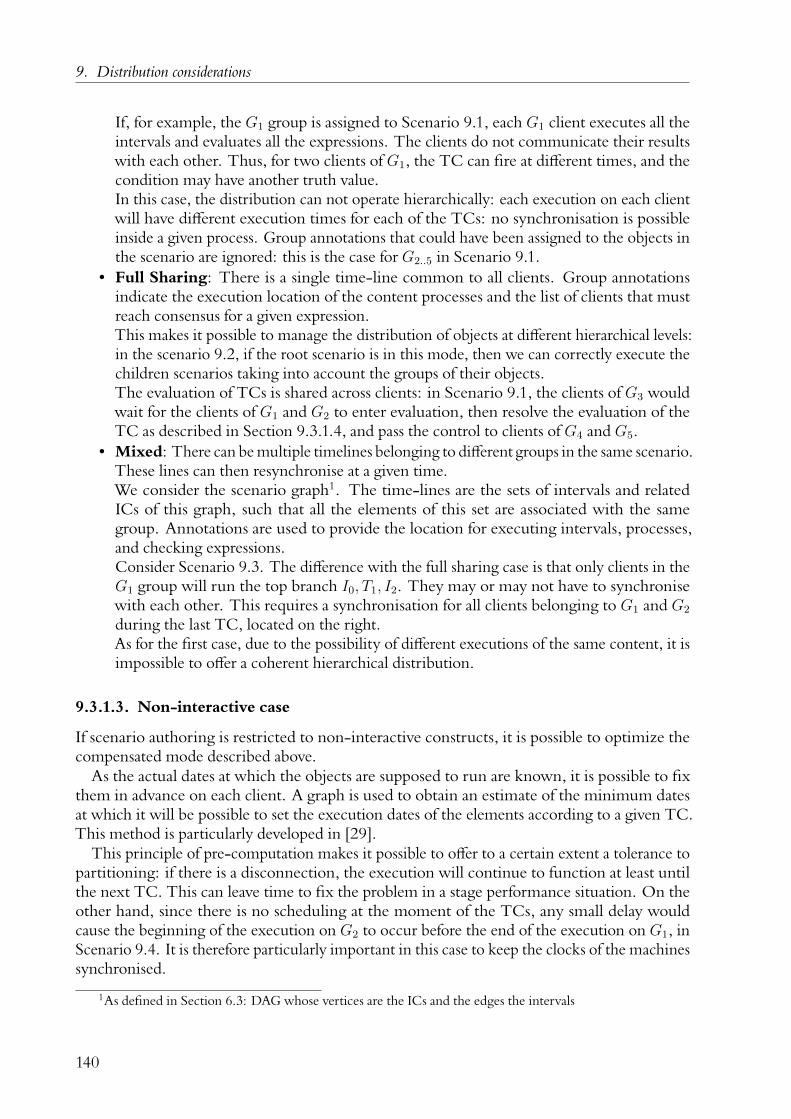
9. Distribution considerations

If, for example, the G1 group is assigned to Scenario 9.1, each G1 client executes all theintervals and evaluates all the expressions. The clients do not communicate their resultswith each other. Thus, for two clients of G1, the TC can fire at different times, and thecondition may have another truth value.In this case, the distribution can not operate hierarchically: each execution on each clientwill have different execution times for each of the TCs: no synchronisation is possibleinside a given process. Group annotations that could have been assigned to the objects inthe scenario are ignored: this is the case for G2..5 in Scenario 9.1.

• Full Sharing: There is a single time-line common to all clients. Group annotationsindicate the execution location of the content processes and the list of clients that mustreach consensus for a given expression.This makes it possible to manage the distribution of objects at different hierarchical levels:in the scenario 9.2, if the root scenario is in this mode, then we can correctly execute thechildren scenarios taking into account the groups of their objects.The evaluation of TCs is shared across clients: in Scenario 9.1, the clients of G3 wouldwait for the clients of G1 and G2 to enter evaluation, then resolve the evaluation of theTC as described in Section 9.3.1.4, and pass the control to clients of G4 and G5.

• Mixed: There can bemultiple timelines belonging to different groups in the same scenario.These lines can then resynchronise at a given time.We consider the scenario graph1. The time-lines are the sets of intervals and relatedICs of this graph, such that all the elements of this set are associated with the samegroup. Annotations are used to provide the location for executing intervals, processes,and checking expressions.Consider Scenario 9.3. The difference with the full sharing case is that only clients in theG1 group will run the top branch I0, T1, I2. They may or may not have to synchronisewith each other. This requires a synchronisation for all clients belonging to G1 and G2

during the last TC, located on the right.As for the first case, due to the possibility of different executions of the same content, it isimpossible to offer a coherent hierarchical distribution.

9.3.1.3. Non-interactive case

If scenario authoring is restricted to non-interactive constructs, it is possible to optimize thecompensated mode described above.

As the actual dates at which the objects are supposed to run are known, it is possible to fixthem in advance on each client. A graph is used to obtain an estimate of the minimum datesat which it will be possible to set the execution dates of the elements according to a given TC.This method is particularly developed in [29].

This principle of pre-computation makes it possible to offer to a certain extent a tolerance topartitioning: if there is a disconnection, the execution will continue to function at least untilthe next TC. This can leave time to fix the problem in a stage performance situation. On theother hand, since there is no scheduling at the moment of the TCs, any small delay wouldcause the beginning of the execution on G2 to occur before the end of the execution on G1, inScenario 9.4. It is therefore particularly important in this case to keep the clocks of the machinessynchronised.

1As defined in Section 6.3: DAG whose vertices are the ICs and the edges the intervals

140

9.3. Distributed execution description

T0 : G2

T1 : G1

T3 : G1

T2 : G2

I0 : G1

I2 : G1

I1 : G2

I3 : G2

(a) A score as written by an author.

T0

T1

T2

T3

I0

I1

I2

I3

(b) Corresponding graph.

Scenario 9.3.: Two branches, each executed by a distinct group.

G1

G2

G3

G1

Scenario 9.4.: The groups G1, G2, G3 execute intervals which may contain processes, one aftereach other.

9.3.1.4. Expressions and interactivity

In the case of no sharing, where a scenario is run entirely in parallel by different clients, there isno particular situation to manage. Each client verifies expressions based on the data they have,and validates them whenever they are able to. This can be useful if for example the partitioninvolves several phones that all run a similar scenario, but where each individual phone canchoose to advance its own local scenario at the rate he wants.

In the case of sharing certain time lines by several clients, it is necessary to synchronise sharedinformation. These are, for example, the evaluation dates of expressions.

• If there is a single timeline, each expression must bear only one truth value over the wholesystem. There must be a consensus on the value of these expressions.Several ways to reach consensus are possible:

– In the case of ICs, at least one client validates or denies the expression.– In the case of TCs, we can set the value of the expression to that of the first client

who verifies it, using the stamps.– In the case of TCs, a majority of clients validate the expression.– All clients validate or deny the expression.

• In the mixed case, the synchronisation must be done at the entry or exit of a branch.There are several possible problems:

141

9. Distribution considerations

• Disconnecting a client when making a decision. In this case, we can learn about thedisconnection, by performing a regular ping, and make the decision with the remainingparticipants.

• The case of an ex-æquo, if a group has an even number of participants. There are severalresolution possibilities:

– Choose according to the stamps: the first choice is the one chosen.– Name a group leader who makes a decision.– Choose at random.

9.3.1.5. Consensus

As mentioned in Section 9.3.1.4, when sharing TCs and ICs, different clients have to agree onthe result of an expression.

We separate the synchronisation of the consensus of the execution mechanism that followsthe resolution of this consensus:

1. The nodes involved in the expression decide the truth value.2. Once this value is known, all the nodes preceding, following, and involving the expression

are included in the decision of the execution date.

9.3.2. Alternative: low-level distribution

Another approach not considered in this work would be to perform the synchronisation at eachclock tick, via a master-slave servo mechanism.

The master runs with a physical clock. At each tick, he sends all clients the date on whichthey must perform their own tick. When clients receive this message, they apply an active wait 1:the program loops until a trigger condition is validated. Until this, the execution of the ticktakes place.

9.3.3. Summary

We introduce a notion of client (potentially a physical machine) and group. A group can containmultiple clients, and a client can be present in more than one group.

A shared document template is chosen for distribution: all clients see the same document,but can each interpret subparts differently, at the discretion of the composer.

Different objects of the score model can be assigned to one or more groups:• Processes.• Temporal conditions.• Intervals.In the case of TCs, several synchronisation levels are presented.Given a group, an interval propagates this group recursively to all its child processes.For the case of the scenario process, the distribution can take place with varying degrees of

information sharing between clients.

1also known as busy wait.

142

9.4. Semantics

9.4. Semantics

We describe here the semantics of the various synchronisation methods studied previously. Theyare described through the temporal model primitives: we already have synchronisation throughTC and message-passing with intervals and the environment, which are enough to implementdistributed systems. For each annotation given by the author, such as in Scenarios 9.5, 9.6, 9.7,we give the required transformation into distributed scores.

9.4.1. Displacement without interactivity

I1 : G1

I2 : G2

Scenario 9.5.: Two time intervals follow each other on two different groups.

The first case, visible in Scenario 9.5, is the case of displacement. Two intervals I1, I2 followeach other.

We note I1 : G1 when the interval I1 runs on the computers of the group G1. Passing fromI1 to I2 happens at a date known beforehand: the system is not waiting for any interaction.

The following transformations are applied:1. A bifurcation is created at the first TC, before I1.2. A temporal interval is introduced I1→2.3. I2 is moved to after the end of this new interval I2.

4a. In the instantaneous asynchronous case (fig. 9.3a).A message M1 is created at the end of I1; it will trigger T1 automatically. This impliesthat I1→2 is flexible. This message will be sent when a consensus on the G1 group will beestablished, with one of the policies described in Section 9.3.1.4.

4b. Compensated asynchronous case (fig. 9.3a).When a consensus is established on the ending date of I1, a message M1 is sent to the G2

clients with this date. This way, they will start executing at the same time that the end ofI1.

4c. Compensated synchronous case (fig. 9.3b).The M1 message is sent at the beginning of I1 rather than the end. On the G1 machines,the T1 TC does not wait for anything. On the G2 machines, it waits for M1. The clientsof the group G1 and G2 can be disconnected after the beginning of the playback: theywill keep working as expected.

A few remarks:• Since there are no expressions, the instantaneous synchronous mode does not bring

anything with regards to the instantaneous asynchronous case. Indeed, the beginning ofI2 implies in all cases the end of I1, because the clients of the group evaluating I1 are theones deciding of the evaluation date of the TC. This is in opposition with the case wherean expression would be evaluated by another group than G1 or G2.

• The compensated case with pre-computations is not compatible with a strong synchro-nisation: in this case, we expect the synchronisation to take place only thanks to theunderlying clocks’ synchronisation, for instance with protocols such as NTP.

143

9. Distribution considerations

M1

T1

I1

I1→2 I2

(a) Instantaneous, compensated, synchronous case.

M1

T1

I1

I1→2 I2

(b) Pre-computed compensated asynchronous case.

Figure 9.3.: Transformations for the execution of two intervals in series on two separate clients.

9.4.2. Displacement with interactivity: simple case

We now consider a simple case, similar to the non-interactive case, but where an external eventis waited upon for the triggering.

T1 : G2I1 : G1

I2 : G3

Scenario 9.6.: The groups G1 and G3 execute the two intervals, while a group G2 awaits for aconsensus on the expression.

Scenario 9.6 can be solved in multiple ways:• If the execution of the TC happens instantaneously, all the clients ofG2 send the triggering

information to all the clients of G1 and G3, without ordering guaranteed; all the TCtrigger immediately.

• If the execution of the TC is compensated:– When its expression becomes true, a stop date for the G1 clients is fixed in the

synchronous case, and for G1 and G3 in the asynchronous case. Besides, in thesynchronous case, a consensus mechanism allowing to ensure that all the membersof G1 have terminated their execution before the start of the interval assigned to G3 .

– If a max bound is reached: a client is necessarily the first to reach this bound. It canthen inform the other clients; this will in turn trigger the continuation of the score.

9.4.3. Displacement with interactivity: extended case

T : G2I1 : G1

I3 : G3

I4 : G4

Scenario 9.7.: A scenario with a TC to be distributed over the groups G1,..,4.

We consider in this case the score 9.7, which has a TC T , managed by the G2 group .

144

9.5. Conclusion

Te

T2

T1

T3

T4

I1 : G1

I3 : G3

I4 : G4

G2

G2

G3

M1,M3,M4

Scenario 9.8.: Distribution of the scenario 9.7 in the asynchronous instantaneous case: inter-vals associated with the groups G1, G4, and the interval associated to the groupG3 will stop and start without an order known beforehand.

We note:• Te: The TC which marks the beginning of the evaluation of the expression of T .• T2: The TC which marks the consensus on the expression of T .• T1: The TC which marks the end of the execution of the interval in G1. It is triggered by

M1.• T4: The TC which marks the end of the execution of the interval in G4. It is triggered by

M4.• T3: The TC which marks the end of the execution of the interval in G3. It is triggered by

M3.In the asynchronous case, in Scenario 9.8, M1,M3,M4 are messages which will trigger

T1, T3, T4 as soon as they are received.In the synchronous case, in Scenario 9.9, the messages are sent as early as possible, but the

triggering of T3 implies the end of the execution of I1 and I4. T3 will start when all the M3

messages have been sent: its expression is a logical conjunction on the reception of M31,..N with1, ..N the groups before T .

In the compensated case, the structure does not change. The sent messages do change,however: M1,M3,M4 fix the date at which T1, T3, T4 must execute, in order to happen at thesame time.

It would be possible to express other variants: for instance enforcing simultaneity for thetermination of I1, I4 but not the start of I3. However, this would often be detrimental toauthoring: we prefer giving access to a few high-level concepts whose necessity has been madeapparent when researching the use cases with the authors.

9.5. Conclusion

A method (previously published in [36]) is presented for splitting the execution of parts of aninteractive scenario based on the temporal model on different machines on a local network.

145

9. Distribution considerations

I4 : G4

G2

G3

Te

G2 T2

T1

T3

T4

I1 : G1

I3 : G3

M1,M4

M3

M3

Scenario 9.9.: Distribution of the scenario 9.7 in the synchronous instantaneous case: intervalsassociated with the groups G1, G4 and the interval associated with the groupG3 will stop in order with a potential delay between the end of G1, G4 and thebeginning of G3.

The goal is to offer new writing possibilities to composers working in a heterogeneousenvironment, including phones, embedded cards like Raspberry Pi, and much more powerfuldesktop machines.

The different possibilities of synchronisation of the temporal structures are introduced. Firstat a TC, allowing various degrees of cohesion with the structure given by the composer, rangingfrom executions not necessarily simultaneous but with low latency, to executions with a higherlatency, but allowing greater simultaneity for the observer. Then in a scenario, where weconsider the possibilities of sharing that there can be between several machines running thesame scenario: all in parallel, some in series and any other variations.

Note that in contrast to the published version, we do not consider the case of varying intervalspeed. This is because this work had been originally based on a different data production model,which did not support audio data but made easier variations of speed for intervals; this will bereintroduced once the specification of time variations in the current system are devised.

The remaining work is about extending the writing possibilities to include more complexinteraction information. For example, we would like to be able to control a parameter such asthe volume of a sound in real time, taking into account the interactions of several participantson their phone. Behaviours such as “take the average value”, “take the highest value” couldthen be introduced into the palette available to the author.

146

Part IV.

Implementation and practicalapplications

147

This part presents the implementation of the research done in this thesis, in Chapter 10: thelibrary libossia for multimedia application modelling, and the software ossia score for the execu-tion of interactive scores. Performance characteristics of the environment are exhibited throughbenchmarks of the various layers of the implementation corresponding to the organization usedfor this thesis. Then, Chapter 11 discusses of the remaining problems with the model, andpresents practical uses in artistic installations.

148

10Implementation

We present in this chapter details on the implementation of the concepts presented earlier. Twomain software artefacts are provided: libossia, the base library, and ossia score (referred to simplyas score in the rest of this chapter), the visual authoring and execution software. The libossialibrary provides an implementation of the chapters 4, 5, 6, 7: data structures and executionalgorithms for the process tree, the data graph, and the parameter tree along with multiplecommunication protocols. The ossia score software implements Section 8.1. Awork-in-progressscore plug-in implements the content of Chapter 9: distributed execution. The ossia scoresoftware itself does not necessarily needs to run with its whole graphic interface: it can beused as a command-line player in headless environments such as embedded boards. A work-in-progress experiment seeks the integration of score itself in other visual environments, such asMax/MSP and Pure Data.

Both are written in C++17, using mainly the Qt and Boost libraries, and are supported acrossthe three main desktop platforms, Linux, macOS and Windows. In addition, libossia hasbeen used on mobile platforms such as Android. A recent version of the C++ language is usedfor the added expressive capacity without loss of performance: clear ownership of data withunique_ptr, lambda-expressions, variants and closed polymorphism.

Care is taken to limit allocations on hot paths: message emission and reception, and graphexecution.

Whenever relevant, flat data structures are used: they enable better cache coherency andan overall better performance for search than the default data structures provided by the lan-guage [186], at the cost of larger insertion speed. In the present case, we aim to make theexecution of a fixed score as fast as possible: insertions must seldom happen in the hot path. Forinstance, during the execution of the scenario process, insertions only happen whenever a TCexecutes in a given tick since the over-ticks are stored in such a data structure. In the practicalscores presented earlier, the number of insertions in such sets is negligible: very few intervalshave synchronised ends.

150

10.1. libossia: general software design

10.1. libossia: general software design

libossia consists of multiple elements:

• A base C++ library, split in three parts: network, dataflow, editor. The first part pro-vides an implementation of the device tree, as well as bindings and implementations ofthe various transport protocols mentioned earlier: OSC using a fork of the OSCPacklibrary1, MIDIusing a fork of the ModernMIDI and RtMidi libraries2, Minuit3, OSC-Query, WebSockets4, HTTP, serial port, and an audio protocol implementation usingPortAudio [167], JACK [187] or SDL5…The second part provides the data graph, andthe third the temporal tree as well as common processes and data nodes implementationssuch as automations, mappings, sound files.

• Bindings of the network part to various creative environments: Max/MSP, Pure Data,Unity3D and C#, SuperCollider, openFrameworks, QML, Faust, Processing and Javaas well as more general purpose programming languages: Python, C89, C++ 98. Doc-umentation for the usage of the library in these environments can be found at https://ossia.github.io/#introduction. In particular, instead of trying to offer an identical APIacross all environments, libossia provides primitives adapted to each system. That is,object-oriented environments such as Python, Unity3D are offered an object-orientedAPI which maps the received values of the network tree to a message queue, since thread-ing is generally not supported. Data-flow environments such as Max/MSP and PureData have specific nodes used for the sake of referencing a tree parameter across multiplepatches easily: the [ossia.remote] object; in addition, they offer primitives to enable en-capsulation of behaviour within a patch. That is, using the ossia.model and ossia.viewobjects, it is possible to reflect the patch organization in the device tree hierarchy: eachnew ossia.model will create a hierarchical level in the tree to which all the surroundingparameters and node will aggregate.

It is hosted at https://github.com/OSSIA/libossia.

10.1.1. Structuring multimedia software with libossia

One of the core problems of software authoring is giving a structure to the software, to facilitateextensibility and modifications: fixing bugs, adding features…

As mentioned in Chapter 2, artistic software and hardware can generally be modelled by atree of parameters. The device tree presented in Chapter 4 is proposed as a way to structuresuch software, to make it both easier for its author to focus on the artistic features of its works ofart, and easier for computers to work with this structure.

1http://www.rossbencina.com/code/oscpack2https://github.com/jcelerier/RtMidi173An OSC-based query protocol, discussed in Section 10.1.6.3.4A bidirectional communication protocol available for use in web pages.5https://www.libsdl.org

151

10. Implementation

10.1.1.1. Traditional programming languages

The most basic case is the integration in traditional imperative and object-oriented programminglanguages. In these cases, libossia is used as a simple library, in line with expectations ofprogrammers in these languages. Examples are given for C (listing 10), C (listing 11), C#(listing 13), Python (listing 12).

Algorithm 10 Creating a tree with as single node in C.

ossia_protocol_t proto = ossia_protocol_oscquery_server_create(1234, 5678);ossia_device_t dev = ossia_device_create(proto, "newDevice");ossia_node_t root = ossia_device_get_root_node(dev);ossia_node_t n1 = ossia_node_create(root, "/color");ossia_parameter_t p = ossia_node_create_parameter(n1, VEC3F_T);ossia_parameter_set_bounding_mode(p, CLIP);ossia_domain_t dom = ossia_domain_make_min_max(0, 255);ossia_parameter_set_domain(p, dom);ossia_parameter_set_unit(p, "rgb");ossia_parameter_push_3f(p, 255, 0, 0);

Algorithm 11 Creating a tree with as single node in C++.

generic_device dev{std::make_unique<oscquery_server_protocol>(),"newDevice"};

auto& n = create_node(dev, "/color");auto& p = *n2.create_parameter(val_type::VEC3F);p.set_domain(make_domain(0, 255));p.set_unit(rgb_u{});p.push_value({255,0,0});

Algorithm 12 Creating a tree with as single node in Python. Further improvements wouldleverage decorators.

local_device = ossia.LocalDevice("newDevice")local_device.create_oscquery_server(1234, 5678, False)node = local_device.add_node("/color")parameter = node.create_parameter(ossia.ValueType.Vec3f)parameter.bounding_mode = ossia.BoundingMode.Clipparameter.unit = 'rgb'parameter.make_domain(0,255)parameter.value = [255,0,0]

10.1.1.2. Patch-like environments

Objects are provided to the composer to allow the construction of this tree, and the bindingof this tree to the parameters of the software. Section 10.1 presents the facilities that weredeveloped in various creative environments to make this step seamless.

152

10.1. libossia: general software design

Algorithm 13 Creating a tree with as single node in C#.

var dev = new Ossia.Device (new Ossia.OSCQuery (1234, 5678), "newDevice");var root = dev.GetRootNode ();var n = Ossia.Node.CreateNode (root, "/color");var p = n.CreateParameter (Ossia.ossia_type.VEC3F);p.SetUnit("rgb");p.SetBoundingMode(Ossia.ossia_bounding_mode.CLIP);p.SetMin(0); p.SetMax(255);p.PushValue(255, 0, 0);

(a) A PureData synthesizer organized with ex-plicit parameters.

(b) A PureData client that can remote-control the device.

(c) Another client for the same device, writ-ten in HTML.

Figure 10.1.: A PureData patch (courtesy of Antoine Villeret) can be organized with parametersthat bear associated attributes. These attributes allow for better control from othersoftware. This example has no hierarchy.

Fig. 10.1 provides an example for a device built in Pure Data.We can make a parallel with prototypal object systems such as JavaScript1’s. In classical object-

oriented languages, one separate the definition of classes with their instantiation. Instead, in thepresent system, the class definition is its instantiation. That is, the nodes of a tree represent atthe same time the type of an object, and an instance of this type. The main point of this is,like before, to enable faster prototyping and development in artistic contexts: doing separatedefinition and instantiation would require more work from composers.

Instead, prototypal behaviour allows to construct types along with a usable instance of thistype.

1A programming language mainly used in web browsers.

153

10. Implementation

10.1.1.3. QML and reactive environments

Remember that QML is a reactive programming language, optimized for the creation of userinterfaces. A simple QML program is given in example in fig. 14. The reactive semantics can beleveraged to provide a set of objects with a similar behaviour than the ones provided for patcherenvironments. In particular, QML programs are structured as tree of objects; this structurecan be followed by the libossia objects to provide a simple experience to the programmer. Anexample of QML program using libossia is given in fig. 15. In this example, a device treeconsisting of the following addresses is created:

• /main/text of string type.• /main/text.1 of string type.• /main/rect/background of vec3f type, with an ARGB unit.• /main/rect/width of float type.• /main/rect/height of float type.Network update to the values will be propagated reactively to the QML objects.

Algorithm 14An example of program in the QML language. A button and a text are displayed.Whenever the button is pressed, a counter increases and the text is updated with the new valueof the counter.

import QtQuick 2.11Window {

property int count: 0Row {Button { onPressed: count++ }Label { text: "Hello" + count }

}}

Algorithm 15 A QML program using libossia.

import QtQuick 2.11Window {

property int count: 0Ossia.Node { name: "main" }Row {Label { Ossia.Property on text { } }Label { Ossia.Property on text { } }Rectangle {

Ossia.Node { name: "rect" }Ossia.Property on background { }Ossia.Property on width { }Ossia.Property on height { }

}}

}

154

10.1. libossia: general software design

Another example of hierarchical environment with reactive elements is Unity3D: propertiesof classes can be changed graphically in real-time through user interface widgets. This featureis leveraged to provide automatic creation of libossia objects for Unity3D object trees: wholescenes can be exposed automatically to the network with no programmatic intervention.

10.1.2. libossia: network implementation notes

The network implementation provides ZeroConf / Bonjour support: that is, the networkdevices are automatically visible from other OSSIA-compatible software. This allows to simplifythe research for devices in the network: there is no need for the author to remember the IPaddress and port of the software to which he wishes to connect to.

The implementation is based on a tree structure built with linked references. The nodesthemselves only contain data; a protocol object is associated with each device and performs theactual conversion of messages in the API into network messages and conversely.

10.1.3. libossia: messaging pipeline

Overall, the proposed framework for controlling parameters behaves as in fig. 10.2:

Message Unit and arrayconversion

Domainfiltering

Repetitionfiltering

Outsideworld

Figure 10.2.: Message emission pipeline.

UserUser interface ele-ment: slider, …

Source parameter ob-ject

Source protocol im-plementation: OSC,Minuit,OSCQuery,MIDI…

Network

Target protocol imple-mentation

Target parameter ob-ject

Target software valueReaction in the target soft-ware: frequency of an oscil-lator, activation of a filter...

Figure 10.3.: Overall communication pipeline. The steps of message emission showcased aboveare provided as a convenience function that can be used in each protocol’s imple-mentation.

10.1.4. libossia: node attributes reference

As mentioned in Section 4.1.6, attributes are attached to nodes. Table 10.1 lists the attributescurrently implemented.

155

10. Implementation

Descriptiondescription A textual description to be shown to the user

tags A list of single words to categorize a particular node

Networkpriority An integer. The higher the priority and the sooner it should be ordered

if multiples messages are to be sent at the same time.critical A critical node should use if available safer means of communication:

for instance a TCP instead of an UDP connection. This attributecan be useful for parameter changes which can cause problems if theyare missing: for instance, a /play message should not ever be missed,while a value change can be discarded by a network router if there isanother value that comes in the next few milliseconds.

hidden The parameter is an implementation detail and should not be exposedto the network.

zombie The node used to exist but does not exist anymore. This is useful inthe context of dynamic nodes. For instance, given an equalizer with avariable number of bands, this allows to remember that at some point,a particular band existed and keep its parameters in memory.

Controlenable An enabled parameter will send and receive messages.mute Amute parameter will not send or receivemessages. Unlike the enable

attribute, muting and unmuting is not propagated to the network.refresh rate The maximum rate at which a parameter should receive and send

changes.step size If the parameter is numeric, the minimal steps a user interface control

should operate at: for instance 0.5.default value The value with which a parameter shall be initialized.access mode A value that indicates whether a parameter is read-only (e.g. a measured

value), write-only (e.g. a play message), or both (most controllableparameters: frequencies, colours, etc.)

instancebounds

A pair of integers representing the minimal and maximal number ofinstances for a given object. This can be useful to enforce limits onremote objects creation.

Table 10.1.: Attributes on nodes.

156

10.1. libossia: general software design

10.1.5. libossia: units and dataspaces

Remember that a dataspace is a union of units pertaining to the same semantic domain, asdefined in Section 4.1.4; any value specified in a unit of a given dataspace can be converted toany other unit of the same dataspace. For instance, both polar and cartesian unit systems pertainto the same “position” dataspace.

Table 10.2 presents the dataspaces and units supported by the current version of the system.These units were chosen from the set offered by the Jamoma project following a discussion withits users.

Colour Position Angle Orientation Distance Gain Speed TimingARGB XYZ Degree Quaternion m Linear m s−1 sRGBA XY Radian Euler dm Midi mph BarkRGB Spherical Axes cm 16-bit dB kmh−1 BPMBGR Polar mm dB Knots Cent

ARGB (8-bit) GL µm Ft s−1 HzHSV Cylindrical nm Ft h−1 Mel

CMY (8-bit) pm Midi PitchXYZ Inch ms

FootMile

Table 10.2.: Units and dataspaces.

10.1.6. libossia: protocols

Multiple communication protocols can be used with the present system. Some may only beable to leverage a part of the feature: for instance the MIDI protocol offers no way to exchangeany kind of metadata. The OSCQuery implementation with the proposed extensions allows toleverage the entirety of the present framework.

10.1.6.1. MIDI

MIDI is a famous protocol published in 1983 for the control of electronic music instruments.Its original goal was to allow synthesizers from different brands to be able to send control signalsto each other.

The protocol is based on message exchange, originally at a fixed baud rate, though morerecent software implementations do not rely on this anymore.

A message generally consists of between 1 and 3 bytes; most values are stored on seven bits outof eight as the most significant bit of each byte is reserved for identification. Some parameters,such as the pitch bend, combine two bytes for their value to provide more precision.

Most MIDI messages are semantically charged: for instance Note On, Note Off, PitchBend, refer specifically to musical concepts; though they can of course be leveraged for otherkinds of controls.

In order to support common MIDI usage, a mapping from usual messages to a tree, schema-tized in fig. 10.4 is provided:

• The first level of the tree is the MIDI channel.• The second level of the tree is the MIDI command.

157

10. Implementation

• The third level of the tree is the first MIDI byte, if it is a command.• The value of a parameter is the second MIDI byte.The nodes and parameters are set up according to the following rules and conventions:• Channels start at 1.• Note On, note Off, Control Change nodes are integers bounded between 0 and 127; the

data is either the velocity or the Control Change value.• Program Change nodes are impulses.• Pitch bend is an integer bounded between 0 and 16383; the default value is 8192.• When relevant, convenience nodes are provided: array messages to set both note pitch

and velocity, or integer message to set a program change by value.For instance:• The message /12/noteon/64 127 represents a C3 at maximal velocity. It is equivalent to

the message /12/noteon 64 127.• The message /1/pitchbend 0 bends to the lowest pitch on the first channel.• The message /3/program/15 sends program change 15 to channel 3. It is equivalent to

the message /3/program 15.

16. . .1

pitchbendprogram

. . .

control

. . .

noteoff

. . .

noteon

127. . .1

Figure 10.4.: MIDI tree.

10.1.6.2. OSC

Since this work uses many core concepts of OSC, let us recapitulate the basics of it. The OSCprotocol was introduced in 1997 [128, 188]. In contrast with MIDI, it is not based on domain-specific messages. As such, it can be more easily leveraged for fields other than music: video,robotics [189], etc.

OSC servers are software or hardware peripherals, with associated OSC methods that receiveOSC messages. An OSC method has an associated address; the OSC server routes any OSCmessage whose pattern matches with its address. OSC containers are akin to folders in filesystem: they contain children containers or methods. We refer to OSC methods or OSCcontainers indifferently as OSC nodes. Addresses are as such similar to traditional UNIXsystem paths: /synth/frequency. Patterns can use a limited form of pattern-matching:/equalizer/*/{freq,gain} would for instance match

/equalizer/123/freq/equalizer/main/gain

but not

/equalizer/123/Q/equalizer/freq

158

10.1. libossia: general software design

AnOSCmessage consists of a pattern and a sequence of values. Values are typed. The availabletypes per the first version of the protocol are: 32-bit integer, 32-bit float, null-terminated stringand blob, an array of raw bytes associated with a fixed size. A further revision of the protocol,OSC 1.1, introduces new required types following existing usage patterns: booleans, a nulltype, and an impulse type.

Examples of OSC messages in a readable form are:/equalizer/freq 440.0/color/? "hello" 1 2 1 -1

These messages are encoded by introducing the type of the parameters after the pattern, andpadding the parts of the message with zeros so that each data fits on 4-bytes alignment; numericvalues are in network byte order:

'/' 'e' 'q' 'u''a' 'l' 'i' 'z''e' 'r' '/' 'f''r' 'e' 'q' 0',' 'f' 0 067 220 0 0

(a) OSC encoding of the above message/equalizer/freq.

'/' 'c' 'o' 'l''o' 'r' '/' '?'0 0 0 0',' 's' 'i' 'i''i' 'i' 0 0'h' 'e' 'l' 'l''o' 0 0 00 0 0 10 0 0 2255 255 255 255

(b) OSC encoding of the above message/color/?.

The most common transport protocol for OSC is UDP, though it has also seen some usageon top of TCP, WebSockets and serial port layers. This has the drawback of leading to lostmessages, due to the lack of guarantees by UDP. This effect varies in practice, depending onthe network configuration: for instance, most operating system kernels have a space-limitedinput and output message queue for UDP; any message departing or arriving while the queue isfull would silently be dropped.

Messages can be grouped in bundles; the OSC server shall then apply the messages of thebundle in order. This allows circumventing the lack of ordering guarantees in UDP.

Queries The OSC protocol does not come with any query mechanism; that is, there is nostandard way to query the current state of an OSC server, or know in a machine-readable waywhat are the objects and attributes that it exposes.

Some approaches are sometimes used to retrieve some information on the state of the server:• dump message: a special message that, when sent to the OSC server, makes it send OSC

messages for all of its methods to the client that requests it. This is also useful for a clientto discover what are the available OSC methods in a given server.

• Argumentless queries: given an OSC method such as /synth/volume with a float param-eter, sending an argumentless message triggers the server in responding with the currentvalue of the parameter.

159

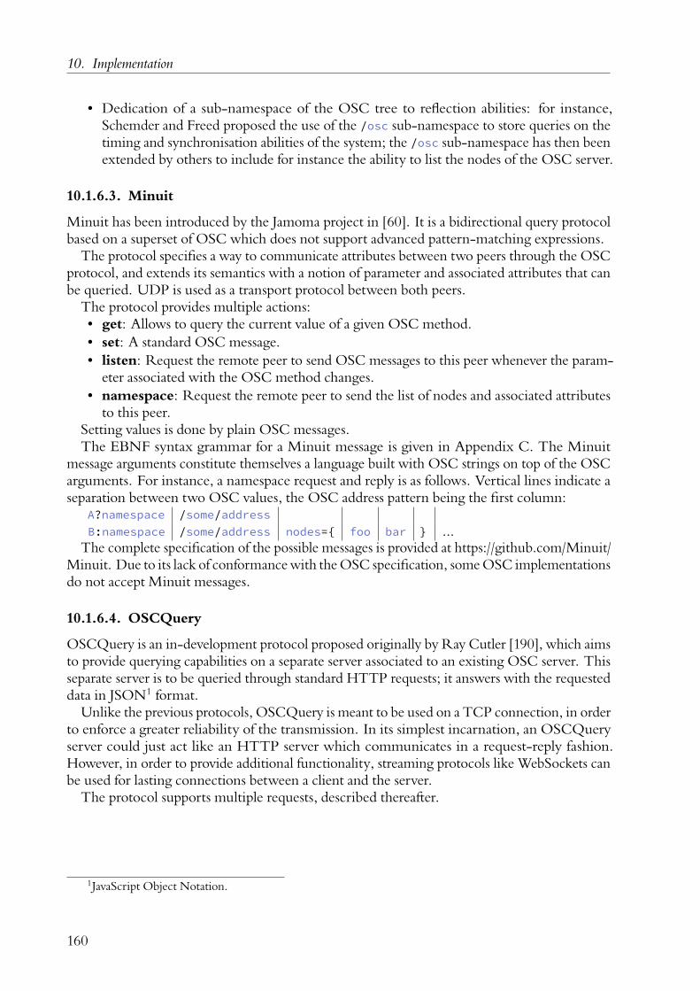
10. Implementation

• Dedication of a sub-namespace of the OSC tree to reflection abilities: for instance,Schemder and Freed proposed the use of the /osc sub-namespace to store queries on thetiming and synchronisation abilities of the system; the /osc sub-namespace has then beenextended by others to include for instance the ability to list the nodes of the OSC server.

10.1.6.3. Minuit

Minuit has been introduced by the Jamoma project in [60]. It is a bidirectional query protocolbased on a superset of OSC which does not support advanced pattern-matching expressions.

The protocol specifies a way to communicate attributes between two peers through the OSCprotocol, and extends its semantics with a notion of parameter and associated attributes that canbe queried. UDP is used as a transport protocol between both peers.

The protocol provides multiple actions:• get: Allows to query the current value of a given OSC method.• set: A standard OSC message.• listen: Request the remote peer to send OSC messages to this peer whenever the param-

eter associated with the OSC method changes.• namespace: Request the remote peer to send the list of nodes and associated attributes

to this peer.Setting values is done by plain OSC messages.The EBNF syntax grammar for a Minuit message is given in Appendix C. The Minuit

message arguments constitute themselves a language built with OSC strings on top of the OSCarguments. For instance, a namespace request and reply is as follows. Vertical lines indicate aseparation between two OSC values, the OSC address pattern being the first column:

A?namespace /some/addressB:namespace /some/address nodes={ foo bar } ...

The complete specification of the possible messages is provided at https://github.com/Minuit/Minuit. Due to its lack of conformancewith theOSC specification, someOSC implementationsdo not accept Minuit messages.

10.1.6.4. OSCQuery

OSCQuery is an in-development protocol proposed originally by Ray Cutler [190], which aimsto provide querying capabilities on a separate server associated to an existing OSC server. Thisseparate server is to be queried through standard HTTP requests; it answers with the requesteddata in JSON1 format.

Unlike the previous protocols, OSCQuery is meant to be used on a TCP connection, in orderto enforce a greater reliability of the transmission. In its simplest incarnation, an OSCQueryserver could just act like an HTTP server which communicates in a request-reply fashion.However, in order to provide additional functionality, streaming protocols like WebSockets canbe used for lasting connections between a client and the server.

The protocol supports multiple requests, described thereafter.

1JavaScript Object Notation.

160

10.1. libossia: general software design

Namespace requestThe OSC methods are mapped to the HTTP GET Request URI [191, page 5.1.2]; this isconvenient due to the similar path-like format used for both.

Making a request for a given node returns a JSON object that describes the method orcontainer and its children.

An OSC container or method is mapped to the JSON object with the following requiredfields:

• DESCRIPTION: user-readable description.• CONTENTS: If any, a JSON array with the children of the given OSC node.• FULL_PATH: OSC address of a given node.Additional fields can be provided depending on the attributes associated with a particular

node. For instance, if the node is an OSC method, its OSC typetag will be sent in the TYPEfield.

Requesting the information for the OSC method /synth/volume on an OSCQuery serverrunning on the same computer on port 5678 can be done by the request:

http://127.0.0.1:5678/synth/volume

The returned data if the node exists would be:

{"DESCRIPTION": "Main volume of the synthesizer","FULL_PATH": "/synth/volume","ACCESS": 1,"TYPE": "f","VALUE": 0.5,"RANGE": { "MIN": 0.0, "MAX": 1.0 }

}

The various attributes mentioned earlier are all encoded as key-value pairs in such objects.

Attribute requestA single attribute can be queried with the GET request’s query parameters:

http://127.0.0.1:5678/synth/volume?VALUE&TYPE

would return:

{"TYPE": "f","VALUE": 0.5}

Listening request Listening has the same semantics as in Minuit: enabling listening on amethod means that as soon as the value of the method changes on the OSC server, the clientsshould be notified of the change.

161

10. Implementation

Additionally, the protocol supports notification of changes to the structure of the OSC server:for instance, if nodes are added, updated or modified at run-time, the clients are kept aware ofsuch changes through the streaming connection. Likewise, the critical attribute mentionedin Table 10.1 can be leveraged: critical OSC messages would be sent through the WebSocketconnection instead of the OSC UDP connection. Furthermore, using WebSockets for OSCtransport would allow web clients to connect to an existing OSC server, which is not possiblewith usual OSC implementations.

Multiple extensions and improvements were proposed by the author to the protocol: inparticular, the semantics of various attributes defined earlier, such as the critical attribute, andchanges due to implementation experience with the protocol.

10.1.6.5. Scriptable protocols

The previous protocols, in particular OSC, Minuit, and OSCQuery, are viable for creatingstructured software: they allow their user to build the tree according to their application’sneeds. The main mechanism for this is creating the relevant domain objects in their authoringenvironment. Others, such as MIDI, are fixed due to a rigid specification.

Finally, in some cases, external programs cannot be simply represented in a tree structure dueto the lack of any schema, or one that would be too complex or too large to duplicate in a singledevice tree. One may want to be able to leverage Web APIs – for instance, real-time weatherforecast has sometimes been used in artistic installations; weather information can be providedthrough web REST1 endpoints and given in specific formats, sometimes custom JSON. It isthen necessary to have a way to map these APIs to our structure. Likewise, embedded deviceswill often communicate with specialized, custom-made protocols (see Section 11.5.3 for anexample of communication with robots).

Hence, we propose the use of an embedded general scripting language to create trees that maymap to such protocols. The JavaScript language is used for this, as part of the QML environment.

Three protocols, sitting under the application OSI2 layer, are available to build upon: Web-Sockets, HTTP, and serial communication.

WebSocketsThe WebSocket protocol is a web protocol which allows packet-oriented connections as anupgrade over an HTTP connection: it is for instance very often used with websites that havelive-feed updated as is nowadays common. Of course, every application is free to send whateverdata it wants: there is no structuring of data. We give the method for binding a customWebSocket API to our device tree: A QML object has to be provided as in Algorithm 16, withtwo functions: onMessage and createTree.

• onMessage is called whenever a message is received from the WebSocket server the objectis connected to, with the message data. This function should return messages to be appliedto the device tree, in the form of an array of JavaScript object representing key-value pairs,the keys being paths in the device tree, and the values being the values to set in the tree.

1Representational State Transfer.2Open Systems Interconnection model.

162

10.1. libossia: general software design

• createTree is called at the initialization of the device: it allows to give a structure to thedevice tree, by returning a tree-like JavaScript object. In particular, it is necessary to havea way to send messages from our environment to the external server: a mapping has to beprovided. This is done with the request member.

– If request is a string, then the string is sent as a message through the connectionwhenever a value is pushed to the network. $val can be used as a wildcard thatwill be replaced with an automated string conversion of the value fitting withJavaScript semantics. In the underlying example, sending locally a green colour tothe parameter /mysocket/lights will send the JSON { "name": "set light","value": [0.0, 1.0, 0.0] } over the network.

– If more complex behaviours are required, it is possible to provide a real functioninstead; this function will be called with the value as an argument. In the example,sending a value of 5.0 to the parameter /mysocket/volume will send the messageintensity = 13.9794000867; over the WS connection.

Algorithm 16 Example of object mapping an external WebSocket-based protocol to a devicetree.

QtObject {function onMessage(message) {

var res = JSON.parse(message);console.log(res.value);if(res.name === "myMessage"){

return [ { address: "/control", value: res.value } ];}return { };

}

function createTree() {return [ { name: "mysocket", children: [

{ name: "lights",unit: "color.rgb",request: "{ \"name\": \"set light\", \"value\": $val }"

},{ name: "volume",

type: Ossia.Float,request: function (value) {

return "intensity = " + Math.log(value) * 20 + ";";}

} ]}

];}}

163

10. Implementation

Other protocolsThis mechanism can be easily extended to other transport protocols, with sometimes differentspecifications. For instance, HTTP, by virtue of being a request-response protocol, supportssetting a custom onMessage function, per parameter of the tree. This is possible because theunderlying protocol guarantees that the response corresponds to the request that had been done.

10.1.7. libossia: data graph implementation notes

We discuss here some specific choices, problems and open questions in the implementation ofthe data graph.

10.1.7.1. Computing the transitive closure

Currently, the transitive closure algorithm used as part of the static schedule, in Section 5.5.3.4is static: the transitive closure of the data graph must be recomputed entirely every time anaddition or removal of a data node happens in the score; traditional methods for this have atime complexity of O(|V |3) with E the edges and V the vertices in the graph. The problem hassince been shown to be reducible to square matrix multiplication [192]. A possibility for furtherperformance improvements when editing the score during its execution can be made througha dynamic computation of the transitive closure [193], that is, updating an existing transitiveclosure after an edge or node addition or removal. Current best algorithms have a complexityof O(|V |2) on update of the closure, with constant query time.

10.1.7.2. Representing audio data

Given the definitions presented earlier, the only relevant way to represent audio data in thedata graph would be as an array of value * int where each value is a floating-point value. Inpractice, this would be wasteful for audio data which comes in buffers: instead, an array wherethe timestamp is the index of each sample in the array is used. Unused samples are set at 0 if atthe beginning of the array. Double-precision floating-point values are used for audio storageand computation.

10.1.8. Graph-only program

We give in Fig. 10.6 an example of program that can be written by leveraging only the datagraph part of libossia. This program is an additive synthesizer built on 60 sine waves. Thefrequency of each sine, and the output volume, can both be controlled by OSC or WebSocketmessages.

164

10.1. libossia: general software design

(a) An extract of the JSON datawhich can be retrieved by mak-ing a browser request to the pagehttp://127.0.0.1:5678 upon run-ning the given program. Furthertools are able for instance to auto-matically generate a user interfaceto control the parameters.

int main() {using namespace ossia;

// a device to expose parameters over the networkoscquery_device osc;tc_graph g; // graph implementation with static schedulingexecution_state e;// a device that maps to the sound card inputs & outputsaudio_device audio;

e.sampleRate = audio.protocol.rate;e.register_device(&audio.device);e.register_device(&osc.device);

// multiplies the inputs by a float valueauto gain = std::make_shared<gain_node>();g.add_node(gain);

// the gain node can be controlled through the OSC address /volume,// and sends data to the sound cardauto gain_param = ossia::create_parameter(osc.device, "/volume", "dB

");gain_param->push_value(-60); // we start at -60dBgain->inputs()[1]->address = gain_param;gain->outputs()[0]->address = &audio.get_main_out();

// 60 sine generators, their frequency controllable by// an OSC address such as /freq.1 /freq.2 ...for(int i = 0; i < 60; i++) {auto node = std::make_shared<sine_node>();g.connect(make_strict_edge(0, 0, node, gain));

auto freq_param = ossia::create_parameter(osc.device, "/freq", "hz");

freq_param->push_value(200 + 12 * i);node->inputs()[0]->address = freq_param;

}

// start callback-based soundcard-driven execution: here// the tick algorithm adds a token of the buffer size to every nodeaudio.protocol.set_tick(tick_all_nodes{e, g});

while(1);}

(b) Code listing of the networked sine synthesizer.

Figure 10.6.: An example of program using the data graph.

165

10. Implementation

Figure 10.7.: An example of score in ossia score.

10.2. ossia score, the user interface

The main software artefact, ossia score, is the implementation of the editor and player for thevisual language. It is hosted at https://github.com/OSSIA/score.

The interface is split in multiple parts, visible in fig. 10.7: by default, the left pane containsthe device trees, the central pane contains the score, and the right pane contains an inspectorwhich can give informations and perform actions on selected objects. Multiple other panes areavailable but hidden by default.

10.2.1. Translation glossary

Particularly, naming the concepts of the software has been a long-lived debate in the community:terms that bear a specific meaning in a scientific context may have a very different meaningin the audio-visual community, which may sometimes lead to misunderstandings from theusers of the software due to their different technical backgrounds. Hence, the choice has beenmade to use less correct but more easily graspable terms in the software implementation. Thisthesis uses a different naming convention, which maps more closely to the model definitions.Wherever applicable, the difference in terms will be highlighted. The equivalence table is givenin Table 10.3 .

Name in the model Name in ScoreProcess ProcessInterval Interval

Instantaneous condition EventTemporal condition Synchronization

Table 10.3.: Name equivalencies between this document and the software.

166

10.2. ossia score, the user interface

10.2.2. Current limitations

The latest release of the current implementation still harbors some design choices which wererelevant to previous iterations of the software: in particular, durations are given in millisecondsinstead of audio samples. Some additional limitations are imposed due to the constraints ofgraphical manipulation. For instance, the length of an element in time may not be less than10 milliseconds: this is to prevent accidentally creating microscopic elements in the interfacewhich would require extreme zooming to notice1.

10.2.3. Plug-in system

The software relies heavily on a plug-in system: all the features of the software are broughtthrough plug-ins arranged in a dependency graph. Some plug-ins provide specific processes: forinstance Javascript scripting or Pure Data integration, while some others are more fundamentaland provide for instance the whole execution algorithm and the whole visual model, whileother provide the distribution features. All the panels are provided as plug-ins; an overview isgiven in Fig. 10.8. During the development, a main benefit of this architecture was to makeexplicit the dependencies between modules, and to allow users of the software to only use theparts that were necessary, without risking the use of more experimental developments thatcould jeopardize a show. It will also allow to provide a number of new features easily: multipleexample plug-ins are provided in https://github.com/OSSIA.

Another benefit is reusability: the application shell and framework developed for the programcan be leveraged in other, unrelated environments. It is for instance the case with the SEGMentproject on game studies, which benefits from the implementation of basic authoring softwarefeatures, such as undo-redo, serialization, multiple panels, and restoration upon crash, for agame creation software.

10.2.4. Local device

score exposes its own dynamic device in order to provide some kind of external control atrun-time, through the OSCQuery protocol. That is, the device reflects the state of the scoreitself: some of the intervals, TCs, ICs’s properties are available for the composer to change.

For example, the conditions can be changed prior to their evaluation, in order to set themin advance at true or false according to ICs that might have occurred previously during theexecution of the score. Some attributes of processes are also made available through this means.

However, while the software supports undo-redo features during the authoring, commandsreceived through the local tree are not submitted to the undo stack.

For instance, Fig. 10.9 show how to control the local device of score through libossia inMax/MSP.

1At the usual audio sample rate, a single sample has a duration of roughly 23 microseconds; assuming a one-hour length show and at least 100 pixels in width to enable to edit comfortably the content of the audio sample, forinstance by giving a name to the behaviour or add several processes, the total width of the score in pixels would beN = 15876000000 pixels. 233 < N < 234: the logical width of the graphical scene would not fit on a traditional32-bit CPU integer which can cause some software engineering problems relative to the drawing library used.

167

10. Implementation

Applicationentry point

lib-core

lib-state

lib-device

lib-process

Core libraries Core plug-ins Extended plug-ins

plugin-explorer

plugin-automation

plugin-scenario

plugin-engine

plugin-loop

plugin-script

plugin-mapping

plugin-...

Figure 10.8.: Overview of ossia score’s architecture. It is built on top of a small shell applicationwhich loads lib-core, which contains the main application logic and utilities: se-rialization, windowing set-up, application settings and command-line parameters.This library then proceeds to scan the available plug-ins and load them in order.Some plug-ins are considered to be “core”, that is, they define the elements usedfor the model presented in this thesis. Then, further plug-ins add optional func-tionalities: loops, processes, sound file and audio effects. Most plug-ins dependon the base libraries: lib-state, lib-device, lib-process, which provide the basicdata structures and interfaces.

Figure 10.9.: A libossia-based Max/MSP patch to control score. The ossia.client device isused to enumerate the remote device. Two ossia.remote objects allow to controlthe /play and /stop parameters of score: the first one is a boolean, the secondan impulse; the type conversions are handled automatically by the ossia.remoteobject. Note that there is no need to specify an absolute address: parameters areaware of their hierarchy level and will try to find a corresponding node in the treeaccording to their hierarchical position in the patchs.

168

10.2. ossia score, the user interface

10.2.5. Component-based design

The software relies on an idea mainly explored in video-game software design: a separationbetween Entities, Components, and Systems [194]. Entities are the domain objects on whichwe operate. In standard ECS1 systems, they can be as simple as a single integer. In our case,they are simple objects with core model data which is only specific to each object’s type: forinstance, durations for intervals, or vertical position for states. The entities, in addition, arehierarchical, according to the visual model’s rules.

Then, these entities are associated with specific objects tasked with visual rendering, commu-nication with the execution engine, exposition in the local device, …These specific objects arecomponents: they are arranged in hierarchies which mirror the entities.

Finally, at the root of each component tree, a system is present: it will contain all the relevantinformation for correct operation of the components of its hierarchy.

New families of components and systems can be added through plug-ins and then inserted orremoved dynamically. In contrast with game engines where components can be associated toindividual objects, we instead perform an automatic creation and association of the componentsfor all the objects in the entity tree as soon as the system is inserted; anything else would beextremely unwieldy for the author.

This software development method has been instrumental to the quick iterative developmentprocess: general systems can be put in place, and components written independently for eachentity when they become necessary, without jeopardizing the general operation of the software.For instance, the execution engine will simply ignore any process which does not provide acomponent for execution: some provided processes do not have impact on execution itself, suchas the possibility to insert images in the score as a guide.

10.2.6. Distribution implementation

The system presented in Chapter 9 is agnostic to the underlying topology of the network: wedefine the messages that must be sent and received, but not the way they transit.

A prototype implementation, made in C++ as a score plug-in, has been made in order tovalidate the approach, without seeking maximum performance. For reasons of simplicity, astar network topology was chosen. A master manages the general execution of the score. Thedifferent clients communicate through this master through messages, with the compromisesthat this implies:

• Ease of analysis and debugging during development: all the messages are exchanged withtheir timestamps and can be analysed from the master.

• Simplicity of consensus: the master makes the decision with the information sent by eachclient, then informs them.

• Intolerance to failure: If the master fails, no recovery is possible.• Non-minimal latency: more messages are exchanged than if all clients were communicat-

ing directly.Other implementations in peer-to-peer mode would be possible.In the implementation, the TCP protocol is used for all the messages relating to the distribu-

tion, in particular for its scheduling guarantees.

1Entity Component System.

169

10. Implementation

Finally, in general, we rely on a good synchronisation of the clocks at the system level. Thecloser the synchronisation of the clocks between the clients, the closer the execution will be tothe unallocated theoretical execution.

10.3. Extensibility and node authoring

The environment provides some facilities for creating custom processes, through new plug-ins.The plug-in API has two levels:• A low-level API which provides complete access to drawing, component trees, execution,

undo-redo commands.• A high-level API specialized for the authoring of data nodes.While limited, the high-level API has the advantage of providing better type safety, as well as

automatic user interface generation for a given set of controls (sliders, combo boxes, etc.).This API, showcased in Fig. 10.10, works in the following way:• The node author creates a structure, and a nested structure named Metadata.• This nested structure carries constexpr1 informations about inputs, controls and outputs

of the node, as well as relevant metadata to show to the user, such as a human-readablename. Controls are expressed through relevant user interface element names (sliders, textedits, combo boxes, as well as music-specific ones such as tempo chooser, logarithmicslider, waveform chooser).

• If a nested struct named State is present in the main structure, it will allow the node tohave ongoing state preserved across ticks.

• The main structure has two required members:– A run method which performs the actual execution algorithm. Static type checking

through template meta-programming enforces that the arguments passed to thismethod correspond to the inputs and outputs declared in the Metadata struct.

– A control_policy type which states the strategy to use for the execution, detailedshortly after.

It provides two benefits:• Type safety: it is impossible to use an incorrect type for the inputs and outputs. For

instance, if the Metadata declares a float slider, a text edit, and a MIDI output, the firstarguments to the run function will be

(const timed_vec<float>&, const timed_vec<std::string>&, ossia::midi_port&, ...)

where timed_vec is an array which associates values to timestamps. Any other functionprototype would produce a compile-time error, which makes it impossible to mistakethe type of an input or output of a node.

• Adaptable time handling: the tick itself be split in separate parts according to the inputmessages and token requests. This is done to cater to common cases in audio processing:for instance, a sound effect must react every time a value is updated or a message is received.In usual APIs, the node programmer must encode this behaviour explicitly for instanceby looping over the received messages.

1constexpr variables in C++ are compile-time constants: it is possible to map such a variable into a typechecked by the type system according to its value.

170

10.3. Extensibility and node authoring

The high-level API proposed here optionally allows a node to choose how it will beexecuted: only for the first or last token requests, or once for every input messages invalue ports (in the current implementation, support for MIDI messages on this part hasnot yet been implemented), with adjusted token requests. This way, the actual authoringcode is simplified.Note that this is a compile-time transformation: code for these intra-tick algorithmsare also generated at compile-time using template meta-programming. The author onlyneeds to add a type member to his structure: using control_policy = last_tick;would for instance trigger an algorithm that runs the node at the last recorded tokenrequest, with the last control values for every parameter. If we take the same case as before,the acceptable prototype will be:

(const float&, const std::string&, ossia::midi_port&, ...)

This way, simple node prototypes which only execute once per root tick can be provided,and then further refactored towards a more precise time handling if necessary.

171

10. Implementation

struct Node{

struct Metadata: Control::Meta_base{static const constexpr auto prettyName = "Gain";static const constexpr auto objectKey = "Gain";static const constexpr auto category = "Audio";static const constexpr auto uuid = make_uuid("6c158669-0f81-41c9-8cc6-45820dcda867");

static const constexpr auto controls = std::make_tuple(Control::FloatSlider{"Gain", 0., 2., 1.});static const constexpr audio_in audio_ins[]{"in"};static const constexpr audio_out audio_outs[]{"out"};

};

using control_policy = ossia::safe_nodes::last_tick;static void run(

const ossia::audio_port& p1, // inputfloat g, // current gainossia::audio_port& p2, // outputossia::token_request,ossia::exec_state_facade)

{const auto chans = p1.samples.size();p2.samples.resize(chans);for (std::size_t i = 0; i < chans; i++){

auto& in = p1.samples[i];auto& out = p2.samples[i];

const auto samples = in.size();out.resize(samples);

for (std::size_t j = 0; j < samples; j++)out[j] = in[j] * g;

}}

};

Figure 10.10.: High-level API for nodes.

172

10.4. Performance considerations

10.4. Performance considerations

10.4.1. Benchmarking environment

We give here the characteristics used for the following benchmarks:

CPU Intel® Core i7-6900kCPU Frequency 3.2ghz

Memory Corsair® CMD64GX4M4C3000C15Memory frequency 3000mhzMemory latencies 15-17-17-35

Sound card RME® Multiface II (PCIe)Operating system Arch Linux 4.14.13-1

Compiler GCC 7.3.0Build options -O3 -march=native -flto

Libraries Boost 1.66, Qt 5.10Audio settings jack2 1.9.12-1 in real-time mode, 64 samples, two periods, 44100 Hz

Table 10.4.: Hardware and software used.

All Intel features relative to run-time CPU frequency adjustment are disabled in the system:in particular, Intel® TurboBoost, Intel® SpeedStep. Sleep states are disabled: the CPU operatesentirely in C0 mode [195]. This is done to ensure meaningful benchmarks: this way, theCPU clock does not deviate from the given 3.2GHz frequency which averts latency spikes.See also [196, 197]. While the optimizations in these guides are mainly targeted at MicrosoftWindows, the general idea stays applicable in every desktop operating system. The benchmarkscan be reproduced on a Unix-like environment by following the given steps, assuming recentversions of the libraries listed in Table 10.4:

git clone --recursive https://github.com/OSSIA/libossia -b v3mkdir build && cd buildcmake ../libossia \

-DCMAKE_BUILD_TYPE=Release -DOSSIA_TESTING=1 -DOSSIA_STATIC=1 \-DCMAKE_C_FLAGS="-O3 -march=native -flto" \-DCMAKE_CXX_FLAGS="-O3 -march=native -flto" \-DCMAKE_EXE_LINKER_FLAGS="-Wl,-O3 -flto"

cmake --build . -- -j8

The various benchmarks are built in the resulting Tests folders and can then be executed.

10.4.2. Building relevant benchmarks

The following tests are built with a focus on real-world usage: in particular, we optimize for themost common use cases found when studying the scores written by associated composers andartists; likewise, scales are given for relevant values in a musical and artistic setting: we coveronly the durations smaller than a few milliseconds since more would go beyond the latencyconstraints that we are trying to fulfil.

173

10. Implementation

10.4.3. Benchmarks: network communication

0.5 1 1.5 2 2.5 3

·104

1

2

3

4

5

·106

Parameter count

Mes

sage

spe

rse

cond

UDP ClientUDP ServerTCP ClientTCP Server

Figure 10.11.: Network performance. Test name: ossia_DeviceBenchmark_Nsec_clientand ossia_DeviceBenchmark_Nsec_server.

This test is a benchmark of the TCP and UDP network implementation provided for theOSCQuery protocol, when considering the exchange of OSC and OSC-like float messagesbetween clients and server. For varying numbers of nodes, random device trees are created. Inaddition, a special pair of start / stop messages are available on the server. This means that themore addresses there is in the set, the longer the hierarchic depth will be on average; we areinterested in particular in the impact of this depth on the communication performance.

The client sends the start message and starts a timer. Then, for ten seconds, messages are sentfrom the client to the server; a counter keeps track of the number of messages sent. After tenseconds, a stop message is sent to the server. The server stops when it receives the stop message,and measures the time taken. The TCP test is identical to the UDP test, but all the nodes aremarked as critical.

Results are shown in Fig. 10.11. They present a bottleneck on emission on the UDP side;there is a slight downward trend.

Note that we only consider local transfer: this is the maximal theoretic performance achiev-able on a single computer. Usage over a network will heavily depend on the network perfor-mance. For instance, assuming a 308-bytes payload (the average packet length as measuredwith Wireshark 1 for this benchmark), the peak transfer rate observed would be approximatively1057 megabits per second, which can saturate most current commodity network hardware.

While the TCP performance is assuredly lower than the UDP performance, we must notetwo factors:

• Generally, the critical attribute should be reserved to specific attributes, and not appliedblindly to every parameter since most will not benefit particularly from the stricter TCPguarantees.

1https://www.wireshark.org

174

10.4. Performance considerations

• The current TCP implementation sends messages one-by-one on each parameter push.It would be feasible to pack them in a single message at each tick instead: doing so reducesthe TCP overhead and can improve performance.

10.4.4. Performance of common processes and nodes

In this section, we study the performance of the nodes of the data graph: in particular, howmany nodes can a user expect to use simultaneously in a given score for various kinds of nodes.

10.4.4.1. Automation and commit performance

200 400 600 800 1,000

50

100

150

200

Automation count

Tick

dura

tion

(µs)

NormalOrderedMerged

(a) Data graph only.

200 400 600 800 1,000

200

400

600

Automation count

Tick

dura

tion

(µs)

NormalOrderedMerged

(b) Complete example: data graph and tempo-ral tree.

Figure 10.12.: Automation performance. Test names: ossia_AutomFloat_benchmark andossia_AutomFloat_databench.

This first benchmark tries to assess the impact of the various commit strategies on a set ofautomation processes. Results are presented in Fig. 10.12. We study two cases: one which onlycovers the data graph, and one which provides an arrangement of object similar to what can beauthored in the visual language, with intervals and processes, in order to assess the impact of thetemporal structure on the overall execution time.

In both cases, all the objects execute in a given tick; we measure the duration of the tickrelative to the number of automations. We can see that the duration of a tick increases linearlywith the number of elements.

The automations write messages in a pool of five parameters: this is to ensure that there willbe multiple messages per parameter in the local environment at the end of the tick, to be able tomeasure the commit performance.

As expected, merging the values can allow running more nodes concurrently: for the cost of1000 merged nodes, it is only possible to run on average 630 ordered nodes.

175

10. Implementation

10.4.4.2. Audio nodes performance

This benchmark now focuses on audio performance: it is based on one of the benchmarkproposed byRobinson et al. in [198], theMixNSines benchmark: a number of nodes (originally60) generate sine waves. A value generator sets the sine wave frequency. The sines are mixed,and a gain is applied to the result.

Discussion on the metrics We believe that some of the metrics in this paper are, if notflawed, at least suboptimal for the researched use case.

• The CPU meter of the system is used: this is fairly unreliable and can lead to hard-to-reproduce results considering that the metering algorithm used by the operating systemcan vary from version to version. We believe that instead, audio-related measurementsshould be used: in particular, an oft requested metric is the maximal capacity of thesystem: how many objects will I be able to use without audio drop-outs. This is the approachfollowed by the audio benchmarking suite DAWBench1. In our case, we will providefor instance the maximal number of sines at which no buffer underruns happen for tenseconds. Another possibility would be an accurate count instructions and clock cyclestaken by the execution algorithm. This is possible to do in simulation environments suchas Valgrind.

• The cyclomatic complexity of the code has not yet been proven as being a reliable codequality and maintainability metric: multiple experiments have failed to prove any kind ofcorrelations between cyclomatic complexity and the amount of bugs in a software [199].We will still provide the measured numbers.

Figure 10.13.: Cumulative memory allocations over time for the MixNSines benchmark with-out addresses. Deallocations are not considered. No memory allocation takeplace after the startup part ended. Allocations are segregated in colour groupscorresponding to the functions which called the allocations functions in the code;the largest groups, in orange at the bottom, corresponds to the audio buffersreserved for the audio nodes. The sum of all allocations is shown in red at thetop. Peak allocation, 4.6MB, is reached after 398 milliseconds.

1http://www.dawbench.com

176

10.4. Performance considerations

Without addresses This first case is identical to the benchmark proposed in the Robinsonpaper.

The measured cyclomatic complexity of the C++ example is of 2; the main function consistsof 23 lines of code. There was at most 638 sines before audio drop-outs started happening(hence 1277 total nodes being executed). A measurement using the Valgrind analyser showsthat the greatest part of the execution time is spent in the sine nodes; the frequency generationnode cost is negligible. Memory usage statistics are presented in Fig. 10.13.

Figure 10.14.: Heap memory usage over time for the MixNSines benchmark with addresses.Peak allocation, 5.4mb, is reached after 433 milliseconds.

With addresses In this case, we use instead external an external OSCQuery device to pro-vide the frequency information to the sine nodes and to the gain. The measured cyclomaticcomplexity of the C++ example is of 2; the main function consists of 30 lines of code. Memoryusage statistics are presented in Fig. 10.14.

There was at most 679 sines before audio drop-outs started happening. Memory usageincreases a bit: this is due to the data structures used for the WebSocket and OSC server, andthe need to create a parameter for each sine.

However, this attests than using a specific external environment structure for the controlof objects in a multimedia software, instead of input-output graph nodes, can allow for betterperformance, while offering more possibilities at the same time, such as remote control withmobile devices.

10.4.4.3. Connection performance

In the following benchmarks, the score is set up with half automation nodes, and half mappingnodes. A certain amount of cables is distributed according to a random Bernoulli distributionbetween nodes. Initially, the nodes are sorted so that automations come first and mappingssecond. For each pair of connectable nodes (that is, an automation and a mapping, or twomappings if their connection does not create a cycle), there is a probability p that a connectionwill happen; p = 1 would mean that every output is connected to every possible input. Variousvalues of p are tested. In addition, every input and output node is assigned a random addressamongst five from a device tree: this means that in the relaxed case, if a node is not connected

177

10. Implementation

to any input or output node, it will still read and produce data. We also count the numberof messages written in the local state every time before commit in the second graph for eachbenchmark: as can be seen, in the absence of merging at the input of nodes, the amount ofmessages stored is exponential, since mappings will produce new messages for every input theyhave.

We compare nodes linked with relaxed connections (in Fig. 10.15), strict connections (in Sec-tion 10.4.4.3), and no connections (in Fig. 10.17, where all the messages are exchanged throughthe local state).

The main observation is that execution time is almost entirely driven by the number ofmessages created in the tick. No meaningful difference exists between relaxed and strictconnections. However, without any connection, every node will produce tokens for all thetokens which were produced before it: this causes a very fast increase in the number of messagesgenerated – on a 100 runs average, 15343 messages will be produced for only 41 nodes. Hence,it is important for any score leveraging the environment for computations to ensure that inputsand outputs will be merged during execution.

200 400 600 800 1,000

500

1,000

1,500

2,000

2,500

Node count

Tick

dura

tion

(µs)

NormalOrderedMerged

500 1,000 1,500

2,000

4,000

6,000

Cable count

Mes

sage

coun

t

(a) Performance with relaxed connection, p = 0.01.

200 400 600 800 1,000

100

200

300

Node count

Tick

dura

tion

(µs)

NormalOrderedMerged

100 200 300 400 500

100

200

300

400

500

Cable count

Mes

sage

coun

t

(b) Performance with relaxed connection, p = 0.00001.

Figure 10.15.: Performance with relaxed connection.

10.4.4.4. Scheduling cost

Scheduling the data graph is an important part of the overall execution. We present in Fig. 10.18benchmarks for the different scheduling algorithms. Benchmarks were done with varyingnumber of nodes, addresses at inputs and outputs, and edges between nodes. The measurementis done for the whole tick: this includes not only the scheduling part but also the execution part,since both are inseparable in the dynamic cases. The baseline is the cost of execution with thestatic scheduling already applied for the given score. Two cases are presented here due to the

178

10.4. Performance considerations

200 400 600 800 1,000

500

1,000

1,500

2,000

Node count

Tick

dura

tion

(µs)

NormalOrderedMerged

200 400 600 8001,0001,2001,4001,600

2,000

4,000

6,000

Cable count

Mes

sage

coun

t

(a) Performance with strict connection, p = 0.01.

200 400 600 800 1,000

100

200

300

Node count

Tick

dura

tion

(µs)

NormalOrderedMerged

100 200 300 400 500

100

200

300

400

500

Cable count

Mes

sage

coun

t

(b) Performance with strict connection, p = 0.00001.

10 20 30 40

1,000

2,000

3,000

4,000

Node count

Tick

dura

tion

(µs)

NormalOrderedMerged

10 20 30 40

0.5

1

1.5·104

Node count

Mes

sage

coun

t

Figure 10.17.: Performance with addresses.

interesting inversion that happens: in one case, using breadth-first search for creation of edgesbetween messages is slower, while in the other case, recomputing the transitive closure is slower.Generally, the cost of the transitive closure-based scheduling will increase with the numberof ports with addresses: every connection done this way will re-trigger a computation of thetransitive closure. If no addresses are used, or a Hamiltonian path exists in the data graph, thenthe transitive closure will only be computed once since no connection can be added.

10.4.5. Temporal graph execution benchmark

We now consider the performance of the temporal tree only: in these cases, no data will beproduced. We are mainly interested in the execution time relative to the number of intervals.The benchmark consists in a single scenario, with varying number of intervals disposed asfollowing:

• One after each other (serial case).

179

10. Implementation

100 200 300 400 500

1

2

3

4

·104

Node count

Sche

dulin

gco

st(µ

s)

DynamicBaseline

Breadth-first searchTransitive closure

(a) 100% chance of edge between two nodes,50% chance of address in each port.

100 200 300 400 500

1

2

3

4

·104

Node count

Sche

dulin

gco

st(µ

s)

(b) 10% chance of edge between two nodes,90% chance of address in each port.

Figure 10.18.: Scheduling costs.

• All together in parallel, with fixed durations (hence no triggers).• The same, but with each interval ending with a trigger.• The random case is constructed as follows: for every new interval, there is half a chance

that it is put after another, and half a chance that it is put in parallel of another.

Results are presented in Fig. 10.19.

The main information is that the cost for intervals in parallel is linear, and constant for intervalin series. In practice, unless huge parallelism happens, this means that the cost of executing thetemporal tree can be considered negligible regarding the overall execution cost of the model.

180

10.4. Performance considerations

0.2 0.4 0.6 0.8 1

·104

500

1,000

1,500

Interval count

Tick

dura

tion

(µs)

SerialParallel (fixed)

Parallel (infinite)Random

Figure 10.19.: Scenario execution performance relative to the number of intervals.

10.4.6. Temporal analysis of a real score

We conclude by a benchmark of the tick duration and jitter obtained from the execution of thescore presented at the end of Section 3.4. This test measures the time taken by the computationsof each tick in a complete score example ran in the visual environment, as well as the variationof this duration in time. Results are presented in Fig. 10.20 and Fig. 10.21. This test helps toensure that the execution does not have other hidden costs, and can, at least for simple scores, besuitable for real-time operation: the duration of an execution tick never goes past a hundred µs,and except for four outliers, all the ticks last for less than 50µs. The reasons for these outliers canvary: the very first tick is the longest, since it may perform required memory allocations. Otherscan be due to remaining interrupts by the operating system. The graph can be divided in threeparts: the first one, between t = 0 and t = 4000 corresponds to the execution of the automationand mapping at the beginning. The second, between t = 4000 and t = 10500 corresponds tothe audio file and effect. During the last part, nothing is playing.

The average measured jitter is 671ns.

181

10. Implementation

0.2 0.4 0.6 0.8 1 1.2 1.4

·104

40

60

80

Tick

Tick

dura

tion

(µs)

(a) Duration of each tick in microseconds, forthe example score given in Section 3.4.

0.2 0.4 0.6 0.8 1 1.2 1.4

·104

2

4

6

·104

Tick

Jitter

(ns)

(b) Jitter between consecutive ticks in nanosec-onds, for the example score given in Sec-tion 3.4.

Figure 10.20.: Jitter analysis.

10 50

1· 102

5· 102

5· 103

1· 104

1· 105

1,000

2,000

3,000

4,000

5,000

6,000

Tick duration (ns)

Jitter

sam

ples

Figure 10.21.: Categorization of the jitter measurements of Fig. 10.20b in temporal bins.

182

10.5. Conclusion

10.5. Conclusion

This chapter presents specificities on the implementation of the work. It was designed to beportable from the ground up; the only remaining common platform where it does not run cor-rectly is embedded in web pages. Recent advances in cross-compilation from C++ to Javascriptand WebAssembly are converging: it is currently possible to build the whole environment witha WebAssembly target, but the user interface support is not finished.

In terms of development, multiple persons did contribute to the C++ software code. Countsfrom the main part of the libossia and score code repositories (not counting tests and otheramenities) are given for the principal authors in Table 10.5.

In addition, a part of the work takes place as documentation and help for environments, suchas Max/MSP or Pure Data patchers: the contributions of Pascal Baltazar, Julien Rabin, PierreCochard, Renaud Rubiano in these areas are extensive. The porting to various environmentscould not have been possible without the contributions of these authors, but also Akané Lévyand Thomas Pachoud. Even if they are not represented in this list due to numerous refactors andredesigns, we note the work of Clément Bossut and Jaime Chao who laid the groundwork forthe current state of affairs. Finally, various students and colleagues provided code contributions:Magali Chauvat, Laurent Garnier, Simon Jamain, Lucile Thienot, and others.

Author libossia Main score repository

Jean-Michaël Celerier 104550 164871Antoine Villeret 10384 1234

Théo de la Hogue 9323 ∅Nicolas Vuaille ∅ 5901Boris Mansencal ∅ 5629

Table 10.5.: Contributions to the development of the software.

183

11Discussion on the model

This chapter will reflect on the overall content of the second part of the thesis: in particular, inorder to identify missing or problematic parts of the model, in Section 11.1. Then, the model iscompared with other models used to describe interactive media, in Section 11.2. The maincoherency problem is discussed in Section 11.3. Various applications will be presented: somecan be used as building blocks for writing scores, in Section 11.4 and others are full-fledgedartistic installations made with the environment, in Section 11.5.

11.1. Execution speed management

Previous instalments of interactive scores have sometimes provided a way to control the executionspeed of some parts of the score: for instance, Marczak et al. provide in [200] an extension ofAllombert’s work which allows real-time temporal control of the processes’ execution speed.However, this was not yet discussed in the present document. This is due to the complexityinvolving a change of execution speed of audio in real-time. Pitch-invariant time-stretch is theability to slow down or increase the execution speed, without changing the apparent pitch ofa musical sound. In order to provide pitch-invariant time-stretch for real-time input, latencyneeds to be introduced in the system [201], and thus taken into account into both the datagraph and the temporal tree to maintain temporal coherency during the course of execution.

11.1.1. Latency compensation

Latency, or delay compensation consists in propagating either statically or dynamically knowndelays introduced by nodes of an execution graph up to root nodes of this graph.

Consider the following graph, where tokens are requested for identical dates:

Automation

Sound Effect A Effect B

If the effectA introduces a latency δ in time-units, then at the input of effectB, the automationvalue will be in advance of δ relative to the sound data. For instance, if the automation is avolume fade-in controlling a gain in effect B, the first δ time units will be silence, and the soundwill start playing while the gain value is already greater than zero, which could lead to clicks inthe sound. Hence, it is necessary to delay back the automation from δ, for instance by bufferingits output.

184

11.1. Execution speed management

However, latency compensation is generally undesirable in the case of interaction with thesystem: there is a trade-off to make between accuracy and reaction. Possible trade-offs areproposed; they were studied in the context of an experiment in connecting the temporal modelwith the LibAudioStream [202] to achieve hierarchical mixing in the system [29].

The first possibility, is to have no latency compensation at all: some sounds will begin eithertoo early or too late with the kind of problems discussed before. If the score is mainly centeredaround interactivity and fast reactions, this can be the best behaviour. Another possibility isto use an algorithm for total latency propagation, such as proposed by Dannenberg in [203].This will ensure some form of temporal correctness between objects of the DFG. However, themain drawback is the need for every value stored in the environment to be buffered, so thatthe values are exposed to the data graph at the logical time at which they were received. Thedelay can sometimes be as long as multiple thousand audio samples: if a lot of data is received bythe score, this could require more memory allocations and lower overall performance. Finally,intermediary steps are possible: an experiment was made with the LibAudioStream that wouldadd an attribute to processes of the temporal tree if they were depending at some point onexternal input. If it is the case, speed control is disabled, recursively up to the top hierarchic level.This means that for instance sound files, or recorded MIDI parts feeding virtual instrumentscan still be slowed down or up: we can statically precompute the delay and start feeding thetime stretch engine earlier. However, speed control has no effect on parts marked as interactive.

11.1.2. Speed implementation

To handle speed in the system, the following method is proposed.

• Each interval is associated with a speed relative to its parent process.• Each interval and each time process is associated with an absolute speed: the speed of the

object relative to the root tick clock.• The execution algorithm of the scenario and the loop multiply the durations by the

relative speed of each interval when processing it: an interval going twice as fast willrequest twice as many time units to its child processes in a given time.

• The absolute speed of each interval and process is added to token requests for the datanodes.

Then, when the data graph runs, the timestamps of the inputs and outputs of each node arescaled with regards to the absolute speed of each token request. Scaling to the absolute clock isnecessary: it is also the speed at which the external environment runs. Hence, any node writingto ports with addresses must be able to scale back to the environment’s time scales. Scaling thetimestamps of individual messages and values is simple, if we keep in mind that using integersfor timestamps can lead to a loss of precision. That is, given the time-stamps 0, 1, 2, 3 and aspeed factor ×0.4, the new time-stamps would be 0, 0, 1, 1.

However, scaling audio data leads to the latency drawback mentioned earlier if one wants toprovide pitch-constant audio playback. In static cases, an analysis of the graph could be possiblein order to reduce temporal downscales and upscales if for instance two connected nodes sharethe same token requests.

185

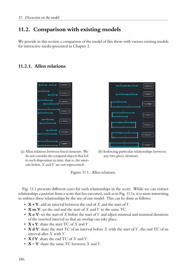
11. Discussion on the model

11.2. Comparison with existing models

We provide in this section a comparison of the model of this thesis with various existing modelsfor interactive media presented in Chapter 2.

11.2.1. Allen relations

(a) Allen relations between fixed elements. Wedo not consider the temporal objects that ledto such disposition in time, that is, the inter-vals before X and Y are not represented.

(b) Enforcing particular relationships betweenany two given elements.

Figure 11.1.: Allen relations.

Fig. 11.1 presents different cases for such relationships in the score. While we can extractrelationships a posteriori from a score that has executed, such as in Fig. 11.1a, it is more interestingto enforce these relationships by the use of our model. This can be done as follows:

• X < Y: add an interval between the end of X and the start of Y .• XmY: set the end and the start of X and Y to the same TC.• X o Y: set the start of X before the start of Y and adjust minimal and maximal durations

of the inserted interval so that an overlap can take place.• X s Y: share the start TC of X and Y .• X d Y: share the start TC of an interval before X with the start of Y , the end TC of an

interval after X with Y .• X f Y: share the end TC of X and Y .• X = Y: share the same TC between X and Y .

186

11.2. Comparison with existing models

K2 K3 K4

Figure 11.2.: Complete graphs.

Figure 11.3.: Scenario equivalent to K4.

11.2.2. Series-parallel models

Multiple models for musical and media composition [202, 204] are based on two base primitives:serial composition and parallel composition. Serial composition of two media objects A and Bcreates a new object which will execute A then execute B. Parallel composition of two mediaobjects A and B creates a new object which will execute A and B at the same time.

However, this restricts the possible compositions: consider the graph G = (V,E) where Vis the set of the beginning and end times of media objects, and E is the set of media objects.Remember that KN is the complete graph with N vertices, that is, the graph where each vertexis connected to every other. Examples are given in fig. 11.2. A single media object is the K2

complete graph: the object lies between its start and end time. A composition built throughrepeated application of serial and parallel composition of K2 graphs forms a series-parallel graph.Series-parallel graphs are exactly graphs constructed through this method.

In particular, any graph which admits a subdivision of K4 as a subgraph is not a series-parallelgraph [205]. This excludes every simple graph with minimum degree greater than 3.

The present model is able to express the K4 graph when considering ICs as vertices andintervals as edges: a construction is provided in fig. 11.3, and thus, a large class of mediacompositions.

11.2.3. Madeus

Madeus extends the Allen relations with three additional relations mentioned in Section 2.1:Parmin(A,B) (the earliest of A and B to end, ends Parmin(A,B)), Parmax(A,B) (the latestof A and B to end, ends Parmax(A,B)), and Parmaster(A,B) (Parmaster(A,B) ends when Aends). These relationships can be recreated with our model, through hierarchical scenarios:

Consider fig. 11.4.

187

11. Discussion on the model

• The Parmin(A,B) case can be done with a variable v, and two intervals ending with astate sending a message on v. The trigger T0 stops when v is received: this will terminatethe execution for the whole structure. Another simpler alternative would be to havetriggers on both A and B’s end, each reacting to v.

• The Parmax(A,B) case can be done with a similar temporal setup. Instead of a singlevariable, each end state in the scenario is associated with its own boolean variable v1, v2which it sets to true. The trigger’s expression is simply v1 ∧ v2.

• The Parmaster(A,B) case can be modelled by a use of hierarchy. Note that a specific usecase given by Layaïda for the use case of Parmaster relationships can be described evenmore simply in our model. The proposed example was using Parmaster to terminate theplayback of a video when a button is pressed. This can simply be implemented in ourmodel by an interval carrying a video-producing process, followed by a trigger reactionon the pressure of such a button.

Figure 11.4.: Example for parmin and parmax Madeus relationships.

This also implies that the proposed model could support SMIL since a translation fromMadeus to SMIL exists [58].

11.3. Potentially incoherent programs and their solutions

An important goal mentioned in Section 3.3.2.2 was the liveness of the system: that is, it mustnot end up in a configuration which would lead to no time interval progressing. The mainproblem occurs when a synchronisation is at the same time requested by the author throughthe introduction of a TC, and impossible because its afferent elements are set up in a way thatprevents them from finishing synchronously. Fig. 11.5 provides an example of such case.

188

11.3. Potentially incoherent programs and their solutions

A B

C

D

(a) A given score.

A B

C

D

(b) A trace of execution for this score: B stopsexecuting early since its max was reached.

Figure 11.5.: A problematic case. A and C can have different durations during the execution,but the end of B and D are synchronised. In this case, the choice made is to stopexecuting the intervals that reached their max duration, and keep executing theothers until their reach their min. The other alternative would be to keep the maxconstraint.

In this case, the policy is to wait until each element has reached its minimal duration to be ableto continue to the next part: conservation of minimal durations is estimated more importantthan early synchronisation. Time will progress in the branches which have not reached theirmin yet. As soon as the min is reached for every afferent interval, the TC is executed. We canassume that if the bounds of an interval are stricter than [0; +∞[, it is due to an explicit choiceof the author which should be prioritized: it means that the interval absolutely has to run untilthe min bound set by the author and must absolutely stop running after the max bound. Thisassumption is done because authors always have the possibility to change these bounds, untilthe removal of the inconsistency.

To reflect on the validity of this solution, we can consider an iterative method: given a scenarioS = (I, C) where I are intervals and C are ICs.

1. Consider the scenario S ′ identical to S, but where all intervals have their min bound setto zero and no max bound. This scenario cannot become incoherent: the execution timeof a given interval is always comprised in [0; +∞[ by definition, hence every reachablestate is a valid state.

2. Now, consider S ′′ where one of the bounds of an interval is set to its value in the originalscenario S. There are two possibilities: either the new, potentially stricter bound doesnot create a possibility of inconsistency, or it does. If it does not, the bound is kept, andthe same process can be applied iteratively to another bound.

3. If S had no possibility of inconsistency, then by repeated application of this process, weobtain S again. Else, we get a scenario similar to S but with at least a min bound left at 0or a max bound left at∞ and no inconsistency.

189

11. Discussion on the model

11.4. Toolbox and common patterns

In this section, we present some common patterns for the usage of the model. We also showthat the model is powerful enough to describe both sequential and loop-based audio sequencingmodels, with only a few elements of the visual syntax.

11.4.1. Reconstructing existing paradigms

(a) A screenshot of the Cubase audio sequencer.Audio and MIDI tracks are arranged hori-zontally, with the possibility of having mul-tiple clips on each track.

(b) Implementation of a two-trackssequencer in our model.

Figure 11.6.: Multi-track sequencing.

In this part we give example of reconstruction of standard audio software behaviours withthe score model: multi-track audio sequencer, looping sequencer and patcher. Both multi-tracksequencers and patchers are commonly used for instance by electro-acoustic music composers,as evidenced by Eaglestone et al. in [1]

Every example has more complexity than the original paradigm it intends to emulate. How-ever, the expressive power is also improved, as shown in Section 11.4.1.4.

11.4.1.1. Audio sequencer

Notable software in this category includes Steinberg Cubase, Avid Pro Tools, …The commonmetaphor for audio sequencers is the track, inspired from mixing desks and tape recorders. Wewill take the example of audio and MIDI tracks. Such an audio sequencer can be modelled by:

190

11.4. Toolbox and common patterns

Cubase Our model

1 audio clip1 interval

1 sound processSilence between audio clips

(no objects)1 interval

1 audio track

1 interval1 scenario process

1 effect chain process1 connection from the scenario output

to the effect chain input1 bus mix effect

1 MIDI track1 virtual instrument

1 interval1 MIDI process

1 effect chain process1 connection from the MIDI output

to the effect chain input1 virtual instrument

1 bus mix effect

Table 11.1.: Semantic elements.

• A root: an infinite interval.• This interval contains two processes: a scenario and an effect bus. The sound output of

the scenario goes to the input of the effect bus.• The scenario contains the actual tracks.• These tracks are also modelled by infinite constraints.Tracks are generally divided in two categories: audio and instrument. Audio tracks are built

with:• A scenario with a single sequence of intervals, some of which may bear sound file processes

and others being empty. The propagate attribute is disabled on the scenario audio output.• An effect bus process. The output of the scenario goes to the input of the effect bus.

Generally, this effect bus would end by channel operations such as panning and volumeadjustment, in a similar fashion to mixing desks.

MIDI tracks are built with:• A scenario with a single sequence of intervals, some of which may bear MIDI notes

processes and others being empty.• An instrument process, which takes MIDI data and outputs sound.• Like before, an effect bus applied to the instrument’s output.This can easily be extended with further features: sends, automations, etc.We can compare the number of strong semantic elements between the target implementation

and our method, in fig. 11.1. we call strong semantic element, an element that the user of theinterface has to set up himself: for instance, an interval must be created by an explicit mousemovement. However, this also creates automatically temporal conditions and states if necessary,which the user does not need to care about if he does not intend to use them.

Fig. 11.6 presents the implementation of two such tracks in the software.

191

11. Discussion on the model

11.4.1.2. Live-looping and hierarchical live-looping

More recently, a different kind of sequencer has emerged: the looping, non-linear sequencer.The prime example of this is Ableton Live. We give the example in fig. 11.7 for a simplified

model of live-looping without quantization.

(a) A screenshot of the Ableton Live audio se-quencer in the session view, which providesa live looping implementation.

(b) Example of an audio live-loopingaudio track implementation inour model.

Figure 11.7.: Live-looping.

These sequencers are also organized in tracks; however, within a track, the musician canchoose a single loop that is currently playing, and regularly switch the current loop.

Hence, the general organization stays the same than for the audio sequencer: most importantly,the way effect buses are applied does not change.

• Each clip of a track is given an index.• Each track has two parameters in the device tree: the next clip to play, /track/N/next of

type int, and the ending, /track/N/end of type pulse. These parameters can be used toenable remote control with specific hardware.

• Both audio and MIDI tracks are intervals containing a scenario process and an effectchain.

• For each clip, an interval with a loop process is inserted in the scenario.• The pattern of the loop processes is given a specific ending temporal condition: pulse /

track/N/end.• Inside the loop pattern, there is a single scenario process. This scenario process has a set

of parallel intervals, each with one sound file.• Every such interval begins with an instantaneous condition that compares the next

parameter to the current clip’s index. Hence, at most one clip is playing at the same timein each track. If the next does not change, the track keeps looping on the sound file.

• These intervals finish with a state which sends the message /track/N/end.

192

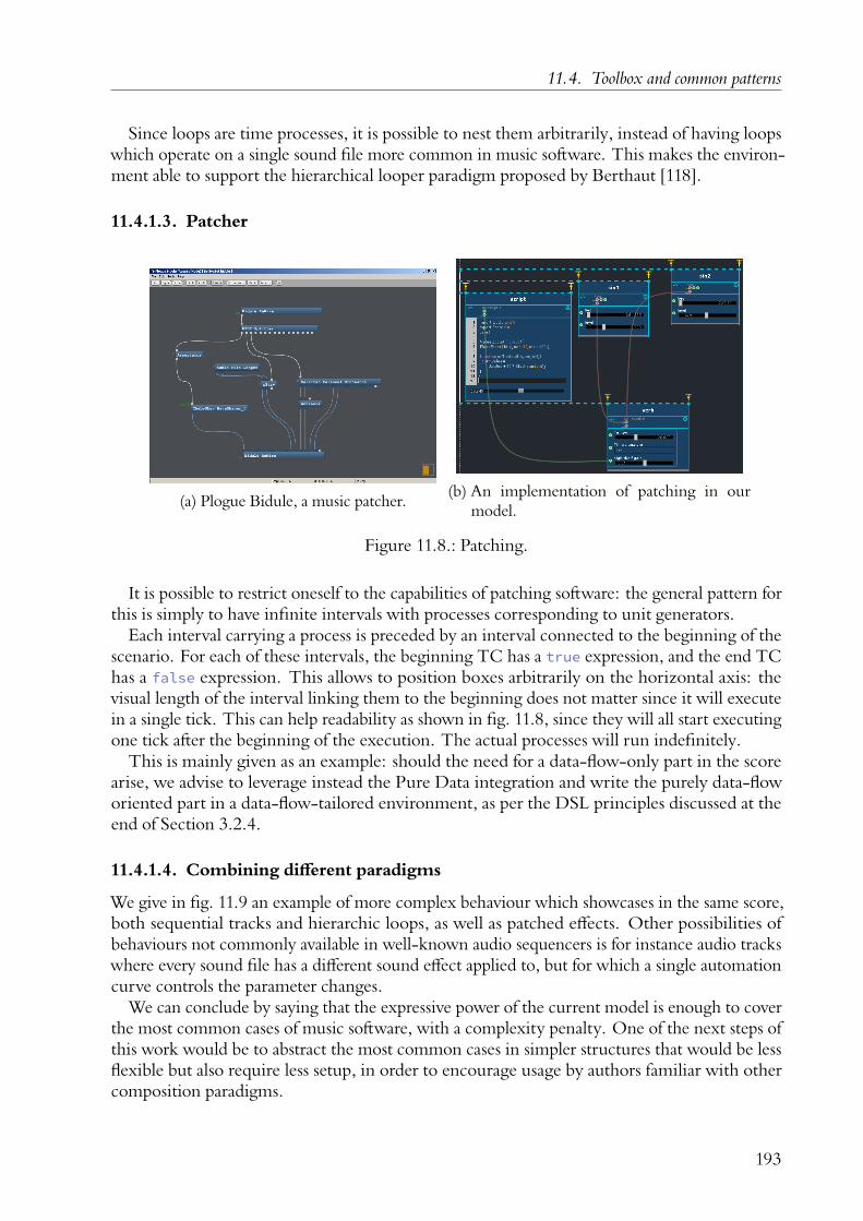
11.4. Toolbox and common patterns

Since loops are time processes, it is possible to nest them arbitrarily, instead of having loopswhich operate on a single sound file more common in music software. This makes the environ-ment able to support the hierarchical looper paradigm proposed by Berthaut [118].

11.4.1.3. Patcher

(a) Plogue Bidule, a music patcher.(b) An implementation of patching in our

model.

Figure 11.8.: Patching.

It is possible to restrict oneself to the capabilities of patching software: the general pattern forthis is simply to have infinite intervals with processes corresponding to unit generators.

Each interval carrying a process is preceded by an interval connected to the beginning of thescenario. For each of these intervals, the beginning TC has a true expression, and the end TChas a false expression. This allows to position boxes arbitrarily on the horizontal axis: thevisual length of the interval linking them to the beginning does not matter since it will executein a single tick. This can help readability as shown in fig. 11.8, since they will all start executingone tick after the beginning of the execution. The actual processes will run indefinitely.

This is mainly given as an example: should the need for a data-flow-only part in the scorearise, we advise to leverage instead the Pure Data integration and write the purely data-floworiented part in a data-flow-tailored environment, as per the DSL principles discussed at theend of Section 3.2.4.

11.4.1.4. Combining different paradigms

We give in fig. 11.9 an example of more complex behaviour which showcases in the same score,both sequential tracks and hierarchic loops, as well as patched effects. Other possibilities ofbehaviours not commonly available in well-known audio sequencers is for instance audio trackswhere every sound file has a different sound effect applied to, but for which a single automationcurve controls the parameter changes.

We can conclude by saying that the expressive power of the current model is enough to coverthe most common cases of music software, with a complexity penalty. One of the next steps ofthis work would be to abstract the most common cases in simpler structures that would be lessflexible but also require less setup, in order to encourage usage by authors familiar with othercomposition paradigms.

193

11. Discussion on the model

Figure 11.9.: An example of more general score, which does not fit exactly in the sequential,live-looping or patcher model.

11.4.2. Methods and tools

In this section, we present smaller individual patterns that can be useful while authoring largerscores.

11.4.2.1. If-then-else and nested conditions

A first example shows how to leverage both IC and TC to perform condition nesting.The construction is as follows: the IC have the expression set as indicated in Fig. 11.10. Both

TC have their expression set to true; the previous intervals have no minimal duration. Hence,at most a tick will pass between the first and the second condition, no matter how long is theinterval visually.

This also showcases how common programming cases of condition can be implemented:• Exclusive if-else is set by having contradictory expressions on two synchronised events:

x = 1 and x ̸= 1

• Exclusive if-else if-else if-... can be supported by nesting sub-cases in the elseclause. Another possibility is to embed the negative conditionals in every IC’s expression,but this can lead to a combinatorial explosion of conditions to write.

• More general non-exclusive pattern matching is possible, as evidenced by the group ofintervals following the conditions on /y. In particular, this leads to the following cases:

– If y < 0: only the fourth interval executes.– If y = 0: no interval executes.– If y = 1: the first and third interval executes.– If y = 3: the second and third interval executes.– For any other value of y, only the third interval executes.

194

11.4. Toolbox and common patterns

Figure 11.10.: Example of if-then-else nesting.

11.4.2.2. Audio part extraction

Figure 11.11.: Applying an effect onlyto specific parts of asound file.

The goal of this part is to show how to apply effectsonly on specific parts of a sound source – for instance, asound file. That is, we want, given a 30-second soundfile, to apply an effect from 10 to 20 seconds, and from25 seconds to the end of the sound.

In order to simplify authoring, in this case we willuse addresses to exchange data. Two addresses are used:/sound and /verb.

The score is as follows: an interval carries three pro-cesses: a sound file, a scenario, and an audio effect. Thescenario contains a sequence of intervals: one from thebeginning to 10 seconds, one from 10 seconds to 20,one from 20 to 25 and one from 25 to the end. Thesound outputs data to the /sound address. The intervalsin the scenario are loaded with a dummy audio mappingprocess which copies its inputs to its outputs.

• For the first (copy1) and the third (copy2) one,the input is set to audio:/sound and the prop-agate attribute is enabled. This means that theaudio will be copied from audio:/sound to theparent hierarchic level when these intervals exe-cute.

• For the second and the fourth one, the input isset to audio:/sound, the output to audio:/verband the propagate attribute is disabled. This

means that the audio will be copied from audio:/sound to audio:/verb when theseintervals execute.

The reverb audio effect input is set to audio:/verb; its output’s propagate attribute is set.

195

11. Discussion on the model

When playing, the sound of the interval goes to the audio mapping processes in sequence:during the first child interval, it goes directly to the parent interval through the mapping process.Then, it goes through the reverb which goes through the parent interval.

Note that for the first segment, since the same audio effect is used for the whole length of thesequence, we keep the reverb queue. However, it is lost at the end of the second case unlessthe top-level interval is set to a duration longer than the sound file’s. A subsequent example,in Section 11.4.2.7, will show a way to solve this.

Finally, the use of addresses has an additional benefit with regards to cable connection: itenables easier copy-pasting of similar structures. While a cable-based approach would requireto explicitly create new cables for each sub-sequence, addresses can be copied and pasted as partof the port data structures.

11.4.2.3. Tempo simulation

One of the simplest use of loops is to build a metronome, shown in Fig. 11.12a.It can be done as follows:• A variable that will receive the pulse needs to be set up; for instance, simply /my/tempo.• The basis is an infinite interval.• A loop process is added to this interval.• The desired tempo has to be converted and be set as the duration of the loop pattern.• The state at the end of the loop pattern will send a message at a regular interval which can

then be leveraged by other processes.

(a) A metronome. (b) An event counter.

Figure 11.12.: Simple patterns.

11.4.2.4. Event counter

This simple example, in Fig. 11.12b shows how to build an event counter: that is, a variable thatincreases every time an event happens.

An address, for instance /count is created: it will carry the count we want to keep. At thebeginning of the score, the count is set to zero by a message. An infinite loop runs. The TCat the end of the loop pattern is set to the expression pulse /message/to/count. The patternhas no minimal nor maximal duration. The state at the end of the pattern contains a processwhich takes for both input and output the /count address, and increments it; a math expressionprocess leveraging the ExprTk library is provided to this end.

196

11.4. Toolbox and common patterns

(a) The implementation of thefixed step sequencer in themodel.

(b) Themessages are sent to thisPure Data patch over thenetwork.

(c) A dynamic step sequencerbuilt on the fig. 11.12ametronome.

Figure 11.13.: Step sequencers.

11.4.2.5. Fixed step sequencer

This example and the following one build on top of the previous examples to provide moreadvanced structures. The first onewill be a rudimentary fixed-duration step sequencer, presentedin fig. 11.13. That is, an object that emits musical notes in a loop at a regular interval.

It is constructed by embedding a scenario in a loop. The duration of the loop pattern is theduration of the whole sequence. The scenario contains a sequence of intervals; the states at thebeginning and between each consecutive intervals holds the note message that must be sent.For instance, given the Pure Data patch in Fig. 11.13, the messages would be akin to /note 12,/note 27, with 12 and 27 being MIDI note numbers.

This first implementation of step sequencing has the advantage of being sample-accurate.However, the composer has to set all the durations explicitly while traditional step sequencersgenerally use a fixed duration for all notes.

11.4.2.6. Dynamic step sequencer

The next example is a step sequencer which opens for more dynamic possibilities: each suc-cessive note will be triggered on reception of a message. For example, we can reuse the earliermetronome object as a trigger source, in the expression of a TC.

Another alternative would be to use an external controller, for instance to trigger each noteon a successive keypress; this would be the first step towards a reimplementation of the Méta-piano[206], a piano-like instrument with only 9 keys which allows to interpret songs by followinga pre-written score.

197

11. Discussion on the model

It is important to note that given the restriction on TC execution dates presented before, thiswill not be sample-accurate in the current implementation, even if the message source is part ofthe score: the note will be activated at the beginning of the following audio buffer.

However, an interesting point is that it is possible to control multiple sequencers with a singletempo source. Another possibility is to introduce rhythmic variations such as syncopation, byreplacing the metronome by a syncopated metronome, which can easily be built by using thesame idea than for the fixed step sequencer.

Figure 11.14.: A constructthat automat-ically stopsreverberation.

These two step-sequencing examples are presented as a tokenof the flexibility of the method at a low level. In practice, for thesake of the ease of use, a step sequencer with a more traditionalinterface is provided as a process.

However, this construct can be useful to provide more ad-vanced behaviours that are not commonly found on step se-quencer objects in other musical environments: for instance, itis possible to automate parameters during the transition betweentwo notes.

11.4.2.7. Auto-stopping reverb

This final construct is a solution to the problem presented inthe audio part extraction example: how to handle reverb cuts.A simple solution would be to leave the reverb running for along time manually by giving a large max to the parent interval,in Fig. 11.11.

However, this can be wasteful in resources: the reverb will keepexecuting its algorithm until the end of the current hierarchicallevel, even though it would only input and output silence.

The example in Fig. 11.14 shows how we can simply use aRMS measure of the signal in order to trigger the end of theparent interval. The only required adjustment is the introduction of an envelope followerprocess, which will measure the running RMS signal during the execution of the process. TheRMS output of the envelope follower is set to a custom address, for instance /track1/rms. Theending TC has for condition /track1/rms < 0.0001 (or any other value adjusted according tothe dynamic range desired by the author; it would however be unwise to force /track1/rms ==0 since some reverberation algorithms could have numerical instabilities in their computations

which could cause the signal to oscillate perpetually around 0).Resource usage could be further optimized: the envelope follower can be inserted in a

scenario instead and be set up to run only when nearing the end of the audio track.

198

11.5. Applications

11.5. Applications

As mentioned at the beginning of this document, the main context in which the model wasdeveloped is at the crossroads of art and science.

In practice, multiple installations and works of art were realised by artists and creators duringthis thesis, in order to define the model and put it and the implementation to trial. In thischapter, we present some of these installations and artistic works.

11.5.1. Open-form piano

In [33], I proposed a musical example inspired from Stockhausen’s Klavierstücke XI, under theform of a collaborative connected experiment at the International Computer Music Conference,in 2016.

The implementation, in Fig. 11.15, follows the general live-looping principle proposedin Section 11.4. The score itself is based on a loop where different MIDI parts can play one at atime, according to the choice of multiple persons connected through their mobile phones.

The score uses multiple devices:• A first device, self, contains local variables: /exit and /count_1 to /count_6.• A MIDI device is used to send the notes to a synthesizer.• A device, ws is used to communicate with a web server.The first state at the beginning of the score resets all the counters to zero.The top-level TC has for condition /count_1 == 2 || /count_2 == 2 || ...: if any part

is played more than twice, the score stops.The pattern TC has for condition pulse /exit. Its state carries a Javascript script process

which is charged from incrementing the play count for each part once it is finished; its code isgiven in Fig. 11.15b.

Each TC at the beginning of parts has for condition /next == i with i the number of thepart. Each state at the end of parts sends the message /exit: when the end of a part is reached,the loop pattern stops and goes back to the beginning of the loop.

The setup uses a Node.js server which hosts a web application to which the participants areconnected. When specific requests are made by the web page, WebSocket messages are sentfrom the Node.js server, to the ws device in the score, in a simple JSON protocol devised for thisexample. The two possible messages are { "speed": k } where k will be a coefficient appliedto the global execution speed of the score, and { "next": n } where n ∈ [1; 6] controls thenext part that will play. The score also sends messages to inform the server from the currentlyplaying part, so that participants can see it on their phone.

199

11. Discussion on the model

(a) The score.

function() {var n = iscore.value('ws:/next');var root = 'self:/part/'return [ {address:

root + 'count_' + n,value:

iscore.value(root + 'count_' + n) + 1},{address:

root + 'next',value: n } ];

}

(b) The script used to update the count.

Figure 11.15.: Score for open-form piano.

200

11.5. Applications

Figure 11.16.: An excerpt of the Nebula score. ©Pascal and Aurélie Baltazar 2015-2017.

11.5.2. Nebula

Nebula is an artistic installation created by the Baltazars: http://www.baltazars.org/project/nebula/. It is based on the control of smoke generators and LEDs. The score, given in Fig. 11.16has no interactivity, lasts for 24 minutes and consists of 217 automations and 295 non-emptystates used to drive a Max/MSP patch through three devices using the Minuit protocol whichin turn controls the smoke generators and LEDs through specific protocols. The score onlyfeatures automations and states: it is a fixed score; the composers were focused on a preciseauthoring of events in time rather than on introducing interactivity.

11.5.3. Metabots

Metabots1 are small quadruped robots, controllable through a custom serial port commandprotocol. A sequence of such commands could be, for instance:

Command Meaning

dx 2 Set lateral speed at 2cm s−1.dy -3 Set forward speed at −3cm s−1.crab Invert the leg joints as to walk like a crab.

Experiments have been made to use metabots as music instruments by leveraging soundsmade by the robot’s displacements. One of such experiments is portrayed in fig. 11.17. Thescore mainly consists of various mappings from a joystick to commands sent to the robot; thesemappings evolve in time.

There are two devices:

1http://www.metabot.fr

201

11. Discussion on the model

(a) The hardware set-up: a joystick and a Metabot.

(b) The score: multiple mappings between the joystick controls and theMetabot commands evolve in time. In the first part of the score, some map-pings are written in Javascript, and others with visual mapping functions.In the second part of the score, some controls of the Metabot are enforceddirectly with automations, while some mappings change.

Figure 11.17.: Controlling a Metabot with a joystick whose mappings evolve in time. ©ThibaudKeller, Edgar Nicouleau 2017.

202

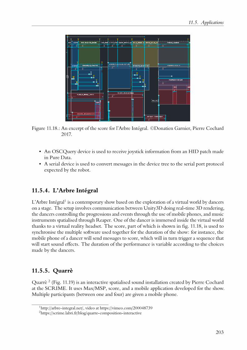
11.5. Applications

Figure 11.18.: An excerpt of the score for l’Arbre Intégral. ©Donatien Garnier, Pierre Cochard2017.

• An OSCQuery device is used to receive joystick information from an HID patch madein Pure Data.

• A serial device is used to convert messages in the device tree to the serial port protocolexpected by the robot.

11.5.4. L’Arbre Intégral

L’Arbre Intégral1 is a contemporary show based on the exploration of a virtual world by dancerson a stage. The setup involves communication between Unity3D doing real-time 3D rendering,the dancers controlling the progressions and events through the use of mobile phones, and musicinstruments spatialised through Reaper. One of the dancer is immersed inside the virtual worldthanks to a virtual reality headset. The score, part of which is shown in fig. 11.18, is used tosynchronise the multiple software used together for the duration of the show: for instance, themobile phone of a dancer will send messages to score, which will in turn trigger a sequence thatwill start sound effects. The duration of the performance is variable according to the choicesmade by the dancers.

11.5.5. Quarrè

Quarrè 2 (Fig. 11.19) is an interactive spatialised sound installation created by Pierre Cochardat the SCRIME. It uses Max/MSP, score, and a mobile application developed for the show.Multiple participants (between one and four) are given a mobile phone.

1http://arbre-integral.net/, video at https://vimeo.com/2000487392https://scrime.labri.fr/blog/quarre-composition-interactive

203

11. Discussion on the model

(a) The installation; participants take place in the center of the loud-speaker circle.

(b) One scene of the score.

Figure 11.19.: Quarrè. ©Pierre Cochard 2016 – 2018.

204

11.5. Applications

Figure 11.20.: An excerpt of the score for the “Nuit des Chercheurs”.

The performance lasts for half an hour. At different moments during the show, the mobileapplications of some participants show that some interactions are available. The possible actionsvary according to the number of participants. The app warns them with a countdown a fewseconds before their next interaction. They then have a definite duration to interact: they canchange the parameter of an effect (such as chorus, distortion), trigger new sounds, or spatialise asound object.

For instance, between t = 1m30 et t = 2m, two attendees will be able to change the intensityof a chorus effect, while two other will be able to move a sound object in the spatial scene.

This project has been an important pathway towards the distribution work presented in Chap-ter 9, by giving practical cases of distribution across multiple mobile devices.

Besides, we can note in this score an effective use of hierarchy, for splitting the show inmultiple distinct acts. Few processes are used: most controls are done live by the participants.

11.5.6. La Nuit Des Chercheurs

La Nuit Européenne des Chercheurs is a french event where the public can meet researchers invarious domains. For this occasion, in 2017, a score showcasing recent advances was made: it isvisible in fig. Fig. 11.20. It is an example of research centered about the notion of distribution.One computer is at the SCRIME, located in Bordeaux; another is at the GMEA located at Albi,300 kilometers to the south-east. Both laboratories have sound spatialisation apparatus set up: adome at the SCRIME, and a wavefield synthesis system at the GMEA.

In the score, participants in both cities will control spatialised sounds according to the score,which is split in two scenes which each convey a different musical imagery. The objects and thecontrols vary in time: for instance, during the first scenery, Albi controls a sound for at most oneminute, then Bordeaux controls another sound, then Albi takes the control back. Triggers allowone city to give back the control to the other city when they decide to with this one minutelimitation. Some parts are shared between both places: the beginning, transition and ending ofthe score are driven by fade-ins and fade-outs.

205

11. Discussion on the model

11.5.7. Carrousel

The Carrousel Musical (in fig. 11.21) is an example of large-scale musical instrument built withossia score by the company Blue Yeti, for the Musical City of the Abbaye aux Dames in Saintes,France.

Each seat on the carrousel has different instrument-like input devices: reactive pads, motionsensors, etc. A run in the carousel generally operates as follows:

• The first few seconds, the rules of the carousel are explained to the participants. Theycan play with their instrument for a minute.

• The song starts: the passengers can start interacting with their instruments. An overallmusic is generated from their interpretation. Played notes stay in predefined scales whichmay vary over time; pre-recorded parts can also be layered on top. The overall songstructure can vary according to the intensity of the played music: for instance, if everyoneplays piano, different instruments may become available in the next section of the song, apart may be shorter or longer, etc. Such variations are written by the composer for eachsong.

• At the end of the song, the participants hear a summarized version of the song they justplayed, with the best parts being highlighted. This version also has additional correctionsand adjustments applied algorithmically: for instance, more quantization.

This project, being one of the most recent being done with the system, leverages most of thework presented earlier: in particular, static and address connections, and buffered connections.The score is built around multiple tracks, each corresponding to an instrument; in addition, aglobal scenario gives informations such as intensity and tempo. This is visible in part in fig. 11.22.

In each track, there is:

• A MIDI piano roll which gives the notes that the performer is allowed to play at a giventime.

• A MIDI piano roll which gives the notes that should be played in case no performer iscurrently on the seat, or if there is no musical input for a long time.

• A Javascript script which combines inputs from both piano rolls and from anOSCmessage,to produce the MIDI note which will be played.

• The script is connected to an effect chain, which performs quantization, sound generationthrough the virtual instruments Kontakt™and Battery™from Native Instruments™, anddynamic compression.

• Each effect chain for individual instruments has its main output going to a main effectchain: the global mix bus, which is then spatialised through 8 loudspeakers with a Faustscript.

• The output of the virtual instruments is also sent to another effect chain for each instrumentbefore dynamic compression: in addition of the 8 main loudspeakers, each musician has acustom monitoring where he hears only his own sound.

An example of such a track is given in fig. 11.23.

206

11.5. Applications

Figure 11.21.: Inside the carrousel. L’Abbaye aux Dames, Saintes, France.

207

11. Discussion on the model

Figure 11.22.: General temporal logic in one of the scores for the carrousel, “Gatebourse”.The same-sized intervals on top contain the handling of each instrument. Theintervals and ICs in the middle of the score handle the changes of volumes, andthe different states of the song: demo mode, play mode, restitution.

Figure 11.23.: One of the instruments of the carrousel in the score “Baroque Électro”. Thevirtual instrument changes at some point in the score: it starts as a piano, andcontinues as an electric organ.

208

11.6. Conclusion

11.6. Conclusion

The aforementioned installations were all done at different research and development statesof this work. For instance, Nebula, one of the earliest long-lasting score produced with theproposed environment, does not use a wide variety of processes, and does not leverage anyinteractive features. More recent scores expand the vocabulary used.

From the statistics in Appendix E and Appendix F, and a study of these scores, we can extractmultiple informations about the composition process of the scores:

• Composers indeed make use of hierarchical nesting, as suggested by the existing researchin creativity. In particular, the author of the Metabot scores, Thibaud Keller, reportedan explicit focus on the automatic hierarchisation features (presented in Section 8.2.4)during the authoring process.

• Scores can vary in scales ranging from entirely fixed (Nebula) to mostly interaction-driven(Voyage).

• Most scores refer to multiple external software or hardware devices and create mappingsbetween these devices during the execution. Further research would be warranted in thisarea: in particular, the research field of instrumental interaction can provide insights onhow to ease the creation of such mappings between controllers and controlled elements,and how to relate such mappings with interactive music [207, 208].

• Most scores make an extensive use of documentational features of the environment:explicit naming of objects, labels, floating comment boxes for instance to indicate theactions to take during the playback or details on the score.

• Some scores are more instant-based while others are more interval-based: that is, somescores rely on successive punctual events happening, while other scores use evolvingbehaviours such as automations and other processes. We can for instance take as a metricthe ratio of non-empty state over non-empty interval: the highest it is, and the moreinstant-based the score is.

• Some capabilities were not used at all, by any author: for instance, char types in the devicetree. Likewise, as expected the most common data type is the float type, followed bythe int type and list type, as can be seen in Fig. E.1 in Appendix E. This should be adeciding factor for optimizations.

209

Part V.

Conclusion

210

12Concluding remarks

This thesis introduced a new model for multimedia software and ISs. A major focus is put onthe relationship between ISs and their surrounding environment: other software and hardware.In order to provide new possibilities to the authors of such scores, a DFG allowing to performcomputations between the processes occurring in the score is introduced. In comparison withexisting approaches, nodes of the graph are allowed to interoperate with the environment directlythrough the use of addresses representing specific data in the environment. Variables of thisenvironment can indistinctly refer to local or remote objects: this allows ISs and more generallyinteractive applications to be authored using an abstraction of the various software and hardwarewhich will produce the media content. Unlike previous approaches for interactive scores, wedo not only rely on external entities to perform audio-visual generation and processing: theimplementation, based on a plug-in approach, can act as an autonomous media sequencer toproduce output. This ensures more rigorous synchronisation between distinct audio and mediaprocesses, since we can rely on precise timing deadlines due to buffer-synchronous operation.

The proposed temporal model, inspired from the various artistic considerations on thenotion of open works, diverges from previous research in the field of interactive scores andinteractive media in that it does not seek to ensure that the scores written by authors arealways temporally coherent. In particular, we consider that while mistakes during the authoringphase are possible, preventing the execution of the score due to invalid constraints would bedetrimental to the authoring and creative process. Hence, the temporal model instead allowsfor temporal constraints to be sometimes unsatisfied, while still providing a relevant behaviourdefined during interactions and exchanges with domain experts: artists, multimedia developers.However, it is still possible to translate part of our model into formally verifiable semantics asan off-line process: for instance, time automatas as defined by Arias [7] can be used to asserttemporal properties on the scores of the model, even though the current algorithmic cost of thisprocess makes it hard to set-up for large scores. A visual language is proposed for this model.Its objects are directly based onthe structures that are executed, which allows easier debuggingand visualization of program state: while using an operational model for execution opens thedoor to reuse of well-known semantics and analysis tools, it also means that there can be bugs attwo different levels: the implementation of the operational model itself (for instance colouredPetri nets), and the visual model itself. Finally, an extension to distributed environments isintroduced: scores can be written not only for one machine, but for a group – or, may we say, anorchestra – of machines which will execute their processes locally and synchronise temporallywith the others in the fashion required by the author.

212

12.1. Perspective: a declarative language for authoring

12.1. Perspective: a declarative language for authoring

Authoring in the system can currently be done in two ways: either through the graphicalinterface of score, or through the C++ API directly. We believe that it can be relevant to be ableto specify scores in a textual general-purpose programming language: in particular, we proposethe use of the QML language to enable the creation of interactive media presentations whichwould allow self-mutating behaviours: for instance, creating a new element in the score everytime the ending of an interval is reached. More generally, this would free the environment fromconstraints necessary in the visual syntax. Some work has already been engaged in order tofind a suitable syntax. The next steps are the integration of the QML environment with thereactive edition loop: the QML script would be seen by the execution engine exactly like theuser modifying the score in the visual interface during an execution. A short example QMLscript is provided afterwards. It models a IC followed by a TC. Every time the TC is triggeredbefore the end of the interval, the interval’s maximum duration increases by two seconds:

Ossia.Sync {id: sync0Ossia.Condition {

id: cond0expression: function() { return Math.rand() > 0.5; }onHappened: itv.max += 2s

}}Ossia.Interval {

id: itvmin: 4sdefault: 6smax: 7sfollows: cond0precedes: sync1group: "video"

}

12.2. Perspective: distribution of the data graph

The distribution research covers only the execution of the temporal tree: both the device treeand the data graph are not taken into account. The next step for this work is to provide accuratetranslations of these models in the distributed space: how can data production be combinedacross machines ?

12.3. Perspective: abstractions in the environment

The visual language currently lacks a way for an author to provide parametrizable abstractions. Itis possible to have “presets” by means such as copy-paste, however, there is no way to repurposeeasily a hierarchical part of the score according to a variable: for instance one could want to copya scenario ten times to make a musical canon, but with each scenario operating on a differentset of instruments. Currently, this requires the author to copy and change the used instrument– for instance a node in the device tree – in every place in which it could be referenced in thescenario.

213

12. Concluding remarks

12.4. Perspective: scoping

Three levels of scoping are supported in the current work: connection scope, local scope, andglobal scope. It has been proposed to link elements of the temporal tree to the notion of scope,in order to make scope of processes a visual element.

12.5. Perspective: spatial representation and reasoning

Interactive media taken at large generally covers the concept of spatial relationship betweenobjects. Some approaches have been explored by the author [35], under the form of specificprocesses. Further work would be warranted in this area to extend the current model todimensions other than time: for instance, intervals could be considered asN-dimensional sphereswith a variable radius, where the position of an interactor in N-dim defines the triggering of TCs.

12.6. Perspective: formal usability studies

As in many visual language environments presented in the literature, most of the argumentsin favour of it are empirical: we can attest that the current incarnation of the language enablescomposers to easily create media art thanks to the artistic production realised with it. In order toimprove on it, the next step would be to apply one of the existing analysis framework proposed inscientific literature, and devise relevant metrics to compare different interactive score authoringsystems in terms of efficiency of artistic production. As a starting point, the measures made onexisting scenarios and referenced in Appendix E could be used, to study more precisely how theauthors are using the software.

12.7. Perspective: real-time transport

Another point not discussed is a GOTO-like mechanism to change the playhead position atrun-time in the score. A first step towards this direction is the content of Section 8.4: the abilityto execute a score with an offset. Of particular interest to the users of the software is the visualrepresentation of this concept in a score.

214

Glossary

API Application Programming Interface. 18, 65, 151, 155, 162, 170, 171, 214ARGB Alpha-Red-Green-Blue. 61, 64, 214automation Term used to denote the variation of a parameter over time following a given

curve. 48, 214

BGR Blue-Green-Red. 61, 214

client In the distributed score model, an individual instance of score connected to a networksession. 137, 214

condition In the visual model, an object which represents an instantaneous condition with anactive expression. 118, 214

CORBA Common Object Request Broker Architecture. 19, 214CTL Computational Tree Logic. 38, 214

DAG Directed Acylic Graph. 29, 33, 96, 132, 140, 214DCOP Desktop COmmunication Protocol. 19, 214DFG Data-flow Graph. 21, 22, 36, 37, 54, 66, 73, 74, 86, 90, 185, 212, 214DMX Digital Multiplexing. 46, 57, 214DSL Domain-Specific Language. 10, 40, 193, 214

easing function Specific mathematical functions often used in artistic applications for transi-tions and smooth movement of objects. See http://easings.net for a list. 48, 214

ECS Entity Component System. 169, 214

Faust Functional Audio Stream, a programming language for signal processing. 40, 214fermata In music, an indication that a particular note may be played for a longer duration than

the one written on the sheet. 5, 214FIFO First-In First-Out, a common model for data exchange. 21, 75, 214FPGA Field-Programmable Gate Array. 214future In programming, a future is a way to encode the result of an asynchronous computation:

when the computation is done, the future can be used to perform an action on its result.62, 214

GLSL GL Shading Language. 40, 214group In the distributed score model, a virtual set of clients. 137, 214

HLL Hierarchical Live-Looping. 29, 45, 214HTSPN Hierarchical Time Stream Petri Net. 34, 214HTTP Hyper-Text Transfer Protocol. 19, 151, 160–162, 164, 214

inlets Input ports of a node in a data graph. 67, 68, 214IS Interactive Score. 4–6, 9, 12, 32, 33, 36, 51, 56, 92, 212, 214

JavaScript A programming language mainly used in web browsers. 153, 162, 163, 214JSON JavaScript Object Notation. 160–163, 165, 199, 214

216

Glossary

leap second Seconds introduced or deleted regularly in the legal hours systems to compensatefor the divergence between the terrestrial rotation and the UTC time. UTC time isobtained by measuring the resonance frequency of cesium atoms, which allows to preciselydefine the duration of a second. A leap second was for example introduced on December31, 2016 after 23:59 and 59 seconds. Their introduction regularly disrupts distributedsystems based on physical clocks: it is possible that two successive calls to the systemfunctions giving the wall clock time return dates in the reverse order that expected, whichmakes the duration computations incorrect.. 214

MIDI Musical Instrument Digital Interface. 36, 46, 56, 57, 63, 66, 70, 71, 124, 151, 157, 158,162, 171, 190–192, 197, 199, 206, 214

Minuit An OSC-based query protocol, discussed in Section 10.1.6.3. 151, 160–162, 201, 214MVC Model-View-Controller. 19, 214

NTCC Non-deterministic Temporal Concurrent Constraints. 32, 214NTP Network Time Protocol. 31, 143, 214

ORB Object Request Broker. 19, 214OSC Open Sound Control. 36, 46, 56, 57, 63–65, 70, 72, 82, 87, 137, 151, 158–162, 164,

214OSCQuery An OSC and WebSocket-based query protocol, discussed in Section 10.1.6.4. 63,

65, 151, 157, 160–162, 214OSI Open Systems Interconnection model. 162, 214ossia In music, a section which can be played in place of another. 5, 214outlets Output ports of a node in a data graph. 67, 68, 214

PTP Precision Time Protocol. 31, 214

QML Qt Markup Language. 40, 162, 214

REST Representational State Transfer. 162, 214RGB Red-Green-Blue. 60, 61, 64, 88, 214RMS Root mean square: in audio, a way to compute the average value of a signal over a short

span of time. 79, 214RPC Remote Procedure Calls: environments able to provide function or method calls across

processes or networks. 65, 214RTSP Real-Time Streaming Protocol. 19, 214

session In the distributed score model, a score and the set of clients connected together inorder to execute this score. 137, 214

SGML Standard Generalized Markup Language. 17, 214SIMD Single Instruction Multiple Data. 69, 214SMDL Standard Music Description Language. 17, 214SMIL Synchronized Multimedia Integration Language. 18, 19, 214state In the visual model, an object which represents a set of instantaneous actions to be

executed by the score at a given point in time.. 116, 214

TC Time Constraint. 214TCC Temporal Concurrent Constraints. 32, 214

217

Glossary

TCP Transmission Control Protocol. 156, 159, 160, 214TP Time Process. 214trigger In the visual model, an object which represents a temporal condition with an active

expression. 118, 214

UDP User Datagram Protocol. 31, 82, 156, 159, 160, 162, 214

WebSocket A bidirectional communication protocol available for use in web pages. 151, 159,160, 162–164, 199, 214

WIMP Windows, Icons, Menus, Pointer, a standard method for human-machine interfacedesign. 9, 214

XML eXtensible Markup Language. 18, 20, 63, 214XPath An expression language used to locate objects in a XML document. 63, 214XSLT eXtensible Stylesheet Language Transformations. 19, 214

218

Bibliography

1. Eaglestone, B., Ford, N., Brown, G. J. & Moore, A. Information Systems and Creativity:An Empirical Study. Journal of Documentation 63, 443–464 (2007).

2. Turner, G. & Edmonds, E. Towards a Supportive Technological Environment for Digital Art inProceedings of the Annual conference of the Computer-Human Interaction, Special Interest Group ofthe Ergonomics Society of Australia. (Brisbane, Australia, 2003).

3. Resnick, M., Myers, B., Nakakoji, K., Shneiderman, B., Pausch, R., Selker, T. &Eisenberg, M. Design Principles for Tools to Support Creative Thinking in Proceedings of theNSF Workshop on Creativity Support Tools (Washington, USA, 2005).

4. Desainte-Catherine, M., Allombert, A. & Assayag, G. Towards a Hybrid TemporalParadigm forMusical Composition and Performance: TheCase of Musical Interpretation.Computer Music Journal 37, 61–72 (2013).

5. Allombert, A.Aspects temporels d’un système de partitions musicales interactives pour la compositionet l’interprétation PhD thesis (Université de Bordeaux, France, 2009).

6. Toro, M. Structured Interactive Scores: From a simple structural description of a multimedia scenarioto a real-time capable implementation with formal semantics PhD thesis (Université Bordeaux I,France, 2012).

7. Arias, J. Formal Semantics and Automatic Verification of Hierarchical Multimedia Scenarios withInteractive Choices PhD thesis (Université de Bordeaux, France, 2015).

8. Arumı, P., Garcıa, D. & Amatriain, X. A Dataflow Pattern Catalog for Sound and MusicComputing in Proceedings of the Pattern Languages of Programs Conference (PLoP) (Portland,USA, 2006).

9. Place, T., Lossius, T. & Peters, N. The Jamoma Audio Graph Layer in Proceedings of theInternational Conference on Digital Audio Effects (DaFX) (Graz, Austria, 2010).

10. Desainte-Catherine, M. & Allombert, A. Interactive Scores: A Model for SpecifyingTemporal Relations between Interactive and Static Events. Journal of New Music Research34, 361–374 (2005).

11. Place, T. A. & Lossius, T. Jamoma: A Modular Standard for Structuring Patches in Max inProceedings of the International Computer Music Conference (ICMC) (New Orleans, USA,2006).

12. Place, T., Lossius, T. & Peters, N. A Flexible And Dynamic C++ Framework And LibraryFor Digital Audio Signal Processing in Proceedings of the International Computer Music Conference(ICMC) (New York, USA, 2010).

13. Baltazar, P., Allombert, A., Marczak, R., Couturier, J.-M., Roy, M., Sèdes, A. &Desainte-Catherine, M. Virage: Une réflexion pluridisciplinaire autour du temps dans la créationnumérique in Proceedings of the Journées d’Informatique Musicale (JIM) (Grenoble, France,2009).

14. Howard, T. J., Culley, S. J. & Dekoninck, E. Describing the Creative Design Processby the Integration of Engineering Design and Cognitive Psychology Literature. Designstudies 29, 160–180 (2008).

220

Bibliography

15. Eco, U. The Open Work translated by Cancogini, A. (Harvard University Press, 1989).

16. Bonardi, A. & Barthélemy, J. Le patch comme document numérique: support de création etde constitution de connaissances pour les arts de la performance in Proceedings of the ConférenceInternationale sur le Document Électronique (Nancy, France, 2007).

17. Guigue, D. & Trajano de Lima, E. La répartition spectrale comme vecteur formel dans laKlavierstück n.11 de Stockhausen (ed Musimédiane) http : / /www.musimediane .com/numero4/Guigue-Trajano/.

18. Vaggione, H. Some Ontological Remarks about Music Composition Processes. ComputerMusic Journal 25, 54–61 (2001).

19. Dixon, S. Digital Performance: A History of New Media in Theater, Dance, Performance Art,and Installation (MIT press, 2007).

20. Krueger, M. W. Responsive Environments in Proceedings of the National Computer Conference(Dallas, Texas, 1977), 423–433.

21. Allombert, A., Assayag, G. & Desainte-Catherine, M. A System of Interactive Scores Basedon Petri Nets in Proceedings of the Sound and Music Computing Conference (SMC) (Lefkada,Greece, 2007).

22. Bohnacker, H., Gross, B., Laub, J. & Lazzeroni, C. Generative Design: Visualize, Program,and Create with Processing (Princeton Architectural Press, 2012).

23. Bach, A. Aesthetics Of Post-Internet Electronic Music in Proceedings of the International ComputerMusic Conference (ICMC) (Shanghai, China, 2017).

24. Magnusson, T. Algorithms As Scores: Coding Live Music. Leonardo Music Journal 21,19–23 (2011).

25. Magnusson, T. The Threnoscope: A Musical Work for Live Coding Performance in Proceedings ofthe InternationalWorkshop on Live Programming, International Conference on Software Engineering(ICSE) (San Francisco, USA, 2013).

26. Meikle, G. Examining the Effects of Experimental/academic Electroacoustic and PopularElectronic Musics on the Evolution and Development of Human–computer Interactionin Music. Contemporary Music Review 35, 224–241 (2016).

27. Spinellis, D. Notable Design Patterns for Domain-specific Languages. Journal of systemsand software 56, 91–99 (2001).

28. Celerier, J.-M., Baltazar, P., Bossut, C., Vuaille, N., Couturier, J.-M., et al. OSSIA:Towards a Unified Interface for Scoring Time and Interaction in Proceedings of the InternationalConference on Technologies for Music Notation and Representation (TENOR) (Paris, France,2015).

29. Celerier, J.-M., Desainte-Catherine, M. & Couturier, J.-M. Rethinking the Audio Work-station: Tree-based Sequencing with i-score and the LibAudioStream in Proceedings of the Soundand Music Computing Conference (SMC) (Hamburg, Germany, 2016).

30. De La Hogue, T., Celerier, J.-M. & Baltazar, P. Présentation D’un Formalisme GraphiquePour L’écriture De Scénarios Interactifs in Proceedings of the Journées d’Informatique Musicale (JIM)(Albi, France, 2016).

221

Bibliography

31. Losco-Lena, M. in Faire théâtre sous le signe de la recherche (Presses Universitaires de Rennes,2017).

32. Arias, J., Celerier, J.-M. & Desainte-Catherine, M. Authoring and Automatic Veri-fication of Interactive Multimedia Scores. Journal of New Music Research 46, 15–33 (12016).

33. Celerier, J.-M., Desainte-Catherine, M. & Couturier, J.-M. Graphical Temporal StructuredProgramming for Interactive Music in Proceedings of the International Computer Music Conference(ICMC) (Utrecht, The Netherlands, 2016).

34. Celerier, J.-M., Desainte-Catherine, M. & Couturier, J.-M. Extending Dataflow with Tem-poral Graphs in Proceedings of the International Computer Music Conference (ICMC) (Shanghai,China, 2017).

35. Celerier, J.-M., Desainte-Catherine, M. & Couturier, J.-M. Outils d’écriture spatiale pourles partitions interactives in Proceedings of the Journées d’InformatiqueMusicale (JIM) (Albi, France,2016).

36. Celerier, J.-M., Desainte-Catherine, M. & Couturier, J.-M. Exécution Répartie De Scé-narios Interactifs in Proceedings of the Journées d’Informatique Musicale (JIM) (Paris, France,2017).

37. Celerier, J.-M. Leveraging Domain-specific Languages in an Interactive Score System in Proceed-ings of the Acoustical Society of Japan Regular Meeting (JSSA) (Tokyo, Japan, 2018).

38. Arias, J., Desainte-Catherine,M.&Dubnov, S.Automatic Construction of InteractiveMachineImprovisation Scenarios from Audio Recordings in Proceedings of the International Workshop onMusical Metacreation (MUME) (Paris, France, 2016).

39. Miranda, E., Antoine, A., Celerier, J.-M. & Desainte-Catherine, M. i-Berlioz: InteractiveComputer-AidedOrchestration with Temporal Control in Proceedings of the International Conferenceon New Music Concepts (ICNMC) (Turin, Italy, 2018).

40. Antoine, A., Miranda, E., Celerier, J.-M. & Desainte-Catherine, M. Generating OrchestralSequences with Timbral Descriptors in Proceedings of the Timbre Conference (Montréal, Canada,2018).

41. Blakowski, G. & Steinmetz, R. A Media Synchronization Survey: Reference Model,Specification, and Case Studies. IEEE Journal on Selected Areas in Communications 14, 5–35(1996).

42. Allen, J. F. Maintaining knowledge about temporal intervals. Communications of the ACM26, 832–843 (1983).

43. Vilain, M., Kautz, H. & Van Beek, P. Constraint propagation algorithms for temporal reasoning:A revised report in Proceedings of the National Conference on Artificial Intelligence (Philadelphia,USA, 1986).

44. Giasson, F., Raimond, Y., Abdallah, S. & Sandler, M. The Music Ontology in Proceedings ofthe International Society for Music Information Retrieval Conference (ISMIR) (Vienna, Austria,2007).

45. Goldfarb, C. F. Hytime: A Standard for Structured Hypermedia Interchange. Computer24, 81–84 (1991).

222

Bibliography

46. SMDL, ISO. IEC, Standard Music Description Language. ISO/IEC DIS 10743 (1995).

47. Good, M. MusicXML: An internet-friendly format for sheet music in Proceedings of the XMLEdge2001: International XML Conference & Expo (Orlando, USA, 2001).

48. Bulterman, D. C. A. & Rutledge, L. W. SMIL 3.0: Flexible Multimedia for Web, MobileDevices and Daisy Talking Books (Springer, 2008).

49. Chung, S. M. & Pereira, A. L. Timed Petri Net Representation of SMIL. IEEE Multi-Media 12, 64–72 (2005).

50. Schäfer, R. MPEG-4: A Multimedia Compression Standard for Interactive Applicationsand Services. Electronics & communication engineering journal 10, 253–262 (1998).

51. Ackermann, P. Direct Manipulation of Temporal Structures in a Multimedia Application Frame-work in Proceedings of the International Conference on Multimedia (ACMMM) (ACM, SanFrancisco, USA, 1994), 51–58.

52. Hirzalla, N., Falchuk, B. & Karmouch, A. A Temporal Model for Interactive MultimediaScenarios. IEEE MultiMedia 2, 24–31 (1995).

53. Song, J., Ramalingam, G., Miller, R. & Yi, B.-K. Interactive Authoring of MultimediaDocuments in a Constraint-based Authoring System. Multimedia Systems 7, 424–437(1999).

54. Vazirgiannis,M., Kostalas, I. & Sellis, T. Specifying andAuthoringMultimedia Scenarios.IEEE MultiMedia 6, 24–37 (1999).

55. Meixner, B. Hypervideos and Interactive Multimedia Presentations. ACM ComputingSurveys 50, 9 (2017).

56. Layaıda, N. Madeus: Système d’édition et de présentation de documents structurés multimédia PhDthesis (Université Joseph-Fourier, Grenoble I, France, 1997).

57. Sabry Ismail, L. Schéma d’exécution pour les documents multimédia distribués PhD thesis(Université Joseph-Fourier, Grenoble I, France, 1999).

58. Villard, L. Modèles de documents pour l’édition et l’adaptation de présentations multimédias PhDthesis (Institut National Polytechnique de Grenoble, France, 2002).

59. Tardif, L. Kaomi: réalisation d’une boıte à outils pour la construction d’environnements d’édition dedocuments multimédias PhD thesis (Institut National Polytechnique de Grenoble, France,2000).

60. Lossius, T., de la Hogue, T., Baltazar, P., Place, T. A., Wolek, N. & Rabin, J. Model-view-controller separation in Max using Jamoma in Proceedings of the Joint International ComputerMusic Conference (ICMC) / Sound and Music Computing Conference (SMC) (Athens, Greece,2014).

61. Taylor, B. & Allison, J. BRAID: A Web Audio Instrument Builder with Embedded Code Blocksin Proceedings of the International Web Audio Conference (Paris, 2015, 2015).

62. Love, R. Get on the D-BUS. Linux Journal (2005).

63. Peterson, J. L. Petri Net Theory and the Modeling of Systems (Prentice Hall, 1981).

64. Halang, W. A., Pereira, C. E. & Frigeri, A. H. Safe Object Oriented Programming of Dis-tributed Real Time Systems in PEARL in Proceedings of the International Symposium on Object-Oriented Real-Time Distributed Computing (Magdeburg, Germany, 2001).

223

Bibliography

65. Dennis, J. B. First Version of a Data Flow Procedure Language in Proceedings of the ProgrammingSymposium – Colloque Sur La Programmation (Springer-Verlag, Paris, France, 1974).

66. Lee, E. A. & Parks, T. M. Dataflow process networks. Proceedings of the IEEE 83, 773–801 (1995).

67. Kahn, G. & Macqueen, D. Coroutines and Networks of Parallel Processes Research Report(Institut National de Recherche en Informatique et Automatique, 1976).

68. Bempelis, E. Boolean Parametric Data Flow Modeling-Analyses-Implementation PhD thesis(Université Grenoble Alpes, France, 2015).

69. Bhattacharyya, S. S., Deprettere, E. F., Leupers, R. & Takala, J. Handbook of SignalProcessing Systems (Springer, 2013).

70. Backus, J. Can Programming Be Liberated from the Von Neumann Style? A FunctionalStyle and Its Algebra of Programs. Communications of the ACM 21, 613–641 (1978).

71. Elliott, C. & Hudak, P. Functional reactive animation. ACM Special Interest Group onProgramming Languages Notices 32, 263–273 (1997).

72. Hudak, P., Courtney, A., Nilsson, H. & Peterson, J. in Advanced Functional Programming:4th International School. Revised Lectures (eds Jeuring, J. & Jones, S. L. P.) 159–187 (Springer,2003).

73. Halbwachs, N. Synchronous programming of reactive systems (Springer, 2013).

74. Halbwachs, N., Caspi, P., Raymond, P. & Pilaud, D. The Synchronous Data FlowProgramming Language LUSTRE. Proceedings of the IEEE 79, 1305–1320 (1991).

75. Benveniste, A., Caspi, P., Le Guernic, P. & Halbwachs, N. Data-flow Synchronous Lan-guages in Proceedings of the Symposium of the REX (Research and Education in ConcurrentSystems) Project (Noordwijkerhout, The Netherlands, 1993).

76. Santos, R. C. M., Lima, G. F., Sant’Anna, F. & Rodriguez, N.CÉU-MEDIA: Local Inter-Media Synchronization Using CÉU in Proceedings of the Brazilian Symposium on Multimediaand the Web (Teresina, Brazil, 2016).

77. Bullock, J. & Frisk, H. The Integra Framework for Rapid Modular Audio Application Develop-ment in Proceedings of the International Computer Music Conference (ICMC) (Huddersfield,England, 2011).

78. Donat-Bouillud, P., Giavitto, J.-L., Cont, A., Schmidt, N. & Orlarey, Y. EmbeddingNative Audio-processing in a Score Following System with Quasi Sample Accuracy in Proceedingsof the International Computer Music Conference (ICMC) (Utrecht, The Netherlands, 2016).

79. Dannenberg, R. B. Combining Visual and Textual Representations for Flexible InteractiveAudio Signal Processing in Proceedings of the International Computer Music Conference (ICMC)(Miami, USA, 2004).

80. Donat-Bouillud, P. Multimedia Scheduling for Interactive Multimedia Systems Master’s thesis(ENS Rennes - Université Rennes 1, France, 2015).

81. Orlarey, Y., Letz, S. & Forber, D. Multicore Technologies in Jack and FAUST in Proceedingsof the International Computer Music Conference (ICMC) (SARC, Belfast, Northern Ireland,2008).

224

Bibliography

82. Sadek, R. Automatic Parallelism for Dataflow Graphs in Proceedings of the Audio EngineeringSociety Convention (AES) (London, United-Kingdom, 2010).

83. Möllenkamp, A. Paradigms of Music Software Development in Proceedings of the Conference onInterdisciplinary Musicology (CIM) (Berlin, Germany, 2014).

84. Vercoe, B. & Ellis, D. Real-time CSOUND: Software Synthesis with Sensing and Controlin Proceedings of the International Computer Music Conference (ICMC) (Glasgow, Scotland,1990), 209–211.

85. Puckette, M. et al. Pure Data: Another Integrated Computer Music Environment in Proceedingsof the Second Intercollege Computer Music Concerts (Tokyo, Japan, 1996).

86. McCartney, J. Rethinking the Computer Music Language: SuperCollider. ComputerMusic Journal 26, 61–68 (2002).

87. Fober, D., Bresson, J., Couprie, P. & Geslin, Y. Les Nouveaux Espaces De La NotationMusicale in Proceedings of the Journées d’Informatique Musicale (JIM) (Montréal, Canada, 2015).

88. Adán, V. & Baa, T. Abjad Documentation http://abjad.mbrsi.org/.

89. Vercoe, B. Csound: A manual for the audio processing system and supporting programs withtutorials (1992).

90. Taube, H. An Introduction to Common Music. Computer Music Journal 21, 29–34 (11997).

91. Cont, A. ANTESCOFO: Anticipatory Synchronization and Control of Interactive Parametersin Computer Music in Proceedings of the International Computer Music Conference (ICMC)(SARC, Belfast, Northern Ireland, 2008), 33–40.

92. Echeveste, J., Giavitto, J.-L. & Cont, A. A Dynamic Timed-Language for Computer-HumanMusical Interaction (INRIA, 2013).

93. Wang, G. & Cook, P. ChucK: A Programming Language for On-the-fly, Real-time Audio Syn-thesis and Multimedia in Proceedings of the International Conference on Multimedia (ACMMM)(New York, USA, 2004).

94. Donat-Bouillud, P. & Giavitto, J.-L. Typing Heterogeneous Dataflow Graphs for Static Buffer-ing and Scheduling in Proceedings of the International Computer Music Conference (ICMC)(Shanghai, China, 2017).

95. Fober, D., Orlarey, Y. & Letz, S. Programmation Événementielle De Partitions MusicalesInteractives in Proceedings of the Journées d’Informatique Musicale (JIM) (Paris, France, 2013).

96. Fober, D., Letz, S., Orlarey, Y. & Bevilacqua, F. Programming Interactive Music Scores withINScore in Proceedings of the Sound and Music Computing Conference (SMC) (Stockholm,Sweden, 2013).

97. Fober, D., Orlarey, Y. & Letz, S.Augmented Interactive Scores for Music Creation in Proceedingsof the Korean Electro-Acoustic Music Society Annual Conference (Seoul, South Korea, 2014).

98. Fober, D., Orlarey, Y. & Letz, S. Representation of Musical Computer Processes in Proceedingsof the Joint International Computer Music Conference (ICMC) / Sound and Music ComputingConference (SMC) (Athens, Greece, 2014).

99. Fober, D., Orlarey, Y. & Letz, S. INScore Time Model in Proceedings of the InternationalComputer Music Conference (ICMC) (Shanghai, China, 2017).

225

Bibliography

100. Bell, A., Hein, E. & Ratcliffe, J. Beyond Skeuomorphism: The Evolution of MusicProduction Software User Interface Metaphors. Journal on the Art of Record Production(2015).

101. Whitley, K. N. Visual Programming Languages and the Empirical Evidence for andAgainst. Journal of Visual Languages & Computing 8, 109–142 (1997).

102. Gilmore, D. J. & Green, T. R. G. Comprehension and Recall of Miniature Programs.International Journal of Man-Machine Studies 21, 31–48 (1984).

103. Puckette, M. Combining Event and Signal Processing in the MAX Graphical Program-ming Environment. Computer Music Journal 15, 68–77 (1991).

104. Assayag, G., Agon, C., Fineberg, J. & Hanappe, P. An Object Oriented Visual Environmentfor Musical Composition in Proceedings of the International Computer Music Conference (ICMC)(Aristotle University, Thessaloniki, Greece, 1997).

105. Bresson, J., Agon, C. & Assayag, G. OpenMusic: visual programming environment for musiccomposition, analysis and research in Proceedings of the International Conference on Multimedia(ACMMM) (Scottsdale, USA, 2011).

106. Laurson, M. PATCHWORK: a Graphic Language in PREFORM (Michigan Publishing,University of Michigan Library, 1989).

107. Garcia, J., Bouche, D. & Bresson, J. Timed Sequences: A Framework for Computer-AidedComposition with Temporal Structures in Proceedings of the International Conference on Technologiesfor Music Notation and Representation (TENOR) (A Coruña, Spain, 2017).

108. Bresson, J. & Giavitto, J.-L. A Reactive Extension of the OpenMusic Visual Program-ming Language. Journal of Visual Languages and Computing 25, 363–375 (2014).

109. Laurson, M., Kuuskankare, M. & Norilo, V. An overview of PWGL, a visual program-ming environment for music. Computer Music Journal 33, 19–31 (2009).

110. Kuuskankare, M. & Laurson, M. Expressive Notation Package. Computer Music Journal30, 67–79 (2006).

111. Agostini, A., Ghisi, D. & de Velázquez, C.-C. Gestures, Events, and Symbols in the BachEnvironment in Proceedings of the Journées d’Informatique Musicale (JIM) (Mons, Belgique,2012).

112. Agostini, A. & Ghisi, D. A Max Library for Musical Notation and Computer-AidedComposition. Computer Music Journal 39, 11–27 (2015).

113. Didkovsky, N. & Hajdu, G. MaxScore: Music notation in Max/MSP in Proceedings of theInternational Computer Music Conference (ICMC) (SARC, Belfast, Northern Ireland, 2008).

114. Puckette, M. Using Pd As a Score Language in Proceedings of the International Computer MusicConference (ICMC) (Gothenburg, Sweden, 2002).

115. Hummel, T. ACommon Lisp Interface for Dynamic Patching with the IRCAMSignal ProcessingWorkstation in Proceedings of the International Computer Music Conference (ICMC) (DanishInstitute of Electroacoustic Music, Denmark, 1994).

116. Coffy, T., Giavitto, J.-L. & Cont, A. AscoGraph: A User Interface for Sequencing and ScoreFollowing for Interactive Music in Proceedings of the Joint International Computer Music Conference(ICMC) / Sound and Music Computing Conference (SMC) (Athens, Greece, 2014).

226

Bibliography

117. Coduys, T. & Ferry, G. Iannix - Aesthetical/Symbolic Visualisations for Hypermedia Com-position in Proceedings of the Sound and Music Computing Conference (SMC) (Paris, France,2004), 18–23.

118. Berthaut, F., Desainte-Catherine, M. & Hachet, M. Drile: an Immersive Environment forHierarchical Live-looping in Proceedings of the New Interfaces for Musical Expression Conference(NIME) (Sydney, Australia, 2010).

119. Orlarey, Y., Fober, D. & Letz, S. Elody: A Java+MidiShare Based Music Composition En-vironment. in Proceedings of the International Computer Music Conference (ICMC) (AristotleUniversity, Thessaloniki, Greece, 1997).

120. Letz, S., Fober, D. & Orlarey, Y. Real-time composition in Elody in Proceedings of the Interna-tional Computer Music Conference (ICMC) (Berlin, Germany, 2000).

121. Scaletti, C. The Kyma/Platypus Computer Music Workstation. Computer Music Journal13, 23–38 (1989).

122. Bencina, R. The metasurface: applying natural neighbour interpolation to two-to-many mappingin Proceedings of the New Interfaces for Musical Expression Conference (NIME) (Vancouver,Canada, 2005).

123. Carôt, A., Hohn, T. & Werner, C. NetJACK-Remote music collaboration with electronic se-quencers on the Internet in Proceedings of the Linux Audio Conference (LAC) (Utrecht, Nether-lands, 2009).

124. Carôt, A., Rebelo, P. & Renaud, A. Networked Music Performance: State of the Art inProceedings of the Audio Engineering Society Convention (AES) (Vienna, Austria, 2007).

125. Koszolko, M. K. Crowdsourcing, Jamming and Remixing: A Qualitative Study ofContemporary Music Production Practices in the Cloud. Journal on the Art of RecordProduction (10 2015).

126. Pignato, J. M. & Begany, G. M. Deterritorialized, Multilocated and Distributed: Musi-cal Space, Poietic Domains and Cognition in Distance Collaboration. Journal of Music,Technology & Education 8, 111–128 (2015).

127. Mills, R. H. Dislocated Sound: A Survey of Improvisation in Networked Audio Platforms inProceedings of the New Interfaces for Musical Expression Conference (NIME) (Sydney, Australia,2010).

128. Freed, A. & Schmeder, A. Features and Future of Open Sound Control version 1.1 in Proceedingsof the New Interfaces for Musical Expression Conference (NIME) (Porto Alegre, Brazil, 2009).

129. Rosselet, U. & Renaud, A. Jam On: a new interface for web-based collective music performancein Proceedings of the New Interfaces for Musical Expression Conference (NIME) (Daejeon, SouthKorea, 2013).

130. Fencott, R. & Bryan-Kinns, N. in Holland, S., Wilkie, K., Mulholland, P. & Seago, A.Music and Human-Computer Interaction (ed Springer) 189–205 (Springer, 2013).

131. Mills, D. L. Internet Time Synchronization: the Network Time Protocol. IEEE Transac-tions on Communications 39, 1482–1493 (1991).

132. Peng-Fei, Y., Qiang, Y., Hui, D., Xing-chuan, B. & Yuan-yuan, M. The research ofprecision time protocol IEEE1588 in Proceedings of the International Conference on ElectricalEngineering (ICEEA) (Boumerdès, Algeria, 2009).

227

Bibliography

133. Lamport, L. Time, Clocks, and the Ordering of Events in a Distributed System. Commu-nications of the ACM 21, 558–565 (1978).

134. Corbett, J. C., Dean, J., Epstein, M., Fikes, A., Frost, C., Furman, J. J., Ghemawat,S., Gubarev, A., Heiser, C. & Hochschild, P. Spanner: Google’s Globally DistributedDatabase. ACM Transactions on Computer Systems (TOCS) 31 (2013).

135. Kulkarni, S. S., Demirbas, M., Madappa, D., Avva, B. & Leone, M. Logical Physical Clocksin Proceedings of the International Conference on Principles of Distributed Systems (OPODIS)(Cortina d’Ampezzo, Italy, 2014).

136. Oda, R., Fiebrink, R., et al. The Global Metronome: Absolute Tempo Sync for NetworkedMusical Performance in Proceedings of the New Interfaces for Musical Expression Conference(NIME) (Brisbane, Australia, 2016).

137. Camurri, A., Haus, G. & Zaccaria, R. Describing and Performing Musical Processes byMeans of Petri Nets. Journal of New Music Research 15, 1–23 (1986).

138. Arias, J., Desainte-Catherine, M. & Rueda, C. Modelling Data Processing for InteractiveScores Using Coloured Petri Nets in Proceedings of the International Conference On ApplicationsOf Concurrency To System Design (ACSD) (Tunis, Tunisia, 2014).

139. Barate, A., Haus, G. & Ludovico, L. A. Real-time Music Composition through P-timed PetriNets in Proceedings of the Joint International Computer Music Conference (ICMC) / Sound andMusic Computing Conference (SMC) (National and Kapodistrian University of Athens,Athens, Greece, 2014), 408–415.

140. Allombert, A., Assayag, G., Desainte-Catherine, M., Rueda, C., et al. Concurrent con-straints models for interactive scores in Proceedings of the Sound and Music Computing Conference(SMC) (Marseille, France, 2006).

141. Toro-Bermúdez, M., Desainte-Catherine, M., et al. Concurrent constraints conditional-branching timed interactive scores in Proceedings of the Sound and Music Computing Conference(SMC) (Barcelona, Spain, 2010).

142. Arias, J., Desainte-Catherine, M., Salvati, S. & Rueda, C. Executing Hierarchical InteractiveScores in ReactiveML in Proceedings of the Journées d’Informatique Musicale (JIM) (Bourges,France, 2014).

143. Arias, J., Desainte-Catherine, M. & Rueda, C. A Framework for Composition, Verificationand Real-Time Performance of Multimedia Interactive Scenarios in Proceedings of the InternationalConference On Applications Of Concurrency To System Design (ACSD) (Brussels, Belgium,2015).

144. Arias, J., Desainte-Catherine, M. & Rueda, C. Exploiting Parallelism in FPGAs for the Real-Time Interpretation of Interactive Multimedia Scores in Proceedings of the Journées d’InformatiqueMusicale (JIM) (Montréal, Canada, 2015).

145. Allombert, A., Desainte-Catherine, M. & Assayag, G. De Boxes à Iscore : vers une écriture del’interaction in Proceedings of the Journées d’Informatique Musicale (JIM) (Albi, France, 2008).

146. Beurivé, A. Un logiciel de composition musicale combinant un modèle spectral, des structures hiérar-chiques et des contraintes in Proceedings of the Journées d’Informatique Musicale (JIM) (Bordeaux,France, 2000).

228

Bibliography

147. Leroy, X., Doligez, D., Frisch, A., Garrigue, J., Rémy, D. & Vouillon, J. The OCamlsystem release 4.04: Documentation and user’s manual (2016).

148. Owens, S. A Sound Semantics for OCaml Light. Programming Languages and Systems,1–15 (2008).

149. Slind, K. & Norrish, M. A Brief Overview of HOL4. Theorem Proving in Higher OrderLogics, 28–32 (2008).

150. Larsen, K. G., Pettersson, P. & Yi, W. UPPAAL in a Nutshell. International Journal onSoftware Tools for Technology Transfer 1, 134–152 (1997).

151. Mathews, M. V., Miller, J. E., Moore, F. R., Pierce, J. R. & Risset, J.-C. The Technologyof Computer Music (MIT Press Cambridge, 1969).

152. Bencina, R.Real-time audio programming 101: time waits for nothing http://www.rossbencina.com/code/real-time-audio-programming-101-time-waits-for-nothing.

153. Bailey, B. P., Konstan, J. A. & Carlis, J. V. Demais: Designing Multimedia Applications withInteractive Storyboards in Proceedings of the International Conference on Multimedia (ACMMM)(Ottawa, Canada, 2001), 241–250.

154. Gross, M. D. & Do, E. Y.-L. Ambiguous Intentions: A Paper-like Interface for Creative Designin Proceedings of the Symposium on User Interface Software and Technology (Seattle, USA, 1996),183–192.

155. Orlarey, Y., Fober, D. & Letz, S. Faust: an efficient functional approach to DSP programmingin New Computational Paradigms for Computer Music (Paris, France, 2007).

156. Ecma International. ECMA-262 Standard http : / / www . ecma - international . org /publications/standards/Ecma-262.htm.

157. Partow, A. The C++ Mathematical Expression Toolkit Library (ExprTk) https://github.com/ArashPartow/exprtk.

158. Brinkmann, P., Kirn, P., Lawler, R., McCormick, C., Roth, M. & Steiner, H.-C.Embedding Pure Data with libpd in Proceedings of the Pure Data Convention (Weimar, Germany,2011).

159. Hudak, P. Domain-specific Languages. Handbook of Programming Languages 3, 21 (1997).

160. Van Deursen, A., Klint, P. & Visser, J. Domain-specific Languages: An AnnotatedBibliography. ACM Sigplan Notices 35, 26–36 (2000).

161. Fowler, M. Domain-specific Languages (Pearson Education, 2010).

162. Dowek, G., Felty, A., Herbelin, H., Huet, G., Werner, B. & Paulin-Mohring, C. TheCOQ proof assistant user’s guide: Version 5.6 (1991).

163. McCarthy, J., Fetscher, B., New, M. S., Feltey, D. & Findler, R. B. A Coq Library forInternal Verification of Running-times in Proceedings of the International Symposium on Functionaland Logic Programming (FLOPS) (Kochi, Japan, 2017).

164. Stowell, D. & McLean, A. Live Music-making: A Rich Open Task Requires a RichOpen Interface. Music and human-computer interaction (ed Springer) 139–152 (2013).

165. Coleman, C. The Sky’s the Limit: Composition with Massive Replication and Time-shifting inProceedings of the International Computer Music Conference (ICMC) (Utrecht, The Nether-lands, 2016).

229

Bibliography

166. Cascone, K. The Aesthetics of Failure: “Post-Digital” Tendencies in ContemporaryComputer Music. Computer Music Journal 24, 12–18 (2000).

167. Bencina, R. & Burk, P. PortAudio - an Open Source Cross Platform Audio API in Proceedingsof the International Computer Music Conference (ICMC) (Havana, Cuba, 2001).

168. Boulanger, R., Lazzarini, V. & Mathews, M. V. The Audio Programming Book (MIT Press,2010).

169. Cáceres, J.-P. & Chafe, C. JackTrip: Under the Hood of an Engine for Network Audio.Journal of New Music Research 39, 183–187 (2010).

170. Perro, J. Audio Programming Interfaces in Real-time Context Master’s thesis (Aalto University,School of Electrical Engineering, Finland, 2014).

171. Shapiro, M., Preguiça, N., Baquero, C. & Zawirski, M. Conflict-free Replicated Data Typesin Proceedings of the Symposium on Self-Stabilizing Systems (Grenoble, France, 2011), 386–400.

172. Dannenberg, R. B. & Bencina, R. Design Patterns for Real-time Computer Music Systems inProceedings of the International Computer Music Conference (ICMC) (Barcelona, Spain, 2005).

173. Moro,G., Bin, A., Jack,R.H.,Heinrichs, C.&McPherson, A. P.Making high-performanceembedded instruments with Bela and Pure Data in Proceedings of the International Conference onLive Interfaces (University of Sussex, Brighton, United Kingdom, 2016).

174. Nuzman, D. & Henderson, R. Multi-platform Auto-vectorization in Proceedings of the Interna-tional Symposium on Code Generation and Optimization (CGO) (New York, USA, 2006).

175. Gelade, W. & Neven, F. Succinctness of the Complement and Intersection of RegularExpressions. ACM Transactions on Computational Logic 13, 4 (2012).

176. Coq, T. & Rosen, J.-P. The SQALE Quality and Analysis Models for Assessing the Quality ofADA Source Code in Proceedings of the International Conference on Reliable Software Technologies(Ada-Europe) (Edinburgh, United Kingdom, 2011), 61–74.

177. Binko, P. C++ Coding Conventions technical report (1998).

178. Murray, A. & Shahabuddin, M. Aquarius’ Object-Oriented, plug and play component-basedflight software in Proceedings of the Aerospace Conference (Big Sky, Montana, USA, 2013),1–11.

179. Vernet, O. & Markenzon, L. Hamiltonian Problems for Reducible Flowgraphs in Proceedings ofthe International Conference of the Chilean Computer Science Society (Valpariso, Chile, 1997),264–267.

180. Nuutila, E. Efficient Transitive Closure Computation in Large Digraphs. Acta PolytechnicaScandinavia: Math. Comput. Eng. 74, 1–124 (July 1995).

181. Dannenberg, R. B. Machine Tongues XIX: Nyquist, a Language for Composition andSound Synthesis. Computer Music Journal 21, 50–60 (1997).

182. Karlesky, M. & Isbister, K. Designing for the Physical Margins of Digital Workspaces: FidgetWidgets in Support of Productivity and Creativity in Proceedings of the International Conference onTangible, Embedded and Embodied Interaction (TEI) (Eindhoven, Netherlands, 2014), 13–20.

230

Bibliography

183. Lanir, J., Booth, K. S. &Tang, A.Multipresenter: A Presentation System for (very) LargeDisplaySurfaces in Proceedings of the International Conference on Multimedia (ACMMM) (Vancouver,Canada, 2008), 519–528.

184. Sheehy, J. There Is No Now. Communications of the ACM 58, 36–41 (2015).

185. Ferrant, J.-L., Gilson, M., Jobert, S., Mayer, M., Ouellette, M., Montini, L., Rodrigues,S. & Ruffini, S. Synchronous Ethernet: A Method to Transport Synchronization. IEEECommunications Magazine 46, 126–134 (2008).

186. Austern, M. Why You Shouldn’t Use Set - and What You Should Use Instead. C++Report 12-4 (2000).

187. Letz, S., Arnaudov, N. & Moret, R. What’s new in JACK2? in Proceedings of the LinuxAudio Conference (LAC) (Utrecht, Netherlands, 2009).

188. Wright, M. Open Sound Control: An Enabling Technology for Musical Networking.Organised Sound 10, 193–200 (2005).

189. Kapur, A., Eigenfeldt, A., Bahn, C. & Schloss, W. A. Collaborative Composition forMusical Robots. Journal of Science and Technology of the Arts 1, 48 (2009).

190. Cutler, R. OSCQuery proposal https://github.com/MrRay/OSCQueryProposal.

191. Fielding, R., Gettys, J., Mogul, J., Frystyk, H., Masinter, L., Leach, P. & Berners-Lee, T.RFC 2616: Hypertext Transfer Protocol–HTTP/1.1 RFC (RFC Editor, 1999).

192. Fischer, M. J. & Meyer, A. R. Boolean Matrix Multiplication and Transitive Closure inProceedings of the Switching and Automata Theory Conference (Washington, USA, 1971).

193. Martin, D. P. Dynamic Shortest Path and Transitive Closure Algorithms: A Survey http ://arxiv.org/abs/1709.00553.

194. Alatalo, T. An Entity-Component Model for Extensible Virtual Worlds. IEEE InternetComputing 15, 30–37 (2011).

195. Naveh, A., Rotem, E., Mendelson, A., Gochman, S., Chabukswar, R., Krishnan, K.& Kumar, A. Power and Thermal Management in the Intel Core Duo Processor. IntelTechnology Journal 10 (2006).

196. Cakewalk.WindowsOptimizationGuide https://www.cakewalk.com/Support/Knowledge-Base/2007013376/Windows-Optimization-Guide.

197. Steinberg. Optimizing Windows for DAWs https : / /www.steinberg .net /en/ support /knowledgebase_new/show_details/kb_show/optimizing-windows-for-daws.html.

198. Robinson, M. & Bullock, J. A Comparison of Audio Frameworks for Teaching, Research,and Development in Proceedings of the Audio Engineering Society Convention (AES) (AudioEngineering Society, San Francisco, USA, 2012).

199. Lopez, M. & Habra, N. Relevance of the Cyclomatic Complexity Threshold for the Java Pro-gramming Language in Proceedings of the Software Measurement European Forum (Rome, Italy,2005), 195.

200. Marczak, R., Desainte-Catherine, M. & Allombert, A. Real-time Temporal Control ofMusical Processes in Proceedings of the International Conference on Advances in Multimedia(MMEDIA) 11 (Budapest, Hungary, 2011), 39.

231

Bibliography

201. Lee, E., Karrer, T. & Borchers, J. O. An Analysis of Startup and Dynamic Latency in PhaseVocoder-Based Time-stretching Algorithms in Proceedings of the International Computer MusicConference (ICMC) (Copenhagen, Denmark, 2007).

202. Letz, S. Spécification de l’extension LibAudioStream technical report (GRAME).

203. Dannenberg, R. B.Time-FlowConcepts and Architectures ForMusic andMedia Synchronizationin Proceedings of the International Computer Music Conference (ICMC) (Shanghai, China,2017).

204. Dannenberg, R. B. Abstract Behaviors for Structured Music Programming in Proceedings of theInternational Computer Music Conference (ICMC) (Copenhagen, Denmark, 2007).

205. Duffin, R. J. Topology of Series-parallel Networks. Journal of Mathematical Analysis andApplications 10, 303–318 (1965).

206. Haury, J. La Pianotechnie OuNotage Des Partitions Musicales Pour Une Interprétation ImmédiateSur Le Métapiano in Proceedings of the Journées d’Informatique Musicale (JIM) (Grenoble,France, 2009).

207. Malloch, J., Birnbaum, D., Sinyor, E. & Wanderley, M. M. Towards a New ConceptualFramework for Digital Musical Instruments in Proceedings of the International Conference on DigitalAudio Effects (DaFX) (Montréal, Canada, 2006), 49–52.

208. Malloch, J., Sinclair, S. & Wanderley, M. M. Libmapper:(a library for connecting things) inProceedings of the Conference on Human Factors in Computing Systems (ACM CHI) (Paris,France, 2013).

232

Appendices

234

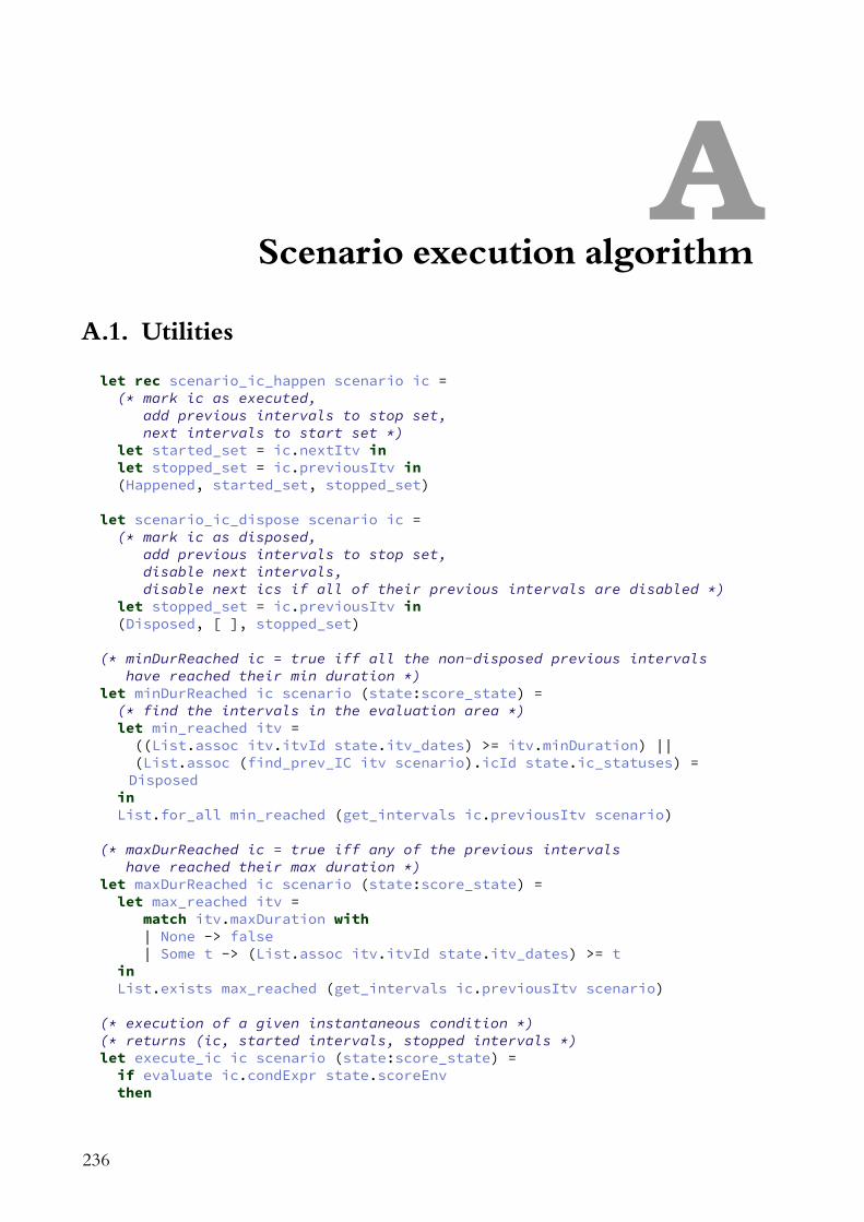
AScenario execution algorithm

A.1. Utilities

let rec scenario_ic_happen scenario ic =(* mark ic as executed,

add previous intervals to stop set,next intervals to start set *)

let started_set = ic.nextItv inlet stopped_set = ic.previousItv in(Happened, started_set, stopped_set)

let scenario_ic_dispose scenario ic =(* mark ic as disposed,

add previous intervals to stop set,disable next intervals,disable next ics if all of their previous intervals are disabled *)

let stopped_set = ic.previousItv in(Disposed, [ ], stopped_set)

(* minDurReached ic = true iff all the non-disposed previous intervalshave reached their min duration *)

let minDurReached ic scenario (state:score_state) =(* find the intervals in the evaluation area *)let min_reached itv =

((List.assoc itv.itvId state.itv_dates) >= itv.minDuration) ||(List.assoc (find_prev_IC itv scenario).icId state.ic_statuses) =Disposed

inList.for_all min_reached (get_intervals ic.previousItv scenario)

(* maxDurReached ic = true iff any of the previous intervalshave reached their max duration *)

let maxDurReached ic scenario (state:score_state) =let max_reached itv =

match itv.maxDuration with| None -> false| Some t -> (List.assoc itv.itvId state.itv_dates) >= t

inList.exists max_reached (get_intervals ic.previousItv scenario)

(* execution of a given instantaneous condition *)(* returns (ic, started intervals, stopped intervals *)let execute_ic ic scenario (state:score_state) =if evaluate ic.condExpr state.scoreEnvthen

236

A.1. Utilities

scenario_ic_happen scenario icelse

scenario_ic_dispose scenario ic

237

A. Scenario execution algorithm

A.2. Execution of temporal conditions

let execute_tc tc scenario (state:score_state) =(* execute the conditions *)let rec execute_all_ics ics (state:score_state) started_itvs ended_itvshappened_ics =match ics with| [] -> (state, started_itvs, ended_itvs, happened_ics)| cond::t -> let (newStatus, started, stopped) =

execute_ic cond scenario state inexecute_all_icst(* update the statuses of the ICs with new values *){ state with ic_statuses = (list_assoc_replace state.ic_statuses

cond.icId newStatus) }(started@started_itvs)(stopped@ended_itvs)(if newStatus = Happened then cond::happened_ics else

happened_ics)inlet (state, started_itv_ids, ended_itv_ids, happened_ics) =

execute_all_ics tc.conds state [] [] [] in

(* start and stop the intervals *)let rec start_all_intervals itvs (state:score_state) funs =

match itvs with| [] -> (state, funs)| itv::t -> let (state,f) = start_interval itv state in

start_all_intervals t state (funs@[f])inlet (state, funs) =

start_all_intervals (get_intervals started_itv_ids scenario) state []in

inlet state =

List.map stop_all_intervals(get_intervals ended_itv_ids scenario) state in

(state, List.flatten funs, happened_ics);;(* this function does the evaluation & execution of a given temporal

condition *)let scenario_process_TC scenario tc (state:score_state) =(* mark all instantaneous conditions with min reached as Pending *)let rec mark_IC_min conds state =

match conds with| [] -> state| cond::t -> mark_IC_min

t(if (minDurReached cond scenario state)

then { state withic_statuses = list_assoc_replace state.

ic_statuses cond.icId Pending }else state)

238

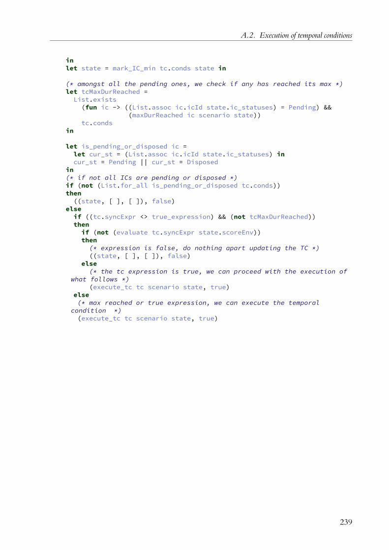
A.2. Execution of temporal conditions

inlet state = mark_IC_min tc.conds state in

(* amongst all the pending ones, we check if any has reached its max *)let tcMaxDurReached =

List.exists(fun ic -> ((List.assoc ic.icId state.ic_statuses) = Pending) &&

(maxDurReached ic scenario state))tc.conds

in

let is_pending_or_disposed ic =let cur_st = (List.assoc ic.icId state.ic_statuses) incur_st = Pending || cur_st = Disposed

in(* if not all ICs are pending or disposed *)if (not (List.for_all is_pending_or_disposed tc.conds))then

((state, [ ], [ ]), false)else

if ((tc.syncExpr <> true_expression) && (not tcMaxDurReached))then

if (not (evaluate tc.syncExpr state.scoreEnv))then

(* expression is false, do nothing apart updating the TC *)((state, [ ], [ ]), false)

else(* the tc expression is true, we can proceed with the execution of

what follows *)(execute_tc tc scenario state, true)

else(* max reached or true expression, we can execute the temporal

condition *)(execute_tc tc scenario state, true)

239

A. Scenario execution algorithm

A.3. Main execution algorithm

let scenario_tick (p:process) olddate newdate pos offset (state:score_state) =

let pid = p.procId inlet scenario = match p.impl with | Scenario s -> s | _ -> raiseWrongProcess in

let dur = newdate - olddate in(* execute the list of root TCs.

l1 : list of executed ICsl2 : list of resulting functions *)

let rec process_root_tempConds tc_list state funs =match tc_list with| [ ] -> (state, funs)| h::t ->

(* try to execute the TC *)let ((state, new_funs, happened_ics), executed) =

scenario_process_TC scenario h state in

if (not executed) then(* The trigger wasn't executed, we keep it *)process_root_tempConds t state (funs@new_funs)

else(* the TC was executed, remove it from the roots *)let cur_rootTCs = List.filter (fun x -> x <> h.tcId) (List.assoc

pid state.rootTCs) inprocess_root_tempConds

t{ state with rootTCs = list_assoc_replace state.rootTCs pid

cur_rootTCs }(funs@new_funs)

in

(* execute a given list of TCs *)let rec process_tempConds tc_list (state:score_state) funs happened_ics =

match tc_list with| [ ] -> (state, funs, happened_ics)| h::t ->

(* try to execute the TC *)let ((state, new_funs, new_hics), _) =

scenario_process_TC scenario h state inprocess_tempConds t state (funs@new_funs) (new_hics@happened_ics)

in

(* execute a list of intervals *)let rec process_intervals itv_list overticks funs dur offset end_TCs (state:score_state) =match itv_list with| [ ] -> (state, overticks, end_TCs, funs)| interval::tail ->

(* run the interval and replace it in a new scenario *)let ((state, new_funs), overticks) =

scenario_run_interval scenario overticks dur offset intervalstate in

process_intervals

240

A.3. Main execution algorithm

tail overticks(funs@new_funs)dur offset((find_end_TC interval scenario)::end_TCs)state

in

let rec finish_tick overticks conds funcs dur offset end_TCs state =match conds with| [ ] ->

(* now we can process remaining end_TCs *)(match end_TCs with(* nothing to execute anymore *)| [ ] -> (state, funcs)(* some TCs reached their end so we execute them *)| _ -> let (state, new_funs, conds) =

process_tempConds end_TCs state [] [] infinish_tick overticks conds (funcs@new_funs) dur offset [ ]

state)

| (cond:condition) :: remaining ->(* look if an over-tick was recorded for the TC *)match (List.assoc_opt (find_parent_TC cond scenario).tcId overticks)

with| None -> finish_tick overticks remaining funcs dur offset end_TCs

state| Some (min_t, max_t) ->

(* we can go forward with executing some intervals *)let (state, overticks, end_TCs, funcs) =

process_intervals(following_intervals cond scenario)overticks funcsmax_t(offset + dur - max_t)end_TCsstate

infinish_tick overticks remaining funcs dur offset end_TCs state

in

(*** actual execution begins here ***)

(* first execute the root temporal conditions, if any *)let (state, funcs) =

process_root_tempConds (get_rootTempConds pid scenario state) state []in

(* run the intervals that follows them *)let running_intervals = (List.filter (is_interval_running scenario state.ic_statuses) scenario.intervals) in

let (state, overticks, end_TCs, funcs) =process_intervals running_intervals [] funcs dur offset [] state in

(* run potential terminating temporal conditions *)let (state, funcs, conds) = process_tempConds end_TCs state funcs [] in

241

A. Scenario execution algorithm

(* loop until the time cannot be advanced in any branch anymore *)let (state, funcs) = finish_tick overticks conds funcs dur offset end_TCs

state in(list_fun_combine funcs, state)

;;

242

BLoop execution algorithm

B.1. Loop execution in the non-interactive case

We give here the loop execution algorithm used when neither of the start TC, end TC, startinterval, end interval, have a non-default condition.

// tick_amount is the amount of time values that has been// requested from the loop process.// tick_offset is the offset in the current buffer.if(tick_amount >= 0){if(interval.get_date() == 0){

start_ic.tick(0_tv, 0., tick_offset);interval.start();interval.tick_current(tick_offset);

}

while(tick_amount > 0){

const auto cur_date = interval.get_date();if(cur_date + tick_amount < itv_dur){

// the current tick will not cause the loop to loop againinterval.tick_offset(tick_amount, tick_offset);break;

}else{

// we will loop: for how long ?auto this_tick = itv_dur - cur_date;

tick_amount -= this_tick;interval.tick_offset(this_tick, tick_offset);tick_offset += this_tick;

end_ic.tick(0_tv, 0., tick_offset);interval.stop();

// loop the patternif(tick_amount > 0){

interval.offset(time_value{});interval.start();interval.tick_current(tick_offset);start_ic.tick(0_tv, 0., tick_offset);

244

B.2. Loop execution in the interactive case

}}

}}

B.2. Loop execution in the interactive case

This algorithm is used whenever an interactive event is non-default. There are specific cases tohandle: for instance, we must take care of not falling in a deadlock when the start IC has a falsecondition, and must ensure that re-evaluation will take place on every tick until the executionis possible.

// We first check the state of the start IC:// is it waiting for execution ? Or has it happened already ?switch(start_ic.get_status()){

case time_event::status::NONE:case time_event::status::PENDING:{

process_tc(m_startNode, start_ic, true, false);if(start_ic.get_status() != time_event::status::HAPPENED){

start_ic.set_status(time_event::status::PENDING);end_ic.set_status(time_event::status::NONE);return;

}break;

}case time_event::status::HAPPENED:

break;case time_event::status::DISPOSED:

start_ic.set_status(time_event::status::PENDING);end_ic.set_status(time_event::status::NONE);return;

}

// If it has happened, we continue and execute the pattern.if (prev_last_date == Infinite)

interval.tick_offset(date, tick_offset);else

interval.tick_offset(ossia::time_value{(date - prev_last_date)},tick_offset);

// We check the status of the end IC: must it be enabled ?// If it's the case, then we must check the end TC.switch (end_ic.get_status()){

case time_event::status::NONE:{

if (interval.get_date() >= interval.get_min_duration()){

end_ic.set_status(time_event::status::PENDING);

245

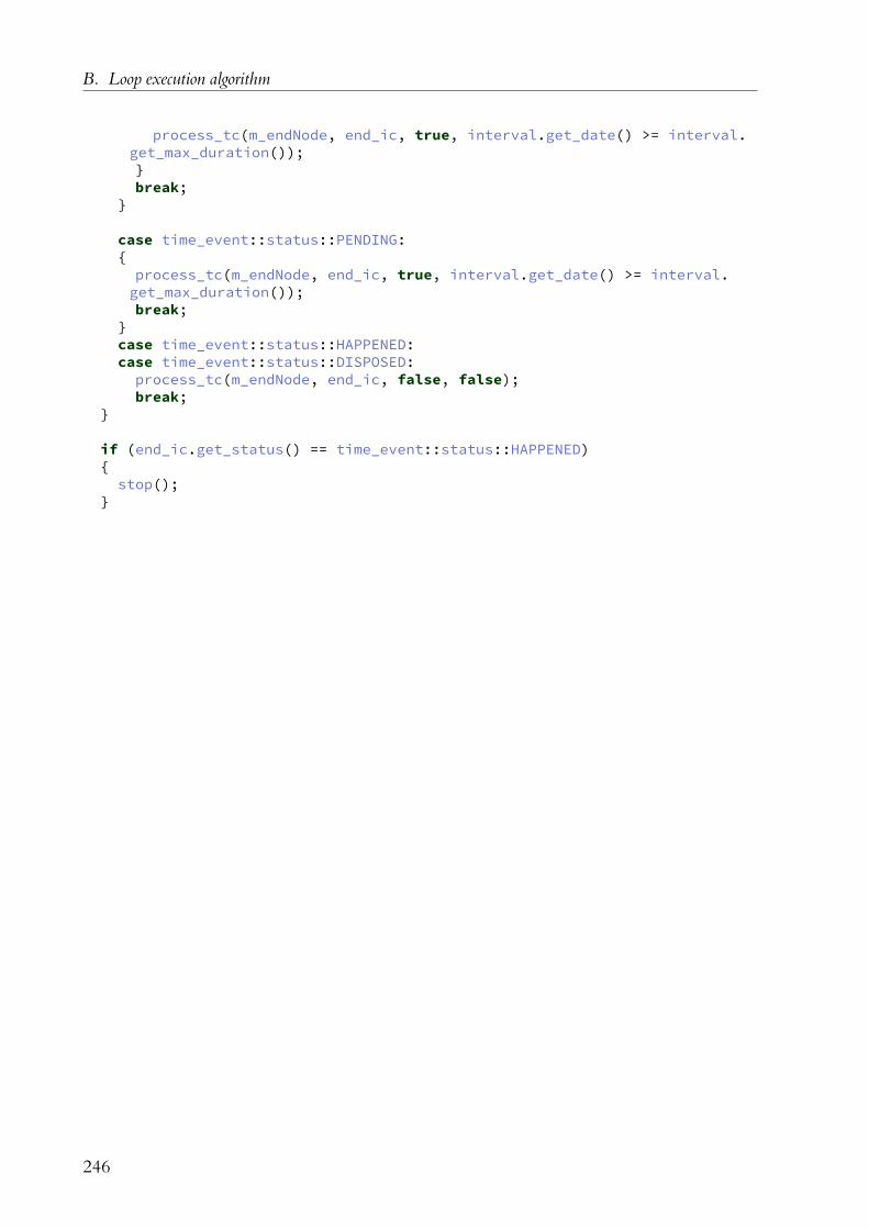
B. Loop execution algorithm

process_tc(m_endNode, end_ic, true, interval.get_date() >= interval.get_max_duration());}break;

}

case time_event::status::PENDING:{

process_tc(m_endNode, end_ic, true, interval.get_date() >= interval.get_max_duration());break;

}case time_event::status::HAPPENED:case time_event::status::DISPOSED:

process_tc(m_endNode, end_ic, false, false);break;

}

if (end_ic.get_status() == time_event::status::HAPPENED){stop();

}

246

CMinuit grammar

zero = '\0'; (* the NULL character *)sep = zero, { sep }; (* zero-padded to 4 bytes *)character = `a' .. `z' | `A' .. `Z' | `0' .. '9';alnum = character, { character };

osc-reserved =`space' | `#' | `*' | `,' | `/'

| `?' | `[' | `]' | `{' | `}';osc-char = ? any printable ASCII character minus osc-reserved ?;

osc-fragment = osc-char, { osc-char };osc-address = `/', { osc-fragment, { osc-address } };osc-types = ( `i' | `f' | `s' | `b' | `T' | `F' | `I' | `T' | `N' ), { osc-

types };osc-typetag = `,', osc-types;osc-int = ? network byte-order 4 bytes int ?;osc-float = ? network byte-order 4 bytes float ?;osc-string = ? any non-null ASCII character ?, zero, sep;osc-blob = osc-int, ? any ASCII character ?, sep;osc-arguments = (osc-int | osc-float | osc-string | osc-blob), { osc-

arguments };

minuit-device = alnum;minuit-attribute = alnum;minuit-action = `namespace' | `listen' | `get';minuit-qualifier = `?' | `:' | `!';minuit-intro = minuit-device, minuit-qualifier, minuit-action;

minuit-query =minuit-intro, sep, osc-address

| minuit-query, sep, osc-address `:' minuit-attribute;

minuit-message = minuit-query, sep, osc-typetag, sep, osc-arguments;

osc-message = osc-address, sep, osc-typetag, sep, osc-arguments;

message = minuit-message | osc-message;

248

DExpression grammar

device = +[a-zA-Z0-9.~()_-];fragment = +[a-zA-Z0-9.~():_-];path_element = fragment;path = ('/', path_element)+ | '/';

address = device, ‘’:, path;dataspace := 'color' || 'distance' || ...;unit_accessor := 'x' | 'y' | 'z' | 'r' | 'g' | 'b' | ...;

(* e.g. color.rgb or color.rgb.r; we make a precomputed table. *)unit_qualifier: dataspace, '.', unit, ('.', unit_accessor)?;address_accessor := Address, '@', (('[', [:int:], ']')* || ('[',

unit_qualifier, ']'));

char := '\'', [:ascii:] - '\'', '\'';str := '"', ([:ascii:] - '"')*, '"';list := '[', (value % ','), ']';bool := 'true' || 'false';int := [:int:];float := [:float:];variant := char || str || list || bool || int || float;value := variant;

relation_member := value || address;relation_op := '<=' || '<' || '>=' || '>' || '==' || '!=';

relation := relation_member, relation_op, relation_member;

pulse := 'impulse(' , Address , ')'

(* Boolean operations *)

expr := or;or := (xor, 'or', or) | xor;xor := (and, 'xor', xor) | and;and := (not, 'and', and) | not;not := ('not', rec) | rec;

rec := ('{', expr, '}') | relation;

250

EDevice statistics

The following tables contains statistics for various scores made by artists with the software.The first table contains general statistics on the device tree: the devices used, their protocol,

the total number of nodes and the number of non-leaf nodes, the depth of the deepest leaf, themaximum number of children for a single node, the average number of children for each node,and the average number of children for each non-leaf node.

The Variables protocol means that a device was only created for the sake of having localvariables to use within the score; by default, in the software, this is done with an OSC device.We can also note that the Local and Midi device, due to their generative nature, bear a largenumber of nodes. They are not taken into account for the study of the authoring methodsused by each author, since they only reflect an implementation detail and are not constructedexplicitly by the author.

Each part of Table E.1 lists all the devices for a given score, in order:• The first four devices, from score toNebula are from the Nebula score from the Baltazars

(see Section 11.5.2).• Thomas Pachoud’s score Voyage.• The score for L’Arbre Intégral (Section 11.5.4) made by Pierre Cochard.• The score for the Nuit des Chercheurs (Section 11.5.6) made by Pierre Cochard and

Thibaud Keller.• Pierre Cochard’s score Quarrè (Section 11.5.5).• A score provided by Antoine Villeret.• A score for Metabot control by Thibaud Keller (Section 11.5.3).Then, Table E.2 lists all the data types used for each node. Fig. E.1 shows combined per-type

parameter counts across all the scores.

252

Table E.1.: Device statistics.Device Protocol Nodes NonLeaf MaxDepth MaxCld AvgCld AvgNCld

score Local 7,942 1,364 8 397 1 5.82

Nebula Minuit 325 58 4 41 0.96 5.36

Eclipse Minuit 35 8 4 8 0.91 4

Shadow Minuit 18 4 4 8 0.89 4

MainVoyage Minuit 866 251 6 16 0.99 3.41

score Local 4,119 831 14 91 1 4.95

reapermidi Midi 8,288 80 3 128 1 103.4

wsserver WebSocket 53 16 4 9 0.91 3

ALBILEMUR OSC 6 2 2 1 0.33 1

var Variables 3 0 1 0 0 0

DOME OSCQuery 76 19 4 24 0.92 3.68

ALBIWFS Minuit 292 50 4 41 0.99 5.8

local Variables 5 0 1 0 0 0

quarreserver Minuit 372 98 6 30 0.99 3.74

voxelstrack OSCQuery 73 9 2 7 0.86 7

dynamicmapping OSCQuery 20 3 2 8 0.7 4.67

ROBOTIS Serial 18 1 2 17 0.94 17

MidiDevice MIDI 8,288 80 3 128 1 103.4

ContactCollider OSCQuery 13 1 2 12 0.92 12

score Local 1,279 270 24 12 1 4.72

PdHid OSCQuery 19 3 2 10 0.84 5.33

253

E. Device statistics

Table E.2.: Parameter statistics.Device Empty Int Impulse Float Bool Vec2F Vec3F Vec4F Tuple String Char

score 1,504 0 622 1,742 2 0 0 0 0 4,072 0

Nebula 82 32 0 185 17 0 0 0 6 3 0

Eclipse 8 2 0 23 2 0 0 0 0 0 0

Shadow 4 1 0 12 1 0 0 0 0 0 0

MainVoyage 203 60 0 515 24 0 0 0 59 5 0

score 928 0 361 624 2 0 0 0 0 2,204 0

reapermidi 16 6,176 2,048 0 0 0 0 0 48 0 0

wsserver 0 0 53 0 0 0 0 0 0 0 0

ALBILEMUR 0 1 0 1 0 0 1 1 2 0 0

var 0 0 0 0 2 1 0 0 0 0 0

DOME 18 5 0 29 14 0 1 0 9 0 0

ALBIWFS 46 85 0 75 0 0 32 0 33 21 0

local 0 4 0 0 1 0 0 0 0 0 0

quarreserver 102 88 6 97 8 0 0 0 66 5 0

voxelstrack 9 19 0 18 0 16 0 7 4 0 0

dynamicmapping 3 2 0 5 4 2 0 4 0 0 0

ROBOTIS 0 3 8 7 0 0 0 0 0 0 0

MidiDevice 16 6,176 2,048 0 0 0 0 0 48 0 0

ContactCollider 1 2 0 9 1 0 0 0 0 0 0

score 280 0 95 230 2 0 0 0 0 672 0

PdHid 3 6 0 0 10 0 0 0 0 0 0

254

Int Impulse Float Bool Vec2F Vec3F Vec4F Tuple String Char0

200

400

600

800

Parameter type

Num

berof

para

meter

Figure E.1.: Number of parameters used in custom devices built by authors either within score,or with external environments connected to score. These figures are based on the7 scores of Appendix E.

255

FScore statistics

The following tables contains statistics for the scores themselves.Table F.1 contains general statistics on the number of temporal elements in the scores: number of intervals,

number of intervals without processes, IC count, TC count, states count, empty states count, conditions (non-default IC), triggers (non-default TC), and maximal hierarchy depth (the depth of the deepest interval where theroot is at level 0).

Table F.2 contains statistics on the usage of specific processes: the number of processes, the average number ofprocesses per interval, the average number of processes per non-empty interval, and the count for multiple specificcategories of processes.

Table F.1.: Score statistics.Score Intervals EmptyItv IC TC States EmptyStates Conds Trigs MaxDepth

Nebula 217 140 226 223 397 102 0 69 1

Voyage 33 15 42 40 54 19 0 36 3

ArbreIntegral 103 59 176 176 183 119 0 176 2

NuitCherch 21 7 25 25 29 8 0 17 2

Quarre 187 175 206 191 276 92 14 191 2

Antoine 41 18 54 54 68 33 0 46 3

Metabot 25 5 54 49 44 35 4 6 5

Table F.2.: Process statistics.Score Procs ProcsPerItv ProcsPerLoadedItv Autom Mapping Scenar Loop Script

Nebula 218 1 2.83 217 0 1 0 0

Voyage 36 1.09 2 27 0 6 2 1

ArbreIntegral 45 0.44 1.02 8 0 37 0 0

NuitCherch 82 3.9 5.86 27 52 3 0 0

Quarre 13 7 · 10−2 1.08 3 6 4 0 0

Antoine 25 0.61 1.09 18 0 1 4 2

Metabot 36 1.44 1.8 6 16 1 6 7

256