An ANN application for water quality forecasting

Marine Pollution Bulletin 56 (2008) 1586–1597

Contents lists available at ScienceDirect

Marine Pollution Bulletin

journal homepage: www.elsevier .com/locate /marpolbul

An ANN application for water quality forecasting

Sundarambal Palani *, Shie-Yui Liong, Pavel TkalichTropical Marine Science Institute, National University of Singapore, 14 Kent Ridge Road, Singapore 119223, Singapore

a r t i c l e i n f o

Keywords:Singapore seawater
Data driven techniqueNeural networkWater qualityPredictionForecastingSoutheast Asia
0025-326X/$ - see front matter � 2008 Elsevier Ltd.doi:10.1016/j.marpolbul.2008.05.021

* Corresponding author. Tel.: +65 6516 3105; fax: +E-mail address: [email protected] (S. Palani).

a b s t r a c t

Rapid urban and coastal developments often witness deterioration of regional seawater quality. As part ofthe management process, it is important to assess the baseline characteristics of the marine environmentso that sustainable development can be pursued. In this study, artificial neural networks (ANNs) wereused to predict and forecast quantitative characteristics of water bodies. The true power and advantageof this method lie in its ability to (1) represent both linear and non-linear relationships and (2) learn theserelationships directly from the data being modeled. The study focuses on Singapore coastal waters. TheANN model is built for quick assessment and forecasting of selected water quality variables at any loca-tion in the domain of interest. Respective variables measured at other locations serve as the input param-eters. The variables of interest are salinity, temperature, dissolved oxygen, and chlorophyll-a. A time lagup to 2Dt appeared to suffice to yield good simulation results. To validate the performance of the trainedANN, it was applied to an unseen data set from a station in the region. The results show the ANN’s greatpotential to simulate water quality variables. Simulation accuracy, measured in the Nash–Sutcliffe coef-ficient of efficiency (R2), ranged from 0.8 to 0.9 for the training and overfitting test data. Thus, a trainedANN model may potentially provide simulated values for desired locations at which measured data areunavailable yet required for water quality models.

� 2008 Elsevier Ltd. All rights reserved.

1. Introduction

Seawater is a primary natural resource for many coastal devel-opment sectors. It is also one of the most sensitive and vulnerableresources, because it is negatively impacted by a variety of anthro-pogenic activities. Deterioration of coastal water quality has trig-gered the initiation of serious management efforts in manycountries. Tourism, recreation, and fishing require at least anacceptable level of seawater quality. Singapore, an island state,has stringent enforcement and continuously upgraded waste han-dling facilities to guarantee seawater of a certain quality.

Most acceptable ecological and social decisions are difficult tomake without careful modeling, prediction/forecasting, and analy-sis of seawater quality for typical development scenarios. Waterquality prediction enables a manager to choose an option that sat-isfies a large number of identified conditions. For instance, waterquality variables, such as salinity, temperature, nutrients, dissolvedoxygen (DO), and chlorophyll-a (Chl-a), in coastal water describe acomplex process governed by a considerable number of hydrologic,hydrodynamic, and ecological controls that operate at a wide rangeof spatiotemporal scales. Sources of the admixtures often cannotbe clearly identified, and the locally influenced complex mass ex-change between the variables may not be known. Due to the cor-

All rights reserved.

65 6872 4067.

relations and interactions between water quality variables, it isinteresting to investigate whether a domain-specific mechanismgoverning observed patterns exists to prove the predictability ofthese variables. The identification of such forecast models is partic-ularly useful for ecologists and environmentalists, since they willbe able to predict seawater pollution levels and take necessary pre-caution measures in advance.

Classical process-based modeling approaches can provide goodestimations of water quality variables, but they usually are toogeneral to be applied directly without a lengthy data calibrationprocess. They often require approximations of various processes,and these approximations may overlook some important factorsaffecting the processes in seawater. A process-based model re-quires a lot of input data and model parameters that are often un-known, while data-driven techniques provide an effectivealternative to conventional process-based modeling. Models devel-oped by data-driven techniques are computationally very fast andrequire fewer input parameters than process-based models. Data-driven modeling techniques have gained popularity in the last 20years. The scientific and engineering communities have acquiredalready extensive experience in the development and usage ofdata-driven techniques. ANNs are, however, still not widely usedtools in the fields of water quality prediction and forecasting. ANNsare able to approximate accurately complicated non-linear input–output relationships. Like their physics-based numerical modelcounterparts, ANNs require training or calibration. After training,

mailto:[email protected]

http://www.sciencedirect.com/science/journal/0025326X

http://www.elsevier.com/locate/marpolbul

S. Palani et al. / Marine Pollution Bulletin 56 (2008) 1586–1597 1587

each application of the trained ANN is an estimation of a simplealgebraic expression with known coefficients and is executed prac-tically instantaneously. The ANN technique is flexible enough toaccommodate additional constraints that may arise in theapplication.

This paper demonstrates the application of ANNs to model thevalues of selected seawater quality variables, having the dynamicand complex processes hidden in the monitored data itself. TheANN model can reveal hidden relationships in the historical data,thus facilitating the prediction and forecasting of seawater quality.The steps followed in the development of such models include thechoice of performance criteria, division and pre-processing of theavailable data, determination of appropriate model inputs and net-work architecture, optimization of the connection weights (train-ing), and model validation. In this paper, a study of ANNmodeling to predict and forecast temperature, salinity, DO, andChl-a in Singapore coastal waters is presented. These water qualityparameters were measured weekly at various locations. Thesemodels could be used as a prediction tool, which complementsthe process-based model and ongoing field monitoring programin the region. The results of the ANN prediction and forecast modelin the East Johor Strait are discussed in this paper.

Fig. 1. Map showing the geographical setting of the present survey area with fourfield monitoring Stations [1. Paku (�20 m water depth), 2. Malang Papan (�13 mwater depth), 2alt Sajahat (�15 m water depth), and 3. Squance (�12 m waterdepth)], Pasir Gudang port, the Causeway, and the major rivers in the East JohorStrait.

2. Materials and methods

2.1. Study area and water quality data

Singapore is a tropical country located between latitudes 1�060Nand 1�240N and longitudes 103�240E and 104�240E, 137 km north ofthe equator. Singapore is located in Southeast Asia at the southerntip of the Malaysian Peninsula between Malaysia and Indonesia.The coastal water of Singapore is bounded by the Johor Strait inthe north and the Singapore Strait in the south. Singapore is a smallisland having a total land area of 699 km2, with air temperatureranging from 21.1 to 35.1 �C, and annual average rainfall of2136 mm (Singapore Department of Statistics, 2005). Because ofits geographical location, its climate is characterized by uniformtemperature and pressure, high humidity, and abundant rainfall,and it is influenced strongly by the Asian monsoon. Singaporehas two main monsoon seasons: the Northeast Monsoon (NEM)season lasts from November to March, and the Southwest Mon-soon (SWM) season lasts from June to September. These seasonsare separated by two shorter inter-monsoon (IM) periods that lastfrom April to May and October to November. The tides in Singaporeare the result of tidal generation in the South China Sea and North-ern Indian Ocean. The hydrodynamic conditions of Singapore aredominated by semi-diurnal tides, having residual currents mainlyin the eastern (SWM) and western (NEM) directions. In the Singa-pore Strait, the monsoon-driven currents and tidal fluctuation aresignificant. Spring tides and neap tides occur two days after thenew/full moon or first/last quarter of the moon, respectively. Tidalvelocities vary spatially from 0.5–1 m/s (in the open waters of theSingapore Strait) to 1.5–2 m/s (in constricted channels between theislands), but they decrease to less than 0.5 m/s in the eastern halfof the Johor Strait (Zhang, 2000; Pang and Tkalich, 2003). Duringflood tides, the tidal current transports water from the Kuala Johorinto the East Johor Strait; during ebb tides, the tidal current re-verses its direction of flow. In southern Kuala Johor, the tidal cur-rent moves westwards during flood water. This direction isopposite to that at ebb tide. Both the surface and near-bottom tidalcurrents in Kuala Johor are stronger than those in the East JohorStrait. In both areas, ebb flows are stronger than flood flows andsurface currents are stronger than near-bottom ones (Lim, 1983;Pang and Tkalich, 2003). Temperature and salinity in the East JohorStrait are influenced mainly by daily and seasonal changes as well

as heavy rainfalls. The daily variation patterns of temperature andsalinity in the East Johor Strait were found to be quite similar tothose of the Singapore Strait, and both patterns are semi-diurnal.Due to freshwater flow from rivers, increased phytoplankton den-sities, higher water temperatures, and lower salinity values wereobserved during low tide.

The data used in this study were derived from the Singaporeseawater quality survey conducted by Chuah (1998) betweenDecember 1996 and June 1997 at the entrance to the East JohorStrait (Fig. 1). The data are used to investigate both, water qualityand the potential for red tide occurrences. The selected four sites(Fig. 1) lie in the area at which the East Johor Strait merges withKuala Johor before entering the main Singapore Strait. This areais strongly influenced by tidal flow in and out of the East JohorStrait. Station 3 is close to the Squance buoy and several marinefish farms. Station 1 is located in deeper waters near the ChangiJetty. Station 2 may depict the transition between Station 3 inthe Strait and Station 1 offshore. During ebb tide, the SerangoonHarbor receives a high volume of water flowing eastward out ofthe East Johor Strait (Lim, 1983; Pang and Tkalich, 2003). Weeklycollected surface seawater samples were analyzed by Chuah(1998) for the estimation of Chl-a, water temperature, salinity,pH, secchi depth (SD), DO, and nutrients like ammonium (NH4), ni-trite (NO2), nitrate (NO3), total nitrogen (TN), phosphate (PO4), andtotal phosphorus (TP). Other water quality variables, including ni-trate nitrogen (NO2 + NO3), dissolved inorganic nitrogen(DIN = NH4 + NO2 + NO3), organic nitrogen (ON = TN � DIN), andorganic phosphorous (OP = TP � PO4), were also derived. The con-centration range of the water quality variables measured betweenJanuary 1997 and May 1997 in the East Johor Strait in the modeldomain is given in Table 1.

2.2. Structure of neural network model

2.2.1. ANN architectureThe concept of artificial neurons was first introduced in 1943

(McCulloch and Pitts, 1943), and applications of ANNs in researchareas began with the introduction of the back-propagation training(BP) algorithm for feedforward ANNs in 1986 (Rumelhart et al.,1986). An ANN is an information processing system that roughlyreplicates the behavior of a human brain by emulating the opera-

Table 1Water quality properties in the ANN model domain measured between January 1997and May 1997 in the East Johor Strait

Parameters Unit Minimum Maximum Mean SD

Temperature �C 27.60 31.80 29.36 1.10Salinity ppt 19.00 31.00 27.63 2.58pH 7.50 8.70 8.26 0.27SD m 0.70 3.20 1.35 0.42DO mg/l 4.31 14.40 7.55 2.08NH4 mg/l 0.34 0.73 0.54 0.09NO2 + NO2 mg/l 0.06 0.20 0.11 0.02DIN mg/l 0.44 0.86 0.65 0.10TN mg/l 1.97 5.77 3.22 0.92ON mg/l 1.30 5.11 2.57 0.88PO4 mg/l 0.01 0.08 0.03 0.02TP mg/l 0.02 0.12 0.06 0.02OP mg/l 0.01 0.07 0.03 0.01Chl-a mg/m3 0.85 71.70 11.58 13.78

1588 S. Palani et al. / Marine Pollution Bulletin 56 (2008) 1586–1597

tions and connectivity of biological neurons. ANNs represent com-plex, non-linear functions with many parameters that are adjusted(calibrated or trained) in such a way that the ANN’s output be-comes similar to measured output on a known data set. ANNs needa considerable amount of historical data to be trained; upon satis-factory training, an ANN should be able to provide output for pre-viously ‘‘unseen” inputs. The main differences between the varioustypes of ANNs involve network architecture and the method fordetermining the weights and functions for inputs and neurodes(training) (Caudill and Butler, 1992). The multilayer perceptron(MLP) neural network has been designed to function well in mod-eling non-linear phenomena. A feed forward MLP network consistsof an input layer and output layer with one or more hidden layersin between. Each layer contains a certain number of artificial neu-rons. An artificial neuron in a typical ANN architecture (Fig. 2) re-ceives a set of inputs (signals (x) with weight (w)), calculates theirweighted average ((z), using the summation function), and thenuses some activation function to produce an output (o = f(z), wherez ¼

Pni¼1xiwi).

The connections between the input layer and the middle or hid-den layer contain weights, which usually are determined throughtraining the system. The hidden layer sums the weighted inputsand uses the transfer function to create an output value. The trans-fer function (local memory) is a relationship between the internalactivation level of the neuron (called the activation function) andthe outputs. A typical transfer function is the sigmoid functionf(z), which varies from 0 to 1 for a range of inputs (Caudill and But-ler, 1992) where f ðzÞ ¼ 1

1þe�z. In time series prediction, supervisedtraining is used to train the ANN in such a way as to minimizethe difference between the network output and the measured tar-

f(z)

SummationFunctionx1

x2

x3

xn

w1

w2

w3

wn

z

ActivationFunction

=

n

jjjwx

1

Fig. 2. A typical multilayer perceptron ANN architecture.

get. Therefore, training is a process of weight adjustment that at-tempts to obtain a desirable outcome with least squaresresiduals. The most common training algorithm used in the ANNliterature is called BP.

General regression neural networks (GRNNs) were invented bySpecht (1991) and are also used in this paper. The GRNN predictscontinuous outputs. GRNN nodes require two main functions tocalculate the difference between all pairs of input pattern vectorsand estimate the probability density function of the input vari-ables. The difference between input vectors is calculated usingthe simple Euclidean distance between data values in attributespace. Weighting the calculated distance of any point by the prob-ability of other points occurring in that area yields a predicted out-put value (Eqs. (1) and (2)).

EY=XðXÞ ¼Z

y�fXYðx; yÞdy=Z

fXYðx; yÞdy; ð1Þ

�y ¼Xn

i¼1

y�i expð�Dðx; xiÞÞ=Xn

i¼1

expð�Dðx; xiÞÞ; ð2Þ

where yi is the ith case actual output value, D(x, xi) is calculatedfrom Eq. (3), and n is the total number of cases in the dataset (Mas-ters, 1993).

Dðx; xiÞ ¼Xp

j¼1

ðxj � xij=rjÞ2; ð3Þ

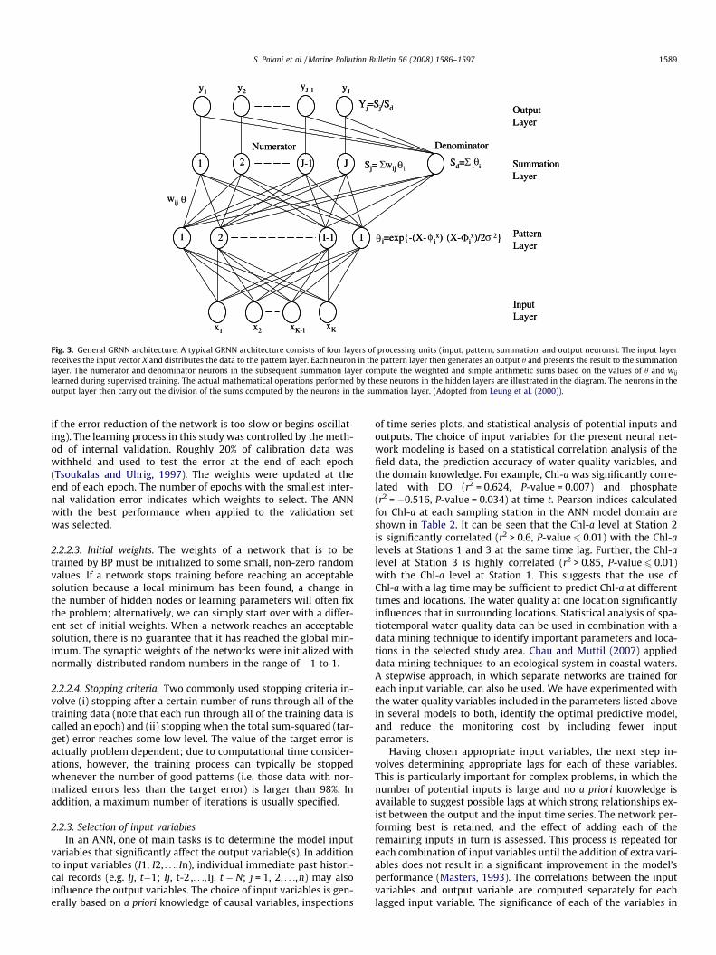
where x is the input vector, xi is the ith case vector, xj is the jth datavalue in the input vector, xij is the jth data value in the ith case vec-tor, and rj is the smoothing factor (Parzen’s window) for the jth var-iable (Masters, 1993). The error is measured by the means of themean square error (MSE). The MSE measures the average of thesquare of the amount by which the estimator differs from the quan-tity to be estimated. After determining the error (and depending onthe optimization technique used), the above calculation may be runnumerous times with different smoothing factors (sigmas). Trainingstops when either a threshold minimum square error value isreached or the test set square error begins to rise. A typical GRNNarchitecture is shown in Fig. 3.

2.2.2. ANN parameter selection2.2.2.1. Hidden layers and nodes. Determining the number of hiddenlayers and nodes is a usually a trial and error task in ANN model-ing. A rule of thumb for selecting the number of hidden nodes re-lies on the fact that the number of samples in the training setshould at least be greater than the number of synaptic weights(Tarassenko, 1998). A one-hidden-layer network is commonlyadopted by most ANN modelers; the number of hidden nodes Min this model is between I and 2I + 1 (Hecht-Nielsen, 1987), whereI is the number of input nodes. As a guide, M should not be lessthan the maximum of I/3 and the number of output nodes O. Theoptimum value of M is determined by trial and error. Networkswith fewer hidden nodes are generally preferable, because theyusually have better generalization capabilities and fewer overfit-ting problems. If the number of nodes is not large enough to cap-ture the underlying behavior of the data, however, then theperformance of the network may be impaired. In this study, a trialand error procedure for hidden node selection was carried out bygradually varying the number of nodes in the hidden layer.

2.2.2.2. Learning rate (g) and momentum (a). The function of theseparameters is to speed up the training process while maintainingerror reduction. There is no specific rule for the selection of valuesfor these parameters. However, the training process is started byadopting one set of values (i.e. g = 0.2, range 0 to 1, and a = 0.5,range 0 to 0.9) and then adjusting these values as necessary (i.e.

y1 y2yJ-1 yJ

x1 x2 xK-1 xK

1 2 I-1 I

1 2 J-1 J

wij

Sj= wij i

i=exp{-(X- ix)’ (X- i

x)/2 2}

Numerator

Yj=Sj/Sd

Sd= i i

Denominator

OutputLayer

SummationLayer

PatternLayer

InputLayer

y1 y2yJ-1 yJ

x1 x2 xK-1 xK

1 2 I-1 I

1 2 J-1 J

wij

Sj= wij

i=exp{-(X- ix)’ (X- i

x)/2 2}

Numerator

Yj=Sj/Sd

Sd= i i

Denominator

OutputLayer

SummationLayer

PatternLayer

InputLayer

θ

θ θ

θ φ Φ σ

Σ Σ

Fig. 3. General GRNN architecture. A typical GRNN architecture consists of four layers of processing units (input, pattern, summation, and output neurons). The input layerreceives the input vector X and distributes the data to the pattern layer. Each neuron in the pattern layer then generates an output h and presents the result to the summationlayer. The numerator and denominator neurons in the subsequent summation layer compute the weighted and simple arithmetic sums based on the values of h and wij

learned during supervised training. The actual mathematical operations performed by these neurons in the hidden layers are illustrated in the diagram. The neurons in theoutput layer then carry out the division of the sums computed by the neurons in the summation layer. (Adopted from Leung et al. (2000)).


if the error reduction of the network is too slow or begins oscillat-ing). The learning process in this study was controlled by the meth-od of internal validation. Roughly 20% of calibration data waswithheld and used to test the error at the end of each epoch(Tsoukalas and Uhrig, 1997). The weights were updated at theend of each epoch. The number of epochs with the smallest inter-nal validation error indicates which weights to select. The ANNwith the best performance when applied to the validation setwas selected.

2.2.2.3. Initial weights. The weights of a network that is to betrained by BP must be initialized to some small, non-zero randomvalues. If a network stops training before reaching an acceptablesolution because a local minimum has been found, a change inthe number of hidden nodes or learning parameters will often fixthe problem; alternatively, we can simply start over with a differ-ent set of initial weights. When a network reaches an acceptablesolution, there is no guarantee that it has reached the global min-imum. The synaptic weights of the networks were initialized withnormally-distributed random numbers in the range of �1 to 1.

2.2.2.4. Stopping criteria. Two commonly used stopping criteria in-volve (i) stopping after a certain number of runs through all of thetraining data (note that each run through all of the training data iscalled an epoch) and (ii) stopping when the total sum-squared (tar-get) error reaches some low level. The value of the target error isactually problem dependent; due to computational time consider-ations, however, the training process can typically be stoppedwhenever the number of good patterns (i.e. those data with nor-malized errors less than the target error) is larger than 98%. Inaddition, a maximum number of iterations is usually specified.

2.2.3. Selection of input variablesIn an ANN, one of main tasks is to determine the model input

variables that significantly affect the output variable(s). In additionto input variables (I1, I2, . . ., In), individual immediate past histori-cal records (e.g. Ij, t�1; Ij, t-2 ,. . ., Ij, t � N; j = 1, 2, . . .,n) may alsoinfluence the output variables. The choice of input variables is gen-erally based on a priori knowledge of causal variables, inspections

of time series plots, and statistical analysis of potential inputs andoutputs. The choice of input variables for the present neural net-work modeling is based on a statistical correlation analysis of thefield data, the prediction accuracy of water quality variables, andthe domain knowledge. For example, Chl-a was significantly corre-lated with DO (r2 = 0.624, P-value = 0.007) and phosphate(r2 = �0.516, P-value = 0.034) at time t. Pearson indices calculatedfor Chl-a at each sampling station in the ANN model domain areshown in Table 2. It can be seen that the Chl-a level at Station 2is significantly correlated (r2 > 0.6, P-value 6 0.01) with the Chl-alevels at Stations 1 and 3 at the same time lag. Further, the Chl-alevel at Station 3 is highly correlated (r2 > 0.85, P-value 6 0.01)with the Chl-a level at Station 1. This suggests that the use ofChl-a with a lag time may be sufficient to predict Chl-a at differenttimes and locations. The water quality at one location significantlyinfluences that in surrounding locations. Statistical analysis of spa-tiotemporal water quality data can be used in combination with adata mining technique to identify important parameters and loca-tions in the selected study area. Chau and Muttil (2007) applieddata mining techniques to an ecological system in coastal waters.A stepwise approach, in which separate networks are trained foreach input variable, can also be used. We have experimented withthe water quality variables included in the parameters listed abovein several models to both, identify the optimal predictive model,and reduce the monitoring cost by including fewer inputparameters.

Having chosen appropriate input variables, the next step in-volves determining appropriate lags for each of these variables.This is particularly important for complex problems, in which thenumber of potential inputs is large and no a priori knowledge isavailable to suggest possible lags at which strong relationships ex-ist between the output and the input time series. The network per-forming best is retained, and the effect of adding each of theremaining inputs in turn is assessed. This process is repeated foreach combination of input variables until the addition of extra vari-ables does not result in a significant improvement in the model’sperformance (Masters, 1993). The correlations between the inputvariables and output variable are computed separately for eachlagged input variable. The significance of each of the variables in

Table 2Pearson indices calculated for Chl-a at each sampling station in the ANN model domain

Parameter Chl-a (t) atStation 1

Chl-a (t � 1) atStation 1


Chl-a (t) atStation 3






�0.50*


0.44* �0.53*


0.86* �0.33* 0.27**


�0.44* 0.88* �0.33* �0.19***


0.22*** �0.47* 0.87* 0.15*** �0.20***


0.61* �0.28** 0.24*** 0.61* �0.21*** 0.13***


�0.31* 0.61* �0.28** �0.17*** 0.62* �0.21*** 0.05***


0.24*** �0.31* 0.61* 0.15*** �0.15*** 0.62* 0.43* 0.06***

*P-Value 6 0.01; **0.01 < P-value 6 0.05; ***P-value > 0.05.


ANN modeling was also investigated using a ‘‘network growing”technique. Initially, water quality variables at time t, t ± 1, andt ± 2 at Stations 1 and 3 were considered as input variables to pre-dict variables at time t. Optimal networks were obtained withthese time-lagged variables. In the next stage, each of the remain-ing variables with the same time lag was considered along withvariables to be predicted as input variables. Optimal networks foreach of these combinations were obtained, and the results werecompared.

2.2.4. Data partitionThe data in neural networks are categorized into three sets:

training or learning sets, test or overfitting test sets, and produc-tion sets. The learning set is used to determine the adjustedweights and biases of a network. The test set is used for calibration,which prevents overtraining networks. The general approach forselecting a good training set from available data series involvesincluding all of the extreme events (i.e. all possible minimumand maximum values in the training set). The overfitting test setshould consist of a representative data set. The order in whichtraining samples were presented to the network was also random-ized from iteration to iteration. Such measures are taken to im-prove the performance of the back-propagation algorithm. It isimportant to divide the data set in such a way that both trainingand overfitting test data sets are statistically comparable. The testset should be approximately 10–40% of the size of the training setof data (Neuroshell 2TM, 2000). In the current case, the water qual-ity data (5 months, total of 32 numbers) from Stations 1 and 3 weredivided into two sets. The first set contained 80% of the records andwas used as a training set; the second test contained 20% of the re-cords and was used as an overfitting test set. The data for Stations 2(11 numbers) and 2alt (5 numbers), which the network had neverseen before, were used as the validation set. A vector pair with oneor more missing measurements cannot be used for training a mod-el, and an input vector with a missing measurement cannot beevaluated by a developed model. Therefore, the efficacy of imple-menting a neural network model is highly dependent on thequantity, historical range, and quality of the data used for itsdevelopment.

2.2.5. Model performance evaluationA model trained on the training set can be evaluated by compar-

ing its predictions to the measured values in the overfitting testset. These values are calibrated by systematically adjusting variousmodel parameters. The performances of the models are evaluated

using the root mean square error (RMSE) [Eq. (4)], the mean abso-lute error (MAE) [Eq. (5)], the Nash–Sutcliffe coefficient of effi-ciency (R2) [(Eq. (6)] (Nash and Sutcliffe, 1970), and thecorrelation coefficient (r). Scatter plots and time series plots areused for visual comparison of the observed and predicted values.R2 values of zero, one, and negative indicate that the observedmean is as good a predictor as the model, a perfect fit, and a betterpredictor than the model (Wilcox et al., 1990), respectively.Depending on sensitivity of water quality parameters and the mis-match between the forecasted water quality variable and thatmeasured, an expert can decide whether the predictability of theANN model is accurate enough to make important decisionsregarding data usage.

RMSE ¼ffiffiffiffiffiffiffiffiffiffiffiffiffiffiffiffiffiffiffiffiffiffiffiffiffiffiffiffiffiffiffiffiffiffiffiffiffiffiffiffiffiffiffiffiffiffiffiffiffiffiffiffiffiffiffiffiffiffi1N

XðXobserved � XpredictedÞ2

rð4Þ

MAE ¼ 1N

XjXpredicted � Xobservedj ð5Þ

R2 ¼ 1� ð FF0Þ

F ¼XðXobserved � XpredictedÞ2 ð6Þ

F0 ¼XðXobserved � Xmean observedÞ2;

where N is the total number of observations in the data set.

2.3. ANN and water resources

Applications of ANNs in the areas of water engineering, ecolog-ical sciences, and environmental sciences have been reported sincethe beginning of the 1990s. In recent years, ANNs have been usedintensively for prediction and forecasting in a number of water-re-lated areas, including water resource study (Liong et al., 1999,2001; Muttil and Chau, 2006), oceanography (Lee et al., 2002,2004; Makarynskyy, 2004), and environmental science (Grubert,2003). The use of data-driven techniques for modeling the qualityof both freshwater (Karul et al., 2000; Chen and Mynett, 2003) andseawater (Barciela et al., 1999; Lee et al., 2000, 2003) has met withsuccess in the past decade. Whitehead et al. (1997), Yabunaka et al.(1997), and French et al. (1998) have modeled the temporalchanges of particular algal species in freshwater systems. Reckhow(1999) studied Bayesian probability network models for guidingdecision making regarding water quality in the Neuse River inNorth Carolina. Blockeel et al. (1999) studied the predictive valueof multiple physico-chemical properties of river water. Dzeroski


et al. (2000) used regression trees with biological and chemicaldata for predicting water quality in Slovenian rivers. Maier andDandy (2000) reviewed recent papers dealing with the use of neu-ral network models for the prediction and forecasting of water re-sources variables. Feedforward networks with sigmoidal-typetransfer functions have been used almost exclusively for the pre-diction and forecasting of water resources variables (Maren et al.,1990; Masters, 1993; Flood and Kartam, 1994; Hassoun, 1995; Ro-jas, 1996). Chau (2006) has reviewed the development and currentprogress of the integration of artificial intelligence (AI) into waterquality modeling.

Only a limited ANN water quality prediction system for coastalwater was available elsewhere. Hatzikos et al. (2005) utilized neu-ral networks with active neurons as a modeling tool for the predic-tion of seawater quality indicators like water temperature, pH, DO,and turbidity. Hatzikos et al. (2007) developed an expert systemusing fuzzy logic that determines when certain environmentalparameters exceed certain ‘‘pollution” limits, which are specifiedeither by the authorities or environmental scientists, and sendsout appropriate alerts. The earliest experimental efforts to under-stand the ecosystem in Singapore seawater were conducted byTham (1953), Gu (1998), Chuah (1998), and Gin et al. (2000). Hui(2000) and Xiaohua (2000) continued to study water quality andeutrophication in Singapore Strait. To understand complex, highlynon-linear water quality dynamics that vary in space and time, onecan use either a process-based, three-dimensional eutrophicationmodel (which is often complex in nature and computationallydemanding) or data-driven models. Gin and Tkalich (1998), Zhang(2000), Cheong et al. (2000), Sundarambal and Tkalich (2003) car-ried numerical water quality modeling studies of tropical coastalwaters in Singapore. The present study attempted to model Singa-pore seawater quality variables using ANN modeling for the firsttime.

Limited water quality data and the high cost of water qualitymonitoring often pose serious problems for process-based model-ing approaches. ANNs provide a particularly good option, becausethey are computationally very fast and require many fewer inputparameters and input conditions than deterministic models. ANNsdo, however, require a large pool of representative data for train-ing. The objective of this study is to investigate whether it is pos-sible to predict the values of water quality variables measured bya seawater quality monitoring program; this task is quite impor-tant for enabling selective monitoring of seawater quality vari-ables. The primary sources of inflow to Singapore that producewater quality changes arise from rivers from Singapore and Malay-sia, abundant rainfall, tidal circulations, and adjacent seas.

A commercial neural net software package Neuroshell 2TM

(2000) Release 4.0 (Ward Systems Group) was used to developthe neural network prediction and forecast model. A set of inputsand outputs were defined, and a suitable training set was selected.The modeling steps involved in the present study were explained

Table 3Different tested ANNs for prediction/forecasting of selected water quality (WQ) variables

Modeled WQ variable Inputs

Prediction model at tTemperature [Location (longitude, latitude), (temperature)t,t�1, t�2]aSalinity [Location (longitude, latitude), (temperature and SalinDO [Location (longitude, latitude), (temperature, Salinity aChl-a [Location (longitude latitude), (DO, PO4, temperature a

Forecast model at t + 1, week aheadTemperature [Location (longitude, latitude), (temperature)t,t+1,t+2] atSalinity [Location (longitude, latitude), (temperature and saliniDO [Location (longitude, latitude), (temperature, salinity aChl-a [Location (longitude latitude), (DO, temperature and C

in Section 2.2. To determine the non-linear relationships betweenthe water quality and eutrophication indicators, ANN modelsbased on BP (wardnet) and the GRNN training algorithm were cho-sen in the present investigation. A typical GRNN architecture con-sists of four layers of processing units (input, pattern, summation,and output neurons) with genetic adaptive calibration. The Ward-net (WN) ANN architecture consisted of BP with three hidden lay-ers with different Gaussian, hyperbolic-tangent, and Gaussian-complement activation functions. BP is especially good at fittinghigh dimensional, continuously-valued functional approximationsto data. A requirement for training and evaluating neural networksis that model data be arranged into input/output vector pairs rep-resenting the variables of interest. Salinity, temperature, DO, andChl-a are represented in the output layer of their respective ANNmodels. The parameters to be modeled, such as temperature, salin-ity, DO, and Chl-a at t and t + 1, were the only output variables con-sidered for the ANN’s prediction and forecast modeling of waterquality variables. When the trained model was applied for temper-ature, salinity, DO, and Chl-a prediction or forecasting, only the se-lected water quality variables at Stations 1 and 3 were used asinput. Data from only two Stations (1 and 3) out of the four avail-able (see Fig. 1) were selected for the ANN training and overfittingtests, and data from Stations 2 and 2alt were selected for ANN val-idation to model the water quality variables. Once the validationswere sufficiently accurate, the field monitoring stations were spa-tially optimally selected; this in turn reduced monitoring cost. De-tails of the input variables, output variable, and ANN architecturewith respect to the temperature, salinity, DO, and Chl-a ANN pre-diction and forecast model are given in Table 3.

3. Results and discussion

3.1. Temperature model results

The ANN model was developed to simulate weekly seawatertemperature in the East Johor Strait of Singapore with respect totime and space. It used an ANN architecture BP with three hiddenlayers with different activation functions (wardnet) and an initialweight of 0.3. The optimum learning rate of 0.1 and momentumof 0.1 were selected as explained in Section 2.2.2. The sensitivitiesof the above parameters for the temperature prediction are smallerfor the training and test data sets than they are for the validationdata set. The parameters that produce the ‘‘best results” for valida-tion data set (Stations 2 and 2alt) were retained for the final tem-perature prediction. Temperature is largely determined by theamount of solar energy absorbed by the water. Temperature isone of the more important measurements to be considered whenexamining water quality. Many biological, physical, and chemicalparameters are dependent on temperature, and temperature candramatically affect the rates of chemical and biological reactions.These include the solubility of chemical compounds in water, the

in the domain of interest

Output Architectures

t Stations 1 and 3 Temperature Ward Netity)t,t�1, t�2]at Stations 1 and 3 Salinity Ward Netnd DO)t,t�1,t�2]at Stations 1 and 3 DO GRNNnd Chl-a)t] at Stations 1 and 3 Chl-a GRNN

Stations 1 and 3 Temperature Ward Netty)t,t+1,t+2] at Stations 1 and 3 Salinity Ward Netnd DO)t,t+1,t+2] at Stations 1 and 3 DO GRNNhl-a)t,t�1,t�2]at Stations 1 and 3 Chl-a GRNN


distribution and abundance of organisms, the rate of growth of bio-logical organisms, water density, mixing of different water densi-ties, and current movements. Fig. 4a and b show the results oftemperature model training and overfitting, validation Station 2,and validation Station 2alt for the prediction and forecasting modelrespectively. The results show that adequate temperature predic-tion/forecasting was obtained with temperature data as the onlyinput. The neural network is able to simulate the water tempera-ture with an accuracy of a degree or less (MSE < 0.5 �C andR2 > 0.7).

3.2. Salinity model results

The ANN model was developed to simulate weekly seawatersalinity in the East Johor Strait of Singapore with respect to timeand space. It used an ANN architecture BP with three hidden layerswith different activation functions (Wardnet) and initial weights of0.3. The optimum learning rate (0.1) and momentum (0.1) were se-lected as explained in Section 2.2.2. The sensitivities of the aboveparameters for the salinity prediction are smaller for the trainingand test data sets than they are for the validation data set. Theparameters that produce the ‘‘best results” for the validation dataset (Station 2 and 2alt) were retained for the final salinity predic-tion. Fig. 5a and b show the salinity prediction and forecastingmodel results respectively. Except for the validation Station 2alt(MSE < 6 ppt), the neural network is able to simulate the watersalinity within 2 ppt (MSE < 1.3 ppt and R2 > 0.66) MSE for training,overfitting and validation Station 2. The results are acceptable, andthe accuracy of the model can be improved by adding either moredata for the validation of Station 2alt or input variables related tofreshwater input.

Training and overfitting test set- Scatter diagram of measured and

predicted Temperature;

MSE=0.01, R2=0.99

24

26

28

30

32

34

24 26 28 30 32 34

Measured Temperature (°C) Measured Te

Measured Temperature (°C) Measured Te

AN

N p

rdic

ted

Tem

pera

ture

(°

C)

AN

N p

rdic

ted

Tem

pera

ture

(°

C)

Validation at stdiagram of m

predicted T

MSE=0.0

24

26

28

30

32

34

24 26 28


ANN Temperature; MSE=0.01,

R2=0.99

24

26

28

30

32

34

24 26 28 30 32 34

AN

N T

empe

ratu

re (

°C)

AN

N T

empe

ratu

re (

°C)

Validation at stdiagram of mea

Temperature; MS

24

26

28

30

32

34

24 26 28

a

b

Fig. 4. Scatter diagram of predicted versus observed temperature for training (pink dtemperature prediction model and (b) temperature forecast model. (For interpretationversion of this article.)

3.3. DO model results

The ANN model was developed to simulate weekly DO concen-trations in the East Johor Strait of Singapore with respect to timeand space using GRNN architecture with genetic adaptive calibra-tion. For GRNN modeling, a genetic breeding size (GBS) of 100 andgenetic adaptive calibration were used. The optimum GBS was se-lected based on the ‘‘best results” for training, overfitting test andvalidation data sets from attempted GBS of 75, 100, and 200. Thesensitivity of the GBS on the DO model prediction and forecastingresults was marginally small. The general findings of our study in-clude (1) with salinity and temperature as input at measurementstations, DO can be correlated to DO at nearby locations throughANN modeling, (2) sensitivities between these variables varygreatly with changing tidal and ambient conditions, and (3) a phys-ical interpretation of the system’s process physics can be readilymade by examining ANN response surfaces.

The developed ANN models accurately simulated the DO con-centrations of Singapore seawater. Typical ANN DO predictionmodel results are shown as a scatter diagram of computed andmeasured DO concentrations for the training and overfitting testsets (R2 = 0.95; MSE = 0.28) in Fig. 6a. Using temperature andsalinity as inputs, the ANN DO prediction model accurately simu-lates the range of DO values at Stations 2 (R2 = 0.47; MSE = 0.61)and 2alt (R2 = �0.26; MSE = 0.49). The model simulates DO con-centrations with a good accuracy, producing MSEs of 0.28, 0.61,and 0.49 mg/l at the four field measurement stations. TypicalDO forecasting results are shown in Fig. 6b for the training, over-fitting test, and validation data sets. There was a small amount ofuncertainty in the DO prediction and forecasting for some fieldmeasurements and ANN-predicted values, but this was likely

mperature (°C) Measured Temperature (°C)

mperature (°C) Measured Temperature (°C)

AN

N p

rdic

ted

Tem

pera

ture

(°

C)

ation 2- Scatter easured and emperature;

9, R2=0.75

30 32 34

Validation at station 2alt- Scatter diagram of measured and predicted Temperature;

MSE=0.19, R2=0.37

24

26

28

30

32

34

24 26 28 30 32 34

AN

N T

empe

ratu

re (

°C)

ation 2- Scatter sured and ANN

E=0.10, R2=0.72

30 32 34

Validation at station 2alt- Scatter diagram of measured and ANN

Temperature; MSE=0.51, R2=-0.87

24

26

28

30

32

34

24 26 28 30 32 34

ot), overfitting (blue dot) tests, validations at Stations 2 and 2alt. Results for (a)of the references to colour in this figure legend, the reader is referred to the web

Training and overfitting test set- Scatter diagram of observed and

measured Salinity; MSE=0.25

R2=0.96

18

20

22

24

26

28

30

32

34

18 20 22 24 26 28 30 32 34

Measured Salinity (ppt)

AN

N p

rdic

ted

Sal

inity

(pp

t)

Validation at station 2- Scatter diagram of measured and

predicted Salinity; MSE=0.67,

R2=0.82

18

20

22

24

26

28

30

32

34

18 20 22 24 26 28 30 32 34


AN

N p

rdic

ted

Sal

inity

(pp

t)

Validation at station 2alt- Scatter diagram of measured and

predicted Salinity; MSE=5.97,

R2=-2.84

18

20

22

24

26

28

30

32

34

18 20 22 24 26 28 30 32 34


AN

N p

rdic

ted

Sal

inity

(pp

t)


ANN Salinity; MSE=0.14, R2=0.98

18

20

22

24

26

28

30

32

34

18 20 22 24 26 28 30 32 34


AN

N S

alin

ity (

ppt)

Validation at station 2- Scatter diagram of measured and ANN

Salinity; MSE=1.27, R2=0.66

18

20

22

24

26

28

30

32

34

18 20 22 24 26 28 30 32 34


AN

N S

alin

ity (

ppt)


Salinity; MSE=3.92, R2=0.37

18

20

22

24

26

28

30

32

34

18 20 22 24 26 28 30 32 34

Measured Salinity (ppt)A

NN

Sal

inity

(pp

t)

a

b

Fig. 5. Scatter diagram of predicted versus observed salinity for training (pink dot), overfitting (blue dot) tests, validations at Stations 2 and 2alt. Results for (a) salinityprediction model and (b) salinity forecast model. (For interpretation of the references to colour in this figure legend, the reader is referred to the web version of this article.)


due to unknown local factors. Even though there was uncertaintyin the training and overfitting test sets during model construc-tion, the performance accuracy of the developed ANN DO predic-tion and forecasting model are shown well in Fig. 6 when it wasapplied to ‘‘unseen” validation sets for Stations 2 and 2alt. Thetrained model can be applied to forecast DO concentrations ofSingapore seawater at any location or time in the domain ofinterest (circled area in Fig. 1).

The ANN model of DO in Singapore seawater was successful insimulating the magnitude and patterns in measured DO concentra-tions that result from seasonal temperature variations, periodicblooms of phytoplankton (production of DO), and point-source dis-charges of oxygen-consuming substances like ammonia and BOD.In tropical seawaters where there are frequent phytoplanktonblooms to increase DO levels, DO concentrations fluctuate andsupersaturate during these blooms (Fig. 7). The Pearson correlationbetween the measured Chl-a and measured DO levels is positive(R2 = 0.624, P = 0.007). The DO models simulate the dynamics ofthe measured concentration and are within the range of the mea-sured values (MSE <0.61 mg/l for the prediction model and1.13 mg/l for the forecasting model). ANN models were successfulin predicting patterns in the weekly DO data, and they can be ap-plied on hourly, daily, monthly, and seasonal time scales. The ANNmodel’s performance was good, with a mean squared error lessthan 1.5 mg/l. High levels of accuracy were observed in the DOestimates (R2 ranging from 0.9 to 1) obtained for training and over-fitting at ‘‘any” location or time in the domain containing the train-ing stations. We have demonstrated that DO levels in seawater canbe forecasted with an acceptable accuracy from a small set ofmeasurements.

3.4. Chl-a model results

Chl-a is one of the most important indicators of the existenceand degree of eutrophication in water bodies. In order to developan ANN model to predict/forecast phytoplankton dynamics, onecan utilize scientific knowledge derived from either a process-based model or available monitoring data in the study area. Chl-a levels have a close, significant correlation with both nutrient spe-cies and water quality variables like salinity, temperature, and sec-chi depth. Measured phytoplankton blooms tended to coincidewith neap tide and close values of DO and PO4 (Fig. 7a and b).We observed that algal biomass underwent short-term variationsthroughout the year; further, the DO levels exhibited correspond-ing fluctuations. Preliminary analysis of the data indicated thatthe most significant bloom events fell during 17th March 1997and 17th April 1997 at Station 3. A similar trend was followed bythe other two stations, but their magnitude was comparatively less(Fig. 7).

The existence of correlations between Chl-a at all monitoringstations and time lags t, t � 1, and t � 3 showed that Chl-a data it-self might be sufficient for developing a Chl-a model with respectto time and space. Chl-a at time (t) was highly correlated with DOand PO4 levels at the Station 1, salinity, temperature, and DO andPO4 levels at Station 3, and NO2 + NO3 and DO levels at Station 2.These correlations indicate a freshwater influence at Stations 1and 3 but a seawater influence at Station 2. The eutrophicationdynamics in the seawater of Singapore with respect to time andspace were modeled in terms of the Chl-a concentration. TheANN models were trained to predict the algal biomass from the in-put of 15 water quality variables, including Chl-a at different


predicted DO; MSE=0.28, R2=0.95

0

2

4

6

8

10

12

14

16

0 2 4 6 8 10 12 14 16 0 2 4 6 8 10 12 14 16 0 2 4 6 8 10 12 14 16

0 2 4 6 8 10 12 14 16 0 2 4 6 8 10 12 14 16 0 2 4 6 8 10 12 14 16

Measured DO (mg/l)

AN

N p

rdic

ted

DO

(m

g/l)

Validation at station 2- Scatter diagram of measured and predicted

DO; MSE=0.61, R2=0.47

0

2

4

6

8

10

12

14

16

Measured DO (mg/l)

AN

N p

rdic

ted

DO

(m

g/l)

Validation at station 2alt- Scatter diagram of measured and

predicted DO; MSE=0.49,R2=-0.26

0

2

4

6

8

10

12

14

16

Measured DO (mg/l)

AN

N p

rdic

ted

DO

(m

g/l)

Validation at station 2- Scatter diagram of measured and ANN

DO; MSE=0.34, R2=0.72

0

2

4

6

8

10

12

14

16

Measured DO (mg/l)

AN

N D

O (

mg/

l)


DO; MSE=1.13, R2=0.77

0

2

4

6

8

10

12

14

16

Measured DO (mg/l)A

NN

DO

(m

g/l)

Training & overfitting test set - Scatter diagram of measured and

ANN DO; MSE=0.5, R2=0.91

0

2

4

6

8

10

12

14

16

Measured DO (mg/l)

AN

N D

O (

mg/

l)

a

b

Fig. 6. (a) Prediction of DO concentration (mg/l) in Singapore seawater. Scatter diagram of the measured and ANN-predicted DO levels (R2 = 0.95; MSE = 0.28) for training(pink dot) and overfitting (blue dot) tests; Validations at Stations 2 (R2 = 0.47; MSE = 0.61) and 2alt (R2 = �0.26; MSE = 0.49); (b) One week ahead forecast of DO concentration(mg/l) in Singapore seawater. Scatter diagram of the measured and ANN-predicted DO levels (R2 = 0.91; MSE = 0.5) for training (pink dot) and overfitting (blue dot) tests;Validations at Stations 2 (R2 = 0.72; MSE = 0.34) and 2alt (R2 = 0.77; MSE = 1.13). (For interpretation of the references to colour in this figure legend, the reader is referred tothe web version of this article.)


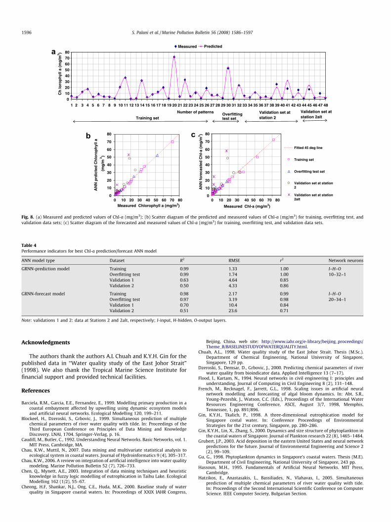
lagged times. Various model scenarios with different inputsparameters and different ANN architectures were tested for theprediction of Chl-a(t). Optimization of the input variables was per-formed by the removal/addition of one parameter at a time. In thisstudy, however, the model scenario that used location (longitudelatitude), DO, PO4, Temp, and Chl-a at lagged time t from Stations1 and 3 only as input parameters and the general regression neuralnetwork architecture performed best for the prediction of Chl-a(t)at any location within modeled domain. The addition of other vari-ables did not significantly improve the performance of the net-work. The developed ANN model predicted the Chl-a and DOdynamics at Stations 2 and 2alt using the water quality observa-tions from Stations 1 and 3. Fig. 8a shows the measured and pre-dicted values of Chl-a (mg/m3) for the best ANN model. Thescatter diagram for the best Chl-a (mg/m3) prediction model andforecasting model for the training, overfitting test, and validationdata sets are shown in Fig. 8b and c, respectively. The results ofANN modeling (Fig. 8) suggest that it is possible to forecast waterquality variables within the study domain with data from just twomonitoring Stations (1 and 3). This approach reduces the monitor-ing cost by allowing researchers to choose an appropriate numberof sampling stations for field monitoring. We suggest that the col-lection of field data and further improvement the ANN should con-tinue, however, because the existing cases may not sufficientlycover the required sampling space. Performance indicators forthe best Chl-a prediction and forecasting ANN model are shownin Table 4.

The ANN models developed were able to predict phytoplank-ton concentration dynamics (in terms of Chl-a) fairly well usingminimal input parameters even though there were unknownfactors affecting seawater quality and limited data sets. The re-

sults show that complex behavior in the eutrophication processcould be modeled using the ANN technique, and we success-fully estimated some extreme values from the validation datasets that were not used in training the neural network. Thedeveloped model can be used to (1) estimate the Chl-a concen-tration when the real value cannot be obtained, (2) estimateinterpolated data between two consecutives samples, and (3)simulate different water quality scenarios for extreme rangesof input and output parameters. This eutrophication modelingapproach is helpful for predicting Chl-a levels at any locationor time (t) in the domain of interest where there are trainingstations. The uncertainty in our results may be due to dynamiccharacteristics of seawater quality around East Johor Strait,hydrodynamic forcing and unknown sources of pollution, orfreshwater addition in the region of interest within a short tem-poral duration. It should be noted that data were measured inweekly intervals at one instance of the tidal cycle. The ANNwas able to satisfactorily model the Chl-a dynamics and DO lev-els in Singapore seawater in a very short computational time.We recognize that a limited number of sampling data recordswere used in this study. More data sampling is thus required,and future work should recalibrate and revalidate the modelsto generalize our conclusions. The Chl-a model for seawater willbe further fine-tuned for higher accuracy by including the tidalcurrents, wave data, and rain data as input parameters. ANNmodeling can optimize monitoring network by removing sta-tions that do not introduce new useful information, might helpto analyze the factors that control the occurrence and develop-ment of HAB, provides fast predictions or forecasting, and min-imizes the number of significant parameters required formodeling.

0

2

4

6

8

10

12

14

16

Date of sampling

DO

(m

g/l)

0

10

20

30

40

50

60

70

80

Chl

orop

hyll

a (m

g/m

3 )

DO at station 1 DO at station 3

DO at station 2/2alt Chlorophyll a at station 1

Chlorophyll a at station 3 Chlorophyll a at station 2/2alt

0

20

40

60

80

100

120

15-J

an-9

7

22-J

an-9

7

29-J

an-9

7

4-F

eb-9

7

12-F

eb-9

7

20-F

eb-9

7

26-F

eb-9

7

6- M

ar-9

7

13-M

ar-9

7

17-M

ar-9

7

26-M

ar-9

7

2-A

pr-9

7

9-A

pr-9

7

17-A

pr-9

7

30-A

pr-9

7

14-M

ay-9

7

30-M

ay-9

7

15-J

an-9

7

22-J

an-9

7

29-J

an-9

7

4-F

eb-9

7

12-F

eb-9

7

20-F

eb-9

7

26-F

eb-9

7

6- M

ar-9

7

13-M

ar-9

7

17-M

ar-9

7

26-M

ar-9

7

2-A

pr-9

7

9-A

pr-9

7

17-A

pr-9

7

30-A

pr-9

7

14-M

ay-9

7

30-M

ay-9

7

Date of sampling

Chl

a(m

g/m

3 )

00.010.020.030.040.050.060.070.080.09

PO

4 (m

g/L)

Chla at station 1 Chla at station 3 Chla at station 2/2alt

PO4 at station 1 PO4 at station 3 PO4 at station 2/2alt

a

b

Fig. 7. Temporal variation of the measured concentrations of Chl-a and PO4 at four monitoring stations in the East Johor Strait.


4. Summary and conclusions

ANN models were developed to predict salinity, water temper-ature, dissolved oxygen and Chl-a concentrations in Singaporecoastal waters both temporally and spatially using continuousweekly measurements of water quality variables at different sta-tions. In spite of largely unknown factors controlling seawaterquality variation and the limited data set size, a relatively goodcorrelation was observed between the measured and predictedvalues. The ANN modeling technique’s application for dynamicseawater quality prediction was presented in this study. TheANN model has tremendous potential as a forecasting tool. AnANN’s prediction capability was tested and found to be fasterthan that from a process-based model with minimal inputrequirements. In particular, we observed that the GRNN andMLP methods were able to ‘‘learn” the mechanism of convectivetransport of water quality variables quite well. Based on the ‘‘bestperformance” in water quality parameter forecasting, we ob-served that Ward Net is the better architecture for the tempera-ture and salinity models, but the GRNN is better for DO andChl-a models. This model could be used in parallel with phys-ics-based models as a new prediction tool. It can identify impor-

tant parameters for enabling both selective physical/chemicalmonitoring and quick water quality assessment of Singapore sea-water. The limitations of this study include its limited data set.The lack of fit between the observed and estimated data indicatesthat new patterns must be incorporated into the model, and thusthe model should be recalibrated and revalidated as more dataare collected. Even though the available data size is relativelysmall, reasonably good results were obtained for the water qual-ity prediction of unseen validation dataset at locations separatefrom the training dataset stations. If more data become available,the proposed approach should provide better predictions. Theaccuracy of the developed models should be compared using n-fold cross-validation, because the available data set is limited.ANN modeling is a promising and useful tool that optimizes mon-itoring networks by identifying essential monitoring stations(thereby permitting cost reduction) and forecasts seawater qual-ity variables with acceptable accuracy. Further studies that applymultivariate models and incorporate new key input variables arenecessary in order to arrive at better results after the pruning ofnon-useful connections. Additionally, future work should use newtypes of algorithms that are more appropriate for time seriesforecasting.

010203040

5060

7080

1 2 3 4 5 6 7 8 9 10 11 12 13 14 15 16 17 18 19 20 21 22 23 24 25 26 27 28 29 30 31 32 33 34 35 36 37 38 39 40 41 42 43 44 45 46 47 48

Number of patterns

Ch

loro

ph

yll a

(m

g/m

3 )

Predicted

Overfitting test setTraining set

Validation set at station 2

Validation set at station 2alt

Measured

0

10

20

30

40

50

60

70

80

0 10 20 30 40 50 60 70 80 0 10 20 30 40 50 60 70 80Measured Chlorophyll a (mg/m3)

AN

N p

rdic

ted

Ch

loro

ph

yll a

(mg

/m3)

0

10

20

30

40

50

60

70

80

Measured Chl-a (mg/m3)

AN

N f

ore

cast

ed C

hl-

a (m

g/m

3 )

Fitted 45 deg line

Training set

Overfitting test set

Validation set at station2

Validation set at station2alt

a

b c

Fig. 8. (a) Measured and predicted values of Chl-a (mg/m3); (b) Scatter diagram of the predicted and measured values of Chl-a (mg/m3) for training, overfitting test, andvalidation data sets; (c) Scatter diagram of the forecasted and measured values of Chl-a (mg/m3) for training, overfitting test, and validation data sets.

Table 4Performance indicators for best Chl-a prediction/forecast ANN model

ANN model type Dataset R2 RMSE r2 Network neurons

GRNN-prediction model Training 0.99 1.33 1.00 I–H–OOverfitting test 0.99 1.74 1.00 10–32–1Validation 1 0.63 4.64 0.85Validation 2 0.50 4.33 0.86

GRNN-forecast model Training 0.98 2.17 0.99 I–H–OOverfitting test 0.97 3.19 0.98 20–34–1Validation 1 0.70 10.4 0.84Validation 2 0.51 23.6 0.71

Note: validations 1 and 2: data at Stations 2 and 2alt, respectively; I-input, H-hidden, O-output layers.


Acknowledgments

The authors thank the authors A.L Chuah and K.Y.H. Gin for thepublished data in ‘‘Water quality study of the East Johor Strait”(1998). We also thank the Tropical Marine Science Institute forfinancial support and provided technical facilities.

References

Barciela, R.M., Garcia, E.E., Fernandez, E., 1999. Modelling primary production in acoastal embayment affected by upwelling using dynamic ecosystem modelsand artificial neural networks. Ecological Modelling 120, 199–211.

Blockeel, H., Dzeroski, S., Grbovic, J., 1999. Simultaneous prediction of multiplechemical parameters of river water quality with tilde. In: Proceedings of theThird European Conference on Principles of Data Mining and KnowledgeDiscovery. LNAI, 1704. Springer-Verlag, p. 16.

Caudill, M., Butler, C., 1992. Understanding Neural Networks. Basic Networks, vol. 1.MIT Press, Cambridge, MA.

Chau, K.W., Muttil, N., 2007. Data mining and multivariate statistical analysis toecological system in coastal waters. Journal of Hydroinformatics 9 (4), 305–317.

Chau, K.W., 2006. A review on integration of artificial intelligence into water qualitymodeling. Marine Pollution Bulletin 52 (7), 726–733.

Chen, Q., Mynett, A.E., 2003. Integration of data mining techniques and heuristicknowledge in fuzzy logic modelling of eutrophication in Taihu Lake. EcologicalModelling 162 (1/2), 55–67.

Cheong, H.F, Shankar, N.J., Ong, C.E., Huda, M.K., 2000. Baseline study of waterquality in Singapore coastal waters. In: Proceedings of XXIX IAHR Congress,

Beijing, China. web site: http://www.iahr.org/e-library/beijing_proceedings/Theme_B/BASELINESTUDYOFWATERQUALITY.html.

Chuah, A.L., 1998. Water quality study of the East Johor Strait. Thesis (M.Sc.).Department of Chemical Engineering, National University of Singapore,Singapore, 129 pp.

Dzeroski, S., Demsar, D., Grbovic, J., 2000. Predicting chemical parameters of riverwater quality from bioindicator data. Applied Intelligence 13 (7–17).

Flood, I., Kartam, N., 1994. Neural networks in civil engineering I: principles andunderstanding. Journal of Computing in Civil Engineering 8 (2), 131–148.

French, M., Recknagel, F., Jarrett, G.L., 1998. Scaling issues in artificial neuralnetwork modelling and forecasting of algal bloom dynamics. In: Abt, S.R.,Young-Pezeshk, J., Watson, C.C. (Eds.), Proceedings of the International WaterResources Engineering Conference, ASCE, August 3/7, 1998, Memphis,Tennessee, 1, pp. 891/896.

Gin, K.Y.H., Tkalich, P., 1998. A three-dimensional eutrophication model forSingapore costal water. In: Conference Proceedings of EnvironmentalStrategies for the 21st century, Singapore, pp. 280–286.

Gin, K.Y.H., Lin, X., Zhang, S., 2000. Dynamics and size structure of phytoplankton inthe coastal waters of Singapore. Journal of Plankton research 22 (8), 1465–1484.

Grubert, J.P., 2003. Acid deposition in the eastern United States and neural networkpredictions for the future. Journal of Environmental Engineering and Science 2(2), 99–109.

Gu, G., 1998. Phytoplankton dynamics in Singapore’s coastal waters. Thesis (M.E).Department of Civil Engineering, National University of Singapore, 243 pp.

Hassoun, M.H., 1995. Fundamentals of Artificial Neural Networks. MIT Press,Cambridge.

Hatzikos, E., Anastasakis, L., Bassiliades, N., Vlahavas, I., 2005. Simultaneousprediction of multiple chemical parameters of river water quality with tide.In: Proceedings of the Second International Scientific Conference on ComputerScience. IEEE Computer Society, Bulgarian Section.

http://www.iahr.org/e-library/beijing_proceedings/Theme_B/BASELINESTUDYOFWATERQUALITY.html

http://www.iahr.org/e-library/beijing_proceedings/Theme_B/BASELINESTUDYOFWATERQUALITY.html


Hatzikos, E., Bassiliades, N., Asmanis, L., Vlahavas, I., 2007. Monitoring water qualitythrough a telematic sensor network and a fuzzy expert system. Expert Systems24 (3), 143–161. 19.

Hecht-Nielsen, R., 1987. Kolmogorov’s mapping neural network existencetheorem. Proceedings of 1st IEEE International Joint Conference ofNeural Networks. Institute of Electrical and Electronics Engineers, NewYork, NY.

Hui, N.S., 2000. Eutrophication studies of estuarine and marine waters. Thesis (M.E).Department of Civil Engineering, National University of Singapore.

Karul, C., Soyupak, S., Cilesiz, A.F., Akbay, N., Germen, E., 2000. Case studies on theuse of neural networks in eutrophication modeling. Ecological Modelling 134,145–152.

Lee, J.H.W., Wong, K.T.M., Huang, Y., Jayawardena, A.W., 2000. A real time earlywarning and modeling system for red tides in Hong Kong. In: Wang, Z.Y. (Ed.),Proceedings of the Eighth International Symposium on Stochastic Hydraulics.Balkema, Beijing, pp. 659–669.

Lee, J.H.W., Huang, Y., Dickmen, M., Jayawardena, A.W., 2003. Neural networkmodelling of coastal algal blooms. Ecological Modelling 159, 179–201.

Lee, T.L., Jeng, D.S., 2002. Application of artificial neural networks in tide forecasting.Ocean Engineering 29, 1003–1022.

Lee, T.L., 2004. Back-propagation neural network for long-term tidal predictions.Ocean Engineering 31, 225–238.

Leung, M.T., Chen, A.S., Daouk, H., 2000. Forecasting exchange rates using generalregression neural networks. Computers and Operations Research 27 (11), 1093–1110. 18.

Lim, L.C., 1983. Coastal fisheries oceanographic studies in Johore Strait, Singapore. I.Current movement in the East Johore Strait and its adjacent waters. SingaporeJournal of Primary Industries 2 (2), 83–97.

Liong, S.Y., Lim, W.H., Paudyal, G., 1999. Real time river stage forecasting for floodstricken Bangladesh: neural network approach. Journal of Computing in CivilEngineering ASCE 14 (1), 1–8.

Liong, S.Y., Khu, S.T., Chan, W.T., 2001. Derivation of pareto front with geneticalgorithm and neural network. Journal of Hydrologic Engineering ASCE 6 (1),56–61.

Maier, H.R., Dandy, G.C., 2000. Neural networks for the prediction and forecasting ofwater resources variables: a review of modelling issues and applications.Environmental Modelling and Software 15, 101–124.

Makarynskyy, O., 2004. Improving wave predictions with artificial neural networks.Ocean Engineering 31, 709–724.

Maren, A.J., Harston, C.T., Pap, R., 1990. Handbook of Neural ComputingApplications. Academic Press, San Diego, CA.

Masters, T., 1993. Advanced Algorithms for Neural Networks. A C++ Sourcebook.John Wiley and Sons, Inc, New York.

McCulloch, W.S., Pitts, W., 1943. A logical calculus of the ideas imminent in nervousactivity. Bulletin and Mathematical Biophysics 5, 115–133.

Muttil, N., Chau, K.W., 2006. Neural network and genetic programming formodelling coastal algal blooms. International Journal of Environment andPollution 28 (3/4), 223–238.

Nash, J.E., Sutcliffe, J.V., 1970. River flow forecasting through conceptual models;part I – a discussion of principles. Journal of Hydrology 10, 282–290.

Neuroshell 2TM, 2000. Neuroshell Tutorial. Ward Systems Group, Inc., Frederick, MD,USA.

Pang, W.C., Tkalich, P., 2003. Modeling tidal and monsoon driven currents in theSingapore Strait. Singapore Maritime and Port Journal, 151–162.

Reckhow, K.H., 1999. Water quality prediction and probability network models.Canadian Journal of Fisheries and Aquatic Sciences 56, 1150–1158.

Rojas, R., 1996. Neural Networks: A Systematic Introduction. Springer-Verlag,Berlin.

Rumelhart, D.E., Hinton, G.E., Williams, R.J., 1986. Learning internal representationsby error propagation. In: Rumelhart, D.E., McClelland, J.L. (Eds.), ParallelDistributed Processing. MIT Press, Cambridge.

Specht, D.F., 1991. A general regression neural network. IEEE Transactions on NeuralNetworks 2 (6), 568–576.

Sundarambal, P., Tkalich, P., 2003. Eutrophication modelling for the Singaporewaters. In: Proceedings International Conference on Port and Maritime R&D andTechnology, 10–12 September 2003, Singapore, vol. 2, pp. 51–58.

Tarassenko, L., 1998. A Guide to Neural Computing Applications. Arnold Publishers,London.

Tham, A.K., 1953. A preliminary study of the physical, chemical and biologicalcharacteristics of Singapore. Fishery Publication 1 (4), 6–39.

Tsoukalas, L.H., Uhrig, R.E., 1997. Fuzzy and Neural Approaches in Engineering.Wiley Interscience, New York. 587 pp.

Whitehead, P.G., Howard, A., Arulmani, C., 1997. Modelling algal growth andtransport in rivers – a comparison of time series analysis, dynamic mass balanceand neural network techniques. Hydrobiologia 349, 39–46.

Wilcox, B.P., Rawls, W.J., Brakensiek, D.L., Wight, J.R., 1990. Predicting runoff fromrangeland catchments: a comparison of two models. Water Resources Research26, 2401–2410.

Xiaohua, L., 2000. Eutrophication studies of Singapore’s coastal waters. Thesis (M.E).Department of Civil Engineering, National University of Singapore.

Yabunaka, K.I., Hosomi, M., Murakami, A., 1997. Novel application of back-propagation artificial neural network model formulated to predict algalbloom. Water Science and Technology 36 (5), 89–97.

Zhang, Q.Y., 2000. A three dimensional eutrophication model for Singapore coastalwater. Thesis (PhD). Dept. of Civil Engineering, National University of Singapore,192 pp.

An ANN application for water quality forecasting

Documents

Transcript of An ANN application for water quality forecasting