An Analysis of the Embedded Frequency Content of Macroeconomic Indicators and their Counterparts...

From:OECD Journal: Journal of Business CycleMeasurement and Analysis

Access the journal at:http://dx.doi.org/10.1787/19952899

An Analysis of the Embedded FrequencyContent of Macroeconomic Indicators and their

Counterparts using the Hilbert-Huang Transform

Patrick M. Crowley, Tony Schildt

Please cite this article as:

Crowley, Patrick M. and Tony Schildt (2012), “An Analysis of theEmbedded Frequency Content of Macroeconomic Indicators and theirCounterparts using the Hilbert-Huang Transform”, OECD Journal:Journal of Business Cycle Measurement and Analysis, Vol. 2012/1.http://dx.doi.org/10.1787/jbcma-2012-5k92snjzsnnr

http://dx.doi.org/10.1787/19952899

http://dx.doi.org/10.1787/jbcma-2012-5k92snjzsnnr

This document and any map included herein are without prejudice to the status of orsovereignty over any territory, to the delimitation of international frontiers and boundaries and tothe name of any territory, city or area.

OECD Journal: Journal of Business Cycle Measurement and Analysis

Volume 2012/1

© OECD 2012

1

An Analysis of the Embedded Frequency Content of Macroeconomic

Indicators and their Counterparts usingthe Hilbert-Huang Transform

An Analysis of the Embedded Frequency Content of Macroeconomic Indicators and their Counterparts…

byPatrick M. Crowley and Tony Schildt*1

Many indicators of business and growth cycles have been constructed by both privateand public agencies and are now in use as monitoring devices of economic conditionsand for forecasting purposes. As these indicators are largely composite constructs usingother economic data, their frequency composition is likely different to that of thevariables that they are used as for indicators.

In this paper, we use the Hilbert-Huang transform which comprises empirical modedecomposition (EMD) and the Hilbert spectrum in order to analyse the frequency contentof comparable OECD confidence indicators, and national sentiment indicators forindustrial production and consumption. We then compare these with the frequencycontent of both industrial production and real consumption growth data. TheHilbert-Huang methodology first uses an iterative process (EMD) to identify theembedded frequencies within a time series and then the changing nature of theseembedded frequencies (IMFs) can be analysed by estimating the instantaneousfrequency (using the Hilbert spectrum). This methodology has several advantages overconventional spectral analysis: it handles non-stationary and non-linear processes, andit can cope with short data series.

The aim of this paper is to decompose both indicator and actual economic variables toevaluate i) whether the number of IMFs are equivalent in both indicators and actualvariables, and ii) to see which frequencies are accounted for in indicators, and whichfrequencies are not.

Key Words: economic growth, Hilbert-Huang transform, empirical mode decomposition,frequency domain, economic indicators, OECD

JEL Classification: C63, E21, E32

* Corresponding author: Crowley (Economics Group, College of Business, Texas A&M University – CorpusChristi, 6300 Ocean Drive, Corpus Christi, TX 78412, USA Texas).

AN ANALYSIS OF THE EMBEDDED FREQUENCY CONTENT OF MACROECONOMIC INDICATORS AND THEIR COUNTERPARTS…

OECD JOURNAL: JOURNAL OF BUSINESS CYCLE MEASUREMENT AND ANALYSIS © OECD 20122

1. IntroductionCyclical indicators aim to condense the information about economic activity

by capturing the cyclical patterns in economic variables into one-dimensional variables

that are tractable and possibly available prior to release of economic variables. In their book

Burns and Mitchell (1946) introduce a system to measure cyclical fluctuations in economic

activity developed by the National Bureau of Economic Research (NBER). Since then,

such regularly collected information is now an integral part of the measurement ex-post

of business cycles or to anticipate ex-ante cyclical fluctuations in economic activity.

Thus, the indicators of business cycles (see for example Kydland and Prescott, 1990)

and growth cycles (see for example Zarnowitz and Ozyildirim, 2002) are routinely used

as monitoring devices in the analysis of macroeconomic conditions and forecasting in

many countries.

A number of public and private institutions have developed cyclical indicators. The

Organisation for Economic Co-operation and Development (OECD) has developed a

comprehensive system of internationally comparable cyclical indicators. The data

surveyed with harmonised business tendency surveys is used with data published by

national agencies in construction of the OECD composite leading indicators. Through a

standardisation procedure, both the business and the consumer confidence indicator data

are made comparable between countries. The European Central Bank (2001) has dissected

the information content of the composite indicators of the euro area and how closely

indicators follow the cyclical pattern of the euro area reference series. As composite

indicators are summary indicators, we might not only be interested in the cyclical

behaviour of the aggregate series, but we might also be interested in determining what

frequencies are at work in the indicators as well as the relevant macroeconomic variables,

so that potential lead/lag relations between frequencies of particular interest can

be identified.

In this empirical paper, we dissect the information content of the OECD standardised

confidence indicators along with some national sentiment indicators and economic

variables for the euro area, Japan and the US. To do this we employ the Hilbert-Huang

transform (HHT) of Huang et al. (1998). The first step is to extract the embedded frequencies

of indicators and economic variables using empirical mode decomposition

(EMD). Secondly, we analyse the embedded frequencies by using a Hilbert spectrum.

As emphasised by Wu and Huang (2004), we use a recently developed variation of EMD

that corrects some recognised problems associated with EMD. Finally, we evaluate

the frequencies in the economic variables that are or are not being captured by the

indicators.

The rest of the paper is organised as follows: Section 2 introduces the cyclical

indicators and describes the data: Section 3 outlines the empirical method to be used;

Section 4 presents the empirical results; and, Section 5 offers some conclusions.


OECD JOURNAL: JOURNAL OF BUSINESS CYCLE MEASUREMENT AND ANALYSIS © OECD 2012 3

2. Data

2.1. Cyclical indicators

The timeliness and extensive geographical breakdown of economic data provides a

vast amount of information available to today’s economic policymaker. As is often the case

in statistical work, extensive economic data is reduced and summarised by computing a

smaller number of derived measures that try to incorporate what is relevant and

informative or even accidental in the cyclical behaviour of economic activity. The

indicators of cyclical behaviour in economic activity, that is cyclical indicators, are

classified by the Conference Board (2001) into three categories of leading, coincident, and

lagging based on the timing of their movements. Coincident indicators are series that

define the business cycle by measuring aggregate economic activity and leading indicators

are series that tend to shift direction in advance of the business cycle, while in contrast,

lagging indicators tend to change direction after the coincident series.

Burns and Mitchell (1946) document the measures of cyclical behaviour developed in

the 1930s by the National Bureau of Economic Research (NBER). The leading economic

indicator approach has been applied to measure business cycles ever since. While the

literature on business cycle theory attempts to explain recurrent fluctuations, the

empirical leading indicator approach is criticised for lack of constituent economic theory.

With regard to criteria of an economic nature, Koopmans (1947) notes that the constituent

series of cyclical indicators are chosen mainly on empirical grounds, rather than on the

basis of economic theory.

It is desirable to properly assess the current and in particular, future economic activity

for effective economic policy-making. For these purposes, business opinion is surveyed

with so-called business tendency surveys of company managers concerning the current

situation of their business and about their plans and expectations for the near future. In

collaboration with the European Commission, the Organisation for Economic Co-operation

and Development (OECD) has developed a system of harmonised business tendency

surveys. The economic data published by national agencies is used together with OECD

harmonised business tendency survey data in order to construct the OECD composite

leading indicators (CLIs) for both OECD member and non-member economies. The system

of OECD (2008) leading indicators is based on the growth cycle approach, which measures

deviations from the long-term trend, whereas the leading indicator approach is based on

repetitive but non-periodic fluctuations in economic activity.

The OECD released new cyclical indicators in December 2006 (OECD, 2006). These new

standardised indicators enhance the existing product range in the OECD CLIs by providing

both comparability between countries and the likelihood of fewer revisions. OECD CLIs are

constructed to predict cycles in a reference series chosen as a proxy measure for the aggregate

economy. The CLIs are released by the OECD on a monthly basis, and given their timeliness, are

appropriate to model short-term movements in economic variables. However, short-term

movements should be interpreted with caution because local volatility and revisions that are a

natural part of the calculation procedure can obscure the main patterns in economic activity.

The new set of OECD standardised cyclical indicators includes both Business

Confidence Indicators (BCIs) and Consumer Confidence Indicators (CCIs). These new

cyclical indicators are in addition to the existing CLIs, also published by the OECD. The BCIs

are presumed to anticipate reference series with shorter and more stable lead times than

the CLIs, and to date they appear to be subject to less revision than the CLIs.



The business confidence indicators are supposed to capture the cyclical patterns in

real-economic activity. Usually the volume of industrial production or real gross domestic

product (GDP) would be used as reference series for these indicators. Mourougane and

Roma (2002) find confidence indicators useful in forecasting real GDP growth rates in the

short run in a number of European countries. Industrial production data is also often used

as a proxy measure for real GDP. While real GDP is a more comprehensive variable for

analysing economy-wide fluctuations, industrial production data has the advantage of

being available on a monthly rather than a quarterly basis.

An article by the European Central Bank (2001) dissects the information content of

composite indicators of the euro area business cycle and the analysis suggests that

composite indicators may with hindsight, have followed developments broadly similar to

those of the business cycle as measured by both industrial production and real GDP

growth. However, the relationship between composite indicators and the business cycle

may not be very stable over time, which hampers the interpretation of the latest readings

of such indicators. For example, Japanese survey forecasts of industrial production were

found to be biased and inconsistent with rational expectations in comparison with the US

by Aggarwal and Mohanty (2000). Furthermore, Fukuda and Onodera (2001) point out that

several research institutes in Japan made serious errors in forecasting business cycles and

prolonged recessions in the 1990s.

Consumer confidence indicators are presumed to capture cyclical patterns in

household consumption behaviour. Andersen and Nielsen (2003) note that the consumer

confidence indicator is often taken as an indicator of the development in consumer

spending, but in general it is not so clear which economic variable, if any, consumer

confidence indicators describe. There is little agreement over the value of consumer

confidence indicators for forecasting consumer spending over what is already captured by

economic fundamentals. Consumer confidence indicators may potentially be used to point

to future behaviour, since households are asked also about their future expectations of the

economic activity. It is however, ambitious to think that the indicator can describe not only

the current, but also future economic development.

Few papers have investigated the usefulness of consumer confidence in modelling

consumer spending (see for example Ludvigson, 2004). Carroll et al. (1994) and Bram and

Ludvigson (1998) report the predictive information content of lagged values of consumer

confidence for US consumer spending. For Japan, Utaka (2003) finds that consumer

confidence has only a short-term effect on fluctuations in economic activity. Other studies

found in Chopin and Darrat (2000), examine the value of consumer attitudes for forecasting

economic performance, but fail to produce a consensus about the value of attitudes from

consumer measures for forecasting consumer behaviour. For example, Garner (1991) finds

the consumer confidence indicator published by the University of Michigan an unreliable

predictor of consumer spending.

For evaluation and proper use of an indicator, it is crucial to know how leading

indicators are constructed and moreover how composite leading indicators are

constructed. Furthermore, in the context of economic policymaking, composite indicators,

by construction, hide the driving factors behind current and short-term changes in

economic activity. Nevertheless, it is clear that many of the components of these indicators

may work at different frequencies, so that compiling composites might lead to internal

frequency mismatches.



2.2. Data description

For our data set, we use a range of economic indicators for the euro area, Japan and the

US. Both the national sentiment indicators and the OECD standardised confidence

indicators are used. The national indicators are also used by the OECD in its construction

of leading indicators so there will be some overlap here. In the frequency domain, we study

the comparable OECD confidence indicators and the nationally published sentiment

indicators alike. The series used for each country are given in Table 1. The data is

seasonally adjusted and the economic variables used as reference series are measured in

real terms for each country.

We follow the OECD (1998) and European Commission (2007) in defining industrial

production for manufacturing (henceforth referred to as industrial production), which is

defined as a reference series for OECD business composite indicator construction. Both the

industrial production data and the business confidence data are published on a monthly

basis (except for Japan where we use the monthly series interpolated by the OECD). More

information on the data used by the OECD is available in OECD (2006).

We define private final consumption expenditure in GDP including non-profit

institutions serving households (henceforth referred to as consumption) as the reference

for consumer confidence. Since the data for consumption is available on a quarterly basis,

we aggregate the consumer confidence indicator series from a monthly into a quarterly

series. The indicator value in a quarter is calculated as the average of the monthly

observations in that quarter for the consumer confidence indicator.

Table 1. Description of indicators and economic variables

Euro area Japan US

Business tendency survey Harmonised EU Business Tendency Survey Indicator1

Short-term Economic Surveyof Enterprises in Japan (TANKAN)3, quarterly.

Monthly Manufacturing Reporton Business

Source: European Commission, OECD Bank of Japan, OECD The Institute for Supply Management

Consumer opinion survey Harmonised EU Consumer Opinion Survey Indicator1

The Consumer Behavior Survey University of Michigan Consumer Sentiment Index

Source: European Commission Economic and Social Research Institute, Cabinet Office

University of Michigan

Business confidence indicator Standardised BusinessConfidence Indicator1

Standardised Business Confidence Indicator

Standardised BusinessConfidence Indicator

Source: OECD OECD OECD

Consumer confidenceindicator

Standardised Consumer Confidence Indicator1

Standardised Consumer Confidence Indicator

Standardised Consumer Confidence Indicator

Source: OECD OECD OECD

Industrial production Volume Index of Production2 Indices of Industrial Production INDPRO, Industrial Production Index

Source: Eurostat Ministry of Economy, Tradeand Industry

Board of Governors of the Federal Reserve System

Consumption Private Final Consumption Expenditure2

Final Consumption Expenditure Final Consumption Expenditure

Source: Eurostat Economic and Social Research Institute, Cabinet Office, IMF, OECD

Bureau of Economic Analysis

1. Euro area, 12 EMU countries up to 2006. 13 EMU countries, including Slovenia since 2007.2. Euro area, 12 EMU countries up to 1989, 13 EMU countries including Slovenia since 1990.3. Interpolated to monthly series by the OECD.



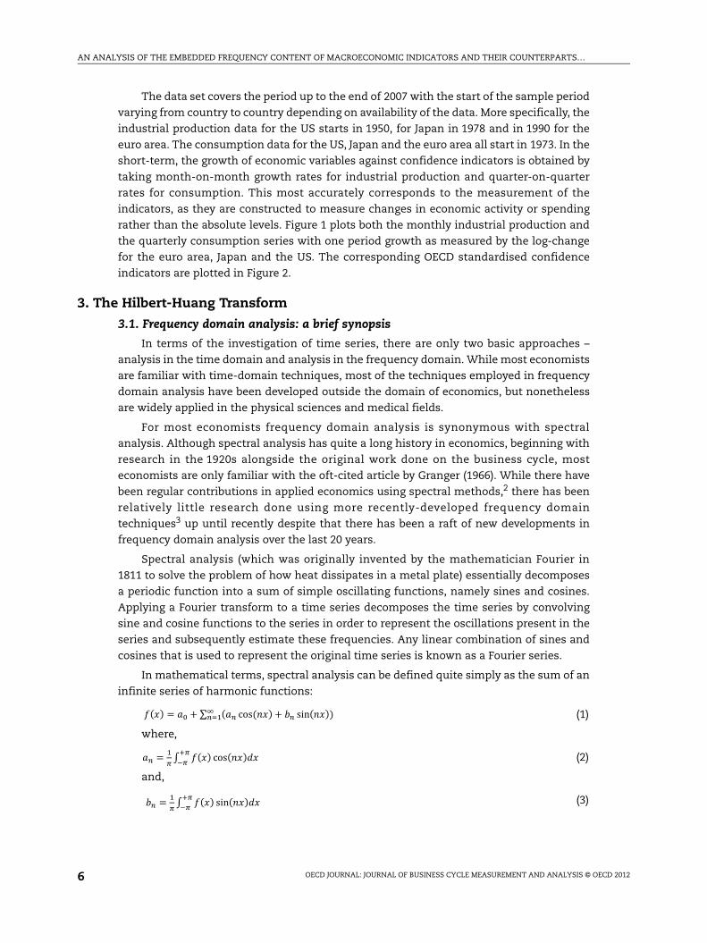
The data set covers the period up to the end of 2007 with the start of the sample period

varying from country to country depending on availability of the data. More specifically, the

industrial production data for the US starts in 1950, for Japan in 1978 and in 1990 for the

euro area. The consumption data for the US, Japan and the euro area all start in 1973. In the

short-term, the growth of economic variables against confidence indicators is obtained by

taking month-on-month growth rates for industrial production and quarter-on-quarter

rates for consumption. This most accurately corresponds to the measurement of the

indicators, as they are constructed to measure changes in economic activity or spending

rather than the absolute levels. Figure 1 plots both the monthly industrial production and

the quarterly consumption series with one period growth as measured by the log-change

for the euro area, Japan and the US. The corresponding OECD standardised confidence

indicators are plotted in Figure 2.

3. The Hilbert-Huang Transform

3.1. Frequency domain analysis: a brief synopsis

In terms of the investigation of time series, there are only two basic approaches –

analysis in the time domain and analysis in the frequency domain. While most economists

are familiar with time-domain techniques, most of the techniques employed in frequency

domain analysis have been developed outside the domain of economics, but nonetheless

are widely applied in the physical sciences and medical fields.

For most economists frequency domain analysis is synonymous with spectral

analysis. Although spectral analysis has quite a long history in economics, beginning with

research in the 1920s alongside the original work done on the business cycle, most

economists are only familiar with the oft-cited article by Granger (1966). While there have

been regular contributions in applied economics using spectral methods,2 there has been

relatively little research done using more recently-developed frequency domain

techniques3 up until recently despite that there has been a raft of new developments in

frequency domain analysis over the last 20 years.

Spectral analysis (which was originally invented by the mathematician Fourier in

1811 to solve the problem of how heat dissipates in a metal plate) essentially decomposes

a periodic function into a sum of simple oscillating functions, namely sines and cosines.

Applying a Fourier transform to a time series decomposes the time series by convolving

sine and cosine functions to the series in order to represent the oscillations present in the

series and subsequently estimate these frequencies. Any linear combination of sines and

cosines that is used to represent the original time series is known as a Fourier series.

In mathematical terms, spectral analysis can be defined quite simply as the sum of an

infinite series of harmonic functions:

(1)

where,

(2)

and,

(3)

�(�) = �� + � (�� cos(��) + � sin(��)�� )

�� =�

� �(�) cos(��)��

� �

� =�

� �(�) sin(��)��

� �



Figure 1. Industrial Production monthly and consumption quarterlywith growth rates as measured by log-change

350 000 000

300 000 000

250 000 000

200 000 000

100 000 000

150 000 000

50 000 000

0

0.08

0.06

0.04

0.02

0

-0.02

-0.04

-0.061973 1983 1993 2003

Japan: consumption (right)Japan: consumption, 1-Q log-change (left)

0.08

0.06

0.04

0.02

0

-0.02

-0.04

-0.06

120

100

80

60

40

20

01950 1960 1970 1980 1990 2000

United States: industrial production index (right)

United States: industrial production index,1-M log-change (left)

Index 2000 = 1000.08 9 000

8 000

7 000

6 000

4 000

5 000

2 000

1 000

3 000

0

0.06

0.04

0.02

0

-0.02

-0.04

-0.061973 1983 1993 2003

United States: consumption (right)United States: consumption, 1-Q log-change (left)

0.08 120

100

80

60

40

20

0

0.06

0.04

0.02

0

-0.02

-0.04

-0.061990 1995 2000 2005

Euro area: industrial production index (right)

Euro area: industrial production index,1-M log-change (left)

Index 2000 = 1000.08 1 600 000

1 400 000

1 200 000

1 000 000

600 000

800 000

200 000

400 000

0

0.06

0.04

0.02

0

-0.02

-0.04

-0.061973 1983 1993 2003

Euro area: consumption (right)Euro area: consumption, 1-Q log-change (left)

0.08 120

100

80

60

40

20

0

0.06

0.04

0.02

0

-0.02

-0.04

-0.061978 1983 1988 1993 1998 2003

Japan: industrial production index (right)

Japan: industrial production index,1-M log-change (left)

Index 2000 = 100

Source: Ministry of Economy, Trade and Industry.

Source: Eurostat.

Source: Board of Governors of the Federal Reserve System.

Source: Eurostat.

Source: Bureau of Economic Analysis.

Source: Economic and Social Research Institute, Cabinet Office,IMF, OECD.



These functions impose clear constraints on the series being analysed: the series should

be stationary; and, it is clearly assumed to be generated by linear combinations of harmonic

functions. Basic spectral analysis also assumes that different fluctuations in the series stay

constant through time, which other than for purely deterministic series, is clearly not the

case. To mitigate this particular concern Windowed Fourier analysis was invented to

essentially do spectral analysis on “windows” which are passed down the time series. In

more conventional statistical language this is called the short time Fourier transform (STFT)

with a rectangular window. If this window is simply moved to different parts of the series, we

can get abrupt changes (leading to what is known as the Gibbs phenomenon) as well as

incorrect estimates of frequencies, particularly if there are local non-stationarities in the

series under study. Subsequent developments in spectral analysis focused on development

of new windowing techniques and functions, some with overlapping windows, in which case

weightings on observations can be specified, giving rise to more complicated windows, such

as Hamming, Hann, Bartlett, Triangular, Gauss and Kaiser windows.

Passing a window down the length of a series in which case the analysis is not just

confined to the frequency domain, is often called “time-varying spectral” or “time-

frequency” analysis. Since its development in the 1970s, more flexible frequency domain

analysis techniques have emerged, mostly from other disciplines which rely more heavily

on this type of analysis (such as electrical engineering, acoustics and medical imaging).

In the 1980s, a chance meeting between a French mathematician (Daubechies) and

signal processor (Mallat) gave birth to wavelet analysis, and in its discrete form what Mallat

called “multi-resolution decomposition”. The basic idea behind wavelet analysis is to

decompose a time series into components corresponding to the fluctuations embedded in

the series over pre-defined ranges of frequencies. The concept is to apply different

functions other than harmonic functions to time series, such as asymmetric functions (as

with the Daubechies wavelet) or other specific features (such as a discrete step “Haar”

wavelet function). The mathematical background for wavelets can be found in Daubechies

(1992). Much of the background for this approach and some applications in economics and

finance can be found in Crowley (2007).

Figure 2. The OECD Standardised Confidence Indicators

Note: Long term average = 100.

110

105

100

95

90

85

801980 1985 1990 1995 2000 2005 1973 1983 1993 2003

110

105

100

95

90

85

80

Japan: OECD standardised BCI, monthly

Euro area: OECD standardised BCI, monthly

United States: OECD standardised BCI, monthly

Euro area: OECD standardised CCI, quarterly

Japan: OECD standardised CCI, quarterly

United States: OECD standardised CCI, quarterly



So why is wavelet analysis seen as superior to time-varying spectral analysis using the

STFT? The answer lies in the uncertainty principle, formulated by the quantum physicist

Heisenberg, which states that locating a particle in a small region of space makes the

velocity of the particle uncertain; and conversely, that measuring the velocity of a particle

precisely makes the position uncertain. Applying this to frequency domain analysis

implies that the exact frequency and time information of a variable at some certain point

in the time-frequency plane cannot be known. So, although we can resolve high

frequencies very well in time, it is less easy to resolve their exact frequency, but conversely

with low frequencies, they can be much better resolved in frequency, but much less well

resolved in time. This means the best we can do is to look at the frequency components

that exist over any given period, and use different “basis” functions as a means of matching

our series with some non-harmonic short function (or wavelet). Wavelets use short

functions, and in the discrete version of the multi-resolution decomposition they utilise

both a trend wavelet function and a “fluctuation” wavelet (referred to in the literature as

“father” and “mother” wavelets respectively). This means wavelets can also analyse non-

stationary time-series, which is a further advantage over traditional spectral analysis.

Wavelet analysis, although only around now for 20 years, has had a huge impact on

frequency domain analysis. Wavelet analyses come in at least two variations: discrete4 and

continuous.5 Discrete analysis relies on filter banks to process sampled data observed at

discrete points in time, whereas continuous analysis assumes that the observed data reflects

a continuous population distribution. Each methodology also has its own drawbacks: first,

discrete wavelet analyses rely on arbitrary selections of a wavelet “basis” function, which can

inevitably lead to some incomplete results if the matching of the series with the wavelet is

suboptimal. Second, wavelet analyses produce a new series for each scale (or frequency

range), with continuous wavelet analysis it depends on how fine the frequency ranges are

being used, whereas with discrete wavelet analyses the range of each scale is pre-defined in

dyadic terms. Therefore, if a particular series had embedded frequencies operating at both a

five-year and a seven-year cycle, then as the pre-defined scale ranges from four to eight year

cycle fluctuations, these two cycles would be combined and represented by a single series (or

“crystal”) at one particular scale. Third, there is “leakage” at the edges of each of these

pre-defined scales; for example, if using the pre-defined scale as above, and we have a

four-year cycle, it might show up in two scale crystals, leading to the impression that there

are two separate embedded frequency cycles, where in fact there is only one.

Because of these problems among others, the Hilbert-Huang transform was

introduced as an alternative to both spectral and wavelet analysis (as well as other

frequency domain methods not discussed here such as waveform dictionaries and the

Wigner distribution).

3.2. The basics of the Hilbert-Huang transform (HHT)

3.2.1. Introduction

The Hilbert-Huang transform (HHT) consists of two steps, of which only the first step is

new; namely empirical mode decomposition (EMD). EMD was pioneered by Huang (1998)

who, at the time, was an US National Aeronautical and Space Administration (NASA)

oceanographer and research scientist. He developed an algorithm which is not

mathematically based, as with spectral and wavelet analysis, but instead is an empirical

method for extracting the embedded frequencies (or what signal processors call “modes”) in

any given time series. The method does not rely on any “basis” function as with spectral and



wavelet analysis, and is a method that operates in the time domain rather than in the

frequency domain. The second part of the HHT (in its original version) uses the Hilbert

transform to obtain instantaneous frequency estimates using the “mode” data around any

given point in time. The resulting output is an improved decomposition and better resolution

of a series into its constituent frequency components. Probably the best review of the HHT

and more recent developments in the methodology can be found in Huang and Wu (2008).

EMD was developed in response to the desire of NASA for a more accurate way of

identifying frequency of oscillations. This is an important development in frequency

domain research as it acknowledges that many variables have oscillations that are time

varying and that many variables are non-stationary. The methodology is still being

developed and refined6 even though it is clear that its flexibility offers major advantages,

and in particular its adaptive basis.

Table 2 gives a basic comparison of empirical methods of analysis. In Table 2, the first

five entries in the first column (labelled “Feature”) refer to whether the characteristic is

required for the types of analysis headed up in the other columns. The last two entries in

the first column, “Measurement” and “Calculation”, refer to how fluctuations are measured

and in what domain the calculations are done in.

Very little research has been done in economics using the HHT, but there are two notable

exceptions: Huang and Shen (2005) applied HHT to US mortgage rates; and the other by

Zhang, Lai and Wang (2007) who applied HHT to oil prices. See Crowley (2009) for more

background on the method and some applications to economic and financial time series.

3.2.2. EMD process

EMD employs an iterative process as follows:

1. identify all local local extrema;

2. connect all local maxima using a cubic spline to form an envelope, and do likewise for

the minima;

3. calculate the mean of the upper and lower envelopes and denote m1;

4. subtract the mean from the series itself, so in equation form, we are left with the so-

called “first protomode”:

h1 = xt – m1 (4)

if h1 does not satisfy stopping criterion, let xt = h1 and go back to step 1;

Table 2. Comparison of empirical methods

Feature Time Series Spectral Wavelet EMD

Stationarity? Yes Yes No No

Linear? Yes Yes No No

Theory? Yes Yes No No

Adaptive? Limited No Limited Yes

Basis? A priori A priori A priori A posterior

Measurement Variance Energy in frequency domain Energy in time-frequency space Energy in time-frequency space

Calculations Time domain Frequency domain Frequency or Time domain Time domain

Note: “Theory?” denotes whether mathematical background is fully developed, “Adaptive?” refers to whether themethodology is able to adapt to structural changes in the series in question, and “Basis?” refers to how eachmethodology is applied to analyse the series in question.



5. if h1 satisfies stopping criterion after k iterations, the first intrinsic mode function (IMF)

is obtained:

c1 = h1k (5)

6. subtract this first IMF from the original data to obtain r1, the first “residual”:

xt – c1 = r1 (6)

7. start the whole process from 1 again but using r1 as new data.

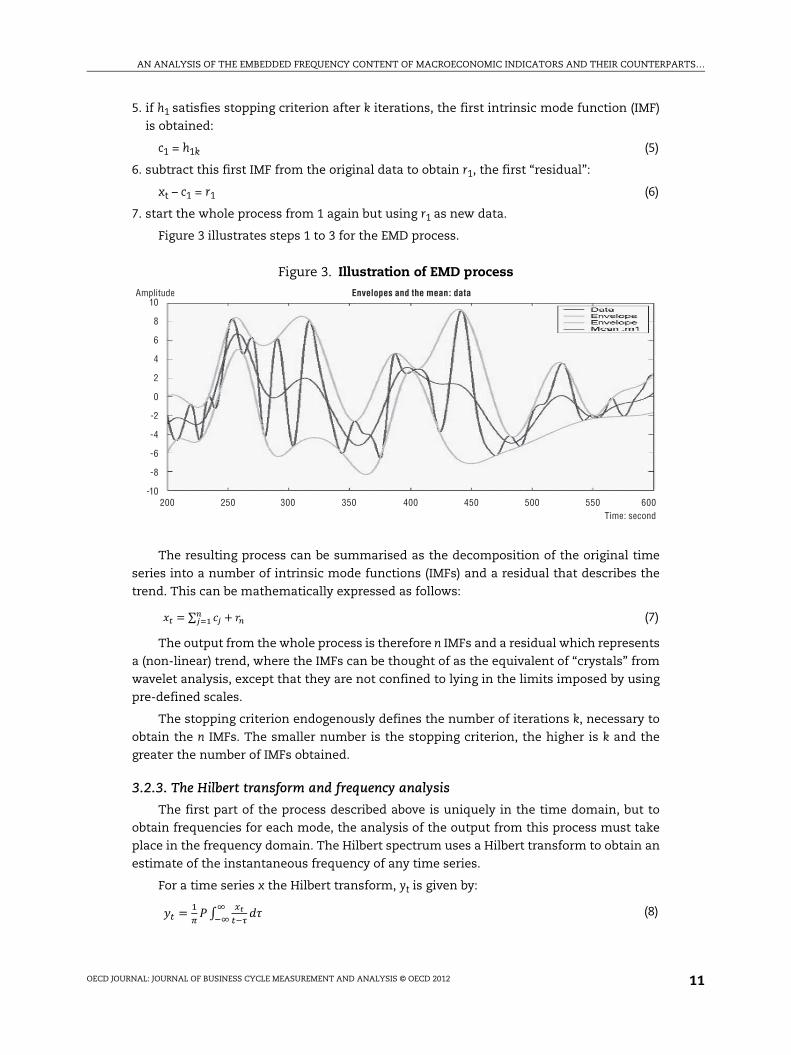
Figure 3 illustrates steps 1 to 3 for the EMD process.

The resulting process can be summarised as the decomposition of the original time

series into a number of intrinsic mode functions (IMFs) and a residual that describes the

trend. This can be mathematically expressed as follows:

(7)

The output from the whole process is therefore n IMFs and a residual which represents

a (non-linear) trend, where the IMFs can be thought of as the equivalent of “crystals” from

wavelet analysis, except that they are not confined to lying in the limits imposed by using

pre-defined scales.

The stopping criterion endogenously defines the number of iterations k, necessary to

obtain the n IMFs. The smaller number is the stopping criterion, the higher is k and the

greater the number of IMFs obtained.

3.2.3. The Hilbert transform and frequency analysis

The first part of the process described above is uniquely in the time domain, but to

obtain frequencies for each mode, the analysis of the output from this process must take

place in the frequency domain. The Hilbert spectrum uses a Hilbert transform to obtain an

estimate of the instantaneous frequency of any time series.

For a time series x the Hilbert transform, yt is given by:

(8)

Figure 3. Illustration of EMD process

10

8

6

4

2

0

-2

-4

-6

-8

-10200 250 300 350 400 450 500 550 600

Amplitude

Time: second

Envelopes and the mean: data

�� = � �� + ��

�� =�

� �

��

��

�



where P is the Cauchy principal value of the singular integral. Given the Hilbert

transform of any arbitrary function (xt) we obtain the analytical output zt, where:

(9)

Note that this output is of necessity complex. The term at then represents the

amplitude at time t, and the phase of the frequency is given by t, which can then be used

to estimate the instantaneous frequency, , which is given as:

(10)

The Hilbert transform, therefore, yields a direct estimate of the instantaneous

frequency of the cyclical activity embedded in the IMF, and thus this can be used as an

estimate of the time-varying frequency of the IMF.

Unfortunately there are two problems regarding the Hilbert transform, notably one of

underestimating the true frequency (due to the so-called “Nuttall theorem”), and also

incompletely extracting the frequency content of the data but leaving some information in

the amplitude variable (due to the so-called “Bedrosian theorem”). Because of these issues,

there has been new research (see Huang, Wu, Long et al, 2008) which suggests that a direct

quadrature method might be an improvement over the Hilbert spectrum for calculating

instantaneous frequency. Here we use the direct quadrature method.

3.3. Ensemble EMD

In this article, we use an Ensemble EMD methodology to separate out the embedded

frequencies in economic variables. Ensemble EMD (or EEMD) came about because of

various problems with EMD associated with “mode mixing”. “Mode mixing” occurs when

either:

● different frequencies are found to reside in the same IMF, or when

● similar frequencies are found to reside in different IMFs.

Wu and Huang (2004) note that various solutions to this problem (notably the

“intermittence test” in Huang, Shen and Long [1999]) were only partially successful in

mitigation, so a new approach was needed. Research on EMD done by Flandrin, Rilling and

Gonclaves (2004), and Flandrin and Gonclaves (2004a) showed that under certain

circumstances the EMD acted like a filter bank (that is, a constant band pass shape),

equivalent to analysis by using wavelet analysis. Further research by Flandrin et al. (2005)

showed that when applied to white noise, the EMD was equivalent to the dyadic filter bank

used by the discrete wavelet transform. Later Wu and Huang (2004) realised that by adding

white noise to the data and running EMD many times this will properly reduce the problem

of “mode mixing”, and yield greater resolution of the IMFs. This is mostly due to the cubic

spline calculation requiring well-defined extrema and by adding white noise to the

data these extrema are more accurately located, giving significant improvements in the

EMD results.

In theory, given N ensemble members, and if is the amplitude of the white noise

added to the data, then it can be shown that the resultant standard deviation of the error

(the difference between the variable and the sum of the corresponding IMFs) amounts to

n, where:

(11)

�� = ��

" =#�

#�

$� =%

&'



So when adding a certain amount of white noise to the data,7 the larger the ensemble

(N), the lower the error, and so improved results are obtained. The steps of EEMD then are

as follows:

1. add white noise to the series;

2. decompose the data with added white noise into IMFs using EMD;

3. repeat 1 and 2 N times, but with different white noise added each time; and

4. obtain the means of the “ensemble” IMFs from each EMD decomposition.

Essentially a chosen amount of white noise is added to each run, which will cancel out

when averaged, and consequently the mean IMFs obtained will be less likely to suffer from

“mode mixing”8 and will more likely be better resolved, particularly at higher frequencies.

Wu and Huang (2008) spend considerable time on applications of EMD and show that

if executed properly it can extract the embedded frequencies operating in most non-linear

and non-stationary empirical data. It has the potential to be of major benefit to any data

analysis toolkit.

3.4. Estimation strategy with economic variables

Here, as we are mostly concerned with lower frequency IMFs, there should be less

concern with using the EMD with economic variables. Nevertheless, the instantaneous

frequencies obtained in the analysis occasionally displayed high levels of “mode mixing”,

particularly in the case of some of the sentiment indicators. As such, most of the indicator

variables were run first using basic EMD and then if “mode mixing” occurs, these were re-

run using EEMD with white noise variance of 20% of the variance of the actual series added

for the ensemble estimation, and a value of N = 400 for the ensemble.9

4. ResultsIn all the results that follow, the data used for the economic (counterpart) variable to

be analysed is the change in the logged value of the variable, and for the indicators, the

actual level of the indicator is used for comparison. This is the most appropriate

comparison, as most indicators are constructed so that they “indicate” a rise or fall in the

economic variable counterpart.

4.1. The US

4.1.1. Industrial production: US industrial production vs. OECD business confidence indicator

The left hand panel of Figure 4 shows the original series (A) for the economic variable

(ln[USIPt]-ln[USIPt-1]), where USIPt is the US indus (B to H) and then the last series in the

stackchart (I) represents the residual (or adaptive trend). The same is done for the indicator

variable, in this case the OECD leading indicator for industrial production, in the right hand

panel of Figure 4.

There are several things to note from the plot. First, seven IMFs were extracted from

USIP, whereas only six IMFs were extracted from the OECD indicator. Noticeably the more

noise in the series to begin with, the higher frequency IMFs will be extracted from the

series. On inspection it appears that there is considerable correlation in movements of

IMFi(USIP) with IMFi-1 (USIPindicator). This correlation appears in the (maximal lag)

correlation of the IMFs in Table 3 where the strongest (significant10) correlation is between



IMF7 for USIP and IMF6 (0.5609) for the indicator, and IMF5 for USIP against IMF4 for the

indicator (0.6833). Second, the business cycle is not separately identified within a particular

frequency and its location depends, as might be expected, on the shape of the downturn;

so for the short sharp recession of the early 1980s, this downturn is found in IMF5, but for

the shallower downturn in the early 2000s, this downturn is located in IMF6. Third, it is

apparent that there are other cycles in the data besides the business cycle, and that some

of these fluctuations in the data are clearly of major significance in terms of amplitude of

fluctuation. These cycles are what Zarnowitz and Ozyildirim (2002) have termed “growth

cycles”, and we use the same terminology here for the remainder of the article. Fourth, the

residual is different for the indicator and for industrial production; the average level of

industrial production increases appears to be falling over time, whereas the indicator

perhaps appears to have a rather long cycle, although this is difficult to tell without

additional data.

The frequency content of the cycles found in the data and the indicator are shown in

Figure 5. The separation of the IMFs in terms of frequency is clear for most of the series

although in the 1980s, there is “mode mixing” and in the late 1990s it reoccurs with IMF5.

Figure 4. US industrial production vs. OECD business confidence indicator: IMFs

Table 3. Correlations of IMFs for US industrial production (USIP)and OECD business confidence indicator (overall = 0.5389) with frequencies

Correlations of USIP IMF2 IMF3 IMF4 IMF5 IMF6 Frequency

IMF2 0.4178* –0.0206 –0.0207 0.0026 –0.0059 1.3477

IMF3 0.0998 0.366* 0.2186* –0.0245 0.1038* 0.7802

IMF4 0.0466 0.3362* –0.1329 –0.028 –0.1465 0.4379

IMF5 0.0206 0.2922* 0.6833* 0.2984* 0.1725* 0.2063

IMF6 0.0499 –0.0439 –0.1519 0.2989* 0.0296 0.1007

IMF7 –0.013 0.0213 0.0915* 0.0586 0.5609* 0.0486

Frequency 1.0464 0.4424 0.2074 0.1062 0.0564

Note: Correlations that are significant at the 5% level are denoted with an asterisk.

1950 1960 1970 1980 1990 2000 1950 1960 1970 1980 1990 2000

A

B

C

D

E

F

G

HI

A

B

C

D

E

F

G

H

EEMD of USIP OECD IndicatorEEMD of USIP



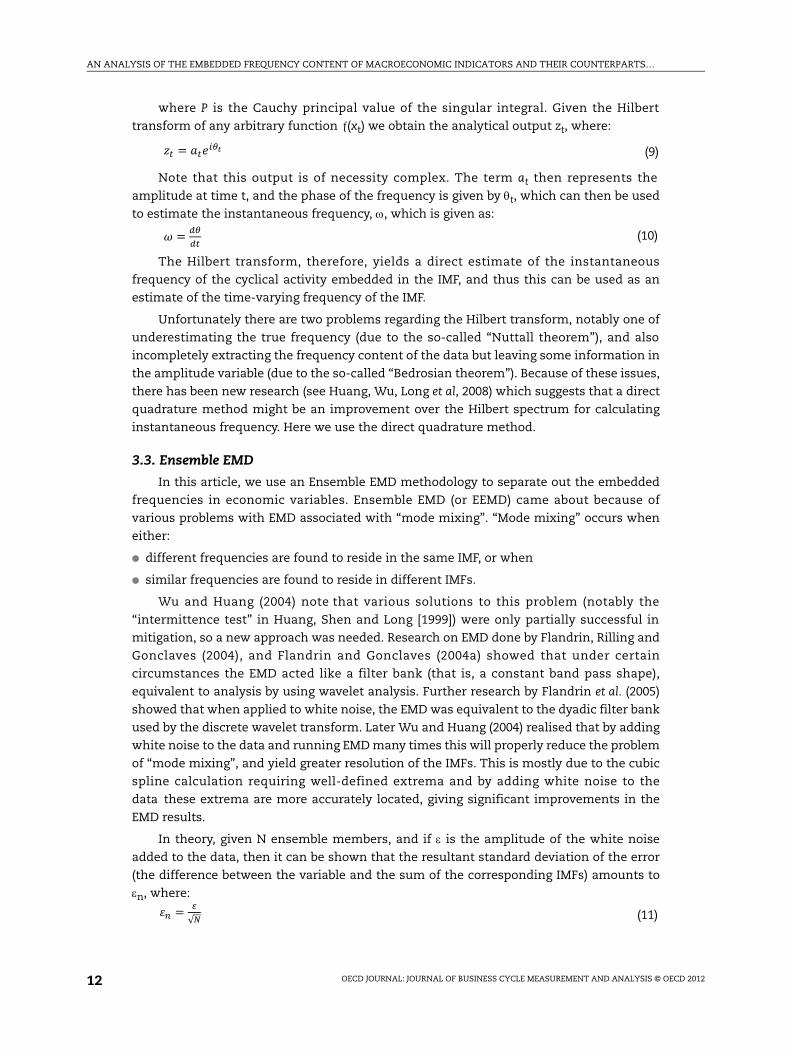
The same patterns are evident in the OECD indicator, which implies that the indicator

captures some of the changing frequency content associated with the different embedded

cycles. Interestingly in terms of longer cycles, there is a 10-year cycle evident in the data as

well as a 20-year cycle. Nothing beyond this is detected.

4.1.2. Industrial production: US industrial production vs. business sentiment indicator

In Figure 6 we show the IMFs obtained from the business sentiment index against

the industrial production data. Note that this is a shortened time series so we obtain

slightly different results for USIP. In Figure 7 the instantaneous frequencies are also

plotted.

In this instance we extract the lower frequency for Table 4 despite the fact there is very

little evidence of a longer cycle in the short span of data being used. Nevertheless, we know

from the full dataset that a longer (around 20-year) cycle is identified in the data. Here the

business cycle is identified in USIP in both IMF4 and IMF5, but in the business sentiment

index the business cycle is located in IMF5, which appears to be a high-amplitude

frequency component. It is noteworthy that IMF4 in USIP is also identified quite well by

IMF3 in the business sentiment index, but these growth cycles are less well identified than

the business cycle as a whole. In terms of the frequency plots, very little mode-mixing

occurs with USIP, but significant mode-mixing appears to occur in the mid-1990s for the

sentiment index, but this appears to be a temporary phenomenon.

4.1.3. Consumption: US consumption vs. OECD consumer confidence indicator

Figure 8 shows the IMFs from the EEMD of US consumption growth and the OECD

leading indicator.

Here the original series clearly shows the “great moderation” in terms of a narrowing

of the amplitude of fluctuations in consumption growth, but this is not readily apparent

when looking at the indicator. In terms of the IMFs, the business cycle is contained mostly

Figure 5. US industrial production vs. OECD business confidence indicator: instantaneous frequency

1950 1960 1970 1980 1990 2000 1950 1960 1970 1980 1990 2000

2.0

1.8

1.6

1.4

1.2

1.0

0.8

0.6

0.4

0.2

0

2.0

1.8

1.6

1.4

1.2

1.0

0.8

0.6

0.4

0.2

0

Inst. freq. for OECD IP IndicatorInst. freq. for USIPCycle year Cycle year



in IMF4 for both the original series and the indicator, with the notable exception being

the 1982 recession, which shows up as a shorter frequency fluctuation in IMF2 in both

cases. What is particularly interesting here is that the growth cycle in IMF2 and IMF3 are

largely reflected in the OECD indicator growth cycles, and that when looking at the

business cycle in IMF4, there is a clear dampening in the actual variable but this is not

apparent in the indicator variable. This suggests that although economic indicators predict

a usual size of amplitude in the business cycle, this does not tend to appear, perhaps due

to offsetting measures such as counter cyclical fiscal and monetary policy.

Figure 6. US industrial production vs. business sentiment indicator: IMFs

Figure 7. US industrial production vs. business sentiment indicator: instantaneous frequency

1985 1990 1995 2000 20051985 1990 1995 2000 2005

EEMD of USIPSIEEMD of USIP

1990 1999 2000 20051990 1999 2000 2005

2.0

1.8

1.6

1.4

1.2

1.0

0.8

0.6

0.4

0.2

0

2.0

1.8

1.6

1.4

1.2

1.0

0.8

0.6

0.4

0.2

0

Inst. freq. for business sentimentInst. freq. for USIPCycle year Cycle year



When looking at the correlation between the cycles (Table 5), it is clear that the

correspondence between the IMFs for both consumption growth and the OECD

consumption indicator is very good, except for the very high growth cycle frequencies.

4.1.4. Consumption: USC vs. consumer sentiment indicator

In this analysis, the Michigan index of consumer sentiment is used and the embedded

frequency fluctuations are compared with the growth of consumption expenditures.

Figure 8 shows the IMFs obtained from EEMD. The IMF4s appear to correspond well to the

business cycle, with the IMF3 identifying the 1974 recession for the sentiment index. One

of the surprising aspects of the analysis is that other growth cycles (IMF2 and IMF3 for

example) do not appear to be detected as well as might be expected. This is confirmed in

Table 6 where consumption growth IMF3 is best identified by two IMFs in the sentiment

index (IMF2 and IMF3), but correlations are relatively low (but significant) in each case. This

also comes out in the frequency plots in Figure 9, where there appears to be frequency

mismatches between the IMFs, but this is actually because some of the features in

consumption growth are captured by different IMFs in the consumer sentiment index.

What does this imply in economic terms? It implies that consumers know when

shocks occur, but have less information about the medium to longer term impact on

consumer spending of these shocks (whether permanent or transitory, for example), and

this shows up in our results. This is in direct contrast to the results obtained for industrial

production, where producers appear to have a better idea about the medium to long-term

impact of shocks on output (perhaps through greater networking and greater monitoring

of economic indicators than for consumers).

Table 4. Correlations of IMFs for US industrial production (USIP)and business sentiment indicator (overall = 0.40) with frequencies

Correlations of USIP IMF2 IMF3 IMF4 IMF5 IMF6 Frequency

IMF2 0.2168* 0.049 –0.0067 –0.018 –0.0137 1.3563

IMF3 0.3169* 0.2445* –0.0009 0.0632 0.0344 0.7433

IMF4 0.2332* 0.5131* 0.3141* –0.0987 0.016 0.4260

IMF5 0.0324 0.1784* 0.6824* 0.4707* –0.1473 0.1499

IMF6 –0.022 0.0647 0.1339* 0.5708* 0.5425* 0.0927

Frequency 1.1053 0.4624 0.1721 0.1013 0.0578


Table 5. Correlations of IMFs for US consumption (USC)and the OECD consumer confidence indicator (overall = 0.40) with frequencies

Correlations of USC IMF2 IMF3 IMF4 IMF5 Frequency

IMF2 0.0488 –0.0302 –0.0111 –0.0516 1.23

IMF3 –0.0618 0.5306* 0.0679 –0.1457 0.54

IMF4 0.1919 0.2255* 0.7229* 0.1321 0.25

IMF5 –0.0262 0.193 0.0259 0.7892* 0.08

Frequency 1.00 0.42 0.19 0.08




Figure 8. US consumption vs. consumer sentiment indicator: IMFs

Table 6. Correlations of IMFs for US consumption (USC) and consumer sentiment indicator (overall = 0.458) with frequencies

Correlations of USC IMF2 IMF3 IMF4 IMF5 Frequency

IMF2 0.0934 0.0063 –0.0056 –0.01 1.293IMF3 0.2127* 0.2913* –0.0572 0.0141 0.662IMF4 0.1465 0.5864* 0.4419* 0.1332 0.296IMF5 0.0008 –0.0484 0.0799 0.4457* 0.0711Frequency 0.916 0.458 0.197 0.143


Figure 9. US consumption vs. consumer sentiment indicator: instantaneous frequencies

1975 1980 1985 1990 1995 2000 20051975 1980 1985 1990 1995 2000 2005

US CSI IMFsUSC IMFs

1975 1980 1985 1990 1995 2000 2005 1975 1980 1985 1990 1995 2000 2005

2.0

1.8

1.6

1.4

1.2

1.0

0.8

0.6

0.4

0.2

0

2.0

1.8

1.6

1.4

1.2

1.0

0.8

0.6

0.4

0.2

0

Inst. freq. for US CSIInst. freq. for USCCycle year Cycle year



4.2. Euro area

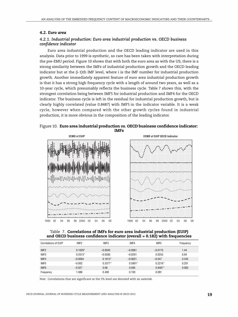
4.2.1. Industrial production: Euro area industrial production vs. OECD business confidence indicator

Euro area industrial production and the OECD leading indicator are used in this

analysis. Data prior to 1999 is synthetic, so care has been taken with interpretation during

the pre-EMU period. Figure 10 shows that with both the euro area as with the US, there is a

strong similarity between the IMFs of industrial production growth and the OECD leading

indicator but at the (i-1)th IMF level, where i is the IMF number for industrial production

growth. Another immediately apparent feature of euro area industrial production growth

is that it has a strong high frequency cycle with a length of around two years, as well as a

10-year cycle, which presumably reflects the business cycle. Table 7 shows this, with the

strongest correlation being between IMF5 for industrial production and IMF4 for the OECD

indicator. The business cycle is left in the residual for industrial production growth, but is

clearly highly correlated (value 0.8487) with IMF5 in the indicator variable. It is a weak

cycle, however when compared with the other growth cycles found in industrial

production, it is more obvious in the composition of the leading indicator.

Figure 10. Euro area industrial production vs. OECD business confidence indicator: IMFs

Table 7. Correlations of IMFs for euro area industrial production (EUIP)and OECD business confidence indicator (overall = 0.182) with frequencies

Correlations of EUIP IMF2 IMF3 IMF4 IMF5 Frequency

IMF2 0.1629* –0.0045 –0.0061 –0.0175 1.44

IMF3 0.2013* –0.0393 –0.0201 0.0253 0.94

IMF4 –0.0004 0.1613* –0.0621 –0.047 0.345

IMF5 –0.002 0.3377* 0.5901* 0.2216* 0.201

IMF6 –0.027 0.08 0.095 0.8487* 0.083

Frequency 1.086 0.400 0.193 0.091


1990 92 94 96 98 2000 0802 04 061990 92 94 96 98 2000 0802 04 06

EEMD of EUIP OECD IndicatorEEMD of EUIP



When looking at the frequencies of the IMFs in Figure 11 it is clear that IMF2 for the

OECD leading indicator has been constructed prior to 1999 as the frequency response is

very different from other IMFs. Both a 5-year and a 10-year cycle can be detected in the

data, and this comes through in both industrial production growth and the OECD leading

indicator.

4.2.2. Consumption: Euro area consumption vs. OECD consumer confidence indicator

In this analysis, euro area consumption growth is decomposed alongside the OECD

leading indicator for the euro area. Figure 12 shows the IMFs and that once again, the longer

cycles present in consumption growth are evident in the leading indicator. Shorter cycles

though are much less evident in the leading indicator, and this is also apparent from the size

of the correlations reported in Table 8, where shorter cycles have lower correlations than the

longer cycles. Here the instantaneous frequencies shown in Figure 13 move together at lower

frequencies, but less so at higher frequencies, although there is some mode mixing

particularly when these movements in higher frequencies do not match.

4.3. Japan

The case of Japan is an interesting one, as it is a country that underwent a sustained

period of stagnation and depression in the 1990s, so hopefully the EEMD approach will still

be able to reveal any growth cycles that occurred during this prolonged contractionary

period.

4.3.1. Industrial production: Japanese industrial production vs. OECD business confidence indicator

Figure 14 shows the IMFs for Japanese industrial production and the OECD leading

indicator. Unlike in the US or euro area case, in this analysis the OECD indicator is clearly

non-stationary, but this poses little problem when applying the EEMD approach as the

Figure 11. Euro area industrial production (EUIP) vs. OECD business confidence indicator: instantaneous frequency

1990 92 94 96 98 02 04 06 082000 1990 92 94 96 98 02 04 06 082000

2.0

1.8

1.6

1.4

1.2

1.0

0.8

0.6

0.4

0.2

0

2.0

1.8

1.6

1.4

1.2

1.0

0.8

0.6

0.4

0.2

0

Inst. freq. for OECD IP IndicatorInst. freq. for EUIPCycle year Cycle year



Figure 12. Euro area consumption vs. OECD consumer confidence indicator: IMFs

Table 8. Correlations of IMFs for euro area consumption (EUC)and OECD consumer confidence indicator (overall = 0.182) with frequencies

Correlations of EUC IMF2 IMF3 IMF4 Frequency

IMF2 0.2198* 0.0012 –0.0156 0.9

IMF3 0.6155* 0.1612* 0.0321 0.5

IMF4 0.0577 0.6624* 0.1297 0.21

IMF5 –0.0061 –0.1884 0.7232* 0.11

Frequency 0.578 0.271 0.133


Figure 13. Euro area consumption vs. OECD consumer confidence indicator: instantaneous frequency

1975 1980 1985 1990 1995 2000 2005 1975 1980 1985 1990 1995 2000 2005

EU OECD LI IMFsEUC IMFs

1975 1980 1985 1990 1995 2000 2005 1975 1980 1985 1990 1995 2000 2005

2.0

1.8

1.6

1.4

1.2

1.0

0.8

0.6

0.4

0.2

0

2.0

1.8

1.6

1.4

1.2

1.0

0.8

0.6

0.4

0.2

0

Inst. freq. for OECD LIInst. freq. for EUCCycle year Cycle year



trend component is found in the residual. The actual long cycle containing the depression

of the 1990s is contained in the JIP residual, but this has no direct corresponding IMF in the

indicator. This suggests that the indicator did not anticipate the longevity of the

depression and that policy efforts to revive the economy, although appearing in the

indicators, largely failed to appear in actual industrial production growth. The level of

correlation between industrial production and the indicator is not high, and the highest

significant correlation is reported to be between high frequency IMFs. Visual inspection of

Figure 14 suggests that the most prominent IMF from the leading indicator (IMF5) appears

to lag that of the similar IMF (IMF4) in the industrial production data.

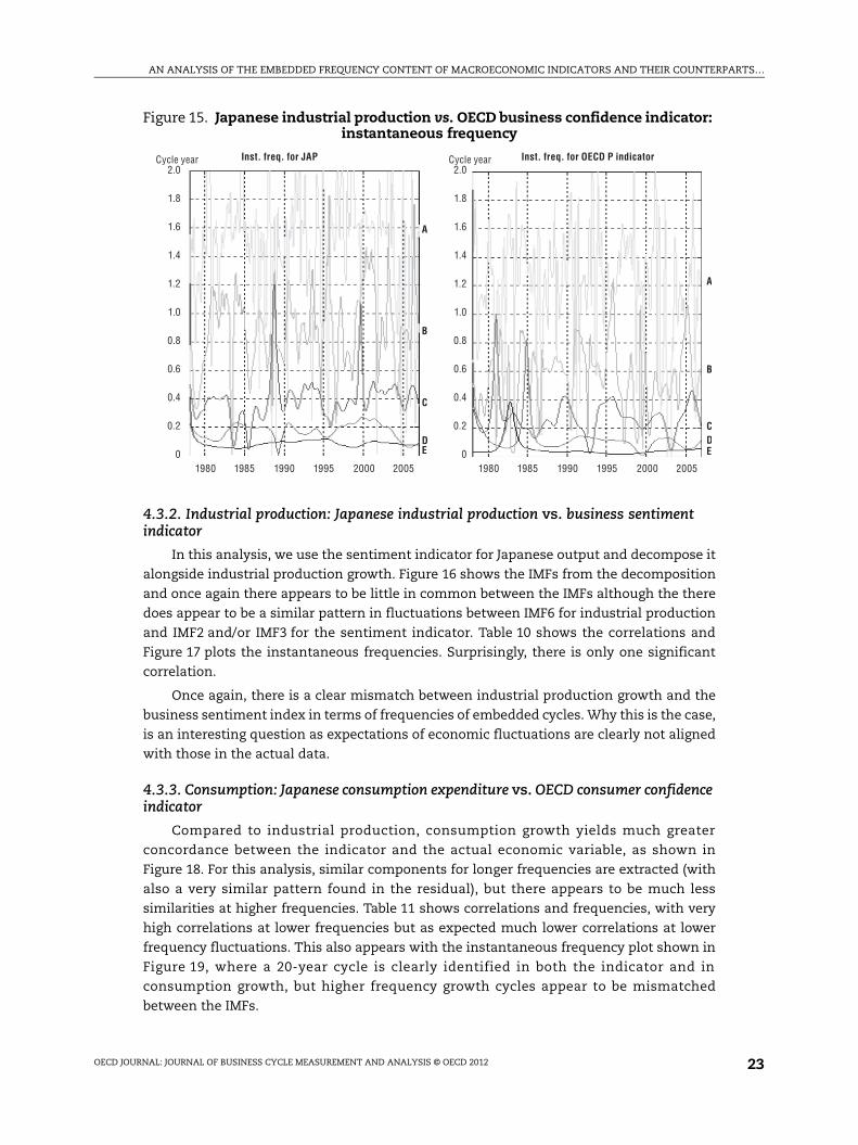
Table 9 shows a clear frequency mismatch across all cycles, and for longer frequencies

the indicator suggests roughly a 20-year cycle in output growth, where as the longest cycle

found in the actual data is an 11.5-year cycle. This is shown graphically in Figure 15.

Figure 14. Japanese industrial production vs. OECD business confidence indicator: IMFs

Table 9. Correlations of IMFs for Japanese industrial production (JAIP) and OECD business confidence indicator (overall = –0.0293) with frequencies

Correlations of JAIP IMF2 IMF3 IMF4 IMF5 IMF6 Frequency

IMF2 0.212* –0.0047 –0.0149 –0.0103 0.0088 1.475IMF3 0.2356* 0.122* 0.0534 0.0202 0.0028 0.889IMF4 0.0132 0.1168 0.057 –0.0063 –0.0173 0.393IMF5 –0.0046 0.0439 –0.0176 0.0073 0.0037 0.170IMF6 0.0045 –0.0049 –0.0167 0.1787* 0.1105 0.086Frequency 1.198 0.548 0.270 0.126 0.053


1980 1985 1990 1995 2000 20051980 1985 1990 1995 2000 2005

EEMD of JAIP OECD IndicatorEEMD of JAIP



4.3.2. Industrial production: Japanese industrial production vs. business sentiment indicator

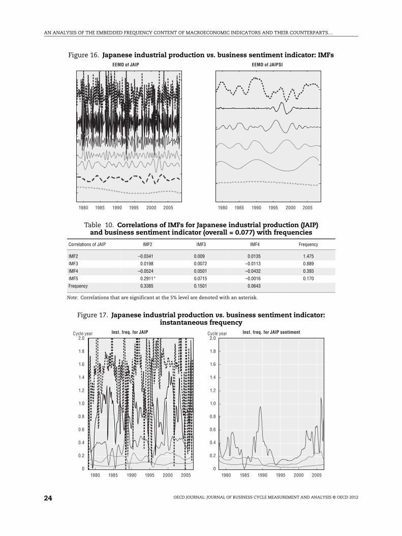
In this analysis, we use the sentiment indicator for Japanese output and decompose it

alongside industrial production growth. Figure 16 shows the IMFs from the decomposition

and once again there appears to be little in common between the IMFs although the there

does appear to be a similar pattern in fluctuations between IMF6 for industrial production

and IMF2 and/or IMF3 for the sentiment indicator. Table 10 shows the correlations and

Figure 17 plots the instantaneous frequencies. Surprisingly, there is only one significant

correlation.

Once again, there is a clear mismatch between industrial production growth and the

business sentiment index in terms of frequencies of embedded cycles. Why this is the case,

is an interesting question as expectations of economic fluctuations are clearly not aligned

with those in the actual data.

4.3.3. Consumption: Japanese consumption expenditure vs. OECD consumer confidence indicator

Compared to industrial production, consumption growth yields much greater

concordance between the indicator and the actual economic variable, as shown in

Figure 18. For this analysis, similar components for longer frequencies are extracted (with

also a very similar pattern found in the residual), but there appears to be much less

similarities at higher frequencies. Table 11 shows correlations and frequencies, with very

high correlations at lower frequencies but as expected much lower correlations at lower

frequency fluctuations. This also appears with the instantaneous frequency plot shown in

Figure 19, where a 20-year cycle is clearly identified in both the indicator and in

consumption growth, but higher frequency growth cycles appear to be mismatched

between the IMFs.

Figure 15. Japanese industrial production vs. OECD business confidence indicator: instantaneous frequency

1980 1985 1990 1995 2000 20051980 1985 1990 1995 2000 2005

2.0

1.8

1.6

1.4

1.2

1.0

0.8

0.6

0.4

0.2

0

2.0

1.8

1.6

1.4

1.2

1.0

0.8

0.6

0.4

0.2

0

A

B

CDE

A

B

C

DE

Inst. freq. for OECD P indicatorInst. freq. for JAPCycle year Cycle year



Figure 16. Japanese industrial production vs. business sentiment indicator: IMFs

Table 10. Correlations of IMFs for Japanese industrial production (JAIP)and business sentiment indicator (overall = 0.077) with frequencies

Correlations of JAIP IMF2 IMF3 IMF4 Frequency

IMF2 –0.0341 0.009 0.0135 1.475

IMF3 0.0198 0.0072 –0.0113 0.889

IMF4 –0.0524 0.0501 –0.0432 0.393

IMF5 0.2911* 0.0715 –0.0016 0.170

Frequency 0.3385 0.1501 0.0643


Figure 17. Japanese industrial production vs. business sentiment indicator: instantaneous frequency

1980 1985 1990 1995 2000 20051980 1985 1990 1995 2000 2005

EEMD of JAIPSIEEMD of JAIP

1980 1985 1990 1995 2000 20051980 1985 1990 1995 2000 2005

2.0

1.8

1.6

1.4

1.2

1.0

0.8

0.6

0.4

0.2

0

2.0

1.8

1.6

1.4

1.2

1.0

0.8

0.6

0.4

0.2

0

Inst. freq. for JAIP sentimentInst. freq. for JAIPCycle year Cycle year



Figure 18. Japanese consumption vs. OECD consumer confidence indicator: IMFs

Table 11. Correlations of IMFs for Japanese consumption (JAC)and OECD consumer confidence indicator (overall = 0.483) with frequencies

Correlations of JAC IMF2 IMF3 IMF4 IMF5 Frequency

IMF2 0.0008 –0.0461 –0.013 –0.0143 1.420

IMF3 0.1769 0.2457* 0.0302 –0.0617 0.803

IMF4 –0.0366 0.4997* 0.4299* –0.1253 0.374

IMF5 0.066 –0.0128 0.7975* 0.9964* 0.101

Frequency 0.853 0.466 0.231 0.097


Figure 19. Japanese consumption vs. OECD consumer confidence indicator: instantaneous frequencies

1985 1990 1995 2000 2005 1985 1990 1995 2000 2005

OECD LI IMFsJAC IMFs

1985 1990 1995 2000 20051985 1990 1995 2000 2005

2.0

1.8

1.6

1.4

1.2

1.0

0.8

0.6

0.4

0.2

0

2.0

1.8

1.6

1.4

1.2

1.0

0.8

0.6

0.4

0.2

0

A

B

C

D

A

B

C

D

Inst. freq. for OECD P indicatorInst. freq. for JACCycle year Cycle year



4.3.4. Consumption: Japanese consumption vs. consumer sentiment indicator

In Figure 20, we decompose over the same time period as for the OECD indicator. It

appears to possess a similar correspondence between consumption growth and the

consumer sentiment index in lower frequency cycles as the OECD indicator does, with less

correspondence at the higher frequencies.11 It is also notable that for Japanese data the

amount of high frequency volatility appears to have been reduced in consumption growth,

but that volatility in sentiment appears to have increased in both the IMF1 and

IMF3 components. Table 12 shows that apart from the long cycle found in the data there is

a significantly correlated shorter cycle of about four years in the data. Figure 21 shows that

the frequency profile of this IMF (IMF4 in both cases) appears to be similar. However, in

terms of amplitude, Figure 18 suggests that this cycle has been losing energy despite that

the sentiment index IMF4 appears to still possess a fairly significant amount of energy.

Figure 20. Japanese consumption vs. consumer sentiment indicator: IMFs

Table 12. Correlations of IMFs for Japanese consumptionand Consumer sentiment indicator (overall = 0.5101) with frequencies

Correlations of JAC IMF2 IMF3 IMF4 Frequency

IMF2 –0.0243 –0.0238 –0.0074 1.443

IMF3 0.1264 0.2357 0.0202 0.764

IMF4 –0.1218 0.4444* 0.5218* 0.376

Frequency 0.959 0.465 0.247


1985 1990 1995 2000 20051985 1990 1995 2000 2005

JA CSI IMFsJAC IMFs



5. ConclusionsIn this article, industrial production and consumption growth, two major drivers of

economic growth, were decomposed in the frequency domain using Ensemble Empirical

Mode Decomposition (EEMD) alongside two different types of indicators for these variables:

a comparable confidence indicator obtained from the OECD, and; the other a nationally

published sentiment indicator.

EEMD is an empirical methodology that permits the decomposition of economic

variables into intrinsic mode functions (IMFs) that represent the cycles embedded in the

variable in a meaningful way. In this study we show how the technique can be used to

separate out the business cycle from other cycles that exist in macroeconomic variables,

and estimate the frequency of the components. The method has potential advantages over

other frequency domain methods as it does not require stationarity (as with spectral

analysis) and yields estimates of instantaneous frequency of each individual frequency

component embedded in the series (something which discrete wavelet analysis does not).

A first result that pertains in particular to the US because of the long data series

available, concerns the length of long cycles in the data. Although Granger (1966) found

that long cycles had the greatest amplitude, this is not found in our results, as highlighted

in Crowley (2010). For US industrial production growth nothing beyond a 20-year cycle

appears in the data, and for US consumption growth there is nothing beyond a 12.5-year

cycle. This result is perhaps due to the fact that EEMD does not require stationarity where

as spectral analysis does. Consequently any attempt to frequency decompose economic

variables using spectral analysis requires some kind of transformation to ensure

stationarity, which was not done by Granger or most of the economists employing spectral

analysis thereafter.

In relation to OECD confidence indicators and national sentiment indicators, the

results we obtain show that there are generally many more cycles embedded in actual

economic variables than in their corresponding indicators or sentiment measures. This is

Figure 21. Japanese consumption vs. consumer sentiment indicator: IMFs

1985 1990 1995 2000 2005 1985 1990 1995 2000 2005

2.0

1.8

1.6

1.4

1.2

1.0

0.8

0.6

0.4

0.2

0

2.0

1.8

1.6

1.4

1.2

1.0

0.8

0.6

0.4

0.2

0

Inst. freq. for JA CSIInst. freq. for JACCycle year Cycle year



to be expected, as there is a certain amount of noise operating in the measurement and

reporting of actual economic variables. In addition, the reporting in sentiment indicators is

much more likely to put more emphasis on medium and longer-term trends in output

growth. For the US and the euro area, OECD indicators have quite similar frequency

content to industrial production and consumption growth, but for Japan there appears to

be a frequency mismatch, with little similarity between the frequency of cycles, in

particular for industrial production.

One of the most interesting results that we obtained is that the sentiment measures of

output from producers of goods and services appears to contain cycles that roughly

correspond to the growth cycles found in actual economic variables. Sentiment measures

of consumption expenditure by consumers however, do not appear to contain as much

information, but rather focus much more on the business cycle.

A further insight that is gained by analysing data in the frequency domain is that

indicators capture longer-term trends much better than shorter-term trends. This is

because the correlation between embedded cycles at shorter frequencies is generally lower

than for those at lower frequencies.

Notes

1. We would like to acknowledge the help of Oskari Vähämaa (Bank of Finland) in collecting some ofthe economic data used here, as well as Zhaohua Wu (Center for Ocean-Land-Atmosphere Studies,Calverton, MD, USA) for providing the MATLAB programs for the basic EEMD analysis (availableonline at http://rcada.ncu.edu.tw). We would also like to thank the Bank of Finland for their kindhospitality during the summers of 2008 and 2009, during which most of this research wasundertaken. Tony Schildt (Danske Capital) was employed at the Bank of Finland when this paperwas originally written and a previous version of this paper appeared as Bank of Finland DiscussionPaper 33/2009. We would like to acknowledge the help of Oskari Vähämaa (Bank of Finland)in collecting some of the economic data used here, as well as Zhaohua Wu (Center forOcean-Land-Atmosphere Studies, Calverton, MD, USA) for providing the MATLAB programs for thebasic EEMD analysis (available online at http://rcada.ncu.edu.tw).

2. See, for example, Hughes Hallett and Richter (2004 and 2006), Ritschl and Uebele (2009), andKorotayev and Tsirel (2010).

3. Perhaps the two exceptions here would be James Ramsay (NYU) and Ramadan Gencay (SimonFraser University).

4. Applications of discrete wavelet analysis in economics include Crowley and Lee (2005), Yogo (2008),and Crowley and Hughes Hallett (2011).

5. Applications of continuous wavelet analysis in economics include Aguiar-Conraria, Soares andAzevedo (2008), Crowley and Mayes (2009), and Rua (2010).

6. See http://rcada.ncu.edu.tw/research1.htm for a website devoted to research on the HHT.

7. The amount of white noise to be added to series is not specified and is variable in EEMD. Theobjective is to minimise mode mixing and resolution.

8. “Mode-mixing” refers to where the frequency of one IMF intersects with the frequency of anotherIMF.

9. MATLAB code for EEMD can be found at http://rcada.ncu.edu.tw/research1_clip_program.htm.

10. The p-value is computed by transforming the correlation to create a t statistic having n-2 degreesof freedom, where n is the number of rows being correlated and the variable is assumed to have amultivariate normal distribution. The confidence bounds are based on an asymptotic normaldistribution of 0.5*log[(1+R)/(1-R)] with variance equal to 1/(n-3).

11. Once again if the lowest frequency IMF is extracted (here IMF5), the correlation between the twowould be 0.99 with both possessing a frequency of roughly 0.05.



References

Aggarwal, R. and S. Mohanty (2000), “Rationality of Japanese Macroeconomic Survey Forecasts:Empirical Evidence and Comparisons with the US”, Japan and the World Economy, Vol. 12, pp. 21-31.

Aguiar-Conraria, L., N. Azevedo and M. Soares (2008), “Using Wavelets to Decompose the Time-Frequency Effects of Monetary Policy”, Physica A: Statistical Mechanics and its Applications, Vol. 387,pp. 2863–2878.

Andersen, A. and L. Nielsen (2003), “Confidence Indicators”, Monetary review 1st Quarter, DanmarksNationalbank, pp. 59-74.

Bram, J. and S. Ludvigson (1998), “Does Consumer Confidence Forecast Household Expenditure? ASentiment Index Horse Race”, Federal Reserve Bank of New York Economic Policy Review (June),pp. 59-78.

Burns, A. and W. Mitchell (1946), “Measuring Business Cycles”, Studies in Business Cycles, No. 2, NationalBureau of Economic Research, New York.

Carroll, C., J. Fuhrer and D. Wilcox (1994), “Does Consumer Sentiment Forecast Household Spending?If So, Why?”, American Economic Review, Vol. 84, pp. 1397-1408.

Chopin, M. and A. Darrat (2000), “Can Consumer Attitudes Forecast the Macroeconomy?”, AmericanEconomist, No. 44, pp. 34-42.

Conference Board (2001), Business Cycle Indicators Handbook, New York, USA.

Crowley, P. (2007), “A Guide to Wavelets for Economists”, Journal of Economic Surveys, Vol. 21(2), pp. 206-276.

Crowley, P. (2009), “How Do You Make a Time Series Sing Like a Choir? Using the Hilbert-HuangTransform to Extracting Embedded Frequencies from Economic and Financial Variables”, Bank ofFinland Research Discussion Paper, 32/2009, Helsinki, Finland. Forthcoming in Studies in NonlinearDynamics and Econometrics (2012).

Crowley, P. (2010), “Long Cycles in Growth: Explorations Using New Frequency Domain Techniqueswith US Data”, Bank of Finland Research Discussion Paper, 6/2010, Helsinki, Finland.

Crowley, P. and A. Hughes Hallett (2011), “The Great Moderation Under the Microscope: Decompositionof Macroeconomic Cycles in US and UK Aggregate Demand”, Bank of Finland Research DiscussionPaper, 13/2011, Helsinki, Finland.

Crowley, P. and J. Lee (2005), “Decomposing the Co-movement of the Business Cycle: A Time-FrequencyAnalysis of Growth Cycles in the Euro Area”, Bank of Finland Research Discussion Paper, 12/2005,Helsinki, Finland.

Crowley, P. and D. Mayes (2009), “How Hard is the Euro Area Core? An Evaluation of Growth CyclesUsing Wavelet Analysis”, Journal of Business Cycle Measurement and Analysis, 2008(1), pp. 76-114.

Daubechies, I. (1992), “Ten Lectures on Wavelets”, Society for Industrial and Applied Mathematics, USA.

European Commission (2007), “The Joint Harmonised EU Programme of Business and ConsumerSurveys: User Guide”, Directorate-General for Economic and Financial Affairs (4 July 2007).

European Central Bank (2001), “The Information Content of Composite Indicators of the Euro AreaBusiness Cycle”, Monthly Bulletin (November), pp. 39-50.

Flandrin, P. and P. Goncalves (2004a), “Empirical Mode Decompositions as Data-Driven Wavelet-LikeExpansions”, International Journal of Wavelets, Multiresolution and Information Processing, No. 2,pp. 477-496.

Flandrin, P., P. Gonclaves and G. Rilling (2005), “EMD Equivalent Filter Banks, from Interpretation toAnalysis”, in Huang and Shen (2005), op. cit., pp. 67-87.

Flandrin, P., G. Rilling and P. Gonclaves (2004), “Empirical Mode Decomposition as a Filter Bank”, IEEESignal Processing Letters, Vol. 11(2), pp. 112-114.

Fukuda S. and T. Onodera (2001), “A New Composite Index of Coincident Economic Indicators in Japan:How Can We Improve Forecast Performances?”, International Journal of Forecasting, No. 17,pp. 483-498.

Garner, A. (1991), “Forecasting Consumer Spending: Should Economists Pay Attention to ConsumerConfidence Surveys?”, Federal Reserve Bank of Kansas City Economic Review (May/June), pp. 57-71.

Granger, C. (1966), “The Typical Spectral Shape of an Economic Variable”, Econometrica, Vol. 34, No. 1,pp. 150-161.



Grasmann, P. and F. Keereman (2001), “An Indicator Based Short-Term Forecast for Quarterly GDP inthe Euro Area”, European Commission Economic Paper, No. 154.

Huang, N. and S. Shen (2005), “Hilbert-Huang Transform and its Applications”, InterdisciplinaryMathematical Sciences Series, Vol. 5, World Scientific Press, Singapore.

Huang, N. and Z. Wu (2008), “A Review on Hilbert-Huang Transform: Method and its Applications toGeophysical Studies”, Review of Geophysics, 46, RG2006, doi: http://dx.doi.org/10.1029/2007RG000228.

Huang, N., Z. Shen and S. Long (1998), “A New View of Nonlinear Water Waves – The Hilbert Spectrum”,Annual Review of Fluid Mechanics, Vol. 31, pp. 417-457.

Huang, N. et al. (1998), “The Empirical Mode Decomposition and the Hilbert Spectrum for Nonlinearand Non-Stationary Time Series Methods”, Proceedings of the Royal Society of London, A 454pp. 903-995.

Huang, N. et al. (2003), “A Confidence Limit for the Empirical Mode Decomposition and Hilbert SpectralAnalysis”, Proceedings of the Royal Society of London, A 459, pp. 2317-2345.

Hughes Hallett, A. and C. Richter (2004), “Spectral Analysis as a Tool for Financial Policy: An Analysisof the Short Term End of the British Term Structure”, Computational Economics, Vol. 23, No. 3,pp. 271-288.

Hughes Hallett, A. and C. Richter (2006), “Measuring the Degree of Convergence among EuropeanBusiness Cycles”, Computational Economics, Vol. 27(2), pp. 229-259.

Janosi, I. and R. Muller (2005), “Empirical Mode Decomposition and Correlation Properties of Long DailyOzone Records”, Physical Review, E 71, pp. 056126:1-5.

Koopmans, T. (1947), “Measurement without Theory”, The Review of Economics and Statistics, Vol. 29,pp. 161-172.

Korotayev, A. and S. Tsirel (2010), “A Spectral Analysis of World GDP Dynamics: Kondratieff Waves,Kuznets Swings, Juglar and Kitchin Cycles in Global Economic Development, and the 2008-2009Economic Crisis”, Structure and Dynamics, Vol. 4, No. 1.

Kydland, F. and E. Prescott (1990), “Business Cycles: Real Facts and a Monetary Myth”, Federal ReserveBank of Minneapolis Quarterly Review, pp. 3-18.

Lahiri, K. and G. Moore (1991), Leading Economic Indicators: New Approaches and Forecasting Record,Cambridge University Press, Cambridge, MA.

Ludvigson, S. (2004), “Consumer Confidence and Consumer Spending”, The Journal of EconomicPerspectives, No. 18, pp. 29-50.

Mourougane, A. and R. Moreno (2002), “Can Confidence Indicators be useful to Predict Short Term RealGDP Growth?”, Working Paper, No. 133, European Central Bank.

OECD (1998), OECD Composite Leading Indicators: A Tool for Short-term Analysis, OECD, Paris.

OECD (2003), Business Tendency Surveys: A Handbook, OECD, Paris.

OECD (2006), “Introducing OECD Standardised Business and Consumer Confidence Indicators andZone Aggregates”, Main Economic Indicators, OECD, Paris.

OECD (2008), “Predicting the Business Cycle: How Good are Early Estimates of OECD CompositeLeading Indicators?”, Statistics Brief, OECD, Paris.

Rilling, G. et al. (2007), “Bivariate Empirical Mode Decomposition”, IEEE Signal Processing Letters,Vol. 14(12), pp. 936-939.

Ritschl, A. and M. Uebele (2009), “Stock Markets and Business Cycle Comovement in Germany beforeWorld War I: Evidence from Spectral Analysis”, Journal of Macroeconomics, Elsevier, Vol. 31(1),pp. 35-57.

Rua, A. (2010), “Measuring Comovement in Time-Frequency space”, Journal of Macroeconomics,Vol. 32(2), pp. 685-691.

Sharpley, R. and V. Vatchev (2004), “Analysis of Intrinsic Mode Functions”, Industrial MathematicsInstitute Preprint Series, No. 2004:12, University of South Carolina, SC, USA.

Utaka, A. (2003), “Confidence and the Real Economy: The Japanese Case”, Applied Economics, Vol. 5,pp. 337-342.



Wu, Z. and N. Huang (2004), “Ensemble Empirical Mode Decomposition: A Noise Assisted DataAnalysis Method”, Technical Report, No. 173, Centre for Ocean-Land-Atmosphere Studies, MD, USA,August.

Wu, Z. and N. Huang (2004a), “A Study of the Characteristics of White Noise Using the EmpiricalDecomposition Method”, Proceedings of the Royal Society of London, A 460, pp. 1597-1611.

Wu, Z., et al. (2007), “On the Trend, Detrending, and the Variability of Nonlinear and Non-StationaryTime Series”, Proceedings of the National Academy of Science, USA, Vol. 104, pp. 14889-14894.

Yogo, M. (2008), “Measuring Business Cycles: A Wavelet Analysis of Economic Time Series”, EconomicsLetters, Vol. 100, No. 2, pp. 208-12.

Zarnowitz, V. and A. Ozyildirim (2002), “Time Series Decomposition and Measurement of BusinessCycles, Trends and Growth Cycles”, Working Paper, No. 8736, NBER, Cambridge, MA, USA.

Zhang, X., K. Lai and S.H. Wang (2008) “A New Approach for Crude Oil Price Analysis Based onEmpirical Mode Decomposition”, Energy Economics, Vol. 30(3), pp. 905-918.

An Analysis of the Embedded Frequency Content of Macroeconomic Indicators and their Counterparts...

Documents

Transcript of An Analysis of the Embedded Frequency Content of Macroeconomic Indicators and their Counterparts...