Calhoun: The NPS Institutional Archive

Theses and Dissertations Thesis Collection

1949

An analysis of precision methods of capacitance

measurements at high frequency

Peale, William Trovillo

Annapolis, Maryland. U.S. Naval Postgraduate School

http://hdl.handle.net/10945/31643

AN ANALYSIS OF PRECISION METHODS OF

C.APACITAJ.~CE MEASUREMENTS AT HIGH FREQ,UENCY

Vi. T. PE.A.LE

LibraryU. S. Naval Postgraduate SchoolAnnapolis. Mel.

.AN ANALYSIS OF PRECI3ION METHODS OF

CAPACITAl.'WE MEASUREMEN'TS AT HIGH FREQ,UENCY

by

William Trovillo PealeLieutenant, United St~tes Navy

Submitted in partial fulfillmentof the requirementsfor the degree ofMASTER OF SCIENCE

inENGINEERING ELECTRONICS

United States Naval Postgraduate SchoolAnnapolis, Maryland

1949

This work is accepted as fulfilling ~I

the thesis requirements for the degree of

W~TER OF SCIENCEin

ENGII{EERING ~LECTRONICS

from the<,,"".

!

United States Naval Postgraduate School

/Chairman ! () /

/

Department of Electronics and Physics 5 -

Approved:

,.;; ....1· t~~ ['):1 :.!...k.. _A.. \.-J il..~ iJ

-i-

Academic Dean

I

PREFACE

The compilation of material for this paper was done

at the General Radio Company, Cambridge, Massachusetts,

during the winter term of the third year of the post­

graduate Electronics course.

The writer wishes to take this opportunity to express

his appreciation and gratitude for the cooperation extended

by the entire Company and for the specific assistance

rendered by Mr. Rohert F. Field and Mr. Robert A. Soderman.

-ii-

TABLE OF CONT.~NTS

LIST OF ILLUSTRATIONS

CF~TER I: I~~ODUCTION 1

1. Series Resonance Methods. 2

2. Parallel Resonance Methods. 4

3. Voltmeter-Mlli~eterMethod. 7

4. Bridge Methods 8

5. The Twin-T Circuit. 10

CHAPI'ER II: THE CAPACITANCE STANDARD 14

CHAPTER III: THE RESIST.ANCE STANDARD 34

CF~ IV: SERIES RESONANCE ~mTHODS 41

1. Substitution Method. 41

2. Resistance Variation Method. 45

3. Reactance Variation Method. 48

CHAPTER V: PARALLEL RESONANCE VIETHODS 51

1. Substitution Method. 51

2. Conductance Variation Method. 53

3. Susceptance Variation Method. 55

CHAPTER VI: THE V~~I.ABLE DIODE CONDUCTANCE 1"rEASURINGCIRCUIT 57

CHAPTER VII: NULL l!IETHODS 67

1. Impedance Bridge. 67

2. Modified Schering Bridge. 67

3. The 1601 VHF Bridge. 74

4. Twin-T Method. 80

CHAPTER VIII: CONCLUSIONS 87

-iii-

BIBLIOGRAPHY

APPENDIX I

APPENDIX II

89

92

95

-iv-

Figure

LIST OF ILLUSTRATIONS

TITLE page

1.

2.

5.

6.

8.

10.

11.

12.

13.

Basis Circuit, Series Resonant Methods.

Basic Circuit, Parallel Resonant Methods.

Basic ~-Meter Circuit.

Impedance Bridge-Basic Circuit.

Modified Schering Bridge-Basic Circuit.

Parallel-T Null Circuit.

Stator Structure of Typical PrecisionCapacitor.

Equivalent Circuit of Dissipationless,Precision Capacitor.

Simplified Equivalent Circuit.

Equivalent Circuit of Precision Capacitor.

Simplified Equivalent Circuit of PrecisionCapacitor.

Parallel Stray Capacitance.

Plot for Determination of Residual Inductanceof Precision Capacitor.

5

5

5

9

9

13

17

i;17

···20, ~'j' 'j

26

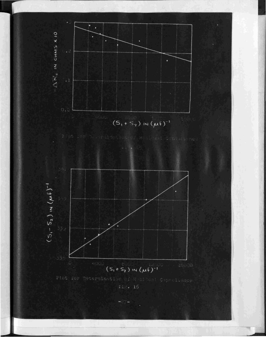
14. Plot for Determination of Residual Resistance. 26

15. Plot for Determination of Residual Conductance.27

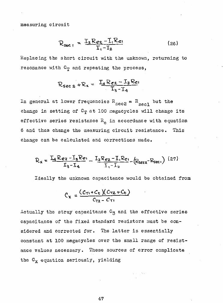
16. Plot for Determination of Residual Capacitance.27

17. Plot for Determination of Residual Inductanceat 5.0 Megacycles.

18. Percentage Variation in Apparent Capacitancefrom Static C.

19. Increments in Capacitance and ConductanceComponents Due to the Residual Inductanceand Metallic Resistance.

20. Current Distribution for Symmetrical Feed.

-v-

21. Percentage Variation in Apparent Capacitancefrom Static C. 32

22. Approximate Equivalent Circuit of FixedResistor. 36

23. Mercury Cup Contact. 36

24. A High Frequency, Variable Precision Resistor. 38

25. Boella Behavior of Solid Carbon Resistors. 39

26. Resistor Stray Capacitance C and EquivalentTransmission Line Circuit. 39

27. Approximate Schematic of Resistor. 39

28. Series Resonant Substitution Circuit. 42

29. Coil Dissipation Factor versus Frequency. 42

30. Series Resonant Resistance Variation Method. 46

31. Series Resonant Reactance Variation Method. 46

32. Resonance Curves, Reactance Variation Method. 49

Parallel Resonant Conductance Variation Method. 52

Parallel Resonance Susceptance Variation Method.56

Resonance Curves, Susceptance Variation Method. 56

Basic Conductance Substitution Circuit. 59

Equivalent Conductance Substitution Circuit. 59

33.

34.

35.

36.

37.

38a.

38b.

39.

40.

41.

42.

43.

44.

45.

Parallel Resonance Substitution Method.

Residuals, Conductance Variation Method.

Simplified Indicator Circuit.

Diode Characteristic.

Conductance Meter Functional Diagram.

Diode Circuit Conductance Calibration.

Diode Circuit Voltage Coefficient.

Residuals, Conductance Measurement Circuit.

General Radio 9l6-A Radio Frequency Bridge.

-vi-

49

52

62

62

63

63

66

66

68

46. General Radio 1601 VHF Bridge. 75

47. Effect of Inductance in Resistance Capacitor,CA, on Indicated Resistance. 78

48. Approximate Equivalent Circuit of CB• 85

49. Approximate Equivalent Circuit of CB IncludingResidual Losses. 85

50. EAlEt versus Re/RL. 96

51. Expansion of Diode Circuit ConductanceCalibration. 96

52. Expansion of Diode Circuit ConductanceCalibration. 97

53. Residuals, Reactance Variation Method. 97

-vii-

CHAPTER I

INTRODUCTION

Within the last decade there has been an ever increasing

demand for the development of test equipment which would be

suitable for use up to 100 megacycles. The upward spiralling

frequency allocations have opened an entirely new field of

measurements, a difficult and barely explored field. Diffi­

cult because in the region of 100 megacycles the transitional,

where lumped constant circuit and slotted line techniques

overlap, is reached; we are approaching the upper limit of

practical lumped constant circuits and have not quite reached

the lower bounds at which distributed constant lines become

important. It is here, in the span between 10 and 200 mega­

cycles, that residual parameters become so serious a problem

in impedance measuring instruments. Most instr~~ents design­

ed for lower frequencies are unusable because of the re­

siduals introduced by the measuring circuits and by the ex­

ternal connections to the circuit to be measured. It is

equally evident that at these frequencies, which are the

lower limit for the use of slotted lines, the physical size

of the lines becomes too great and the mechanical tolerances

too close to insure reas0nablyaccurate results. Therefore

there must be developed a technique for the modification of

lumped constant circuit adapt it to the require-

ments of this frequency range.

In general there are two classes of measurement methods

that may be used at radio and very hIgh frequencies, namely

null and resonance methods. As indicated by the names, the

two methods differ fundamentally only in type of indication;

the first depending upon balancing to a current or voltage

minimum and the latter upon tuning a resonant circuit to a

current or voltage maximum. In the following tabulation,

the major point of difference is in the means of obtaining

the resistive component of the unknown.

I. Resonance Methods.

A. Series Resonance Methods.

(1) Substitution

(2) Resistance Variation

(3) Reactance Variation

B. Parallel Resonance Methods.

(1) Substitution

(2) Conductance Variation

(3) Susceptance Variation

C. Voltmeter-Ammeter Method.

(1) Resonant Rise Method

II. Null Methods.

A. Bridge Methods.

(1) Impedance Bridge

(2) Modified Schering Bridge

B. Double or Twin-T Method.

1. Series resonance methods.

The series resonant methods as the name implies make

use of the principles of series resonance in the secondary

2

circuit. It becomes obvious then that these methods would

lend themselves best to the measurement of unknowns which

would contribute only small series resistive values. Basi­

cally the circuit is as shown in figure 1.

The substitution method is the most straightforward of

the series resonances. The secondary is first tuned to cur­

rent resonance with the unknown connected in series. The

unknown is then replaced by a continuously variable standard

resistor set ~o give the same resonant deflection when CT is

retuned. It is often more satisfactory to use several fixed

standard resistors which would bracket the correct current

reading and then, by interpolation or plotting, arrive at an

eqUivalent series resistance, Ri • Thus the reactance of the

unknown would equal the change in reactance of the tuning

capacitor and the series resistance of the unknown would

equal Ri.

In the resistance variation method, the measuring cir­

cuit is resonated at t he desired frequency and the scale

deflection noted. Then by inserting a suitable standard

resistance and noting the new reading, due to the inverse

relation of meter reading to resistance, the circuit

resistance can be determined. Repeating the above process

with the unknown inserted in series and with the tuning

capacitor reset for resonance, the difference in circuit

resistances yields the unknown series resistance and the

difference in tuning capacitor reactance, the unknown

reactance.

3

The third series resonance method, reactance variation,

completely eliminates the unwieldy problem of resistance

standards and makes use of the properties of the current

resonance curves obtained at constant frequency by varying

CT with and without the unknown in the circuit. From the

difference in the reactive values of the two settings of CT

necessary for resonance, the value of Ox is obtained. Also

the unknown resistance can be deduced, as will be shown

later, from the widths of the resonance curlles.

There are, of course, many modifications of a practical

nature that may be applied to the three series resonant

methods mentioned above. These modifications are however

simply refinements in techniques to arrive at more accurate

results and do not basically alter the procedures outlined.

It is necessary to insure that the mutual coupling be so

small that variations in the secondary or measuring circuit

impedance do not appreciably reflect into the primary tuned

circuit. Thus the induced voltage ~n Ls , -jWMIp , to all

intents and purposes will be constant over the complete

range of secondary variations.

2. Parallel resonance methods.

The parallel resonant methods utilize the properties of

the anti-resonant L-C circuit. In general these methods are

used for the measurement of high impedances. However with

refinements in the indicating circuit~ low impedances Can

*ttAn Improved Conductance Measuring Circuit~ NRL Report R3133.

4

easily and accurately be determined. The basic circuit is

that of figure 2.

As in the series resonant case, the substitution method

is the simplest but again requires the use of a continuously

variable standard resistor (in this case, high resistance)

or a series of fixed high resistance standards. The circuit

is first tuned to voltage resonance with the unknown connect­

ed in parallel with the L-C circuit. Then the unknown is re­

placed with the resistance standard and the circuit is re­

tuned to the same resonant voltage. The unknown susceptance

is given by the change in susceptance of the tuning capaci­

tor CT and the conductance by the reciprocal of the setting

of the variable standard resistor. If a variable resistor

is unobtainable, several fixed standards which will give

resonant voltage readings bracketing the desired reading

can be used and an interpolated value of Rp derived from the

resulting plot of resonant .voltage versus resistance.

The conductiance variation method obviates the need for

the variable standard resistor. With the unknown in parallel

with Ls-CT and CT tuned to resonance, the resonance voltage

is read with and without a parallel fixed resistor. From

these reading the total conductance can be deduced. With the

unknown removed and CT retuned to resonance, the same pro­

cedure will yield the measuring circuit conductance. Thus

the difference in the two circuit conductance values is the

conductance of the unknown and the difference of susceptance

of the settings of CT is the susceptance of the unknown.

6

The susceptance variation method, the method most

widely used, as in the series resonance case, makes use of

the width of the resonance curve of voltage versus tuning

capacitor setting. One such curve is taken with the unknown

connected in parallel. Then, removing the unknown, the

resonance curve of the measuring circuit is plotted. From

the breadth of the two curves, the two conditions of con­

ductance can be deduced. Thus the unknown conductance is

the difference; the unknown susceptance, the difference in

susceptance of the tuning capacitor setting at the peaks

of the resonance curves.

In each of tr~se parallel resonance methods, the

capaci tive coupling Cc ;is made so small that tuning the

measuring circuit has no appreciable effect on the frequency

or amplitude of the high frequency current source.

3. Voltmeter-ammeter method.

One of the more popular of the resonant rise of voltage

methods is the so-called ~-meter. In essence it is a single

series resonant circuit as shown in figure 3.

The resistance R is made so small that any variation in

the measuring cirduit has no appreciable effect on the IR

drop across it; i.e. I is essentially constant. There are

two methods of inserting the unknown to be measured, either

in series with the resonating coil Ls or in parallel with

CT. In general small impedances are best measured by series

injection and large impedances by parallel injection. In

any case, when the measuring circuit is resonated at the

7

desired frequency, the ratio of the resonant rise of voltage

V across the capaci tor CT to the constant input voltage E

is the measure of this effective Q of the circuit. The

voltmeter can be calibrated to read Qe directly. By resonat­

ing the measuring circuit with and without the unknown

connected and noting the values of ~ and CT in each case,

the effective series or parallel parameters of the unknown

can be deduced. There are many precautions necessary for

precise, high frequency measurements with this instrument;

these will be enumerated with further development of the

circuit.

4. Bridge methods.

One of the simplest bridge circuits used today for

impedance measurements at radio frequencies is the equal

arm impedance bridge, the greatly simplified circuit of

which is shown in figure 4. It is obvious that balance

exists when the two lower arms are of equal i~edance.

There are several methods of utilizing the circuit; one,

by inserting the unknown in the lower right arm and two,

by placing a suitable impedance in the lower right arm and

balancing the bridge with and without the unknown in series

with the standard arm. In the first case, the settings of

the tuning capacitor and the standard variable resistor

give the constants of the unknown directly. In the second

case, the difference in reactance of the capacitor settings

is the unknown reactance and the difference in standard

resistor settings, the unknown resistance.-

8

A more widely used bridge is the modified Schering

bridge shown schematically in figure 5. It eliminates the

need for the unsatisfactory variable resistance standard of

the impedance bridge by making the balance dependent upon

the settings of the variable air capacitors, CA and Cp. In

making measurements, the bridge is first balanced with a

short oircuit placed aoross the unknown terminals. Then,

replaoing the short circuit with the unknown and rebalano­

ing, it can be shown that

where CAl' Cpl and CA2 , Cp2 are respectively the initial

and final oapacitor settings. Features of the bridge are

such that the tuning capacitor CA can be calibrated to

read resistance in ohms directly and that Op can be cali­

brated to read reaotance direotly in ohms at anyone given

frequency, say 10 or 100 megacycles.

5. The Twin-T circuit.

The Twin-T oircuit, while not a bridge circuit in the

aocepted sense of the word, naturally falls under the

classification of null methods. It is a oomparatively new

idea and has certain inherent advantages over the accepted

bridge cirouits. Beoause one terminal of each of CB (the

susceptance capacitor), CG (the conductanoe capacitor),

L, the generator and the detector is tied directly to

10

ground, the need of a transformer is eliminated. .Also

certain residual stray capacitances are excluded from the

calculations of the unknown parameters. Capacitances from

points "a" and "c" to ground fall across the generator and

the detector and therefore do not enter into the balance

conditions. Similarly, stray capacitances from points "b"

and "dft to ground are in parallel with CB and CG in both

the initial and final balance positions and thus have no

effect on the measurement of the unknown since onl:y:'the

change of capacitance settings is of importance. Stray

capaci tances across CI, C" J and CU" affect balance rondi-

tions but introduce no error if they are included in the

original calibration. The residual c'apacitance across R

will of course affect its characteristics. However this

can be beneficial if of the right order of magnitUde by

balancing out to some extent the residual inductance of the

standard resistor.

Direct capacitances may exist between points "att_ftc"

and "b,,_ndt! and they must be minimized by shielding.

Thus the Twin-T provides a method of measuring the

unknown conductance and susceptance by direct substitu­

tion methods and of making the results direct reading on

calibrated, precision, variable air capacitor dials.

The balance conditions are given by

(, - R LV'2 C Ie" (I + C6 ) - 0L e'"

11

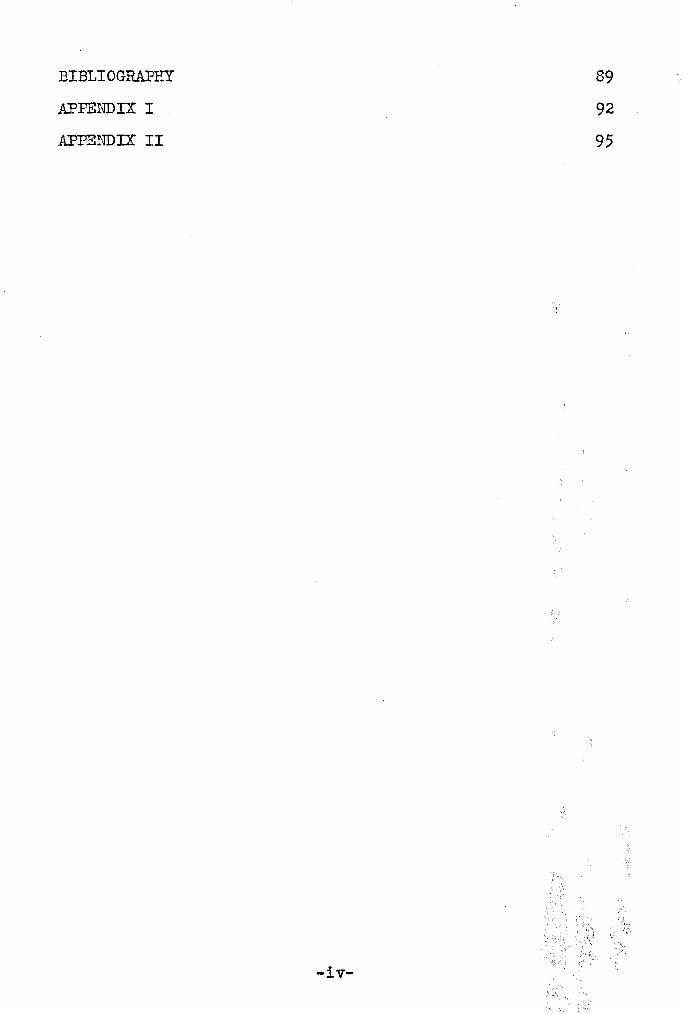
and c + c' +- c '" +- c. 'e II _..J- = 0\3 C III w7-L

The unknown parameters, assuming that there are no residuals

existent, follow:

where the sUbscripts indicate the initial and final readings.

~..

12

CHAP'l:E;R II

TEE C,APACITANCE STANDARDf

One of the most important tools is the precision

standard, variable air capacitor. Even the most casual

inspection of the introduction to high frequency measuring

techniques reveals that indeed this capacitor is the back­

bone of all measurements. However, the assumption that it

is a purely reactive, dissipationless element is untenable

at these high frequencies and a closer examination of the

nature of this standard is in order to determine as pre­

cisely as possible its residual parameters. It is these

residuals that primarily fix the upper frequency limits at

which measurement s may be made.

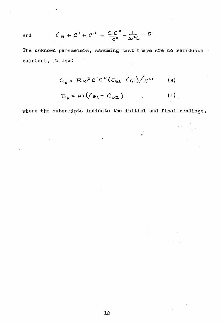
It would be well at this point to examine the structure

of a typical precision cap~citor (General Radio Type 722-M)

and endeavor to isolate the sources of·residuals. Figure 7

is a rough approximation of the stator and its supporting

frame. The current flows in throught the terminal post to

the top stator"plate. Here the current follows two paths;

a small portion passes out through the stator plate to the

rotor plate and back to the ground post. The remaining

current flows down the stator lead to the second stator

plate where a similar division occurs. This process con­

tinues along the stack to the last plate. This current

distribution sets up, in the plane of the plates, a magnetic

flux. The currents in the plates themselves have very little

14

affect on this flux density since they are diffused over

relatively large areas and are shielded to some extent by

the plates. There is then a residual inductance associated

with this flux distribution and such inductance must be

confined primarily to the stator leads and stator supports.

Also, the inductance must remain relatively constant irre­

spective of capacitor setting. This assumption leads to

the following representation of a disf?ipationless capacitor.

See figure 8. This type of circuit has multiple resonances

depending upon the number of sections but at operating fre­

quencies low enough to insure that ,the effective capaci­

tance is within a few percent of the static value, it can

be further simplified. See figure 9. The effective input

capacitance can be found from

Ce =or

. , ( I)-1-=J'wL.--wee we.e

Thus it is evident tbat the residual inductance makes the

effective input capacitance larger than the static value, C.

In addition to the residual inductance, there are

certain losses which must now be considered, losses in both

the metal and dielectric structures. The dielectric losses

will occur in the isolantite or fused quartz supports at

the top and bottom of the stator stack. These supports lie

in a field which is independent of rotor position but

dependent upon voltage. Therefore at anyone frequency,

16

it can be assumed that these losses are constant and can

be represented by two conductances, Gtop and Gbota The

metallic losses will occur in all metal parts but will be

localized almost entirely in contact resistances in the

bolted assemblies and in the sliding rotor contactsa Again

it Can be said that these losses will be essentially in­

dependent of rotor position. Expanding the equivalent

circuit then yields figure 10.

~'lith the previ ous assumptions this can be simplified

to the circuit of figure 11.

Deriving the input impedance from this simplified

circuit,

where

and

Similarly

c.\ - wZ.LC-

we

18

• 1- (.(,)'ZL c..J (l-w'2.L C)2+( (2w'~"L"'6)'

w"2C'2.

At 10 to 100 megacycles, the denominator is very nearly

equal to unity. Thus

and

YI~ = [R(WC)'Z+tt] + j[ \-~;Lcl

Ge = 1«WC.Y~- + q

Examination of these equations reveals that the di­

electric losses introduce a resistive component which is

a function of both frequency and rotor setting and the

metallic losses introduce a conductive component equally a

function of frequency and setting. The residual inductance

increases the effective input capacitance which i's dependent

upon frequency and rotor setting. However the effects of

residuals upon the absolute values of capacitance are not as

interesting as the effects on the capacitive differences.

For it is these differences that are used primarily to

determine the unknown impedance. Thus

•

'::: (', - w7...L C, Cz. -- {!z + W Z ~ C. C"2..(l-w2 L(!l )(1-w2 L.(!:z.)

(\ - C'2.

At 100 megacycles

c, - Cz.

19

(8 )

Also

Correspondingly,

and

It can be seen from the equations above that the di­

electric losses (G/Lv'2.C"2.) 8re :nredomin~nt at low frennency

while the metallic losses (RktC') are of i~~ortance at high

frequency. The error caused by residual inductance in the

capacitance increment is not equal to the average error at

the two settings but is rather more nearly equal to the

sum of the errors. The change in conductance or rather in

the metallic losses component is directly proportional to

the square of the capacitance. The elastance component

however, since the residual inductance is a constant series

element, is errorless in taking elastance differences. The

dielectric losses component of the resistive measurement

introduces an error which is directly proportional to the

square of the elastances or inversely proportional to the

square of the capacitances.

Thus, in the parallel substitution method, the resi­

duals of the tuning capacitor will introduce errors in

21

both the conductance and susceptance measurements. In the

series substitution method, errors appear in the resistive

measurement, but not in the reactive.

If the immediate exterior circuit is examined for

errors closely allied with the tuning capacitor, a small

stray capacitance, in the series substitution method, vdll

be introduced by the insertion of the unknown in the

measuring circuit. This Os appears directly across the

terminals of the standard as shown in figure 12. The

impedance looking into the standard is

which reduces to

'Re II r'Re~ (Ie +Cs 1(WCS)2 - J Lwcs + W(WCeCs/-j

'R e 2. +- l£e+ Cs\"2..\:WCeCsJ

: 'ReCs' J (weeRe)"ZCs~(Ce+-Cs)

(WC~ CS 'R)2.+ (Ce+-~)"2.- W(WCeCs Q)Z+(Ce+Cs)2

At 100 megacycles, where Os = 10-11f,

l-,..., 6 Ke - !--'--)W (Ce+Cs

Therefore

•I + ('S S'el

"S,-S~

1+ Cs (S,+'S2.)

'+CsS~'2

22

Thus the reactive measurement is no longer independent of

residuals associated with the tuning capacitor but is

clearly dependent upon the stray capacitance introduced

across the terminals of the standard.

From eouations (8), (g), (11) and (13) can be seen the

nature of the dependency of the errors upon the residual

parameters associ ated with the standard tuning capacitor.

In each instance, the errors are dependent upon the rotor

setting. If an unknown fixed capacitor were then to be

measured by a substitution method, its impedance and

admittance would vary with initial setting of the tuning

capacitor.

Thus, solving for Ox and Gx by parallel substitution

and Sx and Rx by series substitution, by re~riting equations

I (8), (g), (11) and (13),

Cy. = (Sa)

6)( ;: k?w2.(C,-C2.XC, +C,) -D.C:t o (ga)

"R" = ~'Z (S,-'S:z)(S,+S2) - A'Ro (lla)

and "S)(::. '"'S", - SO'2. ( l3a )

I + esC'S, +$2)where Go and Ro are the changes in circuit conductance and

resistance with the unknown in and out of the circuit. But

and

( (\ - C:z.) .: e)(( S I - Sz..) : S)(

24

G~ -= 'R lOZ C~ ((\+C2.) - ~6o (9b)

K,,'::. ~'2.S'IC('5,+S2.)-A\<.() (llb)

From (Sa) a plot of (01 - C2) versus (01;- C2 ) yields

a straight line of slope -LCx and ordinate intercept of Cx ••Equation (9b), plotted with Go versus (01 + 02)' is a

straight line with a slope af RW'2.Cx and intercept of -Gx •

A plot of (llb) with Ro versus (81 ~ S2) yields a straight

line of slope GSx/w'2. and intercept -Rx • Similarly, (13a),

with (81 - 8 2) versus (81 + 8 2 ) yields a straight line of

slope GsGx and intercept Sx.

ThUS, by measuring a large range of unknown fixed

capacitors and plotting the results as above, a very good

means of determining L, R, G and Os of the variable

'standard capacitor is available. Typical plots (see..

figures 13, 14, 15 and 16) of experimental data taken by

resonance methods at 1.5 megacycles on a General Radio

type 222-M precision capacitor yield the following

residual parameters:

L = 0.0604~h

R = 0.017 ohms

°s: 2.4 JV-f-f

G ; 0.210 micromhds

Further experimental results at 5.0 megacycles for the

determination of L (see figure 17) show the increase of

accuracy with increasing frequency. This method of attack,

using parallel and series substitution methods, should

prove useful and accurate up to a frequency of 30 megacycles.

25

Above this limit, external residual parameters in the

series substitution method (to be discussed below) become

exceedingly difficult to cope with. However, the experi­

mental data could be obtained, using a modified Schering

bridge, at frequencies in the neighborhood of 100 megacycles.

In figure 18 the percentage variation in apparent

capacitance from the static value is plotted versus static

capacitance for frequencies from 1 megacycle to 30 mega­

cycles. The residual inductance of only 0.059l~h obviously

makes the bland acceptance of capacitance readings without

necessary corrections out of the question. At a maximum

setting of 1100 ~~f, the apparent capacitance has increased

by more than a quarter percent at 1 megacycle and by 10

percent at 6 megacycles.

A study of input capacitance shows tba t at low fre­

quencies, where dielectric losses predominate, the con­

ductance is constant at anyone frequency independent of

rotor setting. However at higher frequencies, where the

metallic losses become so' important and are directly pro­

portional at anyone frequency to the square of the

capacitance setting, the input conductance is no longer

constant and such an assumption is seriously in error. The

plots in figure 19 make this fact evident.

Certain design features will reduce several of the

residuals appreciably. The current distribution along the

stator and rotor shafts is essentially as shown wn figure 7.

To a first approximation this can be assumed to be a linear

29

distribution. If R is the resistance and L the inductance

of the rotor shaft to uniform current distribution, the

effective residuals from non-uniform linear current can be

determined from energy relations to be

n _~

"e - "3 l.&e=L3

These values can be reduced by symmetrical feed systems

shown diagrammatically in figure 20 where (a) is center

feed, (b) dual feed, and (c) triple feed. For center feed,

energy relations yield

LL e =­\z,

Further multiple feed reduces the effective resistance and

indu ctance by

'Re =lG L - L (15)1~..Yl '2

e--l1.n-z.

where "n" is the number of feed points. These features have

been incorporated in the General Radio type ?22-N precision

capacitor, particularly designed for high frequency work

with center feed to the rotor shaft. At 1.5 megacycles it

has the following residual parameters:

L - 0.024 "uh

R - 0.008 ohms

G "= 0.3 ?-mhos.

Thus the residual inductance has been reduced by 60 percent,

the residual metallic resistance by over 50 percent. Based

31

on these figures, figure 21 indicates a decreased percentage

rise of effective capacitance versus static capacitance at

anyone frequency. For instance, from figure 18, at 6 mega­

cycles and a setting of 1100 j1Uf, there is a 10 percent

rise in effective capacitance. From figure 21, the ?22-N

capacitor shows less than 4 percent rise at 6 megacycles

and 1100~f setting. Further experimental information

seems to indicate that there are practical limits to the

number. of feedpoints that can satisfactorily be employed.

Also it is extremely difficult to realize a residual in­

ductance L less than 0.006 fLh and R less than 0.002 ohms.

33

CHAPTER III

THE RESISTANCE STANDARD

One of the most difficult problems encountered in the

field of high frequency measurement s today is the design of

a continuously variable, standard resistor such as that

required in the substitution method of both the series and

parallel resonant circuits. Equally as difficult is the use

of fixed, high frequency, standard resistors as required by

the resistance variation and conductance variation methods.

It is exactly these problems which contribute to the limit­

ing of the present useful frequency range of the above

mentioned measuring circuits.

Figure 22 is an approximate equivalent circuit of a

fixed resistor. L represents the series inductance of the

resistor and C, the parallel stray capacitance. The input

impedance is given by

tR-\-iw6)(-i rbc)

R + j ( to2~~- \ )

R - j [WL(w4l~-I) -t- WCR"Z]=

(wC.Rfz" + lw"l.l-C-I)' (16)

'<e ::. 'R./]]wCR.)7. + (Wl.LC- 1)2J (17)

Ge =- R/{tv2 L2 +R~) (l7a)

Xe ~ -3 fwL (u.;2.LC-l) +locR'lL ((..0 CQ)- + (to"2. kC _ \}l. (18)

Be ~ ~w ~(W2.L~-I) +c.Q"Z.J (l8a)

34

If R is large, (k) CR)2 is large and Re decreases with

frequency. With a small R, (w CR)2 is small and, as w'2. LC

approaches unity, (W CR)2 + (UlLC - 1)2« 1 and Reincreases rapidly.

At 100 megacycles the contact resistance introduced

when the fixed resistor is inserted in, say, the resistance(

variation circuit must also be considered. Even with mer-

cury cups, this resistance component cannot be made negli­

gibly small nor can it be made constant. This non-uniformity

Can be a large percentage of the inserted resistance. Also

at these frequencies, the possibility of contact resistance

skin effect must be examined. Consider the following diagram,

figure 23. There is the distinct possibility, in fact, an

almost certainty that there will not be perfect contact

throughout the area of contact, that contact may exist only

near the center of the conductor. And at 100 megacycles,

the center of the conductor carries essentially no current.

Thus the skin currents in the conductor must flow through

an added resistance in the contact and this resistance can

well be attributed to contact skin effect.

The continuously variable, standard resistor has been

solved in one aspect by Weaver and McCool in their work at

the Naval Research Laboratories. In the design of their

variable diode conductance measuring circuit (to be dis­

cussed below), they have adapted the characteristics of the

diode to provide a parallel circuit, variable conductance,

stable and suitable to accurate calibration at 10 megacycles.

35

However there are no continuously variable, mechanical

resistors sUitably precise at these frequencies. There are

new processes available though for the use of carbon deposits

in the manufacture of high frequency, large valued resist­

ances. It is thought possible that, using these~~rocesses,

some sort of mechanical structure such as that of figure 24

might be feasible. It is a nice problem that will bear a

great deal of thought and experimentation.

The greatest difficulty to overcome in the design of a

high frequency, high valued resistor is the Boella effect,

so called after one of the men instrumental in its dis­

covery in the early 1930's. It has been shown and experi­

mentally verified that all resistors above a given nominal

value drop off sharply in a.c. resistance with increasing

~requencies. Boella, G. W. O. Howe and several others have

shown that the following plot, figure 25, of Rac/Rdcversus kfRdc (where f is in cycles and Rdc is in ohns) is

representative.

This resultant drop in the ratio Rac/Rdc is attributed

to the characteristics of the parallel shunt of the residual

stray capacitance. There is an electrostatic field built

from the resistor causing a definite incremental, stray

capacitance to be associated with each segment of length.

Thus as in figure 26, the resistor can be thought of as a

symmetrical transmission line. G. W. O. Howe also has

plotted the input capacitance and arrived at a result

similar in shape to figure 25.

37

Further experimentation by R. F. Field of General Radio

Company on many different types of high valued resistors has

further verified the Boella effect. However his measurements

have shown that the shunt capacitance as plotted against

fRdc (where f is in megacycles and Rdc is in megohms) is

essentially constant; there is no apparent Boella contour.

To explain the decrease in Rac ' Mr. Field proposes that the

stray capacitors be resolved into their effective shunt

capacitance and shunt conductance. This \~uld lead to a

schematic as shown in figure 27. Thus the dielectric

losses in t he stray capa.citanc e F.l.C count for the Rac varia­

tion.

40

CHAPTER IV

SERIES RESONANCE METHODS

1. Substitution method.

The circuit shown in figure 28 includes the most im­

portant of tbe residuals that must be considered. In

general the use of this circuit is limited to frequencies

below approximately 30 megacycles. The simple theory indi­

cates that there is no finite capacitive coupling between

secondary and primary. Actually this is impossible to ob­

tain. There is then a current flow through the coupling Clwhich divides into the many branches to ground yielding a

loop current I which is not everywhere uniform in the second­

ary. This however will not affect the equations for the

unknown.

It would be best if Ls were a pure inductance. Realiz­

ing that this is impossible, the type of coil selected must

be carefully chosen. For work in these high frequency

ranges, the Q of the coil should lie between 300 and 500.

There are four sources of losses in any coil, low frequency

copper loss, high frequency eddy current loss, losses due

to the conductance of the equivalent stray capacitance, ani

losses due to the coiling effect. A log D versus log f plot

of these factors reveals very clearly the SUitability of a

given coil for a certain frequency range.

For a multiple layer coil,

41

where DC:: Dissipation factor due to copper loss

Db ~ Dissipation factor due to coiling effect

De :: Dissipation factor due to eddy current loss

Df = Dissipation factor due to Do

Do = Dissipation factor due to natural resonant

frequency of coil

f o = Natural resonant frequency of coil

d = WIre diameter in inches

n .... Number of insulated strands

a c: 1i!ean coil diameter in inches

b '= Coil length in inches

N c: b

tcoil length

.... ---------::;:~---effective wire diameter

g =- f(b/c, cia}

Thus, by using the coil for frequencies within the

range fl to f 2 , the highest, most uniform Q region is em­

ployed. With banked, pied coil construction, the distribut­

ed capacitance and its associated dielectric losses can be

greatly reduced, increasing f o considerably, thereby in­

creasing the frequency at which minimum dissipation occurs.

43

From experimentation Do has been found to be approximately

0.015 for a ceramic formed coil, 0.020 for phenolic.

Aside from the part played in the determination of the

coil ~, the residuals of the inductance Ls do not upset the

circuit solutions.

Calculation of the circuit to the right of A-A is too

involved for ready investigation. A knowledge of the pro­

cedure for measurements of unknowns will indicate what

residuals must be corrected for in experimental work. With

the short circuit in ylace and CT set to its minimum

position (lOOf7Uf), Ct is varied to resonate the circuit as

indicated by the loop current meter "An and R is adjusted

to yield a suitable meter reading. Then, with Ct unchanged,

the unknown replaces the short circuit and CT and Rare

readjusted to obtain the same meter reading. Thus,

and

e. x ,;::; Coon CTZ

C-rz- Coon

R~ = R\- R%I

The residuals of the trimmer capacitor element Ct will

have no effect on Cx and Rx. As previously shown, CTI and

CT2 must be corrected because of the residuals associated

with the standard capacitor, internally and externally

across its terminals. Then

+

44

From this(

Con C!. V. ~l'l. +c..\\-W"1.LC.-rt '3A\-WZ"LCTz ~

CT,2.. C.,.,\-Lo"1.L C-r'2. \ -t<P..LC-n

In addition the change in the value of R in the low

ohmic regions will change slightly its equivalent series

reactance which must be corrected for.

2. Resistance-variation method.

This method is very similar to the substitution method;

it varies only in the manner of obtaining the unknown re­

sistance. Instead of a continuously variable resistor,

several fixed standards are used. This is actually an ad-

vantage at 100 megacycles because the fixed standards are

much more predictable than the variable. The only added

residuals to consider are the two contact resistances and

the contact skin effect resistance. All other residuals are

similar in nature and value to those in the substitution

method and need not be reconsidered.

After setting CT to a suitable value (lOa~f) with the

short circuit in place and current resonating the circuit

with Ct, insert a given value of R and noted the meter

reading 110 Then, choosing a new value of R and leaving CT

and Ct untouched, the second meter indication is noted.

In all cases of resistor sUbstitution, the length and dia­

meter of the resistors should be identical to insure

approximately equal residuals. "Then, with the nominal

values Rl and R2, ReI and Re2 can be evaluated from

equation 17. If Rsec is the series resistance of the

45

measuring circuit

Replacing the short circuit with the unknown, returning to

resonance with CT and repeating the process,

In general at lower frequencies Rsec2 = Rsecl

but the

change in setting of CT at 100 megacycles will change its

effective series resistance Re in accordance with equation

6 and thus change the measuring circuit resistance. This

change can be calculated and corrections made.

Ideally the unknown capacitance would be obtained from

ex =(C"n+Ct )(CT%.+Ct)en - CII

Actually the stray capacitance C3 and the effective series

capacitance of the fixed standard resistors must be con­

sidered and corrected for. The latter is essentially

constant at 100 megacycles over the small range of resist­

ance values necessary. These sources of error complicate

the Cx equation seriously, yielding

47

where Cte ; Effective trimmer series capacitance,

eRe ~ Effective resistor series capacitance,

CT1 ' CT2 = Initial and final tuning capacitor

settings.

The value of CRe can readily be determined from equation 18

and Cte can easily be measured by parallel substitution

across CT with the unknown replaced by the short circuit.

C3 can be estimated from the circuit construction.

3. Reactance-variation method.

This method has the great advantage of the elimination

of standard resistances and their associated errors. However

measurements are not as readily made since resonance curves

must be plotted for highest accuracy.

The secondary is first current'resonated by varying CT

with the short circuit in place and the meter indication

noted. Then, with CT fixed, the calibrated, vernier

capacitor Ct is varied on each side of resonance and the

meter readings recorded for each position. With the un­

known replacing the short circuit, the process is repeated.

Figure 32 shows the plots of current versus vernier setting

for each circuit.

48

and

Ideally

Cy. -::. leT +ctl )( CT + Ct2..)

CtL - Ctl

R~:: (~~ - \ ) 'Rcsec.

However, taking the residuals into account and simplifying,

resonance curves, Rx can easily be evaluated.

1D \ - \ Ct:'1 + C1;I'2 \ \''-Sec... - - -- -:::2 w Ct:I\ Ctl'z. l.c.>4:11

(30a)

However if the change in the vernier capacitor ohanges the

secondary resistance, the derivation for Rx becomes

extremely involved. The derivation in Appendix I yields

I-to'lL,. (CT","Ctl)Except for the most accurate experimentation, equation (30b)

is far too tedious.

50

CHAPTER V

PARALLEL RESONANCE METHODS

1. Substitution method.

The parallel resonant circuit of figure 33 includes

the most important residuals to be considered. When these

residuals and the errors they cause are carefully analyzed,

the method can be used at frequencies up to 100 megacycles.

The effect of finite capacitance coupling is to couple a

certain amount of conductance into the secondary from the

power source. However if the assumptions of constantfre­

quency and linear output impedance are met, this coupled

conductance will not affect the unknown equations.

The substitution method is very simple in theory. With

the unknown impedance in place, CT is varied to resonate

the circuit as indicated by the voltmeter and the meter

reading is recorded. Then the unknown is replaced by the

high frequency, high valued, standard variable resistor.

CT is readjusted for resonance and R is varied to give the

same meter indication. From these measurements

ex -; (!T'2. - C,I

and G" -; ~Redrawing the circuit to the right of B-B,

51

Y'''J'k -= (c:,,..e2 + GQ.~ +-~,,) +-..\W (C-re7. +CRe +-C,,)

C,£ =- CTe'Z. - C,..el ..... L..Re

• e.T 2. - ell + ~(Lo"Z.Lr<.Ce-I)+CR.R~\ -w"Z.l-,. (Con -t-CTOZ) (3Ia)

In addition to the error introduced by the effective

series inductance of the tuning capacitor CT' there is

another error caused by the stray capacitance of the stan­

dard resistor. Similarly

::: ~T of- R\(wCTZt"-l;T-R, {we"tI)7. + ~ "1-Lu7.La of- (2

=QTL02 (C-T'2.-LTI XCT,tCT1 ) +- R..oz, - '2.. (32a)to'2L12 +1<

2. Conductance-variation method.

This circuit differs very little from the substitution

circuit. It has the distinct advantage of eliminating the

variable standard resistor and substituting in its place a

fixed standard resistor. The disadvantages are an added

pair of mercury cup contacts and twice as many necessary

measurements. With the unknown removed and CT adjusted for

resonance at CTl , if the meter is read as VI and V2 with a

fixed resistor first in and then out of the circuit, the

circuit conductance can be derived. Ideally

53

/' - ,(.:tf2. - ­

RJ

Inserting the unknown and repeating,

= (;,a. \/, ("1'( - Vzx ) +- C:tfl. ", '1- (\/, - VI)(V2 -V, )( I{Z¥: - Vl). )

:: 4ft (J~Vnl - V, Yzy. )lv2.-'" )("7.Y.-VI1.)

Cy: :. cT ,'- c,2

Again considering the residuals, the equations become

slightly more complicated. (See figure 35).

and VI~ [6T + I2T (w4. )>. + lo~2+f2" + ~N + 6..1:: \l2.¥:[GT -r k?T (wen.) '2. ..... ~" + 6-,cJ

- V2.'£_ [6,. +Q T lwC"Tz)2.+ 6,,] (33a)V2.y: -"I"

If it could be assumed that [GT+ RT (W CTZ )2 + GvJ =

{?T+RT( tV CT1)Z + Gvl, (33a) would reduce to (33). Unfortu­

nately this equality doesn't exist; the variation in CT is

54

reflected in its own effective conductance.

. e'l - CT'2.':0'

\ - t.o'2.L,. (CTI +('TZ.)

3. Susceptance variation method.

(34a)

The susceptance variation method is by far the most

widely used of the resonance methods. With proper precautions

measurements can be made at frequencies up to 100 megacycles.

and higher. Its great advantage is the elimination of the

ever troublesome standard resistor. Its disadvantage, as

with the reactance variation method, is the necessity of

using resonance curves.

Disregarding residuals,

and

When the

C)l :; (CT1 -tCt'1 ) - (CTZ +Ct;'2 )

G v : V\-V7..IW(C~ ~ )\Z- 1\- t:-\'Z.

residuals are considered,

C'X ; C-Tt - CT'Z. +- rb ~ Ctz (35a)l-w'2.L,CCTd-CT2.) 1- w'ZLt (Ci;l +C't"2.)

and G'i -= (~~-')<GT +6t:t6,,)+RTW~( ~~CT~-CT:)+~i~tf=~-4~)(36a)

Equat£on (36a) of course demonstrates the complexity in­

volved when the actual measuring circuit conductance cannot

be assumed constant with variation of the tuning capacitor.

55

CHAPTER VI

THE VARIABLE DIODE CONDU,CTANCE MEASURlliG CIRCUIT*

One of tbe most outstanding techniques developed in

recent years is that of Weaver and McCool of the Naval

Research Laboratories. It was their contention that the

existing methods did not combine the best possible accuracy

with the most rapid and simple techniques and least expensive

equipment. With the solution of this problem as their goal,

they have designed a parallel resonant, parallel substitu-

tion circuit of great versatility and high accuracy.

The unique features of this new adaption are: (1) a

high degree of resolution in detecting changes in the reson­

ant voltage of the measuring circuit, (2) the direct sub-

stitution of specimen conductance as well as capacitance,,and (3) the elimination of the necessity of evaluating the

total measuring circuit parameters for calibration.

The basic simplified circuit is shown in the schematic

of figure 38a. The basic nrinciple is to maintain the

resonant output voltage constant before and after sub­

stitution of the unknown by simple manipulation of the

tuning capacitor CT and the equivalent diode conductance by

variation of bias. Simple theory yields then, with the

diode set to give an equivalent conductance Gdl ,

*Vleaver and McCool. An improved conductance measuringcircuit. Problem 39R08-44, NRL Report R-3l33, June, 1947

57

or

Gtl -:: Total circuit conductance =- Go + Gdl

After substitution of the unknown and re-resonating,

Gt2 = Go + Gd2 + Gx

Since Gtl = Gt2 (Eo constant),

.~lso, as in the parallel resonant, substitution method,

First estimation of the source of errors reveals that

the precision of measurement is limited by the accuracy

with which the voltmeter can be reset to Eo and by the

accuracy of calibration of the equivalent diode conductance.

The problem of resetting the voltmeter can best be illus­

trated by an example.

Let the resonant impedance of the measuring circuit be

50,000 ohms and the conductance to be measured, 0.2,..mhos.

What is the change in resonant voltage when the unknown is

inserted?

6 t:"Z.

6tl

-= 4e"Z. -6tl

~'t'

6CD =E 0 2

Substituting values,

58

-bb Eb _ (), 2. 'I. , C> -= 0 . 0 I = I 90Eo'2 'J.,o )( 10-(."

Thus it is obvious that the error possible in resetting the

voltmeter to Eo will be of the same order of magnitude as

the change in the voltage caused by the unknown. Clearly a

method of indication of much greater sensitivity must be

evolved. A clever means of obtaining the desired sensitivity

is indicated basically in figure 39. The diode V2 rectifies

the resonant output voltage and the resulting voltage, Edc ,

is balanced out to ground by the potentiometer arrangement

across the d.c. supply, Ebb.

The possible error in the calibration of the variable

diode conductance can be estimated from the methods of

measurements used. The conductance of the diode can be

measured by substitution for various known conductances or

by analysis of the diode rectification characteristic. These

calibrations have reportedly given results consistently

agreeing to within 1 percent.

Everitt* gives the following diode circuit analysis:

i p '= gpep

i p = 0

when ep > 0

when ep~ 0

Then ep ':; E'coswt - EA ... E' (coseut - cos~) (39)

i p = gpEt(coswt - cos~)

= I o + I leo s Lc) t + I 2cos 2 ( to t 1'" Bz ). •• (40 )

*Everitt, Communication Engineering. p. 427.

60

where I o '= Direct current component

I l '= Fundamental component

I 2 - Second harmonic component, etc.

However, since the parallel resonant circuit is a very

low impedance to all frequency components higher than the

fundamental,

I p = I o + 11costAbt

From Fourier analysis,

I o =- gpE' (sin ~ - 0( cos,,", ) (42)

1T"

and I l = gpE' (2 p(.. - sin201...) (43)

2lf

Since RL =EA/Ioand Re - EIIIl

Re tan p( - p(

RL - oc. - sin-< (44)cos 0<

Elimina ting 0( and plotting EA/E I against Re/RL will

yield the universal diode rectification curve. From the

plot the rectification characteristic of any series diode

will give the effective conductance in terms of the applied

voltage E', the load voltage EA, and the load resistance RL•

A more complete schematic of the conductance measuring

circuit is given in figure 41. The high frequency power

supply is closely regulated so as to regulate in addition

the induced voltage in the measuring circuit. The high

frequency oscillator in the original work was limited to

one frequency (1 megacycle) for simplicity of investigation.

61

However, such need not be the case and there is reason to

believe that the method will operate successfully at 20

and possibly 100 megacycles.

The null detector is a 50-0-50 microammeter and, as a

center reading meter, a voltage change of approximately one

millivolt can be detected. Thus, if the resonant circuit

voltage is 50 volts rms, one part in 50,000 can be detected.

Very simply then, with the unknown out of the circuit, the

high frequency regulated supply is rectified in V3 and the

resonant output voltage in V2 ; the resulting d.c. voltages

are applied to the grids of V4 and V5 respectively and

balanced by means of the balancing potentiometer. With the

unknown in place and the balance untouched, the output of

the measuring circuit at resonance can be controlled by the

variable conductance and can be reset to the initial value

when the null detector is zeroed. Thus the duplication

should be precise to within 0.2 percent. Experimentation

shows the duplication to be within 0.3 to 0.5 percent.

In order to exploit the extremely high sensitivity of

the method, the overall conductance calibration curve

(figure 42) must be exploded into more accurately readable

plots. The method used to accomnlish this is explained in

Appendix II.

The diode circuit has a definite voltage coefficient

such that a change in applied voltage shifts the calibration.

Figure 43 demonstrates the percent change in diode circuit

conductance versus RL. The greatest shift is in the high

64

conductance end of the calibration. Weaver and McCool

pointed out that, when measuring low values of conductance,

the low end of the calibration is used and in this region

tube aging, tube replacement, and voltage coefficient

effects are negligible.

An example of the performance of this circuit is the

measurement of the power factor of dry air which was found

to be 0.000002 ± 50 percent.

There has been no evaluation of some of the more im-

portant residuals of this conductance circuit and it would

be of interest to determine their effect. From figure 44

Go of- G-rel + 41:)1 = L'?D to G,1~2. + GO'2. +-6')(

G~ ':: (~Tel -6.e'2 ) of- (~o, -602 )

:'@T+ 12,. (W('TI )"Z.-~T-RT{WC"T'2.)'Z.]of- (6 D1 - 61n)

Similarly,

C'l = (!"TI - CTz.,- w'2. L. (C-n +CT 2.)

Obviously, in measuring low valued conductances,

(38a)

the residual

series resistance of the standard capacitor must be con-

sidered. It is equally as necessary that the effect of the

residual series inductance, LT, must be appreciated and

corrected for as frequency increases.

65

CHAPTER VII

NULB ~mTrlODS

1. Impedance bridge.

The equal arm impedance type bridge has been found

unsuitable for coramercial development for use at 10 to

100 megacycles. It depends upon the use of a precision

variable resistor in its standard arm. As explained in

Chapter III, it has been common experience that the

design and development of such a precision variable

resistor satisfactory for general use at very high fre­

quencies is a difficult problem not yet solved.

Until such a resistor is available, the impedance

bridge must yield to slightly more comples bridge circuits.

2. Modified Schering bridge.

The General Radio Company manufactures three impedance

bridges which are representative of the modified Schering

bridge. They are the 916-AL, the 916-A and the 1601 which

cover the frequency ranges 50 kilocycles to 5 megacycles,

400 kilocycles to 60 megacycles, and 20 to 140 megacycles

respectively. Only the 916-A and the 1601 will be con-

sidered here.

The basic circuit of the 916-A is shown in figure 5;

the more complete schematic in figure 45. With the added

Cp and CA the resistance dial, calibrated directly in ohms,

and the reactance dial, calibrated at anyone frequency,

67

69

can be set to any position desired and an initial balance

obtained. Thus with the switch in the L position, Cp can

be set to zero (maximum capacitance) for maximum range of

inductance measurement; or, in the C positioh, Cp can be

set at 5000 ohms (minimum capacitance) for greatest range

of capacitance measurement. CN is composed almost entirely

of the stray Capacitance between the outer Cp-Cp shielding

and the grounded Case. The addition of the very small

trimmers, ON and ON' is to insure that the total capaci­

tance from the left hand junction to ground is equal for

both positions of the L-C switch.

The initial balance conditions, with the UNID~OVm ter­

minals short circuited with the appropriate lead, are

12p ':: ~ CAl (45)B-C~

, Rea I

~Cp;'= -RA Ju.JC'-J

where CAl represents the total capacitance of the settings

of CA and CA, and Cpl represents the total series capaci­

tance of Cp and Cpo With the unknown capacitor to be

measured in position (Opl would have been set at 5000 ohms),

the bridge is rebalanced to a null by varying only 0A and

O! and Of remain fixed. Thus.Ii. p

69

\----+JWCp 2 JwCv.

R" = 'Re (C""2. - CA-I)eN

From equations 46 and 47 it is apparent that RAis

necessary only for the initial balance; it does not appear

in the unknown equations. ~NO such resistors are necessary

to provide the rap~e of initial balance as the L-C switch

and the initial setting of Cp are changed. RB is a fixed,

essentially non-reactive, precision resistor. Rp is a ­

necessary balancing resistor and, as will be shown later,

is most conveniently located externally to the bridge.

It is convenient n~~ to consider the effects of the

various residual parameters upon the impedance of the four

bridge arms. Starting with the bridge arm fla_b n , Ri::. is not

and need not be a precision resistor. If the tuning of CAcan overcome the reactances of the residual series induct-

ance and parallel capacitance of RA, the resistor will

function satisfactorily. ~~y stray capacitance from point

fib" to ground falls across the detector and is ineffective;

Stray capacitance from fl a " to ground is across the "d-a"

arm and is equalized for the two switch positions by the

choice of CNand CN.The residuals of the precision capacitor, CA' will

contribute seriously to erroneous results if not accounted

70

for. The effective series inductance due to the current

distribution in the capacitor structure causes the terminal

capacitance to vary from the static capacitance CA by

\-I..(.?LCA

The effect of this on the resistance (equation 45) is to

yield values that are too low, especially at high frequency.

Therefore it is quite necessary to correct the CA resistance

dial readings at the upper frequency limit. The residual

series resistance component of the capacitor introduces a

parallel conductance R(tDCA)2 across RA and modifies the

reactance balance equation by

The error, never greater than about one ohm, causes the

reactive result to be slightly more inductive than it

should be. The residual conductance, GA, of 0A falls across

RA and effects no incremental error since it is independent

of rotor setting.

The precision resistor in the tfb-c" arm must be as

nearly non-reactive as possible. The 9l5-A uses a 0.7 mil,

"straight wire" manganin resistor which is equivalent to a

pure 270 ohms resistance in parallel with approximately

0.4 ~f up to 50 megacycles. This residual capacitance

causes an error in the reactive equation (again in the

inductive direction) as follows:

71

x~ ::: -' (.1. __I ) _ LUes R)<.W CP"2 Cp, 4B

The error caused by this residual capacitance is of the

same order of magnitude as the variation in results obtained

by changing the position of the ungrounded connector to

the unknown •

..t\.gain, any capacitance from point "b" to ground is

unharmfully across the detector. Point "c" has essentially

no stray capacitance to ground due to the completeness of

the shielding.

Since stray capacitances are so deleterious in the arm

"c-d" , a very complete shielding system has been designed.

The c auaci tance between point ftc If and the outer shield is.c _

thrown across the generator and rendered harmless. That

capacitance between the center and inner shield is in

uarallel with Of and affects the initial balance only. The• p

inner shield isolates the variable stray 0 due to the

position of the 0p rotor from the trimmer O~.

It would be advantageous to locate Ru within the.bridge structure. However, so doing would introduce harmful

strays which would upset the balance. For instance, if Rp

were connected in series with c~ within the inner and center

shield, the capacitance between these two shields would

fall across this series combination. Therefore, as Cp is

varied, the equivalent resistance would also change. This

would limit the range over which initial balance could be

obtained. It has been found most practical to locate ~

72

external to the bridge and to shield it such that the

capacitance to ground of the lead from Cp to the unknown

is negligibly small.

Another source of error is the residual conductance

(constant with setting) of Cpo This conductance, which

increases with frequency, is equivalent to a series re­

sistance which varies inversely with frequency and in­

versely with the square of the capacitance setting. This

error becomes insignificant at the high frequencies of

which we are interested.

The bridge arm "d-a" is to all aspects a pure capaci­

tance even at these high frequencies. Its residuals are

so small that they have no observable effects on bridge

balancing.

The General Radio Catalog L averrs that the accuracy

of reactance measurements up to 50 megacycles is ±(2 percent

+ 1 ohm. + 0 .0008 Rf) where R is the measured re si stance in

ohms and f is the frequency in megacycles. It is difficult

to tell whether this is an overall percentage accuracy which

takes every reactance-affecting residual into account.

Suppose that a precision air capacitor set at 500 ~f with

0.02 ohms series residual resistance is to be measured at

50 megacycles. What percentage error may be expected?

Substituting in the formula

6'>< - ± (O.t~1'3 + '.0 + o.0008)(o.ozxso)

'::: ± (\ .I~el) OH..-cS

73

But

This is an apparent possible error of 17.7 percent. It

would be wise in high frequency problems to disregard such

a statement of accuracy and instead to calculate from

formulii and correction graphs supplied the effects of the

residuals.

The stated accuracy for resistance measurements at

50 megacycle s is i: (1 percent + 0.1 ohms). The 0.1 ohms

correction is possibly attributed to inability to read the

dial to greater precision.

3. The 1601 V}.ffi' bridge.

This bridge is basically a higher frequency version

of the 9l6-A. Physically it is much smaller since the size

of the components Darts becomes less as frequency is in­

creased. But the bridge circuit is a modified Schering

type (see figure 5) and the balance conditions are the

same as equations 45, 46 and 47. The complete circuit

diagram is shown in figure 46.

In the design of this bridge from its predecessor, it

was found in some cases that common inductances as small

as 0~5 x 10-9 henries and stray capacitances as small as

Q.05 x 10-12 farads between elements that can not be com-

pletely shielded from one another, cause appreciable error.

Again, by examining each bridge arm individually, the

effects of the residuals can best be evaluated.

As in the 916-A, the residuals in the arm "a-b tf in

74

RA and C1 have no effect on the accuracy of measurement.

However they do seriously affect the initial balance con­

ditions and may so modify the arm impedances that balancing

is impossible. This is especially true when the bridge is

set up to measure a large capacitive reactance. It was

fou4d that the condition could be improved by inserting

in uarallel with R, a fixed resistor and capacitor. (CI- d P

has been eliminated ,and RA has been made adjustable to

accomplish the initial reactive balance). Shielding of

this arm eliminates stray capacitances to ground and to

other arms.

The resistance capacitor, CA, here, as in the 9l6-A,

is not a pure reactance. Its series inductance, LA' affects

the terminal capaci tanc'e as before where

The effective incremental change in capacitance would then

be

6CAe =- ~CA L\ + w2.L" (2CI\I t-DCAj] (50)

From this equation it can be seen that the deviation is

proportional to the square of the frequency and is depen­

dent upon the magnitude of the measured resistance. In

order to reduce this residual error, it was found that an

inductive circuit added in parallel with CN would offer

some compensation. This increases the effective value of

76

eN e. :: (c~ t- c~ )[\ + £02 l.N cc!.J.2.1 (51)CN+~

Since 'K'i. -::;. 'R.8 6C Ae

A CIJ~

it is possible by correctly selecting ~ and CNto correct

to a first order approximation for the error caused by CA.

The remaining deviation is given by

6. R~ =. l,u'2. LA ( C'N +CtJ ) T2~Ra

where Rm is the dial reading. Figure 47 shows the magnitude

of the correction which still must be applied to the re-

sistance dial reading.

In the precision resistance arm tfb-c", any reactive

residuals will cause errors in the reactance measurement.

However, if the constants of the equivalent circuit of the

resistor (figure 22) can be chosen or designed such that

then the series reactive component of the arm will be small

at frequencies which are an appreciable fraction of the

natural resonant frequency. In order to push up this oper­

ating frequency level, Land C must be made small. It was

necessary to go to a cylindrical palladium and palladium

oxide resistor fitted with threaded end caps to eliminate

wire connectors to accomplish this end. With this con-

struction~ C ~.0.3l ~f and L; 0.017 fLh and R = 240 ohms.

77

The UNKNOWN arm ltc_dU is of finite length and must

have a residual inductance, Lp • However, since a series

substitution method is employed and since the residual

inductance is there in both initial and final positions,

it does not affect measured reactance. The initial balance

is affected in that RA must be increased to overcome the

effective rise of Cp due to this inductance.

Because Cp is no longer mused, the balancing resistor

Rp can now become integrated internally. The tri-shield is

similar to that used in the 9l6-A. l~ystray capacitance

between the inner shield and the lead to the Ul~ID~OWn

terminal is directly across Rp • This has no effect on the

bridge accuracy and simply inserts an effective series

capacitance which may be beneficial. If the capacitance

across Rp is such that

12 IF- (54)p: CRp

then the compensation for Lp is very good at frequencies

which are an appreciable fraction of the equivalent

resonant frequency.

Stray capacitance between the inner and middle shield

falls directly across Cp and need only be considered in the

initial calibration. Strays between the middle and outer

shields are across the generator and exert no effect. A

capacitance exists between the lead from Rp to the UNID~OVd~

terminal and the middle and outer shields. By using a very

small diameter lead and by proper shield design, these

79

capacitances can be made negligibly small.

There are no noteworthy residuals to be considered in

the "d-a" arm. From figure 46 it can be seen that all

bridge components except the generator and ~ are enclosed

in a common shield connected to the bridge at point "a".

ON is the capacitance of this shield to ground and is not

a physical capacitor. It is parallelled by the Lw-ONcompensation circuit o

One other residual capacitance need be considered. It

is that between the UNKNOWTI terminal and ground and is of

the order of 1.05~rf. Since it is in parallel with the

unknown capacitance it must be corrected for,

The 1601 is still under experimental test and is not

yet on the market. It is expected that the accuracy of

reactive measurements will be within 5 percent at 140

megacycles and the accuracy of resistive measurements will

be within 2 percent.

4. ~vin-T method.

The General Radio Company version of the parallel-T

circuit is the 82l-A Twin-T impedance measuring circuit. It

utilizes the very convenient parallel substitution method

of inserting the unknown. Balance conditions for the cir­

cuit (figure 6) are as follows:

GL-Rw"2 C'C."(I+ ~II )=0

/) " ," I' (.l. +-l to -L) ,'--B + '- \- C' C" c.'" - tu'2L =0

80

The unknown is then given by:

As was briefly discussed in the introduction, stray

capaci tances from points "aff and "c lf to ground, from "aft to

"b f', "b" to Itc" and "d" to tta" are ineffective or can be

included in the initial calibration. Capacitance across the

standard resistor, if of the correct order of magnitude, can

be beneficial and capacitances from "att to "c tt must be

minimized or eliminated by shielding.

as with any bridge circuit, it must be possible to get

an initial balance and to have a reasonable range of

measurement of conductance and susceptance at any frequency

within the range of the instrument. The measuring circuit

from ttb" to ground is primarily a parallel tuned circuit.

The coil L is shunted by an effective capacitance CB plus

(C f + ott +- 0 fattIc f tt). Because it is not feasible to use just

one coil over the frequency range of 0.5 to 30 megacycles,

provision is made to switch in one of four coils which

cover the range in four steps. Since Cf, 0" and Of" are

essentially fixed capacitors, an additional parallel

capacitor system must supplement 0B in order that an initial

balance may be obtained for any setting. This parallel

supplement consists of four fixed capacitors inserted by

push button control and small trimmer. Similarly the

conductance measuring capacitor, CG, must be parallelled

81

with a coarse and fine trimmer capacitor in order that

CG may be set at zero initially for any measurement.

From equation 57 it can be seen that the conductance

range increases with the square of the frequency; this

would yield a very undesirable 3600:1 ratio of conductance

ranges over the frequency range 0.5 to 30 megacycles. It,

while switching coils, 0 1 and 0" or Olft are switched

simultaneously, any desired ratio may be obtained. This

circuit has been designed to give a range of 0-100 mhos

at 1 megacycle, 0-300 at 3 megacycles, 0-1000 at 10 mega­

cycles and 0-3000 at 30 megacycles.

It is vital at these high frequencies to reduce to a

minimum the inductance of the wiring. It is especially

necessary that the capacitors 0I, Oft and 0 rff and the

resistor R be connected as closely as possible with as

large a diameter connection as is feasible. Therefore,

copper strap has been used and the lead lengths are al~

less than one inch. In addition the junction points "b"

and "dn must be located as close to the capacitor plates

of 0B and 0G as possible. This will minimize the series

inductances in the measuring circuits.

The most critical element in the circuit is 0B which

is a lOO-llOO~~f capacitor utilizing double end-feed of the

rotor stack through 48 current entry points and double feed

to the stator stack. A further gain in reduction of in­

fluential residuals has been realized by making the capaci­

tor a 3-terminal network. This is natural since there must

82

be one stator lead to the ungrounded UNKNO~~ terminal and

one stator lead to the junction point tfb" in addition to

the ground lead. An equivalent circuit of this construction

is shown in figure 48.

The effect of L' is to insert a positive reactance in

series with the unknown. The effective admittance, Y~,

measured at b' is then

YI , 0 I.~ ':' G'l( + J Bx =-

which will differ from the

6 0",)C ;-j __---=__:_

(I-W \....'8~)2 t- W L' Bx

true value (Yx = Gx +- jBx ) in

either direction depending upon the sense of the unknown

susceptanc e •

The effect of the COlillllon inductance Lc is again that

of increasing the effective capacitance over the static

value in accordance with

CBLBe -==

1-L.U2:Lc.C6

This effective increase in capacitance makes the measured

value of susceptance as read from the dial less than the

true value as shown in equation 60.

8~ 'lC LV (Cae, - Ceez ) :e.u(C.e ,-eeL.) (60)

l-l.O'2. L.~ (Ce, +Ce7)

Here again the error encountered is proportional to the

sum of the errors at the initial and final settings of CB•The 3-terminal construction n~kes both Lc and L' about one-

83

half of the inductance that would be measured in a

2-terminal capacitor. This twofold reduction therefore

decreases the errors of equation 60.

Since the susceptance from point b t is the same for

both initial and final settings, the inductance Ln has no

effect on the susceptance measurement. However, since the

circuit actually measures conductance from point bit to

ground,.Lft will affect the conductance measurement. It can

G" .: Gx (61)'{ - (l-w2 L"LBe,>(l-WL'Bx)"2

be seen that L" always makes the conductance measured too

high while Lt will either make it too high or too low,

depending upon the sense of Bx _

To be complete the equivalent circuit (48) must in­

clude the ohmic losses of the inductances and the shunt

conductance of the capacitor. Rt and Rn are so small that

they have negligible effect on the accuracy of measurement.

The conductance is independent of rotor setting and is

therefore constant for initial and final settings. But the

common resistance Rc introduces a conductance term,

(Rc~2CBe2), which is dependent upon the square of the rotor

setting and which will be a source of error in the con­

ductance measurement. This error will be

Thus, when measuring an unknown capacitance, this error

84

86

will tend to make the measured conductance value too small.

These residual parameters which are associated with

the capacitor CB are the limiting factors determining the

upper frequency limit at which accurate measurements may

be made. Experimental results yield the following average

values:

L' = 6.8 x 10-9 henries

LU ::: 3.15 x 10-9 henries

Lc = 6.1 x 10-9 henries

Rc == 0.026 ohms.

86

CHAPTER VIII

CONCLUSIONS

It 'is felt, with no further explanation necessary, that

the series and parallel resonant substitution methods and

the resistance-variation and conductance-variation methods

(excluding the variable diode conductance measuring circuit)

should be eliminated from the consideration of circuits to

be used for highly accurate, high frequency measurement

of capacitors. Further, it seems logical to assume that

the remaining methods will, with due regard for their

frequency limitations, yield results of consistent

accuracy. By taking all the necessary precations indi­

cated, these methods should yield results accurate to

within 2 percent in the frequency range from 30 to 140

megacycles 4

Obviously the null methods offer the easiest means of

measurement. However, they also pose a more difficult

problem in the control of residuals. There is little that

can be done to alter the commercial bridge equipments. The

lower capacitance limit of the 9l6-A at 50 megacycles is

approximately 35/""ff while that of the 1601 is about 8 rrfat 100 megacycles, that of the 82l-A Twin-T is zero at 30

megacycles. The resistance dials of the 9l6-A and the.160l

and the conductance dial of the 821-A would be of little

use in measuring very low loss capacitors.

On the other hand, the two remaining resonance methods

will yield very good results even for low loss capacitors.

87

Inherently they are slower, more,tedious methods because of

the necessary plotting but the control that may be exercised

over the residual parameters is much greater. The reactance­

variation circuit lends itself to the measurement of low

series resistance components and the susceptance-variation

to the measurement of low parallel conductance components.

The variable diode conductance measuring circuit, if

further study reveals that it can be made to operate at

100 megaCYCles, will probably surpass these more convention­

al methods for ease and accuracy of measurement.

88

BIBLIOGRAPHY

1. Breit. G. The distributed capacity of inductance coils.Phys. Rev. 2nd ser. 17:649, June, 1921.

2. Brown, S. L. and Colby, M. Y. Electrical measurementsat radio frequencies. Phys. Rev. 2nd ser, 29:717,May, 1927.

3. Brown, S. L., Weibusch, C. F. and Colby, M. Y. Thehigh frequency resistance of a Bureau of Standardstype air condenser. Phys. Rev. 2nd ser, 29:887,June, 1927.

4. Burke, C. T. Substitution method for the determinationof resistance of inductors and capacitors at radio­frequencies. Trans. A.I.E.E. 46:482, 1927.

5. Easton, I. G. Corrections for residual impedances in theTwin-T. R~print from General Radio Experimenter.

6. Easton, I. G. Impedance bridges assembled from labora­tory parts. General Radio Company, 1943.

7. Everitt. W. L. Communication Engineering. New York andLondon, McGraw-Hill. 1937.

8. Field, R. F. Connection errors in capacitance measure­ments. General Radio Experimenter. 12 No.8, January,1938.

9. Field. R. F. Increased accuracy for the precisioncondenser. General Radio Experimenter. 22 No.1,June, 1947.

10. Field, R. F. and Sinclair, D. B. A method for deter­mining residual inductance and resistance of avariable air condenser at radio frequencies. Reprintfrom Proc. I.R.E. 24 No.2, February, 1936.

11. General Radio Company. Operating instructions for type82l-A Twin-T impedance measuring circuit. Form 566-C.

12. General Radio Company. Operating and maintainance in­structions for type 916-A radio frequency bridge.Form 567-H.

13. General Radio Company. Operating instructions for type9l6-A1 radio frequency bridge. Form 708-A.

14. Hartshorn, L. Radio frequency measurements by bridgeand resonance methods. New York, John Wiley & Sons,Inc., 1943.

89

15. Hartshorn, L. and Ward, W. H. The measurement of thepermitivity and pow~r fact§r of dielectrics atfrequencies from 10 to 10 cycles per second. Froc.Wireless Section I.E.E. (London). 12:6, March, 1937.

16. Howe, G. W. o. Editorial in Wireless Engineering.June, 1935.

17. Howe, G. W. o. Editorial in Wireless Engineering.August, 1935.

18. Jackson, W. The analysis of air condenser loss resis­tance. Froc. I.R.E. 22:957-963, August, 1934.

19. Maibauer,A. E. and Taylor, T. S. The variation of theresistance of condensers with dial setting at radiofrequency. Phys. Rev. 2nd ser, 27:251, February, 1926.

20. Sayee, A. A simple method of measuring capacity andhigh frequency loss od a condenser. Jour. Sci. Instr.3:116, January, 1926.

21. Simmonds, J. C. Apparatus for measurements on balanced­pair cables in the range 10-200 mc/s. Proceedingsof the Wireless Section. 92 III 20:282, December,1945.

22. Simmonds, J. C. Tuned circuit, parallel resistancesubstitution apparatus for measurements on ba1anced­pair cables at frequencies up to 10 mcps. Proceedingsof the Wireless Section. 92 III 18:120, June, 1945.

23. Sinclair, D. Bo A high-frequency model of the precisioncondenser. General Radio Experimenter. 13 Nos. 5 and6, October, 1938.

24. Sinclair, D. B. A radio-frequency bridge for impedancemeasurements from 400 kilocycles to 60 megacycles.Proc. I.R.E. November, 1940.

25. Sinclair, D. B. High-frequency measurements. Radio­Electronic Engineering. December, 1945-January, 1946.

26. Sinclair, D. B. Impedance measurements on broadcastantennas. Communications. June and JUly, 1939.

27. Sinclair, D. B. Parallel-resonance methods for precisemeasurements of high impedances at radio-frequenciesand a comparison with the ordinary series-resonancemethods. Reprint from Proc. I.R.E. 26 No.12, December,19.38.

90

28. Sinclair, D. B. The Tvlin-T, a new type of null instru­ment for measuring impedance at frequencies up to30 megacycles. Proc. I.R.E. July, 1940.

29. smiley, G. ~ccenticity effects of precision rotarydevices. General Radio Experimenter. 22 No.8,January, 1948.

30. Soderman, R. A. A new bridge for impedance measurementsat frequencies between 50 kilocycles and 5 megacycles.General Radio Experimenter. 23 No. 10, March, 1949.

31. Soderman. R. A. A v-h-f bridge for impedance measure­ments at frequencies between 20 and 140 megacycles.General Radio Company.

32. Soderman, R. A. Measurements on i-f transformers withthe 9l6-A r-f bridge. General Radio Experimenter.23 No.8, January, 1949.

33. Soderman, R. A. Sensitivity of the type 916~A radiofrequency bridge. General Radio Experimenter.22 No.8, January, 1948.

34. Sutton, G. W. A method for the determination of theequivalent resistance of air condensers at highfrequencies. Proc. Phys. Soc. (London). 41:126,February, 1929.

35. Taylor, P. B. Method for measurement of high resistanceat high frequencies. Proc. I. R. E. 20:1802-1806,November, 1932.

36. Tuttle, W. N. Bridge-T and parallel-T null circuitsfor measurements at radio frequencies. Proc. I.R.E.January, 1940.

37. Weaver, E. O. and McCool, Vi. A. An improved conductancemeasuring circuit. Naval Research Laboratories.R-3133, June, 1947.

38. Weyl, C. N. and Harris, S. A method of measuring atradio frequencies the equivalent series resistanceof condensers intended for use in radio receivingcircuits. Proc. I.R.E. 13:109-150, February, 1925.

39. Wilmotte, R. M. The comparison of the power factors ofcondensers. Wireless Engineer and ExperimentalWireless. 6:656, December, 1929.

40. Wilmotte, R. M. A quick and sensitive method of measur­ing condenser losses at radio-frequencies. Jour. Sci.Instr. 5:369, December, 1928.

91

APPENDIX I

RESIDUALS, REACTANCE VARIATION METHOD

The following laborious derivation is typical of much

of the work in the field of residuals as encountered in

high frequency measuring circuits. See figure 53.

92

At resonance

At 100 megacycles

93

Similarly

,-ex

94

APPENDIX II

EXPANSION OF THE DIODE CllWUIT CALIBRATION

lZe -= 12"" faY'\ 0(. - 0(r;{ - SIIo,J~ eos <:J..

As RL approaches infinity,

Re- --=--- (). 5R~

(1)

(3 )

In the calibration process the ratio Re/~ is obtained

direotly from the universal diode curve. The range of values

for this ratio is very limited, extending to 0.58 when5RL=10 ohms and Vl 6H6. Let

R..... : Re - 'KL.. '= (Re - 1. ) 'R..., Z \2L Z

RT is a fictitious resistance representing the difference

between the equivalent diode circuit resistance and Rl /2,

the limiting value of Re as ~ approaches infinity. By

plotting RT against ~ and rearranging the equation 3,

Re ;. RL to RT :. G'Z d

Thus from equation 4, the diode circuit conductance can be

computed. It is made up of two parts, (1) RL/2 computed

from the measured value of the load resistance and (2) RTwhich is read from a highly expanded curve. (See figure 51).

Figure 52 is a specimen exploded conductance curve.

95