AN ANALYSIS OF POT CHRYSANTHEMUM PRODUCTION ...

AN ANALYSIS OF POT CHRYSANTHEMUM PRODUCTION

METHODS, DIRECT COSTS AND SPACE USE

By

HENRY VIETH GRIFFITH )\

Bachelor of Science Oklahoma State University

Stillwater, Oklahoma 1949

Master of Science in Commerce University of Alabama University, Alabama

1961

Submitted to the faculty of the Graduate College of the Oklahoma State University

in par ti al fulfi 1 lment of the requirements for the degree of MASTER OF SCIENCE

May, 1969

AN ANALYSIS OF POT CHRYSANTHEMUM PRODUCTION

METHODS, DIRECT COSTS AND SPACE USE

Thesis Approved:

Thesis Advi r

.--u__ ~ f ?( L / ,-

l

a.a.~ Dean of the Graduate College

724862

i i

OXIAHOMA sriATE UNIVERSl11' ILIISRARY

SIEP ~-

.... - - - 4

,,

PREFACE

No single phase of horticulture can be ascribed a predominate role

above alt others. However, one that permeates most other phases and

dramatically affects our daily lives is the commercial production of

horticultural products.

This thesis is concerned with four interrelated factors in the

greenhouse production of horticultural crops: cultural methods, prod

uct quality, direct costs and space use. The means for accomplishing

this study has been the production of pot chrysc1nthemums through three

production cycles. Methods employed to measure results were: the

classification of product quality, the analysis of direct costs and

the comparison of greenhouse space use.

During the three repetitive cycles in the spring, summer ;:md fall,

the data resulting from the five production methods were ac~umul~ted

and studied. The schedules and conditions in each cycle were held as

rigidly similar as the capabilities of the facilities permitted. The

results of this study have been reported in terms of product quality

achieved, direct costs incurred and effectiveness of space use. ln ·

addition a major effort in the study resulted in identifying direct

cost elements and space use needs that are in general applicable to

a11 pot mu.m crops.

I should like to express my sincere appreciation to Dr. Richard

N. Payne not only for making a wealth of material and facilities avail

able to me for this study, but also, and most important, for his

i ii

generous assistance and wise counsel without which the goals of this

study could not have been reached. My gratitude is also e~tended to

Professor W. R. Kays for his sincere interest, guidance and encourage

ment. I am indebted as well to Dr. J. Q. Lynd for taking time' from

his extensive research endeavors in the Agronomy Department to partic

ipate on this committee.

Certainly I would be remiss if I did not recognize the vety real

help my wife and family have given by their enduring patience, their

confidence, and their encouragement. I should also like to thank Mrs.

Clara Yeck for her fine editing and typing.

iv

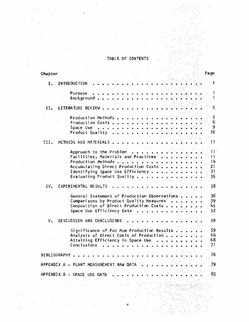
TABLE OF CONTENTS

Chapter Page

I. INTRODUCTION . . . . . •- .. • .. . .. . . 1

II•

HI.

Purpose Background

. . .. . . . . . . .. . . . .. •·· ... -·-· . . . . ' . . . . . . . : . . . ... . . LITERATURE REVIEW •• . . . . . . . . . . . . .. .

Production Methods Production Costs. Space Use Product Qua 1 i ty

METHODS AND MATERIALS.

. . . . . . . . . . . . . .. . . . . . . . . . . . . . . .. . . . . . . . . . . . . . . ..... . . . . . . . . . . . ·•. . . . . . . . . .. . . . ' ..... ~- .

1 1

5

5 6 9

10

11

Approach to the Prob 1 em • • • • • • • • • • • 11 Facilities, Materials and Practices • • • • • • • • • 11 Product i on Methods • • • • • • • • • ·• • • ·• • · • • 14 Accumulating Direct Production Costs • • • • • • • • • 21 Identifying Space Use Efficiency • • • • • . • • • • 31 Evaluating Product Quality. • • • • • • • • • • • 36

IV. EXPERIMENTAL RES UL TS O O Qi ti e e e 9 e e e e e e e e • 38

38 39 45 52

General Statement of Production Observations •• Comparisons by Product Quality Measures Composition of Direct Production Costs •••

• • . . . . .. . Space Use Efficiency Data ••••••••••

V. DISCUSSION AND CONCLUSIONS . . . . . . . . . . . 59

Significance of Pot Mum Production Results...... 59 Analysis of Direct Costs of Production. • • •.• • • • 64 Attaining Efficiency in Space Use • • • • • • • • • • 68 Conclusions • • • • • • • • • • • • • • • 71

BIBLIOGRAPHY . . . . ... . . . . . . . • • . . • • • . . . .• 76

APPENDIX A - PLANT MEASUREMENT RAW DATA . . . . . . :.• . . .. . .·• 79

85 APPENDIX B - SPACE USE DATA . . . . . . . . . . . . . . .

v

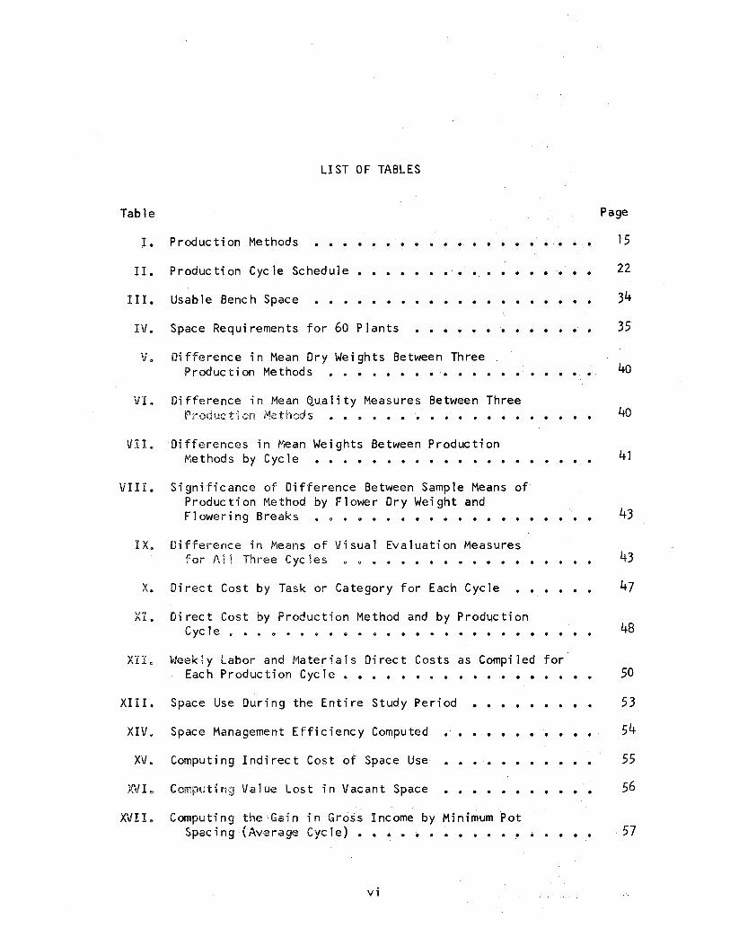
LIST OF TABLES

Table Page

I. Production Methods • ··................. •.• 15

II• Production Cycle Schedule. . . • • • . . . . ........ 22

III. Usable Bench Space . . . . .. .. . . . . . . . . ~ 34

IV. Space Requirements for 60 P 1 ants • • • • • • • • • • • • • 35

v.

VI.

VII.

VIII.

IX.

x.

XI.

Difference in Mean Dry Weights Between Three Production Methods •••••••••••• . . . . . .. .•

Difference in Mean Q.1,1.a 1 i ty Measures Between Three Production Methods •••••••••••.•••••

Differences in Mean Weights Between Production Methods by Cycle •••••••••••••• • •

Significance of Difference Between Sample Means of Production Method by Flower Dry Weight and Flowering Breaks ••••••••••••••

Difference in Means of Visual Evaluation Measures

. . . .

. . . . for A 11 Three Cycles ••••••• . . . . .

Direct Cost by Task or Category for Each Cycle . . . . . . Direct Cost by Production Method and by Production

Cycle. • • • • • • • • • • • • • ••••• . . . . XII. Weekly Labor and Materials Direct Costs as Compiled for

40

40

41

43

43

47

48

Each Production Cycle. • • • • • • • • • • .• • • • • • • 50

XJII. Space Use During the Entire Study Period • • • • • • • • • 53

XIV. Space Management Efficiency Computed • • • • • • • • • • • 54

xv. Computing Indirect Cost of Space Use

XVI~ Computing Value Lost in Vacant Space

. . . . . .

. . . . . . . . ..

55

56

XVII. Computing the·Gain in Gross Income by Minimum Pot Spacing {Average Cycle) • • • • • • • • • • • • • • • • • 57

vi

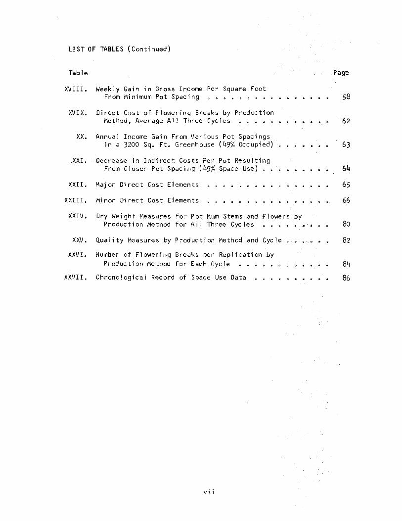
LIST OF TABLES (Continued)

Table

XVIII.

XVI X.

xx.

Weekly Gain in Gross Income Per Square Foot From Minimum Pot Spacing ••• o •••

Direct Cost of Flowering Breaks by Production Method, Average A 11 Three Cycles • o •••

Annual Income Gain From Various Pot Spacings in a 3200 Sqo Fto Greenhouse (49% Occupied)

.. XXI. Decrease in Indirect Costs Per Pot Resulting From Closer Pot Spacing (49% Space Use)

XXII. Maj or Direct Cost Elements . . 0 . XXII I. Minor Direct Cost Elements . . 0 .

•a•oO•fit

e • o ·• II) o o

d • o e • • o

oQe~a•

0 • 0 . . • . . 0

XXIV. Dry Weight Measures for Pot Mum Stems and Flowers by Production Method for A 11 Three Cyc I es

XXV. Quality Measures by Production Method and Cycle

XXVI. Number of Flowering Breaks per Replication by Production Method for Each Cycle

XXVII. Chronological Record of Space Use Data

vii

. • ... •

0 .•

Page

62

63

64

65

66

80

82

84

86

LI ST OF FI GU RES

Figure

1. Space Layout for the North Half of the Greenhouse. • •

2. Space Layout for the South Half of the Greenhouse •• . ... 3. Randomized Rep 1 i cations . . . . . . . . . . . 4. 1511 x 15" Pot Spacing Patterns . . .. . . . . 5. 1311 x 1311 Pot Spacing Patterns . . . 6. Materi a 1 s Used S 1 i p . . .

Materials Consumption List

Dai 1 y Ti me S 1 i p • • • . . . . . . 9. labor Time Sheet Summary Data. . . . . •. . .

10. Production Cost Sheet •• . . . . . . . . . ·.. ... . 11. Standard A and Standard B Methods Compared . . . 12. Comparison of Direct Costs Incurred by Week by Cycle

13. Average Production Cycle Cos'ts for Materials and Labor . .

viii

Page

12

13

16

18

19

23

25

27

28

30

44

49

51

CHAPTER I

INTRODUCTION

Purpose

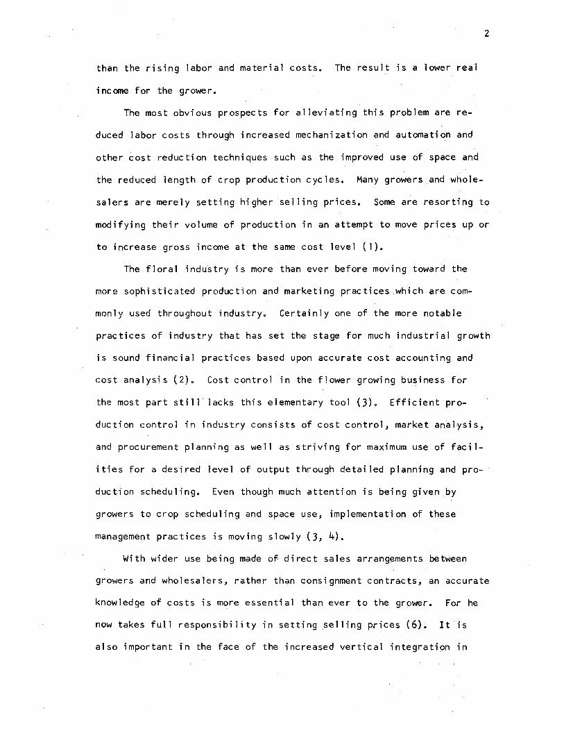
The purpose of this study was to investigate those aspects of com-

mercial greenhouse pot chrysanthemum production which would disclose.

facts leading to improved efficiency and profitability. The immediate

objectives consisted of analyzing production methods. analyzing the

effectiveness of greenhouse space use, deriving direct cost data for

specific greenhouse production operations, and evalu.ating levels of

product quality obtained from various production methods •. The origi~al

statement of these objectives is as foJ.lows:

The objective relating to production methods is limited to investigating methods that will assure efficient and economical operation. Effective space use will be analyzed in evaluating bench space requirements for pot mum growth and the efficient use of total greenhouse space during a production cycle. ·

The direct costs of production wi 11 provide Lise.fut data to identify economical operation in terms of efficient use of labor and materials as compared among production methods used in the study. The objective will be to clearly identify'these costs and an economical level for them.

In the final analysis, standards of product quality constitute the true measure of production efficiency. It is not the objective of this study to propose product standards but to identify stati sti ca 11 y the leve 1 of pot mum qua 1i ty resulting from varied production methods.

B~ckground

The commercial grower of greenhouse crops in Oklahoma is faced

with the di lemma of sel lirig prices of products moving up more slowly

than the rising labor and material costs. The result is a lower real

income for the grower.

2

The most obvious prospects for alleviating this problem are re

duced 1 abor costs through increased mechanization and automation and

other cost reduction techniques such as the improved use of space and

the reduced length of crop production cycles. Many growers and whole

salers are merely setting higher selling prices. Some are resorting to

modifying their volume of production in an attempt to move prices up or

to increase gross income at the same cost level ( 1).

The f 1 ora 1 industry is more than ever before moving toward the

more sophisticated production and marketing practices which are com

mon 1 y used throughout industry. Certainly one of the more notable

practices of industry that has set the stage for much industrial growth

is sound financial practices based upon accurate cost accounting and

cost analysis (2). Cost control in the flower growing business for

the most part still lacks this elementary tool (3). Efficient pro

duction control in industry consiits of cost control, market an~lysis,

and procurement planning as well as striving for maximum use of facil

ities for a desired level of output through detailed planning and pro

duction scheduling. Even though much attention is being given by

growers to crop scheduling and space use, implementation of these

management practices is moving slowly (3, 4).

With wider use being made of direct sa 1 es arrangements be tween

growers and wholesalers, rather than consignment contracts, an accurate

knowledge of costs is more essential than ever to the grower. For he

now takes full responsibility in setting selling prices (6). lt is

also important in the face of the increased vertical integration in

3

the floral industry (7). Cost data make each element of the bu~iness

stand on its own in the matter of contribution to the tot.al profitable-

ness of the business. Sound business practice demands that production

decisions be based on their profitableness to the business. In the

absence of accurate cost information, such decisions are often made by

falling back on personal biases and preferences for certain crops (8).

The floral industry is also faced with dramatic shifts in produc-

tion. Regional areas are no longer isolated from outside competition

even in pot plant production (9, 10). Some production efficiency on

the part of northern growers is reflected in decreased productic>n space

accompanied by increases in production. Growers in the South are

rapidly expanding production to meet increased demands (9). However,

their implementation of production efficiency is not in keeping with

this growth. Thus, growers are not realizing the profitableness that·

should be theirs.

Certainly, more studies which cope with this problem of production

efficiency in the floral industry are in order not only from the stand-

point of the grower but from that of the consumer as well. It is the

consumer who in the long run stands to benefit the most in both higher

product quality and lower prices. It is with this viewpoint in mind

that this study of flower crop production was undertaken.

In this study four significant aspects of production were exam-

ined: production methods, production costs, space use, and product

quality. These aspects come to grips with such major prodLI<;:tion prob-

terns as crop spacing, cost of labor and materials for specif.ic opera-

tions, and production planning (3). No defense is given for narrowing

the study to these four aspects. For, as a minimum, the study has

disclosed information fruitful for further investigation by both the

grower and the researcher. Progressive producers may find such facts

as are disclosed in effective space management and in accumulating

propuction cost data to be directly applicable to their operation.

4

CHAPTER I I

LI TERA 'TURE REVIEW

P rod uc ti on Methods

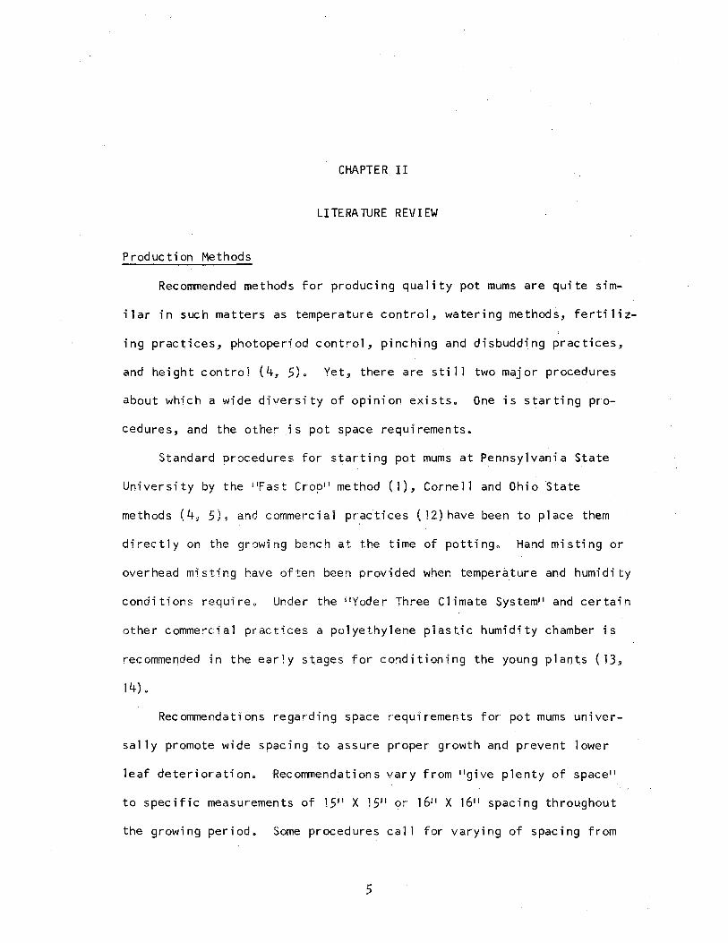
Recommended methods for producing quality pot mums are quite sim

ilar in such matters as temperature control, watering methods, fertiliz

ing practices, photoperiod control, pinching and disbudding practices,

and height control (4, 5L Yet, there are sti 11 two major procedures

about which a wide diversity of opinion exists. One is starting pro

cedures, and the other is pot space requirements.

Standard procedures for starting pot mums at Pennsylvania State

University by the 11Fast Crop 11 method (1), Cornell and Ohio State

methods (4 1 5L and commercial practices ( 12) have been to place them

directly on the growing bench at the time of potting. Hand misting or

overhead misting have often been provided when temperature and humidity

conditions require. Under the 11 Yoder Three Climate System11 and certain

other commercial practices a polyethylene plastic humidity chamber is

recommended in the early stages for conditioning the young plants ( 13,

14).

Recommendations regarding space requirements for pot mums univer

sa11y promote wide spacing to assure proper growth and prevent lower

leaf deterioration. Recommendations vary from 11give plenty of space 11

to specific measurements of 15 11 X 1511 or 1611 X 1611 spacing throughout

the growing period. Some procedures call for varying of spacing from

5

I

6

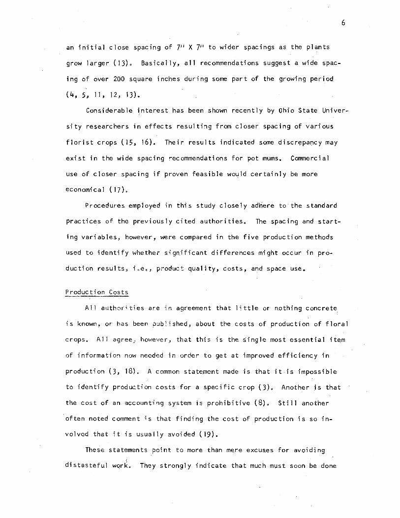
an initial close spacing of ]1 1 X 711 to wider spacings as the plants

grow larger (13). Basically, all recommendations suggest a wide spac-

ing of over 200 square inches during some part of the growing period

(4, 5., 11, 12, 13).

Considerable tnterest has been shown recently by Ohio State Univer-

sity researchers in effects resulting from closer spacing of various

florist crops ( 15, 16). Their results indicated some discrepancy may

exist in the wide spacing recommendations for pot mums. Commercial

use of closer spacing if proven feasible would certainly be more

economi ca 1 ( 17).

Procedures employed in this study closely adhere to the standard

practices of the previously cited authorities. The spacing and start-

ing variables, however, were compared in the five production methods

used to identify whether significant differences might occur in pro-

duction results, i.e., product quality, costs, and space use.

Production Costs

All authorities are in agreement that little or nothing concrete

is known, or has been published, about the costs of production of floral

crops. All agree, however, that this is the single most essential item

of information now needed in order to get at improved efficiency in

production (3, 18). A common statement made is that it is impossible

to identify production costs for a specific crop (3). Anoth~r is that

the cost of an accounting system is prohibitive (8). Still another

often noted comment is that finding the cost of production is so in-

vo1ved that it is usually avoided ( 19).

These statements point to more than mere excuses for avoiding

d • I 1 stasteful work. They strongly indicate that much must soon be done

7

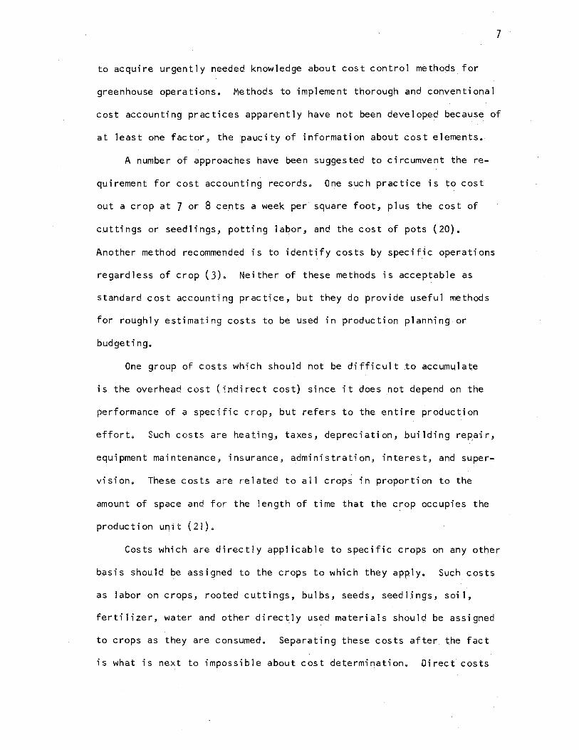
to acquire urgently needed knowledge about cost control methods for

greenhouse operations. Methods to implement thorough and conventional

cost accounting practices apparently have not been developed because of

at least one factor, the paucity of information about cost elements.

A number of approaches have been suggested to circumvent the re.

quirement for cost accounting records. One such practice is to cost

out a crop at 7 or 8 cents a week per square foot, plus the cost of

cuttings or seedlings, potting labor, and th~ cost of pots (20).

Another method recommended is to i den ti f y cos ts by specific operations

regardless of crop (3). Neither of these methods is acceptable as

standard cost accounting practice, but they do provide useful methods

for roughly estimating costs to be used in production planning or

budgeting.

One group of costs which should not be difficult to accumijlate

is. the overhead cost (indirect cost) since it does not depend on the

performance of a specific crop, but refers to the entire production

effort. Such costs are heating, taxes, depreciation, building repafr,

equipment maintenance, insurance, administration, interest, and super

vision. These costs are related to all crops in proportion to the

amount of space and for the length of time that the c.rop occupies the

production unit (21).

Costs whic.h are directly applicable to specific crops on any other

basis should be assigned to the crops to which they apply. Such costs

as tabor on crops, rooted cuttings, bulbs, seeds, seedlirigs, soil,

fertilizer, water and other directly us~d materials should be assigned

to crops as they are consumed. Separating these costs after the fact

is what is next to impossible about cost determination. Direct costs

8

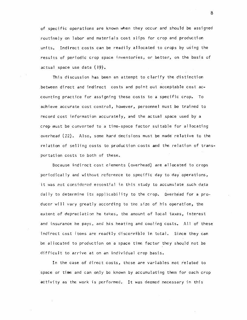
of specific operations are known when they occur and should be assigned

routinely on labor and materials c.qst slips for crop and production

units. Indirect costs can be readily al located to crops by using the

results of periodic crop space inventories, or better, on the basis of

actual space use data ( 19).

This discussion has been an attempt to clarify the distinction

between direct and indirect costs an.d point out acceptable cost ac

counting practice for assigning these costs to a specific crop. To

achieve accurate cost control, however, personnel must be trained to

record cost information accurately, and the actual space used by a

crop must be converted to a time-space factor suitable for allocating

overhead (22). Also, some hard decisions must be made relative to the

relation of selling costs to production costs and the relation of trans

portation costs to both of these.

Because indirect cost elements (0,verhead) are allocated to crops

periodically and without reference to specific day to day operations,

it was not considered essential in this study to accumulate such data

daily to determine its applicability to the crop. Overhead for a pro

ducer wi 11 vary great 1 y ac:co.rding to the size of his opera ti on, the

extent of depreciation he takes, the amount of local taxes, interest

and insurance he pays, and his heating and cooling costs. All of these

indirect cost items are readily discernible in total. Since they can

be al located to production on a space time factor they shquld not be

difficult to arrive at on an 1ndividual crop basis.

In the case of direct costs, these are variables not ~elated to

space or time and can only be known by accumulating them for each crop

activity as the work is performed. It was deemed necessary in this

study to examine these costs and use them as a basis of comparison be

tween production methods, as would also be appropriate for any commer

cial concern. They are costs that can be varied to affect only a

single crop whereas the variation of indirect costs affects all crops

and are not manageable on an individual crop basis.

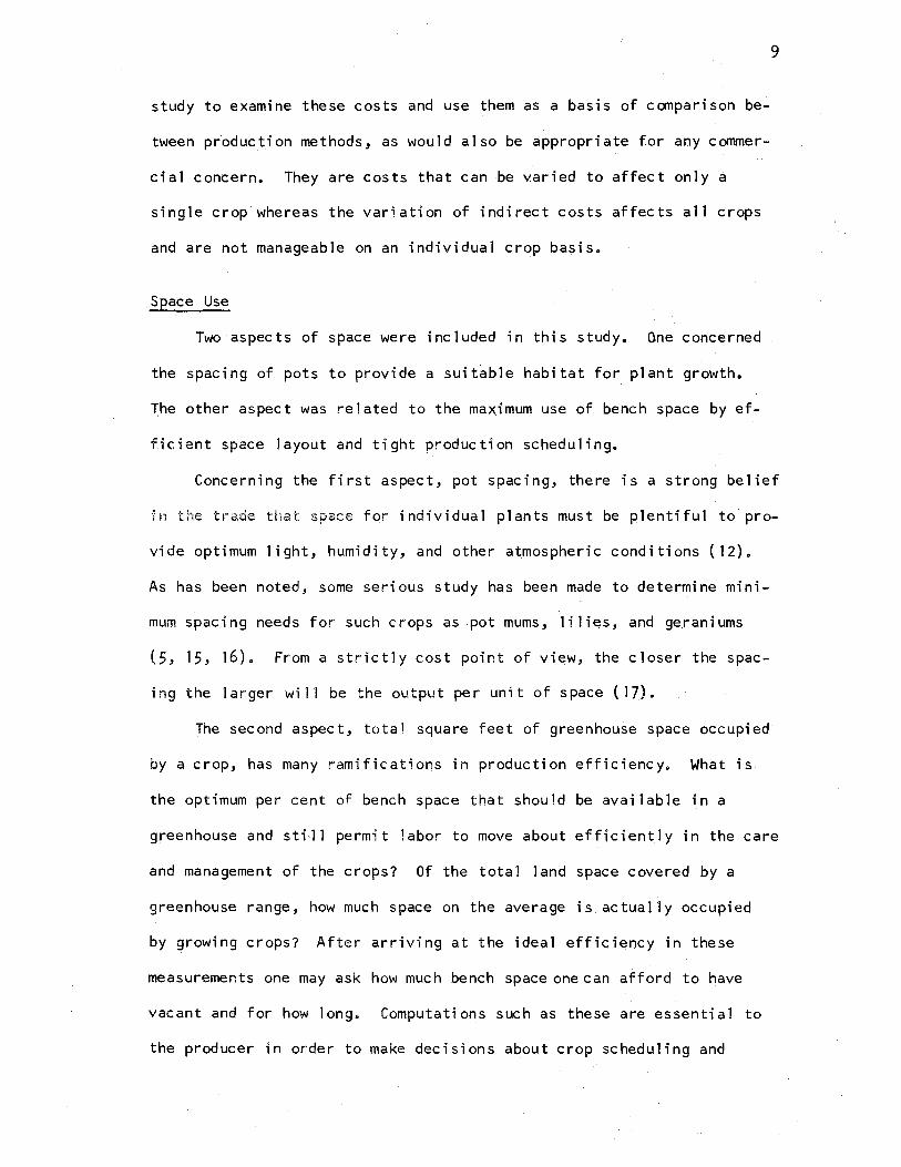
Space Use

Two aspects of space were included in this study. One concerned

the spacing of pots to provide a suitable habitat for plant growth.

The other aspect was related to the maximum use of bench space by ef

ficient space layout and tight production scheduling.

9

Concerning the first aspect, pot spacing, there is a strong belief

in the trade that space for individual plants must be plentiful to pro

vide optimum light, humidity, and other atmospheric conditions ( 12).

As has been noted, some serious study has been made to determine mini

mum spacing needs for such crops as pot mums, lilies, and geraniums

(5, 15, 16). From a strictly cost point of view, the closer the spac

ing the larger will be the output per unit of space (17).

The second aspect, total square feet of greenhouse space occupied

by a crop, has many ramifications in production efficiency. What is

the optimum per cent of bench space that should be available in a

greenhouse and sti,11 permit labor to move about efficiently in the care

and management of the crops? Of the total land space covered by a

greenhouse range, how much space on the average is actually occupied

by growing crops? After arriving at the ideal efficiency in these

measurements one may ask how much bench space one can afford to have

vacant and for how 1 ong. Computations such as these are es sen ti a 1 to

the producer in order to make decisions about crop scheduling and

10

quantities of supplies to order (23, 24). There is, as previously

noted, a direct relationship between indirect costs and space. Thus.,

there is also a close relationship between unoccupied space and the

many i ndi rec'!: costs experienced in greenhouse operati ens. Within a

floral business every square foot of land, whether it has a greenhouse

or plastic film ho4se on it or just an open drive, constitutes a -pace

that must be asse.ssed to some crop. Even though there is no bench cir

pl ant on the bench, it does not e I imi nate the need to assign such un

occupied space with its share of the cost of production. It is a cost

which will have to be assigned to a crop being produced (25).

Product Quality

Grading standards for pot mums have not as yet been forma 11 y

established. However, many tests and research studies which have com

pared the results of producing pot mums under various conditiohs have

consistently used certain measures to indicate the quality of the plants

produced. These measures have been dry weights ( 26), number of f lc,wer

i ng breaks, and plant height (26, 27, 28). Realizing, of course, that

the true value of a plant is more closely related to its aesthetic

value, these quantitative measures were used in this study only as an

expedient to enhance statistical oomparis6ns.

CHAPTER III

METHODS AND MATERI.ALS

Approach to the Problem

Data on .all four facets of the problem, production me,th6ds, direc.t

production costs, s_pace use and product qua 1 i ty, were accumulated si

multaneous 1 y. · This.provided a ma~imum of interaction tc:i support the

findings on production method efficiency and· profitableness, and at the

same time permitted c 1 ose examination of e_ach separate aspect.

Facilities, Materials, and Practices

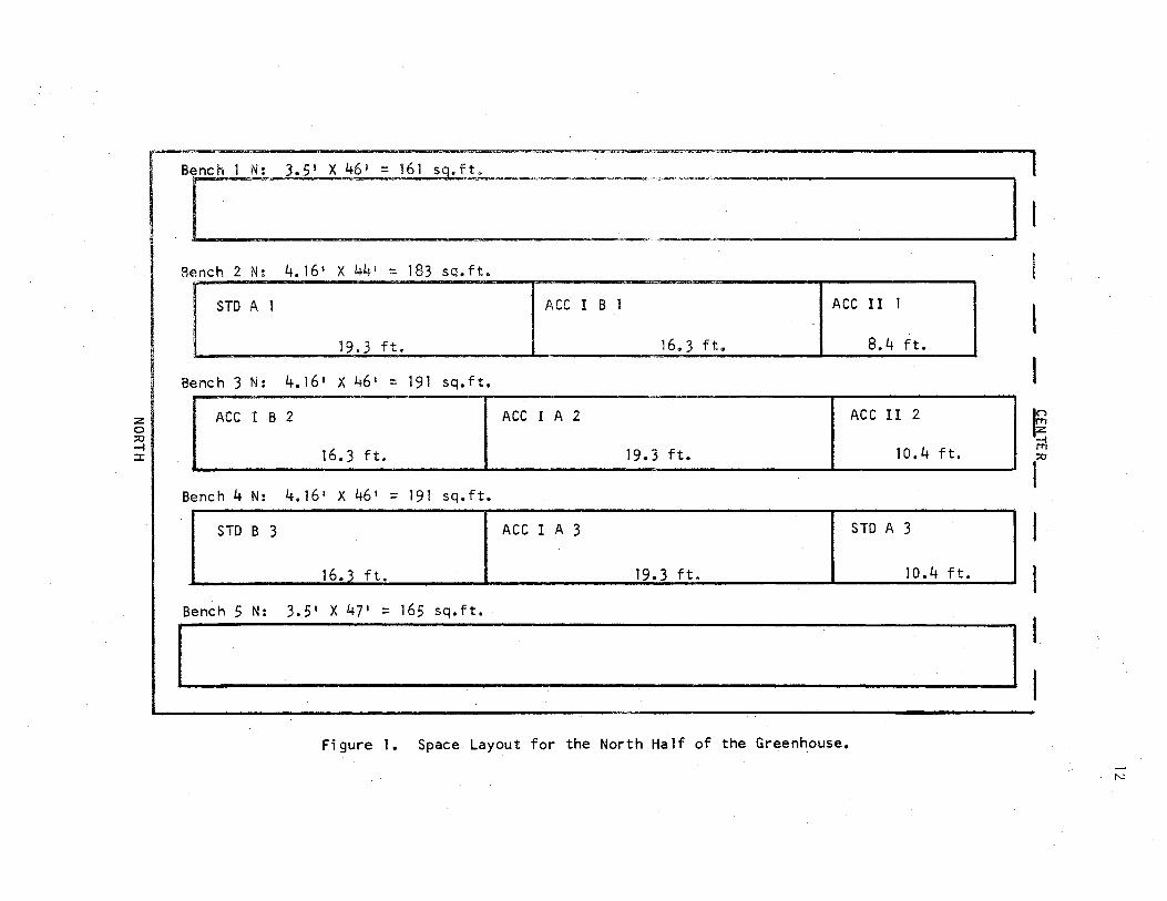
A major portion of a 32 1 X 100 1 gr~enhouse structure was used for

the conduct of the experiment (see Figures 1 and 2). This structure

provided steam heat with poly-tube and exhaust fan ventilation. Summer

coo] i ng was provided by means of evaporative coo1 ing pads and exhau_st

fans. Plants were grown irl pots on 50 inch wide redwood benches with~

out sides. Each bench was equipped with a Chapin irrigating system

containing a 3/411 central header line and individual pot tubes. A

GEWA fertilizer injector system was connected into the line providing

200 ppm each of N, P2o5 and Kz°, using 20-20-20 soluble fertilizer with

each watering. Daylight duration was reduced, when required, with a

manually drawn sateen black cloth ~hade (64 X 104 mesh). A climate

control bench, polyethylene covered and enclosing a mist line, pro-

vided the high temperature and humidity control for designated

11

z 0 :::0 -I ::i:

Bench 1 N: 1.5 1 X 46 1 = 161 sq.ft.

I ---~--- l

Bench 2 N: 4.16 1 X 44 1 = 183 sq.ft.

STD A 1 ACC I B 1 ACC II 1

19.3 ft. 16.3 ft. 8.4 ft.

Bench 3 N: 4.16 1 X 46 1 = 191 sq.ft.

ACC I B 2 ACC I A 2 ACC II 2

16.3 ft. 19.3 ft. 10.4 ft. ~ ;I

r Bench 4 N: 4.16 1 X 46 1 = 191 sq.ft.

STD B 3 ACC I A 3 STD A 3 I 16.1 ft. 19.3 ft. 10.4 ft.

Bench 5 N: 3.5' X 47' = 165 sq.ft. I . ·······~· ~· I : Figure 1. Space Layout for the North Half of the Greenhouse.

N

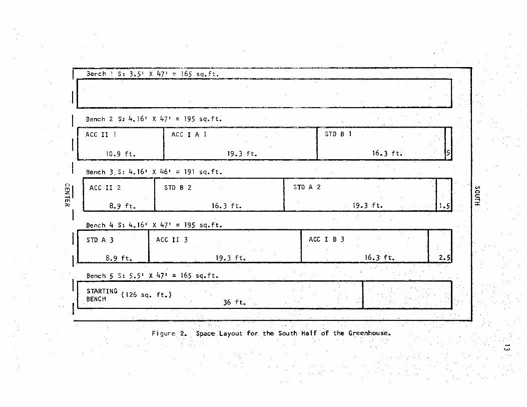
J Bench 1 S: 3.5 1 X 47 1 = 165 sq.ft. ==

,f · < I

· 1

sl .m

:::0

l

Bench 2 -~~ 4.16 1 X 47 1 = 195 sq.ft~

ACC II 1 ACC I A 1

10.9 ft. 19.-3 ft.

Behch 3~S: 4.16 1 X 46• = 191 sq.ft.

ACC II 2 STD B 2

8.9 ft. 16.3ft.

Bench 4 S : 4. 16 1 X 4 7 1 = 195 sq.ft.

STD A 3 ACC II 3

8.9 ft. 19.3 ft.

STD B 1

16. 3 ft. 5

STD A 2

19. 3 ft. . l .5

ACC I B 3 . '

16.3ft. 2.~

Bench 5 ·s: 5.5 1 X 47 1 = 165 sq.ft. : I ~~~~NG(126 sq. ft.) . . . 36 ft; ·• l / • /l Figure_ '2.. Spaee Layo.ut for the South ttalf of the Greenhouse.

(I)

0 c: -I :::J:

. '-"

14

production methods (see Table I). I

The growth retardant A I ar was used

for growth control on al I tal 1 treatment varieties. Standard preventive

practices for disease and insect control were fol lowed using sprays,

fumigants, and dusts as needed.

Production Methods

Although five separate production methods were ex,amined, they

actually constituted a variation of the two common commercial methods:

First, providing long days with a climate control start prior to start-

ing short days and second, placing pats directly on the growing bench

without climate control or initial long day treatment. An additional

two methods we re derived from the two common methods by a pot spacing

variation of 1)1 1 X 1311 in place of 1511 x 1511 • The fifth method was

a variation of the climate control method with climate control provided

after the start of short days. The test was run on three separate

cycles. Each cycle, the growing period for a particular crop, con-

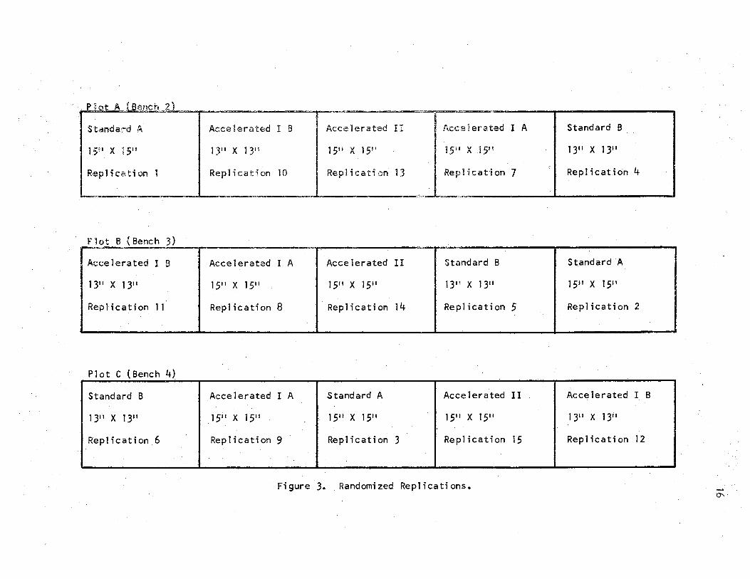
sisted of the five production methods in three randomized replications.

Each replication consisted of two cultivars with the only variable be-

tween rep1 icati ons being greenhouse 1 ocati on ( see Figure 3). There

were a total of 30 plants of each cultivar in each of three replications

for a total of 180 plants in each method. The five methods thus totaled

900 plants for each cycle, or 2700 plants for the total test~ The first

cycle was started on March 11 and continued through May 20. The second

cycle started on May 27 and continued through August 12. The third and

final cycle started on September 10 and ended on November 20. The use

1uni-Royal 85% WP formulation of succinic acid 2,2-dimethyl hydrazide.

Method

Standard A

Standard B

Accelerated 1 A

Accelerated 1 B

Accelerated II

..,_,";,_-

Starting Procedure

7 Long Oays 9

Mist, 65°F plus

"7 Long Days Mist, 65°F plus

No Long Days, No Mist, 62°F

No Long Days, No Mist, 62°F

No Long Days Mist, 65°F plus

TABLE I

PRODUCTION METHODS

Start

711 x 71! I-7th day

711 x T' 1-7th day

1511 x 1511

1311 x 1311

711 x 711 1-7th day

Spacing

Finish Pinching --

Ta 11 : ·l;;'"J';;

SD + 7 ] 51 I X 1511 Short: Start SD

No Alar

1311 x 1311 Ta 11 ~ SD + 7 Shortg Start SD

No Alar

1 51 I x 1511 Ta 11 : SD + 7 Short: SD + 3

No Alar

1311 x 1 311 Ta 11 : SD + 7 Short: SD :+ 3

No Alar

1511 x 1511 Ta 11 : SD + 7 Short: SD :+ 3

No Alar

;',A climate control of increased temperatures, high humidity and additional daylength were provided Standard A and Standard B production methods as indicatedo

**so= short dayso v,

... ~ • • n.- ••-•.• ,,_ A

Standard A Acce1erated I B Accelerated II Accelerated I A Standard B

15e1 X 1511 1311 x 1311 1511 x 1511 1511 x 1511 1311 x 1311

Re.plication 1 Replication 10 Rep1 icati on 13 Replication 7 (

Replication 4

P]ot B (Bench 3)

Accelerated I B Accelerated I A Acee lerated II Standard B · Standard A

1311 x 1 311 1511 x 1511 1511 X 15u 1311 x 1311 1511 x 1511

Replication 11 Rep 1 i cat i on 8 Rep 1 icati ()n 14 Replication 5 Replication 2

Plot C (Bench 4)

Standard B Accelerated I A Standard A Accelerated II . Accelerated I B

1311 x 1311 15j I X 1511 1511 x 1511 1511 x 1511 . 1311 x 13il

Replication 6 Replication 9 Replication 3 Replication 15 Replication 12

Figure J. . Randomized Rep 1i cations. '"':

of three cycles introduced a wide range of climate differences into the

test to further validate results.

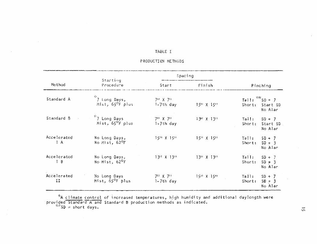
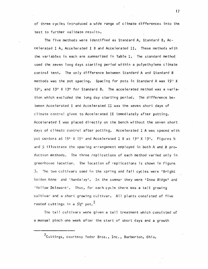
The five methods were identified as Standard A, Standard B, Ac

celerated I A, Accelerated I Band Accelerated II. These methods with

the variables in each are summarized in Table I. The standard method

used the seven long days starting period within a polyethylene climate

contro 1 tent. The on 1 y difference between Standard A and Standard B

methods was the pot spacing. Spacing for pots in Standard A was 1511 X

1511 , and 1311 X 1311 for Standard B. The accelerated method was a varia

tion which excluded the long day starting period. The difference be

tween Accelerated I and Accelerated II was the seven short days of

c 1 imate contro 1 given to Acee 1 erated II immediate 1 y after potting.

Accelerated I was placed directly on the bench without the seven short

days of climate control after potting. Accelerated I A was spaced with

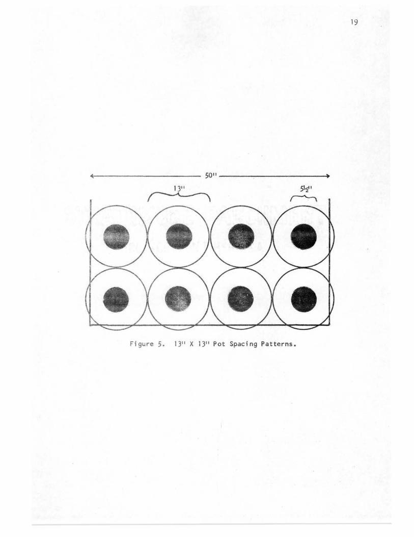
pot centers at 1511 X 1511 and Accelerated I Bat 1311 X 1311. Figures 4

and 5 illustrate the spacing arrangement employed in both A ancl .. B pro

duction methods. The three replications of each method varied only in

greenhouse location. The location of replications is shown in Figure

3. The two cu1tivars used in the spring and fall cycles were 1 Bright

Golden Anneu and 1 Manda1ay 1 • In the summar they were 'Snow Ridge• and

1 Ye11ow Delaware 1 • Thus, for each cycle there was a tall growing

cultivar and a short growing cultivar. All plants consisted of five

rooted cuttings in a 511 1 pot. 2

The ta1 l cul ti vars were given a ta11 treatment which consisted of

a manual pinch one week after the start of short days and a growth

2cuttings, courtesy Yoder ijros., Inc., Barberton, Ohio.

18

5~··

Figure 4. 1511 X 1511 Pot Spacing Patterns.

19

Figure 5. 1311 X 1311 Pot Spacing Patterns.

20

contro 1 treatment of • 25% A 1 ar fo 1i ar spray two weeks after the pinch

(29). In the summer cycle a .50% spray of Alar was used. The short

cultivars were actually given a modified medium treatment with pinching

done on the third day after the start of short days (29). No Alar ap-

plications were made on the short cultivars.

As already noted, a fertilizer application of 20-20-20 soluble

fertilizer was injected at every watering. On the third day afte~ pot-

ting, a 500 ppm starter solution of 20-20-20 fertilizer was applied with

manual watering. Plants were irrigated as weather and soil moisture

conditions permitted. After an initial phasing-in requiring some 11 spot

watering0 of individual pots, a11 plants received the same rate of water-

ing application of 10 ounces at each watering.

Additional cultural practices concerning temperature, light, black

cloth shading, and soi 1 fol lowed the generally accepted commercial prac-

tice in this area. Throughout each cycle, night temperatures were held

to 62°F when possible. During the last two weeks of ~ach cycle the

0 night temperature was reduced as close to 58 Fas possible. The day

0 0 0 temperature was held at 70 to 75 Fon normal days and 65 Fon cloudy

days" Lighting was provided for the standard methods during long day

treatments for four hoursj from 10 p.m. unti 1 2 a.m. each night at the

start of the spring and fall cycles. The black cloth shading was used

for daylength control from March 1 until October 1. It was drawn at

5 p.m. during the spring and fal 1 and at 7 p.m. during the summer, re-

maining on until 8 a.m. each morning. The soil mixture consisted of

one part clay 1oam, one part peat, and one part perlite. Hydrated lime

was added at the rate of 2.7# per cubic yard of soil mix. In the pot-

ting operation rooted cuttings were carefully planted shallow and leaning

21

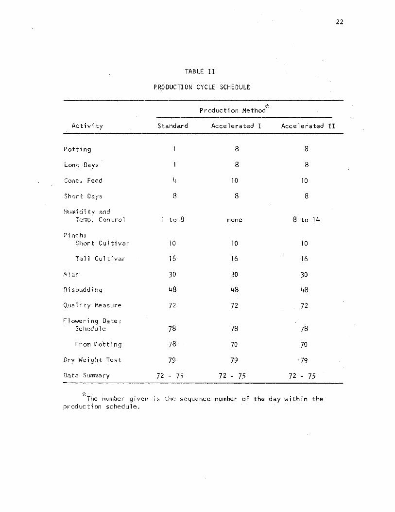
outward at the pot perimeter. A production method sc.hedule is included

in Table II.

Accumulating Direct Production Costs

This study, for reasons previously presented and as discussed be

low, was restricted to direct material and direct labor inputs. Over

head (indirect} costs were excluded because they are prorated to all

production areas after being accumulated centrally without reference to

specific crops. There is nothing novel about isolating indirect costs

in regard to a single crop because they are then simply proportional to

space use and they are not controllable by any single crop.

The identification of direct cost inputs is useful. The level of

such costs is f~irly.unif6rm from one firm to another within wide re7

gional areas, assuming the same or quite similar production methods.

In this test the direct cost data were accumulated for each production

method. Whenever a cost was not directly associated with a production

method, it was prorated uniformly to all production methods.

Each crop cycle in this test was produced as a single lot with all

plants in a lot scheduled to be finished on the same date regardless of

production method. It, therefore, was appropriate to use the simplified

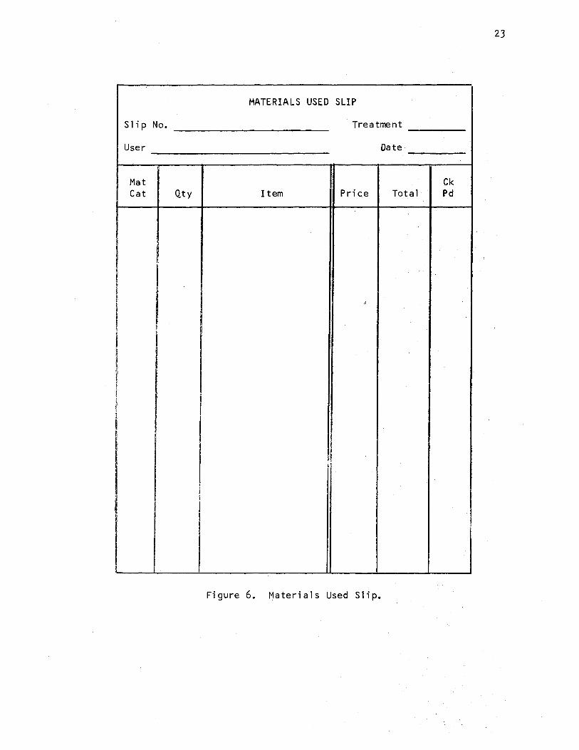
form of job order cost accounting. Costs for materials were recorded

daily on 11Materials Used S1ips11 at the time supplies were drawn for use.

Each slip contained a slip number, user 1 s name, date, production methqd

on which it was used, item, quantity, and price. The format is shown

in Figure 6.

A single slip was prepared for each item or for each group of items

when several were applicable to a single operation. The materials used

slips were accumulated for each week and at the end of the week they

Ac ti vi ty

Potting

Long Days

Cone. Feed

Short Days

Humid ·i ty and Temp., Control

Pinch: Short Cul ti var

Tall Cultivar

Jl.lar

Disbudding

Quality Measure

Flowering Date~. Schedu 1 e

From l?ott·ing

Dr·y Weight Test

Data Summary

·k

TABLE II

PRODUCTION CYCLE SCHEDULE

Production Methol°r

Standard Accelerated I Accelerated II

8 8

8 8

4 10 10

8 8 8

l to 8 none 8 to 14

10 10 10

16 16 16

30 30 30

48 48 48

72 72 72

78 78 78

78 70 70

79 79 79

72 - 75 72 - 75 72 - 75

The number given is the sequence number of the day within the production schedule.

22

23

MATERIALS USE:D SLIP

S 1 i p No. Treatment

User Date

Mat Ck Cat Qty Item Price Total Pd

I f

I " i I

;

f

I ' i ,!

1

l

!

Figure 6. Materials Used Slip.

24

were posted to a .mater.ia.ls c.onsu.mp.tion . .list. (Figure . .7) •. AJl material

was identified by production method whenever possible. Such procedures

as fumigation, Alar applications, and irrigation were uniform for all

methods and were prorated to each method equally. Care was taken to in-

elude all materials costs. Water through the irrigation system wa$ pro-

rated to each product.ion method each week by the rate of 1/5th of 69

gallons, the total quantity distributed at each watering. Such materials

as cleaning and painting supplies or building repair materials were not

included under direct costs of production.

Prices for computing cos.ts of materials were obtained from in-

voices or suppliers' catalogs. All costs were accumulated on the mate-

rials cpnsumption list by the materials categories:

Category

1 • Soi 1

2. Pots and labels

3. Fer ti 1 i zer

4. Insecticides, etc.

5. Water

6. Chemicals

7. Equipment repair

8. Other

Explanation

Components and additives at the time of potting.

Pots, labels, drainage, stakes, and ties.

Both soluble fertilizer and other special purpose fertilizer.

Insecticides, fungicides, and other chemicals for control of diseases and disorders, including spreaders.

All water, both through injector and manual.

For special chemical treatments such as Alar.

Parts, supplies, and materials used in equipment set up, maintenance, and repair.

Clearly identi-.fied.

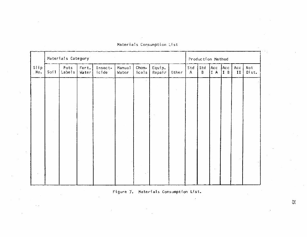
Materials Category

Slip Pots Fert. Insect-No. Soil Labels Water icide

Materials Consumption list

Production Method

Manual Chem- Equip. Std Std Ace Ace Water icat s Repair Other A B I A I B

,

'

Figure 7. Materials Consumption List.

Ace II

Not Di st.

N V1

26

After summarizing each material categ9ry.on· the materials: consumpti.on

list, it was posted to the production cost sheet for the production

eye le.

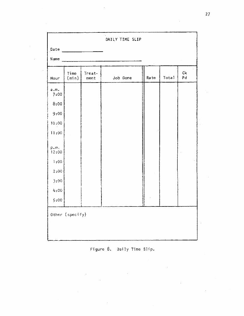
Al 1 labor attributable to the test was recorded at the time per-

formed on a 11 Daily Time Slip11 (Figure 8) by the individual performing

the work. A separate slip was prepared by each individual for each day

he performed work. All labor time that could be identified with a

specific production method such as manual mist,ing of a particular repli-

cation was recorded for that method. Where it was not possible or was

impractical to so identify the labor cost, i.e., pulling black cloth,

irrigating, or potting, the c.osts were prorated evenly to al 1 methods.

Daily time slips contained the name of the worker, inclusive times in

which the work was performed, the date, and the production method.

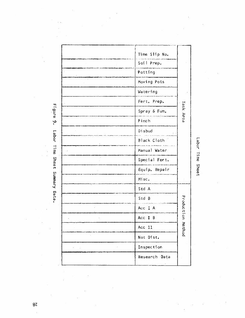
Daily time slips were ac~umulated each week and recorded individ-

ua11y on the Labor Time Data Sheet (Figure 9). Undistributed direct

1abor was prorated evenly to each production method. All laqor per-

formed was recorded at the current federal minimum wage of $1.60 per

hour. Such tasks as building maintenance or heating system repair,

even though performed in the project area, were not included as direct

costs. (These costs would normally be accumulated as indirect costs by

a commerc i a 1 producer.) A 11 work performed was recorded as one of the

sixteen types of tasks:

Task Area

1. Soil preparation

2. Potting

3. Moving pots

Explanation·

Hauling, mixing, ste~ilizing.

Setting up the potting bench, potting, placing pots on bench.

Re-spacing and spacing out.

27

DAI LY TIME SLIP

Date

Name

: " ' . Time Treat- Ck

Hour (min) ment ,. Job Done Rate Total Pd

a.m. 7:00

8:00

9:00

10 :00

11 ; 00 ·

p.m. 12:00

1 :00

2:00

3:00

4:00

5:00

Other (specify)

Figure 8. Daily Time Slip.

8Z

"Tl .... lQ c , CD

\.0 •

' DI co , -I .... ill (/)

;; CD CD c-t

(/)

c ~ DI , '<

c DI c-t DI .

,..--..-. ~ ........ 1----~-

Ti me S 1i p No.

Soil Prep.

Potting

Moving Pots

Watering

Fert. Prep.

Spray & Furn. ·---------·--I-··--···· ....... , .. ,.,.,--------'-!

Pinch

Disbud I- ---··--··--·--·------· . -- -~•----....... - ....... -.-·-······---·--

B 1 ack C 1 oth ··-------·------·------···-·-·······

Manual Water

S peci a 1 Fer t. +-----------------........i,.--.--------

Equip. Repair I .-..!---·--···.,-·------~

Mi SC.

-I DI Vl 7'

)::, , CD Ill

·---------+------·-··------! 1

Std A ~~~i--~~~~~~~-~--~

Std B I ·-···-t··· .. ···· .... _ ......... '" ....... · ..... , •.... _

Ace I A 1------------------------1----------------1

Ace I B

Ace II

Not Di st.

In spec ti on

Research Data

"'O , 0 a. c n c-t .... 0 :::,

if c-t ;; 0 a.

' DI er 0 , -I .... ffi (/) ;; CD CD c-t

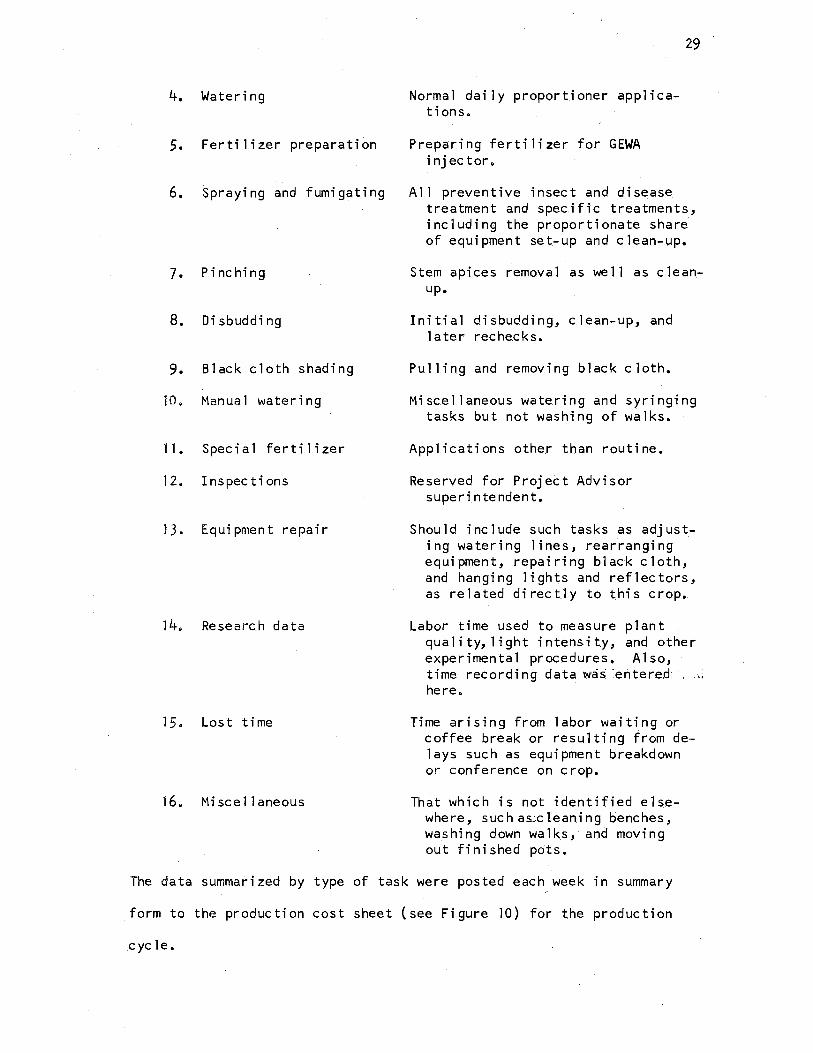
4. Watering

5. Fertilizer preparation

6. Spraying and fumigating

7. Pinching

8. Disbudding

9. Black cloth shading

10. Manual watering

11 • Spec i a 1 fertilizer

12. I nspec ti ons

13. Equipment repair

14. Research data

15. Lost time

16. Miscellaneous

Normal daily proportioner applications.

Preparing ferti 1 i zer for GEWA injector.

29

All preventive insect and disease treatment and specific treatments, including the proportionate share of equipment set.-up and clean-up.

Stem apices remova 1 as we 11 as clean.up.

Initial disbudding, clean-up, and 1 ater reche.cks.

Pulling and removing black cloth.

Miscellaneous watering and syringing tasks but not washing of walks.

Applications other than routine.

Reserved for Project Advisor superintendent.

Should include such tasks as adjusting watering lines, rearranging equipment, repairing black cloth, and hanging lights and reflectors, as related directly to this crop •.

Labor time used to measure plant qualit~ light intensity, and ~ther experimenta 1 procedures. A 1 s.o, time recording data was :entered : here.

Time arising from labor waiting or coffee break or resulting from de-1 ays such as equipment breakdown or conference on crop.

That which is not identified elsewhere, such as.:;cteaning benches, washing down walks, and moving out finished pots.

The data summarized by type of ta_sk were posted each week in summary

form to the production cost sheei (see Figure 10) for the production

c ye le.

30

PRODUCTION COST SHEET

From To ---

Task Week or

Category 1 2 3 4 5 6 7 8 9 10 11 Total

I I I

l I

I l ! I

I i l 1 i I i !

I ! I

i I

I I I I I I I l I

I t !

Comments:

.

I

Figure 10. Production Cost Sheet.

31

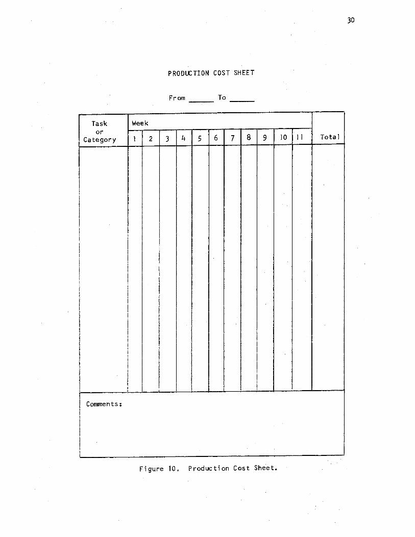
As indicated above, the production cost sheet (Figure 10) was used

-to summarize both materials and labor costs each week during the entire

period of the cycle. Actual costs and prorated costs accumu.lated by

type of task or material category were also summarized each week on the

production cost sheet by production method. This provided a weekly cost

level for each production method for each style. The production cost

sheet thus gave complete direct cost information for each week. Indi

vidual cost elements (categories and tasks) were summed to give totals

for the cycle and for the entire test period.

!dentifting Space Use Efficiency

At the present state of the art, the most si gni fi cant charac teri s

tic of greenhouse bench space in production management is its two di

mens.ional quality. Although attempts have been made and continu.e to be

made to use available cubic space by employing shelves, tier benches,

and racks (30), greenhouse bench space remai~s for all practical pur

poses a single plane dimension.

In order to study space it was necessary to break it down into its

component eleme.nts and to deal with each separately. The foll'Owing

discussion describes terms used to identify space components for this

study. It is suggested that these terms and the. components they rep

resent could be seriously considered as a management tool in greenhouse

production control. They represent a basic approach which has been ac

cepted and successfully used by industrial and marketing firms (31).

For the total greenhouse range structure and land in the immediate

vicinity, the term Total Gross Range Space was used •. This compoMent

was essentially a total of all other components. It inclu.ded land,

surroun~ing the greenhouses, that was used for roads, walks and idle

space between greenhouse units as well as the greenhouse space itself.

Also included were such structures as hotbeds, coldframes, headhouses

and boiler rooms. It did not include land devoted to &eparate field

production.

A major component of the total gross range space was the ground

space actually occupied by thegreenhouse production units. The term

given to this component was Gross Greenhouse Production Space. It in

c 1 uded all bench space, aisles, walks, equipment space, and space ob

structed by structural features such as purlin posts, doors, and pipe-

1 i nes.

32

Space outside of production units was identified as Space in Sup

~t of__!:.roduction. This space included the headhouse, potting sheds,

grading and packing areas, office areas, cold storage facilities, boiler

rooms, rest rooms, as wel 1 as cold frames, hotbeds and seedbeds that are

used in activities directly related to greenhouse production.

The greenhouse production space was further divided into a componemt

represented by the term Usable Bench Space. It was very similar to the

commonly used term in the trade, bench space. This component constituted

actual ground bench space or raised bench space, including shelves and

potential bench space not in use.

Bench space (Usable Bench Space) actually occupied by crops is

called Occupied Bench Space. This space component when compared with

the gross greenhouse production space provided an overal 1 measure of

efficiency in space management. It was described as the Per Cent of

Gross Space Used.

Empty bench space, usable bench space not used for crops, was

identified as Vacant Bench Space. When the vacant bench space was

33

compared with the usable bench space it provided a measure of the ef-

ficiency by which actual space avai table was being managed. It was

~al led.the Per Cent of Usable Space Loss.

Wit.hin the scope of the above defined terms, space use data were

recorded during the period and analyzed. The un_used space was identifielf

and comparisons were made with gross space and usable space to arrive at

a useful description of space effectiveness.

Each unit of space was measured in terms of the possible number of

days it was usable and the numberof square feet it constituted. This

measure was developed in ••square foot-days 11 , meaning that in an average

month each square foot of usable bench space would be thirty 11 square

feet-days 11 • A benc.h with one hund.red square feet would have avai table

3000 square foot-days per month.

By comparing gross greenhouse product.ion space,· measured in sqqare

foot-days, ·with the occupied bench space, a 1 so measured in sq4are foot-

days, a per cent space used figure was readily derived which ac.curat.ely

described the efficiency with which space was being managed. It con-

sidered both space available and time available factors. As an example,

in the test the total gross greenhouse production space/time for one

month was 96,000 square foot days. If the total usable bench space was

ful ty occupie.d during this same period, the occupied bench space time

would be 54,060 square foot-days (refer to Table III). Thus the per

cent of gross space used would have been 56 pe.r cent. This efficiency

figure, assu.mi ng optimum pot spacing, constitutes the b~st use that

could have been made of the greenhouse space unde.r the .present space

1 ayout. It i.s conce,ivab le that other 1 ayout arrangements such as

peni nsut ar benches might increase space use efficiency, however, the

34

TABLE III

USABLE BENCH SPACE

Bench Dimensions ~'(

Net Usable Bench 0 Space Total Project

North 3.5 1 x 46 1 161 -

South 3.5 1 x 47 1 165

2 North 4. 16 1 x 44 1 183 183

2 South 4. 16 1 x 47 1 195 195

3 North 4. 16 1 X 46 1 191 191

3 South 4. 16 1 x 46 1 191 191

4 North 4. 16 1 x 46 1 191 191

4 South 4. 16 1 x 47 1 195 195

5 North 3.5• x 47 1 165

5 South 3.5 1 x 47 1 165 126

Total 1802

'"Ir: Square feet.

35

present arrangement I imi ted efficiency to a maximum of 56 percent.

Any unused space ( the difference be tween usab I e bench space and oc-

cupied bench space) decreases efficiency so that when operating figures

are compared with 56 per cent they wi 11 provide a gauge of efficiency

in space management including both space use and layout planning.

The other space management efficiency figure, Per Cent Usable

Space Loss, concerned the usable bench space/time that was available

during the period and h.ow the occupied bench space/time compared with

this figure. If during a month on various days space was not used that

amounted to 1500 square foot-days (or an average of 50 square feet per

day out of the 1802 available), the per cent usable space loss would

have been 2. 2%.

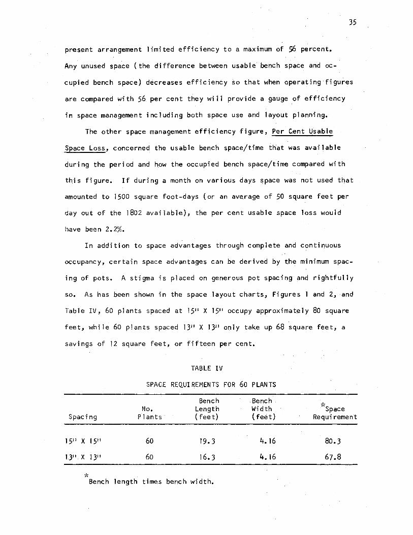
In addition to space advantages through comp I ete and con ti nuo.us

occupancy, certain space advantages can be derived by the minimum spac-

ing of pots. A stigma is placed on generous pot spacing and rightfully

so. As has been shown in the space layout charts, Figures I and 2, and

Table IV, 60 plants spaced at 1511 X 1511 occupy approximately 80 square

feet, while 60 plants spaced 131 1 X 1311 only take up 68 square feet, a

savings of 12 square feet, or fifteen per cent.

TABLE IV

SPACE REQUIREMENTS FOR 60 PLAN TS

Bench Bench No. Length Width

Spacing Plants (feet) ( feet)

1511 x 1511 60 19.3 4. 16

1311 x 1311 60 16.3 4. 16

Bench length times bench width.

-;';Space Requirement

80. 3

67.8

36

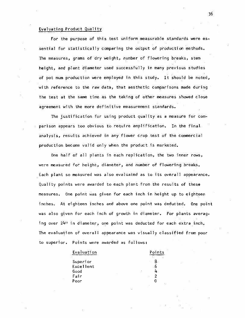
Evaluating Product Quality

For the purpose of this test uniform measurable standards were es-

sential for statistically canparing the output of production methods.

The measures, grams of dry weight, number of flowering breaks, stem

height, and plant diameter used successfully in many previous studies

of pot mum production were employed in this study. It should be noted,

with reference to the raw data, that aesthetic comparisons made during

the test at the same time c!S the taking of other measures showed close

agreement with the more definitive measurement standards.

The justification for using product quality as a measure for com-

parison appears too obvious to require amplific~tion. In the final

analysis, results achieved in any flower crop test of the commercial

production become valid only when the product is marketed.

One half of al 1 plants in each replication, the two inner rows,

were measured for height, diameter, and number of flowering breaks.

Each plant so measured was also evaluated as to its overall appearance.

Quality points were awarded to each plant from the results of these

measures. One point was given for each inch in height up to eighteen

inches. At eighteen inches and above one point was deducted. One point

was also given for each inch of growth in diameter. For plants averag-

ing over 2411 in diameter, one point was deducted for each extra inch.

The evaluation of overall appearance was visually classified from poor

to superior. Points were awarded as follows:

Evaluation Points

Superior 8 Exce 11 ent 6 Good 4 Fair 2 Poor 0

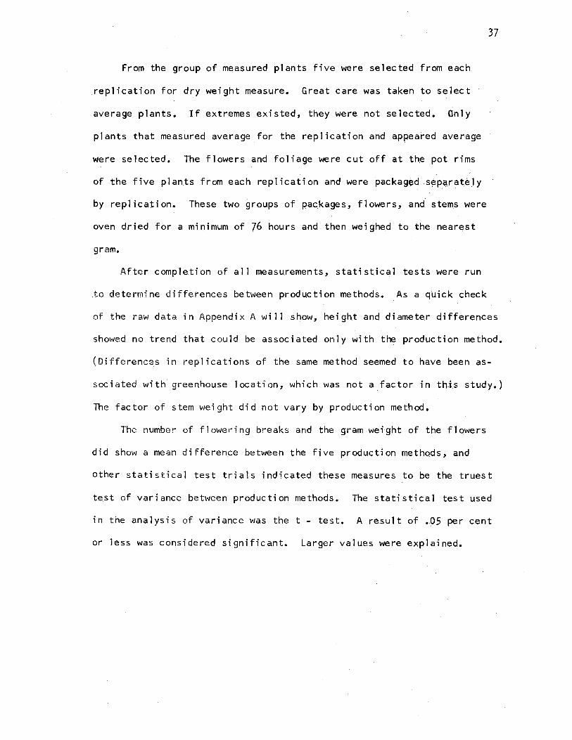
From the group of measured plants five were selected from each

replication for dry weight measure. Great care was taken to select

average plants. If extremes existed, they were not selected. Only

p 1 ants that measu.red average for the rep 1 i cation and appeared average

were selected. The flowers and foliage were cut off at the pot rims

of the five plants from each replication and were packaged s¢p9rately

by replication. These two groups of packages, flowers, and stems were

oven dried for a minimum of 76 hours and then weighed to the nearest

gram.

After completion of all measurements, statistical tests were run

to determine differences between production methods. As a quick check

37

of the raw data in Appendix A wi 11 show, height and diameter differences

showed no trend that could be associated only with the production method.

(Differences in replications of the same method seemed to h.ave been as

sociated with greenhouse location, which was not a factor in tt)is study.}

The factor of stem weight did not vary by production method.

The number of flowering breaks and the gram weight of the flowers

did show a mean difference between the five production methods, and

other statistical test trials indicated these measures to be the truest

test of variance between production methods. The statistical test used

in the analysis of variance was the t - test. A re,sult of .05 per cent

or less was considered significant. Larger values were explained.

CHAPTER IV

EXPERIMENTAL RESULTS

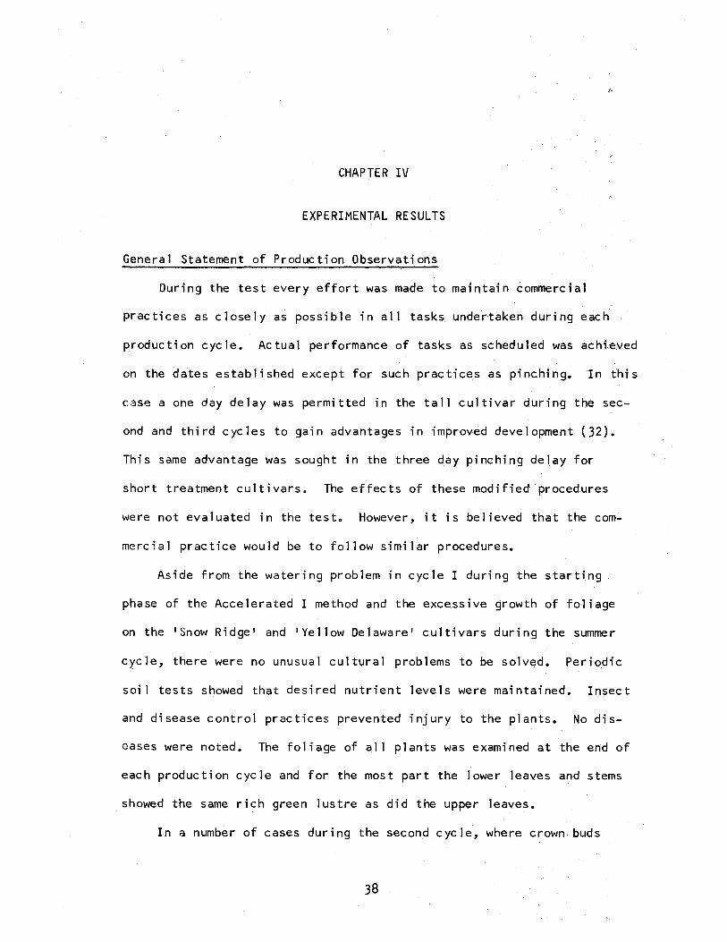
Genera 1 Statement of Production Observations

During the test every effort was made to maintain commercial

practices as closely as possible in all tasks undertaken during each

production cycle. Actual performance of tasks as scheduled was achieved

on the dates established except for such practices as pinching. In this

case a one day delay was permitted in the tall cultivar during the sec

ond and third cycles to gain advantages in improved development (32).

This same advantage was sought in the three ~ay pinching delay for

short treatment cultivars. The effects of these modified procedures

were not evaluated in the test. However, it is believed that the com.:.

mercial practice would be to follow similar procedures.

Aside from the watering problem in cycle I during the starting

phase of the Acce.lerated I method and the excessive growth of foliage

on the 'Snow Ridge• and 'Yellow Delaware• cultivars during the summer

cycle, there were no unusual cultural problems to be solved. Periodic

soil tests showed that desired nutrient levels were maintained. Insect

and disease control practices prevented injury to the plants. No dis

eases were noted. The foliage of all plants was examined at the end of

each production cycle and for the most part the lower leaves and stems

showed the same rich green lustre as did the upper leaves.

In a number of cases during the second cycle, where crown bOds

38

formed before the pinching of the tall cultivar, no imbalance in the

final conformation of the plant was observed. The lateral bud break

that occurred was apparently only a few days ahead of the hormally

pinched plants and growth subsequently evened out.

39

Watering and fertilizing were readily controlled by the irrigating

system and the GEWA injector. A supervisor could assure proper water

control by removing irrigating tubes to prevent add.itional watering

until he replaced the tubes. When a nutrient build up was apparent

during cloudy weather, particularly during the third cycle, the in

jector was shut down so that only water was provided for plant needs

and for leaching.

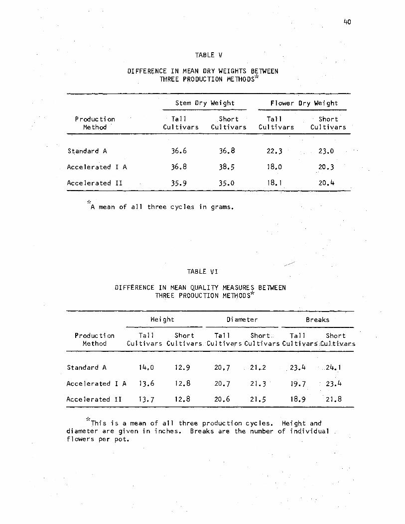
Comparisons by Product Quality Measures

An examination of the differences in mean dry weight and quality

measures was made for the five production methods by tal 1 and short

cu1tivars for all three of the cycles. The results of these computa

tions are shown in Tables V and VI. Only two measures, flower dry

dry weight and number of flowering breaks, demonstrated a consistent

difference among production methods. These differences were consistent

among the tall cultivar replications but were not among the short culti

var replications. Among the three variations in production method (ex

cluding spacing comparison methods) flower dry weight for the tall

cultivars was over four grams heavier for the standard production

\ method than for the accelen:1ted methods. The difference was two and

one-half grams for the short cul ti vars. For the count of the number

of flowering breaks, the standard method for tall cultivars produced

approximately four more breaks than did the accelerated methods. For

short cultivars this difference was approximately one.

40

TABLE V

DIFFERENCE IN MEAN DRY WEIGHTS BETWEEN . ~

THREE PRODUCTION METHODS"

Stem Dry Weight· Flower Dry Weight

Ta11 .Short Tall P roduc ti on Method Cu1tivars Cu1tivars Cu1tivars

Standard A 36.6 36.8 22.3

Accelerated I A 36.8 38.5 18.0

Acee lerated II 35.9 35.0 18.l

·k A mean of a11 three cycles in grams.

TABLE VI

DIFFERENCE IN MEAN QUALITY MEASURES BETWEEN . . .. , ..

THREE PRODUCTION METHODS"

Height Diameter

Production Ta 11 Short Ta 11 Short . Ta 11

Short Cu1ti'-'.'ars

23.0

20. 3

20.4

Breaks

Short Method Cul tivars. Cul ti vars. Cultivars Cu1tivars Cultivars.Cultivars

Standard A 14.o

Accelerated I A 13.6

Accelerated II 13.7

12.9

12.8

12.8

20. 7

20.7

20.6

21.2

21. 3

21.5

. 23.4

19.7

18.9

*This is a mean of all three production cycles. Height and

.24. 1

23.4

. 21. 8

diameter are given in inches. Breaks are the number of ind.ividua1 f 1 owe rs per pot.

41

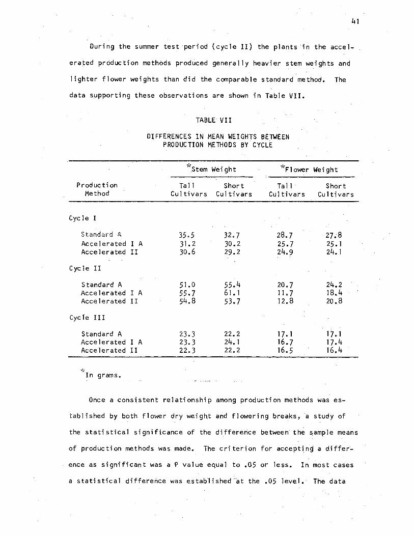
During the summer test period (cycle II) the plants in the accet ..

erated productfon methods produced generally heavier stem weights and

lighter f,1ower weights than did the comparable standard method. The

da.ta supporting these observati. ons are shown in Tab1 e VU.

TABLE VII

DI FFE~ENCE:S IN MEAN WEIGHTS BElWEEN PRODUCTION MElHODS BY CYCLE

-/,• '.Stem Weight ,._.Flower Weight

Production Ta 11 Short Ta11 Short Method Cul tiva.rs Cultivars Cultivars Cultivars

Cycle I

Standard A 35.5 32.7 28.7 27.8 Accelerated I A 31.2 30.2 25.7 25.1 Accelerated II 30.6 29.2 24.9 24. 1

Cycle II

Standard A 51. O 55.4 20. 7 24.2 Acce1era.ted I A 55.7 61. 1 11. 7 18.4 Accelerated II 54.8 53.7 12.8 20.8

Cycle III

Standard A 23. 3 22.2 17. 1 11 •. 1 Accelerated I A 23.3 24. 1 16.7 17.4 Accelerated II 22.3 22.2 16.5 16.4

ir In grams.

Once a consi.stent relationship among production methods was es-

tab1ished by both flower dry weight and flowering breaks, a study of

the statistical significance of the difference be.tween the ~ample means

of production methods was made. The criterion for accepting a differ~

ence as significant was a P value eqµal to .05 or less. In most casjs

a statistical difference was established "at the .05 level •. The data

42

accumulated for all cycles (Appendix A) showed a significant differ-

ence to exist between the standard method and the accelerated method,

as illustrated in Table VIII. No signific_ant difference was demon..;

strated be.tween Standard A and Standard B, indicating the two methods

produced comparable results. A statistical difference betwe_en the

standard and accelerated methods was no,t as clearly establi_shed in the

short cultivar replications as in the tall cultivar replications.

Similar statistical studies made of the other plant measurements,

height and diameter mean differences, did not demonstrate any signifi-

cant differences among production methods. However, a study of the

v.isual evaluation measures showed a difference in means which supports

the observation.s made of flower dry weight and flowering break differ-

ences (see Table IX). ' .

Aside from the noticeable visual differences in eye le II, there

were few readily observable differences among the production methods.

The more observa_ble differences were among replications in a particular

method caused by variations in greenhouse humidity, temperature, and

light conditions. Cycle II differences were apparently the result of

less heat de 1 ay associated with the standard method than with the ac-

celerated methods during the summer period. They, also, probably re

sulted from the s.trong tendency of both 1 Ye11ow Delaware• and 1 Snow

Ridge• to be heavy foliage producers.

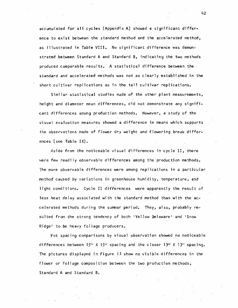
Pot spacing comparisons by visual observation she.wed no noticeable

differences between 1511 X 1511 spacing and the closer 1311 X 1311 spacing.

The pictures displayed in Figure L1 show no visible differences in the

flower or foliage composition between the two production methods,

Standard A and Standard B.

TABL,E VIII

SIGNIFICANCE OF DIFFERENCE BETWEEN SAMPLE MEANS OF PRODUCTION MEll-lOD BY FLOWER DRY WEIGHT

AND FLOWERING BREAKS

43

Production Method

Comparison

Fl owe.r Dry Weight ( grams)

F l0,wer i ng Breaks ( n umbe. r )

Standard A

versus

Standard B Accelerated I A Accelerated II

Significance of

Tall Short Cultivars Cultivars

22.3

Difference:

23.0

21.6 c 20. 3b

20.4

Tal 1 Cultivars

23.4

Short Cul tivars

24.1

23.4 23.4 ' c 21 •. 8

a = p value of .01 less; considered highly significant. or

b p value of .05 less; considered significant. = or

c = P value of • 10 or less but greater than ,05; con,sidered, close to significant.

TABLE IX

DIFFERENCE IN MEANS OF.VISUAL EVALUATION MEASURES FOR ALL lliR.EE CYCLES

Production Method

Standard A Standard B Accelerated I A Acee lerated II

°>'(

'>''.Ta 11 cul tivars

7. 1 7.0 6.2 6.3

Means of quality points assigned to all measured plants. 8 poi.nts equals superior quali.ty.

* .· .Short

cu.1 tivars

7.0 6.9 6.7 6.5

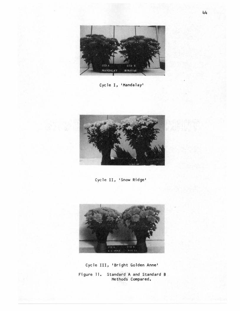
Cycle I, 'Mandalay•

Cycle II, 'Snow Ridge•

Cycle III, 'Bright Golden Anne•

Figure 11. Standard A and Standard B Methods Compared.

44

45

Composition of Direct Production Costs

Generally, the direct production costs when compared among the

three production eye les, were highly uniform ( see Table X). Deviations

from the average cost leve 1 s occurred. i.n ·Cycle I for p6tti ng, moving

pots, manual watering, equipment repair, and 0th.er labor •. For Cycle

II, deviations were noted in irrigating and disbudding. For Cycle

III, deviations occurred in black cloth shading, fertilizer costs and

insecticide costs. Each of these cost deviations is explained below.

For the most part they represent differences which occurred bec.ause of

a change of season or would normally have accumulated over a period of

longer than one production cycle.

Deviation

Cyc 1 e I

Potting

Moving Pots

Manua 1 Watering

Equipment Repair

Other Labor

Cycle II

Irrigating

Explanation

The initial learning period for the workers resulted in slower performance than for potting in later cycles.

The first layout of pats in proper locations for each replication took a longer period of time than in later eye les, when it was better understood.

Establishing the plants for irrigating took one week longer than in the following cycles when the technique was better understood.

Fewer adjustments and repairs in equipment were required during the first cycle than were required later~

Addi ti ona 1 temperature and humidity checks were made im the c Limate. control chamber.·during_.the first Cycle tev eva 1 uate performance.

The incre.ased irrigating during the summer cycle was normat'for the high light and high temperature conditions.

46

Cycle II (Cont 1d)

.Disbudding The vigorous foliage producing cultivars used for this eye le and heat de 1 ay resulted in increased disbudding work.

Cycle II I

Black Cloth Shading

Fertilizer Cost

Insecticide Cost

Black cloth daylength control was req~ired for only the first ten days.of this c ye le.

Less than a full tank was required for each cycle. As a result only half of a tank was required for the final cycle.

A persistent white fly infestation resulted in additional fumigation control measures above that of the first two c ye les.

W-ith further reference to Table X it will be noted that relatively

few of the cost elements constituted a significant cost on a~ average

per pot basis. As would be expected, of the total labor cost (39.50

cents), disbudding (18.36 cents), potting (6.47 cents), and black cloth

pulling (5.26 cents) were the largest. The labor cost of irrigating

was minor (1.65 cents), even less than the small amount of manual water-

ing and misting required (2.64 cents). Materials costs were minor ele-

ments except for cuttings (35.76 cents) and pots (9.00 cents) which '

together constituted almost one-half of the total direct cost of the

plants (92.77 cents) and about 85 per cent of the total materials cost

(53.27 cents). Such costs as labor for moving pots, watering, spray-

ing and pinching, previously thought to be expensive tasks, were less

important in the overall costs. Materials costs, such as high priced

soluble fertilizer, insecticides and water, likewise were found to be

minor expenses.

Production method total direct costs were uniformly the same

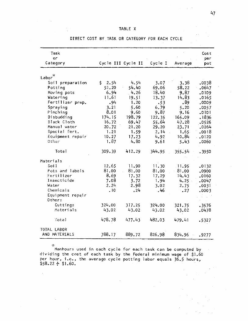
TABLE X

DIRECT COST BY.TASK OR CATE~ORY FOR EACH CYCLE

Task or

Category

Labo/' Soil preparation Potting Moving pots Watering Fertilizer prep. Spraying Pinching Disbudding Black Cloth Manual water Special fert. Equipment repair Other

Total

Materials Soi 1 Pots and labels Ferti 1 i zer Insecticide Water Chemicals Equipment repair Other~

Cuttings Materi a 1 s

Total

TOTAL LABOR AND MA TE RIALS

Cycle III Cycle II Cycle I Average

$ 2.54 51. 20 6.94

11. 61 .94

3.21 8.01

174. 15 16.72 20.72

1. 21 10.27

1. 87

309. 39

12.65 81 .oo 8.69 7.08 2.24 • 10

324.oo 43.02

478.78

788.17

4.54 54.40 4.26

19.51 1. 20 5.60 9.60

198. 79 69.47 21. 20

1. 59 17.23 4. 80

412.29

11. 90 81.00 17.32 3.72 2.98 .24

317.25 43.02

889.72

3.07 69.06 18.40 13.37

.53 6.79 9.87

122.35 55.64 29.20 2. 14 4.92 9.61

344.95

11. 30 81.00 17.29 1.94 3.02 • 46

324.00 43.02

482.03

826.98

3.38 58.22 9.87

14.83 .89

5.20 9. 16

165.09 47.28 2J. 71

1.65 10.84 5.43

355.54

11. 95 81.00 14.43 4.25 2.75 .27

321. 75 43.02

479. 41

834.96

47

Cost per pot

.0038

.0647

.0109

.0165

.0009

.0057

.0101

.1836

.0526

.0264

.0018 .• o 120

.0060

• 3950

.o 132

.0900

.0160

.0047

.0031

.0003

• 3576 .0478

.5327

.9277

Manhours used in each cycle for each task can be computed by dividing the cost of each task by the Federal minimum wage of ~l.60 per hour, i.e., the average cycle potting labor equals 36.5 hours, $58.22-:- $1.6o.

48

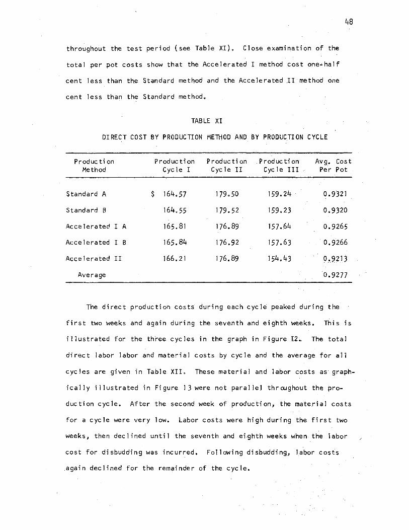
throughout the test period (see Table XI) •. Close examination of the

total per pot costs show that the Accelerated I method cost one-half

cent less than the Standard method and the Accelerated .II method one

cent less than the Standard method.

TABLE XI

DIRECT COST BY PRODUCTION METl-!OD AND BY PRODUCTION CYCLE

Production Production Production Production Avg. Cost Method Cycle I Cycle II Cycle III Per Pot

Standard A $ 164. 57 179.50 159.24 0.9321

Standard B 164.55 179.52 159.23 0.9320

Accelerated I A 165.81 176.89 157.64 0.9265

Accelerated I B 165.84 176.92 157.63 0.9266

Accelerated II 166.21 176. 89 154.43 o_.,9.2_11

Average 0.9277

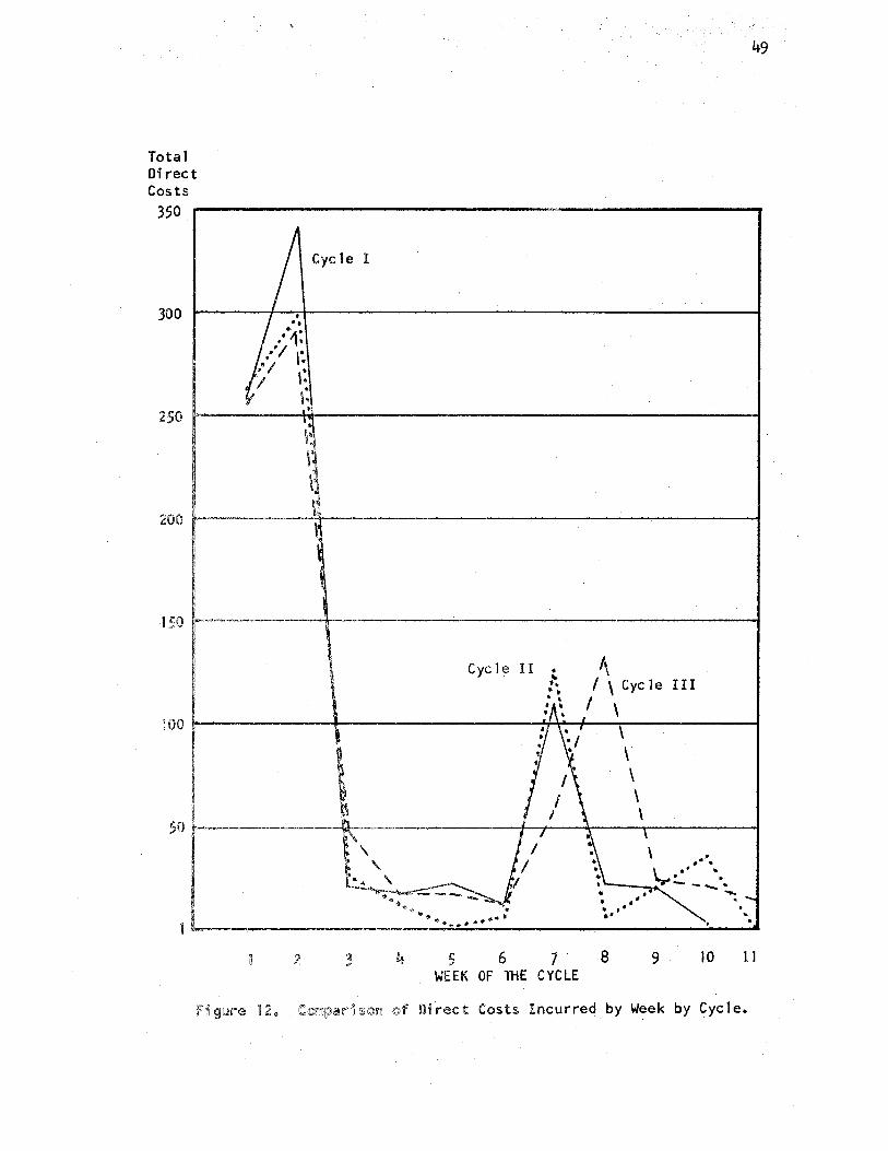
The direct production costs during each cycle peaked during the

first two weeks and again during the seventh and eighth weeks. This is

illustrated for the three cycles in the graph in Figure ti. The total

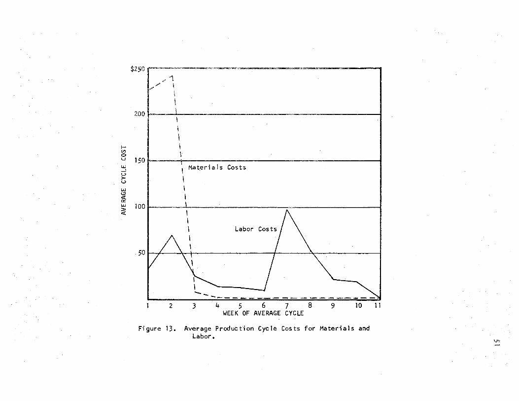
direct labor labor and material costs by cycle and the average for all

cycles are given in Table XII. These material and labor costs as graph-

ical ly i 1 lustrated in Figure 13 were not para] let throughout the pro-

due ti on cycle. After the second week of production, the mate_ri al costs

for a cycle were very low. Labor costs were high du.ring the first two

weeks, then declined u.ntil the seventh and eighth weeks when the labor

cost for disbudding was incurred. Following disbudding, labor costs

again declined for the remainder of the cycle.

Total Direct Costs

350

300

150

100

50

Cycle I

' '

3

Cycle II

~-.. ----. ... "'o • ···e..., ..........

4 5 6 WEEK OF THE

49

,, I\ Cycle III

I \ \ \ \ \ \

\

. - ' .. ' . . •• .. .

7· 8 9 10 l1 CYCLE

figure n. 1Comp~dsi0n of Direct Costs Incurredby Week by Cycle.

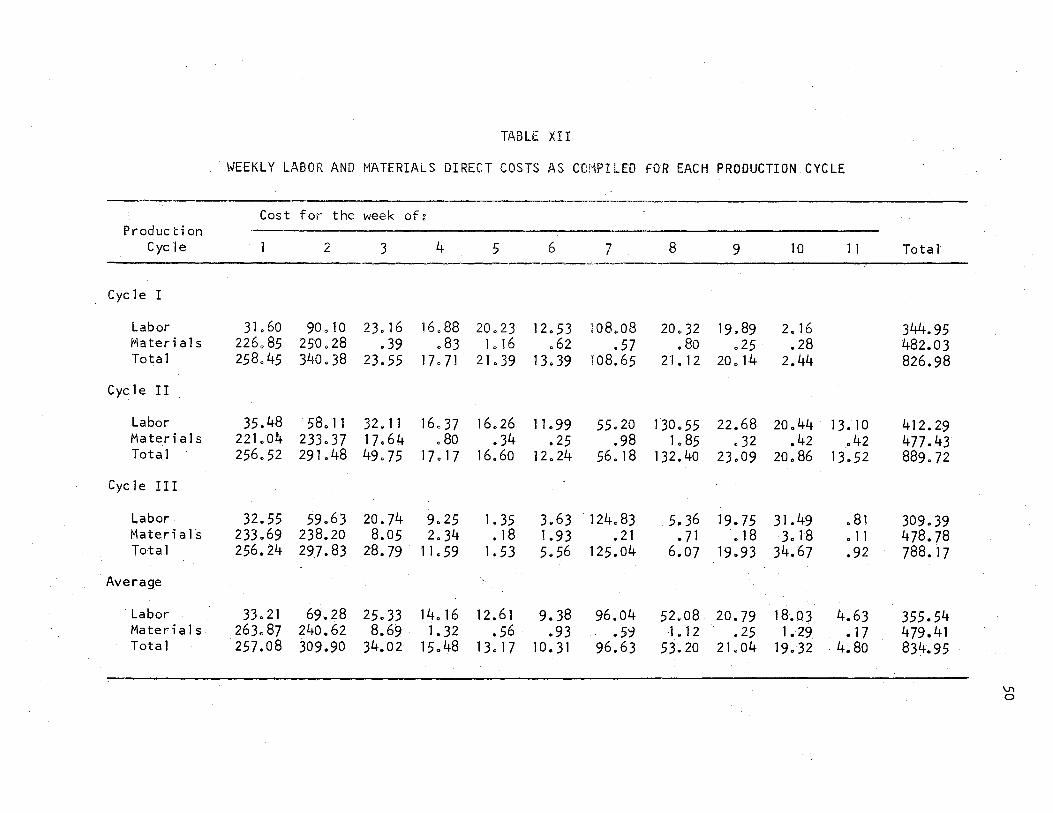
TABLE XII

WEEKLY LABOR AND MATERIALS DIRECT COSTS AS COMP! LEO FOR EACH PRODUCTION CYCLE

Cost for the week of~ Production

Cycle 1 2 3 4 5 6 7 8 9 10 1 1 Total

Cyc 1 e I

Labor 31. 60 90 0 10 23. 16 16.88 20. 23 12.53 108.08 20. 32 19.89 2. 16 344.95 Materials 226.85 250. 28 .39 • 83 1. J 6 .62 .57 • 80 .25 .28 482.03 Total 258.45 340.38 23.55 17.71 21.39 13. 39 108. 65 21. 1 2 , 20 • 14 2.44 826.98

Cycle II

Labor 35.48 58. 11 32. 11 16.37 16.26 11. 99 55.20 130.55 22.68 20.44 13. 10 412.29 Materials 221.04 233.37 17. 64 • 80 .34 .25 .98 1. 85 • 32 .42 .42 477. 43 Total 256.52 291. 48 49.75 17. 17 16.60 12.24 56. 18 1 32. 40 23.09 20.86 13.52 889.72

Cycle III

Labor 32.55 59.63 20.74 9.25 1. 35 3.63 . 124.83 . 5. 36 19.75 31.49 • 81 309.39 Materials 233.69 238.20 8.05 2.34 • 18 1.93 • 21 • 71 0 18 3. 18 • 11 478.78 Total 256.24 297.83 28. 79 11. 59 1. 53 5.56 125.04 6.07 19.93 34.67 .92 788. 17

Average

Labor 33.21 69.28 25.33 14. 16 12.61 9.38 96.04 52.08 20.79 18.03 4.63 355.54 Materials 263.87 240.62 8.69 1. 32 .56 .93 • 59 1. 12 • 25 1.29 • 17 479.41 Total 257.08 309.90 34.02 15.48 13. 17 10. 31 96.63 53. 20 21.04 19.32 4.80 834.95

v, 0

I-U'.)

0 u !Jj

..J u > u

I.I.! CJ c::( 0:: LL.I > c(

$250 rf "~-,,_,~~m~~z™ I

/4 I// I

\ \

200L-~_1_~~--~~~~~~~~~~~~~1 I \

\ I

150 I

I Materi a 1 s C osts

\ I I

100

I I Labor Costs

/\ I I

50

- ...... ___ ..... -- -- - -- ___ _.. ___ _ 2 3 4 5 6 7 8 9 10

WEEK OF AVERAGE CYCLE

Figure 13. Average Production Cycle Costs for Materials and Labor.

11

v,

52

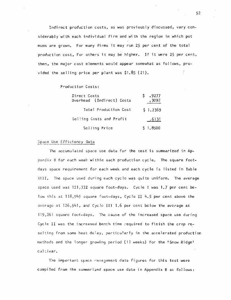
Indirect production costs, as was previously discussed, vary con-

siderably with each individual firm and ~i th the region in which pot

mums are grown. For many firms it may run 25 per cent of the total

production cost, for others it may be higher. If it were 25 per cent,

then, the major cost elements would appear somewhat as fol lows, pro-

vided the selling price per plant was $1.85 (21).

Production Costsg

Direct Costs Overhead (Indirect) Costs

Total Production Cost

Selling Costs and Profit

Selling Price

Spac3- Use_Efficiency Data

$ • 9277 • 3092

$ 1.2369

0 61 31

$ 1. 8500

The accumulated space use data for the test is summarized in Ap-

pendix B for each week within each production cycle. The square foot-

days space requirement for each week and each cycle is listed in Table

)GIL The space used during each cycle was quite uniform. The average

space used was 121,332 square foot-days. Cycle I was 1.7 per cent be-

low this at 118,945 square foot-days, Cycle II 4.5 per cent above the

average at 126,541, and Cycle III 1.6 per cent below the average at

119,261 square foot-days. The cause of the increased space use during

Cycle II was the increased bench time required to finish the crop re-

suiting from some heat delay, particularly in the accelerated production

methods and the longer growing period (11 weeks) for the ~snow Ridge 1

cuttivar.

The tant s management data figures for this test were

compiled from the summarized space use data in Appendix Bas follows:

TABLE XIII

SPACE USE DURING THE ENTIRE STUDY PERIOD ··l,

-·k·k

Week

Cycle 1 2 3 4 5 6 7 8 9

I 4,592 9,860 12, 185 12 ,,488 12,488 12,488 12y488 12,488 12,488

II 4,592 9,860 12,185 12,488 12,488 12,488 12,488 12,488 12,488

III 4,466 9,542 12,185 12,488 12,488 12,488 12,488 12,488 12,488

Total 13,650 29,262 36,555 37,464 37,464 37,464 37,464 37,464 37,464

Average 4,550 9,754 12, 185 12,488 12,488 12,488 12,488 12,488 12,488 -

-·-"Space used for 900 plants plus occupied bench space for other projectso **square foot days.

10 11

12,488 12,488

12,488 12,488

12,488 12,488

37 ,464 22,,432

12,488 7 ,477

Tota 1

118,945

126,541

119, 261

121,332

v, \JJ

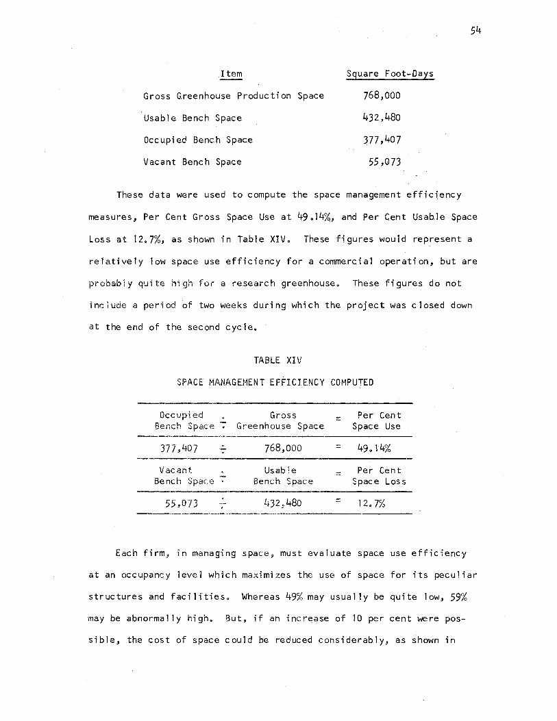
Item

Gross Greenhouse Production Space

Usable Bench Space

Occupied Bench Space

Vacant Bench Space

Square Foot-Days

768,000

432.~480

377 ,407

55 ,073

These data were used to compute the space management efficiency

54

measures, Per Cent Gross Space Use at '-1:9014%, and Per Cent Usable Space

Loss at 12.7%, as shown in Table XIVo These figures would represent a

relatively low space use efficiency for a commerc.ial operation, but are

probably quite high for a research greenhouse. These figures do not

include a period of two weeks during which the project was closed down

at the end of the second cycle.

TABLE XIV

SPACE MANAGEMENT EFFICIENCY COMPUTED

Occupied • Bench Space -:

377 ,407 .:.. . Vacant . -Bench Space .

55 ,073 -.

Gross Greenhouse Space

768,000

Usable Bench Space

432,480

=

=

=

=

Per Cent Space Use

49. 1'4%

Per Cent Space Loss

12.7%

Each firm, in managing space, must evaluate space use efficiency

at an occupancy level which maximizes the use of space for its peculiar

structures and faci Hties. Whereas 49% may usua11y be quite low, 59%

may be abnormally high. But, if an increase of 10 per cent were pos-

sible, the cost of space could be reduced considerably, as shown in

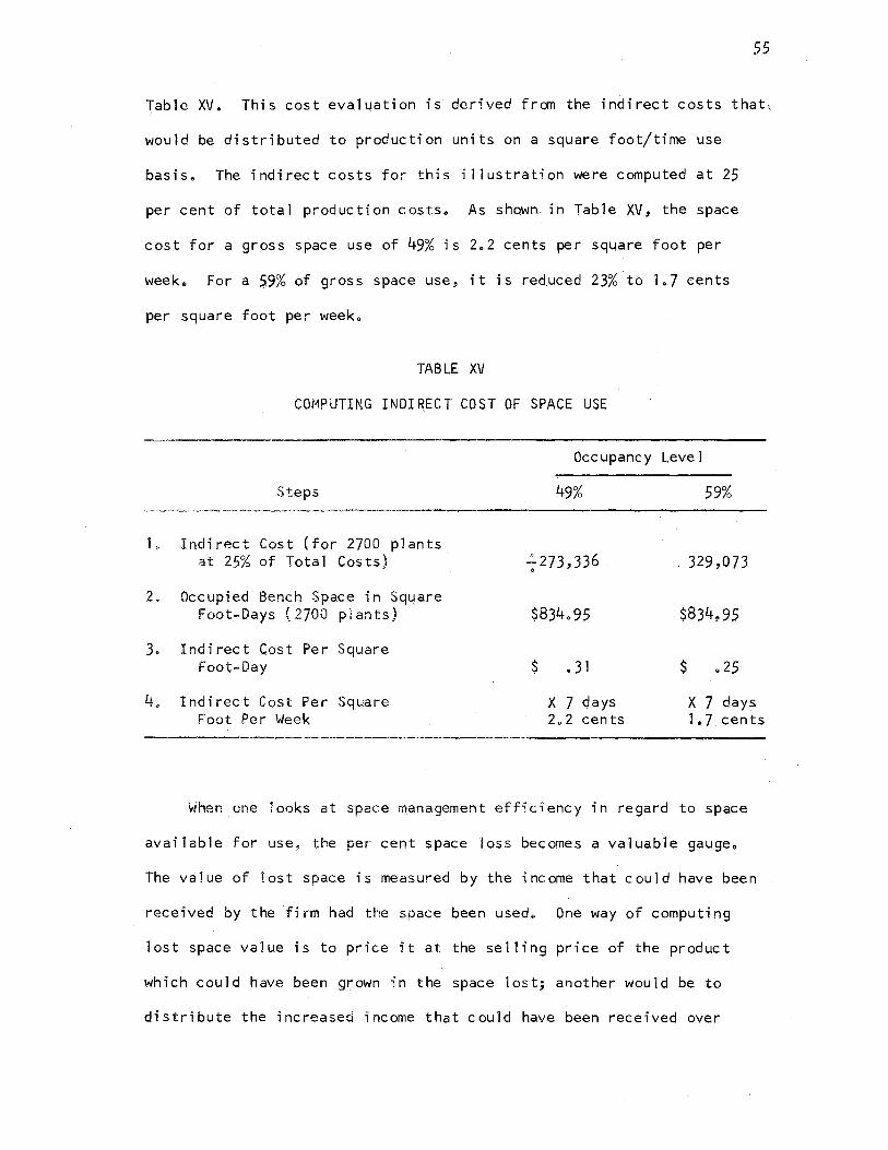
55

Table XV. This cost eva1L.1ation is derived fran the indirect c.osts that,.

would be distributed to production units on a square foot/time use

basis. The indirect costs for this illustration were computed at 25

per cent of total production costso As shown. in Table XV, the space

cost for a gross space use of 49% is 2.2 cents per sq~are foot per

week. For a 59% of gross space use, it is red.uced 23% to 1. 7 cents

per square foot per week.

TABLE XV

COMPUTING INOI~ECT COST OF SPACE USE

Occupancy Leve 1

Steps

1. I ndi rec t Cost ( for 2700 p 1 an ts at 25% of Total Costs)

2. Occupied Bench Space in Sq~are Foot~Days (2700 plants)

3. Indirect Cost Per Square Foot-Day

4. Indirect Cost Per Square Foot Per Week

49%

~273,336 •

$834.95

$ • 31

X 7 clays 2. 2 cents

59%

329 ,073

$834,95

$ • 25

X7 days 1. 7 cents

When one looks at space management efficiency in regard to space

available for use, the per cent space loss becomes a valuable gauge.

The value of lost spac.e is measured by the income that could have been

received by the firm had the· space been used. One way of computing

lost space value is to price it at the selling price of the product

which could have been grown in the space lost; another would be to

distribute the increased income that could have been received over

tota1 output. Since one amounts to the same as the other, the sa1es

va1ue of additional output which is arrived at more direct1y is used

in Tab1e XVI. Had the plants been spaced at 1311 X 1311 , the va1ue of

the 1ost space for this test would have been $369.08.

TABLE XVI ")'(

COMPUTING VALUE LOST IN VACANT SPACE

Steps

1. Vacant Space (square foot days from ~ata in this study)

2. Square foot-days per plant (240 days XI. 15 sq. ft.)

3. Lost production (number of plants)

4. Selling price, per plant

5. Space loss value ( lost production X selling price)

-1:: Assuming a 13 11 X 1311 pot spacing.

Computation

55,073

.: 276 '

199.5

x $ 1. 85

$ 369. 08

Under the section 11 Identlfy"ing Space Use EfficiencyJ 1 in Methods

and Materials, the cost advantages of minimum spacing were pointed out.

Using space data from this test, a clear illustration of this advantage

is shown in Table XVII. The same level of space use efficiency, 49%,

was used to compute the income which could be derived from an average

cycle if the entire space had been used solely for the production of

pot mums. The gain from the decreased pot spacing would be a gross

income of $667.85 for this average cycle. Table VIII shows ,that there

was no difference in quality between the Standard A and'B methods.

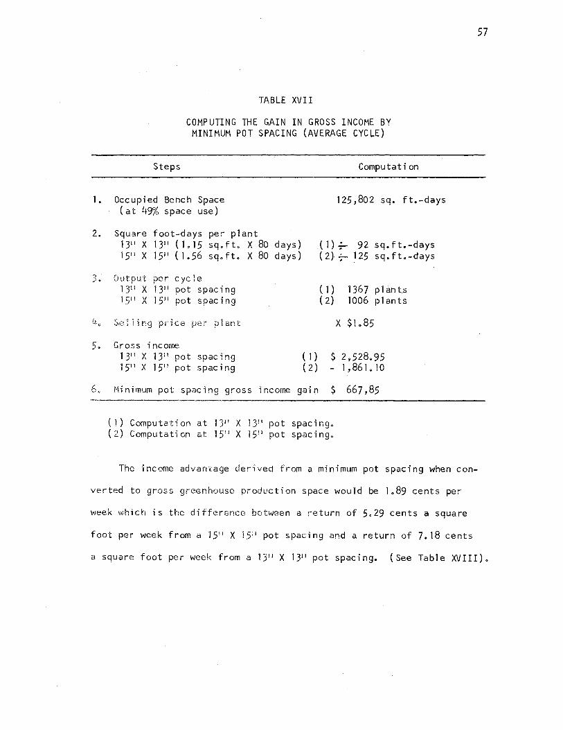
TABLE XV I I

COMPUTING THE GAIN IN GROSS INCOME BY MINIMUM POT SPACING (AVERAGE CYCLE)

Steps

1. Occupied Bench Space (at 49% space use)

2. Square foot-days per plant 1311 X 1311 ( 1.15 sq.ft. X 80 days) 15" X 1511 ( 1.56 sq.ft. X 80 days)

J. Output per cycle 1311 X 1)1 1 pot spac-ing 15 11 X 1511 pot spacing

Selling price per plant

Gross income 1 311 X 1311 pot spacing 1511 X 15 11 pot spacing

( 1 ) (2)

Compu tat i on

125,802 sq. ft.-days

( 1) 7 92 sq.ft.-days ( 2} f- 125 sq. f t.-days

( 1 ) 1 36 7 p 1 an ts (2) 1006 plants

x .$1.85

$ 2,528.95 1 , 861 • 1 O

6. Minimum pot spacing gross ·income gain $ 667,85

(l) Computation at 13 11 X l.3 11 pot spacing. (2) Computation at 1511 X 15 11 pot spacing.

The income advantage derived from a minimum pot spacing when con-

verted to gross greenhouse production space would be 1.89 cents per

week which is the difference between a return of 5.29 cents a square

foot per week from a 15 11 X 1511 pot spacing and a return of 7.18 cents

57

a square foot per week from a 13 11 X 1311 pot spacing. (See Table XVIII).

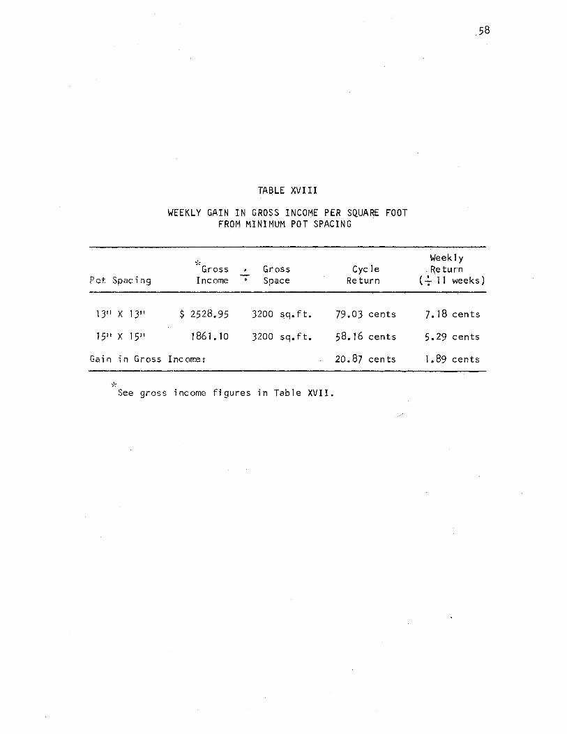
Pot Spacing

1311 x 1311

1511 x 1511

Gain in Gross

·-;'::

See gross

TABLE XVIII

WEEKLY GAIN IN GROSS INCOME PER SQUARE FOOT FROM MINIMUM POT SPACING

7r: Gross .. Gross Cyc 1e -Income t Space Return

$ 2528,95 3200 ~q.ft. 79.03 cents

1861.10 3200 sq.ft. 58.16 cents

Income: 20.87 cents

income figures in Table XVII.

/

58

Week1y , Return

(.;. 11 weeks)

7.18 cents

5.29 cents

1. 89 cents

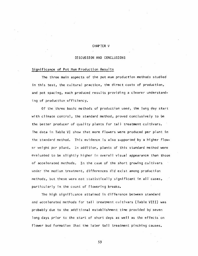
CHAPTER V

DISCUSSION AND CONCLUSIONS

Sign;ficance of Pot Mum Produ.ction Results

The three main aspects of the pot mum production methods studied

in this test, the cultural practice, the direct costs of production,

and pot spacing, each produced results providing a clearer understand-

ing of production efficiency.

Of the three basic methods of production used, the long day start

with climate control, the standard method, proved conclusively to be

the better producer of quality plants for tal 1 treatment cul tivars.

The data in Table VI show that more flowers were produced per plant in

the standard method. This evidence is also supported by a higher flow-\

er weight per plant. In addition, plants of this standard method were

evaluated to be slightly higher in overall visual appearance than those

of accelerated methods. In the case of the short growing cultivars

under the medium treatment, differences did exist among production

methods, but these were not statistically signifi.cant in al 1 cases,

particularly in the count of flowering breaks.

The high si gni fi cance attained in difference be.tween standard

and accelerated methods for tall treatment cultivars (Table VIII) was

probably due to the additional establishment time provided by seven

long days prior to the start of short days as well as the effects.on

flower bud formation that the later tal 1 treatment pinching causes.

59

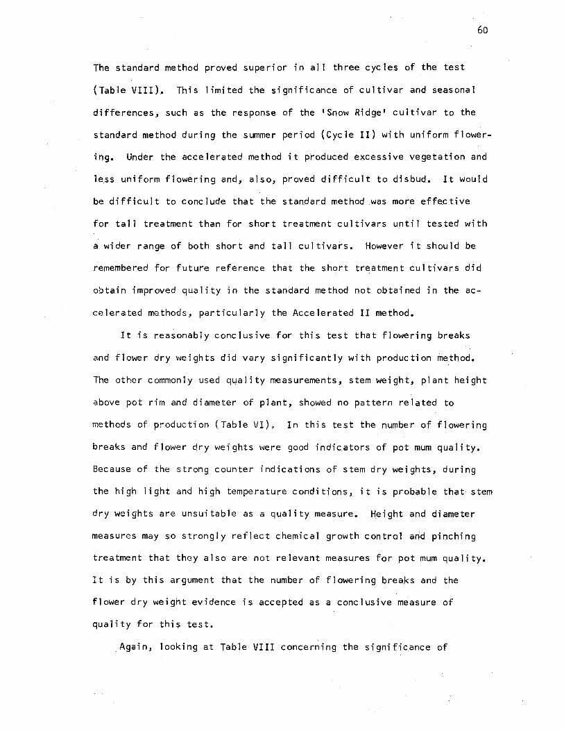
60

The standard method proved superior in a11 three eye 1e.s of the test

(Table VIII). This limited the sign.ificance of cu1tivar and seasonal

differences, such as the response of the •snow Ridge• cultivar to the

standard method during the summe.r period (Cycle II) with uniform flower.,.

ing. Under the ac.celerated method it produced excessive vegetation and

le.ss uniform flowering and, also, proved difficult to disbud. It would

be difficult to conclude that the standard method was more effe_ctive

for tall treatment than for short treatment cultivars until tested with

a wider range of both short a.nd tall cu.ltivars. However it should be

remembered for future reference that the short treatment cul tivars did

obtain improved qua1ity in the standard method not obtained in the ac

celerated methods, particularly the Accelerated II method.

It is reasonably conclusive for this test that flowering breaks

and flower dry weights did vary significantly with production method.

The other commonly used quality measurements, stem weight, plant height

above pot rim and diameter of plant, showed no pattern related to

methods of production (Table VI). In this test the number of flowering

breaks and flower dry weights were good indicators of pot mum quality.

Because of the strong counter indications of stem dry weights, during

the high light and high temperature conditions, it is probable that stem

dry weights are unsuitable as a quality measure. Meight and diameter

measures may so strongly reflect chemical growth control and pinching

treatment that they a 1 so are not relevant measu.res for pot mum qua 1 i ty.

It is by this argument that the number of flowering breaks and the

flower dry we.ight evidence is accepted as a conclusive measure of

quality for this test.

Again, looking at Table VIII concerning the signific.ance of

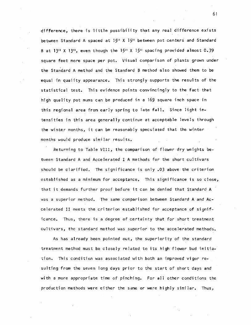
61

difference~ there is 1ittle possibility that any real difference exists

between· Standard A spaced at 1511 X 1511 between pot centers and Standard

Bat 1311 X 1311 , even though the 1511 X 1511 spacing provided almost 0.39

square feet more space per pot. Visual comparison of plants grown under

the Standard A method and the Standard B method a 1 so showed them to be

equal in quality appearance. This strongly supports the results of the

statistical test. This evidence points convincingly to the fact that

high quality pot mums Cc!O be produced in a 169 square inch space in

this regional area from early spring to late fall. Since light in

tensities in this area generally continue at acceptable levels through

the winter months, it can be reasonably speculated that the winte.r

months would produce similar results.

Returning to Table VIII, the comparison of flower dry weights be

tween Standard A and Accelerated I A methods for the short cultivars

should be clarified. The significance is only .03 above the criterion

established as a minimum for acceptance. This si~nificance is so close,

that it demands further proof before it can be denied that Standard A

was a superior method. The same comparison between Standard A and Ac

celerated II meets the criterion established for acceptance of si gnif

icance. Thus, there is a degree of certainty that for short treatment

cultivars, the standard method was superior to the accelerated methods.

As has already been pointed out, the superiority of the standard

treatment method must be closely related to its high flc;,wer bud initia

tion. This condition was associated with both an improved vigor re

sulting from the seven long days prior to the start of short days and

with a more appropriate time of pinching. For all other conditions the

production methods were either the same or were highly similar. Thus,

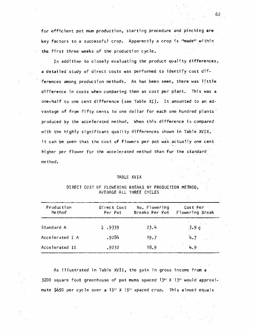
for effident pot mum production, starting procedure and pinching. are

key factors to a successfu1 crop. Apparently a crop is 11inade•i within

the first three weeks of the production cycle.

62

In addition to closely evahiating the product quality differences,

a detailed study of direct costs was performed to identify cost dif-

ferences among production methods. As has been seen, there was little

difference in costs when comparing them as cost per plant.· This was a

one-half to one cent difference (see Table XI). It amounted toan ad-

vantage of from fifty cents to one dol 1 ar for each one hundred plants

produced by the accelerated method. When this difference is compared

with the highly significant quality differences shown in Table XVIX,

" . it can be seen tha.t the cost of flowers per pot was actually one· cent

higher per flower for the accelerated method than for the s.tandard

method.

TABL.E XVIX

DIRECT COST OF FLOWERING BREAK:S BY. PRODUCTION METHOD, AVERAG.E ALL THREE CYCLES

P roduc ti on Direct Cost No. Flowering Cost Per Method Per Pot Breaks Per Pot Flowe.ring Break

Standard A $ • 9339 23.4 3.9 ¢

Accelerated I A .9284 19.7 4.7

Accelerated II .9232 18.9 4.9

As illustrated in Table XVII, the gain in gross income from a

3200 square foot greenhouse of pot mums spaced 1311 X 1311 would approxi-

mate $650 per cycle over a 1511 X 1511 spaced crop. This almost equals

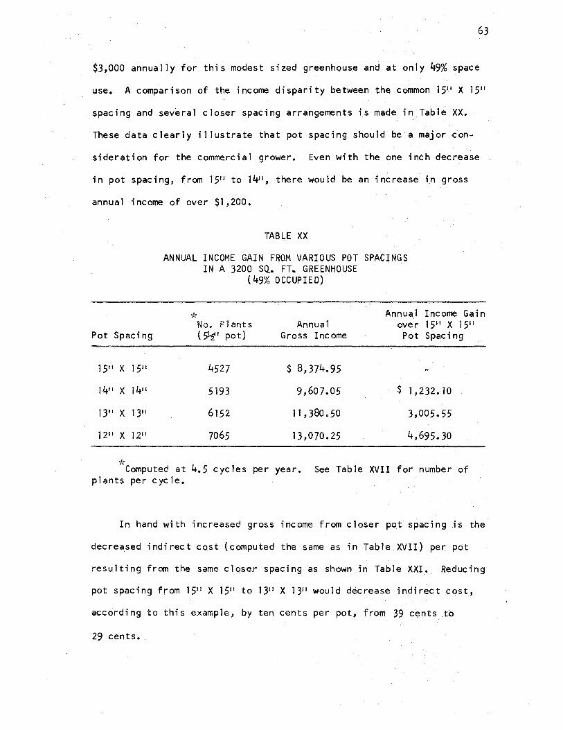
63

$3,000 annua11y for this modest sized greenhouse and at on1y 49% space

use. A compa.rison of the income disparity between the common 1511 X 15 11

spacing and severa1 c1oser spacing arrangements {s made in Tab1e XX.

The.se data c1ear1y i 11ustrate that pot spacing shou1d be a major con.,..

sideratfon for the commercia1 grower. Even with the one inch decrease

in pot spacing, frQITI 1511 to 1411 , there wou1d be an increase i.n gross

annual income of over $1,200.

TABLE XX

ANNUAL INCOME GAIN FROM VARIOUS POT SPACINGS IN A 3200 SQ. FT. GREENHOUSE . ,

( 49% OCCUPIED)

'1: Annua1 Income Gain No. Plants Annua 1 over 1511 x 1511

Pot Spacing ( $1-1 1 pot) Gross Income Pot Spacing

1511 x 1511 4527 $ 8,374.95 ..,;

1411 x 1411 5193 9 ,607.05 $ l,232.10

1311 x 1311 6152 11,380.50 3,005.55

1211 x 1211 7065 13,070. 25 4,695.30

7( Computed at 4.5 cycles per year. See Table XVII for numbe.r of

plants per cycle.

In hand with increased gross income from closer pot spacing .is the

decreased indirect cost (computed the same as in Table XVII) per pot

resulting from the same close.r spacing as shown in Tab1e XXI. Reducing

pot spacing from 1511 X 1511 to 1311 X 1311 wou1d decrease indirect cost,

according to this example, by ten cents per pot, from 39 cents to

29 c¢nts.

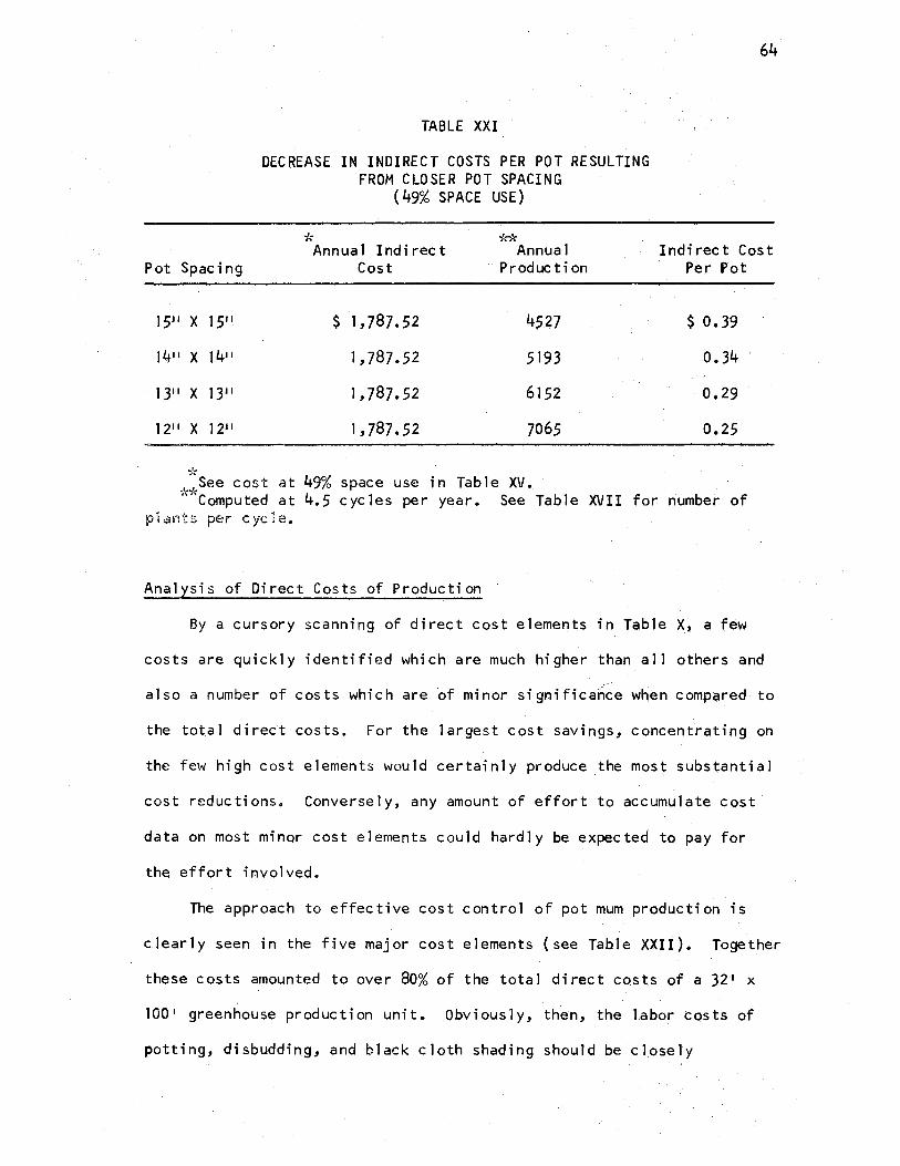
TABLE XXI

DECREASE IN INDIRECT COSTS PER POT RESULTING FROM CLOSER POT SPACING

( 49% SPACE USE)

7( "'/("k

64

Annual Indirect Pot Spacing Cost

Annual Production

Indirect Cost Per Pot

$ 1, 787. 52

1,787.52

1311 x 1311 1,787.52

1211 x 1211 1,787.52

·'·

4$27

5193

6152

7065

$ o. 39

0.34

0.29

0.25

':see cost at 49% space use in Table XV. ·i("'J\

Computed at 4.5 cycles per year. See Table XVII for number of plants per cyc1e.

Ana 1 ys is of Direct Cos ts of P roduc ti on

By a cursory scanning of direct cost elements in Table X, a few

costs are quickly identified which are much higher than all others and

also a number of costs which are of minor si gnifica11ce wh.en compared to

the total direct costs. For the largest cost savings, concentrating on

the few high cost elements would certainly produce the most substantial

cost reductions. Conversely, any amount of effort to accumulate cost

data on most minor cost elements could hardly be expected to pay for

the effort involved.

The approach to effective cost control of pot mum production is

clearly seen in the five major cost elements (see Table XXII). Together

these costs amounted to over 80% of the total direct costs of a 32 1 x

100 1 greenhouse production unit. Obviously, then, the labor costs of

potting, disbudding, and black cloth shading should be closely

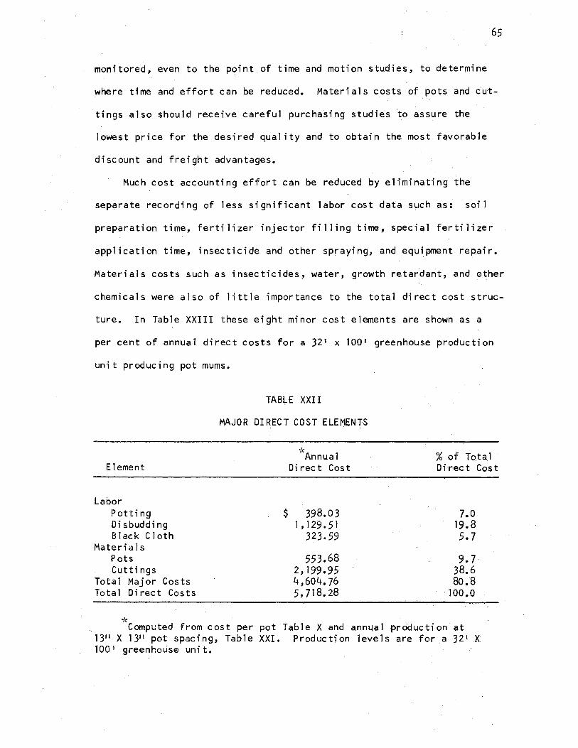
65

monhored~ even _to the point of time and motion studies, to determine

where time and effort can be reduced. Materials costs of pots and cut

tings also should recei~e careful purchasing studies to assure the

lowest price for the desired quality and to obtain the most favorable

discount and freight advantages.

Much cost accounting effort can be reduced by eliminating the

separate recording of less significant labor cost data such as: soil

preparation time, fertilizer injector filling time, special fertilizer

application time, insecticide and other spraying, and equipment repair.

Materials costs such as insecticides, water, growth retardant, and other

chemicals were also of little importance to the total direct cost struc-

ture. In Table XXIII these eight minor cost elements are shown as a

per cent of annual direct costs for a 32 1 x 100 1 greenhouse production

unit producing pot mums.

TABLE XXII

MAJOR DIRECT COST ELEMENTS

Element

Labor Potting Di sbuddi ng Black Cloth

Materi a 1 s Pots Cuttings

Total Major Costs Total Direct Costs

*

$

·k Annual

Direct ·cost

398.03 1,129.51

323.59

553.68 2,199.95 4,604.76 5, ]18. 28

% of Tota.I · Direct Cost

1.0 19.8 5.7

9.7 38.6 80.8

· 100. 0

Computed from cost per pot Table X and annual production at 1311 X 1311 pot spacing, Table XXI. Production levels are for a 32 1 X 100 1 greenhouse unit.

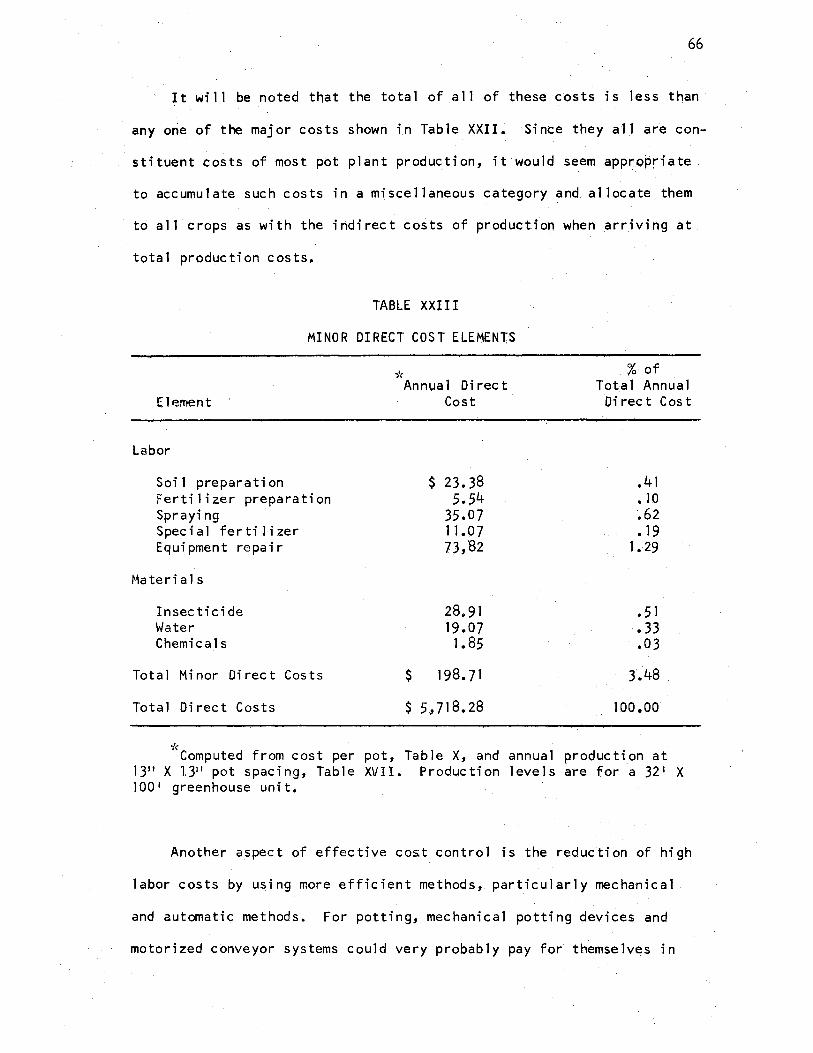
66

It will be noted that the total of.all of these costs is less than

any one of the major costs shown i.n Table XXII. Since they all are con'.'"

stituent costs of most pot plant production, it would seem approprfate .. , ...

to .accumulate such costs in a misce11aneous category and. al locate them

to al 1 crops as with the indirect costs of production when arriving at

total production costs.

TABLE XXIII

MINOR DIRECT COST ElEMENl;S

-/: An nu.a 1 Direct

Element Cost

Labor

Soil preparation $ 23.38 Fertilizer preparation 5.54 Spraying 35.07 Spec i a 1 fertilizer 11.07 Equipment repair 7J,'82

Materials

In sec tici de 28.91 Water 19.07 Chemi ca 1 s 1. 85

Total Mi nor Direct Costs $ 198.71

Total Direct Cos.ts $ 5_,718.28

.% of Total Annual

Direct Cost

.41

.10

.62

.19 1. 29

.51 • 33 .03

J.48

100.00

-le Computed from cost per pot, Tab le X, and annual producti.on at

1311 X l311 pot spacing, Table XVII. Production levels are for a 32 1 X 100 1 greenhouse unit.

Another aspect of effective cost control is the reduction of high

labor costs by using more efficient methods, particularly mechanical

and automatic:: methods. For potting, mechanical potting devices and

motorized conveyor systems could very probably pay for themselves in

Jess than two years for a moderate sized greenhouse range. Extending

· . the figures in Tab le XXII ·to a 20 ;000 square foot range ( X 6. 25) pro-

ducing only pot mums, a system costing $5,000 would be Jess than·the

two year cost of manua11y potting and placing on the bench.

The expense of disbudding is undoubtedly the most disputable of

all expenses to justify in this day of extensive crop research. Cer-

67

tainly with this highest of a11 labor costs:, chemical and genetic ap

proaches to solving the problem should be carefuJJy researched to find

a low laboi input solution. Cultivars that require no disbudding or

the use of an inexpensive chemical disbudding agent would eliminate

over $6,500 in labor costs for the same 20,000 square foot range cited

above. Generous support by commercial growers of extensive research on

this problem certainly makes good business sense.

A common cost reduction technique employed by many firms is me-; ..

chanically operated black cloth shading curtains. Here again the sav-

ings experienced over two years in a 20 ,000 square foot range, approxi-

mately $3,000, would go a long way toward paying the costs of installi.ng

many of the currently used .systems.

The cost of purchased cuttings is an exceedingly high expense.

For a large firm, the possibility of the reduced cost.in propagating

locally would require careful study. A suitable propagating facility

should be entirely possible at the two year cost of over $26,000, the .. .

approximate amount expended for rooted cuttings by a firm contai rd ng

a 20,000 square foot range devoted entirely to pot.mum productio~.

A simplified accounting system such as employed in this test,

with the extraneous cost accumulations eliminated, provides valuable

benefits when it comes to making management decisions o.f the type

68

discussed above. It is true that the illustrations cited are the more

dramatic examples of pr9~uction planning. In a similar fashion, the

more routine activities, just as certainly, require c~reful cost analy

sis.~o accompany any sound decision making. Any firm, even of the

moderate shed 20,000 s.quare foot facility u.sed in the above examples,

has a suffkiently high production cost to afford some sort of cost

accounting procedure. With an annual production of about 38,000 plants

the 20,000 square foot size firm would expend close to $50,000 in pro

duction costs. Or, would it? The answer must be based on rather vague

judgements un.less there are cost accounts to whkh one can re.fer.

~taining Efficiency in Space Use

During the test period, no particular effort was made to assure

maxi mum space use. P roduc ti on schedu 1 i ng was p 1 anned to permit the

proper fi ni shi ng of one crop before another would require the space.

Existing greenhouse bench layout was used. This, of coufse has made

possible an analysis of space man.agement efficiency under conditions

characteristic of those to be found in an undeveloped plan.

As has been observed under Experimenta 1 Results, the leve 1 of ef

ficiency attained was not high. Production scheduling permitted a lag

of several days between the finished date for the crop and the date

that the next crop was placed on the bench. If the gap in lag time

was closed between the production cycles, the per cent usable space

loss would have been reduced from 12.7% to 7.6% of usable bench space,

a 40% decrease in space loss.

Another deficiency in space management was the 18 square feet of

space I oss permitted even during the period of maximum space occupancy.

In addition, there was a one week loss of 63 square feet in the

climate control bench at the start of each cycle. These two minor

losses alone increased space loss by 1% from 11.7% tQ 12.7%.

69

The one method by which space management efficiency could have

been improved most was in the greenhouse space layout plan. With us

able space occupied to a maximum, the per cent gross space use could

not have exce.eded 56%, or 1802 square feet-days per day. A layout of

five foot wide peninsular benches with two foot access aisles and a

main aisle of four feet, permitting two-way traffic, would make 1960

square foot-days of net usable bench space available per day, or a

maximum gross space use of up to 61%. In the present state of green

house layout and mechanization, such a space use is high .indeed. But

with the introduction of truly mechanized systems to include overhead

personnel conveyors ( locating people in the usable space above plants)

and detachable mobile pc;1llet benches put in place with powered lift

trucks, c1isles for many crops would become superf1uous and a gross

space use of 90% or above would become possible. As expensive as land

is for the producer, especially tho.se near large urban centers, a 61%

gross space use should be the starting point rather than the p~ak of

efficiency.

To improve the use of greenhouse space, much more could.have been

done for the test than improving'the liayout or by mechanizing. Struc

tures such as purlin posts, pipe H.nes, and water outlets occupying

space iriterferfog with the placement of be.nches or the use of benches

could have been re located. Entrances could have been re.located to

ai s 1.es instead of at the end of be.nches thus adding l:>ench space to

areas now used for personne 1 and equipment access. Procedures which

reduc:ed the amount of required personne 1 access to pl ants, such as tube

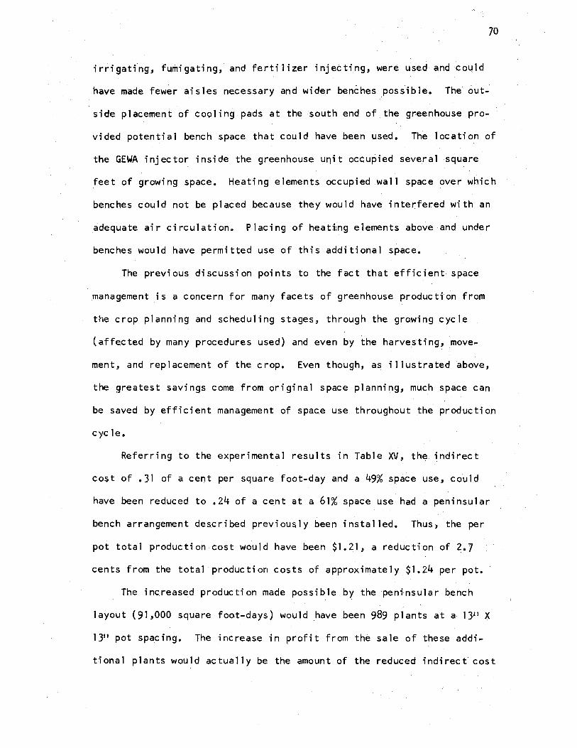
70

;r,;;gating, fumigating, and fertilizer injecting, were used and cot1ld

have made fewer aisles necessary and wider benches possible. The out

side placement of cooling pads at the south end of the greenhouse pro

vided potential bench space that could have been used. The location of

the GEWA injector inside the greenhouse ur,it occupied several square

feet of growing space. Heating elements occupied .wat 1 space over which

benches could not be placed because they would have interfered with an

adequate air circulation. Placing of heat:i:ng elements above and under

benches would have permitted use of this additional space.

The previous discussion points to the fact that efficient space

management is a concern for many facets of greenhouse production from

the crop planning and scheduling stages, through the growing cycle

(affectec;l by many procedures used} and even by the harvesting, move

ment, and replacement of the crop. Even though, as illustrated above,

the greatest savings come from original space planning, much space can

be saved by efficient management of space use throughout the production

eye le.

Referring to the experimental results in Table XV, the indirect

cost of • 31 of a cent per square foot-day and a 49% space use, could

.have been reduced to .24 of a ce.nt at a 61% space use had a penins.ular

bench arrangement des.cribed previously been installed. Thus, the per

pot total production cost would have been $1.21, a reduction of 2~7

cents from the total production costs of approxill)ately $1.24 per pot.

The increased production made possible by the peninsular bench

layout (91 ,000 square foo.t-days} would have been 989 plants at a 1311 X

1311 pot spacing. The increase in profit from the sate of these addi

t.ional plants would actually be the amount of the reduced indirect cost

71

(989 X $~3098), $306.39, plus some transportation. and se11ihg cost re

duction per pot resulting from larger lot distribution. -The gro·ss in

·come from these added plants w.ould be $1829.Q5. It should be remembered

· that in this example only one 3200 square foot greenhouse unit i.s in

volved. A range of 20,000 square feet would have increased production

by about 6200 plants and the gross income would have been alm.ost

$12,000, and the net profit would be $2,000 above the average profit

realized on this number of plants.

Conclusions

Long Day with Climate Control Best. Of the three basic: production

methods tested the seven 1 ong-days method with climate control, stand,ard

method, exceeded the othe.r two methods in qua 1i ty and in economy of

production. To obtain the highest quality in this region it is neces

sary to start pot mums immediately after potting with at least one week

of long days, a high humidity, and above average temperature·s (65°Fto

72°F). This was proven by a statistical test of the signific,ance of the

differences between sample means at the .05 level (Table VIII). For

tall treatment cultivars, a significance at the .01 level wai attairied

between the standard method and the accelerated method~ As for economy

advantages, the standard method in this tes.t produced flowering breaks

at one cent less per flowering break than the other method.s, proving.

it to be not only a high quality method but a most economical one as

we 11.

Closer Pot Spacing Equal. in Quality and More Economical. By

statistical test of significance of difference between sa111ple meahs, no

significance exists between the 1511 X 1511 pot spacing and the 1311 X 131 1

pot spacing in the standard method (Table VIII). The test showed th.at

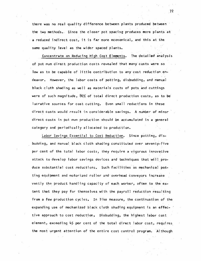
.72

there was no real quality difference between plants produc~d between

· the twC> methods •. Since the closer pot spacing produces more plant.s at

a reduced indirect cost, it is far more econanical, and this .at the

same quality level as the wider spaced plants. . .

Concentrate on Reducing High Cost Elements. The detailed analysis

of pot mum direct production costs revealed that many costs were so

low as to be capable of little contribution to any cost reduction en

deavor. However, the labor costs of potting, disbudding, and man~al

black c 1 oth shading as we 11 as materials cos.ts of pots and cuttfogs

were of such magnitude, 80% of total direct production costs, as to be

lucrative sources for cost cutting. Even small reductions in these

direct costs would result in considerable savings. A number of minor

direct costs in po.t mum production should be accumulated in a general

category and periodically allocated to production.

Labor Savings Essential to Cost Reduction. Since potting, dis~

budding, and manual black cloth shading constituted over seventy-five

per cent of the total labor costs, they require a vigorous in.novative

attack to deve 1 op 1 abor savings devices and techniques that wi 11 pro

duce substi:lntial cost reductions. Such facilities as mechanical pot-

ting equipment and motorized roller and overhead conveyors inc:.rease

vastly the product handling capacity of each worker, often to the ex-

tent that they pay for themselves with the payroll reduction resulting

from a few production cycles. In like measure, the continuation of the

expanding use of mechanized black cloth shading equipment is an e.ffec~

tive approach to c_ost reduction. Disbudding, the highest labor cost

element, excee_ding 45 per cent of the total direct labor cost, requires

the most urgent attention of the entire cost control program. Although

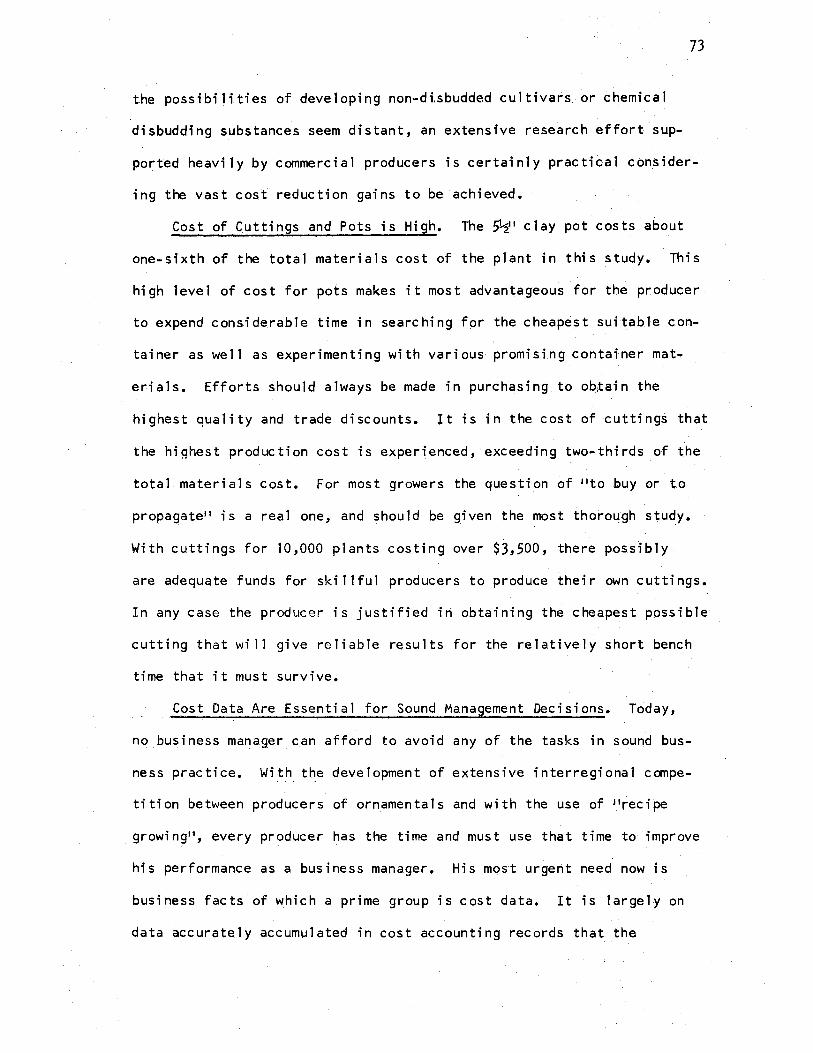
73

the possibilities of developing non-dhbudded cultivars or chemical

disbudding substances seem distant, an extensive research effort sup

po.rted heavily by commercial producers is certainly practical col"ISider

ing the vast cosf reduction gains to be achieved.

Cost of Cuttings and Pots is High. The 5'"2! 1 clay pot costs about

· .one-sixth c;,f the total materials cost of the plant in this st1.1dy. Thh

high level of cost for pots makes it most advantageous for the producer

to expend considerable time in searching f<>r the cheapest suitable con

tainer as well as experimenting with various promising container mat

erials. Efforts should always be made in purchasing to ol:,jl:ain the

highest quality and trade discounts. It is in the cost of cuttings that

the highest production cost .is experienced, exceeding two-thirds oft.he·

total materials cost. For most growers the question of ••to buy or to

propagate" is a real one, and should be given the most thorough study.

With cuttings for 10,000 plants costing over $3,500, there possibly.

are adequate funds for skillful producers to produce their own cuttings.

In any case the producer is justified iri obtaining the cheapest possible

cutting that wi 11 give reliable results for the relatively short bench

time that it must survive.

Cost Data Are Essential for Sound Management Decisions. Today,

no .business ma11ager can afford to avoid any of the tasks in sound bus

ness practice. With the development of extensive interregional compe

tition between producers of ornamentals and with the use of 11 recipe

growin(:111 , every producer has the time and must use that time to improve

his performance as a business manager. His most urgent need now is

business facts of which a prime group is cost data.· It is largely on

data accurate 1 y accumu 1 ated in cost accounting records that the

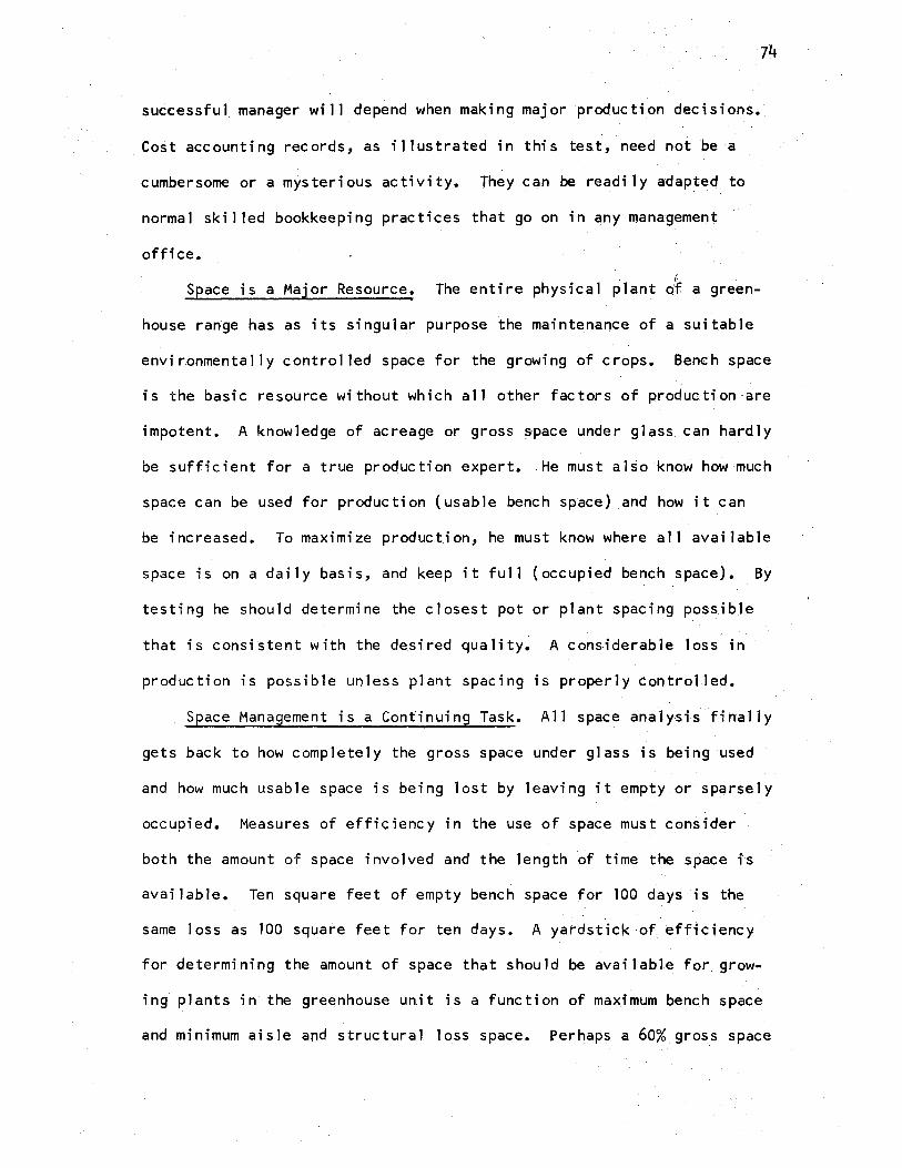
74

successfu 1 manager wi 11 depend when making major production dee is ions.

Cost accounting records, as illustrated in this tes.t, need not be a

cumbersome or a mysterious activity. They can be readily adapted to

normal skilled bookkeeping practices that go on in any management

office. {

Space is a Major Resource. The entire physical plant of a green-

house range has as its singular purpose the maintenance of a suitable

environmentally control led space for the growing of crops. Bench space

is the basic resource without which all other factors of production,are

impotent. A knowledge of acreage or gross space under glass can hardly

be sufficient for a true production expert. He must also know how much

space can be used for production (usable bench space) and how it can

be increased. To maximize production, he must know where all available

space is on a daily basis, and keep it full (occupied bench space). By

testing he should determine the closest pot or plant spacing possible

that is consistent with the desired quality. A considerable loss in

production is possible unless plant spacing is properly controlled.

Space Management is a Continuing Task. All space analysis finally

gets back to how completely the gross space under glass is being used

and how much usable space is being lost by leaving it empty or sparsely

occupied. Measures of efficiency in the use of space must consider

both the amount of space involved and the length of time the space is

available. Ten square feet of empty bench space for 100 days is the

same loss as 100 square feet for ten days. A yatdstick of efficiency

for determining the amount of space that should be available for grow-

ing plants in the greenhouse unit is a function of maximum bench space

and minimum aisle and structural loss space. Perhaps a 60% gross space

75

use approximates the highest level attainable by most firms under pres

ent day production methods. The total elimination of space loss eludes

realization because of the many factors involved in planning, schedul

ing, and managing production. Each manager must confine space loss to

the lowest possible level. Space loss probably should not exceed a

figure of 5% for a period such as one month. Basic tools for efficient

space are: a detailed space plan for one or more years, a planograph

reflecting the space status for the current week, a space data record

showing continuing space use, and a maximum pot spacing allowance record

that each crop must not exceed.

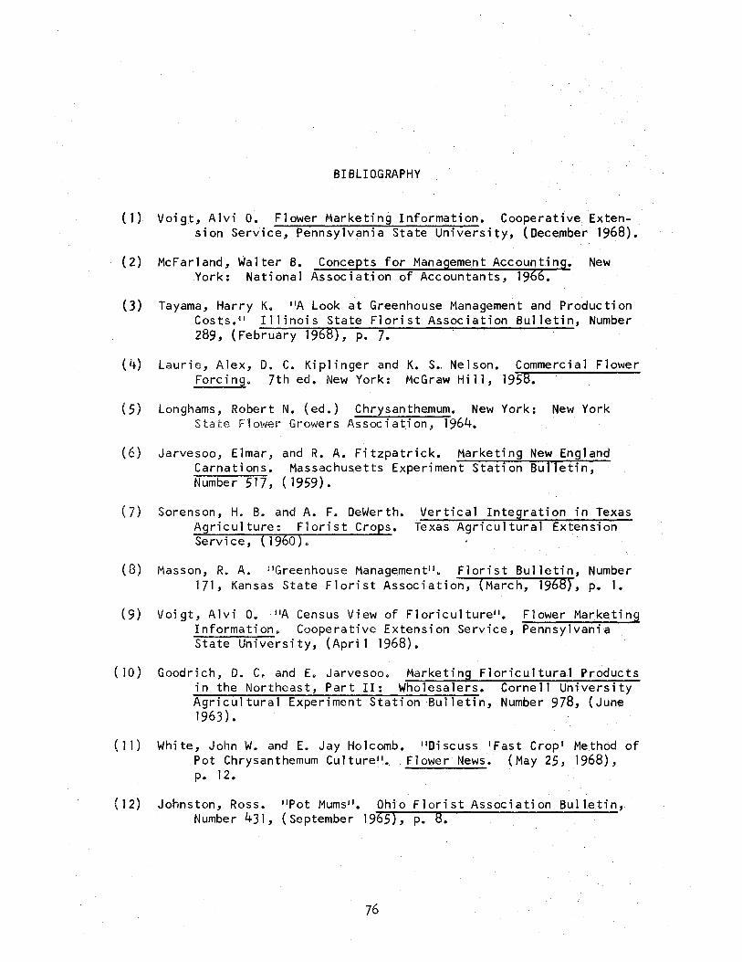
BIBLIOGRAPHY

( 1) Voigt, Alvi O. Flower Marketing Information. Cooperative Extension Service, Pennsylvania State University, (December 1968).

(2) McFarland, Walter B. Concepts for Management Accounting. New York: National Association of Accountants, 1966.

(3) Tayama, Harry K. 11A Look at Greenhouse Management and Production Costs. 11 Illinois State Florist Association Bulletin, Number 289, (February 1968), p. 7.

(l+) Laurie, Alex, D. C. Kiplinger and K. S •. Nelson. Commercial Flower Forcing. 7th ed. New York: McGraw Hi 11, 1958.

(5) Longhams, Robert N. (ed.) Chrysanthemum. New York: New York State Flower Growers Association, 1964.

(6) Jarvesoo, Elmar, and R. A. Fitzpatrick. Marketing New England Carnations. Massachusetts Experiment Station Bulletin, Number 517, (1959).

( 7) Sorenson, H. B. and A. F. DeWerth. Agriculture: Florist Crops. Service, (1960).

Vertical Integration in Texas Texas Agricultural Extension

(8) Masson, R. A. 11 Greenhouse Management11 • Florist Bulletin, Number 171, Kansas State Florist Association, (March, 1968), p. 1.

(9) Voigt, Alvi O. 11A Census View of Floriculture11 • Flower Marketing Information. Cooperative Extension Service, Pennsylvania State University, (Apri 1 1968).

(10) Goodrich, D. C. and E. Jarvesoo. Marketing Floricultural ~roducts in the Northeast, Part II: Wholesalers. Cornell University Agricultural Experiment Station Bulletin, Number 978, (June 1963).

(11) White, John W. and E. Jay Holcomb. 11 Discuss 1 Fast Crop' Method of Pot Chrysanthemum Culture••. Flower News. (May 25, 1968), p. 12.

(12) John.ston, Ross. 11 Pot Mums 11 • Ohio Florist As.sociation Bulletin, Number 431, ( September 1965), p. 8.

76

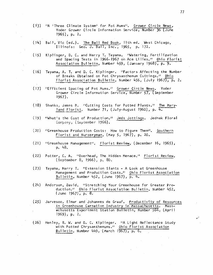
(13) 11A 'Three Climate System' for Pot MumsJ 1• Grower Circle News, Yoder Grower Ci re le Information Service, Number 36 ( June 1965), p. 2.

{14) Ball, Vic (ed.). The Ball Red Book, 11th ed. West Chicago, Illinois: Geo. J. Ball, Inc., 1965, p. 172.

77

(15) Kiplinger, D. C. and Harry T. Tayama. 11Watering:, Fertilization and Spacing Tests in 1966-1967 an Ace Lilies. 11 Ohio Florist Association Bui letin, Number 459, (January 1968), p. 9. .

{ 16) Tayama, A. T. and D. C. Kiplinger. J1Factors Affecting the Number of Breaks Obtained on Pot Chrysanthemum Cuttings.Ji Ohio Florist Association Bulletin, Number 456, (July J967"J";"""'p. 2.

(17) "Efficient Spacing of Pot Mums.Ji Grower Circle News. Yoder Grower Circle Information Service, Number 57, (September 1967).

( 18) Shanks, James B. 11 Cutting Costs for Potted Plants." The Maryland Florist. Num.ber 71, (July-August 1960), p. 4.

(19) "What's the Cost of Production. 11 Jeds Jottings. Jednak Floral Company, (September 1966).

(20) "Greenhouse Production Costs: How to Figure Them11 • Southern Florist and Nurseryman, (May 5, 1967), p. 20.

(21) 11Greenhouse Management 11 • Florist Review, (December 16, 1965), p. 48.

(22) Potter, C. A. "Overhead, The Hidden Menace. 11 Florist Review, (September 8, 1966), p. 80.

( 23) Tayama, Harry T. 11 Extensi on S 1 ants - A Look at Greenhouse Management and Production Costs. 11 Ohio Florist Association Bulletin, Number 452, (June 1967), p. 4.

(24) Anderson, David. 11 Stretching Your Greenhouse for Greater Production.11 Ohio Florist Association Bulletin, Number 452, ( June 1967), p.

( 25) Jarvesao, El mar and Johannes de Graafo Productivity of Re sou re.es in Greenhouse Carnation Industry in Massachusetts. Mass~ achusetts Experiment Station Bulletin, Number·564, (April 1969), p. 2.

(26) Henley, R. W. and D. C. Kiplinger. 11A Light Reflectance Study with Potte·d Chrysanthemums. 11 Ohio Florist Association Bulletin, Number 449, (March 1967), p. 6.

(27) 11 Frequency of Irrigation on Pot Mums. 11 Ohio Florist As.sociation · Bulletin, Number 444, (October 1966), p. 7.

(28) 11 Two Methods of Automatic Watering of Pot Mums•• Ohio Florist Association Bulletin, Number 433, (November 1965), p •. 3.

78

·(29) Ball Mums, Technical B.ulletin, Number 310, West Chicago, Illinois: Geo •. J •. Bal 1, In.c., 1967, p. 36.

(30) 11 Busch Greenhouse. 11 Grower Ta.lk, (January 1968), p. )1.

(31) Defense Supply Agency. 11 Space Control and R.eporting. 11 Storage and Materials Hand 1i ng. Washington, D. C.: U. S. Gove.rnment ~rintin~ Office, 1965, p. 26-1.

(32) 11Pinch Time Affects Growth of Pot Mums. 11 Grower Circle News, Yoder Grower Ci re le Information. Service, Number 60 ( February

. 1968), p. 6.

APPENDIX A

79

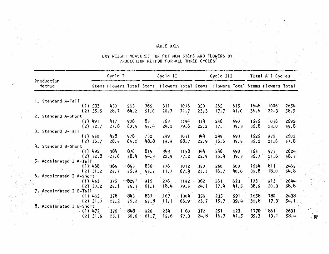
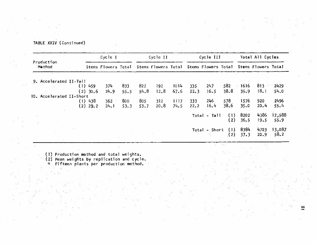
TABLE XXIV (Continued)

Cyc 1e I Cycle II Production

Method · Stems F1 owe rs Tota 1 Stems Flowers Tota1 -

9. Accelerated II-Tall ( 1} 459 374 833 822 (2) 30.6 24.9 55.5 54.8

10. Accelerated II-Short (1) 438 362 800 805 (2) 29.2 24.1 53.3 53.7

{ 1) .Production method and tot a 1 weights. {2) Mean weignts by replication and cycle. * Fifteen plants per proquction method.

192 1014 12.8 67.6

312 1117 20.8 74.5

Cyc 1e Ill Total Al1 Cycles

Stems F1owers Total Stems Flowers Total

335 247 582 1616 813 2429 22.3 16.5 38.8 35.9 18. 1 54.0

333 246 578 1576 920 2496 22.2 16.4 38.6 35.0 20.4 55.4

Total - Tal 1 ( l) 8202 4386 12.,588 ( 2) 36.5 19.5 55.9

Tota 1 - Short ( 1) 8384 4703 13.,087 (2) 37~3 20.9 58.2

(X>

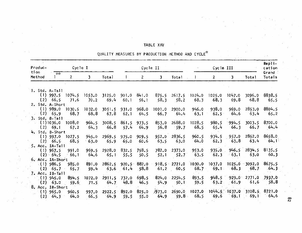
TABLE XXV

QUALITY MEASURES BY PRODUCTION METHOD AND CYCLE*

Repl i-Produc- Cyc 1 e I Cycle fl Cycle III caHon tion

** Grand .

Method 1 2 3 Total 1 2 3 Total I 2 3 Total Tota Is

1. Std. A-Tai I (1) 997.5 1074.5 1053.0 3125.0 901.0 841.0 875.5 2617.5 1024.o 1025.0 1047 .o 3096.0 8838.5 ( 2) 66.5 71.6 70.2 69.4 60.1 56. 1 58.3 58.2 68.3 68.3 69.8 68.8 65.5

2. Std. A-Short ( t) 989.0 1030. 5 10 32.0 3051.5 931.0 968.o 1001.0 2900.0 946.0 938.0 969.0 2853.0 8804.5 ( 2) 65.9 68.7 68.8 67.8 62.1 64.5 66.7 64.4 63.1 62. 5- 64.6 63.4 65.2

3. Std. B-Tall (I) 1036.0 1008.0 964.5 3008. 5 861. 5 973.5 853.0 2688.0 1028.5 980.5 994.5 3003. 5 8700.0 ( 2) 69.1 67.2 64.3 66.8 57.4 64.9 56.8 59.7 •68.5 65.4 66.3 66.7 64.4

4. Std. B-Short (1) 997.0 1027.5 945.0 2969.5 975.0 909.5 952.0 2836.5 960.5 . 934.5 957.0 2852.0 8658.o. ( 2) 66.5 68.5 · 63.0 65.9 65.0 60.6 63.5 63~0 64.o 62.3 63.8 63.4 64. 1:

5. Acc. IA-Tat 1 ( 1) 967.5 991.0 969.5 2928.0 832.5 758.5 782.0 2373.0 953.0 935.0 946.5 2834.5. 8135.5 (2) .. 64.5 . 66.1 64.6 65.l 55.5 50.5 52.1 52.7 63.5 62.3 63.1 63.0 60.3

6. Acc. IA-Short (1) 986.5 985.0 891.0 2862. 5 9 20. 5 · · 882. O 9_18. 5 2721.0 1030.0 )037.0 1025~0 .. · 3092.0 8675.5

... ( 2) 65.7. 65. 7 · 59.4 63.6 61.4 58.8 61.2 60.5 68.7 69.1 ·. 68.3·· .68.7 ·.64.3 7. Acc. IB.;,.Tall

7937.0 . ( l) 945.0 894.5 1072.0 2911. 5 732~0 698.5 824.o _2254.5 893.5 948.5 929.0 2771.0 ( 2) 6J.O 59.6 71.5 64.7 48.8 46~5 54.9 50. 1 59.5 63.2 . 61.9 6t.6 58.8

8. Acc. IB~·short 825.0 )973.0 · 2690.0 . (1) 965.0 960.5 997.0 2922.5 · 892.0 1027;0 1044~5: 1037;0 · JJ08.S: 8721~0

( 2) 64.3 · 64.0 66~5 64.9 59.5 55.0 64.9 59.8 68.5 . 69.6 . 69. 1 . 69.1 ... 64.6 00 ....,

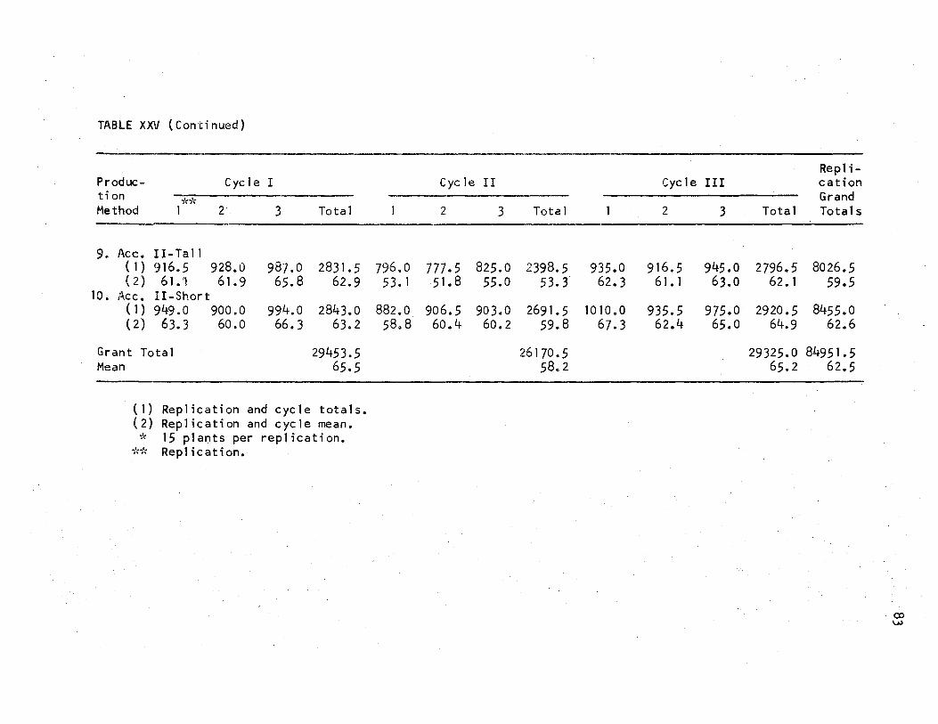
TABLE XX\/ {Continued)

Produc-tion ;'(~' Method 1

9 • Ac c • II - Ta 11 (1) 916.5 (2) 61 .1

10. Acc. II-Short (1) 949.0 ( 2) 63.3

Grant Total Mean

Cyc 1e I

2 3

928.0 987.0 61.9 65.8

900.0 994.0 60.0 66.3

Total

2831. 5 62.9

2843.0 63.2

29453.5 65.5

( I) RepHcation and cycle totals. (2) Replication and cycle mean. * 15 plants per replication.

-Id, Replication.

1

796.0 5 3. 1

882.0 58.8

Cycle II

2 3

777. 5 825.0 51. 8 55.0

906.5 903.0 60.4 60.2

Total ,_,

2398. 5 53.3

2691. 5 59.8

26170. 5 58.2

1

935.0 62.3

1010.0 67.3

Cycle III

2 3

916.5 945.0 61. 1 63.0

935.5 975.0 62.4 65.0

Rep 1 i-cation Grand

Total Totals

2796.5 8026. 5 62. 1 59.5

2920. 5 8455.0 64.9 62.6

29325.0 84951.5 65.2 62.5

co ...,.,

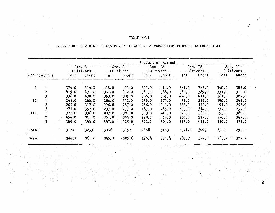
Rep 1 i c at i on s

I I 2 3

II 1 2 3

III 1 2 3

Total

Mean

TABLE XXVI

NUMBER OF FLOWERING BREAKS PER REPLICATION BY PRODUCTION METHOD FOR EACH CYCLE

Production Method Std. A Std. B Acc. IA Ace. IB Acc. II

Cul ti vars Cultivars Cul tivars Cultivars Cultivars Ta 11 Short Ta 11 Short Ta 11 Short Ta 11 Short Tall Short

374.o 414.o 416.o 434.o 391.0 414.o 361.0 383.0 340.0 383.0 419.0 431.0 361.0 412.0 381.0 388.0 360.0 389.0 331.0 312.0 396.o 434.o 353.0 385.0 386.0 365.0 440.0 411. 0 381.0 382.0 263.0 260.0 286.0 332.0 236.0 279.0 139.0 229.0 190.0 249.0 285.0 317.0 298.0 267.0 168.0 244.o 133.0 172.0 191. O 257.0 271.0 352.0 237.0 277.0 187 .o 265.0 255.0 314.o 237.0 254.o 373.0 336.o 407.0 . 381.0 319.0 410.0 270.0 386.o 293.0 389.0 404.o 361.0 361.0 344.o 298.0 4o4.o 300.0 392.0 276.0 347.0 3-89. O 348.o 347.0 325.0 302.0 394.0 313.0 421.0 310.0 372.0

3174 3253 3066 3157 2668 3163 2571.0 3097 2549 2945

352.7 361. 4 340. 7 350.8 296.4 351 .. 4 285.7 344.1 . 283. 2 327.2

(X) ..s:-

APPENDIX B

85

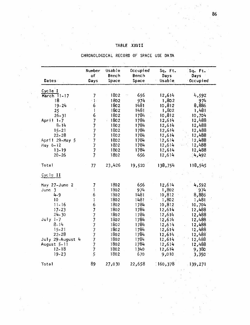
86

TABLE XXVII

CHRONOLOGICAL RECORD OF SPACE USE DATA

Number Usable Occupied Sq. Ft. Sq. Ft. of Bench Bench Days Days

Oates Days Space Space Usable Occupied

cic 1 e I March 11-17 7 1802 656 12,614 4,592

18 1 1802 974 1,802 974 19~24 6 1802 1481 10,812 8,886 25 1 1802 1481 1,802 1, 481 26-31 6 1802 1784 10,812 10, 704

Apr i 1 1- 7 7 1802 1784 12,614 12,488 8-14 7 1802 1784 12,614 12,488

15-21 7 1802 1784 12,614 12,488 22-28 7 1802 1784 12,614 12,488

Apri 1 29-May 5 7 1802 1784 12,614 12,488 May 6-12 7 1802 1784 12,614 12,488

1 3- 19 7 1802 1784 12,614 12,488 20-26 7 1802 656 12,614 :4,492

Total 77 23,426 19,520 138,754 118,545

Cycle II

May 27-June 2 7 1802 656 12,614 4,592 June 3 1 1802 974 1,802 974

4-9 6 1802 1481 10,812 8,886 10 1 1802 1481 1,802 1,481 11- 16 6 1802 1784 l0,812 10. 704 17-23 7 1802 1784 12,614 12,488 24-30 7 1802 1784 12,614 12,488

July 1-7 7 1802 1784 12,614 12,488 8-14 7 1802 1784 12,614 12,488 15-21 7 1802 1784 12,614 12,488 22-28 7 1802 1784 12,614 12,488

July 29-August 4 7 1802 1784 12,614 12,488 August 5-11 7 1802 1784 12,614 12,488

12-18 7 1802 1340 12 ,.614 9,380 19-23 5 1802 670 9,010 3,350

Total 89 27 ,030 22,658 ·• 160,378 139,271

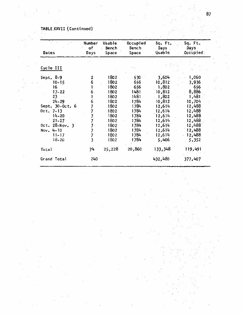
87

TABLE XXVII ~Continued)

Number Usab1e Occupied Sq. Ft. Sq. Ft. of Bench Bench Days D.ays

Dates Days Space .Space lJsab1e Occupied

Clc1e III

Sept. 8 .. 9 2 1802 530 3,604 1,060 10-15 6 1802 656 10,812 3,936 16 1 1802 656 l,802 656 17-22 6 1802 1481 10,812 · 8,886 23 1 1802 1481 1,802 1, 481 24-29 6 1802 1784 10,812 10, 704

Sept. 30-0ct. 6 7 1802 1784 12,614 12,488 Oct. 7-13 · 7 1802 1784 12,614 12,488

14-20 7 1802 1784 12,614 12,488 21-27 7 1802 1784 12,614 12,488

Oct. 28-Nov. 3 7 1802 1784 12,614 12,488 Nov. 4-10 7 1802 1784 12,614 12,488

11-17 7 1802 1784 12,614 12,488 18-20 3 1802 1784 5,406 5,352

Total 74 25,228 20,860 133,348 119, 491

Grand Total 240 432,480 377,407

. VIrA .

Hehry Vieth Griffith

Candidate for the Degree of·

· Mas te.r o.f Science

Thesis: AN ANALYSIS OF POT CHRYSANTHEMUM PRODUCTION METH.ODS, DlRECT COSTS AND SPACE USE

Major Field: Horticulture

Biographical:

Personal Data: Born in Barrington, Rhode Island, October 17, 1923, the son of Mr. and Mrs. Benjamin F. Griffith

Educc1tion: Graduated from Lynbrook High School, Lynbrook, New York in 1941; attended Iowa State College in 194land 1942; attended University of Oklahoma 1946 and· 1947; received the Bachelor of Science degree from Oklahom:a St.ate Unive.rsity in 1949 with a major in Hor ti culture; received a Master of · Science in Commerce from the University of Alabama in .. 1961; completed requirements for a Master of Sdence degree in Horticulture in May 1969.

Professional Experience: Commissioned officer in the U. S. Army Medical Service from 1943 to 1946; recalled to active service in 1950 and held various positions as an Arm.y O'epot Supply Officer unti 1 1957; Instructor of supply subjects, 1958 and 1959; Army Manager of Medical .Material in Europe, 1961 to 1964; Director, Dominican Expeditionary.:·Forces:'.S.up.j:>ly Control Center, 1965; Director, U. S. Army Medical Material Management Training, 1966 ·and 1967; Graduate Te.aching As-: sitant, Horticulture Department, Oklahoma State Uhiversity, 1968-69. .

AN ANALYSIS OF POT CHRYSANTHEMUM PRODUCTION ...

Documents

Transcript of AN ANALYSIS OF POT CHRYSANTHEMUM PRODUCTION ...