An Adaptive Component Mode Synthesis Method forDynamic Analysis of Jointed Structure with Contact

Friction Interfaces

Jie Yuana,∗, Loic Sallesa, Fadi El Haddada, Chian Wongb

aVibration University Technology Centre, Imperial College London SW7 2AZ, London,UKbRolls Royce Plc, DE24 8BJ, Derby, UK

Abstract

Component model synthesis (CMS) has been widely used for model order re-

duction in dynamic analysis of jointed structures with localized non-linearities.

The main drawback of these CMS methods is that their computational efficiency

largely depends on the size of contact friction interfaces. This work proposes an

adaptive reduction approach to improve these CMS based reduction methods in

the application to the assembled structure with frictional interfaces.The main

idea of this method is that, instead of retaining the whole frictional interface

DOFs in the reduced model, only those DOFs in a slipping or separating con-

dition are retained. This would significantly reduce the size of classical CMS

based reduced models for dynamical analysis of jointed structure with micro-slip

motion, leading to an impressive computational saving. This novel approach is

based on a reformulated dynamic system that consists of a underlying linearised

system and including an updating internal variable to account the effects of

non-linear contact friction force on the interface. The paper also describes

the detailed implementation of the proposed approach with harmonic balanced

method for non-linear spectral analysis, where a new updating algorithm is put

forward to enable the size of the reduced model can be automatically updated

according to the contact condition of interface nodes. Two distinct FE joint

∗Corresponding authorEmail address: jie.yuan@imperial.ac.uk (Jie Yuan)

Preprint submitted to Computers and Structures September 20, 2019

models are used to validate the proposed method. It is demonstrated that the

new approach can achieve a considerable computing speed-up comparing to the

classic CMS approach while maintain the same accuracy.

Keywords: Reduced order modelling, Component mode synthesis, Harmonic

balanced methods, Jointed structures, Contact friction

1. Introduction

Mechanical joints have been widely present in both aerospace and civil struc-

tures, e.g. bolted joints in bridges to fir-tree and dovetail joint in aero-engines

[1, 2]. They are represented as an effective and affordable way to hold together

the assembly and transmit the loadings between the components[3, 4]. How-5

ever, due to the relative motions occurring on the jointed interfaces, the forced

dynamic repose of the whole assembly can be substantially changed. This inter-

facial relative motion can introduce additional energy dissipation that would

change the overall stiffness of an assembly and thus lead to a shift of resonance

frequencies [5]. However, the amount of damping due to these joints is typically10

10-100 times higher than normal material damping [6]. The experiments also

consistently exhibit that the damping in these joints vary with the amplitude of

excitation levels [5]. To guarantee the service life of these joints, it is therefore

crucial for engineers to understand their modal properties. However, the cost

involving manufacturing and testing these jointed structure are commonly high15

and sometimes are unaffordable in most cases. It is therefore important to have

predictive models beforehand that can reliably estimate the dynamical response

of such jointed structures. However, due to the strong nonlinearities from the

contact friction in joints, linear or linearised predictive models are not accurate

enough to capture the nonlinear dynamics of these structures [6]. It is necessary20

to include intuitively constitutive models that provide a better description of

joint mechanics in modelling these joints. In this way, nonlinear dynamic effects

in the joints can be taken into account. To obtain the dynamical response for

nonlinear joint models, this would require iterative solvers. Most existing mod-

2

elling approaches including the non-linear contact friction models employ either25

time domain solvers [7] (e.g.Runge-Kutta or Newmark method [8]) or frequency

domain solvers [6, 9] (e.g.harmonic balance methods (HBM)). To solve the full

scale jointed model without reduction for a wide range of frequencies or time,

the computational expense with these solvers is usually unacceptable. HBM is

well known for its high efficiency to obtain the steady state approximations that30

can reduce the computational time by several orders compared to time domain

methods [10]. However, even with the use of HBM, modelling the joints in

high fidelity still suffers from the unaffordable computational cost and numer-

ical stability issues [11]. Fortunately, ROM methods provide a viable solution

to incorporate these accurate contact friction models into assembled models.35

To date, the reduced model for the structure with joints are mostly con-

structed using substruturing methods in the class of CMS techniques [10, 9,

11, 12, 13]. The main concept behind these CMS based methods consists in

assuming two or more connected components in an assembly are distinct sub-

structural elements so that their modal bases can be separately calculated via40

deterministic FE analysis [14]. The full system can be then significantly reduced

via Galerkin Projection [12, 15] using the reduced basis that combines the lin-

ear normal modes from different components with the static impulse modes

associated to retained interface nodes. This can effectively eliminate most in-

ternal DOFs. The CMS based reduced models would retain the whole DOFs45

involved in on the joint interface [16]. The nonlinear contact friction model

therefore can be conveniently integrated through these retained DOFs. Ru-

bin and Craig-Bampton (CB) method are two typical methods based on CMS

techniques[17, 18]. Rubin method combines free interface modes and static ones

obtained from the static solution of applied interface load, which is also called50

attachment modes or flexible residual. In contrast, CB method combines the

normal modes with the fixed interface condition and static solutions (so called

constrain modes) obtained by applying unit displacement at each interface DOF.

Both methods have been proven effective for ROM of the structures with fric-

tional interfaces [9, 10]. Unfortunately, the main drawbacks of these CMS based55

3

approaches is that their size heavily depends on the number of DOFs involved

in contact interfaces [19, 12]. This limitation compromises the computational

efficiency of CMS based ROMs especially in the case where the contact interface

regions are intensive in order to ensure an accurate stress recovery for reliable

fatigue life predictions. To improve these CMS based methods, two interface60

reduction methods were proposed to reduce static impulse modes. One of them

is called common interface reduction approach that was proposed by Becker

and Gaul [20, 21]. The main idea is to replace full size of constrain modes

by a subset of interface modes, which are calculated via performing a second

modal analysis related to interface DOFs. The other one is called joint inter-65

face modes approach proposed by Witteveen [19]. The joint interface modes are

generated explicitly by respecting the Newtons third law across the joint inter-

faces. A comparative study by Becker[20] shows both methods can effectively

reduce interface DOFs but joint interface modes can achieve better convergence

with much less number of interface modes [20]. However, in general, the con-70

vergence of these two methods are problem dependent and heavily reply on a

good selection of such special interface modes. In addition, the evaluation of

these interface models would increase the off-line cost. For these two reasons,

these two interface reduction methods still have not been widely used for the

simulations of jointed structures.75

Instead of using the condensed interface modes, this work aims to develop an

adaptive approach to further improve reduced models constructed by classical

CMS based methods. The main idea of the proposed approach is to adaptively

remove the fully stuck contact nodes from the classical ROMs depending on

the contact condition on the joint interface, which would lead to a significant80

reduction in the number of static modes. This idea is inspired by the previous

findings that, for the majority of structures with joints, the contact interfaces

are mostly in a micro-slip motion where most of the contact nodes are in a stuck

condition under the dynamic loads. This phenomenon has been widely found

in bolted joints structures [5] and fir-tree joints in turbines [22]. Fig.1 shows85

an example of forced frequency response of a turbine with root joints, and also

4

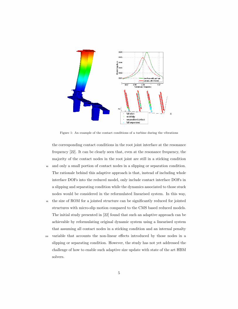
Figure 1: An example of the contact conditions of a turbine during the vibrations

the corresponding contact conditions in the root joint interface at the resonance

frequency [22]. It can be clearly seen that, even at the resonance frequency, the

majority of the contact nodes in the root joint are still in a sticking condition

and only a small portion of contact nodes in a slipping or separation condition.90

The rationale behind this adaptive approach is that, instead of including whole

interface DOFs into the reduced model, only include contact interface DOFs in

a slipping and separating condition while the dynamics associated to those stuck

nodes would be considered in the reformulated linearised system. In this way,

the size of ROM for a jointed structure can be significantly reduced for jointed95

structures with micro-slip motion compared to the CMS based reduced models.

The initial study presented in [22] found that such an adaptive approach can be

achievable by reformulating original dynamic system using a linearised system

that assuming all contact nodes in a sticking condition and an internal penalty

variable that accounts the non-linear effects introduced by those nodes in a100

slipping or separating condition. However, the study has not yet addressed the

challenge of how to enable such adaptive size update with state of the art HBM

solvers.

5

The objective of this paper is to present the entire mathematical derivations

of this adaptive ROM approach for the jointed structure with contact friction105

interfaces; describe a novel updating algorithm to integrate the proposed ap-

proach into state of the art frequency domain solver to achieve the size updat-

ing; validate the adaptive approach using two FE joint models and compare its

performance to classic CMS based approach. The paper is organized as follows:

the formulation of the classic dynamic system, contact friction model for the110

structure with contact interfaces is firstly presented; it then briefly introduces

the CMS based Rubin method that would be used as a benchmarking method;

it is then followed by the theoretical development of the proposed adaptive ap-

proach that include a reformulated dynamic system and corresponding adaptive

reduced model; the paper then describes a new updating algorithm to imple-115

ment the proposed method into harmonic balanced method to enable automatic

size updating; Two test cases, one with 2D joint beams and the other with 3D

joint beams, are then presented, discussed and compared with classical CMS

techniques.

2. Formulation120

2.1. Equation of motion

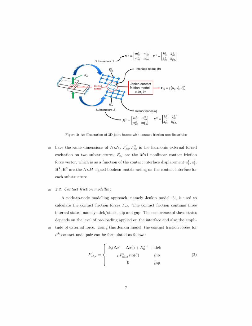
A dynamic system consisting of two connected components with contact in-

terfaces is considered. Fig.2 shows an illustration of such a jointed structure

with localized nonlinearities. Using the finite element discretisation, the ordi-

nary differential governing equation describing the dynamics of this assembled

system can be expressed as:M1 0

0 M2

u1

u2

+

K1 0

0 K2

u1

u2

=

F 1ex

F 2ex

−

B1

B2

Fnl(u1b , u

2b)

(1)

It is assumed the amount of DOFs for each sub-structure is N and the

amount of contact friction DOFs for each contact interface isM . M1,M2,K1,K2

are the mass and stiffness matrix of two connected sub-structures and all of them

6

Substructure 1

Substructure 2

Interface nodes (b)

𝑀" =𝑚%%" 𝑚%&

"

𝑚&%" 𝑚&&

" 𝐾" =𝑘%%" 𝑘%&"

𝑘&%" 𝑘&&"

Interior nodes (i)

𝑀) =𝑚%%) 𝑚%&

)

𝑚&%) 𝑚&&

)𝐾) =

𝑘%%) 𝑘%&)

𝑘&%) 𝑘&&)

Contact surface

Jenkin contact friction model

𝑢, 𝑘𝑡, 𝑘𝑛𝑭./ = 𝑓 𝑁0,𝑢&" ,𝑢&)

𝐹23"

𝐹23)

𝑁0

Figure 2: An illustration of 3D joint beams with contact friction non-linearities

have the same dimensions of NxN ; F 1ex, F

2ex is the harmonic external forced125

excitation on two substructures; Fnl are the Mx1 nonlinear contact friction

force vector, which is as a function of the contact interface displacement u1b , u

2b .

B1,B2 are the NxM signed boolean matrix acting on the contact interface for

each substructure.

2.2. Contact friction modelling130

A node-to-node modelling approach, namely Jenkin model [6], is used to

calculate the contact friction forces Fnl. The contact friction contains three

internal states, namely stick/stuck, slip and gap. The occurrence of these states

depends on the level of pre-loading applied on the interface and also the ampli-

tude of external force. Using this Jenkin model, the contact friction forces for135

ith contact node pair can be formulated as follows:

F inl,x =

kt(∆x

i − ∆xic) +Nx,i0 stick

µF inl,z sin(θ) slip

0 gap

(2)

7

F inl,y =

kt(∆y

i − ∆yic) +Ny,i0 stick

µF inl,z cos(θ) slip

0 gap

(3)

F inl,z =

kn∆zi +Nz,i0 stick or slip

0 gap(4)

Where ∆xi,∆yi and ∆zi are the relative displacement of ith contact node pair

in tangential (x, y) and normal (z) direction; ∆xic,∆yic are the internal state

variables that represent the position of tangential sliders. They would become

zero if the contact node were in a pure sticking condition; N i,x0 , N i,y

0 , N i,z0 is tan-140

gential (x, y) and normal (z) components of interface pre-loading N0 illustrated

in Fig.2; µ is the friction coefficient of the contact interface; F inl,x, Finl,y are the

tangential friction force and F inl,z is the normal contact force; θ is the angle to

decompose the tangential friction force in x and y direction. It is determined

by the predicted tangential force as:145

tan(θ) =kt(∆x

i − ∆xic) +Nx,i0

kt(∆yi − ∆yic) +Ny,i0

(5)

The stick condition occurs when the predicted tangential force is less than

the critical slipping force, namely√

(F inl,x)2 + (F inl,y)2 ≤ µF inl,z. The contact

force would vary proportional to relative displacement and there would be no

energy dissipation on the contact interface. Otherwise, the slip condition would

occur and the amplitude of tangential frictional force would be µF inl,z. The150

energy dissipation would happen then. The gapping condition would happen

when predicted normal force F inl,z were less than zero. In this case, the contact

pair is separated and all the tangential and normal force would become zero.

With this contact friction model, Fnl shown in Eq. 1 can be evaluated and

assembled for all the contact pairs. Assuming that local coordinate systems for155

all the contact nodes are consistent with the global system defined for the FE

8

model, Fnl for m contact pairs can be written as:

Fnl =[F 1nl,x F 1

nl,y F 1nl,z · · · Fmnl,x Fmnl,y Fmnl,z

]T(6)

3. Benchmark Rubin method

This section is to give a brief review of the reduced basis of CMS based

Rubin method, which would be used to benchmark the results from new ROM

in this study. As mentioned in the introduction, Rubin method combines free

interface normal modes and static modes (or called attachment modes) as its

reduced basis [23]. The free interface modes are calculated for each component

as:

−ω2[M(i)

] [φ(i)]

+[K(i)

] [φ(i)]

= 0 (7)

Where φ(i) are the dynamical modes for ith substructure. The static modes

that used to account the interface effects in the high frequency response are

evaluated by solving the static problem of each substructure under applied unit

force on the interface. They are generally the inverse or the generalized inverse of

stiffness matrix if rigid body motions are existing. By eliminating the redundant

information included in the dynamical modes, the static modes G(i) for ith

component can be expressed as:

G(i) = K(i)+ −nθ∑j=1

φ(i)j φ

(i)j

T

ω(i)j

2 (8)

Where K(i)+ the generalized inverse of stiffness matrix; nθ is the number of

dynamic modes; ω(i)j is the the natural frequency to jth mode for ith compo-

nent. The transformation equation without the presence of rigid modes can be

expressed:

u1

u2

=

φ(1) −G(1)B(1)T 0 0

0 0 φ(2) −G(2)B(2)T

︸ ︷︷ ︸

ΦRB

η(1)

λ(1)

η(2)

λ(2)

(9)

9

Where ΦRB is the transformation matrix for the Rubin method; η(1), η(2) are

the modal participation factor for two substructures; λ(1), λ(2) are interface force160

for both substructures. The size of reduced basis is proportional to the size of

contact interface DOFs

4. Adaptive CMS method

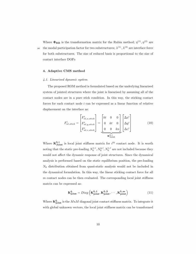
4.1. Linearised dynamic system

The proposed ROM method is formulated based on the underlying linearised

system of jointed structures where the joint is linearised by assuming all of the

contact nodes are in a pure stick condition. In this way, the sticking contact

forces for each contact node i can be expressed as a linear function of relative

displacement on the interface as:

F inl,stick =

F inl,x,stick

F inl,y,stick

F inl,z,stick

=

kt 0 0

0 kt 0

0 0 kn

︸ ︷︷ ︸

KL,iJoint

∆xi

∆yi

∆zi

(10)

Where KL,iJoint is local joint stiffness matrix for ith contact node. It is worth

noting that the static pre-loading Nx,i0 , Ny,i

0 , Nz,i0 are not included because they

would not affect the dynamic response of joint structures. Since the dynamical

analysis is performed based on the static equilibrium position, the pre-loading

N0 distribution obtained from quasi-static analysis would not be included in

the dynamical formulation. In this way, the linear sticking contact force for all

m contact nodes can be then evaluated. The corresponding local joint stiffness

matrix can be expressed as:

KLjoint = Diag

(KL,1

joint,KL,2joint, · · · ,K

L,mjoint

)(11)

Where KLjoint is theMxM diagonal joint contact stiffness matrix. To integrate it

with global unknown vectors, the local joint stiffness matrix can be transformed

10

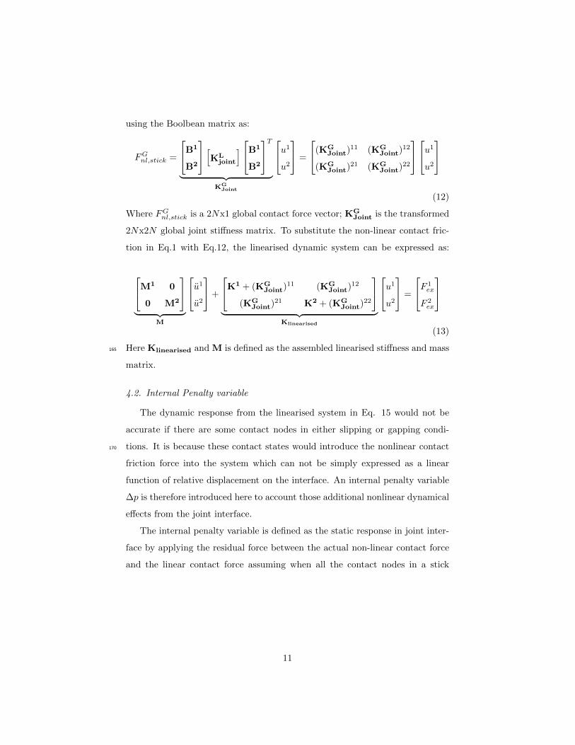
using the Boolbean matrix as:

FGnl,stick =

B1

B2

[KLjoint

]B1

B2

T︸ ︷︷ ︸

KGJoint

u1

u2

=

(KGJoint)

11 (KGJoint)

12

(KGJoint)

21 (KGJoint)

22

u1

u2

(12)

Where FGnl,stick is a 2Nx1 global contact force vector; KGJoint is the transformed

2Nx2N global joint stiffness matrix. To substitute the non-linear contact fric-

tion in Eq.1 with Eq.12, the linearised dynamic system can be expressed as:

M1 0

0 M2

︸ ︷︷ ︸

M

u1

u2

+

K1 + (KGJoint)

11 (KGJoint)

12

(KGJoint)

21 K2 + (KGJoint)

22

︸ ︷︷ ︸

Klinearised

u1

u2

=

F 1ex

F 2ex

(13)

Here Klinearised and M is defined as the assembled linearised stiffness and mass165

matrix.

4.2. Internal Penalty variable

The dynamic response from the linearised system in Eq. 15 would not be

accurate if there are some contact nodes in either slipping or gapping condi-

tions. It is because these contact states would introduce the nonlinear contact170

friction force into the system which can not be simply expressed as a linear

function of relative displacement on the interface. An internal penalty variable

∆p is therefore introduced here to account those additional nonlinear dynamical

effects from the joint interface.

The internal penalty variable is defined as the static response in joint inter-

face by applying the residual force between the actual non-linear contact force

and the linear contact force assuming when all the contact nodes in a stick

11

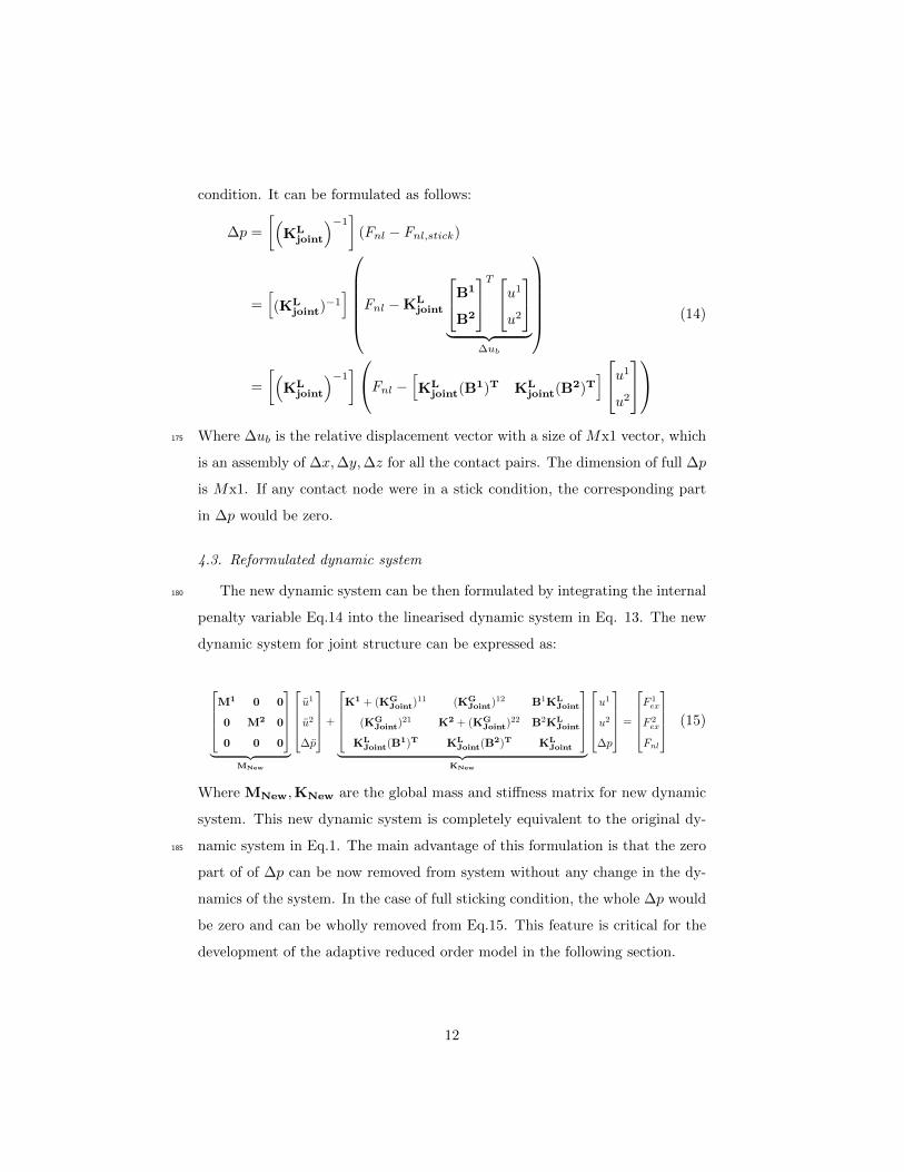
condition. It can be formulated as follows:

∆p =

[(KL

joint

)−1]

(Fnl − Fnl,stick)

=[(KL

joint)−1]Fnl − KL

joint

B1

B2

T u1

u2

︸ ︷︷ ︸

∆ub

=

[(KL

joint

)−1]Fnl − [KL

joint(B1)T KL

joint(B2)T]u1

u2

(14)

Where ∆ub is the relative displacement vector with a size of Mx1 vector, which175

is an assembly of ∆x,∆y,∆z for all the contact pairs. The dimension of full ∆p

is Mx1. If any contact node were in a stick condition, the corresponding part

in ∆p would be zero.

4.3. Reformulated dynamic system

The new dynamic system can be then formulated by integrating the internal180

penalty variable Eq.14 into the linearised dynamic system in Eq. 13. The new

dynamic system for joint structure can be expressed as:

M1 0 0

0 M2 0

0 0 0

︸ ︷︷ ︸

MNew

u1

u2

∆p

+

K1 + (KG

Joint)11 (KG

Joint)12 B1KL

Joint

(KGJoint)

21 K2 + (KGJoint)

22 B2KLJoint

KLJoint(B

1)T KLJoint(B

2)T KLJoint

︸ ︷︷ ︸

KNew

u1

u2

∆p

=

F 1ex

F 2ex

Fnl

(15)

Where MNew,KNew are the global mass and stiffness matrix for new dynamic

system. This new dynamic system is completely equivalent to the original dy-

namic system in Eq.1. The main advantage of this formulation is that the zero185

part of of ∆p can be now removed from system without any change in the dy-

namics of the system. In the case of full sticking condition, the whole ∆p would

be zero and can be wholly removed from Eq.15. This feature is critical for the

development of the adaptive reduced order model in the following section.

12

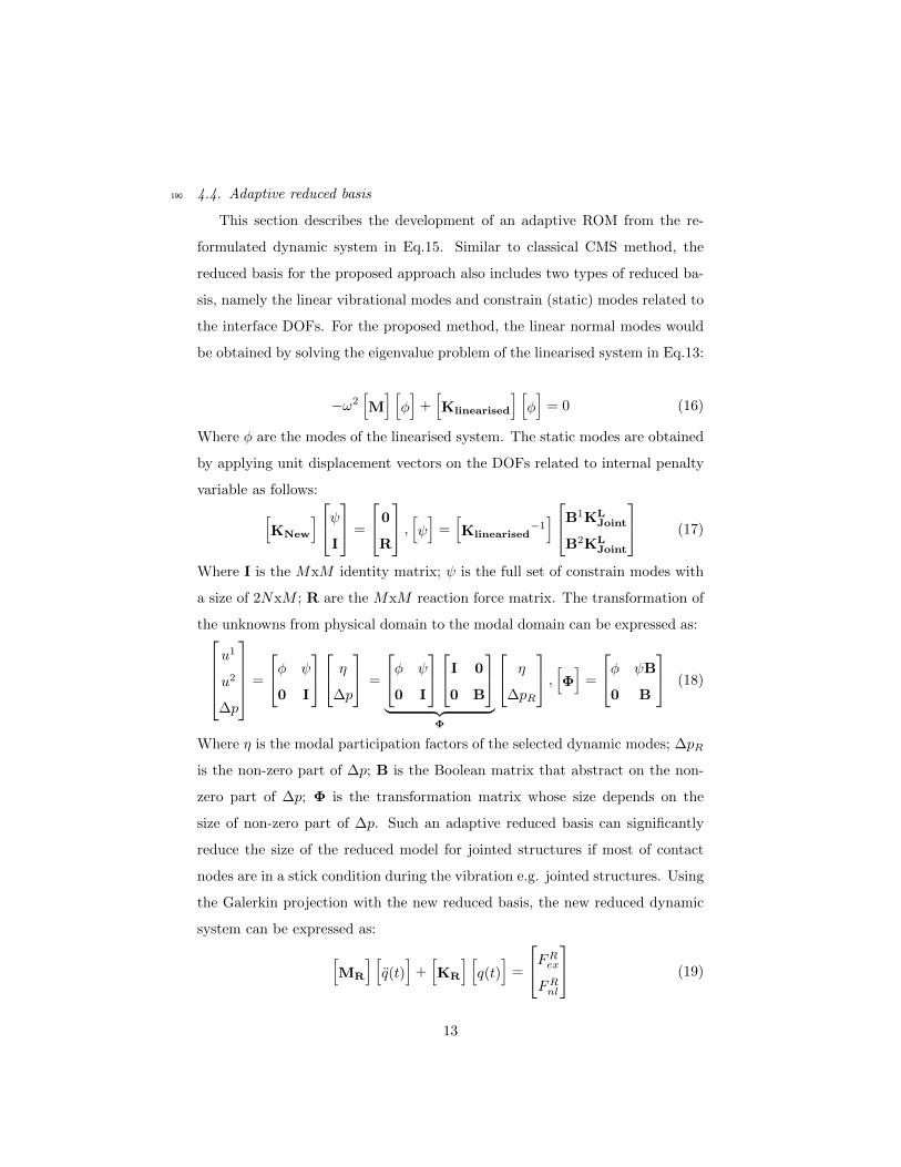
4.4. Adaptive reduced basis190

This section describes the development of an adaptive ROM from the re-

formulated dynamic system in Eq.15. Similar to classical CMS method, the

reduced basis for the proposed approach also includes two types of reduced ba-

sis, namely the linear vibrational modes and constrain (static) modes related to

the interface DOFs. For the proposed method, the linear normal modes would

be obtained by solving the eigenvalue problem of the linearised system in Eq.13:

−ω2[M] [φ]

+[Klinearised

] [φ]

= 0 (16)

Where φ are the modes of the linearised system. The static modes are obtained

by applying unit displacement vectors on the DOFs related to internal penalty

variable as follows:[KNew

]ψI

=

0

R

, [ψ] =[Klinearised

−1]B1KL

Joint

B2KLJoint

(17)

Where I is the MxM identity matrix; ψ is the full set of constrain modes with

a size of 2NxM ; R are the MxM reaction force matrix. The transformation of

the unknowns from physical domain to the modal domain can be expressed as:u1

u2

∆p

=

φ ψ

0 I

η

∆p

=

φ ψ

0 I

I 0

0 B

︸ ︷︷ ︸

Φ

η

∆pR

, [Φ] =

φ ψB

0 B

(18)

Where η is the modal participation factors of the selected dynamic modes; ∆pR

is the non-zero part of ∆p; B is the Boolean matrix that abstract on the non-

zero part of ∆p; Φ is the transformation matrix whose size depends on the

size of non-zero part of ∆p. Such an adaptive reduced basis can significantly

reduce the size of the reduced model for jointed structures if most of contact

nodes are in a stick condition during the vibration e.g. jointed structures. Using

the Galerkin projection with the new reduced basis, the new reduced dynamic

system can be expressed as:[MR

] [q(t)

]+[KR

] [q(t)

]=

FRexFRnl

(19)

13

MR = ΦTMNewΦ,KR = ΦTKNewΦ (20)

q =

η

∆pR

, FRex = ΦTFex, FRnl = ΦTFnl(Φq(t)) (21)

KR and MR are the reduced mass and stiffness matrix of the new dynamic

system;q is the reduced unknown for the dynamic system; FRex and FRnl are the

reduced external modal force and non-linear force vector.

5. HBM with automatic size updating

This section is to describe how to integrate the developed adaptive reduced195

order model with the harmonic balanced method for spectral analysis of non-

linear jointed system. The basic of harmonic balanced method would be briefly

introduced at first followed by the presentation of a novel updating algorithm

for achieving the automatic size updating with the proposed adaptive ROM.

5.1. Harmonic balanced method200

The idea of the multi-harmonic balanced method is to approximate the

steady state response of the system by using a truncated Fourier series. The

main advantage of this HBM is that it allows much faster computations of the

nonlinear steady state response of the system compared to time-domain meth-

ods by several orders. Using HBM, the non-linear displacement q(t) can be

expressed as:

q(t) = Q0 +

nh∑i=1

(Qci cosmiωt+ Qsi sinmiωt) (22)

Where Qc,si are cosine and sine harmonic coefficients for ith harmonic; ω is the

principal excitation frequency; Q0 is the zero harmonic response; nh is the num-

ber of harmonics. Using such a approximation, the size of original unknown

vector would be then expanded by 2nh + 1 times. The framework of HBM

usually includes three components: non-linear solver, Alternating Frequency205

14

𝑬𝒙𝒑𝒂𝒏𝒅𝚽 𝑄" (#)

𝑖𝐷𝐹𝑇

Prediction penalty:

𝐹)* = 𝑘)*(𝑢. − 𝑟)Correction: contact friction law

Update 𝒓

±

𝐹)*$ 𝑅 𝑄5(#) = 𝑺(𝜔(#))𝑄5(#)- [𝐹89:; ;𝐹)*:; ]

YEnd

𝐹)*?@8

𝐹)*AB@

N

(𝑄" # , 𝜔(#))(𝑄" (#CD), 𝜔(#CD))

𝐹)* 𝐹)*$𝐷𝐹𝑇

ReductionΦ′

𝑢G.(#)

𝐹)*:$

𝑺(𝜔(#))=−(𝜔(#))H𝑴𝑹 +𝑲𝑹𝑀:, 𝐾:, 𝐹89:;

Contact friction model

Newton Raphson solver

AFT

ROM

ROM

Residual

𝑢).(#)

𝑢.(#)

𝑅 𝑄5(#) 𝑅(𝑄5 # ,𝜔(#))

Extended Residual

AFT

Convergence?

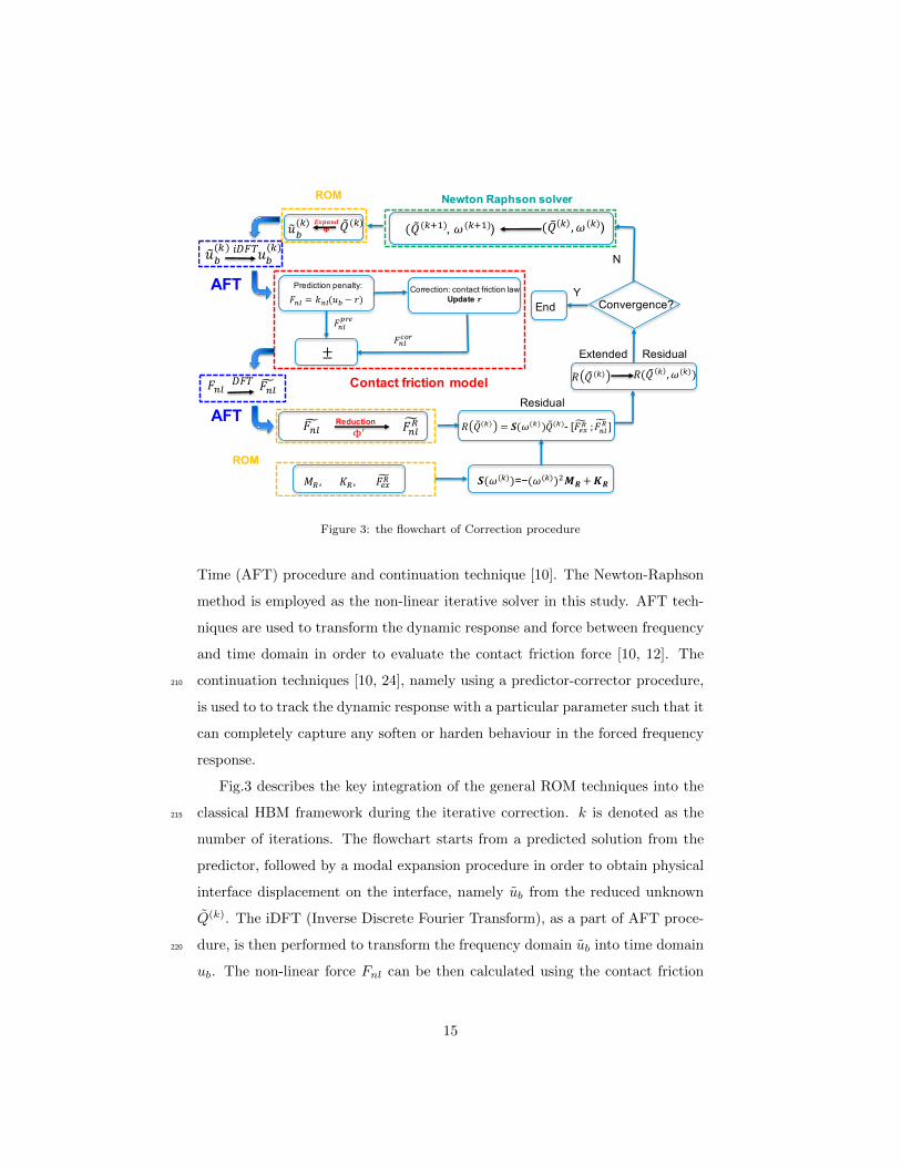
Figure 3: the flowchart of Correction procedure

Time (AFT) procedure and continuation technique [10]. The Newton-Raphson

method is employed as the non-linear iterative solver in this study. AFT tech-

niques are used to transform the dynamic response and force between frequency

and time domain in order to evaluate the contact friction force [10, 12]. The

continuation techniques [10, 24], namely using a predictor-corrector procedure,210

is used to to track the dynamic response with a particular parameter such that it

can completely capture any soften or harden behaviour in the forced frequency

response.

Fig.3 describes the key integration of the general ROM techniques into the

classical HBM framework during the iterative correction. k is denoted as the215

number of iterations. The flowchart starts from a predicted solution from the

predictor, followed by a modal expansion procedure in order to obtain physical

interface displacement on the interface, namely ub from the reduced unknown

Q(k). The iDFT (Inverse Discrete Fourier Transform), as a part of AFT proce-

dure, is then performed to transform the frequency domain ub into time domain220

ub. The non-linear force Fnl can be then calculated using the contact friction

15

Predictor(𝑄#$,𝜔$) = 𝑓$*+ 𝑄#,, 𝐽,, 𝜔,

Corrector(𝑄#,𝜔, 𝐽) = 𝑓.,*(𝑄#$,𝜔$,𝑀0,𝐾0 ,Φ,𝐹+40 )

𝐵 == (𝐵,)

Expand & Save (𝑄#, 𝜔)

Update (𝑄#,,𝜔,, 𝐽,, 𝐵,)=(𝑄# ,𝜔, 𝐽,𝐵)Update𝐵 for next solution by evaluating 𝐹78(Φ, 𝑄#,)

Update old solutions𝑄#,, 𝐽,with 𝐵

Update reduced system 𝑀0, 𝐾0,𝐹+40 , Φ with 𝐵

Classical continuation

Start with initial solution 𝑄#,, 𝜔,, 𝐵, 𝐽,

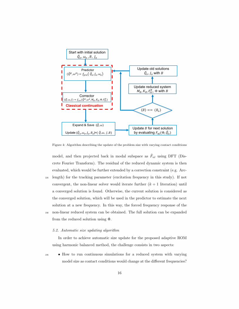
Figure 4: Algorithm describing the update of the problem size with varying contact conditions

model, and then projected back in modal subspace as Fnl using DFT (Dis-

crete Fourier Transform). The residual of the reduced dynamic system is then

evaluated, which would be further extended by a correction constraint (e.g. Arc-

length) for the tracking parameter (excitation frequency in this study). If not225

convergent, the non-linear solver would iterate further (k + 1 literation) until

a converged solution is found. Otherwise, the current solution is considered as

the converged solution, which will be used in the predictor to estimate the next

solution at a new frequency. In this way, the forced frequency response of the

non-linear reduced system can be obtained. The full solution can be expanded230

from the reduced solution using Φ.

5.2. Automatic size updating algorithm

In order to achieve automatic size update for the proposed adaptive ROM

using harmonic balanced method, the challenge consists in two aspects:

• How to run continuous simulations for a reduced system with varying235

model size as contact conditions would change at the different frequencies?

16

• How to predict the contact conditions accurately and efficiently based on

the current solution for the simulation at the next frequency point?

Fig.4 describes the proposed algorithm to achieve the automatic update of the

ROM size according to varying contact conditions during the continuous forced240

frequency analysis. The main feature consists in that the reduced system is

at most updated once at each frequency before the continuation is performed.

The updated reduced reduced model is determined based on the estimation of

contact conditions from the last convergent solution. The detailed procedure of

this algorithm is described in the following steps:245

1. The simulation starts with the initial converged solution (Qo, ωo) together

with Jacobean matrix Jo and the index matrix Bo that used to describe

the contact conditions of interface nodes in Eq.19. It is followed a stan-

dard continuation procedure that includes a prediction stage to get a pre-250

dicted solution (Qp, ωp) and a iterative correction stage to obtained the

converged solution (Q, ω) (shown in Fig.3). It is worth noting that the

size of reduced system would remain consistent during the predictor and

corrector procedure. Also, the contact force are only evaluated for those

predicted slipping or gapping nodes and the other would be assumed in a255

stick condition.

2. Once a converged solution is obtained at a new frequency ω, this solution

needs to be expanded and saved in a full reduced size including all the

zero components in ∆p. This is to make sure all the solutions are saved

in the same dimension that would be easy for post-procession. The old260

solution including (Qo, ωo, Bo, Jo) are also updated for the analysis at the

next frequency.

3. The index matrix B for the next solution at a new frequency needs to

be estimated before moving to the classical continuation procedure. It

is because the contact condition for interface nodes can be different due265

to the change of excitation frequency. In this algorithm, the estimation

17

of contact condition is performed by calling the non-linear contact force

function using the last converged solution Qo. The contact condition for

every contact node will be evaluated in order to sufficiently realize the

evolution of the slipping and gapping area on the contact interface.270

4. If the new B is not the same as the previous Bo, it means the contact

conditions have been changed from the last estimation. In this case, the

reduced system MR,KR,Φ, FRex needs to be updated according to new

B. Also, the size of last converged solution Qo, Jo need to be updated in

order to make the system size consistent. After that, the simulation would275

continue to the classical continuation procedure.

5. If the new B turns out exactly same as the last Bo, it means the the

contact conditions on the interface remain same. In this case, there is

no need to update the system and solution for the next simulation. The

process will directly jump to the classical continuation procedure at a280

continuously new frequency.

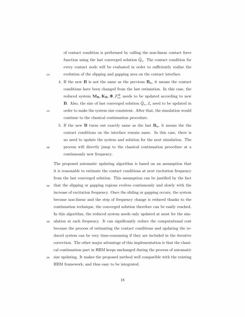
The proposed automatic updating algorithm is based on an assumption that

it is reasonable to estimate the contact conditions at next excitation frequency

from the last converged solution. This assumption can be justified by the fact

that the slipping or gapping regions evolves continuously and slowly with the285

increase of excitation frequency. Once the sliding or gapping occurs, the system

become non-linear and the step of frequency change is reduced thanks to the

continuation technique, the converged solution therefore can be easily reached.

In this algorithm, the reduced system needs only updated at most for the sim-

ulation at each frequency. It can significantly reduce the computational cost290

because the process of estimating the contact conditions and updating the re-

duced system can be very time-consuming if they are included in the iterative

correction. The other major advantage of this implementation is that the classi-

cal continuation part in HBM keeps unchanged during the process of automatic

size updating. It makes the proposed method well compatible with the existing295

HBM framework, and thus easy to be integrated.

18

No

No

Beam 1

Beam 2

Contact surface

x

Y

Figure 5: A 2D joint beam model

Most importantly, with the proposed method, huge computational cost spent

in correction stage can be saved. It is mainly because the size of reduced system

only retain the interface DOFs in a slipping or separating condition that would

be much less than the classical CMS based reduced model. The other reason300

is, instead of calculation the contact friction for all the interface nodes, the

calculation is only performed to those estimated slipping or gapping nodes.

6. Case study: 2D joint beam

6.1. Finite element model

Fig.5 shows a jointed beam model with linear springs connecting the two305

equivalent beam substructures. The length of each beam is 300 mm. The width

and height of the cross section is 25 mm and 6 mm respectively. They are

modelled by using the Euler-Bernoulli beam elements, where each node has

three DOFs (ux, uy, rz). The beams are made of steel with a nominal density of

7850kg/m3 and Young’s modulus of 2.1e11N.m−2. 250 Bernoulli beam elements310

are used for each beam. The contact interface modelled by Jenkin elements

involves 50 contact pairs, namely 300 contact friction DOFs. The total DOFs

of FE model is 1500. For the Jenkin element, the tangential and normal contact

stiffness kt, knis 1e3N/m. Uniform distribution is used for the pre-loading No

on the contact friction interface.315

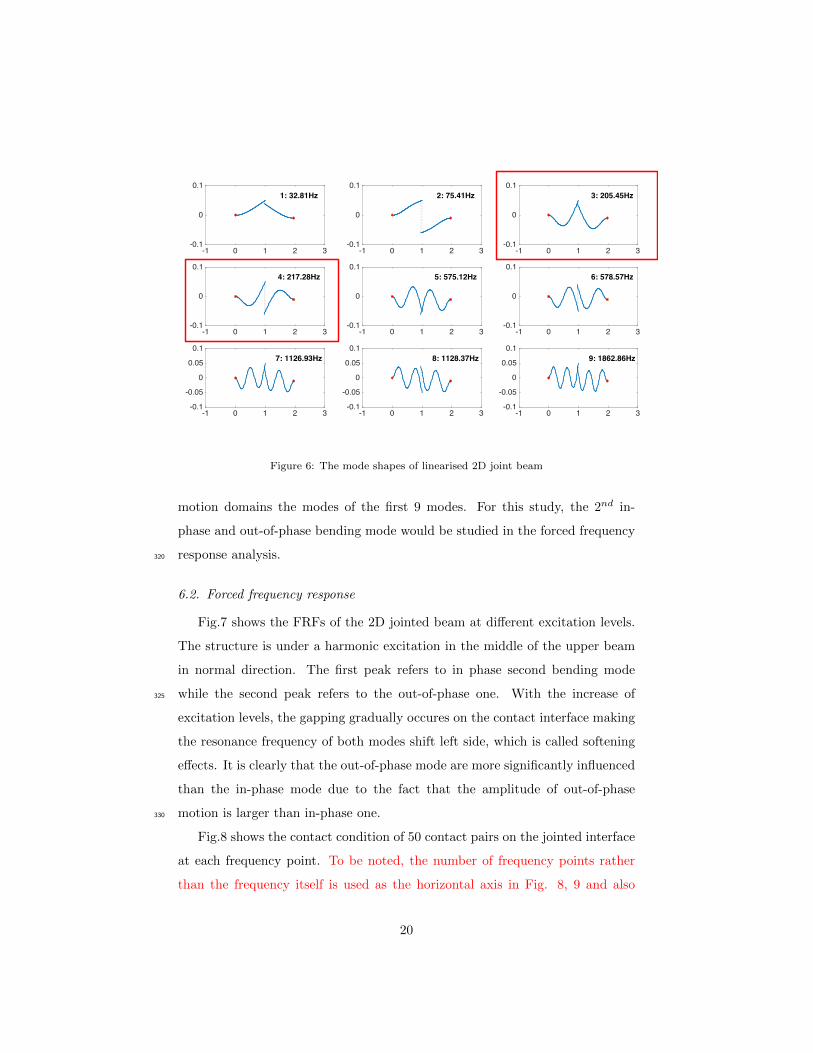
Fig.6 shows the first nine modes of the 2D linearised jointed beam system

assuming all the contact nodes are in a sticking condition. It shows the bending

19

-1 0 1 2 3-0.1

0

0.11: 32.81Hz

-1 0 1 2 3-0.1

0

0.12: 75.41Hz

-1 0 1 2 3-0.1

0

0.13: 205.45Hz

-1 0 1 2 3-0.1

0

0.14: 217.28Hz

-1 0 1 2 3-0.1

0

0.15: 575.12Hz

-1 0 1 2 3-0.1

0

0.16: 578.57Hz

-1 0 1 2 3-0.1

-0.05

0

0.05

0.17: 1126.93Hz

-1 0 1 2 3-0.1

-0.05

0

0.05

0.18: 1128.37Hz

-1 0 1 2 3-0.1

-0.05

0

0.05

0.19: 1862.86Hz

Figure 6: The mode shapes of linearised 2D joint beam

motion domains the modes of the first 9 modes. For this study, the 2nd in-

phase and out-of-phase bending mode would be studied in the forced frequency

response analysis.320

6.2. Forced frequency response

Fig.7 shows the FRFs of the 2D jointed beam at different excitation levels.

The structure is under a harmonic excitation in the middle of the upper beam

in normal direction. The first peak refers to in phase second bending mode

while the second peak refers to the out-of-phase one. With the increase of325

excitation levels, the gapping gradually occures on the contact interface making

the resonance frequency of both modes shift left side, which is called softening

effects. It is clearly that the out-of-phase mode are more significantly influenced

than the in-phase mode due to the fact that the amplitude of out-of-phase

motion is larger than in-phase one.330

Fig.8 shows the contact condition of 50 contact pairs on the jointed interface

at each frequency point. To be noted, the number of frequency points rather

than the frequency itself is used as the horizontal axis in Fig. 8, 9 and also

20

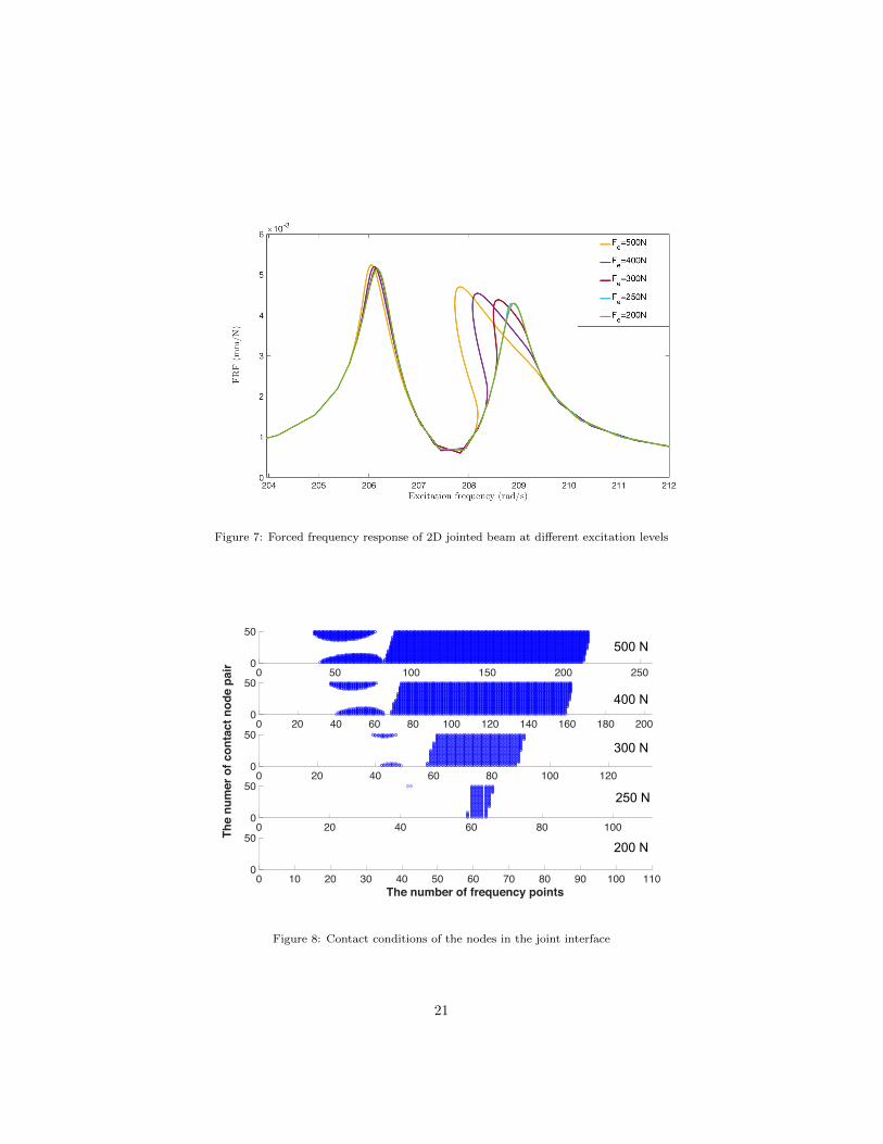
Figure 7: Forced frequency response of 2D jointed beam at different excitation levels

0 50 100 150 200 2500

50

0 20 40 60 80 100 120 140 160 180 2000

50

0 20 40 60 80 100 1200

50

The

num

er o

f con

tact

nod

e pa

ir

0 20 40 60 80 1000

50

0 10 20 30 40 50 60 70 80 90 100 110The number of frequency points

0

50

500 N

400 N

300 N

250 N

200 N

Figure 8: Contact conditions of the nodes in the joint interface

21

0 50 100 150 200 2500

5001000

0 20 40 60 80 100 120 140 160 180 2000

5001000

0 20 40 60 80 1000

5001000

The

size

of r

educ

ed s

yste

m

0 10 20 30 40 50 60 70 80 90 100 110The number of frequency points

05001000

0 20 40 60 80 100 1200

5001000

500 N

400 N

300 N

250 N

200 N

Figure 9: Automatic updated size of the system during the continuation

in Fig.14, 16. It is because that the corresponding forced response point for

a frequency close to the resonance might not be unique due to the soften or335

harden effects. For example, in Fig.7, at the frequency of 208 Hz, there are 3

corresponding forced response points due to the soften effect. As expected, in

this 2D case, there is no slipping state on the contact nodes because the normal

and tangential motion is decoupled. The blue point means the gapping occurs

on the contact interface. The area of the gapping zone expands gradually with340

the increase of excitation force level Fo. For the in-phase mode, the gapping

propagates slowly from both edges of the interface toward the centre part of

the interface. For the out-of-phase mode, the gapping expands quickly from

one edge to the other and the joint interface becomes completely open at large

excitation levels.345

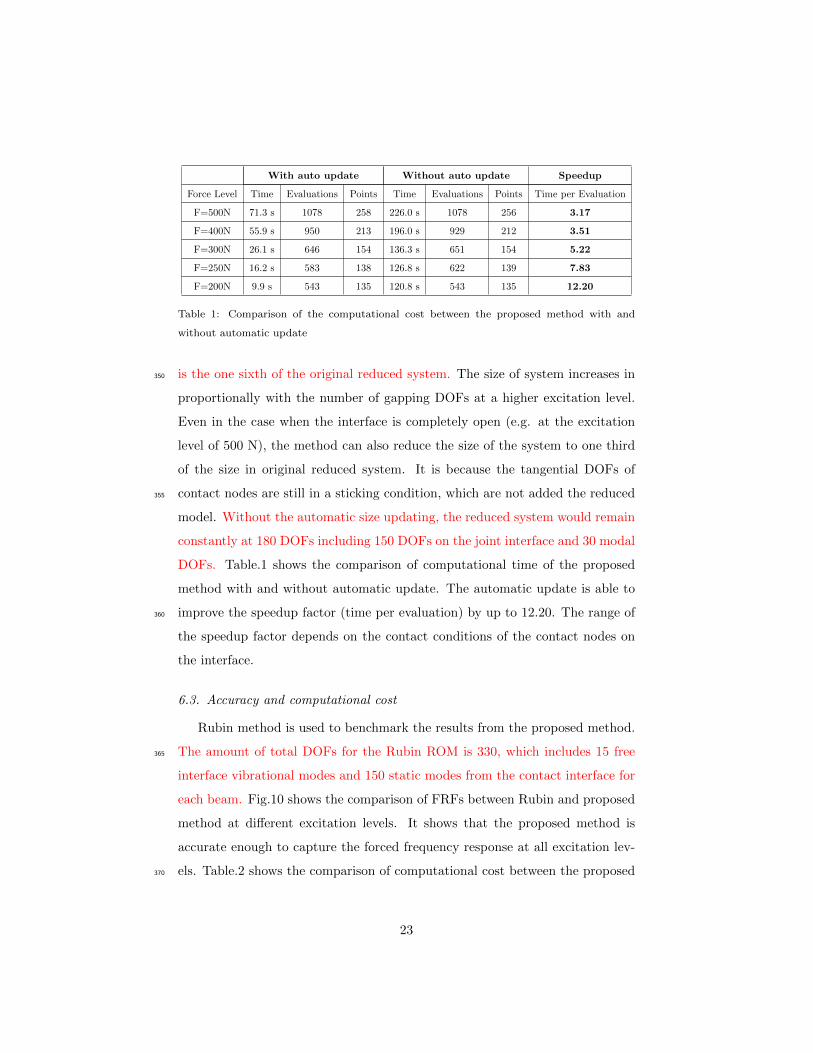
Fig.9 shows the size of a reduced system using the proposed method with

automatic updating algorithm. The size of system can be effectively updated at

each frequency point according to the contact conditions in Fig.8. At the exci-

tation level of 200 N, the DOFs of reduced system reaches minimum 30, which

22

With auto update Without auto update Speedup

Force Level Time Evaluations Points Time Evaluations Points Time per Evaluation

F=500N 71.3 s 1078 258 226.0 s 1078 256 3.17

F=400N 55.9 s 950 213 196.0 s 929 212 3.51

F=300N 26.1 s 646 154 136.3 s 651 154 5.22

F=250N 16.2 s 583 138 126.8 s 622 139 7.83

F=200N 9.9 s 543 135 120.8 s 543 135 12.20

Table 1: Comparison of the computational cost between the proposed method with and

without automatic update

is the one sixth of the original reduced system. The size of system increases in350

proportionally with the number of gapping DOFs at a higher excitation level.

Even in the case when the interface is completely open (e.g. at the excitation

level of 500 N), the method can also reduce the size of the system to one third

of the size in original reduced system. It is because the tangential DOFs of

contact nodes are still in a sticking condition, which are not added the reduced355

model. Without the automatic size updating, the reduced system would remain

constantly at 180 DOFs including 150 DOFs on the joint interface and 30 modal

DOFs. Table.1 shows the comparison of computational time of the proposed

method with and without automatic update. The automatic update is able to

improve the speedup factor (time per evaluation) by up to 12.20. The range of360

the speedup factor depends on the contact conditions of the contact nodes on

the interface.

6.3. Accuracy and computational cost

Rubin method is used to benchmark the results from the proposed method.

The amount of total DOFs for the Rubin ROM is 330, which includes 15 free365

interface vibrational modes and 150 static modes from the contact interface for

each beam. Fig.10 shows the comparison of FRFs between Rubin and proposed

method at different excitation levels. It shows that the proposed method is

accurate enough to capture the forced frequency response at all excitation lev-

els. Table.2 shows the comparison of computational cost between the proposed370

23

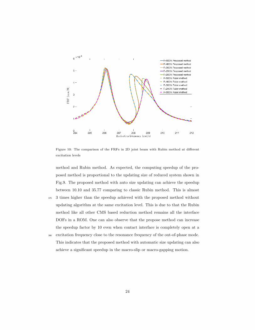
Figure 10: The comparison of the FRFs in 2D joint beam with Rubin method at different

excitation levels

method and Rubin method. As expected, the computing speedup of the pro-

posed method is proportional to the updating size of reduced system shown in

Fig.9. The proposed method with auto size updating can achieve the speedup

between 10.10 and 35.77 comparing to classic Rubin method. This is almost

3 times higher than the speedup achieved with the proposed method without375

updating algorithm at the same excitation level. This is due to that the Rubin

method like all other CMS based reduction method remains all the interface

DOFs in a ROM. One can also observe that the propose method can increase

the speedup factor by 10 even when contact interface is completely open at a

excitation frequency close to the resonance frequency of the out-of-phase mode.380

This indicates that the proposed method with automatic size updating can also

achieve a significant speedup in the macro-slip or macro-gapping motion.

24

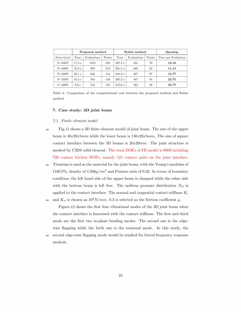
Proposed method Rubin method Speedup

Force Level Time Evaluations Points Time Evaluations Points Time per Evaluation

F=500N 71.3 s 1078 258 297.4 s 445 79 10.10

F=400N 55.9 s 950 213 301.5 s 460 82 11.14

F=300N 26.1 s 646 154 310.3 s 487 87 15.77

F=250N 16.2 s 583 138 295.2 s 467 85 22.75

F=200N 9.9 s 543 135 315.0 s 483 89 35.77

Table 2: Comparison of the computational cost between the proposed method and Rubin

method

7. Case study: 3D joint beam

7.1. Finite element model

Fig.11 shows a 3D finite element model of joint beam. The size of the upper385

beam is 40x20x5mm while the lower beam is 140x20x5mm. The size of square

contact interface between the 3D beams is 20x20mm. The joint structure is

meshed by C3D8 solid element. The total DOFs of FE model is 9009 including

726 contact friction DOFs, namely 121 contact pairs on the joint interface.

Titanium is used as the material for the joint beam, with the Young’s modulus of390

116GPa, density of 4.506g/cm3 and Poisson ratio of 0.32. In terms of boundary

condition, the left hand side of the upper beam is clamped while the other side

with the bottom beam is left free. The uniform pressure distribution NO is

applied to the contact interface. The normal and tangential contact stiffness Kt

and Kn is chosen as 103N/mm. 0.3 is selected as the friction coefficient µ.395

Figure.12 shows the first four vibrational modes of the 3D joint beam when

the contact interface is linearised with the contact stiffness. The first and third

mode are the first two in-plane bending modes. The second one is the edge-

wise flapping while the forth one is the torsional mode. In this study, the

second edge-wise flapping mode would be studied for forced frequency response400

analysis.

25

Figure 11: A finite element model of 3D joint beam

Mode4First Torsion13950Hz

Mode3Second in-plane flapping6060Hz

Mode2First edge-wise flapping3260 Hz

Mode1First in-plane flapping1010 Hz

Figure 12: Mode shapes of the 3D joint beam

26

3100 3150 3200 3250 3300 3350 3400Excitation frequency (rad/s)

0

0.05

0.1

0.15

0.2

0.25

0.3

0.35

0.4

0.45

FRF

(mm

/N)

F=3 N

F=1 N

F=0.5N

F=0.3N

F=0.1 N

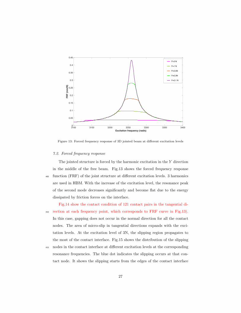
Figure 13: Forced frequency response of 3D jointed beam at different excitation levels

7.2. Forced frequency response

The jointed structure is forced by the harmonic excitation in the Y direction

in the middle of the free beam. Fig.13 shows the forced frequency response

function (FRF) of the joint structure at different excitation levels. 3 harmonics405

are used in HBM. With the increase of the excitation level, the resonance peak

of the second mode decreases significantly and become flat due to the energy

dissipated by friction forces on the interface.

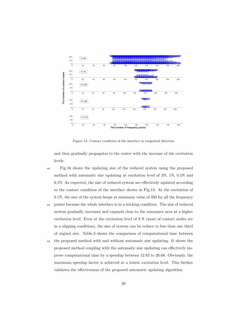
Fig.14 show the contact condition of 121 contact pairs in the tangential di-

rection at each frequency point, which corresponds to FRF curve in Fig.13).410

In this case, gapping does not occur in the normal direction for all the contact

nodes. The area of micro-slip in tangential directions expands with the exci-

tation levels. At the excitation level of 3N, the slipping region propagates to

the most of the contact interface. Fig.15 shows the distribution of the slipping

nodes in the contact interface at different excitation levels at the corresponding415

resonance frequencies. The blue dot indicates the slipping occurs at that con-

tact node. It shows the slipping starts from the edges of the contact interface

27

0 20 40 60 80 100 120 140 160 180 2000

50

100

0 20 40 60 80 100 120 140 160 180 2000

50

100

0 20 40 60 80 100 120 140 160 180 2000

50

100

0 20 40 60 80 100 120 140 160 180 2000

50

100

0 20 40 60 80 100 120 140 160 180 200The number of frequency points

0

50

100

The

num

ber o

f con

tact

nod

es

F= 3N

F= 1N

F= 0.5N

F= 0.3N

F= 0.1N

Figure 14: Contact condition of the interface in tangential direction

and then gradually propagates to the centre with the increase of the excitation

levels.

Fig.16 shows the updating size of the reduced system using the proposed420

method with automatic size updating at excitation level of 3N, 1N, 0.5N and

0.1N. As expected, the size of reduced system are effectively updated according

to the contact condition of the interface shown in Fig.13. At the excitation of

0.1N, the size of the system keeps at minimum value of 350 for all the frequency

points because the whole interface is in a sticking condition. The size of reduced425

system gradually increases and expands close to the resonance area at a higher

excitation level. Even at the excitation level of 3 N (most of contact nodes are

in a slipping condition), the size of system can be reduce to less than one third

of orginal size. Table.3 shows the comparison of computational time between

the proposed method with and without automatic size updating. It shows the430

proposed method coupling with the automatic size updating can effectively im-

prove computational time by a speedup between 12.83 to 26.68. Obviously, the

maximum speedup factor is achieved at a lowest excitation level. This further

validates the effectiveness of the proposed automatic updating algorithm.

28

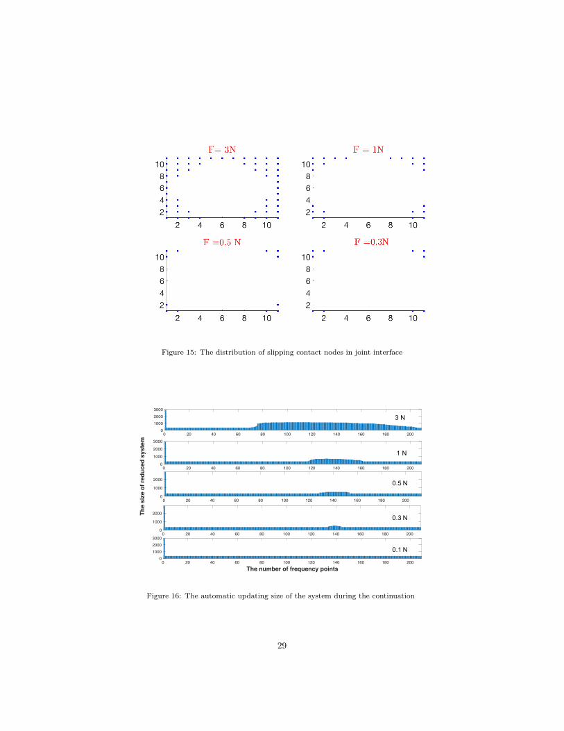
Figure 15: The distribution of slipping contact nodes in joint interface

0 20 40 60 80 100 120 140 160 180 2000

100020003000

0 20 40 60 80 100 120 140 160 180 2000

1000

2000

3000

0 20 40 60 80 100 120 140 160 180 2000

1000

2000

0 20 40 60 80 100 120 140 160 180 200The number of frequency points

0100020003000

The

size

of r

educ

ed s

yste

m

0 20 40 60 80 100 120 140 160 180 2000

1000

2000

3 N

1 N

0.5 N

0.3 N

0.1 N

Figure 16: The automatic updating size of the system during the continuation

29

With auto update Without auto update Speedup

Force Level Time Evaluations Points Time Evaluations Points Time per Evaluation

F=3N 554.5 s 1332 209 3547.5 s 664 209 12.83

F=1N 162.2 s 679 209 3633.2 s 672 209 22.63

F=0.5N 149.7 s 718 213 3693.5 s 683 209 25.94

F=0.3N 143.6 s 706 209 3858.5 s 711 211 26.68

F=0.1N 138.5 s 664 209 3572.7 s 643 209 26.68

Table 3: Comparison of the computational cost between the proposed method with and

without automatic update

Proposed method Rubin method Speedup

Force Level Time Evaluations Points Time Evaluations Points Time per Evaluation

F=3N 554.5 s 1332 209 7790.7 s 424 58 44.14

F=1N 162.2 s 679 209 3946.2 s 223 37 74.08

F=0.5N 149.7 s 718 213 5882.3 s 309 54 91.30

F=0.3N 143.6 s 706 209 7264.4 s 391 72 91.33

F=0.1N 138.5 s 664 209 6970.5 s 362 363 92.32

Table 4: Comparison of the computational cost between the proposed method and Rubin

method

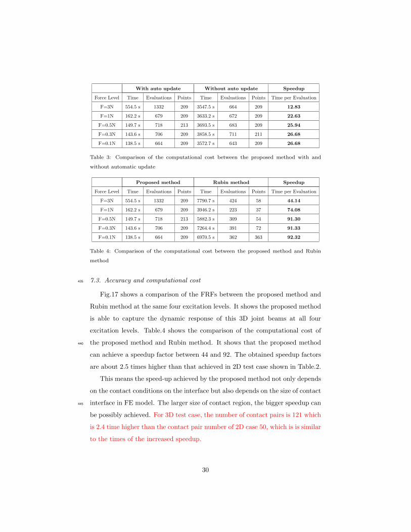
7.3. Accuracy and computational cost435

Fig.17 shows a comparison of the FRFs between the proposed method and

Rubin method at the same four excitation levels. It shows the proposed method

is able to capture the dynamic response of this 3D joint beams at all four

excitation levels. Table.4 shows the comparison of the computational cost of

the proposed method and Rubin method. It shows that the proposed method440

can achieve a speedup factor between 44 and 92. The obtained speedup factors

are about 2.5 times higher than that achieved in 2D test case shown in Table.2.

This means the speed-up achieved by the proposed method not only depends

on the contact conditions on the interface but also depends on the size of contact

interface in FE model. The larger size of contact region, the bigger speedup can445

be possibly achieved. For 3D test case, the number of contact pairs is 121 which

is 2.4 time higher than the contact pair number of 2D case 50, which is is similar

to the times of the increased speedup.

30

3100 3150 3200 3250 3300 3350 3400Excitation frequency (rad/s)

0

0.05

0.1

0.15

0.2

0.25

0.3

0.35

0.4

0.45

FRF

(mm

/N)

F= 3N Proposed method F= 1N Proposed method F=0.5N Proposed method F=0.3N Proposed method F=0.1N Proposed method F= 3N Rubin method F= 1N Rubin method F=0.5N Rubin method F=0.3N Rubin method F=0.1N Rubin method

Figure 17: The comparison of the FRF with Hybrid method

8. Conclusions

A novel adaptive ROM technique for dynamic analysis of the jointed struc-450

ture with contact friction interfaces has been presented. The main feature of

the proposed method is that the reduced model can be automatically update its

size according to the contact condition of contact interface nodes, which is able

to significantly reduce the size of state of the art CMS based reduced models.

The idea of the proposed ROM method mainly consists in a new formulation of455

dynamic system that combines a linearised joint system with an internal penalty

variable that accounts non-linear effects introduced by the slipping or separation

phenomenons on the joint interfaces. This makes the resulting reduced order

model able to only includes the contact DOFs in a slip or gap condition in its

reduced basis. A enormous reduction can be achieved for the jointed structure460

as most of their interface nodes are in a stick condition for jointed structures. To

achieve the automatic size updating with the non-linear solver, a new algorithm

to update its model size according to the varying contact condition has been

presented. The proposed algorithm is well compatible with classic continuation

31

techniques making it easy to be implemented, and able to accurately estimate465

the contact condition for the next solution at a continuous excitation frequency.

The proposed method has been tested in two distinct case studies, one with a

2D jointed beam and the other with a 3D joint beam. As expected, for both case

studies, the proposed method is able to automatically update size of reduced

system according to the contact conditions of nodes on the joint interface. For470

the forced response analysis, a significant speedup has been achieved for both

studies at different excitation levels. The maximum computing speedup, 36 for

the 2D case and 92 for the 3D case, occurs when the whole contact interface is

in a stick condition. However, even when the contact interface is mostly in a

slipping/gapping condition, the proposed method can still achieve speed up of475

10 for the 2D case and 40 for the 3D case. This is mainly because that the size

of reduced system is still comparably less than benchmarking Rubin method via

removing the interface linear DOFs from the other directions, e.g. the normal

contact DOFs can be still removed in a slip condition. Thanks to the proposed

updating algorithm, the proposed ROM techniques works very well with popular480

harmonic balanced method for spectral analysis. The implementation of the

updating algorithm is simple because the classical continuation part can remain

unaffected.

The results also suggest that the efficiency of the proposed techniques de-

pends not only on excitation levels but also on the size of contact friction in-485

terface. The larger the size of contact interface is, the bigger the computing

speedup can be achieved. In this study, the speedup factor for 3D case is al-

most 3 times higher than that for 2D case. The speedup ratio is similar to the

ratio of contact size between 3D and 2D case. With respect to the accuracy,

the proposed ROM method is able to accurately capture the forced frequency490

response at all the excitation levels for both case studies. This study proves

that the proposed adaptive reduction technique can significantly improve the

computational efficiency of CMS based reduction method for the prediction of

dynamics of joint structures. The study also validates that the proposed auto-

matic size updating algorithm can work very well with HBM and the proposed495

32

ROM technique.

Acknowledgement

The authors would like to acknowledge the support of Rolls-Royce plc and

Innovate UK through GEMiniDS WP3 -Innovate UK Project 113088.

References500

[1] C. Schwingshackl, E. Petrov, D. Ewins, Measured and estimated friction

interface parameters in a nonlinear dynamic analysis, Mechanical Systems

and Signal Processing 28 (2012) 574–584.

[2] M. R. W. Brake, D. J. Ewins, C. B. Wynn, Are Joints Necessary?, Springer

International Publishing, Cham, 2018, pp. 25–36.505

[3] H. G. D. Goyder, Damping Due to Joints in Built-Up Structures, Springer

International Publishing, Cham, 2018, pp. 135–147.

[4] B. Titurus, J. Yuan, F. Scarpa, S. Patsias, S. Pattison, Impact hammer-

based analysis of nonlinear effects in bolted lap joint, in: Proceedings of the

ISMA 2016 International Conference on Noise and Vibration Engineering,510

KU Leuven, Departement Werktuigkunde, 2016, pp. 789–801.

[5] R. Lacayo, L. Pesaresi, J. Groß, D. Fochler, J. Armand, L. Salles,

C. Schwingshackl, M. Allen, M. Brake, Nonlinear modeling of structures

with bolted joints: A comparison of two approaches based on a time-domain

and frequency-domain solver, Mechanical Systems and Signal Processing515

114 (2019) 413–438.

[6] S. Bograd, P. Reuss, A. Schmidt, L. Gaul, M. Mayer, Modeling the dynam-

ics of mechanical joints, Mechanical Systems and Signal Processing 25 (8)

(2011) 2801–2826.

33

[7] N. M. Ames, J. P. Lauffer, M. D. Jew, D. J. Segalman, D. L. Gregory,520

M. J. Starr, B. R. Resor, Handbook on dynamics of jointed structures.,

Tech. rep., Sandia National Laboratories (2009).

[8] S. Huang, Dynamic analysis of assembled structures with nonlinearity,

Ph.D. thesis, Dynamics group, Department of Mechanical Engineering, Im-

perial College London (2008).525

[9] E. Petrov, A high-accuracy model reduction for analysis of nonlinear vibra-

tions in structures with contact interfaces, Journal of Engineering for Gas

Turbines and Power 133 (10) (2011) 102503.

[10] M. Krack, L. Salles, F. Thouverez, Vibration prediction of bladed disks cou-

pled by friction joints, Archives of Computational Methods in Engineering530

24 (3) (2017) 589–636.

[11] M. R. W. Brake, J. Groß, R. M. Lacayo, L. Salles, C. W. Schwingshackl,

P. Reuß, J. Armand, Reduced Order Modeling of Nonlinear Structures with

Frictional Interfaces, Springer International Publishing, Cham, 2018, pp.

427–450.535

[12] J. Yuan, F. El-Haddad, L. Salles, C. Wong, Numerical assessment of re-

duced order modeling techniques for dynamic analysis of jointed structures

with contact nonlinearities, Journal of Engineering for Gas Turbines and

Power 141 (3) (2019) 031027.

[13] G. Battiato, C. Firrone, T. Berruti, B. Epureanu, Reduction and coupling540

of substructures via gram–schmidt interface modes, Computer Methods in

Applied Mechanics and Engineering 336 (2018) 187–212.

[14] J. Yuan, F. Scarpa, G. Allegri, B. Titurus, S. Patsias, R. Rajasekaran,

Efficient computational techniques for mistuning analysis of bladed discs:

A review, Mechanical Systems and Signal Processing 87 (2017) 71–90.545

34

[15] R. Pinnau, Model reduction via proper orthogonal decomposition, in:

Model Order Reduction: Theory, Research Aspects and Applications,

Springer, 2008, pp. 95–109.

[16] S. Zucca, B. I. Epureanu, Reduced order models for nonlinear dynamic

analysis of structures with intermittent contacts, Journal of Vibration and550

Control 24 (12) (2018) 2591–2604.

[17] S. Rubin, Improved component-mode representation for structural dynamic

analysis, AIAA journal 13 (8) (1975) 995–1006.

[18] R. Craig, M. Bampton, Coupling of substructures for dynamic analyses,

AIAA journal 6 (7) (1968) 1313–1319.555

[19] W. Witteveen, H. Irschik, Efficient mode based computational approach

for jointed structures: joint interface modes, AIAA Journal 47 (1) (2009)

252–263.

[20] J. Becker, L. Gaul, Cms methods for efficient damping prediction for struc-

tures with friction, Proceedings of the IMAC-XXVI, Orlando.560

[21] L. Gaul, J. Becker, Damping prediction of structures with bolted joints,

Shock and Vibration 17 (4-5) (2010) 359–371.

[22] J. Yuan, L. Salles, C. Wong, S. Patsias, A novel penalty-based reduced order

modelling method for dynamic analysis of joint structures, in: IUTAM

Symposium on Model Order Reduction of Coupled Systems, Stuttgart,565

Germany, May 22-25, 2018.

[23] F. M. Gruber, D. J. Rixen, Evaluation of substructure reduction techniques

with fixed and free interfaces, Strojniski vestnik-Journal of Mechanical En-

gineering 62 (7-8) (2016) 452–462.

[24] E. Sarrouy, J.-J. Sinou, Non-linear periodic and quasi-periodic vibrations570

in mechanical systems-on the use of the harmonic balance methods, in:

Advances in Vibration Analysis Research, InTech, 2011.

35