Allocative Efficiency Measurement Revisited: Do We Really Need Input Prices? Discussion Papers

Oleg Badunenko Michael Fritsch Andreas Stephan

Allocative Efficiency Measurement Revisited: Do We Really Need Input Prices?

Discussion Papers

Berlin, June 2006

Opinions expressed in this paper are those of the author and do not necessarily reflect views of the Institute. IMPRESSUMDIW Berlin, 2006 German Institute for Economic Research Königin-Luise-Str. 5 14195 Berlin Tel. +49 (30) 897 89-0 Fax +49 (30) 897 89-200 http://www.diw.de ISSN print edition 1433-0210 ISSN electronic edition 1619-4535 Available for free downloading from the DIW Berlin website.

Discussion Papers 591

Oleg Badunenko (corresponding author)* Michael Fritsch** Andreas Stephan*** Allocative Efficiency Measurement Revisited – Do We Really Need Input Prices? The research on this project has benefited from the comments of participants of the Royal Economic Society Conference (2005), 3d International Industrial Organization Conference (2005), the 10th Spring Meeting of Young Economists (2005), and the IX European Workshop on Efficiency and Productivity Analysis (2005) Berlin, June 2006 * European University Viadrina, [email protected] ** DIW Berlin, Technical University of Freiberg, Max-Planck Institute of Economics, Jena,

[email protected] *** DIW Berlin, European University Viadrina, astephan @euv-ffo.de

I

Abstract

The traditional approach to measuring allocative efficiency is based on input prices, which are rarely

known at the firm level. This paper proposes a new approach to measure allocative efficiency which is

based on the output-oriented distance to the frontier in a profit – technical efficiency space – and

which does not require information on input prices. To validate the new approach, we perform a

Monte-Carlo experiment which provides evidence that the estimates of the new and the traditional

approach are highly correlated. Finally, as an illustration, we apply the new approach to a sample of

about 900 enterprises from the chemical industry in Germany.

Keywords: Allocative efficiency, data envelopment analysis, frontier analysis, technical efficiency,

Monte-Carlo study, chemical industry.

JEL Classification: D61, L23, L25, L65

Zusammenfassung

“Ein neuer Ansatz zur Messung allokativer Effizienz – Sind Input-Preise wirklich erforderlich?“

Der traditionelle Ansatz zur Messung allokativer Effizienz erfordert Informationen über Input-Preise

der Unternehmen, die allerdings nur selten vorliegen. In diesem Aufsatz schlagen wir eine neue

Methode zur Bestimmung der allokativen Effizienz vor, der als wesentliche Information den Abstand

eines Unternehmens von der Effizienz-Grenze nutzt und keine Information über Input-Preise erfordert.

Ein Monte-Carlo Experiment zur Überprüfung der Tragfähigkeit dieses Ansatzes zeigt, dass die

Schätzwerte nach der traditionellen Methode und dem von uns vorgeschlagenen Verfahren eng

miteinander korreliert sind. Zur Illustration wenden wir den neuen Ansatz auf ein Sample von 900

Unternehmen der Chemischen Industrie in Deutschland an.

Schlagworte: Allokative Effizienz, Data Envelopment Analysis, Frontier Analysis, Technische

Effizienz, Monte-Carlo Methode, Chemische Industrie.

JEL-Klassifikation: D61, L23, L25, L65

II

Discussion Papers 591 Inhaltsverzeichnis

Inhaltsverzeichnis

1 Introduction ...................................................................................................................................... 1

2 Allocative efficiency measurement ................................................................................................. 2 2.1 Traditional approach to allocative efficiency measurement .......................................... 2 2.2 A new approach to allocative efficiency measurement ................................................. 3

3 Monte-Carlo simulation................................................................................................................... 7 3.1 Empirical implementation of the traditional approach .................................................. 7 3.2 Empirical implementation of the new approach ............................................................ 8 3.3 Design of the Monte-Carlo experiments........................................................................ 8 3.4 Results.......................................................................................................................... 10

4 Empirical illustration of the new approach ................................................................................. 18 4.1 Data 18 4.2 Results.......................................................................................................................... 19

5 Conclusions ..................................................................................................................................... 21

I

Discussion Papers 591 Verzeichnis der Tabellen

Verzeichnis der Tabellen

Table 1 Rank correlations, 5.0=ε , 100=N ................................................................................ 10 Table 2 Rank correlations, 1=ε , 100=N .................................................................................... 11 Table 3 Rank correlations, 2=ε , 100=N ................................................................................... 11 Table 4 Rank correlations, 5.0=ε , 400=N ................................................................................ 13 Table 5 Rank correlations, 1=ε , 400=N ................................................................................... 13 Table 6 Rank correlations, 2=ε , 400=N ................................................................................... 14 Table 7 Descriptive statistics of technical and allocative efficiency, N=905................................... 20

Verzeichnis der Abbildungen

Figure 1 Measurement and decomposition of cost efficiency ............................................................. 2 Figure 2 Bound of a profit ................................................................................................................... 4 Figure 3 Relationship between technical efficiency and profit ........................................................... 5 Figure 4 Allocative efficiency in profit-technical efficiency space..................................................... 6 Figure 5 Estimates of Sampling Densities of Corr2 ( 75.0=θ , 500=L , 5.0=ε , 1=ε and

2=ε ) ................................................................................................................................. 12 Figure 6 Allocative efficiency calculated using traditional and new approaches plotted against

ratio of expenditure shares, w 1122 / xwx ( 75.0=θ , 400=N , 5.0=ε , 1=ε and 2=ε ) ................................................................................................................................. 15

Figure 7 Profitability plotted against estimated technical efficiency scores for about 900 German enterprises from the chemical industry.................................................................. 19

Figure 8 Estimates of sampling densities of technical and allocative efficiency scores.................... 20

II

Discussion Papers 591 1 Introduction

1 Introduction

A significant number of empirical studies have investigated the extent and determinants of technical

efficiency within and across industries (see Alvarez and Crespi (2003), Gumbau-Albert and Maudos

(2002), Caves and Barton (1990), Green and Mayes (1991), Fritsch and Stephan (2004a)).

Comprehensive literature reviews of the variety of empirical applications are made by Lovell (1993)

and Seiford (1996, 1997). Compared to this literature, attempts to quantify the extent and distribution

of allocative efficiency are relatively rare (for a survey, see Greene (1997)).1 This is quite surprising

since allocative efficiency has traditionally attracted the attention of economists: what is the optimal

combination of inputs so that output is produced at minimal cost? How much could the profits be

increased by simply reallocating resources? To what extent does competitive pressure reduce the

heterogeneity of allocative inefficiency within industries?2

A firm is said to have realized allocative efficiency if it is operating with the optimal combination of

inputs. The traditional approach to measuring allocative efficiency requires input prices (see Atkinson

and Cornwell (1994), Green (1997), Kumbhakar (1991), Kumbhakar and Tsionas (2005), Oum and

Zhang (1995)) which are hardly available in reality.3 This explains why empirical studies of allocative

efficiency are highly concentrated on certain industries, particularly banking, because information on

input price can be obtained for these industries.

This paper introduces a new approach to estimating allocative efficiency, which is solely based on

quantities and profits and does not require information on input prices. An indicator for allocative

efficiency is derived as the output-oriented distance to a frontier in a profit-technical efficiency space.

What is, however, needed is an assessment of input-saving technical efficiency; i.e., how less input

could be used to produce given outputs.

The paper proceeds as follows: section 2 theoretically derives a new method for estimating allocative

efficiency and introduces a theoretical framework for activity analysis models. Section 3 presents the

results of the Monte-Carlo experiment on comparison of allocative efficiency scores calculated using

both traditional and new approaches. Section 4 provides a rationale and a simple illustration using the

new approach; section 5 concludes.

1 For studies in the financial sector, see the review by Berger and Humphrey (1997) and also Topuz et al. (2005), Färe et al. (2004), Isik and Hassan (2002). Some studies have been performed for the agricultural sector (e.g., Coelli et al., (2002), Chavas et al., (1993, 2005), Grazhdaninova (2005)). Studies for manufacturing sector are relatively rare (e.g., Burki (1997), Kim and Han (2001)). 2 Moreover, allocative efficiency is also import for the analysis of the production process; e.g., to estimate the bias of (i) the cost function parameters, (ii) returns to scale, (iii) input price elasticities, and (iv) cost-inefficiency (Kumbhakar and Wang, forthcoming) or to validate the aggregation of productivity index (Raa (2005)). 3 This includes retrieving allocative efficiency using shadow prices (see Green (1997), Lovell (1993)).

1

Discussion Papers 591 2 Allocative efficiency measurement

2 Allocative efficiency measurement

2.1 Traditional approach to allocative efficiency measurement

A definition of technical and allocative efficiency was made by Farrell (1957). According to this

definition, a firm is technically efficient if it uses the minimal possible combination of inputs for

producing a certain output (input orientation). Allocative efficiency, or as Farrell called it price

efficiency, refers to the ability of a firm to choose the optimal combination of inputs given input

prices. If a firm has realized both technical and allocative efficiency, it is then cost efficient (overall

efficient).

Figure 1 Measurement and decomposition of cost efficiency

Figure 1, similarly to Kumbhakar and Lovell (2000), shows firm A producing output yA represented by

the isoquant L(yA). Dotted lines are the isocosts which show level of expenditures for a certain

combination of inputs. The slope of the isocosts is equal to the ratio of input prices, w(w1,w2). If the

firm is producing output yA with the factor combination xA (a in Figure 1), it is operating technically

inefficient. Potentially, it could produce the same output contracting both inputs x1 and x2 (available at

prices w), proportionally (radial approach); the smallest possible contraction is in point b, representing

(θxA) a factor combination. Having reached this point, the firm is considered to be technically

efficient. Formally, technical efficiency is measured by the ratio of the current input level to the lowest

attainable input level for producing a given amount of output. In terms of Figure 1, technical

inefficiency of unit xA is given by

2


( ) ( )A

AAA

wxxwxyTE θθ ==, (1)

or geometrically by ob/oa. The measure of cost inefficiency (overall efficiency) is given by the ratio of

potentially minimal cost to actual cost:

( ) A

EAAA

wxwxwxyCE =,, (2)

or geometrically by oc/oa. Thus, cost inefficiency is the ratio of expenditures at xE to expenditures at

xA while technical efficiency is the ratio of expenditures at (θxA) to expenditures at xA. The remaining

portion of the cost efficiency is given by the ratio of expenditures at xE to expenditures at (θxA). It is

attributable to the misallocation of inputs given input prices and is known as allocative efficiency:

( )A

A

AE

wxxw

wxwx

TECEAE

θ== (3)

or in terms of Figure 1 is given by oc/ob.

2.2 A new approach to allocative efficiency measurement

When input prices are available, allocative efficiency in the pure Farrell sense can be calculated using,

for example, a non-parametric frontier approach (Färe et al., 1994) or a parametric one (Greene (1997)

among others). However, if input prices are not available these approaches are not applicable. In

contrast to this, the new approach we propose allows measuring allocative efficiency without

information on input prices. An estimate of allocative efficiency can be obtained with the new

approach that is solely based on information on input and output quantities and on profits.

The first step of this new approach involves the estimation of technical efficiency; whereby, in the

second step allocative efficiency is estimated as an output-oriented distance to the frontier in a profit-

technical efficiency space.

In Figure 2, three firms, A, B, and C using inputs xA, xB, and xC, available at prices w,4 produce output

yA, which is measured by the isoquant L(yA). For the sake of argument, firms A, B, and C are all

equally technically efficient (the level of technical efficiency θ, however, is arbitrarily chosen) which

is read from expenditure levels at (θxA), (θxB), and at (θxC), respectively. In geometrical terms obA/oaA

= obB/oaB = obC/oaC . The costs of these three firms are determined by wxA, wxB, and by wxC. The

isocost corresponding to expenditures at xC is the closest possible to the origin o for this level of

4 Let us assume that the ratios of input prices are equal for each firm. This assumption is needed to have the isocosts parallel to each other.

3


technical efficiency and, therefore, implies the lowest level of cost. This is because xC is the

combination of inputs lying on the ray from origin and going through the tangent point of the isocost

(corresponding to expenditure level of wxE) to the isoquant L(yA). This implies that for θ-level of

technical efficiency costs have a lower bound and using the fact that firms are producing the same

output yA, profits have an upper bound. Without loss of generality, for each level θ of technical

efficiency there is a profit maximum, which proves the existence of a frontier in profit—technical

efficiency space.

Proposition 1: Existence of the frontier in profit-technical efficiency space. A profit maximum exists

for any level of technical efficiency.

Figure 2 Bound of a profit

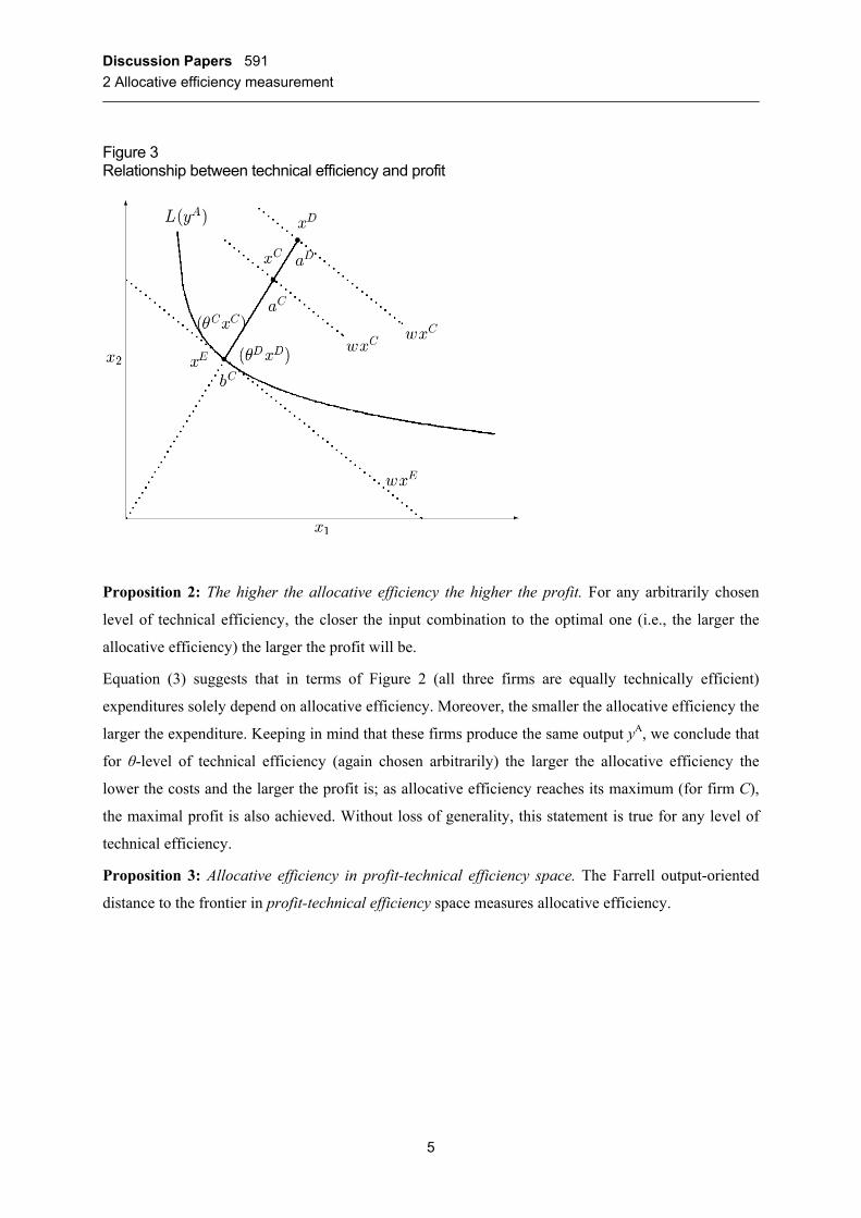
In Figure 3, two firms, C and D, use inputs xC and xD to produce output yA, which is measured by the

isoquant L(yA). Both firms are allocatively efficient because they lie on the same ray from the origin

that goes through the tangent point xE; thus, in terms of proposition 1 we only look at the frontier

points. These firms operate, however, at different levels of technical efficiency θC and θD, respectively.

Since the isocost representing the level of expenditure wxC is closer to the origin than that of the

expenditure level wxD, costs of firm C are smaller than those of firm D and firm C is more profitable

than firm D. Since obC/oaC>obC/oaD, θC > θD, larger technical efficiency is associated with larger

profits for points forming the frontier in profit-technical efficiency space. This proves that such

frontier is upward sloping.

Remark 1: Frontier in profit—technical efficiency space is sloped upwards.

4


Figure 3 Relationship between technical efficiency and profit

Proposition 2: The higher the allocative efficiency the higher the profit. For any arbitrarily chosen

level of technical efficiency, the closer the input combination to the optimal one (i.e., the larger the

allocative efficiency) the larger the profit will be.

Equation (3) suggests that in terms of Figure 2 (all three firms are equally technically efficient)

expenditures solely depend on allocative efficiency. Moreover, the smaller the allocative efficiency the

larger the expenditure. Keeping in mind that these firms produce the same output yA, we conclude that

for θ-level of technical efficiency (again chosen arbitrarily) the larger the allocative efficiency the

lower the costs and the larger the profit is; as allocative efficiency reaches its maximum (for firm C),

the maximal profit is also achieved. Without loss of generality, this statement is true for any level of

technical efficiency.

Proposition 3: Allocative efficiency in profit-technical efficiency space. The Farrell output-oriented

distance to the frontier in profit-technical efficiency space measures allocative efficiency.

5


Figure 4 Allocative efficiency in profit-technical efficiency space

In Figure 4 frontier is the locus of the maximum attainable profits as defined in Proposition 1. The

firms A, B, and C have the same technical efficiency level TE0; however, they have different profit

levels: p1, p2, and p , respectively. The potential level of profit which firms can reach is p . The closer

the observation is to the frontier, the larger the profit is. As we recall from Figure 2, the shift from

firm A to firm C is only possible when the input-mix is changed; i.e., allocative efficiency is improved.

Thus, in Figure 4 the shift from firm A to firm B means an increase in allocative efficiency (distance

AEA is larger then distance AEB), and further increase in allocative efficiency within the same level of

technical efficiency is only possible up to firm Cs observation, for which both profit and allocative

efficiency are at the maximum. Thus, which is most remarkable, the distance from the observation to

the frontier serves as a measure of the allocative efficiency.

To summarize, we have defined a new way of estimating allocative efficiency, specifically, this is the

output-oriented distance to the frontier in profit-technical efficiency space.

6

Discussion Papers 591 3 Monte-Carlo simulation

3 Monte-Carlo simulation

To analyze whether our new approach to measuring allocative efficiency yields valid estimates, we

conducted several Monte-Carlo experiments. According to a micro-economic theory, a firm which

chooses such a combination of inputs, thus their ratio is equal to the ratio of output elasticities of the

respective inputs will be most profitable. When we speak of optimal combination of inputs, the

original notion of allocative efficiency comes into play, and we suggest that the closer the ratio of

inputs to the ratio of elasticities the larger a firm’s allocative efficiency will be.

3.1 Empirical implementation of the traditional approach

The traditional approach can be used when input prices are known. Under technology T such that

( )

= xyxT :, can produce (4)

y

We measure input-oriented technical efficiency as the greatest proportion that the inputs can be

reduced and still produce the same outputs:

( )

= xxyF i λλ :inf, can still produce (5)

y

We employ the Data Envelopment Analysis (DEA) all the way through the empirical estimation. For

K observations, M outputs, and inputs an estimate of the Farrell Input-Saving Measure of

Technical Efficiency can be calculated by solving a linear programming problem for each observation

N

j ( ): Kj ,...,1=

( )

≥⋅≤⋅≥⋅== ∑ ∑= =

0,,:min|,ˆˆ1 1

k

K

k

K

kjknkjkmk

ijj zxxzyyzCxyFET λλ (6)

for and Mm ,...,1= Nn ,...,1= . Note that superscript stands for input orientation while C is the

constant returns-to-scale. Other returns-to-scale are modeled adjusting process operating levels s

(see Färe et al., (1994) for details).

i

kz

When input prices and quantities are given we can calculate the total costs and the minimum attainable

cost (solve linear programming problem) and then compute an estimate of cost efficiency for each

observation j ( ) as in equation (2): Kj ,...,1=

7


( )∑

∑ ∑∑

=

= ==

⋅

≥≤⋅≥⋅⋅= N

njnjn

k

K

k

K

kjknkjkmk

N

njnjn

ij

xw

zxxzyyzxwCwxyC

1

'

1 1

''

10,,:min

|,,ˆ (7)

for and Mm ,...,1= Nn ,...,1= . We refer to the residual of technical and cost efficiencies as Input

Allocative Efficiency, which can be computed for each observation j ( Kj ,...,1= ) as:

( ) ( )( )CxyF

CwxyCCwxyEA

ij

iji

j |,ˆ|,,ˆ

|,,ˆ = . (8)

3.2 Empirical implementation of the new approach

As mentioned above, the main virtue of the new approach is that we do not necessarily need input

prices for measuring allocative efficiency. Technically, we need output-oriented distances to the

frontier in the profit-technical efficiency space. We take advantage of the technical efficiency

estimates (denoted by TE ) obtained as in equation (6) and profitability measure (denoted by Pr ) to

calculate (solve linear programming problem) allocative efficiency for each observation j

( ) as follows: Kj ,...,1=

( )

≥≤⋅≥== ∑ ∑= =

0,,PrPr:max|Pr,ˆˆ ''

1 1

''''k

K

k

K

kjkkjkk

ojj zTETEzzCTEFEA θθ . (9)

3.3 Design of the Monte-Carlo experiments

In each of the Monte-Carlo trials, we study a production process which uses two inputs to produce one

output. Data for the ith observation in each Monte-Carlo experiment were generated using the

following algorithm.

(i) We chose output elasticities of two inputs to be 0.2 and 0.8; this ensures constant returns

to scale. The optimal ratio of inputs, thus, is 4.

(ii) Draw ( )uniform⋅+x λφ~ ; uniform on the interval (0;1). 1

(iii) Draw uniformr ~ ; uniform on the interval (0;8). This is meant to be an experimental

ratio of used inputs.

(iv) Set x 12 xr ⋅= .

(v) Choose ε . In doing so, we allow the ratio of inputs in each Monte-Carlo trial to vary on

the interval [ ]εε −8; while keeping in mind that the optimal ratio is 4. Therefore, we

8


obtain enough variation of inefficient combinations of inputs, or in other words, enough

variation of allocative inefficiency.

(vi) Draw ( )2,0 uN σ+~u and set ‘te_drawn’ equal to ( )u−exp .

(vii) Generate output data assuming trans-log production function, which will contain

inefficiency component:5

drawntexxxxxxy _218.02.0 2112

2222

211121 +⋅⋅+⋅+⋅+⋅+⋅= γγγ .

(viii) Draw price of input :1x ( )uniformw ⋅+ψϕ~1

12 ww

, uniform on the interval (0;1). The price

of input is calculated as 2x ⋅= θ – we want to keep the ratio of input prices

constant to have the isoquants parallel (recall Figure 2).

(ix) Set profit as output (we set output price equal to 1) minus cost and this is divided by

output.

(x) DEA traditional allocative efficiency as in equation (8).

(xi) DEA our measures of allocative efficiency using technical efficiency drawn in step (vi) as

in equation (9).

(xii) Solve for technical efficiency as in equation (6), and DEA our measure of allocative

efficiency using these solved technical efficiency scores.

(xiii) Calculate rank correlation coefficient between allocative efficiency estimates based on

traditional and our approaches.

(xiv) Repeat steps (i) through (xiii) L times.

In each of our experiments we set 1=φ , 7=λ , 1=ϕ , 05.0=ψ , 01.011 =γ , 01.022 =γ and

02.012 −=γ . In order to look at different variabilities of inappropriately chosen ratios of inputs, we

set 5.0=ε , 1=ε , and 2=ε . With 2=ε , variability of allocative efficiency is expected to have been

reduced considerably – range becomes (2;6); and vice versa, 5.0=ε ensures very large variability –

range increases to (0.5;7.5). We conduct three sets of experiments setting to 0.0025, 0.025, and

0.25; this ensures covering a plausible range of standard deviations of technical efficiency.6 In each

experiment we ran L=500 Monte-Carlo trials.7

2uσ

5 Since the DEA is deterministic, we do not incorporate a stochastic term in the Monte-Carlo trials. 6 Using a different experiment, Greene (2005) obtains estimates of technical efficiency with standard deviations from 0.09 to 0.43. 7 The simulation is programmed in SAS 9.1.3; computationally, one run with N=100, L=500 takes about 7 hours on a Pentium IV processor running at 3GHz. Thus, we defined relatively few parameter constellations in the performed experiment.

9


3.4 Results

From tables 1 to 6 it is clearly seen that in all three cases the DEA estimates the drawn technical

efficiency scores fairly accurately – the rank correlation coefficient (Corr4) is close to unity. This is an

expected outcome since we do not assume a stochastic term in the production output generation (step

(vii) of the experiment). The same argument applies to the rank correlation coefficient between

allocative efficiency calculated in step (xi) and that calculated in step (xii) (Corr3). Thus, there is not

much difference in using the true or the estimated technical efficiency in the new approach. However,

what is of most interest to us are the rank correlation coefficients between allocative efficiency

estimates from the traditional and our new approach (Corr1 and Corr2). Corr1 has been computed with

the estimates of allocative efficiency based on ‘true’ technical efficiency while Corr2 has been

computed with the estimates of allocative efficiency based on estimated values of technical efficiency.

As previously mentioned, the rank correlation between these measures is quite high (Corr3). We argue

that it is more appropriate to draw conclusions from Corr2 since we do not know the ‘true’ technical

efficiency in practice.

Table 1 Rank correlations, 5.0=ε , 100=N

2uσ

0.0025 0.025 0.25

θ 0.75 1 1.25 0.75 1 1.25 0.75 1 1.25

mean 0.8566 0.7375 0.6954 0.8608 0.7326 0.6942 0.8087 0.6879 0.6413 Corr1

st.d 0.0442 0.0625 0.0677 0.0434 0.0621 0.0686 0.0649 0.0760 0.0772

mean 0.8642 0.7485 0.7038 0.8695 0.7526 0.7115 0.8712 0.7885 0.7365 Corr2

st.d 0.0416 0.0590 0.0663 0.0407 0.0589 0.0664 0.0469 0.0687 0.0818

mean 0.9899 0.9880 0.9894 0.9915 0.9901 0.9895 0.9468 0.9419 0.9464 Corr3

st.d 0.0194 0.0212 0.0188 0.0148 0.0159 0.0168 0.0531 0.0492 0.0397

mean 0.8928 0.8937 0.8893 0.9524 0.9528 0.9560 0.9830 0.9816 0.9825 Corr4

st.d 0.0409 0.0405 0.0423 0.0275 0.0268 0.0254 0.0124 0.0148 0.0141

Notes: Corr1 is the rank correlation between allocative efficiency calculated in step (x) and that calculated in step (xi). Corr2 is the rank correlation between allocative efficiency calculated in step (x) and that calculated in step (xii). Corr3 is the rank correlation between allocative efficiency calculated in step (xi) and that calculated in step (xii). Corr4 is the rank correlation between technical efficiency calculated in equation (6) and that drawn in step (vi).

10


Table 2 Rank correlations, 1=ε , 100=N

2uσ

0.0025 0.025 0.25

θ 0.75 1 1.25 0.75 1 1.25 0.75 1 1.25

mean 0.8569 0.7043 0.6192 0.8519 0.6991 0.6053 0.7851 0.6381 0.5476 Corr1

st.d 0.0412 0.0653 0.0744 0.0429 0.0685 0.0779 0.0706 0.0803 0.0838

mean 0.8611 0.7111 0.6264 0.8598 0.7197 0.6263 0.8470 0.7481 0.6709 Corr2

st.d 0.0393 0.0641 0.0722 0.0405 0.0654 0.0771 0.0480 0.0753 0.0944

mean 0.9928 0.9922 0.9919 0.9912 0.9903 0.9889 0.9469 0.9356 0.9384 Corr3

st.d 0.0163 0.0152 0.0157 0.0149 0.0146 0.0170 0.0530 0.0542 0.0419

mean 0.9183 0.9209 0.9196 0.9590 0.9633 0.9626 0.9874 0.9870 0.9869 Corr4

st.d 0.0341 0.0344 0.0353 0.0278 0.0248 0.0254 0.0111 0.0111 0.0113

Notes from Table 1 apply.


2uσ

0.0025 0.025 0.25

θ 0.75 1 1.25 0.75 1 1.25 0.75 1 1.25

mean 0.8140 0.5782 0.3386 0.8042 0.5561 0.3168 0.6841 0.4515 0.2602 Corr1 st.d 0.0453 0.0762 0.0835 0.0438 0.0794 0.0928 0.1020 0.1063 0.0984

mean 0.8155 0.5837 0.3448 0.8091 0.5750 0.3498 0.7638 0.6048 0.4864 Corr2 st.d 0.0437 0.0738 0.0828 0.0425 0.0791 0.0937 0.0609 0.0992 0.1294

mean 0.9939 0.9948 0.9938 0.9917 0.9904 0.9878 0.9265 0.9117 0.9049 Corr3 st.d 0.0144 0.0124 0.0130 0.0152 0.0156 0.0202 0.0765 0.0838 0.0652

mean 0.9455 0.9449 0.9443 0.9749 0.9743 0.9731 0.9910 0.9908 0.9910 Corr4 st.d 0.0283 0.0300 0.0300 0.0202 0.0197 0.0206 0.0090 0.0089 0.0075


The first observation worth mentioning is that when variability of sub-optimal ratios decreases (ε

increases): our method is less successful in yielding similar estimates as the traditional one. Hence, our

method deteriorates in terms of exactness when ‘true’ allocative efficiency is not very heterogeneous.

Furthermore, the results show that our approach is robust with respect to variance of the drawn

technical efficiency, . Looking closely at correspondent ratios, one can notice that for the same 2uσ

θ ’s Corr2 is increasing when increases, whereas for other 2uσ θ ’s Corr2 decreases when we increase

; however, the changes are minor. The same argument applies to the standard deviation of Corr2. 2uσ

11


This implies that for different levels of distributions of Corr2 are virtually the same. The skewness

of the variable Corr2 is always negative and is about —0.6 which means that the distribution of Corr2

is skewed to the left and more values are clustered to the right of the mean. Kurtosis is about 0.6, but it

varies more than the skewness; it increases with increase of . Kernel density estimates of Corr2 for

the case

2uσ

2uσ

75.0=θ are shown in Figure 5. Note that we use the Gaussian kernel function and the

Sheather and Jones (1991) rule to determine the “optimal” bandwidth.

500Figure 5 Estimates of Sampling Densities of Corr2 ( 75.0=θ , =L , 5.0=ε , 1=ε and 2=ε )

Note: in each panel the vertical dashed line is the mean value of the corresponding density.

12


The results are better when the sample size is increased to 400 (Tables 4-6). However, the

improvement does not change our main conclusions based on the experiments with sample size 100.

As expected, standard deviations of rank coefficients are almost halved when the sample size is

quadrupled.

Table 4 Rank correlations, 5.0=ε , 400=N

2uσ

0.0025 0.025 0.25

θ 0.75 1 1.25 0.75 1 1.25 0.75 1 1.25

mean 0.8812 0.7551 0.7132 0.8810 0.7543 0.7126 0.8585 0.7297 0.6750 Corr1

st.d 0.0182 0.0288 0.0311 0.0173 0.0286 0.0297 0.0232 0.0308 0.0334

mean 0.8824 0.7567 0.7144 0.8828 0.7605 0.7173 0.8773 0.7675 0.7114 Corr2

st.d 0.0176 0.0287 0.0307 0.0171 0.0281 0.0295 0.0211 0.0418 0.0412

mean 0.9987 0.9990 0.9987 0.9988 0.9985 0.9986 0.9887 0.9856 0.9870 Corr3

st.d 0.0035 0.0031 0.0036 0.0028 0.0030 0.0023 0.0122 0.0215 0.0095

mean 0.9726 0.9730 0.9733 0.9909 0.9905 0.9904 0.9968 0.9969 0.9968 Corr4

st.d 0.0096 0.0106 0.0099 0.0053 0.0063 0.0060 0.0026 0.0025 0.0027



2uσ

0.0025 0.025 0.25

θ 0.75 1 1.25 0.75 1 1.25 0.75 1 1.25

mean 0.8760 0.7169 0.6362 0.8734 0.7185 0.6309 0.8363 0.6754 0.5798 Corr1

st.d 0.0178 0.0334 0.0350 0.0186 0.0316 0.0370 0.0240 0.0350 0.0402

mean 0.8766 0.7185 0.6375 0.8748 0.7247 0.6370 0.8547 0.7185 0.6257 Corr2

st.d 0.0176 0.0333 0.0349 0.0185 0.0313 0.0371 0.0214 0.0395 0.0501

mean 0.9992 0.9991 0.9992 0.9987 0.9984 0.9984 0.9882 0.9845 0.9853 Corr3

st.d 0.0026 0.0028 0.0025 0.0029 0.0031 0.0031 0.0139 0.0144 0.0104

mean 0.9814 0.9809 0.9821 0.9930 0.9932 0.9931 0.9978 0.9978 0.9977 Corr4

st.d 0.0086 0.0086 0.0085 0.0049 0.0047 0.0049 0.0020 0.0019 0.0020


13



2uσ

0.0025 0.025 0.25

θ 0.75 1 1.25 0.75 1 1.25 0.75 1 1.25

mean 0.8337 0.5911 0.3410 0.8269 0.5692 0.3253 0.7463 0.4934 0.2858 Corr1

st.d 0.0195 0.0361 0.0455 0.0205 0.0395 0.0470 0.0359 0.0458 0.0476

mean 0.8339 0.5924 0.3422 0.8271 0.5752 0.3353 0.7661 0.5512 0.3780 Corr2

st.d 0.0192 0.0362 0.0455 0.0206 0.0393 0.0470 0.0302 0.0485 0.0734

mean 0.9994 0.9994 0.9995 0.9990 0.9986 0.9981 0.9840 0.9777 0.9754 Corr3

st.d 0.0025 0.0022 0.0017 0.0021 0.0028 0.0037 0.0175 0.0227 0.0195

mean 0.9884 0.9882 0.9879 0.9955 0.9955 0.9957 0.9985 0.9985 0.9985 Corr4

st.d 0.0066 0.0071 0.0072 0.0037 0.0037 0.0033 0.0015 0.0014 0.0015


Results of one run8 (sample size 500) are summarized in Figure 6; note optimal ratio of inputs is

shown by the vertical-dashed line in each panel. Our methodology almost completely repeats the trend

of the traditional approach for 5.0=ε which is backed by a high correlation coefficient in Tables 1

and 4; as ε becomes larger Figure 6 suggests that our methodology is less able to predicts allocative

efficiency. However, it is most remarkable that our methodology is in line with the traditional

approach.

8 We repeated this experiment many times and the general picture was always similar; however, due to space constraints it is not possible to present all results here.

14


Figure 6 Allocative efficiency calculated using traditional and new approaches plotted against ratio of expenditure shares, (1122 / xwxw 75.0=θ , 400=N , 5.0=ε , 1=ε and 2=ε )

15


Figure 6 (continued) Allocative efficiency calculated using traditional and new approaches plotted against ratio of expenditure shares, (1122 / xwxw 75.0=θ , 400=N , 5.0=ε , 1=ε and 2=ε )

16


Figure 6 (continued) Allocative efficiency calculated using traditional and new approaches plotted against ratio of expenditure shares, (1122 / xwxw 75.0=θ , 400=N , 5.0=ε , 1=ε and 2=ε )

17

Discussion Papers 591 4 Empirical illustration of the new approach

4 Empirical illustration of the new approach

4.1 Data

To illustrate the usefulness of the new approach for measuring allocative efficiency when input prices

are not available, we apply it to micro-data from the German Cost Structure Census9 of manufacturing

for the year 2003. Our sample comprises only enterprises from the chemical industry. The measure of

output is gross production. This mainly consists of the turnover and the net-change of the stock of the

final products.10

The Cost Structure Census contains information for a number of input categories.11 These categories

are payroll, employers’ contribution to the social security system, fringe benefits, expenditure for

material inputs, self-provided equipment, and goods for resale, for energy, for external wage-work,

external maintenance and repair, tax depreciation of fixed assets, subsidies, rents and leases, insurance

costs, sales tax, other taxes and public fees, interest on outside capital as well as “other” costs such as

license fees, bank charges and postage, or expenses for marketing and transport.

Some of the cost categories which include expenditures for external wage-work and external

maintenance and repair contain a relatively high share of reported zero values because many firms do

not utilize these types of inputs. Such zeros make the firms incomparable and, thus, might bias the

DEA results. In order to reduce the number of reported zero input quantities, we aggregated the inputs

into the following categories: (i) material inputs (intermediate material consumption plus commodity

inputs), (ii) labor compensation (salaries and wages plus employer's social insurance contributions),

(iii) energy consumption, (iv) user cost of capital (depreciation plus rents and leases), (v) external

services (e.g., repair costs and external wage-work), and (vi) “other” inputs related to production (e.g.,

transportation services, consulting, or marketing).

9 Aggregate figures are published annually in Fachserie 4, Reihe 4.3 of Kostenstrukturerhebung im Verarbeitenden Gewerbe (various years). The Cost Structure Census is gathered and compiled by the German Federal Statistical Office (Statistisches Bundesamt). Enterprises are legally obliged to respond to the Cost Structure Census; hence, missing observations due to non-response are precluded. The survey comprises all large German manufacturing enterprises which have 500 or more employees. Enterprises with 20-499 employees are included as a random sample that is representative for this size category in a particular industry. For more information about cost structure census surveys in Germany, we refer the reader to Fritsch et al., (2004). 10 We do not include turnover from activities that are classified as miscellaneous such as license fees, commissions, rents, leasing etc. because this kind of revenue cannot adequately be explained by the means of a production function. 11 Though the production theory framework requires real quantities, using expenditures as proxies for inputs in the production function is quite common in the literature (see e.g., Paul et al., (2004), Paul and Nehring (2005)).

18


Profits are computed as one minus the total costs divided by the turnover. Since the DEA requires

positive values, we standardize the profit measure to the interval (0,1) by adding the minimum profit

and dividing this by the range of profits.

4.2 Results

Figure 7 shows profitability plotted against estimated technical efficiency. Remarkably, a frontier, as

could be theoretically expected from Proposition 1, indeed exists. Another observation worth

mentioning is that within a certain level of technical efficiency (i) profitability greatly varies

suggesting variation in allocative efficiency (as firms A, B, and C in Proposition 3) and (ii) profits are

bounded from above. Moreover, the frontier is positively sloped as was stated in the first theoretical

part of this paper. Interestingly, Figure 7 suggests that even with 100 percent technical efficiency

enterprises can be allocatively inefficient.

Figure 7 Profitability plotted against estimated technical efficiency scores for about 900 German enterprises from the chemical industry

We calculated technical efficiency scores as in equation (6). Table 7, which contains descriptive

statistics of the estimated technical efficiencies, suggests that an average German chemical

manufacturing enterprise is fairly inefficient. The median of technical efficiency implies that half of

firms have an efficiency of 68 percent or less. The scores for allocative efficiency are obtained solving

the linear programming problem as in equation (9). Descriptive statistics on allocative efficiency are

also presented in Table 7. At a first glance, the mean and the variation of allocative efficiency appear

to be strikingly similar to that of technical efficiency. However, the distribution of allocative

19


efficiency is more symmetric and has a lower variance compared to the technical efficiency

distribution.

Table 7 Descriptive statistics of technical and allocative efficiency, N=905

Efficiency mean st.d. coef. of var.

skew-ess min 10th

perc. 25th

perc. median 75th perc.

90th perc

Technical 0.6891 0.1507 0.2138 0.4399 0.3253 0.5287 0.5911 0.6817 0.8033 1.0000

Allocative 0.6963 0.1181 0.1696 -0.0018 0.3102 0.5360 0.6084 0.6974 0.7800 0.8523

Kernel estimated density of technical efficiency is shown in the left panel of Figure 8; we use

Gaussian kernel function and the Sheather and Jones (1991) rule to determine the “optimal”

bandwidth. Although the number of firms is quite large, we analyze the sensitivity of efficiency scores

relative to the sampling variations of the estimated frontier in an additional step. Consequently, we

perform the homogeneous bootstrap as described by Simar and Wilson (1998). The geometric mean of

the bias-corrected efficiency scores is 0.6066, which is on average 0.0886 lower than that estimated

via the DEA; the mean variance of bias is 0.0036. In comparison to other studies, however, the bias of

estimates and its standard error are rather low, thereby indicating a robustness of the technical

efficiency scores.

Figure 8 Estimates of sampling densities of technical and allocative efficiency scores

20

Discussion Papers 591 5 Conclusions

5 Conclusions

Allocative inefficiency, introduced in the seminal work by Farrell (1957), has important implications

from the perspective of the firm. How much could firms increase their profits – given a certain output

they produce – just by reallocating resources? On the other hand, the existing empirical evidence on

the extent and determinants of allocative efficiency within and across industries is rather limited. The

main reason is that the traditional approach to assessing allocative efficiency requires input prices.

However, input prices are rarely accessible, which per se, precludes the analysis of the allocative

efficiency with non-parametric approach.

In this paper, a new method is developed which enables calculating allocative efficiency without

knowing input prices. This indicator is derived as the Farrell output-oriented distance to the frontier in

profit-technical efficiency space. Thus, besides input and output quantities, only the profits of the firms

are needed for calculating allocative efficiency. A simple Monte-Carlo experiment was performed to

check the validity of the new methodology. We obtain high-rank correlation coefficients between

allocative efficiency estimates based on both traditional and new approaches for different parameter

constellations. Moreover, the new approach proved to be quite robust with respect to variance of true

technical efficiency. Finally, we applied the new approach to a sample of about 900 enterprises in the

German chemical industry. The results suggest a large variation of allocative efficiency even for

technically efficient enterprises. Thus, the example highlights the usefulness of our method for

obtaining allocative efficiency measures when input prices are not available.

21

Discussion Papers 591 References

References

Alvarez, Roberto and Gustavo Crespi (2003): Determinants of Technical Efficiency in Small Firms.

Small Business Economics 20, 233-244.

Atkinson, S. E. and C. Cornwell (1994): Parametric estimation of technical and allocative inefficiency

with panel data. International Economic Review 35(1), 231--243.

Berger, A. N. and D. Humphrey (1997): Efficiency of financial institutions: international survey and

directions for future research, European Journal of Operational Research 98, 175–212.

Burki, Abid A., Mushtaq A. Khan and Bernt Bratsberg (1997): Parametric tests of allocative

efficiency in the manufacturing sectors of India and Pakistan. Applied Economics 29(1), 11-22.

Caves, Richard E. and David R. Barton (1990): Efficiency in US manufacturing industries, MIT Press,

Cambridge (Mass.).

Chavas, Jean-Paul, Ragan Petrie and Michael Roth (2005): Farm Household Production Efficiency:

Evidence from The Gambia. American Journal of Agricultural Economics 87(1), 160-179.

Chavas, Jean-Paul and M. Aliber.(1993): An Analysis of Economic Efficiency in Agriculture: A

Nonparametric Approach.” American Journal of Agricultural Economics 18, 1-16.

Coelli, T., S. Rahman and C. Thirtle (2002): Technical, Allocative, Cost and Scale Efficiencies in

Bangladesh Rice Cultivation: A Non-parametric Approach. Journal of Agricultural Economics

53(3), 607-626.

Färe, Rolf, Shawna Grosskopf and C. A. Knox Lovell (1994): Production frontiers, Cambridge

University Press, Cambridge. U.K.

Färe, Rolf, Shawna Grosskopf and William L. Weber (2004): The effect of risk-based capital

requirements on profit efficiency in banking. Applied Economics 36, 1731–1743.

Farrell, Michael. J. (1957): The Measurement of Productive Efficiency. Journal of the Royal

Statistical Society. Series A (General), 120(3), 253-290.

Fritsch, Michael and Andreas Stephan (2004a): The Distribution and Heterogeneity of Technical

Efficiency within Industries - An Empirical Assessment. DIW Discussion Paper, (Mimeo),

Berlin.

Fritsch, Michael, Bernd Görzig, Ottmar Hennchen and Andreas Stephan (2004): Cost Structure

Surveys in Germany. Journal of Applied Social Science Studies 124, 1-10.

Gode, Dhananjay K. and Shyam Sunder (1997): What Makes Markets Allocationally Efficient? The

Quarterly Journal of Economics 112(2), 603-630.

Grazhdaninova, Margarita and Lerman Zvi (2005): Allocative and Technical Efficiency of Corporate

Farms in Russia. Comparative Economic Studies 47(1), 200-213.

22

http://www.ingentaconnect.com/search/article?title=allocative+efficiency&title_type=tka&year_from=1997&year_to=2005&database=1&pageSize=50&index=202

http://www.ingentaconnect.com/search/article?title=allocative+efficiency&title_type=tka&year_from=1997&year_to=2005&database=1&pageSize=50&index=202

http://www.ingentaconnect.com/content/routledg/raef


Green, Alison and David Mayes (1991): Technical Inefficiency in Manufacturing Industries. The

Economic Journal 101(406), 523-538.

Greene, William (1997): Frontier Production Functions. In: M. Hashem Pesaran and Peter Schmidt

(eds.): Handbook of Applied Econometrics, vol. II, Blackwell Publishers, 81-166.

Greene, William (2005): Reconsidering heterogeneity in panel data estimators of the stochastic

frontier model. Journal of Econometrics, 126, 269–303.

Gumbau-Albert, Mercedes and Joaquín Maudos (2002): The determinants of efficiency: the case of the

Spanish industry. Applied Economics 34, 1941-1948.

Isik, I. and M.K. Hassan (2002): Technical, scale and allocative efficiencies of Turkish banking

industry. Journal of Banking and Finance 26(4), April 2002, pp. 719-766.

Kim, Sangho and Gwangho Han (2001): A Decomposition of Total Factor Productivity Growth in

Korean Manufacturing Industries: A Stochastic Frontier Approach. Journal of Productivity

Analysis 16(3), 269-281.

Kumbhakar, Subal C. (1991): The measurement and decomposition of cost-inefficiency: The translog

cost system. Oxford Economic Papers, New Series 43(4), 667-683.

Kumbhakar, Subal C. and C. Knox Lovell (2000): Stochastic Frontier Analysis, Cambridge University

Press.

Kumbhakar, Subal C. and Efthymios G. Tsionas (2005): Measuring technical and allocative

inefficiency in the translog cost system: a Bayesian approach. Journal of Econometrics 126, 355–

384.

Kumbhakar, Subal C. and Hung-Jen Wang (forthcoming): Pitfalls in the estimation of a cost function

that ignores allocative inefficiency: A Monte Carlo analysis. Journal of Econometrics.

Lovell, C.A. Knox. (1993): Production Frontier and Productive Efficiency. In: Harold O. Fried, C.A.

Knox Lovell and Shelton S. Schmidt (eds.): The Measurement of Productive Efficiency Ю

Technics and Applications. Oxford University Press, Oxford, 3-67.

Morrison Paul, Catherine J., Richard Nehring (2005): Product Diversification, Production Systems,

and Economic Performance in U.S. Agricultural Production. Journal of Econometrics, 126, 525–

548.

Morrison Paul, Catherine J., Richard Nehring, David Banker and Agapi Somwaru (2004): Scale

Economies and Efficiency in U.S. Agriculture: Are Traditional Farms History? Journal of

Productivity Analysis, 22(3), 185—205.

Oum, T.H. and Y. Zhang (1995): Competition and allocative efficiency: The case of the U.S.

telephone industry. The Review of Economics and Statistics 77(1), 82-96.

23


24

Raa, Thijs Ten (2005): Aggregation of Productivity Indices: The Allocative Efficiency Correction.

Journal of Productivity Analysis 24, 203-209.

Seiford, Lawrence M. (1996):Data envelopment analysis: The Evolution of the State-Of-The-Art

(1978–1995). Journal of Productivity Analysis 7, 2/3, 99–138.

Seiford, Lawrence M. (1997): A Bibliography for Data Envelopment Analysis (1978–1996). Annals of

Operations. Research 73, 393–438.

Sheather, Simon J. and Michael C. Jones (1991): A Reliable Data Based Bandwidth Selection Method

for Kernel Density Estimation. Journal of Royal Statistical Society, Series B, 53, 683-90.

Simar, Leopold and Paul W. Wilson (1998): Sensitivity Analysis of Efficiency Scores: How to

Bootstrap in Nonparametric Frontier Models. Management Science 44, 49-61.

Topuz, John C., Ali F. Darrat and Roger M. Shelor (2005): Technical, Allocative and Scale

Efficiencies of REITs: An Empirical Inquiry. Journal of Business Finance & Accounting 32,

1961-1994.

Allocative Efficiency Measurement Revisited: Do We Really Need Input Prices? Discussion Papers

Documents

Transcript of Allocative Efficiency Measurement Revisited: Do We Really Need Input Prices? Discussion Papers