ALGORITHMS FOR ACTIVE LOCALIZATION AND TRACKING ...

ALGORITHMS FOR ACTIVE LOCALIZATION AND

TRACKING IN IMAGE-GUIDED ROBOTIC SURGERY

SYSTEMS

by

MARK E. RENFREW

Submitted in partial fulfillment of the

requirements for the degree of

Doctor of Philosophy

Dissertation Advisor:

Dr. M. Cenk Cavusoglu

Department of Electrical Engineering and Computer Science

CASE WESTERN RESERVE UNIVERSITY

January 2016

CASE WESTERN RESERVE UNIVERSITY

SCHOOL OF GRADUATE STUDIES

We hereby approve the thesis/dissertation of

Mark Edward Renfrew

Candidate for the degree of Doctor of Philosophy*

Committee Chair

Prof. M. Cenk. Cavusoglu

Prof. Frank Merat

Prof. Wyatt Newman

Prof. Greg Lee

Prof. Kiju Lee

Date of Defense

3 September 2015

*We also certify that written approval has been obtained

for any proprietary material contained therein.

To Emma

For Alice

“But I don’t want to go among mad people,” Alice remarked.

“Oh, you can’t help that,” said the Cat:

“we’re all mad here. I’m mad. You’re mad.”

“How do you know I’m mad?” said Alice.

“You must be,” said the Cat, “or you wouldn’t have come here.”

Contents

List of Figures iv

List of Tables x

Acknowledgements xi

1 Introduction 1

1.1 Contributions . . . . . . . . . . . . . . . . . . . . . . . . . . . . . . . 1

1.2 Organization of the Thesis . . . . . . . . . . . . . . . . . . . . . . . . 3

2 Background 4

3 Active Localization of Needle and Target 10

3.1 Problem Formulation and General Algorithm . . . . . . . . . . . . . . 11

3.2 System Architecture . . . . . . . . . . . . . . . . . . . . . . . . . . . 12

3.2.1 Active Localization . . . . . . . . . . . . . . . . . . . . . . . . 13

3.2.2 Bayesian Filters for Needle and Target Tracking . . . . . . . . 14

3.2.3 Probabilistic Motion Models . . . . . . . . . . . . . . . . . . . 16

3.2.4 Probabilistic Measurement Models . . . . . . . . . . . . . . . 20

3.3 Image Processing Algorithms . . . . . . . . . . . . . . . . . . . . . . 28

3.3.1 Image Processing for Needle Detection . . . . . . . . . . . . . 28

3.3.2 Choosing a Needle Detection Mask . . . . . . . . . . . . . . . 30

i

3.3.3 Image Processing for Target Detection . . . . . . . . . . . . . 36

3.4 Simulation Results . . . . . . . . . . . . . . . . . . . . . . . . . . . . 38

3.4.1 Particle Filters . . . . . . . . . . . . . . . . . . . . . . . . . . 39

3.4.2 Unscented Kalman Filters . . . . . . . . . . . . . . . . . . . . 41

3.5 Experimental Validation . . . . . . . . . . . . . . . . . . . . . . . . . 48

3.5.1 Data Collection . . . . . . . . . . . . . . . . . . . . . . . . . . 48

3.5.2 Experimental Results . . . . . . . . . . . . . . . . . . . . . . . 50

3.6 Discussion . . . . . . . . . . . . . . . . . . . . . . . . . . . . . . . . . 54

4 Segmentation of Intra-Operative Images With the Fast Marching

Method 58

4.1 Level Set Methods . . . . . . . . . . . . . . . . . . . . . . . . . . . . 59

4.2 The Fast Marching Method . . . . . . . . . . . . . . . . . . . . . . . 60

4.3 Image Enhancement . . . . . . . . . . . . . . . . . . . . . . . . . . . 61

4.4 Seeding and Region Merging . . . . . . . . . . . . . . . . . . . . . . . 64

4.5 Implementation . . . . . . . . . . . . . . . . . . . . . . . . . . . . . . 65

4.6 Results . . . . . . . . . . . . . . . . . . . . . . . . . . . . . . . . . . . 65

4.6.1 Manually-Seeded Image Volume . . . . . . . . . . . . . . . . . 66

4.6.2 Automatically-Seeded Image Volume . . . . . . . . . . . . . . 70

4.7 Discussion . . . . . . . . . . . . . . . . . . . . . . . . . . . . . . . . . 73

5 Conclusions 74

A Automated Fuel Cell Segmentation and Characterization 76

A.1 Introduction . . . . . . . . . . . . . . . . . . . . . . . . . . . . . . . . 76

A.2 Background . . . . . . . . . . . . . . . . . . . . . . . . . . . . . . . . 77

A.3 Methods . . . . . . . . . . . . . . . . . . . . . . . . . . . . . . . . . . 79

A.4 Results . . . . . . . . . . . . . . . . . . . . . . . . . . . . . . . . . . . 81

ii

Bibliography 84

iii

List of Figures

3.1 The Markov model of the system. The needle state xNt depends on the

previous state xNt−1 and the needle control input uNt , while the target

state xTt depends only on the previous target state. The measurement

zt depends on the target state, needle state, and the measurement

control input uit which is determined by the active localization algorithm. 13

3.2 Schematic representation of the spline array used to model the needle.

The two splines γ0 and γ1 are uniquely defined by their endpoints and

the tangents of the endpoints. . . . . . . . . . . . . . . . . . . . . . . 18

3.3 One step of axial needle insertion. The original spline (blue) is aug-

mented with a spline extension (green) and a minimum-curvature final

spline (red) is fitted. . . . . . . . . . . . . . . . . . . . . . . . . . . . 22

3.4 (a) An example 4 control point needle, showing flexion of the needle as

it is partially inserted into the simulated tissue. (b) 20 samples from

the posterior distribution of the needle shape after execution of the

needle command shown in (a). . . . . . . . . . . . . . . . . . . . . . . 26

3.5 The figure shows samples drawn from the needle measurement proba-

bility density function p(znc,t|znd,t = true, xt). . . . . . . . . . . . . . . 27

3.6 An MR image showing the spherical target. . . . . . . . . . . . . . . 29

iv

3.7 An example MR image showing the needle and target. The needle

appears in this image as the black dot at the bottom-left corner of the

target (white circle). . . . . . . . . . . . . . . . . . . . . . . . . . . . 29

3.8 The needle is not easily visible in the image gradient. . . . . . . . . . 30

3.9 An image plane showing needle particle intersections with the imabe

plane (red), the standard deviation of the Gaussians (green) and the

detected needle (blue). . . . . . . . . . . . . . . . . . . . . . . . . . . 31

3.10 The histogram of the data filtered with the 3x3 mask, showing known

needle points versus control points. A sharp difference between the

peaks is seen. . . . . . . . . . . . . . . . . . . . . . . . . . . . . . . . 33


needle points versus control points. Again, two distinct peaks are evi-

dent, with the peaks being somewhat more separated than in the 3x3

case. . . . . . . . . . . . . . . . . . . . . . . . . . . . . . . . . . . . . 34


needle points versus control points. No distinction between the dis-

tributions can be discerned, indicating that this mask is too wide to

usefully extract single pixel needle data. . . . . . . . . . . . . . . . . 35

3.13 The MR image gradient. . . . . . . . . . . . . . . . . . . . . . . . . . 36

3.14 The MR image gradient’s edges. . . . . . . . . . . . . . . . . . . . . . 37

3.15 The MR image edges after cropping. . . . . . . . . . . . . . . . . . . 37

3.16 The detected target. . . . . . . . . . . . . . . . . . . . . . . . . . . . 37

3.17 The particle filter’s kernel smoothed density estimates for the needle

tip (a) and target (b) location beliefs. The solid vertical lines indicate

the actual value of the needle tip / target location. . . . . . . . . . . 41

v

3.18 Change in the entropies of the needle tip (solid) and target (solid)

location beliefs during a sample execution of the task. As it can be seen

from the figure, the algorithm successfully alternates between imaging

the target and the needle in order to minimize the total entropy of the

belief. . . . . . . . . . . . . . . . . . . . . . . . . . . . . . . . . . . . 42

3.19 The particle filter tracking the needle and target. The blue line (in-

visible) is the actual needle shape, the green lines are the shapes of

the particles in the needle belief function, the large semi-transparent

sphere is the actual target, the red circles are the centers of the particle

in the target belief function, and the semi-transparent plane is the cur-

rent imaging plane. (a) Initial particle distribution when the location

of the target is unknown. (b) The target is localized at the end of the

linear scanning phase. (c) Particle distribution at the mid point of the

needle insertion. (d) Particle distribution at the end of the task. . . 44

3.20 The Kalman filter’s kernel smoothed density estimates for the needle

tip (a) and target (b) location beliefs. The solid vertical lines indicate

the actual needle tip and target locations. . . . . . . . . . . . . . . . 45

3.21 Change in the entropies of the needle tip (red) and target (green) loca-

tion beliefs during one needle insertion trial. As with the particle filter

algorithm, the unscented Kalman filter algorithm successfully alter-

nates between imaging the target and the needle in order to minimize

the total entropy of the belief. . . . . . . . . . . . . . . . . . . . . . . 46

3.22 The unscented Kalman filter tracking a simulated needle and target.

The blue line is the actual needle shape, the red line is the UKF filter’s

mean needle belief, and the red sphere represents the target belief. . . 47

vi

3.23 The MR-safe needle insertion device. The device is placed on the

beaker in which the tissue phantom and target are. The device is

placed into the MR tube and the flexible needle is inserted by turning

the gears with a crank. . . . . . . . . . . . . . . . . . . . . . . . . . . 49

3.24 MR images of the three needle insertion trials. The needle is not com-

pletely visible in any single image slice. . . . . . . . . . . . . . . . . . 50

3.25 (a) A sample orthogonally-sliced MR image showing the target. (b) A

sample orthogonally-sliced MR image showing the needle intersecting

with the image plane. The needle is very faint relative to the back-

ground noise in this image and is indicated by the arrow. . . . . . . . 53

3.26 (a) The particle filter tracking the needle. Green lines represent the

particles comprising the filter’s belief and red circles represent the tar-

get filter’s particles. The true target position is given by the dark

ellipsoid and the black dots represent the real needle position. (b) The

active localization algorithm calculating the image plane that it will

use in the next timestep according to the system state shown in (a).

The thick blue line shows the total expected information gain of each

imaging plane, while the red line shows the contribution expected from

the needle, and the dashed green line shows the expected information

gain due to the target. . . . . . . . . . . . . . . . . . . . . . . . . . . 56

3.27 (a) The particle filter needle detection image processing algorithm. (b)

The result of the image processing algorithms detecting the needle and

target locations. . . . . . . . . . . . . . . . . . . . . . . . . . . . . . . 57

4.1 CT image showing poorly equalized contrast. . . . . . . . . . . . . . . 62

4.2 The image after adaptive histogram equalization. Note the reduction

in the difference between dark and light regions of the image. . . . . . 63

vii

4.3 The image after Malik-Perona anisotropic diffusion. The lines are pre-

served and the noise is reduced. . . . . . . . . . . . . . . . . . . . . . 63

4.4 An example slice of patient data, showing the distribution of seeds

generated by the automatic seeding technique. . . . . . . . . . . . . . 65

4.5 Original MR image. Note the large liver tumor. . . . . . . . . . . . . 67

4.6 The MR image after the volume was histogram equalized and had

anisotropic diffusion applied to it. . . . . . . . . . . . . . . . . . . . . 67

4.7 The MR image after FMM segmentation. Colors shown are the mean

of the pixels in the segmented regions. . . . . . . . . . . . . . . . . . 68

4.8 MR image after FMM segmentation. Colors shown are false colors

meant to highlight the region boundaries. Shown are ribs(yellow),

heart and aorta(red), liver(brown), and liver tumor(green). . . . . . . 68

4.9 3D representation of the segmented MR volume. The lungs are omit-

ted, as are ribs, chest wall, and other non-organ structures. This

demonstrates a clean segmentation of the heart and aorta (red), liver(light

brown), liver tumor(dark brown), spleen (blue) stomach and intestines

(light green), gall bladder (dark green), and kidneys (yellow). . . . . . 69

4.10 One slice of the volume, showing the result of the 3D automatic seeding

procedure. Note that fewer seeds are generated than for the 2D case. 70

4.11 The slice of the volume after FMM segmentation. The boundaries are

much more sharply distinguished than in the input image. . . . . . . 71

4.12 The slice of the volume after statistical region merging. Note the

sharply reduced number of regions. . . . . . . . . . . . . . . . . . . . 72

4.13 Volumetric rendering of the volume after manual global thresholding.

Some spurious structures are present due to the nature of global thresh-

olding. . . . . . . . . . . . . . . . . . . . . . . . . . . . . . . . . . . . 72

viii

A.1 The hydrogen/oxygen type fuel cell. Hydrogen gas is ionized at the

tripe-phase boundary points in the anode, creating a current across the

load at right. Protons are transported across the ionically conductive

electrode to the triple-phase boundary points in the cathode, where

they combine with oxygen and the free electrons to produce water. . . 79

A.2 (a)A section of an anode image after seeding. Seeds are shown as

red pixels. (b) The regions grown after 20,000 iterations of the FMM

algorithm. (c) The final result of FMM. (d) After statistical region

merging. (e) Result of manual thresholding after FMM segmentation

and statistical region merging. . . . . . . . . . . . . . . . . . . . . . . 83

ix

List of Tables

3.1 Needle localization mean errors and standard deviation (in mm) for

the particle filter in simulation. . . . . . . . . . . . . . . . . . . . . . 40

3.2 Needle localization mean errors and standard deviation (in mm) for

the UKF filter in simulation. . . . . . . . . . . . . . . . . . . . . . . . 43

3.3 Needle and target localization errors in mm for the particle filter track-

ing real data. . . . . . . . . . . . . . . . . . . . . . . . . . . . . . . . 52

3.4 Needle and target localization errors in voxel units for the particle filter

tracking real data. . . . . . . . . . . . . . . . . . . . . . . . . . . . . 52

3.5 Needle and target localization errors for the unscented Kalman filter

tracking real data in mm and voxels. . . . . . . . . . . . . . . . . . . 55

x

Acknowledgements

Human language is not sufficient to express enough thanks to Professor M. Cenk

Cavusoglu. The list of things to thank you for is extensive, and includes but is not

limited to, the opportunity to work in the MeRCIS lab, the advice on my two theses,

always knowing what to do when things don’t work, and for always being a calming

influence.

Thanks to all my fellow graduate students, in the lab and outside. Ozkan Bebek,

Michael Fu, Russell Jackson, Pasu Boonvisut, Zeynep Erson, Erdem Tuna, Taoming

Liu, Tipakorn Greigarn, Orhan Ozguner, Nate Poirot, C.Y. Wo, and any others that

I’ve forgotten. Your contributions to my education, my work, and my mental health

are much appreciated.

Thank you to my parents for always believing in me, and for giving me the habits

of reading and thinking.

Thank you to my wife Emma for being my Virgil as I played Dante. Your love

and your invincible patience are more than I deserve.

This work was supported in part by the National Science Foundation under grant

CNS-1035602, the National Institutes of Health under grant R01 EB018108, and the

State of Ohio Third Frontier Program under Ohio Department of Development Grant

TECH 10-061.

xi

Algorithms for Active localization and Tracking in Image-Guided Robotic Surgery

Systems

Abstract

by

MARK EDWARD RENFREW

Robotic surgery is an emerging technology that promises great improvements in

surgical outcomes and reductions in post-surgical recovery time for patients. Although

several commercial and research robotic surgical systems have been demonstrated,

many challenges remain to be overcome before surgical robotics fully realize their

lifesaving potential. This dissertation details several approaches to improve the state

of the art in the field.

The first contribution of this work is to describe a framework of algorithms for the

active localization and tracking of flexible needles and targets during image-guided

percutaneous interventions. The needle and target configurations are tracked by

Bayesian filters employing models of the needle and target motions and measure-

ments of the current system state obtained from an intra-operative imaging system

which is controlled by an entropy-minimizing active localization algorithm. Versions

of the system were built using particle and unscented Kalman filters and their per-

formance was measured using both simulations and hardware experiments with real

magnetic resonance imaging data of needle insertions into gel phantoms. Perfor-

mance of the localization algorithms is given in terms of accuracy of the predictions

and computational efficiency is discussed.

The second contribution of this work is a level set-based method for the seg-

mentation of biological images. Regions of interest are grown and find the natural

boundaries in the volume. Seeding is done either manually or by an automatic re-

xii

cursive variance-based process. The procedure is run on an MR image volume of a

cancer patient and demonstrated to successfully segment the data.

xiii

Chapter 1

Introduction

Needle insertion procedures are common surgical procedures for diagnostic or ther-

apeutic purposes, for instance, brachytherapy, tissue biopsy, drug delivery, etc. [1].

In these procedures, the needle must be inserted in such a way that the needletip

intersects a target of interest. For example, in brachytherapy, a radioactive seed is

inserted into a tumor. These procedures are made difficult because it is impossible

to maintain perfect knowledge of the positions of the target, needle, and obstacles.

Needles are subject to bending during insertion and extraction, and the targets and

obstacles may move, due to physiological motions such as breathing or to tissue

deformations resulting from the needle-tissue interaction. Intra-operative medical

imaging systems, such as X-ray fluoroscopy, ultrasound, computerized tomography,

and magnetic resonance imaging, can be used to provide real-time information about

the needle and target locations, thus allowing the needle to be steered and enabling

closed-loop needle insertion.

1.1 Contributions

The main contributions of this thesis are:

1

1. Active Localization and Tracking Algorithms. A probabilistic entropy-

based greedy algorithm which controls the intra-operative imaging system and

selects the image plane which will maximize expected information gain. The

algorithm is intended to simultaneously localize a target which is embedded in

tissue and a flexible needle as it travels toward the target. The probabilistic

measurement models account for noise and false detections in the intraoperative

medical images, while Bayesian filters are used to track the motions of the needle

and target using the data obtained from the intra-operative imaging systems.

The long term goal of the research presented in this thesis is the development

and demonstration of computational tools and models to move toward fully

closed-loop robotic needle insertion devices. Specifically, the presented research

focuses on localization and tracking of flexible instruments (such as needles)

and anatomical targets in robotic percutaneous interventions. These tools and

models, when developed and deployed, are intended to reduce the cost of pro-

cedures in terms of money, time, and computational complexity, and to help

to minimize incidents of injury caused by human or system errors in needle

insertion procedures [2, 3, 4].

2. Motion Models. The mathematical models used to represent the needle and

target in the active localization system.

3. Measurement Models. The algorithms used to detect the needle and target

in the images returned from the intraoperative imaging system. The presented

needle detection algorithms employ local biasing based on estimated needle

motion to improve detection in very noisy images.

4. Image Segmentation. The algorithms and techniques used to process intra-

operative medical images into discrete regions to detect volumetric anatomical

structures and percutaneous instruments (such as needles). Two versions of the

volumetric image segmentation algorithm are presented, one that uses known

2

positions placed by experts as a basis for segmentation and one that uses sta-

tistical methods to choose the segmentation seeds.

1.2 Organization of the Thesis

The remainder of this document is organized as follows. Chapter 2 explains the

motivation for this research and the background research in the literature. Chapter

3 details the algorithms and implementation of the active localization algorithm,

and demonstrates results on both simulated and real data. Chapter 4 describes and

demonstrates algorithms used for image segmentation of intra-operative images of

human patients. Although these problems are beyond the scope of this thesis, these

segmentation techniques are intended to be used to aid future researchers working on

the problems of developing measurement models for the detections of needles, targets,

and obstacles during robotic needle insertion surgical procedures, and for the problem

of planning an initial needle insertion path. Conclusions and recommendations for

future research are made in Chapter 5.

3

Chapter 2

Background

A great deal of work has been done on the subject of modeling and tracking needles

during percutaneous interventions. DiMaio et al. [5] first proposed steering flexi-

ble needles to reach targets embedded in soft tissue without disturbing obstacles or

critical areas within the tissue. DiMaio and Salcudean observed deformations that

happen during needle insertion into a gel and simulated needle insertions using a

quasi-static finite element method with measured tissue phantom parameters [6]. Di-

Maio and Salcudean [7] formulated a needle manipulation Jacobian using numerical

needle deflection and soft tissue deformation models. In both simulation and exper-

iments, they were able to steer needles to the target in the presence of obstacles in

soft tissue by manipulating the needle base.

Okamura et al. [8] modeled insertion of deformable needles in elastic tissue. Their

model includes a stiffness term that precedes puncture of the tissue capsule. After

puncture, the force on the needle is composed of cutting and friction forces. Crouch et

al. [9] developed a model of needle insertion force by using experimental optimization

and finite element modeling. They used an optimization approach in tandem with the

FEM model that represented needle force models using piecewise cubic splines. This

work determined that a static linear elastic tissue model combined with a dynamic

4

force function accurately models needle insertion force.

Webster et al. [10], proposed a kinematic model that describe the trajectory of

flexible bevel-tip needles in rigid tissue. Parameters were fit using experimental data.

Their model did not consider the interaction of the needle with an elastic medium.

Misra et al. [11] presented a two dimensional model for a bevel tip needle embedded

in an elastic medium. Their mechanics based model is based on both microscopic and

macroscopic observations of the needle interaction with soft gels.

Park et al. [12] demonstrated a nonholonomic kinematic model to describe how

an ideal needle with bevel tip moves through firm tissue with a numerical example.

The reachability criteria are proven for this model, and an inverse kinematics method

based on the propagation of needle-tip pose probabilities is presented.

Most systems for tracking needles require specialized equipment, such as by placing

electromagnetic beacons on the needle or in the patient’s tissue. Cleary et al. [13]

designed and implemented one such system using an electromagnetic tracking system

with a sensor coil embedded in the needle and a patient model. Wong et al. [14]

demonstrated the successful use of the SonicGPS ultrasound needle guidance system.

In this system, a needle equipped with a radio transmitter is tracked and displayed

on the ultrasound system’s screen in real time.

Glozman and Shoham [15] developed a needle-steering system with fluoroscopic

imaging-based guidance. The system can insert flexible needles with a custom RSPR

6-DOF robot designed to drive the needle tip in a predetermined, curved trajectory by

maneuvering the needle base, based on a needle-tissue interaction model. The system

can detect the needle tip position and considering natural obstacles, can updated

the needle path in real-time. An inverse kinematics algorithm based on a virtual

spring model is applied to calculate flexible needle model. More recently, Neubach

and Shoham used the same model for flexible needle steering inside soft tissues under

real-time ultrasound imaging [16].

5

Bayesian filtering has been used for numerous similar tracking applications. Dong

et al. [17] proposed a framework for localizing needles in ultrasound image frames,

in which they formulated the localization problem as a segmentation problem. Their

proposed method can track needles in highly noisy ultrasound images during image-

guided interventions using level set and partial differential equation based methods.

Koowal et al. [18] developed a system that uses ultrasound images to track a

catheter during heart ablation procedures. The system uses a particle filter approach

to track the expected pose of the catheter and thus the expected shape of the catheter

as it appears on the ultrasound image. Tully [19] demonstrated BodySLAM, a sys-

tem that uses an Extended Kalman filter estimator and snake shape estimation image

processing to guide a HARP surgical robot. Asadian et al. [20] used multiple Kalman

filters in sequence to track deformations of a flexible needle undergoing insertion and

retraction forces. Vrooijink et al. developed a three-dimensional model for tracking

needles intra-operatively with the use of two-dimensional ultrasound [21]. The ultra-

sound probe is controlled by a robotic arm and positioned such that the measurement

contains the expected position of the needletip at the current time.

The active localization with Bayesian filtering framework that is used here was

first proposed and demonstrated in [22]. In that work, the Bayesian filters are imple-

mented with particle filters and framework is demonstrated on simulated data. This

dissertation extends that work by validating the framework on data collected during a

needle insertion into a gel phantom and by comparing the particle filter performance

with a Kalman filters.

Image processing for the detection of needletips in intra-operative medical images

is an ongoing research topic. Okamura et al. [23] induced a vibration in a needle and

used ultrasound to detect the Doppler effects of the vibration in order to localize a

needle. Bebek and Kaya [24, 25] used the Gabor filter to detect needle orientations

in ultrasound images and constructed a probability map to estimate the needletip

6

position. Okazawa et al. [26] used the Hough transform and coordinate mapping to

localize curved needles in two-dimensional ultrasound images. Chatelain et al. [27]

used a volume intensity difference technique to detect needles in three-dimensional

ultrasound volume images and used a Kalman filter to track the needle as it moved

through the medium.

Segmentation of intra-operative images has been and continues to be the subject of

much research. Thresholding was the first and simplest approach and can be used to

good effect to extract gross features. Suzuki and Toriwaki [28] used an iterative global

thresholding to extract soft tissue from head MR images. Gregson used morphological

operations and thresholding to extract the heart from MR images [29]. Hearn [30]

used a two-dimensional competitive fast marching segmentation starting from seeds

automatically generated by a recursive variance-based process. The segmentation

process in this work is partially based on his approach.

The low signal-to-noise ratio of intraoperative medical images makes global thresh-

olding problematic, as does the overlap in image intensity between tissues of different

types. A variety of approaches have been used to mitigate these problems. Clustering

is one common approach. Phillips et al. used fuzzy C-means clustering to segment

MR images containing a glioblastoma multiforme [31]. Liew et al. used fuzzy C-means

with a 3D multiplicative bias field to segment brain MR images [32]. More recently,

Dalmiya et al. used wavelet-based frequency domain decomposition and K-means

clustering to segment mammogram images [33]. Markov random field regularization

is another approach that can be used to incorporate local contextual information into

the thresholding, as done by Zhang et al. to segment brain MR images [34].

Static contour-based approaches such as edge detection are susceptible to noise

and image artifacts and thus are often difficult to use for segmenting intra-operative

images. Active contour approaches in which deformable templates fit objects close to a

known shape by use of gradient-based attraction functions have been used successfully.

7

Hong et al. use active contours to extract lesion locations from ultrasound images

[35].

Machine learning approaches such as artificial neural networks and support vector

machines can be used to segment intraoperative image data, if a sufficiently large

corpus is available as a training set. Bergner et al. extracted brain tumors by using

Raman microspectroscopic imaging and SVM classification [36]. Similarly, Birgani et

al. used neural networks to segment MR images of brain tissue after fuzzy C-means

preprocessing [37].

Region-based techniques have been used to segment intra-operative images. Manousakas

et al. used split-and-merge segmentation, in which the image is decomposed to small

regions and statistically similar regions combined, to segment cranial MR images [38].

Uher et al. used statistical region merging to achieve a multi-organ segmentation of

CT images [39]. Region-growing techniques have been applied to the problem of med-

ical image segmentation, e.g. Heinonen et al. used seeded region growing to achieve

a semi-automatic segmentation of brain lesions [40].

This thesis uses level set methods to grow regions from seeds and statistical region

merging to combine similar regions in order to achieve a segmentation of intraopera-

tive imaging data. Level set methodologies were developed by Osher and Sethian as

a solution to the problem of modeling the behavior of propagating fronts [41]. Level

set-based methods have been used previously for volumetric segmentation of intra-

operative images, e.g. Bailard et al. used level sets in conjunction with a multigrid

minimization-based dense registration technique to segment brain MR images [42].

The fast marching method was developed by Sethian as a fast and efficient implemen-

tation of the level set method [43]. Statistical region merging was invented by Nock

and Nielsen to efficiently segment images based on statistical similarity measurements

[44].

The problem of planning an optimum path for needle insertion is beyond the scope

8

of this thesis, but has been the subject of a great deal of research which influenced this

work. Alterovitz et al., when given an initial insertion plan, used finite element soft

tissue modeling and numerical optimization to produce a final plan that compensates

for expected tissue deformations, avoids obstacles, and minimizes needle insertion

distance [45]. Glozman and Shoham used a virtual spring model to predict tissue

and needle deformation and an optimization model to predict minimum-cost paths

[46]. DiMaiao and Salucidean used a potential field approach to predict needle and

tissue deformations and steer needles away from obstacles [47]. Ko and Baena used

optimization based on a gradient-based curvature polynomial to calculate minimum-

cost needle paths [48]. Recently, Dorelio et al. presented an adaptive needle path

planner that calculates a minimum-cost initial insertion path and intra-insertion it-

erative replanning based on the system’s current estimation of the needle deflection

as measured by an intra-operative imaging system.

9

Chapter 3

Active Localization of Needle and

Target

In this chapter, a probabilistic formulation of the problem of needle and target local-

ization using intra-operative medical imaging is presented. The framework is intended

to simultaneously localize a target which is embedded in tissue and a flexible needle as

it travels toward the target. The probabilistic measurement models account for noise

and false detections in the intraoperative medical images. Bayesian filters are used to

track the motions of the needle and target, using the data obtained from the intra-

operative imaging systems. An entropy minimization technique is then introduced to

actively control the intraoperative imaging system.

The framework of models and algorithms is evaluated in simulations using artificial

motion and imaging data, and in hardware experiments with real magnetic resonance

imaging data of a needle being inserted toward a target in an artificial tissue phantom.

The remainder of this chapter is organized as follows. The problem formulation is

presented in Section 3.1, and the proposed active localization and tracking algorithms

are described in Section 3.2. Experimental validation is done using both simulated

data and using MR imaging data collected during needle insertions into tissue phan-

10

toms in Section 3.5. The algorithm is discussed in Section 3.6.

3.1 Problem Formulation and General Algorithm

The general problem is formulated as follows. A target and a flexible needle are

located inside some medium which is within the viewable workspace of some intra-

operative imaging system. At each timestep, the intra-operative imaging system

images one two-dimensional plane of the workspace. For simplicity, the image planes

are kept orthogonal to the initial needletip direction. This choice of image plane

configurations is not fundamental to the proposed method. Arbitrary image plane

configurations can be used without any modification to the algorithm.

Separate Bayesian filters are maintained to track the system’s belief of the needle

shape and target position. The core problem being addressed is the selection of the

sensing action, which in this application is the image plane. In the approach used

here, information maximization based on entropy minimization is used for sensing

action selection. The proposed system chooses the sensing action that maximizes

the expected information gain. The goal of the system is to optimally localize and

track the needle and the target. This dissertation explicitly focuses on the needle and

target localization problems, as such, the needle steering control problem is outside

its scope.

At each timestep t, the active localization system calculates the control output

uIt , which directs the imaging system to capture an image of the volume such that

the selected image plane is most likely to maximize expected information gain about

the system state xt, which consists of the needle state xNt and target state xTt . It then

uses the imaging system to obtain an image at uIt , processes the image to produce a

measurement zt that consists of the target and needle locations in the image plane

(zTt and zNt , respectively), and uses the current measurement zt to update the beliefs

11

of the Bayesian filters which track the needle and target states bel(xNt ) and bel(xT

t )

(Algorithm 1).

Algorithm 1 The basic algorithm of the entropy minimization-based active localiza-tion algorithm.

Initialize Bayes filter belief bel(x0)Initialize initial control output u0

for each timestep t doSelect ut that maximizes information gainzt ← Imaging(uIt )bel(xt)← BayesFilter(bel(xt−1), zt)

end for

This formulation of the problem makes the implicit assumption that only one

image plane can be imaged at each time step due to time and hardware constraints.

If a function that explicitly models the cost of imaging an arbitrary plane is available,

the cost function can be modeled in the entropy minimization calculations.

3.2 System Architecture

This section describes the overall architecture of the active localization system. The

system consists of four major components: 1) An Imaging System, e.g., ultrasound,

CT, MR, etc., which is controlled by an active localization algorithm in order choose

the image plane that will maximize the information it knows about the environment;

2) Measurement Models, which specify the likelihood of needle and target location

measurements obtained from the imaging system for the given current states of the

needle and the target; 3) Motion Models, which, when given a current state of the

needle and target, specify the state transition probability density functions for their

next states; and, 4) Bayesian Filters, which estimate the needle and target states.

12

xNt-1

uIt-1

xTt-1

zt-1

uNt-1

xNt

uIt

xTt

zt

uNt

xNt+1

uIt+1

xTt+1

zt+1

uNt+1

Figure 3.1: The Markov model of the system. The needle state xNt depends on theprevious state xNt−1 and the needle control input uNt , while the target state xTt dependsonly on the previous target state. The measurement zt depends on the target state,needle state, and the measurement control input uit which is determined by the activelocalization algorithm.

3.2.1 Active Localization

In active localization, a system actively controls one or more of its control inputs in

order to maximize information about the state of the system [49]. In this application

there is a natural decomposition of the system’s control inputs. The intra-operative

medical imaging system can be controlled to actively localize the needle and the tar-

get, while the needle control inputs can be used to execute the task (such as to direct

the needle towards the target). In this work, a greedy exploration algorithm based

on entropy minimization is employed (Algorithm 2). In the algorithm, the system’s

beliefs about the needle and target states are represented using particle filters or

unscented Kalman filters as described in Section 3.2.2. In the particle filter imple-

mentation, the entropies of the beliefs are estimated using the differential entropy

calculation approach proposed by Orguner [50, 51]. In the Kalman filter implemen-

tation, the entropy is directly calculated from the system covariance.

13

Algorithm 2 Greedy active localization algorithm based on entropy minimization.Here it is assumed that the needle control input uNt is separately determined bya needle motion planner and controller based on the current beliefs of the needlebel(xN

t ) and target bel(xTt ) of needle and target states xN

t and xTt . The dependence

of the needle and target measurements on the configuration of the image plane uIt isexplicitly included in the measurement model expressions for clarity. The algorithmcalculates the expected entropy for every possible image plane configuration uIt andselects the one that is expected to increase the knowledge of the system the most.

function ActiveLocalization(bel(xNt ),bel(xT

t ),uNt )for i← Imin → Imax do

uIt = image plane isample xNt ∼ p(xNt |uNt−1, x

Nt−1)

sample zNt ∼ p(zNt |xNt , uIt )bel′(xN

t+1)← BayesFilter(bel(xNt ), uIt , zNt )

ρNi ← Entropy(bel′(xNt+1))

sample xTt ∼ p(xTt |xTt−1)sample zTt ∼ p(zTt |xTt , uIt )bel′(xT

t+1)← BayesFilter(bel(xTt ), uIt , zTt )

ρTi ← Entropy(bel′(xTt+1))

end forreturn argmaxi(ρ

Ni + ρTi )

end function

3.2.2 Bayesian Filters for Needle and Target Tracking

A Bayesian filter (Algorithm 3) is an estimator that relies on Bayes’ Law to prob-

abilistically estimate the current state of a time-varying system [52, 53]. They are

commonly used for applications of this type, in which the estimate of the current

state of a time-varying system is evolved as new measurements are made. In this

work, two implementations of Bayesian filters are used: the unscented Kalman filter

(UKF) [54] and the particle filter (PF) [55].

Bayesian filters estimate the posterior probability of the system state x. At each

timestep t, the system updates its belief bel(xt) of the current state xt. This is done in

two steps - first, by calculating the probability distribution for the current state based

on the previous state and the current control ut, then by multiplying that provisional

belief by the probability of the observation of the current measurement zt.

14

Algorithm 3 The basic Bayesian filter algorithm [56]. bel(xt) is the algorithm’sbelief about the system state x at time t, ut is the control input at time t, and zt isthe measurement.function BayesFilter(bel(xt−1), ut, zt)

bel(xt)←∫p(xt|ut, xt−1)bel(xt−1)dxt−1

bel(xt)← ηp(zt|xt)bel(xt)return bel(xt)end function

Particle Filter

The particle filter (Algorithm 4) is a sequential Monte Carlo sampling approach that

is a nonparametric implementation of the Bayesian filter [55]. In the particle filter,

the posterior belief is represented by set of random samples drawn from the posterior.

These samples are known as particles. Given a large enough set χ of particles, the

distribution of the set approximates the true posterior belief bel(xt).

The algorithm constructs its current particle set χt from its previous estimate

χt−1, a current control input ut, and a measurement zt. Like the general Bayesian

filter, it has two basic steps of operation. First, for each particle xit−1 in χt−1, it gen-

erates a hypothetical current state xit based on the control ut and the state transition

distribution. Then the newly-generated particles are assigned weights wit based on

the measurement evaluation and resampled according to their weight, which tends to

eliminate particles which are unlikely to be the true state of the system.

Unscented Kalman Filter

Like the particle filter, the Kalman filter [57] is an implementation of the general

Bayesian filter algorithm. The belief at time t is represented by a mean µt and a

covariance matrix Σt, and like the particle filter is updated using a current control

input ut and a measurement zt. The basic Kalman filter algorithm assumes linear

system dynamics, i.e., that the current state is a linear function of the last state and

that observations are linear functions of the state. Because these properties cannot be

15

Algorithm 4 The particle filter algorithm. The posterior is represented by theparticle set χt which is made up of M particles, and is altered according to themeasurement zt and the control input ut. The resampling step has the effect ofdiscarding unlikely hypotheses in favor of more likely ones, as determined by theweight vector Wt.

function ParticleFilter(χt−1, ut, zt)χt ← ∅Wt ← ∅for i← 1→M do

sample xit ∼ p(xt|ut, xit−1)wit ← p(zt|xit)add xit to χt and wit to Wt

end forfor i← 1 : M do

χt ←LowVarianceResample(χt,Wt)end forreturn χt

end function

guaranteed in the system being studied here, it is necessary to linearize the system.

This is done using the unscented Kalman Filter (UKF) [54].

The UKF (Algorithm 5) uses the unscented transform to create an approximation

of the underlying function by the use of sigma points. These are denoted by χ and are

located at the mean µt and along the principal axes of the covariance matrix Σt at a

symmetric distance from µt. Each sigma point χi has two weights associated with it,

wim, which is used to calculate µt, and wic which is used to calculate Σt. These sigma

points are used as input to the state transition probability function g. This is used

to generate µt and Σt, the mean and covariance of the transformed Gaussian. The

same procedure is then used to produce Zt, the vector of likelihoods of observations

given the calculated sigma points.

3.2.3 Probabilistic Motion Models

This section describes the probabilistic motion models used with the needle and target

tracking algorithms. These models are used to represent the motion of the needle

16

Algorithm 5 The unscented Kalman filter algorithm. Rt and Qt are the process andprediction noise covariance matrices, respectively. χ is the vector of sigma points,and µt and Σt are the mean and covariance of the current state estimate. In thecalculations of sigma points below β =

√n+ λ, where n is the dimensionality and

λ = α2(n+κ)−n, with the scaling parameters α and κ determining the sigma points’spread from the mean.

function UnscentedKalmanFilter(µt−1,Σt−1,ut, zt)χt−1 ← [µt−1, µt−1 + β

√Σt−1, µt−1 − β

√Σt−1]

χ∗t ← g(µt, χt−1)µt ←

∑2ni=0 w

imχ∗it

Σt ←∑2n

i=0wic(χ∗it − µt)(χ∗it − µt)T +Rt

χt ← [µt, µt + β√

Σt, µt − β√

Σt]Zt ← h(χt)

zt =∑2n

i=0wimZ

it

St =∑2n

i=0 wic(Z

it − zt)(Zi

t − zt)T +Qt

Kt ←∑2n

i=0wic(χ

it − µt)(Zi

t − zt)Tµt ← µt +Kt(zt − zt)Σt ← Σt −KtStK

Tt

return µt,Σt

end function

and target in the Kalman and particle filters. The motion models specify the state

transition probability density functions for the needle and the target and are used in

the prediction step of the Bayesian filters used in the algorithms.

Target Motion Model

The target is assumed to be a spherical object, with radius R, undergoing Brownian

random motion to account for the displacements of the target as a result of unmodeled

tissue deformations. The state of the target at time t consists of the x, y, z coordinates

of the center of the target, and will be denoted as xg,t. Then each coordinate of the

state of the target at time t+∆t is drawn from a Gaussian probability density function

p(xg,t+∆t |xg,t) = N (xg,t+∆t ;xg,t, φ∆t) (3.1)

17

γ'0(0)

γ0(0)

γ0(1)

γ‘0(1)

γ‘1(1)

γ1(1)

γ0 γ1

Figure 3.2: Schematic representation of the spline array used to model the needle.The two splines γ0 and γ1 are uniquely defined by their endpoints and the tangentsof the endpoints.

where φ is the variance of the Brownian motion for unit time, and N (·;µ, σ2) is the

normal distribution function with mean µ and variance σ2.

Needle Motion Model

The needle is modeled kinematically as a piecewise array of K cubic splines, γ (Fig.

3.2). At time t, the shape of the needle is given by the parametric equation

γj,t(λ) = aj,t + bj,tλ+ cj,tλ2 + dj,tλ

3,

j = 0..K − 1, 0 ≤ λ ≤ 1,(3.2)

where aj,t,bj,t, cj,t,dj,t ∈ R3 are the coefficients of the spline segment j at time t, K

is the number of segments, and λ is the parameter of the spline. The continuity of

the needle is enforced by the boundary conditions

γj,t(1) = γj+1,t(0) (3.3)

γ ′j,t(1)

||γ ′j,t(1)||=

γ ′j+1,t(0)

||γ ′j+1,t(0)||, (3.4)

j = 0..K − 2, 0 ≤ λ ≤ 1

18

i.e., the last point of a spline is the first point of the next spline, and the tangents of

the splines are equal at the shared points. The state of the spline at time t, denoted

by γt, can the by defined uniquely by the Cartesian coordinates of the endpoints of

all its control points and their tangents, subject to the continuity conditions above.

Algorithm 6 Algorithm for calculating the current needle state γt+1 from the lastneedle state γt and the needle control input uNt , which consists of the displacementof the needle entry point db, the rotation of the needle base tangent direction Rb,insertion length lins, and rotation Rtip of the needle tip insertion direction. Themodel inculdes random perturbations to the needle motion. The calculation of theperturbation terms dp, Rp1, lp, and Rp2 has not been included due to space constraints.

function NeedleMotion(γt, db, Rb, lins, Rtip)

db ← db + dp

Rb ← Rp1Rb

lins ← lins + lpRtip ← Rp2Rtip

γ1 ← NeedleBaseMotion(γt, db, Rb)γ2 ← NeedleInsertion(γ1, lins, Rtip)γt+1 ← RandomPerturbation(γ2)

return γt+1

end function

The insertion of the needle is modeled as three distinct motion phases (Algorithm

6). The first phase is the change in the needle configuration as a result of the motion

of the needle base, i.e., the displacement of the entry point of the needle into the

tissue and the change of its tangent direction. The second phase is the axial insertion

of the needle into the tissue. The third phase is the addition of random perturbations

to the shape of the needle due to various unmodeled tissue-needle interaction forces

(e.g., friction, tissue deformation, etc.), which modify the state of the needle by

perturbing the positions and tangents of the control points. Figure 3.4 shows examples

of probabilistic needle motion resulting from Algorithm 6. Phases 1 and 2 of this

procedure are shown in Algorithms 7 and 8.

Needle motion consists of three phases: perturbation of the insertion point and

propagation of the perturbation (Algorithm 7), axial insertion of the needle (Algo-

19

rithm 8), and addition of random perturbations. Figure 3.3 shows an example of the

axial insertion procedure.

Algorithm 7 The first needle motion phase is the calculation of the change in thespline array caused by translational and rotational motions db and Rb of its insertionpoint. This is accomplished by perturbing the first spline’s base and then propagatingthe perturbation through all K splines in the spline array under the assumption thatthe spline is rigid. The perturbed spline parameters are found and mixed with theprevious spline parameters according to a weight parameter w. The mixing functionis omitted here for brevity.

function NeedleBaseMotion(γ,db, Rb)for i← 0→ K − 1 do

p0 ← γi(0) + db

t0 ← Rbγ′i(0)

||Rbγ′i(0)||p1 ← (γi(0) + db) +Rb(γi(1)− γi(0))

t1 ← Rbγ′i(1)

||Rbγ′i(1)||γi ←[p0, t0, −3p0 + 3p1 − 2t0 − t1, 2p0 − 2p1 + t0 + t1]db ← p1− γi(1)

end forreturn WeightedCubicSplineMixture(γ,γ, w)end function

3.2.4 Probabilistic Measurement Models

In many medical imaging technologies such as ultrasound and computed tomography,

the images are acquired serially and each image represents a single slice of the patient.

These images are typically processed using an image processing algorithm of some

type in order to detect features of interest. Here, the features of interest are the

presence or absence of the target or the needle in the image, and if either is present, to

determine its location in the image. As with any sensor system, measurement of target

and needle locations using the intra-operative medical imaging system is prone to

measurement errors due to noise. The measurement models described here explicitly

model the inherent uncertainty in the simulated sensor measurements, characterized

in the form of a conditional probability distribution function p(zt|xt). Here, xt is the

system state and includes the needle and target locations as well as the current image

20

Algorithm 8 In the second needle insertion phase, the needle is inserted axiallyby some distance lins. A new quadratic spline extension γext is found which hasstarting point ps, starting tangent ts, ending tangent ts, and length lins. Finally,convex optimization is used to find the minimum-curvature cubic spline of lengthlength(γ)+lext that most closely fits the composite spline found by concatenating thespline extension to the end of the previous spline (Figure 3.3).

function NeedleInsertion(γ, lins, Rtip)

t1 ←γ′K−1

||γ′K−1||

t2 ← Rtipγ′K−1

||γ′K−1||

n← t2×t1||t2×t1||

u← t1+t2||t1+t2||

v← n× uRWL ← [u v n]θ ← atan2 (||t2× t1||, t1 · t2)d← 2lins

asinh(tan θ2

+cot θ2

+sec θ2

)

γext ← RWL

0 d 00 d tan ( θ

2) -d tan ( θ

2)

0 0 0

+ [γ(1) 0 0]

γ ′ ← AppendSplines(γ γext)γnew ← CubicSplineFit(γ ′, length(γ) +lins)

return γnewend function

plane, and zt is the measurement vector.

In the following measurement models, image processing is treated as a black box.

In experiments using real data, additional image processing is required. Section 3.3

describes several image processing methods used with these measurement models.

Needle Measurement Model

The output of the needle measurement model is two logical variables, znd,t and ztd,t,

which indicate, respectively, whether the needle and target have been detected in the

current image. Its output is two image coordinate variables, znc,t and ztc,t, which indi-

cate the locations of the detected needle and target on the image plane. Furthermore,

the measurements of the needle and the target are assumed to be independent, i.e.,

p(zt|xt) = p(zn,t|xt)p(zg,t|xt). For notational simplicity, the measurement outputs for

21

66 66.01 66.02 66.03 66.04 66.05 66.06 66.07 66.0866

66.2

66.4

66.6

66.8

82

84

86

88

90

92

94

96

Figure 3.3: One step of axial needle insertion. The original spline (blue) is augmentedwith a spline extension (green) and a minimum-curvature final spline (red) is fitted.

detection and location the needle and target are denoted by zn,t and zg,t, respectively.

The needle measurement model using the intra-operative imaging system models

both types of needle detection errors, i.e., false positives and misses, as well as error in

image locations of correctly detected needle. In a noise-free sensor, the needle would

be detectable in an image if the needle intersects the current image plane, and the

intersection point on the image plane would be the corresponding image coordinates

of the detected needle. The visibility of the needle in the ideal noise-free image will

be denoted by the logical variable In, where a true value corresponds to an actual

intersection between the needle and the image plane, and the corresponding image

coordinates will be denoted by qn.

In the actual (noisy) imaging system, the needle imaging is assumed to have true

positive and false positive rates of αn,tp and αn,fp, respectively. Then, the true and

22

false positive probabilities can be written, respectively, as:

p(TP|xt) =

if In = true : αn,tp

if In = false : 0, (3.5)

p(FP|xt) =

if In = true : (1− αn,tp)αn,fp

if In = false : αn,fp

.

Adding the true and false positive rates yield the needle detection probability

p(znd,t = true|xt) = p(TP|xt) + p(FP|xt)

=

if In = true : αn,tp + (1− αn,tp)αn,fp

if In = false : αn,fp

(3.6)

and

p(znd,t = false|xt) = 1− p(znd,t = true|xt). (3.7)

For a true positive (TP), the measured needle location in the actual (noisy) imag-

ing system is assumed to have zero-mean Gaussian noise. For a false positive (FP),

the measured locations is assumed to be uniformly distributed over the image plane.

Then, for each of the two coordinates i = 1, 2 on the image,

p(zinc,t|TP, xt) = N (zinc,t; qin, σ

2n,i), (3.8)

p(zinc,t|FP, xt) = U(zinc,t; mini,maxi), (3.9)

where mini,maxi is the minimum and maximum coordinates of the image plane in

the corresponding dimension, and U(·; min,max) is the uniform distribution function

23

in the domain [min,max].

Combining the probability density functions for the needle detection and coor-

dinates, using the conditional probability and total probability equations, yields the

probability density function of the needle measurement model as:

p(znd,t, z1nc,t, z

2nc,t|xt)

= p(z1nc,t, z

2nc,t|znd,t, xt)p(znd,t|xt)

= p(z1nc,t, z

2nc,t|TP, xt)p(TP|xt) (3.10)

+p(z1nc,t, z

2nc,t|FP, xt)p(FP|xt)

= p(z1nc,t|TP, xt)p(TP|xt)p(z2

nc,t|TP, xt)p(TP|xt)

+p(z1nc,t|FP, xt)p(FP|xt)p(z2

nc,t|FP, xt)p(FP|xt),

where, in the last step, the independence of the measured needle location’s noise in

the two dimensions is used.

It is important to note that, in the derivations above, the dependence of the

needle measurement to the configuration of the imaging plane has not been explicitly

included in the equations to simplify the notation.

Simulated Target Measurement Model

The target measurement model is similar to the needle measurement model described

above. In the target measurement model, there is a true positive probability value

that is a function of the target’s cross sectional area visible in the image plane instead

of a constant true positive rate. Specifically, the true positive detection probability

is defined as:

24

ptp(xt) =

Ag < Ao : A/Ao

Ag ≥ Ao : 1(3.11)

where Ag is the target’s cross section area visible in the image plane, and Ao is a

critical area above which the detection probability is equal to 1. Then the true and

false positive probabilities for target detection can be written as:

p(TP|xt) =

if Ig = true : ptp(xt)

if Ig = false : 0, (3.12)

p(FP|xt) =

if Ig = true : (1− ptp(xt))αg,fp

if Ig = false : αg,fp

,

where the variables are defined analogously to the needle model case. The remaining

equations of the target measurement model are similar to the needle measurement

equations (3.6-3.10), with the relevant variables defined in an analogous way, and

will not be repeated here. Similarly to the needle measurement model equations, the

dependence of the target measurement on the configuration of the imaging plane has

not been explicitly included in the equations in order to simplify the notation.

25

−50 −40 −30 −20 −10 0 10 20 30 40 500

20

40

60

80

100

120

140

160

Y−axis

Z−

axis

(a)

−50

0

50

−50

0

50

0

20

40

60

80

100

120

140

160

X−axisY−axis

Z−

axis

(b)

Figure 3.4: (a) An example 4 control point needle, showing flexion of the needle asit is partially inserted into the simulated tissue. (b) 20 samples from the posteriordistribution of the needle shape after execution of the needle command shown in (a).

26

−10 −8 −6 −4 −2 0 2 4 6 8 100

0.5

1Needle Tip Location Belief PDF − x coordinate

0 2 4 6 8 10 12 14 16 18 200

2

4Needle Tip Location Belief PDF − y coordinate

120 122 124 126 128 130 132 134 136 138 1400

1

2Needle Tip Location Belief PDF − z coordinate

Figure 3.5: The figure shows samples drawn from the needle measurement probabilitydensity function p(znc,t|znd,t = true, xt).

27

3.3 Image Processing Algorithms

This section presents the image processing algorithms used in experiments using real

intra-operative imaging data. The needle is detected by looking for dark pixels near

the expected intersection of the needle with the image plane. Because the problem

formulation assumes that the target is spherical, the image processing method used

to detect is to search for objects of the expected shape.

3.3.1 Image Processing for Needle Detection

The speed of an intra-operative imaging system is inversely proportional to the reso-

lution of its images. As such, the needle detection model described here is intended

to be capable of detecting a needle in low-resolution intra-operative imaging data, in

which the cross-sectional area of the needle is small relative to the imaging resolution.

Additionally, the images contain noise, the magnitude of which may be large relative

to the difference between the needle and the background data. Because of this, it is

very difficult to definitively identify the needle in any given image if the search is done

in a global manner. Figure 3.7 shows an example image slice in which the needle is

present, but not easily discernible.

However, the needle is easy to track with the eye if one starts at an image where

the needle is at a known position and iterates sequentially through the image stack.

This indicates that the needle is trackable if a model is built from prior information

and the measurements biased in favor of candidate detections that are close to the

expected detection location. The approach that follows is based on this observation.

The image processing algorithm makes the assumption that the needle’s approxi-

mate insertion location is known and that a model exits that can reliably detect the

needle when its approximate location is known. Then, as the needle is inserted into

the medium, the model biases its search so that locations near the expected needle

28

Figure 3.6: An MR image showing the spherical target.

Figure 3.7: An example MR image showing the needle and target. The needle appearsin this image as the black dot at the bottom-left corner of the target (white circle).

location are given priority.

Given a needletip position pt−1, tangent tt−1 and insertion distance d, the needletip’s

position pt in the next timestep t will be expected to be located near the point

pt = dtt − 1 + pt−1. The deflection error et is the difference between the expected

and actual needletip positions; et = pt−pt. Then it is apparent that a measurement

model searching for the needle in an image should bias its search to the area near the

expected location of the needle.

This measurement bias is done using the current needle estimate provided by the

Bayesian filter. This is done as follows: 1) The image I which was acquired by the

intra-operative imaging system is filtered using a point-detection maskH to obtain the

intermediate image I ′. 2) The intersection point pN,PI of the current needle estimate

and the image I is calculated. 3) I ′ is multiplied with a 2-dimensional Gaussian

29

Figure 3.8: The needle is not easily visible in the image gradient.

function G centered at pN,PI to produce I ′′. 4) If the highest-valued pixel qmax in I ′′

exceeds a preset threshold T , the location qmax is returned as the detected needle.

Details of how the mask H and threshold T were selected are presented in section

3.3.2

For the particle filter, this is done by first finding the intersection of each needle

particle with the image plane. The intersection of the ith needle particle with the

image plane is considered the mean µi of a Gaussian function on the plane. The

standard deviation σ of each Gaussian is set to a small constant, and the procedure

above is followed. The final needle detection is done by a majority vote procedure of

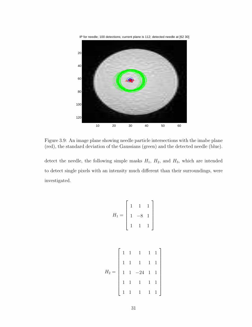
the candidate detections produced by each needle particle, as shown in Figure 3.9.

For the Kalman filter, the mean µ of the Gaussian is centered at the intersection

of the image plane and the Kalman filter’s needle belief. The standard deviation σ is

calculated by using the unscented transform to find sigma points on the plane, which

define the spread of the needle at one standard deviation.

3.3.2 Choosing a Needle Detection Mask

Various features can be extracted from an image by the use of masks with which

the image is convolved, e.g. the Sobel edge-detecting mask used below. In the case

of detecting a needle in low-resolution MR images, the problem reduces to the that

of looking for individual pixels that are notably different than their neighbors. To

30

IP for needle; 100 detections; current plane is 112; detected needle at [62 30]

10 20 30 40 50 60

20

40

60

80

100

120

Figure 3.9: An image plane showing needle particle intersections with the imabe plane(red), the standard deviation of the Gaussians (green) and the detected needle (blue).

detect the needle, the following simple masks H1, H2, and H3, which are intended

to detect single pixels with an intensity much different than their surroundings, were

investigated.

H1 =

1 1 1

1 −8 1

1 1 1

H2 =

1 1 1 1 1

1 1 1 1 1

1 1 −24 1 1

1 1 1 1 1

1 1 1 1 1

31

H3 =

1 1 1 1 1 1 1

1 1 1 1 1 1 1

1 1 1 1 1 1 1

1 1 1 −48 1 1 1

1 1 1 1 1 1 1

1 1 1 1 1 1 1

1 1 1 1 1 1 1

In order to determine which mask to use, and what value to use for the thresh-

olding constant T in order to minimize false positive needle detections, the following

procedure is used. First, a control trial is chosen, and in each timestep of that trial

the needle location is manually marked to form a known corpus of needle pixels. Sec-

ondly, a control trajectory is formed by selecting an equal number of voxels at which

the needle is known not to be. Then, the images are convolved with H1, H2, or H3.

This produces a distribution of the response of each filter H for cases in which it is

filtering the needle and non-needle cases. If the filter is working properly, comparing

the histogram of the two cases will demonstrate widely separated distributions, and

the threshold T can be chosen appropriately by inspecting the distributions.

Figures 3.10 - 3.12 demonstrate the results of this procedure. From these figures,

it is apparent that the 5x5 mask produces the best difference between needle pixels

and control points. Therefore, it was the one which was used in the experiments. The

threshold T was selected to be a value that neatly separates the peaks of the pixel

distributions. In the case of the 5x5 filter, a threshold intensity of 2000 was used.

32

−2000 −1000 0 1000 2000 3000 4000 50000

5

10

15

20

25

30

35

40

45

filter response intensity

coun

t

Filtered data, 3x3 point detecting mask

needle pointsfitted curvescontrol points

Figure 3.10: The histogram of the data filtered with the 3x3 mask, showing knownneedle points versus control points. A sharp difference between the peaks is seen.

33

−2000 0 2000 4000 6000 8000 10000 12000 14000 16000 180000

5

10

15

20

25


coun

t



Figure 3.11: The histogram of the data filtered with the 5x5 mask, showing knownneedle points versus control points. Again, two distinct peaks are evident, with thepeaks being somewhat more separated than in the 3x3 case.

34

−5000 −4000 −3000 −2000 −1000 0 1000 2000 3000 4000 50000

5

10

15


coun

t



Figure 3.12: The histogram of the data filtered with the 7x7 mask, showing knownneedle points versus control points. No distinction between the distributions can bediscerned, indicating that this mask is too wide to usefully extract single pixel needledata.

35

3.3.3 Image Processing for Target Detection

Because this algorithm is designed to detect targets which are roughly spherical, the

algorithm for detecting a target in a given image is straightforward.

First, the original image’s gradient is convolved with a Sobel edge detecting filter

and the result cropped to remove the edge of the gel [58]. Next, an elliptical Hough

transform[59] is applied to search for ellipses that approximately match the expected

radius of the target in the slice. This is done an arbitrary number of times, and the

best-fitting ellipses are averaged to give a final location of the detected target. If no

ellipses are found that fit the input, no target detection is reported. For the purposes

of the work described in this thesis, 50 ellipses were fitted.

This procedure is shown in Figures 3.13 - 3.16.

Figure 3.13: The MR image gradient.

36

Figure 3.14: The MR image gradient’s edges.

Figure 3.15: The MR image edges after cropping.

Figure 3.16: The detected target.

37

The image processing algorithm for target detection is purposely kept simple be-

cause of the simple nature of the phantoms under consideration here. In more com-

plicated phantoms and in real tissue, more complicated shape detection algorithms

would be used to detect the target. An example would be the region-growing approach

demonstrated in Chapter 4.

3.4 Simulation Results

The proposed algorithms were initially validated in simulation, by evaluating the

needle and target tracking performances in a simulated needle insertion task. In these

simulation experiments, a simulated magnetic resonance imaging system is used as

the intra-operative imaging system. The slices of the magnetic resonance images

are orthogonal to the initial needle insertion direction for simplicity. The scanner

has needle and target measurement error variances of σ2n,i = σ2

g,i = (0.2 mm)2, with

αn,fp = 0.02, αn,tp = 0.98, αg,fp = 0.01, and Ao = 75 mm2. In order to reduce the

computational complexity, at the expense of reduced resolution, MR scanner image

planes are assumed to be positioned in 1 mm increments. The needle is aimed at

a target with a radius of approximately 5mm that is located approximately 60 mm

from the needle entry point. During insertion, the needle bevel angle and control

point locations are perturbed slightly, and the target undergoes Brownian motion

with φ∆t = (0.1 mm)2. The needle was inserted straight towards the target in 10

steps, 10 mm per step.

The target position was initially unknown to the localization algorithm, so, prior

to needle insertion, the target region was scanned linearly in 15 steps to determine its

initial position. In the initial scanning phase, only the target localization algorithm

was executed in order to save computation time, and the imaging was performed

for each image plane in linear fashion. Once the target was located, the needle was

38

inserted straight towards the target in 10 steps, 10 mm per step. 500 needle particles

were used to locate the target during scanning, 25 during needle insertion, and 100

needle particles were used during insertion.

Although the model used in the active localization algorithm assumes a nominally

straight needle, the actual needle used in the simulations were given a bevel tip that

varied from 0°to 6°tip deflection per insertion step. The total angular deviation of

the needletip therefore varies up to 60°and the total needletip deviation from nominal

was approximately 40mm for the 100mm insertion. The needle is inserted in open

loop mode, without any explicit feedback control, in order to investigate if the needle

is successfully localized or not.

3.4.1 Particle Filters

The particle filter algorithm is suitable for both local and global localization prob-

lems since particle filters can accommodate arbitrary (including, multi-modal and

non-Gaussian) belief probability distributions. In order to validate both local and

global localization performance of the particle filter-based algorithm, the initial tar-

get position was assumed to be unknown to the localization algorithm. As a result,

the needle insertion task used in the simulation was set up as two phases, namely,

initial target localization and needle insertion. Prior to the needle insertion, the tar-

get region was scanned linearly in 15 steps to determine the initial location of the

target. In this initial target localization phase, only the target localization algorithm

was executed since the needle insertion has not started yet, and the imaging was

performed for each image plane in a linear fashion. Once the target was localized,

the needle insertion proceeded as usual, during which both the needle and target lo-

calization algorithms were executed. During the initial target localization phase, 500

target particles were used to localize the target. During the needle insertion phase,

25 target particles and 100 needle particles were used for tracking, respectively, the

39

target and the needle.

The performance of the particle filter algorithm was measured by performing 10

simulated needle insertions for this experiment and measuring the error between the

actual and estimated (using expected value of the belief functions) locations of the

needle tip and target. Fig. 3.19 shows the active localization algorithm’s beliefs of

the needle and target at four different steps in a sample execution of the task. As it

can be seen from the figure, the active localization algorithm was successfully able to

accurately capture the deviated shape of the needle.

The resulting absolute needletip and target localization errors were 1.07 ± 1.19

mm and 0.83 ± 0.34 mm (mean ± standard deviation), respectively. The needletip

tracking errors per needle bevel are shown in Table 3.4.1.

Fig. 3.17 shows the kernel smoothed density estimates for the target and needle

tip location beliefs, estimated from the corresponding particle filter outputs, at the

end of a sample execution of the task. The results indicate that the target and

needle locations were estimated accurately. Finally, Fig. 3.18 shows the change in

the entropies of the target and needle tip location beliefs during a sample execution

of the task. The figure shows the entropy of the target dropping as it is found during

the scan step, and the entropy of the needle increasing as the needle insertion begins

and falling as the active localization algorithm locates it.

deflection angle per step mean error (std. dev.)0° 0.41 (0.13)1° 0.64 (0.10)2° 0.75 (0.51)3° 0.58 (0.36)4° 0.41 (0.14)5° 0.73 (0.43)6° 3.81 (1.19)

Table 3.1: Needle localization mean errors and standard deviation (in mm) for theparticle filter in simulation.

40

0 20 40 60 80 100 1200

2


0 10 20 30 40 50 600

2


90 100 110 120 130 140 150 160 170 1800


0 20 40 60 80 100 1200

0.5

1Target Belief PDF − x coordinate

0 10 20 30 40 50 600

0.5

1Target Belief PDF − y coordinate

90 100 110 120 130 140 150 160 170 1800

0.2

0.4Target Belief PDF − z coordinate

(a) (b)

Figure 3.17: The particle filter’s kernel smoothed density estimates for the needle tip(a) and target (b) location beliefs. The solid vertical lines indicate the actual valueof the needle tip / target location.

3.4.2 Unscented Kalman Filters

While the unscented Kalman Filter is suitable for tracking an object, it is not suitable

to solving a global localization problem since the unscented Kalman filter assumes

that the beliefs are Gaussian. Therefore, the initial target localization phase is not

performed with the unscented Kalman filter. Instead, an initial estimate of the target

location is assumed to be available to the UKF, and the algorithm directly proceeds

with needle insertion, following a similar procedure described above for the particle

filter case. As with the particle filter algorithm, the performance of the unscented

Kalman filter implementation was measured by performing 30 repetitions of an open-

loop insertion experiment with a simulated needle with a bevel tip that varied from

0 to 6 degrees.

Fig. 3.22 shows the active localization algorithm’s beliefs of the needle and target

at the end of one localization trial. As with the particle filter, it can be seen that

the active localization algorithm was successful in tracking the needle as it deformed

during insertion.

The resulting absolute needletip and target localization errors were 0.58 ± 0.53

mm and 1.85 ± 0.45 mm (mean ± standard deviation), respectively. The needletip

41

0 5 10 15 20 25−10

−5

0

5

10

15

20

25Needle and Target Belief Entropies

NeedleTarget

Figure 3.18: Change in the entropies of the needle tip (solid) and target (solid)location beliefs during a sample execution of the task. As it can be seen from thefigure, the algorithm successfully alternates between imaging the target and the needlein order to minimize the total entropy of the belief.

deviations are given in Table 3.4.2. These results demonstrate that the Kalman filter,

with no knowledge of the needle’s curvature, is capable of accurately tracking a needle

with reasonable deformation.

Fig. 3.20 and 3.22 show sample results from simulated needle insertion tracked

with Kalman filter. Fig. 3.17 shows the kernel smoothed density estimates for the

target and needle tip location beliefs. Fig. 3.18 shows the change in the entropies of

the target and needle tip beliefs. Again, the algorithm successfully alternates between

imaging the target and the needle and minimizes the total entropy of the belief.

These results indicate that, given imaging algorithms that can detect the objects

with some reliability, both the particle filter and the unscented Kalman filter are

capable of successfully tracking a needle and a target as the needle is inserted into a

42

deflection angle per step mean error (std. dev.)0° 0.05 (0.00)1° 0.13 (0.00)2° 0.21 (0.03)3° 0.28 (0.06)4° 1.28 (0.20)5° 1.40 (0.04)6° 0.70 (0.13)

Table 3.2: Needle localization mean errors and standard deviation (in mm) for theUKF filter in simulation.

medium.

43

(a) (b)

(c) (d)

Figure 3.19: The particle filter tracking the needle and target. The blue line (invisible)is the actual needle shape, the green lines are the shapes of the particles in the needlebelief function, the large semi-transparent sphere is the actual target, the red circlesare the centers of the particle in the target belief function, and the semi-transparentplane is the current imaging plane. (a) Initial particle distribution when the locationof the target is unknown. (b) The target is localized at the end of the linear scanningphase. (c) Particle distribution at the mid point of the needle insertion. (d) Particledistribution at the end of the task.

44

−30 −20 −10 0 10 20 300

1


−30 −20 −10 0 10 20 300

1


20 40 60 80 100 120 140 1600

2


(a)

−30 −20 −10 0 10 20 300

0.1

0.2Target Belief PDF − x coordinate

−30 −20 −10 0 10 20 300

0.1

0.2Target Belief PDF − y coordinate

20 40 60 80 100 120 140 1600

0.1

0.2Target Belief PDF − z coordinate

(b)

Figure 3.20: The Kalman filter’s kernel smoothed density estimates for the needle tip(a) and target (b) location beliefs. The solid vertical lines indicate the actual needletip and target locations.

45

0 5 10 15 20 25 30 35 40−20

−15

−10

−5

0

5

10Needle and Target Belief Entropies

Figure 3.21: Change in the entropies of the needle tip (red) and target (green) locationbeliefs during one needle insertion trial. As with the particle filter algorithm, theunscented Kalman filter algorithm successfully alternates between imaging the targetand the needle in order to minimize the total entropy of the belief.

46

Figure 3.22: The unscented Kalman filter tracking a simulated needle and target.The blue line is the actual needle shape, the red line is the UKF filter’s mean needlebelief, and the red sphere represents the target belief.

47

3.5 Experimental Validation

This section describes the experiments done using real imaging data collected from

experiments in which a needle was inserted into a tissue phantom. This was done to

demonstrate the viability of the algorithms on non-simulated data. As with the

simulation experiments, tracking was performed by particle filters and unscented

Kalman Filters and the results compared. The models used in the experiments and

the experimental results are as follows.

3.5.1 Data Collection

Data were collected using magnetic resonance imaging during trials in which a needle

was inserted into a 1% agarose gel medium in which a target was suspended roughly

80mm from the needle entry point. The needle was inserted approximately 10mm in

open-loop fashion at each step, and after each step the entire volume was imaged.

This was repeated until the needle reached the edge of the gel.

Magnetic resonance imaging was chosen as the intraoperative imaging methodol-

ogy because it provides the ability to image an entire volume, allowing the data to be

sliced in arbitrary ways in post-processing, and providing a known reference frame.

In order to collect the data in a manageable time, data were collected at a relatively

low resolution - the volume of data collected at each timestep was 64x128x256 voxels,

each voxel having dimensions of 2x1x1mm. At this resolution, the MR system took

approximately two minutes to image the volume at each timestep. During data col-

lection, the entire volume of the gel phantom was imaged at each timestep. This was

done so that the active localization algorithms would be able to arbitrarily select any

one image plane during each processing step during offline analysis, thus allowing the

processing to be performed exactly as it would be during an actual needle-insertion

procedure in which full-volume imaging at each timestep takes an infeasible amount

48

of time.

Because the data were collected using a 1.5 Tesla MR scanner, a standard steel

surgical needle could not be safely used in this study. Instead, a nylon ersatz needle

was used and fed into the gel using a plastic feeding device built for the purpose

(Figure 3.23. A bevel tip was cut in the needletip, enabling it to be bent in order to

provide a greater or lesser degree of needle flexion during the trial, as desired.

Figure 3.23: The MR-safe needle insertion device. The device is placed on the beakerin which the tissue phantom and target are. The device is placed into the MR tubeand the flexible needle is inserted by turning the gears with a crank.

Data were collected during three open-loop needle insertion trials - one in which

the needle hit the target, one in which the needle closely missed the target, and one in

which the needle widely missed the target. The lateral deviation of the needletips from

straight for these trials was approximately 21mm, 19mm, and 50mm, respectively.

After data collection, the location of the needle in each image slice at each timestep

was manually marked and the approximate target position noted.

49

Figure 3.24: MR images of the three needle insertion trials. The needle is not com-pletely visible in any single image slice.

Unlike the simulated experiments, the target position is fixed during the trials.

Additionally, while the needle shape may deform due to the interaction with the tissue

phantom, the needle does not fluctuate stochastically in the same way that the needle

in the simulation experiments did.

Figure 3.24 shows example images slices from each of the three trials, showing the

needle curvature.

In order to simulate the operation of an intraoperative imaging system, the imag-

ing data were sliced such that the slices were orthogonal to the initial needle insertion

direction. The needle location in each slice was marked manually for later evaluation

purposes and the marked files stored separately, and the unmarked data were used by

the imaging algorithm as input data. Figures 3.25 shows sample images containing a

target and a needle, respectively.

3.5.2 Experimental Results

The above measurement models were implemented using MATLAB and the algo-

rithms were tested using the three magnetic resonance imaging data trials. The

performance of the needle filter was evaluated by measuring the error between the

real needletip, which was determined by marking the image slices manually, and the

50

filter’s belief of the needletip location. The performance of the target filter was sim-

ilarly measured by finding the difference between the target filter’s belief and the

real target location. Because the data is comprised of asymmetric voxels, errors are

reported both in units of millimeters and voxel units.

Because the particle filter is a stochastic algorithm, the results vary by trial and

the mean and standard deviation are reported. The only stochastic elements in the

UKF algorithm are in the sampling which is used in the entropy minimization step.

As the number of samples used in this step increases, the algorithm converges on

the ideal solution. In the trials used in this study, the algorithm chose an identical

sequence of image planes for each trial, and consequently the error for each trial was

identical.

Table 3.3 shows the results for the particle filter tracking the three needle insertion

trials. Table 3.4 shows the results in voxels taking into account asymmetric voxels.

These results indicate that the algorithms are able to track the needle to within 1.5mm

(1.5 voxels) during the trials where the needle deviation is approximately 20mm from

straight, and to within 4.5mm (4.5 voxels) during the trial where the needle deviation

is approximately 50mm. Target localization errors are within 4mm (2.5 voxels). Table

3.5 shows the results for the Kalman filter. The results are comparable, with needle

tracking within 1.5mm (1.5 voxels) for small deflection error case and 5.3mm (5 voxels)

for large deflection error case, and target tracking within 2mm (2 voxels).

Figure 3.27 shows the needle and target being tracked by the particle filter during

one trial, and demonstrates the entropy minimization algorithm calculating the image

plane that will produce the largest expected information gain in the next timestep.

51

trial needle error (std. dev.) target error (std. dev.)1 1.26 (0.04) 3.84 (2.03)2 1.44 (0.25) 3.87 (1.70)3 4.34 (0.43) 2.01 (1.04)

Table 3.3: Needle and target localization errors in mm for the particle filter trackingreal data.

trial needle error (std. dev.) target error (std. dev.)1 1.23 (0.05) 3.24 (2.23)2 1.43 (0.25) 3.58 (1.87)3 4.33 (0.44) 1.95 (1.23)

Table 3.4: Needle and target localization errors in voxel units for the particle filtertracking real data.

52

(a)

(b)

Figure 3.25: (a) A sample orthogonally-sliced MR image showing the target. (b) Asample orthogonally-sliced MR image showing the needle intersecting with the imageplane. The needle is very faint relative to the background noise in this image and isindicated by the arrow.

53

3.6 Discussion

This work serves as a proof of concept for an active sensing approach to needle

and target localization during needle insertion procedures that are guided by intra-

operative imaging system. In trials using real data, the algorithms are able to localize

the needle to a mean precision of approximately 5mm (5 voxels) in all cases and a

mean precision of approximately 1.5mm (1.5 voxels) in cases where the needle bevel

is not severe. In all experiments, the needle model assumed a straight needle, and

had no knowledge of the bevel of the real needle. The experiments with a severe

needle bevel were performed in order to establish the algorithm’s performance when

its needle model is highly erroneous. The needle was found to perform well until a

per-step angular deviation error of approximately 6°was encountered. This serves to

establish a reasonable upper bound for acceptable performance of the system with

the parameters used in these experiments.

The image processing algorithms demonstrated here have shown the ability to

extract target and needle feature information from noisy images. In particular, the

needle detection algorithm shows the ability to detect a needle which has a cross-

sectional area less than a pixel, and is able to accurately detect the needle in image

slices where the needle is obscured by noise. Intra-operative imaging data of greater

precision would lead to more precise localization.

This work was not done with computation time as a chief consideration, and most

of the code base is written in MATLAB r2014a, which is an interpreted language. For

a reasonable number of particles or samples, the particle filter and unscented Kalman

filter implementations both compute each timestep in approximately 2-4 minutes

using an Intel Core Duo CPU at 3.16 GHz. For a production system, considerable

speedup would be achieved by rewriting the implementations in a compiled language

and/or parallelizing the algorithms. Additionally, computation time can be reduced

by such methods as using the geometric knowledge of the system state to reduce the

54

search space for the entropy minimization algorithm.

Because the particle filter and unscented Kalman filter implementations have

demonstrated similar performance in terms of both accuracy and computation time,

the choice of which implementation to use in a production system is not necessarily

straightforward. However, because the particle filter is simpler to implement, sim-

pler to parallelize, and unlike the UKF does not assume that the data is normally

distributed, it should be regarded as the default choice for problems of this type.

trial needle error target errormm voxels mm voxels

1 1.27 1.13 1.52 1.162 1.42 1.41 1.81 1.613 5.23 4.76 1.45 1.42

Table 3.5: Needle and target localization errors for the unscented Kalman filter track-ing real data in mm and voxels.

55

80 90 100 110 120 130 140 150 160 170 1800

2

4

6

8

10

12

14

16

Image plane

Exp

ecte

d In

form

atio

n G

ain

(a) (b)

Figure 3.26: (a) The particle filter tracking the needle. Green lines represent the par-ticles comprising the filter’s belief and red circles represent the target filter’s particles.The true target position is given by the dark ellipsoid and the black dots representthe real needle position. (b) The active localization algorithm calculating the imageplane that it will use in the next timestep according to the system state shown in (a).The thick blue line shows the total expected information gain of each imaging plane,while the red line shows the contribution expected from the needle, and the dashedgreen line shows the expected information gain due to the target.

56

IP for needle; 100 detections; current plane is 137; detected needle at [76.00 56.00]

20 40 60 80 100 120

20

40

60

80

100

120

Current image plane is 137; detected needle at [76.00 56.00]

20 40 60 80 100 120

20

40

60

80

100

120

(a) (b)

Figure 3.27: (a) The particle filter needle detection image processing algorithm. (b)The result of the image processing algorithms detecting the needle and target loca-tions.

57

Chapter 4

Segmentation of Intra-Operative

Images With the Fast Marching

Method

While the simple Hough transform-based method of target detection is sufficient for

detecting targets in phantoms such as those used in the previous chapter, more com-

plex methods are necessary for the characterization of biological tissue. In particular,

a simple binary classification (e.g., target/not target) is inadequate for surgical op-

erations taking place in and around the various geometrically complicated structures

inside the human body. For closed-loop robotic needle insertion to be practicable,

the measurement models will need to distinguish between needle, target, obstacles,

and assign labels to all discrete structures.

Additionally, the problem of needle path planning for needle-based interventions

requires accurate segmentation of the tissue of interest for the calculation of a minimum-

cost path for needle insertion. Generally, the path is that which minimizes the dis-

tance the needle travels in tissue, but the presences of obstacles may cause a longer

path to be chosen [47]. For example, adipose tissue would have a low cost of insertion,

58

skeletal muscle a larger cost, sensitive organs a still greater cost, and obstacles, e.g.

bones and arteries, given an infinite cost. In order to assign such costs, however, it is

necessary to assign labels to the structures in the intra-operative image data.

While the problems of feature recognition and path planning in biological contexts

are subjects of ongoing research and are outside the scope of this dissertation, this

chapter’s purpose is to describe and demonstrate a fast, efficient, and effective method

of segmentation of 2D and 3D intra-operative images, thus supporting the solution

of those problems.

The remainder of this chapter is organized as follows. Level set methods are

discussed in Section 4.1. The fast marching method used here to implement the level

set approach is described in detail in Section 4.2. A fast and effective approach to

automatic seeding and the method used to merge similar regions are described in

Section 4.4. Section 4.5 describes the implementation of the algorithm, and Section

4.6 demonstrates results of the algorithm on sample intra-operative imaging data.

Section 4.7 discusses the results and implementation of these algorithms.

4.1 Level Set Methods

Level set methods have become a widely used way to segment images in various

applications [43]. The level set method is, at its heart, the projection of a function ψ

of N + 1 dimensions onto an N -dimensional space [41]. For an N -dimensional image,

the problem of segmentation is equivalent to finding a N + 1-dimensional function

ψ(x0, x1, .., xN+1, t) such that the curve ψ = 0 coincides with the image’s natural

phase boundaries. This function is found by solving the equation

ψt + F |∇tψ| = 0 (4.1)

where ψt is the difference between the current surface and the next surface, F

59

defines the speed at which the zero-level front of the function propagates, and |∇tψ|

is the gradient of the function at time t.

4.2 The Fast Marching Method

Many methods for implementing the level set method have been proposed and imple-

mented. One of the most powerful, effective, and efficient of these, which also negates

the problem of choosing an appropriate starting function surface, is the fast march-

ing method (FMM). FMM is a discretized implementation of the level set method

in which the function is treated as a front (or fronts) that expands from a starting

point (or points). With the addition of the constraint that the front can only expand

monotonically, it calculates an approximation of the level set front with a single pass

over the input data.

The algorithm, in its 2D formulation, works as follows. Let I(x, y) be the image to

be segmented, F (x, y) be a function defining the front at point (x, y), and T (x, y) be

the time at which the front arrives at (x, y). Then |∇T |F = 1. The T -function used

here is T (x, y) = e−α∇I(x,y), with α being a parameter that specifies how aggressively

the front follows the gradient.

Because the fronts propagate quickly in areas of the image where the gradient is

low and slowly in areas of high gradient, the effect of the algorithm as it proceeds is

to find the natural boundaries of the image.

The algorithm begins from one or more seed points (x0, y0) with T (x0, y0) = 0.

There are three lists, Accepted, initially containing (x0, y0), NarrowBand, initially

containing all 4-connected neighbors of (x0, y0), and FarAway, containing all other

points. In addition, a matrix designated OwnerMarker is maintained which tracks

which segment each pixel belongs to. By starting from multiple seed points and

marking OwnerMarker appropriately, a complete segmentation of I is achieved.

60

The algorithm proceeds as described in Algorithm 9 and terminates when all points

are marked Accepted. The output of this algorithm is a labeled image indicating which

region each pixel belongs to.

It is important to note that as the algorithm proceeds, each pixel (or voxel, in the

three-dimensional version) is marked with the cost between it and the nearest seed

point. Thus, if the costs for voxels are known, the version which proceeds with one

start point is a natural method to find minimum-cost paths from a start point.

Algorithm 9 The fast marching method algorithm in two dimensionsx and y. Thealgorithm is analogous in higher dimensions. [43].

function 2DFastMarch(I)

I: input imageAccepted: initially contains the seed pointsNarrowBand: initially contains the 4-connected neighbors of the seedsFarAway: initially contains all other pointsOwnerMarker: initially zero except for an identifier of each seed at its Accepted

and NarrowBand pointswhile NarrowBand is not empty do

(x, y)← the point in NarrowBand for which the value of T is highestRemove (x, y) from NarrowBand and insert it into AcceptedInsert all neighbors (xn, yn) of (x, y) that are not in Accepted into

NarrowBandend whilereturn OwnerMarker

end function

4.3 Image Enhancement

Two major common problems in medical images are those of of unequal contrast

and noise Fig. 4.1. These problems are mitigated in this work with the use of

two techniques. First, adaptive histogram equalization [60] is applied to the image

(Figure 4.2) to equalize image intensities. In this technique, each pixel is transformed

to more closely match the distribution of its neighbors’ intensities. Next, Perona-

Malik anisotropic diffusion [61] is used to reduce noise. In this technique, the image

61

unfiltered image 12

50 100 150 200 250

20

40

60

80

100

120

140

160

180

Figure 4.1: CT image showing poorly equalized contrast.

is iteratively convolved with isotropic Gaussian filters, the effect being that edges are

preserved and noise is reduced (Fig. 4.3).

These techniques are implemented in both two-dimensional and three-dimensional

variations. Two-dimensional examples are shown here for convenience.

62

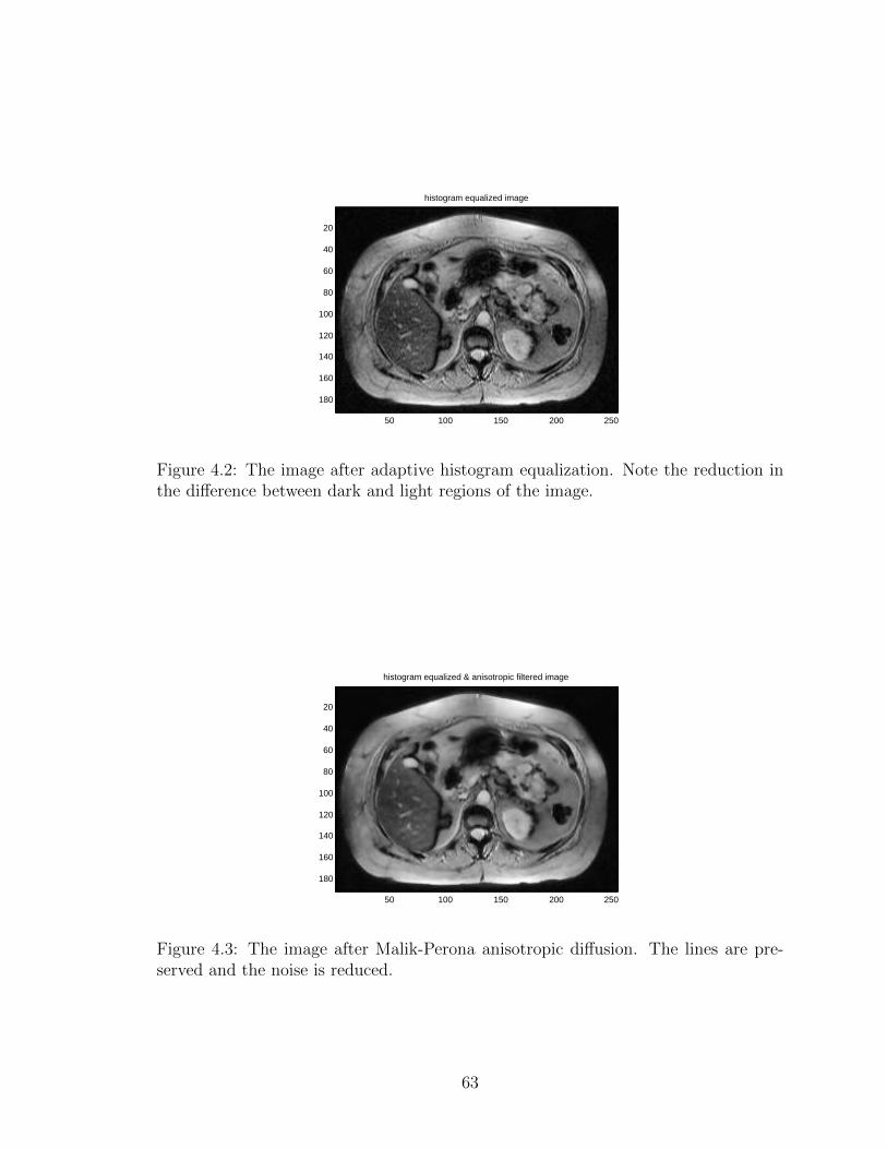
histogram equalized image

50 100 150 200 250

20

40

60

80

100

120

140

160

180

Figure 4.2: The image after adaptive histogram equalization. Note the reduction inthe difference between dark and light regions of the image.

histogram equalized & anisotropic filtered image

50 100 150 200 250

20

40

60

80

100

120

140

160

180

Figure 4.3: The image after Malik-Perona anisotropic diffusion. The lines are pre-served and the noise is reduced.

63

4.4 Seeding and Region Merging

Seeds are the starting points from which the fast marching algorithm grows its regions.

Proper selection of seeds is critical in order to achieve a smooth and correct final

segmentation result. A feature that does not have a seed placed in it will not be

detected in the final segmentation, and if too many seeds are placed in the areas

of high gradient at the boundaries of features, spurious regions will appear in the

segmented image. It is therefore critical that an effective method be chosen for

seeding.

Seeding can be done manually or automatically. If an expert is available to manu-

ally place seeds in the images, the segmentation results will benefit from the expert’s

knowledge of the image’s structure. If there is no such expert, or if the images are

sufficiently large that manual seeding is intractable, seeds can be placed automatically

by the following method.

For each image I in the image volume (or the entire image volume, in the 3D

implementation of the algorithm), the variance var(I) is calculated. Then the image

is divided into subimages Ii, and the subimage variances var(Ii) calculated. If a

subimages variance meets the criterion var(Ii) < β var(I) for a constant β < 1, then

a seed is placed at the center of the subimage. If not, then the subimage is divided

and the process repeats recursively. This process continues until all subimages have

had seeds placed, or until the size of the input image Ii is smaller than a parameter

lmin, in which case the algorithm exits without placing a seed. The effect of this

procedure is to produce seeds in areas of low variance, with a large number of seeds

that are concentrated near the edges of the regions (Figure 4.4).

Because this seeding method produces a huge number of image segments, it is

desirable to merge similar ones together after the fast marching method finishes.

This is done with Nock’s method of statistical region merging (SRM) [44]. In this

method, two adjacent regions R and R′ are merged if |R− R′| ≤√b2(R) + b2(R′) for

64

Figure 4.4: An example slice of patient data, showing the distribution of seeds gen-erated by the automatic seeding technique.

a merging threshold b.

The final step is then to manually threshold the output of SRM and perform

manual corrections, if any are necessary.

4.5 Implementation

These algorithms were implemented in MATLAB code. MEX-files were written to

more efficiently compute the FMM segmentation and mean intensity of the com-

puted segments. Preexisting MATLAB libraries were used for the SRM, histogram

equalization, and anisotropic diffusion portions of the method.

4.6 Results

Below are shown results for two segmentations of a 208x256x88 MR image volume of a

patient with a large liver tumor, which was obtained from the Frederick National Lab

for Cancer Research’s public cancer imaging archive. The first segmentation is done

65

with seeds chosen by hand, and the second is done with seeds chosen automatically.

4.6.1 Manually-Seeded Image Volume

The first segmentation starts from 19 seeds chosen manually: one for outside the

patient, one for the chest wall, one for the ribs, one for each kidney, one for the liver,

one for the liver tumor, one for the gall bladder, one for the stomach, seven for the

complicated structures of the intestines, one for the spleen, one for the heart, and

one for the aorta. The only parameter necessary to choose is the FMM algorithm’s

α parameter, which was chosen to be 500 here.

Running in single-threaded mode on an AMD FX-4100 processor at 3.6 GHz and

with 8 GB of RAM, the algorithm completely processed the data in 147 seconds. The

largest contributor to this time was the anisotropic diffusion step, which took 114

seconds. FMM took approximately 24 seconds, and finding the mean intensity of the

image segments took slightly more than one second.

Figure 4.5 shows a slice of the MR images. Figure 4.6 shows the slice after contrast

equalization and noise reduction. Figure 4.7 shows the mean intensity of the FMM

segmented regions, and Figure 4.8 shows the regions in colors corresponding to the

seed they belong to. The result is also visualized in 3D in Figure 4.9.

66

Figure 4.5: Original MR image. Note the large liver tumor.

Figure 4.6: The MR image after the volume was histogram equalized and hadanisotropic diffusion applied to it.

67

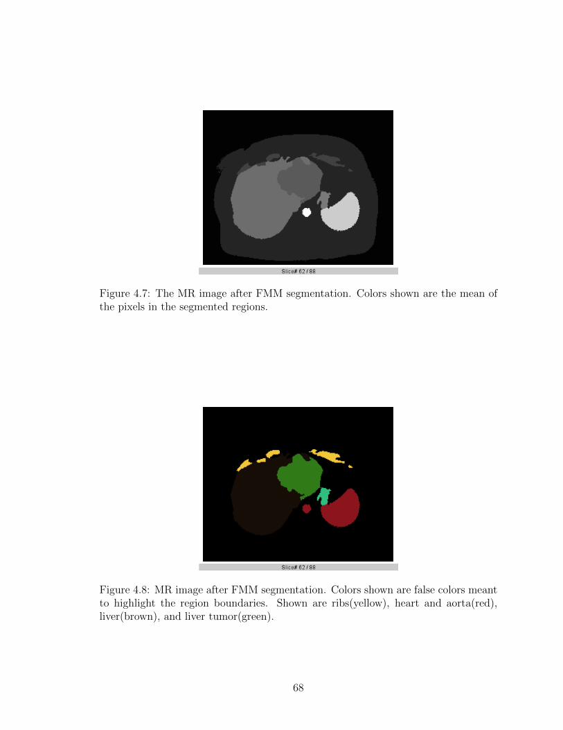
Figure 4.7: The MR image after FMM segmentation. Colors shown are the mean ofthe pixels in the segmented regions.

Figure 4.8: MR image after FMM segmentation. Colors shown are false colors meantto highlight the region boundaries. Shown are ribs(yellow), heart and aorta(red),liver(brown), and liver tumor(green).

68

Figure 4.9: 3D representation of the segmented MR volume. The lungs are omit-ted, as are ribs, chest wall, and other non-organ structures. This demonstrates aclean segmentation of the heart and aorta (red), liver(light brown), liver tumor(darkbrown), spleen (blue) stomach and intestines (light green), gall bladder (dark green),and kidneys (yellow).

69

Figure 4.10: One slice of the volume, showing the result of the 3D automatic seedingprocedure. Note that fewer seeds are generated than for the 2D case.

4.6.2 Automatically-Seeded Image Volume

The second segmentation example is done with automatically-generated seeds and

uses the same input dataset. With the seed generation variance parameter β = 0.1, a

total of 5,743 seeds are generated in the 208x256x88 image volume. Using the same

slice of the example volume as in the previous example, Figure 4.10 shows the result

of the seeding procedure one one slice of the image.

After seeding, the FMM algorithm proceeds as normal. The effect of this is to

produce a number of regions equal to the number of seeds, which when labeled with

the mean intensity of the voxels in their regions show the natural boundaries of the

image (Fig. 4.11).

Next, the SRM algorithm combines adjacent regions that are of sufficiently similar

intensity. Choosing the SRM merging threshold parameter b = 200 produces the

result in Figure 4.12. After this operation, the number of unique regions is reduced

from 5,734 to 2,380.

With this approach, it is necessary to manually crop and threshold in order to

70

Figure 4.11: The slice of the volume after FMM segmentation. The boundaries aremuch more sharply distinguished than in the input image.

segment individual organs and structures. Figure 4.13 shows the results of applying

a global threshold in order to segment the spleen and kidney from the image volume.

The automatically-seeded variation of the algorithm takes longer than the manually-

seeded version, taking a total of 251 seconds to segment the same image data on the

same hardware. Nearly all of that increase, approximately 113 seconds, is due to the

statistical region merging step.

71

Figure 4.12: The slice of the volume after statistical region merging. Note the sharplyreduced number of regions.

Figure 4.13: Volumetric rendering of the volume after manual global thresholding.Some spurious structures are present due to the nature of global thresholding.

72

4.7 Discussion

This work demonstrates an effective, semi-autonomous method to segment and an-

alyze intra-operative imaging data. The algorithm completes quickly and effectively

finds clear boundaries of the structures being segmented. The version in which seeds

are chosen by an expert is faster and does not require the merging of segmented

regions.

The algorithms in use here are all trivially parallelizable, but were were run serially

on the test data set. Considerable additional speedup can be obtained by rewriting

the code from MATLAB into C++ or some other compiled language.

73

Chapter 5

Conclusions

This thesis was focused on the development of technologies for the problem of robotic

image-guided needle insertion interventions. The major work presented here is the

active localization framework in which the needle and target localization system uses

expected entropy maximization to choose the measurement most likely to maximize

its knowledge of the system. With only one measurement per timestep, the system is

able to localize needle and targets as the needle is inserted in open-loop fashion. The

needle and target are tracked by Bayesian filters, and particle filter and unscented

Kalman filter implementations are demonstrated.

In addition, this thesis demonstrates a technique to bias measurements using the

Bayesian filter’s estimate of the system state. This was used to good effect to detect

faint signals in the presence of noise, even when the signal is not discernible to the

human eye.

Finally, this thesis describes and a technique using the fast marching method to

efficiently and effectively segment biomedical volume image data. This is shown to

successfully segment MR data, including segmenting a liver tumor.

The goal of this research is to assist the development of fully closed-loop robotic

needle insertion surgery. While several important steps of the process are developed

74

in this thesis, there is still much work to be done. A successful needle surgery robotic

system represents many problem domains, among them haptics, control theory, intra-

operative imaging technology, image processing, tissue modeling, needle modeling,

etc. While the problem is gigantic, this thesis provides a foundation for the further

advancement of technologies to solve it.

75

Appendix A

Automated Fuel Cell Segmentation

and Characterization

The fast marching algorithm as described in Chapter 4 was implemented and demon-

strated on the problem of segmenting fuel cell electron microscopy images. As the

algorithm provides a useful result on a problem domain that is disparate from that in

the main body of the thesis, the application on fuel cells is described in this appendix.

A.1 Introduction

A fuel cell is an energy conversion device in which fuel is converted directly into elec-

trical current by means of a chemical reaction. While a variety of fuel cell types exist

using various types of fuel, the fuel cells analyzed here are of the hydrogen/oxygen

type, in which hydrogen and oxygen react directly to create water. The structure

of these cells consists of three distinct materials - an electrically-conductive metal,

an ionically-conductive ceramic, and empty space in which the H2 and O2 gas flows.

The chemical reaction occurs at the junctures of these three phases, the triple-phase

boundary (TPB). Performance of fuel cells depends on several factors which affect

the rate of chemical reaction occurring in the fuel cell. It is desirable to maximize

76

the number of TPB points, and to maximize the number of active TPB points, i.e.,

to maximize the number of potential reaction sites at which the ionic conductor is

connected to the electrolyte and the electrical conductor is connected to the load,

and therefore at which the reaction can occur. It is also desirable to maximize the

permeability of the fuel cell to gas to ensure maximum gas flow to the reaction sites.

Fuel cell research depends on effective characterization of sample cells. In order

to characterize a fuel cell, the fuel cell must be imaged in some way and the images

must be segmented so that all phases of the fuel cell are represented by distinct la-

bels. Because the phase boundaries are often a gradient instead of a sharp boundary,

and because the image often contains problems such as noise and non-uniform illu-

mination, thresholding requires extensive manual correction and is time-consuming

when done manually. In addition, it is difficult to the point of intractability to man-

ually classify TPB points as active or inactive or to otherwise quantify the geometric

properties of the fuel cell by hand.

To solve these problems, an automated method for segmenting fuel cell images

is described here. The method automatically generates appropriate seeds among the

material types, grows regions from those seeds, and merges similar regions. Following

this, the segmented images can easily be converted into a graph representation and

the connectedness of the TPB reaction sites can be evaluated using the A* graph

search algorithm.

A.2 Background

In a hydrogen/oxygen type fuel cell, the overall chemical reaction is

2H2 +O2 → 2H2O

This reaction occurs in two stages which occur as follows. The fuel cell is con-

77

structed of a gas-permeable anode, a gas-impermeable but ionically-conductive elec-

trode, and a permeable cathode (Fig.A.1). The anodes and cathodes consist of pores

in which gas flows, ionically-conductive Yttria-stabilized zirconia, or YSZ, and an

electrically-conductive nickel-palladium alloy (NiPd). The reaction proceeds as fol-

lows. H2 gas enters the anode and is ionized at the points where the pores and two

material types meet.

H2 → 2H+ + 2e−

The positively-charged hydrogen ions are conducted through the electrode and the

electrons are conducted through a load, producing a usable current. In the cathode

the oxygen reacts with the electrons and then combines with the free protons to

produce water.

O2 + 4e− → 2O2−

and

2H+ +O2− → H2O

A number of methods have been used for segmentation of fuel cell images. The

most common method is thresholding, with the thresholds being set manually or with

the aid of some statistical method. Joos et al. used a histogram-aided segmentation

approach in which the threshold value is determined by the Otsu clustering algorithm

[62]. Guan et al. use binary thresholding to reconstruct the 3D microstructure of

a fuel cell cathode prior to analysis of its geometric properties [63]. Thiele et al.

use a similar thresholding approach to construct a 3-dimensional model of a fuel cell

catalyst layer [64]. Ostadi et al. examined the effect of threshold variations on a 3-D

reconstruction of a fuel cell [65].

Various active contour based approaches to the problem of segmenting fuel cells

78

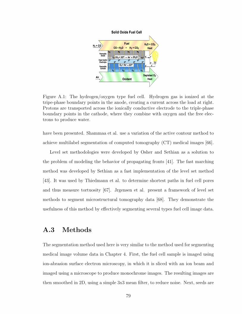
Figure A.1: The hydrogen/oxygen type fuel cell. Hydrogen gas is ionized at thetripe-phase boundary points in the anode, creating a current across the load at right.Protons are transported across the ionically conductive electrode to the triple-phaseboundary points in the cathode, where they combine with oxygen and the free elec-trons to produce water.

have been presented. Shammaa et al. use a variation of the active contour method to

achieve multilabel segmentation of computed tomography (CT) medical images [66].

Level set methodologies were developed by Osher and Sethian as a solution to

the problem of modeling the behavior of propagating fronts [41]. The fast marching

method was developed by Sethian as a fast implementation of the level set method

[43]. It was used by Thiedmann et al. to determine shortest paths in fuel cell pores

and thus measure tortuosity [67]. Jrgensen et al. present a framework of level set

methods to segment microstructural tomography data [68]. They demonstrate the

usefulness of this method by effectively segmenting several types fuel cell image data.

A.3 Methods

The segmentation method used here is very similar to the method used for segmenting

medical image volume data in Chapter 4. First, the fuel cell sample is imaged using

ion-abrasion surface electron microscopy, in which it is sliced with an ion beam and

imaged using a microscope to produce monochrome images. The resulting images are

then smoothed in 2D, using a simple 3x3 mean filter, to reduce noise. Next, seeds are

79

automatically generated using the recursive image variance seeding method described

previously, and the fast marching method is used to grow regions from those seeds. A

gray value is assigned to each region by finding its mean intensity. Because there are

a large number of regions grown from many seeds, Nock’s statistical region merging

algorithm is then used to appropriately combine regions that are similar spatially and

in intensity. The final product is achieved by thresholding the merged images. The

images are then visually inspected and any necessary corrections are made manually.

The fuel cell images used in this study were acquired using ion-abrasion scanning

electron microscopy (IA-SEM), in which the sample of interest is alternately imaged

with a scanning electron microscope and milled by an ion beam[69].

Because this study uses a strategy of using a large number of seeds in order to

capture small features, the output of the FMM step is a large number of regions that

do not necessarily represent the image structure individually, but rather cumulatively.

It is therefore desirable to merge similar regions into larger regions that more closely

represent the material phases shown in the image. As with the automatically-seeded

method for intra-operative images, this is done with Nock’s method of statistical

region merging (SRM).

As discussed previously, the chemical reaction in a fuel cell takes place at the

active TPB points. After segmentation, it is trivial to identify TPB points, but they

cannot be classified as active or inactive simply by examining the segmented images.

Since a TPB point is active if: 1. It is adjacent to a YSZ particle that is connected to

the electrolyte; 2. it is adjacent to an NiPd particle that is connected to the electrical

circut; 3. it is adjacent to a pore in which gas can flow, the problem of classifying TPB

points therefore reduces to the problem of finding paths - if a path exists from the

candidate TPB to the electrolyte, then the TPB is said to be electrically percolated.

If the same is true for the other two phases the TPB is adjacent to, then the TPB is

active. It is straightforward to solve the pathfinding problem in an efficient manner

80

by converting the segmented volume into a graph representation and using the well-

known and computationally efficient A* graph search algorithm.

To convert the volume of segmented images to a graph representation is straight-

forward, the following method is used. Each distinct segment in each image is con-

sidered a vertex in a graph and designated with a unique identifier. Then, for each

node, check to see if it overlaps with a node that is the same segment type. If there

is an overlap, an edge is drawn between the two vertices. Finally, create an artificial

vertex to represent the electrolyte, connect all nodes that are on the left edge of the

images to it, and do the same for the right side to represent the electrode. Gas flow

is similarly represented by two artificial vertices at the top and bottom of the image

stack. The procedure for determining if a given TPB is connected is then:

Let P = (x, y, z) be the TPB point being checked. Find A, B, and C, the

vertices representing the structures which are touching P , with A being the electrical

conductor, B being the ionic conductor, and C being the gas pore. Let Agoal and Bgoal

be the vertices representing the electrolyte and electrode, respectively, and let Cintake

and Cexhaust represent the gas intake and exhaust vertices. Then P is active if and

only if Astar search(start, end) returns true for all of the pairs (A,Agoal), (B,Bgoal),

(C,Cintake), and (C,Cexhaust).

This is repeated for all TPB points in the volume. The result is two lists containing

the coordinates of all active and inactive TPB points.

A.4 Results

The segmentation and methods described above are able to quickly and effectively

segment sets of fuel cell image data. The algorithms were implemented in MATLAB,

with the FMM code being written as C++ MEX-files to improve performance. A

preexisting MATLAB library was used for the statistical region merging algorithm.

81

The test data set consists of 27 1554x408 pixel images of slices of a fuel cell anode.

After segmentation, it was found that the anode consisted of 38.58% NiPd, 39.85%

YSZ, and 21.57% pores.

Figure A.2 shows a sample of a fuel cell image, the result of each intermediate

segmentation step on it, and the final result after thresholding.

Using an Intel Core 2 Duo PC with 4GB RAM, segmentation was completed in

approximately 348 seconds, or 13 seconds per slice. Most of this time (about 11

seconds per slice) was taken up by statistical region merging.

82

(a) (b)

(c) (d)

(e)

Figure A.2: (a)A section of an anode image after seeding. Seeds are shown as redpixels. (b) The regions grown after 20,000 iterations of the FMM algorithm. (c)The final result of FMM. (d) After statistical region merging. (e) Result of manualthresholding after FMM segmentation and statistical region merging.

83

Bibliography

[1] Niki Abolhassani, Rajni Patel, and Mehrdad Moallem. Needle insertion into softtissue: A survey. Medical engineering & physics, 29(4):413–431, 2007.

[2] Joao Luiz Moreira Coutinho Azevedo, Otavio Cansancao Azevedo, Susana AbeMiyahira, Gustavo Peixoto Soares Miguel, Otavio Monteiro Becker Jr, OctavioHenrique Mendes Hypolito, Afonso Cesar Cabral Guedes Machado, WellingtonCardia, Gilmara Aguiar Yamaguchi, Lola Godinho, et al. Injuries caused byveress needle insertion for creation of pneumoperitoneum: a systematic literaturereview. Surgical endoscopy, 23(7):1428–1432, 2009.

[3] M1 Schafer, M Lauper, and L Krahenbahl. Trocar and veress needle injuriesduring laparoscopy. Surgical endoscopy, 15(3):275–280, 2001.

[4] R Palmer. Safety in laparoscopy. Journal of Reproductive Medicine, 13(1):1–5,1974.

[5] S. P. DiMaio. Modelling, simulation and planning of needle motion in soft tissue.Ph.d., University of British Columbia, Vancouver, Canada, 2003.

[6] S.P. DiMaio and S.E. Salcudean. Needle insertion modeling and simulation.Robotics and Automation, IEEE Transactions on, 19(5):864 – 875, 2003.

[7] S.P. DiMaio and S.E. Salcudean. Needle steering and motion planning in softtissues. Biomedical Engineering, IEEE Transactions on, 52(6):965 –974, 2005.

[8] Allison M Okamura, Christina Simone, and Mark D O’Leary. Force modelingfor needle insertion into soft tissue. Biomedical Engineering, IEEE Transactionson, 51(10):1707–1716, 2004.

[9] Jessica R Crouch, Chad M Schneider, Josh Wainer, and Allison M Okamura.A velocity-dependent model for needle insertion in soft tissue. In Medical Im-age Computing and Computer-Assisted Intervention–Miccai 2005, pages 624–632. Springer, 2005.

[10] R. J. Webster III, J. S. Kim, N. J. Cowan, G. S. Chirikjian, and A. M. Okamura.Nonholonomic modeling of needle steering. International Journal of RoboticsResearch, 25(5-6):509–525, May-June 2006.

84

[11] S. Misra, K.B. Reed, B.W. Schafer, K.T. Ramesh, and A.M. Okamura. Obser-vations and models for needle-tissue interactions. In Robotics and Automation,2009. ICRA ’09. IEEE International Conference on, pages 2687–2692, May 2009.

[12] W. Park, J. S. Kim, Y. Zhou, N.J. Cowan, A.M. Okamura, and G.S. Chirikjian.Diffusion-based motion planning for a nonholonomic flexible needle model. InProc. of the IEEE In’l Conf. on Robotics and Automation, pages 4600–4605,2005.

[13] Kevin Cleary, Hui Zhang, Neil Glossop, Elliot Levy, Bradford Wood, and FilipBanovac. Electromagnetic tracking for image-guided abdominal procedures:Overall system and technical issues. In Engineering in Medicine and BiologySociety, 2005. IEEE-EMBS 2005. 27th Annual International Conference of the,pages 6748–6753. IEEE, 2005.

[14] Simon W Wong, Ahtsham U Niazi, Ki J Chin, and Vincent W Chan. Real-timeultrasound-guided spinal anesthesia using the sonixgps® needle tracking system:a case report. Canadian Journal of Anesthesia/Journal canadien d’anesthesie,60(1):50–53, 2013.

[15] D. Glozman and M. Shoham. Image-guided robotic flexible needle steering.Robotics, IEEE Transactions on, 23(3):459 –467, 2007.

[16] Z. Neubach and M. Shoham. Ultrasound-guided robot for flexible needle steering.Biomedical Engineering, IEEE Transactions on, 57(4):799–805, 2010.

[17] B. Dong, E. Savitsky, and S. Osher. A novel method for enhanced needle lo-calization using ultrasound-guidance. In Advances in Visual Computing, volume5875 of Lecture Notes in Computer Science, pages 914–923. Springer Berlin /Heidelberg, 2009.

[18] Aditya Brij Koolwal, Federico Barbagli, Christopher Carlson, and David Liang.An ultrasound-based localization algorithm for catheter ablation guidance in theleft atrium. The International Journal of Robotics Research, 29(6):643–665, 2010.

[19] Stephen T Tully. BodySLAM: Localization and Mapping for Surgical Guidance.PhD thesis, Carnegie Mellon University, 2012.

[20] Ali Asadian, Mehrdad R Kermani, and Rajni V Patel. A novel force modelingscheme for needle insertion using multiple kalman filters. Instrumentation andMeasurement, IEEE Transactions on, 61(2):429–438, 2012.

[21] Gustaaf J Vrooijink, Momen Abayazid, and Sudip Misra. Real-time three-dimensional flexible needle tracking using two-dimensional ultrasound. InRobotics and Automation (ICRA), 2013 IEEE International Conference on,pages 1688–1693. IEEE, 2013.

85

[22] Mark Renfrew, Zhoufu Bai, and M. Cenk Cavusoglu. Particle filter based activelocalization of target and needle in robotic image-guided intervention systems. InAutomation Science and Engineering (CASE), IEEE International Conferenceon, pages 448–454. IEEE, 2013.

[23] Joseph D Greer, Troy K Adebar, Gloria L Hwang, and Allison M Okamura. Real-time 3d curved needle segmentation using combined b-mode and power dopplerultrasound. In Medical Image Computing and Computer-Assisted Intervention–MICCAI 2014, pages 381–388. Springer, 2014.

[24] Mert Kaya and Ozkan Bebek. Gabor filter based localization of needles in ultra-sound guided robotic interventions. In Imaging Systems and Techniques (IST),2014 IEEE International Conference on, pages 112–117. IEEE, 2014.

[25] Mert Kaya and Ozkan Bebek. Needle localization using gabor filtering in 2d ul-trasound images. In Robotics and Automation (ICRA), 2014 IEEE InternationalConference on, pages 4881–4886. IEEE, 2014.

[26] Stephen H Okazawa, Richelle Ebrahimi, Jason Chuang, Robert N Rohling, andSeptimiu E Salcudean. Methods for segmenting curved needles in ultrasoundimages. Medical image analysis, 10(3):330–342, 2006.

[27] Pierre Chatelain, Alexandre Krupa, and Maud Marchal. Real-time needle detec-tion and tracking using a visually servoed 3d ultrasound probe. In Robotics andAutomation (ICRA), 2013 IEEE International Conference on, pages 1676–1681.IEEE, 2013.

[28] Hidetomo Suzuki and Jun-ichiro Toriwaki. Automatic segmentation of head mriimages by knowledge guided thresholding. Computerized medical imaging andgraphics, 15(4):233–240, 1991.

[29] Peter H Gregson. Automatic segmentation of the heart in 3d mr images. In Elec-trical and Computer Engineering, 1994. Conference Proceedings. 1994 CanadianConference on, pages 584–587. IEEE, 1994.

[30] Jonathan Hearn. Competitive medical image segmentation with the fast marchingmethod. PhD thesis, Case Western Reserve University, 2008.

[31] WE Phillips, RP Velthuizen, S Phuphanich, LO Hall, LP Clarke, and ML Sil-biger. Application of fuzzy c-means segmentation technique for tissue differentia-tion in mr images of a hemorrhagic glioblastoma multiforme. Magnetic resonanceimaging, 13(2):277–290, 1995.

[32] Alan W-C Liew and Hong Yan. Current methods in the automatic tissue segmen-tation of 3d magnetic resonance brain images. Current Medical Imaging Reviews,2(1):91–103, 2006.

86

[33] Shruti Dalmiya, Avijit Dasgupta, and Soumya Kanti Datta. Application ofwavelet based k-means algorithm in mammogram segmentation. InternationalJournal of Computer Applications, 52(15):15–19, 2012.

[34] Yongyue Zhang, Michael Brady, and Stephen Smith. Segmentation of brainmr images through a hidden markov random field model and the expectation-maximization algorithm. Medical Imaging, IEEE Transactions on, 20(1):45–57,2001.

[35] J Hong, Takeyoshi Dohi, Makoto Hashizume, K Konishi, and N Hata.An ultrasound-driven needle-insertion robot for percutaneous cholecystostomy.Physics in Medicine and Biology, 49(3):441, 2004.

[36] Norbert Bergner, Thomas Bocklitz, Bernd FM Romeike, Rupert Reichart, RolfKalff, Christoph Krafft, and Jurgen Popp. Identification of primary tumors ofbrain metastases by raman imaging and support vector machines. Chemometricsand Intelligent Laboratory Systems, 117:224–232, 2012.

[37] Parmida Moradi Birgani, Meghdad Ashtiyani, and Saeed Asadi. Mri segmen-tation using fuzzy c-means clustering algorithm basis neural network. In Infor-mation and Communication Technologies: From Theory to Applications, 2008.ICTTA 2008. 3rd International Conference on, pages 1–5. IEEE, 2008.

[38] IN Manousakas, PE Undrill, GG Cameron, and TW Redpath. Split-and-mergesegmentation of magnetic resonance medical images: performance evaluation andextension to three dimensions. Computers and Biomedical Research, 31(6):393–412, 1998.

[39] Gobert N Lee, Mariusz Bajger, and Martin Caon. Multi-organ segmentation ofct images using statistical region merging. 2012.

[40] T Heinonen, P Dastidar, H Eskola, H Frey, P Ryymin, and E Laasonen. Appli-cability of semi-automatic segmentation for volumetric analysis of brain lesions.Journal of medical engineering & technology, 22(4):173–178, 1998.

[41] Stanley Osher and James A Sethian. Fronts propagating with curvature-dependent speed: algorithms based on hamilton-jacobi formulations. Journalof computational physics, 79(1):12–49, 1988.

[42] Caroline Baillard, Pierre Hellier, and Christian Barillot. Segmentation of brain3d mr images using level sets and dense registration. Medical image analysis,5(3):185–194, 2001.

[43] James A Sethian. Fast marching methods. SIAM review, 41(2):199–235, 1999.

[44] Richard Nock and Frank Nielsen. Statistical region merging. Pattern Analysisand Machine Intelligence, IEEE Transactions on, 26(11):1452–1458, 2004.

87

[45] Ron Alterovitz, Ken Goldberg, and Allison Okamura. Planning for steerablebevel-tip needle insertion through 2d soft tissue with obstacles. In Roboticsand Automation, 2005. ICRA 2005. Proceedings of the 2005 IEEE InternationalConference on, pages 1640–1645. IEEE, 2005.

[46] Daniel Glozman and Moshe Shoham. Flexible needle steering and optimal tra-jectory planning for percutaneous therapies. In Medical Image Computing andComputer-Assisted Intervention–MICCAI 2004, pages 137–144. Springer, 2004.

[47] Simon P DiMaio and SE Salcudean. Needle steering and motion planning in softtissues. Biomedical Engineering, IEEE Transactions on, 52(6):965–974, 2005.

[48] Seong Young Ko and Ferdinando Rodriguez y Baena. Toward a miniaturizedneedle steering system with path planning for obstacle avoidance. BiomedicalEngineering, IEEE Transactions on, 60(4):910–917, 2013.

[49] Wolfram Burgardy, Dieter Foxy, and Sebastian Thrunz. Active mobile robotlocalization. 1997.

[50] U. Orguner. Notes on differential entropy calculation using particles. Technicalreport, Department of Electrical Engineering, Linkping University, 2008.

[51] A. Ryan and J. K. Hedrick. Particle filter based information-theoretic activesensing. Robotics and Autonomous Systems, 58(5):574–584, 2010.

[52] Simo Sarkka. Bayesian filtering and smoothing, volume 3. Cambridge UniversityPress, 2013.

[53] Zhe Chen. Bayesian filtering: From kalman filters to particle filters, and beyond.Statistics, 182(1):1–69, 2003.

[54] Eric A Wan and Rudolph Van Der Merwe. The unscented kalman filter for non-linear estimation. In Adaptive Systems for Signal Processing, Communications,and Control Symposium 2000. AS-SPCC. The IEEE 2000, pages 153–158. IEEE,2000.

[55] H Akashi and H Kumamoto. Construction of discrete-time nonlinear filter bymonte carlo methods with variance-reducing techniques. Systems and Control,19(4):211–221, 1975.

[56] Sebastian Thrun, Wolfram Burgard, and Dieter Fox. Probabilistic robotics. MITpress, 2005.

[57] Rudolph Emil Kalman. A new approach to linear filtering and prediction prob-lems. Journal of Fluids Engineering, 82(1):35–45, 1960.

[58] Richard O Duda, Peter E Hart, et al. Pattern classification and scene analysis,volume 3. Wiley New York, 1973.

88

[59] Yonghong Xie and Qiang Ji. A new efficient ellipse detection method. In Pat-tern Recognition, 2002. Proceedings. 16th International Conference on, volume 2,pages 957–960. IEEE, 2002.

[60] Stephen M Pizer, E Philip Amburn, John D Austin, Robert Cromartie, AriGeselowitz, Trey Greer, Bart ter Haar Romeny, John B Zimmerman, and KarelZuiderveld. Adaptive histogram equalization and its variations. Computer vision,graphics, and image processing, 39(3):355–368, 1987.

[61] Pietro Perona and Jitendra Malik. Scale-space and edge detection usinganisotropic diffusion. Pattern Analysis and Machine Intelligence, IEEE Trans-actions on, 12(7):629–639, 1990.

[62] Jochen Joos, Thomas Carraro, Andre Weber, and Ellen Ivers-Tiffee. Recon-struction of porous electrodes by fib/sem for detailed microstructure modeling.Journal of Power Sources, 196(17):7302–7307, 2011.

[63] Yong Guan, Wenjie Li, Yunhui Gong, Gang Liu, Jeff Gelb, Xiaobo Zhang, YingXiong, Yangchao Tian, and Haiqian Wang. The study of the reconstructed three-dimensional structure of a solid-oxide fuel-cell cathode by x-ray nanotomography,2010.

[64] Simon Thiele, Roland Zengerle, and Christoph Ziegler. Nano-morphology of apolymer electrolyte fuel cell catalyst layer - imaging, reconstruction and analysis.Nano Research, 4(9):849–860, 2011.

[65] Hossein Ostadi, P Rama, Y Liu, R Chen, XX Zhang, and K Jiang. Influence ofthreshold variation on determining the properties of a polymer electrolyte fuelcell gas diffusion layer in x-ray nano-tomography. Chemical Engineering Science,65(6):2213–2217, 2010.

[66] Haitham Shammaa, Hiromasa Suzuki, and Yutaka Ohtake. Creeping contours:a multilabel image segmentation method for extracting boundary surfaces ofparts in volumetric images. Journal of Computing and Information Science inEngineering, 11(1):011007, 2011.

[67] Ralf Thiedmann, Gerd Gaiselmann, Werner Lehnert, and Volker Schmidt.Stochastic modeling of fuel-cell components. Fuel Cell Science and Engineer-ing: Materials, Processes, Systems and Technology, pages 669–702, 2012.

[68] Peter Stanley Jørgensen, Karin Vels Hansen, Rasmus Larsen, and Jacob RBowen. A framework for automatic segmentation in three dimensions of mi-crostructural tomography data. Ultramicroscopy, 110(3):216–228, 2010.

[69] Jurgen AW Heymann, Dan Shi, Sang Kim, Donald Bliss, Jacqueline LS Milne,and Sriram Subramaniam. 3d imaging of mammalian cells with ion-abrasionscanning electron microscopy. Journal of structural biology, 166(1):1–7, 2009.

89

ALGORITHMS FOR ACTIVE LOCALIZATION AND TRACKING ...

Documents

Transcript of ALGORITHMS FOR ACTIVE LOCALIZATION AND TRACKING ...