Algebraic Systems, Spring 2014, March, 2014 Edition Gabriel ...

Algebraic Systems, Spring 2014,

March, 2014 Edition

Gabriel Kerr

Contents

Chapter 0. Peano Axioms for Natural Numbers -An Introduction to Proofs 5

0.1. Sets and Logic 5Exercises 70.2. Peano Axioms 8Exercises 150.3. Relations 15Exercises 19

Chapter 1. Basic Arithmetic 211.1. The set Z 21Exercises 231.2. The ring Z 23Exercises 271.3. Factoring integers, part I 27Exercises 301.4. Factoring integers, part II 30Exercises 321.5. Modular Arithmetic 32Exercises 341.6. The fields Q and R 34Exercises 391.7. The field C 39Exercises 40

Chapter 2. Essential Commutative Algebra 412.1. Rings and ideals 41Exercises 432.2. Polynomials, Part I 44Exercises 462.3. Polynomials, Part II 47Exercises 512.4. Vector space dimension 51Exercises 532.5. Field Extensions 54Exercises 552.6. Compass and straight edge 56

3

CHAPTER 0

Peano Axioms for Natural Numbers -An Introduction to Proofs

We begin this course with the construction of the natural number system. ThePeano Axioms form the heart of much of mathematics and lay the foundation foralgebra and analysis. Every attempt will be made to stay away from unnecessaryabstraction. This should be a guiding principle when working out the exercises aswell!

0.1. Sets and Logic

This section should serve as a very short introduction to 20th century mathe-matics. That is, it is an introduction to proofs involving sets. Set theory is in facta subject within itself that was initiated and studied by many in the early 20thcentury. This was in response to several paradoxes that had come up. For us, a setis a collection of things, called elements. For example, Atoms could be the set ofall atoms in the universe while Adams could be the set of all people named Adamin your family. You say there is no Adam in your family? Then Adams is knownas the empty set which is the set that contains no elements at all. The notationfor this important set is

Adams = ∅.Unfortunately, this is just the beginning of new notation. Now that we know

what sets are, we need a slew of symbols to describe how they work and interactwith each other. First, we often write a set with only a few elements by enclosingthe elements inside curly brackets. For example, if we wanted to write the set S ofletters in the alphabet that occur before g we would write

S = {a, b, c, d, e, f}.If you have a set with a lot of elements that are ordered, you can use the dot-dot-dot notation... For example the set of integers T between 3 and 600 and the set ofintegers T ′ greater than 5 can be written

T = {3, 4, ..., 600} T ′ = {6, 7, . . .}.In general, we will be interested in stating whether something is or is not an

element of a given set. If a is in A (which is the same thing as saying a is an elementof A), we write a ∈ A while if it is not, we write a 6∈ A. For the above examples wecould say a ∈ S but a 6∈ T and 5 ∈ T but 5 6∈ T ′.

Sometimes we want to define a set that has elements in another set whichsatisfy a property. For example, if we want to consider atoms H that have only oneproton we can write

H = {a ∈ Atoms : a has one proton }.

5

6 0. PEANO AXIOMS FOR NATURAL NUMBERS - AN INTRODUCTION TO PROOFS

It is clear that any element of the set H is also an element of Atoms, after all, thatwas how H was defined. This is precisely what it means for H to be a subset ofAtoms. To express this relationship we write

H ⊆ Atoms.If we have two sets A and B, we can define a whole lot of new sets. We will

sum many of these constructions (and one property) up in the following definition.

Definition 0.1.1. Suppose A and B are sets.

(1) The set A ∩ B is the intersection of A and B. It consists of elements csuch that c ∈ A and c ∈ B.

(2) Two sets A and B are called disjoint if A ∩B = ∅.(3) The set A ∪ B is the union of A and B. It consists of elements c such

that c ∈ A or c ∈ B.(4) The set A × B is the Cartesian product of A and B. It consists of

elements c = (a, b) where a ∈ A and b ∈ B.

Enough of the definitions. Let’s try proving something algebraic.

Proposition 0.1.1 (Commutativity of intersection). If A and B are sets then

A ∩B = B ∩A

You may think about this a second and say “What’s the big deal? Of course thisis true!”, but us mathematicians really need something better than “of course”... weneed a proof! The way to prove a statement like this is to go back to the definitionand methodically show that the definitions force the statement to be correct. Thisway of proving something is called a direct proof.

Proof. Suppose c ∈ A ∩ B. Then, by definition, c ∈ A and c ∈ B whichimplies that c ∈ B and c ∈ A. But this means, again by definition, that c ∈ B ∩A.Thus A ∩B ⊆ B ∩A.

Conversely, suppose c ∈ B ∩ A. Then, by definition, c ∈ B and c ∈ A whichimplies that c ∈ A and c ∈ B. Again by definition, we get that c ∈ A ∩ B. ThusB ∩A ⊆ A ∩B.

So every element in A ∩B is an element of B ∩ A and vice-versa. This meansthat these two sets consist of the same elements and are therefore equal. �

What should not be lost in this discussion is that a new term was introducedin the title of the proposition, namely commutativity. It simply means that acombined with b equals b combined with a for some way of combining things. It isone of the key ideas in algebra that can sometimes fail, and will come up repeatedlyin the course.

Leaving this fascinating stuff for later, let us return to sets. If you are generousand have a set that you would like to share with others, then you may be temptedto break it up into subsets and pass those subsets around. In fact, the idea ofbreaking up a set into subsets is a precise and important notion in mathematicswhose definition is given below.

Definition 0.1.2. A partition P of a set A is a collection of non-emptysubsets, P = {Ai}i∈I indexed by I such that

(1) For any element a ∈ A, there is an i ∈ I such that a ∈ Ai.(2) For any two distinct elements i, i′ ∈ I, the Ai and Ai′ are disjoint.

EXERCISES 7

In this definition, the indexing set is arbitrary could be called J or Sπ√2

or

anything you want. The important thing is that you have a set P of subsets ofAsatisfying (1) and (2). We will encounter many partitions as we progress throughthis course, but for now, let’s look at a simple example.

Example 0.1.1. For our set Atoms, we can form the partition

P = {An}n∈{1,...,103}where An = {atoms with n protons}.

Now let’s return back to relationships between sets. One way of relating two setsis by defining a function or a map from one to another. Here is the mathematicaldefinition.

Definition 0.1.3. Suppose A and B are sets. A function f from A to B isa subset f ⊂ A × B such that for every a ∈ A there exists exactly one elementc = (a, b) ∈ f . A function can be denoted

f : A→ B

There is a lot of notation that comes along with a function. For example, wewrite f(a) as the unique element b for which (a, b) ∈ f . We also call A the domainof f and B the codomain. This latter term should be prevalent in secondaryschool but is frequently confused with the different notion of range. The range off is defined as the subset

range(f) = {b ∈ B : there is an a ∈ A such that (a, b) ∈ f}.

Connection 0.1.1. Most middle and high school texts (and too many collegetexts) content themselves with saying ’a function is an assignment’. This is a gooddescription of what a function does, but perhaps not what a function is. Neverthe-less, a teacher can usually pull off this type of definition and use it successfully atthe high school and early college level. A worse situation occurs when high schoolstudents are taught that functions always send real numbers to real numbers. Thisis a sad injustice that no student of Math 511 will perpetuate! However, a questionfrom this type of thinking arises. Why does the vertical line test for graphs meanthat a graph is defined by a function?

Functions are most useful when they are combined and compared. The mostcommon way of combining two functions f : A→ B and g : B → C is by compo-sition.

Definition 0.1.4. If f : A→ B and g : B → C are functions then g◦f : A→ Cis defined as the set

g ◦ f = {(a, g(f(a))) : a ∈ A}.

Exercises

(1) Using the notation developed, write the set of vowels V and the set ofintegers I between −100 and 100.

(2) Using your previous notation, write the set EI of even integers between−100 and 100.

(3) Prove that if A ⊆ B then A ∩B = A.


(4) Prove that intersection is an associative operation. I.e. prove that if A,Band C are sets, then

A ∩ (B ∩ C) = (A ∩B) ∩ C

(5) Suppose P = {Ai}i∈I is a partition of A. Prove that the set

π = {(a,Ai) : a ∈ Ai} ⊆ A× P

defines a function π : A→ P.(6) Give an example of a set A and two functions f and g with domain and

codomain A such that f ◦ g 6= g ◦ f .(7) A function f : A→ B is one to one if the equality f(a1) = f(a2) implies

a1 = a2.(a) Give an example of a function that is one to one.(b) Give an example of a function that is not one to one.

(8) A function f : A → B is onto if for every b ∈ B there exists an a ∈ Asuch that f(a) = b.(a) Give an example of a function that is onto.(b) Give an example of a function that is not onto.(c) Give an example of a function that is both onto and one to one.

0.2. Peano Axioms

Let us now write down the basic ingredients that come together to produce theset of the natural numbers which is denoted N.

Axiom 1. The number 0 is a natural number.

Another way of writing this axiom is 0 ∈ N. Even though we have just begun,the first axiom is not without some controversy. To some mathematicians, thenatural numbers start with 1 instead of 0. We will adopt the more mainstreamattitude though and keep Axiom 1 as it is written.

Axiom 2. If n is a natural number, then n++ is also a natural number.

In the context of Peano axioms, the notation n++ is stolen from Terrance Tao’sbook on real analysis. He, in turn, stole it from the world of computer programmingwhere it means to add 1 to the number n. The mathematical way of writing Axiom2 is to say that there is a function ++ : N→ N. Combining Axioms 1 and 2 givesus a way of writing some potentially new natural numbers!

Definition 0.2.1. The number 3 is ((0++)++)++.

Let us try now to prove our first proposition about N.

Proposition 0.2.1. The number 3 is a natural number.

Proof. We work our way step by step to show that the proposition is true.

• 0 is a natural number (Axiom 1).• 0++ is a natural number (Axiom 2). Let’s call this number 1 from now

on!• 1++ is a natural number (Axiom 2). Let’s call this number 2 from now

on!• 2++ is a natural number.

0.2. PEANO AXIOMS 9

We can appeal to Definition 0.2.1 for the meaning of 3 as ((0++)++)++ = 2++.So we conclude that it is indeed a natural number. �

Before moving on, let’s pause and look over that proof again. Each step ap-pealed to either a definition or an axiom. We never made anything up (except thenotation 1 and 2), and directly concluded that the statement in the propositionwas true. Recall that this type of argument, i.e. an unraveling of definitions andaxioms, was called a direct proof.

Let’s return to the axioms.

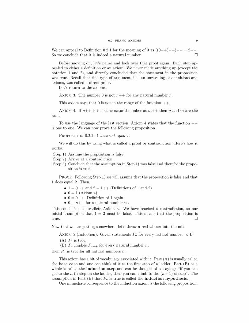
Axiom 3. The number 0 is not n++ for any natural number n.

This axiom says that 0 is not in the range of the function ++.

Axiom 4. If n++ is the same natural number as m++ then n and m are thesame.

To use the language of the last section, Axiom 4 states that the function ++is one to one. We can now prove the following proposition.

Proposition 0.2.2. 1 does not equal 2.

We will do this by using what is called a proof by contradiction. Here’s how itworks.

Step 1) Assume the proposition is false.Step 2) Arrive at a contradiction.Step 3) Conclude that the assumption in Step 1) was false and therefor the propo-

sition is true.

Proof. Following Step 1) we will assume that the proposition is false and that1 does equal 2. Then,

• 1 = 0++ and 2 = 1++ (Definitions of 1 and 2)• 0 = 1 (Axiom 4)• 0 = 0++ (Definition of 1 again)• 0 is n++ for a natural number n .

This conclusion contradicts Axiom 3. We have reached a contradiction, so ourinitial assumption that 1 = 2 must be false. This means that the proposition istrue. �

Now that we are getting somewhere, let’s throw a real winner into the mix.

Axiom 5 (Induction). Given statements Pn for every natural number n. If

(A) P0 is true,(B) Pn implies Pn++ for every natural number n,

then Pn is true for all natural numbers n.

This axiom has a bit of vocabulary associated with it. Part (A) is usually calledthe base case and one can think of it as the first step of a ladder. Part (B) as awhole is called the induction step and can be thought of as saying: “if you canget to the n-th step on the ladder, then you can climb to the (n+ 1)-st step”. Theassumption in Part (B) that Pn is true is called the induction hypothesis.

One immediate consequence to the induction axiom is the following proposition.


Proposition 0.2.3. If n ∈ N then either n = 0 or n is obtained by applying++ to 0 a finite number of times, but not both.

Proof. Let’s try using induction here. The statement in the proposition canbe written

(Pn) Either n = 0 or n = (· · · (0++) · · · )++ but not both.(A) Base case P0. The P0 case is true since 0 = 0 and 0 6= m++ by Axiom 3.(B) Now assume the statement Pn is true (or, with our new vocabulary, assume

the induction hypothesis). Is Pn++ true? If n = 0 then n++ = 0++ and thestatement is true. Otherwise n is obtained by successively applying ++ to 0. Butthen n++ is obtained by applying ++ to zero exactly one more time, which is stilla finite number of times. Also, by Axiom 3 we again have that n 6= 0 since it isthe result of applying ++. Thus Pn++ is true and the induction step is proven.Since we proved the base case and the induction step, we have proved that Pn istrue for all n ∈ N by Axiom 5. But Pn being true for all n is the proposition, sothe proposition is proved. �

The upshot of this is that we can almost write down the natural numbers asthe set

N = {0, 1, 2, 3, 4, 5, . . .}.

Connection 0.2.1. Induction is used throughout high school education. Ex-amples range from Gauss’ trick for adding the first 100 (or 103,211, or ...) numberstogether to the binomial theorem. A high school calculus course can use inductionto prove several formulas such as the power rule

d

dxxn = nxn−1.

One should think of it as an essential instrument in the mathematical toolkit!

We now use induction to prove that addition and multiplication are “well de-fined” operations. What does this mean? It means that they make sense. Beforewe can be sure they make sense though, we have to define them.

Definition 0.2.2. Addition and multiplication, denoted + and · respectively,are binary operations (i.e. functions from N× N to N). Addition is defined as theoperation that satisfies the following two properties for any m ∈ N:

(i) m+ 0 = m.(ii) m+ (n++) = (m+ n)++.

Multiplication is defined as the operation that satisfies the following two propertiesfor any m ∈ N

(i) m · 0 = 0,(ii) m · (n+ +) = m · n+m.

This is what is known as an inductive definition. Let’s prove it makes sense.

Proposition 0.2.4. For any natural numbers m and n, there exists a uniquenumber m+ n and a unique number m · n.

Proof. We will prove the statement involving addition and leave the multi-plication case as an exercise. We prove this by induction (which means we use theaxiom of induction to prove the statement). Take m to be any natural number andlet Pn be the statement

0.2. PEANO AXIOMS 11

(Pn) There is a unique number m+ n.(A) To prove P0 we just use property (i) to see m+ 0 = m.(B) Now assume m + n is defined and unique. Then by property (ii), m +

(n++) = (m + n)++ so that it is defined. Since m + n is unique, (m + n)++ isalso uniquely defined by Axiom 2.Having proved both conditions (A) and (B), we have that Pn is true for all naturalnumbers n and the proposition is proved. �

Try to prove this next proposition out for fun.

Proposition 0.2.5. If n ∈ N then n++ = n+ 1.

Rather than being coy about these operations and forestalling the inevitable,let’s write down straightaway the most important properties. We do this with thenext two theorems which should be taken as foundational and important. In fact,without these theorems, practical arithmetic would be nearly impossible.

Theorem 0.2.1 (Algebraic properties of (N,+)). The following properties hold.

Additive identity: For any n ∈ N, 0 + n = n = n+ 0.Associativity of addition: For any three natural numbers l,m, n ∈ N,

(0.1) (l +m) + n = l + (m+ n)

Commutativity of addition: For any two natural numbers m,n ∈ N,

(0.2) m+ n = n+m

Cancellation law for addition: For any natural number n ∈ N, if n +m1 = n+m2, then m1 = m2.

Proof. We prove these in order.

Additive identity: The right hand equality n = n + 0 follows from Defi-nition 0.2.2, part (i). To see that 0 + n = n, we use induction. The basecase is 0 + 0 = 0 which again follows from Definition 0.2.2, part (i). Nowassume 0 + n = n. We need to prove that 0 + (n++) = n++. For this,we see

0 + (n++) = (0 + n)++ Definition 0.2.2, part (ii)

= n++ Induction hypothesis

Associativity of addition: Here we use induction on n with l and m fixed.For the base case, we need to prove (l+m) + 0 = l+ (m+ 0). But by theadditive identity result we just proved, we see that (l+m)+0 = l+m andl + (m + 0) = l + (m) = l + m. So the base case is proven. Now assumeequation (0.1) holds for n. We must prove

(l +m) + (n++) = l + (m+ (n++)).

Observe,

(l +m) + (n++) = ((l +m) + n)++ Definition 0.2.2, part (ii)

= (l + (m+ n))++ Induction hypothesis

= l + (m+ n)++ Definition 0.2.2, part (ii)

= l + (m+ (n++)) Definition 0.2.2, part (ii)


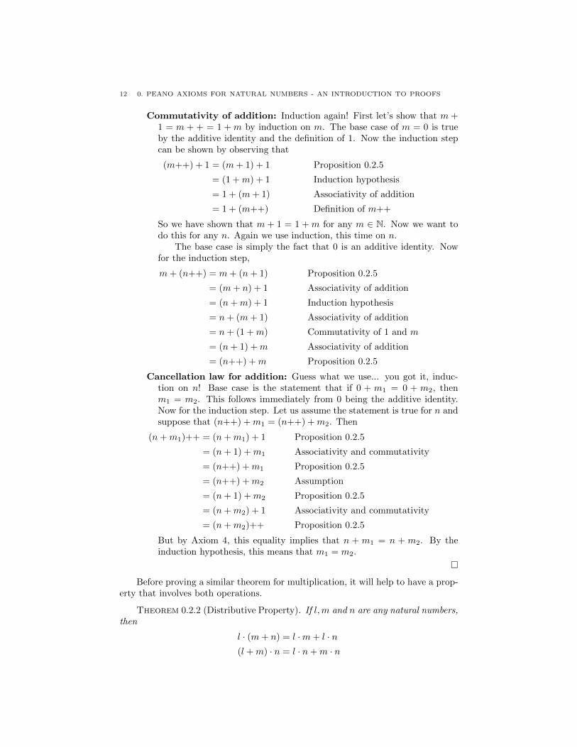
Commutativity of addition: Induction again! First let’s show that m +1 = m + + = 1 + m by induction on m. The base case of m = 0 is trueby the additive identity and the definition of 1. Now the induction stepcan be shown by observing that

(m++) + 1 = (m+ 1) + 1 Proposition 0.2.5

= (1 +m) + 1 Induction hypothesis

= 1 + (m+ 1) Associativity of addition

= 1 + (m++) Definition of m++

So we have shown that m + 1 = 1 + m for any m ∈ N. Now we want todo this for any n. Again we use induction, this time on n.

The base case is simply the fact that 0 is an additive identity. Nowfor the induction step,

m+ (n++) = m+ (n+ 1) Proposition 0.2.5

= (m+ n) + 1 Associativity of addition

= (n+m) + 1 Induction hypothesis

= n+ (m+ 1) Associativity of addition

= n+ (1 +m) Commutativity of 1 and m

= (n+ 1) +m Associativity of addition

= (n++) +m Proposition 0.2.5

Cancellation law for addition: Guess what we use... you got it, induc-tion on n! Base case is the statement that if 0 + m1 = 0 + m2, thenm1 = m2. This follows immediately from 0 being the additive identity.Now for the induction step. Let us assume the statement is true for n andsuppose that (n++) +m1 = (n++) +m2. Then

(n+m1)++ = (n+m1) + 1 Proposition 0.2.5

= (n+ 1) +m1 Associativity and commutativity

= (n++) +m1 Proposition 0.2.5

= (n++) +m2 Assumption

= (n+ 1) +m2 Proposition 0.2.5

= (n+m2) + 1 Associativity and commutativity

= (n+m2)++ Proposition 0.2.5

But by Axiom 4, this equality implies that n + m1 = n + m2. By theinduction hypothesis, this means that m1 = m2.

�

Before proving a similar theorem for multiplication, it will help to have a prop-erty that involves both operations.

Theorem 0.2.2 (Distributive Property). If l,m and n are any natural numbers,then

l · (m+ n) = l ·m+ l · n(l +m) · n = l · n+m · n

0.2. PEANO AXIOMS 13

Proof. We will prove that multiplication is left distributive which is the firstof the two equations. The proof that it is right distributive will be left as an exercise.We use induction on n. The base case can be shown as

l · (m+ 0) = l ·m, Additive identity

= l ·m+ 0, Additive identity

= l ·m+ l · 0. Definition 0.2.2

Now assume the theorem is true for n. Then

l · (m+ (n++)) = l · ((m+ n)++), Definition 0.2.2

= l · (m+ n) + l, Definition 0.2.2

= (l ·m+ l · n) + l, Induction hypothesis

= l ·m+ (l · n+ l), Associativity of addition

= l ·m+ l · (n++). Definition 0.2.2

This concludes the proof of the induction step and the theorem. �

Now let us establish the algebraic properties of multiplication in N.

Theorem 0.2.3 (Algebraic properties of (N, ·)). following properties hold.

Multiplicative identity: For any n ∈ N, 1 · n = n = n · 1.Associativity of multiplication: For any three natural numbers l,m, n,

(0.3) (l ·m) · n = l · (m · n)

Commutativity of multiplication: For any two natural numbers m,n,

(0.4) m · n = n ·m

Cancellation rule for multiplication: For any natural number n, if

n ·m1 = n ·m2 6= 0

then m1 = m2.

Proof. We examine these in order.

Multiplicative identity: Let us prove this by induction on n. The basecase states 1 · 0 = 0 = 0 · 1. The left equation follows from Definition0.2.2. The right follows from this definition as well and the definition that1 = 0 + + via the equation 0 · 1 = 0 · (0++) = 0 · 0 + 0 = 0 + 0 = 0. In thelast equation we used the additive identity. Now assume 1 · n = n = n · 1.Then 1 ·(n++) = 1 ·n+1 = n+1 = n++ by the induction hypothesis andProposition 0.2.5. For the other side we have (n++)·1 = (n++)·(0++) =[(n++) · 0] + n++ = 0 + n++ = n++.

Associativity of multiplication: Again we proceed by induction on n.The base case is easily established

l · (m · 0) = l · 0, Definition 0.2.2

= 0, Definition 0.2.2

= (l ·m) · 0. Definition 0.2.2


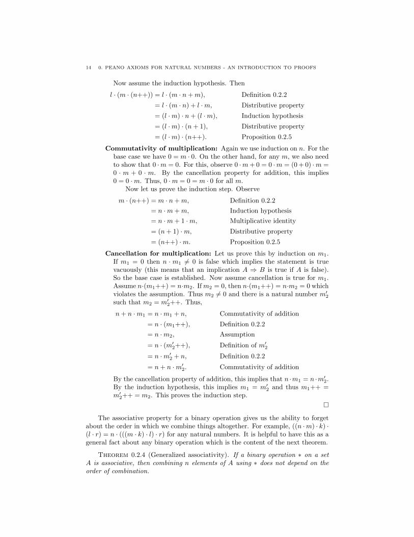
Now assume the induction hypothesis. Then

l · (m · (n++)) = l · (m · n+m), Definition 0.2.2

= l · (m · n) + l ·m, Distributive property

= (l ·m) · n+ (l ·m), Induction hypothesis

= (l ·m) · (n+ 1), Distributive property

= (l ·m) · (n++). Proposition 0.2.5

Commutativity of multiplication: Again we use induction on n. For thebase case we have 0 = m · 0. On the other hand, for any m, we also needto show that 0 ·m = 0. For this, observe 0 ·m+ 0 = 0 ·m = (0 + 0) ·m =0 · m + 0 · m. By the cancellation property for addition, this implies0 = 0 ·m. Thus, 0 ·m = 0 = m · 0 for all m.

Now let us prove the induction step. Observe

m · (n++) = m · n+m, Definition 0.2.2

= n ·m+m, Induction hypothesis

= n ·m+ 1 ·m, Multiplicative identity

= (n+ 1) ·m, Distributive property

= (n++) ·m. Proposition 0.2.5

Cancellation for multiplication: Let us prove this by induction on m1.If m1 = 0 then n · m1 6= 0 is false which implies the statement is truevacuously (this means that an implication A ⇒ B is true if A is false).So the base case is established. Now assume cancellation is true for m1.Assume n·(m1++) = n·m2. Ifm2 = 0, then n·(m1++) = n·m2 = 0 whichviolates the assumption. Thus m2 6= 0 and there is a natural number m′2such that m2 = m′2++. Thus,

n+ n ·m1 = n ·m1 + n, Commutativity of addition

= n · (m1++), Definition 0.2.2

= n ·m2, Assumption

= n · (m′2++), Definition of m′2

= n ·m′2 + n, Definition 0.2.2

= n+ n ·m′2. Commutativity of addition

By the cancellation property of addition, this implies that n ·m1 = n ·m′2.By the induction hypothesis, this implies m1 = m′2 and thus m1++ =m′2++ = m2. This proves the induction step.

�

The associative property for a binary operation gives us the ability to forgetabout the order in which we combine things altogether. For example, ((n ·m) · k) ·(l · r) = n · (((m · k) · l) · r) for any natural numbers. It is helpful to have this as ageneral fact about any binary operation which is the content of the next theorem.

Theorem 0.2.4 (Generalized associativity). If a binary operation ∗ on a setA is associative, then combining n elements of A using ∗ does not depend on theorder of combination.

0.3. RELATIONS 15

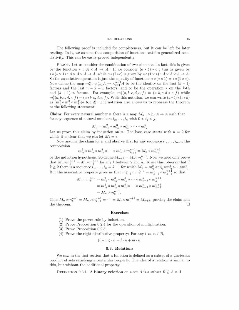
The following proof is included for completeness, but it can be left for laterreading. In it, we assume that composition of functions satisfies generalized asso-ciativity. This can be easily proved independently.

Proof. Let us consider the combination of two elements. In fact, this is givenby the function ∗ : A × A → A. If we consider (a ∗ b) ∗ c , this is given by∗ ◦ (∗× 1) : A×A×A→ A, while a ∗ (b ∗ c) is given by ∗ ◦ (1×∗) : A×A×A→ A.So the associative operation is just the equality of functions ∗◦ (∗×1) = ∗◦ (1×∗).Now define the map mn

k : ×ni=1A → ×n−1i=1 A to be the identity on the first (k − 1)

factors and the last n − k − 1 factors, and to be the operation ∗ on the k-thand (k + 1)-st factors. For example, m6

4(a, b, c, d, e, f) = (a, b, c, d ∗ e, f) whilem6

1(a, b, c, d, e, f) = (a∗ b, c, d, e, f). With this notation, we can write (a∗ b)∗ (c∗d)as (m2

1 ◦m31 ◦m4

3)(a, b, c, d). The notation also allows us to rephrase the theoremas the following statement:

Claim: For every natural number n there is a map Mn : ×ni=1A→ A such thatfor any sequence of natural numbers i2, . . . , in with 0 < ij < j,

Mn = m2i2 ◦m

3i3 ◦m

4i4 ◦ · · · ◦m

nin

Let us prove this claim by induction on n. The base case starts with n = 2 forwhich it is clear that we can let M2 = ∗.

Now assume the claim for n and observe that for any sequence i1, . . . , in+1, thecomposition

m2i2 ◦m

3i3 ◦m

4i4 ◦ · · · ◦m

nin ◦m

n+1in+1

= Mn ◦mn+1in+1

by the induction hypothesis. So define Mn+1 = Mn◦mn+11 . Now we need only prove

that Mn◦mn+1k = Mn◦mn+1

1 for any k between 2 and n. To see this, observe that ifk ≥ 2 there is a sequence i1, . . . , in = k−1 for which Mn = m2

i2◦m3

i3◦m4

i4◦· · ·◦mn

in.

But the associative property gives us that mnk−1 ◦m

n+1k = mn

k−1 ◦mn+1k−1 so that

Mn ◦mn+1k = m2

i2 ◦m3i3 ◦m

4i4 ◦ · · · ◦m

nk−1 ◦mn+1

k ,

= m2i2 ◦m

3i3 ◦m

4i4 ◦ · · · ◦m

nk−1 ◦mn+1

k−1 ,

= Mn ◦mn+1k−1 .

Thus Mn ◦mn+1k = Mn ◦mn+1

k−1 = · · · = Mn ◦mn+11 = Mn+1, proving the claim and

the theorem. �

Exercises

(1) Prove the power rule by induction.(2) Prove Proposition 0.2.4 for the operation of multiplication.(3) Prove Proposition 0.2.5.(4) Prove the right distributive property: For any l,m, n ∈ N,

(l +m) · n = l · n+m · n.

0.3. Relations

We saw in the first section that a function is defined as a subset of a Cartesianproduct of sets satisfying a particular property. The idea of a relation is similar tothis, but without the additional property.

Definition 0.3.1. A binary relation on a set A is a subset R ⊆ A×A.


There are some key properties that a relation might satisfy. These terms per-meate common language because of their relationship to basic logic.

Definition 0.3.2. Let R ⊆ A×A be a binary relation.

(1) R is called reflexive if (a, a) ∈ R for every a ∈ A.(2) R is called symmetric if

(a, b) ∈ R implies (b, a) ∈ R

for every a, b ∈ A.(3) R is called antisymmetric if

(a, b), (b, a) ∈ R implies a = b

(4) R is called transitive if

(a, b), (b, c) ∈ R implies (a, c) ∈ R

for every a, b, c ∈ A.

Let’s take some time to humanize these properties.

Example 0.3.1. Suppose A is the set of all of the people in Kansas. Therelation R(−blank−) is defined as

(a, b) ∈ R(−blank−) if and only if a -blank- b

Which of the properties in Definition 0.3.2 are satisfied by

R(has had lunch with),R(has the same color hair as),R(is a step sibling of) andR(loves)?

There are a couple of relations that have great utility in mathematics. First,let’s go back to preschool and make sure that we understand the “size” of a number.

Definition 0.3.3. A (non-strict) partial order on a set A is a binary relationR that is reflexive, antisymmetric and transitive.

A set with a partial order is sometimes called a poset. Now, as promised, wereturn to our early youth with the following definition.

Definition 0.3.4. If a, b ∈ N we say that a is greater than or equal to b, writtena ≥ b if there exists c ∈ N such that a = b+ c.

This definition is the same as giving the relation R≥ ⊂ N× N defined by

a ≥ b if and only if (a, b) ∈ R≥.

Let’s establish that ≥ is indeed a partial order on N.

Theorem 0.3.1. The relation a ≥ b is a partial order on N.

Proof. We need to show that the relation is reflexive, antisymmetric andtransitive.

Reflexive: Exercise.Antisymmetric: We need to prove

If a ≥ b and b ≥ a then a = b.

0.3. RELATIONS 17

By definition, there are natural numbers c1 and c2 such that

a = b+ c1

b = a+ c2

So that a + 0 = a = b + c1 = (a + c2) + c1 = a + (c2 + c1). But by thecancellation law for addition we have that 0 = c2 + c1. If c1 6= 0, thenc1 = c+ + for some c ∈ N by Proposition 0.2.3. But then 0 = (c2 + c)++which contradicts Axiom 3. Thus c1 = 0 and a = b+ c1 = b+ 0 = b whichproves antisymmetry.

Transitive: Exercise.

�

In fact, the relation ≥ has an additional property, making it a total order.

Proposition 0.3.1. If a and b are natural numbers, then either a ≥ b or b ≥ a.

Proof. Let us prove this by induction on a. The base case of a = 0 is truesince for any b we have b = 0 + b so that b ≥ 0.

Now assume the proposition is true for a. Assume b is any natural number. Ifa ≥ b then since a++ = a + 1 we have a++ ≥ a ≥ b so the transitive propertyimplies a++ ≥ b. On the other hand, if b ≥ a, then b = a + n for some n ∈ N. Ifn = 0 then b = a and a++ ≥ b. If n 6= 0 then n = m++ for some natural numberm and b = a+ (m++) = a+m+ 1 = (a++) +m so that b ≥ a++. This concludesthe proof. �

The following theorem is a very useful and important property of subsets of N.

Theorem 0.3.2 (Well ordering principle). Given any non-empty subset A ⊆ N,there exists a unique smallest element a ∈ A.

By the smallest element, we mean an element a ∈ A such that if b ∈ A thenb ≥ a.

Proof. We use induction for this theorem. First, assume that A ⊆ N doesnot contain a smallest element. Now let Pn be the statement

If m ∈ N such that n ≥ m then m 6∈ A

Let us show the base case is true. Clearly, if 0 ≥ m then m = 0, but m is lessthan or equal to all natural numbers and so m 6∈ A (for otherwise it would be asmallest element). Now if Pn is true, but Pn++ is false, then n ∈ A and there is nom strictly less than n such that m ∈ A. But then for every m ∈ A we must havem ≥ n which means n is a smallest element. This is a contradiction, so Pn++ istrue and we have proven Pn for all n. This means that there is no natural numbern ∈ A and thus, since A ⊆ N, A must be the empty set.

In conclusion, if A is non-empty, then it must have a smallest element (forotherwise the above argument would show it to be empty). �

A partial order is not the only type of binary relation that is important to us.As we will see very shortly, the following notion may be even more important inalgebra.

Definition 0.3.5. A binary relation R on a set A is an equivalence relationif it is reflexive, symmetric and transitive.


As we saw above with ≥, often it is convenient to denote a relation with asymbol separating two elements of the set. We can do this generally for a binaryrelation R ⊆ A×A by writing

a ∼R b if and only if (a, b) ∈ R.

This is just notation to indicate the relation as a “relationship” between elements.For example, in this notation, R is a transitive relation if and only if

a ∼R b and b ∼R c implies a ∼R c.So what can we do with a relation R on A? Well, we can take each element a ∈ Aand make it into a subset [a]R, called the equivalence class of a, by defining

(0.5) [a]R := {b ∈ A : a ∼R b}.If we have a fixed relation that we know about, we will just write [a] instead of[a]R. By the way, the notation := means that we define the left hand side by theright hand side. A cool fact comes up when R is an equivalence relation.

Proposition 0.3.2. Assume R is an equivalence relation on A. For any a, b ∈A either [a] = [b] or [a] is disjoint from [b].

Proof. We can do this directly. Suppose [a] and [b] are not disjoint, thenthere is a c ∈ [a] ∩ [b].

Now suppose d ∈ [a]. Since c is in [a] we have a ∼R c and since R is symmetricc ∼R a. Since d is in [a] we have a ∼R d. Thus c ∼R a and a ∼R d which impliesc ∼R d by the transitivity of R. On the other hand, since c ∈ [b] we have b ∼R c.Since b ∼R c and c ∼R d we get b ∼R d which implies d ∈ [b]. Thus [a] ⊆ [b].

But switching the a and b in the above argument shows [b] ⊆ [a]. Thus [a] = [b]as was to be shown. �

For an equivalence relation R on A we can define

(0.6)A

∼R:= {S ⊆ A : there is an a ∈ A such that S = [a]}.

If Cartesian products are the set theory analog of products of numbers (which theyare), then A

∼R is the set theory analog of a quotient.

Theorem 0.3.3. If R is an equivalence relation then A∼R is a partition of A.

Proof. By definition, we have that if S and S′ are in A∼R then there is an a

and b such that S = [a] and S′ = [b]. By Proposition 0.3.2, we know that eitherS = S′ which means they are the same element in A

∼R or they are disjoint. Thus

property (2) in Definition 0.1.2 is satisfied. To see property (1), namely that everyelement a ∈ A is an element of some S ∈ A

∼R , simply observe that [a] ∈ A∼R by

definition. But since R is reflexive, a ∼R a and a ∈ [a]. �

It is hard to overstate the importance of this last theorem. It manifests itself ina huge number of constructions in algebra, geometry and analysis. The idea thatan equivalence relation makes partitions means that a ∼R b can be thought of assaying a is equal to b in some R sense. So if we want to think about a in the Rsense of equality, we only need to think of the element [a] ∈ A

∼R . For example, saywe think of the set of students S in the class. We can define an equivalence relationR as a ∼R b if and only if student a and student b get the same letter grade. Thenthe quotient S

∼R is the list of grades that the students will receive. Mike and Mary

EXERCISES 19

are equal from the perspective of ∼R if they get the same grade, otherwise they arenot equal. The map π : S → S

∼R from the exercises in Section 0.1 will be equal onR-equivalent elements and will be distinct on R-inequivalent elements.

Exercises

(1) Give an example of a binary relation on a set A that satisfies exactly twoof the conditions in Definition 0.3.2.

(2) Prove the reflexive and transitive properties in Theorem 0.3.1.(3) Give an example of a partially ordered set that does not satisfy the well

ordering principle.(4) Show that there is a converse to Theorem 0.3.3 in the following sense. IfP is a partition of A, define a relation

R = {(a, b) ∈ A×A : there exists S ∈ P such that a, b ∈ S}.Prove that(a) ∼R is an equivalence relation.(b) P = A

∼R .

CHAPTER 1

Basic Arithmetic

While the title of this chapter may strike the college upper class-men as slightlyoffensive, it is my hope that the impression will be overcome by a study of itscontents. For many mathematicians, a modern viewpoint on arithmetic is moresubtle and complicated than several other advanced sounding subjects. So what doI mean by arithmetic? I mean working with integers and their basic operations.

1.1. The set Z

In this section we utilize the construction of the natural numbers N to constructthe integers Z. Let us first define the binary relation ∼ on N× N via

(1.1) (a, b) ∼ (c, d) if and only if a+ d = b+ c.

There are some fundamental facts about this relation that we now establish.

Proposition 1.1.1. The following statements hold with respect to relation 1.1.

(1) The relation ∼ is an equivalence relation.(2) For every (a, b) there exists a unique natural number c ∈ N for which

either (a, b) ∼ (0, c) or (a, b) ∼ (c, 0) with both occurring if and only ifc = 0.

(3) If (a, b) ∼ (a′, b′) and (c, d) ∈ N× N then

(1.2) (a+ c, b+ d) ∼ (a′ + c, b′ + d).

(4) If (a, b) ∼ (a′, b′) and (c, d) ∈ N× N then

(1.3) (a · c+ b · d, a · d+ b · c) ∼ (a′ · c+ b′ · d, a′ · d+ b′ · c)

Proof. We will prove the first two properties and leave the last two as exer-cises.

(1) We need to prove that ∼ is reflexive, symmetric and transitive.reflexive: Let (a, b) ∈ N × N then a + b = a + b since addition is well

defined. By definition of ∼, this implies (a, b) ∼ (a, b) and so ∼ isreflexive.

symmetric: Suppose (a, b) ∼ (c, d). Then c+ b = b+ c = a+d = d+aby commutativity of addition. Thus (c, d) ∼ (a, b) which shows that∼ is symmetric.

21

22 1. BASIC ARITHMETIC

transitive: Now assume (a, b) ∼ (c, d) and (c, d) ∼ (e, f). Then

d+ (a+ f) = (d+ a) + f, associativity

= (a+ d) + f, commutativity

= (b+ c) + f, definition of ∼= b+ (c+ f), associativity

= b+ (d+ e), definition of ∼= (d+ e) + b, commutativity

= d+ (e+ b), associativity

= d+ (b+ e). commutativity

By the cancellation property in Theorem 0.2.1, this implies that a+f = b+ e which in turn yields (a, b) ∼ (e, f). Thus ∼ is transitive.

(2) We first show the existence of such a c. Let us consider the equivalenceclass of the pair (a, b) which is defined as

[(a, b)]∼ := {(c, d) ∈ N× N : (a, b) ∼ (c, d)}.

This is the set of elements that are ∼-equivalent to (a, b). Now we defineanother set,

S(a,b) = {c ∈ N : there exists d ∈ N such that (c, d) ∈ [(a, b)]∼}.

Note that S(a,b) is non-empty since a ∈ S(a,b). Thus, by the Well OrderingPrinciple of N, there is a smallest element e ∈ S(a,b). If e = 0 then there isan element (0, c) ∈ [(a, b)]∼ and we have shown existence. If e > 0, thenwe claim (e, 0) ∈ [(a, b)]∼. If not, then (e, f) ∈ [(a, b)]∼ with e > 0 and

f > 0. Thus f = f + 1 and e = e+ 1 for natural numbers e, f . Note e > eand

e+ f = (e+ 1) + f , definition of e

= e+ (1 + f), associativity

= e+ (f + 1), commutativity

= e+ f, definition of f

= f + e. commutativity

Thus (e, f) ∼ (e, f) implying (e, f) ∈ [(a, b)]∼ and e ∈ S(a,b). But sincee > e and e was assumed to be the smallest element of S(a,b), we haveachieved a contradiction. So we must have that (e, 0) ∈ [(a, b)]∼ showingthe existence of c.

Now we come to uniqueness. There are three options to consider.• Suppose (c, 0) ∼ (a, b) ∼ (c′, 0). Then, since ∼ is transitive (c, 0) ∼

(c′, 0), we have c = c+ 0 = 0 + c′ = c′.• Suppose (c, 0) ∼ (a, b) ∼ (0, c′). Then, since ∼ is transitive (c, 0) ∼

(0, c′), we have c + c′ = 0 + 0 = 0. But this implies that c′ = 0 = c(otherwise 0 = n++ for some natural number n, violating Axiom 3).• Suppose (0, c) ∼ (a, b) ∼ (0, c′). Then, since ∼ is transitive (0, c) ∼

(0, c′), we have c′ = 0 + c′ = c+ 0 = c.

�

1.2. THE RING Z 23

Do not worry, it is OK if you are feeling lost. This proposition may have lookedlooked arbitrary and unnecessary, but now let’s see the motivation by thinkingabout the next definition.

Definition 1.1.1. The set of integers, denoted Z is the quotient

(1.4) Z =N× N∼

If (a, b) ∼ (c, 0), we denote [(a, b)]∼ by c. If (a, b) ∼ (0, c) for c > 0, we denote[(a, b)]∼ by −c.

Thus, we have introduced negative numbers by partitioning relative to theequivalence relation ∼. Let’s extend the order ≥ to the integers.

Definition 1.1.2. We write [(a, b)]∼ ≥ [(c, d)]∼ if and only if a+ d ≥ b+ c.

Nearly all of the properties that held for ≥ on N hold for Z, except the WellOrdering Principle. We write this as a proposition and leave the proof as an exercise.

Proposition 1.1.2. The following properties hold for the relation ≥ on Z.

(1) ≥ is a partial order.(2) If [(a, b)]∼, [(c, d)]∼ ∈ Z then either [(a, b)]∼ ≥ [(c, d)]∼ or [(c, d)]∼ ≥

[(a, b)]∼.

Before moving on, we should assess what we have and what we do not have!What we have is the set of integers Z. However, we do not yet have arithmetic ofthe integers. In fact, we do not even know how to add or multiply two integers,much less whether these operations satisfy the properties in Theorem 0.2.1.

Exercises

(1) Write each of the integers [(2, 4)]∼ and [(5, 4)]∼ in the form ±c for anappropriate natural number c.

(2) Prove part (3) of Proposition 1.1.1.(3) Prove part (4) of Proposition 1.1.1.(4) Draw N × N in the Cartesian plane. Highlight the equivalence classes

[(0, 0)]∼ and [(0, 2)]∼.(5) Prove Proposition 1.1.2.

1.2. The ring Z

Having defined the integers as a set, we now want to extend our arithmetic toinclude these negative numbers. Before we do this, let us introduce a very generaldefinition which we will come back to later on in the text.

Definition 1.2.1. A ring R is a set with two binary operations called addition( + ) and multiplication ( · ), satisfying the following properties.

Identities: There are elements 0 and 1 that are additive and multiplicativeidentities.

Associativity: Both + and · are associative operations.Commutativity of addition: The addition operation is commutative.Distributive property: Multiplication is left and right distributive.Additive inverse: For every r ∈ R, there exists an element −r such thatr + (−r) = 0.


If multiplication is commutative, we call R a commutative ring.

Now our goal is to show that Z is one of these commutative rings, but first weneed to define addition and multiplication.

Definition 1.2.2. If [(a1, b1)]∼ and [(a2, b2)]∼ are integers then define

[(a1, b1)]∼ + [(a2, b2)]∼ = [(a1 + a2, b1 + b2)]∼(1.5)

[(a1, b1)]∼ · [(a2, b2)]∼ = [(a1 · a2 + b1 · b2, a1 · b2 + b1 · a2)]∼(1.6)

As before, it is necessary to prove that these definitions make sense. To do this,we must show that if we represented the equivalence class by different elements,then the resulting sum and product would be the same equivalence class.

Proposition 1.2.1. Addition and multiplication are well defined on Z.

Proof. We need to prove that if (a1, b1) ∼ (a′1, b′1) and (a2, b2) ∼ (a′2, b

′2) then

(a1 + a2, b1 + b2) ∼ (a′1 + a′2, b′1 + b′2)(1.7)

(a1 · a2 + b1 · b2, a1 · b2 + a2 · b1) ∼ (a′1 · a′2 + b′1 · b′2, a′1 · b′2 + a′2 · b′1)(1.8)

We will prove equation 1.7 and leave equation 1.8 as an exercise. Observe

(a1 + a2, b1 + b2) ∼ (a′1 + a2, b′1 + b2), Proposition 1.1.1, part (3)

∼ (a2 + a′1, b2 + b′1), Commutativity of addition

∼ (a′2 + a′1, b′2 + b′1), Proposition 1.1.1, part (3)

∼ (a′1 + a′2, b′1 + b′2). Commutativity of addition

�

It may seem that we took a very hard route to defining the integers in the lastsection. However, this construction allows us to prove the following theorem withease.

Theorem 1.2.1. The integers Z form a commutative ring.

Proof. We will prove some of the properties and leave others as exercises. Inthe interest of saving space, we drop the · notation and write [(a, b)]∼ as [a, b].

Identities: Exercise.Associativity: We leave the proof that addition is associative as an exercise.

Here we prove it for multiplication. Let ∗ = ([a1, b1][a2, b2])[a3, b3], thenusing Definition 1.2.2, Theorems 0.2.1, 0.2.2 and 0.2.3 we have

∗ = ([a1a2 + b1b2, a1b2 + b1a2])[a3, b3]

= [(a1a2 + b1b2)a3 + (a1b2 + b1a2)b3, (a1a2 + b1b2)b3 + (a1b2 + b1a2)a3]

= [a1a2a3 + b1b2a3 + a1b2b3 + b1a2b3, a1a2b3 + b1b2b3 + a1b2a3 + b1a2a3]

= [a1(a2a3 + b2b3) + b1(a2b3 + b2a3), a1(a2b3 + b2a3) + b1(a2a3 + b2b3)]

= [a1, b1][a2a3 + b2b3, a2b3 + b2a3]

= [a1, b1]([a2, b2][a3, b3])

Commutativity: Exercise.

1.2. THE RING Z 25

Distributive Property: We show that multiplication is left distributive.It can then be shown to be right distributive by commutativity of multi-plication. Repeatedly using Definition 1.2.2 and Theorems 0.2.1,0.2.2 wehave

[a, b]([c, d] + [e, f ]) = [a, b][c+ e, d+ f ],

= [a(c+ e) + b(d+ f), a(d+ f) + b(c+ e)],

= [(ac+ bd) + (ae+ bf), (ad+ bc) + (af + be)],

= [ac+ bd, ad+ bc] + [ae+ bf, af + be],

= [a, b][c, d] + [a, b][e, f ].

Additive inverse: This is the property that really separates Z from N.In the latter case, there are no additive inverses. But here we have, if[a, b] ∈ Z, then let −[a, b] = [b, a]. Observe that [a, b] + (−[a, b]) = [a, b] +[b, a] = [a+ b, b+ a]. The additive identity is [0, 0]. But since

(a+ b) + 0 = (b+ a) + 0,

equation 1.1 gives us that (a+ b, b+ a) ∼ (0, 0). Thus [a, b] + (−[a, b]) =[a+ b, b+ a] = [0, 0] proving the existence of an additive inverse.

�

This theorem gives us the capability to add and multiply integers withoutexcessive brackets and with the freedom to reorder the summands and factors inany way we choose. Now that we have these essential properties established, wewill write integers as c and −c instead of as equivalence classes [a, b], and use thelatter notation only in proofs when necessary. We will also use subtraction, whichis defined by the equation

a− b := a+ (−b).Note that such a definition makes sense for any ring.

Connection 1.2.1. Formally proving the basic properties of arithmetic maynot be a part of the secondary school curriculum. However, the properties them-selves are a part of the curriculum and being able to explain why these propertiesare true is very important. Consider ways in which you would explain associativityof addition or commutativity of multiplication.

There is much to say about the integers as a ring, but let’s start by provingthat the elementary algebra rules hold for inequalities.

Theorem 1.2.2. The following properties hold for any a, b, c ∈ Z.

(1) If a ≥ b then a+ c ≥ b+ c.(2) If a ≥ b and c ≥ 0, then a · c ≥ b · c.(3) If a ≥ b and c < 0, then a · c ≤ b · c.

Furthermore, strict inequalities can be used instead of non-strict inequalities.

Proof. Let a = [a1, a2], b = [b1, b2] and c = [c1, c2] and observe that thehypothesis in each property contains the statement that a ≥ b which holds if andonly if

(1.9) a1 + b2 ≥ a2 + b1.


We prove the properties for the non-strict case in order and leave the strict case asan optional exercise.

(1) Note that this statement is true if a, b and c are natural numbers becauseif a ≥ b then there exists d such that a = b + d. But then the samed must satisfy a + c = (b + c) + d implying a + c ≥ b + c. For thegeneral case of integers. Equation (1.9) implies that (a1 +c1)+(b2 +c2) ≥(a2+c2)+(b1+c1) which in turn shows [a1+c1, a2+c2] ≥ [b1+c1, b2+c2].Using the definition of addition in Z we then get a+ c ≥ b+ c.

(2) Again, let us verify this for natural numbers first. We see that if a = b+dthen a · c = b · c + d · c by the distributive property. Thus a · c ≥ b · c.In case of integers, multiplying equation (1.9) on both sides by c givesc · a1 + c · b2 ≥ c · a2 + c · b1 (we can do this by the argument for naturalnumbers and because c ∈ N). But this is equivalent to [c · a1, c · a2] ≥[c · b1, c · b2] or c · a ≥ c · b.

(3) If c < 0, then we can choose c = [0, n] for some natural number n. Bythe definition of multiplication, we have c · a = [n · a2, n · a1] and c · b =[n·b2, n·b1]. Equation (1.9) and the previous property imply n·b2+n·a1 ≥n · b1 + n · a2 which is equivalent to c · b ≥ c · a.

�

Connection 1.2.2. This theorem establishes the properties needed to solvelinear inequalities, a skill in the common core standards. Usually in secondaryschool, they are called rules instead of properties because a rule is not expectedto be proven. However, we still should be able to explain a rule. How would youexplain these rules to a student?

We now show that the cancellation property holds for Z. We follow an abstractpath that will generalize to a broad class of rings.

Definition 1.2.3. A non-zero ring is called a domain if for any two elementsr, s ∈ R, the equation r · s = 0 implies r = 0 or s = 0. It is called an integraldomain if it is a commutative domain.

Now that we have the essential terminology, let’s prove a simple proposition.

Proposition 1.2.2. The ring Z is an integral domain.

Proof. Since we know it is a commutative ring, we need only show that r·s = 0implies r = 0 or s = 0. First observe that for any integer n, 0 · n = (0 + 0) · n =0 · n+ 0 · n and subtracting 0 · n from both sides we have 0 · n = 0. We can provethis by contradiction. If r 6= 0 and s 6= 0 then one of four possibilities can occur.By Exercise 6 either r > 0 or r < 0, and either s > 0 or s < 0. If r > 0 then byTheorem 1.2.2, 0 = r · s > r · 0 = 0 or 0 = r · s < r · 0 = 0, both of which arecontradictions (since a > b is defined to be a ≥ b and a 6= b). On the other hand,if r < 0 then by Theorem 1.2.2, 0 = r · s < r · 0 = 0 or 0 = r · s > r · 0 = 0, yieldinganother set of contradictions. Thus either r or s must be 0. �

The upshot of this is the following theorem.

Theorem 1.2.3 (Cancellation for rings). Let R be a ring and a, b, c ∈ R.

Cancellation for addition: If a+ b = a+ c, then b = c.

1.3. FACTORING INTEGERS, PART I 27

Cancellation for multiplication: If R is a domain, a 6= 0 and a ·b = a ·c,then b = c.

Proof. Cancellation for addition is left as an exercise. To prove cancellationfor multiplication, assume a · b = a · c. Then

a · (b− c) = a · b− a · c, Distributive property

= a · c− a · c, Assumption

= 0. Definition of additive inverse

Since R is a domain, this implies that either a = 0 or b − c = 0. Since a 6= 0 byassumption, we have that b − c = 0 and so b = (b − c) + c = 0 + c = c whichconcludes the proof. �

You may ask why we wrote a proof for a ring instead of for Z. The answer isthat this property comes in handy for several rings later on, and is brings out theessential argument we need in the case of Z. Of course, we can also apply this tothe integers as our first Corollary!

Corollary 1.2.1. The integers have cancellation for addition and multiplica-tion.

Proof. By Proposition 1.2.2, Z is an integral domain and therefore a domain.By Theorem 1.2.3, it has both cancellation properties. �

Exercises

(1) Give an example of a ring that is not Z (you do not need to prove that itis a ring).

(2) Prove that multiplication is well defined on Z by verifying equation 1.8.(3) Using Definition 1.2.2, show that 0 = [(0, 0)]∼ and 1 = [(1, 0)]∼ are the

additive and multiplicative identities, respectively.(4) Prove that addition in Z is associative.(5) Prove that addition and multiplication are commutative in Z.(6) Prove that if c is an integer, then −c = (−1) · c. Conclude that every

integer is either a natural number or the negative of a natural number.

1.3. Factoring integers, part I

We know by the Peano Axioms that every integer can be written as a sum of1’s or −1’s. However, decomposing an integer as a product into elementary factorsis a more subtle game. For this, we first introduce a definition.

Definition 1.3.1. For integers a, b ∈ Z, we say that a divides b if there existsan integer n such that b = a · n. We denote this by a | b.

There are some elementary properties of divisibility that we can establish rightoff the bat.

Proposition 1.3.1. The following properties hold for any integers a, b and c.

(1) If a | b then a | b · c.(2) If a | b and b > 0 then −b ≤ a ≤ b.(3) If a | b and a | c then a | (b+ c).(4) If a | b and b | c then a | c.


(5) If a | b and b | a then a = ±b.

Proof. We leave the first four as exercises and prove the last statement. Ifa | b and b | a then there are integers n and m such that b = a · n and a = b ·m.Thus a = a ·n ·m. The cancellation property of multiplication shows that 1 = n ·mso that n | 1. By part (2) of the proposition, −1 ≤ n ≤ 1 and since n 6= 0 thisimplies n = ±1. Consequently, a = ±b and the claim is justified. �

As we learn in elementary school, sometimes when we divide one integer byanother, we end up with a remainder. It is very useful to formalize this elementaryfact into a theorem.

Theorem 1.3.1. For any integer b ∈ Z and positive integer a, there exists aunique pair of integers q and r for which

(1.10) b = a · q + r

and 0 ≤ r < a.

The letter q is to remind you of quotient and r of remainder.

Proof. Examine the set

R = {n ∈ N : there exists m ∈ Z such that b = a ·m+ n}First observe that R is non-empty. Indeed, if b ≥ 0, then b = a · 0 + b and so b ∈ R.While if b < 0, then since a ≥ 1, we have b ≥ a · b so that n = b − a · b ≥ 0 andn ∈ R.

Thus R is a non-empty subset of N and the Well Ordering Principle impliesthat there is a smallest element in R, which we call r. By the definition of R,there exists q such that equation (1.10) is satisfied. Since r is a natural number0 ≤ r. On the other hand, if r ≥ a, then r > r − a ≥ 0 is a natural number andb = a · (q+ 1) + (r− a) which implies r− a ∈ R. But this contradicts the fact thatr is the smallest element, thus r < a.

To show that q and r are unique, assume that q′ and r′ also satisfy the statementof the theorem. We may assume r ≥ r′ and observe that a · (q′− q) = r− r′ so thata divides r−r′. But a > r > r−r′ ≥ 0 so if (q′−q) < 0 then r−r′ = a · (q′−q) < 0which is a contradiction. While if (q′− q) ≥ 1 then r− r′ = a · (q′− q) ≥ a > r− r′which is another contradiction. The only other possibility is q′ − q = 0 or q′ = qwhich implies r − r′ = a · (q′ − q) = 0 and r = r′. �

Connection 1.3.1. Theorem 1.3.1 is often called the Division Algorithm,which more accurately refers to the algorithm that produces q and r. This al-gorithm is what we learn in elementary school, perhaps never knowing that thereis a theorem to go along with it!

Now that we know that we can divide and find remainders, let’s see the waysin which we can compare divisors of two integers.

Definition 1.3.2. For a, b ∈ Z, not both equal to zero, the greatest commondivisor of a and b is the largest integer that divides both a and b. It is denotedgcd(a, b). If gcd(a, b) = 1, we say that a and b are relatively prime.

Let us just check and make sure that this definition makes sense. Let Da,b ={d : d divides a and b} and observe that any such d must be greater than C =

min{−|a|,−|b|} by Proposition 1.3.1, Part (2). Thus D = {e : e = C + d, d ∈

1.3. FACTORING INTEGERS, PART I 29

Da,b} ⊆ N and is non-empty because 1 ∈ D. So by the Well Ordering Principle D

has a smallest element. By Theorem 1.2.2, this implies D has a smallest element.Multiplying this element by −1 must produce the largest element by Theorem 1.2.2and Proposition 1.3.1. So we know that a greater common divisor must exist.

As it turns out, there is a very old algorithm that produces the greatest commondivisor gcd(a, b) known as the Euclidean Algorithm. You begin by dividing aby b to get a remainder r0 less than b. You continue by dividing b by r0 and getanother remainder r1. Then divide r0 by r1 to get remainder r2 and so on and soforth until you get rn+1 = 0.

a = b · q0 + r0

b = r0 · q1 + r1

r0 = r1 · q2 + r2

......

rn−1 = rn · qn+1 + 0

Once you are at that point, you can conclude that d = rn is the greatest commondivisor. Let us apply this in a computational example.

Example 1.3.1. Let a = 245 and b = 84. Applying the algorithm gives us thefollowing sequence of equations.

245 = 84 · 2 + 77,

84 = 77 · 1 + 7,

77 = 7 · 11 + 0,

So we conclude that 7 = gcd(245, 84).

Now that we know that greatest common divisors exist and how to computethem, let’s show that it can always be obtained by multiplying a and b by integersand adding the result together.

Theorem 1.3.2 (Bezout’s identity). Assume a, b ∈ Z are not both zero andd = gcd(a, b). Then there exist integers n,m ∈ Z such that

(1.11) n · a+m · b = d

Proof. Again we introduce a set

S = {c ∈ N : c > 0 and there exist x, y ∈ Z such that c = x · a+ y · b}

It is clear that S is non-empty since we may take c = a · (±1) or c = b · (±1) to

obtain an element in S. Let d be the smallest element of S and n, m the integerssatisfying

a · n+ b · m = d.

Since d divides a and b, Proposition 1.3.1, Part (1) and (3) imply that d | d. By

Proposition 1.3.1, Part (2), we have that d ≤ d.By Theorem 1.3.1, there exists an qa, ra and an qb, rb for which

a = qa · d+ ra 0 ≤ ra < d,

b = qb · d+ rb 0 ≤ rb < d.


If either ra or rb is non-zero, then we would have

a · (1− qa · n) + b · (−qa · m) = a− qa · d,

= ra < d,

or

a · (−qb · n) + b · (1− qb · m) = b− qb · d

= rb < d,

both of which contradict the fact that d is the smallest element of S. Thus ra = 0 =rb which implies that d divides a and divides b. Said another way, d is a commondivisor of a and b. Since d is the greatest common divisor, we have d ≤ d. Thusd ≤ d ≤ d which implies, by anti-symmetry, that d = d and we are done. �

Reversing the Euclidean algorithm for a and b and using substitution can pro-duce the integers n and m appearing in Bezout’s identity.

Example 1.3.2. Take a = 245 and b = 84 as in Example 1.3.1. There we sawthat 7 was the greatest common divisor. The second equation gives us

7 = 84− 77 · 1

and the first gives us that

77 = 245− 84 · 2.Substituting this into the first equation gives

7 = 84− (245− 84 · 2) = (−1) · 245 + 3 · 84.

So n = −1 and m = 3 solve Bezout’s identity in this case.

Exercises

(1) Prove two of the first four claims in Proposition 1.3.1.(2) Find the greatest common divisor d for 34 and 8. Find integers n and m

satisfying Bezout’s identity in this case.(3) Show that for any a, b ∈ Z not both equal to zero, the integers n,m ∈ Z

solving Bezout’s identity are not unique.(4) Prove that every common divisor of a and b must also be a divisor of

gcd(a, b).

1.4. Factoring integers, part II

One of the deepest mysteries about arithmetic lies in the following definition.

Definition 1.4.1. A prime number p is a natural number, not equal to 1, forwhich n|p implies n = 1 or n = p for any natural number n.

The following proposition gives a few basic properties of prime numbers.

Proposition 1.4.1. (1) If a ∈ N and a > 1, then either there exists aprime p dividing a or a is prime.

(2) If a, b ∈ Z, p is a prime number and p | a · b then p | a or p | b.

1.4. FACTORING INTEGERS, PART II 31

Proof. (1) This is a proof by induction on n for

(Pn) If a ∈ Z and 1 < a ≤ n+2, then either there exists a prime p dividinga or a is prime.

The base case of Pn is true, since the only a satisfying the hypothesis1 < a ≤ 2 is 2 which is prime.

Now suppose it Pn holds. If 1 < a ≤ (n+ 1) + 2 then either a = n+ 3or the conclusion holds by the induction hypothesis. If a = n + 3 is notprime, then there is a natural number m satisfying 1 < m < n + 3 andm | a. But then, again by the induction hypothesis, m is either prime, inwhich case the conclusion holds, or there exists a prime p for which p | m.By Proposition 1.3.1, this implies p | a and we are finished.

(2) Suppose p - a. Then, since 1 and p are the only divisors of p and p doesnot divide a, we have gcd(p, a) = 1. Bezout’s Identity then asserts thereexists integers n,m ∈ Z such that n · p + m · a = 1. Multiplying by b weget n · p · b+m · a · b = b. But p divides both summands on the left, so byProposition 1.3.1, p divides their sum and also b.

�

The key questions which historically vex mathematicians about prime numbersare how they are distributed. However, one question that was answered early onby Euclid, was how many primes exist.

Theorem 1.4.1. The set of prime numbers is infinite.

Proof. Suppose the theorem is false and there are a finite number of primes.We can then list all of them p1, . . . , pn, and we can take their product

N = p1 · p2 · · · pn.

It is clear that N + 1 > N ≥ pi for all primes pi. But since pi | N for every i,pi cannot divide (N + 1) (for then it divides 1 = (N + 1) − N). Thus (N + 1) isnot divisible by any prime and, by Proposition 1.4.1, (N + 1) is prime. But thiscontradicts the fact that it is greater than all prime numbers. �

We come to a central theorem in this chapter.

Theorem 1.4.2 (Fundamental Theorem of Arithmetic). Every natural numbera ∈ N with a > 1 can be expressed as a product of prime numbers

(1.12) a = pr11 · · · prnn .

Moreover, this expression is unique up to reordering the factors.

Proof. We proceed by induction.

(Pn) If a ∈ Z and 1 < a ≤ n + 2, then the Fundamental Theorem of Arithmetic(FTAr) holds. Base case is true since 2 is prime. Now assume Pn is true. If

1 < a ≤ (n + 1) + 2 then either a ≤ n + 2 in which (FTAr) holds, or a = n + 3.In the latter case, Proposition 1.4.1 asserts that either a is prime, in which (FTAr)holds, or a is divisible by a prime p. Then, since 1 < a/p ≤ n + 2, the inductionhypothesis yields a prime factorization a/p = pr11 · · · prnn . Multiplying by p givesa = ppr11 · · · prnn , showing the existence of such a factorization for any a > 1.


To show uniqueness, assume a is the smallest natural number greater than 1for which there exist two distinct prime factorizations

qs11 · · · qsmm = a = pr11 · · · prnn .Then since q1 | a, by Exercise 4, q1 | pi for some 1 ≤ i ≤ n. After reordering wemay assume i = 1. Since p1 is prime and q1 6= 1, this implies that q1 = p1. Butthen

qs1−11 · · · qsmm = a/p1 = pr1−11 · · · prnn .Since a was the smallest element for which prime factorizations were not unique, wemust have that these factorizations are identical after reordering. But this impliesthat the original factorizations were the same contradicting our assumption. Thusevery number has a unique factorization. �

Exercises

(1) Suppose a is not divisible by any number less than or equal to√a. Show

that a is a prime number.(2) Goldbach’s conjecture (still unproven after 272 years) is that every even

natural number greater than two can be written as the sum of two primenumbers. Show that it is true for all such even numbers less ≤ 20.

(3) The twin primes conjecture (still unproven after over 160 years) statesthat there are an infinite number of pairs p, p + 2, both of which areprime. Give an example of one such pair for p ≥ 150.

(4) Use induction and Proposition 1.4.1 to prove that if a prime number p |a1 · · · an then p | ai for at least one 1 ≤ i ≤ n.

1.5. Modular Arithmetic

In this section, we will define a quotient ring. This will have applications inthe coming sections, but for now we will content ourselves with one main example,the ring Z/(n). Let’s start with a definition.

Definition 1.5.1. Assume R is a commutative ring. An ideal in R is a non-empty subset I ⊆ R satisfying

(1) If a, b ∈ I then a+ b ∈ I.(2) If r ∈ R and a ∈ I then r · a ∈ I.

In this case, we write I E R.

In the non-commutative case, the set I above is called a left ideal. Rather thanengage in the highest level of generality, we will constrain the discussion to thecommutative setting.

At this point, our only example of ring is Z, so let’s take a look at some ideals.

Example 1.5.1. For any integer n ∈ Z the set

(n) = {k · n : k ∈ Z}is an ideal. In fact, these are the only ideals in Z.

The ideals in this example have a special name which we describe in the fol-lowing definition.

Definition 1.5.2. Given a ring R, an ideal I is called a principal ideal ifthere exists r ∈ R such that I = {s · r : s ∈ R}.

1.5. MODULAR ARITHMETIC 33

Ideals partition a ring in such a way as to preserve a notion of arithmetic on theequivalence classes. First let’s assume I E R and define the equivalence relation

(1.13) a ≡ b (mod I) if and only if b− a ∈ I.

The following proposition, whose proof is left as an exercise, gives us everything weneed to define quotient rings.

Proposition 1.5.1. If R is a commutative ring and I E R, then

(1) The relation ≡ is an equivalence relation.(2) If a ≡ b (mod I) and c ∈ R then a+ c ≡ b+ c (mod I).(3) If a ≡ b (mod I) and c ∈ R then a · c ≡ b · c (mod I).

Since we have an equivalence relation, we obtain a partition of R. The usualnotation in ring theory differs slightly from the set theory notation and we define

R

I:=

R

≡as a set. Equivalence classes [r] := [r]≡ can be written in different ways, dependingon the author and context. For example, one often sees r or r + I as the notationfor [r]. I will keep our notation of [r] and define addition and subtraction as

[r] + [s] := [r + s]

[r] · [s] := [r · s]

Let us quickly check that these operations do not depend on the choice of represen-tative. If [r1] = [r2] and [s1] = [s2] then applying Proposition 1.5.1 Part (2) twicewe see

[r1 + s1] = [r2 + s1] = [r2 + s2].

Applying Proposition 1.5.1 Part (3) twice we seem

[r1 · s1] = [r2 · s1] = [r2 · s2].

Furthermore, all of the properties for a ring are satisfied with respect to theseoperations, since they are satisfied for R. We have justified the following definition.

Definition 1.5.3. Given a commutative ring R and an ideal I, we call R/Iwith the induced addition and multiplication, the quotient ring of R by I.

Now that we have a general strategy for quotienting rings, let’s apply it to ourone example.

Proposition 1.5.2. The quotient ring Z/(n), pronounced “z mod n”, consistsof exactly n elements

Z/(n) = {[0], [1], . . . , [n− 1]}.Two integers a, b ∈ Z belong to the same equivalence class if and only if n | (b− a).

Proof. Let us prove the second assertion first. The integers a and b belongto the same equivalence class if and only if a ≡ b(mod(n)). This is true if and onlyif (b− a) ∈ (n) which holds if and only if (b− a) = n · k or n | (b− a).

Now suppose [a] ∈ Z/(n), then by Theorem 1.3.1, there exists q and r suchthat a = q ·n+ r with 0 ≤ r < n. But since q ·n = (a− r) we have that [a] = [r], soevery equivalence classes is represented by some integer between 0 and (n− 1). �


From this point on, when we consider elements in Z/(n), we write [a] as rawhere ra is the remainder of a divided by q. For example, in Z/(7) we write [23]as 2 and [19] as 5. When we write our elements this way, funny things occur inour arithmetic mod n. For example, in Z/(2) we have that 1 + 1 = 0 and in Z/(5)we have that 24 = 1 (although we will usually use ≡ (mod a) instead of = toremember what ring we are working in). We can use this to our advantage to gainan upper hand in factoring many numbers.

Example 1.5.2. The number 23k+1 − 62r − 1 is divisible by 7 for all naturalnumbers k and r. We can see this by observing that 23 ≡ 1 (mod 7) and 62 ≡ 1(mod 7), so

23k+1 − 62r − 1 ≡ (23)k · 2− (62)r − 1 (mod 7),

≡ 2− 1− 1 (mod 7),

≡ 0 (mod 7).

Exercises

(1) Prove the claims made in Example 1.5.1. Namely, show that I is an idealof Z if and only if I = (n) for some integer a.

(2) Prove all three properties in Proposition 1.5.1.(3) Explain why 5n − 32m is divisible by 4 for any natural numbers n and m.(4) Prove that the following fact is true. The sum of the digits of a number a

is divisible by 3 if and only if a is divisible by 3.(5) Show that if gcd(a, b) = 1 then there exists an integer c such that b · c ≡ 1

(mod a).(6) Show that Z/(a) is an integral domain if and only if a is a prime number

or 0.

1.6. The fields Q and R

We have already encountered the desire to extend our number system from Nto Z. In fact, we could have considered this as a necessity which arises when solvingthe equation x+ 1 = 0. Indeed, no natural number would do the job here, becauseof Axiom 3. So if we want to solve that equation, we must consider a larger set ofnumbers Z. However, we can now write a new equation n · x− 1 = 0 where n ∈ Zand n 6= 0, and try to solve for x in Z. We find that only when n = ±1 do we havea solution. So we need more numbers!

Before constructing these numbers, let us think about this equation a bit moreand write it as n · x = 1. We know that 1 is the multiplicative identity, so what weare really asking for is a number system in which every non-zero element of Z hasa multiplicative inverse. The same question can be asked for any ring R. In fact,an element u in a ring R that has a multiplicative inverse is called a unit. So wecan ask: For a ring R, does there exist a larger ring S containing R in which everynon-zero element s ∈ S is a unit? The answer in general is no! There is a wholesubject of mathematics dedicated to rings like S, but let us content ourselves nowby making the formal definition.

Definition 1.6.1. A field F is a commutative ring in which all non-zero ele-ments are units.

In fact, we already have an example of a field.

1.6. THE FIELDS Q AND R 35

Example 1.6.1. Let p be a prime number and examine the ring Z/(p). If[a] ∈ Z/(p) is not equal to zero, then gcd(p, a) = 1. But then Bezouts identityimplies that there exists integers m,n such that m·p+n·a = 1 implying p | (n·a−1).Thus n · a ≡ 1 (mod p) and [n] ∈ Z/(p) is a multiplicative inverse of [a].

Before we can verify that Q is a field, we need to construct it! As it turnsout, the construction is a part of a general construction in ring theory which canbe performed for any integral domain R. So, we will assume that R is an integraldomain and denote the set of non-zero elements of R by R∗.

Define an equivalence relation on R×R∗ as follows

(1.14) (a, b) ' (c, d) if and only if a · d = b · c.Note that this is the exact same relation as in Equation 1.1, but with + replacedby ·. We need proposition which mimics Proposition 1.1.1.

Proposition 1.6.1. For an integral domain R, the following properties hold.

(1) The relation ' is an equivalence relation.(2) If (a, b) ' (a′, b′) and (c, d) ∈ R×R∗ then

(1.15) (a · c, b · d) ' (a′ · c, b′ · d).

(3) If (a, b) ' (a′, b′) and (c, d) ∈ R×R∗ then

(1.16) (a · d+ b · c, b · d) ' (a′ · d+ b′ · c, b′ · d)

Proof. We prove the statements in order.

(1) It is easy to see that ' is reflexive and symmetric. To show that it istransitive, suppose (a, b) ' (c, d) and (c, d) ' (e, f). Then a · d = b · c andc · f = d · e. Multiplying the first equation by f and the second by b weobtain a · d · f = b · c · f = b · d · e. Since R is an integral domain, Theorem1.2.3 implies that we can cancel d from both sides to obtain a · f = b · eand therefore (a, b) ' (e, f).

(2) We have that a·b′ = b·a′. Multiplying both sides by c·d gives (a·c)·(b′·d) =(b · d) · (a′ · d) which implies the result.

(3) Again, we have that a · b′ = b · a′. So

(a · d+ b · c)(b′ · d) = (a · b′) · d2 + b · c · b′ · d,= (b · a′) · d2 + b · c · b′ · d,= (a′ · d+ b′ · c)(b · d).

�

Let us now make a very general definition that will come in handy as weprogress.

Definition 1.6.2. Given an integral domain R, the field of fractions of R is

Frac(R) =R×R∗

'.

Addition is defined as

[(a, b)]' + [(c, d)]' = [(a · d+ b · c, b · d)]'

while multiplication is defined as

[(a, b)]' · [(c, d)]' = [(a · c, b · d)]'


We leave it as an exercise to see that the operations of + and · are well definedand satisfy the properties needed in the definition of a ring. We will usually writeelements of the field of fractions as, well, as fractions

a

b:= [(a, b)]'.

When written this way, it is not hard to see that any non-zero element ab has a

multiplicative inverse ba in Frac(R). Thus Frac(R) is a field. We can now define

our beloved rational numbers

Definition 1.6.3. The field of rational numbers, denoted Q, is defined asFrac(Z).

Of course, we want to see that Z is contained in Q in a natural way. In general,Frac(R) is really an extension of the ring R in the sense that it contains a copyof R inside of it. It is high time we made this type of a relationship between tworings a formal definition.

Definition 1.6.4. Let R and S be rings. A function f : R → S is a ringhomomorphism if, for every a, b ∈ R,

(1) f(1R) = 1S(2) f(a+ b) = f(a) + f(b),(3) f(a · b) = f(a) · f(b).

If f is one to one and onto, we call it an isomorphism.

Sometimes condition (1) is omitted for the notion of a ring homomorphismand f is called a unital homomorphism with condition (1). We will usually dropthe adjective “ring” and just say homomorphism if it is clear that the domainand codomain are rings. This definition gives us the ability to compare rings in away that preserves their algebraic structure. Our first application is the followingproposition.

Proposition 1.6.2. If R is an integral domain, then there is a one to onehomomorphism

ι : R→ Frac(R)

defined as ι(r) = r1 .

Proof. We need to show that ι is one to one and that it is a homomorphism.To see that it is one to one, suppose ι(r) = ι(r′). Then (r, 1) ' (r′, 1) which impliesr = r · 1 = 1 · r′ = r′. Thus it is one to one by definition.

To see that it is a homomorphism, we verify that f(1) = 11 which, by exercise

3 is the multiplicative identity in Frac(R). Also,

f(r + r′) =r + r′

1,

=r

1+r′

1,

= f(r) + f(r′),

1.6. THE FIELDS Q AND R 37

and

f(r · r′) =r · r′

1,

=r

1· r′

1,

= f(r) · f(r′).

�

We will usually write r instead of r1 when considering elements in the image of

ι.Returning to the rationals, we can write down some special properties that are

satisfied.

Proposition 1.6.3. Every non-zero element r ∈ Q there exists a unique paira ∈ Z and b ∈ N such that r = a

b and gcd(a, b) = 1. We call such a representationa reduced fraction.

Proof. Let r = a′

b′ and suppose d′ = gcd(a′, b′). If b′ > 0, define a = a′/d′

and b = b′/d′ while if b′ < 0 define a = −a′/d′ and b = −b′/d′. Observe that ifgcd(a, b) = d > 1, then d · d′ is a common divisor of a′ and b′ which is greater thand′. But this cannot occur, so gcd(a, b) = 1. It is immediate from the definition ofa, b and ' that (a, b) ' (a′, b′).

To see that the representative is unique, suppose r = ef with gcd(e, f) = 1.

Then a · f = b · e and if p | b then p | a · f . But since gcd(a, b) = 1, we must thenhave that p | f by Proposition 1.4.1 (since it cannot divide a). A similar resultholds for any power pk of p dividing b. Thus all of the prime powers which divide bdivide f which implies, by the Fundamental Theorem of Arithmetic, that b dividesf . Using the exact same logic, we also have that f divides b. But by Proposition1.3.1, this implies that b = ±f and since both are positive, we have b = f . Thusa · b = b · e and by Theorem 1.2.3, we have a = e as well. �

From this we get the result that confused the ancient Greeks quite a bit.

Theorem 1.6.1. There does not exist a rational number that solves the equationx2 = 2.

Proof. This is a proof by contradiction, so let us suppose that r ∈ Q satisfiedr2 = 2. Then by Proposition 1.6.3, there exists a reduced fraction r = a

b with

gcd(a, b) = 1. Since a2 = 2 · b2, we have that 2 | a and because gcd(a, b) = 1, wehave that 2 - b. Suppose a has prime factorization

a = 2kpr11 · · · prnnwhere k > 0. Then a2 = 4kp2r11 · · · p2rnn = 2b2 so that b2 = 2 · 4k−1 · p2r11 · · · p2rnnwhich implies 2 | b2 = b · b. Applying Proposition 1.4.1 gives that 2 | b, and acontradiction. Thus no such rational number exists. �

So here we are again in a situation where our number system does not haveenough elements to solve an equation. As we will see in the next chapter, solvingthis type of equation leads us into a long and interesting story about rings, fieldsand other algebraic structures we have not yet met. To finish this chapter, let’s givea short construction of the real number system, leaving proofs and elaborations toyour analysis course.


First we must extend the inequality ≥ to Q.

Definition 1.6.5. Suppose r1 and r2 have reduced fractions a1b1

and a2b2

. Wesay r1 ≥ r2 if and only if a1 · b2 ≥ a2 · b1.

We leave the following proposition as an optional exercise.

Proposition 1.6.4. The following properties hold for the relation ≥ on Q.

(1) ≥ is a partial order.(2) If r, s ∈ Q then either r ≥ s or s ≥ r.

We use this partial order to define a real number.

Definition 1.6.6. A Dedekind cut is a subset D ⊂ Q such that

(1) D contains no greatest element,(2) D is neither empty, nor all of Q,(3) if r ∈ D and s ∈ Q satisfies r ≥ s, then s ∈ D.

The best way of thinking about a Dedekind cut is as a half infinite interval(∞, r). The only difference is that that we don’t know if r exists in our numbersystem Q or not. We say that a Dedekind cut D is non-negative, denoted D ≥ 0if it containes an element greater than or equal to zero. Otherwise, we say it isnegative. For any Dedekind cut D, we define −D = {r − d : r < 0 and d 6∈ D}.

Definition 1.6.7. The real numbers R is the set of all Dedekind cuts. Ad-dition is defined as

D1 +D2 := {d1 + d2 : di ∈ Di}.Multiplication is defined first for non-negative D2 as

D1 ·D2 := {r ∈ Q : there exists d1 ∈ D1 such that if d2 6∈ D2 then r < d1 · d2},and then for negative D2 via

D1 ·D2 := −(D1 · (−D2))

It is left as an optional exercise to show that R is a field and that the mapi : Q → R defined as i(r) = {s : s < r} is a one to one homomorphism. Thereal number system has several wonderful properties that are encountered in othermore algebraic settings, but they generally involve the topology of this set and willbe left out of the discussion. One thing we can show is that x2 = 2 does have asolution in R. In fact, we can write it down

√2 := {r ∈ Q : either r ≤ 0 or r2 < 2}.

Connection 1.6.1. This section contained a formal introduction to the algebraof fractions in the abstract setting. There are a variety of ways of teaching this inan informal, explanatory way when developing the rational numbers. On the otherhand, extending the basic algebraic rules to the real numbers involves the difficulttype of definitions that we have introduced. There is a new perspective thoughthat when secondary teachers make the jump from Q to R, they should explicitymention that they are invoking the following basic assumption (see Milgram’s book“The Mathematics Pre-service Teachers Need to Know”).

The Fundamental Assumption of School Mathematics

All the arithmetic properties enjoyed by the rational numbersare also enjoyed by the real numbers.

1.7. THE FIELD C 39

Exercises

(1) Find the multiplicative inverses of 3, 4 and 5 in Z/(13).(2) Prove the reflexive and symmetric conditions in Part (1) of Proposition

1.6.1.(3) Prove the following assertions regarding definition 1.6.2

(a) The operations + and · are well defined on Frac(R) (you need to showthat they do not depend on the element representing the equivalenceclass).

(b) The operations + and · are associative in Frac(R).(c) The operations + and · are commutative in Frac(R).(d) The distributive property is satisfied in Frac(R).(e) The additive and multiplicative identities 0R and 1R in R are the

additive and multiplicative identities in Frac(R).(4) Prove that if F is a field, then ι : F → Frac(F ) is an isomorphism.(5) Suppose I is an ideal of a commutative ring R and is not equal to R.

Show that the function π : R→ R/I defined by π(r) = [r] is an onto, ringhomomorphism.

(6) Show that if r ∈ Q, r ≥ 0 and n ∈ N∗, then there is a solution to xn = rin R.

(7) Prove that every rational number has a repeating decimal expansion.(Hint : Note that, for any a, b ∈ Z with b 6= 0, the set {a, 10a, 102a, . . .}is finite in Z/(b). Observe then that there exist numbers m < n suchthat 10ma ≡ 10na (mod b). Use this observation to conclude that a

b hasa repeating decimal expansion.)

1.7. The field C

This section we give a brief account of the largest number system that is intro-duced in secondary education, the field of complex numbers.

Definition 1.7.1. The field of complex numbers is denoted C and equals theset R× R. Addition and multiplication are defined as

(a, b) + (c, d) := (a+ c, b+ d),

(a, b) · (c, d) := (a · c− b · d, a · d+ b · c).The element (a, b) is denoted a+ bi.

For any z = a+ bi we write <(z) = a and =(z) = b. If =(z) = 0 we say that zis real and if <(z) = 0 we say that z is purely imaginary. The fact that C is a fieldis left as an exercise. We observe that i2 = −1 by definition.

Definition 1.7.2. If z = a + bi ∈ C, we call z = a − bi ∈ C the complexconjugate of z.

We can extend the absolute value on R to C by defining the norm, or modulus,of z = a+ bi to be

|z| =√z · z =

√a2 + b2.

Let’s make some observations about the norm.

Proposition 1.7.1. Let z, w ∈ C.

(1) |z · w| = |z| · |w|,


(2) |z + w| ≤ |z|+ |w|.

Just as we make the real numbers into a line, we geometrically represent com-plex numbers as points on the plane z = a + bi = (a, b). From this viewpoint, thenorm |z| is the distance from the origin 0 to z. Then Proposition 1.7.1, part (2) isknown as the triangle inequality, because it says the sum of the length of two sidesof a triangle is greater then the length of the remaining side.

On the other hand, Proposition 1.7.1 says that the distance of a product ofcomplex numbers from the origin is the product of the distances. In fact, this fitsinto an even more natural description of complex multiplication.

Proposition 1.7.2. Every non-zero complex number z can be written uniquelyas reiθ = r cos(θ) + ir sin(θ) for some θ ∈ [0, 2π).

Proof. If z 6= 0 then |z| 6= 0. It is then clear that z/|z| has unit norm andtherefor lies on the unit circle and can be expressed as (cos(θ), sin(θ)). Lettingr = |z| then shows that z = r cos(θ) + ir sin(θ). To see that this equals reiθ, simplysubstitute iθ into the Taylor series expansion of ex (this can be proven to be aconvergent power series on the complex numbers, but we leave that to the a courseon complex analysis). �

This last theorem yields the famous equality

eiπ = −1,

one of the gems of mathematics. More generally, we can completely solve theequation zn = 1 for any natural number n and obtain exactly n solutions

µn :={e

2πkin : k ∈ N, 0 ≤ k < n

}.

This set is called the set of n-th roots of unity. The n roots can be found evenlydistributed on the unit circle.

Finally, we observe that the proposition, along with the fundamental assump-tion of school mathematics (complex version), gives us the addition formulas forthe trigonometric functions. In particular, for any two real numbers θ, φ ∈ R wehave

cos(θ + φ) + i sin(θ + φ) = ei(θ+φ),

= eiθeiφ,

= (cos(θ) + i sin(θ))(cos(φ) + i sin(φ)),

= (cos(θ) cos(φ)− sin(θ) sin(φ))+

+ i(cos(θ) sin(φ) + sin(θ) cos(φ)).

By taking < and = of both sides, we obtain the addition formulas for sin and cos.

Exercises

(1) Prove that C is a field. You may assume that + and · are associative andcommutative.

(2) Prove that the function f : C → C defined as f(z) = z is a field isomor-phism.

(3) Prove Proposition 1.7.1.

CHAPTER 2

Essential Commutative Algebra

2.1. Rings and ideals

In the last chapter, we constructed the rings Z, Z/(a) and the fields Q, R andC. These rings are really the tip of the iceberg when it comes to the landscapeof commutative rings. Before moving into the discussion of some fundamentalproperties, we start with a short survey of examples.

Example 2.1.1. There are many very interesting rings, other than Q and R,that contain Z and are contained in the field C. One example is the ring of Gaussianintegers

Z[i] = {a+ bi ∈ C : a, b ∈ Z}.This ring has several cousins falling under the category of quadratic integers. Noticethat some prime numbers in Z are no longer prime in Z[i]. For example, 2 =(1 + i)(1− i) and 5 = (1 + 2i)(1− 2i).

The previous example is a typical ring to study in number theory. On the otherhand, we can also think of rings as being more analytic or geometric as in the nextexample.

Example 2.1.2. Let R be a ring and A a set. Write RA as the set of functionsfrom A to R. If f, g ∈ RA, we define addition and multiplication as

(f + g)(a) := f(a) + g(a),

(f · g)(a) := f(a) · g(a).

It is not hard to show that these operations make RA into a ring.

While it is true that if FA is a ring for any field F , it is not the case that FA

is a field.

Example 2.1.3. A subring S of a ring R is a subset of R that is a ring with thesame operations. There are many subrings of the ring RR of interest. In fact, youhave spent much of your mathematical education learning about several of them.Here is a short list.

• The ring of continuous functions C(R).• The ring of differentiable functions C1(R).• The ring of integrable functions L1(R).• The ring of polynomial functions R[x].• The ring of power series R{{x}} with infinite radius of convergence.

The viewpoint of a ring as being made up of functions is the modern perspectiveon all commutative rings. From this perspective, ideals play an important role and,like elements themselves, there are various ways of combining different ideals.

41

42 2. ESSENTIAL COMMUTATIVE ALGEBRA

Proposition 2.1.1. Let R be a commutative ring and I, J ideals in R.

(1) The set I + J := {a+ b : a ∈ I, b ∈ J} is an ideal in R.(2) The set I · J := {

∑mk=1 ak · bk : ak ∈ I, bk ∈ J} is an ideal in R.

(3) The set I ∩ J := {a : a ∈ I, a ∈ J} is an ideal in R.

Let’s observe an example of these constructions.

Example 2.1.4. If (a) and (b) are principal ideals in Z then, since Z is aprincipal ideal domain, there is a d ∈ Z such that (a) + (b) = (d). In fact, anapplication of Bezout’s Identity implies that d = gcd(a, b). Also, it is not hard tosee that the product of ideals (a) · (b) is simply (a · b). On the other hand, theintersection (a) ∩ (b) is also a principal ideal (e). The number e is called the leastcommon multiple of a and b and denoted lcm(a, b).

Given a commutative ring R and an ideal I, we saw last chapter that we coulddefine the quotient ring R/I. We also saw that certain rings had nice and desirableproperties, like integral domains and fields. A natural question to ask is whetherthe quotient ring R/I will have such properties or not.

Definition 2.1.1. Suppose I E R is an ideal of the commutative ring R.

(1) I is called a prime ideal if a · b ∈ I implies either a ∈ I or b ∈ I.(2) I is called a maximal ideal if I 6= R and if any other ideal J containing I

is either equal to I or R.

These definitions are designed for the following theorem.

Theorem 2.1.1. Suppose R is a commutative ring.

(1) The ideal I E R is a prime ideal if and only if R/I is an integral domain.(2) The ideal I E R is a maximal ideal if and only if R/I is a field.

Proof. We prove each part.

(1) Suppose I E R is an ideal. For [a], [b] ∈ R/I the equation [a] · [b] = 0holds if and only if a · b ∈ I. If I is prime, then a ∈ I or b ∈ I whichwould imply that [a] = [0] or [b] = 0 respectively. Thus R/I would be anintegral domain. Conversely, if R/I is an integral domain, then [a] = 0 or[b] = 0 which implies that a or b is in I so that I must be prime.

(2) Now assume that I is a maximal ideal. If R/I is not a field, then thereexists a non-zero element [a] ∈ R/I that is not invertible. But thenthe principal ideal ([a]) E R/I is not all of R/I (for otherwise it wouldcontain 1 and [a] would have an inverse). This implies that the idealJ = {a · r+ b : r ∈ R, b ∈ I} E R is not equal to R or I. But since I ⊂ J ,this contradicts the assumption that I is maximal.

To obtain the converse, assume R/I is a field. Then if r ∈ R is not inI, there exists an s ∈ R such that r · s− 1 ∈ I. Now assume that J E Rcontains I, but does not equal I. Then there exists r ∈ J that is not inI, so there must exist an s ∈ R as above with r · s− 1 = a ∈ I. However,then 1 = r · s− a ∈ J which implies that J = R. So any ideal containingI must equal I or R and therefor I is maximal.

�

EXERCISES 43

Example 2.1.5. Let R = C(R) be the ring of continuous functions on R.Observe that for any p ∈ R the ideal

mp := {f ∈ C(R) : f(p) = 0}

is a maximal ideal. Indeed, R/mp is isomorphic to R and the quotient homomor-phism π : R→ R/mp is simply the evaluation of a function at p. I.e. π(f) = f(p).

While it is true by Theorem 2.1.1 that any maximal ideal is prime, the nextexample shows that converse does not hold.

Example 2.1.6. Consider the ring of polynomials Z[x] in one variable withinteger coefficients. The principal ideal I = (x) has quotient Z[x]/I ≈ Z. Since thelatter is an integral domain, I is a prime ideal. On the other hand, since Z is nota field, I is not a maximal ideal.

The vocabulary for a prime ideal comes directly from considering principalideals.

Definition 2.1.2. Suppose R is a ring, then an element r ∈ R is called primeif (r) is a prime ideal.

Observe that for R = Z, this ring theoretic definition and the definition of aprime number coincide.

The structure of principal ideals is particularly nice and sufficiently rich towarrant a few more definitions.

Definition 2.1.3. A ring is a principal ideal domain if it is an integraldomain in which every ideal is principal.

As was stated in Example 1.5.1, the integers form a principal ideal domain.One of the advantages of these rings is that the following proposition holds.

Proposition 2.1.2. If R is a principal ideal domain, then every prime ideal ismaximal.

Proof. For I a prime ideal and J an ideal in R, there exist a, b ∈ R such thatI = (a) and J = (b). If I ⊆ J then a ∈ I ⊆ J so that a ∈ J and by definitiona = b · c for some c ∈ R. But then b · c ∈ I and, since I is prime, either b ∈ I orc ∈ I. If b ∈ I then (b) ⊆ I and thus J = I. If b 6∈ I then c ∈ I and c = d · a forsome element d ∈ R. Thus a = b · c = b · d · a and since R is an integral domain, wecan apply cancellation to conclude b · d = 1. But this implies (b) = R since for anyr ∈ R we have r = 1 · r = b · d · r ∈ (b). �

Exercises

(1) Prove Proposition 2.1.1.(2) Let p, q ∈ R and describe the ideals mp + mq, mp ·mq and mp ∩mq when

(a) p 6= q,(b) p = q.

(3) Give an example of a set A for which RA is not a principal ideal domain.(4) Prove that if R is a ring with only the ideals (0) and R, then R is a field.


2.2. Polynomials, Part I

In this section we will be initiate the study of polynomial rings. We assumethat R is a commutative ring and consider the ring

R[x] =

{n∑i=0

aixi : n ∈ N, ai ∈ R

}.

If f(x) =∑mi=0 aix

i ∈ R[x] we call ai ∈ R the i-th coefficient and often writef(x) simply as f . If am 6= 0, then we say that am is the leading coefficient off and that f has degree m. We write this deg(f) = m and if deg(f) ≤ 0 we saythat f is a constant polynomial. There is some subtle issue regarding the degreeof 0 ∈ R. Generally, we define deg(0) = −∞ and consider extending addition sothat −∞+n = −∞ for any natural number n. Letting g(x) =

∑ni=0 bix

i we defineaddition and multiplication via

f(x) + g(x) :=

max{m,n}∑k=0

(ai + bi)xi,

f(x) · g(x) :=

m+n∑k=0

∑i+j=k

aibj

xk.

where we take ai = 0 = bj if i > m or j > n. Let’s observe some elementaryproperties of degree.

Proposition 2.2.1. Suppose R is an integral domain. Then for any non-zerof, g ∈ R[x],

(1) deg(f + g) ≤ max{deg(f),deg(g)},(2) deg(f · g) = deg(f) + deg(g),(3) R[x] is an integral domain.

Proof. We prove only the last claim, leaving the first two as exercises. Sup-pose f ·g = 0 but f 6= 0 6= g. By Part (2), we have that deg(f ·g) = deg(f)·deg(g) >−1, but deg(0) = −∞ which is a contradiction. �

We will use the same definition of divisibility as in Section 1.3. In particular, wesay that f | g if there exists an h ∈ R[x] such that g = f · h. The next propositionis nearly the same as Proposition 1.3.1.

Proposition 2.2.2. Let R be an integral domain. The following propertieshold for any in f, g and h in R[x].

(1) If f | g then f | g · h.(2) If f | g and g 6= 0 then deg(f) ≤ deg(g).(3) If f | g and f | h then f | (g + h).(4) If f | g and g | h then f | h.(5) If f | g and g | f then f = u · g for some unit u ∈ R.

Proof. We again prove the last claim leaving the first four as exercises. Ifeither f or g is zero, then it is easy to see that they are both zero and the claimholds. So assume that they are non-zero. Since f | g and g | f , there existsh1, h2 ∈ R[x] such that g = h1 · f and f = h2 · g. Thus g = h1 · h2 · g and sinceR[x] is an integral domain, 1 = h1 · h2. By Proposition 2.2.1, Part (2), we have

2.2. POLYNOMIALS, PART I 45

0 = deg(1) = deg(h1) + deg(h2) which implies deg(h1) = 0 = deg(h2) so thath1, h2 ∈ R. Since h1 and h2 are multiplicative inverses of each other, we have thatu = h2 is a unit and f = u · g. �

It is pretty evident that what we are trying to do in this section is to gener-alize many of the properties we proved about integers to the case of polynomials.However, we can only go so far with R[x] for an integral domain R. To be able tomimic many of the theorems, we need to either further generalize to rings calledEuclidean domains, or we need to specialize to the polynomial rings F [x] where Fis a field. For this course, in order to focus on material which is most significant tosecondary education, we choose the latter option.

Theorem 2.2.1. Suppose F is a field and g, f ∈ F [x] with g 6= 0. Then thereexist a unique pair q, r ∈ F [x] such that

f = q · g + r

and deg(r) < deg(g).

Proof. This proof is similar to the proof given for Theorem 1.3.1. First wedefine the set

S = {h ∈ F [x] : there is a q such that f = q · g + h}.Let r ∈ S be an element that has minimal degree d in S.

Suppose deg(r) ≥ deg(g) and let m = deg(r) − deg(g). Note that xm · g hasthe same degree as r. Let an and bn be the leading coefficients of xm · g and rrespectively and notice that

k = −bna−1n xm · g + r

has degree strictly less than deg(r) (since the leading order terms cancel). Thus

f = q · g + r,

= q · g + bna−1n xm · g + k,

= (q + bna−1n xm) · g + k.

But then k ∈ S and deg(k) < deg(r) which contradicts the minimality of the degreeof r. Thus deg(r) < deg(g).

To show that r is unique (as well as q), assume f = q · g + r and deg(r) <deg(g). Then r − r = g · (q − q). Now, by Proposition 2.2.1, deg(r − r) ≤max{deg(r),deg(r)} < deg(g) and deg(r− r) = deg(g ·(q−q)) = deg(g)+deg(q− q).Thus, deg(g) > deg(g) + deg(q − q) or 0 > deg(q − q) which implies q − q = 0 orq = q. Consequently, r = r and we have shown uniqueness. �

An immediate application of the polynomial Division Algorithm is the followingimportant proposition.

Proposition 2.2.3. For any field F , the ring F [x] is a principal ideal domain.

Proof. Let I be a non-zero ideal in F [x] and let S = {deg(g) : g ∈ I, g 6= 0}.Then by the Well Ordering Principle, S has a minimal element N . Suppose g ∈ Ihas deg(g) = N . If there exists any f ∈ I which is not divisible by g, then byTheorem 2.2.1, there exists q and r such that f = g ·q+r and 0 ≥ deg(r) < deg(g).But then r = f−g·q ∈ I contradicting the minimality of the degree of g. Thus everyf ∈ I is divisible by g implying I = (g). As I was arbitrary (except I = {0} = (0)),


we have shown that every ideal in F [x] is principal and so F [x] is a principal idealdomain by definition. �

To obtain Bezout’s Identity for polynomials, we need to define greatest commondivisor in this context. For this purpose, we first say that a polynomial f ∈ R[x] ismonic if its leading coefficient is 1.

Definition 2.2.1. For f1, f2 ∈ F [x], not both equal to zero, we say g =gcd(f1, f2) is the greatest common divisor of f1 and f2 if it is monic and a commondivisor of f1 and f2 of maximal degree.

Observe that at this point, we have not proven that there is a single greatestcommon divisor of f1 and f2, for all we know, there may be different “greatestcommon divisors” of f1 and f2. The proof of uniqueness follows from the nexttheorem.

Theorem 2.2.2 (Bezout’s Identity). If f1, f2 ∈ F [x] are not both zero andg = gcd(f1, f2), then there exist polynomials h1, h2 such that

h1 · f1 + h2 · f2 = g.

Proof. We mimic the proof for integers. Let S = {h1 ·f1 + h2 ·f2 : hi ∈ F [x]},S = {k ∈ S : k 6= 0} and suppose g is monic and has minimal degree in S. Sinceg | f1 and g | f2, we have g | g so that deg(g) ≤ deg(g). On the other hand, if g doesnot divide either f1 or f2, then we have fi = g · q+ r with 0 ≤ deg(r) < deg(g) andone can see that r ∈ S which contradicts the minimality of the degree of g. Thusg is a common divisor of f1 and f2 and deg(g) ≤ deg(g). Thus deg(g) = deg(g).

Since g | g, we have g = h · g yielding deg(g) = deg(h · g) = deg(h) + deg(g).As deg(g) = deg(g), we must have that deg(h) = 0 which means h ∈ F . But sinceboth g and g are monic, their leading order terms are identical and h = 1 whichimplies g = g. �

From this, we can conclude the following simple fact whose proof is left as anoptional exercise.

Proposition 2.2.4. If f1, f2 ∈ F [x] are not both zero, g = gcd(f1, f2) and his a common divisor then h | g.

We now can reassure ourselves that the greatest common divisor is unique.

Corollary 2.2.1. If f1, f2 ∈ F [x] are not both zero, the greatest commondivisor gcd(f1, f2) is unique.

Proof. If g and g are greatest common divisors, then g | g and g | g byProposition 2.2.4. By Proposition 2.2.1, this implies that g = ug for some unitu ∈ F . But since both g and g are monic, u = 1 and g = g. �

Exercises

(1) Prove the first two claims in Proposition 2.2.1.(2) Give a counter-example to Proposition 2.2.1, Part (2) when R is not an

integral domain.(3) Prove two of the first four claims in Proposition 2.2.2.(4) Perform the Euclidean Algorithm to find the greatest common divisor of

f(x) = x3 − 2x+ 1 by g(x) = x2 + x+ 1 in Z/(3)[x].

2.3. POLYNOMIALS, PART II 47

2.3. Polynomials, Part II

Generalizing the definition of a prime number to arbitrary rings yields a slightlydifferent notion.

Definition 2.3.1. Suppose r ∈ R is not zero or a unit. Then r ∈ R is calledirreducible if r = a·b implies that a or b is a unit. Otherwise r is called reducible.

In the cases of Z and F [x], the two notions of irreducible and prime elementscoincide. However, we generally call elements in F [x] satisfying either propertyirreducible polynomials rather than prime polynomials.

Example 2.3.1. For any field F and any a ∈ F , the polynomial

x− a ∈ F [x]

is irreducible in F [x]. Indeed, if x− a = f · g then either deg(f) = 0 or deg(g) = 0implying one of them is a unit.

In general, it may be difficult to tell whether a given polynomial in F [x] is irre-ducible or not. However, one may sometimes disqualify irreducibility by evaluatinga polynomial and obtaining zero.

Definition 2.3.2. Suppose R is a commutative ring and f(x) ∈ R[x]. Anelement r ∈ R is a root of f if f(r) = 0.

Roots are helpful because, first, it is easy to test and see if r is a root of f andsecond, once you have a root, you can factor your polynomial.

Proposition 2.3.1. Suppose F is a field and f(x) ∈ F [x]. An element a ∈ Fis a root of f(x) if and only if there exists a polynomial q(x) ∈ F [x] such thatf(x) = (x− a) · q(x).

Proof. If f(x) = (x− a) · q(x) then it is clear that a is a root of f .Conversely, assume a is a root of f and divide f by (x− a). Apply the division

algorithm to obtain f(x) = q(x) · (x−a)+r(x) with deg(r) < deg(x−a) = 1. Thusr(x) = c ∈ F is constant and 0 = f(a) = q(a) · (a− a) + c = c. Thus r(x) = 0 andthe proof is complete. �

Example 2.3.2. In calculus, one often sees an application of the IntermediateValue Theorem to establish that every odd degree polynomial f(x) ∈ R[x] has aroot. The last proposition implies then that there are no irreducible polynomialsf(x) ∈ R[x] with deg(f) > 1 and deg(f) odd.

In secondary school, one is often concerned with factoring polynomials in Z[x],Q[x] or R[x]. Of course, factoring degree 2 polynomials is an art learned by everygraduating high school student. Let’s recall this procedure. If f(x) = ax2 + bx+ cwith a 6= 0, we call f(x) a quadratic polynomial. We want to factor f(x) into twodegree 1 polynomials (called linear polynomials). But as we have seen, this is thesame as finding a root of f(x), so we try and solve f(x) = 0. This equation holdsif and only if x2 + b

ax = − ca which holds if and only if(

x+b

2a

)2

= x2 +b

ax+

b2

4a2= − c

a+

b2

4a2=b2 − 4ac

4a2.


The procedure of adding b2

4a2 to x2 + bax is called completing the square. Taking

square roots of both sides gives

x+b

2a= ±√b− 4ac

2aor

x =−b±

√b− 4ac

2a.

Since we have two roots, we can see at once that

f(x) = a

(x− −b+

√b− 4ac

2a

)(x− −b−

√b− 4ac

2a

),

and we have successfully factored f(x) ∈ R[x].This review may fill one with confidence as they look towards more complicated

polynomials or more general fields, but let us find some caution in our optimism.First, when finding the roots of f(x), we took a square root, which in fact is not anoperation that can be applied in any field. For example,

√p does not make sense in

Q for any prime p, and√

3 does not make sense in Z/(5) (i.e. there is no solutionto x2 ≡ 3 (mod 5)). Second, while there are somewhat more complicated formulasfor factoring polynomials of degree 3 and 4 in R[x], there does not exist a generalformula for finding roots or factors of polynomials for degrees greater than or equalto 5. By this, I do not mean we have not found the formulas, I mean it has beenproven that there are no such formulas! This was done by Abel, Ruffini and Galoisnearly two centuries ago and has had a tremendous impact on the development ofabstract mathematics.

So, while we may not fully generalize the quadratic formula, we can develop afew tests to apply when factoring in Z[x]. Let’s start with a definition.

Definition 2.3.3. A polynomial f ∈ Z[x] is called primitive if no primenumber divides all of its coefficients.

Now let’s observe a nice fact about primitive polynomials.

Proposition 2.3.2. If f, g ∈ Z[x] are primitive then f · g is primitive.

Proof. Suppose that p ∈ Z is any prime. We can reduce the coefficients of fand g modulo p to obtain polynomials f , g ∈ Z/(p)[x]. It is also not hard to see

that f · g = ˜f · g (i.e. the function f 7→ f is a ring homomorphism). Since both f

and g are primitive, we have f 6= 0 and g 6= 0. Since Z/(p) is an integral domain,

Proposition 2.2.1 gives that Z/(p)[x] is an integral domain and thus ˜f · g = f ·g 6= 0.But this means that p does not divide all of the coefficients of f · g. Since p was anarbitrary prime, we have that f · g is primitive. �

From this we obtain a helpful criteria on irreducibility of polynomials in Q[x].

Theorem 2.3.1 (Gauss’ Lemma). If f ∈ Z[x] is irreducible as a polynomial inZ[x], then it is irreducible in Q[x].

Proof. Suppose f = g1 · g2 in Q[x]. We may assume that the numeratorsof the coefficients in g2 are relatively prime. Observe that by multiplying by thecommon denominator d1, d2 ∈ Z of all the coefficients in g1 and g2 respectively,we have that d1g1 = g′1 and d2g2 = g′2 are in Z[x] and g2 is primitive. On theother hand, if p | d1g1 then p | d1 · g1 · g2 = d1f so that p | d1, but since d1 is the

2.3. POLYNOMIALS, PART II 49

common denominator, there exists a coefficient am of g1 for which p 6| d1am. Thiscontradicts p | d1g1 and implies that g′1 is also primitive. By Proposition 2.3.2, wehave g′1 · g′2 = d1 · d2 · g1 · g2 = d1 · d2 · f is primitive. But f ∈ Z[x] so d1 = 1 = d2and g1, g2 ∈ Z[x]. Since f is irreducible in Z[x], we must have that gi = ±1 fori = 1 or 2 implying that f is irreducible in Q[x]. �

Connection 2.3.1. In secondary education, students are often encouraged tofactor polynomials by testing values to see if they are roots. Gauss’ Lemma showsthat if you want to factor a polynomial into rational linear polynomials, then youneed only test integers. For example, if f(x) = x3 + x2 + 2x + 1 we can see thatf(x) > 0 for x ≥ 0 and f(x) < 0 for x < −1. Testing at −1 also gives f(−1) = −1so that there is no integer root of f(x) and thus no rational root!

Most of the properties enjoyed by prime numbers established in Section 1.4 alsohold for irreducible polynomails.

Proposition 2.3.3. Let F be any field. Then

(1) If f ∈ F [x] is non-constant and not divisible by an irreducible polynomialg, then f is irreducible.

(2) If f ∈ F [x] is irreducible, n ∈ N∗ and f | (g1 · · · gn) then f | gi for some1 ≤ i ≤ n.

Proof. We prove these in order.

(1) As in the case of integers, this can be proven by induction on deg(f).For the base case, assume deg(f) = 1 and observe that this implies f isirreducible by Example 2.3.1.

Now assume the statement holds for deg(f) ≤ n and let deg(f) =n+ 1. If f is irreducible, we are done. If not, then f = g ·h and deg(f) =deg(g)+deg(h) where deg(g) > 0 and deg(h) > 0. This implies deg(g) ≤ nand thus, by the induction hypothesis, g is divisible by an irreducible. But,by Proposition 2.2.1, this implies f is divisible by an irreducible.

(2) We prove this for n = 2 and leave the general case as an optional exerciseusing induction. If f | (g1 ·g2) and f does not divide g1, then gcd(f, g1) =1 (since any common divisor must divide f and therefore be constant).Bezout’s Identity then asserts that there exist polynomials h1, h2 such thath1 · f + h2 · g1 = 1. Multiplying by g2 gives h1 · f · g2 + h2 · (g1 · g2) = g2.Since f divides both summands on the left, it must divide the sum whichequals g2.

�

The analog of the Fundamental Theorem of Arithmetic holds in greater gener-ality for principal ideal domains. We state this theorem in the case of F [x] leavingthe proof as an exercise.

Theorem 2.3.2. Let F be a field and f ∈ F [x] a non-constant polynomial.There exist irreducible polynomials p1, . . . , pn ∈ F [x] and natural numbers r1, . . . , rnsuch that

f = pr11 · · · prnn .Furthermore, this representations is unique up to reordering the factors and multi-plication by units.


We can apply this theorem to obtain another nice test of irreducibility of poly-nomials in Z[x].

Theorem 2.3.3 (Eisenstein’s Criterion). Let f(x) ∈ Z[x] be the primitive poly-nomial anx

n + · · ·+ a0 of degree n > 1. Suppose there exists a prime p such that

(1) p | ai for all n > i ≥ 0,(2) p - an,(3) p2 - a0.

Then f(x) is irreducible in Q[x].

Proof. Observe that if we reduce coefficients of f mod p, we obtain f =axn ∈ Z/(p)[x] with a 6= 0. If f = ag1 · g2 for monic polynomials g1, g2 then

xn = a−1f = g1 · g2. By Theorem 2.3.2, g1 = xr and g2 = xs for r, s > 1 andr + s = n. But then the constant terms c1, c2 of g1 and g2 are both divisible by pwhich implies the constant term a0 = c1 · c2 of f is divisible by p2. This contradictsassumption (3). Thus no such factors exist in Z[x] and by Gauss’ Lemma, f(x) isirreducible in Q[x]. �

This criterion gives us a way of writing down many irreducible polynomials inQ[x].

Example 2.3.3. For a prime number p > 2, the p-th cyclotomic polynomial isgiven by

fp :=xp − 1

x− 1= xp−1 + · · ·+ x+ 1.

Let x = u+ 1 and observe that, in terms of u, fp equals

(u+ 1)p − 1

u= up−1 +

(p

1

)up−2 + · · ·+

(p

p− 2

)u+

(p

p− 1

).

Now,(pk

)= p!

k!(p−k)! is divisible by p, but not by p2 for every 1 ≤ k ≤ p− 1. Thus

Eisenstein’s Criterion applies to fp(u) and fp(u) is irreducible in Q[u]. But thenit is irreducible in Q[x] (as the map u 7→ x − 1 induces an isomorphism of ringsQ[u]→ Q[x]). This example shows that the only roots of unity in Q are ±1.

Perhaps this whole adventure into the analog of prime numbers in polynomialrings has seemed arduous and, even worse, pointless. However, these results pavethe way for a more nuanced understanding of numbers, algebra and geometry.Recall that we spent some time developing the three fields

Q ⊂ R ⊂ C.In fact, this little tower of fields that we all learn in secondary school hides aninfinite number of fascinating fields that sit between Q and C. Indeed, using thetools developed in this section, we can write down many of these fields. All weneed, is the next easy proposition.

Proposition 2.3.4. If F is a field and f ∈ F [x] is an irreducible polynomial,then the quotient ring F [x]/(f) is a field.

Proof. Notice that (f) is a prime ideal. Indeed, if g1 ·g2 ∈ (f) then f | (g1 ·g2).By Proposition 2.2.1, this implies f | g1 or f | g2 which, in turn, implies g1 ∈ (f)or g2 ∈ (f). Also, the ring F [x] is a principal ideal domain by Proposition 2.2.3and, by Proposition 2.1.2, this implies (f) is a maximal ideal. By Theorem 2.1.1,F [x]/(f) is a field. �

2.4. VECTOR SPACE DIMENSION 51

Thus each of the irreducible polynomials f in Q[x] that we write down gives usa new field Q[x]/(f) which contains Q (this is an exercise). One should questionwhy any such field can also be contained in C. To show this, we need the followingimportant result.

Theorem 2.3.4 (Fundamental Theorem of Algebra). The only irreducible poly-nomials in C[x] are linear.

This is a striking fact that can be rephrased as saying that every polynomial inC[x] has a root. Alas, a rigorous proof of this theorem is out of reach in an intro-ductory algebra course. However, it is certainly within reach of an undergraduatecomplex analysis course or an undergraduate topology course!

Returning to our irreducible polynomial f ∈ Q[x], we observe that while it isirreducible in Q[x], the Fundamental Theorem of Algebra asserts that it has a rootα ∈ C. Now let us define a funny ring homomorphism ev : Q[x] → C given byev(g(x)) = g(α). It is not hard to see that this is a ring homomorphism and that itsends f to 0. In fact, it sends any element of the ideal (f) to zero and this meansthat we can write ev as a composition of two ring homomorphisms ev = j ◦π whereπ : Q[x]→ Q[x]/(f) is the quotient homomorphism and j : Q[x]/(f)→ C. The lastmap j sends an equivalence class [g(x)] to g(α). We leave it as an exercise to seethat j is well defined and a one to one function, meaning Q[x]/(f) can be thoughtof as a subfield of C.

Exercises

(1) Prove that f(x) = x2 − 2 is irreducible in Q[x].(2) Prove that f(x) = x3 + 2x+ 4 is irreducible in Z/(3) and Z/(5), but not

in Z/(7). Find the irreducible factorization of f(x) in Z/(7).(3) Show that x4 + x2 + 1 is reducible in Z/(2).(4) Prove Theorem 2.3.2 by using the proof of the Fundamental Theorem of

Arithmetic as a guide.(5) Show that 4x5 − 6x2 + 3x+ 12 is irreducible in Q[x].(6) Show that −x6 + x5 − x4 + x3 − x2 + x− 1 is irreducible in Q[x].(7) If F is a field and f ∈ F [x] is an irreducible polynomial, show that i :

F → F [x]/(f) given by i(a) = [a] is a one to one homomorphism.(8) Prove the claims made at the end of this section that j : Q[x]/(f)→ C is

a well defined ring homomorphism and that it is one to one.

2.4. Vector space dimension

In this section we consider not commutative rings or fields, but rather an al-gebraic structure that a field “acts” on. It is not our attempt to cover the solidground given in a linear algebra course, but rather to establish that one of the basicconcepts in such a course works when we replace R or C by a field F . Our firstdefinition indicates the main structure of interest.

Definition 2.4.1. A vector space V over a field F is a set with an associative,commutative, binary operation + and a function

m : F × V → V

called scalar multiplication and denoted m(a, v) = a · v. Scalar multiplication mustsatisfy


(1) Left and right distributive property

(a+ b) · v = a · v + b · v,a · (v + w) = a · v + a · w,

(2) Associative property a · (b · v) = (a · b) · v,

for all a, b ∈ F and v, w ∈ V . Elements of V are called vectors.

Note that V has no internal multiplication, just addition and a way for elementsof F to multiply elements of V .

Example 2.4.1. For any field F , we take Fn to be the Cartesion product of Fwith itself n times. We define addition and scalar multiplication as

(c1, . . . , cn) + (d1, . . . , dn) := (c1 + d1, . . . , cn + dn),

a · (c1, . . . , cn) := (a · c1, . . . , a · cn).

One can easily check that this makes Fn into a vector space. When F = R, theseare the familiar vector spaces studied in most undergraduate linear algebra courses.

Definition 2.4.2. A set of vectors {v1, . . . , vm} in V are linearly indepen-dent if

(2.1) a1 · v1 + · · ·+ am · vm = 0

implies a1 = a2 = · · · = am = 0.

The expression on the left in equation (2.1) is called a linear combination ofthe vectors {v1, . . . , vm}. When a linear combination is equal to zero, as in equation(2.1), we call it a linear relation.

Definition 2.4.3. The span of a set of vectors S ⊂ V is the set

Span(S) =

{k∑i=1

aivi : vi ∈ S, ai ∈ F

}.

In particular, the span of a set is the set S of linear combinations of vectors in S.Now, a subset W of a vector space V is called a subspace if, for any w1, w2 ∈W ,w1 + w2 ∈W and for any a ∈ F , a · w1 ∈W .

Proposition 2.4.1. For any set S ⊂ V , the set Span(S) is a vector subspaceof V .

The proof is left as an exercise.

Proposition 2.4.2. Suppose S, T ⊆ V and S ⊆ Span(T ). Then

Span(S) ⊆ Span(T )

The next proposition is an abstract version of the procedure that turns a matrixinto a reduced echelon form matrix.

Proposition 2.4.3 (Reduced Echelon Form). If B = {v1, . . . , vn} is a linearlyindependent set of vectors in V and C = {w1, . . . , wm} spans V , then n ≤ m.

EXERCISES 53

Proof. We prove this by introducing a sequence of modifications of C. Let i1be the smallest number between 1 and m for which v1 =

∑mj=i1

ajwj with ai1 6= 0.

Then write C1 = {w1, . . . , wi1−1, v1, wi1+1, · · · , wm}. More generally, suppose Ck isdefined for some 1 ≤ k < n so that there is a set J ⊂ {1, . . . ,m} such that

Ck = {v1, . . . , vk} ∪ {wj : j ∈ J}.

Then define Ck+1 to equal {v1, . . . , vk+1} ∪ {wj : j ∈ J ′} where J ′ = {j ∈ J : j 6=ik+1} and ik+1 is the minimal element in J for which vk+1 =

∑j∈J ajwj+

∑ki=1 bivi

and ij+1 6= 0.We make two basic claims. First, we claim that Ck is defined for every 1 ≤ k ≤

n. Second we claim that Span(Ck) = V for all 1 ≤ k ≤ n. We prove both claims byinduction on k.

Our base case is k = 1. The fact that C1 is well defined follows from theproperty that Span(C) = V . To see that Span(C1) = V , not that wi1 = a−1i1 (v1 −∑mj=i1+1 wj) ∈ Span(C1) so V = Span(C) ⊆ Span(C1).

For the inductions step, we assume Ck was defined as above and that it spans

V . Since it spans V , we have vk+1 =∑ki=1 bivi +

∑j∈J ajwj for some elements

aj , bi ∈ F . To see that aj 6= 0 for all j ∈ J , we need only note that if they were all

zero, we would have the relation vk+1 −∑ki=1 bivi = 0 which contradicts the fact

that B is linearly independent. Thus there is a minimal ik+1 ∈ J for which aj 6= 0and Ck+1 is well defined. To see that Span(Ck+1) = V , we repeat the argument ofthe base case and observe that

wik+1= a−1ik+1

k∑i=1

bivi +∑j∈J′

ajwj

∈ Span(Ck+1).

By the induction hypothesis, this implies V = Span(Ck) ⊆ Span(Ck+1) which yieldsthe claim.

Now, in each step from Ck to Ck+1 we remove one vector and add one vector,thus Cn has m vectors. But it also contains the n vectors {v1, . . . , vn}. Thusm ≥ n. �

A simple corollary of this fact is the following.

Corollary 2.4.1. If {v1, . . . , vn} and {w1, . . . , wm} are linearly independentsets which span the vector space V , then n = m.

This corollary allows us to make the following important definition.

Definition 2.4.4. We call a finite set B = {v1, . . . , vn} ⊂ V a basis of V if it isa set of linearly independent vectors that span V . If V has a basis with n elements,we say that it is finite dimensional and has dimension n, written dimF (V ) = n.Otherwise, we say V is infinite dimensional and write dimF (V ) =∞.

Exercises

(1) Prove Proposition 2.4.1.(2) Prove Proposition 2.4.2(3) Prove that Fn is an n-dimensional vector space.


2.5. Field Extensions

We now return to our pursuit of exploring the variety of fields that sit betweenQ and C. We start by formalizing the notion of a field within a field.

Definition 2.5.1. If F and E are fields and F ⊂ E, we say that E is a fieldextension of F and write F ≤ E or E/F . As a vector space over F , we write[E : F ] := dimF E. The number [E : F ] is called the degree of E over F , if[E : F ] <∞, we say E is a finite field extension of F .

In this definition, we implicitly observe that if F ≤ E, then E is a vector spaceover F with scalar multiplication and addition arising from the field multiplicationand addition.

Example 2.5.1. We have that C/R is a finite field extension. The set {1, i} inC is a basis for C over R so that [C : R] = 2.

Any degree 2 field extension E/F is called a quadratic extension. The namecomes from the next proposition.

Proposition 2.5.1. If F is a field and f ∈ F [x] is an irreducible polynomialof degree n, then E = F [x]/(f) is a finite field extension of degree n over F .

Proof. We have seen that E is an extension field of F in Proposition 2.3.4.So the only statement that needs to be proved is that [E : F ] = n. For this, letB = {[1], [x], [x2], . . . , [xn−1]}. For any e ∈ E, we have e = [g] for some g ∈ F [x].By Theorem 2.2.1, we have g = q · f + r with deg(r) < deg(f) = n. So g − r ∈ (f)implying e = [r] which is a linear combination of elements in B. Thus B spans Eover F . To see that B consists of linearly independent �

There is a converse to this proposition, but we first need a definition.

Definition 2.5.2. An element e ∈ E of a field extension E/F is called alge-braic over F if there exists a non-zero f(x) ∈ F [x] such that f(e) = 0. A fieldextension E/F is called algebraic if every e is algebraic over F . If E/F is notalgebraic, we call it transcendental.

Example 2.5.2. The field extension C/R is algebraic. Indeed, for any z ∈ Cwhich is not in R, we have

(x− z)(x− z) = x2 − 2<(z)x+ |z|2 ∈ R[x].

Proposition 2.5.2. If E/F is a finite field extension, then E is algebraic overF .

Proof. Let e ∈ E and observe that {1, e, e2, . . . , er} must be linearly depen-dent over F for some natural number r. Thus there exist a0, . . . , ar ∈ F suchthat

arer + · · ·+ a1e+ a0 = 0.

And f(x) =∑ri=0 arx

r ∈ F [x] has e as a root. �

It may occur that a field extension E/F is not algebraic, but there exists anα ∈ E not in F that is algebraic over F . We can then form the field F (α) whichis the smallest field containing F and α. Indeed, this field can be defined as theintersection

F (α) =⋂

F∪{α}⊂K⊂E

K.

2.5. FIELD EXTENSIONS 55

Alternatively, we can define the ring F [α] = {f(α) ∈ E : f ∈ F [x]}.

Proposition 2.5.3. If E is a field extension of F and α ∈ E is algebraic overF , then F (α) = F [α] and they are both finite extension fields of F .

Proof. Let f(x) ∈ F [x] be the monic polynomial of least (positive) degreefor which f(α) = 0. Note that f is uniquely defined by Bezout’s identity and thatf(x) must be irreducible (otherwise 0 = f(α) = g1(α)g2(α) for lower degree g1, g2,contradicting the minimality of the degree of f). Thus F [x]/(f) is a field. Definethe homomorphism i : F [x]/(f)→ F [α] by i([g(x)]) = g(α).

Let us show that i is an isomorphism of rings. First, observe that it is welldefined because i([g(x)]) = i([h(x)]) iff g(α) = h(α) iff (g − h)(α) = 0. If [g(x)] =[h(x)] then g − h ∈ (f) and g(α) − h(α) = f(α)k(α) = 0 so that i is well defined.Generally, if i([g(x)]) = i([h(x)]) Dividing by f we have 0 = (g−h)(α) = f(α)q(α)+r(α) = r(α) and since deg(r) < deg(f) this implies r = 0. So g − h ∈ (f) and[g(x)] = [h(x)], thus i is one to one. On the other hand, it is clear that i isonto because if g(α) ∈ F [α] then g(α) = i([g(x)]). So we conclude that i is anisomorphism.

Thus F [α] ⊂ E is a finite field extension of F and by the definition of F (α),we have F (α) ⊂ F [α]. Conversely, F [α] ⊂ F (α) since the latter is closed underall addition and multiplication operations. Thus F (α) = F [α] and it is a degreedeg(f) field extension of F . �

One way of thinking of a field extension E/F is as a solution space to theequation f(x) = 0 for some irreducible polynomial f ∈ F [x]. How many solutionswe obtain depends on the extension. One thing we can always say is that we neversimultaneously factor relatively prime polynomials.

Proposition 2.5.4. Suppose f1, f2 ∈ F [x]. The following are equivalent:

(1) gcd(f1, f2) = 1.(2) There exists no extension E/F such that f1 and f2 share a root in E.

Proof. We recall Bezout’s identity gives g1, g2 ∈ F [x] such that

g1(x)f1(x) + g2(x)f2(x) = gcd(f1, f2).

If e ∈ E is a common root of f1 and f2, then gcd(f1, f2)(e) = 0. This cannot occurif they are relatively prime. If they are not, then we can take any irreducible factorp(x) of gcd(f1, f2) and take E = F [x]/(p) to obtain e = [x] as a root of both. �

The simple observation of extension fields as vector spaces leads to our nextvery powerful theorem.

Theorem 2.5.1 (Multiplication formula). If K/E and E/F then

(2.2) [K : F ] = [K : E] · [E : F ].

Proof. Let us start by assuming K/E and E/F are finite extensions. Thenthere are bases {e1, . . . , em} and {k1, . . . , kn} of E/F and K/E respectively. Weclaim that B = {eikj : 1 ≤ i ≤ m, 1 ≤ j ≤ n} is a basis for K/F . For this, weneed to check that B spans K and consists of linearly independent elements overF . Note that if k ∈ K, then

k =

n∑i=1

eiki


where ei ∈ E. But, for each ei, there exists a linear combination

ei =

m∑j=1

f ijej

so that

k =

n∑i=1

m∑j=1

f ij(ej · ki).

Thus k ∈ Span(B) and B spans K. To see that B has no linear relations, we checkthat any ai,j ∈ F satisfying ∑

i,j

ai,jej · ki = 0

implies∑mj=1 ai,jej = 0 for all 1 ≤ i ≤ j since {k1, . . . , kn} is linearly independent

over E. But since {e1, . . . , em} is linearly independent over F , we have that ai,j = 0for all i, j. Thus B is a linearly independent set and a basis. In conclusion, [K :F ] = dimF K = |B| = n · m = [K : E] · [E : F ]. If K/E or K/F are infinitefield extensions, the above argument shows that K/F has no finite basis and is alsoinfinite. �

Exercises

(1) Give an example of a field extension E/F that is trancendental.(2) Give an example of two quadratic field extensions of Q that are not iso-

morphic.(3) Give an example of a field extension En/Q of degree n for every positive

natural number n.(4) Prove that for any r ∈ Q, cos (rπ) is algebraic over Q.

2.6. Compass and straight edge

In this section we will imagine ourselves being given a ruler and a compass andask what type of constructions we can make. We will start with two points, 0 and1 on the plane which we identify with C. We write F for the set of all points thatcan be constructed with a compass and straight edge.

Theorem 2.6.1. The set F is a subfield of C.

Proof. We need to prove that if z, w ∈ F , then −z, z + w, z−1, z · w ∈ F .To ease the notation, let `a,b be the line drawn between a and b and Ca,r be thecircle drawn with center a and radius r. Note that if a, b ∈ F , and Ca,|b| can bedrawn by centering the compass at 0 and measuring to b and then recentering ata. Let us start with the easy task of showing that addition and negation are closedoperations in F .

−z ∈ F : For this, take `0,z and C0,|z|. The intersection points C0,|z| ∩ `0,z ={z,−z}, so −z ∈ F .

z + w ∈ F : Observe Cz,|w| ∩ Cw,|z| contains z + w (since 0, z, w, z + w formvertices of a parallelogram).

For multiplication, first observe that if ` is a line drawn in C with a ∈ ` ∩ F , thenthe perpendicular line `⊥ to ` at a can be drawn. To see this, intersect Ca,2 with` and take the two points p1, p2 that result (note that Z is in F since Cn,1 ∩ `0,1 ={n− 1, n+ 1} so one can inductively build Z) . Then take {q1, q2} = Cp1,3 ∩ Cp2,3

2.6. COMPASS AND STRAIGHT EDGE 57

and observe that `q1,q2 is the desired perpendicular line. Now, suppose r is any realnumber in F . Then drawing perpendicular lines i · R and ` to R at 0 and r, and aperpendicular line to i ·R at i, we obtain a rectangle with vertices 0, i, r+ i, r. Theline `0,r+i has slope 1/r and so intersecting with the perpendicular line to R at 1gives 1 + (1/r)i. Thus the circle C1,1+(1/r)i has radius 1/r and recentering to 0 ,and intersecting with R gives 1/r.

Also, given any s ∈ R ∩ F , we can take i · s ∈ C0,s ∩ i · R and draw theperpendicular `s to i · R at i · s. Intersecting gives {rs + is} ∈ `s ∩ `0,r+i and theperpendicular `′ to `s at rs+ is intersects R at rs.

Thus we have shown that we can invert and multiply real numbers in F . Fur-thermore, we can easily see that if r ∈ F∩R and z ∈ F , then r·z ∈ F by intersectingC0,r·|z| with `0,z.

z−1 ∈ F : To see that z ∈ F implies z−1 ∈ F , note that {z, z} = C0,|z|∩C1,|z|so that z ∈ F . Also, intersecting R with C0,|z| gives |z| ∈ F which implies

|z|−2 = (|z|2)−1 ∈ F . Thus z−1 = z · |z|−2 ∈ F .z · w ∈ F : Note that if |z| = 1 = |w|, then by taking the circle C centered

at 1 and going through z, recentering at w and intersecting with C0,1 wefind z · w in the intersection. In the general case, assume z 6= 0 6= w andtake z′ = z

|z| and w′ = w|w| . Then |z′| = 1 = |w′| and so z′ · w′ ∈ F . But

then z · w = |z| · |w| · z′ · w′ ∈ F .

�

It is great to know that F is a field, but what about the set of points that arebuilt out of a finite number of compass and straight edge constructions. Let us bemore specific. If we start with a subset S ⊂ F , we can intersect

(1) two lines à1,b1 ∩ à2,b2 ,(2) a line à1,b1 and a circle Ca2,|a2−b2|, or(3) two circles Ca1,|a1−b1| ∩ Ca2,|a2−b2| .

Then we can add the resulting points to S to obtain S′. Since F is a field, we cantake FS to be the smallest field containing S, split over Q and closed under |z|.This is defined as ∩E∈SE where E ∈ S if and only if S ⊂ E ≤ F and E is closedunder norm and conjugation. Then we can ask what the relation between FS andFS′ .

Theorem 2.6.2. For any S ⊂ F either FS = FS′ or FS′ is a quadratic exten-sion of FS.

Proof. We take this case by case. We assume that if z ∈ FS , then z ∈ FSsince, by induction, FS is a splitting field over Q.

(1) The intersection of two (non-parallel) lines gives the linear equations

a1 + (b1 − a1) · t = a2 + (b2 − a2)s

whose solution t, s must be real. Thus

t =1

b1 − a1(a2 − a1 + (b2 − a2)s)

and =(t) = 0 giving a linear equation in s that can be solved in FS . ThusFS′ = FS in this case.


(2) Note that for any K/FS , c ∈ `a1,b1 ∩ Ca2,|a2−b2| ⊂ K if and only if d :=

b−12 (c− a2) ∈ K. So if we prove that d lies in a quadratic extension of FSthen we are done. But d ∈ `e,f∩C0,1 for some e, f ∈ FS so that |d| = 1 andd = e+ (f − e)t for some real t. Thus if we show that t lies in a quadraticextension of FS then we are done. Note that <(ed) = |e|2 + t<(e(f − e)).Since t = (f − e)−1(d− e), we have

t2 = |t|2 =1

|f − e|2(|d|2 − 2<(ed) + |e|2),

=1

|f − e|2(1− 2(|e|2 + t<(e(f − e))) + |e|2),

=1

|f − e|2(1− 2t<(e(f − e)))− |e|2).

So that t solves a quadratic polynomial with coefficients in FS and thusFS′ is a quadratic extension of FS . Note also that since t ∈ R, d ∈ FS′ sothat FS′ is still closed under conjugation.

(3) For the last case, we again apply a linear transformation to simplify theproblem. In particular, we note that c ∈ Ca1,|a1−b1| ∩ Ca2,|a2−b2| ∈ K ifand only if a2(c − a1) ∈ K. Thus we may take a1 = 0 and a2 ∈ R andassume d ∈ C0,|b1| ∩ Ca2,|a2−b2|. Now let a = <(d) and b = =(d) so that

a2 + b2 = |b1|2 ∈ FS and (a2 − a)2 + b2 = |a2 − b2|2 ∈ FS . Subtractinggives

a2(a2 − 2a) = (a2 − a)2 − a2 ∈ FSwhich implies a2 − 2a ∈ FS and finally, a ∈ FS . But d and d are roots ofthe polynomial

(x− d)(x− d) = x2 − 2<(d)x+ |d|2 = x2 − 2ax+ |b1|2 ∈ FS [x].

Thus FS′ is again a quadratic extension of FS .

�

Now we can prove some very classical results which give a striking applicationof basic field theory. For our first result, we say that a prime number is a Fermatprime if it equals 2m + 1 for some natural number m.

Theorem 2.6.3 (Gauss). If p is prime and not a Fermat prime, then onecannot construct a regular p-gon with a compass and straight-edge.

Proof. Suppose that one could construct the polygon P with vertices V ={v1, . . . , vp}. Then V ⊂ FS for some finite extension FS/Q obtained in n compassand straight-edge operations. Thus [FS : Q] = 2n. The center c of P can becomputed as the average c = 1

p

∑pi=1 vp and so we can translate P to be centered

about the origin 0 ∈ C while staying in FS . We thus assume P to be centered aboutthe origin. Next, we multiply the points in V by v−11 to obtain points on the unitcircle {1, v−11 v2, . . . , v

−11 vp} which also lie in FS . Since these are evenly distributed

about the circle, we see that this is nothing other than the set of p-th roots ofunity µp = {1, ζ, . . . , ζp−1} where ζ = e2πi/p. These all satisfy the p-th cyclotomicpolynomial fp(x) = xp−1 + · · · + x + 1 discussed in Example 2.3.3. There we sawthat fp was irreducible in Q[x] so that Q(ζ) = Q[x]/(fp) and [Q(ζ) : Q] = (p− 1).But Q ≤ Q(ζ) ≤ FS so 2n = [FS : Q] = [FS : Q(ζ)][Q(ζ) : Q] = (p− 1)[FS : Q(ζ)].Since it was assumed that p 6= 2m + 1, there exists an odd prime q | (p− 1) which

2.6. COMPASS AND STRAIGHT EDGE 59

implies q | 2n. This is a contradiction. Therefore, one cannot construct P with acompass and straight-edge. �

The first example of this theorem is the statement that the regular heptagoncannot be constructed with a compass and straight-edge.

Theorem 2.6.4. One cannot trisect an arbitrary angle with a compass andstraight-edge.

Proof. Note that one can build ζ := cos(π/3) + i sin(π/3) = eπi/3 from acompass and straight-edge construction. Thus K = Q[ζ] is a subfield of F . Weclaim that there is no a ∈ K which solves a3 = ζ. Indeed, because ζ2 + ζ + 1 = 0,we see that K is a quadratic extension of Q so that every a ∈ K can be writtena = b+ cζ with b, c ∈ Q. Computing gives

(2.3) a3 = b3 + 3b2cζ + 3bc2ζ2 + c3 = (b3 + c3 − 3bc2) + (3b2c− 3bc2)ζ

So b3 +c3−3bc2 = 0 and 3b2c−3bc2 = 1. Now, we can find a common denominatord of b and c such that a = 1

d (r + sζ) with r, s, d ∈ Z such that there is no prime

number dividing all three (otherwise, we can reduce). Note that since |a|3 = |ζ| = 1we have that |a|2 = 1 and d2 = r2 + s2 + rs. This implies that, for any prime p,if p | d and p | r, then p | s so that gcd(d, r) = 1. A similar argument givesgcd(d, s) = 1. But since 3rs(r − s) = d3 we have that if p | r or p | s then p | d sothat r = ±1 and s = ±1. However, no non-zero integer d has cube equal to ±6,which shows that there is no a solving a3 = ζ.

Thus x3 − ζ ∈ K[x] is irreducible. If p is point in C on the line that trisectsthe angle 2π/3, then the point a in the first quadrant that lies in the intersection`0,p∩C0,1 solves x3−ζ ∈ K[x]. If one could find such a point with a finite number ofm steps, then the field FS/K is a finite extension with [FS : K] = 2m. Furthermore,K ≤ K(a) ≤ FS and, as K(a) ∼ K[x]/(x3 − ζ), we have [K(a) : K] = 3 whichimplies 2m = [FS : K] = [FS : K(a)][K(a) : K] = 3[FS : K(a)] implying 3 | 2m.This is a contradiction, so there is no way to construct p from a compass andstraight-edge. �

Algebraic Systems, Spring 2014, March, 2014 Edition Gabriel ...

Documents

Transcript of Algebraic Systems, Spring 2014, March, 2014 Edition Gabriel ...