1

ALADIN laser frequency stability and its impact on the Aeolus wind error

Oliver Lux1, Christian Lemmerz1, Fabian Weiler1, Thomas Kanitz2, Denny Wernham2,

Gonçalo Rodrigues2, Andrew Hyslop3, Olivier Lecrenier4, Phil McGoldrick5, Frédéric Fabre6,

Paolo Bravetti7, Tommaso Parrinello8 and Oliver Reitebuch1

1Deutsches Zentrum für Luft- und Raumfahrt, Institut für Physik der Atmosphäre, 82234 Oberpfaffenhofen, Germany 5 2European Space Agency, European Space Research and Technology Centre, Noordwijk, 2201 AZ, The Netherlands 3Vitrociset (a Leonardo company), for ESA, Noordwijk, 2201 DK, The Netherlands 4Airbus Defence and Space (Toulouse), Rue des Cosmonautes, 31400 Toulouse, France 5Formerly Airbus Defence and Space (Stevenage), Gunnels Wood Rd, Stevenage SG1 2AS, United Kingdom 6Les Myriades SAS, Consultancy for Optical Systems, 2 Rue Temponières, 31000 Toulouse, France 10 7Airbus Italia S.p.A., Via dei Luxardo, 22-24, 00156 Rome, Italy 8European Space Agency, European Space Research Institute, 00044 Frascati RM, Italy

Correspondence to: Oliver Lux (oliver.lux@dlr.de)

Abstract. The acquisition of atmospheric wind profiles on a global scale was realized by the launch of the Aeolus satellite,

carrying the unique Atmospheric LAser Doppler INstrument (ALADIN), the first Doppler wind lidar in space. One major 15

component of ALADIN is its high-power, ultraviolet (UV) laser transmitter which is based on an injection-seeded, frequency-

tripled Nd:YAG laser and fulfills a set of demanding requirements in terms of pulse energy, pulse length, repetition rate as

well as spatial and spectral beam properties. In particular, the frequency stability of the laser emission is an essential parameter

which determines the performance of the lidar instrument, as the Doppler frequency shifts to be detected are on the order of

108 smaller than the frequency of the emitted UV light. This article reports the assessment of the ALADIN laser frequency 20

stability and its influence on the quality of the Aeolus wind data. Excellent frequency stability with pulse-to-pulse variations

of about 10 MHz (root mean square) is evident for over more than two years of operations in space despite the permanent

occurrence of short periods with significantly enhanced frequency noise (>30 MHz). The latter were found to coincide with

specific rotation speeds of the satellite’s reaction wheels, suggesting that the root cause are micro-vibrations that deteriorate

the laser stability on time scales of a few tens of seconds. Analysis of the Aeolus wind error with respect to ECMWF model 25

winds shows that the temporally degraded frequency stability of the ALADIN laser transmitter has only minor influence on

the wind data quality on a global scale, which is primarily due to the small percentage of wind measurements for which the

frequency fluctuations are considerably enhanced. Hence, although the Mie wind bias is increased by 0.3 m∙s-1 at times when

the frequency stability is worse than 20 MHz, the small contribution of 4% from all Mie wind results renders this effect

insignificant (<0.1 m∙s-1) when all winds are considered. The impact on the Rayleigh wind bias is negligible even at high 30

frequency noise. Similar results are demonstrated for the apparent speed of the ground returns that are measured with the Mie

and Rayleigh channel of the ALADIN receiver. Here, the application of a frequency stability threshold that filters out wind

observations with variations larger than 20 or 10 MHz improves the accuracy of the Mie and Rayleigh ground velocities by

only 0.05 m∙s-1 and 0.10 m∙s-1, respectively, however at the expense of useful ground data.Here, the application of a frequency

2

stability threshold that sorts out wind observations with variations larger than 20 MHz changes the accuracy of the Mie and 35

Rayleigh ground velocities by less than 0.15 m∙s-1.

1 Introduction

The launch of ESA’s Aeolus mission in August 2018 was an influential event in the history of spaceborne active remote

sensing (Stith et al., 2018; Kanitz et al., 2019; Parrinello et al., 2020). Since then, the first Doppler wind lidar in space offers

the acquisition of global wind profiles from the ground up to the lower stratosphere which helps to fill observation gaps in the 40

global wind data coverage, particularly over the oceans, poles, tropics, and the Southern Hemisphere (Stoffelen et al., 2020).

In this manner, the lack of wind data on a global scale which represented a major deficiency in the Global Observing System

(GOS) (Baker et al., 2014; Andersson, 2018; NAS, 2018) was mitigated, thus contributing to improve the accuracy of

numerical weather prediction (NWP) (Straume et al., 2020). On 9 January 2020, the operational assimilation of the Aeolus

wind data started at the European Centre for Medium-Range Weather Forecasts (ECMWF), followed by the German, French, 45

and British weather services Deutscher Wetterdienst (DWD), Météo France, and Met Office in May, June, and December

2020, respectively. Recent assessments of the significance of the Aeolus data for NWP have demonstrated statistically positive

impact, especially in the tropics and at the poles, thus providing a useful contribution to the GOS (Rennie and Isaksen, 2020a;

Rennie and Isaksen, 2020b; Martin et al., 20202021). This was made possible by the identification of and correction for large

systematic errors which had strongly degraded the wind data quality in the initial phase of the mission (Kanitz et al., 2020; 50

Reitebuch et al., 2020). Firstly, dark current signal anomalies on single (“hot”) pixels of the Aeolus detectors which had led to

wind errors of up to 4 m∙s-1 were recognized and successfully accounted for by the implementation of dedicated calibration

instrument modes (Weiler et al., 2020). Secondly, biases that were found to be closely correlated with small variations in the

temperature distribution across the primary telescope mirror (Rennie and Isaksen, 2020a; Weiler et al, 2021) could bewere

corrected. 55

Apart from these two major issues, the performance of Aeolus and particularly the precision of the Rayleigh wind results is

impaired by the lower than expected atmospheric return signal levels which deviated from end-to-end simulations by a factor

of 2.0 to 2.5 already shortly after launch (Reitebuch et al., 2020). The situation was aggravated by a progressive decrease in

emit energy of the laser transmitter during the first year of operation. Consequently, a switch-over to the redundant laser

onboard Aeolus was performed in summer of 2019. The second laser showed higher emit energy at a significantly lower 60

decrease rate (Lux et al., 2020a), so that as of February 2021July 2021, it provides nearly more than 70 mJ of pulse energy.

A common characteristic of both lasers is the occurrence of periods with significantly increased frequency fluctuations that

was not observed in the same manner during on-ground tests. The laser frequency stability is a crucial parameter for the Aeolus

mission and many Doppler wind lidar instruments in general, given the fact that a wind speed of 1 m∙s-1 introduces Doppler

frequency shifts of only a few MHz at the operating ultraviolet (UV) wavelength of the laser. Hence, the frequency fluctuations 65

have to be on the same order to ensure sufficiently low wind errors. Frequency-stable laser emission is also essential for other

3

space lidar technologies like that rely on high spectral resolution lidar (HSRL) or differential absorption lidar (DIAL). These

techniques will be applied in the upcoming space missions EarthCARE (Earth Clouds, Aerosols and Radiation Explorer)

(Illingworth et al., 2015), ACDL (Aerosol & Carbon Detection Lidar) (Liu et al., 2019) and MERLIN (Methane Remote

Sensing Lidar Mission) (Ehret et al., 2017) which are scheduled for launch within the next five years. However, it should be 70

mentioned that not all Doppler lidar and HSRL techniques require high frequency stability, especially if the referencing to the

outgoing signal is performed on a pulse-by-pulse basis (Baidar et al., 2018; Tucker et al., 2018; Bruneau and Pelon, 2021).

In this context of frequency stability, the topic of micro-vibrations and their influence on the stability of spaceborne lasers is

highly relevant. Micro-vibrations are defined as vibrations at frequencies greater thanbeyond ≈1 Hz which cannot be

effectively compensated for by the spacecraft attitude and orbit control system (AOCS) (Toyoshima, 2010). They are generated 75

from mechanical moving devices on a satellite and can propagate along the structural panels, thus disturbing the satellite

payload and causing spacecraft pointing instability (Dennehy and Alvarez-Salazar, 2018). Current research is primarily

focused on the latter effect, especially with regards to optical communication (Chen et al., 2019). However, micro-vibrations

can also materialize as translational accelerations which disturb the optical path difference in interferometers and highly

sensitive accelerometers in gravimetry missions. The detrimental impact of micro-vibrations on the frequency stability 80

performance of space lidar instruments has not been investigated in detail so far. With regard to Aeolus the main susceptibility

to micro-vibrations is related to the alteration of the laser cavity length which leads to frequency fluctuations of the emitted

light. For other space lidar missions like IceSat employing the Geoscience Laser Altimeter System (GLAS) (Abshire et al.,

2005), Ice-Sat-2 which operates the Advanced Topographic Laser Altimeter System (ATLAS) (Martino et al., 2019) or

CALIPSO, deploying the Cloud-Aerosol Lidar with Orthogonal Polarization (CALIOP) (Winker et al., 2006), the requirements 85

in terms of the laser spectral properties are less stringent than for Aeolus and, hence, micro-vibrations play only a minor role

for the stability of the laser. Regarding the Gravity Recovery and Climate Experiment (GRACE) Follow-On mission, the

sensitivity of the Laser Ranging Interferometer instrument at frequencies greater than 0.2 Hz is limited by the frequency

stability of the laser which was assessed by ground tests prior to the launch in 2018 (Abich et al., 2019). Moreover, pPrecise

quantification of the frequency stability is a challenging task and only possible for Aeolus thanks to its unprecedented 90

spectrometers that enable assessment of which allow to assess this parameter in orbit. For these reasons, literature on laser

frequency stability of space lasers and its impact on the data quality of the retrieved products is rather scarce and more related

to the preparation of future space missions (Hovis et al., 2008).

This research article aims to provide a comprehensive overview of the frequency stability of the Aeolus laser transmitters and

to explore its influence on the quality of the Aeolus wind data. After a short description of the ALADIN instrument and 95

measurement principle (section Sect. 2.1), the results from on-ground tests of the laser spectral properties are recapitulated

(section Sect. 2.2). In section Sect. 2.3, the utilization of the Mie receiver channel for the assessment of the laser frequency

stability is explained, followed by an introduction of the periods that were analyzed for the present study (section Sect. 2.4).

Chapter Section 3 comprises the results of the analysis, starting with a presentation of the ALADIN laser frequency stability

over one selected week of the mission (sectionSect. 3.1). Section 3.2 then elaborates on the correlation of this parameter with 100

4

the geolocation of the satellite, leading to the detrimental influence of the reaction wheels on the spectral characteristics of the

laser (section Sect. 3.3) and the identification of micro-vibrations as the most likely root cause (section Sect. 3.4). The fourth

chapter section addresses the question to what extent the Aeolus data quality is diminished by the temporally increased

frequency noise. After a short assessment regarding the amount of affected data in different phases of the mission, the impact

of the degraded frequency stability on the accuracy and precision of the wind results (section Sect. 4.1) as well as on the ground 105

velocities (section Sect. 4.2) is evaluated. Finally, a summary and conclusion of the study is provided in chapter Sect. 5 together

with an outlook to possible improvements in future space lidar missions.

2 Methods and datasets

This chapter section will provides a brief description of the ALADIN instrument and its operating principle. After summarizing

the results from on-ground tests of the laser frequency stability, the approach to assess the frequency stability in-orbit by using 110

the Mie channel is explained. Afterwards, the periods of the Aeolus mission that were selected for analysis are presented in

the context of the overall performance the ALADIN laser transmitters over the course of the two years after launch in 2018.

2.1 ALADIN configuration and measurement principle

The direct-detection Doppler wind lidar ALADIN onboard Aeolus is composed of a pulsed, frequency-stabilized UV laser

transmitter, transmit-receive optics (TRO), a 1.5 m diameter Cassegrain-type telescope and a dual-channel receiver which is 115

sensitive for both molecular and particle backscatter from clouds and aerosols (ESA, 2008; Stoffelen et al., 2005; Reitebuch,

2012, Reitebuch et al. 2018). A schematic diagram of the instrument is illustrated in Figure 1.

A flip-flop mechanism provides the ability to switch between the two fully redundant laser transmitters, referred to as flight

models A and B (FM-A, FM-B). The two fully redundant laser transmitters, referred to as flight models A and B (FM-A, FM-

B), are switchable by a flip-flop mechanism (FFM). Both lasers are realized as diode-pumped Nd:YAG lasers in master 120

oscillator power amplifier configuration that are frequency-tripled to 354.8 nm emission wavelength (ESA, 2008; Cosentino

et al., 2012, Cosentino et al., 2017; Lux et al., 2020a). A nonplanar Nd:YAG ring laser, frequency-locked to an ultra-low-

expansion cavity, provides narrowband seed radiation that is fiber-coupled into the folded cavity of the 80-cm long Q-switched

master oscillator (MO). The MO cavity length is actively controlled by means of a piezo actuator in order to find the optimal

condition for single longitudinal mode operation for each laser pulse (Cosentino et al., 2017). The cavity control scheme is 125

based on the ramp-hold-fire technique (Henderson et al., 1986) which involves the detection of cavity resonances of the

injected seed radiation while sweeping the cavity length and firing the Q-switch at the detected resonance position of the piezo

actuator. The actual implementation of this technique in the ALADIN MO is capable of achieving a cavity control length of

better than a few nanometers. However, it has the drawback of a delay in the millisecond-regime between the detection of the

cavity resonance and the laser pulse emission (Trespiti et al., 2017). 130

5

The infrared (IR) single longitudinal mode output pulses from the MO (energy: 5 mJ to 10 mJ, FWHM pulse duration: 20 ns,

pulse repetition frequency: 50.5 Hz) are amplified in a double-pass pre-amplifier and subsequent single-pass power amplifier

which are each realized by side-pumped and conductively cooled Nd:YAG zigzag slabs. The amplification stage boosts the

energy of the IR pulses to more than 250 mJ, before they are guided to the harmonic generation stage of the laser. The latter

comprises a set of nonlinear lithium triborate (LBO) crystals to generate UV output pulses with a conversion efficiency of 135

about 25%, resulting in an in-flight emit energy in excess of 60 mJ.

6

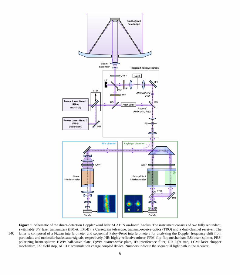
Figure 1. Schematic of the direct-detection Doppler wind lidar ALADIN on-board Aeolus. The instrument consists of two fully redundant,

switchable UV laser transmitters (FM-A, FM-B), a Cassegrain telescope, transmit-receive optics (TRO) and a dual-channel receiver. The

latter is composed of a Fizeau interferometer and sequential Fabry-Pérot interferometers for analyzing the Doppler frequency shift from 140 particulate and molecular backscatter signals, respectively. HR: highly-reflective mirror, FFM: flip-flop mechanism, BS: beam splitter, PBS:

polarizing beam splitter, HWP: half-wave plate, QWP: quarter-wave plate, IF: interference filter, LT: light trap, LCM: laser chopper

mechanism, FS: field stop, ACCD: accumulation charge coupled device. Numbers indicate the sequential light path in the receiver.

7

The UV emit beam from one of the two switchable laser transmitters is then directed to the telescope which is used in

monostatic configuration, i.e., signal emission and reception are realized via the same primary and secondary mirror. A small 145

portion (0.5%) of the radiation beam is separated at a beam splitter (BS) within the TRO configuration and, after being

attenuated, guided to the instrument field stop (FS) and receiver channels. This portion is referred to as internal reference path

(INT) signal and serves the determination of the frequency of the outgoing laser radiationbeam as well as the calibration of the

frequency-dependent transmission of the receiver spectrometers. The INT signal is thus essential for the wind measurement

principle of ALADIN which relies on detecting frequency differences between the emitted laser pulses and those backscattered 150

from the atmospheric particles and molecules moving with the ambient wind. The frequency shift ΔfDoppler in the backscattered

signal that is introduced by virtue of the Doppler effect is proportional to the wind speed vLOS along the laser beam LOS

according to ΔfDoppler = 2 f0 vLOS/c, where c is the speed of light and f0 is the frequency of the emitted light. The atmospheric

return signal collected by the telescope enters the TRO where it passes through a laser chopper mechanism (LCM) before

being spatially overlapped with the INT beam by another beam splitter. Due to the long travel time of the atmospheric return 155

of a few ms, the detection is temporally separated from the INT signal.

The ALADIN receiver consists of two complementary channels which individually derive the Doppler frequency shift from

the narrowband (FWHM ≈ 50 MHz) Mie backscatter from particles like clouds and aerosols on the one hand and from the

broadband (FWHM ≈ 3.8 GHz at 355 nm and 293 K) Rayleigh-Brillouin backscatter from molecules on the other hand. The

Mie channel is realized by a Fizeau interferometer and relies on the fringe-imaging technique (McKay, 2002) where a linear 160

interference pattern (fringe) is vertically imaged onto the detector. The spatial location of the fringe changes approximately

linearly with frequency of the incident light so that a Doppler frequency shift manifests as a spatial displacement of the fringe

centroid position. Derivation of the Doppler shift from the broadband Rayleigh-Brillouin backscatter spectrum is achieved by

two sequential Fabry-Pérot interferometers (FPIs) that are utilized for applying the double-edge technique (Chanin et al., 1989;

Garnier and Chanin, 1992; Flesia and Korb, 1999). The two FPIs act as bandpass filters with adequate width and spacing that 165

are symmetrically placed around the frequency of the emitted laser pulse. Measurement of the contrast between the signals

transmitted through the two filters allows to accurately determine the frequency shift between the emitted and backscattered

laser pulse.

The Mie and Rayleigh signals are finally detected by two accumulation charge-coupled devices (ACCDs) with an array size

of 16 pixels×16 pixels in the imaging zone of the CCD. The electronic charges of all 16 rows in the image zone are then binned 170

together to one row. For the wind profile, this row is transferred to a memory zone. The latter can store 25 rows each

representing one vertical range gate of the measured wind profile. It is important to note that the atmospheric signals from 18

successive laser pulses are accumulated already on-board the spacecraft to so-called “measurements” (duration 0.4 s). Since

February 2019, P = 19 laser pulses are emitted per measurement interval from which one is lost due to the read-out of the

ACCD (P – 1 setting). Post processing on-ground can sum the signals from 30 measurements, i.e., 540 laser pulses, and form 175

one “observation” (duration 12 s). In contrast to the atmospheric return, the INT signal is acquired for each single pulse and

stored directly as one row in the memory zone.

8

According to the above equation for the Doppler frequency shift, a LOS wind speed of 1 m∙s-1 translates to a frequency shift

of 5.63 MHz (at f0 = 844.75 THz, all subsequent frequency stability values given at this UV frequency). Therefore, in order to

measure wind speeds with an accuracy of 1 m∙s-1, the required relative accuracy of the frequency measurement is on the order 180

of 10-8 which poses stringent requirements on the frequency stability of the laser transmitter. This is especially true, as the

atmospheric backscatter signals from multiple outgoing laser pulses are accumulated on the CCD prior to digitization and data

down-linkto measurements before data down-link. This implies that a pulse-to-pulse normalization of the return signal

frequency with the internal reference frequency is not possible. Instead, the determined frequency of the pulses averaged over

one measurement is affected by inhomogeneous cirrus or broken clouds, as only a subset of the 18 pulses may be detected in 185

the atmospheric path. As a result, large frequency variations on measurement level (over periods of 0.4 s) in combination with

atmospheric inhomogeneities results in significant wind errors, that are then vertically correlated below the (cloud) bin that

filters out some of the emitted pulses (Marksteiner et al., 2015). The same holds true for ground return signals from pulses

within one measurement that are reflected off a surface with varying albedo, so that the different weighting of the return signals

in the accumulation of the pulses results in an error of the determined ground velocity. 190

2.2 On-ground assessment of the laser frequency stability

Measurement of the ALADIN laser absolute frequency and its temporal stability was done during pre-flight on-ground tests

under vacuum conditions by means of an external wavelength meter (High Finesse WSU10) that was calibrated using a helium

neon laser (Mondin and Bravetti, 2017). The experimental setup was provided by DLR and represents an integral part of the

diagnostics for determining the spectral properties of the ALADIN Airborne Demonstrator (A2D) (Lemmerz et al., 2017). 195

Using it for characterization of the ALADIN laser, it was found that the laser frequency stability was well within the

specification requirement which states that the root mean square (RMS) variation of the frequency stability over 14 s should

be below 7 MHz. The 14 s time period was chosen to ensure adequate SNR over one Aeolus observation (12 s). In addition,

sensitivity tests with a thermal cycle of ±0.2°C were carried out for about four hours: one at ambient temperature, one with the

laser interface at +35⁰C and two at -2.5⁰C. For all four thermal cycles, the absolute laser frequency varied by less than 25 MHz 200

(peak to peak), demonstrating a good stability also over medium time scales, as thermal variations over one week in orbit were

expected to be even below 0.2°C. However, the test also revealed that operation in a vibrational environment, in this case

introduced by vacuum pumps and a chiller, led to a degraded laser frequency stability with pulse-to-pulse fluctuations above

30 MHz RMS (Mondin and Bravetti, 2017). Further pre-flight on-ground test results are discussed in the context of micro-

vibrations in section Sect. 3.4. 205

2.3 Utilization of the Mie channel as wavelength meter in orbit

An external wavelength meter is not available in space. However, the spectrometer data gained from the Fizeau interferometer

of the Mie channel can be exploited for deriving the spectral properties of the narrowband laser emission. For this purpose, the

INT signal that is usually analyzed after accumulation of multiple pulses to measurement level and contained in the L1A

9

Aeolus data product (Reitebuch et al., 2018) is evaluated for each individual pulse. As stated above, the Mie channel response 210

is represented by the centroid position of the fringe that is imaged onto the Mie detector and then integrated over the 16 lines

of the ACCD. Figure 2 shows the vertically summed ACCD counts over the 16 horizontal pixels for one laser pulse. The fringe

centroid position is calculated by a Nelder-Mead Downhill Simplex Algorithm (Nelder and Mead, 1965) to optimize a

Lorentzian line shape fit of the signal distribution (Reitebuch et al., 2018). In this manner, the Mie response is derived with

high accuracy. Conversion of the Mie response into relative laser frequency is based on dedicated in-flight calibrations of the 215

Mie channel from which a sensitivity of ≈100 MHz/pixel was determined. The accuracy of the “inherent wavemeter” on-board

Aeolus is estimated to be 1 MHz. It is mainly limited by the shot-noise-limited signal-to-noise ratio (SNR) of the Mie signal

and the full width at half maximum (FWHM) of the Fizeau interference fringe (≈1.3 pixels). This could be demonstrated with

A2D laboratory measurements comparing the spectrometer response from the ALADIN pre-development model Fizeau

interferometer and parallel wavemeter measurements using the A2D UV laser (Lux et al., 2019). Hence, frequency fluctuations 220

of the internal path signal can be measured as variations in the calculated Mie response on a pulse-to-pulse basis which allows

to assess the frequency stability of the Aeolus laser transmitter over short- and long-term time scales.

Figure 2. Internal reference path Mie signal for one laser pulse (24/11/2020, 0:23:47 UTC). After vertical integration of imaged fringe on 225 the Mie ACCD (see also Fig. 1), the signal is distributed over 16 pixels (blue bars). A Nelder-Mead Downhill Simplex Algorithm is applied

to determine the centroid position from a Lorentzian line shape fit (dark blue line).

2.4 Analyzed periods of in-orbit Aeolus datasets

The laser frequency stability was analyzed for different periods of the Aeolus mission. Since the satellite is circling around the

Earth with an orbit repeat cycle of one week, it was decided to study the performance over selected seven-day periods. This 230

approach was also motivated by the observed correlation between the frequency stability and the satellite’s geolocation (see

section Sect. 3.2). After one week the maximum coverage of the globe is reached and the operation timeline, particularly the

attitude control sequence of the platform approximately repeats. In total, five weeks between December 2018, when the mission

was still in commissioning phase after its launch on 22 August 2018, and October 2020 were chosen for investigation, as listed

in Table 1. The table contains information on the operated laser transmitter as well as on the MO output energy (IR), the laser 235

10

emit energy (UV) and the laser frequency stability which will be discussed later in the text. The energy values represent the

respective mean values and standard deviations from laser internal photodiode readings. It should be noted that the IR energy

reported by the MO photodiode of the FM-A is considered inaccurate. Here, Q-switch discharges influence the energy

monitoring, as they result in IR radiation with the wrong polarization that is circulating in the MO. This light is partially

incident on the MO photodiodePD, thus corrupting the energy measurement. As can be seen from the table, the UV emit energy 240

of FM-A decreased significantly between December 2018 and May 2019. The degradation of the laser performance was traced

back to a progressive misalignment of the MO (Lux et al., 2020a) and led to the decision to switch to the second laser FM-B.

This was necessary to ensure a sufficient SNR of the backscatter return and thus a low random error of the wind observations.

The FM-B not only delivered a higher initial energy after switch-on in late June 2019 (67 mJ compared to 65 mJ after FM-A

switch-on), but also has been showing a much slower power degradation. After an initial drop by 6 mJ between July 2019 and 245

October 2019, the UV emit energy has decreased by less than 0.08 mJ per week. Thanks to an optimization of the laser cold-

plate temperatures in March 2020 which increased the UV energy by about 4 mJ, the energy has remained above 60 mJ as of

the writing of this papersince then. Despite the better overall performance compared to the FM-A, the FM-B behavior was

observed to be more affected by orbital and seasonal temperature variations of the satellite platform that were transferred to

the laser optical bench. As a consequence, laser anomalies associated with larger energy variations of about ±1 mJ occurred 250

both on shorter (hours) and longer-term time scales (weeks to months).

The periods listed in Table 1 are chosen such that they represent different phases of the mission: the early FM-A phase in

December 2018 when the instrument parameters had settled after launch, but the degradation of the MO was already ongoing;

the late FM-A phase in May 2019 when the degradation had progressed; the early FM-B phase in October after completed

thermalization of the second laser and later FM-B periods in August and September/October 2020 after optimization of the 255

laser cold-plate temperatures. The latter two periods were also chosen to identify the variability of the frequency stability

performance decoupled from the power performance of the laser which was stable in summer and autumn 2020 and free of

temperature-related laser anomalies as stated above.

Table 1. Overview of the periods that were studied in terms of the laser frequency stability. The active laser transmitter operated in the 260 respective period (FM-A or FM-B) and the corresponding master oscillator IR output energy and UV emit energy (as reported by the laser

internal photodiodes) are provided. Note that the reading of the MO photodiode for FM-A is considered inaccurate (see text). The frequency

stability is given as the mean of the standard deviations from all wind observations of the respective week.

Period Laser transmitter MO energy UV emit energy Frequency stability

17/12/2018 - 24/12/2018 FM-A (8.3 ± 0.5) mJ (56.2 ± 0.8) mJ 7.2 MHz

13/05/2019 - 20/05/2019 FM-A (8.9 ± 0.3) mJ (44.2 ± 0.8) mJ 10.7 MHz

14/10/2019 - 21/10/2019 FM-B (5.87 ± 0.03) mJ (60.8 ± 0.8) mJ 8.1 MHz

17/08/2020 - 24/08/2020 FM-B (5.91 ± 0.03) mJ (61.8 ± 0.3) mJ 8.7 MHz

28/09/2020 - 05/10/2020 FM-B (5.88 ± 0.03) mJ (61.4 ± 0.4) mJ 8.6 MHz

11

3 Results

The frequency stability of the ALADIN laser will first be presented at one example, namely the week in October 2019, to 265

illustrate the main temporal characteristics of the spectral behavior as well as the relation to the geolocation of the satellite.

This leads to the correlation of the laser frequency stability with platform parameters, particularly the reaction wheel speeds

which is elaborated on subsequently. This correlation is additionally analyzed for the FM-A period in May 2019 to allow for

a comparison between the two flight model lasers. The chapter section concludes with a discussion of micro-vibrations as the

root cause of the frequency noise. 270

3.1 Frequency stability of the ALADIN laser transmitters

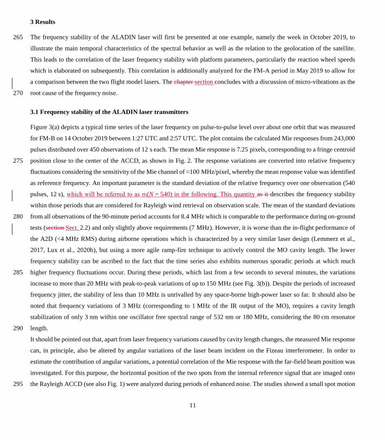
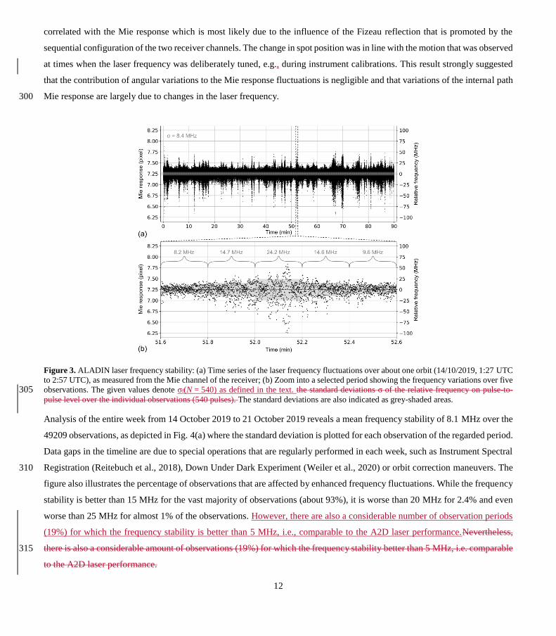
Figure 3(a) depicts a typical time series of the laser frequency on pulse-to-pulse level over about one orbit that was measured

for FM-B on 14 October 2019 between 1:27 UTC and 2:57 UTC. The plot contains the calculated Mie responses from 243,000

pulses distributed over 450 observations of 12 s each. The mean Mie response is 7.25 pixels, corresponding to a fringe centroid

position close to the center of the ACCD, as shown in Fig. 2. The response variations are converted into relative frequency 275

fluctuations considering the sensitivity of the Mie channel of ≈100 MHz/pixel, whereby the mean response value was identified

as reference frequency. An important parameter is the standard deviation of the relative frequency over one observation (540

pulses, 12 s), which will be referred to as σf(N = 540) in the following. This quantity as it describes the frequency stability

within those periods that are considered for Rayleigh wind retrieval on observation scale. The mean of the standard deviations

from all observations of the 90-minute period accounts for 8.4 MHz which is comparable to the performance during on-ground 280

tests (section Sect. 2.2) and only slightly above requirements (7 MHz). However, it is worse than the in-flight performance of

the A2D (<4 MHz RMS) during airborne operations which is characterized by a very similar laser design (Lemmerz et al.,

2017, Lux et al., 2020b), but using a more agile ramp-fire technique to actively control the MO cavity length. The lower

frequency stability can be ascribed to the fact that the time series also exhibits numerous sporadic periods at which much

higher frequency fluctuations occur. During these periods, which last from a few seconds to several minutes, the variations 285

increase to more than 20 MHz with peak-to-peak variations of up to 150 MHz (see Fig. 3(b)). Despite the periods of increased

frequency jitter, the stability of less than 10 MHz is unrivalled by any space-borne high-power laser so far. It should also be

noted that frequency variations of 3 MHz (corresponding to 1 MHz of the IR output of the MO), requires a cavity length

stabilization of only 3 nm within one oscillator free spectral range of 532 nm or 180 MHz, considering the 80 cm resonator

length. 290

It should be pointed out that, apart from laser frequency variations caused by cavity length changes, the measured Mie response

can, in principle, also be altered by angular variations of the laser beam incident on the Fizeau interferometer. In order to

estimate the contribution of angular variations, a potential correlation of the Mie response with the far-field beam position was

investigated. For this purpose, the horizontal position of the two spots from the internal reference signal that are imaged onto

the Rayleigh ACCD (see also Fig. 1) were analyzed during periods of enhanced noise. The studies showed a small spot motion 295

12

correlated with the Mie response which is most likely due to the influence of the Fizeau reflection that is promoted by the

sequential configuration of the two receiver channels. The change in spot position was in line with the motion that was observed

at times when the laser frequency was deliberately tuned, e.g., during instrument calibrations. This result strongly suggested

that the contribution of angular variations to the Mie response fluctuations is negligible and that variations of the internal path

Mie response are largely due to changes in the laser frequency. 300

Figure 3. ALADIN laser frequency stability: (a) Time series of the laser frequency fluctuations over about one orbit (14/10/2019, 1:27 UTC

to 2:57 UTC), as measured from the Mie channel of the receiver; (b) Zoom into a selected period showing the frequency variations over five

observations. The given values denote σf(N = 540) as defined in the text. the standard deviations σ of the relative frequency on pulse-to-305 pulse level over the individual observations (540 pulses). The standard deviations are also indicated as grey-shaded areas.

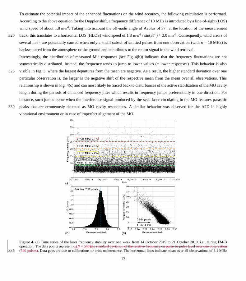
Analysis of the entire week from 14 October 2019 to 21 October 2019 reveals a mean frequency stability of 8.1 MHz over the

49209 observations, as depicted in Fig. 4(a) where the standard deviation is plotted for each observation of the regarded period.

Data gaps in the timeline are due to special operations that are regularly performed in each week, such as Instrument Spectral

Registration (Reitebuch et al., 2018), Down Under Dark Experiment (Weiler et al., 2020) or orbit correction maneuvers. The 310

figure also illustrates the percentage of observations that are affected by enhanced frequency fluctuations. While the frequency

stability is better than 15 MHz for the vast majority of observations (about 93%), it is worse than 20 MHz for 2.4% and even

worse than 25 MHz for almost 1% of the observations. However, there are also a considerable number of observation periods

(19%) for which the frequency stability is better than 5 MHz, i.e., comparable to the A2D laser performance.Nevertheless,

there is also a considerable amount of observations (19%) for which the frequency stability better than 5 MHz, i.e. comparable 315

to the A2D laser performance.

13

To estimate the potential impact of the enhanced fluctuations on the wind accuracy, the following calculation is performed.

According to the above equation for the Doppler shift, a frequency difference of 10 MHz is introduced by a line-of-sight (LOS)

wind speed of about 1.8 m∙s-1. Taking into account the off-nadir angle of Aeolus of 37° at the location of the measurement

track, this translates to a horizontal LOS (HLOS) wind speed of 1.8 m∙s-1 / sin(37°) ≈ 3.0 m∙s-1. Consequently, wind errors of 320

several m∙s-1 are potentially caused when only a small subset of emitted pulses from one observation (with σ = 10 MHz) is

backscattered from the atmosphere or the ground and contributes to the return signal in the wind retrieval.

Interestingly, the distribution of measured Mie responses (see Fig. 4(b)) indicates that the frequency fluctuations are not

symmetrically distributed. Instead, the frequency tends to jump to lower values (= lower responses). This behavior is also

visible in Fig. 3, where the largest departures from the mean are negative. As a result, the higher standard deviation over one 325

particular observation is, the larger is the negative shift of the respective mean from the mean over all observations. This

relationship is shown in Fig. 4(c) and can most likely be traced back to disturbances of the active stabilization of the MO cavity

length during the periods of enhanced frequency jitter which results in frequency jumps preferentially in one direction. For

instance, such jumps occur when the interference signal produced by the seed laser circulating in the MO features parasitic

peaks that are erroneously detected as MO cavity resonances. A similar behavior was observed for the A2D in highly 330

vibrational environment or in case of imperfect alignment of the MO.

Figure 4. (a) Time series of the laser frequency stability over one week from 14 October 2019 to 21 October 2019, i.e., during FM-B

operation. The data points represent σf(N = 540)the standard deviation of the relative frequency on pulse-to-pulse level over one observation

(540 pulses). Data gaps are due to calibrations or orbit maintenance. The horizontal lines indicate mean over all observations of 8.1 MHz 335

14

(green) as well as thresholds to indicate the percentage of observations for which the frequency stability is worse than 15 MHz (yellow),

20 MHz (orange) and 25 MHz (red). (b) Probability density distribution of the Mie internal reference response for the dataset in October

2019. (c) Relationship between the laser frequency stability in terms of σf(N = 540)of the standard deviation on pulse-to-pulse level over one

observation and the mean Mie internal reference response per observation. A response shift by 0.034 pixels translates to a frequency shift

by about 3.4 MHz, corresponding to a HLOS wind speed change of 1 m∙s-1, assuming a constant response of the atmospheric or ground 340 return signal.

3.2 Correlation with the satellite’s geolocation

The enhanced frequency fluctuations of the laser transmitter were detected very early in the mission and attributed to potential

vibrations introduced by the satellite platform which affects the MO cavity length (Lux et al., 2020a). However, a correlation

to platform parameters, particularly the rotation velocity of the satellite’s reaction wheels was not found initially. This was 345

mainly due to the fact that only short timelines were analyzed, typically covering only several minutes to hours, as shown in

Fig. 3. Since the platform parameters vary slowly over the orbit, a relationship to the fast changes in the laser frequency

stability within several seconds was considered unlikely.

During the first year of operation, the assessment of the frequency stability was then focused on the weekly Instrument

Response Calibrations (IRCs, Reitebuch et al., 2018). IRCs are required to determine the relationship between the Doppler 350

frequency shift of the backscattered light, i.e., the wind speed, and the response of the Rayleigh and Mie spectrometers. The

procedure involves a frequency scan over 1 GHz in steps of 25 MHz to simulate well-defined Doppler shifts of the atmospheric

backscatter signal within the limits of the laser frequency stability. During the IRC which takes about 16 minutes, two

observations (12 s) for each of the 40 frequency steps, the contribution of (real) wind related to molecular or particular motion

along the instruments’ LOS is virtually eliminated by rotating the satellite by an angle of 35°. This results in nadir pointing of 355

the instrument and, in case of negligible vertical wind, vanishing LOS wind speed. The IRCs are preferably carried out over

regions with high surface albedo in the UV spectral region, e.g., over ice, to ensure strong return signals, and in turn, high

SNR. This is particularly important for the Mie response calibration which relies on measuring the spectrometer response from

the ground return to be then used for the retrieval of atmospheric winds.

The laser frequency stability was studied for each of the 60 IRCs conducted between 7 September 2018 and 9 December 2019; 360

most of them over Antarctica, while IRCs #31 to #43 were performed over the Arctic. Here, it was found that the frequency

stability was degraded during the IRCs compared to operation in nominal wind velocity mode (WVM). While it was on the

order of 8 to 10 MHz in WVM, the mean stability over the 16-minute IRC period accounted for 12 to 14 MHz when the

satellite was pointing nadir, suggesting an influence of the platform attitude on the laser. This conclusion was strengthened by

the circumstance that the laser temperatures and energies were strongly varying during the nadir and off-nadir slews before 365

and after the IRC, respectively. Moreover, these orbit maneuvers involved thruster firings which also caused increased

frequency noise during the slews before and after the weekly IRC, thus pointing to mechanical disturbances as the root cause.

Furthermore, the frequency stability showed to be significantly better over Antarctica ((11.6 ± 1.7) MHz) than over the Arctic

((15.2 ± 2.1) MHz), although the IRC procedure was the same over both locations. Finally, it was noticed that the progression

of the relative laser frequency featured recurring temporal patterns for those IRCs that were carried out over the same locations 370

15

in subsequent weeks. For instance, an accumulation of periods with increased frequency jitter were observed at the beginning

of the time series for the Antarctica IRCs, whereas numerous high-noise periods, distributed over the entire procedure, were

evident for the Arctic IRCs. Figure 5 depicts the laser frequency variations over selected IRC periods over the two different

geolocations, clearly demonstrating the reproducibility of the jitter patterns for the weekly IRCs.

375

Figure 5. Time series of the laser frequency fluctuations over periods of selected IRCs over Antarctica (a, c) and the Arctic (b, d) together

with the corresponding geolocations of the individual frequency steps in panels (e) – (h). Each dot corresponds to one frequency step (24 s),

whereby the color-coding describes the standard deviation of the relative frequency on pulse-to-pulse level within this period (σf(N = 1080)).

Following these observations, the laser frequency stability was studied over one-week periods to review the influence of the

satellite’s geolocation (see section Sect. 2.4). The performance from the week between 14 October and 21 October 2019 380

(Fig. 4a), based on the Mie response data from more than 27 million laser pulses, is illustrated in Fig. 6. Each dot in the two

maps represents one observation, whereby the color and opacity indicate the frequency stability in terms of σf(N = 540)the

standard deviation of the relative frequency over the 540 pulses within that observation. The analysis revealed that the enhanced

frequency noise does not occur randomly, but is correlated with the location of the satellite over the Earth’s surface. More

strikingly, different linear and circular structures are evident for ascending and descending orbits, which makes clear that the 385

16

frequency stability does not only depend on the geolocation, but also on the satellite’s orientation along the orbit. For ascending

orbits those observations with enhanced frequency fluctuations are accumulated in several bands wrapping around the globe,

most prominently around East Asia and the Pacific Ocean. In contrast, multiple narrow latitudinal bands and a circular structure

over the South Atlantic and South Indian Ocean are apparent for descending orbits.

390

Figure 6. Geolocation of wind observations with enhanced frequency noise for (a) ascending and (b) descending orbits. The plot contains

the data from the week between 14/10/2019 (0 UTC) and 21/10/2019 (0 UTC) (see also Fig. 4). Each dot corresponds to one observation

(12 s), whereby the color-coding describes the σf(N = 540)standard deviation of the relative frequency on pulse-to-pulse level within this

period. Note that the opacity of the dots also scales with the frequency stability so that observations with σ < 10 MHz are not visible.

The geolocational patterns were found to be reproducible for the investigated FM-B periods with only slight variations 395

(<200 km). This is especially true for the linear and circular structures that are formed by neighboring orbits, i.e., with large

temporal distance. On the contrary, continuous phases of enhanced frequency noise over several observations which manifest

as orange and red lines along one orbit, e.g., in Northern Canada or over Northern Europe in Fig. 6(a), were evident at different

geolocations for the weeks in August 2020 and September/October 2020.

Similar correlation of the laser frequency stability with the satellite position was also obvious for the periods in December 400

2018 and May 2019 when FM-A was operated. However, the geolocational patterns for ascending and descending orbits

17

markedly differed from those of the FM-B periods, suggesting that the mechanism introducing the enhanced frequency noise

acts differently on the two laser transmitters, potentially due to the different locations in the payload. The underlying reason

for the observed dependence on geolocation could be traced back to the reaction wheels of the satellite, as will be explained

in the following section. 405

3.3 Influence of the reaction wheels

Precise three-axis attitude control of the Aeolus satellite is accomplished by a set of reaction wheels (RW) which rotate at

different speeds, thereby causing the spacecraft to counterrotate proportionately through the conservation of angular

momentum. Due to external disturbances, mainly aerodynamic drag, the total angular momentum is periodically modified so

that magnetorquers are additionally required to generate an effective external torque. Otherwise the wheel speed would 410

gradually increase in time and reach saturation (Markley and Crassidis, 2014). The attitude and orbit control system of Aeolus

additionally consists of thrusters which allow for larger torque to be exerted on the spacecraft.

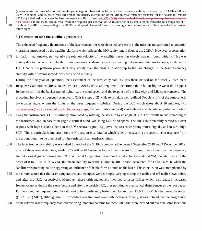
A sketch illustrating the orientation of the reaction wheels within the spacecraft is shown in Fig. 7. The reaction wheel

assemblies (RWAs) are mounted on the spacecraft such that they form a tetrahedron whose axis of symmetry lies along the

+Z axis, i.e., the line-of-sight direction of the telescope. Hence, the normal vectors of the four wheels span a plane parallel to 415

the X-Y plane (Fig. 7(b)) in which the two lasers (including the respective MO axes) are located. Each wheel is canted such

that the angle between its spin axis and each spacecraft axis is 54.74°. The reaction wheels were manufactured by Stork Product

Engineering B.V. in 2005 (design later transferred to Moog Bradford) and have a capacity of 40 Nms and maximum torque of

0.2 Nm. These wheels consist of a rotating inertial mass driven by a brushless DC motor (Bradford space, 2021) and supported

by oil-lubricated bearings. The wheels are all mounted on isolation suspensions to reduce micro-vibrations. 420

Figure 7. (a) Orientation of the four reaction wheels with respect to the spacecraft body. (b) Alignment of the reaction wheel spin axes with

respect to the spacecraft body. The axes of the four wheels are oriented such that |𝜶| = |𝜷| = |𝜸| = 54.74°.

Based on the dataset from the week in October 2019, the frequency stability on observation level, as depicted in Fig. 6, was

correlated with the rotational speed of the three active reaction wheels on-board Aeolus (RWA 4 serves as a backup). The 425

same procedure was performed for the FM-A period in May 2019 (see Table 1). The resulting six correlation plots, which can

also be considered as spectra in terms of the wheel rotation frequency (rotations per second, RPS), are shown in Fig. 8. Note

18

that the plot includes data from both ascending and descending orbits, and that RWA 1 and RWA 3 rotate counterclockwise,

while RWA 2 rotates clockwise. For the sake of better comparability of the three spectra, the absolute wheel speeds are plotted

in the figure and the negative sign for the wheel speeds of RWA 1 and RWA 3 was omitted. The six spectra exhibit pronounced 430

peaks which demonstrates that the laser frequency fluctuations are enhanced at specific rotational speeds of the reaction wheels.

Thus, the latter are subsequently referred to as critical wheel speeds or critical frequencies.

19

Figure 8. Correlation between the laser frequency stability and the speeds of the three active reaction wheels: The plots in panel (a) are

based on data from the FM-A laser for the period between 13 May 2019 and 20 May 2019, while the plots in panel (b) show the correlation 435 for the FM-B laser in the period between 14 October 2019 and 21 October 2019. The colored lines result from a Savitzky-Golay smoothing

with a window size of 201 and polynomial order of two.

20

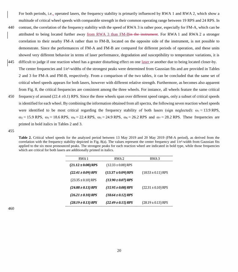
For both periods, i.e., operated lasers, the frequency stability is primarily influenced by RWA 1 and RWA 2, which show a

multitude of critical wheel speeds with comparable strength in their common operating range between 19 RPS and 24 RPS. In

contrast, the correlation of the frequency stability with the speed of RWA 3 is rather poor, especially for FM-A, which can be 440

attributed to being located further away from RWA 3 than FM-Bin the instrument. For RWA 1 and RWA 2 a stronger

correlation to their nearby FM-A rather than to FM-B, located on the opposite side of the instrument, is not possible to

demonstrate. Since the performances of FM-A and FM-B are compared for different periods of operation, and these units

showed very different behavior in terms of laser performance, degradation and susceptibility to temperature variations, it is

difficult to judge if one reaction wheel has a greater disturbing effect on one laser or another due to being located closer-by. 445

The center frequencies and 1/e²-widths of the strongest peaks were determined from Gaussian fits and are provided in Tables

2 and 3 for FM-A and FM-B, respectively. From a comparison of the two tables, it can be concluded that the same set of

critical wheel speeds appears for both lasers, however with different relative strength. Furthermore, as becomes also apparent

from Fig. 8, the critical frequencies are consistent among the three wheels. For instance, all wheels feature the same critical

frequency of around (22.4 ±0.1) RPS. Since the three wheels span over different speed ranges, only a subset of critical speeds 450

is identified for each wheel. By combining the information obtained from all spectra, the following seven reaction wheel speeds

were identified to be most critical regarding the frequency stability of both lasers (sign neglected): ω1 ≈ 13.9 RPS,

ω2 ≈ 15.9 RPS, ω3 ≈ 18.6 RPS, ω4 ≈ 22.4 RPS, ω5 ≈ 24.9 RPS, ω6 ≈ 26.2 RPS and ω7 ≈ 28.2 RPS. These frequencies are

printed in bold italics in Tables 2 and 3.

455

Table 2. Critical wheel speeds for the analyzed period between 13 May 2019 and 20 May 2019 (FM-A period), as derived from the

correlation with the frequency stability depicted in Fig. 8(a). The values represent the center frequency and 1/e²-width from Gaussian fits

applied to the six most pronounced peaks. The strongest peaks for each reaction wheel are indicated in bold type, while those frequencies

which are critical for both lasers are additionally printed in italics.

RWA 1 RWA 2 RWA 3

(21.12 ± 0.08) RPS (12.33 ± 0.08) RPS

(22.41 ± 0.09) RPS (13.37 ± 0.09) RPS (18.53 ± 0.11) RPS

(23.35 ± 0.10) RPS (13.90 ± 0.07) RPS

(24.88 ± 0.13) RPS (15.95 ± 0.08) RPS (22.31 ± 0.10) RPS

(26.21 ± 0.10) RPS (18.64 ± 0.12) RPS

(28.19 ± 0.13) RPS (22.49 ± 0.15) RPS (28.19 ± 0.13) RPS

460

21

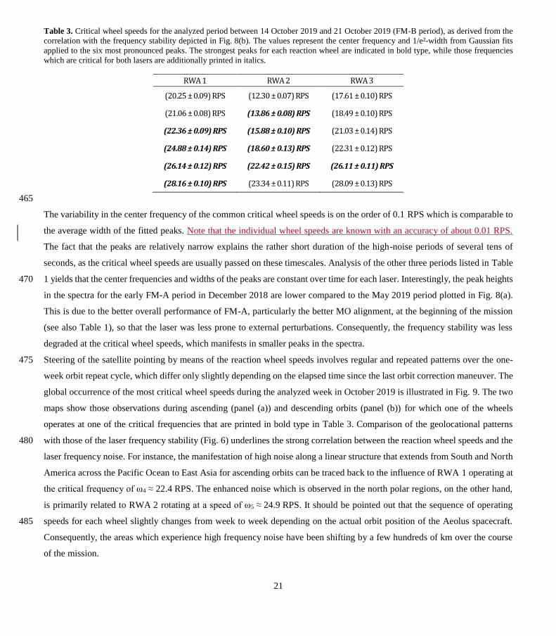
Table 3. Critical wheel speeds for the analyzed period between 14 October 2019 and 21 October 2019 (FM-B period), as derived from the

correlation with the frequency stability depicted in Fig. 8(b). The values represent the center frequency and 1/e²-width from Gaussian fits

applied to the six most pronounced peaks. The strongest peaks for each reaction wheel are indicated in bold type, while those frequencies

which are critical for both lasers are additionally printed in italics.

RWA 1 RWA 2 RWA 3

(20.25 ± 0.09) RPS (12.30 ± 0.07) RPS (17.61 ± 0.10) RPS

(21.06 ± 0.08) RPS (13.86 ± 0.08) RPS (18.49 ± 0.10) RPS

(22.36 ± 0.09) RPS (15.88 ± 0.10) RPS (21.03 ± 0.14) RPS

(24.88 ± 0.14) RPS (18.60 ± 0.13) RPS (22.31 ± 0.12) RPS

(26.14 ± 0.12) RPS (22.42 ± 0.15) RPS (26.11 ± 0.11) RPS

(28.16 ± 0.10) RPS (23.34 ± 0.11) RPS (28.09 ± 0.13) RPS

465

The variability in the center frequency of the common critical wheel speeds is on the order of 0.1 RPS which is comparable to

the average width of the fitted peaks. Note that the individual wheel speeds are known with an accuracy of about 0.01 RPS.

The fact that the peaks are relatively narrow explains the rather short duration of the high-noise periods of several tens of

seconds, as the critical wheel speeds are usually passed on these timescales. Analysis of the other three periods listed in Table

1 yields that the center frequencies and widths of the peaks are constant over time for each laser. Interestingly, the peak heights 470

in the spectra for the early FM-A period in December 2018 are lower compared to the May 2019 period plotted in Fig. 8(a).

This is due to the better overall performance of FM-A, particularly the better MO alignment, at the beginning of the mission

(see also Table 1), so that the laser was less prone to external perturbations. Consequently, the frequency stability was less

degraded at the critical wheel speeds, which manifests in smaller peaks in the spectra.

Steering of the satellite pointing by means of the reaction wheel speeds involves regular and repeated patterns over the one-475

week orbit repeat cycle, which differ only slightly depending on the elapsed time since the last orbit correction maneuver. The

global occurrence of the most critical wheel speeds during the analyzed week in October 2019 is illustrated in Fig. 9. The two

maps show those observations during ascending (panel (a)) and descending orbits (panel (b)) for which one of the wheels

operates at one of the critical frequencies that are printed in bold type in Table 3. Comparison of the geolocational patterns

with those of the laser frequency stability (Fig. 6) underlines the strong correlation between the reaction wheel speeds and the 480

laser frequency noise. For instance, the manifestation of high noise along a linear structure that extends from South and North

America across the Pacific Ocean to East Asia for ascending orbits can be traced back to the influence of RWA 1 operating at

the critical frequency of ω4 ≈ 22.4 RPS. The enhanced noise which is observed in the north polar regions, on the other hand,

is primarily related to RWA 2 rotating at a speed of ω5 ≈ 24.9 RPS. It should be pointed out that the sequence of operating

speeds for each wheel slightly changes from week to week depending on the actual orbit position of the Aeolus spacecraft. 485

Consequently, the areas which experience high frequency noise have been shifting by a few hundreds of km over the course

of the mission.

22

Figure 9. Geolocation of the most critical frequencies of the three active reaction wheels for (a) ascending and (b) descending orbits. The

plot contains the data from the week between 14/10/2019 (0 UTC) and 21/10/2019 (0 UTC) (see also Fig. 6 for the corresponding frequency 490 stability). Each dot corresponds to one observation (12 s) for which one of the wheels operates at one of the critical wheel speeds as listed

in bold type in Table 3.

The occurrence of critical frequencies from different wheels along the orbit suggests that the three wheels act independently

on the laser. This hypothesis was confirmed by further analysis which revealed that enhanced noise is observed almost every

time when one of the wheels rotates at a critical speed, regardless of the speed of the other two wheels. Hence, there is no 495

entanglement of the critical frequencies, even though the speeds of the wheels are related among each other. Additional studies

also showed that the frequency stability is not correlated with the wheel acceleration.

The impact of the reaction wheel speeds on the laser frequency stability is finally demonstrated at an example scene which

clearly illustrates the origination of the geolocation patterns. Figure 10 shows a map with the color-coded frequency stability

per observation (dots on the map) for the period between 16:30 UTC and 17:30 UTC on 18 October 2019. Within this hour 500

the satellite crossed Africa and Europe on an ascending orbit and passed the North Pole before flying over Alaska and the

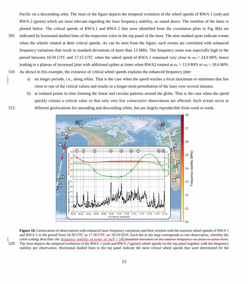
23

Pacific on a descending orbit. The inset of the figure depicts the temporal evolution of the wheel speeds of RWA 1 (red) and

RWA 2 (green) which are most relevant regarding the laser frequency stability, as stated above. The timeline of the latter is

plotted below. The critical speeds of RWA 1 and RWA 2 that were identified from the correlation plots in Fig. 8(b) are

indicated by horizontal dashed lines of the respective color in the top panel of the inset. The nine marked spots indicate events 505

when the wheels rotated at their critical speeds. As can be seen from the figure, such events are correlated with enhanced

frequency variations that result in standard deviations of more than 15 MHz. The frequency noise was especially high in the

period between 16:50 UTC and 17:15 UTC when the wheel speed of RWA 1 remained very close to ω5 ≈ 24.9 RPS, hence

leading to a plateau of increased jitter with additional spikes at times when RWA2 rotated at ω1 ≈ 13.9 RPS or ω3 ≈ 18.6 RPS.

As shown in this example, the existence of critical wheel speeds explains the enhanced frequency jitter 510

a) on longer periods, i.e., along orbits. That is the case when the speed reaches a local maximum or minimum that lies

close to one of the critical values and results in a longer-term perturbation of the laser over several minutes.

b) at isolated points in time forming the linear and circular patterns around the globe. That is the case when the speed

quickly crosses a critical value so that only very few consecutive observations are affected. Such events occur at

different geolocations for ascending and descending orbits, but are largely reproducible from week to week. 515

Figure 10. Geolocation of observations with enhanced laser frequency variations and their relation with the reaction wheel speeds of RWA 1

and RWA 2 in the period from 16:30 UTC to 17:30 UTC on 18/10/2019. Each dot in the map corresponds to one observation, whereby the

color-coding describes the frequency stability in terms of σf(N = 540)standard deviation of the relative frequency on pulse-to-pulse level.

The inset depicts the temporal evolution of the RWA 1 (red) and RWA 2 (green) wheel speeds on the top panel together with the frequency 520 stability per observation. Horizontal dashed lines in the top panel indicate the most critical wheel speeds that were determined for the

24

analyzed week in October 2019 (see Table 3). Additional peaks in the frequency stability are related to other critical frequencies which are

not listed in Table 3 but visible in Fig. 8.

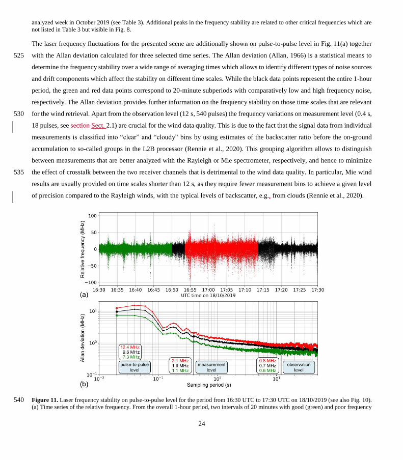
The laser frequency fluctuations for the presented scene are additionally shown on pulse-to-pulse level in Fig. 11(a) together

with the Allan deviation calculated for three selected time series. The Allan deviation (Allan, 1966) is a statistical means to 525

determine the frequency stability over a wide range of averaging times which allows to identify different types of noise sources

and drift components which affect the stability on different time scales. While the black data points represent the entire 1-hour

period, the green and red data points correspond to 20-minute subperiods with comparatively low and high frequency noise,

respectively. The Allan deviation provides further information on the frequency stability on those time scales that are relevant

for the wind retrieval. Apart from the observation level (12 s, 540 pulses) the frequency variations on measurement level (0.4 s, 530

18 pulses, see section Sect. 2.1) are crucial for the wind data quality. This is due to the fact that the signal data from individual

measurements is classified into “clear” and “cloudy” bins by using estimates of the backscatter ratio before the on-ground

accumulation to so-called groups in the L2B processor (Rennie et al., 2020). This grouping algorithm allows to distinguish

between measurements that are better analyzed with the Rayleigh or Mie spectrometer, respectively, and hence to minimize

the effect of crosstalk between the two receiver channels that is detrimental to the wind data quality. In particular, Mie wind 535

results are usually provided on time scales shorter than 12 s, as they require fewer measurement bins to achieve a given level

of precision compared to the Rayleigh winds, with the typical levels of backscatter, e.g., from clouds (Rennie et al., 2020).

Figure 11. Laser frequency stability on pulse-to-pulse level for the period from 16:30 UTC to 17:30 UTC on 18/10/2019 (see also Fig. 10). 540 (a) Time series of the relative frequency. From the overall 1-hour period, two intervals of 20 minutes with good (green) and poor frequency

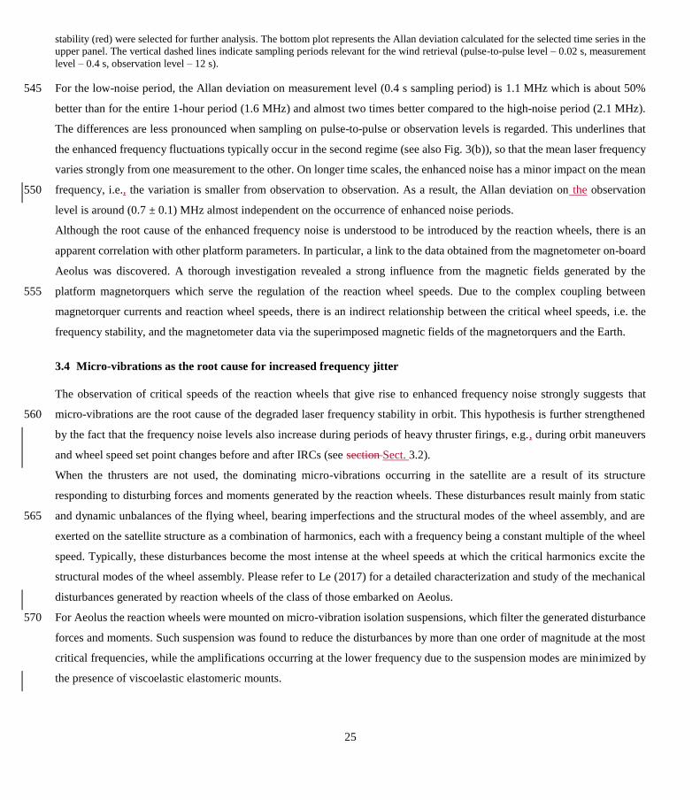
25

stability (red) were selected for further analysis. The bottom plot represents the Allan deviation calculated for the selected time series in the

upper panel. The vertical dashed lines indicate sampling periods relevant for the wind retrieval (pulse-to-pulse level – 0.02 s, measurement

level – 0.4 s, observation level – 12 s).

For the low-noise period, the Allan deviation on measurement level (0.4 s sampling period) is 1.1 MHz which is about 50% 545

better than for the entire 1-hour period (1.6 MHz) and almost two times better compared to the high-noise period (2.1 MHz).

The differences are less pronounced when sampling on pulse-to-pulse or observation levels is regarded. This underlines that

the enhanced frequency fluctuations typically occur in the second regime (see also Fig. 3(b)), so that the mean laser frequency

varies strongly from one measurement to the other. On longer time scales, the enhanced noise has a minor impact on the mean

frequency, i.e., the variation is smaller from observation to observation. As a result, the Allan deviation on the observation 550

level is around (0.7 ± 0.1) MHz almost independent on the occurrence of enhanced noise periods.

Although the root cause of the enhanced frequency noise is understood to be introduced by the reaction wheels, there is an

apparent correlation with other platform parameters. In particular, a link to the data obtained from the magnetometer on-board

Aeolus was discovered. A thorough investigation revealed a strong influence from the magnetic fields generated by the

platform magnetorquers which serve the regulation of the reaction wheel speeds. Due to the complex coupling between 555

magnetorquer currents and reaction wheel speeds, there is an indirect relationship between the critical wheel speeds, i.e. the

frequency stability, and the magnetometer data via the superimposed magnetic fields of the magnetorquers and the Earth.

3.4 Micro-vibrations as the root cause for increased frequency jitter

The observation of critical speeds of the reaction wheels that give rise to enhanced frequency noise strongly suggests that

micro-vibrations are the root cause of the degraded laser frequency stability in orbit. This hypothesis is further strengthened 560

by the fact that the frequency noise levels also increase during periods of heavy thruster firings, e.g., during orbit maneuvers

and wheel speed set point changes before and after IRCs (see section Sect. 3.2).

When the thrusters are not used, the dominating micro-vibrations occurring in the satellite are a result of its structure

responding to disturbing forces and moments generated by the reaction wheels. These disturbances result mainly from static

and dynamic unbalances of the flying wheel, bearing imperfections and the structural modes of the wheel assembly, and are 565

exerted on the satellite structure as a combination of harmonics, each with a frequency being a constant multiple of the wheel

speed. Typically, these disturbances become the most intense at the wheel speeds at which the critical harmonics excite the

structural modes of the wheel assembly. Please refer to Le (2017) for a detailed characterization and study of the mechanical

disturbances generated by reaction wheels of the class of those embarked on Aeolus.

For Aeolus the reaction wheels were mounted on micro-vibration isolation suspensions, which filter the generated disturbance 570

forces and moments. Such suspension was found to reduce the disturbances by more than one order of magnitude at the most

critical frequencies, while the amplifications occurring at the lower frequency due to the suspension modes are minimized by

the presence of viscoelastic elastomeric mounts.

26

The on-ground micro-vibration verification activities were quite extensive within the Aeolus project. These included disturbing

the laser transmitter with representative mechanical excitation spectra, thus identifying susceptibility which allowed 575

identifying particularly susceptible in the 400 Hz to 600 Hz frequency band, as well as around 250 Hz. Moreover, micro-

vibration tests were performed at satellite-level. First, with the aim of characterizing the micro-vibration environment

throughout the satellite, which was achieved by operating the reaction wheels all over their operational speed range, and having

the satellite mounted on doughnut-shaped cushions for isolating it from external disturbances (Lecrenier et al., 2015). These

tests demonstrated that, despite the fact that the peak of disturbances from the reaction wheels coincided with the most 580

susceptible frequencies of the lasers, the vibration levels were lower than the danger-levels previously established to them,

thanks to the isolation suspension. The margins observed between the micro-vibration levels measured during the full-satellite

test and the danger-levels characterized during the preceding laser tests were considered large enough to cover for the

mechanical changes that occur when passing from the ground to the orbital environment. Due to the different support boundary

conditions of the satellite and the effects of gravity and air, the structural damping and natural frequencies of the satellite 585

structure are expected to differ on-orbit from their characterization on-ground. Moreover, a worsening of the disturbance

signature of the reaction wheels as a result of their exposure to the vibrations of the satellite-level tests and the launch

environment is also commonly observed.

These margins were finally confirmed by an in-situ test during the thermal vacuum campaign with the flight model of the

spacecraft. This included operation of the laser whilst the wheels were running at speeds previously identified as critical and 590

after wheel power off. The Mie and Rayleigh frequency response data from these tests clearly showed significant peaks at

several harmonic frequencies (roughly 4.5, 10, 13, 16, 18.5, 21.5, 23, 24, 24.5 RPS) when the wheels were operating. In fact,

the shot-to-shot performance varied along the thermal plateau stronger than during the dedicated reaction wheel test.

Unfortunately, due to programmatic constraints, no tests were ever run with the spacecraft mounted in an isolated configuration

from the ground and with flight-representative time-varying speed profiles whilst operating the laser to check its frequency 595

stability.

4 Impact of the frequency fluctuations on the data quality

After having identified the root cause of the temporally degraded frequency stability in orbit, the question is to what extent the

Aeolus wind data quality is diminished during the periods of enhanced frequency noise. Before answering this question, it is

meaningful to consider how often these periods occur and how long they last. For this purpose, the percentage of observations 600

for which the frequency stability is significantly worse in comparison to the overall performance over a certain period can be

regarded. This information is summarized in Table 4 for the five selected weeks of the mission that were already introduced

in section Sect. 2.4 as being representative for different periods of the Aeolus mission.

27

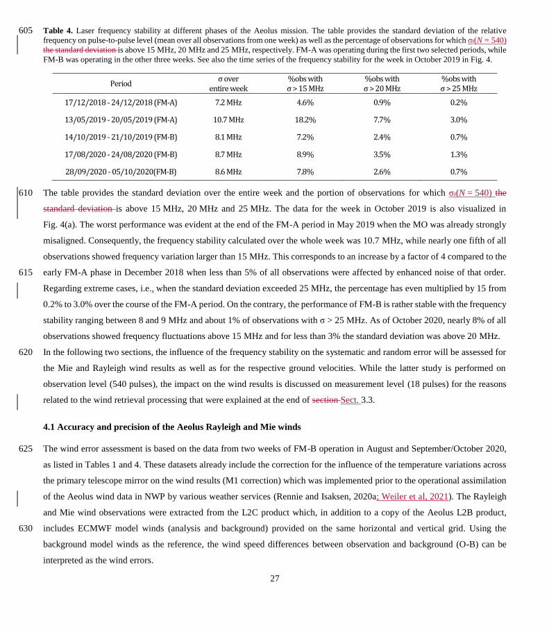
Table 4. Laser frequency stability at different phases of the Aeolus mission. The table provides the standard deviation of the relative 605 frequency on pulse-to-pulse level (mean over all observations from one week) as well as the percentage of observations for which σf(N = 540)

the standard deviation is above 15 MHz, 20 MHz and 25 MHz, respectively. FM-A was operating during the first two selected periods, while

FM-B was operating in the other three weeks. See also the time series of the frequency stability for the week in October 2019 in Fig. 4.

Period σ over

entire week %obs with σ > 15 MHz

%obs with σ > 20 MHz

%obs with σ > 25 MHz

17/12/2018 - 24/12/2018 (FM-A) 7.2 MHz 4.6% 0.9% 0.2%

13/05/2019 - 20/05/2019 (FM-A) 10.7 MHz 18.2% 7.7% 3.0%

14/10/2019 - 21/10/2019 (FM-B) 8.1 MHz 7.2% 2.4% 0.7%

17/08/2020 - 24/08/2020 (FM-B) 8.7 MHz 8.9% 3.5% 1.3%

28/09/2020 - 05/10/2020(FM-B) 8.6 MHz 7.8% 2.6% 0.7%

The table provides the standard deviation over the entire week and the portion of observations for which σf(N = 540) the 610

standard deviation is above 15 MHz, 20 MHz and 25 MHz. The data for the week in October 2019 is also visualized in

Fig. 4(a). The worst performance was evident at the end of the FM-A period in May 2019 when the MO was already strongly

misaligned. Consequently, the frequency stability calculated over the whole week was 10.7 MHz, while nearly one fifth of all

observations showed frequency variation larger than 15 MHz. This corresponds to an increase by a factor of 4 compared to the

early FM-A phase in December 2018 when less than 5% of all observations were affected by enhanced noise of that order. 615

Regarding extreme cases, i.e., when the standard deviation exceeded 25 MHz, the percentage has even multiplied by 15 from

0.2% to 3.0% over the course of the FM-A period. On the contrary, the performance of FM-B is rather stable with the frequency

stability ranging between 8 and 9 MHz and about 1% of observations with σ > 25 MHz. As of October 2020, nearly 8% of all

observations showed frequency fluctuations above 15 MHz and for less than 3% the standard deviation was above 20 MHz.

In the following two sections, the influence of the frequency stability on the systematic and random error will be assessed for 620

the Mie and Rayleigh wind results as well as for the respective ground velocities. While the latter study is performed on

observation level (540 pulses), the impact on the wind results is discussed on measurement level (18 pulses) for the reasons

related to the wind retrieval processing that were explained at the end of section Sect. 3.3.

4.1 Accuracy and precision of the Aeolus Rayleigh and Mie winds

The wind error assessment is based on the data from two weeks of FM-B operation in August and September/October 2020, 625

as listed in Tables 1 and 4. These datasets already include the correction for the influence of the temperature variations across

the primary telescope mirror on the wind results (M1 correction) which was implemented prior to the operational assimilation

of the Aeolus wind data in NWP by various weather services (Rennie and Isaksen, 2020a; Weiler et al, 2021). The Rayleigh

and Mie wind observations were extracted from the L2C product which, in addition to a copy of the Aeolus L2B product,

includes ECMWF model winds (analysis and background) provided on the same horizontal and vertical grid. Using the 630

background model winds as the reference, the wind speed differences between observation and background (O-B) can be

interpreted as the wind errors.

28

The L2B/C wind data is provided on a different temporal grid as the L1A data which is used for the calculation of the Mie

responses and corresponding frequency fluctuations. This is due to the classification of measurement bins into “clear” and

“cloudy” bins (section Sect. 3.3) which results in so-called groups of varying horizontal length. Consequently, for investigating 635

the influence of the frequency stability on the wind accuracy and precision, an adaptation of the different temporal grids of the

L1A/B and L2B/C products has to be performed. Moreover, it has to be considered that each wind profile measured within a

certain period of time generally comprises multiple wind results from the adjacent vertical bins to be compared with the

respective frequency stability within the regarded time interval. Finally, only reliable wind results with low estimated error

should enter the statistics. The estimated wind error is included in the L2B/C product and, in case of the Rayleigh channel, is 640

derived from the SNR and the pressure and temperature sensitivity of the Rayleigh responses (Rennie et al., 2020). For the

Mie channel, it is primarily linked to the SNR. The estimated error also considers the impact of the solar background on the

wind accuracy, which is mainly relevant for the Rayleigh winds. In the analysis presented here, estimated error thresholds of

8 m∙s-1 for the Rayleigh and 4 m∙s-1 Mie channel were used, as airborne validation campaigns have demonstrated that these

values ensure small departures of the Aeolus winds from high-accuracy wind lidar measurements (Witschas et al., 2020). 645

The results of the statistical analysis for one of the two studied periods is shown in Fig. 12. Here, panel (a) depicts a histogram

of the laser frequency stability on measurement level, i.e., calculated as the standard deviation over 18 pulses within 0.4 s, i.e.,

σf(N = 18). After interpolation of the frequency stability data onto the temporal grid of the Mie wind data, the former could be

filtered for those measurements within the week from 17 to 24 August 2020 that yielded valid Mie winds. From the nearly

350,000 Mie (“cloudy”) wind results, more than 78% were obtained at a frequency stability of better than 10 MHz on 650

measurement level, as indicated by the light blue area in the histogram. Regarding the Rayleigh (“clear”) winds, the percentage

is identical, although the amount of wind data is about 2.8 times larger (≈990,000 winds) compared to the Mie channel due to

its usually larger data coverage. The median of the laser frequency stability is 6.6 MHz for the two data subsets, while the

mean values both account for 8.2 MHz which is comparable to the frequency stability on observation level for the August

2020 period stated in Table 4. Although the frequency stability is comparable for the two different processor time scales when 655

the mean over large datasets is considered, the fluctuations are significantly higher on measurement level (>30 MHz) than on

observation level in rare cases when the peak of a short high-noise period falls within one measurement.

In a next step, the Mie and Rayleigh wind results were separated into those for which the frequency stability was better or

worse than 10 MHz on measurement level. The resulting probability density functions (PDFs) of the (O-B) horizontal line-of-

sight (HLOS) wind speed differences are provided in the middle and right columns of Fig. 12. Due to the much smaller amount 660

of wind results for σ > 10 MHz (≈22%), the distribution is a bit noisier than for σ < 10 MHz. Nevertheless, nearly Gaussian

distributions are evident for the two subsets, both for the Mie and Rayleigh channel. The mean of the Mie distribution, or bias,

of the “high-noise” case is slightly larger [(0.214 ± 0.015) m∙s-1] than that of the “low-noise” case [(0.030 ± 0.008) m∙s-1].

Hence, when only considering winds from the week in August 2020 for which the frequency stability was worse than 10 MHz

on measurement level, the bias differs by about 0.18 m∙s-1 from the mean (O-B) wind difference over all winds for which 665

σ < 10 MHz. When the wind data is further restricted to σ > 20 MHz, the change in bias increases to 0.31 m∙s-1 (not shown).

29

Figure 12. (a) Histogram of the laser frequency stability on measurement level for those measurements that yielded valid Mie winds during

the period from 17 to 24 August 2020 (bin size: 0.2 MHz). The probability density functions of the wind speed difference with respect to

the ECMWF model background (O-B) is shown in panels (b) and (c) for measurements with a frequency stability better and worse than 670 10 MHz, respectively (bin size: 0.2 m∙s-1). The bottom panels depict the corresponding statistics for the Rayleigh wind data.

The widths of the two distributions, however, are identical (standard deviation: 4.21 m∙s-1), showing that the frequency stability

has no significant influence on the random error. The same is true for the Rayleigh winds whose PDFs are depicted in Fig. 12(e)

and (f). Here, the differences in the bias and random error for σ < 10 MHz and σ > 10 MHz are below 0.04 m∙s-1. Thus, it can

be concluded that the accuracy of the Rayleigh winds is less affected by the enhanced frequency noise than that of the Mie 675

winds, and that the influence on the random wind error is negligible for both channels.

The same analysis was performed for the week between 28 September and 5 October 2020 and yielded similar results. Here,

the percentage of Mie and Rayleigh wind results for which the frequency stability on measurement level is better than 10 MHz

is 78.6% and 78.9%, respectively. The Mie bias increases from (0.079 ± 0.008) m∙s-1 for σ < 10 MHz to (0.187 ± 0.016) m∙s-1

for σ > 10 MHz, while the Rayleigh bias differs by only 0.02 m∙s-1. The respective random errors are 4.22 m∙s-1 and 4.28 m∙s-1 680

for the Mie and 7.16 m∙s-1 and 7.17 m∙s-1 for the Rayleigh channel, respectively.

In order to further evaluate the impact of the laser frequency noise on the Aeolus wind data quality, a variable frequency

stability threshold was applied and the bias and random error with respect to the ECMWF model background were calculated

for those winds that were measured during periods with frequency fluctuations below the threshold. The statistical results are

depicted in Fig. 13. The mean Mie and Rayleigh wind bias are plotted in the left column, while the respective random errors 685

for the two investigated weeks in August and September/October 2020 are shown on the right. Both values are presented

relative to the statistical parameters that are obtained for a threshold of 8 MHz, as this allows for a direct comparison of the

two different datasets regardless of the absolute values which differ among the analyzed periods and receiver channels due to

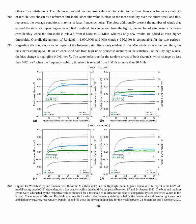
30

other error contributions. The reference bias and random error values are indicated in the round boxes. A frequency stability

of 8 MHz was chosen as a reference threshold, since this value is close to the mean stability over the entire week and thus 690

represents the average conditions in terms of laser frequency noise. The plots additionally present the number of winds that

entered the statistics depending on the applied threshold. As can be seen from the figure, the number of wind results increases

considerably when the threshold is relaxed from 8 MHz to 15 MHz, whereas only few results are added at even higher

thresholds. Overall, the amount of Rayleigh (≈1,000,000) and Mie winds (≈350,000) is comparable for the two periods.

Regarding the bias, a noticeable impact of the frequency stability is only evident for the Mie winds, as seen before. Here, the 695

bias increases by up to 0.05 m∙s-1 when wind data from high-noise periods is included in the statistics. For the Rayleigh winds,

the bias change is negligible (<0.01 m∙s-1). The same holds true for the random errors of both channels which change by less

than 0.02 m∙s-1 when the frequency stability threshold is relaxed from 8 MHz to more than 20 MHz.

Figure 13. Wind bias (a) and random error (b) of the Mie (blue dots) and the Rayleigh channel (green squares) with respect to the ECMWF 700 model background (O-B) depending on a frequency stability threshold for the period between 17 and 24 August 2020. The bias and random

errors were subtracted by the respective values obtained for a threshold of 8 MHz for the sake of comparability (see reference values in the

boxes). The number of Mie and Rayleigh wind results for which the frequency stability is below the threshold are shown in light grey dots

and dark grey squares, respectively. Panels (c) and (d) show the corresponding data for the week between 28 September and 5 October 2020.

31

In conclusion, the temporally degraded frequency stability of the ALADIN laser transmitter has only minor influence on the 705

wind data quality on a global scale. This is primarily due to the small percentage of measurements for which the frequency

fluctuations are considerably enhanced. The biggest impact is observed for the Mie wind bias, which is increased by more than

0.3 m∙s-1 when considering only those phases with strong variations (>20 MHz) on measurement level. However, as these

winds represent only about 4% of all wind results from the studied weeks, the effect is hardly noticeable in the statistics derived

from the entire global dataset. Nevertheless, this study helps to identify an optimal threshold for a quality control (QC) that 710

filters out measurements for which the frequency noise is considerably enhanced. The according QC parameter which describes

the frequency stability in terms of the standard deviation on measurement level is already included in the L1B product.

Since wind observations with enhanced frequency jitter occur over specific geolocations (see Fig. 6), it is interesting to study

whether the wind data is significantly degraded in such affected locations. For this purpose, several areas where one or multiple

critical reaction wheel speeds regularly occur, i.e., in East Asia or Central Africa, were analyzed with regards to the deviations 715

from Aeolus observations from ECMWF model winds (O-B). This preliminary study revealed that, although the percentage

of measurements with frequency stability worse than 15 MHz is increased by a factor of two to three compared to the global

percentage, the change in wind bias and random error is below 0.5 m∙s-1. However, as the number of wind results is drastically

decreased by the restriction to rather small geographical boxes, these results lack statistical significance. Hence, additional

studies using longer periods of wind data are required to verify this small influence on the wind data quality on a local scale. 720

Furthermore, as outlined in the end of section Sect. 2.1, the impact of enhanced frequency noise is most pronounced in cases

when only a small subset of the emitted pulses is detected in the atmospheric path, i.e., in heterogenous atmospheric scenes

(Marksteiner et al., 2015). Therefore, proper extraction of such scenes, e.g., broken cloud conditions, is advisable prior to the

statistical analysis. Nonetheless, the current study has provided a strong hint that the laser frequency stability is not a major

contributor to the systematic and random errors of the Aeolus wind product for the SNR cases analyzed. 725

4.2 Influence on the Rayleigh and Mie ground velocities

In analogy to the approach presented in the previous section, the correlation between the laser frequency stability and the

apparent velocity of the ground returns was investigated. Ground return signals are generally crucial for airborne and

spaceborne radar and lidar systems that rely on the Doppler effect, as they can be exploited for identifying systematic errors

that are, for instance, caused by improper knowledge of the platform attitude or variations in the instrument’s alignment (Bosart 730

et al., 2002; Kavaya et al., 2014; Chouza et al., 2016). For the Aeolus mission, the ground surface could be used as a zero-

wind reference, which allows to estimate unknown wind biases from the measured ground velocities. This method, however,

requires precise differentiation between atmospheric and ground return signals in order to prevent erroneous ground velocities

(also referred to as Zero Wind Calibration or ZWC values), which is particularly challenging due to ALADIN’s coarse vertical

resolution of several hundred meters. The ground detection scheme and its limitations are very similar for ALADIN and the 735

A2D and are explained in detail in Weiler (2017) and Lux et al. (2018).

32

The ground velocities, obtained separately for the Rayleigh and Mie channel, are contained in the AUX_ZWC product which

is generated by the Aeolus L1B processor. The same two weeks in 2020 as in the previous section were studied. However, in

contrast to the wind results, the ground velocities which are part of the L1B baseline 10 data, are not bias corrected using the

M1 telescope mirror temperatures as for the L2B product so that they show rather large deviations from the “ideal value” of 740

0 m∙s-1 (Rayleigh: –18 m∙s-1, Mie: –2 m∙s-1). Hence, the analysis relies on relative changes in the ground velocities depending

on the frequency stability, while the influence of attitude control mis-pointing on this parameter can be neglected. Moreover,

in contrast to the multitude of Rayleigh and Mie wind results which are available from multiple range gates and all over the

globe, ground return signals that are strong enough to be utilized for a potential ZWC of the Aeolus data are rare. Given the

susceptibility to atmospheric contamination, i.e., the detrimental impact of the broadband atmospheric backscatter return signal 745

on the narrowband ground return signal, only ground velocities that were measured from surfaces with high albedo in the UV

spectral range are considered valid, which drastically limits the number of available ZWC values. The useful signal thresholds

applied in the L1B processor are 1000 ACCD counts and 1200 ACCD counts for the Mie and Rayleigh channel, respectively.

For this reason, the ZWC data from the two weeks were combined in order to obtain meaningful statistics. Since only data

from high-albedo regions, i.e., Antarctica, Arctic, sea ice as well as snow covered land areas, entered the statistics, solely the 750

frequency stability over these locations plays a role in the analysis. Here, the precision of the ground returns is impaired by

blowing snow that leads to a narrowband Mie return with a potentially non-vanishing Doppler shift, thus acting as another

source of random errors on the ground returns. Since the ice coverage was comparable in the two weeks in 2020, the studied

locations and thus the influence of the wheel speeds on the respective frequency fluctuations was similar for the individual

periods that contributed nearly the same amount of ground velocity values (≈4000) to the combined dataset. Note also that the 755

ZWC data is provided only on observation level (12 s = 540 pulses), as there is no differentiation between “clear” and cloudy”

bins. Consequently, the ground velocities are correlated with the laser frequency variations on observation level.

Analogous In analogy to Fig. 12(a) and (d), histograms of the laser frequency stability on observation level are depicted in

Fig. 14(a) and (c) for those observations that yielded valid Mie and Rayleigh ground velocities, respectively. The number of

ZWC values is very similar for the two channels (≈4000), suggesting that almost the same observations, i.e., geographical 760

locations, were considered in the statistical analysis. This also explains the agreement of the median and mean frequency

stability on observation level which account for 7.3 MHz and 8.7 MHz, respectively. The fact that these values are slightly

higher than those on measurement level presented in the previous section is most likely due to the restriction to polar regions

where critical wheel speeds are overrepresented (see Fig. 9). The influence of the frequency noise on the Mie and Rayleigh

ground velocities is displayed in Fig. 14(b) and (d) where the respective mean ground velocities are plotted against the 765

frequency stability which was subdivided into bins of 1 MHz. Here, a data point plotted versus a frequency stability of k MHz

represents the mean over those ground velocities that fall in the interval between (k – 1) MHz and k MHz. The velocities were

subtracted by the mean over all ZWC values for which the frequency stability is better than 8 MHz to exclude the large bias

contributions that are different for the two receiver channels. The error bar represents the corresponding standard deviation per

bin. In addition, the number of ground velocities per interval that entered the statistics is plotted in grey. 770

33

Figure 14. Histograms of the laser frequency stability on observation level for those observations that yielded valid Mie ground returns

during the combined periods from 17 to 24 August 2020 and from 28 September to 5 October 2020. (b) Mean Mie ground velocity in

dependence on the frequency stability. The ground velocities were subtracted by the mean over all values for which the frequency stability

is better than 8 MHz for the sake of comparability. A data point plotted versus a frequency stability of k represents the mean over all ground 775 velocities for which the stability is in the interval between (k – 1) MHz and k MHz, while the error bar represents the corresponding standard

deviation. The number of ground velocity values within each interval is shown in grey. The bottom panels (c) and (d) depict the corresponding

statistics for the Rayleigh ground returns.

Like for the wind results, the number of ZWC values strongly decreases when considering only those observations for which

the frequency stability is considerably degraded. The portion of ground velocities with frequency stability worse than 15 MHz 780

is as low as 8.2% for both channels. In accordance with the findings in section Sect. 4.1, there is no significant influence of

the enhanced frequency noise on the Rayleigh channel, whereas the determined Mie ground velocities change almost linearly

with the frequency stability. When regarding only observations with 29 MHz <σ < 30 MHz (rightmost dot in Fig. 14(b)), the

ground velocity is about 2.1 m∙s-1 higher than for those observations with 5 MHz <σ < 6 MHz. However, it should also be

noted that only nine ZWC values contributed to this last data point, resulting in large uncertainty (standard deviation: 1.7 m∙s-785

1) and thus small statistical significance.

The mean ZWC values are additionally calculated for a varying frequency stability threshold, analogous in analogy to Fig. 13,

in order to consider the different weighting of the observations with low and high frequency noise. The results are plotted in

Fig. 15 for the Mie and Rayleigh channel, both for the mean and the standard deviation of the ground velocities of the respective

data subset after applying the threshold. Here, a similarly weak dependency is evident for the Mie and Rayleigh channels 790

where the mean ZWC values (relative to the 8 MHz threshold) increase to 0.15 m∙s-1 as the threshold is relaxed to 30 MHz.

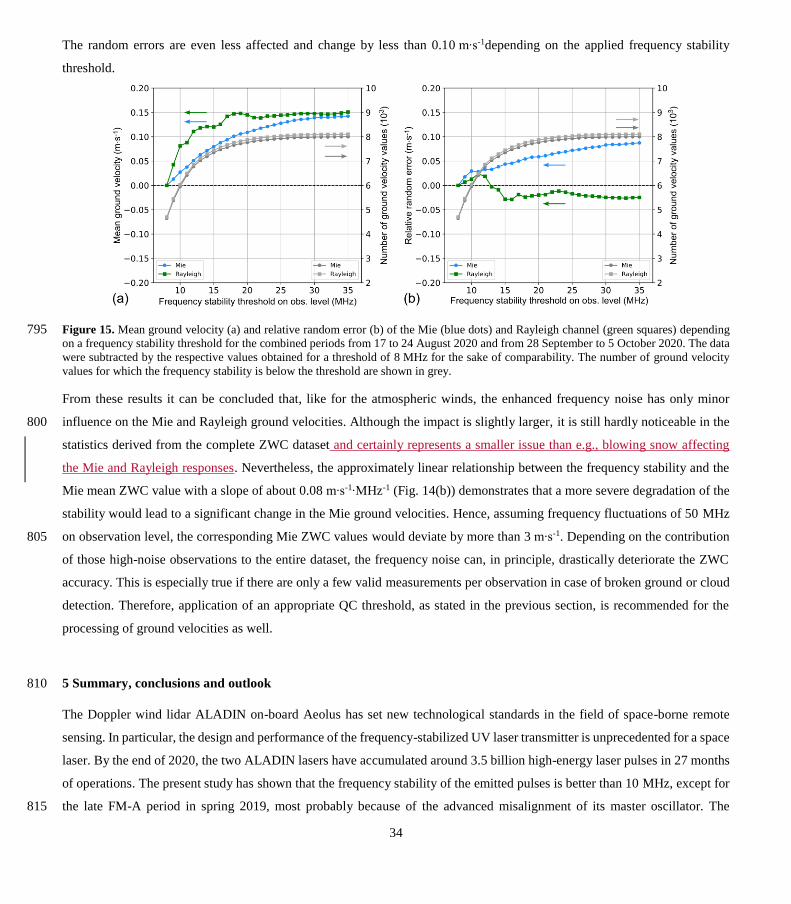
34

The random errors are even less affected and change by less than 0.10 m∙s-1depending on the applied frequency stability

threshold.

Figure 15. Mean ground velocity (a) and relative random error (b) of the Mie (blue dots) and Rayleigh channel (green squares) depending 795 on a frequency stability threshold for the combined periods from 17 to 24 August 2020 and from 28 September to 5 October 2020. The data

were subtracted by the respective values obtained for a threshold of 8 MHz for the sake of comparability. The number of ground velocity

values for which the frequency stability is below the threshold are shown in grey.

From these results it can be concluded that, like for the atmospheric winds, the enhanced frequency noise has only minor

influence on the Mie and Rayleigh ground velocities. Although the impact is slightly larger, it is still hardly noticeable in the 800

statistics derived from the complete ZWC dataset and certainly represents a smaller issue than e.g., blowing snow affecting

the Mie and Rayleigh responses. Nevertheless, the approximately linear relationship between the frequency stability and the

Mie mean ZWC value with a slope of about 0.08 m∙s-1∙MHz-1 (Fig. 14(b)) demonstrates that a more severe degradation of the

stability would lead to a significant change in the Mie ground velocities. Hence, assuming frequency fluctuations of 50 MHz

on observation level, the corresponding Mie ZWC values would deviate by more than 3 m∙s-1. Depending on the contribution 805

of those high-noise observations to the entire dataset, the frequency noise can, in principle, drastically deteriorate the ZWC

accuracy. This is especially true if there are only a few valid measurements per observation in case of broken ground or cloud

detection. Therefore, application of an appropriate QC threshold, as stated in the previous section, is recommended for the

processing of ground velocities as well.

5 Summary, conclusions and outlook 810

The Doppler wind lidar ALADIN on-board Aeolus has set new technological standards in the field of space-borne remote

sensing. In particular, the design and performance of the frequency-stabilized UV laser transmitter is unprecedented for a space

laser. By the end of 2020, the two ALADIN lasers have accumulated around 3.5 billion high-energy laser pulses in 27 months

of operations. The present study has shown that the frequency stability of the emitted pulses is better than 10 MHz, except for

the late FM-A period in spring 2019, most probably because of the advanced misalignment of its master oscillator. The 815

35

excellent stability is achieved despite the permanent occurrence of short periods during which the frequency fluctuations are

considerably enhanced to 30 MHz RMS on observation level (12 s), 50 MHz RMS on measurement level (0.4 s) and even

pulse-to-pulse variations of up to 150 MHz peak-to-peak.

The investigation of the frequency stability during instrument response calibrations has revealed that it depends on the

geolocation of the satellite. Consequently, the correlation between frequency stability and geolocation could be traced back in 820

a clustering of observations with enhanced frequency variations in specific regions of the Earth, forming linear and circular

structures around the globe. The patterns differ for ascending and descending orbits and the two flight-model lasers, but are

stable over the mission life-time.

The underlying reason for the dependency on geolocation is the existence of critical rotation speeds of the satellite’s reaction

wheels, which suggests that micro-vibrations are the root cause for the deterioration of the laser stability on time scales of a 825

few tens of seconds. This hypothesis is supported by the fact that the laser stability is also degraded during thruster firings of

the satellite which introduce high vibration levels also at the location of the power laser head. The identified detrimental

frequencies of the reaction wheels range between 14 RPS and 28 RPS and are consistent among the three active wheels,

although the relative impact on the two lasers is different. Owing to the dependency of the reaction wheel speeds on the

magnetorquer control authority and the strong influence of the latter on the magnetometer readings, there is an indirect link, 830

and hence decent correlation, between the frequency stability and the magnetic field measured by the on-board magnetometer.

In the context of the enhanced frequency noise, the Aeolus wind error with respect to ECMWF model background winds was

studied, pointing out that the temporally degraded stability of the ALADIN laser transmitter has only minor influence on the

global wind data quality. For two studied weeks in 2020, the Mie wind bias is increased by 0.3 m∙s-1 during phases with strong

variations (> 20 MHz) on measurement level. Considering the small portion of such wind measurements (≈4%) during a repeat 835

cycle of one week, the influence on the accuracy of the Mie winds acquired over the entire globe is well below 0.1 m∙s-1.

However, a more noticeable contribution of the high frequency noise to the Mie wind bias is expected in regions where the

reaction wheels are run at the critical speeds, although further studies are necessary for verification. The Rayleigh wind results

are hardly affected, most likely because other noise contributors dominate, such as photon shot noise and fluctuations of the

incidence angle on the spectrometers. Concerning the ground velocities which are only collected in areas with high surface 840

albedo, a similarly small impact of the laser frequency stability was determined. The mean ground-return velocity derived

from the Mie spectrometer changes linearly with the frequency stability on observation level by about 0.08 m∙s-1∙MHz-1,

whereas the Rayleigh ground velocities are nearly independent of the frequency noise over the investigated range.

Despite the small effect on the wind data, application of a QC in the Aeolus processor could be foreseen for the Mie winds to

filter out measurements during which the frequency stability is worse than 20 MHz. The same threshold is suggested for the 845

processing of the Mie and Rayleigh ground velocities, as this will slightly improve the accuracy of the ground velocity values

while their number is not considerably reduced. These QC approaches become more important in case the atmospheric return

SNR is further decreasing within the mission lifetime, as this will increase the share of Mie wind results among the overall

Aeolus wind observations. For the Rayleigh winds, a QC based on the frequency stability is not considered useful, since the

36

error is largely dominated by shot noise. Hence, the discarding of any measurements, even with poor frequency stability, will 850

rather diminish the Rayleigh wind precision given that it is primarily limited by shot noise.

Concerning the use of Aeolus data on smaller geographical scales, e.g., for its validation by on-ground or airborne instruments,

the geolocational dependence of the laser frequency stability should be considered. In rRegions where the reactions wheels

repeatedly rotate at their critical frequencies suffer from enhanced frequency noise during every overpass along Aeolus’

ascending or descending orbit. Consequently, the percentage of wind observations with degraded stability is considerably 855

higher than on a global scale and is expected to have a stronger impact on the wind accuracy, especially for the Mie channel.

With a view to future space lidar missions, particularly those which have strict requirements in terms of the laser frequency

stability like EarthCARE, ACDL, MERLIN or Aeolus follow-on missions, several lessons learnt are derived from the current

study: First, the cavity control scheme of the laser transmitter plays an important role to ensure a sufficiently short dead time

of the feedback loop, and in turn, to filter out vibration frequencies of several hundreds of Hz which potentially deteriorate the 860

laser stability. A modified ramp-delay-fire technique that was developed for the A2D (Lemmerz et al., 2017) allows for fast

responses in the microsecond-regime, thus providing high frequency stability (<4 MHz RMS) even in harsh vibration

environments. Referencing on a pulse-by-pulse basis, as performed in other wind lidar instruments (Baidar et al., 2018; Tucker

et al., 2018; Bruneau and Pelon, 2021), would relax the requirements in terms of frequency stability. This could, for instance,

be realized with avalanche photodiodes (APDs) working in real counting mode. There are studies ongoing with APDs in 865

analogue mode offering very low dark noise. However, in the current state of development, the SNR obtained with these APDs

is still too poor to determine the frequency from atmospheric backscatter of single pulses, so that signal accumulation is

expected to be necessary for most future space (wind) lidar missions.

Second, although the on-ground micro-vibration tests led to the important implementation of isolation suspensions which

effectively attenuated the micro-vibration levels by about one order of magnitude, the tests did not clearly reveal the existence 870

of the critical reaction wheel speeds which would affect performance in a measurable way. This is mainly due to the too short

operation of the wheels at their critical speeds which did not allow for sufficient statistics of the acquired laser data depending

on wheel speed. Therefore, extended tests with the spacecraft mounted in an isolated configuration and with flight-

representative time-varying reaction wheel speeds whilst operating the laser are recommended. Moreover, it is proposed to use

an appropriate number of accelerometers at different locations of the laser bench during such tests to properly characterize the 875

impact of micro-vibrations on the laser behavior, particularly the frequency stability. Finally, a higher temporal resolution of

the laser housekeeping telemetry data than currently available for Aeolus (0.25 Hz) with a focus on cavity control parameters

is advisable to better evaluate the laser performance both on-ground and in space.

Furthermore, it is considered that the installation of accelerometers in the instrument flight model and the acquisition of micro-

vibration measurements in orbit, even resulting in modest amounts of data, is extremely beneficial. These not only will allow 880

a more definitive identification of the spacecraft elements responsible for deviations scientific measurements, but will also

provide a reference for correlation of mechanical models representing orbital conditions.

37

Passive suspensions provide a well-proven solution for the mitigation of micro-vibrations generated by reaction wheels in

orbit. With their simple configuration, they have low mass, consume no electrical power and require no computational

resources. However, inherently to their mechanical architecture, they produce a non-negligible amplification of the 885

disturbances at the frequencies of the suspension modes. Also, extreme isolation at high-frequencies, which can be required

by some applications, is often compromised by the presence of spurious mechanical modes whose effects in orbit are difficult

to predict. As an alternative, active closed-loop vibration isolation systems based on sensing and counteracting the mechanical

disturbances arising in the spacecraft show a great promise in overcoming the limitations of passive systems. These can be

implemented at the level of both the source (Preda et al., 2018) and/or the payload (Sanfedino et al., 2020) and can significantly 890

mitigate the micro-vibration environment in Aeolus follow-on and other future space lidar missions.

Data availability. The presented work includes preliminary data (not fully calibrated/validated and not yet publicly released)

of the Aeolus mission that is part of the European Space Agency (ESA) Earth Explorer Programme. This includes wind

products from before the public data release in May 2020 and/or aerosol and cloud products, which have not yet been publicly 895

released. The preliminary Aeolus wind products will be reprocessed during 2020 and 2021, which will include in particular a

significant L2B product wind bias reduction and improved L2A radiometric calibration. Aerosol and cloud products will

become publicly available by spring 2021. The processor development, improvement and product reprocessing preparation

are performed by the Aeolus DISC (Data, Innovation and Science Cluster), which involves DLR, DoRIT, ECMWF, KNMI,

CNRS, S&T, ABB and Serco, in close cooperation with the Aeolus PDGS (Payload Data Ground Segment). The analysis has 900

been performed in the frame of the Aeolus Data Innovation and Science Cluster (Aeolus DISC). The raw Mie channel data

used for the assessment of the laser frequency stability is included in the Aeolus L1A product which was provided from the

Aeolus Online Dissemination Service ADDF. The housekeeping telemetry data were obtained from the Aeolus MUST tool

which is accessible for members of the Aeolus Data Science and Innovation Cluster (DISC). Aeolus L2B and ECMWF model

winds were extracted from the L2C product which is available from the tool VirES for Aeolus (https://aeolus.services/). The 905

ground velocity data is part of the reprocessed Aeolus AUX_ZWC product and will become publicly available in 2021.

Competing interests. The authors declare that they have no conflict of interest.

Author contribution. OL analyzed the ALADIN laser frequency stability, its correlation with the reaction wheel speeds and its 910

impact on the Aeolus wind data quality. CL, FW, TK, DW and OR supported the data analysis and interpretation of the results.

GR and AH studied the platform parameters related to the Aeolus attitude and orbit control system. GR investigated the results

from the on-ground micro-vibrations tests with regards the in-orbit instrument performance. OLe, PM and FF were involved

in the on-ground micro-vibration tests of the ALADIN instrument and provided insight to the test procedure and findings at

that time. PB provided information of the ALADIN MO cavity control scheme. TP is the Aeolus Mission Manager. OR is 915

scientific coordinator of the Aeolus DISC. The paper was written by OL with contributions from all co-authors.

38

Acknowledgements. The Doppler wind lidar ALADIN was built by Airbus SAS in Toulouse, France, the satellite by Airbus

Ltd in Stevenage, UK, and the laser transmitters by Leonardo S.p.A. in Florence and Pomezia, Italy. The authors acknowledge

Anne Grete Straume (Aeolus Mission Scientist) and Jonas von Bismarck (Aeolus Data Quality Manager) as well as the Aeolus 920

Mission Advisory Group, the Aeolus Space and Ground Segment Operations teams and the Aeolus DISC for their invaluable

contributions. The authors are also grateful for the insightful discussions with colleagues from ESA’s SWARM mission,

particularly Nils Olsen, Anja Strømme, Rune Floberghagen, Laurent Maleville and Jerome Bouffard, regarding the interaction

between the reaction wheels, magnetorquers and magnetometers on-board Aeolus which helped to rule out a direct influence

of the Earth magnetic field on the laser frequency stability. The first author was partly funded by a young scientist grant by 925

ESA within the DRAGON 4 program (contract no. 4000121191/17/I-NB).

References

Abich, K., Abramovici, A., Amparan, B., Baatzsch, A., Okihiro, B. B., Barr, D. C., Bize, M. P., Bogan, C., Braxmaier, C.,

Burke, M. J., Clark, K. C., Dahl, C., Dahl, K., Danzmann, K., Davis, M. A., Vine, G. de, Dickson, J. A., Dubovitsky, S.,

Eckardt, A., Ester, T., Barranco, G. F., Flatscher, R., Flechtner, F., Folkner, W. M., Francis, S., Gilbert, M. S., Gilles, F., 930

Gohlke, M., Grossard, N., Guenther, B., Hager, P., Hauden, J., Heine, F., Heinzel, G., Herding, M., Hinz, M., Howell, J.,

Katsumura, M., Kaufer, M., Klipstein, W., Koch, A., Kruger, M., Larsen, K., Lebeda, A., Lebeda, A., Leikert, T., Liebe,

C. C., Liu, J., Lobmeyer, L., Mahrdt, C., Mangoldt, T., McKenzie, K., Misfeldt, M., Morton, P. R., Müller, V., Murray, A.

T., Nguyen, D. J., Nicklaus, K., Pierce, R., Ravich, J. A., Reavis, G., Reiche, J., Sanjuan, J., Schütze, D., Seiter, C.,

Shaddock, D., Sheard, B., Sileo, M., Spero, R., Spiers, G., Stede, G., Stephens, M., Sutton, A., Trinh, J., Voss, K., Wang, 935

D., Wang, R. T., Ware, B., Wegener, H., Windisch, S., Woodruff, C., Zender, B., and Zimmermann, M.: In-Orbit

Performance of the GRACE Follow-on Laser Ranging Interferometer, Physical Review Letters, 123, 31101,

https://doi.org/10.1103/PhysRevLett.123.031101, 2019.

Abshire, J. B., Sun, X., Riris, H., Sirota, J. M., McGarry, J. F., Palm, S., Yi, D., and Liiva, P.: Geoscience Laser Altimeter

System (GLAS) on the ICESat Mission: On-orbit measurement performance, Geophys. Res. Lett., 32, 405, 940

https://doi.org/10.1029/2005GL024028, 2005.

Allan, D. W.: Statistics of atomic frequency standards, Proc. IEEE, 54, 221–230, https://doi.org/10.1109/PROC.1966.4634,

1966.

Andersson, E.: Statement of Guidance for Global Numerical Weather Prediction (NWP), World Meteorological Organisation,

2018, https://www.wmo.int/pages/prog/www/OSY/SOG/SoG-Global-NWP.pdf (accessed on 23 July 2019) 945

Baker, W. E., Atlas, R., Cardinali, C., Clement, A., Emmitt, G. D., Gentry, B. M., Hardesty, R. M., Källén, E., Kavaya, M. J.,

Langland, R., Ma, Z., Masutani, M., McCarty, W., Pierce, R. B., Pu, Z., Riishojgaard, L. P., Ryan, J., Tucker, S.,

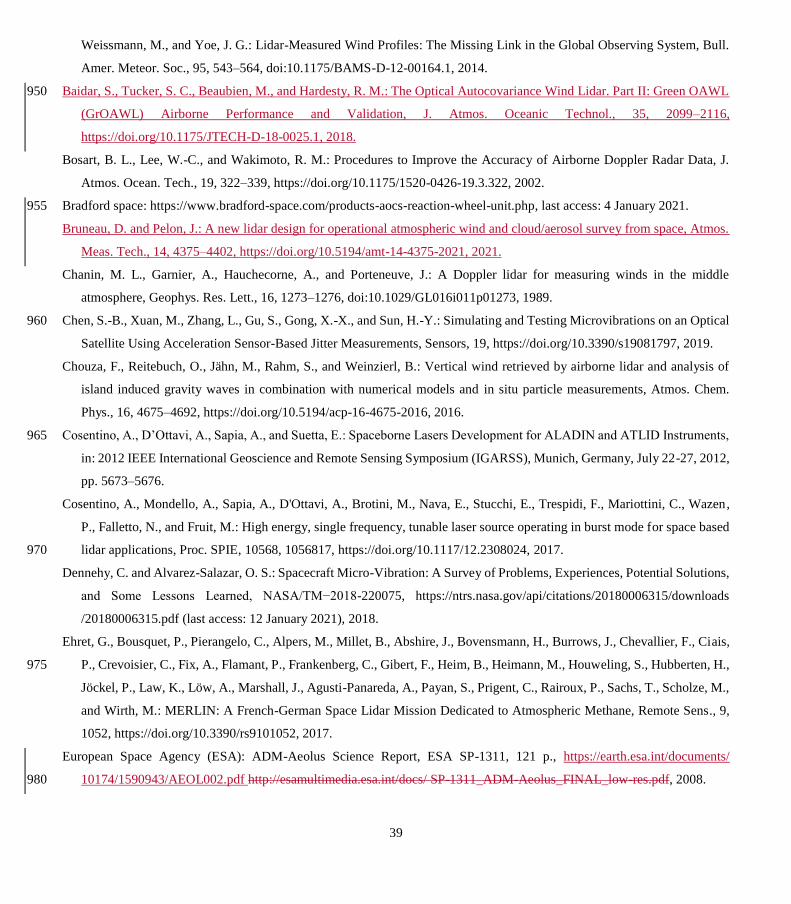
39

Weissmann, M., and Yoe, J. G.: Lidar-Measured Wind Profiles: The Missing Link in the Global Observing System, Bull.

Amer. Meteor. Soc., 95, 543–564, doi:10.1175/BAMS-D-12-00164.1, 2014.

Baidar, S., Tucker, S. C., Beaubien, M., and Hardesty, R. M.: The Optical Autocovariance Wind Lidar. Part II: Green OAWL 950

(GrOAWL) Airborne Performance and Validation, J. Atmos. Oceanic Technol., 35, 2099–2116,

https://doi.org/10.1175/JTECH-D-18-0025.1, 2018.

Bosart, B. L., Lee, W.-C., and Wakimoto, R. M.: Procedures to Improve the Accuracy of Airborne Doppler Radar Data, J.

Atmos. Ocean. Tech., 19, 322–339, https://doi.org/10.1175/1520-0426-19.3.322, 2002.

Bradford space: https://www.bradford-space.com/products-aocs-reaction-wheel-unit.php, last access: 4 January 2021. 955

Bruneau, D. and Pelon, J.: A new lidar design for operational atmospheric wind and cloud/aerosol survey from space, Atmos.

Meas. Tech., 14, 4375–4402, https://doi.org/10.5194/amt-14-4375-2021, 2021.

Chanin, M. L., Garnier, A., Hauchecorne, A., and Porteneuve, J.: A Doppler lidar for measuring winds in the middle

atmosphere, Geophys. Res. Lett., 16, 1273–1276, doi:10.1029/GL016i011p01273, 1989.

Chen, S.-B., Xuan, M., Zhang, L., Gu, S., Gong, X.-X., and Sun, H.-Y.: Simulating and Testing Microvibrations on an Optical 960

Satellite Using Acceleration Sensor-Based Jitter Measurements, Sensors, 19, https://doi.org/10.3390/s19081797, 2019.

Chouza, F., Reitebuch, O., Jähn, M., Rahm, S., and Weinzierl, B.: Vertical wind retrieved by airborne lidar and analysis of

island induced gravity waves in combination with numerical models and in situ particle measurements, Atmos. Chem.

Phys., 16, 4675–4692, https://doi.org/10.5194/acp-16-4675-2016, 2016.

Cosentino, A., D’Ottavi, A., Sapia, A., and Suetta, E.: Spaceborne Lasers Development for ALADIN and ATLID Instruments, 965

in: 2012 IEEE International Geoscience and Remote Sensing Symposium (IGARSS), Munich, Germany, July 22-27, 2012,

pp. 5673–5676.

Cosentino, A., Mondello, A., Sapia, A., D'Ottavi, A., Brotini, M., Nava, E., Stucchi, E., Trespidi, F., Mariottini, C., Wazen,

P., Falletto, N., and Fruit, M.: High energy, single frequency, tunable laser source operating in burst mode for space based

lidar applications, Proc. SPIE, 10568, 1056817, https://doi.org/10.1117/12.2308024, 2017. 970

Dennehy, C. and Alvarez-Salazar, O. S.: Spacecraft Micro-Vibration: A Survey of Problems, Experiences, Potential Solutions,

and Some Lessons Learned, NASA/TM−2018-220075, https://ntrs.nasa.gov/api/citations/20180006315/downloads

/20180006315.pdf (last access: 12 January 2021), 2018.

Ehret, G., Bousquet, P., Pierangelo, C., Alpers, M., Millet, B., Abshire, J., Bovensmann, H., Burrows, J., Chevallier, F., Ciais,

P., Crevoisier, C., Fix, A., Flamant, P., Frankenberg, C., Gibert, F., Heim, B., Heimann, M., Houweling, S., Hubberten, H., 975

Jöckel, P., Law, K., Löw, A., Marshall, J., Agusti-Panareda, A., Payan, S., Prigent, C., Rairoux, P., Sachs, T., Scholze, M.,

and Wirth, M.: MERLIN: A French-German Space Lidar Mission Dedicated to Atmospheric Methane, Remote Sens., 9,

1052, https://doi.org/10.3390/rs9101052, 2017.

European Space Agency (ESA): ADM-Aeolus Science Report, ESA SP-1311, 121 p., https://earth.esa.int/documents/

10174/1590943/AEOL002.pdf http://esamultimedia.esa.int/docs/ SP-1311_ADM-Aeolus_FINAL_low-res.pdf, 2008. 980

40

European Space Agency (ESA): “ADM-Aeolus Mission Requirements Document”, ESA EOP-SM/2047, 57 p.,

https://earth.esa.int/eogateway/documents/20142/1564626/Aeolus-Mission-

Requirements.pdfhttp://esamultimedia.esa.int/docs/EarthObservation/ADM-Aeolus_MRD.pdf, 2016.

Flesia, C. and Korb, C. L.: Theory of the double-edge molecular technique for Doppler lidar wind measurement, Appl. Opt.,

38, 432, doi:10.1364/AO.38.000432, 1999. 985

Garnier, A. and Chanin, M. L.: Description of a Doppler Rayleigh LIDAR for measuring winds in the middle atmosphere,

Appl. Phys. B, 55, 35–40, doi:10.1007/BF00348610, 1992.

Henderson, S. W., Yuen, E. H., and Fry, E. S.: Fast resonance-detection technique for single-frequency operation of injection-

seeded Nd:YAG lasers, Optics Letters, 11, 715–717, https://doi.org/10.1364/OL.11.000715, 1986.

Hovis, F. E., Edelman, J., Schum, T., Rudd, J., and Andes, K.: Recent progress on single frequency lasers for space and high 990

altitude aircraft applications, Proc. SPIE, 6871, 68710E, https://doi.org/10.1117/12.768278, 2008.

Illingworth, A. J., Barker, H. W., Beljaars, A., Ceccaldi, M., Chepfer, H., Clerbaux, N., Cole, J., Delanoë, J., Domenech, C.,

Donovan, D. P., Fukuda, S., Hirakata, M., Hogan, R. J., Huenerbein, A., Kollias, P., Kubota, T., Nakajima, T., Nakajima,

T. Y., Nishizawa, T., Ohno, Y., Okamoto, H., Oki, R., Sato, K., Satoh, M., Shephard, M. W., Velázquez-Blázquez, A.,

Wandinger, U., Wehr, T., and van Zadelhoff, G.-J.: The EarthCARE Satellite: The Next Step Forward in Global 995

Measurements of Clouds, Aerosols, Precipitation, and Radiation, Bull. Amer. Meteor. Soc., 96, 1311–1332,

https://doi.org/10.1175/BAMS-D-12-00227.1, 2015.

Kanitz, T., Lochard, J., Marshall, J., McGoldrick, P., Lecrenier, O., Bravetti, P., Reitebuch, O., Rennie, M., Wernham, D., and

Elfving, A.: Aeolus First Light – First Glimpse, Proc. SPIE, 11180, 111801R, doi: 10.1117/12.2535982, 2019.

Kanitz, T., Witschas, B., Marksteiner, U., Flament, T., Rennie, M., Schillinger, M., Parrinello, T., Wernham, D., and 1000

Reitebuch, O.: ESA’s Wind Lidar Mission Aeolus: Instrument Performance and Stability, EGU General Assembly 2020,

Online, 4–8 May 2020, EGU2020-7146, https://doi.org/10.5194/egusphere-egu2020-7146, 2020.

Kavaya, M. J., Beyon, J. Y., Koch, G. J., Petros, M., Petzar, P. J., Singh, U. N., Trieu, B. C., and Yu, J.: The Doppler Aerosol

Wind (DAWN) Airborne, Wind-Profiling Coherent-Detection Lidar System: Overview and Preliminary Flight Results, J.

Atmos. Ocean. Tech., 31, 826–842, 2014 1005

Le, M. P.: Micro-disturbances in reaction wheels, PhD thesis, Technische Universiteit Eindhoven, 166 pp., available at:

https://research.tue.nl/en/publications/micro-disturbances-in-reaction-wheels (last access: 29 December 2020), 2017.

Lecrenier, O., Fabre, F., and Lochard, J.: The ALADIN instrument and its on-ground characterization, ADM-Aeolus Science

and Cal/Val Workshop 2015, Frascati, Italy, 10–13 February 2015, https://earth.esa.int/documents/700255/3433344/

Day1_PM_O.Lecrenier_J.Lochard.pdf, 2015. 1010

Lemmerz, C., Lux, O., Reitebuch, O., Witschas, B., and Wührer, C.: Frequency and timing stability of an airborne injection-

seeded Nd: YAG laser system for direct-detection wind lidar, Appl. Opt., 56, 9057, doi:10.1364/ao.56.009057, 2017.

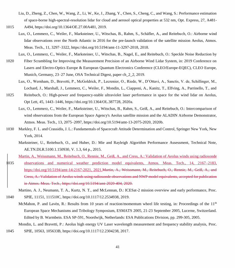
41

Liu, D., Zheng, Z., Chen, W., Wang, Z., Li, W., Ke, J., Zhang, Y., Chen, S., Cheng, C., and Wang, S.: Performance estimation

of space-borne high-spectral-resolution lidar for cloud and aerosol optical properties at 532 nm, Opt. Express, 27, A481-

A494, https://doi.org/10.1364/OE.27.00A481, 2019. 1015

Lux, O., Lemmerz, C., Weiler, F., Marksteiner, U., Witschas, B., Rahm, S., Schäfler, A., and Reitebuch, O.: Airborne wind

lidar observations over the North Atlantic in 2016 for the pre-launch validation of the satellite mission Aeolus, Atmos.

Meas. Tech., 11, 3297–3322, https://doi.org/10.5194/amt-11-3297-2018, 2018.

Lux, O., Lemmerz, C., Weiler, F., Marksteiner, U., Witschas, B., Nagel, E., and Reitebuch, O.: Speckle Noise Reduction by

Fiber Scrambling for Improving the Measurement Precision of an Airborne Wind Lidar System, in: 2019 Conference on 1020

Lasers and Electro-Optics Europe & European Quantum Electronics Conference (CLEO/Europe-EQEC), CLEO Europe,

Munich, Germany, 23–27 June, OSA Technical Digest, paper ch_2_2, 2019.

Lux, O., Wernham, D., Bravetti, P., McGoldrick, P., Lecrenier, O., Riede, W., D’Ottavi, A., Sanctis, V. de, Schillinger, M.,

Lochard, J., Marshall, J., Lemmerz, C., Weiler, F., Mondin, L., Ciapponi, A., Kanitz, T., Elfving, A., Parrinello, T., and

Reitebuch, O.: High-power and frequency-stable ultraviolet laser performance in space for the wind lidar on Aeolus, 1025

Opt Lett, 45, 1443–1446, https://doi.org/10.1364/OL.387728, 2020a.

Lux, O., Lemmerz, C., Weiler, F., Marksteiner, U., Witschas, B., Rahm, S., Geiß, A., and Reitebuch, O.: Intercomparison of

wind observations from the European Space Agency's Aeolus satellite mission and the ALADIN Airborne Demonstrator,

Atmos. Meas. Tech., 13, 2075–2097, https://doi.org/10.5194/amt-13-2075-2020, 2020b.

Markley, F. L. and Crassidis, J. L.: Fundamentals of Spacecraft Attitude Determination and Control, Springer New York, New 1030

York, 2014.

Marksteiner, U., Reitebuch, O., and Huber, D.: Mie and Rayleigh Algorithm Performance Assessment, Technical Note,

AE.TN.DLR.5100.1.150930, V. 1.3, 64 p., 2015.

Martin, A., Weissmann, M., Reitebuch, O., Rennie, M., Geiß, A., and Cress, A.: Validation of Aeolus winds using radiosonde

observations and numerical weather prediction model equivalents, Atmos. Meas. Tech., 14, 2167–2183, 1035

https://doi.org/10.5194/amt-14-2167-2021, 2021.Martin, A., Weissmann, M., Reitebuch, O., Rennie, M., Geiß, A., and

Cress, A.: Validation of Aeolus winds using radiosonde observations and NWP model equivalents, accepted for publication

in Atmos. Meas. Tech., https://doi.org/10.5194/amt-2020-404, 2020.

Martino, A. J., Neumann, T. A., Kurtz, N. T., and McLennan, D.: ICESat-2 mission overview and early performance, Proc.

SPIE, 11151, 111510C, https://doi.org/10.1117/12.2534938, 2019. 1040

McMahon, P. and Lavèn, R.: Results from 10 years of reaction/momentum wheel life testing, in: Proceedings of the 11th

European Space Mechanisms and Tribology Symposium, ESMATS 2005, 21-23 September 2005, Lucerne, Switzerland.

Edited by B. Warmbein. ESA SP-591, Noordwijk, Netherlands: ESA Publications Division, pp. 299-305, 2005.

Mondin, L. and Bravetti, P.: Aeolus high energy UV Laser wavelength measurement and frequency stability analysis, Proc.

SPIE, 10563, 105633B, https://doi.org/10.1117/12.2304238, 2017. 1045

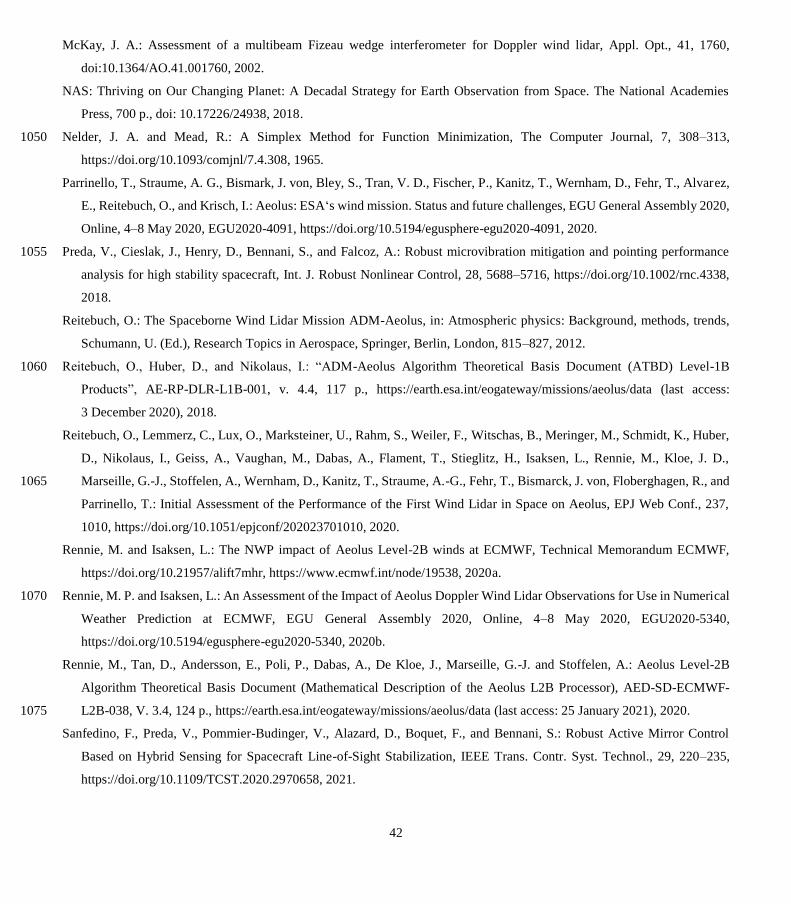
42

McKay, J. A.: Assessment of a multibeam Fizeau wedge interferometer for Doppler wind lidar, Appl. Opt., 41, 1760,

doi:10.1364/AO.41.001760, 2002.

NAS: Thriving on Our Changing Planet: A Decadal Strategy for Earth Observation from Space. The National Academies

Press, 700 p., doi: 10.17226/24938, 2018.

Nelder, J. A. and Mead, R.: A Simplex Method for Function Minimization, The Computer Journal, 7, 308–313, 1050

https://doi.org/10.1093/comjnl/7.4.308, 1965.

Parrinello, T., Straume, A. G., Bismark, J. von, Bley, S., Tran, V. D., Fischer, P., Kanitz, T., Wernham, D., Fehr, T., Alvarez,

E., Reitebuch, O., and Krisch, I.: Aeolus: ESA‘s wind mission. Status and future challenges, EGU General Assembly 2020,

Online, 4–8 May 2020, EGU2020-4091, https://doi.org/10.5194/egusphere-egu2020-4091, 2020.

Preda, V., Cieslak, J., Henry, D., Bennani, S., and Falcoz, A.: Robust microvibration mitigation and pointing performance 1055

analysis for high stability spacecraft, Int. J. Robust Nonlinear Control, 28, 5688–5716, https://doi.org/10.1002/rnc.4338,

2018.

Reitebuch, O.: The Spaceborne Wind Lidar Mission ADM-Aeolus, in: Atmospheric physics: Background, methods, trends,

Schumann, U. (Ed.), Research Topics in Aerospace, Springer, Berlin, London, 815–827, 2012.

Reitebuch, O., Huber, D., and Nikolaus, I.: “ADM-Aeolus Algorithm Theoretical Basis Document (ATBD) Level-1B 1060

Products”, AE-RP-DLR-L1B-001, v. 4.4, 117 p., https://earth.esa.int/eogateway/missions/aeolus/data (last access:

3 December 2020), 2018.

Reitebuch, O., Lemmerz, C., Lux, O., Marksteiner, U., Rahm, S., Weiler, F., Witschas, B., Meringer, M., Schmidt, K., Huber,

D., Nikolaus, I., Geiss, A., Vaughan, M., Dabas, A., Flament, T., Stieglitz, H., Isaksen, L., Rennie, M., Kloe, J. D.,

Marseille, G.-J., Stoffelen, A., Wernham, D., Kanitz, T., Straume, A.-G., Fehr, T., Bismarck, J. von, Floberghagen, R., and 1065

Parrinello, T.: Initial Assessment of the Performance of the First Wind Lidar in Space on Aeolus, EPJ Web Conf., 237,

1010, https://doi.org/10.1051/epjconf/202023701010, 2020.

Rennie, M. and Isaksen, L.: The NWP impact of Aeolus Level-2B winds at ECMWF, Technical Memorandum ECMWF,

https://doi.org/10.21957/alift7mhr, https://www.ecmwf.int/node/19538, 2020a.

Rennie, M. P. and Isaksen, L.: An Assessment of the Impact of Aeolus Doppler Wind Lidar Observations for Use in Numerical 1070

Weather Prediction at ECMWF, EGU General Assembly 2020, Online, 4–8 May 2020, EGU2020-5340,

https://doi.org/10.5194/egusphere-egu2020-5340, 2020b.

Rennie, M., Tan, D., Andersson, E., Poli, P., Dabas, A., De Kloe, J., Marseille, G.-J. and Stoffelen, A.: Aeolus Level-2B

Algorithm Theoretical Basis Document (Mathematical Description of the Aeolus L2B Processor), AED-SD-ECMWF-

L2B-038, V. 3.4, 124 p., https://earth.esa.int/eogateway/missions/aeolus/data (last access: 25 January 2021), 2020. 1075

Sanfedino, F., Preda, V., Pommier-Budinger, V., Alazard, D., Boquet, F., and Bennani, S.: Robust Active Mirror Control

Based on Hybrid Sensing for Spacecraft Line-of-Sight Stabilization, IEEE Trans. Contr. Syst. Technol., 29, 220–235,

https://doi.org/10.1109/TCST.2020.2970658, 2021.

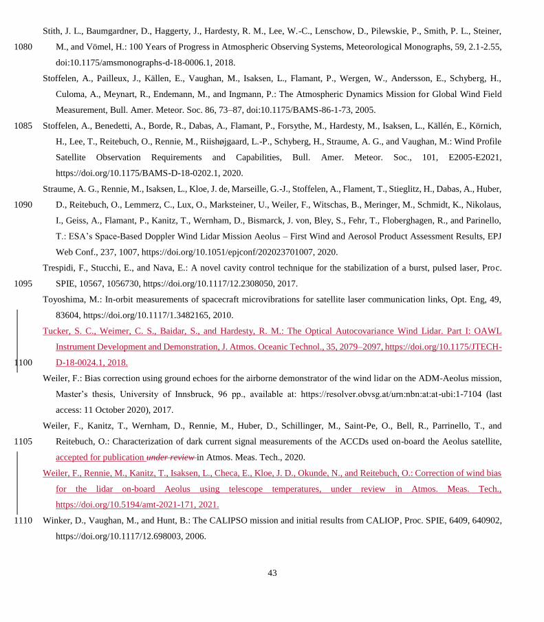
43

Stith, J. L., Baumgardner, D., Haggerty, J., Hardesty, R. M., Lee, W.-C., Lenschow, D., Pilewskie, P., Smith, P. L., Steiner,

M., and Vömel, H.: 100 Years of Progress in Atmospheric Observing Systems, Meteorological Monographs, 59, 2.1-2.55, 1080

doi:10.1175/amsmonographs-d-18-0006.1, 2018.

Stoffelen, A., Pailleux, J., Källen, E., Vaughan, M., Isaksen, L., Flamant, P., Wergen, W., Andersson, E., Schyberg, H.,

Culoma, A., Meynart, R., Endemann, M., and Ingmann, P.: The Atmospheric Dynamics Mission for Global Wind Field

Measurement, Bull. Amer. Meteor. Soc. 86, 73–87, doi:10.1175/BAMS-86-1-73, 2005.

Stoffelen, A., Benedetti, A., Borde, R., Dabas, A., Flamant, P., Forsythe, M., Hardesty, M., Isaksen, L., Källén, E., Körnich, 1085

H., Lee, T., Reitebuch, O., Rennie, M., Riishøjgaard, L.-P., Schyberg, H., Straume, A. G., and Vaughan, M.: Wind Profile

Satellite Observation Requirements and Capabilities, Bull. Amer. Meteor. Soc., 101, E2005-E2021,

https://doi.org/10.1175/BAMS-D-18-0202.1, 2020.

Straume, A. G., Rennie, M., Isaksen, L., Kloe, J. de, Marseille, G.-J., Stoffelen, A., Flament, T., Stieglitz, H., Dabas, A., Huber,

D., Reitebuch, O., Lemmerz, C., Lux, O., Marksteiner, U., Weiler, F., Witschas, B., Meringer, M., Schmidt, K., Nikolaus, 1090

I., Geiss, A., Flamant, P., Kanitz, T., Wernham, D., Bismarck, J. von, Bley, S., Fehr, T., Floberghagen, R., and Parinello,

T.: ESA’s Space-Based Doppler Wind Lidar Mission Aeolus – First Wind and Aerosol Product Assessment Results, EPJ

Web Conf., 237, 1007, https://doi.org/10.1051/epjconf/202023701007, 2020.

Trespidi, F., Stucchi, E., and Nava, E.: A novel cavity control technique for the stabilization of a burst, pulsed laser, Proc.

SPIE, 10567, 1056730, https://doi.org/10.1117/12.2308050, 2017. 1095

Toyoshima, M.: In-orbit measurements of spacecraft microvibrations for satellite laser communication links, Opt. Eng, 49,

83604, https://doi.org/10.1117/1.3482165, 2010.

Tucker, S. C., Weimer, C. S., Baidar, S., and Hardesty, R. M.: The Optical Autocovariance Wind Lidar. Part I: OAWL

Instrument Development and Demonstration, J. Atmos. Oceanic Technol., 35, 2079–2097, https://doi.org/10.1175/JTECH-

D-18-0024.1, 2018. 1100

Weiler, F.: Bias correction using ground echoes for the airborne demonstrator of the wind lidar on the ADM-Aeolus mission,

Master’s thesis, University of Innsbruck, 96 pp., available at: https://resolver.obvsg.at/urn:nbn:at:at-ubi:1-7104 (last

access: 11 October 2020), 2017.

Weiler, F., Kanitz, T., Wernham, D., Rennie, M., Huber, D., Schillinger, M., Saint-Pe, O., Bell, R., Parrinello, T., and

Reitebuch, O.: Characterization of dark current signal measurements of the ACCDs used on-board the Aeolus satellite, 1105

accepted for publication under review in Atmos. Meas. Tech., 2020.

Weiler, F., Rennie, M., Kanitz, T., Isaksen, L., Checa, E., Kloe, J. D., Okunde, N., and Reitebuch, O.: Correction of wind bias

for the lidar on-board Aeolus using telescope temperatures, under review in Atmos. Meas. Tech.,

https://doi.org/10.5194/amt-2021-171, 2021.

Winker, D., Vaughan, M., and Hunt, B.: The CALIPSO mission and initial results from CALIOP, Proc. SPIE, 6409, 640902, 1110

https://doi.org/10.1117/12.698003, 2006.

44

Witschas, B., Lemmerz, C., Geiß, A., Lux, O., Marksteiner, U., Rahm, S., Reitebuch, O., and Weiler, F.: First validation of

Aeolus wind observations by airborne Doppler wind lidar measurements, Atmos. Meas. Tech., 13, 2381–2396,

https://doi.org/10.5194/amt-13-2381-2020, 2020.