Aircraft Performance Model Calibration and Validation forGeneral Aviation Safety Analysis

Tejas Puranik∗, Evan Harrison∗

Georgia Institute of Technology, Atlanta, Georgia, 30332

Imon Chakraborty†

Auburn University, Auburn, Alabama, 36849

Dimitri Mavris‡

Georgia Institute of Technology, Atlanta, Georgia, 30332

Performance models facilitate a wide range of safety analyses in aviation. In an idealscenario, the performance models would show inherently good agreement with the true perfor-mance of the aircraft. However, in reality, this is rarely the case, either owing to underlyingsimplifications or due to the limited fidelity of applicable tools or data. In such cases, calibrationis required to fine-tune the behavior of the performance models. For point-mass steady-stateperformance models, challenges arise due to the fact that there is no obvious, unique metricor flight condition at which to assess the accuracy of the model predictions, and since a largenumber of model parameters may potentially influence model accuracy. This work presents atwo-level approach to aircraft performance model calibration. The first level consists of usingmanufacturer-developed performance manuals for calibration, while the second level providesadditional refinement when flight data is available. The performance models considered inthis work consist of aerodynamic and propulsion models (performance curves) that are ca-pable of predicting the non-dimensional lift, drag, thrust, and torque at any given point intime. The framework is demonstrated on two representative General Aviation aircraft. Thedemonstrated approach results in models that can predict critical energy-based safety metricswith improved accuracy for use in retrospective safety analysis.

I. Introduction and MotivationThe development of models is ubiquitous in a broad range of performance studies and safety analyses. The ability toaccurately model complex phenomena contributes greatly towards enhancing the understanding of their performance ofvehicles in real-world scenarios. One of the main advantages of using performance models in safety analysis is theability to use recorded data to predict unrecorded quantities of interest. For example, using recorded flight data from adigital flight data recorder (DFDR) [1] in conjunction with aircraft performance model can help predict non-dimensionallift, drag, thrust, etc. These quantities along with flight data can be used for various retrospective safety analysessuch as evaluation of energy-based safety metrics [2, 3], monitoring of aircraft performance [4], detecting anomalousflights in a large set of flight data records [5–8], estimating the weight of the aircraft, identifying performance safetyenvelopes [9–12], etc. The quality of insights and results obtained from these retrospective analyses depends on theavailability of well-calibrated performance models for predicting the vehicle’s performance.

General Aviation (GA), according to the Federal Aviation Administration (FAA) is “that portion of civil aviationthat does not include scheduled or unscheduled air carriers or commercial space operations". Despite the improvingsafety record of aviation operations, GA aircraft have traditionally had higher accident and incident rates [13]. Theavailability of additional data in the form of performance model predictions is a valuable asset for incident and accidentinvestigation, retrospective analyses, flight training etc.

The problem being addressed in this paper is the calibration and validation of point-performance steady state modelsof small GA fixed-wing aircraft (such as the Cessna 172). These models are available in the form of variations of

∗Research Engineer II, Aerospace Systems Design Laboratory, Daniel Guggenheim School of Aerospace Engineering, AIAA Member.†Assistant Professor, School of Aerospace Engineering, Auburn University, AIAA Member.‡S.P. Langley NIA Distinguished Regents Professor, Director of Aerospace Systems Design Laboratory, Daniel Guggenheim School of Aerospace

Engineering, AIAA Fellow.

1

important non-dimensional quantities relevant for aircraft performance, such as lift curve, drag polar, propeller polar, etc.A detailed implementation of such models using empirical relations and assumptions can be found in Harrison et al. [14]and Min et al. [15]. In an ideal scenario, the performance models would show inherently good agreement with the trueperformance of the aircraft. However, in reality, this is almost never the case, either owing to underlying simplificationsor assumptions or due to the limited fidelity of available or applicable analysis tools. In the case of point-performancesteady-state performance models, challenges also arise due to the fact that there is no obvious, unique metric or flightcondition at which to assess the accuracy of the model predictions, and since a large number of model parametersmay potentially influence model accuracy. The availability of accurate calibration and validation data can limit theapplicability of developed models. All the limitations mentioned necessitate the calibration of developed empiricalmodels in a systematic fashion in order to deploy them for performance and safety analyses. Lack of data is often a majorhindrance in retrospective safety analysis for GA applications [16]. Performance models aim to alleviate that problem tosome extent by enabling estimation of quantities of interest that are not directly recorded in GA flight data recorders.

Computational Model

Benchmark Data

Adequate?

Accuracy Requirement

Difference

No ? Acquire Additional Benchmark Data

No ? Update/Calibrate Model Parameters

Use Model for Prediction

Validation Metric

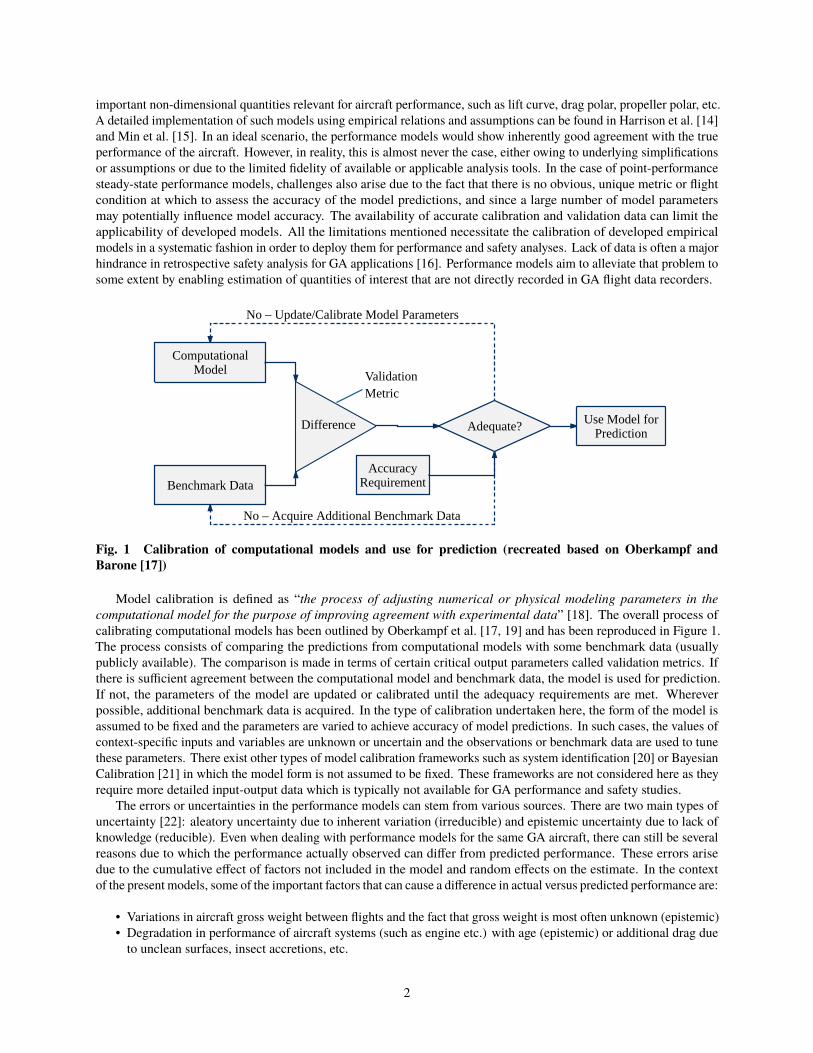
Fig. 1 Calibration of computational models and use for prediction (recreated based on Oberkampf andBarone [17])

Model calibration is defined as “the process of adjusting numerical or physical modeling parameters in thecomputational model for the purpose of improving agreement with experimental data” [18]. The overall process ofcalibrating computational models has been outlined by Oberkampf et al. [17, 19] and has been reproduced in Figure 1.The process consists of comparing the predictions from computational models with some benchmark data (usuallypublicly available). The comparison is made in terms of certain critical output parameters called validation metrics. Ifthere is sufficient agreement between the computational model and benchmark data, the model is used for prediction.If not, the parameters of the model are updated or calibrated until the adequacy requirements are met. Whereverpossible, additional benchmark data is acquired. In the type of calibration undertaken here, the form of the model isassumed to be fixed and the parameters are varied to achieve accuracy of model predictions. In such cases, the values ofcontext-specific inputs and variables are unknown or uncertain and the observations or benchmark data are used to tunethese parameters. There exist other types of model calibration frameworks such as system identification [20] or BayesianCalibration [21] in which the model form is not assumed to be fixed. These frameworks are not considered here as theyrequire more detailed input-output data which is typically not available for GA performance and safety studies.

The errors or uncertainties in the performance models can stem from various sources. There are two main types ofuncertainty [22]: aleatory uncertainty due to inherent variation (irreducible) and epistemic uncertainty due to lack ofknowledge (reducible). Even when dealing with performance models for the same GA aircraft, there can still be severalreasons due to which the performance actually observed can differ from predicted performance. These errors arisedue to the cumulative effect of factors not included in the model and random effects on the estimate. In the contextof the present models, some of the important factors that can cause a difference in actual versus predicted performance are:

• Variations in aircraft gross weight between flights and the fact that gross weight is most often unknown (epistemic)• Degradation in performance of aircraft systems (such as engine etc.) with age (epistemic) or additional drag dueto unclean surfaces, insect accretions, etc.

2

• Changes or modifications made to aircraft that affect its aerodynamic behavior (epistemic)• Variation in aircraft model (C172S versus C172R - epistemic)• Model Inadequacy (epistemic)• Unknown/Inaccurate model parameters (epistemic)• Piloting skill (epistemic)• Noise in recorded data (aleatory)• Environmental conditions (aleatory)Due to all these uncertainties, it is essential to calibrate the aircraft performance models prior to using them for

safety analysis. In consideration of the above observations, the overarching research objective of this paper is identifiedas follows:

To demonstrate a systematic two-level framework for calibration and validation of General Aviation point-performancemodels for aerodynamics and propulsion to enable improved predictions of energy-based safety metrics

The rest of the paper is organized as follows: Section II describes the overall setup of the model calibration framework,Section III contains the implementation of the two-level calibration process utilized in this work to two representativeGA aircraft, Section IV describes the application of calibrated models to an enhance the insights obtained during a safetyanalysis scenario, and Section V contains conclusions drawn from this work and potential avenues for future work.

II. Model Calibration FrameworkWhile performance model can mean something different depending on the application, within the work described in thispaper, the term is used in a specific context. An aircraft performance model consists of two individual disciplinarymodels: aerodynamics and propulsion. The aerodynamics model contains variations of non-dimensional lift and dragwith the airplane angle-of-attack. The propulsion model consists of variations of non-dimensional thrust with vehiclespeed and propeller revolutions per minute (RPM) as well as engine power lapse with altitude and temperature.

Within these general specifications, there exist numerous options for both aerodynamic and propulsive models,differing in terms of their underlying assumptions and fidelity. While the methods or rules for appropriate modelselection in a broad sense is beyond the scope of this work, it is important to note the limitations of calibration asit pertains to model selection. Generally speaking a performance model is selected upon careful consideration ofthe domain of interest, which may include considerations such as the operating regime, vehicle configuration, andmodel application intent. From these considerations a performance model that captures the relevant physics, or otherbehavior of interest, should be selected that affords the most reasonable level of fidelity given the cost of modelimplementation. Once a model is chosen model calibration allows for the tailoring of a general model of behavior to bemore representative of the particular system of interest. However, if the selected model lacks the capability to adequatelydescribe some key aspect of the problem under consideration then the final results of the calibration process describedherein will be modest at best.

Figure 2 outlines the schematic of the two-level process followed in this work for model calibration. Many of thedecisions made in GA safety analysis depend upon the availability of data. The previous empirical models developedfor GA operations ([14, 15]) utilized data from the public domain due to lack of flight data. These models wereindependently calibrated against available benchmarks. However, rarely are such performance models used in isolation.Sometimes, metrics that are not estimable using a single model alone can be estimated using predictions from acombination of models [3, 23]. While this could add uncertainty to the prediction, it opens up new avenues to test,calibrate, and fine-tune model parameters. Similarly, in the event of availability of some amount of flight data, a methodneeds to be available to utilize that information appropriately to improve model predictions. Therefore, two levels ofcalibration-data availability are defined, (i) publicly available data and (ii) flight data, and make up the correspondingtwo levels of the developed model calibration framework.

Three external inputs are required for the entire calibration framework and have been described in this section. Thelevels of the framework are elaborated in the next section on implementation. It is noted that recorded flight data mightnot always be available and therefore Level-II calibration is only possible when such data is available. In cases whererequired flight data is unavailable the calibration process is terminated after Level-I and the model(s) obtained afterLevel-I are used for safety analysis.

3

Fig. 2 Schematic of two-level calibration process

A. Aircraft DataIn order to begin the process, basic data about the geometry of the aircraft along with publicly available performance

data for calibration and validation is required. Ideally, flight data or flight test data should be used, but this may not bereadily available for the aircraft in question. An alternative source for this information is documentation published bythe manufacturer of the aircraft such as the Pilot Operating Handbook (POH). The POH is a document developed by theairplane manufacturer and approved by the FAA which lists important information regarding the design, operations, andlimitations of the aircraft, as well as its performance characteristics. Although the performance tables listed in the POHare idealized capabilities that a brand new aircraft can theoretically attain under ideal conditions, it is nevertheless a veryvaluable source of information for calibrating models. As a POH is also readily available for most aircraft, it wouldenable a calibration process that is easily repeatable. The data from the performance tables in the POH is collected incomma-separated values (CSV) format and compared against predicted performance of aircraft using models. Detailson the data used in each level of the calibration process are provided in the subsequent section.

B. Empirical Performance ModelsFigure 3 shows the flow of information in the individual discipline models used in this work. The initial development

of the models can be found in Harrison et al. [14] and Min et al [15]. Given a set of inputs and environmentalconditions, it is of interest to predict the aerodynamic and propulsive performance of a GA aircraft in terms of certainnon-dimensional coefficients. While these (or similar) models of aerodynamics or propulsion may be validated againstpublished data, it is advantageous to calibrate them together as an aircraft performance model due to the inherentuncertainties associated with using such models on actual flight data. One of the reasons for this is that model inputdata includes factors such as geometry, operational parameters, and ambient conditions, and can come from a range ofsources that may not always be measurable or easily available. The current set of aerodynamic models consist of fourlift-curves and drag polars (one for each of four flap settings - 0, 10, 20, and 30 deg. - as is typical on a GA aircraft). Onthe other hand, the propulsion model consists of a torque and thrust curve. A brief description of the models follows.

1. PropulsionAmong currently operated GA vehicles, the most common means of propulsion is a propeller driven by an internal

combustion engine [24]. Following this trend, the propulsion model is similarly divided into individual models ofinternal combustion engine performance and propeller performance, which combined yield a propulsive model that isappropriate for a large subset of the GA fleet. Many approaches for engine modeling exist within the literature, and a

4

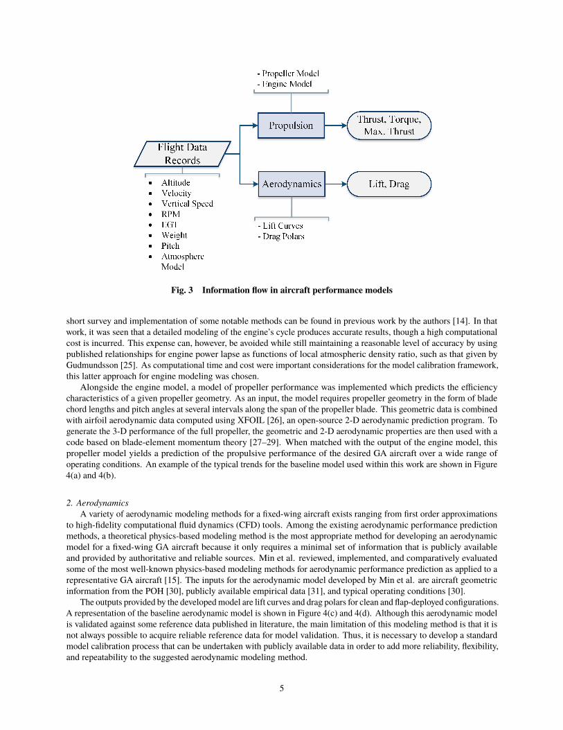
Fig. 3 Information flow in aircraft performance models

short survey and implementation of some notable methods can be found in previous work by the authors [14]. In thatwork, it was seen that a detailed modeling of the engine’s cycle produces accurate results, though a high computationalcost is incurred. This expense can, however, be avoided while still maintaining a reasonable level of accuracy by usingpublished relationships for engine power lapse as functions of local atmospheric density ratio, such as that given byGudmundsson [25]. As computational time and cost were important considerations for the model calibration framework,this latter approach for engine modeling was chosen.

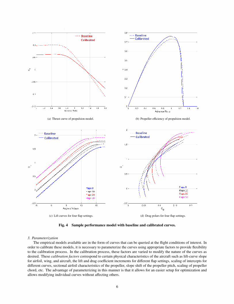
Alongside the engine model, a model of propeller performance was implemented which predicts the efficiencycharacteristics of a given propeller geometry. As an input, the model requires propeller geometry in the form of bladechord lengths and pitch angles at several intervals along the span of the propeller blade. This geometric data is combinedwith airfoil aerodynamic data computed using XFOIL [26], an open-source 2-D aerodynamic prediction program. Togenerate the 3-D performance of the full propeller, the geometric and 2-D aerodynamic properties are then used with acode based on blade-element momentum theory [27–29]. When matched with the output of the engine model, thispropeller model yields a prediction of the propulsive performance of the desired GA aircraft over a wide range ofoperating conditions. An example of the typical trends for the baseline model used within this work are shown in Figure4(a) and 4(b).

2. AerodynamicsA variety of aerodynamic modeling methods for a fixed-wing aircraft exists ranging from first order approximations

to high-fidelity computational fluid dynamics (CFD) tools. Among the existing aerodynamic performance predictionmethods, a theoretical physics-based modeling method is the most appropriate method for developing an aerodynamicmodel for a fixed-wing GA aircraft because it only requires a minimal set of information that is publicly availableand provided by authoritative and reliable sources. Min et al. reviewed, implemented, and comparatively evaluatedsome of the most well-known physics-based modeling methods for aerodynamic performance prediction as applied to arepresentative GA aircraft [15]. The inputs for the aerodynamic model developed by Min et al. are aircraft geometricinformation from the POH [30], publicly available empirical data [31], and typical operating conditions [30].

The outputs provided by the developedmodel are lift curves and drag polars for clean and flap-deployed configurations.A representation of the baseline aerodynamic model is shown in Figure 4(c) and 4(d). Although this aerodynamic modelis validated against some reference data published in literature, the main limitation of this modeling method is that it isnot always possible to acquire reliable reference data for model validation. Thus, it is necessary to develop a standardmodel calibration process that can be undertaken with publicly available data in order to add more reliability, flexibility,and repeatability to the suggested aerodynamic modeling method.

5

(a) Thrust curve of propulsion model. (b) Propeller efficiency of propulsion model.

(c) Lift curves for four flap settings. (d) Drag polars for four flap settings.

Fig. 4 Sample performance model with baseline and calibrated curves.

3. ParameterizationThe empirical models available are in the form of curves that can be queried at the flight conditions of interest. In

order to calibrate these models, it is necessary to parameterize the curves using appropriate factors to provide flexibilityto the calibration process. In the calibration process, these factors are varied to modify the nature of the curves asdesired. These calibration factors correspond to certain physical characteristics of the aircraft such as lift-curve slopefor airfoil, wing, and aircraft, the lift and drag coefficient increments for different flap settings, scaling of intercepts fordifferent curves, sectional airfoil characteristics of the propeller, slope shift of the propeller pitch, scaling of propellerchord, etc. The advantage of parameterizing in this manner is that it allows for an easier setup for optimization andallows modifying individual curves without affecting others.

6

A total of thirty calibration factors are included in the calibration process and a detailed list of each factor, itsdescription, and range of possible values is included in appendix V. For each calibration factor, judgment is used indetermining whether its effect on performance curves should be modeled as being of an additive or multiplicative nature.Similarly, the upper and lower limits are chosen so as to always satisfy physical constraints of the problem.

C. Recorded Flight DataWhen available, recorded flight data from actual flights can be used to undertake Level-II of the calibration

framework. The flight data obtained from the DFDR are a multivariate time series, whose lengths typically vary betweenrecords due to varying duration of flight. The number of parameters varies around 20 (in GA operations) and theseparameters are recorded at a specific frequency (e.g., once per 1 second interval). The data consist of parameters relatedto the state, attitude, basic engine information, environmental conditions, Global Positioning System information, andothers. While typical GA aircraft flight data record may not contain a rich set of parameters, the flight record usedfor calibration is expected to contain a rich set including parameters such as the altitude, true airspeed, vertical speed,engine RPM, outside air temperature, weight of the aircraft (or initial weight and fuel flow rate), position of the flaps,and others. In the current work, data recorded on a Cessna 172 and Piper Archer aircraft equipped with a GarminG1000 system are used. At least one flight data record is required for performing calibration with the requirement ofadditional flight data records for validating the calibrated model.

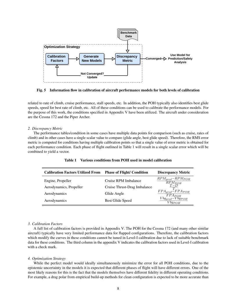
III. Implementation and ResultsEach of the two levels of the calibration framework outlined in Figure 2 follows the same stencil with different algorithms,benchmark data, etc. used for each. Figure 5 illustrates the common stencil used in both levels of the calibrationprocess. The model(s) obtained from the process may be used directly for prediction or analysis or passed on to thenext level in the framework. In order to modify the performance models in a systematic manner during calibration,they are parameterized using certain variables called calibration factors. A full list of calibration factors along with theperformance model they modify and the level during which they are modified is provided in appendix V. The values ofthe calibration factors are collected in a single vector henceforth called the “calibration vector”. Each calibration vectorresults in the generation of a unique set of performance model curves which can then be validated or tested. In eachlevel, there are four important factors that need to be determined prior to calibration:

1) Benchmark Data: The data (either publicly available or collected flight data) used as the truth value in thecalibration process

2) Discrepancy Metrics: The measure of disagreement between the assumed truth value and the model prediction,typically expressed as % root mean squared (RMS) error

3) Calibration Factors: The factors that are varied during the calibration process to optimize/minimize thediscrepancy metric

4) Optimization Strategy: The setup (single vs multi-objective) and algorithm used for the optimization probleminvolved in calibrating the model

The subsequent sections describe the choices made for each of these four factors and the rationale behind these choicesfor Level-I and Level-II calibration. Figure 5 also illustrates how these factors fit into the overall calibration frameworkstencil for each level.

A. Level-I Calibration

1. Benchmark DataAs described previously, empirical models for aerodynamics and propulsion can be obtained independently and

used in making predictions. However, due to the uncertainties noted, there might be context-specific information thatprecludes their efficient use in safety analysis. Therefore, it is preferable to simultaneously calibrate both aerodynamicsand propulsion models. The benchmark data typically used for this level is publicly available information from manualssuch as the POH. The POH lists important information regarding the design, operations, and limitations of the aircraft,as well as its performance characteristics. Although the POH performance tables are for a brand new aircraft underideal conditions, they are nevertheless valuable for calibrating performance models. The POH contains tables that listthe aircraft performance at various operating conditions and phases of flight. While some variation in the format ofdata presented is expected between different handbooks, most have some common performance tables, such as those

7

Calibration Factors

Generate New Models

Discrepancy Metric

Benchmark Data

Not Converged?Update

Converged

Optimization Strategy

Use Model for Prediction/Safety

Analysis

Fig. 5 Information flow in calibration of aircraft performance models for both levels of calibration

related to rate of climb, cruise performance, stall speeds, etc. In addition, the POH typically also identifies best glidespeeds, speed for best rate of climb, etc. All of these conditions can be used to calibrate the performance models. Forthe purpose of this work, the conditions specified in Appendix V have been utilized. The aircraft under considerationare the Cessna 172 and the Piper Archer.

2. Discrepancy MetricThe performance tables/condition in some cases have multiple data points for comparison (such as cruise, rates of

climb) and in other cases have a single scalar value to compare (glide angle, best glide speed). Therefore, the RMS errormetric is computed for conditions having multiple calibration points so that a single value of error metric is obtained foreach performance condition. Each phase of flight outlined in Table 1 will result in a single scalar error which will becombined to yield a vector.

Table 1 Various conditions from POH used in model calibration

Calibration Factors Utilized From Phase of Flight/ Condition Discrepancy Metric

Engine, Propeller Cruise RPM Imbalance RP Mpred−RP MP OH

RP MP OH

Aerodynamics, Propeller Cruise Thrust-Drag Imbalance T −DT

Aerodynamics Glide Angle F P Apred−F P AP OH

F P AP OH

Aerodynamics Best Glide Speed V bgpred−V bgP OH

V bgP OH

3. Calibration FactorsA full list of calibration factors is provided in Appendix V. The POH for the Cessna 172 (and many other similar

aircraft) typically have very limited performance data for flapped configurations. Therefore, the calibration factorswhich modify the curves in these conditions cannot be tuned in Level-I calibration due to lack of suitable benchmarkdata for these conditions. The third column in the appendix V indicates the calibration factors used in Level-I calibrationwith a check mark.

4. Optimization StrategyWhile the perfect model would ideally simultaneously minimize the error for all POH conditions, due to the

epistemic uncertainty in the models it is expected that different phases of flight will have different errors. One of themost likely reasons for this is the fact that the models themselves have different fidelity in different operating conditions.For example, a drag polar from empirical build-up methods for clean configuration is expected to be more accurate than

8

that for a configuration with flaps deployed, due to the inherent additional flow complexity (such as non-linearity, flowseparation, sensitivity to flap geometry, etc.). Another possible reason is that there might be more calibration data forsome conditions than others, leading to better predictions for certain phases of flight.

Since each phase of flight or POH condition will yield a different error metric, the calibration will be a multi-objectiveproblem. A multi-objective optimization algorithm is therefore used for calibrating the performance models to the POHperformance tables which can then enable choosing models as suitable points on a pareto front. Similar applicationshave been used in other contexts such as aircraft subsystem architecture optimization [32]. The well known algorithmNSGA-II is utilized for multi-objective optimization [33]. The implementation of NSGA-II within MATLAB is utilizedto find the Pareto front of calibration vectors. Any model from this front is Pareto-optimal and may be chosen for thepurposes of the application here. It is noted that the calibration up to the end of Level-I and generation of Pareto-optimalmodels is implemented without the use of a single flight data record. This is inherently valuable as detailed recordingcapability may not be readily available for all GA aircraft, even though performance predictions and safety assessmentsare nonetheless desired. In such cases, models calibrated using Level-I of the framework will prove to be useful.

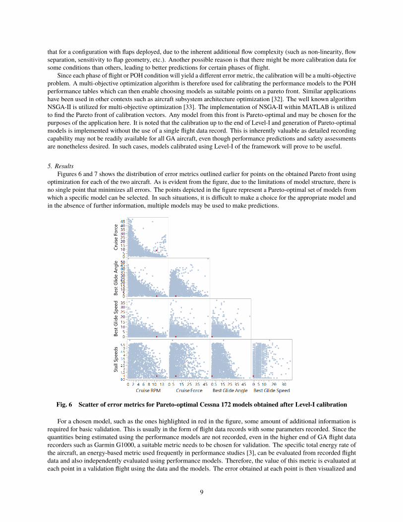
5. ResultsFigures 6 and 7 shows the distribution of error metrics outlined earlier for points on the obtained Pareto front using

optimization for each of the two aircraft. As is evident from the figure, due to the limitations of model structure, there isno single point that minimizes all errors. The points depicted in the figure represent a Pareto-optimal set of models fromwhich a specific model can be selected. In such situations, it is difficult to make a choice for the appropriate model andin the absence of further information, multiple models may be used to make predictions.

Fig. 6 Scatter of error metrics for Pareto-optimal Cessna 172 models obtained after Level-I calibration

For a chosen model, such as the ones highlighted in red in the figure, some amount of additional information isrequired for basic validation. This is usually in the form of flight data records with some parameters recorded. Since thequantities being estimated using the performance models are not recorded, even in the higher end of GA flight datarecorders such as Garmin G1000, a suitable metric needs to be chosen for validation. The specific total energy rate ofthe aircraft, an energy-based metric used frequently in performance studies [3], can be evaluated from recorded flightdata and also independently evaluated using performance models. Therefore, the value of this metric is evaluated ateach point in a validation flight using the data and the models. The error obtained at each point is then visualized and

9

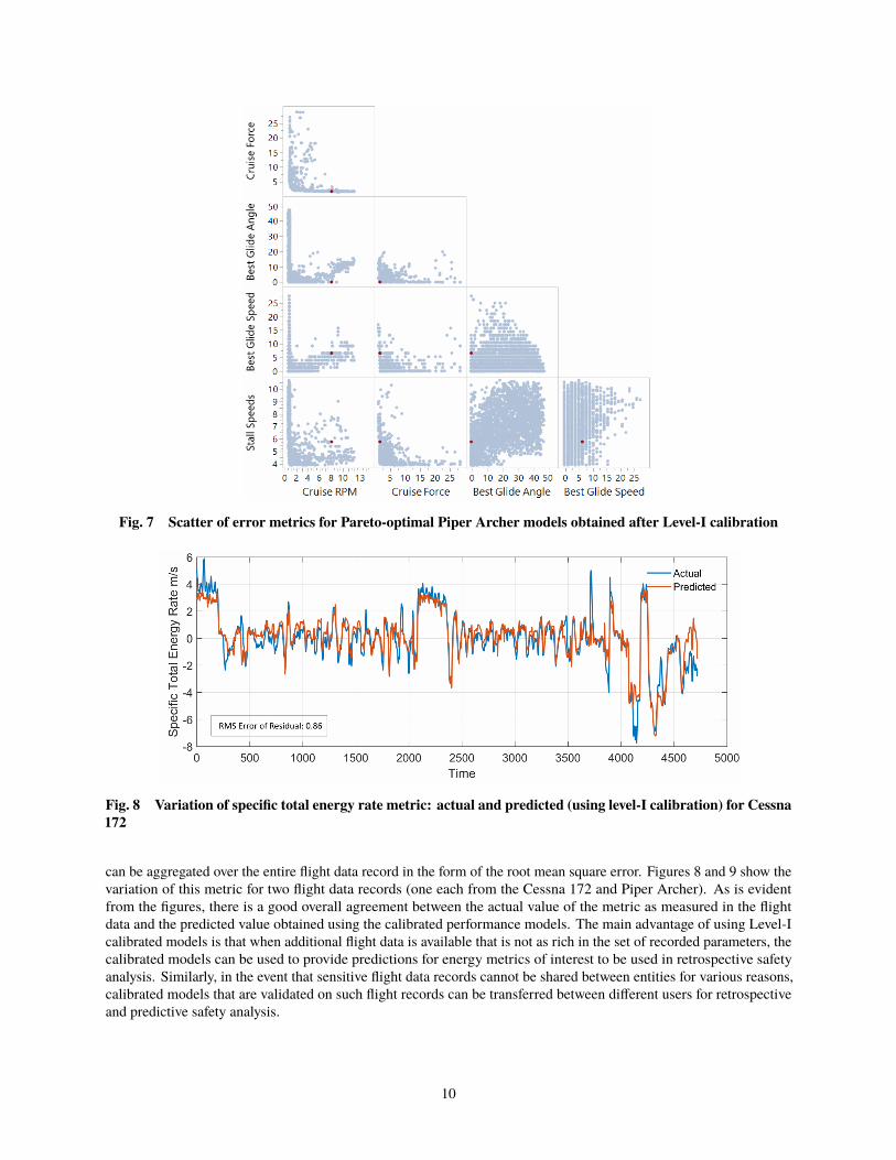
Fig. 7 Scatter of error metrics for Pareto-optimal Piper Archer models obtained after Level-I calibration

Fig. 8 Variation of specific total energy rate metric: actual and predicted (using level-I calibration) for Cessna172

can be aggregated over the entire flight data record in the form of the root mean square error. Figures 8 and 9 show thevariation of this metric for two flight data records (one each from the Cessna 172 and Piper Archer). As is evidentfrom the figures, there is a good overall agreement between the actual value of the metric as measured in the flightdata and the predicted value obtained using the calibrated performance models. The main advantage of using Level-Icalibrated models is that when additional flight data is available that is not as rich in the set of recorded parameters, thecalibrated models can be used to provide predictions for energy metrics of interest to be used in retrospective safetyanalysis. Similarly, in the event that sensitive flight data records cannot be shared between entities for various reasons,calibrated models that are validated on such flight records can be transferred between different users for retrospectiveand predictive safety analysis.

10

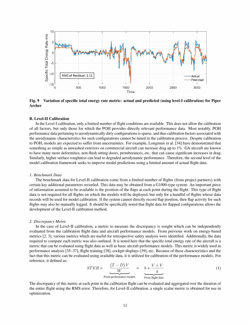
Fig. 9 Variation of specific total energy rate metric: actual and predicted (using level-I calibration) for PiperArcher

B. Level-II CalibrationIn the Level-I calibration, only a limited number of flight conditions are available. This does not allow the calibration

of all factors, but only those for which the POH provides directly relevant performance data. Most notably, POHperformance data pertaining to aerodynamically dirty configurations is sparse, and thus calibration factors associated withthe aerodynamic characteristics for such configurations cannot be tuned in the calibration process. Despite calibrationto POH, models are expected to suffer from uncertainties. For example, Longmuir et al. [34] have demonstrated thatsomething as simple as unwashed exteriors on commercial aircraft can increase drag up to 1%. GA aircraft are knownto have many more deformities, non-flush sitting doors, protuberances, etc. that can cause significant increases in drag.Similarly, higher surface roughness can lead to degraded aerodynamic performance. Therefore, the second level of themodel calibration framework seeks to improve model predictions using a limited amount of actual flight data.

1. Benchmark DataThe benchmark data for Level-II calibration come from a limited number of flights (from project partners) with

certain key additional parameters recorded. This data may be obtained from a G1000-type system. An important pieceof information assumed to be available is the position of the flaps at each point during the flight. This type of flightdata is not required for all flights on which the models will be deployed, but only for a handful of flights whose datarecords will be used for model calibration. If the system cannot directly record flap position, then flap activity for suchflights may also be manually logged. It should be specifically noted that flight data for flapped configurations allows thedevelopment of the Level-II calibration method.

2. Discrepancy MetricIn the case of Level-II calibration, a metric to measure the discrepancy is sought which can be independently

evaluated from the calibration flight data and aircraft performance models. From previous work on energy-basedmetrics [2, 3], various metrics which are useful for retrospective safety analysis were identified. Additionally, the datarequired to compute each metric was also outlined. It is noted here that the specific total energy rate of the aircraft is ametric that can be evaluated using flight data as well as basic aircraft performance models. This metric is widely used inperformance analysis [35–37], flight training [38], cockpit displays [39], etc. Because of these characteristics and thefact that this metric can be evaluated using available data, it is utilized for calibration of the performance models. Forreference, it defined as:

STER =

(T − D

)V

W︸ ︷︷ ︸From performance models

= h +V × V

g︸ ︷︷ ︸From flight data

(1)

The discrepancy of this metric at each point in the calibration flight can be evaluated and aggregated over the duration ofthe entire flight using the RMS error. Therefore, for Level-II calibration, a single scalar metric is obtained for use inoptimization.

11

3. Calibration FactorsUnlike Level-1 calibration using POH data, where the calibration factors are restricted to those for which test

conditions exist in the manual, Level-II calibration can use the entire set of calibration factors (assuming that the flapshave been used at least once in the calibration flights). Therefore, all thirty calibration factors can be varied withintheir range in the Level-II calibration. While this increases the dimensionality of the space being explored, it enablessweeping a larger possible spread of performance curves.

4. Optimization StrategyUnlike Level-I calibration, the Level-II calibration setup uses only a single discrepancy metric. This metric is

calculated at each point in the flight data record(s) available for calibration. Therefore the root mean square (RMS)of this discrepancy over the entire flight is calculated and used. In case multiple flights are available for calibration,the RMS over all the flights can be used. Since this is an indirect calibration process, an evolutionary optimizationalgorithm is chosen. Additionally, as the calibration flight will only have limited flight conditions at which to test thediscrepancy, there may be multiple local minima. Therefore, a genetic algorithm is used to ensure that the best possiblecalibration model is obtained.

Regarding implementation, the initial starting point of the algorithm can be chosen randomly within the ranges ofcalibration factors or using information from prior efforts. In particular, the pareto-optimal set of calibration vectorsobtained from Level-I calibration can be used to “warm start” optimization in Level-II calibration. This may yield fasteralgorithm convergence and provide better results. The implementation of genetic algorithm in MATLAB is utilized forthis purpose∗.

5. ResultsOne of the advantages of Level-I (POH) calibration is that it does not require any flight data records. The resulting

calibrated aircraft performance models obtained from this level are shown to have good predictive capability. Therefore,for Level-II calibration, it is useful to start the optimization from the POH-calibrated models obtained from Level-Icalibration. This can accelerate the convergence of the calibration and produce models that have improved performanceover the models from Level-I calibration. Starting from a Level-I calibrated model that performs well on the validationflight data record is advantageous, as it ensures that the predictive capability of the model is already good. An importantdifference noted previously is that the quantities being predicted by each model are not individually recorded in theflight data. Rather an energy metric that uses the difference between predictions from the two models is used. Therefore,simultaneously varying both models that are already providing good predictions might cause the optimization to moveaway from the minimum. Therefore, in Level-II calibration approach, the aerodynamics and propulsion models arevaried one at a time and the optimization is performed in an iterative manner until convergence. The calibration factorsare appropriately separated into aerodynamics and propulsion specific factors and inactive factors are held to theirLevel-I optima or optima from the previous iteration.

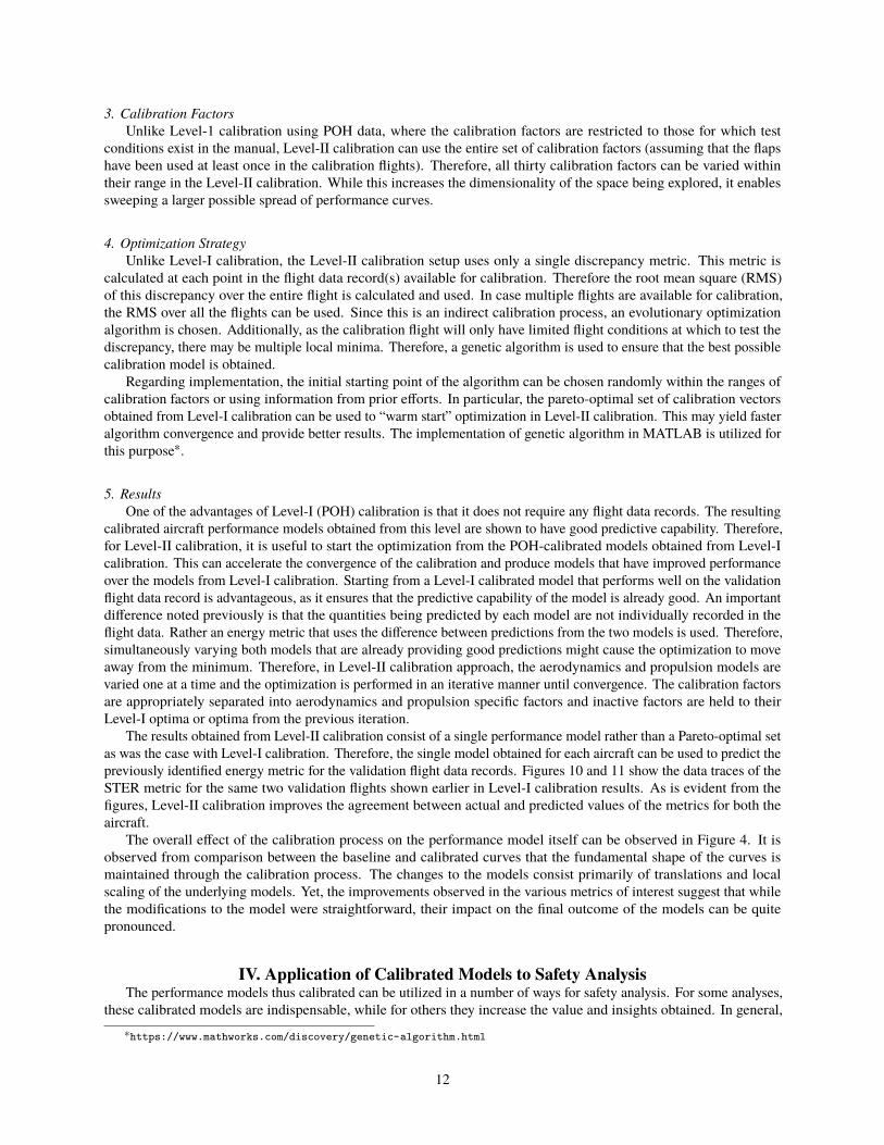
The results obtained from Level-II calibration consist of a single performance model rather than a Pareto-optimal setas was the case with Level-I calibration. Therefore, the single model obtained for each aircraft can be used to predict thepreviously identified energy metric for the validation flight data records. Figures 10 and 11 show the data traces of theSTER metric for the same two validation flights shown earlier in Level-I calibration results. As is evident from thefigures, Level-II calibration improves the agreement between actual and predicted values of the metrics for both theaircraft.

The overall effect of the calibration process on the performance model itself can be observed in Figure 4. It isobserved from comparison between the baseline and calibrated curves that the fundamental shape of the curves ismaintained through the calibration process. The changes to the models consist primarily of translations and localscaling of the underlying models. Yet, the improvements observed in the various metrics of interest suggest that whilethe modifications to the model were straightforward, their impact on the final outcome of the models can be quitepronounced.

IV. Application of Calibrated Models to Safety AnalysisThe performance models thus calibrated can be utilized in a number of ways for safety analysis. For some analyses,

these calibrated models are indispensable, while for others they increase the value and insights obtained. In general,∗https://www.mathworks.com/discovery/genetic-algorithm.html

12

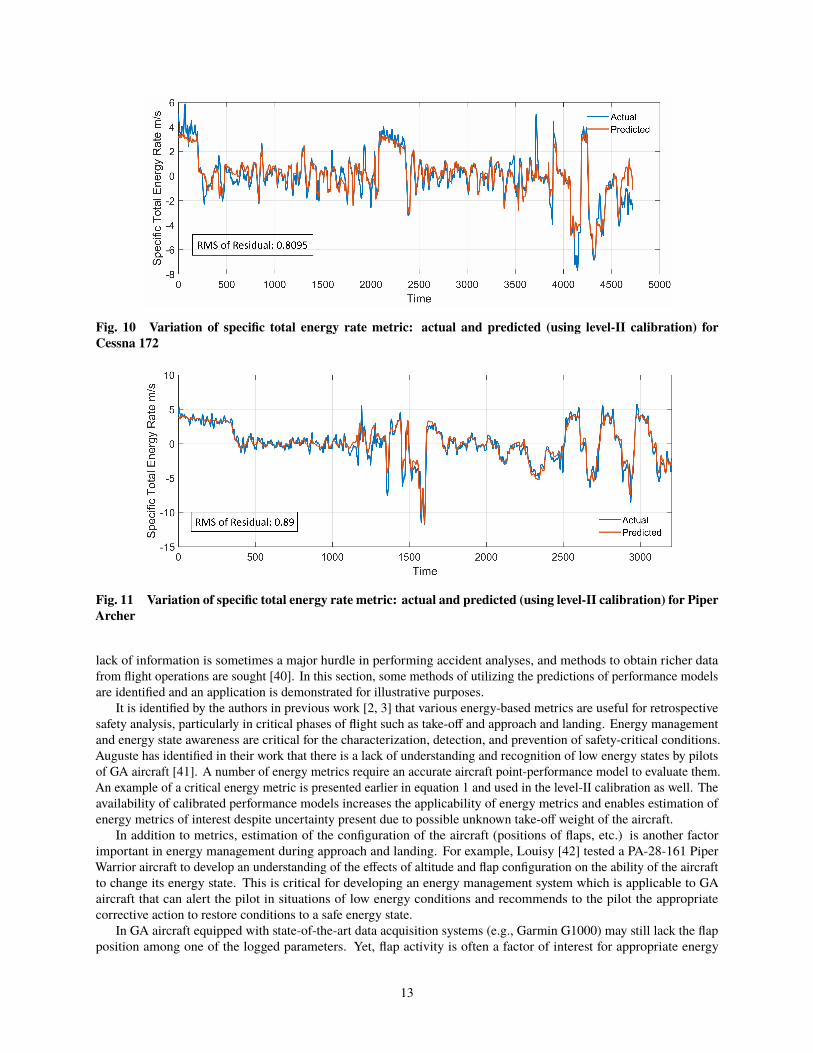
Fig. 10 Variation of specific total energy rate metric: actual and predicted (using level-II calibration) forCessna 172

Fig. 11 Variation of specific total energy rate metric: actual and predicted (using level-II calibration) for PiperArcher

lack of information is sometimes a major hurdle in performing accident analyses, and methods to obtain richer datafrom flight operations are sought [40]. In this section, some methods of utilizing the predictions of performance modelsare identified and an application is demonstrated for illustrative purposes.

It is identified by the authors in previous work [2, 3] that various energy-based metrics are useful for retrospectivesafety analysis, particularly in critical phases of flight such as take-off and approach and landing. Energy managementand energy state awareness are critical for the characterization, detection, and prevention of safety-critical conditions.Auguste has identified in their work that there is a lack of understanding and recognition of low energy states by pilotsof GA aircraft [41]. A number of energy metrics require an accurate aircraft point-performance model to evaluate them.An example of a critical energy metric is presented earlier in equation 1 and used in the level-II calibration as well. Theavailability of calibrated performance models increases the applicability of energy metrics and enables estimation ofenergy metrics of interest despite uncertainty present due to possible unknown take-off weight of the aircraft.

In addition to metrics, estimation of the configuration of the aircraft (positions of flaps, etc.) is another factorimportant in energy management during approach and landing. For example, Louisy [42] tested a PA-28-161 PiperWarrior aircraft to develop an understanding of the effects of altitude and flap configuration on the ability of the aircraftto change its energy state. This is critical for developing an energy management system which is applicable to GAaircraft that can alert the pilot in situations of low energy conditions and recommends to the pilot the appropriatecorrective action to restore conditions to a safe energy state.

In GA aircraft equipped with state-of-the-art data acquisition systems (e.g., Garmin G1000) may still lack the flapposition among one of the logged parameters. Yet, flap activity is often a factor of interest for appropriate energy

13

management as shown by Louisy [42]. Therefore, the ability to infer the flap position from flight data records (if notdirectly logged) with reasonable accuracy is desirable. Flap position may be estimated using point performance modelsin conjunction with energy metrics. Using calibrated performance models, the accuracy of this estimation capabilitycan be further enhanced. For example, in Figures 12 and 13, the flap position is inferred using performance modelsobtained from Level-I and Level-II calibration for the Cessna 172 and Piper Archer aircraft respectively.

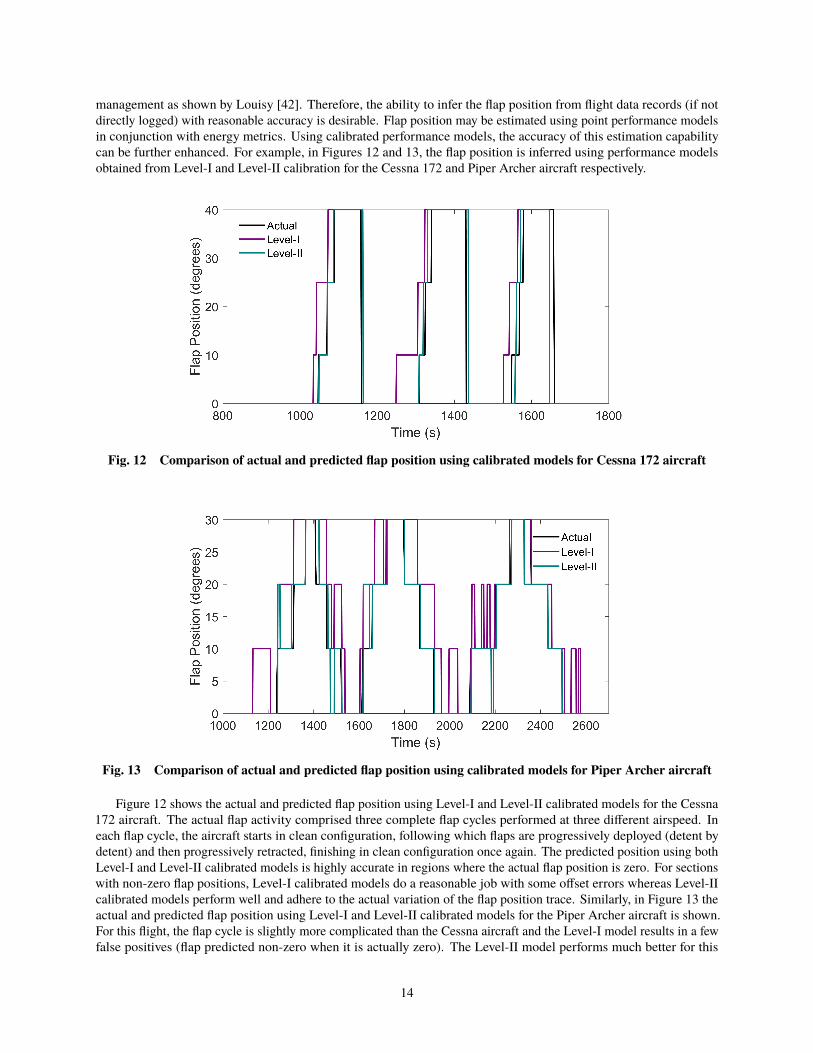
Fig. 12 Comparison of actual and predicted flap position using calibrated models for Cessna 172 aircraft

Fig. 13 Comparison of actual and predicted flap position using calibrated models for Piper Archer aircraft

Figure 12 shows the actual and predicted flap position using Level-I and Level-II calibrated models for the Cessna172 aircraft. The actual flap activity comprised three complete flap cycles performed at three different airspeed. Ineach flap cycle, the aircraft starts in clean configuration, following which flaps are progressively deployed (detent bydetent) and then progressively retracted, finishing in clean configuration once again. The predicted position using bothLevel-I and Level-II calibrated models is highly accurate in regions where the actual flap position is zero. For sectionswith non-zero flap positions, Level-I calibrated models do a reasonable job with some offset errors whereas Level-IIcalibrated models perform well and adhere to the actual variation of the flap position trace. Similarly, in Figure 13 theactual and predicted flap position using Level-I and Level-II calibrated models for the Piper Archer aircraft is shown.For this flight, the flap cycle is slightly more complicated than the Cessna aircraft and the Level-I model results in a fewfalse positives (flap predicted non-zero when it is actually zero). The Level-II model performs much better for this

14

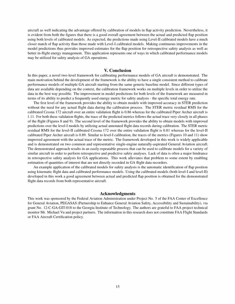
aircraft as well indicating the advantage offered by calibration of models in flap activity prediction. Nevertheless, itis evident from both the figures that there is a good overall agreement between the actual and predicted flap positionusing both levels of calibrated models. As expected, the predictions made using Level-II calibrated models have a muchcloser match of flap activity than those made with Level-I calibrated models. Making continuous improvements in themodel predictions thus provides improved estimates for the flap position for retrospective safety analysis as well asbetter in-flight energy management. This application represents one of ways in which calibrated performance modelsmay be utilized for safety analysis of GA operations.

V. ConclusionIn this paper, a novel two-level framework for calibrating performance models of GA aircraft is demonstrated. Themain motivation behind the development of the framework is the ability to have a single consistent method to calibrateperformance models of multiple GA aircraft starting from the same generic baseline model. Since different types ofdata are available depending on the context, the calibration framework works on multiple levels in order to utilize thedata in the best way possible. The improvement in model predictions for both levels of the framework are measured interms of its ability to predict a frequently used energy metric for safety analysis - the specific total energy rate.

The first level of the framework provides the ability to obtain models with improved accuracy in STER predictionwithout the need for any actual flight data during the calibration process. The STER metric residual RMS for thecalibrated Cessna 172 aircraft over an entire validation flight is 0.86 whereas for the calibrated Piper Archer aircraft is1.11. For both these validation flights, the trace of the predicted metrics follows the actual trace very closely in all phasesof the flight (Figures 8 and 9). The second level of the framework provides the ability to obtain models with improvedpredictions over the level-I models by utilizing actual annotated flight data records during calibration. The STER metricresidual RMS for the level-II calibrated Cessna 172 over the entire validation flight is 0.81 whereas for the level-IIcalibrated Piper Archer aircraft is 0.89. Similar to level-I calibration, the traces of the metrics (Figures 10 and 11) showimproved agreement with the actual trace of the metric. The framework developed in this work is widely applicableand is demonstrated on two common and representative single-engine naturally-aspirated General Aviation aircraft.The demonstrated approach results in an easily-repeatable process that can be used to calibrate models for a variety ofsimilar aircraft in order to perform retrospective and predictive safety analyses. Lack of data is often a major hindrancein retrospective safety analysis for GA applications. This work alleviates that problem to some extent by enablingestimation of quantities of interest that are not directly recorded in GA flight data recorders.

An example application of the calibrated models for safety analysis is the automatic identification of flap positionusing kinematic flight data and calibrated performance models. Using the calibrated models (both level-I and level-II)developed in this work a good agreement between actual and predicted flap position is obtained for the demonstratedflight data records from both representative aircraft.

AcknowledgmentsThis work was sponsored by the Federal Aviation Administration under Project No. 5 of the FAA Center of Excellencefor General Aviation, PEGASAS (Partnership to Enhance General Aviation Safety, Accessibility and Sustainability), viagrant No. 12-C-GA-GIT-018 to the Georgia Institute of Technology. The authors are grateful to FAA project technicalmonitor Mr. Michael Vu and project partners. The information in this research does not constitute FAA Flight Standardsor FAA Aircraft Certification policy.

15

Appendix: Description of Calibration Factors

Table 2 Description of Calibration Factors in Models

Model Factor Description Level-ICalibration

Level-IICalibration

Engine Engine de-rate factor X X

Propeller Vertical shift of airfoil sectional lift curve X X

Propeller Scaling of airfoil sectional lift curve slope X X

Propeller Scaling of airfoil sectional minimum drag X X

Propeller Scaling of airfoil sectional quadratic parameters X X

Propeller Scaling of airfoil sectional lift at min. drag X X

Propeller Slope shift of propeller pitch X X

Propeller Translational shift of propeller pitch X X

Propeller Scaling of propeller chord X X

Aero. Scaling of maximum lift coefficient for flap 0 X X

Aero. Scaling of maximum lift coefficient for flap 10 X X

Aero. Scaling of maximum lift coefficient for flap 20 X X

Aero. Scaling of maximum lift coefficient for flap 30 X X

Aero. Scaling of parasite drag factor for clean configuration X X

Aero. Scaling of induced drag factor for clean configuration X X

Aero. Drag polar shifting factor (CD,minL) for clean configuration X X

Aero. Scaling of parasite drag increment factor for flap 10 setting – – X

Aero. Scaling of induced drag increment factor for flap 10 setting – – X

Aero. Scaling of parasite drag increment factor for flap 20 setting – – X

Aero. Scaling of induced drag increment factor for flap 20 setting – – X

Aero. Scaling of parasite drag increment factor for flap 30 setting – – X

Aero. Scaling of induced drag increment factor for flap 30 setting – – X

Aero. Scaling of lift-curve slope for flap 0 setting X X

Aero. Scaling of lift-curve slope for flap 10 setting X X

Aero. Scaling of lift-curve slope for flap 20 setting X X

Aero. Scaling of lift-curve slope for flap 30 setting X X

Aero. Scaling of lift-curve intercept for flap 0 setting X X

Aero. Scaling of lift-curve intercept for flap 10 setting X X

Aero. Scaling of lift-curve intercept for flap 20 setting X X

Aero. Scaling of lift-curve intercept for flap 30 setting X X

References[1] “Federal Aviation Administration, 14 CFR §121.344 Digital Flight Data Recorders for Transport Category Airplanes,”

https://www.ecfr.gov/cgi-bin/text-idx?tpl=/ecfrbrowse/Title14/14cfr121_main_02.tpl, 2011.

[2] Puranik, T., Harrison, E., Min, S., Jimenez, H., and Mavris, D., “Energy-Based Metrics for General Aviation Flight Data RecordAnalysis,” 16th AIAA Aviation Technology, Integration, and Operations Conference, 2016, p. 3915. doi:10.2514/6.2016-3915,Paper No. AIAA 2016-3915.

16

[3] Puranik, T., Jimenez, H., and Mavris, D., “Energy-Based Metrics for Safety Analysis of General Aviation Operations,” Journalof Aircraft, Vol. 54, No. 6, 2017, pp. 2285–2297. doi:10.2514/1.C034196.

[4] Krajcek, K., Nikolic, D., and Domitrovic, A., “Aircraft Performance Monitoring from Flight Data,” Tehnicki vjesnik/TechnicalGazette, Vol. 22, No. 5, 2015. doi:10.17559/TV-20131220145918.

[5] Puranik, T. G., and Mavris, D. N., “Anomaly Detection in General-Aviation Operations Using Energy Metrics and Flight-DataRecords,” Journal of Aerospace Information Systems, Vol. 15, No. 1, 2018, pp. 22–35. doi:10.2514/1.I010582.

[6] Puranik, T. G., and Mavris, D. N., “Identification of Instantaneous Anomalies in General Aviation Operations using EnergyMetrics,” Journal of Aerospace Information Systems, Vol. Article in Advance, 2019. doi:10.2514/1.I010772.

[7] Puranik, T. G., Jimenez, H., and Mavris, D. N., “Utilizing Energy Metrics and Clustering Techniques to Identify AnomalousGeneral Aviation Operations,” AIAA SciTech Forum, 2017, p. 0789. doi:10.2514/6.2017-0789, Paper No. AIAA 2017-0789.

[8] Puranik, T. G., and Mavris, D. N., “Identifying Instantaneous Anomalies in General Aviation Operations,” 17th AIAA AviationTechnology, Integration, and Operations Conference, 2017, p. 3779. doi:10.2514/6.2017-3779, Paper No: AIAA-2017-3779.

[9] Harrison, E., Jimenez, H., and Mavris, D. N., “Investigation and Flight Dynamic Analysis of General Aviation Safety,” 16thAIAA Aviation Technology, Integration, and Operations Conference, American Institute of Aeronautics and Astronautics, 2016,p. 3108. doi:10.2514/6.2016-3108, Paper Number: AIAA 2016-3108.

[10] Harrison, E. D., “A Methodology for Predicting and Mitigating Loss of Control Incidents for General Aviation Aircraft,” Ph.D.thesis, Georgia Institute of Technology, 2018. URL http://hdl.handle.net/1853/60802.

[11] Min, S., “A Proactive Safety Enhancement Methodology for General Aviation Using a Synthesis of Aircraft Performance Modelsand Flight Data Analysis,” Ph.D. thesis, Georgia Institute of Technology, 2018. URL http://hdl.handle.net/1853/60807.

[12] Puranik, T. G., “A Methodology for Quantitative Data-driven Safety Assessment for General Aviation,” Ph.D. thesis, GeorgiaInstitute of Technology, 2018. URL http://hdl.handle.net/1853/59905.

[13] “National Transportation Safety Board Accident Statistics for 2013,” http://www.ntsb.gov/investigations/data/Pages/AviationDataStats.aspx, 2019. Retrieved: 10/2019.

[14] Harrison, E., Min, S., Jimenez, H., and Mavris, D. N., “Implementataion and Validation of an Internal Combustion Engineand Propeller Model for General Aviation Aircraft Performance Studies,” 15th AIAA Aviation Technology, Integration, andOperations Conference, American Institute of Aeronautics and Astronautics, 2015, p. 2850. doi:10.2514/6.2015-2850, PaperNo. AIAA-2015-2850.

[15] Min, S., Harrison, E., Jimenez, H., and Mavris, D. N., “Development of Aerodynamic Modeling and Calibration Methods forGeneral Aviation Aircraft Performance Analysis - a Survey and Comparison of Models,” AIAA Aviation, American Institute ofAeronautics and Astronautics, 2015, p. 2853. doi:10.2514/6.2015-2853, Paper No. AIAA 2015-2853.

[16] Payan, A. P., Gavrilovski, A., Jimenez, H., and Mavris, D. N., “Improvement of Rotorcraft Safety Metrics Using PerformanceModels and Data Integration,” Journal of Aerospace Information Systems, Vol. 14, No. 1, 2016, pp. 1–14. doi:10.2514/1.I010467.

[17] Oberkampf, W. L., and Barone, M. F., “Measures of Agreement Between Computation and Experiment: Validation Metrics,”Journal of Computational Physics, Vol. 217, No. 1, 2006, pp. 5–36. doi:10.1016/j.jcp.2006.03.037.

[18] AIAA, Guide for the Verification and Validation of Computational Fluid Dynamics Simulations, American Institute ofAeronautics and Astronautics, 1998 AIAA G-077-1998, 1998. doi:10.2514/4.472855.

[19] Oberkampf, W. L., and Roy, C. J., Verification and Validation in Scientific Computing, Cambridge University Press, 2010.doi:10.1017/CBO9780511760396, Cambridge Books Online.

[20] Jategaonkar, R., Flight Vehicle System Identification: a Time Domain Methodology, Vol. 216, AIAA, Reston, VA, USA, 2006.doi:10.2514/4.102790.

[21] Kennedy, M. C., and O’Hagan, A., “Bayesian Calibration of Computer Models,” Journal of the Royal Statistical Society: SeriesB (Statistical Methodology), Vol. 63, No. 3, 2001, pp. 425–464. doi:10.1111/1467-9868.00294.

[22] Roy, C. J., and Oberkampf, W. L., “A Comprehensive Framework for Verification, Validation, and Uncertainty Quantificationin Scientific Computing,” Computer methods in applied mechanics and engineering, Vol. 200, No. 25, 2011, pp. 2131–2144.doi:10.1016/j.cma.2011.03.016.

17

[23] Puranik, T., Harrison, E., Min, S., Jimenez, H., and Mavris, D., “General Aviation Approach and Landing Analysis Using FlightData Records,” 16th AIAA Aviation Technology, Integration, and Operations Conference, 2016, p. 3913. doi:10.2514/6.2016-3913, Paper No. AIAA 2016-3913.

[24] Federal Aviation Administration, “General Aviation and Part 135 Activity Surveys - CY 2015,” https://www.faa.gov/data_research/aviation_data_statistics/general_aviation/CY2015/, November 2016.

[25] Gudmundsson, S., General Aviation Aircraft Design: Applied Methods and Procedures, Butterworth-Heinemann, 2013.doi:10.1016/C2011-0-06824-2.

[26] Drela, M., “XFOIL: An Analysis and Ddesign System for Low Reynolds Number Airfoils,” Low Reynolds number aerodynamics,Springer, 1989, pp. 1–12. doi:10.1007/978-3-642-84010-4_1.

[27] Betz, A., “Airscrews With Minimum Energy Loss,” Tech. rep., Report, Kaiser Wilhelm Institute for Flow Research, 1919.

[28] Goldstein, S., and Prandtl, L., “On the Vortex Theory of Screw Propellers,” Proceedings of the Royal Society of Lon-don. Series A, Containing Papers of a Mathematical and Physical Character, Vol. 123, No. 792, 1929, pp. 440–465.doi:10.1098/rspa.1929.0078.

[29] Theodorsen, T., Theory of propellers, McGraw-Hill Book Company, 1948.

[30] Anon., Information Manual: Cessna Skyhawk SP, 1st ed., Pilot Operating Handbook, Model 172S NAV III GFC 700 AFCS,Cessna Aircraft Company, 2007.

[31] Roskam, J., Airplane Design, Part VI: Preliminary Calculation of Aerodynamic, Thrust and Power Characteristics, RoskamAviation and Engineering corporation, Kansas, 1987.

[32] Rajaram, D., Cai, Y., Puranik, T. G., Chakraborty, I., and Mavris, D. N., “Integrated Sizing and Multi-objective Optimization ofAircraft and Subsystem Architectures in Early Design,” 17th AIAA Aviation Technology, Integration, and Operations Conference,2017, p. 3067. doi:10.2514/6.2017-3067.

[33] Deb, K., Pratap, A., Agarwal, S., and Meyarivan, T., “A Fast and Elitist Multiobjective Genetic Algorithm: NSGA-II,” IEEEtransactions on evolutionary computation, Vol. 6, No. 2, 2002, pp. 182–197. doi:10.1109/4235.996017.

[34] Longmuir, M., and Ahmed, N. A., “Commercial Aircraft Exterior Cleaning Optimization,” Journal of Aircraft, Vol. 46, No. 1,2009, pp. 284–290. doi:10.2514/1.38472.

[35] Rutowski, E. S., “Energy Approach to the General Aircraft Performance Problem,” Journal of the Aeronautical Sciences(Institute of the Aeronautical Sciences), Vol. 21, No. 3, 1954, pp. 187–195. doi:10.2514/8.2956.

[36] Takahashi, T., “Aircraft Concept Design Performance Visualization Using an Energy-Maneuverability Presentation,” AIAAAviation Technology, Integration, and Operations (ATIO) Conferences, 2012, p. 5704. doi:10.2514/6.2012-5704, Paper No.AIAA-2012-5704.

[37] Boyd, J. R., Christie, T. P., and Gibson, J. E., “Energy Maneuverability,” Air Proving Ground Center Report (APGC-TR-66-4),Vol. 1, 1966.

[38] Merkt, J. R., “Flight Energy Management Training: Promoting Safety and Efficiency,” Journal of Aviation Technology andEngineering, Vol. 3, No. 1, 2013, pp. 24–36. doi:10.7771/2159-6670.1072.

[39] Amelink, M. H., Mulder, M., Van Paassen, M., and Flach, J., “Theoretical Foundations for a Total Energy-based Per-spective Flight-path Display,” The International Journal of Aviation Psychology, Vol. 15, No. 3, 2005, pp. 205–231.doi:10.1207/s15327108ijap1503_1.

[40] Gavrilovski, A., Jimenez, H., Mavris, D. N., Rao, A. H., Shin, S., Hwang, I., and Marais, K., “Challenges and Opportunitiesin Flight Data Mining: A Review of the State of the Art,” AIAA SciTech Forum, American Institute of Aeronautics andAstronautics, 2016, p. 0923. doi:10.2514/6.2016-0923, Paper No: AIAA 2016-0923.

[41] Auguste, Y. F., “Comparing Specific Excess Power of General Aviation Aircraft,” Master’s thesis, Florida Institute of Technology,2018. URL http://hdl.handle.net/11141/2777.

[42] Louisy, T. M., “Investigating the Effects of Altitude and Flap Setting on the Specific Excess Power of a PA-28-161 PiperWarrior,” Master’s thesis, Florida Institute of Technology, 2019. URL http://hdl.handle.net/11141/3038.

18