HAL Id: tel-02885754https://tel.archives-ouvertes.fr/tel-02885754

Submitted on 1 Jul 2020

HAL is a multi-disciplinary open accessarchive for the deposit and dissemination of sci-entific research documents, whether they are pub-lished or not. The documents may come fromteaching and research institutions in France orabroad, or from public or private research centers.

L’archive ouverte pluridisciplinaire HAL, estdestinée au dépôt et à la diffusion de documentsscientifiques de niveau recherche, publiés ou non,émanant des établissements d’enseignement et derecherche français ou étrangers, des laboratoirespublics ou privés.

AI-driven Detection, Characterization and Classificationof Chronic Lung Diseases

Guillaume Chassagnon

To cite this version:Guillaume Chassagnon. AI-driven Detection, Characterization and Classification of Chronic LungDiseases. Signal and Image processing. Université Paris Saclay (COmUE), 2019. English. �NNT :2019SACLC101�. �tel-02885754�

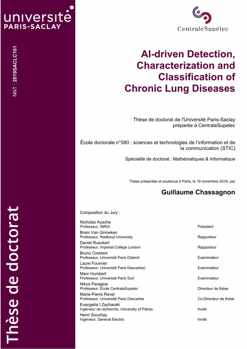
AI-driven Detection, Characterization and

Classification of Chronic Lung Diseases

Thèse de doctorat de l'Université Paris-Saclay préparée à CentraleSupelec

École doctorale n°580 : sciences et technologies de l’information et de la communication (STIC)

Spécialité de doctorat : Mathématiques & Informatique

Thèse présentée et soutenue à Paris, le 19 novembre 2019, par

Guillaume Chassagnon Composition du Jury : Nicholas Ayache Professeur, INRIA Président Bram Van Ginneken Professeur, Radboud University Rapporteur Daniel Rueckert Professeur, Imperial College London Rapporteur Bruno Crestani Professeur, Université Paris Diderot Examinateur Laure Fournier Professeur, Université Paris Descartes) Examinateur Marc Humbert Professeur, Université Paris Sud Examinateur Nikos Paragios Professeur, École CentraleSupelec Directeur de thèse Marie-Pierre Revel Professeur, Université Paris Descartes Co-Directeur de thèse Evangelia I Zacharaki Ingénieur de recherche, University of Patras Invité Henri Souchay Ingénieur, General Electric Invité

NN

T : 2

019S

AC

LC10

1

i

à Pierre Chassagnon (1954-2017)

ii

Acknowledgments

A mes deux directeurs de thèse

- Au professeur Revel. Merci Marie-Pierre de m’avoir pris sous ton aile, de me montrer la voie

et surtout de m’accompagner. Difficile d’imaginer meilleur mentor. Je profite de ces

quelques mots pour témoigner de mon admiration à la médecin hospitalo-universitaire

reconnue mais également à la femme que tu es. Je n’oublierai jamais ton amitié et ton

soutien, en particulier dans les moments difficiles.

- Au professeur Paragios. Je vous remercie d’avoir fait confiance à un radiologue pour faire

une thèse en intelligence artificielle. Au-delà de l’honneur, ça aura été un plaisir de travailler

avec vous est j’espère que cela pourra continuer. Je vous souhaite le meilleur ainsi qu’à votre

famille. Et surtout je vous souhaite le plus grand succès avec Therapanacea et si possible de

réussir à sauver l’humanité du cancer ;-)

To the members of my thesis committee,

- I would like to thank Prof. Bram Van Ginneken and Prof Daniel Rueckert for their valuable

reviewing my thesis. taking out time from your busy schedules.

- I would also like to thank Prof. Nicholas Ayache, Prof. Bruno Crestani, Prof. Laure Fournier

and Prof. Marc Humbert for accepting to be part of the jury. It is a great honor to have them in my jury.

A l’ensemble des personnels du Centre de Vision Numérique de CentraleSupelec et de Thérapanacea et en particulier :

- To Maria Vakalopoulou. It was a great pleasure to work with you and I am sure it will

continue. Thank you for your great help and your explanations. It was a pleasure to learn on

your side. Thank you for your friendship.

- To Eva Zacharaki. It was also a great pleasure to work with you. Thank you for having

initiated me to the art of programming and for your support in a painful period.

- A Rafael Marini. Merci pour ta grande aide pour la maitrise de python et l’utilisation de Drop.

Merci surtout pour ton amitié. J’espère que nous pourrons continuer à aller déjeuner

ensemble

- To Norbert Bus, thank you for your kindness and for the informatic support you provided

me during this thesis. I will try to never crash a machine again ;-)

- A Natalia et à Jana, merci pour votre gentillesse et votre efficacité. Merci Natalia pour ton

support dans une période difficile.

A General Electric Healthcare et en particulier à Henri Souchay, pour avoir soutenu ces travaux de recherches.

A l’équipe de l’UPRES EA-2511 et en particulier à Clémence Martin, Isabelle Fajac, Jennifer Sa Silva,

iii

Lucile Regard, Murielle Dambo et Pierre-Régis Burgel. Merci encore une fois à l’ensemble de l’équipe pour tous ces bons moments passés ensemble, pour cette collaboration enrichissante et pour tout ce qui fait qu’on a envie de continuer à travailler ensemble.

Aux docteurs Nghi Hoang, Charlotte Martin et Thomas Léger, les 3 étudiants de Master 2 qui se sont succédé au cours de cette thèse. Merci pour votre bonne humeur et votre implication dans nos projets de recherche. Continuez comme ça !

A mes collègues des équipes médicales et paramédicales de l’hôpital Cochin pour ces années passées et à venir de à travailler dans la bonne humeur au service des patients. En particulier, je voudrais remercier Anne-Laure Brun, Gaël Freche, Isabelle Parrain, Maxime Barat, Séverine Dangeard, Souhail Bennani et les internes pour l’ambiance qu’ils ont su créer et maintenir sein de l’unité d’imagerie thoracique.

A mes collègues cliniciens des services de pneumologie, de médecine interne et des explorations fonctionnelles pour le plaisir quotidien de travailler ensemble et pour leur aide et leurs précieux conseils dans nos travaux de recherche communs. En particulier, je remercie les professeurs Anh-Tuan Dinh-Xuan et Luc Mouthon ainsi que les docteurs Alexis Régent et Bertrand Dunogue pour leur précieuse collaboration aux travaux de recherche de cette thèse

A Mathilde, pour ton amour, ton intelligence, ta sensibilité, ton écoute, ton soutien et ta présence qui rendent plus belle chaque journée passée à tes côtés.

A toute ma famille et en particulier,

- A mes parents, Pierre et Brigitte. Merci pour tout ce que vous avez fait pour nous et pour votre générosité sans égale. Merci en particulier à mon père pour avoir su m’intéresser depuis mon plus jeune âge à tout ce qui est « technique ». Cette thèse t’est dédicacée.

- A Marianne et Juliette, mes sœurs, qui m’ont supporté toutes ces années, - A Kevin qui est la meilleure « pièce rapportée » que l’on puisse espérer, - A mes grands-parents Colette et Robert pour tout ce qu’ils m’ont donné sans que je puisse

jamais leur rendre et pour avoir si largement participé à la construction de mon identité, - A Christine, Minta et Antoine pour leur gentillesse et leur générosité de tous les instants, - A ma famille paternelle pour leur présence et leur soutien.

A la famille Méot pour m’avoir si bien accueilli parmi vous depuis plus de 10 ans, pour votre gentillesse et pour nos traditionnelles confrontations de point de vue aux déjeuners du dimanche,

A mes amis et en particulier

- A Jean Baptiste, l’ami de toujours et futur grand tibétologue, - A Anthony, Julien, et Nicolas pour ces années d‘amitié et de bonheur en région Centre, et

pour les années à venir, - A Samy et Volodia,

A tous les autres.

iv

Content

LIST OF ABBREVIATIONS ........................................................................................................................... 1

1 INTRODUCTION .................................................................................................................................. 2

1.1 CHRONIC LUNG DISEASES ....................................................................................................................... 3 1.1.1 SYSTEMIC SCLEROSIS .................................................................................................................................. 3 1.1.2 CYSTIC FIBROSIS ........................................................................................................................................ 4 1.2 INTRODUCTION TO MACHINE LEARNING AND ITS APPLICATIONS IN CHEST IMAGING ............................................. 6 1.2.1 TERMINOLOGY ......................................................................................................................................... 6 1.2.2 MAIN CONCEPTS REGARDING MACHINE LEARNING ALGORITHMS ....................................................................... 7 1.2.3 ARTIFICIAL INTELLIGENCE APPLIED TO CHEST RADIOGRAPH (CXR) READING ....................................................... 12 1.2.4 ARTIFICIAL INTELLIGENCE APPLIED TO CHEST CT READING ............................................................................... 14 1.3 INTRODUCTION TO ELASTIC REGISTRATION AND ITS APPLICATIONS IN CHEST IMAGING ........................................ 18 1.3.1 IMAGE REGISTRATION .............................................................................................................................. 18 1.3.2 ELASTIC REGISTRATION APPLIED TO CHEST IMAGING ...................................................................................... 20 1.4 THESIS OUTLINE & CONTRIBUTIONS ........................................................................................................ 20

2 FROM DIGITAL IMAGES TO BIOMARKERS .......................................................................................... 22

2.1 A THRESHOLDING APPROACH FOR AUTOMATED SCORING OF THE CYSTIC FIBROSIS LUNG ..................................... 24 2.1.1 BACKGROUND ........................................................................................................................................ 24 2.1.2 METHODOLOGY ...................................................................................................................................... 24 2.1.3 DATASET AND IMPLEMENTATION ............................................................................................................... 25 2.1.4 EXPERIMENTAL RESULTS ........................................................................................................................... 27 2.1.5 DISCUSSION ........................................................................................................................................... 33 2.2 EVALUATION OF THE THRESHOLDING APPROACH FOR AUTOMATED SEVERITY SCORING OF LUNG DISEASE IN ADULTS WITH PRIMARY CILIARY DYSKINESIA ................................................................................................................. 34 2.2.1 BACKGROUND ........................................................................................................................................ 34 2.2.2 METHODOLOGY ...................................................................................................................................... 34 2.2.3 DATASET AND IMPLEMENTATION ............................................................................................................... 35 2.2.4 EXPERIMENTAL RESULTS ........................................................................................................................... 37 2.2.5 DISCUSSION ........................................................................................................................................... 41 2.3 CT-BASED QUANTIFICATION OF LUNG DISEASE IN CYSTIC FIBROSIS USING RADIOMICS ...................................... 42 2.3.1 METHODOLOGY ...................................................................................................................................... 42 2.3.2 DATASET AND IMPLEMENTATION ............................................................................................................... 45 2.3.3 EXPERIMENTAL RESULTS ........................................................................................................................... 47 2.3.4 DISCUSSION ........................................................................................................................................... 51

3 INTERSTITIAL LUNG DISEASE SEGMENTATION USING DEEP LEARNING .............................................. 52

3.1 DEEP PATCH-BASED PRIORS UNDER A FULLY CONVOLUTIONAL ENCODER-DECODER ARCHITECTURE FOR INTERSTITIAL LUNG DISEASE SEGMENTATION ....................................................................................................................... 55 3.1.1 BACKGROUND ........................................................................................................................................ 55 3.1.2 METHODOLOGY ...................................................................................................................................... 55 3.1.3 DATASET AND IMPLEMENTATION DETAILS ................................................................................................... 57 3.1.4 EXPERIMENTAL RESULTS .......................................................................................................................... 58

v

3.1.5 DISCUSSION ........................................................................................................................................... 60 3.2 DEVELOPMENT OF A MULTI-ATLAS NON-LINEAR DEEP NETWORKS FOR MEDICAL IMAGE SEGMENTATION (ATLASNET) 61 3.2.1 BACKGROUND ........................................................................................................................................ 61 3.2.2 METHODOLOGY ...................................................................................................................................... 62 3.2.3 DATASET AND IMPLEMENTATION ............................................................................................................... 66 3.2.4 EXPERIMENTAL RESULTS .......................................................................................................................... 66 3.2.5 DISCUSSION ........................................................................................................................................... 69 3.3 AUTOMATED ASSESSMENT OF THE EXTENT OF INTERSTITIAL LUNG DISEASE IN SYSTEMIC SCLEROSIS PATIENTS: A DEEP LEARNING-BASED APPROACH ......................................................................................................................... 70 3.3.1 METHODOLOGY ...................................................................................................................................... 70 3.3.2 DATASET AND IMPLEMENTATION ............................................................................................................... 71 3.3.3 EXPERIMENTAL RESULTS ........................................................................................................................... 73 3.3.4 DISCUSSION ........................................................................................................................................... 79

4 MOTION AND REGISTRATION: EXPLOITING DYNAMICS FOR INTERSTITIAL LUNG DISEASE EVALUATION 80

4.1 USE OF ELASTIC REGISTRATION IN PULMONARY MRI FOR THE ASSESSMENT OF PULMONARY FIBROSIS IN SYSTEMIC SCLEROSIS PATIENTS .................................................................................................................................... 82 4.1.1 BACKGROUND ........................................................................................................................................ 82 4.2 METHODOLOGY ................................................................................................................................. 82 4.2.1 DATASET AND IMPLEMENTATION ............................................................................................................... 86 4.2.2 EXPERIMENTAL RESULTS ........................................................................................................................... 87 4.2.3 DISCUSSION ........................................................................................................................................... 90 4.3 ELASTIC REGISTRATION OF FOLLOW-UP CT SCANS FOR LONGITUDINAL ASSESSMENT OF INTERSTITIAL LUNG DISEASE IN SYSTEMIC SCLEROSIS .................................................................................................................................... 92 4.3.1 METHODOLOGY ...................................................................................................................................... 92 4.3.2 DATASET AND IMPLEMENTATION ............................................................................................................... 93 4.3.3 EXPERIMENTAL RESULTS ......................................................................................................................... 100 4.3.4 DISCUSSION ......................................................................................................................................... 102

5 GENERAL CONCLUSION ................................................................................................................... 104

5.1 CONTRIBUTIONS .............................................................................................................................. 104 5.2 FUTURE WORKS ............................................................................................................................... 105

6 GLOSSARY OF FORMULAS ............................................................................................................... 107

7 SYNTHESE ....................................................................................................................................... 108

8 REFERENCES ................................................................................................................................... 110

1

List of abbreviations

AI = artificial intelligence

AUC = area under the curve

BMI = body mass index

CAD = computer aided diagnosis CF = cystic fibrosis

CFTR = cystic fibrosis transmembrane regulator

CNN = convolutional neural network

CT = computed tomography

COPD = chronic obstructive pulmonary disease

CXR = chest radiograph

DLCO = carbon monoxide diffusing capacity

DLP = dose length product

DSC = Dice similarity coefficient

EGFR = epithelial growth factor receptor

ENET = elastic Net

FCN = fully connected network

FEV1 = forced expiratory volume in 1 second

FVC = forced vital capacity

GAN = generative adversarial networks

GPU = graphic processing units

HU = Hounsfield unit

ICC = intraclass correlation coefficient

ILD = interstitial lung disease

IQR = interquartile range

LASSO = least absolute shrinkage and selection operator

MLD = mean lung density

MRI = magnetic resonance imaging

NSIP = nonspecific interstitial pneumonia

PACS = picture archiving and communication systems

PCD = primary ciliary dyskinesia

PFT = pulmonary function testing

ReLU = rectified-linear units

RNN = recurrent neural networks

ROC = receiving operator characteristic

SD = standard deviation

SVM = support vector machine

UIP = usual interstitial pneumonia

2

Chapter 1

1 Introduction

Staging and monitoring of chronic lung diseases is of major importance for patient care as well as

for approval of new treatments. Monitoring of chronic lung diseases mainly relies on physiological

data such as pulmonary function testing (PFT). Among physiological variables, Forced Vital Capacity

(FVC) and Forced Expiratory Volume in 1 second (FEV1) are spirometry-derived parameters that are

often used as primary endpoint in clinical trials on restrictive and obstructive lung syndrome,

respectively. However, spirometry measurements only reflect lung function, not necessarily disease

activity. Furthermore, in some diseases such as cystic fibrosis, spirometry is reported to be less

sensitive than computed tomography (CT) for early detection of structural changes [1,2]. In addition,

small changes in spirometry-derived parameters in an individual are difficult to interpret due to

measurement variability [3]. Thus, recent literature suggests the need for a second outcome

variable to adjudicate whether small decrease in measured lung function represents true decline or

not [3]. Among the suggested second outcome variables, CT offers detailed morphological

assessment of the disease.

Morphological assessment is a key point for diagnosis and staging of many chronic lung diseases.

Among imaging techniques, CT is the gold standard for in vivo morphological assessment of lung

parenchyma and bronchi [4]. This technique currently offers the highest spatial resolution and thus

is widely used in chronic lung diseases. However, its use in clinical practice as an endpoint in clinical

trials remains controversial. The use of magnetic resonance imaging (MRI) for pulmonary evaluation

is limited by the lack of hydrogen protons in the lungs, although recent improvements of MRI

technique are promising [5]. MRI has lower spatial resolution than CT but can provide additional

dynamic and functional information.

There are several limitations to the use of imaging endpoints in clinical trials, such as the lack of

standardization of the acquisition protocols and the radiation dose due to CT. There are also

objective quantification issues. Visual methods are currently the most commonly used for severity

scoring on imaging, but they suffer from poor standardization, complexity of use and lack of expert

availability [4,6]. These drawbacks can be addressed by the development of objective quantitative

scoring methods, but to date quantitative assessment is mainly restricted to CT density-based

quantification of emphysema [7]. Several new quantitative approaches have been proposed,

especially for idiopathic pulmonary fibrosis and chronic obstructive pulmonary disease outside

emphysema [4,8]. These approaches mainly use histogram analysis, airway segmentation or texture

analysis [4,8–10]. However, their use is limited by the heterogeneity of the acquisition protocols,

the CT manufacturer dependence of image characteristics and by the influence of physiological

variables such as the level of inspiration on lung attenuation [4]. Thus, a lot of work remains to be

done for the development of new imaging biomarkers in chronic lung diseases.

3

1.1 Chronic lung diseases

Chronic lung diseases can be related to interstitial, bronchial or vascular changes. In this thesis,

systemic sclerosis (SSc) and cystic fibrosis (CF) were used as models for interstitial lung disease (ILD)

and bronchial disease, respectively.

1.1.1 Systemic sclerosis SSc known as scleroderma, is a chronic connective tissue disorder having a prevalence of 100 to 260

cases per million inhabitants in Europe and in the United States [11] and an incidence of 0.3 to 2.8

per 100,000 individuals per year [12]. The disease is characterized by tissue fibrosis,

microvasculopathy and autoimmunity. It involves multiple organs including the skin, the lungs, the

heart, the gastrointestinal and genitourinary tracts and the musculoskeletal system. Pulmonary

involvement is found at autopsy in 70 to 100% of the cases and represents the main cause of

morbidity and mortality [13]. Two types of lung involvement are observed: ILD due to tissue fibrosis,

and less frequently pulmonary hypertension related to microvasculopathy and/or advanced lung

fibrosis [13]. Most of SSc-related ILD phenotypes (76%) are represented by nonspecific interstitial

pneumonia (NSIP) that typically manifests on CT as reticulations, ground-glass opacities and traction

bronchiectasis with basal and peripheral predominance [11] (Figure 1.1). Usual interstitial

pneumonia (UIP) is less frequently encountered (11%) [11].

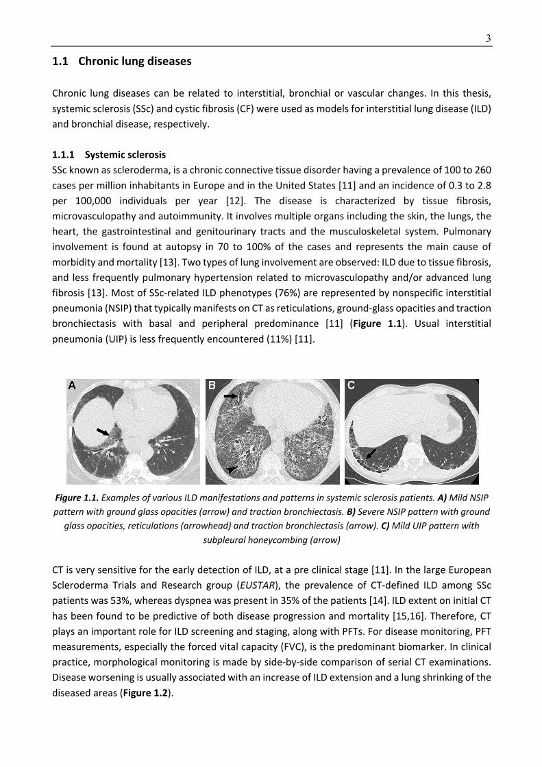
Figure 1.1. Examples of various ILD manifestations and patterns in systemic sclerosis patients. A) Mild NSIP pattern with ground glass opacities (arrow) and traction bronchiectasis. B) Severe NSIP pattern with ground

glass opacities, reticulations (arrowhead) and traction bronchiectasis (arrow). C) Mild UIP pattern with subpleural honeycombing (arrow)

CT is very sensitive for the early detection of ILD, at a pre clinical stage [11]. In the large European

Scleroderma Trials and Research group (EUSTAR), the prevalence of CT-defined ILD among SSc

patients was 53%, whereas dyspnea was present in 35% of the patients [14]. ILD extent on initial CT

has been found to be predictive of both disease progression and mortality [15,16]. Therefore, CT

plays an important role for ILD screening and staging, along with PFTs. For disease monitoring, PFT

measurements, especially the forced vital capacity (FVC), is the predominant biomarker. In clinical

practice, morphological monitoring is made by side-by-side comparison of serial CT examinations.

Disease worsening is usually associated with an increase of ILD extension and a lung shrinking of the

diseased areas (Figure 1.2).

4

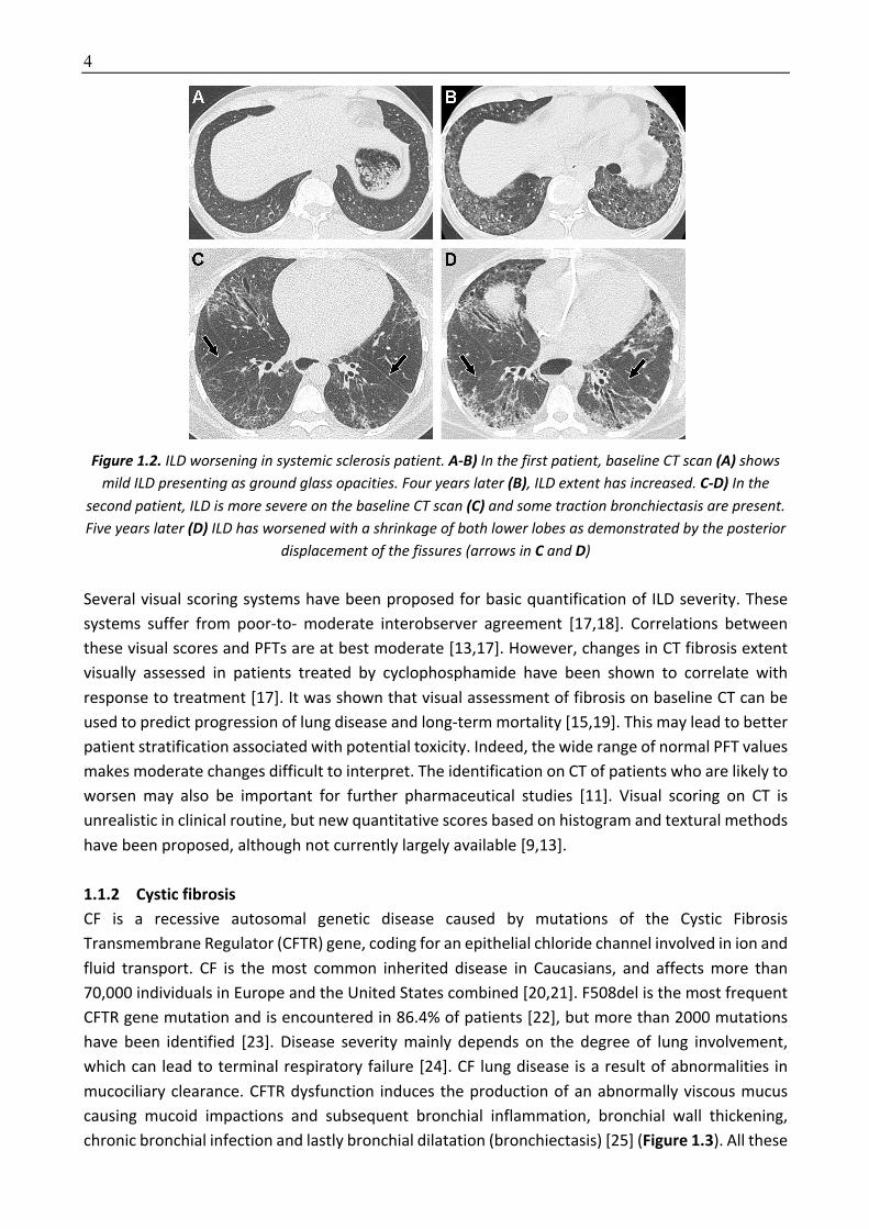
Figure 1.2. ILD worsening in systemic sclerosis patient. A-B) In the first patient, baseline CT scan (A) shows mild ILD presenting as ground glass opacities. Four years later (B), ILD extent has increased. C-D) In the

second patient, ILD is more severe on the baseline CT scan (C) and some traction bronchiectasis are present. Five years later (D) ILD has worsened with a shrinkage of both lower lobes as demonstrated by the posterior

displacement of the fissures (arrows in C and D)

Several visual scoring systems have been proposed for basic quantification of ILD severity. These

systems suffer from poor-to- moderate interobserver agreement [17,18]. Correlations between

these visual scores and PFTs are at best moderate [13,17]. However, changes in CT fibrosis extent

visually assessed in patients treated by cyclophosphamide have been shown to correlate with

response to treatment [17]. It was shown that visual assessment of fibrosis on baseline CT can be

used to predict progression of lung disease and long-term mortality [15,19]. This may lead to better

patient stratification associated with potential toxicity. Indeed, the wide range of normal PFT values

makes moderate changes difficult to interpret. The identification on CT of patients who are likely to

worsen may also be important for further pharmaceutical studies [11]. Visual scoring on CT is

unrealistic in clinical routine, but new quantitative scores based on histogram and textural methods

have been proposed, although not currently largely available [9,13].

1.1.2 Cystic fibrosis CF is a recessive autosomal genetic disease caused by mutations of the Cystic Fibrosis

Transmembrane Regulator (CFTR) gene, coding for an epithelial chloride channel involved in ion and

fluid transport. CF is the most common inherited disease in Caucasians, and affects more than

70,000 individuals in Europe and the United States combined [20,21]. F508del is the most frequent

CFTR gene mutation and is encountered in 86.4% of patients [22], but more than 2000 mutations

have been identified [23]. Disease severity mainly depends on the degree of lung involvement,

which can lead to terminal respiratory failure [24]. CF lung disease is a result of abnormalities in

mucociliary clearance. CFTR dysfunction induces the production of an abnormally viscous mucus

causing mucoid impactions and subsequent bronchial inflammation, bronchial wall thickening,

chronic bronchial infection and lastly bronchial dilatation (bronchiectasis) [25] (Figure 1.3). All these

5

morphological changes can be depicted on CT and authors have demonstrated that CT is more

sensitive than PFTs for their early detection, as well as for monitoring mild disease progression [1,2].

Morphological changes on CT are also correlated with clinical endpoints such as survival [26], quality

of life [2] and exacerbation rate [1,27].

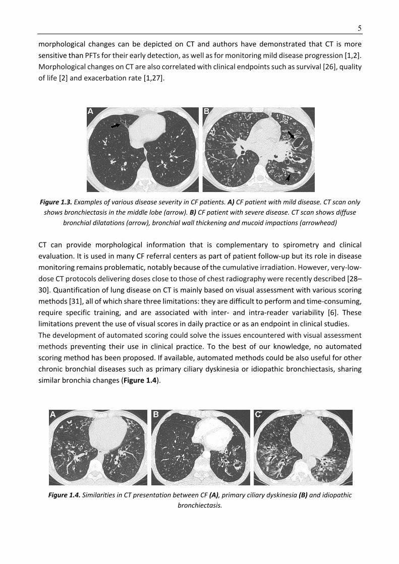
Figure 1.3. Examples of various disease severity in CF patients. A) CF patient with mild disease. CT scan only shows bronchiectasis in the middle lobe (arrow). B) CF patient with severe disease. CT scan shows diffuse

bronchial dilatations (arrow), bronchial wall thickening and mucoid impactions (arrowhead)

CT can provide morphological information that is complementary to spirometry and clinical

evaluation. It is used in many CF referral centers as part of patient follow-up but its role in disease

monitoring remains problematic, notably because of the cumulative irradiation. However, very-low-

dose CT protocols delivering doses close to those of chest radiography were recently described [28–

30]. Quantification of lung disease on CT is mainly based on visual assessment with various scoring

methods [31], all of which share three limitations: they are difficult to perform and time-consuming,

require specific training, and are associated with inter- and intra-reader variability [6]. These

limitations prevent the use of visual scores in daily practice or as an endpoint in clinical studies.

The development of automated scoring could solve the issues encountered with visual assessment

methods preventing their use in clinical practice. To the best of our knowledge, no automated

scoring method has been proposed. If available, automated methods could be also useful for other

chronic bronchial diseases such as primary ciliary dyskinesia or idiopathic bronchiectasis, sharing

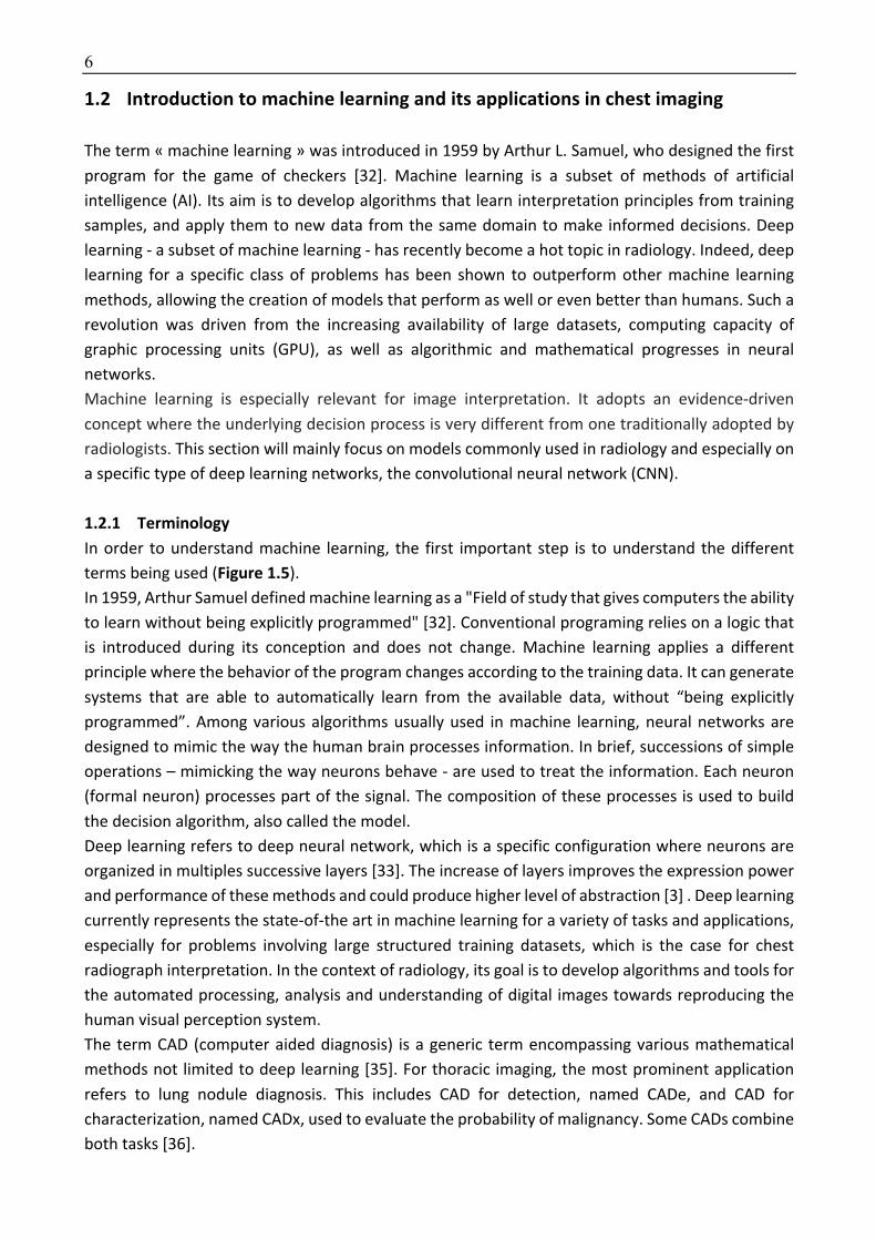
similar bronchia changes (Figure 1.4).

Figure 1.4. Similarities in CT presentation between CF (A), primary ciliary dyskinesia (B) and idiopathic bronchiectasis.

6

1.2 Introduction to machine learning and its applications in chest imaging

The term « machine learning » was introduced in 1959 by Arthur L. Samuel, who designed the first

program for the game of checkers [32]. Machine learning is a subset of methods of artificial

intelligence (AI). Its aim is to develop algorithms that learn interpretation principles from training

samples, and apply them to new data from the same domain to make informed decisions. Deep

learning - a subset of machine learning - has recently become a hot topic in radiology. Indeed, deep

learning for a specific class of problems has been shown to outperform other machine learning

methods, allowing the creation of models that perform as well or even better than humans. Such a

revolution was driven from the increasing availability of large datasets, computing capacity of

graphic processing units (GPU), as well as algorithmic and mathematical progresses in neural

networks.

Machine learning is especially relevant for image interpretation. It adopts an evidence-driven

concept where the underlying decision process is very different from one traditionally adopted by

radiologists. This section will mainly focus on models commonly used in radiology and especially on

a specific type of deep learning networks, the convolutional neural network (CNN).

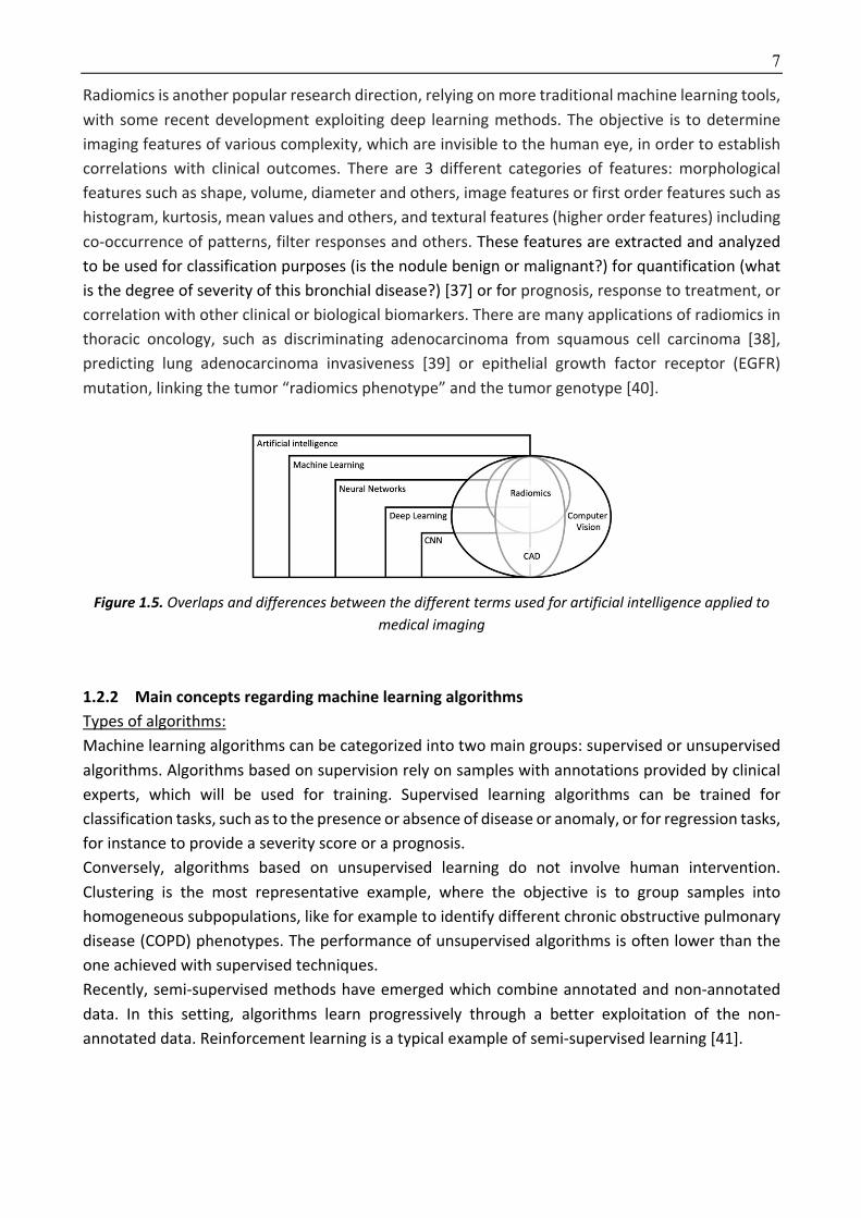
1.2.1 Terminology In order to understand machine learning, the first important step is to understand the different

terms being used (Figure 1.5).

In 1959, Arthur Samuel defined machine learning as a "Field of study that gives computers the ability

to learn without being explicitly programmed" [32]. Conventional programing relies on a logic that

is introduced during its conception and does not change. Machine learning applies a different

principle where the behavior of the program changes according to the training data. It can generate

systems that are able to automatically learn from the available data, without “being explicitly

programmed”. Among various algorithms usually used in machine learning, neural networks are

designed to mimic the way the human brain processes information. In brief, successions of simple

operations – mimicking the way neurons behave - are used to treat the information. Each neuron

(formal neuron) processes part of the signal. The composition of these processes is used to build

the decision algorithm, also called the model.

Deep learning refers to deep neural network, which is a specific configuration where neurons are

organized in multiples successive layers [33]. The increase of layers improves the expression power

and performance of these methods and could produce higher level of abstraction [3] . Deep learning

currently represents the state-of-the art in machine learning for a variety of tasks and applications,

especially for problems involving large structured training datasets, which is the case for chest

radiograph interpretation. In the context of radiology, its goal is to develop algorithms and tools for

the automated processing, analysis and understanding of digital images towards reproducing the

human visual perception system.

The term CAD (computer aided diagnosis) is a generic term encompassing various mathematical

methods not limited to deep learning [35]. For thoracic imaging, the most prominent application

refers to lung nodule diagnosis. This includes CAD for detection, named CADe, and CAD for

characterization, named CADx, used to evaluate the probability of malignancy. Some CADs combine

both tasks [36].

7

Radiomics is another popular research direction, relying on more traditional machine learning tools,

with some recent development exploiting deep learning methods. The objective is to determine

imaging features of various complexity, which are invisible to the human eye, in order to establish

correlations with clinical outcomes. There are 3 different categories of features: morphological

features such as shape, volume, diameter and others, image features or first order features such as

histogram, kurtosis, mean values and others, and textural features (higher order features) including

co-occurrence of patterns, filter responses and others. These features are extracted and analyzed

to be used for classification purposes (is the nodule benign or malignant?) for quantification (what

is the degree of severity of this bronchial disease?) [37] or for prognosis, response to treatment, or

correlation with other clinical or biological biomarkers. There are many applications of radiomics in

thoracic oncology, such as discriminating adenocarcinoma from squamous cell carcinoma [38],

predicting lung adenocarcinoma invasiveness [39] or epithelial growth factor receptor (EGFR)

mutation, linking the tumor “radiomics phenotype” and the tumor genotype [40].

Figure 1.5. Overlaps and differences between the different terms used for artificial intelligence applied to medical imaging

1.2.2 Main concepts regarding machine learning algorithms Types of algorithms:

Machine learning algorithms can be categorized into two main groups: supervised or unsupervised

algorithms. Algorithms based on supervision rely on samples with annotations provided by clinical

experts, which will be used for training. Supervised learning algorithms can be trained for

classification tasks, such as to the presence or absence of disease or anomaly, or for regression tasks,

for instance to provide a severity score or a prognosis.

Conversely, algorithms based on unsupervised learning do not involve human intervention.

Clustering is the most representative example, where the objective is to group samples into

homogeneous subpopulations, like for example to identify different chronic obstructive pulmonary

disease (COPD) phenotypes. The performance of unsupervised algorithms is often lower than the

one achieved with supervised techniques.

Recently, semi-supervised methods have emerged which combine annotated and non-annotated

data. In this setting, algorithms learn progressively through a better exploitation of the non-

annotated data. Reinforcement learning is a typical example of semi-supervised learning [41].

8

Data annotation:

Supervised algorithms rely on annotated data. There are different types of annotations depending

on the task that the algorithm seeks to address (Figure 1.6). For classification tasks (presence or

absence of anomaly or disease), images are simply labeled with two (disease positive or negative)

or more labels. For instance, ChestX-ray 8 database [42] contains around 110 000 chest

radiographies labeled as containing one or more of these eight anomalies: atelectasis, cardiomegaly,

effusion, infiltrates, mass, nodule, pneumonia, pneumothorax. The exact localization of the anomaly

is not provided within the image. This is also referred as a weakly annotated database. Even though

the annotation does not include exact localization, some algorithm might automatically learn to

predict the anatomical position of the anomaly.

The next level of annotation usually refers to a sparse way of providing information [43] or with

boundary boxes indicating the regions of interest [44]. Segmentation tasks require the highest level

of annotation which consists in contouring/delineating the anomalies on each image. This type of

annotation allows building more precise algorithms but is tedious and time consuming. Such

datasets are generally smaller and more difficult to generate.

Figure 1.6. Different types of annotations. In weak annotation, images are simply labeled (nodule = yes or no) and exact localization of the anomaly is not provided. In sparse annotation, a bounding box is drawn

around the nodule, whereas in segmentation the nodule contour is delineated (white area).

Database/dataset:

For machine learning, the quality of data is essential and could be even more important than the

learning algorithm itself. It guarantees the capacity for the model to perform equally well on cases

not seen during training. For obtaining a generalizable model, it is important to have a dataset that

is representative of the disease and also representative of the different acquisition techniques. In

radiology, datasets must include the different acquisition protocols, the various forms of the

evaluated disease and also include examinations from disease-free subjects. A model for lung

fibrosis detection should be trained using a dataset reflecting the heterogeneity of lung fibrosis

patterns but also including normal CT scans, and CT images acquired on various CT manufacturers.

If the training dataset only contains a unique fibrosis pattern or acquisitions all performed on the

same CT unit with the same reconstruction protocol, the risk for the model to be poorly

generalizable is high.

9

The dataset is usually split in three subcategories, training, validation and testing. The training set -

usually corresponding to 60% of the database- is used to train variant versions of the model with

different initialization conditions and model optimization parameters. Once the models have been

trained, their performance is evaluated using 20% of the remaining data, composing what is called

the validation dataset. The model with the best performance on the validation dataset is selected.

This model is finally evaluated using the last 20% of samples, which were never previously used and

compose the test dataset.

An alternative to the dataset splitting between training and validation is the method of k-fold cross

validation which allows training and validating using the entire dataset. This approach is especially

useful when the number of cases is limited. It consists of splitting the training and validation sets to

several random splits with the same proportion of samples and then repeat the training on them.

The average performance of the model on these splits is taken into account to judge the model

performance and acceptability.

Data Preprocessing:

Data preprocessing is not limited to the decomposition of the dataset into training, validation and

test. Images have to be “normalized” before being fed to the machine learning algorithm. Various

degrees of pre-processing can be applied, such as normalization of the physical resolution involving

slice thickness and voxel size and/or normalization of the grey-level distributions to follow

predefined distribution and/or image denoising [45]. Radiomics studies involve features selection,

which are either selected by humans with traditional machine learning techniques or automatically

identified when using deep learning. On the former case, the preprocessing step also involves the

choice of image features, among all 3 categories previously described, to feed the algorithm. Among

these features, the algorithm will select the most prominent ones with respect to the task, using

different possible techniques such as random forest, Lasso (Least Absolute Shrinkage and Selection

Operator), SVM (support vector machine), logistic regression and others.

Deep learning architectures

In radiology, three architectures are predominantly used.

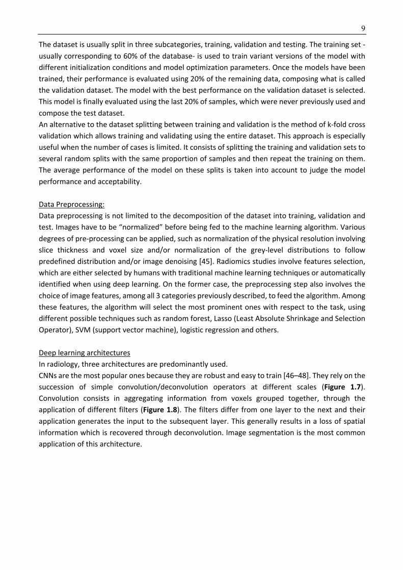
CNNs are the most popular ones because they are robust and easy to train [46–48]. They rely on the

succession of simple convolution/deconvolution operators at different scales (Figure 1.7).

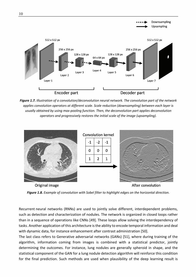
Convolution consists in aggregating information from voxels grouped together, through the

application of different filters (Figure 1.8). The filters differ from one layer to the next and their

application generates the input to the subsequent layer. This generally results in a loss of spatial

information which is recovered through deconvolution. Image segmentation is the most common

application of this architecture.

10

Figure 1.7. Illustration of a convolution/deconvolution neural network. The convolution part of the network applies convolution operators at different scale. Scale reduction (downsampling) between each layer is

usually obtained by using max-pooling function. Then, the deconvolution part applies deconvolution operators and progressively restores the initial scale of the image (upsampling).

Figure 1.8. Example of convolution with Sobel filter to highlight edges on the horizontal direction.

Recurrent neural networks (RNNs) are used to jointly solve different, interdependent problems,

such as detection and characterization of nodules. The network is organized in closed loops rather

than in a sequence of operations like CNNs [49]. These loops allow solving the interdependency of

tasks. Another application of this architecture is the ability to encode temporal information and deal

with dynamic data, for instance enhancement after contrast administration [50].

The last class refers to Generative adversarial networks (GANs) [51], where during training of the

algorithm, information coming from images is combined with a statistical predictor, jointly

determining the outcomes. For instance, lung nodules are generally spheroid in shape, and the

statistical component of the GAN for a lung nodule detection algorithm will reinforce this condition

for the final prediction. Such methods are used when plausibility of the deep learning result is

11

important to consider. Other architectures do not explicitly provide a statistical interpretation of

the results. On the contrary to CNNs and RNNs, GAN architectures are the hardest to train.

Hyper parameters, loss function and optimization strategy

The term hyper parameter refers to all parameters which are defined before training the algorithm,

by opposition to those which will derive from learning. Number and type vary according to the deep

learning architecture. Hyperparameters include the number of layers, the learning rate which

depends on the loss function and optimization strategy.

The loss function is an important concept to understand. It corresponds to the metrics used by the

algorithm during training to test its performance. It quantifies the gap between the prediction by

the algorithm and the ground truth given by the expert annotation/label. The objective of any deep

learning algorithm is always to minimize its loss function, until the discrepancy between the

prediction by the network and the ground truth vanishes. The loss function varies according to the

tasks which is addressed, such as the Dice similarity coefficient loss [52] for segmentation tasks or

the log loss for detection and classification tasks.

Several strategies can be used to optimize the loss function during training. The most commonly

used is the stochastic gradient descent [53]. Gradient descent methods rely on an iterative process

where every iteration allows moving closer to the optimal model. Stochastic gradient descent allows

random perturbation of the model that instantly could degrade its performance but finally converge

to a better solution.

The learning rate and the number of epochs are also important optimization parameters. The

learning rate controls the amount of improvement of the network between two iterations. Low

learning rates guaranty improvements, but of marginal importance. High learning rates refer to

more unstable models where improvement from one iteration to the next could be more significant,

associated with the risk of degrading the overall performance. Epoch is a different concept, which

refers to the number of times where the entire training set has been revisited to update the model

parameters. A highest number of epochs guaranties better performance on the training set, at the

cost of increasing computation complexity as well as the risk of overfitting, by selecting features

which are only specific to the training dataset and are poorly generalizable.

Overfitting and underfitting

Overfitting is the situation where the trained model performs very well on the training dataset but

fails on the testing set. Overfitting occurs when the model performance keeps improving in the

training cohort but decreases in the validation cohort. In other words, the model generates accurate

predictions on the training set, but fails to reproduce them on new unseen cases. This can be

observed when the training set is not well balanced or when the number of samples if not sufficient.

In this situation, it may happen that the algorithm finds an association of features and considers it

as relevant for the outcome, while it is only the result of fortuitous feature combinations learned

from a non-representative dataset. This association would disappear when using a larger or

different sample. Overfitting problems are common with deep learning algorithms containing many

layers generating lots of variables to learn (from several hundred to several millions) from small

training sets.

Another problem that can be seen during training is underfitting. It occurs when the model fails its

12

adaptation to both training and validation sets. The reasons of underfitting can be multiple. In

presence of multiple subpopulations within the training set, models with an insufficient number of

parameters will fail to encompass the entire population. Another possible explanation for

underfitting relates to the nature of the model that has been chosen for the prediction. For example,

when the notion of time is critical for diagnosis (delayed enhancement), a model that ignores this

information will most inevitably fail even if the number of parameters is sufficient.

In summary, overfitting is characterized by a high performance on the training dataset contrasting

with a poor performance on the validation dataset whereas underfitting is characterized by poor

performance in both training and validation datasets Figure 1.9).

Figure 1.9. Underfitting and overfitting. Underfitting is characterized by a high loss in both training and validation datasets, whereas overfitting is characterized by a low loss in the training dataset contrasting

with a high loss on the validation dataset.

1.2.3 Artificial intelligence applied to chest radiograph (CXR) reading The World Health Organization estimates that two thirds of the global population lack access to

imaging and radiology diagnostics [54]. Thoracic imaging techniques such as digital chest

radiography have the major advantage to be easy to use and affordable, even in developing or

underdeveloped areas. It consists of 2D images and several billions have already been stored on

picture archiving and communication systems (PACS) and linked to radiological reports. However,

there is a shortage of experts who can interpret chest radiographies, even when imaging equipment

is available, which opens tremendous perspectives for the impact of artificial intelligence applied to

thoracic imaging.

The first application of artificial intelligence is workflow optimization, by detecting CXR with possible

abnormalities that should be read first among all CXR of the work list. Using density and texture-

based features, [55] developed a CAD system to automatically determine abnormal chest

examinations in the work list of radiologists interpreting chest examinations. The turnaround time

for reporting abnormal CXR was reduced by 44%. CAD can be used for specific detection tasks on

chest radiograph, such as detection of tuberculosis, pneumonia or lung nodule, and even more

advances tasks such as multiple diseases detection are being developed as well [56].

Among specific detection tasks, a major application of CAD is the diagnosis of lung nodules on chest

13

radiography. This includes CAD for detection (CADe), and CAD for characterization (CADx) used to

evaluate the nodule probability of malignancy or a combination of them. Whereas radiomics is often

used for CADx, either using deep learning or classic machine learning techniques, the current

tendency for developing CADe tools is to use deep learning. Traditional pulmonary nodule CAD

systems include image preprocessing, nodule detection using various algorithms, extraction of

features and classification of the candidate lesions as nodules and non-nodules. The number of

selected features (intensity, shape, texture, size) and the classifiers (support vector machine, Fisher

linear discriminant and others) depend on the CAD system. The objective is to have adequate

sensitivity together with a low number of false positives detections. The development of

convolution neural networks has opened new perspectives but require large annotated chest

radiograph datasets.

Transfer learning could overcome this requirement. It consists on training algorithm non-medical,

everyday images on a large data set and initializing the network with its parameters on the smaller

medical image dataset. [57] pre trained a CNN model on a subset of the ImageNet dataset which

contains millions of labeled real-word images and retrained it to classify chest radiographs as

positive or negative for the presence of lung nodules with a sensitivity of 92% and a specificity of

86%.

More recently [58] developed a deep learning-based detection algorithm for malignant pulmonary

nodules on chest radiographs and compared its performance with that of physicians, with half of

them being radiologists. They used a dataset of 43 292 chest radiographs with a normal to diseased

ratio of 3.67. Using an external validation dataset, they found area under the curve (AUC) of the

developed algorithm was higher than that of 17 of the 18 physicians. All physicians showed

improved nodule detection when using the algorithm as second reader [58].

Automated detection of tuberculosis on chest radiographs is another important field of research.

Tuberculosis is an important cause of death worldwide, with a high prevalence in underdeveloped

areas where radiologists are lacking. Several approaches have been used to detect tuberculosis

manifestations in CXRs. Traditional machine learning approaches mainly used textural features, with

or without applying bone suppression as pre-treatment of CXR images. [59] used statistical features

in the image histogram to identify TB positive radiographs and reached an accuracy of 95.7%. Others

used a combination of textural, focal, and shape abnormality analysis [60]. In [61] a deep learning

algorithm for automated detection of active pulmonary tuberculosis on chest radiographs was

developed. Their solution outperformed physicians including thoracic radiologists. In [62] two CNNs

(AlexNet and GoogLeNet) pre-trained on non-medical images on a dataset of 1007 CXRs, with an

equivalent number of positive and negative tuberculosis cases. The AUC was 0.99 for the best

performing classifier combining the 2 pre-trained CNNs which were activated on areas of the lung

where the disease was present, in the upper lobes. However, as acknowledged by the authors, the

model was trained for a specific task, which was differentiating normal versus abnormal CXR

regarding tuberculosis suspicion. This limits the use of the algorithm to areas of high tuberculosis

prevalence and few mimickers, such as lung cancer also affecting the upper lung zones.

In addition to pulmonary nodules and tuberculosis there are acute conditions that can be detected

using such computer-aided solutions, like pneumonia. A deep learning algorithm for pneumonia

detection compared with performance to that of 4 radiologists, using F1 score metric was proposed

in [63]. Their model performed better than the averaged radiologists even though no better than

14

the best radiologist.

Beyond lung nodule detection or other specific detection tasks, detection of multiple abnormalities

is challenging but more in phase with the clinical practice, since frequently there are multiple

abnormalities in the chest radiographs.

Several large databases of annotated chest radiographies are publicly available. One of the largest

databases is chestX-ray8, already mentioned, built from the clinical PACS of the hospitals affiliated

to the National Institute of Health. This database includes 112,120 frontal views of 30,805 patients

and initially the image labels of 8 diseases, then extended to 14 diseases (chestX –ray14), including

atelectasis, consolidation, infiltration, pneumothorax, edema, emphysema, fibrosis, effusion,

pneumonia, pleural thickening, cardiomegaly, nodule, mass, and hernia.

In [64] the performance of Chexnet, trained on chestx-ray14 dataset was compared to the one of 9

radiologists on a validation set of 420 images containing examples of the pathology labels. The

radiologists achieved statistically significantly higher AUC performance on cardiomegaly,

emphysema, and hiatal hernia, whereas for other pathologies, AUCs reached with the algorithm

were either significantly higher (atelectasis) or with no statistically significant difference (other 10

pathologies).

In [65] a deep learning-based algorithm was developed to distinguish normal and abnormal chest

radiograph results, including malignant neoplasm, active tuberculosis, pneumonia, and

pneumothorax. The algorithm was trained on a dataset of 54 221 normal chest radiographs and

35 613 with abnormal findings. External validation using 486 normal and 529 abnormal chest

radiographs was performed. With a median 0.979 AUC, the algorithm demonstrated significantly

higher performance than non-radiology physicians, board-certified radiologists, and thoracic

radiologists. All improved when using the algorithm as second reader.

These results open new perspectives for radiologists and are very likely to modify our practice.

1.2.4 Artificial intelligence applied to chest CT reading The application of medical image analysis to thoracic CT is not a novel research area. CAD has been

used for automated lung nodule detection on CT. Early approaches at the beginning of the 2000’s

were based on traditional machine learning approaches, such as Support Vector Machines (SVMs).

Commercially available computer-aided detection packages were proposed by companies like

Siemens Healthineer (Erlangen, Germany), GE Healthcare (Milwaukee, WI, USA), R2 Technology

(Santa Clara, CA, USA) and others.

Even though none of the two large randomized lung cancer screening studies, NLST (National lung

cancer screening trial) [66] and NELSON [67] used CAD for lung nodule detection, an ancillary study

from the NELSON group, published in 2012 [68] compared CAD and double reading by radiologists,

in a cohort of 400 CT scans randomly selected from the NELSON database. The lung CAD algorithm

used in this study was commercial software from Siemens Healthineer, available since 2006

(LungCAD VB10A). Ground truth was established by a consensus reading from expert chest

radiologists. The sensitivity for lung nodule detection was 78.1% for double reading and 96.7% for

CAD, at an average cost of 3.7 false positive detections per examination. However, there were only

5 subsolid nodules (either non-solid or part-solid) in the 400 selected CT scans, and 2 of them were

not detected by CAD. Using another commercial CAD, only 50% of subsolid nodules were detected

at best with the highest sensitivity setting, at the average cost of 17 CAD marks per CT [69]. Visual

confirmation remains necessary for reducing false positives when using a CAD for the detection of

15

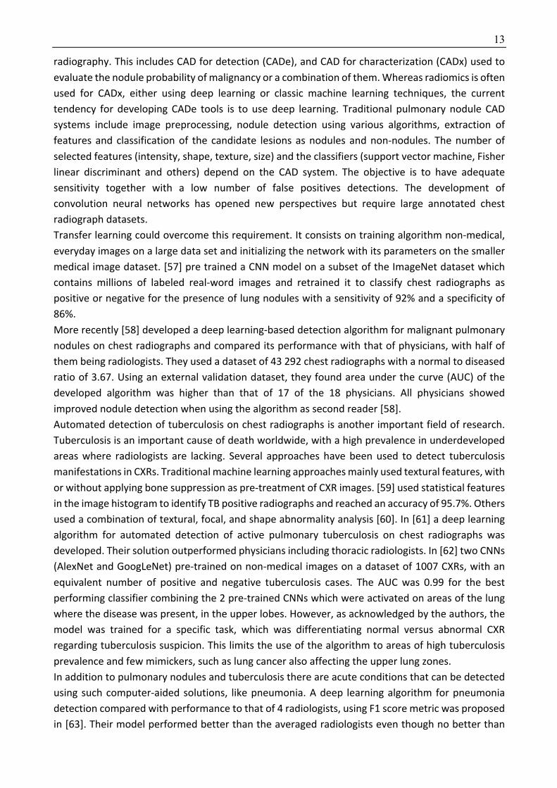
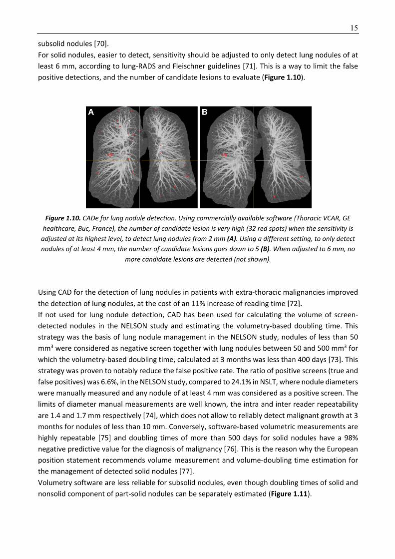
subsolid nodules [70].

For solid nodules, easier to detect, sensitivity should be adjusted to only detect lung nodules of at

least 6 mm, according to lung-RADS and Fleischner guidelines [71]. This is a way to limit the false

positive detections, and the number of candidate lesions to evaluate (Figure 1.10).

Figure 1.10. CADe for lung nodule detection. Using commercially available software (Thoracic VCAR, GE healthcare, Buc, France), the number of candidate lesion is very high (32 red spots) when the sensitivity is

adjusted at its highest level, to detect lung nodules from 2 mm (A). Using a different setting, to only detect nodules of at least 4 mm, the number of candidate lesions goes down to 5 (B). When adjusted to 6 mm, no

more candidate lesions are detected (not shown).

Using CAD for the detection of lung nodules in patients with extra-thoracic malignancies improved

the detection of lung nodules, at the cost of an 11% increase of reading time [72].

If not used for lung nodule detection, CAD has been used for calculating the volume of screen-

detected nodules in the NELSON study and estimating the volumetry-based doubling time. This

strategy was the basis of lung nodule management in the NELSON study, nodules of less than 50

mm3 were considered as negative screen together with lung nodules between 50 and 500 mm3 for

which the volumetry-based doubling time, calculated at 3 months was less than 400 days [73]. This

strategy was proven to notably reduce the false positive rate. The ratio of positive screens (true and

false positives) was 6.6%, in the NELSON study, compared to 24.1% in NSLT, where nodule diameters

were manually measured and any nodule of at least 4 mm was considered as a positive screen. The

limits of diameter manual measurements are well known, the intra and inter reader repeatability

are 1.4 and 1.7 mm respectively [74], which does not allow to reliably detect malignant growth at 3

months for nodules of less than 10 mm. Conversely, software-based volumetric measurements are

highly repeatable [75] and doubling times of more than 500 days for solid nodules have a 98%

negative predictive value for the diagnosis of malignancy [76]. This is the reason why the European

position statement recommends volume measurement and volume-doubling time estimation for

the management of detected solid nodules [77].

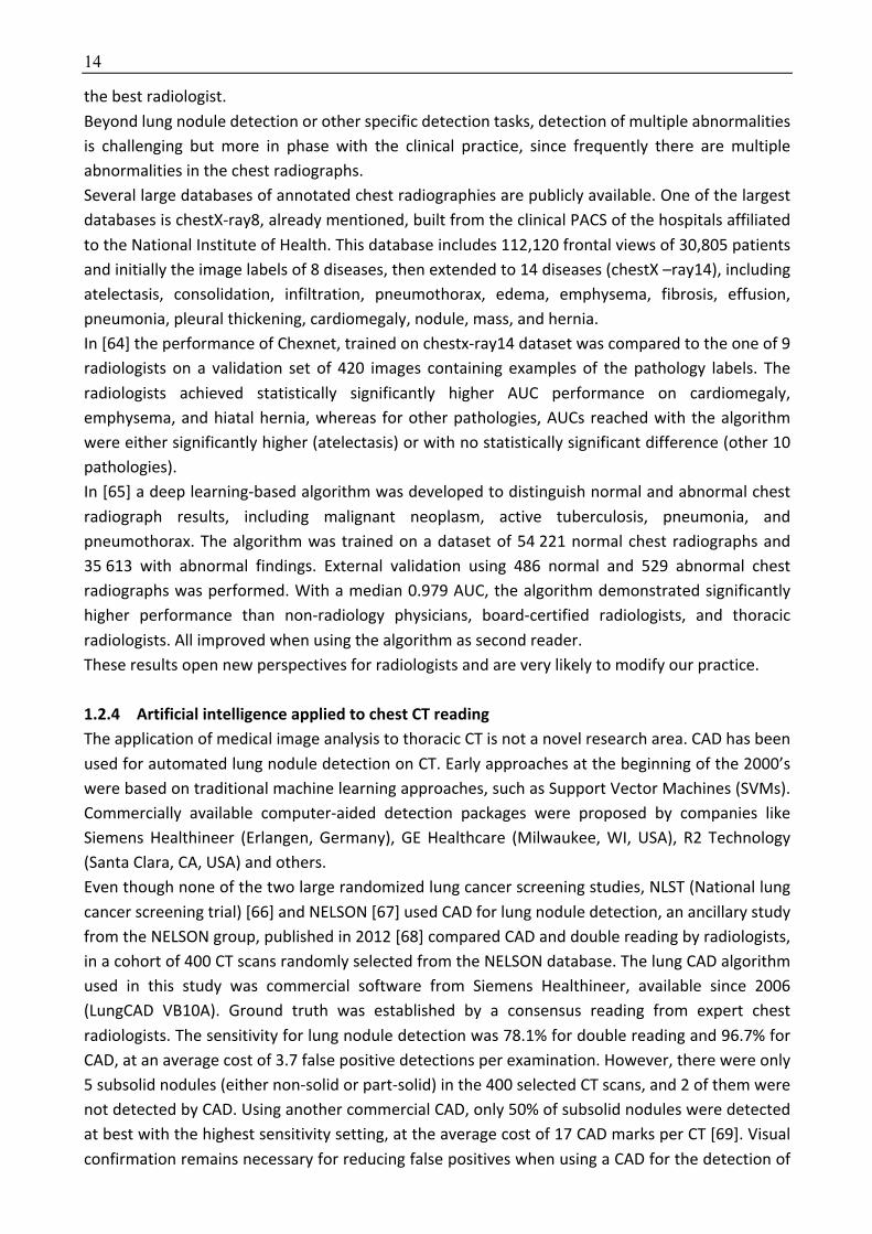
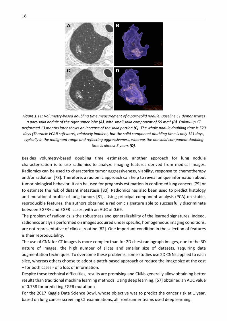
Volumetry software are less reliable for subsolid nodules, even though doubling times of solid and

nonsolid component of part-solid nodules can be separately estimated (Figure 1.11).

16

Figure 1.11: Volumetry-based doubling time measurement of a part-solid nodule. Baseline CT demonstrates

a part-solid nodule of the right upper lobe (A), with small solid component of 59 mm3 (B). Follow-up CT performed 13 months later shows an increase of the solid portion (C). The whole nodule doubling time is 529 days (Thoracic VCAR software), relatively indolent, but the solid component doubling time is only 121 days, typically in the malignant range and reflecting aggressiveness, whereas the nonsolid component doubling

time is almost 3 years (D).

Besides volumetry-based doubling time estimation, another approach for lung nodule

characterization is to use radiomics to analyze imaging features derived from medical images.

Radiomics can be used to characterize tumor aggressiveness, viability, response to chemotherapy

and/or radiation [78]. Therefore, a radiomic approach can help to reveal unique information about

tumor biological behavior. It can be used for prognosis estimation in confirmed lung cancers [79] or

to estimate the risk of distant metastasis [80]. Radiomics has also been used to predict histology

and mutational profile of lung tumors [81]. Using principal component analysis (PCA) on stable,

reproducible features, the authors obtained a radiomic signature able to successfully discriminate

between EGFR+ and EGFR- cases, with an AUC of 0.69.

The problem of radiomics is the robustness and generalizability of the learned signatures. Indeed,

radiomics analysis performed on images acquired under specific, homogeneous imaging conditions,

are not representative of clinical routine [82]. One important condition in the selection of features

is their reproducibility.

The use of CNN for CT images is more complex than for 2D chest radiograph images, due to the 3D

nature of images, the high number of slices and smaller size of datasets, requiring data

augmentation techniques. To overcome these problems, some studies use 2D CNNs applied to each

slice, whereas others choose to adopt a patch-based approach or reduce the image size at the cost

– for both cases - of a loss of information.

Despite these technical difficulties, results are promising and CNNs generally allow obtaining better

results than traditional machine learning methods. Using deep learning, [57] obtained an AUC value

of 0.758 for predicting EGFR mutation x.

For the 2017 Kaggle Data Science Bowl, whose objective was to predict the cancer risk at 1 year,

based on lung cancer screening CT examinations, all frontrunner teams used deep learning.

17

[83] trained a deep learning algorithm on a NLST dataset from 14851 patients, 578 of whom having

developed lung cancer within the next year. They then tested the model on a first test dataset of

6716 cases, achieving an AUC of 94,4%. Comparison to 6 radiologists was performed for a subset of

507 patients, and the model’ performance was equivalent or higher to all of them when a single CT

was analyzed, whereas performances were equivalent when the model and the radiologists made a

decision including patients’ previous CT scans.

The use of CNN for thoracic CT is not restricted to nodule evaluation but can also be applied to

diagnose and stage COPD and predict acute respiratory distress (ARD) and mortality in smokers [84].

Training a CNN on the CT scans of 7,983 COPDGene participants, AUC for the detection of COPD was

0.856 in a nonoverlapping cohort of 1000 another COPDGene participants. AUCs for ARD events

were 0.64 and 0.55 in COPDGene and ECLIPSE participants, respectively. Deep learning has also been

used for emphysema quantification based on X-ray images. The model obtained an AUC of 90.7%

for predicting an emphysema volume of at least 10% [85].

CNNs can also be used for the detection and quantification of infiltrative lung diseases (ILD) or for

automated classification of fibrotic lung diseases. Indeed, even though classification criteria have

been established by consensus of 4 expert societies inter radiologist agreement is only moderate at

best, even among experts, and there is a shortage of experts [86]. [87] trained a CNN algorithm for

automated classification of fibrotic lung disease on a database of 1157 high-resolution CT scans from

two institutions showing evidence of diffuse fibrotic lung disease. When comparing the model

performance with that of 91 radiologists, the model accuracy was 73.3% compared to a median

radiologist accuracy of 70.7%.

The majority of previous work on ILD pattern detection was based on 2D image classification using

a patch-based approach. This approach consists in dividing the lung into numerous small patches of

the same size (e.g., 32×32 pixels) and to classify them into one of the ILD pattern classes. Different

classifiers can be used, such as SVM, Boltzmann machines, CNNs local binary patterns and multiple

instance learning [88]. These classifiers are trained on datasets including thousands of annotated

patches, representatives of each class to identify, normal ground glass, honeycombing, emphysema.

Caliper software was developed using the patch-based approach, for the quantification of disease

extent and change in idiopathic pulmonary fibrosis [89,90]. The two advantages of this approach

are the possibility to separately quantify each anomaly, and the need for only week annotation (e.g.

categorization), which is less time consuming than semantic segmentation which requires precisely

contouring disease extent on CT images.

However – despite the great promises – the aforementioned deep learning methods inherit a

number of limitations as well. First, such methods do not integrate information about the

environment such as the subpleural location and basal predominance. In the central lung portion,

some bronchi may be misclassified as honeycombing, since there is no spatial information with the

patch-based approach. The results might be disappointing when the model is applied to the whole

CT image, in spite of good patch classification results in the test data set. Indeed, problematic

patches including more than one pattern are usually excluded from the training and test datasets,

similarly to frontier patches at the very lung periphery close to the chest wall or at the interface

between two different classes of anomaly.

Another approach is the segmentation of the whole fibrotic extent without quantifying each

component [91]. This requires contouring the abnormal fibrotic areas on every abnormal slices,

18

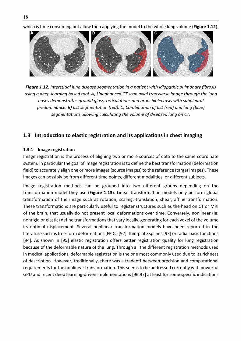
which is time consuming but allow then applying the model to the whole lung volume (Figure 1.12).

Figure 1.12. Interstitial lung disease segmentation in a patient with idiopathic pulmonary fibrosis using a deep-learning based tool. A) Unenhanced CT scan axial transverse image through the lung

bases demonstrates ground glass, reticulations and bronchiolectasis with subpleural predominance. B) ILD segmentation (red). C) Combination of ILD (red) and lung (blue)

segmentations allowing calculating the volume of diseased lung on CT.

1.3 Introduction to elastic registration and its applications in chest imaging

1.3.1 Image registration Image registration is the process of aligning two or more sources of data to the same coordinate

system. In particular the goal of image registration is to define the best transformation (deformation

field) to accurately align one or more images (source images) to the reference (target images). These

images can possibly be from different time points, different modalities, or different subjects.

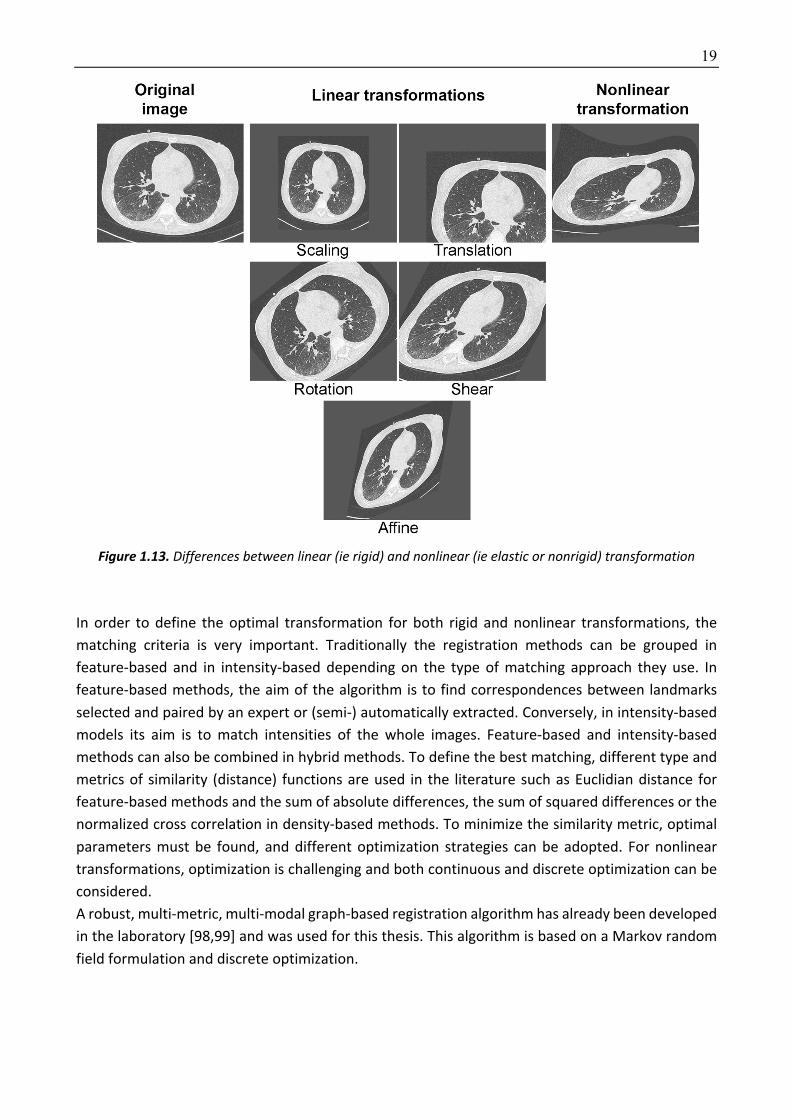
Image registration methods can be grouped into two different groups depending on the

transformation model they use (Figure 1.13). Linear transformation models only perform global

transformation of the image such as rotation, scaling, translation, shear, affine transformation.

These transformations are particularly useful to register structures such as the head on CT or MRI

of the brain, that usually do not present local deformations over time. Conversely, nonlinear (ie:

nonrigid or elastic) define transformations that vary locally, generating for each voxel of the volume

its optimal displacement. Several nonlinear transformation models have been reported in the

literature such as free-form deformations (FFDs) [92], thin-plate splines [93] or radial basis functions

[94]. As shown in [95] elastic registration offers better registration quality for lung registration

because of the deformable nature of the lung. Through all the different registration methods used

in medical applications, deformable registration is the one most commonly used due to its richness

of description. However, traditionally, there was a tradeoff between precision and computational

requirements for the nonlinear transformation. This seems to be addressed currently with powerful

GPU and recent deep learning-driven implementations [96,97] at least for some specific indications

19

Figure 1.13. Differences between linear (ie rigid) and nonlinear (ie elastic or nonrigid) transformation

In order to define the optimal transformation for both rigid and nonlinear transformations, the

matching criteria is very important. Traditionally the registration methods can be grouped in

feature-based and in intensity-based depending on the type of matching approach they use. In

feature-based methods, the aim of the algorithm is to find correspondences between landmarks

selected and paired by an expert or (semi-) automatically extracted. Conversely, in intensity-based

models its aim is to match intensities of the whole images. Feature-based and intensity-based

methods can also be combined in hybrid methods. To define the best matching, different type and

metrics of similarity (distance) functions are used in the literature such as Euclidian distance for

feature-based methods and the sum of absolute differences, the sum of squared differences or the

normalized cross correlation in density-based methods. To minimize the similarity metric, optimal

parameters must be found, and different optimization strategies can be adopted. For nonlinear

transformations, optimization is challenging and both continuous and discrete optimization can be

considered.

A robust, multi-metric, multi-modal graph-based registration algorithm has already been developed

in the laboratory [98,99] and was used for this thesis. This algorithm is based on a Markov random

field formulation and discrete optimization.

20

1.3.2 Elastic registration applied to chest imaging A major application of elastic registration in medical imaging is breathing motion tracking to reduce

dose and irradiation of normal tissue surrounding the tumor in radiotherapy. Indeed, lung

parenchyma is one of the most radiosensitive tissues in the thorax [100]. Additionally, motion may

potentially lead to underdosage to the tumor. To assess the lung deformation during respiration,

elastic registration should either be applied on end-inspiratory to end-expiratory images or on 4D

CT images acquired during a respiratory cycle [101]. Elastic registration between inspiratory and

expiratory images can be used to simulate 4D CT images [102].

In radiology, image registration has been evaluated for the diagnosis of lung cancer on serial chest

CT. Indeed, growth assessment is the most reliable noninvasive method to differentiate between

benign and malignant nodules. Several authors investigated the use of rigid or elastic registration to

re-localize the nodules on the baseline or on the follow-up CT examination [103–105]. [103]

reported a nodule matching accuracy of 81%. These results were improved in [104] where an

accuracy of 97% using a combination of feature-based and intensity-based transformations was

reported. Using a semi-rigid registration method, [105] reported a mean distance error of 1.4 ± 0.8

mm between paired nodules in 12 pairs of patient scans (97 nodules). As underlined this paper,

comparison between methods is challenging because of the use of proprietary datasets and of the

difficulty in precisely implementing a competing method.

In order to allow an independent comparison between registration algorithms on the same dataset

with algorithm parameters set by their designers, the EMPIRE10 (Evaluation of Methods for

Pulmonary Image Registration 2010) challenge was created in 2010 [106]. The deformation fields

were evaluated over four individual categories: lung boundary alignment, fissure alignment,

correspondence of manually annotated point pairs, and the presence of singularities in the

deformation field. This public challenge was based on a dataset of 30 pairs of thoracic CT. The

original challenge was launched in 2010 and 20 teams participated. Nine year later, the EMPIRE10

challenge remains open to new submissions.

In radiology, elastic registration has also been used to assess obstructive disease in COPD patients.

[107] combined elastic registration and density thresholds on inspiratory and expiratory images to

classify every lung voxel in 174 COPD patients from the COPDGene cohort. Their so called “response

parametric map” allowed to identify the extent of small airways disease and emphysema.

Additionally, it provided CT-based evidence supporting there is a continuum originating from

healthy lung, though functional small airways disease and ending at emphysema with increasing

COPD severity. More recently, an elastic registration method to assess lung elasticity on 4D chest

CT images in 13 patients with lung cancer treated by stereotaxic body radiation therapy was

proposed [108]. They found much lower lung elasticity in COPD compared to non-COPD patients.

They also showed that areas of low elasticity matched with areas of emphysema and that a

decreased lung elasticity was a better predictor than emphysema extent for COPD.

1.4 Thesis outline & contributions In the first part of this thesis (Chapter 2) we will focus on building biomarkers for bronchial diseases

and especially for cystic fibrosis. First, we developed a simple density-based CT scoring method for

evaluating high attenuating lung structural abnormalities in patients with CF. The developed score

correlated well with pulmonary function. The originality of our approach was the use of adapted

21

thresholds taking into account CT acquisition-dependent variations in lung density distribution. We

also applied this approach in a cohort of patients with primary ciliary dyskinesia and obtained again

good correlations with pulmonary function. Lastly, we used a radiomics approach to create a CT

score correlating with clinical prognosis scores for CF. Using 5 different machine learning methods,

we were able to create radiomics-based models showing moderate-to-good correlations with 2

clinical prognosis scores, FEV1 and the number of pulmonary exacerbations to occur in the next 12

months.

In the second part (Chapter 3), we will present our work on deep learning used to create a new

biomarker for ILD quantification in SSc. We first evaluated a combination of patched-based and fully-

convolutional encoder-decoder architectures for ILD segmentation. In this work, we created a

framework that integrates deep patch-based priors (trained on publicly available databases) with a

fully convolutional encoder-decoder network (trained on a small number of images). The

combination of the two architectures allowed to transfer the learned features across different

datasets and increased segmentation accuracy. Then we created a new architecture (AtlasNet)

combining elastic registration and encoder-decoder architecture to segment ILD. The concept is to

train a certain number of CNNs, each of the them using a predefined anatomy on which all training

cases are mapped through elastic registration, resulting in a natural data augmentation. This

method has the advantage to decrease the complexity of observations related to anatomical

variability and to increase the “anatomical” consistency of redundancies of the networks. AtlasNet

offered better performances than state-of-art methods for ILD segmentation on chest CT. Lastly, we

augmented the AtlasNet network through a dual auto-decoder architecture in order to guarantee

anatomically plausible disease segmentation results. We showed that this method performed better

than a U-net architecture and as well as radiologists for disease segmentation. The combination of

disease and lung segmentations allowed to calculate normalized ILD extent and we found that the

ILD extent provided by our model correlated well with PFTs, especially diffusing capacity for carbon

monoxide (DLCO), in a large cohort of SSC patients. Additionally, these correlations were confirmed

in an external validation cohort.

In the last part (Chapter 4), we will present our work on elastic registration used to diagnose and

monitor interstitial lung disease. First, we used elastic registration of inspiratory to expiratory lung

MR images for the assessment of pulmonary fibrosis in SSc patients and also evaluated healthy

volunteers. We observed major differences between patients with and without fibrosis. There was

a marked shrinkage of the lung bases during expiration in healthy volunteers and SSc patients

without fibrosis, which was not observed in SSc patients with pulmonary fibrosis. This loss of

elasticity affected the posterior part of the lung bases, which are known to be affected by fibrosis in

scleroderma patients. This work has been published in the Radiology Journal [109].

Then, we used a combination of elastic registration and deep learning to automatically diagnose ILD

worsening on serial CT scans of SSc patients. In SSc patients experiencing either morphological or

functional ILD worsening we observed lung shrinking in the posterior part of the lung bases on the

follow CT scan. This was not observed in other patients. Additionally, a deep learning using the

Jacobian maps as input was able to automatically detect focal lung shrinking and assess disease

progression with a high accuracy.

22

Chapter 2

2 From digital images to biomarkers

In this chapter, we will evaluate different approaches to create biomarkers correlating with disease

severity in bronchial diseases.

In cystic fibrosis (CF), lung morphological changes are known to modify CT density distribution. Most

CF-related morphological changes exhibit higher CT attenuation values than normal lung

parenchyma. This is especially the case of bronchial wall thickening and mucus plugging, both of

which are dramatically improved by new targeted therapies [110]. In [111] it was identified three

histogram shapes depending on the severity of lung disease in CF patients. Therefore, we

hypothesized that changes in lung densities could be used to create new imaging biomarkers and

could help evaluating response to treatment.

First, we developed a simple density-based CT scoring method for evaluating high attenuating lung

morphological changes in patients with CF [112]. By analogy with automated quantification of CT

low-attenuation areas in emphysema [113], we postulated that automated quantification of high-

attenuation structures in CF might objectively reflect disease severity and improvement under the

newly released therapies. The developed score correlated well with FEV1, which is a well-recognized

marker of functional severity that is often used as a surrogate for mortality in CF clinical studies.

One originality of our approach is the use of adapted thresholds taking into account CT acquisition-

dependent variations in lung density distribution. Indeed, as shown in this figure 2.1, the shape of

the histogram curves is different depending on the respiratory phase. Thus, any change in the

degree of inspiration is likely to influence the repartition of lung densities.

[112]

Next, we applied this approach to a cohort of patients with primary ciliary dyskinesia (PCD). PCD is

another bronchial disease with morphological changes close to those observed in CF. Using this

approach, we also obtained good correlation with FEV1. Additionally, we confirmed that the use of

adapted thresholds optimized the correlations with functional parameters compared to fixed

thresholds [114].

Finally, we evaluated the use of a classical radiomics approach to create a CT score correlating with

clinical prognosis scores for CF. Although radiomics has mainly been used to build diagnostic and

prognostic models in oncology [37,115–117], radiomic features from the whole lung can also be

used as biomarkers for evaluating the severity of diffuse lung diseases. Using 5 different machine

learning methods, we created radiomics-based models showing moderate-to-good correlations

with 2 CF clinical prognosis scores, as well as with FEV1 and the number of pulmonary exacerbations

to occur in the next 12 months. These results were validated in an external patient cohort.

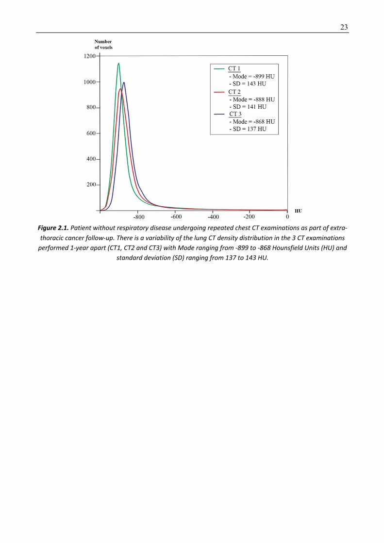
23

Figure 2.1. Patient without respiratory disease undergoing repeated chest CT examinations as part of extra-thoracic cancer follow-up. There is a variability of the lung CT density distribution in the 3 CT examinations

performed 1-year apart (CT1, CT2 and CT3) with Mode ranging from -899 to -868 Hounsfield Units (HU) and standard deviation (SD) ranging from 137 to 143 HU.

24

2.1 A thresholding approach for automated scoring of the cystic fibrosis lung

2.1.1 Background Although the CT attenuation of pulmonary structural abnormalities associated with CF differs from

that of normal lung, few attempts have been made to quantify CF-related pulmonary lesions in

terms of CT density distribution. Quantification of low-attenuation areas in order to assess air

trapping showed a good correlation with residual volume (RV) and maximum mid-expiratory flow

[118–121]. However, most of these correlations were weak, and the need to acquire expiratory

images in addition to standard inspiratory images raises concerns regarding the additional radiation

dose. Quantitative evaluation of airway disease in CF has also been previously performed with other

approaches, focusing on the analysis of airway size and geometry [10,122,123]. In [122] automated

airway analysis reported high negative correlations between enlarged airway dimensions and FEV1

in adults.

[111] has described a flattening of the lung parenchyma CT density distribution in CF patients with

severe lung impairment. By analogy with automated quantification of CT low-attenuation areas in

emphysema [113], we postulated that automated quantification of high-attenuation structures in

CF might objectively reflect disease severity and improvement under the newly released therapies.

The objective of this study was to develop an automated density-based CT scoring method for

evaluating high attenuating lung structural abnormalities in patients with CF.

2.1.2 Methodology The proposed method quantifies structural changes with high attenuation values (e.g. bronchial wall

thickening, mucus plugging/ bronchiolar nodules, consolidation, atelectasis) using a thresholding

approach. Quantification is performed after whole lung segmentation, which consists of separating

the lungs from the chest wall and mediastinum.

Four threshold values were tested (-300, -400, -500 and -600 Hounsfield units (HU)), as well as 10

adapted threshold values, taking into account, for each CT examination, individual histogram

features, namely mode –corresponding to the most highly represented attenuation value–, mean

lung density (MLD), and standard deviation (SD), which are known to be influenced by the

inspiratory level. Expiration flattens the density distribution curve and also shifts it towards higher

density values [118,124] (Figure 2.1). We hypothesized that adapted thresholds based on Mode or

MLD or integrating SD might compensate for the changes of density distribution related to the level

of inspiration.

The automated CT-Density score was expressed as the ratio between the high-attenuating

(diseased) lung volume and total lung volume. For instance, a CT-Density score value of 4 indicated

that 4% of the total lung volume had an attenuation value superior or equal to the threshold.

Our aim was to develop a score only requiring inspiratory images, to keep the CT radiation dose as

low as possible. Indeed, the report by [125] highlighted the increasing exposure to ionizing radiation

in patients with CF, being mainly attributable to CT scanning. This is the reason why we excluded

routinely acquiring expiratory CT images in our center.

25

2.1.3 Dataset and implementation Dataset

This multicenter two-phase retrospective study, including adult outpatients with CF, was approved

by the Paris Ile de France I ethics committee (ref 13.652). The need for informed consent was

waived. All the patient’s characteristics are summarized in Table 2.1.

The development phase involved CF patients from six French CF centers who had at least one gating

(class 3) mutation in the gene coding for the cystic fibrosis transmembrane conductance regulator

(CFTR) protein and who were treated with Ivacaftor, a new therapy correcting the protein

dysfunction in patients with gating mutations. Patients were eligible if they had had at least two

volumetric unenhanced chest CT exams, one before starting ivacaftor and at least one during

treatment, plus spirometric measurements performed within one month before or after each CT

exam, all performed from November 2010 through September 2015. A total of 45 CT scans (17

baseline + 28 follow-up CT scans) from 17 patients were evaluated. The improvement of visual score

in this development cohort has been reported in a previous paper [110].

The validation phase involved an independent cohort of CF patients not treated with ivacaftor. This

cohort included 53 CF outpatients who had unenhanced chest CT and spirometric measurements

performed on the same day at our adult CF reference center in 2013, as part of their routine follow-

up.

Exclusion criteria were the unavailability of CT images reconstructed with a soft kernel or a slice

thickness of more than 2 mm, or the use of contrast injection. Only CT examinations performed as

routine follow-up and outside an exacerbation phase were taken into account.

Table 2.1. Patient characteristics

Development cohort Validation cohort Number of patients 17 53

Age (y) 35 [28-43] 27 [24-33]

Sex, n (%)

Male 14 (82) 30 (57)

Female 3 (18) 23 (43)

FEV1 % predicted 38 [33-77] * 52 [38-68]

Note: Data are medians with interquartile ranges in brackets. The development cohort comprised 45 pre-therapeutic and follow-up chest CT scans of 17 adult CF patients treated with ivacaftor. The validation cohort was composed of 53 adult CF patients not treated with ivacaftor. * FEV1 values before treatment with ivacaftor FEV1 = forced expiratory volume in 1 second

Depending on the center, inspiratory chest CT examinations of the whole lung were obtained with

eight different 16-to-128 multislice CT devices from 4 different vendors (Somatom Sensation 16 and

Somatom Definition DS, Siemens Healthcare, Erlangen, Germany; Lightspeed VCT, Optima CT660

and Discovery HD750, GE Healthcare, Milwaukee, Wi; Ingenuity CT, Philips Healthcare, Best, The

Netherlands; Aquilion, Toshiba Medical System, Otawara, Japan).

Regarding the acquisition protocol, the tube voltage was 80, 100 or 120 kV, depending on body

weight, in 3 (3%), 37 (38%) and 58 (59%) cases, respectively. Images were reconstructed with a slice

26

thickness of 0.625 to 2 mm, with for each case, at least one set of images reconstructed with a

standard reconstruction algorithm. This was true for both pre-treatment and follow-up CT scans.

Median dose length product was 148mGy.cm (interquartile range, IQR=128-185mGy.cm). Iterative

reconstructions were used for some CT examinations. All CT acquisitions targeted the whole lung

volume. Respiratory gating was not used for CT acquisitions which were only acquired at full

inspiration without additional expiratory scanning, since it was not standard of care in the

participating CF centers. The percentage of predicted forced expiratory volume in 1 second (% predicted, FEV1%pred)

measured at the time of CT was used as an endpoint to assess the CT score performance for cross-

sectional evaluation in the two cohorts. Longitudinal evaluation was also performed in the

development cohort. Changes in FEV1%pred (ΔFEV1%pred) contemporary to each follow-up CT scan

were used to assess the performance of the visual and automated scores for patient follow-up. In

patients with more than two follow-up CT scans, the comparison was always performed with the

closest preceding simultaneous CT and functional examinations.

The development cohort included a median of two scans per patient (IQR=2-3) with a median

interval of 17 months between consecutive scans (IQR=12.5-21.7). The median FEV1%pred was 38%

before treatment (IQR=33-77) and increased by a median of +3.9% (predicted) between two

consecutive CT scans on treatment (IQR=-3-+8; range=-17-+28% predicted).

In the validation cohort, a single CT scan and the corresponding FEV1%pred value were evaluated

for each patient. The median FEV1%pred was 52% (IQR=38-68).

Implementation details

Image analysis and disease assessment were performed by 2 radiologists with 5 and 16 years of

experience in thoracic imaging, respectively.

CT images were scored blindly to clinical information and to the date of CT. Both automated and

visual scores were calculated.

Two commercially available lung-segmentation software programs were systematically used for

each CT, in order to later evaluate the lung segmentation software influence on the score results:

Myrian XP-lung software version 1.19.1 (Intrasense, Montpellier, France ;

http://www.intrasense.fr/myrian-clinical-apps/#lung-vessel-liver-abdofat) and Syngo.via Pulmo CT

software version VB1B (Siemens Healthineer ; https://www.siemens-healthineers.com/computed-

tomography/options-upgrades/clinical-applications/syngo-pulmo-ct). The central airways were not

included, contrary to intrapulmonary bronchi and pulmonary vessels.

Myrian lung segmentation was improved by systematically applying a sequence of basic

morphological operators, in an automated mode, and was optionally improved by additional manual

editing with 3D tools, especially to include peripheral consolidations when they had been excluded

from the initial lung segmentation.

Three sets of data were thus obtained for the development cohort: 1. lung segmentation with XP-lung software without manual editing (segmentation 1)

2. lung segmentation with XP-lung software with manual editing (segmentation 2)

3. lung segmentation with Pulmo CT software without manual editing (segmentation 3)

Only segmentation 1 was used for the validation cohort.

To compare with visual assessment of disease severity, images were visually scored using the

the CF-CT score, except that air trapping was not assessed because expiratory images were not

27

available [126]. The visual scores in the two cohorts were calculated by one radiologist who had

received one week of intensive training in a reference center (Lung Analysis, Erasmus Medical

Center, Rotterdam, The Netherlands) in order to achieve good intraobserver agreement in scoring.

Twenty-five CT scans from the development cohort were randomly selected to assess repeatability.

Intraobserver repeatability was evaluated for the visual score and the automated score based on

segmentation 2, which included manual editing, by two reading sessions performed at a one-month

interval. Interobserver repeatability was evaluated for the automated score based on segmentation

2. Repeatability was not assessed for the automated scores based on segmentation 1 or 3, which

did not include manual editing.

The time required to obtain the visual and automated scores was measured in the development

cohort. The percentage of predicted forced expiratory volume in 1 second (% predicted, FEV1%pred)

measured at the time of CT was used as an endpoint to assess the CT score performance for cross-

sectional evaluation in the two cohorts. Longitudinal evaluation was also performed in the

development cohort. Changes in FEV1%pred (ΔFEV1%pred) contemporary to each follow-up CT scan

were used to assess the performance of the visual and automated scores for patient follow-up. In

patients with more than two follow-up CT scans, the comparison was always performed with the

closest preceding simultaneous CT and functional examinations.

2.1.4 Experimental results Spearman's rank correlation coefficient (R) was used to judge the correlation between the CT scores

and FEV1%pred, and the correlation between changes in the CT scores (Δscores) and changes in

FEV1%pred (ΔFEV1%pred). Spearman R values were interpreted as follows: <0.4 = absent to weak

correlation, 0.40-0.59 = moderate correlation, 0.60-0.79 = good correlation, >0.8 = strong

correlation.

The statistical significance of changes in the CT scores and FEV1%pred values between baseline and

last follow-up was evaluated with the Wilcoxon test.

The intraclass correlation coefficient (ICC) and Bland-Altman plots were used to assess repeatability.

Excellent repeatability was assumed when the ICC was 0.8 or more.

Cross-sectional correlation in the development cohort

All CT scans (2 to 4 per patient) with contemporary FEV1%pred values were analyzed for cross-

sectional correlations between the CT scores and FEV1%pred in the development cohort (Table 2.2).

Using segmentation 1, the median values of mode and SD were -912 HU (IQR=-899 to -912 HU) and

170 HU (IQR= 150-183 HU), respectively. All automated CT-Density scores based on adapted

thresholds showed moderate to good correlations with FEV1%pred (R=-0.55 to -0.68, P<0.001),

while those based on fixed thresholds led to weaker correlations (R=-0.43 to -0.57, P≤0.004). The

highest correlation coefficient values were obtained when using Mode+3SD as the threshold (R=-

0.61 to -0.68, depending on the segmentation method, P<0.001). This was also true when

considering only the initial CT for each patient (R= -0.71 to -0.85, P≤0.005).

28

Table 2.2. Cross-sectional correlations between CT-density scores and FEV1%pred

Development cohort Validation cohort Segmentation 1

(17 patients, n=45 CT)

Segmentation 2 (17 patients,

n=45 CT)

Segmentation 3 (17 patients, n=38 CT *)

Segmentation 1 (53 patients,

n=53 CT) Threshold R P value R P value R P value R P value Fixed thresholds

(-) 300 HU -0.54 <0.001 -0.48 <0.001 -0.46 0.004 -0.51 <0.001

(-) 400 HU -0.57 <0.001 -0.52 <0.001 -0.50 0.002 -0.53 <0.001

(-) 500 HU -0.57 <0.001 -0.53 <0.001 -0.51 0.001 -0.54 <0.001

(-) 600 HU -0.56 <0.001 -0.53 <0.001 -0.51 0.001 -0.43 0.001

Adapted thresholds MLD +2.5 SD -0.61 <0.001 -0.58 <0.001 -0.56 <0.001 -0.56 <0.001

MLD +2 SD -0.64 <0.001 -0.61 <0.001 -0.60 <0.001 -0.59 <0.001

MLD +1.5 SD -0.57 <0.001 -0.64 <0.001 -0.57 <0.001 -0.59 <0.001

Mode +500 HU -0.63 <0.001 -0.59 <0.001 -0.55 <0.001 -0.61 <0.001

Mode +400 HU -0.64 <0.001 -0.61 <0.001 -0.58 <0.001 -0.60 <0.001

Mode +300 HU -0.64 <0.001 -0.62 <0.001 -0.59 <0.001 -0.60 <0.001

Mode +3 SD -0.68 <0.001 -0.64 <0.001 -0.61 <0.001 -0.61 <0.001

Mode +2 SD -0.66 <0.001 -0.65 <0.001 -0.64 <0.001 -0.61 <0.001

Mode +1.5SD -0.65 <0.001 -0.64 <0.001 -0.64 <0.001 -0.60 <0.001

Mode +1SD -0.67 <0.001 -0.68 <0.001 -0.67 <0.001 -0.56 <0.001

CT = Computed Tomography, HU = Hounsfield Unit, MLD = Mean Lung Density, SD = Standard Deviation The development cohort comprised 45 pre-therapeutic and follow-up chest CT scans of 17 adult CF patients treated with ivacaftor. The validation cohort was composed by 53 adult CF patients not treated with ivacaftor. For comparison, the correlation between the visual CF-CT score and FEV1%pred was R=-0.72 (P<0.001) in the development cohort and R=-0.64 (P<0.001) in the validation cohort * Lung segmentation using Pulmo-CT software (segmentation 3) failed in 7 of the 45 CT examinations, in 6 patients (see supplemental material)

Compared to fixed thresholds, adapted thresholds taking into account CT acquisition-dependent

variations in lung density distribution improved the correlation with FEV1%pred. Indeed, lung

density is known to be influenced by the level of inspiration, the scanning parameters, the quality

of CT calibration, and even the CT device manufacturer [127–130]. Whereas expiration flattens the

density distribution curve with a shift towards higher density values [118,124], most other

parameters mainly shift the density distribution towards higher or lower values [130,131]. Various

correction methods have been proposed to quantify emphysema and air trapping, but none has

been proposed for quantifying high-attenuating structures [118,130–132]. We suspected that

adapting thresholds based on Mode or MLD might partially correct the shift in density distribution

due to a lower level of inspiration, whereas the use of SD might partially correct the flattening of

the density distribution. The benefit of using adapted thresholds was supported by the stronger

correlations to pulmonary function which were obtained, as compared with fixed thresholds.

Adapted thresholds based on Mode also allow taking into account the attenuation variations due to

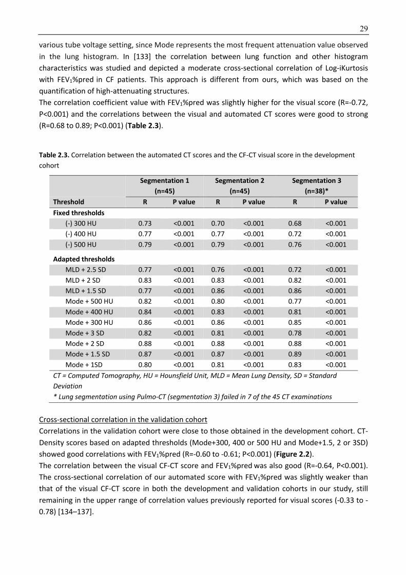
29

various tube voltage setting, since Mode represents the most frequent attenuation value observed

in the lung histogram. In [133] the correlation between lung function and other histogram

characteristics was studied and depicted a moderate cross-sectional correlation of Log-iKurtosis

with FEV1%pred in CF patients. This approach is different from ours, which was based on the

quantification of high-attenuating structures.

The correlation coefficient value with FEV1%pred was slightly higher for the visual score (R=-0.72,

P<0.001) and the correlations between the visual and automated CT scores were good to strong

(R=0.68 to 0.89; P<0.001) (Table 2.3). Table 2.3. Correlation between the automated CT scores and the CF-CT visual score in the development

cohort

Segmentation 1 (n=45)

Segmentation 2 (n=45)

Segmentation 3 (n=38)*

Threshold R P value R P value R P value Fixed thresholds

(-) 300 HU 0.73 <0.001 0.70 <0.001 0.68 <0.001

(-) 400 HU 0.77 <0.001 0.77 <0.001 0.72 <0.001

(-) 500 HU 0.79 <0.001 0.79 <0.001 0.76 <0.001

Adapted thresholds

MLD + 2.5 SD 0.77 <0.001 0.76 <0.001 0.72 <0.001

MLD + 2 SD 0.83 <0.001 0.83 <0.001 0.82 <0.001

MLD + 1.5 SD 0.77 <0.001 0.86 <0.001 0.86 <0.001

Mode + 500 HU 0.82 <0.001 0.80 <0.001 0.77 <0.001

Mode + 400 HU 0.84 <0.001 0.83 <0.001 0.81 <0.001

Mode + 300 HU 0.86 <0.001 0.86 <0.001 0.85 <0.001

Mode + 3 SD 0.82 <0.001 0.81 <0.001 0.78 <0.001

Mode + 2 SD 0.88 <0.001 0.88 <0.001 0.88 <0.001

Mode + 1.5 SD 0.87 <0.001 0.87 <0.001 0.89 <0.001

Mode + 1SD 0.80 <0.001 0.81 <0.001 0.83 <0.001

CT = Computed Tomography, HU = Hounsfield Unit, MLD = Mean Lung Density, SD = Standard Deviation * Lung segmentation using Pulmo-CT (segmentation 3) failed in 7 of the 45 CT examinations

Cross-sectional correlation in the validation cohort

Correlations in the validation cohort were close to those obtained in the development cohort. CT-

Density scores based on adapted thresholds (Mode+300, 400 or 500 HU and Mode+1.5, 2 or 3SD)

showed good correlations with FEV1%pred (R=-0.60 to -0.61; P<0.001) (Figure 2.2).

The correlation between the visual CF-CT score and FEV1%pred was also good (R=-0.64, P<0.001).

The cross-sectional correlation of our automated score with FEV1%pred was slightly weaker than

that of the visual CF-CT score in both the development and validation cohorts in our study, still

remaining in the upper range of correlation values previously reported for visual scores (-0.33 to -

0.78) [134–137].

30

Figure 2.2: Automated CT scoring in the validation cohort of patients with various disease severities. A-B) Axial CT image in a patient with mild lung disease (FEV1%pred =77%). Bronchiectasis and bronchial wall

thickening are seen in the posterior segment of the right upper lobe (white arrow). These lesions are included in areas of high attenuation (pink areas). Scoring with Mode+300 HU yielded a CT-Density score of

4.4. This means that 4.4% of the total lung volume had an attenuation value superior or equal to mode (-899 HU) + 300 HU. C-D) Axial CT image in a patient with moderate disease (FEV1%pred =56%) shows bilateral mucus plugging (yellow arrowheads). The CT-Density score was 9.8. E-F) Axial CT image in a

patient with severe disease (FEV1%pred =31%) shows diffuse bronchiectasis and bronchial wall thickening (yellow arrows). The CT-Density score was 14.5.

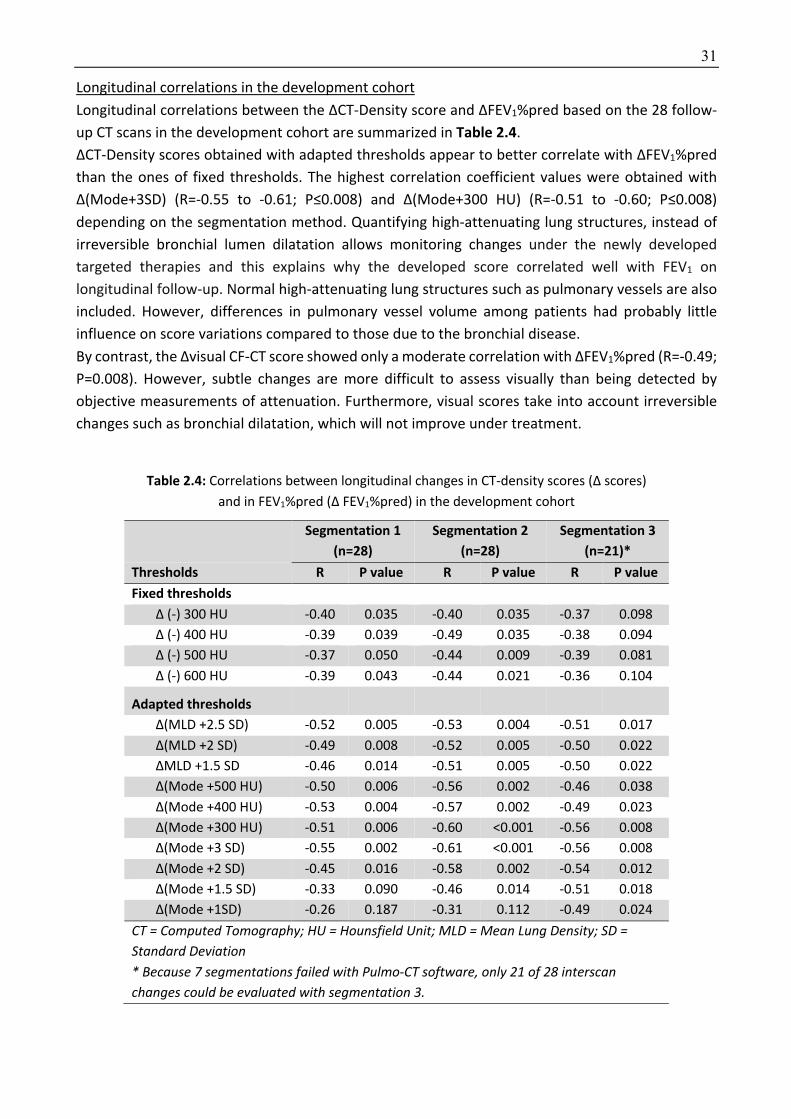
31

Longitudinal correlations in the development cohort

Longitudinal correlations between the ΔCT-Density score and ΔFEV1%pred based on the 28 follow-

up CT scans in the development cohort are summarized in Table 2.4.

ΔCT-Density scores obtained with adapted thresholds appear to better correlate with ΔFEV1%pred

than the ones of fixed thresholds. The highest correlation coefficient values were obtained with

Δ(Mode+3SD) (R=-0.55 to -0.61; P≤0.008) and Δ(Mode+300 HU) (R=-0.51 to -0.60; P≤0.008)

depending on the segmentation method. Quantifying high-attenuating lung structures, instead of

irreversible bronchial lumen dilatation allows monitoring changes under the newly developed

targeted therapies and this explains why the developed score correlated well with FEV1 on

longitudinal follow-up. Normal high-attenuating lung structures such as pulmonary vessels are also

included. However, differences in pulmonary vessel volume among patients had probably little

influence on score variations compared to those due to the bronchial disease.

By contrast, the Δvisual CF-CT score showed only a moderate correlation with ΔFEV1%pred (R=-0.49;

P=0.008). However, subtle changes are more difficult to assess visually than being detected by

objective measurements of attenuation. Furthermore, visual scores take into account irreversible

changes such as bronchial dilatation, which will not improve under treatment.

Table 2.4: Correlations between longitudinal changes in CT-density scores (Δ scores)

and in FEV1%pred (Δ FEV1%pred) in the development cohort

Segmentation 1 (n=28)

Segmentation 2 (n=28)

Segmentation 3 (n=21)*

Thresholds R P value R P value R P value Fixed thresholds

Δ (-) 300 HU -0.40 0.035 -0.40 0.035 -0.37 0.098

Δ (-) 400 HU -0.39 0.039 -0.49 0.035 -0.38 0.094

Δ (-) 500 HU -0.37 0.050 -0.44 0.009 -0.39 0.081

Δ (-) 600 HU -0.39 0.043 -0.44 0.021 -0.36 0.104

Adapted thresholds

Δ(MLD +2.5 SD) -0.52 0.005 -0.53 0.004 -0.51 0.017

Δ(MLD +2 SD) -0.49 0.008 -0.52 0.005 -0.50 0.022

ΔMLD +1.5 SD -0.46 0.014 -0.51 0.005 -0.50 0.022

Δ(Mode +500 HU) -0.50 0.006 -0.56 0.002 -0.46 0.038

Δ(Mode +400 HU) -0.53 0.004 -0.57 0.002 -0.49 0.023

Δ(Mode +300 HU) -0.51 0.006 -0.60 <0.001 -0.56 0.008

Δ(Mode +3 SD) -0.55 0.002 -0.61 <0.001 -0.56 0.008

Δ(Mode +2 SD) -0.45 0.016 -0.58 0.002 -0.54 0.012

Δ(Mode +1.5 SD) -0.33 0.090 -0.46 0.014 -0.51 0.018

Δ(Mode +1SD) -0.26 0.187 -0.31 0.112 -0.49 0.024

CT = Computed Tomography; HU = Hounsfield Unit; MLD = Mean Lung Density; SD = Standard Deviation * Because 7 segmentations failed with Pulmo-CT software, only 21 of 28 interscan changes could be evaluated with segmentation 3.

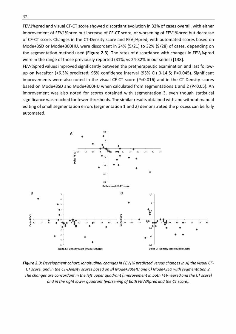
32

FEV1%pred and visual CF-CT score showed discordant evolution in 32% of cases overall, with either

improvement of FEV1%pred but increase of CF-CT score, or worsening of FEV1%pred but decrease

of CF-CT score. Changes in the CT-Density score and FEV1%pred, with automated scores based on

Mode+3SD or Mode+300HU, were discordant in 24% (5/21) to 32% (9/28) of cases, depending on

the segmentation method used (Figure 2.3). The rates of discordance with changes in FEV1%pred

were in the range of those previously reported (31%, vs 24-32% in our series) [138].

FEV1%pred values improved significantly between the pretherapeutic examination and last follow-

up on ivacaftor (+6.3% predicted; 95% confidence interval (95% CI) 0-14.5; P=0.045). Significant

improvements were also noted in the visual CF-CT score (P=0.016) and in the CT-Density scores

based on Mode+3SD and Mode+300HU when calculated from segmentations 1 and 2 (P<0.05). An

improvement was also noted for scores obtained with segmentation 3, even though statistical

significance was reached for fewer thresholds. The similar results obtained with and without manual

editing of small segmentation errors (segmentation 1 and 2) demonstrated the process can be fully

automated.

Figure 2.3: Development cohort: longitudinal changes in FEV1 % predicted versus changes in A) the visual CF-CT score, and in the CT-Density scores based on B) Mode+300HU and C) Mode+3SD with segmentation 2.

The changes are concordant in the left upper quadrant (improvement in both FEV1%pred and the CT score) and in the right lower quadrant (worsening of both FEV1%pred and the CT score).

33

Repeatability and Time Required

The intra-observer repeatability of both the visual CF-CT score and the automated CT-Density score

based on segmentation 2 was excellent (ICC>0.8). However, intra-observer repeatability was higher

with the automated score (ICCs ≥ 0.947), regardless of the threshold.

The interobserver repeatability of the automated score was also excellent (ICC 0.947 to 0.997).

However, we only evaluated repeatability based on the same set of scans, thus only the influence

of variation in the manual edited segmentations was evaluated, no other potential variation factors,

which would require repeating scans within a short time frame.

The average time required to obtain the automated scores was respectively 2.0 ± 0.5 and 0.8 ± 0.2

minutes when based on segmentation 1 and 3 (no manual editing). It was 6.6 ± 2.4 minutes based

on segmentation 2 with manual editing. The visual CF-CT score took an average of 17.8 ± 7.8

minutes. The time required for automated scoring was far shorter than for visual scoring, and is

compatible with clinical practice.

2.1.5 Discussion We report a good cross-sectional correlation between a new automated density-based CT score for

high-attenuating lung structural abnormalities and FEV1%pred in adults with CF. The automated

score better correlates with changes in FEV1%pred among patients treated with ivacaftor than did

the visual score. The developed score was validated in a larger independent cohort of unselected

adult CF patients, with similar results for two different commercially available lung segmentation

software.

[6]Our study has several limitations. First, owing to the retrospective and multicenter design, the

scanning techniques were not standardized. Contrary to visual scoring, density-based automated

scoring is highly dependent on the scanning technique, acquisition setting and reconstruction

parameters The CT examinations used in our development cohort often had different slice

thicknesses and/or tube voltages. This heterogeneity may have been detrimental for our scoring

method. However, this corresponds to routine practice and has not prevented from obtaining good

correlations to the pulmonary function. The use of standardized scanning protocols and calibrated

breath holds, as previously suggested [139,140], would probably even improve the performance of

our automated CT scoring method. Another limitation is that the number of CT scans per patient in

the development cohort was uneven. However, our results were confirmed in the validation cohort,

with only one CT scan and one FEV1%pred value per patient. A third limitation is that FEV1%pred was

the only CF outcome measure. However FEV1%pred measurement is the only surrogate for mortality

to be considered as primary endpoint by the European Medicines Agency for clinical trials in CF

[141]. Correlations with other clinical endpoints such as quality of life, the exacerbation rate, and

survival are important for the validation of chest CT as a surrogate outcome and should be assessed

in further studies [140].

In conclusion, our results demonstrate that CT density-based automated scoring of lung structural

abnormalities is feasible in CF patients. The use of adapted thresholds such as Mode+3SD or

Mode+300HU to quantify high-attenuating CF-related lesions yielded a good correlation with

FEV1%pred, in both cross-sectional and longitudinal analyses. This scoring method, validated in a

second, independent cohort, is much less time-consuming than visual scoring and could prove

suitable both in daily practice and as an objective endpoint for clinical trials.

34

2.2 Evaluation of the thresholding approach for automated severity scoring of lung disease in adults with primary ciliary dyskinesia

2.2.1 Background PCD is a rare genetic disorder characterized by defective ciliary structure and/or function, leading

to inadequate mucociliary clearance and chronic oto-sino-pulmonary disease [142–144]. Organ

laterality is also affected in almost half the patients [143]. Defective mucociliary airway clearance

leads to recurrent and chronic bacterial infections of the lower respiratory tract, and to

bronchiectasis [143].

CT is the gold standard method for the diagnosis of bronchiectasis, but its utility for monitoring PCD

is not yet established [145,146]. Correlations between CT structural changes and disease severity

(lung function) have rarely been studied in PCD, especially in adults [146–154]. However, a large

retrospective study recently suggested that a larger disease burden on CT may predict lung function

decline in adults with PCD, indicating that CT assessment of lung structural abnormalities might be

of value [146].

Most authors who have attempted to quantify bronchial disease in patients with PCD have used

visual scoring methods initially designed to assess lung structural changes in patients with CF. The

correlation between these visual scores and FEV1 remains questionable in patients with PCD [148–

155]. For example, [153] reported a good negative correlation between a visual CT score and FEV1

(R=-0.63, P<0.001), whereas in [152] found no correlation at all (R=-0.36, P=0.61).

Although bronchiectasis, bronchial wall thickening, mucus plugging and mosaic perfusion are

present in both PCD and CF, their relative predominance differs between the two diseases. Mosaic

perfusion and small-airway mucus plugging predominate in PCD, meaning that their respective

weight in the overall CT score should not be the same as in CF [146,152]. This may be why some

authors failed to find a correlation between visual scores and spirometry in PCD patients.

Furthermore, visual scores suffer from several limitations, including the need for dedicated training

and subjectivity in the assessment of CT changes [6].

Most lung structural changes in PCD, especially bronchial wall thickening, mucus plugging,

consolidations and atelectasis are likely to increase lung attenuation and to modify the density

histogram characteristics, which can be extracted from the CT images.

We postulated that disease severity in PCD might also be assessed by quantifying high-attenuating

lung structures and by analyzing changes in the lung density distribution. We therefore developed

an automated CT scoring method based on histogram characteristic analysis and threshold-based

quantification of high-attenuating lung structures in patients with PCD. 2.2.2 Methodology The proposed thresholding method is similar to that we previously used in CF patients.

Several threshold values were tested for their correlation with FEV1 and forced vital capacity (FVC).

Three threshold values were tested (-300, -400 and -500 HU), as well as eight adapted threshold

values taking into account, for each CT examination, individual histogram features, known to be

influenced by the level of inspiration [118,124].

The CT-density scores (one for each tested threshold value) were expressed as the proportion of

lung showing attenuation values above the selected threshold. For instance, a CT-Density score

35

value of 10 indicated that 10% of the lung had an attenuation value superior or equal to the

threshold on CT.

Additionally, the correlation between and spirometry measurements and the following histogram

characteristics was also analyzed: MLD, mode, SD, kurtosis (sharpness of the density distribution),

and skewness (asymmetry of the density distribution).

2.2.3 Dataset and implementation Dataset

This retrospective study, performed in two accredited PCD reference centers, was approved by the

Institutional Review Board of Société Pneumologie de Langue Française. The need for informed

consent was waived, in accordance with French rules for retrospective observational studies.

All adult outpatients, with a diagnosis of PCD according to the European Respiratory Society

guidelines [156] were eligible if they had chest CT exams of the whole thorax performed between

November 2009 and July 2016 and spirometric measurements, both performed within a 6-month

period. Exclusion criteria were the unavailability of CT images with a slice thickness ≤ 2 mm,

reconstructed with a soft kernel, or the administration of iodinated contrast medium during the CT

acquisition. A total of 95 patients with a confirmed diagnosis of PCD were identified, of whom sixty-

two patients were included in this study. Among the 33 excluded patients, 24 had no available CT

examination, 6 patients had CT scans without soft kernel reconstruction or thin-slice images, and

the interval between spirometry and CT exceeded 6 months in the remaining 3 cases. Of the 62

patients who were finally included, PCD diagnosis had been confirmed by electron microscopy of

ciliary ultrastructure in 51. The remaining 11 patients had Kartagener’s syndrome with diffuse

bronchiectasis and situs inversus on CT imaging, a combination of signs considered to validate PCD

diagnosis [154].

All CT examinations had been performed in the supine position at full inspiration, with usual

acquisition parameters, allowing obtaining high resolution CT images of the whole thorax during a

single breath hold. Five different 16-to-64 multislice CT devices from two different vendors

(Somatom Sensation 16 and Somatom Definition DS, Siemens Healthineer ; Lightspeed plus, Bright

Speed 16 and Optima CT 660) had been used, depending on the site and date of the CT

examinations, all performed with equivalent acquisition parameters. The radiation dose resulting

from each CT acquisition was evaluated by collecting the mean dose-length product (DLP) value

from the dose reports. The mean DLP per CT scan was 200.3 ± 100.4 mGy.cm.

Each CT examination was visually analyzed for pulmonary situs type (solitus, inversus or heterotaxy), based on the relationship between the upper-lobe bronchus and the ipsilateral pulmonary artery,

and the morphology of the tracheobronchial tree [157]. A total of 37 patients (60%) had the usual

arrangement of the pulmonary situs (situs solitus), while 24 (39%) had situs inversus and 1 (1%) had

left isomerism. CT images were also checked for prior lobectomy. Nineteen patients (31%) had

previously undergone complete or partial lobectomy, even though bronchial abnormalities are not

usually restricted to a single lobe in PCD and surgical resection is currently not considered an

appropriate treatment for PCD [144]. This proportion is in line with the 41% prevalence reported by

[155]. The resections concerned the middle lobe in 15 patients (24%), the left lower lobe in 1 patient

(2%), the middle lobe plus the left lower lobe in 2 patients (3%), and the middle lobe plus the lingula

in the remaining patient (2%).

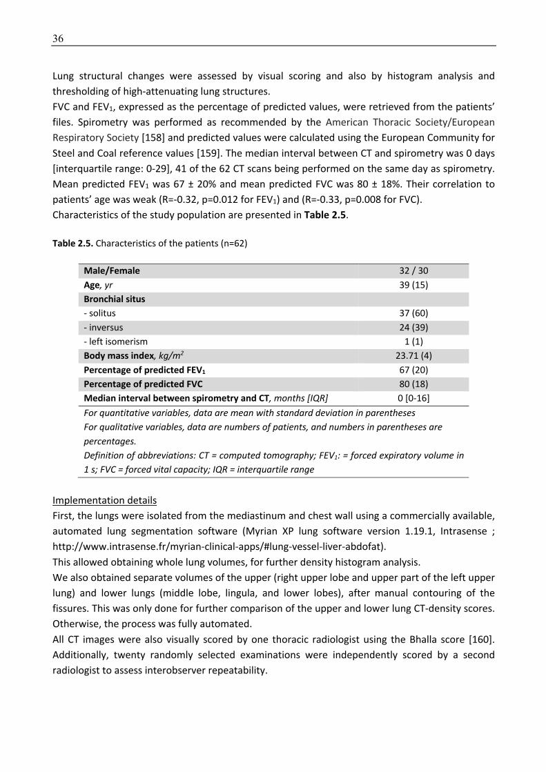
36

Lung structural changes were assessed by visual scoring and also by histogram analysis and

thresholding of high-attenuating lung structures.

FVC and FEV1, expressed as the percentage of predicted values, were retrieved from the patients’

files. Spirometry was performed as recommended by the American Thoracic Society/European

Respiratory Society [158] and predicted values were calculated using the European Community for

Steel and Coal reference values [159]. The median interval between CT and spirometry was 0 days

[interquartile range: 0-29], 41 of the 62 CT scans being performed on the same day as spirometry.

Mean predicted FEV1 was 67 ± 20% and mean predicted FVC was 80 ± 18%. Their correlation to

patients’ age was weak (R=-0.32, p=0.012 for FEV1) and (R=-0.33, p=0.008 for FVC).

Characteristics of the study population are presented in Table 2.5.

Table 2.5. Characteristics of the patients (n=62)

Male/Female 32 / 30

Age, yr 39 (15)

Bronchial situs - solitus 37 (60)

- inversus 24 (39)

- left isomerism 1 (1)

Body mass index, kg/m2 23.71 (4)

Percentage of predicted FEV1 67 (20)

Percentage of predicted FVC 80 (18)

Median interval between spirometry and CT, months [IQR] 0 [0-16]

For quantitative variables, data are mean with standard deviation in parentheses For qualitative variables, data are numbers of patients, and numbers in parentheses are percentages. Definition of abbreviations: CT = computed tomography; FEV1: = forced expiratory volume in 1 s; FVC = forced vital capacity; IQR = interquartile range

Implementation details

First, the lungs were isolated from the mediastinum and chest wall using a commercially available,

automated lung segmentation software (Myrian XP lung software version 1.19.1, Intrasense ;

http://www.intrasense.fr/myrian-clinical-apps/#lung-vessel-liver-abdofat).

This allowed obtaining whole lung volumes, for further density histogram analysis.

We also obtained separate volumes of the upper (right upper lobe and upper part of the left upper

lung) and lower lungs (middle lobe, lingula, and lower lobes), after manual contouring of the

fissures. This was only done for further comparison of the upper and lower lung CT-density scores.

Otherwise, the process was fully automated.

All CT images were also visually scored by one thoracic radiologist using the Bhalla score [160].

Additionally, twenty randomly selected examinations were independently scored by a second

radiologist to assess interobserver repeatability.

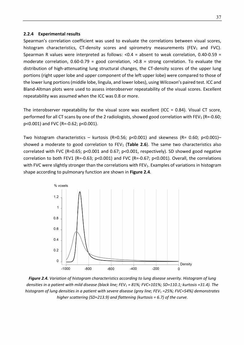
37

2.2.4 Experimental results Spearman’s correlation coefficient was used to evaluate the correlations between visual scores,

histogram characteristics, CT-density scores and spirometry measurements (FEV1 and FVC).

Spearman R values were interpreted as follows: <0.4 = absent to weak correlation, 0.40-0.59 =

moderate correlation, 0.60-0.79 = good correlation, >0.8 = strong correlation. To evaluate the

distribution of high-attenuating lung structural changes, the CT-density scores of the upper lung

portions (right upper lobe and upper component of the left upper lobe) were compared to those of

the lower lung portions (middle lobe, lingula, and lower lobes), using Wilcoxon’s paired test. ICC and

Bland-Altman plots were used to assess interobserver repeatability of the visual scores. Excellent

repeatability was assumed when the ICC was 0.8 or more.

The interobserver repeatability for the visual score was excellent (ICC = 0.84). Visual CT score,

performed for all CT scans by one of the 2 radiologists, showed good correlation with FEV1 (R=-0.60;

p<0.001) and FVC (R=-0.62; p<0.001).

Two histogram characteristics – kurtosis (R=0.56; p<0.001) and skewness (R= 0.60; p<0.001)–

showed a moderate to good correlation to FEV1 (Table 2.6). The same two characteristics also

correlated with FVC (R=0.65; p<0.001 and 0.67; p<0.001, respectively). SD showed good negative

correlation to both FEV1 (R=-0.63; p<0.001) and FVC (R=-0.67; p<0.001). Overall, the correlations

with FVC were slightly stronger than the correlations with FEV1. Examples of variations in histogram

shape according to pulmonary function are shown in Figure 2.4.

Figure 2.4. Variation of histogram characteristics according to lung disease severity. Histogram of lung

densities in a patient with mild disease (black line; FEV1 = 81%; FVC=101%; SD=110.1; kurtosis =31.4). The histogram of lung densities in a patient with severe disease (grey line; FEV1 =25%; FVC=54%) demonstrates

higher scattering (SD=213.9) and flattening (kurtosis = 6.7) of the curve.

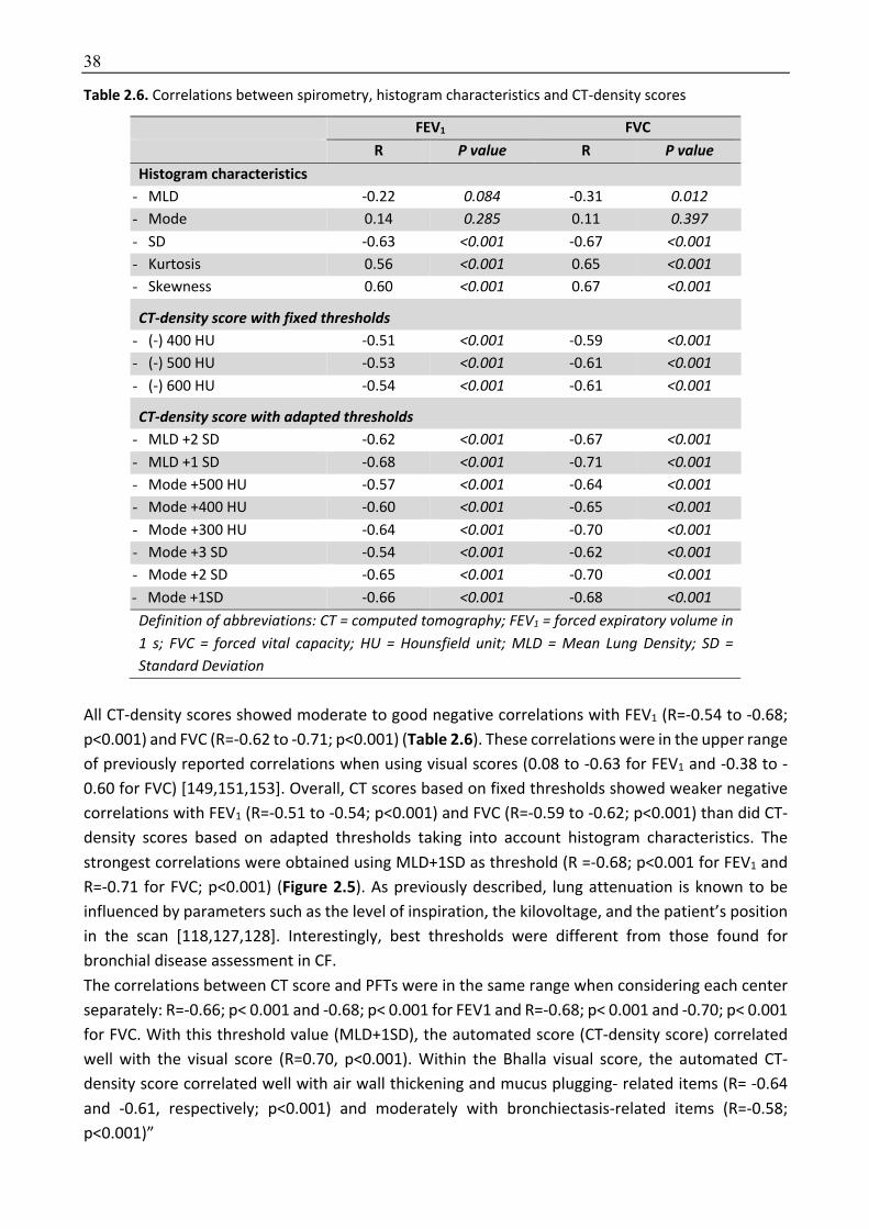
38

Table 2.6. Correlations between spirometry, histogram characteristics and CT-density scores

FEV1 FVC R P value R P value

Histogram characteristics

- MLD -0.22 0.084 -0.31 0.012 - Mode 0.14 0.285 0.11 0.397 - SD -0.63 <0.001 -0.67 <0.001 - Kurtosis 0.56 <0.001 0.65 <0.001 - Skewness 0.60 <0.001 0.67 <0.001

CT-density score with fixed thresholds - (-) 400 HU -0.51 <0.001 -0.59 <0.001 - (-) 500 HU -0.53 <0.001 -0.61 <0.001 - (-) 600 HU -0.54 <0.001 -0.61 <0.001

CT-density score with adapted thresholds - MLD +2 SD -0.62 <0.001 -0.67 <0.001 - MLD +1 SD -0.68 <0.001 -0.71 <0.001 - Mode +500 HU -0.57 <0.001 -0.64 <0.001 - Mode +400 HU -0.60 <0.001 -0.65 <0.001 - Mode +300 HU -0.64 <0.001 -0.70 <0.001 - Mode +3 SD -0.54 <0.001 -0.62 <0.001 - Mode +2 SD -0.65 <0.001 -0.70 <0.001 - Mode +1SD -0.66 <0.001 -0.68 <0.001 Definition of abbreviations: CT = computed tomography; FEV1 = forced expiratory volume in 1 s; FVC = forced vital capacity; HU = Hounsfield unit; MLD = Mean Lung Density; SD = Standard Deviation

All CT-density scores showed moderate to good negative correlations with FEV1 (R=-0.54 to -0.68;

p<0.001) and FVC (R=-0.62 to -0.71; p<0.001) (Table 2.6). These correlations were in the upper range

of previously reported correlations when using visual scores (0.08 to -0.63 for FEV1 and -0.38 to -

0.60 for FVC) [149,151,153]. Overall, CT scores based on fixed thresholds showed weaker negative

correlations with FEV1 (R=-0.51 to -0.54; p<0.001) and FVC (R=-0.59 to -0.62; p<0.001) than did CT-

density scores based on adapted thresholds taking into account histogram characteristics. The

strongest correlations were obtained using MLD+1SD as threshold (R =-0.68; p<0.001 for FEV1 and

R=-0.71 for FVC; p<0.001) (Figure 2.5). As previously described, lung attenuation is known to be

influenced by parameters such as the level of inspiration, the kilovoltage, and the patient’s position

in the scan [118,127,128]. Interestingly, best thresholds were different from those found for

bronchial disease assessment in CF.

The correlations between CT score and PFTs were in the same range when considering each center

separately: R=-0.66; p< 0.001 and -0.68; p< 0.001 for FEV1 and R=-0.68; p< 0.001 and -0.70; p< 0.001

for FVC. With this threshold value (MLD+1SD), the automated score (CT-density score) correlated

well with the visual score (R=0.70, p<0.001). Within the Bhalla visual score, the automated CT-

density score correlated well with air wall thickening and mucus plugging- related items (R= -0.64

and -0.61, respectively; p<0.001) and moderately with bronchiectasis-related items (R=-0.58;

p<0.001)”

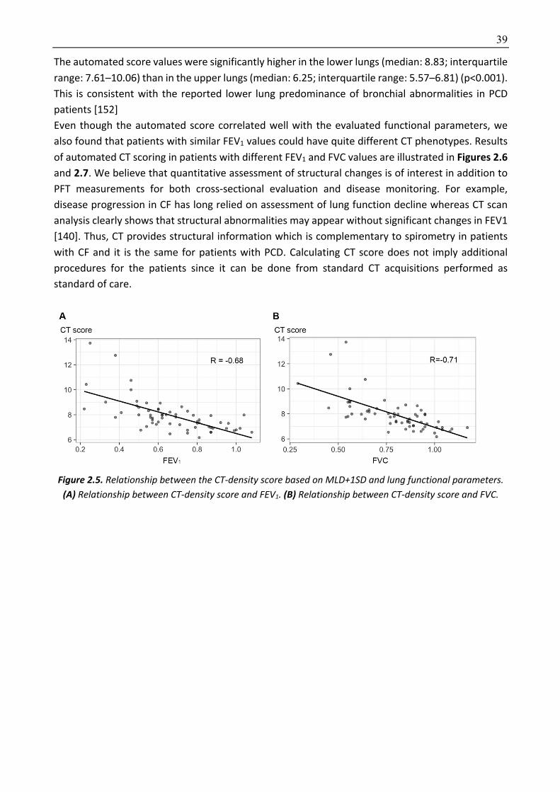
39

The automated score values were significantly higher in the lower lungs (median: 8.83; interquartile

range: 7.61–10.06) than in the upper lungs (median: 6.25; interquartile range: 5.57–6.81) (p<0.001).

This is consistent with the reported lower lung predominance of bronchial abnormalities in PCD

patients [152]

Even though the automated score correlated well with the evaluated functional parameters, we

also found that patients with similar FEV1 values could have quite different CT phenotypes. Results

of automated CT scoring in patients with different FEV1 and FVC values are illustrated in Figures 2.6 and 2.7. We believe that quantitative assessment of structural changes is of interest in addition to

PFT measurements for both cross-sectional evaluation and disease monitoring. For example,

disease progression in CF has long relied on assessment of lung function decline whereas CT scan

analysis clearly shows that structural abnormalities may appear without significant changes in FEV1

[140]. Thus, CT provides structural information which is complementary to spirometry in patients

with CF and it is the same for patients with PCD. Calculating CT score does not imply additional

procedures for the patients since it can be done from standard CT acquisitions performed as

standard of care.

Figure 2.5. Relationship between the CT-density score based on MLD+1SD and lung functional parameters. (A) Relationship between CT-density score and FEV1. (B) Relationship between CT-density score and FVC.

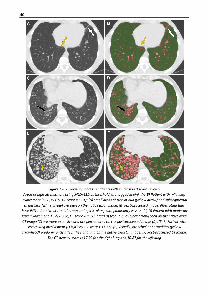
40

Figure 2.6. CT-density scores in patients with increasing disease severity

Areas of high attenuation, using MLD+1SD as threshold, are tagged in pink. (A, B) Patient with mild lung involvement (FEV1 = 80%, CT score = 6.01): (A) Small areas of tree-in-bud (yellow arrow) and subsegmental

atelectasis (white arrow) are seen on the native axial image. (B) Post-processed image, illustrating that these PCD-related abnormalities appear in pink, along with pulmonary vessels. (C, D) Patient with moderate lung involvement (FEV1 = 60%, CT score = 8.37): areas of tree-in-bud (black arrow) seen on the native axial CT image (C) are more extensive and are pink-colored on the post-processed image (D). (E, F) Patient with

severe lung involvement (FEV1=25%, CT score = 13.72): (E) Visually, bronchial abnormalities (yellow arrowhead) predominantly affect the right lung on the native axial CT image. (F) Post-processed CT image.

The CT-density score is 17.59 for the right lung and 10.87 for the left lung

41

Figure 2.7. Different imaging features in patients with similar FEV1 values. (A) Patient with FEV1=38%

predicted and moderate bronchiectasis predominantly affecting the middle lobe. The CT-density score based on MLD+1SD was 7.79. (B) Patient with FEV1=38% predicted but much more severe bronchiectasis on visual

assessment, especially in the lingula. The CT-density score based on MLD+1SD was 12.75. These two examples show that CT imaging provides additional information to spirometry, especially regarding regional

disease distribution (homogeneous versus heterogeneous), and the severity of bronchiectasis, which correspond to irreversible changes.

2.2.5 Discussion To the best of our knowledge, the present study describes the first automated CT scoring method

designed to quantify lung changes associated with primary ciliary dyskinesia, based on the

measurement of high-attenuating structures and considering histogram characteristics on CT. This

approach is close to the quantification of emphysema, based on the measurement of low-

attenuating lung areas. We had previously validated this method in CF patients [112].

Our study has several limitations. Because this study was retrospective, the CT acquisition

parameters were not standardized. This may have influenced the density thresholds. Standardized

scanning protocols would probably improve the performance of the developed score. However, the

fact that the scoring method can be applied to unstandardized CT examinations makes it suitable

for daily clinical use. We did not perform longitudinal evaluation to determine whether changes in

the automated CT score correlated with changes in pulmonary function, and whether, as previously

suggested, CT-scored disease extent can predict the subsequent decline in pulmonary function.

Indeed, our primary objective was to develop and validate an automated CT score by cross-sectional

evaluation. Lastly, due to the relative rarity of PCD, it was not possible to split our population into a

development and validation cohort. Thus, the developed method should further be validated in an

independent cohort of PCD patients.

In conclusion, automated density–based CT scoring, together with histogram characteristic analysis,

is feasible in PCD patients and correlates well with FEV1 and FVC. MLD+1SD offered the best

correlations with both FEV1 and FVC. Quantitative analysis of structural abnormalities on CT scans

may prove useful for objectively evaluating lung disease changes in PCD, which may prove useful

both in daily clinical use and as an outcome in clinical trials.

42

2.3 CT-based Quantification of Lung Disease in Cystic Fibrosis using Radiomics

2.3.1 Methodology We hypothesized that a radiomics approach based on machine learning algorithms could be used

to quantify the degree of lung impairment in CF patients. The objective of this study was to use

radiomics to extract imaging biomarkers to assess the severity of lung disease in adult CF patients

and combine them with state-of-the-art machine learning methods

This method uses a common radiomics approach. First radiomics features are extracted from 3D

lung volumes and then 5 different machines learning are trained to build a radiomics-based CT score

correlating to the Nkam score, a 3-year prognostic score that has been validated in more than 2000

CF adults [161]. The Nkam score was chosen as the target for the radiomics approach because it has

been validated in the largest cohort of patients, is the most recent score and is thus better adapted

to the continuous improvements in CF prognosis [161].

A total of 38 radiomic features are extracted (Table 2.7). These features include global histogram

characteristics (7 features), common textural features (24 features) and fractal dimension (7

features):

• The global histogram characteristics (first order statistics) included mean lung density,

standard deviation, mode, kurtosis, skewness, entropy and energy [162]. These elements

provide global information on the distribution of gray-level intensities but do not take into

account their spatial interrelationship.

• The textural features (second order statistics) were derived from those proposed by Haralick

[163] and extracted using 3D co-occurrence matrices at 2 scales (distance = 1, 2 voxels).

Texture describes different aspects of contextual information, such as local intensity

distribution, the degree of uniformity, or amplitude dispersion.

• The fractal dimension quantifies self-similarity and shape complexity in a given scale. It was

calculated using the box-counting algorithm and 7 box sizes.

43

Table 2.7. Radiomic features

1st order statistics 2nd order statistics Fractal dimensions

Energy Cluster shade (distance = 1) Fractal (distance = 1)

Entropy Cluster shade (distance = 2) Fractal (distance = 2)

Kurtosis Cluster tendency (distance = 1) Fractal (distance = 3)

Mean lung density Cluster tendency (distance = 2) Fractal (distance = 4)

Mode Contrast (distance = 1) Fractal (distance = 5)

Skewness Contrast (distance = 2) Fractal (distance = 6)

Standard deviation Correlation (distance = 1) Fractal (distance = 7)

Correlation (distance = 2)

Energy (distance = 1)

Energy (distance = 2)

Entropy (distance = 1)

Entropy (distance = 2)

Homogeneity (distance = 1)

Homogeneity (distance = 2)

Inertia (distance = 1)

Inertia (distance = 2)

Inverse Variance (distance = 1)

Inverse Variance (distance = 2)

Maximum probability (distance = 1)

Maximum probability (distance = 2)

Sum average (distance = 1)

Sum average (distance = 2)

Variance (distance = 1)

Variance (distance = 2)

Five machine learning techniques are used to develop the model: (i) ridge regression [164], (ii) lasso

(Least Absolute Shrinkage and Selection Operator) regression [165], (iii) elastic net (ENET) [166], (iv)

decision trees [167], and (v) support vector machines (SVM) [168].

Among these 5 techniques, ridge regression, LASSO and ENET produce linear models with the

following equation: !(#) = &' + ∑ &*#*+*,- , where # = [#-, … , #+] is the input feature vector, 2 is

the number of features, &* (beta coefficients) is the weight assigned to feature i and &' (intercept)

is a constant term. These 3 techniques use a loss function, L, combining ordinary least square

method (OLS) or even gradient descent methods,

34&56 =748* − #*:&6

;+

*,-

where y is the response variable, with a different regularization factor.

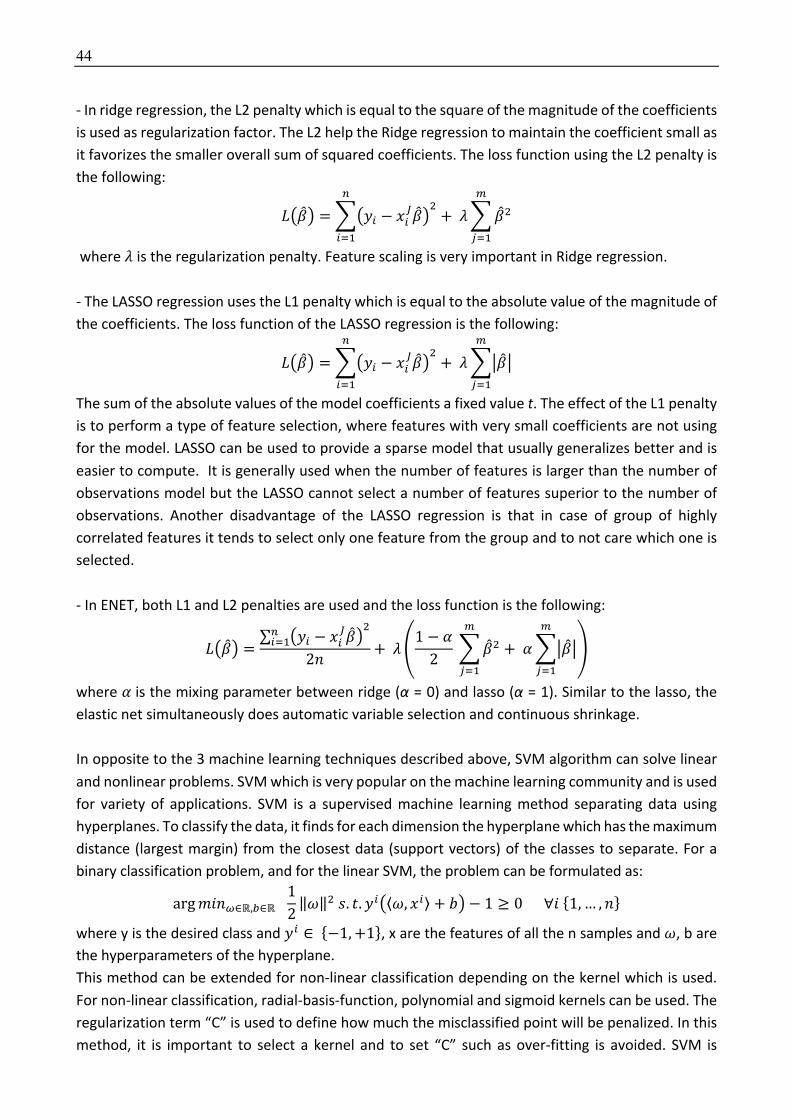
44

- In ridge regression, the L2 penalty which is equal to the square of the magnitude of the coefficients

is used as regularization factor. The L2 help the Ridge regression to maintain the coefficient small as

it favorizes the smaller overall sum of squared coefficients. The loss function using the L2 penalty is

the following:

34&56 =748* − #*:&56

;+

*,-

+ =7&5;>

?,-

where = is the regularization penalty. Feature scaling is very important in Ridge regression.

- The LASSO regression uses the L1 penalty which is equal to the absolute value of the magnitude of

the coefficients. The loss function of the LASSO regression is the following:

34&56 =748* − #*:&56

;+

*,-

+ =7@&5@

>

?,-

The sum of the absolute values of the model coefficients a fixed value t. The effect of the L1 penalty

is to perform a type of feature selection, where features with very small coefficients are not using

for the model. LASSO can be used to provide a sparse model that usually generalizes better and is

easier to compute. It is generally used when the number of features is larger than the number of

observations model but the LASSO cannot select a number of features superior to the number of

observations. Another disadvantage of the LASSO regression is that in case of group of highly

correlated features it tends to select only one feature from the group and to not care which one is

selected.

- In ENET, both L1 and L2 penalties are used and the loss function is the following:

34&56 =∑ 48* − #*

:&56;+

*,-

22+ = B

1 − D2

7&5;>

?,-

+ D7@&5@

>

?,-

E

where D is the mixing parameter between ridge (α = 0) and lasso (α = 1). Similar to the lasso, the

elastic net simultaneously does automatic variable selection and continuous shrinkage.

In opposite to the 3 machine learning techniques described above, SVM algorithm can solve linear

and nonlinear problems. SVM which is very popular on the machine learning community and is used

for variety of applications. SVM is a supervised machine learning method separating data using

hyperplanes. To classify the data, it finds for each dimension the hyperplane which has the maximum

distance (largest margin) from the closest data (support vectors) of the classes to separate. For a

binary classification problem, and for the linear SVM, the problem can be formulated as:

argIJ2K∈ℝ,N∈ℝ 12‖P‖;Q. S. 8*4⟨P, #*⟩ + V6 − 1 ≥ 0∀J{1, … , 2}

where y is the desired class and 8* ∈ {−1,+1}, x are the features of all the n samples and P, b are

the hyperparameters of the hyperplane.

This method can be extended for non-linear classification depending on the kernel which is used.

For non-linear classification, radial-basis-function, polynomial and sigmoid kernels can be used. The

regularization term “C” is used to define how much the misclassified point will be penalized. In this

method, it is important to select a kernel and to set “C” such as over-fitting is avoided. SVM is

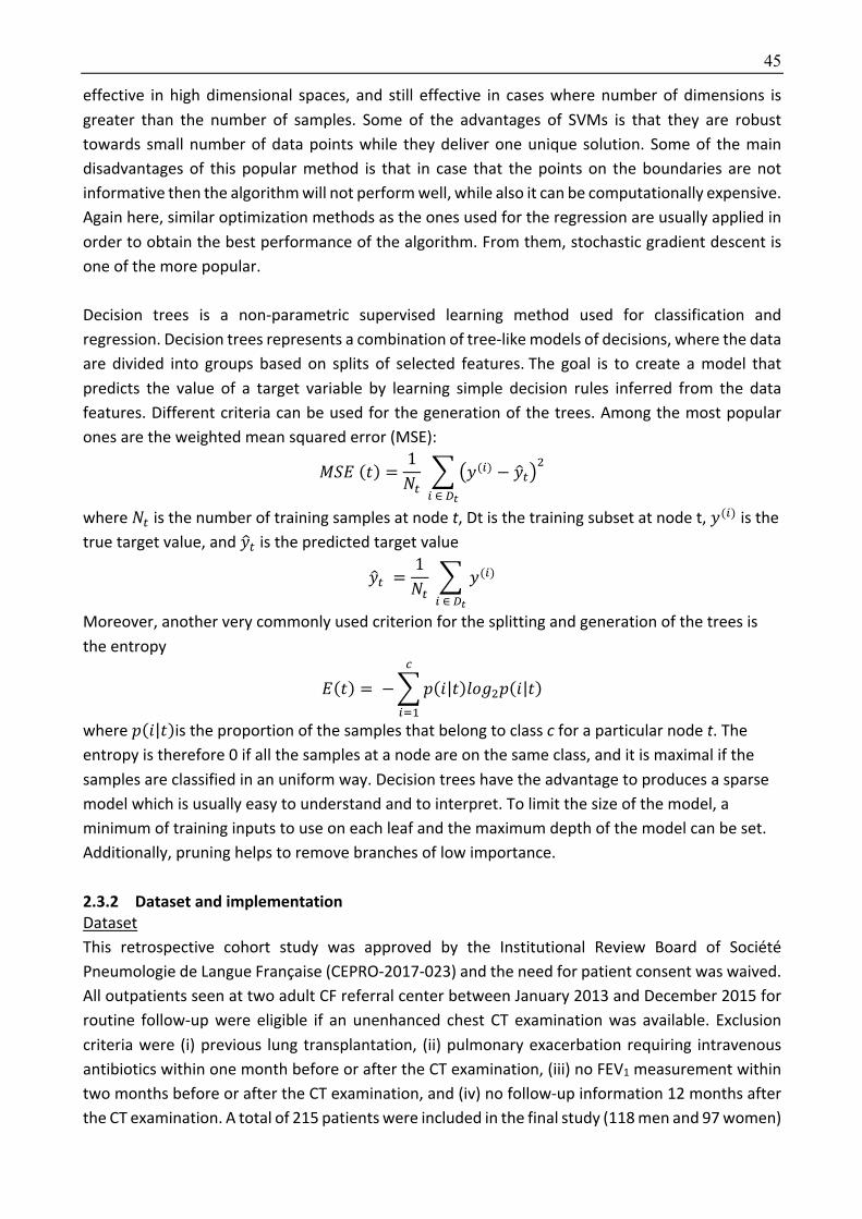
45

effective in high dimensional spaces, and still effective in cases where number of dimensions is

greater than the number of samples. Some of the advantages of SVMs is that they are robust

towards small number of data points while they deliver one unique solution. Some of the main

disadvantages of this popular method is that in case that the points on the boundaries are not

informative then the algorithm will not perform well, while also it can be computationally expensive.

Again here, similar optimization methods as the ones used for the regression are usually applied in

order to obtain the best performance of the algorithm. From them, stochastic gradient descent is

one of the more popular.

Decision trees is a non-parametric supervised learning method used for classification and

regression. Decision trees represents a combination of tree-like models of decisions, where the data

are divided into groups based on splits of selected features. The goal is to create a model that

predicts the value of a target variable by learning simple decision rules inferred from the data

features. Different criteria can be used for the generation of the trees. Among the most popular

ones are the weighted mean squared error (MSE):

\]^(S) =1_` 7 48(*) − 8a`6

;

*∈bc

where _` is the number of training samples at node t, Dt is the training subset at node t, 8(*) is the

true target value, and 8a` is the predicted target value

8a` =1_` 7 8(*)

*∈bc

Moreover, another very commonly used criterion for the splitting and generation of the trees is

the entropy

^(S) = −7d(J|S)fgh;d(J|S)i

*,-

where d(J|S)is the proportion of the samples that belong to class c for a particular node t. The

entropy is therefore 0 if all the samples at a node are on the same class, and it is maximal if the

samples are classified in an uniform way. Decision trees have the advantage to produces a sparse

model which is usually easy to understand and to interpret. To limit the size of the model, a

minimum of training inputs to use on each leaf and the maximum depth of the model can be set.

Additionally, pruning helps to remove branches of low importance.

2.3.2 Dataset and implementation Dataset

This retrospective cohort study was approved by the Institutional Review Board of Société

Pneumologie de Langue Française (CEPRO-2017-023) and the need for patient consent was waived.

All outpatients seen at two adult CF referral center between January 2013 and December 2015 for

routine follow-up were eligible if an unenhanced chest CT examination was available. Exclusion

criteria were (i) previous lung transplantation, (ii) pulmonary exacerbation requiring intravenous

antibiotics within one month before or after the CT examination, (iii) no FEV1 measurement within

two months before or after the CT examination, and (iv) no follow-up information 12 months after

the CT examination. A total of 215 patients were included in the final study (118 men and 97 women)

46

with a median age of 29 years (interquartile range (IQR), 24-36; range, 18-68). One hundred and

sixty-two patients were included from center 1 (training cohort), the remaining 53 being included

from center 2 (test cohort). Patient characteristics are shown in Table 2.8.

CT examinations were performed on 16- or 64-row devices from different vendors depending on

the referral center (Somatom Sensation 16 and Somatom Definition DS, Siemens Healthineer, in

center 1, and LightSpeed VCT and Revolution CT, GE Healthcare in center 2). The entire lung was

scanned at 100, 120 or 140kV, depending on the patient's morphology and local scanning protocols.

Tube current modulation was used at both centers. Images were reconstructed with a slice thickness

of 0.75 to 1.5 mm, using a standard kernel (bf20, bf31 or standard) and a 512 × 512 matrix. All CT

examinations were reconstructed using a filter back projection algorithm at center 1, whereas 48

out of 53 examination were reconstructed using iterative reconstruction at center 2. If patients had

more than one CT during the study, only the CT that was performed furthest from any exacerbations

was taken into account. In addition to the difference in CT equipment, there was a significant

difference regarding the mean CT radiation dose in the 2 centers (median CTDIvol = 3.9 mGy [IQR =

3.2 - 5.0 mGy] at center 1 and 1.2 mGy [1.1 - 3.3 mGy] at center 2, p <0.001).

Regarding clinical data, the percentage of predicted FEV1 at the time of CT (median interval between

CT and FEV1 measurement, 0 days; IQR, 0-0 days; range, 0–31 days) was retrieved, along with the

number of pulmonary exacerbations requiring intravenous antibiotics within 12 months before and

after CT. Additional data available at the time of the CT examination were collected to calculate

three clinical prognostic scores, namely the Nkam, CF-ABLE, and Liou scores [161,169,170]. These

data included age, gender, body mass index (BMI), pancreatic insufficiency, diabetes mellitus,

Staphylococcus aureus colonization, Burkholderia cepacia colonization, hospitalization in the

previous 12 months, long-term oxygen therapy, non-invasive ventilation, and oral corticosteroid

treatment.

Patients from the first center (training cohort) had more severe disease than those from center 2

(test cohort) according to predicted FEV1 (58% [IQR=41-77%] vs 70% [53-82%]; p = 0.002), CF-able

(2.0 [IQR=0.0 - 3.5] vs 1.0 [IQR=0.0 - 3.5], p = 0.02) and Liou (0.9 [IQR=0.7 - 1.0] vs 1.0 [IQR=0.9 - 1.0];

p < <0.001) scores. There was no other significant difference in clinical variables between the

patients from the 2 centers (Table 2.8), especially regarding the Nkam score (p=0.12) which includes

more clinical parameters than the other 2 clinical prognosis scores.

Implementation details

In order to develop and test the models on independent datasets, the cohort from center 1 was

used for training the models whereas the cohort from center 2 was used for testing.

Prior to feature extraction, lungs are segmented using a commercially available automated software

program (Myrian XP-Lung version 1.19.1, Intrasense). Then radiomic features are extracted using

Matlab 2016b (MathWorks, Natick, MA ; https://www.mathworks.com/products/new_products/

release2016b.html).

To prevent data overfitting by the model, parameters such as regularization and kernel type were

optimized for each of the 5 machine learning methods using a 10-fold cross validation in the training

dataset.

The 5 radiomics-based CT scores that were obtained from the development cohort were then

calculated for the patients of the test cohort (center 2) to evaluate the correlation with clinical

prognosis scores and other clinically relevant parameters.

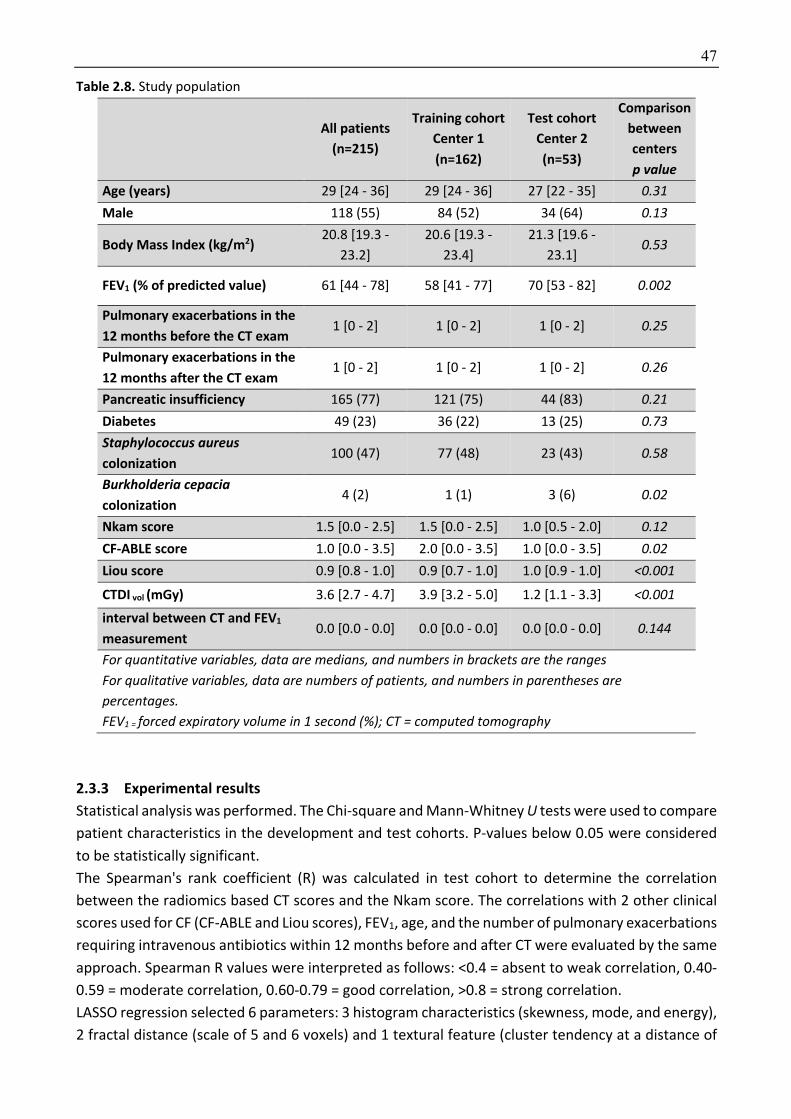
47

Table 2.8. Study population

All patients

(n=215)

Training cohort Center 1 (n=162)

Test cohort Center 2 (n=53)

Comparison between centers p value

Age (years) 29 [24 - 36] 29 [24 - 36] 27 [22 - 35] 0.31 Male 118 (55) 84 (52) 34 (64) 0.13

Body Mass Index (kg/m2) 20.8 [19.3 -

23.2]

20.6 [19.3 -

23.4]

21.3 [19.6 -

23.1] 0.53

FEV1 (% of predicted value) 61 [44 - 78] 58 [41 - 77] 70 [53 - 82] 0.002

Pulmonary exacerbations in the 12 months before the CT exam

1 [0 - 2] 1 [0 - 2] 1 [0 - 2] 0.25

Pulmonary exacerbations in the 12 months after the CT exam

1 [0 - 2] 1 [0 - 2] 1 [0 - 2] 0.26

Pancreatic insufficiency 165 (77) 121 (75) 44 (83) 0.21 Diabetes 49 (23) 36 (22) 13 (25) 0.73 Staphylococcus aureus colonization

100 (47) 77 (48) 23 (43) 0.58

Burkholderia cepacia colonization

4 (2) 1 (1) 3 (6) 0.02

Nkam score 1.5 [0.0 - 2.5] 1.5 [0.0 - 2.5] 1.0 [0.5 - 2.0] 0.12 CF-ABLE score 1.0 [0.0 - 3.5] 2.0 [0.0 - 3.5] 1.0 [0.0 - 3.5] 0.02 Liou score 0.9 [0.8 - 1.0] 0.9 [0.7 - 1.0] 1.0 [0.9 - 1.0] <0.001

CTDI vol (mGy) 3.6 [2.7 - 4.7] 3.9 [3.2 - 5.0] 1.2 [1.1 - 3.3] <0.001 interval between CT and FEV1 measurement

0.0 [0.0 - 0.0] 0.0 [0.0 - 0.0] 0.0 [0.0 - 0.0] 0.144

For quantitative variables, data are medians, and numbers in brackets are the ranges For qualitative variables, data are numbers of patients, and numbers in parentheses are percentages. FEV1 = forced expiratory volume in 1 second (%); CT = computed tomography

2.3.3 Experimental results Statistical analysis was performed. The Chi-square and Mann-Whitney U tests were used to compare

patient characteristics in the development and test cohorts. P-values below 0.05 were considered

to be statistically significant.

The Spearman's rank coefficient (R) was calculated in test cohort to determine the correlation

between the radiomics based CT scores and the Nkam score. The correlations with 2 other clinical

scores used for CF (CF-ABLE and Liou scores), FEV1, age, and the number of pulmonary exacerbations

requiring intravenous antibiotics within 12 months before and after CT were evaluated by the same

approach. Spearman R values were interpreted as follows: <0.4 = absent to weak correlation, 0.40-

0.59 = moderate correlation, 0.60-0.79 = good correlation, >0.8 = strong correlation.

LASSO regression selected 6 parameters: 3 histogram characteristics (skewness, mode, and energy),

2 fractal distance (scale of 5 and 6 voxels) and 1 textural feature (cluster tendency at a distance of

48

1 voxel). The same parameters and 9 additional were selected by ENET. The fact that all the features

selected by LASSO regression were also selected by ENET, showed the stability of the regularization

term used to build the linear model. The intercept (β0) and β coefficients of the models obtained

with LASSO regression, Ridge regression and ENET are provided in Table 2.9. The decision tree

algorithm selected only 2 parameters, namely skewness, and mode (Table 2.10). This resulted in a

non-continuous score with only 9 possible values to quantify the severity of lung disease.

Table 2.9. Beta coefficients for the 3 linear models

Beta coefficients Ridge LASSO Elastic Net Intercept 4,45 3,96 5,07 Energy -0,77 -1,27 -1,13 Entropy 0,65 Kurtosis -1,03 -0,17 Mean lung density -1,51 -1,46 Mode -1,87 -2,78 -2,01 Skewness -1,66 -1,91 -2,67 Standard deviation -0,39 Cluster shade (distance =1) -0,41 Cluster shade (distance =2) -0,28 Cluster tendency (distance =1) -0,67 -0,05 -0,74 Cluster tendency (distance =2) -0,50 Contrast (distance =1) 0,37 Contrast (distance =2) -0,08 Correlation (distance =1) -0,11 Correlation (distance =2) -0,13 Energy (distance =1) 0,27 Energy (distance =2) 0,26 Entropy (distance =1) 0,32 0,36 Entropy (distance =2) 0,35 0,48 Homogeneity (distance =1) -0,26 -0,08 Homogeneity (distance =2) -0,02 Inertia (distance =1) 0,37 Inertia (distance =2) -0,08 Inverse Variance (distance =1) -0,28 Inverse Variance (distance =2) -0,87 -1,11 Maximum probability (distance =1) -0,40 -0,44 Maximum probability (distance =2) -0,23 Sum average (distance =1) 0,02 Sum average (distance =2) 0,04 Variance (distance =1) 0,30 Variance (distance =2) 0,32 Fractal (distance =1) 0,13 Fractal (distance =2) 0,40 0,19 Fractal (distance =3) 0,31 0,12 Fractal (distance =4) -0,28 Fractal (distance =5) 0,24 0,07 0,15 Fractal (distance =6) 0,51 0,72 0,78 Fractal (distance =7) 0,09

49

Among evaluated image histogram characteristics, Kurtosis has already been used in one series of

26 pediatric CF patients, to quantify lung disease extent [133]. The authors reported a modest

correlation between Log-iKurtosis and FEV1. In our study, among the machine learning algorithms

performing feature selection, only ENET selected kurtosis as a significant feature.

The comparable and consistent results of the 5 machine learning algorithms that were independent

of the applied lung segmentation software, confirm the stability of the radiomics approach for

extracting imaging biomarkers able to quantify lung disease severity in adult CF patients.

Compared to the other 4 machine learning techniques evaluated in our study, LASSO has the

advantage of producing a sparse model with a continuous score and selecting fewer features than

ENET. Sparse models are less computationally expensive and a continuous score is better suited to

a wide spectrum of lung disease severity such as that observed in CF.

Table 2.10. CT score built with the decision tree algorithm

Feature Score = S1+ S2 Skewness:

< 0.458

S1 1,91

0.458 - 0.731 1.30

> 0.731 0,45

Mode:

< 0.147

S2 1.34

0.147 - 0.267 0.63

≥ 0.267 0.05

The radiomics-based CT scores obtained with the 5 machine learning techniques showed moderate-

to-good correlation with the Nkam score in the test cohort (R=0.57 to 0.63; p<0.001) (Table 2.11).

CT images from patients with different Nkam scores are shown in Figure 2.8. Thus we showed that

radiomics parameters extracted after whole lung segmentation can be used to quantify lung disease

severity in CF, which is a diffuse bronchial disease.

Correlation was also found with other prognosis scores. The correlation with the Liou score (R=-0.55

to -0.65; p<0.001) was moderate-to-good depending on the machine learning algorithm used,

whereas the correlation with the CF-able score was weak (R=0.28 to 0.38; p = 0.005 to 0.04). The

weak correlation observed with CF-ABLE may be explained by the fact that pulmonary exacerbations

within one month before the CT examination were an exclusion criterion in our study. This probably

had an impact on the correlation with the CF-ABLE score, which takes into account exacerbations in

the last 3-month period, whereas the 2 other scores consider those in the last 12 months.

In relation to individual clinical variables, all radiomics based CT scores correlated well with

predicted FEV1 (R=-0.62 to -0.66; p<0.001). In CF patients monitoring, CT is used to detect and

monitor structural changes in the lung that may precede functional changes [171]. To be recognized

as surrogate outcomes, imaging biomarkers should predict clinical endpoints, especially survival

[31]. However, because of the low annual mortality rate of CF, survival cannot be used to develop a

scoring method for this disease. According to the Guideline on the Clinical Development of Medicinal Products for the Treatment of CF published by the European Medicines Agency, FEV1 is the only

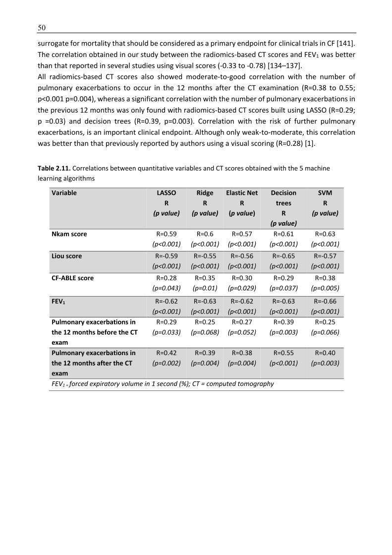
50

surrogate for mortality that should be considered as a primary endpoint for clinical trials in CF [141].

The correlation obtained in our study between the radiomics-based CT scores and FEV1 was better

than that reported in several studies using visual scores (-0.33 to -0.78) [134–137].

All radiomics-based CT scores also showed moderate-to-good correlation with the number of

pulmonary exacerbations to occur in the 12 months after the CT examination (R=0.38 to 0.55;

p<0.001 p=0.004), whereas a significant correlation with the number of pulmonary exacerbations in

the previous 12 months was only found with radiomics-based CT scores built using LASSO (R=0.29;

p =0.03) and decision trees (R=0.39, p=0.003). Correlation with the risk of further pulmonary

exacerbations, is an important clinical endpoint. Although only weak-to-moderate, this correlation

was better than that previously reported by authors using a visual scoring (R=0.28) [1].

Table 2.11. Correlations between quantitative variables and CT scores obtained with the 5 machine

learning algorithms

Variable LASSO R

(p value)

Ridge R

(p value)

Elastic Net R

(p value)

Decision trees

R (p value)

SVM R

(p value)

Nkam score R=0.59

(p<0.001) R=0.6

(p<0.001) R=0.57

(p<0.001) R=0.61

(p<0.001) R=0.63

(p<0.001)

Liou score R=-0.59

(p<0.001) R=-0.55

(p<0.001) R=-0.56

(p<0.001) R=-0.65

(p<0.001) R=-0.57

(p<0.001)

CF-ABLE score

R=0.28

(p=0.043) R=0.35

(p=0.01) R=0.30

(p=0.029) R=0.29

(p=0.037) R=0.38

(p=0.005)

FEV1 R=-0.62

(p<0.001) R=-0.63

(p<0.001) R=-0.62

(p<0.001) R=-0.63

(p<0.001) R=-0.66

(p<0.001) Pulmonary exacerbations in the 12 months before the CT exam

R=0.29

(p=0.033) R=0.25

(p=0.068) R=0.27

(p=0.052) R=0.39

(p=0.003) R=0.25

(p=0.066)

Pulmonary exacerbations in the 12 months after the CT exam

R=0.42

(p=0.002) R=0.39

(p=0.004) R=0.38

(p=0.004) R=0.55

(p<0.001) R=0.40

(p=0.003)

FEV1 = forced expiratory volume in 1 second (%); CT = computed tomography

51

Figure 2.8. A) The calculated value for the Nkam score was 0.5 in this 20-year-old CF patient. Using CT images, the radiomics approach predicted a Nkam score value of 0.35 with Lasso and 0.30 with Decision

trees. B) By comparison, the calculated value for the Nkam score was 3 in this 48-year-old CF patient. Using CT images, the radiomics approach predicted a Nkam score value of 2.96 with Lasso and 2.11 with Decision

trees.

2.3.4 Discussion To the best of our knowledge, this study is the first to evaluate a radiomics-based approach to

quantify lung disease on CT in adults with CF. Moderate-to-good correlations between radiomics-

based models and the Nkam score [161], the Liou score [169], the FEV1 and the number of

pulmonary exacerbations to occur in the next 12 months was found in a patient cohort from a center

different from the training cohort.

A major strength of our study is that the 5 radiomics models developed in one center remained

predictive of disease severity in an independent cohort despite different CT equipment, acquisition

and reconstruction parameters, including the use of iterative reconstructions only in the test center.

The differences in scanning protocols resulted in a significantly lower radiation dose exposure in the

test cohort. The absence of standardized acquisition protocols and the use of standard of care

images is a strength of our study. Indeed, the reproducibility of many textural parameters is

influenced by acquisition and reconstruction parameters [172–174]. Building radiomics-based CT

scores from standardized parameters limits their applicability for routine practice.

This study has several limitations. First, the proposed radiomics-based CT scores provide an overall

estimation of structural changes in the lung but cannot separately quantify irreversible

bronchiectasis and changes such as bronchial wall thickening or mucous plugging which are

potentially reversible using the newly developed therapies [110]. We deliberately based our score

on inspiratory CT images, and did not use expiratory CT images in addition. Indeed, we believe

routine expiratory CT images are not justified in CF patients because of the increase in radiation

dose and the lack of implications for patient care. Finally, our study population only included adult

CF patients and the developed approach should therefore be validated in pediatric CF populations.

In conclusion, radiomics can be used to calculate automated CT scores that are correlated to clinical

prognosis scores, FEV1 and risk of exacerbations in adult CF patients from different institutions. This

offers new perspectives for automated CT assessment of diffuse bronchial diseases.

52

Chapter 3

3 Interstitial lung disease segmentation using deep learning

In this chapter, we investigate a deep learning-based segmentation tool to quantify interstitial lung

disease (ILD) extent on chest CT in systemic sclerosis (SSc) patients.

ILD quantification is a major challenge for patient care in many chronic lung diseases including

systemic sclerosis. It mainly relies on a physiological approach using pulmonary function testing

(PFT), often used as primary endpoint in clinical trials. However, PFT measurements are imperfect

and only reflect lung function, not necessarily disease activity. Additionally, disease extent is known

to be an independent predictor of disease progression and mortality in patients in several ILD,

including idiopathic pulmonary fibrosis and SSc [15,16,175].

Among imaging techniques, CT is the gold standard for in vivo morphological assessment of lung

parenchyma and for the early detection of ILD [11]. Several visual scoring systems have been

proposed but they only allow basic quantification of ILD severity and they suffer from poor-to-

moderate inter-observer agreement [13]. ILD quantification on CT would require an automated and

reproducible segmentation of the diseased lung.

Recently, machine learning has gained a lot of attention with encouraging reports on variety of open

problems from different communities. Artificial neural networks (ANNs) and, in particular,

convolutional neural networks (CNNs) achieved impressive results in a variety of tasks after the

breakthrough of AlexNet architecture in the ImageNet Large Scale Visual Recognition Competition

in 2012 [176]. These powerful algorithms are machine learning models that are mostly inspired from

human intelligence and utilize fairly elementary sequential mathematical operations (linear

operators) that seek to reproduce an outcome using a combination of observations rather than

understanding the process of decision and reproducing it, as a variety of statistical based model are

working [33]. In particular, a very interesting and different component of these algorithms is their

ability to find and automatically generate the characteristics/ features that are more appropriate

for the specific problem they want to address. Networks of this kind have existed for decades [177],

but have only recently managed to achieve adequate performance mainly due to the large volumes

of available annotated data, the massive parallelization capabilities of GPUs and a number of public

contribution libraries that facilitated a lot their usage. The term deep learning is used recently to

describe a set of schemes and tools that are utilized in order to train complex and multi-layered

ANNs using a large amount of data. Since the breakthrough of AlexNet in 2012 [178], more and more

researchers are utilizing deep learning approaches pushing the state of the art performance to a

variety of tasks such as object detection in images [179], image super resolution [180], action

detection in video, natural language processing [181]. Following these very promising advances

from the aforementioned fields, slow and confident strides have also been taken in the fields of

computer assisted medicine [182,183].

In particular, several deep-learning architectures have been evaluated or specifically developed for

segmentation and/ or classification on medical images. These architectures consist of a sequence of

53

layers mainly optimized on the task they need to address. Architectures that address classification

tasks are usually consist of fully convolutional layers forming architectures as the AlexNet [178],

DenseNet [184] or many other architectures proposed recently on the literature. On the other hand,

architectures that address segmentation problems are usually fully convolutional adapting an

encoder-decoder scheme such as U-Net [46] for segmentation on 2D and V-Net [185] for

segmentation of 3D volumes. Moreover, recently recurrent neural networks (RNN) have also been

evaluated by several authors [183].

In general, the networks that are focusing on segmentation tasks in medical imaging aim to

automatically, efficiently and accurately segment different organs or types of diseases. Indeed,

segmentation can be used to evaluate shape, volume and many other characteristics that are very

important from a medical point of view [183]. Image segmentation is one of the most often studied

problems in medical image analysis [186,187]. Segmentation seeks to associate each voxel with a

specific label/class, for instance diseased or healthy area in interstitial lung diseases. Existing

literature can be classified into two distinct categories, model-free and model-based methods.

Model-based methods assume that the geometric prior distribution of the structure to be

segmented can be learned and modeled with sub-space approaches (e.g. active shapes),

probabilistic or graphical models and atlas-based approaches being some representatives in this

category [187]. These methods work well with normal anatomical structures where the notion of

repeatability makes sense but fail to capture disease variation that is in general random. Model-free

approaches on the other hand purely rely on the observation space combining image likelihoods

with different classification techniques. CNNs currently give state of the art results on image

segmentation of medical image analysis. These networks can adapt a patch-based approach, where

the network uses a patch extracted around the voxel that need to be segmented or a dense

pixelwise prediction where the network produces the segmentation of each voxel producing directly

the segmentation mask.

Patch-based approach can also be used with classic machine learning and this has been done with

diverse results [9,188,189]. [190], who used CNN for ILD segmentation with a patch-based approach,

reported an accuracy of 86% for classification of lung voxels in 7 classes. To achieve these results,

they used an algorithm inspired from VGG architecture but with an even more shrunk kernel size

and only 5 convolutional layers. This was further improved by [88] who used a CNN composed of

four convolution layers and two fully connected layers for patch-based ILD segmentation. The

authors reported an accuracy ranging from 85% to 96% depending on their data split and shown the

superiority of CNN over SVM who offered an accuracy of 77 to 90%. As previously mentioned, the

main drawback of the patch-based approach is to not take into account context information such

as the subpleural location and basal predominance usually seen in ILD.

Dense pixelwise prediction based on the entire image has been made popularized since the

introduction of fully convolutional networks (fCNN) [191]. The main limitation to the use of CNN for

dense prediction was the pooling layers of the encoder architecture who allow to take into account

the context but gradually decrease image resolution. By using skip connections during the

upsampling process, fCNN allows to recover spatial resolution to obtain a full resolution prediction

despite the use multiple pooling steps. The fCNN was one of the first encoder-decoder architecture.

Connections between the encoder and the decoder parts have been further improved, for instance

by the transfer of maxpooling indices from the encoder to the decoder parts in SegNet [47] or by

54

direct connection between opposing contracting and expanding convolutional layers using

concatenation in U-Net [46]. U-net which outperformed previous encoder-decoder architectures

has become very popular for medical image analysis. A 3D variant of the U-net, called V-net has

been proposed by [185].

An alternative to the encoder-decoder architecture is the use of atrous convolutions (also termed

dilated convolutions) in the Deeplab architectures. This architecture has been successfully

implemented by [192] for ILD segmentations and it allowed them to improve the balanced cross-

validation accuracy from 72% when using their previous patch-based approach [190] to 82%, while

also decreasing inference time from 237 to 58 ms.

In contrast to patch-based CNNs, dense prediction has the advantage to take into account the full

context of the image and to reduce redundant computation. The use of the full context of the image

is of particular interest in ILD. Indeed, spatial localization is a key element of ILD analysis on CT,

especially for the diagnosis of idiopathic pulmonary fibrosis [193,194]. In SSc, ILD distribution is also

a key feature and usually predominates in the subpleural aspects of the lower lobes [195,196].

The main challenges for deep learning in medical imaging arise from the limited availability of

training samples – that is amplified when targeting 3D architectures –, the lack of discriminant visual

properties, the three-dimensional nature of observations (high dimensional data) and the lack of

context integration in an implicit or explicit manner.

The only available ILD dataset [43] is sparsely annotated and the lack of annotated database is a

common problem for the development of segmentation methods in medical imaging.

In this chapter we investigate a two-fold approach, one that looks into sparse classification through

patch-based CNNs and a second that seeks to deliver full labeling of the disease using also

convolutional neural networks.

First, we evaluated a combination of patched-based and fully-convolutional encoder-decoder

architectures for ILD segmentation [197]. In this work, we created a framework that integrated deep

patch-based priors (trained on publicly available databases) with a fully convolutional encoder-

decoder network (trained on a small number of images). The combination of the two architectures

allowed to transfer the learned features across different datasets and increased segmentation

accuracy. This could help to decrease the amount of fully-annotated images used to train a model.

Secondarily, we created a new architecture (AtlasNet) combining elastic registration and encoder-

decoder architecture to segment ILD [48] The idea is to train n number of CNN, each of them using

a predefined anatomy on which all training cases are mapped through elastic registration, resulting

in a natural data augmentation. This method also has the advantage to decrease the complexity of

observations related to anatomical variability and to increase the “anatomical” consistency of the

networks. AtlasNet offered better performances than state-of-art methods for ILD segmentation on

chest CT. Despite the small number of fully annotated CT scans (17 examinations) used for training

and validation, AtlasNet performed similarly to 3 radiologists.

Lastly, we augmented the AtlasNet network through a dual auto-decoder architecture in order to

guarantee anatomical plausibility in disease segmentation results. We showed that this method

performed better than a U-net architecture and as well as radiologists for disease segmentation.

The combination of disease and lung segmentations allowed to calculate normalized disease extent

and we found that the ILD extent provided by our model was well correlated with PFTs, especially

DLCO, in a cohort of 171 SSc patients. These correlations were confirmed in an external validation

cohort of 31 SSc patients.

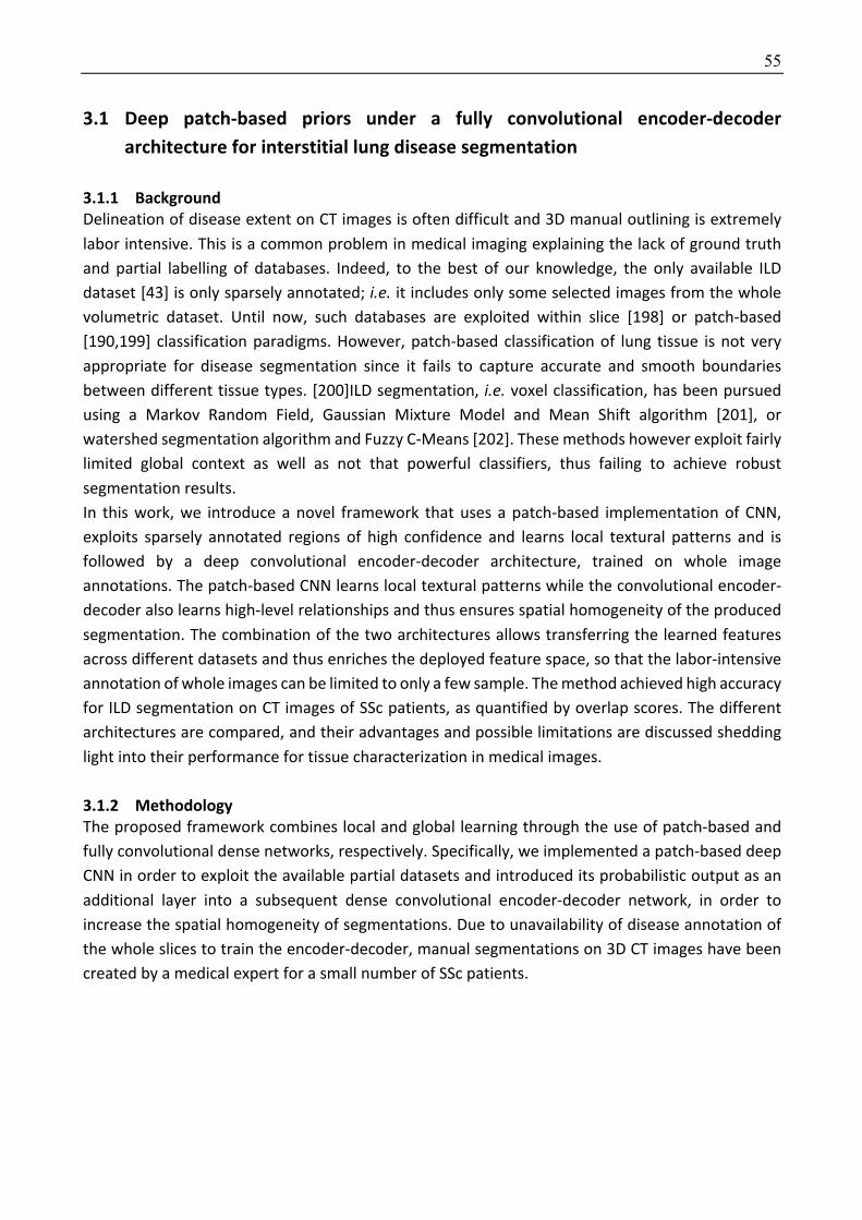
55

3.1 Deep patch-based priors under a fully convolutional encoder-decoder architecture for interstitial lung disease segmentation

3.1.1 Background Delineation of disease extent on CT images is often difficult and 3D manual outlining is extremely

labor intensive. This is a common problem in medical imaging explaining the lack of ground truth

and partial labelling of databases. Indeed, to the best of our knowledge, the only available ILD

dataset [43] is only sparsely annotated; i.e. it includes only some selected images from the whole

volumetric dataset. Until now, such databases are exploited within slice [198] or patch-based

[190,199] classification paradigms. However, patch-based classification of lung tissue is not very

appropriate for disease segmentation since it fails to capture accurate and smooth boundaries

between different tissue types. [200]ILD segmentation, i.e. voxel classification, has been pursued

using a Markov Random Field, Gaussian Mixture Model and Mean Shift algorithm [201], or

watershed segmentation algorithm and Fuzzy C-Means [202]. These methods however exploit fairly

limited global context as well as not that powerful classifiers, thus failing to achieve robust

segmentation results.

In this work, we introduce a novel framework that uses a patch-based implementation of CNN,

exploits sparsely annotated regions of high confidence and learns local textural patterns and is

followed by a deep convolutional encoder-decoder architecture, trained on whole image

annotations. The patch-based CNN learns local textural patterns while the convolutional encoder-

decoder also learns high-level relationships and thus ensures spatial homogeneity of the produced

segmentation. The combination of the two architectures allows transferring the learned features

across different datasets and thus enriches the deployed feature space, so that the labor-intensive

annotation of whole images can be limited to only a few sample. The method achieved high accuracy

for ILD segmentation on CT images of SSc patients, as quantified by overlap scores. The different

architectures are compared, and their advantages and possible limitations are discussed shedding

light into their performance for tissue characterization in medical images.

3.1.2 Methodology The proposed framework combines local and global learning through the use of patch-based and

fully convolutional dense networks, respectively. Specifically, we implemented a patch-based deep

CNN in order to exploit the available partial datasets and introduced its probabilistic output as an

additional layer into a subsequent dense convolutional encoder-decoder network, in order to

increase the spatial homogeneity of segmentations. Due to unavailability of disease annotation of

the whole slices to train the encoder-decoder, manual segmentations on 3D CT images have been

created by a medical expert for a small number of SSc patients.

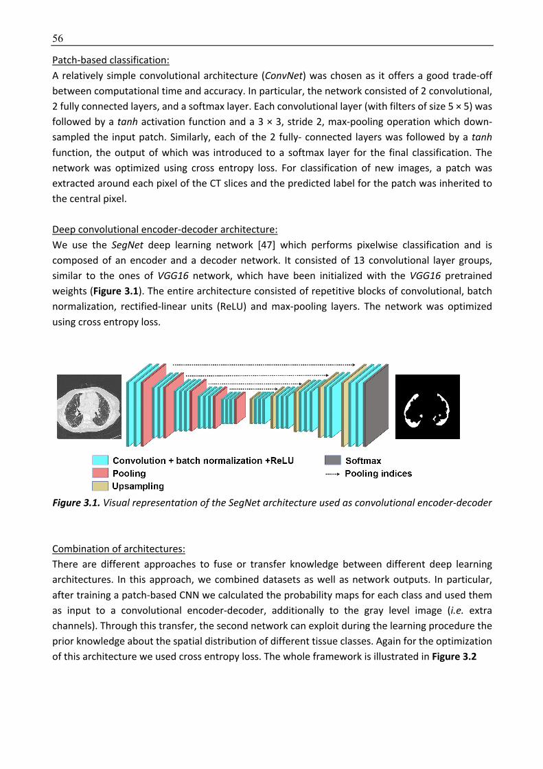
56

Patch-based classification:

A relatively simple convolutional architecture (ConvNet) was chosen as it offers a good trade-off

between computational time and accuracy. In particular, the network consisted of 2 convolutional,

2 fully connected layers, and a softmax layer. Each convolutional layer (with filters of size 5 × 5) was

followed by a tanh activation function and a 3 × 3, stride 2, max-pooling operation which down-

sampled the input patch. Similarly, each of the 2 fully- connected layers was followed by a tanh function, the output of which was introduced to a softmax layer for the final classification. The

network was optimized using cross entropy loss. For classification of new images, a patch was

extracted around each pixel of the CT slices and the predicted label for the patch was inherited to

the central pixel.

Deep convolutional encoder-decoder architecture:

We use the SegNet deep learning network [47] which performs pixelwise classification and is

composed of an encoder and a decoder network. It consisted of 13 convolutional layer groups,

similar to the ones of VGG16 network, which have been initialized with the VGG16 pretrained

weights (Figure 3.1). The entire architecture consisted of repetitive blocks of convolutional, batch

normalization, rectified-linear units (ReLU) and max-pooling layers. The network was optimized

using cross entropy loss.

Figure 3.1. Visual representation of the SegNet architecture used as convolutional encoder-decoder

Combination of architectures:

There are different approaches to fuse or transfer knowledge between different deep learning

architectures. In this approach, we combined datasets as well as network outputs. In particular,

after training a patch-based CNN we calculated the probability maps for each class and used them

as input to a convolutional encoder-decoder, additionally to the gray level image (i.e. extra

channels). Through this transfer, the second network can exploit during the learning procedure the

prior knowledge about the spatial distribution of different tissue classes. Again for the optimization

of this architecture we used cross entropy loss. The whole framework is illustrated in Figure 3.2

57

Figure 3.2. The proposed combination model with the two training datasets.

Note : CED = convolutional encoder-decoder

3.1.3 Dataset and Implementation Details Datasets:

We performed experiments using two different datasets.

The first dataset included (volumetric) CT images from 12 SSc patients. These images had been fully

annotated according to 3 different classes: healthy lung, diseased lung, and background (body tissue

outside the lung and background). Lung segmentation had been performed using Myrian XP-lung

software (Intrasense) and subsequently manually corrected whenever required. ILD segmentation

had been performed by a chest radiologist tracing the disease boundaries in axial view over all CT

slices. Assessment of the method was performed on 20 additional patients with annotations on only

20 selected CT slices, resulting in a total of 400 annotated slices for the test dataset.

The second dataset was a publicly available ILD dataset [43] which contains 905 selected slices from

120 patients including in total 13 ILD labels (such as ground glass, fibrosis, micronodules,

consolidation, etc). This dataset is sparsely annotated, and thus could only be used for the patch-

based model. Since our goal was to segment ILD extent in SSc patients, we were not interested in

the subcategorization of individual tissue abnormalities, thus we merged all the indicated disease

manifestations into a single class.

Implementation details:

For the patch-based CNN, 80000 patches were extracted for each class containing samples from

both datasets (ILD and SSc). For our experiments, we used patches of size 29 × 29. The model was

trained for 50 epochs with learning rate for the stochastic gradient descent (SGD) 0.5 while every 3

epochs the learning rate was reduced to half. The momentum was set to 0.9 and the weight decay

to 5.10-4.

For training of the convolutional encoder-decoder we used around 3400 CT slices and for the

training of the convolutional encoder-decoder with the combined input 150 CT slices. For our

experiments, we used image slices of the original dimension (512 × 512) and we first pre-trained the

model for 60 epochs (without incorporating probability maps) with learning rate for the SGD starting

at 0.01 and then reducing every 20 epochs by 2.5·10-3. Similarly to the patch-based classifier, the

momentum was set to 0.9 and the weight decay to 5.10-4.

We trained the combination convolutional encoder-decoder architecture for 70 epochs, with

combined input (CT images and probability maps), initializing the encoder weights with the ones

calculated from the pre-training phase.

Moreover, for training the convolutional encoder-decoder and the combination models, we

performed median frequency balancing [47] to balance the data, as the samples with disease were

considerably fewer than the rest of the samples. In such a setup, the assigned weight to a class in

58

the loss function was the ratio of the median of class frequencies computed on the entire training

set divided by the class frequency.

In order to assess the importance of information fusion, we also retrained the convolutional

encoder-decoder without using the probability maps from the patch-based network (Table 3.1, row

3) using the same 150 slices as in the proposed scheme.

3.1.4 Experimental Results We evaluated the detection accuracy of each class against any other class, using four metrics,

namely sensitivity, specificity and precision and the Dice similarity coefficient (Appendix). Since the

metrics were calculated for every slice, we averaged the results across slices by weighting the values

based on the coverage of each class within each slice. This should be equivalent to an approximate

estimation of the metrics in 3D. For comparison with others, we reported results for each

architecture individually to approximate the performance of the methods in [190] and [203] by the

patch-based CNN (Table 3.1, 1st row) and [47] by the convolutional encoder-decoder.

Our proposed method offered higher precision and specificity for disease classification, but lower

sensitivity compared to the other three methods (Table 3.1). The high sensitivity of the patch-based

strategy was accompanied by a low precision indicating that it is not appropriate for dense

classification. Additionally, retraining the convolutional encoder-decoder without information

fusion, boosted the results but did not outperformed the proposed method. Moreover, Figure 3.3

shows that the proposed strategy outperformed the other two in respect to the Dice similarity

coefficient for both diseased and healthy lung, with mean values for the diseased tissue of 0.619,

0.694, 0.709 and 0.722 for the patch-based, the convolutional encoder-decoder, the convolutional

encoder-decoder with retrain and the proposed strategy, respectively.

Table 3.1. Different evaluation metrics for the testing dataset

Method Specificity Sensitivity Precision

Disease Healthy Disease Healthy Disease Healthy Patch-based

0.948 0.990 0.902 0.743 0.489 0.924

CED 0.971 0.983 0.906 0.889 0.598 0.923

CED retrain 0.981 0.980 0.819 0.932 0.639 0.891

Proposed 0.989 0.985 0.827 0.943 0.671 0.904

CED = convolutional encoder-decoder

Figure 3.3. The average, maximum and minimum values for the calculated Dice coefficient for diseased and healthy tissue and all employed strategies. Blue and red indicate values above and below the average.

Visual assessment of the segmentation is illustrated for a test subject in Figure 3.4.

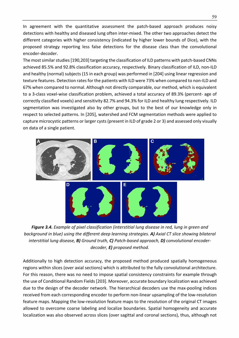
59

In agreement with the quantitative assessment the patch-based approach produces noisy

detections with healthy and diseased lung often inter-mixed. The other two approaches detect the

different categories with higher consistency (indicated by higher lower bounds of Dice), with the

proposed strategy reporting less false detections for the disease class than the convolutional

encoder-decoder.

The most similar studies [190,203] targeting the classification of ILD patterns with patch-based CNNs

achieved 85.5% and 92.8% classification accuracy, respectively. Binary classification of ILD, non-ILD

and healthy (normal) subjects (15 in each group) was performed in [204] using linear regression and

texture features. Detection rates for the patients with ILD were 73% when compared to non-ILD and

67% when compared to normal. Although not directly comparable, our method, which is equivalent

to a 3-class voxel-wise classification problem, achieved a total accuracy of 89.3% (percent- age of

correctly classified voxels) and sensitivity 82.7% and 94.3% for ILD and healthy lung respectively. ILD

segmentation was investigated also by other groups, but to the best of our knowledge only in

respect to selected patterns. In [205], watershed and FCM segmentation methods were applied to

capture microcystic patterns or larger cysts (present in ILD of grade 2 or 3) and assessed only visually

on data of a single patient.

Figure 3.4. Example of pixel classification (interstitial lung disease in red, lung in green and

background in blue) using the different deep learning strategies. A) Axial CT slice showing bilateral interstitial lung disease, B) Ground truth, C) Patch-based approach, D) convolutional encoder-

decoder, E) proposed method.

Additionally to high detection accuracy, the proposed method produced spatially homogeneous

regions within slices (over axial sections) which is attributed to the fully convolutional architecture.

For this reason, there was no need to impose spatial consistency constraints for example through

the use of Conditional Random Fields [203]. Moreover, accurate boundary localization was achieved

due to the design of the decoder network. The hierarchical decoders use the max-pooling indices

received from each corresponding encoder to perform non-linear upsampling of the low-resolution

feature maps. Mapping the low-resolution feature maps to the resolution of the original CT images

allowed to overcome coarse labeling and localize boundaries. Spatial homogeneity and accurate

localization was also observed across slices (over sagittal and coronal sections), thus, although not

60

guaranteed, we do not expect to have a significant gain from the substitution of our 2D networks

by 3D architectures. Furthermore, collection of good quality 3D ground truth is difficult, because

the manual outlining is usually performed over axial slices, thus often lacks smooth boundaries

across the other two planes.

The training of the patch-based model required a bit less than an hour as the architecture was

relatively small. In that strategy, the extraction of patches was the most computationally demanding

task. This is a limitation in the testing phase where the number of voxels to be annotated is

particularly large. On the other hand, the convolutional encoder-decoder required around 24 hours

for the training and another 6 hours for the final training by the combined input. However, for both

of them, the testing phase lasted only a few seconds for segmentation of one lung image.

3.1.5 Discussion In this chapter, we have introduced a novel framework that integrates deep, patch-based (trained

on available databases) priors with a fully convolutional encoder-decoder network (trained on a

small number of images), to improve generalization performance.

Additionally to high detection accuracy, the proposed method produced spatially homogeneous

regions within slices (over axial sections) which is attributed to the fully convolutional architecture.

For this reason, there was no need to impose spatial consistency constraints for example through

the use of Conditional Random Fields [203]. Moreover, accurate boundary localization was achieved

due to the design of the decoder network. The hierarchical decoders use the max-pooling indices

received from each corresponding encoder to perform non-linear upsampling of the low-resolution

feature maps. Mapping the low-resolution feature maps to the resolution of the original CT images

allowed to overcome coarse labeling and localize boundaries. Spatial homogeneity and accurate

localization was also observed across slices (over sagittal and coronal sections), thus, although not

guaranteed, we do not expect to have a significant gain from the substitution of our 2D networks

by 3D architectures. Furthermore, collection of good quality 3D ground truth is difficult, because

the manual outlining is usually performed over axial slices, thus often lacks smooth boundaries

across the other two planes.

The combination of the two architectures allowed enriching the deployed feature space and thus

increased the segmentation accuracy. The method was applied for ILD segmentation on CT images,

but generalizes to other tissue or texture characterization problems as well. It does not incorporate

any shape or deformation priors or physiological models that guide detection, therefore it is not

specialized to the detection of localized structures, such as organs or uniform masses (although it

can handle also this type of problems given enough training data). On the other hand, by learning

only from image content, the method is modular and easy to use. Future work includes the

investigation of 3D convolution and the trade-off between possible gain in volumetric smoothness

over the additional computational cost required to minimize discontinuities of annotations over

sagittal and coronal views.

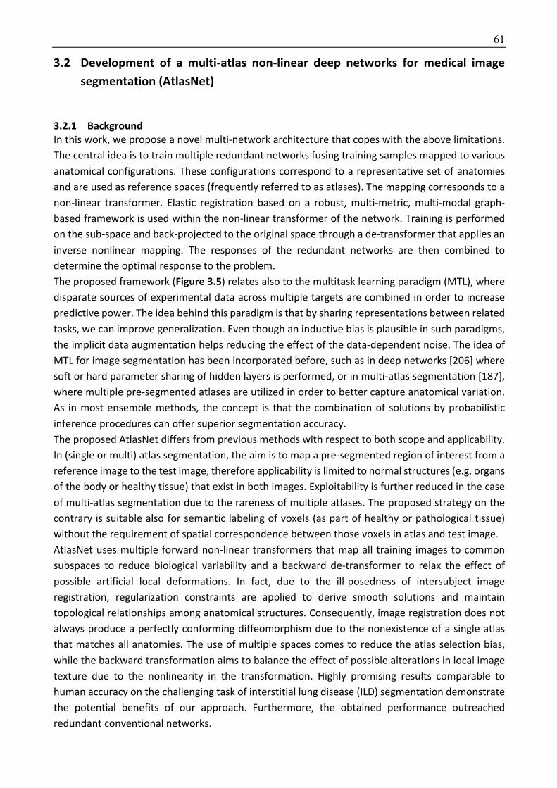
61

3.2 Development of a multi-atlas non-linear deep networks for medical image segmentation (AtlasNet)

3.2.1 Background In this work, we propose a novel multi-network architecture that copes with the above limitations.

The central idea is to train multiple redundant networks fusing training samples mapped to various

anatomical configurations. These configurations correspond to a representative set of anatomies

and are used as reference spaces (frequently referred to as atlases). The mapping corresponds to a

non-linear transformer. Elastic registration based on a robust, multi-metric, multi-modal graph-

based framework is used within the non-linear transformer of the network. Training is performed

on the sub-space and back-projected to the original space through a de-transformer that applies an

inverse nonlinear mapping. The responses of the redundant networks are then combined to

determine the optimal response to the problem.

The proposed framework (Figure 3.5) relates also to the multitask learning paradigm (MTL), where

disparate sources of experimental data across multiple targets are combined in order to increase

predictive power. The idea behind this paradigm is that by sharing representations between related

tasks, we can improve generalization. Even though an inductive bias is plausible in such paradigms,

the implicit data augmentation helps reducing the effect of the data-dependent noise. The idea of

MTL for image segmentation has been incorporated before, such as in deep networks [206] where

soft or hard parameter sharing of hidden layers is performed, or in multi-atlas segmentation [187],

where multiple pre-segmented atlases are utilized in order to better capture anatomical variation.

As in most ensemble methods, the concept is that the combination of solutions by probabilistic

inference procedures can offer superior segmentation accuracy.

The proposed AtlasNet differs from previous methods with respect to both scope and applicability.

In (single or multi) atlas segmentation, the aim is to map a pre-segmented region of interest from a

reference image to the test image, therefore applicability is limited to normal structures (e.g. organs

of the body or healthy tissue) that exist in both images. Exploitability is further reduced in the case

of multi-atlas segmentation due to the rareness of multiple atlases. The proposed strategy on the

contrary is suitable also for semantic labeling of voxels (as part of healthy or pathological tissue)

without the requirement of spatial correspondence between those voxels in atlas and test image.

AtlasNet uses multiple forward non-linear transformers that map all training images to common

subspaces to reduce biological variability and a backward de-transformer to relax the effect of

possible artificial local deformations. In fact, due to the ill-posedness of intersubject image

registration, regularization constraints are applied to derive smooth solutions and maintain

topological relationships among anatomical structures. Consequently, image registration does not

always produce a perfectly conforming diffeomorphism due to the nonexistence of a single atlas

that matches all anatomies. The use of multiple spaces comes to reduce the atlas selection bias,

while the backward transformation aims to balance the effect of possible alterations in local image

texture due to the nonlinearity in the transformation. Highly promising results comparable to

human accuracy on the challenging task of interstitial lung disease (ILD) segmentation demonstrate

the potential benefits of our approach. Furthermore, the obtained performance outreached

redundant conventional networks.

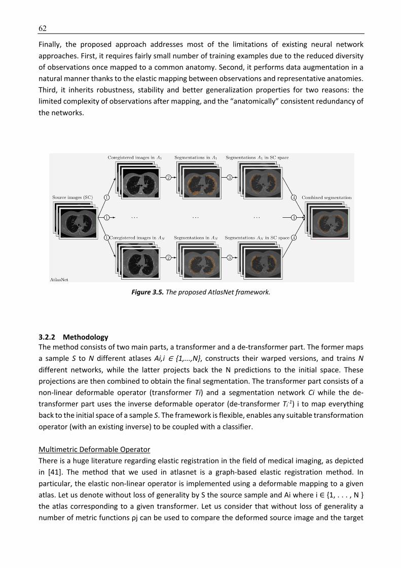
62

Finally, the proposed approach addresses most of the limitations of existing neural network

approaches. First, it requires fairly small number of training examples due to the reduced diversity

of observations once mapped to a common anatomy. Second, it performs data augmentation in a

natural manner thanks to the elastic mapping between observations and representative anatomies.

Third, it inherits robustness, stability and better generalization properties for two reasons: the

limited complexity of observations after mapping, and the “anatomically” consistent redundancy of

the networks.

Figure 3.5. The proposed AtlasNet framework.

3.2.2 Methodology The method consists of two main parts, a transformer and a de-transformer part. The former maps

a sample S to N different atlases Ai,i ∈ {1,...,N}, constructs their warped versions, and trains N

different networks, while the latter projects back the N predictions to the initial space. These

projections are then combined to obtain the final segmentation. The transformer part consists of a

non-linear deformable operator (transformer Ti) and a segmentation network Ci while the de-

transformer part uses the inverse deformable operator (de-transformer Ti-1) i to map everything

back to the initial space of a sample S. The framework is flexible, enables any suitable transformation

operator (with an existing inverse) to be coupled with a classifier.

Multimetric Deformable Operator

There is a huge literature regarding elastic registration in the field of medical imaging, as depicted

in [41]. The method that we used in atlasnet is a graph-based elastic registration method. In

particular, the elastic non-linear operator is implemented using a deformable mapping to a given

atlas. Let us denote without loss of generality by S the source sample and Ai where i ∈ {1, . . . , N }

the atlas corresponding to a given transformer. Let us consider that without loss of generality a

number of metric functions ρj can be used to compare the deformed source image and the target

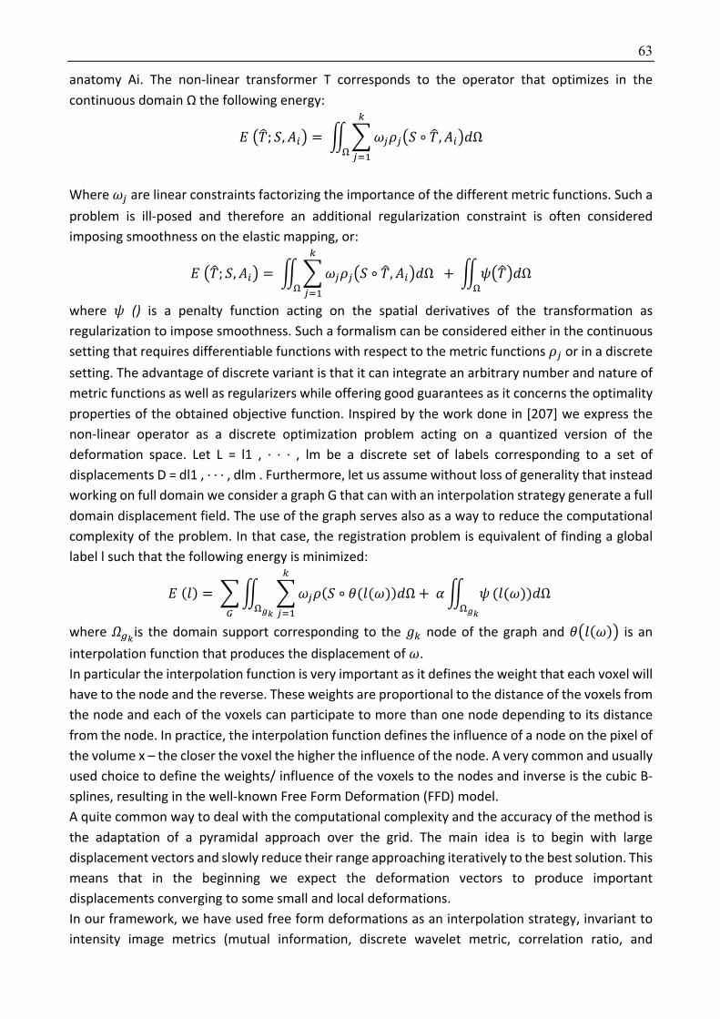
63

anatomy Ai. The non-linear transformer T corresponds to the operator that optimizes in the

continuous domain Ω the following energy:

^4jk; ], m*6 = n 7P?o?4] ∘ jk, m*6qΩ

s

?,-

t

Where P? are linear constraints factorizing the importance of the different metric functions. Such a

problem is ill-posed and therefore an additional regularization constraint is often considered

imposing smoothness on the elastic mapping, or:

^4jk; ], m*6 = n 7P?o?4] ∘ jk, m*6qΩ

s

?,-

t+nu4jk6qΩ

t

where u () is a penalty function acting on the spatial derivatives of the transformation as

regularization to impose smoothness. Such a formalism can be considered either in the continuous

setting that requires differentiable functions with respect to the metric functions o? or in a discrete

setting. The advantage of discrete variant is that it can integrate an arbitrary number and nature of

metric functions as well as regularizers while offering good guarantees as it concerns the optimality

properties of the obtained objective function. Inspired by the work done in [207] we express the

non-linear operator as a discrete optimization problem acting on a quantized version of the

deformation space. Let L = l1 , · · · , lm be a discrete set of labels corresponding to a set of

displacements D = dl1 , · · · , dlm . Furthermore, let us assume without loss of generality that instead

working on full domain we consider a graph G that can with an interpolation strategy generate a full

domain displacement field. The use of the graph serves also as a way to reduce the computational

complexity of the problem. In that case, the registration problem is equivalent of finding a global

label l such that the following energy is minimized:

^(f) = 7n 7P?o(] ∘ v(f(P))qΩ

s

?,-

twx

y

+ Dn u

twx

(f(P))qΩ

where z{x is the domain support corresponding to the hs node of the graph and v4f(P)6 is an

interpolation function that produces the displacement of P.

In particular the interpolation function is very important as it defines the weight that each voxel will

have to the node and the reverse. These weights are proportional to the distance of the voxels from

the node and each of the voxels can participate to more than one node depending to its distance

from the node. In practice, the interpolation function defines the influence of a node on the pixel of

the volume x – the closer the voxel the higher the influence of the node. A very common and usually

used choice to define the weights/ influence of the voxels to the nodes and inverse is the cubic B-

splines, resulting in the well-known Free Form Deformation (FFD) model.

A quite common way to deal with the computational complexity and the accuracy of the method is

the adaptation of a pyramidal approach over the grid. The main idea is to begin with large

displacement vectors and slowly reduce their range approaching iteratively to the best solution. This

means that in the beginning we expect the deformation vectors to produce important

displacements converging to some small and local deformations.

In our framework, we have used free form deformations as an interpolation strategy, invariant to

intensity image metrics (mutual information, discrete wavelet metric, correlation ratio, and

64

normalized cross correlation), pyramidal implementation approach for the optimization and belief

propagation for the estimation of the optimal displacement field in the discrete setting (step 1 in

Algorithm 1, Figure 3.6). Details on the implementation can be found in [208]. After defining the

optimal deformations T between the source image S and the different atlases Ai in the transformer

part, AtlasNet uses the inverse transformations to project back to the initial space of the source

image the predicted segmentation maps (step 3 in Algorithm 1). Different fusion strategies can be

used for the combination of the predicted ]*|}{ (step 4 in Algorithm 1). For the specific application

the final segmentation ]|}{ has been calculated by averaging all the predicted probalilistic ]*|}{.

Figure 3.6. AtlasNet pseudocode

The method consists of two main parts, a transformer and a de-transformer part. The former maps

a sample S to N different atlases Ai,i ∈ {1,...,N}, constructs their warped versions, and trains N

different networks, while the latter projects back the N predictions to the initial space. These

projections are then combined to obtain the final segmentation. The transformer part consists of a

non-linear deformable operator (transformer Ti) and a segmentation network Ci while the de-

transformer part uses the inverse deformable operator (de-transformer Ti-1) i to map everything

back to the initial space of a sample S. The framework is flexible, enables any suitable transformation

operator (with an existing inverse) to be coupled with a classifier.

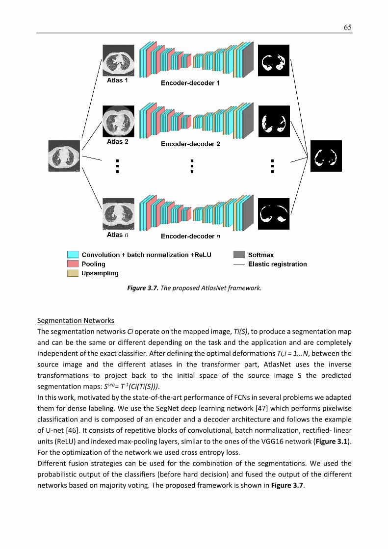
65

Figure 3.7. The proposed AtlasNet framework.

Segmentation Networks

The segmentation networks Ci operate on the mapped image, Ti(S), to produce a segmentation map

and can be the same or different depending on the task and the application and are completely

independent of the exact classifier. After defining the optimal deformations Ti,i = 1...N, between the

source image and the different atlases in the transformer part, AtlasNet uses the inverse

transformations to project back to the initial space of the source image S the predicted

segmentation maps: Sseg= T-1(Ci(Ti(S))). In this work, motivated by the state-of-the-art performance of FCNs in several problems we adapted

them for dense labeling. We use the SegNet deep learning network [47] which performs pixelwise

classification and is composed of an encoder and a decoder architecture and follows the example

of U-net [46]. It consists of repetitive blocks of convolutional, batch normalization, rectified- linear

units (ReLU) and indexed max-pooling layers, similar to the ones of the VGG16 network (Figure 3.1).

For the optimization of the network we used cross entropy loss.

Different fusion strategies can be used for the combination of the segmentations. We used the

probabilistic output of the classifiers (before hard decision) and fused the output of the different

networks based on majority voting. The proposed framework is shown in Figure 3.7.

66

3.2.3 Dataset and Implementation Dataset

The dataset included 17 (volumetric) CT scans consisting of 6888 slices in total, each being of 512 ×

512 dimension, which were fully annotated. Due to the average time required to manually fully

annotate disease on one CT exam (~ 6-10 hours), it was not possible to annotate enough patients

to use a 3D network. Indeed 3D networks consists of a bigger number of parameters than 2D. The

ILD annotation was performed by a medical expert tracing the disease boundaries in axial view over

all slices, which were used for training the classification model. Assessment of the method was

performed on images from 20 additional patients being annotated only on 20 selected CT slices by

three different observers. Images had been acquired at full inspiration on CT scanners from 2

manufacturers (Siemens Healthcare, Erlangen, Germany; Milwaukee, USA).

Implementation Details

For the registration, we used the same parameters for all images and all atlases. Three different

similarity metrics have been used, namely, mutual information, normalized cross correlation and

discrete wavelet metric. For the mutual information 16 bins were used, in the range of −900 to 100.

We used the same parameters for training all SegNet networks (initial learning rate = 0.01, decrease

of learning rate = 2.5·10-3 every 10 epochs, momentum = 0.9, weight decay = 5·10-4). The training of

a single network required around 16 hours on a GeForce GTX 1080 GPU, while the prediction for a

single (volumetric) subject lasted only a few seconds. For data augmentation we performed only

random rotations (between −10 and 10o) and translations (between 0 and 20 pixels per axis)

avoiding local deformations since the anatomy should not artificially change. Moreover, for training,

we performed median frequency balancing [47] to balance the data, as the samples with disease

are considerably fewer than the rest of the samples.

For all experiments we used 6 different atlases and registered both training and testing images to

them. The choice of atlases was made by a radiologist towards integrating important variability of

the considered anatomies.

3.2.4 Experimental Results ILD segmentation on CT images was considered for evaluation of the proposed multi-network

architecture; boundaries are hard to detect, visual characteristics of the disease can significantly

vary and delineation suffers from poor-to-moderate interobserver agreement [13]. Moreover,

although several visual scoring systems have been proposed for the disease, they only allow basic

quantification of ILD severity.

Our experimental evaluation had two objectives: (i) to evaluate robustness and accuracy of AtlasNet

compared to conventional networks and (ii) to examine whether the proposed methodology could

truly be trained with fewer examples while leading to good performance. We used five metrics,

namely sensitivity, precision, Hausdorff distance (Appendix), average contour distance and Dice

similarity coefficient (over the number of epochs) (Appendix), to evaluate the performance of the

proposed method.

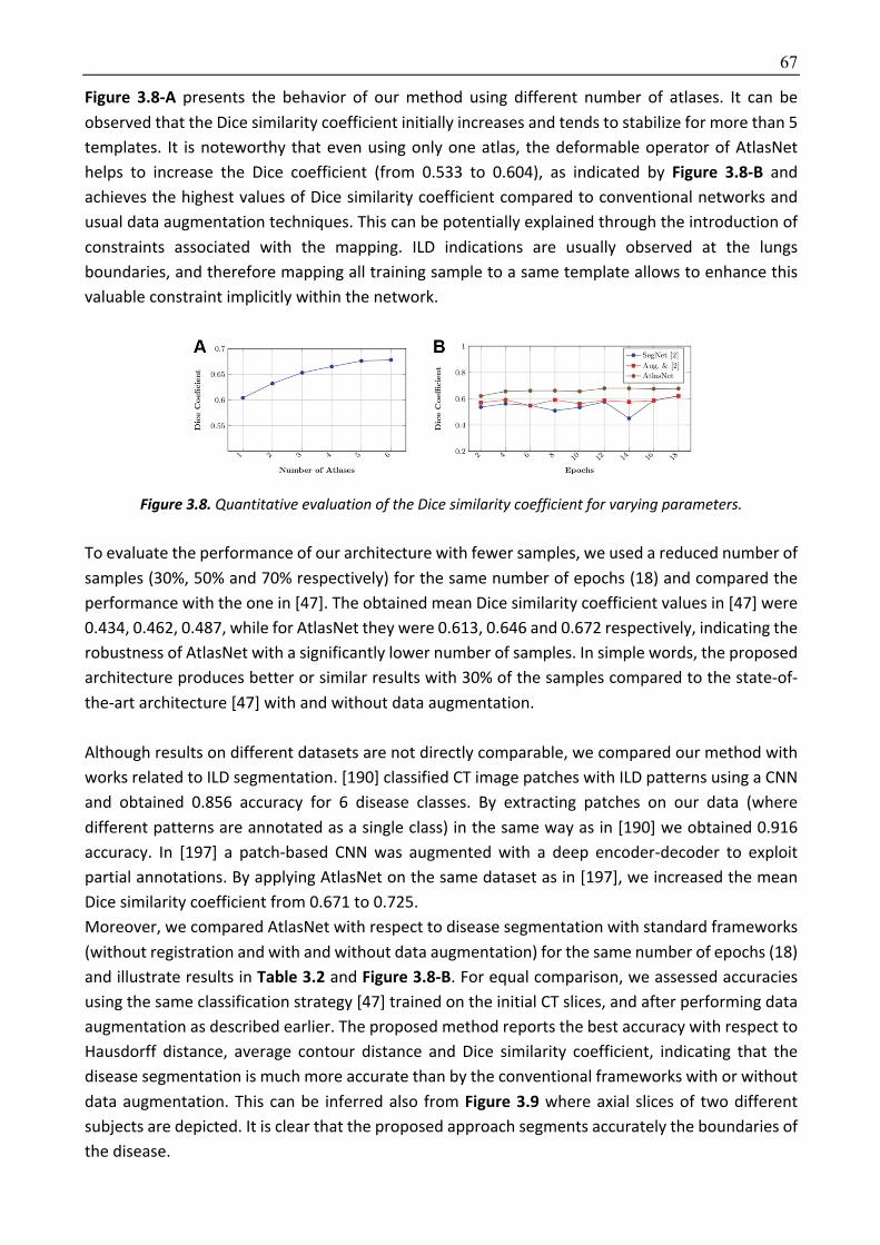
67

Figure 3.8-A presents the behavior of our method using different number of atlases. It can be

observed that the Dice similarity coefficient initially increases and tends to stabilize for more than 5

templates. It is noteworthy that even using only one atlas, the deformable operator of AtlasNet

helps to increase the Dice coefficient (from 0.533 to 0.604), as indicated by Figure 3.8-B and

achieves the highest values of Dice similarity coefficient compared to conventional networks and

usual data augmentation techniques. This can be potentially explained through the introduction of

constraints associated with the mapping. ILD indications are usually observed at the lungs

boundaries, and therefore mapping all training sample to a same template allows to enhance this

valuable constraint implicitly within the network.

Figure 3.8. Quantitative evaluation of the Dice similarity coefficient for varying parameters.

To evaluate the performance of our architecture with fewer samples, we used a reduced number of

samples (30%, 50% and 70% respectively) for the same number of epochs (18) and compared the

performance with the one in [47]. The obtained mean Dice similarity coefficient values in [47] were

0.434, 0.462, 0.487, while for AtlasNet they were 0.613, 0.646 and 0.672 respectively, indicating the

robustness of AtlasNet with a significantly lower number of samples. In simple words, the proposed

architecture produces better or similar results with 30% of the samples compared to the state-of-

the-art architecture [47] with and without data augmentation.

Although results on different datasets are not directly comparable, we compared our method with

works related to ILD segmentation. [190] classified CT image patches with ILD patterns using a CNN

and obtained 0.856 accuracy for 6 disease classes. By extracting patches on our data (where

different patterns are annotated as a single class) in the same way as in [190] we obtained 0.916

accuracy. In [197] a patch-based CNN was augmented with a deep encoder-decoder to exploit

partial annotations. By applying AtlasNet on the same dataset as in [197], we increased the mean

Dice similarity coefficient from 0.671 to 0.725.

Moreover, we compared AtlasNet with respect to disease segmentation with standard frameworks

(without registration and with and without data augmentation) for the same number of epochs (18)

and illustrate results in Table 3.2 and Figure 3.8-B. For equal comparison, we assessed accuracies

using the same classification strategy [47] trained on the initial CT slices, and after performing data

augmentation as described earlier. The proposed method reports the best accuracy with respect to

Hausdorff distance, average contour distance and Dice similarity coefficient, indicating that the

disease segmentation is much more accurate than by the conventional frameworks with or without

data augmentation. This can be inferred also from Figure 3.9 where axial slices of two different

subjects are depicted. It is clear that the proposed approach segments accurately the boundaries of

the disease.

68

For a more complete evaluation, we also compared AtlasNet with the annotations of three different

medical experts. The annotations of one observer have been used as ground truth to evaluate the

rest. From Table 3.2 and Figure 3.9, it can be observed that AtlasNet demonstrates more robust

performance than manual segmentation. Finally, it is worth mentioning that even if the network

operates on 2D slices, without accounting for out-of-slice connections, the fusion of the different

atlases’ predictions makes the final segmentation smooth across all three axes.

Concerning the computational resources, we used a single segmentation network [47] for each of

the N atlases, therefore the time and memory usage for one atlas is that of the CNN, while we also

showed that a small N (such as 6) is sufficient. For segmentation of one volumetric CT on a single

GPU the total testing time (using 6 atlases) is 3–4 min, including the registration step while the

registration cost is negligible since a graph-based GPU algorithm is used taking 3–5 s per subject.

This cost drops linearly with the number and computing power of GPUs. Thus, we believe that the

additional complexity of AtlasNet is fully justified, since it improves performance by more than 20%

and also maintains it stable with only 30% of the training data compared to conventional single

networks.

Figure 3.9. Example of interstitial lung disease segmentation (red color) in 2 patients using the different deep learning strategies.

Table 3.2. Evaluation metrics for the testing dataset for the systemic sclerosis disease.

Method Sensitivity Precision Hausdorff distance

Average distance

DSC

SegNet 0.348 0.623 4.984 1.891 0.533

Augmentation & SegNet

0.534 0.567 4.077 1.309 0.619

Inter-observer 0.693 0.522 4.005 1.317 0.662

AtlasNet 0.682 0.545 3.981 1.274 0.677

DSC = Dice Similarity Coefficient

69

3.2.5 Discussion We present a novel multi-network architecture for (healthy or pathological) tissue or organ

segmentation that maximizes consistency by exploiting diversity. Evaluation of the method on

interstitial lung disease segmentation highlighted its advantages over previous competing

approaches as well as inter-observer agreement. The investigation of techniques for soft parameter

sharing of hidden layers, and information transfer between the different networks and atlases is our

direction for future work. Finally, the extension to multi-organ segmentation including multiple

classes and loss functions is one of the potential directions of our method.

The integration of registration and segmentation is another promising direction of this work.

Currently, the elastic transformer operator is independent to the network. Numerous recent works

have claimed and shown strong experimental evidence that transformation can be learned as well

[97,209]. Proposing and end-to-end network that is able to automatically deform the target towards

different anatomies and distinguish pathologies from healthy tissue will eliminate the registration

dependency and benefit from the mutual coupling of the two terms. In order to achieve this

challenging objective, the approach has to evolve towards 3D networks. Learning 2D deformable

mappings might introduce bias since deformations are often out-of-plane and therefore cannot be

easily and appropriately learned with 2D models.

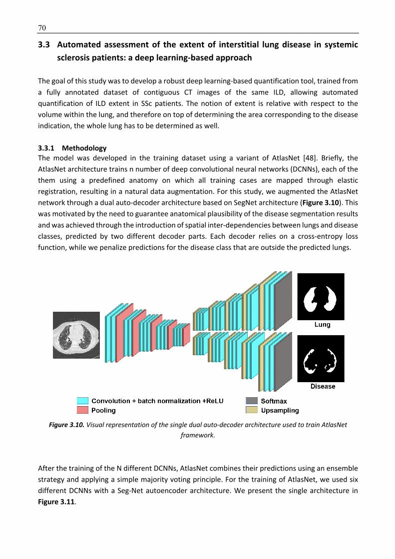
70

3.3 Automated assessment of the extent of interstitial lung disease in systemic sclerosis patients: a deep learning-based approach

The goal of this study was to develop a robust deep learning-based quantification tool, trained from

a fully annotated dataset of contiguous CT images of the same ILD, allowing automated

quantification of ILD extent in SSc patients. The notion of extent is relative with respect to the

volume within the lung, and therefore on top of determining the area corresponding to the disease

indication, the whole lung has to be determined as well.

3.3.1 Methodology The model was developed in the training dataset using a variant of AtlasNet [48]. Briefly, the

AtlasNet architecture trains n number of deep convolutional neural networks (DCNNs), each of the

them using a predefined anatomy on which all training cases are mapped through elastic

registration, resulting in a natural data augmentation. For this study, we augmented the AtlasNet

network through a dual auto-decoder architecture based on SegNet architecture (Figure 3.10). This

was motivated by the need to guarantee anatomical plausibility of the disease segmentation results

and was achieved through the introduction of spatial inter-dependencies between lungs and disease

classes, predicted by two different decoder parts. Each decoder relies on a cross-entropy loss

function, while we penalize predictions for the disease class that are outside the predicted lungs.

Figure 3.10. Visual representation of the single dual auto-decoder architecture used to train AtlasNet framework.

After the training of the N different DCNNs, AtlasNet combines their predictions using an ensemble

strategy and applying a simple majority voting principle. For the training of AtlasNet, we used six

different DCNNs with a Seg-Net autoencoder architecture. We present the single architecture in

Figure 3.11.

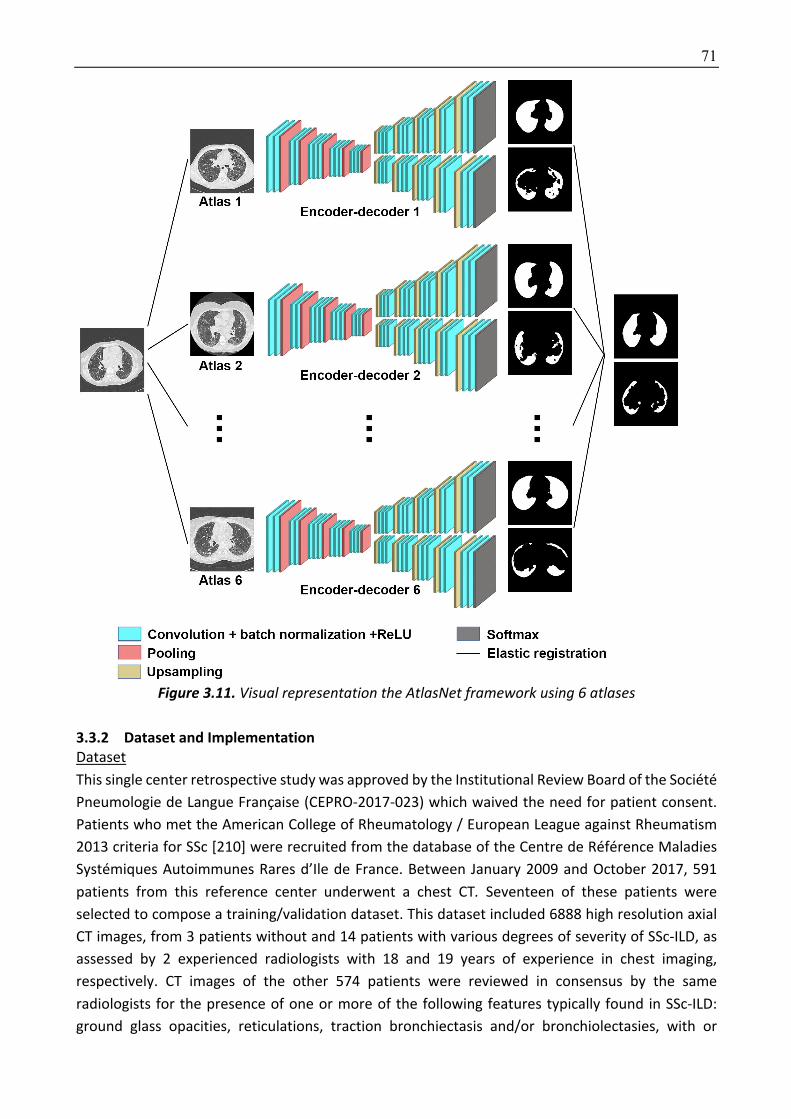
71

Figure 3.11. Visual representation the AtlasNet framework using 6 atlases

3.3.2 Dataset and Implementation Dataset

This single center retrospective study was approved by the Institutional Review Board of the Société

Pneumologie de Langue Française (CEPRO-2017-023) which waived the need for patient consent.

Patients who met the American College of Rheumatology / European League against Rheumatism

2013 criteria for SSc [210] were recruited from the database of the Centre de Référence Maladies

Systémiques Autoimmunes Rares d’Ile de France. Between January 2009 and October 2017, 591

patients from this reference center underwent a chest CT. Seventeen of these patients were

selected to compose a training/validation dataset. This dataset included 6888 high resolution axial

CT images, from 3 patients without and 14 patients with various degrees of severity of SSc-ILD, as

assessed by 2 experienced radiologists with 18 and 19 years of experience in chest imaging,

respectively. CT images of the other 574 patients were reviewed in consensus by the same

radiologists for the presence of one or more of the following features typically found in SSc-ILD:

ground glass opacities, reticulations, traction bronchiectasis and/or bronchiolectasies, with or

72

without honeycombing in a predominantly subpleural location. Exclusion criteria were 1/ motion

artifacts 2/ signs of lung disease other than SSc-ILD 3/ acquisitions in the prone position 4/ contrast

media injection 5/unavailability of complete PFTs measurement within 3 months before or after CT.

Of the 191 patients finally included, 20 patients were randomly assigned to compose a test cohort.

The correlation between PFTs and ILD extent assessed by deep learning was evaluated for the other

171 patients, composing the correlation to PFTs cohort.

An external validation cohort was composed by SSc patients from another institution (Hôpital Saint

Antoine, Paris France), who had been evaluated between March 2009 and March 2014. The same

inclusion and exclusion criteria were used.

For the training, test and correlation to PFTs datasets, whole lung CT examinations were obtained

with 4 different 16-to-128 multislice CT scanners from 2 different manufacturers (Somatom

Sensation 16, Somatom DS and Somatom AS+, Siemens Heathineer ; Revolution HD, General Electric

Healthcare), using non-standardized acquisition parameters. Images were reconstructed with a slice

thickness of 0.625 to 1.5mm, using filter back projection or iterative reconstruction algorithms, and

a high frequency kernel (LUNG, B70f or I70F). In the three datasets, the majority of CT examinations

had been acquired on Siemens equipment (3/17 in the training

For the external validation cohort, CT examinations were obtained with a different multislice CT

scanner (Somatom Sensation 64, Siemens Healthineer) using non-standardized acquisition

parameters. Images were reconstructed with a slice thickness of 1.5mm, using filter back projection

only and a high frequency kernel (B60f) different from the one used at our institution.

Disease segmentation was performed by manually outlining the extent of ILD on axial CT images,

including ground glass opacities, reticulations, traction bronchiectasis and honeycombing. CT

images in the training dataset were fully annotated by one radiologist with 5-year experience in

chest imaging, meaning that disease extent was manually contoured on each CT image showing

signs of ILD. Disease segmentation was performed by manually outlining the extent of ILD on axial

CT images, including ground glass opacities, reticulations, traction bronchiectasis and

honeycombing. CT exams in the test cohort were partially annotated by 3 independent radiologists

with 1 to 4 years of experience in chest imaging. Each of them annotated 20 CT slices equally spaced

from the lung apices to the right diaphragmatic dome, representing a total of 400 annotated slices

for each radiologist. Additionally, lungs were segmented in the training and the test dataset by one

radiologist.

Implementation Details

The 6888 annotated images for both lung and disease, each being of 512×512 dimension have been

used for training. For Atlasnet, we used 6 atlases and the same registration parameters as previously

described. For comparison purposes, we also trained a U-Net architecture [211] on the same data

(Figure 3.12). The same parameters were used for training all networks (initial learning rate = 0.01,

decrease of learning rate = 2.5·10-3 every 10 epochs, momemtum = 0.9, weight decay = 5·10-4).

AtlasNet does not use any conventional data augmentation method. In order to address the request

for comparison, data augmentation was performed for the U-net architecture, involving random

rotations (between -10 and 10 degrees) and translations (between 0 and 20 pixels per axis) avoiding

local deformations since the anatomy should not artificially change.

The training of a single network was completed on approximately 16 hours using a GeForce GTX

1080 GPU, while the prediction for a single CT scan is done in a few seconds.

73

Figure 3.12. Visual representation of the U-net architecture.

The 2 developed algorithms (proposed AtlasNet and U-Net) were then applied to the test cohort,

and ILD contours provided by the algorithm were compared to those from 3 independent

radiologists. In order to assess the clinical relevance of the deep learning method, the correlation

between disease extent (normalized using lung volume) and the PFT measurements was evaluated

in the remaining 171 patients from the data base who had chest CT and PFTs performed within a 3-

month interval and composed the correlation to PFTs cohort. Correlation to PFTs was also evaluated

in the external validation cohort. To calculate normalized disease extent, the volume of the diseased

lung was divided by the whole lung volume, measured using an in-house lung segmentation tool.

3.3.3 Experimental results Statistical analysis

Statistical analysis was performed. Patient characteristics were compared using the Fisher’s exact

test and the Mann-Whitney U test. Dice similarity coefficient (DSC) [52] (Appendix) was calculated

in the test cohort to evaluate the agreement among radiologists’ contours, and between each

radiologist and the contours generated from the two different deep learning algorithm (AtlasNet

and U-Net).

There was no significant difference in patient characteristics between those from the test and the

correlation to PFTs cohorts (p>0.05, Table 3.3) except for a significantly lower proportion of patients

without detectable autoantibodies (p=0.016) and a slightly larger ILD extent in the test cohort 17.5%

versus 12.7% with AtlasNet segmentation (p= 0.043) and 19.0% versus 13.1% with U-Net (p=0.049).

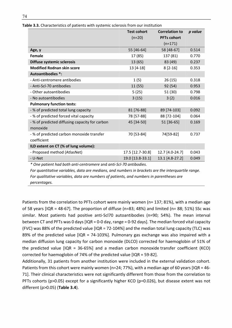
74

Table 3.3. Characteristics of patients with systemic sclerosis from our institution Test cohort

(n=20)

Correlation to PFTs cohort

(n=171)

p value

Age, y 55 [46-64] 58 [48-67] 0.514

Female 17 (85) 137 (81) 0.770

Diffuse systemic sclerosis 13 (65) 83 (49) 0.237

Modified Rodnan skin score 13 [4-18] 8 [2-16] 0.353

Autoantibodies *:

- Anti-centromere antibodies 1 (5) 26 (15) 0.318

- Anti-Scl-70 antibodies 11 (55) 92 (54) 0.953

- Other autoantibodies 5 (25) 51 (30) 0.798

- No autoantibodies 3 (15) 3 (2) 0.016

Pulmonary function tests:

- % of predicted total lung capacity 81 [76-88] 89 [74-103] 0.092

- % of predicted forced vital capacity 78 [57-88] 88 [72-104] 0.064

- % of predicted diffusing capacity for carbon

monoxide

45 [34-50] 51 [36-65] 0.169

- % of predicted carbon monoxide transfer

coefficient

70 [53-84] 74[59-82] 0.737

ILD extent on CT (% of lung volume):

- Proposed method (AtlasNet) 17.5 [12.7-30.8] 12.7 [4.0-24.7] 0.043

- U-Net 19.0 [13.8-33.1] 13.1 [4.8-27.2] 0.049

* One patient had both anti-centromere and anti-Scl-70 antibodies. For quantitative variables, data are medians, and numbers in brackets are the interquartile range. For qualitative variables, data are numbers of patients, and numbers in parentheses are percentages.

Patients from the correlation to PFTs cohort were mainly women (n= 137; 81%), with a median age

of 58 years [IQR = 48-67]. The proportion of diffuse (n=83; 48%) and limited (n= 88; 51%) SSc was

similar. Most patients had positive anti-Scl70 autoantibodies (n=90; 54%). The mean interval

between CT and PFTs was 0 days [IQR = 0-0 day, range = 0-92 days]. The median forced vital capacity

(FVC) was 88% of the predicted value [IQR = 72-104%] and the median total lung capacity (TLC) was

89% of the predicted value [IQR = 74-103%]. Pulmonary gas exchange was also impaired with a

median diffusion lung capacity for carbon monoxide (DLCO) corrected for haemoglobin of 51% of

the predicted value [IQR = 36-65%] and a median carbon monoxide transfer coefficient (KCO)

corrected for haemoglobin of 74% of the predicted value [IQR = 59-82].

Additionally, 31 patients from another institution were included in the external validation cohort.

Patients from this cohort were mainly women (n=24; 77%), with a median age of 60 years [IQR = 46-

71]. Their clinical characteristics were not significantly different from those from the correlation to

PFTs cohorts (p>0.05) except for a significantly higher KCO (p=0.026), but disease extent was not

different (p>0.05) (Table 3.4).

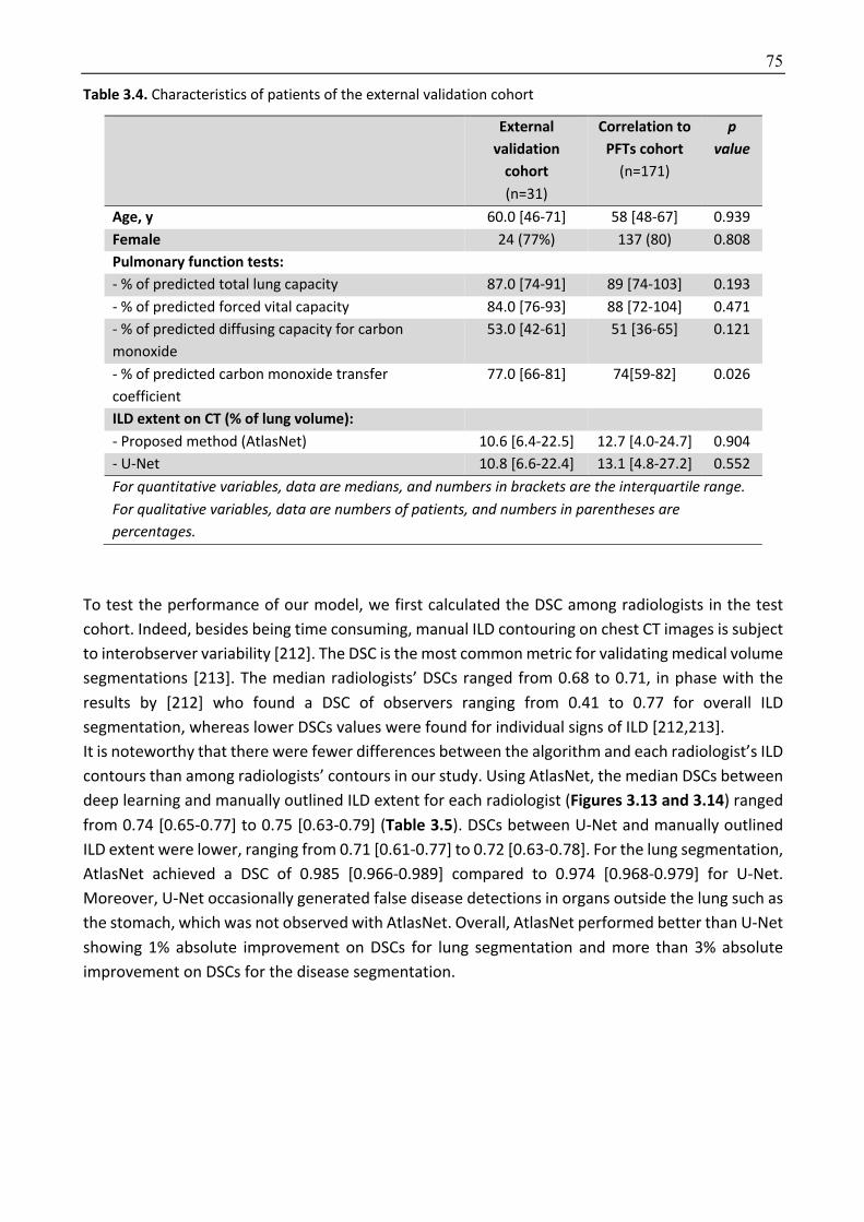
75

Table 3.4. Characteristics of patients of the external validation cohort

External validation

cohort (n=31)

Correlation to PFTs cohort

(n=171)

p

value

Age, y 60.0 [46-71] 58 [48-67] 0.939

Female 24 (77%) 137 (80) 0.808

Pulmonary function tests:

- % of predicted total lung capacity 87.0 [74-91] 89 [74-103] 0.193

- % of predicted forced vital capacity 84.0 [76-93] 88 [72-104] 0.471

- % of predicted diffusing capacity for carbon

monoxide

53.0 [42-61] 51 [36-65] 0.121

- % of predicted carbon monoxide transfer

coefficient

77.0 [66-81] 74[59-82] 0.026

ILD extent on CT (% of lung volume):

- Proposed method (AtlasNet) 10.6 [6.4-22.5] 12.7 [4.0-24.7] 0.904

- U-Net 10.8 [6.6-22.4] 13.1 [4.8-27.2] 0.552

For quantitative variables, data are medians, and numbers in brackets are the interquartile range. For qualitative variables, data are numbers of patients, and numbers in parentheses are percentages.

To test the performance of our model, we first calculated the DSC among radiologists in the test

cohort. Indeed, besides being time consuming, manual ILD contouring on chest CT images is subject

to interobserver variability [212]. The DSC is the most common metric for validating medical volume

segmentations [213]. The median radiologists’ DSCs ranged from 0.68 to 0.71, in phase with the

results by [212] who found a DSC of observers ranging from 0.41 to 0.77 for overall ILD

segmentation, whereas lower DSCs values were found for individual signs of ILD [212,213].

It is noteworthy that there were fewer differences between the algorithm and each radiologist’s ILD

contours than among radiologists’ contours in our study. Using AtlasNet, the median DSCs between

deep learning and manually outlined ILD extent for each radiologist (Figures 3.13 and 3.14) ranged

from 0.74 [0.65-0.77] to 0.75 [0.63-0.79] (Table 3.5). DSCs between U-Net and manually outlined

ILD extent were lower, ranging from 0.71 [0.61-0.77] to 0.72 [0.63-0.78]. For the lung segmentation,

AtlasNet achieved a DSC of 0.985 [0.966-0.989] compared to 0.974 [0.968-0.979] for U-Net.

Moreover, U-Net occasionally generated false disease detections in organs outside the lung such as

the stomach, which was not observed with AtlasNet. Overall, AtlasNet performed better than U-Net

showing 1% absolute improvement on DSCs for lung segmentation and more than 3% absolute

improvement on DSCs for the disease segmentation.

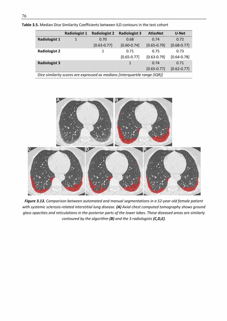
76

Table 3.5. Median Dice Similarity Coefficients between ILD contours in the test cohort

Radiologist 1 Radiologist 2 Radiologist 3 AtlasNet U-Net Radiologist 1 1 0.70

[0.63-0.77]

0.68

[0.60-0.74]

0.74

[0.65-0.79]

0.72

[0.68-0.77]

Radiologist 2 1 0.71

[0.65-0.77]

0.75

[0.63-0.79]

0.73

[0.64-0.78]

Radiologist 3 1 0.74

[0.65-0.77]

0.71

[0.62-0.77]

Dice similarity scores are expressed as medians [interquartile range (IQR)]

Figure 3.13. Comparison between automated and manual segmentations in a 52-year-old female patient with systemic sclerosis-related interstitial lung disease. (A) Axial chest computed tomography shows ground glass opacities and reticulations in the posterior parts of the lower lobes. These diseased areas are similarly

contoured by the algorithm (B) and the 3 radiologists (C,D,E).

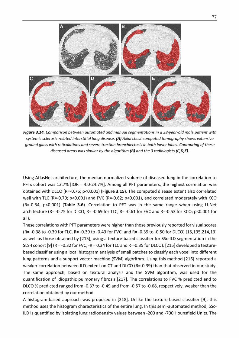
77

Figure 3.14. Comparison between automated and manual segmentations in a 38-year-old male patient with systemic sclerosis-related interstitial lung disease. (A) Axial chest computed tomography shows extensive

ground glass with reticulations and severe traction bronchiectasis in both lower lobes. Contouring of these diseased areas was similar by the algorithm (B) and the 3 radiologists (C,D,E).

Using AtlasNet architecture, the median normalized volume of diseased lung in the correlation to

PFTs cohort was 12.7% [IQR = 4.0-24.7%]. Among all PFT parameters, the highest correlation was

obtained with DLCO (R=-0.76; p<0.001) (Figure 3.15). The computed disease extent also correlated

well with TLC (R=-0.70; p<0.001) and FVC (R=-0.62; p<0.001), and correlated moderately with KCO

(R=-0.54, p<0.001) (Table 3.6). Correlation to PFT was in the same range when using U-Net

architecture (R= -0.75 for DLCO, R= -0.69 for TLC, R= -0.61 for FVC and R=-0.53 for KCO; p<0.001 for

all).

These correlations with PFT parameters were higher than those previously reported for visual scores

(R= -0.38 to -0.39 for TLC, R= -0.39 to -0.43 for FVC, and R= -0.39 to -0.50 for DLCO) [15,195,214,13]

as well as those obtained by [215], using a texture-based classifier for SSc-ILD segmentation in the

SLS-I cohort [9] (R = -0.32 for FVC, -R = 0.34 for TLC and R=-0.35 for DLCO). [215] developed a texture-

based classifier using a local histogram analysis of small patches to classify each voxel into different

lung patterns and a support vector machine (SVM) algorithm. Using this method [216] reported a

weaker correlation between ILD-extent on CT and DLCO (R=-0.39) than that observed in our study.

The same approach, based on textural analysis and the SVM algorithm, was used for the

quantification of idiopathic pulmonary fibrosis [217]. The correlations to FVC % predicted and to

DLCO % predicted ranged from -0.37 to -0.49 and from -0.57 to -0.68, respectively, weaker than the

correlation obtained by our method.

A histogram-based approach was proposed in [218]. Unlike the texture-based classifier [9], this

method uses the histogram characteristics of the entire lung. In this semi-automated method, SSc-

ILD is quantified by isolating lung radiodensity values between -200 and -700 Hounsfield Units. The

78

correlations to the FVC (R =-0.56) and the DLCO (R =-0.67) obtained in that study were close to those

obtained in our’s. However, since there is no anatomical characterization of the disease any cause

of increased lung density, caused by infection, for example, may interfere with the quantification.

We tested the developed algorithm on an external cohort of 31 SSc patients and found correlation

to pulmonary indexes to be in the same range for TLC and FVC, whereas the correlation to DLCO

was less, while remaining superior to that reported for visual scores, as mentioned above.

Correlation levels to TLC and FVC were R=-0.70 to -0.72 and R=-0.57 to-0.60, respectively, whereas

the correlation to DLCO was less, especially for U-Net (R=-0.60) versus AtlasNet (R=-0.65), p<0.001

for both.

Figure 3.15. Relationship between systemic sclerosis-related interstitial lung disease extent measured by the algorithm and pulmonary function test measurements.

DLCO: Percentage of predicted diffusing capacity for carbon monoxide; FVC: Percentage of predicted forced vital capacity; KCO: Percentage of predicted carbon monoxide transfer coefficient; TLC: Percentage of

predicted total lung capacity

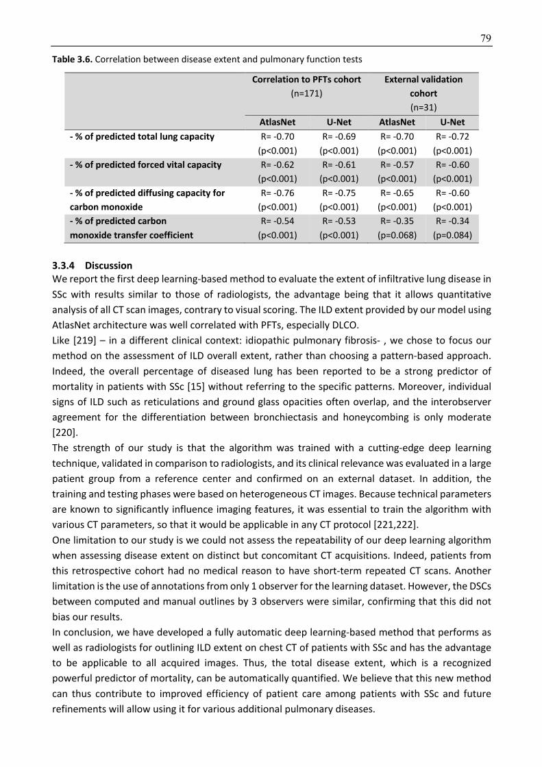
79

Table 3.6. Correlation between disease extent and pulmonary function tests

Correlation to PFTs cohort (n=171)

External validation cohort (n=31)

AtlasNet U-Net AtlasNet U-Net - % of predicted total lung capacity R= -0.70

(p<0.001)

R= -0.69

(p<0.001)

R= -0.70

(p<0.001)

R= -0.72

(p<0.001)

- % of predicted forced vital capacity R= -0.62

(p<0.001)

R= -0.61

(p<0.001)

R= -0.57

(p<0.001)

R= -0.60

(p<0.001)

- % of predicted diffusing capacity for carbon monoxide

R= -0.76

(p<0.001)

R= -0.75

(p<0.001)

R= -0.65

(p<0.001)

R= -0.60

(p<0.001)

- % of predicted carbon monoxide transfer coefficient

R= -0.54

(p<0.001)

R= -0.53

(p<0.001)

R= -0.35

(p=0.068)

R= -0.34

(p=0.084)

3.3.4 Discussion We report the first deep learning-based method to evaluate the extent of infiltrative lung disease in

SSc with results similar to those of radiologists, the advantage being that it allows quantitative

analysis of all CT scan images, contrary to visual scoring. The ILD extent provided by our model using

AtlasNet architecture was well correlated with PFTs, especially DLCO.

Like [219] – in a different clinical context: idiopathic pulmonary fibrosis- , we chose to focus our

method on the assessment of ILD overall extent, rather than choosing a pattern-based approach.

Indeed, the overall percentage of diseased lung has been reported to be a strong predictor of

mortality in patients with SSc [15] without referring to the specific patterns. Moreover, individual

signs of ILD such as reticulations and ground glass opacities often overlap, and the interobserver

agreement for the differentiation between bronchiectasis and honeycombing is only moderate

[220].

The strength of our study is that the algorithm was trained with a cutting-edge deep learning

technique, validated in comparison to radiologists, and its clinical relevance was evaluated in a large

patient group from a reference center and confirmed on an external dataset. In addition, the

training and testing phases were based on heterogeneous CT images. Because technical parameters

are known to significantly influence imaging features, it was essential to train the algorithm with

various CT parameters, so that it would be applicable in any CT protocol [221,222].

One limitation to our study is we could not assess the repeatability of our deep learning algorithm

when assessing disease extent on distinct but concomitant CT acquisitions. Indeed, patients from

this retrospective cohort had no medical reason to have short-term repeated CT scans. Another

limitation is the use of annotations from only 1 observer for the learning dataset. However, the DSCs

between computed and manual outlines by 3 observers were similar, confirming that this did not

bias our results.

In conclusion, we have developed a fully automatic deep learning-based method that performs as

well as radiologists for outlining ILD extent on chest CT of patients with SSc and has the advantage

to be applicable to all acquired images. Thus, the total disease extent, which is a recognized

powerful predictor of mortality, can be automatically quantified. We believe that this new method

can thus contribute to improved efficiency of patient care among patients with SSc and future

refinements will allow using it for various additional pulmonary diseases.

80

Chapter 4

4 Motion and registration: exploiting dynamics for interstitial lung disease

evaluation

In this chapter, we evaluated the use of elastic registration to diagnose and monitor interstitial

lung disease (ILD). We also hypothesized that registration could be used to understand lung

deformation during respiration or over time. To quantify lung deformation, we used the Jacobian

determinant, which can be calculated from the deformation fields (Appendix). The Jacobian

determinant corresponds to the quantitative value of the volume change for each voxel of a

Jacobian matrix. It quantifies the stretching or shrinking of each voxel (Figure 4.1).

Figure 4.1. Illustration of the Jacobian determinant. Jacobian determinant is the quantitative value of the deformation matrix of each voxel. If the voxel size remains similar after deformation (V0=V1), logarithm of the Jacobian determinant (Log_Jac) is 0. If the deformed voxel is smaller than the original, Log_Jac has a

negative value, whereas if the deformed voxel is larger, Log_Jac is positive.

Our approach exploits micro and macro information regarding the spatio-temporal behavior of the

lungs. In particular we introduce two variants, one exploiting the dynamics of the respiratory cycle

using magnetic resonance imaging and one focusing on the longitudinal modeling of the lung

through elastic mapping between follow up computed tomography examinations.

Elastic registration between inspiratory and expiratory images is usually used for tumor tracking in

radiotherapy but can also be used to assess lung deformation during a respiratory cycle. Fibrosis is

known to be associated to a loss of tissue elasticity. Therefore, elastic registration could help the

detection of pulmonary fibrosis. As a demonstration of this hypothesis, we evaluated SSc patients,

known to have a high prevalence of pulmonary fibrosis. The major limitation to the use of CT to

assess lung deformation is the radiation dose. Indeed, CT examination only consists in inspiratory

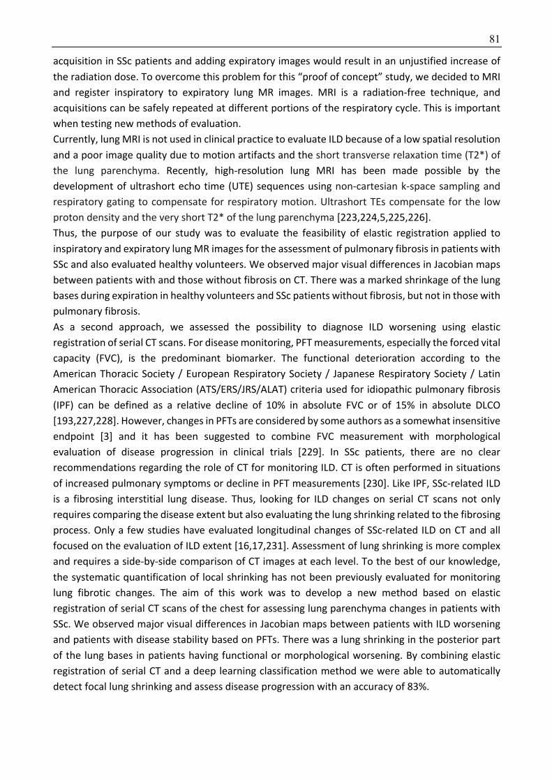
81

acquisition in SSc patients and adding expiratory images would result in an unjustified increase of

the radiation dose. To overcome this problem for this “proof of concept” study, we decided to MRI

and register inspiratory to expiratory lung MR images. MRI is a radiation-free technique, and

acquisitions can be safely repeated at different portions of the respiratory cycle. This is important

when testing new methods of evaluation.

Currently, lung MRI is not used in clinical practice to evaluate ILD because of a low spatial resolution

and a poor image quality due to motion artifacts and the short transverse relaxation time (T2*) of

the lung parenchyma. Recently, high-resolution lung MRI has been made possible by the

development of ultrashort echo time (UTE) sequences using non-cartesian k-space sampling and

respiratory gating to compensate for respiratory motion. Ultrashort TEs compensate for the low

proton density and the very short T2* of the lung parenchyma [223,224,5,225,226].

Thus, the purpose of our study was to evaluate the feasibility of elastic registration applied to

inspiratory and expiratory lung MR images for the assessment of pulmonary fibrosis in patients with

SSc and also evaluated healthy volunteers. We observed major visual differences in Jacobian maps

between patients with and those without fibrosis on CT. There was a marked shrinkage of the lung

bases during expiration in healthy volunteers and SSc patients without fibrosis, but not in those with

pulmonary fibrosis.

As a second approach, we assessed the possibility to diagnose ILD worsening using elastic

registration of serial CT scans. For disease monitoring, PFT measurements, especially the forced vital

capacity (FVC), is the predominant biomarker. The functional deterioration according to the

American Thoracic Society / European Respiratory Society / Japanese Respiratory Society / Latin

American Thoracic Association (ATS/ERS/JRS/ALAT) criteria used for idiopathic pulmonary fibrosis

(IPF) can be defined as a relative decline of 10% in absolute FVC or of 15% in absolute DLCO

[193,227,228]. However, changes in PFTs are considered by some authors as a somewhat insensitive

endpoint [3] and it has been suggested to combine FVC measurement with morphological

evaluation of disease progression in clinical trials [229]. In SSc patients, there are no clear

recommendations regarding the role of CT for monitoring ILD. CT is often performed in situations

of increased pulmonary symptoms or decline in PFT measurements [230]. Like IPF, SSc-related ILD

is a fibrosing interstitial lung disease. Thus, looking for ILD changes on serial CT scans not only

requires comparing the disease extent but also evaluating the lung shrinking related to the fibrosing

process. Only a few studies have evaluated longitudinal changes of SSc-related ILD on CT and all

focused on the evaluation of ILD extent [16,17,231]. Assessment of lung shrinking is more complex

and requires a side-by-side comparison of CT images at each level. To the best of our knowledge,

the systematic quantification of local shrinking has not been previously evaluated for monitoring

lung fibrotic changes. The aim of this work was to develop a new method based on elastic

registration of serial CT scans of the chest for assessing lung parenchyma changes in patients with

SSc. We observed major visual differences in Jacobian maps between patients with ILD worsening

and patients with disease stability based on PFTs. There was a lung shrinking in the posterior part

of the lung bases in patients having functional or morphological worsening. By combining elastic

registration of serial CT and a deep learning classification method we were able to automatically

detect focal lung shrinking and assess disease progression with an accuracy of 83%.

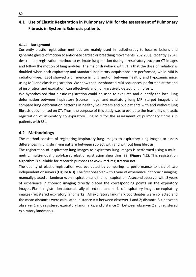
82

4.1 Use of Elastic Registration in Pulmonary MRI for the assessment of Pulmonary Fibrosis in Systemic Sclerosis patients

4.1.1 Background Currently elastic registration methods are mainly used in radiotherapy to localize lesions and

generate ghosts of motion to anticipate cardiac or breathing movements [232,233]. Recently, [234],

described a registration method to estimate lung motion during a respiratory cycle on CT images

and follow the motion of lung nodules. The major drawback with CT is that the dose of radiation is

doubled when both expiratory and standard inspiratory acquisitions are performed, while MRI is

radiation-free. [235] showed a difference in lung motion between healthy and hypoxemic mice,

using MRI and elastic registration. We show that unenhanced MRI sequences, performed at the end

of inspiration and expiration, can effectively and non-invasively detect lung fibrosis.

We hypothesized that elastic registration could be used to evaluate and quantify the local lung

deformation between inspiratory (source image) and expiratory lung MRI (target image), and

compare lung deformation patterns in healthy volunteers and SSc patients with and without lung

fibrosis documented on CT. Thus, the purpose of this study was to evaluate the feasibility of elastic

registration of inspiratory to expiratory lung MRI for the assessment of pulmonary fibrosis in

patients with SSc.

4.2 Methodology The method consists of registering inspiratory lung images to expiratory lung images to assess

differences in lung shrinking pattern between subject with and without lung fibrosis.

The registration of inspiratory lung images to expiratory lung images is performed using a multi-

metric, multi-modal graph-based elastic registration algorithm [99] (Figure 4.2). This registration

algorithm is available for research purposes at www.mrf-registration.net

The quality of elastic registration was evaluated by comparing its performance to that of two

independent observers (Figure 4.3). The first observer with 1 year of experience in thoracic imaging,

manually placed all landmarks on inspiration and then on expiration. A second observer with 3 years

of experience in thoracic imaging directly placed the corresponding points on the expiratory

images. Elastic registration automatically placed the landmarks of inspiratory images on expiratory

images (registered expiratory landmarks). All expiratory landmark coordinates were collected and

the mean distances were calculated: distance A = between observer 1 and 2; distance B = between

observer 1 and registered expiratory landmarks; and distance C = between observer 2 and registered

expiratory landmarks.

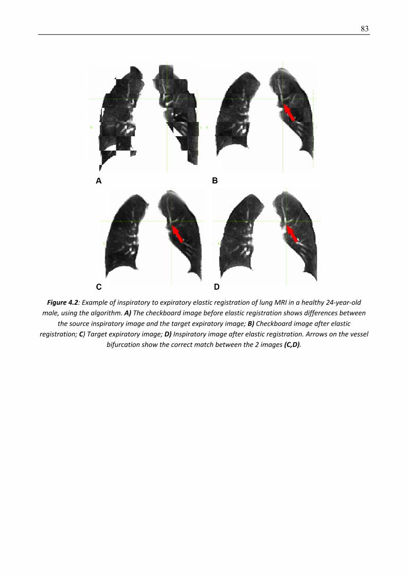
83

Figure 4.2: Example of inspiratory to expiratory elastic registration of lung MRI in a healthy 24-year-old male, using the algorithm. A) The checkboard image before elastic registration shows differences between

the source inspiratory image and the target expiratory image; B) Checkboard image after elastic registration; C) Target expiratory image; D) Inspiratory image after elastic registration. Arrows on the vessel

bifurcation show the correct match between the 2 images (C,D).

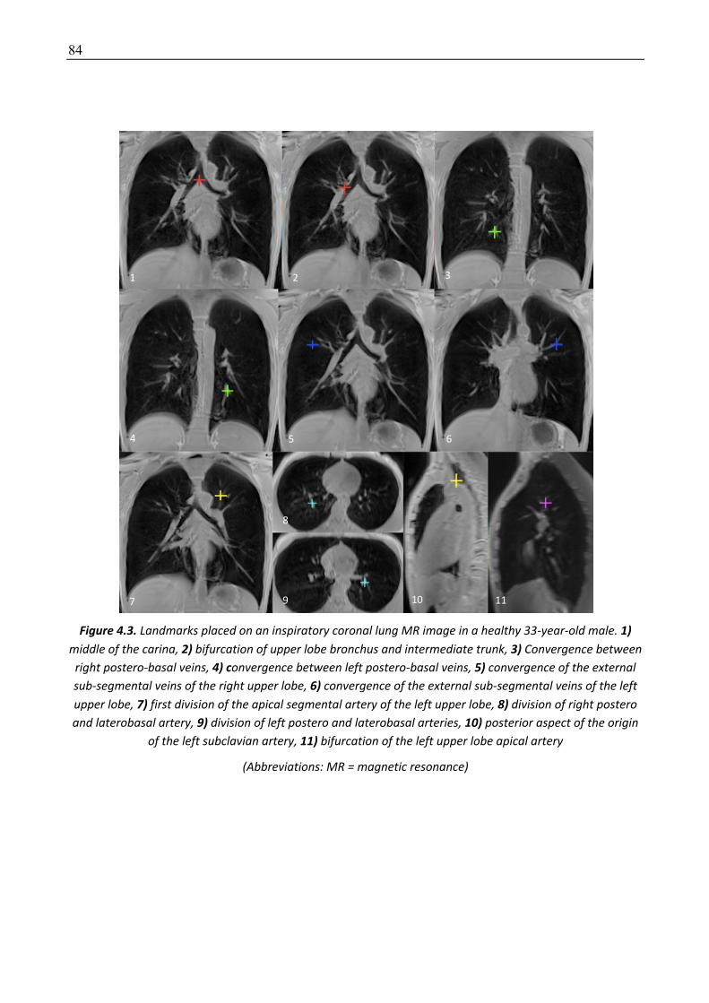
84

Figure 4.3. Landmarks placed on an inspiratory coronal lung MR image in a healthy 33-year-old male. 1) middle of the carina, 2) bifurcation of upper lobe bronchus and intermediate trunk, 3) Convergence between

right postero-basal veins, 4) convergence between left postero-basal veins, 5) convergence of the external sub-segmental veins of the right upper lobe, 6) convergence of the external sub-segmental veins of the left upper lobe, 7) first division of the apical segmental artery of the left upper lobe, 8) division of right postero and laterobasal artery, 9) division of left postero and laterobasal arteries, 10) posterior aspect of the origin

of the left subclavian artery, 11) bifurcation of the left upper lobe apical artery

(Abbreviations: MR = magnetic resonance)

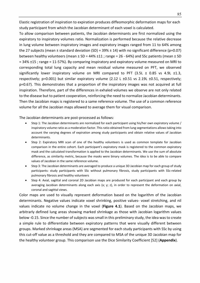
85

Elastic registration of inspiration to expiration produces diffeomorphic deformation maps for each

study participant from which the Jacobian determinant of each voxel is calculated.

To allow comparison between patients, the Jacobian determinants are first normalized using the

expiratory to inspiratory volumes ratio. Normalization is performed because the relative decrease

in lung volume between inspiratory images and expiratory images ranged from 11 to 64% among

the 27 subjects (mean ± standard deviation (SD) = 39% ± 14) with no significant difference (p=0.07)

between healthy volunteers (mean ± SD = 44% ±11 ; range = 26 - 64%) and SSc patients (mean ± SD

= 34% ±15 ; range = 11-57%). By comparing inspiratory and expiratory volume measured on MRI to

corresponding total lung capacity and mean residual volume measured on PFT, we observed

significantly lower inspiratory volume on MRI compared to PFT (3.5L ± 0.85 vs 4.9L ±1.3,

respectively; p=0.001) but similar expiratory volume (2.12 L ±0.51 vs 2.19L ±0.51, respectively;

p=0.67). This demonstrates that a proportion of the inspiratory images was not acquired at full

inspiration. Therefore, part of the differences in exhaled volumes we observe are not only related

to the disease but to patient cooperation, reinforcing the need to normalize Jacobian determinants.

Then the Jacobian maps is registered to a same reference volume. The use of a common reference

volume for all the Jacobian maps allowed to average them for visual comparison.

The Jacobian determinants are post-processed as follows:

• Step 1: The Jacobian determinants are normalized for each participant using his/her own expiratory volume /

inspiratory volume ratio as a moderation factor. This ratio obtained from lung segmentations allows taking into

account the varying degrees of expiration among study participants and obtain relative values of Jacobian

determinants.

• Step 2: Expiratory MRI scan of one of the healthy volunteers is used as common template for Jacobian

comparison in the entire cohort. Each participant’s expiratory mask is registered to the common expiratory

mask and the calculated transformation is applied to the Jacobian determinants. We use the sum of absolute

difference, as similarity metric, because the masks were binary volumes. The idea is to be able to compare

values of Jacobian in the same reference volume.

• Step 3: The Jacobian determinants are averaged to produce a unique 3D Jacobian map for each group of study

participants: study participants with SSc without pulmonary fibrosis, study participants with SSc-related

pulmonary fibrosis and healthy volunteers

• Step 4: Axial, sagittal and coronal 2D Jacobian maps are produced for each participant and each group by

averaging Jacobian determinants along each axis (x; y; z), in order to represent the deformation on axial,

coronal and sagittal views.

Color maps are used to visually represent deformation based on the logarithm of the Jacobian

determinants. Negative values indicate voxel shrinking, positive values- voxel stretching, and nil

values indicate no volume change in the voxel (Figure 4.1). Based on the Jacobian maps, we

arbitrarly defined lung areas showing marked shrinkage as those with Jacobian logarithm values

below -0.15. Since the number of subjects was small in this preliminary study, the idea was to create

a simple rule to differentiate between expiratory patterns that were visually different between

groups. Marked shrinkage areas (MSA) are segmented for each study participants with SSc by using

this cut-off value as a threshold and they are compared to MSA of the unique 3D Jacobian map for

the healthy volunteer group. This comparison use the Dice Similarity Coefficient [52] (Appendix).

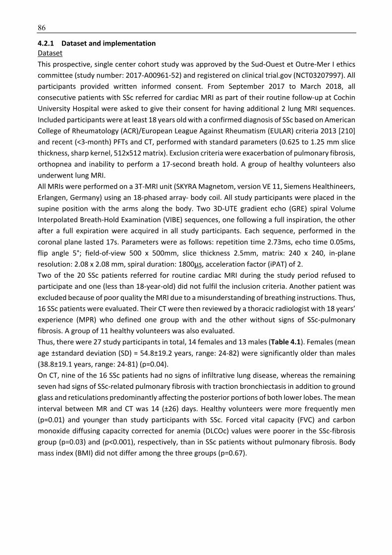
86

4.2.1 Dataset and implementation Dataset

This prospective, single center cohort study was approved by the Sud-Ouest et Outre-Mer I ethics

committee (study number: 2017-A00961-52) and registered on clinical trial.gov (NCT03207997). All

participants provided written informed consent. From September 2017 to March 2018, all

consecutive patients with SSc referred for cardiac MRI as part of their routine follow-up at Cochin

University Hospital were asked to give their consent for having additional 2 lung MRI sequences.

Included participants were at least 18 years old with a confirmed diagnosis of SSc based on American

College of Rheumatology (ACR)/European League Against Rheumatism (EULAR) criteria 2013 [210]

and recent (<3-month) PFTs and CT, performed with standard parameters (0.625 to 1.25 mm slice

thickness, sharp kernel, 512x512 matrix). Exclusion criteria were exacerbation of pulmonary fibrosis,

orthopnea and inability to perform a 17-second breath hold. A group of healthy volunteers also

underwent lung MRI.

All MRIs were performed on a 3T-MRI unit (SKYRA Magnetom, version VE 11, Siemens Healthineers,

Erlangen, Germany) using an 18-phased array- body coil. All study participants were placed in the

supine position with the arms along the body. Two 3D-UTE gradient echo (GRE) spiral Volume

Interpolated Breath-Hold Examination (VIBE) sequences, one following a full inspiration, the other

after a full expiration were acquired in all study participants. Each sequence, performed in the

coronal plane lasted 17s. Parameters were as follows: repetition time 2.73ms, echo time 0.05ms,

flip angle 5°; field-of-view 500 x 500mm, slice thickness 2.5mm, matrix: 240 x 240, in-plane

resolution: 2.08 x 2.08 mm, spiral duration: 1800µs, acceleration factor (iPAT) of 2.

Two of the 20 SSc patients referred for routine cardiac MRI during the study period refused to

participate and one (less than 18-year-old) did not fulfil the inclusion criteria. Another patient was

excluded because of poor quality the MRI due to a misunderstanding of breathing instructions. Thus,

16 SSc patients were evaluated. Their CT were then reviewed by a thoracic radiologist with 18 years’

experience (MPR) who defined one group with and the other without signs of SSc-pulmonary

fibrosis. A group of 11 healthy volunteers was also evaluated.

Thus, there were 27 study participants in total, 14 females and 13 males (Table 4.1). Females (mean

age ±standard deviation (SD) = 54.8±19.2 years, range: 24-82) were significantly older than males

(38.8±19.1 years, range: 24-81) (p=0.04).

On CT, nine of the 16 SSc patients had no signs of infiltrative lung disease, whereas the remaining

seven had signs of SSc-related pulmonary fibrosis with traction bronchiectasis in addition to ground

glass and reticulations predominantly affecting the posterior portions of both lower lobes. The mean

interval between MR and CT was 14 (±26) days. Healthy volunteers were more frequently men

(p=0.01) and younger than study participants with SSc. Forced vital capacity (FVC) and carbon

monoxide diffusing capacity corrected for anemia (DLCOc) values were poorer in the SSc-fibrosis

group (p=0.03) and (p<0.001), respectively, than in SSc patients without pulmonary fibrosis. Body

mass index (BMI) did not differ among the three groups (p=0.67).

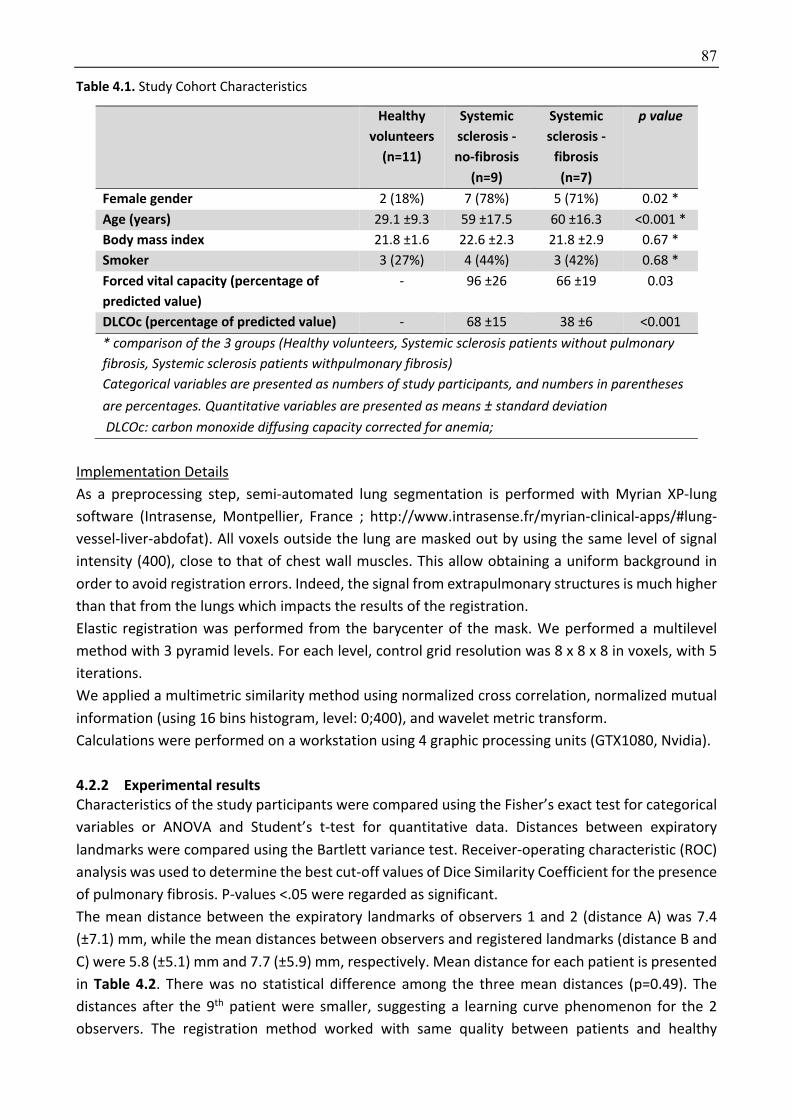
87

Table 4.1. Study Cohort Characteristics

Healthy volunteers

(n=11)

Systemic sclerosis -no-fibrosis

(n=9)

Systemic sclerosis -

fibrosis

(n=7)

p value

Female gender 2 (18%) 7 (78%) 5 (71%) 0.02 *

Age (years) 29.1 ±9.3 59 ±17.5 60 ±16.3 <0.001 *

Body mass index 21.8 ±1.6 22.6 ±2.3 21.8 ±2.9 0.67 *

Smoker 3 (27%) 4 (44%) 3 (42%) 0.68 *

Forced vital capacity (percentage of predicted value)

- 96 ±26 66 ±19 0.03

DLCOc (percentage of predicted value) - 68 ±15 38 ±6 <0.001

* comparison of the 3 groups (Healthy volunteers, Systemic sclerosis patients without pulmonary fibrosis, Systemic sclerosis patients withpulmonary fibrosis) Categorical variables are presented as numbers of study participants, and numbers in parentheses are percentages. Quantitative variables are presented as means ± standard deviation

DLCOc: carbon monoxide diffusing capacity corrected for anemia;

Implementation Details

As a preprocessing step, semi-automated lung segmentation is performed with Myrian XP-lung

software (Intrasense, Montpellier, France ; http://www.intrasense.fr/myrian-clinical-apps/#lung-

vessel-liver-abdofat). All voxels outside the lung are masked out by using the same level of signal

intensity (400), close to that of chest wall muscles. This allow obtaining a uniform background in

order to avoid registration errors. Indeed, the signal from extrapulmonary structures is much higher

than that from the lungs which impacts the results of the registration.

Elastic registration was performed from the barycenter of the mask. We performed a multilevel

method with 3 pyramid levels. For each level, control grid resolution was 8 x 8 x 8 in voxels, with 5

iterations.

We applied a multimetric similarity method using normalized cross correlation, normalized mutual

information (using 16 bins histogram, level: 0;400), and wavelet metric transform.

Calculations were performed on a workstation using 4 graphic processing units (GTX1080, Nvidia).

4.2.2 Experimental results Characteristics of the study participants were compared using the Fisher’s exact test for categorical

variables or ANOVA and Student’s t-test for quantitative data. Distances between expiratory

landmarks were compared using the Bartlett variance test. Receiver-operating characteristic (ROC)

analysis was used to determine the best cut-off values of Dice Similarity Coefficient for the presence

of pulmonary fibrosis. P-values ˂.05 were regarded as significant.

The mean distance between the expiratory landmarks of observers 1 and 2 (distance A) was 7.4

(±7.1) mm, while the mean distances between observers and registered landmarks (distance B and

C) were 5.8 (±5.1) mm and 7.7 (±5.9) mm, respectively. Mean distance for each patient is presented

in Table 4.2. There was no statistical difference among the three mean distances (p=0.49). The

distances after the 9th patient were smaller, suggesting a learning curve phenomenon for the 2

observers. The registration method worked with same quality between patients and healthy

88

volunteers (Figure 4.4).

Table 4.2. Mean landmarks distance for each patient.

Patient 1 2 3 4 5 6 7 8 9 10 11 12 13 14 15 16 17 18 19 20 21 22 23 24 25 26 27 Mean ±SD

Distance A 10.8 9.9 8.9 26.5 6.5 23.2 10.7 21.8 10.1 2.0 3.2 2.4 2.1 3.2 1.6 2.2 3.2 4.8 3.6 9.0 4.2 9.8 2.5 3.6 3.0 4.4 1.8 7.4±7.1

Distance B 7.7 7.8 4.4 27.8 4.2 4.3 5.9 5.1 12.8 7.0 3.8 2.5 2.6 3.4 2.5 2.2 4.4 2.9 6 9.2 3.8 8.4 3.5 4.9 4.7 4.8 2.3 5.8±5.1

Distance C 12.4 12 10.6 5.9 7.4 25.5 11.1 23.1 13.6 7.3 3.7 3.2 3.3 3.0 2.4 3.5 4.2 5.6 4.7 9.6 6.2 8.5 3.4 5.6 4.2 6.9 2.4 7.7±5.9

Figure 4.4: Elastic registration in a healthy volunteer (A-D) and a SSc patient (E-H).

In the healthy volunteer, A and B show the same point (arrow) on the warped image (A) and the target image (B). Images C and D show the checkboard image of source and warped images (C) and the

checkboard image of target and warped images (D). In the SSc patient, E and F show the same point (arrow) on the warped image (E) and the target image (F). Images G and H show the checkboard image of source and warped images (G) and checkboard image of

target and warped images (H).

Visual analysis of color maps showed differences in the distribution of the Jacobian determinants

among the study participants with SSc and healthy volunteers. We observed the same expiratory

deformation pattern in healthy volunteers and SSc patients without fibrosis, with a decrease in

volume (areas with marked deformation during expiration) mainly found in the posterior lung bases.

This was not observed in patients with fibrosis (Figure 4.5). Under the assumption that a loss of

elasticity might precede the appearance of fibrotic changes on CT we also included SSc patients

having no signs of infiltrative lung disease on CT. However, this hypothesis was not confirmed in our

sample.

89

Figure 4.5: Projection in x; y; z axis of the mean of the Jacobian determinants, in each group. The marked shrinkage areas (red color) are found in the dorsal aspect of the lung bases in healthy volunteers and in SSc

patients without high resolution CT evidence for pulmonary fibrosis. In the corresponding areas, the lungs of patients with evidence for systemic sclerosis -fibrosis show little deformation with mean Jacobian

determinant near to 0 (green color). These lung areas are those with signs of fibrosis on CT.

90

Quantitative analysis

Regarding the localization of marked shrinkage areas in the lung, the mean Dice Similarity

Coefficient value was 0.44±0.13 for study participants without fibrosis and 0.25±0.15 for those with

fibrosis (p=0.02). Its best cut-off value for the presence of fibrosis was 0.36 on receiving operator

characteristic (ROC) curve analysis, with a sensitivity of 86% (95% confidence interval (CI)

[0.46;0.99]), and a specificity of 75% (95% CI [0.53;0.89]), (AUC=0.81; 95% CI [0.54; 1], p=0.04)

(Figure 4.6).

Figure 4.6. ROC curve of Dice coefficient for the entire cohort. The best Dice coefficient cut-off value for the presence of fibrosis was 0.36, with a sensitivity of 86% (95% CI [46;99]), and a specificity of 75% (95% CI

[53;89]), (AUC= 0.81; 95% CI [0.54; 1], p=0.04)

(Abbreviations: CI = confidence interval)

4.2.3 Discussion This preliminary study evaluating elastic registration of inspiratory to expiratory MRI for the

detection of pulmonary fibrosis in SSc patients showed major visual differences in Jacobian maps

between those with and those without fibrosis on CT. There was a marked shrinkage of the lung

bases during expiration in healthy volunteers and SSc patients without fibrosis, but not in those with

pulmonary fibrosis. So far, the evaluation of pulmonary fibrosis on MRI has mostly been based on

gadolinium-enhanced sequences. [236] evaluated late contrast enhancement [237] performed

contrast imaging at different times, and showed differences in enhancement patterns between

inflammatory and non-inflammatory fibrotic lesions. Currently elastic registration methods are

mainly used in radiotherapy to localize lesions and generate ghosts of motion to anticipate cardiac

or breathing movements [232,233]. Recently, [234], described a registration method to estimate

lung motion during a respiratory cycle on CT images and follow the motion of lung nodules. The

major drawback with CT is that the dose of radiation is doubled when both expiratory and standard

inspiratory acquisitions are performed, while MRI is radiation-free. [235] showed a difference in

lung motion between healthy and hypoxemic mice, using MRI and elastic registration. We show that

unenhanced MRI sequences, performed at the end of inspiration and expiration, can effectively and

non-invasively detect lung fibrosis.

There are several limitations to our study. First, this feasibility study only included a small number

of study participants resulting in large confidence intervals for sensitivity and specificity.

91

Furthermore, healthy and diseased subjects were not age- and sex-matched. For practical and

ethical reasons, lung MR sequences were not repeated to assess the method repeatability. Also, we

did not take into account the clinical scoring of skin sclerosis. Patients with high Rodnan scores (>20)

[238] have marked skin sclerosis, which can result in decreased chest expansion. However, the basal

shrinkage in SSc-fibrosis patients supports our hypothesis that this method effectively identifies

fibrosis-related loss of elasticity, because restriction from skin sclerosis would not be predominantly

basal. Finally, we only evaluated patients who could hold their breath for 17 seconds, thus this

method is probably not applicable to patients with advanced lung disease.

In conclusion, elastic registration of inspiratory to expiratory MRI offers new perspectives in the

non-invasive evaluation of lung fibrosis in patients with SSc. These results must be confirmed in a

larger cohort, but could apply to other fibrotic lung diseases.

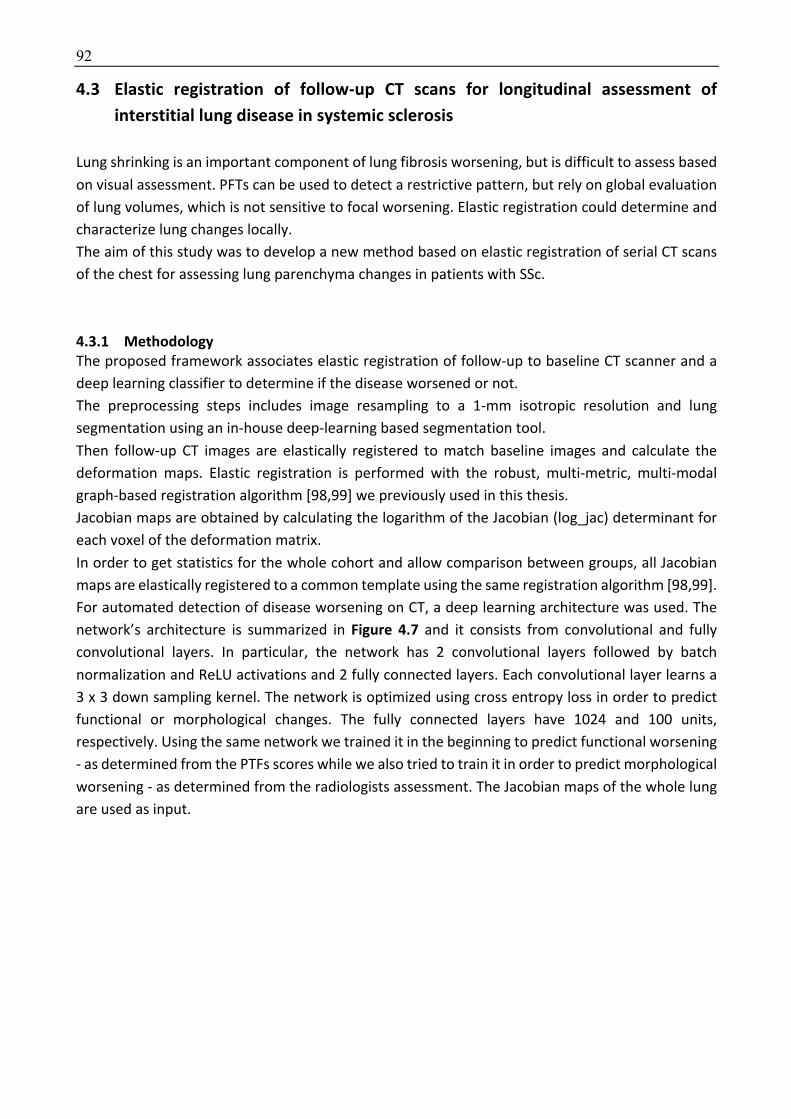
92

4.3 Elastic registration of follow-up CT scans for longitudinal assessment of interstitial lung disease in systemic sclerosis

Lung shrinking is an important component of lung fibrosis worsening, but is difficult to assess based

on visual assessment. PFTs can be used to detect a restrictive pattern, but rely on global evaluation

of lung volumes, which is not sensitive to focal worsening. Elastic registration could determine and

characterize lung changes locally.

The aim of this study was to develop a new method based on elastic registration of serial CT scans

of the chest for assessing lung parenchyma changes in patients with SSc.

4.3.1 Methodology The proposed framework associates elastic registration of follow-up to baseline CT scanner and a

deep learning classifier to determine if the disease worsened or not.

The preprocessing steps includes image resampling to a 1-mm isotropic resolution and lung

segmentation using an in-house deep-learning based segmentation tool.

Then follow-up CT images are elastically registered to match baseline images and calculate the

deformation maps. Elastic registration is performed with the robust, multi-metric, multi-modal

graph-based registration algorithm [98,99] we previously used in this thesis.

Jacobian maps are obtained by calculating the logarithm of the Jacobian (log_jac) determinant for

each voxel of the deformation matrix.

In order to get statistics for the whole cohort and allow comparison between groups, all Jacobian

maps are elastically registered to a common template using the same registration algorithm [98,99].

For automated detection of disease worsening on CT, a deep learning architecture was used. The

network’s architecture is summarized in Figure 4.7 and it consists from convolutional and fully

convolutional layers. In particular, the network has 2 convolutional layers followed by batch

normalization and ReLU activations and 2 fully connected layers. Each convolutional layer learns a

3 x 3 down sampling kernel. The network is optimized using cross entropy loss in order to predict

functional or morphological changes. The fully connected layers have 1024 and 100 units,

respectively. Using the same network we trained it in the beginning to predict functional worsening

- as determined from the PTFs scores while we also tried to train it in order to predict morphological

worsening - as determined from the radiologists assessment. The Jacobian maps of the whole lung

are used as input.

93

Figure 4.7. The architecture of the classifier used for our experiments consists of two fully-convolutional layers, followed by two fully-connected layers. For convolutional layers, "3 x 3" denotes the kernel size, while

S and P denote respectively, the stride and padding used. The number in brackets is the number of output channels. For the fully-connected layers, the numbers at each layer denote the number of hidden units in it.

The final prediction is the class probability. The entire classifier was trained with the binary cross entropy loss.

4.3.2 Dataset and implementation Dataset

This single-center, retrospective cohort study was approved by the Institutional Review Board of

Société de Pneumologie de Langue Française (CEPRO-2017-023) which waived the need for patients’

consent. Patients who met the American College of Rheumatology (ACR) / European League against

Rheumatism (EULAR) 2013 criteria for SSc [210] were recruited from the database of the Centre de

Référence Maladies Systémiques Autoimmunes Rares d’Ile de France at Cochin Hospital. This

database collects the socio-demographic, clinical, morphological and biological characteristics as

well as PFTs measurement of SSc patients referred to this tertiary care center. SSc patients who

were evaluated at our institution between January 2009 and October 2017 were eligible if they had

at least 2 consecutive unenhanced CT of the chest performed in the supine position. Exclusion

criteria were 1/ presence of motion artifacts, 2/ signs of another lung disease on CT, and 3/

unavailability of PFTs within 3 months of the CT scans. If patients had more than two CT meeting

the inclusion criteria, only the oldest and the more recent CT scans were taken into account.

During the study period, 591 SSc patients from our reference center underwent a chest CT at our

radiology department. Among the 295 patients who had at least 2 unenhanced CT of the chest

performed in the supine position, 212 fulfilled the inclusion criteria (Flow chart, Figure 4.8). The

majority of them were women (n=177; 83%) with limited cutaneous disease (n=128; 60%) (table 4.3).

94

Figure 4.8. Flow chart

Table 4.3. Patient characteristics according to functional changes

All (n=212)

Functional worsening

(n=91)

Functional stability

(n=121)

P value

Age (years) 53 [45;62] 54 [48;63] 52 [42;62] 0.117

Female 177 (83) 79 (87) 98 (81) 0.350

Limited cutaneous systemic sclerosis 128 (60) 51 (56) 77 (64) 0.321

Rodnan score at baseline 6 [2;13] 7 [2;14] 6 [2,13] 0.649

Baseline pulmonary function tests:

- %TLC 95 [81;108] 94 [78;109] 96 [87;107] 0.330

- %FVC 91 [75;104] 91 [74;106] 93 [75;103] 0.606

- %DLCOc 63 [49;76] 62 [46;75] 65 [50;77] 0.366

- %KCOc 79 [68;91] 79 [67;90] 80 [70;91] 0.783

Interval time between baseline and follow-up chest CT (months)

37 [23;53] 45 [34;65] 27 [16;49] <0.001

ILD on baseline CT 147 (69) 71 (78) 75 (62) 0.016

Changes in pulmonary function tests:

- %TLC 0 [-7; +5] -4 [-10; +3] 1 [-3; +6] 0.013

- %FVC -2 [-8; +6] -8 [-12; -2] +3 [-3; +7] <0.001

- %DLCOc -4 [-11; 0] -13 [-18; -8] -2 [-5; +3] <0.001

- %KCOc -6 [-14; +2] -13 [-22; -5] -2 [-7; +5] <0.001

Morphological worsening on CT 73 (34) 47 (52) 26 (21) <0.001

Mean log_jac 0.02

[-0.05;+0.07]

0.05

[+0.00;+0.11]

0.01

[-0.08;+0.03]

<0.001

Note: %DLCOc = percentage of predicted diffusing capacity for carbon monoxide; %KCOc = percentage of predicted carbon monoxide transfer coefficient; %FVC = percentage of predicted forced vital capacity; %TLC = percentage of predicted total lung capacity; CT = computed tomography; ILD = interstitial lung disease; Log_jac = logarithm of the Jacobian determinant

95

Inspiratory unenhanced CT scans of the whole lung were acquired on multislice CT devices

(Somatom Sensation 16, Somatom DS and Somatom AS+ from Siemens Healthineer; and Revolution

HD from General Electric Healthcare). Acquisition and reconstruction parameters were those

fulfilling CT criteria: images were reconstructed with a slice thickness of 0.625 to 1.25mm using

either a filter back projection or iterative reconstruction algorithms, and a high frequency kernel.

Visual image analysis was performed by two chest radiologists in consensus with 5 and 18-year

experience in chest imaging, respectively. The two radiologists were blinded to the PFT

measurements and the results of the deep learning classifier. CT exams were reviewed for the

presence of ILD, defined by the presence of ground glass opacities, reticulations, traction

bronchiectasis or honey combing in various combinations. Then, side-by-side comparison of

baseline and follow-up CT images was performed to assess whether ILD showed morphological

stability, worsening or improvement. CT scans were considered to show improvement when

associated with a volume decrease of the ground glass. Worsening consisted either in an increase

of ILD extent or an increase of traction bronchiectasis and/or honey combing with or without

increase of ILD extent.

PFTs measurements performed within 3 months of the baseline and follow-up chest CT acquisition

were retrieved from the database. PFTs measurements included percentage of predicted forced

vital capacity (%FVC), total lung capacity (%TLC), diffusing capacity for carbon monoxide (%DLCOc)

and carbon monoxide transfer coefficient (%KCOc). The percentage of predicted DLCOc and KCOc

had been corrected for measured haemoglobin. Functional changes were evaluated according to

the ATS/ERS/JRS/ALAT criteria. Functional worsening was defined by a decrease in absolute FVC of

10% or a decrease in absolute DLCO of 15% [193].

At baseline, median age was 53 years [IQR = 45;62 years] and 69% (n=146/212) had ILD on CT

examination. Median %FVC was 91% [IQR = 75; 104] with 18 % of patients (n=38/212) having a FVC

lower than 70% of the predicted value. DLCO measurement at baseline was available for 196

patients (92%). Median %DLCOc was 63% [IQR=49;76] with 61% of patients (n=120/196) having

DLCOc lower than 70% of the predicted value. Patient characteristics in the learning (172 patients)

and test cohorts (40 patients) were not statistically different (Table 4.4).

Median interval time between baseline and follow-up was 37 months [IQR = 23; 53 months]. It was

significantly longer for patients with functional worsening (median = 45 months; [IQR = 34; 65] than

for patients with functional stability (median = 27 months; [IQR = 16; 46]) (p<0.001). It was also

significantly longer in patients showing morphological worsening on CT (median = 43 months; [IQR

= 32; 59]) compared to those having morphological stability (median = 32 months; [IQR = 19; 49])

(P=0.01) on visual assessment.

On PFTs, lung fibrosis not only decreases lung volumes but is also associated with a decrease in

DLCO and KCO. These parameters are reported to correlate to ILD extent on CT in both SSc and IPF

[15,207,205,13,9,210,230]. Both FVC and DLCO have been long used to monitor ILD progression in

SSc [231]. Regarding PFTs, all but 25 patients had both baseline and follow-up measurement of

DLCOc. Overall, we observed a mild decline in pulmonary function with -2% [IQR = -8; +6] and -4%

[IQR = -11; 0] median changes in %FVC and %DLCO, respectively. Ninety-one patients (43%) met the

ATS/ERS/JRS/ALAT criteria for functional deterioration. Visual comparison between baseline and

follow-up CT showed morphological worsening in 73 patients (n=73/212, 34%), including 8 patients

who developed an ILD. In 7 patients (n=7/212, 3%), ILD had improved on the follow-up CT

96

examination, whereas in the remaining 132 patients (n=132/212, 62%) the disease was considered

as morphologically stable.

Table 4.4. Patient characteristics in the learning and test cohorts

Learning cohort

(n=172)

Test cohort

(n=40)

P value

Age (years) 54 [45; 63] 52 [45; 59] 0.434

Female 142 (83) 35 (88) 0.636

Limited cutaneous systemic sclerosis

102 (59) 26 (65) 0.592

Rodnan score at baseline 7 [3;14] 6 [2;11] 0.174

Baseline pulmonary function tests:

- %TLC 95 [79: 108] 96 [90; 107] 0.387

- %FVC 91 [75; 104] 94 [81; 104] 0.498

- %DLCOc 62 [48; 76] 69 [52; 75] 0.387

- %KCOc 78 [67; 91] 83 [77; 90] 0.216

Interval time between baseline and follow-up chest CT (months)

37 [23; 53] 44 [25; 56] 0.411

ILD on baseline CT 118 (69) 28 (70) 1

Changes in pulmonary function tests :

- %TLC -1 [-7; +5] 1 [-5; +4] 0.828

- %FVC -2 [-8; +6] -1 [-7; +4] 0.516

- %DLCOc -4 [-11; +1] -5 [-12; -2] 0.895

- %KCOc -6 [-14; +3] -6 [-14; +1] 0.929

Functional deterioration according to ATS/ERS/JRS/ALAT guidelines

73 (42) 18 (45) 0.86

Morphological worsening on CT 59 (34) 12 (35) 1

Mean log_jac 0.02

[-0.05; +0.07]

0.02

[-0.05; +0.07]

0.796

Note: %DLCOc = percentage of predicted diffusing capacity for carbon monoxide; %KCOc = percentage of predicted carbon monoxide transfer coefficient; %FVC = percentage of predicted forced vital capacity; %TLC = percentage of predicted total lung capacity; CT = High resolution computed tomography; ILD = interstitial lung disease; Log_jac = logarithm of the Jacobian determinant

Morphological worsening was significantly more frequent in patients with functional worsening

(n=47/91, 52%) than in patients with functional stability (n=26/121, 21%) (p<0.001) (table 4.3 and

figure 4.9). Similarly, PFT changes were significantly different between patients showing

morphological worsening, stability or improvement (p≤0.001) (table 4.5 and figure 4.10). The

decline in %TLC, %FVC, %DLCOc and %KCOc was significantly more frequent for patients with visual

worsening on CT as compared to patients with visual stability (P = 0.010; P< 0.001; P<0.001 and P=

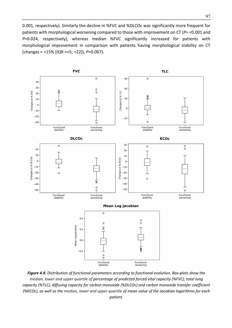
97

0.001, respectively). Similarly the decline in %FVC and %DLCOc was significantly more frequent for

patients with morphological worsening compared to those with improvement on CT (P= <0.001 and

P=0.024, respectively), whereas median %FVC significantly increased for patients with

morphological improvement in comparison with patients having morphological stability on CT

(changes = +15% [IQR =+5; +22]), P=0.007).

Figure 4.9. Distribution of functional parameters according to functional evolution. Box-plots show the median, lower and upper quartile of percentage of predicted forced vital capacity (%FVC), total lung

capacity (%TLC), diffusing capacity for carbon monoxide (%DLCOc) and carbon monoxide transfer coefficient (%KCOc), as well as the median, lower and upper quartile of mean value of the Jacobian logarithms for each

patient.

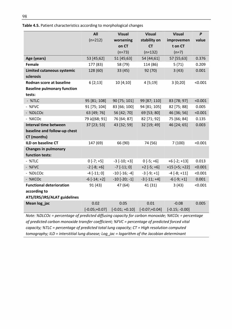
98

Table 4.5. Patient characteristics according to morphological changes

All (n=212)

Visual worsening

on CT

(n=73)

Visual stability on

CT

(n=132)

Visual improvemen

t on CT

(n=7)

P value

Age (years) 53 [45;62] 51 [45;63] 54 [44;61] 57 [55;63] 0.376

Female 177 (83) 58 (79) 114 (86) 5 (71) 0.209

Limited cutaneous systemic sclerosis

128 (60) 33 (45) 92 (70) 3 (43) 0.001

Rodnan score at baseline 6 [2;13] 10 [4;10] 4 [5;19] 3 [0;20] <0.001

Baseline pulmonary function tests:

- %TLC 95 [81; 108] 90 [75; 101] 99 [87; 110] 83 [78; 97] <0.001

- %FVC 91 [75; 104] 83 [66; 100] 94 [81; 105] 82 [75; 88] 0.005

- %DLCOc 63 [49; 76] 56 [42; 70] 69 [53; 80] 46 [36; 56] <0.001

- %KCOc 79 à)[68; 91] 76 [64; 87] 82 [71; 92] 75 [66; 84] 0.135

Interval time between baseline and follow-up chest CT (months)

37 [23; 53] 43 [32; 59] 32 [19; 49] 46 [24; 65] 0.003

ILD on baseline CT 147 (69) 66 (90) 74 (56) 7 (100) <0.001

Changes in pulmonary function tests:

- %TLC 0 [-7; +5] -3 [-10; +3] 0 [-5; +6] +6 [-2; +13] 0.013

- %FVC -2 [-8; +6] -7 [-11; 0] +2 [-5; +6] +15 [+5; +22] <0.001

- %DLCOc -4 [-11; 0] -10 [-16; -4] -3 [-9; +1] -4 [-8; +11] <0.001

- %KCOc -6 [-14; +2] -10 [-20; -1] -3 [-11; +4] -6 [-9; +1] 0.001

Functional deterioration according to ATS/ERS/JRS/ALAT guidelines

91 (43) 47 (64) 41 (31) 3 (43) <0.001

Mean log_jac 0.02

[-0.05;+0.07]

0.05

[-0.01; +0.10]

0.01

[-0.07;+0.04]

-0.08

[-0.15; -0.00]

0.005

Note: %DLCOc = percentage of predicted diffusing capacity for carbon monoxide; %KCOc = percentage of predicted carbon monoxide transfer coefficient; %FVC = percentage of predicted forced vital capacity; %TLC = percentage of predicted total lung capacity; CT = High resolution computed tomography; ILD = interstitial lung disease; Log_jac = logarithm of the Jacobian determinant

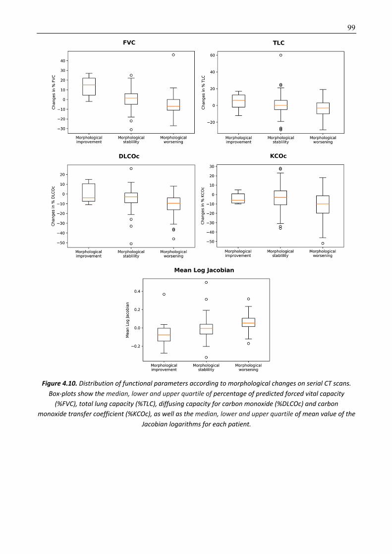
99

Figure 4.10. Distribution of functional parameters according to morphological changes on serial CT scans. Box-plots show the median, lower and upper quartile of percentage of predicted forced vital capacity

(%FVC), total lung capacity (%TLC), diffusing capacity for carbon monoxide (%DLCOc) and carbon monoxide transfer coefficient (%KCOc), as well as the median, lower and upper quartile of mean value of the

Jacobian logarithms for each patient.

100

Implementation details

For the registration of medical volumes we used the similar framework that described in Chapter 3

using normalized cross correlation, mutual information and discrete wavelet transform. We used as

regularization between the unary and pairwise terms the value of 3.0 while the entire framework

has been optimized using FastPD algorithm which is quite efficient and fast [239].

Jacobian maps were visually compared between patients with functional stability or functional

worsening, and between patients with improvement, stability or worsening based on visual

morphological assessment. The registered Jacobian maps were averaged for each patient group to

produce a unique 3D Jacobian map for visual comparison of each group. Mean log_jac values of

each patient were also calculated for comparison between groups and evaluation of the correlation

with PFT changes.

To train the deep learning-based classifiers, patients were randomly split into a learning (172

patients, including 80% for training and 20% for validation) and a test dataset (40 patients). The

learning rate was initialized to 0.0001 and reduced by a factor of 0.2 every 50 epochs. Training was

done for 500 epochs. We used the Adam optimizer with a batch size of 8 and a weight decay of

0.0005. We trained a network with the same architecture as this in the beginning to predict

functional worsening - as determined from the PTFs scores while we also tried to train it in order to

predict morphological worsening - as determined from the radiologists assessment. The Jacobian

maps of the whole lung are used as input.

4.3.3 Experimental results Characteristics of the study participants were compared using the Fisher’s exact test for categorical

variables or ANOVA and Mann-Whitney test for quantitative data. Correlation between mean

log_jac values and changes in PFT parameters (%TLC, %CVF, %DLCO and %KCO) was evaluated

calculating Spearman correlation coefficient. Sensitivity, specificity and accuracy of the classifiers to

predict morphological or functional worsening were respectively calculated using visual analysis of

CT or functional changes as reference. P-values ˂0.05 were regarded as significant.

The qualitative assessment of the distribution of the lung log_jac values has produced clear visual

separation between the patient groups. Sagittal views summarizing the lung distribution of log_jac

values in each group have shown homogeneous log_jac values in patients with stable disease either

based on functional (figure 4.11) or morphological criteria (figure 4.12). Conversely, there was a

lung shrinking (negatives log_jac values) in the posterior part of the lung bases in patients having

functional or morphological worsening, whereas the same areas showed expansion (positive log_jac

values) in the small group of patients with morphological improvement on native CT images. Thus,

by calculating Jacobian determinant maps, we were able to demonstrate that lung shrinking

predominates in the posterior areas of lung bases which are the predominant location of ILD in SSc

patients. Using a conceptually similar registration approach on lung magnetic resonance images, we

had previously shown that the posterior areas of lung bases were those showing the most important

deformation between inspiration and expiration in healthy individuals and that such deformation

was lost in SSc patients with lung fibrosis [109]

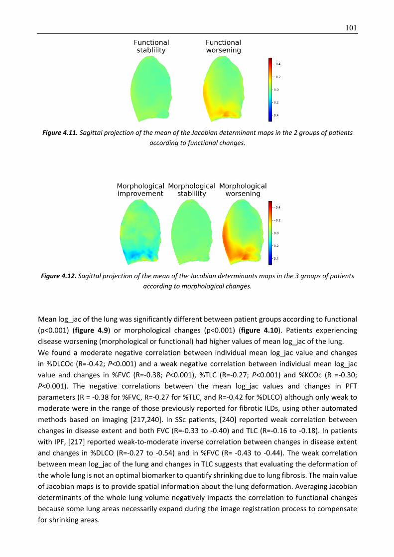
101

Figure 4.11. Sagittal projection of the mean of the Jacobian determinant maps in the 2 groups of patients according to functional changes.

Figure 4.12. Sagittal projection of the mean of the Jacobian determinants maps in the 3 groups of patients according to morphological changes.

Mean log_jac of the lung was significantly different between patient groups according to functional

(p<0.001) (figure 4.9) or morphological changes (p<0.001) (figure 4.10). Patients experiencing

disease worsening (morphological or functional) had higher values of mean log_jac of the lung.

We found a moderate negative correlation between individual mean log_jac value and changes

in %DLCOc (R=-0.42; P<0.001) and a weak negative correlation between individual mean log_jac

value and changes in %FVC (R=-0.38; P<0.001), %TLC (R=-0.27; P<0.001) and %KCOc (R =-0.30;

P<0.001). The negative correlations between the mean log_jac values and changes in PFT

parameters (R = -0.38 for %FVC, R=-0.27 for %TLC, and R=-0.42 for %DLCO) although only weak to

moderate were in the range of those previously reported for fibrotic ILDs, using other automated

methods based on imaging [217,240]. In SSc patients, [240] reported weak correlation between

changes in disease extent and both FVC (R=-0.33 to -0.40) and TLC (R=-0.16 to -0.18). In patients

with IPF, [217] reported weak-to-moderate inverse correlation between changes in disease extent

and changes in %DLCO (R=-0.27 to -0.54) and in %FVC (R= -0.43 to -0.44). The weak correlation

between mean log_jac of the lung and changes in TLC suggests that evaluating the deformation of

the whole lung is not an optimal biomarker to quantify shrinking due to lung fibrosis. The main value

of Jacobian maps is to provide spatial information about the lung deformation. Averaging Jacobian

determinants of the whole lung volume negatively impacts the correlation to functional changes

because some lung areas necessarily expand during the image registration process to compensate

for shrinking areas.

102

When using ATS/ERS/JRS/ALAT functional deterioration criteria as reference to train and test the

classifier, we reached a sensitivity of 89%, a specificity of 77% and an accuracy of 83% to predict

disease worsening (16 true positives, 17 true negatives, 5 false positives and 2 false negatives).

When using visual assessment of morphological changes as reference to train and test the model,

we obtained a sensitivity of 79%, a specificity of 81% and an accuracy of 80% (11 true positives, 21

true negatives, 5 false positives and 3 false negatives).

The 80 to 83% accuracy obtained for predicting worsening was only based on an evaluation of the

lung deformation, without taking into account increase in disease extent, which is also a factor of

worsening [217,240] and may not be associated with a significant lung shrinking in the early phase

of fibrosis. Thus, combining lung deformation assessment with automated quantification of lung

disease extent could improve the detection of ILD worsening. The added value of this approach

remains to be evaluated.

In order to create an approach which can be generalized for other ILDs, we only evaluated patients

who underwent chest CT in the supine position, because this is the way most CT examinations are

performed to diagnose and monitor ILDs of any cause. Contrary to computer aided diagnosis tools

based on disease segmentation, elastic registration does not depend on the ILD pattern, with

variable proportions of ground glass, reticulation and honey combing according to the specific cause

of fibrosis [11,241]. We believe that our approach could be suitable for monitoring other causes of

pulmonary fibrosis such as IPF. For other fibrotic diseases where pulmonary fibrosis does not

predominate in the lung bases, such as sarcoidosis [242], another Jacobian maps classifier should

probably be specifically trained to accurately predict worsening during CT follow-up.

4.3.4 Discussion To the best of our knowledge, this study is the first to use elastic registration for an automated

assessment of worsening during the evolution of a fibrotic interstitial lung disease. Elastic

registration applied to serial CT images, in combination with a deep learning classification method

was able to automatically detect focal lung shrinking and assess disease progression. The developed

method was able to predict functional impairment with an accuracy of 83% and could be used for

an automated assessment of ILD worsening in SSc.

Our study suffers from several limitations. First, some of the follow-up CT examinations may have

been performed to explore pulmonary function decline due to causes other than fibrosis, which may

have underestimated the correlation between functional deterioration and lung deformation.

Additionally, due to the retrospective design, the range of time interval between baseline and

follow-up CT examinations was uneven and significantly shorter in patients with stable disease.

Lastly, functional deterioration in SSc is not always due to pulmonary fibrosis. Patients can also

develop pulmonary hypertension which will not be depicted by an analysis of lung deformation. This

was not taken into account in our study. On the other hand, a discrepancy between functional

deterioration and lack of lung shrinking might raise the suspicion for pulmonary hypertension as the

cause of impairment. Also, we did not take into account worsening of skin sclerosis as a factor of

lung function deterioration. High Rodnan scores (>20) can result in decreased chest expansion [238].

However, this phenomenon would not predominantly affect the lung bases contrary to lung

shrinking, as depicted on lung deformation maps.

In conclusion, lung shrinking detected using an elastic registration of serial CT scans can be used for

103

an automated assessment of ILD worsening in patients with SSc. This method could prove useful for

other causes of lung fibrosis, especially IPF. The proposed formulation exploits in two distinct sets

elastic registration and deep neural networks prediction methods. These two steps remain

independent, and therefore the most natural extension will be to couple them into a single neural

network architecture as recently suggested from [209].

104

Chapter 5

5 General conclusion In this thesis we propose a holistic approach to assess severity of lungs diseases through optimal

exploitation of spatiotemporal information. Our approach is of increasing complexity, targeting

initially the use of radiomics for global disease classification, the use of deep learning for precise

delineation of disease boundaries and concludes with the integration of dynamic/spatio-temporal

data for better characterization of disease and its progression.

5.1 Contributions In the first part of the thesis we proposed different models to score bronchial disease severity on

CT scanner. For this, we used a simple thresholding approach and a more sophisticated machine

learning approach. The main difficulty when developing such score is the lack of ground truth to

define disease severity. However, using radiomics we were able to build a score correlated to a 3-

year prognosis score and the number of exacerbations to occur in the upcoming year in an

independent cohort from another hospital with images acquired using a more recent CT scanner

model resulting in a lower radiation dose exposure. Despite the large size of the cohort in view of

the disease prevalence, the number of patients was too small to expect a deep learning approach

to improve the results. Our work contributes to show that automated CT scoring of bronchial

diseases is doable and that a radiomic approach evaluating the whole lung volume can be used for

scoring diffuse bronchial diseases. This offers new perspectives for the use of CT imaging-based

biomarkers, for both patient monitoring and evaluation of newly developed drugs. Additionally, we

confirmed that scoring methods used in cystic fibrosis can be adapted for other diffuse bronchial

diseases such as primary ciliary dyskinesia.

In the second part of the thesis, we demonstrated that combining deep learning and elastic

registration to atlases (AtlasNet) improves the performance for image segmentation. We also

showed that using this method, a small number of representative patients was sufficient to produce

a model performing as well as radiologists to segment interstitial lung disease (ILD) in patients with

systemic sclerosis. The model provided a biomarker well correlated to several pulmonary function

indexes and was generalizable to an independent cohort from another hospital. The use of such

biomarker opens new perspectives for disease evaluation but also for research aiming to

understand the relationship between morphological changes and clinical data including survival.

The combination of deep learning and elastic registration is not limited to the segmentation of

intestinal lung disease but can also be used for other segmentation tasks and adapted for

classification tasks.

In the third part of the thesis, we demonstrated that evaluating lung deformation during respiration

can be used to detect fibrotic changes of the lung and that the study of lung deformation over time

can be used for monitoring fibrotic lung diseases. Although it is known that lung fibrosis is associated

with elasticity loss and shrinking of diseased areas, these features had not been previously evaluated

105

in fibrotic interstitial lung diseases (ILD). Even though lung MRI provides less morphological

information than CT, we were able to automatically detect fibrosis in systemic sclerosis patients only

by looking at lung deformation between inspiratory and expiratory lung MR images. Additionally,

we showed that looking at lung shrinking over time on CT it was possible to reliably diagnose ILD

worsening. The study of lung deformation, including the possible use of MRI, offers new

perspectives for diagnosis and follow up of patients with fibrosing ILDs.

5.2 Future works Coupling detection, delineation and spatiotemporal progression. In this thesis, we have mostly

exploited three well known techniques in medical imaging; biomarkers discovery, segmentation &

elastic registration. These three different components were treated in an independent fashion and

were combined through a sequential paradigm. The integration of these steps into a

couple/interchangeable formulation could greatly improved performance. Segmentation can

benefit from registration and vice-versa. Dynamic biomarkers discovery and classification could

benefit from the outcome of elastic registration. Deep neural networks offer great perspectives in

this direction and are currently under investigation.

Using radiomics and deep learning in diffuse bronchial lung diseases. In this thesis, we mainly

focused on creating CT scores predicting disease severity. However, since the beginning of our work,

new therapies have been introduced and can now be used in cystic fibrosis patients having the

predominant genetic mutation. These therapies dramatically improve a large proportion of patients

but are very costly and are associated to side effects. Assessment of treatment response is a possible

application of the models proposed in this thesis. Beyond this, using radiomics and deep learning to

predict response to the newly developed drugs is a new research field for which patient databases

are currently being created.

Evaluating automated interstitial lung disease (ILD) extent as a prognostic factor. As a first step,

we developed a deep-learning based automated segmentation model for the evaluation of ILD

extent showing good correlations with pulmonary function. To confirm the clinical value of this

biomarker, the correlation with survival remains to be evaluated. Additionally, we believe that

disease extent could be combined with other clinical and functional data to build a composite

prognosis score.

Combining ILD segmentation and elastic registration for ILD monitoring. In this thesis, we

separately evaluated ILD disease extent and lung deformation due to the development of fibrosis.

However, the information obtained by these 2 approaches could be combined.

Firstly, disease extent could be used as a constraint for the elastic registration between serial

examinations or between inspiratory and expiratory CT images. This could improve the registration

process.

Secondly, for disease monitoring, changes in disease extent could be used to enrich the model.

Indeed, disease progression may combine increased disease extent and lung shrinking. In our

experience, some patients with systemic sclerosis suffer from a progressive increase of ILD extent

without significant lung shrinking, especially in the initial phase of the disease, whereas other

106

develop shrinking within a stable disease extent.

Evaluating the developed methods on other ILD. In this thesis, we focused on systemic sclerosis as

a model of fibrosing interstitial lung disease. However, among fibrosing ILDs, idiopathic pulmonary

fibrosis is the most frequent and severe one, with a 5-year survival of approximatively 50%. The

methods for ILD quantification and ILD monitoring that we developed could be of great interest in

this context, especially in view of the newly developed anti fibrotic drugs, which could be evaluated

through collaboration with other centers.

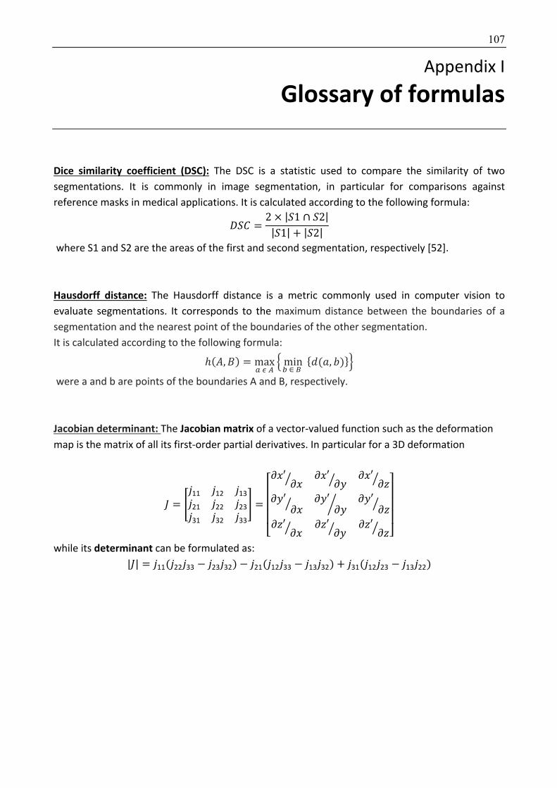
107

Appendix I

6 Glossary of formulas

Dice similarity coefficient (DSC): The DSC is a statistic used to compare the similarity of two

segmentations. It is commonly in image segmentation, in particular for comparisons against

reference masks in medical applications. It is calculated according to the following formula:

~]� =2 × |]1 ∩ ]2||]1| + |]2|

where S1 and S2 are the areas of the first and second segmentation, respectively [52].

Hausdorff distance: The Hausdorff distance is a metric commonly used in computer vision to

evaluate segmentations. It corresponds to the maximum distance between the boundaries of a

segmentation and the nearest point of the boundaries of the other segmentation.

It is calculated according to the following formula:

ℎ(m, É) = maxÜáà

âminN∈å

{q(ç, V)}é

were a and b are points of the boundaries A and B, respectively.

Jacobian determinant: The Jacobian matrix of a vector-valued function such as the deformation

map is the matrix of all its first-order partial derivatives. In particular for a 3D deformation

è = êë11 ë12 ë13

ë21 ë22 ë23

ë31 ë32 ë33

í =

⎣⎢⎢⎢⎡ñ#′

ñ#ò ñ#′ñ8ò ñ#′

ñôò

ñ8′ñ#ò ñ8′

ñ8ö ñ8′ñôò

ñô′ñ#ò ñô′

ñ8ò ñô′ñôò ⎦⎥⎥⎥⎤

while its determinant can be formulated as:

|è| = ë11(ë22ë33 − ë23ë32) − ë21(ë12ë33 − ë13ë32) + ë31(ë12ë23 − ë13ë22)

108

Appendix II

7 Synthèse Dans cette thèse, nous évaluons des méthodes d’intelligence artificielle pour la détection, la

caractérisation et la classification des maladies pulmonaires chroniques en imagerie.

L’évaluation de gravité et la surveillance des maladies pulmonaires chroniques représentent deux

challenges importants pour la prise en charge des patients et l’évaluation des traitements. La

surveillance repose principalement sur les données fonctionnelles respiratoires, incluant en

particulier le volume expiratoire maximal en 1 seconde (VEMS) pour les pathologies bronchiques

obstructives et la capacité fonctionnelle vitale (CVF) pour les pneumopathies fibrosantes.

Cependant, l’évaluation morphologique reste un point essentiel pour le diagnostic et l’évaluation

de sévérité. Pour cela, le scanner pulmonaire est l’examen de référence car il permet d’obtenir des

images haute résolution du parenchyme. Dans cette thèse, nous nous intéressons à la

mucoviscidose et la sclérodermie, que nous utilisons respectivement comme modèles de pathologie

bronchique obstructive et de pneumopathie fibrosante.

Dans le chapitre 2, nous évaluons différentes approches pour quantifier la sévérité de pathologies

bronchiques chroniques au scanner. Une approche simple consiste à quantifier les zones

hyperdenses dues aux remaniements inflammatoires par une méthode de seuillage ayant pour

particularité d’utiliser un seuillage adaptatif. Cette méthode est également évaluée dans une autre

maladie bronchique chronique, la dyskinésie ciliaire primitive. Une méthode plus sophistiquée de

radiomique est également évaluée pour prédire un modèle complexe d’évaluation de la gravité

clinique. Nos résultats montrent qu’il est possible de quantifier l’atteinte pulmonaire à l’aide d’une

approche globale évaluant la totalité du volume pulmonaire.

Dans la seconde partie, nous présentons une approche locale visant à contourer automatiquement

les zones d’atteinte fibrosante de la sclérodermie en scanner pour en quantifier la sévérité. Pour

cela une méthode d’apprentissage profond (deep learning) de type réseau neuronal convolutif est

utilisée. Une architecure combinant recalage élastique à des atlas anatomiques et réseaux

neuronaux convolutifs est proposée dans le but de réaliser une augmentation de données, de

diminuer la complexité du problème liée aux variations anatomiques et de renforcer la cohérence

anatomique de chaque réseau neuronal. En pratique, une étape préliminaire de recalage des

données d’imagerie à plusieurs atlas anatomiques est réalisée puis un réseau neuronal indépendant

est entrainé pour chacun des atlas. Cette architecture améliore significativement les performances

du modèle obtenu qui présente des performances équivalentes à celles des radiologues et permet

de quantifier l’extension de la maladie au sein des poumons. L’application de cette méthode de

contourage est ensuite réalisée sur une large cohorte de patients atteints de sclérodermie et les

résultats obtenus sont bien corrélés à la sévérité fonctionnelle.

Dans la dernière partie, nous nous intéressons à l’utilisation des données dynamiques visant à

évaluer l’évolution de l’atteinte fibrosante de la sclérodermie. La fibrose est habituellement

responsable d’une perte des propriétés élastiques du tissu et d’une rétraction tissulaire. La

combinaison d’images IRM pulmonaire acquises en inspiration et en expiration et d’une méthode

109

de recalage élastique est utilisée pour évaluer les profils de contraction pulmonaire au cours de la

respiration, en fonction de la présence ou non d’une fibrose. Cette méthode permet de différencier

les sujets sains et ceux atteints de fibrose, pour lesquels il existe une perte de contraction des bases

pulmonaires entre inspiration et expiration. La même méthode est utilisée pour évaluer la

contraction pulmonaire liée à l’aggravation de la fibrose au cours du suivi. Combinée à un réseau

neuronal profond cette approche permet de diagnostiquer de manière automatique l’aggravation

fibreuse chez les patients sclérodermiques.

110

8 References [1] Brody AS, Sucharew H, Campbell JD, Millard SP, Molina PL, Klein JS, et al. Computed

tomography correlates with pulmonary exacerbations in children with cystic fibrosis. Am J Respir Crit Care Med 2005;172:1128–32. doi:10.1164/rccm.200407-989OC.

[2] Tepper LA, Caudri D, Utens EMWJ, van der Wiel EC, Quittner AL, Tiddens HAWM. Tracking CF disease progression with CT and respiratory symptoms in a cohort of children aged 6-19 years. Pediatr Pulmonol 2014;49:1182–9. doi:10.1002/ppul.22991.

[3] Wells AU. Forced vital capacity as a primary end point in idiopathic pulmonary fibrosis treatment trials: making a silk purse from a sow’s ear. Thorax 2013;68:309–10. doi:10.1136/thoraxjnl-2012-202640.

[4] Hansell DM, Goldin JG, King TE, Lynch DA, Richeldi L, Wells AU. CT staging and monitoring of fibrotic interstitial lung diseases in clinical practice and treatment trials: a position paper from the Fleischner Society. Lancet Respir Med 2015;3:483–96. doi:10.1016/S2213-2600(15)00096-X.

[5] Dournes G, Grodzki D, Macey J, Girodet P-O, Fayon M, Chateil J-F, et al. Quiet Submillimeter MR Imaging of the Lung Is Feasible with a PETRA Sequence at 1.5 T. Radiology 2015;276:258–65. doi:10.1148/radiol.15141655.

[6] Calder AD, Bush A, Brody AS, Owens CM. Scoring of chest CT in children with cystic fibrosis: state of the art. Pediatr Radiol 2014;44:1496–506. doi:10.1007/s00247-013-2867-y.

[7] Xie X, de Jong PA, Oudkerk M, Wang Y, Ten Hacken NHT, Miao J, et al. Morphological measurements in computed tomography correlate with airflow obstruction in chronic obstructive pulmonary disease: systematic review and meta-analysis. Eur Radiol 2012;22:2085–93. doi:10.1007/s00330-012-2480-8.

[8] Hoffman EA, Simon BA, McLennan G. State of the Art. A structural and functional assessment of the lung via multidetector-row computed tomography: phenotyping chronic obstructive pulmonary disease. Proc Am Thorac Soc 2006;3:519–32. doi:10.1513/pats.200603-086MS.

[9] Kim HG, Tashkin DP, Clements PJ, Li G, Brown MS, Elashoff R, et al. A computer-aided diagnosis system for quantitative scoring of extent of lung fibrosis in scleroderma patients. Clin Exp Rheumatol 2010;28:S26-35.

[10] de Jong PA, Nakano Y, Hop WC, Long FR, Coxson HO, Paré PD, et al. Changes in airway dimensions on computed tomography scans of children with cystic fibrosis. Am J Respir Crit Care Med 2005;172:218–24. doi:10.1164/rccm.200410-1311OC.

[11] Bussone G, Mouthon L. Interstitial lung disease in systemic sclerosis. Autoimmun Rev 2011;10:248–55. doi:10.1016/j.autrev.2010.09.012.

[12] Chifflot H, Fautrel B, Sordet C, Chatelus E, Sibilia J. Incidence and prevalence of systemic sclerosis: a systematic literature review. Semin Arthritis Rheum 2008;37:223–35. doi:10.1016/j.semarthrit.2007.05.003.

[13] Camiciottoli G, Orlandi I, Bartolucci M, Meoni E, Nacci F, Diciotti S, et al. Lung CT densitometry in systemic sclerosis: correlation with lung function, exercise testing, and quality of life. Chest 2007;131:672–81. doi:10.1378/chest.06-1401.

[14] Meier FMP, Frommer KW, Dinser R, Walker UA, Czirjak L, Denton CP, et al. Update on the profile of the EUSTAR cohort: an analysis of the EULAR Scleroderma Trials and Research group database. Ann Rheum Dis 2012;71:1355–60. doi:10.1136/annrheumdis-2011-200742.

111

[15] Goh NSL, Desai SR, Veeraraghavan S, Hansell DM, Copley SJ, Maher TM, et al. Interstitial lung disease in systemic sclerosis: a simple staging system. Am J Respir Crit Care Med 2008;177:1248–54. doi:10.1164/rccm.200706-877OC.

[16] Moore OA, Goh N, Corte T, Rouse H, Hennessy O, Thakkar V, et al. Extent of disease on high-resolution computed tomography lung is a predictor of decline and mortality in systemic sclerosis-related interstitial lung disease. Rheumatology 2013;52:155–60. doi:10.1093/rheumatology/kes289.

[17] Goldin J, Elashoff R, Kim HJ, Yan X, Lynch D, Strollo D, et al. Treatment of scleroderma-interstitial lung disease with cyclophosphamide is associated with less progressive fibrosis on serial thoracic high-resolution CT scan than placebo: findings from the scleroderma lung study. Chest 2009;136:1333–40. doi:10.1378/chest.09-0108.

[18] Warrick JH, Bhalla M, Schabel SI, Silver RM. High resolution computed tomography in early scleroderma lung disease. J Rheumatol 1991;18:1520–8.

[19] Roth MD, Tseng C-H, Clements PJ, Furst DE, Tashkin DP, Goldin JG, et al. Predicting treatment outcomes and responder subsets in scleroderma-related interstitial lung disease. Arthritis Rheum 2011;63:2797–808. doi:10.1002/art.30438.

[20] Stephenson AL, Stanojevic S, Sykes J, Burgel P-R. The changing epidemiology and demography of cystic fibrosis. Presse Med 2017. doi:10.1016/j.lpm.2017.04.012.

[21] Patient Registry: Annual Data Report to the Center Directors 2013 2014.

[22] Farrell PM. The prevalence of cystic fibrosis in the European Union. J Cyst Fibros 2008;7:450–3. doi:10.1016/j.jcf.2008.03.007.

[23] Cystic Fibrosis Mutation Database 2015.

[24] Martin C, Hamard C, Kanaan R, Boussaud V, Grenet D, Abély M, et al. Causes of death in French cystic fibrosis patients: The need for improvement in transplantation referral strategies! J Cyst Fibros Off J Eur Cyst Fibros Soc 2016;15:204–12. doi:10.1016/j.jcf.2015.09.002.

[25] Wood BP. Cystic fibrosis: 1997. Radiology 1997;204:1–10. doi:10.1148/radiology.204.1.9205213.

[26] Loeve M, Hop WCJ, de Bruijne M, van Hal PTW, Robinson P, Aitken ML, et al. Chest computed tomography scores are predictive of survival in patients with cystic fibrosis awaiting lung transplantation. Am J Respir Crit Care Med 2012;185:1096–103. doi:10.1164/rccm.201111-2065OC.

[27] Loeve M, Gerbrands K, Hop WC, Rosenfeld M, Hartmann IC, Tiddens HA. Bronchiectasis and pulmonary exacerbations in children and young adults with cystic fibrosis. Chest 2011;140:178–85. doi:10.1378/chest.10-1152.

[28] O’Connor OJ, Vandeleur M, McGarrigle AM, Moore N, McWilliams SR, McSweeney SE, et al. Development of low-dose protocols for thin-section CT assessment of cystic fibrosis in pediatric patients. Radiology 2010;257:820–9. doi:10.1148/radiol.10100278.

[29] Miéville FA, Berteloot L, Grandjean A, Ayestaran P, Gudinchet F, Schmidt S, et al. Model-based iterative reconstruction in pediatric chest CT: assessment of image quality in a prospective study of children with cystic fibrosis. Pediatr Radiol 2013;43:558–67. doi:10.1007/s00247-012-2554-4.

[30] Ernst CW, Basten IA, Ilsen B, Buls N, Van Gompel G, De Wachter E, et al. Pulmonary disease in cystic fibrosis: assessment with chest CT at chest radiography dose levels. Radiology 2014;273:597–605. doi:10.1148/radiol.14132201.

[31] Szczesniak R, Turkovic L, Andrinopoulou E-R, Tiddens HAWM. Chest imaging in cystic fibrosis studies: What counts, and can be counted? J Cyst Fibros Off J Eur Cyst Fibros Soc

112

2017;16:175–85. doi:10.1016/j.jcf.2016.12.008.

[32] Samuel AL. Some Studies in Machine Learning Using the Game of Checkers. IBM J Res Dev 1959;3:210–29. doi:10.1147/rd.33.0210.

[33] LeCun Y, Bengio Y, Hinton G. Deep learning. Nature 2015;521:436–44. doi:10.1038/nature14539.

[34] Greenspan H, van Ginneken B, Summers RM. Guest Editorial Deep Learning in Medical Imaging: Overview and Future Promise of an Exciting New Technique. IEEE Trans Med Imaging 2016;35:1153–9. doi:10.1109/TMI.2016.2553401.

[35] Suzuki K. A review of computer-aided diagnosis in thoracic and colonic imaging. Quant Imaging Med Surg 2012;2:14.

[36] Firmino M, Angelo G, Morais H, Dantas MR, Valentim R. Computer-aided detection (CADe) and diagnosis (CADx) system for lung cancer with likelihood of malignancy. Biomed Eng Online 2016;15:2. doi:10.1186/s12938-015-0120-7.

[37] Gillies RJ, Kinahan PE, Hricak H. Radiomics: Images Are More than Pictures, They Are Data. Radiology 2015;278:563–77. doi:10.1148/radiol.2015151169.

[38] Zhu X, Dong D, Chen Z, Fang M, Zhang L, Song J, et al. Radiomic signature as a diagnostic factor for histologic subtype classification of non-small cell lung cancer. Eur Radiol 2018;28:2772–8. doi:10.1007/s00330-017-5221-1.

[39] Fan L, Fang M, Li Z, Tu W, Wang S, Chen W, et al. Radiomics signature: a biomarker for the preoperative discrimination of lung invasive adenocarcinoma manifesting as a ground-glass nodule. Eur Radiol 2019;29:889–97. doi:10.1007/s00330-018-5530-z.

[40] Tu W, Sun G, Fan L, Wang Y, Xia Y, Guan Y, et al. Radiomics signature: A potential and incremental predictor for EGFR mutation status in NSCLC patients, comparison with CT morphology. Lung Cancer Amst Neth 2019;132:28–35. doi:10.1016/j.lungcan.2019.03.025.

[41] Sutton RS, Barto AG. Reinforcement learning: an introduction. Cambridge, Mass: MIT Press; 1998.

[42] Wang X, Peng Y, Lu L, Lu Z, Bagheri M, Summers RM. ChestX-Ray8: Hospital-Scale Chest X-Ray Database and Benchmarks on Weakly-Supervised Classification and Localization of Common Thorax Diseases. 2017 IEEE Conf. Comput. Vis. Pattern Recognit. CVPR, Honolulu, HI: IEEE; 2017, p. 3462–71. doi:10.1109/CVPR.2017.369.

[43] Depeursinge A, Vargas A, Platon A, Geissbuhler A, Poletti P-A, Müller H. Building a reference multimedia database for interstitial lung diseases. Comput Med Imaging Graph 2012;36:227–38. doi:10.1016/j.compmedimag.2011.07.003.

[44] Setio AAA, Traverso A, de Bel T, Berens MSN, Bogaard C van den, Cerello P, et al. Validation, comparison, and combination of algorithms for automatic detection of pulmonary nodules in computed tomography images: The LUNA16 challenge. Med Image Anal 2017;42:1–13. doi:10.1016/j.media.2017.06.015.

[45] Kim HJ, Li G, Gjertson D, Elashoff R, Shah SK, Ochs R, et al. Classification of parenchymal abnormality in scleroderma lung using a novel approach to denoise images collected via a multicenter study. Acad Radiol 2008;15:1004–16. doi:10.1016/j.acra.2008.03.011.

[46] Ronneberger O, Fischer P, Brox T. U-Net: Convolutional Networks for Biomedical Image Segmentation. In: Navab N, Hornegger J, Wells WM, Frangi AF, editors. Med. Image Comput. Comput.-Assist. Interv. – MICCAI 2015, vol. 9351, Cham: Springer International Publishing; 2015, p. 234–41. doi:10.1007/978-3-319-24574-4_28.

[47] Badrinarayanan V, Kendall A, Cipolla R. SegNet: A Deep Convolutional Encoder-Decoder Architecture for Image Segmentation. IEEE Trans Pattern Anal Mach Intell 2017;39:2481–95. doi:10.1109/TPAMI.2016.2644615.

113

[48] Vakalopoulou M, Chassagnon G, Bus N, Marini-Silva R, Zacharaki, Revel MP, et al. AtlasNet: Multi-Deep Non-linear Elastic networks for multi-organ medical image segmentation. Med. Image Comput. Comput.-Assist. Interv. − MICCAI 2018, n.d.

[49] Donahue J, Anne Hendricks L, Guadarrama S, Rohrbach M, Venugopalan S, Saenko K, et al. Long-Term Recurrent Convolutional Networks for Visual Recognition and Description, 2015, p. 2625–34.

[50] Lee PQ, Guida A, Patterson S, Trappenberg T, Bowen C, Beyea SD, et al. Model-free prostate cancer segmentation from dynamic contrast-enhanced MRI with recurrent convolutional networks: A feasibility study. Comput Med Imaging Graph 2019;75:14–23. doi:10.1016/j.compmedimag.2019.04.006.

[51] Goodfellow I, Pouget-Abadie J, Mirza M, Xu B, Warde-Farley D, Ozair S, et al. Generative Adversarial Nets. In: Ghahramani Z, Welling M, Cortes C, Lawrence ND, Weinberger KQ, editors. Adv. Neural Inf. Process. Syst. 27, Curran Associates, Inc.; 2014, p. 2672–2680.

[52] Dice LR. Measures of the Amount of Ecologic Association Between Species. Ecology 1945;26:297–302. doi:10.2307/1932409.

[53] Bottou L. Large-Scale Machine Learning with Stochastic Gradient Descent. In: Lechevallier Y, Saporta G, editors. Proc. COMPSTAT2010, Physica-Verlag HD; 2010, p. 177–86.

[54] Mollura DJ, Azene EM, Starikovsky A, Thelwell A, Iosifescu S, Kimble C, et al. White Paper Report of the RAD-AID Conference on International Radiology for Developing Countries: identifying challenges, opportunities, and strategies for imaging services in the developing world. J Am Coll Radiol JACR 2010;7:495–500. doi:10.1016/j.jacr.2010.01.018.

[55] Kao E-F, Liu G-C, Lee L-Y, Tsai H-Y, Jaw T-S. Computer-aided detection system for chest radiography: reducing report turnaround times of examinations with abnormalities. Acta Radiol Stockh Swed 1987 2015;56:696–701. doi:10.1177/0284185114538017.

[56] Qin C, Yao D, Shi Y, Song Z. Computer-aided detection in chest radiography based on artificial intelligence: a survey. Biomed Eng Online 2018;17:113. doi:10.1186/s12938-018-0544-y.

[57] Bush I. Lung nodule detection and classification. Vol 2016;20:196–209.

[58] Nam JG, Park S, Hwang EJ, Lee JH, Jin K-N, Lim KY, et al. Development and Validation of Deep Learning-based Automatic Detection Algorithm for Malignant Pulmonary Nodules on Chest Radiographs. Radiology 2019;290:218–28. doi:10.1148/radiol.2018180237.

[59] Rohmah RN, Susanto A, Soesanti I. Lung tuberculosis identification based on statistical feature of thoracic X-ray. 2013 Int. Conf. QiR, IEEE; 2013, p. 19–26.

[60] Hogeweg L, Sánchez CI, Maduskar P, Philipsen R, Story A, Dawson R, et al. Automatic Detection of Tuberculosis in Chest Radiographs Using a Combination of Textural, Focal, and Shape Abnormality Analysis. IEEE Trans Med Imaging 2015;34:2429–42. doi:10.1109/TMI.2015.2405761.

[61] Hwang EJ, Park S, Jin K-N, Kim JI, Choi SY, Lee JH, et al. Development and Validation of a Deep Learning-Based Automatic Detection Algorithm for Active Pulmonary Tuberculosis on Chest Radiographs. Clin Infect Dis Off Publ Infect Dis Soc Am 2018. doi:10.1093/cid/ciy967.

[62] Lakhani P, Sundaram B. Deep Learning at Chest Radiography: Automated Classification of Pulmonary Tuberculosis by Using Convolutional Neural Networks. Radiology 2017;284:574–82. doi:10.1148/radiol.2017162326.

[63] Rajpurkar P, Irvin J, Zhu K, Yang B, Mehta H, Duan T, et al. Chexnet: Radiologist-level pneumonia detection on chest x-rays with deep learning. ArXiv Prepr ArXiv171105225 2017.

[64] Rajpurkar P, Irvin J, Ball RL, Zhu K, Yang B, Mehta H, et al. Deep learning for chest radiograph diagnosis: A retrospective comparison of the CheXNeXt algorithm to practicing radiologists. PLoS Med 2018;15:e1002686. doi:10.1371/journal.pmed.1002686.

114

[65] Hwang EJ, Park S, Jin K-N, Kim JI, Choi SY, Lee JH, et al. Development and Validation of a Deep Learning-Based Automated Detection Algorithm for Major Thoracic Diseases on Chest Radiographs. JAMA Netw Open 2019;2:e191095. doi:10.1001/jamanetworkopen.2019.1095.

[66] National Lung Screening Trial Research Team, Aberle DR, Berg CD, Black WC, Church TR, Fagerstrom RM, et al. The National Lung Screening Trial: overview and study design. Radiology 2011;258:243–53. doi:10.1148/radiol.10091808.

[67] Ru Zhao Y, Xie X, de Koning HJ, Mali WP, Vliegenthart R, Oudkerk M. NELSON lung cancer screening study. Cancer Imaging Off Publ Int Cancer Imaging Soc 2011;11 Spec No A:S79-84. doi:10.1102/1470-7330.2011.9020.

[68] Zhao Y, de Bock GH, Vliegenthart R, van Klaveren RJ, Wang Y, Bogoni L, et al. Performance of computer-aided detection of pulmonary nodules in low-dose CT: comparison with double reading by nodule volume. Eur Radiol 2012;22:2076–84. doi:10.1007/s00330-012-2437-y.

[69] Benzakoun J, Bommart S, Coste J, Chassagnon G, Lederlin M, Boussouar S, et al. Computer-aided diagnosis (CAD) of subsolid nodules: Evaluation of a commercial CAD system. Eur J Radiol 2016;85:1728–34. doi:10.1016/j.ejrad.2016.07.011.

[70] Silva M, Schaefer-Prokop CM, Jacobs C, Capretti G, Ciompi F, van Ginneken B, et al. Detection of Subsolid Nodules in Lung Cancer Screening: Complementary Sensitivity of Visual Reading and Computer-Aided Diagnosis. Invest Radiol 2018;53:441–9. doi:10.1097/RLI.0000000000000464.

[71] MacMahon H, Naidich DP, Goo JM, Lee KS, Leung ANC, Mayo JR, et al. Guidelines for Management of Incidental Pulmonary Nodules Detected on CT Images: From the Fleischner Society 2017. Radiology 2017;284:228–43. doi:10.1148/radiol.2017161659.

[72] Vassallo L, Traverso A, Agnello M, Bracco C, Campanella D, Chiara G, et al. A cloud-based computer-aided detection system improves identification of lung nodules on computed tomography scans of patients with extra-thoracic malignancies. Eur Radiol 2019;29:144–52. doi:10.1007/s00330-018-5528-6.

[73] Xu DM, Gietema H, de Koning H, Vernhout R, Nackaerts K, Prokop M, et al. Nodule management protocol of the NELSON randomised lung cancer screening trial. Lung Cancer Amst Neth 2006;54:177–84. doi:10.1016/j.lungcan.2006.08.006.

[74] Revel M-P, Bissery A, Bienvenu M, Aycard L, Lefort C, Frija G. Are two-dimensional CT measurements of small noncalcified pulmonary nodules reliable? Radiology 2004;231:453–8. doi:10.1148/radiol.2312030167.

[75] Revel M-P, Lefort C, Bissery A, Bienvenu M, Aycard L, Chatellier G, et al. Pulmonary nodules: preliminary experience with three-dimensional evaluation. Radiology 2004;231:459–66. doi:10.1148/radiol.2312030241.

[76] Revel M-P, Merlin A, Peyrard S, Triki R, Couchon S, Chatellier G, et al. Software volumetric evaluation of doubling times for differentiating benign versus malignant pulmonary nodules. AJR Am J Roentgenol 2006;187:135–42. doi:10.2214/AJR.05.1228.

[77] Oudkerk M, Devaraj A, Vliegenthart R, Henzler T, Prosch H, Heussel CP, et al. European position statement on lung cancer screening. Lancet Oncol 2017;18:e754–66. doi:10.1016/S1470-2045(17)30861-6.

[78] Coroller TP, Agrawal V, Huynh E, Narayan V, Lee SW, Mak RH, et al. Radiomic-Based Pathological Response Prediction from Primary Tumors and Lymph Nodes in NSCLC. J Thorac Oncol Off Publ Int Assoc Study Lung Cancer 2017;12:467–76. doi:10.1016/j.jtho.2016.11.2226.

[79] Fried DV, Tucker SL, Zhou S, Liao Z, Mawlawi O, Ibbott G, et al. Prognostic value and

115

reproducibility of pretreatment CT texture features in stage III non-small cell lung cancer. Int J Radiat Oncol Biol Phys 2014;90:834–42. doi:10.1016/j.ijrobp.2014.07.020.

[80] Coroller TP, Grossmann P, Hou Y, Rios Velazquez E, Leijenaar RTH, Hermann G, et al. CT-based radiomic signature predicts distant metastasis in lung adenocarcinoma. Radiother Oncol J Eur Soc Ther Radiol Oncol 2015;114:345–50. doi:10.1016/j.radonc.2015.02.015.

[81] Rios Velazquez E, Parmar C, Liu Y, Coroller TP, Cruz G, Stringfield O, et al. Somatic Mutations Drive Distinct Imaging Phenotypes in Lung Cancer. Cancer Res 2017;77:3922–30. doi:10.1158/0008-5472.CAN-17-0122.

[82] Robinson K, Li H, Lan L, Schacht D, Giger M. Radiomics robustness assessment and classification evaluation: A two-stage method demonstrated on multivendor FFDM. Med Phys 2019;46:2145–56. doi:10.1002/mp.13455.

[83] Ardila D, Kiraly AP, Bharadwaj S, Choi B, Reicher JJ, Peng L, et al. End-to-end lung cancer screening with three-dimensional deep learning on low-dose chest computed tomography. Nat Med 2019. doi:10.1038/s41591-019-0447-x.

[84] González G, Ash SY, Vegas-Sánchez-Ferrero G, Onieva Onieva J, Rahaghi FN, Ross JC, et al. Disease Staging and Prognosis in Smokers Using Deep Learning in Chest Computed Tomography. Am J Respir Crit Care Med 2018;197:193–203. doi:10.1164/rccm.201705-0860OC.

[85] Campo MI, Pascau J, José Estépar RS. EMPHYSEMA QUANTIFICATION ON SIMULATED X-RAYS THROUGH DEEP LEARNING TECHNIQUES. Proc IEEE Int Symp Biomed Imaging 2018;2018:273–6. doi:10.1109/ISBI.2018.8363572.

[86] Walsh SLF, Calandriello L, Sverzellati N, Wells AU, Hansell DM, UIP Observer Consort. Interobserver agreement for the ATS/ERS/JRS/ALAT criteria for a UIP pattern on CT. Thorax 2016;71:45–51. doi:10.1136/thoraxjnl-2015-207252.

[87] Walsh SLF, Calandriello L, Silva M, Sverzellati N. Deep learning for classifying fibrotic lung disease on high-resolution computed tomography: a case-cohort study. Lancet Respir Med 2018;6:837–45. doi:10.1016/S2213-2600(18)30286-8.

[88] Kim GB, Jung K-H, Lee Y, Kim H-J, Kim N, Jun S, et al. Comparison of Shallow and Deep Learning Methods on Classifying the Regional Pattern of Diffuse Lung Disease. J Digit Imaging 2018;31:415–24. doi:10.1007/s10278-017-0028-9.

[89] Jacob J, Bartholmai BJ, Rajagopalan S, Kokosi M, Nair A, Karwoski R, et al. Automated Quantitative Computed Tomography Versus Visual Computed Tomography Scoring in Idiopathic Pulmonary Fibrosis: Validation Against Pulmonary Function. J Thorac Imaging 2016;31:304–11. doi:10.1097/RTI.0000000000000220.

[90] Jacob J, Bartholmai BJ, Rajagopalan S, Kokosi M, Egashira R, Brun AL, et al. Serial automated quantitative CT analysis in idiopathic pulmonary fibrosis: functional correlations and comparison with changes in visual CT scores. Eur Radiol 2018;28:1318–27. doi:10.1007/s00330-017-5053-z.

[91] Vakalopoulou M, Chassagnon G, Bus N, Marini R, Zacharaki EI, Revel M-P, et al. Atlasnet: Multi-atlas non-linear deep networks for medical image segmentation. Int. Conf. Med. Image Comput. Comput.-Assist. Interv., Springer; 2018, p. 658–666.

[92] Rueckert D, Sonoda LI, Hayes C, Hill DLG, Leach MO, Hawkes DJ. Nonrigid registration using free-form deformations: application to breast MR images. IEEE Trans Med Imaging 1999;18:712–21. doi:10.1109/42.796284.

[93] Rohr K, Stiehl HS, Sprengel R, Buzug TM, Weese J, Kuhn MH. Landmark-based elastic registration using approximating thin-plate splines. IEEE Trans Med Imaging 2001;20:526–34. doi:10.1109/42.929618.

116

[94] Fornefett M, Rohr K, Stiehl HS. Elastic registration of medical images using radial basis functions with compact support. Proc. 1999 IEEE Comput. Soc. Conf. Comput. Vis. Pattern Recognit. Cat No PR00149, vol. 1, 1999, p. 402-407 Vol. 1. doi:10.1109/CVPR.1999.786970.

[95] Blaffert T, Wiemker R. Comparison of different follow-up lung registration methods with and without segmentation. Med. Imaging 2004 Image Process., vol. 5370, International Society for Optics and Photonics; 2004, p. 1701–8. doi:10.1117/12.535345.

[96] Christodoulidis S, Sahasrabudhe M, Vakalopoulou M, Chassagnon G, Revel R, Mougiakakou S, et al. Linear and Deformable Image Registration with 3D Convolutional Neural Networks. Int. Workshop Reconstr. Anal. Mov. Body Organs - RAMBO 2018, Grenada: 2018, p. 13–22.

[97] Balakrishnan G, Zhao A, Sabuncu MR, Guttag J, Dalca AV. VoxelMorph: A Learning Framework for Deformable Medical Image Registration. IEEE Trans Med Imaging 2019;38:1788–800. doi:10.1109/TMI.2019.2897538.

[98] Ferrante E, Dokania PK, Marini R, Paragios N. Deformable Registration Through Learning of Context-Specific Metric Aggregation. In: Wang Q, Shi Y, Suk H-I, Suzuki K, editors. Mach. Learn. Med. Imaging, vol. 10541, Springer International Publishing; 2017, p. 256–65. doi:10.1007/978-3-319-67389-9_30.

[99] Glocker B, Sotiras A, Komodakis N, Paragios N. Deformable medical image registration: setting the state of the art with discrete methods. Annu Rev Biomed Eng 2011;13:219–44. doi:10.1146/annurev-bioeng-071910-124649.

[100] Jaffray DA, Lindsay PE, Brock KK, Deasy JO, Tomé WA. Accurate accumulation of dose for improved understanding of radiation effects in normal tissue. Int J Radiat Oncol Biol Phys 2010;76:S135-139. doi:10.1016/j.ijrobp.2009.06.093.

[101] Sarrut D. Deformable registration for image-guided radiation therapy. Z Med Phys 2006;16:285–97.

[102] Sarrut D, Boldea V, Miguet S, Ginestet C. Simulation of four-dimensional CT images from deformable registration between inhale and exhale breath-hold CT scans. Med Phys 2006;33:605–17. doi:10.1118/1.2161409.

[103] Brown MS, McNitt-Gray MF, Goldin JG, Suh RD, Sayre JW, Aberle DR. Patient-specific models for lung nodule detection and surveillance in CT images. IEEE Trans Med Imaging 2001;20:1242–50. doi:10.1109/42.974919.

[104] Betke M, Hong H, Thomas D, Prince C, Ko JP. Landmark detection in the chest and registration of lung surfaces with an application to nodule registration. Med Image Anal 2003;7:265–81.

[105] Sun S, Rubin GD, Paik D, Steiner RM, Zhuge F, Napel S. Registration of lung nodules using a semi-rigid model: method and preliminary results. Med Phys 2007;34:613–26. doi:10.1118/1.2432073.

[106] Murphy K, van Ginneken B, Reinhardt JM, Kabus S, Ding K, Deng X, et al. Evaluation of registration methods on thoracic CT: the EMPIRE10 challenge. IEEE Trans Med Imaging 2011;30:1901–20. doi:10.1109/TMI.2011.2158349.

[107] Galbán CJ, Han MK, Boes JL, Chughtai KA, Meyer CR, Johnson TD, et al. Computed tomography–based biomarker provides unique signature for diagnosis of COPD phenotypes and disease progression. Nat Med 2012;18:1711–5. doi:10.1038/nm.2971.

[108] Hasse K, Neylon J, Min Y, O’Connell D, Lee P, Low DA, et al. Feasibility of deriving a novel imaging biomarker based on patient-specific lung elasticity for characterizing the degree of COPD in lung SBRT patients. Br J Radiol 2019;92:20180296. doi:10.1259/bjr.20180296.

[109] Chassagnon G, Martin C, Marini R, Vakalopolou M, Régent A, Mouthon L, et al. Use of Elastic Registration in Pulmonary MRI for the Assessment of Pulmonary Fibrosis in Patients with Systemic Sclerosis. Radiology 2019;291:487–92. doi:10.1148/radiol.2019182099.

117

[110] Chassagnon G, Hubert D, Fajac I, Burgel P-R, Revel M-P, investigators. Long-term computed tomographic changes in cystic fibrosis patients treated with ivacaftor. Eur Respir J 2016;48:248–52. doi:10.1183/13993003.01918-2015.

[111] Palumbo AA, Luccichenti G, Belgrano M, La Grutta L, Runza G, Cova MA, et al. Three-dimensional quantitative assessment of lung parenchyma in cystic fibrosis: preliminary results. Radiol Med (Torino) 2007;112:21–30. doi:10.1007/s11547-007-0117-9.

[112] Chassagnon G, Martin C, Burgel P-R, Hubert D, Fajac I, Paragios N, et al. An automated computed tomography score for the cystic fibrosis lung. Eur Radiol 2018. doi:10.1007/s00330-018-5516-x.

[113] Gevenois PA, De Vuyst P, de Maertelaer V, Zanen J, Jacobovitz D, Cosio MG, et al. Comparison of computed density and microscopic morphometry in pulmonary emphysema. Am J Respir Crit Care Med 1996;154:187–92. doi:10.1164/ajrccm.154.1.8680679.

[114] Hoang-Thi T-N, Revel M-P, Burgel P-R, Bassinet L, Honoré I, Hua-Huy T, et al. Automated computed tomographic scoring of lung disease in adults with primary ciliary dyskinesia. BMC Pulm Med 2018;18:194. doi:10.1186/s12890-018-0758-6.

[115] Huang P, Park S, Yan R, Lee J, Chu LC, Lin CT, et al. Added Value of Computer-aided CT Image Features for Early Lung Cancer Diagnosis with Small Pulmonary Nodules: A Matched Case-Control Study. Radiology 2018;286:286–95. doi:10.1148/radiol.2017162725.

[116] Phillips I, Ajaz M, Ezhil V, Prakash V, Alobaidli S, McQuaid SJ, et al. Clinical applications of textural analysis in non-small cell lung cancer. Br J Radiol 2018;91:20170267. doi:10.1259/bjr.20170267.

[117] Limkin EJ, Sun R, Dercle L, Zacharaki EI, Robert C, Reuzé S, et al. Promises and challenges for the implementation of computational medical imaging (radiomics) in oncology. Ann Oncol Off J Eur Soc Med Oncol 2017;28:1191–206. doi:10.1093/annonc/mdx034.

[118] Goris ML, Zhu HJ, Blankenberg F, Chan F, Robinson TE. An automated approach to quantitative air trapping measurements in mild cystic fibrosis. Chest 2003;123:1655–63.

[119] Bonnel A-S, Song SM-H, Kesavarju K, Newaskar M, Paxton CJ, Bloch DA, et al. Quantitative air-trapping analysis in children with mild cystic fibrosis lung disease. Pediatr Pulmonol 2004;38:396–405. doi:10.1002/ppul.20091.

[120] DeBoer EM, Swiercz W, Heltshe SL, Anthony MM, Szefler P, Klein R, et al. Automated CT scan scores of bronchiectasis and air trapping in cystic fibrosis. Chest 2014;145:593–603. doi:10.1378/chest.13-0588.

[121] Loeve M, Rosenow T, Gorbunova V, Hop WCJ, Tiddens HAWM, de Bruijne M. Reversibility of trapped air on chest computed tomography in cystic fibrosis patients. Eur J Radiol 2015;84:1184–90. doi:10.1016/j.ejrad.2015.02.011.

[122] Wielpütz MO, Eichinger M, Weinheimer O, Ley S, Mall MA, Wiebel M, et al. Automatic airway analysis on multidetector computed tomography in cystic fibrosis: correlation with pulmonary function testing. J Thorac Imaging 2013;28:104–13. doi:10.1097/RTI.0b013e3182765785.

[123] Montaudon M, Berger P, Cangini-Sacher A, de Dietrich G, Tunon-de-Lara JM, Marthan R, et al. Bronchial measurement with three-dimensional quantitative thin-section CT in patients with cystic fibrosis. Radiology 2007;242:573–81. doi:10.1148/radiol.2422060030.

[124] Goris ML, Zhu HJ, Robinson TE. A critical discussion of computer analysis in medical imaging. Proc Am Thorac Soc 2007;4:347–9. doi:10.1513/pats.200701-014HT.

[125] O’Connell OJ, McWilliams S, McGarrigle A, O’Connor OJ, Shanahan F, Mullane D, et al. Radiologic imaging in cystic fibrosis: cumulative effective dose and changing trends over 2 decades. Chest 2012;141:1575–83. doi:10.1378/chest.11-1972.

118

[126] Wainwright CE, Vidmar S, Armstrong DS, Byrnes CA, Carlin JB, Cheney J, et al. Effect of bronchoalveolar lavage-directed therapy on Pseudomonas aeruginosa infection and structural lung injury in children with cystic fibrosis: a randomized trial. JAMA 2011;306:163–71. doi:10.1001/jama.2011.954.

[127] Robinson PJ, Kreel L. Pulmonary tissue attenuation with computed tomography: comparison of inspiration and expiration scans. J Comput Assist Tomogr 1979;3:740–8.

[128] Levi C, Gray JE, McCullough EC, Hattery RR. The unreliability of CT numbers as absolute values. AJR Am J Roentgenol 1982;139:443–7. doi:10.2214/ajr.139.3.443.

[129] Yuan R, Mayo JR, Hogg JC, Paré PD, McWilliams AM, Lam S, et al. The effects of radiation dose and ct manufacturer on measurements of lung densitometry. Chest 2007;132:617–23. doi:10.1378/chest.06-2325.

[130] Kemerink GJ, Lamers RJ, Thelissen GR, van Engelshoven JM. Scanner conformity in CT densitometry of the lungs. Radiology 1995;197:749–52. doi:10.1148/radiology.197.3.7480750.

[131] Perhomaa M, Jauhiainen J, Lähde S, Ojala A, Suramo I. CT lung densitometry in assessing intralobular air content. An experimental and clinical study. Acta Radiol 2000;41:242–8.

[132] Parr DG, Stoel BC, Stolk J, Nightingale PG, Stockley RA. Influence of calibration on densitometric studies of emphysema progression using computed tomography. Am J Respir Crit Care Med 2004;170:883–90. doi:10.1164/rccm.200403-326OC.

[133] de Lavernhe I, Le Blanche A, Dégrugilliers L, Carette M-F, Bayat S. CT density distribution analysis in patients with cystic fibrosis: correlation with pulmonary function and radiologic scores. Acad Radiol 2015;22:179–85. doi:10.1016/j.acra.2014.09.003.

[134] Shah RM, Sexauer W, Ostrum BJ, Fiel SB, Friedman AC. High-resolution CT in the acute exacerbation of cystic fibrosis: evaluation of acute findings, reversibility of those findings, and clinical correlation. AJR Am J Roentgenol 1997;169:375–80. doi:10.2214/ajr.169.2.9242738.

[135] Dorlöchter L, Nes H, Fluge G, Rosendahl K. High resolution CT in cystic fibrosis--the contribution of expiratory scans. Eur J Radiol 2003;47:193–8.

[136] de Jong PA, Ottink MD, Robben SGF, Lequin MH, Hop WCJ, Hendriks JJE, et al. Pulmonary disease assessment in cystic fibrosis: comparison of CT scoring systems and value of bronchial and arterial dimension measurements. Radiology 2004;231:434–9. doi:10.1148/radiol.2312021393.

[137] Brody AS, Klein JS, Molina PL, Quan J, Bean JA, Wilmott RW. High-resolution computed tomography in young patients with cystic fibrosis: distribution of abnormalities and correlation with pulmonary function tests. J Pediatr 2004;145:32–8. doi:10.1016/j.jpeds.2004.02.038.

[138] de Jong PA, Lindblad A, Rubin L, Hop WCJ, de Jongste JC, Brink M, et al. Progression of lung disease on computed tomography and pulmonary function tests in children and adults with cystic fibrosis. Thorax 2006;61:80–5. doi:10.1136/thx.2005.045146.

[139] Mueller KS, Long FR, Flucke RL, Castile RG. Volume-monitored chest CT: a simplified method for obtaining motion-free images near full inspiratory and end expiratory lung volumes. Pediatr Radiol 2010;40:1663–9. doi:10.1007/s00247-010-1671-1.

[140] Loeve M, Krestin GP, Rosenfeld M, Bruijne M de, Stick SM, Tiddens HA. Chest computed tomography: a validated surrogate endpoint of cystic fibrosis lung disease? Eur Respir J 2013;42:844–57. doi:10.1183/09031936.00051512.

[141] Committee for Medicinal Products for Human Use. Guideline on the clinical development of medicinal products for the treatment of cystic fibrosis. London: European Medicines Agency;

119

2009 2009.

[142] Afzelius BA. A human syndrome caused by immotile cilia. Science 1976;193:317–9.

[143] Meeks M, Bush A. Primary ciliary dyskinesia (PCD). Pediatr Pulmonol 2000;29:307–16.

[144] Honoré I, Burgel P-R. Primary ciliary dyskinesia in adults. Rev Mal Respir 2016;33:165–89. doi:10.1016/j.rmr.2015.10.743.

[145] Barbato A, Frischer T, Kuehni CE, Snijders D, Azevedo I, Baktai G, et al. Primary ciliary dyskinesia: a consensus statement on diagnostic and treatment approaches in children. Eur Respir J 2009;34:1264–76. doi:10.1183/09031936.00176608.

[146] Shah A, Shoemark A, MacNeill SJ, Bhaludin B, Rogers A, Bilton D, et al. A longitudinal study characterising a large adult primary ciliary dyskinesia population. Eur Respir J 2016;48:441–50. doi:10.1183/13993003.00209-2016.

[147] Kennedy MP, Noone PG, Leigh MW, Zariwala MA, Minnix SL, Knowles MR, et al. High-resolution CT of patients with primary ciliary dyskinesia. AJR Am J Roentgenol 2007;188:1232–8. doi:10.2214/AJR.06.0965.

[148] Santamaria F, Montella S, Tiddens HAWM, Guidi G, Casotti V, Maglione M, et al. Structural and functional lung disease in primary ciliary dyskinesia. Chest 2008;134:351–7. doi:10.1378/chest.07-2812.

[149] Maglione M, Bush A, Montella S, Mollica C, Manna A, Esposito A, et al. Progression of lung disease in primary ciliary dyskinesia: is spirometry less accurate than CT? Pediatr Pulmonol 2012;47:498–504. doi:10.1002/ppul.21569.

[150] Magnin ML, Cros P, Beydon N, Mahloul M, Tamalet A, Escudier E, et al. Longitudinal lung function and structural changes in children with primary ciliary dyskinesia. Pediatr Pulmonol 2012;47:816–25. doi:10.1002/ppul.22577.

[151] Pifferi M, Bush A, Pioggia G, Caramella D, Tartarisco G, Di Cicco M, et al. Evaluation of pulmonary disease using static lung volumes in primary ciliary dyskinesia. Thorax 2012;67:993–9. doi:10.1136/thoraxjnl-2011-200137.

[152] Cohen-Cymberknoh M, Simanovsky N, Hiller N, Gileles Hillel A, Shoseyov D, Kerem E. Differences in disease expression between primary ciliary dyskinesia and cystic fibrosis with and without pancreatic insufficiency. Chest 2014;145:738–44. doi:10.1378/chest.13-1162.

[153] Boon M, Vermeulen FL, Gysemans W, Proesmans M, Jorissen M, De Boeck K. Lung structure-function correlation in patients with primary ciliary dyskinesia. Thorax 2015;70:339–45. doi:10.1136/thoraxjnl-2014-206578.

[154] Frija-Masson J, Bassinet L, Honoré I, Dufeu N, Housset B, Coste A, et al. Clinical characteristics, functional respiratory decline and follow-up in adult patients with primary ciliary dyskinesia. Thorax 2017;72:154–60. doi:10.1136/thoraxjnl-2015-207891.

[155] Kennedy MP, Omran H, Leigh MW, Dell S, Morgan L, Molina PL, et al. Congenital heart disease and other heterotaxic defects in a large cohort of patients with primary ciliary dyskinesia. Circulation 2007;115:2814–21. doi:10.1161/CIRCULATIONAHA.106.649038.

[156] Lucas JS, Barbato A, Collins SA, Goutaki M, Behan L, Caudri D, et al. European Respiratory Society guidelines for the diagnosis of primary ciliary dyskinesia. Eur Respir J 2017;49. doi:10.1183/13993003.01090-2016.

[157] Chassagnon G, Morel B, Carpentier E, Ducou Le Pointe H, Sirinelli D. Tracheobronchial Branching Abnormalities: Lobe-based Classification Scheme. Radiographics 2016:150115. doi:10.1148/rg.2016150115.

[158] Miller MR, Hankinson J, Brusasco V, Burgos F, Casaburi R, Coates A, et al. Standardisation of spirometry. Eur Respir J 2005;26:319–38. doi:10.1183/09031936.05.00034805.

120

[159] Quanjer PH, Tammeling GJ, Cotes JE, Pedersen OF, Peslin R, Yernault JC. Lung volumes and forced ventilatory flows. Report Working Party Standardization of Lung Function Tests, European Community for Steel and Coal. Official Statement of the European Respiratory Society. Eur Respir J Suppl 1993;16:5–40.

[160] Bhalla M, Turcios N, Aponte V, Jenkins M, Leitman BS, McCauley DI, et al. Cystic fibrosis: scoring system with thin-section CT. Radiology 1991;179:783–8. doi:10.1148/radiology.179.3.2027992.

[161] Nkam L, Lambert J, Latouche A, Bellis G, Burgel PR, Hocine MN. A 3-year prognostic score for adults with cystic fibrosis. J Cyst Fibros Off J Eur Cyst Fibros Soc 2017. doi:10.1016/j.jcf.2017.03.004.

[162] Lubner MG, Smith AD, Sandrasegaran K, Sahani DV, Pickhardt PJ. CT Texture Analysis: Definitions, Applications, Biologic Correlates, and Challenges. Radiogr Rev Publ Radiol Soc N Am Inc 2017;37:1483–503. doi:10.1148/rg.2017170056.

[163] Haralick RM. Statistical and structural approaches to texture. Proc IEEE 1979;67:786–804. doi:10.1109/PROC.1979.11328.

[164] Hoerl A, Kennard R. Ridge regression. Encycl. Stat. Sci., vol. 8, New York: Wiley; 1988, p. 129–36.

[165] Tibshirani R. Regression Shrinkage and Selection via the Lasso. J R Stat Soc Ser B Stat Methodol 1996;58:267–88.

[166] Zou H, Hastie T. Regularization and variable selection via the elastic net. J R Stat Soc Ser B Stat Methodol 2005;67:301–20. doi:10.1111/j.1467-9868.2005.00503.x.

[167] Quinlan JR. Induction of decision trees. Mach Learn 1986;1:81–106. doi:10.1007/BF00116251.

[168] Schölkopf B, Smola AJ. Learning with kernels: support vector machines, regularization, optimization, and beyond. MIT Press. Cambridge, MA: 2002.

[169] Liou TG, Adler FR, Fitzsimmons SC, Cahill BC, Hibbs JR, Marshall BC. Predictive 5-year survivorship model of cystic fibrosis. Am J Epidemiol 2001;153:345–52.

[170] McCarthy C, Dimitrov BD, Meurling IJ, Gunaratnam C, McElvaney NG. The CF-ABLE score: a novel clinical prediction rule for prognosis in patients with cystic fibrosis. Chest 2013;143:1358–64. doi:10.1378/chest.12-2022.

[171] Cademartiri F, Luccichenti G, Palumbo AA, Maffei E, Pisi G, Zompatori M, et al. Predictive value of chest CT in patients with cystic fibrosis: a single-center 10-year experience. AJR Am J Roentgenol 2008;190:1475–80. doi:10.2214/AJR.07.3000.

[172] Shafiq-Ul-Hassan M, Zhang GG, Latifi K, Ullah G, Hunt DC, Balagurunathan Y, et al. Intrinsic dependencies of CT radiomic features on voxel size and number of gray levels. Med Phys 2017;44:1050–62. doi:10.1002/mp.12123.

[173] Lu L, Ehmke RC, Schwartz LH, Zhao B. Assessing Agreement between Radiomic Features Computed for Multiple CT Imaging Settings. PLoS ONE 2016;11. doi:10.1371/journal.pone.0166550.

[174] Midya A, Chakraborty J, Gönen M, Do RKG, Simpson AL. Influence of CT acquisition and reconstruction parameters on radiomic feature reproducibility. J Med Imaging Bellingham Wash 2018;5:011020. doi:10.1117/1.JMI.5.1.011020.

[175] Jacob J, Bartholmai BJ, Rajagopalan S, Kokosi M, Nair A, Karwoski R, et al. Mortality prediction in IPF: evaluation of automated computer tomographic analysis with conventional severity measures. Eur Respir J 2016. doi:10.1183/13993003.01011-2016.

[176] Russakovsky O, Deng J, Su H, Krause J, Satheesh S, Ma S, et al. ImageNet Large Scale Visual Recognition Challenge. Int J Comput Vis 2015;115:211–52. doi:10.1007/s11263-015-0816-y.

121

[177] Lecun Y, Bottou L, Bengio Y, Haffner P. Gradient-based learning applied to document recognition. Proc IEEE 1998;86:2278–324. doi:10.1109/5.726791.

[178] Krizhevsky A, Sutskever I, Hinton GE. ImageNet Classification with Deep Convolutional Neural Networks. In: Pereira F, Burges CJC, Bottou L, Weinberger KQ, editors. Adv. Neural Inf. Process. Syst. 25, Curran Associates, Inc.; 2012, p. 1097–1105.

[179] Ren S, He K, Girshick R, Sun J. Faster R-CNN: Towards Real-Time Object Detection with Region Proposal Networks. IEEE Trans Pattern Anal Mach Intell 2017;39:1137–49. doi:10.1109/TPAMI.2016.2577031.

[180] Dong C, Loy CC, He K, Tang X. Image Super-Resolution Using Deep Convolutional Networks. IEEE Trans Pattern Anal Mach Intell 2016;38:295–307. doi:10.1109/TPAMI.2015.2439281.

[181] Mikolov T, Sutskever I, Chen K, Corrado GS, Dean J. Distributed Representations of Words and Phrases and their Compositionality n.d.:9.

[182] De Fauw J, Ledsam JR, Romera-Paredes B, Nikolov S, Tomasev N, Blackwell S, et al. Clinically applicable deep learning for diagnosis and referral in retinal disease. Nat Med 2018;24:1342–50. doi:10.1038/s41591-018-0107-6.

[183] Litjens G, Kooi T, Bejnordi BE, Setio AAA, Ciompi F, Ghafoorian M, et al. A survey on deep learning in medical image analysis. Med Image Anal 2017;42:60–88. doi:10.1016/j.media.2017.07.005.

[184] Iandola F, Moskewicz M, Karayev S, Girshick R, Darrell T, Keutzer K. DenseNet: Implementing Efficient ConvNet Descriptor Pyramids. ArXiv14041869 Cs 2014.

[185] Çiçek Ö, Abdulkadir A, Lienkamp SS, Brox T, Ronneberger O. 3D U-Net: Learning Dense Volumetric Segmentation from Sparse Annotation. In: Ourselin S, Joskowicz L, Sabuncu MR, Unal G, Wells W, editors. Med. Image Comput. Comput.-Assist. Interv. – MICCAI 2016, Springer International Publishing; 2016, p. 424–32.

[186] Paragios N, Ferrante E, Glocker B, Komodakis N, Parisot S, Zacharaki EI. (Hyper)-graphical models in biomedical image analysis. Med Image Anal 2016;33:102–6. doi:10.1016/j.media.2016.06.028.

[187] Iglesias JE, Sabuncu MR. Multi-atlas segmentation of biomedical images: A survey. Med Image Anal 2015;24:205–19. doi:10.1016/j.media.2015.06.012.

[188] Depeursinge A, Van de Ville D, Platon A, Geissbuhler A, Poletti P-A, Müller H. Near-affine-invariant texture learning for lung tissue analysis using isotropic wavelet frames. IEEE Trans Inf Technol Biomed 2012;16:665–75. doi:10.1109/TITB.2012.2198829.

[189] Song Y, Cai W, Zhou Y, Feng DD. Feature-based image patch approximation for lung tissue classification. IEEE Trans Med Imaging 2013;32:797–808. doi:10.1109/TMI.2013.2241448.

[190] Anthimopoulos M, Christodoulidis S, Ebner L, Christe A, Mougiakakou S. Lung Pattern Classification for Interstitial Lung Diseases Using a Deep Convolutional Neural Network. IEEE Trans Med Imaging 2016;35:1207–16. doi:10.1109/TMI.2016.2535865.

[191] Long J, Shelhamer E, Darrell T. Fully convolutional networks for semantic segmentation. 2015 IEEE Conf. Comput. Vis. Pattern Recognit. CVPR, 2015, p. 3431–40. doi:10.1109/CVPR.2015.7298965.

[192] Anthimopoulos M, Christodoulidis S, Ebner L, Geiser T, Christe A, Mougiakakou S. Semantic Segmentation of Pathological Lung Tissue With Dilated Fully Convolutional Networks. IEEE J Biomed Health Inform 2019;23:714–22. doi:10.1109/JBHI.2018.2818620.

[193] Raghu G, Collard HR, Egan JJ, Martinez FJ, Behr J, Brown KK, et al. An official ATS/ERS/JRS/ALAT statement: idiopathic pulmonary fibrosis: evidence-based guidelines for diagnosis and management. Am J Respir Crit Care Med 2011;183:788–824. doi:10.1164/rccm.2009-040GL.

122

[194] Lynch DA, Sverzellati N, Travis WD, Brown KK, Colby TV, Galvin JR, et al. Diagnostic criteria for idiopathic pulmonary fibrosis: a Fleischner Society White Paper. Lancet Respir Med 2018;6:138–53. doi:10.1016/S2213-2600(17)30433-2.

[195] Ooi GC, Mok MY, Tsang KWT, Wong Y, Khong PL, Fung PCW, et al. Interstitial Lung disease in Systemic Sclerosis. An HRCT-clinical correlative study. Acta Radiol 2003;44:258–64. doi:10.1034/j.1600-0455.2003.00058.x.

[196] Goldin JG, Lynch DA, Strollo DC, Suh RD, Schraufnagel DE, Clements PJ, et al. High-resolution CT scan findings in patients with symptomatic scleroderma-related interstitial lung disease. Chest 2008;134:358–67. doi:10.1378/chest.07-2444.

[197] Vakalopoulou M, Chassagnon G, Paragios N, Revel M-P, Zacharaki EI. Deep patch-based priors under a fully convolutional encoder-decoder architecture for interstitial lung disease segmentation. 2018 IEEE 15th Int. Symp. Biomed. Imaging ISBI 2018, Washington, DC: IEEE; 2018, p. 855–8. doi:10.1109/ISBI.2018.8363706.

[198] Shin H-C, Roth HR, Gao M, Lu L, Xu Z, Nogues I, et al. Deep Convolutional Neural Networks for Computer-Aided Detection: CNN Architectures, Dataset Characteristics and Transfer Learning. IEEE Trans Med Imaging 2016;35:1285–98. doi:10.1109/TMI.2016.2528162.

[199] Song Y, Cai W, Huang H, Zhou Y, Feng DD, Yue Wang null, et al. Large Margin Local Estimate With Applications to Medical Image Classification. IEEE Trans Med Imaging 2015;34:1362–77. doi:10.1109/TMI.2015.2393954.

[200] Verma R, Zacharaki EI, Ou Y, Cai H, Chawla S, Lee S-K, et al. Multiparametric Tissue Characterization of Brain Neoplasms and Their Recurrence Using Pattern Classification of MR Images. Acad Radiol 2008;15:966–77. doi:10.1016/j.acra.2008.01.029.

[201] Dash JK, Madhavi V, Mukhopadhyay S, Khandelwal N, Kumar P. Segmentation of interstitial lung disease patterns in HRCT images. In: Hadjiiski LM, Tourassi GD, editors., Orlando, Florida, United States: 2015, p. 94142R. doi:10.1117/12.2079072.

[202] Noor NM, Rosid R, Azmi MH, Rijal OM, Kassim RM, Yunus A. Comparing watershed and FCM segmentation in detecting reticular pattern for interstitial lung disease. 2012 IEEE-EMBS Conf. Biomed. Eng. Sci., Langkawi, Malaysia: IEEE; 2012, p. 944–9. doi:10.1109/IECBES.2012.6498170.

[203] Gao M, Xu Z, Lu L, Wu A, Nogues I, Summers RM, et al. Segmentation label propagation using deep convolutional neural networks and dense conditional random field. 2016 IEEE 13th Int. Symp. Biomed. Imaging ISBI, Prague, Czech Republic: IEEE; 2016, p. 1265–8. doi:10.1109/ISBI.2016.7493497.

[204] Hamzah MFM, Kasim RM, Yunus A, Rijal OM, Noor NM. Detection of Interstitial Lung Disease using correlation and regression methods on texture measure. 2017 IEEE Int. Conf. Imaging Vis. Pattern Recognit. IcIVPR, Dhaka, Bangladesh: IEEE; 2017, p. 1–4. doi:10.1109/ICIVPR.2017.7890877.

[205] Ming JTC, Rijal OM, Kassim RM, Yunus A, Noor NM. Texture-based classification for reticular pattern and ground glass opacity in high resolution computed tomography Thorax images. 2016 IEEE EMBS Conf. Biomed. Eng. Sci. IECBES, Malaysia: IEEE; 2016, p. 230–4. doi:10.1109/IECBES.2016.7843448.

[206] Ruder S. An Overview of Multi-Task Learning in Deep Neural Networks. ArXiv170605098 Cs Stat 2017.

[207] Glocker B, Komodakis N, Tziritas G, Navab N, Paragios N. Dense image registration through MRFs and efficient linear programming☆. Med Image Anal 2008;12:731–41. doi:10.1016/j.media.2008.03.006.

[208] Ferrante E, Dokania PK, Silva RM, Paragios N. Weakly Supervised Learning of Metric

123

Aggregations for Deformable Image Registration. IEEE J Biomed Health Inform 2019;23:1374–84. doi:10.1109/JBHI.2018.2869700.

[209] Estienne T, Vakalopoulou M, Christodoulidis S, Battistela E, Lerousseau M, Carre A, et al. U-ReSNet: Ultimate Coupling of Registration and Segmentation with Deep Nets. In: Shen D, Liu T, Peters TM, Staib LH, Essert C, Zhou S, et al., editors. Med. Image Comput. Comput. Assist. Interv. – MICCAI 2019, Springer International Publishing; 2019, p. 310–9.

[210] van den Hoogen F, Khanna D, Fransen J, Johnson SR, Baron M, Tyndall A, et al. 2013 classification criteria for systemic sclerosis: an American College of Rheumatology/European League against Rheumatism collaborative initiative. Arthritis Rheum 2013;65:2737–47. doi:10.1002/art.38098.

[211] Ronneberger O, Fischer P, Brox T. U-Net: Convolutional Networks for Biomedical Image Segmentation. ArXiv150504597 Cs 2015.

[212] O’Neil AQ, Murchison JT, van Beek EJR, Goatman KA. Crowdsourcing Labels for Pathological Patterns in CT Lung Scans: Can Non-experts Contribute Expert-Quality Ground Truth? In: Cardoso MJ, Arbel T, Lee S-L, Cheplygina V, Balocco S, Mateus D, et al., editors. Intravasc. Imaging Comput. Assist. Stenting Large-Scale Annot. Biomed. Data Expert Label Synth., vol. 10552, Springer International Publishing; 2017, p. 96–105. doi:10.1007/978-3-319-67534-3_11.

[213] Taha AA, Hanbury A. Metrics for evaluating 3D medical image segmentation: analysis, selection, and tool. BMC Med Imaging 2015;15. doi:10.1186/s12880-015-0068-x.

[214] Diot E, Boissinot E, Asquier E, Guilmot JL, Lemarié E, Valat C, et al. Relationship between abnormalities on high-resolution CT and pulmonary function in systemic sclerosis. Chest 1998;114:1623–9.

[215] Cortes C, Vapnik V. Support-vector networks. Mach Learn 1995;20:273–97. doi:10.1007/BF00994018.

[216] Tashkin DP, Volkmann ER, Tseng C-H, Kim HJ, Goldin J, Clements P, et al. Relationship between quantitative radiographic assessments of interstitial lung disease and physiological and clinical features of systemic sclerosis. Ann Rheum Dis 2016;75:374–81. doi:10.1136/annrheumdis-2014-206076.

[217] Humphries SM, Swigris JJ, Brown KK, Strand M, Gong Q, Sundy JS, et al. Quantitative high-resolution computed tomography fibrosis score: performance characteristics in idiopathic pulmonary fibrosis. Eur Respir J 2018;52. doi:10.1183/13993003.01384-2018.

[218] Salaffi F, Carotti M, Di Donato E, Di Carlo M, Ceccarelli L, Giuseppetti G. Computer-Aided Tomographic Analysis of Interstitial Lung Disease (ILD) in Patients with Systemic Sclerosis (SSc). Correlation with Pulmonary Physiologic Tests and Patient-Centred Measures of Perceived Dyspnea and Functional Disability. PloS One 2016;11:e0149240. doi:10.1371/journal.pone.0149240.

[219] Humphries SM, Yagihashi K, Huckleberry J, Rho B-H, Schroeder JD, Strand M, et al. Idiopathic Pulmonary Fibrosis: Data-driven Textural Analysis of Extent of Fibrosis at Baseline and 15-Month Follow-up. Radiology 2017:161177. doi:10.1148/radiol.2017161177.

[220] Watadani T, Sakai F, Johkoh T, Noma S, Akira M, Fujimoto K, et al. Interobserver variability in the CT assessment of honeycombing in the lungs. Radiology 2013;266:936–44. doi:10.1148/radiol.12112516.

[221] Gierada DS, Bierhals AJ, Choong CK, Bartel ST, Ritter JH, Das NA, et al. Effects of CT section thickness and reconstruction kernel on emphysema quantification relationship to the magnitude of the CT emphysema index. Acad Radiol 2010;17:146–56. doi:10.1016/j.acra.2009.08.007.

124

[222] Lu L, Ehmke RC, Schwartz LH, Zhao B. Assessing Agreement between Radiomic Features Computed for Multiple CT Imaging Settings. PloS One 2016;11:e0166550. doi:10.1371/journal.pone.0166550.

[223] Johnson KM, Fain SB, Schiebler ML, Nagle S. Optimized 3D ultrashort echo time pulmonary MRI. Magn Reson Med 2013;70:1241–50. doi:10.1002/mrm.24570.

[224] Ohno Y, Koyama H, Yoshikawa T, Seki S. State-of-the-Art Imaging of the Lung for Connective Tissue Disease (CTD). Curr Rheumatol Rep 2015;17:69. doi:10.1007/s11926-015-0546-8.

[225] Roach DJ, Crémillieux Y, Serai SD, Thomen RP, Wang H, Zou Y, et al. Morphological and quantitative evaluation of emphysema in chronic obstructive pulmonary disease patients: A comparative study of MRI with CT. J Magn Reson Imaging JMRI 2016. doi:10.1002/jmri.25309.

[226] Delacoste J, Chaptinel J, Beigelman-Aubry C, Piccini D, Sauty A, Stuber M. A double echo ultra short echo time (UTE) acquisition for respiratory motion-suppressed high resolution imaging of the lung. Magn Reson Med 2017. doi:10.1002/mrm.26891.

[227] Wells AU. Interstitial lung disease in systemic sclerosis. Presse Med 2014;43:e329-343. doi:10.1016/j.lpm.2014.08.002.

[228] Le Gouellec N, Duhamel A, Perez T, Hachulla A-L, Sobanski V, Faivre J-B, et al. Predictors of lung function test severity and outcome in systemic sclerosis-associated interstitial lung disease. PloS One 2017;12:e0181692. doi:10.1371/journal.pone.0181692.

[229] Khanna D, Seibold J, Goldin J, Tashkin DP, Furst DE, Wells A. Interstitial lung disease points to consider for clinical trials in systemic sclerosis. Rheumatol Oxf Engl 2017;56:v27–32. doi:10.1093/rheumatology/kex203.

[230] Wallace B, Vummidi D, Khanna D. Management of connective tissue diseases associated interstitial lung disease: a review of the published literature. Curr Opin Rheumatol 2016;28:236–45. doi:10.1097/BOR.0000000000000270.

[231] Tashkin DP, Roth MD, Clements PJ, Furst DE, Khanna D, Kleerup EC, et al. Mycophenolate mofetil versus oral cyclophosphamide in scleroderma-related interstitial lung disease (SLS II): a randomised controlled, double-blind, parallel group trial. Lancet Respir Med 2016;4:708–19. doi:10.1016/S2213-2600(16)30152-7.

[232] Zhang Y, Yang J, Zhang L, Court LE, Balter PA, Dong L. Modeling respiratory motion for reducing motion artifacts in 4D CT images. Med Phys 2013;40:041716. doi:10.1118/1.4795133.

[233] Liu F, Hu Y, Zhang Q, Kincaid R, Goodman KA, Mageras GS. Evaluation of deformable image registration and a motion model in CT images with limited features. Phys Med Biol 2012;57:2539–54. doi:10.1088/0031-9155/57/9/2539.

[234] Han L, Dong H, McClelland JR, Han L, Hawkes DJ, Barratt DC. A hybrid patient-specific biomechanical model based image registration method for the motion estimation of lungs. Med Image Anal 2017;39:87–100. doi:10.1016/j.media.2017.04.003.

[235] Sundaram TA, Gee JC. Towards a model of lung biomechanics: pulmonary kinematics via registration of serial lung images. Med Image Anal 2005;9:524–37. doi:10.1016/j.media.2005.04.002.

[236] Brady D, Lavelle LP, McEvoy SH, Murphy DJ, Gallagher A, Gibney B, et al. Assessing fibrosis in pulmonary sarcoidosis: late-enhanced MRI compared to anatomic HRCT imaging. QJM Mon J Assoc Physicians 2016;109:257–64. doi:10.1093/qjmed/hcv200.

[237] Yi CA, Lee KS, Han J, Chung MP, Chung MJ, Shin KM. 3-T MRI for differentiating inflammation- and fibrosis-predominant lesions of usual and nonspecific interstitial pneumonia: comparison study with pathologic correlation. AJR Am J Roentgenol 2008;190:878–85.

125

doi:10.2214/AJR.07.2833.

[238] Rodnan GP, Lipinski E, Luksick J. Skin thickness and collagen content in progressive systemic sclerosis and localized scleroderma. Arthritis Rheum 1979;22:130–40.

[239] Komodakis N, Tziritas G, Paragios N. Fast, Approximately Optimal Solutions for Single and Dynamic MRFs, IEEE; 2007, p. 1–8. doi:10.1109/CVPR.2007.383095.

[240] Kim HJ, Brown MS, Elashoff R, Li G, Gjertson DW, Lynch DA, et al. Quantitative texture-based assessment of one-year changes in fibrotic reticular patterns on HRCT in scleroderma lung disease treated with oral cyclophosphamide. Eur Radiol 2011;21:2455–65. doi:10.1007/s00330-011-2223-2.

[241] Desai SR, Veeraraghavan S, Hansell DM, Nikolakopolou A, Goh NSL, Nicholson AG, et al. CT features of lung disease in patients with systemic sclerosis: comparison with idiopathic pulmonary fibrosis and nonspecific interstitial pneumonia. Radiology 2004;232:560–7. doi:10.1148/radiol.2322031223.

[242] Criado E, Sánchez M, Ramírez J, Arguis P, de Caralt TM, Perea RJ, et al. Pulmonary Sarcoidosis: Typical and Atypical Manifestations at High-Resolution CT with Pathologic Correlation. RadioGraphics 2010;30:1567–86. doi:10.1148/rg.306105512.

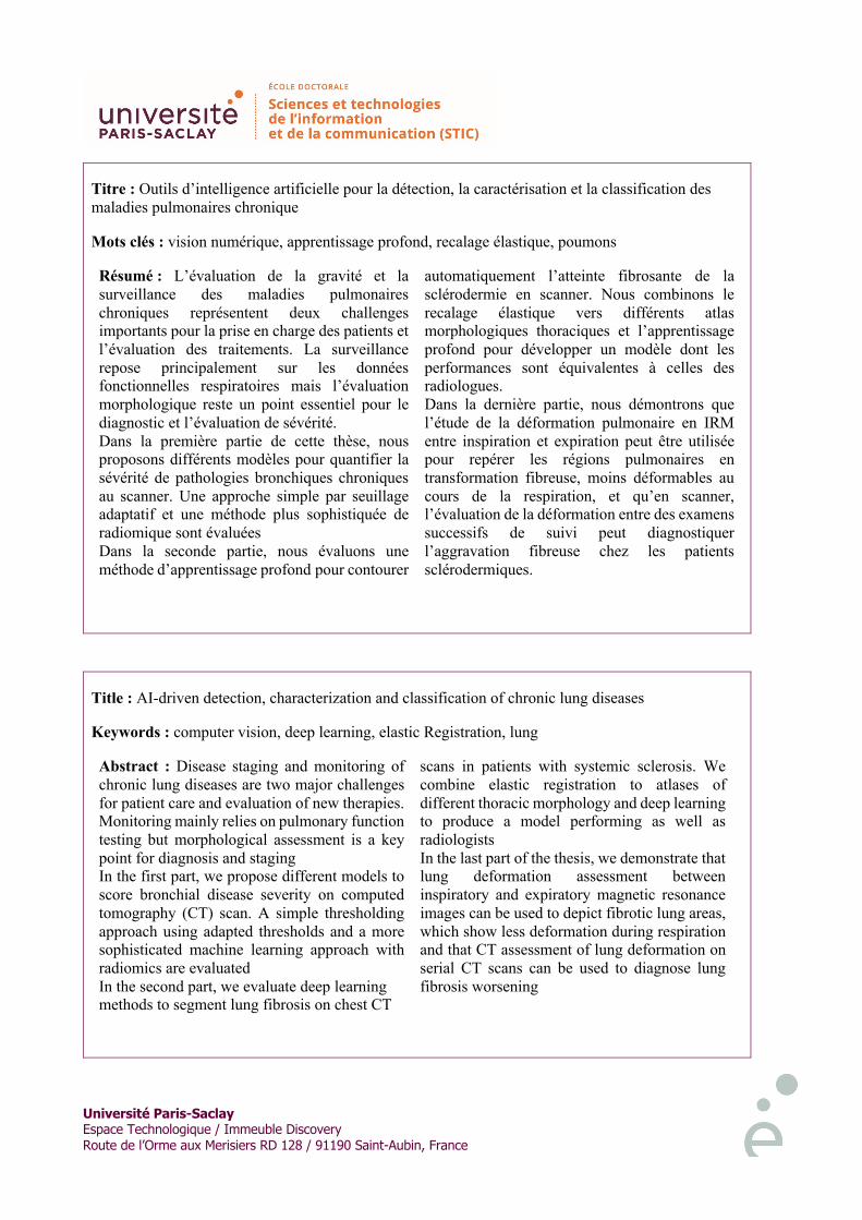
Université Paris-Saclay Espace Technologique / Immeuble Discovery

Route de l’Orme aux Merisiers RD 128 / 91190 Saint-Aubin, France

Titre : Outils d’intelligence artificielle pour la détection, la caractérisation et la classification des maladies pulmonaires chronique

Mots clés : vision numérique, apprentissage profond, recalage élastique, poumons

Résumé : L’évaluation de la gravité et la surveillance des maladies pulmonaires chroniques représentent deux challenges importants pour la prise en charge des patients et l’évaluation des traitements. La surveillance repose principalement sur les données fonctionnelles respiratoires mais l’évaluation morphologique reste un point essentiel pour le diagnostic et l’évaluation de sévérité. Dans la première partie de cette thèse, nous proposons différents modèles pour quantifier la sévérité de pathologies bronchiques chroniques au scanner. Une approche simple par seuillage adaptatif et une méthode plus sophistiquée de radiomique sont évaluées Dans la seconde partie, nous évaluons une méthode d’apprentissage profond pour contourer

automatiquement l’atteinte fibrosante de la sclérodermie en scanner. Nous combinons le recalage élastique vers différents atlas morphologiques thoraciques et l’apprentissage profond pour développer un modèle dont les performances sont équivalentes à celles des radiologues. Dans la dernière partie, nous démontrons que l’étude de la déformation pulmonaire en IRM entre inspiration et expiration peut être utilisée pour repérer les régions pulmonaires en transformation fibreuse, moins déformables au cours de la respiration, et qu’en scanner, l’évaluation de la déformation entre des examens successifs de suivi peut diagnostiquer l’aggravation fibreuse chez les patients sclérodermiques.

Title : AI-driven detection, characterization and classification of chronic lung diseases

Keywords : computer vision, deep learning, elastic Registration, lung

Abstract : Disease staging and monitoring of chronic lung diseases are two major challenges for patient care and evaluation of new therapies. Monitoring mainly relies on pulmonary function testing but morphological assessment is a key point for diagnosis and staging In the first part, we propose different models to score bronchial disease severity on computed tomography (CT) scan. A simple thresholding approach using adapted thresholds and a more sophisticated machine learning approach with radiomics are evaluated In the second part, we evaluate deep learning methods to segment lung fibrosis on chest CT

scans in patients with systemic sclerosis. We combine elastic registration to atlases of different thoracic morphology and deep learning to produce a model performing as well as radiologists In the last part of the thesis, we demonstrate that lung deformation assessment between inspiratory and expiratory magnetic resonance images can be used to depict fibrotic lung areas, which show less deformation during respiration and that CT assessment of lung deformation on serial CT scans can be used to diagnose lung fibrosis worsening