IFPRI Discussion Paper No. 00695 March 2007

Agricultural Growth Linkages in Ethiopia:

Estimates using Fixed and Flexible Price Models

Xinshen Diao, International Food Policy Research Institute Belay Fekadu, International Food Policy Research Institute

Steven Haggblade, Michigan State University Alemayehu Seyoum Taffesse, International Food Policy Research Institute

Kassu Wamisho, International Food Policy Research Institute Bingxin Yu, International Food Policy Research Institute

Development Strategy and Governance Division

INTERNATIONAL FOOD POLICY RESEARCH INSTITUTE. The International Food Policy Research Institute (IFPRI) was established in 1975. IFPRI is one of 15 agricultural research centers that receive principal funding from governments, private foundations, and international and regional organizations, most of which are members of the Consultative Group on International Agricultural Research.

Financial Contributors and Partners

IFPRI’s research, capacity strengthening, and communications work is made possible by its financial contributors and partners. IFPRI gratefully acknowledges the generous unrestricted funding from Australia, Canada, China, Denmark, Finland, France, Germany, India, Ireland, Italy, Japan, Netherlands, Norway, Philippines, Sweden, Switzerland, United Kingdom, United States, and World Bank.

IFPRI Discussion Paper No. 00695 March 2007

Agricultural Growth Linkages in Ethiopia:

Estimates using Fixed and Flexible Price Models

Xinshen Diao, International Food Policy Research Institute Belay Fekadu, International Food Policy Research Institute

Steven Haggblade, Michigan State University Alemayehu Seyoum Taffesse, International Food Policy Research Institute

Kassu Wamisho, International Food Policy Research Institute Bingxin Yu, International Food Policy Research Institute

Development Strategy and Governance Division

PUBLISHED BY

INTERNATIONAL FOOD POLICY RESEARCH INSTITUTE 2033 K Street, NW Washington, DC 20006-1002 USA Tel.: +1-202-862-5600 Fax: +1-202-467-4439 Email: ifpri@cgiar.org

www.ifpri.org

Notices: 1 Effective January 2007, the Discussion Paper series within each division and the Director General’s Office of IFPRI were merged into one IFPRI-wide Discussion Paper series. The new series begins with number 689, reflecting the prior publication of 688 discussion papers within the dispersed series. The earlier series are available on IFPRI’s website at www.ifpri.org/pubs/otherpubs.htm#dp. 2 IFPRI Discussion Papers contain preliminary material and research results. They have not been subject to formal external reviews managed by IFPRI’s Publications Review Committee, but have been reviewed by at least one internal and/or external researcher. They are circulated in order to stimulate discussion and critical comment.

Copyright © 2007 International Food Policy Research Institute. All rights reserved. Sections of this material may be reproduced for personal and not-for-profit use without the express written permission of but with acknowledgment to IFPRI. To reproduce the material contained herein for profit or commercial use requires express written permission. To obtain permission, contact the Communications Division at ifpri-copyright@cgiar.org.

iii

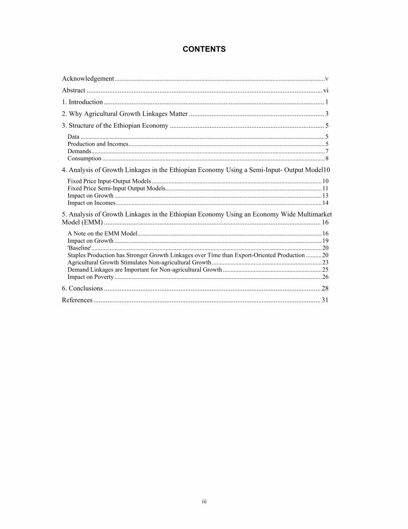
CONTENTS

Acknowledgement........................................................................................................................................V

Abstract ........................................................................................................................................ vi

1. Introduction ............................................................................................................................... 1

2. Why Agricultural Growth Linkages Matter .............................................................................. 3

3. Structure of the Ethiopian Economy ......................................................................................... 5 Data ..............................................................................................................................................................5 Production and Incomes...............................................................................................................................5 Demands.......................................................................................................................................................7 Consumption ................................................................................................................................................8

4. Analysis of Growth Linkages in the Ethiopian Economy Using a Semi-Input- Output Model10 Fixed Price Input-Output Models ..............................................................................................................10 Fixed Price Semi-Input Output Models.....................................................................................................11 Impact on Growth ......................................................................................................................................13 Impact on Incomes.....................................................................................................................................14

5. Analysis of Growth Linkages in the Ethiopian Economy Using an Economy Wide Multimarket Model (EMM) ............................................................................................................................. 16

A Note on the EMM Model.......................................................................................................................16 Impact on Growth ......................................................................................................................................19 'Baseline'.....................................................................................................................................................20 Staples Production has Stronger Growth Linkages over Time than Export-Oriented Production ..........20 Agricultural Growth Stimulates Non-agricultural Growth .......................................................................23 Demand Linkages are Important for Non-agricultural Growth ................................................................25 Impact on Poverty ......................................................................................................................................26

6. Conclusions ............................................................................................................................. 28

References ................................................................................................................................... 31

iv

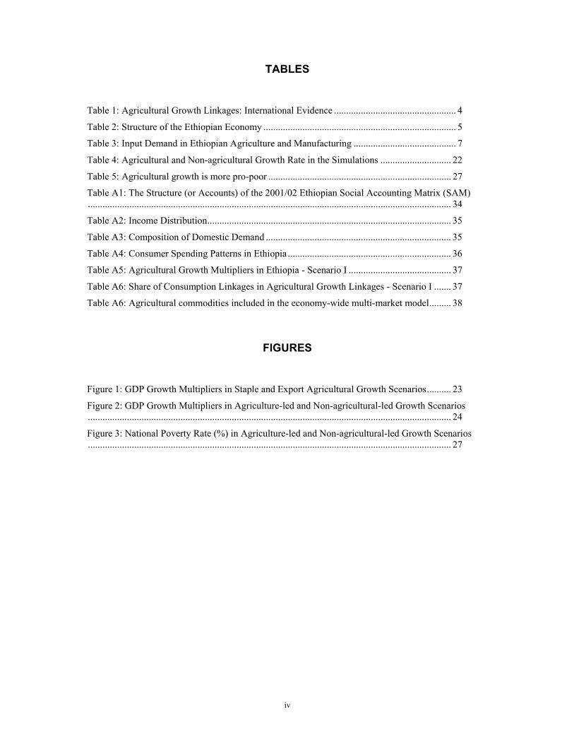
TABLES

Table 1: Agricultural Growth Linkages: International Evidence .................................................. 4

Table 2: Structure of the Ethiopian Economy ............................................................................... 5

Table 3: Input Demand in Ethiopian Agriculture and Manufacturing .......................................... 7

Table 4: Agricultural and Non-agricultural Growth Rate in the Simulations ............................. 22

Table 5: Agricultural growth is more pro-poor ........................................................................... 27

Table A1: The Structure (or Accounts) of the 2001/02 Ethiopian Social Accounting Matrix (SAM)..................................................................................................................................................... 34

Table A2: Income Distribution.................................................................................................... 35

Table A3: Composition of Domestic Demand ............................................................................ 35

Table A4: Consumer Spending Patterns in Ethiopia ................................................................... 36

Table A5: Agricultural Growth Multipliers in Ethiopia - Scenario I .......................................... 37

Table A6: Share of Consumption Linkages in Agricultural Growth Linkages - Scenario I ....... 37

Table A6: Agricultural commodities included in the economy-wide multi-market model......... 38

FIGURES

Figure 1: GDP Growth Multipliers in Staple and Export Agricultural Growth Scenarios.......... 23

Figure 2: GDP Growth Multipliers in Agriculture-led and Non-agricultural-led Growth Scenarios..................................................................................................................................................... 24

Figure 3: National Poverty Rate (%) in Agriculture-led and Non-agricultural-led Growth Scenarios..................................................................................................................................................... 27

v

ACKNOWLEDGMENTS

The authors would like to thank Eleni Z. Gaber-Madhin for her sustained interest, valuable

comments, and patience. The authors would like to thank participants of the IFPRI/ESSP Conference

(June 2006), the Ethiopian Economic Association (EEA) conference, and the EEA seminar. Finally,

the authors gratefully acknowledge the generous contribution of the Ministry of Finance and

Economic Development and, especially, the Ethiopian Central Statistical Agency and its staff for

providing the bulk of the data used.

vi

Abstract

Accelerating growth and poverty reduction, and the ultimate achievement of structural

transformation, are the critical policy challenges in present day Ethiopia. This paper examines relevant

growth options in terms of their impact on overall growth and poverty reduction in the country. It

deploys a fixed-price semi-input-output model and a flexible-price economy-wide multi-market model

for that purpose. The paper finds that agricultural growth can induce higher overall growth and faster

poverty reduction than non-agricultural growth, although the latter can also have large growth effects

in some cases. Among sub-sectors within agriculture, staple crops have stronger growth linkages.

Decomposition of these effects also reveals that consumption linkages are much stronger than

production linkages, i.e., the impact of increased consumption demand due to growth (agricultural and

non-agricultural) is much larger than that of the corresponding expansion in input demand. Moreover,

non-agricultural sectors have to grow in order to match growing supply of agricultural products and

increasing demand for non-agricultural products. Otherwise, falling relative prices of agricultural

products may dampen the realized gains in growth and poverty reduction.

1

1. Introduction

All major economies of the world, even the richest, started out as primarily agrarian

economies. Over time, economic development has stimulated a process of structural transformation

during which broad-based productivity growth accompanied a shifting sectoral composition of

economic activity. There is widespread agreement that the share of agriculture will fall during this

transformation and that transfers of capital and labour from agriculture help fuel growth in the

expanding industrial and service sectors of developing economies (Chenery and Syrquin 1975).

Disagreements emerge, however, about whether policy makers can siphon resources from agriculture

with impunity or whether prior investments in agricultural productivity are necessary to enable these

resource transfers to take place without raising food prices, urban wage rates and choking off

industrial development (Timmer 1988).

Early development strategists emphasized the importance of promoting industrialization first

(Lewis 1954). Albert Hirschman's (1958) influential early writings advocated focusing development

resources in lead industries with strong spillovers throughout the economy. His pro-industrial

prescription rested on the supposedly feeble production linkages between agriculture and the rest of

the economy. In his words, "agriculture certainly stands convicted on the count of its lack of direct

stimulus to the setting up of new activities through linkage effects - the superiority of manufacturing

in this respect is crushing" (Hirschman 1958). This view contributed to a common neglect of

agriculture, particularly during the 1960’s. Yet in spite of Hirschman’s confident assertion, import-

substituting industrialization strategies broadly failed to stimulate broad-based economic growth

(Bruton 1990).

As a result, many development specialists have come to believe that early investments in

agricultural productivity constitute a necessary precondition for overall economic growth. For

without rising farm productivity, the transfer of labour and capital from agriculture will lead to falling

agricultural output, rising food prices and growing poverty (Johnston and Mellor 1961). Indeed, apart

from a handful of city states and small island countries such as Mauritius, the vast majority of large

economies worldwide have initiated growth through agriculture. According to a recent review by

Michael Lipton (2005), “Since 1700, virtually all instances worldwide of mass dollar poverty

reduction began with a sharp rise in labour income due to higher productivity on small family farms.”

Ethiopia’s aims to follow this standard pattern of agriculture-led economic growth. The

country has formally adopted Agriculture Development Led Industrialisation (ADLI) as a

development strategy in 1994, with the aim of investing in agricultural productivity in order to

stimulate farm output and incomes, thus generating growth for both farm inputs and consumer goods.

This strategy has been justified because agriculture is the largest sector in terms of output and,

particularly, employment and exports; the bulk of the poor live in the agriculture-centred rural areas;

considerable gaps exist between rural and urban average levels across key dimensions of well-being

2

including health and education; and there exists substantial potential to raise agricultural productivity

via the widespread introduction of modern technology (MoFED, 2002). Strategic thinking on the role

of agriculture in growth has somewhat evolved recently, with the explicit acknowledgement in the

new Plan for Accelerated and Sustained Development to End Poverty (PASDEP) that with ADLI ‘the

overall growth performance has not yielded the hoped-for poverty-reduction results over the long-

term’ (PASDEP, 2005). Thus, the Plan articulates a more comprehensive strategy which focuses on

commercialisation and intensification of agriculture, favours a geographically differentiated strategy,

recognises the dangers of volatile economic growth and rapid population growth, and highlights the

importance of the urban sector.

In the face of a broad strategy based on agricultural growth, there remain considerable

specific policy choices that involve carefully considering the options as to: which sectors have larger

prospective linkages; what is the growth and poverty-reduction potential of these sectors and

constraints thereof; and which policy interventions are capable of unlocking the growth potential. In

order to answer these questions, it is necessary to empirically identify which types of agricultural

growth linkages are potentially available and to establish how large they are. The assessment needs to

be disaggregated since the extent of these linkages varies across branches of the large and diverse

agricultural sector. Finally, growth options need to be systematically linked with policy interventions

such that the instruments of achieving the desired goals are ascertained. The types and scale of public

investment are clearly vital, in this regard.

In light of the above, this paper applies both fixed price semi-input-output modelling and

flexible price multi-market modelling to measure the potential income-generating power of

agricultural growth linkages in Ethiopia and to contrast it with that from non-agricultural growth. The

estimates and corresponding analysis use recent data and primarily rely on a newly constructed Social

Accounting Matrix (SAM) for the economy as of 2001/02. Specifically, the analysis explores the

implication of alternative growth patterns to overall growth, the level and distribution of income, and

thus poverty reduction in Ethiopia. Since linkages can vary substantially across sectors, the paper

focuses on the growth linkages emanating from key sub-sectors of agriculture (essentially, staples and

exportables) and manufacturing.

The rest of the paper has five main parts. Parts 2-3 set the scene by considering the question

of growth linkages broadly and highlighting the relevant structural features of the Ethiopian economy.

Part 4 describes the semi-input-output approach and reports the findings of its application to Ethiopia,

while Part 5 does the same for the economy-wide multi-market approach. Part 6 concludes.

3

2. Why Agricultural Growth Linkages Matter1

As agriculture grows, it stimulates series of economic linkages with the rest of the economy.

The resulting demand linkages, which constitute the focus of this study, fall into two broad categories:

production linkages, and consumption linkages.2

Production linkages include backward linkages – the input demands by farmers for farm

equipment, pumps, fuel, fertilizer and repair services – as well as forward linkages from agriculture to

non-farm processors of agricultural raw materials. In prosperous agricultural zones, these linkages

prove substantial as pump suppliers, input dealers, grain traders, processing industries and transporters

emerge to supply agricultural inputs and process and distribute farm output. Empirical work on these

relationships has focused on measurement of input-output coefficients to establish the strength of the

forward and backward supply linkages.

Consumption linkages include spending by farm families on locally produced consumer

goods and services. Early work in Green Revolution India indicated that higher-income small farmers

spent about half of their incremental farm income on non-farm goods and services as well as another

third on perishable agricultural commodities such as milk, fruit and vegetables (Mellor and Lele

1971). Thus, consumption linkages from growing farm income can induce sizable second rounds of

rural growth via increased consumer demand for non-agricultural goods and services as well as

perishable, high-value farm commodities such as milk, meat and vegetables. In places like India,

where many non-farm goods and services are produced by labour-intensive methods, the spending

multipliers not only accelerate growth but also enhance the equity of agriculture-led growth.

Following an initial spurt in farm productivity and incomes, production and consumption

linkages together induce second rounds of demand-led growth. Empirical evidence from around the

developing world suggests that a $1 increase in agricultural income will generate an additional $0.30

to $0.80 income in rural non-farm economy. Linkages are even higher when consumption of urban-

produced products is included. In Africa and Asia, consumption linkages typically account for over

80 percent total spending linkages.

This evidence contrasts with Hirschman’s claim of feeble agricultural growth linkages

(Hirschman (1958)). Where did Hirschman go wrong? He underestimated agricultural growth

linkages in two very fundamental ways. As Johnston and Kilby (1975) originally pointed out,

agricultural technology changed during the green revolution. The new high-yielding varieties

demanded pumps, sprayers, fertilizer, cement, construction labour, and repair facilities from

1 Although the discussion below focuses explicitly on agricultural growth and linkages thereof, the approach and concepts therein apply to growth in other sectors as well. 2 It is important to emphasise that this study, and almost all studies of its kind, focus on demand linkages described in the following paragraphs. Aside from demand linkages, there are other inter-sectoral linkages in an economy. Briefly, these operate via saving and investment (private and public), labour flows, and transfers including taxes.

4

non-agricultural firms, thus generating substantial backward linkages. Furthermore, considerable

milling, processing and distribution of agricultural produce took place in rural areas, thus generating

important forward production linkages as well. The new agricultural technology fundamentally

altered input-output relationships.

Still more important were the consumption linkages that Hirschman had ignored altogether.

As Mellor and Lele (1973) originally pointed out, consumption linkages from growing farm income

induce sizable second rounds of rural growth via increased consumer demand. Where new

technology or investment in agriculture leads to increased income, farm families spend large

increments of additional earnings on high-value processed foods and on consumer goods and services

such as transport, education, health, construction and personal services.

Available evidence indicates, however, that demand linkages vary considerably across

locations and farm technologies. As Table 1 indicates, they typically prove highest in Asia and lowest

in Africa because of higher input linkages with Green Revolution Asian agriculture and because of

higher income levels which lead to more rapid diversification of consumer spending into non-foods.

The accumulating evidence briefly noted in the previous paragraphs induced a shift in the

policy prescriptions concerning sectoral and overall growth. Reversing the industry-first orthodoxy of

the 1950's, the results of Adelman’s (1984) classic study suggest that agricultural demand-led

industrialization can generate superior growth and equity when contrasted with the alternative of

export promoting industrialization strategies. Better identified and measured growth linkages thus led

to the recognition of agriculture as a potentially powerful engine of economic growth.3 The same

evidence also revealed that this potential is neither present nor equally realizable everywhere.4

Consequently, it became vital to consider two sets of policy relevant questions. Globally, it is

necessary to answer, under what conditions agriculture can become a leading sector to induce faster

growth, how does agriculture grow, and do government policies matter a lot to agricultural growth.

Specific to each economy, it is indispensable to establish the size of potential agricultural growth

linkages and the extent to which it is possible to realize them. This paper attempts to accomplish the

former with respect to Ethiopia.

Table 1: Agricultural Growth Linkages: International Evidence

Additional Income Growth Source of Linkages (%)

Initial Agricultural

Income Growth Other

AgricultureNon-farm Activities Total Consumption Production

Asia 1.00 0.06 0.58 0.64 81.00 19.00 Africa 1.00 0.17 0.30 0.47 87.00 13.00 Latin America 1.00 0.05 0.21 0.26 42.00 58.00 Source: Haggblade and Hazell (1989).

3 Prominent writers such as Irma Adelman, Peter Hazell, Peter Kilby, Bruce Johnston, Uma Lele, Michael Lipton and John Mellor highlight the potential power of agriculture-led growth strategies, particularly in the early stages of economic development. 4 A good summary of the relevant issues and evidence can be found in Sarris (January 2001).

5

3. Structure of the Ethiopian Economy

A key message from the previous section is that production and consumption patterns play a

crucial role in determining the direction and importance of growth linkages. Accordingly, this section

broadly outlines the structure of the Ethiopian economy in order to provide the background and

context of the linkages analysis of subsequent sections.

Data

Most of the data for the analysis is extracted from the 2001/02 Ethiopian SAM. The 2001/02

Ethiopian SAM is a 63x63 matrix and contains an account for each of twenty production activities,

five factors of production, twenty-five commodities, transactions costs, three household groupings,

three enterprise types, recurrent government, three types of public investment, savings/investments of

institutions other than the government, and the rest of the world.5 The details of the structure of the

SAM are presented in Table A1 in the annex. As can be surmised from that table, the SAM captures

the diversity in production activities and the interdependencies among the various sectors and

institutions that characterise the Ethiopian economy.

Production and Incomes

In order to measure the interactions between agriculture and other sectors of the economy, it

is necessary to have an up-to-date measurement of production linkages among sectors as well as links

from various production activities to household incomes. Both of these elements, the input-output

relationships (Table 3) and functional distribution of income (Table A2) are summarized in the social

accounting matrix for 2001/02, constructed for this purpose.

Table 2: Structure of the Ethiopian Economy

Agriculture Manufacturing Crops Livestock Others Large Small

Mining, Construction,

Utilities Services

GDP at Factor Cost

Value-added Level (million Birr) 12642 8073 3761 2213 1181 4659 27681 60210.9Share (%) 21.0 13.4 6.2 3.7 2.0 7.7 46.0 100.0

Export earnings Level (million Birr) 2711 852 301 4420 Share (%) 32.7 10.3 3.6 53.4

Share in MerchandiseExport Earnings (%) 70.2 22.1 7.78

Source: Ethiopian SAM 2001/02.

5 Choosing the year for which a SAM is to be built is one of the first key tasks. The year selected should ideally be a 'normal' year. It is not always easy to follow this rule, partly because what is ‘normal’ is relative. With this caveat, in the present case, the year 2001/02 was chosen because it is the most 'normal' recent year. It also has the additional attraction of being the year covered by the Ethiopian Agricultural Sample Enumeration (EASE) survey.

6

Agriculture dominates the Ethiopian economy, accounting for 80 percent of national

employment, 41 percent of gross domestic product (GDP) and 33 percent of total exports or 70

percent of merchandise exports (Table 2).6 More than 80 percent of these agricultural output and

value-added (amounting to more than a quarter and a third of national output and value-added,

respectively) is generated by subsistence farming.7 More interestingly, subsistence livestock

production accounts for close to 40 percent of agricultural output and a third of value-added.

In comparison, the small industrial sector produces only 14 percent of GDP, the top three

industrial sub-sectors being construction, large-scale manufacturing, and utilities. Surprisingly, the

small capacity in industry, particularly in large/medium manufacturing, is not utilised fully. Capacity

utilisation in large/medium manufacturing is so low that actual output represented 48 percent of

annual capacity in 2001/2002 (CSA (October, 2003b)).8 This contrasts with the substantial

importation of manufactured goods such as textiles and leather products.

Another striking feature of the Ethiopian economy is the size of its services sector. The share

of services in national GDP is a few percentage points higher than two-fifth - much higher than what

is appears to be consistent with the country's level of development.9

6 The employment figure is obtained from the labour force survey CSA (November, 1999). 7 Output and value-added shares reported for agriculture in this section are out of output and value-added in ‘agriculture, forestry, and fishing’. 8 The rate of capacity utilisation displays considerable variation around this average rate. For further details see CSA (October, 2003b). Furthermore, low capacity utilisation is not unique to 2001/02. In 2003/04 only 48 percent and 66 percent production capacity was on actually used by the private and public firms belonging to the sector, respectively (CSA (October, 2003)). Indeed, low capacity utilisation is a perennial problem in manufacturing. During 1997/98-2003/04 period, private manufacturing enterprise could, on average, use only 34 percent of their full capacity. The corresponding rate in public manufacturing was 55 percent. 9 A note on the size of the service sector. Using data from the World Bank and the OECD, Easterly et al (1994) attempt to develop an international norm for the appropriate size of services at different levels of development. They suggest that service sector shares of 50 per cent and above in GDP are appropriate for countries in the middle and upper-income countries. This implies that for low-income developing countries the size of the service sector should be lower, much lower for very poor countries like Ethiopia, than this level. This general understanding is corroborated by the share of services in the GDP in many developing countries (World Bank (2006)). Similarly, the regression results of Kongsamut, Rebelo and Xie (1999) imply that the GDP share of the services sector in Ethiopia corresponds to per capita GDP of close to US$4000 - a level many times over the per capita GDP of Ethiopia in 2001/02.

7

Table 3: Input Demand in Ethiopian Agriculture and Manufacturing

Manufacturing Crops Livestock

Food Textile and Leather

Other Manufacturing Shares of output

(%)

Subsistence Modern Subsistence Large Small Large Small Large Small

Input source Agriculture 9.1 5.6 30.8 23.3 8.0 35.1 0.0 1.5 0.5 Industry 4.0 13.2 0.0 24.3 48.9 38.3 46.5 56.7 42.1 Services 0.0 0.0 0.0 2.2 6.9 0.8 11.0 4.0 2.8

Total Inputs 13.2 18.8 30.8 49.8 63.8 74.1 57.5 62.3 45.5 Value-added 86.8 81.2 69.2 32.1 36.1 17.7 42.5 27.0 54.3 Indirect taxes 0.0 0.0 0.0 18.1 0.1 8.2 0.0 10.7 0.2

Total 86.8 81.2 69.2 50.2 36.2 25.9 42.5 37.7 54.5 Total Gross Output 100.0 100.0 100.0 100.0 100.0 100.0 100.0 100.0 100.0

Share of Imports in raw materials (%) 4.0 13.2 27.6 23.8 74.3

Source: Ethiopian SAM 2001/02. Notes: Imported inputs in agricultural essentially fertilisers.

Demands

By far the largest two components of domestic demand are household consumption and

intermediate consumption (Table A3 in the annex). Household consumption (44 percent) constitutes

the largest component of domestic demand, followed by intermediate demand (33 percent) and

investment (13 percent). Not surprisingly, the share of household consumption is much higher (70

percent) in domestic demand for agricultural commodities. In contrast, intermediate consumption

dominates (41 percent) domestic demand for industrial commodities.

These demands are covered by domestic production and imports, with the latter accounting

for 17 percent. The share of imports reaches a third with respect to the demand for industrial goods,

and is much higher for petroleum products, chemicals, and machinery and equipment. Indeed,

industrial imports make up close to 75 percent of total imports. 10 That the largest fraction of domestic

industrial demand is for intermediate consumption and that imports provide for a third of this demand

means that access to these commodities is likely to be a binding constraint to economic growth. On

the other hand, it indicates to considerable room for import substitution – an opportunity.

Despite its large size and expected comparative advantage, the agricultural sector provide

only about a quarter of intermediate inputs and most of this to itself (Table 3). The sector's demand for

inputs originating in other sectors is also very small. Indeed, the rather limited use of modern inputs

10 It is noteworthy that 13% and 28% of the demand for cereals and textile/leather products is met by imports, respectively. Food aid makes up almost all of cereal imports.

8

constitutes one of the sources of low productivity in the sector. Comparatively, industrial goods

represent close to half of intermediate consumption, but the bulk of this are imported.11

Consumption

The SAM provides more details about household consumption. However, since it summarizes

current spending patterns, its column coefficients represent average budget shares. But incremental

household spending typically differs from that initial average. As a result marginal budget shares are

more realistic projectors of consumption spending as income grows. Wamisho and Yu (2006)

describes how these marginal budget shares were estimated using household expenditure data from

1999/2000, while Table A4 summarizes the key resulting parameters used in the linkages analysis.

As income increases, the share of food expenditure in total expenditure drops steadily.

Consumption shares decrease with increased income for most food items, with the exception of teff

and processed agricultural products. When disposable incomes increase, households tend to allocate

more income to industrial goods and service. This is especially the case for private service sector

(including hospitality, recreation, entertainment and personal services), and average expenditure on

private services surges fourfold from the lowest to the highest income quintile in rural areas.

Marginal propensity to consume (MPC) decreases across income level for most commodities

except for processed agricultural products in rural and service sector in urban areas. However, despite

declining marginal propensity to consume in staple food across income, the absolute level of

consumption exhibits a strong upward trend due to significant income gaps. Thus, it is observed that

absolute level of demand for most staple foods increases with income growth, and the relative

increase is more manifest among poor households.

Briefly, agriculture figures prominently in the Ethiopian economy, especially in employment

and exports; the small manufacturing sector imports a lot of its inputs and appears to be

uncompetitive; and there is a large and growing services sector. Moreover, household consumption is

dominated by food, though manufactures and services grow in importance at higher incomes. On the

other hand, inter-activity domestic input demands are not very large while imports form a

considerable fraction of input demand within manufacturing. Indeed, the dominant subsistence

farming sector's use of modern inputs is so limited that it is identified as a key bottleneck to further

growth in farm productivity. Finally, manufacturing production capacity is commonly not utilised in

full.

The pattern of potential growth linkages in the Ethiopia economy would reflect its key

features briefly noted above. For instance, limited inter-industry demands for domestic inputs imply

11 It is rather surprising that small-scale food processing has a larger intermediate input use as a fraction of output than large-scale food processing. The dominance of grain milling within the former explains the outcome. Relative to their size, most small grain mills use considerable amounts of electricity obtained from the national grid or self-produced via diesel generators. This amounts more than half of intermediate consumption, while the corresponding level in large-scale food processing is about a quarter.

9

that production linkages are likely to be weak. In contrast, the prominence of consumption in total

expenditure indicates to the possibility of large consumption linkages. Still another example is the

observed presences of considerable unused capacity in manufacturing - it means that, in principle, the

sector can meet some of the growth-induced expansion in demand. In short, the direction and size of

the growth linkages reported below should be interpreted in light of such structural features of the

Ethiopian economy.

10

4. Analysis of Growth Linkages in the Ethiopian Economy Using a Semi-Input- Output Model

A variety of economic models are available for measuring agricultural growth linkages. The

following analysis applies a fixed-price semi-output model, while subsequent dynamic analysis

supplements this with a recursive price-endogenous model in the next section.

A Note on the Fixed Price Models

Fixed Price Input-Output Models

Studies of growth linkages most commonly apply some variant of the linear input-output (IO)

model. In its most basic form, the input-output model uses fixed IO coefficients and assumes fixed

prices and perfectly elastic supply in all sectors. With perfectly elastic supply, any increase in

demand leads only to higher output, with no change in price. Total supply in each sector (Z) is

modelled as the sum inter-industry input demand (AZ) and final demand (F), where final demand

includes consumption by households (βY) and exogenous sources of demand such as exports (E).

Income (Y) is related to production through a fixed value added share (v) in gross commodity output

(Z).

(1)Z AZ FAZ Y EAZ Z E

ββν

= += + += + +

LLLLLLLLLLLL

Since supply is assumed to be perfectly elastic in all sectors12, total output and incomes are

determined by the level of exogenous demand (E) and a matrix of multipliers (C).

1( ) (2)Z I C E−= − LLLLLLLLLLLL

Perfectly elastic supply in all sectors is, of course, an unrealistic assumption in many

developing countries, particularly for some sectors. Given high rates of seasonal labour

underemployment, typically low capital requirements and substantial rates of reported excess capacity

in many rural non-farm businesses, a highly elastic supply of rural non-farm goods and services is

frequently an appropriate assumption.13 In contrast, shortages of skilled labour, foreign exchange, and

fixed capital frequently constrain output in the formal industrial sector. Likewise in agriculture,

12As Bigsten and Collier (1995) and Haggblade, Hammer and Hazell (1991) note, the existence of a real multiplier hinges on the existence of slack resources which can be pulled into productive activity. 13Bagachwa (1981), Liedholm and Chuta (1976) and Steel (1977) report rates of excess capacity between 33 percent and 60 percent for the countries of Tanzania, Sierra Leone and Ghana. See Bagachwa and Stewart (1992) for a detailed summary.

11

seasonal labour bottlenecks, land availability, soil fertility, input supply, marketing infrastructure and

moisture constraints frequently limit supply responses.

Even so, some analysts suggest that agricultural supply elasticities may be high, at least over a

certain range (Delgado et al. 1998; Thorbecke 1994). Anecdotal reports of piles of rotting fruit,

unable to find their way to market, and excess bags of grain unevacuated from specific remote regions

bolster these claims in some, limited circumstance. Yet apart from these episodic special cases, the

overwhelming bulk of empirical evidence points to a low aggregate supply response in agriculture

(Binswanger 1989). If farmers in the developing world could, in fact, increase crop output in

unlimited amounts, agriculture would indeed represent a powerful engine of economic growth, for

both malnutrition and poverty would vanish overnight as hungry farmers availed themselves of this

perfectly elastic cornucopia.

By ignoring supply constraints altogether, unconstrained input-output and SAM multiplier

models exaggerate the size of the inter-sectoral linkages. Given that over half of the reported indirect

effects in these unconstrained models come from demand-induced growth in food grains and other

allegedly elastically supplied agricultural commodities, this questionable assumption biases

anticipated indirect income gains substantially upwards. Side-by-side comparison with alternative

formulations suggests that the unconstrained input-output models overstate agricultural growth

multipliers by a factor of two to ten (Haggblade, Hammer and Hazell 1991).

Fixed Price Semi-Input Output Models

To better simulate real-world supply rigidities, semi-input-output (SIO) models classify

sectors into two groups, those that are supply-constrained (Z1) and others that are perfectly elastic in

supply (Z2).14 As described in equations (3) and (4), the SIO model permits output responses only in

the supply responsive sectors (Z2). Perfectly elastic supply ensures fixed prices for these (Z2) goods.

In the other group, of supply-constrained products (Z1), perfect substitutability between domestic

goods and imports guarantees that world prices will ensure fixed prices for these goods as well. For

these models to produce a reasonable approximation of reality, the supply-constrained sectors must

correspond to tradeable goods whose domestic supply remains fixed at the prevailing output price. In

these supply-constrained sectors (Z1), increases in domestic demand merely reduce net exports (E1),

which then become endogenous to the system and determined by the matrix of semi-input-output

multipliers (C*).

14 See Bell and Hazell (1980), Kuyvenhoven (1978) and Tinbergen (1966) for further discussion of the semi-input-output method. In cases where equations are specified for all accounts of a complete social accounting matrix, semi-input-output models are also termed "constrained SAM multiplier models".

12

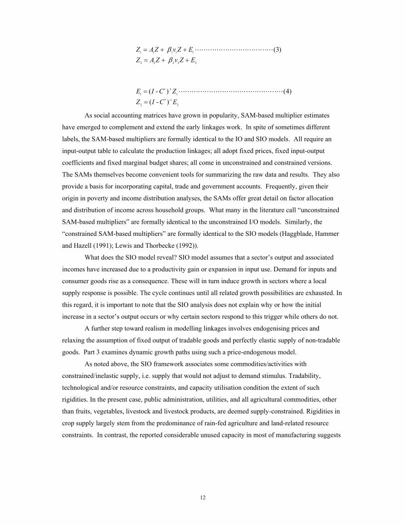
1 1 1 1 1

2 2 2 2 2

-11 1

* -12 2

(3)

( - ) (4)( - )

Z A Z v Z EZ A Z v Z E

E I C ZZ I C E

ββ

∗

= + += + +

=

=

LLLLLLLLLLLL

LLLLLLLLLLLLLLLL

As social accounting matrices have grown in popularity, SAM-based multiplier estimates

have emerged to complement and extend the early linkages work. In spite of sometimes different

labels, the SAM-based multipliers are formally identical to the IO and SIO models. All require an

input-output table to calculate the production linkages; all adopt fixed prices, fixed input-output

coefficients and fixed marginal budget shares; all come in unconstrained and constrained versions.

The SAMs themselves become convenient tools for summarizing the raw data and results. They also

provide a basis for incorporating capital, trade and government accounts. Frequently, given their

origin in poverty and income distribution analyses, the SAMs offer great detail on factor allocation

and distribution of income across household groups. What many in the literature call “unconstrained

SAM-based multipliers” are formally identical to the unconstrained I/O models. Similarly, the

“constrained SAM-based multipliers” are formally identical to the SIO models (Haggblade, Hammer

and Hazell (1991); Lewis and Thorbecke (1992)).

What does the SIO model reveal? SIO model assumes that a sector’s output and associated

incomes have increased due to a productivity gain or expansion in input use. Demand for inputs and

consumer goods rise as a consequence. These will in turn induce growth in sectors where a local

supply response is possible. The cycle continues until all related growth possibilities are exhausted. In

this regard, it is important to note that the SIO analysis does not explain why or how the initial

increase in a sector’s output occurs or why certain sectors respond to this trigger while others do not.

A further step toward realism in modelling linkages involves endogenising prices and

relaxing the assumption of fixed output of tradable goods and perfectly elastic supply of non-tradable

goods. Part 3 examines dynamic growth paths using such a price-endogenous model.

As noted above, the SIO framework associates some commodities/activities with

constrained/inelastic supply, i.e. supply that would not adjust to demand stimulus. Tradability,

technological and/or resource constraints, and capacity utilisation condition the extent of such

rigidities. In the present case, public administration, utilities, and all agricultural commodities, other

than fruits, vegetables, livestock and livestock products, are deemed supply-constrained. Rigidities in

crop supply largely stem from the predominance of rain-fed agriculture and land-related resource

constraints. In contrast, the reported considerable unused capacity in most of manufacturing suggests

13

the possibility of expanding supply without significant incremental costs.15 Therefore, all

manufacturing, mining and construction, and services (except public administration) are identified as

supply-unconstrained.16

The impact of growth in the output of two staple crops (maize and teff), an export crop

(coffee), livestock, and two manufactures (textiles, other manufactures) is examined under the

conditions specified. The aim is to provide a contrasting analysis that can inform the dialogue on

investment strategies in Ethiopia. More specifically, the results allow a comparison across three broad

investment strategies for the country: growth in staple crops (maize and teff), growth in export crops

(coffee) and growth in manufacturing. Differences in technology are also explored by positing

‘traditional’ and ‘modern’ technologies in crop production.17

Impact on Growth

Under the assumptions summarised above, a 1 Birr increase in maize output under traditional

agricultural production will generate 1.97 Birr rise in total GDP. The analogous change in GDP are

2.18 Birr for teff, 3.45 Birr for coffee, 1.40 Birr for textiles, and 1.16 Birr for other manufactures (see

Table A5).

The contrast between agricultural products and manufactures is marked. This difference arises

primarily because of smaller value-added generated by the direct increase in manufacturing output. As

a fraction of the gross value of output, material inputs used in manufacturing range from 46 percent in

small-scale other manufacturing to 81 percent in large-scale textile production with an average of 65

percent. Value added, thus, comprises on average 36 percent of output only. By comparison, the value

added in total output is much higher in the agricultural sub-sectors, accounting for 78 percent on

average. Consequently, a 1 Birr increase in agricultural output produces a bigger direct impact on

GDP – 0.61 Birr and 0.70 Birr, for maize and teff production, respectively. An identical expansion in

textiles and other manufactures output can only generate, respectively, 0.12 Birr and 0.05 Birr direct

increase in GDP.

The gap between the direct increase in GDP and the total change in GDP originate in the

second and third round linkages, the input demand and consumption growth emanating from the

injection of agricultural growth. Consumption linkages in particular are clearly important. They

account for over half of total additional income created via growth in traditional agriculture with the

exception of traditional coffee farming (Table A6, last row). Coffee's lower consumption share in

15 For instance, CSA survey data reveals that capacity utilisation within large/medium-scale manufacturing averaged just above 50 percent during 1997/98-2003/04. More tellingly, this rate of capacity utilisation varies very little across years. 16 For comparative purposes, the SIO simulations were run for a more constrained scenario in which all agricultural commodities, all manufactures (except manufactured food, beverages, and tobacco), utilities, and public administration are supply-constrained. 17 ‘Traditional’ technology corresponds with input-output configurations in subsistence crop production derived from the 2001/02 Ethiopian SAM, while ‘modern’ technology coincides with those prevailing in commercial farming.

14

linkages effect is explained by the fact that, as a major export crop, it is associated with substantial

trading/processing and hence larger production linkages. On the other hand, manufacturing induces

smaller production and consumption linkages though the former are larger due to stronger forward

and backward linkages combined with much higher intermediate consumption.

In short, almost all sectors generate large linkages. But those induced by agricultural activities

are larger, primarily because of larger initial value added (income) and consequently larger second

round of consumer spending on local goods and services (i.e., input demand and consumption

linkages additional to first round effects).

Impact on Incomes

Table A5 also reports the total change in income induced by growth and its distribution

among the three household groups. A 1 Birr increase in maize output under traditional agricultural

production will generate 1.32 Birr rise in total household income; while an equivalent change in

traditional teff and coffee production will increase total household income by 1.48 Birr and 1.88 Birr,

respectively. Growth in manufacturing output has much lower positive impact on household incomes.

In terms of the distribution of income across households, expansion of maize and teff

production with traditional technology naturally benefits farm households most. The case of coffee is

worth noting, in this regard. A substantial proportion of coffee output is exported and, partly due to

that, very high transport and trade margins are associated with the crop. As a consequence, a relatively

small fraction of the income gained from growth in coffee production accrues to farm households.

Most of this income goes to wage earners and entrepreneurs.

With the farm households forming the bulk of the poor, the potential impact on income

poverty is thus greatest with growth in staple crops production. A more direct measurement reported

in Part 5 below supports this finding.

It is clear that technological change would be significant to the direction and extent of growth

linkages. Accordingly, as part of examining the linkage effects, a simple simulation was conducted to

assess this significance. The simulation identifies the input configuration in subsistence farming as

representing 'traditional technology' while that in commercial farming as representing 'modern

technology.' A comparison of outcomes respectively generated by assuming that all crops are

produced using 'traditional' or 'modern' technology provide a rough way of exploring the effect of

technological change. Table A5 reports the corresponding estimates.

By taking into account the linkage effect only (and ignoring the productivity growth-effect

that often results in more efficient use of input), a shift from traditional to modern technology in

staples (maize and teff) production will marginally reduce the gains in total household incomes from a

same unit increase in the staple crop production since intermediate input use rises (see Table A5).

More significantly, it modifies income distribution in favour of wage earners as wage labour

substitutes for family labour due to the change in technology. While this outcome may underestimate

15

the gains from technology change that is often embodied in the use of modern inputs, it raises an

important concern in promoting the use of modern inputs. With the introduction of modern

technology, intermediate inputs will account for a growing share of total production revenue. This, in

turn, may possibly weaken the agricultural growth linkages by reducing farmers’ direct income gains,

per unit of output, and thus reducing subsequent spending on locally produced goods and services.

This potentially lower growth linkage effect compounds the problem some observers have raised

about high-input technology increasing smallholder reliance on input markets beyond their direct

control.

In conclusion, growth in agriculture produces stronger linkages than growth in non-

agriculture. The potential benefits of stimulating growth in agricultural production (albeit

differentiated by products) are thus substantial. Nevertheless, the size of this potential as well as the

extent of its realisation depends on a parallel expansion in non-agricultural sectors (particularly in

those associated with growing input or consumption demand). Estimates obtained by varying the set

of non-agricultural sectors assumed to be supply unconstrained show this dependence clearly.18

Moreover, the estimates in the next part show this more directly. Finally, it is important to note that

the assumptions underlying the SIO framework imply that the reported magnitude of growth linkages

(attributed to agriculture or non-agriculture) are likely to be upper bounds of the potential gains. 19

18 For instance, if all sectors are unconstrained and thus can respond to the demand stimulus fully, a 1 Birr increase in maize output under traditional agricultural production will generate 2.93 Birr rise in total GDP. The analogous change in GDP are 3.43 Birr for teff, 3.05 Birr for coffee, 3.45 Birr for livestock products, and 2.26 Birr for textiles. These increases are accompanied by greater gains in household incomes. The complete simulation results can be obtained from the authors upon request. 19 These, rather strong, assumptions are fixed prices and perfectly elastic supply response in some sectors.

16

5. Analysis of Growth Linkages in the Ethiopian Economy Using an Economy Wide Multimarket Model (EMM)

Ethiopia has an open economy. However, high transportation and other marketing costs,

partly explained by considerable geographic distances and an inadequate road network, prevent world

market prices from automatically translating into domestic prices. As a consequence, many

commodity prices, especially those of agricultural products, are actually determined by supply and

demand conditions in the domestic market. For these reasons, it is necessary to take into account for

the interaction of prices and growth (the price effect) in analyzing agriculture-non-agriculture

linkages. Accordingly, this section reports the findings of an economy wide multimarket (EMM)

model, in which prices of most agricultural and non-agricultural products are endogenous variables.

A Note on the EMM Model

The EMM model20 captures the detailed structure of Ethiopian agricultural sectors, while the

non-agricultural economy has a similar structure as the SAM discussed above (i.e., it includes 10

aggregate sectors). The original EMM model was developed by Diao and Nin Pratt (2007) in which

there were only two aggregated non-agricultural sectors and intermediate inputs were not taken into

account. This model is extended and modified for this study in order to be consistent with the non-

agricultural economy described by the SAM discussed above, while detail agricultural sectors are still

kept as before. Specifically, there are 32 agricultural commodities or commodity groups (see Table

A6 in the annex for a list of agricultural commodities/sectors included in the model). In contrast with

the SAM that represents the national economy, both agricultural and non-agricultural production and

consumption in the EMM model are further disaggregated into sub-national regions in order to

capture the geographic heterogeneity of sectors and households. Limited by the data, the model

captures totally 56 administrative zones and all supply and demand functions are defined at the zonal

level.

The EMM model is based on neoclassical microeconomic theory. In the model, an aggregate

producer represents a specific zone’s production of a specific sector. There are a total of 2,352 (42

sub-sectors x 56 zones) such representative producers. Consistent with the setup of many other

multimarket models, the supply function, rather than the production function, is used to capture each

representative producer’s response to market conditions. Specifically, the supply functions are derived

under producer profit-maximization and based on the producer prices of all commodities (including

20 While the CGE approach is preferable for economy wide analysis and more comparable with above SIO analysis, the EMM model is more disaggregated in both commodities and regions. Moreover, the growth-poverty linkages can also be analyzed using the model.

17

the prices for the 10 non-agricultural commodities). Risk and market imperfections are not taken into

account and therefore do not affect producers’ profit-maximization decision in the model.21 In the

crop sub-sectors, the supply functions have two components: (i) yield functions that are used to

capture supply response to the own prices given farmland allocated to this crop; and (ii) land

allocation functions that are functions of all prices and hence are responsive to changing profitability

across crops given the total available land. The own-price elasticities employed in the yield functions

are the combination of authors’ estimates, assumptions and results drawn from other studies, while the

cross price elasticities in the area functions are calibrated according to the share of each commodity in

regional total production.

The production of major staple crops and livestock products involves a variety of

technologies. For staple crops, modern inputs and their effects on crop productivity are captured

through the identification of 15 different technologies, maize production, for example, incorporates

four primary modern inputs—fertilizer, improved seeds, pesticide, and irrigation (individually or

jointly)—and also includes production without modern inputs. While the model captures the average

difference in crop yields across technologies, the marginal effect of increased use of an input for a

given technology is not captured because input uses are not explicitly included in the supply function.

The yield gaps for a specific crop among the 15 technologies are defined at the zonal level and are

consistent, by zone, with data from the national agricultural sample surveys for 1997 and 2000. Data

on irrigation was also available for cash crop production and hence was employed in supply functions

for those crops.

For livestock, the model captures the productivity difference between traditional and modern

technologies. For example, three types of cattle are raised to produce beef: draught animals, from

which beef is a by-product; beef animals, using traditional technology; and beef stock, using

improved technology. The productivity (yield) gaps resulting from the use of different types of

technologies in animal production are reflected in the supply function. Moreover, the supply function

also captures the difference in feed use between traditional and modern technologies. Livestock

production under modern technology requires feed grain, while under traditional production it

assumes feeding via grazing only. The feed-grain demand function is therefore defined only for

improved technology, and is a function of grain crop prices. Different technologies are similarly

defined for dairy, poultry, and sheep and goats.

Demand functions are also disaggregated to the zonal level on per capita (rural or urban)

basis. A representative consumer’s demand for each consumption good is derived from maximizing a

Stone-Geary utility function and the subsistence level of consumption is calibrated to the first quintile

households’ consumption (rural and urban separately). Data used to calibrate the demand functions

21 Weather risk is high in many areas of the country as evidenced by frequent drought and very limited irrigation. While such risk is not explicitly modelled, a drought scenario is designed and discussion about this scenario can be found in Diao et al. (2005).

18

are from the 1999/2000 Household Income, Consumption, and Expenditure Survey (HICES [CSA

2000]). Both income and price elasticities for any specific commodity vary across zone due to

different consumption patterns and income levels (see Wamisho and Yu (2006) for the estimation of

income and price elasticities). Such differences not only imply that the aggregate effect of consumers’

market responses is often non-linear and much more complicated than that in the case where demand

is defined at the national level, but also indicate the possible differential effect on poverty reduction

with similar income increases. These are a focus of model simulations which will be discussed later.

Distinguished from most multimarket models that are usually partial equilibrium in nature,

the per capita income at the zonal-level is an endogenous variable in the EMM model. It is determined

by the zonal-level value added divided by population, rural and urban, respectively. Because of such

setup, the model has a general equilibrium nature, which allows production and consumption

decisions to be linked at the zonal level. Similar as a CGE model, intermediate inputs are explicitly

included in the model through fixed input-output relationship with sector’s production. The IO

coefficients are drawn from the SAM developed in Taffesse, Belay, and Wamisho (2006) for the

purpose of growth linkages analysis. The aggregate of agricultural production value added equals

agricultural GDP (henceforth, AgGDP), and the sum-total of agricultural and non-agricultural value

added equals national GDP.22 Both AgGDP and GDP are endogenous in the model.

As the name of the model suggests, a multiple market structure is specified. It is further

assumed that there is perfect substitution between domestically and internationally produced

commodities. However, transportation and other market costs distinguish trade in the domestic market

from imports and exports. For example, while imported maize is assumed to be perfectly substitutable

with domestically produced maize in consumers’ demand functions, maize may still not be profitable

to import if its domestic price is lower than the import parity price less any transactions costs. Maize

imports can only occur when domestic demand for maize grows faster than domestic supply and the

local market price rises significantly. A similar situation applies to exported commodities. Even

though certain horticultural products are exportable, if domestic production is not competitive in

international markets, either due to low productivity or high transactions costs, then exports will not

be profitable. Only when domestic producer prices plus transactions costs are lower than the export

parity price of the same product does it become profitable to export.

The model does not capture bilateral trade flows across sub-national regions, although it does

identify sub-national regions as being food surplus or deficit by comparing regional level demand and

supply for total food commodities. While producers and consumers in different regions operate in the

same national markets for specific commodities, prices can vary across regions due to differences in

transportation and market costs. For example, domestic marketing margins are defined at the regional

22 The model includes neither government expenditure, nor any government tax or other policy instruments.

19

level according to the distance to Addis Ababa, which represents the central market for the country.23

For a food surplus region, food crop prices faced by local producers are equal to the prices in the

central market subtracting marketing margins, while for a food deficit region local prices are higher

than those in the central market due to marketing margins.

The EMM model thus characterised is deployed to explore growth linkages and impact on

poverty reduction. The initial stimulus to growth is introduced as an exogenous productivity growth.

Moreover, a 'baseline' and four different productivity growth scenarios are considered. To make the

resulting linkage estimates comparable, the impact of sectoral size and growth potential need to be

take into account. Assuming similar growth rates at the sub-sector level, greater economywide growth

will be generated by the larger sub-sectors, in turn producing a (generally) larger effect on poverty.

On the other hand, small sub-sectors have greater capacity to grow rapidly and require the investment

of fewer resources to do so. Thus, in determining whether a sub-sector will ultimately drive growth,

both the linkage effects on the economy and poverty as well as the growth potential (determined by

supply and demand factors) must be considered. In order to ensure comparable quantitative

measurement across the agricultural sub-sectors modelled, those exhibiting similar total GDP growth

but different productivity growth were examined to assess the growth effect of each on overall

economic growth and poverty reduction.

To analyze the growth-poverty effect, the nationally-defined poverty line is adopted in the

model rather than using the World Bank’s ‘a-dollar-a-day’ measure. National poverty lines are

typically measured by household total expenditure, since household income is often significantly

underreported in developing countries. The household level expenditure data from HICES is used to

develop a micro-simulation model to capture detailed household consumption patterns. This micro-

simulation model is linked with the EMM model for calculating poverty rates at the regional or

national level. The calculation of poverty lines and fraction of populations below the poverty lines in

the simulations and other detailed mathematical descriptions of the model can be found in Diao et al.

(2005).

The following sections report a number of key results concerning impact on growth and

poverty.

Impact on Growth

A large number of previous studies have concluded that agriculture, especially food crops,

have strong growth linkages and multiplier effects; that is, increased agricultural (or food crop)

production would generate a disproportionately large increase in the country’s total GDP, through

increased demand for inputs, and more importantly, through increased consumption demand as a

23 The model cannot capture commodity chains that often link producers and consumers directly. Recent market development in Ethiopia shows certain new trends in grain trade flows and Addis Ababa is not necessarily a central market for some trade flows. The model, however, has to simplify the trade flow by ignoring such new trends.

20

result of higher agricultural incomes.24 As the SIO model of the previous section, the EMM model is

used to derive sectoral-level growth multipliers, deriving from total factor productivity (TFP) shocks

in corresponding agricultural sub-sectors.

'Baseline'

Prior to the comparative analysis of agriculture-non-agriculture growth linkages, the EMM

model is employed to assess a business-as-usual scenario (also known as the “baseline”) in which the

economy is assumed to grow following its current trajectory through 2015 (and 2003 is the base-year

used in the model). The business-as-usual growth path is based on average agricultural and non-

agricultural growth trends for 1995–2004, during which time about 70 percent and 50 percent of the

increase in total crop production and cereal production, respectively, resulted from area expansion.

Over the same period, the cereal production growth rate was 2.9 percent per year – 0.4 percent higher

than the 2.5 percent population growth rate – and the growth rates of total staple crop and cereal

yields were about 0.8 and 1.5 percent per year, respectively. Under the business-as-usual scenario to

2015, and based on livestock production growth of 4.1 percent per year and non-agricultural growth

of 5.3 percent per year, GDP is projected to increase at 4.5 percent per year, and AgGDP at 3.7

percent per year.

On this basis, the livelihood of the majority of rural Ethiopians will not get significantly

improved by 2015. The national poverty rate will fall to 32.1 percent by 2015, from the high 2003

level of 44.4 percent. Given 2.5 percent yearly population growth during 2003–15, the decline in the

number of people living below the poverty line will only occur in the urban areas, while the number

of the poor in the rural areas is estimated to increase by 83 thousand by 2015.

Staples Production has Stronger Growth Linkages over Time than Export-Oriented Production

It is thus clear from the business-as-usual scenario that without additional growth in both

agriculture and non-agriculture, it will be impossible for the country to meet the first MDG of halving

the poverty rate by 2015. On the other hand, achieving the objectives of halving poverty requires a

greater understanding of which sub-sectors can best drive the economywide growth and cut poverty

faster. Hence, this section focuses on an evaluation of two broad agricultural sub-sectors in terms of

the country’s growth and poverty reduction strategy. The two sub-sectors are staples (cereals, root

crops, pulses, oilseeds and livestock) and exportables (coffee, selected fruits and vegetables, cotton,

chat, sesame seed, sugar, and other horticultural products). Specifically, these sub-sectors’

contribution is assessed by exogenously increasing the productivity growth rate of one sub-sector,

while maintaining the growth of the others at their baseline levels.

24 See Bell and Hazell (1980) for an early methodological discussion of alternative multiplier models used in growth linkage analysis, and the discussion of Haggblade, Hammer, and Hazell (1991) on the improvement in the multiplier models with limited price endogeneity.

21

With 86 percent of AgGDP and 44 percent of GDP, staples represent the largest agricultural

sub-sector in terms of value-added. In contrast, the export sub-sector constitutes quite small shares

accounting for about 10 percent of AgGDP and 5 percent of total GDP. Thus, the simulated additional

annual growth for cereals’ productivity was first determined, at 1.5 percent, which implies 2.2 percent

additional annual growth in livestock. In total, additional 1.8 percent of annual growth rate is obtained

for the aggregated staple food sector (staple crops and livestock, Table 4). With such growth rate in

the staple sector, total GDP will grow at 5.5 percent (partly through strong linkage effects on the non-

agricultural sector that will be discussed later). In order to produce the same 5.5 percent of GDP

growth rate, the agricultural exports sector needs to grow at 15.6 percent, with additional 12.5 percent

of annual growth compared with the base-run (Table 4).

22

Table 4: Agricultural and Non-agricultural Growth Rate in the Simulations

Growth Rate Base-runStaple crop led growth

Export crop led growth

Agricutlure led growth

Nonagriculture led growth

GDP growth rate 4.5 5.5 5.5 5.5 5.5

Ag GDP growth rate 3.7 4.1 5.7 4.5 4.2

NAg GDP growth rate 5.3 6.8 5.4 6.4 6.7

Total staple crop and livestock growth rate 3.1 4.9 3.0 4.3 3.2

Cereal output growth rate 2.9 4.5 2.9 4.2 3.0

Livestock output growth rate 4.1 6.4 4.0 5.2 4.2

Total export crop growth rate 3.1 2.7 15.6 7.7 3.0

Nontraditional export crop growth rate 4.0 3.7 15.0 8.0 4.0

Nontraditional exports growth rate 8.0 4.8 31.2 18.3 6.4Source: Authors calculation from the EMM model results

To make the impacts more clearly comparable growth multipliers are used. The multipliers

are defined as the total increase in real GDP divided by the increase in the shocked sector’s total

output, both measured at the initial (base-year) level of prices. The resulting multipliers derived using

an economy wide and endogenous price models are in general relatively smaller than the standard

fixed-price multipliers.25 Our model’s simulation results show that the staple sector’s growth

multipliers are consistently greater than one and increase overtime (Figure 1). These results imply that

one unit (not one percent) increase in staple production will generate more than one unit of increase in

total GDP. Moreover, such growth linkages become stronger over time. For example, one unit of

increase in staple production can have 1.03 – 1.12 units of increase in total GDP in the first five years

in the simulation, while the same one unit of increase in staple production will generate 1.29 units of

GDP by 2015. On the other hand, the linkages from agricultural export sector to total GDP is strong

only in the initial five years, while the linkages become weaker overtime, and the growth multipliers

fall to below one by 2015.

25 See Dorosh and Haggblade (2003) for a comparison of CGE and fixed-price multipliers for several Sub-Saharan African countries.

23

Figure 1: GDP Growth Multipliers in Staple and Export Agricultural Growth Scenarios (Both with 5.5% GDP annual growth)

0.9

1.0

1.1

1.2

1.3

1.4

1.5

2004 2006 2008 2010 2012 2014

One-unit staple output One-unit export ag ouput

Source: Authors calculation from the EMM model results

The strong growth linkage effect from staples sector to total GDP is mainly due to induced

growth in the non-agricultural sector. In the scenario in which growth is driven by productivity

increases in the staple sector, the non-agricultural GDP’s annual growth rises to 6.76 percent, from its

5.26 percent in the base run. The additional 1.5 percentage points of annual growth is solely driven by

growth in staple sector, as there is no additional exogenous growth shock imposed on the non-

agricultural sector in this scenario. On the other hand, if the economy wide growth is driven by

additional growth in agricultural export sector, the annual growth rate in the non-agricultural sector

rises only to 5.36 percent, with additional 0.1 percentage points of annual growth compared with the

base run.

Agricultural Growth Stimulates Non-agricultural Growth

Two more scenarios are run to further analyze the linkages between agricultural and non-

agricultural growth. In Scenario 3, it is assumed that an additional productivity growth shock occur

withinthe agricultural sector only, while in Scenario 4, a similar productivity growth shock is imposed

on the non-agricultural sector only. Again, the target is a 5.5 percent annual growth rate of GDP in

both scenarios. To generate such growth in total GDP (by taking into account the linkage effects),

grain production grows at 4.5 percent, with 1.5 percentage points of additional annual growth from

the base run, and livestock grows at 4.7 percent, additional 1.1 percentage points of annual growth.

This results in a staple sector growth of 4.3 percent, an additional 1.2 percentage points of annual

growth. A relatively higher growth rate (7.7 percent) is needed for the export agriculture with 4.5

percent of additional annual growth. This results in total agricultural output (not AgGDP) to grow at

24

4.7 percent per year, instead of the 3.1 percent in the base run, and thus leading to a 1.6 percent of

additional annual growth.

Growth in agriculture significantly stimulates the non-agricultural sector’s growth. Measured

by total non-agricultural GDP, the annual growth rises to 6.42 percent, instead of 5.26 percent in the

base-run. The additional 1.2 percentage points of non-agricultural annual growth are thus induced by

the growth in agriculture. Calculated GDP growth multipliers are 1.05 – 1.13 in the first five years

and increase to 1.29 by 2015 in this scenario (Figure 2). That is to say, a one unit increase in total

agricultural output (measured at the base-year’s prices) can generate more than one unit of total GDP

and its impact will reach 1.29 units of GDP by 2015.

Figure 2: GDP Growth Multipliers in Agriculture-led and Non-agricultural-led Growth Scenarios (both with 5.5% GDP annual growth)

0.6

0.7

0.8

0.9

1.0

1.1

1.2

1.3

1.4

2004 2006 2008 2010 2012 2014

One-unit agricultural output One-unit nonagricultural output

Source: Authors calculation from the EMM model results

In Scenario 4 the initial exogenous increase in productivity is assumed to happen in the non-

agricultural sector only. The non-agricultural sector grows by 5.26 percent in the base run. In order to

induce total GDP to grow at 5.5 percent annually, the sector’s annual growth rises to 6.76 percent,

with 1.5 percentage points of additional annual growth. However, the non-agricultural sector can

stimulate the growth in the agricultural sector only slightly. Agricultural GDP's growth rate rises to

4.15 percent, instead of 3.70 percent in the base run. The calculated GDP growth multipliers in this

scenario are less than one, 0.72 in 2004 and 0.68 in 2015. In other words, a one unit increase in non-

agricultural real output (not non-agricultural GDP) can only generate a less than one unit increase in

total GDP (see Figure 2 for the growth multiplier comparison between the two scenarios).

25

Demand Linkages are Important for Non-agricultural Growth

Strong demand linkages explain why faster agricultural growth, especially of food production,

has such strong growth linkage effect on the non-agricultural sector. Empirical studies show that

agriculture-demand linkages are the dominant factor to stimulate non-agricultural growth in low-

income countries. For low-income countries, a majority of the population lives in the rural areas and

mainly depends on agriculture for its livelihood. This has two implications for the overall growth in

the economy. First, it implies that it is unlikely to have any broad-based growth without agriculture.

Growth in agriculture, especially in those sub-sectors in which a majority of farmers is engaged, can

become an engine strong enough to generate overall economic growth. This is the direct effect of

agricultural growth on the economy-wide growth. Second, it implies that rural demand is the

dominant factor to provide enough market opportunities for both industrial products and services

produced in the economy. Increased farm income has to be spent on both agricultural and non-

agricultural commodities, including services. Income elasticity of demand for the non-agricultural

commodities and services is often greater than that for the agricultural goods, which implies that

farmer will spend more of the additional income on non-agricultural consumption. This is the indirect

effect – through demand linkages – of agriculture on the overall economic growth.

With more than 85 percent of population living in the rural areas, rural demand is the major

component of total demand in the Ethiopian domestic market. Even though per capita rural income is

40 percent lower than the urban income on average and each rural individual’s non-agricultural

consumption is 60 percent below the level for an average urban consumer, because of the dominant

size of rural population in the country, more than 70 percent of non-agricultural products and services

are actually consumed by rural households.26 As many poor rural households can barely have

additional cash income left after meeting basic food consumption, increased income, especially cash

income, will be spent disproportionately more on non-agricultural consumption. The estimated

marginal propensity to consume shows that for each one Birr of additional income, rural household

would spend 0.6 Birr on non-agricultural consumption, though the average budget share of non-

agricultural consumption is about 30 percent. Moreover, the marginal budget share (MBS) of non-

agricultural spending is higher among the low income groups than that for the higher income groups

among the rural population. For example, the MBS for the non-agricultural products and services is as

high as 0.74 for the lowest income quintile in the rural areas. This share declines as income increases,

and it is 0.47 for the highest income quintile. Agriculture is the main income source for many poor

rural households. Given their extremely low level of non-agricultural consumption, with increased

income generated from agricultural growth, rural households will provide steady growing market

opportunities for the country’s non-agricultural sector.

26 Calculated from HICES for the data of 1999/00

26

Impact on Poverty

It is widely anticipated that Ethiopia is unlikely to meet the first MDG of halving poverty by

2015 unless the country’s growth performance improves dramatically. Ethiopia needs to not only

accelerate the level of growth, but also find ways to enhance the ‘pro-poorness’ of growth. In other

words, identify the kind or composition of growth that is most effective at reducing poverty. In this

regard, it is necessary to consider the relative importance of agriculture and industry in helping the

country achieve its development objective of significantly reducing poverty.

The EMM model is thus used to examine how differences in the pattern of growth in the

country influence the rate of poverty reduction. More specifically, using the same four scenarios

discussed above, the growth-poverty linkages is also analysed by comparing the effectiveness of

additional growth in reducing poverty under different growth assumptions. To make the results

comparable, poverty-growth elasticities are calculated for each of the four scenarios.27 Table 5 shows

that the poverty-growth elasticity is larger when additional growth is driven by agriculture rather than

non-agriculture. A one percent annual increase in per capita GDP driven by agricultural-led growth

leads to 1.9 percent reduction in the poverty headcount rate per year. By contrast, a similar increase in

per capita GDP driven by non-agriculture leads to only 1.1 percent fall in the poverty rate. These

disparities in poverty-growth elasticities can translate into different reductions in the poverty

headcount over time. For example, with 5.5 percent of GDP growth in both scenarios, the poverty

headcount falls to 25 percent in the agriculture-led growth scenario, compared with 28 percent in the

non-agriculture-led growth scenario (Figure 3). Given its larger impact on poverty, agricultural-led

growth in Ethiopia lifts an additional 2.9 million rural people out of poverty compared to non-

agricultural-led growth. Though in the non-agriculture-led growth urban poverty population reduces

more than that in the agriculture-led growth, in total, there will be additional 2.6 million people lifting

out of poverty in the agriculture-led growth compared to non-agriculture-led growth, despite the fact

that overall GDP grows at the similar rate under the two scenarios.

27 The poverty-growth elasticity used in this study measures the responsiveness of the poverty rate to changes in the per capita GDP growth rate. The formula for this elasticity is:

Δ Δ= ⋅

Δ Δ

P P P GDPpc0 0 0GDPpc GDPpc GDPpc P0

where ΔP0 and ΔGDPpc are average annual changes (from the base-year) in the poverty headcount rate and level of per

capita GDP; and P0 and GDPpc are the base-year poverty headcount rate and per capita GDP. The poverty-growth elasticity

measures the percentage change in the poverty headcount rate caused by a one-percent increase in per capita GDP. This is not equivalent to a percentage point change in the poverty headcount rate.

27

Table 5: Agricultural growth is more pro-poor

Baseline scenario

Agriculture-led growth scenario

Non-agriculture-led growth scenario

Annual per capita GDP growth rate (%) 1.9 2.9 2.9 Annual non-agricultural production growth rate (%) 5.9 6.1 7.7 Annual agricultural production growth rate (%) 3.1 4.7 3.2 Staples (staple crops and livestock) 3.1 4.3 3.2 Export crops 3.1 7.7 3.0 Poverty headcount by 2015 (%) 32.1 25.1 28.0 Difference in poor population in 2015 (1,000) -6,332 -3,682 Poverty-growth elasticity - -1.9 -1.2

Source: Authors calculation from the EMM model results

Figure 3: National Poverty Rate (%) in Agriculture-led and Non-agricultural-led Growth Scenarios

Both with 5.5% GDP annual growth

24

26

28

30

32

34

36

38

40

42

44

2003 2005 2007 2009 2011 2013 2015Ag Nonag

Source: Authors calculation from the EMM model results

28

6. Conclusions

The paper applied two complementary approaches to assess agricultural growth linkages in

Ethiopia. Both approaches reveal the same pattern of linkages, albeit with differences in the

magnitudes involved.

Estimates based on a fixed-price semi-input-output (SIO) model indicate that large growth

linkages are generated by most of the sectors examined. Nevertheless, those induced by agricultural

activities are larger. This difference arises primarily because of much higher value-added created by

the direct increase in agricultural outputs. As a fraction of the gross value of output, value-added can

be as high 91 percent in agriculture, the sectoral average being 78 percent. The flexible-price

economywide multimarket (EMM) model, which also accounts for spatial differences, produces

comparable, albeit smaller, estimates for staples and agricultural exportables.

Model results reveal that the impact of growth on poverty is larger when the additional

growth is driven by agriculture rather than non-agriculture. Given its larger impact on poverty,

agricultural-led growth in Ethiopia lifts more rural people out of poverty compared to non-

agricultural-led growth. Non-agriculture-led growth reduces urban poverty more than agriculture-led

growth. In total, however, there will be a larger number of people coming out of poverty in the

agriculture-led growth compared to non-agriculture-led growth, despite the fact that overall GDP

grows at the same rate in both scenarios.

Estimates also imply that growth in staple production will generate more than proportionate

increase in total GDP. Moreover, such growth linkages become stronger over time. On the other hand,

the linkages from agricultural exports to total GDP is strong only in the initial five years, the linkages

become weaker overtime, and the growth multipliers fall below one by 2015.

In light of the usual focus on exports, it is useful to briefly comment on why growth in staple

crops has such a significant effect. Cereals and other staple crops are the most important income

source for the majority of small farmers. Domestic supply of staple crops is the most important source

of food energy for both rural and urban poor consumers. Both of these features are likely to continue

to apply for the next 10 years or so (the horizon being examined, that is) Thus, raising productivity in

staple crops will increase the food supply, lower food prices, and help reduce the poverty rate in both

rural and urban areas. Clearly, better incentives and improved production conditions will give farmers

more opportunities to diversify. As a consequence, many presently subsistence crops grown

extensively by poor farmers can become marketable commodities and this shift would further increase

poor farmers’ cash income.

Furthermore, once growth in the agricultural sector is combined with improved marketing

margins through cross-sector linkage effects, both GDP and agricultural GDP grow more rapidly.

Reducing marketing costs primarily benefits smallholders via the increased net prices they receive for

29

their goods, thereby raising their income from the same level of output. Improving market conditions

also creates a more efficient trading sector as well as other service sectors, which itself can generate

greater non-agricultural income without increasing costs. Due to such cross-sector linkages and

positive price effects, the poverty rate can decline significantly, the decline being more pronounced in

rural areas.

While market improvement supports agricultural growth and generates additional non-

agricultural growth (though mainly in trade-related services), broad non-agricultural growth,

including manufacturing and other services, is also critical. Non-agricultural growth not only creates

non-farm opportunities and rural income but also increases urban income; further, rural non-farm

income creates market demand for agriculture. Cross-sector linkage effects induce additional non-

agricultural growth over and above that generated by the agricultural growth and market

improvements discussed above. As a consequence, GDP grows faster and poverty declines more

rapidly.

As noted at the beginning of the paper, Ethiopia has embarked upon an agriculture-based

growth strategy to meet the challenges of accelerating overall growth and poverty reduction. Three

sets of key questions were subsequently highlighted as relevant to the implementation of such a

strategy. These were: which sectors have large prospective linkages; what are the growth and poverty-

reduction potential of these sectors and constraints thereof; and what policy interventions are capable

of unlocking the growth potential. Relative to these, the key findings of this analysis are that:

Agricultural growth induces higher overall growth than non-agricultural growth. It also leads

to faster poverty reduction since it generates proportionately more income for farm households who

represent the bulk of the poor. From within agriculture, staple crops have stronger growth linkages.

Consumption linkages are much stronger than production linkages. In most cases, the impact

of increased consumption demand due to growth (agricultural and non-agricultural) is much larger

than that of the corresponding expansion in input demand.

Non-agricultural growth cannot be neglected, however. Such growth can, in its own right,

have large growth effects in some cases. More importantly, non-agricultural sectors have to grow in

order to match growing supply of agricultural products and increasing demand for non-agricultural

products. Otherwise, falling prices of agricultural products may dampen the realized gains in growth

and poverty reduction. Given the rather small industrial sector, import-substitution investments in the

relevant sectors appear necessary to achieve success.

The key message is, therefore, that exploiting the potential growth linkages towards poverty

reduction and structural transformation require a diversified (or ‘balanced’) growth strategy that

encompasses agricultural staples and exportables as well as non-agricultural sectors. On the one hand,

the explorations of this paper imply that the emphasis of ADLI and PASDEP on agricultural growth

is, in principle, warranted. On the other hand, the results also clearly show that exclusive focus on

agriculture (or insufficient attention to non-agriculture) is counter-productive. It would at best lead to

30

unsatisfactory outcomes in growth and poverty reduction. The greater comprehensiveness of PASDEP

suggests that policy-makers may have learnt that lesson.

Finally, the models employed by the paper are specifically designed to measure the size and

composition of growth linkages triggered by a growing sector. As such they are not directly useful as

a means of exploring questions like why and how growth, be it in agriculture or any other sector,

occurs in the first place. The returns to an in-depth diagnostics are clearly substantial.

31

References

Adelman, Irma (1984) ‘Beyond Export-led Growth,’ World Development, 12, 9: 937-949.

Bagachwa, M.S.D. (1981): “The Urban Informal Enterprise Sector: The Case Study of Arusha Town”, ERB Paper, No. 81.4,

University of Dar es Salaam.

Bagachwa, M., and T. Stewart. 1992. “Rural Industries and Rural Linkages in Sub-Saharan Africa: A Survey,” in F. Stewart,

S. Lall, and S. Wangwe (eds) Alternative Development Strategies for Sub-Saharan Africa. Macmillan, London.

Bell, C. L. G., and P. B. R. Hazell (1980). “Measuring the Indirect Effects of an Agricultural Investment Project on its

Surrounding Region,” American Journal of Agricultural Economics, 62 (February): 75–86.

Bigsten, A., and P. Collier (1995). “Linkages from agricultural growth in Kenya,” in J. W. Mellor. (ed.) Agriculture on the

Road to Industrialization, Johns Hopkins University Press for the International Food Policy Re search Institute:

Baltimore, Md., U.S.A.

Binswanger, Hans (1989). “How Agricultural Producers Respond to Prices and Government Investments,” Annual Bank

Conference on Development Economics, World Bank, Washington, D.C.

Block, Steven A. (1999). “Agriculture and Economic Growth in Ethiopia: Growth Multipliers from a Four-Sector Simulation

Model,” Agricultural Economics, 20, 241-252.

Bruton, Henry J. (1989). “Import Substitution as a Development Strategy,” in Hollis Chenery and T. N. Srinivasan (eds.)

(1989). Handbook of Development Economics, Volume II, Elsevier Science B. V., Amsterdam, The Netherlands.

Chenery, Hollis B., and Moshe Syrquin (1975). Patterns of Development, 1950-1970, Oxford University Press, London.

CSA (May 2006). ‘Report on the 2005 National Labour Force Survey,’ Statistical Bulletin, No. 365, Ethiopian Central

Statistical Agency (CSA), Addis Ababa, Ethiopia.

CSA (October, 2003). ‘Report on Large and Medium Scale Manufacturing and Electricity Industries Survey 2002,’

Statistical Bulletin, No. 281, Ethiopian Central Statistical Authority, Addis Ababa, Ethiopia.

CSA (2000). Household Income, Consumption, and Expenditure Survey 1999/2000. Ethiopian Central Statistical Authority

(CSA), Addis Ababa: Ethiopia.

CSA (November, 1999). ‘Report on the 1999 National Labour Force Survey,’ Statistical Bulletin, No. 225, Ethiopian Central

Statistical Authority (CSA), Addis Ababa, Ethiopia.

Delgado, Christopher L., Jane Hopkins, Valerie A. Kelly, with Peter Hazell, Anna A. McKenna, Peter Gruhn, Behjat Hojjati,

Jayashree Sil, and Claude Courbois (1998). Agricultural Growth Linkages in Sub-Saharan Africa, International

Food Policy Research Institute, Washington, D.C..

Diao, Xinshen, and Alejandro Nin Pratt (2007). "Growth Options and Poverty Reduction in Ethiopia: A Economy-wide

Model Analysis," Food Policy 32: 205-228.

Diao, Xinshen, and Alejandro Nin Pratt with Madhur Gautam, James Keough, Jordan Chamberlin, Liangzhi You, Detlev

Puetz, Danielle Resnick, and Bingxin Yu (July 2005). "Growth Options and Poverty Reduction in Ethiopia: A

Spatial, Economy-wide Model Analysis for 2004–15," DSGD Discussion Paper, No. 20, Development Strategy

and Governance Division, International Food Policy Research Institute (IFPRI).

Dorosh, Paul, and Steven Haggblade (1994). Growth Linkages in Madagascar: Implications for Sectoral Investment

Priorities, Cornell Food and Nutrition Policy Program.

Dorosh, Paul, and Steven Haggblade (2003). “Growth Linkages, Price Effects and Income Distribution in Sub-Saharan

Africa,” Journal of African Economies, 2003; 12, 2: 207-235.

Easterly, W., M. de Melo and S. Ofer (1994). “ Services as a Major Source of Growth in Russia and Other Former Soviet

States”, World Bank Policy Research Paper, No. 1292, World Bank.

FAO (April 2001). “The Role of Agriculture in the Development of LDCs and their Integration into the World Economy,”

Paper prepared for the Third United Nations Conference on the Least Developed Countries (Brussels, 14-20 May

2001), Food and Agriculture Organization (FAO), Rome.

32

Haggblade, S., and P. Hazell (1989). “Agricultural Technology and Farm-NonFarm Growth Linkages,” Agricultural

Economics, 3: 345-364.

Haggblade, S., J. Hammer, and P. B. R. Hazell. 1991. “Modeling agricultural growth multiplier,” American Journal of

Agricultural Economics, 73(2): 361–374.

Haggblade, S., J. Hammer, and P. Hazell. 1991. “Modeling agricultural growth multipliers,” American Journal of

Agricultural Economics 73 (2): 361-74.

Hirschman, Albert O. (1958). The Strategy of Economic Development. Yale University Press, New Haven.

IFPRI (2005). The Future of Small Farms: Proceedings of a Research Workshop, International Food Policy Research

Institute (IFPRI), held in Wye, UK, June 26-29, 2005. Washington, DC.

Johnston, B.F., and P. Kilby. 1975. Agriculture and Structural Transformation: Economic Strategies in Late-Developing

Countries. New York: Oxford University Press.

Johnston, Bruce F., and John W. Mellor (1961). "The Role of Agriculture in Economic Development," American Economic

Review, Vol. 51, No. 4: 566-593.

Kongsamut, P., S. Rebelo, and D. Xie (1997). “ Beyond Balanced Growth”, NBER Working Paper, No. 6159, National

Bureau of Economic Research.

Kuyvenhoven, Arie. (1978). Planning with the Semi-Input-Output Method: With Empirical Applications to Nigeria,

Martinus Nijhoff Social Sciences Division, Leiden.

Lewis, Blane D., and Erik Thorbecke (1992). “District-Level Economic Linkages in Kenya: Evidence Based on a Small

Regional Social Accounting Matrix,” World Development, 20, 6:881-897

Lewis, W. A. (1954). “Economic Development with Unlimited Supplies of Labour,” Manchester School of Economic and

Social Studies, 22 (May): 139-191

Liedholm, C. and E. Chuta. 1976. The Economics of Rural and Urban Small-Scale Industries In Sierra Leone. African Rural

Economy paper No. 14, Department of Agricultural Economics, Michigan State University, East Lansing,

Michgan.

Lipton, M. 2005. “Can Small Farms Survive, Prosper, or be the Key Channel to Cut Mass Poverty?” Paper presented at the

Food and Agriculture Organization’s Symposium on Agricultural Commercialisation and the Small Farmer, May

4–5, Rome.

Mellor, John W and Uma J. Lele (1971). “A Labor Supply Theory of Economic development,” Occasional Paper, No. 43,

Department of Agricultural Economics, Cornell University, Ithaca, NY.

MoFED (July, 2002). Ethiopia: Sustainable Development and Poverty Reduction Program, Ministry of Finance and

Economic Development (MOFED), Federal Democratic Republic of Ethiopia (FDRE), Addis Ababa, Ethiopia.

MoFED. (October 2005). Ethiopia: Building on Progress: A Plan for Accelerated and Sustained Development to End

Poverty (PASDEP) (2005/06-2009/10), Ministry of Finance and Economic Development (MoFED), Federal

Democratic Republic of Ethiopia, Addis Ababa.

Ruijsa, Arjan, Caspar Schweigmanb, and Clemens Lutzc (2004). "The Impact of Transport- and Transaction-Cost

Reductions on Food Markets in Developing Countries: Evidence for Tempered Expectations form Burkina Faso,"

Agricultural Economics, 31, 219–228.

Sarris, Alexander H. (January 2001). The Role of Agriculture in Economic Development and Poverty Reduction: An

Empirical and Conceptual Foundation, Paper prepared for the Rural Development Department of the World Bank,

mimeo.

Steel, William F. (1977). Small-Scale Employment and Production in Developing Countries: Evidence from Ghana, Praeger,

New York.

Taffesse, Alemayehu Seyoum, and Tadele Ferede (May 2004). “The Structure of the Ethiopian Economy - A SAM-based

Characterisation,” mimeo.

33

Taffesse, Alemayehu Seyoum, Belay Fekadu, and Kassu Wamisho (August 2006). “A Profile of the Ethiopian Economy,”

ESSP/IFPRI, mimeo.

The Future of Small Farms (April 4, 2006), DRAFT.

Thorbecke, Erik, (1994). Intersectoral Linkages and their Impact on Rural Poverty Alleviation: A Social Accounting Matrix

Approach, UNIDO, Vienna.

Timmer, C.P. (1988). “The Agricultural Transformation,” in Hollis Chenery and T. N. Srinivasan (eds.) (1988). Handbook

of Development Economics, Volume I, Elsevier Science B. V., Amsterdam, The Netherlands.

Tinbergen, J. (1966). Economic Policy: Principles and Design, North-Holland, Amsterdam.

Vogel, Stephen J. (1994). “Structural Changes in Agriculture: Production Linkages and Agricultural Demand-Led

Industrialization,” Oxford Economic Papers, New Series, Vol. 46, No. 1, 136-156.

Wamisho, Kassu, and Bingxen Yu (2006). “Estimates of Consumer Demand Parameters for Ethiopia,” ESSP/IFPRI, mimeo.

World Bank (2006). World Development Indicators, 2006, The World Bank.

34

Appendix A

Table A1: The Structure (or Accounts) of the 2001/02 Ethiopian Social Accounting Matrix (SAM) Activities (Sectors) Commodities Factors

Subsistence Crop Farming - Highland Barley Family labour Subsistence Crop Farming - Lowland Maize Wage labour Subsistence Livestock Farming - Highland Sorghum and Millet Capital - infrastructural Subsistence Livestock Farming - Lowland Teff Capital - other Commercial farming - public Wheat Land Commercial farming - private Other Cereals Forestry and Fishing Pulses and oilseeds Households Large/medium-scale Manufacturing Root crops Subsistence Farm households

Food, beverages, and tobacco Coffee, tea, and chat Wage earners Textile and leather Fruits Entrepreneurs (self-employed and/or capitalists) Other Vegetables

Small-scale, Cottage, and Handicraft Manufacturing/processing Other crops Firms/Enterprises Food, beverages, and tobacco Livestock Subsistence household farms Textile and leather Livestock products Private Enterprises Other Forestry and Fishing Public enterprises

Mining and Construction Manufactured food, beverages, and Utilities Textile and leather Saving/Investment (or Capital) Trade, Transport, and Communications Other manufactured products Government Investment on Infrastructure Tourism, Hotels, and Restaurants Mining and Construction Government Investment on Education and Health Health and Education Utilities Government Investment - Other Public Administration Trade, transport, and communications Capital - Other Other Services Tourism, hotels, and restaurants

Health and education Others Public administration Government recurrent Other services Transactions Costs Rest of the World

35

Table A2: Income Distribution28 Household Type Income (in million Birr) Share (%)Farm Households 27,448 50.4 Wage earners 16,334 30.0 Entrepreneurs 10,717 19.7 Total 54,499 100.0

Source: Ethiopian SAM 2001/02.

Table A3: Composition of Domestic Demand

Share in Domestic Demand (%)

Commodity/Sector Household

Consumption Intermediate Consumption

Government consumption Investment

Domestic Production Imports

Cereals 84.9 15.1 0.0 0.0 86.4 13.6 Pulses and oilseeds 81.5 18.5 0.0 0.0 98.9 1.1 Coffee, tea, and chat 63.0 33.6 0.0 3.4 98.6 1.4 Fruits and Vegetables 92.5 7.5 0.0 0.0 99.3 0.7 Other Crops 98.6 1.4 0.0 0.0 99.4 0.6 Livestock and Livestock Products 68.1 31.9 0.0 0.0 99.7 0.3 Forestry and Fishing 30.9 50.6 0.0 18.5 99.9 0.1 Agriculture 69.6 27.0 0.0 3.4 96.0 4.0 Manufactured food, beverages, and tobacco 76.1 18.6 0.0 5.3 96.8 3.2 Textile and leather 83.5 12.6 0.0 3.9 71.9 28.1 Other manufactured products 12.8 56.7 0.0 30.6 36.4 63.6 Other Industrial Products 8.8 37.4 0.0 53.8 100.0 0.0 Industry 28.2 41.3 0.0 30.5 66.6 33.4 Trade, transport, and communications 26.3 73.7 0.0 0.0 70.2 29.8 Services - Other 36.2 21.7 38.9 3.2 91.9 8.1 Services 34.9 28.6 33.8 2.8 89.0 11.0 Total 43.7 32.8 10.1 13.3 82.9 17.1

Source: Ethiopian SAM 2001/02.

28 The total income of rural households does not exactly coincide with that of farm households. Many rural households derive their incomes mainly from non-farm activities. Also, the income of farm households itself is underestimated since a fraction of such households are likely to earn some income from non-agricultural activities. Indeed, non-agricultural activities account for about 12 percent of rural employment (CSA (November 1999) and CSA (May 2006)). On the other hand, it is fairly accurate to identify wage-earners and entrepreneurs as urban dwellers and estimate urban income as the sum of their incomes.

36

Table A4: Consumer Spending Patterns in Ethiopia Average Budget Share (%) Marginal Budget Shares (%)

Item Farm Wage Entrepreneurs Farm Wage EntrepreneursCereals Barley 2.8 0.6 0.2 0.9 0.1 0.1 Maize 8.3 3.2 0.5 2.4 -0.9 -0.5 Sorghum and Millet 5.1 1.5 0.2 2.8 -0.3 -0.2 Teff 6.9 15.5 7.6 7.0 5.0 2.9 Wheat 5.6 4.0 1.3 5.8 0.5 0.3 Other Cereals 0.0 0.2 0.2 0.3 0.4 0.2 Sub-total 28.7 25.0 10.0 19.2 4.8 2.8 Other Food

Pulses and oilseeds 6.5 5.0 2.1 3.9 1.0 0.6 Root crops 7.2 1.9 0.6 1.3 0.2 0.1 Coffee, tea, and chat 4.2 3.2 1.5 5.1 1.1 0.6 Fruits 0.3 0.2 0.2 0.8 0.2 0.2 Vegetables 2.2 3.4 2.1 1.2 2.2 1.3 Other crops 3.6 3.1 1.6 2.0 1.3 0.8 Livestock 0.1 0.0 0.0 0.4 0.0 0.0 Livestock products 6.0 5.3 5.6 8.5 8.3 5.1 Forestry and Fishing 7.0 3.6 1.6 3.4 0.9 0.5 Manufactured food, beverages, and 3.7 11.2 7.3 -5.0 8.3 5.1

Sub-total 40.8 36.9 22.6 21.6 23.5 14.3 Non-food - Industry

Textile and leather 8.6 9.3 10.9 12.9 16.7 10.3 Other manufactured products 4.8 7.1 10.0 7.3 19.1 13.3 Mining and Construction 0.1 0.1 0.2 0.9 1.6 1.1 Utilities 1.6 3.2 2.5 0.9 2.9 1.8

Sub-total 15.1 19.7 23.6 22.0 40.3 26.5 Non-food - Services

Trade, transport, and communications 0.6 2.1 4.0 1.2 5.0 4.9 Tourism, hotels, and restaurants 0.7 0.9 1.6 1.1 1.8 1.1 Health and education 0.2 0.4 0.5 0.2 0.8 0.5 Public administration 0.3 0.4 0.5 0.3 0.7 0.5 Other services 13.6 14.7 37.3 34.6 23.2 49.3

Sub-total 15.4 18.5 43.9 37.4 31.5 56.3 Total 100.0 100.0 100.0 100 100 100

Source: Wamisho and Yu (2006).

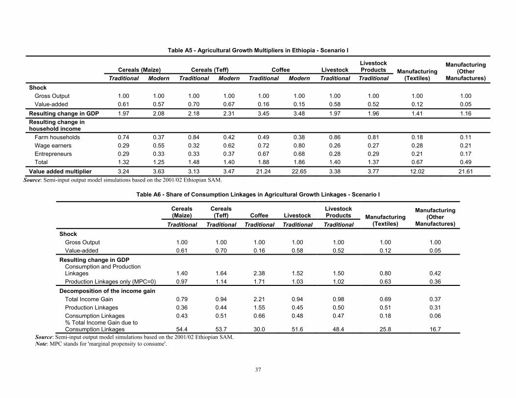
37

Table A5 - Agricultural Growth Multipliers in Ethiopia - Scenario I

Cereals (Maize) Cereals (Teff) Coffee Livestock Livestock Products

Traditional Modern Traditional Modern Traditional Modern Traditional Traditional Manufacturing

(Textiles)

Manufacturing (Other

Manufactures) Shock

Gross Output 1.00 1.00 1.00 1.00 1.00 1.00 1.00 1.00 1.00 1.00 Value-added 0.61 0.57 0.70 0.67 0.16 0.15 0.58 0.52 0.12 0.05

Resulting change in GDP 1.97 2.08 2.18 2.31 3.45 3.48 1.97 1.96 1.41 1.16 Resulting change in household income

Farm households 0.74 0.37 0.84 0.42 0.49 0.38 0.86 0.81 0.18 0.11 Wage earners 0.29 0.55 0.32 0.62 0.72 0.80 0.26 0.27 0.28 0.21 Entrepreneurs 0.29 0.33 0.33 0.37 0.67 0.68 0.28 0.29 0.21 0.17 Total 1.32 1.25 1.48 1.40 1.88 1.86 1.40 1.37 0.67 0.49

Value added multiplier 3.24 3.63 3.13 3.47 21.24 22.65 3.38 3.77 12.02 21.61 Source: Semi-input output model simulations based on the 2001/02 Ethiopian SAM.

Table A6 - Share of Consumption Linkages in Agricultural Growth Linkages - Scenario I

Cereals (Maize)

Cereals (Teff) Coffee Livestock

Livestock Products

Traditional Traditional Traditional Traditional Traditional Manufacturing

(Textiles)

Manufacturing (Other

Manufactures)

Shock Gross Output 1.00 1.00 1.00 1.00 1.00 1.00 1.00 Value-added 0.61 0.70 0.16 0.58 0.52 0.12 0.05

Resulting change in GDP Consumption and Production Linkages 1.40 1.64 2.38 1.52 1.50 0.80 0.42 Production Linkages only (MPC=0) 0.97 1.14 1.71 1.03 1.02 0.63 0.36

Decomposition of the income gain Total Income Gain 0.79 0.94 2.21 0.94 0.98 0.69 0.37 Production Linkages 0.36 0.44 1.55 0.45 0.50 0.51 0.31 Consumption Linkages 0.43 0.51 0.66 0.48 0.47 0.18 0.06 % Total Income Gain due to Consumption Linkages 54.4 53.7 30.0 51.6 48.4 25.8 16.7

Source: Semi-input output model simulations based on the 2001/02 Ethiopian SAM. Note: MPC stands for 'marginal propensity to consume'.

38

Table A6: Agricultural commodities included in the economy-wide multi-market model

Maize, Teff, Wheat, Sorghum, Barley, Millet, Oats, Rice,

Potatoes, Sweet potatoes, Enset, Other root crops,

Beans, Peas, Other pulses,

Groundnuts, Rapeseed, Sesame, Other oil crops,

Domestic vegetables, Bananas, Other domestic fruits,

Exportable vegetables, Other horticultural crops, Chat, Cotton,

Coffee,

Sugar, Beverages and spices

Bovine meat, Goat meat and mutton, Other meat,

Milk and dairy products,

Poultry and eggs, Fish

39

Related Publications

Agricultural Growth and Investment Options for Poverty Reduction in Rwanda by Xinshen Diao, Shenggen Fan,

Sam Kanyarukiga, and Bingxin Yu, January 2007

Comparing the Evolution of Spatial Inequality in China and India: A Fifty-Year Perspective by Kiran Gajwani,

Ravi Kanbur and Xiaobo Zhang, December 2006

Development Domains for Ethiopia: Capturing the Geographical Context of Smallholder Development Options by

Jordan Chamberlin, John Pender and Bingxin Yu, November 2006

Exploring Growth Linkages and Market Opportunities for Agriculture in Southern Africa by Alejandro Nin Pratt

and Xinshen Diao, September 2006

A Multilevel Analysis of Public Spending, Growth and Poverty Reduction in Egypt by Shenggen Fan, Perrihan Al-

Riffai, Moataz El-Said, Bingxin Yu, and Ahmed Kamaly, September 2006

Assessing Potential Impact of Avian Influenza on Poultry in West Africa – A Spatial Equilibrium Model Analysis by

Liangzhi You and Xinshen Diao, September 2006

Agricultural Trade Liberalization Under Doha: The Risks Facing African Countries by Ousmane Badiane,

September 2006

Shocks, Livestock Asset Dynamics and Social Capital in Ethiopia by Tewodaj Mogues, August 2006

From “Best Practice” to “Best Fit”: A Framework for Analyzing Pluralistic Agricultural Advisory Services

Worldwide by Regina Birner, Kristin Davis, John Pender, Ephraim Nkonya, Ponniah Anandajayasekeram,

Javier Ekboir, Adiel Mbabu, David J. Spielman, Daniela Horna, Samuel Benin, and Marc Cohen, August

2006

Has Trade Liberalization in South Africa Affected Men and Women Differently? by James Thurlow, July 2006

Public Investment to Reverse Dutch Disease: The Case of Chad by Stephanie Levy, June 2006

Moving Up and Down: A New Way of Examining Country Growth Dynamics by Marc* Rockmore and Xiaobo

Zhang, June 2006

Trade Liberalization under CAFTA: An Analysis of the Agreement with Special Reference to Agriculture and

Smallholders in Central America by Sam Morley, May 2006

Shocks, Sensitivity and Resilience: Tracking the Economic Impacts of Environmental Disaster on Assets in Ethiopia

and Honduras by Michael R. Carter, Peter D. Little, Tewodaj Mogues, and Workneh Negatu, April 2006

Village Inequality in Western China: Implications for Development Strategy in Lagging Regions by Li Xing,

Shenggen Fan, Xiaopeng Luo, and Xiaobo Zhang, February 2006

Does Good Governance Contribute to Pro-poor Growth?: A Review of the Evidence from Cross-Country Studies by

Danielle Resnick and Regina Birner (February 2006)

40

The Role of Agriculture in Development: Implications for Sub-Saharan Africa by Xinshen Diao, Peter Hazell,

Danielle Resnick, and James Thurlow, February 2006

Asymmetric Property Rights in China’s Economic Growth by Xiaobo Zhang, January 2006

Determinants of Change in Household-Level Consumption and Poverty in Uganda, 1992/93-1999/00 by Sam Benin

and Samuel Mugarura, January 2006

Geographic Space, Assets, Livelihoods and Well-being in Rural Central America: Empirical Evidence from

Guatemala, Honduras and Nicaragua by Jeffrey Alwang, Hans G.P. Jansen, Paul B. Siegel and Francisco

Pichon, November 2005

Social Capital and the Reproduction of Economic Inequality in Polarized Societies by Tewodaj Mogues and

Michael R. Carter, November 2005

Rural Nonfarm Development in China and India: The Role of Policies and Institutions by Anit Mukherjee and

Xiaobo Zhang, September 2005

Rural and Urban Dynamics and Poverty: Evidence from China and India by Shenggen Fan, Connie Chan-Kang and

Anit Mukherjee, August 2005

The Dragon and the Elephant: Agricultural and Rural Reforms in China and India by Ashok Gulati, Shenggen Fan

and Sara Dalafi, August 2005

Fiscal Decentralization and Political Centralization in China: Implications for Regional Inequality by Xiaobo

Zhang, July 2005

Growth Options and Poverty Reduction in Ethiopia: A Spatial, Economywide Model Analysis for 2004-15 by

Xinshen Diao and Alejandro Nin Pratt with Madhur Gautam, James Keough, Jordan Chamberlin, Liangzhi

You, Detlev Puetz, Danille Resnick and Bingxi Yu, May 2005

Identifying the Drivers of Sustainable Rural Growth and Poverty Reduction in Honduras by Hans G.P. Jansen, Paul

B. Siegel and Francisco Pichón, April 2005

Public Investment and Poverty Reduction in Tanzania: Evidence from Household Survey Data by Shenggen Fan,

David Nyange and Neetha Rao, April 2005

Achieving Regional Growth Dynamics in African Agriculture by Awudu Abdulai, Xinshen Diao and Michael

Johnson, January 2005

The Road to Pro-poor Growth in Zambia: Past Lessons and Future Challenges by James Thurlow and Peter Wobst,

December 2004

Institutions and Economic Policies for Pro-poor Agricultural Growth by Andrew Dorward, Shenggen Fan, Jonathan

Kydd, Hans Lofgren, Jamie Morrison, Colin Poulton, Neetha Rao, Laurence Smith, Hardwick Tchale,

Sukhadeo Thorat, Ian Urey, and Peter Wobst, November 2004

41

Strategic Analysis and Knowledge Support Systems for Rural Development Strategies in Sub-Saharan Africa by

Michael Johnson and Danielle Resnick, with Simon Bolwig, Jordan Chamberlin, Liangzhi You, Stanley

Wood, and Peter Hazell, October 2004

Blunt to Sharpened Razor: Incremental Reform and Distortions in the Product and Capital Markets in China by

Xiaobo Zhang and Kong-Yam Tan, August 2004

Road Development, Economic Growth, and Poverty Reduction in China by Shenggen Fan and Connie Chan-Kang,

August 2004

Prospects for Growth and Poverty Reduction in Zambia, 2001-2015 by Hans Lofgren, James Thurlow, and Sherman

Robinson, August 2004

Bridging Research, Policy, and Practice in African Agriculture by Steven Were Omamo, July 2004

Smallholder African Agriculture: Progress and Problems in Confronting Hunger and Poverty by Danielle Resnick,

July 2004

Cross-Country Typologies and Development Strategies to End Hunger in Africa by Xiaobo Zhang, Michael

Johnson, Danielle Resnick, and Sherman Robinson, June 2004

The Importance of Public Investment for Reducing Rural Poverty in Middle-income Countries: The Case of

Thailand by Shenggen Fan, Somchai Jitsuchon, and Nuntaporn Methakunnavut, June 2004

Security Is Like Oxygen: Evidence from Uganda by Xiaobo Zhang, May 2004

Food Aid for Market Development in Sub-Saharan Africa by Awudu Abdulai, Christopher B. Barrett, and Peter

Hazell, April 2004

Public Expenditure, Growth, and Poverty Reduction in Rural Uganda by Shenggen Fan, Xiaobo Zhang, and Neetha

Rao, March 2004

The Effect of WTO and FTAA on Agriculture and the Rural Sector in Latin America by Samuel Morley and Valeria

Piñeiro, February 2004

Exploring Regional Dynamics in Sub-Saharan African Agriculture by Xinshen Diao and Yukitsugu Yanoma,

October 2003

Market Opportunities for African Agriculture: An Examination of Demand-Side Constraints on Agricultural

Growth by Xinshen Diao, Paul Dorosh, and Shaikh Mahfuzur Rahman with Siet Meijer, Mark Rosegrant,

Yukitsugu Yanoma, and Weibo Li, September 2003

42

43

INTERNATIONAL FOOD POLICY RESEARCH INSTITUTE

www.ifpri.org

IFPRI HEADQUARTERS

2033 K Street, NW Washington, DC 20006-1002 USA Tel.: +1-202-862-5600 Fax: +1-202-467-4439 Email: ifpri@cgiar.org

IFPRI ADDIS ABABA

P. O. Box 5689 Addis Ababa, Ethiopia Tel.: +251 11 6463215 Fax: +251 11 6462927 Email: ifpri-addisababa@cgiar.org

IFPRI NEW DELHI

CG Block, NASC Complex, PUSA New Delhi 110-012 India Tel.: 91 11 2584-6565 Fax: 91 11 2584-8008 / 2584-6572 Email: ifpri-newdelhi@cgiar.org