The space of embedded minimal surfaces of fixed genus in a 3-manifold I; Estimates off the axis for...

arX

iv:m

ath/

0210

106v

1 [

mat

h.A

P] 7

Oct

200

2

THE SPACE OF EMBEDDED MINIMAL SURFACES OF FIXED GENUS

IN A 3-MANIFOLD I; ESTIMATES OFF THE AXIS FOR DISKS

TOBIAS H. COLDING AND WILLIAM P. MINICOZZI II

0. Introduction

This paper is the first in a series where we attempt to give a complete description ofthe space of all embedded minimal surfaces of fixed genus in a fixed (but arbitrary) closedRiemannian 3-manifold. The key for understanding such surfaces is to understand the localstructure in a ball and in particular the structure of an embedded minimal disk in a ball inR3 (with the flat metric). This study is undertaken here and completed in [CM6]; see also[CM8], [CM9] where we have surveyed our results about embedded minimal disks. Theselocal results are then applied in [CM7] where we describe the general structure of fixed genussurfaces in 3-manifolds.

We show here that if such an embedded minimal disk in R3 starts off as an almost flatmulti-valued graph, then it will remain so indefinitely.

Let P be the universal cover of the punctured plane C\0 with global (polar) coordinates(ρ, θ). An N -valued graph Σ over the annulus Dr2 \Dr1 (see fig. 1) is a (single-valued) graphover

(ρ, θ) ∈ P | r1 < ρ < r2 and |θ| ≤ π N . (0.1)

The middle sheet ΣM (an annulus with a slit as in [CM3]) is the portion over

(ρ, θ) ∈ P | r1 < ρ < r2 and 0 ≤ θ ≤ 2 π . (0.2)

x3-axis

u(ρ, θ)

u(ρ, θ + 2π)

Figure 1. A multi-valued graph.

The first author was partially supported by NSF Grant DMS 9803253 and an Alfred P. Sloan ResearchFellowship and the second author by NSF Grant DMS 9803144 and an Alfred P. Sloan Research Fellowship.

1

http://arXiv.org/abs/math/0210106v1

2 TOBIAS H. COLDING AND WILLIAM P. MINICOZZI II

Theorem 0.3. See fig. 2. Given τ > 0, there exist N,Ω, ǫ > 0 so: Let Ω r0 < 1 < R0/Ω,Σ ⊂ BR0 ⊂ R3 be an embedded minimal disk, ∂Σ ⊂ ∂BR0 . If Σ contains an N -valued graphΣg over D1 \Dr0 with gradient ≤ ǫ and Σg ⊂ x2

3 ≤ ǫ2(x21 +x2

2), then Σ contains a 2-valuedgraph Σd over DR0/Ω \Dr0 with gradient ≤ τ and (Σg)

M ⊂ Σd.

Figure 2. Theorem 0.3 - extending asmall multi-valued graph in a disk.

Σ

Small multi-valued graph near 0.

Figure 3. Theorem 0.4 - finding asmall multi-valued graph in a disk neara point of large curvature.

Theorem 0.3 is particularly useful when combined with a result from [CM4] assertingthat an embedded minimal disk with large curvature at a point contains a small almost flatmulti-valued graph nearby. Namely:

Theorem 0.4. [CM4]. See fig. 3. Given N,ω > 1, ǫ > 0, there exists C = C(N,ω, ǫ) > 0so: Let 0 ∈ Σ2 ⊂ BR ⊂ R3 be an embedded minimal disk, ∂Σ ⊂ ∂BR. If supBr0∩Σ |A|2 ≤4C2 r−2

0 and |A|2(0) = C2 r−20 for some 0 < r0 < R, then there exist R < r0/ω and (after a

rotation) anN -valued graph Σg ⊂ Σ over DωR\DR with gradient ≤ ǫ, and distΣ(0,Σg) ≤ 4 R.

Combining these two results with a standard blow up argument gives:

Theorem 0.5. [CM4]. Given N ∈ Z+, ǫ > 0, there exist C1, C2 > 0 so: Let 0 ∈ Σ2 ⊂BR ⊂ R3 be an embedded minimal disk, ∂Σ ⊂ ∂BR. If maxBr0∩Σ |A|2 ≥ 4C2

1 r−20 for some

0 < r0 < R, then there exists (after a rotation) an N -valued graph Σg ⊂ Σ over DR/C2\D2r0

with gradient ≤ ǫ and Σg ⊂ x23 ≤ ǫ2 (x2

1 + x22).

The multi-valued graphs given by Theorem 0.5 should be thought of (see [CM6]) as thebasic building blocks of an embedded minimal disk. In fact, one should think of such a diskas being built out of such graphs by stacking them on top of each other. It will follow fromProposition II.2.12 that the separation between the sheets in such a graph grows sublinearly.

An important component of the proof of Theorem 0.3 is a version of it for stable minimalannuli with slits that start off as multi-valued graphs. Another component is a curvatureestimate “between the sheets” for embedded minimal disks in R3; see fig. 4. We will thinkof an axis for such a disk Σ as a point or curve away from which the surface locally (in anextrinsic ball) has more than one component. With this weak notion of an axis, our estimateis that if one component of Σ is sandwiched between two others that connect to an axis,then the one that is sandwiched has curvature estimates; see Theorem I.0.8. The example tokeep in mind is a helicoid and the components are “consecutive sheets” away from the axis.

GRAPHICAL OFF THE AXIS 3

Axis

“Betweenthe sheets”

Figure 4. The estimate between thesheets: Theorem I.0.8.

Theorems 0.3, 0.4, 0.5 are local and are for simplicity stated and proven only in R3

although they can with only very minor changes easily be seen to hold for minimal disks ina sufficiently small ball in any given fixed Riemannian 3-manifold.

The paper is divided into 4 parts. In Part I, we show the curvature estimate “betweenthe sheets” when the disk is in a thin slab. In Part II, we will show that certain stable diskswith interior boundaries starting off as multi-valued graphs remain very flat (cf. Theorem0.3). This result will be needed together with Part I in Part III to generalize the results ofPart I to when the disk is not anymore assumed to lie in a slab. Part II will also be usedtogether with Part III in Part IV to show Theorem 0.3.

Let x1, x2, x3 be the standard coordinates on R3 and Π : R3 → R2 orthogonal projectionto x3 = 0. For y ∈ S ⊂ Σ ⊂ R3 and s > 0, the extrinsic and intrinsic balls and tubes are

Bs(y) = x ∈ R3 | |x− y| < s , Ts(S) = x ∈ R3 | distR3(x, S) < s , (0.6)

Bs(y) = x ∈ Σ | distΣ(x, y) < s , Ts(S) = x ∈ Σ | distΣ(x, S) < s . (0.7)

Ds denotes the disk Bs(0)∩x3 = 0. KΣ the sectional curvature of a smooth compact surfaceΣ and when Σ is immersed AΣ will be its second fundamental form. When Σ is oriented,nΣ is the unit normal. We will often consider the intersection of curves and surfaces withextrinsic balls. We assume that these intersect transversely since this can be achieved by anarbitrarily small perturbation of the radius.

Part I. Minimal disks in a slab

Let γp,q denote the line segment from p to q and p, q the ray from p through q. A curve γ ish-almost monotone if given y ∈ γ, then B4 h(y)∩ γ has only one component which intersectsB2 h(y). Our curvature estimate “between the sheets” is (see fig. 5):

Theorem I.0.8. There exist c1 ≥ 4, 2c2 < c4 < c3 ≤ 1 so: Let Σ2 ⊂ Bc1 r0 be an embeddedminimal disk with ∂Σ ⊂ ∂Bc1 r0 and y ∈ ∂B2 r0. Suppose Σ1,Σ2,Σ3 are distinct componentsof Br0(y) ∩ Σ and γ ⊂ (Br0 ∪ Tc2 r0(γ0,y)) ∩ Σ is a curve with ∂γ = y1, y2 where yi ∈Bc2 r0(y)∩Σi and each component of γ \Br0 is c2 r0-almost monotone. Then any componentΣ′

3 of Bc3 r0(y) ∩ Σ3 with y1, y2 in distinct components of Bc4 r0(y) \ Σ′3 is a graph.

The idea for the proof of Theorem I.0.8 is to show that if this were not the case, then wecould find an embedded stable disk that would be almost flat and lie in the complement ofthe original disk. In fact, we can choose the stable disk to be sandwiched between the twocomponents as well. The flatness would force the stable disk to eventually cross the axis inthe original disk, contradicting that they were disjoint.


Σ′3

Σ1

Σ2

y2

y1

Bc1r0

γ

Figure 5. y1, y2, Σ1, Σ2, Σ′3, and γ

in Theorem I.0.8.

In this part, we prove Theorem I.0.8 when the surface is in a slab, illustrating the keypoints (the full theorem, using the results of this part, will be proven later). Two simple factsabout minimal surfaces in a slab will be used: (1) Stable surfaces in a slab must be graphicalaway from their boundary (see Lemma I.0.9 below) and (2) the maximum principle, andcatenoid foliations in particular, force these surfaces to intersect a narrow cylinder aboutevery vertical line (see the appendix).

Lemma I.0.9. Let Γ ⊂ |x3| ≤ β h be a stable embedded minimal surface. There existCg, βs > 0 so if β ≤ βs and E is a component of R2 \ Th(Π(∂Γ)), then each component ofΠ−1(E) ∩ Γ is a graph over E of a function u with |∇R2u| ≤ Cg β.

Proof. If Bh(y) ⊂ Γ, [Sc] gives that |A|2 ≤ Cs h−2 on Bh/2(y). Since ∆Γx3 = 0, [ChY] yields

supBh/4(y)

|∇Γx3| ≤ Cg h−1 sup

Bh/2(y)

|x3| ≤ Cg β , (I.0.10)

where Cg = Cg(Cs). Since |∇R2u|2 = |∇Γx3|2 / (1 − |∇Γx3|2), this gives the lemma.

The next lemma shows that if an embedded minimal disk Σ in the intersection of a ballwith a thin slab is not graphical near the center, then it contains a curve γ coming close tothe center and connecting two boundary points which are close in R3 but not in Σ. Theconstant βA is defined in (A.6).

Lemma I.0.11. Let Σ2 ⊂ B60 h ∩ |x3| ≤ βA h be an embedded minimal disk with ∂Σ ⊂∂B60 h and let zb ∈ ∂B50 h. If a component Σ′ of B5 h∩Σ is not a graph, then there are distinctcomponents S1, S2 of B8 h(zb) ∩Σ, zi ∈ Bh/4(zb) ∩ Si and a curve γ ⊂ (B30 h ∪ Th(γq,zb

)) ∩ Σwith ∂γ = z1, z2 and γ ∩ Σ′ 6= ∅. Here q ∈ B50 h(zb) ∩ ∂B30 h.

Proof. See fig. 6. Since Σ′ is not graphical, we can find z ∈ Σ′ with Σ vertical at z (i.e.,|∇Σx3|(z) = 1). Fix y ∈ ∂B4 h(z) so γy,z is normal to Σ at z. Then fy(z) = 4 h (see (A.5)).Let y′ be given by that y′ ∈ ∂B10 h(y) and z ∈ γy,y′. The first step is to use the catenoidfoliation fy to build the desired curve on the scale of h; see fig. 7. The second and thirdsteps will bring the endpoints of this curve out near zb.

Any simple closed curve σ ⊂ Σ \ fy > 4 h bounds a disk Σσ ⊂ Σ. By Lemma A.8,fy has no maxima on Σσ ∩ fy > 4 h so Σσ ∩ fy > 4 h = ∅. On the other hand, byLemma A.7, we get a neighborhood Uz ⊂ Σ of z where Uz ∩ fy = 4 h \ z is the union of


z

Vertical plane tangent

y

to Σ at z.

Figure 6. Proof of Lemma I.0.11:Vertical plane tangent to Σ at z. SinceΣ is minimal, we get locally near z onone side of the plane two different com-ponents. Next place a catenoid folia-tion centered at y and tangent to Σ atz.

y′

γa

yy1

y2

y1 and y2 are in differentcomponents of Σ in the ball B4h(y).

Figure 7. Proof of Lemma I.0.11:Step 1: Using the catenoid foliation,we build out the curve to scale h.

2n ≥ 4 disjoint embedded arcs meeting at z. Moreover, Uz \ fy ≥ 4 h has n componentsU1, . . . , Un and Ui ∩ Uj = z for i 6= j. If a simple curve σz ⊂ Σ \ fy ≥ 4 h connectsU1 to U2, connecting ∂σz by a curve in Uz gives a simple closed curve σz ⊂ Σ \ fy > 4 hwith σz ⊂ σz and σz ∩ fy ≥ 4 h = z. Hence, σz bounds a disk Σσz ⊂ Σ \ fy > 4 h.By construction, Uz ∩ Σσz \ ∪iUi 6= ∅, which is a contradiction. This shows that U1, U2 are

contained in components Σ14 h 6= Σ2

4 h of Σ \ fy ≥ 4 h with z ∈ Σ14 h ∩ Σ2

4 h. For i = 1, 2,Lemma A.8 and (A.6) give ya

i ∈ Bh/4(y) ∩ Σi4 h. Corollary A.10 gives νi ⊂ Th(γy,y′) ∩ Σ

with ∂νi = yai , y

bi where yb

i ∈ Bh/4(y′). There are now two cases: If yb

1 and yb2 do not

connect in B4 h(y′) ∩ Σ, then take γ0 ⊂ B5 h(y) ∩ Σ from ya

1 to ya2 and set γa = ν1 ∪ γ0 ∪ ν2

and yi = ybi . Otherwise, if γ0 ⊂ B4 h(y

′) ∩ Σ connects yb1 and yb

2, set γa = ν1 ∪ γ0 ∪ ν2 andyi = ya

i . After possibly switching y and y′, we get a curve γa ⊂ (Th(γy,y′) ∪ B5 h(y′)) ∩ Σ

with ∂γa = y1, y2 ⊂ Bh/4(y) and yi ∈ Sai for components Sa

1 6= Sa2 of B4 h(y) ∩ Σ. This

completes the first step.Second, we use the maximum principle to restrict the possible curves from y1 to y2; see

fig. 8. Set

H = x | 〈y − y′, x− y〉 > 0 . (I.0.12)

If η1,2 ⊂ Th(H) ∩ Σ connects y1 and y2, then η1,2 ∪ γa bounds a disk Σ1,2 ⊂ Σ. Sinceη1,2 ⊂ Th(H), ∂B8 h(y

′) ∩ ∂Σ1,2 consists of an odd number of points in each Sai and hence

∂B8 h(y′)∩Σ1,2 contains a curve from Sa

1 to Sa2 . However, Sa

1 and Sa2 are distinct components

of B4 h(y) ∩ Σ, so this curve contains

y1,2 ∈ ∂B4 h(y) ∩ ∂B8 h(y′) ∩ Σ1,2 . (I.0.13)

By construction, Π(y1,2) is in an unbounded component of R2\Th/4(Π(∂Σ1,2)), contradictingCorollary A.11. Hence, y1 and y2 cannot be connected in Th(H) ∩ Σ.

Third, we extend γa. There are two cases: (A) If zb ∈ H , Corollary A.10 gives

ν1, ν2 ⊂ Th(γy,zb) ∩ Σ ⊂ Th(H) ∩ Σ (I.0.14)


If y1 and y2 can be connected by a curveH

y′y1

y

η1,2

γa

y2

connect the two components of Σ1,2in B4h(y) - this is impossible.

η1,2 ⊂ H ∩ Σ, then γa ∪ η1,2 bounds

a curve in ∂B8h(y′) ∩ Σ1,2 would

a disk Σ1,2 ⊂ Σ and soB4h(y)

Figure 8. Proof of Lemma I.0.11:Step 2: y1 and y2 cannot connect inthe half-space H since this would givea point in Σ1,2 far from ∂Σ1,2, contra-dicting Corollary A.10.

from y1, y2 to z1, z2 ∈ Bh/4(zb), respectively. (B) If zb /∈ H , then fix zc ∈ ∂B20 h(y) ∩ Π(∂H)

on the same side of Π(y, y′) as Π(zb) and fix zd ∈ ∂B10 h(zc) \H with γzc,zdorthogonal to ∂H

(so Π(y′),Π(y), zc, zd form a 10 h by 20 h rectangle). Corollary A.10 gives

ν1, ν2 ⊂ Th(γy,zc ∪ γzc,zd∪ γzd,zb

) ∩ Σ (I.0.15)

from y1, y2 to z1, z2 ∈ Bh/4(zb), respectively. In either case, set γ = ν1 ∪ γa ∪ ν2. Setq = ∂B30 h(y) ∩ γy,zb

(in (A)) or q = ∂B30 h(y) ∩ γzc,zb(in (B)). Applying Corollary A.11 as

above, z1, z2 are in distinct components of B8 h(zb) ∩ Σ.

The next result illustrates the main ideas for Theorem I.0.8 in the simpler case where Σis in a slab. Set β3 = minβA, βs, tan θ0/(2Cg); Cg, βs are defined in Lemma I.0.9, θ0 in(A.3), and βA in (A.6).

Proposition I.0.16. Let Σ ⊂ B4 r0 ∩ |x3| ≤ β3 h be an embedded minimal disk with∂Σ ⊂ ∂B4 r0 and let y ∈ ∂B2 r0 . Suppose that Σ1,Σ2,Σ3 are distinct components of Br0(y)∩Σand γ ⊂ (Br0 ∪ Th(γ0,y)) ∩ Σ is a curve with ∂γ = y1, y2 where yi ∈ Bh(y) ∩ Σi and eachcomponent of γ \Br0 is h-almost monotone. Then any component Σ′

3 of Br0−80 h(y)∩Σ3 forwhich y1, y2 are in distinct components of B5 h(y) \ Σ′

3 is a graph.

Proof. We will suppose that Σ′3 is not a graph and deduce a contradiction. Fix a vertical

point z ∈ Σ′3. Define z0, y0, yb on the ray 0, y by z0 = ∂B3 r0−21 h ∩ 0, y, y0 = ∂B3 r0−10 h ∩ 0, y,

and yb = ∂B4 r0 ∩ 0, y. Set zb = ∂B50 h(z) ∩ γz,z0. Define the half-space

H = x | 〈x− z0, z0〉 > 0 . (I.0.17)

The first step is to find a simple curve γ3 ⊂ (Br0−20 h(y) ∪ Th(γy,yb)) ∩ Σ which can be

connected to Σ′3 in Br0−20 h(y) ∩ Σ, with ∂γ3 ⊂ ∂Σ, and so ∂Br0−10 h(y) ∩ γ3 consists of an

odd number of points in each of two distinct components of H ∩ Σ. To do that, we beginby applying Lemma I.0.11 to get q ∈ B50 h(zb) ∩ ∂B30 h(z), distinct components S1, S2 of


B8 h(zb) ∩ Σ with zi ∈ Bh/4(zb) ∩ Si, and a curve

γ⋆3 ⊂ (B30 h(z) ∪ Th(γq,zb

)) ∩ Σ, ∂γ⋆3 = z1, z2 , γ⋆

3 ∩ Σ′3 6= ∅ . (I.0.18)

Corollary A.10 gives h-almost monotone curves ν1, ν2 ⊂ Th(γzb,z0 ∪ γz0,yb) ∩ Σ from z1, z2,

respectively, to ∂Σ. Then γ3 = ν1 ∪ γ⋆3 ∪ ν2 extends γ⋆

3 to ∂Σ. Fix z+ ∈ Bh(y0) ∩ ν1 andz− ∈ Bh(y0)∩ν2. We will show that z+, z− do not connect in H ∩Σ. If η−+ ⊂ H ∩Σ connectsz+ and z−, then η−+ together with the portion of γ3 from z+ to z− bounds a disk Σ−

+ ⊂ Σ.Using the almost monotonicity of each νi, ∂B50 h(z) ∩ ∂Σ−

+ consists of an odd number ofpoints in each Si. Consequently, a curve σ−

+ ⊂ ∂B50 h(z) ∩ Σ−+ connects S1 to S2 and so

σ−+ \ B8 h(zb) 6= ∅. This would contradict Corollary A.11 and we conclude that there are

distinct components Σ+H and Σ−

H of H ∩Σ with z± ∈ Σ±H . Finally, removing any loops in γ3

(so it is simple) gives the desired curve.The second step is to find disjoint stable disks Γ1,Γ2 ⊂ Br0−2h(y) \ Σ with ∂Γi ⊂

∂Br0−2 h(y) and graphical components Γ′i of Br0−4 h(y) ∩ Γi so Σ′

3 is between Γ′1,Γ

′2 and

y1, y2,Σ′3 are each in their own component of Br0−4 h(y) \ (Γ′

1 ∪ Γ′2). To achieve this, we will

solve two Plateau problems using Σ as a barrier and then use that Σ′3 separates y1, y2 near y

to get that these are in different components. Let Σ′1,Σ

′2 be the components of Br0−2 h(y)∩Σ

with y1 ∈ Σ′1, y2 ∈ Σ′

2. By the maximum principle, each of these is a disk. Let Σy2 be thecomponent of B3 h(y1)∩Σ with y2 ∈ Σy2 . Since y1 /∈ Σy2 , Lemma A.8 gives y′2 ∈ Σy2 \Nθ0(y1)with θ0 > 0 from (A.3). Hence, the vector y1 − y′2 is nearly orthogonal to the slab, i.e.,

|Π(y′2 − y1)| ≤ |y′2 − y1| cos θ0 . (I.0.19)

Since Σ′3 separates y1, y2 in B5 h(y), we get y3 ∈ γy1,y′

2∩Σ′

3. Fix a component Ω1 of Br0−2 h(y)\Σ containing a component of γy1,y3 \ Σ with exactly one endpoint in Σ′

1. By [MeYa], we geta stable embedded disk Γ1 ⊂ Ω1 with ∂Γ1 = ∂Σ′

1. Similarly, let Ω2 be a component ofBr0−2h(y) \ (Σ ∪ Γ1) containing a component of γy3,y′

2\ (Σ ∪ Γ1) with exactly one endpoint

in Σ′2. Again by [MeYa], we get a stable embedded disk Γ2 ⊂ Ω2 with ∂Γ2 = ∂Σ′

2. Since∂Γ1, ∂Γ2 are linked in Ω1,Ω2 with (segments of) γy1,y3, γy3,y′

2, respectively, we get components

Γ′i of Br0−4h(y) ∩ Γi with zΓ

1 ∈ Γ′1 ∩ γy1,y3 and zΓ

2 ∈ Γ′2 ∩ γy3,y′

2. By Lemma I.0.9, each Γ′

i is a

graph of a function ui with |∇ui| ≤ Cg β3. Hence, since 1 + C2g β

23 < 1/ cos2 θ0,

Γ′i \ zΓ

i ⊂ Nθ0(zΓi ) . (I.0.20)

By (I.0.19), γy1,y′2∩ Nθ0(z

Γi ) = ∅, so (I.0.20) implies that Γ′

i ∩ γy1,y′2

= zΓi . In particular,

y1, y2, y3 are in distinct components of Br0−4 h \ (Γ′1 ∪ Γ′

2). This completes the second step.Set y = ∂Br0+10 h ∩ γ0,y. Let γ be the component of Br0+10 h ∩ γ with Br0 ∩ γ 6= ∅. Then

∂γ = y1, y2 with yi ∈ Bh(y) ∩ Σ′i.

The third step is to solve the Plateau problem with γ3 together with part of ∂Σ ⊂ ∂B4 r0 asthe boundary to get a stable disk Γ3 ⊂ B4r0 \Σ passing between y1, y2. To do this, note thatthe curve γ3 divides the disk Σ into two sub-disks Σ+

3 ,Σ−3 . Let Ω+,Ω− be the components of

B4 r0 \ (Σ ∪ Γ1 ∪ Γ2) with γ3 ⊂ ∂Ω+ ∩ ∂Ω−. Note that Ω+,Ω− are mean convex in the senseof [MeYa] since ∂Γ1 ∪∂Γ2 ⊂ Σ and ∂Σ ⊂ ∂B4 r0 . Using the first step, we can label Ω+,Ω− soz+, z− do not connect in H ∩Ω+. By [MeYa], we get a stable embedded disk Γ3 ⊂ Ω+ with∂Γ3 = ∂Σ+

3 . Using the almost monotonicity, ∂Br0−10 h(y) ∩ ∂Γ3 consists of an odd numberof points in each of Σ+

H , Σ−H . Hence, there is a curve γ−+ ⊂ ∂Br0−10 h(y)∩Γ3 from Σ+

H to Σ−H .


By construction, γ−+ \ B8 h(y0) 6= ∅. Hence, since ∂Br0−10 h(y) ∩ Th(∂Γ3) ⊂ B3 h(y0), LemmaI.0.9 gives z ∈ Bh(y1) ∩ γ−+ . By the second step, Γ3 is between Γ′

1 and Γ′2.

Let Γ3 be the component of Br0+19 h ∩ Γ3 with z ∈ Γ3. By Lemma I.0.9, Γ3 is a graph.

Finally, since γ ⊂ Br0+10 h and Γ3 passes between ∂γ, this forces Γ3 to intersect γ. Thiscontradiction completes the proof.

Part II. Estimates for stable annuli with slits

In this part, we will show that certain stable disks starting off as multi-valued graphsremain the same (see Theorem II.0.21 below). This is needed in Part III when we generalizethe results of Part I to when the surface is not anymore in a slab and in Part IV when weshow Theorem 0.3.

Theorem II.0.21. Given τ > 0, there exist N1,Ω1, ǫ > 0 so: Let Ω1 r0 < 1 < R0/Ω1,Σ ⊂ BR0 be a stable embedded minimal disk, ∂Σ ⊂ Br0 ∪ ∂BR0 ∪ x1 = 0, ∂Σ \ ∂BR0 isconnected. If Σ contains an N1-valued graph Σg over D1 \Dr0 with gradient ≤ ǫ, Π−1(Dr0)∩ΣM ⊂ |x3| ≤ ǫ r0, and a curve η ⊂ Π−1(Dr0) ∩ Σ \ ∂BR0 connects Σg to ∂Σ \ ∂BR0 , thenΣ contains a 2-valued graph Σd over DR0/Ω1

\Dr0 with gradient ≤ τ .

Two analytical results go into the proof of this extension theorem. First, we show that ifan almost flat multi-valued graph sits inside a stable disk, then the outward defined intrinsicsector from a curve which is a multi-valued graph over a circle has a subsector which isalmost flat (see Corollary II.1.23 below). As the initial multi-valued graph becomes flatterand the number of sheets in it go up, the subsector becomes flatter. The second analyticalresult that we will need is that in a multi-valued minimal graph the distance between thesheets grows sublinearly (Proposition II.2.12).

After establishing these two facts, the first application (Corollary II.3.1) is to extendingthe middle sheet as a multi-valued graph. This is done by dividing the initial multi-valuedgraph (or curve in the graph that is itself a multi-valued graph over the circle) into threeparts where the middle sheet is the second part. The idea is then that the first and thirdparts have subsectors which are almost flat multi-valued graphs and the middle part (whichhas curvature estimates since it is stable) is sandwiched between the two others. Hence itssector is also almost flat.

A thing that adds some technical complications to the above picture is that in the analyt-ical result about almost flat subsectors it is important that the ratio between the size of theinitial multi-valued graph and how far one can go out is fixed. This is because the estimatefor the subsector comes from a total curvature estimate which is in terms of this ratio (see(II.1.2)) and can only be made small by looking at a fixed large number of rotations for thegraph. This forces us to successively extend the multi-valued graph. The issue is then tomake sure that as we move out in the sector and repeat the argument we have essentiallynot lost sheets. This is taken care of by using the sublinear growth of the separation be-tween the sheets together with the Harnack inequality (Lemma II.3.8) and the maximumprinciple (Corollary II.3.1). (The maximum principle is used to make sure that as we try torecover sheets after we have moved out then we don’t hit the boundary of the disk before wehave recovered essentially all of the sheets that we started with.) The last thing is a resultfrom [CM3] to guarantee that as we patch together these multi-valued graphs coming fromdifferent scales then the surface that we get is still a multi-valued graph over a fixed plane.


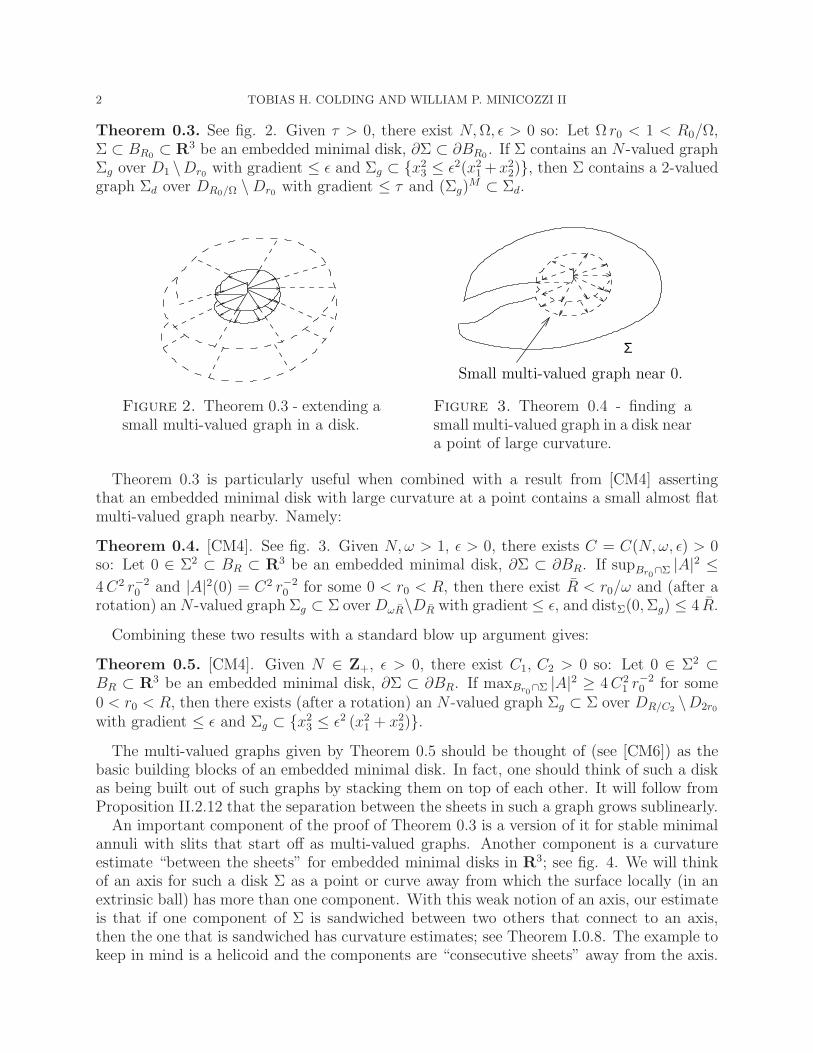
Unless otherwise stated in this part, Σ will be a stable embedded disk. Let γ ⊂ Σ be asimple curve with unit normal nγ and geodesic curvature kg (with respect to nγ). We willalways assume that γ′ does not vanish. Given R1 > 0, we define the intrinsic sector, see fig.9,

SR1(γ) = ∪x∈γγx , (II.0.22)

where γx is the (intrinsic) geodesic starting at x ∈ γ, of length R1, and initial directionnγ(x). For 0 < r1 < R1, set Sr1,R1(γ) = SR1(γ) \ Sr1(γ) and ρ(x) = distSR1

(γ)(x, γ). For

example, if γ = ∂Dr1 ⊂ R2 and nγ(x) = x/|x|, then Sr2,R1 is the annulus DR1+r1 \Dr2+r1.

γnγ

x

Geodesic γx

SR1(γ)

Σ

Figure 9. An intrinsic sector over acurve γ defined in (II.0.22).

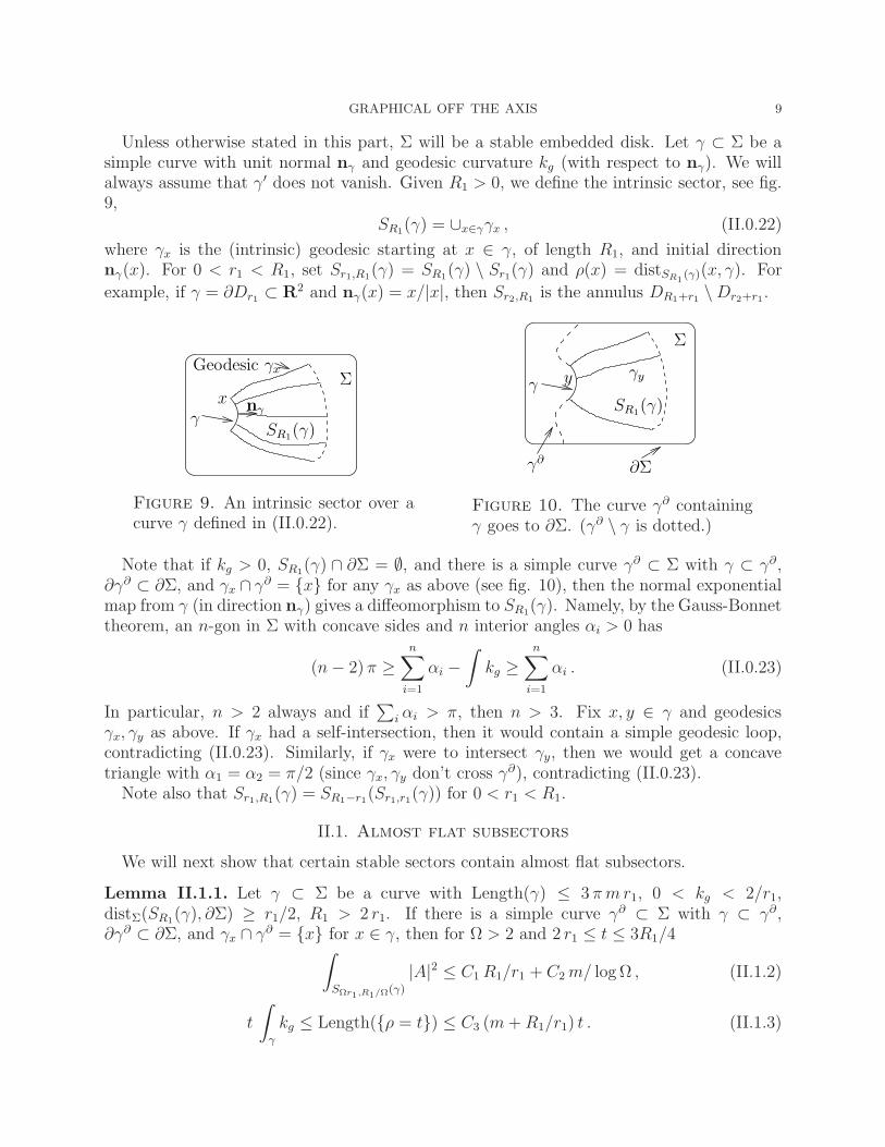
γγy

Σ

∂Σ

SR1(γ)

y

γ∂

Figure 10. The curve γ∂ containingγ goes to ∂Σ. (γ∂ \ γ is dotted.)

Note that if kg > 0, SR1(γ) ∩ ∂Σ = ∅, and there is a simple curve γ∂ ⊂ Σ with γ ⊂ γ∂,∂γ∂ ⊂ ∂Σ, and γx ∩ γ∂ = x for any γx as above (see fig. 10), then the normal exponentialmap from γ (in direction nγ) gives a diffeomorphism to SR1(γ). Namely, by the Gauss-Bonnettheorem, an n-gon in Σ with concave sides and n interior angles αi > 0 has

(n− 2) π ≥n

∑

i=1

αi −∫

kg ≥n

∑

i=1

αi . (II.0.23)

In particular, n > 2 always and if∑

i αi > π, then n > 3. Fix x, y ∈ γ and geodesicsγx, γy as above. If γx had a self-intersection, then it would contain a simple geodesic loop,contradicting (II.0.23). Similarly, if γx were to intersect γy, then we would get a concavetriangle with α1 = α2 = π/2 (since γx, γy don’t cross γ∂), contradicting (II.0.23).

Note also that Sr1,R1(γ) = SR1−r1(Sr1,r1(γ)) for 0 < r1 < R1.

II.1. Almost flat subsectors

We will next show that certain stable sectors contain almost flat subsectors.

Lemma II.1.1. Let γ ⊂ Σ be a curve with Length(γ) ≤ 3 πmr1, 0 < kg < 2/r1,distΣ(SR1(γ), ∂Σ) ≥ r1/2, R1 > 2 r1. If there is a simple curve γ∂ ⊂ Σ with γ ⊂ γ∂,∂γ∂ ⊂ ∂Σ, and γx ∩ γ∂ = x for x ∈ γ, then for Ω > 2 and 2 r1 ≤ t ≤ 3R1/4

∫

SΩr1,R1/Ω(γ)

|A|2 ≤ C1R1/r1 + C2m/ log Ω , (II.1.2)

t

∫

γ

kg ≤ Length(ρ = t) ≤ C3 (m+R1/r1) t . (II.1.3)


Proof. The boundary of SR1 = SR1(γ) has four pieces: γ, ρ = R1, and the sides γa, γb. Set

ℓ(t) = Length (ρ = t) , (II.1.4)

K(t) =

∫

St

|A|2 . (II.1.5)

Since the exponential map is an embedding, an easy calculation gives

ℓ′(t) =

∫

ρ=t

kg > 0 . (II.1.6)

Let dµ be 1-dimensional Hausdorff measure on the level sets of ρ. The Jacobi equation gives

d

dt(kg dµ) = |A|2/2 dµ . (II.1.7)

Set K(t) =∫ t

0K(s) ds. Integrating (II.1.7) twice, (II.1.6) yields

ℓ(t) = ℓ(0) +

∫ t

0

(∫

γ

kg +K(s)/2

)

ds = Length(γ) + t

∫

γ

kg + K(t)/2 . (II.1.8)

This gives the first inequality in (II.1.3). Again by the coarea formula, (II.1.8) gives

R−21 Area(SR1) = R−2

1

∫ R1

0

ℓ(t) ≤ R−11 Length(γ) +

∫

γ

kg/2 +R−21

∫ R1

0

K(t)/2

≤ 6 πm+R−21

∫ R1

0

K(t)/2 , (II.1.9)

where the last inequality used kg < 2/r1 on γ, Length(γ) ≤ 3 πmr1, and R1 > 2 r1.Define a function ψ on SR1 by ψ = ψ(ρ) = 1− ρ/R1 and set dS = distΣ(·, γa ∪ γb). Define

functions χ1, χ2 on SR1 by

χ1 =χ1(dS) =

dS/r1 if 0 ≤ dS ≤ r1 ,

1 otherwise ,(II.1.10)

χ2 =χ2(ρ) =

ρ/r1 if 0 ≤ ρ ≤ r1 ,

1 otherwise .(II.1.11)

Set χ = χ1 χ2. Using |A|2 ≤ C r−21 (by [Sc]) and standard comparison theorems to bound

the area of a tubular neighborhood of the boundary, we get

Area(SR1 ∩ χ < 1) ≤ C (R1 r1 +mr21) , (II.1.12)

E(χ1) +

∫

SR1∩χ1<1

|A|2 ≤ C R1/r1 , (II.1.13)

E(χ) +

∫

SR1∩χ<1

|A|2 ≤ C (R1/r1 +m) . (II.1.14)


Substituting χψ into the stability inequality, the Cauchy-Schwarz inequality and (II.1.14)give

∫

|A|2χ2ψ2 ≤∫

|∇(χψ)|2 =

∫

(

χ2|∇ψ|2 + 2χψ〈∇χ,∇ψ〉 + ψ2|∇χ|2)

≤ 2

∫

χ2|∇ψ|2 + 2 C(R1/r1 +m) . (II.1.15)

Using (II.1.14) and the coarea formula, we have∫ R1

0

ψ2(t)K ′(t) =

∫

SR1

|A|2ψ2 ≤∫

|A|2χ2ψ2 + C (R1/r1 +m) . (II.1.16)

Integrating by parts twice in (II.1.16), (II.1.15) gives

2R−21

∫ R1

0

K(t) =

∫ R1

0

K(t)(ψ2)′′ = −∫ R1

0

K(t)(ψ2)′ (II.1.17)

=

∫ R1

0

ψ2K ′(t) ≤ 3 C (R1/r1 +m) + 2R−21

∫ R1

0

ℓ(t) .

Note that all integrals in (II.1.17) are in one variable and there is a slight abuse of notationin regarding ψ as a function on both [0, R1] and SR1 . Substituting (II.1.9), (II.1.17) gives

4R−21

∫ R1

0

ℓ(t) ≤ 24 πm+ 3 C (R1/r1 +m) + 2R−21

∫ R1

0

ℓ(t) . (II.1.18)

In particular, (II.1.18) gives

R−21 Area(SR1) ≤ C4 (R1/r1 +m) . (II.1.19)

Since ℓ(t) is monotone increasing (by (II.1.6)), (II.1.19) gives the second inequality in (II.1.3)for t = 3R1/4. Since the above argument applies with R1 replaced by t where 2 r1 < t < R1,we get (II.1.3) for 2 r1 ≤ t ≤ 3R1/4.

To complete the proof, we will use the stability inequality together with the logarithmiccutoff trick to take advantage of the quadratic area growth. Define a cutoff function ψ1 by

ψ1 = ψ1(ρ) =

log(ρ/r1)/ log Ω on Sr1,Ω r1 ,

1 on SΩ r1,R1/Ω ,

− log(ρ/R1)/ log Ω on SR1/Ω,R1,

0 otherwise .

(II.1.20)

Using (II.1.3) and (II.1.19), we get

E(ψ1) ≤ C(m+R1/r1)/ log Ω . (II.1.21)

As in (II.1.15), we apply the stability inequality to χ1ψ1 to get∫

|A|2χ21ψ

21 ≤ 2E(ψ1) + 2E(χ1) ≤ 2C(m+R1/r1)/ log Ω + 2C R1/r1 . (II.1.22)

Combining (II.1.13) and (II.1.22) completes the proof.

Using Lemma II.1.1, we show that large stable sectors have almost flat subsectors:


Corollary II.1.23. Given ω > 8, 1 > ǫ > 0, there exist m1,Ω1 so: Suppose γ ⊂ B2 r1 ∩ Σis a curve with 1/(2 r1) < kg < 2/r1, Length(γ) = 32 πm1 r1, distΣ(SΩ2

1 ω r1(γ), ∂Σ) ≥ r1/2.

If there is a simple curve γ∂ ⊂ Σ with γ ⊂ γ∂, ∂γ∂ ⊂ ∂Σ, and γx ∩ γ∂ = x for x ∈ γ,then (after rotating R3) SΩ2

1 ω r1(γ) contains a 2-valued graph Σd over D2 ω Ω1 r1 \DΩ1 r1/2 with

gradient ≤ ǫ/2, |A| ≤ ǫ/(2 r), and distSΩ2

1ω r1

(γ)(γ,Σd) < 2 Ω1 r1.

Proof. We will choose Ω1 > 12 and then set m1 = ωΩ21 log Ω1. By Lemma II.1.1 (with

Ω = Ω1/6, R1 = Ω21 ω r1, and m = 32m1/3),

∫

SΩ1 r1/6,6 Ω1 ω r1(γ)

|A|2 ≤ C(Ω21 ω +m1/ log Ω1) = 2Cm1/ log Ω1 . (II.1.24)

Fix m1 disjoint curves γ1, . . . , γm1 ⊂ γ with Length(γi) = 32 π r1. By (II.1.24) and since theSΩ2

1 ω r1(γi) are pairwise disjoint, there exists γi with

∫

SΩ1 r1/6,6 Ω1 ω r1(γi)

|A|2 ≤ 2C/ log Ω1 . (II.1.25)

To deduce the corollary from (II.1.25) we need a few standard facts. First, define a mapΦ : [0,Ω2

1ωr1] ×ρ/(2 r1)+1 [0,Length(γ)] → Σ by Φ(ρ, x) = γx(ρ). By the Riccati comparisonargument (using KΣ ≤ 0 and kg > 1/(2 r1) on γ),

Φ is distance nondecreasing and kg >1

ρ+ 2 r1. (II.1.26)

Second, let γi/2 ⊂ γi be the subcurve of length 16 π r1 with distγ(γi/2, ∂γi) = 8 π r1. Sincekg > 1/(2 r1) on γ, we have

∫

γi/2kg > 8 π. By (II.1.7),

∫

SΩ2

1ω r1

(γi/2)∩ρ=tkg is monotone

nondecreasing. In particular, we can choose a curve γ ⊂ γi/2 with∫

SΩ2

1ω r1

(γ)∩ρ=Ω1 r1/3

kg = 8 π . (II.1.27)

Set S = SΩ1 r1/3,3Ω1 ω r1(γ) and γ = S ∩ ρ = Ω1 r1/3.

Third, by the Gauss-Bonnet theorem, (II.1.25), and (II.1.27), (for Ω1 large)

8 π ≤∫

S∩ρ=t

kg ≤ 8 π +

∫

S

|A|2/2 ≤ 8 π + C/ log Ω1 ≤ 9 π . (II.1.28)

Note also that, by (II.1.26) and (II.1.28), Length(S ∩ ρ = t) ≤ 9 π (t+ 2 r1) ≤ 14 π t.Finally, observe that, by stability, (II.1.25), and using (II.1.26), the meanvalue theorem

gives for y ∈ Ssup

Bρ(y)/3(y)

|A|2 ≤ C1 ρ−2(y)/ logΩ1 . (II.1.29)

Integrating (II.1.29) along rays and level sets of ρ, we get

maxx,y∈S

distS2(n(x),n(y)) ≤ C2 (logω + 1)/√

log Ω1 . (II.1.30)

We can now combine these facts to get the corollary. Choose Ω1 so that C2 (logω +1)/

√log Ω1 < C3 ǫ. For C3 small, after rotating R3, S is locally a graph over x3 = 0 with

gradient ≤ ǫ/2. Since γ ⊂ B2 r1 and Ω1 > 12, we have γ ⊂ B2 r1+Ω1 r1/3 ⊂ BΩ1 r1/2. ChoosingΩ1 even larger and combining (II.1.26), (II.1.28), (II.1.29), and (II.1.30), we see that (the


orthogonal projection) Π(γ) is a convex planar curve with total curvature at least 7 π, sothat its Gauss map covers S1 three times. Given x ∈ γ, set γx = S ∩ γx. By (II.1.29), γx hastotal (extrinsic geodesic) curvature at most C2 logω/

√log Ω1 < C3 ǫ and hence γx lies in a

narrow cone centered on its tangent ray at x = γx ∩ γ. For C3 small, this implies that γx

does not rotate and

|Π(x) − Π(γx ∩ ρ = t)| ≥ 9 (t− Ω1 r1/3)/10 . (II.1.31)

Hence, Π(∂γx \ x) /∈ D2 ω Ω1 r1 which gives Σd and also distSΩ2

1ω r1

(γ)(γ,Σd) < 2 Ω1 r1.

Remark II.1.32. For convenience, we assumed that kg < 2/r1 in Corollary II.1.23. Thiswas used only to apply Lemma II.1.1 and it was used there only to bound

∫

γkg in (II.1.9).

Recall that a domain Ω is 1/2-stable if and only if, for all φ ∈ C0,10 (Ω), we have the

1/2-stability inequality:

1/2

∫

|A|2φ2 ≤∫

|∇φ|2 . (II.1.33)

Note that the interior curvature estimate of [Sc] extends to 1/2-stable surfaces.In light of Remark II.1.32, it is easy to get the following analog of Corollary II.1.23:

Corollary II.1.34. Given ω > 8, 1 > ǫ > 0, C0, N , there exist m1,Ω1 so: Suppose Σ is anembedded minimal disk, γ ⊂ ∂Br1(y) ⊂ Σ is a curve,

∫

γkg < C0m1, Length(γ) = m1 r1. If

Tr1/8(SΩ21 ω r1

(γ)) is 1/2-stable, then (after rotating R3) SΩ21 ω r1

(γ) contains anN -valued graphΣN over Dω Ω1 r1 \DΩ1 r1 with gradient ≤ ǫ, |A| ≤ ǫ/r, and distS

Ω21

ω r1(γ)(γ,ΣN) < 4 Ω1 r1.

Note that, in Corollary II.1.34, kg ≥ 1/r1 and the injectivity of the exponential map bothfollow immediately from comparison theorems.

II.2. The sublinear growth

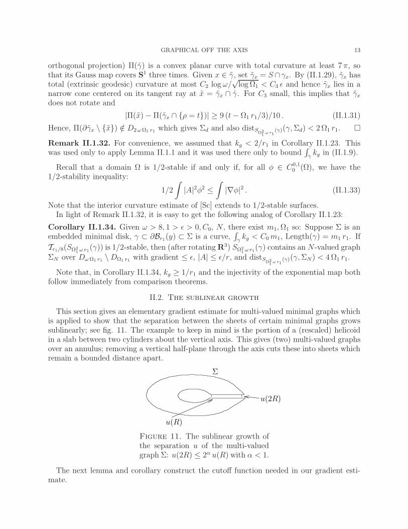
This section gives an elementary gradient estimate for multi-valued minimal graphs whichis applied to show that the separation between the sheets of certain minimal graphs growssublinearly; see fig. 11. The example to keep in mind is the portion of a (rescaled) helicoidin a slab between two cylinders about the vertical axis. This gives (two) multi-valued graphsover an annulus; removing a vertical half-plane through the axis cuts these into sheets whichremain a bounded distance apart.

u(R)

Σ

u(2R)

Figure 11. The sublinear growth ofthe separation u of the multi-valuedgraph Σ: u(2R) ≤ 2α u(R) with α < 1.

The next lemma and corollary construct the cutoff function needed in our gradient esti-mate.


Lemma II.2.1. Given N > 36/(1 − e−1/3)2, there exists a function 0 ≤ φ ≤ 1 on P withE(φ) ≤ 4 π/ logN ,

φ =

1 if R/e ≤ ρ ≤ eR and |θ| ≤ 3 π ,

0 if ρ ≤ e−N R or eN R ≤ ρ or |θ| ≥ πN .(II.2.2)

Proof. After rescaling, we may assume that R = 1. Since energy is conformally invariant onsurfaces, composing with z3 N implies that (II.2.2) is equivalent to E(φ) ≤ 4 π/ logN ,

φ =

1 if | log ρ| < 1/(3N) and |θ| ≤ π/N ,

0 if | log ρ| > 1/3 or |θ| ≥ π/3 .(II.2.3)

This is achieved (with E(φ) = 2 π/ log[N(1 − e−1/3)/6]) by setting

φ =

1 on B6/N (1, 0) ,

1 − log[N distP ((1,0),·)/6]

log[N(1−e−1/3)/6]on B1−e−1/3(1, 0) \ B6/N (1, 0) ,

0 otherwise .

(II.2.4)

Given an N -valued graph Σ, let Σθ1,θ2r3,r4

⊂ Σ be the subgraph (cf. (0.1)) over

(ρ, θ) | r3 ≤ ρ ≤ r4, θ1 ≤ θ ≤ θ2 . (II.2.5)

Corollary II.2.6. Given ǫ0, τ > 0, there exists N > 0 so if Σ ⊂ R3 is an N -valued graphover DeN R \De−N R with gradient ≤ τ , then there is a cutoff function 0 ≤ φ ≤ 1 on Σ withE(φ) ≤ ǫ0, φ|∂Σ = 0, and

φ ≡ 1 on Σ−π,3πR/2,5R/2 . (II.2.7)

Proof. Since Σ−π,3πR/2,5R/2 ⊂ Σ−3π,3π

R/e,eR and the projection from Σ to P is bi-Lipschitz with bi-

Lipschitz constant bounded by√

1 + τ 2, the corollary follows from Lemma II.2.1.

If u > 0 is a solution of the Jacobi equation ∆u = −|A|2u on Σ, then w = log u satisfies

∆w = −|∇w|2 − |A|2 . (II.2.8)

The Bochner formula, (II.2.8), KΣ = −|A|2/2, and the Cauchy-Schwarz inequality give

∆|∇w|2 = 2 |Hessw|2 + 2〈∇w,∇∆w〉 − |A|2 |∇w|2

≥ 2 |Hessw|2 − 4 |∇w|2 |Hessw| − 4 |∇w| |A| |∇A| − |A|2 |∇w|2

≥ −2 |∇w|4 − 3 |A|2 |∇w|2 − 2 |∇A|2 . (II.2.9)

Since the Jacobi equation is the linearization of the minimal graph equation over Σ, analogsof (II.2.8) and (II.2.9) hold for solutions of the minimal graph equation over Σ. In particular,standard calculations give the following analog of (II.2.8):

Lemma II.2.10. There exists δg > 0 so if Σ is minimal and u is a positive solution of theminimal graph equation over Σ (i.e., x+u(x)nΣ(x) | x ∈ Σ is minimal) with |∇u|+|u| |A| ≤δg, then w = log u satisfies on Σ

∆w = −|∇w|2 + div(a∇w) + 〈∇w, a∇w〉+ 〈b,∇w〉 + (c− 1)|A|2 , (II.2.11)

for functions aij, bj , c on Σ with |a|, |c| ≤ 3 |A| |u|+ |∇u| and |b| ≤ 2 |A| |∇u|.


The following gives an improved gradient estimate, and consequently an improved boundfor the growth of the separation between the sheets, for multi-valued minimal graphs:

Proposition II.2.12. Given α > 0, there exist δp > 0, Ng > 5 so: Let Σ be an Ng-valuedminimal graph over DeNg R \De−Ng R with gradient ≤ 1. If 0 < u < δpR is a solution of theminimal graph equation over Σ with |∇u| ≤ 1, then for R ≤ s ≤ 2R

supΣ0,2π

R,2R

|AΣ| + supΣ0,2π

R,2R

|∇u|/u ≤ α/(4R) , (II.2.13)

supΣ0,2π

R,s

u ≤ (s/R)α supΣ0,2π

R,R

u . (II.2.14)

Proof. Fix ǫE > 0 (to be chosen depending only on α). Corollary II.2.6 gives N (depending

only on ǫE) and a function 0 ≤ φ ≤ 1 with compact support on Σ−Nπ,Nπe−N R,eN R

E(φ) ≤ ǫE and φ ≡ 1 on Σ−π,3πR/2,5R/2 . (II.2.15)

Set Ng = N + 1, so that distΣ(Σ−Nπ,Nπe−N R,eNR

, ∂Σ) > e−N R/2 and hence |A| ≤ CeN/R on

Σ−Nπ,Nπe−NR,eN R

. Now fix x ∈ Σ0,2πR,2R. Substituting φ into the stability inequality, (II.2.15) bounds

the total second fundamental form of Σ−π,3πR/2,5R/2 by ǫE . Hence, by elliptic estimates for the

minimal graph equation,

supB3 R/8(x)

(R2 |∇AΣ|2 + |AΣ|2) ≤ C ǫER−2 . (II.2.16)

Since Σ and the graph of u are (locally) graphs with bounded gradient, it is easy to see that

supΣ−Nπ,Nπ

e−N R,eN R

|∇u| ≤ C eN supΣ

|u|/R ≤ C eN δp . (II.2.17)

Set w = log u. Choose δp > 0 (depending only on N), so that (II.2.17) implies that w

satisfies (II.2.11) on Σ−Nπ,Nπe−NR,eNR

with |a|, |b|/|A|, |c| ≤ 1/4. Applying Stokes’ theorem to

div(φ2∇w − φ2a∇w) and using the absorbing inequality gives∫

BR/2(x)

|∇w|2 ≤∫

φ2|∇w|2 ≤ C E(φ) ≤ C ǫE . (II.2.18)

Combining (II.2.11) and (II.2.16), an easy calculation (as in (II.2.9)) shows that on B3R/8(x)

∆|∇w|2 ≥ −C |∇w|4 − C ǫE R−2 |∇w|2 − C ǫE R

−4 . (II.2.19)

By the rescaling argument of [CiSc] (using the meanvalue inequality), (II.2.18) and (II.2.19)imply a pointwise bound for |∇w|2 on BR/4(x); combining this with (II.2.16) gives (II.2.13)for ǫE small. Integrating (II.2.13) and using that (s−R)/R ≤ 2 log(s/R) gives (II.2.14).

II.3. Extending multi-valued graphs in stable disks

Throughout this section Σ ⊂ BR0 is a stable embedded minimal disk with ∂Σ ⊂ Br0 ∪∂BR0 ∪ x1 = 0 and ∂Σ \ ∂BR0 connected. Fix 0 < τk < 1/4 so if Σg is a multi-valuedminimal graph over D2R \ DR/2 with gradient ≤ τk, then Π−1(∂DR) ∩ Σg has geodesiccurvature 1/(2R) < kg < 2/R (with respect to the outward normal).


The next corollary shows that for certain such Σ containing multi-valued graphs, themiddle sheet ΣM extends to a larger scale. The main point is to apply Corollary II.1.23 toget two 2-valued graphs on a larger scale with ΣM pinched between them. We first use theconvex hull property to construct the curves γ∂

j needed for Corollary II.1.23.

Corollary II.3.1. Given ω,m > 1, 1/4 ≥ ǫ > 0, there exist Ω1, m0, δ so for r0, r2, R2, R0

with 4 Ω1 r0 ≤ 4 Ω1 r2 < R2 < R0/(4 Ω1 ω): Suppose Σg ⊂ Σ is an m0-valued graph overDR2 \Dr2 with gradient ≤ τk, Π−1(Dr2) ∩ Σg ⊂ |x3| ≤ r2/2, and separation between thetop and bottom sheets ≤ δ R2 over ∂DR2 . If a curve η ⊂ Π−1(Dr2) ∩ Σ \ ∂BR0 connects Σg

to ∂Σ \ ∂BR0 , then ΣM extends to an m-valued graph over Dω R2 \ Dr2 with gradient ≤ 1and |A| ≤ ǫ/r over Dω R2 \DR2 .

Proof. First, we set up the notation. Let Ω1, m1 > 1 be given by Corollary II.1.23. Assumethat Ω2

1 ω,m,m1 ∈ Z. Set m0 = 24 Ω21 ω+ 32m1 +m+ 1 and γ = Π−1(∂DR2/Ω1)∩Σg. Since

Π−1(Dr2) ∩ Σg ⊂ |x3| ≤ r2/2, the gradient bound gives for r2 ≤ R ≤ R2

maxΠ−1(∂DR)∩Σg

|x3| ≤ r2/2 + τk (R − r2) ≤ R/2 , (II.3.2)

so that γ ⊂ B2R2/Ω1 . By the definition of τk, Ω1/(2R2) < kg < 2 Ω1/R2 on γ. Arguing onpart of Σ itself, by the convex hull property, there are m0 components of γ∩x1 ≥ R2/(2 Ω1)which are in distinct components of Σ ∩ x1 ≥ R2/(2 Ω1). Hence, see fig. 12, there are m0

distinct yi ∈ γ and (nodal) curves σ0, . . . , σm0−1 ⊂ x1 = R2/Ω1 ∩ Σ with ∂σi = yi, zi,σi ∩ γ = yi, zi ∈ ∂Σ ∩ x1 = R2/Ω1 ⊂ ∂BR0 , and for i 6= j

distΣ(σi, σj) > R2/Ω1 . (II.3.3)

Order the σi’s using the ordering of the yi’s in γ and set i1 = 0, i2 = 8 Ω21 ω + 16m1,

i3 = 16 Ω21 ω + 16m1 + m, and i4 = m0 − 1. Let γ1, γ2, γ3 ⊂ γ be the curves from y4Ω2

1 ω toy4Ω2

1 ω+16 m1, from y12Ω2

1 ω+16 m1to y12Ω2

1 ω+16 m1+m, and from y20Ω21 ω+16 m1+m to y20Ω2

1 ω+32 m1+m,respectively. Hence, γ1, γ2, γ3 ⊂ γ are 16m1-, m-, 16m1-valued graphs, respectively, with γ2

centered on ΣM , each γj between yij and yij+1, and for j = 1, 2, 3

mink | yk∈γj

|ij − k|, |ij+1 − k| ≥ 4 Ω21 ω . (II.3.4)

Next, we construct the curves γ∂j needed to apply Corollary II.1.23 to each γj. We will

also use (II.3.3) and (II.3.4) to separate the γj’s. For k1 < k2, let γ(k1, k2) ⊂ Σ be theunion of σk1, σk2 , and the curve in γ from yk1 to yk2. Since Σ is a disk, ∂γ(k1, k2) ⊂ ∂Σ, and∂Σ\∂BR0 is connected, one component Σ(k1, k2) of Σ\γ(k1, k2) has ∂Σ(k1, k2)∩∂Σ ⊂ ∂BR0 .Using that the σi’s do not cross η, it is easy to see that nγ points into Σ(k1, k2) and

Σ(j1, j2) ∩ Σ(k1, k2) = Σ(maxj1, k1,minj2, k2) , (II.3.5)

where, by convention, Σ(k1, k2) = ∅ if k1 > k2. Set γ∂j = γ(ij, ij+1) and note that γj ⊂ γ∂

j

and ∂γ∂j ⊂ ∂Σ. Set Sj = SΩ1 ω R2(γj). By (II.3.4) and (II.3.5), any curve η ⊂ Σ(ij , ij+1) from

γj to γ∂j \(γ∪∂BR0) hits at least 4 Ω2

1 ω of the σi’s and so, by (II.3.3), Length(η) > 2 Ω1 ω R2.Combining this with R0 > 4Ω1 ω R2, we get

distΣ(ij ,ij+1)(γj, ∂Σ(ij , ij+1) \ γj) > 2 Ω1 ω R2 . (II.3.6)


Fix x ∈ γj and γx (the geodesic normal to γj at x and of length Ω1 ωR2). By (II.0.23), thefirst point (after x) where γx hits ∂Σ(ij , ij+1) cannot be in γ. Consequently, (II.3.6) impliesthat γx ⊂ Σ(ij , ij+1) so γx ∩γ∂

j = x and γ∂j separates Sj from Sk ∪TR2/(2 Ω1)(∂Σ) for j 6= k.

The rest of the proof (see fig. 13) is to sandwich ΣM between two graphs that will begiven by Corollary II.1.23 and then deduce from stability that ΣM itself extends to a graph.Namely, applying Corollary II.1.23 to γ1, γ3 (with r1 = R2/Ω1), we get 2-valued graphsΣd,1 ⊂ S1, Σd,3 ⊂ S3 over B2 ω R2 ∩ Pi \ BR2/2 (i = 1, 3) with |A| ≤ ǫ/(2 r) and gradient≤ ǫ/2 ≤ 1/8. Here Pi is a plane through 0. Using |A| ≤ ǫ/(2 r) and distSi

(γ,Σd,i) < 2R2,it is easy to see that Σd,i ∩ Σg 6= ∅. Hence, Σd,i contains a 3/2-valued graph Σi overD3 ω R2/2 \D2 R2/3 with gradient ≤ tan (tan−1(1/4) + 2 tan−1(1/8)) < 3/4. By construction,ΣM is pinched between Σ1,Σ3 which are graphs over each other with separation ≤ ωC δ R2

(by the Harnack inequality). Since Σ is stable, it follows that if δ is small, then ΣM extendsto an m-valued graph Σ2 over D5 ω R2/4\D4 R2/5 with Σ2 between Σ1 and Σ3. In particular, Σ2

is a graph over Σ1. Finally, using that Σ1 is a graph with gradient ≤ 3/4 and |A| ≤ ǫ/(2 r),we get that Σ2 is a graph with gradient ≤ 1 and |A| ≤ ǫ/r (cf. Lemma I.0.9).

Plane x1 = R2/Ω1.

Distinct nodal curves.

In different sheets.

σj

σi

Figure 12. The proof of CorollaryII.3.1: The nodal curves.

Σ3

ΣM is between Σ1 and Σ3.Σ1

Figure 13. The proof of Corol-lary II.3.1: Sandwiching between twographical pieces.

Combining this and Proposition II.2.12, ΣM extends with separation growing sublinearly:

Corollary II.3.7. Given 1/4 ≥ ǫ > 0, there exist Ω0, m0, δ0 > 0 so for any r0, r2, R2, R0

with Ω0 r0 ≤ Ω0 r2 < R2 < R0/Ω0: Suppose Σg ⊂ Σ is an m0-valued graph over DR2 \Dr2

with gradient ≤ τ1 ≤ τk, Π−1(Dr2) ∩ Σg ⊂ |x3| ≤ r2/2, and separations between the topand bottom sheets of ΣM(⊂ Σg) and Σg are ≤ δ1 R2 and ≤ δ0 R2, respectively, over ∂DR2 .If a curve η ⊂ Π−1(Dr2) ∩ Σ \ ∂BR0 connects Σg to ∂Σ \ ∂BR0 , then ΣM extends as a graphover D2 R2 \Dr2 with gradient ≤ τ1 +3 ǫ, |A| ≤ ǫ/r over D2 R2 \DR2 , and, for R2 ≤ s ≤ 2R2,separation ≤ (s/R2)

1/2 δ1R2 over Ds \DR2 .

Proof. Let δp > 0, Ng > 5 be given by Proposition II.2.12 with α = 1/2. Let Ω1, m0, δ > 0 begiven by Corollary II.3.1 with m = Ng + 3 and ω = 2 eNg . We will set δ0 = δ0(δ, δp, Ng) with

δ > δ0 > 0 and Ω0 = 4 Ω1 eNg . By Corollary II.3.1, ΣM extends to a graph Σ−(Ng+3)π,(Ng+3)π

r2,2 eNg R2

of a function v with |∇v| ≤ 1 and |A| ≤ ǫ/r over D2 eNg R2\ DR2 . Integrating |∇|∇v|| ≤

|A| (1 + |∇v|2)3/2 ≤ 23/2 ǫ/r, we get that |∇v| ≤ τ1 + 4 ǫ log 2 ≤ τ1 + 3 ǫ on D2R2 \DR2 .For δ0 = δ0(Ng, δp) > 0, writing Σ as a graph over itself and using the Harnack inequality,

we get a solution 0 < u < δp R2 of the minimal graph equation on an Ng-valued graph overDeNg R2

\De−Ng R2. Applying Proposition II.2.12 to u gives the last claim.


The next lemma uses the Harnack inequality to show that if ΣM extends with smallseparation, then so do the other sheets. The only complication is to keep track of ∂Σ.

Lemma II.3.8. Given N ∈ Z+, there exist C3, δ2 > 0 so for r0 ≤ s < R0/8: SupposeΣg ⊂ Σ∩|x3| ≤ 2 s is an N -valued graph over D2 s \Ds. If a curve η ⊂ Π−1(Ds)∩Σ\∂BR0

connects Σg to ∂Σ\∂BR0 , and ΣM extends graphically over D4 s \Ds with gradient ≤ τ2 ≤ 1and separation ≤ δ3 s ≤ δ2 s, then Σg extends to an N -valued graph over D3 s \ Ds withgradient ≤ τ2 + C3 δ3 and separation between the top and bottom sheets ≤ C3 δ3 s.

Proof. Suppose N is odd (the even case is virtually identical). Fix y−N , . . . , yN ∈ Σg withyj over ρ = 2 s, θ = j π. Let γ0, γ2 ⊂ ΣM be the graphs over 2s ≤ ρ ≤ 3s, θ = 0 and2s ≤ ρ ≤ 3s, θ = 2 π, respectively, with ∂γ0 = y0, z0 and ∂γ2 = y2, z2.

Arguing as in the proof of Corollary II.3.1, there are nodal curves σ−N , . . . , σN ⊂ x1 =−2 s ∩ Σ from yj (for j odd) to ∂BR0 so: (1) Any curve in Σ \ Π−1(∂D2 s) from z0 to∂Σ \ ∂BR0 hits either every σj with j > 0 or every σj with j < 0; (2) for i < j, σi and σj donot connect in Π−1(D4s) ∩ x1 ≤ −2 s ∩ Σ; and (3) dist(∪jσj , ∂Σ \ ∂BR0) ≥ s. Note that(2) follows easily from the convex hull property when i 6= −N or j 6= N ; the case i = −Nand j = N follows since Σ separates y−N , yN in Π−1(D4s) ∩ x1 ≤ −2 s.

By [Sc] and the Harnack inequality for the minimal graph equation, there exist C4, δ4 > 0so if z3, z4 ∈ Σ \ Ts/4(∂Σ), Π(z3) = Π(z4), and 0 < |z3 − z4| ≤ δ5 s ≤ δ4 s, then Bs/8(z4) isa graph over (a subset of) Bs/7(z3) of a function u > 0 with |∇u| ≤ min1/2, C4 δ5. Thelemma now follows easily by repeatedly applying this and using (1)–(3) to stay away from∂Σ until we have recovered all N sheets.

II.4. Proof of Theorem II.0.21

Let again Σ ⊂ BR0 be a stable embedded disk with ∂Σ ⊂ Br0 ∪ ∂BR0 ∪ x1 = 0 and∂Σ \ ∂BR0 connected. We will use the notation of (II.2.5), so that Σ0,2π

r3,r4is an annulus with

a slit as defined in [CM3]. An easy consequence of theorem 3.36 of [CM3] is:

Lemma II.4.1. Given τ0 > 0, there exists 0 < ǫ1 = ǫ1(τ0) < 1/24 so: If 2r0 ≤ 1 < r3 ≤ R0/2and Σ0,2π

1,r3⊂ Σ is the graph of a function u with |∇u| ≤ 1/12, maxΣ0,2π

1,1(|u| + |∇u|) ≤ 2 ǫ1,

|A| ≤ ǫ1/r, and for 1 ≤ t ≤ r3 the separation over ∂Dt is ≤ 4 π ǫ1 t1/2, then |∇u| ≤ τ0.

Lemma II.4.1 follows from theorem 3.36 of [CM3] and two facts. First, since Σ is a graphover a larger set in P (using stability and that ∂Σ ⊂ Br0 ∪ ∂BR0 ∪ x1 = 0), the bound forthe separation and estimates for the minimal graph equation over Σ give a bound for thedifference in the two values of ∇u along the slit (cf. Proposition II.2.12). Second, theorem3.36 of [CM3] actually applies directly to B3r3/4∩Σ0,2π

1,r3\B2 to get |∇u| ≤ τ0/2 on Dr3/2 \D2;

integrating |∇|∇u|| ≤ |A| (1 + |∇u|2)3/2 ≤ 2 ǫ1/r then gives |∇u| ≤ τ0 on Dr3 \D1.We will prove Theorem II.0.21 by repeatedly applying Corollary II.3.7 to extend ΣM as a

graph, Lemma II.4.1 to get an improved gradient bound, and then Lemma II.3.8 to extendadditional sheets.

Proof. (of Theorem II.0.21). Set τ0 = minτ, τk, 1/24/2 and let 0 < ǫ1 = ǫ1(τ0) < 1/72be given by Lemma II.4.1. Ω0, m0, δ0 be given by Corollary II.3.7 (depending on ǫ1) andC3, δ2 > 0 be from Lemma II.3.8 with N = m0. Set N1 = m0, Ω1 = 2 Ω0, and choose ǫ > 0


so:

ǫ < min ǫ12,

τ04 π 21/2C3

,δ0

2 π 21/2C3

,δ0

2 πm0

,δ2

4 π 21/2 , (II.4.2)

Π−1(Dr0)∩Σg ⊂ |x3| ≤ r0/2, and |A| ≤ ǫ1/r on ΣM \B2 r0. To arrange the last condition,we use the gradient bound, stability, and second derivative estimates for the minimal graphequation (in terms of the gradient bound). Note that, using gradient ≤ ǫ, the separationbetween the top and bottom sheets of Σ0,2π

r0,1 and Σ−m0π,m0πr0,1 over ∂Dt are at most 2 π ǫ t and

2 πm0 ǫ t, respectively. Note also that Π−1(D3 r0) ∩ Σg ⊂ |x3| ≤ 3 ǫ r0.(1) Apply Corollary II.3.7 (with r2 = r0, R2 = 1, τ1 = 2 τ0) to extend Σ0,2π

r0,1 to a graph

Σ0,2πr0,2 with gradient ≤ 2 τ0 + 3 ǫ1 < 1/12, |A| ≤ ǫ1/r over D2 \D1, and, for 1 ≤ t ≤ 2,

separation ≤ 2 πǫ t1/2 over ∂Dt . (II.4.3)

(2) By Lemma II.4.1 (with r3 = 2), Σ0,2π1,2 and hence Σ0,2π

r0,2 have gradient ≤ τ0.

(3) By Lemma II.3.8 (with N = m0, s = 1/2, τ2 = τ0, δ3 = 4 πǫ 21/2), Σ0,2πr0,3/2 is contained in

an m0-valued graph Σ−m0π,m0πr0,3/2 ⊂ Σ over D3/2 \Dr0 with gradient ≤ τ0 + C3 4 πǫ 21/2 < 2 τ0

and separation ≤ C3 2 πǫ 21/2 < δ0.Repeat (1)–(3) with: (1) R2 = 3/2 to extend Σ0,2π

r0,3/2 to Σ0,2πr0,3 with (II.4.3) holding for

1 ≤ t ≤ 3, (2) r3 = 3 so that Σ0,2πr0,3 has gradient ≤ τ0, (3) s = 3/2 to get Σ−m0π,m0π

r0,9/2 ⊂ Σ, and

then again (1) R2 = 9/2, etc., giving the theorem.

Part III. The general case of Theorem I.0.8

III.1. Constructing multi-valued graphs in disks in slabs

Using Part I, we show next that an embedded minimal disk in a slab contains a multi-valued graph if it is not a graph. We can therefore apply Part II to get almost flatness of acorresponding stable disk past the slab. This is needed when the minimal surface is not ina thin slab.

Proposition III.1.1. There exists β > 0 so: If Σ2 ⊂ Br0 ∩ |x3| ≤ β h is an embeddedminimal disk, ∂Σ ⊂ ∂Br0 , and a component Σ1 of B10 h ∩ Σ is not a graph, then Σ containsan N -valued graph over Dr0−2 h \D(60+20 N) h.

Proof. The proof has four steps. First we show, by using Lemma I.0.11 twice, that over atruncated sector in the plane, i.e., over

Ss1,s2(θ1, θ2) = (ρ, θ) | s1 ≤ ρ ≤ s2, θ1 ≤ θ ≤ θ2 (III.1.2)

we have 3 components of Σ. Second, we separate these by stable disks and order them byheight. Third, we use Proposition I.0.16 to show that the “middle” component is a graphover a large sector. Fourth, we repeatedly use the appendix to extend the top and bottomcomponents around the annulus and then Proposition I.0.16 to extend the middle componentas a graph. This will give the desired multi-valued graph.

For j = 1, 2, let Σj be the component of B20 j h ∩ Σ containing Σ1. By the maximumprinciple, each Σj is a disk. Rado’s theorem gives zj ∈ Π−1(∂D(20 j−10) h) ∩ Σj for j = 1, 2where Σ is not graphical (see, e.g., [CM1]). Rotate R2 so z1, z2 ∈ x1 ≥ 0 and set z =


Applying Lemma I.0.11 twice gives at

in (III.1.4).

In different components by Lemma I.0.11.

least 3 different components of Σ

γ1

γ2

x3 = −β h

x3 = β h

Figure 14. Proof of PropositionIII.1.1: Step 1: Finding the 3 compo-nents.

(r0, 0, 0). Apply Lemma I.0.11 twice as in the first step of the proof of Proposition I.0.16 toget (see fig. 14): (1) Disjoint curves γ1, γ2 ⊂ Σ with ∂γk ⊂ ∂Br0/2,

γk ⊂ B5 h(zk) ∪ Th(∂D(20 k−10) h ∩ x1 ≥ 0) ∪ Th(γ0,z/2) , (III.1.3)

and which are C β h-almost monotone in Th(γ0,z/2) \ B20 k h. (2) For k = 1, 2 and y0 ∈γ0,z/2 \ B20 k h, there are components Σ′

y0,k,1 6= Σ′y0,k,2 of B5 h(y0) ∩ Σ each containing points

of Bh(y0) ∩ γk. It follows from (2) that, for k = 1, 2, there are components Σk,1,Σk,2

of Π−1(S42h,r0−2 h(−3π/4, 3π/4)) ∩ Σ with Σ′z/2,k,i ⊂ Σk,i and which do not connect in

Π−1(S40h,r0(−7π/8, 7π/8)) ∩ Σ. Namely, Σ would otherwise contain a disk violating themaximum principle (as in the second step of Lemma I.0.11). The same argument givesΣi1,i1,Σi2,i2 ,Σi3,i3 which do not connect in

Π−1(S40h,r0(−7π/8, 7π/8)) ∩ Σ . (III.1.4)

By the second step of Proposition I.0.16, if Σi,j ,Σk,ℓ do not connect in Π−1(S40h,r0(−7π/8, 7π/8))∩Σ, then there is a stable embedded disk Γα with ∂Γα ⊂ Σ, Γα ∩Σ = ∅, and a graph Γ′

α ⊂ Γα

over S41h,r0−h(−13π/16, 13π/16) separating Σi,j ,Σk,ℓ. Applying this twice (and reorderingthe kℓ, iℓ), we get Γ′

1 ⊂ Γ1, Γ′2 ⊂ Γ2 so each Σkℓ,iℓ is below Γ′

ℓ which is below Σkℓ+1,iℓ+1. Let

γt1 and γb

1 be top and bottom components of ∪jγj \B40 h intersecting ∂Br0/2. Since Σ1 ⊂ Σ2,a curve γm

1 ⊂ B40 h ∩ Σ connects γt1 to γb

1.See fig. 15. By a slight variation of Proposition I.0.16 (with γ = γt

1 ∪ γm1 ∪ γb

1), the middlecomponent Σk2,i2 is a graph over S42 h,r0−2 h(−3π/4, 3π/4). This variation follows from stepsone and three of that proof (step two there constructs barriers Γi which were constructedhere above).

See fig. 16. Corollary A.10 gives curves γt2, γ

b2 ⊂ (B44 h ∪ Th(γ0,(0,r0,0)) \ Π−1(D42 h)) ∩ Σ

from ∂B43 h ∩ γt1 and ∂B43 h ∩ γb

1, respectively, to ∂Br0/2. In particular, γb2 is below Σk2,i2 and

γt2 is above Σk2,i2; i.e., Σk2,i2 is still a middle component. Again by the maximum principle,

this gives 3 distinct components of Π−1(S46 h,r0−2 h(−π/4, 5π/4))∩Σ which do not connect inΠ−1(S45 h,r0(−3π/8, 11π/8))∩Σ. By Proposition I.0.16, Σk2,i2 further extends as a graph over

S46 h,r0−2 h(−π/4, 5π/4), giving a graph Σ−3π/4,5π/446 h,r0−2 h over S46 h,r0−2 h(−3π/4, 5π/4). By Rado’s

theorem, this graph cannot close up. Repeating this with γt3, γ

b3 ⊂ (B49 h ∪ Th(γ0,(−r0,0,0)) \

Π−1(D47 h)) ∩ Σ, etc., eventually gives the proposition.


“between the sheets.”

γm1

γb1

γt1

Extends since it is

Figure 15. Proof of PropositionIII.1.1: Step 3: Extending the middlecomponent as a graph.

Extends by the maximum principle.

Graphical middle component.

γb1

γm1

γt1

Figure 16. Proof of PropositionIII.1.1: Step 4: Extending the top andbottom components by the maximumprinciple. They stay disjoint since themiddle component is a graph separat-ing them.

III.2. Proof of Theorem I.0.8

In this section, we generalize Proposition I.0.16 to when the minimal surface is not in aslab; i.e., we show Theorem I.0.8. Σ2 ⊂ Bc1 r0 ⊂ R3 will be an embedded minimal disk,∂Σ ⊂ ∂Bc1 r0 , c1 ≥ 4, and y ∈ ∂B2 r0. Σ1,Σ2,Σ3 will be distinct components of Br0(y) ∩ Σ.

Lemma III.2.1. Given β > 0, there exist 2 c2 < c4 < c3 ≤ 1 so: Let Σ′3 be a component

of Bc3 r0(y) ∩ Σ3 and yi ∈ Bc2 r0(y) ∩ Σi for i = 1, 2. If y1, y2 are in distinct components ofBc4 r0(y)\Σ′

3, then there are disjoint stable embedded minimal disks Γ1,Γ2 ⊂ Br0(y)\Σ with∂Γi = ∂Σi, and (after a rotation) graphs Γ′

i ⊂ Γi over D3 c3 r0(y) so that y1, y2,Σ′3 are each

in their own component of Π−1(D3 c3 r0(y)) \ (Γ′1 ∪ Γ′

2) and Γ′1,Γ

′2 ⊂ |x3 − x3(y)| ≤ β c3 r0.

Proof. This follows exactly as in the second step of the proof of Proposition I.0.16.

σ∂

σg

γb

γt σt

σb Planex1 = constant

Figure 17. The curve γ3 in the proofof Theorem I.0.8. (γ3 = σb ∪ γb ∪ σg ∪γt ∪ σt ∪ σ∂.)


Proof. (of Theorem I.0.8). Let N1,Ω1, ǫ > 0 be given by Theorem II.0.21 (with τ = 1).Assume that N1 is even. Let β > 0 be from Proposition III.1.1. Set

β = min βs, ǫ, ǫ/Cg, β/(6 [60 + 20 (N1 + 3)]) /(5 Ω1) , (III.2.2)

where βs, Cg are from Lemma I.0.9. Let c2, c3, c4 and Γ′i ⊂ Γi be given by Lemma III.2.1.

Set c5 = (60 + 20 (N1 + 3))β c3/β, so that c5 ≤ c3/(30 Ω1). Finally, set c1 = 16 Ω1.We will suppose that Σ′

3 is not a graph at z′ ∈ Σ′3 and deduce a contradiction. Set

z = Π(z′). Since Σ′3 separates y1, y2, it is in the slab between Γ′

1,Γ′2. Using Proposition

III.1.1 (with h = β c3 r0/β) and (III.2.2), Σ contains an (N1 + 3)-valued graph Σg overDc3 r0(z)\Dc5 r0(z) and Σg is also in the slab. Let σg ⊂ Σg be the (N1 +2)-valued graph over∂Dc5 r0(z) (see fig. 17). Let E be the region in Π−1(Dc3 r0/2(z) \Dc3 r0/(2 Ω1)(z)) between thesheets of the (concentric) (N1 + 1)-valued subgraph of Σg.

The first step is to find a curve γ3 ⊂ Σ containing σg so any stable disk with boundary γ3 isforced to spiral. γ3 will have six pieces: σg, two segments, γt, γb, in Σg which are graphs overa portion of the x1 > x1(z) part of the x1-axis, two nodal curves, σt, σb, in x1 = constant,and a segment σ∂ in ∂Σ. Since Σg is a graph, there are graphs γt, γb ⊂ Σg over a portionof the x1 > x1(z) part of the x1-axis from ∂σg to yt, yb ∈ x1 = x1(z) + 3 c5 r0 ∩ Σ.By the maximum principle (as in the proof of Corollary II.3.1), there are nodal curvesσt, σb ⊂ x1 = x1(z) + 3 c5 r0 ∩ Σ from yt, yb, respectively, to yt

0, yb0 ∈ ∂Σ. Finally, connect

yt0, y

b0 by a curve σ∂ ⊂ ∂Σ and set γ3 = σb ∪ γb ∪ σg ∪ γt ∪ σt ∪ σ∂. By [MeYa], there is a

stable embedded disk Γ ⊂ Bc1 r0 \ Σ with ∂Γ = γ3. Note that ∂Γ \ ∂Br0 is connected.We claim that σt, σb do not intersect between any two of the components σi ofB(c3−2c5) r0

(z)∩x1 = x1(z) + 3 c5 r0 ∩ Σg. If not, we can assume that a curve σ ⊂ σt connects yt to apoint y0 between σi, σi+1. By (a slight variation of) Proposition I.0.16, the portion Σy0 of Σbetween the i-th and (i + 1)-st sheets of B(c3−c5) r0

(z) ∩ Σg \ Π−1(D2 c5 r0(z)) is a graph (infact, “all the way around”). Note that B3 c5 r0(z) ∩ Σy0 and B3 c5 r0(z) ∩ Σg are in the samecomponent of B3 c5 r0(z)∩Σ, since else the stable disk between them given by [MeYa] would,using Lemma I.0.9, intersect Σg. We can therefore apply the maximum principle as in theproof of Corollary II.3.1 (i.e., the case y0 ∈ σj for some j) to get the desired contradiction.

We will show next that Γ contains an N1-valued graph Γg over Dc3 r0/2(z) \Dc3 r0/(2 Ω1)(z)with gradient ≤ ǫ, Π−1(Dc3 r0/(2 Ω1)(z))∩ (Γg)

M ⊂ |x3 −x3(z)| ≤ ǫ c3 r0/(2 Ω1), and a curveη ⊂ Π−1(Dc3 r0/(2 Ω1)(z)) ∩ Γ \ ∂Br0 connects Γg to ∂Γ \ ∂Br0 . By the previous paragraph,

distΓ(E ∩ Γ, ∂Γ) > c3 r0/(5 Ω1) . (III.2.3)

By (the proof of) Lemma I.0.9 (with h = c3 r0/(5 Ω1) and β = 5 Ω1 β), (III.2.2), and (III.2.3),we have that each component of E∩Γ is a multi-valued graph with gradient ≤ 5Cg Ω1 β ≤ ǫ.Let σc ⊂ E be a graph over ∂Dc3 r0/(2 Ω1)(z). Using that σc separates Π−1(∂Dc3 r0/(2 Ω1)(z))∩γt

and Π−1(∂Dc3 r0/(2 Ω1)(z)) ∩ γb in the cylinder Π−1(∂Dc3 r0/(2 Ω1)(z)) (and the description of∂Γ), there is a curve η ⊂ Π−1(Dc3 r0/(2 Ω1)(z)) ∩ Γ \ ∂Br0 from Γ ∩ σc to ∂Γ \ ∂Br0 . Hence,since E is between the sheets of an (N1 + 1)-valued graph, we get the desired Γg.

Combining all of this, Theorem II.0.21 gives a 2-valued graph Γd ⊂ Γ over Dc1 r0/(2 Ω1)(z) \Dc3 r0/(2 Ω1)(z) with gradient ≤ 1. Let γ be the component of B(2−2 c3) r0 ∩ γ intersecting Br0 .Note that since ∂γ = y1, y2 is separated by the slab between Γ′

1,Γ′2 and γ \ Br0 is c2 r0-

almost-monotone, Γd separates the endpoints of ∂γ. Finally, as in the proof of PropositionI.0.16, we must have Γd ∩ γ 6= ∅. This contradiction completes the proof.


Many variations of Theorem I.0.8 hold with almost the same proof. One such is:

Theorem III.2.4. There exist d1 ≥ 8 and d2 ≤ 1 so: Let Σ2 ⊂ Bd1 r0 ⊂ R3 be an embeddedminimal disk with ∂Σ ⊂ ∂Bd1 r0 and let y ∈ ∂D5 r0. Suppose that Σ1,Σ2 ⊂ Σ are disjointgraphs overD3r0(y) with gradient ≤ d2 and which intersect Bd2r0(y). If they can be connectedin B3r0 ∩ Σ, then any component of Br0(y) ∩ Σ which lies between them is a graph.

Part IV. Extending multi-valued graphs off the axis

In this section Σ ⊂ BR0 ⊂ R3 will be an embedded minimal disk with ∂Σ ⊂ ∂BR0 . Incontrast to the results of Part II, Σ is no longer assumed to be stable.

Note that, by [Sc], we can choose d3 > 4 so that: If Γ0 ⊂ Bd3 s with ∂Γ0 ⊂ ∂Bd3 s is stable,then each component of B4 s ∩ Γ0 is a graph (over some plane) with gradient ≤ 1/2.

Proof. (of Theorem 0.3). The proof has two steps. First, the proof of Theorem I.0.8 andLemma II.3.8 give a stable disk Γ ⊂ BR0 \ Σ and a 4-valued graph Γ4 ⊂ Γ so ΣM “passesbetween” Γ4. Second, (a slight variation of) Theorem III.2.4 gives the 2-valued graph Σd ⊂ Σ.

Before proceeding, we choose the constants. Let C3, δ2 be given by Lemma II.3.8 (withN = 4), d1, d2 be from Theorem III.2.4, and Cg, βs be from Lemma I.0.9. Set τ1 =minτ/(5Cg), βs/5, d2/10 and τ2 = minδ2/3, τ1/(1 + 3C3). Let N1,Ω1, ǫ be given byTheorem II.0.21 (with τ there equal to τ2). For convenience, assume that N1 ≥ 16 is even,Ω1 > 4, and rename this ǫ as ǫ1. Set N = N1 + 3, Ω = maxd1, 8 d3 Ω1, and

ǫ = min ǫ1, ǫ1/(5Cg), βs/5, 1/4, d2/10 . (IV.0.5)

For N2 ≤ N and r0 ≤ r2 < r3 ≤ 1, let EN2r2,r3

be the region in Π−1(Dr3 \Dr2) between the

sheets of the (concentric) N2-valued subgraph of Σg. Note that EN2r2,r3

⊂ x23 ≤ ǫ2 (x2

1 + x22).

As in the proof of Theorem I.0.8, let σg ⊂ Σg be an (N1 + 2)-valued graph over ∂Dr0 andlet γ3 ⊂ Σ be a curve with six pieces: σg, two segments, γt, γb, in Σg which are graphs overa portion of the positive part of the x1-axis, two nodal curves, σt, σb, in x1 = 2 d3 r0, andσ∂ ⊂ ∂Σ. By [MeYa], there is a stable embedded disk Γ ⊂ BR0 \ Σ with ∂Γ = γ3.

Let σi be the components of B5/8 ∩x1 = 2 d3 r0∩Σg and suppose that a curve σ ⊂ σt

connects γt to a point y0 between σi, σi+1. By Theorem III.2.4, the portion Σy0 with y0 ∈ Σy0

of EN1+5/23 r0,5/8 ∩Σ is a graph. Note that Bd3 r0 ∩Σy0 and B3 r0 ∩Σg are in the same component of

Bd3 r0 ∩Σ, since else the stable disk between them given by [MeYa] would intersect Σg (using[Sc]). Applying the maximum principle as before gives the desired contradiction. Hence,σt, σb do not intersect between any of the σi’s. Therefore, if z ∈ EN1+1

4d3 r0,1/2 ∩ Γ, then

distΓ(z, ∂Γ) ≥ |Π(z)|/4 . (IV.0.6)

By the same linking argument as before, EN1+14d3 r0,1/2 ∩ Γ contains an N1-valued graph Γg over

D1/2 \ D4 d3 r0 with gradient ≤ 5Cg ǫ, Π−1(∂D4 d3 r0) ∩ Γg ⊂ |x3| ≤ 4 ǫ d3 r0, and a curveη ⊂ Π−1(D4 d3 r0)∩Γ\∂BR0 connects Γg to ∂Γ\∂BR0 . Since Ω1 < 1/(8 d3 r0), Theorem II.0.21implies that Γ contains a 2-valued graph Γd over DR0/Ω1 \ D4 d3 r0 with gradient ≤ τ2 < 1.In particular, Γd ⊂ x2

3 ≤ τ 22 (x2

1 + x22). Next, we apply Lemma II.3.8 to extend Γd to a

4-valued graph Γ4 over D5 R0/(6Ω1) \D5 d3 r0 with gradient ≤ τ2 + 3C3 τ2 ≤ τ1. Let EΓ be theregion in Π−1(DR0/(2 Ω1) \D15 d3 r0) between the sheets of the (concentric) 3-valued subgraphof Γ4, so that EΓ ⊂ x2

3 ≤ τ 21 (x2

1 + x22).


If z ∈ EΓ ∩ Σ, then there is a curve γz ⊂ Γ4 with each component of γz \ Π−1(D5 d3 r0)a graph over the segment γ0,z, ∂γz = y2

z , y4z, and y2

z , y4z are in distinct components of

B3 |Π(z)|/5(Π(z)) ∩ Γ with z between these components. By (a slight variation of) TheoremIII.2.4 (using Σ ∪ Γ as a barrier rather than just Σ), the portion of Σ inside BR0/d1

∩ EΓ isa graph over Γ4. This is nonempty since (Σg)

M begins in EΓ, so we get the desired 2-valuedgraph Σd with gradient ≤ 5Cg τ1 ≤ τ (by Lemma I.0.9).

Appendix A. Catenoid foliations

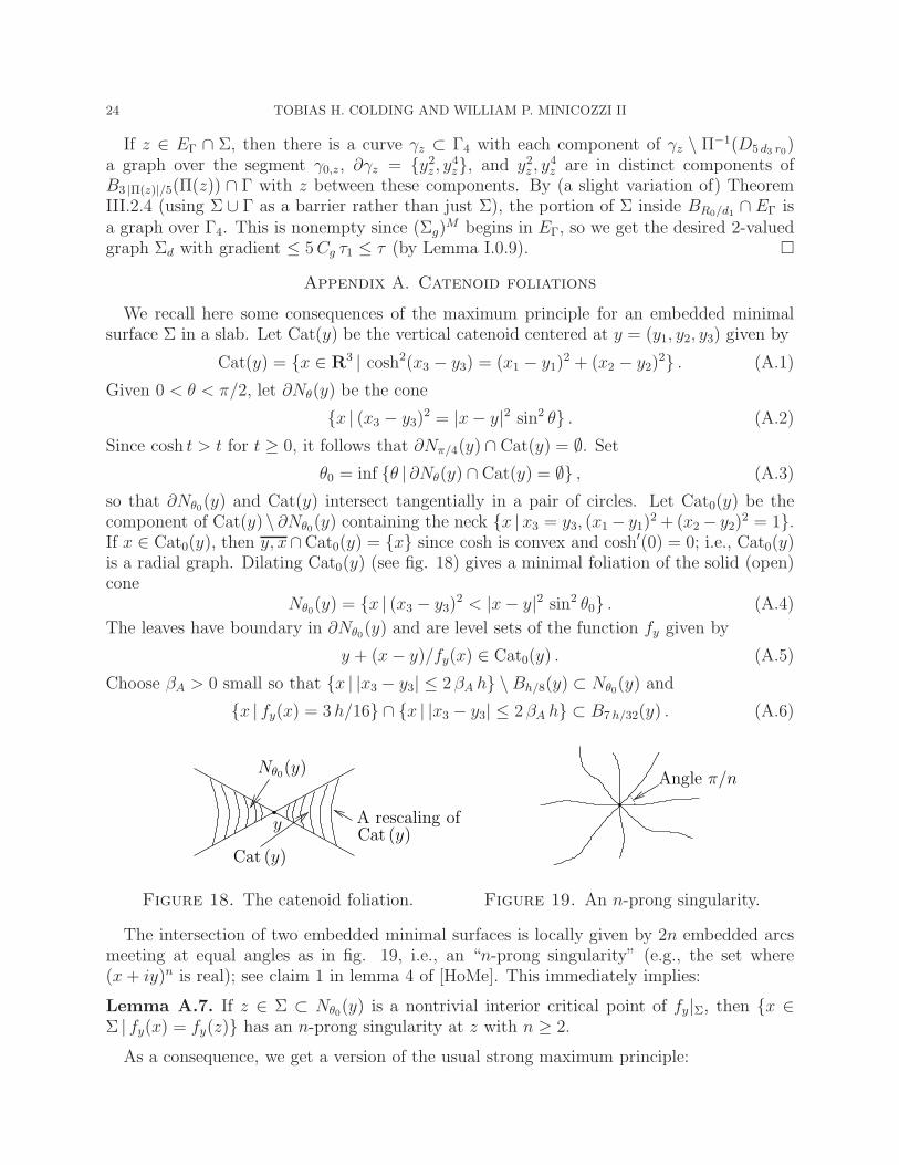
We recall here some consequences of the maximum principle for an embedded minimalsurface Σ in a slab. Let Cat(y) be the vertical catenoid centered at y = (y1, y2, y3) given by

Cat(y) = x ∈ R3 | cosh2(x3 − y3) = (x1 − y1)2 + (x2 − y2)

2 . (A.1)

Given 0 < θ < π/2, let ∂Nθ(y) be the cone

x | (x3 − y3)2 = |x− y|2 sin2 θ . (A.2)

Since cosh t > t for t ≥ 0, it follows that ∂Nπ/4(y) ∩ Cat(y) = ∅. Set

θ0 = inf θ | ∂Nθ(y) ∩ Cat(y) = ∅ , (A.3)

so that ∂Nθ0(y) and Cat(y) intersect tangentially in a pair of circles. Let Cat0(y) be thecomponent of Cat(y) \ ∂Nθ0(y) containing the neck x | x3 = y3, (x1 − y1)

2 +(x2 − y2)2 = 1.

If x ∈ Cat0(y), then y, x∩Cat0(y) = x since cosh is convex and cosh′(0) = 0; i.e., Cat0(y)is a radial graph. Dilating Cat0(y) (see fig. 18) gives a minimal foliation of the solid (open)cone

Nθ0(y) = x | (x3 − y3)2 < |x− y|2 sin2 θ0 . (A.4)

The leaves have boundary in ∂Nθ0(y) and are level sets of the function fy given by

y + (x− y)/fy(x) ∈ Cat0(y) . (A.5)

Choose βA > 0 small so that x | |x3 − y3| ≤ 2 βA h \Bh/8(y) ⊂ Nθ0(y) and

x | fy(x) = 3 h/16 ∩ x | |x3 − y3| ≤ 2 βA h ⊂ B7 h/32(y) . (A.6)

y

Cat (y)

A rescaling ofCat (y)

Nθ0(y)

Figure 18. The catenoid foliation.

Angle π/n

Figure 19. An n-prong singularity.

The intersection of two embedded minimal surfaces is locally given by 2n embedded arcsmeeting at equal angles as in fig. 19, i.e., an “n-prong singularity” (e.g., the set where(x+ iy)n is real); see claim 1 in lemma 4 of [HoMe]. This immediately implies:

Lemma A.7. If z ∈ Σ ⊂ Nθ0(y) is a nontrivial interior critical point of fy|Σ, then x ∈Σ | fy(x) = fy(z) has an n-prong singularity at z with n ≥ 2.

As a consequence, we get a version of the usual strong maximum principle:


Lemma A.8. If Σ ⊂ Nθ0(y), then fy|Σ has no nontrivial interior local extrema.

Corollary A.9. If Σ ⊂ Bh(y)∩x | |x3−y3| ≤ 2 βA h, ∂Σ ⊂ ∂Bh(y), and B3 h/4(y)∩Σ 6= ∅,then Bh/4(y) ∩ Σ 6= ∅.Proof. Scaling (A.6) by 4, x ∈ Σ | fy(x) = 3 h/4 ⊂ B7 h/8(y) \ B3 h/4(y). By Lemma A.8,fy has no interior minima in Σ so the corollary now follows from fy(x) ≤ |x− y|.

Iterating Corollary A.9 along a chain of balls gives:

Corollary A.10. If Σ ⊂ |x3| ≤ 2 βA h, p, q ∈ x3 = 0, Th(γp,q) ∩ ∂Σ = ∅, and yp ∈Bh/4(p) ∩ Σ, then a curve ν ⊂ Th(γp,q) ∩ Σ connects yp to Bh/4(q) ∩ Σ.

Proof. Choose y0 = p, y1, y2, . . . , yn = q ∈ γp,q with |yi−1 − yi| = h/2 for i < n and |yn−1 −yn| ≤ h/2. Repeatedly applying Corollary A.9 for 1 ≤ i ≤ n, gives νi : [0, 1] → Bh(yi) ∩ Σwith ν1(0) = yp, νi(1) ∈ Bh/4(yi) ∩ Σ, and νi+1(0) = νi(1). Set ν = ∪n

i=1 νi.

This produces curves which are “h-almost monotone” in the sense that if y ∈ ν, thenB4 h(y) ∩ ν has only one component which intersects B2 h(y).

Corollary A.11. If Σ ⊂ |x3| ≤ 2 βA h and E is an unbounded component of R2 \Th/4(Π(∂Σ)), then Π(Σ) ∩ E = ∅.Proof. Given y ∈ E, choose a curve γ : [0, 1] → R2\Th/4(Π(∂Σ)) with |γ(0)| > supx∈Σ |x|+hand γ(1) = y. Set Σt = x ∈ Σ | fγ(t)(x) = 3 h/16. By (A.6), Σt ⊂ B7 h/32(γ(t)), so thatΣ0 = ∅ and Σt ∩ ∂Σ = ∅. By Lemma A.8, either Σt = ∅ or Σt contains an arc of transverseintersection. In particular, there cannot be a first t > 0 with Σt 6= ∅, giving the corollary.

References

[ChY] S.Y. Cheng and S.T. Yau, Differential equations on Riemannian manifolds and their geometric appli-cations, Comm. Pure Appl. Math. 28 (1975) 333-354.

[CiSc] H.I. Choi and R. Schoen, The space of minimal embeddings of a surface into a three-dimensionalmanifold of positive Ricci curvature, Invent. Math. 81 (1985) 387-394.

[CM1] T.H. Colding and W.P. Minicozzi II, Minimal surfaces, Courant Lecture Notes in Math., v. 4, 1999.[CM2] T.H. Colding and W.P. Minicozzi II, Estimates for parametric elliptic integrands, International Math-

ematics Research Notices, no. 6 (2002) 291-297.[CM3] T.H. Colding and W.P. Minicozzi II, Minimal annuli with and without slits, Jour. of Symplectic

Geometry, vol. 1, issue 1 (2002) 47–62.[CM4] T.H. Colding and W.P. Minicozzi II, The space of embedded minimal surfaces of fixed genus in a

3-manifold II; Multi-valued graphs in disks, preprint.[CM5] T.H. Colding and W.P. Minicozzi II, The space of embedded minimal surfaces of fixed genus in a

3-manifold III; Planar domains, preprint.[CM6] T.H. Colding and W.P. Minicozzi II, The space of embedded minimal surfaces of fixed genus in a

3-manifold IV; Locally simply connected, preprint.[CM7] T.H. Colding and W.P. Minicozzi II, The space of embedded minimal surfaces of fixed genus in a

3-manifold V; Fixed genus, in preparation.[CM8] T.H. Colding and W.P. Minicozzi II, Embedded minimal disks, To appear in The Proceedings of the

Clay Mathematics Institute Summer School on the Global Theory of Minimal Surfaces. MSRI.[CM9] T.H. Colding and W.P. Minicozzi II, Disks that are double spiral staircases, preprint.[HoMe] D. Hoffman and W. Meeks III, The asymptotic behavior of properly embedded minimal surfaces of

finite topology, JAMS 2, no. 4 (1989) 667–682.[MeYa] W. Meeks III and S. T. Yau, The existence of embedded minimal surfaces and the problem of

uniqueness, Math. Zeit. 179 (1982) 151-168.


[Sc] R. Schoen, Estimates for stable minimal surfaces in three-dimensional manifolds, Seminar on Minimalsubmanifolds, Ann. of Math. Studies, v. 103, Princeton University Press (1983).

Courant Institute of Mathematical Sciences and MIT, 251 Mercer Street, New York,

NY 10012 and 77 Mass. Av, Cambridge, MA 02139

Department of Mathematics, Johns Hopkins University, 3400 N. Charles St., Baltimore,

MD 21218

E-mail address : [email protected] and [email protected]

The space of embedded minimal surfaces of fixed genus in a 3-manifold I; Estimates off the axis for...

Documents

Transcript of The space of embedded minimal surfaces of fixed genus in a 3-manifold I; Estimates off the axis for...