Working Paper in Economics and Development Studies

Department of EconomicsPadjadjaran University

AGEFIS:Applied General Equilibrium for FIScal Policy Analysis

Arief Anshory Yusufa)

No. 200807

Center for Economics and Development Studies,Department of Economics, Padjadjaran UniversityJalan Cimandiri no. 6, Bandung, Indonesia. Phone/Fax: +62-22-4204510http://www.lp3e-unpad.org

For more titles on this series, visit:http://econpapers.repec.org/paper/unpwpaper/

Arief Anshory Yusufa)

Djoni Hartonob)

Wawan Hermawana)

Yayana)

a)Center for Economics and Development Studies (CEDS), Padjadjaran Universityb)Graduate Program of Economics, University of Indonesia

October 2008

1

AGEFIS:

Applied General Equilibrium for FIScal Policy Analysis1

Arief Anshory Yusuf a), Djoni Hartono b), Wawan Hermawan a), Yayan a)

a) Center for Economics and Development Studies (CEDS), Padjadjaran University2

b) Graduate Program in Economics, Faculty of Economics, University of Indonesia

Abstract

AGEFIS (Applied General Equilibrium model for FIScal Policy Analysis) is a Computable General

Equilibrium (CGE) model designed specifically, but not limited, to analyze various aspects of fiscal policies

in Indonesia. It is yet, the first Indonesian fully-SAM-based CGE model solved by Gempack. This paper

describes the structure of the model and illustrates its application.

Keywords: AGEFIS, CGE, Fiscal Policy, Indonesia

JEL Codes: C68, D58, H30

1. Background

This paper introduces AGEFIS (Applied General Equilibrium model for FIScal Policy Analysis). It

starts by introducing the motivation behind building the model, followed by describing the

process of constructing the model, and then the theoretical structure and the model’s database.

A relevant application of the model is illustrated for demonstration purpose.

AGEFIS was built under the capacity building activity carried out by the CGE Modeling Unit

(CCMU), Center for Economics and Development Studies (CEDS)3, Faculty of Economics,

Padjadjaran University, for Fiscal Policy Agency (Badan Kebijakan Fiskal/BKF), The Ministry of

Finance Republic of Indonesia. It was developed to anticipate the need of the Ministry of

Finance to analyze the impact of various fiscal policies on the economy, as well as the impact of

various economic shocks to the fiscal position of the budget of the Indonesian government4.

AGEFIS was built from scratch in the sense that it was created from a ‘blank’ TABLO5 code. The

process took the following stages:

1. Building the idea of the model’s theoretical structure.

1 Address for correspondence: Dr. Arief Anshory Yusuf, email: arief.yusuf@fe.unpad.ac.id

2 Readers who are interested to use the model can visit CEDS website, download and fill in the application

form and send it by email to arief.yusuf@fe.unpad.ac.id. The purpose of filling the form is to maintain

network of the AGEFIS users.

3 CEDS website: http://ceds.fe.unpad.ac.id, CCMU website: http://ceds.fe.unpad.ac.id/unit/ccmu.html

4 AGEFIS is open for public use and can be downloaded from CEDS website, http://ceds.fe.unpad.ac.id

5 Tablo is a text editor, where all the equations of the model are written. It is part of GEMPACK a General

Equilibrium Modeling Package developed by Center of Policy Studies (CoPS), Monash University.

2

2. Writing down the structural equations of the model i.e. both linear and non-linear equation

in level.

3. Linearizing the level equations into percentage change form (as required by Gempack).

4. Writing down the linearized equations into TABLO file.

5. Building the database of the model from the 2003 Indonesian Social Accounting Matrix.

Unlike most Indonesian CGE models solved by GEMPACK which use Input-Output (I-O) table as

its basic database (such as INDORANI, WAYANG, INDOCEEM), AGEFIS uses Social Accounting

Matrix as its core database. The use of the SAM is necessary if fiscal aspect will be the focus

application. Information from an I-O table would be far from sufficient.

To analyze the fiscal aspects, we need information of transaction flow on the source of each item

of government income and how they are spent. This information is unavailable from an I-O

table. Hence, the only way is to build a model which is based on a SAM. AGEFIS is yet the first

Indonesian fully-SAM-based CGE model solved by GEMPACK i.e., the structure of the SAM is in

line with the structure of the CGE model, similar to most GAMS6-based model.

Although in structure, the AGEFIS Model resembles the other SAM-based models, AGEFIS’

interface is designed to abridge the fiscal analyses. Users, for example, can run the exogenous

shocks on the component of the government budget and observe easily those impacts on the

fiscal position of the budget.

AGEFIS Model may be far from perfection and need various modification and extension to be

complete. For example, the number of sectors in AGEFIS which is only 23 commodities offers

less flexibility. Besides, it has no theoretical link between government revenue with

government spending for investment (capital expenditure). In the future, those weaknesses can

be improved.

2. Summary of the Structure and Database of AGEFIS

As an overview (the details would be in the next section), the theoretical structure of the model

can be summarized as follows:

1. The production structure of 23 economic sectors is based on nested Leontief production

function for intermediate input and value added, while the value added production function

is specified as a CES (constant elasticity of substitution). There are two primary production

factors in the model, i.e. capital and labor.

2. The optimization of import and domestic goods composition is conducted by an economic

agent via Armington specification.

3. The household sector maximizes a Cobb-Douglas utility function.

4. The household receives income from the ownership of production factors, as well as from

transfers from a range of other institutions (government, companies and foreign).

5. The government receives their income from indirect tax, direct tax, returns to factor

ownership and transfer from other institution such as the rest of the world. Government

spends the budget for consumption, to subsidize commodities and to send transfer to other

institution such as households.

6. The closure of AGEFIS is flexible, below is some examples:

a. Long term closure: full employment of factor; capital and labor mobile among sectors.

b. Short term closure: capital is mobile among sectors; aggregate employment can change

(unemployment of factors is possible).

6 General Algebraic Modeling System, a popular software to solve CGE modeling. See

http://www.gams.com for more detail.

3

c. Short term closure with full employment that capital can not make a move among

sectors, but the labor always in full employment.

d. Different closure from fiscal side, such as government saving (for government

investment also) is exogenous, or no surplus/deficit but automatically increase the

government spending for consumption, etc.

List of Sectors of production in AGEFIS model:

1. CROPS Agricultural food crops

2. OCROP Other agricultural food crops

3. LIVEST Livestock and the products

4. FOREST Forestry and hunting

5. FISHR Fishery

6. MINE Mining and other quarrying

7. QUARY Quarrying of coal & metal ores, oil and natural gas

8. FOOD Manufacture of food, beverage and tobacco

9. TEXT Manufacture of spinning, textile, and leather

10. WOOD Manufacture of wood and wood-based product

11. PAPER Manufacture of paper, printing, metal-based transportation and other industries

12. CHEM Manufacture of chemical, fertilizer, cement and fabricated metal product

13. ELEC Electricity, gas and water supply

14. CONST Construction

15. TRADE Wholesale trade and retail, transportation support service and wear house

16. REST Restaurant

17. HOTEL Hotel

18. LNDTR Land transportation

19. AIRTR Air transport and water transport, communication

20. BANK Bank and insurance

21. REAL Real estate and corporate service

22. GOVSR Government and defense, education, health, other social service

23. SERV Personal service, household and other service

The above sector classification follows the classification in the official Social Accounting Matrix.

4

The SAM that constitutes the core database of AGEFIS is summarized on Table 1 as follows:

Table 1. Summary of Social Accounting Matrix of AGEFIS (SAM 2003, Rp Trillion)

FAC HH COR GOV AGR MAN SER SAV ITX SUB ROW TOTAL

FAC 509 666 796 9 1,980

HH 1,448 90 48 42 10 1,638

COR 403 58 7 468

GOV 62 18 124 48 132 -5 0 379

AGR 205 0 68 312 57 -4 132 770

MAN 608 16 47 670 229 294 442 2,305

SER 468 142 115 357 271 4 112 1,469

SAV 109 226 105 441

ITX 7 55 37 33 132

SUB -5 0 -5

ROW 67 140 11 27 25 251 79 145 473 1,217

TOTAL 1,980 1,638 468 379 770 2,305 1,469 441 132 -5 1,217 10,793

Note: FAC = primary factor of production; HH = household; COR = corporate sector; GOV = government

sector; AGR = agriculture; MAN = manufacturing; SER = services; SAV = saving-investment; ITX = indirect

tax; SUB = subsidy; ROW = rest of the world.

3. The use of AGEFIS

Table 2 shows how AGEFIS model can be applied to various aspects of fiscal policies.

Table 2. The Use of Model AGEFIS

Instrument/Scenario Example Case

The impact of fiscal

policy (revenue

side)

Indirect tax for

various commodity

To reform indirect taxation (e.g. reduce or

increase the indirect tax rate) to find the most

optimal (in terms of GDP and employment

generation or composition of sectors) indirect

tax structure.

Income tax

(household/

individual)

Intensification (increasing direct tax rate) or

extensification (direct tax object), the impact

to economic

Corporate tax

(transfer for

corporate)

Intensification and extensification of

tax/transfer from corporate sector and its

economic impact

Foreign aid The impact of the foreign aid or foreign loan

The impact of fiscal

policy (expenditure

side)

Subsidy for various

commodity

The impact of increasing, decreasing, or even

removing subsidy of commodity, e.g.

electricity subsidy, etc toward economic,

employment, and sector side.

Government

consumption

The impact of increase or decrease the overall

government consumption on specific sector

on economic, employment, and sectoral side.

Transfers for various

institution

The impact of changing transfer from

government to other institution e.g.

household, corporate, or foreign toward

5

economic, employment and sector side.

combination of

income –

expenditure side

Combination of

various instrument

either from income

side or expenditure

side

The impact of electricity subsidy reduction,

and to look for alternative expenditure

reallocation: to subsidize other sectors, to

transfer the households, or spend for specific

sector (which is the most optimum)

The impact on fiscal

position

The impact of

exogenous various

economic shocks on

fiscal position

1. The impact of international commodities

price shock

2. The impact of supply shock in certain

sector, such as dryness in agriculture

3. The impact of the increase of productivity

towards government income from tax, and

how the most optimum fiscal response.

4. The impact of investment in certain sector

towards fiscal position.

4. Illustration of Simulation using AGEFIS

This section will illustrate the case of electricity subsidy removal7. To remove the subsidy, we

need to know first how much the initial rate of the subsidy (in proportion to its basic price) and

then use those numbers for calculating the amount of shock statement. We can find this

information from the data AGEFIS.HAR8. The data contains a header called ‘indirect tax

instrument by sector’.

7 This does not reflect accurately the removal of subsidy on electricity sector because the sectors

represent also, gas and water supply sector.

8 At the Model/Data menu in RUNGEM, right-click data and view with viewhar.

6

AGEFIS is run using the user-friendly RUNGEM9 interface. To implement the shock, we only

need to go to the shock menu and choose which variable to be shocked. In this case, the variable

is subsidy rate i.e, delSC. We then choose the commodity and the amount of the shock, in this

case -0.63941. The shock statement is:

shock delSC(“ELEC”) = -0.63941;

9 RUNGEM is free to download. The url address for downloading RUNGEM is:

http://www.monash.edu.au/policy/gprgem.htm

Electricity subsidy rate is

6.4%.

7

The fiscal impact can be seen from variable delBUDGET (nominal change in billion rupiahs) as

illustrated below.

The impact on GDP and its components (from expenditure side) can be seen from variable

gdpcompexp (in percentage of change), as illustrated below:

Subsidy fell by Rp 4.7

trillion.

Balanced budget

assumption

Government budget

surplus change by Rp

4.2 trillion

8

The impact on output by sector can be viewed from variable xtot, as

illustrated on the left figure:

The output of electricity sector falls for by 1.76%. The other sector’s

outputs generally decline.

The aggregate employment (see variable xfacsup) falls by 0.15%.

If we want to know the impact of reallocating the money saved from

reducing this subsidy to other posts in the budget, we can change that in

the closure specification. Suppose that we want to allocate that to

households as transfers, then we need only add the following statement

in the closure:

swap delSG = delTRHOGO;

Household

consumption fall

by 0.23%

Real GDP falls by 0.09%

9

The budgetary impact using that closure will be the following:

The impact on GDP as follows:

Other than the above scenarios, we can also do a variety of scenarios which changes the budget

items, e.g. allocation to the government consumption expenditure, decrease indirect tax of other

goods, or decrease overall indirect tax rate. All things can be done conveniently using RUNGEM

interface of AGEFIS model.

No addition on

saving

Transfer to household

increase 4.6 trillion

GDP decreases.

Real consumption of

households increases

by almost 1%

10

5. The Structure of AGEFIS Database

The database of AGEFIS model is stored in the file agefis.har which consists of a range of

coefficients recording the transaction values among economic agents, some parameters, and

also other information such as the fiscal instruments. The following table summarizes the

agefis.har.

Table 3. List of coefficients in AGEFIS databse

Coefficient Dimension Value

(million

rupiahs)

Remark

DEMAND

VXINT_S COM*IND 2,478,376 Transaction value of intermediate demand

VXHOU_S COM 1,416,045 Transaction value of house holds consumption

demand

VXINV_S COM 364,116 Transaction value of investment goods

VXG_S COM 163,701 Transaction value of government consumption

demand

VXEXP COM 685,851 Transaction value of export

VXD COM*SRC 4,422,238 Transaction value by source (domestic or import)

PRIMARY PRODUCTION FACTORS

VXFAC FAC*IND 1,971,180 Payment of primary production factors by

industry

VXFACRO FAC 8,579 Payment of production factors by rest of the

world

VXFG FAC 61,565 Payment of production factors that owned by

government

VXFCO FAC 402,604 Payment of production factors that owned by

corporation

VXFRO FAC 67,400 Revenue of production factors income that

owned by rest of the world

VXFACSH FAC 1,448,190 Revenue of production factors income that

owned by household

TRANSACTION RELATED TO FISCAL INSTRUMENT

VTX COM 99,270 Government income from indirect tax

VSC COM 5,448 Government expenditure to subsidize goods and

services

VTM COM 32,927 Government income from import excise tax

VYTAX 1 18,246 Government income from household’ income tax

VCORTAX 1 124,183 Government income from corporate tax

INSTSEC IND*INST0

1

1.55 Indirect tax rate and subsidy rate

DIRECTTAX INST02 0.28 Direct tax rate (household and corporate)

11

TRANSFERS BETWEEN INSTITUTIONS10

SAVH 1 109,148 Saving of households

VTRROHO 1 4,258 Transfer from households to rest of the world

VTRHOHO 1 90,400 Transfer from households to other households

VTRROGO 1 20,426 Transfer from government to rest of the world

VTRHOGO 1 41,709 Transfer from government to household

VTRGOGO 1 48,135 Transfer from government to other government

VTRHOCO 1 48,192 Transfer from corporate to household

VTRCOCO 1 57,518 Transfer from corporate to corporate

VTRROCO 1 11,260 Transfer from corporate to rest of the world

VTRGORO 1 86 Transfer from rest of the world to government

VTRCORO 1 7,445 Transfer from rest of the world to corporate

VTRHORO 1 9,604 Transfer from rest of the world to household

VTRRORO 1 472,998 Transfer from rest of the world to rest of the

world

PARAMETER

SIGARM COM 46 Armington Elasticities

SIGMAPRIM IND 11.5 Elasticities of Factor Production

EXPELAS COM 115 Export elasticity of demand

The database agefis.har come from Indonesian Social Accounting Matrix 2003.

7. Understanding the Tablo File of AGEFIS

This section will explain the statements in file tablo agefis.tab, especially the structural

equations and identities.

Tablo file agefis.tab can be divided into the following parts.

1. File statement. In file statement, logical filename (here is ‘database’) is defined. The

physical file is agefis.har. In agefis.tab, file statement is written as:

file database # database model agefis # ;

[note: statement between # is a comment]

2. Set statement. In set statement, the name of set and elements from each sets are declared.

In tablo agefis.tab, set statement is written as follows:

set

10 To be easier to remember, the coefficient of inter institution transfer is initiated with VTR (the value of

transfer), then followed by XX and then YY or VTRXXYY. XX imply the institution who receives the

transfer, while YY represent the institution who gives the transfer. Those institutions are as follows: HO =

household; GO = government; CO = Corporate; RO =Rest of The World. So the coefficient VTRHOCO,

means the value of transfer received by households from corporate sector or the value of transfer given

by corporate sector to households.

12

COM # commodity # (CROPS, OCROP, LIVEST, FOREST, FISHR, MINE, QUARY, FOOD, TEXT, WOOD, PAPER, CHEM, ELEC, CONST, TRADE, REST,

HOTEL, LNDTR, AIRTR, BANK, REAL, GOVSR, SERV); FAC # factor # (labor, capital); SRC (dom, imp); IND = COM;

3. Coefficient declaration. Coefficients is distinguished from variables. Coefficient is the

representation of data read from the model database. In the coefficient declaration, all of the

coefficients are declared, and those values would be read from database or calculated using

formulas. In general, coefficients can be divided into two types: (1) coefficients of which

their value must be read directly from the headers in database, these are called basic

coefficients; and (2) coefficients of which their value are calculated based on the basic

coefficient in formula statements. Coefficients are written in uppercase.

4. Read statement. Read statement is a statement to fill the values of basic coefficient by

reading it from database.

5. Formula statement. Formula statement is a statement to calculate the coefficients not read

from the database, but as a function of other coefficients (such as basic coefficients).

6. Variable declaration. A variable essentially is the unknown in the model the value of which

is to be solved when the model is solved. Almost all variable in AGEFIS model are in

percentage change. Some exception is when the variable is in nominal ordinary change. In

this part of the Tablo file, those variables are declared.

7. Update statement. Update statement is a statement to update the basic coefficient using

their corresponding and relevant variables after the simulations.

8. Equation statement. Equation statement is essentially the core of the Tablo file of AGEFIS.

Here the structural equations of the model are written.

7.1 Conventions

In AGEFIS model, there are two kinds of variables: scalar variables and a vector or matrices

variables. Vector or matrix variable has subscript. To make it easy to remember the following

convention for subscript will be used.

� c for commodity

� i for industry

� f for factor of production, i.e., labor and capital

� s for source i.e., where the commodity come from i.e., domestic or foreign

Almost all variables in AGEFIS are in percentage change. They are written in lowercase. There

are also ordinary change variables. The name of these variables start with ‘del’. The rest of the

convention for naming the variable is as follows:

1. Variables with lowercase means that variable are in percentage change.

2. Variable that starts with ‘del’, such as delXX, delTX or delSC are ordinary change.

13

3. Coefficients are written with uppercase and are in level

4. Variables or coefficients that start with letter V (or w) are value.

5. Variables or coefficients that start with letter P (or p) are price.

6. Variables or coefficients that start with letter X (or x) are quantity or real variables.

Underline in a variable name means something in AGEFIS. A variable that has underline is

usually a result of aggregation (we call it composite variable, sometimes).

1. _c is aggregate or average over commodities (over COM (commodities))

2. _s c is aggregate or average over source (over SRC (dom+imp))

3. _i c is aggregate or average over industries (over IND (Industries))

7.2 Coefficient declaration

In this part of Tablo file, the coefficients are declared as follows: [note: underlined rows indicate

basic coefficient]

coefficient

(all,c,COM) VXD_S(c) # Value of Demand Composite Import Domestic # ;

(all,c,COM)(all,s,SRC) VXD(c,s) # Value of Demand by sources # ;

(all,c,COM) VTX(c) # Indirect Taxes Revenue # ;

(all,c,COM) VXCIF(c) # Value of Import at CIF # ;

(parameter) (all,c,COM) SIGARM(c) # Armingtong Elasticities # ;

(all,c,COM)(all,i,IND) VXINT_S(c,i) # Value of Intermediate Demand # ;

(all,c,COM) VXHOU_S(c) # Value of Household Consumption # ;

(all,c,COM) VXINV_S(c) # Value of Investment # ;

(all,c,COM) VXG_S(c) # Value of Government Consumption by Commodities # ;

(parameter) (all,i,IND) SIGMAPRIM(i) # Elasticities of Factor Production # ;

(all,f,FAC)(all,i,IND) SFAC(f,i) # Factor cost share # ;

(all,f,FAC) VXFACRO(f) # Value of Demand for Factor from Rest of The World # ;

(all,f,FAC)(all,i,IND) VXFAC(f,i) # Value of Demand for factor # ;

(all,f,FAC) VXFG(f) # Value of factor supply from government sector # ;

(all,f,FAC) VXFCO(f) # Value of factor supply from corporate sector # ;

(all,f,FAC) VXFRO(f) # Value of factor supply from Rest of The World # ;

(all,i,IND) VTOT(i) # Total value of output (Supply) # ;

(all,i,IND) VXPRIM(i) # Value of demand for factor of production # ;

(all,c,COM) VXEXP(c) # Value of total export by commodities # ;

VYH # Value of household income # ;

(all,f,FAC) VXFACSH(f) # Value of factor pof production by household # ;

VTRHOGO # Value of transfer from government to household # ;

VTRHOCO # Value of transfer from corporate to household # ;

VTRHOHO # Value of transfer from household to household # ;

VYTAX # Household income tax revenue # ;

SAVH # Saving from household # ;

VYGC # Value Government Revenue # ;

(all,c,COM) VTM(c) # Value of import tarrif by commodities # ;

VCORTAX # Value of transfer from corporate to government # ;

14

VTRGORO # Value of transfer from ROW to government # ;

VTRGOGO # Value of transfer from government to government # ;

VTRROGO # Value of transfer from Gov't to ROW # ;

(all,c,COM) VSC(c) # Value of subsidies by commodities # ;

VEGC # Value of Government Expenditure # ;

VYCO # Value of income by corporate sector # ;

VTRCORO # Value of transfer from ROW to corporate # ;

VTRCOCO # Value of transfer from corporate to Corporate # ;

VECO # Value of Corporate Expenditure # ;

VYRO # Value of income from Rest of The World # ;

VTRROHO # Value of transfer from HH to Rest of The World # ;

VTRHORO # Value of transfer from ROW to Household # ;

VERO # Value of expenditure by Rest of The World # ;

VTRRORO # Value of transfer from ROW to ROW # ;

VTRROCO # Value of transfer from corporate to ROW # ;

(parameter) (all,c,COM) EXPELAS(c) # Expenditure elas by commodities # ;

(all,c,COM) VXIMP(c) # Value of Import including tarrif # ;

(all,f,FAC) VXFACSUP(f) # Value of all factor supply # ;

(all,f,FAC) SXFACSH(f) # share of factor owned by household # ;

(all,f,FAC) SXFG(f) # share of factor owned by government # ;

(all,f,FAC) SXFCO(f) # share of factor owned by corporate # ;

(all,f,FAC) SXFRO(f) # share of factor owned by rest of the world # ;

VCORFINC # corporate factor income # ;

7.3 Read statement

In a read statement, all the value of basic coefficient will be read from the database. It refers to a

certain header in file database agefis.har.

read SIGARM from file database header "SIGA" ; SIGMAPRIM from file database header "SIGP" ; EXPELAS from file database header "EELA" ; VXD from file database header "VXD" ; VTX from file database header "VTX" ; VTM from file database header "VTM"; VXINT_S from file database header "VINT" ; VXHOU_S from file database header "VHOU"; VXINV_S from file database header "VINV" ; VXG_S from file database header "VXG"; VXFAC from file database header "VFAC" ; VXFACRO from file database header "VFAR" ; VXFG from file database header "VFG" ; VXFCO from file database header "VFCO"; VXFRO from file database header "VFRO"; VXEXP from file database header "VEXP" ; VXFACSH from file database header "VFHO"; VTRHOGO from file database header "VRHG"; VTRHOCO from file database header "VRHC"; VTRHOHO from file database header "VRHH"; VYTAX from file database header "VYTX" ;

15

SAVH from file database header "VSAV" ; VCORTAX from file database header "VRGC"; VTRGORO from file database header "VRGR"; VTRROGO from file database header "VRRG"; VSC from file database header "VSC" ; VTRCORO from file database header "VRCR"; VTRCOCO from file database header "VRCC"; VTRROHO from file database header "VRRH"; VTRHORO from file database header "VRHR"; VTRGOGO from file database header "VRGG"; VTRRORO from file database header "VRRR"; VTRROCO from file database header "VRRC";

7.4 Formula statement

In the formula statement, the coefficients that have been declared but not one of the basic

coefficients are calculated. Each of the coefficient is a function of those basic coefficients.

formula (all,c,COM) VXD_S(c) = SUM{i,IND,VXINT_S(c,i)} + VXHOU_S(c) + VXG_S(c)+ VXINV_S(c); (all,c,COM) VXIMP(c) = VXD(c,"IMP" ); (all,c,COM) VXCIF(c) = VXIMP(c) - VTM(c); (all,i,IND) VXPRIM(i) = SUM{f,FAC,VXFAC(f,i)}; (all,f,FAC)(all,i,IND) SFAC(f,i) = VXFAC(f,i) / ID01[VXPRIM(i)]; (all,i,IND) VTOT(i) = VXPRIM(i)+ SUM{c,COM, VXINT_S(c,i)}; VYGC = SUM{i,IND,VTX(i)} + SUM{c,COM,VTM(c)} + VYTAX + VCORTAX + VTRGORO + SUM{f, FAC,VXFG(f)} + VTRGOGO; VYH = SUM{f,FAC,VXFACSH(f)} + VTRHOGO + VTRHOCO + VTRHORO + VTRHOHO;

VECO = VTRROCO + VTRHOCO + VTRCOCO; VEGC = SUM{c, COM,VXG_S(c)} + VTRHOGO + VTRROGO + SUM{c,COM,VSC(c)} +

VTRGOGO; VYCO = SUM{f,FAC,VXFCO(f)} - VCORTAX + VTRCORO + VTRCOCO; VERO = SUM{c,COM,VXEXP(c)} + VTRCORO + VTRGORO + VTRHORO + VTRRORO + SUM{f,FAC,VXFACRO(f)}; VYRO = SUM{f,FAC,VXFRO(f)} + VTRROGO + VTRROHO + SUM{c,COM,VXCIF(c)}

+ VTRRORO + VTRROCO; (all,f,FAC) VXFACSUP(f) = VXFACSH(f) + VXFG(f) + VXFCO(f) + VXFRO(f); (all,f,FAC) SXFACSH(f) = VXFACSH(f)/VXFACSUP(f); (all,f,FAC) SXFG(f) = VXFG(f)/VXFACSUP(f); (all,f,FAC) SXFCO(f) = VXFCO(f)/VXFACSUP(f); (all,f,FAC) SXFRO(f) = VXFRO(f)/VXFACSUP(f); VCORFINC = SUM{f,FAC,SXFCO(f)*VXFACSUP(f)};

7.5 Variable declaration

In this part of the tablo file, all the variables which are part of the of structural model equation

are declared.

variable (all,c,COM)(all,s,SRC) pq(c,s) # Consumer price for commodity c, source s # ; (all,c,COM)(all,s,SRC) xd(c,s) # Demand for commodity c, source s # ; (all,c,COM) pq_s(c ) # Consumer price of composite good c # ; (all,c,COM) xd_s(c ) # Demand for commodity composites # ; (all,c,COM)(all,i,IND) xint_s(c,i) # Demand for commodity by industry # ; (all,c,COM) xhou_s(c) # Demand for commodity by household # ; (all,c,COM) xinv_s(c ) # Demand for commodity for investment # ; (all,c,COM) xg_s(c ) # Demand for commodity by government # ;

16

(all,i,IND) xprim(i) # Industry demand for primary-factor composite # ; (all,f,FAC)(all,i,IND) xfac(f,i) # Demand for primary factor by industry i # ; (all,f,FAC) xfacro(f) # Supply of factor f by rest of the world # ; (all,i,IND) pprim(i) # Price of Primary factor composite # ; (all,c,COM) xtot(c ) # Output or supply commodity # ; (all,i,IND) ptot(i) # Producer's price or unit cost of production # ;

yh # Household income # ; trhogo # Transfer to household from central government # ; trhoco # Transfer to household from coorporate # ; trhoro # Transfer to household from rest of the world # ; trhoho # Transfer to household from inter household # ; eh # Household expenditure # ; ygc # govenrment income # ; trgoco # Transfer to cental government from coorporate # ; trgoro # Transfer to cental government from rest of the wo rld # ; trgogo # transfer from government to government # ; trrogo # Transfer to rest of the world from government # ; (change) delSG # govenrment saving # ;

egc # govenrment expenditure # ; yco # Coorporate income # ; trcoro # Transfer to coorporate from rest of the world # ; trcoco # Transfer to coorporate from cental government # ; eco # Coorporate expenditure # ; trroco # Transfer to rest of the world from corporate # ; (change) delSCO # Coorporate saving # ; (all,c,COM) ximp(c ) # Demand for commodity by import # ;

yro # Rest of the world income # ; (all,f,FAC) pfac(f) # Price of factor f # ;

trroho # Transfer to rest of the world from household # ; exr # Exchange rate # ; (all,c,COM) pfimp(c ) # International price of commodity # ; (all,c,COM) xexp(c ) # Total export for commodity # ; (all,c,COM) fxexp(c) # q-shifter of export demand # ; (change) delSRO # Rest of the world saving # ;

ero # Rest of the world expenditure # ; trroro # transfer from ROW to ROW # ; (change)(all,c,COM) delTX(c) # Ordinary change in rate of commodity tax # ; (change)(all,c,COM) delSC(c) # Ordinary change in rate of comm. subsidy # ; (change)(all,c,COM) delTM(c) # Ordinary change in rate of import tarrif # ; (change)delTAXH # Ordinary change in rate of household tax # ; (change)delMPSH # Ordinary change in rate of household saving # ; (all,i,IND) atot(i) # all factors technical change # ; (all,i,IND) aprim(i) # neutral technical change # ; (all,f,FAC)(all,i,IND) afac(f,i) # factor saving technical change # ; (all,f,FAC)(all,i,IND) wdist(f,i) # factor price distortion # ; (all,f,FAC) xfacsup(f) # total factor supply # ; (all,f,FAC) yfac(f) # factor income # ; (all,c,COM) fxg_s(c) # government expenditure shifter by commodity # ;

fxg_sc # overall government expenditure shifter # ; (change) delCORTAX # corporate tax rate # ; (change) delCORFINC # change in corporate factor income # ;

The details of those variables above would be discussed on the next section.

17

7.6 Update statement

In update statement, basic coefficients read from the database will be updated by using the

change in their relevant variables.

update (all,c,COM)(all,s,SRC) VXD(c,s) = pq(c,s)*xd(c,s); (change) (all,i,IND) VTX(i) = 0.01*VTX(i)*[100*(VTOT(i)/ID01[VTX(i)])*delTX(i) + ptot(i) + xtot(i)]; (all,c,COM)(all,i,IND) VXINT_S(c,i) = pq_s(c)*xint_s(c,i); (all,c,COM) VXHOU_S(c) = pq_s(c)*xhou_s(c); (all,c,COM) VXINV_S(c) = pq_s(c)*xinv_s(c); (all,c,COM) VXG_S(c) = pq_s(c)*xg_s(c); (all,f,FAC) VXFACRO(f) = pfac(f)*xfacro(f); (all,f,FAC)(all,i,IND) VXFAC(f,i) = pfac(f)*wdist(f,i)*xfac(f,i); (change)(all,f,FAC) VXFG(f) = 0.01*SXFG(f)*VXFACSUP(f)*yfac(f); (change)(all,f,FAC) VXFCO(f) = 0.01*SXFCO(f)*VXFACSUP(f)*yfac(f); (change) (all,f,FAC) VXFRO(f) = 0.01*SXFRO(f)*VXFACSUP(f)*yfac(f); (change) (all,f,FAC) VXFACSH(f) = 0.01*SXFACSH(f)*VXFACSUP(f)*yfac(f); (all,c,COM) VXEXP(c) = pq_s(c)*xexp(c);

VTRHOGO = trhogo; VTRHOCO = trhoco; VTRHOHO = trhoho; (change) VYTAX = 0.01*VYTAX*[100*(VYH/VYTAX)*delTAXH + yh]; (change) SAVH = (VYH-VYTAX)*delMPSH + [SAVH/(VYH-VYTAX)] * [0.01*VYH*yh - delTAXH*VYH - 0.01*VYTAX*yh]; (change) (all,c,COM) VTM(c) = 0.01*VTM(c)*[100*(VXCIF(c)/ID01[VTM(c)])*delTM(c) + exr + pfimp(c) + ximp(c)];

VCORTAX = trgoco; VTRGORO = trgoro; VTRROGO = trrogo; VTRGOGO = trgogo; (change) (all,i,IND) VSC(i) = 0.01*VSC(i)*[100*(VTOT(i)/ID01[VSC(i)])*delSC(i) + ptot(i) + xtot(i)];

VTRCORO = trcoro; VTRCOCO = trcoco; VTRROCO = trroco; VTRROHO = trroho; VTRHORO = trhoro; VTRRORO = trroro;

7.7 Equation statement

In the equation statement, structural equations of the model are written. The basic system of

equation is divided into several parts:

1. Domestic-import sourcing (which determines the composition of import-domestic source

according to Armington specification).

2. Purchaser’s price. The equation that relates the producer price, or international price to the

purchaser’s price.

3. Demand for commodities. The equation that model the demand for goods by various users.

4. Production sector. The equation related to the production of goods and services.

5. Market clearing. The equation that equates the supply with demand, both for commodity as

well as production factors.

18

6. Factor Income. The equation related to the payment of return to factor ownership.

7. Institution. The equation related to the income and expenditure of various institutions i.e.,

households, government, corporate sector, and the rest of the world.

Domestic-import sourcing

Equation eq_xd and eq_pq_s define the optimum allocation of domestic or foreign source

commodity for every given unit of commodity composite.

! domestic-import sourcing ! eq_xd # domestic-import sourcing # (all,c,COM)(all,s,SRC) xd(c,s) = xd_s(c) - SIGARM(c)*[pq(c,s) - pq_s(c)];

eq_pq_s # zero profit in domestic-import sourcing # (all,c,COM) VXD_S(c)*[pq_s(c) + xd_s(c)] = SUM{s,SRC,VXD(c,s)*[pq(c,s) + xd(c,s)]};

The demand structure can be summarized in the figure below. For each commodity c, user as

represented by an agent (representing the whole range of customers i.e., industry, household,

investor, and government) find its optimum composition of domestic and impor content.

The economic agent (wholesaler) who optimizes the composition of domestic and import

content minimize cost subject to CES aggregation, or more formally,

XD_S(c)

XINT_S(c,i) XHOU_S(c) XINV_S(c) XGOV_S(c)

CES

XD(c,”dom”) XD(c,”imp”)

Demand for good c

19

Minimize s

PQ(c,s)·XD(c,s)∑

Subject to

1(c)

(c)

s

XD _S(c) CES(XD(c,s) | (c)) (c,s) (c,s)XD(c,s)ρ

ρσ α δ−

− = =

∑

First order condition from this optimization is

1 11 1 1

PQ(c,s)XD(c,s) (c,s) .XD _ S(c) (c,s) .( )

PQ _ S(c)

ρρ ρ ρα δ

− −+ + +=

or in the linear or percentage change form:

xd(c,s) xd _ s(c) (c)(p(c,s) p _ s(c))σ= − −

Where σ(c) = 1/(1+ρ(c)) is the Armington elasticity of substitution. This is the equation eq_xd in the tablo file.

The next equation is equation of CES aggregation CES or constraint equation. Constraint equation also can be replaced with the zero-profit equation as follows:

s

PQ _ S(c)XD _ S(c) PQ(c,s)XD(c,s)=∑

In the linear form,

( ) ( )c

VXD _ S(c) pq _ s(c) xd _ s(c) VXD(c,s) pq(c,s) xd(c,s)+ = +∑

where VXD _ S(c) PQ _ S(c)XD _ S(c)= , and VXD(c,s) PQ(c,s)XD(c,s)= . The above

equation is equation eq_pq_s in the tablo file. To linearize equation eq_pq_s, we use the ordinary

linearization rules to linearize A*B i.e., A*a + B*b.

Purchaser’s price

These equations relates the basic/producer price and international to the price faced by directly

by consumers.

! purchaser's prices ! eq_pqdom # purchaser's price of domestic commodities # (all,c,COM) pq(c,"dom" ) = ptot(c) + 100*[VTOT(c)/(VTOT(c) + VTX(c) - VSC(c))] * [delTX(c) - delSC(c)];

eq_pqimp # purchaser price of imported commodity # (all,c,COM) pq(c,"imp" ) = pfimp(c) + exr + 100*[VXCIF(c)/ID01[VXCIF(c) + VTM(c)]]*delTM(c);

Equation eq_pqdom links the consumer’s price and producer’s price. The consumer’s price is a

net price after tax and or subsidy are added. The tax will increase the price while the subsidy

will decrease the price. In level, the equation is:

20

PQ(c,"dom") = (1 + TX(c) - SC(c))*PTOT(c)

where,

PQ(c,"dom") : domestic price of each commodity (c) faced by consumer.

TX (c) : indirect tax

SC(c) : indirect subsidy.

PTOT(c) : basic/producer price of each commodity (c)

To describe the linearization process of the above equation, we start by simplifying the

equation:

( )C PP 1 t s P= + −

We can write the tax rate or t, as:

P

P

tP Q TRTt

P Q VTOT= = where:

t : tax or tax revenue

PP : producer’s price

Q : Output

TRT : Total revenue or the total revenue from tax

VTOT : Total Value

Similarly, the subsidy rate s can be written as:

TRSs

VTOT=

where:

s : subsidy

TRS : revenue from the subsidy

The linearized form of (1 + t - s) then can be written as:

( )� ( )

( )

TRS VTOT TRT TRSTRTVTOT VTOT VTOT

1 t s t s t s t s1 t s 100 100 100 100

1 t s 1 t s 1

VTOT100 t s

VTOT TRT TRS

+ −

∆ + − ∆ − ∆ ∆ − ∆ ∆ − ∆+ − = = = =+ − + − + −

= ∆ − ∆+ −

The percentage change form of consumer’s price equation then becomes:

( )C P VTOTˆ ˆP P 100 t sVTOT TRT TRS

= + ∆ − ∆+ −

Where ɵC

P is the percentage change of PC and ɵP

P is the percentage change of PP

In the Tablo file of AGEFIS, it is finally written as:

21

( )VTOT(c)pq(c,"dom") ptot(c) 100 TX(c) SC(c)

VTOT(c) VTX(c) VSC(c)= + ∆ − ∆

+ −

where :

pq(c,"dom") : Domestic price of each commodity (c).

ptot(c) : Price of each commodity (c).

VTOT(c) : Value of goods of each commodity (c).

VTX(c) : Value of tax revenue from each commodity (c).

VSC(c) : Value of subsidy revenue from each commodity (c).

TX (c) : Tax that liable to commodity (c).

C(c) : Subsidy that liable to commodity (c).

.

These are equations eq_pqdom in tablo file.

Equation eq_pqimp links the international price to the price that consumer have to pay for each

commodity, or:

PQ(c,"imp") = EXR*(1 + tm(c))*PFIMP(c)

Where EXR is the exchange rate and tm(c) is the tariff rate. The linearization process is similar

to the linearization process of domestic price equation. First we simplify the equation and

define tariff rate as:

m f mm

f m

t P Q VTMt

P Q VCIF= =

Where

tm : Import tariff

Pf : Import price

Qm : Quantity of imported goods

VTM : Revenue from the tariff

VCIF : Value of imported commodities at the world price exclusive of tariff

The term (1 + tm(c)) can be linearized as follows:

( )� ( )m m mm

m m VCIF VTMVCIF

m

1 t t t1 t 100 100 100

1 t 1 t

VCIF100 t

VCIF VTM

+

∆ + ∆ ∆+ = = =+ +

= ∆+

The whole term of the equation:

( )C f mP P EXR 1 t= ⋅ ⋅ +

can be linearized as:

C f mVCIFˆ ˆP P exr 100 tVCIF VTM

= + + ∆+

22

Finally in the Tablo file, the complete equation is written as:

VCIF(c)pq(c,"imp") pfimp(c) + exr + 100 delTM(c)

VCIF(c) VTM(c)=

+

That is the equation eq_pqimp in tablo file.

Demand

The equations that describe the demand for commodities by various economic agents is written

as follows:

! demand for commodities ! eq_xint_s # intermediate demand # (all,c,COM)(all,i,IND)

xint_s(c,i) - atot(i) = xtot(i); eq_xhou_s # household demand for commodities # (all,c,COM)

xhou_s(c) = eh - pq_s(c); eq_xg_s # government expenditure/demand # (all,c,COM) xg_s(c) = fxg_s(c) + fxg_sc;

eq_xexp # export demand # (all,c,COM) xexp(c) = fxexp(c) - expelas(c)*[(pq(c,"dom" ) - exr) - pfimp(c)];

eq_xd_s # total demand for composite commodities # (all,c,COM) VXD_S(c)*xd_s(c) = SUM{i,IND,VXINT_S(c,i)*xint_s(c,i)}

+ VXHOU_S(c)*xhou_s(c) + VXG_S(c)*xg_s(c) + VXINV_S(c)*xinv_s(c);

Equation eq_int_s is the result of producer’s optimization: minimize cost of production subject

to Leontief production function, or:

c

min PPRIM(i) XPRIM(i) PQ _ S(c) XINT _ S(c, i)

subject to

⋅ + ⋅∑

1 XINT _S(c,i) XPRIM(i)XTOT(i) MIN ALL,c,COM : ,

ATOT(i) AINT(c, i) APRIM(i)

=

The demand equation for intermediate goods from the optimization is:

XINT _ S(c, i)XTOT(i)

ATOT(i)=

and its linearized form is:

x int_ s(c, i) atot(i) xtot(i)− =

which simply states that intermediate demand follow the total output and technical change

proportionally. This is the equation eq_xint_s in the Tablo file. Following the specification of

23

most Gempack-based models such as ORANI-G, MINIMAL, or WAYANG, the production structure

is illustrated in the following figure11:

Production Structure

Household maximizes Cobb-Douglas utility function subject to a given disposable income:

(c)

c c

max U XHOU _ S(c) s.t. PQ _ S(c) XHOU _ S(c) EHα= ⋅ =∏ ∑

where EH is disposable income and PQ_S is the price for each commodity. The equation of the

demand for commodities produced by the optimization is:

XHOU_S(c) = α(c)*[EH/PQ_S(c)]

And its linearized form is:

xhou _ s(c) eh pq _ s(c)= −

this is equation e_xhou_s in tablo file.

The demand for commodities by government is set to be exogenous.:

xg _ s(c) fxg _ s(c) fxg _ sc= −

where fxg_s(c) is shifter per commodity, while fxg_sc is shifter for all commodities. These shifters can be shocked in simulations.

In AGEFIS, foreign demand for domestic goods is price-sensitive. If the domestic price of a

certain good increase relatively to the international price, the export demand will increase.

11 Source of the figure: Horridge, Mark, 2001, MINIMAL: A Simplified General Equilibrium Model, Center

of Policy Studies, Monash University.

24

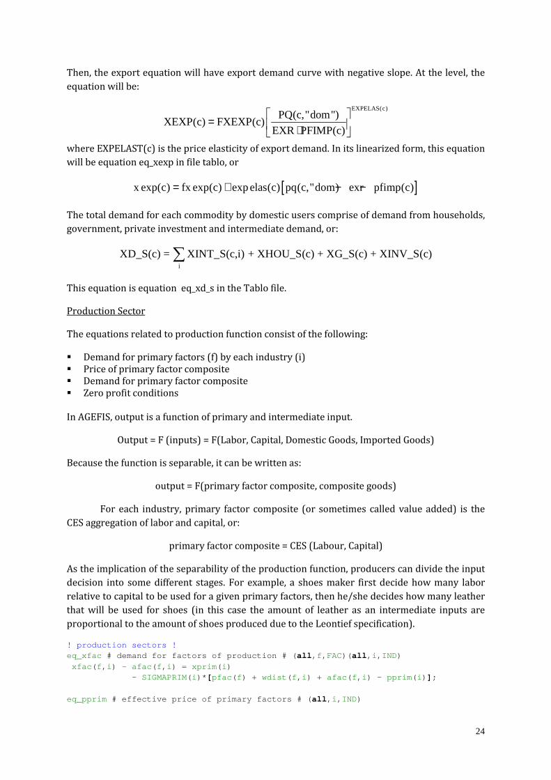
Then, the export equation will have export demand curve with negative slope. At the level, the

equation will be:

EXPELAS(c)PQ(c,"dom")

XEXP(c) FXEXP(c)EXR PFIMP(c)

= ⋅

where EXPELAST(c) is the price elasticity of export demand. In its linearized form, this equation

will be equation eq_xexp in file tablo, or

[ ]x exp(c) fx exp(c) expelas(c) pq(c,"dom) exr pfimp(c)= + − −

The total demand for each commodity by domestic users comprise of demand from households,

government, private investment and intermediate demand, or:

i

XD_S(c) = XINT_S(c,i) + XHOU_S(c) + XG_S(c) + XINV_S(c)∑

This equation is equation eq_xd_s in the Tablo file.

Production Sector

The equations related to production function consist of the following:

� Demand for primary factors (f) by each industry (i)

� Price of primary factor composite

� Demand for primary factor composite

� Zero profit conditions

In AGEFIS, output is a function of primary and intermediate input.

Output = F (inputs) = F(Labor, Capital, Domestic Goods, Imported Goods)

Because the function is separable, it can be written as:

output = F(primary factor composite, composite goods)

For each industry, primary factor composite (or sometimes called value added) is the

CES aggregation of labor and capital, or:

primary factor composite = CES (Labour, Capital)

As the implication of the separability of the production function, producers can divide the input

decision into some different stages. For example, a shoes maker first decide how many labor

relative to capital to be used for a given primary factors, then he/she decides how many leather

that will be used for shoes (in this case the amount of leather as an intermediate inputs are

proportional to the amount of shoes produced due to the Leontief specification).

! production sectors ! eq_xfac # demand for factors of production # (all,f,FAC)(all,i,IND)

xfac(f,i) - afac(f,i) = xprim(i) - SIGMAPRIM(i)*[pfac(f) + wdist(f,i) + afac(f,i) - pprim(i)];

eq_pprim # effective price of primary factors # (all,i,IND)

25

pprim(i) = SUM{f,FAC,SFAC(f,i)*[pfac(f) + wdist(f,i) + afac(f,i)]};

eq_xprim # demand for primary factor composite # (all,i,IND)

xprim(i) - aprim(i) - atot(i) = xtot(i); eq_ptot # zero profit in production # (all,i,IND) VTOT(i)*[ptot(i) + xtot(i)] = VXPRIM(i)*[pprim(i) + xprim(i)] + SUM{c,COM, VXINT_S(c,i)*[pq_s(c) + xint_s(c,i)]};

The equation of production factor demand (eq_xfac) is the first order condition of cost

minimization subject to a CES production function, or:

( ) ( )f

min WDIST(f , i) PFAC f XFAC f , i⋅ ⋅∑

subject to 1

ff

XFAC(f , i)XPRIM(i)

AFAC(f , i)

ρρ

δ

−−

= ∑

where XFAC(f,i) is demand for factor f by industry i, PFAC(f) is price of production factor f, and

WDIST(f,i) if distortion12 premium of factor f in industry i. XPRIM(i) is total value added. First

order condition or demand for factors in percentage of change is as follows:

( ) ( )( ) ( ) ( ) ( )PRIM

xfac f , i afac f , i xprim(i)

i pfac f wdist f , i afacf , i) pprim iσ

− =

− − + −

where

( ) ( ) ( ) ( ) ( )f

pprim i SFAC f , i pfac f wdist f , i afac f , i= ⋅ + + ∑

where SFAC(f,i) is cost share factor f in industry i, and σPRIM is the elasticity of substitution

among production factors. The above equation is equation eq_xfac and eq_pprim in the Tablo

file.

Equation eq_xprim is the result of cost minimization optimization subject to the Leontief

production, or:

c

min PPRIM(i) XPRIM(i) PQ _ S(c) XINT _ S(c, i)

subject to

⋅ + ⋅∑

1 XINT _S(c,i) XPRIM(i)XTOT(i) MIN ALL,c,COM : ,

ATOT(i) AINT(c, i) APRIM(i)

=

The first order condition will produce the demand for primary factor composite:

XPRIM(i)APRIM(i) XTOT(i)

ATOT(i)= ⋅

and in percentage change, it becomes:

12 Distortion premium is needed to accommodate a specification of specific factor model where factor of

production is immobile among sectors.

26

xprim(i) aprim(i) atot(i) xtot(i)− − =

This is equation eq_xprim in tablo agefis.tab.

Market clearing Equations

Market clearing equations for commodities guarantee that the total demand for goods must be

the same as its supply.

! market clearing ! eq_xtot # market clearing for commodities # (all,c,COM) [VTOT(c) + VTX(c) - VSC(c)]*[xtot(c)] = VXD(c,"dom" )*[xd(c,"dom" )] + VXEXP(c)*[xexp(c)];

In level, the equation is

( ) ( )XTOT c XD c,"dom" XEXP(c)= +

The linearization process is as follows:

( ) ( ) ( ) ( )

( ) ( )( ) ( ) ( ) ( ) ( ) ( )

( ) ( ) ( )( ) ( )( ) ( ) ( ) ( ) ( ) ( ) ( )

( ) ( ) ( )( ) ( )( )

XTOT c xtot c XD c,"dom" xd c,"dom"

XEXP c x exp c

PQ c,"dom" XTOT c xtot c PQ c,"dom" XD c,"dom" xd c,"dom"

PQ c,"dom" XEXP c x exp c

1 TX c TS c PTOT c XTOT c xtot c PQ c,"dom" XD c,"dom"xd c,"dom"

PQ c,"dom" XEXP c x exp c

VTOT c VTX(c) VSC c xt

=

+ ⋅

=

+

+ − ⋅ =

+

+ − ( ) ( ) ( )( ) ( )

ot c VXD c,"dom" xd c,"dom"

VXEXP c x exp c

=

+

Market clearing equation for factor of production also equates the supply of and the demand for

production factor. In the Tablo file, the equation is as follows (note: the left hand side is demand

and the right hand side is supply):

eq_pfac # market clearing for factors # (all,f,FAC) SUM{i,IND,VXFAC(f,i)*xfac(f,i)} + VXFACRO(f)*xfacro(f) = VXFACSUP(f)*xfacsup(f);

In level,

( )i

XFAC f , i XFACRO(f ) XFACSUP(f )+ =∑

Equation eq_yfac defines the total amount of payment from using the primary factor of

production factors.

! factor income ! eq_yfac # total factor income # (all,f,FAC) VXFACSUP(f)*yfac(f) = SUM{i,IND,VXFAC(f,i)*[pfac(f) + wdist(f,i) + xfac(f,i)]} + VXFACRO(f)*[xfacro(f) + pfac(f)];

Institutions

! institution: household ! eq_yh # household income #

27

VYH*yh = SUM{f,FAC,SXFACSH(f)*VXFACSUP(f)*yfac(f)}

+ VTRHOGO*trhogo + VTRHOCO*trhoco + VTRHORO*trhoro + VTRHOHO*trhoho;

Households receive income from their ownership of production factor (f). They also receive

payment from transfers from other institutions i.e., central government (TRHOGO), corporate

(TRHOCO), rest of the world (TRHORO) and from other households (TROHHO). In level, the

equation is:

( )f

YH SFACSH f YFAC(f ) TRHOGO TRHOCO TRHORO TRHOHO= + + + +∑

where SFACSH(f) is household share of factor ownership [Note: in a SAM-based model,

households are not the only institution that own factor of production. Corporate sector,

government, and the rest of the world can also own factor of production].

eq_eh # household disposable income # eh = yh - 100*[VYH/(VYH - VYTAX)]*delTAXH - 100*[(VYH - VYTAX)/(VYH - VYTAX - SAVH)]*delMPSH;

Equation eq_eh define household disposable income: household income (YH) net of tax and

saving. In level, it can be written as:

EH = MPCH*(1 – TAXH)*YH

Where MPCH is propensity to consume and TAXH is income tax ratem and:

MPCH + MPSH = 1

Where MPSH is propensity to save, hence:

EH = (1 - MPSH)(1 - TAXH)YH

To linearize the equation above, we simplify the equation as follows [Note: ‘^’ over a variable

indicate its percentage change]:

( )( )( )� ( )�

E 1 s 1 t Y

ˆ ˆE 1 s 1 t Y

= − −

= − + − +

Where:

( )TRH SH

t ,and sY 1 t Y

= =−

where SH is saving and TRH is government revenue from income tax.

Linearizing (1-t):

( )� ( )TRH Y TRH

Y Y

1 t t t t1 t 100 100 100 100

1 t 1 t 1

Y100 t

Y TRH

−

∆ − ∆ ∆ ∆− = = − = − = −− − −

= − ∆−

Linearizing (1- s) :

28

( )� ( )( ) ( )TRH

Y

SH SH SHY TRH1 t Y 1 Y

Y TRH SHY TRH

1 s s s s s1 s 100 100 100 100 100

1 s 1 s 1 1 1

s Y TRH100 100 s

Y TRH SH

−− −

− −−

∆ − ∆ ∆ ∆ ∆− = = − = − = − = −− − − − −

∆ −= − = − ∆− −

Linearizing E:

Y Y TRHˆ ˆE Y 100 t 100 sY TRH Y TRH SH

−= − ∆ − ∆− − −

Or as written in equation eq_eh.

! institution: government ! eq_ygc # government revenue # VYGC*ygc = SUM{i,IND,VTX(i)*[100*(VTOT(i)/VTX(i))*delTX(i) + ptot(i) + xtot(i)]} + SUM{c,COM,VTM(c)*[100*(VXCIF(c)/VTM(c))*delTM(c) + exr + pfimp(c) + ximp(c)]} + VYTAX*[100*(VYH/VYTAX)*delTAXH + yh]

+ VCORTAX*trgoco+ VTRGOGO*trgogo + VTRGORO*trgoro + SUM{f, FAC,SXFG(f)*VXFACSUP(f)*yfac(f)};

Government revenue (YGC) is a sum of the following revenue sources:

1. Revenue from indirect tax of goods and services

2. Revenue from import duty (or tariff) from each commodity

3. Revenue from household Income tax

4. Revenue from corporate income tax

5. Transfer from rest of the world

6. Revenue from the payment of the ownership of production factors

In level,

i c

f

YGC TX(i) PTOT(i) XTOT(i) TM(c) EXR PFIMP(c) XIMP(c)

TAXH YH VTAXCOR TRGORO SXFG(f ) YFAC(f )

= ⋅ ⋅ + ⋅ ⋅ ⋅

+ ⋅ + + + ⋅

∑ ∑

∑

Government spends its revenue on expenditure on goods and services and transfer to other

institutions such as households and the rest of the world. Subsidy on commodities, in AGEFIS, is

also part of government spending. In level, the equation for government expenditure is as

follows:

c

i

EGC PQ _ S(c)XG _ S(c) TRHOGO TRROGO TRGOGO

SC(i)PTOT(i)XTOT(i)

= + + +

+

∑

∑

The percentage change of this equation is equation eq_egc in the Tablo file:

eq_egc # government expenditure # VEGC*egc = SUM{c, COM,VXG_S(c)*[pq_s(c) + xg_s(c)]}

+ VTRHOGO*trhogo + VTRROGO*trrogo + VTRGOGO*trgogo + SUM{c,COM, VSC(c)*[100*(VTOT(c)/VSC(c))*delSC(c) + ptot(c) + xtot(c)]};

29

Government budget surplus is defined as:

SG YGC EGC= −

Its percentage change form is equation eq_sgc in the Tablo file:

eq_sgc # government budget surplus/deficit # delSG = 0.01*[VYGC*ygc - VEGC*egc];

Equation e_delCORINC below define the revenue received by the corporate sector from its

ownership of production factors:

e_delCORINC # change in corporate factor income # delCORFINC = 0.01*SUM{f,FAC,SXFCO(f)*VXFACSUP(f)*yfac(f)} ;

The rest of the following equationss define revenue, expenditure, and saving from other

instutions. Its derivation is similar to the derivation done previously for household and

government.

! institution: corporate sector ! eq_yco # coorporate income # VYCO*yco = 100*delCORFINC - 100*[VCORFINC*delCORTAX + (VCORTAX/VCORFINC)*delCORFINC]

+ VTRCORO*trcoro + VTRCOCO*trcoco;

eq_eco # corporate spending # VECO*eco = VTRROCO*trroco + VTRHOCO*trhoco + VTRCOCO*trcoco; eq_sco # corporate saving # delSCO = 0.01*[VYCO*yco - VECO*eco];

! institution: rest of the world ! eq_ximp # import by commodities # (all,c,COM)

ximp(c) = xd(c,"imp" ); eq_yro # foreign income # VYRO*yro = SUM{f,FAC,SXFRO(f)*VXFACSUP(f)*yfac(f)}

+ VTRROGO*trrogo + VTRROHO*trroho + VTRRORO*trroro + VTRROCO*trroco + SUM{c,COM,VXCIF(c)*[exr + pfimp(c) + ximp(c)]};

eq_ero # foreign expenditure # VERO*ero = SUM{c,COM,VXEXP(c)*[pq(c,"dom" ) + xexp(c)]} + VTRCORO*trcoro

+ VTRGORO*trgoro + VTRHORO*trhoro + VTRRORO*trroro + SUM{f,FAC,VXFACRO(f)*(xfacro(f) + pfac(f))};

eq_sro # foreign saving # delSRO = 0.01*[VYRO*yro - VERO*ero];

30

To summarize, Table 4 below lists of all variables and equations in AGEFIS.

Table 4. List of Variables in AGEFIS

Variable Dimension Remark

pq(c,s) c~COM s~SRC Consumer price for commodity c, source s

xd(c,s) c~COM s~SRC Demand for commodity c, source s

pq_s(c) c~COM Consumer price of composite good c

xd_s(c) c~COM Demand for commodity composites

xint_s(c,i) c~COM i~IND Demand for commodity by industry

xhou_s(c) c~COM Demand for commodity by household

xinv_s(c) c~COM Demand for commodity for investment

xg_s(c) c~COM Demand for commodity by government

xprim(i) i~IND Industry demand for primary-factor composite

xfac(f,i) f~FAC i~IND Demand for primary factor by industry i

xfacro(f) f~FAC Supply of factor f by the rest of the world

pprim(i) i~IND Price of Primary factor composite

xtot(c) c~COM Output or supply commodity

ptot(i) i~IND Producer's price or unit cost of production

Yh Household income

trhogo Transfer to household from central government

trhoco Transfer to household from corporate

trhoro Transfer to household from the rest of the world

trhoho Transfer to household from inter household

Eh Household expenditure

Ygc government income

Trgoco Transfer to central government from corporate

Trgoro

Transfer to central government from the rest of the

world

Trgogo transfer from government to government

Trrogo Transfer to the rest of the world from government

delSG government saving

Egc government expenditure

Yco Corporate income

Trcoro Transfer to corporate from the rest of the world

Trcoco Transfer to corporate from cental government

Eco Corporate expenditure

Trroco Transfer to the rest of the world from corporate

delSCO Corporate saving

ximp(c) c~COM Demand for commodity by import

Yro Rest of the world income

pfac(f) f~FAC Price of factor f

trroho Transfer to the rest of the world from household

Exr Exchange rate

pfimp(c) c~COM International price of commodity

xexp(c) c~COM Total export for commodity

31

Table 4 (continued). List of Variables in AGEFIS

Variable Dimension Remark

fxexp(c) c~COM q-shifter of export demand

delSRO The rest of the world saving

Ero The rest of the world expenditure

Trroro transfer from ROW to ROW

delTX(c) c~COM Ordinary change in rate of commodity tax

delSC(c) c~COM Ordinary change in rate of commodity subsidy

delTM(c) c~COM Ordinary change in rate of com import tarrif

delTAXH Ordinary change in rate of household tax

delMPSH Ordinary change in rate of household saving

atot(i) i~IND all factors technical change

aprim(i) i~IND neutral technical change

afac(f,i) f~FAC i~IND factor saving technical change

wdist(f,i) f~FAC i~IND factor price distortion

xfacsup(f) f~FAC total factor supply

yfac(f) f~FAC factor income

fxg_s(c) c~COM government expenditure shifter by commodity

fxg_sc overall government expenditure shifter

delCORTAX corporate tax rate

delCORFINC change in corporate factor income

Cpi consumer's price index

delTRHOGO Transfer to household from government

delTRROGO Transfer to the rest of the world from government

delTRGOGO transfer from government to government

delTRHOCO Transfer to household from corporate

delTRROCO Transfer to the rest of the world from corporate

delTRCOCO Transfer to corporate from corporate

Ftrco shifter of corporate transfer to all institution

delTRHORO Transfer to household from the rest of the world

delTRGORO

Transfer to cental government from the rest of the

world

delTRCORO Transfer to coorporate from the rest of the world

delTRRORO transfer from ROW to ROW

delTRHOHO Transfer to household from inter household

delTRROHO Transfer to the rest of the world from household

wcon_c nominal consumption

winv_c nominal investment

wgov_c nominal government spending

wexp_c nominal export

wimp_c nominal import

xcon_c real consumption

xinv_c real investment

xgov_c real government spending

xexp_c real export

ximp_c real import

32

Table 4 (continued). List of Variables in AGEFIS

Variable Dimension Remark

pcon_c price of consumption

pinv_c price of investment

pgov_c price of government spending

pexp_c price of export

pimp_c price of import

gdpcompexp(i,j)

i~GDPEXP

j~GDPITEM GDP by expenditure

xgdpfac gdp at factor cost

wgdpexp gdp from expenditure side

pgdpexp gdp deflator - expenditure side

xgdpexp real gdp - expenditure side

wgdpinc nominal GDP from income side

delINDTAXC(c) c~COM indirect tax by commodity

delINDTAX net indirect tax

xgdpinc Real GDP from the income side

continctax Tax part of income side real GDP decomposition

continctech

Tech change part of income side real GDP

decomposition

delBUDGET(f,i) f~FIS i~ITEM Government Budget

Table 5. List of Equations in AGEFIS

Equation Dimension Remark

eq_xd(c,s) c~COM s~SRC domestic-import sourcing

eq_pq_s(c) c~COM zero profit in domestic-import sourcing

eq_pqdom(c) c~COM purchaser's price of domestic commodities

eq_pqimp(c) c~COM purchaser price of imported commodity

eq_xint_s(c,i) c~COM i~IND intermediate demand

eq_xhou_s(c) c~COM household demand for commodities

eq_xg_s(c) c~COM government expenditure/demand

eq_xexp(c) c~COM export demand

eq_xd_s(c) c~COM total demand for composite commodities

eq_xfac(f,i) f~FAC i~IND demand for factors of production

eq_pprim(i) i~IND effective price of primary factors

eq_xprim(i) i~IND demand for primary factor composite

eq_ptot(i) i~IND zero profit in production

eq_xtot(c) c~COM market clearing for commodities

eq_pfac(f) f~FAC market clearing for factors

eq_yfac(f) f~FAC total factor income

eq_yh household income

eq_eh household disposable income

eq_ygc government revenue

eq_egc government expenditure

eq_sgc government budget surplus/deficit

33

Table 5 (continued). List of Equations in AGEFIS

Equation Dimension Remark

e_delCORINC change in corporate factor income

eq_yco corporate income

eq_eco corporate spending

eq_sco corporate saving

eq_ximp(c) c~COM import by commodities

eq_yro foreign income

eq_ero foreign expenditure

eq_sro foreign saving

e_cpi consumer's price index

e_trhogo gov't to household

e_trrogo gov't to ROW

e_trgogo gov't to gov't

e_trhoco corporate to household

e_trgoco corporate to gov't

e_trroco corporate to ROW

e_trcoco corporate to corporate

e_trhoro ROW to household

e_trgoro ROW to gov't

e_trroro ROW to ROW

e_trcoro ROW to corporate

e_trhoho Household to household

e_trroho Household to ROW

e_wcon_c nominal consumption

e_winv_c nominal investment

e_wgov_c nominal government spending

e_wexp_c nominal export

e_wimp_c nominal import

e_pcon_c price of consumption

e_pinv_c price of investment

e_pgov_c price of government spending

e_pexp_c price of export

e_pimp_c price of import

e_xcon_c real consumption

e_xinv_c real investment

e_xgov_c real government spending

e_xexp_c real export

e_ximp_c real import

eq_xgdpfac gdp at factor cost

eq_wgdpexp gdp from expenditure side

eq_pgdpexp gdp from expenditure side

eq_xgdpexp real GDP - expenditure side

eq_delINDTAXC(c) c~COM indirect tax by commodity

eq_delINDTAX net indirect tax

34

Table 5 (continued). List of Equations in AGEFIS

Equation Dimension Remark

eq_wgdpinc nominal gdp from income side

eq_xgdpinc Decomposition of real GDP from income side

8. Closure

In a CGE model, the number of equations must be equal to the number of endogenous variables.

In general after the model is specified, the number of variable is more than the number of

equations. Therefore, we need to assigned some variables as exogenous to ‘close’ the model. We

need what we usually call a ‘closure’ for the model.

As far as the factor market is concerned, there are 2 standard closures in AGEFIS. First is a long

run standard closure, and second is a short run standard closure

Long run closure

In the long-run closure, the supply of factor of production for all factors (labor and capital) i.e.,

variable xfacsup(f) is exogenous (or fully-employed), and the production factor can move across

sectors. As its implication, the price of factor pfac(f) will be the same for all sector. To

accommodate this, we assign the distortion premium, wdist(f,i), xogenous, and pfac(f)

endogenous or the equilibrating variable. Therefor, variable pfac(f) is not present in the closure

file (cmf file) because it is not part of exogenous variables.

Variables that are common to be assigned exogenous are tax rate, import, tariff pajak, inter-

institutions transfer, technology parameter is assigned exogenous in this closure. In AGEFIS,

exchange rate (exr) is the numeraire.

! standard long-run closure ! exogenous

! Factor market closure ! ! Capital is fully mobile; full employment of facto rs ! xfacro ! f~FAC Supply of factor f by rest of the world xfacsup ! supply of factor of produciton wdist ! f~FAC factor price distortion

! technical change ! atot ! i~IND all input technical change aprim ! i~IND netral/all factor technical change afac ! f~FAC i~IND factor saving techncial change ! Transfer institution

! Government transfer to other institution ! delTRHOGO !# Transfer to household from government #; delTRROGO !# Transfer to rest of the world from government # ; delTRGOGO !# transfer from government to government #;

35

! corporate transfer to other institution ! delTRHOCO !# Transfer to household from coorporate #; delTRROCO !# Transfer to rest of the world from corporate #; delTRCOCO !# Transfer to corporate from corporate #; ftrco !# shifter of corporate transfer to all institution

! Rest of the World transfer to other institution ! delTRHORO !# Transfer to household from rest of the world #; delTRGORO !# Transfer to cental government from rest of the w orld #; delTRCORO !# Transfer to coorporate from rest of the world #; delTRRORO !# transfer from ROW to ROW #;

! Household transfer to other institution ! delTRHOHO !# Transfer to household from inter household #; delTRROHO !# Transfer to rest of the world from household #; ! fiscal instrument ! delTX !c~COM Ordinary change in rate of commodity tax delSC !c~COM Ordinary change in rate of commodity subsidy delTM !c~COM Ordinary change in rate of com import tarrif delTAXH ! Ordinary change in rate of household tax delCORTAX ! ordinary change in corporate income/profit tax ra te delMPSH ! Ordinary change in rate of household saving

! exogenous final demand xinv_s !c~COM Demand for commodity for investment fxg_s !# government expenditure shifter by commodity #; fxg_sc !# overall government expenditure shifter #; fxexp ! q-shifter of export demand ! world/foreign price pfimp !c~COM International price of commodity ! Numneraire exr ! Exchange rate ; rest endogenous ;

Short run closure

In the short run closure, capital is sector-specific. They cannot move to other sectors or

immobile. Capital becomes fixed input for each industry. We assign variable xfac(“capital”,IND)

exogenous, and assign variable wdist(“capital”,ind) endogenous (not in closure). In this closure,

we also assume that of aggregate employment can change. We implement this by endogenizing

labor supply or xfacsup(“labor”), and exogenize price of labor pfac(“labor”), hence introducing

labor market rigidity (we assume that there is nominal wage rigidity in economy).

! standard short-run closure ! exogenous

! Factor market closure ! ! Capital is sector specific; aggregate employment is endogenous ! xfacro ! f~FAC Supply of factor f by rest of the world

36

xfac("capital" ,IND) wdist("labor" ,IND) pfac ! price of factor of production

! technical change ! atot ! i~IND all input technical change aprim ! i~IND netral/all factor technical change afac ! f~FAC i~IND factor saving techncial change

! Transfer institution ! Government transfer to other institution ! delTRHOGO !# Transfer to household from government #; delTRROGO !# Transfer to rest of the world from government # ; delTRGOGO !# transfer from government to government #;

! corporate transfer to other institution ! delTRHOCO !# Transfer to household from coorporate #; delTRROCO !# Transfer to rest of the world from corporate #; delTRCOCO !# Transfer to corporate from corporate #; ftrco !# shifter of corporate transfer to all institution

! Rest of the World transfer to other institution ! delTRHORO !# Transfer to household from rest of the world #; delTRGORO !# Transfer to cental government from rest of the w orld #; delTRCORO !# Transfer to coorporate from rest of the world #; delTRRORO !# transfer from ROW to ROW #;

! Household transfer to other institution ! delTRHOHO !# Transfer to household from inter household #; delTRROHO !# Transfer to rest of the world from household #;

! fiscal instrument ! delTX !c~COM Ordinary change in rate of commodity tax delSC !c~COM Ordinary change in rate of commodity subsidy delTM !c~COM Ordinary change in rate of com import tarrif delTAXH ! Ordinary change in rate of household tax delCORTAX ! ordinary change in corporate income/profit tax ra te delMPSH ! Ordinary change in rate of household saving

! exogenous final demand xinv_s !c~COM Demand for commodity for investment fxg_s !# government expenditure shifter by commodity #; fxg_sc !# overall government expenditure shifter #; fxexp ! q-shifter of export demand

! world/foreign price pfimp !c~COM International price of commodity

! Numneraire exr ! Exchange rate ; rest endogenous ;