Advanced Quantum Theory - University of Waterloo
177
Advanced Quantum Theory AMATH473/673, PHYS454 Achim Kempf Department of Applied Mathematics University of Waterloo Canada c Achim Kempf, November 2020 (Please do not copy: textbook in progress)
-
Upload
khangminh22 -
Category
Documents
-
view
4 -
download
0
Transcript of Advanced Quantum Theory - University of Waterloo

Advanced Quantum TheoryAMATH473/673, PHYS454
Achim Kempf
Department of Applied MathematicsUniversity of Waterloo
Canada
c© Achim Kempf, November 2020
(Please do not copy: textbook in progress)

2

Contents
1 A brief history of quantum theory 91.1 The classical period . . . . . . . . . . . . . . . . . . . . . . . . . . . . . 91.2 Planck and the “Ultraviolet Catastrophe” . . . . . . . . . . . . . . . . 91.3 Discovery of h . . . . . . . . . . . . . . . . . . . . . . . . . . . . . . . . 101.4 Mounting evidence for the fundamental importance of h . . . . . . . . . 111.5 The discovery of quantum theory . . . . . . . . . . . . . . . . . . . . . 121.6 Relativistic quantum mechanics . . . . . . . . . . . . . . . . . . . . . . 131.7 Quantum field theory . . . . . . . . . . . . . . . . . . . . . . . . . . . . 151.8 Renormalization . . . . . . . . . . . . . . . . . . . . . . . . . . . . . . . 171.9 Beyond quantum field theory? . . . . . . . . . . . . . . . . . . . . . . . 171.10 Experiment and theory . . . . . . . . . . . . . . . . . . . . . . . . . . . 19
2 Classical mechanics in Hamiltonian form 212.1 Newton’s laws for classical mechanics cannot be upgraded . . . . . . . 212.2 Levels of abstraction . . . . . . . . . . . . . . . . . . . . . . . . . . . . 222.3 Classical mechanics in Hamiltonian formulation . . . . . . . . . . . . . 23
2.3.1 The energy function H contains all information . . . . . . . . . 232.3.2 The Poisson bracket . . . . . . . . . . . . . . . . . . . . . . . . 252.3.3 The Hamilton equations . . . . . . . . . . . . . . . . . . . . . . 272.3.4 Symmetries and Conservation laws . . . . . . . . . . . . . . . . 292.3.5 A representation of the Poisson bracket . . . . . . . . . . . . . . 31
2.4 Summary: The laws of classical mechanics . . . . . . . . . . . . . . . . 322.5 Classical field theory . . . . . . . . . . . . . . . . . . . . . . . . . . . . 33
3 Quantum mechanics in Hamiltonian form 353.1 Reconsidering the nature of observables . . . . . . . . . . . . . . . . . . 363.2 The canonical commutation relations . . . . . . . . . . . . . . . . . . . 373.3 From the Hamiltonian to the equations of motion . . . . . . . . . . . . 403.4 From the Hamiltonian to predictions of numbers . . . . . . . . . . . . . 44
3.4.1 Linear maps . . . . . . . . . . . . . . . . . . . . . . . . . . . . . 443.4.2 Choices of representation . . . . . . . . . . . . . . . . . . . . . . 453.4.3 A matrix representation . . . . . . . . . . . . . . . . . . . . . . 46
3

4 CONTENTS
3.4.4 Example: Solving the equations of motion for a free particle withmatrix-valued functions . . . . . . . . . . . . . . . . . . . . . . 49
3.4.5 Example: Solving the equations of motion for a harmonic oscil-lator with matrix-valued functions . . . . . . . . . . . . . . . . . 50
3.4.6 From matrix-valued functions to number predictions . . . . . . 523.5 Initial conditions . . . . . . . . . . . . . . . . . . . . . . . . . . . . . . 553.6 Emergence of probabilities . . . . . . . . . . . . . . . . . . . . . . . . . 563.7 The Hilbert space of quantum mechanics, and Dirac’s notation . . . . . 59
3.7.1 Hilbert spaces . . . . . . . . . . . . . . . . . . . . . . . . . . . . 603.7.2 Hilbert bases . . . . . . . . . . . . . . . . . . . . . . . . . . . . 633.7.3 Discrete wave functions and matrix representations . . . . . . . 643.7.4 The domain of operators . . . . . . . . . . . . . . . . . . . . . . 663.7.5 Changes of basis . . . . . . . . . . . . . . . . . . . . . . . . . . 67
4 Eigenbases of Observables and the Spectral Theorem 714.1 Self-adjointness . . . . . . . . . . . . . . . . . . . . . . . . . . . . . . . 714.2 The spectrum of an operator . . . . . . . . . . . . . . . . . . . . . . . . 724.3 The spectral theorem for self-adjoint operators . . . . . . . . . . . . . . 75
4.3.1 Case 1: The self-adjoint operator f possesses only a point spectrum 764.3.2 Case 2: The spectrum of f is purely continuous . . . . . . . . . 774.3.3 Case 3: The self-adjoint operator f has a point spectrum and a
continuous spectrum . . . . . . . . . . . . . . . . . . . . . . . . 794.4 The spectral theorem for unitary operators . . . . . . . . . . . . . . . . 81
5 The position, momentum and energy representations 835.1 The eigenbasis of the position operator . . . . . . . . . . . . . . . . . . 835.2 The energy eigenbasis of a harmonic oscillator . . . . . . . . . . . . . . 855.3 The position representation . . . . . . . . . . . . . . . . . . . . . . . . 875.4 Shorthand notation for operators acting on wave functions . . . . . . . 895.5 The momentum representation . . . . . . . . . . . . . . . . . . . . . . . 905.6 Energy representations: bound states and scattering states . . . . . . . 92
6 Continuous versus discrete in quantum mechanics 956.1 It takes only a countable infinite amount of information to specify a
quantum state . . . . . . . . . . . . . . . . . . . . . . . . . . . . . . . . 956.2 Stieltjes integration explains the Dirac delta . . . . . . . . . . . . . . . 966.3 The Stieltjes integral explains operators such as |x〉〈x|. . . . . . . . . . 99
7 Uncertainty principles 1017.1 The Heisenberg uncertainty relations . . . . . . . . . . . . . . . . . . . 1017.2 The time and energy uncertainty relation . . . . . . . . . . . . . . . . . 1047.3 The impact of quantum uncertainty on the dynamics . . . . . . . . . . 107

CONTENTS 5
8 Pictures of the time evolution 111
8.1 The time-evolution operator . . . . . . . . . . . . . . . . . . . . . . . . 111
8.1.1 Calculating U(t) . . . . . . . . . . . . . . . . . . . . . . . . . . 112
8.1.2 Significance of U(t) . . . . . . . . . . . . . . . . . . . . . . . . . 115
8.2 The pictures of time evolution . . . . . . . . . . . . . . . . . . . . . . . 117
8.2.1 The Heisenberg picture . . . . . . . . . . . . . . . . . . . . . . . 117
8.2.2 The Schrodinger picture . . . . . . . . . . . . . . . . . . . . . . 117
8.2.3 The Dirac picture . . . . . . . . . . . . . . . . . . . . . . . . . . 122
8.2.4 The Feynman picture . . . . . . . . . . . . . . . . . . . . . . . . 126
9 Measurements and state collapse 131
9.1 Ideal measurements . . . . . . . . . . . . . . . . . . . . . . . . . . . . . 131
9.2 State collapse . . . . . . . . . . . . . . . . . . . . . . . . . . . . . . . . 131
9.3 Probability for finding measurement outcomes: the Born rule . . . . . . 133
9.4 1-bit measurements . . . . . . . . . . . . . . . . . . . . . . . . . . . . . 134
9.5 The case of degenerate eigenspaces . . . . . . . . . . . . . . . . . . . . 135
9.6 Successive versus simultaneous measurements . . . . . . . . . . . . . . 136
9.7 States versus state vectors . . . . . . . . . . . . . . . . . . . . . . . . . 139
10 Mixed states 141
10.1 Density matrix . . . . . . . . . . . . . . . . . . . . . . . . . . . . . . . 142
10.2 Dynamics of a mixed state . . . . . . . . . . . . . . . . . . . . . . . . . 144
10.3 How to quantify the mixedness . . . . . . . . . . . . . . . . . . . . . . 144
10.4 Shannon entropy . . . . . . . . . . . . . . . . . . . . . . . . . . . . . . 145
11 Thermal states 151
11.1 Methods for determining density matrices . . . . . . . . . . . . . . . . 151
11.2 Thermal equilibrium states . . . . . . . . . . . . . . . . . . . . . . . . . 153
11.3 Thermal states are states of maximum ignorance . . . . . . . . . . . . . 154
12 Composite quantum systems 159
12.1 Beyond thermal baths . . . . . . . . . . . . . . . . . . . . . . . . . . . 159
12.2 Mixedness arising from interaction . . . . . . . . . . . . . . . . . . . . 160
12.3 The collapse picture of interactions . . . . . . . . . . . . . . . . . . . . 161
12.4 Heisenberg cuts . . . . . . . . . . . . . . . . . . . . . . . . . . . . . . . 162
12.5 Combining quantum systems via tensor products . . . . . . . . . . . . 164
12.5.1 The tensor product of Hilbert spaces . . . . . . . . . . . . . . . 165
12.5.2 The tensor product of operators . . . . . . . . . . . . . . . . . . 167
12.5.3 Bases . . . . . . . . . . . . . . . . . . . . . . . . . . . . . . . . . 168

6 CONTENTS
13 Change of Heisenberg cut turns entanglement into mixedness 17113.1 Review: traces . . . . . . . . . . . . . . . . . . . . . . . . . . . . . . . . 17113.2 Partial traces . . . . . . . . . . . . . . . . . . . . . . . . . . . . . . . . 17213.3 How to calculate the state of a subsystem . . . . . . . . . . . . . . . . 17313.4 Entangled subsystems are mixed subsystems . . . . . . . . . . . . . . . 174

Introduction
Quantum theory, together with general relativity, represents humanity’s so-far deepestunderstanding of the laws of nature. And quantum phenomena are not rare or difficultto observe. In fact, we experience quantum phenomena constantly! For example, thevery stability of the desk at which you are sitting now has its origin in a quantumphenomenon. This is because atoms are mostly empty space and the only reasonwhy atoms don’t collapse is due to the uncertainty relations. Namely, the uncertaintyrelations imply that it costs plenty of momentum (and therefore energy) to compressatoms. Also, for example, the spectrum of sunlight is shaped by quantum effects - ifPlanck’s constant were smaller, the sun would be bluer.
Over the past century, the understanding of quantum phenomena has led to anumber of applications which have profoundly impacted society, applications rangingfrom nuclear power, lasers, transistors and photovoltaic cells, to the use of MRI inmedicine. Ever new sophisticated applications of quantum phenomena are being de-veloped, among them, for example, quantum computers which have the potential torevolutionize information processing.
Also on the level of pure discovery, significant progress is currently being made, forexample, in the field of cosmology, where both quantum effects and general relativisticeffects are important: high-precision astronomical data obtained by satellite telescopesover the past 15 years show that the statistical distribution of matter in the universeagrees with great precision with the distribution which quantum theory predicts tohave arisen from quantum fluctuations shortly after the big bang. All structure inthe universe, and ultimately therefore also we, appear to have originated in quantumfluctuations.
The aim of this course is to explain the mathematical structure underlying all quan-tum theories and to apply it to the relatively simple case of nonrelativistic quantummechanics. Nonrelativistic quantum mechanics is the quantum theory that replacesNewton’s mechanics. The more advanced quantum theory of fields, which is necessaryfor example to describe the ubiquitous particle creation and annihilation processes, isbeyond the scope of this course, though of course I can’t help but describe some of it.
For example, the first chapter of these notes, up to section 1.5, describes the historyof quantum theory as far as we will cover it in this course. The introduction goeson, however, with a historical overview that outlines the further developments, from
7

8 CONTENTS
relativistic quantum mechanics to quantum field theory and on to the modern day questfor a theory of quantum gravity with applications in quantum cosmology. Quantumtheory is still very much a work in progress and original ideas are needed as much asever!
Note: This course prepares for a number of graduate courses, for example, the grad-uate course Quantum Field Theory for Cosmology (AMATH872/PHYS785) that Inormally teach every other year.

Chapter 1
A brief history of quantum theory
1.1 The classical period
At the end of the 19th century, it seemed that the basic laws of nature had been found.The world appeared to be a mechanical clockwork running according to Newton’s lawsof mechanics. Light appeared to be fully explained by the Faraday-Maxwell theory ofelectromagnetism which held that light was a wave phenomenon. Also, for example,heat had been understood as a form of energy. Together, the then known theoriesconstituted “Classical Physics”. Classical physics was so successful that it appearedthat theoretical physics was almost complete, the only task left being to add more digitsof precision. At that time, young Max Planck, for example, was an undergraduatestudent at the University of Munich. One of his instructors there was Philipp vonJolly. In the spirit of the time then, von Jolly advised Planck against a career inphysics. Planck stuck with it though and became one of those whose work overthrewclassical physics.
1.2 Planck and the “Ultraviolet Catastrophe”
The limits to the validity of classical physics first became apparent in measurementsof the spectrum of heat radiation. It had been known that very hot objects, such asa smith’s hot iron, are emitting light. They do because matter consists of chargedparticles whose motion makes them act like little antennas that emit and absorb elec-tromagnetic waves.
This of course also means that even relatively cold objects emit and absorb electro-magnetic radiation. Their heat radiation is not visible to us because it too weak andmostly of too long wavelength for our eyes to see, but the heat radiatioin even of coldobjects is easily measurable with instruments.
Black objects are those that absorb electromagnetic radiation (of whichever fre-quency range under consideration) most easily and by time reversal symmetry they
9

10 CHAPTER 1. A BRIEF HISTORY OF QUANTUM THEORY
are therefore also the objects that emit electromagnetic heat radiation of that fre-quency range most readily. For that reason, for example, tea in a tea pot that is blackcools down faster than tea in a white or reflecting tea pot.
Now in the late 1800s, when researchers had completed the theorioes of classicalphysics, they were finally ready to try to calculate the spectrum of the radiation emittedby black bodies. To everybody’s surprise, the calculations, which were first performedby Rayleigh and Jeans, predicted far more emission of waves of short wavelengths (suchas ultraviolet and shorter wavelengths) than what experimental measurements seemedto indicate.
Actually, this was not a small discrepancy: the laws of classical physics were foundto predict that any object would actually emit an infinite amount of heat radiation inan arbitrarily short time. Roughly speaking, this was because, according to classicalphysics and its equipartition theorem, as a system (such as a cup of tea) is left aloneand starts to thermally equilibrate, every physical degree of freedom, such as the kineticenergy of an atom or molecule - or such as the energy of an electromagnetic wave of agiven wavelength - should acquire an average energy of kT/2. Here, k is the Boltzmannconstant and T the temperature in Kelvin. This prediction, however, was problematicbecause there are infinitely many wavelengths and each was supposed to acquire kT/2.Even if we put the hot cup of tea in a metal box of finite size that there is a limitto how large the wavelengths of electromagnetic field can be, there is no limit to howshort the wavelengths can be. Hence, the prediction of classical physics that even thejust the heat of a simple hot cup of tea should excite electromagnetic waves, i.e., thatit should emit an infinite amount of heat radiation of arbitrarily short wavelengths.
At first, this was not seen as a reason to doubt the laws of classical physics. Itseemed obvious that this nonsensical prediction could only be due to an error in thecalculation. Eventually, however, as time passed and nobody appeared to be able tofind a flaw in the calculation, the problem became considered serious enough to becalled the “ultraviolet catastrophe”. Planck decided to study this problem.
1.3 Discovery of h
From about 1890 to 1900, Planck dedicated himself to thoroughly analyzing all assump-tions and steps in the calculations of Rayleigh and Jeans. To his great disappointmentand confusion he too did not find an error. In the year 1900, Planck then learned ofa new precision measurement of the heat radiation spectrum. Those measurementswere precise enough to allow curve fitting. By that time, Planck had so much experi-ence with the calculations of heat radiation that on the same day that he first saw thecurve of the heat radiation spectrum he correctly guessed the formula for the frequencyspectrum of heat radiation, i.e., the formula that is today called Planck’s formula. Af-ter two further months of trying he was able to derive his formula from a simple butrather strange hypothesis. Planck’s hypothesis was that matter cannot radiate energy

1.4. MOUNTING EVIDENCE FOR THE FUNDAMENTAL IMPORTANCE OFH11
continually, but only in discrete portions of energy which he called “quanta”.Concretely, Planck postulated that light of frequency f could only be emitted in
discrete packets of energy, with each packet, or quantum, carrying the energy Eq = hf .Planck found that the value of this constant, h, must be about 6.6 10−34Kg m2/s forthe prediction of the heat radiation spectrum to come out right. The reason why thiscures the ultraviolet catastrophe is that it means that electromagnetic waves of veryshort wavelengths are energetically expensive: Unlike in classical physics where a wavecan have a very small amplitude and therefore small energy, now we have that to excitea wave of frequency f , at least the amount of energy hf must be invested to create atleast one quantum (i.e., photon) of that wavelength. The equipartition law of classicalphysics is broken thereby:
We said that the charges that make up the cup of tea have random motions andtherefore act like currents in an antenna, creating electromagnetic waves. Now, ifthese charges, acting like antennas, want to emit a photon of frequency f , they mustmuster the energy hf . But the charges only possess a typical energy, due to theirthermal motion, of the order of kT . The charges that make up the cup of tea are,therefore, statistically unlikely to muster enough energy to create photons whose energyhf exceeds kT . This is why the spectrum of a lit candle of a few hundred degrees peaksin the red and then falls of quickly for higher frequencies. It’s also why the spectrumof sunlight, at 6000 degrees, peaks in the green and then falls of quickly towards theultraviolet.
Planck’s quantum hypothesis was in clear contradiction to classical physics: lightwas supposed to consist of continuous waves. After all, light was known to be ableto produce interference patterns1. The quantum hypothesis was perceived so radical,therefore, that most researchers, including Planck himself, still expected to find anexplanation of the quantum hypothesis within classical physics.
1.4 Mounting evidence for the fundamental impor-
tance of h
The significance of Planck’s constant was at first controversial and even Planck washesitant to view his quantum hypothesis as anything more than a mathematical trickthat would presumably find some explanation within a continuum theory eventually.Einstein, however, was prepared to take Planck’s finding at face value and in 1906, Ein-stein used it to quantitatively explain the photoelectric effect: Light can kick electrons
1It is easy to see these interference patterns: in a dark room, have a candle burning on a desk,then sit a few meters away from it. Close one of your eyes and hold a hair in front of your other eye,about 1cm in front of the eye, vertically. Align the hair with the flame of the candle. Do you see aninterference pattern, i.e., the flame plus copies of it to its left and right? From the apparent distancebetween the copies of the flame and the distance of the hair to the flame you can work out the ratioof the thickness of the hair to the wavelength of the light.

12 CHAPTER 1. A BRIEF HISTORY OF QUANTUM THEORY
out of a metal’s surface. Classical physics predicted that this ability depends on thebrightness of the light. Einstein’s quantum physics correctly explained that it insteaddepends on the color of the light: Einstein’s radical idea was that light of frequency fcomes in quanta, i.e., in packets of energy hf . Then, he reasoned, the light’s energypackets must be of high enough energy and therefore of high enough frequency to beable to free electrons from the metal. Einstein’s explanation of the photoelectric effectis the only result for which he was awarded a Nobel prize.
At about the same time, work by Rutherford and others had shown that atomsconsist of charged particles which had to be assumed to be orbiting another. This hadled to another deep crisis for classical physics: If matter consisted of charged particlesthat orbit another, how could matter ever be stable? When a duck swims in circles ina pond, it continually makes waves and the production of those waves costs the ducksome energy. Similarly, an electron that orbits a nucleus should continually createelectromagnetic waves. Just like the duck, also the electron should lose energy as itradiates off electromagnetic waves. A quick calculation showed that any orbiting elec-tron should rather quickly lose its energy and therefore fall into the nucleus. Accordingto classical physics, therefore, matter would not be stable and we could not exist.
Finally, in 1913, Bohr was able to start explaining the stability of atoms. However,to this end he too had to make a radical hypothesis involving Planck’s constant h: Bohrhypothesized that, in addition to Newton’s laws, the orbiting particles should obey astrange new equation. The new equation says that a certain quantity calculated fromthe particle’s motion (the so called “action” from the action principle), can occuronly in integer multiples of h. In this way, only certain orbits would be allowed. Inparticular, there would be a smallest orbit of some finite size, and this would be theexplanation of the stability of atoms. Bohr’s hypothesis also helped to explain anotherobservation which had been made, namely that atoms absorb and emit light preferablyat certain discrete frequencies.
1.5 The discovery of quantum theory
Planck’s quantum hypothesis, Einstein’s light quanta hypothesis and Bohr’s new equa-tion for the hydrogen atom all contained Planck’s h in an essential way, and none of thiscould be explained within the laws of classical physics. Physicists, therefore, came tosuspect that the laws of classical physics might have to be changed according to someoverarching new principle, in which h would play a crucial role. They were looking fora new kind of physics, a quantum physics. The theoretical task at hand was enormous:One would need to find a successor to Newton’s mechanics, which would be called quan-tum mechanics. And, one would need to find a successor to Faraday and Maxwell’selectromagnetism, which would be called quantum electrodynamics. The new quan-tum theory would have to reproduce all the successes of classical physics while at thesame time explaining in a unified way all the quantum phenomena, from Planck’s heat

1.6. RELATIVISTIC QUANTUM MECHANICS 13
radiation formula, to the stability and the absorbtion and emission spectra of atoms.This task took more than twenty years of intense experimental and theoretical
research by numerous researchers. Finally, in 1925, it was Werner Heisenberg whofirst found “quantum mechanics”, the successor to Newton’s mechanics. (At the time,Heisenberg was a 23 year old postdoctoral fellow with a Rockefeller grant at Bohr’sinstitute in Copenhagen). Soon after, Erwin Schrodinger found a simpler formulation ofquantum mechanics which turned out to be equivalent. Shortly after, Dirac was able tofully clarify the mathematical structure of quantum mechanics, thereby finally revealingthe deep principles that underlie quantum theory. Dirac’s textbook “Principles ofQuantum Mechanics” is a key classic.
The new theory of ”Quantum Mechanics”, being the successor to Newton’s me-chanics, correctly described how objects move under the influence of electromagneticforces. For example, it described how electrons and protons move under the influenceof their mutual electromagnetic attraction. Thereby, quantum mechanics explained thestability of atoms and the details of their energy spectra. In fact, quantum mechanicswas soon applied to explain the periodic table and the chemical bonds.
What was still needed, however, was the quantum theory of those electromagneticforces, i.e., the quantum theoretic successor to Faraday and Maxwell’s electromag-netism. Planck’s heat radiation formula was still not explained from first principles!Fortunately, the discovery of quantum mechanics had already revealed most of thedeep principles that underlie quantum theory. Following those principles, Maxwell’stheory of electromagnetism was “quantized” to arrive at quantum electrodynamics sothat Planck’s formula for the heat radiation spectrum could be derived.
It then became clear that quantum mechanics, i.e., the quantization of classicalmechanics, was merely the starting point. Somehow, quantum mechanics would haveto be upgraded to become consistent with the brand new theory of relativity whichEinstein had discovered! And then it would have to be covariantly combined withthe quantization of electrodynamics in order to be able to describe both matter andradiation and their interactions.
1.6 Relativistic quantum mechanics
Already by around 1900, Lorentz, Einstein and others had realized that Newton’s me-chanics, with its assumptions of an absolute space and time, was in fact incompatiblewith Faraday and Maxwell’s theory of electromagnetism, for reasons unrelated to quan-tum theory, thereby contributing to the crisis of classical physics. In a daring move,Einstein accepted Faraday and Maxwell’s relatively new theory of electromagnetism assuperior and questioned the validity of Newton’s notion of absolute space and time:
Maxwell was able to calculate the speed of electromagnetic waves from first prin-ciples, and found it to match with the measured speed of light. His calculations alsoshowed, however, that a traveller with some large constant velocity would find the

14 CHAPTER 1. A BRIEF HISTORY OF QUANTUM THEORY
same speed of light. (Today we would say that this is because the Maxwell equationsare covariant).
At the time, this was rather surprising as it clearly contradicted Newton’s classi-cal mechanics which says that velocities are simply additive. For example, accordingto Newton, a passenger who walks forward at v1 = 5km/h in a train travelling atv2 = 100km/h has a speed of v3 = v1+v2 = 105km/h relative to the ground. In fact, shedoes not. Her speed to the ground is v3 = (v1+v2)/(1+v1v2/c
2) = 104.9999994...km/h.Today, the nonadditivity of velocities is an easy-to-measure everyday phenomenonwhich is built into GPS systems, for example. At the time, the nonadditivity of veloc-ities was first confirmed experimentally by Michelson and Moreley, who compared thespeed of two light rays travelling parallel and orthogonal to the motion of the eartharound the sun. The new theory that explained it all was of course Einstein’s specialrelativity. By 1916, Einstein developed the theory further into general relativity, whichsuperseded Newton’s laws of gravity. General relativity very elegantly explains gravityas curvature of space-time.
Historically, the discovery of relativity therefore happened more or less simulta-neously with the discovery of quantum theory. Yet, the two theories were developedvirtually independently of another. In actual experiments, special relativity effectsseemed of little importance to quantum mechanical effects and vice versa. For exam-ple, it was easy to estimate that an electron which orbits the nucleus of a hydrogenatom would travel at most at speeds smaller than one percent of the speed of light.Also, since gravity is extremely weak compared to the electromagnetic forces that rulethe atom it was clear that general relativity would be even less important than spe-cial relativity for those early quantum mechanical studies. Conversely, the uncertaintyprinciple appeared irrelevant at the astrophysical scales where general relativity wasapplied.
Nevertheless, soon after quantum mechanics had been found in 1925 it becameapparent that at least the tiny special relativistic effect of the speed of an electronorbiting a nucleus was indeed measurable. This meant that there was experimentalguidance for the development of an improved version of quantum mechanics that wouldbe compatible with special relativity. Indeed, Klein, Gordon, Dirac and others soondeveloped “relativistic quantum mechanics2”. Dirac’s analysis, in particular, led him tocorrectly predict surprising magnetic properties of electrons, and it led him to correctlypredict the existence and properties of antiparticles such as the positron!
However, the fact that particles are able to create and annihilate another in col-lisions, which had clearly been observed, was beyond the power of even relativisticquantum mechanics. It was clear that a significant enlargement of the framework ofquantum theory was needed.
2This relativistic quantum mechanics is an improvement of quantum mechanics which is consistentmerely with special relativity. The search for a quantum theory that is consistent also with generalrelativity is still on today.

1.7. QUANTUM FIELD THEORY 15
1.7 Quantum field theory
The way forward was called “second quantization”. The starting observation wasthat, in quantum mechanics, the wave functions behave completely deterministically,namely according to the Schrodinger equation. Given the initial wave function, one cancalculate its evolution with absolute certainty. It was felt that to be able to predict theevolution of something, here the wavefunction, with absolute certainty was unusual fora quantum theory. The idea of second quantization was, therefore, to apply quantumtheory to quantum theory itself. To this end, the quantum mechanical wave functionswere to be treated as classical fields, much like the classical electromagnetic fields.Then, the aim was to find the quantum version of those fields. Since quantum theorywas to be applied to the wave functions themselves, the amplitudes of wave functionswould no longer be numbers but they would be operators instead. (An operator is alinear map on an infinite dimensional vector space). As a consequence, in quantum fieldtheory, the amplitudes of the wave functions would be subject to uncertainty relations.One should not be able to be sure of the values of the wave function, nor should onebe able to be sure of the norm of the wave function. In quantum mechanics, thenormalization of the wave function to norm 1 means that there is exactly one particle,somewhere. In second quantization with its uncertainty principles, one could generallyno longer be sure how many particles there are. Roughly speaking, it is in this waythat the quantum fluctuations of the wave functions themselves would then accountfor the creation and annihilation of particles3.
The problem of finding a quantum theory for fields had of course already been en-countered when one had first tried to find the quantum theoretic successor to Faradayand Maxwell’s electrodynamics (which was consistent with special relativity from thestart). As it turned out, guided by the general principles underlying quantum mechan-ics the quantum theory of the electromagnetic fields alone was not too hard to find.Following these lines, one was eventually able to write down a unifying quantum theoryboth of charged particles and their antiparticles, and also of their interaction throughelectromagnetic quanta, i.e., photons. While this theory succeeded well in describingall the interactions, including particle annihilation and creation processes, it did yieldmuch more than one had bargained for. The reason was that, since now the particlenumber was no longer conserved, the time-energy uncertainty principle made it possi-ble for short time intervals that energy (and therefore all kinds of particles) could bevirtually “borrowed” from the vacuum.
As a consequence, the new quantum field theory, called quantum electrodynam-ics, necessarily predicted that, for example, that an electron would sometimes spon-taneously borrow energy from the vacuum to emit a photon which it then usuallyquickly reabsorbs. During its brief existence, this so-called “virtual” photon even hasa chance to split into a virtual electron-positron pair which shortly after annihilates to
3Yes, third and higher quantization has been considered, but with no particular successes so far.

16 CHAPTER 1. A BRIEF HISTORY OF QUANTUM THEORY
become the virtual photon again. In fact, the virtual electron (or the positron) duringits short existence, might actually emit and quickly reabsorb a virtual photon. Thatphoton, might briefly split into an electron positron pair, etc etc ad infinitum. Evenmore intriguing is that even without a real electron to start with, the vacuum alone ispredicted to have virtual particles continually appearing and disappearing! All of thishappens under the veil of the time-energy uncertainty principle.
It turned out that the quantum field theory’s predictions was in good agreementwith experimental results for the very simplest interactions. It was hoped that whentaking into account also the predicted virtual processes hidden under the veil of thetime-energy uncertainty principle, the accuracy of the predictions would increase evenfurther.
Not so! These calculations typically yielded divergent integrals and so, at first, oneonly obtained seemingly meaningless predictions of infinite numbers. It took the com-bined efforts of numerous scientists, such as Feynman, Tomanaga, Weisskopf, Dysonand others, over about twenty years, to solve this problem.
It turned out that those calculations that had yielded infinities did make sense afterall, if one suitably recalibrated the parameters of the theory, such as the fundamentalmasses and charges. This process of recalibration, called renormalization, also occursin condensed matter physics, where it is easier to understand intuitively: Consider anelectron that is traveling through a crystal. It has the usual mass and charge. But ifyou want to influence the electron’s motion you will find that the traveling electronbehaves as if it had a several times larger mass and a smaller charge. That’s becausethe electron slightly deforms the crystal by slightly displacing the positive and negativecharges that it passes by. It is these deformations of the crystal, which travel with theelectron, which make the electron behave as if it were heavier and they also shield itscharge. Also, the closer we get to the electron with our measurement device, the lessis its charge shielded, i.e., the more we see of the bare charge of the electron.
The key lesson here is that the masses and charges that one observes in a crystal aregenerally not the “bare” masses and charges that the particles fundamentally possesses.The observed masses and charges even depend on how closely one looks at the electron.
Now when fundamental particles travel through the vacuum, then they deform thedistribution of those virtual particles that pop in and out of existence under the veilof the time-energy uncertainty principle. Again, this makes particles behave as if theyhad a different mass and a different charge. The masses and charges that are observedare not the “bare” masses and charges that the particles fundamentally possess. Theobserved masses and charges actually depend again on how closely one looks at theparticles, i.e., at what energy one observes them, say with an accelerator. In quantumfield theory, it turns out that the bare masses and charges may formally even tend tozero or be divergent. This is okay, as long as the predicted measured values come outright.

1.8. RENORMALIZATION 17
1.8 Renormalization
Technically, if you like to know the gist of renormalization already, renormalizationconsists of the following steps: First, artificially render all predictions finite, say bycutting off the divergent integrals. It turned out that this can be achieved by postu-lating the existence of a smallest possible distance ε between any two particles and bycalculating virtual processes accordingly. Next, adjust the parameters of the theory(charges, masses etc) such that a handful of predictions come out in agreement withexperiment (namely as many as there are free parameters such as masses and charges inthe theory). Now let ε→ 0, while at the same time letting the bare parameters of thetheory run so that the same handful of predictions comes out right. (The parameters ofthe theory will thereby usually tend to 0 or ∞.) Crucially, all other (infinitely many!)possible predictions of the theory will now also come out finite in the limit ε → 0 -and they can be compared to experiment. Indeed, predictions so-obtained throughrenormalization, for example for the energy levels of the hydrogen atom, match theexperimental results to more than a dozen digits behind the comma!
Of course, renormalization has always been seen as mathematically and conceptu-ally unsatisfactory. Nevertheless, it did open the door to the successful application ofquantum field theory for the description of all the many species of particles that havebeen discovered since, from neutrinos and muons to quarks.
It is important also to mention two developments related to quantum field theory:First, on the applied side, it turned out that quantum field theoretic methods can alsobe used for the description of wave phenomena in solids. These are crucial, for example,for the understanding of superconductivity. Second, on the theoretical side, Feynmanin his work on quantum electrodynamics, found an equivalent but very insightful andmathematically powerful new formulation for the principles of quantum theory, calledthe path integral formulation. I will briefly outline the path integral formulation ofquantum mechanics later in this course.
1.9 Beyond quantum field theory?
Today, quantum field theory has served as the basis of elementary particle physics (andtherefore as the basis for the description of all that we are made of) for about fifty years.Even though numerous new particles and even new forces have been discovered over theyears, quantum field theory itself never needed to undergo any fundamental changes.Similarly successful has been Einstein’s general relativity, which has now served asthe basis of all gravitational physics for over 80 years. Even the most sophisticatedexperiments seem to merely confirm the validity of quantum field theory and generalrelativity with more and more precision.
Could it be, therefore, that these two theories constitute the final laws of nature andthat this is all there is? Should one discourage students from a career in the subject?

18 CHAPTER 1. A BRIEF HISTORY OF QUANTUM THEORY
Certainly not! In fact, the situation resembles in many ways the situation at the timePlanck was a student. We have two highly successful theories - but they are inconsis-tent! As long as we consider gravity to be a fixed background for quantum theory somecalculations can be performed. Hawking’s prediction of black hole radiation is of thiskind. However, once we fully take into account the dynamics of general relativity, weface a problem: The predictions of infinities in quantum field theory appear to persist.In the renormalization procedure, the limit ε → 0 does no longer seem to work (notfor lack of trying!).
This problem is very deep. Many believe that this indicates that there actuallyexists a finite shortest length, ε, in nature, much like there is a finite fastest speed.Indeed, if we put together what we know from general relativity and what we knowfrom quantum theory, we can conclude that we cannot even in principle devise anexperimental operation that would allow us to resolve distances as small as about10−35m, which is the so-called Planck scale:
Consider the task of resolving some very small structure. To this end, we need toshine on it some probing particles of very short wavelength. Due to quantum theory,the shorter the wavelength, the higher is the energy uncertainty of the probing particle.According to general relativity, energy gravitates and curves space. Thus, the probingparticles will randomly curve space to the extent of their energy uncertainty. Assumenow that a distance of 10−35m or smaller is to be resolved. A short calculation showsthat to this end the probing particles would have to be of such short wavelength, i.e., ofsuch high energy uncertainty that they would significantly curve and thereby randomlydisturb the region that they are meant to probe. It therefore appears that the verynotion of distance loses operational meaning at distances of about 10−35m.
In order to describe the structure of space-time and matter at such small scales wewill need a unifying theory of quantum gravity. Much effort is being put into this. Inthis field of research, it is widely expected that within the unified quantum gravity the-ory there will be a need for renormalization, but not for infinite renormalization. Thisyet-to-be found theory of quantum gravity may also solve several other major prob-lems of quantum theory. In particular, it could yield an explanation for the particularmasses and charges of the elementary particles, and perhaps even an explanation forthe statistical nature of quantum theoretical predictions.
A very concrete major problem awaiting resolution in the theory of quantum grav-ity is the derivation of the cosmological constant, which represents the energy of thevacuum. Quantum field theory predicts the vacuum to possess significant amounts ofenergy due to vacuum fluctuations: Each field can be mathematically decomposed intoa collection of quantum theoretical harmonic oscillators, each of which contributes afinite ground state energy of ~ω/2. General relativity predicts that the vacuum energyshould gravitate, just like any other form of energy.
Evidence from recent astronomical observations of the expansion rate of the universeindicates that the cosmological constant has a small but nonzero value. How muchvacuum energy does quantum field theory predict? Straightforwardly, quantum field

1.10. EXPERIMENT AND THEORY 19
theory predicts the vacuum energy density to be infinite. If we augment quantumfield theory by the assumption that the Planck length is the shortest length in nature,then quantum field theory predicts a very large vacuum energy. In fact, it is by afactor of about 10120 larger than what is experimentally observed. This is the today’s“ultraviolet catastrophe”. It appears that whoever tries to reconcile quantum theorywith general relativity must be prepared to question the very foundations of all weknow of the laws of nature. Original ideas are needed that may be no less radical thanthose of Planck or Einstein. Current attempts are, for example, string theory and loopquantum gravity.
1.10 Experiment and theory
In the past, progress in the search for the theory of quantum gravity has been severelyhampered by the fact that one cannot actually build a microscope with sufficientlystrong resolving power to probe Planck scale physics. Even the best microscopes today,namely particle accelerators, can resolve distances only down to at most 10−20m, whichis still many orders of magnitude away from the Planck scale of 10−35m. Of course,guidance from experiments is not strictly necessary, as Einstein demonstrated when hefirst developed general relativity. Nevertheless, any candidate theory must be testedexperimentally before it can be given any credence.
In this context, an important recent realization was that there are possibilitiesfor experimental access to the Planck scale other than through accelerators! Onepossibility could be the study of the very highly energetic cosmic rays that occasionallyhit and locally briefly light up the earth’s atmosphere. Another recently much discussedpossibility arises from the simple fact that the universe itself was once very small andhas dramatically expanded since. The idea is, roughly speaking, that if the earlyexpansion was rapid enough then the universe might have acted as a microscope bystretching out everything to a much larger size. Astronomical evidence obtained overthe past few years indicate that this did happen.
The statistical distribution of matter in the universe is currently being measuredwith great precision, both by direct observation of the distribution of galaxies, andthrough the measurement of the cosmic microwave background. Experimental evidenceis mounting for the theory that the matter distribution in the universe agrees with whatone would expect if it originated as tiny primordial quantum fluctuations - which wereinflated to cosmic size by a very rapid initial expansion of the universe! It appearsthat the universe itself has acted as a giant microscope that enlarged initially smallquantum phenomena into an image on our night sky! It is just possible that eventhe as yet unknown quantum phenomena of Planck length size have left an imprintin this image. Some of my own research is in this area. See, for example, this paper:https://doi.org/10.1103/PhysRevLett.119.031301. New satellite based telescopes arecurrently further exploring these phenomena.

20 CHAPTER 1. A BRIEF HISTORY OF QUANTUM THEORY

Chapter 2
Classical mechanics in Hamiltonianform
2.1 Newton’s laws for classical mechanics cannot
be upgraded
When physicists first tried to find the laws of quantum mechanics they knew fromexperiments that Planck’s constant h would have to play an important role in thoselaws. Imagine yourself in the situation of these physicists. How would you go aboutguessing the laws of quantum mechanics? Clearly, quantum mechanics would haveto strongly resemble classical mechanics. After all, quantum mechanics should bean improvement over classical mechanics. Thus, it would have to reproduce all thesuccessful predictions of classical mechanics, from the motion of the planets to the forcesin a car’s transmission. So how if we try to carefully improve one or several Newton’sthree axioms of classical mechanics by suitably introducing Planck’s constant?
For example, could it be that F = ma should really be F = ma + h instead?After all, h is such a small number that one could imagine that this correction termmight have been overlooked for a long time. However, this attempt surely can’t beright on the trivial grounds that h does not have the right units: F and ma have theunits Kgm/s2 while the units of h are Kgm2/s. But then, could the correct secondlaw perhaps be F = ma(1 + h/xp)? The units would match. Also this attempt can’tbe right because whenever x or p are small, the term h/xp would be enormous, andwe could therefore not have overlooked this term for all the hundreds of years sinceNewton. Similarly, also F = ma(1 + xp/h) can’t be right because for the values of xand p that we encounter in daily life the term xp/h would usually be big enough tohave been seen.
In fact, no attempt to improve on Newton’s laws in such a manner works. This iswhy historically this search for the laws of quantum mechanics actually took a quartercentury! When the first formulations of quantum mechanics were eventually found by
21

22 CHAPTER 2. CLASSICAL MECHANICS IN HAMILTONIAN FORM
Heisenberg and Schrodinger, they did not at all look similar to classical mechanics.It was Dirac who first clarified the mathematical structure of quantum mechanics
and thereby its relation to classical mechanics. Dirac remembered that a more abstractformulation of classical mechanics than Newton’s had long been developed, namelyHamiltonian’s formulation of classical mechanics. Hamilton’s formulation of classicalmechanics made use of a mathematical tool called Poisson brackets. Dirac showedthat the laws of classical mechanics, once formulated in their Hamiltonian form, canbe repaired by suitably introducing h into its equations, thereby yielding quantummechanics correctly. In this way, Dirac was able to show how quantum mechanicsnaturally supersedes classical mechanics while reproducing the successes of classicalmechanics. We will follow Dirac in this course1.
2.2 Levels of abstraction
In order to follow Dirac’s thinking, let us consider the levels of abstraction in math-ematical physics: Ideally, one starts from abstract laws of nature and at the end oneobtains concrete number predictions for measurement outcomes. In the middle, thereis usually a hierarchy of mathematical problems that one has to solve.
In particular, in Newton’s formulation of classical mechanics one starts by writingdown the equations of motion for the system at hand. The equations of motion willgenerally contain terms of the type mx and will therefore of the type of differentialequations. We begin our calculation by solving those differential equations, to obtainfunctions. These functions we then solve for variables. From those variables we even-tually obtain some concrete numbers that we can compare with a measurement value.The hierarchy of abstraction is, therefore:
Differential equations⇓
Functions⇓
Variables⇓
Numbers
This begs the question if there is a level of abstraction above that of differential equa-tions? Namely, can the differential equations of motion be obtained as the solution of
1In his paper introducing the Schrodinger equation, Schrodinger already tried to motivate hisequation by an analogy with some aspect of Hamilton’s work (the so called Hamilton Jacobi theory).This argument did not hold up. But, another part of Schrodinger’s intuition was right on: His intuitionwas that the discreteness in quantum mechanics (e.g., of the energy levels of atoms and molecules)has its mathematical origin in the usual discreteness of the resonance frequencies of wave phenomena.

2.3. CLASSICAL MECHANICS IN HAMILTONIAN FORMULATION 23
some higher level mathematical problem? The answer is yes, as Dirac remembered:Already in the first half of the 19th century, Lagrange, Hamilton and others had foundthis higher level formulation of classical mechanics. Their methods had proven usefulfor solving the dynamics of complicated systems, and some of those methods are stillbeing used, for example, for the calculation of satellite trajectories. Dirac thought thatif Newton’s formulation of classical mechanics was not upgradable, it might be worthinvestigating if the higher level formulation of Hamilton might be upgradable to ob-tain quantum mechanics. Dirac succeeded and was thereby able to clearly display thesimilarities and differences between classical mechanics and the quantum mechanics ofHeisenberg and Schrodinger. To see this is our first goal in this course.
Remark: For completeness, I should mention that there are two equivalent ways topresent classical mechanics on this higher level of abstraction: One is due to Hamiltonand one is due to Lagrange. Lagrange’s formulation of classical mechanics is alsoupgradable, i.e., that there is a simple way to introduce h to obtain quantum mechanicsfrom it, as Feynman first realized in the 1940s. In this way, Feynman discovered a wholenew formulation of quantum mechanics, which is called the path integral formulation.I will explain Feynman’s formulation of quantum mechanics later in the course.
2.3 Classical mechanics in Hamiltonian formulation
2.3.1 The energy function H contains all information
What was Hamilton’s higher level of abstraction? How can classical mechanics be for-mulated so that Newton’s differential equations of motion are themselves the solutionof a higher level mathematical problem? Hamilton’s crucial observation was the fol-lowing: the expression for the total energy of a system already contains the completeinformation about that system! In particular, if we know a system’s energy function,then we can derive from it the differential equations of motion of that system. InHamilton’s formulation of classical mechanics the highest level description of a systemis therefore through its energy function. The expression for the total energy of a systemis also called the Hamiltonian. The hierarchy of abstraction is now:
Hamiltonians⇓
Differential equations⇓
Functions⇓
Variables⇓
Numbers

24 CHAPTER 2. CLASSICAL MECHANICS IN HAMILTONIAN FORM
As a very simple example, let us consider a system of two point2 masses, m1 andm2, which are connected by a spring with spring constant k. We write their re-spective position vectors as ~x(r) = (x
(r)1 , x
(r)2 , x
(r)3 ) and their momentum vectors as
~p(r) = (p(r)1 , p
(r)2 , p
(r)3 ), where r is 1 or 2 respectively (we will omit the superscript (r)
when we talk about one mass only). The positions and momenta are of course func-
tions of time. Let us, therefore, keep in mind that for example x(1)3 is just a short hand
notation for the function x(1)3 (t). Since this is a simple system, it is easy to write down
its equations of motion:
d
dtx
(r)i =
p(r)i
mr
(2.1)
d
dtp
(1)i = −k(x
(1)i − x
(2)i ) (2.2)
d
dtp
(2)i = −k(x
(2)i − x
(1)i ) (2.3)
Here, r ∈ 1, 2 labels the objects and i ∈ 1, 2, 3 labels their coordinates. Hamil-ton’s great insight was that these equations of motion (as well as those of arbitrarilycomplicated systems) can all be derived from just one piece of information, namelythe expression for the system’s total energy H alone! This is to say that Hamiltondiscovered that the expression for the total energy is what we now call the generatorof the time evolution. The Hamiltonian H, i.e., the total energy of the system, is thekinetic energy plus the potential energy. In our example:
H =
(~p(1))2
2m1
+
(~p(2))2
2m2
+k
2
(~x(1) − ~x(2)
)2(2.4)
Here,(~p(1))2
=∑3
i=1
(p
(1)i
)2
etc. Now imagine that the system in question is instead
a complicated contraption with plenty of wheels, gears, discs, levers, weights, strings,masses, bells and whistles. Using Newton’s laws it is possible to determine the equa-tions of motion for that system but it will be complicated and will typically involvedrawing lots of diagrams with forces. Hamilton’s method promises a lot of simplifi-cation here. We just write down the sum of all kinetic and potential energies, whichis generally not so difficult, and then Hamilton’s methods should yield the equationsof motion straightforwardly. In practice we won’t be interested in complicated con-traptions. We’ll be interested in systems such as molecules, quantum computers orquantum fields, which all can be quite complicated too.
2In this course, we will always restrict attention to point masses: all known noncomposite particles,namely the three types of electrons and neutrinos, six types of quarks, the W and Z particles (whichtransmit the weak force responsible for radioactivity), the gluons (which transmit the strong forceresponsible for the nuclear force) and the photon are all point-like as far as we know.

2.3. CLASSICAL MECHANICS IN HAMILTONIAN FORMULATION 25
But what is the technique with which one can derive the equations of motion froma Hamiltonian, for example, Eqs.2.1-2.3 from Eq.2.4? Exactly how does the generator,H, of the time evolution generate the time evolution equations Eqs.2.1-2.3?
2.3.2 The Poisson bracket
The general procedure by which the equations of motion can be derived from a Hamil-tonian H requires the use of a powerful mathematical operation, called “Poissonbracket”3:
The Poisson bracket is a particular kind of multiplication: Assume that f and gare polynomials in terms of the positions and momenta of the system, say f = −2p1
and g = 3x21 + 7p4
3 − 2x32p
31 + 6. Then, the Poisson bracket of f and g is written as
f, g and the evaluation of the bracket will yield another polynomial in terms of theposition and momenta of the system. In this case:
−2p1 , 3x21 + 7p4
3 − 2x32p
31 + 6 = 12x1 (2.5)
But how does one evaluate such a Poisson bracket to obtain this answer? The rules forevaluating Poisson brackets are tailor-made for mechanics. There are two sets of rules:
A) By definition, for each particle, the Poisson brackets of the positions and momentaare:
xi, pj = δi,j (2.6)
xi, xj = 0 (2.7)
pi, pj = 0 (2.8)
for all i, j ∈ 1, 2, 3. Here, δi,j is the Kronecker delta, which is 1 if i = j and is 0 ifi 6= j. But these are only the Poisson brackets between linear terms. How to evaluatethen the Poisson bracket between two polynomials? The second set of rules allow usto reduce this general case to the case of the Poisson brackets between linear terms:
B) By definition, the Poisson bracket of two arbitrary expressions in the positions andmomenta, f(x, p) and g(x, p), obey the following rules:
f, g = − g, f antisymmetry (2.9)
cf, g = c f, g, for any number c linearity (2.10)
f, g + h = f, g+ f, h addition rule (2.11)
3Remark: In elementary particle physics there is a yet higher level of abstraction, which allows oneto derive Hamiltonians. The new level is that of so-called “symmetry groups”. The Poisson bracketoperation plays an essential role also in the definition of symmetry groups. (Candidate quantumgravity theories such as string theory aim to derive these symmetry groups from a yet higher level ofabstraction which is hoped to be the top level.)

26 CHAPTER 2. CLASSICAL MECHANICS IN HAMILTONIAN FORM
f, gh = f, gh+ gf, h product rule (2.12)
0 = f, g, h+ h, f, g+ g, h, f Jacobi id. (2.13)
Let us postpone the explanation for why these definitions had to be chosen in exactlythis way4. For now, note that an immediate consequence of these rules is that thePoisson bracket of a number always vanishes:
c, f = 0 if c is a number (2.14)
The point of the second set of rules is that we can use them to successively breakdown the evaluation of a Poisson bracket like that of Eq.2.5 into sums and products ofexpressions that can be evaluated by using the first set of rules, Eqs.2.6,2.7,2.8. Usingthe product rule we immediately obtain, for example:
x3, p23 = x3, p3p3 + p3x3, p3 = 1p3 + p31 = 2p3 (2.15)
Here now is the first set of exercises. These exercises, and all exercises up until Sec.2.3.5are to be solved using only the above axioms for the Poisson bracket. In Sec.2.3.5, wewill introduce a representation of the Poisson bracket in terms of derivatives5. You canuse this representation only for the exercises from Sec.2.3.5 onward.
Exercise 2.1 Prove Eq.2.14.
Exercise 2.2 Show that f, f = 0 for any f .
Exercise 2.3 Assume that n is a positive integer. Evaluate x1, pn1.
Exercise 2.4 Verify Eq.2.5.
Exercise 2.5 Show that the Poisson bracket is not associative by giving a counterexample.
So far, we defined the Poisson brackets of polynomials in the positions and momentaof one point mass only. Let us now consider the general case of a system of n pointmasses, m(r) with position vectors ~x(r) = (x
(r)1 , x
(r)2 , x
(r)3 ) and momentum vectors ~p(r) =
(p(r)1 , p
(r)2 , p
(r)3 ), where r ∈ 1, 2, ..., n. How can we evaluate the Poisson brackets of
4If the product rule already reminds you of the product rule for derivatives (i.e., the Leibniz rule)this is not an accident. As we will see, the Poisson bracket can in fact be viewed as a sophisticatedgeneralization of the notion of derivative.
5The abstract, axiomatically-defined Poisson bracket that we defined above may sometimes be abit tedious to evaluate but it is very powerful because of its abstractness. As Dirac first showed, thisabstract, axiomatically-defined Poisson bracket is the exact same in classical and quantum mechanics.As we will see in Sec.2.3.5, there is a representation of this abstract Poisson bracket in terms ofderivatives, which is more convenient to work with but this representation only works in classicalmechanics.

2.3. CLASSICAL MECHANICS IN HAMILTONIAN FORMULATION 27
expressions that involve all those positions and momentum variables? To this end, weneed to define what the Poisson brackets in between positions and momenta of differentparticles should be. They are defined to be simply zero. Therefore, to summarize, wedefine the basic Poisson brackets of n masses as
x(r)i , p
(s)j = δi,j δr,s (2.16)
x(r)i , x
(s)j = 0 (2.17)
p(r)i , p
(s)j = 0 (2.18)
where r, s ∈ 1, 2, ..., n and i, j ∈ 1, 2, 3. The evaluation rules of Eqs.2.9-2.13 aredefined to stay just the same.
Exercise 2.6 Mathematically, the set of polynomials in positions and momenta is anexample of what is called a Poisson algebra. A general Poisson algebra is a vectorspace with two extra multiplications: One multiplication which makes the vector spaceinto an associative algebra, and one (non-associative) multiplication , , called the Liebracket, which makes the vector space into what is called a Lie algebra. If the twomultiplications are in a certain sense compatible then the set is said to be a Poissonalgebra. Look up and state the axioms of a) a Lie algebra, b) an associative algebra andc) a Poisson algebra. Give your source(s). The source is to be a textbook, and not asite such as Wikipedia. Wikipedia is anonymous and therefore often inaccurate. Writeout the answer and make sure you understand the answer. Such material is consideredexaminable.
2.3.3 The Hamilton equations
Let us recall why we introduced the Poisson bracket: A technique that uses the Poissonbracket is supposed to allow us to derive all the differential equations of motion of asystem from the just one piece of information, namely from the expression of the totalenergy of the system, i.e., from its Hamiltonian.
To see how this works, let us consider an arbitrary polynomial f in terms of thepositions and momentum variables x
(r)i , p
(s)j of the system in question, for example,
something like f = 7x(3)2
(x
(1)3
)3
− 2 cos(4t2)(p(1)1 )7 + 3/2. This f depends on time for
two reasons: There is an explicit dependence on time through the cosine term, andthere is an implicit dependence on time because the positions and momenta generallydepend on time. According to Hamilton’s formalism, the equation of motion for f isthen given by:
df
dt= f,H+
∂f
∂t(2.19)
Here, the notation ∂f/∂t denotes differentiation of f with respect to only its explicittime dependence. In the example above it is the derivative of the time dependence inthe term cos(4t2).

28 CHAPTER 2. CLASSICAL MECHANICS IN HAMILTONIAN FORM
Eq.2.19 is a famous equation which is called the Hamilton equation. Why is itfamous? If you know how to evaluate Poisson brackets then the Hamilton equationEq.2.19 encodes for you all of classical mechanics! Namely, given H, equation Eq.2.19yields the differential equation of motion for any entity f by the simple procedure ofevaluating the Poisson bracket on its right hand side.
If f is dependent on time only through x and p (say if we choose for f a polynomialin x and p’s with constant coefficients) then ∂f/∂t = 0 and Hamilton’s equationsimplifies to:
d
dtf = f,H (2.20)
In the remainder of this book, unless otherwise specified, we will always choose ourfunctions f, g, h to have no explicit dependence on time, i.e., they will depend on timeonly implicitly, namely through the time dependence of the x and p’s. In particular,the most important choices for f are of this kind: f = x
(r)i or f = p
(r)i . For these
choices of f we immediately obtain the fundamental equations of motion:
d
dtx
(r)i = x(r)
i , H (2.21)
d
dtp
(r)i = p(r)
i , H (2.22)
Here is a concrete example: A single free particle of mass m possesses only kineticenergy. Its Hamiltonian is:
H =3∑j=1
p2j
2m(2.23)
By using this H in Eqs.2.21,2.22, we obtain the following equations of motion for thepositions and momenta:
d
dtxi =
xi ,
3∑j=1
p2j
2m
=
pim
(2.24)
and
d
dtpi =
pi ,
3∑j=1
p2j
2m
= 0 (2.25)
They agree with what was expected: pi = mxi and xi = 0, where the dot indicates thetime derivative. For another example, consider again the system of two point massesm1,m2 which are connected by a spring with spring constant k. Its Hamiltonian Hwas given in Eq.2.4. By using this H in Eqs.2.21,2.22 we should now be able to derive

2.3. CLASSICAL MECHANICS IN HAMILTONIAN FORMULATION 29
the system’s equations of motion (as given in Eqs.2.1-2.3). Indeed:
d
dtx
(r)i = x(r)
i , H (2.26)
=p
(r)i
mr
(2.27)
d
dtp
(1)i = p(1)
i , H (2.28)
= −k(x(1)i − x
(2)i ) (2.29)
d
dtp
(2)i = p(2)
i , H (2.30)
= −k(x(2)i − x
(1)i ) (2.31)
Let us omit the proof that Hamilton’s formulation of classical mechanics always yieldsthe same equations of motion as Newton’s.
Exercise 2.7 Consider f = gh, where g and h are some polynomial expressions in theposition and momentum variables. There are two ways to calculate df/dt: Either weuse the Leibnitz rule, i.e., f = gh+ gh, and apply Eq.2.20 to both g and h, or we applyEq.2.20 directly to gh and use the product rule (Eq.2.12) for Poisson brackets. Provethat both methods yield the same result.
This exercise shows that a property of the derivative on the left hand side of Eq.2.20determines a rule for how the Poisson bracket had to be defined. In fact, such require-ments of consistency are the main reason why the Poisson bracket is defined the wayit is.
Exercise 2.8 Use Eq.2.13 to prove that:
d
dtf, g = f , g+ f, g (2.32)
2.3.4 Symmetries and Conservation laws
Our reason for reviewing the Hamiltonian formulation of mechanics is that it will beuseful for the study of quantum mechanics. Before we get to that, however, let us askwhy the Hamiltonian formulation of mechanics was useful for classical mechanics. Itwas, after all, developed more than half a century before quantum mechanics.
Sure, it was fine to be able to derive all the differential equations of motion fromthe one unifying equation. Namely, if for simplicity, we are now assuming that f(x, p)

30 CHAPTER 2. CLASSICAL MECHANICS IN HAMILTONIAN FORM
is chosen not to have any explicit dependence on time, the universal Hamilton equationwhich expresses the differential equation of all variables f , is:
f = f,H (2.33)
Ultimately, however, one obtains this way just the same equations of motion as New-ton’s methods would yield. Was there any practical advantage to using Hamilton’sformulation of mechanics? Indeed, there is an important practical advantage: Themain advantage of Hamilton’s formulation of mechanics is that it gives us powerfulmethods for studying conserved quantities, such as the energy or angular momentum.In general, for complicated systems (such as planetary systems, for example), there canbe much more complicated conserved quantities than these. To know conserved quan-tities usually significantly helps in solving the dynamics of complicated systems. Thisfeature of Hamilton’s formulation of mechanics will carry over to quantum mechanics,so studying it here will later help us also in quantum mechanics.
Consider a polynomial f in x and p’s with constant coefficients. Then, ∂f/∂t = 0and Eq.2.33 applies. We can easily read off from Eq.2.33 that any such f is conservedin time if and only if its Poisson bracket with the Hamiltonian vanishes:
f,H = 0 ⇒ f = 0 (2.34)
Consider, for example, a free particle. Its Hamiltonian is given in Eq.2.23. We expectof course that its momenta pi are conserved. Indeed:
pi =
pi,
3∑j=1
p2j/2m
= 0 (2.35)
For another example, consider a system whose Hamiltonian is any polynomial in x’sand p’s with constant coefficients. The proof that this system’s energy is conserved isnow fairly trivial to see (using Axiom Eq.2.9):
H = H,H = 0 (2.36)
I mentioned that in order to be able to find solutions to the equations of motion ofcomplicated real-life systems it is often crucial to find as many conserved quantitiesas possible. Here is an example. Consider a 3-dimensional isotropic (i.e., rotationinvariant) harmonic oscillator. Because of its symmetry under rotations, it angularmomentum is conserved. But this oscillator has actually a much larger symmetry andtherefore more conserved quantities. This is because a harmonic oscillator, being of theform x2 + p2 also possesses rotation symmetry in phase space. I will here only remarkthat this means that the 3-dimensional isotropic harmonic oscillator possesses SO(3)rotational symmetry as well as a larger SU(3) symmetry.
Powerful methods for discovering symmetries and constructing the implied con-served quantities for arbitrary systems have been developed on the basis of Eq.2.33

2.3. CLASSICAL MECHANICS IN HAMILTONIAN FORMULATION 31
and the Poisson bracket. A key technique is that of so-called canonical transforma-tions, i.e., of changes variables for which the Poisson brackets remain the same. Youcan find these methods in classical mechanics texts under the keywords “canonicaltransformations” and “Hamilton Jacobi theory”.
In fact, Poisson bracket methods reveal a very deep one-to-one correspondencebetween conserved quantities and so-called symmetries. For example, the statementthat an experiment on a system gives the same result no matter when we performthe experiment, is the statement of a “symmetry” which is called time-translationinvariance symmetry. In practice, it means that the Hamiltonian of the system doesnot explicitly depend on time: ∂H/∂t = 0. As we just saw, this implies energyconservation: dH/dt = 0.
Similarly, the statement that an experiment on a system gives the same resultwherever we perform the experiment is the statement of space-translation symmetry.It implies and is implied by momentum conservation. Further, the statement that anexperiment on a system gives the same result whatever the angular orientation of theexperiment is the statement of rotation symmetry. It implies and is implied by angularmomentum conservation.
These are examples of the Noether theorem, of Emmi Noether. Her theorem playsa crucial role both in practical applications, and in fundamental physics6. We will latercome back to Noether’s theorem.
Exercise 2.9 Show that if H is a polynomial in the positions and momenta with ar-bitrary (and possibly time-dependent) coefficients, it is true that dH/dt = ∂H/∂t.
Exercise 2.10 Consider the system with the Hamiltonian of Eq.2.4. Show that thetotal momentum is conserved, i.e., that p
(1)i + p
(2)i is conserved for all i.
2.3.5 A representation of the Poisson bracket
In principle, we can evaluate any Poisson bracket f, g by using the rules Eqs.2.6-2.12 if, as we assume, f and g are polynomials or well-behaved power series in theposition and momentum variables. This is because the product rule allows us to breakPoisson brackets that contain polynomials into factors of Poisson brackets that containpolynomials of lower degree. Repeating the process, we are eventually left with havingto evaluate only Poisson brackets of linear terms, which can easily be evaluated usingthe first set of rules.
6Mathematically, symmetries are described as groups (for example, the composition of two rotationsyields a rotation and to every rotation there is an inverse rotation). In elementary particle physics,symmetry groups are one abstraction level higher than Hamiltonians: It has turned out that thecomplicated Hamiltonians which describe the fundamental forces, i.e., the electromagnetic, weak andstrong force, are essentially derivable as being the simplest Hamiltonians associated with with threeelementary symmetry groups.

32 CHAPTER 2. CLASSICAL MECHANICS IN HAMILTONIAN FORM
This is all good and fine but when f or g contain high or even infinite powers of theposition and momentum variables, then the evaluation of the Poisson bracket f, gcan become rather tedious and cumbersome.
For practical purposes it is of interest, therefore, to have a shortcut for the evalua-tion of Poisson brackets. Indeed, for complicated f and g, the Poisson bracket f, gcan be evaluated usually faster by the following formula:
f, g =n∑r=1
3∑i=1
(∂f
∂x(r)i
∂g
∂p(r)i
− ∂f
∂p(r)i
∂g
∂x(r)i
)(2.37)
Exercise 2.11 Use Eq.2.37 to evaluate x8p6, x3p4.
Exercise 2.12 Show that Eq.2.37 is indeed a representation of the Poisson bracket,i.e., that it always yields the correct answer. To this end, check that it obeys Eqs.2.9-2.13 and Eqs.2.16-2.18 (except: no need to check the Jacobi identity as that would bestraightforward but too tedious).
Exercise 2.13 Find the representation of the Hamilton equations Eq.2.19 and Eqs.2.21,2.22 obtained by using Eq.2.37.
Remark: Some textbooks start with these representations of the Hamilton equations,along with the representation Eq.2.37 of the Poisson bracket - without reference tothe Hamilton equations’ more abstract origin in Eq.2.19 and Eqs.2.21, 2.22. This isunfortunate because those representations using Eq.2.37 do not carry over to quantummechanics, while the more abstract equations Eq.2.19 and Eqs.2.21, 2.22 will carryover to quantum mechanics unchanged, as we will see!
2.4 Summary: The laws of classical mechanics
We already discussed that quantum mechanics must have strong similarities with clas-sical mechanics, since it must reproduce all the successes of classical mechanics. Thissuggested that the laws of quantum mechanics might be a slight modification of New-ton’s laws which would somehow contain Planck’s constant h. Since this did not work,we reformulated the laws of classical mechanics on a higher level of abstraction, namelyin Hamilton’s form. Before we now try to guess the laws of quantum mechanics, let usrestate Hamilton’s formulation of classical mechanics very carefully:
The starting point is the energy function H of the system in question. It is called theHamiltonian, and it is an expression in terms of the position and momentum variablesof the system. Then, assume we are interested in the time evolution of some quantity

2.5. CLASSICAL FIELD THEORY 33
f which is also a polynomial in the x and p’s (say with constant coefficients). Then wecan derive the equation of motion for f through:
d
dtf = f,H (2.38)
In particular, f can be chosen to be any one of the position and momentum variablesof the system, and we obtain their equations of motion as Eqs.2.21,2.22. In order toobtain explicit differential equations from Eqs.2.38,2.21,2.22 we evaluate the Poissonbracket on its right hand side. To this end, we use the definitions Eqs.2.6-2.13. Theso-obtained differential equations are then solved to obtain the positions x
(r)i (t) and
momenta p(r)i (t) as functions of time.
We note that the Poisson bracket which is defined by the axioms Eqs.2.6-2.12 possessesan often convenient explicit representation through Eq.2.37. We need to keep in mind,however, that Eq.2.37 merely provides a convenient shortcut for evaluating the Poissonbracket. This shortcut only works in classical mechanics. In quantum mechanics, therewill also be a representation of the Poisson bracket but it will look very different fromEq.2.37.
2.5 Classical field theory
This section is a mere comment. In classical mechanics, the dynamical variables arethe positions of particles, together with their velocities or momenta. For each particlethere are three degrees of freedom of position and momenta.
In a field theory, such as Maxwell’s theory, positions (and momenta) are not dynam-ical variables. After all, unlike a particle that moves around, a field can be everywhereat the same time. In the case of a field theory, what is dynamical is its amplitude.
Consider say a scalar field φ. At every point x in space it has an amplitude φ(x, t)that changes in time with a ‘velocity’ of φ(x, t) which we may call the canonicallyconjugate momentum field: π(x, t) := φ(x, t). Unlike the three degrees of freedom thatparticle possesses, a field therefore possesses uncountably many degrees of freedom,one at each position x. Now one can define the Poisson brackets of the first kind forthem in analogy to the Poisson brackets for particles:
φ(x, t), π(x′, t) = δ3(x− x′) (2.39)
φ(x, t), φ(x′, t) = 0 (2.40)
π(x, t), π(x′, t) = 0 (2.41)
Here, δ3(x − x′) is the three dimensional Dirac delta distribution. The second setof axioms for the Poisson bracket is unchanged, i.e., it is still given by Eqs.2.9-2.13.There is also a representation of the Poisson bracket for fields in terms of derivatives
34 CHAPTER 2. CLASSICAL MECHANICS IN HAMILTONIAN FORM
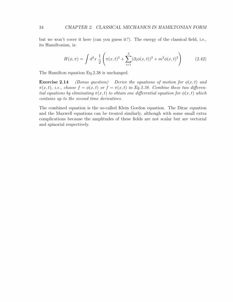
but we won’t cover it here (can you guess it?). The energy of the classical field, i.e.,its Hamiltonian, is:
H(φ, π) =
∫d3x
1
2
(π(x, t)2 +
3∑i=1
(∂iφ(x, t))2 +m2φ(x, t)2
)(2.42)
The Hamilton equation Eq.2.38 is unchanged.
Exercise 2.14 (Bonus question) Derive the equations of motion for φ(x, t) andπ(x, t), i.e., choose f = φ(x, t) or f = π(x, t) in Eq.2.38. Combine these two differen-tial equations by eliminating π(x, t) to obtain one differential equation for φ(x, t) whichcontains up to the second time derivatives.
The combined equation is the so-called Klein Gordon equation. The Dirac equationand the Maxwell equations can be treated similarly, although with some small extracomplications because the amplitudes of these fields are not scalar but are vectorialand spinorial respectively.

Chapter 3
Quantum mechanics in Hamiltonianform
We formulated the laws of classical mechanics on a higher level of abstraction, assummarized in Sec.2.4 because classical mechanics appeared to be not upgradeablewhen written in Newton’s formulation. We are now ready to upgrade the more abstractHamiltonian laws of classical mechanics to obtain quantum mechanics. A modificationis needed which is a small enough to preserve all the successes of classical mechanicswhile it must also introduce h in order to correctly predict quantum mechanical effects.
For example, could it be that Eq.2.38 needs to be modified to obtain quantum me-chanics? Could the correct equation be, say, d
dtf = f,H+h or d
dtf = f+h2/f,H,
where h is Planck’s constant? Those two equations can’t be right, of course, alreadybecause the units generally don’t match. Could it be then that to obtain quantummechanics we will have to change the definitions for the Poisson bracket? Could it bethat the definition Eq.2.12 needs to be changed? This, of course, is unlikely too becausethe definitions for the Poisson bracket were fixed by consistency conditions (recall, e.g.,Exercise 2.7). The structure of our Poisson algebra is quite tightly constrained.
No, the necessary upgrade of the Hamiltonian formalism is actually much moresubtle! Let us remember that when we defined the Poisson algebra structure in theprevious section we did not make any assumptions about the mathematical nature ofthe functions x(t) and p(t) (let us omit writing out the indices). In particular, we didnot make the assumption that these functions are number-valued. We can start witha Hamiltonian, i.e., a polynomial in the x and p and then by using the rules of thePoisson bracket we can derive the differential equations of motion. In the process, wenever need to assume that the functions x(t) and p(t) are number valued. Could itbe that the x(t) and p(t) need not be number valued and that this holds the key toupgrading classical mechanics to obtain quantum mechanics? Actually yes!
Before we get to this, we have to consider though that we actually did assume thex and p to be number valued at one specific point at the very end of the previouschapter. There, we wrote down a convenient representation of the Poisson bracket in
35

36 CHAPTER 3. QUANTUM MECHANICS IN HAMILTONIAN FORM
Eq.2.37, and there we needed the x and p to be number-valued - because to use thisconvenient representation we needed to be able to differentiate with respect to the xand p. We can conclude from this that if allowing the x(t) and p(t) to be something elsethan number valued is the key to upgrading to quantum mechanics, then the Poissonbracket will not be representable any more through Eq.2.37.
In fact, as we will see, this is how it will play out. Everything we did in theprevious chapter, except for the representation Eq.2.37 will still exactly hold true inquantum mechanics. In particular, the differential equations of motion derived fromthe Hamiltonian will look exactly the same in quantum and classical mechanics. That’sbecause they are derived from the same Hamiltonian polynomial in the x and p by usingthe same rules for the Poisson bracket. But then, if not in the equations of motion,how does the upgrade involve h at all?
3.1 Reconsidering the nature of observables
At this point, let us reconsider the very basics: How do the symbols we write on paperrelate to real systems? We measure a system with concrete measurement devicesin the lab, for example, devices for the measurement of positions and devices for themeasurement of momenta. As usual, we invent for each kind of measurement a symbol,say x
(r)i and p
(r)i . At this stage we need to be careful not to over-interpret these
symbols. At this stage, these symbols have nothing to do (yet) with numbers, vectors,matrices, operators or bananas. Instead, these symbols are merely names for kinds ofmeasurement. We need to find out more about the nature of these x
(r)i and p
(r)i .
Now according to our everyday experience, the operation of a position measurementdevice does not interfere with the operation of a momentum measurement device: itseems that we can always measure both, positions and momenta. For example, GPSunits are able to tell both position and velocity at the same time to considerableaccuracy. It is tempting to assume, therefore, that there is no limit, in principle, tohow accurately positions and velocities can be determined. And that would mean thatwe can let each of the symbols x
(r)i (t) and p
(r)i (t) stand for its measurement devices’s
output number at time t.It is at this very point, namely when we make the assumption that positions and
momenta can be accurately measured simultaneously, that we make the assumptionthat the symbols x
(r)i (t) and p
(r)i (t) can be represented mathematically as number-
valued functions of time. And number-valued functions have the property of beingcommutative:
x(r)i p
(s)j − p
(s)j x
(r)i = 0 (3.1)
Since measurement values cannot be just any number but always come out real, wealso have the law: (
x(r)i
)∗= x
(r)i and
(p
(s)j
)∗= p
(s)j (3.2)

3.2. THE CANONICAL COMMUTATION RELATIONS 37
Similarly, we have H∗ = H. Technically, the *-operation is an example of was is calledan involution.
Exercise 3.1 Find and list the defining property of an involution and give your source.The source is to be a textbook, and not a site such as Wikipedia. That’s becauseWikipedia is anonymous and therefore often inaccurate. Write out the answer andmake sure you understand the answer. Such material is considered examinable.
The statements above, namely that position and momentum measurements arecompatible and come out as real numbers are indeed a nontrivial part of the laws ofclassical mechanics. For completeness we should have included them in the summaryof classical mechanics in Sec.2.4.
A reality property of the form of Eq.3.2 will still be true in quantum mechanics.But the commutativity property expressed in Eq.3.1 and its underlying assumptionthat the operation of position and momentum measurement devices do not interferewith another needs to be abandoned and upgraded. It turns out that position andmomentum measurements are like taking a shower and working out at the gym. Itmatters in which sequence one does them:
gym·shower - shower·gym = sweat (3.3)
3.2 The canonical commutation relations
For the remainder of this course, we will need a way to make it transparent in everyequation whether a variable is number valued or not. To this end, we will decoratevariables that may not be number valued with a hat, for example, H, p, x, or morespecifically x
(r)i and p
(r)i for each position and momentum measurement device. Now
how can the interference of the measurement devices mathematically be expressed asproperties of the symbols x
(r)i and p
(r)i ?
According to classical mechanics one would be able to operate all measurement de-vices all the time and they would not interfere with another. We could therefore choosethe x
(r)i (t) and p
(r)i (t) to stand for the number-valued outcomes of those measurements
as functions of time. Crucially, the fact that we can’t actually know positions andmomenta simultaneously means that we can no longer choose the x
(r)i (t) and p
(r)i (t) to
stand simply for number-valued outcomes of those measurements as functions of time.Mathematically, it was the commutativity law of Eq.3.1 which expressed that in
classical mechanics the symbols x(r)i (t) and p
(r)i (t) can be represented as number valued
functions. Could it be that Eq.3.1 has to be modified to include h so that the x(r)i (t)
and p(r)i (t) become non-commutative and therefore can no longer be number-valued
functions?Are position and momentum measurements noncommuting similar to how doing
sports and having a shower don’t commute?

38 CHAPTER 3. QUANTUM MECHANICS IN HAMILTONIAN FORM
It was Dirac who first realized that all of the Poisson algebra structure that wedefined above can be kept (and therefore the ability to derive the equations of motion),
while changing just one little thing: allowing the symbols x(r)i (t) and p
(r)i (t) to be
noncommutative in a very particular way.Before we can follow Dirac’s argument, let us first reconsider the product rule for
the Poisson bracket:
f, gh = f, gh+ gf, h (3.4)
Using the antisymmetry rule, f, g = − g, f, the product rule can be rewritten inthis form:
gh, f = g, fh+ gh, f (3.5)
Using Eqs.3.4,3.5, we can now follow Dirac’s argument for why the Poisson algebrastructure imposes strict conditions on the form that any noncommutativity can take.Dirac considered the Poisson bracket
u1u2, v1v2 (3.6)
where u1, u2, v1, v2 are arbitrary polynomials in the variables x(r)i and p
(s)j . Expression
Eq.3.6 can be decomposed into simpler Poisson brackets in two ways, namely usingfirst Eq.3.4 and then Eq.3.5, or vice versa. And, of course, any noncommutativity ofthe x
(r)i and p
(s)j has to be such that both ways yield the same outcome:
u1u2, v1v2 = u1u2, v1v2+ u1, v1v2u2 (3.7)
= u1(v1u2, v2+ u2, v1v2) + (v1u1, v2+ u1, v1v2)u2
must agree with:
u1u2, v1v2 = v1u1u2, v2+ u1u2, v1v2 (3.8)
= v1(u1u2, v2+ u1, v2u2) + (u1u2, v1+ u1, v1u2)v2
We can, therefore, conclude that, independently of whether or not we have commuta-tivity, it must always be true that:
u1, v1(v2u2 − u2v2) = (v1u1 − u1v1)u2, v2 (3.9)
And this equation has to be true for all possible choices of u1, u2, v1, v2. How can weensure this? As is easy to check, Eq.3.9 will be true1 if we require all expressions u, vin the position and momentum variables obey:
vu− uv = ku, v (3.10)
1We will not show here that, vice versa, only the condition Eq.3.10 ensures that Eq.3.9 holds true.If you are interested, there is plenty of literature on the topic of “quantization”.

3.2. THE CANONICAL COMMUTATION RELATIONS 39
with k being some constant that commutes with everything. This is because in thiscase, the left and right hand sides of Eq.3.9 are automatically identical. But whatvalue does k take? Of course, the case k = 0 would be classical mechanics, because itimplies that all expressions in the positions and momenta commute.
However, it turns out that in order to eventually yield the correct experimentalpredictions (we will later see how), we have to set k = −ih/2π, i.e., we have
uv − vu = i~u, v (3.11)
where we used the convenient definition:
~ =h
2π(3.12)
In particular, choosing for u and v the variables x(r)i and p
(s)j , and using Eqs.2.6-2.8,
we now obtain the quantum mechanical commutation relations for n particles:
x(r)i p
(s)j − p
(s)j x
(r)i = i~ δi,jδr,s (3.13)
x(r)i x
(s)j − x
(s)j x
(r)i = 0 (3.14)
p(r)i p
(s)j − p
(s)j p
(r)i = 0 (3.15)
Let us keep in mind that we did not modify the rules of the Poisson bracket. We stillhave:
xi, pj = δi,j (3.16)
xi, xj = 0 (3.17)
pi, pj = 0 (3.18)
f, g = − g, f antisymmetry (3.19)
cf, g = c f, g, for any number c linearity (3.20)
f, g + h = f, g+ f, h addition rule (3.21)
f, gh = f, gh+ gf, h product rule (3.22)
0 = f, g, h+ h, f, g+ g, h, f Jacobi id. (3.23)
Because the rules for the Poisson bracket did not change with the upgrade to quantummechanics, one arrives in quantum mechanics at the same equations of motion asin classical mechanics. This is as long as one does not unnecessarily commute anyvariables.
The equations Eqs.3.13-3.15 are called the “Canonical Commutation Relations”(CCRs). The appearance of the imaginary unit i will be necessary to ensure that mea-surements are predicted as real numbers, as we will see below. Eqs.3.14,3.15 express

40 CHAPTER 3. QUANTUM MECHANICS IN HAMILTONIAN FORM
that position measurements among another and momentum measurements among an-other do not interfere. Only positions and momenta of the same particle and in thesame direction, i.e., for i = j and r = s, are noncommutative.
In conclusion, we upgrade classical mechanics to quantum mechanics by first formu-lating classical mechanics in Hamiltonian form to identify the Poisson algebra structure.Then, we realize that while keeping all the rules for the Poisson bracket intact, thereis still the freedom to make the associative multiplication in the Poisson algebra non-commutative, parametrized by some constant k. Nature chose the modulus of k to benonzero though very small, namely ~. The fact that the Poisson bracket stays the samewhen quantizing explains why quantum mechanics has the same equation of motionas does classical mechanics. The fact that ~ is so small explains why it took long todiscover quantum mechanics.
In spite of the tremendous similarity between classical and quantum mechanics fromthis perspective, quantum mechanical calculations will in practise look rather differentfrom classical calculations. This is because they will require representations of thex
(r)i (t) and p
(r)i (t) variables as explicit non-number valued mathematical entities that
obey the commutation relations. Even though there is only a slight noncommutativityin the Poisson algebra of quantum mechanics its representations will necessarily lookquite different from the representation of the classical commutative Poisson algebra.This will explain why the Schrodinger equation looks rather different from Newton’sequations.
3.3 From the Hamiltonian to the equations of mo-
tion
In quantum mechanics, as in classical mechanics, the energy function H encodes allinformation about the system. It is still called the Hamiltonian and it is in generalsome polynomial (or well-behaved power series) in the positions and momenta x
(r)i
and p(r)i of the system. In quantum mechanics, the sequence of steps that lead from
the Hamiltonian down to concrete number predictions for experiments can be drawnschematically in this form:
Hamiltonian⇓
Equations of motion⇓
Differential equations⇓
Non-number-valued functions⇓
Number-valued functions

3.3. FROM THE HAMILTONIAN TO THE EQUATIONS OF MOTION 41
⇓Number predictions
So far, we can perform the first step, namely the derivation of the equations of motionfrom the Hamiltonian: Assume that we are interested in the time evolution of some fwhich is a polynomial in the x and p’s (say with constant coefficients). Then we canderive the equation of motion for f through:
d
dtf = f , H (3.24)
where , is the usual Poisson bracket, as defined in Eqs.2.6-2.12. In particular, f canbe chosen to be any one of the position and momentum variables of the system, so thatwe obtain for their equations of motion, exactly as in Eqs.2.21,2.22:
d
dtx
(r)i = x(r)
i , H (3.25)
d
dtp
(r)i = p(r)
i , H (3.26)
By evaluating the Poisson bracket on the right hand side of Eqs.3.25,3.26 these equa-tions of motion then become differential equations for the entities x
(r)i (t) and p
(r)i (t).
Clearly, the resulting equations of motion will be analogous to those of classical me-chanics. The entities x
(r)i (t) and p
(r)i (t) must also still obey Eq.3.2, which in quantum
mechanics is usually written as:(x
(r)i
)†= x
(r)i and
(p
(s)j
)†= p
(s)j (3.27)
We will call any polynomial or well-behaved power series f in the x and p an “observ-able”, if it obeys f † = f . As we will see later, the condition f † = f will indeed implythat measurement outcomes are predicted as real numbers. In addition to the positionvariables x
(r)i (t) and momentum variables p
(s)j (t) also, e.g., the energy H(t) and the
angular momentum variables Li(t) are observables.
While classical mechanics requires the Poisson algebra to be commutative, quantummechanics requires that the equations of motion be solved by entities x
(r)i (t) and p
(r)i (t)
which are noncommutative:
x(r)i p
(s)j − p
(s)j x
(r)i = i~ δi,jδr,s (3.28)
x(r)i x
(s)j − x
(s)j x
(r)i = 0 (3.29)
p(r)i p
(s)j − p
(s)j p
(r)i = 0 (3.30)

42 CHAPTER 3. QUANTUM MECHANICS IN HAMILTONIAN FORM
Technically, we will, therefore, need to solve differential equations of motion with non-commutative entities. In practice, the task is then to start from the top level ofabstraction, the Hamiltonian of a system, then working one’s way down by calculat-ing the equations of motion, and then solving them to obtain something from whicheventually predictions can be made of numbers that can be measured in experimentson the system. In the next section, we will investigate what kind of noncommutativemathematical objects, such as, for example, matrices, may represent the position andmomentum variables.
Exercise 3.2 For classical mechanics, formula Eq.2.37 provided a convenient repre-sentation of the Poisson bracket. However, Eq.2.37 is not a valid representation of thePoisson bracket in the case of quantum mechanics. In quantum mechanics, we have a(not so convenient) representation of the Poisson bracket through Eq.3.11:
u, v =1
i~(uv − vu) (3.31)
Use this representation, and the canonical commutation relations to evaluate the Pois-son bracket x2, p.
Let us introduce an often-used notation, called “the commutator”:
[A,B] := A B − B A (3.32)
For simplicity, assume that H and f are polynomials in the positions and momentawhich depend on time only through their dependence on the x and p. Then theHamilton equation Eq.3.24 holds and takes the form:
i~d
dtf(t) = [f(t), H] (3.33)
(3.34)
and, in particular:
i~d
dtx
(r)i (t) = [x
(r)i (t), H]
i~d
dtp
(r)i (t) = [p
(r)i (t), H] (3.35)
These equations are called the Heisenberg equations of motion.
Remark: The particular method by which in the past few sections we upgradedclassical mechanics to quantum mechanics is called canonical quantization. I covered it

3.3. FROM THE HAMILTONIAN TO THE EQUATIONS OF MOTION 43
in some detail because of its importance: Essentially the same method was used to findquantum electrodynamics starting from Faraday and Maxwell’s electromagnetism. Allthe quantum field theories of elementary particles can be derived this way. Even stringtheory and most other modern attempts at finding the unifying theory of quantumgravity try to employ canonical quantization. I should mention too that the problemof canonical quantization for constrained classical systems was also pioneered by Diracbut is still not fully understood. A simple example of a constrained system wouldbe a particle that is constrained to move on a curved surface. The most importantconstrained system is general relativity.
Exercise 3.3 Reconsider the system with the Hamiltonian Eq.2.4, which consists oftwo particles that are attracted to another through a harmonic force (a force which isproportional to their distance). In practice, for example the force that binds diatomicmolecules and the force that keeps nucleons (i.e., neutrons and protons) inside a nucleusare approximately harmonic for small oscillations. In those cases, the effect of ~ cannotbe neglected. One obtains the correct quantum theoretic Hamiltonian from the classicalHamiltonian of Eq.2.4 by simply placing hats on the x and p’s. Find explicitly all theequations of motion which the x
(r)i and p
(r)j (where r ∈ 1, 2) of this system must obey.
Exercise 3.4 To obtain the quantum Hamiltonian from the classical Hamiltonian andvice versa by placing or removing hats on the x and p’s is generally not as straight-forward as in the previous exercise! Namely, there can occur so-called “ordering am-biguities”: Consider the two Hamiltonians H1 = p2/2m + a(x2px − xpx2) and H2 =p2/2m + b(pxp2 − p2xp) where a and b are constants with appropriate units. Checkwhether or not these two Hamiltonians are the same in classical mechanics. Also findall choices of a, b for which the two Hamiltonians are the same in quantum mechanics.
Exercise 3.5 Find a Hamiltonian which contains at least one thousand powers of xand which also agrees with the Hamiltonian H1 of the previous exercise in classicalmechanics. Make sure that your Hamiltonian is formally hermitean, i.e., that it obeysH† = H. Help: To ensure hermiticity, you can symmetrize. For example, xp2 is nothermitean but (xp2 + p2x)/2 is hermitean.
Remark: In quantum theory, the choice of Hamiltonian always has an ordering am-biguity because one could always add to the Hamiltonian any extra terms that areproportional to (xp− px) because those terms don’t affect what the Hamiltonian is inclassical mechanics. In principle, experiments are needed to decide which Hamiltonianis the correct one. In practice, the simplest choice is usually the correct choice. Thesimplest choice is obtained by symmetrizing the given classical Hamiltonian and thennot adding any extra terms that are proportional to xp− px. This is called the Weylordered Hamiltonian.

44 CHAPTER 3. QUANTUM MECHANICS IN HAMILTONIAN FORM
3.4 From the Hamiltonian to predictions of num-
bers
In the framework of classical mechanics we know how to descend from the most abstractlevel, where the system is described simply by giving its Hamiltonian H, down tothe concrete level of predicting numbers for measurement outcomes. Now we willhave to develop methods for descending in quantum mechanics from the level of theHamiltonian down to the concrete predictions of numbers in experiments.
In the previous section, we already took the first step: we found that we can usethe Hamiltonian to derive the differential equations of motion of the system. Since thePoisson brackets have not changed as we went from classical to quantum mechanics,the equations of motion are the same as those of classical mechanics2.
The big change compared to classical mechanics, is that now the position andmomentum variables x
(r)i (t) and p
(s)j (t) are noncommutative according to Eqs.3.28-3.30,
and that they, therefore, can no longer be represented by number-valued functionsof time. This means that the equations of motion can no longer be interpreted asdifferential equations for number-valued functions!
But we need to find a way to descend the ladder of abstractions all the way fromthe Hamiltonian on the top of the ladder down to concrete predictions of numbers atthe bottom of the ladder. To that end, in order now to be able to solve the equationsof motion as explicit differential equations, the x
(r)i (t) and p
(s)j (t) must be viewed as
functions of time whose values are some kind of noncommutative mathematical objects.What kind of mathematical objects could these be?
3.4.1 Linear maps
Actually, every mathematical object can be viewed as a map, if need be, as a trivialmap. For example the number 5 can be identified with the map that maps everythingto 5. So let us look at maps. Let’s try to represent the symbols x
(r)i (t) and p
(s)j (t) as
some kind of explicit map-valued functions of time. A simple kind of maps is the linearmaps. And they can be noncommutative! So this looks promising.
For example, any square matrix that acts on a finite-dimensional vector space ofcolumn vectors represents a linear map. And square matrices are generally noncom-mutative! In principle, we need the matrices to be square matrices so that they mapback into the same vector space, so that we can multiply any two matrices on the samevector space. As we will see later, with some precautions, we can also consider infinite-by-infinite matrices that act as linear maps on infinite-dimensional vector spaces.
2Except for the ordering ambiguity: when going from the classical to the quantum Hamiltonian wecould (if we had any experimental reason to do so) add to the quantum Hamiltonian any hermiteanterms that are proportional to ~, such as terms like ig(x)(xp − px)g(x) where g is some polynomialin x.

3.4. FROM THE HAMILTONIAN TO PREDICTIONS OF NUMBERS 45
There are actually many kinds of linear maps and they may not act on vector spacesof column vectors at all!
Let us consider, for example, the infinite-dimensional vector space V := C7(R) ofseven times continuously differentiable functions on the real line. The set V forms avector space because it obeys the defining axioms of a vector space: in brief, one cansuitably add any two elements of V and get an element of V and one can suitablymultiply any element of V with a number and get an element of V .
Exercise 3.6 Find and list the precise axioms that a set has to obey to be called avector space.
Definition: A map on a vector space that is infinite dimensional is called an operator.
For example, the derivative operator, D, acts on functions in V in this way:
D : g(λ)→ d
dλg(λ) (3.36)
The operatorD is a linear operator, i.e., it is a linear map, because it obeys ∂λ (c g(λ)) =c ∂λg(λ) for all numbers c and because ∂λ(g1(λ) + g2(λ)) = ∂λg1(λ) + ∂λg2(λ). Here,in order to simplify the notation, we introduced the notation: ∂λ := d
dλ
Exercise 3.7 Check whether or not the multiplication operator, M , which maps M :g(λ)→ λg(λ) is a linear operator.
Exercise 3.8 Show that the two operators D and M on V do not commute, namelyby calculating (DM −MD)g(λ).
Exercise 3.9 Check whether or not the operator Q which acts on functions in V asQ : g(λ)→ λ5g(λ) is a linear operator.
3.4.2 Choices of representation
We have just seen examples of linear maps and, since they generally do not commute,they may be useful for representing the variables x
(r)i (t) and p
(s)j (t) as explicit math-
ematical objects. And this is what we need to be able to descend further down theladder of abstractions, down to predictions of numbers for measurement outcomes.
But could it be that one should use representations of the x(r)i (t) and p
(s)j (t) as
nonlinear maps instead? Non-linear representations have been considered in the liter-ature. There are articles by Steven Weinberg, for example, on this topic. This workhas shown, however, that any attempt at using nonlinear spaces or nonlinear operatorsto define quantum theories generally leads to physically incorrect predictions. We will,therefore, here only consider linear representations.

46 CHAPTER 3. QUANTUM MECHANICS IN HAMILTONIAN FORM
Now that we have settled on representations of the variables x(r)i (t) and p
(s)j (t) as
linear operators, we still have plenty of choice, because there are so many vector spacesand so many linear operators on them. And this leads to a worry: could it happen thatwe invest great effort in developing one particular kind of representation of the variablesx
(r)i (t) and p
(s)j (t) as operators, say as matrices, and then it turns out that we have bet
on the wrong horse? Maybe, we should have instead developed a representation of thex
(r)i (t) and p
(s)j (t) as, for example, multiplication and differentiation operators?
Fortunately, essentially3 all linear representations of variables x(r)i (t) and p
(s)j (t) that
obey the canonical commutation relations are equivalent, i.e., they lead to the exactsame predictions! This is the content of the Stone von Neumann theorem, which wewill later cover more precisely. Technically, as we will see, all linear representationsare the same, up to a change of basis in the vector space. It may seem strange that,for example, a space of column vectors with countably infinitely many entries could beisomorphic to some space of functions on the real line. But this is what will turn outto be the case4!
So to recapitulate: our task is to solve the equations of motion, the hermiticityconditions and the canonical commutation relations for x
(r)i (t) and p
(s)j (t) as linear-
map-valued (instead of number-valued) functions of time.
We now know that the choice of which kind of linear representation we use willultimately not matter when calculating physical predictions.
As our first choice, let us, therefore, use the most concrete kind of linear maps torepresent the x
(r)i (t) and p
(s)j (t), namely, let us try to represent them as matrix-valued
functions in time. Historically, quantum mechanics was actually first written down interms of matrix-valued functions, back in June 1925 when the young Heisenberg hadsome quiet time while escaping his hay fever on the island of Helgoland in the NorthSea.
3.4.3 A matrix representation
Let us now find out how the variables x(r)i (t) and p
(s)j (t) can be represented as matrix-
valued functions in time, and how, therefore, the abstract equations of motion canbe represented as explicit matrix differential equations for matrix-valued functions oftime. To keep the number of indices in check, we will restrict ourselves here to the caseof just one x(t) and one p(t) operator.
3There is a small subtlety, arising from the fact that, as we’ll see later, the x and p are what arecalled unbounded operators. This leaves some loopholes, in principle, but nature does not appear tomake use of those.
4If you want to know the essence already: the space of functions will be the set of equivalence classesof square-integrable functions, two functions being in the same equivalence class if their difference hasvanishing integral over its norm squared. In this space of equivalence classes one can find bases ofcountably infinitely many basis vectors.

3.4. FROM THE HAMILTONIAN TO PREDICTIONS OF NUMBERS 47
The canonical commutation relations are of course to hold at all times. To beginwith, let us ask whether it is possible to find two N × N matrices x(t0) and p(t0) sothat at the starting time, t0, of the experiment the canonical commutation relationshold:
x(t0) p(t0) − p(t0) x(t0) = i~ 1 (3.37)
Here, 1 is the identity matrix. At this point it is useful to remember that the trace ofmatrices Tr(A) =
∑nAn,n is linear and cyclic:
Tr(A+B) = Tr(A) + Tr(B) and Tr(AB) = Tr(BA) (3.38)
Exercise 3.10 Verify Eqs.3.38 by writing the matrices in an orthonormal basis, i.e.,with indices, and by then evaluating the trace by summing up the matrix elements onthe diagonal.
We see that the trace of the left hand side of Eq.3.37 vanishes, while the trace of theright hand side is i~N . Thus, there are in fact no N × N matrices, i.e., there are nofinite-dimensional matrices x(t0) and p(t0) that obey the commutation relation Eq.3.37!For infinite dimensional matrices, however, the trace may be ill-defined on both sides,and our argument then does not apply. In fact, there exist infinite-dimensional matriceswhich do obey the commutation relation.
In order to find such matrices we start by defining the ∞×∞ dimensional matrix:
an,m =
0√
1 0 0 00 0
√2 0 0
0 0 0√
3 00 0 0 0
√4
0 0 0 0 0. . .
n,m
(3.39)
The hermitean conjugate is:
a†n,m =
0 0 0 0 0√1 0 0 0 0
0√
2 0 0 00 0
√3 0 0
0 0 0√
4 0. . .
n,m
(3.40)
Their commutation commutation relation is:
aa† − a†a = 1 (3.41)

48 CHAPTER 3. QUANTUM MECHANICS IN HAMILTONIAN FORM
Since they are not numbers, we should decorate a and a† with hats but traditionallyone doesn’t put hats on these operators.
Remark: In case you are wondering because you feel that you have seen similar thingsbefore: fundamentally, these operators a and a† have absolutely nothing to do withharmonic oscillators. What we are currently doing will be good for any choice of system,not just harmonic oscillators. We are currently developing a representation of thevariables x(t) and p(t) as matrices and this representation will, of course, be good forany arbitrary choice of Hamiltonian5.
Exercise 3.11 Verify Eq.3.41.
Using a and a†, we can now represent x(t0) and p(t0) as matrices that obey the canonicalcommutation relation, namely by defining:
x(t0) = L(a† + a) (3.42)
and
p(t0) =i~2L
(a† − a) (3.43)
Here, L is some arbitrary real number with units of length, which we need because xhas a unit of length while a and a† do not have units. The definitions are such thatthe realness conditions Eqs.3.27 are obeyed, i.e., such that the matrices are formally6
hermitean: x†(t0) = x(t0) and p†(t0) = p(t0).
Exercise 3.12 Verify that the two matrices defined in Eqs.3.42,3.43 with the help ofEqs.3.39,3.40, are formally hermitean. I am using the term “formally” here to indicatethat, for the purposes of this exercise, you need not worry about potential subtleties thatmay arise because these matrices are infinite dimensional.
Exercise 3.13 Show that the hermitean conjugation of matrices reverses the order,i.e., that if A and B are linear maps, then (AB)† = B†A†. To this end, write out thematrices with indices and use that hermitean conjugating a matrix means transposingand complex conjugating it.
Technically, † is a map from the Poisson algebra into itself which is called an involutionbecause it is its own inverse. Because it also reverses the order it is called an “anti”algebra mapping: First multiplying and then applying † is the same as first applying †
and then multiplying, up to the reversal of the order.We see, therefore, why the imaginary unit i appeared in the canonical commutation
relations: If we apply † to the commutation relations xp− px = k1 we obtain px− px =k∗1, i.e., we obtain k = −k∗. Thus, k has to be imaginary. And of course it is: k = i~.
5Still, it is true also that the use of the a and a† will be particularly convenient when consideringthe special case of harmonic oscillators.
6I am writing here “formally” hermitean, because the issue of whether a matrix is hermitean,symmetric or self-adjoint is quite subtle for infinite-dimensional matrices, as we will see later.

3.4. FROM THE HAMILTONIAN TO PREDICTIONS OF NUMBERS 49
3.4.4 Example: Solving the equations of motion for a freeparticle with matrix-valued functions
In the case of the free particle which moves in one dimension, the Hamiltonian isH = p2/2m. The Hamilton equations or, equivalently, the Heisenberg equations, yieldthe abstract equations of motion:
d
dtx(t) =
1
mp(t) (3.44)
d
dtp(t) = 0 (3.45)
Let us view these equations as matrix equations. Using the results of the previoussection, it becomes clear that these equations are solved through
x(t) = x(t0) +(t− t0)
mp(t0) (3.46)
andp(t) = p(t0), (3.47)
where x(t0) and p(t0) are the matrices of Eqs.3.42,3.43. Concretely, by substituting inthe matrices a and a†, we have:
x(t)n,m =
0
√1(L− i~(t−t0)
2Lm
)0
√1(L+ i~(t−t0)
2Lm
)0
√2(L− i~(t−t0)
2Lm
)0
√2(L+ i~(t−t0)
2Lm
)0
. . .
(3.48)
p(t)n,m =
0 −
√1 i~
2L0√
1 i~2L
0 −√
2 i~2L
0√
2 i~2L
0. . .
(3.49)
For simplicity, not all the many zeros in these matrices are shown. The only nonzeroterms are immediately to the left and right of the diagonal.
Exercise 3.14 Show that the matrices x(t) and p(t) obey at all times t > t0 all thequantum mechanical conditions, i.e., the equations of motion, the hermiticity condition,and the commutation relation.
Remark: We had constructed the representation in such a way that the commuta-tion relation and the hermiticity condition hold at the initial time t0. Having solved

50 CHAPTER 3. QUANTUM MECHANICS IN HAMILTONIAN FORM
the equations of motion we found that the commutation relation and the hermitic-ity conditions continue to hold at all times t. This is nontrivial but it is not a co-incidence. As we will soon see, the quantum mechanical time evolution of all sys-tems7 preserves the commutation relations and hermiticity. The preservation of thecommutation relations is of course the preservation of the Poisson bracket. And wehave in classical and quantum mechanics that the Poisson brackets between the po-sitions and momenta are preserved by the dynamics through the Hamilton equation:d/dt x, p = x, p, H = 1, H = 0. We can also turn the logic around. Assumewe know nothing about Hamiltonians and about the dynamics of quantum systems.Except, we may want to assume that, whatever the time evolution is, it must preservethe Poisson algebra structure, i.e., we require that the Poisson brackets be conserved intime. The structure of the Poisson algebra then demands (we don’t show this explicitlyhere) that the time evolution must be generated through an equation of the type ofthe Hamilton equation, by some generator which we may call H, and which we maythen as well call the Hamiltonian.
3.4.5 Example: Solving the equations of motion for a har-monic oscillator with matrix-valued functions
The vibrational degree of freedom of a diatomic molecule such as HF, CO or HCl canbe described as a harmonic oscillator (as long as the oscillations are small). Now letx stand for the deviation from the equilibrium distance between the two nuclei. Thisdistance oscillates harmonically and is described by this effective Hamiltonian of theform of a harmonic oscillator:
H =p2
2m+mω2
2x2 (3.50)
The term “Effective Hamiltonian” expresses the fact that this Hamiltonian is not reallythe exact Hamiltonian but that it is a good approximation to the Hamiltonian in theregime of low energies (i.e., of small oscillations) that we are considering here. By theway, how do we know that the true Hamiltonian is not simply a harmonic oscillator?Easy: we know from experiments that diatomic molecules will, for example, split apartat sufficiently high temperatures, i.e., that they do not have infinite binding energy.A harmonic oscillator potential, however, just keeps going up faster with distance andtherefore if you tried to pull apart the two particles in the diatomic molecule, theywould just get pulled together more and more strongly. Diatomic molecules couldnever be split if they were truly harmonically bound.
So then if we know that the true potential is not harmonic, how do we knowthat a harmonic potential is a good approximation at low energies? That’s because
7With the possible exception of systems that involve black hole horizons or other gravitationalhorizons or singularities.

3.4. FROM THE HAMILTONIAN TO PREDICTIONS OF NUMBERS 51
any potential V (x) is normally well described by a smooth function V (x) with aminimum at, say x0, around which we can Taylor expand the potential: V (x) =V (x0) + V ′(x0)(x − x0) + 1
2V ”(x0)(x − x0)2 + .... Here, V ′(x0) = 0 because x0 is as-
sumed to be the minimum and therefore in the regime of small oscillations, where x isclose to x0, any potential starts out quadratic, i.e., as a harmonic oscillator.
Now let us remember that the matrix-valued functions x(t) and p(t) that we wantto solve the harmonic oscillator problem Eq.3.50 have to obey three conditions, asalways in quantum theory. First, the matrix-valued functions x(t) and p(t) must obeythe equations of motion of the harmonic oscillator given in Eq.3.50. Second, theymust be hermitean, x(t) = x†(t) and p(t) = p†(t). Third, they must obey the canonicalcommutation relation [x(t), p(t)] = i~1 (where 1 is now to be represented by the identitymatrix).
Now the first problem would seem easy to solve: we know that the equations ofmotion are solved any linear combination of sin(ωt) and cos(ωt). But these are justnumber-valued functions and cannot by themselves obey the commutation relations!On the other hand, we do have matrices a and a† that are beautifully noncommutative.But they are constant in time and therefore cannot alone describe the dynamics givenby the equations of motion. This suggests that we try to construct the solution bycombining the a and a† matrices with the sine and cosine solutions. Let’s try thisansatz8
x(t) = ξ(t)a+ ξ∗(t)a†, (3.51)
and let us choose ξ(t) to be a linear combination of the sine and cosine solutions tothe equations of motion:
ξ(t) := r sin(ωt) + s cos(ωt) (3.52)
Here, for now, r and s can be any complex numbers. By the way, whenever one makesan ansatz of this kind (and one often does, especially in quantum field theory), then ξ(t)is called a mode function. The task now is to find out if we can find coefficients r ands such that the matrix-valued function x(t) and the corresponding p(t) = m ˙x(t) obeythe equations of motion, are hermitean and obey the canonical commutation relation.
Exercise 3.15 Show that for any arbitrary choice of complex numbers r, s, the matrix-valued functions x(t) and p(t) defined through Eqs.3.51,3.52 obey the equations of mo-tion at all time.
Exercise 3.16 Show that, again for any arbitrary choice of complex numbers r, s, thematrix-valued functions x(t) and p(t) defined through Eqs.3.51,3.52 obey the hermiticityconditions at all time.
8An ansatz is an educated guess.

52 CHAPTER 3. QUANTUM MECHANICS IN HAMILTONIAN FORM
Exercise 3.17 Find the equation that the complex numbers r, s have to obey so thatthe matrix-valued functions x(t) and p(t) defined through Eqs.3.51,3.52 obey the canon-ical commutation relations at all time. This equation for r, s is called the Wronskiancondition and it has many solutions. Give an example of a pair of complex numbersr, s that obey the Wronskian condition and write down x(t) explicitly with these valuesfor r, s filled in.
Since there are many pairs r, s that obey the Wronskian condition, our ansatz givenby Eqs.3.51,3.52 allows us to generate many solutions! We knew that there are alwaysmany linear representations of x(t) and p(t) in quantum theory (and that they are allphysically equivalent because they are all related by changes of bases). Here, with ouransatz we have found already infinitely many of these representations of x(t) and p(t)for the harmonic oscillator. Actually, among the representations that we just found,some representations are particularly convenient and most of the time one uses one ofthose. These choices of r, s turn out to be convenient because the matrix-representationof the Hamiltonian H(t) is much simpler for clever choices of r, s than for other choices.
Exercise 3.18 Use Eqs.3.51,3.52 to express the Hamiltonian in terms of functionsand the operators a, a†. There should be terms proportional to a2, to (a†)2, aa† and a†a.
Exercise 3.19 It turns out that it is possible to choose the coefficients r and s so thatthe terms in the Hamiltonian which are proportional to a2 and (a†)2 drop out. Findthe condition which the equation that r and s have to obey for this to happen. Choosea pair of complex numbers r, s such that the Hamiltonian simplifies this way, and ofcourse such that the Wronskian condition is obeyed. Write down H(t) as an explicitmatrix for this choice of r, s. It should be a diagonal matrix.
Remark: Notice that this convenient choice of r, s depends on the parameters m andω of the harmonic oscillator. This means that each harmonic oscillator has its ownoptimal choices of parameters r, s. Making such wise choices of the parameters r, sis particularly useful in quantum field theory where each wavevector (and thereforefrequency ω) of a quantum field has its own harmonic oscillator degree of freedom,and should therefore best have its own convenient choice of r, s that diagonalizes itsHamiltonian.
3.4.6 From matrix-valued functions to number predictions
Let us assume now that we have solved a quantum mechanical problem in the sensethat we have found explicit matrix-valued functions x
(r)i (t) and p
(j)j (t) which obey
the canonical commutation relations, the hermiticity conditions, and the equations ofmotion. For example, the quantum mechanical problem of the free particle in onedimension is solved by the matrix-valued functions given in Eqs.3.48,3.49.

3.4. FROM THE HAMILTONIAN TO PREDICTIONS OF NUMBERS 53
How then are we to further descend the ladder of abstraction, down to the mostconcrete level, namely that of predictions of numbers that will be measured in experi-ments? How can we extract from those matrix-valued functions the information whichwill let us predict the outcome of say a position or a momentum measurement at sometime t?
To this end, assume that we have solved the dynamics, i.e., that we have calculatedx(t) and p(t) as explicit matrix-valued functions of time. Then we can also immediatelywrite down the time evolution of any polynomial f(x(t), p(t)) of the x(t) and p(t)that we may be interested in. For example, we can write down the time evolution ofthe Hamiltonian H(x(t), p(t)) or say the first component of the angular momentum:L3(t) = x2(t)p3(t)− p2(t)x3(t).
Mathematically, the problem now boils boils down to this question: Given sucha matrix valued function f(x(t), p(t)), let us pick a time t. Then f(x(t), p(t)) at thetime t is an explicit infinite-by-infinite matrix. How can we extract from that matrixa prediction for the number-valued outcome, f(t), of an experiment that measures f?For example, say we want to measure the position at time t. Given the matrix x(t) bywhat method can we extract from that matrix a prediction for the position x(t)?
To find that method, let us start with the observation that the method by whichwe extract a number-valued prediction f(t) from a matrix f(t) should not depend onthe basis in which we write down the matrix f(t). The reason is that a change of basisin a vector space yields merely another way to write down the same linear map. Andphysical predictions should not depend on any human choice of how (i.e., in whichbasis) to write down a map. This means that f(t) should be a scalar formed from thematrix f(t).
Now how can one get a scalar from a matrix? By using the scalar product of course.So assume that we are given two column vectors with coefficients ψi and φi. Then
∞∑n,m=1
ψ∗nfn,m(t)φm (3.53)
is scalar. Could this be the prediction for the measurement outcome? No this cannotbe quite right because this quantity is generally complex while measurement outcomesare of course always real numbers. This leaves us with the conjecture that the predicted

54 CHAPTER 3. QUANTUM MECHANICS IN HAMILTONIAN FORM
value, which we will denote by f(t) for a measurement of f(t) at time t, is9 of the form:
f(t) =∞∑
n,m=1
ψ∗nfn,m(t)ψm (3.54)
Now that we are using the same vector left and right, this number is guaranteed tobe real for all quantities f which are hermitean, f † = f , i.e., for all quantities that inclassical mechanics are real-valued, as it should be.
Let us check that Eq.3.54 always comes out real if f is what is called an observable,i.e., if f obeys f † = f , i.e., if f ∗s,r = fr,s. Indeed10:
f(t)∗ =
(∞∑
r,s=1
ψ∗r fr,s(t)ψs
)∗=
∞∑r,s=1
ψrf∗r,s(t)ψ
∗s =
∞∑r,s=1
ψ∗s fs,r(t)ψr = f(t) (3.55)
So this works! And, for example, the predictions for measurements at time t of theposition, momentum, angular momentum or energy are, therefore:
x(t) =∞∑
n,m=1
ψ∗nxn,m(t)ψm (3.56)
p(t) =∞∑
n,m=1
ψ∗npn,m(t)ψm (3.57)
L(i)(t) =∞∑
n,m=1
ψ∗nL(i)n,m(t)ψm (3.58)
H(t) =∞∑
n,m=1
ψ∗nHn,m(t)ψm (3.59)
9There is a more general possibility: clearly, f should depend on f linearly (they have the same
units) and this leaves the possibility that f(t) = Tr(ρf(t)) =∑i,j ρi,j fj,i(t) where ρ is some hermitean
matrix. As we will see, we will make use of this possibility when describing a system whose initialconditions we are not quite sure of, where we can only give probabilities of initial conditions, i.e.,where we don’t even know for sure even the initial expectation values of the various observables. Inthis case, we say that the system is described by a mixed state and the matrix ρ is called the mixedstate matrix. The term “mixed” is used because the uncertainties in predictions then have mixedorigins - both from quantum effects but also from our ignorance of the system to start with. What weconsider so far are so-called pure states ψ, which are the special case where ρi,j = ψ∗i ψj . For generalρ, the normalization condition
∑i ψ∗i ψi = 1 is replaced by Tr(ρ) = 1.
10This argument is correct for finite-dimensional matrices only. Quantum mechanics requiresinfinite-dimensional matrices where the sums are infinite sums and analytic issues therefore arise.That there is a fundamental difference between finite and infinite-dimensional vector spaces we sawearlier when we found that the canonical commutation relations do not possess finite-dimensionalrepresentations. We will, therefore, later revisit the issue of hermiticity.

3.5. INITIAL CONDITIONS 55
3.5 Initial conditions
In order to obtain those scalar functions for predictions, f(t), we had to introduce acomplex vector with infinitely many coefficients!
ψn =
ψ1
ψ2
ψ3...
(3.60)
We are free to choose ψ, and it is a convention to choose a vector ψ of unit length, i.e.,for which
∑∞n ψ∗nψn = 1. We call such vectors normalized. For example, the vector ψ
could be given by:
ψn =1
5
43i00...
(3.61)
There are, of course, infinitely many choices for such vectors ψ. But what does makinga choice of such a vector ψ mean? What is the physics of that choice?
Obviously the choice of ψ determines the predictions that we make for all possiblemeasurements at any time t! The choice of ψ in fact even determines what the expectedoutcome is for measurements at the initial time t0! And this last observation revealswhat the choice of the vector ψ means physically: the choice of ψ is the choice of initialconditions!
Remember that when we solved the equations of motion to obtain those matrix-valued functions x(t) and p(t), we did not have an opportunity to specify the initialconditions of the experimental setup. We did not have an opportunity to specify, forexample, whether the particle was initially, i.e., at the time t0, fast or slow, or wherethe particle was at the initial time t0.
Now we have an opportunity to specify how the system started off at time t0: Thechoice of ψ encodes our specification of the initial state of the system: by choosinga vector ψ we are choosing an experimental starting condition at time t0. Namely,by choosing ψ, we are choosing what measurement outcomes to expect if we measureany arbitrary observable, f , right at the initial time t0. Since there are infinitely manyobservables, it is plausible that we get to choose infinitely coefficients in ψ to fix theirinitial conditions. For example, some of these observables are:
x(t0) =∞∑
n,m=1
ψ∗nxn,m(t0)ψm (3.62)
p(t0) =∞∑
n,m=1
ψ∗npn,m(t0)ψm (3.63)

56 CHAPTER 3. QUANTUM MECHANICS IN HAMILTONIAN FORM
L(i)(t0) =∞∑
n,m=1
ψ∗nL(i)n,m(t0)ψm (3.64)
H(t0) =∞∑
n,m=1
ψ∗nHn,m(t0)ψm (3.65)
And of course also for any f obeying f † = f , we have
f(t0) =∞∑
n,m=1
ψ∗nfn,m(t0)ψm (3.66)
3.6 Emergence of probabilities
The fact that we have equations of motion and that initial conditions are to be specifiedis not unusual of course, because this is also what one does in classical mechanics. Butwhat seems unusual here is that we have to specify so many initial conditions. Inorder to choose a vector ψ that describes the initial state of our quantum system,we get to choose its infinitely many coefficients ψi (with the only constraint beingthat ψ should be normalized). Why are there so many initial conditions? In classicalmechanics, it sufficed to specify the initial position and the initial momentum and thatdetermined the initial state completely! And from that initial condition you could thencalculate x(t) and p(t). And, in classical mechanics, once you have x(t) and p(t) youautomatically also have the predictions for any f(x(t), p(t)).
So let us ask: in quantum mechanics, does it really matter which values we choosefor the infinitely many coefficients of ψ or do perhaps only two of these coefficientsmatter? Isn’t it the case that once we can make a prediction x(t) and p(t) we can alsopredict any f(x(t), p(t))? If that were true, then this should be true:
f(x(t), p(t)) = f(x(t), p(t)) (3.67)
Actually, this equation does generally not hold in quantum mechanics! Mathematically,it is because, for example, when A is a square matrix and v is a vector then generallyv†Anv 6= (v†Av)n. Therefore, just because we have a prediction for the position andthe momentum does not mean that we have a prediction for other measurements suchas the energy or the angular momentum!
Exercise 3.20 Give a counter example for Eq.3.67. To this end, write out Eq.3.67explicitly, i.e., in matrix form, for the case f(x(t), p(t)) = x2. Then choose a suitablenormalized ψ so that Eq.3.67 is seen to be violated. (It is not difficult to find such aψ, almost every one will do.)
On one hand, this explains why, mathematically, we have to specify so many initialconditions in quantum mechanics, namely all those coefficients ψi. But what is thephysics of this?

3.6. EMERGENCE OF PROBABILITIES 57
To see this, let us have a closer look at the observation that knowing the number-valued predictions x(t), p(t) does not alone suffice to make predictions of the outcomeof other measurements f . Namely, this means, in particular, that even if we havea prediction for, say, the position, x(t), we actually don’t automatically have also aprediction for the square of the position: x2(t).
From the perspective of classical mechanics this is weird. If we have a prediction forthe position shouldn’t we have a prediction for the square of it too? Well yes. Except,if the prediction is not certain, if it has some statistical spread or uncertainty. Then,even in classical physics, the square of the expectation value of a measurement neednot be the expectation value of the square. In fact, as is well known, the statisticalvariance (∆(Q))2 of any variable Q is defined as the difference between the two
(∆(Q))2 :=(Q− Q
)2= Q2 − Q2 (3.68)
which, as the middle term shows, is also the mean of the squared deviation from themean. ∆Q is called the uncertainty in Q.
Now in quantum mechanics, if f is an observable, i.e., if it is hermitean, so is f 2.This is because if f † = f then (f 2)† = f 2. And it is important that in quantummechanics they are independent observables. For example, their initial values can bespecified independently. This is because, as always in statistics, we generally havef 2 6= f 2. The average of some squared numbers is rarely the same as the square of theaverage of those numbers: generally, e.g. (a2
1 + a22)/2 6= ((a1 + a2)/2)2. Interestingly,
this means that quantum mechanics also allows us to calculate the variance in the setof measurement outcomes of each observable f , namely through this mean value:
(∆f(t))2 = (f(t)− f(t))2 = f 2(t)− f 2 (3.69)
For example, from Eq.3.69:
(∆x(t))2 =∞∑
r,s,t=1
ψ∗r xr,sxs,tψt −
(∞∑
u,v=1
(ψ∗uxu,vψv)
)2
(3.70)
Here, the number xr,s is the matrix element of the matrix x with indices r, s. Similarly,given ψ, also all the higher moments of the probability distributions of positions andmomenta are predictable, such as xn(t) and pn(t).
What we have found, therefore, is that in quantum mechanics, since the predictionsgenerally (i.e., except for special cases) obey
f(x(t), p(t)) 6= f(x(t), p(t)), (3.71)
the predictions should come with uncertainty. They should be statistical. Our predic-tions for observables f(t) such as x(t), p(t), H(t), Li(t), ... can only be predictions forexpectation values. There will generally be a spread of outcomes, i.e., there will be

58 CHAPTER 3. QUANTUM MECHANICS IN HAMILTONIAN FORM
nontrivial variances. This crucial finding, namely that the predicted expectation valuesof observables f are largely independent, also explains why it takes so many numbers,namely all the coefficients ψi to specify initial conditions in quantum mechanics. Ineffect, one has to specify all the initial expectation values of all the possible observ-ables. And there are infinitely many polynomials f(x, p) that obey f(x, p)† = f(x, p).In effect, we need to specify so many initial conditions because we need to fix an entireprobability distribution.
We therefore arrive at this interpretation: Assume we run an ensemble of experi-ments, each with the same initial experimental setup, i.e., all described by the sameinitial state vector ψ. Then, having calculated the solutions to the equations of motionas in Eqs.3.48,3.49, we can calculate the mean of any observable f(t), such as, forexample, position x(t) and momentum p(t) that will be measured in an ensemble ofmeasurements by using Eqs.3.56,3.57. In fact, we can only predict means. But thisalso includes the ability to predict the variance of any variable, because the varianceof an observable is a mean value too, as Eq.3.69 shows.
Remark: Also for systems of many particles, such as a molecule, all observables f(t),
such as x(r)i and p
(s)j , can be represented as matrices acting in the same vector space.
The choice of ψ in this vector space determines how all the constituent particles startoff, because all f(t0) are determined, including, e.g., x
(r)i (t0) =
∑i ψ∗i x
(r)i (t0)ψi etc.
Remark: We say that ψ is the so-called state vector of the system. It is clear fromEqs.3.54 that if two state vectors ψ and φ differ only by a phase, ψn = eiαφn for alln, then they yield the same predictions and are, therefore, describing the same state.The state vector of any system is defined only up to an overall phase.
Remark: Conversely, assume we prepare an experimental setup for which we knowthe ensemble mean values at initial time f(t) for all observables f :
x(t0) = a1, p(t0) = a2, x2(t0) = a3, p2(t0) = a4, x3(t0) = a5, ... (3.72)
There are, clearly, infinitely many observables f (with f † = f) whose initial values canbe specified. Which ψ describes a system with so-specified initial conditions? ψ can becalculated from Eqs.3.72, which are infinitely many equations for the unknown vectorcomponents ψi in terms of the given coefficients aj:∑i,j
ψ∗i xi,j(t0)ψj = a1,∑i,j
ψ∗i pi,j(t0)ψj = a2,∑i,j,k
ψ∗i xi,kxk,j(t0)ψj = a3, ... (3.73)
Mathematically, we are dealing with a so-called moment problem. We must ask, inparticular, what conditions the coefficients ai must obey for there to exist a matchingstate ψ. Physically, this is the question which initial conditions can actually occurin an experimental setup. We anticipate, of course, that the ai cannot be chosencompletely arbitrarily because some observables are interfering variables. This questionwill later lead us to Heisenberg’s famous uncertainty relations.

3.7. THE HILBERT SPACE OF QUANTUMMECHANICS, ANDDIRAC’S NOTATION59
Exercise 3.21 Verify that ψ of Eq.3.61 is normalized. For this choice of ψ, calculateexplicitly the expectation values x(t), p(t) as well as the uncertainties in those predic-tions, i.e., the standard deviations ∆x(t) and ∆p(t) for the free particle. Your resultsshould show that neither the position nor the momentum are predicted with certainty atany time, not even at the initial time t0. The fact that ∆x(t) grows in time expressesthat a momentum uncertainty over time leads to increasing position uncertainty. ∆p(t)remains constant in time, expressing that the momentum of a free particle, no matterwhat value it has, remains unchanged.
Finally, we also have to conclude that if we measure our system at time say t1 thenwe gain information and we have to update our initial state vector accordingly to anew initial state vector ψ′ which is such as to encode our knowledge of the initial stateof the system at t1. We will later revisit the question of this so-called wave functioncollapse.
Exercise 3.22 Spell out the step of the second equality in Eq.3.68.
3.7 The Hilbert space of quantum mechanics, and
Dirac’s notation
In the previous sections, we solved the equations of motion for matrix-valued functionsx(t)ij and p(t)ij. And, of course, once we have the x(t)ij and p(t)ij, we can easily
calculate from them the matrix-valued function of time f(t)ij for every observable f ,
i.e., for every polynomial in the x and p that obeys f = f †.We also found out how to specify initial conditions, namely by choosing vector
coefficients ψi. Of course, the coefficients ψi themselves are numbers and not vectors.The ψi are the coefficients of an abstract vector. Following Dirac, we will call thatabstract vector a “ket” and denote by |ψ〉. By working with column vectors andmatrices, we have implicitly chosen a basis in the vector space. Let us give these basisvectors the names |bn〉, for n = 1, 2, ....
The fact that the numbers ψi are the coefficients of |ψ〉 in the basis |bn〉∞n=1 thatwe have implicitly chosen is expressed in the equation:
|ψ〉 =∑n
ψn|bn〉 (3.74)
Therefore, the abstract vector |ψ〉 is an element of the abstract vector space of initialstate vectors. Once we choose a basis, then the abstract vector |ψ〉 has a uniquecollection of coefficients ψn that expand |ψ〉 in that basis. The coefficients ψn areusually arranged in a column and that column of numbers is also being called a columnvector. But keep in mind that this column is really just the collection of the numbersψn. This column vector of coefficients is not the state vector |ψ〉. Instead, one says

60 CHAPTER 3. QUANTUM MECHANICS IN HAMILTONIAN FORM
that the column vector of the coefficients represents the abstract initial state vector|ψ〉 in the basis |bn〉∞n=1.
Similarly, the matrix elements x(t)ij themselves are of course simply numbers. Theyare the coefficients of the abstract linear map x(t) from the vector space into itself, inthe basis |bn〉∞n=1. We say that the matrices, such as (x(t)ij)
∞i,j=1 provide a represen-
tation of the abstract operator x(t) that maps the abstract vector space of initial statevectors into itself. Whenever then we change basis in the vector space, as we will freelydo later, then this implies a corresponding change of the coefficients of the matricesx(t)ij, p(t)ij, ..., f(t)ij as well as the coefficients ψi of the vector ψ. The abstract initial
state vector |ψ〉 and the abstract operators such as x(t), p(t) and f(t) stay the sameas we change the choice of basis. But their representation in terms of column vectorsand matrices will change11.
The representations that we have used so far have been so-called discrete represen-tations, i.e., representations that use a basis of countably many, i.e., discretely-labeledbasis vectors |bn〉∞n=1. One of the perks of working with infinite-dimensional vectorspaces is that they also admit so-called continuous representations. One may looselythink of these representations as using a set of continuously-labeled basis |bλ〉λ∈Kwhere K = R or K ⊂ R. It is also possible to have representations using bases thatare in part discrete and in part continuous12. This means that the way that concretequantum mechanical calculations look like can depend very much on which basis onechooses to work with, i.e., on the choice of representation.
Always, however, the number-valued predictions of expectation values of a quantumtheory only depend on the abstract operators x(t), p(t),... and on the abstract vectorsψ. The predictions, x(t), p(t), ... f(t) are scalars, i.e., they are basis independent.Choices of basis, i.e., choices of representation are merely issues of convenience.
Let us now study what ultimately matters, namely the abstract structure of thevector space of initial state vectors and the structure of the abstract operators actingas maps on this abstract vector space.
3.7.1 Hilbert spaces
We begin by reviewing the definition of a complex vector space. In brief, a complexvector space is a set, H, which is an abelian group over the complex numbers:
Definition: Any set H is called a complex vector space, if
11Notice that we can always rotate any basis so that in the new basis the vector |ψ〉 is the vectorwith the coefficients ψi = δi,0. This is usually not convenient but it is possible.
12For example, the eigenbasis of the Hamiltonian of the Hydrogen atom is of this form, containinga countable number of eigenstates that are bound states and an uncountable number of eigenstatesthat are scattering states.

3.7. THE HILBERT SPACE OF QUANTUMMECHANICS, ANDDIRAC’S NOTATION61
a) it possesses an operation H×H → H called “addition” which obeys the rules for acommutative (i.e., also called abelian) group and if
b) the set H has a multiplication C × H → H obeying the following axioms for all|v〉, |w〉 ∈ H and for all α, β ∈ C:
(α + β)|v〉 = α|v〉+ β|v〉 (3.75)
α(|v〉+ |w〉) = α|v〉+ α|w〉 (3.76)
(αβ)|v〉 = α(β|v〉) (3.77)
1|v〉 = |v〉 (3.78)
Notice that every set obeying these axioms is a complex vector space. To illustratethis point, consider, for example, the set of 3 × 2 matrices with complex entries. Wecan add such matrices and we can multiply them with complex numbers. It is easyto check that the above axioms are obeyed, so this set is a complex vector space.Also, consider, for example, the set of complex-valued continuous functions on R4,such as g(x1, x2, x3, x4) = x1 cos(x2x
x3)eix2x4 or h(x1, x2, x3, x4) = x1 + i(x2 + x3
4). Wecan add such functions and we can multiply them with complex numbers and we willalways get yet another continuous function on R4. It is easy to check that the set ofcomplex-valued continuous functions on R4 is a complex vector space (which is infinitedimensional). Also, and this will be very important, given any complex vector spaceone can construct another complex vector space, called the dual vector space, H∗.
Definition: For any complex vector space, H, we define the complex vector spacecalled its dual space, H∗, as the set of continuous13 linear maps v → C. We callthe elements of H∗ “bra” vectors and use the notation 〈r| ∈ H∗. They linearly mapelements of H into complex numbers:
〈r| : H → C (3.79)
〈r| : |v〉 → 〈r|v〉 (3.80)
That they are linear maps means:
〈r| : (α|v〉+ β|w〉)→ α〈r|v〉+ β〈r|w〉 (3.81)
Exercise 3.23 Verify that H∗ is a complex vector space.
13Aren’t all linear maps continuous? Well no, not necessarily in infinite-dimensional spaces! Con-sider for example the map φ : H → C that maps vectors |ψ〉 into numbers through |ψ〉 → φ(|ψ〉) :=∑n n!ψn in some basis. The map φ is clearly a map from the vector space into the complex numbers
that is linear. But φ is not continuous. To see this, consider that arbitrarily small changes to thevector |ψ〉 (i.e., to the coefficients ψn) can change φ(|ψ〉) arbitrarily strongly.

62 CHAPTER 3. QUANTUM MECHANICS IN HAMILTONIAN FORM
Definition: A complex vector space is said to possess a scalar product or also calledinner product if it possesses a map H × H → C that obeys certain conditions thatwe’ll discuss below. So an inner product takes two vectors in H and maps then intoa number. Equivalently, a vector space with an inner product is a vector space thatpossesses a map H → H∗ obeying certain conditions. How does this yield an innerproduct of two vectors in H? Take the first vector, map it into a vector in H∗ andthen use that dual vector to linearly map the second vector in H to obtain a number,which is then the value of the inner product.
Concretely, such a map is usually denoted by † : H → H∗ and it is called ahermitean conjugation map. We can use the hermitean conjugation map to map anyelement |v〉 ∈ H into an element in |v〉† ∈ H∗. One could give this image of thevector |v〉 any name but one traditionally chooses to call it by the same name as itspre-image: 〈v| := |v〉† ∈ H∗. The hermitian conjugation map is required to be what iscalled anti-linear, i.e., linear but with a complex conjugation:
† : H → H∗ (3.82)† : r|v〉+ s|w〉 → r∗〈v|+ s∗〈w| ∀|v〉, |w〉 ∈ H,∀r, s ∈ C (3.83)
What then is the list of requirements that defines an inner product, or scalar product?A scalar product is required to map any two vectors |v〉, |w〉 ∈ H into a complex numberdenoted by 〈v|w〉 ∈ C, obeying these conditions:
〈u| (α|v〉+ β|w〉) = α〈u|v〉+ β〈u|w〉 (3.84)
〈v|w〉∗ = 〈w|v〉 (3.85)
〈v|v〉 ≥ 0 (3.86)
〈v|v〉 = 0 only if |v〉 = 0 (3.87)
Definition: A complex vector space equipped with a scalar product is called a unitaryvector space or inner product space or also pre-Hilbert space.
Definition: The “length” or “norm”, || |v〉||, of a vector |v〉 ∈ H is defined as|| |v〉|| = 〈v|v〉1/2. We say that |v〉 is normalized if || |v〉|| = 1.
Definition: The distance d(|v〉, |w〉) between two vectors is defined as ||(|v〉 − |w〉)||.
Since quantum mechanics requires infinite-dimensional representations, we will have tobe concerned with sequences of vectors and their convergence. For example, if we areto make sense of a series such as Eq.3.74 we need to define what it means to sum upan infinite number of basis vectors.
Definition: We say that a sequence of vectors |vn〉 converges (namely to some vec-tor |v〉), and we write limn→∞ |vn〉 = |v〉, iff (i.e., if and only if) it is true that

3.7. THE HILBERT SPACE OF QUANTUMMECHANICS, ANDDIRAC’S NOTATION63
limn→∞ d(|vn〉, |v〉) = 0.
Definition: A sequence |vn〉 is called fundamental (or Cauchy), if and only iflimn,m→∞ d(|vn〉, |vm〉) = 0. By this is meant that ∀ε > 0, ∃R so that ∀n,m > R:d(|vn〉, |vm〉) < ε.
Definition: A pre-Hilbert space is called a Hilbert space if all its fundamental se-quences converge14.
Remark: Since the distance to a vector of infinite length would be infinite, no se-quence could converge to a vector of infinite length. All vectors in a Hilbert space havefinite length.
How then, do these abstract concepts relate to the concrete vector components ψn andexplicit matrix elements xr,s, pr,s and fr,s?
To see this connection, we need the concept of Hilbert basis:
3.7.2 Hilbert bases
Definition: We say that a set of orthonormal vectors |bn〉, i.e., a set of vectors obey-ing 〈bn|bm〉 = δn,m, is a Hilbert basis for H, if all |ψ〉 ∈ H have a unique representationof the form:
|ψ〉 =∑n
ψn|bn〉 (3.88)
Definition: A Hilbert space H is called “separable”, if it possesses a countable Hilbertbasis.
Are they big enough for quantum mechanics? Yes, actually we know already that inquantum mechanics we can work with a separable Hilbert because we have succeeded
14This means that in order to obtain a Hilbert space from a given pre-Hilbert space it may benecessary to add new elements to it - for the Cauchy sequences to converge to - until every Cauchysequence has an element to converge to. This is similar to how the set of real numbers R is obtainedfrom the set of rational numbers, Q: There are Cauchy sequences in Q which have no rational numberto converge to. Consider, for example, the sequence of rational numbers sn where sn = trunkn(
√2),
namely, sn is given by the first n digits of√
2. Clearly, the sequence (sn) is a Cauchy sequence butit does not converge to any number in Q. That’s because
√2 /∈ Q. So we add
√2 and all other
such irrational numbers to finally obtain R. Now you may say yes but coming from Q we don’t knowwhat, for example,
√2 is. How can we add it to Q then? Good that you ask! Here is roughly how
you can do it. Consider all Cauchy sequences that seem to want to converge to the same point, say√2. How do we know that two Cauchy sequences want to converge to the same point? When their
difference converges to zero. All these Cauchy sequences that want to converge to the same pointin that sense form an equivalence class of sequences. We can call that equivalence class
√2. In this
way, any real number is really a set of equivalence classes of Cauchy sequences, where the elementswithin an equivalence class all converge to the same point (in the sense above). The completion of apre-Hilbert space to obtain a Hilbert space is analogous.

64 CHAPTER 3. QUANTUM MECHANICS IN HAMILTONIAN FORM
above in representing the canonical commutation relations in a representation of matri-ces and column vectors. In fact, in quantum mechanics, it always suffices to considera separable Hilbert space. Separable Hilbert spaces are the smallest Hilbert spacesafter finite-dimensional Hilbert spaces. Recall that there are different kinds of infinity:following Cantor, we say that two sets have the same number of elements, or have thesame “cardinality”, if their elements can be mapped bijectively into another. For ex-ample, there are just as many even numbers, as there are natural numbers, as there arerational numbers. There are, however, many more real numbers, i.e., their cardinalityis higher. Quantum field theory does appear to require nonseparable Hilbert spaceswhose bases have the cardinality of the real numbers. If nature possesses a shortestlength scale then a separable Hilbert space could suffice for quantum field theory aswell.
Theorem: All Hilbert bases of a given Hilbert space have the same cardinality.
This theorem implies for quantum mechanics, because we know its Hilbert space isseparable, that all its Hilbert bases are countable. This means that whatever Hilbertbasis we may choose, our vectors will always be represented as column vectors andour x, p and general f will be represented as matrices. It also means that the Hilbertspace of a single 1-dimensional harmonic oscillator has the same dimension (namelycountable infinity) as does the Hilbert space of a space ship15.
As we will see later, there is a way to use what amounts to a continuous basis, butthese come at the cost of the “basis vectors” having infinite length and therefore notbeing in the Hilbert space.
3.7.3 Discrete wave functions and matrix representations
Following up on Eq.3.88, it is important now to note that the coefficients ψn of thevector |ψ〉 in the |bn〉 basis can be calculated through the scalar products:
ψn = 〈bn|ψ〉 (3.89)
Eq.3.89 is easily verified by applying 〈bm| from the left in Eq.3.88:
〈bm|ψ〉 = 〈bm|∑n
ψn|bn〉
15Following up on previous comments: In quantum field theory, which supersedes quantum mechan-ics, the Hilbert space is, in principle, non-separable. That’s because every wave vector, of which thereare continuously infinitely many, has its own harmonic oscillator. To avoid this problem, in practicewe can consider a finite region of spacetime so that the set of wave vectors becomes discrete. If wefurther consider only wavelengths larger than some very small cutoff then only finitely many wavevectors remain and the Hilbert space is then separable. It is generally considered likely that there isa smallest length scale in nature, due to quantum gravity effects.

3.7. THE HILBERT SPACE OF QUANTUMMECHANICS, ANDDIRAC’S NOTATION65
=∑n
ψn〈bm|bn〉
=∑n
ψnδn,m
= ψm
Definition: We call the set of coefficients ψn = 〈bn|ψ〉 the “wave function” of thestate |ψ〉 in the basis |bn〉.
Remark: We have not yet introduced “continuous bases” such as the “position basis”|x〉 because they come with another set of issues to discuss. But it may be worthmentioning already that for them the corresponding definition will be: We call the setof coefficients ψ(x) = 〈x|ψ〉 the “wave function” of the state |ψ〉 in the basis of the |x〉.
A very useful observation is that the elements |bn〉 of any Hilbert basis can be used toprovide a representation of the identity map in this way:
1 =∑
n
|bn〉〈bn| (3.90)
This is called the resolution of the identity in terms of the basis vectors |bn〉. Forexample, using Eq.3.89:
1|ψ〉 =∞∑
n=1
|bn〉〈bn|ψ〉 =∑
n
ψn|bn〉 (3.91)
Resolutions of the identity are commonly used for the important task of turning ab-stract equations into equations for concrete matrices and concrete vector coefficients.For example, let us insert the identity in the expression for the length of a vector:
〈ψ|ψ〉 = 〈ψ|1|ψ〉 (3.92)
=∑n
〈ψ|bn〉〈bn|ψ〉 (3.93)
=∑n
ψ∗nψn (3.94)
Since all vectors |ψ〉 ∈ H are of finite length, we conclude that the vector componentsmust be square summable: ∑
n
ψ∗nψn <∞ (3.95)
Further, if matrix elements fr,s are given in the |bn〉 basis, then they define a linear
map f :
f =∞∑
r,s=1
|br〉 fr,s 〈bs| (3.96)

66 CHAPTER 3. QUANTUM MECHANICS IN HAMILTONIAN FORM
Conversely, the matrix elements of a linear map f in the basis of the |bn〉 can becalculated as scalar products:
fr,s = 〈br|f |bs〉 (3.97)
This equation follows from Eq.3.96 by applying to it 〈bn| and |bm〉 from the left andright respectively.
3.7.4 The domain of operators
We need to be careful because in infinite-dimensional Hilbert spaces linear maps nor-mally cannot be allowed to act on all vectors of the Hilbert space! This is because if|ψ〉 ∈ H and if therefore
∑n ψ∗nψn < ∞, this does not imply that f |ψ〉 ∈ H. This is
because the coefficients φn =∑
m fn,mψm may not be square summable:∑
n φ∗nφn =
divergent, i.e., we may have |φ〉 /∈ H.
For example, consider this matrix:
(f)n,m :=
12 0 0 00 22 0 00 0 32 00 0 0 42
. . .
n,m
(3.98)
The column vector16
(ψ)n =
1/11/21/31/4
...
n
(3.99)
is square summable17. Therefore, the coefficients ψn define a vector |ψ〉 ∈ H. Now theaction of the matrix (f)n,m on this column vector would yield a column vector with thecomponents φn =
∑∞m=1 fnmψm = n. But the length of this column vector φ would be
infinite because∑∞
n=1 n2 =∞. Therefore, the numbers φn cannot be the coefficients of
any vector in the Hilbert space relative to any basis. Therefore, the abstract operatorf defined by the matrix above cannot be allowed to act on the abstract Hilbert spacevector |ψ〉 defined by the column vector above (namely because it would map it outsidethe Hilbert space).
Definition: We call the set Df ⊆ H of vectors on which f is allowed to act the domain
of f . In general, we have some freedom in choosing the domain of an operator. But
16Keep in mind that this so-called ‘column vector’ is really just the collection of the coefficients ofan abstract Hilbert space vector relative to a choice of basis.
17Namely,∑∞n=1 1/n2 = π2/6. In the year 1735, Leonard Euler, who was 28 at the time, was the
first to solve this tough old problem and that started his fame.

3.7. THE HILBERT SPACE OF QUANTUMMECHANICS, ANDDIRAC’S NOTATION67
we have to keep in mind that domains must always be chosen such that the image ofevery vector in the domain is also inside the Hilbert space:
∀|v〉 ∈ Df : f |v〉 ∈ H (3.100)
Note that we can allow the matrix (f)n,m of Eq.3.98 to act, for example, on all columnvectors which possess only finitely many nonzero components, i.e., all the correspondingstates are in the domain of the linear map f =
∑n,m fn,m|bn〉〈bm| that is defined by the
matrix elements of Eq.3.98. But of course the domain of this f can be made a littlelarger by allowing it to act on vectors with infinitely many nonzero coefficients that,however, have to decay fast enough.
Exercise 3.24 Let us consider how large we can make the domain Df ⊂ H of the
operator f defined in Eq.3.98. Concretely, how fast do the coefficients ψn of |ψ〉 haveto decay, as n→∞. For this exercise, assume that the coefficients |ψn| scale as ns forn → ∞. What then are the allowed values for s? Hint: The so-called Dirichlet seriesrepresentation of the Riemann zeta function ζ(r) :=
∑∞n=1 1/nr diverges for r ≤ 1 but
converges for r > 1.
3.7.5 Changes of basis
Using the Dirac bra-ket notation, we can now rewrite equations such as Eq.3.54 in amuch more compact form:
f(t) = 〈ψ|f(t)|ψ〉 (3.101)
We can easily recover Eq.3.54 from Eq.3.101, simply by twice inserting the resolutionof the identity:
f(t) = 〈ψ|f(t)|ψ〉 (3.102)
= 〈ψ|1f(t)1|ψ〉 (3.103)
=∞∑
n,m=1
〈ψ|bn〉〈bn|f |bm〉〈bm|ψ〉 (3.104)
=∞∑
n,m=1
ψ∗nfn,mψm (3.105)
The beauty of Dirac’s notation is that it does not refer to any particular choice ofbasis. If we do want to work in a particular basis, say |bn〉∞n=1 then we can simplysuitably insert resolutions of the identity in terms of the basis vectors. If we then wishto change basis then we can do this by inserting resolutions of the identity for the newbasis, say |cn〉∞n=1:
f(t) = 〈ψ|f(t)|ψ〉 (3.106)

68 CHAPTER 3. QUANTUM MECHANICS IN HAMILTONIAN FORM
=∑n,m
〈ψ|bn〉〈bn|f |bm〉〈bm|ψ〉 (3.107)
=∑n,m
〈ψ|1|bn〉〈bn|1f1|bm〉〈bm|1|ψ〉 (3.108)
=∑
n,m,r,s,u,v
〈ψ|cr〉〈cr|bn〉〈bn|cs〉〈cs|f |cu〉〈cu|bm〉〈bm|cv〉〈cv|ψ〉 (3.109)
Let us denote the linear map that maps the basis vectors of one basis into the basisvectors of the other basis by U :
U : |bn〉 → U |bn〉 = |cn〉 (3.110)
Since U is a linear map, it can be written in the form:
U =∑r,s
|br〉 Urs 〈bs| (3.111)
Applying 〈bm| to the right of U |bn〉 = |cn〉 we can now identify the change of basiscoefficents of Eq.3.109 as the matrix elements of U :
〈bm|cn〉 = Umn (3.112)
Exercise 3.25 By comparing Eqs.3.108 and Eq.3.109, find out how to express thewave function of |ψ〉 in the b basis in terms of its wave function in the c basis, usingthe matrix of U . Also express the representation of f as a matrix in the b basis interms of its representation as a matrix in the c basis, using the matrix representationof U . Finally write Eq.3.109 in terms of a row vector, some matrices and a columnvector.
Exercise 3.26 Assume that the basis vectors |bn〉 are orthonormal. Show that if thenew vectors |cn〉 are to be an orthonormal basis too then U has to obey U † = U−1. Thismeans that U is what is called a unitary operator.
Definition: An operator that obeys U † = U−1 is called a unitary operator.
Remark: In real vector spaces, matrices R that obey Rt = R−1 are called rotationmatrices because they rotate orthonormal basis vectors into orthonormal basis vectors.Here, we are working with Hilbert spaces, i.e., with complex vector spaces. Here, asEq.3.110 shows, the unitaries play the role of rotations of orthonormal basis vectorsinto orthonormal basis vectors. Notice that Rt is defined through Rt
nm = Rmn, i.e., itis the transpose of R. In contrast, U † is the transposed and also complex conjugated ofU , i.e., it obeys U †nm = (Umn)∗.

3.7. THE HILBERT SPACE OF QUANTUMMECHANICS, ANDDIRAC’S NOTATION69
In Dirac’s notation it is clear that all the physical predictions f(t) = 〈ψ|f |ψ〉 onlydepend on f(t), which is a linear map, and on the choice of state vector |ψ〉. Thepredictions do not depend on the basis which we choose in the vector space while thecoefficients ψn of |ψ〉 as a column vector and the matrix elements fr,s of f(t) as a matrixstrongly depend on the choice of basis.
Recall, in particular, that when we represented x and p using the matrices a anda†, in Eqs.3.42,3.43 we encountered the arbitrary constant L. In fact, the very choiceof matrices a and a† was merely convenient, but not unique. In general, there areinfinitely many solutions to the quantum mechanical equations of motion, canonicalcommutation relations and hermiticity conditions in terms of matrix-valued functions.As we mentioned already, the Stone von Neumann theorem assures us that all thosedifferent matrix-valued function solutions to the quantum mechanical problem merelydiffer by a choice of basis. All physical predictions f(t) are obtained basis independentlyand are, therefore, identical.
Exercise 3.27 Assume that b, b† are linear maps on a Hilbert space and are obeying[b, b†] = 1, where 1 is the identity map. Assume that there is a normalized18 vector,which we denote by |0〉, which obeys b|0〉 = 0. Show that the vector |z〉 which is definedthrough |z〉 = ezb
†|0〉 is an eigenvector of b if z is any complex number. These vectorsare related to so-called coherent states which are of practical importance, for example,in quantum optics (light is often found in a similar quantum state). These states arealso of importance regarding the problem of “decoherence” in quantum measurementtheory, as we will discuss later.
18Notice that |0〉 is normalized, i.e., that it is of length one. This means that, in spite of itsmisleading (but usual) name, |0〉 is certainly not the zero-length vector of the Hilbert space.

70 CHAPTER 3. QUANTUM MECHANICS IN HAMILTONIAN FORM

Chapter 4
Eigenbases of Observables and theSpectral Theorem
We saw that quantum mechanics requires its Hilbert spaces to be infinite dimensional.The reason was that if commutation relations of the form [x, p] = i~1 had a represen-tation in terms of N -dimensional matrices then the trace could be taken on both sidesof the equation, yielding the contradiction 0 = i~N .
Exercise 4.1 Are there any values of β for which the commutation relation [x, p] =i~(1 + βp2) may possess a finite-dimensional Hilbert space representation?
We will now study in more detail the properties that operators in infinite-dimensionalHilbert spaces can possess. In particular, we know that every self-adjoint matrix Qin a finite-dimensional Hilbert space can be diagonalized, i.e., that there exists anorthonormal basis of eigenvectors of Q in the Hilbert space. The situation is moresubtle in infinite dimensions, as the full spectral theorem for self-adjoint operatorson general Hilbert spaces shows. Physicists speak of self-adjoint operators that pos-sess non-normalizable eigenvectors which are not in the Hilbert space. What is theunderlying mathematics?
4.1 Self-adjointness
What we have to look out for when defining self-adjointness in the infinite-dimensionalcase is that an operator can only act on those Hilbert space vectors that it maps intovectors that are in the Hilbert space, i.e., that are again normalizable. Since thisrequirement is nontrivial in infinite dimensional Hilbert spaces, the domain DQ of an
operator Q, i.e., the set of vectors on which it is allowed to act can be smaller than theentire the Hilbert space.
Actually, for an operator on an infinite-dimensional Hilbert space it happens easilythat its domain is smaller than the Hilbert space. For example, recall the operator
71

72CHAPTER 4. EIGENBASES OF OBSERVABLES AND THE SPECTRAL THEOREM
Q whose matrix representation in a Hilbert basis is diagonal with the diagonal entriesbeing 1, 25, 35, 45, ..., and consider the vector with the coefficients (1, 1/2, 1/3, 1/4, ...) inthe same basis. The vector is is in the Hilbert space because its coefficients are square-summable. But this vector is not in the domain of the operator Q. That’s because theimage of our vector would be the vector with the coefficients (1, 24, 34, 44, ...) and thisvector is not normalizable and therefore not in the Hilbert space.
As a consequence, in the case of infinite-dimensional Hilbert spaces we have tocarefully define the domain of all operators. Here is the definition of what we mean bythe adjoint operator of an operator Q, which is careful enough to be applicable alsofor infinite-dimensional Hilbert spaces:
Definition (adjoint operator): Assume that Q is an operator on a Hilbert space Hwith domain DQ, the domain being the maximal set of Hilbert space vectors that Q
maps into the Hilbert space. Then the domain of the adjoint operator, denoted Q† is:
DQ† =|φ〉 ∈ H | ∃ |ϕ〉 ∈ H so that 〈ϕ|ψ〉 = 〈φ|Q|ψ〉 ∀|ψ〉 ∈ DQ
(4.1)
Then, Q† is defined to act on its domain as:
Q†|φ〉 = |ϕ〉 (4.2)
Definition (self-adjoint operator): An operator Q is called self-adjoint if it is thesame operator as its adjoint, and this includes that the requirement that their domainsagree: DQ = DQ† .
4.2 The spectrum of an operator
Going back to the basics, we begin by reviewing the concept of eigenvector.
Definition (eigenvector): For an operator Q on a Hilbert space H (finite or infinitedimensional), an eigenvector is any vector |ψ〉 ∈ DQ ⊂ H for which there is a numberλ, called an eigenvalue, such that:
Q|ψ〉 = λ|ψ〉 (4.3)
The notions of eigenvector and eigenvalue are useful for infinite-dimensional Hilbertspaces too but we need the more general notions of spectrum and spectral resolution.To arrive at these notions, it will be useful to rewrite Eq.4.3 in this form:
(Q− λ1)|ψ〉 = 0 (4.4)
This equation shows us that the eigenvector |ψ〉 is a vector that the operator (Q− λ1)maps into the zero-vector. As a consequence, the operator (Q − λ1) maps any set of

4.2. THE SPECTRUM OF AN OPERATOR 73
vectors that differ only by multiples of the vector |ψ〉 to the same vector. Therefore,we can draw the important conclusion that if λ is an eigenvalue of Q, then the operator(Q− λ1) is not invertible1.
This is a very important observation because we can now refer to eigenvalues with-out referring to eigenvectors! That will come in handy when we want to deal with whatwould be eigenvectors if they weren’t non-normalizable. We are now ready to definethe spectrum of an operator on a Hilbert space H.
Definition (spectrum): For any operator Q on a Hilbert spaceH, any number λ ∈ Cis said to be in the spectrum of Q, if the operator (Q−λ1) does not possess an inversethat is defined on the entire Hilbert space H.
According to this definition, eigenvalues clearly are part of the spectrum because forthem, as we just saw, (Q− λ1) does not possess an inverse. We define:
Definition (point spectrum): The set of eigenvalues forms the subset of the spec-trum that is called the point spectrum.
So what other values can there possibly be in the spectrum, besides eigenvalues? Theanswer is that - in infinite-dimensional Hilbert spaces - in can happen that there arevalues λ for which (Q− λ1) does have an inverse (Q− λ1)−1, but this inverse cannotbe defined on the entire Hilbert space H, i.e., its domain is smaller than the Hilbertspace. By the way, (Q− λ1)−1 is also called the resolvent.
Definition (continuous spectrum): The set of λ ∈ C for which (a) the resolvent(Q − λ1)−1 exists but (b) the domain of (Q − λ1)−1 is smaller than H and (c) noHilbert space vector is orthogonal to the domain of the resolvent, forms the subset ofthe spectrum that is called the continuous spectrum.
Definition (residual spectrum): In principle, for arbitrary operators Q on a Hilbertspace, there is also the possibility that (a) (Q − λ1)−1 exists but (b) the domain of(Q−λ1)−1 is smaller than H and (c) there are Hilbert space vectors orthogonal to thedomain of (Q− λ1)−1 (in this case, we say that the domain of (Q− λ1)−1 is not densein H). The set of these λ forms what is called the residual spectrum of Q.
Proposition: The residual spectrum of self-adjoint and unitary operators is the emptyset.
Therefore, we won’t be concerned much with residual spectra.
Remark: It can be shown that the values in the continuous spectrum never arise asisolated points (unlike in the case of the point spectrum) but that they arise in con-tinuous intervals, hence the naming.
1Technically, the operator is not injective. Let’s recall the relevant definitions: A map is calledinjective (or one-to-one) if every element of the target set is hit at most once. Injectivity is thecondition needed for invertibility. A map is called surjective (or onto) if every element of the targetset is hit at least once. A map is called bijective if it is both injective and surjective, i.e., if everyelement of the target set is hit exactly once.

74CHAPTER 4. EIGENBASES OF OBSERVABLES AND THE SPECTRAL THEOREM
It is clear that the values of the continuous spectrum are not eigenvalues because eigen-values possess eigenvectors in the Hilbert space. Instead, we have:
Definition (approximate eigenvalues): The elements, λ, of the continuous spec-trum are called approximate eigenvalues.
This terminology is justified because it can be shown that:
Proposition: If λ is in the continuous spectrum, i.e., if it is an approximate eigenvalue,then:
∀ε > 0 ∃|ψ〉 ∈ H with || |ψ〉 || = 1 so that ||(Q− λ1)|ψ〉|| < ε (4.5)
Therefore, there will always be Hilbert space vectors that approximate what wouldbe eigenvectors arbitrarily closely, namely in the sense of Eq.4.5. It is in this sensethat one speaks of an approximate eigenvalue having an approximate eigenvector oran improper eigenvector or a non-normalizable eigenvector.
In quantum mechanics, there are plenty of operators which possess a continuousspectrum, such as the position and momentum operators. We see here already thatthese operators will not have eigenvectors for their continuous spectrum. However thefact that the continuous spectrum consists of approximate eigenvalues will translateinto the important statement that their “eigenfunctions”, such as Dirac deltas, canalways be approximated with square integrable functions. For example, the Diracdelta can be approximated in this way:
∫ b
a
f(x) δ(x) dx = limε→0
∫ b
a
f(x)ε
π
1
x2 + ε2dx (4.6)
Terminology (bound and scattering states): In quantum mechanics, one oftenencounters operators that possess both a point spectrum and a continuous spectrum.For example, the Hamilton operators for systems such as an atom or a molecule willhave both a point spectrum and a continuous spectrum. This is because these systemshave bound states and scattering states. For example, the electron of a Hydrogen atomis not able to escape a nucleus if it is in a low energy eigenstate. Its wave functiondecays away from the nucleus and is normalizable. The energy levels of bound statesbelong to the point spectrum and are discrete, therefore. However, we can also shootan electron very fast by a proton. Since we can do so with arbitrary increments of theenergy we expect that this is the case of the continuous spectrum. And yes, in thiscase, the wave function is coming in from infinitely far, getting scattered off the protonand also spreading away infinitely far. Such wave functions are not normalizable. Ifthey are energy eigenstates they can therefore only be approximate eigenvectors andbelong to the continuous spectrum.

4.3. THE SPECTRAL THEOREM FOR SELF-ADJOINT OPERATORS 75
4.3 The spectral theorem for self-adjoint operators
Theorem (Spectral theorem for self-adjoint operators): Assume that f is aself-adjoint operator: f = f †. Then, the spectrum of f is real and consists of a pointspectrum or a continuous spectrum, or both. The operator f possesses an eigenbasisconsisting of a discrete set of eigenvectors corresponding to the eigenvalues from thepoint spectrum and a continuous set of approximate eigenvectors corresponding to thecontinuous spectrum.
Exercise 4.2 Assume that |ψ〉 is an eigenvector of a self-adjoint operator f with eigen-value λ. Show that λ is real.
Definition: Instead of the terms eigenvectors and approximate eigenvectors, onesometimes also speaks of proper and improper eigenvectors respectively.
In the case of self-adjoint operators on finite-dimensional Hilbert spaces, the spec-trum consists purely of a point spectrum because in finite dimensional Hilbert spacesall vectors can be normalized. The spectral theorem in finite dimensions guaranteesthat the corresponding eigenvectors span the Hilbert space. For example, consider aself-adjoint operator Q in an N -dimensional Hilbert space and its eigenbasis |qn〉Nn=1
and the corresponding (point) spectrum of eigenvalues q1, ..., qN . In this case, it is easyto write down a resolution of the identity by summing over the values of the spectrum:
1 =N∑n=1
|qn〉〈qn| (4.7)
Similarly, we have the spectral representation of Q:
Q =N∑n=1
qn |qn〉〈qn| (4.8)
On infinite-dimensional Hilbert spaces, however, the spectra will generally contain bothcontinuous and discrete parts. Resolutions of the identity and spectral representationsof operators should therefore contain also integrals. In practice, most physicists simplywrite down sums and integrals as needed with a tacit understanding that there maybe subtleties.
But there is a mathematically rigorous way to treat these sums and integrals in aunified way, namely through the notion of Stieltjes integral which we will come backto in Sec.6.2.
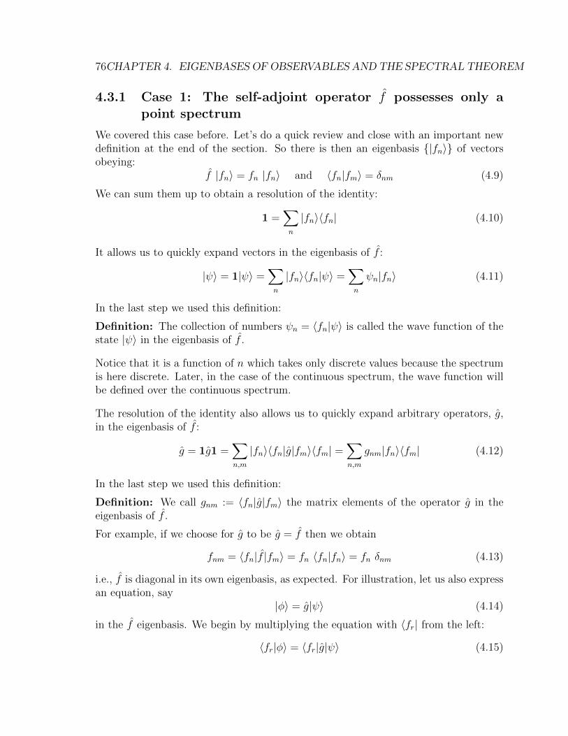
76CHAPTER 4. EIGENBASES OF OBSERVABLES AND THE SPECTRAL THEOREM
4.3.1 Case 1: The self-adjoint operator f possesses only apoint spectrum
We covered this case before. Let’s do a quick review and close with an important newdefinition at the end of the section. So there is then an eigenbasis |fn〉 of vectorsobeying:
f |fn〉 = fn |fn〉 and 〈fn|fm〉 = δnm (4.9)
We can sum them up to obtain a resolution of the identity:
1 =∑n
|fn〉〈fn| (4.10)
It allows us to quickly expand vectors in the eigenbasis of f :
|ψ〉 = 1|ψ〉 =∑n
|fn〉〈fn|ψ〉 =∑n
ψn|fn〉 (4.11)
In the last step we used this definition:
Definition: The collection of numbers ψn = 〈fn|ψ〉 is called the wave function of thestate |ψ〉 in the eigenbasis of f .
Notice that it is a function of n which takes only discrete values because the spectrumis here discrete. Later, in the case of the continuous spectrum, the wave function willbe defined over the continuous spectrum.
The resolution of the identity also allows us to quickly expand arbitrary operators, g,in the eigenbasis of f :
g = 1g1 =∑n,m
|fn〉〈fn|g|fm〉〈fm| =∑n,m
gnm|fn〉〈fm| (4.12)
In the last step we used this definition:
Definition: We call gnm := 〈fn|g|fm〉 the matrix elements of the operator g in theeigenbasis of f .
For example, if we choose for g to be g = f then we obtain
fnm = 〈fn|f |fm〉 = fn 〈fn|fn〉 = fn δnm (4.13)
i.e., f is diagonal in its own eigenbasis, as expected. For illustration, let us also expressan equation, say
|φ〉 = g|ψ〉 (4.14)
in the f eigenbasis. We begin by multiplying the equation with 〈fr| from the left:
〈fr|φ〉 = 〈fr|g|ψ〉 (4.15)

4.3. THE SPECTRAL THEOREM FOR SELF-ADJOINT OPERATORS 77
Therefore:〈fr|φ〉 = 〈fr|g1|ψ〉 =
∑n
〈fr|g|fn〉〈fn|ψ〉 (4.16)
We obtain the following equation for explicit column vectors (the wave functions) anda matrix:
φr =∑n
gr,nψn (4.17)
We obtained these expansions of vectors and operators and their equations in eigenbasesby using the resolution of the identity. It it will be very useful later also to considerpartial resolutions of the identity, namely by not summing all the way:
Definition: We define a partial resolution of the identity:
EN :=N∑n
|fn〉〈fn| (4.18)
Clearly, in the limit, we obtain the resolution of the identity:
limN→∞
EN = 1 (4.19)
It will be important later that each EN is an operator, defined on the entire Hilbertspace, which is a projector, namely, that it obeys EN = E†N and E2
N = EN .
Definition: An operator P is called a projector if it is self-adjoint, and obeys:P 2 = P .
Exercise 4.3 Show that EN is a projector.
We now come to case 2 of the spectral theorem:
4.3.2 Case 2: The spectrum of f is purely continuous
In this case, let us give the spectrum a name:
J := spec(f) ⊆ R (4.20)
Notice that J can be a subset of the real line but it can also be the full real line. J canalso consist of several disconnected pieces2. To start with, let us use the notation that
2For example, the Hamiltonian of electrons in a periodic potential, e.g., in a crystal, tends topossess a continuous spectrum that consists of several disjoint stretches, called bands. Insulators,semiconductors and conductors are distinguished by the degree to which the states in the highestenergetically accessible band are filled with electrons.

78CHAPTER 4. EIGENBASES OF OBSERVABLES AND THE SPECTRAL THEOREM
is common in physics. In physics notation, f has a basis of approximate eigenvectors|f〉f∈J that are continuum normalized
〈f |f ′〉 = δ(f − f ′) (4.21)
and yield a resolution of the identity:
1 =
∫J
|f〉〈f | df (4.22)
Similarly to case 1 where f possesses only a purely point spectrum, here too we obtainwave functions for states and matrix elements for operators:
|ψ〉 = 1|ψ〉 =
∫J
|f〉〈f |ψ〉 df =
∫J
ψ(f) |f〉 (4.23)
In the last step we used this definition:
Definition: We call ψ(f) := 〈f |ψ〉 the wave function of the state |ψ〉 in the eigenbasisof f . Here, f runs through the spectrum of f .
Further, we obtain for operators:
g = 1g1 =
∫J
∫J
|f〉〈f |g|f ′〉〈f ′| df df ′ =∫J
∫J
g(f, f ′)|f〉〈f ′| df df ′ (4.24)
In the last step we used this definition:
Definition: We call g(f, f ′) := 〈f |g|f ′〉 the matrix elements of g in the eigenbasis off . We may also sometimes use the notation gf,f ′ for g(f, f ′). The function g(f, f ′) is
also called the integral kernel of g in the continuous eigenbasis of f .
Notice that gf,f ′ behaves like a matrix with continuous rather than discrete indices. Infact, everything is the same as for a matrix, except that summations over indices arenow integrations.
For example, let us express the equation |φ〉 = g|ψ〉 in the f eigenbasis, as in thediscussion of case 1 above. Now, however, we pick an operator f whose spectrum iscontinuous. We begin by multiplying the equation with 〈f | from the left:
〈f |φ〉 = 〈f |g|ψ〉 (4.25)
Therefore:
〈f |φ〉 = 〈f |g1|ψ〉 =
∫J
〈f |g|f ′〉〈f ′|ψ〉 df ′ (4.26)
We obtain the following equation for explicit column vectors (the wave functions) anda matrix, though now all indices are continuous:
φ(f) =
∫J
g(f, f ′)ψ(f ′) df ′ (4.27)

4.3. THE SPECTRAL THEOREM FOR SELF-ADJOINT OPERATORS 79
Let us also quickly consider the matrix elements, i.e., the integral kernel, of f in itseigenbasis, in the case where the spectrum is continuous:
f(f, f ′) = 〈f |f |f ′〉 = f ′〈f |f ′〉 = f ′ δ(f − f ′) (4.28)
Therefore:
f =
∫J
∫J
f ′ δ(f − f ′)|f〉〈f ′| df df ′ =∫J
f |f〉〈f | df (4.29)
4.3.3 Case 3: The self-adjoint operator f has a point spectrumand a continuous spectrum
In this case, we have:
1 =∑n
|fn〉〈fn|+∫J
|f〉〈f | df (4.30)
f =∑n
fn |fn〉〈fn|+∫J
f |f〉〈f | df (4.31)
Exercise 4.4 Derive the expression for the abstract equation |φ〉 = g|ψ〉 in this basis.
Exercise 4.5 Look up and state the complete spectrum of the Hamiltonian of the Hy-drogen atom (without spin or higher order corrections of any form). Give the exactsource in a textbook.
Hint: Essentially every textbook on quantum mechanics treats the Hydrogen atom.What do they do, from our perspective? They start with the Hamiltonian of theHydrogen atom, expressed in the position basis. Then they calculate the eigenbasisof the Hamiltonian, i.e., they calculate the energy eigenstate’s wave functions in theposition basis. They are the wave functions of the Hydrogen orbitals. In principle,it’s just like we will calculate in Ch.?? the eigenstates of the position operator in theeigenbasis of a harmonic oscillator and vice versa. But never mind the details of this.It’s not what the question is about.
The question is merely about the spectrum of the Hamiltonian of the Hydrogenatom. What are the proper eigenvalues and what are the approximate eigenvalues?I.e., the task is for you to learn to read the literature with the new mathematical andphysical insights in the background. The question is to thereby find out the pointspectrum and also the continuous spectrum of the Hamiltonian of the Hydrogen atom.Yes, the Hamiltonian of the Hydrogen atom has both types of spectrum. If yourtextbook doesn’t mention the continuous spectrum (whose eigenfunctions describeselectrons that are not bound to the proton but merely scatter off it), check anothertextbook. Regarding the point spectrum, do list also how often each eigenvalue occurs.

80CHAPTER 4. EIGENBASES OF OBSERVABLES AND THE SPECTRAL THEOREM
Remember that eigenvalues can be degenerate, i.e., the eigenspace to an eigenvalue canbe multi-dimensional. I.e., list the dimension of each eigenvalue’s eigenspace. No needto list the wave functions of the Hamiltonian’s eigenvectors.
Comment: We can see here why a smart phone battery demands about 5V from theUSB charger and why nuclear fuel can release about a million times more energy perkilo fuel than a chemical fuel such as oil or coal does:
You’ll find that the spacing of the first energy levels of the Hydrogen atom isusually given in a unit of energy that is called an electronvolt, [eV]. By definition, 1eV is the amount of energy that an electron gains when you let it travel between twoelectrodes that have a voltage bias of 1 Volt between them. The larger spacings betweenthe discrete energy levels (belonging to bound states) of the Hydrogen atom, and ofmolecules in general, is in the range of a few eV. This is the reason why batteries andphotovoltaic cells operate at the voltage levels of a few eV. All chemical and biochemicalreactions operate in the range of just a few eV too.
The formation of a molecules of Vitamin D, for example, happens to require anamount of energy, namely about 4.2 eV, that is in the upper range in the field ofbiochemistry and the other molecules of our bodies just don’t have that kind of largeenergy gap available! That’s why we need to consume vitamin D or make it usingultraviolet-B sunlight. UV-B photons that carry the required 4.2eV of energy neededto make Vitamin D molecules have a wavelength of about 295nm. We can’t see sunlightof such short wavelength. Ultraviolet light is bluer than blue or even violet, which is whyit is called ultraviolet. Sunlight scatters of air molecules through Rayleigh scatteringand that effect is the stronger the smaller the wavelength. That’s why during theday the sky is full of scattered light - which is blue. UV-B light makes it all the waydown to the surface essentially only when the sun stands steeper in the sky than about45 degrees. Else, it’s just scattered around and away. So that’s why we get enoughvitamin D from sunlight only is the summer. In the winter, it’s good to have vitaminD supplements. You know, the tablets that taste like dust. Yummy!
Now atomic nuclei also have a Hamiltonian. These nuclei can be excited so thatthey vibrate (point spectrum) or so that they split apart into non-bound fragments(continuous spectrum). The typical energy gaps in the spectra of nuclei are 1 MeV.That’s why you can get roughly on the order of a million times more energy out ofa kilo of plutonium than out of a litre of oil. Still, I am not advocating for nuclearenergy. Why? The tremendous amount of energy in nuclear fuel also means that unlikea chemical fire that runs out of energy in a few days, radioactive contamination caneasily spew radioactive radiation energy for millions of days (depending on the elementof course). I flew over Fukushima. It’s terrible.

4.4. THE SPECTRAL THEOREM FOR UNITARY OPERATORS 81
4.4 The spectral theorem for unitary operators
The spectral theorem for self-adjoint operators f translates directly into a spectraltheorem for unitary operators, i.e., for operators obeying U † = U−1. This is becausethere is a bijective map, called the Cayley transform, that maps every self-adjointoperator into a unitary operator and vice versa:
U := (f − i1)(f + i1)−1 (4.32)
Exercise 4.6 Show that U is unitary.
The Cayley transform is invertible:
f = −i(U − 1)−1(U + 1) (4.33)
Clearly, in the eigenbasis of f , where f is diagonal, also U is diagonal. This meansthat f and U possess the same eigenvectors and approximate eigenvectors, with thesame multiplicities (i.e. with the same dimension of the eigenspaces). Further, sinceboth operators are simultaneously diagonal, if r ∈ R is in the spectrum of f , thenα = (r − i)(r + i)−1 (which is a Moebius transform of r), is in the spectrum of U .
Exercise 4.7 Show that each α is a complex number on the unit circle of the complexplane, i.e., that its modulus squared is αα∗ = 1.
Therefore, the spectral theorem for self-adjoint operators implies a correspondingspectral theorem for unitary operators. They too only possess a point and or a contin-uous spectrum, with corresponding eigenvectors and approximate eigenvectors.
Remark: You may wonder why we here did we not use exponentiation to obtain aunitary operator for any self-adjoint operator, through U := exp(if). The reason isthat, while we could use exponentiation, it has a drawback. The drawback is that theexponentiation map is not invertible because of the periodicity of exp(ir). Multipleeigenvalues of f could map into one eigenvalue for U . The Cayley transform is invert-ible, i.e., it maps each unitary operator uniquely to a self-adjoint operator and viceversa.
The most general spectral theorem is for normal operators: The spectral the-orem naturally generalizes beyond self-adjoint and unitary operators, namely to alloperators that are called normal. An operator Q is called normal if it commutes withits adjoint, i.e., if [Q, Q†] = 0. For example, the operators a and a† that obey [a, a†] = 1are clearly not normal. Indeed, the eigenstates of a that you calculated in Exercise3.27, the so-called coherent states, can be shown to be not orthogonal to another.

82CHAPTER 4. EIGENBASES OF OBSERVABLES AND THE SPECTRAL THEOREM
Exercise 4.8 Assume that f is a self-adjoint operator with a purely point spectrumfn. Further assume that U is the Cayley transform of f . Determine whether or notthe operator Q := f + U is a normal operator. If not, why not? If yes, what is thespectrum of Q?

Chapter 5
The position, momentum andenergy representations
5.1 The eigenbasis of the position operator
We had found a representation of the position operator (parametrized by a parameterL that specifies the unit of length) in Eqs.3.42,3.48:
xn,m =
0
√1L 0 0√
1L 0√
2L 00
√2L 0
√3L
0 0√
3L 0. . .
n,m
(5.1)
Here, the subscript n,m indicates the matrix element in the (n+1)’st row and (m+1)’stcolumn, because we will count from 0. We are here obviously dealing with a discrete,i.e., countable, basis. Let us call these basis vectors |En〉 for n = 0, 1, 2, 3, .... Then wehave
〈En|x|Em〉 = xn,m (5.2)
and
x =∞∑
n,m=0
|En〉xn,m〈Em| (5.3)
Clearly, x is not diagonal in the |En〉 basis. Now to find a basis in which x is diagonal,i.e., to find an eigenbasis of x, we need to find the solutions to the eigenvalue equation:
x|x〉 = x|x〉 (5.4)
To this end, we first act with 〈En| from the left to obtain:
〈En|x|x〉 = x〈En|x〉 (5.5)
83

84CHAPTER 5. THE POSITION, MOMENTUMAND ENERGYREPRESENTATIONS
Inserting a resolution of the identity we obtain a concrete eigenvalue equation in abasis:
∞∑m=0
〈En|x|Em〉〈Em|x〉 = x〈En|x〉 (5.6)
We know the matrix elements 〈En|x|Em〉 of the position operator, namely
〈En|x|Em〉 = L
0√
1 0 0 0√1 0
√2 0 0
0√
2 0√
3 00 0
√3 0
√4
0 0 0√
4 0. . .
n,m
(5.7)
and our task is to determine for which real eigenvalues x there exists a column vectorthat is an eigenvector. Its components are then the wave function 〈En|x〉 for a positioneigenstate |x〉 in the |En〉 basis. Once we have these wave functions, 〈En|x〉, ofposition eigenstates, we can write down the position eigenvectors |x〉 themselves in thebasis |En〉:
|x〉 =∑n
|En〉〈En|x〉 (5.8)
Now Eq.5.6 yields an equation for each n ∈ 0, 1, 2, .... These equations are
L√
1〈E1|x〉 = x〈E0|x〉 (5.9)
L√
1〈E0|x〉+ L√
2〈E2|x〉 = x〈E1|x〉 (5.10)
L√
2〈E1|x〉+ L√
3〈E3|x〉 = x〈E2|x〉 (5.11)
and so on. We have arrived at a recursion for the coefficients 〈En|x〉 which gives usa solution, i.e., a full set of coefficients 〈En|x〉 for any choice of x! This is becauseonce we pick an arbitrary value for the first coefficient, 〈E0|x〉, we can then calculatethe second coefficient, namely 〈E1|x〉. From these two we can calculate the third,〈E2|x〉. In this way, iteratively, all 〈En|x〉 are determined and can be calculated. Animportant conclusion we can draw from this is that no matter what value for x we try,we always find an eigenvector for it! This means that the spectrum of x is the real line:spec(x) = R.
The recursion problem can be solved in closed form. Without proof (which isstraightforward but tedious) we only state the result:
〈En|x〉 =e−
x2
4L2√π1/22n(n)!
Hn
(x√2L
)(5.12)

5.2. THE ENERGY EIGENBASIS OF A HARMONIC OSCILLATOR 85
Here, Hn is the n’th Hermite polynomial, defined through:
Hn(z) := (−1)n ez2 dn
dzne−z
2
(5.13)
But then, didn’t we have for each eigenvalue x a choice in what value we wanted togive to the first coefficient, 〈E0|x〉 ? Yes we did. In the equation Eq.5.12, can wemake this choice such that the eigenvectors |x〉 come out normalizable? Here, let usremember that we just established that the spectrum is the real line and is, therefore,purely continuous. From the spectral theorem, we conclude that the eigenvectors |x〉are not normalizable. Instead, therefore, the choice of the first coefficient is made foreach x such that the resulting eigenvectors come out to be what is called continuumnormalized. Namely, one can show that with Eq.5.12, we have:
〈x|x′〉 =∞∑n=0
〈x|n〉〈n|x′〉 = δ(x− x′) (5.14)
Therefore, we have now found the wave function 〈En|x〉 of each position eigenstate |x〉in the basis |En〉n. In fact, we have inadvertently also obtained the position wavefunctions of the eigenstates of harmonic oscillators! To see this, let us briefly reviewaspects of the harmonic oscillator.
5.2 The energy eigenbasis of a harmonic oscillator
Following up on Exercise (3.19), we express the harmonic oscillator’s Hamiltonian
H =p2
2m+mω2
2x2 (5.15)
in terms of operators a, a† which obey [a, a†] = 1. In the |En〉 basis, these operatorshave the matrix elements given in Eqs.3.39,3.40. We make again the ansatz:
x = L(a† + a), p = iK(a† − a) with L,K ∈ R (5.16)
So far, the parameters L and K are still arbitrary real numbers. The ansatz needsto solve the hermiticity conditions x = x† and p = p† and it obviously does. A littlecalculation shows that this ansatz also succeeds in solving the canonical commutationrelations [x, p] = i1, namely if we choose K = (2L)−1 which we will henceforth do.Now, only L is still left as a free parameter in our ansatz. (For now, let us not worryabout the time evolution and consider only one arbitrary point in time.) Therefore,we have found a valid way of writing x and p.
At this point we are still free to choose any real value for L and, in principle, anyvalue of L is as good as any other. Let us now express the Hamiltonian in terms of thea, a† operators:
H =−1
2m 4L2
((a†)2 − a†a− aa† + a2
)+mω2L2
2
((a†)2 + a†a+ aa† + a2
)(5.17)

86CHAPTER 5. THE POSITION, MOMENTUMAND ENERGYREPRESENTATIONS
We notice that we can make the (a†)2 and a2 terms cancel by choosing L so that theprefactors match, i.e., so that
1
8mL2=mω2L2
2(5.18)
which is solved by:L = (2mω)−1/2 (5.19)
We conclude that for every harmonic oscillator, when expressing the x and p operatorsin terms of a and a†, there is an especially convenient choice of L :
x =1√
2mω(a† + a), p = i
√mω
2(a† − a) (5.20)
This is because with this choice of L, the form of the oscillator’s Hamiltonian, after ashort calculation, simplifies to:
H = ~ω(a†a+ 1/2) (5.21)
How does this help us to find the spectrum of H? Recall that we know the matrixelements an,m = 〈En|a|Em〉 and a†n,m = 〈En|a†|Em〉 of the operators a and a† in thebasis |E0〉, |E1〉, |E2〉, |E3〉, ..., namely:
an,m =
0√
1 0 0 00 0
√2 0 0
0 0 0√
3 00 0 0 0
√4
0 0 0 0 0. . .
n,m
(5.22)
The hermitean conjugate is:
a†n,m =
0 0 0 0 0√1 0 0 0 0
0√
2 0 0 00 0
√3 0 0
0 0 0√
4 0. . .
n,m
(5.23)
Clearly then, the matrix elements of the so-called number operator N := a†a in thebasis |E0〉, |E1〉, ... are
Nn,m = (a†a)n,m = n δn,m =
0 0 0 0 00 1 0 0 00 0 2 0 00 0 0 3 00 0 0 0 4
. . .
n,m
(5.24)

5.3. THE POSITION REPRESENTATION 87
Clearly, N is a self-adjoint operator, N † = N , since it is diagonal in the basis |E0〉, |E1〉, ...and is, therefore, diagonalizable. Since
H = ~ω(N + 1/2) (5.25)
we have that the Hamiltonian is diagonal in the basis |E0〉, |E1〉, ..., i.e., that H|En〉 =En|En〉, and that its eigenvalues are En = ~ω(n + 1/2) for n ∈ 0, 1, 2, .... Thespectrum of the Hamiltonian of a harmonic oscillator is, therefore, purely a pointspectrum.
Therefore, this Hamiltonian reads in its eigenbasis:
H =p2
2m+mω2
2x2 =
∞∑n=0
En|En〉〈En| (5.26)
The state |En〉 can therefore also be interpreted the n’th excited state of a harmonicoscillator with frequency ω. Now what is the position wave function of the n’th eigen-state of this harmonic oscillator? By definition it is given by 〈x|En〉. But we have〈x|En〉 = (〈En|x〉)∗ = 〈En|x〉 because 〈En|x〉 is real. This means that we have inad-vertently also obtained the position wave functions of the eigenstates of the harmonicoscillator!
Exercise 5.1 Consider the harmonic oscillator of above, choose L = (2mω)−1/2 andassume that the oscillator system is in this state:
|ψ〉 =1√2
(|E0〉 − |E1〉) (5.27)
Calculate H and x and the position wave function ψ(x) := 〈x|ψ〉.
5.3 The position representation
We established that the spectrum of x is R, with each of these approximate eigen-values coming with a corresponding approximate (i.e., non-normalizable) eigenvector|x〉x∈R. This means that we have a new resolution of the identity1:
1 =
∫R|x〉〈x| dx (5.28)
It allows us to express arbitrary states in the eigenbasis of x, i.e., we can now calculate:
|ψ〉 =
∫R|x〉〈x|ψ〉 dx =
∫Rψ(x) |x〉 dx (5.29)
1We are here using physicists’ notation. The functional analytic details of operators with continuousspectra will be in an Appendix.

88CHAPTER 5. THE POSITION, MOMENTUMAND ENERGYREPRESENTATIONS
Here, ψ(x) = 〈x|ψ〉 is the position wave function of the state |ψ〉. Further, we can nowcalculate the scalar product of states in the position basis:
〈ψ|φ〉 = 〈ψ|1|φ〉 =
∫R〈ψ|x〉〈x|φ〉 dx =
∫Rψ(x)∗φ(x) dx (5.30)
For example, the normalization condition of a state |ψ〉 takes the form:
1 = 〈ψ|ψ〉 =
∫Rψ(x)∗ψ(x) dx (5.31)
Operators can be expanded in the position eigenbasis by inserting resolutions of theidentity:
f = 1f1 =
∫R
∫R|x〉〈x|f |x′〉〈x′| dx dx′ =
∫R
∫Rf(x, x′)|x〉〈x′| dx dx′ (5.32)
Here, the f(x, x′) = 〈x|f |x′〉 are called the matrix elements of f in the position repre-sentation. Of course, since x is a continuous rather than a discrete index for the matrixelements, we are not really dealing with a conventional matrix here. While the termmatrix element is commonly used in the physics literature, the alternative terminologyin proper mathematical language is to say that f(x, x′) is the integral kernel of f inthe position eigenbasis.
Definition: If f is an operator, and |λ〉 is a continuous basis (such as the positioneigenbasis) then we call f(λ, λ′) := 〈λ|f |λ′〉 the matrix elements of f in the |λ〉 basis.Of course, f(λ, λ′), which could also be written as fλ,λ′ , is a matrix whose two indicestake continuous values. When such a ‘matrix’ acts on a vector then the common in-dex needs to be integrated instead of summed: 〈λ|f |ψ〉 =
∫f(λ, λ′)ψ(λ′)dλ′. For this
reason, f(λ, λ′) is also called the integral kernel of f in the |λ〉 basis.
For example, for the operator f = x we find that its integral kernel,
x(x, x′) = 〈x|x|x′〉 = x〈x|x′〉 = xδ(x− x′), (5.33)
is diagonal in the sense that the kernel vanishes off the diagonal, i.e., for x 6= x′. Letus also express the position operator in the position basis:
x = x1 =
∫Rx |x〉〈x| dx =
∫Rx |x〉〈x| dx (5.34)
Let us now calculate the momentum operator’s matrix elements in the position repre-sentation:
p(x, x′) = 〈x|p|x′〉 =∑n,m
〈x|En〉〈En|p|Em〉〈Em|x′〉 = i~d
dx′δ(x− x′) (5.35)

5.4. SHORTHANDNOTATION FOROPERATORS ACTINGONWAVE FUNCTIONS89
Here, we inserted resolutions of the identity in terms of the eigenbasis |En〉 of a har-monic oscillator. This is useful because we already know the matrix elements 〈n|p|m〉 ofp explicitly from Eqs.5.20,5.22,5.23 and we know the coefficients 〈En|x〉 from Eq.5.12.The last step, i.e., to work out the sums over n and m is quite tedious and we skip thedetails here.
But what is the derivative of the Dirac delta? The Dirac delta itself is defined to obey:∫Rf(x)δ(x− x′) dx = f(x′) (5.36)
Now for the derivative of the Dirac delta we obtain via integration by parts:∫Rf(x)
d
dxδ(x− x′) dx = −
∫R
(d
dxf(x)
)δ(x− x′) dx = − df
dx(x′) (5.37)
We now obtain the operator p in the position representation:
p =
∫R
∫Ri~(d
dx′δ(x− x′)
)|x〉〈x′| dx dx′ (5.38)
Remember that already in Eqs.3.48,3.49, we had found a representation of the operatorsx and p as infinite-by-infinite matrices. Now, with Eqs.5.33,5.35, we have found arepresentation of x and p in a continuous basis, namely in the eigenbasis of the positionoperator.
5.4 Shorthand notation for operators acting on wave
functions
Let us consider an operator Q that maps a vector |ψ〉 into a vector |φ〉 = Q|ψ〉. Since|ψ〉 and |φ〉 both possess position wave functions, namely ψ(x) and φ(x), we have thatQ also induces a map of wave functions into wave functions, namely Q : ψ(x)→ φ(x).This is conveniently described by an important shorthand notation:
Definition: We denote the induced action of an operator on a wave function by a dot.For example, an operator Q acts on a state |ψ〉 by mapping it into a state |φ〉, i.e., wehave |φ〉 = Q|ψ〉. If we choose some basis |λ〉, this also means that Q maps the wavefunction ψ(λ) into the wave function φ(λ). We write this as:
φ(λ) = Q.ψ(λ) (5.39)
For example, in the case of the position operator and the position eigenbasis:
φ(x) = 〈x|φ〉 = 〈x|x|ψ〉 = x〈x|ψ〉 = xψ(x) (5.40)

90CHAPTER 5. THE POSITION, MOMENTUMAND ENERGYREPRESENTATIONS
In the shorthand notation, we can therefore write that the action of the position oper-ator on position wave functions is:
x.ψ(x) = xψ(x) (5.41)
What then is the action of p on position wave functions? Abstractly, we have |ϕ〉 =p|ψ〉. In the position eigenbasis, this is:
φ(x) = 〈x|φ〉 = 〈x|p|ψ〉 (5.42)
=
∫R〈x|p|x′〉〈x′|ψ〉 dx′ (5.43)
=
∫Ri~(d
dx′δ(x− x′)
)ψ(x′) dx′ (5.44)
= −i~∫Rδ(x− x′) d
dx′ψ(x′) dx′ + i~ [δ(x− x′)ψ(x′)]
x′=∞x′=−∞ (5.45)
= −i~ ddxψ(x) (5.46)
This means that in the shorthand notation we can write:
p.ψ(x) = −i~ ddxψ(x) (5.47)
Exercise 5.2 Verify the canonical commutation relation in the position representation,i.e., verify that, for all (differentiable) wave functions ψ(x):
(xp− px− i~1).ψ(x) = 0 (5.48)
5.5 The momentum representation
Similar to how we diagonalized the position operator, we could now calculate alsothe momentum operator’s eigenbasis. Namely, we could diagonalize the momentumoperator’s matrix representation Eq.3.49 in the |En〉∞n=0 basis of a harmonic oscillator.Instead, it will be more convenient to calculate the momentum operator’s spectrumand eigenbasis by diagonalizing it in the position representation. Concretely, let ussolve the eigenvector equation
p|p〉 = p|p〉 (5.49)
in the position basis, i.e., with the momentum eigenvector |p〉 written in the form:
|p〉 = 1|p〉 =
∫R|x〉〈x|p〉 dx (5.50)

5.5. THE MOMENTUM REPRESENTATION 91
Here, 〈x|p〉 is the wave function of the momentum eigenvector |p〉 to eigenvalue p inthe position basis. If we can calculate 〈x|p〉, then we have the momentum eigenvector|p〉 through Eq.5.50. From Eq.5.49 we obtain:
〈x|p1|p〉 = p 〈x|p〉 (5.51)∫R〈x|p|x′〉〈x′|p〉 dx′ = p 〈x|p〉 (5.52)∫
Ri~(d
dx′δ(x− x′)
)〈x′|p〉 dx′ = p 〈x|p〉 (5.53)∫
R−i~δ(x− x′) d
dx′〈x′|p〉 dx′ = p 〈x|p〉 (5.54)
Therefore, the function 〈x|p〉 must obey:
−i~ d
dx〈x|p〉 = p 〈x|p〉 (5.55)
Notice that we could have found immediately that Eq.5.49 translates into Eq.5.55 inthe position basis by using the shorthand notation Eq.5.47. Clearly, the solution toEq.5.55 is:
〈x|p〉 = N eixp~ (5.56)
Since, therefore, we are able to find an eigenvector |p〉 for each value p ∈ R, we can con-clude that spec(p) = R. The spectrum is, therefore, continuous and the approximateeigenfunctions 〈x|p〉 therefore require continuum normalization:
δ(p− p′) = 〈p|p′〉 (5.57)
=
∫R〈p|x〉〈x|p′〉 dx (5.58)
=
∫RN∗ e
−ixp~ N e
ixp′~ dx (5.59)
= N∗N
∫Re
ix~ (p−p′) dx (5.60)
At this point we use the fact that∫Reiab da = 2π δ(b) (5.61)
to conclude that N = (2π~)−1/2. We obtain the continuum normalized position eigen-functions of the momentum eigenvectors:
〈x|p〉 =1√2π~
eixp~ (5.62)

92CHAPTER 5. THE POSITION, MOMENTUMAND ENERGYREPRESENTATIONS
Notice that this also yields the momentum wave functions of the position eigenvectors:
〈p|x〉 = 〈x|p〉∗ =1√2π~
e−ixp
~ (5.63)
We obtain, analogously to the calculation for x before, a resolution of the identity anda spectral resolution of the momentum operator:
1 =
∫R|p〉〈p| dp, and p =
∫Rp |p〉〈p| dp (5.64)
The momentum wave function of a state |ψ〉 is then obtained from:
|ψ〉 = 1|ψ〉 =
∫R|p〉〈p|ψ〉 dp =
∫Rψ(p) |p〉 dp (5.65)
Here, ψ(p) := 〈p|ψ〉 is a common notation for the momentum wave function. Thescalar product of two states is now calculated through
〈φ|ψ〉 =
∫R〈φ|p〉〈p|ψ〉 dp =
∫Rφ(p)∗ψ(p) dp (5.66)
We can now derive how the momentum wave function ψ(p) can be expressed in termsof the position wave function ψ(x):
ψ(p) = 〈p|ψ〉 (5.67)
=
∫ ∞−∞〈p|x〉〈x|ψ〉dx (5.68)
=1√2π~
∫ ∞−∞
ψ(x) e−ixp
~ dx (5.69)
We conclude that the position and momentum representations (i.e., bases) are relatedby Fourier transformation. Similarly, as we saw earlier, the position eigenbasis andthe eigenbasis of the Hamiltonian of a harmonic oscillator are related by a Hermitetransformation. Analogously, any two choices of (appropriately orthonormalized) basesare related by a transformation that implements the unitary change of basis.
Exercise 5.3 Derive the action of x and p on momentum wave functions, i.e., derivethe short hand notation x.ψ(p) =?ψ(p) and p.ψ(p) =?ψ(p) analogously to how wederived the short hand notation for the position representation.
5.6 Energy representations: bound states and scat-
tering states
Consider an arbitrary quantum system with Hamiltonian H. Since H is normallyself-adjoint, it possesses an eigenbasis, the so-called energy eigenbasis. Let us denote

5.6. ENERGY REPRESENTATIONS: BOUND STATES AND SCATTERING STATES93
the normalizable and nonnormalizable eigenvectors of H by |Eµ〉 where µ is an indexthat runs through a continuous, a discrete or a mixed index set, as the case may be.Remember that, the Hamiltonians of some systems possess a purely discrete spectrum,as is the case for the harmonic oscillator. The Hamiltonians of other systems are purelycontinuous, as for example, that of the free particle. The spectrum can also consist of adiscrete and a continuous spectrum, as, for example, the spectrum of the Hamiltonianof the hydrogen atom. What does this mathematical property of the spectrum beingdiscrete or continuous make correspond to, physically?
To see the physical difference, let us recall that eigenvalues En of H that are in thepoint spectrum En ∈ specdiscr.(H) come with eigenvectors |En〉 that are normalizableand that, in contrast, the approximate eigenvalues E ∈ speccont.(H) of the continuousspectrum, the so-called approximate eigenvalues, come with non-normalizable approxi-mate eigenvectors |E〉. Let us consider these normalizable and non-normalizable vectorsin the position eigenbasis, i.e., ψEn(x) = 〈x|En〉 and ψE(x) = 〈x|E〉 respectively.
Since each state |En〉 is normalizable, 〈En|En〉 = 1, we have from Eq.5.31 that itsposition wave function is square integrable:∫ ∞
−∞ψEn(x)∗ψEn(x) dx = 1 (5.70)
This implies that the wave function must decay quickly towards ±∞. For this reason,particles described by such a wave function are fairly localized and we say that theyare in a bound state. This could be, for example, an electron bound to a proton,described by one of Hydrogen’s orbital wave functions. In contrast, the wave functionsψE(x) belonging to states of the continuous spectrum are not normalizable and describeparticles that are entirely delocalized, much like plane waves. These eigenstates of theHamiltonian describe particles that come in from infinity, interact with our system,perhaps change direction a bit and then go away out to infinity. The states of thecontinuous spectrum of the Hamiltonian are, therefore, also called scattering states.The Hamiltonians of electrons that orbit the nuclei of an atom or a molecule alwayspossess both a discrete energy spectrum and above it also a continuous energy spectrumthat reaches up to infinite energies. This is because the electrons can be bound to thenuclei at discrete energy levels, until at sufficiently high energies the nuclei can nolonger hold on to the particle and the particle merely scatters off the nuclei.
There is a classical analog in the solar system. Comets are in bound states aroundthe sun. In contrast, the extra-solar rock called Oumuamua, for example, had muchmore kinetic energy than a comet and it only scattered off our solar system when itvisited our solar system in 2017. Similarly, the hydrogen atom’s well known discreteenergy levels constitute only the point spectrum. The Hamiltonian of an electroninteracting with a proton also possesses a continuous spectrum which ranges from 0 toinfinity.

94CHAPTER 5. THE POSITION, MOMENTUMAND ENERGYREPRESENTATIONS

Chapter 6
Continuous versus discrete inquantum mechanics
6.1 It takes only a countable infinite amount of in-
formation to specify a quantum state
Let us review how it can be that a state |ψ〉 can be specified by both, an uncountableamount or also by a countable amount of coefficients. Namely, |ψ〉 can be specifiedthrough uncountably many numbers ψ(x) = 〈x|ψ〉, where x runs through all the un-countably infinitely many real numbers, or also through the countably infinitely manynumbers ψn = 〈n|ψ〉 where n runs through a countably infinite number of integers.
The answer is subtle. The countably many coefficients ψn really do suffice to specify|ψ〉 because |ψ〉 =
∑∞n=1 ψn|n〉. Therefore, when we instead describe |ψ〉 through the
uncountably infinitely many data ψ(x) ∀x ∈ R this description must possess a largeredundancy. Indeed, there are many wave functions that describe the same state!
Consider two wave functions ψ(x) and φ(x) which are exactly the same for allx ∈ R, except at a finite number of points x1, x2, ..., xN , where they differ, for example,φ(x2) = 77 but ψ(x2) = −3.2. Any such pairs of wave functions ψ(x) and φ(x) areactually physically equivalent in the sense that the predictions come out the same.The reason is that when we calculate an expectation value with either ψ(x) or φ(x)the prediction always comes out to be the same. Consider, for example, the positionexpectation value: x =
∫ψ∗(x)xψ(x) =
∫φ∗(x)xφ(x). The reason is that the value
of an integral is insensitive to changing the value of its integrand function at a finitenumber of points.
Why? It’s because when you integrate, i.e., when you calculate the area under acurve, then if you make the integrand function have a spike at one isolated point, thisdoes not have any effect on the area under the curve. A spike at a single point doesn’taffect the area under the curve because such a spike is just a line and lines don’t havearea. If you are interested in the details of the integration theory behind this, look up
95

96CHAPTER 6. CONTINUOUS VERSUS DISCRETE IN QUANTUMMECHANICS
the notion of Lebesgue integration.So in conclusion, since we can add isolated spikes everywhere on the x axis, each
position wave function has uncountably infinitely many brother and sister position wavefunctions that differ only at individual points and that are indistinguishable under theintegral and are, therefore, also indistinguishable in the calculation of any expectationvalue. So they are physically equivalent.
Each individual state |ψ〉, possesses, therefore, an equivalence class of uncountablyinfinitely many position wave functions. What is specified by |ψ〉 is merely the equiva-lence class, but not any particular wave function in it. This can pose a problem whenwanting to differentiate the wave function. That’s because wherever the wave functionis not differentiable because of one of those spikes, we can only differentiate before andafter the spike but there is no derivative at the spike. That’s not a problem underthe integrals because it happens only at isolated points, but it’s tedious. Therefore,in practice, we always choose the most differentiable member of the equivalence class.I know, all these things are often not spelled out in textbooks, as many authors justfollow the herd. But in this course we are not afraid to dig somewhat deeper intowhat’s really going on.
So the redundancy in the form of wave functions grouping into large equivalenceclasses for each state is why it is that a(n) (equivalence class of) position wave functionψ(x) can be specified by just giving countably many data, such as the data ψn forn = 1, 2, .... Namely, by specifying, for example, the ψn we obtain |ψ〉 =
∑∞n=1 ψn|n〉
and from it we obtain a ψ(x) = 〈x|ψ〉. Let us remember that it is not the unique ψ(x)that we obtain in this way. It’s just the differentiable member of a whole equivalenceclass of wave functions, such as φ(x) that would describe the exact same physics.
6.2 Stieltjes integration explains the Dirac delta
Definition (Stieltjes integral): The Stieltjes integral∫ b
a
f(x) dm(x) (6.1)
requires an integrand, i.e., a function f(x) to be integrated over and a function m(x),called the integrator (or measure) which is monotonically increasing (i.e., which obeysm(x2) ≥ m(x1) when x2 > x1). The integration is performed by considering partitionsx0 < x1 < x2 < ... < xn of the interval [a, b], i.e., x0 = a and xn = b. We then define:∫ b
a
f(x) dm(x) := limε→0
∑i
f(xi) (m(xi+1)−m(xi)) (6.2)
Here, f(xi) is f evaluated at an arbitrary point in the i’th interval: xi ∈ [xi, xi+1]and the limit is the limit in which the maximum spacing, ε occurring in a sequence

6.2. STIELTJES INTEGRATION EXPLAINS THE DIRAC DELTA 97
of partitionings goes to zero. Notice that if the integrator function is constant, thenthe integral vanishes. Also, if we add any constant to the integrator function m(x),this makes no difference to the integral because only differences of its values occur inEq.6.2.
Now how does the Stieltjes integral relate to ordinary integration?
Proposition: Assume that the integrator function is differentiable and that the deriva-tive m′(x) of m(x) is continuous. Then the Stieltjes integral can be expressed in termsof the ordinary integral: ∫ b
a
f(x) dm(x) =
∫ b
a
f(x)dm(x)
dxdx (6.3)
So in particular, if we choose the integrator function to be m(x) = x then we havedm/dx = 1 and we recover the ordinary integral over f .
But what then is the advantage of the Stieltjes integration method? The key advantageis that we can do more types of integrals now because the integrator function m neednot have a continuous derivative! For example, consider the case of m being a Heavisidestep function:
m(x) = θ(x) =
0 if x < 0
1/2 if x = 01 if x > 0
(6.4)
Assuming that a < 0 < b and applying the definition Eq.6.2 shows that the Stieltjesintegral in this case yields: ∫ b
a
f(x) dm(x) = f(0) (6.5)
For comparison, the Dirac delta is defined to be the mathematical object that obeys:∫ b
a
f(x) δ(x)dx = f(0) (6.6)
Comparing with Eq.6.3, we now see that the Dirac delta behaves like the derivative ofthe Heaviside function
d
dxθ(x) = δ(x) (6.7)
This equation is commonly stated but let us keep in mind that, strictly speaking, thisequation holds when functions are being integrated over using the Stieltjes integrationmethod.
Exercise 6.1 Explain Eq.6.5 using a sketch of the plot of a function and a partitioningof the integration interval.

98CHAPTER 6. CONTINUOUS VERSUS DISCRETE IN QUANTUMMECHANICS
Similarly, we can generate a sum by using an integrator function with multiple steps.For example, m(x) =
∑i θ(x− xi) yields.∫ b
a
f(x) dm(x) =∑i
f(xi) (6.8)
More generally, by using an integrator function that is in some parts of the real linesmooth and in some parts of the real line it has steps of various sizes, one single Stielt-jes integral can express arbitrarily complicated combinations of sums and Riemannintegrals.
Exercise 6.2 Sketch the graph of an integrator function m(x) which integrates overthe intervals [3, 6] and [9, 11] and sums over the values of the integrand at the pointsx = 5 and x = 6.
Let us recall why we here introduce the Stieltjes integral. It is because it allows usto avoid using the Dirac delta. Of course, we could bring back the Dirac delta. Forexample, using the Dirac Delta, we could rewrite Eq.6.8:∫ b
a
f(x) dm(x) =
∫ b
a
f(x)dm(x)
dxdx =
∫ b
a
f(x)∑i
δ(x− xi) dx =∑i
f(xi) (6.9)
In practice, working with the Dirac delta is indeed convenient, even though it is nota function but is instead what is called a distribution1. The reason why we need away to work without using the Dirac delta is that when it comes to integrating notover functions but integrating over operators, then we need to be able to work withoperator-valued functions, such as |x〉〈x| rather than working with operator-valueddistributions such as δ(x). The problem with “operator” such as |x〉〈x| is that they arenot really operators because, for example, we cannot multiply them onto themselves:|x〉〈x|x〉〈x| = δ(0)|x〉〈x| is undefined.
The Dirac delta is a distributional generalization of a number-valued function. Butwe would here need distributional generalizations also of vector- and operator-valuedfunctions too, because this would come up in resolutions of the identity and in spectralrepresentations of observables. Even if in practice one works with operator-valueddistributions as if there were no subtlety, it is good to know, at least in principle, howthings can be put on a solid footing by using the Stieltjes integral.
1A distribution such as the Dirac delta can be viewed as a continuous linear map from a specifiedspace of functions to numbers. For example, the Dirac delta in
∫f(x) δ(x−x0) dx maps the function
f linearly into the number f(x0). For details, see, e.g., the appendix on distributions in Messiah’sbook on quantum mechanics. Distributions can also be viewed as elements of a type of Hilbert spacecalled a Sobolev space, in which the inner product involves derivatives.

6.3. THE STIELTJES INTEGRAL EXPLAINS OPERATORS SUCH AS |X〉〈X|.99
6.3 The Stieltjes integral explains operators such
as |x〉〈x|.In order to make sense of expressions such as |x〉〈x|, let us first define the notion of apartial resolution of the identity:
Definition: Assume that f is a self-adjoint operator whose spectrum is purely con-tinuous and consists of the entire real line. Then we define the partial resolution of theidentity in the eigenbasis of f in this way:
E(f) :=
∫ f
−∞|f〉〈f | df (6.10)
We recover the full resolution of the identity as:
1 = E(∞) = limf→∞
∫ f
−∞|f〉〈f | df (6.11)
The partial resolution of the identity in Eq.6.10 has the advantage that we can differ-entiate it with respect to the integration boundary:
dE(f)
df= |f〉〈f | (6.12)
So now we have found an expression for the object that we are interested in: |x〉〈x|.How does this help? Let us rewrite the resolution of the identity:
1 =
∫R|f〉〈f | =
∫R
dE(f)
dfdf (6.13)
From this, we now obtain, in the Stieltjes sense:
1 =
∫RdE(f) (6.14)
And similarly:
f =
∫Rf dE(f) (6.15)
Why are Eqs.6.14,6.15 useful? Remember that, in keeping with physics notation, weused expressions such as |f〉〈f | which are actually ill defined if |f〉 is an improper or‘approximate’ eigenvector. For example, its square is infinite: |f〉〈f |f〉〈f | = δ(0) |f〉〈f |.
It would seem that so far not much is gained. Doesn’t Eq.6.14 still make use of|f〉〈f |? It does not! Let us look at the definition of the Stieltjes integral in Eq.6.2 again.The role of m(x) there is played here by E(f). Notice that in Eq.6.2 only evaluations ofm(x) occur and that there is no need to evaluate its derivative dm(x)/dx ever. Similarly

100CHAPTER 6. CONTINUOUS VERSUS DISCRETE IN QUANTUMMECHANICS
here, in Eqs.6.14,6.15, only E(f) occurs but not anymore its derivative (which wouldbe |f〉〈f |).
And E(f) is a perfectly well-behaved operator! One can show that for every valueof f it is a projector. For this reason, Eqs.6.14,6.15 are at the heart of the rigorousmathematical formulations and applications of the spectral theorem.
In fact, while in the current section we only considered the case where the spec-trum of f is the real line, the spectrum of a self-adjoint operator can of course containarbitrary continuous and discrete parts. The Stieltjes integral takes care of this auto-matically, i.e., we no longer have to use a mix of sums and integrals. All we need isthe Stieltjes integrals Eqs.6.14,6.15 over the full real line. In them, the summationsof the point spectrum, see, e.g., Eqs.4.30,4.31, arise, as usual for Stieltjes integrals,through discontinuities in the integrator function E(f). The continuous spectrum iswhere the integrator function changes continuously and on stretches of R where thereis no continuous or point spectrum, the integrator function E(f) is constant.

Chapter 7
Uncertainty principles
7.1 The Heisenberg uncertainty relations
To solve a quantum mechanical problem is to choose or determine the initial statevector |ψ〉 and to calculate the position and momentum operators x(t), p(t) subjectto the equations of motion, the canonical commutation relations and subject to thehermiticity conditions x(t) = x(t)† and p(t) = p(t)†.
Once the x(t), p(t) (usually with indices indicating dimensions and particle number)and the initial state vector |ψ〉 of the system are known, we can calculate everything:Consider any observable f(t), i.e., any polynomials or well-behaved power series inthe positions and momenta obeying f †(t) = f(t). Then we can calculate its ensembleexpectation values f(t) = 〈ψ|f(t)|ψ〉. Here, the term ensemble expectation value meansthe average outcome of the measurement of the observable f(t) if the same experiment(i.e., with the same initial conditions) is either repeated many times, or is performedmany times simultaneously. An ensemble of experimental runs can be an ensemble intime or an ensemble in space.
Now if f(t) is an observable, i.e., if it obeys f(t) = f(t)† then also f(t)2 is anobservable, i.e., it obeys f(t)2 = (f(t)2)†. Thus, for any observable f(t) we can predictnot only its ensemble average f(t), but we can also predict the ensemble average valuef 2(t) of the square of that observable.
In classical mechanics, this would not be surprising. For example, when the initialconditions for throwing an object (such as a ball or a particle) are known then the dis-tance that the object will fly (say in vacuum) before hitting the ground is an observablethat can be predicted. Let’s say the prediction is 50m. Well then clearly we can alsopredict the square of that distance: It will be 2500m2. Since in classical mechanics weare sure about the distance we are also sure about the square of the distance.
In quantum mechanics, we saw that the prediction for the squares of the distancemeasurements is generally not the square of the prediction for the distance measure-ments! Knowing the average outcome of the measurement of an observable does not
101

102 CHAPTER 7. UNCERTAINTY PRINCIPLES
automatically tell us the average outcome of the square of that observable: In general(i.e., in most cases), we have f 2 6= f 2. This means that the predictions cannot becertain, there must be a spread of the measurement outcomes. For example, the mea-surement outcomes for the distance might be 49m, 50m and 51m with probabilities1/3 each. Then the prediction is 50m but the predicted square of the distances is then(492 + 502 + 512)/3 m2 = (2500 + 2/3)m2.
We conclude that quantum mechanics implies that when performing an ensemble ofidentical experiments, each time measuring f at the end, then the measurement valuesfor f must have a spread. Only this way can we have that f 2 6= f 2. The predictionsof quantum mechanics are generally probabilistic. We can only predict the outcome ofa measurement with certainty if the observable in question happens to obey f 2 = f 2.
The extent to which the equation f 2 = f 2 is violated quantifies how large the spreadof the outcomes of the f measurements will be in an ensemble of experimental runs.
In fact the difference between the left hand side and the right hand side of thatequation coincides with the variance of the measurement outcomes. Remember thatthe variance of a statistical distribution is the average of the squared deviation fromthe average. Here, in Dirac notation:
(∆f(t))2 = (f(t)− f(t))2 (7.1)
= 〈ψ|(f(t)− 〈ψ|f(t)|ψ〉
)2
|ψ〉 (7.2)
= 〈ψ|f 2(t)|ψ〉 − 〈ψ|f |ψ〉2 (7.3)
= f(t)2 − f(t)2
(7.4)
We can now derive Heisenberg’s famous uncertainty relations for the variances and thesquare roots of the variances (the so called standard deviation) between any pairs ofobservables:
Proposition: Assume f(t) and g(t) are observables and assume that the system is inthe state |ψ〉. Then:
∆f(t) ∆g(t) ≥ 1
2|〈ψ|[f(t), g(t)]|ψ〉| (7.5)
In particular, we have for all states |ψ〉:
∆x(t) ∆p(t) ≥ 1
2|〈ψ|i~|ψ〉| = ~
2(7.6)
In this way, the noncommutativity of the positions and momenta directly imply that ina state in which the position x(t) is predicted sharply, i.e., with small standard deviation∆x(t), the prediction p(t) of the momentum must come with a correspondingly largestandard deviation ∆p(t), and vice versa. In general, we have of course:
∆x(r)i (t) ∆p
(s)j (t) ≥ ~
2δi,jδr,s (7.7)

7.1. THE HEISENBERG UNCERTAINTY RELATIONS 103
Recall that initial conditions can be posed by specifying the mean values f(t0), g(t0)etc. of all observables f(t0), g(t0) including their arbitrary powers. We asked underwhich conditions so-posed initial conditions determine a state |ψ〉. We see now thatthe Heisenberg uncertainty relations impose restrictions on which so-described initialconditions can occur.
Proof of the Heisenberg uncertainty principle: Assume |ψ〉 is normalized andassume that f and g are observables at some time t. (To keep the formulas from gettingtoo long we will simply write g, f instead of g(t), f(t)). We start by considering thevector
|φ〉 =(f − f1 + iα(g − g1)
)|ψ〉 (7.8)
where α is an arbitrary real number. No vector’s norm is negative. In particular,〈φ|φ〉 ≥ 0, i.e.:
〈ψ|(
(f − f1)− iα(g − g1))(
(f − f1) + iα(g − g1))|ψ〉 ≥ 0 (7.9)
Thus:〈ψ|(f − f1)2|ψ〉+ α2〈ψ|(g − g1)2|ψ〉+ α〈ψ|i(fg − gf)|ψ〉 ≥ 0 (7.10)
Therefore:(∆f)2 + α2(∆g)2 + α〈ψ|i[f , g]|ψ〉 ≥ 0 (7.11)
Thus, completing the squares for α:
(∆f)2 + (∆g)2
(α +〈ψ|i[f , g]|ψ〉
2(∆g)2
)2
−
(〈ψ|i[f , g]|ψ〉
)2
(2(∆g)2)2 (∆g)2 ≥ 0 (7.12)
In the last step, we assumed1 that ∆g 6= 0. We observe that if we were to chooseα very large, then the big bracket is large and the inequality is trivially obeyed.Conversely, for any given |ψ〉, we obtain the most stringent inequality for the stan-dard deviations by choosing α such that the big bracket vanishes, i.e., if we chooseα = −〈ψ|i[f , g]|ψ〉/(2(∆g)2). We obtain:
(∆f)2(∆g)2 − 〈ψ|i[f , g]|ψ〉2
4≥ 0 (7.13)
and therefore, finally:
∆f(t) ∆g(t) ≥ 1
2|〈ψ|[f(t), g(t)]|ψ〉| (7.14)
1 If ∆g = 0 then it depends on whether or not also 〈ψ|i[f , g]|ψ〉 is zero. First, we observe that
〈ψ|i[f , g]|ψ〉 is a real number because(i[f , g]
)†= i[f , g]. Now if ∆g = 0 and 〈ψ|i[f , g]|ψ〉 = 0, then
Eq.7.11 implies no condition on ∆f . If, however, ∆g = 0 and 〈ψ|i[f , g]|ψ〉 6= 0, then ∆f = +∞because it must then be larger than any positive real number (since α can be chosen arbitrarily).

104 CHAPTER 7. UNCERTAINTY PRINCIPLES
Exercise 7.1 There are indications from studies of quantum gravity2, that the un-certainty relation between positions and momenta acquire corrections due to gravityeffects and should be of the form: ∆x∆p ≥ ~
2(1 + β(∆p)2 + ...), where β is a small
positive number. (a) Show that this type of uncertainty relation arises if the canonicalcommutation relation is modified to read [x, p] = i~(1 + βp2). (b) Sketch the modifieduncertainty relation ∆x∆p ≥ ~
2(1 +β(∆p)2) in the ∆p versus ∆x plane. (c) Show that
this resulting uncertainty relation implies that the uncertainty in position can never besmaller than ∆xmin = ~
√β.
Technical remark: In this case, the position observables x cannot possess eigen-vectors nor close approximations to eigenvectors, because they would have vanishingposition uncertainty. Such x therefore cannot be diagonalizable and therefore, by theso-called spectral theorem, they cannot be self-adjoint (i.e., the domains of x and x†
do not coincide). Such position operators are what is called symmetric operators,i.e., they obey only the bare minimum condition on an observable namely that allits expectation values are real: f is called symmetric iff 〈ψ|f |ψ〉 ∈ R ∀|ψ〉 ∈ Df .In linear algebra, i.e., when the Hilbert spaces are finite dimensional, the notions ofself-adjoint operator and symmetric operator coincide. In infinite-dimensional Hilbertspaces, all self-adjoint operators are also symmetric but not all symmetric operators areself-adjoint. In the international mathematical literature, the definitions of self-adjointoperator and symmetric operator are generally agreed upon. Unfortunately, however,there is no agreement on the definition of the term hermitean operator, which can meaneither self-adjoint or symmetric operator, depending on the author. In the physics lit-erature, the term hermitean is often used but its definition is rarely specified. Here,we will use the hermitean operator as synonymous to symmetric operator. The termdescribes the bare minimum requirement on any observable: Its expectation valuesmust be real. We will write f = f † with the tacit understanding that the domains off and f † may not coincide.
7.2 The time and energy uncertainty relation
We have seen that in quantum mechanics the position coordinates are observableswhose uncertainties can be calculated through ∆x = 〈ψ|(x− 〈ψ|x|ψ〉)2|ψ〉1/2. In con-trast, quantum mechanics treats the time coordinate t as a mere parameter. Therefore,
2Gravity comes in this way: Momentum, just like energy, gravitates by curving space. Assume thatwe want to measure positions very precisely, i.e., we try to make ∆x very small. This, however, leadsto a large momentum uncertainty ∆p and therefore ultimately to a large uncertainty in the curvatureof space at the location where we try to resolve the position. It can be shown that if ∆x were about10−35m or smaller, the resulting curvature uncertainty would significantly disturb the precision of theposition predictions. Thus, in simple models, a finite lower bound ≈ 10−35m to the uncertainty inpositions is expected. The critical length 10−35m is called the Planck length. In my thesis, I happenedto find the first Hilbert space representations for such minimal-length uncertainty relations. A lot offollow-up papers (about two a week) are calculating the impact on atoms, black holes and cosmology.

7.2. THE TIME AND ENERGY UNCERTAINTY RELATION 105
if we are looking to derive an uncertainty relation that involves time, we first need toclarify what we mean by an uncertainty ∆t in time.
To this end, consider an observable f(t). Its expectation value, f(t), and its uncer-tainty ∆f(t) generally change over time.
Now consider that we prepare an ensemble (i.e., a collection) of identical experi-ments, all starting with the same initial condition. Let’s say that in a sub-ensemblewe measure the observable f at a time t0 and in the remaining cases of the ensemblewe measure the observable at a time t0 + ∆t. The individual outcomes of the measure-ments of f(t0) will generally differ from the outcomes of the individual measurementsof f(t0 +∆t). There are two reasons for this. One reason is that the system has evolvedfrom time t0 to time t0 + ∆t and so the expectation values f(t0) and f(t0 + ∆t) aregenerally different and so of course the typical measurement outcomes are different atthe two times. The other reason why the measurements generally differ at the timest0 and t0 + ∆t is that there are quantum fluctuations, namely as predicted by ∆f(t0)and ∆f(t0 + ∆t).
This leads to the question which of the two reasons is the dominant one. Andthat depends! If we choose a short ∆t then the system will not have had much timeto evolve and therefore f(t0) and f(t0 + ∆t) are still approximately the same. Thismeans that the differing outcomes of the measurements of f at t0 and at t0 + ∆t arealmost entirely due to quantum fluctuations. If one the other hand, we make ∆t verylarge then the system had time to evolve significantly and the expectation values f(t0)and f(t0 + ∆) can therefore differ significantly. In this case the difference between theindividual outcomes of the individual measurements of f at t0 or t0 + ∆t are almostentirely due to the evolution of the system and not due to the quantum fluctuations.
There must be a ∆t that is the threshold between the two cases! Namely, startingfrom some time t0, how much time, ∆t do we have to wait until the expectation valueof f has changed appreciably, i.e., until it exceeds the quantum uncertainty? That timeis crucial: it is the time we have to wait to be able to see the evolution of a quantumsystem in spite of the presence of quantum noise!
Concretely, we need to determine the amount of time, ∆t, that it takes for theexpectation value f(t) to change by the average standard deviation ∆f . Here, wedefine the average standard deviation as the time-average over the standard deviationfrom t0 to t0 + ∆t:
∆f :=
∫ t0+∆t
t0∆f(t) dt
∆t(7.15)
We want to determine that amount of time ∆t that it takes for the change of theexpectation value f to start exceeding ∆f , because that’s the amount of time it takesfor change due to the dynamics of the system to dominate over the quantum noise. Sowe are looking for that amount of time ∆t for which:
|f(t0 + ∆t)− f(t0)| = ∆f (7.16)

106 CHAPTER 7. UNCERTAINTY PRINCIPLES
Combining Eqs.7.15,7.16, we obtain for the critical ∆t:
∆t =
∫ t0+∆t
t0∆f(t) dt
|f(t0 + ∆t)− f(t)|(7.17)
Interestingly, quantum mechanics implies a fundamental relation between the amountof time, ∆t, that it takes for an expectation value f to change by more than the averagequantum fluctuation and the uncertainty in the energy ∆H. Namely, assuming thatthe Hamiltonian does not depend on time3, we obtain:
∆f(t)∆H ≥ 1
2
∣∣∣〈ψ|[f(t), H]|ψ〉∣∣∣ (7.18)
anddf(t)
dt=
1
i~[f(t), H] (7.19)
we obtain:
∆f(t)∆H ≥ ~2
∣∣∣∣∣〈ψ|df(t)
dt|ψ〉
∣∣∣∣∣ =~2
∣∣∣∣ ddt〈ψ|f(t)|ψ〉∣∣∣∣ (7.20)
We used that the initial state vector |ψ〉 does not depend on time. We obtain:
∆f(t)∆H ≥ ~2
∣∣∣∣df(t)
dt
∣∣∣∣ (7.21)
Integrating over time, we obtain:
∆H
∫ t0+∆t
t0
∆f(t) dt ≥ ~2
∫ t0+∆t
t0
∣∣∣∣df(t)
dt
∣∣∣∣ dt (7.22)
≥ ~2
∣∣∣∣∫ t0+∆t
t0
df(t)
dtdt
∣∣∣∣ =~2|f(t0 + ∆t)− f(t0)|
Now inserting Eq.7.17 we finally obtain the time-energy uncertainty relation:
∆t ∆H ≥ ~2
(7.23)
It is quite remarkable that this uncertainty relation looks so similar to that betweenposition and momentum! And, notice that all dependence on the choice of f hasdropped out. What this means is that if the energy of a system has uncertainty ∆Hthen for every observable f it takes at least an amount of time ∆t that obeys Eq.7.23for the mean value f of the observable to change appreciably, i.e., for it to change by at
3Of course, if we allow ourselves to change the Hamiltonian arbitrarily then we can make observableschange arbitrarily quickly too.

7.3. THE IMPACT OF QUANTUM UNCERTAINTY ON THE DYNAMICS 107
least the average uncertainty ∆f . In the extreme case where we know the energy of asystem precisely, then none of its observables possesses any time variation. Consider, forexample, a system in its lowest energy state, say a hydrogen atom. If we know that thehydrogen atom is in its lowest energy state and if we are sure, therefore, what its energyis, ∆H = 0, then none of the observables f of the hydrogen atom changes over time!For example, there is definitely no observable rotation of the electron about the protonin any way - because all observables’ expectation values are constant. Conversely, if asystem is to possess any observables f which do change appreciably on a short timescale ∆t, for example, if we want to run a fast quantum computer, then the systemmust be in a state in which its energy is uncertain by a large amount ∆H, obeyingEq.7.23.
Exercise 7.2 Ultimately, every clock is a quantum system, with the clock’s pointeror display consisting of one or more observables of the system. Even small quantumsystems such as a nucleus, an electron, atom or molecule have been made to serve asclocks. Assume now that you want to use a small system, such as a molecule, as a clockby observing how one of its observables changes over time. Assume that your quantumclock possess a discrete and bounded4 energy spectrum E1 ≤ E2 ≤ E3 ≤ ... ≤ Emaxwith Emax − E1 = 1eV (1eV=1 electronvolt) which is a typical energy scale in atomicphysics. (a) Calculate the maximum uncertainty in energy, ∆E that your quantumclock can possess. (b) Calculate the maximally achievable accuracy for such a clock.I.e., what is the shortest time interval (in units of seconds) within which any observableproperty of the clock could change its expectation value by a standard deviation?
7.3 The impact of quantum uncertainty on the dy-
namics
The fact that, in general, (f)n 6= fn is also important for the dynamics of quantumsystems because, as we will see, it implies that quantum mechanical mean values suchas x(t) and p(t) do not follow the same equations of motion as the classical positionsand momenta x(t) and p(t).
We begin by considering the special cases in which, in spite of all the subtleties ofquantum mechanics, the mean values x
(r)i , p
(s)j of the positions and momenta sometimes
do obey exactly the same equations of motion as the those of Newton. Consider, forexample, the harmonic oscillator H = p2
2m+ k
2x2. Using the Heisenberg equations, we
obtaindx
dt=
p
mand
dp
dt= −kx (7.24)
4The energy could be bounded for several reasons. For example, your quantum clock could be amolecule that is such that if you were to supply any more energy that Emax to your quantum clock,it would break up, i.e., you would reach the continuous spectrum.

108 CHAPTER 7. UNCERTAINTY PRINCIPLES
and, therefore:
〈ψ|dxdt|ψ〉 = 〈ψ| p
m|ψ〉 and 〈ψ|dp
dt|ψ〉 = −k〈ψ|x|ψ〉 (7.25)
Since the state |ψ〉 does not depend on time, we obtain these Ehrenfest equations:
dx
dt=
p
mand
dp
dt= −kx (7.26)
The number-valued mean values x(t), p(t) therefore obey the classical Newton equa-tions! This means that without even solving the canonical commutation relations,equations of motion and hermiticity conditions for matrix-valued functions we canquickly solve Eqs.7.26 the same we would classically to obtain that x(t) and p(t) oscil-late with frequency ω =
√k/m.
This is all very useful, also because many systems can be approximated as a har-monic oscillator near the minimum of their potential. However, for general quantumsystems, the mean values x(t) and p(t) do not obey Newton’s equations. Consider, for
example, the non-harmonic oscillator H = p2
2m+ αx4, which leads to
dx
dt=
p
mand
dp
dt= −4αx3 (7.27)
and, therefore:
d
dt〈ψ|x|ψ〉 = 〈ψ| p
m|ψ〉 and
d
dt〈ψ|p|ψ〉 = −4α〈ψ|x3|ψ〉 (7.28)
We obtain these equations for the expectation values:
dx
dt=
p
mand
dp
dt= −4αx3 (7.29)
We remember now that, in general, 〈ψ|x3|ψ〉 6= 〈ψ|x|ψ〉3, i.e., x3 6= x3. Therefore,the equations Eqs.7.29 do not match Newton’s equations, which would have to be:dxdt
= pm
and dpdt
= −4αx3.
We now observe that the equations for the mean values x(r)i (t) and p
(s)j (t) of positions
and momenta obey Newton’s equation only if the Hamiltonian is a polynomial of degreeat most two in the positions and momenta.
The proof is simple. The Hamilton equations hold true also in quantum mechanics:
dx(r)i (t)
dt= x(r)
i (t), H = f(x, p) anddp
(r)i (t)
dt= p(r)
i (t), H = g(x, p) (7.30)
Here, x, p stand for all position and momentum variables. If H is a polynomial ofdegree ≤ 2 in the positions and momenta, then the right hand sides f(x, p), g(x, p) of

7.3. THE IMPACT OF QUANTUM UNCERTAINTY ON THE DYNAMICS 109
these equations are linear functions in the positions and momenta. This implies thatf(x, p) = f(x, p) and g(x, p) = g(x, p), so that we obtain that the expectation valuesobey equations whose form is identical to Newton’s equations:
dx(r)i
dt= f(x, p) and
dp(s)j
dt= g(x, p) (7.31)
Remark: Examples of such systems are free particles, particles in harmonic oscillatorpotentials as well as particles exposed to constant electromagnetic fields.
Remark: For Hamiltonians of the form H = p2
2m+ V (x) where V is not a polynomial
of degree ≤ 2, the dynamics of the mean values of positions and momenta is generallyquite different from Newton’s dynamics. However, if the particle is well-localized, thenthe variance (∆x)2 is small, i.e., we have (∆x)2 = x2 − x2 ≈ 0 and, more generally:xn ≈ xn. We conclude that as long as such a particle is well localized, its position andmomentum expectation values x(t) and p(t) approximately obey the Newton equations.
Remark: The fact that the lowest eigenvalue of the harmonic oscillator’s Hamiltonianis larger than zero (we calculated it in a previous exercise) can be explained, similarly,intuitively: a classical particle in a harmonic oscillator has as its lowest energy statethe state in which it is at rest at the origin. A particle in the lowest energy state of aharmonic oscillator has a position spread, i.e., ∆x > 0 for that state (if it were zero,∆p would have to be infinite). This means that the particle sees the potential not onlyat the origin but also a bit to either side, where it is elevated. It therefore sees in effecta finite average value of the potential even when it is in the lowest energy state.

110 CHAPTER 7. UNCERTAINTY PRINCIPLES

Chapter 8
Pictures of the time evolution
8.1 The time-evolution operator
A system of N particles possesses 3N degrees of freedom in the sense that it has 3Npairs of position and momentum observables x
(r)i , p
(s)j . These obey the 6N equations
of motion Eqs.3.35,3.35, which are in practice 6N coupled differential equations for3N matrix-valued functions of time. Obviously it becomes very difficult to solve allthose equations if N is large. Fortunately, there is a technique that allows us to avoidhaving to solve all that many differential equations: In fact, it suffices to solve just onedifferential equation of motion for just one matrix-valued function U(t)!
Definition: The solution, U(t), to the equations
i~d
dtU(t) = U(t)H(t) (8.1)
and
U(t0) = 1 (8.2)
where 1 is the identity matrix (or identity map) is called the system’s time-evolutionoperator.
Proposition: Assume we have found matrices x(r)i (t0), p
(s)j (t0) which obey the canon-
ical commutation relations and hermiticity conditions at the initial time t0. Then, thesolutions x
(r)i (t), p
(s)j (t) can easily be obtained from the time-evolution operator:
x(r)i (t) = U †(t)x
(r)i (t0)U(t) (8.3)
p(s)j (t) = U †(t)p
(s)j (t0)U(t) (8.4)
Proof: The proof is straightforward. For example, let us check that the x(t) definedin terms of the initial x(t0) and the time evolution operator in equation Eq.8.3 does
111

112 CHAPTER 8. PICTURES OF THE TIME EVOLUTION
obey the correct equation of motion:
i~d
dtx(t) = i~
d
dt
(U †(t)x(t0)U(t)
)= i~
(˙U†(t)x(t0)U(t) + U †(t)x(t0)
˙U(t)
)= −H(t)U †(t)x(t0)U(t) + U †(t)x(t0)U(t)H(t)
(we used that i~ ˙U = UH implies − i~ ˙
U†
= HU †)
= −H(t)x(t) + x(t)H(t)
= [x(t), H(t)] (8.5)
The proof for p(t) is similar.
Exercise 8.1 Assume that f(t) is any observable which does not explicitly depend ontime (i.e., which is a polynomial or a well-behaved power series in the position andmomentum operators with constant coefficients). Show that the time evolution of anysuch f(t) is given by:
f(t) = U †(t)f(t0)U(t) (8.6)
Later we will see that the time evolution also automatically conserves the hermiticityconditions and the canonical commutation relations.
Remark: Not only does the Hamiltonian determine the time-evolution operator U(t),but conversely U(t) also determines the Hamiltonian. From Eq.8.1, we obtain:
H(t) = i~U−1(t)d
dtU(t) (8.7)
Finally, let us remember that the Hamiltonian encodes all there is to know about agiven system. Once we know the Hamiltonian, all equations of motion can be derived.Eq.8.7 shows that also the time-evolution operator encodes all information about aquantum system. This observation is the starting point in Feynman’s formulation ofquantum mechanics which we will discuss later in the course.
8.1.1 Calculating U(t)
We are left with having to solve Eqs.8.1,8.2. For systems whose Hamiltonian H doesnot depend on time we can immediately write down the solution! Namely:
U(t) = e1i~ (t−t0)H (8.8)
Of course, to make sense of this formula, we need to define what we mean by theexponentiation of a matrix or operator. This is easy. We exponentiate matrices the

8.1. THE TIME-EVOLUTION OPERATOR 113
same way that we exponentiate numbers, namely through the power series: ex =∑∞n=0
xn
n!. In our case:
U(t) =∞∑n=0
1
n!
((t− t0)
i~
)nHn (8.9)
Here, we also defined that the zero’th power of the matrix H is the identity matrix:H0 = 1. This ensures that the initial condition Eq.8.2 holds true for the U(t) definedby Eq.8.9. Let us check that also Eq. 8.1 is obeyed:
i~d
dtU(t) =
i~i~e
1i~ (t−t0)HH = U(t)H (8.10)
In the main step, we differentiated the power series Eq.8.9 term by term.
We must ask whether there is any chance that we could actually sum up this powerseries for a given Hamiltonian matrix H. The answer is yes: First of all, if we are givena Hamiltonian which happens to be a diagonal matrix then its exponentiation is easyto obtain U(t)! That is because if
H =
E1 0 0 00 E2 0 00 0 E3 00 0 0 E4
. . .
(8.11)
then
Hn =
En
1 0 0 00 En
2 0 00 0 En
3 00 0 0 En
4. . .
(8.12)
and, therefore:
U(t) =
e
(t−t0)i~ E1 0 0 00 e
(t−t0)i~ E2 0 0
0 0 e(t−t0)
i~ E3 00 0 0 e
(t−t0)i~ E4
. . .
(8.13)
Of course, if H is given as a non-diagonal matrix, then the calculation of its arbitrarypowers to obtain U(t) may not be doable. However, Hamiltonians are self-adjoint op-erators and for those there is always a basis in which they are diagonal. The problemof finding a basis in which a time-independent Hamiltonian is diagonal is, therefore, ofgreat practical importance and various methods to this end have been devised.

114 CHAPTER 8. PICTURES OF THE TIME EVOLUTION
In practice, Hamiltonians often possess an explicit time-dependence. For example,when working with nuclei, atoms or molecules in a quantum computer, the experi-menter may want to be able to turn a knob to change and control the energy levels ofnuclei, atoms or molecules so that, for example, the gaps between certain energy levelscan be made at will to go in or out of resonance with incoming photons. To manip-ulate the energy levels of a nucleus, atom or molecule requires that the Hamiltonianhas parameters in it that can be tuned externally. This can be achieved by applyingfrom the outside, for example, a suitable magnetic or electric field whose strengthscan be changed at will. For example, for a free charged particle exposed to a classicalelectromagnetic field the Hamiltonian H = p2/2m becomes:
H =1
2m
(~p+
e
c~A(~x, t)
)2
− eΦ(~x, t) (8.14)
Here, the vector potential ~A and the potential Φ can be made to suitably change overtime. When the application of an external electric field changes the energy levels ofan atom or molecule, it is called the Stark effect. When the application of an externalmagnetic field changes the energy levels of an atom or molecule then it is called aZeeman effect1. We have to keep in mind, however, that there are limitations to thevalidity of Eq.8.14. In particular, the electromagnetic field is itself a quantum systemand therefore the ~A and Φ should obey suitable field commutation relations and beoperator valued2. We will later see why it is that the electromagnetic field oftenbehaves approximately as if it were a classical field, justifying that Eq.8.14 is then agood approximation.
Given that time-dependent Hamiltonians are important, for example, for the controlof quantum systems, the question must be addressed if one can give a closed formulafor the time evolution operator U(t) also for systems whose Hamiltonian, H(t), is timedependent. The answer is yes, but it is complicated because the Hamiltonian H(t1) ata time t1 and the Hamiltonian H(t2) at time t2 are then generally quite different andhave no reason to commute with another! The time-evolution operator is then:
U(t) = Te1i~
∫ tt0H(t) dt
(8.15)
Its simple looks are deceiving. Here, T is the so-called time-ordering operator. Appliedto a product of Hamiltonians it orders them with respect to time:
T(H(t1)H(t2)...H(tn)
)= H(t1)H(t2)...H(tn) (8.16)
The set of times tini=1 is the same as the set of times tini=1, but it is ordered:t1 ≤ t2 ≤ ... ≤ tn. So, for example:
T(H(3.4s)H(4.1s)H(2.7s)
)= H(2.7s)H(3.4s)H(4.1s). (8.17)
1The Zeeman effect is used to measure, for example, magnetic fields in far away galaxies: thesefields change the absorption and transmission spectra of light that passes through gases in the galaxies.
2The full quantum theory of the electromagnetic field is called quantum electrodynamics.

8.1. THE TIME-EVOLUTION OPERATOR 115
The time ordering operator T is needed because H(t) and U(t) generally don’t commutewhen H(t) depends on time. Explicitly, Eq.8.15 reads:
U(t) =∞∑n=0
1
n!
(1
i~
)n ∫ t
t0
∫ t
t0
...
∫ t
t0
T(H(t1)H(t2)...H(tn)
)dt1 dt2 ... dtn (8.18)
Exercise 8.2 Bonus question: Show that Eq.8.18 solves Eq.8.1, i.e., show that, in thisway, we achieve that differentiation of U(t) yields a factor of H(t) to the right of U(t).
Of course, if H does not depend on time, we recover the formula Eq.8.9 for U(t). Noticethat if H does not depend on time the Hamiltonian commutes with U(t), because theHamiltonian H commutes with any power of itself (as does every matrix: [A,An] = 0).
8.1.2 Significance of U(t)
The general expression for the time-evolution operator U(t) given in Eq.8.18 is of coursedifficult to use in practical calculations. But it can be very useful for abstract studies.For example, it can be used to show that the time-evolution operator is unitary, i.e.,that it obeys:
U(t)† = U(t)−1 (8.19)
In the simpler case of Eq.8.9 this is easy to see:
U(t)† =
(∞∑m=0
1
m!
((t− t0)H
i~
)m)†(8.20)
=∞∑m=0
1
m!
(−(t− t0)H
i~
)m
(8.21)
= U(t)−1 (8.22)
The last step is justified because even for power series of matrices we have eAe−A = 1.The reason is that there is only one matrix A involved, i.e., noncommutativity doesnot come into play and the power series in the matrix A therefore behaves just like apower series in a number. The fact that the time evolution operator U(t) is unitary3
is in many ways of great mathematical and physical significance4. In particular, thisfact allows us to prove:
3If a number obeys u∗ = u−1 the number must be a phase, i.e., it must be of the form eiα for areal α. Unitary operators behave in many ways like phases. In particular, there is always a basis inwhich a given unitary operator is diagonal. Then, its diagonal elements are all phases. We saw anexample of this in Eq.8.13.
4Possible exceptions to the unitarity of time evolution are being considered for the case of blackholes horizons. There is a conundrum because unitary matrices are always invertible, but a fall into

116 CHAPTER 8. PICTURES OF THE TIME EVOLUTION
Proposition: Assume that x(r)i (t0) and p
(s)j (t0) obey the canonical commutation rela-
tions and the hermiticity conditions at the initial time t0. Then, the quantum mechan-ical time evolution operator U(t) yields x
(r)i (t) and p
(s)j (t) which obey the canonical
commutation relations and the hermiticity conditions at all subsequent times.
Proof: In the case of the hermiticity conditions we have to show, for example, that(x
(r)i (t)
)†= x
(r)i (t). Indeed:
(x
(r)i (t)
)†=
(U †(t)x
(r)i (t0)U(t)
)†(8.23)
= U †(t)(x
(r)i (t0)
)†U(t) (8.24)
= U †(t)x(r)i (t0)U(t) (8.25)
= x(r)i (t) (8.26)
Similarly, any f obeying f(t0) = f †(t0) will also obey f(t) = f †(t) for all subsequent t.
Exercise 8.3 (a) Use the time evolution operator to prove that the canonical com-mutation relations are conserved, i.e., that, for example, [x(t0), p(t0)] = i~ implies[x(t), p(t)] = i~ for all t. (b) Consider the possibility that (due to quantum gravityeffects) at some time t0 the xp commutation relations take the form [x(t0), p(t0)] =i~(1 +βp(t0)2) (where β is a small positive constant). Assume that the Hamiltonian isself-adjoint, i.e., that the time evolution operator is still unitary. Will these commu-tation relations be conserved under the time evolution? (Remark: such commutationrelations would imply that gravity induces a corresponding change in the Poisson brack-ets between the x and p).
Exercise 8.4 Consider a system with a Hamiltonian that has no explicit time depen-dence. Assume that we prepare the system in a state so that its energy at the initialtime t0 is known precisely. a) Show that the energy of the system will stay sharp, i.e.,without uncertainty, at that value. b) Consider now the specific example of a harmonicoscillator system. Its positions and momenta evolve according to Eqs.7.26. Given thetime-energy uncertainty relations, what more can you conclude for the time-evolutionof x(t) and p(t) if the system is in a state with vanishing uncertainty in the energy?
a black hole appears to be nonreversible. I think it could be that the resolution of the conundrumwill involve time evolution that is described not by a unitary operator but by a merely isometricoperator. Isometric operators preserve the hermiticity and canonical commutation relations withoutbeing invertible. In finite dimensional Hilbert spaces, isometry and unitarity are the same. Unitaryand isometric operators are closely related (namely via the so-called Cayley transform) to self-adjointand symmetric operators respectively, which we discussed before.

8.2. THE PICTURES OF TIME EVOLUTION 117
8.2 The pictures of time evolution
8.2.1 The Heisenberg picture
We had found that to solve a quantum mechanical problem of N particles we can solvethe 6N equations of motion Eqs.3.35,3.35 for its 6N basic observables x
(r)i (t), p
(s)j (t). In
practice, this requires solving 6N coupled differential equations for infinite by infinitematrices. This method goes back all the way to when Heisenberg first discoveredquantum mechanics. When working this way, we say we are working in the “Heisenbergpicture”.
In the last section we saw that the number of matrix differential equations thatneed to be solved in the Heisenberg picture, namely 6N , can be reduced to a singledifferential equation, namely Eq.8.1 for the time-evolution operator, U(t). The time
evolution of the 6N observables x(r)i (t), p
(s)j (t) is then immediately obtained through
Eqs.8.3,8.4.
In fact, the computational effort in solving a quantum mechanical problem can befurther reduced. Namely, instead of solving this one matrix differential equation, itactually suffices to solve just one vector-differential equation:
8.2.2 The Schrodinger picture
A key observation about the mathematics of quantum mechanics is that we never di-rectly measure either the matrix elements f(t)n,m of an observable f(t) nor do we everdirectly measure the vector components ψn of the system’s state vector |ψ〉. We canonly measure the scalar expectation values f(t) = 〈ψ|f(t)|ψ〉 =
∑n,m ψ
∗nf(t)n,mψm.
The deeper reason for this is that physical predictions cannot depend on the basiswhich we choose in the vector space. Of course, only scalars are basis independent,while vector and matrix components depend on the choice of basis in the vector space.
Therefore, in order to make physical predictions, our primary goal is to find the mea-surable functions f(t). And there is a shortcut to calculating these! To see this, firstwe use
f(t) = U †(t)f(t0)U(t) (8.27)
to write f(t) in the form:
f(t) = 〈ψ|(U †(t)f(t0)U(t)
)|ψ〉 (8.28)
=∑i,j,n,m
ψ∗i
(U †i,j(t)fj,n(t0)Un,m(t)
)ψm (8.29)

118 CHAPTER 8. PICTURES OF THE TIME EVOLUTION
Since the multiplication of matrices and their action on vectors is associative, i.e.,a(bc) = (ab)c, we can place the brackets also differently:
f(t) =(〈ψ|U †(t)
)f(t0)
(U(t)|ψ〉
)(8.30)
=∑i,j,n,m
(ψ∗i U
†i,j(t)
)fj,n(t0)
(Un,m(t)ψm
)(8.31)
This suggests to define time-dependent states |ψ(t)〉:
|ψ(t)〉 = U(t)|ψ〉 (8.32)
These states are called “Schrodinger states”, as opposed to the time-independent states|ψ〉 that we have dealt with so far and that are called “Heisenberg states”. From Eq.8.2we have that at the initial time t0 the Schrodinger state starts out as identical to theHeisenberg state: |ψ(t0)〉 = |ψ〉.Using the Schrodinger states we have:
f(t) = 〈ψ(t)|f(t0)|ψ(t)〉 (8.33)
So we have now reformulated the calculation of f(t) so that we no longer need to knowthe time evolution of any observable f(t). It suffices to know the operators f(t0) of anobservable only at the initial time.
Now, however, we need instead to calculate the time-dependent vectors |ψ(t)〉.Have we really gained any advantage? Don’t we still first have to calculate U(t) tothen obtain |ψ(t)〉 through Eq.8.32? Actually, no, there is a way to calculate |ψ(t)〉without calculating U(t) first. To see this, let us rewrite the differential equation Eq.8.1for U(t), using U †(t)U(t) = 1, to obtain:
i~d
dtU(t) = U(t)H(t)U †(t)U(t) (8.34)
Applying this equation to the Heisenberg state |ψ〉 we obtain:
i~d
dtU(t)|ψ〉 = U(t)H(t)U †(t)U(t)|ψ〉 (8.35)
This yields for the Schrodinger state |ψ(t)〉:
i~d
dt|ψ(t)〉 = U(t)H(t)U †(t)|ψ(t)〉 (8.36)
This suggests to define:
HS(t) = U(t)H(t)U †(t) (8.37)

8.2. THE PICTURES OF TIME EVOLUTION 119
The operator Hs(t) is called the “Hamilton operator in the Schrodinger picture”. Withthis definition, we conclude that the time-dependent Schrodinger state |ψ(t)〉 can becalculated by solving the differential equation:
i~d
dt|ψ(t)〉 = HS(t)|ψ(t)〉 (8.38)
This is the famous Schrodinger equation. It is a differential equation for a vector-valued function, namely |ψ(t)〉. It is, therefore, a good deal simpler than the differentialequations for matrix-valued functions that we had dealt with so far. Choosing a Hilbertbasis, the Schrodinger equation reads in components:
i~d
dtψn(t) =
∑m
HS(t)n,mψ(t)m (8.39)
Once we obtain the Schrodinger state |ψ(t)〉, the prediction for the mean value of anyobservable f follows from:
f(t) = 〈ψ(t)|f(t0)|ψ(t)〉 (8.40)
=∑n,m
ψ∗n(t)fn,m(t0)ψm(t) (8.41)
Of course, in order to be able to solve the Schrodinger equation we first need to knowthe Hamiltonian HS(t) in the Schrodinger picture. And we found in Eq.8.37 that theSchrodinger picture Hamiltonian HS(t) generally differs from the Heisenberg pictureHamiltonian H(t). If quantization of classical mechanics primarily yields the Heisen-berg operator, then we now have to ask how we can find the Schrodinger Hamiltonian.Will we have to first calculate the unitary time evolution operator U(t) so that wecan then use Eq.8.37? Having to first calculate the time evolution operator would ofcourse defeat the purpose - because the whole point of using the Schrodinger picture isto avoid having to calculate an operator-valued function U(t) and instead only havingto calculate a vector-valued function |ψ(t)〉.
Indeed, there is a direct way to obtain the Schrodinger Hamiltonian from the Heisen-berg Hamiltonian: In Eq.8.37, the Heisenberg Hamiltonian is, as always, a polynomialor suitable power series of the position and momentum operators (with generally time-dependent coefficients). Therefore:
HS(t) = U(t)H(x(t), p(t), t)U †(t) (8.42)
Since U †(t)U(t) = 1, we can also write:
HS(t) = H(U(t)x(t)U †(t), U(t)p(t)U †(t), t
)(8.43)

120 CHAPTER 8. PICTURES OF THE TIME EVOLUTION
For example, U(t) (p(t)p(t)) U †(t) =(U(t)p(t)U †(t)
)(U(t)p(t)U †(t)
).
Now from Eqs.8.3,8.4 we have
U(t)x(t)U †(t) = x(t0) and U(t)p(t)U †(t) = p(t0) (8.44)
so that we finally obtain:
HS(t) = H (x(t0), p(t0), t) (8.45)
We conclude that the Schrodinger Hamiltonian is the exact same polynomial or powerseries in the position and momentum operators as the Heisenberg Hamiltonian, i.e.,its polynomial or power series has the same generally time-dependent coefficients. Theonly difference is that the position and momentum operators in the Schrodinger Hamil-tonian are frozen at the initial time.
Finally, let us recall the equation of motion for the time evolution operator:
i~d
dtU(t) = U(t)H(t) (8.46)
Using Eq.8.37, which is also H(t) = U †(t)HS(t)U(t), in Eq.8.46, we find that U(t) canalso be calculated directly from the Schrodinger Hamiltonian, namely through:
i~d
dtU(t) = HS(t)U(t) (8.47)
Notice that, in the similar equation Eq.8.1 for calculating U(t) from the Heisenberg5
Hamiltonian H(t), the order on the right hand side is reversed.
Exercise 8.5 Eq.8.37 shows that, in general, H 6= HS because in general the Heisen-berg Hamiltonian does not commute with the time evolution operator. And this isbecause time-dependent Heisenberg Hamiltonians generally don’t even commute withthemselves at different times. Show that if the Heisenberg Hamiltonian H does not ex-plicitly depend on time (i.e., if it is a polynomial in the x and p with time-independentcoefficients, i.e., if we do not introduce an explicit time-dependence manually) then itcoincides with the Schrodinger Hamiltonian.
Exercise 8.6 Assuming that f is an observable that has no explicit time dependence(i.e., that depends on time only through the operators x(t) and p(t)), show that thefollowing equation holds true in the Schrodinger picture and in the Heisenberg picture:
i~d
dt〈ψ|f |ψ〉 = 〈ψ|[f , H]|ψ〉 (8.48)
5For simplicity we will keep denoting the Heisenberg Hamiltonian H(t) instead of HH(t)

8.2. THE PICTURES OF TIME EVOLUTION 121
The Schrodinger equation in the position representation
Since we now have the resolution of the identity in the position eigenbasis, we can useit to express the abstract Schrodinger equation
i~d
dt|ψ(t)〉 = H|ψ(t)〉 (8.49)
in the position basis. For example, for the harmonic oscillator we have
i~d
dt|ψ(t)〉 =
(p2
2m+mω2
2x2
)|ψ(t)〉 (8.50)
and therefore:
i~ 〈x| ddt|ψ(t)〉 = 〈x|
(p2
2m+mω2
2x2
)|ψ(t)〉 (8.51)
On the left hand side, we can pull the time derivative before the matrix element because〈x| is constant in time, since we are here working in the Schrodinger picture. On theright hand side, we insert resolutions of the identity in terms of the position eigenbasis.Then we use the definition ψ(x, t) = 〈x|ψ(t)〉 and our knowledge of the matrix elementsof x and p from Eqs.5.33,5.35 to obtain:
i~d
dt〈x|ψ(t)〉 = 〈x|
(1
2mp1p1 +
mω2
2x2
)|ψ(t)〉 (8.52)
=
∫R
∫R
1
2m〈x|p|x′〉〈x′|p|x′′〉〈x′′|ψ(t)〉 dx′ dx′′ + mω2
2〈x|x2|ψ(t)〉
=
∫R
∫R
1
2mi~[d
dx′δ(x− x′)
] [i~
d
dx′′δ(x′ − x′′)
]ψ(x′′, t) dx′ dx′′
+mω2
2x2ψ(x, t)
=
∫R
∫R
−~2
2m
[d
dx′δ(x− x′)
]δ(x′ − x′′)−d
dx′′ψ(x′′, t) dx′ dx′′
+mω2
2x2ψ(x, t)
=
∫R
−~2
2m
[d
dx′δ(x− x′)
]−ddx′
ψ(x′, t) dx′ +mω2
2x2ψ(x, t)
=
∫R
−~2
2mδ(x− x′) d2
dx′2ψ(x′, t) dx′ +
mω2
2x2ψ(x, t)
=−~2
2m
d2
dx2ψ(x, t) dx′ +
mω2
2x2ψ(x, t)
Therefore, we finally arrive at a Schrodinger equation in the position representation:
i~d
dtψ(x, t) =
−~2
2m
d2
dx2ψ(x, t) +
mω2
2x2ψ(x, t) (8.53)

122 CHAPTER 8. PICTURES OF THE TIME EVOLUTION
That this calculation was a little tedious shows how useful the shortcut notation ofEqs.5.41,5.47 is in comparison. Using the shortcut notation, we can immediately gofrom the abstract Schrodinger equation Eq.8.50 to the one in the position basis, Eq.8.53.To this end, we use the shorthand notation to quickly express any abstract Schrodingerequation
i~d
dt|ψ(t)〉 = H(x, p)|ψ(t)〉, (8.54)
such as Eq.8.50, in the position representation:
i~d
dtψ(x, t) = H(x., p.)ψ(x, t) (8.55)
And, therefore, with the shortcut notations Eqs.5.41,5.47, we immediately obtain theSchrodinger equation in the position representation:
i~d
dtψ(x, t) = H
(x,−i~ d
dx
)ψ(x, t) (8.56)
which in the above example of the harmonic oscillator, is directly Eq.8.53.
8.2.3 The Dirac picture
Let us remember that when working in the “Heisenberg picture”, we calculate predic-tions f(t) through:
f(t) = 〈ψ|f(t)|ψ〉 = 〈ψ|(U †(t)f(t0)U(t)
)|ψ〉 (8.57)
To this end, we have to solve the Heisenberg equation i~ ddtf(t) = [f(t), H(t)] (at
least for the basic position and momentum operators) to obtain the time-dependentoperators f(t). The state |ψ〉 is time independent. In contrast, when working in the“Schrodinger picture”, we calculate predictions f(t) through:
f(t) = 〈ψ(t)|f(t0)|ψ(t)〉 =(〈ψ|U †(t)
)f(t0)
(U(t)|ψ〉
)(8.58)
Here, we have to solve the Schrodinger equation i~ ddt|ψ(t)〉 = HS(t)|ψ(t)〉, to obtain
the time-dependent states |ψ(t)〉. The position and momentum operators are timeindependent.
One might think that it is always easiest to work in the Schrodinger picture, be-cause in it we have to solve merely a vector differential equation rather than a matrixdifferential equation. Actually, under certain circumstances, it is possible to furthersimplify the calculation of the predictions, f(t). This is, when the system possesses aSchrodinger Hamiltonian Hs(t) which consists of two parts
HS(t) = H(e)S (t) + H
(d)S (t) (8.59)

8.2. THE PICTURES OF TIME EVOLUTION 123
where H(e)S (t) is an easy-to-handle Hamiltonian (hence the superscript (e)) and H
(d)S (t)
is a Hamiltonian that is difficult to handle (hence the superscript (d)). For example,
H(e)S (t) might be the Hamiltonian that contains only the kinetic energy terms of a bunch
of particles, and H(d)S (t) could contain terms that describe complicated interactions
of these particles. Or, H(e)S (t) might describe the time evolution of a gate within
a quantum computer. The additional term H(d)S (t) might describe a special kind of
interaction that the gate has with its environment. In such cases one would often callH
(e)S (t) a “free” Hamiltonian while calling H
(d)S (t) an “interaction Hamiltonian”. So if
the interaction Hamiltonian H(d)S (t) were absent we could easily solve the dynamics of
the system in either the Heisenberg or the Schrodinger picture. Only the presence ofH
(d)S (t) makes it difficult to calculate f(t).
This raises the question: Is there a way that we can make use of the fact that H(e)S (t)
is easy, i.e., that we can easily obtain the time-evolution operator U (e)(t) that solves:
i~d
dtU (e)(t) = H
(e)S (t)U (e)(t) (8.60)
The answer is yes: As Dirac first recognized, we can choose to work in what is called the“Dirac picture” which is also called the “interaction picture”. Just like the Heisenbergand the Schrodinger pictures, also the Dirac picture is obtained by a clever bracketingin the expression:
f(t) = 〈ψ|U †(t)f(t0)U(t)|ψ〉 (8.61)
(For simplicity, let us continue to consider only observables f(t) which do not possess anexplicit manually-introduced time dependence). Namely, to obtain the Dirac picture,the time evolution operator in this expression is first written as the product of twoevolution operators. One will be bracketed so that it goes with the state and one willbe bracketed so that it goes with the observables.
The overall idea for Dirac picture is that the simple time evolution according toH(e)(t) is given to the operators through an equation similar to the Heisenberg equation.The remaining, more difficult time evolution is then given to the state vectors throughan equation similar to the Schrodinger equation.
We begin by defining the unitary operator U ′(t) that expresses the difference be-tween the full time evolution and the simple time evolution of only the easy-to-handlepart of the Hamiltonian:
U ′(t) := U (e)†(t)U(t) (8.62)
Notice that in the special case where the full Hamiltonian consists of only the easy-to-handle Hamiltonian, i.e., if HS(t) = H
(e)S (t), then U(t) = U (e)(t) and therefore
U ′(t) = 1.
Exercise 8.7 Show that U ′(t) is unitary.

124 CHAPTER 8. PICTURES OF THE TIME EVOLUTION
From Eq.8.62, we have:U(t) = U (e)(t)U ′(t) (8.63)
Inserted into Eq.8.61, we obtain:
f(t) = 〈ψ|U ′†(t)U (e)†(t)f(t0)U (e)(t)U ′(t)|ψ〉 (8.64)
Now in order to obtain the Dirac picture, we choose to place brackets this way:
f(t) =(〈ψ|U ′†(t)
)(U (e)†(t)f(t0)U (e)(t)
)(U ′(t)|ψ〉
)(8.65)
Accordingly, we define the operators and states in the Dirac picture through:
fD(t) = U (e)†(t)f(t0)U (e)(t) (8.66)
and|ψ(t)〉D = U ′(t)|ψ〉 (8.67)
In the Dirac picture, the time evolution operator U (e)(t) solves Eq.8.60 and is byassumption easy to obtain. Therefore, fD(t) is by assumption easy to obtain viaEq.8.66. Similar to the Heisenberg picture, the fD(t) obey this equation:
i~d
dtfD(t) = [fD(t), H
(e)D (t)] (8.68)
as is easy to show from Eq.8.66. Notice that, in H(d)D (t), the position and momentum
operators possess the time evolution of the Dirac picture, i.e., they evolve according toEq.8.66, as do all observables in the Dirac picture.
Now, the remaining part of the time evolution, namely the by assumption moredifficult to handle part is described through the time evolution of the Dirac states. Aswe will now see, this time evolution is governed by an equation that is similar to aSchrodinger equation:
Proposition: The time evolution of the states |ψ(t)〉D in the Dirac picture obeys theequations
i~d
dt|ψ(t)〉D = H
(d)D |ψ(t)〉D (8.69)
|ψ(t0)〉D = |ψ〉 (8.70)
where H(d)D is given by:
H(d)D (t) = U (e)†(t)H
(d)S (t)U (e)(t) (8.71)
In H(d)D , (as we saw for H
(e)D (t) above) the position and momentum operators evolve
according to the Dirac picture, i.e., according to the time evolution generated by theeasy-to-handle part of the Hamiltonian: From Eq.8.66 we see that H
(d)D (t) is the same

8.2. THE PICTURES OF TIME EVOLUTION 125
polynomial or power series in the positions and momenta as is H(d)S (t) - except that
in H(d)D (t) the position and momentum operators evolve according to the easy time
evolution operator U (e). Since, in the Dirac picture, all observables evolve accordingthe easy time evolution operator U (e), we can also say that H
(d)D (t) is obtained by taking
H(d)S (t) and writing it in the Dirac picture, i.e., by letting its operators evolve according
to the easy time evolution.
Proof: We begin with:
i~d
dtU(t) = HS(t)U(t) (8.72)
Therefore, with the dot denoting the time derivative:
i~(
˙U (e)U ′ + U (e) ˙
U ′)
=(H
(e)S +H
(d)S
)U (e)U ′
i~ ˙U (e)U ′ + i~U (e) ˙
U ′ = i~ ˙U (e)U (e)†U (e)U ′ + H
(d)S U (e)U ′
i~U (e) ˙U ′ = H
(d)S U (e)U ′
i~ ˙U ′ = U (e)†H
(d)S U (e)U ′
i~ ˙U ′ = H
(d)D U ′
i~ ˙U ′|ψ〉 = H
(d)D U ′|ψ〉
i~d
dt|ψ(t)〉D = H
(d)D |ψ(t)〉D
To summarize, in the Dirac picture, we first split the Hamiltonian as in Eq.8.59 intoan “easy” and a “difficult” Hamiltonian. We let the operators fD(t) evolve accordingto the easy Hamiltonian as given by Eqs.8.60,8.66 and we let the states |ψ(t)〉D evolvewith respect to the difficult Hamiltonian according to Eqs.8.69,8.71. All predictionsare then obtained through
f(t) = D〈ψ(t)|fD(t)|ψ(t)〉D (8.73)
where D〈ψ(t)| denotes the dual (i.e., bra-) vector to |ψ(t)〉D.
For example, consider the Schrodinger Hamiltonian
HS(t) :=p(t0)2
2m+mω2
2x(t0)2 + e−αt
2
p(t0)x(t0)3p(t0) (8.74)
In this case, the first two terms amount to a harmonic oscillator, which, on its own, issolvable. We could, therefore, work with these definitions for the Dirac picture:
H(e)S (t) :=
p(t0)2
2m+mω2
2x(t0)2 (8.75)
H(d)S (t) := e−αt
2
p(t0)x(t0)3p(t0) (8.76)

126 CHAPTER 8. PICTURES OF THE TIME EVOLUTION
In practice, the Dirac picture is in fact used ubiquitously. For example, when studyingthe interaction between an atom and the quantized electromagnetic field, the easy-to-handle part of the total Hamiltonian consists of the Hamiltonian of the atom andthe Hamiltonian of the electromagnetic field. The difficult-to-handle part of the totalHamiltonian is the part that describes the interaction between the photon field andthe atom.
8.2.4 The Feynman picture
So far, we saw that the Heisenberg, Schrodinger and Dirac pictures are obtained bysuitably bracketing in the general expression for the calculation of quantum theoreticpredictions6:
f(t) = 〈ψ|U †(t)f(t0)U(t)|ψ〉 (8.77)
= 〈ψ|(U †(t)f(t0)U(t)
)|ψ〉 (Heisenberg picture)
=(〈ψ|U †(t)
)f(t0)
(U(t)|ψ〉
)(Schrodinger picture)
= 〈ψ|U ′†(t)U (e)†(t)f(t0)U (e)(t)U ′(t)|ψ〉
=(〈ψ|U ′†(t)
)(U (e)†(t)f(t0)U (e)(t)
)(U ′(t)|ψ〉
)(Dirac picture)
In the Heisenberg, Schrodinger and Dirac pictures we avoid calculating the time evo-lution operator, U(t), by bracketing it either with the states or with the observablesor with both. Instead of solving the equation of motion Eq.8.60 for U(t), we then needsolve the Heisenberg or Schrodinger equations or the corresponding equations in theDirac picture7.
In contrast, the Feynman picture consists of calculating the time evolution operatorU(t). Once we have U(t), we can then calculate all predictions f(t) with the statesand observables frozen at the initial time, using Eq.8.77:
f(t) = 〈ψ|U †(t)f(t0)U(t)|ψ〉 (Feynman picture)
When written in a basis, the Feynman picture is called the Green’s function methodand we will study it now. Later in the course, we will return to the Green’s functionmethod to see that the Feynman picture goes very much further and in fact offers acomplete re-formulation of quantum theory.
6The formalism applies, unchanged, to all quantum theories, including quantum field theorieswhere the Dirac picture is normally used. The the free evolution of all particles described by an“easy” Hamiltonian while the particle interactions are described by a “difficult” Hamiltonian.
7The term Dirac equation exists but refers to a relativistic wave equation that is unrelated to theDirac picture.

8.2. THE PICTURES OF TIME EVOLUTION 127
The Green’s function method
We have studied how to represent observables and states in various representations,such as the position and momentum eigenbases. Let us now consider the time-evolutionoperator in representations. The time evolution operator in a representation is calleda Green’s function8.
But why would we want to calculate a time evolution operator? Solving for U(t)is to solve for an operator-valued function of time. Normally, solving the Schrodingerequation is easier because it is an equation of motion for a vector-valued function |ψ(t)〉.One reason why it is sometimes useful to solve for the time evolution operator is thatfinding U(t) means solving the quantum mechanical problem for all initial conditionsat once. In contrast, the Schrodinger equation must be solved for each initial conditionseparately. Namely, in the Schrodinger picture, we have to solve
i~d
dt|ψ(t)〉 = HS|ψ(t)〉 (8.78)
separately for each initial condition
|ψ(t0)〉 = |ψ0〉 (8.79)
In contrast, assume we calculated the time-evolution operator U(t) that obeys:
i~d
dtU(t) = HS(t)U(t) and U(t0) = 1 (8.80)
Then, using U(t) we can immediately obtain |ψ(t)〉 for all initial conditions any initialstate |ψ0〉:
|ψ(t)〉 = U(t)|ψ0〉 (8.81)
With this motivation for studying the time evolution operator in mind, let us considerthe form this takes in a basis.
Definition: For any basis |λ〉λ∈Λ we call the matrix elements
G(λ, λ′, t) := 〈λ|U(t)|λ′〉 (8.82)
the Green’s function in the basis |λ〉. Here, the values λ run through the entire indexset Λ that labels the basis.
Often, one considers the Green’s function in the position basis:
G(x, x′, t) := 〈x|U(t)|x′〉 (8.83)
8Green was actually primarily a miller by profession and he did science on the side. Cayley by theway was primarily a lawyer and he wrote almost a thousand scientific papers.

128 CHAPTER 8. PICTURES OF THE TIME EVOLUTION
We are now ready to repeat the basis-independent arguments Eqs.8.78-8.81 in theposition representation. To this end, in principle, we need to multiply these basis-independent equations from the left by 〈x| and we need to insert resolutions of theidentity of the position eigenbasis between any two operators and between any opera-tor and a state vector. In this way, a number of integrals arise from the resolutions ofthe identity and a number of Dirac deltas (and their derivative) arise from the matrixelements of x and p in the position basis. Fortunately, we can speed up these calcula-tions by using the shorthand notation that we introduced in Sec.5.4.
Namely, in the Schrodinger picture, we need to solve the Schrodinger equation
i~d
dtψ(x, t) = HS(x., p.)ψ(x, t) (8.84)
which is, remembering the shorthand dot notation:
i~d
dtψ(x, t) = HS(x,−i~ d
dx) ψ(x, t) (8.85)
And we need to solve it separately for each initial condition:
ψ(x, t0) = ψ0(x) (8.86)
Instead, writing Eqs.8.80,8.81 in the position basis we can solve the Schrodinger equa-tion for all initial conditions ψ0(x) at once:
Proposition: Consider the solution G(x, x′, t) of the differential equation
i~d
dtG(x, x′, t) = HS(x,−i~ d
dx) G(x, x′, t) (8.87)
with the initial conditionG(x, x′, t0) = δ(x− x′). (8.88)
Notice that this means that G(x, x′, t) is the Green’s function in the position basis.Using G(x, x′, t), the time-dependent solution ψ(x, t) for any initial condition ψ0(x) isthen obtained through:
ψ(x, t) =
∫RG(x, x′, t) ψ0(x′) dx′ (8.89)
You may wonder why this is called a solution. Don’t we still have to perform anintegral to obtain ψ(x, t)? The answer is that, in physics, a problem such as solving for aquantum system’s evolution, is usually considered solved once the end result is reducedto the performing of an integral over known functions. This because an integral canusually be done straightforwardly either analytically or numerically without requiringany further creativity.

8.2. THE PICTURES OF TIME EVOLUTION 129
Exercise 8.8 Show that ψ(x, t) of Eq.8.89 does obey the Schrodinger equation Eq.8.84and the initial condition Eq.8.86.
Example: For the harmonic oscillator with
HS =p2
2m+mω2
2x2 (8.90)
the Green’s function obeys:
i~d
dtG(x, x′, t) =
(−~2
2m
d2
dx2+mω2
2x2
)G(x, x′, t) and G(x, x′, t0) = δ(x− x′)
(8.91)Setting t0 = 0, the solution can be shown to be:
G(x, x′, t) =
(mω
2πi~ sin(ωt)
)1/2
eimω
2~ sin(ωt)((x2+x′2) cos(ωt)−2xx′) (8.92)
Using this Green’s function, we can now calculate the time evolution of the wavefunction of any arbitrary initial state without needing to solve any further differentialequation, namely merely by performing an integral:
ψ(x, t) =
∫RG(x, x′, t)ψ0(x′)dx′ (8.93)
Of course, once we know G(x, x′, t) (and therefore U(t)), we can similarly use it insteadto immediately calculate the time evolution of all operators in the Heisenberg picture,if desired.
Remark: Since the Hamiltonian of the harmonic oscillator is quadratic in both x andp, its evolution has periodicity and, in suitable units, circular symmetry (in classicalphase space). This leads to a curious special case for the time evolution that we canread off from the Green’s function: Let us consider the time tq where ωtq = π/2, i.e.,the time when one quarter period is up. At that time, cos(ωtq) = 0 and, therefore,G(x, x′, tq) ∝ eic2xx
′, i.e., the Green’s function reduces to a Fourier factor! Concretely:
ψ(x, tq) =
∫RG(x, x′, tq)ψ0(x′)dx′ (8.94)
=
∫R
( mω2πi~
)1/2
e−imω
~ xx′ψ0(x′)dx′ (8.95)
This means that the wave function of a harmonic oscillator is initially some arbitrarysquare integrable function ψ0(x), then a quarter period later, the position wave functionhas evolved into its Fourier transform, up to a constant prefactor. One can, therefore,use a quantum harmonic oscillator to quickly Fourier transform any wavefunction - itonly takes a quarter period. By the way, fast ways of Fourier transforming (thoughnot usually done in this way) are important in quantum computing. For example, inShor’s algorithm for the factoring of integers.

130 CHAPTER 8. PICTURES OF THE TIME EVOLUTION

Chapter 9
Measurements and state collapse
9.1 Ideal measurements
Assume that at a time tm, a quantum system is in a state |ψ〉 and we measure anobservable f . Let us call the number that we obtained the measurement outcomefm. In practice, there can be many engineering obstacles to measuring accurately.We will disregard these engineering obstacles and we will instead assume that weperformed an ideal measurement. By an ideal measurement is meant a measurementwhose outcome can be trusted completely, in the sense that if, right after the time tmwe perform a repeat measurement of the observable f , we can be certain to find thesame measurement value fm again.
This means that, when we make an ideal measurement and find the measurementvalue f , then right after the measurement the state of the system must be a state,|ψafter〉, for which the expectation value is f = fm and for which the uncertainty is∆f = 0.
This means that a measurement can change the state of a quantum system. We saythat the state |ψ〉 of the system just prior to the measurement collapses to become anew state |ψafter〉 right after the measurement. The term “collapse” is used because ifwe assume that the measurement happens at a point in time, then the change of statehappens instantaneously at that time.
9.2 State collapse
But how can it be that because of a measurement the state suddenly collapses into anew state? This is not the usual smooth type of unitary time evolution! Yes, accordingto classical mechanics, in principle we could perform an ideal measurement where wehave everything completely under control and where we could arrange, therefore, thatthe measurement process does not significantly disturb the measured system. But thefact that in reality even an ideal measurement can change the state (though it doesn’t
131

132 CHAPTER 9. MEASUREMENTS AND STATE COLLAPSE
have to) should not be surprising. That’s because a measurement requires some kindof interaction and in quantum theory, because of the uncertainty principle, we cannothave everything perfectly under control, as we will see later.
Concerning the fact that the state’s collapse is not governed by the usual kindof smooth unitary evolution described by the unitary time-evolution operator, let usremember that we have so far only considered the quantum mechanics of isolatedsystems. The systems that we developed the Heisenberg and Schrodinger equations forcan be arbitrarily large - but we have not investigated at all yet what happens when ourquantum system is coupled to some other system externally. Now during the durationof a measurement process our system is not isolated and therefore it actually cannotbe described by the Heisenberg or Schrodinger equation. The time evolution of oursystem is not governed by a unitary time evolution operator during the measurementprocess!
Instead, the evolution of a quantum system that interacts with some other systemis governed by what is called a quantum channel1, and that mathematical frameworkwill allow us to calculate also the processes that happen during a measurement.
For now, let us draw an important conclusion from the fact that right after an idealmeasurement of f that found a value fm, the new state of the system must be a state,|ψafter〉, for which the expectation value is f = fm and for which the uncertainty is∆f = 0. Namely, we can draw the conclusion that after the measurement, the state|ψafter〉 of the system is an eigenstate of f with the eigenvalue fm. To see this, we use
that |ψafter〉 must be such that the uncertainty in f vanishes:
0 = (∆f)2 (9.1)
= 〈ψafter|(f − 〈ψafter|f |ψafter〉
)2
|ψafter〉 (9.2)
=[〈ψafter|
(f − 〈ψafter|f |ψafter〉
)] [(f − 〈ψafter|f |ψafter〉
)|ψafter〉
](9.3)
= 〈φ|φ〉 (9.4)
where
|ϕ〉 =(f − 〈ψafter|f |ψafter〉
)|ψafter〉 (9.5)
Since the length of this vector vanishes, || |ϕ〉 || = 0, we can conclude that |ϕ〉 = 0 andtherefore that:
f |ψafter〉 = fm|ψafter〉 (9.6)
1You may wonder if this quantum channel is something beyond quantum mechanics. Fortunately, itis not. We can can calculate such quantum channels simply by pursuing the usual quantum mechanicalstudy using the Schrodinger or Heisenberg equations as we have done all along so far. As we’ll seelater, we just have to apply the laws of quantum mechanics to the total quantum system that consistsof our to-be-measured system plus the quantum system that is the measuring device. This is becausethat total system can be an isolated system and so our methods apply.

9.3. PROBABILITY FOR FINDINGMEASUREMENTOUTCOMES: THE BORNRULE133
Here, we were able to use 〈ψafter|f |ψafter〉 = fm because we performed an ideal mea-surement. Therefore, due to the measurement, the state |ψ〉 of the system collapsesinto a state |ψafter〉 which is an eigenstate of the measured observable, with the eigen-value being the value that was found in the measurement.
Corollary: An important conclusion that we can draw from the above is that anideal measurement of an observable f can only ever produce a measurement outcomevalue fm that is among the eigenvalues of the operator f , i.e., the measurement out-comes must be elements of the spectrum of our observable: fm ∈ spec(f). For exam-ple, the set of eigenvalues of the quantized harmonic oscillator consists of the valuesEn = ~ω(n + 1/2) with n = 0, 1, 2, .... An ideal measurement of the energy of a har-monic oscillator can therefore only ever find any one of these values En and the stateright after the measurement can therefore only ever be one of the energy eigenstates,i.e., |ψafter〉 = |En〉 for some positive integer m.
9.3 Probability for finding measurement outcomes:
the Born rule
Let us now assume again that the state of the system before the measurement is |ψ〉.What then is the probability that if we perform an ideal measurement, we will findthe system in a particular eigenstate |ψafter〉 = |fj〉? So far, we have only seen how tocalculate expectation values. How can we calculate a probability? Fortunately, suchprobabilities are simply expectation values of a particular kind of observables. We can,therefore, use our knowledge of how to calculate expectation values of observables toobtain these probabilities. Namely, let us consider this observable:
Q := |fj〉〈fj| (9.7)
This operator can be called an observable because it is, obviously, self-adjoint: Q† = Q.Assume we have a measurement apparatus that allows us to measure the observableQ. By the corollary above, the possible measurement outcomes are the eigenvaluesof Q. The spectrum of Q is easy to determine because Q is actually diagonal in theeigenbasis of f :
Q|fi〉 = |fj〉〈fj|fi〉 = δi,j |fi〉 (9.8)
Therefore, the eigenbasis |fi〉 of f is also an eigenbasis of Q but the eigenvalues ofQ are only 0 and 1. From the corollary above we can conclude, therefore, that whenwe measure the observable Q, then the only possible outcomes can be the values 0 or1. Now given that the state of the system is |ψ〉 right before the measurement, we canuse our methods to calculate the expectation value of the outcome of measuring theobservable Q in an ensemble of measurements:
Q = 〈ψ|Q|ψ〉 = 〈ψ|fj〉〈fj|ψ〉 = |〈fj|ψ〉|2 (9.9)

134 CHAPTER 9. MEASUREMENTS AND STATE COLLAPSE
Since the outcome of every individual measurement of Q is either zero or one, dependingon whether we find the state |fj〉 or not, the expectation value Q is actually theprobability for finding the state |fj〉.
Corollary: We can now draw the important conclusion that when a system is in apure state |ψ〉 then if we measure whether or not the system is in state |φ〉 then theprobability that we will find it to be in the state |φ〉 is given by
probability = |〈φ|ψ〉|2 (9.10)
This is called the Born rule.
9.4 1-bit measurements
The observable Q = |fn〉〈fn| and more generally any observable of the form Q =|φ〉〈φ| is an example of a projection operator. Let us recall the definition of projectionoperators: An operator P is called a projection operator, or projector, if it obeys:
P = P † and P 2 = P (9.11)
Since projection operators are self-adjoint, the spectral theorem tells us that they canbe diagonalized. Let us calculate which possible eigenvalues, q, projection operatorscan possess:
q|q〉 = Q|q〉 = Q2|q〉 = q2|q〉 (9.12)
Since q = q2 implies that q ∈ 0, 1, we conclude that the eigenvalues of a projectorcan only be 0 or 1. This also means that when measuring an observable that is aprojector, there are only those two possible measurement outcomes. These are 1-bitmeasurements.
Exercise 9.1 Assume that spec(Q) = 0, 1 for a normal operator Q. Does this meanthat Q is a projector, and why?
The observable Q = |fj〉〈fj| of the previous section is a projection operator because it
obeys the conditions Eqs.9.11. Since Q|ψ〉 = (〈fj|ψ〉)|fj〉, which is a vector proportional
to |fj〉, we say that Q is the projection operator onto the eigenspace of f with eigenvaluefj.
Now assume that we measure the observable Q and find the eigenvalue 1. We canthen write:
|ψafter〉 =1
|| Q|ψ〉 ||Q|ψ〉 (9.13)
The denominator is needed to ensure that |ψafter〉 is normalized. Now what if we
measure Q and find the outcome 0? To see what happens then, let us consider the

9.5. THE CASE OF DEGENERATE EIGENSPACES 135
observable R := 1 − Q. R is a projector and it is the 1-bit observable that is com-plementary to Q in the sense that it yields 1 when measuring Q yields 0 and viceversa (and Q and R can be measured simultaneously because they commute). Since,therefore, measuring 0 for Q means measuring 1 for R, we can conclude that the statethen collapses into the state:
|ψafter〉 =1
|| R|ψ〉 ||R|ψ〉 (9.14)
=1
|| (1− Q)|ψ〉 ||(1− Q)|ψ〉 (9.15)
We notice that, because the denominators contain |ψ〉, the state collapse from the state|ψ〉 before the measurement to the state |ψafter〉 after the measurement is a nonlinearmap. This shows that the state collapse cannot be described by a unitary (and thereforelinear) operator of the kind that would arise from the equation of motion for the timeevolution operator in an isolated quantum system. As we will later see, the collapseis part of the unitary evolution of the larger quantum system consisting of our systemand the measurement apparatus. When both are quantum mechanically described, themeasurement process can be described as the interaction between two subsystems.
9.5 The case of degenerate eigenspaces
Let us now consider the case that the measurement value fj ∈ R that was measured
is an eigenvalue of f which is degenerate, i.e., the eigenspace of f with eigenvalue fjis N -dimensional with N > 1. Let the vectors |fja〉Na=1 be an orthonormal eigenbasis
of that eigenspace. We can then define the projector Q onto that eigenspace:
Q :=N∑a=1
|fja〉〈fja | (9.16)
Exercise 9.2 Verify that this operator Q is a projector.
Definition: We say that a projector is of rank N , if (as is the case here), the dimensionof its image is N .
Notice that, since Q is a projector, it is still a 1-bit observable and its measurementoutcomes are 0 or 1. By the same reasoning as previously for the rank 1 projectors,the expectation value Q is the probability for finding the measurement outcome fn ina measurement of f . Also, analogous to the case where the eigenvalue fj was non-
degenerate, the collapse of the state |ψ〉 can be expressed using Q:
|ψafter〉 =1
|| Q|ψ〉 ||Q|ψ〉 (9.17)

136 CHAPTER 9. MEASUREMENTS AND STATE COLLAPSE
As before, the denominator is needed to make sure that |ψafter〉 is normalized.
Exercise 9.3 Let us check that the prescription Eq.9.17 describes the collapse cor-rectly. To see this we need to check if it obeys the condition that it describes theoutcome of an ideal measurement, i.e., of a measurement that, when immediately re-peated, will yield the same result. Show that when the collapse described by Eq.9.17 isapplied twice, it yields the same state as after the first application.
Notice that every projector, Q is a 1-bit observable. In particular, the sum in Eq.9.16can be chosen to contain infinitely many terms, and the sum can also be replaced byan integral, for continuously labeled vectors.
Exercise 9.4 (a) Consider a free electron in one dimension. Write down the 1-bitobservable Q which yields the measurement outcome 1 if the electron is measured inthe interval [xa, xb] and 0 if it is found outside this interval. (b) Consider a one-dimensional harmonic oscillator. Write down the 1-bit observable Q which yields themeasurement outcome 1 if the energy of the oscillator is up to 7~ω/2 and is 0 if theenergy is above 7~ω/2.
9.6 Successive versus simultaneous measurements
Let us consider the time evolution in the Schrodinger picture. The dynamics of oursystem is then described as the dynamics of the state vector. We start at a time t0with the system in a state |ψ0〉. Then the state evolves in time, |ψ(t)〉, according tothe Schrodinger equation until a time t1 when a measurement of some observable f isperformed. An outcome, fm ∈ spec(f), is found with probability Q := 〈ψ(t1)|Q|ψ(t1)〉where Q is the projector onto the eigenspace of f with eigenvalue fm. The measure-ment takes a short amount of time, ε. The state |ψ(t1 + ε)〉 immediately after themeasurement is:
|ψ(t1 + ε)〉 =1
|| Q|ψ(t1)〉 ||Q|ψ(t1)〉 (9.18)
The system is then again evolving according to the Schrodinger equation until a timet2 when we perform the measurement of a second observable, say g. An outcome,gm ∈ spec(g), is found with probability Q := 〈ψ(t2)|Q|ψ(t2)〉 where Q is the projectoronto the eigenspace of g with eigenvalue gm. The state |ψ(t2 + ε)〉 immediately afterthe second measurement (again of some small duration ε′) is
|ψ(t2 + ε′)〉 =1
|| Q|ψ(t2)〉 ||Q|ψ(t2)〉 (9.19)
After that, the state proceeds to evolve according to the Schrodinger equation untilthe next measurement, and so on. As we will later discuss, these measurements can bedescribed as interactions of our system with the rest of the world. Vice versa, when the

9.6. SUCCESSIVE VERSUS SIMULTANEOUS MEASUREMENTS 137
system interacts with the rest of the world this can generally be seen as measurementsof the system.
An important special case is the case where we measure g so soon after measuringf that the Schrodinger time evolution of the state between the two measurements isnegligible. In this case, are we justified to say we measured f and g simultaneously?
The answer depends on whether f and g commute with another or not. Let us firstassume that [f , g] 6= 0. In this case, their respective projection operators Q generallydo not commute. This means that it makes a difference whether we first measure fand then g or vice versa. For this reason, we cannot claim that we measure f and gsimultaneously. One must be before the other because the result of the two projectionsdepends on the order of the projections.
Now let us assume that [f , g] = 0. In this case, their respective projection operatorsQ do not commute. This means that it makes no difference whether we first measuref and then g or vice versa. For this reason, we can measure f and g simultaneously.If in experiments, we are not absolutely accurate and sometimes we measure one alittle bit earlier than the other or vice versa, it makes no difference because the twowave function collapses of the two measurements commute. In this sense, commutingobservables correspond to compatible measurements, i.e., to measurements that can beperformed simultaneously.
In general, we are able to measure any number of observables f (i) simultaneously,if they commute:
[f (i), f (j)] = 0 (9.20)
Intuitively, this is because for commuting observables the uncertainty principle posesno constraints on measuring them simultaneously. If two observables commute thereis no obstruction to finding states for which the uncertainty in both observables van-ishes at the same time because the uncertainty relation for commuting observables istrivially ∆f (i)∆f (j) ≥ 0. Technically, the key point is that commuting observables canbe jointly diagonalized:
Proposition: Self-adjoint matrices can be simultaneously diagonalized if and only ifthey commute.
Proof: Assume that they can be jointly diagonalized. In this case, they are simulta-neously diagonal in a basis (their joint eigenbasis) and they do, therefore, commute.This proves one direction of the proposition. To see the other direction, assume theycommute. First, diagonalize f (1). Pick the degenerate subspace V to an eigenvalue,say λ. I.e., we have that f (1)|φ〉 = λ|φ〉 for all |φ〉 ∈ V . We now show that f (2) mapsthis eigenspace into itself: f (2) : V → V . This is important because it means that f (2)
is represented on V as a self-adjoint matrix. We have to show that if |φ〉 ∈ V then
also f (2)|φ〉 ∈ V , i.e., we have to show that f (1)(f (2)|φ〉
)= λ
(f (2)|φ〉
). But this is
the case because f (1) and f (2) commute:
f (1)f (2)|φ〉 = f (2)f (1)|φ〉 = f (2)λ|φ〉 = λ(f (2)|φ〉
)(9.21)

138 CHAPTER 9. MEASUREMENTS AND STATE COLLAPSE
Now that we know that f (2) maps V into itself and is therefore a self-adjoint matrixon V , we know from the spectral theorem for self-adjoint operators that there existsa basis in that subspace that diagonalizes f (2). If there is still a degenerate subspace,we proceed by also diagonalizing a third commuting observable f (3), and so on. Thiscompletes the proof of the proposition.
State collapse: Let us now assume that the system is in a state |ψ〉 and we thenmeasure r commuting observables simultaneously. Let us call the r measurement out-comes f
(1)m1 , f
(2)m2 , ..., f
(3)mr . What is the state collapse? Each measurement contributes
a projection operator Qf (i) . After the r simultaneous measurements, the state |ψ〉 iscollapsed into the state:
|ψafter〉 =1
||∏r
i=1 Qf (i) |ψ〉 ||
r∏i=1
Qf (i)|ψ〉 (9.22)
The prefactor has to be this factor to make |ψafter〉 normalized. Notice that the se-
quence of operators in the product does not matter because the projectors Qf (i) com-
mute. This is because the r commuting observables f (i) and therefore their projectorsare all diagonal in the same joint eigenbasis.
Maximal sets of commuting observables. After simultaneously measuring a suffi-ciently large set of r commuting observables f (1), f (2), ..., f (r) and obtaining r measure-ment values f (1), f (2), ..., f (r), the state |ψafter〉 that the system collapses into is fullycharacterized by the r measured eigenvalues, i.e., i.e., joint eigenspaces of all these ob-servables are all one-dimensional. These joint eigenvectors are then commonly denotedby their joint eigenvalues:
|ψafter〉 = |f (1), f (2), ..., f (r)〉 (9.23)
Remark: In the quantum mechanics of a finite number of particles, there always ex-ist finite maximal sets of commuting observables. When such a set of observables ismeasured simultaneously, any state collapses onto one-dimensional subspaces. Mea-suring more commuting observables would not bring more information in this case: InEq.9.22, we would be multiplying more projectors but any additional projectors wouldmerely act as the identity on the already one-dimensional space on which the otherprojectors are already projecting.
Remark: In quantum mechanics, in principle, even just one suitably-chosen observ-able f suffices to perform a complete measurement, i.e., a measurement that projectsthe state onto a one dimensional subspace. Any observable f whose spectrum is non-degenerate will do. In practice, however, it is often convenient to measure severalcommuting observables at the same time.
In the quantum mechanics of N particles in three dimensions, a maximal set of com-muting observables is, for example, given by the set of their 3N momentum operators.

9.7. STATES VERSUS STATE VECTORS 139
For an electron in the Hydrogen atom (omitting the spin for now), a maximal set is also(H, L2, L3) and their joint eigenvectors are then denoted by |f (1), f (2), f (3)〉 = |En, l,m〉.
9.7 States versus state vectors
Comment regarding the uniqueness of |ψafter〉: The vector |ψafter〉, because ithas to be normalized, 〈ψafter|ψafter〉 = 1, is unique only up to a phase: If |ψafter〉 is anormalized eigenvector to the eigenvalue f , then so is eiα|ψafter〉 for any α ∈ R. It doesnot matter which of these vectors we pick to represent the state after the measurementbecause these vectors all yield the same predictions for every observable, g:
g = 〈ψafter|g|ψafter〉 = 〈ψafter|e−iα g eiα|ψafter〉 (9.24)
We say that these vectors represent the same state, i.e., a state is actually an equiva-lence class of normalized vectors that differ only by a phase.
For completeness, I should mention that there are very special cases when suchphases can actually matter. These are cases where the Hamiltonian has a set of pa-rameters and when in this parameter space the topology is nontrivial (e.g. if there areforbidden regions in this parameter space). This leads to so-called topological phasessuch as the so-called Berry phase. Such phases are currently of great interest in effortsto develop quantum computers. The reason is that quantum computers are generallyvulnerable to small environmental disturbances but topological structures are globaland therefore less susceptible to small perturbations.

140 CHAPTER 9. MEASUREMENTS AND STATE COLLAPSE

Chapter 10
Mixed states
So far in this course, we always assumed that the state |ψ〉 of the system is known. Inthis case, the prediction for an observable f is calculated through:
f = 〈ψ|f |ψ〉 (10.1)
In these lucky circumstances, where we know the state of the system for sure, we saythat the state of the system is a pure state.
In practice, however, the state is usually not known for sure and we can at bestassign probabilities to the system being one of many states. In this general case, wesay that the system is in a mixed state. A mixed state, therefore, describes not onlythe state of the system per se but also our state of knowledge about the system.
There are two main situations in which we can determine the probabilities for whatstate a system may be in. One of them is case where the system has been in contactwith a thermal bath of known temperature. Roughly speaking, the system will bethe less likely to be in a particular state, the higher the energy is in this state. And,the higher the temperature, the higher is the probability that the system is in a highenergy state nevertheless. We will later calculate the exact probabilities as a functionof the state’s energy and as a function of the temperature of the heat bath.
The second situation in which it is straightforward to calculate the probabilities forwhich state a system is in, is right after an observable of a system has been measured.That’s because we can calculate probabilities of measurement outcomes and we can,therefore, calculate the probabilities for the states that the system will be in after themeasurement. Of course, these probabilities become certainties once we read the outputof the measurement apparatus. Nevertheless, keeping track of the probabilities can beimportant, especially if, for all measurement outcomes, we let the system continue itsevolution after the measurement.
Regarding the dynamics of the system, when we know only the probabilities for thestates that a system may be in, it is clear that we need to keep track of the dynamicsof pure each state that the system may be in. This means that we will need to study
141

142 CHAPTER 10. MIXED STATES
the evolution of mixed states. For this purpose, how can we describe mixed statesefficiently?
10.1 Density matrix
Let us assume that our system is in a mixed state. Concretely then, let us denote theprobability for our system to be in one of the states |bn〉 of a Hilbert basis |bn〉n byρn ∈ [0, 1]:
ρn = probability(|bn〉) (10.2)
The probabilities have to sum up to one:∑n
ρn = 1 (10.3)
When the state of the system is a mixed state, the expectation value of an observablef is of course the arithmetic mean of the expectation values for each of the |bn〉:
f =∑n
ρn〈bn|f |bn〉 (10.4)
For book keeping purposes, let us now define the so-called density operator for themixed state:
Definition: We use the coefficients ρn of a mixed state to define the so-called densityoperator or density matrix ρ:
ρ :=∑n
ρn |bn〉〈bn| (10.5)
Since the operator ρ describes the mixed state, it is common to call ρ itself the mixedstate. We see that, by construction, ρ possesses a basis in which it is diagonal andpossesses only real eigenvalues. We can conclude, therefore, that ρ is a self-adjointoperator.
Proposition: Assuming that a system is in a mixed state ρ, we can now express allpredictions f for observables f , i.e., Eq.10.4 in a compact form:
f = Tr(ρf)
(10.6)
Let us recall that all predictions of quantum theory are predictions of expectationvalues f for observables f and that these f must be scalars because measurementoutcomes cannot depend on human choices of bases. Notice that f in Eq.10.6 is indeedbasis-independent. This is because the trace, i.e., the sum over the diagonal elements

10.1. DENSITY MATRIX 143
of an operator A can be evaluated in any Hilbert basis, for example, in the |bn〉nbasis:
Tr(A) =∑n
〈bn|A|bn〉 (10.7)
We can now prove Eq.10.6 by using Eq.10.4:
Tr(ρf) =∑n
〈bn|ρf |bn〉 (10.8)
=∑n
〈bn|∑m
ρm|bm〉〈bm|f |bn〉 (10.9)
=∑n,m
ρmδn,m〈bm|f |bn〉 (10.10)
=∑n
ρn〈bn|f |bn〉 (10.11)
= f (10.12)
Exercise 10.1 (a) Prove that Tr(ρ) = 1. (b) Prove that Tr(ρ2) ≤ 1 and that Tr(ρ2) =1 if and only if ρ is the density operator of a pure state.
Any self-adjoint operator ρ whose spectrum is discrete, and for which spec(ρ) ⊂ [0, 1]and Tr(ρ) = 1 can be viewed as a density operator of a mixed state. To see this, wecan diagonalize ρ to obtain Eq.10.5.
Let us briefly return to pure states, i.e., to the situation where we know for sure thatthe system is in some particular state that we may call |ψ〉. Let us rename that state|b1〉 := |ψ〉 and let us add arbitrary orthonomal vectors |bn〉∞n=2 so that |bn〉∞n=1 isa Hilbert basis. We can, therefore, view any pure state as the special case of a mixedstate whose probability distribution ρn is particularly simple: ρn = δn,1. This meansthat, if a system is in a pure state |b1〉 or |ψ〉 then its density operator is a projectorof rank 1:
ρ = |b1〉〈b1| (10.13)
= |ψ〉〈ψ| (10.14)
Correspondingly, the way that we now calculate predictions for mixed states, f =Tr(f ρ) reduces for pure states ρ = |ψ〉〈ψ| to the old way of calculating predictions forpure states, namely f = 〈ψ|f |ψ〉. Indeed:
f = Tr(ρf) (10.15)
= Tr(|ψ〉〈ψ|f) (10.16)
=∑n
〈bn|ψ〉〈ψ|f |bn〉 (10.17)

144 CHAPTER 10. MIXED STATES
=∑n
〈ψ|f |bn〉〈bn|ψ〉 (10.18)
= 〈ψ|f |ψ〉 (10.19)
Here, |bn〉n is any Hilbert basis.
The reason why mixed states are called mixed is that in this case the randomness in theoutcome of predictions has mixed origins. On one hand, the outcome of measurementsis still unpredictable because of quantum fluctuations. On the other hand, the outcomeof measurements is also uncertain because we don’t know with certainty which statevector describes the system.
10.2 Dynamics of a mixed state
Let us now consider that a quantum mechanical system is at a time t0 in a mixed statedescribed by a matrix ρ. Recall that, depending on the basis one may choose, ρ mayor may not be diagonal. But one can always choose a Hilbert basis |bn〉n so that ρis diagonal, because ρ is self-adjoint. The system can therefore be viewed as being inthe state |bn〉 with probability ρn.
Now assume that we let the system evolve for t > t0 while being isolated from anyenvironment. In the Schrodinger picture, whichever state |bn〉 our systems is in at timet0, it will evolve according to the Schrodinger equation as a state |bn(t)〉 for t > t0. Wedon’t know which state the system is actually in but we do know the system’s initialmixed state density operator ρ(t0). Using the Schrodinger equation, one can show thatthe density operator obeys the so-called von Neumann equation:
i~d
dtρ(t) = [HS(t), ρ(t)] (10.20)
Exercise 10.2 Use the Schrodinger equation and the definition of the density operatorto prove the von Neumann equation Eq.10.20.
How does ρ evolve in the Heisenberg picture? Not at all since then only the observablesevolve.
10.3 How to quantify the mixedness
Sometimes, we may be relatively sure about which state vector describes the systemand at other times we may be very uncertain. For example, intuitively, it is clear thata system exposed to an environment that is very cold is likely to be found in of thelowest energy states. If it is instead exposed to a hot environment then there will be afair probability to find it high energy states.

10.4. SHANNON ENTROPY 145
Concretely, let us assume that we know the complete set of probabilities ρn forthe system to be described by any one of the vectors |bn〉 of a Hilbert basis |bn〉.Given these data, i.e., given the density matrix, ρ, how can we quantify how certainor uncertain we are about the true state the system is in? The answer is that ourignorance is best quantified by the so-called von Neumann entropy1
SvN [ρn] := −∑n
ρn ln ρn (10.21)
We can re-write the von Neumann entropy in a basis-independent form:
SvN [ρ] = −Tr (ρ ln(ρ)) (10.22)
Remark: Methods for defining a function of an operator (“Functional Cal-culus”). In Eq.10.22, we need to define the logarithm of an operator. Remember that,when we need to define a function of an operator, one method is to use the Taylor ex-pansion of that function together with the fact that we do know how to take powers ofan operator. This method works as long as the function in question possesses a Taylorexpansion and as long as the eigenvalues of the operator don’t exceed the radius ofconvergence of the Taylor expansion. The full set on conditions for non-normal oper-ators is nontrivial. Here in Eq.10.22, however, we need to define the logarithm of anoperator and the logarithm does not even possess a Taylor expansion about zero (andneither does the function x ln(x)). Fortunately, we can use here another method fordefining the function of an operator. This method can be applied to any operator thatis normal, i.e., which commutes with its adjoint, i.e., which, by the spectral theorem,can be diagonalized. The method consists in defining the function of the operatorin the eigenbasis of the operator, by applying the function on each eigenvalue. Thismethod can be applied to define the logarithm of ln(ρ) because ρ is self-adjoint andtherefore normal.
Exercise 10.3 Prove Eq.10.22 using Eq.10.21.
10.4 Shannon entropy
But what is the origin of the von Neumann entropy formula? Actually, the problem ofhow to quantify how much ignorance is expressed in an arbitrary (classical) probabilitydistribution ρnn is an old problem that occurs with any conventional probabilitydistribution. The solution is that the natural measure of the ignorance expressed by aprobability distribution is given by its Shannon entropy. The von Neumann entropy ofthe probability distribution of states is just a special case of a Shannon entropy (which
1Given that ln(0) = −∞, does this formula have a problem if one or some of the ρi vanish? It isactually not a problem because the terms in the von Neumann formula are ρn ln(ρn) and such a termbehaves well in that limit: limρn→0+ ρn ln(ρn) = 0. Therefore, we set ρn ln(ρn) = 0 if ρn = 0.

146 CHAPTER 10. MIXED STATES
is why we will henceforth drop the subscript in SvN and denote it simply by S.
Definition: For any probability distribution ρnn, independently of whether it arisesin quantum mechanics, in Las Vegas or elsewhere, i.e., for any set of numbers obeyingρn ∈ [0, 1] and
∑n ρn = 1, its Shannon entropy is defined as:
S[ρn] := −∑n
ρn ln ρn (10.23)
But why is the Shannon entropy a good definition? First, it passes a simple test.Assume that only one of the ρn, say ρn0 , is nonzero. In this case, the sum in theShannon entropy has only one term: S[ρnn] = −ρn0 ln ρn0 . And that term vanishestoo because ρn0 = 1 and therefore ln ρn0 = 0. This means that when we are sure of theoutcome, i.e., when we have zero uncertainty, then the Shannon entropy indeed yieldsthe value of zero as it should be.
But, of course, many other definitions would also yield that result. For examplethe 27th power of the Shannon entropy would. So why should we quantify the amountof uncertainty or ignorance that is contained in a probability distribution through theparticular formula given in Eq.10.23?
To derive Eq.10.23, Shannon considered two independent systems (classical systemsin his case) with independent probability distributions, say ρi and ρ′j. Shannon’singenious insight was that, whatever the formula S[ρn] is, it has to be such thatthe ignorance about independent probability distributions is additive. If we have theamount of ignorance S about one system and the amount of ignorance S ′ about another,independent system, then the amount of ignorance that we have about the combinedsystem should be Stot = S + S ′.
Concretely, if ρn and ρ′m are the individual probabilities for the states n and m ofthe two independent systems respectively, then the probability that if we check bothsystems at once that the joint outcome is the pair of outcomes (n,m) is given by theproduct of the probabilities:
ρn,m = ρn ρ′m (10.24)
The numbers ρn,m form the probability distribution of the combined system. Now wehave the two individual probability distributions plus the probability distribution ofthe total system. Notice that the new probability distribution ρn,m has a double index(n,m) but it works just the same way as a single index. For example, we still havethat the sum of the probabilities add up to one, only that we now have to sum overthe double index:
∑n,m=1 ρn,m = 1 (as is easy to check). Shannon stipulated that
whatever the definition of the ignorance, S, for a probability distribution is, it shouldhave the property of being additive:
S[ρn,m] = S[ρi] + S[ρ′j] (10.25)

10.4. SHANNON ENTROPY 147
Exercise 10.4 Use Eq.10.24 to show that the Shannon entropy definition Eq.10.23obeys the additivity condition Eq.10.25. Hint: the ignorance about the combined system,S[ρn,m], is calculated with the same formula, namely:
S[ρn,m] = −∑n,m
ρn,m ln(ρn,m) (10.26)
Also, you may use that 1 =∑
n ρn =∑
m ρ′m =
∑n,m ρn,m.
To be precise, the Shannon entropy definition in Eq.10.23 is not the only definition thatsatisfies Eq.10.25. Instead, we could have also defined an entropy with the logarithmto some base a > 0 that is different from e:
Sa[ρn] := −∑n
ρn loga ρn (10.27)
Using the fact that loga b = ln(b)/ ln(a) we have that this would yield merely a re-scaling of the entropy:
Sb[ρn] = logb(a) Sa[ρn] (10.28)
So which value of a we choose to define the entropy does not matter much. Still, whatdoes the choice of the value a correspond to?
It turns out that a has a beautiful interpretation: the amount of ignorance, i.e., theentropy, S, is the number of questions - of the type that possess a possible outcomes -that we would need to have answered to remove our ignorance.
To see this, let us consider the special case of a finite and uniform probabilitydistribution ρn := 1/N for n = 1, ..., N . So this is the special case where our systemcan be in N different states and each state has the same probability, 1/N . Further,let’s assume that N is a power of 2, say N = 2r. Now in this case, how many binaryquestions (i.e., questions with a = 2 possible outcomes) do we need to have answeredto find out in which of the N possible states our system is in? The answer is r. Why?It’s because any integer from 1 to N can be written as a binary string of r bits. Nowlet us calculate the Shannon entropy S2 for this probability distribution:
S2[ρn] = −∑n
1
Nlog2
(1
N
)= log2(N) = r (10.29)
So the Shannon entropy S2 is indeed the number of binary questions that would needto be answered to remove our ignorance, i.e., to tell us which state the system is in.
Now what if instead we use questions that allow a = 3 three possible answers? Inthat case, we could go through the same calculation as above but we would need torequire that N is a power of 3, say N = 3u. Then we can conclude that any integerbetween 1 and N can be represented by a string of u so-called trits (which are likebits but have three possible values). We conclude that, therefore, S3 of a probability

148 CHAPTER 10. MIXED STATES
distribution is the number of questions with three possible outcomes that we wouldneed to have answered to specify the exact state that our system is in. One can prove:
Proposition: The entropy Sa[ρn] of a probablity distribution quantifies the ig-norance as the number of questions with a possible answers that would need to beanswered to remove the ignorance about the state. We are here ignoring the fact thatthe number of questions should be an integer.
Remark: In our arguments to arrive at the number of bits or trits etc, we used proba-bility distributions that are uniform, i.e., where all states are equally likely. In the casewhere the probability distribution is non-uniform, the statement about the number ofquestions that need to be asked is still true but it’s not as easy to see. For example,when there are N states but some states very rarely occur, then this will effectivelyreduce the number of questions that need to be asked2. Uniform probability distribu-tions possess the maximal entropy. For a full explanation of how to interpret the ofnumber questions in the case of nonuniform probability distributions, I recommend thefamous text by Shannon and Weaver: Mathematical Theory of Communication. Thisis one of the most influential books of all times because it started information theory.Have a look also at the important notion of Kolmogorov complexity which describeshow much information there is in a file by asking how much it can be compressed.
Definition: We say that the entropy Sa[ρn] measures the ignorance in units of bitsif a = 2, nats if a = e, trits if a = 3 and decimals if a = 10. In physics one usuallyuses the unit of nats, i.e., one chooses the base e in the logarithm. Ultimately, whetherwe measure ignorance in bits, trits, decimals or nats is arbitrary because, as we sawin Eq.10.28, the difference choices merely differ by a constant prefactor in front of theentropy. So to measure distances in bits or nats is like measuring say distances inkilometers or miles3.
2This is in effect because there are clever choices for which questions to ask in order to exploitthe rarity. This is intimately related to the concept of data compression: in maximally compresseddata, all symbols occur equally likely because any unequal probability distributon could be exploitedfor further compression. By the way we are here of course talking about lossless data compression.Lossy data compression, such as that employed most frequently for images and sound does not relateas closely to measuring the information content in a file.
3However, there is ultimately a fundamental difference between bits and nats on one hand andkilometers and miles on the other hand. This is because the very notion of length should break downat the Planck scale of about 10−35m, as we discussed earlier (and so will notions of distances in time).This can happen because ultimately, our notion of distance stems from everyday experiences and weare not used to quantum fluctuating spacetime effects in our experience at ordinary scales. A priori,there is no reason to think that notions that we formed on the basis of everyday experiences hold upunder extreme conditions. Now the notion of information is different. No matter how counter-intuitiveprocesses become at extremely small scales, it is to be expected that it always makes sense to ask howmuch information is needed to describe the situation and how it evolves. The notion of informationand its units of bits, nats etc are in this sense more robust than notions such as distance and its

10.4. SHANNON ENTROPY 149
units of km or miles. It could be that physics ultimately needs to be fully reformulated in (quantum)information-theoretic terms.

150 CHAPTER 10. MIXED STATES

Chapter 11
Thermal states
11.1 Methods for determining density matrices
In the previous chapter, we introduced the notion of density matrix, ρ, to describesituations in which we do not know the state of the system for sure and where insteadwe assign probabilities to the states that the system may be in. But this then leads tothe question of how one can determine these probabilities. How do we find out whatthe density matrix is for a quantum system?
A very powerful and very often used technique for determining the density matrix,ρ, of a quantum system is based on information theory. It is based on the principlethat the less we know about a particle, the larger is the von Neumann entropy of itsdensity matrix. The technique consists of calculating ρ as that density matrix whichpossesses the maximum von Neumann entropy (expressing our complete ignorance),subject to the constraints that we do generally know a few things about the densitymatrix ρ of the quantum system. Mathematically, the technique consists of treatingthis as a problem of constrained optimization by using Lagrange multipliers.
To obtain an example for the information-theoretic methods of obtaining the densitymatrix of a quantum system, we could consider, for example, diatomic molecules1 such
1 The full system of a diatomic molecule such as O2 with all its electrons and the two nuclei hasmany degrees of freedom. Interestingly, the relative motion of the two nuclei can often be treatedseparately. Why? Don’t the nuclei also interact with the electrons? The answer is that yes the twonuclei do interact with the electrons but the nuclei are thousands of times heavier than the electronsand therefore much slower. The two nuclei are like two lazy whales surrounded by lots of quicklittle electron fish. To the lazy nuclei the electrons just look like some negatively charged cloud thatsurrounds them. The two oxygen nuclei are bound together by the negatively charged electron cloudsthat act like glue, so that the nuclei can’t get too far from another. But the oxygen nuclei also cannotget to close to another because of the repulsion due to their equal charges. As a consequence, thedistance between the two nuclei will generally oscillate around the equilibrium position. We will herenot spend the time to mathematically justify it but the upshot is that one can show that the relativemotion of the two oxygen nuclei can be described as a quantum system where xi operators i = 1, 2, 3
describe the distance vector between the nuclei. The Hamiltonian has a kinetic term ~p2/2m (with m
151

152 CHAPTER 11. THERMAL STATES
as the O2 molecules that float around in the air.Concretely, we start by writing down facts that we do know about the density
matrix ρ, with each fact being written down as an equation. These equations arecalled the constraint equations. Then we set up a function Q consisting of the vonNeumann entropy and the constraints added with Lagrange multipliers. Then we solvethat optimization problem.
In the example of an O2 molecule in air, what do we know about its density matrix?We know that the molecule is being kicked around like a soccer ball in the interactionswith its neighbors in the air. In these interactions, sometimes the O2 molecule willreceive energy and go into a higher-energetic state, sometimes it may drop to a lower-energetic state and give away energy. For us, there is no way of knowing which purestate the O2 molecule may be in at any moment.
But if we assume that the air is of uniform temperature and if we assume that theO2 molecule has been in the air for a while then we can conclude that the probabilitiesfor finding the O2 molecule in the various states have stabilized, i.e., that they areno longer changing. In this case, we say that our system, here the O2 molecule, hasthermalized. Here we have the first fact that we know about the density matrix of theO2 molecule: After thermalization (which happens very fast for a small system such asan O2 molecule in air), the density matrix is no longer changing:
dρ/dt = 0 (11.1)
Further, we also know about our O2 molecule that the expectation value of its energyis not infinite but is some finite value, that we may call E. This means that we havea second equation that the density matrix must fulfill:
E = Tr(ρH) (11.2)
Finally, a third fact that we know about the density matrix is that, as always, it musthave trace 1:
Tr(ρ) = 1. (11.3)
being a reduced mass) plus a potential term V (x). From the perspective of the slow nuclei, all thefast and complicated dynamics of the electrons is simply reduced to the existence of this potentialthat binds them together. Now that potential has its minimum at the equilibrium distance wherethe nuclei as much repel as attract another. The potential increases to the left and right of thatspecial distance. For a diatomic system like this we therefore always obtain some quantum oscillator.The potential V (x) can be Taylor expanded around the equilibrium distance. The linear term willvanish because we are expanding around the minimum of the potential. The quadratic terms in theexpansion would give a harmonic potential but there are generally also higher order terms. We obtainthat our system is some 3-dimensional nonharmonic oscillator, which means that the energy levelswill generally not be equidistantly spaced. In this system the nuclei will vibrate against each otherand they will also generally rotate around each other. If the system receives too much energy, the O2
molecule breaks apart. Mathematically, this is described by the potential flattening and the spectrumbecoming continuous above some energy. We will assume that the energies don’t suffice for that, i.e.,we will assume the heat bath to be not too hot. For example, at room temperature, O2 is essentiallystable.

11.2. THERMAL EQUILIBRIUM STATES 153
These facts now fully determine the density matrix of our O2 molecule. More generally,we can determine the density matrix of any system for which conditions Eqs.11.1,11.2,11.3hold. Let us first state the result and then prove it.
11.2 Thermal equilibrium states
Definition: We will call any system whose Hamiltonian has a purely discrete spectrumand for which conditions Eqs.11.1,11.2,11.3 hold a “test system”. We use the term testbecause such systems don’t affect their environment much, they only test it. We requirethat the spectrum be discrete so that we can form traces2. We will call a test system’senvironment (such as the air in the case of the O2 molecule) its heat bath.
Proposition: Consider a test system that is exposed to a heat bath environment offixed temperature T . Then, after thermalization, the test system is in the thermalstate described by this density operator:
ρ =1
Tr(e−
HkT
) e−HkT (11.4)
We see here that ρ is an exponential function of the Hamiltonian. The fraction is amere numerical pre-factor that will plays the role of a normalization factor that makessure that Tr(ρ) = 1. Further, k here is the Boltzmann constant. It is the conversionfactor between Kelvins and Joules. The units of T are Kelvins but kT is an energyand the units of kT are Joules.
Definition: (Partition function) The function
Z(T ) := Tr(e−
HkT
)(11.5)
is called the partition function.
It is convenient to introduce a new variable, the so-called inverse temperature:
β :=1
kT(11.6)
2Recall that when a Hamiltonian has a continuous spectrum it means that there are non-normalizable states corresponding to unbound particles, such as plane waves. We can ensure thatthe spectrum of the Hamiltonian is discrete by assuming that our system is in a large box becausethat prevents the existence of unbound states. Since the box may be chosen as large as trillions oflight years across, this box regularization, also called infrared regularization, is a harmless technicaltool that does not impact practical physical predictions.

154 CHAPTER 11. THERMAL STATES
We then have:
ρ =1
Tr(e−βH
) e−βH (11.7)
Remark: Notice that for high temperatures, i.e., for β → 0, ρ becomes closer andcloser to the identity matrix, i.e., all states become more and more equally likely.
Exercise 11.1 Show that, conversely, as the temperature is driven to zero, β → ∞,the density matrix tends towards the pure ground state of the Hamiltonian.
11.3 Thermal states are states of maximum igno-
rance
Let us now derive the formula Eq.11.7 for the thermal state of a test system by usingthe information-theoretic strategy that we described above. First, we remember thatall the information that we do have about the mixed state ρ of our test system iscontained in Eqs.11.1,11.2,11.3.
Beyond that we know nothing about the state that the test system may be in. Thislatter statement is not an empty statement! That’s because it means that the densityoperator of the test system should possess the maximal von Neumann entropy allowed,given the constraints expressed in Eqs.11.1,11.2,11.3.
This allows us to set up a concrete maximization problem for the entropy of the testsystem while using Lagrange multipliers to implement the two constraints. Namely,we need to find the operator ρ and numbers λ and µ (the Lagrange multipliers) thatextremize the expression:
Q(ρ, µ, λ) := −Tr(ρ ln ρ)− λ(Tr(ρH)− E)− µ (Tr(ρ)− 1) (11.8)
By setting the derivatives with respect to λ and µ to zero we obtain, as it should be,the constraints:
Tr(ρH) = E and Tr(ρ) = 1 (11.9)
Finally, we set the derivative with respect to ρ equal to zero and obtain:
− ln(ρ)− 1− λH− µ1 = 0 (11.10)
Did we just differentiate with respect to an operator? Here is how we can do thisin this special case. From the condition of thermal equilibrium, Eq.11.1, and usingthe von Neumann equation that describes the evolution of the density matrix in theSchrodinger picture3, Eq.10.20, it follows that
[HS(t), ρ(t)] = 0 (11.11)
3In the Heisenberg picture the pure states don’t evolve and therefore the micxed states don’t either.In the Heisenberg picture, all the dynamics in the observables.

11.3. THERMAL STATES ARE STATES OF MAXIMUM IGNORANCE 155
Now we remember that any two self-adjoint matrices A = A† and B = B† haveeigenbases4, say A|an〉 = an|an〉 and B|bn〉 = bn|bn〉. It is a theorem that if theseoperators also obey [A,B] = 0 then they possess a joint eigenbasis, i.e., |an〉 = |bn〉 ∀n.
Therefore, we can consider Eq.11.8 in the joint eigenbasis of ρ and of H so that allmatrices are diagonal. Then, by differentiating Eq.11.8 with respect to the diagonalelements of ρ, setting the resulting equations to zero and collecting these equations asone matrix equation, we obtain Eq.11.10. Now from Eq.11.10, defining µ′ := µ+ 1, weobtain:
ρ = e−µ′1−λH = e−µ
′e−λH (11.12)
We still need to implement the constraints Eq.11.2 and Eq.11.3 and these two con-straints will fix the two variables λ and µ′. First, from the normalization constraint,Eq.11.3, we obtain:
Tr(ρ) = e−µ′
Tr(e−λH) = 1 (11.13)
Therefore
e−µ′=
1
Tr(e−λH)(11.14)
so that we obtain:
ρ =1
Tr(e−λH)e−λH (11.15)
Now the energy constraint E = Tr(ρH) will allow us also to determine the λ. Namely,the energy constraint is
E =1
Tr(e−λH)Tr(H e−λH) (11.16)
Concretely, in the eigenbasis of ρ and H, with H|En〉 = En|En〉, the energy constraintbecomes:
E =
∑nEn e
−λEn∑m e−λEm
(11.17)
Now what does this tell us about the physics of λ? It tells us that, whatever the precisephysical role of λ is, it should have something to do with the temperature of the testsystem’s heat bath environment. The intuition is that if we want our test system tohave a certain energy expectation value E then the parameter λ of the heat bath maybe adjusted to provide for that. Could it be that λ is the temperature? Almost!
If we want E to be large, then the temperature of the heat bath (e.g. the airaround our O2 molecule) must be high, and vice versa. Each temperature correspondsto an energy expectation value and vice versa. Now we have just seen that the energyexpectation value E depends on the parameter λ that arose as a Lagrange multiplier.So shouldn’t λ be the temperature? Here is why it is not the temperature:
4We postpone the consideration of cases of continuous spectra.

156 CHAPTER 11. THERMAL STATES
Exercise 11.2 Differentiate Eq.11.16 with respect to λ and show that this derivativeis always ≤ 0. Hint: Recall the definition of the variance (of the energy).
From the result of the exercise, namely that E increases as λ is decreasing, we concludethat λ cannot be the temperature. But it could be and is in fact its inverse:
Definition (temperature): We obtained in Eq.11.17 a fundamental relationship be-tween the energy expectation value of a test system and the Lagrange multiplier λ.The Lagrange multiplier λ is called the inverse temperature β, i.e., we have β = λ.
Remark: In this course, we left behind classical mechanics and are building up quan-tum mechanics from scratch. We can define what we mean by the notion of temperaturein the way we derived it above.
Now from Eqs.11.6,11.15 and with λ = β, we finally proved the expression Eq.11.4 forthe density operator of a test system in a thermal environment:
ρ =1
Tr(e−
HkT
) e−HkT (11.18)
Exercise 11.3 Consider a quantum harmonic oscillator of frequency ω in a thermalenvironment with temperature T . a) Calculate its thermal state ρ. b) Explicitly cal-culate the energy expectation value E(β) as a function of the inverse temperature β.Hint: Consider using the geometric series
∑∞n=0 e
−αn =∑∞
n=0 (e−α)n
= 1/(1 − e−α)which holds for all α > 0. Also the derivative of this equation with respect to α isuseful.
Definition (the freezing out of degrees of freedom): In the calculation of part b)of this exercise, the result will show that the energy expectation value E depends on theoscillator frequency ω. For large ω, the energy expectation E value drops off sharply.There is an intuitive explanation: Consider a harmonic oscillator with large frequencyω. Its first excited state is energetically the amount ~ω above the ground state. If theharmonic oscillator is placed in a relatively cold environment, i.e., if ~ω kT , thenits random interactions with the cold environmental particles are likely insufficient toexcite our test system. It is likely to stay in the ground state. When a test system’slowest energy gap is so large compared to the temperature that the test system is veryunlikely to get excited by the environment then we say that the degrees of freedomof the test system are frozen out. The test system is almost guaranteed to be in itsground state, in spite of being in contact with an environment.
Remark (ultraviolet catastrophe): Remember that the first strong hint that clas-sical mechanics is in trouble came from the calculation of the thermal radiation spec-trum. The spectrum came out to be divergent. Ultimately, this divergence can betraced back the equipartition theorem of classical mechanics. For harmonic oscillators

11.3. THERMAL STATES ARE STATES OF MAXIMUM IGNORANCE 157
the equipartition theorem says that each classical harmonic oscillator that is exposed toa thermal environment will have an energy expectation value of kT , independently ofthe frequency of the harmonic oscillator. Now as we discussed earlier, the electromag-netic field when Fourier decomposed, consists of infinitely many harmonic oscillators,namely oscillators for each wave vector. This means that there are infinitely manyoscillators, of arbitrarily high frequencies, each acquiring kT of thermal energy in ther-mal equilibrium. This predicts an infinite energy density in the electromagnetic field,at every nonzero temperature. That was the original ultraviolet catastrophe.
Planck solved the problem when he calculated what amounts to part b) of the aboveexercise: He found that in quantum theory, equipartition does not hold. Instead, theharmonic oscillators of the electromagnetic field which have very high frequencies areeffectively frozen out: they contribute very little to the total energy density in theelectromagnetic field.

158 CHAPTER 11. THERMAL STATES

Chapter 12
Composite quantum systems
As we mentioned before, there are two instances in which we can calculate the densitymatrix of a system relatively straightforwardly. One instance is where the system inquestion has thermalized with a heat bath. The other instance is when the system inquestion is being measured or interacted with.
12.1 Beyond thermal baths
In the previous chapter, we discussed how the density matrix of a system can be ob-tained when the system has interacted with a thermal bath long enough to equilibrate,i.e., for its density matrix to no longer change. It turned out that in this case, it is notnecessary to study the quantum mechanics of the heat bath. Instead, we found thatan information-theoretic strategy is sufficient to obtain the density matrix:
Calculate ρ as that density matrix which expresses maximum ignorance of the stateof the system subject to the constraints that we do know a number of properties of thedensity matrix. In fact, this information-theoretic strategy is successful also in morecomplicated situations, for example, when our system is able to exchange particles withthe heat bath.
This method of calculating density matrices is very useful because, in practice,quantum mechanical systems are generally exposed to a heat bath, even if we try toavoid this. For example, we may place our quantum system, let’s say an atom, in aclosed box that we have pumped empty of other particles. Even then, our atom willbe exposed to a heat bath. This is because as long as the walls of the box have sometemperature above zero, particles and photons will evaporate from (and condense backto) the wall, thereby filling the box with a heat bath whose temperature is of thesame temperature as the walls of the box. Every quantum system is, therefore, proneto become mixed by interacting with its environment. This is why, to minimize thissource of mixedness, quantum experiments and quantum technologies such as quantumcomputing often operate at extremely low temperatures.
159

160 CHAPTER 12. COMPOSITE QUANTUM SYSTEMS
In what follows, let us assume again, as we tacitly did before the section on thermalstates, that our quantum system is sufficiently isolated in a sufficiently cool environmentso that the system’s interactions with the environment are negligible on the time scalethat we consider. In this case, a system that is initially prepared in a pure state canbecome mixed due to a measurement or interaction.
12.2 Mixedness arising from interaction
An important circumstance in which we can calculate the density matrix of a systemis when we run an ensemble of experiments after the measurement of an observablef . This is because, knowing the state of the system before the measurement, we cancalculate the probabilities for the measurement outcomes of the f measurement. Wecan calculate, therefore, the probabilities for the system to collapse into any one of the|fn〉, i.e., we can calculate the density matrix for the mixed state that the system isin after the measurement. (To keep things simple, we assume that the spectrum off is purely discrete and nondegenerate. The generalization to the case with arbitraryspectra is straightforward.)
Of course, if we were not to run an ensemble but considered an individual run ofthe experiment then after reading off the measurement outcome from the display of themeasurement apparatus, the system would be in a pure state. However, often needsto consider the entire ensemble and in which case the mixed density matrix of theensemble is needed.
To see this, let us remember that there is no minimum size for a measurementapparatus. This also means that for a state vector to collapse, human observers arenot necessary. Any measurement device, no matter how small, can collapse the stateof a system. Even a single stray particle that strikes our quantum system can serveas a measurement device that collapses the state of our system. For example, ourquantum system of interest could be an atom. Then even when just a single strayelectron or a single stray photon could be scattering off of our atom and thereby learnsome observable f about our atom.
Of course, the electron will not bring any measuring equipment, notebooks andinternet connection along for its interaction with the atom. But the electron willmeasure the atom in the sense that after its collision with the atom, it will carry someinformation about the atom, such as roughly where it was and how fast it was: ifwe could find and measure the atom before and after the collision, we could learnsuch information about the atom. This is why the stray particle in effect performs ameasurement on our system and therefore collapses its state.
Which observable, f , it is that the stray particle measures about our atom dependson the initial state of the stray particle and it depends on the type of interaction it haswith our atom, as we will discuss in detail later. The outcome is that, by effectivelyperforming a measurement f on our system, the stray particle collapses the state of

12.3. THE COLLAPSE PICTURE OF INTERACTIONS 161
our atom. Of course, when this happens, we humans generally don’t ever learn whatthis electron or photon has measured (unless we design a suitable apparatus to catchand measure it). Therefore, we have to treat our atom as having been measured andthe measurement outcome as not being known. This means that we have to describeour atom as being in a mixed state after it was struck by the stray particle.
The fact that any even small system can measure a quantum system means ofcourse that quantum systems are very susceptible to being measured. After all, anyquantum system is usually surrounded by particles that could interact with it. There-fore, we often have the situation that a quantum system evolves unitarily accordingthe Schrodinger equation only in between interactions with its environment.
12.3 The collapse picture of interactions
Let us now summarize mathematically how, in an ensemble of experiments, a systemcollapses from a pure to a mixed state when being measured. The measurement couldbe by an apparatus or by a system as small as a stray particle. It will be convenientto use the Schrodinger picture for this discussion.
The scenario is that we run an ensemble of experiments where at a time t0 weprepare the system always in the same pure state |ψ0〉. Then we let the system evolveundisturbed until an observable f is being measured (e.g. by a stray particle) duringa short time interval [t1, t1 + ε]. Then the probability that the state right after themeasurement of f , at the time t1 + ε collapsed to |fn〉 is given by:
pn := |〈fn|ψ(t1)〉|2 (12.1)
Independent of the measurement outcome, i.e., independently of which state the systemcollapsed into, we always (i.e., for all experiments in the ensemble) let the collapsedstates evolve further. Now, at the starting time (t1 + ε), our system is in a mixed statedescribed by this density matrix:
ρ(t1 + ε) =∑n
pn|fn〉〈fn| (12.2)
At a later time, t2, another observable g could be measured, e.g. again by a strayparticle. We can then predict the ensemble average value g(t2) through:
g(t2) = Tr(ρ(t2)g) (12.3)
Here, the density matrix ρ(t2) is obtained by solving the von Neumann equation ofmotion with Eq.12.2 as the initial condition. We can also predict the probability forindividual measurement outcomes gn and therefore the collapses in to states |gn〉, i.e.,we can calculate the density matrix of the system after the second measurement.

162 CHAPTER 12. COMPOSITE QUANTUM SYSTEMS
In conclusion, we see here how a system can collapse into new mixed states wheneverit is being measured. We assumed here that the measurement outcome is either notknown, as in the case of a measurement by a stray particle or that irrespective of therecorded measurement outcome, the evolution is continued for the entire ensemble ofexperiments.
However, so far two questions have remained open here. One is the question of howto find out what observable a stray particle would measure. The second question is howthe sudden state collapse can be explained as being part of the usual smooth quantummechanical evolution according to the Schrodinger equation. In order to answer thesequestions, we will have to treat both, our system, and the apparatus (or e.g. strayparticle) that measures it as quantum mechanical systems that are together forming abigger quantum mechanical system.
In this way, we can re-examine the measurement process, namely as a process of aninteraction between two subsystems of a quantum system.
12.4 Heisenberg cuts
As far as we know, everything in the universe behaves quantum mechanically. Thismeans that we can choose to describe any subset of the universe as one quantum systemand consider the rest of the universe as belonging to the “environment” of our quantumsystem. We can make the part of the universe that we consider to be our quantumsystem of interest larger or smaller, as we please.
So let us assume that have conceptually carved out a part of the universe andconsider it to be our quantum system. We then consider the rest of the universe as itsenvironment. The conceptual cut that separates the quantum system that we carvedout from the rest of the universe is called the Heisenberg cut. That we can makeany Heisenberg cut that we want is tremendously useful. For example, shifting theHeisenberg cut allows us to better understand the process by which a the state of aquantum system collapses when the quantum system is measured.
How so? By considering two different Heisenberg cuts, we can describe a measure-ment process in two complementary ways: First, there is the Heisenberg cut that wehave implicitly used all along. This is the Heisenberg cut around our system of interest,such as an atom. The stray particle that measures our atom is part of the rest of theuniverse. With this Heisenberg cut, the measurement process induced a non-unitaryevolution of the density matrix of the electron.
To see this, let us briefly review why a unitary time evolution can evolve pure statesonly into pure but never mixed states: First, let us recall that a density operator ispure if it can be brought into the form:
ρ = |ψ〉〈ψ| (12.4)

12.4. HEISENBERG CUTS 163
Let us assume a system is in such a pure state initially. After a unitary time evolution
|ψ〉 → |φ〉 = U |ψ〉 (12.5)
the state isρ′ = U |ψ〉〈ψ|U † = |φ〉〈φ| (12.6)
which is still the density matrix of a state that is pure.But if quantum mechanics, whose evolution is always unitary, describes everything,
how can it then describe that the state of say an atom evolves from a pure to a mixedstate when struck by a stray particle? Do we need physics beyond the Schrodingerequation to describe the nonunitary evolution during a measurement process? Theanswer is no. To see why we will expand or dilate the Heisenberg cut to include thestray particle (or whichever other measurement device we may be using):
Namely, let us now choose an alternative, second Heisenberg cut, namely the cutthat now includes the quantum system that we were originally interested in (e.g., anatom) plus the stray particle (or other measurement apparatus). They are now bothwithin the new Heisenberg cut and together they form one quantum system with its ownSchrodinger equation. What is the benefit of the new Heisenberg cut? The tremendousadvantage of the new Heisenberg cut is that the interaction between the atom and themeasurement apparatus (or stray particle) is no longer a measurement process thatthe environment performs on our electron. No, now the same process is merely aninteraction between two parts of a single larger (or dilated) quantum system. Thislarger quantum system is fully described by its Schrodinger equation. Therefore, thedilated quantum system follows unitary evolution! No physics beyond the Schrodingerequation is now needed.
We will study this dynamics in detail later. For now, we can anticipate that quan-tum mechanics is self-contained and no new rules beyond the Schrodinger equation arerequired to describe measurements in this sense. This is because the interaction of ourelectron with the remnant atom can be fully described by the Schrodinger equation.The price to pay was that it’s not just the Schrodinger equation for our electron alone!Now it’s the Schrodinger equation for the electron plus the atom that interacts withthe electron.
To conclude, what we do in order to calculate through such a measurement processis to change the Heisenberg cut to a larger, dilated, system. This total system has itsown Schrodinger equation and as long as there is no outside interference with this totalsystem, it will evolve unitarily. The Hamiltonian governing the evolution of this largersystem is, as always, the sum of all the energies involved: It is, therefore, the sum of thefree Hamiltonian of our system, Hsys, plus the free Hamiltonian of our measurement
device (such as a stray particle), Hmea, plus a Hamiltonian Hint that describes theenergies involved in their interaction:
Htotal = Hsys + Hmea + Hint (12.7)

164 CHAPTER 12. COMPOSITE QUANTUM SYSTEMS
For example, the free Hamiltonians could be of the simple form p2/2m and theinteraction Hamiltonian may be describing (roughly), for example, some electrostaticattraction, say Hint = −α/|xel− xa| (assuming for simplicity that the atom is charged).
Now when the interaction between our electron and the atom takes place it is simplypart of the unitary evolution within this larger system. There is no collapse from theperspective of this larger combined system.
This will allow us to calculate the collapse or more precisely the pure-to-mixed statetransition from the perspective of the electron in all detail! Namely, the strategy isthis: First we solve for the unitary time evolution of the combined system. Then weanalyze what the unitary time evolution of the big system implies for the subsystemof only the electron. In the process we will gain insights into the interplay of thenotions of measurement, decoherence, pure and mixed states and into the deep rolethat entanglement plays in this.
But first we need to find out how to construct the Hilbert space of a dilated,i.e., composite system and how the operators, such as the Hamiltonians and otherobservables act on it. That this is somewhat nontrivial becomes clear if we reconsiderthis sum of the free plus interaction energies of above: Htotal = Hsys+Hmea+Hint. Oneoften finds a formula like this in the literature but in this form the formula is actuallyabbreviated and as it stands it is not quite correct: The three Hamiltonians act ondifferent Hilbert spaces and therefore cannot be added. As we will see, the correct wayto write the sum of the Hamiltonians, so that they all act on the same Hilbert space,namely that of the large system is
Htotal = Hsys ⊗ 1 + 1⊗ Hmea + Hint (12.8)
So we need the notion of tensor product.
Remark: Instead of combining two systems A and B into a combined system AB, onecan also start with the large system and divide it into two subsystems. To this end wewould use that the observables of one subsystem commute with the observables of theother subsystem, which implies that observables of the two subsystems can be jointlydiagonalized. The mathematical structure - the so-called tensor product - that resultsform dividing a large system into two in this way is of course the same as the tensorproduct obtained by combining the two subsystems to form the large system.
12.5 Combining quantum systems via tensor prod-
ucts
Beyond the motivation to better understand measurement and decoherence processes,there are many more situations where we may want to combine quantum systems: Forexample, we may want to consider the combined quantum system of an atom and the

12.5. COMBINING QUANTUM SYSTEMS VIA TENSOR PRODUCTS 165
quantum system of the electromagnetic field. By working in the larger quantum systemthat contains them both, we can calculate emission and absorption processes. Or wemay want to study how the interplay of subsystems forms a larger system, such as howatoms form molecules or crystals.
Let us, therefore, now consider two quantum systems that we will call systems Aand B. Each quantum system has its Hilbert space of states that we denote H(A) andH(B) respectively. System A has its Hamiltonian, H(A) and observables f (A) that allact on the Hilbert space H(A). Similarly, system B has its Hamiltonian, H(B) andobservables f (B) that act on the Hilbert space H(B). Now instead of considering thetwo systems separately, let us choose the Heisenberg cut around both of them suchthat we obtain one quantum system which consists of the two subsystems A and B.
12.5.1 The tensor product of Hilbert spaces
Let us first ask what is the Hilbert space of the combined system. The Hilbert spaceof the combined system is what is called the tensor product of the two subsystems’Hilbert spaces and the notation is:
H(AB) := H(A) ⊗H(B) (12.9)
But what is the right hand side, what is ⊗? To define the right hand side, i.e., todefine H(A) ⊗H(B) we first need to explain what the elements of H(A) ⊗H(B) are. Tobegin with, for any pair of vectors |ψ〉 ∈ H(A) and |φ〉 ∈ H(B) we define the expression:
|ψ〉 ⊗ |φ〉 (12.10)
Each such expression is, by definition, an element of our new Hilbert space H(A)⊗H(B).And, because H(A)⊗H(B) should obey the axioms of a Hilbert space we must now alsoinclude all finite linear combinations of such pairs in H(A) ⊗H(B):∑
i
|ψi〉 ⊗ |φi〉 ∈ H(A) ⊗H(B) (12.11)
In order for H(A)⊗H(B) to be a linear vector space, the tensor product must be definedto obey these rules for all α, α1, α2 ∈ C:
α (|ψ〉 ⊗ |φ〉) = (α|ψ〉)⊗ |φ〉 = |ψ〉 ⊗ (α|φ〉) (12.12)
(α1|ψ1〉+ α2|ψ2〉)⊗ |φ〉 = α1|ψ1〉 ⊗ |φ〉+ α2|ψ2〉 ⊗ |φ〉 (12.13)
|ψ〉 ⊗ (α1|φ1〉+ α2|φ2〉) = α1|ψ〉 ⊗ |φ1〉+ α2|ψ〉 ⊗ |φ2〉 (12.14)
We are now ready for an important definition:

166 CHAPTER 12. COMPOSITE QUANTUM SYSTEMS
Definition: Any state |Ω〉 ∈ H(AB) which can be written in the form of a singleproduct,
|Ω〉 = |ψ〉 ⊗ |φ〉 (12.15)
is called an unentangled state. Any state |Ω〉 that cannot be written in this way, i.e.,that requires a sum of terms,
|Ω〉 =∑i
|ψi〉 ⊗ |φi〉 (12.16)
is called an entangled state.
Remark: Notice that, for example, the state |Ω〉 ∈ H(AB) given by
|Ω〉 = |ψ〉 ⊗ |φ〉+ |ψ〉 ⊗ |ϕ〉 (12.17)
is actually unentangled. That’s because, by Eq.12.13, it can be written as a simpleproduct:
|Ω〉 = |ψ〉 ⊗ |ξ〉 (12.18)
with |ξ〉 = |φ〉+ |ϕ〉.Definition: We denote the dual Hilbert space by H(AB)∗. Its elements are given byall expressions of the form
〈ψ| ⊗ 〈φ| (12.19)
and their finite linear combinations.
Hermitean conjugation is now defined through:
(|ψ〉 ⊗ |φ〉)† := 〈ψ| ⊗ 〈φ| (12.20)
The inner product between the vectors |ψ1〉 ⊗ |φ1〉 and |ψ2〉 ⊗ |φ2〉 is then definedthrough
(〈ψ1| ⊗ 〈φ1|) (|ψ2〉 ⊗ |φ2〉) = 〈ψ1|ψ2〉〈φ1|φ2〉 (12.21)
and it extends by linearity to the inner product of all elements of H(AB) (which maybe linear combinations of vectors of the form |ψ〉 ⊗ |φ〉). Now that we have the innerproduct between vectors in H(AB), we can also calculate, as usual for Hilbert spaces,the length or what is also called the norm of vectors |ϕ〉 ∈ H(AB) through || |ϕ〉 || :=〈ϕ|ϕ〉1/2. And using the norm we can calculate the distance between two vectors inH(AB) as usual through: d (|ϕ1〉, |ϕ2〉) := || |ϕ1〉 − |ϕ2〉 ||. Using the notion of distance,following standard procedure for the construction of Hilbert spaces, we can define theCauchy sequences. Similar again to how one completes the set of rational numbersto obtain the set of real numbers we now add to the Hilbert space all the sequencesof vectors that are Cauchy sequences with respect to this distance. In this way, theconstruction of the Hilbert space H(AB) is completed and one can verify that all theHilbert space axioms hold for H(AB).

12.5. COMBINING QUANTUM SYSTEMS VIA TENSOR PRODUCTS 167
12.5.2 The tensor product of operators
Now that we have the Hilbert space H(AB) of the combined system AB, let us ask howarbitrary operators f (A) and f (B) of the subsystems A and B can be made to act on thatbigger Hilbert space. To this end, let us first remember that operators form a vectorspace: That’s simply because any linear combination of operators is again an operator.But if the operators of system A form a vector space and the operators of system Bform a vector space then we can form the tensor product of these two vector spaces,i.e., we can form tensor products of operators, again with linearity rules analogous tothose of Eqs.12.12,12.13,12.14 but now for the vector space of operators:
α(f (A) ⊗ f (B)
)=(αf (A)
)⊗ f (B) = f (A) ⊗
(αf (B)
)(12.22)(
α1f(A)1 + α2f
(A)2
)⊗ f (B) = α1f
(A)1 ⊗ f (B) + α2f
(A)2 ⊗ f (B) (12.23)
f (A) ⊗(α1f
(B)1 + α2f
(B)2
)= α1f
(A) ⊗ f (B)1 + α2f
(A) ⊗ f (B)2 (12.24)
Remark: We will not need to make vector spaces of operators into Hilbert spaces,i.e., at this stage we will not need an inner product on these spaces. The vector spacestructure with its linearity is all we need here.
Now we can answer the question of how, e.g., the measurement outcomes of an ob-servable f (A) of system A can be predicted when working in the Hilbert space of thecombined system H(AB). The problem is that f (A) acts on H(A) but not on H(AB).
The answer is that if f (A) is an observable on the Hilbert space H(A), then theoperator f (A) ⊗ 1 acts on the total Hilbert space H(AB) and represents the observablein the larger system. Its action is:(
f (A) ⊗ 1)
(|ψ〉 ⊗ |φ〉) =(f (A)|ψ〉
)⊗ |φ〉 (12.25)
Let us verify this by calculating the expectation value of (A) both within system A
〈ψ|f (A)|ψ〉 = f (A) (12.26)
and as part of the bigger system AB:
(〈ψ| ⊗ 〈φ|)(f (A) ⊗ 1
)(|ψ〉 ⊗ |φ〉) = 〈ψ|f (A)|ψ〉〈φ|φ〉 = 〈ψ|f (A)|ψ〉 = f (A) (12.27)
More generally, we have that if two operators A and B act on the Hilbert spaces H(A)
and H(B) respectively, then their tensor product is an operator that acts on elementsof H(AB) in this way: (
A⊗ B)
(|ψ〉 ⊗ |φ〉) =(A|ψ〉
)⊗(B|φ〉
)(12.28)

168 CHAPTER 12. COMPOSITE QUANTUM SYSTEMS
The general case is obtained by linearity. Remember that the generic case involvesgeneric vectors of the combined Hilbert space and these are linear combinations ofpairs of vectors, as described in Eq.12.11. And, a generic operator on the Hilbert spaceof the combined system AB will have the form of a linear combination of products:
W (AB) =∑r
Ar ⊗ Br (12.29)
An example is the sum of the Hamiltonians that we discussed at the end of Sec.12.4:
Htotal = Hel ⊗ 1 + 1⊗ Ha + Hint (12.30)
12.5.3 Bases
Assume that the vectors |an〉 ∈ H(A) form a Hilbert basis |an〉n of H(A). Similarly,assume that the vectors |bn〉 ∈ H(B) form a Hilbert basis |bn〉n of H(B). Then onecan show that the following vectors form a Hilbert basis of the Hilbert space H(AB)ofthe combined system:
|an〉 ⊗ |bm〉n,m (12.31)
This means that every vector in the combined system, |Γ〉 ∈ H(AB), can be expandedin this basis
|Γ〉 =∑n,m
Γn,m|an〉 ⊗ |bm〉 (12.32)
where:Γn,m = (〈an| ⊗ 〈bm|) |Γ〉 (12.33)
Remark: The Hilbert space of the system AB, just like any other Hilbert space,possesses infinitely many bases and in general there is no need to pick a basis of theproduct kind above. For example, we could use the eigenbasis |Λn〉n any self-adjointoperator Λ on H(AB).
Continuing with the basis |an〉 ⊗ |bm〉n,m made out of the product of basis vectors ofthe subsystems, we obtain a resolution of the identity in the combined Hilbert space:
1 =∑n,m
(|an〉 ⊗ |bm〉) (〈an| ⊗ 〈bm|) (12.34)
Remark: In the literature, it is common not to write the tensor product symbol ⊗,i.e., it is understood that |ψ〉|φ〉 = |ψ〉 ⊗ |φ〉 (which is similar to how one usuallydoes not write out the product symbol: ab = a · b. Actually, I already used thatabbreviated notation in Eq.12.34: An expression such as |ψ〉〈φ| is really shorthand:|ψ〉〈φ| = |ψ〉 ⊗ 〈φ|, and it lives in |ψ〉 ⊗ 〈φ| ∈ H ⊗H∗.
Finally, how can we expand an arbitrary operator f (AB) of the combined quantum

12.5. COMBINING QUANTUM SYSTEMS VIA TENSOR PRODUCTS 169
system in a basis of the combined system? First, using the basis |Λn〉n we obtain asusual:
f (AB) =∑r,s
f (AB)r,s |Λr〉〈Λs| (12.35)
If we use a basis obtained from products of basis vectors of the subsystems then weobtain:
f (AB) =∑i,j,k,l
f(AB)i,j,k,l (|ai〉 ⊗ |bj〉) (〈ak| ⊗ 〈bl|) (12.36)

170 CHAPTER 12. COMPOSITE QUANTUM SYSTEMS

Chapter 13
Change of Heisenberg cut turnsentanglement into mixedness
Our aim is now to calculate from the properties of system AB the properties of one of itssubsystems, let’s say subsystem A. Concretely, the aim is to calculate from knowledgeof the state ρ(AB)(t) of the composite system AB the state ρ(A)(t) of subsystem A. Thedensity operator ρ(A)(t) of the subsystem A of a composite system AB will be calledthe reduced density operator.
The key technical tool for calculating the reduced density operator of the subsystemA from the density operator of the larger system AB is the so-called partial trace. Letus begin by briefly reviewing the usual trace.
13.1 Review: traces
First, let us recall that in order to calculate the expectation value of an observable f (AB)
for an arbitrary state of the quantum system AB, we have, as always, the equationf (AB) = Tr(f (AB)ρ(AB)). The trace can be calculated in any Hilbert basis, say someHilbert basis denoted by |Λr〉. Or, we can use the Hilbert basis |an〉⊗|bm〉 obtainedfrom Hilbert bases of the subsystems A and B. We obtain, equivalently:
Tr(f (AB)) =∑r
〈Λr|f (AB)|Λr〉 (13.1)
=∑n,m
(〈an| ⊗ 〈bm|) f (AB) (|an〉 ⊗ |bm〉) (13.2)
Exercise 13.1 Assume that the density operator of system A is ρ(A) and that f (A) isan observable in system A. Then the prediction for f (A) is given as always by f =Tr(ρ(A)f (A)). Now assume that the density operator of a combined system AB happens
171

172CHAPTER 13. CHANGEOF HEISENBERG CUT TURNS ENTANGLEMENT INTOMIXEDNESS
to be of the form ρ(AB) = ρ(A) ⊗ ρ(B). Show that the operator f (A) ⊗ 1 represents theobservable f (A) on the larger system AB, which means that the prediction f (A) canalso be calculated within the large system AB, namely as the expectation value of the
observable f (A) ⊗ 1. I.e., the task is to show that f (A) = Tr(ρ(AB)(f (A) ⊗ 1)
).
In exercise Ex.13.1, we showed that an observable f (A) of the subsystem A is also anobservable in the total system AB, namely f (A)⊗ 1. Now the question arises: How canwe instead start from knowledge of ρ(AB) and calculate from it the so-called reduceddensity matrix ρ(A) so that we can then calculate the predictions f (A) directly in theHilbert space A as f (A) = Tr(ρ(A)f (A))?
13.2 Partial traces
A key new concept that arises when considering quantum systems and their subsystemsis the notion of partial trace. It is obtained by taking the trace over only the Hilbertspace of one of the subsystems:
Definition: (Partial trace) Consider an operator f (AB) of combined quantum sys-tem. Its partial trace over the Hilbert space H(B) is an operator on the Hilbert spaceH(A):
TrB(f (AB)) :=∑r
〈br|f (AB)|br〉 (13.3)
=∑r
〈br|
(∑ijkl
fijkl (|ai〉 ⊗ |bj〉) (〈ak| ⊗ 〈bl|)
)|br〉 (13.4)
=∑rijkl
fijklδrjδrl|ai〉〈ak| (13.5)
=∑rik
firkr|ai〉〈ak| (13.6)
We see that the partial trace sets the indices of the second Hilbert space equal andsums over them - analogous to summing over the diagonal, but only for the secondHilbert space. The end result is an operator on the Hilbert space H(A). Analogously,the partial trace over the Hilbert space H(A) yields an operator on the Hilbert spaceH(B).
Proposition: Assume that S(AB) is an operator on the Hilbert space H(AB). Thendefine g(A) := TrB
(S(AB)
). Assume that f (A) is an operator on the Hilbert space H(A).
Then the partial trace obeys:
Tr((f (A) ⊗ 1
)S(AB)
)= Tr
(f (A)g(A)
)(13.7)

13.3. HOW TO CALCULATE THE STATE OF A SUBSYSTEM 173
Exercise 13.2 Prove the proposition above. Hint: Notice that the trace on the lefthand side is a trace in the large Hilbert space H(AB) while the trace on the right handside is a trace over only the Hilbert space H(A).
13.3 How to calculate the state of a subsystem
Definition: (Reduced density operator) Assume ρ(AB) is the density operatoracting on the Hilbert spaceH(AB) of a composite system AB. Then the so-called reduceddensity operator, which acts on the Hilbert space H(A) of subsystem A is by definitionobtained by tracing out subsystem B:
ρ(A) := TrB(ρ(AB)
)(13.8)
From this, along with the proposition of Eq.13.7, we obtain an important consequence:
Corollary: Assume that a composite system AB is in an arbitrary state ρ(AB). Con-sider an observable f (A) of subsystem A. Then, the expectation value f (A) can becalculated in two ways, corresponding to the two different Heisenberg cuts. If we workwith the large Heisenberg cut that encompasses the system AB, then we can use thatthe observable f (A) of subsystem A is represented in the large system AB by the oper-ator f (A) ⊗ 1 which acts on the Hilbert space H(AB). So with the large Heisenberg cutwe obtain the prediction for f (A) through:
f (A) = Tr(
(f (A) ⊗ 1)ρ(AB))
(13.9)
But we can also work with the Heisenberg cut that encompasses only subsystem A.We can then use the proposition of Eq.13.7 to calculate the prediction f (A) through:
f (A) = Tr(f (A)ρ(A)
)where ρ(A) = TrB(ρ(AB)) (13.10)
Since this is true for all observables of system A we can conclude that when a compositesystem AB is in an arbitrary1 state ρ(AB) then the subsystem A is in the state ρ(A) =TrB(ρ(AB)). We can conclude this because the predictions f (A) for all observables f (A)
of system A come out right if we assume that system A is in the state ρ(A). The same istrue of course with the roles of systems A and B exchanged: when a composite systemAB is in an arbitrary state ρ(AB) then the subsystem B is in the state ρ(B) = TrA(ρ(AB)).
1Notice that here ρ(AB) is a completely arbitrary density matrix (i.e., self-adjoint and withTr(ρ(AB)) = 1) that, unlike in the earlier exercise Ex.13.1, does not need to be of the formρ(AB) = ρ(A) ⊗ ρ(B) which would mean that ρ(AB) is unentangled. So, in particular, the densitymatrix ρ(AB) is allowed to be entangled or unentangled, and of course also mixed or pure.

174CHAPTER 13. CHANGEOF HEISENBERG CUT TURNS ENTANGLEMENT INTOMIXEDNESS
13.4 Entangled subsystems are mixed subsystems
In our analysis now, we will always assume2 that the system AB is in a pure state,|Ω〉. Our aim is to find out under which circumstances the density matrix ρ(A) of asubsystem is pure.
The first case that we will consider is the case case in which the system AB isunentangled, i.e., the case in which |Ω〉 is of the form:
|Ω〉 = |ψ〉|φ〉 (13.11)
For convenience, as is often done in the literature, we dropped the tensor productsymbol ⊗. The density matrix of the pure and unentangled system AB is then:
ρ(AB) = |Ω〉〈Ω| = |ψ〉|φ〉〈ψ|〈φ| (13.12)
From Eq.13.10 we know that the density matrix ρ(A) of subsystem A is the reduceddensity matrix obtained by taking the partial trace over the Hilbert space of systemB. Using an arbitrary Hilbert basis |bn〉 of H(B) we obtain:
ρ(A) = TrB(ρ(AB)) (13.13)
=∑n
〈bn| (|ψ〉|φ〉〈ψ|〈φ|) |bn〉 (13.14)
=∑n
|ψ〉〈bn|φ〉〈ψ|〈φ|bn〉 (13.15)
=∑n
|ψ〉〈ψ|〈φ|bn〉〈bn|φ〉 (13.16)
= |ψ〉〈ψ|〈φ|φ〉 (13.17)
= |ψ〉〈ψ| (a pure state) (13.18)
We arrive at the important conclusion that if the state ρ(AB) of a composite system ABis unentangled then the state of its subsystem, ρ(A), is pure. Since we could interchangethe roles of subsystems A and B here, this also means that the state ρ(B) of subsystemB is pure, namely: ρ(B) = |φ〉〈φ|.
Now conversely, let us assume that the subsystem A is in a pure state ρ(A) = |ψ〉〈ψ|.Does this mean that the state
|Ω〉 =∑n,m
Ωn,m|an〉|bm〉 (13.19)
2The so-called Stinespring dilation theorem shows that if need be it is always possible to enlarge amixed system’s Heisenberg cut (in practice or just mathematically) so that it becomes the subsystemof a larger system which is in a pure state.

13.4. ENTANGLED SUBSYSTEMS ARE MIXED SUBSYSTEMS 175
of the composite system AB must be unentangled if pure? We have:
ρ(A) = |ψ〉〈ψ| (13.20)
= TrB (|Ω〉〈Ω|) (13.21)
= TrB
( ∑n1,m1,n2,m2
Ωn1,m1Ω∗n2,m2|an1〉|bm1〉〈an2|〈bm2|
)(13.22)
=∑m
〈bm|
( ∑n1,m1,n2,m2
Ωn1,m1Ω∗n2,m2|an1〉|bm1〉〈an2|〈bm2|
)|bm〉 (13.23)
=∑
n1,n2,m
Ωn1,mΩ∗n2,m|an1〉〈an2 | (13.24)
Here, the Hilbert bases |an〉 and |bn〉 of the Hilbert spaces H(A) and H(B) can bechosen arbitrarily. But there is a particularly useful choice for us now: let us choosethe Hilbert basis |an〉 of H(A) so that |a1〉 = |ψ〉. We then have from Eqs.13.20,13.24:
|a1〉〈a1| =∑
n1,n2,m
Ωn1,mΩ∗n2,m|an1〉〈an2| (13.25)
Therefore: ∑m
Ωn1,mΩ∗n2,m= δn1,1δn2,1 (13.26)
Choosing n1 = n2 = n, we obtain:∑m
|Ωn,m|2 = 0 ∀n > 1 (13.27)
When this sum of positive terms vanishes, each term must vanish. As a consequence,Ωn,m has this form:
Ωn,m = δn1,1ωm (13.28)
Thus:
|Ω〉 =∑n,m
ωmδn,1|an〉|bm〉 =∑m
|a1〉ωm|bm〉 (13.29)
= |a1〉|v〉 where |v〉 :=∑m
ωm|bm〉 (13.30)
Since |Ω〉 = |a1〉|v〉 is an unentangled state, as we set out to prove, we can now sum-marize our findings in this way:
Summary: Consider a composite system AB which is in a pure state |Ω〉 ∈ H(AB).Then, subsystem A is in a pure state if and only if system AB is unentangled. There-fore, system A is in a mixed state, if and only if system AB is entangled. Since we

176CHAPTER 13. CHANGEOF HEISENBERG CUT TURNS ENTANGLEMENT INTOMIXEDNESS
can interchange the roles of subsystems A and B in our calculations above, the samestatements hold for subsystem B: System B is in a mixed state if and only if systemAB is entangled.
Discussion: This finding means something rather curious for any composite systemAB that is in a pure state that is entangled: In this case, even though AB is in a purestate, i.e., even though we know exactly what state the system AB is in, we are unsureabout the exact pure state that a part of it, namely system A, is in, and we have todescribe the state ρ(A) as mixed.
This is curious because we are used to thinking that if we know all there is to beknown about a system, say a house, then we know all about its parts, such as thekitchen. In quantum theory that’s not so! The process of dividing up a quantumsystem AB into constituent parts A and B can introduce mixedness! Intuitively, thisis because information about of the total system, namely its entanglement is storednonlocally, i.e., it is distributed over the subsystems. If we draw our Heisenberg cutaround a subsystem, this information is lost, making the state of the subsystem mixed.
Conversely, an alternative way of looking at this phenomenon is this: assume eachof two subsystems A,B is in a mixed state. If we draw the Heisenberg cut so as toinclude both of them at once then this larger system AB can be (though it does notneed to be) in a pure state. In fact, as the so-called Stinespring dilation theorem shows,for every system A that is in a mixed state, one can either physically find or at leastmathematically define a partner system B such that the combined, so called dilatedsystem AB, is in a pure state.
Comment: Consider a system A that interacts with an experimenter. The experi-menter and his or her equipment are all made of quantum particles and so we maydescribe the experimenter and their equipment collectively as system B. Now system Amay be in a mixed state while system AB is in an entangled but pure state. Therefore,from the experimenter’s perspective, the Heisenberg cut is drawn around system Aalone and the mixedness of the state of A expresses classical uncertainty. However, foran observer outside of system AB, system AB is in a pure state. From the perspectiveof such an observer, all that happens in system A, including all of its randomness, isof quantum origin. This means that one observer’s classical uncertainty can actuallybe another observer’s quantum uncertainty! It depends on which sides of Heisenbergcuts these observers are!
Example: An instance of this phenomenon is Schrodinger’s cat. In this example,we have a cat in a spaceship. The poor cat is rigged up to a system that will kill itwhen a radioactive atom decays. Here, the cat is system A. System B is the rest ofthe spaceship, including, in particular, the killing machine, the astronauts and all therest that makes up the spaceship. Now assume that the spaceship is flying through

13.4. ENTANGLED SUBSYSTEMS ARE MIXED SUBSYSTEMS 177
completely empty space so that it doesn’t interact with anything3 and that, therefore,if the spaceship starts in a pure state it will unitarily evolve and stay in a pure state.In the meantime, the killing machine in the spaceship may or may not be triggered bya radioactive decay. The astronauts on board will see the cat live or die. These arethe only two possibilities for the astronauts on board of the spaceship. If an ensembleof such experiment is performed then according to the astronauts on these spaceships,there are probabilities for the cat to be dead or alive at any given time. But for ob-servers outside the spaceship, the spaceship will always follow the exact same unitaryevolution! In every run of an ensemble of these experiments, the evolution of the space-ship and its contents will be following the exact same evolution - described by purestate density matrix that evolves unitarily. For the the outside observers, therefore,the cat is neither dead or alive - until they interact with the spaceship by opening itand looking inside.
Exercise 13.3 Consider two systems, A and B, with Hilbert spaces H(A) and H(B)
which each are only two-dimensional. Assume that |a1〉, |a2〉 and |b1〉, |b2〉 areorthonormal bases of the Hilbert spaces H(A) and H(B) respectively. Assume that thecomposite system AB is in a pure state |Ω〉 ∈ H(AB) given by:
|Ω〉 := α(|a1〉|b2〉+ 3|a2〉|b1〉) (13.31)
Here, α ∈ R is a constant so that |Ω〉 is normalized: 〈Ω|Ω〉 = 1.
a) Calculate α.
b) Is |Ω〉 an entangled or unentangled state?
c) Calculate the density matrix ρ(A) of subsystem A. Is it pure or mixed? Hint: youcan use your reply to b).
3In practice, this is of course not possible because the universe is filled, for example, with the pho-tons of the cosmic microwave background radiation and will incessantly interact with any spaceship.However, it is possible to create setups in which small systems such as molecules that propagate insidea empty cavity without significant interactions for an appreciable amount of time. Similarly, a houseand its kitchen are never fully isolated from an environment.