
Advanced Mathematical Tools for Automatic Control ...
803
-
Upload
khangminh22 -
Category
Documents
-
view
3 -
download
0
Transcript of Advanced Mathematical Tools for Automatic Control ...

Advanced Mathematical Tools forAutomatic Control Engineers

To my teachers and my students

Advanced Mathematical Tools forAutomatic Control Engineers
Volume 1: Deterministic Techniques
Alexander S. Poznyak
AMSTERDAM • BOSTON • HEIDELBERG • LONDON • NEW YORK • OXFORD
PARIS • SAN DIEGO • SAN FRANCISCO • SINGAPORE • SYDNEY • TOKYO

Elsevier
Linacre House, Jordan Hill, Oxford OX2 8DP, UK
Radarweg 29, PO Box 211, 1000 AE Amsterdam, The Netherlands
First edition 2008
Copyright © 2008 Elsevier Ltd. All rights reserved
No part of this publication may be reproduced, stored in a retrieval system or transmitted in any form or by
any means electronic, mechanical, photocopying, recording or otherwise without the prior written permission
of the publisher
Permissions may be sought directly from Elsevier’s Science & Technology Rights Department in
Oxford, UK: phone (+44) (0) 1865 843830; fax (+44) (0) 1865 853333; email: [email protected].
Alternatively you can submit your request online by visiting the Elsevier web site at http://elsevier.com/
locate/permissions, and selecting Obtaining permissions to use Elsevier material
Notice
No responsibility is assumed by the publisher for any injury and/or damage to persons or property as a
matter of products liability, negligence or otherwise, or from any use or operation of any methods, products,
instructions or ideas contained in the material herein. Because of rapid advances in the medical sciences, in
particular, independent verification of diagnoses and drug dosages should be made
British Library Cataloguing in Publication DataA catalogue record for this book is available from the British Library
Library of Congress Cataloging-in-Publication DataA catalog record for this book is available from the Library of Congress
ISBN: 978 0 08 044674 5
For information on all Elsevier publications
visit our web site at books.elsevier.com
Printed and bound in Hungary
08 09 10 10 9 8 7 6 5 4 3 2 1

Contents
Preface xvii
Notations and Symbols xxi
List of Figures xxvii
PART I MATRICES AND RELATED TOPICS 1
Chapter 1 Determinants 3
1.1 Basic definitions 3
1.1.1 Rectangular matrix 3
1.1.2 Permutations, number of inversions and diagonals 3
1.1.3 Determinants 4
1.2 Properties of numerical determinants, minors and cofactors 6
1.2.1 Basic properties of determinants 6
1.2.2 Minors and cofactors 10
1.2.3 Laplace’s theorem 13
1.2.4 Binet–Cauchy formula 14
1.3 Linear algebraic equations and the existence of solutions 16
1.3.1 Gauss’s method 16
1.3.2 Kronecker–Capelli criterion 17
1.3.3 Cramer’s rule 18
Chapter 2 Matrices and Matrix Operations 19
2.1 Basic definitions 19
2.1.1 Basic operations over matrices 19
2.1.2 Special forms of square matrices 20
2.2 Some matrix properties 21
2.3 Kronecker product 26
2.4 Submatrices, partitioning of matrices and Schur’s formulas 29
2.5 Elementary transformations on matrices 32
2.6 Rank of a matrix 36
2.7 Trace of a quadratic matrix 38
v

vi Contents
Chapter 3 Eigenvalues and Eigenvectors 41
3.1 Vectors and linear subspaces 41
3.2 Eigenvalues and eigenvectors 44
3.3 The Cayley–Hamilton theorem 53
3.4 The multiplicities and generalized eigenvectors 54
3.4.1 Algebraic and geometric multiplicities 54
3.4.2 Generalized eigenvectors 56
Chapter 4 Matrix Transformations 59
4.1 Spectral theorem for Hermitian matrices 59
4.1.1 Eigenvectors of a multiple eigenvalue for Hermitian matrices 59
4.1.2 Gram–Schmidt orthogonalization 60
4.1.3 Spectral theorem 61
4.2 Matrix transformation to the Jordan form 62
4.2.1 The Jordan block 62
4.2.2 The Jordan matrix form 62
4.3 Polar and singular-value decompositions 63
4.3.1 Polar decomposition 63
4.3.2 Singular-value decomposition 66
4.4 Congruent matrices and the inertia of a matrix 70
4.4.1 Congruent matrices 70
4.4.2 Inertia of a square matrix 70
4.5 Cholesky factorization 73
4.5.1 Upper triangular factorization 73
4.5.2 Numerical realization 75
Chapter 5 Matrix Functions 77
5.1 Projectors 77
5.2 Functions of a matrix 79
5.2.1 Main definition 79
5.2.2 Matrix exponent 81
5.2.3 Square root of a positive semidefinite matrix 84
5.3 The resolvent for a matrix 85
5.4 Matrix norms 88
5.4.1 Norms in linear spaces and in Cn 88
5.4.2 Matrix norms 90
5.4.3 Compatible norms 93
5.4.4 Induced matrix norm 93
Chapter 6 Moore–Penrose Pseudoinverse 97
6.1 Classical least squares problem 97
6.2 Pseudoinverse characterization 100

Contents vii
6.3 Criterion for pseudoinverse checking 102
6.4 Some identities for pseudoinverse matrices 104
6.5 Solution of least squares problem using pseudoinverse 107
6.6 Cline’s formulas 109
6.7 Pseudo-ellipsoids 109
6.7.1 Definition and basic properties 109
6.7.2 Support function 111
6.7.3 Pseudo-ellipsoids containing vector sum of two pseudo-ellipsoids 112
6.7.4 Pseudo-ellipsoids containing intersection of two pseudo-ellipsoids 114
Chapter 7 Hermitian and Quadratic Forms 115
7.1 Definitions 115
7.2 Nonnegative definite matrices 117
7.2.1 Nonnegative definiteness 117
7.2.2 Nonnegative (positive) definiteness of a partitioned matrix 120
7.3 Sylvester criterion 124
7.4 The simultaneous transformation of a pair of quadratic forms 125
7.4.1 The case when one quadratic form is strictly positive 125
7.4.2 The case when both quadratic forms are nonnegative 126
7.5 Simultaneous reduction of more than two quadratic forms 128
7.6 A related maximum–minimum problem 129
7.6.1 Rayleigh quotient 129
7.6.2 Main properties of the Rayleigh quotient 129
7.7 The ratio of two quadratic forms 132
Chapter 8 Linear Matrix Equations 133
8.1 General type of linear matrix equation 133
8.1.1 General linear matrix equation 133
8.1.2 Spreading operator and Kronecker product 133
8.1.3 Relation between the spreading operator and the Kronecker product 134
8.1.4 Solution of a general linear matrix equation 136
8.2 Sylvester matrix equation 137
8.3 Lyapunov matrix equation 137
Chapter 9 Stable Matrices and Polynomials 139
9.1 Basic definitions 139
9.2 Lyapunov stability 140
9.2.1 Lyapunov matrix equation for stable matrices 140
9.3 Necessary condition of the matrix stability 144
9.4 The Routh–Hurwitz criterion 145
9.5 The Liénard–Chipart criterion 153
9.6 Geometric criteria 154

viii Contents
9.6.1 The principle of argument variation 154
9.6.2 Mikhailov’s criterion 155
9.7 Polynomial robust stability 159
9.7.1 Parametric uncertainty and robust stability 159
9.7.2 Kharitonov’s theorem 160
9.7.3 The Polyak–Tsypkin geometric criterion 162
9.8 Controllable, stabilizable, observable and detectable pairs 164
9.8.1 Controllability and a controllable pair of matrices 165
9.8.2 Stabilizability and a stabilizable pair of matrices 170
9.8.3 Observability and an observable pair of matrices 170
9.8.4 Detectability and a detectable pair of matrices 173
9.8.5 Popov–Belevitch–Hautus (PBH) test 174
Chapter 10 Algebraic Riccati Equation 175
10.1 Hamiltonian matrix 175
10.2 All solutions of the algebraic Riccati equation 176
10.2.1 Invariant subspaces 176
10.2.2 Main theorems on the solution presentation 176
10.2.3 Numerical example 179
10.3 Hermitian and symmetric solutions 180
10.3.1 No pure imaginary eigenvalues 180
10.3.2 Unobservable modes 184
10.3.3 All real solutions 186
10.3.4 Numerical example 186
10.4 Nonnegative solutions 188
10.4.1 Main theorems on the algebraic Riccati equation solution 188
Chapter 11 Linear Matrix Inequalities 191
11.1 Matrices as variables and LMI problem 191
11.1.1 Matrix inequalities 191
11.1.2 LMI as a convex constraint 192
11.1.3 Feasible and infeasible LMI 193
11.2 Nonlinear matrix inequalities equivalent to LMI 194
11.2.1 Matrix norm constraint 194
11.2.2 Nonlinear weighted norm constraint 194
11.2.3 Nonlinear trace norm constraint 194
11.2.4 Lyapunov inequality 195
11.2.5 Algebraic Riccati–Lurie’s matrix inequality 195
11.2.6 Quadratic inequalities and S-procedure 195
11.3 Some characteristics of linear stationary systems (LSS) 196
11.3.1 LSS and their transfer function 196
11.3.2 H2 norm 196
11.3.3 Passivity and the positive-real lemma 197

Contents ix
11.3.4 Nonexpansivity and the bounded-real lemma 199
11.3.5 H∞ norm 201
11.3.6 γ -entropy 201
11.3.7 Stability of stationary time-delay systems 202
11.3.8 Hybrid time-delay linear stability 203
11.4 Optimization problems with LMI constraints 204
11.4.1 Eigenvalue problem (EVP) 204
11.4.2 Tolerance level optimization 204
11.4.3 Maximization of the quadratic stability degree 205
11.4.4 Minimization of linear function Tr (CPCᵀ)under the Lyapunov-type constraint 205
11.4.5 The convex function log det A−1 (X) minimization 206
11.5 Numerical methods for LMI resolution 207
11.5.1 What does it mean “to solve LMI”? 207
11.5.2 Ellipsoid algorithm 207
11.5.3 Interior-point method 210
Chapter 12 Miscellaneous 213
12.1 �-matrix inequalities 213
12.2 Matrix Abel identities 214
12.2.1 Matrix summation by parts 214
12.2.2 Matrix product identity 215
12.3 S-procedure and Finsler lemma 216
12.3.1 Daneš’ theorem 216
12.3.2 S-procedure 218
12.3.3 Finsler lemma 220
12.4 Farkaš lemma 222
12.4.1 Formulation of the lemma 222
12.4.2 Axillary bounded least squares (LS) problem 223
12.4.3 Proof of Farkaš lemma 224
12.4.4 The steepest descent problem 225
12.5 Kantorovich matrix inequality 226
PART II ANALYSIS 229
Chapter 13 The Real and Complex Number Systems 231
13.1 Ordered sets 231
13.1.1 Order 231
13.1.2 Infimum and supremum 231
13.2 Fields 232
13.2.1 Basic definition and main axioms 232
13.2.2 Some important properties 233

x Contents
13.3 The real field 233
13.3.1 Basic properties 233
13.3.2 Intervals 234
13.3.3 Maximum and minimum elements 234
13.3.4 Some properties of the supremum 235
13.3.5 Absolute value and the triangle inequality 236
13.3.6 The Cauchy–Schwarz inequality 237
13.3.7 The extended real number system 238
13.4 Euclidean spaces 238
13.5 The complex field 239
13.5.1 Basic definition and properties 239
13.5.2 The imaginary unite 241
13.5.3 The conjugate and absolute value of a complex number 241
13.5.4 The geometric representation of complex numbers 244
13.6 Some simple complex functions 245
13.6.1 Power 245
13.6.2 Roots 246
13.6.3 Complex exponential 247
13.6.4 Complex logarithms 248
13.6.5 Complex sines and cosines 249
Chapter 14 Sets, Functions and Metric Spaces 251
14.1 Functions and sets 251
14.1.1 The function concept 251
14.1.2 Finite, countable and uncountable sets 252
14.1.3 Algebra of sets 253
14.2 Metric spaces 256
14.2.1 Metric definition and examples of metrics 256
14.2.2 Set structures 257
14.2.3 Compact sets 260
14.2.4 Convergent sequences in metric spaces 261
14.2.5 Continuity and function limits in metric spaces 267
14.2.6 The contraction principle and a fixed point theorem 273
14.3 Summary 274
Chapter 15 Integration 275
15.1 Naive interpretation 275
15.1.1 What is the Riemann integration? 275
15.1.2 What is the Lebesgue integration? 276
15.2 The Riemann–Stieltjes integral 276
15.2.1 Riemann integral definition 276
15.2.2 Definition of Riemann–Stieltjes integral 278
Contents xi
15.2.3 Main properties of the Riemann–Stieltjes integral 279
15.2.4 Different types of integrators 284
15.3 The Lebesgue–Stieltjes integral 294
15.3.1 Algebras, σ -algebras and additive functions of sets 294
15.3.2 Measure theory 296
15.3.3 Measurable spaces and functions 304
15.3.4 The Lebesgue–Stieltjes integration 307
15.3.5 The “almost everywhere” concept 311
15.3.6 “Atomic” measures and δ-function 312
15.4 Summary 314
Chapter 16 Selected Topics of Real Analysis 315
16.1 Derivatives 315
16.1.1 Basic definitions and properties 315
16.1.2 Derivative of multivariable functions 319
16.1.3 Inverse function theorem 325
16.1.4 Implicit function theorem 327
16.1.5 Vector and matrix differential calculus 330
16.1.6 Nabla operator in three-dimensional space 332
16.2 On Riemann–Stieltjes integrals 334
16.2.1 The necessary condition for existence of Riemann–Stieltjes
integrals 334
16.2.2 The sufficient conditions for existence of Riemann–Stieltjes
integrals 335
16.2.3 Mean-value theorems 337
16.2.4 The integral as a function of the interval 338
16.2.5 Derivative integration 339
16.2.6 Integrals depending on parameters and differentiation under
integral sign 340
16.3 On Lebesgue integrals 342
16.3.1 Lebesgue’s monotone convergence theorem 342
16.3.2 Comparison with the Riemann integral 344
16.3.3 Fatou’s lemma 346
16.3.4 Lebesgue’s dominated convergence 347
16.3.5 Fubini’s reduction theorem 348
16.3.6 Coordinate transformation in an integral 352
16.4 Integral inequalities 355
16.4.1 Generalized Chebyshev inequality 355
16.4.2 Markov and Chebyshev inequalities 355
16.4.3 Hölder inequality 356
16.4.4 Cauchy–Bounyakovski–Schwarz inequality 358
16.4.5 Jensen inequality 359
16.4.6 Lyapunov inequality 363
16.4.7 Kulbac inequality 364
16.4.8 Minkowski inequality 366

xii Contents
16.5 Numerical sequences 368
16.5.1 Infinite series 368
16.5.2 Infinite products 379
16.5.3 Teöplitz lemma 382
16.5.4 Kronecker lemma 384
16.5.5 Abel–Dini lemma 385
16.6 Recurrent inequalities 387
16.6.1 On the sum of a series estimation 387
16.6.2 Linear recurrent inequalities 388
16.6.3 Recurrent inequalities with root terms 392
Chapter 17 Complex Analysis 397
17.1 Differentiation 397
17.1.1 Differentiability 397
17.1.2 Cauchy–Riemann conditions 398
17.1.3 Theorem on a constant complex function 400
17.2 Integration 401
17.2.1 Paths and curves 401
17.2.2 Contour integrals 403
17.2.3 Cauchy’s integral law 405
17.2.4 Singular points and Cauchy’s residue theorem 409
17.2.5 Cauchy’s integral formula 410
17.2.6 Maximum modulus principle and Schwarz’s lemma 415
17.2.7 Calculation of integrals and Jordan lemma 417
17.3 Series expansions 420
17.3.1 Taylor (power) series 420
17.3.2 Laurent series 423
17.3.3 Fourier series 428
17.3.4 Principle of argument 429
17.3.5 Rouché theorem 431
17.3.6 Fundamental algebra theorem 432
17.4 Integral transformations 433
17.4.1 Laplace transformation(K (t, p) = e−pt) 434
17.4.2 Other transformations 442
Chapter 18 Topics of Functional Analysis 451
18.1 Linear and normed spaces of functions 452
18.1.1 Space mn of all bounded complex numbers 452
18.1.2 Space lnp of all summable complex sequences 452
18.1.3 Space C [a, b] of continuous functions 452
18.1.4 Space Ck [a, b] of continuously differentiable functions 452
18.1.5 Lebesgue spaces Lp [a, b] (1 ≤ p <∞) 453
18.1.6 Lebesgue spaces L∞ [a, b] 453
18.1.7 Sobolev spaces Slp (G) 453
Contents xiii
18.1.8 Frequency domain spaces Lm×kp , RLm×kp , Lm×k∞ and RLm×k∞ 454
18.1.9 Hardy spaces Hm×kp , RHm×k
p , Hm×k∞ and RHm×k
∞ 454
18.2 Banach spaces 455
18.2.1 Basic definition 455
18.2.2 Examples of incomplete metric spaces 455
18.2.3 Completion of metric spaces 456
18.3 Hilbert spaces 457
18.3.1 Definition and examples 457
18.3.2 Orthogonal complement 458
18.3.3 Fourier series in Hilbert spaces 460
18.3.4 Linear n-manifold approximation 462
18.4 Linear operators and functionals in Banach spaces 462
18.4.1 Operators and functionals 462
18.4.2 Continuity and boundedness 464
18.4.3 Compact operators 469
18.4.4 Inverse operators 471
18.5 Duality 474
18.5.1 Dual spaces 475
18.5.2 Adjoint (dual) and self-adjoint operators 477
18.5.3 Riesz representation theorem for Hilbert spaces 479
18.5.4 Orthogonal projection operators in Hilbert spaces 480
18.6 Monotonic, nonnegative and coercive operators 482
18.6.1 Basic definitions and properties 482
18.6.2 Galerkin method for equations with monotone operators 485
18.6.3 Main theorems on the existence of solutions for equations
with monotone operators 486
18.7 Differentiation of nonlinear operators 488
18.7.1 Fréchet derivative 488
18.7.2 Gâteaux derivative 490
18.7.3 Relation with “variation principle” 491
18.8 Fixed-point theorems 491
18.8.1 Fixed points of a nonlinear operator 491
18.8.2 Brouwer fixed-point theorem 493
18.8.3 Schauder fixed-point theorem 496
18.8.4 The Leray–Schauder principle and a priori estimates 497
PART III DIFFERENTIAL EQUATIONS AND OPTIMIZATION 499
Chapter 19 Ordinary Differential Equations 501
19.1 Classes of ODE 501
19.2 Regular ODE 502
19.2.1 Theorems on existence 502
19.2.2 Differential inequalities, extension and uniqueness 507

xiv Contents
19.2.3 Linear ODE 516
19.2.4 Index of increment for ODE solutions 524
19.2.5 Riccati differential equation 525
19.2.6 Linear first-order partial DE 528
19.3 Carathéodory’s type ODE 530
19.3.1 Main definitions 530
19.3.2 Existence and uniqueness theorems 531
19.3.3 Variable structure and singular perturbed ODE 533
19.4 ODE with DRHS 535
19.4.1 Why ODE with DRHS are important in control theory 535
19.4.2 ODE with DRHS and differential inclusions 540
19.4.3 Sliding mode control 544
Chapter 20 Elements of Stability Theory 561
20.1 Basic definitions 561
20.1.1 Origin as an equilibrium 561
20.1.2 Positive definite functions 562
20.2 Lyapunov stability 563
20.2.1 Main definitions and examples 563
20.2.2 Criteria of stability: nonconstructive theory 566
20.2.3 Sufficient conditions of asymptotic stability: constructive theory 572
20.3 Asymptotic global stability 576
20.3.1 Definition of asymptotic global stability 576
20.3.2 Asymptotic global stability for stationary systems 577
20.3.3 Asymptotic global stability for nonstationary system 579
20.4 Stability of linear systems 581
20.4.1 Asymptotic and exponential stability of linear time-varying systems 581
20.4.2 Stability of linear system with periodic coefficients 584
20.4.3 BIBO stability of linear time-varying systems 585
20.5 Absolute stability 587
20.5.1 Linear systems with nonlinear feedbacks 587
20.5.2 Aizerman and Kalman conjectures 588
20.5.3 Analysis of absolute stability 589
20.5.4 Popov’s sufficient conditions 593
20.5.5 Geometric interpretation of Popov’s conditions 594
20.5.6 Yakubovich–Kalman lemma 595
Chapter 21 Finite-Dimensional Optimization 601
21.1 Some properties of smooth functions 601
21.1.1 Differentiability remainder 601
21.1.2 Convex functions 605
21.2 Unconstrained optimization 611
21.2.1 Extremum conditions 611
Contents xv
21.2.2 Existence, uniqueness and stability of a minimum 612
21.2.3 Some numerical procedure of optimization 615
21.3 Constrained optimization 621
21.3.1 Elements of convex analysis 621
21.3.2 Optimization on convex sets 628
21.3.3 Mathematical programing and Lagrange principle 630
21.3.4 Method of subgradient projection to simplest convex sets 636
21.3.5 Arrow–Hurwicz–Uzawa method with regularization 639
Chapter 22 Variational Calculus and Optimal Control 647
22.1 Basic lemmas of variation calculus 647
22.1.1 Du Bois–Reymond lemma 647
22.1.2 Lagrange lemma 650
22.1.3 Lemma on quadratic functionals 651
22.2 Functionals and their variations 652
22.3 Extremum conditions 653
22.3.1 Extremal curves 653
22.3.2 Necessary conditions 653
22.3.3 Sufficient conditions 654
22.4 Optimization of integral functionals 655
22.4.1 Curves with fixed boundary points 656
22.4.2 Curves with non-fixed boundary points 665
22.4.3 Curves with a nonsmoothness point 666
22.5 Optimal control problem 668
22.5.1 Controlled plant, cost functionals and terminal set 668
22.5.2 Feasible and admissible control 669
22.5.3 Problem setting in the general Bolza form 669
22.5.4 Mayer form representation 670
22.6 Maximum principle 671
22.6.1 Needle-shape variations 671
22.6.2 Adjoint variables and MP formulation 673
22.6.3 The regular case 676
22.6.4 Hamiltonian form and constancy property 677
22.6.5 Nonfixed horizon optimal control problem and zero property 678
22.6.6 Joint optimal control and parametric optimization problem 681
22.6.7 Sufficient conditions of optimality 682
22.7 Dynamic programing 687
22.7.1 Bellman’s principle of optimality 688
22.7.2 Sufficient conditions for BP fulfilling 688
22.7.3 Invariant embedding 691
22.7.4 Hamilton–Jacoby–Bellman equation 693
22.8 Linear quadratic optimal control 696
22.8.1 Nonstationary linear systems and quadratic criterion 696
22.8.2 Linear quadratic problem 697

xvi Contents
22.8.3 Maximum principle for DLQ problem 697
22.8.4 Sufficiency condition 698
22.8.5 Riccati differential equation and feedback optimal control 699
22.8.6 Linear feedback control 699
22.8.7 Stationary systems on the infinite horizon 702
22.9 Linear-time optimization 709
22.9.1 General result 709
22.9.2 Theorem on n-intervals for stationary linear systems 710
Chapter 23 H2 and H∞ Optimization 713
23.1 H2-optimization 713
23.1.1 Kalman canonical decompositions 713
23.1.2 Minimal and balanced realizations 717
23.1.3 H2 norm and its computing 721
23.1.4 H2 optimal control problem and its solution 724
23.2 H∞-optimization 728
23.2.1 L∞, H∞ norms 728
23.2.2 Laurent, Toeplitz and Hankel operators 731
23.2.3 Nehari problem in RLm×k∞ 742
23.2.4 Model-matching (MMP) problem 747
23.2.5 Some control problems converted to MMP 757
Bibliography 763
Index 767

Preface
Mathematics is playing an increasingly important role in the physical, biological and
engineering sciences, provoking a blurring of boundaries between scientific disciplines
and a resurgence of interest in the modern as well as the classical techniques of applied
mathematics. Remarkable progress has been made recently in both theory and applications
of all important areas of control theory.
Modern automatic control theory covers such topics as the algebraic theory of linear
systems (including controllability, observability, feedback equivalence, minimality of real-
ization, frequency domain analysis and synthesis etc.), Lyapunov stability theory, input–
output method, optimal control (maximum principle and dynamic programing), observers
and dynamic feedback, robust control (in Hardy and Lebesgue spaces), delay-systems con-
trol, the control of infinite-dimensional systems (governed by models in partial differential
equations), conflict and game situations, stochastic processes and effects, and many others.
Some elegant applications of control theory are presently being implemented in aerospace,
biomedical and industrial engineering, robotics, economics, power systems etc.
The efficient implementation of the basic principles of control theory to different
applications of special interest requires an interdisciplinary knowledge of advanced math-
ematical tools and such a combined expertise is hard to find. What is needed, therefore,
is a textbook making these tools accessible to a wide variety of engineers, researchers
and students.
Many suitable texts exist (practically there are no textbooks) that tackle some of the
areas of investigation mentioned above. Each of these books includes one or several
appendices containing the minimal mathematical background that is required of a reader
to actively work with this material. Usually it is a working knowledge of some mathe-
matical tools such as the elements of linear algebra, linear differential equations, fourier
analysis and, perhaps, some results from optimization theory, as well. In fact, there are no
textbooks containing all (or almost all) of the mathematical knowledge required for suc-
cessful studying and research within the control engineering community. It is important
to emphasize that the mathematical tools for automatic control engineers are specific and
significantly differ from those needed by people involved in fluid mechanics, electrical
engineering etc. To our knowledge, no similar books or publications exist. The material
in these books partially overlaps with several other books. However, the material covered
in each book cannot be found in a single book (dealing with deterministic or stochas-
tic systems). Nevertheless, some books may be considered as partially competitive. For
example:
• Guillemin (1949) The Mathematics of Circuit Analysis: Extensions to the MathematicalTraining of Electrical Engineers, John Wiley and Sons, Inc., New York. In fact this
xvii

xviii Preface
book is nicely written, but it is old, does not have anything on stochastic and is oriented
only to electrical engineers.• Modern Mathematics for the Engineer (1956), edited by E.F. Beckenbah, McGraw-Hill,
New York. This is, in fact, a multi-author book containing chapters written by the best
mathematicians of the second half of the last century such as N. Wiener, R. Bellman
and others. There is no specific orientation to the automatic control community.• Systèmes Automatisés (in French) (2001), Hermes-Science, Paris, five volumes. These
are multi-authored books where each chapter is written by a specific author or authors.• Hinrichsen & Pritchard (2005) Mathematical Systems Theory I: Modelling, State SpaceAnalysis, Stability and Robustness, Texts in Applied Mathematics, Springer. This excel-
lent book is written by mathematicians for mathematicians working with mathematical
aspects of control theory.
The wide community of automatic control engineers requires a book like this. The primary
reason is that there exist no similar books, and, secondly, the mathematical tools are
spread over many mathematical books written by mathematicians and the majority of
them are unsuitable for the automatic control engineering community.
This book was conceived as a hybrid monograph/textbook. I have attempted to make
the development didactic. Most of the material comes from reasonably current periodic
literature and a fair amount of the material (especially in Volume 2) is my own work.
This book is practically self-contained since almost all lemmas and theorems within
contain their detailed proofs. Here, it makes sense to remember the phrase of David
Hilbert: “It is an error to believe that rigor in the proof is the enemy of simplicity. The
very effort for rigor forces us to discover simpler methods of proof. . . .”
Intended audience
My teaching experience and developing research activities convinced me of the need
for this sort of textbook. It should be useful for the average student yet also provide a
depth and rigor challenging to the exceptional student and acceptable to the advanced
scholar. It should comprise a basic course that is adequate for all students of automatic
control engineering regardless of their ultimate speciality or research area. It is hoped that
this book will provide enough incentive and motivation to new researchers, both from
the “control community” and applied and computational mathematics, to work in the
area. Generally speaking, this book is intended for students (undergraduate, postdoctoral,
research) and practicing engineers as well as designers in different industries. It was
written with two primary objectives in mind:
• to provide a list of references for researchers and engineers, helping them to find
information required for their current scientific work, and• to serve as a text in an advanced undergraduate or graduate level course in mathematics
for automatic control engineering and related areas.
The particular courses for which this book might be used as a text, supplementary text
or reference book are as follows:

Preface xix
Volume 1
• Introduction to automatic control theory,
• Linear and nonlinear control systems,
• Optimization,
• Control of robotic systems,
• Robust and adaptive control,
• Optimal control,
• Discrete-time and impulse systems,
• Sliding mode control,
• Theory of stability.
Volume 2
• Probability and stochastic processes in control theory,
• Signal and systems,
• Identification and parameters estimation,
• Adaptive stochastic control,
• Markov processes,
• Game theory,
• Machine learning,
• Intelligent systems,
• Design of manufacturing systems and operational research,
• Reliability,
• Signal processing (diagnosis, pattern recognition etc.).
This book can also be used in several departments: electrical engineering and electronics,
systems engineering, electrical and computer engineering, computer science, information
science and intelligent systems, electronics and communications engineering, control engi-
neering, systems science and industrial engineering, cybernetics, aerospace engineering,
econometrics, mathematical economics, finance, quality control, applied and computa-
tional mathematics, and applied statistics and operational research, quality management,
chemical engineering, mechanical engineering etc.
The book is also ideal for self-study.It seems to be more or less evident that any book on advanced mathematical methods is
predetermined to be incomplete. It will also be evident that I have selected for inclusion
in the book a set of methods based on my own preferences, reflected by my own expe-
rience, from among a wide spectrum of modern mathematical approaches. Nevertheless,
my intention is to provide a solid package of materials, making the book valuable for
postgraduate students in automatic control, mechanical and electrical engineering, as well
as for all engineers dealing with advance mathematical tools in their daily practice. As
I intended to write a textbook and not a handbook, the bibliography is by no means
complete. It comprises only those publications which I actually used.

xx Preface
Acknowledgments
I have received invaluable assistance in many conversations with my friend and
colleague Prof. Vladimir L. Kharitonov (CINVESTAV-IPN, Mexico). Special thanks are
due to him for his direct contribution to the presentation of Chapter 20 concerning stability
theory and for his thought-provoking criticism of many parts of the original manuscript.
I am indebted to my friend Prof. Vadim I. Utkin (Ohio State University, USA) for being
so efficient during my work with Chapters 9, 19 and 22 including the topics of theory
of differential equations with discontinuous right-hand side and of sliding mode control.
I also wish to thank my friend Prof. Kaddour Najim (Polytechnic Institute of Toulouse,
France) for his initial impulse and suggestion to realize this project. Of course, I feel
deep gratitude to my students over the years, without whose evident enjoyment and
expressed appreciation the current work would not have been undertaken. Finally, I wish
to acknowledge the editors at Elsevier for being so cooperative during the production
process.
Alexander S. Poznyak
Mexico, 2007

Notations and Symbols
R — the set of real numbers.
C — the set of complex numbers.
C− := {z ∈ C | Rez < 0} — the left open complex semi-plane.
F — an arbitrary field (a set) of all real or all complex numbers, i.e.,
F :={
R in the case of real numbers
C in the case of complex numbers
A = [aij ]m,n
i,j=1— rectangular m × n matrix where aij denotes the elements of this table
lying on the intersection of the ith row and j th column.
Rm×n — the set of all m× n matrices with real elements from R.
Cm×n — the set of all m× n matrices with complex elements from C.
(j1, j2, . . . , jn) — permutation of the numbers 1, 2, . . . , n.
t (j1, j2, . . . , jn) — a certain number of inversions associated with a given permutation
(j1, j2, . . . , jn).
detA — the determinant of a square matrix A ∈ Rn×n.Aᵀ — the transpose of the matrix A obtained by interchanging the rows and columns of A.
A — the conjugate of A, i.e. A := ∥∥aij∥∥m,ni,j=1.
A∗ := (A)ᵀ
— the conjugate transpose of A.
Mij — the minor of a matrix A ∈ Rn×n equal to the determinant of a submatrix of A
obtained by striking out the ith row and j th column.
Aij := (−1)i+j Mij — the cofactor (or ij -algebraic complement) of the element aij of
the matrix A ∈ Rn×n.V1,n — the Vandermonde determinant.
A
(i1 i2 · · · ipj1 j2 · · · jp
):= det [aikjk ]
p
k=1— the minor of order p of A.
A
(i1 i2 · · · ipj1 j2 · · · jp
)c— the complementary minor equal to the determinant of a square
matrix A resulting from the deletion of the listed rows and columns.
Ac(i1 i2 · · · ipj1 j2 · · · jp
):= (−1)s A
(i1 i2 · · · ipj1 j2 · · · jp
)c— the complementary cofactor where
s = (i1 + i2 + · · · + ip
)+ (j1 + j2 + · · · + jp
)xxi

xxii Notations and symbols
rank A — the minimal number of linearly independent rows or columns of A ∈ Rm×n.
diag [a11, a22, . . . , ann] :=
⎡⎢⎢⎣a11 0 · 0
0 a22 · 0
· · · ·0 0 · ann
⎤⎥⎥⎦ — the diagonal matrix with the mentioned
elements.
In×n := diag [1, 1, . . . , 1] — the unit (or identity) matrix of the corresponding size.
adjA :=([Aji]
n
j,i=1
)ᵀ— the adjoint (or adjugate) of a square matrix A ∈ Rn×n.
A−1 — inverse to A.
Cim := m!i! (m− i)! — the number of combinations containing i different numbers from
the collection (1, 2, . . . , m). Here accepted that 0! = 1.
j — the imaginary unite, j 2 = −1.
A⊗B := [aijB]m,n
i,j=1∈ Rmp×nq — the direct (tensor) Kronecker product of two matrices,
may be of different sizes, i.e. A ∈ Rm×n, B ∈ Rp×q .
O, Ol×k — zero matrices (sometimes with the indication of the size l × k) containing the
elements equal to zero.
trA :=n∑i=1
aii — the trace of a quadratic matrix A ∈ Cn×n (may be with complex
elements).
(a, b) := a∗b =n∑i=1
aibi — a scalar (inner) product of two vectors a ∈ Cn×1 and b ∈ C1×n
which for real vectors a, b ∈ Rn becomes (a, b) := aᵀb =n∑i=1
aibi .
span {x1, x2, . . . , xk} := {x = α1x1 + α2x2 + . . .+ αkxk : αi ∈ C, i = 1, . . . , k} — the set
(a subspace) of all linear combinations of x1, x2, . . . , xk over C.
δij ={1 if i = j0 if i �= j — the Kronecker (delta-function) symbol.
S⊥ = span {xk+1, xk+2, . . . , xn}— the orthogonal completion of a subspace S ⊂ Cn where
the vectors xk+j (j = 1, . . . , n− k) are orthonormal.
KerA = N (A) := {x ∈ Cn : Ax = 0} — the kernel (or null space) of the linear transfor-
mation A : Cn −→ Cm.
ImA = R(A) := {y ∈ Cm : y = Ax, x ∈ Cn} — the image (or range) of the linear
transformation A : Cn −→ Cm.
def A := dimKerA — the dimension of the subspace KerA = N (A).λ(r) ∈ C — a right eigenvalue corresponding to a right eigenvector x of a matrix A,
i.e., Ax = λ(r)x.λ(l) ∈ C — a left eigenvalue corresponding to a left eigenvector x of a matrix A,
i.e., x∗A = λ(l)x∗.
Notations and symbols xxiii
σ (A) := {λ1, λ2, . . . , λn} — the spectrum (the set of all eigenvalues) of A.
ρ (A) := max1≤i≤n
|λi | — the spectral radius of A.
σi (A) := √λi (A∗A) = √
λi (AA∗) — ith singular value of A ∈ Cn×n.
In A := {π (A), ν (A), δ (A)} — the inertia of a square matrix A ∈ Rn×n, where π (A)denotes the number of eigenvalues of A, counted with their algebraic multiplicities,
lying in the open right half-plane of C; ν (A) denotes the number of eigenvalues of
A, counted with their algebraic multiplicities, lying in the open left half-plane of C;δ (A) is the number of eigenvalues of A, counted with their algebraic multiplicities,
lying on the imaginary axis.
sig H := π (H)− ν (H) — referred to as the signature of H .
Rλ (A) := (λIn×n − A)−1 — the resolvent of A ∈ Cn×n defined for all λ ∈ C which do
not belong to the spectrum of A.
H+ := limδ→0
(HᵀH + δ2In×n
)−1Hᵀ = lim
δ→0Hᵀ (
HHᵀ + δ2In×n)−1
— the pseudoinverse
(the generalized inverse) of H in the Moore–Penrose sense.
‖x‖1 := max1≤i≤n
|xi | — the modul–sum vector norm.
‖x‖2 :=(
n∑i=1
x2i
)1/2
— the Euclidean vector norm.
‖x‖p :=(
n∑i=1
|xi |p)1/p
, p ≥ 1 — the Hölder vector norm.
‖x‖∞ := max1≤i≤n
|xi | — the Chebyshev vector norm.
‖x‖H := √(Hx, x) = √
x∗Hx — the weighted vector norm.
‖A‖F :=(
n∑i=1
n∑j=1
∣∣aij ∣∣2)1/2
— the Frobenius (Euclidean) matrix norm.
‖A‖p :=(
n∑i=1
n∑j=1
∣∣aij ∣∣p)1/p
, 1 ≤ p ≤ 2 — the Hölder matrix norm.
‖A‖p := n max1≤i,j≤n
∣∣aij ∣∣ — the weighted Chebyshev matrix norm.
‖A‖tr :=√tr (A∗A) = √
tr (AA∗) — the trace matrix norm.
‖A‖σ :=√max σi (A)
1≤i≤n— the maximal singular-value matrix norm.
‖A‖S :=∥∥SAS−1
∥∥ — the S-matrix norm where S is any nonsingular matrix and ‖·‖ is
any matrix norm.
co {λ1, λ2, . . . , λn} — the convex hull of the values λ1, λ2, . . . , λn.
colA := (a1,1, . . . , a1,n, a2,1, . . . , a2,n, . . . , am,1, . . . , am,n
)ᵀ— the spreading operator for
some matrix A ∈ Cm×n.

xxiv Notations and symbols
pA (λ) = λn+ a1λn−1+ · · ·+ an−1λ+ an — the monic (a0 = 1) characteristic polynomial
associated with a matrix A.
HA :=
⎡⎢⎢⎢⎢⎢⎢⎢⎢⎢⎢⎣
a1 a3 a5 · · 0
1 a2 a4 ·0 a1 a3 ·· 1 a2 · · ·· 0 a1 · · ·· · 1 · an ·· · · an−1 0
0 0 0 · · an−2 an
⎤⎥⎥⎥⎥⎥⎥⎥⎥⎥⎥⎦— the Hurwitz matrix associated with pA (λ).
U (ω) := RepA (jω) — the real part and V (ω) := ImpA (jω) — the imaginary part.
C := [B AB A2B · · ·An−1B
]— the controllability matrix.
O :=
⎡⎢⎢⎢⎢⎢⎣
C
CA
CA2
...
CAn−1
⎤⎥⎥⎥⎥⎥⎦ — the observability matrix.
[a, b) := {x : a ≤ x < b}.|x| =
{x if x ≥ 0
−x if x < 0.
i — the imaginary unit such that i2 = −1.
z := a − ib for z = a + ib.cosh y := e
y + e−y2
, sinh y := ey − e−y
2.
A ∼ B — means A is equivalent to B.⋃α∈A
Eα — the union of sets Eα .⋂α∈A
Eα — the intersection of sets Eα .
B −A := {x : x ∈ B, but x /∈ A}.Ac — the complement of A.
cl E := E ∪ E ′ — the closure of E where E ′ is the set of all limit points of E .∂E = cl E∩ cl(X − E) — the boundary of the set E ⊂ X .
int E := E − ∂E — the set of all internal points of the set E .diam E := sup
x,y∈Ed (x, y) — the diameter of the set E .
f ∈ R[a,b] (α) — means that f is integrable in the Riemann sense with respect to α on
[a, b].
μ (A) — the Lebesgue measure of the set A.
f ∈ L (μ)— means that f is integrable (or summable) on E in the Lebesgue sense with
respect to the measure μ on E .f ∼ g on E — means that μ ({x | f (x) �= g (x)} ∩ E) = 0.

Notations and symbols xxv
ess sup f := infc∈R
c such that μ ({x | f (x) > c}) = 0 — the essential supremum of f
(sometimes denoted also by “vraimax f ”).
ess inf f := supc∈R
c such that μ ({x | f (x) < c}) = 0 — the essential infimum of f
(sometimes denoted also by “vraimin f ”).
δ (x − x0)— the Dirac delta-function acting as∫
X⊂R
f (x) δ (x − x0) dx = f (x0) for anycontinuous function f : R → R.
f ′+ (c) and f′− (c) — the right- and left-hand side derivatives of f (x) in the point c.
g∪ : R → R — a convex downward (or simply convex) function.
g∩ : R → R — a convex upward (or simply concave) function.
�C (a, b) — the arc length of a path C on [a, b].∫C
f (z)dz — the contour integral of the function f along C.∮C
f (z) dz = 0 — the contour integral of the function f (z) around a closed path C.
resf (a) := 1
2πi
∮C
f (z) dz — the residue of the function f (z) at the singular point a
within a contour C.
F (p) :=∞∫t=0
f (t)K (t, p) dt— the integral transformation of f (t) via the kernelK (t, p).
(f ∗ g) :=t∫
τ=0
f (τ) g (t − τ) dτ — the convolution of two functions.
L {f } — the Laplace transformation of f .
L−1 {F } — the inverse Laplace transformation of F .
F (ω) := 1√2π
∞∫t=−∞
f (t) e−iωtdt — the Fourier transformation of f .
C [a, b] — the space of continuous functions.
Ck [a, b] — the space of k-times continuously differentiable functions.
Lp [a, b] (1 ≤ p <∞) — the Lebesgue space.
Slp (G) — the Sobolev spaces.
Hm×kp , RHm×k
p , Hm×k∞ and RHm×k
∞ — the Hardy spaces.
‖A‖ := supx∈D(A), x �=0
‖Ax‖Y‖x‖X
= supx∈D(A), ‖x‖X=1
‖Ax‖Y — the induced norm of the operator A.
L (X ,F) — the space of all linear bounded functional (operators) acting from X to F .
f (x) or 〈x, f 〉 — the value of the linear functional f ∈ X ∗ on the element x ∈ X .
d� (x0 | h) := 〈h,�′ (x0)〉 — the Fréchet derivative of the functional � in a point
x0 ∈ D (�) in the direction h.
δ� (x0 | h) = Ax0 (h) =⟨h,Ax0
⟩— the Gateaux derivative of � in the point x0 (inde-
pendently on h).

xxvi Notations and symbols
SN (x0, . . . , xN) :={x ∈ X | x =
N∑i=0
λixi, λi ≥ 0,
N∑i=0
λi = 1
}— an N -simplex.
DR |x (t)| := lim0<h→0
1
h[|x (t + h)| − |x (t)|] — the right-derivative for x ∈ C1 [a, b].
Conva.a. t∈[α,β]
∪ x (t) — a convex closed set containing ∪ x (t) for almost all t ∈ [α, β].
SIGN (S (x)) := (sign (S1 (x)) , . . . , sign (Sm (x)))ᵀ.∂f (x) — a subgradient of the function f at the point x.
conv Q ={x =
n+1∑i=1
λixi | xi ∈ Q,λi ≥ 0,
n+1∑i=1
λi = 1
}— the convex hull of a set
Q ⊆ Rn.
πQ {x} = argminy∈Q
‖x − y‖ — a projectional operator.[A B
C D
]— referred to as a state space realization.
F∼(s) := Fᵀ (−s) .
�G : Lk2 → Lm2 — the Laurent (or multiplication) operator.
�G :(Hk
2
)⊥ → Hm2 — the Hankel operator.
�G : Hk2 → Hm
2 — the Toeplitz operator.
�g : Lk2 [0,∞)→ Lm2 [0,∞) — the time-domain Hankel operator.
List of Figures
1.1 Illustration of Sarrius’s rule 5
9.1 The godograph of pA(iω) 157
9.2 The zoom-form of the godograph of pA(iω) 157
9.3 The godograph of pA(iω) 158
9.4 The godograph of pA(iω) 158
9.5 Illustration of Kharitonov’s criterion 161
9.6 Illustration of Polyak–Tsypkin criterion 163
10.1 Hamiltonian eigenvalues 176
13.1 The complex number z in the polar coordinates 244
13.2 The roots of 4√−1 247
14.1 Two sets relations 254
15.1 Riemann’s type of integration 275
15.2 Lebesgue’s type of integration 276
15.3 The function of bounded variation 292
15.4 The first nondecreasing function 293
15.5 The second nondecreasing function 294
16.1 The convex g∪(x) and concave g∩(x) functions 360
16.2 The function Rρ(S) 386
16.3 Illustration of the inequality (16.247) 393
17.1 Types of curves in the complex plane 401
17.2 The closed contour C = C1 + C2 within the region D 404
17.3 Multiply-connected domains (n = 3) 408
17.4 The contour C ′k with cuts AB and CD 418
17.5 The annular domains 424
17.6 The contour C 427
18.1 N -simplex and its triangulation 493
18.2 The Sperner simplex 494
19.1 The signum function 538
19.2 The “chattering effect” 539
19.3 The right-hand side of the differential inclusion xt = −sign(xt ) 541
19.4 Multivalued functions 542
19.5 The sliding surface and the rate vector field at the point x = 0 545
19.6 The velocity of the motion 545
19.7 A tracking system 547
19.8 The finite time error cancellation 547
19.9 The finite time tracking 548
xxvii

xxviii List of figures
19.10 The sliding motion on the sliding surface s(x) = x2 + cx1 548
19.11 The amplitude-phase characteristic of the low-pass filter 556
20.1 Lyapunov’s stability illustration 564
20.2 Asymptotic local stability illustration 565
20.3 Potential surfaces 572
20.4 A linear system with a nonlinear feedback 588
20.5 A function u = ϕ(y) from the class F 588
20.6 The geometric interpretation of the Popov’s “criterion” 595
20.7 Analysis of the admissible zone for the nonlinear feedback 596
21.1 A convex function 605
21.2 Illustration of the separation theorem 623
21.3 Subgradients 626
22.1 Illustration of the Brachistochrone problem 659
22.2 Illustration of Bellman’s principle of optimality 689
23.1 The Nyquist plot of F(iω) 729
23.2 The Bode magnitude plot |F(iω)| 730
23.3 Time domain interpretation of the Hankel operator 737
23.4 The block scheme for the MMP problem 748
23.5 The block scheme of a linear system with an external
input perturbation and an internal feedback 757
23.6 Filtering problem illustration 761

PART IMatrices and RelatedTopics

This page intentionally left blank
1 Determinants
Contents
1.1 Basic definitions . . . . . . . . . . . . . . . . . . . . . . . . . . . . . . . 3
1.2 Properties of numerical determinants, minors and cofactors . . . . . . . . . 6
1.3 Linear algebraic equations and the existence of solutions . . . . . . . . . . 16
The material presented in this chapter as well as in the next chapters is based on
the following classical books dealing with matrix theory and linear algebra: Lancaster
(1969), Lankaster & Tismenetsky (1985), Marcus & Minc (1992), Bellman (1960)
and Gantmacher (1990). The numerical methods of linear algebra can be found in
Datta (2004).
1.1 Basic definitions
1.1.1 Rectangular matrix
Definition 1.1. An ordered array of elements aij (i = 1, . . . , m; j = 1, . . . , n) takenfrom arbitrary field F (here F will always be the set of all real or all complex numbers,denoted by R and C, respectively) written in the form of the table
A =
⎡⎢⎢⎢⎢⎢⎢⎣
a11 a12 · · · a1na21 a22 · · · a2n· · ·· · ·· · ·am1 am2 · · · amn
⎤⎥⎥⎥⎥⎥⎥⎦ = [aij ]
m,n
i,j=1(1.1)
is said to be a rectangular m × n matrix where aij denotes the elements of this tablelying on the intersection of the ith row and j th column.
The set of all m × n matrices with real elements will be denoted by Rm×n and with
complex elements by Cm×n.
1.1.2 Permutations, number of inversions and diagonals
Definition 1.2. If j1, j2, . . . , jn are the numbers 1, 2, . . . , n written in any orderthen (j1, j2, . . . , jn) is said to be a permutation of 1, 2, . . . , n. A certain numberof inversions associated with a given permutation (j1, j2, . . . , jn) denoted briefly byt (j1, j2, . . . , jn).
3

4 Advanced Mathematical Tools for Automatic Control Engineers: Volume 1
Clearly, there exists exactly n! = 1 · 2 · · · n permutations.
Example 1.1. (1, 3, 2), (3, 1, 2), (3, 2, 1), (1, 2, 3), (2, 1, 3), (2, 3, 1) are the permu-tations of 1, 2, 3.
Example 1.2. t (2, 4, 3, 1, 5) = 4.
Definition 1.3. A diagonal of an arbitrary square matrix A ∈ Rn×n is a sequence ofelements of this matrix containing one and only one element from each row and one andonly one element from each column. Any diagonal of A is always assumed to be orderedaccording to the row indices; therefore it can be written in the form
a1j1 , a2j2 , . . . , anjn
Any matrix A ∈ Rn×n has n! different diagonals.
Example 1.3. If (j1, j2, . . . , jn) = (1, 2, . . . , n) we obtain the main diagonal
a11, a22, . . . , ann
If (j1, j2, . . . , jn) = (n, n− 1, . . . , 1) we obtain the secondary diagonal
a1n, a2(n−1), . . . , an1
1.1.3 Determinants
Definition 1.4. The determinant detA of a square matrix A ∈ Rn×n is defined by
detA :=∑
j1,j2,...,jn
(−1)t(j1,j2,...,jn) a1j1a2j2 · · · anjn
=∑
j1,j2,...,jn
(−1)t(j1,j2,...,jn)n∏k=1
akjk
(1.2)
In other words, detA is a sum of n! products involving n elements of A belonging to
the same diagonal. This product is multiplied by (+1) or (−1) according to whether
t (j1, j2, . . . , jn) is even or odd, respectively.
Example 1.4. If A ∈ R2×2 then
det
[a11 a12a21 a22
]= a11a22 − a12a21

Determinants 5
Example 1.5. (Sarrius’s rule) If A ∈ R3×3 (see Fig. 1.1) then
det
⎡⎣ a11 a12 a13a21 a22 a23a31 a32 a33
⎤⎦
= a11a22a33 + a12a23a31 + a21a13a32− a31a22a13 − a32a11a23 − a21a12a33
Example 1.6.
det
⎡⎢⎢⎢⎢⎣
0 a12 0 0 0
0 0 0 a24 0
0 0 a33 a34 0
a41 a42 0 0 0
0 0 0 a54 a55
⎤⎥⎥⎥⎥⎦ = (−1)t(2,4,3,1,5) a12a24a33a41a55
= (−1)4 a12a24a33a41a55 = a12a24a33a41a55
Example 1.7. The determinant of a low triangular matrix is equal to the product of itsdiagonal elements, that is,
det
⎡⎢⎢⎢⎢⎢⎢⎣
a11 0 · · · 0a21 a22 0 · · 0· · · 0 · ·· · · · 0 ·0 · · · · 00 · · 0 an,n−1 ann
⎤⎥⎥⎥⎥⎥⎥⎦ = a11a22 · · · ann =
n∏i=1
aii
a11
a21
a31 a32 a33
a23a22
a12 a13
1
a11
a21
a31 a32 a33
a23a22
a12 a13
2
Fig. 1.1. Illustration of the Sarrius’s rule.

6 Advanced Mathematical Tools for Automatic Control Engineers: Volume 1
Example 1.8. The determinant of an upper triangular matrix is equal to the product ofits diagonal elements, that is,
det
⎡⎢⎢⎢⎢⎢⎢⎣
a11 a12 · · · a1n0 a22 a23 · · a2n0 0 a33 a34 · ·· · 0 · · ·0 · · 0 · an−1,n
0 · · 0 0 ann
⎤⎥⎥⎥⎥⎥⎥⎦ = a11a22 · · · ann =
n∏i=1
aii
Example 1.9. For the square matrix A ∈ Rn×n having only zero elements above(or below) the secondary diagonal
detA = (−1)n(n−1)/2 a1na2,n−1 · · · an1Example 1.10. The determinant of any matrix A ∈ Rn×n containing a zero row(or column) is equal to zero.
1.2 Properties of numerical determinants, minors and cofactors
1.2.1 Basic properties of determinants
Proposition 1.1. If A denotes a matrix obtained from a square matrix A by multiplyingone of its rows (or columns) by a scalar k, then
det A = k detA (1.3)
Corollary 1.1. The determinant of a square matrix is a homogeneous over field F,that is,
det (kA) = det [kaij ]n,n
i,j=1= kn detA
Proposition 1.2.
detA = detAᵀ
where Aᵀ is the transpose of the matrix A obtained by interchanging the rows andcolumns of A, that is,
Aᵀ =
⎡⎢⎢⎢⎢⎢⎢⎣
a11 a21 · · · an1a12 a22 · · · an2· · ·· · ·· · ·a1n a2n · · · ann
⎤⎥⎥⎥⎥⎥⎥⎦ = [aji]
n,n
i,j=1

Determinants 7
Proof. It is not difficult to see that a diagonal a1j1 , a2j2 , . . . , anjn , ordered according to
the row indices and corresponding to the permutation (j1, j2, . . . , jn), is also a diag-
onal of Aᵀ since the elements of A and Aᵀ are the same. Consider now pairs of
indices
(1, j1), (2, j2), . . . , (n, jn) (1.4)
corresponding to a term of detA and pairs
(k1, 1), (k2, 2), . . . , (jn, n) (1.5)
obtained from the previous pairs collection by a reordering according to the second
term and corresponding to the term of detAᵀ with the same elements. Observe that
each interchange of pairs in (1.4) yields a simultaneous interchange of numbers in the
permutations (1, 2, . . . , n), (j1, j2, . . . , jn) and (k1, k2, . . . , kn). Hence,
t (j1, j2, . . . , jn) = t (k1, k2, . . . , kn)
This completes the proof. �
Proposition 1.3. If the matrix B ∈ Rn×n is obtained by interchanging two rows (orcolumns) of A ∈ Rn×n then
detA = − detB (1.6)
Proof. Observe that the terms of detA and detB consist of the same factors taking
one and only one from each row and each column. It is sufficient to show that the
signs of each elements are changed. Indeed, let the rows be in general position with
rows r and s (for example, r < s). Then with (s − r)-interchanges of neighboring rows,
the rows
r, r + 1, . . . , s − 1, s
are brought into positions
r + 1, r + 2, . . . , s, r
A further (s − r − 1)-interchanges of neighboring rows produces the required order
s, r + 1, r + 2, . . . , s − 1, r
Thus, a total 2 (s − r)− 1 interchanges is always odd that completes the proof. �
Corollary 1.2. If the matrix A ∈ Rn×n has two rows (or columns) alike, then
detA = 0

8 Advanced Mathematical Tools for Automatic Control Engineers: Volume 1
Proof. It follows directly from the previous proposition that since making the interchang-
ing of these two rows (or columns) we have
detA = − detA
which implies the result. �
Corollary 1.3. If a row (or column) is a multiple of another row (or column) of the samematrix A then
detA = 0
Proof. It follows from the previous propositions that
det
⎡⎢⎢⎢⎢⎢⎢⎣
a11 a21 · · · an1· · · · · ·a1j a2j · · · anjka1j ka2j · · · kanj· · ·a1n a2n · · · ann
⎤⎥⎥⎥⎥⎥⎥⎦
= k det
⎡⎢⎢⎢⎢⎢⎢⎣
a11 a21 · · · an1· · · · · ·a1j a2j · · · anja1j a2j · · · anj· · ·a1n a2n · · · ann
⎤⎥⎥⎥⎥⎥⎥⎦ = 0
The result is proven. �
Proposition 1.4. Let B be the matrix obtained from A by adding the elements of theith row (or column) to the corresponding elements of its kth (k �= i) row (or column)multiplied by a scalar α. Then
detB = detA (1.7)
Proof. Taking into account that in the determinant representation (1.2) each term contains
only one element from each row and only one from each column of the given matrix, we
have
detA=∑
j1,j2,...,jn
(−1)t(j1,j2,...,jn) b1j1b2j2 · biji · bnjn=
∑j1,j2,...,jn
(−1)t(j1,j2,...,jn) a1j1a2j2 ·(aiji + αakjk
) · akjk · anjn=
∑j1,j2,...,jn
(−1)t(j1,j2,...,jn) a1j1a2j2 · aiji · akjk · anjn+ α
∑j1,j2,...,jn
(−1)t(j1,j2,...,jn) a1j1a2j2 · akjk · akjk · anjn
Determinants 9
The second determinant is equal to zero since it has two rows alike. This proves
the result. �
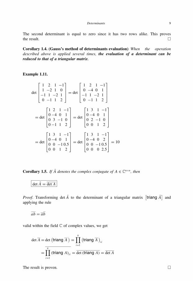
Corollary 1.4. (Gauss’s method of determinants evaluation) When the operationdescribed above is applied several times, the evaluation of a determinant can bereduced to that of a triangular matrix.
Example 1.11.
det
⎡⎢⎢⎣
1 2 1 −1
1 −2 1 0
−1 1 −2 1
0 −1 1 2
⎤⎥⎥⎦ = det
⎡⎢⎢⎣
1 2 1 −1
0 −4 0 1
−1 1 −2 1
0 −1 1 2
⎤⎥⎥⎦
= det
⎡⎢⎢⎣1 2 1 −1
0−4 0 1
0 3 −1 0
0−1 1 2
⎤⎥⎥⎦ = det
⎡⎢⎢⎣1 3 1 −1
0−4 0 1
0 2 −1 0
0 0 1 2
⎤⎥⎥⎦
= det
⎡⎢⎢⎣1 3 1 −1
0−4 0 1
0 0 −1 0.5
0 0 1 2
⎤⎥⎥⎦ = det
⎡⎢⎢⎣1 3 1 −1
0−4 0 2
0 0 −1 0.5
0 0 0 2.5
⎤⎥⎥⎦ = 10
Corollary 1.5. If A denotes the complex conjugate of A ∈ Cn×n, then
det A = detA
Proof. Transforming det A to the determinant of a triangular matrix[triang A
]and
applying the rule
ab = ab
valid within the field C of complex values, we get
detA= det(triang A
) = n∏i=1
(triang A
)ii
=n∏i=1
(triang A)ii = det (triang A) = detA
The result is proven. �
10 Advanced Mathematical Tools for Automatic Control Engineers: Volume 1
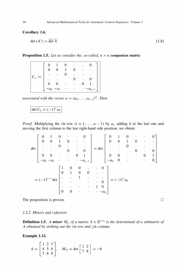
Corollary 1.6.
det (A∗) = detA (1.8)
Proposition 1.5. Let us consider the, so-called, n× n companion matrix
Ca :=
⎡⎢⎢⎢⎢⎢⎢⎣
0 1 0 · · 0
0 0 1 0 · ·· · 0 · · ·· · 0 · 0
0 0 · · 0 1
−a0 −a1 · · · −an−1
⎤⎥⎥⎥⎥⎥⎥⎦
associated with the vector a = (a0, . . . , an−1)ᵀ. Then
detCa = (−1)n a0
Proof. Multiplying the ith row (i = 1, . . . , n− 1) by ai , adding it to the last one and
moving the first column to the last right-hand side position, we obtain
det
⎡⎢⎢⎢⎢⎢⎢⎣
0 1 0 · · 0
0 0 1 0 · ·· · 0 · · ·· · 0 · 0
0 0 · · 0 1
−a0 −a1 · · · −an−1
⎤⎥⎥⎥⎥⎥⎥⎦ = det
⎡⎢⎢⎢⎢⎢⎢⎣
0 1 0 · · 0
0 0 1 0 · ·· · 0 · · ·· · 0 · 0
0 0 · · 0 1
−a0 0 · · · 0
⎤⎥⎥⎥⎥⎥⎥⎦
= (−1)n−1 det
⎡⎢⎢⎢⎢⎢⎢⎣
1 0 0 · · 0
0 1 0 0 · ·· · 1 · · ·· · · · 0
· · · · 1 0
0 0 · · · −a0
⎤⎥⎥⎥⎥⎥⎥⎦ = (−1)n a0
The proposition is proven. �
1.2.2 Minors and cofactors
Definition 1.5. A minor Mij of a matrix A ∈ Rn×n is the determinant of a submatrix ofA obtained by striking out the ith row and j th column.
Example 1.12.
A =⎡⎣ 1 2 3
4 5 6
7 8 9
⎤⎦, M23 = det
[1 2
7 8
]= −6

Determinants 11
Definition 1.6. The cofactor Aij (or ij -algebraic complement) of the element aij of thematrix A ∈ Rn×n is defined as
Aij := (−1)i+j Mij (1.9)
Example 1.13.
A =⎡⎣ 1 2 3
4 5 6¯
7 8 9
⎤⎦, A23 = (−1)2+3 det
[1 2
7 8
]= 6
Lemma 1.1. (Cofactor expansion) For any matrix A ∈ Rn×n and any indices i, j =1, . . . , n
detA =n∑j=1
aijAij =n∑i=1
aijAij (1.10)
Proof. Observing that each term in (1.2) contains an element of the ith row (or, analo-
gously, of the j th column) and collecting together all terms containing aij we obtain
detA :=∑
j1,j2,...,jn
(−1)t(j1,j2,...,jn) a1j1a2j2 · · · anjn
=n∑ji=1
aiji
[ ∑jk,k �=i
(−1)t(j1,j2,...,jn)∏k �=iakjk
]
To fulfill the proof it is sufficient to show that
Aiji :=∑jk,k �=i
(−1)t(j1,j2,...,jn)∏k �=iakjk = Aiji
In view of the relation
(−1)t(j1,j2,...,jn) = (−1)i+ji (−1)t(j1,j2,...,ji−1,jj+1,...,jn)
it follows that
Aiji = (−1)i+ji[ ∑jk,k �=i
(−1)t(j1,j2,...,ji−1,jj+1,...,jn)∏k �=iakjk
]= (−1)i+ji Miji = Aiji
which completes the proof. �

12 Advanced Mathematical Tools for Automatic Control Engineers: Volume 1
Example 1.14.
det
⎡⎣ 1 2 3
4 5 6
7 8 9
⎤⎦= 1 (−1)1+1 det
[5 6
8 9
]
+ 4 (−1)2+1 det
[2 3
8 9
]+ 7 (−1)3+1
[2 3
5 6
]= −3− 4 (−6)+ 7 (−3) = 0
Lemma 1.2. For any matrix A ∈ Rn×n and any indices i �= r, j �= s (i, j = 1, . . . , n) itfollows that
n∑j=1
aijArj =n∑i=1
aijAis = 0
Proof. The result follows directly if we consider the matrix obtained from A by replacing
the row i (column j ) by the row r (column s) and then use the property of a determinant
with two rows (or columns) alike that says that it is equal to zero. �
Lemma 1.3. Vandermonde determinant
V1,n := det
⎡⎢⎢⎢⎢⎣
1 1 · · · 1
x1 x2 · · · xnx21 x22 · · · x2n· · · · · ·xn−11 xn−1
2 · · · xn−1n
⎤⎥⎥⎥⎥⎦ =
n∏j=1
n∏i>j
(xi − xj
)
Proof. Adding the ith row multiplied by (−x1) to the (i + 1) row (i = n − 1,
n− 2, . . . , 1) and applying the iteration implies
Vn = det
⎡⎢⎢⎢⎢⎣1 1 · · · 1
0 x2 − x1 · · · xn − x10 x22 − x1x2 · · · x2n − x1xn· · · · · ·0 xn−1
2 − x1xn−22 · · · xn−1
n − x1xn−2n
⎤⎥⎥⎥⎥⎦
= det
⎡⎢⎢⎣
x2 − x1 · · · xn − x1(x2 − x1) x2 · · · (xn − x1) xn
· · · · ·(x2 − x1) xn−2
2 · · · (xn − x1) xn−2n
⎤⎥⎥⎦
Determinants 13
= (x2 − x1) · · · (xn − x1) det
⎡⎢⎢⎣
1 · · · 1
x2 · · · xn· · · · ·xn−22 · · · xn−2
n
⎤⎥⎥⎦
=n∏i=2
(xi − x1) V2,n = · · · =n∏j=1
n∏i>j
(xi − xj )Vn,n =n∏j=1
n∏i>j
(xi − xj )
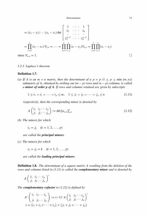
since Vn,n = 1. �
1.2.3 Laplace’s theorem
Definition 1.7.
(a) If A is an m × n matrix, then the determinant of a p × p (1 ≤ p ≤ min (m, n))submatrix of A, obtained by striking out (m−p) rows and (n−p) columns, is calleda minor of order p of A. If rows and columns retained are given by subscripts
1 ≤ i1 < i2 < · · · < ip ≤ m, 1 ≤ j1 < j2 < · · · < jp ≤ n (1.11)
respectively, then the corresponding minor is denoted by
A
(i1 i2 · · · ipj1 j2 · · · jp
):= det [aikjk ]
p
k=1(1.12)
(b) The minors for which
ik = jk (k = 1, 2, . . . , p)
are called the principal minors.
(c) The minors for which
ik = jk = k (k = 1, 2, . . . , p)
are called the leading principal minors.
Definition 1.8. The determinant of a square matrix A resulting from the deletion of therows and columns listed in (1.11) is called the complementary minor and is denoted by
A
(i1 i2 · · · ipj1 j2 · · · jp
)cThe complementary cofactor to (1.12) is defined by
Ac
(i1 i2 · · · ipj1 j2 · · · jp
):= (−1)s A
(i1 i2 · · · ipj1 j2 · · · jp
)cs = (
i1 + i2 + · · · + ip)+ (
j1 + j2 + · · · + jp)

14 Advanced Mathematical Tools for Automatic Control Engineers: Volume 1
Example 1.15. For A = [aij ]5
i,j=1we have
A
(2 3 5
1 2 4
)=
⎡⎣ a21 a22 a24a31 a32 a34a51 a52 a54
⎤⎦
A
(2 3 5
1 2 4
)c= A
(1 4
3 5
)=
[a13 a15a43 a45
]
Ac(
2 3 5
1 2 4
)= (−1)17
[a13 a15a43 a45
]= − (a13a45 − a15a43)
Theorem 1.1. (Laplace’s theorem) Let A be an arbitrary n × n matrix and let any prows (or columns) of A be chosen. Then
detA =∑
j1,j2,···,jpA
(i1 i2 · · · ipj1 j2 · · · jp
)Ac
(i1 i2 · · · ipj1 j2 · · · jp
)(1.13)
where the summation extends over all Cpn :=n!
p! (n− p)! distinct sets of column indices
j1, j2, · · ·, jp(1 ≤ j1 < j2 < · · · < jp ≤ n
)Or, equivalently,
detA =∑
i1,j2,···,ipA
(i1 i2 · · · ipj1 j2 · · · jp
)Ac
(i1 i2 · · · ipj1 j2 · · · jp
)(1.14)
where
1 ≤ i1 < i2 < · · · < ip ≤ n
Proof. It can be arranged similarly to that of the cofactor expansion formula (1.10). �
1.2.4 Binet–Cauchy formula
Theorem 1.2. (Binet–Cauchy formula) Two matrices A ∈ Rp×n and B ∈ Rn×p aregiven, that is,
A =
⎡⎢⎢⎣a11 a12 · a1na21 a22 · a2n· · · ·ap1 ap2 · apn
⎤⎥⎥⎦, B =
⎡⎢⎢⎣b11 b12 · b1pb21 b22 · b2p· · · ·bn1 bn2 · bnp
⎤⎥⎥⎦

Determinants 15
Multiplying the rows of A by the columns of B let us construct p2 numbers
cij =n∑k=1
aikbkj (i, j = 1, . . . , p)
and consider the determinant D := ∣∣cij ∣∣pi,j=1. Then
1. if p ≤ n we have
D =∑
1≤j1<j2<···<jp≤nA
(1 2 · · · pj1 j2 · · · jp
)B
(j1 j2 · · · jp1 2 · · · p
)(1.15)
2. if p > n we have
D = 0
Proof. It follows directly from Laplace’s theorem. �
Example 1.16. Let us prove that
⎡⎢⎢⎢⎣
n∑k=1
akck
n∑k=1
akdk
n∑k=1
bkck
n∑k=1
bkdk
⎤⎥⎥⎥⎦ =
∑1≤j<k≤n
[aj akbj bk
] [cj ckdj dk
](1.16)
Indeed, considering two matrices
A =[a11 a12 · a1na21 a22 · a2n
], B =
⎡⎢⎢⎣c11 d12c21 d22· ·cn1 dn2
⎤⎥⎥⎦
and applying (1.15) we have (1.16).
Example 1.17. (Cauchy identity) The following identity holds
(n∑i=1
aici
)(n∑i=1
bidi
)−(
n∑i=1
aidi
)(n∑i=1
bici
)=
∑1≤j<k≤n
(ajbk − akbj
) (cjdk − ckdj
)
It is the direct result of (1.16).

16 Advanced Mathematical Tools for Automatic Control Engineers: Volume 1
1.3 Linear algebraic equations and the existence of solutions
1.3.1 Gauss’s method
Let us consider the set of m linear equations (a system of linear equations)
a11x1 + a12x2+ · · · + a1nxn = b1a21x1 + a22x2+ · · · + a2nxn = b2
· · ·am1x1 + am2x2+ · · · + amnxn = bm
(1.17)
in n unknowns x1, x2, . . . , xn ∈ R and m × n coefficients aij ∈ R. An n-tuple(x∗1 , x
∗2 , . . . , x
∗n
)is said to be a solution of (1.17) if, upon substituting x∗i instead of
xi (i = 1, . . . n) in (1.17), equalities are obtained. A system of linear equations (1.17)
may have
• a unique solution;• infinitely many solutions;• no solutions (to be inconsistent).
Definition 1.9. A system of linear equations
a11x1 + a12x2 + · · · + a1nxn = b1a21x1 + a22x2 + · · · + a2nxn = b2
· · ·am1x1 + am2x2 + · · · + amnxn = bm
(1.18)
is said to be equivalent to a system (1.17) if their sets of solutions coincide or they donot exist simultaneously.
It is easy to see that the following elementary operations transform the given system
of linear equations to an equivalent one:
• interchanging equations in the system;• multiplying an equation in the given system by a nonzero constant;• adding one equation, multiplied by a number, to another.
Proposition 1.6. (Gauss’s rule) Any system of m linear equations in n unknowns has anequivalent system in which the augmented matrix has a reduced row-echelon form, forexample, for m < n
a11x1 + a12x2 + · · · + a1nxn = b1a21x1 + a22x2 + · · · + a2nxn = b2
· · ·0 · x1 + · · · + 0 · xn−m−1 + amnxn−m + · · · + amnxn = bm
· · ·0 · x1 + 0 · x2 + · · · + 0 · xn = 0
Determinants 17
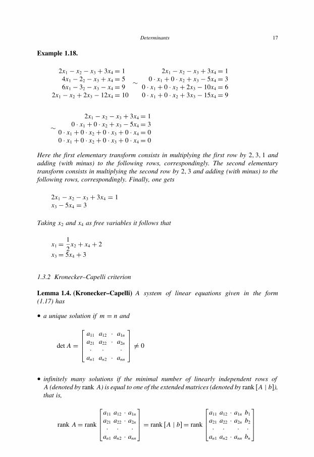
Example 1.18.
2x1 − x2 − x3 + 3x4 = 1
4x1 − 22 − x3 + x4 = 5
6x1 − 32 − x3 − x4 = 9
2x1 − x2 + 2x3 − 12x4 = 10
∼2x1 − x2 − x3 + 3x4 = 1
0 · x1 + 0 · x2 + x3 − 5x4 = 3
0 · x1 + 0 · x2 + 2x3 − 10x4 = 6
0 · x1 + 0 · x2 + 3x3 − 15x4 = 9
∼2x1 − x2 − x3 + 3x4 = 1
0 · x1 + 0 · x2 + x3 − 5x4 = 3
0 · x1 + 0 · x2 + 0 · x3 + 0 · x4 = 0
0 · x1 + 0 · x2 + 0 · x3 + 0 · x4 = 0
Here the first elementary transform consists in multiplying the first row by 2, 3, 1 andadding (with minus) to the following rows, correspondingly. The second elementarytransform consists in multiplying the second row by 2, 3 and adding (with minus) to thefollowing rows, correspondingly. Finally, one gets
2x1 − x2 − x3 + 3x4 = 1
x3 − 5x4 = 3
Taking x2 and x4 as free variables it follows that
x1 = 1
2x2 + x4 + 2
x3 = 5x4 + 3
1.3.2 Kronecker–Capelli criterion
Lemma 1.4. (Kronecker–Capelli) A system of linear equations given in the form(1.17) has
• a unique solution if m = n and
detA =
⎡⎢⎢⎣a11 a12 · a1na21 a22 · a2n· · ·an1 an2 · ann
⎤⎥⎥⎦ �= 0
• infinitely many solutions if the minimal number of linearly independent rows ofA (denoted by rank A) is equal to one of the extended matrices (denoted by rank [A | b]),that is,
rank A= rank
⎡⎢⎢⎣a11 a12 · a1na21 a22 · a2n· · ·an1 an2 · ann
⎤⎥⎥⎦ = rank [A | b]= rank
⎡⎢⎢⎣a11 a12 · a1n b1a21 a22 · a2n b2· · · ·an1 an2 · ann bn
⎤⎥⎥⎦

18 Advanced Mathematical Tools for Automatic Control Engineers: Volume 1
• no solutions (to be inconsistent) if
rank A �= rank [A | b]
The proof of this fact will be clarified in the next chapter where the inverse matrix will
be introduced.
1.3.3 Cramer’s rule
Proposition 1.7. (Cramer) If m = n and detA �= 0 the unique solution of (1.17) isgiven by
xi = 1
detA
⎡⎢⎢⎣a11 · a1,i−1 b1 a1,i+1 · a1na21 · a2,i−1 b2 a2,i+1 · a2n· · · · · · ·an1 · an,i−1 bn an,i+1 · ann
⎤⎥⎥⎦ (i = 1, . . . , n)
The proof of this fact will be also done in the next chapter.
Example 1.19.
x1 − 2x2 = 1
3x1 − 4x2 = 7
}, detA =
∣∣∣∣1 −2
3 −4
∣∣∣∣ = 2 �= 0
x1 = 1
2
∣∣∣∣1 −2
7 −4
∣∣∣∣ = 10
2, x2 = 1
2
∣∣∣∣1 1
3 7
∣∣∣∣ = 4
2= 2

2 Matrices and Matrix Operations
Contents2.1 Basic definitions . . . . . . . . . . . . . . . . . . . . . . . . . . . . . . . 19
2.2 Some matrix properties . . . . . . . . . . . . . . . . . . . . . . . . . . . . 21
2.3 Kronecker product . . . . . . . . . . . . . . . . . . . . . . . . . . . . . . 26
2.4 Submatrices, partitioning of matrices and Schur’s formulas . . . . . . . . . 29
2.5 Elementary transformations on matrices . . . . . . . . . . . . . . . . . . . 32
2.6 Rank of a matrix . . . . . . . . . . . . . . . . . . . . . . . . . . . . . . . 36
2.7 Trace of a quadratic matrix . . . . . . . . . . . . . . . . . . . . . . . . . . 38
2.1 Basic definitions
2.1.1 Basic operations over matrices
The definition of a matrix has been done in (1.1). Here the basic properties of matrices
and the operations with them will be considered.
Three basic operations over matrices are defined: summation, multiplication and
multiplication of a matrix by a scalar.
Definition 2.1.
1. The sum A + B of two matrices A = [aij ]m,n
i,j=1and B = [bij ]
m,n
i,j=1of the same size is
defined as
A+ B := [aij + bij ]m,ni,j=1
2. The product C of two matrices A = [aij ]m,n
i,j=1and B = [bij ]
n,p
i,j=1may be of different
sizes (but, as required, the number of columns of the first matrix coincides with thenumber of rows of the second one) and is defined as
C = [cij ]m,p
i,j=1= AB :=
[n∑k=1
aikbkj
]m,pi,j=1
(2.1)
(If m = p = 1 this is the definition of the scalar product of two vectors). In general,
AB �= BA
19

20 Advanced Mathematical Tools for Automatic Control Engineers: Volume 1
3. The operation of multiplication of a matrix A ∈ Rm×n by a scalar α ∈ R is definedas follows
αA = Aα := [αaij ]m,n
i,j=1
4. The difference A − B of two matrices A = [aij ]m,n
i,j=1and B = [bij ]
m,n
i,j=1of the same
size is called a matrix X satisfying
X + B = A
Obviously,
X = A− B := [aij − bij ]m,ni,j=1
2.1.2 Special forms of square matrices
Definition 2.2.
1. A diagonal matrix is a particular case of a squared matrix (m = n) for which allelements lying outside the main diagonal are equal to zero:
A =
⎡⎢⎢⎣a11 0 · 0
0 a22 · 0
· · · ·0 0 · ann
⎤⎥⎥⎦ = diag [a11, a22, . . . , ann]
If a11 = a22 = . . . = ann = 1 the matrix A becomes the unit (or identity) matrix
In×n :=
⎡⎢⎢⎣1 0 · 0
0 1 · 0
· · · ·0 0 · 1
⎤⎥⎥⎦
(usually, the subindex in the unit matrix definition is omitted). If a11 = a22 = . . . =ann = 0 the matrix A becomes a zero-square matrix:
On×n :=
⎡⎢⎢⎣0 0 · 0
0 0 · 0
· · · ·0 0 · 0
⎤⎥⎥⎦
2. The matrix Aᵀ ∈ Rn×m is said to be transposed to a matrix A ∈ Rm×n if
Aᵀ = [aji]n,m
j,i=1
Matrices and matrix operations 21
3. The adjoint (or adjudged) of a square matrix A ∈ Rn×n, written adj A, is defined tobe the transposed matrix of cofactors Aji (1.9) of A, that is,
adjA :=([Aji]
n
j,i=1
)ᵀ
4. A square matrix A ∈ Rn×n is said to be singular or nonsingular according to whetherdetA is zero or nonzero.
5. A square matrix B ∈ Rn×n is referred to as an inverse of the square matrixA ∈ Rn×n if
AB = BA = In×n (2.2)
and when this is the case, we write B = A−1.6. A matrix A ∈ Cn×n
• is normal if AA∗ = A∗A and real normal if A ∈ Rn×n and AAᵀ = AᵀA;• is Hermitian if A = A∗ and symmetric if A ∈ Rn×n and A = Aᵀ;• is skew-Hermitian if A∗ = −A and skew-symmetric if A ∈ Rn×n and Aᵀ = −A.
7. A matrix A ∈ Rn×n is said to be orthogonal if AᵀA = AAᵀ = In×n, or, equivalently,if Aᵀ = A−1 and unitary if A ∈ Cn×n and A∗A = AA∗ = In×n, or, equivalently, ifA∗ = A−1.
2.2 Some matrix properties
The following matrix properties hold:
1. Commutativity of the summing operation, that is,
A+ B = B + A
2. Associativity of the summing operation, that is,
(A+ B)+ C = A+ (B + C)
3. Associativity of the multiplication operation, that is,
(AB)C = A (BC)
4. Distributivity of the multiplication operation with respect to the summation operation,
that is,
(A+ B)C = AC + BC,C (A+ B) = CA+ CBAI = IA = A

22 Advanced Mathematical Tools for Automatic Control Engineers: Volume 1
5. For A = [aij ]m,n
i,j=1and B = [bij ]
n,p
i,j=1it follows that
AB =n∑k=1
a(k)b(k)ᵀ (2.3)
where
a(k) :=⎛⎜⎝ a1k...amk
⎞⎟⎠, b(k) :=
⎛⎜⎝bk1...bkp
⎞⎟⎠
6. For the power matrix Ap (p is a nonnegative integer number) defined as
Ap = AA · · · A︸ ︷︷ ︸p
, A0 := I
the following exponent laws hold
ApAq =Ap+q(Ap)q =Apq
where p and q are any nonnegative integers.
7. If two matrices commute, that is,
AB = BA
then
(AB)p = ApBp
and the formula of Newton’s binom holds:
(A+ B)m =m∑i=0
CimAm−iBi
where Cim :=m!
i! (m− i)! .8. A matrix U ∈ Cn×n is unitary if and only if for any x, y ∈ Cn
(Ux,Uy) := (Ux)∗ Uy = (x, y)
Indeed, if U ∗U = In×n then (Ux,Uy) = (x, U ∗Uy) = (x, y). Conversely, if
(Ux,Uy) = (x, y), then ([U ∗U − In×n] x, y
) = 0 for any x, y ∈ Cn that proves the
result.
9. If A and B are unitary, then AB is unitary too.

Matrices and matrix operations 23
10. If A and B are normal and AB = BA (they commute), then AB is normal too.
11. If Ai are Hermitian (skew-Hermitian) and αi are any real numbers, then the matrixm∑i=1
αiAi is Hermitian (skew-Hermitian) too.
12. Any matrix A ∈ Cn×n can be represented as
A = H + iK
where
H = A+ A∗
2, K = A− A
∗
2i, i2 = −1
are both Hermitian. If A ∈ Rn×n, then
A = S + T
where
S = A+ Aᵀ
2, T = A− A
ᵀ
2
and S is symmetric and T is skew-symmetric.
13. For any two square matrices A and B the following determinant rule holds:
det (AB) = det (A) det (B)
This fact directly follows from Binet–Cauchy formula (1.15).
14. For any A ∈ Rm×n and B ∈ Rn×p
(AB)T = BᵀAᵀ
Indeed,
(AB)T =[
n∑k=1
ajkbki
]m,pi,j=1
=[
n∑k=1
bkiajk
]m,pi,j=1
= BᵀAᵀ
15. For any A ∈ Rn×n
adjAᵀ = (adjA)TadjIn×n = In×n
adj (αA) = αn−1adjA for any α ∈ F
16. For any A ∈ Cn×n
adjA∗ = (adjA)∗

24 Advanced Mathematical Tools for Automatic Control Engineers: Volume 1
17. For any A ∈ Rn×n
A (adjA) = (adjA)A = (detA) In×n (2.4)
This may be directly proven if we calculate the matrix product in the left-hand side
using the row expansion formula (1.10) that leads to a matrix with the number detA
in each position on its main diagonal and zeros elsewhere.
18. If detA �= 0, then
A−1 = 1
detAadjA (2.5)
This may be easily checked if we substitute (2.5) into (2.2) and verify its validity,
using (2.4). As a consequence of (2.5) we get
det (adjA) = (detA)n−1
As a consequence, we have
det(A−1
) = 1
detA(2.6)
This follows from (2.5) and (2.4).
19. If detA �= 0, then
(A−1
)ᵀ = (Aᵀ)−1
Indeed,
In×n = AA−1 = (AA−1
)ᵀ = (A−1
)ᵀAᵀ
So, by definitions,(A−1
)ᵀ = (Aᵀ)−1.
20. If A and B are invertible matrices of the same size, then
(AB)−1 = B−1A−1
As the result, the following fact holds: if detA = detB, then there exists a matrix C
such that
A=BCdetC = 1
Indeed, C = B−1A and
detC = det(B−1A
) = det(B−1
)detA = detA
det (B)= 1

Matrices and matrix operations 25
21. It is easy to see that for any unitary matrix A ∈ Cn×n is always invertible and the
following properties hold:
A−1 = A∗
detA = ±1
Indeed, since A∗A = AA∗ = In×n, it follows that A−1 = A∗. Also in view of (1.8)
we have
detA∗A = det In×n = 1
detA∗A = (detA∗) (detA) = (detA
)(detA) = |detA| = 1
22. Let A ∈ Rn×n, B ∈ Rn×r , C ∈ Rr×r and D ∈ Rr×n
(a) If A−1 and(Ir×r +DA−1BC
)−1exist, then
(A+ BCD)−1
= A−1 − A−1BC(C + CDA−1BC
)−1CDA−1
= A−1 − A−1BC(Ir×r +DA−1BC
)−1DA−1
(2.7)
Indeed, the simple matrix multiplication implies[A−1 − A−1BC
(C + CDA−1BC
)−1CDA−1
](A+ BCD)
= In×n − A−1BC(C + CDA−1BC
)−1CD + A−1BCD
−A−1BC(C + CDA−1BC
)−1 [−C + C + CDA−1BC]D
= In×n − A−1BC(C + CDA−1BC
)−1CD + A−1BCD
−A−1BC(C + CDA−1BC
)−1CD − A−1BCD = In×n
Analogously,[A−1 − A−1BC
(Ir×r +DA−1BC
)−1DA−1
](A+ BCD)
= In×n − A−1BC(Ir×r +DA−1BC
)−1D + A−1BCD
−A−1BC(Ir×r +DA−1BC
)−1 [−Ir×r + Ir×r +DA−1BC]D
= In×n − A−1BC(Ir×r +DA−1BC
)−1D + A−1BCD
+A−1BC(Ir×r +DA−1BC
)−1D − A−1BCD = In×n
(b) In the partial case when r = 1, C = 1, B = u, D = vᵀ and vᵀA−1u �= −1, we
obtain the Sherman–Morrison formula:
(A+ uvᵀ)−1 = A−1 − A−1vᵀA−1
1+ vᵀA−1u(2.8)

26 Advanced Mathematical Tools for Automatic Control Engineers: Volume 1
The next statement seems to be important for understanding the internal relationship
within different classes of matrices.
Claim 2.1.
1. Any complex unitary, Hermitian, skew-Hermitian and real orthogonal, symmetricand skew-symmetric matrix is normal, that is, it satisfies the condition
AA∗ = A∗A for complex matrices
and
AAᵀ = AᵀA for real matrices
2. AmatrixA is normal if and only if the matricesA andA∗ have the same eigenvectors.
Both of these properties can be easily checked directly.
2.3 Kronecker product
Definition 2.3. For two matrices A ∈ Rm×n, B ∈ Rp×q the direct (tensor) Kroneckerproduct, written A⊗ B, is defined to be the partitioned matrix
A⊗ B :=
⎡⎢⎢⎣a11B a12B · a1nB
a21B a22B · a2nB
· · · ·am1B am2B · amnB
⎤⎥⎥⎦
= [aijB]m,n
i,j=1∈ Rmp×nq
(2.9)
Example 2.1. If
A =[a11 a12 a13a21 a22 a23
], B = [
b11 b12]
then
A⊗ B =[a11b11 a11b12 a12b11 a12b12 a13b11 a13b12a21b11 a21b12 a22b11 a22b12 a23b11 a23b12
]The following properties for the Kronecker product are fulfilled:
(a)
In×n ⊗ A =
⎡⎢⎢⎢⎢⎣A O · · O
O A · · ·· · · · ·· · O A O
O · · O A
⎤⎥⎥⎥⎥⎦ = diag [A,A, . . . , A] (2.10)

Matrices and matrix operations 27
(b) Im×n ⊗ Ip×q = Imp×nq
(c) for any α ∈ F it follows that
(αA)⊗ B = A⊗ (αB) = α (A⊗ B)
(d) (A+ C)⊗ B = A⊗ B + C ⊗ B
(e) A⊗ (B + C) = A⊗ B + A⊗ C
(f) (A⊗ B)⊗ C = A⊗ (B ⊗ C)
(g) (A⊗ B)ᵀ = Aᵀ ⊗ Bᵀ
and for complex matrices
(A⊗ B) = A⊗ B(A⊗ B)∗ = A∗ ⊗ B∗
Next, very useful properties are less obvious.
Proposition 2.1. If A ∈ Rm×n, B ∈ Rp×q, C ∈ Rn×k and D ∈ Rq×r then
(A⊗ B) (C ⊗D) = (AC)⊗ (BD) (2.11)
Proof. It follows from the identity that
n∑j=1
(aijB
) (cjsD
) =(
n∑j=1
aij cjs
)BD
�Corollary 2.1. If A ∈ Rn×n, B ∈ Rm×m then1.
A⊗ B = (A⊗ In×n) (Im×m ⊗ B) = (Im×m ⊗ B) (A⊗ In×n)
(to prove this it is sufficient to take C = In×n and D = Im×m).2.
(A1 ⊗ B1) (A2 ⊗ B2) · · ·(Ap ⊗ Bp
)= (A1A2 · · · Ap
)⊗ (B1B2 · · · Bp
)for all matrices Ai ∈ Rn×n and Bi ∈ Rm×m (i = 1, . . . , p).

28 Advanced Mathematical Tools for Automatic Control Engineers: Volume 1
3.
(A⊗ B)−1 = A−1 ⊗ B−1
provided that both A−1 and B−1 exist. Indeed,
(A⊗ B) (A⊗ B)−1 = (A⊗ B) (A−1 ⊗ B−1)
= (AA−1
)⊗ (BB−1
) = In×n ⊗ Im×m = Inm×nmProposition 2.2. If A ∈ Rn×n, B ∈ Rm×m then there exists a permutation P ∈ Rnm×nm
such that
Pᵀ (A⊗ B)P = B ⊗ A
Proof. It is easy to check that there exists a permutation matrix such that
Pᵀ (A⊗ In×n) P = In×n ⊗ APᵀ (Im×m ⊗ B)P = B ⊗ Im×m (2.12)
Then, since for any permutation matrix PPᵀ = Inm×nm, by (2.1) it follows that
Pᵀ (A⊗ B)P = Pᵀ (A⊗ In×n) (Im×m ⊗ B)P= Pᵀ (A⊗ In×n) PPᵀ (Im×m ⊗ B)P= (In×n ⊗ A) (B ⊗ Im×m) = B ⊗ A
�
Corollary 2.2.
det (A⊗ B) = (detA)n(detB)
m (2.13)
Indeed, by (2.1)
det (A⊗ B) = [det (A⊗ In×n)] [det (Im×m ⊗ B)]
In view of (2.12) and (2.10) one has
det (A⊗ In×n)= det [Pᵀ (In×n ⊗ A)P ]= det [PPᵀ (In×n ⊗ A)] = det (In×n ⊗ A)= det (diag (A,A, . . . , A)) = (detA)n
Analogously,
det (Im×m ⊗ B) = (detB)m
which completes the proof.

Matrices and matrix operations 29
2.4 Submatrices, partitioning of matrices and Schur’s formulas
Given matrix A = [aij ]m,n
i,j=1, if a number of complete rows or columns of A are deleted,
or if some complete rows or complete columns are deleted, the new matrix that is obtained
is called a submatrix of A. A division of matrices into submatrices is referred to as a
partition of the matrix.
Proposition 2.3. If the matrices A and B are partitioned as follows
A =[A11 A12
A21 A22
], B =
[B11 B12
B21 B22
]
where the corresponding submatrices Aij and Bij have the same size, then by directcomputation we get
A± B =[A11 ± B11 A12 ± B12
A21 ± B21 A22 ± B22
](2.14)
and
AB =[A11B11 + A12B21 A11B12 + A12B22
A21B11 + A22B21 A21B12 + A22B22
](2.15)
Proposition 2.4. If A11 and A22 are square matrices then
1. for
A =[A11 O
A21 A22
]
it follows that
detA = (detA11) (detA22)
2. for
A =[A11 A12
A21 O
]∈ Rn×n
A12 ∈ Rp×p, A12 ∈ R(n−p)×(n−p)

30 Advanced Mathematical Tools for Automatic Control Engineers: Volume 1
it follows that
detA = (−1)(n+1)p (detA12) (detA21)
Proposition 2.5. If A is block-diagonal, that is,
A = diag[A11 A22 · · ·Ann
]then1.
detA =n∏i=1
detAii
2.
rank diag[A11 A22 · · ·Ann
] = n∑i=1
(rank Aii)
Lemma 2.1. (Schur’s formulas) For block-matrix
A =[A B
C D
]
where A and D may be of different sizes, the following properties hold:
det A =
⎧⎪⎪⎨⎪⎪⎩
detA det(D − CA−1B
)if detA �= 0
det(A− BD−1C
)detD if detD �= 0
det (AD − CB) if AC = CAdet (AD − BC) if CD = DC
(2.16)
Proof. Notice that for the case when detA �= 0, we have
[A B
C D
]=
[I O
CA−1 I
] [A O
OD − CA−1B
] [I A−1B
O I
]
which leads directly to the first formula. The second formula, when detD �= 0, may be
proven by the analogous way taking into account the decomposition

Matrices and matrix operations 31
[A B
C D
]=
[I BD−1
O I
] [A− BD−1C O
O D
] [I O
D−1C I
]
For proofs of formulas three and four see Gantmacher (1990). �
Lemma 2.2. (on the inversion of a block-matrix) If
S :=[S11 S12S21 S22
], S11 ∈ Rl×l , S22 ∈ Rk×k
then
S−1 :=[A B
C D
]A = (
S11 − S12S−122 S21
)−1 ∈ Rl×l
B = −S−111 S12D
C = −S−122 S21A
D = (S22 − S21S−1
11 S12)−1 ∈ Rk×k
provided by the condition that all inverse matrices exist.
Proof. In view of the identity
SS−1 =[S11A+ S12C S11B + S12DS21A+ S22C S21B + S22D
]= I(l+k)×(l+k)
it is sufficient to check the equalities
S11A+ S12C = Il×lS11B + S12D =Ol×kS21A+ S22C =Ok×lS21B + S22D = Ik×k
The second and third ones hold automatically. Then we have:
S11A+ S12C = S11A− S12S−122 S21A
= (S11 − S12S−1
22 S21)A = A−1A = Il×l
and
S21B + S22D = −S21S−111 S12D + S22D
= (S22 − S21S−1
11 S12)D = D−1D = Ik×k
�
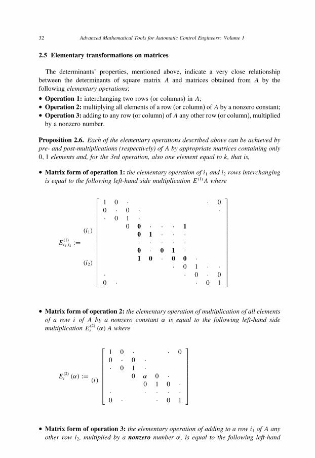
32 Advanced Mathematical Tools for Automatic Control Engineers: Volume 1
2.5 Elementary transformations on matrices
The determinants’ properties, mentioned above, indicate a very close relationship
between the determinants of square matrix A and matrices obtained from A by the
following elementary operations:
• Operation 1: interchanging two rows (or columns) in A;
• Operation 2:multiplying all elements of a row (or column) of A by a nonzero constant;
• Operation 3: adding to any row (or column) of A any other row (or column), multiplied
by a nonzero number.
Proposition 2.6. Each of the elementary operations described above can be achieved bypre- and post-multiplications (respectively) of A by appropriate matrices containing only0, 1 elements and, for the 3rd operation, also one element equal to k, that is,
• Matrix form of operation 1: the elementary operation of i1 and i2 rows interchangingis equal to the following left-hand side multiplication E(1)A where
E(1)i1,i2
:=(i1)
(i2)
⎡⎢⎢⎢⎢⎢⎢⎢⎢⎢⎢⎢⎢⎢⎢⎢⎢⎣
1 0 · · 0
0 · 0 · ·· 0 1 ·
0 0 · · · 10 1 · · ·· · · · ·0 · 0 1 ·1 0 · 0 0 ·
· 0 1 · ·· · 0 · 0
0 · · 0 1
⎤⎥⎥⎥⎥⎥⎥⎥⎥⎥⎥⎥⎥⎥⎥⎥⎥⎦
• Matrix form of operation 2: the elementary operation of multiplication of all elementsof a row i of A by a nonzero constant α is equal to the following left-hand sidemultiplication E(2)i (α)A where
E(2)i (α) := (i)
⎡⎢⎢⎢⎢⎢⎢⎢⎢⎣
1 0 · · 0
0 · 0 ·· 0 1 ·
0 α 0 ·0 1 0 ·
· · · · ·0 · · 0 1
⎤⎥⎥⎥⎥⎥⎥⎥⎥⎦
• Matrix form of operation 3: the elementary operation of adding to a row i1 of A anyother row i2, multiplied by a nonzero number α, is equal to the following left-hand
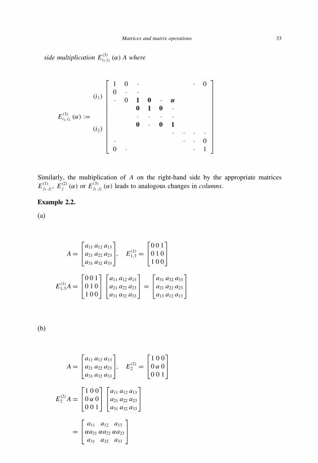
Matrices and matrix operations 33
side multiplication E(3)i1,i2 (α)A where
E(3)i1,i2(α) :=
(i1)
(i2)
⎡⎢⎢⎢⎢⎢⎢⎢⎢⎢⎢⎢⎢⎣
1 0 · · 0
0 · ·· 0 1 0 · α
0 1 0 ·· · · ·0 · 0 1
· · · ·· · · 0
0 · · 1
⎤⎥⎥⎥⎥⎥⎥⎥⎥⎥⎥⎥⎥⎦
Similarly, the multiplication of A on the right-hand side by the appropriate matrices
E(1)j1,j2, E
(2)j (α) or E
(3)j1,j2(α) leads to analogous changes in columns.
Example 2.2.
(a)
A=⎡⎣a11 a12 a13a21 a22 a23a31 a32 a33
⎤⎦, E
(1)1,3 =
⎡⎣0 0 1
0 1 0
1 0 0
⎤⎦
E(1)1,3A=
⎡⎣0 0 1
0 1 0
1 0 0
⎤⎦⎡⎣a11 a12 a13a21 a22 a23a31 a32 a33
⎤⎦ =
⎡⎣a31 a32 a33a21 a22 a23a13 a12 a13
⎤⎦
(b)
A=⎡⎣a11 a12 a13a21 a22 a23a31 a32 a33
⎤⎦, E
(2)2 =
⎡⎣1 0 0
0 α 0
0 0 1
⎤⎦
E(2)2 A=
⎡⎣1 0 0
0 α 0
0 0 1
⎤⎦⎡⎣a11 a12 a13a21 a22 a23a31 a32 a33
⎤⎦
=⎡⎣ a11 a12 a13αa21 αa22 αa23a31 a32 a33
⎤⎦

34 Advanced Mathematical Tools for Automatic Control Engineers: Volume 1
(c)
A =⎡⎣ a11 a12 a13a21 a22 a23a31 a32 a33
⎤⎦, E
(3)1,3 (α) =
⎡⎣ 1 0 α
0 1 0
0 0 1
⎤⎦
E(3)1,3 (α)A =
⎡⎣ 1 0 α
0 1 0
0 0 1
⎤⎦⎡⎣ a11 a12 a13a21 a22 a23a31 a32 a33
⎤⎦
=⎡⎣ a11 + αa31 a12 + αa32 a13 + αa33
a21 a22 a23a31 a32 a33
⎤⎦
Proposition 2.7. For any subindices
detE(1)i1,i2
= −1, detE(2)i (α) = α, detE
(3)i1,i2(α) = 1 (2.17)
and
detE(1)i1,i2A = detAE
(1)j1,j2
= detA
detE(2)i (α)A = detAE
(2)j (α) = α detA
detE(3)i1,i2(α)A = detAE
(3)j1,j2(α) = detA
Proof. The formulas above are the simple mathematical expressions of the determinants,
properties (1.6), (1.3) and (1.7). �
Proposition 2.8. For any m × n matrix A there exists a finite sequence of elementarymatrices E1, E2, . . . , Ek+s such that
Ek · · · E2E1AEk+1 · · · Ek+sis one of the following matrices
1. In×n for m = n
2.[Im×m Om×(n−m)
]for m < n
3.
[In×n
O(m−n)×n
]for m > n
4.
[Ir×r Or×(n−r)
O(n−r)×r O(n−r)×(n−r)
]( r ≤ min (m, n))
(2.18)
known as canonical ones.
Proof. It follows directly from the elementary operations definition and its relation to the
canonical matrix forms. �

Matrices and matrix operations 35
Example 2.3. For
A =⎡⎣ 0 1 2 −1
−2 0 0 6
4 −2 −4 −10
⎤⎦
we get
A1 := E(2)2 (−1/2) A =⎡⎣ 0 1 2 −1
1 0 0 −3
4 −2 −4 −10
⎤⎦
A2 := E(3)2,3 (−4) A1 =⎡⎣ 0 1 2 −1
1 0 0 −3
0 −2 −4 2
⎤⎦
A3 := E(1)1,2A2 =⎡⎣ 1 0 0 −3
0 1 2 −1
0 −2 −4 2
⎤⎦
A4 := E(3)3,2 (2) A3 =⎡⎣ 1 0 0 −3
0 1 2 −1
0 0 0 0
⎤⎦
A5 := A4E(3)4,1 (3) =
⎡⎣ 1 0 0 0
0 1 2 −1
0 0 0 0
⎤⎦
A6 := A5E(3)4,2 (1) =
⎡⎣ 1 0 0 0
0 1 2 0
0 0 0 0
⎤⎦
A7 := A6E(3)3,2 (−2) =
⎡⎣ 1 0 0 0
0 1 0 0
0 0 0 0
⎤⎦
that is,
E(3)3,2 (2) E
(1)1,2E
(3)2,3 (−4) E
(2)2 (−1/2) AE
(3)4,1 (3) E
(3)4,2 (1) E
(3)3,2 (−2)
=[I2×2 O
O O
]
Corollary 2.3. For any m × n matrix A there exist matrices P (det P �= 0) and Q(detQ �= 0) such that PAQ is equal to one of the canonical matrices (2.18).

36 Advanced Mathematical Tools for Automatic Control Engineers: Volume 1
Proof. It follows from (2.7) and the fact that
det
(k∏i=1
Ei
)=
k∏i=1
det (Ei) �= 0
�
Definition 2.4. Two matricesA and B are said to be equivalent (or belonging to the sameequivalent class) if they may be transformed by the elementary operations application tothe same canonical matrix form. This is written as A ∼ B.
Proposition 2.9. An n× n matrix A is nonsingular if and only if A ∼ In×n.
Proof. Since
det (PAQ) = (detA) (det P) (detQ) = det S
where S is one of the canonical matrices (2.18), we have
detA = det S
(det P) (detQ)�= 0
if and only if S = In×n. �
Definition 2.5. A square n × n matrix A is said to be simple if it is equivalent to adiagonal matrix D.
These definitions will be used frequently below.
2.6 Rank of a matrix
Definition 2.6. For a matrix A ∈ Rm×n the size
r (1 ≤ r ≤ min (m, n))
of the identity matrix in the canonical form for A is referred to as the rank of A, writtenr = rankA. If A = Om×n then rankA = 0, otherwise rankA ≥ 1.
For each four canonical forms in (2.18) we have
rank In×n = n for m = n
rank[Im×m Om×(n−m)
] = m for m < n
rank
[In×n
O(m−n)×n
]= n for m > n

Matrices and matrix operations 37
[Ir×r Or×(n−r)
O(n−r)×r O(n−r)×(n−r)
]= r for r ≤ min (m, n)
Proposition 2.10. For a square matrix A ∈ Rn×n rankA = n if and only if it is nonsin-gular.
Proof. It follows straightforwardly from proposition (2.9). �
Corollary 2.4. The rank of a matrix A ∈ Rm×n is equal to the order of its largest nonzerominor.
Several important properties of rank are listed below.
1. (Frobenius inequality) If A,B and C are rectangular matrices and the product ABC
is well defined, then
rank(AB)+ rank(BC) ≤ rank(A)+ rank(ABC) (2.19)
rank(AB) ≤ min {rank(A), rank(B)} (2.20)
Indeed, taking in (2.19) first A and C to be appropriate size we obtain (2.20).
2. For any complex matrix A
rank(A) = rank(AA∗) = rank(A∗A)
3. If P and Q are nonsingular and A is square, then
rank(PAQ) = rank(A) (2.21)
Indeed, by (2.20) it follows
rank(PAQ) ≤ min {rank(P ), rank(AQ)}= min {n, rank(AQ)} = rank(AQ)
≤ min {rank(A), rank(Q)} = rank(A)
= rank(P−1 [PAQ]Q−1
)≤ min
{rank
(P−1
), rank
([PAQ]Q−1
)}= rank
([PAQ]Q−1
)≤ min
{rank(PAQ), rank
(Q−1
)} = rank(PAQ)
4.
rank(A) = rank(Aᵀ) = rank(A∗) (2.22)
5. For any A,B ∈ Rm×n
rank(A+ B) ≤ rank(A)+ rank(B) (2.23)
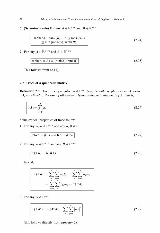
38 Advanced Mathematical Tools for Automatic Control Engineers: Volume 1
6. (Sylvester’s rule) For any A ∈ Rm×n and B ∈ Rn×p
rank(A)+ rank(B)− n ≤ rank(AB)
≤ min {rank(A), rank(B)} (2.24)
7. For any A ∈ Rm×m and B ∈ Rn×m
rank(A⊗ B) = (rankA) (rankB) (2.25)
This follows from (2.11).
2.7 Trace of a quadratic matrix
Definition 2.7. The trace of a matrix A ∈ Cn×n (may be with complex elements), writtentrA, is defined as the sum of all elements lying on the main diagonal of A, that is,
trA :=n∑i=1
aii (2.26)
Some evident properties of trace follow.
1. For any A,B ∈ Cn×n and any α, β ∈ C
tr(αA+ βB) = α trA+ β trB (2.27)
2. For any A ∈ Cm×n and any B ∈ Cn×m
tr(AB) = tr(BA) (2.28)
Indeed,
tr(AB) :=m∑i=1
n∑k=1
aikbki =m∑i=1
n∑k=1
bkiaik
=n∑k=1
m∑i=1
bkiaik = tr(BA)
3. For any A ∈ Cn×n
tr(AA∗) = tr(A∗A) =n∑i=1
n∑j=1
∣∣aij ∣∣2 (2.29)
(this follows directly from property 2).

Matrices and matrix operations 39
4. If S−1(S ∈ Cn×n
)exists then for any A ∈ Cn×n
tr(S−1AS
) = tr(SS−1A
) = tr(A) (2.30)
5. For any A ∈ Cn×n and any B ∈ Cp×p
tr(A⊗ B) = tr(A) tr(B) (2.31)
Indeed,
tr(A⊗ B) :=n∑i=1
(aii
p∑j=1
bii
)
=(
n∑i=1
aii
)(p∑j=1
bii
)= tr(A) tr(B)

This page intentionally left blank
3 Eigenvalues and Eigenvectors
Contents3.1 Vectors and linear subspaces . . . . . . . . . . . . . . . . . . . . . . . . . 41
3.2 Eigenvalues and eigenvectors . . . . . . . . . . . . . . . . . . . . . . . . . 44
3.3 The Cayley–Hamilton theorem . . . . . . . . . . . . . . . . . . . . . . . . 53
3.4 The multiplicities and generalized eigenvectors . . . . . . . . . . . . . . . 54
3.1 Vectors and linear subspaces
Definition 3.1. The matrix A ∈ Cn×1 := Cn, written as
a :=⎛⎜⎝a1...an
⎞⎟⎠
is called a vector a ∈ Cn×1.
Definition 3.2. The matrix product (2.1), written for a ∈ Cn×1 and b ∈ C1×n, is called ascalar (inner) product of two vectors a and b and denoted by
(a, b) := a∗b =n∑i=1
aibi (3.1)
which for real vectors a, b ∈ Rn becomes
(a, b) := aᵀb =n∑i=1
aibi (3.2)
Definition 3.3. For the set of vectors x1, x2, . . . , xk ∈ Cn and elements α1, α2, . . . , αk ∈C the following notions may be introduced:
1. Linear combinations of x1, x2, . . . , xk≤n over C are an element of the form
α1x1 + α2x2 + . . .+ αkxk2. The set of all linear combinations of x1, x2, . . . , xk over C is called a subspace or the
span of x1, x2, . . . , xk , denoted by
span {x1, x2, . . . , xk} :={x = α1x1 + α2x2 + . . .+ αkxk : αi ∈ C, i = 1, . . . , k} (3.3)
41

42 Advanced Mathematical Tools for Automatic Control Engineers: Volume 1
3. Some vectors x1, x2, . . . , xk ∈ Cn are said to be linearly dependent over C if there
exist α1, α2, . . . , αk ∈ C not all zero
(n∑i=1
|αi |2 > 0
)such that
α1x1 + α2x2 + . . .+ αkxk = 0
Otherwise, they are said to be linearly independent.4. If S is a subspace of Cn, then a set of vectors x1, x2, . . . , xk ∈ Cn is called a basis forS if
• x1, x2, . . . , xk are linearly independent;• S = span {x1, x2, . . . , xk}.Such basis for a subspace S is not unique: all bases for S have the same number ofelements which is called the dimension of S, denoted by dim S.
5. Vectors x1, x2, . . . , xk ∈ Cn are mutually orthogonal if(x∗i , xj
) = 0 for all i �= j
and are orthonormal if for all i, j = 1, . . . , n(x∗i , xj
) = δijwhere x∗i = (xi)ᵀ and δij =
{1 if i = j0 if i �= j is the Kronecker (delta-function) symbol.
6. The orthogonal completion S⊥ of a subspace S ⊂ Cn is defined by
S⊥ = span {xk+1, xk+2, . . . , xn} (3.4)
where the vectors xk+j (j = 1, . . . , n− k) are orthonormal.
Any matrix A ∈ Cm×n may be considered as a linear transformation from Cn
to Cm, i.e.,
A : Cn −→ Cm
Definition 3.4.
(a) The kernel (or null space) of the linear transformation A : Cn −→ Cm is defined by
KerA = N (A) := {x ∈ Cn : Ax = 0} (3.5)
(b) The image (or range) of the linear transformation A : Cn −→ Cm is
ImA = R(A) := {y ∈ Cm : y = Ax, x ∈ Cn} (3.6)
(c) The dimension of the subspace KerA = N (A) is referred to as the defect of thetransformation A and is denoted by defA, that is,
defA := dimKerA (3.7)
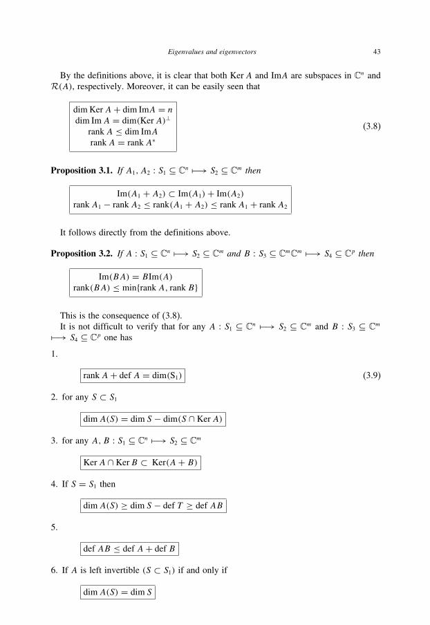
Eigenvalues and eigenvectors 43
By the definitions above, it is clear that both KerA and ImA are subspaces in Cn and
R(A), respectively. Moreover, it can be easily seen that
dim KerA+ dim ImA = ndim ImA = dim(KerA)⊥
rankA ≤ dim ImA
rankA = rankA∗(3.8)
Proposition 3.1. If A1, A2 : S1 ⊆ Cn −→ S2 ⊆ Cm then
Im(A1 + A2) ⊂ Im(A1)+ Im(A2)
rankA1 − rankA2 ≤ rank(A1 + A2) ≤ rankA1 + rankA2
It follows directly from the definitions above.
Proposition 3.2. If A : S1 ⊆ Cn −→ S2 ⊆ Cm and B : S3 ⊆ CmCm −→ S4 ⊆ Cp then
Im(BA) = BIm(A)rank(BA) ≤ min{rankA, rankB}
This is the consequence of (3.8).
It is not difficult to verify that for any A : S1 ⊆ Cn −→ S2 ⊆ Cm and B : S3 ⊆ Cm
−→ S4 ⊆ Cp one has
1.
rankA+ def A = dim(S1) (3.9)
2. for any S ⊂ S1dimA(S) = dim S − dim(S ∩ KerA)
3. for any A,B : S1 ⊆ Cn −→ S2 ⊆ Cm
KerA ∩ KerB ⊂ Ker(A+ B)
4. If S = S1 then
dimA(S) ≥ dim S − def T ≥ def AB
5.
def AB ≤ def A+ def B
6. If A is left invertible (S ⊂ S1) if and only if
dimA(S) = dim S
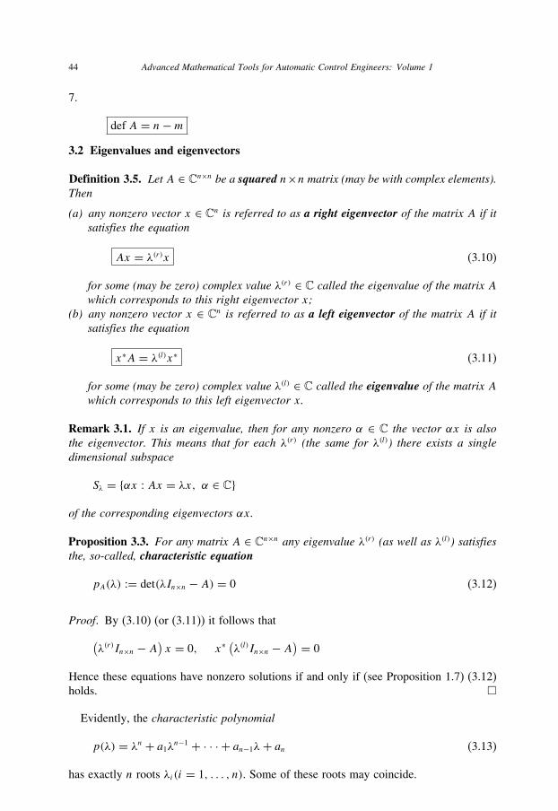
44 Advanced Mathematical Tools for Automatic Control Engineers: Volume 1
7.
def A = n−m3.2 Eigenvalues and eigenvectors
Definition 3.5. Let A ∈ Cn×n be a squared n×n matrix (may be with complex elements).Then
(a) any nonzero vector x ∈ Cn is referred to as a right eigenvector of the matrix A if itsatisfies the equation
Ax = λ(r)x (3.10)
for some (may be zero) complex value λ(r) ∈ C called the eigenvalue of the matrix Awhich corresponds to this right eigenvector x;
(b) any nonzero vector x ∈ Cn is referred to as a left eigenvector of the matrix A if itsatisfies the equation
x∗A = λ(l)x∗ (3.11)
for some (may be zero) complex value λ(l) ∈ C called the eigenvalue of the matrix Awhich corresponds to this left eigenvector x.
Remark 3.1. If x is an eigenvalue, then for any nonzero α ∈ C the vector αx is alsothe eigenvector. This means that for each λ(r) (the same for λ(l)) there exists a singledimensional subspace
Sλ = {αx : Ax = λx, α ∈ C}
of the corresponding eigenvectors αx.
Proposition 3.3. For any matrix A ∈ Cn×n any eigenvalue λ(r) (as well as λ(l)) satisfiesthe, so-called, characteristic equation
pA(λ) := det(λIn×n − A) = 0 (3.12)
Proof. By (3.10) (or (3.11)) it follows that(λ(r)In×n − A
)x = 0, x∗
(λ(l)In×n − A
) = 0
Hence these equations have nonzero solutions if and only if (see Proposition 1.7) (3.12)
holds. �
Evidently, the characteristic polynomial
p(λ) = λn + a1λn−1 + · · · + an−1λ+ an (3.13)
has exactly n roots λi(i = 1, . . . , n). Some of these roots may coincide.

Eigenvalues and eigenvectors 45
Definition 3.6. The set of all roots of pA(λ) is called the spectrum of A and is denoted by
σ(A) := {λ1, λ2, . . . , λn}
where λj satisfies
pA(λj ) = 0
The maximum modulus of the eigenvalues is called the spectral radius of A, denoted by
ρ(A) := max1≤j≤n
∣∣λj ∣∣ (3.14)
The following remark seems to be evident.
Remark 3.2. The spectrum of A contains all right eigenvalues as well as all left eigen-values which implies that any λ(r)j has an equal λ(l)j , that is, there exist two indices i andj such that
λ(r)i = λ(l)j
Proposition 3.4. If x is a right (left) eigenvector of a real matrix A ∈ Rn×n with thecorresponding eigenvalue λ, that is, Ax = λx, then the complex conjugated vector x isalso an eigenvector of A with the corresponding eigenvalue λ.
Proof. Let x = u+ iv and λ = α + iβ. Then we have
Ax = A(u+ iv) = Au+ i(Av)= λx = (α + iβ)(u+ iv) = (αu− βv)+ i(βu+ αv)
This implies
Au = αu− βvAv = βu+ αv
or, equivalently,
Au = αu− (−β)(−v)A(−v) = (−β)u+ α(−v)
which, after multiplication of the second equality by the complex unite i and summation
of both equalities, leads to the following identity
A(u− iv) = Ax = (α − iβ)(u− iv) = λx
For the left eigenvalues the proof is similar. �

46 Advanced Mathematical Tools for Automatic Control Engineers: Volume 1
Corollary 3.1. The following presentation of the characteristic polynomial p(λ) (3.13)takes place
p(λ) =n∏i=1
(λ− λi) =(
s∏i=1
[λi − ui])(
n−s∏i=1
[(λi − ui)2 + v2i
])(3.15)
where s is the number of pure real eigenvalues and
ui = Reλi, vi = Imλi
Example 3.1. For
A =⎡⎣1−1 0
2 3 2
1 1 2
⎤⎦
by Sarrius’s rule we have
pA(λ)= det(λI3×3 − A) = det
⎡⎣λ− 1 1 0
−2 λ− 3 −2
−1 −1 λ− 2
⎤⎦
= (λ− 1)(λ− 3)(λ− 2)+ 2− 2(λ− 1)+ 2(λ− 2)
= (λ− 1)(λ− 2)(λ− 3)
which implies
λ1 = 1, λ2 = 2, λ3 = 3
One of the solutions of the equation Ax(i) = λix(i) (i = 1, 2, 3) is
x(1) =⎡⎣−1
0
1
⎤⎦, x(2) =
⎡⎣−2
2
1
⎤⎦, x(2) =
⎡⎣−1
2
1
⎤⎦
In this example a nonsymmetric matrix has real eigenvalues and the corresponding
eigenvectors. The next proposition shows when this occurs.
Proposition 3.5. If a square n× n matrix A is Hermitian or real symmetric, that is, if
A∗ = A or A = Aᵀ
then obligatory all eigenvalues λj are real. If A is real symmetric, then the correspondingeigenvectors x(j) (j = 1, . . . , n) are real too.
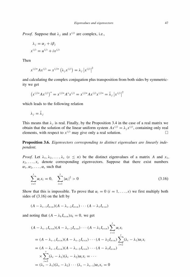
Eigenvalues and eigenvectors 47
Proof. Suppose that λj and x(j) are complex, i.e.,
λj = αj + iβjx(j) = u(j) + iv(j)
Then
x(j)∗Ax(j) = x(j)∗ (λjx(j)) = λj ∣∣x(j)∣∣2and calculating the complex conjugation plus transposition from both sides by symmetric-
ity we get(x(j)∗Ax(j)
)∗ = x(j)∗A∗x(j) = x(j)∗Ax(j)x(j)∗ = λj∣∣x(j)∣∣2
which leads to the following relation
λj = λjThis means that λj is real. Finally, by the Proposition 3.4 in the case of a real matrix we
obtain that the solution of the linear uniform system Ax(j) = λjx(j), containing only real
elements, with respect to x(j) may give only a real solution. �
Proposition 3.6. Eigenvectors corresponding to distinct eigenvalues are linearly inde-pendent.
Proof. Let λ1, λ2, . . . , λs (s ≤ n) be the distinct eigenvalues of a matrix A and x1,
x2, . . . , xs denote corresponding eigenvectors. Suppose that there exist numbers
α1, α2, . . . , αs such that
s∑i=1
αixi = 0,
s∑i=1
|αi |2 > 0 (3.16)
Show that this is impossible. To prove that αi = 0 (i = 1, . . . , s) we first multiply both
sides of (3.16) on the left by
(A− λs−1In×n)(A− λs−2In×n) · · · (A− λ1In×n)
and noting that (A− λkIn×n)xk = 0, we get
(A− λs−1In×n)(A− λs−2In×n) · · · (A− λ1In×n)s∑i=1
αixi
= (A− λs−1In×n)(A− λs−2In×n) · · · (A− λ2In×n)s∑i=2
(λi − λ1)αixi= (A− λs−1In×n)(A− λs−2In×n) · · · (A− λ3In×n)×
s∑i=3
(λi − λ1)(λi − λ2)αixi = · · ·= (λs − λ1)(λs − λ2) · · · (λs − λs−1)αsxs = 0

48 Advanced Mathematical Tools for Automatic Control Engineers: Volume 1
which implies that αs = 0. Analogously, we may prove that
α1 = α2 = · · · = αs−1 = 0
So, all αi = 0 which contradicts (3.16). �
Proposition 3.7. Eigenvectors of an Hermitian matrix (A = A∗), corresponding todistinct eigenvalues, are orthogonal, that is,
x(i)∗x(j) = 0 (3.17)
for any indices i and j such that λi �= λj .
Proof. Pre-multiplying both equations below
x(j)∗ : Ax(i) = λix(i)x(i)∗ : Ax(j) = λjx(j)
by x(j)∗ and x(j), we derive
x(j)∗Ax(i) = (Ax(j)
)∗x(i) = λix(j)∗x(i)(
x(i)∗Ax(j))∗ = (
Ax(j))∗x(i) = λj
(x(i)∗x(j)
)∗ = λjx(j)∗x(i)Multiplying the second equation by (−1) and summing both equalities we obtain
0 = (λi − λj )x(j)∗x(i)
Since λi �= λj the result follows. �
Example 3.2. The matrix A = uvᵀ (u, v ∈ Rn×1) has one eigenvalue λ1 equal to vᵀu(with the corresponding eigenvector x(1) = u) and all other eigenvalues λi �=1 equal to 0
(with the corresponding eigenvectors x(i �=1) = w(i �=1)⊥v). Indeed,Au = u(vᵀu) = (vᵀu)uAv(i �=1) = u(vᵀw(i �=1)) = On×1 = 0 · w(i �=1) (i = 2, . . . , n)
Proposition 3.8. If B = T −1AT and pA(λ) is the characteristic polynomial of A, then
pA(λ) = pB(λ)
that is, equivalent matrices have the same characteristic polynomials.
Proof. Indeed,
pA(λ) = det(λIn×n − A) = det T · det(λIn×n − A) · det T −1
= det(λT In×nT −1 − TAT −1) = det(λIn×n − B) = pB(λ)
�
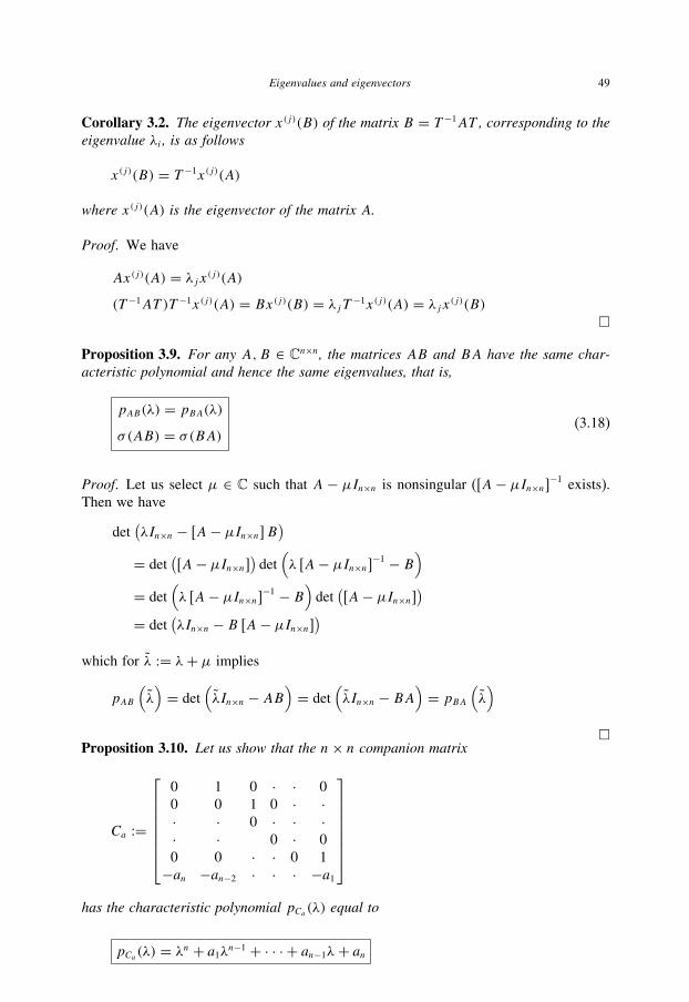
Eigenvalues and eigenvectors 49
Corollary 3.2. The eigenvector x(j)(B) of the matrix B = T −1AT , corresponding to theeigenvalue λi , is as follows
x(j)(B) = T −1x(j)(A)
where x(j)(A) is the eigenvector of the matrix A.
Proof. We have
Ax(j)(A) = λjx(j)(A)(T −1AT )T −1x(j)(A) = Bx(j)(B) = λjT −1x(j)(A) = λjx(j)(B)
�
Proposition 3.9. For any A,B ∈ Cn×n, the matrices AB and BA have the same char-acteristic polynomial and hence the same eigenvalues, that is,
pAB(λ) = pBA(λ)σ (AB) = σ(BA) (3.18)
Proof. Let us select μ ∈ C such that A − μIn×n is nonsingular ([A− μIn×n]−1exists).
Then we have
det(λIn×n − [A− μIn×n]B
)= det
([A− μIn×n]
)det
(λ [A− μIn×n]−1 − B
)= det
(λ [A− μIn×n]−1 − B
)det
([A− μIn×n]
)= det
(λIn×n − B [A− μIn×n]
)which for λ := λ+ μ implies
pAB
(λ)= det
(λIn×n − AB
)= det
(λIn×n − BA
)= pBA
(λ)
�Proposition 3.10. Let us show that the n× n companion matrix
Ca :=
⎡⎢⎢⎢⎢⎢⎢⎣
0 1 0 · · 0
0 0 1 0 · ·· · 0 · · ·· · 0 · 0
0 0 · · 0 1
−an −an−2 · · · −a1
⎤⎥⎥⎥⎥⎥⎥⎦
has the characteristic polynomial pCa (λ) equal to
pCa (λ) = λn + a1λn−1 + · · · + an−1λ+ an

50 Advanced Mathematical Tools for Automatic Control Engineers: Volume 1
Proof. Indeed,
pCa (λ)O = det
⎡⎢⎢⎢⎢⎢⎢⎣
λ −1 0 · · 0
0 λ −1 0 · ·· · · · · ·· · · · 0
0 0 · · · −1
an an−1 · · · λ+ a1
⎤⎥⎥⎥⎥⎥⎥⎦
= (λ+ a1) det
⎡⎢⎢⎢⎢⎣λ −1 0 · ·0 λ −1 0 ·· · · · ·· · · −1
0 0 · · λ
⎤⎥⎥⎥⎥⎦
− a2 det
⎡⎢⎢⎢⎢⎣λ −1 0 · 0
0 λ −1 0 ·· · · · ·· · λ 0
0 0 · · −1
⎤⎥⎥⎥⎥⎦
+ · · · −an−1 det
⎡⎢⎢⎢⎢⎣λ 0 · · 0
0 −1 0 · ·· · · · ·· · · 0
0 · · · −1
⎤⎥⎥⎥⎥⎦
+ an det
⎡⎢⎢⎢⎢⎣−1 0 · · 0
λ −1 0 · ·· · · · ·· · · 0
0 · · λ −1
⎤⎥⎥⎥⎥⎦
= (λ+ a1)λn−1 + a2λn−2 + · · · + an−1λ+ an�
Proposition 3.11. For any square n× n matrix A
an = detA =n∏i=1
λi
an−1 = trA =n∑i=1
λi
(3.19)
Proof. The first formula follows directly from (3.15) if λ = 0. To prove that an−1 =n∑i=1
λi
it is sufficient to open parentheses in
pA(λ) =n∏i=1
(λ− λi) = λn +n∑i=1
aiλn−i (3.20)

Eigenvalues and eigenvectors 51
and to calculate the coefficient corresponding λ in the right-hand side. The second identity
trA = ∑n
i=1 λi may be easily proven using the so-called diagonal form transformation
which can be done below. �
Corollary 3.3.
trA = d
dλdet(λIn×n − A) |λ=0 (3.21)
Proof. It follows directly from (3.20). �
Proposition 3.12. The spectrum of a unitary matrix U lies on the unit circle.
Proof. If Ux = λx and x∗x = 1, then
(Ux)∗Ux = x∗U ∗Ux = x∗x = 1
On the other hand
(Ux)∗Ux = (λx)∗(λx) = x∗λ∗λx = |λ|2 x∗x = |λ|2
The comparison yields |λ|2 = 1. �
Proposition 3.13. If x is a complex nonzero vector in Cn, then the Householder matrixdefined as
H = In×n − 2xx∗
x∗x(3.22)
is unitary.
Proof. We should show that
HH ∗ = H ∗H = In×nOne has
HH ∗ = H ∗H =(In×n − 2
xx∗
x∗x
)(In×n − 2
xx∗
x∗x
)
= In×n − 4xx∗
x∗x+ 4x(x∗x)x∗
(x∗x)2= In×n
�
52 Advanced Mathematical Tools for Automatic Control Engineers: Volume 1
Proposition 3.14. For any square n× n matrix A with the eigenvectors x(i)(A) corres-ponding to the eigenvalue λi(A) (i = 1, . . . n) it follows
1.
x(i)(A) = x(i)(In×n − A)λi(In×n − A) = 1− λi(A)
Indeed,
(In×n − A)x(i)(A)= x(i)(A)− Ax(i)(A)= x(i)(A)− λi(A)x(i)(A)= [1− λi(A)] x(i)(A)
2.
x(i)(Ap) = x(i)(A), p = 2, 3, . . .
λi(Ap) = λpi (A)
since
Apx(i)(A)= A(p−1)Ax(i)(A) = λi(A)A(p−1)x(i)(A)
= λ2i (A)A(p−2)x(i)(A) = · · · = λpi (A)x(i)(A)3. If, in addition, A is real orthogonal (Aᵀ = A−1) and (In×n + A) is nonsingular
(λi(In×n + A) �= 0 for all i = 1, . . . , n), then A can be represented as (Cayleytransformation)
A = (In×n − S)(In×n + S)−1 (3.23)
where S is a real skew-matrix (2.6), i.e. Sᵀ = −S. This result follows directly basedon the construction of S: if (3.23) holds then
A(In×n + S) = (In×n − S)AS + S = In×n − AS = (In×n − A)(In×n + A)−1
and
Sᵀ = [(In×n + A)−1
]ᵀ(In×n − A)ᵀ
= (In×n + Aᵀ)−1(In×n − Aᵀ)
= (In×n + A−1)−1(In×n − A−1)
= [A−1(A+ In×n)
]−1 [A−1(A− In×n)
]= [(A+ In×n)
]−1 [AA−1
](A− In×n) = −S
which means that S is a skew matrix.
Eigenvalues and eigenvectors 53
3.3 The Cayley–Hamilton theorem
The theorem discussed in this subsection plays a key role in matrix theory and has
important applications to Classical Control Theory.
Theorem 3.1. (Cayley–Hamilton theorem) If
pA(λ) = λn + a1λn−1 + · · · + an−1λ+ an = 0 (3.24)
is the characteristic polynomial of a squared matrix A, then
pA(A) := An + a1An−1 + · · · + an−1A+ anIn×n = 0 (3.25)
that is, the matrix A satisfies its characteristic equation.
Proof. By (2.5)
A−1 = 1
detAadjA
we have
A adjA = (detA)In×n
which leads to the following identity
(λIn×n − A)adj(λIn×n − A)= (det(λIn×n − A))In×n = pA(A)In×n
(3.26)
It is clear that adj(λIn×n − A) is matrix λn−1 as the maximal order, i.e.,
adj(λIn×n − A) = Bn−1λn−1 + Bn−2λ
n−2 + · · · + B1λ+ B0
Then (3.26) becomes
(λIn×n − A)(Bn−1λn−1 + Bn−2λ
n−2 + · · · + B1λ+ B0)
= (λn + a1λn−1 + · · · + an−1λ+ an)In×nComparing coefficients, we obtain
Bn−1 = In×nBn−2 − ABn−1 = a1In×n
...
B0 − AB1 = an−1In×n−AB0 = anIn×n

54 Advanced Mathematical Tools for Automatic Control Engineers: Volume 1
Multiplying the first of these equalities by An, the second one by An−1, the jth by An−j+1
and adding them together yields
0 = An + a1An−1 + · · · + an−1A+ anIn×n
which is exactly (3.25). �
Corollary 3.4. If A−1 exists (A is nonsingular), then
A−1 = − 1
an(An−1 + a1An−2 + · · · + an−2A+ an−1In×n)
Proof. Since A is nonsingular (A has no zero eigenvalues) we have that an �= 0. Then
the result follows from the identity
A−1pA(A) = A−1(An + a1An−1 + · · · + an−1A+ anIn×n) = 0
�
3.4 The multiplicities and generalized eigenvectors
3.4.1 Algebraic and geometric multiplicities
For any n× n matrix A it may happen that some of its eigenvalues are equal, that is,
the corresponding characteristic polynomial pA(λ) may have the following structure
pA(λ) =K∏i=1
(λ− λi)μi ,K∑i=1
μi = n (3.27)
where μi is the number of times the factor (λ− λi) appears in (3.27).
Definition 3.7.
(a) the number μi is called the algebraic multiplicity of the eigenvalue λi of thematrix A;
(b) the number
κi := dimKer(λiIn×n − A) (3.28)
is called the geometric multiplicity of the eigenvalue λi of the matrix A.
Example 3.3. For
A =[0 1
0 0
]

Eigenvalues and eigenvectors 55
we have
pA(λ) = det
[λ −1
0 λ
]= λ2
λ1 = λ2 = 0
which implies
μ1 = 2
and
κ1 = dimKer((λ1In×n − A)) = dimKer(A) = 1
Here we see that in this example κ1 < μ1.
In general, the following property holds.
Lemma 3.1. The geometric multiplicity of an eigenvalue does not exceed its algebraicmultiplicity, that is, for any i = 1, . . . , K
κi ≤ μi (3.29)
Proof. If r is the rank of (λiIn×n − A), then by (3.9) r = n − μi and all minors of
(λiIn×n − A) greater than (n− μi) are equal to zero. Hence, in
pA(λ) =n∏i=1
(λ− λi) = λn +n∑i=1
an−iλi
for all i ≤ μi − 1 we have ai = 0, which leads to the following
pA(λ) =n∏i=μi(λ− λi)
This means that the last polynomial has a zero of multiplicity greater than or equal to μiwhich implies the result. �
Corollary 3.5.
K∑i=1
κi ≤K∑i=1
μi = n (3.30)

56 Advanced Mathematical Tools for Automatic Control Engineers: Volume 1
3.4.2 Generalized eigenvectors
Definition 3.8. Let an eigenvalue λi of a square n × n matrix A have the algebraicmultiplicity μi . Then the vectors x(i,k)(A) satisfying the equations
[A− λiIn×n] x(i,k)(A) = x(i,k−1)(A), k = 2, 3, . . . , r ≤ μi (3.31)
are called the generalized eigenvectors of A. Evidently,
x(i,1)(A) = x(i)(A)
is the corresponding eigenvector of A (by the definition x(i,0)(A) ≡ 0). The sequence ofvectors x(i,1)(A), x(i,2)(A), . . . , x(i,r)(A) is called a Jordan chain of length r ≤ μi .
If the eigenvector x(i,1)(A) = x(i)(A) is selected, then the next vectors x(i,2)(A), . . . ,
x(i,r)(A) are generated successively as far as the nonhomogeneous equation (3.31) has a
solution.
Proposition 3.15. x(i,k)(A) (k ≥ 2) is a generalized eigenvector of A if and only if thevector [A− λiIn×n]k−1
x(i,k)(A) is the eigenvector of A, or equivalently, if and only if
[A− λiIn×n]k x(i,k)(A) = 0
Proof.
(a) Necessity. Let us prove this fact by induction. For k = 2 we have
[A− λiIn×n] x(i,2)(A) = x(i,1)
and, hence, pre-multiplying by A implies
A([A− λiIn×n] x(i,2)(A)
) = Ax(i,1)= λix(i,1) = λi
([A− λiIn×n] x(i,2)(A)
)This means that
([A− λiIn×n] x(i,2)(A)
)is the eigenvector of A. Notice that the last
identity may be rewritten as
0= A ([A− λiIn×n] x(i,2)(A)
)− λi ([A− λiIn×n] x(i,2)(A))= [A− λiIn×n]
([A− λiIn×n] x(i,2)(A)
) = [A− λiIn×n]2 x(i,2)(A)
So, for k = 2 the proposition is true. Suppose that it is valid for some k. Show that
it will be valid for k + 1 too. By this supposition we have
[A− λiIn×n]k x(i,k)(A) = 0

Eigenvalues and eigenvectors 57
Then
[A− λiIn×n] x(i,k+1)(A) = x(i,k)
and pre-multiplying by [A− λiIn×n]k implies
[A− λiIn×n]k([A− λiIn×n] x(i,k+1)(A)
) = [A− λiIn×n]k x(i,k) = 0
or, equivalently,
[A− λiIn×n]k+1x(i,k+1)(A) = 0
(b) Sufficiency. It follows directly from the definition of a generalized vector.
�
Proposition 3.16. Any Jordan chain consists of linearly independent elements.
Proof. Suppose that there exist αs(s = 1, . . . , r) such that
r∑s=1
αix(i,s)(A) = 0
Applying the transformation [A− λiIn×n]r−1to both sides, we get
0 =r∑s=1
αi [A− λiIn×n]r−1−s[A− λiIn×n]s x(i,s)(A) = αr
Then applying again the transformation [A− λiIn×n]r−2, in view of the result before, we
obtain that αr−1 = 0. Repeating this procedure, we obtain the contradiction, and hence,
the result is established. �

This page intentionally left blank
4 MatrixTransformations
Contents
4.1 Spectral theorem for Hermitian matrices . . . . . . . . . . . . . . . . . . . 59
4.2 Matrix transformation to the Jordan form . . . . . . . . . . . . . . . . . . 62
4.3 Polar and singular-value decompositions . . . . . . . . . . . . . . . . . . . 63
4.4 Congruent matrices and the inertia of a matrix . . . . . . . . . . . . . . . . 70
4.5 Cholesky factorization . . . . . . . . . . . . . . . . . . . . . . . . . . . . 73
4.1 Spectral theorem for Hermitian matrices
4.1.1 Eigenvectors of a multiple eigenvalue for Hermitian matrices
Proposition 4.1. Let x(i,1), x(i,2), . . . , x(i,μi ) be the eigenvectors of an n × n Hermitianmatrix A ∈ Cn×n corresponding to the eigenvalue λi (which by (3.5) is always real)with the algebraic multiplicity μi . Then these vectors may be supposed to be linearlyindependent.
Proof. Indeed, if rank(λiIn×n − A) = n − μi , then, selecting the last components
z(i,2) :=[x(i)μi+1, x
(i)μi+2, . . . , x
(i)n
]ᵀas free variables and solving the linear systems
(λiIn×n − A) x(i) = 0
with respect to z(i,1) :=(x(i)1 , x
(i)2 , . . . , x
(i)n−μi
)ᵀ, we get
x(i) :=(z(i,1)
z(i,2)
), A :=
(A11 A12
A21 A22
), rankA11 = n− μi[(
λiI(n−μi)×(n−μi) − A11
) −A12
−A21
(λiIμi×μi − A22
)](z(i,1)z(i,2)
)= 0
and, hence,
(λiI(n−μi)×(n−μi) − A11
)z(i,1) = A12z
(i,2)
or, equivalently,
z(i,1) =[(λiI(n−μi)×(n−μi) − A11
)−1A12
]z(i,2) (4.1)
59

60 Advanced Mathematical Tools for Automatic Control Engineers: Volume 1
Taking then the free components as x(i,r)s = δs,r (s, r = μi + 1, . . . , n), we may define
the following linearly independent (in Cn−μi ) vectors
z(i,2,r) =
⎛⎜⎜⎜⎜⎜⎜⎝
x(i,r)μi+1
x(i,r)μi+2
...
x(i,r)n
⎞⎟⎟⎟⎟⎟⎟⎠, r = 1, . . . , n− μi
Evidently, in spite of the fact that z(i,1,r) are linearly dependent on z(i,2,r) by (4.1), the
joint vectors
(z(i,1,r)
z(i,2,r)
)= x(i,r) remain linearly independent. �
4.1.2 Gram–Schmidt orthogonalization
Proposition 4.2. Eigenvectors of a Hermitian matrix are linearly independent; some ofthem even correspond to the same eigenvalues.
Proof. This result immediately follows from the previous proposition and from (3.17).
�
Let{x(1), x(2), . . . , x(n)
}be the set of linearly independent eigenvectors of an n × n
Hermitian matrix A ∈ Cn×n.
Lemma 4.1. (Gram–Schmidt orthogonalization process) The set{x(1), x(2) , . . . ,
x(n)}of vectors obtained from
{x(1), x(2), . . . , x(n)
}by the procedure
x(1) = x(1)
x(r) =[In×n −
r−1∑s=1
x(s)x(s)ᵀ∥∥x(s)∥∥2
]x(r), (r = 2, . . . , n)
(4.2)
is orthogonal, that is,
(x(r), x(s)
) = 0 (r �= s = 1, . . . , n) (4.3)
Proof. Let us do it by induction. For r = 2 we have
x(2) =[In×n − x
(1)x(1)ᵀ∥∥x(1)∥∥2
]x(2) = x(2) − x(1)∥∥x(1)∥∥2
(x(1), x(2)
)and, as the result, it follows that(
x(1), x(2)) = (
x(1), x(2))− (
x(1), x(2)) = 0

Matrix transformations 61
Supposing that the vectors x(1), x(2), . . . , x(r−1) are orthogonal, we get
(x(r−1), x(r)
)= (x(r−1), x(r)
)− r−1∑s=1
(x(r−1), x(s)
)∥∥x(s)∥∥2
(x(s), x(r)
)
= (x(r−1), x(r)
)− (x(r−1), x(r−1)
)∥∥x(r−1)∥∥2
(x(r−1), x(r)
) = 0
�
Remark 4.1. The set of the vectors
{x(1)∥∥x(1)∥∥ , . . . , x
(n)∥∥x(n)∥∥}
may be considered as an
orthonormal basis in Cn.
4.1.3 Spectral theorem
Theorem 4.1. (Spectral theorem) If{x(1), x(2), . . . , x(n)
}is the set of linearly independ-
ent eigenvectors of an n×n Hermitian matrix A ∈ Cn×n corresponding to the eigenvaluesλ1, . . . , λn (maybe multiple), then the following representation holds
A = X�X−1 = X�X∗ =n∑i=1
λix(i)x(i)
∗(4.4)
where � = diag {λ1, . . . , λn} and X := [x(1) x(2) · · · x(n) ] is unitary matrix, i.e., X∗ =
X−1.
Proof. Notice that the relations
Ax(i) = λix(i), i = 1, . . . , n
may be rewritten as
AX = X� (4.5)
Since x(1), x(2), . . . , x(n) are linearly independent it follows that X−1 exists and, hence,
A =X�X−1
A∗ =A = (X−1
)∗�X∗
and
A(X−1
)∗ = (X−1
)∗� (4.6)
The comparison of (4.5) and (4.6) implies
X = (X−1
)∗, X∗ = X−1

62 Advanced Mathematical Tools for Automatic Control Engineers: Volume 1
and, hence, by (2.3) it follows that
A = X�X−1 = X�X∗ = X⎡⎢⎣λ1x
(1)∗...
λnx(n)∗
⎤⎥⎦ =
n∑i=1
λix(i)x(i)
∗
�
4.2 Matrix transformation to the Jordan form
This subsection deals with the transformation of nonobligatory Hermitian matrices to
triplet form analogous to one given before.
4.2.1 The Jordan block
Definition 4.1. The matrix
Ji :=
⎡⎢⎢⎢⎢⎣λi 1 0 · 0
0 λi 1 · ·· 0 · · 0
· · · λi 1
0 · · 0 λi
⎤⎥⎥⎥⎥⎦ (4.7)
is referred to as a Jordan block (or cell) of order μi corresponding to the eigenvalue λi .
4.2.2 The Jordan matrix form
Theorem 4.2. (The Jordan normal canonical representation) For any square com-plex matrix A ∈ Cn×n there exists a nonsingular matrix T such that
A = T JT −1 (4.8)
where
J = diag(J1, J2, . . . , JK)
Ji ∈ Cμi×μi
with
K∑i=1
μi = n
and with λi (i = 1, . . . , K) as the distinct eigenvalues of A with the multiplicity μi . Thetransformation T has the following form

Matrix transformations 63
T = [T1 T2 · · · TK
]Ti =
[x(i,1) x(i,2) · · · x(i,μi ) ] (4.9)
where x(i,1) are the eigenvectors of A corresponding to the eigenvalue λi and x(i,s)
(s = 2, . . . , μi) are the generalized vectors of A generated by (3.31).
Proof. Taking sufficiently large space, nevertheless it may be realized by the direct
verification of the identity AT = T J . �
Example 4.1.
A =⎡⎣ 6 2 2
−2 2 0
0 0 2
⎤⎦
We have
det(A− λI3×3) = (2− λ) (4− λ)2
So,
λ1 = 2, λ2 = 4 with μ2 = 2
and
x(1) = [0 −1 1
]ᵀ, x(2,1) = [
2 −2 0]ᵀ
(A− λI3×3) x(2,2) = x(2,1) =⇒ x(2,2) = [
1 0 0]ᵀ
As the result we have
A = T⎡⎣2 0 0
0 4 10 0 4
⎤⎦ T −1
T = [x(1) x(2,1) x(2,2)
] =⎡⎣ 0 2 1
−1 −2 0
1 0 0
⎤⎦
4.3 Polar and singular-value decompositions
4.3.1 Polar decomposition
Proposition 4.3. (Polar factorization) For any square complex matrix A ∈ Cn×n thereexist unique positive semidefinite (λi ≥ 0 for all i = 1, . . . , n) Hermitian matrices H, Kand unitary matrices U, V all in Cn×n such that
A = UH = KV (4.10)
64 Advanced Mathematical Tools for Automatic Control Engineers: Volume 1
Proof. First, notice the matrix A∗A is Hermitian and, hence, by (3.5) it has all eigenvalues
real. Moreover, all of them are nonnegative, since by
x(i)∗ : A∗Ax(i) = λix(i)
one has
x(i)∗A∗Ax(i) = ∥∥Ax(i)∥∥2 = λix(i)∗x(i) = λi∥∥x(i)∥∥2
and, hence, for all i = 1, . . . , n
λi =∥∥Ax(i)∥∥2∥∥x(i)∥∥2
≥ 0 (4.11)
Define r21 := λ1, r22 := λ2, . . . , r2n := λn such that
ri > 0 for i = 1, . . . , k
and
ri = 0 for i = k + 1, . . . , n
Then, for i, j = 1, . . . , k and for the corresponding orthonormal eigenvectors x(i), x(j)((x(i), x(j)
) = δij), we have
(Ax(i)
ri,Ax(j)
rj
)=
(A∗Ax(i), x(j)
rirj
)= δij r
2i
rirj
and thus the vectors
z(i) := Ax(i)
ri, i = 1, . . . , k (4.12)
are orthonormal. Define also two unitary matrices
X := [x(1) . . . x(k) . . . x(n)
]Z := [
z(1) . . . z(k)] (4.13)
Then by (4.12) we have
Ax(i) = z(i)ri
or, with R := diag {r1, . . . , rn},
AX = ZR

Matrix transformations 65
which, by post-multiplying by X∗, implies
AXX∗ = A = ZRX∗ (4.14)
Now, let
U = ZX∗, H = XRX∗ (4.15)
Clearly, U is unitary since X and Z are unitary. H evidently is Hermitian and has
all eigenvalues nonnegative, or in other words, it is positive semidefinite. Moreover,
by (4.14)
UH = ZX∗XRX∗ = ZRX∗ = A
Applying the above result to A∗ we obtain A = KV . �
Corollary 4.1. If A ∈ Cn×n is nonsingular (or, equivalently all eigenvalues λi = r2i ofA∗A are strictly positive (k = n)), then
Hᵀ = H, Kᵀ = K, Uᵀ = U−1, V ᵀ = V −1
and
AᵀA = H 2, AAᵀ = V 2
Example 4.2. For
A =[1 0
2 −1
]
it follows that
AᵀA =[
5 −2
−2 1
]λ1 (A
ᵀA) = 3− 2√2, x(1) =
[√2− 1
1
]
λ2 (AᵀA) = 3+ 2
√2, x(2) =
[−√2− 1
1
]
Notice that(x(1), x(2)
) = 0. The normalized eigenvectors are
x(1) = 1√2(2−√
2)[√
2− 1
1
]=
[0.38268
0.92388
]
x(2) = 1√2(2+√
2)[−√2− 1
1
]=
[−0.92388
0.38268
]
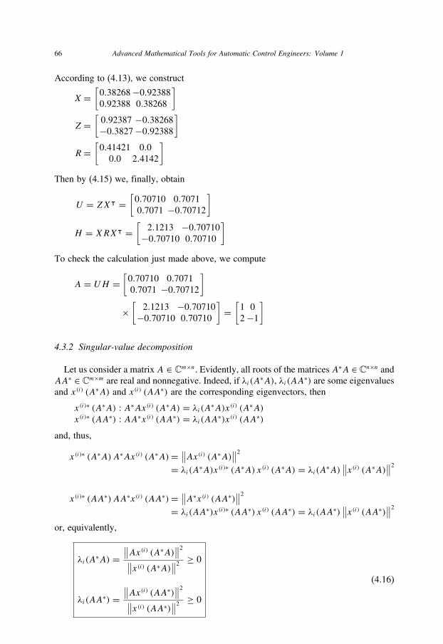
66 Advanced Mathematical Tools for Automatic Control Engineers: Volume 1
According to (4.13), we construct
X=[0.38268−0.92388
0.92388 0.38268
]
Z =[0.92387 −0.38268
−0.3827−0.92388
]
R =[0.41421 0.0
0.0 2.4142
]
Then by (4.15) we, finally, obtain
U = ZXᵀ =[0.70710 0.7071
0.7071 −0.70712
]
H = XRXᵀ =[
2.1213 −0.70710
−0.70710 0.70710
]To check the calculation just made above, we compute
A = UH =[0.70710 0.7071
0.7071 −0.70712
]
×[
2.1213 −0.70710
−0.70710 0.70710
]=
[1 0
2−1
]
4.3.2 Singular-value decomposition
Let us consider a matrix A ∈ Cm×n. Evidently, all roots of the matrices A∗A ∈ Cn×n andAA∗ ∈ Cm×m are real and nonnegative. Indeed, if λi(A
∗A), λi(AA∗) are some eigenvalues
and x(i) (A∗A) and x(i) (AA∗) are the corresponding eigenvectors, then
x(i)∗ (A∗A) : A∗Ax(i) (A∗A) = λi(A∗A)x(i) (A∗A)x(i)∗ (AA∗) : AA∗x(i) (AA∗) = λi(AA∗)x(i) (AA∗)
and, thus,
x(i)∗ (A∗A)A∗Ax(i) (A∗A)= ∥∥Ax(i) (A∗A)∥∥2
= λi(A∗A)x(i)∗ (A∗A) x(i) (A∗A) = λi(A∗A)∥∥x(i) (A∗A)
∥∥2
x(i)∗ (AA∗) AA∗x(i) (AA∗)= ∥∥A∗x(i) (AA∗)∥∥2
= λi(AA∗)x(i)∗ (AA∗) x(i) (AA∗) = λi(AA∗)∥∥x(i) (AA∗)
∥∥2
or, equivalently,
λi(A∗A) =
∥∥Ax(i) (A∗A)∥∥2∥∥x(i) (A∗A)∥∥2
≥ 0
λi(AA∗) =
∥∥Ax(i) (AA∗)∥∥2∥∥x(i) (AA∗)∥∥2
≥ 0
(4.16)
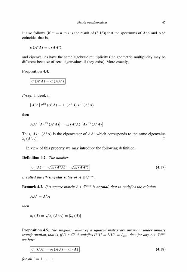
Matrix transformations 67
It also follows (if m = n this is the result of (3.18)) that the spectrums of A∗A and AA∗
coincide, that is,
σ(A∗A) = σ(AA∗)
and eigenvalues have the same algebraic multiplicity (the geometric multiplicity may be
different because of zero eigenvalues if they exist). More exactly,
Proposition 4.4.
σi(A∗A) = σi(AA∗)
Proof. Indeed, if
[A∗A] x(i) (A∗A) = λi (A∗A) x(i) (A∗A)
then
AA∗ [Ax(i) (A∗A)] = λi (A∗A)
[Ax(i) (A∗A)
]Thus, Ax(i) (A∗A) is the eigenvector of AA∗ which corresponds to the same eigenvalue
λi (A∗A). �
In view of this property we may introduce the following definition.
Definition 4.2. The number
σi (A) := √λi (A∗A) = √
λi (AA∗) (4.17)
is called the ith singular value of A ∈ Cn×n.
Remark 4.2. If a square matrix A ∈ Cn×n is normal, that is, satisfies the relation
AA∗ = A∗A
then
σi (A) =√λi (A∗A) = |λi (A)|
Proposition 4.5. The singular values of a squared matrix are invariant under unitarytransformation, that is, if U ∈ Cn×n satisfies U ∗U = UU ∗ = In×n, then for any A ∈ Cn×n
we have
σi (UA) = σi (AU) = σi (A) (4.18)
for all i = 1, . . . , n.

68 Advanced Mathematical Tools for Automatic Control Engineers: Volume 1
Proof. Indeed,
σi (UA) =√λi (A∗U ∗UA) =√
λi (A∗A) = σi (A)
and
σi (AU)=√λi (U ∗A∗AU) =
√λi (U ∗A∗AU)∗
=√λi (AUU ∗A∗) =√
λi (AA∗) = σi (A)
�The next theorem represents the main result of this subsection.
Theorem 4.3. (Singular-value decomposition) Let A ∈ Cm×n and σi (A) (i = 1, . . . ,
r ≤ min {m, n}) be the nonzero singular values of A. Then A can be represented in thetriplet form
A = UDV ∗ (4.19)
where U ∈ Cm×m and V ∈ Cn×n are unitary (i.e. satisfy U ∗U = UU ∗ = Im×m andV ∗V = VV ∗ = In×n) and D ∈ Cm×n has σi (A) in the (i, i)th position (i = 1, . . . , r) andzero elsewhere.
Proof. Following (4.12) we have that
Ax(i) = σi (A) z(i), i = 1, . . . , r
Ax(i) = 0, i = r + 1, . . . , n(4.20)
where x(i) are orthogonal eigenvectors of A∗A and z(i) are orthogonal eigenvectors of
AA∗. Constructing the matrices
V = [x(1) x(2) · · · x(n) ]
U = [z(1) z(2) · · · z(m) ]
we may note that in view of (4.15) they are unitary by the construction. Then (4.20)
implies
AV = [σ1 (A) z
(1) σ2 (A) z(2) · · · σr (A) z(r) 0 · · · 0
] = UDor, equivalently,
A = UDV −1 = UDV ∗
The result is established. �
Example 4.3. For
A =⎡⎣1 0
0 1
1 0
⎤⎦
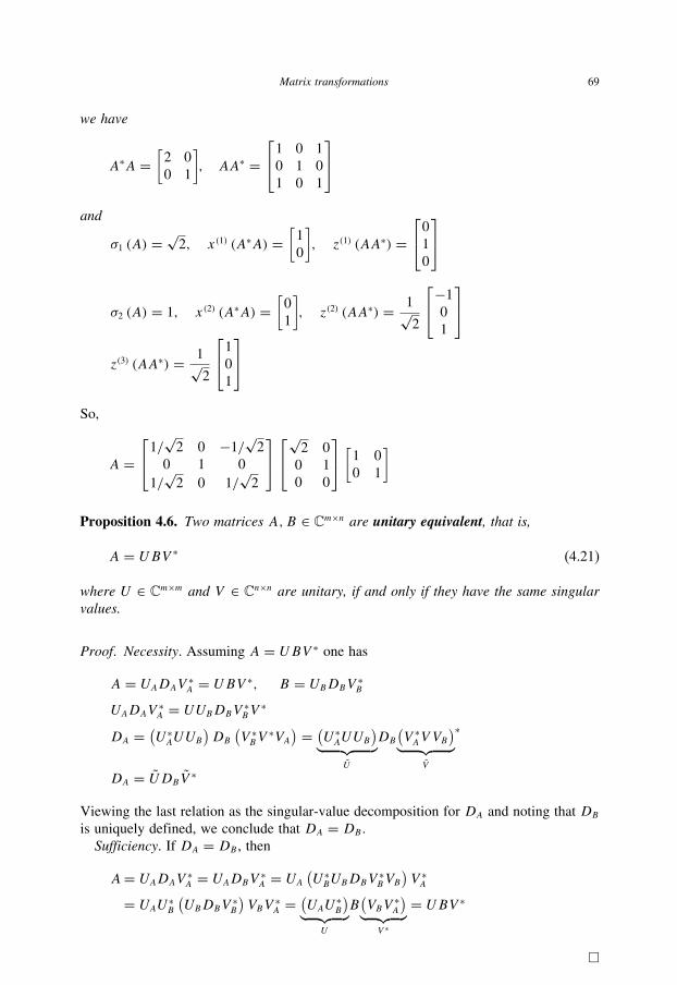
Matrix transformations 69
we have
A∗A =[2 0
0 1
], AA∗ =
⎡⎣1 0 1
0 1 0
1 0 1
⎤⎦
and
σ1 (A) =√2, x(1) (A∗A) =
[1
0
], z(1) (AA∗) =
⎡⎣0
1
0
⎤⎦
σ2 (A) = 1, x(2) (A∗A) =[0
1
], z(2) (AA∗) = 1√
2
⎡⎣−1
0
1
⎤⎦
z(3) (AA∗) = 1√2
⎡⎣1
0
1
⎤⎦
So,
A =⎡⎣1/
√2 0 −1/
√2
0 1 0
1/√2 0 1/
√2
⎤⎦⎡⎣√2 0
0 1
0 0
⎤⎦[
1 0
0 1
]
Proposition 4.6. Two matrices A,B ∈ Cm×n are unitary equivalent, that is,
A = UBV ∗ (4.21)
where U ∈ Cm×m and V ∈ Cn×n are unitary, if and only if they have the same singularvalues.
Proof. Necessity. Assuming A = UBV ∗ one has
A = UADAV ∗A = UBV ∗, B = UBDBV ∗
B
UADAV∗A = UUBDBV ∗
BV∗
DA =(U ∗AUUB
)DB
(V ∗BV
∗VA) = (
U ∗AUUB
)︸ ︷︷ ︸U
DB(V ∗AV VB
)︸ ︷︷ ︸V
∗
DA = UDBV ∗
Viewing the last relation as the singular-value decomposition for DA and noting that DBis uniquely defined, we conclude that DA = DB .
Sufficiency. If DA = DB , thenA= UADAV ∗
A = UADBV ∗A = UA
(U ∗BUBDBV
∗BVB
)V ∗A
= UAU ∗B
(UBDBV
∗B
)VBV
∗A =
(UAU
∗B
)︸ ︷︷ ︸U
B(VBV
∗A
)︸ ︷︷ ︸V ∗
= UBV ∗
�

70 Advanced Mathematical Tools for Automatic Control Engineers: Volume 1
4.4 Congruent matrices and the inertia of a matrix
4.4.1 Congruent matrices
Definition 4.3. Two square matrices A,B ∈ Cn×n are said to be congruent if thereexists a nonsingular matrix P ∈ Cn×n such that
A = PBP ∗ (4.22)
It is clear that for a unitary P the matrix A is unitary equivalent to B.
Theorem 4.4. Any Hermitian matrix H ∈ Cn×n is congruent to the matrix
�0 :=⎡⎣Is×s 0 0
0 I(r−s)×(r−s) 0
0 0 0(n−r)×(n−r)
⎤⎦ (4.23)
where r = rankH, and s is the number of positive eigenvalues of H counted accordingto multiplicity.
Proof. By the spectral theorem (4.4) any H can be represented as
H = X�X∗ (4.24)
where � is a diagonal matrix of eigenvalues of H and X is unitary. Ordering the
eigenvalues so that the first s scalars λ1, . . . , λs on the main diagonal of � are positive
and the next (r − s) numbers λs+1, . . . , λr−s are negative, one may write
� = U�1�0�1U∗ (4.25)
where �0 is as in (4.23) and
�1 = diag(√λ1, . . . ,
√λs,
√|λs+1|, . . . ,√|λr−s |, 0, . . . , 0
)The matrix U is a permutation (and therefore a unitary) matrix. So, substituting (4.25)
into (3.22) gives
H = X�X∗ = (XU�1)�0 (�1U∗X∗) = P�0P
∗
with P = XU�1. Theorem is proven. �
4.4.2 Inertia of a square matrix
Definition 4.4. The inertia of a square matrix A ∈ Rn×n, written as InA, is the tripleof integers
InA := {π (A), ν (A), δ (A)} (4.26)

Matrix transformations 71
where
• π (A) denotes the number of eigenvalues of A, counted with their algebraic multiplic-ities, lying in the open right half-plane of C;
• ν (A) denotes the number of eigenvalues of A, counted with their algebraic multiplici-ties, lying in the open left half-plane of C;
• δ (A) is the number of eigenvalues of A, counted with their algebraic multiplicities,lying on the imaginary axis.
Notice that
π (A)+ ν (A)+ δ (A) = n (4.27)
Remark 4.3. In the particular case of Hermitian matrices π (H) and ν (H) merelydenote the number of positive and, negative eigenvalues of H respectively. Notice thatfor Hermitian matrices
π (H)+ ν (H) = rankH
The difference
sigH := π (H)− ν (H) (4.28)
is referred to as the signature of H .
Theorem 4.5. Let A,B ∈ Rn×n be Hermitian matrices of the same rank r and
A = MBM∗
for some matrix M (not obligatory nonsingular). Then
InA = InB
Proof. By Theorem 4.4 there exist nonsingular matrices P and Q such that
PAP ∗ = diag [It ,−Ir−t , 0] := �0 (A)
Q−1B(Q−1
)∗ = diag [Is,−Ir−s , 0] := �0 (B)
t = π (A), s = π (B)To prove the theorem it is sufficient to show that t = s. Suppose that s < t and let us
seek a contradiction. Notice that since A = MBM∗ we have
�0 (A) = PAP ∗ = PMBM∗P ∗
= (PMQ)�0 (B) (Q∗M∗P ∗) = R�0 (B)R
∗
R := PMQ(4.29)
Let x ∈ Cn as
x =[x
0
], x ∈ Ct, ‖x‖ > 0

72 Advanced Mathematical Tools for Automatic Control Engineers: Volume 1
Then
x∗�0 (A) x =t∑i=1
|xi |2 = ‖x‖2 > 0 (4.30)
Partitioning of R in the form
R∗ :=[R11 R12
R21 R22
], R11 ∈ Cs×t
implies that x can be chosen such that
R11x = 0
keeping x �= 0. Define now y = R21x ∈ Cn−s which leads to the following identity
R∗x =[0
y
]
Then by (4.29)
x∗�0 (A) x = x∗R�0 (B)R∗x = y∗�0 (B) y = −
r−s∑j=1
∣∣yj ∣∣2 = −‖y‖2 ≤ 0
which contradicts (4.30). Similarly, interchanging the roles of �0 (A) and �0 (B), one
can find that t < s is impossible. Hence, s = t . Theorem is proven. �
Corollary 4.2. (Sylvester’s law of inertia) Congruent Hermitian matrices have thesame inertia characteristics.
Proof. Since A = PBP ∗ and P is nonsingular, then rankA = rankB and the result
follows. �
Example 4.4. Consider the quadratic form
fA (x) = (x,Ax) = 2x1x2 + 2x2x3 + x23which corresponds to the following matrix
A =⎡⎣0 1 0
1 0 1
0 1 1
⎤⎦
The transformation
x = T z, T =⎡⎣0 0 1
0 1 1
1 −1 −1
⎤⎦

Matrix transformations 73
implies
fA (x)= (x,Ax) =(z [, T ᵀAT ] z
)
=⎛⎝z,
⎡⎣1 0 0
0 −1 0
0 0 1
⎤⎦ z
⎞⎠ = z21 − z22 + z23
So,
r = 3, π (A) = 2, ν (A) = 1, δ (A) = 0
4.5 Cholesky factorization
In this subsection we follow Highan (1996).
4.5.1 Upper triangular factorization
Theorem 4.6. (Cholesky factorization) Let A = Aᵀ ∈ Rn×n be a real symmetric n× nmatrix with positive definite eigenvalues λi(A) > 0 (i = 1, . . . , n). Then there is a uniqueupper triangular matrix R ∈ Rn×n with positive diagonal elements such that
A = RᵀR (4.31)
Proof. It may be done by induction. For n = 1 the result is clear. Assume that it is true
for (n− 1). Let us consider An = Aᵀn ∈ Rn×n which can be represented in the following
block form
An =[An−1 c
cᵀ α
], c ∈ R1×(n−1), α ∈ R (4.32)
where An−1 = Aᵀn−1 ∈ R(n−1)×(n−1) by the assumption of the induction method has a
unique Cholesky factorization An−1 = Rᵀn−1Rn−1. Then (4.32) may be rewritten as
An =[An−1 c
cᵀ α
]=
[R
ᵀn−1 0
rᵀ β
] [Rn−1 r
0 β
]:= Rᵀ
n Rn (4.33)
if
Rᵀn−1r = c (4.34)
rᵀr + β2 = α (4.35)

74 Advanced Mathematical Tools for Automatic Control Engineers: Volume 1
Notice that (4.34) has a unique solution since Rᵀn−1 is nonsingular. Then (4.35) gives
β2 = α − rᵀr = α −[(R
ᵀn−1
)−1c]ᵀ [(
Rᵀn−1
)−1c]
= α − cᵀ (Rn−1)−1(R
ᵀn−1
)−1c = α − cᵀA−1
n−1c
It remains to check that there exists a unique real positive β satisfying this equation, that
is, we need to show that
α − cᵀA−1n−1c > 0
One has
0 < detAn = det(Rᵀn Rn) = det(Rᵀ
n ) det(Rn)
= [det(R
ᵀn−1)β
][det(Rn−1)β] = [det(Rn−1)]
2β2
which implies
β2 = detAn
[det(Rn−1)]2> 0
Hence there is a unique β > 0. So, (4.33) is valid. �
Corollary 4.3. Given the Cholesky factorization
AᵀA = RᵀR
the system of linear equations
Ax = b
or, equivalently,
(AᵀA) x = Aᵀb := b
can be solved via the two triangular linear systems
Rᵀy = bRx = y
which can be resolved by the simple Gaussian elimination procedure (1.6).
Corollary 4.4. Let rij be the elements of R andD := diag(r211, . . . r
2nn
)> 0. The Cholesky
factorization A = RᵀR (4.31) may be represented as
A = LDLᵀ
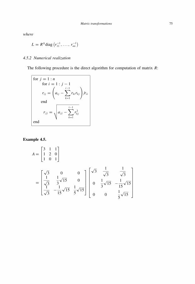
Matrix transformations 75
where
L = Rᵀdiag(r−111 , . . . , r
−1nn
)4.5.2 Numerical realization
The following procedure is the direct algorithm for computation of matrix R:
for j = 1 : nfor i = 1 : j − 1
rij =(aij −
i−1∑k=1
rkirkj
)/rii
end
rjj =√√√√ajj − i−1∑
k=1
r2kj
end
Example 4.5.
A=⎡⎣3 1 1
1 2 0
1 0 1
⎤⎦
=
⎡⎢⎢⎢⎢⎣√3 0 01√3
1
3
√15 0
1√3
− 1
15
√15
1
5
√15
⎤⎥⎥⎥⎥⎦
⎡⎢⎢⎢⎢⎢⎢⎣
√3
1√3
1√3
01
3
√15 − 1
15
√15
0 01
5
√15
⎤⎥⎥⎥⎥⎥⎥⎦

This page intentionally left blank
5 Matrix Functions
Contents
5.1 Projectors . . . . . . . . . . . . . . . . . . . . . . . . . . . . . . . . . . . 77
5.2 Functions of a matrix . . . . . . . . . . . . . . . . . . . . . . . . . . . . . 79
5.3 The resolvent for a matrix . . . . . . . . . . . . . . . . . . . . . . . . . . 85
5.4 Matrix norms . . . . . . . . . . . . . . . . . . . . . . . . . . . . . . . . . 88
5.1 Projectors
Definition 5.1. A Hermitian n× n matrix P is said to be a projector or an idempotentmatrix if it satisfies the condition
P ∗P = PP ∗ = P 2 = P = P ∗ (5.1)
Proposition 5.1. If P ∈ Cn×n is a projector, then
(a) the matrix
Q := In×n − P (5.2)
is a projector too and named the complementary projector to P;(b)
Im(In×n − P) = Ker P (5.3)
(c)
Ker(In×n − P) = ImP (5.4)
Proof.
(a) To prove that Q is a projector too, note that
(In×n − P)2 = In×n − P − P + P 2
= In×n − P − P + P = In×n − P(b) If y ∈ Im(In×n − P), then y = (In×n − P) x for some x ∈ Cn. Thus,
Py = P (In×n − P) x =(P − P 2
)x = 0
It means that y ∈ Ker P .
77
78 Advanced Mathematical Tools for Automatic Control Engineers: Volume 1
(c) By a similar argument, if y ∈ ImP , then y = Px for some x ∈ Cn and, hence,
(In×n − P) y = (In×n − P)Px =(P − P 2
)x = 0
which exactly means (5.4).�
Corollary 5.1. If P ∈ Cn×n is a projector, then
Ker P + Im P = Cn
Proof. Evidently, any x ∈ Cn may be represented as
x = (In×n − P) x + Px = x(1) + x(2)x(1) := (In×n − P) x ∈ Ker P
x(2) := Px ∈ Ker(In×n − P) = Im P
�
Corollary 5.2. Any x(1) ∈ Ker P and x(2) ∈ Im P are orthogonal, that is
(x(1), x(2)
) = 0
Proof. By the previous corollary, we have
x(1)∗x(2) = x∗ (In×n − P)∗ Px= x∗ (In×n − P)Px = x∗
(P − P 2
)x = 0
�
The property given above in (5.2) exactly justifies the name projector for P .
Theorem 5.1. If P ∈ Cn×n is a projector, then
1. its eigenvalues λi (P ) are either equal to 1 or 0;2. it is a simple matrix, that is, it is equivalent to a diagonal matrix with the diagonal
elements equal to 1 or 0;3. it may be represented as
P =r∑i=1
x(i)x(i)∗ (5.5)
where r = rank P and{x(1), . . . , x(r)
}is the system of the eigenvectors of P corre-
sponding to λi (P ) = 1.
Matrix functions 79
Proof.
1. If x(i) (P ) is an eigenvector of P corresponding to an eigenvalue λi (P ), then
Px(i) (P ) = λi (P ) x(i) (P )and pre-multiplication of this identity by (In×n − P) implies
0= (In×n − P)Px(i) (P ) = λi (P ) (In×n − P) x(i) (P )= λi (P )
[x(i) (P )− Px(i) (P )] = λi (P ) [x(i) (P )− λi (P ) x(i) (P )]
= λi (P ) [1− λi (P )] x(i) (P )which proves the first assertion.
(2) and (3) result from (1) and the spectral theorem (4.4).
�5.2 Functions of a matrix
5.2.1 Main definition
Definition 5.2. Let A ∈ Cn×n be any square complex matrix and T ∈ Cn×n is thenonsingular matrix T , defined by (4.9), transforming A to the Jordan canonical form,that is,
A= T JT −1
J = diag(J1, J2, . . . , JK)
where Ji ∈ Cμi×μi is the ith Jordan block defined by (4.7). Also let
f (λ) : C −→ C
be a function which is (l − 1)-times differentiable in a neighborhood of each λi ∈ σ (A)where
l := maxi=1,...,K
μi,
K∑i=1
μi = n
(μi is the multiplicity of λi). Then
f (A) := T diag(f (J1) , f (J2) , . . . , f (JK)) T −1 (5.6)
where
f (Ji) :=
⎡⎢⎢⎢⎢⎢⎢⎣
f (λi)1
1!f(1)
(λi) · · · 1
(μi − 1)!f(μi−1)
(λi)
0 f (λi). . .
......
. . .. . .
1
1!f(1)
(λi)
0 · · · 0 f (λi)
⎤⎥⎥⎥⎥⎥⎥⎦ (5.7)
and f (k) (λ) is the kth derivative of f (λ) in the point λ.
80 Advanced Mathematical Tools for Automatic Control Engineers: Volume 1
Example 5.1. Let
A =⎡⎣ 6 2 2
−2 2 0
0 0 2
⎤⎦
Then the eigenvalues, the corresponding eigenvectors and the generalized eigenvectorsare as follows
λ1 = 2, x(1) =⎡⎣ 0
−1
1
⎤⎦, μ1 = 1
λ2 = 4, x(2,1) =⎡⎣−2
2
0
⎤⎦, μ2 = 2
From equation (3.31)
(A− 4I3×3) x(2,2) = x(2,1)
we obtain
x(2,2) =⎡⎣1
0
0
⎤⎦
and, hence
T =⎡⎣ 0 −2 1
−1 2 0
1 0 0
⎤⎦, T −1 =
⎡⎣0 0 1
0 1/2 1/2
1 1 1
⎤⎦
So, for example,
(a)
ln (A)= T⎡⎣ ln 2 0 0
0 ln 4 1/4
0 0 ln 4
⎤⎦ T −1
=⎡⎣ 0 −2 1
−1 2 0
1 0 0
⎤⎦⎡⎣ ln 2 0 0
0 ln 4 1/4
0 0 ln 4
⎤⎦⎡⎣0 0 1
0 1/2 1/2
1 1 1
⎤⎦
=⎡⎣0.88629 −0.5 −0.5
0.5 1.8863 1.1931
0.0 0.0 0.69315
⎤⎦
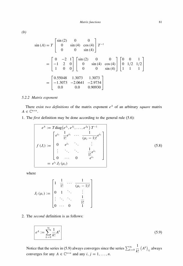
Matrix functions 81
(b)
sin (A)= T⎡⎣sin (2) 0 0
0 sin (4) cos (4)
0 0 sin (4)
⎤⎦ T −1
=⎡⎣ 0 −2 1
−1 2 0
1 0 0
⎤⎦⎡⎣sin (2) 0 0
0 sin (4) cos (4)
0 0 sin (4)
⎤⎦⎡⎣0 0 1
0 1/2 1/2
1 1 1
⎤⎦
=⎡⎣ 0.55048 1.3073 1.3073
−1.3073 −2.0641 −2.9734
0.0 0.0 0.90930
⎤⎦
5.2.2 Matrix exponent
There exist two definitions of the matrix exponent eA of an arbitrary square matrix
A ∈ Cn×n.
1. The first definition may be done according to the general rule (5.6):
eA := T diag(eJ1 , eJ2 , . . . , eJK ) T −1
f (Ji) :=
⎡⎢⎢⎢⎢⎢⎢⎣
eλi1
1!eλi · · · 1
(μi − 1)!eλi
0 eλi. . .
......
. . .. . .
1
1!eλi
0 · · · 0 eλi
⎤⎥⎥⎥⎥⎥⎥⎦
= eλi JI (μi)
(5.8)
where
JI (μi) :=
⎡⎢⎢⎢⎢⎢⎢⎣
11
1! · · · 1
(μi − 1)!0 1
. . ....
.... . .
. . .1
1!0 · · · 0 1
⎤⎥⎥⎥⎥⎥⎥⎦
2. The second definition is as follows:
eA :=∞∑k= 0
1
k!Ak (5.9)
Notice that the series in (5.9) always converges since the series∑∞k= 0
1
k!(Ak
)ijalways
converges for any A ∈ Cn×n and any i, j = 1, . . . , n.

82 Advanced Mathematical Tools for Automatic Control Engineers: Volume 1
Lemma 5.1. Definitions (5.8) and (5.9) coincide.
Proof. For normal matrices this claim is evident since in this case the Jordan blocks
are diagonal. In general cases this result can be checked by the simple evaluation (by
induction) of Ak using both definitions (5.8) and (5.9). �
A rather surprising formula holds.
Lemma 5.2.
det(eA) = exp (trA) (5.10)
Proof. Using (5.8) and (3.19) one has
det(eA)= det
(T diag
(eJ1 , eJ2 , . . . , eJK
)T −1
)= [det T ]
[det diag
(eJ1 , eJ2 , . . . , eJK
)] [det T −1
]= [
det diag(eJ1 , eJ2 , . . . , eJK
)] = K∏i=1
det eJi
=K∏i=1
[exp(λi)]μi =
K∏i=1
exp(μiλi) = exp
(K∑i=1
μiλi
)
= exp
(n∑s=1
λs
)= exp(trA)
�
Example 5.2. For the matrix A from the previous example (5.1) we have
exp
⎛⎝⎡⎣ 6 2 2
−2 2 0
0 0 2
⎤⎦⎞⎠
=⎡⎣ 0 −2 1
−1 2 0
1 0 0
⎤⎦⎡⎣e2 0 0
0 e4 e4
0 0 e4
⎤⎦⎡⎣0 0 1
0 1/2 1/2
1 1 1
⎤⎦
=⎡⎣−54.598 −109.20 −109.20
109.20 163.79 156.41
0.0 0.0 7.3891
⎤⎦
and by (5.10)
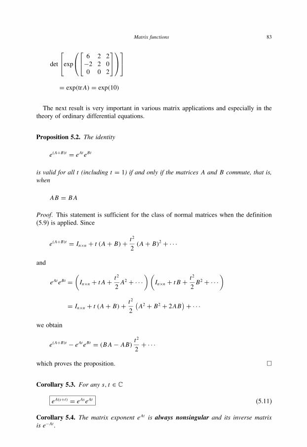
Matrix functions 83
det
⎡⎣exp
⎛⎝⎡⎣ 6 2 2
−2 2 0
0 0 2
⎤⎦⎞⎠⎤⎦
= exp(trA) = exp(10)
The next result is very important in various matrix applications and especially in the
theory of ordinary differential equations.
Proposition 5.2. The identity
e(A+B)t = eAteBt
is valid for all t (including t = 1) if and only if the matrices A and B commute, that is,when
AB = BA
Proof. This statement is sufficient for the class of normal matrices when the definition
(5.9) is applied. Since
e(A+B)t = In×n + t (A+ B)+ t2
2(A+ B)2 + · · ·
and
eAteBt =(In×n + tA+ t
2
2A2 + · · ·
)(In×n + tB + t
2
2B2 + · · ·
)
= In×n + t (A+ B)+ t2
2
(A2 + B2 + 2AB
)+ · · ·
we obtain
e(A+B)t − eAteBt = (BA− AB) t2
2+ · · ·
which proves the proposition. �
Corollary 5.3. For any s, t ∈ C
eA(s+t) = eAseAt (5.11)
Corollary 5.4. The matrix exponent eAt is always nonsingular and its inverse matrixis e−At .

84 Advanced Mathematical Tools for Automatic Control Engineers: Volume 1
Proof. Indeed, taking in (5.11) s = −t we get
eA·0 = In×n = e−AteAt
which implies the result. �
5.2.3 Square root of a positive semidefinite matrix
In this subsection we will discuss the construction of the function which satisfies the
condition
A = A1/2A1/2 (5.12)
The formal implementation of the definition (5.6) demands to consider only the matrices
with nonnegative spectrum of eigenvalues, that is, when λi (A) ≥ 0 for all i = 1, . . . , n.
But to fulfill (5.12) this is not sufficient. Indeed, if there exists at least one complete
Jordan block this property never holds. Thus, we need to ask whether the Jordan block
would not be presented which is true only for Hermitian (in the case of real matrices,
symmetric) matrices. So, now we are ready to formulate the following proposition.
Proposition 5.3. The matrix A1/2 is well defined for a positive semidefinite Hermitianmatrix and, moreover, it is positive semidefinite Hermitian itself.
Proof. For Hermitian matrices the transforming matrix T is always unitary, that is,
T −1 = T ∗ and all eigenvalues are real. Thus,
A1/2 = T diag((J1)
1/2, (J2)1/2, . . . , (JK)
1/2)T −1
and, hence,(A1/2
)∗ = (T −1
)∗diag
((J1)
1/2, (J2)1/2, . . . , (JK)
1/2)T ∗
= T diag((J1)
1/2, (J2)1/2, . . . , (JK)
1/2)T −1 = A1/2
�
Example 5.3.[3 1
1 1
]1/2=
[√2+ 1 −√2+ 1
1 1
]
×[√√
2+ 2 0
0√
2−√2
]⎡⎢⎢⎣√2+ 2
4√2+ 4
√2
4√2+ 4
−1
4
√2
1
4
√2+ 1
2
⎤⎥⎥⎦
=[1.6892 0.38268
0.38268 0.92388
]

Matrix functions 85
5.3 The resolvent for a matrix
The complex function theory provides a third approach to the definition of f (A)
applicable when f (λ) is an analytical function of a complex variable λ. Sure, this approach
is consistent with general definition (5.6) of f (A) valid for multiplying differentiable
functions defined on the spectrum of A.
Let us consider a matrix A (λ) : C → Cm×n whose elements are functions of a complex
variable λ and define also
• the derivatives
dr
dλrA (λ) = A(r) (λ), r = 0, 1, 2, . . . (5.13)
of the matrix A (λ) to be the matrix obtained by differentiating each element of A (λ);
• the integral∫L
A (λ) dλ (5.14)
of the matrix A (λ) to be the matrix obtained by integrating each element of A (λ)
in the positive direction along a path L in a complex plane, which will be assumed
to be a finite system of simple piecewise smooth closed contours without points of
intersections.
Example 5.4. For a normal matrix A ∈ Cn×n using the series representation (5.9) thefollowing properties may be proven:
1.
d
dt
(eAt
) = AeAt = eAtA (5.15)
2.
d
dt(A (t))2 =
(d
dtA (t)
)A+ A
(d
dtA (t)
)(5.16)
Notice that in general
d
dt(A (t))2 �= 2A
(d
dtA (t)
)
3. if all derivatives exist and p = 1, 2, . . . then
d
dt(A (t))p =
p∑i=1
Ai−1
(d
dtA (t)
)Ap−i (5.17)

86 Advanced Mathematical Tools for Automatic Control Engineers: Volume 1
4.
d
dt(A (t))−p = −A−p
[p∑i=1
Ai−1
(d
dtA (t)
)Ap−i
]A−p (5.18)
This relation may be easily proven by simply differentiating the identity
A−pAp = In×n
which implies
[d
dt(A (t))−p
]Ap + A−p
[d
dt(A (t))p
]= On×n
and, thus,
[d
dt(A (t))−p
]= −A−p
[d
dt(A (t))p
]A−p
Definition 5.3. The matrix
Rλ (A) := (λIn×n − A)−1 (5.19)
defined for all λ ∈ C which do not belong to the spectrum of A ∈ Cn×n is known as theresolvent of A.
The following properties of Rλ (A) seem to be important for the considerations below.
Proposition 5.4. For all λ /∈ σ (A)1.
Rλ (A)− Rμ (A) = (μ− λ)Rλ (A)Rμ (A) (5.20)
2.
d
dλRλ (A) = −R2
λ (A) (5.21)
3.
dr
dλrRλ (A) = (−1)r r!Rr+1
λ (A) (5.22)

Matrix functions 87
Proof. Formula (5.22) may be proven by induction taking into account (5.21). But (5.21)
results from (5.20). To prove (5.20) notice that
R−1λ (A) [Rλ (A)− Rμ (A)]R−1
μ (A)
= R−1λ (A)
[(λIn×n − A)−1 − (μIn×n − A)−1
]R−1μ (A)
= R−1μ (A)− R−1
λ (A) = (μ− λ) In×n
which implies (5.20). �
Theorem 5.2. The resolvent Rλ (A) of A ∈ Cn×n is a rational function of λ with polesat the points of the spectrum of A and R∞ (A) = 0. Moreover, each λk ∈ σ (A) is a poleof Rλ (A) of order μk where μk is the multiplicity of the eigenvalue λk , that is,
Rλ (A) = 1
m(λ)
K−1∑j=1
(K−1∑i=1
γijλi
)Aj (5.23)
where m(λ) =K∏s=1
(λ− λs)μs ,K∑s=1
μs = n.
Proof. Evidently
m(λ)−m(μ)λ− μ =
K−1∑i=1
K−1∑j=1
γijλiμj
for some numbers γij . Using the matrix polynomial definition (as in the Cayley–Hamilton
theorem) for λk /∈ σ (A) the last relation (after formal substituting A for μ) implies
[m(λ) In×n −m(A)]Rλ (A) =K−1∑i=1
K−1∑j=1
γijλiAj
Since by the Cayley–Hamilton theorem m(A) = 0, we obtain (5.23). �
Thus, using the terminology of complex analysis, the spectrum of a matrix A can be
described in terms of its resolvent. The next theorem establishes this relation exactly.
Theorem 5.3. (Cauchy integral theorem for matrices) Let f (λ) be a function of thecomplex variable λ analytical in an open set D ∈ C, that is, f (λ) has a convergentTaylor series expansion about each point of D. If A ∈ Cn×n has distinct eigenvalues

88 Advanced Mathematical Tools for Automatic Control Engineers: Volume 1
λ1, . . . , λs≤n, the path L is a closed contour having λ1, . . . , λs as its interior, and f (λ)is continuous in and analytic within L, then
f (A)= 1
2πi
∫L
f (λ)[(λIn×n − A)−1
]dλ
= 1
2πi
∫L
f (λ)Rλ (A) dλ
(5.24)
Proof. This result may be established using (5.23) and the Cauchy theorem which
asserts that
f (r) (λ0) = r!2πi
∫L
f (λ0)
(λ− λ0)r+1dλ
for any λ0 ∈ D. �
Corollary 5.5. The following identities are valid for any A ∈ Cn×n:
In×n = 1
2πi
∫L
Rλ (A) dλ
A = 1
2πi
∫L
λRλ (A) dλ
(5.25)
5.4 Matrix norms
5.4.1 Norms in linear spaces and in Cn
Definition 5.4. A real-valued function ‖x‖ : L → R defined on all elements x of alinear space L of complex or real numbers, is called a norm (on L), if it satisfies thefollowing axioms:
1.
‖x‖ ≥ 0
for all x ∈ L and ‖x‖ = 0 if and only if x = 0;2.
‖αx‖ = |α| ‖x‖
for all x ∈ L and all α ∈ C;3. the triangle inequality holds, that is,
‖x + y‖ ≤ ‖x‖ + ‖y‖
for all x, y ∈ L.

Matrix functions 89
A linear space L together with a norm defined on it is called a normed linear space.
Consider the following examples of norms in Cn.
Example 5.5. Let x = (x1, x2, . . . , xn)ᵀ be a typical vector in Cn (or, in particular,
in Rn). Then the following functions are norms in a finite-dimensional spaceCn (or Rn):
1. Modul-sum norm
‖x‖1 := max1≤i≤n
|xi | (5.26)
2. Euclidean norm
‖x‖2 :=(
n∑i=1
x2i
)1/2
(5.27)
3. Hölder norm
‖x‖p :=(
n∑i=1
|xi |p)1/p
, p ≥ 1 (5.28)
4. Chebyshev norm
‖x‖∞ := max1≤i≤n
|xi | (5.29)
5. Weighted norm
‖x‖H := √(Hx, x) = √
x∗Hx (5.30)
where H is a Hermitian (or symmetric) matrix with all positive definite eigenvalues.
It is not so difficult to check that functions (5.26)–(5.30) satisfy all three norm axioms.
Definition 5.5. Two norms ‖x‖′ and ‖x‖′′ are said to be equivalent in L, if there existpositive numbers r1, r2 ∈ (0,∞) such that for any x ∈ L
‖x‖′ ≥ r2 ‖x‖′′, ‖x‖′′ ≥ r1 ‖x‖′

90 Advanced Mathematical Tools for Automatic Control Engineers: Volume 1
Proposition 5.5. Any two norms in a finite-dimensional linear space are equivalent.
Proof. It is clear that a norm in a finite-dimensional linear space is a continuous function
since the inequality
‖x + z‖ ≤ ‖x‖ + ‖z‖
leads to the following relations
‖x + z‖ − ‖x‖ ≤ ‖z‖
and
‖y‖ − ‖x‖ ≤ ‖y − x‖|‖y‖ − ‖x‖| ≤ ‖y − x‖
if z = y − x. The last inequality corresponds exactly to the continuity definition. Let us
consider two sets
X1 :={x ∈ L : ‖x‖′ = 1
}X2 :=
{x ∈ L : ‖x‖′′ = 1
}By the continuity property there exist two elements x01 ∈ X1 and x02 ∈ X2 such that
0 < γ1 := infx∈X1
‖x‖′′ = ‖x01‖′
0 < γ2 := infx∈X2
‖x‖′ = ‖x02‖′
Thus, for any nonzero element x ∈ L and the second norm axiom it follows that
0 < γ1 := infx∈X1
‖x‖′′ ≤∥∥∥∥ x
‖x‖′∥∥∥∥′′
= ‖x‖′′‖x‖′
0 < γ2 := infx∈X2
‖x‖′ ≤∥∥∥∥ x
‖x‖′′∥∥∥∥′
= ‖x‖′‖x‖′′
which for r1 = γ2 and r2 = γ1 corresponds to the desired result. �
5.4.2 Matrix norms
Here we will pay attention to norms on the linear space Cn×n, or in other words, to
norms in a space of squared matrices. Sure, all properties of norms discussed before
should be valid for the matrix case. However, some additional axiom (or axioms) are
required because of the possibility of multiplying any two matrices that give rise to the
question regarding the relation of ‖AB‖ and ‖A‖, ‖B‖ for any two matrices A,B ∈ Cn×n.

Matrix functions 91
Definition 5.6. (Axiom 4 for matrix norms) The function ‖A‖ defined for anyA ∈ Cn×n
is said to be a matrix or submultiplicative norm (in contrast to a standard norm in Cn×n)if the following axiom holds
‖AB‖ ≤ ‖A‖ ‖B‖ (5.31)
Example 5.6. It is not difficult to check that the function
max1≤i,j≤n
∣∣aij ∣∣where aij is an element of A ∈ Cn×n, is a norm on Cn×n, but it is not a matrix norm.
Proposition 5.6. The following functions are the matrix norms for the matrixA = [aij ]1≤i,j≤n:
1. Frobenius (Euclidean) norm
‖A‖F :=(
n∑i=1
n∑j=1
∣∣aij ∣∣2)1/2
(5.32)
2. Hölder norm
‖A‖p :=(
n∑i=1
n∑j=1
∣∣aij ∣∣p)1/p
(5.33)
is a matrix norm if and only if
1 ≤ p ≤ 2
3. Weighted Chebyshev norm
‖A‖p := n max1≤i,j≤n
∣∣aij ∣∣ (5.34)
4. Trace norm
‖A‖tr :=√tr (A∗A) = √
tr (AA∗) (5.35)

92 Advanced Mathematical Tools for Automatic Control Engineers: Volume 1
5. Maximal singular-value norm
‖A‖σ :=√max σi (A)
1≤i≤n
= √max λi (A∗A)
1≤i≤n=√
max λi (AA∗)1≤i≤n
(5.36)
6. S-norm
‖A‖S :=∥∥SAS−1
∥∥ (5.37)
where S is any nonsingular matrix and ‖·‖ is any matrix norm.
We leave the proof of this proposition for readers as an exercise. The next statement also
seems to be evident.
Proposition 5.7. For any matrix norm ‖·‖
‖In×n‖ ≥ 1∥∥Ak∥∥ ≤ ‖A‖k, k = 2, 3, . . .
∥∥A−1∥∥ ≥ 1
‖A‖
There exists an estimate of any matrix norm related to the spectral radius (3.14).
Lemma 5.3. For any matrix A ∈ Cn×n with the spectral radius ρ (A) = max1≤i≤n
|λi | andany matrix norm ‖·‖ the following estimate holds
‖A‖ ≥ ρ (A) (5.38)
Proof. Let λ be the eigenvalue of A with the maximal module, i.e., ρ (A) = |λ|. Thenthere exists the corresponding eigenvector x �= 0 such that Ax = λx. Define an n × nmatrix
B := [x 0 0 · · · 0]
and observe that
AB = λB

Matrix functions 93
Then by the second and fourth norm axioms we deduce that
‖λB‖ = |λ| ‖B‖ = ρ (A) ‖B‖ ≤ ‖A‖ ‖B‖
Since B �= 0 it follows that ‖B‖ > 0 which proves the desired result (5.38). �
The following comments are very important for practical applications.
Remark 5.1.
1. The spectral radius ρ (A) itself cannot be considered as a matrix norm (and as anynorm in general) since it does not satisfy the first norm axiom, that is, if ρ (A) = 0,
we cannot conclude that A = On×n (one can consider the matrix A =[0 1
0 0
]as an
example).2. The inequality (5.38) may be considered as an upper estimate for the spectral radiusρ (A).
5.4.3 Compatible norms
Definition 5.7. The vector norm ‖·‖v and matrix norm ‖·‖ are said to be compatible ifthe inequality
‖Ax‖v ≤ ‖A‖ ‖x‖v (5.39)
is valid for any x ∈ Cn and any A ∈ Cn×n.
It is not difficult to check that
• the Frobenius matrix (5.32) and Euclidean vector (5.27) norm are compatible;• the weighted Chebyshev norm (5.34) is compatible with Hölder norms (5.28) in Cn for
p = 1, 2,∞.
5.4.4 Induced matrix norm
Proposition 5.8. The quotient
f (A) := supx∈Cn,x �=0
‖Ax‖v‖x‖v (5.40)
can be considered as a matrix norm induced by the vector norm ‖·‖v . In particular,the matrix norm induced by the Euclidean vector norm is known as the spectral matrixnorm. For calculus purposes it may be calculated as
f (A) := maxx∈Cn:‖x‖v=1
‖Ax‖v (5.41)
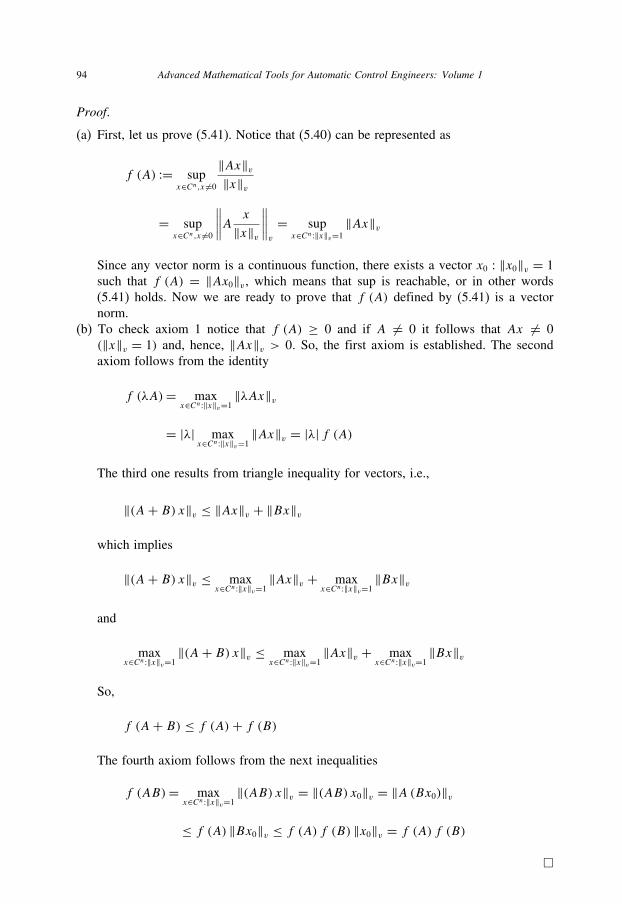
94 Advanced Mathematical Tools for Automatic Control Engineers: Volume 1
Proof.
(a) First, let us prove (5.41). Notice that (5.40) can be represented as
f (A) := supx∈Cn,x �=0
‖Ax‖v‖x‖v
= supx∈Cn,x �=0
∥∥∥∥A x
‖x‖v
∥∥∥∥v
= supx∈Cn:‖x‖v=1
‖Ax‖v
Since any vector norm is a continuous function, there exists a vector x0 : ‖x0‖v = 1
such that f (A) = ‖Ax0‖v , which means that sup is reachable, or in other words
(5.41) holds. Now we are ready to prove that f (A) defined by (5.41) is a vector
norm.
(b) To check axiom 1 notice that f (A) ≥ 0 and if A �= 0 it follows that Ax �= 0
(‖x‖v = 1) and, hence, ‖Ax‖v > 0. So, the first axiom is established. The second
axiom follows from the identity
f (λA)= maxx∈Cn:‖x‖v=1
‖λAx‖v
= |λ| maxx∈Cn:‖x‖v=1
‖Ax‖v = |λ| f (A)
The third one results from triangle inequality for vectors, i.e.,
‖(A+ B) x‖v ≤ ‖Ax‖v + ‖Bx‖v
which implies
‖(A+ B) x‖v ≤ maxx∈Cn:‖x‖v=1
‖Ax‖v + maxx∈Cn:‖x‖v=1
‖Bx‖v
and
maxx∈Cn:‖x‖v=1
‖(A+ B) x‖v ≤ maxx∈Cn:‖x‖v=1
‖Ax‖v + maxx∈Cn:‖x‖v=1
‖Bx‖v
So,
f (A+ B) ≤ f (A)+ f (B)
The fourth axiom follows from the next inequalities
f (AB)= maxx∈Cn:‖x‖v=1
‖(AB) x‖v = ‖(AB) x0‖v = ‖A (Bx0)‖v
≤ f (A) ‖Bx0‖v ≤ f (A) f (B) ‖x0‖v = f (A) f (B)
�

Matrix functions 95
Several properties of the induced norm given below turn out to be important in many
practical implementations.
Proposition 5.9.
1. For any induced norm
f (In×n) = 1 (5.42)
2. If A is unitary
f (A) = 1
3. If f (A) is the spectral norm then
f (A) =√max λi (A∗A)
1≤i≤n=
√max λi (AA∗)
1≤i≤n
4. If U is a unitary matrix then
f (AU) = f (UA) = f (A)
5. For the vector norm (5.26) the corresponding induced norm is
f1 (A) = max1≤j≤n
n∑i=1
∣∣aij ∣∣The proof of this proposition results in simple vector calculations and these therefore
are omitted here.
Example 5.7.
f1
([2 −1
2 3
])= max {3; 5} = 5

This page intentionally left blank

6 Moore–Penrose Pseudoinverse
Contents
6.1 Classical least squares problem . . . . . . . . . . . . . . . . . . . . . . . . 97
6.2 Pseudoinverse characterization . . . . . . . . . . . . . . . . . . . . . . . . 100
6.3 Criterion for pseudoinverse checking . . . . . . . . . . . . . . . . . . . . . 102
6.4 Some identities for pseudoinverse matrices . . . . . . . . . . . . . . . . . 104
6.5 Solution of least squares problem using pseudoinverse . . . . . . . . . . . 107
6.6 Cline’s formulas . . . . . . . . . . . . . . . . . . . . . . . . . . . . . . . 109
6.7 Pseudo-ellipsoids . . . . . . . . . . . . . . . . . . . . . . . . . . . . . . . 109
In this subsection we follow Albert (1972).
6.1 Classical least squares problem
Lemma 6.1. Let x be a vector and L is a linear manifold in Rn (that is, if x, y ∈ L, thenαx + βy ∈ L for any scalars α, β). Then if
x = x + x (6.1)
where x ∈ L and x ⊥ L, then x is “nearest” to x, or, in other words, it is the projectionof x to the manifold L.
Proof. For any y ∈ L we have
∥∥x − y∥∥2 = ∥∥x + x − y∥∥2 = ∥∥(x − y)+ x∥∥2
= ∥∥x − y∥∥2 + 2(x − y, x)+ ∥∥x∥∥2 = ∥∥x − y∥∥2 + ∥∥x∥∥2
≥ ∥∥x∥∥2 = ∥∥x − x∥∥2
with strict inequality holding unless∥∥y − x∥∥2 = 0. �
Theorem 6.1. Let z be an n-dimensional real vector and H ∈ Rn×m.1. There is always a vector, in fact a unique vector x of minimal (Euclidean) norm, which
minimizes
∥∥z−Hx∥∥2
97

98 Advanced Mathematical Tools for Automatic Control Engineers: Volume 1
2. The vector x is the unique vector in the range
R (Hᵀ) := {x : x = Hᵀz, z ∈ Rn}
which satisfies the equation
Hx = z
where z is the projection of z on R (H).
Proof. By (6.1) we can write
z = z+ z
where z is the projection of z on the kernel (the null space)
N (Hᵀ) := {z ∈ Rn : 0 = Hᵀz}
Since Hx ∈ R (H) for any x ∈ Rm, it follows that
z−Hx ∈ R (H)
and, since z ∈ R⊥ (H),
z ⊥ z−Hx
Therefore,∥∥z−Hx∥∥2 = ∥∥(z−Hx)+ z∥∥2
= ∥∥z−Hx∥∥2 + ∥∥z∥∥2 ≥ ∥∥z∥∥2 = ∥∥z− z∥∥2
This low bound is attainable since z, being the range of H , is the afterimage of some x∗,that is, z = Hx∗.1. Let us show that x∗ has a minimal norm. Since x∗ may be decomposed into two
orthogonal vectors
x∗ = x∗ + x∗
where x∗ ∈ R(H⊥) and x∗ ∈ N (H). Thus Hx∗ = Hx we have
∥∥z−Hx∗∥∥2 = ∥∥z−Hx∥∥2
and ∥∥x∗∥∥2 = ∥∥x∗∥∥2 + ∥∥x∗∥∥2 ≥ ∥∥x∗∥∥2
with strict inequality unless x∗ = x∗. So, x∗ may be selected equal to x∗.

Moore–Penrose pseudoinverse 99
2. Show now that x∗ = x∗ is unique. Suppose that Hx∗ = Hx∗∗ = z. Then
(x∗ − x∗∗) ∈ R (H)
But H (x∗ − x∗∗) = 0, which implies,
(x∗ − x∗∗) ∈ N (H) = R⊥ (H⊥)Thus (x∗ − x∗∗) is orthogonal to itself, which means that
∥∥x∗ − x∗∗∥∥2 = 0, or equiv-
alently, x∗ = x∗∗. �
Corollary 6.1.∥∥z−Hx∥∥2
is minimized by x0 if and only if Hx0 = z where z is theprojection of z on R (H) .
Corollary 6.2. There is always an n-dimensional vector y such that
∥∥z−HHᵀy∥∥2 = inf
x
∥∥z−Hx∥∥2
and if
∥∥z−Hx0∥∥2 = infx
∥∥z−Hx∥∥2
then ∥∥x0∥∥2 ≥ ∥∥Hᵀy∥∥2
with strict inequality unless x0 = Hᵀy. The vector y satisfies the equation
HHᵀy = z
Theorem 6.2. (on the system of normal equations) Among those vectors x, whichminimize
∥∥z−Hx∥∥2, x, the one having minimal norm, is the unique vector of the form
x = Hᵀy (6.2)
satisfying
HᵀHx = Hᵀz (6.3)
Proof. By direct differentiation we have
∂
∂x
∥∥z−Hx∥∥2 = 2Hᵀ (z−Hx) = 0
which gives (6.3). The representation (6.2) follows from the previous corollary. �

100 Advanced Mathematical Tools for Automatic Control Engineers: Volume 1
6.2 Pseudoinverse characterization
We are now in the position to exhibit an explicit representation for the minimum norm
solution to a least square problem.
Lemma 6.2. For any real symmetric matrix A ∈ Rn×n the limit
PA := limδ→0(A+ δIn×n)−1A (6.4)
always exists. For any vector z ∈ Rn
z = PAz
is the projection of x on R (A).
Proof. By symmetricity of A for all δ > 0 such that 0 < |δ| < minj :λj (A)�=0
∣∣λj (A)∣∣ the matrix
(A+ δIn×n)−1 exists. Any z ∈ Rn may be represented as
z = z+ z
where z ∈ R (A), z ∈ N (A) and Az = Az. There exists x0 such that z = Ax0, so
(A+ δIn×n)−1Az = (A+ δIn×n)−1Az = (A+ δIn×n)−1A (Ax0)
By the spectral theorem (4.4) for symmetric matrices it follows that
A = T�Tᵀ
where � = diag (λ1, . . . , λn) and Tᵀ = T −1. Thus
(A+ δIn×n)−1Az= (A+ δIn×n)−1A2x0
= (T �Tᵀ + δT Tᵀ)−1 T�2T ᵀx0
= (T [�+ δIn×n] Tᵀ)−1
T�2T ᵀx0
= T ( [�+ δIn×n]−1�2
)T ᵀx0
It is plain to see that
limδ→0
[�+ δIn×n]−1�2 = lim
δ→0[�+ δIn×n]−1
[�+ δIn×n − δIn×n]�
= limδ→0
[In×n − δ [�+ δIn×n]−1
]�
=[limδ→0
diag
(1− δ
λ1 + δ , . . . , 1−δ
λn + δ)]� = �
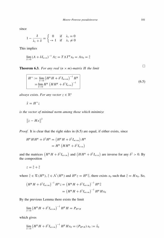
Moore–Penrose pseudoinverse 101
since
1− δ
λi + δ ={
0 if λi = 0
→ 1 if λi �= 0
This implies
limδ→0(A+ δIn×n)−1Az = T�Tᵀx0 = Ax0 = z
�Theorem 6.3. For any real (n×m)-matrix H the limit
H+ := limδ→0
(HᵀH + δ2Im×m
)−1Hᵀ
= limδ→0Hᵀ (
HHᵀ + δ2In×n)−1 (6.5)
always exists. For any vector z ∈ Rn
x = H+z
is the vector of minimal norm among those which minimize
∥∥z−Hx∥∥2
Proof. It is clear that the right sides in (6.5) are equal, if either exists, since
HᵀHHᵀ + δ2Hᵀ = (HᵀH + δ2Im×m
)Hᵀ
= Hᵀ (HHᵀ + δ2In×n
)and the matrices
(HᵀH + δ2Im×m
)and
(HHᵀ + δ2In×n
)are inverse for any δ2 > 0. By
the composition
z = z+ z
where z ∈ R (Hᵀ), z ∈ N (Hᵀ) and Hᵀz = Hᵀz, there exists x0 such that z = Hx0. So,(HᵀH + δ2Im×m
)−1Hᵀz= (
HᵀH + δ2Im×m)−1Hᵀz
= (HᵀH + δ2Im×m
)−1HᵀHx0
By the previous Lemma there exists the limit
limδ→0
(HᵀH + δ2Im×m
)−1HᵀH = PHᵀH
which gives
limδ→0
(HᵀH + δ2Im×m
)−1HᵀHx0 = (PHᵀH ) x0 := x0
102 Advanced Mathematical Tools for Automatic Control Engineers: Volume 1
where x0 is the projection on R (HᵀH) = R (Hᵀ). Thus we conclude that
x0 = limδ→0
(HᵀH + δ2Im×m
)−1Hᵀz
= limδ→0
(HᵀH + δ2Im×m
)−1Hᵀz
always exists and is an element of R (Hᵀ) satisfying z = Hx0. �
Definition 6.1. The matrix limit H+ (6.5) is called the pseudoinverse (the generalizedinverse) of H in the Moore–Penrose sense.
Remark 6.1. It follows that
• (HH+z) is the projection of z on R (H);• (H+Hx) is the projection of x on R (Hᵀ);• (In×n −HH+)z is the projection of z on N (Hᵀ);• (In×n −H+H)x is the projection of x on N (H).
The following properties can be proven by the direct application of (6.5).
Corollary 6.3. For any real n×m matrix H
1.
H+ = (HᵀH)+Hᵀ (6.6)
2.
(Hᵀ)+ = (H+)T (6.7)
3.
H+ = Hᵀ (HHᵀ)+ (6.8)
4.
H+ = H−1 (6.9)
if H is square and nonsingular.
6.3 Criterion for pseudoinverse checking
The next theorem represents the criterion for a matrix B, to be the pseudoinverse H+
of H .

Moore–Penrose pseudoinverse 103
Theorem 6.4. For any real n×m matrix H the matrix B = H+ if and only if
1.
HB and BH are symmetric (6.10)
2.
HBH = H (6.11)
3.
BHB = B (6.12)
Proof.
1. Necessity. Let B = H+.(a) Since
HH+ = limδ→0HHᵀ (
HHᵀ + δ2In×n)−1
(HH+)T =
(H limδ→0
(HᵀH + δ2Im×m
)−1Hᵀ
)T
= H[limδ→0
(HᵀH + δ2Im×m
)−1]Hᵀ = HH+
and
H+H =[limδ→0Hᵀ (
HHᵀ + δ2In×n)−1
]H
(H+H
)T =([
limδ→0Hᵀ (
HHᵀ + δ2In×n)−1
]H)T
Hᵀlimδ→0
(HᵀH + δ2Im×m
)−1H = H+H
the symmetricity (6.10) takes place.
(b) Since by (6.1) HH+ is a projector on R (H) and the projection of any vector
from R (H) coincides with the same vector, one has for any z ∈ Rn
HH+ (Hz) = Hz
which gives (6.11). By (6.6)
H+H = (HᵀH)+ (HᵀH)

104 Advanced Mathematical Tools for Automatic Control Engineers: Volume 1
which, in view of (6.11) and the symmetricity property (6.10) of HH+, implies
H+ = (HᵀH)+Hᵀ = (HᵀH)+(HH+H
)T= (HᵀH)+Hᵀ (
HH+)T = (HᵀH)+Hᵀ (HH+)
= (HᵀH)+ (HᵀH)H+ = H+HH+
So, (6.12) is proven.
2. Sufficiency. Suppose B satisfies (6.10), (6.11) and (6.12). Since
BH = (BH )T , H = HBH
then
H = HBH = H (BH)T
Using this representation and since HH+H = H , we derive
H+H = H+H (BH)T = [HH+H
]TBᵀ = HᵀBᵀ = BH (6.13)
Analogously, since B = BHB and HB is symmetric, we have
Bᵀ = HBBᵀ
Pre-multiplying this identity by HH+, we obtain
HH+Bᵀ = HH+HBBᵀ = HBBᵀ = Bᵀ
Taking transposes and in view of (6.13) we get
B = B (HH+)T = B (
HH+) = BHH+ = H+HH+ = H+
�The theorem above is extremely useful as a method for proving identities. If one thinks
that a certain expression coincides with the pseudoinverse of a certain matrix H , a good
way to decide is to run the expressions through conditions (6.10), (6.11), (6.12) and
observe whether or not they hold.
6.4 Some identities for pseudoinverse matrices
Lemma 6.3. b ∈ R (A) := Im (A) ⊆ Rn if and only if
AA+b = b (6.14)
Proof.
(a) Necessity. If b ∈ R (A), then there exists a vector d ∈ Rn such that b = Ad , and,therefore,
AA+b = AA+ (Ad) = (AA+A
)d = Ad = b
Moore–Penrose pseudoinverse 105
(b) Sufficiency. Suppose that (6.14) is true. Any vector b can be represented as
b = Ad + b⊥ with b⊥ ⊥ Ad, namely, b⊥ = (I − AA+) v. Then
AA+ (Ad + b⊥) = Ad + b⊥which implies AA+b⊥ = b⊥, and, hence,
AA+ (I − AA+) v = 0 = (I − AA+) v = b⊥
So, b⊥ = 0, and, hence, b = Ad, or, equivalently, b ∈ R (A). Lemma is proven. �
The following identities can be proven more easily by simple verification of (6.10),
(6.11), (6.12).
Claim 6.1.
1.
(Om×n)+ = On×m (6.15)
2. For any x ∈ Rn (x �= 0)
x+ = xᵀ
‖x‖2 (6.16)
3.
(H+)+ = H (6.17)
4. In general,
(AB)+ �= B+A+ (6.18)
The identity takes place if
AᵀA= I or
BBᵀ = I or
B =Aᵀ or
B =A+ or
both A and B are of full rank, or
rankA = rankB
The identity in (6.18) holds if and only if
R (BBᵀAᵀ) ⊆ R (Aᵀ) (6.19)

106 Advanced Mathematical Tools for Automatic Control Engineers: Volume 1
and
R (AᵀAB) ⊆ R (B) (6.20)
5.
(AB)+ = B+1 A
+1 (6.21)
where
B1 = A+AB
A1 = AB1B+1
6.
(HᵀH)+ = H+ (Hᵀ)+, (HHᵀ)+ = (Hᵀ)+H+ (6.22)
7. If A is symmetric and α > 0, then
(Aα)+ = (A+)α
Aα (Aα)+ = (Aα)+Aα = AA+
A+Aα =AαA+(6.23)
8. If A = U�Vᵀ where U,V are orthogonal and � is a diagonal matrix, then
A+ = V�+Uᵀ (6.24)
9. Greville’s formula (Greville 1960): if Cm+1 =[Cm...cm+1
]then
C+m+1 =
⎡⎣C+
m
[I − cm+1k
ᵀm+1
]· · · · · · · · · · · · · · ·
kᵀm+1
⎤⎦ (6.25)
where
km+1 =
⎧⎪⎪⎪⎪⎨⎪⎪⎪⎪⎩
[I − CmC+m ] cm+1∥∥[I − CmC+m ] cm+1
∥∥2if [I − CmC+
m ] cm+1 �= 0
(C+m
)TC+mcm+1
1+ ∥∥C+mcm+1
∥∥2otherwise
10. If H is rectangular and S is symmetric and nonsingular then
(SH)+ = H+S−1
[I − (
QS−1)+ (QS−1
)](6.26)
Moore–Penrose pseudoinverse 107
where
Q = I −H+H
Example 6.1. Simple verification of (6.10), (6.11), (6.12) shows that⎡⎣ 1 2
3 4
5 6
⎤⎦+
=[ −1.333 −0.333 0.667
1.8033 0.333 −0.4167
]
6.5 Solution of least squares problem using pseudoinverse
Theorem 6.5.(a) The vector x0 minimizes ‖z−Hx‖2 if and only if it is of the form
x0 = H+z+ (I −H+H
)y (6.27)
for some vector y.(b) Among all solutions x0 (6.27) the vector
x0 = H+z (6.28)
has the minimal Euclidean norm.
Proof. By theorem (6.3) we know that H+z minimizes ‖z−Hx‖2 and by (6.1), any x0minimizes ‖z−Hx‖2 if and only if Hx0 = z where z is the projection of z on R (H).In view of that
Hx0 = H(H+z
)This means that x0 −H+z is a null vector of H that is true if and only if
x0 −H+z = (I −H+H
)y
for some y. So, (a) (6.27) is proven. To prove (b) (6.28) it is sufficient to notice that
∥∥x0∥∥2 = ∥∥H+z+ (I −H+H
)y∥∥2 = ∥∥H+z
∥∥2
+ (H+z,
(I −H+H
)y)+ ∥∥(I −H+H
)y∥∥2 = ∥∥H+z
∥∥2
+ ((I −H+H
)TH+z, y
)+ ∥∥(I −H+H)y∥∥2 = ∥∥H+z
∥∥2
+ ((I −H+H
)H+z, y
)+ ∥∥(I −H+H)y∥∥2
= ∥∥H+z∥∥2 + ∥∥(I −H+H
)y∥∥2 ≥ ∥∥H+z
∥∥2 = ∥∥x0∥∥2
�

108 Advanced Mathematical Tools for Automatic Control Engineers: Volume 1
Corollary 6.4. (LS problem with constraints) Suppose the set
J = {x : Gx = u}
is not empty. Then the vector x0 minimizes∥∥z−Hx∥∥2
over J if and only if
x0 = G+u+ H+z+ (I −G+G
) (I − H+H
)y
H := H (I −G+G
) (6.29)
and among all solutions
x0 = G+u+ H+z (6.30)
has the minimal Euclidean norm.
Proof. Notice that by the Lagrange multipliers method x0 solves the problem if it mini-
mizes the Lagrange function
∥∥z−Hx∥∥2 + (λ,Gx − u)
for some λ. This λ and x0 satisfy the equation
∂
∂x
[∥∥z−Hx∥∥2 + (λ,Gx − u)]= −2Hᵀ (z−Hx0)+Gᵀλ = 0
or, equivalently,
HᵀHx0 =[Hᵀz− 1
2Gᵀλ
]:= z
which in view of (6.27) implies
x0 = (HᵀH)+ z+ [I − (HᵀH)+ (HᵀH)
]y
= (HᵀH)+[Hᵀz− 1
2Gᵀλ
]+ [I − (HᵀH)+ (HᵀH)
]y
(6.31)
But this x0 should satisfy Gx0 = u which leads to the following equality
Gx0 = G[(HᵀH)+
(Hᵀz− 1
2Gᵀλ
)+ [I − (HᵀH)+ (HᵀH)
]y
]= u
or, equivalently,
[G(HᵀH)+
](1
2Gᵀλ
)=G(HᵀH)+Hᵀz
+G [I − (HᵀH)+ (HᵀH)
]y − u

Moore–Penrose pseudoinverse 109
or
1
2Gᵀλ = [
G(HᵀH)+]+ [G(HᵀH)+Hᵀz
+ G [I − (HᵀH)+ (HᵀH)
]y − u]
+[I − [
G(HᵀH)+]+ [G(HᵀH)+
]]y
(6.32)
Substitution of (6.32) into (6.31) and using the properties of the pseudoinverse implies
(6.29). The statement (6.30) is evident. �
6.6 Cline’s formulas
In fact, the direct verification leads to the following identities (see Cline (1964, 1965)).
Claim 6.2. (Pseudoinverse of a partitioned matrix)
[U... V
]+=
⎡⎣U+ − U+V J· · · · · · · · · · · ·
J
⎤⎦ (6.33)
where
J =C+ + (I − C+C
)KVᵀ (
U+)T U+ (I − VC+)C = (
I − UU+)VK = (
I + [U+V
(I − C+C
)]T [U+V
(I − C+C
)])−1
(6.34)
Claim 6.3. (Pseudoinverse of sums of matrices)
(UUᵀ + VVᵀ)+ = (CCᵀ)+ + [I − (
VC+)T ]× [(UUᵀ)+ − (UUᵀ)+ V
(I − C+C
)KVᵀ (UUᵀ)+
]× [I − (
VC+)T ] (6.35)
where C and K are defined in (6.34).
6.7 Pseudo-ellipsoids
6.7.1 Definition and basic properties
Definition 6.2. We say that the set ε (x, A) ∈ Rn is the pseudo-ellipsoid (or ellipticcylinder) in Rn with the center at the point x ∈ Rn and with the matrix 0 ≤ A = Aᵀ ∈Rn×n if it is defined by
ε (x, A) := {x ∈ Rn | ‖x − x‖2A = (x − x, A (x − x)) ≤ 1
}(6.36)

110 Advanced Mathematical Tools for Automatic Control Engineers: Volume 1
If A > 0 the set ε (x, A) is an ordinary ellipsoid with the semi-axis equal to λ−1i (A)
(i = 1, . . . , n).
Remark 6.2. If
(a) A > 0, then ε (x, A) is a bounded set;(b) A ≥ 0, then ε (x, A) is an unbounded set.
Lemma 6.4. If 0 < A = Aᵀ ∈ Rn×n, b ∈ Rn and α < 1− ‖b‖2A−1 , then the set given by
(x,Ax)− 2 (b, x)+ α ≤ 1
is the ellipsoid ε
(A−1b,
1
1− α + ‖b‖2A−1
A
).
Proof. It follows from the identity
∥∥x − A−1b∥∥2
A− ‖b‖2A−1 = ‖x‖2A − 2 (b, x)
�
Lemma 6.5. If 0 ≤ A = Aᵀ ∈ Rn×n, b ∈ R (A) ⊆ Rn and α < 1 − ‖b‖2A+ , then the setgiven by
(x,Ax)− 2 (b, x)+ α ≤ 1
is the pseudo-ellipsoid ε
(A+b,
1
1− α + ∥∥b∥∥2
A+A
).
Proof. It follows from the identity
∥∥x − A+b∥∥2
A− ‖b‖2A+ = ‖x‖2A − 2 (b, x)
�
Lemma 6.6.
ε(A+Ax,A
) = ε (x, A) (6.37)
Proof. Indeed,(x − A+Ax,A
(x − A+Ax
)) = (x − A+Ax,Ax − Ax)
(x,Ax)− (A+Ax,Ax
)− (x,Ax)+ (A+Ax,Ax
)= (x,Ax)− 2 (x,Ax)+ (x, Ax) = (x − x, A (x − x))
�
Moore–Penrose pseudoinverse 111
6.7.2 Support function
Definition 6.3. The function fS : Rn → R defined by
fS (y) := maxx∈S (y, x) (6.38)
is called the support (or Legendre) function (SF) of the convex closed set S ⊆ Rn.
Lemma 6.7. If S is the pseudo-ellipsoid ε (x, A) (6.36), that is,
S = ε (x, A) = {x ∈ Rn | ‖x − x‖2A = (x − x, A (x − x)) ≤ 1
}then
fS (y) = yᵀx +√yᵀA+y (6.39)
Proof. Using the Lagrange principle (see Theorem 21.12), for any y ∈ Rn we have
argmaxx∈S (y, x) = argmin
λ≥0maxx∈RnL(x, λ | y)
L(x, λ | y) := (y, x)+ λ [(x − x, A (x − x))− 1]
and, therefore, the extremal point (x∗, λ∗) satisfies
0 = ∂
∂xL(x∗, λ∗ | y) = y + λ∗A (x∗ − x)
λ∗ [(x∗ − x, A (x∗ − x))− 1] = 0
The last identity is referred to as the complementary slackness condition. The x satisfyingthe first equation can be represented as follows
argx∈Rn
{y + λA (x − x) = 0} = argminx∈Rn
‖y + λA (x − x)‖2
If λ = 0, it follows that y = 0. But L(x, λ | y) is defined for any y ∈ Rn. So, λ > 0,
and hence, by (6.27),
x∗ − x = 1
λ∗A+y + (
I − A+A)v, v ∈ Rn
Substitution of this expression in the complementary slackness condition and taking into
account that A+ = (A+)T implies
1=(
1
λ∗A+y + (
I − A+A)v,
1
λ∗AA+y
)
= 1
(λ∗)2(y,A+AA+y
)+ (A+A
(I − A+A
)v,
1
λ∗y
)= 1
(λ∗)2(y,A+y
)

112 Advanced Mathematical Tools for Automatic Control Engineers: Volume 1
or, equivalently, λ∗ = √(y,A+y), which finally gives
fS (y)= maxx∈S (y, x) = L(x
∗, λ∗ | y) = (y, x∗)
=(y, x + 1
λ∗A+y + (
I − A+A)v
)= (y, x)+ 1
λ∗(y,A+y
)+ (y,
(I − A+A
)v)
= (y, x)+(y,A+y
)√(y,A+y)
− (λA (x − x), (I − A+A
)v)
= (y, x)+(y,A+y
)√(y,A+y)
− (λ (x − x), A (
I − A+A)v)
= (y, x)+(y,A+y
)√(y,A+y)
Lemma is proven. �
6.7.3 Pseudo-ellipsoids containing vector sum of two pseudo-ellipsoids
The support function fS (y) (6.38) is particularly useful since the vector sum of convex
closed sets and a linear transformation A of S have their simple counterparts in the
support function description (see Appendix in Schlaepfer & Schweppe (1972)).
Lemma 6.8. (on SF for the vector sum of convex sets) Let
S1 ⊕ S2 := {x ∈ Rn | x = x1 + x2, x1 ∈ S1, x2 ∈ S2}
where S1, S2 are convex closed sets. Then
fS1⊕S2 (y) = fS1 (y)+ fS2 (y) (6.40)
Proof. By (6.38), it follows
fS1⊕S2 (y)= maxx∈S (y, x) = max
x1∈S1,x2∈S2((y, x1)+ (y, x2))
= maxx1∈S1
(y, x1)+maxx2∈S2
(y, x2) = fS1 (y)+ fS2 (y)
which completes the proof. �
Lemma 6.9. (on SF for a linear transformation) Let
BS := {x ∈ Rn | x = Bz, z ∈ S}
where B ∈ Rn×n is an (n× n) matrix. Then
fBS (y) = fS (Bᵀy) (6.41)

Moore–Penrose pseudoinverse 113
Proof. By (6.38), we have
fBS (y) = maxx∈BS
(y, x) = maxz∈S (y, Bz) = max
z∈S (Bᵀy, z) = fS (Bᵀy)
which proves the lemma. �
Lemma 6.10. (on SF for closed sets) If two convex closed sets are related as S1 ⊇ S2,then for all y ∈ S
fS1 (y) ≥ fS2 (y) (6.42)
Proof. It follows directly from the definition (6.38):
fS1 (y) = maxx∈S1
(y, x) ≥ maxx∈S2
(y, x) = fS2 (y)
�
Lemma 6.11. (on SF for the vector sum of two ellipsoids) Let S1 and S2 be twopseudo-ellipsoids, that is, Si = ε (xi, Ai) (i = 1, 2). Then
fS1⊕S2 (y) = fS (y) = yᵀ (x1 + x2)+√yᵀA+
1 y +√yᵀA+
2 y (6.43)
Proof. It results from (6.39) and (6.40). �
To bound S1 ⊕ S2 by some pseudo-ellipsoid S∗S1⊕S2 means to find (x∗, A∗) such that
(see Lemma 6.11) for all y ∈ Rn
yᵀ (x1 + x2)+√yᵀA+
1 y +√yᵀA+
2 y ≤ yᵀx∗ +√yᵀ (A∗)+ y (6.44)
Lemma 6.12. The choice
x∗ = x1 + x2A∗ = (
γ −1A+1 + (1− γ )−1A+
2
)+, γ ∈ (0, 1) (6.45)
is sufficient to satisfy (6.44).
Proof. Taking x∗ = x1 + x2, we should to prove that√yᵀA+
1 y +√yᵀA+
2 y ≤√yᵀ (A∗)+ y
or, equivalently,
(√yᵀA+
1 y +√yᵀA+
2 y
)2
≤ yᵀ (A∗)+ y

114 Advanced Mathematical Tools for Automatic Control Engineers: Volume 1
for some A∗. Applying the inequality (12.2), for any ε > 0 we have(√yᵀA+
1 y +√yᵀA+
2 y)2 ≤ (1+ ε) yᵀA+
1 y +(1+ ε−1
)yᵀA+
2 y
= yᵀ [(1+ ε)A+
1 +(1+ ε−1
)A+
2
]y
Denoting γ −1 := (1+ ε) and taking into account the identity (6.17) we get (6.45). �
6.7.4 Pseudo-ellipsoids containing intersection of two pseudo-ellipsoids
If Si = ε (xi, Ai) (i = 1, 2) are two pseudo-ellipsoids, then S1 ∩ S2 is not a pseudo-
ellipsoid. Sure, there exists a lot of pseudo-ellipsoids S∗S1∩S2 (in fact, a set) containing
S1 ∩ S2. To bound S1 ∩ S2 by S∗S1∩S2 means to find (x∗, A∗) such that
S1 ∩ S2 ⊆ S∗S1∩S2where
S1 ∩ S2 := {x ∈ Rn | (x − x1, A1 (x − x1)) ≤ 1
and (x − x2, A2 (x − x2)) ≤ 1}S∗S1∩S2 := {x ∈ Rn | (x − x∗, A∗ (x − x∗)) ≤ 1}
(6.46)
Lemma 6.13. Let S1 ∩ S2 �= ∅. Then (x∗, A∗) can be selected as follows
x∗ =A+γ bγ
bγ = γA1x1 + (1− γ )A2x2Aγ = γA1 + (1− γ )A2, γ ∈ (0, 1)
(6.47)
and
A∗ = 1
βγAγ
βγ = 1− αγ +∥∥bγ∥∥2
A+γαγ = γ (x1, A1x1)+ (1− γ ) (x2, A2x2)
(6.48)
Proof. Notice that S∗S1∩S2 can be selected as
S1 ∩ S2 := {x ∈ Rn | γ (x − x1, A1 (x − x1))+ (1− γ ) (x − x2, A2 (x − x2)) ≤ 1}, γ ∈ (0, 1)
Straightforward calculations imply
γ (x − x1, A1 (x − x1))+ (1− γ ) (x − x2, A2 (x − x2))= (x,Aγ x
)− 2(bγ , x
)+ αγ ≤ 1
Applying Lemma 6.5 we get (6.48). Lemma is proven. �
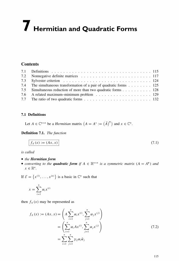
7 Hermitian and Quadratic Forms
Contents
7.1 Definitions . . . . . . . . . . . . . . . . . . . . . . . . . . . . . . . . . . 115
7.2 Nonnegative definite matrices . . . . . . . . . . . . . . . . . . . . . . . . 117
7.3 Sylvester criterion . . . . . . . . . . . . . . . . . . . . . . . . . . . . . . 124
7.4 The simultaneous transformation of a pair of quadratic forms . . . . . . . . 125
7.5 Simultaneous reduction of more than two quadratic forms . . . . . . . . . . 128
7.6 A related maximum–minimum problem . . . . . . . . . . . . . . . . . . . 129
7.7 The ratio of two quadratic forms . . . . . . . . . . . . . . . . . . . . . . . 132
7.1 Definitions
Let A ∈ Cn×n be a Hermitian matrix(A = A∗ := (
A)T )
and x ∈ Cn.
Definition 7.1. The function
fA (x) := (Ax, x) (7.1)
is called
• the Hermitian form• converting to the quadratic form if A ∈ Rn×n is a symmetric matrix (A = Aᵀ) andx ∈ Rn.
If E = {x(1), . . . , x(n)
}is a basic in Cn such that
x =n∑i=1
αix(i)
then fA (x) may be represented as
fA (x) := (Ax, x)=(A
n∑i=1
αix(i),
n∑j=1
αjx(j)
)
=(
n∑i=1
αiAx(i),
n∑j=1
αjx(j)
)
=n∑i=1
n∑j=1
γijαiαj
(7.2)
115

116 Advanced Mathematical Tools for Automatic Control Engineers: Volume 1
where
γij =(Ax(i), x(j)
), i, j = 1, . . . , n
If the basis E is the standard basis (orthonormal in the sense of the standard inner product,
i.e.,(x(i), x(j)
)= δij ), then (7.2) becomes
fA (x) := (Ax, x) =n∑i=1
γii |αi |2 (7.3)
Conjecture 7.1. (Sylvester’s law of inertia for quadratic forms) The positive π (A)and negative ν(A) squares in (7.3) are invariants of the Hermitian form fA (x) indepen-dent of an orthogonal basis in Cn, namely,
fA (x) =π(A)∑i=1
∣∣α′i∣∣2 − ν(A)∑j=1
∣∣α′j ∣∣2 = π(A)∑i=1
∣∣α′′i ∣∣2 − ν(A)∑j=1
∣∣α′′j ∣∣2where
x =n∑i=1
α′ix(i)′, x =
n∑i=1
α′′i x(i)′′
and{x(i)′
},{x(i)′′
}are the orthogonal bases in Cn.
Proof. Suppose that T is a unitary matrix(T ∗ = T −1
)transforming an orthogonal basis
E to another orthogonal one E ′, i.e.,(x(1)
′, . . . , x(n)
′) = T (x(1), . . . , x(n)
)(x(i)
′, x(j)
′) = (T x(i), T x(j)
) = (T ∗T x(i), x(j)
) = (x(i), x(j)
) = δijThen by (7.3)
fA (x) := (Ax, x) =n∑i=1
γ ′ii∣∣α′i∣∣2
γij =(Ax(i)′, x(j)′
) = (AT x(i), T x(j)
) = (T ∗AT x(i), x(j)
)Then by theorem on congruent Hermitian matrices there always exists a nonsingular
matrix P such that
PAP ∗ = diag [It ,−Ir−t , 0] := �0 (A)
and (7.3) under the transformation x = Px ′ becomes
fA (x) := (Ax, x)=(P ∗APx(i), x(j)
)=
n∑i=1
γii∣∣α′i∣∣2 = π(A)∑
i=1
∣∣α′i∣∣2 − ν(A)∑j=1
∣∣α′j ∣∣2

Hermitian and quadratic forms 117
For any other basis the unitary transformation U provides
fA (x) := (Ax, x) =(U ∗P ∗APUx ′′, x ′′
)which by (7.3) does not change the invariant indices InA. Theorem is proven. �
Claim 7.1. If A = Aᵀ is real and x = u+ iv, then
fA (x) := (Ax, x) = fA (u)+ fA (v) (7.4)
Corollary 7.1. (on the extension)
• Any real quadratic fA (u) can be uniquely extended up to the corresponding Hermitianform fA (x), using formula (7.4).
• It is very convenient to realize this extension by changing the product uiuj with Re xix∗j(and, hence, |ui |2 with |xi |2).
• If
fA (u) = |aᵀu|2 + (bT u) (cT u) (7.5)
then
fA (x) = |a∗x|2 + Re (b∗u) (c∗u) (7.6)
Corollary 7.2. Evidently, by (7.4), fA (x) > 0 (fA (x) ≥ 0) for any x ∈ Cn if and only iffA (u) > 0 (fA (u) ≥ 0) for all u ∈ Rn.
Claim 7.2. If x =(x(1)
x(2)
)and A =
[A11 A12
A∗12 A22
], then
fA (x) := (Ax, x)= (A11x
(1), x(1))+ 2Re
(A12x
(2), x(1))+ (
A22x(2), x(2)
) (7.7)
7.2 Nonnegative definite matrices
7.2.1 Nonnegative definiteness
Definition 7.2. A symmetric matrix S ∈ Rn×n is said to be nonnegative definite if
xᵀSx ≥ 0 (7.8)
for all x ∈ Rn.
The next simple lemma holds.
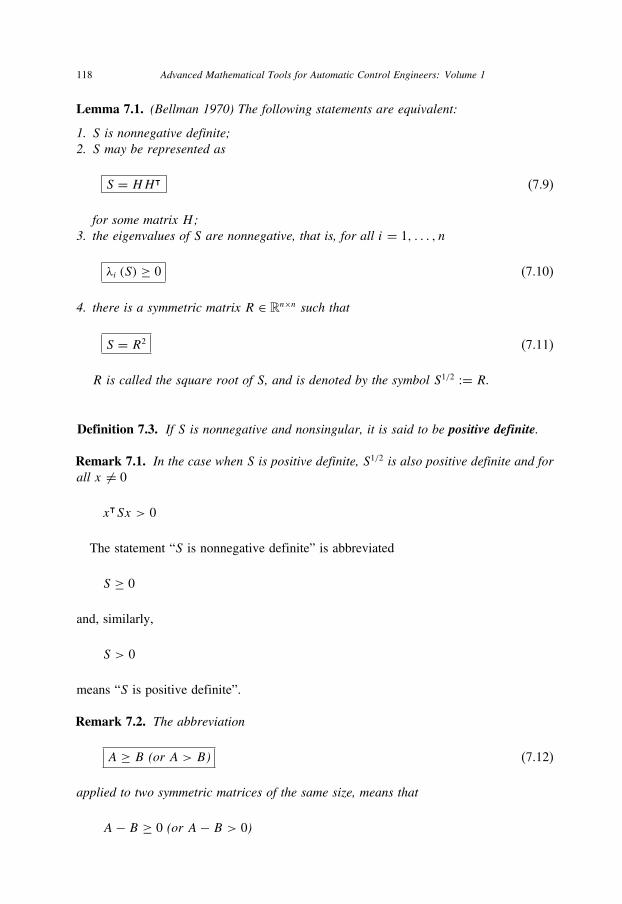
118 Advanced Mathematical Tools for Automatic Control Engineers: Volume 1
Lemma 7.1. (Bellman 1970) The following statements are equivalent:
1. S is nonnegative definite;2. S may be represented as
S = HHᵀ (7.9)
for some matrix H ;3. the eigenvalues of S are nonnegative, that is, for all i = 1, . . . , n
λi (S) ≥ 0 (7.10)
4. there is a symmetric matrix R ∈ Rn×n such that
S = R2 (7.11)
R is called the square root of S, and is denoted by the symbol S1/2 := R.
Definition 7.3. If S is nonnegative and nonsingular, it is said to be positive definite.
Remark 7.1. In the case when S is positive definite, S1/2 is also positive definite and forall x �= 0
xᵀSx > 0
The statement “S is nonnegative definite” is abbreviated
S ≥ 0
and, similarly,
S > 0
means “S is positive definite”.
Remark 7.2. The abbreviation
A ≥ B (or A > B) (7.12)
applied to two symmetric matrices of the same size, means that
A− B ≥ 0 (or A− B > 0)

Hermitian and quadratic forms 119
Remark 7.3. Evidently, if A > 0 then for any quadratic nonsingular B (detB �= 0) itfollows that
BABᵀ > 0
and, inversely, if BABᵀ > 0 for some nonsingular matrix B, then A > 0.
Remark 7.4. If A ≥ B (or A > B), then for any quadratic nonsingular T (det T �= 0)
T ATᵀ ≥ T BTᵀ (or TATᵀ > TBTᵀ)
and, inversely, if TATᵀ ≥ T BTᵀ (or TATᵀ > TBTᵀ) for some nonsingular T , thenA ≥ B (or A > B).
Proposition 7.1. If
A > B > 0
then
B−1 > A−1 > 0
Proof. Let TA be an orthogonal transformation which transforms A to a diagonal matrix
�A := diag (λ1(A), . . . , λn(A)) and
�A = �1/2A �
1/2A , �
1/2A = diag
(√λ1(A), . . . ,
√λn(A)
)> 0
Then, by the previous remark,
TAATᵀA = �A > TABTᵀ
A
In×n > �−1/2A TABT
ᵀA�
−1/2A
Denoting by T an orthogonal transformation which transforms the right-hand side of the
last inequality to a diagonal matrix �, we obtain
In×n = T Tᵀ > T(�−1/2A TABT
ᵀA�
−1/2A
)Tᵀ = � = diag (λ1, . . . , λn)
Inverting this inequality by components, we have
In×n < �−1 =[T(�−1/2A TABT
ᵀA�
−1/2A
)Tᵀ
]−1 = T(�
1/2A TAB
−1TᵀA�
1/2A
)Tᵀ
which implies
In×n < �1/2A TAB
−1TᵀA�
1/2A

120 Advanced Mathematical Tools for Automatic Control Engineers: Volume 1
and
�−1A < TAB
−1TᵀA
Hence,
TᵀA�
−1A TA = A−1 < B−1
Proposition is proven. �
Proposition 7.2. If S ≥ 0 and T ≥ 0, then
S + T ≥ 0
with strict inequality holding if and only if
N (S) ∩N (T ) = ∅
The proof of these statements is evident.
7.2.2 Nonnegative (positive) definiteness of a partitioned matrix
Theorem 7.1. (Albert 1972) Let S be a square matrix partitioned as
S =[S11 S12
Sᵀ12 S22
]
where S11 is a symmetric n× n matrix and S22 is a symmetric m×m matrix. Then
(a) S ≥ 0 if and only if
S11 ≥ 0
S11S+11S12 = S12
S22 − Sᵀ12S
+11S12 ≥ 0
(7.13)
(b) S > 0 if and only if (Schur’s complement)
S11 > 0
S22 > 0
S11 − S12S−122 S
ᵀ12 > 0
S22 − Sᵀ12S
−111 S12 > 0
(7.14)
Proof.
(a) Necessity. Suppose that S ≥ 0. Then there exists a matrix H with (n+m) rows suchthat S = HHᵀ. Let us write H as a partitioned matrix

Hermitian and quadratic forms 121
H =[X
Y
], X ∈ Rn×n, Y ∈ Rm×m
Then
S = HHᵀ =[XXᵀ XYᵀ
YXᵀ YYᵀ
]
so that
S11 = XXᵀ ≥ 0, S12 = XYᵀ
By (6.8)
S11S+11 = (XXᵀ) (XXᵀ)+ = X [
Xᵀ (XXᵀ)+] = XX+
so that
S11S+11S12 = XX+ (XYᵀ) = (
XX+X)Yᵀ = XYᵀ = S12
Finally, if we let
U := Y − Sᵀ12S
+11X
then
0 ≤ UUᵀ = S22 − Sᵀ12S
+11S12
Sufficiency. Let (7.13) hold. Define
U :=[In×n
...On×m
], V :=
[Om×n
...Im×m
]
X := S1/211 U
Y := Sᵀ12S
+11S
1/2
11 U + (S22 − Sᵀ
12S+11S12
)1/2V
Since
UVᵀ = On×m
we can see that
0 ≤⎡⎣ X· · ·Y
⎤⎦⎡⎣ X· · ·Y
⎤⎦ᵀ
=[XXᵀ XYᵀ
YXᵀ YYᵀ
]=
[S11 S12S
ᵀ12 S22
]= S

122 Advanced Mathematical Tools for Automatic Control Engineers: Volume 1
(b) Necessity. Suppose that S > 0. Then by part (a), S11 ≥ 0. Assuming that S11 has a
zero eigenvalue with the corresponding eigenvector x �= 0, we can see that for the
nonzero
(x
0
)we have
(x
0
)ᵀS
(x
0
)= xᵀS11x = 0
which contradicts the fact that S > 0. So, S11 is nonsingular and S11 > 0. Similarly,
by (a)
S22 − Sᵀ12S
+11S12 = S22 − Sᵀ
12S−111 S12 ≥ 0
and by the same argument (by contradiction) S22 > 0.
The eigenvalues of S−1 are reciprocals of S’s and so, S−1 > 0 if S > 0. Therefore
S−1 =[A B
Bᵀ C
]> 0,
with 0 < A ∈ Rn×n, 0 < C ∈ Rm×m, so that A−1 > 0 and C−1 > 0. The condition
SS−1 = I(n+m)×(n+m)
dictates that(S11 − S12S−1
22 Sᵀ12
)A = In×n(
S22 − Sᵀ12S
−111 S12
)C = Im×m
or, equivalently,(S11 − S12S−1
22 Sᵀ12
) = A−1 > 0(S22 − Sᵀ
12S−111 S12
) = C−1 > 0
This proves the necessity of (7.14).
Sufficiency. Suppose that (7.14) holds. By part (a), S ≥ 0. Define
A := (S11 − S12S−1
22 Sᵀ12
)−1
C := (S22 − Sᵀ
12S−111 S12
)−1
B := −S−111 S12C
It is easy to show that
B = −S−111 S12C = −A [
A−1S−111 S12C
]= −A
[(S11 − S12S−1
22 Sᵀ12
)S−111 S12
(S22 − Sᵀ
12S−111 S12
)−1]
= −A[(S11S
−111 S12 − S12S−1
22 Sᵀ12S
−111 S12
) (Im×m − S−1
22 Sᵀ12S
−111 S12
)−1S−122
]

Hermitian and quadratic forms 123
= −A[S12
(Im×m − S−1
22 Sᵀ12S
−111 S12
) (Im×m − S−1
22 Sᵀ12S
−111 S12
)−1S−122
]= −AS12S−1
22
Then routine calculations verify that
S
[A B
Bᵀ C
]= I(n+m)×(n+m)
So, S is nonsingular.
�
Corollary 7.3. Suppose that in the previous theorem m=1, that is, the following repre-sentation holds
Sn+1 =[Sn snsᵀn σn+1
]sn ∈ Rn, σn+1 ∈ R
(7.15)
where 0 ≤ Sn ∈ Rn×n. Let
tn := S+n sn, αn := σn+1 − sᵀn S+n snβn := 1+ ‖tk‖2, Tn − tntᵀn /βn
Then
(a) Sn+1 ≥ 0 if and only if
Sntn = sn and αn ≥ 0 (7.16)
and
S+n+1 =
⎧⎪⎪⎪⎨⎪⎪⎪⎩
[S+n + tntᵀn α−1
n −tnα−1n
−tᵀn α−1n α−1
n
]if αn > 0[
TnS+n Tn TnS
+n tnβ
−1n(
TnS+n tnβ
−1n
)T (tᵀn S
+n tn
)β−2n
]if αn = 0
(7.17)
(b) Sn+1 > 0 if and only if
αn = σn+1 − sᵀn S−1n sn > 0 (7.18)
and
S−1n+1 =
[S−1n + [
S−1n sns
ᵀn S
−1n
]α−1n − (
S−1n sn
)α−1n
− (S−1n sn
)Tα−1n α−1
n
](7.19)
The proof of this corollary follows directly from the previous theorem and the appli-
cation of Cline’s formula (6.33).

124 Advanced Mathematical Tools for Automatic Control Engineers: Volume 1
7.3 Sylvester criterion
Here we present a simple proof of the known criterion which gives a power instrument
for the numerical test of positive definiteness.
Theorem 7.2. (Sylvester criterion) A symmetric matrix S ∈ Rn×n is positive definiteif and only if all leading principal minors (1.12) are strictly positive, that is, for allp = 1, 2, . . . , n
A
(1 2 · · · p1 2 · · · p
)> 0 (7.20)
Proof. Let us prove this result by the induction method. For n = 2 the result is evident.
Indeed, for
S =[a11 a12a12 a22
]
under the assumption that a11 �= 0, we have
xᵀSx = a11x21 + 2a12x1x2 + a22x22= a11
(x1 + a12
a11
)2+(a22 − a
212
a11
)x22
from which it follows that xᵀSx > 0 (x �= 0), or equivalently, S > 0 if and only if
a11 > 0, a22 − a212
a11= det S > 0
Let us represent S ∈ Rn×n in the form (7.15)
Sn =[Sn−1 sn−1
sᵀn−1 σn
]sn−1 ∈ Rn−1, σn ∈ R
and suppose that Sn−1 > 0. This implies that det Sn−1 > 0. Then by (7.3) Sn > 0 if and
only if the condition (7.18) holds, that is, when
αn−1 = σn − sᵀn−1S−1n−1sn−1 > 0
But by the Schur’s formula
A
(1 2 · · · n
1 2 · · · n
)= det S = det
(σn − sᵀn−1S
−1n−1sn−1
)(det Sn−1)
= (σn − sᵀn−1S
−1n−1sn−1
)(det Sn−1) = αn−1 (det Sn−1) > 0
if and only if (7.18) holds, which proves the result. �
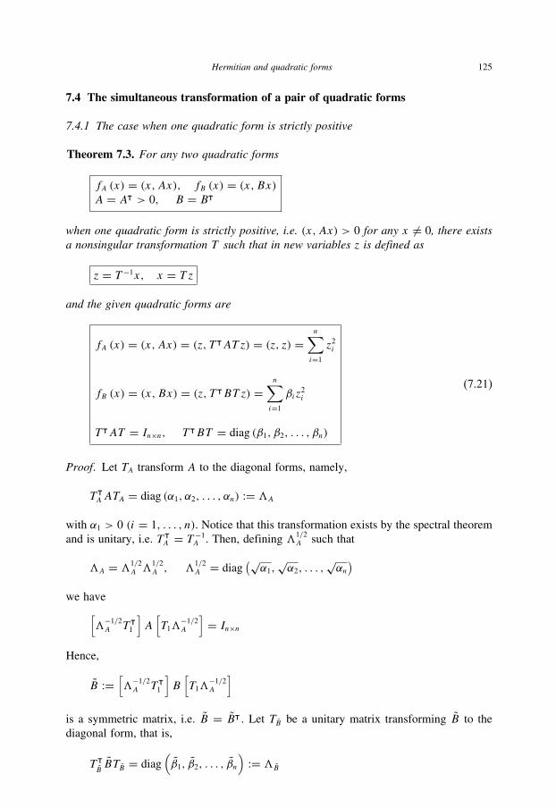
Hermitian and quadratic forms 125
7.4 The simultaneous transformation of a pair of quadratic forms
7.4.1 The case when one quadratic form is strictly positive
Theorem 7.3. For any two quadratic forms
fA (x) = (x,Ax), fB (x) = (x, Bx)A = Aᵀ > 0, B = Bᵀ
when one quadratic form is strictly positive, i.e. (x,Ax) > 0 for any x �= 0, there existsa nonsingular transformation T such that in new variables z is defined as
z = T −1x, x = T z
and the given quadratic forms are
fA (x) = (x,Ax) = (z, TᵀAT z) = (z, z) =n∑i=1
z2i
fB (x) = (x, Bx) = (z, TᵀBT z) =n∑i=1
βiz2i
TᵀAT = In×n, TᵀBT = diag (β1, β2, . . . , βn)
(7.21)
Proof. Let TA transform A to the diagonal forms, namely,
TᵀA ATA = diag (α1, α2, . . . , αn) := �A
with α1 > 0 (i = 1, . . . , n). Notice that this transformation exists by the spectral theorem
and is unitary, i.e. TᵀA = T −1
A . Then, defining �1/2A such that
�A = �1/2A �
1/2A , �
1/2A = diag
(√α1,
√α2, . . . ,
√αn)
we have[�−1/2A T
ᵀ1
]A[T1�
−1/2A
]= In×n
Hence,
B :=[�−1/2A T
ᵀ1
]B[T1�
−1/2A
]is a symmetric matrix, i.e. B = Bᵀ. Let TB be a unitary matrix transforming B to the
diagonal form, that is,
TᵀBBTB = diag
(β1, β2, . . . , βn
):= �B

126 Advanced Mathematical Tools for Automatic Control Engineers: Volume 1
Then the transformation T defined by
T :=[T1�
−1/2A
]TB
exactly realizes (7.21) since
TᵀAT = TᵀB
([�−1/2A T
ᵀ1
]A[T1�
−1/2A
])TB = Tᵀ
BTB = In×n
�
Corollary 7.4.
T =[T1�
−1/2A
]TB (7.22)
where the matrices T1, �1/2A and TB realize the following transformations
TᵀA ATA = diag (α1, α2, . . . , αn) := �A
�1/2A = diag
(√α1,
√α2, . . . ,
√αn)
TᵀB
([�−1/2A T
ᵀ1
]A[T1�
−1/2A
])TB = diag
(β1, β2, . . . , βn
):= �B
7.4.2 The case when both quadratic forms are nonnegative
Theorem 7.4. Let two quadratic forms
fA (x) = (x,Ax), fB (x) = (x, Bx)
be nonnegative, that is,
A = Aᵀ ≥ 0, B = Bᵀ ≥ 0
Then there exists a nonsingular matrix T such that
TATᵀ =
⎡⎢⎢⎢⎢⎣∑1
0 0 0
0 I 0 0
0 0 0 0
0 0 0 0
⎤⎥⎥⎥⎥⎦
(T −1
)TBT −1 =
⎡⎢⎢⎢⎢⎢⎣
∑1
0 0 0
0 0 0 0
0 0∑2
0
0 0 0 0
⎤⎥⎥⎥⎥⎥⎦
(7.23)

Hermitian and quadratic forms 127
with∑i (i = 1, 2) diagonal and positive definite, that is,
∑i
= diag(σ(i)1 , . . . , σ
(i)ni
), σ (i)s > 0 (s = 1, . . . , ni)
Proof. Since A is positive and semidefinite, then there exists a unitary matrix T1 such
that T1ATᵀ1 =
[I 0
0 0
]. Then, let it be
(T
ᵀ1
)−1BT −1
1 =[B11 B12
B21 B22
]. Again, there exists
a unitary matrix U1 such that U1B11Uᵀ1 =
[(∑1
)20
0 0
]with
∑1 > 0. Define the unitary
matrix Tᵀ2 by
(T
ᵀ2
)−1 =[U1 0
0 I
]. Then we have
(T
ᵀ2
)−1 (T
ᵀ1
)−1BT −1
1 (T2)−1 =
⎡⎢⎢⎣(∑
1
)2
0 Q121
0 0 Q122
Qᵀ121 Q
ᵀ122 Q22
⎤⎥⎥⎦
with Q122 = 0 since B ≥ 0. Define(T
ᵀ3
)−1 =
⎡⎢⎢⎣
I 0 0
0 I 0
−Qᵀ121
(∑1
)2
0 I
⎤⎥⎥⎦. Then
(T
ᵀ3
)−1 (T
ᵀ2
)−1 (T
ᵀ1
)−1BT −1
1 (T2)−1 (T3)
−1
=
⎡⎢⎢⎢⎣(∑
1
)2
0 0
0 0 0
0 0
[Q22 −Qᵀ
121
(∑1
)2
Q121
]⎤⎥⎥⎥⎦
Next, define the unitary matrix U2 such that
U2
[Q22 −Qᵀ
121
(∑1
)2
Q121
]U
ᵀ2 =
[∑2
0
0 0
]
with∑
2 > 0, and define also the unitary matrix T4 such that(T
ᵀ4
)−1 =⎡⎢⎣(∑
1
)−1/2
0 0
0 I 0
0 0 U2
⎤⎥⎦. Then it is easy to check that for
T = T4T3T2T1 (7.24)
we get (7.23). �

128 Advanced Mathematical Tools for Automatic Control Engineers: Volume 1
Corollary 7.5. The product of two nonnegative matrices is similar to a nonnegativematrix, that is, for T defined by (7.24) it follows that
T (AB) T −1 =[(∑
1
)2
0
0 0
](7.25)
Proof. Indeed,
T (AB) T −1 = [TATᵀ][(T −1
)TBT −1
]
=
⎡⎢⎢⎣∑
10 0 0
0 I 0 0
0 0 0 0
0 0 0 0
⎤⎥⎥⎦⎡⎢⎢⎢⎣∑
10 0 0
0 0 0 0
0 0∑
20
0 0 0 0
⎤⎥⎥⎥⎦ =
[(∑1
)2
0
0 0
]
which completes the proof. �
7.5 Simultaneous reduction of more than two quadratic forms
For the case of two quadratic forms define
T2 = T
where T is given by (7.22). Let us apply the induction method, namely, suppose that
the transformation Tk−1 transforms simultaneously one strictly positive definite form with
a matrix A = Aᵀ > 0 and (k − 2) another quadratic form with the matrices Bi = Bᵀi
(i = 1, . . . , k − 1) to the sum of pure positive quadratics and the rest to the sum of
quadratic elements (maybe with zero coefficients). Then the matrix
Bk := Tk−1BkTk−1
is a symmetric one. Hence, by the spectral theorem, there exists a unitary transformation
TBn such that
TᵀBkBkTBk = �Bk := diag
(β(k)1 , . . . , β
(k)n
)T
ᵀBkTBk = In×n
Then the transformation
Tk := Tk−1TBk
will keep all previous quadratic forms in the same presentation and will transform the
last one to a diagonal form.
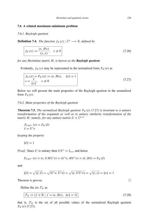
Hermitian and quadratic forms 129
7.6 A related maximum–minimum problem
7.6.1 Rayleigh quotient
Definition 7.4. The function fH (x) : Cn −→ R, defined by
fH (x) := (x,Hx)(x, x)
, x �= 0 (7.26)
for any Hermitian matrix H , is known as the Rayleigh quotient.
Evidently, fH (x) may be represented in the normalized form FH (e) as
fH (x) = FH (e) := (e,He), ‖e‖ = 1
e = x
‖x‖ , x �= 0(7.27)
Below we will present the main properties of the Rayleigh quotient in the normalized
form FH (e).
7.6.2 Main properties of the Rayleigh quotient
Theorem 7.5. The normalized Rayleigh quotient FH (e) (7.27) is invariant to a unitarytransformation of the argument as well as to unitary similarity transformation of thematrix H , namely, for any unitary matrix U ∈ Cn×n
FUHU∗ (e) = FH (e)e = U ∗e
keeping the property
‖e‖ = 1
Proof. Since U is unitary then UU ∗ = In×n and hence
FUHU∗ (e) = (e, UHU ∗e) = (U ∗e,HU ∗e) = (e, H e) = FH (e)
and
‖e‖ =√(e, e) =√
(U ∗e, U ∗e) =√(e, UU ∗e) =√
(e, e) = ‖e‖ = 1
Theorem is proven. �
Define the set FH as
FH := {f ∈ R | f = (e,He), ‖e‖ = 1} (7.28)
that is, FH is the set of all possible values of the normalized Rayleigh quotient
FH (e) (7.27).

130 Advanced Mathematical Tools for Automatic Control Engineers: Volume 1
Lemma 7.2. FH contains the spectrum σ (H) of all eigenvalues of H , i.e.,
σ (H) ⊂ FH (7.29)
Proof. If λ ∈ σ (H), then there exists an eigenvector e of H which corresponds to this
λ, that is,
He = λe
and hence,
(e,He) = (e, λe) = λ (e, e) = λ
So, λ ∈ FH . Thus, σ (H) ⊂ FH . �
Let now λ1, λ2, . . . , λn be the eigenvalues of H .
Theorem 7.6. FH coincides with the convex hull co {λ1, λ2, . . . , λn} of the eigenvaluesof H , namely,
FH ≡ co {λ1, λ2, . . . , λn} (7.30)
where
co {λ1, λ2, . . . , λn}
:={λ | λ =
n∑i=1
αiλi,
n∑i=1
αi = 1, αi ≥ 0 (i = 1, . . . , n)
}(7.31)
Proof. Since H is Hermitian, there exists a unitary matrix U , such that
UHU ∗ = � = diag {λ1, λ2, . . . , λn}
Hence by theorem (7.5), one has FH = F�. So, it is sufficient to show that the field
of the eigenvalues of the diagonal matrix � coincides with co {λ1, λ2, . . . , λn}. Indeed,by (7.31)
λj =n∑i=1
αiλi when αi = δij
�
Corollary 7.6.
FH ≡ co {λ1, λ2, . . . , λn} =[λ1 := min
i=1,...,nλi, λn := max
i=1,...,nλi
](7.32)

Hermitian and quadratic forms 131
Corollary 7.7.
mine:‖e‖=1
(e,He) = minx �=0
(x,Hx)
(x, x)= λ1 := min
i=1,...,nλi = λmin (H)
maxe:‖e‖=1
(e,He) = maxx �=0
(x,Hx)
(x, x)= λn := max
i=1,...,nλi = λmax (H)
(7.33)
Corollary 7.8. If H = ∥∥hij∥∥i,j=1,n, then
λ1 ≤ hij ≤ λnnλ1 ≤ trH ≤ nλn (7.34)
Corollary 7.9. (Stationary property) If λi is an eigenvalue of a symmetric matrix A =Aᵀ with the corresponding eigenvector x(i), then for fA(x) = (x,Ax)
(x, x)(x �= 0) it follows
that
fA(x(i)) = λi (7.35)
and the stationary property holds, that is, for any i = 1, . . . , n one has
∂
∂xfA(x) |x=x(i) = 0 (7.36)
Proof. The identity (7.35) follows directly from the simple calculation of fA(x(i)). As for
(7.36) it is sufficient to notice that
∂
∂xfA(x) = ∂
∂x
(x,Ax)
(x, x)= 2Ax (x, x)− 2x (x,Ax)
(x, x)2
and hence
∂
∂xfA(x) |x=x(i) = 2Ax(i)
(x(i), x(i)
)− 2x(i)(x(i), Ax(i)
)(x(i), x(i)
)2= 2
λix(i)(x(i), x(i)
)− x(i) (x(i), λix(i))(x(i), x(i)
)2= 2λi
(x(i)(
x(i), x(i)) − x(i)(
x(i), x(i))) = 0
Corollary is proven. �
132 Advanced Mathematical Tools for Automatic Control Engineers: Volume 1
7.7 The ratio of two quadratic forms
Consider the ratio r(x) of two quadratic forms, i.e.,
r(x) = (x,Hx)(x,Gx)
, (x,Gx) > 0
H = Hᵀ, G = Gᵀ > 0
(7.37)
Theorem 7.7.
minx:(x,Gx)>0
r(x) = λmin
(G−1/2HG−1/2
)(7.38)
and
maxx:(x,Gx)>0
r(x) = λmax
(G−1/2HG−1/2
)(7.39)
Proof. Using the presentation
G = G1/2G1/2
valid for any symmetric nonnegative matrix, for z = G1/2x we have
r(x)= (x,Hx)(x,Gx)
= r(x) = (x,Hx)(x,G1/2G1/2x
) = (x,Hx)(G1/2x,G1/2x
)=
(G−1/2z,HG−1/2z
)(z, z)
=(z,[G−1/2HG−1/2
]z)
(z, z)
The result follows from corollary (7.7). �
8 Linear Matrix Equations
Contents
8.1 General type of linear matrix equation . . . . . . . . . . . . . . . . . . . . 133
8.2 Sylvester matrix equation . . . . . . . . . . . . . . . . . . . . . . . . . . . 137
8.3 Lyapunov matrix equation . . . . . . . . . . . . . . . . . . . . . . . . . . 137
8.1 General type of linear matrix equation
8.1.1 General linear matrix equation
Here we consider the general linear matrix equation
A1XB1 + A2XB2 + · · · + ApXBp = C (8.1)
where Aj ∈ Cm×m, Bj ∈ Cn×n (j = 1, . . . , p) are the given matrices and X ∈ Cm×n is
the unknown matrix to be found.
8.1.2 Spreading operator and Kronecker product
Together with the Kronecker matrix product definition
A⊗ B := ∥∥aijB∥∥ ∈ Rn2×n2
A ∈ Cn×n, B ∈ Cn×n(8.2)
given before let us introduce the spreading operator col {·} for some matrix A ∈ Cm×n as
colA := (a1,1, . . . , a1,n, a2,1, . . . , a2,n, . . . , am,1, . . . , am,n
)ᵀ(8.3)
that is,
colA :=
⎡⎢⎢⎢⎣A∗1A∗2...
A∗n
⎤⎥⎥⎥⎦ ∈ Cmn, A = [
A∗1 A∗2 · · ·A∗n], A∗j ∈ Cm
133

134 Advanced Mathematical Tools for Automatic Control Engineers: Volume 1
Let col−1A be the operator inverse to colA. Evidently, for any A,B ∈ Cm×n and
α, β ∈ C
col {αA+ βB} = α col {A} + β col {B} (8.4)
8.1.3 Relation between the spreading operator and the Kronecker product
Lemma 8.1. For any matrices A ∈ Cm×m, B ∈ Cn×n and X ∈ Cm×n the followingproperties hold
1.
col {AX} = (In×n ⊗ A) colX (8.5)
2.
col {XB} = (Bᵀ ⊗ Im×m) colX (8.6)
3.
col {AX +XB} = [(In×n ⊗ A)+ (Bᵀ ⊗ Im×m)] colX (8.7)
4.
col {AXB} = (Bᵀ ⊗ A) col {X} (8.8)
Proof. Properties 1–3 (8.5)–(8.7) follow directly from property 4 (8.8) and (8.4). So, let
us prove (8.8). By definition (8.3) the j th column (AXB)∗,j of the matrix AXB can be
expressed as
(AXB)∗,j = AX (B)∗,j =n∑s=1
bs,j (AX)∗,s =n∑s=1
(bs,jA
)X∗,j
= [b1,jA b2,jA · · · bn,jA
]colX
which corresponds to (8.8). �
Lemma 8.2. The eigenvalues of (A⊗ B) are
λiμj (i = 1, . . . , m; j = 1, . . . , n) (8.9)
where λi are the eigenvalues of A ∈ Cm×m and μj are the eigenvalues of B ∈ Cn×n. Theycorrespond to the following eigenvectors
eij := xi ⊗ yj (8.10)
where xi and yj are the eigenvectors of A and B, that is,
Axi = λixi , Byj = μj yj
Linear matrix equations 135
Proof. We have
(A⊗ B) eij =
∥∥∥∥∥∥∥∥a11B
... a12B... · · · ... a1nB· · ·
an1B... an2B
... · · · ... annB
∥∥∥∥∥∥∥∥⎛⎝x1i yj· · ·xni yj
⎞⎠
=∥∥∥∥∥∥a11x1iByj + · · · + a1nxniByj
· · ·an1x1iByj + · · · + annxniByj
∥∥∥∥∥∥=
∥∥∥∥∥∥a11x1i
(μj yj
)+ · · · + a1nxni(μj yj
)· · ·
an1x1i(μj yj
)+ · · · + annxni(μj yj
)∥∥∥∥∥∥ = Axi ⊗ μj yj
= λixi ⊗ μj yj = λiμj(xi ⊗ yj
) = λiμj eijwhich proves the lemma. �
Corollary 8.1. The eigenvalues of the matrix (the Kronecker sum)
[(In×n ⊗ A)+ (B ⊗ Im×m)] (8.11)
are as follows
λi + μj (i = 1, . . . , m; j = 1, . . . , n) (8.12)
with the corresponding eigenvector
eij := yj ⊗ xi (8.13)
Proof. Let us check that the vector (8.13) is the eigenvector of the matrix (8.11) with the
eigenvalue(λi + μj
). By (8.9) and taking into account that for the unitary matrix In×n
any vector is an eigenvector with the eigenvalue equal to 1 and the relation
(A⊗ B) (xi ⊗ yj) = (Axi)⊗ (Byj
)we get
[(In×n ⊗ A)+ (B ⊗ Im×m)] eij = (In×n ⊗ A) eij + (B ⊗ Im×m) eij= (In×n ⊗ A)
(yj ⊗ xi
)+ (B ⊗ Im×m) (yj ⊗ xi)= (In×nyj
)⊗ (Axi)+ (Byj
)⊗ (Im×mxi)= (1 · λi)
(xi ⊗ yj
)+ (μi · 1) (xi ⊗ yj) = (λi + μj
)eij
�
136 Advanced Mathematical Tools for Automatic Control Engineers: Volume 1
Corollary 8.2. Since the spectrum of eigenvalues for a transposed matrix coincides withthe spectrum of eigenvalues for the original matrix then
λi + μj (i = 1, . . . , m; j = 1, . . . , n)
will be eigenvalues for the following matrices
[(In×n ⊗ A)+ (Bᵀ ⊗ Im×m)]
[(In×n ⊗ Aᵀ)+ (B ⊗ Im×m)]
[(In×n ⊗ Aᵀ)+ (Bᵀ ⊗ Im×m)]
8.1.4 Solution of a general linear matrix equation
Theorem 8.1. The general linear matrix equation (8.1) has the solution X ∈ Cm×n ifand only if the vector x = colX is the solution of the vector equation
Gx = c (8.14)
where
G :=p∑i=1
(B
ᵀi ⊗ Ai
)c := colC
(8.15)
Proof. By the property (8.8) and since the operator col is linear, applying this operator
to both sides of (8.1), we have
c = colC = col
{p∑i=1
(AiXBi)
}=
p∑i=1
col {AiXBi}
=p∑i=1
(B
ᵀi ⊗ Ai
)colX = Gx
�
Corollary 8.3. The general linear matrix equation (8.1) has the unique solutionX ∈ Cm×n given by
X = col−1{G−1c
}(8.16)
if and only if
detG �= 0 (8.17)

Linear matrix equations 137
8.2 Sylvester matrix equation
Now we will consider an important particular case of (8.1).
Lemma 8.3. The Sylvester matrix equation
AX +XB = −Q
A ∈ Cm×m, B ∈ Cn×n and X,C ∈ Cm×n(8.18)
has the unique solution
X = col−1{[(Bᵀ ⊗ A)]−1
colC}
(8.19)
if and only if
λi + μj �= 0 for any i, j = 1, . . . , n (8.20)
where λi are the eigenvalues of A and μj are the eigenvalues of B.
Proof. This follows directly from (8.16). �
8.3 Lyapunov matrix equation
Lemma 8.4. Lyapunov (1892) The Lyapunov matrix equation
AP + PAᵀ = −Q
A,P,Q = Qᵀ ∈ Rn×n(8.21)
has the unique symmetric solution P = Pᵀ if and only if the matrix A has no neutraleigenvalues lying at the imaginary axis, i.e.,
Re λi �= 0 (i = 1, . . . , n) (8.22)
Proof. Equation (8.21) is a particular case of the Sylvester equation (8.18) with B = Aᵀ,which by (8.20) implies the uniqueness of the solution providing for all (i, j = 1, . . . , n)
λi + λj �= 0
This condition obviously is fulfilled if and only if (8.22) holds. �

This page intentionally left blank
9 Stable Matrices and Polynomials
Contents
9.1 Basic definitions . . . . . . . . . . . . . . . . . . . . . . . . . . . . . . . 139
9.2 Lyapunov stability . . . . . . . . . . . . . . . . . . . . . . . . . . . . . . 140
9.3 Necessary condition of the matrix stability . . . . . . . . . . . . . . . . . . 144
9.4 The Routh–Hurwitz criterion . . . . . . . . . . . . . . . . . . . . . . . . . 145
9.5 The Liénard–Chipart criterion . . . . . . . . . . . . . . . . . . . . . . . . 153
9.6 Geometric criteria . . . . . . . . . . . . . . . . . . . . . . . . . . . . . . . 154
9.7 Polynomial robust stability . . . . . . . . . . . . . . . . . . . . . . . . . . 159
9.8 Controllable, stabilizable, observable and detectable pairs . . . . . . . . . . 164
9.1 Basic definitions
Definition 9.1. A real valued n × n matrix is said to be stable if all its eigenvaluesbelong to the left open complex semi-plane
C− := {z ∈ C | Re z < 0} (9.1)
that is,
λi (A) < 0 for any i = 1, . . . , n (9.2)
Denote the characteristic polynomial of a matrix A ∈ Rn×n by pA (λ), i.e.,
pA (λ) := det ‖A− λIn×n‖ = λn + a1λn−1 + · · · + an−1λ+ an (9.3)
Notice that pA (λ) is a monic polynomial whose leading coefficient (the coefficient of the
highest power) is 1. It is clear from (9.3) that the stability property of a matrix A ∈ Rn×n
is definitely related to the values of the coefficients ai (i = 1, . . . , n) in (9.3) since λi (A)
are the roots of the polynomial equation
pA (λ) =n∏i=1
[λ− λi (A)] = 0 (9.4)
Below we will present several results providing the verification of the matrix stability
property based only on the coefficients of the characteristic polynomial.
139

140 Advanced Mathematical Tools for Automatic Control Engineers: Volume 1
9.2 Lyapunov stability
9.2.1 Lyapunov matrix equation for stable matrices
Lemma 9.1. Lyapunov (1892)
1. If the Lyapunov’s matrix equation (8.21)
AP + PAᵀ = −QA,P,Q = Qᵀ ∈ Rn×n
(9.5)
holds for some positive definite
Q = Qᵀ > 0
and
P = Pᵀ > 0
then A is stable.2. Equation (8.21) has a positive definite solution
P = Pᵀ =∞∫
t=0
eAtQeAᵀt dt > 0 (9.6)
if and only if matrix A is stable (Hurwitz) and(a) or
Q = Qᵀ > 0
(if Q = Qᵀ ≥ 0, then P = Pᵀ ≥ 0),
(b) or Q has the structure as
Q = BBᵀ
such that the pair (A,B) is controllable, that is,
rank
[B... AB
... A2B... · · · ... An−1B
]= n (9.7)
Proof.
1(a) Claim 1 of this lemma follows directly from the previous lemma 8.4 if let in (8.21)
B = A, X = Ptaking into account that the inequality (8.20) always fulfilled for different
(nonconjugated) eigenvalues and for complex conjugated eigenvalues
μj = λi = ui − iviλi = ui + ivi
Stable matrices and polynomials 141
The inequality (8.20) implies the existence of a solution P . The symmetry of P follows
from the following fact: applying the transposition procedure to both sides of (8.21)
we get
PᵀAᵀ + APᵀ = −Qᵀ = −Q
which coincides with (8.21). But this equation has a unique solution, hence P = Pᵀ.1(b) Let λi be an eigenvalue of Aᵀ, that is,
Aᵀxi = λixi, xi �= 0
Then we also have
x∗i A = λix∗i(here A∗ := (Aᵀ), i.e., the transposition together with the complex conjugation).
Multiplying the left-hand side of (8.21) by x∗i and the right-hand side by xi , it
follows that
x∗i (AP + PAᵀ) xi = λix∗i P xi + x∗i P λixi= (λi + λi
)x∗i P xi = −x∗i Qxi < 0
and, since, by the supposition, x∗i P xi > 0, we obtain(λi + λi
) = 2 Re λi < 0, which
means that A is stable.
2. Sufficiency. Let A be stable. Defining the matrices
H (t) := eAtQ, U (t) := eAᵀt
it follows that
dH (t) := AeAtQ dt, dU (t) := eAᵀtAᵀdt
Then we have
T∫t=0
d [H (t) U (t)]= H (T )U (T )−H (0) U (0)
= eATQeAᵀT −Q
=T∫
t=0
H (t) dU (t)+T∫
t=0
dH (t) U (t)
=T∫
t=0
eAtQeAᵀtAᵀ dt +
T∫t=0
AeAtQeAᵀt dt
=⎡⎣ T∫t=0
eAtQeAᵀt dt
⎤⎦Aᵀ + A
⎡⎣ T∫t=0
eAtQeAᵀt dt
⎤⎦
(9.8)

142 Advanced Mathematical Tools for Automatic Control Engineers: Volume 1
The stability of A implies
eAT ReAᵀT −→
T −→∞ 0
and, moreover, the integral
P := limT −→∞
⎡⎣ T∫t=0
eAtQeAᵀt dt
⎤⎦
exists, since∥∥∥∥∥∥T∫
t=0
eAtQeAᵀt dt
∥∥∥∥∥∥≤T∫
t=0
∥∥eAtQeAᵀt∥∥ dt≤ ‖Q‖
T∫t=0
∥∥eAt∥∥2dt ≤ ‖Q‖
T∫t=0
e2λmaxAt dt
≤ ‖Q‖T∫
t=0
e2αt dt ≤ ‖Q‖∞∫
t=0
e−2|α|t dt = 1
2 |α| ‖Q‖ <∞
where
λmax (A) ≤ −miniRe |λi | := α < 0
So, taking T −→ ∞ in (9.8), we obtain (9.5), which means that (9.6) is the solution
of (9.5).
(a) If Q > 0, then
P =∞∫
t=0
eAtQeAᵀt dt ≥ λmin (Q)
∞∫t=0
e(A+Aᵀ)t dt > 0
(b) If Q = BBᵀ, then for any x ∈ Rn
xᵀPx =∞∫
t=0
xᵀeAtBBᵀeAᵀt x dt =
∞∫t=0
∥∥BᵀeAᵀt x
∥∥2dt (9.9)
Suppose that there exist x �= 0 and the interval (t0, t1) (t0 < t1) such that∥∥xᵀeAtB∥∥2 = 0 for all t ∈ (t0, t1) (t0 < t1)
and, hence,
xᵀeAtB = 0 (9.10)
Then the sequent differentiation of (9.10) by t gives
xᵀeAtAB = 0, xᵀeAtA2B = 0,· · ·, xᵀeAtA(n−1)B = 0

Stable matrices and polynomials 143
which may be rewritten in the matrix form as follows
xᵀeAt[B... AB
... A2B... · · · ... A(n−1)B
]= 0
for all t ∈ (t0, t1) (t0 < t1). It means that
rank
[B... AB
... A2B... · · · ... An−1B
]< n
which is in contradiction to (9.7). So,
∥∥xᵀeAtB∥∥2> 0
at least at one interval (t0, t1) and, hence, by (9.9)
xᵀPx =∞∫
t=0
∥∥BᵀeAᵀt x
∥∥2dt ≥
t1∫t=t0
∥∥BᵀeAᵀt x
∥∥2dt > 0
for all x �= 0. It means that P > 0.
Necessity. Suppose that there exists a positive solution P > 0 given by (9.6). Then
this integral exists only if A is stable.
(a) But P may be positive only if Q > 0 (this is easily seen by contradiction).
(b) Let x∗i �= 0 be an unstable mode (a left eigenvector of A corresponding to an
unstable eigenvalue λi), that is,
x∗iA = λix∗i , Re λi ≥ 0
By the relation
0 < x∗iP xi =∞∫
t=0
∥∥x∗ieAtB∥∥2dt =
∞∫t=0
∥∥∥∥∥x∗i[ ∞∑l=0
1
l! (At)l
]B
∥∥∥∥∥2
dt
=∞∫
t=0
∥∥∥∥∥[ ∞∑l=0
1
l!x∗iAlt l
]B
∥∥∥∥∥2
dt =∞∫
t=0
∥∥∥∥∥[x∗i
∞∑l=0
1
l!λli tl
]B
∥∥∥∥∥2
dt
=∞∫
t=0
∥∥x∗ieλtB∥∥2dt =
∞∫t=0
e2λt∥∥x∗iB∥∥2
dt
it follows that it should be
x∗iB �= 0
because if not, we get x∗iP xi = 0. But this means that the pair (A,B) is controllable
(see PBH-test below). Lemma is proven. �

144 Advanced Mathematical Tools for Automatic Control Engineers: Volume 1
Remark 9.1. Notice that for Q = qI the matrix P as the solution of (9.5) can berepresented as
P = Pᵀ = q∞∫
t=0
eAteAᵀt dt > 0
but never as q∞∫t=0
e(A+Aᵀ)t dt , that is,
P �= q∞∫
t=0
e(A+Aᵀ)t dt
since
eAteAᵀt �= e(A+Aᵀ)t
that may be verified by the use of the Taylor series expansion for the matrix exponent(see Proposition 5.2).
9.3 Necessary condition of the matrix stability
Here we will present only a necessary condition of a matrix stability that gives the
simple rule how quickly can we detect if a matrix is unstable.
Let {λi (A)}mi=1 be the set of zeros (roots) of the characteristic polynomial (9.3)
pA (λ) = λn + a1λn−1 + · · · + an−1λ+ an
or, in another representation,
pA (λ) = (λ− λ1) (λ− λ2) · · · (λ− λm) (9.11)
Theorem 9.1. (Stodola’s rule) If a matrix A is stable (or, equivalently, its characteristicpolynomial pA (λ) (9.3) is Hurwitz) then all coefficients ai in (9.3) are strictly positive,that is,
ai > 0 (i = 1, . . . , n) (9.12)
Proof. Since the roots {λi (A)}mi=1 of pA (λ) (9.11) in general are complex values, one
can represent (9.11) as follows
pA (λ) =nr∏j=1
(λ− λj
) · nc/2∏k=1
(λ− λk)(λ− λk
)(9.13)

Stable matrices and polynomials 145
where
λj = −uj , j = 1, . . . , nr
λk = −uk + ivk, k = 1, . . . , nc/2
So, the first nr roots are purely real and the rest of them are complex. By the stability
property of A all real parts are strictly positive, i.e., uj > 0, j = 1, . . . , nr , and uk > 0,
k = 1, . . . , nc/2. Hence
pA (λ) =nr∏j=1
(λ+ uj
) nc/2∏k=1
(λ2 + 2ukλ+ u2k + v2k
)The right-hand side is a polynomial on λ with only positive coefficients which proves
the theorem. �
The next useful conclusion follows immediately.
Corollary 9.1. If the polynomial pA (λ) has coefficients of different signs (or some ofthem are absent (ai = 0 for at least one i)) the corresponding matrix A is unstable.
Example 9.1. The polynomials
pA (λ)= λ5 + 3λ4 − λ3 + λ2 + λ+ 1
pA (λ)= λ5 + λ3 + λ2 + λ+ 1
and, hence, the corresponding matrices A, are unstable. Indeed, in the first polynomiala2 = −1 < 0 and in the second one a1 = 0.
9.4 The Routh–Hurwitz criterion
In this section we will present the necessary and sufficient conditions (or, in another
words, the criterion) of a matrix stability.
Let us define the, so-called, Hurwitz matrix HA as follows:
HA :=
⎡⎢⎢⎢⎢⎢⎢⎢⎢⎢⎢⎣
a1 a3 a5 · · 0
1 a2 a4 ·0 a1 a3 ·· 1 a2 · · ·· 0 a1 · · ·· · 1 · an ·· · · an−1 0
0 0 0 · · an−2 an
⎤⎥⎥⎥⎥⎥⎥⎥⎥⎥⎥⎦
(9.14)
Here in the main diagonal the coefficients are assigned starting from a1. Each column
has the aligned coefficients in increasing order. Denote also by HAi (i = 1, . . . , n) the
leading principal minors of H, that is,
HAi := HA
(1 2 · · · i
1 2 · · · i
)(9.15)

146 Advanced Mathematical Tools for Automatic Control Engineers: Volume 1
such that
HAn = det HA
Lemma 9.2. (Orlando’s formula) Let λi (i = 1, . . . , n) be zeros of the polynomialpA (λ). Then
HAn−1 = (−1)n(n−1)/2
n∏k=1
k−1∏i=1
(λi + λk) (9.16)
Proof. The proof may be done by the induction by n. For n = 2, evidently,
Hn−1 = H1 = − (λ1 + λ2)
Suppose that (9.16) is valid for the polynomial of the order n. So, we need to prove that
(9.16) is true for any polynomial of the order (n+ 1). To do that let us introduce the
polynomial fA,h(λ) according to the following formula:
fA,h(λ) = (λ+ h) pA (λ)= λn+1 + a1λn + · · · + an−1λ
2 + anλ+hλn + ha1λn−1 + · · · + han−1λ+ han
= λn+1 + (a1 + h) λn + (ha1 + a2) λn−1
+ · · · + (han−1 + an) λ+ hanThis polynomial has the roots
λi (i = 1, . . . , n), λn+1 = −h
Constructing the corresponding Hurwitz matrix HA,h for fA,h(λ) we get
HA,h :=
⎡⎢⎢⎢⎢⎢⎢⎢⎢⎣
(a1+h) (ha2+ a3) (ha4+ a5) · · · 0
1 ha1+ a2 ha3+ a4 · ·0 (a1+h) ha2+ a3 · ·· 1 ha1+ a2 · · ·· 0 (a1+h) · ·· · · han−1+ an 0
0 0 0 · · han−3+ an−2 han
⎤⎥⎥⎥⎥⎥⎥⎥⎥⎦
and
HA,hn = det
⎡⎢⎢⎢⎢⎢⎢⎢⎢⎣
(a1+h) (ha2+ a3) (ha4+ a5) · · · 0
1 ha1+ a2 ha3+ a4 ·0 (a1+h) ha2+ a3 · ·· 1 ha1+ a2 · ·· 0 (a1+h) · · 0
· · 1 · · han· · · · han−1+ an
⎤⎥⎥⎥⎥⎥⎥⎥⎥⎦

Stable matrices and polynomials 147
Introduce the, so-called, “bordering” determinant:
D = det
⎡⎢⎢⎢⎢⎢⎢⎢⎢⎣
(a1+h) (ha2+ a3) (ha4+ a5) · · 0 0
1 ha1+ a2 ha3+ a4 · ·0 (a1+h) ha2+ a3 · · ·· 1 ha1+ a2 · · ·· 0 (a1+h) · 0 ·· · · · han−1+ an an−1
0 0 · · · 0 (−1)n
⎤⎥⎥⎥⎥⎥⎥⎥⎥⎦
(9.17)
Obviously,
D = (−1)n HA,hn
Let us now apply some simple transformation to the determinant (9.17) which does not
change its value. First, adding (−h) times the column (r + 1) to the column r for all
r = 1, 2, . . . , n leads to
D = det
⎡⎢⎢⎢⎢⎢⎢⎢⎢⎢⎢⎣
a1 a3 a5 · · · a2n−1 hn
1 a2 a4 · −hn−1
0 a1 a3 · · ·0 1 a2 · · ·· 0 a1 · · 0 ·· · 1 · · 0 (−1)n−2 h2
· · · · an (−1)n−1 h
0 0 · · · an−3 an−1 (−1)n
⎤⎥⎥⎥⎥⎥⎥⎥⎥⎥⎥⎦
Then replacing the first row by
1st row− a1 (2nd row) + a2 (3rd row) − · · · + (−1)n an([n+ 1] st row
),
one can see that the last term of this row is exactly pA (h) and all others are zeros which
implies
D = (−1)n pA (h)HAn−1 (9.18)
Comparing (9.17) with (9.18) and using (9.16) and (9.4) for h = −λn+1, we get
HA,hn = pA (h) |h=−λn+1
HAn−1
=n∏i=1
[−λn+1 − λi (A)] (−1)n(n−1)/2
n∏k=1
k−1∏i=1
(λi + λk)
= (−1)n (−1)n(n−1)/2
n∏i=1
[λn+1 + λi (A)]n∏k=1
k−1∏i=1
(λi + λk)
= (−1)(n+1)n/2
n+1∏k=1
k−1∏i=1
(λi + λk)
Lemma is proven. �

148 Advanced Mathematical Tools for Automatic Control Engineers: Volume 1
Lemma 9.3. Defining HA0 := 1, for the leading minors
vj := V(1 2 · · · j1 2 · · · j
)(9.19)
of the n× n matrix
V :=
⎡⎢⎢⎢⎣a0a1 0 a0a3 · · ·0 −a0a3 + a1a2 0 · · ·a0a3 0 a0a5 − a1a4 + a2a3 · · ·...
......
...
⎤⎥⎥⎥⎦ (9.20)
with the elements vij given by
vij :=
⎧⎪⎪⎪⎨⎪⎪⎪⎩
i∑k=1
(−1)k+i ak−1ai+j−k if j ≥ ivji if j < i
⎫⎪⎬⎪⎭ for (i + j) even
0 for (i + j) odd
for all j = 1, . . . , n the following property holds
vj = HAj H
Aj−1 (9.21)
where HAj is the j th leading minor (9.15) of the Hurwitz matrix HA (9.14).
Proof. Permute the rows and columns of V symmetrically, bring odd numbered columns
and rows into the leading positions and even numbered rows and columns into the last
positions which is achieved with the permutation matrix
P := [e1e3e5 · · · | e2e4e6 · · ·
]and leads to the resulting matrix
Dn×n := PᵀVP
=
⎧⎪⎪⎪⎨⎪⎪⎪⎩
D2m×2m =[Em×m 0
0 Fm×m
]for n = 2m
D(2m+1)×(2m+1) =[E(m+1)×(m+1) 0
0 Fm×m
]for n = 2m+ 1
(the subscript denotes the order of the square matrices). Thus we get
Stable matrices and polynomials 149
det V ={v2m for n = 2m
v2m+1 for n = 2m+ 1
={
detD2m×2m = detEm×m det Fm×m for n = 2m
detD(2m+1)×(2m+1) = detE(m+1)×(m+1) det Fm×m for n = 2m+ 1
(9.22)
Then define the matrices
K2m×m :=
⎡⎢⎢⎢⎢⎢⎢⎢⎣
0 · · · 0 −a0... 0 a1· · −a0 a20 a3−a0a1 a3 · · · a2m−1
⎤⎥⎥⎥⎥⎥⎥⎥⎦
K(2m+1)×(m+1) :=
⎡⎢⎢⎢⎢⎢⎢⎢⎢⎢⎢⎣
0 · · · 0 0 a0... 0 0 −a1· · 0 a0 a20 · 0 −a1 −a30 0 a0 a2 a4
...
a1 a3 · · · a2m−1
⎤⎥⎥⎥⎥⎥⎥⎥⎥⎥⎥⎦
which satisfy the identities
HAK2m×m =[
0
Fm×m
]for n = 2m
HAK(2m+1)×(m+1) =[
0
E(m+1)×(m+1)
]for n = 2m+ 1
Therefore it is easily deduced that by (9.22)
det HA = HA2m = det Fm×m for n = 2m
det HA = HA2m+1 = detE(m+1)×(m+1) for n = 2m
and
v2m = detEm×m det Fm×m = HA2m−1H
A2m for n = 2m
v2m+1 = detE(m+1)×(m+1) det Fm×m for n = 2m+ 1
Hence, in any case
vj = HAj H
Aj−1
Lemma is proven. �
150 Advanced Mathematical Tools for Automatic Control Engineers: Volume 1
Corollary 9.2. HAj (j = 1, . . . , n) are positive if and only if vj (j = 1, . . . , n) are
positive too, or, equivalently by the Sylvester criterion, HAj (j = 1, . . . , n) are positive
if and only if the matrix V (9.20) is positive definite.
Let us now introduce the companion matrix Acom defined by the coefficients of
pA (λ) (9.3):
Acom :=
⎡⎢⎢⎢⎢⎢⎢⎣
−a1 −a2 · · · −an1 0 · · 0 0
0 1 0 · · 0
0 0 · · · ·· · · · · ·0 0 · 0 1 0
⎤⎥⎥⎥⎥⎥⎥⎦ (9.23)
Note that Acom is a stable matrix if and only if all zeros of pA (λ) have negative real
parts. Indeed,
γn := det (λIn×n − A) = det
⎡⎢⎢⎢⎢⎢⎢⎣
λ+ a1 a2 · · · an−1 λ · · 0 0
0 −1 λ · · 0
0 0 · · · ·· · · · · ·0 0 · 0 −1 λ
⎤⎥⎥⎥⎥⎥⎥⎦
= λ det
⎡⎢⎢⎢⎢⎣λ+ a1 a2 · · an−1
−1 λ · · 0
0 −1 λ · ·0 0 · · ·· · · −1 λ
⎤⎥⎥⎥⎥⎦
+ (−1)1+n an
⎡⎢⎢⎢⎢⎣−1 λ · · 0
0 −1 λ · ·0 0 · · ·· · · · λ
0 0 · 0 −1
⎤⎥⎥⎥⎥⎦
= λγn−1 + (−1)1+n an (−1)n−1
= λγn−1 + an = λ [λγn−2 + an−1]+ an = λ2γn−2 + λan−1 + an= · · · = pA (λ)
The claim is true.
Lemma 9.4. The matrices Acom (9.23) and V (9.20) are related as
AᵀcomV + VAcom = −W (9.24)
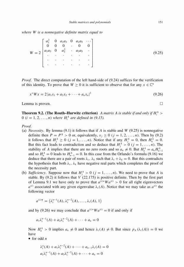
Stable matrices and polynomials 151
where W is a nonnegative definite matrix equal to
W = 2
⎡⎢⎢⎢⎢⎢⎢⎣
a21 0 a1a3 0 a1a5 · · ·0 0 0 · 0 0
a1a3 0 a23 · a3a5 ·· · · · · ·· · · · · ·· · · · · ·
⎤⎥⎥⎥⎥⎥⎥⎦ (9.25)
Proof. The direct computation of the left hand-side of (9.24) suffices for the verification
of this identity. To prove that W ≥ 0 it is sufficient to observe that for any x ∈ Cn
x∗Wx = 2 |a1x1 + a2x2 + · · · + anxn|2 (9.26)
Lemma is proven. �
Theorem 9.2. (The Routh–Hurwitz criterion) A matrix A is stable if and only if HAi >
0 (i = 1, 2, . . . , n) where HAi are defined in (9.15).
Proof.(a) Necessity. By lemma (9.1) it follows that if A is stable and W (9.25) is nonnegative
definite then P = Pᵀ > 0 or, equivalently, vj ≥ 0 (j = 1, 2, . . . , n). Then by (9.2)
it follows that HAj ≥ 0 (j = 1, . . . , n). Notice that if any HA
j = 0, then HAn = 0.
But this fact leads to contradiction and so deduce that HAj > 0 (j = 1, . . . , n). The
stability of A implies that there are no zero roots and so an �= 0. But HAn = anHA
n−1
and so HAn = 0 leads to HA
n−1 = 0. In this case from the Orlando’s formula (9.16) we
deduce that there are a pair of roots λi, λk such that λi + λk = 0. But this contradicts
the hypothesis that both λi, λk have negative real parts which completes the proof of
the necessity part.
(b) Sufficiency. Suppose now that HAj > 0 (j = 1, . . . , n). We need to prove that A is
stable. By (9.2) it follows that V (22.175) is positive definite. Then by the first part
of Lemma 9.1 we have only to prove that a(i)∗Wa(i) > 0 for all right eigenvectors
a(i) associated with any given eigenvalue λi(A). Notice that we may take as a(i) the
following vector
a(i)ᵀ = (λn−1i (A), λn−2
i (A), . . . , λi(A), 1)
and by (9.26) we may conclude that a(i)∗Wa(i) = 0 if and only if
a1λn−1i (A)+ a2λn−2
i (A)+ · · · + an = 0
Now HAn > 0 implies an �= 0 and hence λi(A) �= 0. But since pA (λi(A)) = 0 we
have• for odd n
λni (A)+ a1λn−2i (A)+ · · · + an−1λi(A) = 0
a1λn−1i (A)+ a3λn−3
i (A)+ · · · + an = 0

152 Advanced Mathematical Tools for Automatic Control Engineers: Volume 1
Hence
[1 a2 a4 · · · an−1
a1 a3 a5 · · · an
]⎡⎢⎢⎣λn−1i (A)...
λ2i (A)
1
⎤⎥⎥⎦ = 0
• for even n
λni (A)+ a2λn−2i (A)+ · · · + an = 0
a1λn−1i (A)+ a3λn−3
i (A)+ · · · + an−1λi(A) = 0
Hence
[1 a2 · · · an−2 ana1 a3 · · · an−1 0
]⎡⎢⎢⎣λni (A)...
λ2i (A)
1
⎤⎥⎥⎦ = 0
Thus in both cases for odd or even n we obtain
a1a2 − a3 = 0, a1a4 − a5 = 0, . . .
and the second row and column of V are zero which contradicts our deduction
that V is positive definite. Hence a(i)∗Wa(i) �= 0 and thus A is stable. Theorem is
proven. �
Example 9.2. The polynomial
p (λ) = λ4 + 2λ3 + 3λ2 + 2λ+ 1− αβ (9.27)
has the following Hurwitz matrix (9.14)
HA =
⎡⎢⎢⎣2 2 0 0
1 3 1− αβ 0
0 2 2 0
0 1 3 1− αβ
⎤⎥⎥⎦
So, by the Routh–Hurwitz criterion the corresponding matrix A is stable if and only if allprincipal minors HAi (i = 1, . . . , 4) are strictly positive, that is,
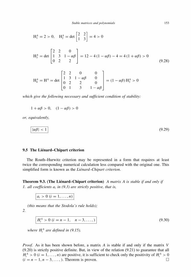
Stable matrices and polynomials 153
HA1 = 2 > 0, HA2 = det
[2 2
1 3
]= 4 > 0
HA3 = det
⎡⎣2 2 0
1 3 1− αβ0 2 2
⎤⎦ = 12− 4 (1− αβ)− 4 = 4 (1+ αβ) > 0
HA4 = HA = det
⎡⎢⎢⎣2 2 0 0
1 3 1− αβ 0
0 2 2 0
0 1 3 1− αβ
⎤⎥⎥⎦ = (1− αβ)HA3 > 0
(9.28)
which give the following necessary and sufficient condition of stability:
1+ αβ > 0, (1− αβ) > 0
or, equivalently,
|αβ| < 1 (9.29)
9.5 The Liénard–Chipart criterion
The Routh–Hurwitz criterion may be represented in a form that requires at least
twice the corresponding numerical calculation less compared with the original one. This
simplified form is known as the Liénard–Chipart criterion.
Theorem 9.3. (The Liénard–Chipart criterion) A matrix A is stable if and only if1. all coefficients ai in (9.3) are strictly positive, that is,
ai > 0 (i = 1, . . . , n)
(this means that the Stodola’s rule holds);2.
HAi > 0 (i = n− 1, n− 3, . . . , ) (9.30)
where HAi are defined in (9.15).
Proof. As it has been shown before, a matrix A is stable if and only if the matrix V
(9.20) is strictly positive definite. But, in view of the relation (9.21) to guarantee that all
HAi > 0 (i = 1, . . . , n) are positive, it is sufficient to check only the positivity of HA
i > 0
(i = n− 1, n− 3, . . . , ). Theorem is proven. �
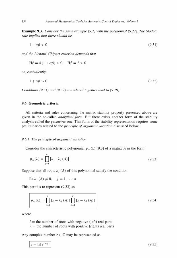
154 Advanced Mathematical Tools for Automatic Control Engineers: Volume 1
Example 9.3. Consider the same example (9.2) with the polynomial (9.27). The Stodolarule implies that there should be
1− αβ > 0 (9.31)
and the Liénard–Chipart criterion demands that
HA3 = 4 (1+ αβ) > 0, HA1 = 2 > 0
or, equivalently,
1+ αβ > 0 (9.32)
Conditions (9.31) and (9.32) considered together lead to (9.29).
9.6 Geometric criteria
All criteria and rules concerning the matrix stability property presented above are
given in the so-called analytical form. But there exists another form of the stability
analysis called the geometric one. This form of the stability representation requires some
preliminaries related to the principle of argument variation discussed below.
9.6.1 The principle of argument variation
Consider the characteristic polynomial pA (λ) (9.3) of a matrix A in the form
pA (λ) =n∏j=1
[λ− λj (A)] (9.33)
Suppose that all roots λj (A) of this polynomial satisfy the condition
Re λj (A) �= 0, j = 1, . . . , n
This permits to represent (9.33) as
pA (λ) =l∏j=1
[λ− λj (A)]r∏k=1
[λ− λk (A)] (9.34)
where
l = the number of roots with negative (left) real parts
r = the number of roots with positive (right) real parts
Any complex number z ∈ C may be represented as
z = |z| ei arg z (9.35)

Stable matrices and polynomials 155
where arg z is the angle formed by the vector z in the complex plane with the real axis
measured in the clockwise (positive) direction. Moreover, if |z| <∞ and Re z �= 0, then
the simple complex function
f (iω) := iω − z = |iω − z| ei arg(iω−z)
has the following argument variation∞�
ω=−∞ arg f (iω) (when ω varies from −∞ to ∞):
∞�
ω=−∞ arg f (iω) ={π if Re z < 0
−π if Re z > 0(9.36)
Lemma 9.5. (The principle of argument variation) The polynomial (9.34) verifies thefollowing
∞�
ω=−∞ argpA (iω) = (l − r) π (9.37)
Proof. By the evaluation of (9.34) using (9.35) we have
p (iω)=l∏j=1
[λ− λj (A)]r∏k=1
[λ− λk (A)]
=n∏j=1
(∣∣iω − λj (A)∣∣) exp i(
l∑j=1
arg(iω − λj (A))+r∑k=1
arg (iω − λk (A)))
So,
argpA (iω) =l∑j=1
arg(iω − λj (A)
)+ r∑k=1
arg(iω − λk (A)
)
and by (9.36) we derive (9.37). Lemma is proven. �
Corollary 9.3. For any stable polynomial its argpA (jω) is a monotonically increasingfunction of ω.
Corollary 9.4. For the polynomials without neutral roots
∞�ω=0
argpA (iω) = (l − r) π2
(9.38)
9.6.2 Mikhailov’s criterion
Based on the previous lemma (9.5) we may present the following important result.

156 Advanced Mathematical Tools for Automatic Control Engineers: Volume 1
Theorem 9.4. (Mikhailov’s criterion) The polynomial pA (λ) (9.3) of order n isHurwitz(or, equivalently the corresponding matrix A is stable) if and only if the godograph ofpA (λ) (the corresponding curve in the coordinates)
U (ω) := RepA (iω)
as the abscise and
V (ω) := Im pA (iω)
as the ordinate such that
pA (iω) = U (ω)+ iV (ω)
has rotation in the clockwise (positive) direction and passes exactly n quadrants in thecomplex plane without crossing the origin when ω varies from 0 up to ∞.
Proof. By definition pA (λ) is Hurwitz if and only if it has the representation (9.34) with
l = n. Hence, by lemma (9.5) in view of (9.37) it follows that
∞�ω=∞ argpA (iω) = nπ
or, by corollary (9.38) to this lemma,
∞�ω=0
argp (iω) = nπ2
The criterion is proven. �
Consider now several examples illustrating the application of Mikhailov’s criterion.
Example 9.4. Let us consider the characteristic polynomial
pA (λ) = λ5 + 5λ4 + 10λ3 + 11λ2 + 7λ+ 2 (9.39)
We need to determine whether it is Hurwitz or not applying the geometric criterion.Taking λ = iω for (9.39) one has
pA (iω)= iω5 + 5ω4 − i10ω3 − 11ω2 + i7ω + 2
= [5ω4 − 11ω2 + 2
]+ i [ω (ω4 − 10ω2 + 7)]
So,
U (ω)= 5ω4 − 11ω2 + 2
V (ω)= ω (ω4 − 10ω2 + 7)
The corresponding godograph and its zoom-form are depicted at Figs. 9.1 and 9.2correspondingly.

Stable matrices and polynomials 157
500
240
230
220
210
10
0100 150 200 250 300 350
�50
��
V( )
U( )�
Fig. 9.1. The godograph of pA (iω).
26
24
22
0
2
222324 21 1 20
V(�)
U(�)
��
�50
Fig. 9.2. The zoom-form of the godograph of pA (iω).
In view of the geometric form of this godograph we may conclude that this polynomial
is Hurwitz.
Using this geometric approach one may determine not only if a polynomial is stable or
not, but also determine the exact number (l) of stable, (r) unstable and (m) neutral roots.
Example 9.5. Suppose that the polynomial pA (λ) has the order n = 5 and its godographhas the form as at Fig. 9.3. Notice that this godograph does not cross the origin (0, 0)and therefore pA (λ) does not have neutral (with a real part equal to zero) roots, that is,m = 0. Hence by (9.37) we conclude that
l + r +m = n = 5
m = 0, l − r = 3

158 Advanced Mathematical Tools for Automatic Control Engineers: Volume 1
V(�)
U(�)
�50
��
Fig. 9.3. The godograph of pA (iω).
�
�
� 5 �0. 0
� 1 � 5�2
V(�)
U(�)
� 5 0
Fig. 9.4. The godograph of pA (iω).
which gives
l = 4, r = 1, m = 0
Example 9.6. Suppose that the godograph of pA (iω) is as at Fig. 9.4 and correspondsto a polynomial pA (λ) of the order n = 6. One can see that this godograph crosses theorigin (0, 0). This means that pA (λ) has a root a with a real part equal to zero. But, aswe have only one cross which corresponds to a frequency ω = ω0 �= 0, it means thatthere exist two complex conjugated roots such that
λi (A) = iω0, λi (A) = −iω0

Stable matrices and polynomials 159
This means that m = 2. So, by (9.37) we conclude that
l + r +m = n = 6∞�ω=0
argp (iω) = π, l − r = 2, m = 2
This finally gives:
l = 3, r = 1, m = 2
9.7 Polynomial robust stability
9.7.1 Parametric uncertainty and robust stability
As shown before, the stability property of a matrix A ∈ Rn×n is characterized by the
root’s location of the corresponding characteristic polynomial pA (λ) (9.3). Evidently,
any variations �A of the matrix A, namely, A = A0 + �A, are transformed into
the variations of the coefficients aj (j = 1, . . . , n) of the corresponding characteristic
polynomial pA (λ). Denote the collection of its coefficients by
a := (a1, . . . , an)ᵀ ∈ Rn (9.40)
and suppose that this vector of coefficients belongs to a connected set A ∈ Rn that
corresponds to possible variations �A of the matrix A or maybe includes them, that is,
a ∈ A ∈ Rn (9.41)
Definition 9.2. A characteristic polynomial pA (λ) (9.3) is said to be robust stable, iffor any a ∈ A the roots of the corresponding polynomial belongs to the left-hand side ofthe complex plane C, i.e.,
Re λj (A) < 0 (j = 1, . . . , n) (9.42)
for all a ∈ A.
Definition 9.3. Denote by QA (ω) the set of all values of the vector
pA (iω) = U (ω)+ iV (ω)
given in C under a fixed ω ∈ [0,∞) when the parameters a take all possible values inA, that is,
QA (ω) := {z : z = pA (iω) | a ∈ A} (9.43)
The next result represents the criterion of the polynomial robust stability and is a
keystone in robust control theory.

160 Advanced Mathematical Tools for Automatic Control Engineers: Volume 1
Theorem 9.5. (The criterion of polynomial robust stability) The characteristic poly-nomial pA (λ) (9.3) is robust stable if and only if1. The class A of polynomials pA (λ) (9.3) contains at least one Hurwitz polynomialp∗A (λ), named a basic one.
2. The following principle of “zero-excluding” holds: the set QA (ω) does not containthe origin (“zero-point”), i.e.,
0 /∈ QA (ω) (9.44)
Proof. Since the vector z = pA (jω) ∈ C is continually dependent on the vector parameter
a, then a “transition” from stable polynomial to unstable one (when we are varying the
coefficients a) may occur (this is always possible since the set A of parameters is a
connected set) only when one of its roots crosses the imaginary axis, or, in other words,
when there exists ω0 ∈ [0,∞) such that pA (iω0) = U (ω0) + iV (ω0) = 0. But this is
equivalent to the following identity
U (ω0) = V (ω0) = 0
which means exactly that 0 ∈ QA (ω). Evidently, to avoid this effect it is necessary and
sufficient to fulfill conditions 1 and 2 of this theorem. Theorem is proven. �
9.7.2 Kharitonov’s theorem
Theorem 9.6. Kharitonov (1978) Let the set A, characterizing a parametric uncer-tainty, be defined as
A :={a ∈ Rn : a−i ≤ ai ≤ a+i (i = 1, . . . n)
}(9.45)
Then the polynomial pA (λ) (9.3) is robust stable if and only if four polynomials given
below are stable (Hurwitz):
p(1)A (λ) := 1+ a−1 λ+ a+2 λ2 + a+3 λ3 + a−4 λ4 + a−5 λ5 + · · ·p(2)A (λ) := 1+ a+1 λ+ a+2 λ2 + a−3 λ3 + a−4 λ4 + a+5 λ5 + · · ·p(3)A (λ) := 1+ a+1 λ+ a−2 λ2 + a−3 λ3 + a+4 λ4 + a+5 λ5 + · · ·p(4)A (λ) := 1+ a−1 λ+ a−2 λ2 + a+3 λ3 + a+4 λ4 + a−5 λ5 + · · ·
(9.46)
Proof. For any a ∈ A
U (ω) = 1− a2ω2 + a4ω4 − · · ·V (ω) = a1ω − a3ω3 + a5ω5 · · ·
and hence for any ω ∈ [0,∞)
U− (ω) ≤ U (ω) ≤ U+ (ω) and V − (ω) ≤ V (ω) ≤ V + (ω)

Stable matrices and polynomials 161
where
U− (ω) = 1− a+2 ω2 + a−4 ω4 − · · ·U+ (ω) = 1− a−2 ω2 + a+4 ω4 − · · ·
and
V − (ω) = a−1 ω − a+3 ω3 + a−5 ω5 · · ·V + (ω) = a+1 ω − a−3 ω3 + a+5 ω5 · · ·
That’s why for any ω ∈ [0,∞) the set QA (ω) (9.43) is rectangular (see Fig. 9.5) with
width [U+ (ω)− U− (ω)] and height [V + (ω)− V − (ω)] and with the center in the point
pA (jω) corresponding to the stable polynomial with parameters ai = 1
2
(a−i + a+i
).
Notice that the vertices of the set QA (ω) correspond exactly to the polynomials (9.46).
Suppose now that this rectangle touches the origin by one of its sides. Since the argument
monotonically increases the vertices of this touching side will rotate in the clock-wise
direction, and, hence, will become non-vertical which contradicts our previous concept.
So, the direct application of the previous Theorem 9.5 leads to the formulated result.
Theorem is proven. �
Example 9.7. Let us find the parameter β for which the polynomial
pA (λ) = 1+ a1λ+ a2λ2 + a3λ31− β ≤ a1 ≤ 1+ β1.5 ≤ a2 ≤ 2, a3 = 1
is robust stable. To do this construct four polynomials (9.46):
p(1)A (λ) := 1+ (1− β) λ+ 2λ2 + λ3p(2)A (λ) := 1+ (1+ β) λ+ 2λ2 + λ3p(3)A (λ) := 1+ (1+ β) λ+ 1.5λ2 + λ3p(4)A (λ) := 1+ (1− β) λ+ 1.5λ2 + λ3
QA(v)
V (�)
U (�)
�50
��
Fig. 9.5. Illustration of the Kharitonov’s criterion.

162 Advanced Mathematical Tools for Automatic Control Engineers: Volume 1
The corresponding Hurwitz matrices HA are as follows:
⎡⎣1− β 1 0
1 2 0
0 (1− β) 1
⎤⎦,
⎡⎣1+ β 1 0
1 2 0
0 (1+ β) 1
⎤⎦
⎡⎣1+ β 1 0
1 1.5 0
0 1+ β 1
⎤⎦,
⎡⎣1− β 1 0
1 1.5 0
0 1− β 1
⎤⎦
By the Liénard–Chipart criterion we find that the conditions of the robust stability are
1− β > 0, 1+ β > 0 or, equivalently, |β| < 1
and
2 (1− β)− 1 > 0, 2 (1+ β)− 1 > 0
1.5 (1+ β)− 1 > 0, 1.5 (1− β)− 1 > 0
which leads to the following:
β < 0.5, β > −0.5, β >2
3− 1 = −1
3, β < 1− 2
3= 1
3
or, equivalently,
|β| < 0.5, |β| < 1
3
Finally, all constraints taken together give
|β| < 1
3
9.7.3 The Polyak–Tsypkin geometric criterion
Let the set A of all possible parameters a be defined as follows:
A := {a ∈ Rn : ∣∣ai − a∗i ∣∣ ≤ γαi (i = 1, . . . , n) , γ > 0
}(9.47)

Stable matrices and polynomials 163
Construct the following polynomials:
Ua (ω) := 1− a2ω2 + a4ω4 − · · ·
Va (ω) := a1ω − a3ω3 + a5ω5 · · ·
Ta (ω) := 1
ωVa (ω), ω > 0
S (ω) := 1+ α2ω2 + α4ω4 + · · ·
V (ω) := α1ω + α3ω3 + α5ω5 · · ·
T (ω) := 1
ωV (ω), ω > 0
(9.48)
and define
X (ω) := Ua∗ (ω)S (ω)
, Y (ω) := Ta∗ (ω)T (ω)
(9.49)
Theorem 9.7. Polyak & Tsypkin (1990) The characteristic polynomial pA (λ) (9.3) isrobust stable if and only if the godograph
Z (iω) := X (ω)+ iY (ω) (9.50)
passes exactly n quadrants, when ω varies from 0 up to ∞, and does not cross thequadrant �γ with the center in the origin and with the board equal to 2γ (see Fig. 9.6)
6�
�
6
X(�)
Y(�)
�50
�5�
Fig. 9.6. Illustration of the Polyak–Tsypkin criterion.

164 Advanced Mathematical Tools for Automatic Control Engineers: Volume 1
such that
|X (0)|, |Y (0)|, |X (∞)|, |Y (∞)| > γ (9.51)
Proof. For any a ∈ A we have
|Ua (ω)− Ua∗ (ω)| ≤ γ S (ω)|Va (ω)− Va∗ (ω)| ≤ γV (ω)
or
|Ta (ω)− Ta∗ (ω)| ≤ γ T (ω)
The condition that
0 ∈ QA (ω)
for some ω > 0 means that Ua (ω) = Va (ω) = 0 for some a ∈ A which implies
|Ua (ω)− Ua∗ (ω)| = |Ua∗ (ω)| ≤ γ S (ω)|Va (ω)− Va∗ (ω)| = |Va∗ (ω)| ≤ γV (ω)
and
|Ta (ω)− Ta∗ (ω)| = |Ta∗ (ω)| ≤ γ T (ω)
Since S (ω) > 0 and T (ω) > 0, we obtain
|X (ω)| =∣∣∣∣Ua∗ (ω)S (ω)
∣∣∣∣ ≤ γ, |Y (ω)| =∣∣∣∣Ta∗ (ω)T (ω)
∣∣∣∣ ≤ γwhich means that
Z (iω) ∈ �γContrarily, the conditions that 0 /∈ QA (ω0) are
Z (iω) /∈ �γ|X (0)|, |Y (0)|, |X (∞)|, |Y (∞)| > γ
Then the result follows from Theorem 9.5. Theorem is proven. �
Remark 9.2. The “maximal stability radius” γ = γmax corresponds to the maximal quad-rant �γmax
which touches the godograph Z (jω) from inside.
9.8 Controllable, stabilizable, observable and detectable pairs
In this subsection we shall turn to some important concepts that will be used frequently
in the following.
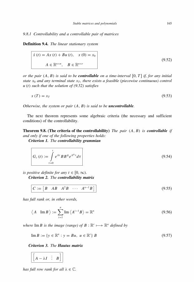
Stable matrices and polynomials 165
9.8.1 Controllability and a controllable pair of matrices
Definition 9.4. The linear stationary system
x (t) = Ax (t)+ Bu (t), x (0) = x0A ∈ Rn×n, B ∈ Rn×r
(9.52)
or the pair (A,B) is said to be controllable on a time-interval [0, T ] if, for any initialstate x0 and any terminal state xT , there exists a feasible (piecewise continuous) controlu (t) such that the solution of (9.52) satisfies
x (T ) = xT (9.53)
Otherwise, the system or pair (A,B) is said to be uncontrollable.
The next theorem represents some algebraic criteria (the necessary and sufficient
conditions) of the controllability.
Theorem 9.8. (The criteria of the controllability) The pair (A,B) is controllable ifand only if one of the following properties holds:
Criterion 1. The controllability grammian
Gc (t) :=t∫
τ=0
eAτBBᵀeAᵀτ dτ (9.54)
is positive definite for any t ∈ [0,∞).Criterion 2. The controllability matrix
C := [B AB A2B · · · An−1B
](9.55)
has full rank or, in other words,
⟨A ImB
⟩ := n∑i=1
Im⟨Ai−1B
⟩ = Rn (9.56)
where ImB is the image (range) of B : Rr −→ Rn defined by
ImB := {y ∈ Rn : y = Bu, u ∈ Rr} B (9.57)
Criterion 3. The Hautus matrix
[A− λI ... B
]has full row rank for all λ ∈ C.

166 Advanced Mathematical Tools for Automatic Control Engineers: Volume 1
Criterion 4. For any left eigenvalues λ and the corresponding eigenvectors x of thematrix A, i.e., x∗A = λx∗, the following property holds: x∗B �= 0. In other words, allmodes of A are B-controllable.
Criterion 5. The eigenvalues of the matrix (A+ BK) can be freely assigned by asuitable selection of K .
Proof. Criterion 1.(a) Necessity. Suppose that the pair (A,B) is controllable, but for some t1 ∈ [0, T ] the
grammian of controllability Gc (T ) is singular, that is, there exists a vector x �= 0
such that
0= xᵀ
⎡⎣ t1∫τ=0
eAτBBᵀeAᵀτ dτ
⎤⎦ x
=⎡⎣ t1∫τ=0
xᵀeAτBBᵀeAᵀτ xdτ
⎤⎦ =
t1∫τ=0
∥∥BᵀeAᵀτ x
∥∥2dτ
So,
xᵀeAτB = 0 (9.58)
for all τ ∈ [0, t1]. Select t1 as a terminal instant, that is, t1 = T and x (T ) = xT = 0.
Then by (9.59)
0 = x (t1) = eAt1x0 +t1∫
τ=0
eA(t1−τ)Bu (τ) dτ
and pre-multiplying the last equation by xᵀ we obtain
0 = xᵀx (t1) = xᵀeAt1x0 +t1∫
τ=0
xᵀeA(t1−τ)Bu (τ) dτ = xᵀeAt1x0
Selecting the initial conditions x0 = e−At1x, we obtain ‖x‖2 = 0, or x = 0, which
contradicts the assumption that x �= 0.
(b) Sufficiency. Suppose conversely: Gc (t) > 0 for all t ∈ [0, T ]. Hence, Gc (T ) > 0.
Define
u (t) := −BᵀeAᵀ(T−t)G−1
c (T )[eAT x0 − xT
]Then, by (9.52),
x (t) = eAtx0 +t∫
τ=0
eA(t−τ)Bu (τ) dτ (9.59)

Stable matrices and polynomials 167
which gives
x (T )= eAT x0 −⎡⎣ T∫τ=0
eA(T−τ)BBᵀeAᵀ(T−t)G−1
c (T )[eAT x0 − xT
]dτ
⎤⎦
= eAT x0 −⎡⎣ T∫τ=0
eA(T−τ)BBᵀeAᵀ(T−t) dτ
⎤⎦G−1
c (T )[eAT x0 − xT
]T−τ=s= eAT x0
+⎡⎣ 0∫s=TeAsBBᵀeA
ᵀs ds
⎤⎦G−1
c (T )[eAT x0 − xT
] = eAT x0− Gc (T )G−1
c (T )[eAT x0 − xT
] = xTSo, the pair (A,B) is controllable. The first criterion is proven.
Criterion 2.(a) Necessity. Suppose that Gc (t) > 0 for any t ∈ [0, T ], but the controllability matrix
C has no full rank, that is, there exists a nonzero-vector v ∈ Rn such that
v∗AiB = 0 for all i = 0, 1 . . . , n− 1
But by the Cayley–Hamilton theorem any matrix satisfies its own characteristic
equation, namely, if
det (A− λI) = a0λn + a1λn−1 + · · · + an−1λ+ an = 0, a0 �= 0
then
a0An + a1An−1 + · · · + an−1A+ anI = 0, a0 �= 0
or, equivalently,
An = −(a1
a0An−1 + · · · + an−1
a0A+ an
a0I
)
and hence
v∗AnB = −(a1
a0v∗An−1B + · · · + an−1
a0v∗AB + an
a0v∗B
)= 0
By the same reason
v∗An+1B = −(a1
a0v∗AnB + · · · + an−1
a0v∗A2B + an
a0v∗AB
)= 0
and so on. So,
v∗AiB = 0 for any i ≥ 0 (9.60)

168 Advanced Mathematical Tools for Automatic Control Engineers: Volume 1
But since eAt =∞∑i=0
1
i! (At)i , in view of (9.60), for all t ≥ 0 we have
v∗eAtB =∞∑i=0
1
i!v∗AiBti = 0
which implies
0 = v∗t1≤T∫t=0
eAtBBᵀeAᵀt dt = v∗Gc (t1)
for all t1 ≤ T which is in contradiction with the assumption thatGc (t1) is nonsingular.
So, C should have full rank.
(b) Sufficiency. Conversely, suppose now that C has full rank, but Gc (t) is singular for
some t = t1 ≤ T . Then, by (9.58), there exists a vector xᵀ �= 0 such that xᵀeAτB = 0
for all τ ∈ [0, t1]. Taking t = 0, we get xᵀB = 0. Evaluating the ith derivatives at
the point t = 0, we have
0 = xᵀ(d
dτeAτ
)t=0
B = xᵀAiB, i = 0, 1, . . . , n− 1
which implies
[B AB A2B . . . An−1B
] = xᵀC = 0
It means that C has no full rank. This is in contradiction with the initial assumption
that C has full rank. So, Gc (t) should be nonsingular for all t ∈ [0, T ]. The second
criterion is proven too.
Criterion 3.(a) Necessity. On the contrary, suppose that [A− λI ... B] has no full row rank for some
λ ∈ C, that is, there exists a vector x∗ �= 0 such that x∗[A − λI ... B] = 0 but the
system is controllable (C has full rank). This is equivalent to the following:
x∗A = λx∗, x∗B = 0
which results in
x∗C = x∗ [B AB A2B · · · An−1B]
=[x∗B︸︷︷︸
0
λx∗B︸︷︷︸0
λ2x∗B︸︷︷︸0
· · · λn−1x∗B︸︷︷︸0
]= 0
But this is in contradiction with the assumption that C has full rank.

Stable matrices and polynomials 169
(b) Sufficiency. Suppose that [A− λI ... B] has full row rank for all λ ∈ C, but C has no
full rank, i.e., x∗C = 0 for some x �= 0. Representing this x as a linear combination
of the eigenvectors xi∗ of the matrix A as
x∗ =n∑i=1
αixi∗ ,
(n∑i=1
α2i > 0
)
we get
0= x∗C =n∑i=1
αixi∗C
=n∑i=1
αixi∗[B AB A2B · · · An−1B
]=
n∑i=1
αixi∗[B λiB λ2i B · · · λn−1
i B]
=n∑i=1
αixi∗ [I λiI λ2i I · · · λn−1
i I]B = x∗B
where
x∗ :=n∑i=1
αixi∗ [I λiI λ2i I · · · λn−1
i I]
So, there exists a vector x �= 0 such that x∗B = 0 and
x∗A=n∑i=1
αixi∗ [I λiI λ2i I · · · λn−1
i I]A
= x∗A =n∑i=1
αixi∗A
[I λiI λ2i I · · · λn−1
i I]
=n∑i=1
αiλixi∗ [I λiI λ2i I · · · λn−1
i I] = λx∗
where
λ := x∗Axx∗x
which is in contradiction with the assumption that the Hautus matrix [A− λI ... B] hasfull row rank.
Criterion 4. It directly follows from Criterion 3.
Criterion 5. The proof can be found in Zhou et al., 1996.Theorem is proven. �
170 Advanced Mathematical Tools for Automatic Control Engineers: Volume 1
9.8.2 Stabilizability and a stabilizable pair of matrices
Definition 9.5. The linear stationary system (9.52) or the pair (A,B) is said to bestabilizable if there exists a state feedback u (t) = Kx (t) such that the closed-loopsystem is stable, i.e., the matrix A + BK is stable (Hurwitz). Otherwise, the system orpair (A,B) is said to be unstabilizable.
Theorem 9.9. (Two criteria of stabilizability) The pair (A,B) is stabilizable if andonly if
Criterion 1. The Hautus matrix [A− λI ... B] has the full rank for all Re λ ≥ 0.
Criterion 2. For all λ and x such that x∗A = λx∗ and Re λ ≥ 0, it follows thatx∗B �= 0.
Proof. This theorem is a consequence of the previous one. �
9.8.3 Observability and an observable pair of matrices
Let us consider the following stationary linear system supplied by an output model:
·x (t) = Ax (t)+ Bu (t), x (0) = x0, t ∈ [0,∞]
y (t) = Cx (t)A ∈ Rn×n, B ∈ Rn×r
⎫⎪⎬⎪⎭ (9.61)
where y (t) ∈ Rm is treated as an output vector and C ∈ Rm×n is an output matrix.
Definition 9.6. The stationary linear system (9.61) or the pair (C,A) is said to beobservable if, for any time t1, the initial state x (0) = x0 can be determined from thehistory of the input u (t) and the output y (t) within the interval [0, t1]. Otherwise, thesystem or pair (C,A) is said to be unobservable.
Theorem 9.10. (The criteria of observability) The pair (C,A) is observable if and onlyif one of the following criteria hold:
Criterion 1. The observability grammian
Go (t) :=t∫
τ=0
eAᵀτCᵀCeAτdτ (9.62)
is positive definite for any t ∈ [0,∞).
Stable matrices and polynomials 171
Criterion 2. The observability matrix
O :=
⎡⎢⎢⎢⎢⎢⎣
C
CA
CA2
...
CAn−1
⎤⎥⎥⎥⎥⎥⎦ (9.63)
has the full column rank or, in other words,
n⋂i=1
Ker(CAi−1
) = 0 (9.64)
where Ker (A) is the kernel or null space of A : Rn −→ Rmdefined by
Ker (A) = N (A) := {x ∈ Rn : Ax = 0} (9.65)
Criterion 3. The Hautus matrix[A− λIC
]
has full column rank for all λ ∈ C.Criterion 4. Let λ and y be any eigenvalue and any corresponding right eigenvector
of A, that is, Ay = λy, then Cy �= 0.Criterion 5. The eigenvalues of the matrix A+ LC can be freely assigned (complex
eigenvalues are in conjugated pairs) by a suitable choice of L.Criterion 6. The pair (Aᵀ, Cᵀ) is controllable.
Proof. Criterion 1.(a) Necessity. Suppose that the pair (C,A) is observable, but for some t1 the grammian
of observability G0 (t1) is singular, that is, there exists a vector x �= 0 such that
0= xᵀ
⎡⎣ t1∫τ=0
eAᵀτCᵀCeAτ dτ
⎤⎦ x
=⎡⎣ t1∫τ=0
xᵀeAᵀτCᵀCeAτx dτ
⎤⎦ =
t1∫τ=0
∥∥CeAτx∥∥2dτ
So,
CeAτx = 0 (9.66)
for all τ ∈ [0, t1]. Then by (9.59)
x (t1) = eAt1x0 +t1∫
τ=0
eA(t1−τ)Bu (τ) dτ

172 Advanced Mathematical Tools for Automatic Control Engineers: Volume 1
and, hence,
y (t1) = Cx (t1) = CeAt1x0 +t1∫
τ=0
CeA(t1−τ)Bu (τ) dτ
or
v (t1) := y (t1)−t1∫
τ=0
CeA(t1−τ)Bu (τ) dτ = CeAt1x0
Selecting the initial conditions x0 = 0, we obtain v (t1) = 0. But we have the same
results for any x0 = x �= 0 satisfying (9.66) which means that x0 cannot be determined
from the history of the process. This contradicts that (C,A) is observable.
(b) Sufficiency. Suppose conversely: Go (t) > 0 for all t ∈ [0,∞]. Hence,
0 < xᵀ
⎡⎣ t∫τ=0
eAᵀτCᵀCeAτ dτ
⎤⎦ x
=⎡⎣ t1∫τ=0
xᵀeAᵀτCᵀCeAτ x dτ
⎤⎦ =
t1∫τ=0
∥∥CeAτx∥∥2dτ
which implies that there exists a time τ0 ∈ [0, t] such that∥∥CeAτ0x∥∥2
> 0 for any
x �= 0. This means that CeAτ0 is a full rank matrix(eA
ᵀτ0CᵀCeAτ0 > 0). Then
v (τ0) := y (τ0)−τ0∫
τ=0
CeA(τ0−τ)Bu (τ) dτ = CeAτ0x0
and, hence,
eAᵀτ0Cᵀv (τ0) = eAᵀτ0CᵀCeAτ0x0
and
x0 =[eA
ᵀτ0CᵀCeAτ0]−1eA
ᵀτ0Cᵀv (τ0)
So, the pair (C,A) is observable. The first criterion is proven.
Criterion 2.(a) Necessity. Suppose that the pair (C,A) is observable, but that the observability matrix
O does not have full column rank, i.e., there exists a vector x �= 0 such that Ox = 0
or, equivalently,
CAix = 0 ∀i = 0, 1, . . . , n− 1

Stable matrices and polynomials 173
Suppose now that x0 = x. Then, by the Cayley–Hamilton theorem
v (t) := y (t)−t∫
τ=0
CeA(t−τ)Bu (τ) dτ = CeAtx0
= C∞∑i=0
1
i! (At)i x0 =
n−1∑i=0
t i
i!CAix0︸ ︷︷ ︸0
+2n−1∑i=n
t i
i!CAix0︸ ︷︷ ︸0
+ ...︸︷︷︸0
= 0
(9.67)
which implies
v (t) = CeAtx0 = 0
and, hence, x0 cannot be determined from v (t) ≡ 0. We obtain the contradiction.
(b) Sufficiency. From (9.67) it follows that
v :=
⎡⎢⎢⎢⎢⎢⎣v (0)
v (0)
v (0)...
v(n−1) (0)
⎤⎥⎥⎥⎥⎥⎦ =
⎡⎢⎢⎢⎢⎢⎣
C
CA
CA2
...
CAn−1
⎤⎥⎥⎥⎥⎥⎦ x0 = Ox0
and since O has a full rank, then OᵀO > 0 and hence
x0 = [OᵀO]−1 Oᵀv
which means that x0 may be uniquely defined. This completes the proof.
Criteria 3–6. They follows from by the duality of Criterion 6 to the corresponding
criteria of controllability, since the controllability of the pair (Aᵀ, Cᵀ) is equivalent to
the existence of a matrix Lᵀ such that Aᵀ + CᵀLᵀ is stable. But then it follows that
(Aᵀ + CᵀLᵀ)ᵀ = A+ LC
is also stable which coincides with Criteria 6 of observability.
Theorem is proven. �
9.8.4 Detectability and a detectable pair of matrices
Definition 9.7. The stationary linear system (9.61) or the pair (C,A) is said to bedetectable if the matrix A+LC is stable (Hurwitz) for some L. Otherwise, the system orpair (C,A) is said to be undetectable.
Theorem 9.11. (The criteria of detectability) The pair (C,A) is detectable if and onlyif one of the following criteria holds:
Criterion 1. The Hautus matrix
[A− λIC
]has full column rank for all Re λ ≥ 0.

174 Advanced Mathematical Tools for Automatic Control Engineers: Volume 1
Criterion 2. Let λ and y be any eigenvalue and any corresponding right eigenvectorof A, such that Ay = λy, Re λ ≥ 0, then Cy �= 0.
Criterion 3. There exists a matrix L such that the matrix A+ LC is stable.Criterion 4. The pair (Aᵀ, Cᵀ) is stabilizable.
Proof. It follows from the duality of Criterion 4 of this theorem to the corresponding
criterion of stabilizability. Theorem is proven. �
9.8.5 Popov–Belevitch–Hautus (PBH) test
Definition 9.8. Let λ be an eigenvalue of the matrix A, or equivalently, a mode of thesystem (9.61). Then the mode λ is said to be1. controllable if
x∗B �= 0
for all left eigenvectors x∗ of the matrix A associated with this λ, i.e.,
x∗A = λx∗, x∗ �= 0
2. observable if
Cx �= 0
for all right eigenvectors x of the matrix A associated with this λ, i.e.,
Ax = λx, x �= 0
Otherwise, the mode is called uncontrollable (unobservable).
Using this definition we may formulate the following test-rule (Popov–Belevitch–Hautus
PBH-test (Hautus & Silverman (1983)) for the verification of the properties discussed
above.
Claim 9.1. (PBH test) The system (9.61) is1. controllable if and only if every mode is controllable;2. stabilizable if and only if every unstable mode is controllable;3. observable if and only if every mode is observable;4. detectable if and only if every unstable mode is observable.

10 Algebraic Riccati Equation
Contents10.1 Hamiltonian matrix . . . . . . . . . . . . . . . . . . . . . . . . . . . . . . 17510.2 All solutions of the algebraic Riccati equation . . . . . . . . . . . . . . . . 17610.3 Hermitian and symmetric solutions . . . . . . . . . . . . . . . . . . . . . . 18010.4 Nonnegative solutions . . . . . . . . . . . . . . . . . . . . . . . . . . . . 188
10.1 Hamiltonian matrix
Let us consider the matrix Riccati equation1
PA+ AᵀP +Q− PBR−1BᵀP = 0 (10.1)
and the associated 2n× 2n Hamiltonian matrix:
H :=[A −BR−1Bᵀ
−Q −Aᵀ
](10.2)
Lemma 10.1. The spectrum σ (H) of the set of eigenvalues of H (10.2) is symmetricabout the imaginary axis.
Proof. To see this, introduce the 2n× 2n matrix:
J :=[
0 −In×nIn×n 0
](10.3)
having the evident properties
J 2 =−I2n×2n
J−1 =−JSo, we have
J−1HJ = −JHJ = −Hᵀ (10.4)
which implies that λ is an eigenvalue of H (10.2) if and only if(−λ) is too
(see Fig. 10.1). �
1 In the Russian technical literature this equation is known as the matrix Lurie equation.
175

176 Advanced Mathematical Tools for Automatic Control Engineers: Volume 1
�
�
Im
Re
i
]�
]�
Fig. 10.1. Hamiltonian eigenvalues.
10.2 All solutions of the algebraic Riccati equation
10.2.1 Invariant subspaces
Definition 10.1. Let A : Cn −→ Cn be a linear transformation (matrix), λ be an eigen-value of A and x be a corresponding eigenvector of A, that is, Ax = λx. So, A (αx) =λ (αx) for any α ∈ R.
1. We say that the eigenvector x defines a one-dimensional subspace which is invariantwith respect to pre-multiplication by A since
Ak (αx) = λk (αx) k = 1, . . .
2. Generalizing the definition before, we say that a subspace S ⊂ Cn is invariant withrespect to the transformation A, or A-invariant, if
Ax ∈ S for any x ∈ Sor, in other words,
AS ⊂ S
3. If one of the eigenvalues has a multiplicity l, i.e. λ1 = λ2 = . . . = λl , then thegeneralized eigenvectors xi (i = 1, . . . , l) are obtained by the following rule
(A− λ1I ) xi = xi−1, i = 1, . . . , l, x0 := 0 (10.5)
10.2.2 Main theorems on the solution presentation
Theorem 10.1. Let � ⊂ C2n be an n-dimensional invariant subspace of H , that is, ifz ∈ � then Hz ∈ �, and let P1, P2 ∈ Cn×n be two complex matrices such that
� = Im
[P1
P2
]

Algebraic Riccati equation 177
which means that the columns of
[P1
P2
]may be considered as a basis in �. If P1 is
invertible, then
P = P2P−11 (10.6)
is a solution to the matrix Riccati equation (10.1) which is independent of a specificchoice of bases of �.
Proof. Since � is an invariant subspace of H , there exists a matrix � ∈ Cn×n such that
H
[P1
P2
]=
[P1
P2
]� (10.7)
Indeed, let the matrix
[P1
P2
]be formed by the eigenvectors of H such that
[P1
P2
]= [v1 · · · vn
]where each vector vi satisfies the equation
Hvi = λivi
Here λi are the corresponding eigenvalues. Combining these equations for all i = 1, . . . , n,
we obtain
H
[P1
P2
]= H [
v1 · · · vn] = [
λ1v1 · · · λnvn]
= [v1 · · · vn
] ⎡⎣ λ1 0 · · · 0 0
0 · · · 0
0 0 · · · 0 λn
⎤⎦ =
[P1
P2
]�
� = diag {λ1, . . . , λn}
In the extended form, the relation (10.7) is
[A −BR−1Bᵀ
−Q −Aᵀ
] [P1
P2
]=
[P1
P2
]� (10.8)
Post-multiplying this equation by P−11 we get
[A −BR−1Bᵀ
−Q −Aᵀ
][In×n(P2P
−11
)]=
[In×n(P2P
−11
)]P1�P
−11

178 Advanced Mathematical Tools for Automatic Control Engineers: Volume 1
Then, the pre-multiplication of this equality by[− (P2P
−11
) ... In×n ] implies
[− (P2P
−11
) ... In×n ][A −BR−1Bᵀ
−Q −Aᵀ
] [In×n(P2P
−11
)]
=[− (P2P
−11
) ... In×n ][A− BR−1Bᵀ (
P2P−11
)−Q− Aᵀ (
P2P−11
) ]
= − (P2P
−11
)A+ (
P2P−11
)BR−1Bᵀ (
P2P−11
)−Q− Aᵀ (P2P
−11
)=
[− (P2P
−11
) ... In×n ][In×n(P2P
−11
)]P1�P−11 = 0
which means that P := P2P−11 satisfies (10.1). Let T be a nonsingular matrix. Then any
other basis from
[P1
P2
]spanning � can be represented as
[P1
P2
]=
[P1
P2
]T =
[P1T
P2T
][P1
P2
]=
[P1
P2
]T −1 =
[P1T
−1
P2T−1
]
and, hence,
P = P2P−11 =
(P2T
−1
)(P1T
−1
)−1
= P2T−1T
(P1
)−1 = P2
(P1
)−1
which proves the theorem. �
Corollary 10.1. The relation (10.8) implies
AP1 − BR−1BᵀP2 = P1�
A− (BR−1Bᵀ)P = P1�P
−11 (10.9)
Theorem 10.2. If P ∈ Cn×n is a solution to the matrix Riccati equation (10.1), then thereexist matrices P1, P2 ∈ Cn×n with P1 invertible such that (10.6) holds, that is,
P = P2P−11
and the columns of
[P1
P2
]form a basis of �.
Algebraic Riccati equation 179
Proof. Define
� := A− (BR−1Bᵀ)P
Pre-multiplying it by P gives
P� := PA− P (BR−1Bᵀ)P = −Q− AᵀP
These two relations may be rewritten as
[A −BR−1Bᵀ
−Q −Aᵀ
] [In×nP
]=
[In×nP
]�
Hence, the columns of
[In×nP
]span the invariant subspace � and defining P1 := In×n
and P2 = P completes the proof. �
10.2.3 Numerical example
Example 10.1. Let
A =[ −3 2
−2 1
], B =
[0
1
], R = I 2×2, Q = 0
H =
⎡⎢⎢⎣
−3 2
−2 1
0 0
0 −1
0 0
0 0
3 2
−2 −1
⎤⎥⎥⎦
Then the eigenvalues of H are 1, 1, (−1), (−1) and the eigenvector and the generalizedeigenvector (10.5) corresponding to λ1 = λ2 = 1 are
v1 = (1, 2, 2,−2)T , v2 = (−1,−3/2, 1, 0)T
and the eigenvector and the generalized eigenvector corresponding to λ3 = λ4 = −1 are
v3 = (1, 1, 0, 0)T , v4 = (1, 3/2, 0, 0)T
Several possible solutions of (10.1) are given below:
1. span{v1, v2} :={z ∈ C2n×2n : z = αv1 + βv2, α, β ∈ R
}is H-invariant: let[
P1
P2
]= [
v1 v2]

180 Advanced Mathematical Tools for Automatic Control Engineers: Volume 1
then
P = P2P−11 =
[2 1
−2 0
] [1 −1
2 −3/2
]−1
=[
2 1
−2 0
] [ −3.0 2.0
−4.0 2.0
]=[ −10.0 6.0
6.0 −4.0
]
2. span {v1, v3} is H -invariant: let
[P1
P2
]= [
v1 v3], then
P = P2P−11 =
[2 0
−2 0
] [1 1
2 1
]−1
=[
2 0
−2 0
] [ −1.0 1.0
2.0 −1.0
]=[ −2.0 2.0
2.0 −2.0
]
3. span {v3, v4} is H-invariant: let[P1
P2
]= [
v3 v4], then
P = P 2P−11 =
[0 0
0 0
] [1 1
0 3/2
]−1
=[0 0
0 0
]
4. Notice that here span {v1, v4}, span {v2, v3} and span {v2, v4} are not H-invariant.
Remark 10.1. If a collection of eigenvectors of H forms a basis in Cn which defines asolution of the Riccati matrix equation given by P = P 2P
−11 , then the number NRic of all
possible solutions of this equation is
NRic = (2n)!n! (2n− n)! =
(2n)!(n!)2
10.3 Hermitian and symmetric solutions
10.3.1 No pure imaginary eigenvalues
Theorem 10.3. Let � ⊂ C2n be an n-dimensional invariant subspace of H and let
P1, P2 ∈ Cn×n be two complex matrices such that � = Im
[P1
P2
]. Then the assumption
λi + λj �= 0 for all i, j = 1, . . . , 2n (10.10)
where λi, λj are the eigenvalues of H , implies

Algebraic Riccati equation 181
1. P ∗1 P2 is Hermitian, that is,
P ∗1 P2 = P ∗
2 P1
2. if, in addition, P1 is nonsingular, the matrix P = P2P−11 is Hermitian too, that is,
P ∗ = (P2P
−11
)∗ = PRemark 10.2. The condition (10.10) is equivalent to the restriction
Re λi �= 0 for all i = 1, . . . , 2n (10.11)
which means that H has no eigenvalues on the imaginary axis.
Proof. Since � is an invariant subspace of H , then there exists a matrix � such that
spectrums of the eigenvalues of � and H coincide, that is,
σ (�) = σ (H)
and (10.7) holds:
H
[P1
P2
]=
[P1
P2
]� (10.12)
Pre-multiplying this equation by
[P1
P2
]∗J, we get
[P1
P2
]∗JH
[P1
P2
]=
[P1
P2
]∗J
[P1
P2
]�
By (10.4), it follows that JH is symmetric and, hence, is Hermitian (since H is real).
So, we obtain that the left-hand side is Hermitian, and, as a result, the right-hand side is
Hermitian too:[P1
P2
]∗J
[P1
P2
]�= �∗
[P1
P2
]∗J ∗
[P1
P2
]
= −�∗[P1
P2
]∗J
[P1
P2
]
which implies
X�+�∗X = 0
X := (−P ∗1 P2 + P ∗
2 P1
)

182 Advanced Mathematical Tools for Automatic Control Engineers: Volume 1
But this is a Lyapunov equation which has a unique solutionX = 0 if λi (�)+ λj (�) �= 0.
But, since the spectrum of eigenvalues of � and H coincides, we obtain the proof of the
claim. Moreover, if P1 is nonsingular, then for P = P2P−11 it follows that
P ∗ = (P2P
−11
)∗ = (P−11
)∗P ∗2 =
(P−11
)∗ (P ∗1 P2P
−11
)= (P ∗1
)−1P ∗1 P2P
−11 = P2P
−11 = P
Theorem is proven. �
Theorem 10.4. Suppose a Hamiltonian matrix H (10.2) has no pure imaginary eigen-values and X− (H) and X+ (H) are n-dimensional invariant subspaces correspondingto eigenvalues λi (H) (i = 1, . . . n) in Re s < 0 and to λi (H) (i = n+ 1, . . . , 2n) inRe s > 0, respectively, that is, X− (H) has the basis
[v1 · · · vn
] =⎡⎢⎢⎢⎢⎢⎢⎣
v1,1 · vn,1· · ·v1,n · vn,nv1,n+1 · vn,n+1
· · ·v1,2n · vn,2n
⎤⎥⎥⎥⎥⎥⎥⎦ =
[P1
P2
]
P1 =⎡⎣ v1,1 · vn,1
· · ·v1,n · vn,n
⎤⎦, P2 =
⎡⎣ v1,n+1 · vn,n+1
· · ·v1,2n · vn,2n
⎤⎦
Then P1 is invertible, i.e. P−11 exists if and only if the pair (A,B) is stabilizable.
Proof. Sufficiency. Let the pair (A,B) be stabilizable. We want to show that P1 is
nonsingular. Contrariwise, suppose that there exists a vector x0 �= 0 such that P1x0 = 0.
Then we have the following. First, notice that
x∗0P∗2
(BR−1Bᵀ)P2x0 =
∥∥R−1/2BᵀP2x0∥∥2 = 0 (10.13)
or, equivalently,
R−1/2BᵀP2x0 = 0 (10.14)
Indeed, the pre-multiplication of (10.12) by[I 0
]implies
AP1 −(BR−1Bᵀ)P2 = P1� (10.15)
where� = diag (λ1, . . . , λn) is a diagonal matrix with elements from Re s < 0. Then, pre-
multiplying the last equality by x∗0P∗2 , post-multiplying by x0 and using the symmetricity
of P ∗2 P1 = P ∗
1 P2 we get

Algebraic Riccati equation 183
x∗0P∗2
[AP1 −
(BR−1Bᵀ)P2
]x0
= −x∗0P ∗2
(BR−1Bᵀ)P2x0 = x∗0P ∗
2 P1�x0
= x∗0P ∗1 P2�x0 = (P1x0)
∗ P2�x0 = 0
which implies (10.13). Pre-multiplying (10.12) by[I 0
], we get
−QP1 − AᵀP2 = P2� (10.16)
Post-multiplying (10.16) by x0 we obtain
(−QP1 − AᵀP2) x0 = −AᵀP2x0 = P2�x0 = λ0P2x0
where
λ0 = x∗0�x0
‖x0‖2
which implies
0 = AᵀP2x0 + P2λ0x0 = (Aᵀ + λ0I ) P2x0
Taking into account that, by (10.13),
(BR−1Bᵀ)P2x0 = 0
it follows that
[ (Aᵀ + λ0I )...(BR−1Bᵀ) ]P2x0 = 0
Then, the stabilizability of (A,B) (see Criterion 1 of stabilizability) implies that
P2x0 = 0. So,[P1
P2
]x0 = 0
and, since
[P1
P2
]forms the basis and, hence, has a full rank, we get x0 = 0, which is a
contradiction.
Necessity. Let P1 be invertible. Hence, by (10.15)
A− (BR−1Bᵀ)P2P
−11 = P1�P
−11
Since the spectrum of the eigenvalues of P1�P−11 coincides with one of �, we may
conclude that the matrix
Aclosed := A−(BR−1Bᵀ)P2P
−11

184 Advanced Mathematical Tools for Automatic Control Engineers: Volume 1
is stable and, hence, the pair(A,BR−1Bᵀ) is stabilizable (in the corresponding definition
K = P2P−11 ). It means that for all λ and x such that Ax = λx and Re λ ≥ 0, in other
words, for all unstable modes of A
x∗BR−1Bᵀ �= 0 (10.17)
which implies
x∗B �= 0
Indeed, by the contradiction, assuming that x∗B = 0, we obtain x∗BR−1Bᵀ = 0 which
violates (10.17). �
Corollary 10.2. The stabilizability of the pair (A,B) implies that the matrix
Aclosed := A−(BR−1Bᵀ)P2P
−11 (10.18)
is stable (Hurwitz).
Proof. Post-multiplying (10.12) by P−11 we get
H
[I
P
]=
[I
P2
]P1�P
−11 , P = P2P
−11
which after pre-multiplication by[I 0
]gives
[I 0
]H
[I
P2P−11
]
= [I 0
] [A− (BR−1Bᵀ)P
−Q− AᵀP
]= A− (
BR−1Bᵀ)P= Aclosed =
[I 0
] [ IP2
]P1�P
−11 = P1�P
−11
But P1�P−11 is stable, and hence Aclosed is stable too. �
10.3.2 Unobservable modes
Theorem 10.5. Assuming that the pair (A,B) is stabilizable, the Hamiltonian matrix H(10.2) has no pure imaginary eigenvalues if and only if the pair (C,A), whereQ = CᵀC,has no unobservable mode on the imaginary axis, that is, for all λ and x1 �= 0 such thatAx1 = λx1, λ = iω, it follows that Cx1 �= 0.
Algebraic Riccati equation 185
Proof. Suppose that λ = iω is an eigenvalue and the corresponding eigenvector
[x1x2
]�= 0.
Then
H
[x1x2
]=
[Ax1 − BR−1Bᵀx2−CᵀCx1 − Aᵀx2
]= iω
[x1x2
]=
[iωx1iωx2
]
After rearranging, we have
(A− iωI) x1 = BR−1Bᵀx2− (Aᵀ − iωI) x2 = CᵀCx1
(10.19)
which implies
(x2, (A− iωI) x1) =(x2, BR
−1Bᵀx2) = ∥∥R−1/2Bᵀx2
∥∥− (x1, (Aᵀ − iωI) x2) = − ((A− iωI) x1, x2) = (x1, CᵀCx1) = ‖Cx1‖2
As a result, we get
∥∥R−1/2Bᵀx2∥∥+ ‖Cx1‖2 = 0
and, hence,
Bᵀx2 = 0, Cx1 = 0
In view of this, from (10.19) it follows that
(A− iωI) x1 = BR−1Bᵀx2 = 0
− (Aᵀ − iωI) x2 = CᵀCx1 = 0
Combining the four last equations we obtain
x∗2[(A− iωI) B ] = 0[
(A− iωI)C
]x1 = 0
The stabilizability of (A,B) provides the full range for the matrix[(A− iωI) B] and
implies that x2 = 0. So, it is clear that iω is an eigenvalue of H if and only if it is an
unobservable mode of (C,A), that is, the corresponding x1 = 0 too. �

186 Advanced Mathematical Tools for Automatic Control Engineers: Volume 1
10.3.3 All real solutions
Theorem 10.6. Let � ⊂ C2n be an n-dimensional invariant subspace of H and let
P1, P2 ∈ Cn×n be two complex matrices such that the columns of
[P1
P2
]form a basis of
� and P1 is nonsingular. Then P = P2P−11 is real if and only if � is conjugated
symmetric, i.e. z ∈ � implies that z ∈ �.
Proof. Sufficiency. Since � is conjugated symmetric, then there exists a nonsingular
matrix N such that
[P1
P2
]=
[P1
P2
]N
Therefore,
P = P2P−11 = (P2N ) (P1N )−1 = P2NN−1P−1
1 = P2P−11 = P
So, P is real.
Necessity. We have P = P . By assumption P ∈ Rn×n and, hence,
Im
[I
P
]= � = Im
[I
P
]
Therefore, � is a conjugated symmetric subspace. �
Remark 10.3. Based on this theorem, we may conclude that to form a basis in aninvariant conjugated symmetric subspace we need to use the corresponding pairs of thecomplex conjugated symmetric eigenvectors or its linear nonsingular transformation(if n is odd then there exists a real eigenvalue to which an eigenvector should be addedto complete a basis) which guarantees that P is real.
10.3.4 Numerical example
Example 10.2. Let
A =[ −1 2
0 1
], B =
[0
1
], R = I2×2, Q =
[1 0
0 1
]
H =
⎡⎢⎢⎣−1 2 0 0
0 1 0 −1
−1 0 1 0
0 −1 −2 −1
⎤⎥⎥⎦

Algebraic Riccati equation 187
The eigenvalues λi and the corresponding eigenvectors vi are as follows:
λ1 = −1.4053+ 0.68902i v1 =
⎡⎢⎢⎣
−0.4172− 0.50702i
0.25921− 4.0993× 10⁻²i
−0.10449− 0.24073i
0.59522− 0.27720i
⎤⎥⎥⎦
λ2 = −1.4053− 0.68902i v2 =
⎡⎢⎢⎣
−0.50702− 0.4172i
−4.0993× 10⁻²+ 0.25921i
−0.24073− 0.10449i
−0.27720+ 0.59522i
⎤⎥⎥⎦
λ3 = 1.4053+ 0.68902i v3 =
⎡⎢⎢⎣2.9196× 10⁻²+ 0.44054i
−0.11666+ 0.53987i
−0.49356− 0.24792i
0.41926− 0.1384i
⎤⎥⎥⎦
λ4 = 1.4053− 0.68902i v4 =
⎡⎢⎢⎣−0.44054− 2.9196× 10⁻²
i
−0.53987+ 0.11666i
0.24792+ 0.49356i
0.1384− 0.41926i
⎤⎥⎥⎦
Notice that (−iv2) = v1 and (iv4) = v3 which corresponds to the fact that the eigenvectorsstay the same being multiplied by a complex number. Then forming the basis in two-dimensional subspace as[
v1 v2]
=
⎡⎢⎢⎣
−0.4172− 0.50702i −0.50702− 0.4172i
0.25921− 4.0993× 10⁻²i −4.0993× 10⁻²+ 0.25921i
−0.10449− 0.24073i −0.24073− 0.10449i
0.59522− 0.27720i −0.27720 + 0.59522i
⎤⎥⎥⎦
we may define
P1 :=[ −0.4172− 0.50702i −0.50702− 0.4172i
0.25921− 4.0993× 10⁻²i −4.0993× 10⁻²+ 0.25921i
]
P−11 =
[−0.13800+ 0.8726i 1.7068+ 1.4045i
−0.8726+ 0.13800i −1.4045− 1.7068i
]
and
P2:=[−0.10449− 0.24073i −0.24073− 0.10449i
0.59522− 0.27720i −0.27720+ 0.59522i
]Hence,
P = P 2P−11 =
[0.44896 0.31952
0.31949 2.8105
]
188 Advanced Mathematical Tools for Automatic Control Engineers: Volume 1
and we may see that P is a real matrix. Also we have
Aclosed := A−(BR−1Bᵀ)P2P
−11
=[ −1.0 2.0
−0.31949 −1.8105
]
with the eigenvalues:
λ1 (Aclosed) = −1.4053+ 0.68902i
λ2 (Aclosed) = −1.4053− 0.68902i
10.4 Nonnegative solutions
10.4.1 Main theorems on the algebraic Riccati equation solution
Theorem 10.7. The matrix Riccati equation (10.1)
PA+ AᵀP +Q− PBR−1BᵀP = 0 (10.20)
has a unique nonnegative definite solution P = Pᵀ ≥ 0 which provides stability to thematrix
Aclosed := A− BR−1BᵀP (10.21)
corresponding to the original dynamic system
x = Ax + Bu (10.22)
closed by the linear feedback control given by
u = −Kx = −R−1BᵀPx with K = R−1BᵀP (10.23)
if and only if the pair (A,B) is stabilizable and the pair (C,A) where
Q = CᵀC (10.24)
has no unobservable mode on the imaginary axis.
Proof. The existence of P = P2P−11 and its symmetricity and reality are already proven.
We need to prove only that P ≥ 0. Let us represent (10.1) in the following form
PA+ AᵀP +Q−KᵀRK = 0
RK = BᵀP(10.25)

Algebraic Riccati equation 189
By (10.25) it follows that
PAclosed + AᵀclosedP = − (Q+KᵀRK)
Aclosed := A− BK, K = R−1BᵀP(10.26)
Since (Q+KᵀRK) ≥ 0, by the Lyapunov Lemma 9.1 it follows that P ≥ 0. �
Example 10.3. Let us consider the following simple scalar dynamic system given by
x = ax + bu, y = cx
with
a �= 0, b = 1, c = 0
Notice that this system is completely unobservable! The corresponding Riccati equation(with R = r = 1) is 2ap − p2 = p (2a − p) = 0 and its solutions are p1 = 0, p2 = 2a.The case a = 0 corresponds to the case when the Hamiltonian (22.70) has the eigenvalues(0, i0) on the imaginary axis. That’s why this case is disregarded.
1. The case a < 0. There exists the unique nonnegative solution p = p1 = 0 of theRiccati equation which makes the closed-loop system stable. Indeed,
aclosed := a − p = a < 0
2. The case a > 0. Here the unique nonnegative solution of the Riccati equation makingthe closed-loop system stable is p = p2 = 2a, since
aclosed := a − p = −a < 0
So, the observability of a linear system is not necessary for making the closed-loopsystem stable with a stationary feedback designed as in (10.26)!
Theorem 10.8. (On a positive definite solution) If under the assumptions of the previ-ous theorem additionally the pair (C,A) is observable, i.e. the matrix O (9.63) has thefull column rank, then the solution P of the matrix Riccati equation (10.20) is strictlypositive, that is, P > 0.
Proof. Let us rewrite (10.20) as
PA+ AᵀP − PBR−1BᵀP = −Q (10.27)
Suppose that for some vector x �= 0 the condition P x = 0 holds. Then the post- and
pre-multiplication of (10.27) by x and x∗ leads to the following identity
0 = −x∗Qx = −‖Cx‖2 = 0
190 Advanced Mathematical Tools for Automatic Control Engineers: Volume 1
This means that Cx = 0, or, equivalently, x belongs to the unobservable subspace.
Post-multiplying (10.27) by x implies also that
PAx = 0
Using this fact, the post- and pre-multiplication of (10.27) by Ax and x∗Aᵀ leads to the
identity
0 = −x∗AᵀQAx = −‖CAx‖2 = 0
This means that CAx = 0, or, equivalently, Ax belongs to the unobservable subspace.
Also it follows that
PA2x = 0
Iterating this procedure we get that, for any k = 0, 1, . . . , n− 1, the following identities
hold:
CAkx = 0, PAkx = 0
This means exactly that Ox := 0 where x �= 0. So, O is not a full column rank that
contradicts the assumption of theorem, and, hence, P > 0. Theorem is proven. �
Corollary 10.3. If there exists a vector x �= 0 such that P x = 0, then the pair (C,A) isunobservable.
Summary 10.1. The matrix Riccati equation (10.1) has a unique positive definitesolution:
1. if and only if the pair (A,B) is stabilizable and the pair (C,A) has no neutral (onthe imaginary axis) unobservable modes, that is,
if Ax = λx, λ = iω, then Cx �= 0
2. and if, in addition, the pair (C,A) is observable, that is,
rank O = nThe next simple example shows that the observability of the pair (C,A) is not neces-
sary for the existence of a positive definite solution.
Example 10.4. (Zhou, Doyle & Glover (1996)) Indeed, for
A =[1 0
0 2
], B =
[1
1
], C = [
0 0]
such that (A,B) is stabilizable, but (C,A) is not observable (even not detectable) thesolution of the Riccati equation (10.1) is
P =[
18 −24
−24 36
]> 0
11 Linear Matrix Inequalities
Contents11.1 Matrices as variables and LMI problem . . . . . . . . . . . . . . . . . . . 191
11.2 Nonlinear matrix inequalities equivalent to LMI . . . . . . . . . . . . . . . 194
11.3 Some characteristics of linear stationary systems (LSS) . . . . . . . . . . . 196
11.4 Optimization problems with LMI constraints . . . . . . . . . . . . . . . . . 204
11.5 Numerical methods for LMI resolution . . . . . . . . . . . . . . . . . . . . 207
This chapter follows the fundamental book of Boyd et al. (1994) where there is shown
that a wide variety of problems arising in system and control theory can be reduced to
a few standard convex (or quasiconvex) optimization problems involving linear matrixinequalities (LMIs). Here we will also touch briefly the, so-called, interior point methodNesterov & Nemirovsky (1994) providing a powerful and efficient instrument to solve
numerical LMIs arising in control theory.
11.1 Matrices as variables and LMI problem
11.1.1 Matrix inequalities
Definition 11.1. A linear matrix inequality (LMI) has the block form
0< F (X) :=[F11 (X) F12 (X)
F21 (X) F22 (X)
]
=[S11 +G11XH 11 +Hᵀ
11XGᵀ11 S12 +G12XH 12 +Hᵀ
12XGᵀ12
S21 +G21XH 21 +Hᵀ21XG
ᵀ21 S22 +G22XH 22 +Hᵀ
22XGᵀ22
](11.1)
where the matrices X ∈ Rn×n, Sii ∈ Rn×n (i = 1, 2) are symmetric and
Sij = Sji ∈ Rn×n, Gij = Gji ∈ Rn×n, Hij = Hji ∈ Rn×n (i, j = 1, 2)
such that each block Fij (X) is an affine transformation (mapping) from Rn×n to Rn×n.This inequality means that F (X) is positive definite, i.e. uᵀF (X) u > 0 for all nonzerou ∈ R2n. A nonstrict LMI has the form
F (X) ≥ 0 (11.2)
191
192 Advanced Mathematical Tools for Automatic Control Engineers: Volume 1
Both inequalities (11.1) and (11.2) are closely related since the last one is equivalent to
the following inequality
F (X) := F (X)+Q ≥ Q > 0
where Q ∈ R2n×2n is any positive definite matrix. So, without loss of generality we will
consider below only strict LMIs (11.1).
Multiple LMIs
F (1) (X) > 0, . . . , F (p) (X) > 0 (11.3)
can be expressed as a single LMI
diag(F (1) (X) , . . . , F (p) (X)
)> 0 (11.4)
Therefore we will make no distinction between a set of LMIs (11.3) and a single
LMI (11.1).
Remark 11.1. Nonlinear (convex) inequalities may be converted to LMI form using Schurcomplements. The basic idea of this relation is as follows: the LMI (11.1) is equivalent(see (7.14)) to the following systems of matrix inequalities:
F11 (X) > 0
F22 (X) > 0
F11 (X)− F12 (X) F−122 (X) F
ᵀ12 (X) > 0
F22 (X)− Fᵀ12 (X) F
−111 (X) F12 (X) > 0
(11.5)
11.1.2 LMI as a convex constraint
Lemma 11.1. The LMI (11.1) is a convex constraint on X, i.e., the set
{X | F(X) > 0} (11.6)
is convex.
Proof. Let for some X, Y ∈ Rn×n
F (X) > 0, F (Y ) > 0

Linear matrix inequalities 193
Define Z := λX + (1− λ) Y for some λ ∈ [0, 1]. Then
F(Z)=[S11 +G11ZH 11 +Hᵀ
11ZGᵀ11 S12 +G12ZH 12 +Hᵀ
12ZGᵀ12
S21 +G21ZH 21 +Hᵀ21ZG
ᵀ21 S22 +G22ZH 22 +Hᵀ
22ZGᵀ22
]
= λ[S11 +G11XH 11 +Hᵀ
11XGᵀ11 S12 +G12XH 12 +Hᵀ
12XGᵀ12
S21 +G21XH 21 +Hᵀ21XG
ᵀ21 S22 +G22XH 22 +Hᵀ
22XGᵀ22
]
+ (1− λ)[S11 + λG11YH 11 + λHᵀ
11YGᵀ11 S12 + λG12YH 12 + λHᵀ
12YGᵀ12
S21 +G21YH 21 +Hᵀ21XG
ᵀ21 S22 +G22YH 22 +Hᵀ
22YGᵀ22
]
= λF(X)+ (1− λ) F (Y ) > 0
which proves the result. �
11.1.3 Feasible and infeasible LMI
Given an LMI F(X) > 0 (11.1), the corresponding LMI problem is to find a feasible
Xfeas such that F(Xfeas) > 0 or determine that this LMI is infeasible, or, in other words,
LMI has no solution. Represent LMI F(X) > 0 (11.1) in the form
0 < F(X) = S +G(X) (11.7)
where
S :=[S11 S12S21 S22
]
G(X) :=[G11XH11 +Hᵀ
11XGᵀ11 G12XH12 +Hᵀ
12XGᵀ12
G21XH21 +Hᵀ21XG
ᵀ21 G22XH22 +Hᵀ
22XGᵀ22
]LMI F(X) > 0 (11.1) is infeasible means that the affine set
{F(X) > 0 | X ∈ Rn×n
}does not intersect the positive-definite cone. From convex analysis this is equivalent to
the existence of a linear functional l that is positive on the positive-definite cone and
nonpositive on the affine set of the matrix. By the Riss theorem 18.14 the linear functionals
that are positive on the positive-definite cone are of the form l = Tr(LF), L ≥ 0, L �= 0.
Here there is used the fact that the scalar product in the matrix space is Tr(·). Since l isnon-positive on the affine set
{F(X) > 0 | X ∈ Rn×n
}we may conclude that
Tr (LS) ≤ 0, Tr (LG) = 0 (11.8)
So, to prove that LMI (11.1) is infeasible means find a nonzero matrix L ≥ 0, L �= 0
which verifies (11.8) where S and G is the representation (11.7) of F(X).

194 Advanced Mathematical Tools for Automatic Control Engineers: Volume 1
11.2 Nonlinear matrix inequalities equivalent to LMI
11.2.1 Matrix norm constraint
The matrix norm constraint
‖Z(X)‖ < 1 (11.9)
(where Z(X) ∈ Rn×q depends affinely on X), or, equivalently,
In×n − Z(X)Zᵀ(X) > 0
is represented as
[In×n Z(X)
Zᵀ(X) In×n
]> 0 (11.10)
11.2.2 Nonlinear weighted norm constraint
The nonlinear weighted norm constraint
cᵀ(X)P−1 (X) c(X) < 1 (11.11)
(where c(X) ∈ Rn, 0 < P(X) ∈ Rn×n depend affinely on X) is expressed as the
following LMI
[P(X) c(X)
cᵀ(X) 1
]> 0 (11.12)
11.2.3 Nonlinear trace norm constraint
The nonlinear trace norm constraint
Tr(Sᵀ(X)P−1 (X) S(X)
)< 1 (11.13)
(where S(X) ∈ Rn×q, 0 < P(X) ∈ Rn×n depend affinely on X) is handled by introducing
a new (slack) variable Q = Qᵀ ∈ Rp×p and the following LMI in X
Tr(Q) < 1,
[Q Sᵀ(X)S(X) P (X)
]> 0 (11.14)

Linear matrix inequalities 195
11.2.4 Lyapunov inequality
The Lyapunov inequality
XA+ AᵀX < 0 (11.15)
where A ∈ Rn×n is a stable matrix, is equivalent to the following LMI
[−XA− AᵀX 0n×n0n×n In×n
]> 0 (11.16)
11.2.5 Algebraic Riccati–Lurie’s matrix inequality
The algebraic Riccati–Lurie’s matrix inequality
XA+ AᵀX +XBR−1BᵀX +Q < 0 (11.17)
where A,B,Q = Qᵀ, R = Rᵀ > 0 are given matrices of appropriate sizes and
X = Xᵀ is variable, is a quadratic matrix inequality in X. It may be represented as the
following LMI:
[−XA− AᵀX −Q XB
BᵀX R
]> 0 (11.18)
11.2.6 Quadratic inequalities and S-procedure
Let us consider the quadratic functions given by
Fi ( ζ ) = ζᵀAiζ + 2bᵀi ζ + ci (i = 0, 1, . . . , L)
with Ai = Aᵀi (i = 0, 1, . . . , L). Consider also the following conditions on F0 (ζ ),
F1 (ζ ) , . . . , FL(ζ ):
F0 ( ζ ) ≥ 0 for all ζ such that Fi ( ζ ) ≥ 0 (i = 1, . . . , L) (11.19)
Obviously if there exist such numbers τi ≥ 0 (i = 1, . . . , L) such that for all ζ
F0 (ζ )−L∑i=1
τiFi (ζ ) ≥ 0 (11.20)
then (11.19) holds.

196 Advanced Mathematical Tools for Automatic Control Engineers: Volume 1
Remark 11.2. It is a nontrivial fact that for L = 1 the converse also holds, providedthat there is some ζ 0 such that F0
(ζ 0)> 0. The Farkaš lemma states the fact that
in the general case, when L ≥ 1 and when all functions Fi (ζ ) are affine, i.e. Ai = 0
(i = 0, 1, . . . , L), (11.19) and (11.20) are equivalent.
The last inequality (11.20) can be represented as
eᵀSe ≥ 0, e := ζ/ ‖ζ‖, ζ �= 0
S :=[A0 b0b
ᵀ0 c0
]−
L∑i=1
τi
[Ai bib
ᵀi ci
](11.21)
which is equivalent to the LMI inequality S ≥ 0.
11.3 Some characteristics of linear stationary systems (LSS)
11.3.1 LSS and their transfer function
Let us consider a linear stationary system given by the following equations
x (t) = Ax (t)+ Bww (t)x (0)= x0 is fixed
z (t) = Czxx (t)+Dzww (t)
⎫⎬⎭ (11.22)
where xt ∈ Rn is the state of the system at time t , zt ∈ Rm is its output and wt ∈ Rk is
an external input (or noise). The matrix A is assumed to be stable and the pair (A,Bw)
is controllable, or, equivalently, the controllability grammian Wc defined as
Wc :=∞∫
t=0
eAtBwBᵀw e
Aᵀt dt (11.23)
is strictly positive definite, i.e. Wc > 0. Applying the Laplace transformation to (11.22)
we found that the transfer function of this LSS is equal to the following matrix
H (s) = Czx (sIn×n − A)−1 Bw +Dzw (11.24)
where s ∈ C.
11.3.2 H2 norm
The H2 norm of the LSS (11.22) is defined as
‖H (s)‖2 :=
√√√√√ 1
2πTr
⎛⎝ ∞∫ω=0
H (jω)H ∗ (jω) dω
⎞⎠ (11.25)
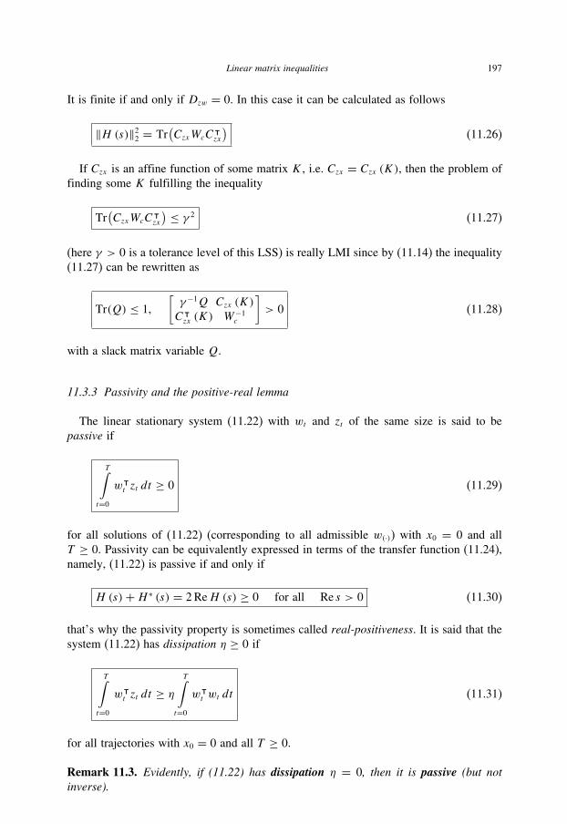
Linear matrix inequalities 197
It is finite if and only if Dzw = 0. In this case it can be calculated as follows
‖H (s)‖22 = Tr(CzxWcC
ᵀzx
)(11.26)
If Czx is an affine function of some matrix K , i.e. Czx = Czx (K), then the problem of
finding some K fulfilling the inequality
Tr(CzxWcC
ᵀzx
) ≤ γ 2 (11.27)
(here γ > 0 is a tolerance level of this LSS) is really LMI since by (11.14) the inequality
(11.27) can be rewritten as
Tr(Q) ≤ 1,
[γ −1Q Czx (K)
Cᵀzx (K) W
−1c
]> 0 (11.28)
with a slack matrix variable Q.
11.3.3 Passivity and the positive-real lemma
The linear stationary system (11.22) with wt and zt of the same size is said to be
passive if
T∫t=0
wᵀt zt dt ≥ 0 (11.29)
for all solutions of (11.22) (corresponding to all admissible w(·)) with x0 = 0 and all
T ≥ 0. Passivity can be equivalently expressed in terms of the transfer function (11.24),
namely, (11.22) is passive if and only if
H (s)+H ∗ (s) = 2ReH (s) ≥ 0 for all Re s > 0 (11.30)
that’s why the passivity property is sometimes called real-positiveness. It is said that the
system (11.22) has dissipation η ≥ 0 if
T∫t=0
wᵀt zt dt ≥ η
T∫t=0
wᵀt wt dt (11.31)
for all trajectories with x0 = 0 and all T ≥ 0.
Remark 11.3. Evidently, if (11.22) has dissipation η = 0, then it is passive (but notinverse).

198 Advanced Mathematical Tools for Automatic Control Engineers: Volume 1
Suppose that there exists a quadratic function V (x) := xᵀPx, P > 0, such that for
all xt and wt, satisfying (11.22), the following inequality holds
d
dtV (xt )− 2wᵀ
t zt + 2ηwᵀt wt ≤ 0 (11.32)
Then, integrating this inequality within [0, T ]-interval with x0 = 0 yields
V (xt )−T∫
t=0
wᵀt zt dt + η
T∫t=0
wᵀt wt dt ≤ 0
and, since,
0 ≤ V (xT ) ≤T∫
t=0
wᵀt zt dt − η
T∫t=0
wᵀt wt dt
we obtain (11.31). So, if (11.32) holds, then one may guarantee the η-dissipation for
(11.22). Simple substitution
d
dtV (xt )= 2x
ᵀt P xt = 2x
ᵀt P [Axt + Bwwt ]
= xᵀt [PA+ AᵀP ] xt + xᵀ
t [PBw]wt + wᵀt [Bᵀ
wP ] xt
and
zt = Czxxt +Dzwwt
into (11.32) implies
(xtwt
)ᵀ [PA+ AᵀP PBw − CzxBᵀwP − Cᵀ
zx 2ηIn×n −(Dᵀzw +Dzw
)]( xtwt
)≤ 0
or, equivalently, as the following LMI
[−PA− AᵀP −PBw + Czx−Bᵀ
wP + Cᵀzx −2ηIn×n +
(Dᵀzw +Dzw
)] ≥ 0 (11.33)
So, if there exists a matrix P = Pᵀ > 0 satisfying (11.33) then the linear system (11.22)
is η-dissipative.
Lemma 11.2. (The positive-real lemma) Under the technical condition
Dᵀzw +Dzw > 2ηIn×n (11.34)

Linear matrix inequalities 199
the sufficient condition of η-dissipativity (11.33) is equivalent to the existence of thepositive definite solution P to the following Riccati inequality
PA+AᵀP+ [PBw − Czx]
[(Dᵀzw +Dzw
)− 2ηIn×n]−1 [
BᵀwP − Cᵀ
zx
] ≤ 0(11.35)
Remark 11.4. It is possible to show that LMI (11.35) is feasible if and only if (11.22) ispassive.
11.3.4 Nonexpansivity and the bounded-real lemma
The linear stationary system (11.22) is said to be nonexpansive if
T∫t=0
zᵀt zt dt ≤T∫
t=0
wᵀt wt dt (11.36)
for all solutions of (11.22) (corresponding to all admissible w(·)) with x0 = 0 and all
T ≥ 0. Nonexpansivity can be equivalently expressed in terms of the transfer function
(11.24), namely, (11.22) is nonexpansive if and only if the following bounded-realcondition holds
H ∗ (s)H (s) ≤ I for all Re s > 0 (11.37)
that is why this condition is sometimes called nonexpansivity. This is sometimes exp-
ressed as
‖H‖∞ ≤ 1 (11.38)
where
‖H‖∞ := sup {λmax (H∗ (s)H (s)) | Re s > 0}
= sup {λmax (H∗ (iω)H (iω)) | ω ∈ (−∞,∞)} (11.39)
Suppose that there exists a quadratic function V (x) := xᵀPx, P > 0, such that for
all xt and wt, satisfying (11.22), the following inequality holds
d
dtV (xt )− 2wᵀ
t wt + 2zᵀt zt ≤ 0 (11.40)
Then, integrating this inequality within the [0, T ]-interval with x0 = 0 yields
V (xt )−T∫
t=0
wᵀt wt dt +
T∫t=0
zᵀt zt dt ≤ 0
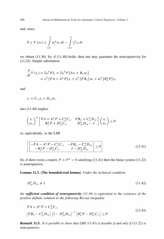
200 Advanced Mathematical Tools for Automatic Control Engineers: Volume 1
and, since,
0 ≤ V (xT ) ≤T∫
t=0
wᵀt wt dt −
T∫t=0
zᵀt zt dt
we obtain (11.36). So, if (11.40) holds, then one may guarantee the nonexpansivity for
(11.22). Simple substitution
d
dtV (xt )= 2x
ᵀt P xt = 2x
ᵀt P [Axt + Bwwt ]
= xᵀt [PA+ AᵀP ] xt + xᵀ
t [PBw]wt + wᵀt [Bᵀ
wP ] xt
and
zt = Czxxt +Dzwwt
into (11.40) implies
(xtwt
)ᵀ [PA+ AᵀP + Cᵀ
zxCzx PBw + CᵀzxDzw
BᵀwP +Dᵀ
zwCzx DᵀzwDzw − I
](xtwt
)≤ 0
or, equivalently, as the LMI
[−PA− AᵀP − CᵀzxCzx −PBw − Cᵀ
zxDzw−Bᵀ
wP −DᵀzwCzx I −Dᵀ
zwDzw
]≥ 0 (11.41)
So, if there exists a matrix P = Pᵀ > 0 satisfying (11.41) then the linear system (11.22)
is nonexpansive.
Lemma 11.3. (The bounded-real lemma) Under the technical condition
DᵀzwDzw �= I (11.42)
the sufficient condition of nonexpansivity (11.36) is equivalent to the existence of thepositive definite solution to the following Riccati inequality
PA+ AᵀP + CᵀzxCzx[
PBw − CᵀzxDzw
] [I −Dᵀ
zwDzw]−1 [
BᵀwP −Dᵀ
zwCzx] ≤ 0
(11.43)
Remark 11.5. It is possible to show that LMI (11.43) is feasible if and only if (11.22) isnonexpansive.
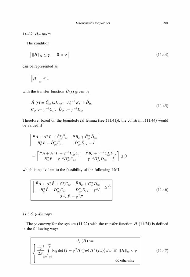
Linear matrix inequalities 201
11.3.5 H∞ norm
The condition
‖H‖∞ ≤ γ, 0 < γ (11.44)
can be represented as
∥∥∥H∥∥∥∞≤ 1
with the transfer function H (s) given by
H (s) = Czx (sIn×n − A)−1 Bw + DzwCzx := γ −1Czx, Dzx := γ −1Dzx
(11.45)
Therefore, based on the bounded-real lemma (see (11.41)), the constraint (11.44) would
be valued if
[PA+ AᵀP + Cᵀ
zxCzx PBw + CᵀzxDzw
BᵀwP + Dᵀ
zwCzx DᵀzwDzw − I
]
=[PA+ AᵀP + γ −2Cᵀ
zxCzx PBw + γ −2CᵀzxDzw
BᵀwP + γ −2Dᵀ
zwCzx γ −2DᵀzwDzw − I
]≤ 0
which is equivalent to the feasibility of the following LMI
[PA+ AᵀP + Cᵀ
zxCzx PBw + CᵀzxDzw
Bᵀw P +Dᵀ
zwCzx DᵀzwDzw − γ 2I
]≤ 0
0 < P = γ 2P
(11.46)
11.3.6 γ -Entropy
The γ -entropy for the system (11.22) with the transfer function H (11.24) is defined
in the following way:
Iγ (H) :=⎧⎪⎪⎨⎪⎪⎩−γ 2
2π
∞∫ω=−∞
log det(I − γ 2H (jω)H ∗ (jω)
)dω if ‖H‖∞< γ
∞ otherwise
(11.47)
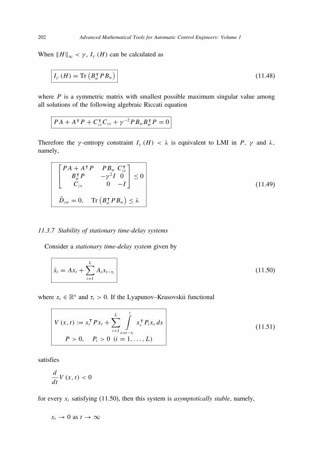
202 Advanced Mathematical Tools for Automatic Control Engineers: Volume 1
When ‖H‖∞ < γ , Iγ (H) can be calculated as
Iγ (H) = Tr(BᵀwPBw
)(11.48)
where P is a symmetric matrix with smallest possible maximum singular value among
all solutions of the following algebraic Riccati equation
PA+ AᵀP + CᵀzxCzx + γ −2PBwB
ᵀwP = 0
Therefore the γ -entropy constraint Iγ (H) < λ is equivalent to LMI in P, γ and λ,
namely,
⎡⎣PA+ AᵀP PBw C
ᵀzx
BᵀwP −γ 2I 0
Czx 0 −I
⎤⎦ ≤ 0
Dzw = 0, Tr(BᵀwPBw
) ≤ λ(11.49)
11.3.7 Stability of stationary time-delay systems
Consider a stationary time-delay system given by
xt = Axt +L∑i=1
Aixt−τi (11.50)
where xt ∈ Rn and τi > 0. If the Lyapunov–Krasovskii functional
V (x, t) := xᵀt P xt +
L∑i=1
t∫s=t−τi
xᵀs Pixs ds
P > 0, Pi > 0 (i = 1, . . . , L)
(11.51)
satisfies
d
dtV (x, t) < 0
for every xt satisfying (11.50), then this system is asymptotically stable, namely,
xt → 0 as t →∞

Linear matrix inequalities 203
This can be verified by the simple calculation
d
dtV (x, t) = yᵀ
t Wyt
W :=
⎡⎢⎢⎢⎢⎢⎢⎣
[PA+ AᵀP +
L∑i=1
Pi
]PA1 · · · PAL
Aᵀ1 P −P1 · · · 0...
.... . .
...
AᵀLP 0 · · · −PL
⎤⎥⎥⎥⎥⎥⎥⎦
yᵀt = (
xt , xt−τ1 , · · ·, xt−τL)
(11.52)
providing that the matrices P > 0, Pi > 0 (i = 1, . . . , L) are satisfying LMI W < 0.
11.3.8 Hybrid time-delay linear stability
Let us consider the following hybrid time-delay linear system given by
x1 (t) = A0x1 (t)+ A1x2 (t − τ)x2 (t) = A2x1 (t)+ A3x2 (t − τ)x1 (0)= x10, x2 (θ) = ψ (θ) θ ∈ [−τ, 0]
(11.53)
where A0 ∈ Rn×n, A1 ∈ Rn×m, A2 ∈ Rm×n, A3 ∈ Rm×m are the given matrices of
the corresponding dimensions and ψ : R1 → Rm is a function from C [−τ, 0]. Noticethat the first equation in (11.53) is an ordinary differential equation and the second one
is a difference equation in continuous time that justifies the name “hybrid time-delay
system”.
We are interested in finding the conditions of asymptotic stability for this system.
Following Rasvan (1975), let us introduce the energetic (Lyapunov–Krasovskii-type)
functional
V (x1(t), x2) := xᵀ1 (t) P x1 (t)+
t∫θ=t−τ
xᵀ2 (θ) Sx2 (θ) dθ
0 ≤ P = Pᵀ ∈ Rn×n, 0 ≤ S = Sᵀ ∈ Rm×m
(11.54)
Its derivative on the trajectories of (11.53) is as follows:
d
dtV (x1(t), x2) = zᵀ (t)Wz (t) (11.55)

204 Advanced Mathematical Tools for Automatic Control Engineers: Volume 1
where
zᵀ (t) := (x1(t), x2 (t − τ)) (11.56)
and
W =[A
ᵀ0 P + PA0 + Aᵀ
2 SA2 PA1 + Aᵀ2 SA3
Aᵀ1 P + Aᵀ
3 SA2 Aᵀ3 SA3 − S
](11.57)
As it is shown in Rasvan (1975), the existence of the matrices P and S such that the
following LMI holds
W < 0
implies the asymptotic stability of (11.53).
11.4 Optimization problems with LMI constraints
11.4.1 Eigenvalue problem (EVP)
The eigenvalue problem (EVP) consists of the minimization of the maximum eigenvalue
of an n× n matrix A(P ) that depends affinely on a variable, subject to LMI (symmetric)
constraint B(P ) > 0, i.e.,
λmax(A(P ))→ minP=Pᵀ
B(P ) > 0(11.58)
This problem can be equivalently represented as follows:
λ→ minλ,P=Pᵀ[
λIn×n − A(P ) > 0 0
0 B(P )
]> 0
(11.59)
11.4.2 Tolerance level optimization
The tolerance level optimization problem can be represented in the following manner:
γ → min0<γ,P=Pᵀ
PA+ AᵀP + CᵀC + γ −1PBBᵀP < 0
(11.60)

Linear matrix inequalities 205
Equivalently, it can be rewritten as an optimization problem with LMI constraints:
γ → min0<γ,0<P=Pᵀ
⎡⎣−PA− AᵀP − CᵀC PB 0
BᵀP γ I 0
0 0 P
⎤⎦ > 0
(11.61)
11.4.3 Maximization of the quadratic stability degree
The quadratic stability degree of a stable n×n matrix A is defined as a positive value
α satisfying the matrix inequality
AᵀP + PA < −αP
for some positive definite matrix P . The problem of the maximization of the quadratic
stability degree consists of the following optimization problem
α→ max0<α,0<P=Pᵀ
AᵀP + PA+ αP < 0
(11.62)
which can be expressed as an optimization with LMI constraint, namely,
α→ max0<α,P=Pᵀ[−AᵀP − PA− αP 0
0 P
]> 0
(11.63)
11.4.4 Minimization of linear function Tr (CPCᵀ) under the Lyapunov-typeconstraint
Lemma 11.4. (Polyak & Sherbakov (2002)) Let
1. the matrix A ∈ Rn×n be Hurwitz;2. the pair (A,B) be controllable, i.e. there exists a matrix K such that (A+KB) is
Hurwitz.Then for any matrix C ∈ Rk×n the solution of the problem
Tr (CPCᵀ)→ minP≥0
(11.64)
under the constraint
AP + PAᵀ + BBᵀ ≤ 0 (11.65)

206 Advanced Mathematical Tools for Automatic Control Engineers: Volume 1
is attained on the Lyapunov matrix equation
AP ∗ + P ∗Aᵀ + BBᵀ = 0 (11.66)
Proof. Suppose that the minimizing solution satisfies the equation
AP + PAᵀ + BBᵀ = −Q < 0
Then, by Lemma 9.1,
P =∞∫
t=0
eAt (Q+ BBᵀ) eAᵀt dt ≥
∞∫t=0
eAtBBᵀeAᵀt dt = P ∗
and, hence,
Tr (CPCᵀ) = Tr (CP ∗Cᵀ)+ Tr
⎛⎝C ∞∫
t=0
eAtQeAᵀt dtCᵀ
⎞⎠≥ Tr (CP ∗Cᵀ)
This means that P ∗ is a minimizer. Lemma is proven. �
11.4.5 The convex function log det A−1 (X) minimization
First notice that log det A−1 (X) is a convex function of A. We will encounter the
following:
log detA−1 (X)→ minX=Xᵀ∈Rn×n
(11.67)
subjected to the following constraints
A(X) > 0, B(X) > 0 (11.68)
where A(X), B(X) are symmetric matrices that depend affinely on X.
Example 11.1. As an example of the problem (11.67)–(11.68) consider the following:find a minimal ellipsoid
ε := {z | zᵀPz ≤ 1} , P > 0 (11.69)
containing the set of given points vi (i = 1, . . . , L), i.e. vi ∈ ε. Since the volume of ε isproportional to (det P)−1/2, minimizing log det P−1 is the same as minimizing the volumeof ε, this problem is converted into the following:
log det P−1 → minP∈Rn×n
P > 0, vᵀi P vi ≤ 1
(11.70)

Linear matrix inequalities 207
11.5 Numerical methods for LMI resolution
11.5.1 What does it mean “to solve LMI”?
There exist several efficient methods for LMI resolution. By “solve an LMI” we
mean here:
• determine whether or not the LMI (or the corresponding problem) is feasible;• if it is, compute a feasible point with “an objective value” that exceeds the global
minimum by less than some prespecified accuracy.
What does “an objective value” mean? It depends on each concrete problem to be
solved. Here we will assume that the problem we are solving has at least one “optimal
point”, i.e., the constraints are feasible.
To realize the numerical methods described below, first, let us represent the matrix X ∈Rn×n as the corresponding extended vector x ∈ Rn
2
obtained by the simple implementation
of the operator col, that is,
x := colX (11.71)
11.5.2 Ellipsoid algorithm
In a feasible problem, we may consider any feasible point as being optimal. The basicidea of the ellipsoid algorithm is as follows:
1. One may start with an ellipsoid that is guaranteed to contain an optimal point.
2. Then the cutting plane for our problem is computed which passes through the center
point x(0) of the initial ellipsoid ε(0). This means that we need to find a nonzero vector
g(0) (namely, a vector orthogonal to the plane to be computed) such that an optimal
point lies in the half-space{z ∈ Rn
2 | g(0)ᵀ (z− x(0)) < 0
}(11.72)
(Below, we shall present some examples of how to calculate g(0) in some concrete
problems.)
3. After this we may conclude that the sliced half-ellipsoid
ε(0) ∩{z ∈ Rn
2 | g(0)ᵀ (z− x(0)) < 0
}contains an optimal point.
4. Then we compute the ellipsoid ε(1) of a minimum volume that contains this sliced
half-ellipsoid. This ellipsoid ε(1) is guaranteed to contain an optimal point, but its
volume is expected to be less than the volume of the initial ellipsoid ε(0).
5. The process is then iterated.
More explicitly, this algorithm may be described as follows. Any ellipsoid ε may be
associated with some positive definite matrix, that is,
ε :={z ∈ Rn
2 | (z− a)ᵀA−1 (z− a) ≤ 1}
(11.73)

208 Advanced Mathematical Tools for Automatic Control Engineers: Volume 1
where A = Aᵀ > 0. The minimum volume ellipsoid ε containing the sliced half-ellipsoid
{z ∈ Rn
2 | (z− a)ᵀA−1 (z− a) ≤ 1, gᵀ (z− a) < 0}
is given by the matrix A and the vector a, namely,
ε :={z ∈ Rn
2 | (z− a)ᵀ A−1 (z− a) ≤ 1}
a = a − Ag
m+ 1, m := n2 > 1
A = m2
m2 − 1
(A− 2
m+ 1AggᵀA
)
g = g√gᵀAg
(11.74)
(In the case of one variable (m = 1) the minimal length interval containing a half-interval
is the half-interval itself.) So, the ellipsoid algorithm starts with the initial points x(0) and
the initial matrix A(0). Then for each intermediate pair x(k) and A(k) (k = 0, 1, 2, . . .)
one may compute a vector g(k) and then calculate
x(k+1) = x(k) − A(k)g
m+ 1, m := n2 > 1
A(k+1) = m2
m2 − 1
(A(k) − 2
m+ 1A(k)ggᵀA(k)
)
g = g(k)√g(k)ᵀA(k)g(k)ᵀ
It turns out that the volume vol ε(k) = det A(k) of these ellipsoids decreases geometrically,
that is,
vol ε(k+1) ≤ e−k/2m vol ε(k)
This means that the recursion above generates a sequence of ellipsoids that is guaranteed
to contain an optimal point and converges to it geometrically. It may be proven that
this algorithm converges more quickly, namely, in “polynomial time” (see Nesterov &
Nemirovsky (1994) and references within).
The next examples illustrate the rule of selection of the nonzero orthogonal vector g
orthogonal to the cutting plane which is specified for each concrete problem.

Linear matrix inequalities 209
Example 11.2. If LMI is represented in the form
F (x) := F0 +m∑i=1
xiFi > 0 (11.75)
where Fi (i = 0, 1, 2, . . . , m) are symmetric matrices. If x is infeasible, this means thatthere exists a nonzero vector u such that
uᵀF (x) u ≤ 0
Define g = (g1, . . . , gm)ᵀ by
gi = −uᵀFiu (11.76)
Then for any z satisfying gᵀ (z− x) ≥ 0 it follows
uᵀF (z) u= uᵀ[F0 +
m∑i=1
ziFi
]u = uᵀF0u+
m∑i=1
ziuᵀFiu
= uᵀF0u−m∑i=1
zigi = uᵀF0u− gᵀz = uᵀF0u+ gᵀx − gᵀ (z− x)
= uᵀF (x) u− gᵀ (z− x) ≤ 0
So, any feasible point belongs to the half-plane
{z ∈ Rm | gᵀ (z− x) < 0}
or, in other words, this g, given by (11.76), is a cutting plane for this LMI problem atthe point x.
Example 11.3. If we deal with the minimization problem of linear function cᵀx subjectedLMI (11.75), that is,
cᵀx → minx∈Rn
2
F (x) := F0 +m∑i=1
xiFi > 0
we encounter two possible situations:
1. x is infeasible, i.e., F (x) ≤ 0; in this case g can be taken as in the previous example(11.76) since we are discarding the half-plane{
z ∈ Rn2 | gᵀ (z− x) > 0
}because all such points are infeasible;
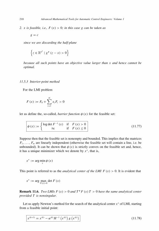
210 Advanced Mathematical Tools for Automatic Control Engineers: Volume 1
2. x is feasible, i.e., F (x) > 0; in this case g can be taken as
g = csince we are discarding the half-plane
{z ∈ Rn
2 | gᵀ (z− x) > 0}
because all such points have an objective value larger than x and hence cannot beoptimal.
11.5.3 Interior-point method
For the LMI problem
F (x) := F0 +m∑i=1
xiFi > 0
let us define the, so-called, barrier function φ (x) for the feasible set:
φ (x) :={log det F−1 (x) if F (x) > 0
∞ if F (x) ≤ 0(11.77)
Suppose then that the feasible set is nonempty and bounded. This implies that the matrices
F1, . . . , Fm are linearly independent (otherwise the feasible set will contain a line, i.e. be
unbounded). It can be shown that φ (x) is strictly convex on the feasible set and, hence,
it has a unique minimizer which we denote by x∗, that is,
x∗ := argminxφ (x)
This point is referred to as the analytical center of the LMI F (x) > 0. It is evident that
x∗ := arg maxF(x)>0
det F (x)
Remark 11.6. Two LMIs F (x) > 0 and T ᵀF (x) T > 0 have the same analytical centerprovided T is nonsingular.
Let us apply Newton’s method for the search of the analytical center x∗ of LMI, starting
from a feasible initial point:
x(k+1) = x(k) − α(k)H−1(x(k)
)g(x(k)
)(11.78)
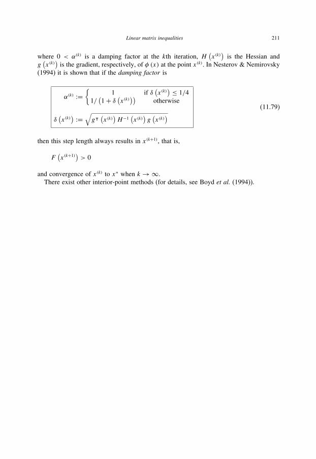
Linear matrix inequalities 211
where 0 < α(k) is a damping factor at the kth iteration, H(x(k)
)is the Hessian and
g(x(k)
)is the gradient, respectively, of φ (x) at the point x(k). In Nesterov & Nemirovsky
(1994) it is shown that if the damping factor is
α(k) :={
1 if δ(x(k)
) ≤ 1/4
1/(1+ δ (x(k))) otherwise
δ(x(k)
) :=√gᵀ (
x(k))H−1
(x(k)
)g(x(k)
) (11.79)
then this step length always results in x(k+1), that is,
F(x(k+1)
)> 0
and convergence of x(k) to x∗ when k→∞.
There exist other interior-point methods (for details, see Boyd et al. (1994)).

This page intentionally left blank

12 Miscellaneous
Contents
12.1 �-matrix inequalities . . . . . . . . . . . . . . . . . . . . . . . . . . . . . 213
12.2 Matrix Abel identities . . . . . . . . . . . . . . . . . . . . . . . . . . . . 214
12.3 S-procedure and Finsler lemma . . . . . . . . . . . . . . . . . . . . . . . . 216
12.4 Farkaš lemma . . . . . . . . . . . . . . . . . . . . . . . . . . . . . . . . . 222
12.5 Kantorovich matrix inequality . . . . . . . . . . . . . . . . . . . . . . . . 226
12.1 �-matrix inequalities
Lemma 12.1. For any matrices X, Y ∈ Rn×m and any symmetric positive definite matrix� ∈ Rn×n the following inequalities hold
XT Y + Y TX ≤ XT�X + Y T�−1Y (12.1)
and
(X + Y )ᵀ (X + Y ) ≤ XT (In×n +�)X + Y T (In×n +�−1)Y (12.2)
Proof. Define
H := XT�X + Y T�−1Y −XT Y − Y TX
Then for any vector v we may introduce the vectors
v1 := �1/2Xv and v2 := �−1/2Yv
which implies
vTHv = vT1 v1 + vT2 v2 − vT1 v2 − vT2 v1 = ‖v1 − v2‖2 ≥ 0 (12.3)
or, in matrix form:
H ≥ 0
which is equivalent to (12.3). The inequality (12.2) is a direct consequence of (12.1). �
213
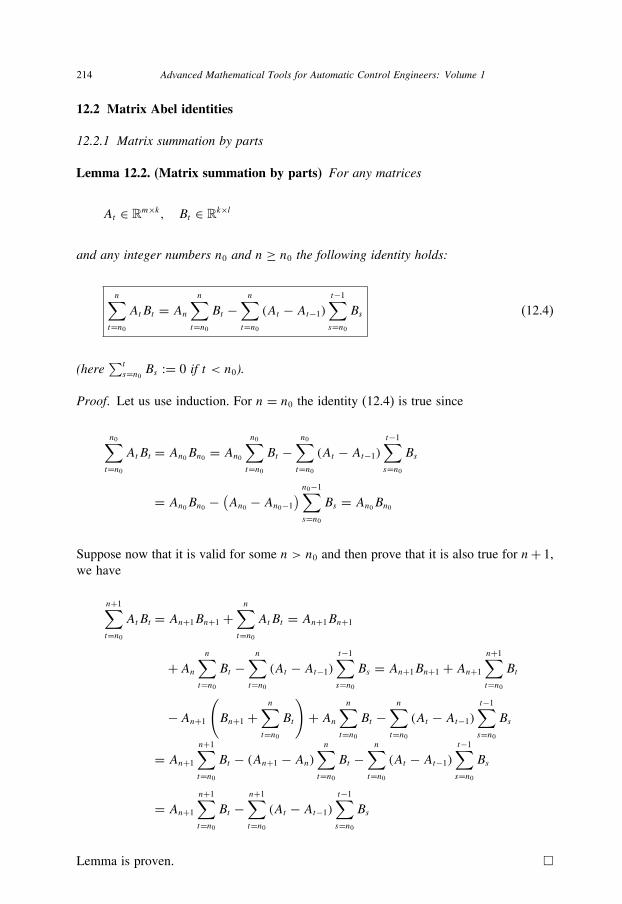
214 Advanced Mathematical Tools for Automatic Control Engineers: Volume 1
12.2 Matrix Abel identities
12.2.1 Matrix summation by parts
Lemma 12.2. (Matrix summation by parts) For any matrices
At ∈ Rm×k, Bt ∈ Rk×l
and any integer numbers n0 and n ≥ n0 the following identity holds:
n∑t=n0AtBt = An
n∑t=n0Bt −
n∑t=n0(At − At−1)
t−1∑s=n0Bs (12.4)
(here∑t
s=n0 Bs := 0 if t < n0).
Proof. Let us use induction. For n = n0 the identity (12.4) is true since
n0∑t=n0AtBt = An0Bn0 = An0
n0∑t=n0Bt −
n0∑t=n0(At − At−1)
t−1∑s=n0Bs
= An0Bn0 −(An0 − An0−1
) n0−1∑s=n0Bs = An0Bn0
Suppose now that it is valid for some n > n0 and then prove that it is also true for n+ 1,
we have
n+1∑t=n0AtBt = An+1Bn+1 +
n∑t=n0AtBt = An+1Bn+1
+Ann∑t=n0Bt −
n∑t=n0(At − At−1)
t−1∑s=n0Bs = An+1Bn+1 + An+1
n+1∑t=n0Bt
−An+1
(Bn+1 +
n∑t=n0Bt
)+ An
n∑t=n0Bt −
n∑t=n0(At − At−1)
t−1∑s=n0Bs
= An+1
n+1∑t=n0Bt − (An+1 − An)
n∑t=n0Bt −
n∑t=n0(At − At−1)
t−1∑s=n0Bs
= An+1
n+1∑t=n0Bt −
n+1∑t=n0(At − At−1)
t−1∑s=n0Bs
Lemma is proven. �
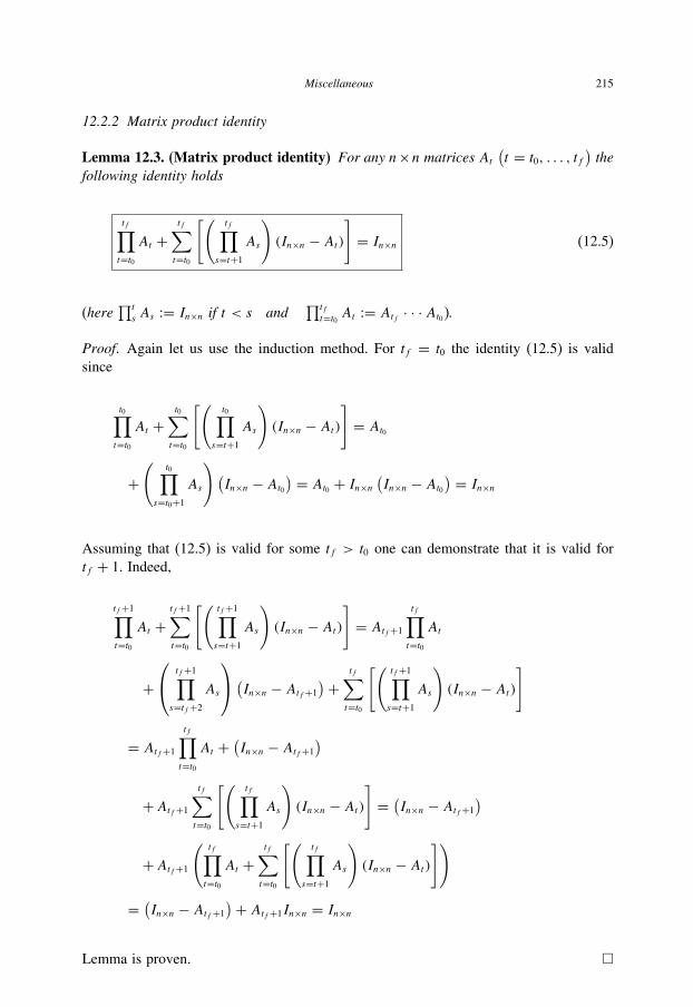
Miscellaneous 215
12.2.2 Matrix product identity
Lemma 12.3. (Matrix product identity) For any n×n matrices At(t = t0, . . . , tf
)the
following identity holds
tf∏t=t0At +
tf∑t=t0
[(tf∏
s=t+1
As
)(In×n − At)
]= In×n (12.5)
(here∏t
s As := In×n if t < s and∏tft=t0 At := Atf · · · At0 ).
Proof. Again let us use the induction method. For tf = t0 the identity (12.5) is valid
since
t0∏t=t0At +
t0∑t=t0
[(t0∏
s=t+1
As
)(In×n − At)
]= At0
+(
t0∏s=t0+1
As
)(In×n − At0
) = At0 + In×n (In×n − At0) = In×n
Assuming that (12.5) is valid for some tf > t0 one can demonstrate that it is valid for
tf + 1. Indeed,
tf+1∏t=t0At +
tf+1∑t=t0
[(tf+1∏s=t+1
As
)(In×n − At)
]= Atf+1
tf∏t=t0At
+⎛⎝ tf+1∏s=tf+2
As
⎞⎠(In×n − Atf+1
)+ tf∑t=t0
[(tf+1∏s=t+1
As
)(In×n − At)
]
= Atf+1
tf∏t=t0At +
(In×n − Atf+1
)
+Atf+1
tf∑t=t0
[(tf∏
s=t+1
As
)(In×n − At)
]= (In×n − Atf+1
)
+Atf+1
(tf∏t=t0At +
tf∑t=t0
[(tf∏
s=t+1
As
)(In×n − At)
])
= (In×n − Atf+1
)+ Atf+1In×n = In×n
Lemma is proven. �

216 Advanced Mathematical Tools for Automatic Control Engineers: Volume 1
12.3 S-procedure and Finsler lemma
12.3.1 Daneš’ theorem
Let F(x) = xᵀFx and G(x) = xᵀGx be real quadratic forms with F,G ∈ Rn×n.Consider the mapping Rn → R2 defined by
η1 = F(x), η2 = G(x) (12.6)
which transforms any point from Rn into the real plane R2. The following theorem
represents the important geometric result (Daneš 1972) arising in the theory of quadratic
forms.
Theorem 12.1. (Daneš’ theorem) The range
P := {(η1, η2) ∈ R2 | η1 = F(x), η2 = G(x), x ∈ Rn
}(12.7)
of the transformation (12.6) is a convex cone, i.e., the set P together with y ∈ R2 containsalso λy for any λ ≥ 0 (P is a cone) and together with vectors y(1), y(2) ∈ R2 containsalso y = αy(1) + (1− α) y(2) for any α ∈ [0, 1] (P is a convex set).
Proof. Let y = (η1, η2)ᵀ be a point in R2.
(a) Obviously, P is a cone since there exists a point x ∈ Rn such that
y = (F(x), G(x))
Then
λy =(F(√λx), G(
√λx)
)This means that λy ∈ P .
(b) Show now that P is a convex set. Let
y(1) = (F(x(1)), G(x(1))
), y(2) = (
F(x(2)), G(x(2)))
In other words, we need to show that for any point y(0) =(η(0)1 , η
(0)2
)ᵀ ∈ [y(1), y(2)
]there exists a vector x(0) ∈ Rn such that
y(0) = (F(x(0)), G(x(0))
)Let Aη1 +Bη2 = C be the line L crossing the points y(1) and y(2). Consider the function
ϕ (ξ1, ξ2) := AF(ξ1x(1) + ξ2x(2))+ BG(ξ1x(1) + ξ2x(2))
Miscellaneous 217
and the mapping R2 → R2:
y = (F(ξ1x(1) + ξ2x(2)), G(ξ1x(1) + ξ2x(2))
)Since the points (1, 0) and (0, 1) are transformed to the points y(1) and y(2), respectively,
then in view of the properties
F(x) = F(−x), G(x) = G(−x)
the points (−1, 0) and (0,−1) are transformed also to the same points y(1) and y(2).
Consider then the set M defined as
M := {(ξ1, ξ2) : ϕ (ξ1, ξ2) = C}
This set is nonempty since, evidently, (±1, 0), (0,±1) ∈ M. The function ϕ (ξ1, ξ2) may
be represented as
ϕ (ξ1, ξ2) = αξ 21 + 2βξ1ξ2 + γ ξ 22where α, β, γ are some real numbers. If α = β = γ = 0 (and, hence, C = 0), then Mis the complete plane R2. Let |α| + |β| + |γ | > 0. Denote δ := αγ − β2. The curve
ϕ (ξ1, ξ2) = C is
• an ellipse, if δ > 0;• a hyperbola, if δ < 0;• a pair of parallel direct lines (maybe coincided), if δ = 0.
Notice also that this curve is symmetric with respect to an origin (0, 0). So, either
M is a connected set or it is represented by two sets symmetric with respect to the
origin.
Case 1: M is a connected set. Then the points (1, 0) and (0, 1) may be connected by a
continuous curve without leaving the set M. Let ξ1 = ξ1 (t), ξ2 = ξ2 (t) (0 ≤ t ≤ 1) be
this connecting curve and y = y(t) be the corresponding continuous line. Obviously, this
line lies in L and connects the points y(1) and y(2).
Case 2: M is two sets symmetric with respect the origin. In this case the points (1, 0)
and (0, 1) lie in different connected parts of the curve M = M1∪M2, say, (1, 0) ∈ M1
and (0, 1) ∈ M2. Then by symmetricity of the curve M with respect the origin, the
points (1, 0) and (−1, 0) belong to the different connected curves, i.e., (−1, 0) ∈ M2.
So, we may connect the points (−1, 0) ∈ M2 and (0, 1) ∈ M2 (whose images are y(1)
and y(2), respectively) by a continuous curve ξ1 = ξ1 (t), ξ2 = ξ2 (t) (0 ≤ t ≤ 1) staying
in M2 such that y = y(t) is again a continuous line lying in L.In both cases y(t) ∈ L (0 ≤ t ≤ 1). This curve “covers” the interval
[y(1), y(2)
], that
is, for any point y(0) ∈ [y(1), y(2)
]there exists t0 ∈ [0, 1], such that y(0) = y (t0). The
point y(0) = (ξ1 (t0), ξ2 (t0)) will correspond to the vector x(0) = ξ1 (t0) x(1) + ξ2 (t0) x(2)verifying
y(0) = (F(x(0)), G(x(0))
)Theorem is proven. �

218 Advanced Mathematical Tools for Automatic Control Engineers: Volume 1
12.3.2 S-procedure
In this subsection we follow Gelig et al. (1978).
Theorem 12.2. (S-procedure for two quadratic forms) Let
F(x) ≥ 0 for all x where G(x) ≥ 0 (12.8)
Then there exist real numbers
τ1 ≥ 0, τ2 ≥ 0, τ1 + τ2 > 0 (12.9)
such that for all x ∈ Rn
τ1F(x)− τ2G(x) ≥ 0 (12.10)
Proof. By Daneš’ theorem the set P is a convex cone. Define Q as
Q := {(η1, η2) : η1 < 0, η2 ≥ 0}
By the assumptions of this theorem P ∩Q = ∅. Since P and Q are both convex cones,
there exists (loosely) a plane separating them, that is, there exists τ1, τ1 (nonobligatory
nonnegative) |τ1| + |τ2| > 0 such that
τ1η1 − τ2η2 ≤ 0 if (η1, η2) ∈ Q1η1 − τ2η2 ≥ 0 if (η1, η2) ∈ P (12.11)
Taking into account that (−1, 0) ∈ Q and (−ε, 1) ∈ Q (ε > 0), then τ1 (−1) ≤ 0 implies
τ1 ≥ 0 and −τ1ε − τ2 ≤ 0
Taking ε → 0 gives τ2 ≥ 0. Since (F(x),G(x)) ∈ P for any x ∈ Rn, then the second
inequality in (12.11) leads to (12.10). Theorem is proven. �
Corollary 12.1. Let there exist a vector x(0) such that
G(x(0)) > 0 (12.12)
Then the following two claims are equivalent:
1.
F(x) ≥ 0 for all x where G(x) ≥ 0
2. there exists τ ≥ 0 such that
F(x)− τG(x ≥ 0) for all x ∈ Rn (12.13)

Miscellaneous 219
Proof. Since (12.10) holds it is sufficient to show that τ1 > 0. Suppose the converse,
namely, that τ1 = 0. Then by (12.10) it follows that τ2G(x) ≤ 0 for all x, and hence,
particularly, for x = x(0), that implies τ2 = 0. So, τ1 = τ2 = 0, but this contradicts the
condition (12.9). Hence, τ1 > 0. Defining τ := τ2/τ1 we obtain the main result. Corollary
is proven. �
Corollary 12.2. (The case of the strict basic inequality) Again let there exist a vectorx(0) such that
G(x(0)) > 0
Then the following two claims are equivalent:
1.
F(x) > 0 for all x where G(x) ≥ 0, x �= 0 (12.14)
2. there exists τ ≥ 0 such that
F(x)− τG(x) > 0 for all x ∈ Rn, x �= 0 (12.15)
Proof. Evidently, (12.15) implies (12.14). Indeed, if τ = 0, then F(x) > 0 for any x �= 0.
If τ > 0, then F(x) > τG (x) and F(x) > 0 for any x �= 0 such that G(x) ≥ 0. Now, let
(12.14) hold. Define the set J := {x : ‖x‖ = 1, G(x) ≥ 0}. It is bounded and closed. So,
by (12.14) F(x) > 0 for any x ∈ J . Hence, infx∈J
F(x) = ε > 0, and, as a result, F(x)−ε ≥ 0 for any x ∈ J . If G(x) ≥ 0, x �= 0, then
x
‖x‖ ∈ J . That’s why F(x
‖x‖)−ε ≥ 0,
or equivalently, F(x)− ε ‖x‖2 ≥ 0. So, F(x) := F(x)− ε ‖x‖2 ≥ 0 under G(x) ≥ 0 and
the previous Corollary (12.1) there exists τ ≥ 0 such that F(x) − ε ‖x‖2 − τG(x) ≥ 0.
Hence, F(x)− τG(x) ≥ ε ‖x‖2 > 0. Corollary is proven. �
Remark 12.1. The claim, analogous to (12.2) where nonstrict constraint G(x) ≥ 0 ischanged to the strict one, i.e., G(x) > 0, is not correct which can be shown with a simplecounterexample.
The following matrix interpretation of Theorem 12.2 takes place.
Theorem 12.3. Let inequalities
Gi (x) := xᵀGix ≤ αi (i = 1, . . . , m) (12.16)
imply
F(x) := xᵀFx ≤ α0 (12.17)

220 Advanced Mathematical Tools for Automatic Control Engineers: Volume 1
where αi (i = 0, 1, . . . , m) are some real numbers. If there exists τi ≥ 0 (i = 1, . . . , m)
such that
F ≤m∑i=1
τiGi , α0 ≥m∑i=1
τiαi (12.18)
then (12.16) implies (12.17). Inversely, if (12.16) implies (12.17) and, additionally, oneof the following conditions is fulfilled:1.
m = 1
2.
m = 2, n ≥ 3
and there exists a vector x(0), μ1, μ2 such that
Gi (x(0)) < αi (i = 1, 2)
μ1G1 + μ2G2 > 0
then there exists τi ≥ 0 (i = 1, . . . , m) such that (12.18) holds.For m > 2 the analogue result is not true.
Proof. Sufficiency is trivial. Necessity follows from the previous Theorem 12.2 and
Corollaries 12.1 and 12.2. The simple counterexample may show that this theorem is not
valid for m > 2. �
12.3.3 Finsler lemma
The following statement is a partial case of Theorems 12.2 and 12.3.
Lemma 12.4. (Finsler 1937) Let F(x) := xᵀFx ≥ 0 (or strictly > 0) for all x ∈ Rn,
x �= 0 and such that
G(x) := xᵀGx = 0 (12.19)
Then there exists a real τ such that
F + τG ≥ 0 (or strictly > 0) (12.20)
Proof. This lemma is a partial case of Corollary 12.2 if we can show that in here
the assumption (12.12) is not essential. Indeed, if (12.12) holds then Corollary 12.2
implies (12.20). If x(0) does not exist, where G(x(0)) > 0, we deal only with two
situations:
(a) there exist x(0) where G(x(0)) < 0,
(b) G(x) = 0 for all x.

Miscellaneous 221
In case (a) changing G to (−G) we obtain the previous situation when (12.12) holds. In
case (b) (12.20) holds automatically. �
Below we will illustrate the role of the Finsler lemma in the quadratic stabilization
analysis (Polyak & Sherbakov 2002). Consider the linear plant
x = Ax + Bu (12.21)
with the linear feedback given by
u = Kx (12.22)
The corresponding closed-loop system is
x = AclxAcl := A+ BK (12.23)
The quadratic form V (x) = xᵀPx will be the Lyapunov function for (12.23) then and
only then when
AᵀclP + PAcl < 0, P > 0
or, equivalently, when there exist matrices K and P > 0 such that
(A+ BK)ᵀ P + P (A+ BK) < 0 (12.24)
This relation represents a nonlinear matrix inequality with respect to two matrices K
and P. Fortunately, the variable changing
Y := KQ, Q := P−1 (12.25)
transforms (12.24) into a linear one by pre- and post-multiplying (12.24) by Q:
QAᵀ + AQ+ YᵀBᵀ + BY < 0, Q > 0 (12.26)
Using the Finsler lemma 12.4 the variable Y may be excluded from (12.26). Indeed, the
quadratic function
F(x) := xᵀ (YᵀBᵀ + BY) x = 2 (Bᵀx, Yx)
is equal to zero at the subspace Bᵀx = 0, or when
G(x) := (Bᵀx, Bᵀx) = xᵀ (BBᵀ) x = 0

222 Advanced Mathematical Tools for Automatic Control Engineers: Volume 1
Supposing additionally that G(x(0)) > 0 for some x(0) (but this is not a real constraint)
Lemma 12.4 implies that there exists a real τ such that
F(x)+ τG(x) ≥ 0
that is,
YᵀBᵀ + BY ≥ −τBBᵀ
We may take τ > 0 since BBᵀ ≥ 0. So, (12.26) implies
QAᵀ + AQ− τBBᵀ ≤ QAᵀ + AQ+ YᵀBᵀ + BY < 0, Q > 0
But the left inequality is reachable if we take
Y := −τ2Bᵀ
Since K = YQ−1 does not depend on τ , we may take τ = 2 and obtain the following
result.
Claim 12.1. If Q is the solution of the Lyapunov inequality
QAᵀ + AQ− 2BBᵀ < 0
then the regulator (12.22) with
K = −BᵀQ−1
stabilizes the system (12.21) and the quadratic function
V (x) = xᵀQ−1x
is the Lyapunov function for the closed system (12.23).
12.4 Farkaš lemma
12.4.1 Formulation of the lemma
The Farkaš lemma (Farkaš 1902) is a classical result belonging to a class of the,
so-called, “theorem of the alternative” which characterizes the optimality conditions of
different optimization problems.

Miscellaneous 223
Lemma 12.5. (Farkaš 1902) Let A be a real m × n matrix and c be a real nonzerovector. Then
1. either the primal system
Ax ≥ 0, cᵀx < 0 (12.27)
has a solution x ∈ Rn
2. or the dual system
Aᵀy = c, y ≥ 0 (12.28)
has a solution y ∈ Rm,but never both.
The question of which of the two systems is solvable is answered by considering the
bounded least squares problem discussed below.
12.4.2 Axillary bounded least squares (LS) problem
Here we follow Dax (1997). Consider the following bounded LS problem:
minimize ‖Aᵀy − c‖2 by y ∈ Rm (12.29)
subject to y ≥ 0 (12.30)
where ‖·‖ denotes the Euclidean norm.
Lemma 12.6. The vector y∗ ∈ Rm solves the problem (12.29)–(12.30) if and only if y∗
and the residual vector
r∗ := Aᵀy∗ − c (12.31)
satisfy the conditions
y∗ ≥ 0, Ar∗ ≥ 0
(y∗)ᵀAr∗ = 0(12.32)
Proof.(a) Necessity. Assume that y∗ solves (12.29)–(12.30) and consider the one-parameter
quadratic function
fi (θ) :=∥∥Aᵀ (
y∗ + θe(i))− c∥∥2 = ∥∥θa(i) + r∗∥∥2, i = 1, . . . , m
(12.33)

224 Advanced Mathematical Tools for Automatic Control Engineers: Volume 1
where(a(i)
)ᵀis the ith row of A, θ is a real variable and e(i) denotes the ith column
of the m×m unit matrix Im×m. Then, clearly, θ = 0 solves the problem
minimize fi (θ) = θ 2∥∥a(i)∥∥2 + 2θ
(a(i)
)ᵀr∗ + ‖r∗‖2
subject to y∗i + θ ≥ 0
since for any y (θ) := y∗ + θe(i)
‖Aᵀy (θ)− c‖2 ≥ ‖Aᵀy∗ − c‖2
and y (0) := y∗. Therefore, taking into account that
f′i (0) =
(a(i)
)ᵀr∗
we have that y∗i > 0 implies(a(i)
)ᵀr∗ = 0, while y∗i = 0 implies
(a(i)
)ᵀr∗ ≥ 0,
which constitute (12.32).
(b) Sufficiency. Conversely, assume that (12.32) holds and let z be an arbitrary point in
Rm such that z ≥ 0. Define also u := z − y∗. Then y∗i = 0 implies ui ≥ 0, while
(12.32) leads to
uᵀAr∗ ≥ 0
Hence, the identity
‖Aᵀz− c‖2 = ‖Aᵀy∗ − c‖2 + 2uᵀAr∗ + ‖Aᵀu‖2
shows that
‖Aᵀz− c‖2 ≥ ‖Aᵀy∗ − c‖2
Lemma is proven.
�12.4.3 Proof of Farkaš lemma
Notice that cᵀx < 0 implies x �= 0, while Aᵀy = c means y �= 0.
1. First, show that it is not possible that both systems are solvable. This can be seen from
the following consideration: if both (12.27) and (12.28) hold then
cᵀx = (Aᵀy)ᵀ x = yᵀAx ≥ 0
which contradicts cᵀx < 0.
2. Assuming that y∗ exists and combining (12.31) and (12.32) gives
cᵀr∗ = (Aᵀy∗ − r∗)ᵀ r∗ = (Aᵀy∗)ᵀ r∗ − (r∗)ᵀ r∗ = −‖r∗‖2

Miscellaneous 225
which leads to the following conclusion:
Conclusion 12.1. Let y∗ solve (12.29)–(12.30). If r∗ = 0 then y∗ solves (12.28). Other-wise, r∗ solves (12.27) and cᵀr∗ = −‖r∗‖2.3. It remains to establish the existence of a point y∗ solving (12.29)–(12.30). It follows
from the observation that
Z := {Aᵀy | y ≥ 0}
is a closed set in Rn. Using the closure of Z, we obtain that
B := {z ∈ Z | ‖z− c‖ ≤ ‖c‖}
is a nonempty closed bounded set of Rn. Note also that ϕ (x) := ‖x − c‖2 is a
continuous function on x. Therefore, by the well-known Weierstrass’ theorem, ϕ (x)
achieves its minimum over B. Denote it by z∗. Since B ⊆ Z, there exists y∗ ∈ Rm
such that y∗ ≥ 0 and z∗ = Aᵀy∗. Therefore, y∗ solves (12.29)–(12.30). However, y∗
is not necessarily unique. By (6.29) from Chapter 6 dealing with the pseudoinverse,
any vector
y∗ = u+ (Aᵀ)+ c with any u ≥ 0
is a solution of (12.29)–(12.30).
12.4.4 The steepest descent problem
Corollary 12.3. Let y∗ and r∗ �= 0 solve (12.29)–(12.30). Then the normalized vectorr∗/ ‖r∗‖ solves the steepest descent problem
minimize cᵀx
subject to Ax ≥ 0 and ‖x‖ = 1
Proof. Let x satisfy the constraints above. Then
(y∗)ᵀAx ≥ 0
while the Cauchy–Bounyakovski–Schwartz inequality gives∣∣(r∗)ᵀ x∣∣ ≤ ‖r∗‖ · ‖x‖ = ‖r∗‖
Combining these two relations shows that
cᵀx = (Aᵀy∗ − r∗)ᵀ x = (Aᵀy∗)ᵀ x − (r∗)ᵀ x≥ − (r∗)ᵀ x ≥ − ∣∣(r∗)ᵀ x∣∣ ≥ −‖r∗‖

226 Advanced Mathematical Tools for Automatic Control Engineers: Volume 1
Therefore, since (Aᵀy∗)ᵀ r∗ = 0 and
cᵀr∗/ ‖r∗‖ = [(Aᵀy∗)ᵀ r∗ − (r∗)ᵀ r∗] / ‖r∗‖ = −‖r∗‖
the claim is proven. �
12.5 Kantorovich matrix inequality
Theorem 12.4. If A is an n× n positive definite Hermitian matrix and e ∈ Cn is a unitevector (i.e. e∗e = 1), then
1 ≤ (e∗Ae) (e∗A−1e) ≤ 1
4
(√λmax (A)
λmin (A)+√λmin (A)
λmax (A)
)2
(12.34)
Proof. The left-hand side of (12.34) follows from the Cauchy–Bounyakovski–Schwartz
inequality
1 = √e∗e = √
e∗A1/2A−1/2e =√(A1/2e,A−1/2e
)
≤ ∥∥A1/2e∥∥ · ∥∥A−1/2e
∥∥ =√(e∗Ae)
(e∗A−1e
) ≤ (e∗Ae) (e∗A−1e)
The right-hand side of (12.34) can be stated in the following manner using the matrix
� inequality (valid in a scalar case for any ε > 0):
√(e∗Ae)
(e∗A−1e
) ≤ 1
2
[(εe∗Ae)+ ε−1
(e∗A−1e
)]= 1
2e∗[εA+ ε−1A−1
]e ≤ 1
2λmax
(εA+ ε−1A−1
)= 1
2λmax
(T[εA+ ε−1A−1
]T −1
)= 1
2λmax
(diag
[ελi + ε−1λ−1
i
]i=1,...,n
)= 1
2maxi
(ελi + ε−1λ−1
i
)Here we have used TAT −1 = diag (λ1, . . . , λn). The function
f (λ) := ελ+ ε−1λ−1
is convex for all λ ∈ [λmin (A), λmax (A)] and therefore it takes its maximum in one of
the boundary points, that is,
maxi
(ελi + ε−1λ−1
i
)= max
{(ελmax (A)+ ε−1λ−1
max (A)),(ελmin (A)+ ε−1λ−1
min (A))}
Miscellaneous 227
Taking ε := 1√λmax (A) λmin (A)
we have
max{(ελmax (A)+ ε−1λ−1
max (A)),(ελmin (A)+ ε−1λ−1
min (A))}
=√λmax (A)
λmin (A)+√λmin (A)
λmax (A)
which implies
√(e∗Ae)
(e∗A−1e
) ≤ 1
2
(√λmax (A)
λmin (A)+√λmin (A)
λmax (A)
)
and, as the result, we obtain (12.34). �
Remark 12.2. The right-hand side of (12.34) is achievable for A = λI since in this caseλmax (A) = λmin (A) = λ and
1
4
(√λmax (A)
λmin (A)+√λmin (A)
λmax (A)
)2
= 1

This page intentionally left blank

PART IIAnalysis

This page intentionally left blank

13 The Real and Complex NumberSystems
Contents
13.1 Ordered sets . . . . . . . . . . . . . . . . . . . . . . . . . . . . . . . . . 231
13.2 Fields . . . . . . . . . . . . . . . . . . . . . . . . . . . . . . . . . . . . . 232
13.3 The real field . . . . . . . . . . . . . . . . . . . . . . . . . . . . . . . . . 233
13.4 Euclidean spaces . . . . . . . . . . . . . . . . . . . . . . . . . . . . . . . 238
13.5 The complex field . . . . . . . . . . . . . . . . . . . . . . . . . . . . . . 239
13.6 Some simple complex functions . . . . . . . . . . . . . . . . . . . . . . . 245
In this part of the book we will follow the following classical publications: Rudin (1976),
Apostol (1974), Fuchs & Shabat (1964) and Lavrentiev & Shabat (1987).
13.1 Ordered sets
13.1.1 Order
Definition 13.1. Let S be a set of elements. An order on S is a relation, denoted by <,with the following properties:
1. If x ∈ S and y ∈ S then one and only one of the statements is true:
x < y, x = y, y < x
2. If x, y, z ∈ S and, in addition, x < y and y < z, then x < z.
The statement “x < y” is referred to as “x is less (or smaller) than y”. The notation
“x ≤ y” is the negation of “y > x”.
Definition 13.2. An ordered set is a set S in which an order is defined.
13.1.2 Infimum and supremum
Definition 13.3. Suppose S is an ordered set and E ⊂ S. If there exists an elementβ ∈ S such that x ≤ β for any x ∈ E, we say that the subset E is bounded above andcall β an upper bound of E. A low bound is defined in the same way with “≥” in placeof “≤”.
231

232 Advanced Mathematical Tools for Automatic Control Engineers: Volume 1
Definition 13.4. Suppose S is an ordered set and E ⊂ S is bounded above. Supposealso there exists an α ∈ S such that
(a) α is an upper bound for E.(b) If γ < α then γ is not an upper bound of E.
Then α is called the least upper bound of E or the supremum of E which will bewritten as
α = supE = supx∈Ex (13.1)
The greatest lower bound, or infimum of E, which is bound below, is defined in thesame manner, namely,
α = inf E = infx∈E x (13.2)
This means that α is a low bound of E and there is no β > α which is low bound too.
13.2 Fields
13.2.1 Basic definition and main axioms
Definition 13.5. A field is a set F of elements with two operations:
1. Addition;2. Multiplication.
Both mentioned operations should satisfy the following “field axioms”:
(A): Axioms for addition(A1) If x, y ∈ F then (x + y) ∈ F .
(A2) x + y = y + x for all x, y ∈ F which means that addition is commutative.(A3) (x + y) + z = y + (x + z) for all x, y, z ∈ F which means that addition is
associative.(A4) F contains an element called 0 such that x + 0 = x for all x ∈ F .
(A5) For any x ∈ F there exists an element (−x) ∈ F such that x + (−x) = 0.
(M): Axioms for multiplication(M1) If x, y ∈ F then xy ∈ F .
(M2) xy = yx for all x, y ∈ F which means that multiplication is commutative.(M3) (xy) z = y (xz) for all x, y, z ∈ F which means that multiplication is
associative.(M4) F contains an element called 1 such that 1x = x for all x ∈ F .
(M5) For any x ∈ F and x �= 0 there exists an element 1/x ∈ F such that
x (1/x) = 1.
(D): The distributive lawFor all x, y, z ∈ F the following identity holds:
x (y + z) = xy + xz

The real and complex number systems 233
13.2.2 Some important properties
Proposition 13.1. (Resulting from axioms (A))(a) If x + y = x + z then y = z (cancellation law).(b) If x + y = x then y = 0.(c) If x + y = 0 then y = −x.(d) − (−x) = x.Proposition 13.2. (Resulting from axioms (M))(a) If xy = xz and x �= 0 then y = z.(b) If xy = x and x �= 0 then y = 1.(c) If xy = 1 and x �= 0 then y = 1/x.(d) If x �= 0 then 1/(1/x) = x.
Proposition 13.3. (Resulting from (A), (M) and (D))(a) 0x = 0.
(b) If x �= 0 and y �= 0 then xy �= 0.
(c) (−x) y = (−x) y = − (xy) .(d) (−x) (−y) = xy.Definition 13.6. An ordered field is a field F which is also an ordered set such that(a) x + y < x + z if x, y, z ∈ F and y < z.(b) xy > 0 if x, y ∈ F and x > 0, y > 0 or x < 0, y < 0.
If x > 0 we call x positive and if x < 0 we call x negative.
In every ordered field the following statements are true.
Proposition 13.4.(a) If x > 0 then −x < 0.
(b) If x > 0 and y < z then xy < xz.(c) If x < 0 and y < z then xy > xz.(d) If x �= 0 then x2 := xx > 0.
(e) If 0 < x < y then 0 < 1/y < 1/x.
Below we will deal with two commonly used fields: real and complex. It will beshown that the real field is an ordered field and the complex field is nonordered.
13.3 The real field
13.3.1 Basic properties
The following existence theorem holds.
Theorem 13.1. There exists an ordered field R which possesses the following properties:
• If E ⊂ R and E is not empty and bounded above, then supE exists in R;• R contains the set Q of all rational numbers r (r = m/n where m, n are integers(. . .− 1, 0, 1, . . .) and n �= 0) is a subfield.

234 Advanced Mathematical Tools for Automatic Control Engineers: Volume 1
Proof of this theorem is rather long and tedious and therefore is omitted. It can be
found in the appendix to Chapter 1 of Rudin (1976).
Definition 13.7. The members of R are called real numbers and R itself is called thereal field.
The members of R have several simple properties given below.
Claim 13.1.(a) Archimedean property: If x, y ∈ R and x > 0, then there exists a positive integer
number n such that nx > y.(b) Q-density property in R: If x, y ∈ R and x < y, then there exists a rational
number p ∈ Q such that x < p < y.(c) The root existence: For any nonnegative real x ∈ R (x ≥ 0) and any integer n > 0
there is one and only one real y ∈ R such that yn = x. This number y is written as
y = n√x = x1/n
13.3.2 Intervals
Definition 13.8.• The open interval (a, b) is the set of real numbers x such that a < x < b, i.e.,
(a, b) := {x : a < x < b}• The closed interval [a, b] is the set of real numbers x such that a ≤ x ≤ b, i.e.,
[a, b] := {x : a ≤ x ≤ b}
• The semi-open intervals [a, b) and (a, b] are the sets of real numbers such that a ≤x < b and a < x ≤ b, i.e.,
[a, b) := {x : a ≤ x < b}(a, b] := {x : a < x ≤ b}
13.3.3 Maximum and minimum elements
Definition 13.9. Let S be a set of real numbers.(a) If a smallest upper bound α = sup S is also a member of S then α is called the largest
number or the maximum element of S and denoted by max S, that is, in this case
α = max S = sup S (13.3)
(b) If the greatest low bound β = inf S is also a member of S then β is called the smallestnumber or the minimum element of S and denoted by max S, that is, in this case
β := min S = inf S (13.4)
The real and complex number systems 235
Example 13.1.
1. For S = [a, b] it follows that
max S = sup S = bmin S = inf S = a
2. For S = (a, b) it follows thatmax S does not exist, sup S = bmin S does not exist, inf S = a
3. For S = [0, 1− 1/2, 1− 1/3, . . . , 1− 1/k, . . .) it follows that
max S does not exist, sup S = 1
min S = inf S = 0
13.3.4 Some properties of the supremum
Lemma 13.1. (Approximation property) Let S be a nonempty set of real numbers withsupremum, say b = sup S. Then S contains numbers arbitrarily close to its supremum,that is, for every a < b there is some x ∈ S such that
a < x ≤ b
Proof. One has that x ≤ b for all x ∈ S. Supposing that x ≤ a for all x ∈ S we obtain thata is an upper bound for S which is strictly less than b which contradicts the assumption
that b is the lowest upper bound. So, x > a. �
Lemma 13.2. (Additive property) Given nonempty sets A and B of R, let C denote theset
C := {z ∈ R : z = x + y, x ∈ A, y ∈ B}
If each of A and B has a supremum, then C has a supremum too and
sup C = supA+ supB (13.5)
Proof. Denoting a := supA and b := supB we have that z = x + y ≤ a + b. Hence,(a + b) is a supremum for C. So, C has a supremum, say c := sup C and c ≤ a+b. Shownext that a + b ≤ c. By Lemma 13.1 it follows that there exist x ∈ A and y ∈ B such
that
a − ε < x ≤ a, b − ε < y ≤ b
for any chosen ε > 0. Adding these inequalities we find a + b − 2ε < x + y or,
equivalently, a + b < x + y + 2ε. So, a + b < c + 2ε. Taking ε → 0, we obtain that
a + b ≤ c and together with c ≤ a + b states that c = a + b. �
236 Advanced Mathematical Tools for Automatic Control Engineers: Volume 1
Lemma 13.3. (Comparison property) Given nonempty sets S and T of R such thats ≤ t for any s ∈ S and t ∈ T . If T has an infimum β = inf T then S has a supremum and
sup S ≤ inf T (13.6)
Proof. sup S exists by the property s ≤ t . Denote α := sup S. By Lemma 13.1 for any
ε > 0 there exists s ∈ S such that α − ε < s and there is t such that β + ε > t . So,
α − ε < s ≤ t < β + ε
or, α < β + 2ε. Tending ε to zero leads to (13.6). �
Lemma 13.4. If A ⊆ B ⊂ R, then
supA ≤ supBinf A ≥ inf B (13.7)
Proof. It evidently follows from (13.1) and (13.2). �
13.3.5 Absolute value and the triangle inequality
Definition 13.10. For any real number x the absolute value of x, denoted by |x|, isdefined as follows:
|x| ={x if x ≥ 0
−x if x < 0(13.8)
Evidently, |x| ≥ 0 always.
Lemma 13.5. (The fundamental inequality) If |x| ≤ a then
−a ≤ x ≤ a (13.9)
Proof. This is a simple consequence of (13.8). �
Theorem 13.2. (The triangle inequality) For any real x, y ∈ R we have
|x + y| ≤ |x| + |y| (13.10)
Proof. Adding two inequalities
− |x| ≤ x ≤ |x|− |y| ≤ y ≤ |y|

The real and complex number systems 237
gives
− |x| − |y| ≤ x + y ≤ |x| + |y|
which implies
|x + y| ≤ |x| + |y|
Theorem is proven. �
Corollary 13.1. For any real x, y, z ∈ R we have1.
|x − z| ≤ |x − y| + |y − z| (13.11)
2.
|x ± y| ≥ |x| − |y| (13.12)
3. For any real numbers xi ∈ R(i = 1, n
)∣∣∣∣∣n∑i=1
xi
∣∣∣∣∣ ≥ |x1| − |x2| − . . .− |xn|
Proof. The inequality (13.11) follows from (13.10) written as
|x + y| ≤ |x| + |y| (13.13)
if we take x := x − z and y := − (y − z). The inequality (13.12) follows from (13.13)
if we take x := x ± y and y := ∓y. The third inequality may be easily proven by
induction. �
13.3.6 The Cauchy–Schwarz inequality
Theorem 13.3. (The Cauchy–Schwarz inequality) For any real numbers xi, yi ∈ R(i = 1, n
)the following inequality holds
(n∑i=1
xiyi
)2
≤(
n∑i=1
x2i
)(n∑i=1
y2i
)(13.14)
238 Advanced Mathematical Tools for Automatic Control Engineers: Volume 1
Proof. For any z ∈ R we have
0 ≤n∑i=1
(xiz+ yi)2 =n∑i=1
[z2 (xi)
2 + 2zxiyi + y2i]
= Az2 + 2Bz+ C
where
A :=n∑i=1
x2i , B :=n∑i=1
xiyi, C :=n∑i=1
y2i
This quadratic polynomial may be nonnegative for any z ∈ R if and only if
B2 − AC ≤ 0
which is equivalent to (13.14). �
13.3.7 The extended real number system
Definition 13.11. The extended real number system consists of the real field R and twosymbols: +∞ (or simply ∞) and −∞ which possess the following properties:
(a) for any real x ∈ R
−∞ < x <∞
(b) for any real x ∈ R
x +∞ =∞x −∞ = −∞x
∞ = x
−∞ = 0
(c) if x > 0 then
x · ∞ = ∞ and x · (−∞) = −∞
if x < 0 then
x · ∞ = −∞ and x · (−∞) = ∞
13.4 Euclidean spaces
Let us consider an integer positive k and let Rk be the set of all ordered k-tuples
x := (x1, x2, . . . , xk)
The real and complex number systems 239
where xi (i = 1, . . . , k) are real numbers, called the coordinates of x. The elements of
Rk are called points (or vectors). Defining two operations
x + y := (x1 + y1, x2 + y2, . . . , xk + yk)αx := (αx1, αx2, . . . , αxk), α ∈ R
(13.15)
it is easy to see that they satisfy the commutative, associative and distributive law
that make Rk into a vector space over the vector field with 0 elements all of whose
coordinates are 0.
We also may define the, so-called, inner (scalar) product of two vectors x and y by
x · y = (x, y) :=k∑i=1
xiyi (13.16)
and the corresponding norm of x by
‖x‖=√(x, x) :=(
k∑i=1
x2i
)1/2
(13.17)
Definition 13.12. The vector space Rk with the above inner product (13.16) and norm(13.17) is called Euclidean k-space.
The following properties of the norm (13.17) hold.
Remark 13.1. The Cauchy–Schwarz inequality (13.14) for the Euclidean k-space Rk
may be rewritten as
(x, y)2 ≤ ‖x‖2 ‖y‖2 (13.18)
or, equivalently,
|(x, y)| ≤ ‖x‖ ‖y‖ (13.19)
13.5 The complex field
13.5.1 Basic definition and properties
Definition 13.13.(a) A complex number is an “ordered” pair x = (x1, x2) of real numbers where the first
member x1 is called the real part of the complex number and the second member x2 iscalled the imaginary part. “Ordered” means that (x1, x2) and (x2, x1) are regardedas distinct if x1 �= x2.

240 Advanced Mathematical Tools for Automatic Control Engineers: Volume 1
(b) Two complex numbers x = (x1, x2) and y = (y1, y2) are said to be equal (we writex = y) if and only if
x1 = y1 and x2 = y2
(c) The sum (x + y) and the product (xy) are defined by the equations
x + y = (x1 + y1, x2 + y2)xy = (x1y1 − x2y2, x1y2 + x2y1) (13.20)
The set of all complex numbers is denoted by C.
It is easy to check that the main field operations, namely, addition and multiplication
(13.20) satisfy the commutative, associative and distributive laws.
The following properties hold in C.
Proposition 13.5.1.
(x1, x2)+ (0, 0)= (x1, x2)(x1, x2) (0, 0)= (0, 0)(x1, x2) (1, 0)= (x1, x2)
(x1, x2)+ (−x1,−x2)= (0, 0)
2. Given two complex numbers x = (x1, x2) and y = (y1, y2) there exists a complexnumber z = (z1, z2) such that x + z = y. In fact,
z := y − x = (y1 − x1, y2 − x2)
The complex number (−x1,−x2) is denoted by (−x).3. For any two complex numbers x and y we have
(−x) y = x (−y) = − (xy) = (−1, 0) (xy)
4. Given two complex numbers x = (x1, x2) �= (0, 0) and y = (y1, y2) there exists acomplex number z = (z1, z2) such that
xz = y, namely, z := y/x = yx−1
x−1 :=(
x1
x21 + x22,− x2
x21 + x22
)
Remark 13.2. The complex number (x1, 0) = x1 is the real number x1. This identificationgives us the real field as a subfield of the complex field.

The real and complex number systems 241
13.5.2 The imaginary unite
Definition 13.14. The imaginary unite i is the complex number (0, 1), that is,
i := (0, 1) (13.21)
Lemma 13.6.
i2 = −1 (13.22)
Proof. Indeed, by (13.20) and (13.2)
i2 = (0, 1) (0, 1) = (−1, 0) = −1
Lemma is proven. �
Lemma 13.7. Any complex number x = (x1, x2) can be represented as
x = x1 + ix2 (13.23)
Proof. Since by (13.2)
x1 = (x1, 0)ix2 = (0, 1) (x2, 0) = (0, x2)
it follows that
x1 + ix2 = (x1, 0)+ (0, x2) = (x1, x2) = x
Lemma is proven. �
13.5.3 The conjugate and absolute value of a complex number
Definition 13.15. If a and b are real and z = a + ib, then(a) the complex number
z = a − ib (13.24)
is called the conjugate of z and
a = Re z and b = Im z (13.25)
are referred to as the real and imaginary parts of z;

242 Advanced Mathematical Tools for Automatic Control Engineers: Volume 1
(b) the nonnegative real number |z| given by
|z| = √a2 + b2 (13.26)
is called the absolute value (or module) of the complex number z.
Proposition 13.6. If x and z are complex then
1.
x + z = x + z
2.
xz = xz
3.
z+ z = 2 Re z
z− z = 2 Im z
4.
zz = |z|2
5. The identity |z| = 0 implies that z = 0 = (0, 0).6.
|z| = |z||xz| = |x| |z|
7.
|Re z| ≤ |z|
8.
|x/z| = |x| / |z| for z �= 0
9. The triangle inequality holds:
|x + z| ≤ |x| + |z|

The real and complex number systems 243
Proof. Propositions 1–7 can be checked directly using the definition only. The proof of
8 follows from the identity
|x/z| =√(
x
z
)(x
z
)=
√(x
z
)(x
z
)=
√xx
zz=
√|x|2|z|2
To prove 9 notice that xz is the conjugate of xz, which is why by property 3
xz+ xz = 2 Re (xz)
and, hence,
|x + z|2 = (x + z) (x + z)= xx + zz+ xz+ xz = |x|2 + |z|2 + 2 Re (xz)
≤ |x|2 + |z|2 + 2 |xz| = |x|2 + |z|2 + 2 |x| |z|= (|x| + |z|)2
which proves 9. �
Theorem 13.4. (Schwarz inequality for complex numbers)If ai, bi ∈ C
(i = 1, n
)then
∣∣∣∣∣n∑i=1
aibi
∣∣∣∣∣2
≤(
n∑i=1
|ai |2)(
n∑i=1
|bi |2)
(13.27)
Proof. Denote
A :=n∑i=1
|ai |2, B :=n∑i=1
|bi |2, C :=n∑i=1
aibi
Notice that A,B are real and C is complex. If B = 0 then all bi = 0 and the inequality
is trivial. Assume now that B > 0. Then by (13.6)
0 ≤n∑i=1
| Bai − Cbi |2 =n∑i=1
(Bai − Cbi)(Bai − Cbi
)
= B2
n∑i=1
|ai |2 − BCn∑i=1
aibi − BCn∑i=1
aibi + |C|2n∑i=1
|bi |2
= B2A− B |C|2 − B |C|2 + |C|2 B = B2A− B |C|2= B (
BA− |C|2)So, BA− |C|2 ≥ 0 coincides with (13.27). Theorem is proven. �

244 Advanced Mathematical Tools for Automatic Control Engineers: Volume 1
13.5.4 The geometric representation of complex numbers
Let us consider the plane with Cartesian (Decartes) coordinates x (as the abscise) and
y (as the ordinate). So the complex number z = (x, y) may be considered as the point
on this plane or, equivalently, as the vector with the coordinates x and y (see Fig. 13.1).
In the polar coordinates (r, ϕ) the same vector is expressed as
z = x + iy = r (cosϕ + i sin ϕ) (13.28)
where r = |z| is the module of the complex number z and ϕ is its argument (or phase)denoted by Arg z, that is,
ϕ = Arg z :=⎧⎨⎩ arctan
(yx
)+ 2πk for I and IV quadrants
arctan(yx
)+ (2k + 1) π for II and III quadrants
(13.29)
where arctan(yx
)means the principal (main) value of Arctan
(yx
), i.e., the value which
is more than (−π/2) and does not exceed (π/2), and k = 0, 1, 2, . . . is any integer
number. As it follows from the definitions above, the module is uniquely defined while
the argument is not uniquely defined.
Proposition 13.7.1. For any z1, z2 ∈ C
z1z2 = |z1| |z2| (cos (ϕ1 + ϕ2)+ i sin (ϕ1 + ϕ2)) (13.30)
z1
z2= |z1||z2| (cos (ϕ1 − ϕ2)+ i sin (ϕ1 − ϕ2)), z2 �= 0 (13.31)
r
z 5 (x, y ) 5 x1iy
y
x
Fig. 13.1. The complex number z in the polar coordinates.
The real and complex number systems 245
2. For any z1, z2, . . . , zn ∈ C
n∏i=1
zi =n∏i=1
|zi |(cos
(n∑i=1
ϕi
)+ i sin
(n∑i=1
ϕi
))(13.32)
Proof. The property (13.30) follows from (13.28) and the identities
cos (ϕ1) cos (ϕ2)− sin (ϕ1) sin (ϕ2) = cos (ϕ1 + ϕ2)cos (ϕ1) sin (ϕ2)+ sin (ϕ1) cos (ϕ2) = sin (ϕ1 + ϕ2)
Indeed,
z1z2 = r1r2 (cosϕ1 + i sin ϕ1) (cosϕ2 + i sin ϕ2)= r1r2 [cos (ϕ1) cos (ϕ2)− sin (ϕ1) sin (ϕ2)
i (cos (ϕ1) sin (ϕ2)+ sin (ϕ1) cos (ϕ2))]
= r1r2 (cos (ϕ1 + ϕ2)+ i sin (ϕ1 + ϕ2))
The property (13.31) related to the quotientz1
z2results from the relations
z1
z2= z1z2z2z2
= 1
|z2|2 z1z2z1z2 = r1r2 (cosϕ1 − i sin ϕ1) (cosϕ2 − i sin ϕ2)
= r1r2 (cosϕ1 + i sin (−ϕ1)) (cosϕ2 + i sin (−ϕ2))
with the following application of (13.30). The identity (13.32) results from (13.30) by
induction. �
Example 13.2.
z−1 = r−1 (cosϕ + i sin (−ϕ)) = r−1 (cosϕ − i sin ϕ) (13.33)
13.6 Some simple complex functions
13.6.1 Power
Definition 13.16. The nth power of the complex number z is the product
zn := zn−1z, z0 = 1, n= 0, 1, 2, . . .
z−n := (z−1
)n, z �= 0, n= 1, 2, . . .
(13.34)

246 Advanced Mathematical Tools for Automatic Control Engineers: Volume 1
By (13.32) and (13.33) it follows that
zn = rn [cos (nϕ)+ i sin (nϕ)]z−n = r−n [cos (nϕ)− i sin (nϕ)] (13.35)
Example 13.3.
(a)
i4k+3 = i4ki3 = (i4)k(−i) = −i
(b)
(1− i)−2 =(
1
1− i)2
=(
1+ i(1− i) (1+ i)
)2
=(1+ i2
)2
= 1
4
(1+ 2i + i2) = i
2
13.6.2 Roots
Definition 13.17. If two complex numbers w and z are related by the equation
wn = z, n = 1, 2, . . . (13.36)
then w is called a root of degree n of the number z and denoted as
w := n√z (13.37)
Lemma 13.8. (The Moivre–Laplace formula) There exist exactly n roots of n√z which
may be expressed as
wk := n√r
[cos
(ϕ + 2πk
n
)+ i sin
(ϕ + 2πk
n
)]for z = r (cosϕ + i sin ϕ), k = 0, 1, 2, . . . , n− 1
(13.38)
Proof. Denoting w = ρ (cos θ + i sin θ), by (13.36) and (13.35) we derive
wn = ρn [cos (nθ)+ i sin (nθ)] = r (cosϕ + i sin ϕ) = z
This leads to the following relations:
ρ = n√r, nθ = ϕ + 2πk
which completes the proof. �

The real and complex number systems 247
Example 13.4.
4√−1= cos
(π + 2πk
n
)+ i sin
(π + 2πk
n
)
=
⎧⎪⎪⎪⎪⎪⎪⎪⎪⎪⎨⎪⎪⎪⎪⎪⎪⎪⎪⎪⎩
cos(π4
)+ i sin
(π4
)k = 0
cos(π4+ π
2
)+ i sin
(π4+ π
2
)k = 1
cos(π4+ π
)+ i sin
(π4+ π
)k = 2
cos
(π
4+ 3
2π
)+ i sin
(π
4+ 3
2π
)k = 3
=
⎧⎪⎪⎪⎪⎪⎪⎨⎪⎪⎪⎪⎪⎪⎩
w1 = (1+ i) /√2, k = 0
w2 = (−1+ i) /√2, k = 1
w3 = (−1− i) /√2, k = 2
w4 = (1− i) /√2, k = 3
The roots in the complex plane are depicted at Fig. 13.2.
13.6.3 Complex exponential
Definition 13.18. (Euler’s formula) If z = x + iy is a complex number, we define thecomplex exponent ez = ex+iy to be the complex number
ez = ex (cos y + i sin y) (13.39)
Re
W1
Im
W4W3
W2
2 2Œw
Fig. 13.2. The roots of 4√−1.

248 Advanced Mathematical Tools for Automatic Control Engineers: Volume 1
Evidently, the complex exponent ez possesses the following properties which can be
easily proven using only the definition (13.39).
Proposition 13.8. For any complex numbers z, z1 and z2
1.
ez1+z2 = ez1ez2
2.
eze−z = e0 = 1
ez �= 0
3.
∣∣eiy∣∣ = 1
4. ez = 1 if and only if z = 2πn · i (n is an integer).5. ez1 = ez2 if and only if z1 − z2 = 2πn · i (n is an integer).6.
z = |z| eiArg z = |z| eiarg z := arctg (y/x)
(13.40)
13.6.4 Complex logarithms
Definition 13.19. The number w is called the (natural) logarithm of the complex numberz �= 0 (the notation is w = Ln z) if ew = z.
Putting w = u+ iv from the definition above it follows that z = eueiv . Comparing this
with (13.39) implies
|z| = euv = Arg z = arg z+ 2πk
So, u = ln |z| and, thus,
w = Ln z = ln |z| + i Arg z = ln |z| + i (arg z+ 2πk) (13.41)
Formula (13.41) defines an infinite number of complex numbers which are logarithms of
the nonzero z ∈ C. Of these, the particular value corresponding to k = 0 is called the
principal value of the complex logarithm and is denoted by
ln z := ln |z| + i arg z (13.42)
The real and complex number systems 249
Example 13.5.
1.
Ln i =(π2+ 2πk
)i
ln i = π2i
2.
Ln (−1)= (2k + 1) πi
ln (−1)= πi
Lemma 13.9. If z1z2 �= 0 then
Ln (z1z2)= Lnz1 + Lnz1= ln |z1| + ln |z2| + i [arg z1 + arg z1 + 2π (k1 + k2)]
where k1, k2 are integers.
Proof.
Ln (z1z2)= ln |z1z2| + iArg (z1z2)= ln |z1| + ln |z2| + i [Arg (z1)+ Arg (z1)] �
13.6.5 Complex sines and cosines
Taking in Euler’s formula (13.39) x = 0 we have
eiy = cos y + i sin ye−iy = cos y − i sin y
which implies
cos y = eiy + e−iy
2, sin y = e
iy − e−iy2i
valid for any real y ∈ R. Extending these formulas to the complex plane C one may
suggest the following definition.
Definition 13.20. Given a complex number z, we define
cos z = eiz + e−iz
2
sin z = eiz − e−iz
2i
(13.43)

250 Advanced Mathematical Tools for Automatic Control Engineers: Volume 1
Lemma 13.10. For z = x + iy
cos z= cos x cosh y − i sin x sinh ysin z = sin x cosh y + i cos x sinh y (13.44)
where
cosh y := ey + e−y
2, sinh y := e
y − e−y2
Proof. The result follows from the identities
2 cos z = eiz + e−iz = e−y+ix + ey−ix= e−y [cos x + i sin x]+ ey [cos x − i sin x]= cos x
(ey + e−y)− i sin x (ey − e−y)
which gives the first representation in (13.44). The proof for sin z is similar. �
Exercise 13.1.
1. Defining
tan z := sin z
cos z(13.45)
it is easy to show by direct calculation that
tan z = sin 2x + i sinh 2ycos 2x + cosh 2y
(13.46)
2. For any complex z and n = 1, 2, . . .
zn − 1 =n∏k=1
(z− e2πki/n) (13.47)
14 Sets, Functions and Metric Spaces
Contents
14.1 Functions and sets . . . . . . . . . . . . . . . . . . . . . . . . . . . . . . 251
14.2 Metric spaces . . . . . . . . . . . . . . . . . . . . . . . . . . . . . . . . . 256
14.3 Summary . . . . . . . . . . . . . . . . . . . . . . . . . . . . . . . . . . . 274
14.1 Functions and sets
14.1.1 The function concept
Definition 14.1. Let us consider two sets A and B whose elements may be any objectswhatsoever. Suppose that with each element x ∈ A there is associated, in some manner,an element y ∈ B which we denote by y = f (x).1. Then f is said to be a function from A to B or a mapping of A into B.2. If E ⊂ A then f (E) is defined to be the set of all elements f (x), x ∈ E and it is
called the image of E under f . The notation f (A) is called the range of f (evidently,f (A) ⊆ B). If f (A) = B we say that f maps A onto B.
3. For D ⊂ B the notation f −1 (D) denotes the set of all x ∈ A such that f (x) ∈ B. Wecall f −1 (D) the inverse image of D under f . So, if y ∈ D then f −1 (y) is the set ofall x ∈ A such that f (x) = y. If for each y ∈ B the set f −1 (y) consists of at mostone element of A then f is said to be one-to-one mapping of A to B.The one-to-one mapping f means that f (x1) �= f (x2) if x1 �= x2 for any x1, x2 ∈ A.
We will often use the following notation for the mapping f :
f : A → B (14.1)
If, in particular, A = Rn and B = Rm we will write
f : Rn → Rm (14.2)
Definition 14.2. If for two sets A and B there exists a one-to-one mapping then we saythat these sets are equivalent and we write
A ∼ B (14.3)
251

252 Advanced Mathematical Tools for Automatic Control Engineers: Volume 1
Claim 14.1. The relation of equivalency (∼) clearly has the following properties:
(a) it is reflexive, i.e., A ∼ A;(b) it is symmetric, i.e., if A ∼ B then B ∼ A;(c) it is transitive, i.e., if A ∼ B and B ∼ C then A ∼ C.
14.1.2 Finite, countable and uncountable sets
Denote by Jn the set of positive numbers 1, 2, . . . , n, that is,
Jn = {1, 2, . . . , n}
and by J we will denote the set of all positive numbers, namely,
J = {1, 2, . . .}
Definition 14.3. For any A we say:
1. A is finite if
A ∼ J n
for some finite n (the empty set ∅, which does not contain any element, is alsoconsidered as finite);
2. A is countable (enumerable or denumerable) if
A ∼ J
3. A is uncountable if it is neither finite nor countable;4. A is at most countable if it is both finite or countable.
Evidently, if A is infinite then it is equivalent to one of its subsets. Also it is clear that
any infinite subset of a countable set is countable.
Definition 14.4. By a sequence we mean a function f defined on the set J of all positiveintegers. If xn = f (n) it is customary to denote the corresponding sequence by
{xn} := {x1, x2, . . .}
(sometimes this sequence starts with x0 but not with x1).
Claim 14.2.
1. The set N of all integers is countable;2. The set Q of all rational numbers is countable;3. The set R of all real numbers is uncountable.
Sets, functions and metric spaces 253
14.1.3 Algebra of sets
Definition 14.5. Let A and � be sets. Suppose that with each element α ∈ A there isassociated a subset Eα ⊂ �. Then(a) The union of the sets Eα is defined to be the set S such that x ∈ S if and only ifx ∈ Eα at least for one α ∈ A. It will be denoted by
S :=⋃α∈A
Eα (14.4)
If A consists of all integers (1, 2, . . . , n), which means A = Jn, we will use thenotation
S :=n⋃α=1
Eα (14.5)
and if A consists of all integers (1, 2, . . .), which means A = J , we will use thenotation
S :=∞⋃α=1
Eα (14.6)
(b) The intersection of the sets Eα is defined as the set P such that x ∈ P if and only ifx ∈ Eα for every α ∈ A. It will be denoted by
S :=⋂α∈A
Eα (14.7)
If A consists of all integers (1, 2, . . . , n), which means A = Jn, we will use thenotation
S :=n⋂α=1
Eα (14.8)
and if A consists of all integers (1, 2, . . .), which means A = J , we will use thenotation
S :=∞⋂α=1
Eα (14.9)
If for two sets A and B we have A ∩ B = ∅, we say that these two sets are disjoint.(c) The complement of A relative to B, denoted by B −A, is defined to be the set
B −A := {x : x ∈ B, but x /∈ A} (14.10)

254 Advanced Mathematical Tools for Automatic Control Engineers: Volume 1
A A A
B B B
A:B A"B B2A
Fig. 14.1. Two sets relations.
The sets A ∪ B, A ∩ B and B −A are illustrated at Fig. 14.1. Using these graphic
illustrations it is possible to prove easily the following set-theoretical identities for union
and intersection.
Proposition 14.1.
1.
A ∪ (B ∪ C) = (A ∪ B) ∪ C, A ∩ (B ∩ C) = (A ∩ B) ∩ C
2.
A ∩ (B ∪ C) = (A ∩ B) ∪ (A ∩ C)
3.
(A ∪ B) ∩ (A ∪ C) = A ∪ (B ∩ C)
4.
(A ∪ B) ∩ (B ∪ C) ∩ (C ∪A) = (A ∩ B) ∪ (A ∩ C) ∪ (B ∩ C)
5.
A ∩ (B − C) = (A ∩ B)− (A ∩ C)
6.
(A− C) ∩ (B − C) = (A ∩ B)− C
7.
(A− B) ∪ B = A
if and only if B ⊆ A.8.
A ⊂ A ∪ B, A ∩ B ⊂ A

Sets, functions and metric spaces 255
9.
A ∪∅ = A, A ∩∅ = ∅
10.
A ∪ B = B, A ∩ B = A
if A ⊂ B.
The next relations generalize the previous unions and intersections to arbitrary ones.
Proposition 14.2.
1. Let f : S → T be a function and A,B any subsets of S. Then
f (A ∪ B) = f (A) ∪ f (B)
2. For any Y ⊆ T define f −1 (Y) as the largest subset of S which f maps into Y . Then(a)
X ⊆ f −1 (f (X ))
(b)
f(f −1 (Y)
) ⊆ Y
and
f(f −1 (Y)
) = Y
if and only if T = f (S).(c)
f −1 (Y1 ∪ Y2) = f −1 (Y1) ∪ f −1 (Y2)
(d)
f −1 (Y1 ∩ Y2) = f −1 (Y1) ∩ f −1 (Y2)
(e)
f −1 (T − Y) = S − f −1 (Y)
and for subsets B ⊆ A ⊆ S it follows that
f (A− B) = f (A)− f (B)

256 Advanced Mathematical Tools for Automatic Control Engineers: Volume 1
14.2 Metric spaces
14.2.1 Metric definition and examples of metrics
Definition 14.6. A set X , whose elements we shall call points, is said to be a metricspace if with any two points p and q of X there is associated a real number d (p, q),called a distance between p and q, such that(a)
d (p, q) > 0 if p �= qd (p, p) = 0
(14.11)
(b)
d (p, q) = d (q, p) (14.12)
(c) for any r ∈ X the following “triangle inequality” holds:
d (p, q) ≤ d (p, r)+ d (r, q) (14.13)
Any function with these properties is called a distance function or a metric.
Example 14.1. The following functions are metrics:
1. For any p, q from the Euclidean space Rn
(a) the Euclidean metric:
d (p, q) = ‖p − q‖ (14.14)
(b) the discrete metric:
d (p, q) ={0 if p = q1 if p �= q (14.15)
(c) the weighted metric:
d (p, q) = ‖p − q‖Q :=√(p − q)ᵀQ(p − q)
Q = Qᵀ > 0(14.16)
(d) the module metric:
d (p, q) =n∑i=1
|pi − qi | (14.17)
(e) the Chebyshev’s metric:
d (p, q) = max {|p1 − q1| , . . . , |pn − qn|} (14.18)
Sets, functions and metric spaces 257
(f) the Prokhorov’s metric:
d (p, q) = ‖p − q‖1+ ‖p − q‖ ∈ [0, 1) (14.19)
2. For any z1 and z2 of the complex plane C
d (z1, z2)= |z1 − z2|=
√(Re (z1 − z2))2 + (Im (z1 − z2))2 (14.20)
14.2.2 Set structures
Let X be a metric space. All points and sets mentioned below will be understood to
be elements and subsets of X .
Definition 14.7.
(a) A neighborhood of a point x is a set Nr (x) consisting of all points y such thatd (x, y) < r where the number r is called the radius of Nr (x), that is,
Nr (x) := {y ∈ X : d (x, y) < r} (14.21)
(b) A point x ∈ X is a limit point of the set E ⊂ X if every neighborhood of x containsa point y �= x such that y ∈ E .
(c) If x ∈ E and x is not a limit point of E then x is called an isolated point of E .(d) E ⊂ X is closed if every limit of elements from E is a point of E .(e) A point x ∈ E is an interior point of E if there is a neighborhood of Nr (x) of x such
that Nr (x) ⊂ E .(f) E is open if every point of E is an interior point of E .(g) The complement E c of E is the set of all points x ∈ X such that x /∈ E .(h) E is bounded if there exist a real numberM and a point x ∈ E such that d (x, y) < M
for all y ∈ E .(i) E is dense in X if every point x ∈ X is a limit point of E , or a point of E , or both.(j) E is connected in X if it is not a union of two nonempty separated sets, that is, E
cannot be represented as E = A ∪ B where A �= ∅, B �= ∅ and A ∩ B = ∅.
Example 14.2. The set Jopen (p) defined as
Jopen := {x ∈ X , d (x, p) < r}
is an open set but the set Jclosed (p) defined as
Jclosed (p) := {x ∈ X , d (x, p) ≤ r}
is closed.

258 Advanced Mathematical Tools for Automatic Control Engineers: Volume 1
The following claim seems to be evident and that is why they are given without proofs.
Claim 14.3.
1. Every neighborhood Nr (x) ⊂ E is an open set.2. If x is a limit point of E then every neighborhood Nr (x) ⊂ E contains infinitely many
points of E .3. A finite point set has no limit points.Let us prove the following lemma concerning complement sets.
Lemma 14.1. Let {Eα} be a collection (finite or infinite) of sets Eα ⊆ X . Then
(⋃α
Eα)c
=⋂α
E cα (14.22)
Proof. If x ∈(⋃α
Eα)c
then, evidently, x /∈ ⋃α
Eα and, hence, x /∈ Eα for any α. This
means that x ∈ ⋂α
E cα . Thus,(⋃α
Eα)c
⊆⋂α
E cα (14.23)
Conversely, if x ∈ ⋂α
E cα then x ∈ E cα for every α and, hence, x /∈ ⋃α
Eα . So, x ∈(⋃α
Eα)c
which implies
⋂α
E cα ⊆(⋃
α
Eα)c
(14.24)
Combining (14.23) and (14.24) gives (14.22). Lemma is proven. �
This lemma provides the following corollaries.
Corollary 14.1.
(a) A set E is open if and only if its complement E c is closed.(b) A set E is closed if and only if its complement E c is open.(c) For any collection {Eα} of open sets Eα the set
⋃α
Eα is open.
(d) For any collection {Eα} of closed sets Eα the set⋂α
E cα is closed.
(e) For any finite collection {E1, . . . , En} of open sets Eα the set⋂α
E cα is open too.
(f) For any finite collection {E1, . . . , En} of closed sets Eα the set⋃α
Eα is closed too.
Definition 14.8. Let X be a metric space and E ⊂ X . Denote by E ′ the set of all limitpoints of E . Then the set cl E defined as
cl E := E ∪ E ′ (14.25)
is called the closure of E .
Sets, functions and metric spaces 259
The next properties seem to be logical consequences of this definition.
Proposition 14.3. If X is a metric space and E ⊂ X , then
(a) cl E is closed;(b) E = cl E if and only if E is closed;(c) cl E ⊂ P for every closed set P ⊂ X such that E ⊂ P;(d) If E is a nonempty set of real numbers which is bounded above, i.e., ∅ �= E ⊂ R andy := sup E <∞. Then y ∈ cl E and, hence, y ∈ E if E is closed.
Proof.
(a) If x ∈ X and x /∈ cl E then x is neither a point of E nor a limit point of E . Hence xhas a neighborhood which does not intersect E . Therefore the complement E c of E is
an open set. So, cl E is closed.
(b) If E = cl E then by (a) it follows that E is closed. If E is closed then for E ′, definedin (14.8), we have that E ′ ⊂ E . Hence, E = cl E .
(c) P is closed and P ⊃ E (defined in (14.8)) then P ⊃ P ′ and, hence, P ⊃ E ′. ThusP ⊃ cl E .
(d) If y ∈ E then y ∈ cl E . Assume y /∈ E . Then for any ε > 0 there exists a point
x ∈ E such that y− ε < x < y, otherwise (y − ε) would be an upper bound of E that
contradicts the supposition sup E = y. Thus y is a limit point of E . Hence, y ∈ cl E .The proposition is proven. �
Definition 14.9. Let E be a set of a metric space X . A point x ∈ E is called a boundarypoint of E if any neighborhood Nr (x) of this point contains at least one point of E andat least one point of X − E . The set of all boundary points of E is called the boundaryof the set E and is denoted by ∂E .
It is not difficult to verify that
∂E = cl E ∩ cl (X − E) (14.26)
Denoting by
int E := E − ∂E (14.27)
the set of all internal points of the set E , it is easily verified that
int E = X− cl (X − E)int (X − E) = X− cl E
int (int E) = int EIf cl E ∩ clD = ∅ then ∂ (E ∪D) = ∂E ∪ ∂D
(14.28)

260 Advanced Mathematical Tools for Automatic Control Engineers: Volume 1
14.2.3 Compact sets
Definition 14.10.
1. By an open cover of a set E in a metric space X we mean a collection {Gα} of opensubsets of X such that
E ⊂⋃α
Gα (14.29)
2. A subset K of a metric space X is said to be compact if every open cover of Kcontains a finite subcover; more exactly, there are a finite number of indices α1, . . . , αnsuch that
K ⊂ Gα1 ∪ · · · ∪ Gαn (14.30)
Remark 14.1. Evidently, every finite set is compact.
Theorem 14.1. A set K ⊂ Y ⊂ X is a compact relative to X if and only if K is a compactrelative to Y .
Proof. Necessity. Suppose K is a compact relative to X . Hence, by the definition (14.30)
there exists its finite subcover such that
K ⊂ Gα1 ∪ · · · ∪ Gαn (14.31)
where Gαi is an open set with respect to X . On the other hand K ⊂⋃α
Vα where {Vα} isa collection of sets open with respect to Y . But any open set Vα can be represented as
Vα = Y ∩ Gα . So, (14.31) implies
K ⊂ Vα1 ∪ · · · ∪ Vαn (14.32)
Sufficiency. Conversely, if K is a compact relative to Y then there exists a finite collection
{Vα} of open sets in Y such that (14.32) holds. Putting Vα = Y ∩ Gα for a special
choice of indices α1, . . . , αn it follows that Vα ⊂ Gα which implies (14.31). Theorem is
proven. �
Theorem 14.2. Compact sets of metric spaces are closed.
Proof. Suppose K is a compact subset of a metric space X . Let x ∈ X but x /∈ Kand y ∈ K. Consider the neighborhoods Nr (x)Nr (y) of these points with r <
1
2d (x, y).
Since K is a compact there are finitely many points y1, . . . , yn such that
K ⊂ N r (y1) ∪ · · · ∪ Nr (yn) = N
If V = Nr1 (x) ∩ · · ·∩ Nrn (x), then evidently V is a neighborhood of x which does not
intersect N and, hence, V ⊂ Kc. So, x is an interior point of Kc. Theorem is proven. �The following two propositions seem to be evident.
Sets, functions and metric spaces 261
Proposition 14.4.
1. Closed subsets of compact sets are compacts too.2. If F is closed and K is compact then F ∩K is compact.
Theorem 14.3. If E is an infinite subset of a compact set K then E has a limit point in K.
Proof. If no point of K were a limit point of E then y ∈ K would have a neighborhood
Nr (y) which contains at most one point of E (namely, y if y ∈ E). It is clear that no
finite subcollection{Nrk (y)
}can cover E . The same is true of K since E ⊂ K. But this
contradicts the compactness of K. Theorem is proven. �
The next theorem explains the compactness property especially in Rn and is often
applied in a control theory analysis.
Theorem 14.4. If a set E ⊂ Rn then the following three properties are equivalent:
(a) E is closed and bounded.(b) E is compact.(c) Every infinite subset of E has a limit point in E .
Proof. It is the consequence of all previous theorems and propositions and left for readers’
consideration. The details of the proof can be found in Chapter 2 of Rudin (1976). �
Remark 14.2. Notice that properties (b) and (c) are equivalent in any metric space, but(a) is not.
14.2.4 Convergent sequences in metric spaces
14.2.4.1 ConvergenceDefinition 14.11. A sequence {xn} in a metric space X is said to converge if there is apoint x ∈ X which for any ε > 0 there exists an integer nε such that n ≥ nε implies thatd (xn, x) < ε. Here d (xn, x) is the metric (distance) in X . In this case we say that {xn}converges to x, or that x is a limit of {xn}, and we write
limn→∞xn = x or xn →
n→∞ x (14.33)
If {xn} does not converge, it is usually said to diverge.
Example 14.3. The sequence {1/n} converges to 0 in R, but fails to converge inR+ := {x ∈ R | x > 0}.
Theorem 14.5. Let {xn} be a sequence in a metric space X .
1. {xn} converges to x ∈ X if and only if every neighborhood Nε (x) of x contains allbut (excluding) finitely many of the terms of {xn}.
2. If x ′, x ′′ ∈ X and
xn →n→∞ x
′ and xn →n→∞ x
′′
262 Advanced Mathematical Tools for Automatic Control Engineers: Volume 1
then
x ′ = x ′′
3. If {xn} converges then {xn} is bounded.4. If E ⊂ X and x is a limit point of E then there is a sequence {xn} in E such thatx = lim
n→∞xn.
Proof.
1. (a) Necessity. Suppose xn →n→∞ x and let Nε (x) (for some ε > 0) be a neighborhood
of x. The conditions d (y, x) < ε, y ∈ X imply y ∈ Nε (x). Corresponding to this
ε there exists a number nε such that for any n ≥ nε it follows that d (xn, x) < ε.Thus, xn ∈ Nε (x). So, all xn are bounded.
(b) Sufficiency. Conversely, suppose every neighborhood of x contains all but finitely
many of the terms of {xn}. Fixing ε > 0 denoting by Nε (x) the set of all y ∈ Xsuch that d (y, x) < ε. By assumption there exists nε such that for any n ≥ nε itfollows that xn ∈ Nε (x). Thus d (xn, x) < ε if n ≥ nε and, hence, xn →
n→∞ x.
2. For the given ε > 0 there exist integers n′ and n′′ such that n ≥ n′ implies d (xn, x′) <
ε/2 and n ≥ n′′ implies d (xn, x′′) < ε/2. So, for n ≥ max {n′, n′′} it follows d (x ′, x ′′)
≤ d (x ′, xn)+ d (xn, x ′′) < ε. Taking ε small enough we conclude that d (x ′, x ′′) = 0.
3. Suppose xn →n→∞ x. Then, evidently there exists an integer n0 such that for all n ≥ n0 we
have d (xn, x) < 1. Define r := max{1, d (x1, x) , . . . , d
(xn0 , x
)}. Then d (xn, x) < r
for all n = 1, 2, . . . .
4. For any integer n = 1, 2, . . . there exists a point xn ∈ E such that d (xn, x) < 1/n. For
any given ε > 0 define nε such that εnε > 1. Then for n ≥ nε one has d (xn, x) <
1/n < ε which means that xn →n→∞ x.
This completes the proof. �
14.2.4.2 SubsequencesDefinition 14.12. Given a sequence {xn} let us consider a sequence {nk} of positiveintegers satisfying n1 < n2 < · · ·. Then the sequence
{xnk
}is called a subsequence
of {xn}.
Claim 14.4. If a sequence {xn} converges to x then any subsequence{xnk
}of {xn}
converges to the same limit point x.
Proof. This result can be easily proven by contradiction. Indeed, assuming that two
different subsequences{xnk
}and
{xnj
}have different limit points x ′ and x ′′, it follows
that there exist 0 < ε < d (x ′, x ′′) and a number kε such that for all k ≥ kε we shall have:d(xnk , xnj
)> ε which is in contradiction with the assumption that {xn} converges. �
Theorem 14.6.
(a) If {xn} is a sequence in a compact metric space X then it contains some subsequence{xnk
}convergent to a point of X .
(b) Any bounded sequence in Rn contains a convergent subsequence.
Sets, functions and metric spaces 263
Proof.
(a) Let E be the range of {xn}. If {xn} converges then the desired subsequence is this
sequence itself. Suppose that {xn} diverges. If E is finite then there is a point x ∈ Eand numbers n1 < n2 < · · · such that xn2 = xn2 = · · · = x. The subsequence
{xnk
}so obtained converges evidently to x. If E is infinite then by Theorem (14.3) E has
a limit point x ∈ X . Choose n1 so that d(xn1 , x
)< 1, and, hence, there are integers
ni > ni−1 such that d(xni , x
)< 1/i. This means that xni converges to x.
(b) This follows from (a) since Theorem (14.4) implies that every bounded subset of Rn
lies in a compact subset of Rn.
Theorem is proven. �
14.2.4.3 Cauchy sequencesDefinition 14.13. A sequence {xn} in a metric space X is said to be a Cauchy (funda-mental) sequence if for every ε > 0 there is an integer nε such that d (xn, xm) < ε ifboth n ≥ nε and m ≥ nε.
Defining the diameter of E as
diam E := supx,y∈E
d (x, y) (14.34)
one may conclude that if Enε consists of the points{xnε , xnε+1, . . .
}then {xn} is a Cauchy
sequence if and only if
limnε→∞diam E = 0 (14.35)
Theorem 14.7.
(a) If cl E is the closure of a set E in a metric space X then
diam E = diam cl E (14.36)
(b) If {Kn} is a sequence of compact sets inX such thatKn ⊃ Kn−1 (n = 2, 3, . . .) then the
setK :=∞⋂n=1
Kn consists exactly of one point.
Proof.
(a) Since E ⊆ cl E it follows that
diam E ≤ diam cl E (14.37)
Fix ε > 0 and select x, y ∈ cl E . By definition (14.25) there are two points x ′, y ′ ∈ Esuch that both d (x, x ′) < ε and d (y, y ′) < ε which implies
d (x, y)≤ d (x, x ′)+ d (x ′, y ′)+ d (y ′, y)< 2ε + d (x ′, y ′) ≤ 2ε + diam E

264 Advanced Mathematical Tools for Automatic Control Engineers: Volume 1
As a result, we have
diam cl E ≤ 2ε + diam E
and since ε is arbitrary it follows that
diam cl E ≤ diam E (14.38)
The inequalities (14.37) and (14.38) give (14.36).
(b) If K contains more than one point then diam K > 0. But for each n we have that
Kn ⊃ K, so that diam Kn ≥ diam K. This contradicts that diam Kn →n→∞ 0.
Theorem is proven. �The next theorem explains the importance of fundamental sequence in the analysis of
metric spaces.
Theorem 14.8.
(a) Every convergent sequence {xn} given in a metric space X is a Cauchy sequence.(b) If X is a compact metric space and if {xn} is a Cauchy sequence in X then {xn}
converges to some point in X .(c) In Rn a sequence converges if and only if it is a Cauchy sequence.
Usually, claim (c) is referred to as the Cauchy criterion.
Proof.
(a) If xn → x then for any ε > 0 there exists an integer nε such that d (xn, x) < ε for
all n ≥ nε. So, d (xn, xm) ≤ d (xn, x) + d (x, xm) < 2ε if n,m ≥ nε. Thus {xn} is aCauchy sequence.
(b) Let {xn} be a Cauchy sequence and the set Enε contains the points xnε , xnε+1, xnε+2, . . .
Then by Theorem (14.7) and in view of (14.35) and (14.36)
limnε→∞diam cl Enε = lim
nε→∞diam Enε = 0 (14.39)
Being a closed subset of the compact space X each cl Enε is compact (see Proposition
14.4). And since En ⊃ En+1 then cl En ⊃ cl En+1. By Theorem (14.7b), there is a
unique point x ∈ X which lies in cl En. The expression (14.39) means that for any
ε > 0 there exists an integer nε such that diam cl En < ε if n ≥ nε. Since x ∈ cl Enthen d (x, y) < ε for any y ∈ cl En which is equivalent to the following: d (x, xn) < ε
if n ≥ nε. But this means that xn → x.
(c) Let {xn} be a Cauchy sequence in Rn and define Enε as in statement (b) but with
xn ∈ Rn instead of xn. For some nε we have that diam Enε < 1. The range of {xn}is the union of En and the finite set
{x1, x2, . . . , xnε−1
}. Hence, {xn} is bounded and
since every bounded subset in Rn has a compact closure in Rn, the statement follows
from statement (b).
Theorem is proven. �
Definition 14.14. A metric space where each Cauchy sequence converges is said to becomplete.

Sets, functions and metric spaces 265
Example 14.4.
1. By Theorem 14.8 it follows that all Euclidean spaces are complete.
2. The space of all rational numbers with the metric d (x, y) = |x − y| is not complete.3. In Rn any convergent sequence is bounded but not any bounded sequence obligatory
converges.
There is a special case when bounded sequence obligatory converges. The next theorem
specifies such sequences.
Theorem 14.9. (Weierstrass theorem) Any monotonic sequence {sn} of real numbers,namely, when
(a) {sn} is monotonically nondecreasing: sn ≤ sn+1;(b) {sn} is monotonically nonincreasing: sn ≥ sn+1;
converges if and only if it is bounded.
Proof. If {sn} converges it is bounded by Theorem 14.5, claim 3. Suppose that {sn} isbounded, namely, sup sn = s < ∞. Then sn ≤ s and for every ε > 0 there exists an
integer nε such that s− ε ≤ sn ≤ s for otherwise s− ε would be an upper bound for {sn}.Since {sn} increases and ε is arbitrarily small this means sn → s. The case sn ≥ sn+1 is
considered analogously. Theorem is proven. �
14.2.4.4 Upper and lower limits in R
Definition 14.15. Let {sn} be a sequence of real numbers in R.
(a) If for every real M there exists an integer nM such that sn ≥ M for all n ≥ nM wethen write
sn →∞ (14.40)
(b) If for every real M there exists an integer nM such that sn ≤ M for all n ≥ nM wethen write
sn →−∞ (14.41)
(c) Define the upper limit of a sequence {sn} as
lim supn→∞
sn := limt→∞ sup
n≥tsn (14.42)
which may be treated as the biggest limit of all possible subsequences.(d) Define the lower limit of a sequence {sn} as
lim infn→∞ sn := lim
t→∞ infn≥t sn (14.43)
which may be treated as a lowest limit of all possible subsequences.

266 Advanced Mathematical Tools for Automatic Control Engineers: Volume 1
The following theorem, whose proof is quite trivial, is often used in many practical
problems.
Theorem 14.10. Let {sn} and {tn} be two sequences of real numbers in R. Then thefollowing properties hold:1.
lim infn→∞ sn ≤ lim sup
n→∞sn (14.44)
2.
lim supn→∞
sn = ∞ if sn →∞lim infn→∞ sn = −∞ if sn →−∞ (14.45)
3.
lim supn→∞
(sn + tn) ≤ lim supn→∞
sn + lim supn→∞
tn (14.46)
4.
lim infn→∞ (sn + tn) ≥ lim inf
n→∞ sn + lim infn→∞ tn (14.47)
5. If limn→∞sn = s then
lim infn→∞ sn = lim sup
n→∞sn = s (14.48)
6. If sn ≤ tn for all n ≥ M which is fixed then
lim supn→∞
sn ≤ lim supn→∞
tn
lim infn→∞ sn ≤ lim inf
n→∞ tn(14.49)
Example 14.5.
1.
lim supn→∞
sin(π2n)= 1, lim inf
n→∞ sin(π2n)= −1
2.
lim supn→∞
tan(π2n)= ∞, lim inf
n→∞ tan(π2n)= −∞

Sets, functions and metric spaces 267
3. For sn = (−1)n
1+ 1/n
lim supn→∞
sn = 1, lim infn→∞ sn = −1
14.2.5 Continuity and function limits in metric spaces
14.2.5.1 Continuity and limits of functionsLet X and Y be metric spaces and E ⊂ X , f maps E into Y and p ∈ X .
Definition 14.16.
(a) We write
limx→pf (x) = q (14.50)
if there is a point q ∈ Y such that for every ε > 0 there exists aδ = δ (ε, p) > 0 forwhich dY (f (x), q) < ε for all x ∈ E for which dX (x, p) < δ. The symbols dY anddX are referred to as the distance in X and Y , respectively. Notice that f may benot defined at p since p may not belong to E .
(b) If, in addition, p ∈ E and dY (f (x), f (p)) < ε for every ε > 0 and for all x ∈ Efor which dX (x, p) < δ = δ (ε) then f is said to be continuous at the point p.
(c) If f is continuous at every point of E then f is said to be continuous on E .(d) If for any x, y ∈ E ⊆ X
dY (f (x), f (y)) ≤ Lf dX (x, y), Lf <∞ (14.51)
then f is said to be Lipschitz continuous on E .
Remark 14.3. If p is a limit point of E then f is continuous at the point p if andonly if
limx→pf (x) = f (p) (14.52)
The proof of this result follows directly from the definition above.
The following properties related to continuity are evidently fulfilled.
Proposition 14.5.
1. If for metric spaces X ,Y,Z the following mappings are defined:
f : E ⊂ X → Y , g : f (E)→ Z
and
h (x) := g (f (x)), x ∈ E
268 Advanced Mathematical Tools for Automatic Control Engineers: Volume 1
then h is continuous at a point p ∈ E if f is continuous at p and g is continuousat f (p).
2. If f : X →Rn and f (x) := (f1 (x) , . . . , fn (x)) then f is continuous if and only ifall fi (x)
(i = 1, n
)are continuous.
3. If f, g : X →Rn are continuous mappings then f + g and (f, g) are continuoustoo on X .
4. A mapping f : X → Y is continuous on X if and only if f −1 (V) is open (closed) inX for every open (closed) set V ⊂ Y .
14.2.5.2 Continuity, compactness and connectednessTheorem 14.11. If f : X → Y is a continuous mapping of a compact metric space Xinto a metric space Y then f (X ) is compact.
Proof. Let {Vα} be an open cover of f (X ). By continuity of f and in view of Proposition
14.5 it follows that each of the sets f −1 (Vα) is open. By the compactness of X there are
finitely many indices α1, . . . , αn such that
X ⊂n⋃i=1
f −1(Vαi
)(14.53)
Since f(f −1 (E)
) ⊂ E for any E ⊂ Y it follows that (14.53) implies that f (X )⊂n⋃α=1
Vαi .This completes the proof. �
Corollary 14.2. If f : X → Rn is a continuous mapping of a compact metric space Xinto Rn then f (X ) is closed and bounded, that is, it contains all its limit points and‖f (x)‖ ≤ M <∞ for any x ∈ X .
Proof. It follows directly from Theorems 14.11 and 14.4. �
The next theorem is particularly important when f is real.
Theorem 14.12. (Weierstrass theorem) If f : X → Rn is a continuous mapping of acompact metric space X into R and
M = supx∈Xf (x), m = inf
x∈Xf (x)
then there exist points xM, xm ∈ X such that
M = f (xM), m = f (xm)
This means that f attains its maximum (at xM ) and its minimum (at xm), that is,
M = supx∈Xf (x) = max
x∈Xf (x), m = inf
x∈Xf (x) = min
x∈Xf (x)

Sets, functions and metric spaces 269
Proof. By Theorem 14.11 and its corollary it follows that f (X ) is a closed and bounded
set (say, E) of real numbers. So, if M ∈ E then M ∈ cl E . Suppose M /∈ E . Then for
any ε > 0 there is a point y ∈ E such that M − ε < y < M , for otherwise (M − ε)would be an upper bound. Thus y is a limit point of E . Hence, y ∈ cl E proves the
theorem. �
The next theorem deals with the continuity property for inverse continuous one-to-one
mappings.
Theorem 14.13. If f : X → Y is a continuous one-to-one mapping of a compact metricspace X into a metric space Y then the inverse mapping f −1 : Y → X defined by
f −1 (f (x)) = x ∈ X
is a continuous mapping too.
Proof. By Proposition 14.4, applied to f −1 instead of f , one can see that it is sufficient
to prove that f (V) is an open set of Y for any open set V ⊂ X . Fixing a set V we may
conclude that the complement Vc of V is closed in X and, hence, by Proposition 14.5 it
is a compact. As the result, f (Vc) is a compact subset of Y (14.11) and so, by Theorem
14.2, it is closed in Y . Since f is one-to-one and onto, f (V) is the complement of f (Vc)and, hence, it is open. This completes the proof. �
14.2.5.3 Uniform continuityDefinition 14.17. Let f : X → Y be a mapping of a space X into a metric space Y .A mapping f is said to be
(a) uniformly continuous on X if for any ε > 0 there exists δ = δ (ε) > 0 such thatdY (f (x), f (x
′)) < ε for all x, x ′ ∈ X for which dX (x, x′) < δ.
(b) uniformly Lipschitz continuous on a (x, z)-set E with respect to x, if there exists apositive constant Lf <∞ such that
dY(f (x, z), f
(x ′, z
)) ≤ Lf dX(x, x ′
)for all x, x ′, z ∈ E .
Remark 14.4. The difference between the concepts of continuity and uniform continuityconcerns two aspects:
(a) uniform continuity is a property of a function on a set, whereas continuity is definedfor a function in a single point;
(b) δ, participating in the definition (14.50) of continuity, is a functionof ε andapointp, thatis, δ = δ (ε, p), whereas δ, participating in the definition (14.17) of the uniform conti-nuity, is a function of ε only serving for all points of a set (space) X , that is, δ = δ (ε).
Evidently, any uniformly continued function is continuous but not inverse. The next
theorem shows when both concepts coincide.
Theorem 14.14. If f : X → Y is a continuous mapping of a compact metric space Xinto a metric space Y then f is uniformly continuous on X .

270 Advanced Mathematical Tools for Automatic Control Engineers: Volume 1
Proof. Continuity means that for any point p ∈ X and any ε > 0 we can associate a
number δ (ε, p) such that
x ∈ X , dX (x, p) < δ (ε, p) implies dY (f (x), f (p)) < ε/2 (14.54)
Define the set
J (p) := {x ∈ X : dX (x, p) < δ (ε, p)/2}
Since p ∈ J (p) the collection of all sets J (p) is an open cover of X and by the
compactness of X there are a finite set of points p1, . . . , pn such that
X ⊂ J (p1) ∪ · · · ∪ J (pn) (14.55)
Put
δ (ε) := 1
2min {δ (ε, p1) , . . . , δ (ε, pn)} > 0
Now let x ∈ X satisfy the inequality dX (x, p) < δ (ε). By the compactness (namely, by
(14.55)) there is an integer m (1 ≤ m ≤ n) such that p ∈ J (pm) implies
dX (x, pm) <1
2δ (ε, pm)
and, as the result,
dX (x, pm) ≤ dX (x, p)+ dX (p, pm) ≤ δ (ε)+ 1
2δ (ε, pm) ≤ δ (ε, pm)
Finally, by (14.54)
dY (f (x), f (p)) ≤ dY (f (x), f (pm))+ dY (f (pm), f (p)) ≤ ε
which completes the proof. �
Remark 14.5. The alternative proof of this theorem may be obtained in thefollowing manner: assuming that f is not uniformly continuous we conclude that thereexists ε > 0 and the sequences {xn}, {pn} on X such that dX (xn, pn) →
n→∞ 0 but
dY (f (xn), f (pn)) > ε. The last is in contradiction with Theorem 14.3.
Next examples show that compactness is essential in the hypotheses of the previous
theorems.
Example 14.6. If E is a noncompact in R then
1. There is a continuous function on E which is not bounded, for example,
f (x) = 1
x − 1, E := {x ∈ R : |x| < 1}

Sets, functions and metric spaces 271
Here, E is a noncompact, f (x) is continuous on E , but evidently unbounded. It is easyto check that it is not uniformly continuous.
2. There exists a continuous and bounded function on E which has no maximum, forexample,
f (x) = 1
1+ (x − 1)2, E := {x ∈ R : |x| < 1}
Evidently,
supx∈Ef (x) = 1
whereas1
2≤ f (x) < 1 and, hence, has no maximum on E .
14.2.5.4 Continuity of a family of functions: equicontinuityDefinition 14.18. A family F of functions f (x) defined on some x set E is said to beequicontinuous if for any ε > 0 there exists aδ = δ (ε), the same for all class F , suchthat dX (x, y) < δ implies dY (f (x), f (y)) < ε for all x, y ∈ E and any f ∈ F .
The most frequently encountered equicontinuous families F occur when f ∈ F are
uniformly Lipschitz continuous on X ⊆ Rn and there exists an Lf > 0 which is a
Lipschitz constant for all f ∈ F . In this case δ = δ (ε) can be chosen as δ = ε/Lf .The following claim can be easily proven.
Claim 14.5. If a sequence of continuous functions on a compact set X ⊆ Rn is uniformlyconvergent on X , then it is uniformly bounded and equicontinuous.
The next two assertions are usually referred to as the Ascoli–Arzelà’s theorems (see
the reference in Hartman (2002)). They will be used below for the analysis of ordinary
differential equations.
Theorem 14.15. (on the propagation, Ascoli–Arzelà, 1883–1895) Let, on a compactx-set of E , the sequence of functions {fn (x)}n=1,2,... be equicontinuous and convergent ona dense subset of E . Then there exists a subsequence
{fnk (x)
}k=1,2,...
which is uniformlyconvergent on E .
Another version of the same fact is as follows.
Theorem 14.16. (on the selection, Ascoli–Arzelà, 1883–1895) Let, on a compact x-setof E ⊂ Rn, the sequence of functions {fn (x)}n=1,2,... be uniformly bounded and equicon-
tinuous. Then there exists a subsequence{fnk (x)
}k=1,2,...
which is uniformly conver-gent on E .
Proof. Let us consider the set of all rational numbers R ⊆ E . Since R is countable, all of
its elements can be designated by numbers, i.e., R = {rj}(j = 1, . . . ). The numerical
vector-sequence {fn (r1)}n=1,2,... is norm-bounded, say, ‖fn (r1)‖ ≤ M . Hence, we can
272 Advanced Mathematical Tools for Automatic Control Engineers: Volume 1
choose a convergent sequence{fnk (r2)
}k=1,2,...
which is also bounded by the same M .
Continuing this process we obtain a subsequence{fp
(rq)}p=1,2,...
that converges in a
point rq, q = 1, 2, . . . . Let fp := fp(rp). Show that the sequence
{fp}is uniformly
convergent on E to a continuous function f ∈ C (E). In fact, {fp} converges in any point
of R by the construction. To establish its convergence in any point of E , it is sufficient toshow that for any fixed x ∈ E the sequence
{fp (x)
}converges on itself. Since
{fp (x)
}is equicontinuous, for any ε > 0 there exists δ = δ (ε) such that for ‖x − x ′‖ < δ andx, x ′ ∈ E there is
∥∥fp (x)− fp (x ′)∥∥ < ε. Choose rj such that∥∥x − rj∥∥ < δ implies∥∥fp (x)− fp (rj)∥∥ < ε. But the sequence {fp (rj)} converges on itself. Hence, there is
a number p0 such that∥∥fp (x)− fp′ (x ′)∥∥ < ε whenever p, p′ > p0. So,∥∥fp (x)− fp′ (x ′)∥∥ ≤ ∥∥fp (x)− fp (rj)∥∥
+∥∥fp (rj)− fp′ (rj)∥∥+ ∥∥fp′ (rj)− fp′ (x ′)∥∥ ≤ 3ε
Thus{fp (x)
}converges at each x ∈ E . It remains to prove that
{fp (x)
}converges
uniformly on E and, therefore, its limit f is from C (E). Again, by the assumption on
equicontinuity, one can cover the set E with the finite δ-set containing, say, l-subsets.
In each of them select rational numbers, say, r1, . . . , rl . By the convergence of{fp (x)
}there exists p0 such that
∥∥fp (rj)− fp′ (rj)∥∥ < ε whenever p, p′ > p0, so that
∥∥fp (x)− fp′ (x)∥∥ ≤ ∥∥fp (x)− fp (rj)∥∥+∥∥fp (rj)− fp′ (rj)∥∥+ ∥∥fp′ (rj)− fp′ (x)∥∥ ≤ 3ε
where j is selected in such a way that rj belongs to the same δ-subset as x. Taking
p′ → ∞, this inequality implies∥∥fp (x)− f (x)∥∥ ≤ 3ε for all x from the consid-
ered δ-subset, but this means the uniform converges on{fp (x)
}exactly. Theorem is
proven. �
14.2.5.5 ConnectednessThe definition of the connectedness of a set E has been given in Definition 14.7. Here
we will discuss its relation with the continuity property of a function f .
Lemma 14.2. If f : X → Y is a continuous mapping of a metric space X into a metricspace Y , and if E is a connected subset of X , then f (E) is connected.
Proof. On the contrary, assume that f (E) = A ∪ B with nonempty sets A,B ⊂ Y such
that A∩B = ∅. Put G = E∩ f −1 (A) and H = E∩ f −1 (B). Then E = G ∪H and both Gand H are nonempty. Since A ⊂ clA it follows that G ⊂f −1 (clA) and f (clG) ⊂ cl A.
Taking into account that f (H) = B and clA ∩ B = ∅ we may conclude that G ∩H = ∅.
By the same argument we conclude that G ∩ cl H = ∅. Thus, G and H are separated
which is impossible if E is connected. Lemma is proven. �
This theorem serves as an instrument to state the important result in R which is
known as the Bolzano theorem which concerns a global property of real-valued functions
continuous on a compact interval [a, b] ∈ R: if f (a) < 0 and f (b) > 0 then the graph of
the function f (x) must cross the x-axis somewhere in between. But this theorem as well

Sets, functions and metric spaces 273
as other results concerning the analysis of functions given on Rn will be considered in
detail below in Chapter 16.
14.2.5.6 HomeomorphismsDefinition 14.19. Let f : S → T be a function mapping points from one metricspace (S, dS) to another (T , dT ) such that it is one-to-one mapping or, in other words,f −1 : T → S exists. If additionally f is continuous on S and f −1 on T then suchmapping f is called a topological mapping or homeomorphism, and the spaces (S, dS)and (f (S), dT ) are said to be homeomorphic.
It is clear from this definition that if f is homeomorphic then f −1 is homeomorphic
too. The important particular case of a homeomorphism is the so-called isometry, i.e., itis a one-to-one continuous mapping which preserves the metric, namely, which for all
x, x ′ ∈ S keeps the identity
dT (f (x), f (x′)) = dS (x, x
′) (14.56)
14.2.6 The contraction principle and a fixed point theorem
Definition 14.20. Let X be a metric space with a metric d. If ϕ maps X into X and ifthere is a number c ∈ [0, 1) such that
d (ϕ (x), ϕ (x ′)) ≤ cd (x, x ′) (14.57)
for all x, x ′ ∈ X , then ϕ is said to be a contraction of X into X .
Theorem 14.17. (The fixed point theorem) If X is a complete metric space and ifϕ is a contraction of X into X , then there exists one and only one point x ∈ Xsuch that
ϕ (x) = x (14.58)
Proof. Pick x0 ∈ X arbitrarily and define the sequence {xn} recursively by setting xn+1 =ϕ (xn), n = 0, 1, . . . . Then, since ϕ is a contraction, we have
d (xn+1, xn)= d (ϕ (xn), ϕ (xn−1))
≤ cd (xn, xn−1) ≤ · · · ≤ cnd (x1, x0)
Taking m > n and in view of the triangle inequality, it follows that
d (xm, xn)≤m∑
i=n+1
d (xi, xi−1) ≤(cm−1 + · · · + cn) d (x1, x0)
≤ cn (cm−1−n + · · · + 1)d (x1, x0) ≤ cn (1− c)−1 d (x1, x0)

274 Advanced Mathematical Tools for Automatic Control Engineers: Volume 1
Thus {xn} is a Cauchy sequence, and since X is a complete metric space, it should
converge, that is, there exists limn→∞xn := x. And, since ϕ is a contraction, it is continuous (in
fact, uniformly continuous). Therefore ϕ (x) = limn→∞ϕ (xn) = lim
n→∞xn = x. The uniquenessfollows from the following consideration. Assume that there exists another point y ∈ Xsuch that ϕ (y) = y. Then by (14.57) it follows that d (x, y) ≤ cd (ϕ (x), ϕ (y)) =cd (x, y) which may only happen if d (x, y) = 0 which proves the theorem. �
14.3 Summary
The properties of sets which remain invariant under every topological mapping are
usually called the topological properties. Thus properties of being open, closed, or com-
pact are topological properties.
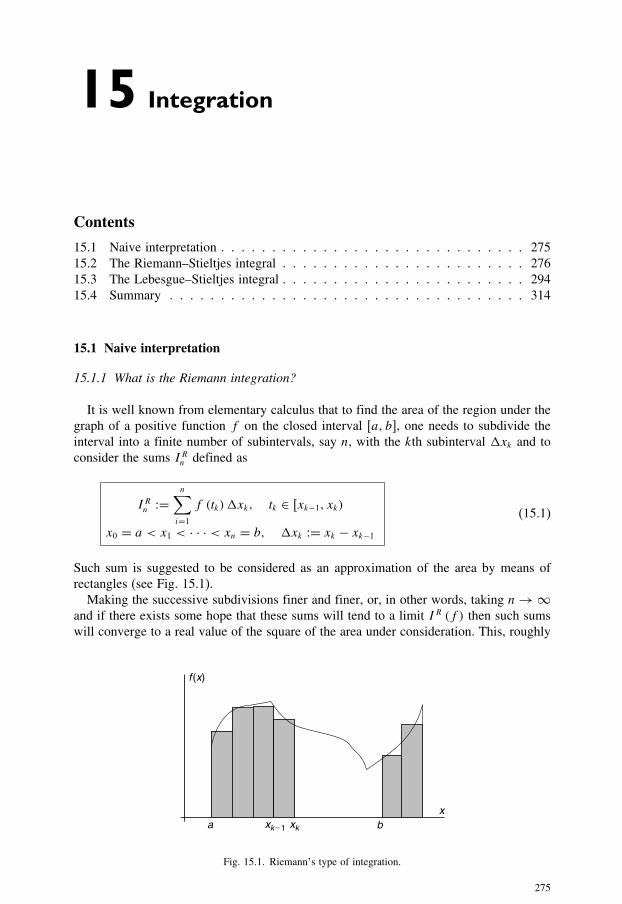
15 Integration
Contents
15.1 Naive interpretation . . . . . . . . . . . . . . . . . . . . . . . . . . . . . . 275
15.2 The Riemann–Stieltjes integral . . . . . . . . . . . . . . . . . . . . . . . . 276
15.3 The Lebesgue–Stieltjes integral . . . . . . . . . . . . . . . . . . . . . . . . 294
15.4 Summary . . . . . . . . . . . . . . . . . . . . . . . . . . . . . . . . . . . 314
15.1 Naive interpretation
15.1.1 What is the Riemann integration?
It is well known from elementary calculus that to find the area of the region under the
graph of a positive function f on the closed interval [a, b], one needs to subdivide the
interval into a finite number of subintervals, say n, with the kth subinterval �xk and to
consider the sums IRn defined as
IRn :=n∑i=1
f (tk)�xk, tk ∈ [xk−1, xk)
x0 = a < x1 < · · · < xn = b, �xk := xk − xk−1
(15.1)
Such sum is suggested to be considered as an approximation of the area by means of
rectangles (see Fig. 15.1).
Making the successive subdivisions finer and finer, or, in other words, taking n→∞and if there exists some hope that these sums will tend to a limit IR (f ) then such sums
will converge to a real value of the square of the area under consideration. This, roughly
f (x)
ax
xk21 xk b
Fig. 15.1. Riemann’s type of integration.
275

276 Advanced Mathematical Tools for Automatic Control Engineers: Volume 1
f (x)
bax
fk
fk21
mesk
Fig. 15.2. Lebesgue’s type of integration.
speaking, is what is involved in Riemann’s definition of the definite integral∫ bx=a f (x) dx
which is studied in detail within the elementary calculus course. This type of integration
is well defined for the class of continuous or partially continuous functions.
15.1.2 What is the Lebesgue integration?
If a function has some more complex structure and admits any discontinuity of a
more complex nature then another generalizing integration method is required. One of
such method is the Lebesgue integration. It corresponds to the following approximation
scheme (see Fig. 15.2):
ILn :=n∑i=1
(fk − fk−1)mesk
f0 := infx∈[a,b]
f(x) < f1 < · · · < fn := supx∈[a,b]
f(x)
mesk is the longitude of all intervals where
fk−1 ≤ f (x) < fk
(15.2)
If a limit IL of ILn (when n→∞) exists it is called the Lebesgue integral of f(x) on
[a, b] and is denoted by IL (f ) := ∫ bx=a f . It is closely related to a measure of a set. This
chapter considers both integration schemes in detail and rigorously from a mathematical
point of view.
15.2 The Riemann–Stieltjes integral
15.2.1 Riemann integral definition
Let [a, b] be a given interval and a partition Pn of [a, b] be defined as a finite
collection of points
a = x0 < x1 < · · · < xn = b

Integration 277
We write
�xi := xi − xi−1, i = 1, . . . , n
Definition 15.1. Suppose f is a bounded real function defined on [a, b] and
Mi := supx∈[xi−1,xi )
f(x), mi := infx∈[xi−1,xi )
f(x) (15.3)
Then
U (Pn, f ) :=n∑i=1
Mi�xi (15.4)
and
L (Pn, f ) :=n∑i=1
mi�xi (15.5)
are called the upper and lower Darboux sums, respectively.
Definition 15.2.
1. The upper Riemann integral IU (f ) is defined as follows:
I u (f ) := lim supn→∞
supPn
U (Pn, f ) (15.6)
where supPn
is taken over all partitions Pn of the interval [a, b].
2. The lower Riemann integral IL (f ) is defined as follows:
I l (f ) := lim infn→∞ inf
PnL (Pn, f ) (15.7)
where infPn
is taken over all partitions Pn of the interval [a, b].
3. If
I l (f ) = I u (f )then the Riemann integral IR (f ), often written as
IR (f ) =b∫
x=af (x) dx
is defined by
IR (f ) =b∫
x=af(x) dx := I l (f ) = I u (f ) (15.8)

278 Advanced Mathematical Tools for Automatic Control Engineers: Volume 1
Notice that for any partition Pn we have
mini=1,...,n
Mi := m ≤ L (Pn, f ) ≤ U (Pn, f ) ≤ M := maxi=1,...,n
Mi
So, the numbers L (Pn, f ) and U (Pn, f ) form a bounded set and, hence, are correctly
defined. The question of the integrability of f (when (15.8) holds) is a delicate question
which will be discussed below.
15.2.2 Definition of Riemann–Stieltjes integral
We shall be working here with a compact set [a, b] ∈ R and all functions will be
assumed to be real-valued functions defined on [a, b]. Complex-valued functions will be
considered below in Chapter 18.
Let Pn := {a = x0, x1, . . . , xn = b} be a partition of [a, b], tk be a point within the
interval [xk−1, xk) and �αk := α (xk) − α (xk−1) where α : R → R is a real function
defined on [a, b].
Definition 15.3.
1. A partition P ′ of [a, b] is said to be finer than P (or a refinement of P ) if
P ⊆ P ′ (15.9)
2. A sum of the form
S (Pn, f, α) :=n∑k=1
f (tk)�αk (15.10)
is called a Riemann–Stieltjes sum of f with respect to α corresponding to a givenpartition Pn.
3. We say that f is integrable in the Riemann sense with respect to α on [a, b] and wewill write f ∈ R[a,b] (α) if there exists a number IR−S having the following property:for any ε > 0 there exists a partition Pε of [a, b] such that for any partition P finerthan Pε and for any choice of the points tk ∈ [xk−1, xk) we have
∣∣S (P, f, α)− IR−S∣∣ < ε (15.11)
4. When such number IR−S exists, it is uniquely determined and is denoted by
IR−S :=b∫
x=af (x) dα (x) (15.12)
This is the Riemann–Stieltjes integral (or simply the Stieltjes integral) of f withrespect to α on [a, b].
5. The functions f and α are referred to as the integrand and the integrator, respectively.

Integration 279
Remark 15.1. The letter x in (15.12) is a “dummy variable”, so it may be replaced byany other convenient symbol, for example,
IR−S :=b∫
x=af(x) dα (x) =
b∫ζ=af(ζ ) dα (ζ ) (15.13)
Remark 15.2. By taking α (x) = x, the Riemann integral (15.8) is seen to be a special(partial) case of the Riemann–Stieltjes integral (15.12).
15.2.3 Main properties of the Riemann–Stieltjes integral
Theorem 15.1. (on linear properties)
1. If f, g ∈ R[a,b] (α) then for any c1, c2 ∈ R
c1f + c2g ∈ R[a,b] (α) (15.14)
and
b∫x=a
[c1f (x)+ c2g (x)] dα (x)
= c1b∫
x=af (x) dα (x)+ c2
b∫x=ag (x) dα (x)
(15.15)
2. If f ∈ R[a,b] (α) and at the same time f ∈ R[a,b] (β) then for any c1, c2 ∈ R
f ∈ R[a,b] (c1α + c2β) (15.16)
and
b∫x=af (x) d [c1α (x)+ c2β (x)]
= c1b∫
x=af (x) dα (x)+ c2
b∫x=af (x) dβ (x)
(15.17)
Proof. It follows directly from the linear property for the Riemann–Stieltjes sums (15.10)
S (P, c1f + c2g, α) and S (P, h, c1α + c2β). �

280 Advanced Mathematical Tools for Automatic Control Engineers: Volume 1
Theorem 15.2. (on intervals summation) Assume that c ∈ [a, b]. If two of the threeintegrals in the next identity exist then the third one also exists and
b∫x=af (x) dα (x) =
c∫x=af (x) dα (x)+
b∫x=cf (x) dα (x) (15.18)
Proof. If P is a partition of [a, b] and c ∈ P then we may introduce the corresponding
partitions of [a, c] and [c, b], respectively, as follows:
P ′ := P ∩ [a, c], P ′′ := P ∩ [c, b]
Then by the linear property for the Riemann–Stieltjes sums (15.10) we have
S (P, f, α) = S (P ′, f, α)+ S (P ′′, f, α
)which implies the proof of the desired result. �
Corollary 15.1.
1. If a < b and f ∈ R[a,b] (α) then
a∫x=bf (x) dα (x) = −
b∫x=af (x) dα (x) (15.19)
whenever∫ bx=a f (x) dα (x) exists.
2.
a∫x=af (x) dα (x) = 0 (15.20)
3. The identity (15.18) can be represented as
b∫x=af (x) dα (x)+
c∫x=bf (x) dα (x)+
a∫x=cf (x) dα (x) = 0 (15.21)
Theorem 15.3. (on integration by parts) If f ∈ R[a,b] (α) then
1.
α ∈ R[a,b] (f ) (15.22)

Integration 281
2.
b∫x=af (x) dα (x)+
b∫x=aα (x) df (x)
= f (b) α (b)− f (a) α (a)(15.23)
Proof. Sinceb∫
x=af (x) dα (x) exists then for every ε > 0 there is a partition Pε of [a, b]
such that for every P ′ ⊇ Pε we have∣∣∣∣∣∣S(P ′, f, α
)− b∫x=af (x) dα (x)
∣∣∣∣∣∣ < εThen for an arbitrary (P ⊇ Pε) Riemann–Stieltjes sum it follows that
S (Pn, α, f ) =n∑k=1
α (tk)�fk =n∑k=1
α (tk) f (xk)−n∑k=1
α (tk) f (xk−1)
Define
A := f (b) α (b)− f (a) α (a) =n∑k=1
f (xk) α (xk)−n∑k=1
f (xk−1) α (xk−1)
Subtracting the last two equations we derive
S (Pn, α, f )− A=n∑k=1
f (xk) [α (tk)− α (xk)]
+n∑k=1
f (xk−1) [α (xk−1)− α (tk)]
Two sums in the right-hand side can be considered as a single one of the form S (P ′, f, α)where P ′ is a partition of [a, b] obtained by taking the points xk and tk together. So, for
such a partition it follows P ′ ⊇ Pε and, hence,
A− S (P, α, f )−b∫
x=af (x) dα (x) =
n∑k=1
f (xk) [α (xk)− α (tk)]
+n∑k=1
f (xk−1) [α (tk)− α (xk−1)]−b∫
x=af (x) dα (x)
= S (P ′, α, f )−b∫
x=af (x) dα (x)
282 Advanced Mathematical Tools for Automatic Control Engineers: Volume 1
As the result, we obtain
∣∣∣∣∣∣A− S (Pn, α, f )−b∫
x=af (x) dα (x)
∣∣∣∣∣∣=
∣∣∣∣∣∣S (P ′, α, f )−b∫
x=af (x) dα (x)
∣∣∣∣∣∣ < εwhich is exactly the statement that
∫ bx=a α (x) df (x) exists and equals A − ∫ b
x=a f (x)dα (x). The theorem is proven. �
Theorem 15.4. (on the change of variables) Let f ∈ R[a,b] (α) and let g : R → R bea strictly monotonic increasing (or decreasing) function defined on the interval [c, d],that is,
g (x) < g(x ′)
if x < x ′
Assume that
g (c) = a, g (d) = b (15.24)
and
h (x) := f (g (x)), β (x) := α (g (x)) (15.25)
are the composite functions defined for any x ∈ [c, d]. Then
h ∈ R[c,d] (β) and
b∫x=af (x) dα (x) =
d∫x=ch (x) dβ (x) (15.26)
or, equivalently,
g(d)∫g(c)
f (t) dα (t) =d∫
x=cf (g (x)) dα (g (x)) (15.27)
Proof. By strict monotonicity it follows that for every partition Pn := {y0, y1, . . . , yn}of [c, d] there corresponds one and only one partition P ′
n := {x0, x1, . . . , xn} of [a, b].In fact,
P ′n = g (Pn), Pn = g−1
(P ′n
)
Integration 283
and, moreover, any refinement of Pn produces a corresponding refinement of P ′n and
conversely. If Pn ⊇ Pε (ε > 0) then let us consider
S (Pn, h, β) :=n∑k=1
h (uk)�βk, uk ∈ [yk−1, yk), �βk := β (yk)− β (yk−1)
If putting tk := g (uk) and xk := g (yk) we obtain P ′n ⊇ P ′
ε for which
∣∣∣∣∣∣S(P ′n, f, α
)− b∫a
f (t) dα (t)
∣∣∣∣∣∣ < εThen
S (Pn, h, β)=n∑k=1
h (g (uk)) [α (g (xk))− α (g (xk−1))]
=n∑k=1
f (tk) (α (xk)− α (xk−1)) = S(P ′n, f, α
)
since tk ∈ [xk, xk−1). Therefore,
∣∣∣∣∣∣S (Pn, h, β)−b∫a
f (t) dα (t)
∣∣∣∣∣∣=
∣∣∣∣∣∣S(P ′n, f, α
)− b∫a
f (t) dα (t)
∣∣∣∣∣∣ < εwhich completes the proof of this theorem. �
Exercise 15.1. If f, f 2 ∈ R[a,b] (α) and g, g2 ∈ R[a,b] (α) then
1
2
b∫x=a
⎡⎣ b∫y=a
(det
[f (x) g (x)
f (y) g (y)
])2
dα (y)
⎤⎦ dα (x)
=⎡⎣ b∫x=af 2 (x) dα (x)
⎤⎦⎡⎣ b∫x=ag2 (x) dα (x)
⎤⎦
−⎡⎣ b∫x=af (x) g (x) dα (x)
⎤⎦2
(15.28)

284 Advanced Mathematical Tools for Automatic Control Engineers: Volume 1
Exercise 15.2. If f, g, f · g ∈ R[a,b] (α) then
1
2
b∫x=a
⎡⎣ b∫y=a(f (y)− f (x)) (g (y)− f (x)) dα (y)
⎤⎦ dα (x)
= [α (b)− α (a)]b∫
x=af (x) g (x) dα (x)
−⎡⎣ b∫x=af (x) dα (x)
⎤⎦⎡⎣ b∫x=ag (x) dα (x)
⎤⎦
(15.29)
15.2.4 Different types of integrators
15.2.4.1 Differentiable integratorsTheorem 15.5. (on a reduction to the Riemann integral) Given f ∈ R[a,b] (α) assumethat the integrator α (x) can be represented as
α (x) =x∫
t=aα′ (t) dt (15.30)
where α′ (t), called the derivative of α (x) at the point x ∈ [a, b], is a continuous functionon [a, b]. Then
1. There exists the Riemann integral
b∫a
f (x) α′ (x) dx
2. The following identity holds
b∫a
f (x) dα (x) =b∫a
f (x) α′ (x) dx (15.31)
Proof. For a partition Pn of [a, b] define
S (Pn, g, x) :=n∑k=1
g (tk)�xk
g (tk) := f (tk) α′ (tk), �xk := xk − xk−1
S (Pn, f, α) :=n∑k=1
f (tk)�αk
Integration 285
By continuity of α′ (x) it follows that
�αk = α′(vk)�xk, vk ∈ [xk−1, xk]
and that α′ (x) is uniformly continuous on [a, b], that is, for any ε > 0 there exists
δ = δ (ε) > 0 such that 0 < |x − x ′| < δ implies |α′ (x)− α′ (x ′)| < ε. Hence,
|S (Pn, g, x)− S (Pn, f, α)| =∣∣∣∣∣n∑k=1
f (tk)[α′ (tk)− α′
(vk)]�xk
∣∣∣∣∣≤
n∑k=1
|f (tk)|∣∣α′ (tk)− α′ (vk)∣∣ |�xk| ≤ ε n∑
k=1
|f (tk)| |�xk| ≤ εM (b − a)
whereM := supx∈[a,b]
f (x). On the other hand, since f ∈ R[a,b] (α), there exists a partition Pn
finer than Pε such that∣∣∣∣∣∣S (P, f, α)−b∫a
f (x) dα (x)
∣∣∣∣∣∣ < εwhich leads to the following:∣∣∣∣∣∣S (Pn, g, x)−
b∫a
f (x) dα (x)
∣∣∣∣∣∣ =∣∣[S (Pn, g, x)− S (Pn, f, α)]
+⎡⎣S (Pn, f, α)−
b∫a
f (x) dα (x)
⎤⎦∣∣∣∣∣∣ ≤ |S (Pn, g, x)− S (Pn, f, α)|
+∣∣∣∣∣∣S (Pn, f, α)−
b∫a
f (x) dα (x)
∣∣∣∣∣∣ ≤ εM (b − a)+ ε = ε [1+M (b − a)]The arbitrary of ε implies (15.31) which completes the proof. �
15.2.4.2 Step functionsIf the integrator α (x) is a constant over the interval [a, b] then the integral∫ baf (x) dα (x) exists and is equal to zero for any partially continuous function f (x). How-
ever, if α (x) is a constant except for a jump discontinuity at one point, then the integral∫ baf (x) dα (x) not obligatory exists, but if it does exist, its value need not be zero. The
next theorem clarifies this situation.
Theorem 15.6. (on a single jump integrator) Given a < c < b let us assume that
(a) the values α (a), α (c) and α (b) are arbitrary;(b) α (x) defined on [a, b] is a step function, i.e.,
α (x) ={α (a) if a ≤ x < cα (b) if c < x ≤ b

286 Advanced Mathematical Tools for Automatic Control Engineers: Volume 1
(c) f : R → R is defined on [a, b] in such a way that at least one of the functions for α is continuous from left at c (this means that there exists lim
x→c−0f (x) = f (c) or
limx→c−0
α (x) = α (c)) and at least one is continuous from right at c.
Then the integral∫ baf (x) dα (x) exists, that is, f ∈ R[a,b] (α) and
b∫a
f (x) dα (x) = f (c)�α
�α := α (c + 0)− α (c − 0)
(15.32)
where �α is the jump of the function α (x) at the point c.
Remark 15.3. The result also holds if c = a provided that
α (c − 0) := α (c)and if c = b defining
α (c + 0) := α (b)Proof. Supposing c ∈ Pn implies
S (Pn, f, α)= f (tk−1) [α (c)− α (c − 0)]
+f (tk) [α (c + 0)− α (c)] = [f (tk−1)− f (c)] [α (c)− α (c − 0)]
+ [f (tk)− f (c)] [α (c + 0)− α (c)]+ γγ := f (c) [α (c + 0)− α (c − 0)]
where tk−1 ≤ c ≤ tk . So, for � := S (Pn, f, α)− γ one has
|�| ≤ ∣∣[f (tk−1)− f (c)] [α (c)− α (c − 0)]∣∣
+ [f (tk)− f (c)] [α (c + 0)− α (c)] ≤ ε (∣∣[α (c)− α (c − 0)]∣∣)
+ ε (∣∣[α (c + 0)− α (c)]∣∣) ≤ ε · constif |f (tk−1)− f (c)| < ε and |f (tk)− f (c)| < ε which may be done by the corresponding
partitioning of [a, b]. This proves the theorem. �
Next, let us consider a step function f (x) defined on [a, b] by a partition Pn :={a = x0, x1, . . . , xn = b} such that α (x) is a constant on each open subinterval (xk−1, xk)
and has jumps
�αk := α (xk + 0)− α (xk − 0), k = 2, . . . , n− 1
�α1 := α (x1 + 0)− α (x1)�αn := α (xn)− α (xn − 0)
Then the following theorem provides the connecting link between the Riemann–Stieltjes
integral and finite sums depending on values of the integrator function jumps.

Integration 287
Theorem 15.7. (on multiple jumps) If a function f defined on [a, b] in such a way thatneither f nor α are discontinuous from the right or from the left at each jump point xkthen
∫ baf (x) dα (x) exists, that is, f ∈ R[a,b] (α) and
b∫a
f (x) dα (x) =n∑k=1
f (xk)�αk (15.33)
Proof. Evidently, by the additivity property (15.18) the integral∫ baf (x) dα (x) can be
rewritten as a sum of integrals with a single jump that proves the theorem. �
Example 15.1. Denote by [x] the, so-called, greatest-integer function defined as theunique integer satisfying the inequality
[x] ≤ x < [x]+ 1 (15.34)
Then any finite sum∑n
k=1 ak can be represented as a Riemann–Stieltjes integral asfollows:
n∑k=1
ak =n∫
x=0
f (x) d [x]
f (x) = ak if x ∈ (k − 1, k], f (0) = 0
(15.35)
Example 15.2. (Euler’s summation formula) If f has a continuous derivative f ′ (see(15.30)) on [a, b] then
[b]∑k=[a]+1
f (n) =b∫
x=af (x) dx +
b∫x=af ′ (x) d
(x − [x]
)+f (a) (a − [a]
)− f (b) (b − [b]) (15.36)
If a and b are integers then (15.36) becomes
b∑k=af (n) =
b∫x=af (x) dx +
b∫x=af ′ (x)
(x − [x]− 1/2
)dx
+ [f (a)+ f (b)] /2(15.37)

288 Advanced Mathematical Tools for Automatic Control Engineers: Volume 1
Notice that (15.36) may be obtained using integration by part (15.23):
b∫x=af (x) d
(x − [x]
)
= −b∫
x=a
(x − [x]
)df (x)+ f (b) (b − [b]
)− f (a) (a − [a])
= −b∫
x=a
(x − [x]
)f ′ (x) dx + f (b) (b − [b]
)− f (a) (a − [a])
15.2.4.3 Monotonically nondecreasing integratorsWhen α is nondecreasing on [a, b], i.e., when α (x) ≤ α (x ′) if x ≤ x ′, the differences
�αk which appear in the Riemann–Stieltjes integral are all nonnegative which plays
a vital role in the development of the integration theory. For brevity, we will use the
abbreviation
“α ↑ on [a, b]” (15.38)
to mean that α (x) is nondecreasing on [a, b]. The following properties seem to be evident.
Proposition 15.1. Assume α ↑ on [a, b] and f, g ∈ R[a,b] (α). Then
1. If f (x) ≤ g (x) for all x ∈ [a, b] we have
b∫x=af (x) dα (x) ≤
b∫x=ag (x) dα (x) (15.39)
2. If g (x) ≥ 0 for all x ∈ [a, b] it follows
0 ≤b∫
x=ag (x) dα (x) (15.40)
which can be obtained from (15.39) taking f (x) = 0;3.
|f | ∈ R[a,b] (α) (15.41)
and ∣∣∣∣∣∣b∫
x=af (x) dα (x)
∣∣∣∣∣∣ ≤b∫
x=a|f (x)| dα (x) (15.42)

Integration 289
which follows from the inequality
||f (x)| − |f (y)|| ≤ |f (x)− f (y)|
4.
f 2 ∈ R[a,b] (α) (15.43)
5.
f · g ∈ R[a,b] (α) (15.44)
which follows from the identity
2f (x) g = (f (x)+ g (x))2 − f 2 (x)− g2 (x)
Proposition 15.2. (The Cauchy–Schwarz inequality) If f, f 2, g, g2 ∈ R[a,b] (α) and,
in addition, α ↑ on [a, b], then
⎡⎣ b∫x=af (x) g (x) dα (x)
⎤⎦2
≤⎡⎣ b∫x=af 2 (x) dα (x)
⎤⎦⎡⎣ b∫x=ag2 (x) dα (x)
⎤⎦
(15.45)
Proof. It follows directly from (15.28) since the left-hand side of this identity is
nonnegative. �
Proposition 15.3. If f, g, f · g ∈ R[a,b] (α), both f and g are either nondecreasing ornonincreasing and α ↑ on [a, b], then
⎡⎣ b∫x=af (x) dα (x)
⎤⎦⎡⎣ b∫x=ag (x) dα (x)
⎤⎦
≤ [α (b)− α (a)]b∫
x=af (x) g (x) dα (x)
(15.46)
Proof. It follows directly from (15.29) since the left-hand side of this identity is
nonnegative. �
290 Advanced Mathematical Tools for Automatic Control Engineers: Volume 1
15.2.4.4 Integrators of bounded variationDefinition 15.4. If Pn is a partition of a compact interval [a, b], �αk := α (xk) −α (xk−1) and there exists a positive number M such that
n∑k=1
|�αk| ≤ M (15.47)
for all partitions Pn of the interval [a, b], then α is said to be of bounded variation on[a, b].Lemma 15.1. If α is monotonic on [a, b] then it is of bounded variation on [a, b].
Proof. Let α be nondecreasing. Then �αk ≥ 0 for all k = 1, . . . , n and, hence,
n∑k=1
|�αk| =n∑k=1
�αk = α (xn)− α (x0) = α (b)− α (a)
If f is nonincreasing then �αk ≤ 0 and |�αk| = −�αk which gives
n∑k=1
|�αk| = α (a)− α (b)
Lemma is proven. �
Lemma 15.2. If α is continuous on [a, b] and if α′ exists and is bounded (say,supx∈[a,b]
|α′ (x)| ≤ M <∞) then α is of bounded variation on [a, b].
Proof. Since�αk = α (xk)−α (xk−1) = α′ (tk) (xk − xk−1)where tk ∈ (xk−1, xk) it follows
that
n∑k=1
|�αk| =n∑k=1
∣∣α′ (tk) (xk − xk−1)∣∣ = n∑
k=1
∣∣α′ (tk)∣∣ (xk − xk−1)
≤Mn∑k=1
(xk − xk−1) = M (b − a) <∞
which completes the proof. �
Lemma 15.3. If α is of bounded variation on [a, b], say∑n
k=1|�αk| ≤ M for all
partitions of [a, b], then α is bounded on [a, b], namely,
α (x) ≤ α (a)+M (15.48)
Proof. For any x ∈ (a, b), using the special partition P := {a, x, b}, we find
|α (x)− α (a)| + |α (b)− α (x)| ≤ M

Integration 291
which implies |α (x)− α (a)| ≤ M , or, equivalently, α (x) ≤ α (a) + M . The same
inequality is valid if x = a or x = b. Lemma is proven. �
To work more exactly with functions of bounded variations we need the following
definition.
Definition 15.5. For a function α of bounded variation on [a, b] the number
Vα [a, b] := supP
{n∑k=1
|�αk|}
(15.49)
(where sup is taken over all possible partitions of [a, b]) is called the total variation ofα on the interval [a, b].
The following properties of Vα [a, b] are evident:
1. Since α is of bounded variation the number Vα [a, b] is finite;
2.
Vα [a, b] ≥ 0 (15.50)
3.
Vα [a, b] = 0
if and only if α (x) = const on [a, b];
4.
Vα+β [a, b] ≤ Vα [a, b]+ Vβ [a, b] (15.51)
5.
Vα·β [a, b] ≤ AVα [a, b]+ BVβ [a, b]
A := supx∈[a,b]
|β (x)|, B := supx∈[a,b]
|α (x)| (15.52)
6. If c ∈ (a, b) then
Vα [a, b] = Vα [a, c]+ Vα [c, b] (15.53)
7. If x ∈ (a, b) then the function
V (x) := Vα [a, x] (15.54)

292 Advanced Mathematical Tools for Automatic Control Engineers: Volume 1
possesses the following properties:
(a)
V (a) = 0
(b) V (x) is a nondecreasing function on [a, b];
(c) [V (x)− α (x)] is a nondecreasing function on [a, b];
(d) Any point of continuity of α (x) is a point of continuity of V (x) and inversely.
The following theorem gives the simple and elegant characterization of functions of
bounded variations.
Theorem 15.8. (on a difference of increasing functions) Let α be defined on [a, b].Then α is of bounded variation on [a, b] if and only if α can be represented as thedifference of two nondecreasing functions, namely, if and only if
α (x) = α+ (x)− α− (x) (15.55)
where α+ ↑ on [a, b] and α− ↑ on [a, b].
Proof. Define α+ (x) = V (x), where V (x) is the function (15.54), and α− (x) :=V (x)− α (x). By the statement 7(b–c) of the previous claim it follows that both α+ (x)and α− (x) are nondecreasing which proves the theorem. �
Corollary 15.2. If α (x) is continuous at the point x, then α+ (x) and α− (x) are alsocontinuous at x.
Example 15.3. Consider the function (see Fig. 15.3)
3
2
1
0 1 2 3 4
�(x)
x
Fig. 15.3. The function of bounded variation.
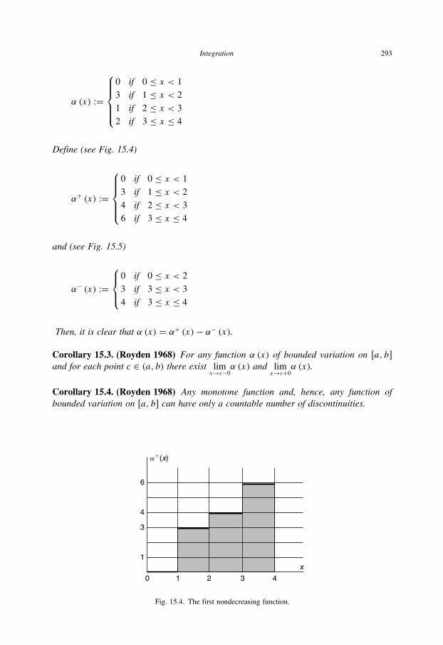
Integration 293
α (x) :=
⎧⎪⎪⎪⎨⎪⎪⎪⎩0 if 0 ≤ x < 1
3 if 1 ≤ x < 2
1 if 2 ≤ x < 3
2 if 3 ≤ x ≤ 4
Define (see Fig. 15.4)
α+ (x) :=
⎧⎪⎪⎪⎨⎪⎪⎪⎩0 if 0 ≤ x < 1
3 if 1 ≤ x < 2
4 if 2 ≤ x < 3
6 if 3 ≤ x ≤ 4
and (see Fig. 15.5)
α− (x) :=
⎧⎪⎨⎪⎩0 if 0 ≤ x < 2
3 if 3 ≤ x < 3
4 if 3 ≤ x ≤ 4
Then, it is clear that α (x) = α+ (x)− α− (x).
Corollary 15.3. (Royden 1968) For any function α (x) of bounded variation on [a, b]
and for each point c ∈ (a, b) there exist limx→c−0
α (x) and limx→c+0
α (x).
Corollary 15.4. (Royden 1968) Any monotone function and, hence, any function ofbounded variation on [a, b] can have only a countable number of discontinuities.
6
4
3
1
0 1 2 3 4
�1(x)
x
Fig. 15.4. The first nondecreasing function.

294 Advanced Mathematical Tools for Automatic Control Engineers: Volume 1
4
3
1
0 1 2 3 4
�2(x)
x
Fig. 15.5. The second nondecreasing function.
Proof. It follows from the fact that for any monotone function α (x) the number of points
where
|α (x + 0)− α (x − 0)| > 1/sn
sn :=n∑k=1
[�αk]−, [x]− := min {0; x}
for any partition Pn is finite. �
Corollary 15.5. (Royden 1968) If α (x) is a function of bounded variation on [a, b], thenα′ (x) exists for almost all x ∈ [a, b], that is, α (x) is differentiable almost everywhereon [a, b].
15.3 The Lebesgue–Stieltjes integral
The purpose of this section is to present the fundamental concepts of the Lebesgue
theory of measure and integration and to prove some crucial theorems in a rather general
setting without obscuring the main lines of the developments by a mass of comparatively
trivial detail.
15.3.1 Algebras, σ -algebras and additive functions of sets
Definition 15.6. A family F of subsets of � is called an algebra (or a ring) generatedby �, if for any finite n <∞ and for any subsets Ai ∈ �(i = 1, . . . , n)
1.
� ∈ F (15.56)
Integration 295
2.
n⋃k=1
Ak ∈ F (15.57)
3.
n⋂k=1
Ak ∈ F (15.58)
4. for any A ∈ �
A �= �−A ∈ F (15.59)
Definition 15.7. A system F of subsets of � is called an σ -algebra (or a σ -ring) gen-erated by �, if
1. it is algebra;2. for any sequences of subsets {Ai}, Ai ∈ F
∞⋃i=1
Ai ∈ F,∞⋂i=1
Ai ∈ F (15.60)
Definition 15.8.
1. A set function φ : F → R defined for every A ∈ F is said to be additive if A∩B = ∅
and B ∈ F implies
φ (A ∪ B) = φ (A)+ φ (B) (15.61)
2. A set function φ : F → R defined for every A from a σ -algebra F is said to becountably additive if Ai ∩
i �=j Aj = ∅ and Ai ,Aj ∈ F implies
φ
( ∞⋃i=1
Ai
)=
∞∑i=1
φ (Ai ) (15.62)
We shall also assume that
• the range of φ does not contain both (+∞) and (−∞), for if it did the right-hand side
of (15.61) could become meaningless;• we exclude functions whose only value is (+∞) or (−∞).Assuming, in addition, for an additive φ that
(a)
φ (∅) = 0 (15.63)

296 Advanced Mathematical Tools for Automatic Control Engineers: Volume 1
(b) for all A ∈ F
φ (A) ≥ 0 (15.64)
the following properties are easily verified.
Proposition 15.4.
1. If Ai ∩i �=j Aj = ∅ and Ai ,Aj ∈ F then
φ
(n⋃i=1
Ai
)=
n∑i=1
φ (Ai ) (15.65)
2. For any A1,A2 ∈ F we have
φ (A1 ∪A2)+ φ (A1 ∩A2) = φ (A1)+ φ (A2) (15.66)
3. If A1 ⊂ A2 ∈ F then
φ (A1) ≤ φ (A2) (15.67)
4. If B ⊂ A ∈ F and φ (B) <∞ then
φ (A− B) = φ (A)− φ (B) (15.68)
For countably additive φ the following result holds.
Theorem 15.9. Suppose φ is countably additive on σ -algebra F and Ai ∈ F(i = 1, 2, . . .), A1 ⊂ A2 ⊂ · · ·, A := ⋃∞
i=1 Ai ∈ F . Then, as n→∞
φ (An)→ φ (A) (15.69)
Proof. Define B1 := A1 and Bn := An −An−1 (n = 2, 3, . . .). Then
Bi ∩i �=j Bj = ∅, An = B1 ∪ B2 ∪ · · · ∪ Bn, A =
∞⋃i=1
Bi
Hence, φ (An) =∑n
i=1 φ (Bi ) and φ (A) =∑∞i=1 φ (Bi ). Theorem is proven. �
15.3.2 Measure theory
This subsection deals with construction of the, so-called, Lebesgue measure which
plays the key role in the definition of the Lebesgue–Stieltjes integral.

Integration 297
15.3.2.1 IntervalsDefinition 15.9. Intervals in p-dimensional Euclidean space Rp are defined as follows:
1. the closed interval
[a, b] := {x := {
x1, . . . , xp} : ai ≤ xi ≤ bi (i = 1, f
)}2. the semi-open interval
[a, b) := {x := {
x1, . . . , xp} : ai ≤ xi < bi (i = 1, f
)}or
(a, b] := {x := {
x1, . . . , xp} : ai < xi ≤ bi (i = 1, f
)}3. the open interval
(a, b) := {x := {
x1, . . . , xp} : ai < xi < bi (i = 1, f
)}The possibility that ai = bi for any value of i is not ruled out; in particular, the empty
set is included among the intervals. If A is a union of a finite number of intervals it is
called an elementary set.
15.3.2.2 Additive set functionsDefinition 15.10. If I is an interval, we define
m(I) :=p∏i=1
(bi − ai) (15.70)
and if A = I1 ∪ · · · ∪ Ip then we set
m(A) := m(I1)+ · · · +m (Ip)
(15.71)
We let E denote the family of elementary subsets of Rp.
At this point, the following properties should be easily verified.
Proposition 15.5.
1. E is algebra (ring), but not a σ -algebra;2. If A ∈ E then A is a union of a finite number of disjoint intervals;3. If A ∈ E then m(A) is well defined by (15.71) on E;4. m is additive on E .
Remark 15.4. If p = 1, 2, 3 then m is length, area and volume, respectively.

298 Advanced Mathematical Tools for Automatic Control Engineers: Volume 1
Definition 15.11. A nonnegative additive set function φ : E → R defined on E is saidto be regular if for every A ∈ E and every ε > 0 there exist sets F,G ∈ E such that Fis closed, G is open, F ⊂ A ⊂ G and
φ (G)− ε ≤ φ (A) ≤ φ (F)+ ε (15.72)
Example 15.4.
1. If A = I is an interval then m (15.70) is regular.
2. For p = 1 let α : R → R be a nondecreasing function possibly having discontinuitypoints. Put
μ([a, b]
) := α (b + 0)− α (a − 0)
μ([a, b)
) := α (b − 0)− α (a − 0)
μ((a, b]
) := α (b + 0)− α (a + 0)
μ ((a, b)) := α (b − 0)− α (a + 0)
(15.73)
μ is regular on E .
15.3.2.3 Countably additive set functionsOur next objective is to show that every regular set function on E can be extended to
a countably additive set function on σ -algebra containing E .
Definition 15.12. Define
μ∗ (E) := inf
∞∑n=1
μ (An) (15.74)
where⋃∞i=1 Ai is a countable covering of E ⊂ Rp by open elementary sets An, that is,
E ⊂ ⋃∞i=1 Ai , μ is additive, regular, nonnegative and finite on E , and inf being taken
over all countable coverings of E by open elementary set. μ∗ (E) is called the outermeasure of E corresponding to μ.
Theorem 15.10.
1. For every A ∈ E
μ∗ (A) = μ (A) (15.75)
2. The following subadditivity property holds: if E = ⋃∞i=1 Ei then
μ∗ (E) ≤∞∑i=1
μ∗ (Ei) (15.76)
Integration 299
Proof.
1. Choose A ∈ E and ε > 0. By the regularity of μ, A is contained in an open elementary
set G such that μ (G) ≤ μ (A)+ε. Since μ∗ (A) ≤ μ (G) and arbitrarity it follows that
μ∗ (A) ≤ μ (A) (15.77)
By the definition (15.74) there is a sequence {An} of open elementary sets whose
union contains A such that∑∞n=1 μ (An) ≤ μ∗ (A) + ε. The regularity of μ shows
also that A contains a closed elementary set such that μ (F) ≥ μ (A)− ε. Since F is
a compact we have F ⊂ A1∪ · · · ∪AN for some N . Hence,
μ (A)≤μ (F)+ ε ≤ μ (A1 ∪ · · · ∪AN)+ ε
≤N∑n=1
μ (An)+ ε ≤ μ∗ (A)+ 2ε(15.78)
which, in conjunction with (15.77), proves (15.75).
2. Suppose E = ⋃∞i=1 Ei and μ
∗ (En) <∞ for all n. Given ε > 0 there are covering sets
{Ank}k=1,2,... of En by open elementary sets such that∑∞k=1 μ (Ank) ≤ μ∗ (En) + 2−nε
which leads to the inequality
μ∗ (E)≤∞∑n=1
∞∑k=1
μ (Ank) ≤∞∑n=1
μ∗ (En)
+∞∑n=1
2−nε =∞∑n=1
μ∗ (En)+ ε
and (15.76) follows. In the excluded case when μ∗ (En) = ∞ for some n, (15.76)
trivially holds. Theorem is proven.
�
15.3.2.4 μ-measurable setsDefinition 15.13.
1. For any A,B ⊂ Rp let us define the set S (A,B), called the symmetric difference ofA and B, as
S (A,B) := (A− B) ∪ (B −A) (15.79)
2. The distance function (metric) is defined as follows
d (A,B) := μ∗ (S (A,B)) (15.80)

300 Advanced Mathematical Tools for Automatic Control Engineers: Volume 1
3. We will write An → A when n→∞ if
limn→∞d (An,A) = 0 (15.81)
4. If there is a sequence {An} of elementary sets such that An → A, we say that A isfinitely μ-measurable and write
A ∈ Mf in (μ) (15.82)
5. If A is the union of a countable collection of finitely μ-measurable sets, we say thatA is μ-measurable and write
A ∈ M (μ) (15.83)
Some properties of S (A,B) are summarized in the following claim.
Claim 15.1.
1.
S (A,A) = ∅ (15.84)
2.
S (A,B) = S (B,A) (15.85)
3.
S (A,B) ⊂ S (A, C) ∪ S (C,B) (15.86)
which follows from
(A− B) ⊂ (A− C) ∪ (C − B)(B −A) ⊂ (C −A) ∪ (B − C)
4.
S (A1 ∪A2,B1 ∪ B2)
S (A1 ∩A2,B1 ∩ B2)
S (A1 −A2,B1 − B2)
⎫⎪⎬⎪⎭ ⊂ S (A1,B1) ∪ S (A2,B2) (15.87)
which follows from(A1 ∪A2)− (B1 ∪ B2) ⊂ (A1 − B1) ∪ (A2 − B2)
S (A1 ∩A2,B1 ∩ B2) = S(Ac
1 ∪Ac2,Bc1 ∪ Bc2
) ⊂S(Ac
1,Bc1) ∪ S (Ac
2,Bc2) = S (A1,B1) ∪ S (A2,B2)
where Ac := Rp −A is the complement of AA1 −A2 = A1 ∩Ac
2
The next properties of d (A,B) can be checked directly from the definition (15.80).
Integration 301
Claim 15.2.
1.
d (A,A) = 0 (15.88)
2.
d (A,B) = d (B,A) (15.89)
3.
d (A,B) ≤ d (A, C)+ d (C,B) (15.90)
4.
d (A1 ∪A2,B1 ∪ B2)
d (A1 ∩A2,B1 ∩ B2)
d (A1 −A2,B1 − B2)
⎫⎬⎭ ≤ d (A1,B1)+ d (A2,B2) (15.91)
which follows from (15.87);5.
|μ∗ (A)− μ∗ (B)| ≤ d (A,B) (15.92)
6. If d (A,B) = 0 this does not imply A = B. By this property d (A,B) is “quasi-metric”.
The next theorem will enable us to obtain the desired extension of the measure μ
(15.73).
Theorem 15.11. (The main theorem on a measure extension) M (μ), defined by(15.83), is a σ -algebra (σ -ring) and μ∗ (15.74) is countably additive on M (μ).
Proof.
(a) Let A,B ∈ Mf in (μ). Choose {An}, {Bn} such that An,Bn ∈ E and An → A,Bn → B. Then by (15.91) and (15.92) An ∪ Bn → A ∪ B, An ∩ Bn → A ∩ B,An − Bn → A − B, μ∗ (An) → μ∗ (A). Also, μ∗ (A) < ∞ since d (An,A) → 0.
This implies that Mf in (μ) is an algebra (ring). By (15.66) we have μ (An) + μ (Bn)= μ (An ∪ Bn) + μ (An ∩ Bn). Letting n → ∞ we obtain μ∗ (A) + μ∗ (B) =μ∗ (A ∪ B) + μ∗ (A ∩ B). If A∩B = ∅ then μ∗ (A ∩ B) = 0. So, μ∗ is additive onMf in (μ).
302 Advanced Mathematical Tools for Automatic Control Engineers: Volume 1
(b) Let A ∈ M (μ). Then A can be represented as the union of countable collection
of disjoint sets of Mf in (μ) and for A = ⋃∞n=1 A′
n with A′n ∈ M (μ). Define A1 =
A′1 and
An :=(A′
1 ∪A′2 ∪ · · · ∪A′
n
)− (A′
1 ∪A′2 ∪ · · · ∪A′
n−1
)Then A = ⋃∞
n=1 An is the required representation. By the subadditivity property
(15.76) μ∗ (A) ≤ ∑∞i=1 μ
∗ (Ai ). On the other hand,
A ⊃ (A1 ∪A2 ∪ · · · ∪An)
and, by the additivity of μ∗on Mf in (μ), we have
μ∗ (A) ≥ μ∗ (A1 ∪A2 ∪ · · · ∪An) =n∑i=1
μ∗ (Ai )
which implies
μ∗ (A) =∞∑i=1
μ∗ (Ai ) (15.93)
Suppose μ∗ (A) is finite. Put Bn := A1 ∪ A2 ∪ · · · ∪ An. Then
d (A,Bn) := μ∗( ∞⋃i=n+1
Ai
)=
∞∑i=n+1
μ∗ (Ai )→ 0
as n→∞. This means that Bn → A and, since Bn ∈ Mf in (μ), it is easily seen that
A ∈ Mf in (μ). So, we have thus shown that A ∈ Mf in (μ) if A ∈ M (μ) and μ∗ (A)<∞. Now it is evident that μ∗ is countably additive on M (μ). For if A = ⋃∞
i=1 Ai
where {Ai} is a sequence of disjoint sets of M (μ) we have just shown that (15.93)
holds if μ∗ (An) < ∞ for any n = 1, 2, . . ., and, in other cases, it looks trivial.
(c) Finally, we have to show that M (μ) is σ -algebra (σ -ring). If An ∈ M (μ), it is clear
that⋃∞i=1 Ai ∈ M (μ). Suppose A,B ∈ M (μ) where A = ⋃∞
i=1 Ai , B = ⋃∞i=1 Bi and
An,Bn ∈ Mf in (μ). Then the identity An∩B = ⋃∞i=1 (An ∩ Bi ) implies that (An ∩ B)
∈ M (μ). In view of μ∗ (An ∩ B) ≤ μ∗ (An) <∞ we have (An ∩ B) ∈ Mf in (μ) and,
hence, (An − B) ∈ Mf in (μ), and (A− B) ∈M (μ) since (A− B)=⋃∞n=1 (An − B).
Theorem is proven. �
So, now we may replace μ∗ (A) by μ (A) if A ∈ M (μ) and thus μ, originally defined
only on E , is extended to a countable additive set function defined on the σ -algebra
M (μ).
Integration 303
Corollary 15.6.
(a) If A is open, then A ∈ M (μ) since for every open set in Rp there is the union of acountable collection of open intervals.
(b) Every closed set A is also in M (μ) which follows from previous comment by takingcomplements.
(c) If A ∈ M (μ) and ε > 0 there exist a closed set F and an open set G such that
F ⊂ A ⊂ G (15.94)
and
μ (G −A) < ε, μ (A− F) < ε (15.95)
Now we are ready to give the main definition of this section.
Definition 15.14.
(a) Such extended set function μ∗ (15.74) is called a countably additive measure.(b) The special case μ = m (see (15.74)) is called the Lebesgue measure on Rp.
15.3.2.5 Borel setsDefinition 15.15. E is said to be a Borel set if E can be obtained by a countablenumber of operations, starting from open sets, each operation consisting of taking unions,intersections, or complements.
The difference between a Borel set and σ -algebra (ring) (15.7) is that � in the case of
a Borel set must be an open set.
The following facts take place for Borel sets.
Claim 15.3.
1. The collection B of all Borel sets in Rp is a σ -algebra (ring). In fact, it is the smallestσ -algebra (ring) which contains all open sets, that is, if E ∈ B then E ∈ M (μ).
2. If A ∈ M (μ), there exist Borel sets F and G such that F ⊂ A ⊂ G and
μ (G −A) = μ (A− F ) = 0 (15.96)
This follows from (15.95) if we take ε = 1/n and let n→∞.3. If A = F ∪ (A− F) one can see that A ∈ M (μ) is the union of a Borel set and a
set of measure zero.4. Borel sets are μ-measurable for every μ (for details see below), but the sets of measure
zero (that is, the sets E for which μ∗ (E) = 0) may be different for different μ’s.5. For every μ the sets of measure zero from σ -algebra (ring).6. In the case of the Lebesgue measure (μ = m) every countable set has measure zero.
But there are uncountable (in fact, perfect) sets of measure zero (see Rudin (1976)Chapter 11 with the Cantor set as an example).
304 Advanced Mathematical Tools for Automatic Control Engineers: Volume 1
15.3.3 Measurable spaces and functions
15.3.3.1 Measurable spacesConsider X which is a set, not necessarily a subset, of a Euclidean space, or indeed of
any metric space.
Definition 15.16.
• X is said to be a measure space if there exist a σ -algebra (ring) M of subsets of X(which are called measurable sets) and a nonnegative countable additive function μ(which is called a measure) defined on M.
• If, in addition, X ∈ M then X is called a measurable space.
Example 15.5.
1. Take X = Rp, then M is the collection of all Lebesgue measurable subsets of Rp andμ is the Lebesgue measure.
2. Let X be the set of all positive integers. Then M is the collection of all subsets of Xand μ (E) is the number of elements of E .
3. Another example is provided by probability theory where events are considered as setsand the corresponding probability of the occurrence of events is a countably additiveset function.
15.3.3.2 Measurable functionsDefinition 15.17. Let f : X → R be a function, defined on the measurable space X ,with values in R. The function f is said to be measurable if the set {x | f (x) > a} ismeasurable for every real a, that is, when for any a ∈ R
{x | f (x) > a} ⊂ X (15.97)
Example 15.6. If X = Rp with M = M (μ) defined in (15.83) then any continuous func-tion f is measurable, since (15.97) is an open set.
Lemma 15.4. Each of the following four conditions implies the other three:
1. for every real a
{x | f (x) > a} is measurable (15.98)
2. for every real a
{x | f (x) ≥ a} is measurable (15.99)
3. for every real a
{x | f (x) < a} is measurable (15.100)

Integration 305
4. for every real a
{x | f (x) ≤ a} is measurable (15.101)
Proof. The relations
{x | f (x) ≥ a} =∞⋂n=1
{x | f (x) ≥ a − 1/n}{x | f (x) < a} = X − {x | f (x) ≥ a}{x | f (x) ≤ a} =
∞⋂n=1
{x | f (x) < a − 1/n}{x | f (x) > a} = X − {x | f (x) ≤ a}
being applied successfully demonstrate that (15.15) implies (15.99), (15.99) implies
(15.100), (15.100) implies (15.101) and (15.101) implies (15.15). Lemma is proven. �
Lemma 15.5. If f is measurable then |f | is measurable.
Proof. It follows from the relation
{x | |f (x)| < a} = {x | f (x) < a} ∩ {x | f (x) > −a}
and the previous lemma. �
Theorem 15.12. Let {fn} be a sequence of measurable functions.Then
g(x) := supn
fn (x)
and
h(x) := lim supn
fn (x)
are measurable too.
Proof. Indeed,
{x | g(x) > a} =∞⋃n=1
{x | fn(x) > a}
and
h(x) = limm→∞ sup
n≥mfn (x) = inf
nsupn≥mfn (x)
which implies the desired result. �

306 Advanced Mathematical Tools for Automatic Control Engineers: Volume 1
Corollary 15.7.
(a) If f and g are measurable then max {f, g} and min {f, g} are measurable.(b) If
f + := max {f, 0} and f − := −min {f, 0} (15.102)
then it follows that f + and f − are measurable.(c) The limit of a convergent sequence of measurable functions is measurable.
Theorem 15.13. Let f and g be measurable real-valued functions defined on X , and letF be real and continuous on R2. Put
h (x) := F (f (x), g (x))
Then h is measurable and, in particular, (f + g) and (f · g) are measurable.
Proof. Define Gn := {(u, v) | F (u, v) > a}. Then Gn is an open subset of R2 which can
be represented as Gn = ⋃∞n=1
{x | fn(x) > a} where
In := {(u, v) | an < u < bn, cn < v < dn}
Since the set
{x | an < f (x) < bn} = {x | f (x) > an} ∩ {x | f (x) < bn}
is measurable, it follows that the set
{x | (f (x), g (x)) ∈ In} = {x | an < f (x) < bn} ∩ {x | cn < g (x) < dn}
is measurable too. Hence, the same is true for the set
{x | h (x) > a} = {x | (f (x), g (x)) ∈ Gn}
=∞⋃n=1
{x | (f (x), g (x)) ∈ In}
which completes the proof. �
Summary 15.1.
(a) Summing up, we may say that all ordinary operations of analysis, including limitoperations, being applied to measurable functions, lead to measurable functions aswell. In other words, all functions that are ordinarily met with are measurable. But thisis, however, only a rough statement since, for example, the function h(x) = f (g(x)),where f is measurable and g is continuous, is not necessarily measurable.

Integration 307
(b) The concrete measure has not been mentioned in the discussions above. In fact, theclass of measurable functions on X depends only on the σ -algebra (ring) M. That’swhy we may speak of Borel-measurable functions on Rp, that is, of functions forwhich the set {x | f (x) > a} is always a Borel set, without reference to any particularmeasure.
15.3.4 The Lebesgue–Stieltjes integration
15.3.4.1 Simple functionsDefinition 15.18.
1. If the range of a real-valued function s : X → R, defined on X , is finite, we say thats is a simple function.
2. Define the characteristic function χE of a set E ⊂ X as follows:
χE (x) :={1 if x ∈ E0 if x /∈ E (15.103)
It is evident that if the range of a simple function s consists of the distinct numbers
c1, c2, . . . , cn then s can be represented as a finite linear combination of characteristic
functions, namely,
s (x) =n∑i=1
ciχEi (x) (15.104)
where
Ei := {x | s (x) = ci}, i = 1, 2, . . . n (15.105)
It is clear by the construction that s is measurable if and only if the sets Ei (i = 1, 2, . . . n)
are measurable.
The next theorem shows that any function can be approximated by simple functions.
Theorem 15.14. Let f : X → R be a real function on X . There exists a sequence{sn} of simple functions such that sn (x) → f (x) as n → ∞ for every x ∈ X . If f ismeasurable, {sn} can be chosen to be a sequence of measurable functions. If f ≥ 0, {sn}can be chosen as a monotonically nondecreasing sequence.
Proof. For f ≥ 0 define
En,i (x) := {x | (i − 1)/2n ≤ f (x) ≤ i/2n}Fn (x) := {x | f (x) ≥ n}
for i = 1, 2, . . . , n2n and n = 1, 2, . . . . Put
sn (x) :=n2n∑i=1
(i − 1)
2nχEn,i (x)+ nχFn (x)
308 Advanced Mathematical Tools for Automatic Control Engineers: Volume 1
It is not difficult to see that such constructed sn (x) converges to f . In the general case, let
f = f + − f − (15.106)
and apply the preceding construction for f + and f −. Theorem is proven. �
Remark 15.5. The sequence sn (x) converges monotonically to f if f is bounded.
15.3.4.2 IntegrationHere we shall define integration on a measurable space X in which M is the σ -algebra
(ring) of measurable sets and μ is the measure.
Definition 15.19. (Integral of a nonnegative function) Suppose
s (x) =n∑i=1
ciχEi (x), x ∈ X , ci ≥ 0 (15.107)
is measurable, and suppose E ⊂ M. Define
IE (s) :=n∑i=1
ciμ (E ∩ Ei ) (15.108)
If f is measurable and nonnegative, we define
∫E
f dμ := sup IE (s) (15.109)
where the sup is taken over all measurable simple functions such that 0 ≤ s (x) ≤ f (x)for all x ∈ X . The left-hand side member of (15.109) is called the Lebesgue–Stieltjes(or, simply, Lebesgue) integral of f with respect to measure μ over the set E . It shouldbe noted that integrals may have the value (+ ∞).
Claim 15.4. It is easy to verify that
∫E
s dμ = IE (s) (15.110)
Definition 15.20. (Integral of a measurable function) Let f be measurable. Considertwo Lebesgue integrals∫
E
f + dμ and∫E
f − dμ (15.111)

Integration 309
where f + and f − are defined by (15.102). If at least one of the integrals in (15.111) isfinite, we may define
∫E
f dμ :=∫E
f + dμ−∫E
f − dμ (15.112)
If both integrals in (15.102) are finite then the left-hand side in (15.112) is finite too, andwe say that f is integrable (or summable) on E in the Lebesgue sense with respect tothe measure μ. We write
f ∈ L (μ) on E (15.113)
Proposition 15.6. The following properties of the Lebesgue integral are evident:
1. If f is measurable and bounded on E and if μ (E) <∞, then f ∈ L (μ) on E .2. If a ≤ f (x) ≤ b on E and if μ (E) <∞, then
aμ (E) ≤∫E
f dμ ≤ bμ (E) (15.114)
3. If f, g ∈ L (μ) on E and if f (x) ≤ g (x) for all x ∈ E , then∫E
f dμ ≤∫E
g dμ (15.115)
4. If f ∈ L (μ) on E , then cf ∈ L (μ) for every finite constant c, and
∫E
cf dμ = c∫E
f dμ (15.116)
5. If μ (E) = 0 and f is measurable, then
∫E
f dμ = 0 (15.117)
6. If f ∈ L (μ) on E , A ∈ M and A ⊂ E , then f ∈ L (μ) on A.
Theorem 15.15.
(a) Suppose f is measurable and nonnegative on X . For A ∈ M define
φ (A) =∫A
f dμ (15.118)
Then φ is countably additive on M.
310 Advanced Mathematical Tools for Automatic Control Engineers: Volume 1
(b) The same conclusion is valid if f ∈ L (μ) on X .
Proof. Claim (b) follows from (a) if we write f = f + −f − and apply (a) to f + and f −.To prove (a) we have to show that φ (A) can be represented as φ (A) = ∑∞
n=1 φ (An)
if An ∈ M, Ai ∩ Aj = ∅ if i �= j and A =⋃∞n=1 An. This can be done if the simple
function approximation is applied that proves (a). �
Corollary 15.8. If A ∈ M, B ⊂ A and μ (A− B) = 0, then
∫A
f dμ =∫B
f dμ (15.119)
that is, the sets of measure zero are negligible in integration.
Proof. It follows from Remark (15.117) and the representation A = B ∪ (A− B). �
Lemma 15.6. If f ∈ L (μ) on E then |f | ∈ L (μ) on E , and
∣∣∣∣∣∣∫E
f dμ
∣∣∣∣∣∣ ≤∫E
|f | dμ (15.120)
Proof. Let us represent E as E = A ∪ B where f (x) ≥ 0 on A and f (x) < 0 on B.Then by Theorem 15.15 it follows that
∫E
|f | dμ =∫A
|f | dμ+∫B
|f | dμ =∫A
f + dμ+∫A
f − dμ <∞
so that |f | ∈ L (μ) on E . Since f ≤ |f | and −f ≤ |f | one can see that
∫E
f dμ ≤∫E
|f | dμ and −∫E
f dμ ≤∫E
|f | dμ
which proves (15.120). �
Lemma 15.7. Suppose f is measurable on E , |f | ≤ g and g ∈ L (μ) on E . Thenf ∈ L (μ) on E .
Proof. It follows from the inequalities f + ≤ g and f − ≤ g. �
Integration 311
15.3.5 The “almost everywhere” concept
Definition 15.21. Let us write
f ∼ g on E (15.121)
if the set {x | f (x) �= g (x)} ∩ E has measure zero:
μ ({x | f (x) �= g (x)} ∩ E) = 0 (15.122)
Proposition 15.7. It is evident that on E1. f ∼ f ;2. f ∼ g implies g ∼ f ;3. f ∼ g and g ∼ h imply f ∼ h which means that the relation “∼” is an equivalence
relation.4. If f ∼ g on E then
∫A
f dμ =∫A
g dμ (15.123)
provided the integrals exist for every A ⊂ E .
Definition 15.22. (The “almost everywhere” concept) If some property P holds forevery x ∈ E −A and if μ (A) = 0 then it is customary to say that P holds for almost allx ∈ E , or that P holds almost everywhere on E .
This concept depends, of course, on the particular measure to be in use. In the literature,
unless something is said to the contrary, it usually refers to the Lebesgue measure.
Example 15.7. If f ∈ L (μ) on E it is clear that f (x) must be finite almost everywhereon E .
15.3.5.1 Essential supremum and infimumDefinition 15.23. Let us consider a measurable function f : R → R defined on X .
(a) The essential supremum “ess sup f ” of f (sometimes denoted also by “vraimax f ”)is defined as follows:
ess sup f := infc∈R
c (15.124)
such that
μ ({x | f (x) > c}) = 0 (15.125)
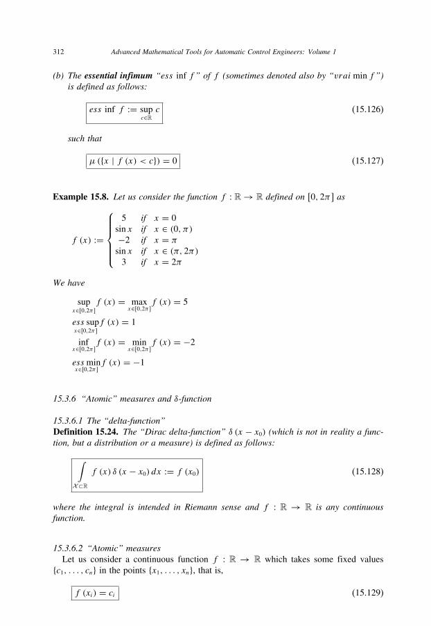
312 Advanced Mathematical Tools for Automatic Control Engineers: Volume 1
(b) The essential infimum “ess inf f ” of f (sometimes denoted also by “vraimin f ”)is defined as follows:
ess inf f := supc∈R
c (15.126)
such that
μ ({x | f (x) < c}) = 0 (15.127)
Example 15.8. Let us consider the function f : R → R defined on [0, 2π ] as
f (x) :=
⎧⎪⎪⎪⎪⎨⎪⎪⎪⎪⎩
5 if x = 0
sin x if x ∈ (0, π)−2 if x = πsin x if x ∈ (π, 2π)3 if x = 2π
We have
supx∈[0,2π ]
f (x) = maxx∈[0,2π ]
f (x) = 5
ess supx∈[0,2π ]
f (x) = 1
infx∈[0,2π ]
f (x) = minx∈[0,2π ]
f (x) = −2
essminx∈[0,2π]
f (x) = −1
15.3.6 “Atomic” measures and δ-function
15.3.6.1 The “delta-function”Definition 15.24. The “Dirac delta-function” δ (x − x0) (which is not in reality a func-tion, but a distribution or a measure) is defined as follows:
∫X⊂R
f (x) δ (x − x0) dx := f (x0) (15.128)
where the integral is intended in Riemann sense and f : R → R is any continuousfunction.
15.3.6.2 “Atomic” measuresLet us consider a continuous function f : R → R which takes some fixed values
{c1, . . . , cn} in the points {x1, . . . , xn}, that is,
f (xi) = ci (15.129)

Integration 313
Consider also the sum
S :=n∑i=1
ciμi, μi ≥ 0 (i = 1, . . . , n) (15.130)
In fact, if some multipliers μi are negative, one can rewrite the product ciμi as
ciμi = (−ci) (−μi) = (−ci) |μi |
obtaining the previous case with nonnegative weights.
Using (15.128) and in view of the additivity property of the Riemann integral, S can
be represented as
S :=n∑i=1
ciμi =∞∫
−∞f (x)
n∑i=1
μiδ (x − xi) dx (15.131)
Let us consider also the step function α (x) defined on [a, b] by a partition Pn :={a = x0, x1, . . . , xn = b} such that α (x) is a constant on each open subinterval (xk−1, xk)
and has jumps
μk := α (xk + 0)− α (xk − 0), k = 2, . . . , n− 1
μ1 := α (x1 + 0)− α (x1)μn := α (xn)− α (xn − 0)
(15.132)
Then, using the Riemann–Stieltjes integral representation (15.12) with the integrator α (x)
of a step-function type, we can represent (15.131) as follows:
S :=n∑i=1
ciμi =∞∫
−∞f (x)
n∑i=1
μiδ (x − xi) dx =b∫a
f (x) dα (x) (15.133)
So, symbolically, we can write
dα (x) :=n∑i=1
μiδ (x − xi) dx (15.134)
and
α′ (x) :={
0 if x ∈ (xk−1, xk)
μiδ (x − xi) if x = xk (15.135)
associating α (x) with the “measure” of points xi ∈ [a, x) supplied by the weights μi . In
fact, α (x) is the atomic measure concentrated in the isolated points {x1, . . . , xn}.

314 Advanced Mathematical Tools for Automatic Control Engineers: Volume 1
15.4 Summary
Based on the presentations above, we may conclude that any sum S (15.130) with finite
or infinite n (if it exists) can be represented by the Riemann–Stieltjes integral (15.133)
with the integrator α (x) as the step-function (15.132). The same sum S (15.130) can be
symbolically treated as the Lebesgue integral with the measure μ (x) = α (x) referred to
as the “atomic” measure concentrated in the points {x1, . . . , xn} with the corresponding
nonnegative weights {μ1, . . . , μn}.

16 SelectedTopics of Real Analysis
Contents
16.1 Derivatives . . . . . . . . . . . . . . . . . . . . . . . . . . . . . . . . . . 315
16.2 On Riemann–Stieltjes integrals . . . . . . . . . . . . . . . . . . . . . . . . 334
16.3 On Lebesgue integrals . . . . . . . . . . . . . . . . . . . . . . . . . . . . 342
16.4 Integral inequalities . . . . . . . . . . . . . . . . . . . . . . . . . . . . . . 355
16.5 Numerical sequences . . . . . . . . . . . . . . . . . . . . . . . . . . . . . 368
16.6 Recurrent inequalities . . . . . . . . . . . . . . . . . . . . . . . . . . . . . 387
16.1 Derivatives
16.1.1 Basic definitions and properties
16.1.1.1 Definition of a derivativeDefinition 16.1. Let f : S → R be defined as a closed interval S ⊂ R and assume thatf is continuous at the point c ∈ S. Then(a) f is said to have a right-hand derivative at c if the right-hand limit
limx→c+0
f (x)− f (c)x − c (16.1)
exists as a finite value, or if the limit is (+∞) or (−∞). This limit will be denotedas f ′+ (c) ;
(b) f is said to have a left-hand derivative at c if the right-hand limit
limx→c−0
f (x)− f (c)x − c (16.2)
exists as a finite value, or if the limit is (+∞) or (−∞). This limit will be denotedas f ′− (c) ;
(c) f is said to have a derivative f ′ (c) (or be differentiable) at c if
f ′+ (c) = f ′− (c) := f ′ (c) (16.3)
and |f ′ (c)| <∞; we say that f ′ (c) = +∞ (or −∞) if both the right- and left-handderivatives at c are +∞ (or −∞);
(d) f is said to be differentiable on S if it is differentiable at each point c ∈ S.
315

316 Advanced Mathematical Tools for Automatic Control Engineers: Volume 1
16.1.1.2 Differentiability and continuityLemma 16.1. Let f be defined on [a, b]. If f is differentiable at a point c ∈ [a, b], thenf is continuous at c.
Proof. By the definition (16.3), for any ε > 0 there exists δ = δ (ε) such that the
inequality |x − c| ≤ δ implies∣∣∣∣f (x)− f (c)x − c − f ′ (c)∣∣∣∣ ≤ ε
which is equivalent to the following inequalities
f (x)− f (c) ≤ [f ′ (c)+ ε] (x − c) ≤ [|f ′ (c)| + ε] |x − c| ≤ δ [|f ′ (c)| + ε]
Hence, |f (x)− f (c)| ≤ ε, if take δ := ε/ [|f ′ (c)| + ε] which proves the lemma. �
Remark 16.1. The converse of Lemma 16.1 is not true. To see this it is sufficient toconstruct the continuous function which fails to be differential at an isolated point. Forexample, f (x) = |x| which is not differentiable at the point x = 0 since
−1 = f ′− (c) �= f ′+ (c) = 1
The next claim describes the usual formulas for differentiation of the sum, difference,
product, quotient of two functions and function composition.
Claim 16.1. Suppose f and g are defined on [a, b] and are differentiable at a pointx ∈ [a, b]. Then
(a) for any α, β
[αf (x)± βg (x)]′ = αf ′ (x)± βg′ (x) (16.4)
(b)
[f (x) g (x)]′ = f ′ (x) g (x)+ f (x) g′ (x) (16.5)
(c) if g (x) �= 0
[f (x)/g (x)]′ = f
′ (x) g (x)− g′ (x) f (x)g2 (x)
(16.6)
Proof.(a) is evident by the property (16.3). For h = fg we have
h (t)− h (x) = f (t) [g (t)− g (x)]+ g (x) [f (t)− f (x)]

Selected topics of real analysis 317
If we divide by (t − x) and notice that f (t) → f (x) as t → x (b) follows. Taking
h = f/g, (c) follows from the identity
h (t)− h (x)t − x = 1
g (t) g (x)
[g (x)
f (t)− f (x)t − x − f (x) g (t)− g (x)
t − x]
letting t → x. �
Claim 16.2. (The chain rule) Suppose f is defined on [a, b] and g is defined on aninterval, containing the range of f , and g is differentiable at the point f (x). Then, thefunction h (x) = g (f (x)) is differentiable at the point x and
h′ (x) = g′ (f (x)) f ′ (x) (16.7)
Proof. Let y = f (x). By the derivative definition, we have
f (t)− f (x) = (t − x) [f ′ (x)+ u (t)], u (t) →t→x 0
g (s)− g (y) = (s − y) [g′ (y)+ v (s)], v (t) →s→y 0
which leads to the following identity
h (t)− h (x) = g (f (t))− g (f (x))= [f (t)− f (x)] [g′ (y)+ v (s)]= (t − x) [f ′ (x)+ u (t)] [g′ (y)+ v (s)]
or, if t �= xh (t)− h (x)(t − x) = [f ′ (x)+ u (t)] [g′ (y)+ v (s)]
Letting t → x in view of the continuity of f (x) we obtain (16.7). �
16.1.1.3 Higher order derivativesDefinition 16.2. If f has a derivative on an interval, and if f ′ is itself differentiable, wedenote the derivative of f ′ by f ′′ and call f ′′ the second derivative of f . Continuing inthis manner, namely,
f (n) = (f (n−1)
)′, n = 1, 2, . . . (16.8)
we obtain the functions f ′, f ′′, . . . , f (n−1), f (n) each of which is the derivative of the pre-vious one.
In order for f (n) (x) to exist at a point x, f (n−1) (t) must exist in a neighborhood of x
(or in a one-side neighborhood, if x is an endpoint of the interval on which f is defined).
Sure, since f (n−1) (t) must exist in a neighborhood of x, f (n−2) (t) must be differentiable
in that neighborhood.
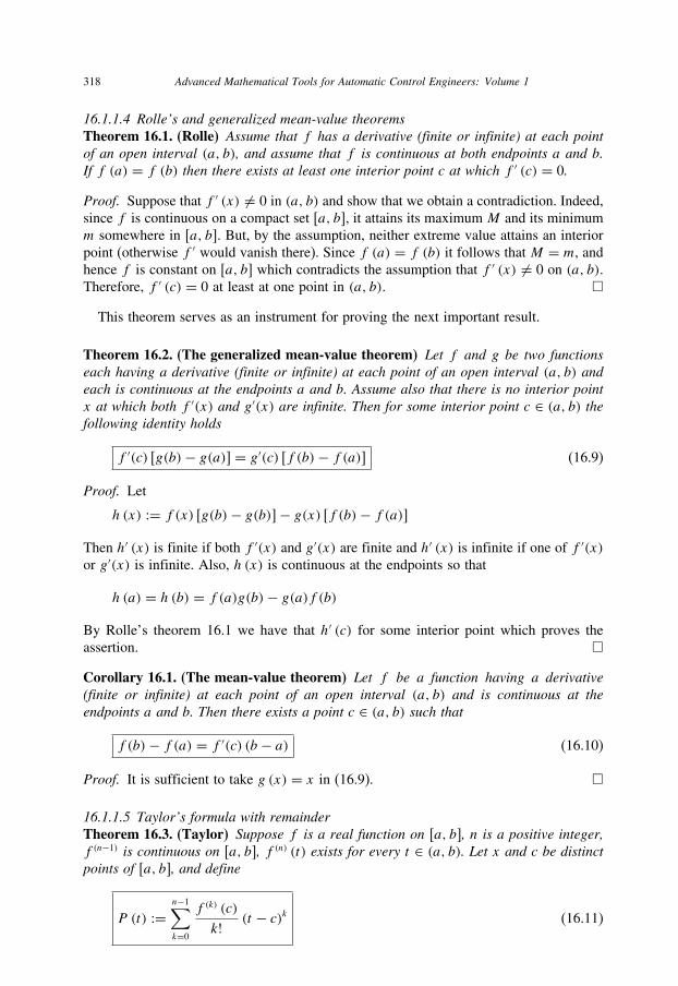
318 Advanced Mathematical Tools for Automatic Control Engineers: Volume 1
16.1.1.4 Rolle’s and generalized mean-value theoremsTheorem 16.1. (Rolle) Assume that f has a derivative (finite or infinite) at each pointof an open interval (a, b), and assume that f is continuous at both endpoints a and b.If f (a) = f (b) then there exists at least one interior point c at which f ′ (c) = 0.
Proof. Suppose that f ′ (x) �= 0 in (a, b) and show that we obtain a contradiction. Indeed,
since f is continuous on a compact set [a, b], it attains its maximumM and its minimum
m somewhere in [a, b]. But, by the assumption, neither extreme value attains an interior
point (otherwise f ′ would vanish there). Since f (a) = f (b) it follows that M = m, andhence f is constant on [a, b] which contradicts the assumption that f ′ (x) �= 0 on (a, b).
Therefore, f ′ (c) = 0 at least at one point in (a, b). �
This theorem serves as an instrument for proving the next important result.
Theorem 16.2. (The generalized mean-value theorem) Let f and g be two functionseach having a derivative (finite or infinite) at each point of an open interval (a, b) andeach is continuous at the endpoints a and b. Assume also that there is no interior pointx at which both f ′(x) and g′(x) are infinite. Then for some interior point c ∈ (a, b) thefollowing identity holds
f ′(c) [g(b)− g(a)] = g′(c) [f (b)− f (a)] (16.9)
Proof. Let
h (x) := f (x) [g(b)− g(b)]− g(x) [f (b)− f (a)]Then h′ (x) is finite if both f ′(x) and g′(x) are finite and h′ (x) is infinite if one of f ′(x)or g′(x) is infinite. Also, h (x) is continuous at the endpoints so that
h (a) = h (b) = f (a)g(b)− g(a)f (b)By Rolle’s theorem 16.1 we have that h′ (c) for some interior point which proves the
assertion. �
Corollary 16.1. (The mean-value theorem) Let f be a function having a derivative(finite or infinite) at each point of an open interval (a, b) and is continuous at theendpoints a and b. Then there exists a point c ∈ (a, b) such that
f (b)− f (a) = f ′(c) (b − a) (16.10)
Proof. It is sufficient to take g (x) = x in (16.9). �
16.1.1.5 Taylor’s formula with remainderTheorem 16.3. (Taylor) Suppose f is a real function on [a, b], n is a positive integer,f (n−1) is continuous on [a, b], f (n) (t) exists for every t ∈ (a, b). Let x and c be distinctpoints of [a, b], and define
P (t) :=n−1∑k=0
f (k) (c)
k! (t − c)k (16.11)
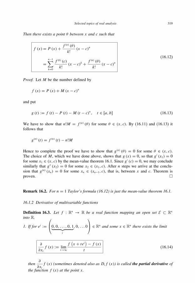
Selected topics of real analysis 319
Then there exists a point θ between x and c such that
f (x)= P (x)+ f(n) (θ)
k! (x − c)n
=n−1∑k=0
f (k) (c)
k! (x − c)k + f(n) (θ)
k! (x − c)n(16.12)
Proof. Let M be the number defined by
f (x) = P (x)+M (x − c)n
and put
g (t) := f (t)− P (t)−M (t − c)n, t ∈ [a, b] (16.13)
We have to show that n!M = f (n) (θ) for some θ ∈ (x, c). By (16.11) and (16.13) it
follows that
g(n) (t) = f (n) (t)− n!M
Hence to complete the proof we have to show that g(n) (θ) = 0 for some θ ∈ (x, c).The choice of M , which we have done above, shows that g (x) = 0, so that g′ (x1) = 0
for some x1 ∈ (x, c) by the mean-value theorem 16.1. Since g′ (c) = 0, we may conclude
similarly that g′′ (x2) = 0 for some x2 ∈ (x1, c). After n steps we arrive at the conclu-
sion that g(n) (xn) = 0 for some xn ∈ (xn−1, c), that is, between x and c. Theorem is
proven. �
Remark 16.2. For n = 1 Taylor’s formula (16.12) is just the mean-value theorem 16.1.
16.1.2 Derivative of multivariable functions
Definition 16.3. Let f : Rn → R be a real function mapping an open set E ⊂ Rn
into R.
1. If for ei :=⎛⎝0, 0, . . . , 0, 1︸ ︷︷ ︸
i
, 0, . . . 0
⎞⎠ ∈ Rn and some x ∈ Rn there exists the limit
∂
∂xif (x) := lim
t→∞f(x + tei)− f (x)
t(16.14)
then∂
∂xif (x) (sometimes denoted also as Dif (x)) is called the partial derivative of
the function f (x) at the point x.

320 Advanced Mathematical Tools for Automatic Control Engineers: Volume 1
2. If there exist the partial derivatives∂
∂xif (x) of the function f (x) at the point x for
all i = 1, . . . , n, then the vector
∇f (x) :=(∂
∂x1f (x) , . . . ,
∂
∂xnf (x)
)ᵀ(16.15)
(often denoted also as∂
∂xf (x)) is called the gradient of the function f (x) at the
point x.3. If for some u ∈ Rn and some x ∈ Rn there exists a vector a ∈ Rn such that
limt→∞
∣∣∣∣f (x + tu)− f (x)t− aᵀu
∣∣∣∣ = 0 (16.16)
then the number aᵀu (often denoted also as Duf (x)) is called the directional deriva-tive of the function f (x) in the direction u.
Remark 16.3. In fact, the vector a in (16.16) is the gradient ∇f (x), that is, a = ∇f (x)and, therefore,
Duf (x) = ∇ᵀf (x) u = (∇f (x), u) (16.17)
Indeed, any u ∈ Rn can be represented as u =∑n
i=1 uiei . Taking uj = δi,j we obtain
f (x + tu)− f (x)t
− aᵀu = f (x + tu)− f (x)t
−n∑i=1
ui(a, ei
) = f (x + tu)− f (x)t
− ai
which, according to the definition (16.14), implies the identity ai = ∂
∂xif (x) that
proves (16.17).
16.1.2.1 Mixed partial derivativesDefinition 16.4. We call the function
Dk (Dif (x)) = ∂
∂xk
(∂
∂xif (x)
)= ∂2
∂xk∂xif (x) (16.18)
the second order ik-partial derivative of the function f (x) at point x. Higher orderpartial derivatives are similarly defined.
The following example shows that in general
∂2
∂xk∂xif (x) �= ∂2
∂xi∂xkf (x)

Selected topics of real analysis 321
Example 16.1. Let us consider the function
f (x, y) =⎧⎨⎩xy
x2 − y2x2 + y2 if x2 + y2 > 0
0 if x = y = 0
Then one has
∂
∂xf (x, y) =
⎧⎨⎩y
x4 + 4x2y2 − y4(x2 + y2)2 if x2 + y2 > 0
0 if x = y = 0
Hence,∂
∂xf (0, y) = −y and
∂2
∂y∂xf (0, y) = −1
On the other hand,
∂
∂yf (x, y) =
⎧⎨⎩x
x4 + 4x2y2 − y4(x2 + y2)2 if x2 + y2 > 0
0 if x = y = 0
which implies∂
∂yf (x, 0) = x and
∂2
∂x∂yf (x, 0) = 1. So, we see that
−1 = ∂2
∂y∂xf (0, 0) �= ∂2
∂x∂yf (0, 0) = 1
It is not so difficult to prove the following result (see Theorem 12.13 in Apostol
(1974)).
Theorem 16.4. If both partial derivatives∂2
∂y∂xf (x, y) and
∂2
∂x∂yf (x, y) exist in a
neighborhood of the point (x, y) and both are continuous at this point, then
∂2
∂y∂xf (x, y) = ∂2
∂x∂yf (x, y)
Corollary 16.2. A differential [P (x, y) dx +Q(x, y) dy], where∂
∂yP (x, y) and
∂
∂xQ (x, y) exist and are continuous, can be represented as a complete differential of
some function f (x, y), namely,
P (x, y) dx +Q(x, y) dy = df (x, y) (16.19)
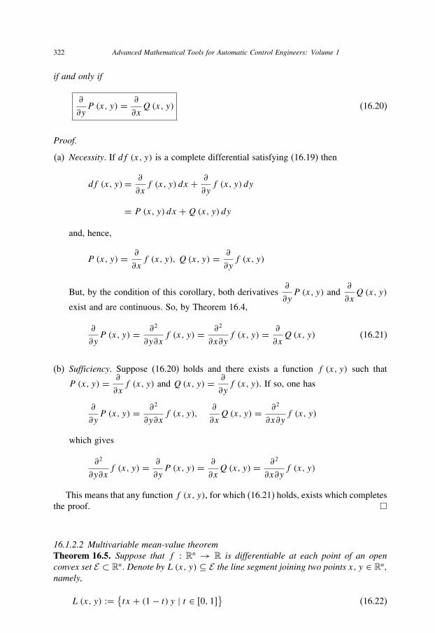
322 Advanced Mathematical Tools for Automatic Control Engineers: Volume 1
if and only if
∂
∂yP (x, y) = ∂
∂xQ (x, y) (16.20)
Proof.
(a) Necessity. If df (x, y) is a complete differential satisfying (16.19) then
df (x, y)= ∂
∂xf (x, y) dx + ∂
∂yf (x, y) dy
= P (x, y) dx +Q(x, y) dy
and, hence,
P (x, y) = ∂
∂xf (x, y), Q (x, y) = ∂
∂yf (x, y)
But, by the condition of this corollary, both derivatives∂
∂yP (x, y) and
∂
∂xQ (x, y)
exist and are continuous. So, by Theorem 16.4,
∂
∂yP (x, y) = ∂2
∂y∂xf (x, y) = ∂2
∂x∂yf (x, y) = ∂
∂xQ (x, y) (16.21)
(b) Sufficiency. Suppose (16.20) holds and there exists a function f (x, y) such that
P (x, y) = ∂
∂xf (x, y) and Q(x, y) = ∂
∂yf (x, y). If so, one has
∂
∂yP (x, y) = ∂2
∂y∂xf (x, y),
∂
∂xQ (x, y) = ∂2
∂x∂yf (x, y)
which gives
∂2
∂y∂xf (x, y) = ∂
∂yP (x, y) = ∂
∂xQ (x, y) = ∂2
∂x∂yf (x, y)
This means that any function f (x, y), for which (16.21) holds, exists which completes
the proof. �
16.1.2.2 Multivariable mean-value theoremTheorem 16.5. Suppose that f : Rn → R is differentiable at each point of an openconvex set E ⊂ Rn. Denote by L (x, y) ⊆ E the line segment joining two points x, y ∈ Rn,namely,
L (x, y) := {tx + (1− t) y | t ∈ [0, 1]
}(16.22)

Selected topics of real analysis 323
Then for any x, y ∈ Rn there exists a point z ∈ L (x, y) such that
f (y)− f (x) = (∇f (z), y − x) (16.23)
Proof. Let u := y − x. Since E is open and L (x, y) ⊆ E , then there is a δ > 0 such that
x+ tu ∈ E for some t ∈ (−δ, 1+ δ). Define on (−δ, 1+ δ) the real function F(t) by the
relation F(t) := f (x + tu). Then F(t) is differentiable on (−δ, 1+ δ) and by (16.16)
for any t ∈ (−δ, 1+ δ)F
′(t) = (∇f (x + tu), u)
By the usual mean-value theorem 16.1, we have
F (1)− F (0) = F ′(θ), θ ∈ (0, 1)
or, equivalently,
f (x + u)− f (x) = f (y)− f (x) = (∇f (x + θu), u)
= (∇f (x (1− θ)+ θy), y − x) = (∇f (z), y − x)which proves the theorem. �
16.1.2.3 Taylor’s formulaTheorem 16.6. Assume that f and all its partial (mixed) derivatives of order less thanm are differentiable at each point of an open set S ⊂ Rn. If x and y are two pointsof S such that L (x, y) ⊂ S (L (x, y) is defined by (16.22)), then there exists a pointz ∈ L (x, y) such that
f (y)−f (x) = (∇f (x), y − x)
+ 1
2
(y − x,
∥∥∥∥ ∂2
∂xi∂xkf (x)
∥∥∥∥i,k=1,...,n
(y − x))+ . . .
+ 1
(m− 1)!n∑i1=1
. . .
n∑im−1=1
∂(m−1)
∂xi1 . . . ∂xim−1
f (x)
m−1∏s=1
(yis − xis
)
+ 1
(m)!n∑i1=1
. . .
n∑im−1=1
∂(m−1)
∂xi1 . . . ∂xim−1
f (z)
m−1∏s=1
(yis − xis
)
(16.24)
Proof. Define g (t) :=f (x + t (y − x)). Then f (y)−f (x)=g (1)− g (0). By applying
the one-dimensional Taylor formula (16.12) we obtain
g (1)− g (0) =m−1∑k=1
1
k!g(k) (0)+ 1
m!g(m) (θ), θ ∈ (0, 1)
Applying the chain rule (see Claim 16.2) we obtain the result. �
324 Advanced Mathematical Tools for Automatic Control Engineers: Volume 1
16.1.2.4 Lemma on a finite incrementLemma 16.2. (on a finite increment) If f is differentiable in open set S ⊂ Rn and itsgradient ∇f (x) satisfies the Lipschitz condition on S, that is, for all x, y ∈ S thereexists a positive constant L∇ such that
‖∇f (x)− ∇f (y)‖ ≤ L∇ ‖x − y‖
then for all x, y ∈ S the following inequality holds
|f (y)− f (x)− (∇f (x), y − x)| ≤ L∇2‖x − y‖2 (16.25)
Proof. It follows from the identities
1∫t=0
(∇f (x + t (y − x)), y − x) dt =1∫t=0
d [f (x + t (y − x))]
= f (y)− f (x) f (y)− f (x)− (∇f (x), y − x)
=1∫t=0
(∇f (x + t (y − x))− ∇f (x), y − x) dt
Taking the module of both parts and applying the Cauchy–Schwartz inequality, we get
|f (y)− f (x)− (∇f (x), y − x)|
=∣∣∣∣∣∣
1∫t=0
(∇f (x + t (y − x))− ∇f (x), y − x) dt∣∣∣∣∣∣
≤1∫t=0
‖∇f (x + t (y − x))− ∇f (x)‖ ‖y − x‖ dt
≤1∫t=0
L∇ t ‖y − x‖2 dt = L∇2‖x − y‖2
Lemma is proven. �

Selected topics of real analysis 325
16.1.3 Inverse function theorem
Theorem 16.7. (on the inverse function) Suppose f is a continuously differentiable
mapping from an open set E ⊂ Rn into Rn, the matrix∂
∂xf (x) :=
∥∥∥∥ ∂∂xk fi (x)∥∥∥∥i,k=1,...,n
is invertible in a point x = a ∈ E and f (a) = b. Then(a) there exist open sets U and V in Rn such that a ∈ U , b ∈ V , f is one-to-one on
U and
f (U) = V (16.26)
(b) if f −1 is the inverse of f (which exists by (a)), defined on V by
f −1 (f (x)) = x, x ∈ U (16.27)
then f −1 is continuously differentiable on V .
Proof.
(a) Denote A := ∂
∂xf (a) and choose λ so that
2λ∥∥A−1
∥∥ = 1 (16.28)
where∥∥A−1
∥∥ :=√λmax
(A−1
(A−1
)ᵀ). Since
∂
∂xf (x) is continuous in a, there
exists a ball U ⊂ E , with center in a, such that for all x ∈ U∥∥∥∥ ∂∂x f (x)− A∥∥∥∥ < λ (16.29)
Let us associate to each point y ∈ Rn the function ϕy defined by
ϕy (x) := x + A−1 (y − f (x)) (16.30)
Note that y = f (x) if and only if x is a fixed point of ϕy . (16.28) and (16.29) imply∥∥∥∥ ∂∂x ϕy (x)∥∥∥∥=
∥∥∥∥I − A−1∂
∂xf (x)
∥∥∥∥ =∥∥∥∥A−1
(A− ∂
∂xf (x)
)∥∥∥∥≤ ∥∥A−1
∥∥∥∥∥∥A− ∂
∂xf (x)
∥∥∥∥ < ∥∥A−1∥∥ λ = 1
2
Hence, by the mean-value theorem 16.5 it follows that
∥∥ϕy (x ′)− ϕy (x ′′)∥∥ ≤ supθ∈U
∥∥∥∥ ∂∂x f (θ)∥∥∥∥∥∥x ′ − x ′′∥∥ < 1
2
∥∥x ′ − x ′′∥∥ (16.31)

326 Advanced Mathematical Tools for Automatic Control Engineers: Volume 1
which means, by Theorem 14.17, that ϕy (x) has at most one fixed point in U . So,
y = f (x) for at most one point x ∈ U . And, since∂
∂xf (x) is invertible in U , we
conclude that f is one-to-one in U . Next, put f (U) = V and pick y0 ∈ V . Theny0 = f (x0) for some x0 ∈ U . Let B be an open ball with the center in x0 and
radius r > 0, so small that its closure B lies in U . Let us show that y ∈ V whenever
‖y − y0‖ < λr . Fix y such that ‖y − y0‖ < λr . By (16.30) we have∥∥ϕy (x0)− x0∥∥ = ∥∥A−1 (y − y0)∥∥ ≤ ∥∥A−1
∥∥ ‖y − y0‖ < ∥∥A−1∥∥ λr = r/2
If x ∈ B, then it follows from (16.31) that∥∥ϕy (x)− x0∥∥= ∥∥[ϕy (x)− ϕy (x0)]+ [ϕy (x0)− x0]∥∥ ≤ ∥∥ϕy (x)− ϕy (x0)∥∥
+∥∥ϕy (x0)− x0∥∥ < 1
2‖x − x0‖ + r/2 ≤ r
Hence, ϕy (x) ∈ B. Note that (16.31) also holds if x ′, x ′′ ∈ B. Thus ϕy (x) is a
contraction of B into B. Being a closed subset of Rn, B is complete. Then by the
fixed-point theorem 14.17 we conclude that ϕy (x) has a fixed point x ∈ B. For thisx it follows that f (x) = y. Thus y ∈ f (
B) ⊂ f (U) = V which proves (a).
(b) Pick y ∈ V and y + z ∈ V . Then there exist x ∈ U and x + h ∈ U so that y = f (x)and y + z = f (x + h). So,
ϕy (x + h)− ϕy (x) = h+ A−1 [f (x)− f (x + h)] = h− A−1z
By (16.31) we have
∥∥h− A−1z∥∥ < 1
2‖h‖
which, by the inequality ‖a − b‖ ≥ ‖a‖ − ‖b‖, implies
‖h‖ − ∥∥A−1z∥∥ ≤ ∥∥h− A−1z
∥∥ < 1
2‖h‖
and, therefore,
1
2‖h‖ < ∥∥A−1z
∥∥or, equivalently,
‖h‖ < 2∥∥A−1z
∥∥ ≤ 2∥∥A−1
∥∥ ‖z‖ = ‖z‖/λ (16.32)
Since∂
∂xf (x) has an inverse on U , say T , we get
g (y + z)− g (y)− T z = h− T z = −T[f (x + h)− f (x)− ∂
∂xf (x) h
]

Selected topics of real analysis 327
which in view of (16.32) implies
‖g (y + z)− g (y)− T z‖‖z‖ ≤ ‖T ‖
λ
∥∥∥∥f (x + h)− f (x)− ∂
∂xf (x) h
∥∥∥∥‖h‖
As z → 0, (16.32) shows that h → 0 and therefore the right-hand side of the last
inequality tends to zero which is true of the left. This proves that∂
∂xg (y) = T . But
T is chosen to be the inverse of∂
∂xf (x) = ∂
∂xf (g (y)). Thus
∂
∂xg (y) =
[∂
∂xf (g (y))
]−1
(16.33)
for y ∈ V . But both g and∂
∂xf (x) are locally continuous which together with
(16.33) implies that g is continuously differentiable on V .Theorem is proven. �
Summary 16.1. The inverse function theorem 16.7 states, roughly speaking, that acontinuous differentiable mapping f (x) is invertible in a neighborhood of any point x
at which the linear transformation∂
∂xf (x) is invertible.
Corollary 16.3. The system of n equations
yi = fi (x1, . . . , xn), i = 1, . . . , n
can be solved for (x1, . . . , xn) in terms of (y1, . . . , yn) if∂
∂xf (x) is invertible in a
neighborhood of the point x = (x1, . . . , xn).
16.1.4 Implicit function theorem
For x ∈ Rn and y ∈ Rm let us consider the extended vector z := (xᵀ, yᵀ)ᵀ ∈ Rn+m.Then any linear transformation A : Rn+m → Rn can be represented as
Az = [Ax Ay
](xy
)= Axx + Ayy
Then the following result seems to be obvious.
Lemma 16.3. (A linear version) If Ax is invertible, then for every y ∈ Rm there existsa unique x ∈ Rn such that
Axx + Ayy = 0 (16.34)

328 Advanced Mathematical Tools for Automatic Control Engineers: Volume 1
This x can be calculated as
x = − (Ax)−1Ayy (16.35)
The theorem given below represents the, so-called, implicit function theorem for nonlinear
mappings.
Theorem 16.8. (The implicit function theorem) Let f be a continuously differentiablemapping of an open set E ⊂ Rn+m into Rn such that
f (x, y) = 0 (16.36)
for some point z := (xᵀ, yᵀ)ᵀ ∈ E . DenoteA := ∂
∂zf (z) and assume thatAx := ∂
∂xf (z)
is invertible. Then there exist open sets U ⊂ Rn+m and W ⊂ Rm with z ∈ U and y ∈ W ,having the following properties:
1. To every y ∈ W there exists a unique x such that
z =(x
y
)∈ U and f (x, y) = 0 (16.37)
2. If x is defined to be g (y), then g is continuously differentiable on W , g (y) = x, forany y ∈ W
f (g (y), y) = 0 (16.38)
and
∂
∂yg (y) = − (Ax)−1Ay (16.39)
where Ay := ∂
∂yf (z).
Proof. For z ∈ E define
F (x, y) :=(f (x)
y
)
Then F is a continuously differentiable mapping of E into Rn+m. Show now that∂
∂zF (z)
is an invertible element in Rn+m. Indeed, since f (z) = 0, we have
f (x + h, y + k) = A(h
k
)+ r (h, k)
Selected topics of real analysis 329
where r (h, k) is a remainder that occurs in the definition of A = ∂
∂zf (z). Again, since
F (x + h, y + k)− F (x, y) =(f (x + h, y + k)
k
)
=⎛⎝A
(h
k
)k
⎞⎠+
(r (h, k)
0
)
it follows that∂
∂zF (z) is the linear operator on Rn+m that maps
(h
k
)to
⎛⎝A
(h
k
)k
⎞⎠.
It is seen that∂
∂zF (z) is one-to-one and hence it is invertible. So, the inverse function
theorem can therefore be applied to F that proves (1). To prove (2) define g (y) for
y ∈ W so that �(y) :=(g (y)
y
)∈ U and (16.38) holds. Then F (g (y), y) =
(0
y
)
and∂
∂y� (y) k =
⎛⎝ ∂
∂yg (y) k
k
⎞⎠. In view of the identity f (� (y)) = 0 the chain rule
shows that
∂
∂zf (� (y))
∂
∂y� (y) = 0
Thus
A∂
∂y� (y) = 0
which gives
Ax∂
∂yg (y) k + Ayk = A ∂
∂y� (y) = 0
This completes the proof. �
Example 16.2. Let
f1 (x1, x2, y1, y2, y5)= 2ex1 + x2y1 − 4y2 + 3 = 0
f2 (x1, x2, y1, y2, y5)= x2 cos x1 − 6x1 + 2y1 − 4y3 = 0
and x = (0 1
)ᵀ, y = (
3 2 7). Then
Ax =[
2 3
−6 1
], Ay =
[1 −4 0
2 0 −1
]
Notice that detAx = 20 �= 0 and hence Ax is invertible and x in a neighborhood of x, ycan be represented as a function of y, that is, x = g (y).

330 Advanced Mathematical Tools for Automatic Control Engineers: Volume 1
16.1.5 Vector and matrix differential calculus
16.1.5.1 Differentiation of scalar functions with respect to a vectorAssuming that x, y ∈ Rn, P ∈ Rn×n, A ∈ Rm×n, the direct calculation shows that
∂
∂x(xᵀy) = ∂
∂x(yᵀx) = y (16.40)
∂
∂x(Px) = Pᵀ,
∂
∂x(xᵀPy) = Py (16.41)
∂
∂x(yᵀPx) = Pᵀy,
∂
∂x(xᵀPx) = (P + Pᵀ) x
and∂
∂x(xᵀPx) = 2Px only when P = Pᵀ
⎫⎪⎬⎪⎭ (16.42)
∂
∂xᵀ (Ax) = A (16.43)
∂
∂x‖x‖2 = x
‖x‖2 , x �= 0 (16.44)
∂
∂x(x ⊗ y) = e ⊗ y = col {In×n ⊗ y}
e := (1, 1, . . . , 1)ᵀ
}(16.45)
16.1.5.2 Differentiation of scalar fun!ctions with respect to a matrixFor the matrices A,B and C the direct calculation implies
∂
∂Atr (A) = A (16.46)
∂
∂Atr (BAC) = BᵀCᵀ,
∂
∂Atr (BAᵀC) = CB (16.47)
∂
∂Atr (ABAᵀ) = ABᵀ + AB, ∂
∂Atr (ABA) = AᵀBᵀ + BᵀAᵀ (16.48)
∂
∂Atr (BACA)=CᵀAᵀBᵀ + BᵀAᵀCᵀ
∂
∂Atr (BACAᵀ)=BAC + BᵀACᵀ
⎫⎪⎬⎪⎭ (16.49)

Selected topics of real analysis 331
∂
∂Atr (AᵀA) = 2A (16.50)
∂
∂Atr (BAᵀAC)= ACB + ABᵀCᵀ
∂
∂Atr (BAAᵀC) = CBA+ BᵀCᵀA
⎫⎪⎬⎪⎭ (16.51)
∂
∂Atr (BAᵀABᵀ) = 2ABᵀB,
∂
∂Atr (BAAᵀBᵀ) = 2BᵀBA (16.52)
∂
∂Atr(Bᵀ (AᵀA)2 B
)= ∂
∂Atr (BᵀAᵀ (AAᵀ) AB)
= 2A (AᵀA)BᵀB + 2ABᵀB (AᵀA)
⎫⎪⎬⎪⎭ (16.53)
∂
∂Atr (exp (A)) = exp (A) (16.54)
∂
∂Adet (BAC) = det (BAC)
(A−1
)ᵀ(16.55)
∂
∂Atr(Ak
) = k (Ak−1)ᵀ,
∂
∂Atr(BAk
) = k−1∑i=0
(AiBAk−i−1
)ᵀ(16.56)
∂
∂Atr(BA−1C
) = − (A−1CBA−1
)ᵀ(16.57)
∂
∂Alog det (A) = − (Aᵀ)−1 (16.58)
∂
∂Adet (Aᵀ) = ∂
∂Adet (A) = (Aᵀ)−1 det (A) (16.59)
∂
∂Adet
(Ak
)= ∂
∂A[det (A)]
k
= k [det (A)]k−1 ∂
∂Adet (A)
= k [det (A)]k−1(Aᵀ)−1 det (A) = k (Aᵀ)−1 det
(Ak
)
⎫⎪⎪⎪⎪⎪⎪⎪⎪⎬⎪⎪⎪⎪⎪⎪⎪⎪⎭
(16.60)

332 Advanced Mathematical Tools for Automatic Control Engineers: Volume 1
16.1.6 Nabla operator in three-dimensional space
Definition 16.5. Define
1. the differential nabla operator ∇ or gradient, acting to a differentiable functionϕ : R3 → R1, by the following formula
∇ϕ (x, y, z) :=
⎛⎜⎜⎜⎜⎜⎜⎝
∂
∂xϕ (x, y, z)
∂
∂yϕ (x, y, z)
∂
∂zϕ (x, y, z)
⎞⎟⎟⎟⎟⎟⎟⎠ (16.61)
2. the differentiable operator div (divergence), acting to a differentiable functionf : R3 → R3, by the following formula
divf (x, y, z) := ∂
∂xfx (x, y, z)+ ∂
∂yfy (x, y, z)+ ∂
∂zfz (x, y, z) (16.62)
3. the differentiable operator rot (rotor), acting to a differentiable function f : R3 → R3,by the following formula
rotf (x, y, z) :=
⎡⎢⎢⎣
i j k∂
∂x
∂
∂y
∂
∂zf1 (x, y, z) f2 (x, y, z) f3 (x, y, z)
⎤⎥⎥⎦
= i(∂
∂yf3 (x, y, z)− ∂
∂zf2 (x, y, z)
)
+ j(∂
∂zf1 (x, y, z)− ∂
∂xf3 (x, y, z)
)
+k(∂
∂xf2 (x, y, z)− ∂
∂yf1 (x, y, z)
)
where (i, j,k) is the orthogonal basis in R3.
Remember some important properties of the scalar (a, b) and the vector product [a, b] of
the vectors a = (ax, ay, az
)ᵀand b = (
bx, by, bz)ᵀ
in R3 which are defined by
(a, b) := axbx + ayby + azbz (16.63)

Selected topics of real analysis 333
and
[a, b] :=⎡⎣ i j kax ay azbx by bz
⎤⎦
= i(aybz − azby
)+ j (azbx − axbz)+ k(axby − aybx
) (16.64)
It is necessary to check that
(a, a)= ‖a‖2(a, b)= (b, a)(a, b)= 0 if a ⊥ b
(a, b + c)= (a, b)+ (a, c)
(16.65)
and
[a, b] = − [b, a]
[a, (b + c)] = [a, b]+ [a, c]
[a, b] = 0 if a = λb, λ ∈ R(a, [b, c]
) = (b, [c, a]
) = (c, [a, b]
)[a, [b, c]] = b (a, c)− c (a, b)
[a, [b, c]]+ [b, [c, a]]+ [c, [a, b]] = 0
(16.66)
Notice also that the operators div and rot, using the definitions above, can be represented
in the following manner
div ϕ = (∇, ϕ)rot ϕ = [∇, ϕ] (16.67)
Applying rules (16.65) and (16.66) one can prove that
div (αf + βg) = α div f + β div g
α, β ∈ R(16.68)
div grad ϕ = (∇,∇ϕ) = �ϕ
�ϕ := ∂2
∂x2fx (x, y, z)+ ∂2
∂y2fy (x, y, z)+ ∂2
∂y2fx (x, y, z)
where � is the Laplace operator
(16.69)
334 Advanced Mathematical Tools for Automatic Control Engineers: Volume 1
div rot f = (∇, [∇, f ]) = ([∇,∇], f ) = 0 (16.70)
rot rot f = [∇, [∇, f ]]= ∇ (∇, f )− (∇,∇) f = grad div f −�f (16.71)
16.2 On Riemann–Stieltjes integrals
16.2.1 The necessary condition for existence of Riemann–Stieltjes integrals
Here we will examine the following statement: when α is of bounded variation on[a, b], continuity of f is sufficient for the existence of the Riemann–Stieltjes inte-gral
∫ bx=a f (x) dα (x)? We conclude that: continuity of f throughout [a, b] is by no
means necessary, however! The next theorem shows that common discontinuities (fromthe right or from the left) should be avoided if the integral
∫ bx=a f (x) dα (x) is to exist.
Define
U (Pn, f, α) :=n∑i=1
Mi�αi
Mi := sup{f (x) : x ∈ [xi−1, xi]
}L (Pn, f, α) :=
n∑i=1
Mi�αi
mi := inf{f (x) : x ∈ [xi−1, xi]
}(16.72)
which coincide with the upper and lower Darboux sums, respectively, (see (15.4) and
(15.5)) for the case α (x) = x.
Theorem 16.9. (The necessary condition) Assume that α ↑ on [a, b] and c ∈ (a, b).Assume further that both f and α are discontinuous simultaneously from the right atx = c, that is, assume that there exists ε > 0 such that for every δ > 0 there are valuesof x and y within the interval (c, c + δ) for which
|f (x)− f (y)| ≥ ε and |α (x)− α (y)| ≥ ε
Then the integral∫ bx=a f (x) dα (x) cannot exist. The integral also fails to exist if f and
α are discontinuous simultaneously from the left at x = c.
Selected topics of real analysis 335
Proof. Let Pn be a partition of [a, b] containing the point c as a point of subdivision.
Then one has
U (Pn, f, α)− L (Pn, f, α) :=n∑i=1
(Mi −mi)�αi (16.73)
If the ith interval has c as its left endpoint then
U (Pn, f, α)− L (Pn, f, α) ≥ (Mi −mi) [αi (xi)− αi (c)]
since each term in (16.73) is nonnegative. If c is a common discontinuity point from the
right, we may assume that the point xi is chosen in such a way that [αi (xi)− αi (c)] ≥ ε.Moreover, by the assumptions of the theorem (Mi −mi) ≥ ε. So,
U (Pn, f, α)− L (Pn, f, α) ≥ ε2 (16.74)
But by the definition (15.11) of the Riemann–Stieltjes integral there exists n such that
|U (Pn, f, α)− S (Pn, f, α)| < ε2
2, |L (Pn, f, α)− S (Pn, f, α)| < ε
2
2
and, hence,
U(Pn, f, α)− L (Pn, f, α) = [U (Pn, f, α)− S (Pn, f, α)]+ [S (Pn, f, α)− L (Pn, f, α)] ≤ |U (Pn, f, α)− S (Pn, f, α)|+ |S (Pn, f, α)− L (Pn, f, α)| < ε2
which is in contradiction with (16.74). If c is a common discontinuity from the left the
argument is similar. Theorem is proven. �
16.2.2 The sufficient conditions for existence of Riemann–Stieltjes integrals
Theorem 16.10. (First sufficient (Riemann’s) condition) Assume that α ↑ on [a, b].If for any ε > 0 there exists a partition Pε of [a, b] such that Pn is finer than Pε implies
0 ≤ U (Pn, f, α)− L (Pn, f, α) < ε (16.75)
then f ∈ R[a,b] (α).
Proof. Since by α ↑ on [a, b] we have
U (Pn, f, α) ≤ S (Pn, f, α) ≤ L (Pn, f, α)
In view of (16.75) this means that S (Pn, f, α) has a limit when n → ∞ which, by the
definition (15.11), is the Riemann–Stieltjes integral. Theorem is proven. �
336 Advanced Mathematical Tools for Automatic Control Engineers: Volume 1
Theorem 16.11. (Second sufficient condition) If f is continuous on [a, b] and α is ofbounded variation on [a, b], then f ∈ R[a,b] (α).
Proof. Since by (15.55) any α of bounded variation can be represented as α (x) =α+ (x) − α− (x) (where α+ ↑ on [a, b] and α− ↑ on [a, b]), it suffices to prove the
theorem when α ↑ on [a, b] with α (a) < α (b). Continuity of f on [a, b] implies
uniform continuity, so that if ε > 0 is given, we can find δ = δ (ε) > 0 such that
|x − y| < δ implies |f (x)− f (y)| < ε/A where A = 2 [α (b)− α (a)]. If Pε is
a partition with the biggest interval less than δ, then any partition Pn finer than Pεgives
Mi −mi ≤ ε/A (16.76)
since
Mi −mi = sup{f (x)− f (y) : x, y ∈ [xi−1, xi]
}Multiplying (16.76) by �αi and summing, we obtain
U (Pn, f, α)− L (Pn, f, α) ≤ ε/An∑i=1
�αi = ε2< ε
So, Riemann’s condition (16.75) holds. Theorem is proven. �
Corollary 16.4. For the special case of the Riemann integral when α (x) = x Theorem16.11 together with (15.23) state that each of the following conditions is sufficient forthe existence of the Riemann integral
∫ bx=a f (x) dx:
1. f is continuous on [a, b];2. f is of bounded variation on [a, b].
The following theorem represents the criterion (the necessary and sufficient condition)
for the Riemann integrability.
Theorem 16.12. (Lebesgue’s criterion for integrability) Let f be defined and boundedon [a, b]. Then it is the Riemann integrable on [a, b], which is f ∈ R[a,b] (x), if and onlyif f is continuous almost everywhere on [a, b].
Proof. Necessity can be proven by contradiction assuming that the set of discontinuity
has a nonzero measure and demonstrating that in this case f is not integrable. Sufficiencycan be proven by demonstrating that Riemann’s condition (16.75) (when α (x) = x) issatisfied assuming that the discontinuity points have measure zero. The detailed proof
can be found in Apostol (1974). �

Selected topics of real analysis 337
16.2.3 Mean-value theorems
Although integrals occur in a wide variety of problems (including control), there
are relatively few cases when the explicit value of the integral can be obtained. How-
ever, it is often sufficient to have an estimate for the integral rather than its exact
value. The mean-value theorems of this subsection are especially useful in making such
estimates.
Theorem 16.13. (First mean-value theorem) Assume that f ∈ R[a,b] (α) with α ↑ on[a, b]. Denote
M := supx∈[a,b]
f (x), m := infx∈[a,b]
f (x)
Then there exists a real number c ∈ [m,M] such that
b∫x=af (x) dα (x) = c
b∫x=adα (x) = c [α (b)− α (a)] (16.77)
Proof. If a = b both sides of (16.77) are zero and the result holds trivially. Assume that
α (a) < α (b). By (16.72) we have
m [α (b)− α (a)]≤L (Pn, f, α) ≤b∫x=af (x) dα (x)
≤U (Pn, f, α) ≤ M [α (b)− α (a)]
which proves (16.77). Theorem is proven. �
Remark 16.4. Evidently, if f is continuous on [a, b] then there exists x0 ∈ [a, b] suchthat c = f (x0).
Theorem 16.14. (Second mean-value theorem) Assume that α (x) is continuous on[a, b] and f ↑ on [a, b]. Then there exists a point x0 ∈ [a, b] such that
b∫x=af (x) dα (x) = f (a)
x0∫x=adα (x)+ f (b)
a∫x=x0
dα (x) (16.78)
Proof. Integrating by parts (see (15.23)) implies
b∫x=af (x) dα (x) = f (b) α (b)− f (a) α (a)−
b∫x=aα (x) df (x)

338 Advanced Mathematical Tools for Automatic Control Engineers: Volume 1
Applying (16.77) to the integral on the right-hand side of the last identity we have
b∫x=af (x) dα (x)= f (b) α (b)− f (a) α (a)− c
b∫x=adf (x)
= f (b) α (b)− f (a) α (a)− α (x0) [f (b)− f (a)]= f (b) [α (b)− α (x0)]+ f (a) [α (x0)− α (a)]
which is the statement we set out to prove. �
Corollary 16.5. (The Riemann integrals case) Let g be continuous on [a, b] and f ↑on [a, b]. Then1. there exists a point x0 ∈ [a, b] such that
b∫x=af (x) g (x) dx = A
x0∫x=ag (x) dx + B
b∫x=x0
g (x) dx (16.79)
where A ≤ f (a + 0) and B ≥ f (b − 0);2. Bonnet’s theorem holds, namely, if, in addition, f (x) ≥ 0 on [a, b] then A = 0 in
(16.79) which gives
b∫x=af (x) g (x) dx = B
b∫x=x0
g (x) dx (16.80)
16.2.4 The integral as a function of the interval
Theorem 16.15. Let α : R → R be of bounded variation on [a, b] and f ∈ R[a,b] (α).For any x ∈ [a, b] define
F (x) :=x∫s=af (s) dα (s) (16.81)
Then
(a) F is of bounded variation on [a, b] ;(b) Every point of continuity of α is also a point of continuity of F ;(c) If f ↑ on [a, b] then the derivative F ′ (x) exists at each point x ∈ (a, b) where α′ (x)
exists and where f is continuous. For such x
F ′ (x) = f (x) α′ (x) (16.82)

Selected topics of real analysis 339
Proof. It is sufficient to assume that α ↑ on [a, b]. If x �= y by (16.77) it follows that
F (y)− F (x) =y∫s=xf (s) dα (s) = c [α (y)− α (x)]
where c ∈ [m,M]. So, statements (a) and (b) follow at once from this equation. To prove
(c) it is sufficient to divide both sides by (y − x) and observe that c → f (x) when
y → x. Theorem is proven. �
Corollary 16.6.
1. If f ∈ R[a,b] (α) then for any x ∈ [a, b] and the functions F and G defined as
F (x) :=x∫s=af (s) ds and G(x) :=
x∫s=ag (s) ds
we have
b∫s=af (s) g (s) ds =
b∫s=af (s) dG (s) =
b∫s=ag (s) dF (s) (16.83)
2. In the Riemann case, when α (x) = x, from (16.82) we obtain the, so-called, firstfundamental theorem of integral calculus:
F ′ (x) = f (x) (16.84)
16.2.5 Derivative integration
Theorem 16.16. Assume f ∈ R[a,b] (α) and g, defined on [a, b], has the derivative g′ in(a, b) such that for each x ∈ (a, b)
g′ (x) = f (x) (16.85)
If in the endpoints
g (a)− g (a + 0) = g (b)− g (b − 0)
then the Newton–Leibniz formula (the second fundamental theorem of integral calculus)holds, namely,
b∫x=af (x) dx =
b∫x=ag′ (x) dx = g (b)− g (a) (16.86)

340 Advanced Mathematical Tools for Automatic Control Engineers: Volume 1
Proof. For every partition Pn of [a, b] and in view of the mean-value theorem (16.77)
we have
g (b)− g (a) =n∑i=1
[g (xi)− g (xi−1)] =n∑i=1
g′ (ti)�xi =n∑i=1
f (ti)�xi
where ti ∈ [xi−1, xi]. But, since f is integrable, for any ε > 0 the partition Pn can be
selected so fine that∣∣∣∣∣∣g (b)− g (a)−b∫x=af (x) dx
∣∣∣∣∣∣ =∣∣∣∣∣∣n∑i=1
f (ti)�xi −b∫x=af (x) dx
∣∣∣∣∣∣ < εwhich proves the theorem. �
16.2.6 Integrals depending on parameters and differentiation under integral sign
Theorem 16.17. Let f : R2 → R be continuous at each point (x, y) ∈ Q where
Q := {(x, y) | a ≤ x ≤ b, c ≤ y ≤ d} (16.87)
Assume that α is of bounded variation on [a, b] and F is the function defined on [c, d]
by the equation
F (y) =b∫x=af (x, y) dα (x) (16.88)
Then F is continuous on [c, d], or, in other words, if y0 ∈ [c, d] then
limy→y0
b∫x=af (x, y) dα (x)=
b∫x=a
limy→y0
f (x, y) dα (x)
=b∫x=af (x, y0) dα (x)
(16.89)
Proof. Assume α ↑ on [a, b]. Since Q is a compact then f is uniformly continuous on
Q. Hence, for any ε > 0 there exists δ = δ (ε) such that for any pair of points z := (x, y)and z′ := (x ′, y ′) such that ‖z− z′‖ < δ we have |f (x, y)− f (x ′, y ′)| ≤ ε. So, if
|y − y ′| < δ we have
∣∣F (y)− F (y ′)∣∣ ≤ b∫
x=a
∣∣f (x, y)− f (x ′, y ′
)∣∣ dα (x) ≤ ε [α (b)− α (a)]which establishes the continuity of F (y). �

Selected topics of real analysis 341
Corollary 16.7. (The Riemann integral case) If f is continuous on Q and g ∈ R[a,b]
(x) then function F (y), defined by (16.88), is continuous on [c, d], that is, if y0 ∈ [c, d]
then
limy→y0
b∫x=ag(x)f (x, y) dx =
b∫x=ag(x) lim
y→y0f (x, y) dx
=b∫x=ag(x)f (x, y0) dx
(16.90)
Proof. Define G(x) := ∫ xs=a g(s)ds. Then by (16.83) F (y) may be represented as
F(y) = ∫ bx=a f (x, y) dG(x). Now, applying Theorem 16.17, we obtained the desired
result. �
Theorem 16.17 permits to establish the following important result.
Theorem 16.18. Assume that α is of bounded variation on [a, b] and F defined on [c, d]
by the equation F (y) = ∫ bx=a f (x, y) dα (x) exists for every y ∈ [c, d]. If the partial
derivative∂
∂yf (x, y) is continuous on Q (16.87) then F ′ (y) exists on [c, d] and it is
given by the formula
F ′ (y) =b∫x=a
∂
∂yf (x, y) dα (x) (16.91)
Proof. Assuming that y0 ∈ (c, d) then we have
F (y)− F (y0)y − y0 =
b∫x=a
f (x, y)− f (x, y0)y − y0 dα (x)
=b∫x=a
∂
∂yf (x, y) dα (x), y ∈ [y0, y]
Since∂
∂yf (x, y) is continuous on Q, taking y0, y → y0 we obtain the validity of (16.91)
in the point y = y0. Theorem is proven. �

342 Advanced Mathematical Tools for Automatic Control Engineers: Volume 1
The following statement can be checked directly.
Proposition 16.1. If ϕ1 (t) and ϕ2 (t) are differentiable on [a, b], the function f (t, τ ) ∈R[a,b] (α) is differentiable on t and continuous on τ for any fixed t ∈ [a, b], then
d
dt
ϕ2(t)∫τ=ϕ1(t)
f (t, τ ) dα (τ)
= ϕ′2 (t) f (t, ϕ2 (t)) α′ (ϕ2 (t))
− ϕ′1 (t) f (t, ϕ1 (t)) α′ (ϕ1 (t))+ϕ2(t)∫τ=ϕ1(t)
∂
∂tf (t, τ ) dα (τ)
(16.92)
Particularly,
d
dt
ϕ2(t)∫τ=ϕ1(t)
f (t, τ ) dτ
= ϕ′2 (t) f (t, ϕ2 (t))
−ϕ′1 (t) f (t, ϕ1 (t))+ϕ2(t)∫τ=ϕ1(t)
∂
∂tf (t, τ ) dα (τ)
(16.93)
16.3 On Lebesgue integrals
16.3.1 Lebesgue’s monotone convergence theorem
Theorem 16.19. (The monotone convergence theorem) Suppose E ∈ M and let {fn}be a sequence of measurable nonnegative functions such that for all x ∈ E
0 ≤ f1 (x) ≤ f2 (x) ≤ · · · ≤ (16.94)
Let f be defined by
fn (x) →n→∞ f (x), x ∈ E (16.95)
Then ∫E
fn dμ →n→∞
∫E
f dμ (16.96)

Selected topics of real analysis 343
Proof. By (16.94) it evidently follows that∫E
fn dμ →n→∞ α ≤
∫E
f dμ (16.97)
for some α ≥ 0 since∫
E fn dμ ≤ ∫E f dμ. Choose c ∈ (0, 1), and let s be a simple
measurable function (15.104) such that 0 ≤ s ≤ f . Put
En := {x | fn (x) ≥ cs (x)}, n = 1, 2, . . .
By (16.94) E1 ⊂ E2 ⊂ · · · and by (16.95) it follows that E = ⋃∞n=1 En. For every n we
have∫E
fn dμ ≥∫En
fn dμ ≥ c∫En
s dμ
Let now n→∞. By Theorem 15.15 we obtain α ≥ c ∫En s dμ. Letting c→ 1 we see that
α ≥ ∫En s dμ and (15.109) implies α ≥ ∫
En f dμ which together with (16.97) proves the
theorem. �
Corollary 16.8. Suppose fi (i = 1, 2) are Lebesgue measurable, that is, fi ∈ L (μ) onE . Then f = (f1 + f2) ∈ L (μ) on E and
∫E
f dμ =∫E
f1 dμ+∫E
f2 dμ (16.98)
Proof.
(a) Suppose, first, that f1 ≥ 0 and f2 ≥ 0. Choose monotonically increasing sequences{s ′n}and
{s ′′n}of nonnegative measurable simple functions which converge to f1
and f2, respectively. Since for simple functions (16.98) follows trivially, then for
sn = s ′n + s ′′n it follows that∫E
sn dμ =∫E
s ′n dμ+∫E
s ′′n dμ
Taking n→∞ and applying Theorem 16.19 we obtain (16.98).
(b) If f1 ≥ 0 and f2 ≤ 0 let us put
A := {x | f (x) ≥ 0}, B := {x | f (x) < 0}
Then it follows that f, f1 and (−f2) are nonnegative on A. Hence, by the previous
consideration,∫A
f1 dμ =∫A
f dμ+∫A
(−f2) dμ =∫A
f dμ−∫A
f2 dμ (16.99)
344 Advanced Mathematical Tools for Automatic Control Engineers: Volume 1
Similarly, −f, f1 and (−f2) are nonnegative on B, so that∫B
(−f2) dμ =∫B
f1 dμ+∫B
(−f ) dμ =∫B
f1 dμ−∫B
(f ) dμ
(16.100)
Adding (16.99) and (16.100) implies (16.98).
(c) In the general case, E can be discomposed into four sets Ei on each of which f1 and
f2 are of constant sign. By previous considerations we have proved that∫Ei
f dμ =∫Ei
f1 dμ+∫Ei
f2 dμ(i = 1, 4
)
and (16.98) follows by adding these four equations. �
Corollary 16.9. Suppose E ∈ M and let {fn} be a sequence of measurable nonnegativefunctions such that
f (x) =∞∑n=1
fn (x), x ∈ E (16.101)
Then
∫E
f dμ =∞∑n=1
∫E
fn dμ (16.102)
Proof. The partial sum of (16.101) forms a monotonically increasing sequence that
implies (16.102). �
16.3.2 Comparison with the Riemann integral
Let the measurable space X be the interval [a, b] of the real line with the measure
μ = m (the Lebesgue measure) and M be the family of Lebesgue-measurable subsets of
[a, b], that is, the Borel σ -algebra.
Theorem 16.20.
(a) If f ∈ R[a,b] (m) then f ∈ L (μ) on [a, b], that is, each function which is Riemannintegrable on an interval is also Lebesgue integrable, and also both integrals areequal, i.e.,
b∫x=af (x) dx =
∫E=[a,b]
f dμ (16.103)

Selected topics of real analysis 345
(b) Suppose f is bounded on [a, b]. Then f ∈ R[a,b] (m) if and only if f is continuousalmost everywhere on [a, b].
Proof.(a) follows from Theorem 16.12. To prove (b) suppose that {Pk} is a sequence of
partitions of [a, b] such that Pk+1 is a refinement of Pk . Using the definition (16.72)
for α(x) = x, namely,
L (Pn, f, x) :=n∑i=1
mi�xi, U (Pn, f, x) :=n∑i=1
Mi�xi
mi := infx∈(xi−1,xi ]
f (x), Mi := supx∈(xi−1,xi ]
f (x)
and defining
Un (x) =n∑i=1
Miχ(x ∈ (xi−1, xi]
)Ln (x) =
n∑i=1
miχ(x ∈ (xi−1, xi]
)
such that Ui (a) = Li (a) = f (a) we obtain
L1 (x) ≤ L2 (x) ≤ · · · ≤ f (x) ≤ · · · ≤ U2 (x) ≤ U1 (x) (16.104)
which leads to the existence of the limits
L (x) := limk→∞Lk (x), U (x) := lim
k→∞Uk (x)
for which for any x ∈ [a, b]
L (x) ≤ f (x) ≤ U (x)
By (16.104) and Theorem 16.19 it follows that there exist the integrals
IL := limk→∞L (Pn, f, x) =
b∫x=aL (x) dx,
IU := limk→∞U (Pn, f, x) =
b∫x=aU (x) dx
So far, nothing has been assumed about f except that it is bounded on [a, b]. To
complete the proof note that f ∈ R[a,b] (x) if and only if IL = IU , or equivalently, ifand only if
∫ bx=a L (x) dx =
∫ bx=a U (x) dx. But, in view of the fact that L (x) ≤ U (x),
this happens if and only if L (x) = U (x) for almost all x ∈ [a, b]. This implies that
346 Advanced Mathematical Tools for Automatic Control Engineers: Volume 1
L (x) = f (x) = U (x) for almost all x ∈ [a, b], so far as f is measurable and (16.103)
follows. �
16.3.3 Fatou’s lemma
Lemma 16.4. Suppose E ∈ M and let {fn} be a sequence of measurable nonnegativefunctions. Then
∫E
lim infn→∞ fn dμ ≤ lim inf
n→∞
∫E
fn dμ
≤ lim supn→∞
∫E
fn dμ ≤∫E
lim supn→∞
fn dμ(16.105)
Proof. The intermediate inequality
lim infn→∞
∫E
fn dμ ≤ lim supn→∞
∫E
fn dμ
trivially follows from the definitions of the upper and lower limits. Denote for all x ∈ E
g−n (x) := infk≥n fk (x), g
+n (x) := sup
k≥nfk (x)
f − (x) := lim infn→∞ fn (x) = lim
n→∞g−n (x)
f + (x) := lim supn→∞
fn (x) = limn→∞g
+n (x)
(16.106)
Then g−n (x) and g+n (x) are measurable on E (see (15.12)) and
0 ≤ g−1 (x) ≤ g−2 (x) ≤ · · ·g−n (x) ≤ fn (x), g−n (x)→ f − (x)
· · · ≥ g+2 (x) ≥ g+1 (x) ≥ 0
g+n (x) ≥ fn (x), g+n (x)→ f + (x)
The integration of the inequality g−n (x) ≤ fn (x) and the direct application of Theorem
16.19 for{g−1 (x)
}leads to∫
E
f − dμ ≤ lim infn→∞
∫E
fn dμ
Analogously, the integration of the inequality g+n (x) ≥ fn (x) in view of Theorem 16.19
gives
lim supn→∞
∫E
fn dμ ≤∫E
f + dμ
Lemma is proven. �

Selected topics of real analysis 347
Strict inequalities may hold in (16.105) (see the example in Exercise 5 in Chapter 11
of Rudin (1976)).
16.3.4 Lebesgue’s dominated convergence
Theorem 16.21. (on a dominate convergence) Suppose E ∈ M and let {fn} be asequence of measurable functions such that for all x ∈ E
fn (x) →n→∞ f (x) (16.107)
If there exists a function g ∈ L (μ) on E such that for n = 1, 2, . . .
|fn (x)| ≤ g (x) (16.108)
almost everywhere on E , then
limn→∞
∫E
fn dμ =∫E
f dμ (16.109)
that is, the operation of limn→∞ and the Lebesgue integration can be interchanged if (16.107)
and (16.108) are fulfilled.
Proof. The inequality (16.108) and Theorem 15.7 imply that fn ∈ L (μ) and f ∈ L (μ)on E . Since fn + g ≥ 0 the Fatou’s lemma 16.4 shows that∫
E
(f + g) dμ≤ lim infn→∞
∫E
(fn + g) dμ
≤ lim infn→∞
∫E
fn dμ+ lim infn→∞
∫E
(g) dμ
or, equivalently,∫E
f dμ ≤ lim infn→∞
∫E
fn dμ (16.110)
Similarly, since g − fn ≥ 0 we have∫E
(g − f ) dμ≤ lim infn→∞
∫E
(g − fn) dμ
≤ lim infn→∞
∫E
g dμ+ lim infn→∞
∫E
(−fn) dμ

348 Advanced Mathematical Tools for Automatic Control Engineers: Volume 1
so that
−∫E
f dμ ≤ lim infn→∞
∫E
(−fn) dμ
which is the same as∫E
f dμ ≥ lim infn→∞
∫E
fn dμ (16.111)
Hence, (16.109) follows from (16.110) and (16.111). �
One important application of Theorem 16.21 refers to a bounded interval.
Theorem 16.22. (Apostol 1974) Let I be a bounded interval. Assume that {fn} is asequence of measurable functions in L (μ) on I which is boundedly convergent almosteverywhere on I. That is, assume there is a limit function f and positive constant Msuch that
limn→∞fn (x) = f (x) and |fn (x)| ≤ M almost everywhere on I
Then f ∈ L (μ) and
limn→∞
∫I
fn (x) dμ =∫I
f (x) dμ
Proof. It follows from Theorem 16.21 if we take g (x) := M for all x ∈ I. Theng ∈ L (μ) on I, since I is a bounded interval. Theorem is proven. �
16.3.5 Fubini’s reduction theorem
The Lebesgue integral defined on subsets in R and described in Chapter 15 can be
generalized to provide a theory of Lebesgue integration for the function defined on subsets
of n-dimensional space Rn. A multiple integral in Rn can be evaluated by calculating
a succession of n one-dimensional integrals. This result is referred to as the Fubini’stheorem.
Definition 16.6.(a) If I := I1 × I2 × · · · × In is a bounded interval in Rn, where Ik := [ak, bk], then the
n-measure μ (I) of I may be defined by the equation
μ (I) := μ (I1) · · · μ (In) (16.112)
where μ (Ik) is the one-dimensional measure, or length, of Ik .

Selected topics of real analysis 349
(b) Analogously to the single-dimensional case, a property is said to be of zero n-measureor, to hold almost everywhere on a set S ⊂ Rn, if it holds everywhere on S exceptfor a subset of zero n-measure.
If Pk is a partition of Ik , then the Cartesian product P := P1 × · · · × Pn is called a
partition of I . So that, if Pk decomposes Ik into mk one-dimensional subintervals, then P
decomposes I into m = m1 · · ·mn n-dimensional subintervals, say J1, . . . , Jm.
Definition 16.7.
(a) A function s defined on I is called a step function if a partition P of I exists suchthat s is constant on the interior of each subinterval Jk , say,
s (x) = ck if x ∈ Jk(b) The n-dimensional Lebesgue integral of s over I is defined by the relation
∫I
s dμ :=n∑k=1
ckμ (Jk) (16.113)
Definition 16.8. A real-valued function f on I ∈ Rn is called an upper function on I ,and we write f ∈ U (I), if there exists an increasing (nondecreasing) sequence {sn} ofstep functions sn such that
(a) sn → f almost everywhere on I ,(b) lim
n→∞∫I
sn dμ exists.
The sequence {sn} is said to generate f and the integral f over I is defined by theequation
∫I
f dμ := limn→∞
∫I
sn dμ (16.114)
The integral∫If dμ is also denoted by
∫I
f (x) dxor=∫I
f (x1, . . . , xn) d (x1, . . . , xn) (16.115)
The notation∫I
f (x1, . . . , xn) dx1 · · · dxn
is also used. Double integrals are often written with two integral signs, namely,∫∫I
f (x, y) dx dy

350 Advanced Mathematical Tools for Automatic Control Engineers: Volume 1
Theorem 16.23. (Fubini’s theorem for step functions) Let s be a step function on R2.Then for each fixed y ∈ R the integral
∫Rf (x, y) dx exists and, as a function of x, it
is Lebesgue integrable on R. Similarly, for each fixed x ∈ R the integral∫
Rf (x, y) dy
exists and, as a function of y, it is Lebesgue integrable on R. Moreover, we have
∫∫R2
f (x, y) dx dy
=∫R
⎡⎣∫
R
f (x, y) dx
⎤⎦ dy = ∫
R
⎡⎣∫
R
f (x, y) dy
⎤⎦ dy
(16.116)
Proof. There is a compact interval I = [a, b]× [c, d] such that s is a step function on I
and s (x, y) = 0 if (x, y) /∈ I . There is a partition P of I into mn subrectangles Iij =[xi−1, xi]× [yi−1, yi] such that s is constant on Iij , say,
s (x, y) = cij if (x, y) ∈ int Iij
Then
∫∫Iij
f (x, y) dx dy = cij (xi − xi−1) (yi − yi−1)
=yi∫yi−1
⎡⎣ xi∫xi−1
f (x, y) dx
⎤⎦ dy = xi∫
xi−1
⎡⎣ yi∫yi−1
f (x, y) dy
⎤⎦ dx
Summing on i and j we find
∫∫I
f (x, y) dx dy
=d∫c
⎡⎣ b∫a
f (x, y) dx
⎤⎦ dy = b∫
a
⎡⎣ d∫c
f (x, y) dy
⎤⎦ dx
Since s vanishes outside I this proves (16.116). �
The next theorem is the extension of the previous result to the general class of Lebesgue
integrable functions.
Theorem 16.24. (Fubini’s theorem for double integrals) Assume f is Lebesgue inte-grable on R2. Then (16.116) holds.

Selected topics of real analysis 351
Proof.
(a) First, let us prove this result for upper functions. If f ∈ U (R2
)then there exists an
increasing (nondecreasing) sequence {sn} of step functions sn such that sn (x, y) →f (x, y) for all (x, y) ∈ R2 − S (S is a set of measure zero). Hence, by (16.114)∫∫
R2
f (x, y) dx dy = limn→∞
∫∫R2
sn (x, y) dx dy
and (16.116) results from Theorem 16.23.
(b) To prove (16.116) for Lebesgue functions it is sufficient to notice that any f ∈ L (μ)can be represented as f = u − v where u ∈ U (
R2)and v ∈ U (
R2). Theorem is
proven.
�
Corollary 16.10. Assume that f is defined and bounded on a compact rectangleI = [a, b]×[c, d], and also that f is continuous almost everywhere on I . Then f ∈ L (μ)on I and∫∫
I
f (x, y) dx dy
=d∫c
⎡⎣ b∫a
f (x, y) dx
⎤⎦ dy = b∫
a
⎡⎣ d∫c
f (x, y) dy
⎤⎦ dx
(16.117)
Corollary 16.11. If f is Lebesgue integrable on Rm+k then the following extension ofthe Fubini’s theorem 16.24 to high-dimensional integrals holds:
∫Rm+ k
f dμ=∫Rk
⎡⎣∫
Rm
f (x, y) dx
⎤⎦ dy
=∫Rm
⎡⎣∫
Rk
f (x, y) dy
⎤⎦ dy
(16.118)
16.3.5.1 Tonelli–Hobson test for integrability in R2
Theorem 16.25. (The Tonelli–Hobson theorem) Assume that f is measurable on R2
and that at least one of two iterated integrals
∫R
⎡⎣∫
R
|f (x, y)| dx⎤⎦ dy or
∫R
⎡⎣∫
R
|f (x, y)| dy⎤⎦ dy

352 Advanced Mathematical Tools for Automatic Control Engineers: Volume 1
exists. Then
(a) f ∈ L (μ) on R2;(b) The formula (16.116) holds.
Proof. Part (b) follows from (a) because of the Fubini’s theorem (16.24). To prove (a)
assume that the iterated integral
∫R
⎡⎣∫
R
|f (x, y)| dx⎤⎦ dy
exists. Let {sn} be an increasing (nondecreasing) sequence of nonnegative step functions
defined by the formula
sn (x, y) ={n if |x| ≤ n and |y| ≤ n0 if otherwise
Let also fn (x, y) := min {sn (x, y), |f (x, y)|}. Notice that both sn and |f | are measurable
on R2. So, fn is measurable and, since
0 ≤ |fn (x, y)| ≤ sn (x, y)
so fn is dominated by a Lebesgue integrable function. Therefore, by Theorem 16.21
fn ∈ L (μ) on R2. Hence, we can apply Fubini’s theorem 16.24 to fn along with the
inequality
0 ≤ fn (x, y) ≤ |fn (x, y)|
to obtain
∫R2
fn dμ =∫R
⎡⎣∫
R
fn (x, y) dx
⎤⎦ dy ≤ ∫
R
⎡⎣∫
R
|fn (x, y)| dx⎤⎦ dy
Since {fn} is increasing this shows that limn→∞
∫R2 fn dμ exists. But {fn (x, y)} → |fn (x, y)|
almost everywhere on R2. So, |f | ∈ L (μ) on R2. Since f is measurable, it follows
that f ∈ L (μ) on R2 which proves (a). The proof is similar if the other integral exists.
Theorem is proven. �
16.3.6 Coordinate transformation in an integral
Definition 16.9. Let T be an open set of Rn. A vector function g : T → Rn is calleda coordinate transformation (or deffeomorphism) on T if it has the following threeproperties:
(a) g ∈ C1 on T , that is, g is continuously differentiable (g has the first-order partialswhich are continuous) on T ;
(b) g is globally one-to-one on T ;

Selected topics of real analysis 353
(c) for all t ∈ T the Jacobian determinant Jg (t) of the transformation g is not equal tozero, that is,
Jg (t) := det
[∂
∂tkgi (t)
]i,k=1,n
�= 0 (16.119)
Remark 16.5. The properties of the coordinate transformation g mentioned above pro-vide the existence of g−1 which is also continuously differentiable on g (T ).
Remark 16.6. (The Jacobian chain rule) Assume that g is a coordinate transformation
on T and that h is a coordinate transformation on the image g (T ). Then the composition
k = h ◦ g := h (g (t)) (16.120)
is also a deffeomorphism on T with the Jacobian determinant Jk (t) satisfying the equation
Jk (t) = Jh (g (t)) Jg (t) (16.121)
Proof. It follows from the relations
[∂
∂tkhi (t)
]i,k=1,n
=[∂
∂gshi (t)
]i,s=1,n
[∂
∂tkgs (t)
]s,k=1,n
det
[∂
∂tkhi (t)
]i,k=1,n
= det
[∂
∂gshi (g (t))
]i,s=1,n
det
[∂
∂tkgs (t)
]s,k=1,n
�
Theorem 16.26. Let T be an open subset of Rn, g be a coordinate transformation onT and f be a real-valued function defined on the image g (T ) such that the Lebesgueintegral
∫g(T ) f (x) dx exists. Then
∫g(T )
f (x) dx =∫T
f (g (t))∣∣Jg (t)∣∣ dt (16.122)
Proof. The proof is divided into three parts:
(a) Part 1 shows that (16.122) holds for every linear coordinate transformation
α : T → Rn with the corollary that
μ (α (A)) = |det α|μ (A) (16.123)
for any subset A ⊂ T .

354 Advanced Mathematical Tools for Automatic Control Engineers: Volume 1
(b) In Part 2 one needs to consider a general coordinate transformation g : T → Rn and
show that (16.122) is valid when f is the characteristic function of a compact cube
K ⊂ g (T ) that gives
μ (K) =∫
g−1(K)
∣∣Jg (t)∣∣ dt (16.124)
(c) In Part 3 equation (16.124) is used to deduce (16.122) in the general form. The details
of this proof can be found in Chapter 15.10 of Apostol (1974).
�
Example 16.3. (The spherical coordinates transformation) Let us take t := (ρ, θ, ϕ)and
T := {t : ρ > 0, θ ∈ [0, 2π ], ϕ ∈ [0, π ]
}The coordinate transformation g maps each point t = (ρ, θ, ϕ) ∈ T onto the point(x, y, z) in g (T ) given by the equations
⎛⎝xyz
⎞⎠ =
⎛⎝ρ cos θ sin ϕρ sin θ sin ϕ
ρ cosϕ
⎞⎠
The Jacobian determinant is
Jg (t) = det
⎡⎢⎢⎢⎢⎢⎣
∂x
∂ρ
∂x
∂θ
∂x
∂ϕ∂y
∂ρ
∂y
∂θ
∂y
∂ϕ∂z
∂ρ
∂z
∂θ
∂z
∂ϕ
⎤⎥⎥⎥⎥⎥⎦
= det
⎡⎣ cos θ sin ϕ sin θ sin ϕ cosϕ
−ρ sin θ sin ϕ ρ cos θ sin ϕ 0
ρ cos θ cosϕ ρ sin θ cosϕ −ρ sin θ
⎤⎦ = −ρ2 sin θ
So, for any f to be a real-valued function defined on the image g (T ) we have
∫∫∫g(T )
f (x, y, z) dx dy dz
=∫∫∫
(ρ,θ,ϕ)∈Tf (ρ cos θ sin ϕ, ρ sin θ sin ϕ, ρ cosϕ) ρ2 |sin θ | dρ dθ dϕ

Selected topics of real analysis 355
16.4 Integral inequalities
16.4.1 Generalized Chebyshev inequality
Theorem 16.27. (The generalized Chebyshev inequality) Let g : R → R be a non-negative nondecreasing function defined on the interval [0,∞), i.e.,
g(x) ≥ 0 ∀x ∈ [0,∞), g(x1) ≥ g(x2) ∀x1 ≥ x2 (16.125)
and ϕ ∈ L (μ) on E ⊂ R such that g (|ϕ|) ∈ L (μ) on E , that is,
∫E
g (|ϕ|) dμ <∞ (16.126)
Then for any nonnegative value a ≥ 0 the following inequality holds:
∫E
g (|ϕ|) dμ ≥ g(a)μ ({x | |ϕ (x)| ≥ a}) (16.127)
Proof. By the additivity property of the Lebesgue integral for E = E1 ∪ E2 where
E1 := {x | |ϕ (x)| ≥ a}E2 := {x | |ϕ (x)| < a}
and in view of the assumptions of this theorem it follows that
∫E
g (|ϕ|) dμ=∫E1
g (|ϕ|) dμ+∫E2
g (|ϕ|) dμ
≥∫E1
g (|ϕ|) dμ ≥∫E1
g (a) dμ = g (a) μ (E1)
which completes the proof. �
16.4.2 Markov and Chebyshev inequalities
Using the generalizedChebyshev inequality (16.127) one can obtain the following impor-
tant and commonly used integral relations known as Markov and Chebyshev inequalities.
Theorem 16.28. (The Markov inequality) Put in (16.127)
g(x) = xr, x ∈ [0,∞), r > 0 (16.128)
356 Advanced Mathematical Tools for Automatic Control Engineers: Volume 1
Then for any a > 0 the inequality (16.127) becomes
μ ({x | |ϕ (x)| ≥ a}) ≤ a−r∫E
|ϕ|r dμ (16.129)
Two partial cases corresponding to r = 1, 2 present a special interest.
Corollary 16.12. (The first Chebyshev inequality) For r = 1 the Markov inequality(16.129) becomes
μ ({x | |ϕ (x)| ≥ a}) ≤ 1
a
∫E
|ϕ| dμ (16.130)
Corollary 16.13. (The second Chebyshev inequality) For r = 2 the Markov inequality(16.129) becomes
μ ({x | |ϕ (x)| ≥ a}) ≤ 1
a2
∫E
ϕ2 dμ (16.131)
16.4.3 Hölder inequality
Theorem 16.29. (The Hölder inequality) Let p and q be positive values such that
p > 1, q > 1, p−1 + q−1 = 1 (16.132)
and ϕ, η ∈ L (μ) on E ⊂ R such that
|ϕ|p ∈ L (μ), {|η|q ∈ L (μ)} (16.133)
Then the following inequality holds:
∫E
|ϕη| dμ ≤⎛⎝∫
E
|ϕ|p dμ⎞⎠1/p⎛⎝∫
E
|η|q dμ⎞⎠1/q
(16.134)
Proof. If∫
E |ϕ|p dμ = ∫E |η|q dμ = 0 on E then ϕ (x) = η (x) = 0 almost everywhere
on E and (16.134) looks trivial. Suppose that∫
E |ϕ|p dμ > 0 and∫
E |η|q dμ > 0.
Since the function ln(x) is concave for any x, y, a, b > 0 the following inequality holds:
ln(ax + by) ≥ a ln(x)+ b ln(y) (16.135)

Selected topics of real analysis 357
or, equivalently,
ax + by ≥ xayb (16.136)
Taking a := 1/p, b := 1/q and
x�= |ϕ|p∫
E
|ϕ|p dμ, y
�= |η|p∫E
|η|p dμ
implies
1/p|ϕ|p∫
E
|ϕ|p dμ+ 1/q
|η|p∫E
|η|p dμ≥ |ϕ|⎛
⎝∫E
|ϕ|p dμ⎞⎠1/p
|η|⎛⎝∫
E
|η|p dμ⎞⎠1/q
Integrating both sides of this inequality and using the assumption that p−1 + q−1 = 1
proves (16.134). �
Corollary 16.14. In the case of the Borel measure when
μ ({x | x < c ∈ (a, b)}) = c − a
on E = [a, b] we have
∫E
ϕ dμ =b∫x=aϕ (x) dx,
∫E
η dμ =b∫x=aη (x) dx
and (16.134) becomes
b∫x=a
|ϕ (x) η (x)| dx
≤⎛⎝ b∫x=a
|ϕ (x)|p dx⎞⎠1/p⎛⎝ b∫
x=a|η (x)|q dx
⎞⎠1/q (16.137)
Corollary 16.15. In the vector case when
ϕ := (ϕ1, . . . , ϕn) ∈ Rn, η := (η1, . . . , ϕn) ∈ Rn

358 Advanced Mathematical Tools for Automatic Control Engineers: Volume 1
which corresponds to the “atomic” measure concentrated in the points x = {x1, . . . , xn}with the weights μ := (μ1, . . . , μn), μi ≥ 0 (i = 1, . . . , n) we have
dμ =n∑i=1
δ (x − xi) μi dx, ϕi := ϕ (xi), ηi := η (xi)
∫E
ϕ dμ =n∑i=1
ϕiμi,
∫E
η dμ =n∑i=1
ηiμi
(16.138)
and (16.134) becomes
n∑i=1
|ϕiηi |μi ≤(
n∑i=1
|ϕi |p μi)1/p( n∑
i=1
|ηi |q μi)1/q
(16.139)
For the “atomic” uniform measure when μi := μ0/n (μ0 > 0) we have
μ0
n
n∑i=1
|ϕiηi | ≤(μ0
n
n∑i=1
|ϕi |p)1/p(
μ0
n
n∑i=1
|ηi |q)1/q
(16.140)
or, equivalently,
n∑i=1
|ϕiηi | ≤(
n∑i=1
|ϕi |p)1/p( n∑
i=1
|ηi |q)1/q
(16.141)
16.4.4 Cauchy–Bounyakovski–Schwarz inequality
The following particular case p = q = 2 of (16.134) is the most common in use.
Corollary 16.16. (The CBS inequality)
∫E
|ϕη| dμ ≤√√√√∫
E
|ϕ|2 dμ√√√√∫
E
|η|2 dμ (16.142)
and the equality in (16.142) is reached if
ϕ (x) = kη (x) for any real k (16.143)
and almost all x ∈ E .
Proof. To prove (16.143) it is sufficient to substitute ϕ (x) = kη (x) into (16.142). �
Selected topics of real analysis 359
Corollary 16.17. 1. In the Borel measure case we have
b∫x=a
|ϕ (x) η (x)| dx ≤
√√√√√ b∫x=a
|ϕ (x)|2 dx
√√√√√ b∫x=a
|η (x)|2 dx (16.144)
2. In the case of the “atomic” measure for any nonnegative μi ≥ 0 (i = 1, . . . , n)
we have
n∑i=1
|ϕiηi |μi ≤√√√√ n∑
i=1
|ϕi |2 μi√√√√ n∑
i=1
|ηi |2 μi (16.145)
which for the uniform measure when
μi := μ0/n
becomes
μ0
n
n∑i=1
|ϕiηi | ≤√√√√μ0
n
n∑i=1
|ϕi |2√√√√μ0
n
n∑i=1
|ηi |2 (16.146)
or, equivalently,
n∑i=1
|ϕiηi | ≤√√√√ n∑
i=1
|ϕi |2√√√√ n∑
i=1
|ηi |2 (16.147)
16.4.5 Jensen inequality
Theorem 16.30. (The Jensen inequality) Let g∪ : R → R and g∩ : R → R be convexdownward (or, simply, convex) and convex upward (or, simply, concave), respectively(see Fig. 16.1) and ϕ : R → R be a measurable function such that ϕ ∈ L (μ) on E ⊂ R.Let also
∫E dμ = 1. Then
g∪
⎛⎝∫
E
ϕ dμ
⎞⎠ ≤
∫E
g∪ (ϕ) dμ (16.148)
and
g∩
⎛⎝∫
E
ϕ dμ
⎞⎠ ≥
∫E
g∩ (ϕ) dμ (16.149)

360 Advanced Mathematical Tools for Automatic Control Engineers: Volume 1
x0 x
g �(x) g �(x)
x0 x
Fig. 16.1. The convex g∪ (x) and concave g∩ (x) functions.
Proof. By the convexity (concavity) definition (see Fig. 16.1) we may conclude that
in both convexity and concavity cases there exists a number λ(x0) such that for any
x, x0 ∈ R the following inequalities are fulfilled:
g∪(x) ≥ g∪(x0)+ λ(x0)(x − x0)
g∩(x) ≤ g∩(x0)+ λ(x0)(x − x0)(16.150)
Taking x := ϕ (x), x0 :=∫
E ϕ dμ in (16.150) we obtain
g∪ (ϕ (x)) ≥ g∪⎛⎝∫
E
ϕ dμ
⎞⎠+ λ
⎛⎝∫
E
ϕ dμ
⎞⎠⎛⎝ϕ (x)− ∫
E
ϕ dμ
⎞⎠
g∩ (ϕ (x)) ≤ g∩⎛⎝∫
E
ϕ dμ
⎞⎠+ λ
⎛⎝∫
E
ϕ dμr
⎞⎠⎛⎝ϕ (x)− ∫
E
ϕ dμ
⎞⎠
The application of the Lebesgue integration to both sides of these inequalities leads to
(16.148) and (16.149), respectively. Theorem is proven. �
Corollary 16.18. 1. In the Borel measure case(when dμ = dx
b − a)
we have
g∪
⎛⎝ 1
b − ab∫x=aϕ (x) dx
⎞⎠ ≤ 1
b − ab∫x=ag∪ (ϕ (x)) dx
g∩
⎛⎝ 1
b − ab∫x=aϕ (x) dx
⎞⎠ ≥ 1
b − ab∫x=ag∩ (ϕ (x)) dx
(16.151)

Selected topics of real analysis 361
2. In the case of the “atomic” measure for any nonnegative μi ≥ 0 (i = 1, . . . , n) suchthat
∑n
i=1 μi = 1 we have
g∪
(n∑i=1
ϕiμi
)≤
n∑i=1
g∪ (ϕi) μi
g∩
(n∑i=1
ϕiμi
)≥
n∑i=1
g∩ (ϕi) μi
(16.152)
which for the uniform measure when μi := 1/n becomes
g∪
(1
n
n∑i=1
ϕi
)≤ 1
n
n∑i=1
g∪ (ϕi)
g∩
(1
n
n∑i=1
ϕi
)≥ 1
n
n∑i=1
g∩ (ϕi)
(16.153)
3. For any n = 1, 2, . . . ,(a) any even k = 2s (s = 1, 2, . . .) and any ϕi ∈ R (i = 1, . . . n) it follows that
(n∑i=1
ϕi
)k≤ nk−1
n∑i=1
(ϕi)k (16.154)
(b) any odd k = 2s − 1 (s = 1, 2, . . .) and any ϕi ≥ 0 (i = 1, . . . n) the inequality(16.154) also holds.
Proof. Indeed, by (16.153) we have
(1
n
n∑i=1
ϕi
)k≤ 1
n
n∑i=1
(ϕi)k
which implies (16.154) for an even k, since the function xk is convex in all axis R. For
an even k this function is convex only at the semi-axis [0,∞] which permits to use the
inequality (16.153) only within this region. �
Example 16.4. For g∩(x) := ln(|x|) we have
ln
⎛⎝∫
E
|ϕ| dμ⎞⎠ ≥
∫E
ln (|ϕ|) dμ (16.155)
362 Advanced Mathematical Tools for Automatic Control Engineers: Volume 1
and
ln
(n∑i=1
|ϕi |μi)≥
n∑i=1
ln (|ϕi |) μi
ln
(1
n
n∑i=1
|ϕi |)≥ 1
n
n∑i=1
ln (|ϕi |)(16.156)
valid for any μi > 0 (i = 0, 1, . . . , n) such that∑n
i=1 μi = 1.
Corollary 16.19. (The weighted norm case) If ϕ : R→ Rn and P = Pᵀ ≥ 0 then
∥∥∥∥∥∥1
b − ab∫x=aϕ (x) dx
∥∥∥∥∥∥2
P
≤ 1
b − ab∫x=a
‖ϕ (x)‖2P dx (16.157)
Proof. By the definition of the weighted norm and using the matrix-root representation
we have
∥∥∥∥∥∥b∫x=aϕ (x) dx
∥∥∥∥∥∥2
P
=⎛⎝ b∫x=aϕ (x) dx, P
b∫x=aϕ (x) dx
⎞⎠
=⎛⎝P 1/2
b∫x=aϕ (x) dx, P 1/2
b∫x=aϕ (x) dx
⎞⎠
=⎛⎝ b∫x=az (x) dx,
b∫x=az (x) dx
⎞⎠
where z (x) := P 1/2ϕ (x). Hence, it follows that
∥∥∥∥∥∥1
b − ab∫x=aϕ (x) dx
∥∥∥∥∥∥2
P
=n∑i=1
⎛⎝ 1
b − ab∫x=azi (x) dx
⎞⎠2
Applying (16.151) for g∪ (s) = s2 to each term in the sum on the right-hand side we have
n∑i=1
⎛⎝ 1
b − ab∫x=azi (x) dx
⎞⎠2
≤n∑i=1
1
b − ab∫x=az2i (x) dx =
1
b − ab∫x=a
n∑i=1
z2i (x) dx

Selected topics of real analysis 363
= 1
b − ab∫x=a
‖z (x)‖2 dx = 1
b − ab∫x=a
∥∥P 1/2ϕ (x)∥∥2dx
= 1
b − ab∫x=a(ϕ (x), Pϕ (x)) dx = 1
b − ab∫x=a
‖ϕ (x)‖2P dx
which proves (16.157). �
16.4.6 Lyapunov inequality
The inequality below is a particular case of the Jensen inequality (16.148).
Corollary 16.20. (The Lyapunov inequality) For any measurable function ϕ : R → R
such that |ϕ|t ∈ L (μ) on E ⊂ R (t > 0) and when∫
E dμ = 1 the following inequalityholds
⎛⎝∫
E
|ϕ|s dμ⎞⎠1/s
≤⎛⎝∫
E
|ϕ|t dμ⎞⎠1/t
(16.158)
where 0 < s ≤ t .
Proof. Define r := t
s. Taking in (16.148) ϕ := |ϕ|s and g∪(x) := |x|r implies
∣∣∣∣∣∣∫E
|ϕ|s dμ∣∣∣∣∣∣t/s
=∣∣∣∣∣∣∫E
|ϕ|s dμ∣∣∣∣∣∣r
≤∫E
(|ϕ|s)r dμ =∫E
|ϕ|t dμ
which completes the proof. �
Corollary 16.21. For any measurable function ϕ : R → R such that |ϕ|k ∈ L (μ) (k > 2
is an integer) on E ⊂ R the following inequalities hold
∫E
|ϕ| dμ ≤⎛⎝∫
E
|ϕ|2 dμ⎞⎠1/2
≤ · · · ≤⎛⎝∫
E
|ϕ|k dμ⎞⎠1/k
(16.159)
Corollary 16.22.
1. In the Borel measure case we have
⎛⎝ 1
b − ab∫x=a
|ϕ (x)|s dx⎞⎠1/s
≤⎛⎝ 1
b − ab∫x=a
|ϕ (x)|t dx⎞⎠1/t
(16.160)

364 Advanced Mathematical Tools for Automatic Control Engineers: Volume 1
and
1
b − ab∫x=a
|ϕ (x)| dx ≤⎛⎝ 1
b − ab∫x=a
|ϕ (x)|2 dx⎞⎠1/2
≤ · · · ≤⎛⎝ 1
b − ab∫x=a
|ϕ (x)|k dx⎞⎠1/k
2. In the case of the “atomic” measure for any nonnegative μi ≥ 0 (i = 1, . . . , n) suchthat
∑n
i=1μi = 1 we have
(n∑i=1
|ϕi |s μi)1/s
≤(
n∑i=1
|ϕi |t μi)1/t
(16.161)
and
n∑i=1
|ϕi |μi ≤(
n∑i=1
|ϕi |2 μi)1/2
≤ · · · ≤(
n∑i=1
|ϕi |k μi)1/k
which for the uniform measure when μi := 1/n becomes
(1
n
n∑i=1
|ϕi |s)1/s
≤(1
n
n∑i=1
|ϕi |t)1/t
(16.162)
and
1
n
n∑i=1
|ϕi | ≤(1
n
n∑i=1
|ϕi |2)1/2
≤ · · · ≤(1
n
n∑i=1
|ϕi |k)1/k
16.4.7 Kulbac inequality
Theorem 16.31. (The continuous version) Suppose p : R → R and q : R → R areany positive function on E ⊂ R such that the Lebesgue integral
IE(p, q) :=∫E
ln(p(x)
q(x))p(x)dx (16.163)
is finite, that is, IE(p, q) <∞ and the following normalizing condition holds
∫E
q(x) dx = 1,
∫E
p(x) dx = 1 (16.164)

Selected topics of real analysis 365
Then
IE(p, q) ≥ 0 (16.165)
and IE(p, q) = 0 if and only if p(x) = q(x) almost everywhere on E .
Proof. Notice that (−ln(x)) is a convex function on (0,∞), i.e., −ln(x) = g∪(x). Hence,by the Jensen inequality (16.151) we have
IE(p, q)=∫E
ln
(p(x)
q(x)
)p(x)dx =
∫E
ln
(−(q(x)
p(x)
))p(x)dx
≥−ln
∫E
(q(x)
p(x)
)p(x)dx = −ln
∫E
q(x)dx = −ln 1 = 0
which proves (16.165). Evidently, IE(p, q) = 0 if p(x) = q(x) almost everywhere on E .Suppose IE(p, q) = 0 and p(x) �= q(x) for some x ∈ E0 ⊂ E such that μ (E0) =∫
E0dx > 0. Then the Jensen inequality (16.151) implies
0 = IE(p, q)= −∫E0
ln
(q(x)
p(x)
)p(x)dx ≥ −ln
⎛⎝∫
E0
(q(x)
p(x)
)p(x)
⎞⎠ dx
= −ln
⎛⎝∫
E0
q(x)dx
⎞⎠ = −ln α > 0
where α := ∫E0q(x)dx < 1 which can always be done selecting E0 small enough. The
last inequality represents a contradiction. So, μ (E0) = 0. Theorem is proven. �
Theorem 16.32. (The discrete version) Suppose p = (p1, . . . , pn) and q =(q1, . . . , qn) are any vectors with positive components such that
n∑i=1
qi = 1,
n∑i=1
pi = 1 (16.166)
Define
I (p, q) :=n∑i=1
pi ln
(pi
qi
)(16.167)
Then
I (p, q) ≥ 0 (16.168)
and I (p, q) = 0 if and only if pi = qi for all i = 1, . . . , n.

366 Advanced Mathematical Tools for Automatic Control Engineers: Volume 1
Proof. It practically repeats the proof of the previous theorem where instead of (16.151)
we have the inequality (16.152) where g∪ (·) := −ln (·), ϕi := qi
piand μi = pi . Theorem
is proven. �
16.4.8 Minkovski inequality
Theorem 16.33. (The Minkovski inequality) Suppose ϕ : R → R and η : R → R
are measurable functions such that |ϕ|p ∈ L (μ) and |η|p ∈ L (μ) on E ⊂ R for somep ∈ [1,∞). Then the following inequality holds:
⎛⎝∫
E
|ϕ + η|p dμ⎞⎠1/p
≤⎛⎝∫
E
|ϕ|p dμ⎞⎠1/p
+⎛⎝∫
E
|η|p dμ⎞⎠1/p
(16.169)
Proof. Consider the following inequality
|ϕ + η|p = |ϕ + η| |ϕ + η|p−1 ≤ |ϕ| |ϕ + η|p−1 + |η| |ϕ + η|p−1
which after integration becomes∫E
|ϕ + η|p dμ ≤∫E
|ϕ| |ϕ + η|p−1 dμ+∫E
|η| |ϕ + η|p−1 dμ (16.170)
Applying the Hölder inequality (16.134) to each term in the right-hand side of (16.170)
we derive:
∫E
|ϕ| |ϕ + η|p−1 dμ≤⎛⎝∫
E
|ϕ|p dμ⎞⎠1/p⎛⎝∫
E
|ϕ + η|(p−1)q dμ
⎞⎠1/q
=⎛⎝∫
E
|ϕ|p dμ⎞⎠1/p⎛⎝∫
E
|ϕ + η|p dμ⎞⎠1/q
since p = (p − 1)q, and
∫E
|η| |ϕ + η|p−1 dμ≤⎛⎝∫
E
|η|p dμ⎞⎠1/p⎛⎝∫
E
|ϕ + η|(p−1)q dμ
⎞⎠1/q
=⎛⎝∫
E
|η|p dμ⎞⎠1/p⎛⎝∫
E
|ϕ + η|p dμ⎞⎠1/q
Selected topics of real analysis 367
Using these inequalities for the right-hand side estimation in (16.170) we get
∫E
|ϕ + η|p dμ≤⎡⎣⎛⎝∫
E
|ϕ|pdμ⎞⎠1/p
+⎛⎝∫
E
|η|pdμ⎞⎠1/p⎤⎦
⎛⎝∫
E
|ϕ + η|p dμ⎞⎠1/q
which implies
⎛⎝∫
E
|ϕ + η|p dμ⎞⎠1−1/q
=⎛⎝∫
E
|ϕ + η|p dμ⎞⎠1/p
≤⎡⎣⎛⎝∫
E
|ϕ|p dμ⎞⎠1/p
+⎛⎝∫
E
|η|p dμ⎞⎠1/p⎤⎦
Theorem is proven. �
Corollary 16.23.
1. In the Borel measure case the inequality (16.134) becomes
⎛⎝ b∫x=a
|ϕ (x)+ η (x)|p dx⎞⎠1/p
≤⎛⎝ b∫x=a
|ϕ (x)|p dx⎞⎠1/p
+⎛⎝ b∫x=a
|η (x)|p dx⎞⎠1/p
(16.171)
2. In the case of the “atomic” measure for any nonnegative μi ≥ 0 (i = 1, . . . , n)
we have
(n∑i=1
|ϕi + ηi |p μi)1/p
≤(
n∑i=1
|ϕi |p μi)1/p
+(
n∑i=1
|ηi |p μi)1/p
(16.172)

368 Advanced Mathematical Tools for Automatic Control Engineers: Volume 1
which for the uniform measure when μi := μ0/n (μ0 > 0) becomes
(μ0
n
n∑i=1
|ϕi + ηi |p)1/p
≤(μ0
n
n∑i=1
|ϕi |p)1/p
+(μ0
n
n∑i=1
|ηi |p)1/p
(16.173)
or, equivalently,
(n∑i=1
|ϕi + ηi |p)1/p
≤(
n∑i=1
|ϕi |p)1/p
+(
n∑i=1
|ηi |p)1/p
(16.174)
16.5 Numerical sequences
16.5.1 Infinite series
16.5.1.1 Partial sums and sumsLet {an} be a sequence of real numbers. Form a new sequence {sn} where each term is
defined as follows:
sn :=n∑t=1
at (16.175)
Definition 16.10. The number sn is called the nth partial sum of the series. The seriesis said to converge (or to diverge) accordingly as {sn} is convergent or divergent. If {sn}converges to s, that is, there exists the limit lim
n→∞sn = s, then s is called the sum of series.
It is clear that every theorem about sequences {an} can be stated in terms of series
putting a1 := s1 and an := sn − sn−1 (for n > 1), and vice versa. But it is neverthe-
less useful to consider both concepts. So, the Cauchy criterion 14.8 can be restated as
follows.
16.5.1.2 Criterion for series convergenceCriterion 16.1. (The Cauchy criterion for series) The series sn = ∑n
t=1 at (16.175)converges if and only if for every ε > 0 there is an integer n0 (ε) such that
∣∣∣∣∣m∑t=nat
∣∣∣∣∣ ≤ ε (16.176)
if m ≥ n ≥ n0 (ε).

Selected topics of real analysis 369
Corollary 16.24. (The necessary condition of convergent) If the series sn = ∑n
t=1 at(16.175) converges then
an →n→∞ 0 (16.177)
Proof. Taking in (16.176) m := n+ 1 we obtain (16.177). �
Theorem 16.34. (The criterion for monotonic sequences) Suppose {an} is monotonic.Then {an} converges if and only if it is bounded.
Proof.
(a) Necessity. Let {an} converges. Then it is bounded by Theorem 14.5.
(b) Sufficiency. Let {an} be bounded and suppose that an ≤ an+1 (the proof is analogous
in the other case). Let A be the range of {an}. If {an} is bounded, then there exist the
least upper bound a+ on A and for all n = 1, 2, . . . it follows an ≤ a+. For everyε > 0 there exists an integer n0 (ε) such that
a+ − ε ≤ an0(ε) ≤ a+
for otherwise(a+ − ε) would be an upper bound. By monotonicity it follows that
a+ − ε ≤ an ≤ a+
for all n ≥ n0 (ε) which shows that {an} converges to a+. �
16.5.1.3 Sum of series and telescopic seriesLemma 16.5.
1. Let{san}and
{sbn}be convergent series, namely,
san :=n∑t=1
at →n→∞ s
a, sbn :=n∑t=1
bt →n→∞ s
b
Then for every pair of constants α and β
∞∑t=1
(αat + βbt) = α∞∑t=1
at + β∞∑t=1
bt = αsa + βsb (16.178)
2. If {an} and {bn} are two telescopic series such that
an := bn+1 − bn

370 Advanced Mathematical Tools for Automatic Control Engineers: Volume 1
then∑n
t=1 at converges if and only if limn→∞bn exists, in which case we have
∞∑t=1
at = limn→∞bn − b1 (16.179)
Proof. The identity (16.178) results from
n∑t=1
(αat + βbt) = αn∑t=1
at + βn∑t=1
bt
and (16.179) follows from the identity
n∑t=1
at =n∑t=1
(bt+1 − bt ) = bn+1 − b1
�16.5.1.4 Series of nonnegative termsTheorem 16.35. (The “partial sum” criterion) A series of nonnegative terms convergesif and only if its partial sums form a bounded sequence.
Proof. It follows directly from Theorem 16.34. �
Theorem 16.36. (“2k-criterion”) Suppose a1 ≥ a2 ≥ · · · ≥ 0. The series∑∞n=1 an
converges if and only if the series∑∞k=1 2
ka2k converges.
Proof. According to Theorem 16.34 it is sufficient to consider boundedness of the fol-
lowing partial sums
sn := a1 + a2 + . . .+ antk := a1 + 2a2 + . . .+ 2ka2k
For n < 2k we have
sn ≤ a1 + (a2 + a3)+ . . .+ (a2k + . . . a2k+1−1)
≤ a1 + 2a2 + . . .+ 2ka2k = tk
On the other hand, for n ≥ 2k
sn ≥ a1 + (a2 + a3)+ . . .+ (a2k + . . . a2k+1−1)
≥ 1
2a1 + a2 + . . .+ 2k−1a2k = 1
2tk
Selected topics of real analysis 371
So that
1
2tk ≤ sn ≤ tk
This means that the sequences {sn} and {tn} are either both bounded or unbounded. This
completes the proof. �
Corollary 16.25.
∞∑n=1
1
n (log n)p
{<∞ if p > 1
= ∞ if p ≤ 1(16.180)
Proof. Indeed, since the function log n is monotonically increasing it follows that the
function1
n (log n)p is monotonically decreasing. Applying Theorem 16.36 we obtain
∞∑k=1
2k1
2k (log 2k)p =
∞∑k=1
1
(k log 2)p =
1
(log 2)p
∞∑k=1
1
kp
which, in view of Corollary 16.30 to Lemma 16.12 (see below), implies the desired
result. �
Corollary 16.26. Continuing the same procedure one can prove that
∞∑n=1
1
n log n (log log n)p
{<∞ if p > 1
= ∞ if p ≤ 1(16.181)
16.5.1.5 Alternating seriesDefinition 16.11. If an > 0 for all n, then the series
∑∞n=1 (−1)n+1 an is called an
alternating series.
Theorem 16.37. (on the convegence of alternating series) If {an} is a non-increasingsequence (an > 0) converging to zero, then the alternating series
∑∞n=1 (−1)n+1 an con-
verges, that is,
sn :=n∑k=1
(−1)k+1 ak →n→∞ s (16.182)
and for all n = 1, 2, . . .
0 < (−1)n (s − sn) < an+1 (16.183)

372 Advanced Mathematical Tools for Automatic Control Engineers: Volume 1
Proof. Define bk := a2k−1 − a2k ≥ 0. Then
sn = (a1 − a2)+ (a3 − a4)+ . . .+((−1)n an−1 + (−1)n+1 an
)
=
⎧⎪⎪⎪⎪⎨⎪⎪⎪⎪⎩
n∑k=1
bk if n = 2l
n−2∑k=1
bk + an if n = 2l − 1
(l = 1, 2, . . .)
And, since an → 0, the series sn converges if and only if βn := ∑n
k=1 bk converges, that
is, sn → s if and only if βn → s. But βn is the series with nonnegative terms. So, it is
monotonically nondecreasing and bounded because of the inequality
βn = a1 − (a2 − a3)− . . .− (a2n−2 − a2n−1)− a2n < a1
Hence, βn converges. The inequality (16.183) is a consequence of the following relations:
(−1)n (s − sn)=∞∑k=1
(−1)k+1 an+k =∞∑k=1
(an+2k−1 − an+2k) > 0
(−1)n (s − sn)= an+1 −∞∑k=1
(an+2k − an+2k+1) < an+1
�16.5.1.6 Absolutely convergent seriesDefinition 16.12. A series
∑∞t=1 at is called absolutely convergent if
∞∑t=1
|at | <∞ (16.184)
Lemma 16.6. Absolute convergence of∑∞t=1 at implies convergence.
Proof. It is sufficient to apply the Cauchy criterion (16.1) to the inequality∣∣∣∣∣n+p∑s=nat
∣∣∣∣∣ ≤n+p∑s=n
|at |
�
16.5.1.7 The geometric seriesLemma 16.7. If |x| < 1 then the partial geometric series
Sn := 1+ x + x2 + x3 + . . .+ xn (16.185)

Selected topics of real analysis 373
converges:
Sn → (1− x)−1 (16.186)
If |x| ≥ 1, the series disconverges.
Proof. The result (16.186) follows from the identity
(1− x) Sn =n∑k=0
(xk − xk+1
) = 1− xn+1
If |x| ≥ 1, the general term does not tend to zero and, hence, series cannot converge. �
16.5.1.8 Some tests of convergenceTheorem 16.38. (Integral test) Let f be a positive non-increasing function defined on[1,∞) such that f (x) →
x→∞ 0. For integers n = 1, 2, . . . define
sn :=n∑k=1
f (k), tn :=n∫x=1
f (x) dx, dn := sn − tn (16.187)
Then
1.
0 < f (n+ 1) ≤ dn+1 ≤ dn ≤ f (1) (16.188)
2. there exists the limit
d := limn→∞dn (16.189)
3. the sequence {sn} converges if and only if the sequence {tn} converges;4.
0 ≤ dn − d ≤ f (n) (16.190)
374 Advanced Mathematical Tools for Automatic Control Engineers: Volume 1
Proof.
1. By monotonicity, one has
tn+1 =n∑k=1
k+1∫k
f (x) dx ≤n∑k=1
k+1∫k
f (k) dx =n∑k=1
f (k) = sn
This implies
f (n+ 1) = sn+1 − sn ≤ sn+1 − tn+1 = dn+1
In addition, we have
dn − dn+1 = (tn+1 − tn)− (sn+1 − sn)
=n+1∫n
f (x) dx − f (n+ 1) ≥n+1∫n
f (n+ 1) dx − f (n+ 1) = 0
which proves (1) since
dn+1 ≤ dn ≤ · · · ≤ d1 = f (1)
2. But (1) implies (2);
3. And (2) implies (3) since by (1) {sn} dominates {tn} and
limn→∞sn = d + lim
n→∞tn
4. To prove (16.190) notice that
dn − dn+1 =n+1∫n
f (x) dx − f (n+ 1) ≤n+1∫n
dx − f (n+ 1)
= f (n)− f (n+ 1)
Then summing these inequalities leads to the following inequality
dk − dn+1 =n∑r=k(dr − dr+1) ≤
n∑r=k
[f (r)− f (r + 1)]
= f (r)− f (n+ 1) ≤ f (k)and, hence, when n→∞ we get
dk − d ≤ f (k)
Theorem is proven. �

Selected topics of real analysis 375
Theorem 16.39. (Dirichlet’s test) Let An := ∑n
k=1 ak be a partial sum of a boundedseries, namely, for any n = 1, 2, . . . let
|An| ≤ M <∞
and let {bn} be a non-increasing sequence of positive numbers converging to zero, i.e.,bn ↓
n→∞0. Then the series
∑∞k=1 akbk converges, that is,
sn :=n∑k=1
akbk →n→∞ s (16.191)
Proof. Notice that by the Abel formula (12.4)
n+p∑k=nakbk = bn+p
n+p∑k=nak +
n+p∑k=n(bk−1 − bk)Ak−1
and, hence,
∣∣∣∣∣n+p∑k=nakbk
∣∣∣∣∣≤ bn+p∣∣∣∣∣n+p∑k=nak
∣∣∣∣∣+n+p∑k=n(bk−1 − bk) |Ak−1|
≤ bn+pM +n+p∑k=n(bk−1 − bk)M = Mbn−1
Since bn ↓n→∞
0 for any ε > 0 there exists an integer n0 (ε) such that for all n ≥ n0 (ε)we have 0 ≤ bn ≤ ε. Taking in the previous inequality n := n0 (ε)+ 1 we obtain
∣∣∣∣∣n+p∑k=nakbk
∣∣∣∣∣ ≤ Mbn0(ε) ≤ MεThis means that the Cauchy criterion (16.1) holds which proves the theorem. �
Corollary 16.27. (Abel’s test) The series∑∞k=1 akbk converges if
∑∞k=1 ak converges and
if {bn} is a monotonically convergent sequence.
Proof. Denote b := limn→∞bn and A := lim
n→∞An. Assume that {bn} is monotonically nonin-
creasing. Then we have
sn :=n∑k=1
akbk =n∑k=1
ak (bk − b)+ bn∑k=1
ak
376 Advanced Mathematical Tools for Automatic Control Engineers: Volume 1
So,∑n
k=1 akbk if∑n
k=1 ak (bk − b) converges. But the last satisfies the condition of
Theorem 16.39 sincen∑k=1
ak is bounded (it is convergent) and (bn − b) ↓n→∞
0. If {bn} ismonotonically nondecreasing then
sn :=n∑k=1
akbk = −n∑k=1
ak (b − bk)+ bn∑k=1
ak
and by the same arguments{−∑n
k=1 ak (b − bk)}converges. Corollary is proven. �
16.5.1.9 Multiplication of seriesDefinition 16.13. Given two series
∑∞k=0 ak and
∑∞k=0 bk . Define
cn :=n∑k=0
akbn−k , n = 0, 1, 2, . . . (16.192)
The series∑∞k=0 ck is referred to as the Cauchy (or convoluting) product.
Lemma 16.8. (Mertens) If the series∑∞k=0 ak converges absolutely and the series∑∞
k=0 bk converges then∑∞k=0 ck also converges and
∞∑k=0
ck =( ∞∑k=0
ak
)( ∞∑k=0
bk
)(16.193)
Proof. Define the partial sums
Cn :=n∑k=0
ck, An :=n∑k=0
ak, Bn :=n∑k=0
bk
and the series sums
A :=∞∑k=0
ak, B :=∞∑k=0
bk
Then
Cn =n∑k=0
k∑s=0
asbk−s =n∑k=0
n∑s=0
asbk−sχs≤k =n∑s=0
as
n∑k=0
bk−sχs≤k

Selected topics of real analysis 377
=n∑s=0
as
n∑k=sbk−s =
n∑s=0
as
n−s∑τ=0
bτ =n∑s=0
asBn−s
=n∑s=0
asB +n∑s=0
as (Bn−s − B) = AnB +n∑s=0
as (Bn−s − B)
To complete the proof it is sufficient to show that
en :=n∑s=0
as (Bn−s − B) →n→∞ 0
Define S :=∑∞
s=0|as | and select ε > 0. Let for all n ≥ n0 (ε) we have
|Bn − B| ≤ ε
2Sand
∞∑s=n0(ε)+1
|as | ≤ ε
2M
where |Bn − B| ≤ M for all n. Then for n > 2n0 (ε) we have
|en| ≤n∑s=0
|as | |Bn−s − B| =n0(ε)∑s=0
|as | |Bn−s − B|
+n∑
s=n0(ε)+1
|as | |Bn−s − B| ≤ ε
2S
n0(ε)∑s=0
|as | +Mn∑
s=n0(ε)+1
|as |
≤ ε
2S
∞∑s=0
|as | +M ε
2M= ε
Hence, Cn → AB as n→∞ which proves the lemma. �
Remark 16.7. (Abel) The statement of this lemma remains valid if the series∑∞k=0 ak
converges (not obligatory absolutely).
16.5.1.10 Cesàro summabilityDefinition 16.14. (Cesàro sum) Let An := ∑n
k=0 ak be a partial sum of the series∑∞k=0 ak and {sn} be the sequence of arithmetic means defined by
sn := A1 + . . .+ Ann
= 1
n
n∑k=0
Ak = 1
n
n∑k=0
k∑s=0
as (16.194)

378 Advanced Mathematical Tools for Automatic Control Engineers: Volume 1
The series∑∞k=0 ak is said to be Cesàro summable if {sn} converges. If lim
n→∞sn = S then
S is called the Cesàro sum (or (C, 1)-sum) of∑∞k=0 ak and we write
∞∑k=0
ak = S (C, 1) (16.195)
Example 16.5. Let an = xn, 0 < x < 1. Then
An = 1− xn+1
1− x
sn = 1
1− x −x
n (1− x)n∑k=1
xk = 1
1− x −x(1− xn+1
)n (1− x)2
Therefore,
sn → 1
1− xand, hence,
∞∑k=0
xk = 1
1− x (C, 1)
Claim 16.3. If∑∞k=0 ak is summable then it is also (C, 1)-summable.
Proof. It follows directly from (16.210) (see below). �
Example 16.6. Let an = (−1)n+1 n. Then
An = 1− 2+ 3− 4+ . . . (−1)n+1 n
=
⎧⎪⎨⎪⎩
−n2
if n = 2k
1+ n2
if n = 2k + 1
(k = 1, 2, . . .)
and, therefore,
lim supn→∞
sn = 1
2, lim inf
n→∞ sn = 0
and, hence,∑∞n=0 (−1)n+1 n is not (C, 1)-summable.
Selected topics of real analysis 379
16.5.2 Infinite products
Definition 16.15. We say that an infinite product∏∞n=1 un converges if there exists a
limit
π := limn→∞
∞∏n=1
un (16.196)
finitely, that is, |π | <∞.
16.5.2.1 Cauchy criterion for a productTheorem 16.40. (The Cauchy criterion for a product) The infinite product
∏∞n=1 un
converges if and only if for every ε > 0 there exists an integer n0 (ε) such that n ≥ n0 (ε)implies for all k = 1, 2, . . .
∣∣∣∣∣n+k∏t=n+1
ut − 1
∣∣∣∣∣ < ε (16.197)
Proof.
(a) Necessity. Denote πn :=∏n
t=1 ut and suppose that there exists the limit limn→∞πn = π .
Sure, we can assume that no un = 0 (since if they are, the results become trivial)
and, hence, we can assume that π �= 0. Therefore there exists M > 0 such that
|πn| > M . This means that {πn} satisfies the Cauchy criterion for convergence (see
Theorem 14.8). Hence, given ε > 0, there is n0 (ε) such that n ≥ n0 (ε) implies for
all k = 1, 2, . . .
|πn+k − πn| < εM
Dividing by |πn| we obtain (16.197).
(b) Sufficiency. Now assume that (16.197) holds. Denote qn := ∏n
t=n0(ε)+1 ut and take
ε = 1/2 in (16.197). Then evidently1
2< |qn| < 3
2. So, if {qn} converges, it cannot
converge to 0. Let ε now be arbitrary. Then we can rewrite (16.197) as follows:∣∣∣∣qn+kqn − 1
∣∣∣∣ < ε, which gives
|qn+k − qn| < ε |qn| < ε 32
Therefore, {qn} satisfies the Cauchy criterion (see Theorem 14.8) and, hence, is
convergent. This means that πn converges too. Theorem is proven. �

380 Advanced Mathematical Tools for Automatic Control Engineers: Volume 1
16.5.2.2 Relation between a product and a sumTheorem 16.41. Assume un ≥ 0 (n = 1, 2, . . .). Then the product
∏∞n=1 (1+ un) con-
verges, that is,
∞∏n=1
(1+ un) <∞ (16.198)
if and only if the series∑∞n=1 un converges, that is,
∞∑n=1
un <∞ (16.199)
Proof. Denote πn :=∏n
t=1 (1+ ut) and sn :=∑n
t=1 ut . Based on the inequality
1+ x ≤ ex (16.200)
valid for any x, we have πn ≤ exp (sn). So, if {sn} converges, then {πn} converges too.But, on the other hand, the following inequality seems to be obvious: πn ≥ sn implies the
convergence of {sn} if {πn} is convergent. Theorem is proven. �
Theorem 16.42. Assume un > 0 (n = 1, 2, . . .). Then
∞∏n=1
(1− un) = 0 (16.201)
if and only if the series
∞∑n=1
un = ∞ (16.202)
Proof. Again, by the inequality (16.200), the convergence of πn :=∏n
t=1 (1− ut) to zero
follows from the fact that sn →∞. On the other hand, by the inequality
ln (1− ut) ≥ −utvalid for ut > 0, we have
πn = exp (ln πn) = exp
(n∑t=1
ln (1− ut))
≥ exp
(−
n∑t=1
ut
)= exp (−sn)
So, if πn → 0, then sn →∞ which proves the theorem. �

Selected topics of real analysis 381
16.5.2.3 Some low estimates for a productLemma 16.9. (Nazin & Poznyak 1986) Let a ∈ [0, 1), β ∈ (0, 1). Then the followinglow estimates hold:
(a)
∞∏k=1
(1+ aβk) ≥ exp
(aβ
1− β[1− aβ
2 (1+ β)])
(16.203)
(b)
∞∏k=1
(1− aβk) ≥ (1− a)1−1/ ln β (16.204)
(c)
∞∏k=1
(1− aβk−1
)k ≥ (1− a)1−1/ ln β+1/ ln2 β (16.205)
Proof.
(a) By the inequality
1+ x ≥ exp(x − x2/2)
valid for any x ≥ 0, we have
∞∏k=1
(1+ aβk) ≥ exp
( ∞∑k=1
[aβk − a2β2k/2
])
which implies (16.203).
(b) Applying the inequality
1− x ≥ exp
(x
x − 1
)(16.206)
valid for any x ∈ [0, 1), we have
∞∏k=1
(1− aβk)≥ exp
( ∞∑k=1
aβk
aβk − 1
)
≥ exp
⎛⎝ ∞∫x=0
aβx
aβx − 1dx
⎞⎠ = (1− a)−1/ ln β
which gives (16.204).
382 Advanced Mathematical Tools for Automatic Control Engineers: Volume 1
(c) In (16.206) take x := aβk−1 which implies
∞∏k=1
(1− aβk−1
)k = (1− a) exp( ∞∑k=2
k ln(1− aβk−1
))
≥ (1− a) exp(−
∞∑k=2
kaβk−1
1− aβk−1
)
≥ (1− a) exp⎛⎝− ∞∫
x=1
kaβx−1
1− aβx−1dx
⎞⎠
= (1− a) exp⎛⎝− ∞∫
x=0
aβx
1− aβx dx −∞∫x=0
xaβx
1− aβx dx⎞⎠
Since
∞∫x=0
xaβx
1− aβx dx =1
ln β
∞∫x=0
ln (1− aβx) dx ≤ 1
ln β
∞∫x=0
aβx
1− aβx dx
we derive
∞∏k=1
(1− aβk−1
)k ≥ (1− a) exp⎛⎝−(
1− 1
ln β
) ∞∫x=0
aβx
1− aβx dx⎞⎠
= (1− a) exp(−(1− 1
ln β
)ln (1− a)
ln β
)= (1− a)1−1/ ln β+1/ ln2 β
which proves (16.205). Lemma is proven. �
16.5.3 Teöplitz lemma
Lemma 16.10. (Teöplitz) Let {an} (n = 1, 2, . . .) be a sequence of nonnegative realnumbers such that
bn :=n∑t=1
at →∞ when n→∞ (16.207)
and {xn} (n = 1, 2, . . .) be a sequence of real numbers which converges to x∗, that is,
xn →n→∞ x
∗ (16.208)
Selected topics of real analysis 383
Then
(a) there exists an integer n0 such that bn > 0 for all n ≥ n0;(b)
1
bn
n∑t=1
atxt → x∗ when n0 ≤ n→∞ (16.209)
Proof. The claim (a) results from (16.207). To prove (b) let us select ε > 0 and
n′0 (ε)≥ n0 such that for all n ≥ n′0 (ε)we have (in view of (16.208)) |xn − x∗| ≤ ε. Then itfollows that∣∣∣∣∣ 1bn
n∑t=1
atxt − x∗∣∣∣∣∣=
∣∣∣∣∣ 1bnn∑t=1
at (xt − x∗)∣∣∣∣∣ ≤ 1
bn
n∑t=1
at |xt − x∗|
= 1
bn
n′0(ε)−1∑t=1
at |xt − x∗| + 1
bn
n∑n′0(ε)
at |xt − x∗|
≤ 1
bn
n′0(ε)−1∑t=1
at |xt − x∗| + ε
bn
n∑n′0(ε)
at
≤ const
bn+ ε→ ε when bn →∞
Since this is true for any ε > 0 we obtain the proof of the lemma. �
Corollary 16.28. If xn →n→∞ x
∗ then
1
n
n∑t=1
xt →n→∞ x
∗ (16.210)
Proof. To prove (16.210) it is sufficient in (16.209) to take an = 1 for all
n = 1, 2, . . . . �
Corollary 16.29. Let {an} (n = 1, 2, . . .) be a sequence of nonnegative real numberssuch that
n∑t=1
at →∞ when n→∞ (16.211)
and for some numerical nonzero sequence {bn} of real numbers there exists the limit
limn→∞b
−1n
n∑t=1
at = α (16.212)

384 Advanced Mathematical Tools for Automatic Control Engineers: Volume 1
Let also {xn} (n = 1, 2, . . .) be a sequence of real numbers which converges to x∗,that is,
xn →n→∞ x
∗ (16.213)
Then
limn→∞b
−1n
n∑t=1
atxn = αx∗ (16.214)
Proof. Directly applying the Teöplitz lemma (16.10) we derive
b−1n
n∑t=1
atxn =[b−1n
n∑t=1
at
]⎡⎣( n∑t=1
at
)−1 n∑t=1
atxn
⎤⎦→ αx∗
�
16.5.4 Kronecker lemma
Lemma 16.11. (Kronecker) Let {an} (n = 1, 2, . . .) be a sequence of nonnegative non-decreasing real numbers such that
0 ≤ bn ≤ bn →∞ when n→∞ (16.215)
and {xn} (n = 1, 2, . . .) be a sequence of real numbers such that the series∑n
t=1 xtconverges, that is,
sn :=n∑t=n0xt →n→∞ s
∗, |s∗| <∞ (16.216)
Then(a) there exists an integer n0 such that bn > 0 for all n ≥ n0;(b)
1
bn
n∑t=1
btxt → 0 when n0 ≤ n→∞ (16.217)
Proof. Applying the Abel identity (12.4) for the scalar case, namely, using the identity
n∑t=n0αtβt = αn
n∑t=n0βt −
n∑t=n0(αt − αt−1)
t−1∑s=n0βs

Selected topics of real analysis 385
we derive
1
bn
n∑t=n0btxt = 1
bn
[bn
n∑t=n0xt −
n∑t=n0(bt − bt−1)
t−1∑s=n0xs
]
= sn − 1
bn
n∑t=n0(bt − bt−1) st−1
Denote at := bt − bt−1. Then
bn =n∑t=n0at + bn0 =
n∑t=n0at
[1+ bn0/
n∑t=n0at
]
and hence, by the Teöplitz Lemma 16.10, we have
1
bn
n∑t=n0btxt = sn −
[1+ bn0/
n∑t=n0at
]−1 ( n∑t=n0at
)−1 n∑t=n0atst−1
→ s∗ − s∗ = 0
which proves (16.217). �
16.5.5 Abel–Dini lemma
Lemma 16.12. (Abel–Dini) For any nonnegative number sequence {un}n=1,2,... such that
Sn :=n∑t=1
ut →∞ when n→∞ (16.218)
the following properties hold:
(a) There exists an integer n0 such that Sn > 0 for all n ≥ n0;(b) The series
∑n
t=n0ut
S1+ρt
converges if ρ > 0 and it disconverges if ρ = 0, that is,
∞∑t=n0
ut
S1+ρt
{<∞ if ρ > 0
= ∞ if ρ = 0(16.219)
Proof. (a) follows from (16.218). Evidently ut = St − St−1, so
Vρ (n) :=n∑t=n0
ut
S1+ρt
=n∑t=n0
St − St−1
S1+ρt
To prove (b) for all positive S define the function Rρ (S) := S−(1+ρ) (see Fig. 16.2). Thedashed area corresponds exactly to the function Vρ (n).
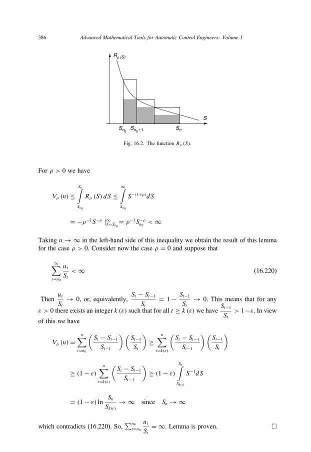
386 Advanced Mathematical Tools for Automatic Control Engineers: Volume 1
R� (S)
Sn0Sn011 Sn
S
Fig. 16.2. The function Rρ (S).
For ρ > 0 we have
Vρ (n)≤Sn∫Sn0
Rρ (S) dS ≤∞∫Sn0
S−(1+ρ)dS
= −ρ−1S−ρ |∞S=Sn0= ρ−1S−ρn0 <∞
Taking n→∞ in the left-hand side of this inequality we obtain the result of this lemma
for the case ρ > 0. Consider now the case ρ = 0 and suppose that
∞∑t=n0
ut
St<∞ (16.220)
Thenut
St→ 0, or, equivalently,
St − St−1
St= 1 − St−1
St→ 0. This means that for any
ε > 0 there exists an integer k (ε) such that for all t ≥ k (ε) we have St−1
St> 1−ε. In view
of this we have
Vρ (n)=n∑t=n0
(St − St−1
St−1
)(St−1
St
)≥
n∑t=k(ε)
(St − St−1
St−1
)(St−1
St
)
≥ (1− ε)n∑
t=k(ε)
(St − St−1
St−1
)≥ (1− ε)
Sn∫Sk(ε)
S−1dS
= (1− ε) ln Sn
Sk(ε)→∞ since Sn →∞
which contradicts (16.220). So,∑∞t=n0
ut
St= ∞. Lemma is proven. �

Selected topics of real analysis 387
Corollary 16.30.
∞∑t=n0
1
n1+ρ
{<∞ if ρ > 0
= ∞ if ρ = 0(16.221)
Proof. It follows from Lemma 16.12 if we take ut ≡ 1. �
16.6 Recurrent inequalities
16.6.1 On the sum of a series estimation
Lemma 16.13. (Nazin & Poznyak 1986)1 Let the numerical sequences {γn} and {gn}satisfy the conditions
0 < γn+1 ≤ γn, G := supn
∣∣∣∣∣n∑t=1
gt
∣∣∣∣∣ <∞ (16.222)
Then the following upper estimate holds
∣∣∣∣∣n∑t=1
gtγ−1t
∣∣∣∣∣ ≤ 2Gγ −1n (16.223)
and, hence, for n→∞
1
hn
n∑t=1
gtγ−1t → 0 (16.224)
where {hn} is any sequence of positive real numbers such that
hnγn → 0, hn > 0 (16.225)
Proof. Using the Abel identity (12.4) of the summation by part in the scalar form, namely,
n∑t=1
αtβt = αnn∑t=1
βt −n∑t=1
(αt − αt−1)
t−1∑s=1
βs
1 This lemma as well as Lemma 16.16 given below were first proven by A.V. Nazin (see the citations in
Nazin & Poznyak 1986).

388 Advanced Mathematical Tools for Automatic Control Engineers: Volume 1
for αn := γ −1n and βn := gn, we have∣∣∣∣∣
n∑t=1
gtγ−1t
∣∣∣∣∣=∣∣∣∣∣γ −1n
n∑t=1
gt −n∑t=1
(γ −1t − γ −1
t−1
) t−1∑s=1
gs
∣∣∣∣∣ ≤ γ −1n sup
n
∣∣∣∣∣n∑t=1
gt
∣∣∣∣∣+
n∑t=1
(γ −1t − γ −1
t−1
)supt
∣∣∣∣∣t−1∑s=1
gs
∣∣∣∣∣ ≤ 2γ −1n sup
n
∣∣∣∣∣n∑t=1
gt
∣∣∣∣∣which implies (16.223). Lemma is proven. �
16.6.2 Linear recurrent inequalities
Lemma 16.14. (on linear recurrent inequalities) Let us consider a real numerical non-negative sequence {un} which satisfies the following recurrent inequality
0 ≤ un+1 ≤ un (1− αn)+ βn (16.226)
where {αn} and {βn} are numerical sequences such that
0 < αn ≤ 1,
∞∑n=1
αn = ∞0 ≤ βn, lim sup
n→∞(βn/αn) = p <∞
(16.227)
Then
lim supn→∞
un ≤ p (16.228)
Proof. By the definition of lim sup it follows that for any ε > 0 there exists an integer
n0 (ε) such that for any n ≥ n0 (ε) we have
∣∣∣∣supt≥n(βt/αt )− p
∣∣∣∣ ≤ ε, which implies the
inequality
supt≥n(βt/αt ) ≤ p + ε (16.229)
Taking n > n0 (ε) and making the recursion back up to n0 (ε) we obtain
un+1 ≤ un (1− αn)+ βn ≤ un−1 (1− αn) (1− αn−1)
+ [βn + βn−1 (1− αn)] ≤ · · · ≤ un0(ε)n∏
t=n0(ε)(1− αt)
+n∑
t=n0(ε)βt
n∏t=t+1
(1− αt)

Selected topics of real analysis 389
(here we accept that∏n
t=m (1− αt) := 1 if m > n). Applying the inequality (16.229) to
the right-hand side we derive
un+1 ≤ un0(ε)n∏
t=n0(ε)(1− αt)+
n∑t=n0(ε)
βt
n∏t=t+1
(1− αt)
= un0(ε)n∏
t=n0(ε)(1− αt)+
n∑t=n0(ε)
(βt
αt
)αt
n∏t=t+1
(1− αt)
≤ un0(ε)n∏
t=n0(ε)(1− αt)+ (p + ε)
n∑t=n0(ε)
αt
n∏t=t+1
(1− αt)
Using the Abel identity (12.5) (the scalar version)
n∏t=n0(ε)
(1− αt)+n∑
t=n0(ε)αt
n∏t=t+1
(1− αt) = 1
and the inequality 1− x ≤ e−x , valid for any x, we get
un+1 ≤ un0(ε)n∏
t=n0(ε)(1− αt)+ (p + ε)
[1−
n∏t=n0(ε)
(1− αt)]
= (p + ε)+ (un0(ε) − p − ε
) n∏t=n0(ε)
(1− αt)
≤ (p + ε)+ (un0(ε) − p − ε
) n∏t=n0(ε)
exp (−αt)
= (p + ε)+ (un0(ε) − p − ε
)exp
(−
n∑t=n0(ε)
αt
)→ (p + ε)
since exp(−∑n
t=n0(ε) αt) → 0 by the property (16.227). Since ε > 0 may be selected
arbitrarily small the statement (16.228) follows. Lemma is proven. �
Lemma 16.15. (Nazin & Poznyak 1986) Suppose that sequences {un} and {wn} for alln ≥ n0 satisfy the following recurrent inequalities
un+1 ≤ un(1− cn−1
)+ dn−(p+1)
wn+1 ≥ wn(1− cn−1
)+ dn−(p+1)
(16.230)
where c > p > 0. Then
lim supn→∞
(npun) ≤ d
c − p ≤ lim infn→∞ (npwn) (16.231)
Moreover, there exist the sequences {un} and {wn} for which the identities in (16.231)are attained.

390 Advanced Mathematical Tools for Automatic Control Engineers: Volume 1
Proof. Without loss of generality we may accept that n0 ≥ c. Let us introduce the
sequence {yn} generated by the recurrent relation
yn+1 = yn(1− cn−1
)+ dn−(p+1) (16.232)
Show that
limn→∞ (n
pyn) = d
c − p (16.233)
For all n ≥ n0 from (16.232) we have
yn+1 = yn0n∏
k=n0
(1− c
k
)+
n∑k=n0
d
kp+1
n∏m=k+1
(1− c
m
)(16.234)
Since
n−p − (n+ 1)−p = n−p − n−p (1+ n−1)−p = n−p − n−p [1− pn−1 +O (
n−2)]
= pn−(p+1) +O (n−(p+2)
)we have
d
np+1= d
c − p[(c − p) 1
p
(1
np− 1
(n+ 1)p
)+O (
n−(p+2))]
= d
c − p[
1
(n+ 1)p− 1
np+ c
pnp
(1− np
(n+ 1)p
)+O (
n−(p+2))]
= d
c − p[
1
(n+ 1)p− 1
np+ c
pnp
(1− p 1
n+O (
n−2))+O (
n−(p+2))]
= d
c − p[
1
(n+ 1)p−(1− c
n
) 1
np+O (
n−(p+2))]
Substitution of this identity into (16.234) implies
yn+1 = yn0n∏
k=n0
(1− c
k
)+ d
c − p[
1
(n+ 1)p− 1
n0p
n∏m=n0
(1− c
m
)
+n∑
k=n0O(k−(p+2)
) n∏m=k+1
(1− c
m
)] (16.235)
Taking into account that
n∏k=n0
(1− c
k
)≤ exp
(−
n∑k=n0
c
k
)≤ const exp (−c ln n) = O (
n−c)
Selected topics of real analysis 391
and
n∑k=n0O(k−(p+2)
) n∏m=k+1
(1− c
m
)
=n∏
m=n0
(1− c
m
) n∑k=n0O(k−2
)k−p
k∏m=n0
(1− c
m
)−1
O(n−c
) n∑k=n0O(k−2
)k−p = const
np+ε
n∑k=n0O(k−(2−ε)
) kc−p−εnc−p−ε
= o (n−p)
(here ε ∈ (0, c − p)) from (16.235) it follows that
yn+1 = d
c − p (n+ 1)−p + o (n−p) (16.236)
We also have yn ≥ un if yn0 = un0 and yn ≤ wn if yn0 = wn0 which together with (16.236)leads to (16.231). �
Corollary 16.31. (Chung 1954) Let the sequence {un} of nonnegative real numbers sat-isfy the following recurrent equation:
un+1 = un(1− cnn−1
)+ dnn−(p+1), n ≥ n0 (16.237)
where {cn} and {dn} are the sequences or real numbers such that
limn→∞cn = c > p > 0, lim
n→∞dn = d > 0 (16.238)
then
limn→∞n
pun = d
c − p (16.239)
Proof. By lim definition for any ε > 0 there exists a number n0 such that for all n ≥ n0
|cn − c| ≤ ε, |dn − d| ≤ ε
which implies
c − ε ≤ cn ≤ c + ε, d − ε ≤ dn ≤ d + ε

392 Advanced Mathematical Tools for Automatic Control Engineers: Volume 1
Using these inequalities in (16.237) gives
un+1 ≤ un(1− c − ε
n
)+ d + εnp+1
un+1 ≥ un(1− c + ε
n
)+ d − εnp+1
Applying Lemma 16.15 we obtain
d − εc + ε − p ≤ lim inf
n→∞ npun ≤ lim supn→∞
npun ≤ d + εc − ε − p
Taking ε→+0 proves (16.239). �
16.6.3 Recurrent inequalities with root terms
The lemmas below seem to be extremely important for the Lyapunov-like stability
analysis for discrete time nonlinear systems.
Lemma 16.16. (Nazin & Poznyak 1986) Let the sequence {un} of nonnegative realnumbers satisfy the following recurrent equation:
un+1 ≤ un (1− αn)+ βn + δnurn, n ≥ n0 (16.240)
where r ∈ (0, 1) and {αn}, {βn}, {δn} are sequences of real numbers such that
lim infn→∞
(nαnαn
) ≥ c, lim supn→∞
(ntβn) ≤ d, lim supn→∞
(nsδn) ≤ a (16.241)
for some c, d and a satisfying
a ≥ 0, c > 0, d ≥ 0, α ∈ (0, 1), t > α, s > α (16.242)
Then
(a) if s > rα + (1− r) t and under α = 1, c > t − 1, it follows that
lim supn→∞
(nt−αun
) ≤ d
c (α)
c (α) = c − (t − 1) χ (α = 1)
χ (α = 1) ={1 if α = 1
0 if α �= 1
(16.243)

Selected topics of real analysis 393
(b) if s = rα + (1− r) t and under α = 1, c > t − 1, it follows that
lim supn→∞
(nt−αun
) ≤ f (16.244)
where f > 0 is the root of the nonlinear equation
c (α) f = d + af r (16.245)
(for r = 1/2 we have f =(a +√
a2 + 4c (α) d
2c (α)
)2
);
(c) if s < rα + (1− r) t and under α = 1, c > λ = s − α1− r , it follows that
lim supn→∞
(nλun
) ≤ (a
c − λχ (α = 1)
)1/(1−r)(16.246)
Proof. Let us use the inequality
xr ≤ (1− r) xr0 +r
x1−r0
x (16.247)
valid for any x, x0 > 0. Indeed (see Fig. 16.3),
xr ≤ l (x) = c + kxwhere the parameters of the linear function l (x) can be found from the following system
of linear equations
c + kx0 = xr0, (xr)′ |x=x0= k
which gives k = rxr−10 , c = (1− r) xr0 and, hence, xr ≤ c + kx = (1− r) xr0 + rxr−1
0 x.
Taking
x := un, x0 := f n−ρ (ρ := min {t − α, λ})
y
c
x0 x
l(x) 5 c 1kx
y 5xr
Fig. 16.3. Illustration of the inequality (16.247).

394 Advanced Mathematical Tools for Automatic Control Engineers: Volume 1
and using the obtained inequality for urn in (16.240), for all n ≥ n0 we obtain
un+1 ≤ un(1− c + o(1)
n+ r (a + o (1))f 1−rns−(1−r)/ρ
)
+d + o(1)nt
+ (1− r) (a + o (1)) fr
ns+rρ
Now the results (16.243), (16.244) and (16.246) follow immediately if applied to
the last inequality Lemma 16.15 for the case α = 1 and Corollary 16.31 for the
case α < 1. �
Lemma 16.17. (Nazin & Poznyak 1986) Let the sequence {un} of nonnegative realnumbers satisfy the following recurrent equation:
un+1 ≤ un (1− αn)+ βn + δnurn, n ≥ n0 (16.248)
where r ∈ (0, 1) and {αn}, {βn}, {δn} are sequences of nonnegative real numbers suchthat
∞∑n=n0
αn ≥ c, lim supn→∞
(βn/αn) = b, lim supn→∞
(δn/αn
) = dαn ∈ (0, 1], βn ≥ 0, δn ≥ 0
(16.249)
Then
lim supn→∞
un ≤ infc>ru (c) (16.250)
where
u (c) :=(1− r
c
)−1 [b + (1− r) cr/(1−r)d1/(1−r)] (16.251)
Proof. Using the inequality (16.247) for x = un and x0 = cδn/αn, c > r in (16.248), we
derive
un+1 ≤ un[1− αn
(1− r
c
)]+ βn + (1− r)
(cδn/αn
)r/(1−r)n
δn

Selected topics of real analysis 395
or, equivalently,
un+1 ≤ un [1− αn]+ βn
αn := αn(1− r
c
), βn := βn + (1− r)
(cδn/αn
)r/(1−r)n
δn
Then applying Lemma 16.14 we obtain
lim supn→∞
un ≤ lim sup(βn/αn
):=
n→∞u (c)
Taking infc>r
of the right-hand side we get (16.250) and (16.251). Lemma is proven. �

This page intentionally left blank
17 Complex Analysis
Contents17.1 Differentiation . . . . . . . . . . . . . . . . . . . . . . . . . . . . . . . . 397
17.2 Integration . . . . . . . . . . . . . . . . . . . . . . . . . . . . . . . . . . 401
17.3 Series expansions . . . . . . . . . . . . . . . . . . . . . . . . . . . . . . . 420
17.4 Integral transformations . . . . . . . . . . . . . . . . . . . . . . . . . . . . 433
17.1 Differentiation
17.1.1 Differentiability
Let f be a complex-valued function of a complex variable z. Any complex function
can be represented as follows
f (z)= u (x, y)+ iv (x, y)z= x + iy (17.1)
We refer to u and v as the real and imaginary parts of f and write
u = Ref, v = Imf (17.2)
Example 17.1.
f (z) = z2 = (x + iy)2 = x2 − y2 + i2xy
u (x, y) = x2 − y2, v (x, y) = xyDefinition 17.1. If f is defined in some neighborhood of a finite point z and
lim�z→0
f (z+�z)− f (z)�z
exists finitely we say that the function f (z) is differentiable at
the point z. This limiting value is called the derivative of f (z) at z and we write
f ′ (z) := lim�z→0
f (z+�z)− f (z)�z
(17.3)
397

398 Advanced Mathematical Tools for Automatic Control Engineers: Volume 1
17.1.2 Cauchy–Riemann conditions
The next theorem gives conditions which must be imposed on the functions u (x, y)
and v (x, y) in order that f (z) should be differentiable at the point z.
Theorem 17.1. (The necessary conditions of differentiability) Let f be defined in aneighborhood of the point z ∈ C and be differentiable at z. Then
(a) the partial derivatives
∂
∂xu(x, y),
∂
∂yu(x, y),
∂
∂xv(x, y),
∂
∂yv (x, y)
exist;(b) and the following relations hold:
∂
∂xu (x, y) = ∂
∂yv (x, y),
∂
∂yu (x, y) = − ∂
∂xv (x, y) (17.4)
Proof. Since f ′(z) exists then for any given ε > 0 there exists δ = δ (ε) > 0 such that∣∣∣∣f (z+�z)− f (z)�z− f ′ (z)
∣∣∣∣ < ε (17.5)
whenever 0 < |�z| < δ. Representing �z as �z = teiα, where t = |�z| and α = arg z
(see (13.40)), we can see that (17.5) is fulfilled independently of α when 0 < t < δ. Let
us take α = 0. This means that �z = t = �x. This implies
f ′ (z)= lim�x→0
[u (x +�x, y)− u (x, y)
�x+ i v (x +�x, y)− v (x, y)
�x
]
= ∂
∂xu (x, y)+ i ∂
∂xv (x, y)
(17.6)
Taking α = π/2 we find that �z = it = i�y and, therefore,
f ′ (z)= lim�y→0
[u (x, y +�y)− u (x, y)
i�y+ i v (x, y +�y)− v (x, y)
i�y
]
= 1
i
∂
∂yu (x, y)+ ∂
∂yv (x, y) = −i ∂
∂yu (x, y)+ ∂
∂yv (x, y)
(17.7)
Comparing (17.6) with (17.7) we obtain (17.4). Theorem is proven. �
The conditions (17.4) are called the Cauchy–Riemann conditions. They are also
known as the d’Alembert–Euler conditions. The theorem given below shows that these
conditions are also sufficient to provide the differentiability.

Complex analysis 399
Theorem 17.2. (The sufficient conditions of differentiability) The Cauchy–Riemannconditions (17.4) are also sufficient for the differentiability of f (z) provided the func-tions u (x, y) and v (x, y) are totally differentiable (all partial derivatives exist) at theconsidered point. The derivative f ′ (z) can be calculated as
f ′ (z) = ∂
∂xu (x, y)+ i ∂
∂xv (x, y) = ∂
∂yv (x, y)− i ∂
∂yu (x, y) (17.8)
Proof. By the total differentiability it follows that
�u := u (x +�x, y +�y)− u (x, y) = ∂u∂x�x + ∂u
∂y�y + o (|�z|)
�v := v (x +�x, y +�y)− v (x, y) = ∂v
∂x�x + ∂v
∂y�y + o (|�z|)
Therefore
f (z+�z)− f (z)�z
= �u+ i�v�x + i�y
=
(∂u
∂x�x + ∂u
∂y�y
)+ i
(∂v
∂x�x + ∂v
∂y�y
)+ o (|�z|)
�x + i�yUsing now the Cauchy–Riemann conditions (17.4), the simple rearrangement gives
f (z+�z)− f (z)�z
=
([∂u
∂x+ i ∂v∂x
]�x +
[∂u
∂y+ i ∂v∂y
]�y
)+ o (|�z|)
�x + i�y
=
([∂u
∂x+ i ∂v∂x
]�x +
[−i ∂u∂y
+ ∂v∂y
]i�y
)+ o (|�z|)
�x + i�y
=
([∂u
∂x+ i ∂v∂x
]�x +
[i∂v
∂x+ ∂u∂x
]i�y
)+ o (|�z|)
�x + i�y
=[∂u
∂x+ i ∂v∂x
]+ o(1)
where o(1)→ 0 whenever |�z| → 0. So that f ′ (z) exists and is given by
f ′ (z) = ∂u∂x
+ i ∂v∂x
which completes the proof. �

400 Advanced Mathematical Tools for Automatic Control Engineers: Volume 1
Example 17.2. For the same function f (z) = z2 as in Example 17.1 we have
∂u
∂x= ∂v
∂x= 2x,
∂u
∂y= ∂v∂y
= −2y
f ′ (z) = 2x − i2y
Definition 17.2. A function f (z), differentiable at each point of an open set D ⊂ C,is called regular (or holomorphic) on D. Sure, here we assume that we deal witha single-valued (or uniform) function since the notion of differentiability (17.3) hasbeen introduced only for single-valued functions. If a regular function f (z) possesses acontinuous derivative on D then it is called an analytic function.1
Below these definitions will be extensively used.
Example 17.3. It is easy to check that, as in real analysis,
d
dzez = ez, d
dzln z = 1
z
d
dzsin z = cos z,
d
dzcos z = −sin z
d
dztan z = 1
cos2 z,
d
dzcot z = − 1
sin2 z
(17.9)
17.1.3 Theorem on a constant complex function
An application of the Cauchy–Riemann equations (17.4) is given in the next lemma.
Lemma 17.1. Let f = u+ iv be a function with a derivative everywhere in an open discD ⊂ C centered at the point z = (a, b).1. If any of u, v or |f |2 := u2 + v2 is constant on D, then f is constant on D.2. Also, f is constant on D if f ′(z) = 0 for all z ∈ D.
Proof. Suppose u is a constant on D. By (17.4) it follows that∂v
∂x= ∂v∂y
= 0. Therefore
v (x, y) = v (a, b)
So, v is a constant on D. By the same argument we show that u is a constant on D if v
is a constant. Now suppose that |f |2 := u2 + v2 is a constant. This, in view of (17.4),
implies
0 = u∂u∂x
+ v ∂v∂x
= u∂u∂y
+ v ∂v∂y
= −u∂v∂x
+ v ∂u∂x
1 It can be shown that the existence of f ′(z) on D automatically implies continuity of f ′(z) on D (Goursat
1900). So, regularity and analyticity can be considered as two definitions having an identical mathematical
sense.
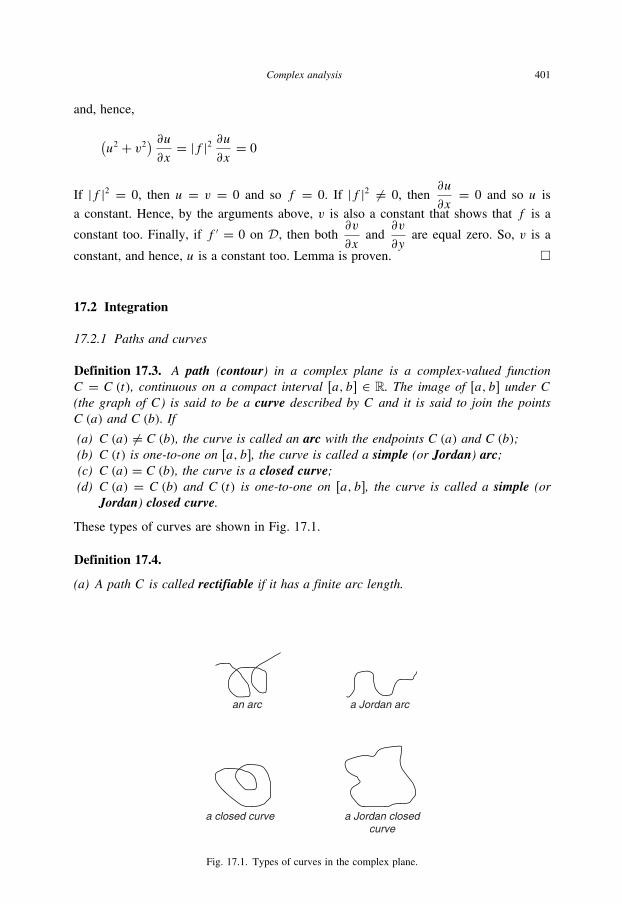
Complex analysis 401
and, hence,
(u2 + v2) ∂u
∂x= |f |2 ∂u
∂x= 0
If |f |2 = 0, then u = v = 0 and so f = 0. If |f |2 �= 0, then∂u
∂x= 0 and so u is
a constant. Hence, by the arguments above, v is also a constant that shows that f is a
constant too. Finally, if f ′ = 0 on D, then both∂v
∂xand
∂v
∂yare equal zero. So, v is a
constant, and hence, u is a constant too. Lemma is proven. �
17.2 Integration
17.2.1 Paths and curves
Definition 17.3. A path (contour) in a complex plane is a complex-valued functionC = C (t), continuous on a compact interval [a, b] ∈ R. The image of [a, b] under C(the graph of C) is said to be a curve described by C and it is said to join the pointsC (a) and C (b). If
(a) C (a) �= C (b), the curve is called an arc with the endpoints C (a) and C (b);(b) C (t) is one-to-one on [a, b], the curve is called a simple (or Jordan) arc;(c) C (a) = C (b), the curve is a closed curve;(d) C (a) = C (b) and C (t) is one-to-one on [a, b], the curve is called a simple (or
Jordan) closed curve.
These types of curves are shown in Fig. 17.1.
Definition 17.4.
(a) A path C is called rectifiable if it has a finite arc length.
an arc a Jordan arc
a Jordan closedcurve
a closed curve
Fig. 17.1. Types of curves in the complex plane.

402 Advanced Mathematical Tools for Automatic Control Engineers: Volume 1
(b) A path C is called piecewise smooth if it has a bounded derivative C ′ which iscontinuous everywhere on [a, b] except (possibly) a finite number of points for whichit is required that both right- and left-hand derivatives exist.
(c) A piecewise smooth closed path is called a circuit.(d) The arc length �C (a, b) of a path C on [a, b] is defined by
�C (a, b) := supPm
{�Cm (a, b) : Pm ∈ P (a, b)
}�CPm (a, b) :=
m∑i=1
|C (ti)− C (ti−1)|(17.10)
where P (a, b) is the set of all possible partitions of [a, b].
Lemma 17.2. A path C is rectifiable if and only if C (t) is of bounded variation on [a, b].
Proof. If Pm := {t0 = a, t1, t2, . . . , tm = b} is a partition of [a, b], and if C (t) is a functionof bounded variation on [a, b], that is, for all a ≤ ti−1 ≤ ti ≤ b
|C (ti)− C (ti−1)| ≤ M (ti − ti−1)
then
�C (a, b)= supPm
{m∑i=1
|C (ti)− C (ti−1)|}
≤ supPm
{M
m∑i=1
(ti − ti−1)
}= M (b − a) <∞
which proves this lemma. �
Corollary 17.1. The arc length �C (a, b) may be calculated as the Lebesgue integral
�C (a, b) =b∫
t=a
∣∣C ′ (t)∣∣ dt (17.11)
and
�C (a, b) = �C (a, c)+�C (c, b) (17.12)
Definition 17.5. If a ∈ C, r > 0 and the path C is defined by the equation
C (t) := a + reit , t ∈ [0, 2π ] (17.13)

Complex analysis 403
then this path is called a positively (counterclockwise) oriented circle (or a sphere inC) with the center at a and the radius r . It is denoted by B (a, r) and is referred to asC = B (a, r).
17.2.2 Contour integrals
Let C be a path in the complex plane C with domain [a, b], and f : C → C be a
complex-valued function
f (z) = u (x, y)+ iv(x, y), z = x + iy
defined on the graph of C.
Definition 17.6. The contour integral of f along C, denoted by∫Cf (z)dz, is
defined by
∫C
f (z)dz :=b∫
t=af (C (t))dC (t) = lim
m→∞ supPm
s(Pm, ζ
(m)k
)
s(Pm, ζ
(m)k
):=
m∑k=1
f (ζk) (zk − zk−1)
zk ∈ C, z0 = C(a), zk = C (tk), zm = C(b)
� (Pm) := maxk=1,...,m
|zk − zk−1| →m→∞ 0
(17.14)
whenever the Riemann–Stieltjes integral∫ bt=a f (C (t))dC (t) on the right-hand side of
(17.14) exists. If the contour C is closed, that is, C(a) = C(b) (see Fig. 17.2), then theintegral (17.14) is denoted by
∮C
f (z) dz :=b=a∫t=af (C (t))dC (t) (17.15)
Remark 17.1. If f (z) is a partially continuous bounded function, the integral (17.14)always exists.

404 Advanced Mathematical Tools for Automatic Control Engineers: Volume 1
Lemma 17.3. The calculation of the contour integral∫Cf (z) dz (17.14) can be realized
by the calculation of four real integrals according to the following formula:
∫C
f (z) dz=∫C
[u (x, y) dx − v (x, y) dy]
+ i∫C
[u (x, y) dy + v (x, y) dx](17.16)
Proof. It follows from the presentation
m∑k=1
f (ζk) (zk − zk−1) =m∑k=1
[uk�xk − vk�yk]+ im∑k=1
[uk�yk + vk�xk]
uk := u(xk, yk), vk := v (xk, yk)
�xk := xk − xk−1, �yk := yk − yk−1, zk = xk + iyk = C (tk)
�
Denote by C− the same contour C but passed in the clockwise direction (see Fig. 17.2).
Then the following properties seem to be evident.
Proposition 17.1.
1. ∫C
f (z) dz = −∫C−
f (z) dz (17.17)
C 5 C11C2
C1
D
C2
b
a
C12
Fig. 17.2. The closed contour C = C1 + C2 within the region D.
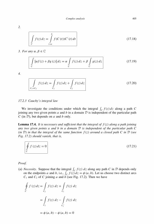
Complex analysis 405
2.
∫C
f (z) dz =b∫
t=af (C (t))C ′ (t) dt (17.18)
3. For any α, β ∈ C
∫C
[αf (z)+ βg (z)] dz = α∫C
f (z) dz+ β∫C
g(z) dz (17.19)
4. ∫C1+C2
f (z) dz =∫C1
f (z) dz+∫C2
f (z) dz (17.20)
17.2.3 Cauchy’s integral law
We investigate the conditions under which the integral∫Cf (z) dz along a path C
joining any two given points a and b in a domain D is independent of the particular path
C (in D), but depends on a and b only.
Lemma 17.4. It is necessary and sufficient that the integral of f (z) along a path joiningany two given points a and b in a domain D is independent of the particular path C(in D) in that the integral of the same function f (z) around a closed path C in D (seeFig. 17.2) should vanish, that is,
∮C
f (z) dz = 0 (17.21)
Proof.
(a) Necessity. Suppose that the integral∫Cf (z) dz along any path C in D depends only
on the endpoints a and b, i.e.,∫Cf (z) dz = φ (a, b). Let us choose two distinct arcs
C1 and C2 of C joining a and b (see Fig. 17.2). Then we have∮C
f (z) dz=∫C2
f (z) dz+∫C1
f (z) dz
=∫C2
f (z) dz−∫C−1
f (z) dz
= φ (a, b)− φ (a, b) = 0

406 Advanced Mathematical Tools for Automatic Control Engineers: Volume 1
(b) Sufficiency. Suppose now that (17.21) holds for a domain D. Suppose a, b ∈ D and
select any two paths C−1 and C2 in D joining a to b. Since C = C1 +C2 and (17.21)
holds, we get
0 =∮C
f (z) dz=∫C2
f (z) dz+∫C1
f (z) dz
=∫C2
f (z) dz−∫C−1
f (z) dz
Hence,∫C2f (z) dz = ∫
C−1f (z) dz for any paths C2 and C−
1 . This means that∫Cf (z) dz = φ (a, b) exactly. The lemma is proven. �
17.2.3.1 Simply-connected domainsNow we are ready to formulate the following fundamental integral theorem.
Theorem 17.3. (Cauchy’s integral law) If f (z) is a regular function in a simply-connected domain2 D, then the integral of f (z) along any path C in D depends only onthe endpoints of this path, or in other words, if C is any closed contour in D then
∮C
f (z) dz = 0
Proof. By (17.16) it suffices to show that each of the real line integrals
∮C
[u (x, y) dx − v (x, y) dy],∮C
[u (x, y) dy + v (x, y) dx]
vanishes. By Corollary 16.2 (from the Real Analysis chapter) it follows that
∮C
[P (x, y) dx +Q(x, y) dy] = 0
along any closed contour in a simply-connected domain D if and only if the partial
derivative of the real functions P (x, y) and Q(x, y) exist and are continuous in D and
∂
∂yP (x, y) = ∂
∂xQ (x, y) (17.22)
2 We are reminded that a domain D in an open plane is simply connected if and only if any closed Jordan
contour C in D is reducible in D, that is, can be continuously shrunk to a point in D without leaving D.

Complex analysis 407
at each point of D. Indeed,
P (x, y) dx +Q(x, y) dy = dϕ (x, y)
and ∮C
[P (x, y) dx +Q(x, y) dy] =∮C
dϕ (x, y)
= ϕ (x(a), y (a))− ϕ (x(b), y (b)) = 0
since a = b. But, in our case,
u (x, y) = P(x, y), v (x, y) = −Q(x, y)
for the first integral, and
v (x, y) = P(x, y), u (x, y) = Q(x, y)
So, (17.22) coincides exactly with the Cauchy–Riemann conditions (17.4) which proves
the theorem. �
Remark 17.2. The converse of Theorem 17.3 is also true, namely, if f (z) is continuousin a simply-connected domain D and
∮Cf (z) dz = 0 for every closed contour C in D,
then f (z) is regular in D. The proof can be found in Fuchs & Shabat (1964).
As it follows from the consideration above, Theorem 17.3 enables us to give an
equivalent alternative definition of a regular function: a single-valued function f(z) isregular in D if it is continuous in D and its integral around any closed contour C inD is equal to zero.
17.2.3.2 Multiply-connected domainsThe Cauchy theorem 17.3 can be generalized so as to apply to multiply-connected
domains. Let D be an (n+ 1)-ply connected bounded domain whose frontier consists
of (n+ 1) disjoint contours C0 (the external boundary component), C1, . . . , Cn, and let
f (z) be regular at each point of the closed region D (see Fig. 17.3 showing a case in
which n = 3).
By taking suitable (disjoint) cuts γ1, γ2, . . . γn we form from D a simply-connected
domain D′ whose boundary we denote by C. We will consider each cut γi (i = 1, . . . , n)
as two-edged as in Fig. 17.3.
Theorem 17.4. If f (z) is regular at each point of the closed region D whose frontier Cconsists of a finite number of disjoint contours Ci (i = 0, 1, . . . , n), that is, C = ⋃n
i=0 Ci ,then the integral
∮Cf (z) dz of f (z) around the boundary of D (taken so that each
component of the boundary is traversed in a sense such that the interior D of D remainson the left) is equal to zero.

408 Advanced Mathematical Tools for Automatic Control Engineers: Volume 1
D
C0
C1
D
C2
C3
�3
�1
�2
Fig. 17.3. Multiply-connected domains (n = 3).
Proof. As C is piecewise smooth and f (z) is regular in the domain D∗ containing D it
follows by Theorem 17.3 that∮Cf (z) dz = 0. So, C0 is traversed in the anti-clockwise
(positive) sense and Ci (i = 1, . . . , n) in the clockwise (negative) sense. Each of cuts
γ1, γ2, . . . γn is traversed twice: first, in one sense and then in the opposite sense. As the
integrals along the two edges of each cut conceal each other, it follows by the standard
properties of the contour integral (17.1) that
∮C
f (z) dz =∮C0
f (z) dz−n∑i=1
∮Ck
f (z) dz
=∮C0
f (z) dz+n∑i=1
x
∮C−k
f (z) dz = 0
(17.23)
Theorem is proven. �
Corollary 17.2. Assuming that the conditions under which (17.23) holds are satisfied,we have
∮C0
f (z) dz =n∑i=1
∮Ck
f (z) dz (17.24)
which for n = 1 gives
∮C0
f (z) dz =∮C1
f (z) dz (17.25)

Complex analysis 409
17.2.4 Singular points and Cauchy’s residue theorem
17.2.4.1 Types of singularitiesDefinition 17.7. Consider a function f (z) which is regular (analytic) everywhere onan open set D bounded by a closed contour C (here we are writing C for C0), exceptat a finite number of isolated points a1, a2, . . . , an. These exceptional points are calledsingular points (singularities) of f (z).
Isolated singularities are divided into three types according to the behavior of the
function in a deleted neighborhood of the point concerned.
Definition 17.8. An isolated singularity a of the function f (z) is said to be
1. a removable singularity, if limz→af (z) exists finitely;
2. a pole, if limz→af (z) = ±∞;
3. an essential singularity, f (z) does not tend to a limit (finite or infinite) as z→ a.
Remark 17.3. All of these notions are closely connected with the, so-called, Laurentexpansion of the function f (z) which will be discussed below. There will be shown that
• a removable singularity cannot contain the termc
(z− a)n for any finite n ≥ 1 (for
example, the functionsin z
zat the point z = a = 0 has a removable singularity);
• evidently, that a function f (z) defined in some deleted neighborhood of z = a has a
pole at z = a if and only if the function g (z) := 1
f (z)is regular at a and has zero at
z = a, i.e., g (a) = 0 (while g (z) is not identically equal to zero);• in the case of isolated essential singularity there exist (the Sokhotsky–Cazoratti theorem,1868) at least two sequences
{z′n}
and{z′′n}, each converging to a, such that the
corresponding sequences{f(z′n)}
and{f(z′′n)}
tend to different limits as n → ∞(for example, the function e1/z at the point z = a = 0 has an essential singularity andis regular for all other z).
Definition 17.9. A function f (z) is called meromorphic (ratio type) if its singularitiesare only poles.
From this definition it immediately follows that in any bounded closed domain of the
complex plane a meromorphic function may have only a finite number of poles: for,
otherwise, there would exist a sequence of distinct poles converging to a (finite) point in
the region; such point would necessarily be a nonisolated singularity that contradicts our
hypothesis that any finite singular point of this function must be a pole.
Example 17.4. Meromorphic functions are 1/ sin z, tan z, cot z.
17.2.4.2 Cauchy’s residue theoremWe enclose the ak by mutually disjoint circles Ck in D such that each circle Ck
enclosing no singular points other than the corresponding point ak . It follows readily

410 Advanced Mathematical Tools for Automatic Control Engineers: Volume 1
from (17.25) that the integral of f (z) around Ck is equal to the integral around any other
contour C ′k in D which also encloses ak , but does not enclose or pass through any other
singular point of f (z). Thus the value of this integral is a characteristic of f (z) and the
singular point ak .
Definition 17.10. The residue of f (z) at the singular point ak is denoted by res f (ak)
and is defined by
resf (ak) := 1
2πi
∮Ck
f (z) dz (17.26)
Formula (17.24) leads immediately to the following result.
Theorem 17.5. (Cauchy’s residue theorem) Let D be an open domain bounded by aclosed contour C and let f (z) be regular (analytic) at all points of D with the exceptionof a finite number of singular points a1, a2, . . . , an contained in the domain D. Then theintegral of f (z) around C is 2πi times the sum of its residues at the singular points,that is,
∮C
f (z) dz = 2πi
n∑k=1
resf (ak) (17.27)
Corollary 17.3. The residue of f (z) at a removable singularity is equal to zero.
The next subsection deals with method of residues calculating without integration.
17.2.5 Cauchy’s integral formula
17.2.5.1 Representation of an analytic function through its contour integralThe theorem below reveals a remarkable property of analytical functions: it relates the
value of an analytical function at a point with the value on a closed curve not containing
the point.
Theorem 17.6. (Cauchy’s integral formula) Assume f is regular (analytic) on an openset D, and let C be any contour (circuit) in D which encloses a point z ∈ D but doesnot cross it. Then
∮C
f (w)
w − zdw = f (z)∮C
1
w − zdw (17.28)
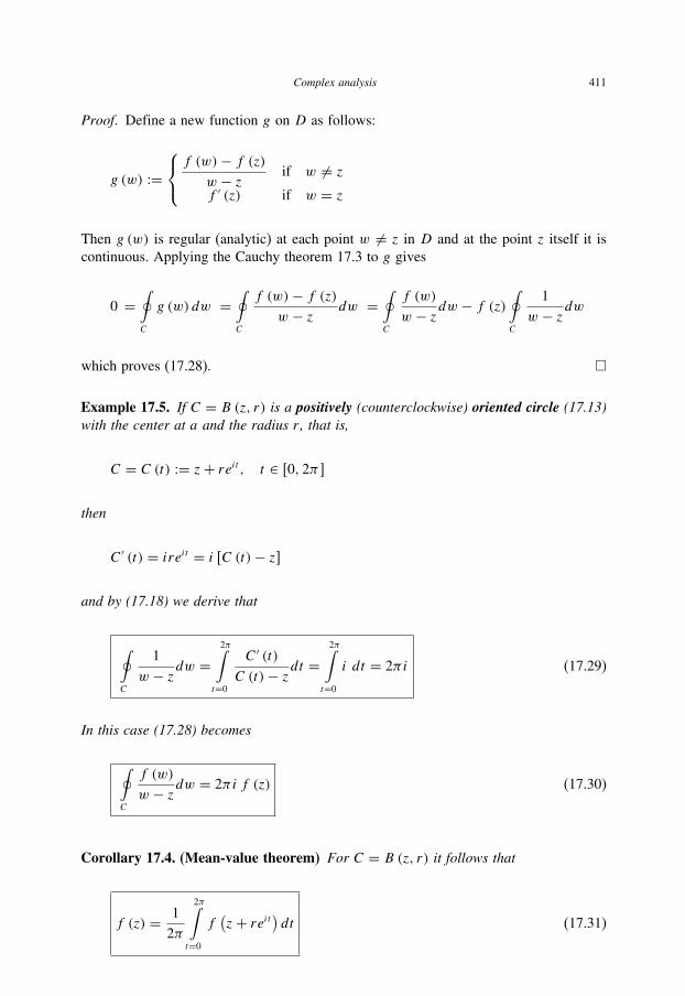
Complex analysis 411
Proof. Define a new function g on D as follows:
g (w) :=⎧⎨⎩f (w)− f (z)w − z if w �= zf ′ (z) if w = z
Then g (w) is regular (analytic) at each point w �= z in D and at the point z itself it is
continuous. Applying the Cauchy theorem 17.3 to g gives
0 =∮C
g (w) dw =∮C
f (w)− f (z)w − z dw =
∮C
f (w)
w − zdw − f (z)∮C
1
w − zdw
which proves (17.28). �
Example 17.5. If C = B (z, r) is a positively (counterclockwise) oriented circle (17.13)with the center at a and the radius r , that is,
C = C (t) := z+ reit , t ∈ [0, 2π ]
then
C ′ (t) = ireit = i [C (t)− z]
and by (17.18) we derive that
∮C
1
w − zdw =2π∫
t=0
C ′ (t)C (t)− zdt =
2π∫t=0
i dt = 2πi (17.29)
In this case (17.28) becomes
∮C
f (w)
w − zdw = 2πi f (z) (17.30)
Corollary 17.4. (Mean-value theorem) For C = B (z, r) it follows that
f (z) = 1
2π
2π∫t=0
f(z+ reit) dt (17.31)

412 Advanced Mathematical Tools for Automatic Control Engineers: Volume 1
Proof. By (17.18) and (17.30) we have
2πif (z)=∮C
f (w)
w − zdw
=2π∫
t=0
f(z+ reit) C ′ (t)
C (t)− zdt
=2π∫
t=0
f(z+ reit) i dt
which proves (17.31). �
The next theorem shows that formula (17.30) holds not only for positively oriented
circles (17.13) but for any circuit containing z as an internal point.
Theorem 17.7. If f is regular (analytic) on an open set D, and let C be any contour(circuit) in D (not obligatory C = B (z, r)) which encloses a point z ∈ D but does notcross it, then
∮C
1
w − zdw = 2πin (C, z) (17.32)
where n (C, z) is an integer called the winding number (or index) of C with respect to zwhich is the number of times the point C (t) “winds around” the point z as t varies overthe interval [a, b].
Proof. By (17.18) it follows that
∮C
1
w − zdw =b∫
t=a
C ′ (t)C (t)− zdt
Define the complex-valued function F(x) by the equation
F(x) :=x∫
t=a
C ′ (t)C (t)− zdt, t ∈ [a, b]
To prove the theorem we must show that F (b) = 2πin for some integer n. Notice that
F(x) is continuous and F ′(x) = C ′ (x)C (x)− z at each point where C ′ (t) exists, and, hence,
the function G(x) defined by
G(x) := e−F(x) [C (x)− z]

Complex analysis 413
is also continuous on [a, b] and, moreover, at each point, where C ′ (t) exists, we have
G′ (x)= e−F(x)C ′ (x)− F ′(x)e−F(x) [C (x)− z]
= e−F(x)C ′ (x)− C ′ (x)C (x)− ze
−F(x) [C (x)− z] = 0
Therefore, G′ (x) = 0 for each t in [a, b] except (possibly) for a finite number of points.
By continuity of G(x) on [a, b] we conclude that G(x) is a constant throughout [a, b]
that implies G(a) = G(b) or, equivalently,
G(b) = e−F(b) [C (b)− z] = G(a) = e−F(a) [C (a)− z] = C (a)− z
Since C (a) = C (b) �= z we find e−F(b) = 1 that gives F(b) = 2πin exactly where n
is an integer and corresponds to the number of times the point C (t) “winds around” the
point z as t varies over the interval [a, b]. This completes the proof. �
Corollary 17.5. Cauchy’s integral formula (17.28) can now be restated in the form
1
2πi
∮C
f (w)
w − zdw = n (C, z) f (z) (17.33)
Example 17.6. Let C be any contour enclosing the point a ∈ C. We need to calculateJ := ∮
C(z− a)n dz for every integer n = . . . ,−1, 0, 1, . . . By (17.25) it follows that
J =∮C
(z− a)n dz =∮
B(a,r)
(z− a)n dz
Letting z− a = reiϕ we get dz = reiϕi dϕ, and hence,
J =∮
B(a,r)
(z− a)n dz =2π∫
ϕ=0
rneinϕreiϕi dϕ = irn+1
2π∫ϕ=0
ei(n+1)ϕ dϕ
Since∫ekϕ dϕ = 1
kekϕ +K, k �= 0, K = const
one gets
J = irn+1
2π∫ϕ=0
ei(n+1)ϕ dϕ = rn+1
n+ 1ei(n+1)ϕ
∣∣∣∣ ϕ = 0
ϕ = 2π
= rn+1
n+ 1
(ei2π(n+1) − 1
)if n �= −1
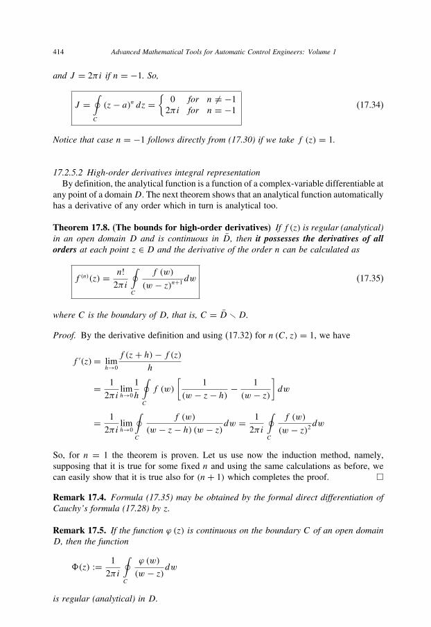
414 Advanced Mathematical Tools for Automatic Control Engineers: Volume 1
and J = 2πi if n = −1. So,
J =∮C
(z− a)n dz ={
0 for n �= −1
2πi for n = −1(17.34)
Notice that case n = −1 follows directly from (17.30) if we take f (z) = 1.
17.2.5.2 High-order derivatives integral representationBy definition, the analytical function is a function of a complex-variable differentiable at
any point of a domainD. The next theorem shows that an analytical function automatically
has a derivative of any order which in turn is analytical too.
Theorem 17.8. (The bounds for high-order derivatives) If f (z) is regular (analytical)in an open domain D and is continuous in D, then it possesses the derivatives of allorders at each point z ∈ D and the derivative of the order n can be calculated as
f (n)(z) = n!2πi
∮C
f (w)
(w − z)n+1dw (17.35)
where C is the boundary of D, that is, C = D �D.
Proof. By the derivative definition and using (17.32) for n (C, z) = 1, we have
f ′(z)= limh→0
f (z+ h)− f (z)h
= 1
2πilimh→0
1
h
∮C
f (w)
[1
(w − z− h) −1
(w − z)]dw
= 1
2πilimh→0
∮C
f (w)
(w − z− h) (w − z)dw = 1
2πi
∮C
f (w)
(w − z)2 dw
So, for n = 1 the theorem is proven. Let us use now the induction method, namely,
supposing that it is true for some fixed n and using the same calculations as before, we
can easily show that it is true also for (n+ 1) which completes the proof. �
Remark 17.4. Formula (17.35) may be obtained by the formal direct differentiation ofCauchy’s formula (17.28) by z.
Remark 17.5. If the function ϕ (z) is continuous on the boundary C of an open domainD, then the function
�(z) := 1
2πi
∮C
ϕ (w)
(w − z)dw
is regular (analytical) in D.

Complex analysis 415
Example 17.7.
1
πi
∮C
sin (w)
(w − z)3 dw = 2!2πi
∮C
sin (w)
(w − z)2+1dw = sin(2)(z) = −sin z
17.2.5.3 Cauchy’s inequalitiesFormula (17.35) leads directly to the following important inequalities known as
the Cauchy’s inequalities for the module of the nth derivative. Indeed, from (17.35) it
follows that
∣∣f (n)(z)∣∣ = n!2π
∣∣∣∣∣∣∮C
f (w)
(w − z)n+1dw
∣∣∣∣∣∣ ≤n!2π
Ml
rn+1(17.36)
where r is the distance between the point z and the boundary C, i.e., r := infw∈C
‖z− w‖,M is the supremum of the module of f (w) in D, i.e., M := sup
z∈D|f (z)| and l is the
length of C, i.e., l := |∮Cdw|. In particular, if f (w) is analytical in the disc D =
{w ∈ C : |w − z| < r}, then l = 2πr and we obtain
∣∣f (n)(z)∣∣ ≤ Mn!rn
(17.37)
17.2.5.4 Liouville’s theoremDefinition 17.11. A function analytical everywhere on C is called an entire function.
Example 17.8. Entire functions are polynomials, sin z and cos z, and ez.
Theorem 17.9. (Liouville) Every bounded entire function is constant.
Proof. Suppose |f (z)| ≤ M for all z ∈ C. Then by (17.37) applied for n = 1 it follows
that∣∣f (n)(z)∣∣ ≤ M
rfor every r > 0. Letting r →∞ implies f ′(z) = 0 for every z ∈ C
which completes the proof. �
17.2.6 Maximum modulus principle and Schwarz’s lemma
Theorem 17.10. (Maximum modulus principle) If a function f (z) is analytic and notconstant on an open region D and is continuous on D, then its module |f (z)| cannotachieve its maxima in any point D, that is, every contour
C = B (a, r) := {z ∈ C | |z− a| = r} ⊂ Dcontains points z such that
|f (z)| > |f (a)| (17.38)
416 Advanced Mathematical Tools for Automatic Control Engineers: Volume 1
Proof. By continuity of |f (z)| it achieves its maximum M on D. Denote by E the set of
all extrema points, i.e.,
E := {z ∈ D| |f (z)| = M}
Suppose that E = D. This means that |f (z)| = M for all points z ∈ D and, by
Lemma 17.1, it follows that f (z) = const on D that contradicts with the assumptions
of the theorem. Suppose now that E ⊂ D, namely, there exists a boundary point z0 ∈ Esuch that it is an internal point of D. Let us construct a circuit C = B (z0, r) which
contains a point z1 ∈ D such that z1 /∈ E (this can always be done since z0 is a
boundary point). Then |f (z)| < M , and for any small enough ε > 0, by continuity
of f (z), there exists a set C1, which is a part of C where |f (z)| < M − ε. DenoteC2 := C\C1. Evidently that for any z ∈ C2 one has |f (z)| ≤ M . Then by Theorem 17.4 it
follows that
f (z0) = 1
2π
2π∫=0
f (z) dϕds=rdϕ= 1
2πr
⎛⎝ ∫
C1
f (z) dz+∫C2
f (z) dz
⎞⎠
which implies
|f (z0)| = M ≤ 1
2πr
([M − ε] l1 +Ml2
) = M − εl1
2πr
l1 :=∫C1
dz, l2 :=∫C2
f (z) dz
But the last inequality is impossible which leads to the contradiction. Theorem is
proven. �
Corollary 17.6. (Minimum modulus principle) If a function f (z) is analytical and not
constant on D, and it is continuous and nonequal to zero on D, then the minimum of|f (z)| cannot be achieved on D.
Proof. It can be easily done if we apply Theorem 17.10 to the function g (z) =1/f (z). �
Using the maximum modulus principle it is possibly easy to state the following useful
result.
Lemma 17.5. (Schwartz, around 1875) If function f (z) is analytical in the opendomain |z| < 1, it is continuous on |z| ≤ 1, and, in the addition,
f (0) = 0, |f (z)| ≤ 1
Complex analysis 417
then
|f (z)| ≤ |z| (17.39)
If at least in one internal point of the domain |z| < 1 the exact equality |f (z)| = |z|holds, then this equality takes place at any point of this domain and, besides,
f (z) = eiαz (17.40)
where α is a real constant.
Proof. To prove this result it is sufficient to consider the function
ϕ (z) :=⎧⎨⎩f (z)
zif z �= 0
f ′ (0) if z = 0
which is analytical on the set 0 < |z| < 1 and continuous in |z| ≤ 1. Applying to this
function the maximum modulus principle 17.10 we derive that on the circle |z| = 1
we have
|ϕ (z)| =∣∣∣∣f (z)z
∣∣∣∣ ≤ 1
and by this principle, |ϕ (z)| ≤ 1 everywhere on |z| ≤ 1, which gives |f (z)| ≤ |z|. So,the first part of the lemma is proven. If in some internal point z0 we have |f (z0)| = |z0|,then in this point |ϕ (z)| = 1 and, again by maximum modulus principle 17.10, it follows
that |ϕ (z)| ≡ 1 everywhere on |z| ≤ 1. By Lemma 17.1 we have that ϕ (z) = const
which can be represented as eiα which implies (17.40). �
17.2.7 Calculation of integrals and Jordan lemma
17.2.7.1 Real integral calculation using the Cauchy’s residue theoremThe main idea of integral calculus using Cauchy’s residue theorem consists of the
following. Assume we must calculate the usual (Riemann) integral∫ bx=a f (x) dx of the
real function f (x) over the given interval (finite or infinite) (a, b) ∈ R. Let us complete
this interval with some curve C ′ which together with (a, b) contains a domain D. Let us
then extend (analytically) our given function f (x) up to a function f (z) defined on D.
Hence, by Cauchy’s residue theorem (17.27)
∮C′∪(a,b)
f (z) dz =b∫
x=af (x) dx +
∮C′
f (z) dz = 2πi
n∑k=1
res f (ak)
which gives
b∫x=af (x) dx = 2πi
n∑k=1
resf (ak)−∮C′
f (z) dz (17.41)

418 Advanced Mathematical Tools for Automatic Control Engineers: Volume 1
If the integral over C ′ can be calculated or expressed as a function of the integral∫ bx=a f (x) dx, then the problem of the integral calculus might be solved! This technique
clearly shows that the integral of a real function f (x) can be calculated as the sum
of residues in its singular points that is significantly simpler especially in the case of
poles.
Remark 17.6. Usually to simplify calculations, the extended function f (z) is selectedin such a manner that on (a, b) it would be its real or imaginary part that permits tocalculate
∫ bx=a f (x) dx by simple separation of real and imaginary parts.
17.2.7.2 Improper integrals and Jordan lemmaIf the interval is infinite, then one may be considered an extended family of the contours
C ′k ∪ (ak, bk) ⊂ C ′
k+1 ∪ (ak+1, bk+1) such that (ak, bk) → (a, b) as k → ∞. In this case
it is not obligatory to calculate the integral∮C′kf (z) dz but it is sufficient only to find
its limit. Very often it turns out that this limit is equal to zero. This fact may be shown
using the lemma given below.
Lemma 17.6. (Jordan) If on some sequence{C ′k
}of contours cuts
C ′k :=
{z ∈ C | |z| = Rk, Im z > −a, Rk →
k→∞ ∞, a is fixed}
the function g (z) tends to zero uniformly on arg z, then for any λ > 0
limk→∞
∮C′k
g (z) eiλz dz = 0 (17.42)
Proof. Denote z = x + iy = reiϕ , Mk := maxC′k
|g (z)| and αk := arc sina
Rk. By the
lemma assumption, Mk →k→∞ 0 and αk →
k→∞ 0 such that αkRk →k→∞ a. Let a > 0
(see Fig. 17.4).
y
E
B
ADa
x
C'k
Rk�k
Fig. 17.4. The contour C ′k with cuts AB and CD.
Complex analysis 419
On the cuts AB and CD we have∣∣eiλz∣∣ = e−λy ≤ eαλ, therefore
∣∣∣∣∣∣∫
AB∪CDg (z) eiλz dz
∣∣∣∣∣∣ ≤ MkeαλαkRk →
k→∞ 0
Applying the inequality sin ϕ ≥ 2
πϕ valid3 for ϕ ∈ [0, 2π ] we get
∣∣ eiλz∣∣ = e−λRk sin ϕ ≤ e−2λRkπ ϕ
at the cut BE which implies
∣∣∣∣∣∣∫BE
g (z) eiλzdz
∣∣∣∣∣∣ ≤ MkRk
π/2∫ϕ=0
e−2λRk
πϕ
dϕ = Mk
π
2λ
(1− e−λRk) →
k→∞ 0
Analogously,∣∣∫ECg (z) eiλz dz
∣∣ →k→∞ 0 which proves the lemma for the case a > 0.
If a < 0, the proof is significantly simpler since there does not need to calculate integrals
over the cuts AB and CD. Lemma is proven. �
Example 17.9. Let us calculate the, so-called, Laplace integral∫∞t=0
cos t
t2 + b2 dt . Selectthe auxiliary function f (z) = eiz
z2 + b2 and the contour C ′Rk
as in Fig. 17.4 with a = 0.
Since the function g (z) := 1
z2 + b2 satisfies on C ′Rk
the inequality |g (z)| < 1
R2k − b2
,
then it converges uniformly to zero as Rk →∞ and hence, by the Jordan lemma (17.6),∫C′Rkf (z) dz = ∫
C′Rkg (z) eiz dz →
k→∞ 0. Then, for any Rk > |b| by Cauchy’s residue
theorem (17.27) it follows that
Rk∫t=−Rk
eit
t2 + b2 dt +∫C′Rk
f (z) dz = 2πie−|b|
2 |b|
3 To prove this inequality it is sufficient to notice that
(sin ϕ
ϕ
)′= cosϕ
ϕ2(ϕ − tan ϕ) < 0 at (0, 2π) and,
hence, the functionsin ϕ
ϕdecreases at this interval.
420 Advanced Mathematical Tools for Automatic Control Engineers: Volume 1
since f (z) inside the joint contour has the unique singular point (pole of the multiplicityone) z = |b| i. Separating the real and imaginary parts and using that the function f (z)is even, we finally conclude that
∞∫t=0
cos t
t2 + b2 dt = πe−|b|
|b| (17.43)
17.3 Series expansions
In this section we will consider the problem of the representation of analytical functions
by power-series expansions and their generalizations (“negative power”). More exactly,
we will deal with a series given by
∞∑n=−∞
cn (z− a)n = . . .+ c−n (z− a)−n . . .+ c−1 (z− a)−1
+ c0 + c1 (z− a)+ . . .+ cn (z− a)n + . . . (17.44)
where z is a complex variable, and cn and a are constants named coefficients and the
center of the series, respectively.
17.3.1 Taylor (power) series
Theorem 17.11. (O. Cauchy, 1831) A function f (z) can be represented by the corre-sponding Taylor series
f (z) = f (a)+ f′(a)1! (z− a)+ . . .+ f
(n)(a)
n! (z− a)n + Rnf (n)(a) are given by (17.35)
Rn = (z− a)n+1
2πi
∮C
f (w)
(w − z) (w − a)n+1dw
(17.45)
in any open domain circle with a boundary C = B (a, r) where this function is analytical.In any closed domain R, belonging to this circle, this Taylor series converges uniformly,that is, Rn → 0 when n→∞ independently of z ∈ R.
Proof. Let us use the known formula of the geometric progression
1− qn+1
1− q = 1+ q + q2 + . . .+ qn
valid not only for real, but for complex variables q ∈ C (q �= 1), rewriting it as
1
1− q = 1+ q + q2 + . . .+ qn + qn+1
1− q (17.46)
Complex analysis 421
Fixing some point a ∈ D (D is the open domain where f (z) is analytical) and using
(17.46) we may write
1
(w − z) =1
(w − a)
⎡⎢⎣ 1
1− z− aw − a
⎤⎥⎦
= 1
(w − a)
⎡⎢⎣1+ z− a
w − a + . . .(z− aw − a
)n+ 1
1− z− aw − a
(z− aw − a
)n+1
⎤⎥⎦
Multiplying both sides by1
2πif (w) and integrating along the contour C = B (a, r),
lying in D and containing both points z and a, and applying Cauchy’s formula (17.28),
we obtain (17.45). Let us now consider any positive r ′ such that 0 < r ′ < r , where r isthe radius of the circle C = B (a, r), and the circle |z− a| ≤ kr ′ with any k satisfying
0 < k < 1. Let z belong to this last circle and C ′ = B (a, r ′). Then |w − a| = r ′, andhence,
|w − z| = |(w − a)+ (a − z)|≥ |w − a| − |z− a| ≥ r ′ − kr ′ = (1− k)r ′
Applying this inequality to (17.45) we have
|Rn| =∣∣∣∣∣∣ (z− a)n+1
2πi
∮C
f (w)
(w − z) (w − a)n+1dw
∣∣∣∣∣∣≤ k
n+1 (r ′)n+1
2π· M2πr ′
(1− k) (r ′)n+2= Mk
n+1
1− kwhere M = sup
z:|z−a|≤r ′|f (z)| (the function f (z) is analytical within this circle and, hence,
it is bounded). Since k < 1, we obtain Rn → 0 when n → ∞ for every z satisfying
|z− a| ≤ kr ′. Theorem is proven. �
Claim 17.1. (The Cauchy–Adhamar formula) Every power (Taylor) series has a defi-nite radius of convergence
R :={z ∈ C | |z− a| < R,
∣∣∣∣∣∞∑n=0
cn (z− a)n∣∣∣∣∣ <∞
}
which is finite or +∞ and may be calculated as
R = 1
lim supn→∞
n√|cn| (17.47)
422 Advanced Mathematical Tools for Automatic Control Engineers: Volume 1
Proof. To prove this result it is sufficient to show that for any z, for which |z− a| ≤ kR,0 < k < 1, the series
∑∞n=0 cn (z− a)n converges, and for any z, for which |z− a| > R,
this series disconverges. By the upper limit definition, for any ε > 0 there exists n0 (ε)
such that n√|cn| < 1
R+ ε for all n ≥ n0 (ε). Selecting ε such that
1
R+ ε < 1
R
(k + 1
2
) ,
we obtain
|cn (z− a)n| < knRn
Rn
(k + 1
2
)n = (2k
k + 1
)n= qn
0 < q = 1− 1− k1+ k < 1
for any n ≥ n0 (ε) and z satisfying |z− a| ≤ kR. So, we get∣∣∣∣∣∞∑n=0
cn (z− a)n∣∣∣∣∣ ≤
∞∑n=0
|cn (z− a)n| ≤∞∑n=0
qn = 1
1− q <∞
To prove the rest of the theorem, again notice that by the definition of the upper limit, for
any ε > 0 there exists a subsequence n = nk such that nk
√∣∣cnk ∣∣ > 1
R− ε, or, equivalently,
∣∣ cnk (z− a)nk ∣∣ >[(
1
R− ε
)|z− a|
]nk
But if |z− a| > R we can always select ε such that
(1
R− ε
)|z− a| > 1. This means
that the term cnk (z− a)nk will tend to ∞ and, hence,∑∞n=0 cn (z− a)n disconverges.
Claim is proven. �
Example 17.10.
(a) The following series converge for any z ∈ C
ez = 1+ z+ 1
2!z2 + 1
3!z3 + . . . ;
sin z = 1− 1
3!z3 + 1
5!z5 − . . . ; cos z = 1− 1
2!z2 + 1
4!z4 − . . .
sinh z = z+ 1
3!z3 + 1
5!z5 + . . . ; cosh z = 1+ 1
2!z2 + 1
4!z4 + . . .

Complex analysis 423
(b) The following series converge for any z such that |z| < 1
ln (1+ z) = z− 1
2!z2 + 1
3!z3 + . . .
(1+ z)a = 1+ az+ a (a − 1)
2! z2 + a (a − 1) (a − 2)
3! z3 + . . .
Remark 17.7. If f (z) is regular at z = a and f (a) = 0 (f (z) is not zero identically),then by Taylor’s theorem it may be presented by the power series (17.44) as follows
f (z) =∞∑
n=N(f,a)cn (z− a)n = cN (z− a)N + . . . (17.48)
where cN �= 0 and N (f, a) ≥ 1. The number N (f, a), appearing in (17.48), is calledthe order of the zero of f (z) at z = a.
Lemma 17.7. (Parseval’s identity) For any function analytical on the disk |z− a| ≤ Rand any r ∈ [0, R) the following identity holds
1
2π
2π∫θ=0
∣∣f (a + reiθ)∣∣2 dθ = ∞∑
n=0
|cn|2 r2n (17.49)
Proof. By the direct calculation of the circuit integral of |f (z)|2 over the |z− a| = rusing the Taylor expansion f (z) =∑∞
n=0 cn (z− a)n gives (17.49). �
17.3.2 Laurent series
Suppose f (z) is regular in the annulus K defined by r < |z− a| < R, 0 ≤ r <R ≤ ∞. We construct the annular domains K ′ and K ′′ defined by r ′ < |z− a| < R′ andr ′′ < |z− a| < R′′ where r < r ′ < r ′′ < R′′ < R′ < R so that K contains K ′ and K ′
contains K ′′ (see Fig. 17.5).
As f (z) is regular on K ′, by the Cauchy integral formula (17.30) it can be
represented as
f (z) = f1 (z)+ f2 (z)
f1 (z)= 1
2πi
∮CR′
f (ζ )
ζ − zdζ, f2 (z) = − 1
2πi
∮Cr′
f (ζ )
ζ − zdζ(17.50)

424 Advanced Mathematical Tools for Automatic Control Engineers: Volume 1
where CR′ and Cr ′ denote circles of the respective radii R′ and r ′ with centers at the point
a (see Fig. 17.5). Then for all points ζ on CR′ it follows that
∣∣∣∣ z− aζ − a∣∣∣∣ < R′′
R′ := q1 < 1.
So, the fraction 1/(ζ − z) can be expended as a geometric series uniformly convergent
on ζ on CR′ , that is,
1
(ζ − z) =(
1
ζ − z)/
(1− z− a
ζ − a)
= 1
ζ − z +z− a(ζ − z)2 + . . .+
(z− a)n(ζ − z)n+1
+ . . .
Substitution of this expansion in (17.50) gives
1 (z) = 1
2πi
∮CR′
f (ζ )
ζ − zdζ =∞∑n=0
cn (z− a)n (17.51)
where
cn = 1
2πi
∮CR′
f (ζ )
(ζ − z)n+1dζ (17.52)
K
K"
Cr
CR'
CR
Cr'
Cr"
CR"
K'
Fig. 17.5. The annular domains.

Complex analysis 425
Notice that, in general, cn cannot be represented in the formf (n) (a)
n! since f (z) is not
regular at z = a. Analogously, for any ζ on Cr ′ we have∣∣∣∣ζ − az− a
∣∣∣∣ < r ′r ′′ := q2 < 1. Hence,
1
(ζ − z) = −(
1
z− a)/
(1− ζ − a
z− a)
= − 1
z− a −ζ − a(z− a)2 − . . .−
(ζ − a)n−1
(z− a)n − . . .
and, as the result,
f2 (z) = − 1
2πi
∮Cr′
f (ζ )
ζ − zdζ =∞∑n=0
c−n (z− a)−n (17.53)
with
c−n = 1
2πi
∮Cr′
f (ζ ) (ζ − a)n−1 dζ (17.54)
Combining (17.52) and (17.54) in (17.50) we obtain the following result.
Theorem 17.12. (Laurent, 1843) Every function f (z) which is regular in the annulusK := {z ∈ C | r < |z− a| < R} can be represented in this annulus by its Laurent series
f (z) =∞∑
n=−∞cn (z− a)n = f1 (z)+ f2 (z)
f1 (z) :=∞∑n=0
cn (z− a)n, f2 (z) :=−∞∑n=−1
cn (z− a)n
cn = 1
2πi
∮CR′
f (ζ )
(ζ − z)n+1dζ (n = 0,±1,±2, . . .)
(17.55)
The term f1 (z) is called the regular part of the Laurent series and the term f2 (z) iscalled the principal part of the Laurent series, respectively.
Corollary 17.7. Cauchy’s inequalities for the Laurent series are as
|cn| < M/ρn (17.56)
if the function f (z) is bounded on the circle |z− a| = ρ ∈ (r, R), i.e., |f (z)| ≤ M .

426 Advanced Mathematical Tools for Automatic Control Engineers: Volume 1
Example 17.11. The function
f (z) = 1
(z− 1) (z− 2)= 1
z− 2− 1
z− 1
is regular in the annulus (“rings”)
K1 := {z ∈ C | 0 ≤ |z| < 1}K2 := {z ∈ C | 1 < |z| < 2}K3 := {z ∈ C | 2 < |z|}
So, in K1
1
z− 2= −1
2
(1
1− z/2)= −1
2
(1+ z
2+ z
2
4+ . . .
)1
z− 1= − 1
1− z = − (1+ z+ z2 . . .)
f (z) = −1
2
(1+ z
2+ z
2
4+ . . .
)+ (
1+ z+ z2 . . .)= 1
2+ 3
4z+ 7
8z2 + . . .
In K2
1
z− 2= −1
2
(1
1− z/2)= −1
2
(1+ z
2+ z
2
4+ . . .
)1
z− 1= 1
z
1
1− 1/z= 1
z
(1+ z−1 + z−2 . . .
)
f (z) = −1
2
(1+ z
2+ z
2
4+ . . .
)− (z−1 + z−2 . . .
)In K3
1
z− 2= 1
z
(1
1− 2/z
)= 1
z
(1+ 2
z+ 4
z2+ . . .
)1
z− 1= 1
z
1
1− 1/z= 1
z
(1+ z−1 + z−2 . . .
)f (z) =
(1
z+ 2
z2+ 4
z3+ . . .
)− (z−1 + z−2 . . .
) = z−2 + 3z−3 + . . .
Example 17.12. Let us calculate Euler’s integral∫∞x=−∞
sin x
xdx. Evidently,
IE =∞∫
x=0
sin x
xdt +
0∫x=−∞
sin t
xdt = 2
∞∫x=0
sin x
xdx

Complex analysis 427
Introduce the auxiliary function f (z) = eiz
zand select the contour
C := Cr ∪ [r, R] ∪ CR ∪ [−R,−r]
as it is shown in Fig. 17.6. Within this contour the function f (z) is regular and, hence,by Cauchy’s residue theorem (17.27) it follows that
0=∮C
f (z) dz
=∫Cr
f (z) dz+R∫r
f (z) dz+∫CR
f (z) dz+−r∫
−Rf (z) dz
(17.57)
By Jordan’s lemma (17.6) limR→∞
∫CRf (z) dz = 0. To estimate
∫Crf (z) dz let us consider
the Laurent expansion (17.55) of f (z) in the neighborhood of the point z = 0:
f (z) =1+ iz+ (iz)
2
2+ . . .
z= 1
z+ P (z)
where P(z) is a function continuous in z = 0. Thus, using representation z = reiϕ , wealso have∫
Cr
f (z) dz=∫Cr
eiz
zdz
=∫Cr
1
zdz+
∫Cr
P (z) dz
=0∫
ϕ=π
1
reiϕ
(reiϕidϕ
)+O (r)= −iπ +O (r)
x
y
2R 2r r R
CR
Cr
Fig. 17.6. The contour C.

428 Advanced Mathematical Tools for Automatic Control Engineers: Volume 1
So, (17.57) can be rewritten as
0 = −iπ +R∫r
f (z) dz+−r∫
−Rf (z) dz+O
(1
R
)+O (r) (17.58)
where, in view of z = x + iy,R∫r
f (z) dz+−r∫
−Rf (z) dz=
R∫r
eix
xdx +
−r∫−R
eix
xdx
=R∫r
eix − e−ixx
dx =R∫r
2isin x
xdx
Taking R→∞ and r → 0 from (17.58) we obtain∫∞0
sin x
xdx = π
2and, finally
∞∫x=−∞
sin x
xdx = π (17.59)
17.3.3 Fourier series
Let function f (z) be analytical in annulus
K := {z ∈ C | 1− ε < |z| < 1+ ε}
Thus within this annulus it may be represented by the Laurent expansion (17.55)
f (z)=∞∑
n=−∞cnz
n
cn = 1
2πi
∮|z|=1
f (ζ )
ζ n+1dζ = 1
2π
2π∫θ=0
f(eiθ
)e−inθ dθ
(17.60)
In particular, for the points z = eit of the unitary circle we obtain
ϕ (t) := f (eit)= ∞∑
n=−∞cne
int = c0 +∞∑n=1
(cne
int + c−ne−int)
= a02+
∞∑n=1
[an cos (nt)+ bn sin (nt)](17.61)
Complex analysis 429
where a0 := 2c0, an := cn + c−n, bn := i (cn − c−n), and, hence, by (17.60),
a0 = 1
π
2π∫θ=0
f(eiθ
)dθ, an = 1
π
2π∫θ=0
f(eiθ
)cos (nt) dθ
bn = 1
π
2π∫θ=0
f(eiθ
)sin (nt) dθ
(17.62)
The series (17.60) is known as the Fourier series of the function ϕ (t) written in
complex form.
17.3.4 Principle of argument
Theorem 17.13. (The principle of the argument) Let D be the interior domainbounded by a contour C and f (z) be a function having a finite number of multi-poles b1,b2, . . . , bP with the respective orders p1, p2, . . . , pP and a finite number of multi-zerosa1, a2, . . . , aN with the respective orders n1, n2, . . . , nN . Then the logarithmic derivativef ′(z)/f (z) is regular on C, and has in D at most a finite number of singularities suchthat the following identity holds
∮C
f ′ (z)f (z)
dz = 2πi(Nf − Pf
) = i �C arg f (z)Nf := n1 + n2 + . . .+ nN, Pf := p1 + p2 + . . .+ pP
�C arg f (z) := 1
2π
(Nf − Pf
) (17.63)
Proof. Considering the multi-connected domain Dε,μ (with the “joint” boundary Cε,μ),
obtained from D by excluding (deleting) all singularity points (in this case zeros and
poles), we conclude that the logarithmic derivative f ′ (z)/f (z) is regular on Dε,μ, and,
hence, by (17.23) the integral∮C
f ′ (z)f (z)
dz can be represented as a finite sum of the
individual integrals taken over the contours
Czerok := {z ∈ C | |z− ak| = εk > 0}, k = 1, . . . , N
Cpoles := {z ∈ C | |z− bs | = μs > 0}, s = 1, . . . , P
Indeed, by (17.23)
0=∮Cε,μ
f ′ (z)f (z)
dz
=∮C
f ′ (z)f (z)
dz−N∑k=1
∮Czerok
f ′ (z)f (z)
dz−P∑s=1
∮Cpoles
f ′ (z)f (z)
dz

430 Advanced Mathematical Tools for Automatic Control Engineers: Volume 1
which implies
∮C
f ′ (z)f (z)
dz =N∑k=1
∮Czerok
f ′ (z)f (z)
dz+P∑s=1
∮Cpoles
f ′ (z)f (z)
dz (17.64)
So, it is sufficient to consider the individual integrals∮Czerok
f ′ (z)f (z)
dz and∮Cpoles
f ′ (z)f (z)
dz
for each fixed k and s. For the zero ak by (17.48) it follows that
f (z) = cnk (z− a)nk + cnk+1 (z− a)nk+1 + . . . (cnk �= 0
)and hence,
f ′ (z) = nkcnk (z− a)nk−1 + (nk + 1) cnk+1 (z− a)nk + . . .
f ′ (z)f (z)
= nkcnk (z− a)nk−1 + (nk + 1) cnk+1 (z− a)nk + . . .
cnk (z− a)nk + cnk+1 (z− a)nk+1 + . . .
= 1
z− ankcnk + (nk + 1) cnk+1 (z− a)+ . . .
cnk + cnk+1 (z− a)+ . . .
= 1
z− a[nk + c0 (z− a)+ c1 (z− a)2 + . . .
]= nk
z− a + c0 + c1 (z− a)+ . . .
in some neighborhood of the point a. Thus, the logarithmic residue of a regular function
at a zero is equal to the order nk of that zero. Analogously, for the pole bk in some of its
deleted neighborhood we have
f (z) = c−pk(z− a)pk +
c−pk+1
(z− a)pk−1+ . . . (
cpk �= 0)
and, hence,
f ′ (z) = − pkc−pk(z− a)pk+1
− (pk − 1)c−pk+1
(z− a)pk + . . .
f ′ (z)f (z)
= − 1
z− bkpkc−pk + (pk − 1) c−pk+1 (z− bk)+ . . .
c−pk + c−pk+1 (z− bk)+ . . .
= − pk
z− a + c0 (z− bk)+ c1 (z− bk)2 + . . .
Thus, the logarithmic residue of f (z) at a pole is equal to the order pk of that pole
with the sign reversed. Combining these two logarithmic residues in (17.64) we derive

Complex analysis 431
the relation∮C
f ′ (z)f (z)
dz = 2πi(Nf − Pf
). To complete the proof it is sufficient to notice
that∮C
f ′ (z)f (z)
dz = �C ln f (z) where ln f (z) denotes a value of the logarithm which
varies continuously as z makes one complete circuit of C (starting from some fixed point,
z0, say) and �C ln f (z) denotes the corresponding variation of ln f (z). Since
�C ln f (z) = �C ln |f (z)| + i�C arg f (z)
�C ln |f (z)| = ln |f (z0)| − ln |f (z0)| = 0
we have∮C
f ′(z)f (z)
dz = i�C arg f (z) which completes the proof. �
17.3.5 Rouché theorem
One of the important applications of the principle of the argument is the following
theorem.
Theorem 17.14. (Rouché) Let D be the interior domain bounded by a contour C. Iffunctions f (z) and g (z) are analytical on D, continuous on D and satisfy the inequality
|f (z)| > |g (z)| (17.65)
at each point z on C, then the functions f (z) and [f (z)+ g (z)] have the same numberof zeros in D, each zero being counted according to its multiplicity.
Proof. Notice that by the assumption of this theorem |f (z)| > 0 on C and
|f (z)+ g (z)| ≥ |f (z)| − |g (z)| > 0
Hence, the functions f (z) and [f (z)+ g (z)] have no zeros on C and the principle of
the arguments is applicable to both. Based on the identity
arg [f (z)+ g (z)] = arg f (z)+ arg
(1+ g (z)
f (z)
)
we derive
�C arg [f (z)+ g (z)] = �C arg f (z)+�C arg(1+ g (z)
f (z)
)
432 Advanced Mathematical Tools for Automatic Control Engineers: Volume 1
But �C arg
(1+ g (z)
f (z)
)= 0 since the point w = 1 + g (z)
f (z)always remains inside the
circle |w − 1| < 1. So, �C arg [f (z)+ g (z)] = �C arg f (z) and to complete the proof
one needs to apply the formula (17.63), namely, since Pf = Pf+g = 0 we have
Nf = Nf − Pf = 1
2πi
∮C
f ′ (z)f (z)
dz
= 1
2π�C arg f (z)
= 1
2π�C arg [f (z)+ g (z)]
= 1
2πi
∮C
f ′ (z)+ g′ (z)f (z)+ g (z) dz
= Nf+g − Pf+g = Nf+gTheorem is proven. �
17.3.6 Fundamental algebra theorem
Theorem 17.15. (The fundamental theorem of algebra) Any polynomial of degreen ≥ 1 has a zero (root), that is, for any n ≥ 1 there exists a point z0 ∈ C such that
pa (z0) = 0 (17.66)
where
pa (z) := a0zn + a1zn−1 + . . .+ an−1z+ an, a0 �= 0 (17.67)
Corollary 17.8. Every polynomial pa (z) (17.67) of degree n ≥ 1 has exactly n zeros(roots), that is, for any z ∈ C the polynomial pa (z) can be represented as
pa (z) = a0n∏i=1
(z− zi) (17.68)
First proof. (based on Liouville’s theorem) Assume that pa (z) (17.67) has no zero
and prove that pa (z) is a constant. Let f (z) = 1/pa (z). Then f is analytic everywhere
on C since, by the assumption, pa (z) �= 0 in C. Since
pa (z) = zn[a0 + a1z−1 + . . .+ an−1z
−n+1 + anz−n]→∞

Complex analysis 433
as |z| → ∞, so |f (z)| → 0 as |z| → ∞. Therefore, f (z) is bounded on C, and so, by
Liouville’s theorem 17.9, f (z) and hence pa (z) is a constant on C that is possible if
and only if ai = 0 for i = 0, 1, . . . , n − 1. This contradicts with the condition a0 �= 0.
Theorem is proven. �
Second proof. (based on the Rouché theorem) Let us put g (z) := a1zn−1 + . . . +an−1z + an and select R large enough such that on the circle |z| = R there would be
|f (z)| > |g (z)| (this always may be done since |f (z)| = |a0|Rn and |g (z)| ≤ |a1|Rn−1 + . . .+ |an−1|R + |an|). Then by the Rouché theorem (17.14) these two functions
f (z) and [f (z)+ g (z)] have the same number of roots. But f (z) := a0zn has exactlyn roots which completes the proof. �
Example 17.13. Let us define how many roots the polynomial
pa (z) = z8 − 4z5 + z2 − 1
has in the disc |z| < 1. Define f (z) := z8 − 4z5 and g (z) := z2 − 1. Notice that on thecircle |z| = 1 we have |f (z)| = ∣∣z3 − 4
∣∣ ≥ 4− ∣∣z3∣∣ = 3 and |g (z)| ≤ ∣∣z2∣∣+1 = 2. Thus,by the Rouché theorem (17.14) the number of roots of pa (z) is equal to the number ofroots of f (z) := z8 − 4z5 = z5 (z3 − 4
)in the disc |z| < 1 which is equal to 5 (since
z3 − 4 �= 0 within the disc).
17.4 Integral transformations
In this section we will consider the class of the, so-called, integral transformationsof an original complex function f (t) of a real argument (defined on R+) into the
corresponding function F (p), called the image, defined on the complex plane C. This
class of transformations is given by the relation
F (p) :=∞∫
t=0
f (t)K (t, p) dt (17.69)
where the function K : R+ × C → C is called the kernel of the integral transformation
(17.69). Such sorts of transformations are actively applied in theory of differential equa-
tions and many other fields of physics and engineering practice. Let us briefly present
the most important of them. In any case, we will assume that the original function f (t)
satisfies the following conditions:
A1 It satisfies Hölder’s condition, i.e., for any t ∈ R+ (maybe with the exception of
some exclusive points) there exists positive constants L, h0 and α ≤ 1 such that for
all h : |h| ≤ h0
|f (t + h)− f (t)| ≤ L |h|α (17.70)

434 Advanced Mathematical Tools for Automatic Control Engineers: Volume 1
A2
f (t) ≡ 0 if t < 0 (17.71)
A3 There exist such constants M > 0 and s0 ≥ 0 such that
|f (t)| ≤ Mes0t (17.72)
(the constant s0 is called the increment index of the function f ).4
17.4.1 Laplace transformation(K (t, p) = e−pt)
17.4.1.1 Direct Laplace transformationDefinition 17.12. The Laplace image of the function f (t) satisfying assumptions A1–A3is called the complex function F : C → C of the complex variable p := s + iσ definedby the relation
F (p) :=∞∫
t=0
f (t) e−ptdt (17.73)
where the integral is taken over the positive semi-axis.5 We will write
F (p) = L {f } (17.74)
Theorem 17.16. For any original function f (t) satisfying assumptions A1–A3 itsLaplace image F(p) is correctly defined within the semi-plane Rep = s > s0, where s0is the increment index of f , and F(p) is analytical (regular) within this semi-plane.
Proof. Indeed, for any p such that Rep = s > s0 the integral (17.73) converges
absolutely since by A3 (17.72) it is estimated from above by a convergent integral,
that is,∣∣∣∣∣∣∞∫
t=0
f (t) e−pt dt
∣∣∣∣∣∣ ≤∞∫
t=0
|f (t)| e−pt dt ≤∞∫
t=0
Me−(s−s0)t dt = M
s − s0 <∞
(17.75)
4 More exactly,
s0 := inf
{s ≥ 0 : lim sup
t→∞|f (t)| e−s0 t ≤ M
}5 It is known also as the, so-called, double-side Laplace transformation defined by
F (p) :=∞∫
t=−∞f (t) e−pt dt

Complex analysis 435
Then, for any p within the semi-plane Rep ≥ s1 > s0 we have
∣∣F ′(p)∣∣ =
∣∣∣∣∣∣d
dp
∞∫t=0
f (t) e−pt dt
∣∣∣∣∣∣
=∣∣∣∣∣∣
∞∫t=0
f (t) te−pt dt
∣∣∣∣∣∣ ≤∞∫
t=0
|f (t)| te−pt dt ≤∞∫
t=0
Mte−(s−s0)t dt
= M
(s1 − s0)2 <∞ (17.76)
which exactly means that the function F(p) possesses its derivative and, hence, is
analytical in any point of the semi-plane Rep > s0. Theorem is proven. �
Corollary 17.9. If p→∞ such that Rep = s →∞, then F(p) tends to zero, i.e.,
lims→∞F(p) = 0 (17.77)
Proof. It follows directly from (17.75). �
17.4.1.2 Inverse Laplace transformationTo obtain the main result on the inverse Laplace transformation we need the following
simple lemma.
Lemma 17.8. For any function φ (x) integrable (in Riemann sense) on the interval [α, β],we have
limb→∞
β∫x=αφ (x) sin (bx) dx = 0 (17.78)
Proof. If φ (x) is continuously differentiable then the integration by parts implies
β∫x=αφ (x) sin (bx) dx = −φ (x) cos (bx)
b|βα +
β∫x=αφ′ (x)
cos (bx)
bdx →
b→∞ 0
If φ (x) is an integrable function then for any ε > 0 there exists a conti-
nuously differentiable function φε (x) and the constant bε > 0 such that
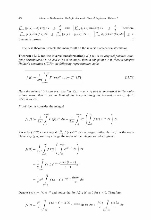
436 Advanced Mathematical Tools for Automatic Control Engineers: Volume 1
∫ βx=α |φ (x)− φε (x)| dx ≤ ε
2and
∣∣∣∫ βx=α φε (x) sin (bx) dx∣∣∣ ≤ ε
2. Therefore,∣∣∣∫ βx=α φ (x) sin (bx) dx∣∣∣ ≤ ∫ β
x=α |φ (x)− φε (x)| dx +∣∣∣∫ βx=α φε (x) sin (bx) dx∣∣∣ ≤ ε.
Lemma is proven. �
The next theorem presents the main result on the inverse Laplace transformation.
Theorem 17.17. (on the inverse transformation) If f (t) is an original function satis-fying assumptions A1–A3 and F(p) is its image, then in any point t ≥ 0 where it satisfiesHölder’s condition (17.70) the following representation holds
f (t) = 1
2πi
a+i∞∫a−i∞
F (p) ept dp := L−1 {F } (17.79)
Here the integral is taken over any line Rep = a > s0 and is understood in the main-valued sense, that is, as the limit of the integral along the interval [a − ib, a + ib]when b→∞.
Proof. Let us consider the integral
fb (t) := 1
2πi
a+ib∫a−ib
F (p) ept dp = 1
2πi
a+ib∫a−ib
ept
⎛⎝ ∞∫τ=0
f (τ) e−pτ dτ
⎞⎠ dp
Since by (17.75) the integral∫∞τ=0f (τ) e−pτ dτ converges uniformly on p in the semi-
plane Rep ≥ a, we may change the order of the integration which gives
fb (t)= 1
2πi
∞∫τ=0
f (τ)
⎛⎝ a+ib∫
a−ibep(t−τ) dp
⎞⎠ dτ
= 1
π
∞∫τ=0
f (τ) ea(t−τ)sin b (t − τ)t − τ dτ
= 1
πeat
∞∫τ=−t
f (x + t) e−a(x+t) sin bxxdx
Denote g (t) := f (t)e−at and notice that by A2 g (t) ≡ 0 for t < 0. Therefore,
fb (t) = eat
π
∞∫τ=−∞
g (x + t)− g (t)x
e−a(x+t) sin bx dx + f (t)π
∞∫τ=−∞
sin bx
xdx
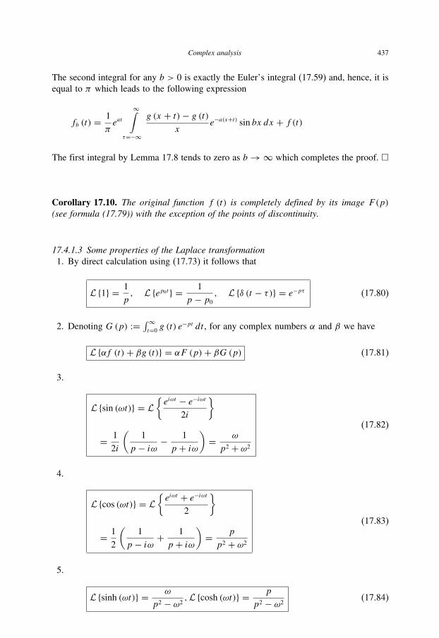
Complex analysis 437
The second integral for any b > 0 is exactly the Euler’s integral (17.59) and, hence, it is
equal to π which leads to the following expression
fb (t) = 1
πeat
∞∫τ=−∞
g (x + t)− g (t)x
e−a(x+t) sin bx dx + f (t)
The first integral by Lemma 17.8 tends to zero as b→∞ which completes the proof. �
Corollary 17.10. The original function f (t) is completely defined by its image F(p)(see formula (17.79)) with the exception of the points of discontinuity.
17.4.1.3 Some properties of the Laplace transformation1. By direct calculation using (17.73) it follows that
L {1} = 1
p, L {ep0t} = 1
p − p0
, L {δ (t − τ)} = e−pτ (17.80)
2. Denoting G(p) := ∫∞t=0g (t) e−pt dt , for any complex numbers α and β we have
L {αf (t)+ βg (t)} = αF (p)+ βG (p) (17.81)
3.
L {sin (ωt)} = L{eiωt − e−iωt
2i
}
= 1
2i
(1
p − iω − 1
p + iω)= ω
p2 + ω2
(17.82)
4.
L {cos (ωt)} = L{eiωt + e−iωt
2
}
= 1
2
(1
p − iω + 1
p + iω)= p
p2 + ω2
(17.83)
5.
L {sinh (ωt)} = ω
p2 − ω2,L {cosh (ωt)} = p
p2 − ω2(17.84)
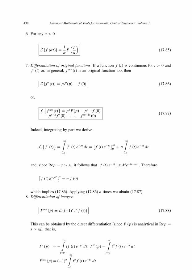
438 Advanced Mathematical Tools for Automatic Control Engineers: Volume 1
6. For any α > 0
L {f (αt)} = 1
αF(pα
)(17.85)
7. Differentiation of original functions: If a function f (t) is continuous for t > 0 and
f ′ (t) or, in general, f (n) (t) is an original function too, then
L {f ′ (t)} = pF(p)− f (0) (17.86)
or,
L{f (n) (t)
} = pnF (p)− pn−1f (0)
−pn−2f ′ (0)− . . .− f (n−1) (0)(17.87)
Indeed, integrating by part we derive
L{f ′ (t)
} = ∞∫t=0
f ′ (t) e−pt dt = [f (t) e−pt
]∞0+ p
∞∫t=0
f (t) e−pt dt
and, since Rep = s > s0, it follows that∣∣f (t) e−pt ∣∣ ≤ Me−(s−s0)t . Therefore
[f (t) e−pt
]∞0= −f (0)
which implies (17.86). Applying (17.86) n times we obtain (17.87).
8. Differentiation of images:
F (n) (p) = L {(−1)n tnf (t)} (17.88)
This can be obtained by the direct differentiation (since F (p) is analytical in Rep =s > s0), that is,
F ′ (p) =−∞∫
t=0
tf (t) e−pt dt, F ′′ (p) =∞∫
t=0
t2f (t) e−pt dt
F (n) (p)= (−1)n
∞∫t=0
tnf (t) e−pt dt

Complex analysis 439
Example 17.14.
L {tn} = n!pn+1
, L {tnep0t} = n!(p − p0)
n+1
L {t sin (ωt)} = 2pω(p2 + ω2
)2L {t cos (ωt)} = p2 − ω2(
p2 + ω2)2
(17.89)
9. Integration of original functions:
L
⎧⎨⎩
t∫τ=0
f (τ) dτ
⎫⎬⎭ = F(p)
p(17.90)
It follows from (17.86) that if we take g (t) := ∫ tτ=0f (τ) dτ and calculate F(p)
= L {f (t)} = L {g′ (t)} = pG (p) that gives G(p) = F(p)p
.
10. Integration of images: If the integral∫∞pF (p) dp (the path of integrations completely
belongs to the semi-plane Rep ≥ a > s0) converges, then∞∫p
F (p) dp = L{f (t)
t
}(17.91)
It follows from changing the order of integration:
∞∫p
F (p) dp =∞∫
t=0
f (t)
⎛⎝ ∞∫p
e−pt dp
⎞⎠ dt = ∞∫
t=0
f (t)
te−pt dt
11. Theorem on delay effect: For any positive τ
L {f (t − τ)} = e−pτF (p) (17.92)
12. Theorem on shifting effect:
L {ep0t f (t)} = F (p − p0) (17.93)
13. Multiplication (Borel) theorem: Denoting the convolution (f ∗ g) of two functions by
(f ∗ g) :=t∫
τ=0
f (τ) g (t − τ) dτ (17.94)
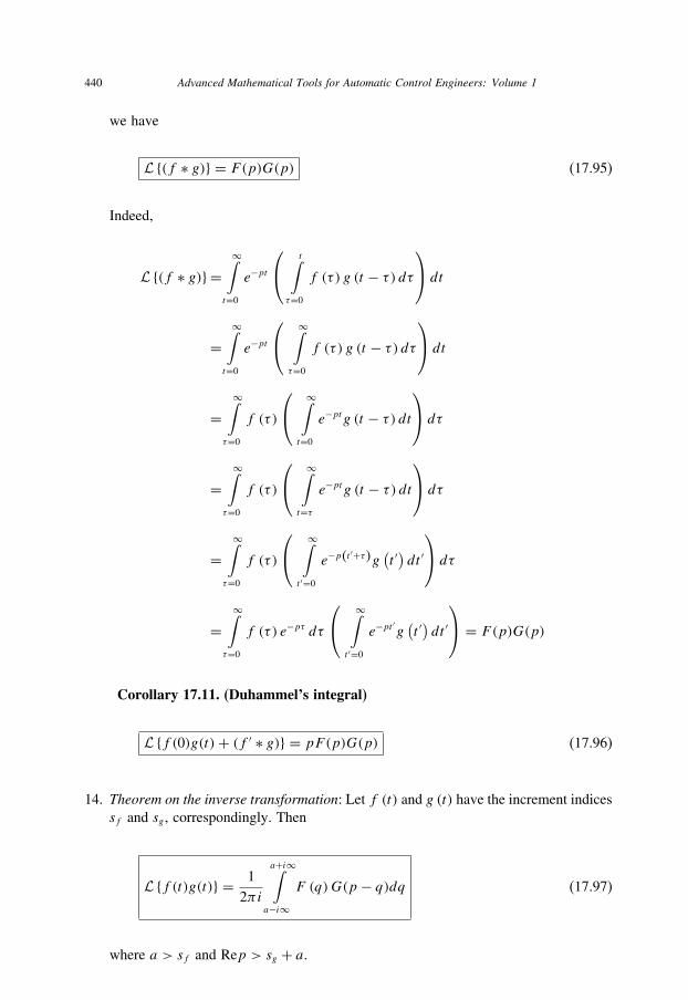
440 Advanced Mathematical Tools for Automatic Control Engineers: Volume 1
we have
L {(f ∗ g)} = F(p)G(p) (17.95)
Indeed,
L {(f ∗ g)} =∞∫
t=0
e−pt
⎛⎝ t∫τ=0
f (τ) g (t − τ) dτ⎞⎠ dt
=∞∫
t=0
e−pt
⎛⎝ ∞∫
τ=0
f (τ) g (t − τ) dτ⎞⎠ dt
=∞∫
τ=0
f (τ)
⎛⎝ ∞∫
t=0
e−ptg (t − τ) dt⎞⎠ dτ
=∞∫
τ=0
f (τ)
⎛⎝ ∞∫
t=τe−ptg (t − τ) dt
⎞⎠ dτ
=∞∫
τ=0
f (τ)
⎛⎝ ∞∫
t ′=0
e−p(t′+τ)g
(t ′)dt ′
⎞⎠ dτ
=∞∫
τ=0
f (τ) e−pτ dτ
⎛⎝ ∞∫
t ′=0
e−pt′g(t ′)dt ′
⎞⎠ = F(p)G(p)
Corollary 17.11. (Duhammel’s integral)
L {f (0)g(t)+ (f ′ ∗ g)} = pF(p)G(p) (17.96)
14. Theorem on the inverse transformation: Let f (t) and g (t) have the increment indices
sf and sg , correspondingly. Then
L {f (t)g(t)} = 1
2πi
a+i∞∫a−i∞
F (q)G(p − q)dq (17.97)
where a > sf and Rep > sg + a.

Complex analysis 441
Indeed,
L {f (t)g(t)} =∞∫
t=0
f (t)g (t) e−pt dt
= 1
2πi
∞∫t=0
⎡⎣ a+i∞∫a−i∞
F (q) eqtdq
⎤⎦ g (t) e−pt dt
= 1
2πi
⎡⎣ a+i∞∫a−i∞
F (q)
∞∫t=0
g (t) e−(p−q)tdt
⎤⎦ dq
= 1
2πi
a+i∞∫a−i∞
F (q)G(p − q) dq
15. First theorem on the expansion: If in a neighborhood of a point p such that |p| ≥ R(R is large enough) the function F(p) may be presented by the Laurent series
F(p) =∞∑k=1
ck
pk(17.98)
then its original f (t) = L−1 {F(p)} can be represented as
f (t) =∞∑k=1
ck
(k − 1)! tk−1 (17.99)
This can be obtained using formulas (17.89).
16. Second theorem on the expansion: Let the function F(p) be a meromorphic in a semi-
plane Rep > s0, for any a > s0 the integral∫ a+i∞a−i∞ F(p) dp converges absolutely
and there exists a system of circles Cn (|p| = Rn →∞, R1 < R2 < . . . ) such that
F(p)→ 0 uniformly respectively argp. Then F(p) is the image of the function
f (t) =∑(pk)
respkF (p)ept (17.100)
where the sum is taken over all singular points pk . This result may be proven using
Cauchy’s residue theorem (17.27) and the Jordan lemma (17.6).
Corollary 17.12. If F(p) = A(p)B(p)
is rational such that
degA(p) < degB(p) =Np∑k=1
nk

442 Advanced Mathematical Tools for Automatic Control Engineers: Volume 1
with pk is a pole of F (p) and nk is its multiplicity, then
f (t) =Np∑k=1
1
(nk − 1)! limp→pkdnk−1
dpnk−1[F(p) (p − pk)nk ept ] (17.101)
17.4.2 Other transformations
17.4.2.1 Heavyside transformationIt is given by (17.69) with
K (t, p) = pe−pt (17.102)
17.4.2.2 Fourier transformation K (t, iω) = 1√2πe−iωt
Main definitionsIf in the double-side Laplace transformations [(in the direct one (17.73) put the incre-
ment index (17.72) s0 = 0 and in the inverse transformation (17.79)) put a = 0] such
that the integration is done over the imaginary axis (p = iω), we obtain the, so-called,
Fourier transformation:
F (ω) := 1√2π
∞∫t=−∞
f (t) e−iωtdt
f (t) = 1√2π
∞∫ω=−∞
F (ω) eiωtdω
(17.103)
In physics the function F (ω) is called the spectral function of the “oscillations” f (t).
Remark 17.8. The range of the application of the Fourier transformation (17.103) issignificantly narrower than one for the Laplace transformation (17.73) since the corre-sponding first nonproper integral in (17.103) converges if the function f (t) is absolutelyintegrable, i.e.,
∫∞t=−∞ |f (t)| dt < ∞. In the case of the Laplace transformation (17.73)
such condition becomes as∫∞t=−∞
∣∣f (t) e−st ∣∣ dt <∞ (s > s0) which significantly extendsthe class of the original functions. From a physical point of view the Fourier transfor-mation (17.103) is more natural than the Laplace transformation (17.73) since formulas(17.103) coincide (maybe some constants are different) with those of the representationof the original function f (t) as the Fourier series (17.62)
f (t) =∞∑
n=−∞Gne
in(2π/T )t , Gn = 1
T
T∫t=0
f (t) e−in(2π/T )t dt

Complex analysis 443
valid for periodical (with the period T ) functions f (t) treated as “oscillations”.
The auxiliary function hλ (ω)According to Rudin (1973) put
H (t) := e−|t |, t ∈ (−∞,∞)
and notice that
0 < H (t) ≤ 1, H (λt)→ 1 as λ→ 0
Define also the following parametric family of functions
hλ (ω) := 1√2π
∞∫t=−∞
H (λt) eitω dt , λ > 0, ω ∈ R
A simple computation gives
hλ (ω) =√
2
π
λ
λ2 + ω2
and, therefore,
∞∫ω=−∞
hλ (ω) dω =√2π (17.104)
Proposition 17.2. If a function g : R+→ R is absolutely integrable on [0,∞), that is,
∞∫t=0
|g (t)| dt <∞, g (t) = 0 for t < 0
and its Laplace transformation is G(p), then
(g � hλ) (ω) := 1√2π
∞∫y=−∞
g (ω − y) hλ (y) dy
= 1
2π
∞∫t=−∞
H (λt)G (it) eitω dt
(17.105)
444 Advanced Mathematical Tools for Automatic Control Engineers: Volume 1
Proof. The simple application of Fubini’s reduction theorem 16.24 gives
(g � hλ) (ω)= 1
2π
∞∫y=−∞
g (ω − y)⎡⎣ ∞∫t=−∞
H (λt) eity dt
⎤⎦ dy
= 1
2π
∞∫t=−∞
H (λt)
⎡⎣ ∞∫y=−∞
g (ω − y) eitydy⎤⎦ dt
= 1
2π
∞∫t=−∞
H (λt)
⎡⎣ ∞∫y=−∞
g (y) eit(ω−y)dy
⎤⎦ dt
= 12π
∞∫t=−∞
H (λt) eitω
⎡⎣ ∞∫y=0
g (y) e−itydy
⎤⎦ dt
= 1
2π
∞∫t=−∞
H (λt) eitωG (it) dt
�
Proposition 17.3. If a function g : R → R is bounded almost everywhere, that is, ess sup|g (ω)| < ∞, and it is continuous at a point ω, then
(g ∗ hλ) (ω) := 1√2π
∞∫y=−∞
g (ω − y) hλ (y) dy → g (ω) (17.106)
as λ→ 0.
Proof. In view of (17.104) and by the dominated convergence theorem we have
(g ∗ hλ) (ω)− g (ω)= 1√2π
∞∫x=−∞
[g (ω − y)− g (ω)]hλ (y) dy
= 1√2π
∞∫x=−∞
[g (ω − y)− g (ω)] λ−1hλ=1
(yλ
)dy
= 1√2π
∞∫s=−∞
[g (ω − λs)− g (ω)]hλ=1 (s) ds → 0 as λ→ 0
�

Complex analysis 445
Corollary 17.13. For any p ∈ [1,∞)
‖(g � hλ)− g‖Lp → 0 as λ→ 0
The Plancherel theoremOne of the most important results of the Fourier transformation theory is the next
theorem.
Theorem 17.18. (Plancherel, around 1800) If f (t) ∈ L2 [0,∞) and its Laplace trans-formation (17.73) is F (p) ∈ H2,6 then the following identity (known as Parseval’sidentity) holds:
‖f ‖L2:=
⎛⎝ ∞∫t=0
|f (t)|2 dt⎞⎠1/2
= ‖F‖H2:=
⎛⎝ 1
2π
∞∫ω=−∞
F (jω) F∼ (jω) dω
⎞⎠1/2
where F∼ (s) := F (−s)
(17.107)
Proof. Recalling that f (t) = 0 for t < 0, define the function
g (x) :=(f � f
)(x)
where f (x) := f (−x). Then
g (t) = 1√2π
∞∫y=−∞
f (t − y) f (−y) dy = 1√2π
∞∫y=0
f (t + y) f (y) dy
and, in view of (17.95), its Laplace transformation is
G(p) = 1√2πF (p) F (−p)
6 The exact definitions of the functional spaces L2 [0,∞) and H2 are given in Chapter 18.

446 Advanced Mathematical Tools for Automatic Control Engineers: Volume 1
Indeed,
L {g} =∞∫
t=0
e−pt
⎛⎝ 1√
2π
∞∫y=0
f (t + y) f (y) dy⎞⎠ dt
= 1√2π
∞∫y=0
f (y)
⎛⎝ ∞∫
t=0
e−ptf (t + y) dt⎞⎠ dy
= 1√2π
∞∫y=0
f (y)
⎛⎝ ∞∫
t=0
e−p(t′−y)f
(t ′)dt ′
⎞⎠ dy
= 1√2π
∞∫y=0
f (y) epy
⎛⎝ ∞∫
t=0
e−pt′f(t ′)dt ′
⎞⎠ dy
= 1√2πF (p) F (−p)
It is easy to see that g (x) is a continuous function. But it is also bounded since
|g (x)| ≤ 1√2π
√√√√√∞∫
y=−∞f 2 (x + y) dy
√√√√√∞∫
y=−∞f 2 (y) dy
≤ 1√2π
∞∫y=−∞
f 2 (y) dy <∞
Therefore, by Propositions 17.2 and 17.3, it follows that
(g ∗ hλ) (0) = 1
2π
∞∫ω=−∞
H (λω)G (iω) dω
But
limλ→0(g ∗ hλ) (0) = g (0) = 1√
2π
∞∫y=0
f 2 (y) dy = 1√2π
‖f ‖2L2
Complex analysis 447
and
limλ→0
1
2π
∞∫ω=−∞
H (λω)G (iω) dω = 1
2π
∞∫ω=−∞
G(iω) dω
1
2π
∞∫ω=−∞
[1√2πF (iω) F (−iω)
]dω = 1√
2π‖F‖2
H2
which completes the proof. �
Corollary 17.14. If f (t), g (t) ∈ L2 [0,∞) and their Laplace transformation (17.73)are F(p),G(p) ∈ H2, then the following identity holds:
〈f, g〉L2:=
⎛⎝ ∞∫
t=0
f (t) g (t) dt
⎞⎠1/2
= 〈F,G〉H2:=
⎛⎝ 1
2π
∞∫ω=−∞
F (jω)G∼ (jω) dω
⎞⎠1/2
where G∼ (s) := G(−s)
(17.108)
Proof. It completely repeats the proof of the previous theorem. �
17.4.2.3 Two-dimensional Fourier transformationIt is given by
G(σ, τ) := 1
2π
∞∫x=−∞
∞∫y=−∞
g (x, y) e−i(σx+τy) dx dy
g (x, y) = 1
2π
∞∫σ=−∞
∞∫τ=−∞
G(σ, τ) ei(σx+τy) dσ dτ
(17.109)
448 Advanced Mathematical Tools for Automatic Control Engineers: Volume 1
17.4.2.4 Both-side Laplace transformationIf we refuse assumption A2 (17.71) and in the Fourier transformation (17.103) make
the integration in the range (−∞,∞), we obtain the, so-called, both-side Laplace trans-formation given by
F (p) :=∞∫
t=−∞f (t) e−pt dt, f (t) = 1
2πi
a+i∞∫a−i∞
F (p) ept dp (17.110)
17.4.2.5 Melline transformationIn (17.110) if we change p with (−p) and t with ln τ , we get
F (−p) :=∞∫
t=−∞f (ln τ) ep ln τ
dτ
τ, f (ln τ) = 1
2πi
a+i∞∫a−i∞
F (−p) e−p ln τ dp
Defining g (τ) := f (ln τ) and G(p) := F (−p) we obtain the, so-called, Melline trans-formation:
G(p) :=∞∫
τ=−∞g (τ) τp−1 dτ, g (τ ) = 1
2πi
a+i∞∫a−i∞
G(p)
τpdp (17.111)
Denote this transformation by G(p) := M {g (τ)}.
Claim 17.2. It is easy to check that1.
M {g (ατ)} = G(p)αp
, α > 0 (17.112)
2.
M {ταg (τ )} = G(p + α) (17.113)
3.
M {f (τ) g (τ )} =a+i∞∫a−i∞
F(q)G(p − q) dq (17.114)

Complex analysis 449
4.
M {g′ (τ )} = − (p − 1)G(p − 1)
M {τg′ (τ )} = −pG(p)
M{τ 2g′ (τ )
}= (p + 1) pG(p)
(17.115)
This transformation turns out to be very useful for the solution of partial differentialequations of a heating type.
17.4.2.6 Hankel (Fourier–Bessel) transformationLet us in (17.109) make the transformation to the polar coordinates, i.e., y = r sin ϕ,
σ = ρ cos θ, τ = ρ sin θ which gives
G(ρ, θ) = 1
2π
∞∫r=−∞
r
⎡⎣ ∞∫ϕ=−∞
g (r, ϕ) e−irρ cos(ϕ−θ) dϕ
⎤⎦ dr
g (r, ϕ) = 1
2π
∞∫ρ=−∞
ρ
⎡⎣ 2π∫θ=0
G(ρ, θ) eirρ cos(ϕ−θ) dθ
⎤⎦ dρ
Representing g (r, ϕ) as g (r, ϕ) = e−inϕg (r) (where n is an integer) and (ϕ − θ) asϕ − θ = π
2+ t , we derive
G(ρ, θ) = 1
2πe−in(θ+π/2)
∞∫r=0
g (r) r
⎡⎣ 2π∫t=0
ei(rρ sin t−nt) dt
⎤⎦ dr
Defining Jn (z) := 1
2π
∫ 2π
t=0cos (nt − z sin t) dt, Gn (ρ) = ein(θ+π/2)G (ρ, θ), we may
write
Gn (ρ) =2π∫
t=0
g (r) Jn (rρ) r dr (17.116)
and, hence, substituting θ − ϕ = t − π2
we obtain
g (r) = 1
2π
∞∫ρ=−∞
Gn (ρ) ρ
⎡⎣ 2π∫
θ=0
ei[n(ϕ−θ−π/2)+rρ cos(ϕ−θ)] dθ
⎤⎦ dρ

450 Advanced Mathematical Tools for Automatic Control Engineers: Volume 1
which, finally, implies
g (r) =∞∫
ρ=−∞Gn (ρ) Jn (rρ) ρ dρ (17.117)
Formulas (17.116) and (17.117) are called the Hankel (Fourier–Bessel) transformation. Itis frequently used for the solution of the partial differential equation describing potential
electric two-dimensional fields.

18 Topics of Functional Analysis
Contents
18.1 Linear and normed spaces of functions . . . . . . . . . . . . . . . . . . . . 452
18.2 Banach spaces . . . . . . . . . . . . . . . . . . . . . . . . . . . . . . . . 455
18.3 Hilbert spaces . . . . . . . . . . . . . . . . . . . . . . . . . . . . . . . . . 457
18.4 Linear operators and functionals in Banach spaces . . . . . . . . . . . . . . 462
18.5 Duality . . . . . . . . . . . . . . . . . . . . . . . . . . . . . . . . . . . . 474
18.6 Monotonic, nonnegative and coercive operators . . . . . . . . . . . . . . . 482
18.7 Differentiation of nonlinear operators . . . . . . . . . . . . . . . . . . . . 488
18.8 Fixed-point theorems . . . . . . . . . . . . . . . . . . . . . . . . . . . . . 491
In Chapter 14 important concepts were introduced such as
1. Lineality of a space of elements;
2. Metric (or norm) in a space;
3. Compactness, convergence of a sequence of elements and Cauchy sequences;4. Contraction principle.
As examples we have considered in detail the finite dimensional spaces Rn and Cn
of real and complex vectors (numbers). But the same definitions of lineality and norms
remain true if we consider as another example a functional space (where an element is
a function) or a space of sequences (where an element is a sequence of real or complex
vectors). The specific feature of such spaces is that they are all infinite dimensional. Thischapter deals with the analysis of such spaces which is called “functional analysis”.
Let us introduce two important additional concepts which we will use below.
Definition 18.1. The subset V of a linear normed space X is said to be dense in X if itsclosure is equal to X .
This property means that every element x ∈ X may be approximated as closely as we
like by some element v ∈ V , that is, for any x ∈ X and any ε > 0 there exists an element
v ∈ V such that ‖x − v‖ < ε.All normed linear spaces have dense subsets, but they need not be obligatory countable
subsets.
Definition 18.2. A normed linear space X is said to be separable if it contains at leastone dense subset which is countable.
The separable spaces have special properties that are important in different applications.
In particular, denoting the elements of such countable subsets by {ei}i=1, . . . it is possible
to represent each element x ∈ X as the convergent series
451

452 Advanced Mathematical Tools for Automatic Control Engineers: Volume 1
x =∞∑i=1
ξiei (18.1)
where the scalars ξi ∈ R are called the coordinates of the element x in the basis {ei}i=1, . . ..
18.1 Linear and normed spaces of functions
Below we will introduce examples of some functional spaces with the corresponding
norm within. The lineality and main properties of a norm (metric) can be easily verified
that is why we leave this for the reader as an exercise.
18.1.1 Space mn of all bounded complex numbers
Let us consider a set m of sequences x := {xi}∞i=1 such that
xi ∈ Cn and supi
‖xi‖ <∞ (18.2)
where ‖xi‖ :=√∑n
s=1 xis xis and introduce the norm in m as
‖x‖ := supi
‖xi‖ (18.3)
18.1.2 Space lnp of all summable complex sequences
By definition
lnp :=⎧⎨⎩x = {xi}∞i=1 | xi ∈ Cn, ‖x‖lnp :=
( ∞∑i=1
‖xi‖p)1/p
⎫⎬⎭ <∞ (18.4)
18.1.3 Space C [a, b] of continuous functions
It is defined as follows
C [a, b] :={f (t) | f is continuous for all t ∈ [a, b],
‖f ‖C[a,b] := maxt∈[a,b]
∣∣∣∣f (t)∣∣∣∣ <∞
} (18.5)
18.1.4 Space Ck [a, b] of continuously differentiable functions
It contains all functions which are k-times differentiable and the kth derivative is
continuous, that is,

Topics of functional analysis 453
Ck [a, b] :={f (t) | f (k) exists and is continuous
for all t ∈ [a, b], ‖f ‖Ck [a,b] :=k∑i=0
maxt∈[a,b]
∣∣f (i) (t)∣∣ <∞} (18.6)
18.1.5 Lebesgue spaces Lp [a, b] (1 ≤ p <∞)
For each 1 ≤ p <∞ it is defined by the following way:
Lp [a, b] :=⎧⎨⎩f (t) : [a, b]→ C |
b∫t=a
|f (t)|p dt <∞
(here the integral is understood in the Lebesgue sense),
‖f ‖p :=⎛⎝ b∫t=a
|f (t)|p dt⎞⎠1/p
⎫⎪⎬⎪⎭
(18.7)
Remark 18.1. Sure, here functions f (t) are not obligatory continuous.
18.1.6 Lebesgue spaces L∞ [a, b]
It contains all measurable functions from [a, b] to C, namely,
L∞ [a, b] :={f (t) : [a, b]→ C |
‖f ‖∞ := ess supt∈[a,b]
|f (t)| <∞} (18.8)
18.1.7 Sobolev spaces Slp (G)
It consists of all functions (for simplicity, real valued) f (t) defined on G which have
p-integrable continuous derivatives f (i) (t) (i = 1, . . . , l), that is,
Slp (G) :=⎧⎨⎩f (t) : G→ R |<∞ (i = 1, . . . , l)
(the integral is understood in the Lebesgue sense),
‖f ‖Slp(G) :=⎛⎝ ∫t∈G
|f (t)|p dt +l∑i=1
∫t∈G
∣∣f (i) (t)∣∣p dt⎞⎠1/p⎫⎬
⎭(18.9)
More exactly, the Sobolev space is the completion (see definition below) of (18.9).

454 Advanced Mathematical Tools for Automatic Control Engineers: Volume 1
18.1.8 Frequency domain spaces Lm×kp , RLm×kp , Lm×k∞ and RLm×k∞
By definition
1. The Lebesgue space Lm×kp is the space of all p-integrable complex matrices, i.e.,
Lm×kp :=⎧⎨⎩F : C → Cm×k |
‖F‖Lm×kp
:=⎛⎝ 1
2π
∞∫ω=−∞
(tr {F (jω) F∼ (jω)})p−1dω
⎞⎠1/p
<∞⎫⎬⎭
(here F∼ (jω) := Fᵀ (−jω) )
(18.10)
2. The Lebesgue space RLm×kp is the subspace of Lm×kp containing only complex matrices
with rational elements, i.e., in
F = ∥∥Fi,j (s)∥∥i=1,m; j=1,k
each element Fi,j (s) represents the polynomial ratio
Fi,j (s) =a0i,j + a1i,j s + . . .+ api,ji,j spi,ji,j
b0i,j + b1i,j s + . . .+ bqi,ji,j sqi,ji,jpi,j and qi,j are positive integers
(18.11)
Remark 18.2. If pi,j ≤ qi,j for each element Fij of (18.11), then F (s) can be inter-preted as a matrix transfer function of a linear (finite-dimensional) system.
3. The Lebesgue space Lm×k∞ is the space of all complex matrices bounded (almost
everywhere) on the imaginary axis elements, i.e.,
Lm×k∞ :={F : C → Cm×k |
‖F‖Lm×k∞ := ess sup
s:Re s>0λ1/2max {F (s) F∼ (s)}
}= ess sup
ω∈(−∞,∞)λ1/2max {F (jω) F∼ (jω)} <∞
(18.12)
(the last equality may be regarded as the generalization of the maximum modulus
principle 17.10 for matrix functions).
4. The Lebesgue space RLm×k∞ is the subspace of Lm×k∞ containing only complex matrices
with rational elements given in the form (18.11).
18.1.9 Hardy spaces Hm×kp , RHm×k
p , Hm×k∞ and RHm×k
∞
The Hardy spaces Hm×kp , RHm×k
p , Hm×k∞ and RHm×k
∞ are subspaces of the corresponding
Lebesgue spaces Lm×kp , RLm×kp , Lm×k∞ and RLm×k∞ containing complex matrices with only
regular (holomorphic) (see Definition 17.2) elements on the open half-plane Re s > 0.
Topics of functional analysis 455
Remark 18.3. If pi,j ≤ qi,j for each element Fij of, then F (s) ∈ RHm×kp can be inter-
preted as a matrix transfer function of a stable linear (finite-dimensional) system.
Example 18.1.
1
2− s ∈ RL2 := RL1×12 ,
1− s2− s ∈ RL∞ := RL1×1
∞
1
2+ s ∈ HL2 := HL1×12 ,
1− s2+ s ∈ RH∞ := RH1×1
∞
e−s
2− s ∈ L2 := L1×12 ,
e−s
2+ s ∈ H2 := H1×12
e−s1− s2− s ∈ L∞ := L1×1
∞ , e−s1− s2+ s ∈ H∞ := H1×1
∞
18.2 Banach spaces
18.2.1 Basic definition
Remember that a linear normed (topological) space X is said to be complete (see
Definition 14.14) if every Cauchy (fundamental) sequence has a limit in the same space X .
The concept of a complete space is very important since even without evaluating the limit
one can determine whether a sequence is convergent or not. So, if a metric (topological)
space is not complete it is impossible to talk about a convergence, limits, differentiation
and so on.
Definition 18.3. A linear, normed and complete space is called a Banach space.
18.2.2 Examples of incomplete metric spaces
Sure, not all linear normed (metric) spaces are complete. The example given below
illustrates this fact.
Example 18.2. (of a noncomplete normed space) Let us consider the space CL [0, 1]
of all continuous functions f : [0, 1] → R which are absolutely integrable (in this case,in the Riemann sense) on [0, 1], that is, for which
‖f ‖CL[0,1] :=1∫
t=−1
|f (t)| dt <∞ (18.13)
Consider the sequence {fn} of the continuous functions
fn :={nt if t ∈ [0, 1/n]
1 if t ∈ [1/n, 1]

456 Advanced Mathematical Tools for Automatic Control Engineers: Volume 1
Then for n > m
‖fn − fm‖CL[0,1] =1∫
t=0
|fn (t)− fm (t)| dt
=1/n∫t=0
|nt −mt | dt +1/m∫
t=1/n
|1−mt | dt +1∫
t=1/m
|1− 1| dt
(n−m)2n2
+ (1−m/n)2
2m= 1
2
(1
m− 1
n
)→ 0
as n,m→∞. So, {fn} is a Cauchy sequence. However, its pointwise limit is
fn (t)→{1 if 0 < t ≤ 1
0 if t = 0
In other words, the limit is a discontinuous function and, hence, it is not in CL [0, 1].This means that the functional space CL [0, 1] is not complete.
Example 18.3. By the same reason, the spaces CLp [0, 1] (the space of continuous andp-integrable functions) are not complete.
18.2.3 Completion of metric spaces
There exist two possibilities to correct the situation and to provide the completeness
property for a linear normed space if initially some is not complete:
• try to change the definition of a norm;• try to extend the class of considered functions (it was suggested by Cauchy).
18.2.3.1 Changing of a normTo illustrate the first approach related to changing of a norm let us consider again the
space of all functions continuous at the interval [0, 1], but instead of the Lebesgue norm
(18.13) we consider the Chebyshev type norm ‖f ‖C[a,b] as in (18.5). This means that
instead of the space CL [0, 1] we will consider the space C [a, b] (18.5). Evidently, that
this space is complete, since it is known that uniform convergent sequences of continuous
functions converge to a continuous function. Hence, C [a, b] is a Banach space under
this norm.
Claim 18.1. By the same reasons it is not difficult to show that all spaces Ck [a, b] (18.6)are Banach.
Claim 18.2. The spaces Lp [a, b] (1 ≤ p <∞) (18.7), L∞ [a, b] (18.8), Lm×kp (23.19)and Lm×k∞ (18.12) are Banach too.

Topics of functional analysis 457
18.2.3.2 Completion
Theorem 18.1. Any linear normed space X with a norm ‖x‖X can be considered
as a linear manifold which is complete in some Banach space X . This space X is calledthe completion of X .
Proof. Consider two fundamental sequences {xn} and{x ′n}with elements from X . We
say that they are equivalent if∥∥xn− x ′n∥∥→ 0 as n→∞ and we will write {xn} ∼
{x ′n}.
The set of all fundamental sequences may be separated ( factorized) at noncrossed classes:{xn} and
{x ′n}are included in the same class if and only if {xn} ∼
{x ′n}. The set of all
such classes Xi we denoted by X . So,
X :=⋃i
Xi , Xi ∩i �=j Xj = ∅
Let us make the space X a normed space. To do that, define the operation of summing ofthe classes Xi by the following manner: if {xn} ∈ Xi and {yn} ∈ Xj then class
(Xi + Xj
)may be defined as the class containing {xn + yn}. The operation of the multiplication bya constant may be introduced as follows: we denoted by λXi the class containing {λxn}if {xn} ∈ Xi . It is evident that X is a linear space. Define now the norm in X as
‖Xi‖ := limn→∞
‖xn‖X ({xn} ∈ Xi )
It easy to check the norm axioms for such norm and to show that
(a) X may be considered as a linear manifold in X ;
(b) X is dense in X , i.e., there exists {xn} ∈ X such that ‖xn − Xi‖X → 0 as n → ∞for some Xi ∈ X ;
(c) X is complete (Banach).
This completes the proof. �
This theorem can be interpreted as the following statement.
Corollary 18.1. For any linear norm space X there exists a Banach space X and alinear, injective map T : X → X such that T (X ) is dense in X and for all x ∈ X
‖T x‖X = ‖x‖X
18.3 Hilbert spaces
18.3.1 Definition and examples
Definition 18.4. A Hilbert space H is an inner (scalar) product space that is completeas a linear normed space under the induced norm
‖z‖H := √〈z, z〉 (18.14)

458 Advanced Mathematical Tools for Automatic Control Engineers: Volume 1
Example 18.4. The following spaces are Hilbert
1. The space ln2 of all summable complex sequences (see (18.4) for p = 2) under theinner product
〈x, y〉ln2 :=∞∑i=1
xiyi (18.15)
2. The Lebesgue space L2 [a, b] of all integrable (in Lebesgue sense) complex functions(see (18.7) for p = 2) under the inner product
〈x, y〉L2[a,b]:=
b∫t=ax(t)y(t) dt (18.16)
3. The Sobolev’s space Sl2 (G) of all l times differentiable on G quadratically integrable(in Lebesgue sense) complex functions (see (18.9) for p = 2) under the inner product
〈x, y〉Slp(G) :=l∑i=0
⟨di
dt ix,di
dt iy
⟩L2[a,b]
(18.17)
4. The frequency domain space Lm×k2 of all p-integrable complex matrices (23.19) underthe inner product
〈x, y〉Lm×kp
:=∞∫
ω=−∞tr{X (jω) Y∼ (jω)} dω (18.18)
5. The Hardy spaces Hm×k2 (the subspace of Lm×k2 containing only holomorphic in the
right-hand semi-plan C+ := {s ∈ C |Res > 0} functions) under the inner product(18.18).
18.3.2 Orthogonal complement
Definition 18.5. Let M be a subset of a Hilbert space H, i.e., M ⊂ H. Then thedistance between a point x ∈ H and M is defined by
ρ (x,M) := infy∈M
‖x − y‖ (18.19)
The following claim seems to be evident.
Claim 18.3. If x ∈ M, then ρ (x,M) = 0. If x /∈ M and M is a closed set (seeDefinition 14.7), then ρ (x,M) > 0.

Topics of functional analysis 459
Corollary 18.2. If M ⊂ H is a closed convex set and x /∈ M, then there exists a uniqueelement y ∈ M such that ρ (x,M) = ‖x − y‖.
Proof. Indeed, suppose that there exists another element y∗ ∈ M such that
ρ (x,M) = ‖x − y‖ = ‖x − y∗‖ := d
Then
4d2 = 2 ‖x − y‖2 + 2 ‖x − y∗‖2
= ‖x − y∗‖2 + 4
∥∥∥∥x − y + y∗2
∥∥∥∥2
≥ ‖x − y∗‖2 + 4 infy∈M
‖x − y‖2
≥ ‖x − y∗‖2 + 4d2
which gives ‖x − y∗‖2 ≤ 0, or, equivalently, y = y∗. �
Corollary 18.3. If M ⊂ H is a subspace of H (this means that it is a closed convexlinear manifold in H) then for any x ∈ H there exists a unique element xM ∈ M suchthat
ρ (x,M) := infy∈M
‖x − y‖ = ‖x − xM‖ (18.20)
This element xM ∈ M is called the orthogonal projection of the element x ∈ H ontothe subspace M ⊂ H.
Lemma 18.1. Let ρ (x,M) = ‖x − xM‖ where M is a subspace of a Hilbert space Hwith the inner product 〈x, y〉H. Then (x − xM) ⊥ M, that is, for any y ∈ M
〈x − xM, y〉H = 0 (18.21)
Proof. By the definition (18.20) for any λ ∈ C (here xM + λy ∈ M) we have
‖x − (xM + λy)‖ ≥ ‖x − xM‖
which implies
λ 〈x − xM, y〉H + λ 〈y, x − xM〉H + λλ ‖y‖2 ≥ 0
Taking λ = −〈x − xM, y〉H‖y‖2 one has −|〈x − xM, y〉|2
‖y‖2 ≥ 0 which leads to the equality
〈x − xM, y〉H = 0. Lemma is proven. �

460 Advanced Mathematical Tools for Automatic Control Engineers: Volume 1
Definition 18.6. If M is a subspace of a Hilbert space H then the orthogonal comple-ment M⊥ is defined by
M⊥ := {x ∈ H | 〈x, y〉H = 0 for all y ∈ M
}(18.22)
It is easy to show that M⊥ is a closed linear subspace of H and that H can be uniquely
decomposed as the direct sum
H = M⊕M⊥(18.23)
This means that any element x ∈ H has the unique representation
x = xM + xM⊥ (18.24)
where xM ∈ M and xM⊥ ∈ M⊥ such that ‖x‖2 = ‖xM‖2 + ‖xM⊥‖2.
Theorem 18.2. Let M be a subspace of a Hilbert space H. M is dense in H if and onlyif M⊥ = {0}.Proof.
(a) Necessity. Let M be dense in H. This means that M = H. Assume that there exists
x0 ∈ H such that x0 ⊥ M. Let {yn} ⊂ M and yn → y ∈ H. Then 0 = 〈yn, x0〉 →〈y, x0〉 = 0 since M is dense in H. Taking y = x0 we get that 〈x0, x0〉 = 0 which
gives x0 = 0.
(b) Sufficiency. Let M⊥ = {0}, that is, if 〈y, x0〉 = 0 for any y ∈ M, then x0 = 0.
Suppose that M is not dense in H. This means that there exists x0 /∈ M. Then by
the orthogonal decomposition x0 = y0 + z0 where y0 ∈ M and z0 ∈(M
)⊥ = M⊥.Here z0 �= 0 for which 〈z0, y〉H = 0 for any y ∈ M. By the assumption such element
z0 = 0. We get the contradiction. Theorem is proven. �
18.3.3 Fourier series in Hilbert spaces
Definition 18.7. An orthonormal system (set) {φn} of functions in a Hilbert space H isa nonempty subset {φn | n ≥ 1} of H such that
〈φn, φm〉H = δn,m ={1 if n = m0 if n �= m (18.25)
1. The series∑∞n=1 αkφn is called the series in H with respect to the system {φn} (18.25);
2. For any x ∈ H the representation (if it exists)
x (t) =∞∑n=1
αnφn (t) (18.26)
is called the Fourier expansion of x with respect to {φn}.

Topics of functional analysis 461
Lemma 18.2. In (18.26)
αk = 〈x, φk〉H (18.27)
Proof. Pre-multiplying (18.26) by φk and using (18.25) we find
〈x, φk〉H =∞∑n=1
αn 〈φk, φn〉H =∞∑k=1
αkδk,n = αk
which proves (18.27). Lemma is proven. �
Corollary 18.4. (The Parseval equality)
‖x‖2 =∞∑n=1
|〈x, φn〉H|2 (18.28)
Proof. It follows from the relation
〈x, x〉H =∞∑n=1
∞∑m=1
〈x, φn〉H 〈x, φm〉H 〈φn, φm〉H
=∞∑n=1
∞∑m=1
〈x, φn〉H 〈x, φm〉Hδn.m =∞∑n=1
|〈x, φn〉H|2
�
Example 18.5.
1. Classical Fourier expansion. In H =L2 [0, 1] the corresponding orthogonal basis{φn} is
{φn} ={1,
√2 sin (2πnt),
√2 cos (2πnt), n ≥ 1
}which implies
x (t) = a0 +√2
∞∑n=1
an sin (2πnt)+√2
∞∑n=1
bn cos (2πnt)
where
a0 =1∫
t=0
x (t) dt, an =1∫
t=0
x (t)√2 cos (2πnt) dt
bn =1∫
t=0
x (t)√2 sin (2πnt) dt
462 Advanced Mathematical Tools for Automatic Control Engineers: Volume 1
2. Legendre expansion. In H =L2 [0, 1] the corresponding orthogonal basis {φn} is{φn} = {pn} where
pk := 1
2kk!dk
dtk
[(t2 − 1
)k], k ≥ 1
18.3.4 Linear n-manifold approximation
Definition 18.8. The collection of the elements
un :=n∑k=1
ckφk ∈ H, ck ∈ C (k ≥ 1) (18.29)
is called the linear n-manifold generated by the system of functions {φk}k=1,n.
Theorem 18.3. The best L2-approximation of any elements x ∈ H by the element unfrom the n-manifold (18.29) is given by the Fourier coefficients ck = αk (18.27), namely,
infck :k=1,n
∥∥∥∥∥x −n∑k=1
ckφk
∥∥∥∥∥2
L2
=∥∥∥∥∥x −
n∑k=1
αkφk
∥∥∥∥∥2
L2
(18.30)
Proof. It follows from the identity
‖x − un‖2L2=
∥∥∥∥∥x −n∑k=1
ckφk
∥∥∥∥∥2
L2
=∥∥∥∥∥
∞∑n=1
αnφn (t)−n∑k=1
ckφk
∥∥∥∥∥2
L2
=∞∑
k=n+1
|αk|2 ‖φk‖2L2+
n∑k=1
|αk − ck|2 ‖φk‖2L2
which reaches the minimum if ck = αk(ck : k = 1, n
). Theorem is proven. �
18.4 Linear operators and functionals in Banach spaces
18.4.1 Operators and functionals
Definition 18.9.
1. Let X and Y be linear normed spaces (usually either Banach or Hilbert spaces)and T : D → Y be a transformation (or operator) from a subset D ⊂ X to Y .D = D (T ) is called the domain (image) of the operator T and values T (D) constitutethe range (the set of possible values) R (T ) of T . If the range of the operator T isfinite-dimensional then we say that the operator has finite range.
Topics of functional analysis 463
2. If Y is a scalar field F (usually R) then the transformations T are called functionals.3. A functional T is linear if it is additive, i.e., for any x, y ∈ D
T (x + y) = T x + Ty
and homogeneous, i.e., for any x ∈ D and any λ ∈ F
T (λx) = λT x
4. Operators for which the domain D and the range T (D) are in one-to-one correspon-dence are called invertible. The inverse operator is denoted by T −1 : T (D)→ D, sothat
D ⊇T −1 (T (D))
Example 18.6.
1. The shift operator Tsh : lnp → lnp defined by
Tshxi = xi+1
for any i = 1, 2, . . . .
2. The integral operator Tg : L2 [a, b]→ R defined by
Tgf :=b∫
t=af (t) g (t) dt
for any f, g ∈ L2 [a, b].
3. The differential operator Td : D (T ) = C1 [a, b] → C [a, b] defined by
Tdf := d
dtf (t)
for any f ∈ C1 [a, b] and any t ∈ [a, b].
It is evident in the following claim.
Claim 18.4.
1. T is invertible if and only if it is injective, that is, T x = 0 implies x = 0. The set{x ∈ D | T x = 0} is called the kernel of the operator and denoted by
ker T := {x ∈ D | T x = 0}
So, T is injective if and only if ker T = {0}.2. If T is linear and invertible then T −1 is also linear.
464 Advanced Mathematical Tools for Automatic Control Engineers: Volume 1
18.4.2 Continuity and boundedness
18.4.2.1 ContinuityDefinition 18.10.
1. Let T : D (T )→ Y be a map (operator) between two linear normed spaces X (witha norm ‖·‖X ) and Y (with a norm ‖·‖Y ). It is said to be continuous at x0 ∈ X if,given ε > 0, there exists a δ = δ (ε) > 0 such that ‖T (x)− T (x0)‖Y < ε, whenever‖x − x0‖X < δ.
2. T is semi-continuous at a point x0 ∈ X if it transforms any convergent sequence{xn} ⊂ D (T ), xn → x0, n→∞ into a sequence {T (xn)} ⊂ R (T ) weakly convergentto T (x0), i.e., ‖T (xn)→ T (x0)‖ → 0 when n→∞.
3. T is continuous (or semi-continuous) on D (T ) if it is continuous (or semi-continuous)at every point in D (T ).
Lemma 18.3. Let X and Y be Banach spaces and A be a linear operator defined at X .If A is continuous at the point 0 ∈ X , then A is continuous at any point x0 ∈ X .
Proof. This result follows from the identity Ax − Ax0 = A (x − x0). If x → x0, then
z := x − x0 → 0. By continuity at zero Az→ 0 that implies Ax −Ax0 → 0. Lemma is
proven. �
So, a linear operator A may be called continuous if it is continuous at the point
x0 = 0.
18.4.2.2 Boundedness
Definition 18.11.
1. A linear operator A : D (A) ⊂ X → Y between two linear normed spaces X (witha norm ‖·‖X ) and Y (with a norm ‖·‖Y ) is said to be bounded if there exists a realnumber c > 0 such that for all x ∈ D (A)
‖Ax‖Y ≤ c ‖x‖X (18.31)
The set of all bounded linear operators A : D (A) ⊂ X → Y is usually denoted byL (X ,Y).
2. A linear operator A : D (A) ⊂ X → Y is called a compact operator if it maps anybounded subset of X onto a compact set of Y .
3. The induced norm of a linear bounded operator A : D (A) ⊂ X → Y may beintroduced as follows
‖A‖ := supx∈D(A), x �=0
‖Ax‖Y‖x‖X
= supx∈D(A), ‖x‖X=1
‖Ax‖Y (18.32)
(here it is assumed that if D (A) = {0} then by definition ‖A‖ = 0 since A0 = 0).
It seems to be evident that the continuity and boundedness for linear operators are
equivalent concepts.

Topics of functional analysis 465
Claim 18.5. A linear operator A : D (A) ⊂ X → Y is continuous if and only if it isbounded.
Example 18.7.
1. If β :=( ∞∑i,j=1
∣∣aij ∣∣q)1/q
<∞ (q > 1), then the “weighting” operator A defined by
y = Axi :=∞∑j=1
aijxj (18.33)
making from lp to lq(p−1 + q−1 = 1
)is linear and bounded since by the Hölder
inequality (16.134)
‖Axi‖qlq =∞∑i=1
∣∣∣∣∣∞∑j=1
aijxj
∣∣∣∣∣q
≤∞∑i=1
( ∞∑j=1
∣∣aij ∣∣q)( ∞∑
j=1
∣∣xj ∣∣p)q/p
= β( ∞∑j=1
∣∣xj ∣∣p)q/p
= β ‖x‖qlp
2. If β := ∫ bx=a
∫ bs=a |K (x, s)|q ds dx <∞, then the integral operator A : X = Lp [a, b]
→ Y = Lq [a, b] = Y(p−1 + q−1 = 1
)defined by
y = Af :=b∫
s=aK (x, s) f (s) ds (18.34)
is linear and bounded since by the Hölder inequality (16.134)
‖Af ‖qLq [a,b] :=b∫
x=a
∣∣∣∣∣∣b∫
s=aK (x, s) f (s) ds
∣∣∣∣∣∣q
dx
≤b∫
x=a
⎛⎝ b∫s=a
|K (x, s)|q ds⎞⎠⎛⎝ b∫s=a
|f (s)|p ds⎞⎠q/p
dx = β ‖f ‖qLp [a,b]
3. If β := maxt∈D
∑l
α=0|aα (t)| <∞, then the differential operator A : D ⊂ X = Ck [a, b]
→ Y = C [a, b] = Y defined by
y = Af :=l∑α=0
aα (t) f(α) (t) (18.35)

466 Advanced Mathematical Tools for Automatic Control Engineers: Volume 1
is linear and bounded since
‖Af ‖C[a,b] := maxt∈D
∣∣∣∣∣l∑α=0
aα (t) f(α) (t)
∣∣∣∣∣≤ max
t∈D
(l∑α=0
|aα (t)|l∑α=0
∣∣f (α) (t)∣∣)≤ β ‖f ‖Cl [a,b]
18.4.2.3 Sequence of linear operators and uniform convergenceIt is possible to introduce several different notions of a convergence in the space of
linear bounded operators L (X ,Y) acting from X to Y .
Definition 18.12. Let {An} ⊂ L (X ,Y) be a sequence of operators.
1. We say that• An uniformly converges to A ∈ L (X ,Y) if ‖An − A‖ → 0 whenever n → ∞.Here the norm ‖An − A‖ is understood as in (18.32);
• An strongly converges to A ∈ L (X ,Y) if ‖Anf − Af ‖Y → 0 whenever n→ ∞for any f ∈ X .
2. If the operator A is dependent on the parameter α ∈ A, then• A (α) is uniformly continuous at α0 ∈ A, if
‖A (α)− A (α0)‖ → 0 as α→ α0
• A (α) is strongly continuous at α0 ∈ A, if for all f ∈ X
‖A (α) f − A (α0) f ‖Y → 0 as α→ α0
In view of this definition the following claim seems to be evident.
Claim 18.6. An uniformly converges toA ∈ L (X ,Y) if and only ifAnf →Af uniformlyon f ∈ X in the ball ‖f ‖X ≤ 1.
Theorem 18.4. If X is a linear normed space and Y is a Banach space, then L (X ,Y)is a Banach space too.
Proof. Let {An} be a fundamental sequence in the metric of L (X ,Y), that is, for anyε > 0 there exists a number n0 = n0 (ε) such that for any n > n0 and any natural p we
have∥∥An+p − A∥∥ < ε. Then the sequence {Anf } is also fundamental. But Y is complete,
and, hence, {Anf } converges. Denote y := limn→∞Anf . By this formula any element f ∈ X
is mapped into an element of Y , and, hence, it defines the operator y = Af . Let us
prove that the linear operator A is bounded (continuous). First, notice that {‖An‖} is alsofundamental. This follows from the inequality |‖An+p‖ − ‖An‖ | ≤ ‖An+p − An‖. But itmeans that {‖An‖} is bounded, that is, there exists c > 0 such that ‖An‖ ≤ c for everyn ≥ 1. Hence, ‖Anf ‖ ≤ c ‖f ‖. Taking the limit in the right-hand side we obtain ‖Af ‖≤ c ‖f ‖ which shows that A is bounded. Theorem is proven. �

Topics of functional analysis 467
18.4.2.4 Extension of linear bounded operatorsBounded linear operators that map into a Banach space always have a unique extension
to the closure of their domain without changing of its norm value.
Theorem 18.5. Let A : D (A) ⊂ X → Y be a linear bounded operator (functional)mapping the linear normed space X into a Banach space Y . Then it has a unique boundedextension A : D (A)→ Y such that1. Af = Af for any f ∈ D (A);2.
∥∥A∥∥ = ‖A‖.
Proof. If f ∈ D (A), put Af = Af . Let f ∈ X , but x /∈ D (A). By the density of
D (A) in X , there exists the sequence {fn} ⊂ D (A) converging to x. Put Af = limn→∞Afn.
Let us show that this definition is correct, namely, that the limit exists and it does not
depend on the selection of the convergent sequence {fn}. The existence follows from
the completeness property of Y since ‖Afn − Afm‖ ≤ ‖A‖ ‖fn − fm‖X . Hence, limn→∞Afn
exists. Supposing that there exists another sequence{f ′n} ⊂ D (A) converging to f we
may denote a := limn→∞Afn and b := lim
n→∞Af′n. Then we get
‖a − b‖ ≤ ‖a − Afn‖ +∥∥Afn − Af ′n∥∥+ ∥∥Af ′n − b∥∥ →
n→∞ 0
But ‖Afn‖ ≤ ‖A‖ ‖fn‖ that for n → ∞ implies∥∥Af ∥∥ ≤ ‖A‖ ‖f ‖, or, equivalently,∥∥A∥∥ ≤ ‖A‖. We also have
∥∥A∥∥ := sup‖f ‖X≤1
∥∥Af ∥∥ ≥ supf∈D(A), ‖f ‖X≤1
∥∥Af ∥∥ = ‖A‖. So, wehave
∥∥A∥∥ = ‖A‖. The linearity property of A follows from the linearity of A. Theorem
is proven. �
Definition 18.13. The operator A constructed in Theorem 18.5 is called the extensionof A to the closure D (A) of its domain D (A) without increasing its norm.
The principally more complex case arises when D (A) = X . The following important
theorem says that any linear bounded functional (operator) can be extended to the wholespace X without increasing into a norm. A consequence of this result is the existence of
nontrivial linear bounded functionals on any normed linear space.
Theorem 18.6. (The Hahn–Banach theorem) Any linear bounded functional A : D (A)⊂ X → Y defined on a linear subspace D (A) of a linear normed space X can beextended to a linear bounded functional A defined on the whole X with the preservationof the norm, i.e., Af = Af for any f ∈ D (A) such that
∥∥A∥∥ = ‖A‖.
Proof. Here we present only the main idea of the proof.
(a) If X is separable, then the proof is based on Theorem 18.5 using the following
lemma.
Lemma 18.4. Let X be a real normed space and L a linear manifold in X where thereis defined a linear functional A. If f0 /∈ L and L1 := {f + tf0 | f ∈ L, t ∈ R} is a linearmanifold containing all elements f + tf0, then there exists a linear bounded functional

468 Advanced Mathematical Tools for Automatic Control Engineers: Volume 1
A1 defined on L1 such that it coincides with A on L and preserving the norm on L1,namely, ‖A1‖ = ‖A‖.
Then, since X is separable, there exists a basis {fn}n≥1 such that we can construct the
sequence of s-manifolds
Ls≥1 :={
s∑i=1
λifi | fi ∈ X , λi ∈ R
}
connected by Ls+1 = Ls + {fn+1}, L0 := ∅. Then we make the extension of A to each
of the subspaces Ls≥1 based on the lemma above. Finally we apply Theorem 18.5 to the
space X = ∪s≥1
Ls using the density property of X .
(b) In general, the proof is based on Zorn’s lemma (see Yoshida (1979)). �
Corollary 18.5. Let X be a normed (topological) space and x ∈ X , x �= 0. Then thereexists a linear bounded functional f , defined on X , such that its value at any point x isequal to
f (x) := 〈x, f 〉 = ‖x‖ (18.36)
and
‖f ‖ := supx∈D(f ),‖x‖≤1
〈x, f 〉 = 1 (18.37)
Proof. Consider the linear manifold L := {tx}, t ∈ R where we define f as follows:
〈tx, f 〉 = t ‖x‖. So, we have 〈x, f 〉 = ‖x‖. Then for any y = tx it follows |〈y, f 〉| =|t | · ‖x‖ = ‖tx‖ = ‖y‖. This means that ‖f ‖ = 1 and completes the proof. �
Corollary 18.6. Let in a normed space X there be defined a linear manifold L and theelement x0 /∈ L having the distance d up to this manifold, that is, d := inf
x∈L‖x − x0‖.
Then there exists a linear functional f defined on the whole X such that1. 〈x, f 〉 = 0 for any x ∈ L2. 〈x0, f 〉 = 1
3. ‖f ‖ = 1/d
Proof. Take L1 := L + {x0}. Then any element y ∈ L1 is uniquely defined by
y = x + tx0 where x ∈ L and t ∈ R. Define on L1 the functional f := t . Now, if y ∈L, then t = 0 and 〈y, f 〉 = 0. So, statement 1 holds. If y = x0, then t = 1 and, hence,
〈x0, f 〉 = 1 which verifies statement 2. Finally,
|〈y, f 〉| = |t | = |t | · ‖y‖‖y‖ = ‖y‖∥∥∥x
t+ x0
∥∥∥ ≤ ‖y‖d

Topics of functional analysis 469
which gives ‖f ‖ ≤ 1/d . On the other hand, by the “inf” definition, there exists a sequence
{xn} ∈ L such that d = limn→∞
‖xn − x0‖. This implies
1 = 〈x0 − xn, f 〉 ≤ ‖xn − x0‖ · ‖f ‖
Taking limit in the last inequality we obtain 1 ≤ d ‖f ‖ which gives ‖f ‖ ≥ 1/d.
Combining both inequalities we conclude the statement 3. Corollary is proven. �
Corollary 18.7. A linear manifold L is not dense in a Banach space X if andonly if there exists a linear bounded functional f �= 0 such that 〈x, f 〉 = 0 forany x ∈ L.
Proof.
(a) Necessity. Let L �= X . Then there exists a point x0 ∈ X such that the distance
between x0 and L is positive, namely, ρ (x0,L) = d > 0. By Corollary 18.6 there
exists f such that 〈x0, f 〉 = 1, that is, f �= 0 but 〈x, f 〉 = 0 for any x ∈ L.(b) Sufficiency. Let now L = X . Then for any x ∈ X , in view of the density property,
there exists {xn} ∈ L such that xn → x when n → ∞. By the condition that there
exists f �= 0, = 0 for any x ∈ L, we have 〈x, f 〉 = limn→∞
〈xn, f 〉 = 0. Since x is
arbitrary, it follows that f = 0. Contradiction. Corollary is proven.
�
Corollary 18.8. Let {xk}n1 be a system of linearly independent elements in a normedspace X . Then there exists a system of linear bounded functionals {fl}n1 , defined on thewhole X , such that
〈xk, fl〉 = δkl (k, l = 1, . . . , n) (18.38)
These two systems {xk}n1 and {fl}n1 are called bi-orthogonal.
Proof. Take x1 and denote by L1 the linear span of the elements x2, . . . , xn. By linear
independency, it follows that ρ (x1, L1) > 0. By Corollary 18.6 we can find the linear
bounded functional f1 such that 〈x1, f1〉 = 1, 〈x, f1〉 = 0 on L1. Iterating this process
we construct the desired system {fl}n1. �
18.4.3 Compact operators
In this subsection we will consider a special subclass of bounded linear operators
having properties rather similar to those enjoyed by operators on finite-dimensional
spaces.
Definition 18.14. Let X and Y be normed linear spaces. An operator A ∈ L (X ,Y) issaid to be a compact operator if A maps a bounded set of X onto relative compact setsof Y , that is, A is linear and for any bounded sequence {xn} in X the sequence {Axn}has a convergence subsequence in Y .
470 Advanced Mathematical Tools for Automatic Control Engineers: Volume 1
Claim 18.7. Let X and Y be normed linear spaces and A : X → Y be a linear operator.Then the following assertions holds:(a) If A is bounded, that is, A ∈ L (X ,Y) and dim (Ax) < ∞, then the operator A is
compact.(b) If dim (X ) <∞, then A is compact.(c) The range of A is separable if A is compact.(d) If {An} is a sequence of compact operators from X to Banach space Y that converges
uniformly to A, then A is a compact operator.(e) The identity operator I on the Banach space X is compact if and only if dim (X ) <∞.(f) If A is a compact operator in L (X ,Y) whose range is a closed subspace of Y , then
the range of A is finite-dimensional.
Proof. It can be found in Rudin (1976) and Yoshida (1979). �
Example 18.8.
1. Let X = l2 and A : l2 → l2 be defined by Ax :=(x1,x2
2,x3
3, . . .
). Then A is compact.
Indeed, defining An by
Anx :=(x1,x2
2,x3
3, . . . ,
xn
n, 0, 0, . . .
)we have
‖Ax − Anx‖2 =∞∑
k=n+1
1
k2|xi |2 ≤ ‖x‖2
(n+ 1)2
and, hence, ‖A− An‖ ≤ (n+ 1)−1. This means that An converges uniformly to A and,by the previous claim (d), A is compact.
2. Let k (t, s) ∈ L2
([a, b]× [a, b]
). Then the integral operator K : L2
([a, b]
) →L2
([a, b]
)defined by (Ku) (t) := ∫ b
s=a k (t, s) u (s) ds is a compact operator (seeYoshida (1979)).
Theorem 18.7. (Approximation theorem) Let� :M⊂ X → Y be a compact operatorwhere X ,Y are Banach spaces and M is a bounded nonempty subset of X . Then forevery n = 1, 2, . . . there exists a continuous operator �n : M → Y such that
supx∈M
‖�(x)−�n (x)‖ ≤ n−1 and dim (span �n (M)) <∞ (18.39)
as well as �n (M) ⊆ co �(M) – the convex hull of �(M).
Proof. (see Zeidler (1995)). For every n there exists a finite (2n)−1-net for A (M) and
elements uj ∈ �(M) (j = 1, . . . , J ) such that for all x ∈ M
min1≤j≤J
∥∥�(x)− uj∥∥ ≤ (2n)−1
Topics of functional analysis 471
Define for all x ∈ M the, so-called, Schauder operator An by
�n (x) :=J∑j=1
aj (x) uj
(J∑j=1
aj (x)
)−1
where
aj (x) := max{n−1 − ∥∥�(x)− uj∥∥; 0}
are continuous functions. In view of this An is also continuous and, moreover,
‖�(x)−�n (x)‖ =�n (x) =∥∥∥∥∥J∑j=1
aj (x)(uj −�n (x)
)∥∥∥∥∥(
J∑j=1
aj (x)
)−1
≤J∑j=1
aj (x)∥∥(uj −�n (x))∥∥
(J∑j=1
aj (x)
)−1
≤J∑j=1
aj (x) n−1
(J∑j=1
aj (x)
)−1
= n−1
Theorem is proven. �
18.4.4 Inverse operators
Many problems in the theory of ordinary and partial differential equations may be
presented as a linear equation Ax = y given in functional spaces X and Y where
A : X → Y is a linear operator. If there exists the inverse operator A−1 : R (A)→ D (A),then the solution of this linear equation may be formally represented as x = A−1y.
So, it seems to be very important to notice under which conditions the inverse operator
exists.
18.4.4.1 Set of nulls and isomorphic operatorsLet A : X → Y be a linear operator where X and Y are linear spaces such that
D (A) ⊆ X and R (A) ⊆ Y .
Definition 18.15. The subset N (A) ⊆ D (A) defined by
N (A) := {x ∈ D (A) | Ax = 0} (18.40)
is called the null space of the operator A.
Notice that
1. N (A) �= ∅ since 0 ∈ N (A).
2. N (A) is a linear subspace (manifold).
Theorem 18.8. An operator A is isomorphic (it transforms each point x ∈ D (A) onlyinto a unique point y ∈ R (A)) if and only if N (A) = {0}, that is, when the set of nullsconsists only of the single 0-element.

472 Advanced Mathematical Tools for Automatic Control Engineers: Volume 1
Proof.
(a) Necessity. Let A be isomorphic. Suppose that N (A) �= {0}. Take z ∈ N (A) such
that z �= 0. Let also y ∈ R (A). Then the equation Ax = y has a solution. Consider
a point x∗ + z. By lineality of A it follows A (x∗ + z) = y. So, the element y has
at least two different images x∗ and x∗ + z. We have obtained the contradiction to
isomorphic property assumption.
(b) Sufficiency. Let N (A) = {0}. But assume that there exist at least two x1, x2 ∈ D (A)such that Ax1 = Ax2 = y and x1 �= x2. The last implies A (x1 − x2) = 0. But this
means that (x1 − x2) ∈ N (A) = {0}, or, equivalently, x1 = x2. Contradiction. �
Claim 18.8. Evidently,
• if a linear operator A is isomorphic then there exists the inverse operator A−1;• the operator A−1 is a linear operator too.
18.4.4.2 Bounded inverse operatorsTheorem 18.9. An operator A−1 exists and, simultaneously, is bounded if and only ifthe following inequality holds
‖Ax‖ ≥ m ‖x‖ (18.41)
for all x ∈ D (A) and some m > 0.
Proof.
(a) Necessity. Let A−1 exists and be bounded on D(A−1
) = R (A). This means that
there exists c > 0 such that for any y ∈ R (A) we have∥∥A−1y
∥∥ ≤ c ‖y‖. Takingy = Ax in the last inequality, we obtain (18.41).
(b) Sufficiency. Let now (18.41) hold. Then if Ax = 0 then by (18.41) we find that
x = 0. This means that N (A) = {0} and by Theorem 18.8 it follows that A−1 exists.
Then taking in (18.41) x = A−1y we get∥∥A−1y
∥∥ ≤ m−1 ‖y‖ for all y ∈ R (A) whichproves the boundedness of A−1. �
Definition 18.16. A linear operator A : X → Y is said to be continuously invertible ifR (A) = Y , A is invertible and A−1 ∈ L (X ,Y) (that is, it is bounded).
Theorem 18.9 may be reformulated in the following manner.
Theorem 18.10. An operator A is continuously invertible if and only if R (A) = Y andfor some constant m > 0 the inequality (18.41) holds.
It is not so difficult to prove the following result.
Theorem 18.11. (Banach) If A ∈ L (X ,Y) (that is, A is linear bounded), R (A) = Yand A is invertible, then it is continuously invertible.
Example 18.9. Let us consider in C [0, 1] the following simplest integral equation
(Ax) (t) := x (t)−1∫
s=0
tsx (s) ds = y (t) (18.42)

Topics of functional analysis 473
The linear operator A : C [0, 1] → C [0, 1] is defined by the left-hand side of (18.42).
Notice that x (t) = y (t) + ct , where c = ∫ 1
s=0sx (s) ds. Integrating the equality
sx (s) = sy (s) + cs2 on [0, 1], we obtain c = 3
2
∫ 1
s=0sy (s) ds. Hence, for any y (t)
in the right-hand side of (18.42) the solution is x (t) = y (t) + 3
2
∫ 1
s=0tsy (s) ds :=(
A−1y)(t). Notice that A−1 is bounded, but this means by definition that the operator A
is continuously invertible.
Example 18.10. Let y (t) and ai (t) (i = 1, . . . , n) be continuous on [0, T ]. Consider thefollowing linear ordinary differential equation (ODE)
(Ax) (t) := x(n) (t)+ a1 (t) x(n−1) (t)+ . . .+ an (t) x (t) = y (t) (18.43)
under the initial conditions x (0) = x ′ (0) = . . . = x(n−1) (0) = 0 and define the operatorA as the left-hand side of (18.43) which is, evidently, linear with D (A) consisting of allfunctions which are n-times continuously differentiable, i.e., x (t) ∈ Cn [0, T ]. We willsolve the Cauchy problem finding the corresponding x (t). Let x1 (t), x2 (t) , . . . , xn (t)be the system of n linearly independent solutions of (18.43) when y (t) ≡ 0. Constructthe, so-called, Wronsky’s determinant
W (t) :=
∣∣∣∣∣∣∣∣∣x1 (t) · · · xn (t)
x ′1 (t) · · · x ′n (t)...
......
x(n−1)1 (t) x(n−1)
n (t)
∣∣∣∣∣∣∣∣∣It is well known (see, for example, El’sgol’ts (1961)) that W (t) �= 0 for all t ∈ [0, T ].According to the Lagrange approach dealing with the variation of arbitrary constantswe may find the solution of (18.43) for any y (t) in the form
x (t) = c1 (t) x1 (t)+ c2 (t) x2 (t)+ . . .+ cn (t) xn (t)
which leads to the following ODE-system for ci (t) (i = 1, . . . , n):
c′1 (t) x1 (t)+ c′2 (t) x2 (t)+ . . .+ c′n (t) xn (t) = 0
c′1 (t) x′1 (t)+ c′2 (t) x ′2 (t)+ . . .+ c′n (t) x ′n (t) = 0
· · ·c′1 (t) x
(n−1)1 (t)+ c′2 (t) x(n−1)
2 (t)+ . . .+ c′n (t) x(n−1)n (t) = y (y)
⎫⎪⎪⎬⎪⎪⎭
Resolving this system by Cramer’s rule we derive c′k (t) =wk (t)
W (t)y (t) (k = 1, . . . , n)
where wk (t) is the algebraic complement of the kth element of the last nth row. Takinginto account the initial conditions we conclude that
x (t) =n∑k=1
xk (t)
t∫s=0
wk (s)
W (s)y (s) ds := (
A−1y)(t)
474 Advanced Mathematical Tools for Automatic Control Engineers: Volume 1
which implies the following estimate ‖x‖C[0,T ] ≤ c ‖y‖C[0,T ] with c = maxt∈[0,T ]
∑n
k=1|xk (t)|∫ t
s=0
∣∣∣∣wk (s)W (s)
∣∣∣∣ ds that proves that the operator A is continuously invertible.
18.4.4.3 Bounds for∥∥A−1
∥∥Theorem 18.12. Let A ∈ L (X ,Y) be a linear bounded operator such that ‖I − A‖ < 1
where I is the identical operator (which is, obviously, continuously invertible). Then Ais continuously invertible and the following bounds hold:
∥∥A−1∥∥ ≤ 1
1− ‖I − A‖ (18.44)
∥∥I − A−1∥∥ ≤ ‖I − A‖
1− ‖I − A‖ (18.45)
Proof. Consider in L (X ,Y) the series(I + C + C2 + . . .) where C := I − A. Since∥∥Ck∥∥ ≤ ‖C‖k this series uniformly converges (by the Weierstrass rule), i.e.,
Sn := I + C + C2 + . . . Cn →n→∞ S
It is easy to check that
(I − C) Sn = I − Cn+1
Sn (I − C) = I − Cn+1
Cn+1 →n→∞ 0
Taking the limits in the last identities we obtain
(I − C) S = I, S (I − C) = I
which shows that the operator S is invertible and S−1 = I − C = A. So, S = A−1 and
‖Sn‖ ≤ ‖I‖ + ‖C‖ + ‖C‖2 + . . . ‖C‖n = 1− ‖C‖n+1
1− ‖C‖
‖I − Sn‖ ≤ ‖C‖ + ‖C‖2 + . . . ‖C‖n = ‖C‖ − ‖C‖n+1
1− ‖C‖Taking n→∞ we obtain (18.44) and (18.45). �
18.5 Duality
Let X be a linear normed space and F be the real axis R, if X is real, and be the
complex plane C, if X is complex.
Topics of functional analysis 475
18.5.1 Dual spaces
Definition 18.17. Consider the space L (X ,F) of all linear bounded functionals definedon X . This space is called dual to X and is denoted by X ∗, so that
X ∗ := L (X ,F) (18.46)
The value of the linear functional f ∈ X ∗ on the element x ∈ X we will denote by f (x),or 〈x, f 〉, that is,
f (x) = 〈x, f 〉 (18.47)
The notation 〈x, f 〉 is analogous to the usual scalar product and turns out to be very usefulin concrete calculations. In particular, the lineality of X and X ∗ implies the following
identities (for any scalars α1, α2, β1, β2, any elements x1, x2 ∈ X and any functionals
f, f1, f2 ∈ X ∗):
〈α1x1 + α2x2, f 〉 = α1 〈x1, f 〉 + α2 〈x2, f 〉〈x, β1f1 + β2f2〉 = β1 〈x, f1〉 + β2 〈x, f2〉 (18.48)
(β means the complex conjugated value to β. In a real case β = β). If 〈x, f 〉 = 0
for any x ∈ X , then f = 0. This property can be considered as the definition of the
“null”-functional. Less trivial seems to be the next property.
Lemma 18.5. If 〈x, f 〉 = 0 for any f ∈ X ∗, then x = 0.
Proof. It is based on Corollary 18.5 of the Hahn–Banach theorem 18.6. Assuming the
existence of x �= 0, we can find f ∈ X ∗ such that f �= 0 and 〈x, f 〉 = ‖x‖ �= 0 which
contradicts the identity 〈x, f 〉 = 0 valid for any f ∈ X ∗. So, x = 0. �
Definition 18.18. In X ∗ one can introduce two types of convergence.
• Strong convergence (on the norm in X ∗):fn →
n→∞ f (fn, f ∈ X ∗), if ‖fn − f ‖ →n→∞ 0.
• Weak convergence (in the functional sense):fn
∗→n→∞ f (fn, f ∈ X ∗), if for any x ∈ X one has
〈x, fn〉 →n→∞
〈x, f 〉 .
Remark 18.4.
1. Notice that the strong convergence of a functional sequence {fn} implies its weakconvergence.
2. (Banach–Shteingauss): fn∗→
n→∞ f if and only if
(a) {‖fn‖} is bounded;(b) 〈x, fn〉 →
n→∞〈x, f 〉 on some dense linear manifold in X .
Claim 18.9. Independently of the fact whether the original topological space X is Banachor not, the space X ∗ = L (X ,F) of all linear bounded functionals is always Banach.
476 Advanced Mathematical Tools for Automatic Control Engineers: Volume 1
Proof. It can be easily seen from Definition 18.3. �
More exactly this statement can be formulated as follows.
Lemma 18.6. X ∗ is a Banach space with the norm
‖f ‖ = ‖f ‖X ∗ := supx∈X , ‖x‖X≤1
|f (x)| (18.49)
Furthermore, the following duality between two norms ‖·‖X and ‖·‖X ∗ takes place:
‖x‖X = supf∈X ∗, ‖f ‖X∗≤1
|f (x)| (18.50)
Proof. The details of the proof can be found in Yoshida (1979). �
Example 18.11. The spaces Lp [a, b] and Lq [a, b] are dual, that is,
L∗p [a, b] = Lq [a, b] (18.51)
where p−1 + q−1 = 1, 1 < p < ∞. Indeed, if x (t) ∈ Lp [a, b] and y (t) ∈ Lq [a, b],then the functional
f (x) =b∫
t=ax (t) y (t) dt (18.52)
is evidently linear, and boundedness follows from the Hölder inequality (16.137).
Since the dual space of a linear normed space is always a Banach space, one can consider
the bounded linear functionals on X ∗, which we shall denote by X ∗∗. Moreover, each
element x ∈ X gives rise to a bounded linear functional f ∗ in X ∗ by f ∗ (f ) = f (x),f ∈ X ∗. It can be shown that X ⊂ X ∗∗, called the natural embedding of X into X ∗∗.Sometimes it happens that these spaces coincide. Notice that this is possible if X is
a Banach space (since X ∗∗ is always Banach).
Definition 18.19. If X = X ∗∗, the Banach space X is called reflexive.
Such spaces play an important role in different applications since they possess many
properties resembling those in Hilbert spaces.
Claim 18.10. Reflexive spaces are all Hilbert spaces, Rn, lnp, and Lp>1(G).
Theorem 18.13. The Banach space X is reflexive if and only if any bounded (by a norm)sequence of its elements contains a subsequence which weakly converges to some pointin X .
Proof. See Trenogin (1980), Section 17.5, and Yoshida (1979) p. 264, the Eberlein–
Shmulyan theorem. �
Topics of functional analysis 477
18.5.2 Adjoint (dual) and self-adjoint operators
Let A ∈ L (X ,Y) where X and Y are Banach spaces. Construct the linear functional
ϕ (x) = 〈x, ϕ〉 := 〈Ax, f 〉 where x ∈ X and f ∈ Y∗.
Lemma 18.7. (1) D (ϕ) = X , (2) ϕ is a linear operator, (3) ϕ is bounded.
Proof. (1) is evident. (2) is valid since
ϕ (α1x1 + α2x2)= 〈A (α1x1 + α2x2), f 〉
= α1 〈A (x1), f 〉 + α2 〈A (x2), f 〉
= α1ϕ (x1)+ α2ϕ (x2)
And (3) holds since |ϕ (x)| = |〈Ax, f 〉| ≤ ‖Ax‖ ‖f ‖ ≤ ‖A‖ ‖f ‖ ‖x‖. �
From this lemma it follows that ϕ ∈ X ∗. So, the linear continuous operator ϕ = A∗f is
correctly defined.
Definition 18.20. The operator A∗ ∈ L (Y∗,X ∗) defined by
〈x,A∗f 〉 := 〈Ax, f 〉 (18.53)
is called the adjoint (or dual) operator of A.
Lemma 18.8. The representation 〈Ax, f 〉 = 〈x, ϕ〉 is unique (ϕ ∈ X ∗) for any x ∈ D (A)if and only if D (A) = X .
Proof.
(a) Necessity. Suppose D (A) �= X . Then by Corollary 18.7 from the Hahn–Banach
theorem 18.6 there exists ϕ0 ∈ X ∗, ϕ0 �= 0 such that 〈x, ϕ0〉 = 0 for all x ∈ D (A). Butthen 〈Ax, f 〉 = 〈x, ϕ + ϕ0〉 = 0 for all x ∈ D (A) which contradicts the assumption
of the uniqueness of the presentation.
(b) Sufficiency. Let D (A) = X . If 〈Ax, f 〉 = 〈x, ϕ1〉 = 〈x, ϕ2〉 then 〈x, ϕ1 − ϕ2〉 = 0
and by the same Corollary 18.7 it follows that ϕ1 − ϕ2 = 0 which means that the
representation is unique. �Lemma 18.9. If A ∈ L (X ,Y) where X and Y are Banach spaces, then ‖A∗‖ = ‖A‖.
Proof. By property (3) of the previous lemma we have ‖ϕ‖ ≤ ‖A‖ ‖f ‖, i.e., ‖A∗‖ ≤‖A‖. But, by Corollary 18.5 from the Hahn–Banach theorem 18.6, for any x0 such that
Ax0 �= 0 there exists a functional f0 ∈ Y∗ such that ‖f0‖ = 1 and |〈Ax0, f0〉| = ‖Ax0‖which leads to the following estimate:
‖Ax0‖ = |〈Ax0, f0〉| = |〈x0, A∗f0〉| ≤ ‖A∗‖ ‖f0‖ ‖x0‖ = ‖A∗‖ ‖x0‖
So, ‖A∗‖ ≥ ‖A‖ and, hence, ‖A∗‖ = ‖A‖ which proves the lemma. �

478 Advanced Mathematical Tools for Automatic Control Engineers: Volume 1
Example 18.12. Let X = Y = Rn be n-dimensional Euclidean spaces. Consider thelinear operator
y = Ax(yi :=
n∑k=1
aikxk , i = 1, . . . , n
)(18.54)
Let z ∈ (Rn)∗ = Rn. Since in Euclidean spaces the action of an operator is the corre-sponding scalar product, then 〈Ax, z〉 = (Ax, z) = (x,Aᵀz) = 〈x,A∗z〉 . So,
A∗ = Aᵀ (18.55)
Example 18.13. Let X = Y = L2 [a, b]. Let us consider the integral operator y = Kxgiven by
y (t) =b∫
s=ak (t, s) x (s) ds (18.56)
with the kernel k (t, s) which is continuous on [a, b] × [a, b]. We will consider the casewhen all variables are real. Then we have
〈Kx, z〉 =b∫
t=a
⎛⎝ b∫s=ak (t, s) x (s) ds
⎞⎠ z (t) dt
=b∫
s=a
⎛⎝ b∫t=ak (t, s) z (t) dt
⎞⎠ x (s) ds
=b∫
t=a
⎛⎝ b∫s=ak (s, t) z (s) ds
⎞⎠ x (t) dt = 〈x,K∗z〉
which shows that the operator K∗ (ω = K∗z) is defined by
ω (t) =b∫
s=ak (s, t) z (s) ds (18.57)
that is, K∗ is also integral with the kernel k (s, t) which is inverse to the kernelk (t, s) of K .
Definition 18.21. The operator A ∈ L (X ,Y), where X and Y are Hilbert spaces, issaid to be self-adjoint (or Hermitian) if A∗ = A, that is, if it coincides with its adjoint(dual) form.
Remark 18.5. Evidently for self-adjoint operators D (A) = D (A∗).

Topics of functional analysis 479
Example 18.14.
1. In Rn, where any linear operator A is a matrix transformation, it will be self-adjointif it is symmetric, i.e., A = Aᵀ, or, equivalently, aij = aji .
2. In Cn, where any linear operator A is a complex matrix transformation, it will beself-adjoint if it is Hermitian, i.e., A = A∗, or, equivalently, aij = aj i .
3. The integral operator K in Example 18.13 is self-adjoint in L2 [a, b] if its kernel issymmetric, namely, if k(t, s) = k(s, t).
It is easy to check the following simple properties of self-adjoint operators.
Proposition 18.1. Let A and B be self-adjoint operators. Then
1. (αA+ βB) is also self-adjoint for any real α and β.2. (AB) is self-adjoint if and only if these two operators commute, i.e., if AB = BA.
Indeed, (ABx, f ) = (Bx,Af ) = (x, BAf ).3. The value (Ax, x) is always real for any x ∈ F (real or complex).4. For any self-adjoint operator A we have
‖A‖ = sup‖x‖≤1
|(Ax, x)| (18.58)
18.5.3 Riesz representation theorem for Hilbert spaces
Theorem 18.14. (F. Riesz) If H is a Hilbert space (complex or real) with a scalarproduct (·, ·), then for any linear bounded functional f , defined on H, there exists theunique element y ∈ H such that for all x ∈ H one has
f (x) = 〈x, f 〉 = (x, y) (18.59)
and, furthermore, ‖f ‖ = ‖y‖.
Proof. Let L be a subspace of H. If L = H, then for f = 0 one can take y = 0 and
the theorem is proven. If L �= H, there exists z0 ⊥ L, z0 �= 0 (it is sufficient to consider
the case f (z0) = 〈z0, f 〉 = 1; if not, instead of z0 we can consider z0/〈z0, f 〉). Let nowx ∈ H. Then x − 〈x, f 〉 z0 ∈ L, since
〈x − 〈x, f 〉 z0, f 〉 = 〈x, f 〉 − 〈x, f 〉 〈z0, f 〉 = 〈x, f 〉 − 〈x, f 〉 = 0
Hence, [x − 〈x, f 〉 z0] ⊥ z0 which implies
0 = (x − 〈x, f 〉 z0, z0) = (x, z0)− 〈x, f 〉 ‖z0‖2
or, equivalently, 〈x, f 〉 = (x, z0/‖z0‖2
). So, we can take y = z0/‖z0‖2. Show now the
uniqueness of y. If 〈x, f 〉 = (x, y) = (x, y), then (x, y − y) = 0 for any x ∈ H. Taking
x = y − y we obtain ‖y − y‖2 = 0 which proves the identity y = y. To complete
the proof we need to prove that ‖f ‖ = ‖y‖. By the Cauchy–Bounyakovski–Schwarz
inequality |〈x, f 〉| = |(x, y)| ≤ ‖f ‖ ‖y‖. By the definition of the norm ‖f ‖ it follows
that ‖f ‖ ≤ ‖y‖. On the other hand, 〈y, f 〉 = (y, y) ≤ ‖f ‖ ‖y‖ which leads to the inverseinequality ‖y‖ ≤ ‖f ‖. So, ‖f ‖ = ‖y‖. Theorem is proven. �

480 Advanced Mathematical Tools for Automatic Control Engineers: Volume 1
A different application of this theorem can be found in Riesz & Nagy (1978 (original
in French, 1955)).
18.5.4 Orthogonal projection operators in Hilbert spaces
Let M be a subspace of a Hilbert space H.
Definition 18.22. The operator P ∈ L (H,M) (y = Px), acting in H such that
y := argminz∈M
‖x − z‖ (18.60)
is called the orthogonal projection operator to the subspace M .
Lemma 18.10. The element y = Px is unique and (x − y, z) = 0 for any z ∈ M .
Proof. See subsection 18.3.2. �
The following evident properties of the projection operator hold.
Proposition 18.2.
1. x ∈ M if and only if Px = x.2. Let M⊥ be the orthogonal complement to M , that is,
M⊥ := {z ∈ H � z ⊥ M} (18.61)
Then any x ∈ H can be represented as x = y + z where y ∈ M and z ⊥ M . Thenthe operator P⊥ ∈ L
(H,M⊥), defining the orthogonal projection any point from H
to M⊥, has the following representation:
P⊥ = I − P (18.62)
3. x ∈ M⊥ if and only if Px = 0.4. P is a linear operator, i.e., for any real α and β we have
P (αx1 + βx2) = αP (x1)+ βP (x2) (18.63)
5.
‖P ‖ = 1 (18.64)
Indeed, ‖x‖2 = ‖Px + (I − P) x‖2 = ‖Px‖2 + ‖(I − P) x‖2 which implies ‖Px‖2≤ ‖x‖2 and thus ‖P ‖ ≤ 1. On the other hand, if M �= {0}, take x0 ∈ M with‖x0‖ = 1. Then 1 = ‖x0‖ = ‖Px0‖ ≤ ‖P ‖ ‖x0‖ = ‖P ‖. The inequalities ‖P ‖ ≤ 1
and ‖P ‖ ≥ 1 give (18.64).

Topics of functional analysis 481
6.
P 2 = P (18.65)
since for any x ∈ M we have P 2 (Px) = Px.7. P is self-adjoint, that is,
P ∗ = P (18.66)
8. For any x ∈ H
(Px, x) = (P 2x, x
) = (Px, Px) = ‖Px‖2 (18.67)
which implies
(Px, x) ≥ 0 (18.68)
9. ‖Px‖ = ‖x‖ if and only if x ∈ M .10. For any x ∈ H
(Px, x) ≤ ‖x‖2 (18.69)
which follows from (18.67), the Cauchy–Bounyakovsk–Schwarz inequality and(18.64).
11. Let A = A∗ ∈ L (H,H) and A2 = A. Then A is obligatory an orthogonal projectionoperator to some subspace M = {x ∈ H |Ax = x} ⊂ H. Indeed, since x = Ax +(I − A) x it follows that Ax = A2x = A (Ax) ∈ M and (I − A) x ∈ M⊥.
The following lemma can be easily verified.
Lemma 18.11. Let P1 be the orthogonal projector to a subspace M1 and P2 be theorthogonal projector to a subspaceM2. Then the following four statements are equivalent:
1.
M2 ⊂ M1
2.
P1P2 = P2P1 = P2
3. ‖P2x‖ ≤ ‖P1x‖ for any x ∈ H.4. (P2x, x) ≤ (P1x, x) for any x ∈ H.
Corollary 18.9.
1. M2 ⊥ M1 if and only if P1P2 = 0.2. P1P2 is a projector if and only if P1P2 = P2P1.

482 Advanced Mathematical Tools for Automatic Control Engineers: Volume 1
3. Let Pi (1 = 1, . . . , N) be a projection operator. Then∑N
i=1 Pi is a projection operatortoo if and only if
PiPk = δikPi
4. P1 − P2 is a projection operator if and only if P1P2 = P2, or, equivalently, whenP1 ≥ P2.
18.6 Monotonic, nonnegative and coercive operators
Remember the following elementary lemma from real analysis.
Lemma 18.12. Let f : R → R be a continuous function such that
(x − y) [f (x)− f (y)] ≥ 0 (18.70)
for any x, y ∈ R and
xf (x)→∞ when |x| → ∞ (18.71)
Then the equation f (x) = 0 has a solution. If (17.80) holds in the strong sense, i.e.,
(x − y) [f (x)− f (y)] > 0 when x �= y (18.72)
then the equation f (x) = 0 has a unique solution.
Proof. For x < y from (17.80) it follows that f (x) is a nondecreasing function and, in
view of (17.81), there exist numbers a and b such that a < b, f (a) < 0 and f (b) < 0.
Then, considering f (x) on [a, b], by the theorem on intermediate values, there exists a
point ξ ∈ [a, b] such that f (ξ) = 0. If (18.72) is fulfilled, then f (x) is a monotonically
increasing function and the root of the function f (x) is unique. �
The following definitions and theorems represent the generalization of this lemma to
functional spaces and nonlinear operators.
18.6.1 Basic definitions and properties
Let X be a real separable normed space and X ∗ be a space dual to X . Consider a
nonlinear operator T : X → X ∗ (D (T ) = X , R (T ) ⊂ X ∗) and, as before, denoted by
f (x) = 〈x, f 〉 the value of the linear functional f ∈ X ∗ on the element x ∈ X .
Definition 18.23.
1. An operator T is said to be monotone if for any x, y ∈ D (T )
〈x − y, T (x)− T (y)〉 ≥ 0 (18.73)

Topics of functional analysis 483
2. It is called strictly monotone if for any x �= y
〈x − y, T (x)− T (y)〉 > 0 (18.74)
and the equality is possible only if x = y.3. It is called strongly monotone if for any x, y ∈ D (T )
〈x − y, T (x)− T (y)〉 ≥ α (‖x − y‖) ‖x − y‖ (18.75)
where the nonnegative function α (t), defined at t ≥ 0, satisfies the condition α (0) = 0
and α (t)→∞ when t →∞.4. An operator T is called nonnegative if for all x ∈ D (T )
〈x, T (x)〉 ≥ 0 (18.76)
5. An operator T is positive if for all x ∈ D (T )
〈x, T (x)〉 > 0 (18.77)
6. An operator T is called coercive (or, strongly positive) if for all x ∈ D (T )
〈x, T (x)〉 ≥ γ (‖x‖) (18.78)
where function γ (t), defined at t ≥ 0, satisfies the condition γ (t)→∞ when t →∞.
Example 18.15. The function f (x) = x3 + x − 1 is the strictly monotone operatorin R.
The following lemma installs the relation between monotonicity and coercivity
properties.
Lemma 18.13. If an operator T : X → X ∗ is strongly monotone then it is coercive with
γ (‖t‖) = α (t)− ‖T (0)‖ (18.79)
Proof. By the definition (when y = 0) it follows that
〈x, T (x)− T (0)〉 ≥ α (‖x‖) ‖x‖
This implies
〈x, T (x)〉 ≥ 〈x, T (0)〉 + α (‖x‖) ‖x‖ ≥ α (‖x‖) ‖x‖−‖x‖ ‖T (0)‖ = [α (‖x‖)− ‖T (0)‖] ‖x‖
which proves the lemma. �

484 Advanced Mathematical Tools for Automatic Control Engineers: Volume 1
Remark 18.6. Notice that if an operator T : X → X ∗ is coercive then ‖T (x)‖ → ∞when ‖x‖ → ∞. This follows from the inequalities
‖T (x)‖ ‖x‖ ≥ 〈x, T (x)〉 ≥ γ (‖x‖) ‖x‖
or, equivalently, from ‖T (x)‖ ≥ γ (‖x‖)→∞ when ‖x‖ → ∞.
The next theorem generalizes Lemma 18.12 to the nonlinear vector-function case.
Theorem 18.15. Trenogin (1980) Let T : Rn → Rn be a nonlinear operator (a vectorfunction) which is continuous everywhere in Rn and such that for any x, y ∈ X
〈x − y, T (x)− T (y)〉 ≥ c ‖x − y‖2, c > 0 (18.80)
(i.e., in (18.75) α (t) = ct). Then the system of nonlinear equations
T (x) = 0 (18.81)
has a unique solution x∗ ∈ Rn.
Proof. Let us apply the induction method. For n = 1 the result is true by Lemma
18.12. Let it be true in Rn−1 (n ≥ 2). Show that this result holds in Rn. Consider in
Rn a standard orthonormal basis {ei}ni=1
(ei = (δik)nk=1
). Then T (x) can be represented
as T (x) = {Ti(x)}ni=1, x =∑n
j=1 xjej . For some fixed t ∈ R define the operator Tt by
Tt : Rn−1 → Rn−1 for all x = ∑n−1
j=1 xjej acting as Tt(x) := {Ti(x + ten)}n−1i=1 . Evidently,
Tt(x) is continuous on Rn−1 and, by the induction supposition, for any x, y ∈ Rn−1 it
satisfies the following inequality
〈x − y, Tt (x)− Tt(y)〉 = (t − t) [Tn(x + ten)− Tn(y + ten)]
+n−1∑t=1
(xi − yi) [Ti(x + ten)− Ti(y + ten)] ≥ c ‖x − y‖2
This means that the operator Tt also satisfies (18.80). By the induction supposition the
system of nonlinear equations
Ti(x + ten) = 0, i = 1, . . . , n− 1 (18.82)
has a unique solution x ∈ Rn−1. This means exactly that there exists a vector-function
x = ∑n−1
j=1 xjej : R → Rn−1 which solves the system of nonlinear equations Tt (x) = 0.
It is not difficult to check that the function x = x (t) is continuous. Consider then the
function ψ (t) := Tn(x + ten). It is also not difficult to check that this function satisfies
all conditions of Lemma 18.12. Hence, there exists such τ ∈ R that ψ (τ) = 0. This
exactly means that the equation (18.81) has a unique solution. �
The following proposition seems useful.
Topics of functional analysis 485
Theorem 18.16. Trenogin (1980) Let T : Rn → Rn be a continuous monotonic operatorsuch that for all x ∈ Rn with ‖x‖ > λ the following inequality holds:
(x, T (x)) ≥ 0 (18.83)
Then the equation T (x) = 0 has a solution x∗ such that ‖x∗‖ ≤ λ.Proof. Consider the sequence {εk}, 0 < εk →
k→∞ 0 and the associated sequence {Tk},T : Rn → Rn of the operators defined by Tk (x) := εkx + T (x). Then, in view of
monotonicity of T , we have for all x, y ∈ Rn
〈x − y, Tk(x)− Tk(y)〉 = (x − y, Tk(x)− Tk(y))= εk (x − y, (x − y)+ (x − y, T (x)− T (y)) ≥ εk ‖x − y‖2
Hence, by Theorem 18.15 it follows that the equation Tk(x) = 0 has the unique solution
x∗k such that∥∥x∗k∥∥ ≤ λ. Indeed, if not, we obtain the contradiction: 0 = (
x∗k , Tk(x∗k ))
≥ εk∥∥x∗k∥∥2
> 0. Therefore, the sequence{x∗k} ⊂ Rn is bounded. By the Bolzano–
Weierstrass theorem there exists a subsequence{x∗kt
}convergent to some point x ⊂ Rn
when kt →∞. This implies 0 = Tkt (x∗kt ) = εx∗kt x∗kt + T(x∗kt
). Since T (x) is continuous
then when kt →∞ we obtain T (x). Theorem is proven. �
18.6.2 Galerkin method for equations with monotone operators
The technique given below presents the constructive method for finding an approxi-
mative solution of the operator equation T (x) = 0 where T : X → X ∗ (D (T ) = X ,R (T ) ⊂ X ∗). Let {ϕk}∞k=1 be a complete sequence of linearly independent elements from
X , and Xn be a subspace spanned on ϕ1, . . . , ϕn.
Definition 18.24. The element xn ∈ X having the construction
xn =n∑l=1
clϕl (18.84)
is said to be the Galerkin approximation to the solution of the equation T (x) = 0 withthe monotone operator T if it satisfies the following system of equations
〈ϕk, T (xn)〉 = 0, k = 1, . . . , n (18.85)
or, equivalently,
n∑l=1
〈ϕl, T (xn)〉ϕl = 0 (18.86)
Remark 18.7.
1. It is easy to prove that xn is a solution of (18.85) if and only if 〈u, T (xn)〉 = 0 for anyu ∈ Xn.

486 Advanced Mathematical Tools for Automatic Control Engineers: Volume 1
2. The system (18.85) can be represented in the operator form Jncn = xn where theoperator Jn is defined by (18.85) with cn := (c1, . . . , cn). Notice that ‖Jn‖ ≤√∑n
l=1‖ϕl‖2. In view of this, the equation (18.85) can be rewritten in the standard
basis as
〈ϕk, T (Jncn)〉 = 0, k = 1, . . . , n (18.87)
Lemma 18.14. If an operator T : X → X ∗ (D (T ) = X , R (T ) ⊂ X ∗) is strictlymonotone (18.74) then
1. The equation (18.81) has a unique solution.2. For any n the system (18.85) has a unique solution.
Proof. If u and v are two solutions of (18.81), then T (u) = T (v) = 0, and, hence,
〈x − y, T (u)− T (v)〉 = 0 which, in view of (18.74), takes place if and only if u = v.Again, if x ′n and x ′′n are two solutions of (18.85) then
⟨x ′n, T
(x ′′n)⟩ = ⟨
x ′′n , T(x ′n)⟩ =⟨
x ′n, T(x ′n)⟩ = ⟨
x ′′n , T(x ′′n)⟩ = 0, or, equivalently,⟨
x ′n − x ′′n , T(x ′n)− T (
x ′′n)⟩ = 0
which, by (18.74), is possible if and only if x ′n = x ′′n . �
Lemma 18.15. Trenogin (1980) Let an operator T : X → X ∗ (D (T ) = X , R (T ) ⊂X ∗) be monotone and semi-continuous, and there exists a constant λ > 0 such that forall x ∈ X with ‖x‖ > λ we have 〈x, T (x)〉 > 0. Then for any n the system (18.85) hasthe solution xn ∈ X such that ‖xn‖ ≤ λ.
Proof. It is sufficient to introduce in Rn the operator Tn defined by
Tn (cn) := {〈ϕk, T (Jncn)〉}nk=1
and to check that it satisfies all condition of Theorem 18.16. �
Based on these two lemmas it is possible to prove the following main result on theGalerkin approximations.
Proposition 18.3. Trenogin (1980) Let the conditions of Lemma 18.15 be fulfilled and{xn} is the sequence of solutions of the system (18.85). Then the sequence {T (xn)} weaklyconverges to zero.
18.6.3 Main theorems on the existence of solutions for equations with monotoneoperators
Theorem 18.17. Trenogin (1980) Let T : X → X ∗ (D (T ) = X , R (T ) ⊂ X ∗) be anoperator, acting from a real separable reflexive Banach space X into its dual space X ∗,which is monotone and semi-continuous. Let also there exist a constant λ > 0 such thatfor all x ∈ X with ‖x‖ > λ we have 〈x, T (x)〉 > 0. Then the equation T (x) = 0 hasthe solution x∗ such that ‖x∗‖ ≤ λ.

Topics of functional analysis 487
Proof. By Lemma 18.15 for any n the Galerkin system (18.85) has the solution xn such
that ‖xn‖ ≤ λ. By reflexivity, from any sequence {xn} one can take out the subsequence
{xn′ } weakly convergent to some x0 ∈ X such that ‖x0‖ ≤ λ. Then, by monotonicity of
T , it follows that
Sn′ := 〈x − xn′ , T (x)− T (xn′)〉 ≥ 0
But Sn′ = 〈x − xn′ , T (x)〉 − 〈x, T (xn′)〉, and, by Proposition 18.3, 〈x, T (xn′)〉 → 0
weakly if n′ → ∞. Hence, Sn′ → 〈x − x0, T (x)〉, and, therefore for all x ∈ X
〈x − x0, T (x)〉 ≥ 0 (18.88)
If T (x0) = 0 then the theorem is proven. Let now T (x0) �= 0. Then, by Corollary 18.5
from the Hahn–Banach theorem 18.6 (for the case X = X ∗∗), it follows the existence of
the element z0 ∈ X such that 〈z0, T (x0)〉 = ‖T (x0)‖. Substitution of x := x0−tz0 (t > 0)
into (18.88) implies 〈z0, T (x0 − tz0)〉 ≤ 0, which for t → +0 gives 〈z0, T (x0)〉 =‖T (x0)‖ ≤ 0. This is equivalent to the identity T (x0) = 0. So, the assumption that
T (x0) �= 0 is incorrect. Theorem is proven. �
Corollary 18.10. Let an operator T be, additionally, coercive. Then the equation
T (x) = y (18.89)
has a solution for any y ∈ X ∗.
Proof. For any fixed y ∈ X ∗ define the operator F(x) : X → X ∗ acting as F(x) :=T (x)− y. It is monotone and semi-continuous too. So, we have
〈x, F (x)〉 = 〈x, T (x)〉 − 〈x, y〉 ≥ γ (‖x‖) ‖x‖ − ‖y‖ ‖x‖= [γ (‖x‖)− ‖y‖] ‖x‖
and, therefore, there exists λ > 0 such that for all x ∈ X with ‖x‖ > λ one has 〈x, F (x)〉> 0. Hence, the conditions of Theorem 18.17 hold which implies the existence of the
solution for the equation F (x) = 0. �
Corollary 18.11. If in Corollary 18.10 the operator is strictly monotone, then the solutionof (18.89) is unique, i.e., there exists the operator T −1 inverse to T .
Example 18.16. (Existence of the unique solution for ODE boundary problem)Consider the following ODE boundary problem
Dx (t)− f (t, x) = 0, t ∈ (a, b)Dx (t) :=
m∑l=1
(−1)l Dl{Pl (x)D
lx (t)},
D := d
dtis the differentiation operator
Dkx (a) = Dkx (b) = 0, 0 ≤ k ≤ m− 1
⎫⎪⎪⎪⎪⎪⎪⎬⎪⎪⎪⎪⎪⎪⎭
(18.90)

488 Advanced Mathematical Tools for Automatic Control Engineers: Volume 1
in the Sobolev space Sm2 (a, b) (18.9). Suppose that f (t, x) for all x1 and x2 satisfies thecondition
[f (t, x1)− f (t, x2)] (x1 − x2) ≥ 0
Let for the functions Pl (x) the following additional condition be fulfilled for some α > 0:
b∫t=a
(m∑l=1
Pl (x)[Dlx (t)
]2)dt ≥ α ‖x‖Sm2 (a,b)
Consider now in Sm2 (a, b) the bilinear form
b (x, z) :=b∫
t=a
m∑l=1
Pl (x)[Dlx (t)
] [Dlz (t)
]dt +
b∫t=af (t, x (t)) z (t) dt
defining in Sm2 (a, b) the nonlinear operator
(T (x), z)Sm2 (a,b) = b (x, z)
which is continuous and strongly monotone since
b (x1, z)− b (x2, z) ≥ α ‖x1 − x2‖Sm2 (a,b)Then by Theorem 18.17 and Corollary 18.10 it follows that the problem (18.90) has theunique solution.
18.7 Differentiation of nonlinear operators
Consider a nonlinear operator � : X → Y acting from a Banach space X to another
Banach space Y and having a domain D (�) ⊂ X and a range R (T ) ⊂ Y .
18.7.1 Fréchet derivative
Definition 18.25. We say that an operator � : X → Y (D (�) ⊂ X , R (�) ⊂ Y) actingin Banach spaces is Fréchet differentiable in a point x0 ∈ D (�), if there exists a linearbounded operator �′ (x0) ∈ L (X ,Y) such that
�(x)−�(x0) = �′ (x0) (x − x0)+ ω (x − x0)‖ω (x − x0)‖ = o (‖x − x0‖) (18.91)
or, equivalently,
limx→x0
�(x)−�(x0)− 〈x − x0,�′ (x0)〉‖x − x0‖ = 0 (18.92)

Topics of functional analysis 489
Definition 18.26. If the operator � : X → Y (D (�) ⊂ X , R (�) ⊂ Y), acting inBanach spaces, is Fréchet-differentiable in a point x0 ∈ D (�) the expression
d� (x0 | h) := 〈h,�′ (x0)〉 (18.93)
is called the Fréchet differential of the operator � in the point x0 ∈ D (�) under thevariation h ∈ X , that is, the Fréchet differential of � in x0 is nothing more than thevalue of the operator �′ (x0) at the element h ∈ X .
Remark 18.8. If originally �(x) is a linear operator, namely, if �(x) = Ax where A∈ L (X ,Y), then �′ (x0) = A in any point x0 ∈ D (A).
Several simple propositions follow from these definitions.
Proposition 18.4.
1. If F,G : X → Y and both operators are Fréchet differentiable in x0 ∈ X then
(F +G)′ (x0) = F ′ (x0)+G′ (x0) (18.94)
and for any scalar α
(αF)′ (x0) = αF ′ (x0) (18.95)
2. If F : X → Y is Fréchet-differentiable in x0 ∈ D (A) and G : Z → X is Fréchet-differentiable in z0 ∈ D (G) such that G(z0) = x0 then there is well-defined andcontinuous in the point z0 the superposition (F ◦G) of the operators F andG, namely,
F (G (z)) := (F ◦G) (z) (18.96)
and
(F ◦G)′ (z0) = F ′ (x0)G′ (z0) (18.97)
Example 18.17. In finite-dimensional spaces F : X = Rk → Y = Rl and G : Z = Rm
→ X = Rk we have the systems of two algebraic nonlinear equations
y = F(x), x = G(z)and, moreover,
F ′(x0) = A :=∥∥∥∥∂fi (x0)∂xj
∥∥∥∥i=1,...,k;j=1,...,l
where A is called the Jacobi matrix. Additionally, (18.97) is converted into the followingrepresentation:
(F ◦G)′ (z0) =∥∥∥∥∥
k∑j=1
∂fi (x0)
∂xj
∂gj (z0)
∂zs
∥∥∥∥∥i=1,...,l;s=1,...,m

490 Advanced Mathematical Tools for Automatic Control Engineers: Volume 1
Example 18.18. If F is the nonlinear integral operator acting in C [a, b] and isdefined by
F(u) := u(x)−b∫
t=af (x, t, u(t)) dt
then F ′(u0) exists in any point u0 ∈ C [a, b] such that
F ′(u0)h = h (x)−b∫
t=a
∂f (x, t, u0(t))
∂uh(t) dt
18.7.2 Gâteaux derivative
Definition 18.27. If for any h ∈ X there exists the limit
limt→+0
�(x0 + th)−�(x0)t
= δ� (x0 | h) (18.98)
then the nonlinear operator δ� (x0 | h) is called the first variation of the operator �(x)in the point x0 ∈ X at the direction h.
Definition 18.28. If in (18.98)
δ� (x0 | h) = Ax0 (h) =⟨h,Ax0
⟩(18.99)
where Ax0 ∈ L (X ,Y) is a linear bounded operator then � is Gâteaux-differentiable ina point x0 ∈ D (�) and the operator Ax0 := �′ (x0) is called the Gâteaux derivative of� in the point x0 (independently on h). Moreover, the value
d� (x0 | h) :=⟨h,Ax0
⟩(18.100)
is known as the Gâteaux differential of � in the point x0 at the direction h.
It is easy to check the following connections between the Gâteaux and Fréchet differ-
entiability.
Proposition 18.5.
1. Fréchet-differentiability implies Gâteaux-differentiability.2. Gâteaux-differentiability does not guarantee Fréchet-differentiability. Indeed, for the
function
f (x, y) ={1 if y = x20 if y �= x2

Topics of functional analysis 491
which, evidently, is not differentiable in the point (0, 0) in the Fréchet sense, the Gâteauxdifferential in the point (0, 0) exists and is equal to zero since, in view of the properties
f (0, 0) = 0 and f (th, tg) = 0 for any (h, g), we havef (th, tg)− f (0, 0)
t= 0.
3. The existence of the first variation does not imply the existence of the Gâteauxdifferential.
18.7.3 Relation with “variation principle”
The main justification of the concept of differentiability is related to the optimization
(or optimal control) theory in Banach spaces and is closely connected with the, so-called,
variation principle which allows us to replace a minimization problem by an equivalent
problem in which the loss function is linear.
Theorem 18.18. Aubin (1979) Let � : U → Y be a functional Gâteaux-differentiableon a convex subset X of a topological space U . If x∗ ∈ X minimizes �(x) on X then
〈x∗,�′ (x∗)〉 = minx∈X
〈x,�′ (x∗)〉 (18.101)
In particular, if x∗ is an interior point of X , i.e., x∗ ∈ int X , then this condition implies
�′ (x∗) = 0 (18.102)
Proof. Since X is convex then y = x∗ + λ (x − x∗) ∈ X for any λ ∈ (0, 1] wheneverx ∈ X . Therefore, since x∗ is a minimizer of �(x) on X , we have
�(y)−�(x∗)λ
≥ 0.
Taking the limit λ→ +0 we deduce from the Gâteaux-differentiability of�(x) on X that
〈x − x∗,�′ (x∗)〉 ≥ 0 for any x ∈ X . In particular if x∗ ∈ int X then for any y ∈ X there
exists ε > 0 such that x = x∗ + εy ∈ X , and, hence, 〈x − x∗,�′ (x∗)〉 = ε 〈y,�′ (x∗)〉 ≥ 0
which is possible for any y ∈X if�′ (x∗) = 0. Theorem is proven. �
18.8 Fixed-point theorems
This section deals with the most important topics of functional analysis related with
• The existence principle;• The convergence analysis.
18.8.1 Fixed points of a nonlinear operator
In this section we follow Trenogin (1980) and Zeidler (1995).
Let an operator � : X → Y (D (�) ⊂ X , R (�) ⊂ Y) acts in Banach space X .
Suppose that the set M� := D (�) ∩R (�) is not empty.
Definition 18.29. The point x∗ ∈ M� is called a fixed point of the operator � if itsatisfies the equality
�(x∗) = x∗ (18.103)

492 Advanced Mathematical Tools for Automatic Control Engineers: Volume 1
Remark 18.9. Any operator equation (18.81): T (x) = 0 can be transformed to the form(18.103). Indeed, one has
T (x) := T (x)+ x = x
That’s why all results, concerning the existence of the solution to the operator equation(18.81), can be considered as ones but with respect to the equation T (x) = x. Theinverse statement is also true.
Example 18.19. The fixed points of the operator�(x) = x3 are {0,−1, 1} which followsfrom the relation 0 = x3 − x = x (x2 − 1
) = x (x − 1) (x + 1).
Example 18.20. Let us try to find the fixed points of the operator
�(x) :=1∫
s=0
x (t) x (s) ds + f (t) (18.104)
assuming that it acts in C [0, 1] (which is real) and that∫ 1
t=0f (t) dt ≤ 1/4. By the
definition (18.103) we have x (t)∫ 1
s=0x (s) ds + f (t) = x (t). Integrating this equation
leads to the following:
⎛⎝ 1∫t=0
x (t) dt
⎞⎠2
+1∫
t=0
f (t) dt =1∫
t=0
x (t) dt
which gives
1∫t=0
x (t) dt = 1
2±
√√√√√1
4−
1∫t=0
f (t) dt (18.105)
So, any function x (t) ∈ C [0, 1] satisfying (18.105) is a fixed point of the operator(18.104).
The main results related to the existence of the solution of the operator equation
�(x) = x (18.106)
are as follows:
• The contraction principle (see (14.17)) or the Banach theorem (1920) which states
that if the operator � : X→ X (X is a compact) is k-contractive, i.e., for all x, x ′ ∈ X∥∥�(x)−� (x ′)∥∥ ≤ k ∥∥x − x ′∥∥, k ∈ [0, 1)
then
(a) the solution of (18.106) exists and is unique;

Topics of functional analysis 493
(b) the iterative method xn+1 = �(xn) exponentially converges to this solution.
• The Brouwer fixed-point theorem for finite-dimensional Banach space.• The Schauder fixed-point theorem for infinite-dimensional Banach space.• The Leray–Schauder principle which states that a priori estimates yield existence.
There are many other versions of these fixed-point theorems such as Kakutani, Ky-Fan
etc. related some generalizations of the theorems mentioned above. For details see Aubin
(1979) and Zeidler (1986).
18.8.2 Brouwer fixed-point theorem
To deal correctly with the Brouwer fixed-point theorem we need the preparations
considered below.
18.8.2.1 The Sperner lemmaLet
SN (x0, . . . , xN) :={x ∈ X | x =
N∑i=0
λixi, λi ≥ 0,
N∑i=0
λi = 1
}(18.107)
be an N -simplex in a finite-dimensional normed space X and {S1, . . . , SJ } be a
triangulation of SN consisting of N -simplices Sj (j = 1, . . . , J ) (see Fig. 18.1) such that
(a) SN =J∪j=1Sj ;
(b) if j �= k, then the intersection Sj ∩j �=k Sk or is empty or a common face of dimension
less than N .
Let one of the numbers (0, 1, . . . , N) be associated with each vertex v of the simplex
Sj . So, suppose that if v ∈ Sj := Sj(xi0 , . . . , xiN
), then one of the numbers i0, . . . , iN is
associated with v.
Definition 18.30. Sj is called a Sperner simplex if and only if all of its vertices carrydifferent numbers, i.e., the vertices of SN carry different numbers 0, 1, . . . , N .
Lemma 18.16. (Sperner) The number of Sperner simplices is always odd.
S1 S2
S3S4
S
u0 u1
u2
Fig. 18.1. N -simplex and its triangulation.

494 Advanced Mathematical Tools for Automatic Control Engineers: Volume 1
Proof. It can be easily proven by induction that for N = 1 each Sj is a 1-simplex
(segment). In this case a 0-face (vertex) of Sj is called distinguished if and only if
it carries the number 0. So, one has exactly two possibilities (see Fig. 18.2a): (i) Sjhas precisely one distinguished (N − 1)-faces, i.e., Sj is a Sperner simplex; (ii) Sj has
precisely two or more distinguished (N − 1)-faces, i.e., Sj is not a Sperner simplex.
But since the distinguished 0-face occurs twice in the interior and once on the bound-
ary, the total number of distinguished 0-faces is odd. Hence, the number of Sperner
simplices is odd. Let now N = 2 (see Fig. 18.2b). Then Sj is 2-simplex and a 1-face
(segment) of Sj is called distinguished if and only if it carries the numbers 0, 1. Conditions
(i) and (ii) given above are satisfied for N = 2. The distinguished 1-faces occur twice in
the interior and, by the case N = 1, it follows that the number of the distinguished 1-faces
is odd. Therefore, the number of Sperner simplices is odd. Now let N ≥ 3. Supposing
that the lemma is true for (N − 1), as in the case N = 2, we easily obtain the result. �
18.8.2.2 The Knaster–Kuratowski–Mazurkiewicz (KKM) lemmaLemma 18.17. (Knaster–Kuratowski–Mazurkiewicz) Let SN (x0, . . . , xN) be an N -simplex in a finite-dimensional normed space X . Suppose we are given closed sets {Ci}Ni=1
in X such that
SN (x0, . . . , xN) ⊆k⋃m=0
Cim (18.108)
for all possible systems of indices {i0, . . . , ik} and all k = 0, . . . , N . Then there exists apoint v ∈ SN (x0, . . . , xN) such that v ∈ Cj for all j = 0, . . . , N .
Proof. Since for N = 0 the set S0 (x0) consists of a single point x0, and the statement
looks trivial. Let N ≥ 1. Let v be any vertex of Sj (j = 0, . . . , N) (for a triangulation
S1, . . . , SN ) such that v ∈ Sj(xi0 , . . . , xiN
). By the assumptions of this lemma there
exists a set Ck such that v ∈ Ck . We may associate the index k with the vertex v.
By the Sperner lemma 18.16 it follows that there exists a Sperner simplex Sj whose
vertices carry the numbers 0, . . . , N . Hence the vertices v0, . . . , vN satisfy the condi-
tion vk ∈ Ck (k = 0, . . . , N). Consider now a sequence of triangulations of simplex
SN (x0, . . . , xN) such that the diameters of the simplices of the triangulations tend to zero
x0 x1
(a)
(b)0
0
2
0 1 10
2
11
x2
x1x0
Spernersimplex
Fig. 18.2. The Sperner simplex.

Topics of functional analysis 495
(selecting, for example, a sequence barycentric subdivision of S). So, there are points
v(n)k ∈ Ck (k = 0, . . . , N; n = 1, 2, . . .) such that lim
n→∞diam SN(v(n)0 , . . . , v
(n)N
)= 0. Since
the simplex SN (x0, . . . , xN) is a compact, there exists a subsequence{v(s)k
}such that
v(s)k →
s→∞ v ∈ SN (x0, . . . , xN) for all k = 0, . . . , N . And since the set Ck is closed, this
implies v ∈ Ck for all k = 0, . . . , N . Lemma is proven. �
Now we are ready to formulate the main result of this section.
18.8.2.3 The Brouwer theoremTheorem 18.19. (Brouwer 1912) The continuous operator � : M → M has at leastone fixed point when M is a compact, convex, nonempty set in a finite-dimensionalnormed space over the field F (real or complex).
Proof.
(a) Consider this operator when M = SN and demonstrate that the continuous operator
� : SN → SN (N = 0, 1, . . .) has at least one fixed point when SN = SN (x0, . . . , xN)is an N -simplex in a finite-dimensional normed space X . For N = 0 the set S0consists of a single point and the statement is trivial. For N = 1 the statement is
also trivial. Let now N = 2. Then S2 = S2 (x0, x1, x2) and any point x in S2 can be
represented as
x =2∑i=0
λi (x) xi, λi ≥ 0,
2∑i=0
λi = 1 (18.109)
We set
Ci := {x ∈ SN | λi (�x) ≤ λi (x), i = 0, 1, 2}
Since λi (x) and � are continuous on SN , the sets Ci are closed and the condition
(18.108) of Lemma 18.17 is fulfilled, that is, SN ∈ k∪m=0Cim (k = 0, 1, 2). Indeed, if
it is not true, then there exists a point x ∈ S2(xi0 , xi1 , xi2
)such that x /∈ k∪
m=0Cim ,
i.e., λim (�x) > λim (x) for all m = 0, . . . , k. But this is in contradiction to the
representation (18.109). Then by Lemma 18.17 there is a point y ∈ S2 such that y ∈Cj (j = 0, 1, 2). This implies λi (�y) ≤ λi (y) for all j = 0, 1, 2. Since also �y ∈ S2we have
2∑i=0
λi (y) =2∑i=0
λi (�y) = 1
and, hence, λi (�y) = λi (y) for all j = 0, 1, 2 which is equivalent to the expression
�y = y. So, y is the desired fixed point of � in the case N = 2. In N ≥ 3 one can
use the same arguments as for N = 2.
(b) Now, when M is a compact, convex, nonempty set in a finite-dimensional
normed space, it is easy to show that M is homeomorphic to some N -simplex

496 Advanced Mathematical Tools for Automatic Control Engineers: Volume 1
(N = 0, 1, 2, . . .). This means that there exist homeomorphisms � : M → B and
C : SN → B such that the map
C−1 ◦� : M �→BC−1→SN
is the desired homeomorphism from the given set M onto the simplex SN . Using
now this fact shows that each continuous operator � : M → M has at least one
fixed point. This completes the proof.
�Corollary 18.12. The continuous operator B : K → K has at least a fixed point whenK is a subset of a normed space that is homeomorphic to a set M as it is considered inTheorem 18.19.
Proof. Let C : M → K be a homeomorphism. Then the operator
C−1 ◦ B ◦ C : M C→K B→KC−1→M
is continuous. By Theorem 18.19 there exists a fixed point x∗ of the operator
� := C−1◦B ◦C, i.e., C−1 (B (Cx∗)) = x∗. Let y = Cx. Then By = y, y ∈ K. Therefore
B has a fixed point. Corollary is proven. �
18.8.3 Schauder fixed-point theorem
This result represents the extension of the Brouwer fixed-point theorem 18.19 to a
infinite-dimensional Banach space.
Theorem 18.20. (Schauder 1930) The compact operator � : M → M has at least onefixed point when M is a bounded, closed convex, nonempty subset of a Banach space Xover the field F (real or complex).
Proof. Zeidler (1995) Let x ∈ M. Replacing x with x − x0, if necessary, one may
assume that 0 ∈ M. By Theorem 18.7 on the approximation of compact operators it
follows that for every n = 1, 2, . . . there exists a finite-dimensional subspace Xn of Xand a continuous operator �n : M → Xn such that ‖�n (x)−�n (x)‖ ≤ n−1 for any x
∈ M. Define Mn := M∩Xn. Then Mn is a bounded, closed, convex subset of Xn with0 ∈ Mn and �n (M) ⊆ M since M is convex. By the Brouwer fixed-point theorem
18.19 the operator �n : Mn → Mn has a fixed point, say xn, that is, for all n = 1, 2, . . .
we have �n (xn) = xn ∈ Mn. Moreover, ‖�(xn)− xn‖ ≤ n−1. Since Mn ⊆ M, the
sequence {xn} is bounded. The compactness of � : M → M implies the existence of a
sequence {xn} such that �(xn)→ v when n→∞. By the previous estimate
‖v − xn‖ =∥∥[v −�(xn)]+ [�(xn)− xn]
∥∥≤ ∥∥[v −�(xn)]∥∥+ ‖�(xn)− xn‖ →
n→∞ 0
So, xn → v. Since �(xn) ∈ M and the set M is closed, we get that v ∈ M. And, finally,
since the operator � : M → M is continuous, it follows that �(x) = x ∈ M. Theorem
is proven. �

Topics of functional analysis 497
Example 18.21. (Existence of solution for integral equations) Let us solve the followingintegral equation
u (t) = λb∫
y=aF (t, y, u(y)) dy
−∞ < a < b <∞, t ∈ [a, b], λ ∈ R
(18.110)
Define
Qr :={(t, y, u) ∈ R3 | t, y ∈ [a, b], |u| ≤ r}
Proposition 18.6. Zeidler (1995) Assume that
(a) The function F : Qr → R is continuous;
(b) |λ|μ ≤ r , μ := 1
b − a max(t,x,u)∈Qr
|F (t, x, u)|;Setting X := C [a, b] and M := {u ∈ X | ‖u‖ ≤ r}, it follows that the integral
equation (18.110) has at least one solution u ∈ M.
Proof. For all t ∈ [a, b] define the operator
(Au) (t) := λb∫
y=aF (t, y, u(y)) dy
Then the integral equation (18.110) corresponds to the following fixed-point problem
Au = u ∈ M. Notice that the operator A : M → M is compact and for all u ∈ M
‖Au‖ ≤ |λ| maxt∈[a,b]
∣∣∣∣∣∣b∫
y=aF (t, y, u(y)) dy
∣∣∣∣∣∣ ≤ |λ|μ ≤ r
Hence, A (M) ⊆ M. Thus, by the Schauder fixed-point theorem 18.20 it follows that
equation (18.110) has a solution. �
18.8.4 The Leray–Schauder principle and a priori estimates
In this subsection we will again concern ourselves with the solution of the operator
equation
�(x) = x ∈ X (18.111)
using the properties of the associated parametrized equation
t� (x) = x ∈ X , t ∈ [0, 1) (18.112)

498 Advanced Mathematical Tools for Automatic Control Engineers: Volume 1
For t = 0 equation (18.112) has the trivial solution x = 0, and for t = 1 coincides with
(18.111). Assume that the following condition holds:
(A) There is a number r > 0 such that if x is a solution of (18.112), then
‖x‖ ≤ r (18.113)
Remark 18.10. Here we do not assume that (18.112) has a solution and, evidently, thatthe assumption (A) is trivially satisfied if the set �(X ) is bounded since ‖�(x)‖ ≤ r forall x ∈ X .
Theorem 18.21. (Leray–Schauder 1934) If the compact operator � : X → X given onthe Banach space X over the field F (real or complex) satisfies assumption (A), then theoriginal equation (18.111) has a solution (nonobligatory unique).
Proof. Zeidler (1995) Define the subset
M := {x ∈ X | ‖x‖ ≤ 2r}
and the operator
B (x) :=⎧⎨⎩
�(x) if ‖�(x)‖ ≤ 2r
2r� (x)
‖�(x)‖ if ‖�(x)‖ > 2r
Obviously, ‖B (x)‖ ≤ 2r for all x ∈ X which implies B (M) ⊆ M. Show that B : M→ M is a compact operator. First, notice that B is continuous because of the continuity
of �. Then consider the sequences {un} ∈ M and {vn} such that (a) {vn} ∈ M or
(b) {vn} /∈ M. In case (a) the boundedness of M and the compactness of � imply that
there is a subsequence{vnk
}such that B
(vnk
) = �(vnk
) → z as n → ∞. In case
(b) we may choose this subsequence so that 1/∥∥� (
vnk)∥∥→ α and �
(vnk
)→ z. Hence,
B(vnk
) → 2rαz. So, B is compact. The Schauder fixed-point theorem 18.20 being
applied to the compact operator B : M → M provides us with a point x ∈ M such that
x = B (x). So, if ‖�(x)‖ ≤ 2r , then B (x) = �(x) = x and we obtain the solution of theoriginal problem. Another case ‖�(x)‖ > 2r is impossible by assumption (A). Indeed,
suppose �(x) = x for ‖�(x)‖ > 2r . Then x = Bx = t� (x) with t := 2r/‖�(x)‖ < 1.
This forces ‖x‖ = t ‖�(x)‖ = 2r which contradicts with assumption (A). Theorem is
proven. �
Remark 18.11. Theorem 18.21 turns out to be very useful for the justification of theexistence of solutions for different types of partial differential equations (such as thefamous Navier–Stokes equations for viscous fluids, quasi-linear elliptic etc.).

PART IIIDifferential Equations andOptimization

This page intentionally left blank

19 Ordinary Differential Equations
Contents
19.1 Classes of ODE . . . . . . . . . . . . . . . . . . . . . . . . . . . . . . . . 501
19.2 Regular ODE . . . . . . . . . . . . . . . . . . . . . . . . . . . . . . . . . 502
19.3 Carathéodory’s type ODE . . . . . . . . . . . . . . . . . . . . . . . . . . 530
19.4 ODE with DRHS . . . . . . . . . . . . . . . . . . . . . . . . . . . . . . . 535
19.1 Classes of ODE
In this chapter we will deal with the class of functions satisfying the following ordinarydifferential equation
x (t) = f (t, x (t)) for almost all t ∈ [t0, t0 + θ ]x (t0) = x0
f : R× X → X(19.1)
where f is a nonlinear function and X is a Banach space (any concrete space of functions).
Cauchy’s problem for (19.1) consists of resolving (19.1), or, in other words, in finding a
function x (t) which satisfies (19.1).
For simplicity we will also use the following abbreviations:
• ODE meaning an ordinary differential equation,• DRHS meaning the discontinuous right-hand side.
Usually the following three classes of ODE (19.1) are considered:
1. Regular ODE:f (t, x) is continuous in both variables. In this case x (t), satisfying (19.1), should be
continuous differentiable, i.e.,
x (t) ∈ C1 [t0, t0 + θ ] (19.2)
2. ODE of Carathéodory’s type:f (t, x) in (19.1) is measurable in t and continuous in x.
3. ODE with discontinuous right-hand side:f (t, x) in (19.1) is continuous in t and discontinuous in x. In fact, this type of ODE
equation is related to the differential inclusion:
x (t) ∈ F (t, x (t)) (19.3)
where F (t, x) is a set in R× X . If this set for some pair (t, x) consists of one point,
then F (t, x) = f (t, x).501
502 Advanced Mathematical Tools for Automatic Control Engineers: Volume 1
19.2 Regular ODE
19.2.1 Theorems on existence
19.2.1.1 Theorem based on the contraction principleTheorem 19.1. (on local existence and uniqueness) Let f (t, x) be continuous in t on[t0, t0 + θ ], (θ ≥ 0) and for any t ∈ [t0, t0 + θ ] it satisfies the, so-called, local Lipschitzcondition in x, that is, there exist constants c, Lf > 0 such that
‖f (t, x)‖ ≤ c
‖f (t, x1)− f (t, x2)‖ ≤ Lf ‖x1 − x2‖(19.4)
for all t ∈ [t0, t0 + θ] and all x, x1, x2 ∈ Br (x0) where
Br (x0) := {x ∈ X | ‖x − x0‖ ≤ r}
Then Cauchy’s problem (19.1) has a unique solution on the time-interval [t0, t0 + θ1],where
θ1 < min{r/c, L−1
f , θ}
(19.5)
Proof.
1. First, show that Cauchy’s problem (19.1) is equivalent to finding the continuous
solution to the following integral equation
x (t) = x0 +t∫
s=t0
f (s, x (s)) ds (19.6)
Indeed, if x (t) is a solution of (19.1), then, obviously, it is a differentiable function
on [t0, t0 + θ1]. By integration of (19.1) on [t0, t0 + θ1] we obtain (19.6). Inversely,
suppose x (t) is a continuous function satisfying (19.6). Then, by the assumption (19.4)
of the theorem, it follows
‖f (s, x (s))− f (s0, x (s0))‖ =∥∥[f (s, x (s))− f (s, x (s0))]
+ [f (s, x (s0))− f (s0, x (s0))]∥∥ ≤ ‖f (s, x (s))− f (s, x (s0))‖
+‖f (s, x (s0))− f (s0, x (s0))‖ ≤ Lf ‖x (s)− x (s0)‖+‖f (s, x (s0))− f (s0, x (s0))‖
This implies that if s, s0 ∈ [t0, t0 + θ1] and s → s0, then the right-hand side of the
last inequality tends to zero, and, hence, f (s, x (s)) is continuous at each point of the
interval [t0, t0 + θ1]. And, moreover, we also obtain that x (t) is differentiable on this
interval, satisfies (19.1) and x (t0) = x0.
Ordinary differential equations 503
2. Using this equivalence, let us introduce the Banach space C [t0, t0 + θ1] of abstractcontinuous functions x (t) with values in X and with the norm
‖x (t)‖C := maxt∈[t0,t0+θ1]
‖x (t)‖X (19.7)
Consider in C [t0, t0 + θ1] the ball Br (x0) and notice that the nonlinear operator
� : C [t0, t0 + θ1] → C [t0, t0 + θ1] defined by
�(x) = x0 +t∫
s=t0
f (s, x (s)) ds (19.8)
transforms Br (x0) into Br (x0) since
‖�(x)− x0‖C = maxt∈[t0,t0+θ1]
∥∥∥∥∥∥t∫
s=t0
f (s, x (s)) ds
∥∥∥∥∥∥≤ maxt∈[t0,t0+θ1]
t∫s=t0
‖f (s, x (s))‖ ds ≤ θ1c < r
Moreover, the operator � is a contraction (see Definition 14.20) on Br (x0). Indeed,
by the local Lipschitz condition (19.4), it follows that
‖�(x1)−�(x2)‖C = maxt∈[t0,t0+θ1]
∥∥∥∥∥∥t∫
s=t0
[f (s, x1 (s))− f (s, x2 (s))] ds∥∥∥∥∥∥
≤ maxt∈[t0,t0+θ1]
t∫s=t0
‖f (s, x1 (s))− f (s, x2 (s))‖ ds
≤ θ1Lf ‖x1 − x2‖C = q ‖x1 − x2‖Cwhere q := θ1Lf < 1 for small enough r . Then, by Theorem (the contraction principle)
14.17, we conclude that (19.6) has a unique solution x (t) ∈ C [t0, t0 + θ1]. Theoremis proven. �
Corollary 19.1. If in the conditions of Theorem 19.1 the Lipschitz condition (19.4) isfulfilled not locally, but globally, that is, for all x1, x2 ∈ X (which corresponds with thecase r = ∞), then Cauchy’s problem (19.1) has a unique solution for [t0, t0 + θ ] for anyθ big enough.
Proof. It directly follows from Theorem 19.1 if we take r →∞. But here we prefer to
present also another proof based on another type of norm different from (19.7). Again, let
us use the integral equivalent form (19.6). Introduce in the Banach space C [t0, t0 + θ1]the following norm equivalent to (19.7):
‖x (t)‖max := maxt∈[t0,t0+θ ]
∥∥e−Lf tx (t)∥∥X (19.9)
504 Advanced Mathematical Tools for Automatic Control Engineers: Volume 1
Then
‖�(x1)−�(x2)‖ ≤ Lft∫
s=t0
e−Lf seLf s ‖x1 (s)− x2 (s)‖C ds
= Lft∫
s=t0
eLf s(e−Lf s ‖x1 (s)− x2 (s)‖C
)ds
≤ Lft∫
s=t0
eLf s ‖x1 (t)− x2 (t)‖max ds
= Lft∫
s=t0
eLf s ds ‖x1 (t)− x2 (t)‖max =(eLf t − 1
) ‖x1 (t)− x2 (t)‖max
Multiplying this inequality by e−Lf t and taking maxt∈[t0,t0+θ ]
we get
‖�(x1)−�(x2)‖max ≤(1− e−Lf θ) ‖x1 (t)− x2 (t)‖max
Since q := 1− e−Lf θ < 1 we conclude that � is a contraction. Taking θ big enough we
obtain the result. Corollary is proven. �
Remark 19.1. Sure, the global Lipschitz condition (19.4) with r = ∞ holds for a verynarrow class of functions which is known as the class of “quasi-linear” functions, thatis why Corollary 19.1 is too conservative. On the other hand, the conditions of Theorem19.1 for finite (small enough) r < ∞ are not so restrictively valid for any functionsatisfying somewhat mild smoothness conditions.
Remark 19.2. The main disadvantage of Theorem 19.1 is that the solution of Cauchy’sproblem (19.1) exists only on the interval [t0, t0 + θ1] (where θ1 satisfies (19.5)), but notat the complete interval [t0, t0 + θ ], which is very restrictive. For example, the Cauchyproblem
x (t) = x2 (t), x (0) = 1
has the exact solution x (t) = 1
1− t which exists only on [0, 1) but not for all [0,∞).
The theorem presented below gives a constructive (direct) method of finding a unique
solution of the problem (19.1). It has several forms. Here we present the version of this
result which does not use any Lipschitz conditions: neither local, nor global.
Theorem 19.2. (Picard–Lindelöf 1890) Consider Cauchy’s problem (19.1) where thefunction f (t, x) is continuous on
S := {(t, x) ∈ R1+n | |t − t0| ≤ θ ≤ θ, ‖x − x0‖C ≤ r
}(19.10)

Ordinary differential equations 505
and the partial derivative∂
∂xf : S → Rn is also continuous on S. Define the numbers
M := max(t,x)∈S
‖f (t, x)‖, L := max(t,x)∈S
∥∥∥∥ ∂∂x f (t, x)∥∥∥∥ (19.11)
and choose the real number θ such that
0 < θ ≤ r, θM ≤ r, q := θL < 1 (19.12)
Then
1. Cauchy’s problem (19.1) has a unique solution on S;2. the sequence {xn (t)} of functions generated iteratively by
xn+1 (t) = x0 +t∫
s=t0
f (s, xn (s)) ds
x0 (t) = x0, n = 0, 1, . . . ; t0 − θ ≤ t ≤ θ + t0(19.13)
converges to x (t) in the Banach space X with the norm (19.7) geometrically as
‖xn+1 (t)− x (t)‖C ≤ qn+1 ‖x0 − x (t)‖C (19.14)
Proof. Consider the integral equation (19.6) and the integral operator � (19.8) given on
S. So, (19.6) can be represented as
�(x (t)) = x(t), x (t) ∈ Br (x0)
where � : M → X . For all t ∈ [t0, t0 + θ ] we have
‖�(x (t))− x0‖ = maxt∈[t0,t0+θ ]
∥∥∥∥∥∥t∫
s=t0
f (s, xn (s)) ds
∥∥∥∥∥∥≤ maxt∈[t0,t0+θ ]
(t − t0) max(t,x)∈S
‖f (t, x)‖ ≤ θM ≤ r
i.e., �(M) ⊆ M . By the classical mean value theorem 16.5
‖f (t, x)− f (t, y)‖ =∥∥∥∥ ∂∂x f (t, z) |z∈[x,y] (x − y)
∥∥∥∥ ≤ L ‖x − y‖

506 Advanced Mathematical Tools for Automatic Control Engineers: Volume 1
and, hence,
‖�(x (t))−�(y (t))‖ = maxt∈[t0,t0+θ ]
∥∥∥∥∥∥t∫
s=t0
[f (s, x (s))− f (s, y (s))] ds∥∥∥∥∥∥
≤ θL maxt∈[t0,t0+θ ]
‖x (t)− y (t)‖ = q ‖x (t)− y (t)‖C
Applying now the contraction principle we obtain that (19.6) has a unique solution
x ∈ Br (x0). We also have
‖xn+1 (t)− x (t)‖C = maxt∈[t0,t0+θ ]
t∫s=t0
[f (s, xn (s))− f (s, x (s))] ds
≤ q ‖xn (t)− x (t)‖C ≤ qn+1 ‖x0 − x (t)‖CTheorem is proven. �
19.2.1.2 Theorem based on the Schauder fixed-point theoremThe next theorem to be proved drops the assumption of Lipschitz continuity but, also,
the assertion of uniqueness.
Theorem 19.3. (Peano 1890) Consider Cauchy’s problem (19.1) where the functionf (t, x) is continuous on S (19.10) where the real parameter θ is selected in such away that
0 < θ ≤ r, θM ≤ r (19.15)
Then Cauchy’s problem (19.1) has at least one solution on S.
Proof.
(a) For the Schauder fixed-point theorem use Zeidler (1995). By the same arguments as
in the proof of Theorem 19.2 it follows that the operator � : Br (x0) → Br (x0) is
compact (see Definition 18.14). So, by the Schauder fixed-point theorem 18.20 we
conclude that the operator equation �(x (t)) = x (t), x (t) ∈ Br (x0) has at least onesolution. This completes the proof.
(b) Direct proof (Hartman 2002). Let δ > 0 and x0(t) ∈ C1 [t0 − δ, t0] satisfy on
[t0 − δ, t0] the following conditions: x0(t) = x0, ‖x0(t)− x0‖ ≤ r and∥∥x ′0(t)∥∥ ≤ d .
For 0 < ε ≤ δ define a function xε(t) on [t0 − δ, t0 + ε] by putting xε(t0) = x0 on
[t0 − δ, t0] and
xε(t) = x0 +t∫
s=t0
f (s, xε (s − ε)) ds (19.16)
on [t0, t0 + ε]. Note that xε(t) is a C0-function on [t0 − δ, t0 + ε] satisfying
‖xε(t)− x0‖ ≤ r and ‖xε(t)− xε(s)‖ ≤ d |t − s|

Ordinary differential equations 507
Thus, for the family of functions{xεn(t)
}, εn → 0 whereas for n → ∞ it follows
that the limit x(t) = limn→∞xεn(t) exists uniformly on [t0− δ, t0+ θ ], which implies that
∥∥f (t, xεn (t − εn)
)− f (t, x (t))∥∥→ 0
uniformly as n → ∞. So, term-by-term integration of (19.16) with ε = εn gives
(19.6) and, hence, x (t) is a solution of (19.1). �
The following corollary of Peano’s existence theorem is often used.
Corollary 19.2. (Hartman 2002) Let f (t, x) be continuous on an open (t, x)-set of E
⊆ R1+n satisfying ‖f (t, x)‖ ≤ M. Let also E0 be a compact subset of E. Then thereexists a θ > 0, depending on E, E0 and M, such that if (t0, x0) ∈ E0, then (19.6) has asolution on |t − t0| ≤ θ .
19.2.2 Differential inequalities, extension and uniqueness
The most important technique in ODE theory involves the “integration” of the, so-
called, differential inequalities. In this subsection we present results dealing with this
integration process which is extensively used throughout; there will be presented its
immediate application to the extension and uniqueness problems.
19.2.2.1 Bihari and Gronwall–Bellman inequalitiesLemma 19.1.(Bihari 1956) Let
1. v (t) and ξ (t) be nonnegative continuous functions on [t0,∞), that is,
v (t) ≥ 0, ξ (t) ≥ 0 ∀t ∈ [t0,∞), v (t), ξ (t) ∈ C [t0,∞) (19.17)
2. for any t ∈ [t0,∞) the following inequality holds
v (t) ≤ c +t∫
τ=t0
ξ (τ )� (v (τ)) dτ (19.18)
where c is a positive constant (c > 0) and�(v) is a positive nondecreasing continuousfunction, that is,
0 < �(v) ∈ C [t0,∞) ∀v ∈ (0, v), v ≤ ∞ (19.19)
Denote
� (v) :=v∫
s=c
ds
� (s)(0 < v < v) (19.20)

508 Advanced Mathematical Tools for Automatic Control Engineers: Volume 1
If in addition
t∫τ=t0
ξ (τ ) dτ < �(v − 0), t ∈ [t0,∞) (19.21)
then for any t ∈ [t0,∞)
v (t) ≤ �−1
⎛⎝ t∫τ=t0
ξ (τ ) dτ
⎞⎠ (19.22)
where �−1 (y) is the function inverse to � (v), that is,
y = �(v), v = �−1 (y) (19.23)
In particular, if v = ∞ and � (∞) = ∞, then the inequality (19.22) is fulfilled withoutany constraints.
Proof. Since �(v) is a positive nondecreasing continuous function the inequality (19.18)
implies that
�(v (t)) ≤ �⎛⎝c + t∫
τ=t0
ξ (τ )� (v (τ)) dτ
⎞⎠
and
ξ (t)� (v (t))
�
⎛⎝c + t∫
τ=t0
ξ (τ )� (v (τ)) dτ
⎞⎠
≤ ξ (t)
Integrating the last inequality, we obtain
t∫s=t0
ξ (s)� (v (s))
�
⎛⎝c + s∫
τ=t0
ξ (τ )� (v (τ)) dτ
⎞⎠ds ≤
t∫s=t0
ξ (s) ds (19.24)
Denote
w (t) := c +t∫
τ=t0
ξ (τ )� (v (τ)) dτ
Ordinary differential equations 509
Then evidently
w (t) = ξ (t)� (v (t))
Hence, in view of (19.20), the inequality (19.24) may be represented as
t∫s=t0
w (s)
� (w (s))ds =
w(t)∫w=w(t0)
dw
� (w)= � (w (t))−� (w (t0)) ≤
t∫s=t0
ξ (s) ds
Taking into account that w (t0) = c and � (w (t0)) = 0, from the last inequality it
follows that
� (w (t)) ≤t∫
s=t0
ξ (s) ds (19.25)
Since
�´(v) = 1
�(v)(0 < v < v)
the function � (v) has the uniquely defined continuous monotonically increasing inverse
function �−1 (y) defined within the open interval (�(+0),� (v − 0)). Hence, (19.25)
directly implies
w (t) = c +t∫
τ=t0
ξ (τ )� (v (τ)) dτ ≤ �−1
⎛⎝ t∫s=t0
ξ (s) ds
⎞⎠
which, in view of (19.18), leads to (19.22). Indeed,
v (t) ≤ c +t∫
τ=t0
ξ (τ )� (v (τ)) dτ ≤ �−1
⎛⎝ t∫s=t0
ξ (s) ds
⎞⎠
The case v = ∞ and � (∞) = ∞ is evident. Lemma is proven. �
Corollary 19.3. Taking in (19.22)
�(v) = vm (m > 0,m �= 1)
it follows that
v (t) ≤⎡⎣c1−m + (1−m) t∫
τ=t0
ξ (τ ) dτ
⎤⎦
1m−1
for 0 < m < 1 (19.26)

510 Advanced Mathematical Tools for Automatic Control Engineers: Volume 1
and
v (t) ≤ c⎡⎣1− (1−m) cm−1
t∫τ=t0
ξ (τ ) dτ
⎤⎦− 1
m−1
for
m > 1 and
t∫τ=t0
ξ (τ ) dτ <1
(m− 1) cm−1
Corollary 19.4. (Gronwall 1919) If v (t) and ξ (t) are nonnegative continuous func-tions on [t0,∞) verifying
v (t) ≤ c +t∫
τ=t0
ξ (τ ) v (τ ) dτ (19.27)
then for any t ∈ [t0,∞) the following inequality holds:
v (t) ≤ c exp⎛⎝ t∫s=t0
ξ (s) ds
⎞⎠ (19.28)
This result remains true if c = 0.
Proof. Taking in (19.18) and (19.20)
�(v) = v
we obtain (19.193) and, hence, for the case c > 0
� (v) :=v∫
s=c
ds
s= ln
(vc
)
and
�−1 (y) = c · exp (y)
which implies (19.28). The case c = 0 follows from (19.28) applying c→ 0. �

Ordinary differential equations 511
19.2.2.2 Differential inequalitiesHere we follow Hartman (2002) completely.
Definition 19.1. Let f (t, x) be a continuous function on a plane (t, x)-set E. By amaximal solution x0(t) of Cauchy’s problem
x(t) = f (t, x), x (t0) = x0 ∈ R (19.29)
is meant to be a solution of (19.29) on a maximal interval of existence such that if x (t)is any solution of (19.29) then
x (t) ≤ x0(t) (19.30)
holds (by component-wise) on the common interval of existence of x (t) and x0(t). Theminimal solution is similarly defined.
Lemma 19.2. Let f (t, x) be a continuous function on a rectangle
S+ := {(t, x) ∈ R2 | t0 ≤ t ≤ t0 + θ ≤ t0, ‖x − x0‖C ≤ r
}(19.31)
and on S+
‖f (t, x)‖ ≤ M and α := min {θ; r/M}
Then Cauchy’s problem (19.29) has a solution on [t0, t0 + α) such that every solutionx = x(t) of x(t) = f (t, x), x (t0) ≤ x0 satisfies (19.30) on [t0, t0 + α).
Proof. Let 0 < α′ < α. Then, by Peano’s existence theorem 19.3, the Cauchy problem
x(t) = f (t, x)+ 1
n, x(t0) = x0 (19.32)
has a solution x = xn(t) on [t0, t0 + α′] if n is sufficiently large. Then there exists
a subsequence {nk}k=1,2,... such that the limit x0 (t) = limk→∞xnk (t) exists uniformly on
[t0, t0 + α′] and x0 (t) is a solution of (19.29). To prove that (19.30) holds on [t0, t0 + α′]it is sufficient to verify
x (t) ≤ xn(t) on [t0, t0 + α′] (19.33)
for large enough n. If this is not true, then there exists a t = t1 ∈ (t0, t0 + α′) such that
x (t1) > xn(t1). Hence there exists a largest t2 on [t0, t1) such that x (t2) = xn(t2) andx (t) > xn(t). But by (19.32) x ′n(t2) = x ′ (t2) +
1
ne, so that xn(t) > x (t) for t > t2 near
t2. This contradiction proves (19.33). Since α′ < α is arbitrary, the lemma follows. �
Corollary 19.5. Let f (t, x) be a continuous function on an open set E and (t0, x0) ∈E ⊆ R2. Then Cauchy’s problem (19.29) has a maximal and minimal solution near (t0, x0).

512 Advanced Mathematical Tools for Automatic Control Engineers: Volume 1
19.2.2.3 Right derivativesLemma 19.3.
1. If n = 1 and x ∈ C1 [a, b] then |x (t)| has a right derivative
DR |x (t)| := lim0<h→0
1
h[|x (t + h)| − |x (t)|] (19.34)
such that
DR |x (t)| ={x ′ (t) sign (x (t)) if x (t) �= 0
|x ′ (t)| if x (t) = 0(19.35)
and
|DR |x (t)|| = |x ′ (t)| (19.36)
2. If n > 1 and x ∈ C1 [a, b] then ‖x (t)‖ has a right derivative
DR ‖x (t)‖ := lim0<h→0
1
h[‖x (t + h)‖ − ‖x (t)‖] (19.37)
such that on t ∈ [a, b)
‖DR ‖x (t)‖‖ = maxk=1,...,n
DR |xk (t)|
≤ ‖x ′ (t)‖ := max{∣∣x ′1 (t)∣∣ , . . . , ∣∣x ′n (t)∣∣} (19.38)
Proof. Assertion (1) is clear when x (t) �= 0 and the case x (t) = 0 follows from the
identity
x (t + h) = x (t)+ hx ′ (t)+ o (h) = h [x ′ (t)+ o (1)]so that, in general, when h→ 0
|x (t + h)| = |x (t)| + h[ ∣∣x ′ (t)∣∣+ o (1) ]
The multidimensional case (2) follows from (1) if we take into account that
|xk (t + h)| = |xk (t)| + h[ ∣∣x ′k (t)∣∣+ o (1) ]
Taking the maxk=1,...,n
of these identities, we obtain
‖x (t + h)‖ = ‖x (t)‖ + h[maxk=1,...,n
∣∣x ′k (t)∣∣+ o (1)]
whereas h→ 0. This proves (19.38). �

Ordinary differential equations 513
Example 19.1. Let x (t) := (t − t0)2. Then x ′ (t) := 2 (t − t0) is continuous and, hence,x (t) ∈ C1. By Lemma 19.3 it follows that DR |x (t)| = 2 |t − t0|.
19.2.2.4 Differential inequalitiesThe next theorem deals with the integration of differential inequalities and is frequently
used in the ODE theory.
Theorem 19.4. (Hartman 2002) Let f (t, x) be continuous on an open (t, x)-set E ⊆ R
and x0(t) be the maximal solution of (19.6). Let v (t) be continuous on [t0, t0 + α] functionsuch that
v (t0) ≤ x0, (t, v) ∈ E
DRv (t) ≤ f (t, v (t))}
(19.39)
Then, on the common interval of existence of x0(t) and v (t)
v (t) ≤ x0(t) (19.40)
Remark 19.3. If the inequalities (19.39) are reversed with the left derivative DLv (t)instead of DRv (t), then the conclusion (19.40) must be replaced by v (t) ≥ x0(t) wherex0(t) is the minimal solution of (19.6).
Proof. It is sufficient to show that there exists a δ > 0 such that (19.40) holds for
[t0, t0 + δ]. Indeed, if this is the case and if v (t) and x0(t) are defined on [t0, t0 + β],then it follows that the set of t-values, where (19.40) holds, cannot have an upper bound
different from β. In Lemma 19.2 let n > 0 be large enough and δ be chosen independent
of n such that (19.32) has a solution x = xn(t) on [t0, t0 + δ]. In view of Lemma 19.2
it is sufficient to verify that v (t) ≤ xn(t) on [t0, t0 + δ]. But the proof of this fact is
absolutely identical to the proof of (19.33). Theorem is proven. �
In fact, the following several consequences of this theorem are widely used in the ODE
theory.
Corollary 19.6. If v (t) is continuous on [t0, tf ] and DRv (t) ≤ 0 when t ∈ [t0, tf ], then
v (t) ≤ v (t0) for any t ∈ [t0, tf ] (19.41)
Corollary 19.7. (Lemma on differential inequalities) Let f (t, x), x0(t) be as inTheorem 19.4 and g (t, x) be continuous on an open (t, x)-set E ⊆ R2 satisfying
g (t, x) ≤ f (t, x) (19.42)
Let also v (t) be a solution of the following ODE:
v (t) = g(t, v (t)), v (t0) := v0 ≤ x0 (19.43)

514 Advanced Mathematical Tools for Automatic Control Engineers: Volume 1
on [t0, t0 + α]. Then
v (t) ≤ x0(t) (19.44)
holds on any common interval of existence of v (t) and x0(t) to the right of t0.
Corollary 19.8. Let x0(t) be the maximal solution of
x (t) = f (t, x (t)), x (t0) := x0 ∈ R
and x0(t) be the minimal solution of
x (t) = −f (t, x (t)), x (t0) := x0 ≥ 0
Let also y = y (t) be a C1 vector valued function on [t0, t0 + α] such that
x0 ≤ ‖y (t0)‖ ≤ x0 (t, y) ∈ E ⊆ R2
d
dt(‖y (t)‖) ≤ f (t, ‖y (t)‖) (19.45)
Then the first (second) of two inequalities
x0 (t) ≤ ‖y (t)‖ ≤ x0 (t) (19.46)
holds on any common interval of existence of x0 (t) and y (t) (or x0 (t) and y (t)).
Corollary 19.9. Let f (t, x) be continuous and nondecreasing on x when t ∈ [t0, t0 + α].Let x0 (t) be a maximal solution of (19.6) which exists on [t0, t0 + α]. Let anothercontinuous function v (t) satisfy on [t0, t0 + α] the integral inequality
v (t) ≤ v0 +t∫
s=t0
f (s, v (s)) ds (19.47)
where v0 ≤ x0. Then
v (t) ≤ x0 (t) (19.48)
holds on [t0, t0 + α]. This result is false if we omit: f (t, x) is nondecreasing on x.
Proof. Denote by V (t) the right-hand side of (19.47), so that v (t) ≤ V (t), and, by the
monotonicity property with respect to the second argument, we have
V (t) = f (t, v (t)) ≤ f (t, V (t))
By Theorem 19.4 we have V (t) ≤ x0 (t) on [t0, t0 + α]. Thus v (t) ≤ x0 (t) which
completes the proof. �

Ordinary differential equations 515
19.2.2.5 Existence of solutions on the complete axis [t0,∞)Here we show that the condition ‖f (t, x)‖ ≤ k ‖x‖ guarantees the existence of the
solutions of ODE x (t) = f (t, x (t)), x (t0) = x0 ∈ Rn for any t ≥ t0. In fact, the
following more general result holds.
Theorem 19.5. (Wintner 1945) Let for any t ≥ t0 and x ∈ Rn
(x, f (t, x)) ≤ � (‖x‖2) (19.49)
where the function � satisfies the condition
∞∫s=s0
ds
� (s)= ∞, � (s) > 0 as s ≥ s0 ≥ 0 (19.50)
Then Cauchy’s problem
x (t) = f (t, x (t)), x (t0) = x0 ∈ Rn
has a solution on the complete semi-axis [t0,∞) for any x0 ∈ Rn.
Proof. Notice that for the function w (t) := ‖x (t)‖2 in view of (19.49) we have
d
dtw (t)= 2 (x(t), x (t)) = 2 (x(t), f (t, x (t)))
≤ 2�(‖x (t)‖2) = 2� (w (t))
Then by Theorem 19.4 (see (19.44)) it follows that w (t0) ≤ s0 implies w (t) ≤ s (t),where s (t) satisfies
s (t) = 2�(s (t)), s (t0) = s0 := ‖x0‖2
But the solution of the last ODE is always bounded for any finite t ≥ t0. Indeed,s(t)∫
s=s0
ds
� (s)= 2 (t − t0) (19.51)
and � (s) > 0 as s ≥ s0 implies that s (t) > 0, and, hence, s (t) > 0 for all t > t0. But
the solution s (t) can fail to exist on a bounded interval [t0, t0 + a] only if it exists on
[t0, t0 + α] with α < a and s (t) → ∞ if t → t0 + a. But this gives the contradiction
to (19.50) since the left-hand side of (19.51) tends to infinity and the right-hand side of
(19.51) remains finite and equal to 2a. �
Remark 19.4. The admissible choices of � (s) may be, for example, C, Cs, Cs ln s,…for large enough s and C as a positive constant.
516 Advanced Mathematical Tools for Automatic Control Engineers: Volume 1
Remark 19.5. Some generalizations of this theorem can be found in Hartman (2002).
Example 19.2. If A (t) is a continuous n×n matrix and g (t) is continuous on [t0, t0 + a]vector function, then Cauchy’s problem
x (t) = A (t) x (t)+ g(t), x (t0) = x0 ∈ Rn (19.52)
has a unique solution x (t) on [t0, t0 + a]. It follows from the Wintner theorem 19.5 if wetake � (s) := C (1+ s) with C > 0.
19.2.2.6 The continuous dependence of the solution on a parameter and on theinitial conditions
Theorem 19.6. If the right-hand side of ODE
x (t) = f (t, x(t), μ), x (t0) = x0 ∈ Rn (19.53)
is continuous with respect to μ on [μ−, μ+] and satisfies the condition of Theorem 19.1with the Lipschitz constant Lf which is independent of μ, then the solution x (t, μ)of (19.53) depends continuously on μ ∈ [μ−, μ+] ∈ Rm as well as on x0 in someneighborhoods.
Proof. The proof of this assertion repeats word by word the proof of Theorem 19.1.
Indeed, by the same reasons as in Theorem 19.1, the solution x (t, μ) is a continuous
function of both t and μ if Lf is independent of μ. As for the proof of the continuous
dependence of the solution on the initial conditions, it can be transformed to the proof of
the continuous dependence of the solution on the parameter. Indeed, putting
τ := t − t0, z := x (t, μ)− x0we obtain that (19.53) is converted to
d
dτz = f (τ + t0, z+ x0, μ), z (0) = 0
where x0 may be considered as a new parameter so that f is continuous on x0 by the
assumption. This proves the theorem. �
19.2.3 Linear ODE
19.2.3.1 Linear vector ODELemma 19.4. The solution x (t) of the linear ODE (or the corresponding Cauchy’sproblem)
x (t) = A (t) x(t), x (t0) = x0 ∈ Rn×n, t ≥ t0 (19.54)
where A (t) is a continuous n× n-matrix function, may be presented as
x (t) = �(t, t0) x0 (19.55)
Ordinary differential equations 517
where the matrix �(t, t0) is the, so-called, fundamental matrix of the system (19.54) andsatisfies the following matrix ODE
d
dt� (t, t0) = A (t)�(t, t0), � (t0, t0) = I (19.56)
and fulfills the group property
�(t, t0) = �(t, s)� (s, t0) ∀s ∈ (t0, t) (19.57)
Proof. Assuming (19.55), the direct differentiation of (19.55) implies
x (t) = d
dt� (t, t0) x0 = A (t)� (t, t0) x0 = A (t) x (t)
So, (19.55) verifies (19.54). The uniqueness of such a presentation follows from Example
19.2. The property (19.57) results from the fact that
x (t) = �(t, s) xs = �(t, s)� (s, t0) x (t0) = �(t, t0) x (t0)
Lemma is proven. �
19.2.3.2 Liouville’s theoremThe next result serves as a demonstration that the transformation�(t, t0) is nonsingular
(or has its inverse) on any finite time interval.
Theorem 19.7. (Liouville 1836) If �(t, t0) is the solution to (19.56), then
det�(t, t0) = exp
⎧⎨⎩
t∫s=t0
trA (s) ds
⎫⎬⎭ (19.58)
Proof. The usual expansion for the determinant det�(t, t0) and the rule for differentiating
the product of scalar functions show that
d
dtdet�(t, t0) =
n∑j=1
det �j (t, t0)
where �j (t, t0) is the matrix obtained by replacing the j th row�j,1 (t, t0) , . . . , �j,n (t, t0)
of �(t, t0) by its derivatives �j,1 (t, t0) , . . . , �j,n (t, t0). But since
�j,k (t, t0) =n∑i=1
aj,i (t)�i,k(t, t0), A (t) =∥∥aj,i (t)∥∥j.i=1,...,n

518 Advanced Mathematical Tools for Automatic Control Engineers: Volume 1
it follows that
det �j (t, t0) = aj,j (t) det�(t, t0)
which gives
d
dtdet�(t, t0)=
n∑j=1
d
dtdet �j (t, t0)
=n∑j=1
aj,j (t) det�(t, t0) = tr {A (t)} det�(t, t0)
and, as a result, we obtain (19.58) which completes the proof. �
Corollary 19.10. If for the system (19.54)
T∫s=t0
trA (s) ds > −∞ (19.59)
then for any t ∈ [t0, T ]
det�(t, t0) > 0 (19.60)
Proof. It is the direct consequence of (19.58). �
Lemma 19.5. If (19.59) is fulfilled, namely,∫ Ts=t0 trA (s) ds > −∞, then the solution
x (t) on [0, T ] of the linear nonautonomous ODE
x (t) = A (t) x (t)+ g(t), x (t0) = x0 ∈ Rn×n, t ≥ t0 (19.61)
where A (t) and f (t) are assumed to be continuous matrix and vector functions, may bepresented by the Cauchy formula
x (t) = �(t, t0)⎡⎣x0 +
t∫s=t0
�−1 (s, t0) g (s) ds
⎤⎦ (19.62)
where �−1 (t, t0) exists for all t ∈ [t0, T ] and satisfies
d
dt�−1 (t, t0) = −�−1 (t, t0) A(t), �
−1 (t0, t0) = I (19.63)

Ordinary differential equations 519
Proof. By the previous corollary, �−1 (t, t0) exists within the interval [t0, T ]. The direct
derivation of (19.62) implies
x (t)= � (t, t0)⎡⎣x0 +
t∫s=t0
�−1 (s, t0) g (s) ds
⎤⎦+ �(t, t0)�
−1 (t, t0) g (t)
= A(t)� (t, t0)⎡⎣x0 +
t∫s=t0
�−1 (s, t0) g (s) ds
⎤⎦+ g (t) = A(t)x (t)+ g (t)
which coincides with (19.61). Notice that the integral in (19.62) is well defined in view
of the continuity property of the participating functions to be integrated. By identities
�(t, t0)�−1 (t, t0) = I
d
dt
[�(t, t0)�
−1 (t, t0)] = � (t, t0)�−1 (t, t0)+�(t, t0) d
dt�−1 (t, t0) = 0
it follows that
d
dt�−1 (t, t0)= −�−1 (t, t0)
[� (t, t0)
]�−1 (t, t0)
= −�−1 (t, t0) [A (t)� (t, t0)]�−1 (t, t0) = −�−1 (t, t0) A (t)
Lemma is proven. �
Remark 19.6. The solution (19.62) can be rewritten as
x (t) = �(t, t0) x0 +t∫
s=t0
�(t, s) g (s) ds (19.64)
since by (19.57)
�(t, s) = �(t, t0)�−1 (s, t0) (19.65)
19.2.3.3 Bounds for norm of ODE solutionsLet ‖A‖ := sup
‖x‖=1
‖Ax‖ where ‖x‖ is Euclidean or Chebishev’s type.
Lemma 19.6. Let x (t) be a solution of (19.61). Then
‖x (t)‖ ≤ (‖x (t0)‖+t∫
s=t0
‖g (s)‖ ds) exp(t∫
s=t0
‖A (s)‖ ds) (19.66)

520 Advanced Mathematical Tools for Automatic Control Engineers: Volume 1
Proof. By (19.61) it follows that
‖x (t)‖ ≤ ‖A (t)‖ ‖x (t)‖ + ‖g (t)‖
Let v (t) be the unique solution of the following ODE:
v (t) = ‖A (t)‖ v (t)+ ‖g (t)‖, v (t0) = ‖x (t0)‖
which solution is
v (t) = [v (t0)+t∫
s=t0
‖f (s)‖ exp(−s∫
r=t0
‖A (r)‖ dr)ds] exp(t∫
s=t0
‖A (s)‖ ds)
Then, by Lemma 19.7, it follows that ‖x (t)‖ ≤ v (t) for any t ≥ t0 which gives
(19.66). �
Corollary 19.11. Similarly, if w (t) is the solution of
v (t) = −‖A (t)‖ v (t)− ‖g (t)‖, w (t0) = ‖x (t0)‖
then ‖x (t)‖ ≥ v (t) for any t ≥ t0 that gives
‖x (t)‖ ≥ (‖x (t0)‖ −t∫
s=t0
‖g (s)‖ ds) exp(−t∫
s=t0
‖A (s)‖ ds) (19.67)
19.2.3.4 Stationary linear ODEIf in (19.1) A (t) = A is a constant matrix, then it is easy to check that
�(t, t0) := eA(t−t0) where eAt =∞∑k=0
1
k!Aktk (19.68)
and (19.62), (19.64) become
x (t)= eA(t−t0)⎡⎣x0 +
t∫s=t0
e−A(s−t0)g (s) ds
⎤⎦
= eA(t−t0)x0 +t∫
s=t0
eA(t−s)g (s) ds
(19.69)
Ordinary differential equations 521
19.2.3.5 Linear ODE with periodic matricesIn this subsection we show that the case of variable, but periodic, coefficients can be
reduced to the case of constant coefficients.
Theorem 19.8. (Floquet 1883) Let in ODE
x (t) = A (t) x (t) (19.70)
the matrix A (t) ∈ Rn×n (−∞ < t <∞) be continuous and periodic of period T , that is,for any t
A (t + T ) = A (t) (19.71)
Then the fundamental matrix �(t, t0) of (19.70) has a representation of the form
�(t, t0) = � (t − t0) = Z (t − t0) eR(t−t0)
Z (τ ) = Z (τ + T )(19.72)
and R is a constant n× n matrix.
Proof. Since � (τ ) is a fundamental matrix of (19.70), then � (τ + T ) is fundamental
too. By the group property (19.57) it follows that � (τ + T ) = � (τ ) � (T ). Since
det � (T ) �= 0 one can represent � (T ) as � (T ) = eRT and hence
� (τ + T ) = � (τ ) eRT (19.73)
So, defining Z (τ) := � (τ ) e−Rτ , we get
Z (τ + T )= � (τ + T ) e−R(τ+T )
=[� (τ + T ) e−RT
]e−Rτ
= � (τ ) e−Rτ = Z (τ)which completes the proof. �
19.2.3.6 First integrals and related adjoint linear ODEDefinition 19.2. A function F = F (t, x) : R × Cn → C, belonging to C1 [R× Cn], iscalled the first integral to ODE (19.1) if it is constant over trajectories of x (t) generatedby (19.1), that is, if for any t ≥ t0 and any x0 ∈ Cn
d
dtF (t, x (t)) = ∂
∂tF (t, x (t))+
(∂
∂xF (t, x (t)), x (t)
)
= ∂
∂tF (t, x)+
(∂
∂xF (t, x (t)), f (t, x (t))
)= 0
(19.74)

522 Advanced Mathematical Tools for Automatic Control Engineers: Volume 1
In the case of linear ODE (19.54) the condition (19.74) is converted into the following:
∂
∂tF (t, x)+
(∂
∂xF (t, x (t)), A (t)
)= 0 (19.75)
Let us try to find a first integral for (19.54) as a linear form of x (t), i.e., let us try to
satisfy (19.75) selecting F as
F (t, x) = (z(t), x (t)) := z∗ (t) x (t) (19.76)
where z∗ (t) ∈ Cn is from C1 [Cn].
The existence of the first integral for ODE (19.1) permits to decrease the order of the
system to be integrated since if the equation F (t, x (t)) = c can be resolved with respect
to one of the components, say,
xα (t) = ϕ (t, x1 (t) , . . . , xα−1(t), xα+1 (t) , . . . , xn (t))
then the order of ODE (19.1) becomes equal to (n− 1). If one can find all n first integrals
Fα (t, x (t)) = cα (α = 1, . . . , n) which are linearly independent, then the ODE system
(19.1) can be considered to be solved.
Lemma 19.7. A first integral F (t, x) for (19.54) is linear on x (t) as in (19.76) if andonly if
z (t) = −A∗ (t) z (t), z (t0) = z0 ∈ Rn×n, t ≥ t0 (19.77)
Proof.
(a) Necessity. If a linear F (t, x) = (z(t), x (t)) is a first integral, then
d
dtF (t, x (t))= (z(t), x (t))+ (z(t), x (t))
= (z(t), x (t))+ (z(t), A (t) x (t))= (z(t), x (t))+ (A∗ (t) z(t), x (t))
= (z (t)+ A∗ (t) z(t), x (t))
(19.78)
Suppose that z (t ′)+ A∗ (t ′) z (t ′) �= 0 for some t ′ ≥ t0. Put
x(t ′) := z (t ′)+ A∗ (t ′) z (t ′)
Since x (t ′) = �(t ′, t0) x0 and �−1 (t ′, t0) always exists, then for x0 = �−1 (t ′, t0)x (t ′) we obtain
d
dtF (t ′, x (t ′))= (z (t ′)+ A∗ (t ′) z(t ′), x (t ′))
= ‖z (t ′)+ A∗ (t ′) z (t ′)‖2 �= 0

Ordinary differential equations 523
which is in contradiction with the assumption that F (t, x (t)) is a first integral.
(b) Sufficiency. It directly results from (19.78).
Lemma is proven. �
Definition 19.3. The system (19.77) is called the ODE system adjoint to (19.54). Forthe corresponding inhomogeneous system (19.61) the adjoint system is
z (t) = −A∗ (t) z (t)− g(t), z (t0) = z0 ∈ Rn×n, t ≥ t0 (19.79)
There are several results concerning the joint behavior of (19.54) and (19.77).
Lemma 19.8. A matrix �(t, t0) is a fundamental matrix for the linear ODE (19.54) ifand only if (�∗ (t, t0))−1 = (
�−1 (t, t0))∗
is a fundamental matrix for the adjoint system(19.77).
Proof. Since �(t, t0)�−1 (t, t0) = I by differentiation it follows that
d
dt�−1 (t, t0) = −�−1 (t, t0)
d
dt� (t, t0)�
−1 (t, t0) = −�−1 (t, t0) A (t)
and taking the complex conjugate transpose of the last identity gives
d
dt
(�−1 (t, t0)
)∗ = −A∗ (t)(�−1 (t, t0)
)∗The converse is proved similarly. �
Lemma 19.9. The direct (19.61) and the corresponding adjoint (19.79) linear systemscan be presented in the Hamiltonian form, i.e.,
x (t) = ∂
∂zH(z, x), z (t) = − ∂
∂xH (z, x) (19.80)
where
H (t, z, x) := (z, f (t, x)) = (z, A (t) x + g (t)) (19.81)
is called the Hamiltonian function for the system (19.61). In the stationary homogeneouscase when
x (t) = Ax(t), x (t0) = x0 ∈ Rn×n, t ≥ t0 (19.82)
the Hamiltonian function is a first integral for (19.82).
524 Advanced Mathematical Tools for Automatic Control Engineers: Volume 1
Proof. The representation (19.80) follows directly from (19.81). In the stationary, when∂
∂tH (t, z, x) = 0, we have
d
dtH (t, z, x)= ∂
∂tH (t, z, x)+
(∂
∂zH(z, x), z
)+(∂
∂xH(z, x), x
)
=(∂
∂zH(z, x),− ∂
∂xH (z, x)
)+(∂
∂xH(z, x),
∂
∂zH (z, x)
)= 0
So, H (t, z, x) is a constant. �
Lemma 19.10. If A (t) = −A∗ (t) is skew Hermitian, then
‖x (t)‖ = constt
(19.83)
Proof. One has directly
d
dt‖x (t)‖2 = (x(t), x (t))+ (x(t), x (t))
= (A (t) x(t), x (t))+ (x(t), A (t) x (t))= (A (t) x(t), x (t))+ (A∗ (t) x(t), x (t))
= ([A (t)+ A∗ (t)] x(t), x (t)
) = 0
which proves the result. �
Lemma 19.11. (Green’s formula) Let A (t), g (t) and g (t) be continuous for t ∈ [a, b];x (t) be a solution of (19.61) and z (t) be a solution of (19.79). Then for all t ∈ [a, b]
t∫s=a
[gᵀ (s) z (s)− x (s)ᵀ g (s)] ds = xᵀ (t) z (t)− xᵀ (a) z (a) (19.84)
Proof. The relation (19.84) is proved by showing that both sides have the same deriva-
tives, since (Ay, z) = (y,A∗z). �
19.2.4 Index of increment for ODE solutions
Definition 19.4. A number τ is called a Lyapunov order number (or the index of theincrement) for a vector function x (t) defined for t ≥ t0, if for every ε > 0 there existpositive constants C0
ε and Cε such that
‖x (t)‖ ≤ Cεe(τ+ε)t for all large t
‖x (t)‖ ≤ C0ε e(τ−ε)t for some arbitrary large t
(19.85)

Ordinary differential equations 525
which equivalently can be formulated as
τ = lim supt→∞
t−1 ln ‖x (t)‖ (19.86)
Lemma 19.12. If x (t) is the solution of (19.61), then it has the Lyapunov order number
τ ≤ lim supt→∞
t−1 ln
⎛⎝‖x (t0)‖ +
t∫s=t0
‖f (s)‖ ds⎞⎠
+ lim supt→∞
t−1
t∫s=t0
‖A (s)‖ ds(19.87)
Proof. It follows directly from (19.66). �
19.2.5 Riccati differential equation
Let us introduce the symmetric n×n matrix function P (t) = Pᵀ (t) ∈ C1 [0, T ] which
satisfies the following ODE:
−P (t) = P (t)A (t)+ A (t)ᵀ P (t)−P (t) R (t) P (t)+Q(t)
P (T ) = G ≥ 0
⎫⎪⎪⎬⎪⎪⎭ (19.88)
with
A(t), Q (t) ∈ Rn×n, R (t) ∈ Rm×m (19.89)
Definition 19.5. We call ODE (19.88) the matrix Riccati differential equation.
Theorem 19.9. (on the structure of the solution) Let P (t) be a symmetric nonnegativesolution of (19.88) defined on [0, T ]. Then there exist two functional n × n matricesX(t), Y (t) ∈ C1 [0, T ] satisfying the following linear ODE
(X (t)
Y (t)
)= H (t)
(X (t)
Y (t)
)
X (T ) = I, Y (T ) = P (T ) = G(19.90)
with
H (t) =[A (t) −R (t)−Q(t) −Aᵀ (t)
](19.91)
526 Advanced Mathematical Tools for Automatic Control Engineers: Volume 1
where A (t) and Q(t) are as in (19.88) and such that P (t) may be uniquely representedas
P (t) = Y (t)X−1 (t) (19.92)
for any finite t ∈ [0, T ].
Proof.
(a) Notice that the matrices X (t) and Y (t) exist since they are defined by the solution
to the ODE (19.90).
(b) Show that they satisfy the relation (19.92). Firstly, remark that X (T ) = I , so
detX (T ) = 1 > 0. From (19.90) it follows that X (t) is a continuous matrix function
and, hence, there exists a time τ such that for all t ∈ (T − τ, T ] detX (t) > 0. As a
result, X−1 (t) exists within the small semi-open interval (T − τ, T ]. Then, directlyusing (19.90) and in view of the identities
X−1 (t) X (t) = I, d
dt
[X−1 (t)
]X (t)+X−1 (t) X (t) = 0
it follows that
d
dt
[X−1 (t)
]= −X−1 (t) X (t) X−1 (t)
= −X−1 (t) [A (t)X (t)− R (t) Y (t)]X−1 (t)
= −X−1 (t) A (t)+X−1 (t) R (t) Y (t)X−1 (t)
(19.93)
and, hence, for all t ∈ (T − τ, T ] in view of (19.88)
d
dt
[Y (t)X−1 (t)
]= Y (t) X−1 (t)+ Y (t) ddt
[X−1 (t)
]= [−Q(t)X (t)− Aᵀ (t) Y (t)]X−1 (t)
+Y (t) [−X−1 (t) A (t)+ X−1 (t) R (t) Y (t)X−1 (t)]
= −Q(t)− Aᵀ (t) P (t)− P (t)A (t)
+P (t) R (t) P (t) = P (t)
which impliesd
dt
[Y (t)X−1 (t)− P (t)] = 0, or,
Y (t)X−1 (t)− P (t) = constt∈(T−τ,T ]
But for t = T we have

Ordinary differential equations 527
constt∈(T−τ,T ]
= Y (T )X−1 (T )− P (T ) = Y (T )− P (T ) = 0
So, for all t ∈ (T − τ, T ] it follows that P (t) = Y (t)X−1 (t).
(c) Show that detX (T − τ) > 0. The relations (19.90) and (19.92) lead to the following
presentation within t ∈ t ∈ (T − τ, T ]
X (t) = A (t)X (t)− R (t) Y (t) = [A (t)− R (t) P (t)]X (t)
and, by Liouville’s theorem 19.7, it follows that
detX (T − τ) = detX (0) exp
⎧⎨⎩
T−τ∫t=0
tr [A (t)− R (t) P (t)] dt⎫⎬⎭
1 = detX (T ) = detX (0) exp
⎧⎨⎩
T∫t=0
tr [A (t)− R (t) P (t)] dt⎫⎬⎭
detX (T − τ) = exp
⎧⎨⎩−
T∫t=T−τ
tr [A (t)− R (t) P (t)] dt⎫⎬⎭ > 0
By continuity, again there exists a time τ1 > τ that detX (t) > 0 for any
t ∈ [T − τ, T − τ1]. Repeating the same considerations we may conclude that
detX (t) > 0 for any t ∈ [0, T ].
(d) Show that the matrix G(t) := Y (t)X−1 (t) is symmetric. One has
d
dt[Yᵀ (t) X (t)−Xᵀ (t) Y (t)] = Yᵀ (t) X (t)+ Yᵀ (t)
d
dt[X (t)]
− d
dtXᵀ (t) Y (t)−Xᵀ (t) Y (t) = [−Q(t)X (t)− Aᵀ (t) Y (t)]ᵀX (t)
+Yᵀ (t) [A (t)X (t)− R (t) Y (t)]− [A (t)X (t)− R (t) Y (t)]ᵀ Y (t)
−Xᵀ (t) [−Q(t)X (t)− Aᵀ (t) Y (t)] = 0
and Y (T )ᵀX (T ) − [X (T )]ᵀY (T ) = Yᵀ (T ) − Y (T ) = Gᵀ − G = 0 that implies
Yᵀ (t) X (t) − Xᵀ (t) Y (t) = 0 for any t ∈ [0, T ]. So, Yᵀ (t) = Xᵀ (t) Y (t)X−1 (t)
= Xᵀ (t) P (t) and, hence, by the transposition operation we get Y (t) = Pᵀ (t) X (t)and P (t) = Y (t)X−1 (t) = Pᵀ (t). The symmetricity of P (t) is proven.
(e) The Riccati differential equation (19.88) is uniquely solvable with P (t) =Y (t)X−1 (t) ≥ 0 on [0, T ] since the matrices X (t) and Y (t) are uniquely defined
by (19.92). �
528 Advanced Mathematical Tools for Automatic Control Engineers: Volume 1
19.2.6 Linear first order partial DE
Consider the following linear first order partial DE
n∑i=1
Xi (x, z)∂z
∂xi= Z (x, z) (19.94)
where x ∈ Rn is a vector of n independent real variables and z = z (x) is a real-valued
function of the class C1 (X ), x ∈ X ⊆ Rn. Defining
X (x, z) := (X1(x, z), . . . , Xn (x, z))ᵀ,
∂z
∂x:=
(∂z
∂x1, . . . ,
∂z
∂xn
)T
equation (19.94) can be rewritten as follows
(X(x, z),
∂z
∂x
)= Z (x, z) (19.95)
Any function z = z (x) ∈ C1 (X ) satisfying (19.95) is its solution. If so, then its full
differential dz is
dz =(∂z
∂x, dx
)=
n∑i=1
∂z
∂xidxi (19.96)
Consider also the following auxiliary system of ODE:
dx1
X1 (x, z)= · · · = dxn
Xn (x, z)= dz
Z (x, z)(19.97)
or, equivalently,
X−11 (x, z)
dx1
dz= · · · = X−1
n (x, z)dxn
dz= Z−1 (x, z) (19.98)
or,
dx1
dz= X1 (x, z) Z
−1 (x, z)
· · ·dxn
dz= Xn (x, z) Z−1 (x, z)
⎫⎪⎪⎪⎬⎪⎪⎪⎭ (19.99)
which is called the system of characteristic ODE related to (19.95). The following
important result, describing the natural connection of (19.95) and (19.98), is given below.
Lemma 19.13. If z = z (x) satisfies (19.97), then it satisfies (19.95) too.
Ordinary differential equations 529
Proof. Indeed, by (19.99) and (19.96) we have
dxi =Xi (x, z) Z−1 (x, z) dz
dz=n∑i=1
∂z
∂xidxi =
n∑i=1
∂z
∂xiXi (x, z) Z
−1 (x, z) dz
which implies (19.94). �
19.2.6.1 Cauchy’s method of characteristicsThe method, presented here, permits to convert the solution of a linear first order partial
DE of a system of nonlinear ODE.
Suppose that we can solve the system (19.98) of ODE and its solution is
xi = xi(z, ci), i = 1, . . . , n (19.100)
where ci are some constants.
Definition 19.6. The solutions (19.100) are called the characteristics of (19.94).
Assume that this solution can be resolved with respect to the constants ci , namely,
there exist functions
ψi = ψi (x, z) = ci (i = 1, . . . , n) (19.101)
Since these functions are constants on the solutions of (19.98) they are the first integrals
of (19.98). Evidently, any arbitrary function � : Rn → R of constants ci (i = 1, . . . , n)
is a constant too, that is,
�(c1, . . . , cn) = const (19.102)
Without the loss of a generality we can take const = 0, so the equation (19.102) becomes
�(c1, . . . , cn) = 0 (19.103)
Theorem 19.10. (Cauchy’s method of characteristics) If the first integrals (19.74)ψi (x, z) of the system (19.98) are independent, that is,
det
[∂ψi (x, z)
∂xj
]i,j=1,...,n
�= 0 (19.104)
then the solution z = z (x) of (19.97) can be found from the algebraic equation
�(ψ1 (x, z) , . . . , ψn (x, z)) = 0 (19.105)
where �(ψ1, . . . , ψn) is an arbitrary function of its arguments.
530 Advanced Mathematical Tools for Automatic Control Engineers: Volume 1
Proof. By Theorem 16.8 on an implicit function, the systems (19.74) can be uniquely
resolved with respect to x if (19.104) is fulfilled. So, the obtained functions
(19.100) satisfy (19.99) and, hence, by Lemma 19.13 it follows that z = z (x)
satisfies (19.95). �
Example 19.3. Let us integrate the equation
n∑i=1
xi∂z
∂xi= pz ( p is a constant) (19.106)
The system (19.97)
dx1
x1= · · · = dxn
xn= dz
pz
has the following first integrals
xp
i − z = ci (i = 1, . . . , n)
So, z = z (x) can be found from the algebraic equation
�(xp
1 − z, . . . , xpn − z) = 0
where �(ψ1, . . . , ψn) is an arbitrary function, for example,
�(ψ1, . . . , ψn) :=n∑i=1
λiψi,
n∑i=1
λi �= 0
which gives
z =(
n∑i=1
λi
)−1 n∑i=1
λixp
i
19.3 Carathéodory’s type ODE
19.3.1 Main definitions
The differential equation
x (t) = f (t, x (t)), t ≥ t0 (19.107)
in the regular case (with the continuous right-hand side in both variables) is known to be
equivalent to the integral equation
x (t) = x (t0)+t∫
s=t0
f (s, x (s)) ds (19.108)

Ordinary differential equations 531
Definition 19.7. If the function f (t, x) is discontinuous in t and continuous in x ∈ Rn,then the functions x (t), satisfying the integral equation (19.108) where the integral isunderstood in the Lebesgue sense, is called the solution of ODE (19.107).
The material presented below follows Filippov (1988).
Let us define more exactly the conditions which the function f (t, x) should satisfy.
Condition 19.1. (Carathéodory’s conditions) In the domain D of the (t, x)-space letthe following conditions be fulfilled:
1. the function f (t, x) be defined and continuous in x for almost all t;2. the function f (t, x) be measurable (see (15.97)) in t for each x;3.
‖f (t, x)‖ ≤ m(t) (19.109)
where the function m(t) is summable (integrable in the Lebesgue sense) on each finiteinterval (if t is unbounded in the domain D).
Definition 19.8.
(a) Equation (19.107), where the function f (t, x) satisfies conditions 19.1, is calledCarathéodory’s type ODE.
(b) A function x (t), defined on an open or closed interval l, is called a solution ofCarathéodory’s type ODE if
• it is absolutely continuous on each interval [α, β] ∈ l;• it satisfies almost everywhere this equation or, which under conditions 19.1 is thesame thing, satisfies the integral equation (19.108).
19.3.2 Existence and uniqueness theorems
Theorem 19.11. (Filippov 1988) For t ∈ [t0, t0 + a] and x : ‖x − x0‖ ≤ b let the func-tion f (t, x) satisfy Carathéodory’s conditions 19.1. Then on a closed interval [t0, t0 + d]there exists a solution of Cauchy’s problem
x (t) = f (t, x (t)), x (t0) = x0 (19.110)
In this case one can take an arbitrary number d such that
0 < d ≤ a, ϕ (t0 + d) ≤ b where ϕ (t) :=t∫
s=t0
m(s) ds (19.111)
(m(t) is from (19.109)).
532 Advanced Mathematical Tools for Automatic Control Engineers: Volume 1
Proof. For integer k ≥ 1 define h := d/k, and on the intervals [t0 + ih, t0 + (i + 1) h]
(i = 1, 2, . . . , k) construct iteratively an approximate solution xk (t) as
xk (t) := x0 +t∫
s=t0
f (s, xk−1 (s)) ds (t0 < t ≤ t0 + d) (19.112)
(for any initial approximation x0(s), for example, x0 (s) = const). Remember that if
f (t, x) satisfies Carathéodory’s conditions 19.1 and x (t) is measurable on [a, b], then the
composite function f (t, x (t)) is summable (integrable in the Lebesgue sense) on [a, b].
In view of this and by the condition (19.111) we obtain ‖xk (t)− x0‖ ≤ b. Moreover, for
any α, β : t0 ≤ α < β ≤ t0 + d
‖xk (β)− xk (α)‖ ≤t∫
s=t0
m(s) ds = ϕ (β)− ϕ (α) (19.113)
The function ϕ (t) is continuous on the closed interval [t0, t0 + d] and therefore uniformly
continuous. Hence, for any ε > 0 there exists a δ = δ (ε) such that for all |β − α| < δ theright-hand side of (19.113) is less than ε. Therefore, the functions xk (t) are equicontinuous
(see (14.18)) and uniformly bounded (see (14.17)). Let us choose (by the Arzelà’s theorem
14.16) from them a uniformly convergent subsequence having a limit x (t). Since
‖xk (s − h)− x (s)‖ ≤ ‖xk (s − h)− xk (s)‖ + ‖xk (s)− x (s)‖
and the first term on the right-hand side is less than ε for h = d/k < δ, it follows thatxk (s − h) tends to x(s), by the chosen subsequence. In view of continuity of f (t, x)
in x, and the estimate ‖f (t, x)‖ ≤ m(t) (19.109) one can pass to the limit under
the integral sign in (19.112). Therefore, we conclude that the limiting function x (t)
satisfies equation (19.108) and, hence, it is a solution of the problem (19.110). Theorem is
proven. �
Corollary 19.12. If Carathéodory’s conditions 19.1 are satisfied for t0 − a ≤ t ≤ t0 and‖x − x0‖ ≤ b, then a solution exists on the closed interval [t0 − d, t0] where d satisfies(19.111).
Proof. The case t ≤ t0 is reduced to the case t ≥ t0 by the simple substitution of
(−t) for t . �
Corollary 19.13. Let (t0, x0) ∈ D ⊆ R1+n and let there exist a summable function l (t)(in fact, this is a Lipschitz constant) such that for any two points (t, x) and (t, y) of D
‖f (t, x)− f (t, y)‖ ≤ l (t) ‖x − y‖ (19.114)
Then in the domain D there exists at most one solution of the problem (19.110).

Ordinary differential equations 533
Proof. Using (19.114) it is sufficient to check Carathéodory’s conditions 19.1. �
Theorem 19.12. (on the uniqueness) If in Corollary 19.13 instead of (19.114) there isfulfilled the inequality
(f (t, x)− f (t, y), x − y) ≤ l (t) ‖x − y‖2 (19.115)
then in the domain D there exists the unique solution of the problem (19.110).
Proof. Let x (t) and y (t) be two solutions of (19.110). Define for t0 ≤ t ≤ t1 the functionz (t) := x (t)− y (t) for which it follows that
d
dt‖z‖2 = 2
(z,d
dtz
)= 2 (f (t, x)− f (t, y), x − y)
almost everywhere. By (19.115) we obtaind
dt‖z‖2 ≤ l (t) ‖z‖2 and, hence,
d
dt
(e−L(t) ‖z‖2) ≤ 0 where L (t) = ∫ t
s=t0 l (s) ds. Thus, the absolutely continuous func-
tion (i.e., it is a Lebesgue integral of some other function) e−L(t) ‖z‖2 does not increase,
and it follows from z (t0) = 0 that z (t) = 0 for any t ≥ t0. So, the uniqueness is
proven. �
Remark 19.7. The uniqueness of the solution of the problem (19.110) implies that ifthere exists two solutions of this problem, the graphs of which lie in the domain D, thenthese solutions coincide on the common part of their interval of existence.
Remark 19.8. Since the condition (19.114) implies the inequality (19.115) (this followsfrom the Cauchy–Bounyakoski–Schwarz inequality), thus the uniqueness may be consid-ered to be proven for t ≥ t0 also under the condition (19.114).
19.3.3 Variable structure and singular perturbed ODE
19.3.3.1 Variable structure ODEIn fact, if by the structure of ODE (19.107) x (t) = f (t, x (t)) we will understand
the function f (t, x), then evidently any nonstationary system may be considered as
a dynamic system with a variable structure, since for different t1 �= t2 we will have
f (t1, x) �= f (t2, x). From this point of view such treatment seems to be naive and has
no correct mathematical sense. But if we consider the special class of ODE (19.107)
given by
x (t) = f (t, x (t)) :=N∑i=1
χ(t ∈ [ti−1, ti)
)f i (x (t)) (19.116)

534 Advanced Mathematical Tools for Automatic Control Engineers: Volume 1
where χ (·) is the characteristic function of the corresponding event, namely,
χ(t ∈ [ti−1, ti)
) := {1 if t ∈ [ti−1, ti)
0 if t /∈ [ti−1, ti), ti−1 < ti (19.117)
then ODE (19.116) can also be treated as ODE with “jumping” parameters (coefficients).
Evidently, if f i (x) are continuous on a compact D and, hence, are bounded, that is,
maxi=1,...,N
maxx∈D
∥∥f i (x)∥∥ ≤ M (19.118)
then the third Carathéodory’s condition (19.109) will be fulfilled on the time interval
[α, β], since
m(t) = MN∑i=1
χ(t ∈ [ti−1, ti)
) = MN <∞ (19.119)
Therefore, such ODE equation (19.116) has at most one solution. If, in addition, for each
i = 1, . . . , N the Lipschitz condition holds, i.e.,
(f i (x)− f i(y), x − y) ≤ li ‖x − y‖2
then, as it follows from Theorem 19.12, this equation has a unique solution.
19.3.3.2 Singular perturbed ODEConsider the following ODE containing a singular type of perturbation:
x (t) = f (x (t))+N∑i=1
μiδ(t − ti), t, ti ≥ t0 (19.120)
where δ (t − ti) is the “Dirac delta-function” (15.128), μi is a real constant and f is a
continuous function. The ODE (19.120) must be understood as the integral equation
x (t) = x (t0)+t∫
s=t0
f (x (s)) dt +N∑i=1
μi
t∫s=t0
δ (t − ti) dt (19.121)
The last term, by the property (15.134), can be represented as
N∑i=1
μi
t∫s=t0
dχ (s > ti) =N∑i=1
μiχ (t > ti)

Ordinary differential equations 535
where χ (t ≥ ti) is the “Heavyside’s (step) function” defined by (19.117). Let us apply
the following state transformation:
x (t) := x (t)+N∑i=1
μiχ (t > ti)
New variable x (t) satisfies (with μ0 := 0) the following ODE:
d
dtx (t)= f
(x (t)−
N∑i=1
μiχ (t > ti)
)
=N∑i=1
χ (t > ti) f
(x (t)−
i∑s=1
μi
)
=N∑i=1
χ (t > ti) fi (x (t))
(19.122)
where
f i (x (t)) := f(x (t)−
i∑s=1
μi
)
Claim 19.1. This means that the perturbed ODE (19.120) are equivalent to a variablestructure ODE (19.116).
19.4 ODE with DRHS
In this section we will follow Utkin (1992), Filippov (1988) and Geligle et al. (1978).
19.4.1 Why ODE with DRHS are important in control theory
Here we will present some motivating consideration justifying our further study of
ODE with DRHS. Let us start with the simplest scalar case dealing with the following
standard ODE which is affine (linear) on control:
x (t) = f (x (t))+ u(t), x (t) = x0 is given (19.123)
where x(t), u (t) ∈ R are interpreted here as the state of the system (19.123) and,
respectively, the control action applied to it at time t ∈ [0, T ]. The function f : R −→ R
is a Lipschitz function satisfying the, so-called, Lipschitz condition, that is, for any
x, x ′ ∈ R∣∣f (x)− f (x ′)∣∣ ≤ L ∣∣x − x ′∣∣, 0 ≤ L <∞ (19.124)
536 Advanced Mathematical Tools for Automatic Control Engineers: Volume 1
Problem 19.1. Let us try to stabilize this system at the point x∗ = 0 using the, so-called,feedback control
u (t) := u (x (t)) (19.125)
considering the following informative situations
• the complete information case when the function f (x) is exactly known;• the incomplete information case when it is only known that the function f (x) isbounded as
|f (x)| ≤ f0 + f + |x|, f0 <∞, f + <∞ (19.126)
(this inequality is assumed to be valid for any x ∈ R).
There are two possibilities:
1. use any continuous control, namely, take u : R −→ R as a continuous function,
i.e., u ∈ C;2. use a discontinuous control which will be defined below.
19.4.1.1 The complete information caseEvidently, at the stationary point x∗ = 0 any continuous control u (t) := u (x (t))
should satisfy the following identity
f (0)+ u (0) = 0 (19.127)
For example, this property may be fulfilled if we use the control u (x) containing the
nonlinear compensating term
ucomp (x) := −f (x)and the linear correction term
ucor (x) := −kx, k > 0
that is, if
u (x) = ucomp (x)+ ucor (x) = −f (x)− kx (19.128)
The application of this control (19.128) to the system (19.123) implies that
x (t) = −kx (t)and, as the result, one gets
x (t) = x0 exp (−kt) →t→0
0
So, this continuous control (19.128) in the complete information case solves the stabi-lization problem (19.1).

Ordinary differential equations 537
19.4.1.2 The incomplete information caseSeveral informative situations may be considered.
1. f (x) is unknown, but a priori it is known that f (0) = 0. In this situation the
Lipschitz condition (19.124) is transformed into
|f (x)| = |f (x)− f (0)| ≤ L |x|
which for the Lyapunov function candidate V (x) = x2/2 implies
V (x (t))= x (t) x (t)= x (t) [f (x (t))+ u (x (t))] ≤ |x (t)| |f (x (t))|+ x (t) u (x (t)) ≤ L |x (t)|2 + x (t) u (x (t))
(19.129)
Since f (x) is unknown let us select u (x) in (19.128) as
u (x) = ucor (x) = −kxucomp (x) := 0
(19.130)
The use of (19.130) in (19.129) leads to the following identity:
V (x (t)) ≤ Lx2 (t)+ x (t) u (x (t)) = (L− k) x2 (t) = −2 (k − L)V (x (t))
Selecting k big enough (this method is known as the “high-gain control”) we get
V (x (t))≤ −2 (k − L)V (x (t)) ≤ 0
V (x (t))≤ V (x0) exp(−2 [k − L] t) →
t→00
This means that in the considered informative situation the “high-gain control” solvesthe stabilization problem.
2. f (x) is unknown and it is admissible that f (0) �= 0. In this situation the condition
(19.127) never can be fulfilled since we do not know exactly the value f (0) and,
hence, neither the control (19.128) nor the control (19.130) can be applied. Let us try
to apply a discontinuous control, namely, let us take u (x) in the form of the, so-called,
sliding-mode (or relay) control:
u (x) = −kt sign(x), kt > 0 (19.131)
where
sign (x) :=⎧⎨⎩
1 if x > 0
−1 if x < 0
∈ [−1, 1] if x = 0
(19.132)

538 Advanced Mathematical Tools for Automatic Control Engineers: Volume 1
1
21
sign (x)
x
Fig. 19.1. The signum function.
(see Fig. 19.1). Starting from some x0 �= 0, analogously to (19.129) and using (19.126),
we have
V (x (t)) = x (t) x (t) = x (t) [f (x (t))+ u (x (t))]
≤ |x (t)| |f (x (t))| + x (t) u (x (t)) ≤ |x (t)| (f0 + f + |x (t)|)− ktx (t) sign (x (t)) = |x (t)| f0 + f + |x (t)|2 − kt |x (t)|
Taking
kt = k(x (t)) := k0 + k1 |x (t)|
k0 > f0, k1 > f +
(19.133)
we have
V (x (t)) ≤ − |x (t)| (k0 − f0)− (k1 − f +) |x (t)|2
≤ − |x (t)| (k0 − f0) = −√2(k0 − f0
)√V (x (t)) ≤ 0
Hence,
dV (x (t))√V (x (t))
≤ −√2(k0 − f0
)dt
which leads to the following identity
2(√V (x (t))−√
V (x0))≤ −√2
(k0 − f0
)t
or, equivalently,
√V (x (t)) ≤√
V (x0)− k0 − f0√
2t
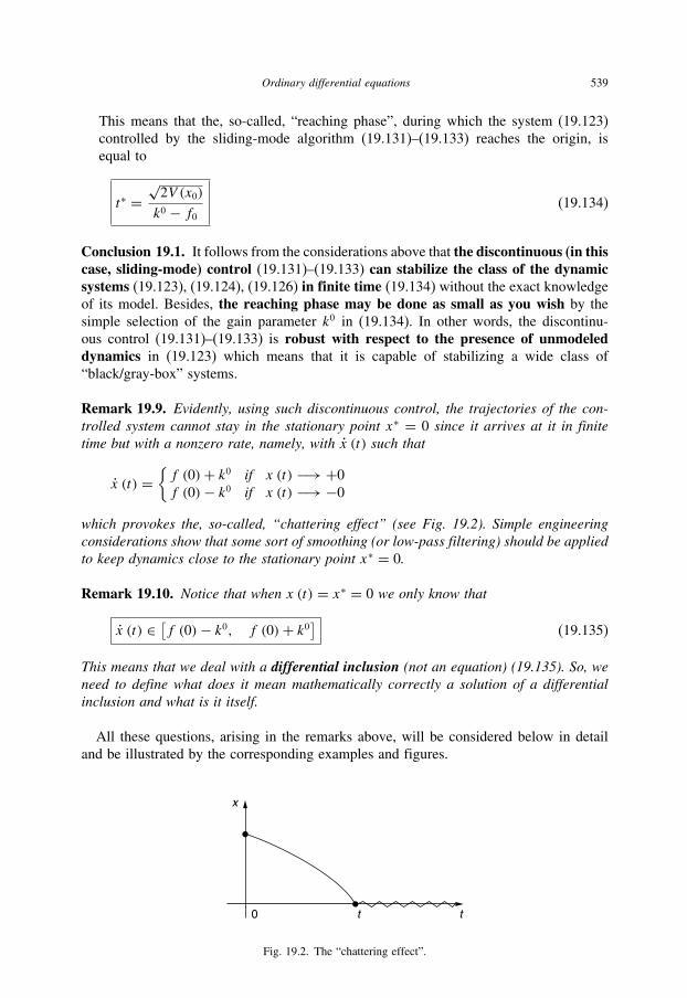
Ordinary differential equations 539
This means that the, so-called, “reaching phase”, during which the system (19.123)
controlled by the sliding-mode algorithm (19.131)–(19.133) reaches the origin, is
equal to
t∗ =√2V (x0)
k0 − f0 (19.134)
Conclusion 19.1. It follows from the considerations above that the discontinuous (in thiscase, sliding-mode) control (19.131)–(19.133) can stabilize the class of the dynamicsystems (19.123), (19.124), (19.126) in finite time (19.134) without the exact knowledgeof its model. Besides, the reaching phase may be done as small as you wish by the
simple selection of the gain parameter k0 in (19.134). In other words, the discontinu-
ous control (19.131)–(19.133) is robust with respect to the presence of unmodeleddynamics in (19.123) which means that it is capable of stabilizing a wide class of
“black/gray-box” systems.
Remark 19.9. Evidently, using such discontinuous control, the trajectories of the con-trolled system cannot stay in the stationary point x∗ = 0 since it arrives at it in finitetime but with a nonzero rate, namely, with x (t) such that
x (t) ={f (0)+ k0 if x (t) −→ +0
f (0)− k0 if x (t) −→ −0
which provokes the, so-called, “chattering effect” (see Fig. 19.2). Simple engineeringconsiderations show that some sort of smoothing (or low-pass filtering) should be appliedto keep dynamics close to the stationary point x∗ = 0.
Remark 19.10. Notice that when x (t) = x∗ = 0 we only know that
x (t) ∈ [f (0)− k0, f (0)+ k0] (19.135)
This means that we deal with a differential inclusion (not an equation) (19.135). So, weneed to define what does it mean mathematically correctly a solution of a differentialinclusion and what is it itself.
All these questions, arising in the remarks above, will be considered below in detail
and be illustrated by the corresponding examples and figures.
x
t t0
Fig. 19.2. The “chattering effect”.

540 Advanced Mathematical Tools for Automatic Control Engineers: Volume 1
19.4.2 ODE with DRHS and differential inclusions
19.4.2.1 General requirements to a solutionAs it is well known, a solution of the differential equation
x (t) = f (t, x (t)) (19.136)
with a continuous right-hand side is a function x (t) which has a derivative and satisfies
(19.136) everywhere on a given interval. This definition is not, however, valid for DE
with DRHS since in some points of discontinuity the derivative of x (t) does not exist.
That’s why the consideration of DE with DRHS requires a generalization of the concept
of a solution. Anyway, such a generalized concept should necessarily meet the following
requirements:
• For differential equations with a continuous right-hand side the definition of a solution
must be equivalent to the usual (standard) one.• For the equation x (t) = f (t) the solution should be the functions x (t)= ∫
f (t) dt + conly.
• For any initial data x (t0) = xinit within a given region the solution x (t) should exist
(at least locally) for any t > t0 and admit the possibility to be continued up to the
boundary of this region or up to infinity (when (t, x)→∞).• The limit of a uniformly convergent sequence of solutions should be a solution too.• Under the commonly used changes of variables a solution must be transformed into a
solution.
19.4.2.2 The definition of a solutionDefinition 19.9. A vector-valued function f (t, x), defined by a mapping f : R×Rn →Rp, is said to be piecewise continuous in a finite domain G ⊆ Rn+1 if G consists of afinite number of a domain Gi (i = 1, . . . , l), i.e.,
G =l⋃i=1
Gi
such that in each of them the function f (t, x) is continuous up to the boundary
Mi := Gi\Gi (i = 1, . . . , l) (19.137)
of a measure zero.
The most frequent case is the one where the set
M =l⋃i=1
Mi
of all discontinuity points consists of a finite number of hypersurfaces
0 = Sk (x) ∈ C1, k = 1, . . . , m
where Sk (x) is a smooth function.

Ordinary differential equations 541
Definition 19.10. The set M defined as
M = {x ∈ Rn | S (x) = (S1 (x) , . . . , Sm (x))ᵀ = 0} (19.138)
is called a manifold in Rn. It is referred to as a smooth manifold if Sk (x) ∈ C1,
k = 1, . . . , m.
Now we are ready to formulate the main definition of this section.
Definition 19.11. (A solution in Filippov’s sense) A solution x (t) on a time interval[t0, tf ] of ODE x (t) = f (t, x (t)) with DRHS in Filippov’s sense is called a solution ofthe differential inclusion
x (t) ∈ F (t, x (t)) (19.139)
that is, an absolutely continuous on [t0, tf ] function x (t) (which can be represented as aLebesgue integral of another function) satisfying (19.139) almost everywhere on [t0, tf ],where the set F (t, x) is the smallest convex closed set containing all limit values of thevector-function f (t, x∗) for (t, x∗) /∈ M, x∗ → x, t = const.
Remark 19.11. The set F (t, x)1. consists of one point f (t, x) at points of continuity of the function f (t, x);2. is a segment (a convex polygon, or polyhedron), which in the case when (t, x) ∈ Mi
(19.137) has the vertices
fi (t, x) := lim(t,x∗)∈Gi , x∗→x
f (t, x∗) (19.140)
All points fi (t, x) are contained in F (t, x), but it is not obligatory that all of themare vertices.
Example 19.4. For the scalar differential inclusion
x (t) ∈ −sign (x (t))
the set F (t, x) is as follows (see Fig. 19.3):
1
x
21
2sign(x)
�(t, 0) � [21, 1]
Fig. 19.3. The right-hand side of the differential inclusion xt = −sign (xt ).
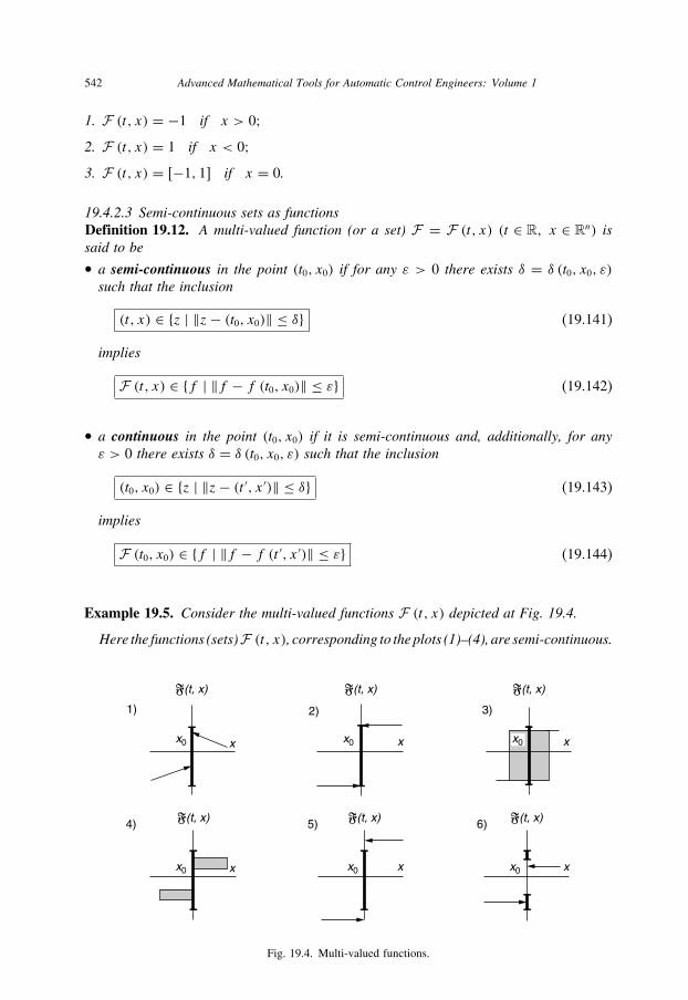
542 Advanced Mathematical Tools for Automatic Control Engineers: Volume 1
1. F (t, x) = −1 if x > 0;2. F (t, x) = 1 if x < 0;3. F (t, x) = [−1, 1] if x = 0.
19.4.2.3 Semi-continuous sets as functionsDefinition 19.12. A multi-valued function (or a set) F = F (t, x) (t ∈ R, x ∈ Rn) issaid to be
• a semi-continuous in the point (t0, x0) if for any ε > 0 there exists δ = δ (t0, x0, ε)such that the inclusion
(t, x) ∈ {z | ‖z− (t0, x0)‖ ≤ δ} (19.141)
implies
F (t, x) ∈ {f | ‖f − f (t0, x0)‖ ≤ ε} (19.142)
• a continuous in the point (t0, x0) if it is semi-continuous and, additionally, for anyε > 0 there exists δ = δ (t0, x0, ε) such that the inclusion
(t0, x0) ∈ {z | ‖z− (t ′, x ′)‖ ≤ δ} (19.143)
implies
F (t0, x0) ∈ {f | ‖f − f (t ′, x ′)‖ ≤ ε} (19.144)
Example 19.5. Consider the multi-valued functions F (t, x) depicted at Fig. 19.4.
Here the functions (sets)F (t, x), corresponding to the plots (1)–(4), are semi-continuous.
�(t, x)
x0 x
1)
�(t, x)
x0 x
2)
�(t, x)
x0 x
3)
�(t, x)
x0 x
4) �(t, x)
x0 x
5) �(t, x)
x0 x
6)
Fig. 19.4. Multi-valued functions.

Ordinary differential equations 543
19.4.2.4 Theorem on the local existence of solutionFirst, let us formulate some useful result which will be applied in the following
considerations.
Lemma 19.14. If x (t) is absolutely continuous on the interval t ∈ [α, β] and within thisinterval ‖x (t)‖ ≤ c, then
1
β − α(xβ − xα
) ⊂ Conva.a. t∈[α,β]
∪ x (t) (19.145)
where Conv is a convex closed set containing ∪ x (t) for almost all t ∈ [α, β].
Proof. By the definition of the Lebesgue integral
1
β − α(xβ − xα
) = 1
β − αβ∫
t=αx (t) dt = lim
k→∞sk
where
sk =k∑i=1
μi
|β − α| x(ti), μi ≥ 0,
k∑i=1
μi = |β − α|
are Lebesgue sums of the integral above. But sk ∈ Conva.a. t∈[α,β]
∪ x (t). Hence, the same fact
is valid for the limit vectors limk→∞sk which proves the lemma. �
Theorem 19.13. (on the local existence) Suppose that
A1. a multi-valued function (set) F (t, x) is a semi-continuous at each point
(t, x) ∈ Dγ,ρ (t0, x0) := {(t, x) | ‖x − x0‖ ≤ γ, |t − t0| ≤ ρ}
A2. the set F (t, x) is a convex compact and sup ‖y‖ = c whenever
y ∈ F (t, x) and (t, x) ∈ Dγ,ρ (t0, x0)
Then for any t such that |t − t0| ≤ τ := ρ/c there exists an absolutely continuousfunction x (t) (maybe not unique) such that
x (t) ∈ F(t, x), x (t0) = x0
that is, the ODE x (t) = f (t, x (t)) with DRHS has a local solution in Filippov’s sense(see Definition 19.11).
544 Advanced Mathematical Tools for Automatic Control Engineers: Volume 1
Proof. Divide the interval [t0 − τ, t0 + τ ] into 2m-parts t(m)i := t0 + j
τ
m(i = 0,±1, . . .±m) and construct the, so-called, partially linear Euler’s curves
xm (t) := xm(t(m)i
)+(t − t (m)i
)f(m)i (t
(m)i ), t ∈
[t(m)i , t
(m+1)i
]xm
(t(m)0
)= x0, f (m)i
(t(m)i
)∈ F
(t(m)i , xm
(t(m)i
))By the assumption (A2) it follows that xm (t) is uniformly bounded and continuous
on Dγ,ρ (t0, x0). Then, by Arzelà’s theorem 14.16 there exists a subsequence{xmk (t)
}which uniformly converges to some vector function x (t). This limit evidently has a
Lipschitz constant on Dγ,ρ (t0, x0) and satisfies the initial condition x (t0) = x0. In view
of Lemma 19.14, for any h > 0 we have
h−1 [xmk (t + h)− xmk (t)] ⊂ Conva.a.[t0−τ,t0+τ ]
mk⋃i=−mk
f(mk)i
⊂ Conva.a. λ∈
[t0− τ
mk,t0+ τ
mk+h
]mk⋃
i=−mkf(mk)i (λ) := Ak
Since F (t, x) is semi-continuous, it follows that supx∈Ak
infy∈A
‖x − y‖ → 0 whenever k→∞(here A := Conv
a.a. λ∈[t,t+h]∪mli=−ml f (λ, xλ)). The convexity of F (t, x) implies also that
supx∈A
infy∈F(t,x)
‖x − y‖ → 0 when h → 0 which, together with previous property, proves
the theorem. �
Remark 19.12. By the same reasons as for the case of regular ODE, we may concludethat the solution of the differential inclusion (if it exists) is continuously dependent on t0and x0.
19.4.3 Sliding mode control
19.4.3.1 Sliding mode surfaceConsider the special case where the function f (t, x) is discontinuous on a smooth
surface S given by the equation
s (x) = 0, s : Rn→ R, s (·) ∈ C1 (19.146)
The surface separates its neighborhood (in Rn) into domains G+ and G−. For t = const
and for the point x∗ approaching the point x ∈ S from the domains G+ and G− let us
suppose that the function f (t, x∗) has the following limits:
lim(t,x∗)∈G−, x∗→x
f (t, x∗) = f − (t, x)lim
(t,x∗)∈G+, x∗→xf (t, x∗) = f + (t, x) (19.147)
Then by Filippov’s definition, F (t, x) is a linear segment joining the endpoints of the
vectors f − (t, x) and f + (t, x). Two situations are possible.

Ordinary differential equations 545
• If for t ∈ (t1, t2) this segment lies on one side of the plane P tangent to the surface S
at the point x, the solutions for these t pass from one side of the surface S to the other
one (see Fig. 19.5 depicted at the point x = 0);• If this segment intersects the plane P , the intersection point is the endpoint of the
vector f 0 (t, x) which defines the velocity of the motion
x (t) = f 0 (t, x (t)) (19.148)
along the surface S in Rn (see Fig. 19.6 depicted at the point x = 0). Such a solution,
lying on S for all t ∈ (t1, t2), is often called a sliding motion (or mode). Defining the
projections of the vectors f − (t, x) and f + (t, x) to the surface S (∇s (x) �= 0) as
p− (t, x) :=(∇s(x), f − (t, x))
‖∇s (x)‖ , p+ (t, x) :=(∇s(x), f + (t, x))
‖∇s (x)‖one can find that when p− (t, x) < 0 and p+ (t, x) > 0
f 0 (t, x) = αf − (t, x)+ (1− α) f + (t, x)
Here α can be easily found from the equation
(∇s(x), f 0 (t, x)) = 0
G2
f1 f 2
G1
x3
x2
x1 S(x) 5 0
P
Fig. 19.5. The sliding surface and the rate vector field at the point x = 0.
f 1
f 2
G1
G2
x3
x2
f 0
x1S(x) 5 0
P
Fig. 19.6. The velocity of the motion.

546 Advanced Mathematical Tools for Automatic Control Engineers: Volume 1
or, equivalently,
0= (∇s(x), αf − (t, x)+ (1− α) f + (t, x))= αp− (t, x)+ (1− α) p+ (t, x)
which implies
α = p+ (t, x)p+ (t, x)− p− (t, x)
Finally, we obtain that
f 0 (t, x) = p+ (t, x)p+ (t, x)− p− (t, x)f
− (t, x)
+(1− p+ (t, x)
p+ (t, x)− p− (t, x))f + (t, x)
(19.149)
19.4.3.2 Sliding mode surface as a desired dynamicLet us consider in this subsection several examples demonstrating that a desired
dynamic behavior of a controlled system may be expressed not only in the traditional
manner, using some cost (or payoff ) functionals as possible performance indices, but
also representing a nominal (desired) dynamic in the form of a surface (or manifold) in
a space of coordinates.
First-order tracking system: consider a first-order system given by the following ODE:
x (t) = f (t, x (t))+ u (t) (19.150)
where u (t) is a control action and f : R×R → R is supposed to be bounded, that is,
|f (t, x (t))| ≤ f + <∞
Assume that the desired dynamics (signal), which should be tracked, is given by a smooth
function r (t) (|r (t)| ≤ ρ), such that the tracking error et is (see Fig. 19.7)
e (t) := x (t)− r (t)
Select a desired surface s as follows
s (e) = e = 0 (19.151)
which exactly corresponds to an “ideal tracking” process. Then, designing the control
u (t) as
u (t) := −k sign (e (t))

Ordinary differential equations 547
controllerr e u x
plant
Fig. 19.7. A tracking system.
0
e
tf
t
Fig. 19.8. The finite time error cancellation.
we derive that
e (t) = f (t, x (t))− r (t)− k sign (e (t))
and for V (e) = e2/2 we have
V (e (t))= e (t) e (t) = e (t) [f (t, x (t))− r (t)− k sign (e (t))]
= e (t) [f (t, x (t))− r (t)]− k |e (t)| ≤ |e (t)| [f + + ρ]− k |e (t)|
= |e (t)| [f + + ρ − k] = −√2 [k − f + − ρ]√V (e (t))and, hence,
√V (et ) ≤
√V (e0)− 1√
2
[k − f + − ρ] t
So, taking k > f + +ρ implies the finite time convergence of et (with the reaching phase
tf =√2V (e0)
k−f+−ρ ) to the surface (19.151) (see Figs. 19.8 and 19.9).
Stabilization of a second order relay system: let us consider a second order relay systemgiven by the following ODE
x (t)+ a2x (t)+ a1x (t) = u (t)+ ξ (t)u (t) = −k sign (s (t))− the relay-control
s (t) := x (t)+ cx(t), c > 0
|ξ (t)| ≤ ξ+ − a bounded unknown disturbance
(19.152)

548 Advanced Mathematical Tools for Automatic Control Engineers: Volume 1
rr, x
tft
Fig. 19.9. The finite time tracking.
x 5 x2
x�
s(x) 5 x 1 cx 5 0
x 5 x1
x�
Fig. 19.10. The sliding motion on the sliding surface s(x) = x2 + cx1.
We may rewrite the dynamic (x1 := x) as
x1 (t)= x2 (t)x2 (t)= −a1x1 (t)− a2x2 (t)+ u (t)+ ξ (t)u (t) = −ksign (x2 (t)+ cx1 (t))
(19.153)
Here the sliding surface is
s (x) = x2 + cx1
So, the sliding motion, corresponding to the dynamics s (t) := x (t)+cx (t) = 0, is given
by (see Fig. 19.10)
x (t) = x0e−ct
Let us introduce the following Lyapunov function candidate:
V (s) = s2/2

Ordinary differential equations 549
for which the following property holds:
V (s)= ss = s (x (t))[∂s (x (t))
∂x1x1 (t)+ ∂s (x (t))
∂x2x2 (t)
]= s (x (t)) [cx2 (t)− a1x1 (t)− a2x2 (t)+ u (t)+ ξ (t)]≤ |s (x (t))| [|a1| |x1 (t)| + (c + |a2|) |x2 (t)| + ξ+]− ks (x (t)) sign (s (x (t)))= − [k − |a1| |x1 (t)| − (c + |a2|) |x2 (t)| − ξ+] |s (x (t))| ≤ 0
if we take
k = |a1| |x1 (t)| + (c + |a2|) |x2 (t)| + ξ+ + ρ, ρ > 0 (19.154)
This implies V (s) ≤ −ρ√2V (s), and, hence, the reaching time tf (see Fig. 19.9) is
tf =√2V (s0)
ρ= |x0 + cx0|
ρ(19.155)
Sliding surface and a related LQ-problem: consider a linear multi-dimensional plant
given by the following ODE
x (t) = A (t) x (t)+ B (t) u (t)+ ξ (t)x0 is given, x (t) ∈ Rn, u (t) ∈ Rr
Bᵀ (t) B (t) > 0 rank [B (t)] = r for any t ∈ [ts, t1]
ξ (t) is known as external perturbation
(19.156)
A sliding mode is said to be taking place in this system (19.156) if there exists a finite
reaching time ts , such that the solution x (t) satisfies
σ (x, t) = 0 for all t ≥ ts (19.157)
where σ (x, t) : Rn×R+ → Rr is a sliding function and (21.65) defines a sliding surfacein Rn+1. For each t1 > 0 the quality of the system (19.156) motion in the sliding surface
(21.65) is characterized by the performance index (Utkin (1992))
Jts ,t1 =1
2
t1∫ts
(x(t), Qx (t)) dt, Q = Qᵀ ≥ 0 (19.158)
Below we will show that the system motion in the sliding surface (21.65) does not depend
on the control function u, that’s why (19.158) is a functional of x and σ (x, t) only. Let
us try to solve the following problem.

550 Advanced Mathematical Tools for Automatic Control Engineers: Volume 1
Problem formulation: for the given linear system (19.156) and t1 > 0 define the optimal
sliding function σ = σ (x, t) (21.65) providing the optimization in the sense of (19.158)
in the sliding mode, that is,
Jts ,t1 → infσ∈� (19.159)
where � is the set of the admissible smooth (differentiable on all arguments) sliding
functions σ = σ (x, , t). So, we wish to minimize the performance index (19.158) varying
(optimizing) the sliding surface σ ∈ �.Introduce a new state vector z defined by
z = T (t) x (19.160)
where the linear nonsingular transformations T (t) are given by
T (t) :=[I(n−r)×(n−r) −B1 (t) (B2 (t))
−1
0 (B2 (t))−1
](19.161)
Here B(n−r)×(n−r)1 (t) ∈ Rr×r and B2 (t) ∈ Rr×r represent the matrices B (t) in the form
B (t) =[B1 (t)
B2 (t)
], det [B2 (t)] �= 0 ∀ t ≥ 0 (19.162)
Applying (19.162) to the system (19.156), we obtain (below we will omit the time
dependence)
z =(z1z2
)=
(A11z1 + A12z2
A21z1 + A22z2
)+(0
u
)+(ξ1
ξ2
)(19.163)
where z1 ∈ Rn−r , z2 ∈ Rr and
A =[A11 A12
A21 A22
]= TAT −1 + T T −1,
(ξ1 (t)
ξ2 (t)
)= T ξ (t) (19.164)
Using the operator T −1, it follows x = T −1z and, hence, the performance index (19.158)
in new variables z may be rewritten as
Jts ,t1 =1
2
t1∫ts
(x,Qx) dt = 1
2
t1∫ts
(z, Qαz
)dt
= 1
2
t1∫ts
[(z1, Q
α11z1
)+ 2
(z1, Q
α12z2
)+(z2, Q
α22z2
)]dt
Q := (T −1
)ᵀQT −1 =
[Q11 Q12
Q21 Q22
](19.165)
Ordinary differential equations 551
and the sliding function σ = σ (x, t) becomes
σ = σ (T −1z, t) := σ (z, t) (19.166)
Remark 19.13. The matrices Q11, Q12, Q21 and Q22 are supposed to be symmetric.Otherwise, they can be symmetrized as follows:
Jts ,t1 =1
2
t1∫ts
[(z1, Q11z1
)+ 2(z1, Q12z2
)+ (z2, Q22z2
)]dt
Qα11 :=(Q11 + Qᵀ
11
)/2, Q22 :=
(Q22 + Qᵀ
22
)/2
Q12 =(Q12 + Qᵀ
12 + Q21 + Qᵀ21
)/2
(19.167)
Assumption (A1): we will look for the sliding function (19.166) in the form
σ (z, t) := z2 + σ0 (z1, t) (19.168)
If the sliding mode exists for the system (19.163) in the sliding surface σ (z, t) = 0 under
assumption (A1), then for all t ≥ ts the corresponding sliding mode dynamics, driven by
the unmatched disturbance ξ1 (t), are given by
z1 = A11z1 + A12z2 + ξ1z2 = −σ0 (z1, t)
(19.169)
with the initial conditions z1 (ts) = (T x (ts))1. Defining z2 as a virtual control, that is,
v := z2 = −σ0 (z1, t) (19.170)
the system (19.169) may be rewritten as
z1 = A11z1 + A12v + ξ1 (19.171)
and the performance index (19.165) becomes
Jts ,t1 =1
2
t1∫ts
[(z1, Q
α11z1
)+ 2
(z1, Q
α12v
)+(v, Qα22v
)]dt (19.172)
In view of (19.171) and (19.172), the sliding surface design problem (19.159) is reduced
to the following one:
Jts ,t1 → infv∈Rr (19.173)

552 Advanced Mathematical Tools for Automatic Control Engineers: Volume 1
But this is the standard LQ-optimal control problem. This means that the optimal control
v∗t = v∗(z1,t , t
), optimizing the cost functional (19.172), defines the optimal sliding
surface σ ∗ (x, t) (see (19.171) and (19.168)) in the following manner:
v∗(z1,t , t
)=−σ0 (z1, t)σ (z, t)= z2 − v∗
(z1,t , t
) = 0
or, equivalently,
σ ∗ (x, t) = (T x)2 − v∗ ((T x)1, t) = 0 (19.174)
19.4.3.3 Equivalent control methodEquivalent control construction: here a formal procedure will be described to obtain
sliding equations along the intersection of sets of discontinuity for a nonlinear system
given by
x (t) = f (t, x(t), u (t))x0 is given
x (t) ∈ Rn, u (t) ∈ Rr
(19.175)
and the manifold M (19.138) defined as
S (x) = (S1 (x) , . . . , Sm (x))ᵀ = 0 (19.176)
representing an intersection of m submanifolds Si (x) (i = 1, . . . , m).
Definition 19.13. Hereinafter the control u (t) will be referred to (according to V. Utkin)as the equivalent control u(eq) (t) in the system (19.175) if it satisfies the equation
S (x (t)) = G(x (t)) x (t) = G(x (t)) f (t, x(t), u (t)) = 0
G(x (t)) ∈ Rm×n, G (x (t)) = ∂
∂xS (x (t))
(19.177)
It is quite obvious that, by virtue of the condition (19.177), a motion starting at
S (x (t0)) = 0 in time t0 will proceed along the trajectories
x (t) = f (t, x(t), u(eq) (t)
)(19.178)
which lies on the manifold S (x) = 0.
Definition 19.14. The above procedure is called the equivalent control method (Utkin1992; Utkin et al. 1999) and equation (19.178), obtained as a result of applying thismethod, will be regarded as the sliding mode equation describing the motion on themanifold S (x) = 0.
Ordinary differential equations 553
From the geometric viewpoint, the equivalent control method implies a replacement
of the undefined discontinued control on the discontinuity boundary with a continuous
control which directs the velocity vector in the system state space along the discontinuity
surface intersection. In other words, it realizes the velocity f 0(t, x(t), u(eq) (t)
)(19.149)
exactly corresponding to Filippov’s definition of the differential inclusion in the point
x = x (t).Consider now the equivalent control procedure for an important particular case of a
nonlinear system which is affine on u, the right-hand side of whose differential equation
is a linear function of the control, that is,
x (t) = f (t, x (t))+ B (t, x (t)) u (t) (19.179)
where f : R × Rn → Rn and B : R × Rn → Rn×r are all argument continuous vector
and matrix, respectively, and u (t) ∈ Rr is a control action. The corresponding equivalent
control should satisfy (19.177), namely,
S (x (t))= G(x (t)) x (t) = G(x (t)) f (t, x(t), u (t))
= G(x (t)) f (t, x (t))+G(x (t)) B (t, x (t)) u (t) = 0
(19.180)
Assuming that the matrix G(x (t)) B (t, x (t)) is nonsingular for all x (t) and t , one can
find the equivalent control from (19.180) as
u(eq) (t) = − [G(x (t)) B (t, x (t))]−1G(x (t)) f (t, x (t)) (19.181)
Substitution of this control into (19.179) yields the following ODE:
x (t) = f (t, x (t))−B (t, x (t)) [G(x (t)) B (t, x (t))]−1
G(x (t)) f (t, x (t))(19.182)
which describes the sliding mode motion on the manifold S (x) = 0. Below the corre-
sponding trajectories in (19.182) will be referred to as x (t) = x(sl) (t).
Remark 19.14. If we deal with an uncertain dynamic model (19.175) or, particularly,with (19.179), then the equivalent control u(eq) (t) is not physically realizable.
Below we will show that u(eq) (t) may be successfully approximated (in some sense)
by the output of the first-order low-pass filter with the input equal to the corresponding
sliding mode control.

554 Advanced Mathematical Tools for Automatic Control Engineers: Volume 1
Sliding mode control design: let us try to stabilize the system (19.179) by applying the
sliding mode approach. For the Lyapunov function V (x) := ‖S (x)‖2/2, considered on
the trajectories of the controlled system (19.179), we have
V (x (t))= (S(x (t)), S (x (t))
)= (S(x (t)),G (x (t)) f (t, x (t))+G(x (t)) B (t, x (t)) u (t))
= (S(x (t)),G (x (t)) f (t, x (t)))+ (S(x (t)),G (x (t)) B (t, x (t)) u (t))
≤ ‖S (x (t))‖ ‖G(x (t)) f (t, x (t))‖ + (S(x (t)),G (x (t)) B (t, x (t)) u (t))
Taking u (t) as a sliding mode control, i.e.,
u (t)= u(sl) (t)
u(sl) (t) := −kt [G(x (t)) B (t, x (t))]−1sign (S (x (t)))
kt > 0, sign (S (x)) := (sign (S1 (x)) , . . . , sign (Sm (x)))ᵀ(19.183)
we obtain
V (x (t)) ≤ ‖S (x)‖ ‖G(x (t)) f (t, x (t))‖ − ktm∑i=1
|Si (x (t))|
which, in view of the inequality, ‖S‖ ≥m∑i=1
|Si |, implies
V (x (t)) ≤ −‖S (x)‖ (kt − ‖G(x (t)) f (t, x (t))‖)
Selecting
kt = ‖G(x (t)) f (t, x (t))‖ + ρ, ρ > 0 (19.184)
gives V (x (t)) ≤ −ρ ‖S (x)‖ = −ρ√2V (x (t)) which provides the reaching phase in
time
tf =√2V (x0)
ρ= ‖S (x0)‖
ρ(19.185)
Remark 19.15. If the sliding motion on the manifold S(x) = 0 is stable then there existsa constant k0 ∈ (0,∞) such that
‖G(x (t)) f (t, x (t))‖ ≤ k0

Ordinary differential equations 555
and, hence, kt (19.184) may be selected as a constant
kt := k = k0 + ρ (19.186)
Low-pass filtering: to minimize the influence of the chattering effect arising after the
reaching phase let us consider the property of the signal obtained as an output of a
low-pass filter with the input equal to the sliding mode control, that is,
μu(av) (t)+ u(av) (t) = u(sl)(t), u(av)0 = 0, μ > 0 (19.187)
where u(sl) (t) is given by (19.183). The next simple lemma states the relation between
the, so-called, averaged control u(av) (t), which is the filtered output, and the input signal
u(sl) (t).
Lemma 19.15. If
g+ ≥ ‖GB (t, x (t))‖ := λ1/2max
([Bᵀ (t, x (t))Gᵀ] [GB (t, x (t))]
)≥ λ1/2min
([Bᵀ (t, x (t))Gᵀ] [GB (t, x (t))]
) ≥ κIr×r , κ > 0
(19.188)
then for the low-pass filter (19.187) the following properties hold:1. The difference between the input and output signals are bounded, i.e.,
u(av) (t) = u(sl) (t)+ ζ (t)
‖ζ (t)‖ ≤ 2c, c := (g+ + ρ)m/κ∥∥u(av) (t)∥∥ ≤ 2c/μ
(19.189)
2. The amplitude-frequency characteristic A (ω) of the filter is
A (ω) = 1√1+ (μω)2 , ω ∈ [0,∞) (19.190)
whose plot is depicted at Fig. 19.11 for μ = 0.01, where y = A (ω) and x = ω.Proof.
1. The solution of the ODE (19.183) and its derivative are as follows:∥∥∥kt [GB (t, xt )]−1∥∥∥ ≤ (‖Gf (t, xt )‖ + ρ)∥∥∥[GB (t, xt )]−1
∥∥∥= (‖Gf (t, xt )‖ + ρ)λ1/2
min
([Bᵀ (t, xt )Gᵀ] [GB (t, xt )]
) ≤ κ−1(g+ + ρ)
∥∥u(sl)t ∥∥ ≤ κ−1(g+ + ρ)m := c

556 Advanced Mathematical Tools for Automatic Control Engineers: Volume 1
107.552.50
1
0.9988
0.9975
0.9963
x
y
Fig. 19.11. The amplitude-phase characteristic of the low-pass filter.
and by (19.187)
u(av)t = 1
μ
t∫s=0
e−(t−s)/μu(sl)s ds
u(av)t = 1
μ
⎡⎣u(sl)t − 1
μ
t∫s=0
e−(t−s)/μu(sl)s ds
⎤⎦
(19.191)
which implies
μ
∥∥∥u(av)t
∥∥∥ ≤ ∥∥∥u(sl)t ∥∥∥+ 1
μ
t∫s=0
e−(t−s)/μ∥∥u(sl)s ∥∥ ds ≤ c + c
μ
t∫s=0
e−(t−s)/μds
= c + ct∫
s=0
e−(t−s)/μd (s/μ)
= c + ct/μ∫s=0
e−(t/μ−s)ds = c + c (1− e−t/μ) ≤ 2c
Hence, (19.189) holds.
2. Applying the Fourier transformation to (19.187) leads to the following identity:
μjωU(av) (jω)+ U(av) (jω) = U(sl) (jω)
or, equivalently,
U(av) (jω) = 1
1+ μjωU(sl) (jω) = 1− μjω
1+ (μω)2U(sl) (jω)

Ordinary differential equations 557
So, the amplitude-frequency characteristic
A (ω) :=√[ReU(av) (jω)]
2 + [ImU(av) (jω)]2
of the filter (19.187) is as in (19.190). Lemma is proven. �
19.4.3.4 The realizable approximation of the equivalent controlBy (19.191) u
(av)t may be represented as u
(av)t = ∫ t
s=0u(sl)s d
(e−(t−s)/μ
). Consider
the dynamics x(av)t of the system (19.175) controlled by u
(av)t (19.191) at two time intervals:
during the reaching phase and during the sliding mode regime.
1. Reaching phase (t ∈ [0, tf ]). Here the integration by part implies
u(av)t =t∫
s=0
u(sl)s d(e−(t−s)/μ
) = u(sl)t − u(sl)0 e−t/μ −
t∫s=0
u(sl)s e−(t−s)/μ ds
Supposing that u(sl)t (19.183) is bounded almost everywhere, i.e.,
∥∥∥u(sl)t ∥∥∥ ≤ d . Theabove identity leads to the following estimation:
∥∥∥u(av)t − u(sl)t∥∥∥ ≤ ∥∥∥u(sl)0
∥∥∥ e−t/μ + d t∫s=0
e−(t−s)/μ ds
=∥∥∥u(sl)0
∥∥∥ e−t/μ + μd t∫s=0
e−(t−s)/μd (s/μ)
=∥∥∥u(sl)0
∥∥∥ e−t/μ + μdt/μ∫s=0
e−(t/μ−s)ds
=∥∥∥u(sl)0
∥∥∥ e−t/μ + μd (1− e−t/μ) = μd +O (e−t/μ
)So, u
(av)t may be represented as
u(av)t = u(sl)t + ξt (19.192)
where ξt may be done as small as you wish taking μ tending to zero, since
‖ξt‖ ≤ μd +O(e−t/μ
)As a result, the trajectories x
(sl)t and x
(av)t will differ slightly. Indeed,
x(sl)t = f
(t, x
(sl)t
)− B
(t, x
(sl)t
)u(sl)t
x(av)t = f
(t, x
(av)t
)− B
(t, x
(av)t
)u(av)t
558 Advanced Mathematical Tools for Automatic Control Engineers: Volume 1
Defining
B = B(t, x(av)t ), G = G(x(av)t ), f = f (t, x(av)t
)and omitting the arguments for simplicity, the last equation may be represented as
x(sl)t = f − Bu(sl)t , x(av)t = f − Bu(av)t
Hence by (19.192), the difference �t := x(sl)t − x(av)t satisfies
�t = �0 −t∫
s=0
[(f − f
)− Bu(sl)s + Bu(av)s
]ds
= �0 −t∫
s=0
[(f − f
)− Bu(sl)s + B (
u(sl)s + ξs)]ds
Taking into account that �0 = 0 (the system starts with the same initial conditions
independently on an applied control) and that f (t, x) and B (x) are Lipschitz (with
the constant Lf and LB) on x it follows that
‖�t‖ ≤t∫
s=0
[∥∥∥f − f ∥∥∥+ ∥∥∥(B − B) u(sl)s + Bξs∥∥∥] ds
≤t∫
s=0
[Lf ‖�s‖ + LB ‖�s‖
∥∥u(sl)s ∥∥+ ∥∥B∥∥ ‖ξs‖] ds
≤t∫
s=0
[(Lf + LB
∥∥u(sl)s ∥∥) ‖�s‖ + ∥∥B∥∥ (μd +O (e−s/μ
))]ds
Since O(e−t/μ
) = μO (1
μe−t/μ
)= μo (1) ≤ με and
∥∥u(sl)s ∥∥ ≤ u(sl)+ <∞, ∥∥B∥∥ ≤ B+ <∞
we finally have
‖�t‖ ≤t∫
s=0
[(Lf + LBu(sl)+
) ‖�s‖ + B+μ (d + ε)] ds≤ B+μ (d + ε) tf +
t∫s=0
(Lf + LBu(sl)+
) ‖�s‖ ds
Ordinary differential equations 559
Now let us apply the Gronwall lemma which says that if v (t) and ξ (t) are nonnegative
continuous functions on [t0,∞) verifying
v (t) ≤ c +t∫
s=t0
ξ (s) v (s) ds (19.193)
then for any t ∈ [t0,∞) the following inequality holds:
v (t) ≤ c exp⎛⎝ t∫s=t0
ξ (s) ds
⎞⎠ (19.194)
This result remains true if c = 0. In our case
v (t) = ‖�t‖ , c = B+μ (d + ε) tf , ξ (s) = Lf + LBu(sl)+
for any s ∈ [0, tf). So,
‖�t‖ ≤ δ := B+μ (d + ε) tf exp((Lf + LBu(sl)+
)tf
)(19.195)
Claim 19.2. For any finite reaching time tf and any small value δ > 0 there exists asmall enough μ such that ‖�t‖ is less than δ.
2. Sliding mode phase (t > tf ). During the sliding mode phase we have
S(x(sl)t
) = S (x(sl)t ) = G (f − Bu(eq)t
) = 0 (19.196)
if ut = u(eq)t for all t > tf . Applying ut = u(av)t we cannot guarantee (19.196) already.
Indeed,
S(x(av)t
) = S (x(av)tf
)+
t∫s=tf
S(x(av)s
)ds
and, by (19.195),∥∥∥S (x(av)tf
)∥∥∥ = ∥∥∥S (x(av)tf
)-S
(x(sl)tf
)∥∥∥≤∥∥∥G((sl)tf
)�tf
∥∥∥≤O(μ)Hence, in view of (19.196),
∥∥∥S (x(av)t
)∥∥∥ = O(μ).Claim 19.3. During the sliding-mode phase∥∥∥S (x(av)t
)∥∥∥ = O(μ) (19.197)

This page intentionally left blank

20 Elements of StabilityTheory
Contents
20.1 Basic definitions . . . . . . . . . . . . . . . . . . . . . . . . . . . . . . . 561
20.2 Lyapunov stability . . . . . . . . . . . . . . . . . . . . . . . . . . . . . . 563
20.3 Asymptotic global stability . . . . . . . . . . . . . . . . . . . . . . . . . . 576
20.4 Stability of linear systems . . . . . . . . . . . . . . . . . . . . . . . . . . 581
20.5 Absolute stability . . . . . . . . . . . . . . . . . . . . . . . . . . . . . . . 587
This chapter deals with the basic notions concerning the stability property of
certain solutions or sets of solutions of the different classes of ordinary differential
equations (ODE).
In the famous work of A.M. Lyapunov (Lyapunov 1892) there is given some very
simple (but philosophically very profound) theorems (hereafter referred to as the directLyapunov’s method) for deciding the stability or instability of an equilibrium point of an
ODE. The idea of this approach consists of the generalization of the concept of “energy”
and its “power” the usefulness of which lies in the fact that the decision on stability can
be made by investigating the differential equation itself (in fact, its right-hand side only)
but not by finding its exact solution.
The purpose of this chapter is to give an introduction to some of the fundamental ideas
and problems in the field which can be successfully applied to some problems arising in
automatic control theory.
20.1 Basic definitions
20.1.1 Origin as an equilibrium
Definition 20.1. The vector-valued function y (t, y0, t0) ∈ Rn is said to be the dynamicmotion satisfying
y (t) = g (t, y (t)), y (t0) = y0
if
• there exists no other function satisfying this ODE with the same initial conditions;• it is differentiable in t for all t ≥ t0.
561

562 Advanced Mathematical Tools for Automatic Control Engineers: Volume 1
Remark 20.1. Evidently, by this definition, y (t0, y0, t0) = y0.
Consider the, so-called, nominal dynamic motion y∗ (t, y0, t0) satisfying
y∗ (t) = g∗ (t, y∗ (t)), y∗ (t0) = y∗0 ∈ Rn
and the dynamic motion in deviations x (t, x0, t0) ∈ Rn, defined by
x (t, x0, t0) := y (t, y0, t0)− y∗ (t, y0, t0)x (t)= f (t, x (t))x (t0)= x0 := y0 − y∗0
f (t, x) := g (t, x − y∗)− g∗ (t, y∗)(20.1)
Definition 20.2. Supposing that equation (20.1)admits thedynamicmotionx (t, 0, t0) ≡ 0.We will also call it the trivial solution or the equilibriumwhich can be expressed by
f (t, 0) = 0, t ≥ t0 (20.2)
Further we will assume that the solution, belonging to the initial point x0 in a certainneighborhood ‖x0‖ < δ of the origin, exists for all t ≥ t0 and is uniquely determined bythe initial values x0, t0.1
In this chapter we will study different aspects of stability of the equilibrium point
x = 0.
20.1.2 Positive definite functions
First, let us introduce the following definitions which will be intensively used hereafter.
Definition 20.3. A real function V = V (t, x), specified in the domain ‖x‖ ≤ h
(x ∈ Rn, h > 0) for all t ≥ t0, is called positive-definite if there exists a real continuousfunction W (x) defined for ‖x‖ ≤ h such that
1.
W (0) = 0 (20.3)
2. for ‖x‖ > 0
W (x) > 0 (20.4)
3. for all t ≥ t0V (t, x) ≥ W (x) (20.5)
1 We may assume that f (t, x) is an n-dimensional vector function which is locally (uniformly on t) Lipschitz
on x in a neighborhood of the point x = 0.

Elements of stability theory 563
If the properties (2)–(3) are replaced by W (x) < 0 and V (t, x) ≤ W (x), then thefunction V (t, x) will be negative-definite.
Example 20.1.
V (t, x) = x21 + x22 + x1x2 sin t
is precisely such a function. Indeed,
V (t, x)= x21 + x22 + x1x2 sin t ≥ x21 + x22 − |x1| |x2|= (|x1| − |x2|)2 + |x1| |x2| ≥ |x1| |x2| := W (x)
So, all conditions of Definition 20.3 are fulfilled for the function W (x).
Definition 20.4. Denote by x (t, x0, t0) the dynamic motion (trajectory) which satisfies(20.1) when x (t0) = x0. Then, if there exists the time derivative of the function V (t) :=V (t, x (t, x0, t0)), then the function V (t, x) is said to be differentiable along the integralcurves (or the path) x (t, x0, t0) of the system (20.1).
Claim 20.1. The full time derivative of the differentiable function V (t) is calculated asfollows
d
dtV (t) = d
dtV (t, x (t, x0, t0)) = ∂
∂tV (t, x (t, x0, t0))
+n∑i=1
∂V
∂xi(t, x (t, x0, t0)) fi (t, x (t, x0, t0))
(20.6)
In short (20.6) is written as
d
dtV (t, x) = ∂
∂tV (t, x)+
n∑i=1
∂V
∂xi(t, x) fi (t, x) (20.7)
20.2 Lyapunov stability
20.2.1 Main definitions and examples
Definition 20.5. The equilibrium zero-point (or zero-state) x = 0 of the system given byODE (20.1) is said to be1. Lyapunov stable, or locally stable, if for any ε > 0 there exist t ′0 ≥ t0 ≥ 0 and δ =δ(t ′0, ε
)> 0 such that for all t ≥ t0 we have
∥∥x (t, x0, t ′0)∥∥ < ε whenever x (t ′0) = x0and ‖x0‖ < δ;
2. uniformly Lyapunov stable, or uniformly locally stable, if it is Lyapunov stable forany t ′0 ≥ t0, that is, δ is independent on t ′0;
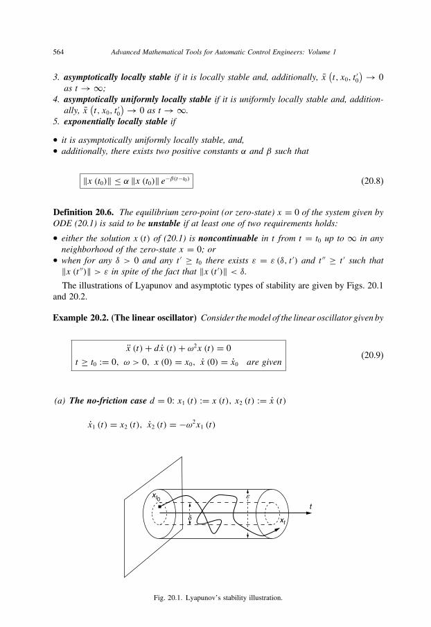
564 Advanced Mathematical Tools for Automatic Control Engineers: Volume 1
3. asymptotically locally stable if it is locally stable and, additionally, x(t, x0, t
′0
) → 0
as t →∞;4. asymptotically uniformly locally stable if it is uniformly locally stable and, addition-
ally, x(t, x0, t
′0
)→ 0 as t →∞.5. exponentially locally stable if
• it is asymptotically uniformly locally stable, and,• additionally, there exists two positive constants α and β such that
‖x (t0)‖ ≤ α ‖x (t0)‖ e−β(t−t0) (20.8)
Definition 20.6. The equilibrium zero-point (or zero-state) x = 0 of the system given byODE (20.1) is said to be unstable if at least one of two requirements holds:
• either the solution x (t) of (20.1) is noncontinuable in t from t = t0 up to ∞ in anyneighborhood of the zero-state x = 0; or
• when for any δ > 0 and any t ′ ≥ t0 there exists ε = ε (δ, t ′) and t ′′ ≥ t ′ such that‖x (t ′′)‖ > ε in spite of the fact that ‖x (t ′)‖ < δ.The illustrations of Lyapunov and asymptotic types of stability are given by Figs. 20.1
and 20.2.
Example 20.2. (The linear oscillator) Consider themodel of the linear oscillator given by
x (t)+ dx (t)+ ω2x (t) = 0
t ≥ t0 := 0, ω > 0, x (0) = x0, x (0) = x0 are given(20.9)
(a) The no-friction case d = 0: x1 (t) := x (t), x2 (t) := x (t)
x1 (t) = x2 (t), x2 (t) = −ω2x1 (t)
t
xt
xt0 �
Fig. 20.1. Lyapunov’s stability illustration.

Elements of stability theory 565
xt t
xt0
Fig. 20.2. Asymptotic local stability illustration.
and
x1 (t) = x (t) = x0 cosωt + x0ω
sinωt
x2 (t) = x (t) = −x0ω sinωt + x0ω
cosωt
So, for |x0| ≤ δ and |x0| ≤ δ we have
|x (t)| ≤ |x0| +∣∣∣∣ x0ω
∣∣∣∣ ≤ δ (1+ ω−1) ≤ ε
|x (t)| = |x0ω| + |x0| ≤ δ (ω + 1) ≤ ε
if δ := ε/max{1+ ω−1; 1+ ω}
This means that the state
(0
0
)is uniformly locally stable.
(b) The friction case d > 0: x1 (t) := x (t), x2 (t) := x (t)
x1 (t) = x2 (t), x2 (t) = −ω2x1 (t)− dx2 (t)
and
x1 (t) = x (t) = c1eλ1t + c2eλ2tx2 (t) = x (t) = c1λ1eλ1t + c2λ2eλ2t
λ1,2 = −d2±√(
d
2
)2
− ω2

566 Advanced Mathematical Tools for Automatic Control Engineers: Volume 1
In any case, Re λi < 0 (i = 1, 2) which implies
|x1 (t)| = |x (t)| ≤ |c1| eRe λ1t + |c2| eRe λ2t → 0 as t →∞|x2 (t)| = |x (t)| ≤ |λ1| |c1| eRe λ1t + |λ2| |c2| eRe λ2t
≤ maxi=1,2
(|λi | |ci |) emaxi=1,2
(Re λi )t → 0 as t →∞
Therefore the stationary state
(0
0
)is exponentially locally stable with α =max
i=1,2(|λi | |ci |)
and β = −maxi=1,2
(Re λi).2
20.2.2 Criteria of stability: nonconstructive theory
The theory, designed by A.M. Lyapunov (Doctor thesis 1892, the first translations from
Russian are in Lyapunov 1907), says that if for a system (20.1) there exists a Lyapunov(positive-definite “energetic”) function, then the zero-state is Lyapunov stable. So,this theory deals with the, so-called, sufficient conditions of stability. But there exists
another concept (see Zubov 1962, 1964) which states that if the zero-state of (20.1) islocally stable, then obligatory there exists a corresponding Lyapunov function. Thismeans exactly that the existence of a Laypunov function is also a necessary condition of
stability.
In this subsection we will present the “joint result” (due to Zubov (1962)) on the
necessary and sufficient conditions of local stability or, in other words, the criterion oflocal, asymptotic and exponential stability for nonlinear systems governed by (20.1).
20.2.2.1 Criterion of Lyapunov (local) stabilityTheorem 20.1. (The criterion of stability (Zubov 1964)) The zero-state of the system(20.1) is Lyapunov (or, locally) stable if and only if there exists a function V (t, x), calledthe Lyapunov function, satisfying the following conditions:
1. V (t, x) is defined for ‖x‖ ≤ h and t ≥ t0;2. V (t, 0) = 0 for all t ≥ t0 and is continuous in x for all t ≥ t0 in the point x = 0;3. V (t, x) is positive-definite, that is, there exists a function W (x) such that
V (t, x) ≥ W (x) for all t ≥ t0W (0) = 0, W (x) > 0 for ‖x‖ > 0
4. the function V (t) := V (t, x (t, x0, t0)) does not increase3 in t ≥ t0 for all x0 satisfying‖x0‖ ≤ h.
2 In fact, here it is proven more accurately: this state is globally exponentially stable (the exact definition in
subsection 20.2.3), since the property∥∥x (t, x0, t ′0)∥∥ ≤ α exp (−βt) →
t→∞ 0 is true for any x0 and any t ′0 ≥ 0.
3 Notice that here it is not required for Vt to be t-differentiable.

Elements of stability theory 567
Proof.
(a) Sufficiency. Suppose that there exists a function V (t, x) satisfying all conditions (1)–
(4) of Theorem 20.1. Take ε < h and consider the sphere ‖x‖ = ε. By condition (3)
infx:‖x‖=ε
W (x) := λ > 0
By the continuity of V (t, x) (the properties (1)–(2)) it follows that there is a number
δ = δ (t0, ε) > 0 such that V (t0, x) < λ as ‖x‖ < δ. Take any point x0 satisfying
‖x0‖ < δ. Then V (t0, x0) < λ and by property (4) the function V (t, x (t, x0, t0)) is
not increasing for t ≥ t0 which implies
V (t, x (t, x0, t0)) ≤ V (t0, x0) < λ (20.10)
Hence, ‖x (t, x0, t0)‖ < ε for all t ≥ t0, otherwise there exists an instant time t > t0such that
∥∥x (t , x0, t0)∥∥ = ε and, therefore,V(t , x
(t , x0, t0
)) ≥ W (x(t , x0, t0
)) ≥ λwhich contradicts (20.10). The sufficiency is proven.
(b) Necessity. Let the stationary zero-point be Lyapunov stable. Consider the solution
x (t, x0, t0) of (20.1) for ‖x0‖ ≤ h. Define the function V (t, x) as follows
V (t, x) := sups≥t
‖x (s, x, t)‖ (20.11)
where x (s, x, t) is the solution (20.1) started at the point x at time t . So, the condition
(1) of Theorem 20.1 holds. Since x = 0 is a stationary point (an equilibrium), then
V (t, 0) = 0 which follows from (20.11). Additionally, this function is continuous at
the point x = 0 for any t ≥ t0. Indeed, for ε > 0, by the stability property, there
exists δ = δ (t0, ε) such that ‖x (t, x0, t0)‖ < ε whenever ‖x0‖ < δ. By (20.11),
V (t0, x0) < ε which proves the fulfillment of condition (2) of Theorem 20.1. One
can see also that when ‖x0‖ > 0
V (t0, x0) ≥ ‖x (t0, x0, t0)‖ = ‖x0‖ := W (x0) > 0
So, V (t, x) is positive-definite and condition (3) is also fulfilled. To demonstrate the
validity of condition (4) it is sufficient to establish that
V(t ′, x
(t ′, x0, t0
)) ≤ V (t ′′, x
(t ′′, x0, t0
))if t ′′ ≥ t ′ ≥ t0
To do this, it is sufficient to notice that by formula (20.11)
V (t ′, x (t ′, x0, t0)) = sups≥t ′
‖x (s, x (t ′, x0, t0), t ′)‖≥ sups≥t ′′
‖x (s, x (t ′, x0, t0), t ′)‖ = sups≥t ′′
‖x (s, x (t ′′, x0, t0), t ′′)‖= V (t ′′, x (t ′′, x0, t0))
which means that the function does not increase along the solutions x (t, x0, t0). This
completes the proof of the necessity of the conditions of Theorem 20.1. �

568 Advanced Mathematical Tools for Automatic Control Engineers: Volume 1
Remark 20.2. Condition (4) of Theorem 20.1 seems to be restrictive since the integralcurves x (t, x0, t0) are not given analytically and, therefore, are unknown if we do notknow the exact analytical solution of (20.1). However, this problem can be slightlysimplified if we remember the following fact:
“By one of the Lebesgue theorems (see Corollary 15.5), the derivative of a monotonefunction exists almost everywhere.”
Therefore, by the condition (4) the function V (t) := V (t, x (t, x0, t0)) is monotone onany integral curve x (t, x0, t0) and, hence, there exists the derivative
d
dtV (t). Admitting
also the existence of the partial derivatives∂V (t, x)
∂tand
∂V (t, x)
∂xifor all t ≥ t0 and
all x in a neighborhood of the origin, condition (4) can be verified by checking theinequality
d
dtV (t) = ∂V (t, x)
∂t+
n∑i=1
∂V (t, x)
∂xifi (t, x) ≤ 0 (20.12)
Sure, the derivatives∂V (t, x)
∂tand
∂V (t, x)
∂xiof the function V (t, x), as it is defined
in (20.11), cannot be calculated analytically. So, this means that Theorem 20.1 makesonly a “philosophical sense”, but not a practical one: it says that any system with thestable zero-state has a Lyapunov function.
Corollary 20.1. (Lyapunov 1892)4 If the function V (t, x) is positive-definite and con-tinuous in x at x = 0 uniformly in t for all t ≥ t0 and
d
dtV (t, x (t, x0, t0)) ≤ 0 (20.13)
then the stationary point x = 0 of the system (20.1) is uniformly local stable.
Proof. In the proof of Theorem 20.1 a number δ = δ (t0, ε) is selected from the condition
(20.10) such that V (t0, x0) < λ for ‖x0‖ < δ. Since V (t, x) is continuous in x at the
point x = 0 uniformly in t for all t ≥ t0, then there exists a number δ = δ (ε) such that
V (t0, x0) < λ for all ‖x0‖ < δ (ε) at all t0 which proves the corollary. �
20.2.2.2 Criterion of asymptotic stabilityTheorem 20.2. (The criterion of AS (Zubov 1964)) The state x = 0 of the system(20.1) is asymptotically stable if and only if all assumptions of Theorem 20.1 hold andin the condition (4) the function V (t) := V (t, x (t, x0, t0)) decreases monotonically upto zero, that is,
V (t) := V (t, x (t, x0, t0)) ↓ 0 as t →∞ (20.14)
4 This result is referred to as the second Lyapunov’s theorem (method).

Elements of stability theory 569
Proof.
(a) Necessity. If x = 0 is asymptotically stable, then ‖x (s, x, t)‖ → 0 as t → ∞, and,
therefore, by the construction (20.11), it follows that
V (t) := V (t, x (t, x0, t0)) = sups≥t
‖x (s, x, t)‖ →t→∞ 0
Monotonicity results from the inequality
V (t) := V (t, x (t, x0, t0)) = sups≥t
‖x (s, x, t)‖≥ sups≥t ′>t
‖x (s, x, t)‖ = V (t ′, x (t ′, x0, t0)) = V (t ′)
(b) Sufficiency. If sups≥t
‖x (s, x, t)‖ →t→∞ 0, then it follows that
x (t, x0, t0) →t→∞ 0
Theorem is proven. �
20.2.2.3 Criterion of exponential stabilityTheorem 20.3. (on exponential stability) For any solution x (t, x0, t0) of (20.1) to beexponentially stable (see Definition 20.5) it is necessary and sufficient that there existtwo positive-definite functions V (t, x) and W (t, x) such that
1. for any x and any t ≥ t0 there exists β > 0 for which
W (t, x) ≥ βV (t, x) (20.15)
2. the functions V (t, x) and W (t, x) are related by
d
dtV (t, x (t, x0, t0)) = −W (t, x (t, x0, t0)) (20.16)
Proof.
(a) Necessity. Let the solution x (t, x0, t0) of (20.1) be exponentially stable with some
α > 0 and β > 0. Define W (t, x) and V (t0, x0)
W (t, x) := ‖x‖2, V (t, x) :=∞∫
s=tW (s, x (s, x, t)) ds (20.17)
The relation (20.16) is evident. Show that V (t, x), as it is defined above, satisfies the
condition (20.15). By (20.8) we have
V (t, x) =∞∫
s=t‖x (s, x, t)‖2 ds
≤∞∫
s=tα2 ‖x‖2 exp (−2β (s − t)) ds ≤ α2
2β‖x‖2 = α2
2βW (t, x)
This means that V (t, x) satisfies (20.15) with β := 2β
α2.

570 Advanced Mathematical Tools for Automatic Control Engineers: Volume 1
(b) Sufficiency. Show that (20.16) and (20.15) imply (20.8). Considering
V (t, x (t, x0, t0)) �= 0 (if not, we already have the stability since x (s, x0, t0) = 0 for
all s ≥ t) and integrating (20.16) lead to
t∫s=t0
dV
V= −
t∫s=t0
W (s, x (s, x0, t0))
V (s, x (s, x0, t0))ds
and, hence, by (20.15)
V (t, x (t, x0, t0)) = V (t0, x0) exp⎛⎝− t∫
s=t0
W (s, x (s, x0, t0))
V (s, x (s, x0, t0))ds
⎞⎠
V (t0, x0) exp
⎛⎝− t∫
s=t0
β ds
⎞⎠ = V (t0, x0) exp
(−β [t − t0])(20.18)
which corresponds to the exponential stability (20.8) with α = V (t0, x0) and β = β.Theorem is proven. �
20.2.2.4 Criterion of instabilityTheorem 20.4. (Criterion of instability (Zubov 1964)) For the state x = 0 of the sys-tem (20.1) to be unstable, it is necessary and sufficient that there exist two scalar con-tinuous functions V (t, x) and W (t, x) ≥ 0, defined in (t, x)-domain � (which includesthe point x = 0), such that
1. V (t, x) is bounded in �;2. for any t ≥ t0 and δ > 0 there exists x (t ′) : ‖x (t ′)‖ < δ, t ′ ≥ t such that in this point
the inequality V (t ′, x (t ′)) > 0 holds;3. there exists the time derivative
d
dtV (t, x (t, x0, t0))
= λV (t, x (t, x0, t0))+W (t, x (t, x0, t0)) , λ > 0
(20.19)
Proof.
(a) Necessity. Suppose there is instability. This means exactly that there exists ε > 0
such that for any t ≥ t0 and any δ > 0 it is possible to find x (t ′) : ‖x (t ′)‖ < δ suchthat the inequality
∥∥x (t , x (t ′), t ′)∥∥ < ε fails to hold for all t ≥ t ′ ≥ t . Take any
point (x (t ′), t ′) satisfying the inequalities ‖x (t ′)‖ < δ, t ′ ≥ t0 and 0 < δ < ε. Then
two cases may occur: either (1)∥∥x (t , x (t ′), t ′)∥∥ ≤ ε for all t ≥ t ′, or (2) there exists
an instant t = t (x (t ′), t ′) when ∥∥x (t, x (t ′), t ′)∥∥ = ε and∥∥x (t , x (t ′), t ′)∥∥ < ε for
all t ′ ≤ t < t . Let V (t , x (t ′)
) = 0 in the first case and V(t , x (t ′)
) = e−(t−t) = et−tin the second one. Thus the function V (t, x) is defined at any point of the set
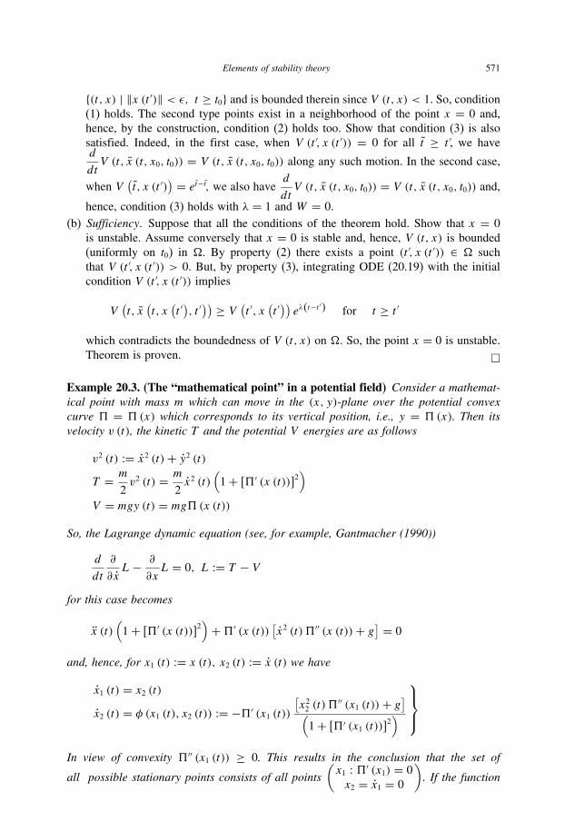
Elements of stability theory 571
{(t, x) | ‖x (t ′)‖ < ε, t ≥ t0} and is bounded therein since V (t, x) < 1. So, condition
(1) holds. The second type points exist in a neighborhood of the point x = 0 and,
hence, by the construction, condition (2) holds too. Show that condition (3) is also
satisfied. Indeed, in the first case, when V (t ′, x (t ′)) = 0 for all t ≥ t ′, we haved
dtV (t, x (t, x0, t0)) = V (t, x (t, x0, t0)) along any such motion. In the second case,
when V(t , x (t ′)
) = et−t, we also haved
dtV (t, x (t, x0, t0)) = V (t, x (t, x0, t0)) and,
hence, condition (3) holds with λ = 1 and W = 0.
(b) Sufficiency. Suppose that all the conditions of the theorem hold. Show that x = 0
is unstable. Assume conversely that x = 0 is stable and, hence, V (t, x) is bounded
(uniformly on t0) in �. By property (2) there exists a point (t ′, x (t ′)) ∈ � such
that V (t ′, x (t ′)) > 0. But, by property (3), integrating ODE (20.19) with the initial
condition V (t ′, x (t ′)) implies
V(t, x
(t, x
(t ′), t ′
)) ≥ V (t ′, x
(t ′))eλ(t−t
′) for t ≥ t ′
which contradicts the boundedness of V (t, x) on �. So, the point x = 0 is unstable.
Theorem is proven. �
Example 20.3. (The “mathematical point” in a potential field) Consider a mathemat-ical point with mass m which can move in the (x, y)-plane over the potential convexcurve = (x) which corresponds to its vertical position, i.e., y = (x). Then itsvelocity v (t), the kinetic T and the potential V energies are as follows
v2 (t) := x2 (t)+ y2 (t)T = m
2v2 (t) = m
2x2 (t)
(1+ [ ′ (x (t))]2
)V = mgy (t) = mg (x (t))
So, the Lagrange dynamic equation (see, for example, Gantmacher (1990))
d
dt
∂
∂xL− ∂
∂xL = 0, L := T − V
for this case becomes
x (t)
(1+ [ ′ (x (t))]2
)+ ′ (x (t))
[x2 (t) ′′ (x (t))+ g] = 0
and, hence, for x1 (t) := x (t), x2 (t) := x (t) we have
x1 (t) = x2 (t)x2 (t) = φ (x1 (t), x2 (t)) := − ′ (x1 (t))
[x22 (t)
′′ (x1 (t))+ g](
1+ [ ′ (x1 (t))]2)
⎫⎪⎬⎪⎭
In view of convexity ′′ (x1 (t)) ≥ 0. This results in the conclusion that the set of
all possible stationary points consists of all points
(x1 : ′ (x1) = 0
x2 = x1 = 0
). If the function
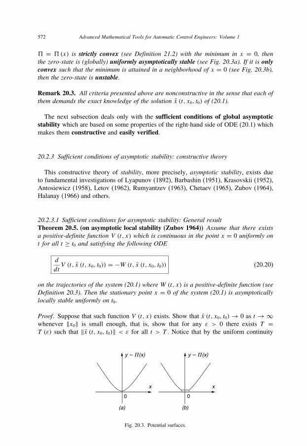
572 Advanced Mathematical Tools for Automatic Control Engineers: Volume 1
= (x) is strictly convex (see Definition 21.2) with the minimum in x = 0, thenthe zero-state is (globally) uniformly asymptotically stable (see Fig. 20.3a). If it is onlyconvex such that the minimum is attained in a neighborhood of x = 0 (see Fig. 20.3b),then the zero-state is unstable.
Remark 20.3. All criteria presented above are nonconstructive in the sense that each ofthem demands the exact knowledge of the solution x (t, x0, t0) of (20.1).
The next subsection deals only with the sufficient conditions of global asymptoticstability which are based on some properties of the right-hand side of ODE (20.1) which
makes them constructive and easily verified.
20.2.3 Sufficient conditions of asymptotic stability: constructive theory
This constructive theory of stability, more precisely, asymptotic stability, exists due
to fundamental investigations of Lyapunov (1892), Barbashin (1951), Krasovskii (1952),
Antosiewicz (1958), Letov (1962), Rumyantzev (1963), Chetaev (1965), Zubov (1964),
Halanay (1966) and others.
20.2.3.1 Sufficient conditions for asymptotic stability: General resultTheorem 20.5. (on asymptotic local stability (Zubov 1964)) Assume that there existsa positive-definite function V (t, x) which is continuous in the point x = 0 uniformly ont for all t ≥ t0 and satisfying the following ODE
d
dtV (t, x (t, x0, t0)) = −W (t, x (t, x0, t0)) (20.20)
on the trajectories of the system (20.1) where W (t, x) is a positive-definite function (seeDefinition 20.3). Then the stationary point x = 0 of the system (20.1) is asymptoticallylocally stable uniformly on t0.
Proof. Suppose that such function V (t, x) exists. Show that x (t, x0, t0)→ 0 as t →∞whenever ‖x0‖ is small enough, that is, show that for any ε > 0 there exists T =T (ε) such that ‖x (t, x0, t0)‖ < ε for all t > T . Notice that by the uniform continuity
y 5 �(x)
0
(b)(a)
0
x x
y 5 �(x)
Fig. 20.3. Potential surfaces.
Elements of stability theory 573
V (t, x) and by Corollary 20.1 all trajectories x (t, x0, t0) of (20.1) remain within the
region where ‖x (t, x0, t0)‖ < ε if ‖x0‖ < δ. So, the function W (t, x (t, x0, t0)) remains
bounded too. Suppose that ‖x (t, x0, t0)‖ does not converge to zero. By monotonicity of
V (t, x (t, x0, t0)), this means that there exists ε > 0 and a moment T = T (ε) such that
for all t ≥ T (ε) we have ‖x (t, x0, t0)‖ > ε. SinceW (t, x) is a positive-definite function,it follows that
W (t, x (t, x0, t0)) > α > 0
for all t ≥ T (ε) and, hence, by (20.20) we have
V (t, x (t, x0, t0)) = V (t0, x (t0, x0, t0))−t∫
s=t0
W (s, x (s, x0, t0)) ds
≤ V (t0, x (t0, x0, t0))− αt →−∞
which contradicts the condition that V (t, x) is a positive-definite function. The fact that
this result is uniform on t0 follows from Corollary 20.1. Theorem is proven. �
20.2.3.2 Asymptotic stability for stationary systemConsider the stationary (autonomous) ODE
x (t) = f (x (t)), f (0) = 0, t ≥ t0 (20.21)
Notice that the right-hand side of (20.21) can be represented as follows:
f (x) = Ax + h (x)h (x) := f (x)− Ax (20.22)
Below we will give three very important results concerning the asymptotic stability
property of the zero-state x = 0 for the stationary systems governed by (20.21).
Theorem 20.6. (Lyapunov 1892)5 If1. the matrix A ∈ Rn×n in (20.22) is stable (Hurwitz), i.e., for all i = 1, . . . , n
Re λi (A) < 0 (20.23)
2. and
h (x)
‖x‖ → 0 whenever ‖x‖ → 0 (20.24)
then the stationary point x = 0 is exponentially locally stable.
5 This result is referred to as the first Lyapunov’s theorem (method).

574 Advanced Mathematical Tools for Automatic Control Engineers: Volume 1
Proof. By the Lyapunov Lemma 9.1 for any 0 < Q = Qᵀ ∈ Rn×n and a given stable A
there exists 0 < P = Pᵀ ∈ Rn×n such that
AP + PAᵀ = −Q
Then for the Lyapunov function V (x) := xᵀPx we have
d
dtV (t, x (t, x0, t0)) = 2xᵀ (t) P x (t)
= 2xᵀ (t) P [Ax (t)+ h (x (t))] = 2xᵀ (t) PAx (t)
+ 2xᵀ (t) Ph (x (t)) = xᵀ (t) [PA+ AᵀP ] x (t)
+ 2x (t)ᵀ Ph (x (t)) = −xᵀ (t)Qx (t)+ 2xᵀ (t) Ph (x (t))
≤ −xᵀ (t)Qx (t)+ 2 ‖x (t)‖ ‖P ‖ = −xᵀ (t)Qx (t)
+ 2 ‖x (t)‖2 ‖P ‖ ‖h (x (t))‖ / ‖x (t)‖ ≤ −xᵀ (t)Qx (t)
+ xᵀ (t)Qx (t)(2 ‖P ‖ λmax
(Q−1
) ‖h (x (t))‖ / ‖x (t)‖)By assumption (2) of this theorem, for ε <
[2 ‖P ‖ λmax
(Q−1
)]−1always exists δ such
that if ‖x (t0)‖ ≤ δ, then ‖h (x (t0))‖ / ‖x (t0)‖ ≤ ε. Taking the corresponding x (t0) from
the last differential inequality we find that
d
dtV (t, x (t, x0, t0))
≤ −xᵀ (t)Qx (t)[1− 2 ‖P ‖ λmax
(Q−1
)ε] = −αV (t, x (t, x0, t0))
α := 1− 2 ‖P ‖ λmax
(Q−1
)ε > 0
and, hence,
V (t, x (t, x0, t0)) ≤ V (t0, x (t0, x0, t0)) e−αt → 0 as t →∞
Theorem is proven. �
Remark 20.4. If the function f (x) is differentiable at x = 0, then the matrix A in theLyapunov theorem 20.6 is
A = ∂
∂xf (x) |x=0 (20.25)
that is, A is the linear approximation of the nonlinear vector function f (x) in the origin.
Example 20.4. Consider the second-order ODE
x (t)+ βx (t)− k(
a
c − x (t) − x (t))= 0, a, c, β, k > 0
Elements of stability theory 575
which can be rewritten as the following extended first-order ODE
x1 (t) := x (t), x2 (t) := x (t)x1 (t) = f1 (x1 (t), x2 (t)) := x2 (t)
x2 (t) = f2 (x1 (t), x2 (t)) := k(
a
c − x1 (t) − x1 (t))− βx2 (t)
⎫⎪⎬⎪⎭
The stationary points
x∗1 =1
2
(c +√
c2 − 4a), x∗2 = 0
x∗∗1 = 1
2
(c −√
c2 − 4a), x∗∗2 = 0
exist if c2 ≥ 4a. Using the Taylor expansion in a small neighborhood of the stationarypoints, the function f (x1, x2) can be represented as
f (x1, x2) = f2(x∗.∗∗1 , x∗.∗∗2
)︸ ︷︷ ︸0
+ A(∗,∗∗)x + o (‖x‖) = A(∗,∗∗)x + o (‖x‖)
where
A(∗) = ∂
∂xf (x) |x=x∗ =
[0 1
b∗ −β], b∗ := −k
(1+ a(
c − x∗1)2)
A(∗∗) = ∂
∂xf (x) |x=x∗∗ =
⎡⎣ 0 1
b∗∗ −β
⎤⎦, b∗∗ := −k
(1+ a(
c − x∗2)2)
In both cases the eigenvalues of A satisfy the quadratic equation
λ2 + βλ− b = 0
and are equal
λ1,2 = −β ±√β2 + 4b
2, b = b∗.∗∗ = −kc
2
2a
(1±
√1− 4a
c2
)≤ 0
Hence, the points x∗,∗∗ are exponentially locally stable by the Lyapunov theorem 20.6when c2 > 4a, since Re λ1,2 < 0.
Example 20.5. (Lefschetz 1965) For which a, b and f (0) the following system
x(3) (t)+ f (x (t)) x (t)+ ax (t)+ bx (t) = 0 (20.26)

576 Advanced Mathematical Tools for Automatic Control Engineers: Volume 1
is asymptotically locally stable? Here the function f (z) is assumed to be differentiablein the point z = 0. Let us apply the Lyapunov theorem 20.6 and represent (20.26) in thematrix form:
x1 (t) := x (t), x2 (t) := x (t), x3 (t) := x (t)
x (t) := (x1 (t), x2 (t), x3 (t))ᵀ⎛⎝ x1 (t)x2 (t)
x3 (t)
⎞⎠ = A
⎛⎝x1 (t)x2 (t)
x3 (t)
⎞⎠+ h (x (t))
where
A =⎡⎣ 0 1 0
0 0 1
−b −a −f (0)
⎤⎦, h (x) =
⎛⎝ 0
0
[−f ′ (0) x2 + o (‖x2‖)] x3
⎞⎠
Firstly, notice that
h (x) / ‖x‖ → 0 as ‖x‖ → 0
So, to answer the initial question we should try to find the conditions when the matrix Ais stable. The corresponding characteristic polynomial is
pA (λ) = λ2 (f (0)+ λ)+ b + aλ
and it is Hurwitz if and only if (see Criterion 9.3)
f (0) > 0, a > 0, b > 0, af (0) > b
which gives the relation among the parameters guaranteeing the exponential localstability.
20.3 Asymptotic global stability
20.3.1 Definition of asymptotic global stability
Definition 20.7. The equilibrium zero-point (or zero-state) x = 0 of the system given byODE (20.1) is said to be asymptotically globally stable6 if x (t, x0, t0)→ 0 when t →∞for any initial state x0 = x (t0) of a bounded norm.
6 Sometimes such asymptotically globally stable systems are called, by R. Kalman, mono-stable (or having
the dichotomy property) systems.

Elements of stability theory 577
20.3.2 Asymptotic global stability for stationary systems
Theorem 20.7. (Barbashin & Krasovskii 1952) To guarantee the asymptotic globalstability of the unique stationary point x = 0 of (20.21) with the continuous right-handside it is sufficient to show the existence of a differentiable function V = V (x) such that(a) V (0) = 0 and for any x �= 0
V (x) > 0 (20.27)
(b) for ‖x‖ → ∞
V (x)→∞ (20.28)
(c) for any t0, x0 ∈ R and any x (t, x0, t0) �= 0
d
dtV (x (t, x0, t0)) < 0 (20.29)
Proof. By assumption (c) V (x (t, x0, t0)) monotonically decreases and is bounded from
below. Therefore, by the Weierstrass theorem 14.9 V (x (t, x0, t0)) ↓ V ∗ monotonically.
By property (b) x (t, x0, t0) remains to be bounded. Suppose that V ∗ > 0. Hence, by
property (a) there exist ε > 0 and T = T (ε) ≥ t0 such that inft≥T (ε)
‖x (t, x0, t0)‖ > ε.Therefore, by (20.29) we get
supt≥T (ε)
d
dtV (x (t, x0, t0)) < −ε′, ε′ > 0
which implies the inequality
0 < V ∗ < V (x (t, x0, t0)) = V (x (T , x (T ), T ))
+t∫
s=T
d
dtV (x (s, x0, t0)) ds ≤ V (x (T , x (T ), T ))− ε′ (t − T )
making the right-hand side negative for large enough t . This leads to the contradiction.
So, V ∗ = 0. Theorem is proven. �
Theorem 20.8. (Krasovskii 1952) Assume that(a) the function f (x) in (20.21) is differentiable everywhere in x and the stationary pointx = 0 (where f (x) = 0) is unique;
(b) there exists a positive-definite matrix B = Bᵀ > 0 such that the functional matrixM (x) defined by
M (x) := ∂
∂xf (x)ᵀ B + B ∂
∂xf (x) (20.30)
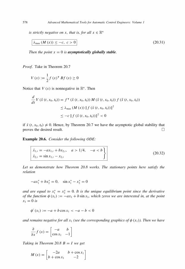
578 Advanced Mathematical Tools for Automatic Control Engineers: Volume 1
is strictly negative on x, that is, for all x ∈ Rn
λmax (M (x)) ≤ −c, c > 0 (20.31)
Then the point x = 0 is asymptotically globally stable.
Proof. Take in Theorem 20.7
V (x) := 1
2f (x)ᵀ Bf (x) ≥ 0
Notice that V (x) is nonnegative in Rn. Then
d
dtV (x (t, x0, t0))= f ᵀ (x (t, x0, t0))M (x (t, x0, t0)) f (x (t, x0, t0))
≤ λmax (M (x)) ‖f (x (t, x0, t0))‖2
≤ −c ‖f (x (t, x0, t0))‖2 < 0
if x (t, x0, t0) �= 0. Hence, by Theorem 20.7 we have the asymptotic global stability that
proves the desired result. �
Example 20.6. Consider the following ODE:
x1,t = −ax1,t + bx2,t , a > 1/4, −a < bx2,t = sin x1,t − x2,t
}(20.32)
Let us demonstrate how Theorem 20.8 works. The stationary points here satisfy therelation
−ax∗1 + bx∗2 = 0, sin x∗1 − x∗2 = 0
and are equal to x∗1 = x∗2 = 0. It is the unique equilibrium point since the derivativeof the function φ (x1) := −ax1 + b sin x1, which zeros we are interested in, at the pointx1 = 0 is
φ′ (x1) := −a + b cos x1 < −a − b < 0
and remains negative for all x1 (see the corresponding graphics of φ (x1)). Then we have
∂
∂xf (x) =
[ −a b
cos x1 −1
]
Taking in Theorem 20.8 B = I we get
M (x) =[ −2a b + cos x1b + cos x1 −2
]
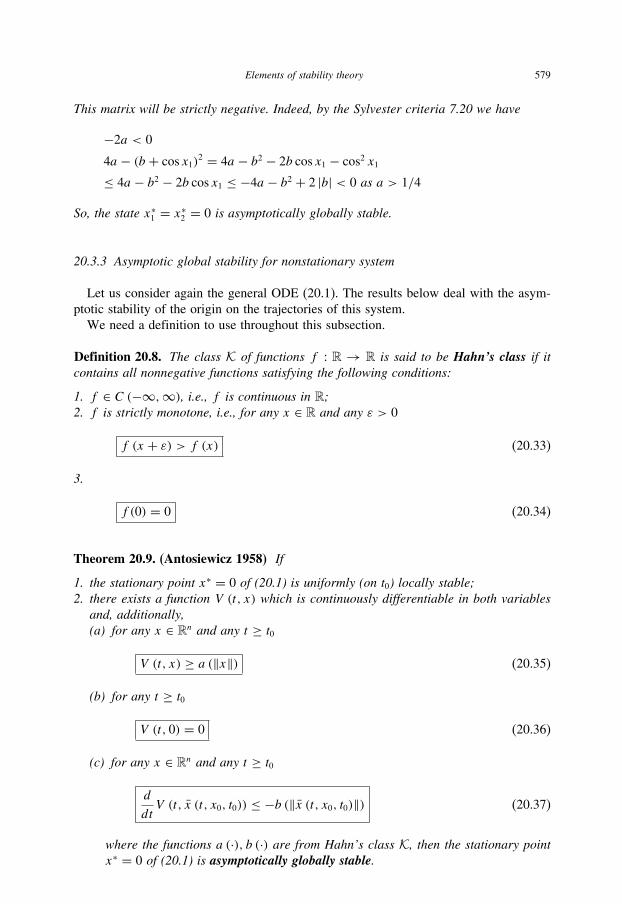
Elements of stability theory 579
This matrix will be strictly negative. Indeed, by the Sylvester criteria 7.20 we have
−2a < 0
4a − (b + cos x1)2 = 4a − b2 − 2b cos x1 − cos2 x1
≤ 4a − b2 − 2b cos x1 ≤ −4a − b2 + 2 |b| < 0 as a > 1/4
So, the state x∗1 = x∗2 = 0 is asymptotically globally stable.
20.3.3 Asymptotic global stability for nonstationary system
Let us consider again the general ODE (20.1). The results below deal with the asym-
ptotic stability of the origin on the trajectories of this system.
We need a definition to use throughout this subsection.
Definition 20.8. The class K of functions f : R → R is said to be Hahn’s class if itcontains all nonnegative functions satisfying the following conditions:
1. f ∈ C (−∞,∞), i.e., f is continuous in R;2. f is strictly monotone, i.e., for any x ∈ R and any ε > 0
f (x + ε) > f (x) (20.33)
3.
f (0) = 0 (20.34)
Theorem 20.9. (Antosiewicz 1958) If
1. the stationary point x∗ = 0 of (20.1) is uniformly (on t0) locally stable;2. there exists a function V (t, x) which is continuously differentiable in both variables
and, additionally,(a) for any x ∈ Rn and any t ≥ t0
V (t, x) ≥ a (‖x‖) (20.35)
(b) for any t ≥ t0
V (t, 0) = 0 (20.36)
(c) for any x ∈ Rn and any t ≥ t0
d
dtV (t, x (t, x0, t0)) ≤ −b (‖x (t, x0, t0)‖) (20.37)
where the functions a (·), b (·) are from Hahn’s class K, then the stationary pointx∗ = 0 of (20.1) is asymptotically globally stable.

580 Advanced Mathematical Tools for Automatic Control Engineers: Volume 1
Proof. By the conditions of the theorem it follows that any trajectory x (t, x0, t0)
obligatory will arrive at some small neighborhood � containing the point x = 0 and will
never leave it. Indeed, by condition (2c)d
dtV (t, x (t, x0, t0)) < 0 whenever ‖x‖ > 0 and,
hence, decreases reaching � in a finite time t ′ uniformly on t0. By condition (1) after
this moment it will always belong to �. Suppose that ‖x (t, x0, t0)‖ does not converge
to zero. By monotonicity of V (t, x (t, x0, t0)) (see the condition (20.37)), this means
that there exists ε > 0 and a moment T = T (ε) such that for all t ≥ T (ε) we have
‖x (t, x0, t0)‖ > ε. Since b (‖x‖) belongs to Hahn’s class K, it follows that
b (‖x (t, x0, t0)‖) > α > 0
and, hence, by (20.37)
V (t, x (t, x0, t0))≤ V (t0, x (t0, x0, t0))
−t∫
s=t ′b(∥∥x (s, x (t ′), t ′)∥∥) ds ≤ V (t0, x0)− αt →−∞
which contradicts the assumption (20.35) that V (t, x) ≥ a (‖x‖). So, ‖x (t, x0, t0)‖ → 0
as t →∞. Theorem is proven. �
Corollary 20.2. (Halanay 1966) The result of Theorem 20.9 remains true if instead ofassumption (2c) there is
d
dtV (t, x (t, x0, t0)) ≤ −cV (t, x (t, x0, t0)), c (·) ∈ K (20.38)
Proof. It is sufficient to take in Theorem 20.9
b (‖x‖) := c (a (‖x‖))
since c (V (t, x)) ≥ c (a (‖x‖)). �
Theorem 20.10. (Chetaev 1965) Let there exist the function k (·) ∈ C, a (·) ∈ K andV (t, x) ∈ C1 such that
1. for any x ∈ Rn and any t ≥ t0
V (t, x) ≥ k (t) a (‖x‖) (20.39)
2. for any t ≥ t0
d
dtV (t, x (t, x0, t0)) ≤ 0 (20.40)

Elements of stability theory 581
3. k (·) ∈ K, i.e., for any t ≥ t0 k (t) ≥ 0 and k (t)→ ∞ as t →∞.Then the stationary point x∗ = 0 of (20.1) is asymptotically globally stable.
Proof. Evidently, by condition (2), V (t, x (t, x0, t0)) is a nondecreasing function of t
and, hence, in view of condition (1),
∞ > lim supt→∞
V (t, x (t, x0, t0)) ≥ lim inft→∞
V (t, x (t, x0, t0))
≥ lim inft→∞
k (t) a (‖x (t, x0, t0)‖) ≥ 0
But, by condition (3), k (t) → ∞ and, hence, a (‖x (t, x0, t0)‖) → 0 as t → ∞. And
since a (·) ∈ K it follows that ‖x (t, x0, t0)‖ → 0 as t →∞. Theorem is proven. �
20.4 Stability of linear systems
20.4.1 Asymptotic and exponential stability of linear time-varying systems
Consider the linear time-varying system given by the following ODE:
x (t) = A (t) x (t), x (t0) = x0, t ≥ t0 (20.41)
Its solution can be presented as
x (t) = �(t, t0) x0 (20.42)
where �(t, t0) is the corresponding fundamental matrix defined by (19.56). This presen-
tation, evidently, implies the following proposition.
Proposition 20.1. The system (20.41) is(a) locally stable if and only if
c := supt≥t0
‖�(t, t0)‖ <∞ (20.43)
(b) asymptotically globally stable if and only if
‖�(t, t0)‖ → 0 whereas t →∞ (20.44)
Let A (t) satisfy the inequality
∞∫s=t
tr A (s) ds > −∞ (20.45)

582 Advanced Mathematical Tools for Automatic Control Engineers: Volume 1
which by the Liouville’s theorem 19.7 implies that det�(t, t0) �= 0 for all t ≥ t0, and as
a result there exists a constant a > 0 such that
∞∫s=t�ᵀ (s, t)� (s, t) ds ≥ a (20.46)
Below we present the criterion of exponential stability expressed in terms of Lyapunov’sapproach (see Theorem 20.3). It is interesting to note that for the class of linear systemsthis approach turns out to be constructive.
Theorem 20.11. (on exponential stability (Zubov 1964)) For the solution x (t, x0, t0)of (20.41) satisfying (20.45) to be exponentially globally stable (see Definition 20.5) itis necessary and sufficient to show the existence of two quadratic forms
V (t, x) = xᵀP(t)x and W (t, x) = xᵀQ(t)x (20.47)
such that1. both quadratic forms are positive definite and increase no quicker than the quadratic
function, i.e.,
a1 ‖x‖2 ≤ V (t, x) ≤ a2 ‖x‖2b2 ‖x‖2 ≥ W (t, x) ≥ b1 ‖x‖2
a1, a2, b1, b2 are positive constants
(20.48)
2. V (t, x) and W (t, x) are related as
d
dtV (t, x (t, x0, t0)) = −W (t, x (t, x0, t0)) (20.49)
Proof.
(a) Necessity. Let ‖x (t, x0, t0)‖ ≤ α exp (−β (t − t0)). DefineW (t, x) := ‖x‖2
V (t, x) :=∞∫
t=tW (s, x (s, x, t)) ds
(20.50)
Evidently, in this case b1 = b2 = 1. Show that V (t, x) as it is defined above satisfies
the conditions (20.48) and (20.49). By (20.42) and in view of (20.46) we have
V (t, x)=∞∫
s=txᵀ (s, x, t) x (s, x, t) ds
= xᵀ
⎡⎣ ∞∫s=t�ᵀ (s, t)� (s, t) ds
⎤⎦ x ≥ a ‖x‖2

Elements of stability theory 583
By the inequality (20.8) one has
a ‖x‖2 ≤ V (t, x) ≤∞∫
s=tα2 ‖x‖2 e−2β(s−t)ds = 1
2βα2 ‖x‖2
This means that V (t, x) satisfies (20.48) with a1 = a and a2 = 1
2βα2. Obviously,
V (t, x), as it is defined in (20.50), satisfies (20.49).
(b) Sufficiency. Show that (20.49) together with (20.47) and (20.48) imply (20.8). Inte-
grating (20.49) for V �= 0 leads to
t∫s=t0
dV
V= −
t∫s=t0
W (s, x (s, x0, t0))
V (s, x (s, x0, t0))ds
and, hence,
V (t, x (t, x0, t0)) = V (t0, x0) exp⎛⎝− t∫
s=t0
W (s, x (s, x0, t0))
V (s, x (s, x0, t0))ds
⎞⎠ (20.51)
Notice that
b1
a2≤ x
ᵀQ(s)xxᵀP(s)x
= W (s, x (s, x0, t0))V (s, x (s, x0, t0))
Application of these estimates in (20.51) gives
a1 ‖x (t, x0, t0)‖2 ≤ V (t, x (t, x0, t0)) ≤ V (t0, x0) exp(−b1a2
[t − t0])
Using the estimates (20.15) for V (t0, x0) implies
a1 ‖x (t, x0, t0)‖2 ≤ V (t, x (t, x0, t0)) ≤ a2 ‖x0‖2 exp(−b1a2
[t − t0])
and, therefore, we obtain the exponential global stability (20.8) for the zero-state
x = 0 with
α :=√a2
a1, β := b1
2a2
Theorem is proven. �
Remark 20.5. Since
d
dtV (t, x (t, x0, t0))= dx
ᵀ
dtP (t)x + xᵀ d
dtP (t)x + xᵀP(t)
dx
dt
= xᵀ[Aᵀ (t) P (t)+ d
dtP (t)+ P(t)A (t)
]x
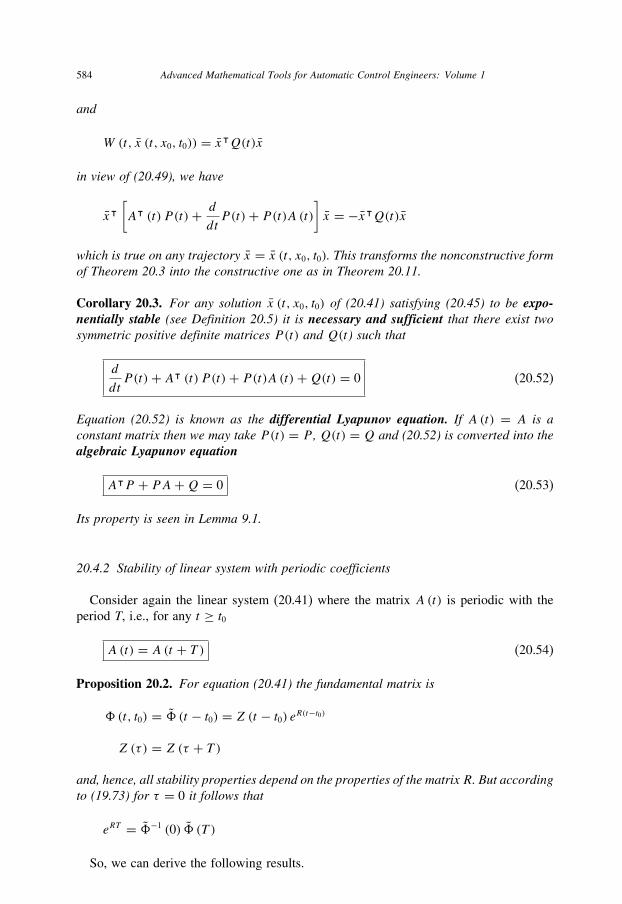
584 Advanced Mathematical Tools for Automatic Control Engineers: Volume 1
and
W (t, x (t, x0, t0)) = xᵀQ(t)x
in view of (20.49), we have
xᵀ[Aᵀ (t) P (t)+ d
dtP (t)+ P(t)A (t)
]x = −xᵀQ(t)x
which is true on any trajectory x = x (t, x0, t0). This transforms the nonconstructive formof Theorem 20.3 into the constructive one as in Theorem 20.11.
Corollary 20.3. For any solution x (t, x0, t0) of (20.41) satisfying (20.45) to be expo-nentially stable (see Definition 20.5) it is necessary and sufficient that there exist twosymmetric positive definite matrices P(t) and Q(t) such that
d
dtP (t)+ Aᵀ (t) P (t)+ P(t)A (t)+Q(t) = 0 (20.52)
Equation (20.52) is known as the differential Lyapunov equation. If A (t) = A is aconstant matrix then we may take P(t) = P , Q(t) = Q and (20.52) is converted into thealgebraic Lyapunov equation
AᵀP + PA+Q = 0 (20.53)
Its property is seen in Lemma 9.1.
20.4.2 Stability of linear system with periodic coefficients
Consider again the linear system (20.41) where the matrix A (t) is periodic with the
period T, i.e., for any t ≥ t0
A (t) = A (t + T ) (20.54)
Proposition 20.2. For equation (20.41) the fundamental matrix is
�(t, t0) = � (t − t0) = Z (t − t0) eR(t−t0)
Z (τ ) = Z (τ + T )
and, hence, all stability properties depend on the properties of the matrix R. But accordingto (19.73) for τ = 0 it follows that
eRT = �−1 (0) � (T )
So, we can derive the following results.
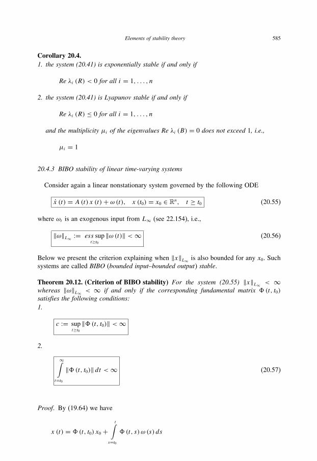
Elements of stability theory 585
Corollary 20.4.1. the system (20.41) is exponentially stable if and only if
Re λi (R) < 0 for all i = 1, . . . , n
2. the system (20.41) is Lyapunov stable if and only if
Re λi (R) ≤ 0 for all i = 1, . . . , n
and the multiplicity μi of the eigenvalues Re λi (B) = 0 does not exceed 1, i.e.,
μi = 1
20.4.3 BIBO stability of linear time-varying systems
Consider again a linear nonstationary system governed by the following ODE
x (t) = A (t) x (t)+ ω (t), x (t0) = x0 ∈ Rn, t ≥ t0 (20.55)
where ωt is an exogenous input from L∞ (see 22.154), i.e.,
‖ω‖L∞ := ess supt≥t0
‖ω (t)‖ <∞ (20.56)
Below we present the criterion explaining when ‖x‖L∞ is also bounded for any x0. Such
systems are called BIBO (bounded input–bounded output) stable.
Theorem 20.12. (Criterion of BIBO stability) For the system (20.55) ‖x‖L∞ < ∞whereas ‖ω‖L∞ < ∞ if and only if the corresponding fundamental matrix �(t, t0)satisfies the following conditions:1.
c := supt≥t0
‖�(t, t0)‖ <∞
2.
∞∫t=t0
‖�(t, t0)‖ dt <∞ (20.57)
Proof. By (19.64) we have
x (t) = �(t, t0) x0 +t∫
s=t0
�(t, s) ω (s) ds

586 Advanced Mathematical Tools for Automatic Control Engineers: Volume 1
Sufficiency follows directly from this formula since
‖x (t)‖ ≤ ‖�(t, t0) x0‖ +∥∥∥∥∥∥
t∫s=t0
�(t, s) ω (s) ds
∥∥∥∥∥∥≤ c ‖x0‖ + ‖ω‖L∞
t∫s=t0
‖�(t, s)‖ ds <∞
Let us prove necessity. Suppose that ‖x‖L∞ < ∞. Taking ω (t) ≡ 0 we have x (t) =�(t, t0) x0 that proves the necessity of which condition (1). Take now x0 = 0 and suppose
that condition (2) is violated, that is, there exists at least one element (i0, j0) of the matrix
�(t, t0) such that
t∫s=t0
∣∣�i0j0 (t, s)∣∣ ds →∞ as t →∞
Hence,
‖x (t)‖ =∥∥∥∥∥∥
t∫s=t0
�(t, s) ω (s) ds
∥∥∥∥∥∥
=
√√√√√ n∑i=1
∣∣∣∣∣∣t∫
s=t0
n∑j=1
�ij (t, s) ωj (s) ds
∣∣∣∣∣∣2
≥
√√√√√∣∣∣∣∣∣n∑j=1
t∫s=t0
�i0j (t, s) ωj (s) ds
∣∣∣∣∣∣2
Taking then
ωj (s) :={sign �i0j0 (t, s) if j = j0
0 if j �= j0
from the last inequality we obtain
‖x (t)‖ ≥t∫
s=t0
∣∣�i0j0 (t, s)∣∣ ds →∞ as t →∞
But this contradicts the assumption that ‖x‖L∞ < ∞. Theorem is proven. �
Example 20.7. Consider the system given by
x (t)+ [a + sin (ω0t)] x (t) = ω (t), x (t0) = x0 ∈ R, a > 0
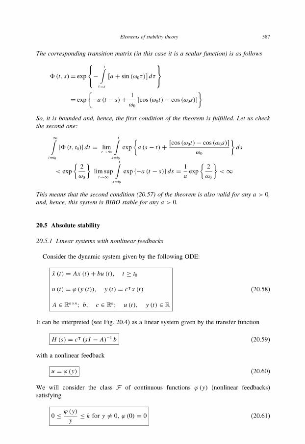
Elements of stability theory 587
The corresponding transition matrix (in this case it is a scalar function) is as follows
�(t, s)= exp
⎧⎨⎩−
t∫τ=s
[a + sin (ω0τ)] dτ
⎫⎬⎭
= exp
{−a (t − s)+ 1
ω0
[cos (ω0t)− cos (ω0s)]
}
So, it is bounded and, hence, the first condition of the theorem is fulfilled. Let us checkthe second one:
∞∫t=t0
|�(t, t0)| dt = limt→∞
t∫s=t0
exp
{a (s − t)+ [cos (ω0t)− cos (ω0s)]
ω0
}ds
< exp
{2
ω0
}lim supt→∞
t∫s=t0
exp {−a (t − s)} ds = 1
aexp
{2
ω0
}<∞
This means that the second condition (20.57) of the theorem is also valid for any a > 0,and, hence, this system is BIBO stable for any a > 0.
20.5 Absolute stability
20.5.1 Linear systems with nonlinear feedbacks
Consider the dynamic system given by the following ODE:
x (t) = Ax (t)+ bu (t), t ≥ t0u (t) = ϕ (y (t)), y (t) = cᵀx (t)
A ∈ Rn×n; b, c ∈ Rn; u (t), y (t) ∈ R
(20.58)
It can be interpreted (see Fig. 20.4) as a linear system given by the transfer function
H (s) = cᵀ (sI − A)−1 b (20.59)
with a nonlinear feedback
u = ϕ (y) (20.60)
We will consider the class F of continuous functions ϕ (y) (nonlinear feedbacks)
satisfying
0 ≤ ϕ (y)y
≤ k for y �= 0, ϕ (0) = 0 (20.61)

588 Advanced Mathematical Tools for Automatic Control Engineers: Volume 1
yu Linear system
H (iw)
(y)
Fig. 20.4. A linear system with a nonliner feedback.
(y)
kyu
y
Fig. 20.5. A function u = ϕ(y) from the class F .
Definition 20.9. The nonlinear system (20.58) is said to be absolutely stable in the classF if the solution x (t) ≡ 0 (or zero-state) is asymptotically globally stable (see Definition20.7) for any nonlinear feedback (20.60) satisfying (20.61).
In this section we are interested in finding the conditions guaranteeing the absolute
stability of the system (20.58) in the class F .
20.5.2 Aizerman and Kalman conjectures
Proposition 20.3. (Conjecture of M.A. Aizeman, 1949) Let the system (20.58) be stablefor any
ϕ (y) = αy, α ∈ [0, k]
It seems to be true that this system remains stable for any feedback ϕ (y) satisfying(20.61), namely, for any ϕ (y) such that
0 ≤ ϕ (y)y
≤ k for y �= 0, ϕ (0) = 0

Elements of stability theory 589
Proposition 20.4. (Conjecture of R. Kalman, 1957) Let the system (20.58) be stable forany
ϕ (y) = αy, α ∈ [0, k]
It seems to be natural to admit that this system remains stable for any feedback ϕ (y)satisfying the conditions:
ϕ (y) is differentiable, ϕ (0) = 0
0 ≤ ϕ′ (y) ≤ k
Claim 20.2. Conjectures of Both M.A. Aizerman and R. Kalman are not valid.
Proof. See a number of counterexamples in Pliss (1964). �
Counterexample (Pliss 1964) Let
H (s) = s2[(s + 0.5)
2 + (0.9)2] [(s + 0.5)2 + (1.1)2]
The closed-loop system is stable for any u = ky with
k ∈ [−0, 7124,∞)
It follows for example from the Routh–Hurwitz criterion (see Theorem 9.2), applied tothe closed-loop system. But for
ϕ (y) ={y3 for |y| ≤ √|k|ky for |y| > √|k|
in this system auto-oscillations arise, and, hence, there is no asymptotic stability.These conjectures were proposed before the keystone result of V.M. Popov who found
the exact conditions of absolute stability of the linear system (20.58) with any feedback
satisfying (20.61).
20.5.3 Analysis of absolute stability
To guarantee the absolute stability of the system (20.58)–(20.61), according to the
Barbashin–Krasovskii theorem 20.7, it is sufficient that there exists the Lyapunov function
V (x) such that
(a) V (0) = 0 and
V (x) > 0 for any x �= 0
(b)
V (x)→∞ whereas ‖x‖ → ∞
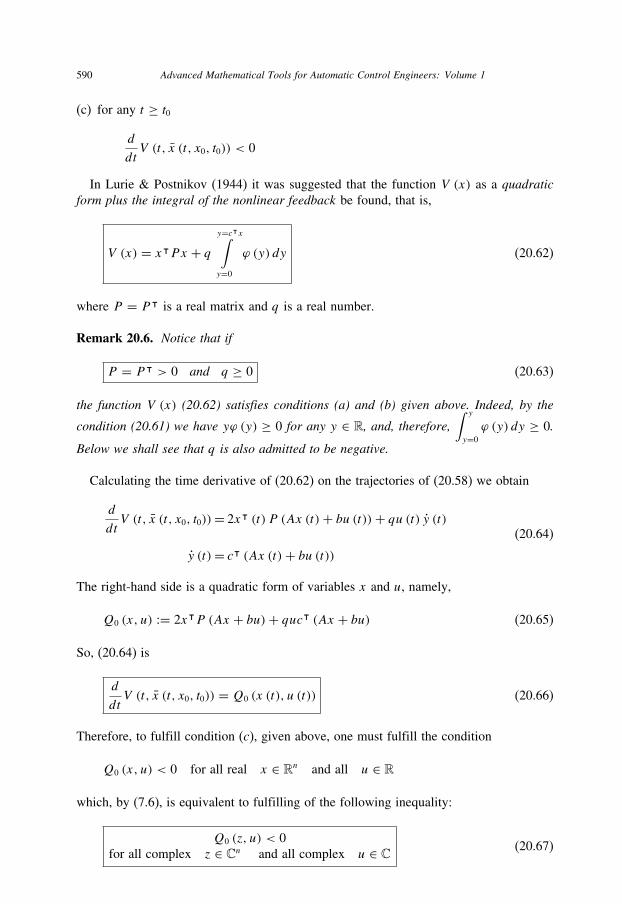
590 Advanced Mathematical Tools for Automatic Control Engineers: Volume 1
(c) for any t ≥ t0d
dtV (t, x (t, x0, t0)) < 0
In Lurie & Postnikov (1944) it was suggested that the function V (x) as a quadraticform plus the integral of the nonlinear feedback be found, that is,
V (x) = xᵀPx + qy=cᵀx∫y=0
ϕ (y) dy (20.62)
where P = Pᵀ is a real matrix and q is a real number.
Remark 20.6. Notice that if
P = Pᵀ > 0 and q ≥ 0 (20.63)
the function V (x) (20.62) satisfies conditions (a) and (b) given above. Indeed, by the
condition (20.61) we have yϕ (y) ≥ 0 for any y ∈ R, and, therefore,∫ y
y=0
ϕ (y) dy ≥ 0.
Below we shall see that q is also admitted to be negative.
Calculating the time derivative of (20.62) on the trajectories of (20.58) we obtain
d
dtV (t, x (t, x0, t0))= 2xᵀ (t) P (Ax (t)+ bu (t))+ qu (t) y (t)
y (t)= cᵀ (Ax (t)+ bu (t))(20.64)
The right-hand side is a quadratic form of variables x and u, namely,
Q0 (x, u) := 2xᵀP (Ax + bu)+ qucᵀ (Ax + bu) (20.65)
So, (20.64) is
d
dtV (t, x (t, x0, t0)) = Q0 (x (t), u (t)) (20.66)
Therefore, to fulfill condition (c), given above, one must fulfill the condition
Q0 (x, u) < 0 for all real x ∈ Rn and all u ∈ R
which, by (7.6), is equivalent to fulfilling of the following inequality:
Q0 (z, u) < 0
for all complex z ∈ Cn and all complex u ∈ C(20.67)
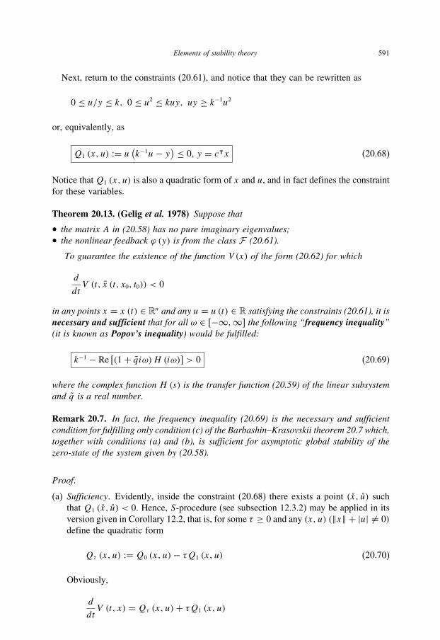
Elements of stability theory 591
Next, return to the constraints (20.61), and notice that they can be rewritten as
0 ≤ u/y ≤ k, 0 ≤ u2 ≤ kuy, uy ≥ k−1u2
or, equivalently, as
Q1 (x, u) := u(k−1u− y) ≤ 0, y = cᵀx (20.68)
Notice thatQ1 (x, u) is also a quadratic form of x and u, and in fact defines the constraint
for these variables.
Theorem 20.13. (Gelig et al. 1978) Suppose that
• the matrix A in (20.58) has no pure imaginary eigenvalues;• the nonlinear feedback ϕ (y) is from the class F (20.61).
To guarantee the existence of the function V (x) of the form (20.62) for which
d
dtV (t, x (t, x0, t0)) < 0
in any points x = x (t) ∈ Rn and any u = u (t) ∈ R satisfying the constraints (20.61), it isnecessary and sufficient that for all ω ∈ [−∞,∞] the following “frequency inequality”(it is known as Popov’s inequality) would be fulfilled:
k−1 − Re [(1+ qiω)H (iω)] > 0 (20.69)
where the complex function H (s) is the transfer function (20.59) of the linear subsystemand q is a real number.
Remark 20.7. In fact, the frequency inequality (20.69) is the necessary and sufficientcondition for fulfilling only condition (c) of the Barbashin–Krasovskii theorem 20.7 which,together with conditions (a) and (b), is sufficient for asymptotic global stability of thezero-state of the system given by (20.58).
Proof.
(a) Sufficiency. Evidently, inside the constraint (20.68) there exists a point (x, u) such
that Q1 (x, u) < 0. Hence, S-procedure (see subsection 12.3.2) may be applied in its
version given in Corollary 12.2, that is, for some τ ≥ 0 and any (x, u) (‖x‖ + |u| �= 0)
define the quadratic form
Qτ (x, u) := Q0 (x, u)− τQ1 (x, u) (20.70)
Obviously,
d
dtV (t, x) = Qτ (x, u)+ τQ1 (x, u)
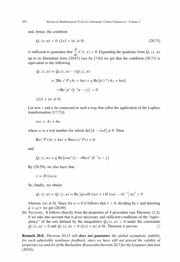
592 Advanced Mathematical Tools for Automatic Control Engineers: Volume 1
and, hence, the condition
Qτ (x, u) < 0 (‖x‖ + |u| �= 0) (20.71)
is sufficient to guarantee thatd
dtV (t, x) < 0. Expanding the quadratic formQτ (x, u)
up to its Hermitian form (20.67) (see by (7.6)) we get that the condition (20.71) is
equivalent to the following
Qτ (z, u) = Q0 (z, u)− τQ1 (z, u)
= 2Re z∗P (Az+ bu)+ q Re [u∗cᵀ (Az+ bu)]
−τRe [u∗ (k−1u− y)] < 0
(‖z‖ + |u| �= 0)
Let now z and u be connected in such a way that (after the application of the Laplace
transformation (17.73))
iωz = Az+ bu
where ω is a real number for which det [A− iωI ] �= 0. Then
Rez∗P (Az+ bu) = Reiω (z∗Pz) = 0
and
Qτ (z, u) = q Re [iωu∗y]− τRe u∗ (k−1u− y)By (20.59), we also have that
y = H (iω) u
So, finally, we obtain
Qτ (z, u) = Qτ (z, u) = Re[qiωH (iω)+ τH (iω)− τk−1
] |u|2 < 0
whereas (|u| �= 0). Since for ω = 0 it follows that τ > 0, dividing by τ and denoting
q = q/τ we get (20.69).
(b) Necessity. It follows directly from the properties of S-procedure (see Theorem 12.3),
if we take into account that it gives necessary and sufficient conditions of the “equiv-
alency” of the sets defined by the inequalities Q0 (x, u) < 0 under the constraints
Q1 (x, u) < 0 and Qτ (x, u) < 0 (‖x‖ + |u| �= 0). Theorem is proven. �
Remark 20.8. Theorem 20.13 still does not guarantee the global asymptotic stabilityfor each admissible nonlinear feedback, since we have still not proved the validity ofproperties (a) and (b) of the Barbashin–Krasovskii theorem 20.7 for the Lyapunov function(20.62).

Elements of stability theory 593
20.5.4 Popov’s sufficient conditions
The next theorem gives such additional conditions.
Theorem 20.14. (Sufficient conditions (Popov 1961)) Let
(a) in (20.58) the matrix A is stable (Hurwitz);(b) for some q (not obligatory nonnegative) and for all ω ∈ [−∞,∞] Popov’s frequency
condition (20.69) holds.Then the system (20.58), (20.61) is absolutely stable in class F .
Proof. To complete the proof we need to prove the validity of conditions (a) and (b). Let
(20.69) hold. For u = 0 the inequality (20.71) implies
Qτ (x, u) = 2xᵀPAx = xᵀ (PA+ AᵀP) x < 0
or, equivalently,
PA+ AᵀP < 0
So, by the Lyapunov Lemma 9.1, it follows that P > 0.
(a) For q = qr ≥ 0, by the condition (20.61) we have yϕ (y) ≥ 0 for any y ∈ R, and,
therefore,
∫ y
y=0
ϕ (y) dy ≥ 0. Hence we derive that V (0) = 0, V (x) > 0 for any x �= 0
and V (x)→∞ whereas ‖x‖ → ∞.
(b) Let q = qr < 0. Taking u = μy (0 ≤ μ ≤ k) we get ddtV (t, x) < 0 for the system
(20.58), (20.68) with u = μy. Then, the matrix Aμ := A + μbcᵀ of the corresponding
closed-loop system has no eigenvalues on the imaginary axis since Aμ is Hurwitz for
any μ : 0 ≤ μ ≤ k. For such a system the direct substitution shows that the Lyapunov
function (20.62) is
Vμ (x) = xᵀ(P + qμ
2ccᵀ
)x
and, sinced
dtV (t, x) < 0, it follows (by the same Lyapunov Lemma 9.1) that
P + qμ2ccᵀ > 0
which gives k �= ∞. For μ = k we get
Vk (x) = xᵀ(P + qk
2ccᵀ
)x > 0 for x �= 0

594 Advanced Mathematical Tools for Automatic Control Engineers: Volume 1
Let now ϕ ∈ F . In this case the form V (x) (20.62) can be represented as
V (x)= xᵀPx + qy=cᵀx∫y=0
ϕ (y) dy
= xᵀ(P + qk
2ccᵀ
)x − q
y=cᵀx∫y=0
[ky − ϕ (y)] dy
So, V (0) = 0, V (x) > 0 for any x �= 0 and V (x)→∞ whereas ‖x‖ → ∞ completes
the proof. �
Remark 20.9. As it is mentioned in Gelig, Leonov & Yakubovich (1978), Popov’sfrequency condition (20.69) guarantees the absolute stability for the system (20.58),(20.61) with a much wider class of nonlinear feedback, namely, for all nolinearities thatsatisfy the condition
tn∫t=t0
[u (t)
(y (t)− k−1u (t)
)+ qu (t) y (t)] dt ≥ −γ > −∞ (20.72)
for some {tn}, tn → ∞. It may include also unstable linear systems (where A is notobligatory stable).
Remark 20.10. For q = 0 in (20.69) the corresponding Popov’s frequency condition iscalled “the circle criterion” which is valid also for a much wider class of nolinearitiesincluding multi-valued functions such as hysteresis elements.
20.5.5 Geometric interpretation of Popov’s conditions
Let us represent the transfer function H (iω) as
H (iω)=U (ω)+ iV (ω)
U (ω) := Re H (iω), V (ω) := Im H (iω)
(20.73)
Then Popov’s frequency condition (20.69) can be represented as follows:
qωV (ω) > U (ω)− k−1 (20.74)
Definition 20.10. The line
qωV (ω) = U (ω)− k−1 (20.75)
in the plane (U (ω), ωV (ω)) is called Popov’s line, with tanψ = q (see Fig. 20.6).
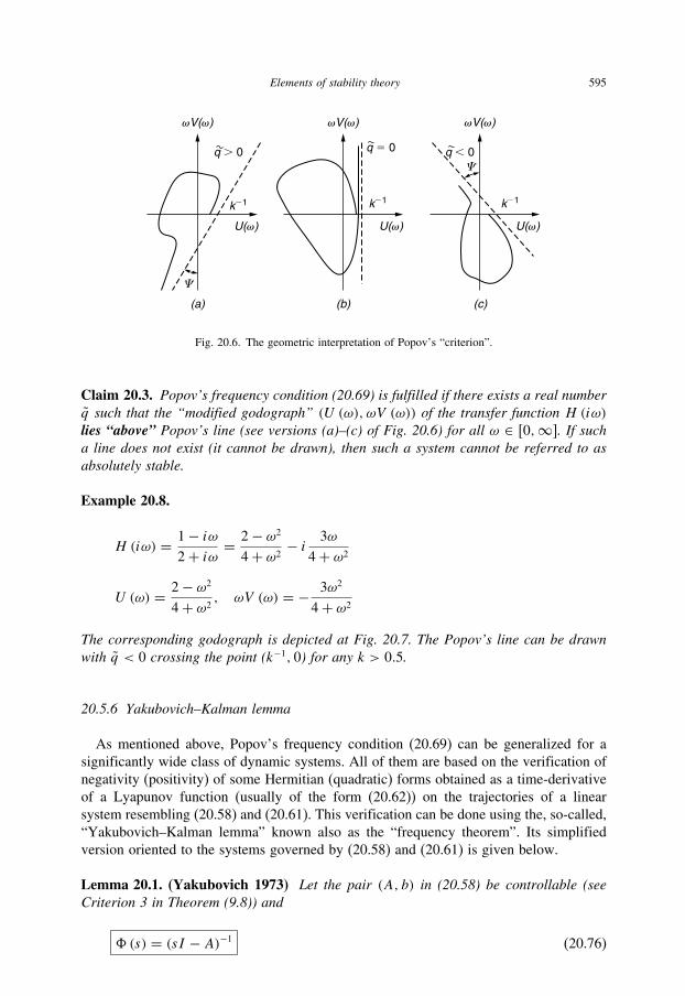
Elements of stability theory 595
�V(�)
U(�)
q . 0
k21
�
�
(a)
�V(�)
U(�)
q 5 0
k21
(b)
�V(�)
U(�)
q , 0
k21
(c)
Fig. 20.6. The geometric interpretation of Popov’s “criterion”.
Claim 20.3. Popov’s frequency condition (20.69) is fulfilled if there exists a real numberq such that the “modified godograph” (U (ω), ωV (ω)) of the transfer function H (iω)lies “above” Popov’s line (see versions (a)–(c) of Fig. 20.6) for all ω ∈ [0,∞]. If sucha line does not exist (it cannot be drawn), then such a system cannot be referred to asabsolutely stable.
Example 20.8.
H (iω) = 1− iω2+ iω = 2− ω2
4+ ω2− i 3ω
4+ ω2
U (ω) = 2− ω2
4+ ω2, ωV (ω) = − 3ω2
4+ ω2
The corresponding godograph is depicted at Fig. 20.7. The Popov’s line can be drawnwith q < 0 crossing the point (k−1, 0) for any k > 0.5.
20.5.6 Yakubovich–Kalman lemma
As mentioned above, Popov’s frequency condition (20.69) can be generalized for a
significantly wide class of dynamic systems. All of them are based on the verification of
negativity (positivity) of some Hermitian (quadratic) forms obtained as a time-derivative
of a Lyapunov function (usually of the form (20.62)) on the trajectories of a linear
system resembling (20.58) and (20.61). This verification can be done using the, so-called,
“Yakubovich–Kalman lemma” known also as the “frequency theorem”. Its simplified
version oriented to the systems governed by (20.58) and (20.61) is given below.
Lemma 20.1. (Yakubovich 1973) Let the pair (A, b) in (20.58) be controllable (seeCriterion 3 in Theorem (9.8)) and
�(s) = (sI − A)−1 (20.76)

596 Advanced Mathematical Tools for Automatic Control Engineers: Volume 1
U(�)
�
0
21
22
23
1 2
�V(�)
k21
q , 0
Fig. 20.7. Analysis of the admissible zone for the nonlinar feedback.
Let
G(x, u) := x∗Gx + 2Re (x∗gu)− |γ |2 u∗u
be a Hermitian form of (x, u) where x ∈ Cn and u ∈ C.1. If
G [�(iω) bu, u] ≤ 0 (20.77)
for all u ∈ C and all ω ∈ [−∞,∞], then there exist a Hermitian matrix P = P ∗ ∈Cn×n, a vector h ∈ Cn and a constant γ ∈ C such that the following identity holds
2Re x∗P (Ax + bu)+G(x, u) = − |h∗x − γ u|2 (20.78)
where P, h and γ satisfy the equations (the “resolving Lourie’s equations”)
PA+ AᵀP + hh∗ +G = 0
Pb − hγ + g = 0
}(20.79)
(If A, b and G are real, then P = Pᵀ, h and γ can be also real.)2. If
G [�(iω) bu, u] < 0 (20.80)
for all ω ∈ [−∞,∞] and all u �= 0, then there exists a Hermitian matrix P = P ∗ ∈Cn×n such that
2Rex∗P (Ax + bu)+G(x, u) < 0 (20.81)
whenever ‖x‖ + |u| �= 0.

Elements of stability theory 597
3. If for all u ∈ C
G(0, u) ≡ − |γ |2 |u|2, γ �= 0 (20.82)
then
det(sI − (
A− bk∗)) = |γ |−1 gh (s)
k := |γ |−1 h(20.83)
where the polynomial gh (s) can be selected as stable (Hurwitz) by the correspondingselection of h.
Proof. To prove (1) it is sufficient to compare the vector and matrix parameters in both
parts of equation (20.78) which leads to (20.79). Indeed, the right-hand side of (20.78) is
− |h∗x − γ u|2 = x∗hh∗x − |γ |2 u∗u+ 2x∗ (hγ ) u=−x∗ (hh∗) x − |γ |2 u∗u+ 2Re x∗ (hγ ) u
(20.84)
In turn, using the identity
2Re x∗PAx = x∗ (PA+ AᵀP) x
the left-hand side of (20.78) can be represented as
2Re x∗P (Ax + bu)+G(x, u) = 2Re x∗PAx+ 2Re x∗Pbu+ x∗Gx + 2Re (x∗gu)− |γ |2 u∗u= x∗ (PA+ AᵀP +G) x + 2Re
(x∗ [g + Pb] u)− |γ |2 u∗u
(20.85)
Comparing the coefficients in (20.84) and (20.85) we get
PA+ AᵀP +G = −hh∗g + Pb = hγ
which coincides with (20.79).
To prove (2) let us rewrite (20.81) as follows
G [�(iω) bu, u] = − (iω) |u|2
where (iω) is continuous and satisfies
(iω) ≥ 0 > 0
Introduce also the regularized Hermitian form Gε (x, u) defined by
Gε (x, u) = G(x, u)+ ε(‖x‖2 + |u|2), ε > 0

598 Advanced Mathematical Tools for Automatic Control Engineers: Volume 1
Then, evidently,
Gε (x, u) ≤ − 0 |u|2 + ε (1+ c)(‖x‖2 + |u|2) ≤ 0
where the constant c satisfies the inequality ‖�(iω) b‖2 ≤ c. But, by property (1) it
follows that there exists P = P ∗ such that
2Re x∗P (Ax + bu)+Gε (x, u) = − |h∗x − γ u|2 ≤ 0
which proves (20.81). Property (3) follows directly from the assumptions of the
theorem. �
Remark 20.11. This lemma is also valid when b = B is a matrix. This generalizationcan be found in Vidyasagar (1993).
Corollary 20.5. The matrix algebraic Riccati equation
PA+ AᵀP −KᵀPK +Q = 0
RK = BᵀP(20.86)
has a unique positive definite solution P = Pᵀ > 0 and the corresponding K such thatthe matrix [A− BK] is stable, if R > 0, the pair (A,B) is controllable and one of twoconditions is fulfilled:(a)
Q > 0
(b)
Q = CᵀCthe pair (C,A) is observable
Proof. The existence of P and K satisfying (20.86) is equivalent to fulfilling the identity
2Re [x∗ (−P) (Ax + By)]− (x∗Qx + y∗Ry)= − (y +Kx)∗ R (y +Kx)
valid for all complex x and y. By the Yakubovich–Kalman Lemma 20.1 to have this
identity it is sufficient that
G [�(iω) by, y] = − (x∗Qx + y∗Ry) ≤ 0
Since R > 0 this property holds. Moreover, the strict condition (20.80) also holds and
G(0, y) = −y∗Ry < 0

Elements of stability theory 599
if y �= 0. Hence, from Lemma 20.1 it follows also that there exists a unique solution P,
K for which A := [A− BK] is stable. Since (20.86) is equivalent to
P A+ AᵀP = −KᵀRK −Q = Q, K = R−1BᵀP
then for Q > 0 we have Q > 0 and, by the Lyapunov Lemma 9.1, there exists P > 0
resolving the last matrix equation. If Q = CᵀC, the existence of the positive definite
solution also follows from Lemma 9.1 (statement (2)). �
Remark 20.12. It seems to be useful to compare the statement of Corollary 20.5 withTheorem 10.7 which gives the same conditions for the existence of a strictly positivesolution of the matrix Riccati equation making the closed-loop system stable.

This page intentionally left blank

21 Finite-Dimensional Optimization
Contents21.1 Some properties of smooth functions . . . . . . . . . . . . . . . . . . . . . 601
21.2 Unconstrained optimization . . . . . . . . . . . . . . . . . . . . . . . . . . 611
21.3 Constrained optimization . . . . . . . . . . . . . . . . . . . . . . . . . . . 621
This chapter deals with the simplest problems of optimization in finite-dimensional spaces
starting with unconstrained optimization of smooth convex functions and proceeds to
investigate the influence of different complicating factors such as nonsmoothness, singu-
larity of a minimum point and constraints of equality and inequality types. Each class of
problems is analyzed in a similar way: first, the necessary conditions of extremality are
derived, then sufficient conditions of an extremum are proved, followed by the results
concerning existence, uniqueness and the stability of a solution. Finally some numerical
methods (with their analysis) are presented. The selected method of the presentation
follows (Polyak 1987).
21.1 Some properties of smooth functions
21.1.1 Differentiability remainder
Definition 21.1. The function f : Rn → R is said to be
1. differentiable at a point x ∈ Rn if there exists a vector a ∈ Rn such that for all y ∈ Rn
f (x + y) = f (x)+ (a, y)+ o (‖y‖)a = ∇f (x) =
[∂
∂xjf (x)
]i=1,...,n
(21.1)
(the vector a is usually called the gradient of f (x) at the point x ∈ Rn);2. twice differentiable at a point x ∈ Rn if there exists a symmetric matrix H ∈ Rn×n
such that for all y ∈ Rn
f (x + y)= f (x)+ (∇f (x), y)+ (Hy, y)+ o (‖y‖2)H =∇2f (x) =
[∂2
∂xi∂xjf (x)
]i,j=1,...,n
(21.2)
(the matrix H is called the matrix of second derivatives of Hessian of f (x) at thepoint x ∈ Rn).
601

602 Advanced Mathematical Tools for Automatic Control Engineers: Volume 1
Lemma 21.1. (on a finite increment)
1. If f (x) is differentiable on [x, x + y], then
f (x + y) = f (x)+ (∇f (x), y)
+1∫
τ=0
(∇f (x + τy)− ∇f (x), y) dτ (21.3)
2. If f (x) is twice differentiable on [x, x + y], then
f (x + y) = f (x)+ (∇f (x), y)+ 1
2
(∇2f (x) y, y)
+1∫
t=0
t∫τ=0
([∇2f (x + τy)− ∇2f (x)]y, y
)dτ dt
(21.4)
Proof. For any x, y ∈ Rn define the function
φ (τ) := f (x + τy) (21.5)
which is, obviously, differentiable (twice differentiable) if f (x) is differentiable (twice
differentiable). The identity (21.3) follows from the Newton–Leibniz formula
φ (1) = φ (0)+1∫
τ=0
φ′ (τ ) dτ (21.6)
and (21.4) results from the Taylor formula
φ (1) = φ (0)+ φ′ (0)+1∫
t=0
t∫τ=0
φ′′ (τ ) dτ dt
Lemma is proven. �
Corollary 21.1.
(a) If ∇f (x) satisfies the Lipschitz condition on [x, x + y], that is,
‖∇f (u)− ∇f (v)‖ ≤ Lf ‖u− v‖, u, v ∈ [x, x + y] (21.7)
then for all x, y ∈ Rn
|f (x + y)− f (x)− (∇f (x), y)| ≤ Lf2‖y‖2 (21.8)

Finite-dimensional optimization 603
(b) If for all x, y ∈ Rn
∥∥∇2f (x + τy)∥∥ ≤ L∇2 , τ ∈ [0, 1] (21.9)
then for all x, y ∈ Rn
|f (x + y)− f (x)− (∇f (x), y)| ≤ L∇2
2‖y‖2 (21.10)
(c) If for all x, y ∈ Rn
∥∥∇2f (x + y)− ∇2f (x)∥∥ ≤ L∇2 ‖y‖ (21.11)
then for all x, y ∈ Rn
∣∣∣∣f (x + y)− f (x)− (∇f (x), y)− 1
2
(∇2f (x) y, y)∣∣∣∣
≤ L∇2
6‖y‖3
(21.12)
Proof. The inequality (21.8) follows directly from (21.3), (21.7) and (21.11) if we take
into account that
∣∣∣∣∣∣1∫
τ=0
(∇f (x + τy)− ∇f (x), y) dτ∣∣∣∣∣∣ ≤
1∫τ=0
|(∇f (x + τy)− ∇f (x), y)| dτ
≤1∫
τ=0
‖∇f (x + τy)− ∇f (x)‖ ‖y‖ dτ ≤1∫
τ=0
Lf τ ‖y‖2 dτ ≤ Lf2‖y‖2
The inequalities (21.10) and (21.12) result from (21.4) and (21.9) since
∣∣∣∣∣∣1∫
t=0
t∫τ=0
(∇2f (x + τy) y, y) dτ dt∣∣∣∣∣∣ ≤
1∫t=0
t∫τ=0
∣∣(∇2f (x + τy) y, y)∣∣ dτ dt
≤1∫
t=0
t∫τ=0
∥∥∇2f (x + τy)∥∥ ‖y‖2 dτ dt ≤ 1∫t=0
t∫τ=0
L∇2 ‖y‖2 dτ dt ≤ L∇2
2‖y‖2
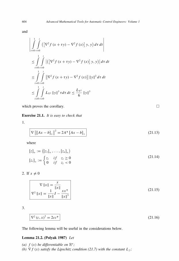
604 Advanced Mathematical Tools for Automatic Control Engineers: Volume 1
and ∣∣∣∣∣∣1∫
t=0
t∫τ=0
([∇2f (x + τy)− ∇2f (x)]y, y
)dτ dt
∣∣∣∣∣∣≤
1∫t=0
t∫τ=0
∣∣([∇2f (x + τy)− ∇2f (x)]y, y
)∣∣ dτ dt≤
1∫t=0
t∫τ=0
∥∥∇2f (x + τy)− ∇2f (x)∥∥ ‖y‖2 dτ dt
≤1∫
t=0
t∫τ=0
L∇2 ‖y‖3 τdτ dt ≤ L∇2
6‖y‖3
which proves the corollary. �
Exercise 21.1. It is easy to check that
1.
∇ ∥∥[Ax − b]+∥∥2 = 2Aᵀ [Ax − b]+ (21.13)
where
[z]+ :=([z1]+ , . . . , [zn]+
)[zi]+ :=
{zi if zi ≥ 0
0 if zi < 0
(21.14)
2. If x �= 0
∇ ‖x‖ = x
‖x‖∇2 ‖x‖ = 1
‖x‖I −xxᵀ
‖x‖3(21.15)
3.
∇2 (c, x)2 = 2ccᵀ (21.16)
The following lemma will be useful in the considerations below.
Lemma 21.2. (Polyak 1987) Let
(a) f (x) be differentiable on Rn;(b) ∇f (x) satisfy the Lipschitz condition (21.7) with the constant Lf ;

Finite-dimensional optimization 605
(c) f (x) be bounded from below, i.e., f (x) ≥ f ∗ > −∞ for all x ∈ Rn.
Then
‖∇f (x)‖2 ≤ 2Lf (f (x)− f ∗) (21.17)
Proof. Putting in (21.8) y := −L−1f ∇f (x) we obtain
f ∗ ≤ f (x + y) = f (x − L−1f ∇f (x))
≤ f (x)− (∇f (x), L−1f ∇f (x)
)+ Lf2
∥∥L−1∇f (x)∥∥2
= f (x)− 1
2Lf
∥∥L−1f ∇f (x)
∥∥2
which implies (21.17). Lemma is proven. �
21.1.2 Convex functions
21.1.2.1 Main definitionDefinition 21.2. A scalar valued function f (x) defined on Rn is said to be
1. convex (see Fig. 21.1) if for any x, y ∈ Rn and any α ∈ [0, 1]
f (αx + (1− α) y) ≤ αf (x)+ (1− α) f (y) (21.18)
2. strictly convex if for any x �= y ∈ Rn and any α ∈ [0, 1]
f (αx + (1− α) y) < αf (x)+ (1− α) f (y) (21.19)
f (x)
f (y)
�x 1y(12�)
�f (x)1(12�) f (y)
(y)
yx
f(�x 1y(12�) )
Fig. 21.1. A convex function.

606 Advanced Mathematical Tools for Automatic Control Engineers: Volume 1
3. strongly convex with the constant l > 0 if for any x, y ∈ Rn and any α ∈ [0, 1]
f (αx + (1− α) y) ≤ αf (x)+ (1− α) f (y)
− lα (1− α) ‖x − y‖2(21.20)
4. concave (strictly, strongly with the given constant) if the function [−f (x)] is convex(strictly, strongly with the same constant).
21.1.2.2 Some properties of convex (not obligatory differentiable) functionsClaim 21.1. From Definition 21.2 it follows directly that
(a) the affine function f (x) = (a, x)+ b is both convex and concave;(b) if the functions fi (x) are convex (concave) then the functions
f (x) =k∑i=1
γifi (x), γi ≥ 0 (i = 1, . . . , k)
and
f (x) = maxi=1,...,k
fi (x)
are convex (concave) too.
Claim 21.2. If f (x) is convex on Rn, then for any x(1), . . . , x(k) ∈ Rn and anyα1, . . . , αk such that αi ≥ 0 (i = 1, . . . , k),
∑k
i=1 αi = 1 the following inequality holds
f
(k∑i=1
αix(i)
)≤
k∑i=1
αif(x(i)
)(21.21)
Proof. It follows directly from the Jensen inequality (16.152). �
Lemma 21.3. Any convex function is continuous.
Proof. Let us prove this result by contradiction. Suppose that there exists a point x where
a convex function f (x) is discontinuous. This means that in any δ-neighborhood of x,
containing x as an internal point, there are always two points x ′ and x ′′ such that
|f (x ′)− f (αx ′′ + (1− α) x ′)| > ε > 0 for any 0 < α− < α < α+ < 1. Assuming that
f (x ′)≥ f (x ′′), we have f (x ′)+ ε > f (x ′′). But, by the convexity property, we also have
f(αx ′′ + (1− α) x ′) ≤ αf (
x ′′)+ (1− α) f (
x ′)
for any α ∈ [0, 1], or equivalently,
f (x ′)+ ε > f (x ′′) ≥ f (x ′)+ 1
α[f (αx ′′ + (1− α) x ′)− f (x ′)] ≥ f (x ′)+ ε
α
which, for α satisfying 0 < α− < α < α+ < 1, implies contradiction. �

Finite-dimensional optimization 607
Corollary 21.2. If f (x) is convex, then the set
Qα := {x ∈ Rn | f (x) ≤ α} (21.22)
is convex and closed.
Lemma 21.4. Any convex function f (x) at any arbitrary point has a one side deriva-tive in any direction y and this derivative is uniformly bounded with respect to thisdirection.
Proof. One has
f ′+ (x, y) := limα→+0
f (x + αy)− f (x)α
= limα→+0
f ((1− α) x + α (x + y))− f (x)α
≤ limα→+0
αf (x + y)+ (1− α) f (x)− f (x)α
≤ f (x + y)− f (x) ≤ maxz:‖z‖=‖y‖
[f (x + z)− f (x)]
(21.23)
which completes the proof. �
Corollary 21.3. (Rademacher theorem) Any convex function is differentiable almosteverywhere (excepting a set of measure zero).
21.1.2.3 Some properties of convex differentiable functionsLemma 21.5. If a function f (x) on Rn is differentiable, then
1. its convexity is equivalent to the inequality
f (x + z) ≥ f (x)+ (∇f (x), z) (21.24)
valid for all x, y ∈ Rn;2. its strict convexity is equivalent to the inequality
f (x + z) > f (x)+ (∇f (x), z) (21.25)
valid for all x ∈ Rn and all z �= 0 (z ∈ Rn);3. its strong convexity is equivalent to the inequality
f (x + z) ≥ f (x)+ (∇f (x), z)+ l
2‖z‖2 (21.26)
valid for all x, z ∈ Rn.
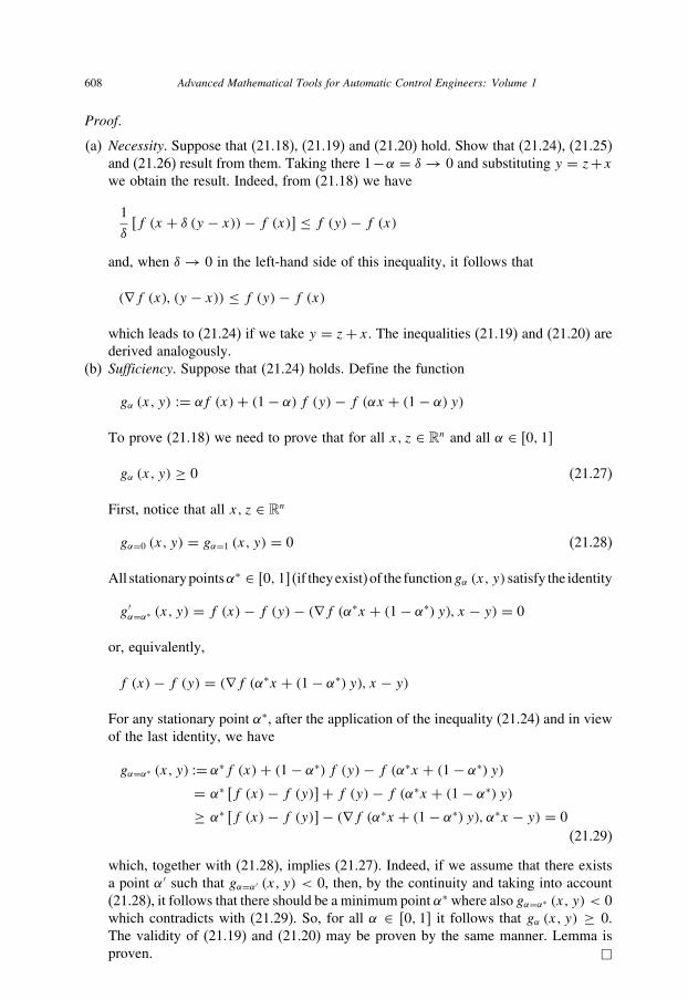
608 Advanced Mathematical Tools for Automatic Control Engineers: Volume 1
Proof.
(a) Necessity. Suppose that (21.18), (21.19) and (21.20) hold. Show that (21.24), (21.25)
and (21.26) result from them. Taking there 1−α = δ→ 0 and substituting y = z+xwe obtain the result. Indeed, from (21.18) we have
1
δ[f (x + δ (y − x))− f (x)] ≤ f (y)− f (x)
and, when δ→ 0 in the left-hand side of this inequality, it follows that
(∇f (x), (y − x)) ≤ f (y)− f (x)
which leads to (21.24) if we take y = z+ x. The inequalities (21.19) and (21.20) are
derived analogously.
(b) Sufficiency. Suppose that (21.24) holds. Define the function
gα (x, y) := αf (x)+ (1− α) f (y)− f (αx + (1− α) y)
To prove (21.18) we need to prove that for all x, z ∈ Rn and all α ∈ [0, 1]
gα (x, y) ≥ 0 (21.27)
First, notice that all x, z ∈ Rn
gα=0 (x, y) = gα=1 (x, y) = 0 (21.28)
All stationarypointsα∗ ∈ [0, 1] (if theyexist) of the functiongα (x, y) satisfy the identity
g′α=α∗ (x, y) = f (x)− f (y)− (∇f (α∗x + (1− α∗) y), x − y) = 0
or, equivalently,
f (x)− f (y) = (∇f (α∗x + (1− α∗) y), x − y)
For any stationary point α∗, after the application of the inequality (21.24) and in view
of the last identity, we have
gα=α∗ (x, y) := α∗f (x)+ (1− α∗) f (y)− f (α∗x + (1− α∗) y)= α∗ [f (x)− f (y)]+ f (y)− f (α∗x + (1− α∗) y)≥ α∗ [f (x)− f (y)]− (∇f (α∗x + (1− α∗) y), α∗x − y) = 0
(21.29)
which, together with (21.28), implies (21.27). Indeed, if we assume that there exists
a point α′ such that gα=α′ (x, y) < 0, then, by the continuity and taking into account
(21.28), it follows that there should be a minimum point α∗ where also gα=α∗ (x, y) < 0
which contradicts with (21.29). So, for all α ∈ [0, 1] it follows that gα (x, y) ≥ 0.
The validity of (21.19) and (21.20) may be proven by the same manner. Lemma is
proven. �
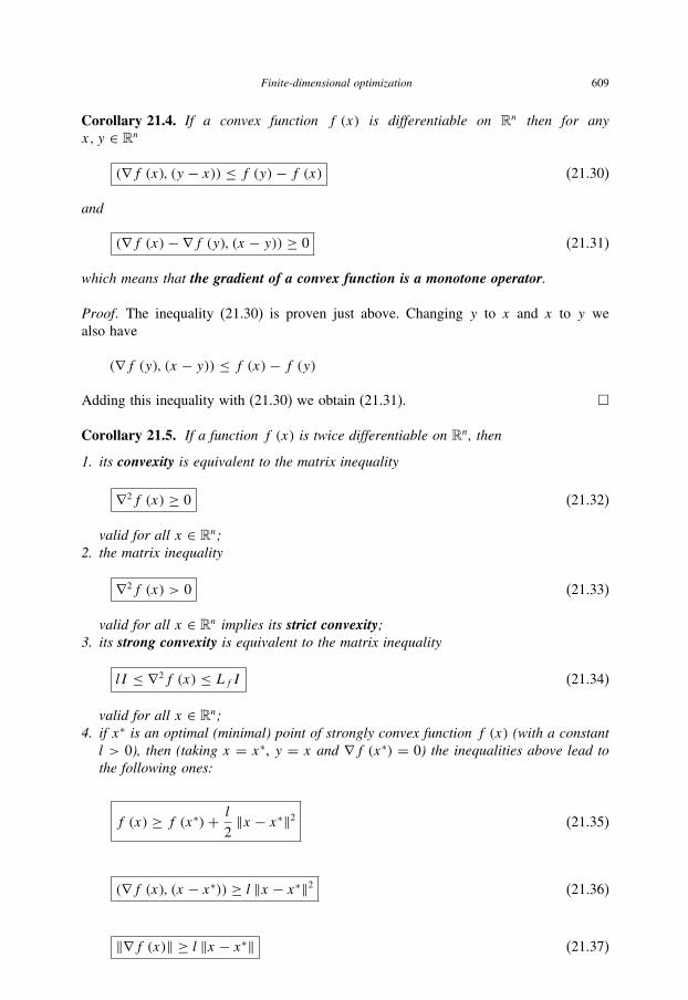
Finite-dimensional optimization 609
Corollary 21.4. If a convex function f (x) is differentiable on Rn then for anyx, y ∈ Rn
(∇f (x), (y − x)) ≤ f (y)− f (x) (21.30)
and
(∇f (x)− ∇f (y), (x − y)) ≥ 0 (21.31)
which means that the gradient of a convex function is a monotone operator.
Proof. The inequality (21.30) is proven just above. Changing y to x and x to y we
also have
(∇f (y), (x − y)) ≤ f (x)− f (y)
Adding this inequality with (21.30) we obtain (21.31). �
Corollary 21.5. If a function f (x) is twice differentiable on Rn, then
1. its convexity is equivalent to the matrix inequality
∇2f (x) ≥ 0 (21.32)
valid for all x ∈ Rn;2. the matrix inequality
∇2f (x) > 0 (21.33)
valid for all x ∈ Rn implies its strict convexity;3. its strong convexity is equivalent to the matrix inequality
lI ≤ ∇2f (x) ≤ Lf I (21.34)
valid for all x ∈ Rn;4. if x∗ is an optimal (minimal) point of strongly convex function f (x) (with a constantl > 0), then (taking x = x∗, y = x and ∇f (x∗) = 0) the inequalities above lead tothe following ones:
f (x) ≥ f (x∗)+ l
2‖x − x∗‖2 (21.35)
(∇f (x), (x − x∗)) ≥ l ‖x − x∗‖2 (21.36)
‖∇f (x)‖ ≥ l ‖x − x∗‖ (21.37)

610 Advanced Mathematical Tools for Automatic Control Engineers: Volume 1
Example 21.1.
1. The function f (x) = x2 is strongly convex (and, hence, convex and strictly convex)with l = 2.
2. The functions f (x) = x4 and f (x) = ex are strictly convex (and, hence, convex, butnot strongly convex).
The next two lemmas will be used hereinafter.
Lemma 21.6. (Polyak 1987) Let
(a) f (x) be convex and twice differentiable on Rn;(b) ∇f (x) satisfies the Lipschitz condition (21.7) with the constant Lf .
Then for all x, y ∈ Rn
(∇f (x)− ∇f (y), x − y) ≥ L−1f ‖∇f (x)− ∇f (y)‖2 (21.38)
Proof. By (21.6) we have
∇f (y)=∇f (x)+1∫
τ=0
d
dτ∇f (x + τ (y − x)) dτ
=∇f (x)+1∫
τ=0
∇2f (x + τ (y − x)) (y − x) dτ = A (y − x)
where, by the strict convexity condition and the property (21.32),
A = Aᵀ :=1∫
τ=0
∇2f (x + τ (y − x)) dτ ≥ 0
which, implies (in view of the inequalities ‖A‖ I ≥ A and ‖A‖ ≤ Lf )
(∇f (y)− ∇f (x), (y − x)) = (y − x)ᵀA (y − x)
= 1
‖A‖ (y − x)ᵀA1/2 (‖A‖ I )A1/2 (y − x)
≥ 1
‖A‖ (y − x)ᵀA1/2AA1/2 (y − x)
= 1
‖A‖ (y − x)ᵀAᵀA (y − x) = 1
‖A‖ ‖A (y − x)‖2
≥ 1
Lf‖A (y − x)‖2 = 1
Lf‖∇f (y)− ∇f (x)‖2
Lemma is proven. �

Finite-dimensional optimization 611
Lemma 21.7. If
1. the function f (x) is differentiable strongly convex on Rn (see (21.20)) with the constantl > 0,
2. x∗ is its minimum point, then for all x ∈ Rn
‖∇f (x)‖2 ≥ 2l [f (x)− f (x∗)] (21.39)
Proof. The inequality (21.26) can be rewritten as follows
∥∥∥∥∥√
1
2l∇f (x)
∥∥∥∥∥2
≥ f (x)− f (x + z)+∥∥∥∥∥√
1
2l∇f (x)+
√l
2z
∥∥∥∥∥2
which, for z := x∗ − x, leads to the following inequality
1
2l‖∇f (x)‖2 ≥ f (x)− f (x∗)+
∥∥∥∥∥√
1
2l∇f (x)+
√l
2z
∥∥∥∥∥2
≥ f (x)− f (x∗)
which completes the proof. �
21.2 Unconstrained optimization
21.2.1 Extremum conditions
Definition 21.3.
• The point x∗ is called a local minimum of f (x) on Rn if there exists δ > 0 such thatf (x) ≥ f (x∗) for all x satisfying ‖x − x∗‖ ≤ δ.
• The point x∗ is called a global minimum (simply minimum) of the function f (x) onRn if f (x) ≥ f (x∗) for all x ∈ Rn.
21.2.1.1 Necessary conditionsTheorem 21.1. (on necessary conditions) Let x∗ be a local minimum of f (x) on Rn.
1. The first-order necessary condition (Fermat). If f (x) is differentiable at x∗, then
∇f (x∗) = 0 (21.40)
2. The second-order necessary condition. If f (x) is twice differentiable at x∗, then
∇2f (x∗) ≥ 0 (21.41)
Proof. To prove (1) suppose that ∇f (x∗) �= 0. Then τ > 0 we have
f (x∗ − τ∇f (x∗))= f (x∗)+ (∇f (x∗),−τ∇f (x∗))+ o (τ)= f (x∗)− τ ‖∇f (x∗)‖2 + o (τ) > f (x∗)

612 Advanced Mathematical Tools for Automatic Control Engineers: Volume 1
for small enough τ which contradicts the fact that x∗ is a minimum. So, (21.40) holds.
To prove (2) let us use (21.2) which for any y ∈ Rn and a small positive τ > 0
gives
f (x∗)≤ f (x∗ + τy)= f (x∗)+ (∇f (x∗), τy)+ (∇2f (x∗) τy, τy
)+ o (τ 2)= f (x∗)+ τ 2 (∇2f (x∗) y, y
)+ o (τ 2)or, equivalently,
0 ≤ τ 2 (∇2f (x∗) y, y)+ o (τ 2)
Dividing by τ 2 and tending τ to zero implies(∇2f (x∗) y, y
)which is equivalent to
(21.41). Theorem is proven. �
21.2.1.2 Sufficient conditionsTheorem 21.2.
1. The first-order sufficient condition. Let f (x) be a convex on Rn function differentiableat a point x∗ such that the first-order necessary condition (21.40) holds, that is,∇f (x∗) = 0. Then x∗ is a global minimum point of f (x) on Rn.
2. The second-order sufficient condition. Let f (x) be twice differentiable at a pointx∗ and
∇f (x∗) = 0, ∇2f (x∗) > 0 (21.42)
Then x∗ is a local minimum point.
Proof. The first-order sufficient condition follows directly from (21.24) since for any
z ∈ Rn
f (x∗ + z) ≥ f (x∗)+ (∇f (x∗), z) = f (x∗)
The second-order sufficient condition follows from the Taylor formula (21.2) since
f (x∗ + τz)=f (x∗)+ (∇f (x∗), τz)+τ 2 (∇2f (x∗) y, y
)+ o (τ 2 ‖y‖2) ≥ f (x∗)+τ 2λmin
(∇2f (x∗)) ‖y‖2 + o (τ 2 ‖y‖2) ≥ f (x∗)
for small enough τ > 0 which proves the result. �
21.2.2 Existence, uniqueness and stability of a minimum
21.2.2.1 Existence of a minimumTheorem 21.3. (Weierstrass) If(a) f (x) is continuous on Rn,

Finite-dimensional optimization 613
(b) the set
Qα := {x ∈ Rn | f (x) ≤ α} (21.43)
is nonempty and bounded for some α ∈ R.Then there exists a global minimum of f (x) on Rn.
Proof. For some vector-sequence{x(k)
}we have
f(x(k)
)→ infx∈Rnf (x) < α as k→∞
Then x(k) ∈ Qα for large enough k. But the set Qα is a compact and, hence, the sequence{x(k)
}has a limit x∗ ∈ Qα . But from the continuity of f (x) it follows that f (x∗) =
infx∈Rnf (x) which proves the theorem. �
21.2.2.2 Uniqueness of a minimumDefinition 21.4.
1. A minimum point is called locally unique if there are no other minimum points insome neighborhood of this point.
2. x∗ is said to be a nonsingular minimum point if the second-order sufficient conditions(21.42) hold, that is, if ∇f (x∗) = 0, ∇2f (x∗) > 0.
Theorem 21.4. A nonsingular minimum point is locally unique.
Proof. Suppose that x∗ is a nonsingular minimum point, but there exists another minimum
point x∗∗ �= x∗ in any small neighborhood of x∗, that is, f (x∗) = f (x∗∗)when ‖x∗∗ − x∗‖< δ for any small enough δ. Then we have
f (x∗∗)= f (x∗ + (x∗∗ − x∗)) = f (x∗)+ (∇f (x∗), x∗∗ − x∗)+ (∇2f (x∗) (x∗∗ − x∗), (x∗∗ − x∗))+ o (‖x∗∗ − x∗‖2)
= f (x∗)+ (∇2f (x∗) (x∗∗ − x∗), (x∗∗ − x∗))+ o (‖x∗∗ − x∗‖2) > f (x∗)since(∇2f (x∗) (x∗∗ − x∗), (x∗∗ − x∗)) > o (‖x∗∗ − x∗‖2)So, we have obtained the contradiction that x∗ is a minimum point. Theorem is proven.
�Proposition 21.1. A minimum point of a strictly convex function is globally unique.
Proof. It follows directly from the definition (21.19). Indeed, putting in (21.19) y := x∗we get (for α > 0)
0 <1
α[f (y + α (x − y))− f (y)]
= 1
α[f (x∗ + α (x − x∗))− f (x∗)] < f (x)− f (x∗)
�
614 Advanced Mathematical Tools for Automatic Control Engineers: Volume 1
21.2.2.3 Stability of a minimumDefinition 21.5. A local minimum point x∗ of f (x) is called
(a) locally stable if every local minimizing sequence converges to x∗, that is, there existsδ > 0 such that
f(x(k)
) →k→∞ f (x
∗),∥∥x(k) − x∗∥∥ ≤ δ
implies
x(k) →k→∞ x
∗
(b) globally stable if any minimizing sequence converges to x∗.
Theorem 21.5. (Polyak 1987) A local minimum point x∗ of a continuous function f (x)is locally stable if it is locally unique.
Proof. Let{x(k)
}be a local minimizing sequence. By the compactness of a unit sphere
in Rn, from any sequence there can be extracted a convergent subsequence, namely, there
exists{x(ki )
}such that x(ki ) → x. But from the definition of a local minimizing sequence
one gets ‖x − x∗‖ ≤ δ. By the continuity property, we have
f (x) = limi→∞f
(x(ki )
) = f (x∗)which implies x = x∗ since x∗ is a local minimum point. The same is true for any other
convergent subsequence, so, x(k) → x∗, and therefore x∗ is locally stable. �
The next result turns out to be often useful in different applications.
Lemma 21.8. (on regularized (perturbed) functions) The stability property impliesthat a minimum point of a nonperturbed functions is closed to a minimum point of aperturbed function, namely, if x∗ is a nonsingular minimum point of f (x) and g (x) iscontinuously differentiable in a neighborhood of x∗, then, for sufficiently small ε > 0,the function Fε (x) := f (x)+ εg (x) has a local minimum point x∗ε in a neighborhood ofx∗, and
x∗ε = x∗ − ε[∇2f (x∗)
]−1 ∇g (x∗)+ o (ε) (21.44)
Proof. By Definition 21.4 it follows that x∗ε satisfies
∇Fε(x∗ε) = ∇f (
x∗ε)+ ε∇g (x∗ε ) = 0

Finite-dimensional optimization 615
and, hence, we have
0= ∇Fε(x∗ε) = ∇f (
x∗ε)+ ε∇g (x∗ε )
= ∇f (x∗ + (
x∗ε − x∗))+ ε∇g (x∗ε ) = ∇2f (x∗)
(x∗ε − x∗
)+ ε [∇g (x∗)+ (∇g (x∗ε )− ∇g (x∗))]+ o(∥∥x∗ε − x∗∥∥2
)By the continuity property of ∇g (x) at the point x = x∗ it follows that for any ε > 0
there exists δ > 0 such that ‖x − x∗‖ ≤ δ implies ‖∇g (x)− ∇g (x∗)‖ < ε. Takinghere x := x∗ε , δ := kε (where, maybe, k < 1) and ε := ε, from the last identity it
follows that
0 = ∇2f (x∗)(x∗ε − x∗
)+ ε∇g (x∗)+ o (ε)which implies (21.44). Lemma is proven. �
Remark 21.1. When g (x) ≥ 0 for all x ∈ Rn then g (x) is usually called a regularizingterm and the function Fε (x) is called the regularized function.
21.2.3 Some numerical procedure of optimization
Let us consider the following numerical procedure for finding a minimum point
x∗ ∈ Rn of the function f (x) on Rn using only the value of its gradient ∇f (xn) in a
current point xn:
xn+1 = xn − γnHn+1∇f (xn)
x0 = x, n = 0, 1, 2, . . .
0 < γn ∈ R, 0 < Hn = Hᵀn ∈ Rn×n
(21.45)
21.2.3.1 Strong (argument) convergenceTheorem 21.6. (on strong (argument) convergence)Assume that
1. x∗ is an optimal point of strongly convex differentiable function f (x) with a constantl > 0 (such point always exists by Proposition (21.1));
2. ∇f (x) satisfies the Lipschitz condition (21.7) with the constant Lf ;3. for any n = 0, 1, . . .
αn := λmax
(H 1/2n H
−1n+1H
1/2n
)− 2γnlλmin (Hn)
+ γ 2n L
2f λmax (Hn+1) λmax (Hn) ≤ q < 1
(21.46)
Then for the sequence {xn} generated by (21.45) with any initial conditions x we havethe following exponential convergence:
Wn := ‖xn − x∗‖2H−1n= O (qn) = O ([
eln q]n)→ 0 (21.47)
whereas n→∞.

616 Advanced Mathematical Tools for Automatic Control Engineers: Volume 1
Proof. We have the following recursion:
Wn+1 := ‖xn+1 − x∗‖2H−1n+1
= ‖(xn − x∗)− γnHn+1∇f (xn)‖2H−1n+1
= ‖xn − x∗‖2H−1n+1
− 2(γnH
−1n+1Hn+1∇f (xn), xn − x∗
)+ ‖γnHn+1∇f (xn)‖2H−1n+1
= ‖xn − x∗‖2H−1/2n
(H
1/2n H−1
n+1H1/2n
)H−1/21
− 2γn (∇f (xn), xn − x∗)+ γ 2n ‖∇f (xn)‖2Hn+1
(21.48)
Recall that
H−1n+1 = H−1/2
n
(H 1/2n H
−1n+1H
1/2n
)H−1/2n ≤ λmax
(H 1/2n H
−1n+1H
1/2n
)H−1n
By the condition (21.36),
(∇f (xn), xn − x∗) ≥ l ‖xn − x∗‖2
and by (21.7)
‖∇f (xn)− ∇f (x∗)‖ = ‖∇f (xn)‖ ≤ Lf ‖xn − x∗‖
We also have
‖xn − x∗‖2 =((xn − x∗),H−1/2
n HnH−1/2n (xn − x∗)
)λmin (Hn)Wn ≤ ‖xn − x∗‖2 ≤ λmax (Hn)Wn
Substitution of these inequalities into (21.48) implies
Wn+1 ≤ λmax
(H 1/2n H
−1n+1H
1/2n
) ‖xn − x∗‖2H−1n
− 2γnl ‖xn − x∗‖2 + γ 2n L
2f λmax (Hn+1) ‖xn − x∗‖2
≤ λmax
(H 1/2n H
−1n+1H
1/2n
)Wn − 2γnlλmin (Hn)Wn
+ γ 2n L
2f λmax (Hn+1) λmax (Hn)Wn
= αnWn ≤ qWn ≤ · · · ≤ qnW0 → 0
Theorem is proven. �
Corollary 21.6. (on the gradient method convergence) If in(21.45) we take
γn := γ, Hn := I (21.49)
Finite-dimensional optimization 617
we get the gradient method
xn+1 = xn − γ∇f (xn), x0 = x, n = 0, 1, 2, . . .
0 < γ < 2l/L2f
(21.50)
which converges exponentially as
Wn := ‖xn − x∗‖2 = O (qn)
with
q = 1− γ (2l − γL2f
)Corollary 21.7. (on the modified Newton’s method) If in (21.45) we take
γn := γ, Hn :=[∇2f (xn−1)
]−1(21.51)
we get the modified Newton’s method
xn+1 = xn − γ[∇2f (xn)
]−1 ∇f (xn)x0 = x, n = 0, 1, 2, . . .
γ = l3/L3f
(21.52)
which converges exponentially as
Wn := ‖xn − x∗‖2H−1n= O (qn)
with
αn := λmax
(H 1/2n H
−1n+1H
1/2n
)− 2γ lλmin (Hn)
+ γ 2L2f λmax (Hn+1) λmax (Hn)
≤ Lf /l − 2γ l/Lf + γ 2L2f / l
2 = Lf /l − l4/L4f := q < 1
within the class of strongly convex functions satisfying
0.755 ≤ l/Lf < 1
Proof. It follows from the estimates (in view of (21.34)) that
λmax (Hn+1) = λmax
([∇2f (xn)]−1
)= 1
λmin
([∇2f (xn)]
) ≤ l−1
λmin (Hn) = 1
λmax
([∇2f (xn)]
) ≥ 1/Lf
(21.53)
618 Advanced Mathematical Tools for Automatic Control Engineers: Volume 1
and
λmax
(H 1/2n H
−1n+1H
1/2n
) ≤ λmax
(H−1n+1
)λmax (Hn)
= λmax
(∇2f (xn))λmax
([∇2f (xn)]−1
)≤ Lf 1
λmin
(∇2f (xn)) ≤ Lf /l
if we use them in (21.46). Moreover, defining x := l/Lf < 1, we get
q = Lf /l − l4/L4f = x−1 − x4 < 1
if x ≥ 0.755. �
Below we show that there exist other modifications of Newton’s method working
within much wider classes of functions.
21.2.3.2 Weak (functional) convergenceTheorem 21.7. (on weak (functional) convergence) Assume that
1. the function f (x) is differentiable and is bounded from below, i.e.,
f (x) ≥ f ∗ > −∞ (21.54)
2. ∇f (x) satisfies the Lipschitz condition (21.7) with the constant Lf ;3. for all n = 0, 1, 2, . . .
λmax (Hn+1) ≤ λ+
γn ≤ γ := 2 (1− κ)
Lf λ+, κ ∈ (0, 1)
γnλmin (Hn+1) ≥ c− > 0
(21.55)
Then for the sequence {xn} generated by (21.45) with any initial conditions x we havethe following property:
f (xn+1) ≤ f (xn)‖∇f (xn)‖ → 0 as n→∞ (21.56)
whereas n→∞.
Proof. By (21.3) and (21.53) we have
f (xn+1)= f (xn)− γn ‖∇f (xn)‖2Hn+1
− γn1∫
τ=0
(∇f (xn − τγnHn+1∇f (xn))− ∇f (xn),Hn+1∇f (xn)) dτ
≤ f (xn)− γn ‖∇f (xn)‖2Hn+1+ γ 2
n
Lf
2‖Hn+1∇f (xn)‖2
≤ f (xn)− γn(1− γn Lf
2λmax (Hn+1)
)‖∇f (xn)‖2Hn+1
≤ f (xn)− γnκ ‖∇f (xn)‖2Hn+1
≤ f (xn)− κγnλmin (Hn+1) ‖∇f (xn)‖2
Finite-dimensional optimization 619
or, equivalently,
c− ‖∇f (xn)‖2 ≤ γnλmin (Hn+1) ‖∇f (xn)‖2
≤ κ−1 [f (xn)− f (xn+1)]
(21.57)
We also have
f (xn+1) ≤ f (xn)
which, by the Weierstrass theorem 14.9 in view of the boundedness from below, implies
the existence of the limit
limn→∞f (xn) = f > −∞
Summing the inequalities (21.57) on n = 0, 1, .., T and taking T →∞, we get
∞∑n=0
‖∇f (xn)‖2 ≤ (κc−)−1[f (x0)− f
]<∞
which implies ‖∇f (xn)‖ → 0 as n→∞. Theorem is proven. �
Corollary 21.8. (on the gradient method) If in (21.45) we take
γn := γ, Hn := I
we get the gradient method
xn+1 = xn − γ∇f (xn), x0 = x, n = 0, 1, 2, . . .
0 < γn ≤ γ := 2 (1− κ)
Lf
for which
limn→∞f (xn) = f > −∞, f (xn+1) ≤ f (xn)‖∇f (xn)‖ → 0 as n→∞
(21.58)
for any initial conditions x ∈ Rn.
Corollary 21.9. (on the modified Newton’s method) If in(21.45) we take
γn := γ, Hn :=[∇2f (xn−1)
]−1

620 Advanced Mathematical Tools for Automatic Control Engineers: Volume 1
and if we get the modified Newton’s method
xn+1 = xn − γ[∇2f (xn)
]−1 ∇f (xn)x0 = x, n = 0, 1, 2, . . .
0 < γ ≤ γ := 2 (1− κ)
Lf λ+
then again (21.58) is valid.
Remark 21.2. (One more modification) Let the function f (x) be twice differentiable,its second derivative satisfies the Lipschitz condition with the constant L∇2 and be stronglyconvex (with the constant l > 0) on Rn. Taking in (21.45)
γn :=
⎧⎪⎪⎨⎪⎪⎩γ ≤ γ = 2 (1− κ) l
L∇2
, κ ∈ (0, 1) if ‖∇f (xn)‖ ≥ 2l2
L∇2
1 if ‖∇f (xn)‖ < 2l2
L∇2
Hn :=[∇2f (xn−1)
]−1
we get the modified Newton’s method with a switched step-parameter for which, at theend of optimization, we obtain the, so-called, “quadratic” exponential convergence
‖xn − x∗‖ ≤ 2l
Lfq2
n
, q = Lf2l2
‖∇f (xn∗)‖
xn∗ := infn=0,1,2,...
{xn | L∇2
2l2‖∇f (xn)‖ < 1
} (21.59)
starting from xn∗ which is sufficiently close to the minimum point x∗ such that
L∇2
2l2‖∇f (xn∗)‖ < 1
Proof. First, notice that in this case λmax (Hn+1) ≤ λ+ = l−1. Evidently, by Theorem
21.7 we have ‖∇f (xn)‖ → 0 as n → ∞, and, hence, there exists the number n∗ for
whichL∇2
2l2‖∇f (xn∗)‖ < 1. Consider n ≥ n∗. Taking x = xn and y := −γ [∇2f (xn)
]−1
∇f (xn) in the inequality∥∥∇f (x + y)− ∇f (x)− ∇2f (x) y
∥∥ ≤ L∇2
2‖y‖2 we get
xn+1 = x + y and∥∥∥∇f (xn+1)− ∇f (xn)− ∇2f (xn)
(− [∇2f (xn)
]−1 ∇f (xn))∥∥∥
= ‖∇f (xn+1)‖ ≤ L∇2
2
∥∥∥[∇2f (xn)]−1
∥∥∥2 ‖∇f (xn)‖2 ≤ L∇2
2l2‖∇f (xn)‖2
Denoting zn := ‖∇f (xn)‖ we obtain zn+1 ≤(L∇2/2l2
)z2n. Integrating this inequality
we get zn ≤ 2l2
L∇2
q2n
. Applying then the inequality (21.37) we get (21.59). Corollary is
proven. �

Finite-dimensional optimization 621
Many other methods of unconstrained optimization can be found in (Polyak 1987) and
the references within.
21.3 Constrained optimization
21.3.1 Elements of convex analysis
21.3.1.1 Convex setsDefinition 21.6.
1. A set Q ⊆ Rn is convex if it contains any segment with the endpoints lying in Q, i.e.,λx + (1− λ) y ∈ Q for any λ ∈ [0, 1] whenever x, y ∈ Q.
2. The convex hull conv Q of a set Q ⊆ Rn is an intersection of all convex setscontaining Q, or, equivalently, Carathéodory’s lemma, see Rockafellar (1970),
conv Q ={x =
n+1∑i=1
λixi | xi ∈ Q, λi ≥ 0,
n+1∑i=1
λi = 1
}(21.60)
Claim 21.3.
• It is easy to check that• if Q is bounded and closed then
conv Q = Q• if Q is convex then the sets
αQ := {x = αx ′ ∈ Rn | α ∈ R, x ′ ∈ Q}AQ := {
x = Ax ′ ∈ Rn | A ∈ Rn×m, x ′ ∈ Q}are convex too;
• if Q1 and Q2 are convex then Q1 ∩Q2 is convex.
Claim 21.4. For a convex function f (x) the set
Qα := {x ∈ Rn | f (x) ≤ α} (21.61)
is convex.
Proof. Let x ′, x ′′ ∈ Qα . Then, by the convexity property (21.18),
f (λx ′ + (1− λ) x ′′)≤ λf (x ′)+ (1− λ) f (x ′′)≤ λα + (1− λ) α = α
which means that z := λx ′ + (1− λ) x ′′ ∈ Qα . �
Definition 21.7. A function f (x) is called quasi-convex if the setsQα (21.61) are convexfor any α.

622 Advanced Mathematical Tools for Automatic Control Engineers: Volume 1
Remark 21.3. If the setsQα are convex, then f (x) is not obligatory convex, for example,f (x) = e−x2 .
21.3.1.2 Projections and their propertiesDefinition 21.8. The projection of the point x ∈ Rn onto the set Q ⊆ Rn is a pointπQ {x} ∈ Q such that
πQ {x} = argminy∈Q
‖x − y‖ (21.62)
Proposition 21.2. The following assertions seem to be evident:
(a) If x ∈ Q then
πQ {x} = x(b)
πQ {x} = argminy∈Q
‖x − y‖2
(c) If Q is closed convex then πQ {x} is unique, since φ (y) := ‖x − y‖2 is a strictlyconvex function and, hence, has a unique minimum point.
Lemma 21.9. If Q is closed convex then
1. for all x ∈ Rn and all y ∈ Q(x − πQ {x}, y − πQ {x}
) ≤ 0 (21.63)
2. for all x, y ∈ Rn
∥∥πQ {x} − πQ {y}∥∥ ≤ ‖x − y‖ (21.64)
Proof.
1. Since, by Definition 21.8 and in view of the closeness and the convexity of Q, for any
y ∈ Q we have∥∥x − πQ {x}∥∥2 ≤ ‖x − y‖2
and ∥∥x − πQ {x}∥∥2 = ∥∥(x − y)+ (y − πQ {x}
)∥∥2 = ‖x − y‖2
+ 2(x − πQ {x}, y − πQ {x}
)+ ∥∥y − πQ {x}∥∥2 ≤ ‖x − y‖2
or, equivalently,
2(x − πQ {x}, y − πQ {x}
) ≤ −∥∥y − πQ {x}∥∥2 ≤ 0

Finite-dimensional optimization 623
2. By Definition 21.8 we have∥∥πQ {x} − πQ {y}∥∥2 ≤ ∥∥x − πQ {y}∥∥2
∥∥πQ {y} − πQ {x}∥∥2 ≤ ∥∥y − πQ {x}∥∥2
Summing both inequalities with the weights α ∈ [0, 1] and (1− α) one gets:∥∥πQ {x} − πQ {y}∥∥2 ≤ α ∥∥x − πQ {y}∥∥2 + (1− α)∥∥y − πQ {x}∥∥2
= α ∥∥(x − y)+ (y − πQ {y}
)∥∥2 + (1− α)∥∥(y − x)+ (x − πQ {x}
)∥∥2
= ‖x − y‖2 + α ∥∥y − πQ {y}∥∥2 + (1− α)∥∥x − πQ {x}∥∥2
+ 2α(x − y, y − πQ {y}
)+ 2 (1− α) (y − x, x − πQ {x})= ‖x − y‖2 + α ∥∥y − πQ {y}∥∥2 + (1− α)∥∥x − πQ {x}∥∥2
+ 2α([x − πQ {y}]− [y − πQ {y}], y − πQ {y}
)+ 2 (1− α) ([y − πQ {x}]− [x − πQ {x}], x − πQ {x}
) = ‖x − y‖2+ 2
(α [x − πQ {x}], [y − πQ {y}]
)+ 2(x − πQ {x}, (1− α) [y − πQ {y}]
)− α ∥∥y − πQ {y}∥∥2 − (1− α)∥∥x − πQ {x}∥∥2 ≤ ‖x − y‖2+ 2
√α∥∥x − πQ {x}∥∥∥∥y − πQ {y}∥∥
+ 2√1− α ∥∥x − πQ {x}∥∥∥∥y − πQ {y}∥∥
− α ∥∥y − πQ {y}∥∥2 − (1− α)∥∥x − πQ {x}∥∥2 ≤ ‖x − y‖2
−(√
1− α ∥∥x − πQ {x}∥∥2 −√α∥∥x − πQ {x}∥∥)2 ≤ ‖x − y‖2
Lemma is proven. �
21.3.1.3 Separation theoremsHere we will formulate and prove the theorem, named the separation theorem, see
Fig. 21.2 for a finite dimensional space (in infinite dimensional spaces this result is knownas the Hahn–Banach theorem), which plays a key role in constrained optimization.
Q
x1
x2
a
0
(a ,x)
Fig. 21.2. Illustration of the separation theorem.
624 Advanced Mathematical Tools for Automatic Control Engineers: Volume 1
Theorem 21.8. (Alexeev et al. 1979)Let Q ⊆ Rn be a convex subspace (or a set) of Rn which does not contain the point 0,that is, 0 /∈ Q. Then there exists a vector a = (a1, . . . , an)ᵀ ∈ Rn such that for any x =(x1, . . . , xn)
ᵀ ∈ Q the following inequality holds:
(a, x) =n∑i=1
aixi ≥ 0 (21.65)
In other words, the plane∑n
i=1 αixi = 0 separates the space Rn in two subspaces, oneof which contains the set Q completely.
Proof. Let linQ be a minimal linear subspace of Rn containing Q. Only two cases are
possible:
linQ �= Rn or linQ = Rn
1. If lin Q �= Rn, then lin Q is a proper subspace in Rn and, therefore, there exists a
hyperplane∑n
i=1 αixi = 0 containing Q as well as the point 0. This plane may be
selected as the one we are interested in.
2. If lin Q = Rn, then from vectors belonging toQ we may select n-linearly independent
ones forming a basis in Rn. Denote them by
e1, . . . , en(ei ∈ Q, i = 1, . . . , n
)Consider then the two convex sets (more exactly cones): a nonnegative “orthant” K1
and a “convex cone” K2 defined by
K1 :={x ∈ Rn : x =
n∑i=1
βiei, βi < 0
}
K2 :=
⎧⎪⎨⎪⎩x ∈ Rn : x =
s∑i=1
ai ei , ai ≥ 0, ei ∈ Q
i =, 1, . . . , s (s ∈ N is any natural number)
⎫⎪⎬⎪⎭
(21.66)
These two cones are not crossed, that is, they do not contain a common point. Indeed,
suppose that there exists a vector
x = −n∑i=1
βiei, βi > 0
which also belongs to K2. Then one is obliged to find s ∈ N, ai ≥ 0 and ei such that
x =∑s
i=1 ai ei . But this is possible only if 0 ∈ Q, since, in this case, the point 0 might
be represented as a convex combination of some points from Q, i.e.,
0 =
s∑i=1
ai ei − x
s∑i=1
ai +n∑i=1
βi
=
s∑i=1
ai ei +
n∑i=1
βiei
s∑i=1
ai +n∑i=1
βi
(21.67)

Finite-dimensional optimization 625
=s∑i=1
(ai + βi
)s∑j=1
(ai + βj
)ei
But this contradicts with the assumption that 0 /∈ Q. So,
K1 ∩K2 = ∅ (21.68)
3. Since K1 is an open set, then any point x ∈ K1 cannot belong to conv K2 in the same
time. Note that conv K2 is a closed and convex set. Let us consider any point x0 ∈ K1,
for example, x0 = −∑n
i=1 ei and try to find the point y0 ∈ conv K2 closer to x0.
Such point obligatory exists, namely, it is the point minimizes the continuous function
f (y) := ‖x − y‖ within all y belonging to the compact
conv K2 ∩{x ∈ K1 :
∥∥x − ∥∥x0∥∥∥∥ ≤ ε − small enough}
4. Then let us construct the hyperplane H orthogonal to the (x0–y0) and show that this
is the plane that we are interested in, that is, show that 0 ∈ H and Q belongs to a half
closed subspace separated by this surface, namely,
intH ∩ convK2 = ∅
and, since, Q ⊆ convK2, then
Q ⊆ (Rn�intH
)By contradiction, let us suppose that there exists a point y ∈ (
intH ∩ K2
). Then the
angle ∠x0y0y is less than π/2, and, besides, since convK2 is convex, it follows that[y0, y
] ∈ convK2. Let us take the point y ′ ∈ (y0, y
)such that
(x0, y ′
) ⊥ (y0, y
)and
show that y ′ is not a point from convK2 close to x0. Indeed, the points y0, y and y ′
belong to the same line and y ′ ∈ intH . But, if y ′ ∈ [y0, y
]and y ′ ∈ convK2, then
obligatory∥∥x0 − y ′∥∥ < ∥∥x0 − y0∥∥ (a shortest distance is less than any other one). At
the same time, y ′ ∈ (y0, y
), so
∥∥x0 − y∥∥ < ∥∥x0 − y0∥∥. Also we have 0 ∈ H , since
if not, the line [0,∞), crossing y0 and belonging to K2, should obligatory have the
common points with convK2. Theorem is proven. �
Definition 21.9. The convex sets Q1 and Q2 in Rn are said to be disjoint (or separable)if there exists a number α and a vector a ∈ Rn (a �= 0) such that (a, x) ≥ α for allx ∈ Q1 and (a, x) ≤ α for all x ∈ Q2. These sets are called strictly disjoint (or strictlyseparable) if (a, x) ≥ α1 for all x ∈ Q1 and (a, x) ≤ α2 for all x ∈ Q2 and α2 < α1.
Lemma 21.10. (Polyak 1987) If Q1, Q2 be convex disjoint (separable) sets in Rn and,additionally, Q2 be closed and bounded. Then Q1 and Q2 are strictly separable.
Proof. First, notice that the function
ϕ1 (x) :=∥∥x − πQ1
(x)∥∥
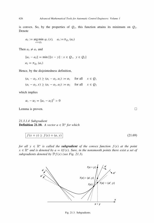
626 Advanced Mathematical Tools for Automatic Control Engineers: Volume 1
is convex. So, by the properties of Q2, this function attains its minimum on Q2.
Denote
a2 := argminx∈∈Q2
ϕ1 (x), a1 :=πQ2(a2)
Then a2 �= a1 and
‖a1 − a2‖ = min {‖x − y‖ : x ∈ Q1, y ∈ Q2}a2 = πQ2
(a1)
Hence, by the disjointedness definition,
(a1 − a2, x) ≥ (a1 − a2, a1) := α1 for all x ∈ Q1
(a1 − a2, x) ≥ (a1 − a2, a2) := α2 for all x ∈ Q2
which implies
α1 − α2 = ‖a1 − a2‖2 > 0
Lemma is proven. �
21.3.1.4 SubgradientDefinition 21.10. A vector a ∈ Rn for which
f (x + y) ≥ f (x)+ (a, y) (21.69)
for all y ∈ Rn is called the subgradient of the convex function f (x) at the pointx ∈ Rn and is denoted by a = ∂f (x). Sure, in the nonsmooth points there exist a set ofsubgradients denoted by Df (x) (see Fig. 21.3).
f (x 1 y )
f (x )1 (a9, y )
f (x ) f (x) 1 (a99, y )
a9
a9a99
a99
x
x 1 y
Fig. 21.3. Subgradients.
Finite-dimensional optimization 627
The following properties of the subgradients of convex functions seem to be evident.
Claim 21.5.
1. Analogously to (21.31) the subgradient of a convex function is a monotone operator,i.e., for any x, y ∈ Rn and any ∂f (x) ∈ Df (x), ∂f (y) ∈ Df (y)
(∂f (x)− ∂f (y), x − y) ≥ 0 (21.70)
2. f ′+ (x, y), as it is defined in (21.23), for any x, y ∈ Rn can be calculated asfollows
f ′+ (x, y) = maxa∈Df (x)
(a, y) (21.71)
3.
∂
(m∑i=1
γifi (x)
)=
m∑i=1
γi∂fi (x), γi ≥ 0 (21.72)
4. For the convex functions f1 (x) and f2 (x) we have
Dmax {f1 (x); f2 (x)} = Conv [Df1 (x) ∪Df2 (x)] (21.73)
5. For any matrix A ∈ Rn×n and any x ∈ Rn
∂f (Ax) = Aᵀ∂f (x) (21.74)
Exercise 21.2. The following relations seem to be useful:
1.
∂ ‖x‖ =⎧⎨⎩
x
‖x‖ if x �= 0
a with ‖a‖ ≤ 1 if x = 0
(21.75)
2.
∂
m∑i=1
∥∥(ai, x)− bi∥∥ = m∑i=1
ai sign∥∥(ai, x)− bi∥∥ (21.76)
Lemma 21.11. The set Df (x) at any point x ∈ Rn is nonempty, convex, closed andbounded.
Proof. Consider in Rn+1 the set Qα := {x, α : f (x) ≤ α} (which is called the epigraph
of f (x)). Obviously, this set is convex, and, by Lemma 21.3, it has an interior point,
since the points {x, f (x)} form its boundary. By the convexity of Qα , there exists a
supporting hyperplane for Qα at the point x, given by {a,−1} for some a. Thus, a is
a subgradient of f (x) at x. The convexity, closedness and boundedness follow from
Lemma 21.4. �

628 Advanced Mathematical Tools for Automatic Control Engineers: Volume 1
21.3.2 Optimization on convex sets
Here we will be interested in the following optimization problem
minx∈Qf (x) (21.77)
where Q is a convex (not obligatory bounded) set and f (x) is assumed to be smooth
(differentiable) on Q if any special assumptions are accepted.
Definition 21.11. We say that the point x∗ ∈ Q is
(a) a local minimum of f (x) on Q if f (x∗) ≤ f (x) for all x ∈ Q and such that‖x − x∗‖ ≤ δ, δ > 0;
(b) a global minimum of f (x) on Q if f (x∗) ≤ f (x) for all x ∈ Q.
21.3.2.1 Necessary first-order minimum conditionTheorem 21.9. (The necessary condition) Let
1. f (x) be differentiable at the global minimum point x∗;2. the set Q be a convex set.
Then for all x ∈ Q
(∇f (x∗), x − x∗) ≥ 0 (21.78)
Proof. We will prove this theorem by contradiction. Suppose that (∇f (x∗), x − x∗) < 0
for some x ∈ Q. Then, by the convexity of Q, the point xα := x∗ + α (x − x∗) ∈ Q for
all α ∈ [0, 1], and, hence, for small enough α
f (xα) = f (x∗)+ α (∇f (x∗), x − x∗)+ o (α) < f (x∗)
which contradicts the assumption that x∗ is a minimum point. Theorem is proven. �
21.3.2.2 Sufficient first-order minimum conditionTheorem 21.10. (The sufficient condition of optimality) Let
1. f (x) be differentiable at the point x∗ ∈ Q;2. the set Q be a convex set;3. for all x ∈ Q the following inequality holds
(∇f (x∗), x − x∗) ≥ ρ ‖x − x∗‖, > 0 (21.79)
Then the point x∗ is a local minimum point on Q.
Proof. Take ε ≥ ε1 > 0, so that
|f (x)− f (x∗)− (∇f (x∗), x − x∗)| ≤ α2‖x − x∗‖
Finite-dimensional optimization 629
for all x ∈ Q such that ‖x − x∗‖ ≤ ε1. Then, by (21.79),
f (x) ≥ f (x∗)+ (∇f (x∗), x − x∗)− α
2‖x − x∗‖ ≥ f (x∗)+ α
2‖x − x∗‖
which means the local optimality of x∗. Theorem is proven. �
Remark 21.4. Notice that x∗ in (21.79) cannot be an interior point of Q, and, therefore,under the conditions of Theorem 21.10 the minimum is attained at a boundary point ofQ.
21.3.2.3 Criterion of optimality for convex (not obligatory differentiable) functionsTheorem 21.11. (The criterion of optimality) Let
1. f (x) be convex on Rn;2. Q ⊆ Rn be a convex set.
Then the point x∗ ∈ Q is a global minimum on Q if and only if
(∂f (x∗), x − x∗) ≥ 0 (21.80)
for some subgradient ∂f (x∗) ∈ Df (x∗) and all x ∈ Q.
Proof.
(a) Necessity. Suppose that there is no such subgradient. Then the sets Df (x∗) andS := {y ∈ Rn : (y, x − x∗) ≥ 0, x ∈ Q} do not intersect. Notice that S is convex
and closed. By Lemma 21.11, the set Df (x∗) is convex, closed and bounded. So,
in the separation lemma 21.10, there exists c ∈ Rn such that (c, a) ≤ −α < 0 for
all a ∈ Df (x∗) and (c, y) > 0 for all y ∈ S. Denote by � the closure of the cone
generated by all feasible directions, i.e.,
� :={x ∈ Rn : x = lim
k→∞λk(xk − x∗), λk > 0, xk ∈ Q
}If c �= �, then again there exists a vector b such that (b, x) ≥ 0 for all x ∈ �and (c, b) < 0. But b ∈ S and, therefore, the inequality (c, b) < 0 contradicts the
condition (c, y) > 0 for all y ∈ S. So, c = �, and, hence, one can find the sequences
λk > 0 and xk ∈ Q such that λk(xk − x∗)→ c. Taking k large enough such that∥∥λk (xk − x∗)− c∥∥ ≤ α/(2a+), a+ := max
a∈Df (x∗)‖a‖, α > 0
we obtain
f ′+(x, λk
(xk − x∗)) := lim
α→+0
f(x + αλk
(xk − x∗))− f (x)α
= maxa∈Df (x∗)
(a, λk
(xk − x∗))
= maxa∈Df (x∗)
(a, c)+ maxa∈Df (x∗)
(a, λk
(xk − x∗)− c)
= −α + 1
2α = −1
2α

630 Advanced Mathematical Tools for Automatic Control Engineers: Volume 1
and, hence, f ′+(x, λk
(xk − x∗)) < 0. Therefore, for sufficiently small γ > 0, it
follows that
f(x∗ + γ (xk − x∗)) < f (x∗)
which contradicts the assumption that x∗ is a minimum point. The necessity is proven.
(b) Sufficiency. Let (21.80) hold for all x ∈ Q and some subgradient ∂f (x∗). Then
f (x) ≥ f (x∗)+ (∂f (x∗), x − x∗) ≥ f (x∗)
i.e., x∗ is a global minimum point on Q. Lemma is proven. �
Remark 21.5. In the case of no constraints, the criterion (21.80) becomes
0 ∈ Df (x∗) (21.81)
21.3.3 Mathematical programing and Lagrange principle
21.3.3.1 Nonlinear programing problemThe general problem of nonlinear programing is formulated as follows:
minx∈Rnf (x)
gi (x) ≤ 0, i = 1, . . . , r
hj (x) = 0, j = 1, . . . , r ′
(21.82)
Notice that any equality constraint hi (x) = 0 can be represented as two inequality-type
constraints:
{x ∈ Rn | hi (x) = 0} = {x ∈ Rn | hi (x) ≤ 0, −hi (x) ≤ 0}
So, the general nonlinear programing problem (21.82) can be represented as
minx∈Rnf (x)
gi (x) ≤ 0, i = 1, . . . , m
(21.83)
where m = r + 2r ′ with
gi(x) ={hj (x) if i = r + j−hj (x) if i = r + r ′ + j
(j = 1, . . . , r ′
)

Finite-dimensional optimization 631
21.3.3.2 Lagrange principleThe theorem below follows the scheme of presentation given in (Alexeev et al. 1979)
where the same result is formulated in a more general case in Banach (not obligatory
in finite dimensional) space. It permits to represent the given constraint optimizationproblem as another (but already) unconstrained optimization problem.
Theorem 21.12. (Lagrange principle) Consider the general nonlinear programingproblem (21.83) where the functions f (x) and gi (x) (i = 1, . . . , m) are assumed to bedifferentiable but not convex.
A. (Necessary conditions, Karush–John). If x∗ is a local minimum point, then there existnonnegative constants μ∗ ≥ 0 and ν∗i ≥ 0 (i = 1, . . . , m) such that the following twoconditions hold:
1. “local minimality condition to Lagrange function”
L (x, μ, ν) := μf (x)+m∑i=1
νigi (x) (21.84)
namely,
L (x∗, μ∗, ν∗) ≤ L (x, μ∗, ν∗) (21.85)
or, equivalently,
μ∗∇f (x∗)+m∑i=1
ν∗i ∇gi (x∗) = 0 (21.86)
2. “complementary slackness”:
ν∗i gi(x∗) = 0 (i = 1, . . . , m) (21.87)
B. (Sufficient conditions). If μ∗ > 0 (the regular case), or equivalently, if the vec-tors ∇gi (x∗) (i = 1, . . . , m), corresponding to the active indices for which ν∗i > 0,are linearly independent, then conditions (1)–(2) above turn out to be sufficient toguarantee that x∗ is a local minimum point;
C. To guarantee the existence of μ∗ > 0 it is sufficient that the, so-called, Slater’scondition holds, namely, that in a neighborhood �(x∗) of x∗ there exists xsuch that
gi (x) < 0 (i = 1, . . . , m) (21.88)
Proof. First, define the set
C := {η ∈ Rm+1 | ∃ x ∈ �(x∗) :
f (x)− f (x∗) < η0, gi(x) ≤ ηi (i = 1, . . . , m)(21.89)

632 Advanced Mathematical Tools for Automatic Control Engineers: Volume 1
A. The set C is nonempty and convex. Indeed, the vector η with positive components
belongs to C since in (21.89) we may take x = x∗. So, C is nonempty. Let us show
that it is convex. To do that we need to prove the existence of a vector xα ∈ �(x∗)(�(x∗) can always be selected as a convex set) such that for any ηα := η + α (η′ − η),α ∈ [0, 1] we have
f (xα)− f (x∗) < ηα0 , gi(xα) ≤ ηαi (i = 1, . . . , m)
if for some x, x ′ ∈ �(x∗)
f (x)− f (x∗) < η0, gi(x) ≤ ηi (i = 1, . . . , m)
f (x ′)− f (x∗) < η′0, gi(x′) ≤ η′i (i = 1, . . . , m)
Denote xα := x + α (x ′ − x), α ∈ [0, 1] which, by the convexity of �(x∗), alsobelongs to�(x∗). Since the functions f (x) and gi(x) (i = 1, . . . , m) are differentiable
in �(x∗), it follows that
f (x)− f (x∗) = (∇f (x∗), x − x∗)+ o (‖x − x∗‖) < η0f (x ′)− f (x∗) = (∇f (x∗), x ′ − x∗)+ o (‖x ′ − x∗‖) < η0o (‖xα − x∗‖) = o (‖x ′ − x∗‖)+ o (‖x − x∗‖)
and, hence,
f (xα)− f (x∗)= (∇f (x∗), xα − x∗)+ o (‖xα − x∗‖)= α [(∇f (x∗), x ′ − x∗)+ o (‖x ′ − x∗‖)]+ (1− α) [(∇f (x∗), x − x∗)+ o (‖x − x∗‖)]< αη′0 + (1− α) η0 = ηα0
Analogously, gi(xα) ≤ ηαi , which implies ηα ∈ C. So, C is nonempty and convex.
B. The point 0 does not belong to C. Indeed, if so, in view of the definition (21.89),
there exists a point x ∈ X0 satisfying
f (x)− f (x∗) < 0
gi(x) ≤ 0 (i = 1, . . . , m)(21.90)
which is in contradiction to the fact that x∗ is a local solution of the problem. So, 0 /∈ C.Based on this fact and taking into account the convexity property of C, we may apply
the separation principle (see Theorem 21.8): there exist constants(μ∗, ν∗1 , . . . , ν
∗m
)such that for all η ∈ C
μ∗η0 +m∑i=1
ν∗i ηi ≥ 0 (21.91)
C. Multipliers μ∗ and ν∗i (i = 1, . . . , m) in (21.91) are nonnegative. In (A) we have
already mentioned that any vector η ∈ RL+1 with positive components belongs to
Finite-dimensional optimization 633
C, and, particularly, the vector
⎛⎝ε, . . . , ε, 1︸ ︷︷ ︸
l0
, ε, . . . , ε
⎞⎠ (ε > 0). Substitution of this
vector into (21.91) leads to the following inequalities
ν∗i0 ≥ −μ∗ε − εm∑i=l0ν∗l if 1 ≤ l0 ≤ m
μ∗ ≥ −εm∑i=1
ν∗l if l0 = 0
⎫⎪⎪⎪⎪⎬⎪⎪⎪⎪⎭
(21.92)
Tending ε to zero in (21.92) implies the nonnegativity property for the multipliers
μ∗ and ν∗i (i = 1, . . . , m).
D. Multipliers ν∗i (i = 1, . . . , m) satisfy the complementary slackness condition (21.87).
Indeed, if gl0 (x∗) = 0, then the identity ν∗l0gl0 (x
∗) = 0 is trivial. Suppose that
gl0 (x∗) < 0. Then the point⎛⎜⎝δ, 0, . . . , 0, gl0 (x∗)︸ ︷︷ ︸
l0
, 0, . . . , 0
⎞⎟⎠ (δ > 0) (21.93)
belongs to the set C. To check this it is sufficient to take x = x∗ in (21.89). Substitutionof this point into (21.91) implies
ν∗l0gl0 (x∗) ≥ −μ∗δ (21.94)
Tending δ to zero we obtain that ν∗l0gl0 (x∗) ≥ 0, and since gl0 (x
∗) < 0, it follows
that ν∗l0 ≤ 0. But in (C) it has been proven that ν∗l0 ≥ 0. So, ν∗l0 = 0, and, hence,
ν∗l0gl0 (x∗) = 0.
E. Minimality condition to Lagrange function. As it follows from (21.89), for x ∈ �(x∗)the point
(f (x)− f (x∗)+ δ, g1 (x) , . . . , gm (x))
belongs to C for any δ > 0. Substitution of this point into (21.91), in view of (D),
yields
L (x, μ∗, ν∗) :=μ∗f (x)+m∑i=1
ν∗i gi (x)
=(μ∗ [f (x)− f (x∗)+ δ]+
m∑i=1
ν∗i gi (x)
)+μ∗f (x∗)− μ∗δ ≥ μ∗f (x∗)− μ∗δ
= μ∗f (x∗)+m∑i=1
ν∗i gi (x∗)− μ∗δ = L (x∗, μ∗, ν∗)− μ∗δ
(21.95)
Taking δ→ 0 we obtain (21.85).
634 Advanced Mathematical Tools for Automatic Control Engineers: Volume 1
F. If μ∗ > 0 (the regular case), then the conditions (A1) and (A2) are sufficient for theoptimality. Indeed, in this case it is clear that we may take μ∗ = 1, and, hence, for
any x satisfying gi (x) ≤ 0 (i = 1, . . . , m)
f (x)≥ f (x)+m∑i=1
ν∗i gi (x) = L (x, 1, ν∗)
≥L (x∗, 1, ν∗) = f (x∗)+m∑i=1
ν∗i gi (x∗) = f (x∗)
This means that x∗ is the optimal solution. Notice also that, by (21.86), if μ∗ = 0 it
follows that
m∑i=1
ν∗i ∇gi (x∗) =m∑
i:ν∗i >0ν∗i ∇gi (x∗) = 0
which means linear dependence of the vectors ∇gi (x∗) corresponding to the active
constraints.
G. Slater’s condition of the regularity. Suppose that Slater’s condition is fulfilled, but
μ∗ = 0. We directly obtain the contradiction. Indeed, since not all ν∗i are equal to
zero simultaneously, it follows that
L (x, 0, ν∗) =L∑l=1
ν∗i gi (x) < 0 = L (x∗, 0, ν∗)
which is in contradiction with (E). Theorem is proven. �
21.3.3.3 Convex programingTheorem 21.13. (Kuhn & Tucker 1951) Suppose that
1. all functions f (x) and gi (x) (i = 1, . . . , m) in the general nonlinear programingproblem (21.83) are differentiable1 and convex in Rn;
2. Slater’s condition (“the existence of an internal point”) holds, i.e., there exists x ∈ Rn
such that
gi (x) < 0 (i = 1, . . . , m) (21.96)
Then, for a point x∗ ∈ Rn to be a global solution of (21.83) it is necessary andsufficient to show the existence of nonnegative constants ν∗i ≥ 0 (i = 1, . . . , m) suchthat the, so-called, saddle-point property for the Lagrange function (21.84) holds for anyx ∈ Rn and any νi ≥ 0 (i = 1, . . . , m)
L (x, 1, ν∗) ≥ L (x∗, 1, ν∗) ≥ L (x∗, 1, ν) (21.97)
1 Here we present the version of the theorem dealing with differential functions. In fact the same result
remains valid without the assumption on differentiability (see (Polyak 1987)).

Finite-dimensional optimization 635
or, in another form,
minx∈Rn
L (x, 1, ν∗)= minx∈Rn
maxν≥0L (x, 1, ν)
=L (x∗, 1, ν∗)=max
ν≥0minx∈Rn
L (x, 1, ν) = maxν≥0
L (x∗, 1, ν)(21.98)
Proof.
(a) Necessity. By Slater’s condition (see item C in Theorem 21.12) we deal with the
regular case, and, therefore, we may take μ∗ = 1. If x∗ is a global minimum of
(21.83), then, in view of the convexity condition, it is a local minimum also. Hence,
by Theorem 21.12, we have L (x∗, 1, ν∗) ≤ L (x, 1, ν∗). On the other hand,
L (x∗, 1, ν∗)= f (x∗)+m∑i=1
ν∗i gi (x∗) = f (x∗)
≥ f (x∗)+m∑i=1
νigi (x∗) = L (x∗ (T ), 1, ν)
(21.99)
which proves the necessity.
(b) Sufficiency. Suppose that (21.97) holds. Then
L (x∗, 1, ν∗)= f (x∗)+m∑i=1
ν∗i gi (x∗)
≥ L (x∗, 1, ν) = f (x∗)+m∑i=1
νigi (x∗)
which implies
m∑i=1
ν∗i gi (x∗) ≥
m∑i=1
νigi (x∗)
for all νi ≥ 0 (i = 1, . . . , m). This is possible if and only if (this can be proven by
the contradiction)
gi (x∗) ≤ 0, ν∗i gi (x
∗) = 0 (i = 1, . . . , m)
So, we have
L (x∗, 1, ν∗)= f (x∗)+m∑i=1
ν∗i gi (x∗) = f (x∗)
≤ L (x, 1, ν∗) = f (x)+m∑i=1
ν∗i gi (x) ≤ f (x)+m∑i=1
ν∗i gi (x∗) = f (x)
which means that x∗ is a solution of (21.83). Theorem is proven. �

636 Advanced Mathematical Tools for Automatic Control Engineers: Volume 1
Remark 21.6. The construction of the Lagrange function in the form (21.84)
L (x, μ, ν) = μf (x)+m∑i=1
νigi (x)
with μ ≥ 0 is very essential. Indeed, the usage of this form only as L (x, 1, ν), whenthe regularity conditions are not valid, may provoke a serious error in the optimizationprocess. The following counterexample demonstrates this effect. Consider the simpleconstrained optimization problem formulated as
h0(x) := x1 → minx∈R2
g (x) := x21 + x22 ≤ 0
}(21.100)
This problem evidently has the unique solution x1 = x2 = 0. But the direct usage of theLagrange principle with μ = 1 leads to the following contradiction:
L (x, 1, ν∗) = x1 + ν∗(x21 + x22
)→ minx∈R2
∂
∂x1L (x∗, 1, ν∗) = 1+ 2ν∗x∗1 = 0
∂
∂x2L (x∗, 1, ν∗) = 2ν∗x∗2 = 0
ν∗ �= 0, x∗2 = 0, x∗1 = − 1
2ν∗�= 0
⎫⎪⎪⎪⎪⎪⎪⎪⎪⎬⎪⎪⎪⎪⎪⎪⎪⎪⎭
(21.101)
Notice that for this example Slater’s condition (21.96) is not valid.
21.3.4 Method of subgradient projection to simplest convex sets
Let us consider the constrained optimization problem (21.77)
minx∈Q f (x)
where the function f (x) is supposed to be convex, and the set Q is convex and having a
simple structure such that the projection operation πQ {x} (21.62) can be easily realized.
Consider also the following iterative procedure:
xn+1 = πQ {xn − γn∂f (xn)} (21.102)
where ∂f (xn) is any subgradient form Df (xn), and γn ≥ 0 is “the step of the procedure”.
Denote by x∗ ∈ Q the solution of the constrained optimization problem (21.77) with the
convex f .
Theorem 21.14. (on strong convergence) Suppose that
1. f (x) has on Q a unique global minimum point x∗, that is,
f (x) > f (x∗) for all x ∈ Q, x �= x∗ (21.103)
Finite-dimensional optimization 637
2. for any x ∈ Q and any ∂f (x) ∈ Df (x)
‖∂f (x)‖2 ≤ c0 + c1 ‖x − x∗‖2 (21.104)
3. the step size γn satisfies the conditions
γn ≥ 0,
∞∑n=0
γn = ∞,∞∑n=0
γ 2n <∞ (21.105)
Then for any initial value x0 ∈ Q the vector sequence {xn}, generated by the procedure(21.102), converges to x∗ whereas n→∞.
Proof. By the projection operator property (21.64), and in view of the inequality (21.70)
(∂f (x)− ∂f (y), x − y) ≥ 0
it follows that
‖xn+1 − x∗‖2 =∥∥πQ {xn − γn∂f (xn)} − x∗∥∥2
≤ ‖xn − γn∂f (xn)− x∗‖2 = ‖xn − x∗‖2 − 2γn (∂f (xn), xn − x∗)+ γ 2
n ‖∂f (xn)‖2 = ‖xn − x∗‖2 − 2γn (∂f (xn)− ∂f (x∗), xn − x∗)− 2γn (∂f (x
∗), xn − x∗)+ γ 2n
(c0 + c1 ‖x − x∗‖2
)≤ (
1+ c1γ 2n
) ‖xn − x∗‖2 − 2γn (∂f (x∗), xn − x∗)+ γ 2
n c0
So, defining vn := ‖xn − x∗‖2, we have
vn+1 ≤(1+ c1γ 2
n
)vn + γ 2
n c0 − 2γn (∂f (x∗), xn − x∗) (21.106)
By (21.80) it follows that (∂f (x∗), xn − x∗) ≥ 0, and hence, (21.106) implies
vn+1 ≤(1+ c1γ 2
n
)vn + γ 2
n c0 (21.107)
Let us consider the sequence (Gladishev’s transformation) {wn} defined by
wn := vn∞∏i=n
(1+ c1γ 2
i
)+ c0 ∞∑i=nγ 2i
∞∏s=n+1
(1+ c1γ 2
s
)(21.108)
The variable wn is correctly defined since, in view of the inequality 1 + x ≤ ex , it
follows that
∞∏i=n
(1+ c1γ 2
i
) ≤ exp
(c1
∞∑i=nγ 2i
)<∞

638 Advanced Mathematical Tools for Automatic Control Engineers: Volume 1
For this variable, using (21.107), we have
wn+1 = vn+1
∞∏i=n+1
(1+ c1γ 2
i
)+ c0 ∞∑i=n+1
γ 2i
∞∏s=n+2
(1+ c1γ 2
s
)≤ vn
∞∏i=n
(1+ c1γ 2
i
)+ γ 2n c0
∞∏i=n+1
(1+ c1γ 2
i
)+ c0 ∞∑i=n+1
γ 2i
∞∏s=n+2
(1+ c1γ 2
s
)= vn
∞∏i=n
(1+ c1γ 2
i
)+ c0 ∞∑i=nγ 2i
∞∏s=n+1
(1+ c1γ 2
s
) = wnSo, 0 ≤ wn+1 ≤ wn, and, hence, by the Weierstrass theorem, this sequence converges, i.e.,
wn → w∗ as n→∞
In view of (21.108), it follows that vn also converges (in fact, to the same limit point),
that is
vn → v∗ as n→∞
Returning to (21.106), after summing these inequalities, we obtain
vn+1 ≤ v0 + c1n∑i=0
γ 2i vi + c0
n∑i=0
γ 2i − 2
n∑i=0
γi (∂f (x∗), xi − x∗)
or, equivalently,
2
n∑i=0
γi (∂f (x∗), xi − x∗)≤ v0 + c1
n∑i=0
γ 2i vi + c0
n∑i=0
γ 2i − vn+1
≤ v0 + c1n∑i=0
γ 2i vi + c0
n∑i=0
γ 2i ≤ const <∞
Taking n→∞, we get
∞∑i=0
γn (∂f (x∗), xn − x∗) <∞
Since, by the assumption of this theorem,∑∞i=0 γn = ∞, we may conclude that there
exists a subsequence {nk} such that(∂f (x∗), xnk − x∗
)→ 0 whereas k→∞. But, by the
uniqueness of the global minimum (see the condition (21.103)), we derive that xnk → x∗
as k→∞, or equivalently, vnk → 0. But {vn} converges, and, therefore, all subsequenceshave the same limit v∗, which implies v∗ = 0. Theorem is proven. �
Finite-dimensional optimization 639
21.3.5 Arrow–Hurwicz–Uzawa method with regularization
Consider again the general non-linear convex programing problem in the form
(21.83), i.e.,
minx∈Q⊂Rn
f (x)
gi (x) ≤ 0, i = 1, . . . , m(21.109)
when all functions are assumed to be convex (not obligatory strictly convex), the set Q
is a convex compact, and Slater’s condition (21.96) is fulfilled. Additionally, we will
assume that
Q⋂( ⋂
i=1,...,m
{x ∈ Rn : gi (x) ≤ 0})�= ∅
Associate with this problem the following regularized Lagrange function
Lδ (x, 1, ν) := L (x, 1, ν)+ δ2
(‖x‖2 − ‖ν‖2), δ ≥ 0
L (x, 1, ν) = f (x)+m∑i=1
νigi (x)(21.110)
First, notice that the function Lδ (x, 1, ν) for δ > 0 is strictly convex on x for any fixed ν,
and it is strictly concave on ν for any fixed x, and, hence, it has the unique saddle point
(x∗ (δ), ν∗ (δ)) for which the following inequalities hold: for any ν with nonnegative
components and any x ∈ Rn
Lδ (x, 1, ν∗ (δ)) ≥ Lδ (x∗ (δ), 1, ν∗ (δ)) ≥ Lδ (x∗ (δ), 1, ν) (21.111)
As for the function L (x, 1, ν), it may have several (not obligatory unique) saddle points
(x∗, ν∗). The next proposition describes the dependence of the saddle point (x∗ (δ), ν∗ (δ))of the regularized Lagrange function (21.110) on the regularizing parameter δ and analyses
its asymptotic behavior when δ→ 0.
Proposition 21.3.
1. For any x ∈ Rn and any ν with nonnegative components the following inequalityholds:
(x − x∗ (δ), ∂
∂xLδ (x, 1, ν)
)−(ν − ν∗ (δ), ∂
∂νLδ (x, 1, ν)
)≥ δ
2
(‖x − x∗ (δ)‖2 + ‖ν − ν∗ (δ)‖2) (21.112)
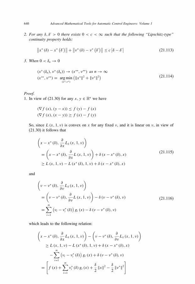
640 Advanced Mathematical Tools for Automatic Control Engineers: Volume 1
2. For any δ, δ′ > 0 there exists 0 < c < ∞ such that the following “Lipschitz-type”continuity property holds:
∥∥x∗ (δ)− x∗ (δ′)∥∥+ ∥∥ν∗ (δ)− ν∗ (δ′)∥∥ ≤ c ∣∣δ − δ′∣∣ (21.113)
3. When 0 < δn → 0
(x∗ (δn), ν∗ (δn))→ (x∗∗, ν∗∗) as n→∞(x∗∗, ν∗∗) = argmin
(x∗,ν∗)
(‖x∗‖2 + ‖ν∗‖2) (21.114)
Proof.1. In view of (21.30) for any x, y ∈ Rn we have
(∇f (x), (y − x)) ≤ f (y)− f (x)(∇f (x), (x − y)) ≥ f (x)− f (y)
So, since L (x, 1, ν) is convex on x for any fixed ν, and it is linear on ν, in view of
(21.30) it follows that(x − x∗ (δ), ∂
∂xLδ (x, 1, ν)
)
=(x − x∗ (δ), ∂
∂xL (x, 1, ν)
)+ δ (x − x∗ (δ), x)
≥ L (x, 1, ν)− L (x∗ (δ), 1, ν)+ δ (x − x∗ (δ), x)
(21.115)
and (ν − ν∗ (δ), ∂
∂νLδ (x, 1, ν)
)
=(ν − ν∗ (δ), ∂
∂νL (x, 1, ν)
)− δ (ν − ν∗ (δ), ν)
=m∑i=1
(νi − ν∗i (δ)
)gi (x)− δ (ν − ν∗ (δ), ν)
(21.116)
which leads to the following relation:(x − x∗ (δ), ∂
∂xLδ (x, 1, ν)
)−(ν − ν∗ (δ), ∂
∂νLδ (x, 1, ν)
)≥ L (x, 1, ν)− L (x∗ (δ), 1, ν)+ δ (x − x∗ (δ), x)−
m∑i=1
(νi − ν∗i (δ)
)gi (x)+ δ (ν − ν∗ (δ), ν)
=[f (x)+
m∑i=1
ν∗i (δ) gi (x)+δ
2‖x‖2 − δ
2‖ν∗‖2
]

Finite-dimensional optimization 641
−[L (x∗ (δ), 1, ν)+ δ
2‖x∗ (δ)‖2 − δ
2‖ν‖2
]+[δ
2‖x‖2 − δ (x∗ (δ), x)+ δ
2‖x∗ (δ)‖2
]+[δ
2‖ν‖2 − δ (ν∗ (δ), ν)+ δ
2‖ν∗‖2
]= Lδ (x, 1, ν∗ (δ))
− Lδ (x∗ (δ), 1, ν)+ δ2
(‖x − x∗ (δ)‖2 + ‖ν − ν∗ (δ)‖2)≥ δ
2
(‖x − x∗ (δ)‖2 + ‖ν − ν∗ (δ)‖2)
(21.117)
which proves (21.112).
2. The inequality (21.113) results from the linear dependence of the regularized Lagrange
function on δ.
3. Taking in (21.117) x = x∗, ν = ν∗ (one of the saddle points of the nonregularized
Lagrange function) and applying the inequalities
L (x∗, 1, ν∗)− L (x∗ (δ), 1, ν∗) ≤ 0m∑i=1
(ν∗i − ν∗i (δ)
)gi (x
∗) = −m∑i=1
ν∗i (δ) gi (x∗) ≥ 0
leads to the following relation:
0≤L (x∗, 1, ν∗)− L (x∗ (δ), 1, ν∗)+ δ (x∗ − x∗ (δ), x∗)
−m∑i=1
(ν∗i − ν∗i (δ)
)gi (x
∗)+ δ (ν∗ − ν∗ (δ), ν∗)
≤ δ (x∗ − x∗ (δ), x∗)+ δ (ν∗ − ν∗ (δ), ν∗)
Dividing both sides by δ > 0 we obtain
0 ≤ (x∗ − x∗ (δ), x∗)+ (ν∗ − ν∗ (δ), ν∗) (21.118)
which is valid for any saddle point (x∗, ν∗) of the nonregularized Lagrange function.
We also have
Lδ (x∗ (δ), 1, ν∗)=L (x∗ (δ), 1, ν∗)+ δ
2‖x∗ (δ)‖2 − δ
2‖ν∗‖2
≤ L (x∗, 1, ν∗ (δ))+ δ2‖x∗‖2 − δ
2‖ν∗ (δ)‖2
=Lδ (x∗, 1, ν∗ (δ))
Dividing by δ > 0 implies
‖x∗ (δ)‖2 + ‖ν∗ (δ)‖2 ≤ 2
δ[L (x∗ (δ), 1, ν∗)− L (x∗, 1, ν∗ (δ))]
+‖x∗‖2 + ‖ν∗‖2 <∞
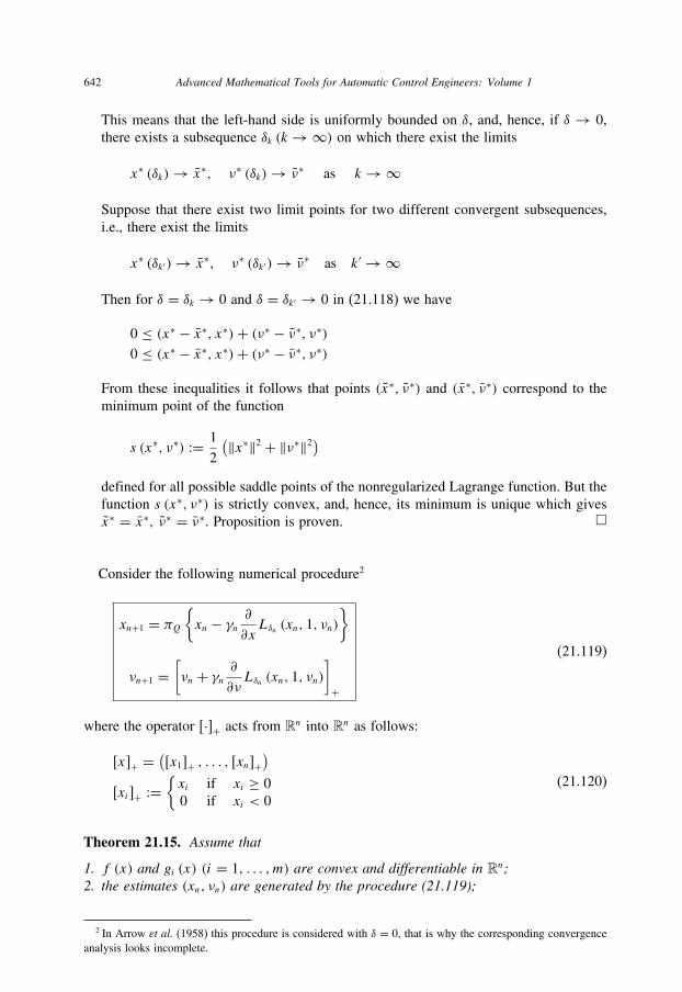
642 Advanced Mathematical Tools for Automatic Control Engineers: Volume 1
This means that the left-hand side is uniformly bounded on δ, and, hence, if δ → 0,
there exists a subsequence δk (k→∞) on which there exist the limits
x∗ (δk)→ x∗, ν∗ (δk)→ ν∗ as k→∞
Suppose that there exist two limit points for two different convergent subsequences,
i.e., there exist the limits
x∗ (δk′)→ x∗, ν∗ (δk′)→ ν∗ as k′ → ∞
Then for δ = δk → 0 and δ = δk′ → 0 in (21.118) we have
0 ≤ (x∗ − x∗, x∗)+ (ν∗ − ν∗, ν∗)0 ≤ (x∗ − x∗, x∗)+ (ν∗ − ν∗, ν∗)
From these inequalities it follows that points (x∗, ν∗) and (x∗, ν∗) correspond to the
minimum point of the function
s (x∗, ν∗) := 1
2
(‖x∗‖2 + ‖ν∗‖2)defined for all possible saddle points of the nonregularized Lagrange function. But the
function s (x∗, ν∗) is strictly convex, and, hence, its minimum is unique which gives
x∗ = x∗, ν∗ = ν∗. Proposition is proven. �
Consider the following numerical procedure2
xn+1 = πQ{xn − γn ∂
∂xLδn (xn, 1, νn)
}
νn+1 =[νn + γn ∂
∂νLδn (xn, 1, νn)
]+
(21.119)
where the operator [·]+ acts from Rn into Rn as follows:
[x]+ =([x1]+ , . . . , [xn]+
)[xi]+ :=
{xi if xi ≥ 0
0 if xi < 0
(21.120)
Theorem 21.15. Assume that
1. f (x) and gi (x) (i = 1, . . . , m) are convex and differentiable in Rn;2. the estimates (xn, νn) are generated by the procedure (21.119);
2 In Arrow et al. (1958) this procedure is considered with δ = 0, that is why the corresponding convergence
analysis looks incomplete.

Finite-dimensional optimization 643
3. the step size γn and the regularizing parameter δn satisfy the following conditions:
0 < γn → 0, 0 < δn → 0 as n→∞∞∑n=0
γnδn = ∞γn
δn→ λ which is small enough,
|δn+1 − δn|γnδn
→ 0 as n→∞
Then for any initial value x0 ∈ Q and any ν0 with nonnegative components the vectorsequences {xn}, {νn}, generated by the procedure (21.119), converge as n → ∞ tox∗∗, ν∗∗ defined by (21.114).
Proof. Using the property (21.64) of the projection operator we get the following recur-
sion for the variable wn := ‖xn − x∗ (δn)‖2 + ‖νn − ν∗ (δn)‖2:
wn+1 ≤∥∥∥∥xn − γn ∂∂x Lδn (xn, 1, νn)− x∗ (δn+1)
∥∥∥∥2
+∥∥∥∥νn + γn ∂∂ν Lδn (xn, 1, νn)− ν∗ (δn+1)
∥∥∥∥2
=∥∥∥∥[xn − x∗ (δn)]− γn ∂∂x Lδn (xn, 1, νn)+ [x∗ (δn)− x∗ (δn+1)]
∥∥∥∥2
+∥∥∥∥[νn − ν∗ (δn)]+ γn ∂∂ν Lδn (xn, 1, νn)+ [ν∗ (δn)− ν∗ (δn+1)]
∥∥∥∥2
=wn + ‖x∗ (δn)− x∗ (δn+1)‖2 + ‖ν∗ (δn)− ν∗ (δn+1)‖2
− 2γ n
[(xn− x∗ (δn), ∂
∂xLδn (xn, 1, νn)
)−(νn− ν∗ (δn), ∂
∂νLδn (xn, 1, νn)
)]
+ 2
(x∗ (δn)− x∗ (δn+1), [xn − x∗ (δn)]− γn ∂
∂xLδn (xn, 1, νn)
)
+ 2
(ν∗ (δn)− ν∗ (δn+1), [νn − ν∗ (δn)]+ γn ∂
∂νLδn (xn, 1, νn)
)
+ γ 2n
(∥∥∥∥ ∂∂x Lδn (xn, 1, νn)∥∥∥∥2
+∥∥∥∥ ∂∂ν Lδn (xn, 1, νn)
∥∥∥∥2)
Taking into account that
∥∥∥∥ ∂∂x Lδn (xn, 1, νn)∥∥∥∥2
≤ c0 + c1 ‖νn‖2 ≤ C0 + C1wn∥∥∥∥ ∂∂ν Lδn (xn, 1, νn)∥∥∥∥2
≤ c2

644 Advanced Mathematical Tools for Automatic Control Engineers: Volume 1
and applying the inequalities (21.112) and (21.113) the last recursion can be estimated as
follows:
wn+1 ≤wn + c2 |δn+1 − δn|2 − γnδnwn+ 2 ‖x∗ (δn)− x∗ (δn+1)‖
(‖xn − x∗ (δn)‖ + γn (√C0 +√C1
√wn
))+ 2 ‖ν∗ (δn)− ν∗ (δn+1)‖
(‖νn − ν∗ (δn)‖ + γn√c2)+ γ 2
n (C0 + C1wn + c2) ≤ wn(1− γnδn + C1γ
2n
)+ c2 |δn+1 − δn|2+ C2 |δn+1 − δn|√wn + C3 |δn+1 − δn| + γ 2
n (C0 + c2)≤wn
(1− γnδn [1− C1γn/δn]
)+ C2 |δn+1 − δn|√wn+ C4 |δn+1 − δn| + γ 2
n C5
(21.121)
Here ci (i = 1, 2) and Ci (i = 0, . . . , 5) are positive constants. By Lemma 16.17 applied
for the case r = 1/2 and for
αn := γnδn − C1γ2n = γnδn [1− C1γn/δn] = γnδn [1+ o(1)]
βn :=C4 |δn+1 − δn| + γ 2n C5, δn := C2 |δn+1 − δn|
in view of the conditions of this theorem, we have
c is any large real number, b = 0, d = 0
and, hence, u(c) = 0 which proves the theorem. �
Corollary 21.10. Within the class of numerical sequences
γn := γ0
(n+ n0)γ , γ0, n0, γ > 0
δn := δ0
(n+ n0)δ , δ0, δ > 0
(21.122)
the conditions of Theorem 21.15 are satisfied if
γ + δ ≤ 1, γ ≥ δ, γ < 1 (21.123)
Proof. It follows from the estimates that
γnδn = O(
1
nγ+δ
)
|δn+1 − δn| =O(
1
nδ− 1
(n+ 1)δ
)
=O(
1
(n+ 1)δ
[(1+ 1
n
)δ− 1
])

Finite-dimensional optimization 645
= O(
1
(n+ 1)δ
[(1
n
)δ+ o(1)
])= O
(1
nδ+1
)
and
|δn+1 − δn|γnδn
= O(
1
n1−γ
)
which implies (21.123). Corollary is proven. �
Corollary 21.11. Within the class (21.122) of the parameters of the procedure (21.119)the rate κ of convergence
‖xn − x∗∗‖2 + ‖νn − ν∗∗‖2 = O(
1
nκ
)
is equal to
κ = min {γ − δ; 1− γ ; δ} (21.124)
The maximal rate κ∗ of convergence is attained for
γ = γ ∗ = 2/3, δ = δ∗ = 1/3 (21.125)
Proof. By Lemma 16.16 and in view of (21.121) it follows that for κ0 characterizing the
rate of convergence
wn := ‖xn − x∗ (δn)‖2 + ‖νn − ν∗ (δn)‖2 = O(
1
nκ0
)
we have κ0 = min {γ − δ; 1− γ }. But, by (21.113), it follows that
‖xn − x∗∗‖2 + ‖νn − ν∗∗‖2 = wn +O (δn)
= O(
1
nκ0
)+O
(1
nδ
)= O
(1
nmin{κ0;δ}
)
which implies (21.124). The maximal value κ∗ of κ is attained when γ − δ = 1−γ = δ,i.e., when (21.125) holds which completes the proof. �
Remark 21.7. Many other numerical methods, solving the general nonlinear programingproblem (21.83), are discussed in (Polyak 1987).

This page intentionally left blank

22 Variational Calculus and OptimalControl
Contents22.1 Basic lemmas of variation calculus . . . . . . . . . . . . . . . . . . . . . . 647
22.2 Functionals and their variations . . . . . . . . . . . . . . . . . . . . . . . 652
22.3 Extremum conditions . . . . . . . . . . . . . . . . . . . . . . . . . . . . . 653
22.4 Optimization of integral functionals . . . . . . . . . . . . . . . . . . . . . 655
22.5 Optimal control problem . . . . . . . . . . . . . . . . . . . . . . . . . . . 668
22.6 Maximum principle . . . . . . . . . . . . . . . . . . . . . . . . . . . . . . 671
22.7 Dynamic programing . . . . . . . . . . . . . . . . . . . . . . . . . . . . . 687
22.8 Linear quadratic optimal control . . . . . . . . . . . . . . . . . . . . . . . 696
22.9 Linear-time optimization . . . . . . . . . . . . . . . . . . . . . . . . . . . 709
Since the fabric of the universe is most perfect, and is the work of a most wise Creator,nothing whatsoever takes place in the universe in which some form of maximum andminimum does not appear.
Leonard Euler, 1744.
22.1 Basic lemmas of variation calculus
The following lemmas represent the basic instrument for proving the main results of
variation calculus theory and optimal control theory (see, for example, Gel’fand & Fomin
(1961), Ivanov & Faldin (1981) and Troutman (1996)).
22.1.1 Du Bois–Reymond lemma
First, let us prove the following simple auxiliary result.
Lemma 22.1. If 0 ≤ p ∈ C [a, b] and∫ bx=a p (x) dx = 0, then p (x) = 0 for all
x ∈ [a, b].
Proof. Since p (x) ≥ 0, for any x ∈ [a, b] we have
0 ≤ P (x) :=x∫
t=ap (t) dt ≤
b∫t=ap (t) dt = 0
So, P (x) ≡ 0 on [a, b], and, hence, P ′ (x) ≡ 0 too. This exactly means p (x)= P ′ (x) ≡ 0
which proves the statement of this lemma. �647
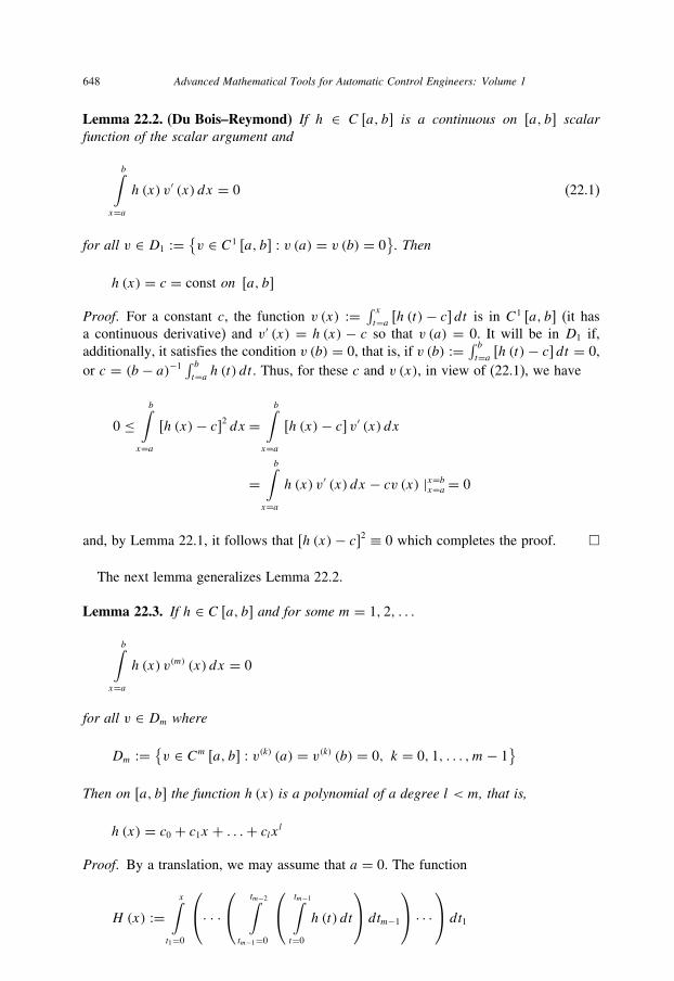
648 Advanced Mathematical Tools for Automatic Control Engineers: Volume 1
Lemma 22.2. (Du Bois–Reymond) If h ∈ C [a, b] is a continuous on [a, b] scalarfunction of the scalar argument and
b∫x=ah (x) v′ (x) dx = 0 (22.1)
for all v ∈ D1 :={v ∈ C1 [a, b] : v (a) = v (b) = 0
}. Then
h (x) = c = const on [a, b]
Proof. For a constant c, the function v (x) := ∫ xt=a [h (t)− c] dt is in C1 [a, b] (it has
a continuous derivative) and v′ (x) = h (x) − c so that v (a) = 0. It will be in D1 if,
additionally, it satisfies the condition v (b) = 0, that is, if v (b) := ∫ bt=a [h (t)− c] dt = 0,
or c = (b − a)−1∫ bt=a h (t) dt . Thus, for these c and v (x), in view of (22.1), we have
0 ≤b∫
x=a[h (x)− c]2 dx =
b∫x=a
[h (x)− c] v′ (x) dx
=b∫
x=ah (x) v′ (x) dx − cv (x) |x=bx=a = 0
and, by Lemma 22.1, it follows that [h (x)− c]2 ≡ 0 which completes the proof. �
The next lemma generalizes Lemma 22.2.
Lemma 22.3. If h ∈ C [a, b] and for some m = 1, 2, . . .
b∫x=ah (x) v(m) (x) dx = 0
for all v ∈ Dm where
Dm :={v ∈ Cm [a, b] : v(k) (a) = v(k) (b) = 0, k = 0, 1, . . . , m− 1
}Then on [a, b] the function h (x) is a polynomial of a degree l < m, that is,
h (x) = c0 + c1x + . . .+ clxl
Proof. By a translation, we may assume that a = 0. The function
H (x) :=x∫
t1=0
⎛⎝· · ·
⎛⎝ tm−2∫tm−1=0
⎛⎝ tm−1∫t=0
h (t) dt
⎞⎠ dtm−1
⎞⎠ · · ·
⎞⎠ dt1
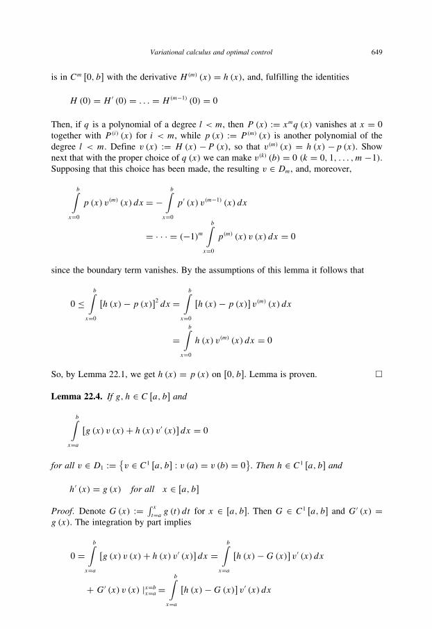
Variational calculus and optimal control 649
is in Cm [0, b] with the derivative H(m) (x) = h (x), and, fulfilling the identities
H (0) = H ′ (0) = . . . = H(m−1) (0) = 0
Then, if q is a polynomial of a degree l < m, then P (x) := xmq (x) vanishes at x = 0
together with P (i) (x) for i < m, while p (x) := P (m) (x) is another polynomial of the
degree l < m. Define v (x) := H (x) −P (x), so that v(m) (x) = h (x) −p (x). Shownext that with the proper choice of q (x) we can make v(k) (b) = 0 (k = 0, 1, . . . , m−1).
Supposing that this choice has been made, the resulting v ∈ Dm, and, moreover,
b∫x=0
p (x) v(m) (x) dx = −b∫
x=0
p′ (x) v(m−1) (x) dx
= · · · = (−1)m
b∫x=0
p(m) (x) v (x) dx = 0
since the boundary term vanishes. By the assumptions of this lemma it follows that
0 ≤b∫
x=0
[h (x)− p (x)]2 dx =b∫
x=0
[h (x)− p (x)] v(m) (x) dx
=b∫
x=0
h (x) v(m) (x) dx = 0
So, by Lemma 22.1, we get h (x) = p (x) on [0, b]. Lemma is proven. �
Lemma 22.4. If g, h ∈ C [a, b] and
b∫x=a
[g (x) v (x)+ h (x) v′ (x)] dx = 0
for all v ∈ D1 :={v ∈ C1 [a, b] : v (a) = v (b) = 0
}. Then h ∈ C1 [a, b] and
h′ (x) = g (x) for all x ∈ [a, b]
Proof. Denote G(x) := ∫ xt=a g (t) dt for x ∈ [a, b]. Then G ∈ C1 [a, b] and G′ (x) =
g (x). The integration by part implies
0 =b∫
x=a[g (x) v (x)+ h (x) v′ (x)] dx =
b∫x=a
[h (x)−G(x)] v′ (x) dx
+ G′ (x) v (x) |x=bx=a =b∫
x=a[h (x)−G(x)] v′ (x) dx
650 Advanced Mathematical Tools for Automatic Control Engineers: Volume 1
By Lemma 22.2, it follows that h (x)−G(x) ≡ c = const, so that
h (x) = G(x)+ c, h′ (x) = G′ (x) = g (x)
which proves the lemma. �
Corollary 22.1. If g ∈ C [a, b] and∫ bx=a g (x) v (x) dx = 0 for all v ∈ D1, then g (x) ≡ 0
on [a, b].
Proof. It is sufficient to put h (x) ≡ 0 in Lemma 22.4. �
This corollary also admits the following generalization.
22.1.2 Lagrange lemma
Lemma 22.5. (Lagrange) If g ∈ C [a, b] and for some m = 0, 1, . . .
b∫x=ag (x) v (x) dx = 0
for all v ∈ Dm where
Dm :={v ∈ Cm [a, b] : v(k) (a) = v(k) (b) = 0, k = 0, 1, . . . , m− 1
}then g (x) ≡ 0 on [a, b].
Proof. Suppose, by contradiction, that g (c) > 0 for some c ∈ (a, b). Then by continuity,
there exists an interval [α, β] ⊆ (a, b) which contains c and such that
|g (x)− g (c)| ≤ g (c)/2
or, equivalently, g (x) ≥ g (c)/2 > 0. On the other hand, the function
v (x) :={(x − a) (β − x)m+1 for x ∈ [α, β]
0 for x /∈ [α, β]
is inCm [a, b] and nonnegative. This implies that the product g (x) v (x) is also continuous,
nonnegative, and not identically zero. Thus,∫ bx=a g (x) v (x) dx > 0, which contradicts
the hypotheses of this lemma. Lemma is proven. �
The vector-valued version of Lemma 22.4 is also admitted.
Lemma 22.6. If d = 1, 2, 3, . . . and G,H ∈ (C [a, b]
)n(G(x),H (x) ∈ Rn) so that
b∫x=a
[(G (x),H (x))+ (
H (x), V ′ (x))]dx = 0

Variational calculus and optimal control 651
for any V ∈ D1 :={v ∈ (
C1 [a, b])n : V (a) = V (b) = 0
}(here 0 is the zero-vector),
then H ∈ (C1 [a, b]
)nand H ′ (x) = G(x) on [a, b].
Proof. It follows directly from Lemma 22.4 after its application to each individual
component taking V (x) =⎛⎝0, . . . , v (x)︸ ︷︷ ︸
i
, 0, . . . , 0
⎞⎠ᵀ
for i = 1, . . . , n. �
Corollary 22.2. If H ∈ (C [a, b]
)nand
∫ bx=a (G (x),H (x)) dx = 0 for all V ∈ D1, then
H (x) = const ∈ Rn on [a, b].
Proof. It is sufficient to take G(x) ≡ 0 in Lemma 22.6. �
22.1.3 Lemma on quadratic functionals
Lemma 22.7. (Gel’fand & Fomin 1961) If q, p ∈ C [a, b] and
I (y) =b∫
x=a
[q (x) y2 (x)+ p (x) (y ′ (x))2] dx ≥ 0 (22.2)
for any function y ∈ D1 :={y ∈ C1 [a, b] : y (a) = y (b) = 0
}, then p (x) ≥ 0 on [a, b].
Proof. By the contradiction method, suppose that there exists x0 ∈ (a, b) such that
p (x0) < 0. Select the function
y (x) = yσ (x) :=
⎧⎪⎪⎪⎪⎪⎪⎨⎪⎪⎪⎪⎪⎪⎩
√σ
(1+ x − x0
σ
)if x0 − σ ≤ x ≤ x0
√σ
(1− x − x0
σ
)if x0 ≤ x ≤ x0 + σ
0 if x /∈ [x0 − σ, x0 + σ ]
(here σ > 0 is small enough). Then(y ′σ (x)
)2 = σ−1 and, by the mean-value theorem,
∣∣∣∣∣∣b∫
x=aq (x) y2σ (x) dx
∣∣∣∣∣∣ =∣∣∣∣∣∣
x0+σ∫x=x0−σ
q (x) y2σ (x) dx
∣∣∣∣∣∣ ≤ |q (x0)| 2σ 2
and
b∫x=ap (x)
(y ′σ (x)
)2dx =
x0+σ∫x=x0−σ
p (x)(y ′σ (x)
)2dx = 2p (x)

652 Advanced Mathematical Tools for Automatic Control Engineers: Volume 1
where x ∈ [x0 − σ, x0 + σ ]. For small enough σ , so that p (x) < 0, we have
I (y)≤∣∣∣∣∣∣
b∫x=aq (x) y2σ (x) dx
∣∣∣∣∣∣+b∫
x=ap (x)
(y ′σ (x)
)2dx
≤ |q (x0)| 2σ 2 + 2p (x) < 0
which contradicts the hypotheses of this lemma. So, p (x0) ≥ 0 for any internal point of
the interval [a, b]. As for the boundary points a, b, the values p (a), p (b) also cannot
be negative since, if so, by the continuity property, p (x) should be negative in a small
internal neighborhood which is impossible. Lemma is proven. �
22.2 Functionals and their variations
Here we will briefly remember the main definitions of the first and second variation
of functionals in some functional Banach space B.
Definition 22.1. The functional J (y) defined in a Banach space B with a norm ‖·‖B issaid to be
1. strongly differentiable (in the Fréchet sense) at the “point” y0 ∈ B, if there exists alinear (with respect to variation h ∈ B) functional ϕ1 (y0, h) such that for any h ∈ B
�J (y0, h) := J (y0 + h)− J (y0)
= ϕ1 (y0, h)+ α (y0, h) ‖h‖B
(22.3)
where α (y0, h)→ 0 as ‖h‖B → 0;2 twice strongly differentiable (in the Fréchet sense) at the “point” y0 ∈ B, if�J (y0, h)(22.3) can be represented as
�J (y0, h) = ϕ1 (y0, h)+ 1
2ϕ2 (y0, h)+ α (y0, h) ‖h‖2B (22.4)
where ϕ1 (y0, h) is a linear (with respect to the variation h ∈ B) functional, ϕ2 (y0, h)is a quadratic functional with respect to the variation h ∈ B, i.e., for any λ1, λ2 ∈ R
and any h, h1, h2, h, h1, h2 ∈ B
ϕ2 (y0, h) := ϕ2(y0, h, h
)|h=h∈B
ϕ2
(y0, λ1h1 + λ2h2, h
)= λ1ϕ2
(y0, h1, h
)+ λ2ϕ2
(y0, h2, h
)ϕ2
(y0, h, λ1h1 + λ2h2
)= λ1ϕ2
(y0, h, h1
)+ λ2ϕ2
(y0, h, h2
)and, again, α (y0, h)→ 0 as ‖h‖B → 0.

Variational calculus and optimal control 653
Definition 22.2. The functionals ϕ1 (y0, h) and ϕ2 (y0, h), defined above, are called thefirst and second strong differentials of J (y) and are denoted (according to (18.93)) by
d� (x0 | h) = 〈h,�′ (x0)〉 := ϕ1 (y0, h)
d2�(x0 | h) := ϕ2 (y0, h)(22.5)
There exist other differentials, namely, weak differentials (in the Gâteaux sense). For
details concerning these functionals and their relation with strong ones see section 18.7.2.
Below we shall use only Fréchet differentials.
22.3 Extremum conditions
22.3.1 Extremal curves
The, so-called, variation principle (see Theorem 18.18) will be actively used in this
section for the solution of various problems of variation calculus theory.
Definition 22.3.
1. A functional J (y), defined in a Banach space B with a norm ‖·‖B, has a localextremum in a region G (defining some additional constraints to the class of admissiblefunctions) at the curve (function) y0 ∈ B ∩ G, if there exists a neighborhood
�δ :={y ∈ B ∩ G | ‖y − y0‖B < δ
}such that for all y ∈ �δ one has J (y) ≥ J (y0). The function y0 is said to be anextremal curve.
2. If J (y) ≥ J (y0) for all y ∈ B ∩ G, then the extremal curve y0 is said to be a globalextremum of the functional J (y) on B ∩ G.
22.3.2 Necessary conditions
Reformulate here Theorem 18.18 for the case of the Fréchet differential existence.
Theorem 22.1. (on the necessary conditions) Let the curve y0 ∈ int (B ∩ G) be a localextremal (minimal) curve of the functional J (y) which is assumed to be strongly (Fréchet)differentiable at the “point” y0.
1. (The first-type necessary conditions) Then for any admissible h ∈ B ∩ G
ϕ1 (y0, h) ≡ 0 (22.6)
2. (The second-type necessary conditions) If, additionally, J (y) is twice strongly(Fréchet) differentiable at the “point” y0, then for any admissible h ∈ B ∩ G
ϕ2 (y0, h) ≥ 0 (22.7)

654 Advanced Mathematical Tools for Automatic Control Engineers: Volume 1
Proof. Let J (y) ≥ J (y0) for all y within some �δ .
1. Then, by Definition 22.3 and in view of the property (22.3), for any (y0 + h) ∈ �δwe have
�J (y0, h) := J (y0 + h)− J (y0) = ϕ1 (y0, h)+ α (y0, h) ‖h‖B ≥ 0
If ϕ1 (y0, h0) < 0 for some admissible h0, then for small enough α it follows that
�J (y0, h) = ϕ1 (y0, h)+ α (y0, h) ‖h‖B < 0
which contradicts the optimality of y0 in �δ . Suppose that ϕ1 (y0, h) > 0 for some
admissible h0. Since the strong (Fréchet) differential is linear on h and y0 ∈ int (B ∩ G),it follows that (y0 − h0) ∈ �δ and, therefore,
ϕ1 (y0,−h0) = −ϕ1 (y0, h0) < 0
and, as the result, again
�J (y0, h) = −ϕ1 (y0, h)+ α (y0, h) ‖h‖B < 0
for small enough α, which contradicts the optimality of y0 in �δ .
2. According to the first-type necessary condition (22.6) in view of the optimality of the
curve y0 ∈ int (B ∩ G) we have
�J (y0, h) = 1
2ϕ2 (y0, h)+ α (y0, h) ‖h‖2B ≥ 0
Again, if for some admissible h0 ((y0 − h0) ∈ �δ) we suppose ϕ2 (y0, h0) < 0, then
for small enough ε > 0 we have
�J (y0, εh0)= 1
2ϕ2 (y0, εh0)+ α (y0, εh0) ‖εh0‖2B
= ε2[1
2ϕ2 (y0, h0)+ α (y0, εh0) ‖h0‖2B
]< 0
since α (y0, εh0) → 0 whereas ε → 0 for any h0. But the last inequality contradicts
the condition of optimality of the curve y0. �
22.3.3 Sufficient conditions
Theorem 22.2. (on the sufficient conditions) Let
1. the functional J (y) be twice strongly (Fréchet) differentiable in B ∩ G;2. for some y0 ∈ B ∩ G and any admissible h : (y0 − h) ∈ B ∩ G, h ∈ �δ
ϕ1 (y0, h) ≡ 0

Variational calculus and optimal control 655
and
ϕ2 (y0, h) ≥ k ‖h‖2B, k > 0
Then y0 is the unique local minimal curve of the functional J (y) on B ∩ G.
Proof.
1. By (22.4) and in view of the condition of this theorem, for any admissible h
�J (y0, h) = 1
2ϕ2 (y0, h)+ α (y0, h) ‖h‖2B
For any small enough ε > 0 it follows that
�J (y0, εh) = 1
2ϕ2 (y0, εh)+ α (y0, εh) ‖εh‖2B
= ε2[1
2ϕ2 (y0, h)+ α (y0, εh) ‖h‖2B
]
≥ ε2[1
2k ‖h‖2B + α (y0, εh) ‖h‖2B
]= ε2 ‖h‖2B
[1
2k + α (y0, εh)
]≥ 0
(22.8)
since α (y0, εh) → 0 whereas ε → 0 for any admissible h. This means that y0 is a
local extremal (minimum) curve.
2. Suppose that in �δ there exists two extremal curves y0 and y ′0 such that J (y0) =J(y ′0) ≤ J (y). Then, taking h := y ′0 − y0 in (22.8), we get
�J (y0, h) = 0 = 1
2ϕ2 (y0, h)+ α (y0, h) ‖h‖2B
≥ ‖h‖2B[1
2k + α (y0, h)
]
For small enough δ and any h ∈: �δ , we have 1
2k+α (y0, h) > 0 which together with
the previous inequality leads to the following conclusions: 0 = ‖h‖2B, or, equivalently,y ′0 = y0. Theorem is proven. �
22.4 Optimization of integral functionals
In this section we will consider the following main problem of variation calculus:
b∫x=aF(x, y, y ′
)dx → min
y∈C1[a,b](22.9)
where the function F : R3→ R is assumed to be twice differentiable in all arguments.

656 Advanced Mathematical Tools for Automatic Control Engineers: Volume 1
22.4.1 Curves with fixed boundary points
22.4.1.1 Scalar caseHere, we will additionally suppose that we are looking for the extremum (minimum)
of the integral function in (22.9) over all continuously differentiable curves y ∈ C1 [a, b]
satisfying the following boundary conditions:
y (a) = α, y (b) = β (22.10)
The necessary conditions for this problem are given below.
1. The first-type necessary condition (22.6):
0 = ϕ1 (y, h)=b∫
x=a
(∂
∂yFh+ ∂
∂y ′Fh′
)dx
=b∫
x=a
(∂
∂yF − d
dx
∂
∂y ′F
)h dx
(22.11)
where the variation curves h ∈ C1 [a, b] and satisfies the boundary conditions
h(a) = h(b).2. The second-type necessary condition (22.7):
0≤ ϕ2 (y, h)
=b∫
x=a
[∂2
∂y2Fh2 + 2
∂2
∂y∂y ′Fhh′ + ∂2
∂y ′∂y ′F(h′)2]dx
=b∫
x=a
[(∂2
∂y2F − d
dx
∂2
∂y∂y ′F
)h2 + ∂2
∂y ′∂y ′F(h′)2]dx
(22.12)
where y(x) satisfies (22.11) and the variation curves h ∈ C1 [a, b] and fulfills the
boundary conditions h(a) = h(b).In (22.11) and (22.12) the following relations obtained by the integration by parts are
used:
b∫x=a
∂
∂y ′Fh′ dx =
(∂
∂y ′F
)h |x=bx=a −
b∫x=a
(d
dx
∂
∂y ′F
)h dx
=b∫
x=a
(− ddx
∂
∂y ′F
)h dx
Variational calculus and optimal control 657
and
b∫x=a
2∂2
∂y ∂y ′Fhh′dx =
(∂2
∂y ∂y ′F
)h2 |x=bx=a −
b∫x=a
(d
dx
∂2
∂y ∂y ′F
)h2dx
=b∫
x=a
(− ddx
∂2
∂y ∂y ′F
)h2 dx
Theorem 22.3. (Euler–Lagrange) The first-type necessary condition for a curve y ∈C1 [a, b], satisfying (22.10), to be an extremal curve is:
∂
∂yF (x, y, y ′)− d
dx
∂
∂y ′F (x, y, y ′) = 0 (22.13)
Proof. It follows directly from (22.11) if we apply Lemma 22.4. �
The condition (22.13) is referred to as the Euler–Lagrange condition.
Theorem 22.4. (Legendre) The second-type necessary condition for a curve y ∈C1 [a, b], satisfying (22.10) and (22.13), to be an extremal (minimizing) curve is:
∂2
∂y ′ ∂y ′F (x, y, y ′) ≥ 0 (22.14)
Proof. It follows directly from (22.12) if we apply Lemma 22.7. �
The condition (22.14) is often referred to as the Legendre condition.The sufficient conditions, guaranteeing that a curve y (x) is minimizing for the func-
tional J (y), may be formulated in the following manner.
Theorem 22.5. (Jacobi) If for some curve y ∈ C1 [a, b], verifying (22.10), the followingconditions are fulfilled:
1. it satisfies the Euler–Lagrange necessary condition (22.13);2. it satisfies the strong Legendre condition
∂2
∂y ′ ∂y ′F (x, y, y ′) ≥ k > 0 (22.15)
3. there exists a function u ∈ C1 [a, b], which is not equal to zero on [a, b], and satisfyingthe next ODE (the Jacobi ODE):
Qu− d
dx(Pu′) = 0
Q := ∂2
∂y2F − d
dx
∂2
∂y ∂y ′F, P := ∂2
∂y ′∂y ′F
(22.16)
then this curve provides the local minimum to the functional J (y).
658 Advanced Mathematical Tools for Automatic Control Engineers: Volume 1
Proof. It follows directly from Theorem 22.2 if we define ‖h‖2B for B = C1 [a, b]
(see (18.6)) as
‖h‖C1[a,b] := maxx∈[a,b]
|h (t)| + maxx∈[a,b]
∣∣h′ (x)∣∣Indeed, by the assumptions of this theorem, we have
ϕ2 (y, h)=b∫
x=a
[Qh2 + P (
h′)2]dx =
b∫x=a
[(Qu)
h2
u+ P (
h′)2]dx
=b∫
x=a
[d
dx
(Pu′
) h2u+ P (
h′)2]dx =
(Pu′
h2
u
)|x=bx=a
+b∫
x=a
[−Pu′ d
dx
(h2
u
)+ P (
h′)2]dx =
b∫x=aP
[(h′)2 − u′ d
dx
(h2
u
)]dx
=b∫
x=aP
[(h′)2 − 2h′
(hu′
u
)+ h
2
u2
(u′)2]dx =
b∫x=aP
(h′ − hu
′
u
)2
dx
≥ kb∫
x=a
(h′ − hu
′
u
)2
dx = k ‖h‖2C1[a,b]
b∫x=a
(h′ − hu
′
u
)2
dx
where h := h/‖h‖C1[a,b] satisfies∥∥∥h∥∥∥C1[a,b]
≤ 1,
∥∥∥h′∥∥∥C1[a,b]
≤ 1
Notice also that
κ := infh:‖h‖C1[a,b]≤1, ‖h′‖C1[a,b]≤1, h(a)=h(b)=0
b∫x=a
(h′ − hu
′
u
)2
dx > 0
since, if not, one has h′ − hu′
u= 0, and, as a result, h = u. But, by the assumption of this
theorem, u (a) �= 0 and u (b) �= 0, which contradicts with h (a) = h (b) = 0. So, finally,
it follows that
ϕ2 (y, h) ≥ k ‖h‖2C1[a,b]
b∫x=a
(h′ − hu
′
u
)2
dx ≥ kκ ‖h‖2C1[a,b]
Theorem is proven. �
Example 22.1. (“Brachistochrone” problem) The problem (formulated by JohannBernoulli, 1696) consists of finding the curve AB (see Fig. 22.1) such that, during thesliding over of this curve in a gravity field with the initial velocity equal to zero, the
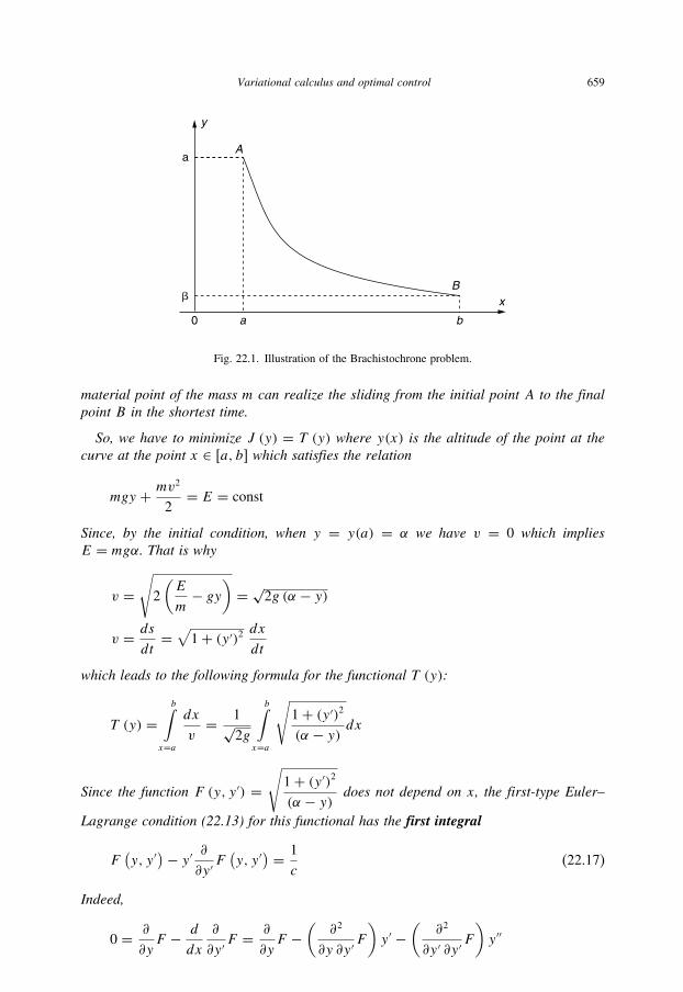
Variational calculus and optimal control 659
y
A
B
a b0
xb
a
Fig. 22.1. Illustration of the Brachistochrone problem.
material point of the mass m can realize the sliding from the initial point A to the finalpoint B in the shortest time.
So, we have to minimize J (y) = T (y) where y(x) is the altitude of the point at thecurve at the point x ∈ [a, b] which satisfies the relation
mgy + mv2
2= E = const
Since, by the initial condition, when y = y(a) = α we have v = 0 which impliesE = mgα. That is why
v =√2
(E
m− gy
)= √
2g (α − y)
v = dsdt
=√1+ (y ′)2 dx
dt
which leads to the following formula for the functional T (y):
T (y) =b∫
x=a
dx
v= 1√
2g
b∫x=a
√1+ (y ′)2(α − y) dx
Since the function F (y, y ′) =√
1+ (y ′)2(α − y) does not depend on x, the first-type Euler–
Lagrange condition (22.13) for this functional has the first integral
F(y, y ′
)− y ′ ∂∂y ′F(y, y ′
) = 1
c(22.17)
Indeed,
0 = ∂
∂yF − d
dx
∂
∂y ′F = ∂
∂yF −
(∂2
∂y ∂y ′F
)y ′ −
(∂2
∂y ′ ∂y ′F
)y ′′

660 Advanced Mathematical Tools for Automatic Control Engineers: Volume 1
Multiplying both sides by y ′ we get
0 = d
dx
(F − y ′ ∂
∂y ′F
)
which implies (22.17). In our case it is equivalent to the following ODE:
1
c=
√1+ (y ′)2(α − y) − (y
′)2(1+ (y ′)2)−1/2
√(α − y)
=
√1+ (y ′)2
(1− (y ′)2
1+ (y ′)2)
√(α − y) = 1√
(α − y)√1+ (y ′)2
Squaring gives
c2 = (α − y)[1+ (
y ′)2]
or,
1 = y ′√
(α − y)c2 − (α − y) (22.18)
With the introduction of the dependent variable θ = θ (x) such that
(α − y) = c2 sin2 θ2= c
2
2(1− cos θ), θ ∈ [0, 2π ]
then
c2 − (α − y) = c2 cos2 θ2, y ′ = c2θ ′ sin θ
2cosθ
2
By substitution of these expressions into (22.18) yields
1 = c2θ ′ sin2 θ2
or 1 = c2
2θ ′ (1− cos θ)
Integrating givesc2
2[θ − sin θ ] = x − c1. Denoting c2 := c2
2, we get the parametric
(Brachistochrone) curve (of the cycloid type)
x = c2 [θ − sin θ ]+ c1, c2 > 0
y = α − c2 (1− cos θ), θ ∈ [0, 2π ](22.19)
The constants c1 and c2 can be found from the boundary conditions
θ = θA = 0 : A = c1, y (A) = αθ = θB : B = A+ c2 [θB − sin θB], y (B) = β = α − c2 (1− cos θB)

Variational calculus and optimal control 661
Example 22.2. Let us try to answer the following question: which stable linear systemof the first order, given by
x (t) = ax (t), x (0) = x0, x (∞) = 0 (22.20)
provides the minimum of the functional
J (x) :=∞∫
t=0
[α0x
2 (t)+ α1x2 (t)]dt (22.21)
where α0, α1 > 0.
1. Variation calculus application. The first-type necessary condition of the optimalityfor this functional is
α0x (t)− α1x (t) = 0
since F = α0x2 + α1x2. Its general solution is
x (t) = c1e−kt + c2ekt , k :=√α0/α1
Taking into account the boundary conditions we get: c2 = 0, c1 = x0 which givesx (t) = x0e−kt , or, equivalently, x (t) = −kx (t). So, the optimal a = a∗ in (22.20) isa = a∗ = −√α0/α1. Let us show that the obtained curve is minimizing. To do thiswe need to check conditions (2) and (3) of the Jacobi theorem 22.5. First, notice that∂2
∂x ∂xF = 2α1 > 0. So, condition (2) is fulfilled. The Jacobi equation (22.16) is as
follows
α0u− α1u′′ = 0
Q := ∂2
∂y2F − d
dx
∂2
∂y ∂y ′F = 2α0, P := ∂2
∂y ′ ∂y ′F = 2α1
It has a nontrivial solution u (t) = u0e−kt > 0 or u0 > 0. This means that condition(3) is also valid. So, the curve x (t) = −kx (t), x (0) = x0 is minimizing.
2. Direct method.1 Assuming that the minimal value of the cost functional (22.21) is finite,i.e., x (t)→ 0 with t →∞, we can represent it in the following equivalent form
J (x) :=∞∫
t=0
[α0x
2 (t)+ 2√α0α1x (t) x (t)+ α1x2 (t)
]dt
− 2√α0α1
∞∫t=0
x (t) x (t) dt =∞∫
t=0
[√α0x (t)+√
α1x (t)]2dt
+ √α0α1x
2 (0) ≥ √α0α1x
2 (0)
1 The author has been informed of this elegant and simple solution by Prof. V. Utkin.

662 Advanced Mathematical Tools for Automatic Control Engineers: Volume 1
The last inequality becomes the equality when
√α0x (t)+√
α1x (t) = 0
or, equivalently, when
x (t) = −kx (t), k =√α0/α1
which coincides with the previous result.
22.4.1.2 Vector caseConsider the following optimization problem
b∫x=aF(x, y1, . . . yn, y
′1, . . . , y
′n
)dx → min
yi∈C1[a,b](22.22)
where the function F : R2n+1→ R is assumed to be twice differentiable in all arguments,
and the functions yi satisfy the following boundary conditions
yi (a) = αi, yi (b) = βi (i = 1, . . . , n) (22.23)
Theorem 22.6. (The Euler–Lagrange vector form) The first-type necessary conditionfor curve yi ∈ C1 [a, b], satisfying (22.23), to be extremal curves is:
∂
∂yiF (x, y, y′)− d
dx
∂
∂y ′iF (x, y, y′) = 0
y := (y1, . . . yn)ᵀ, y′ := (y ′1, . . . y
′n
)ᵀ(22.24)
Proof. It follows directly from the identity
0 = ϕ1 (y, h)=b∫
x=a
n∑i=1
(∂
∂yiFhi + ∂
∂y ′iFh′i
)dx
=b∫
x=a
n∑i=1
(∂
∂yiFi − d
dx
∂
∂y ′iF
)hi dx
if we take into account the independence of the variation functions hi (i = 1, . . . , n),
and apply Lemma 22.4. �
Theorem 22.7. (The Legendre vector form) The second-type necessary condition forcurve yi ∈ C1 [a, b], satisfying (22.23) and (22.24), to be extremal curves is:
∇2y′,y′F (x, y, y
′) ≥ 0 (22.25)
Variational calculus and optimal control 663
where the matrix in (22.25) is defined by
∇2y′,y′F
(x, y, y′
) := [∂2
∂y ′i ∂y ′jF(x, y, y′
)]i,j=1,...,n
Proof. It follows directly from (22.7) and the relation
0 ≤ ϕ2 (y, h)=b∫
x=a
[(∇2y,yF
(x, y, y′
)h,h
)+ 2
(∇2y,y′F (x, y, y
′)h,h′)+ (∇2
y′,y′F (x, y, y′)h′,h′
)]dx
=b∫
x=a
[([∇2
y,yF(x, y, y′
)− d
dx∇2
y,y′F(x, y, y′
)]h,h
)
+ (∇2y′,y′F (x, y, y
′)h′,h′) ]dx
if we apply the vector version of Lemma 22.7. �The next theorem gives the sufficient conditions for the vector function y to be a
minimizer in the problem (22.22).
Theorem 22.8. (The Jacobi vector form) If for some vector function y ∈ (C1 [a, b]
)n,
verifying (22.23), the following conditions are fulfilled:
1. it satisfies the Euler–Lagrange necessary condition (22.24);2. it satisfies the strong Legendre vector condition
∇2y′,y′F (x, y, y
′) ≥ kIn×n, k > 0 (22.26)
3. there exists vector functions ui ∈ (C1 [a, b]
)n(i = 1, . . . , n), such that
det[u1 (x) · · · un (x)] �= 0 for all x ∈ [a, b]
ui (a) = 0,d
dxui (a) = ei :=
⎛⎝0, . . . , 1︸ ︷︷ ︸
i
, 0, . . . , 0
⎞⎠ᵀ
(22.27)
and satisfying the next ODE (the Jacobi vector form ODE):
Qu− d
dx
(Pu′
) = 0 (22.28)
with
Q := ∇2y,yF (x, y, y
′)− d
dx∇2
y,y′F (x, y, y′)
P := ∇2y′,y′F (x, y, y
′)
then this vector function provides the local minimum to the functional J (y).
664 Advanced Mathematical Tools for Automatic Control Engineers: Volume 1
Proof. It follows directly from the vector form of Theorem 22.2 if we define ‖h‖2B for
B = (C1 [a, b]
)n(see (18.6)) as
‖h‖2(C1[a,b])
n :=n∑i=1
(maxx∈[a,b]
∣∣hi (t)∣∣+ maxx∈[a,b]
∣∣∣∣ ddx hi (x)∣∣∣∣)
and, practically, repeat the proof of Theorem 22.5. �
22.4.1.3 Integral functional depending on derivatives of an order more than oneLet us consider the first-type necessary condition of the optimality for the integral
functions
J (y) =b∫
x=aF (x, y, y(1), . . . , y(n)) dx (22.29)
within the functions y ∈ Cn [a, b], satisfying the boundary conditions
y(i) (a) = αi, y(i) (b) = βi (i = 1, . . . , n) (22.30)
First, notice that
ϕ1 (y, h) =b∫
x=a
[n∑i=0
∂F
∂y(i)h(i)
]dx, y(0) := y
where the variation functions h(i) satisfy the conditions
h(i) (a) = h(i) (b) = 0 (i = 1, . . . , n)
Integrating each integral term∫ bx=a
∂F
∂y(i)h(i) dx of this equality i-times we derive
ϕ1 (y, h) =b∫
x=a
[∂F
∂y+
n∑i=1
(−1)id
dxi
∂F
∂y(i)
]h dx (22.31)
Theorem 22.9. (Euler–Poisson) Let the curve y ∈ Cn [a, b], satisfying (22.30), be anextremal (minimum or maximum) curve for the functional (22.29). Then it should satisfythe following ODE:
∂F
∂y+
n∑i=1
(−1)id
dxi
∂F
∂y(i)= 0 (22.32)
Proof. It follows directly from (22.31) applying the Lagrange lemma 22.5. �

Variational calculus and optimal control 665
22.4.2 Curves with non-fixed boundary points
Problem formulation: among all smooth curves y = y (x) with the boundary points
(x0, y0) and (x1, y1), belonging to the given curves (“sliding surfaces”) y = ϕ (x) andy = ψ (x), find one which minimizes the functional
J (y) =x1:y(x1)=ψ(x1)∫
x=x0:y(x0)=ϕ(x0)F (x, y (x), y ′ (x)) dx (22.33)
Realizing the function variation (y + h) such that
h (xi) ' δy (xi)− y ′ (xi) δxi, i = 0, 1
δy (x0) ' ϕ′ (x0) δx0, δy (x1) ' ψ ′ (x1) δx1(22.34)
and integrating by parts, we derive
ϕ1 (y0, h)=x1∫
x=x0
(∂F
∂yh+ ∂F
∂y ′h′)dx + F (
x, y, y ′)δx |x=x1x=x0
=x1∫
x=x0
(∂F
∂y− d
dx
∂F
∂y ′
)h dx + ∂F
∂y ′h |x=x1x=x0 + F
(x, y, y ′
)δx |x=x1x=x0
(22.35)
Remark 22.1. Since the problem in 22.4.2 contains as a partial case the problem (22.9)with fixed boundary points, then any solution of the problem in 22.4.2 should satisfy theEuler–Lagrange condition (22.13), which simplifies (22.35) up to
ϕ1 (y0, h) = ∂F∂y ′h |x=x1x=x0 +F
(x, y, y ′
)δx |x=x1x=x0 (22.36)
Applications (22.34) to (22.36) imply
ϕ1 (y0, h)= ∂F∂y ′δy |x=x1x=x0 +
(F − ∂F
∂y ′y ′)δx |x=x1x=x0
=(∂F
∂y ′ψ ′ + F − ∂F
∂y ′y ′)|x=x1 δx1
+(∂F
∂y ′ϕ′ + F − ∂F
∂y ′y ′)|x=x0 δx0
(22.37)
Theorem 22.10. If some curve y = y(x) ∈ C1 with the boundary points (x0, y0) and(x1, y1), belonging to the given curves (“sliding surfaces”) y = ϕ (x) and y = ψ (x)provides an extremum to the functional (22.33), then

666 Advanced Mathematical Tools for Automatic Control Engineers: Volume 1
1. it satisfies the Euler–Lagrange condition (22.13), i.e.,
∂F
∂y− d
dx
∂F
∂y ′= 0
2. it should, additionally, satisfy the, so-called, transversality conditions
[F + ∂F
∂y ′(ψ ′ − y ′)
]|x=x1= 0[
F + ∂F∂y ′(ψ ′ − y ′)
]|x=x0= 0
(22.38)
Proof. The relations (22.38) result from (22.37) if we take into account that the variations
δx0 and δx1 are independent. �
Example 22.3.
J (y) =x1:y(x1)=2−x∫x0=0:y(x0)=0
√1+ (y ′ (x))2
xdx
The Euler–Lagrange condition (22.13) is − ddx
y ′
x√1+ (y ′)2 = 0, which leads to the fol-
lowing relation
y ′
x√1+ (y ′)2 = c1, y ′ = ± xc1√
1− x2c21y = ∓ 1
c1
√1− x2c21 + c2, (y − c2)2 = 1/c21 − x2
The boundary condition y (0) = 0 gives c21 = 1/c22. So, finally, the Euler–Lagrangecondition (22.13) is (y − c2)2 + x2 = c22. The transversality conditions (22.38) imply
0 = y ′ = − x
y − c2 = 1, which, together with y = 2 − x, gives c2 = 2. Finally, the
extremal curve is as follows:
(y − 2)2 + x2 = 4
22.4.3 Curves with a nonsmoothness point
If an extremal curve has a nonsmooth point x∗ ∈ [a, b] in the problem (22.9) with a
fixed boundary point, that is,
y (x) is continuous in x∗
y ′ (x) |x→x∗−0 �= y ′ (x) |x→x∗+0
thenϕ1 (y0, h) = ϕ1,1 (y0, h)+ ϕ1,2 (y0, h) = 0

Variational calculus and optimal control 667
where (we can consider at each semi-interval [a, x∗] and [x∗, b] the boundary point x∗
as a non-fixed one)
ϕ1,1 (y0, h) = ∂F∂y ′δy |x=x∗−0 +
(F − ∂F
∂y ′y ′)δx |x=x∗−0
ϕ1,2 (y0, h) = −∂F∂y ′δy |x=x∗+0 −
(F − ∂F
∂y ′y ′)δx |x=x∗+0
which gives
0= ϕ1 (y0, h)
=(∂F
∂y ′|x=x∗−0 −∂F
∂y ′|x=x∗+0
)δy
+[(F − ∂F
∂y ′y ′)|x=x∗−0 −
(F − ∂F
∂y ′y ′)|x=x∗+0
]δx
Since here δy and δx are admitted to be arbitrary, we obtain the, so-called, Weierstrass–Erdmann conditions:
∂F
∂y ′|x=x∗−0 = ∂F
∂y ′|x=x∗+0
(F − ∂F
∂y ′y ′)|x=x∗−0 =
(F − ∂F
∂y ′y ′)|x=x∗+0
(22.39)
Example 22.4. Consider the functional
J (y) =b∫
x=a
(y ′)2 (
1− y ′)2 dxThe boundary points are assumed to be fixed. The Euler–Lagrange condition (22.13)gives y = c1x + c2. The Weierstrass–Erdmann conditions (22.39) are
2y ′ (1− y ′) (1− 2y ′) |x=x∗−0 = 2y ′ (1− y ′) (1− 2y ′) |x=x∗+0
− (y ′)2 (1− y ′) (1− 3y ′) |x=x∗−0 = − (y ′)2 (1− y ′) (1− 3y ′) |x=x∗+0
which are fulfilled for extremal curves such that
y ′ |x=x∗−0 = 0, y ′ |x=x∗+0 = 1 or y ′ |x=x∗−0 = 1, y ′ |x=x∗+0 = 0

668 Advanced Mathematical Tools for Automatic Control Engineers: Volume 1
22.5 Optimal control problem
22.5.1 Controlled plant, cost functionals and terminal set
Consider the controlled plant given by the following system of ordinary differential
equations (ODE)
·x (t) = f (x (t), u (t), t), a.e. t ∈ [0, T ]
x (0) = x0}
(22.40)
where x = (x1, . . . , xn
)T ∈ Rn is its state vector, u = (u1, . . . , ur
)T ∈ Rr is the control
that may run over a given control region U ⊂ Rr with the cost functional
J (u (·)) := h0(x (T ))+T∫
t=0
h (x (t), u (t), t) dt (22.41)
containing the integral term as well as the terminal one and with the terminal setM ⊆ Rn given by the inequalities
M = {x ∈ Rn : gl(x) ≤ 0 (l = 1, . . . , L)} (22.42)
The time process or horizon T is supposed to be fixed or nonfixed and may be finite or
infinite.
Definition 22.4.
(a) The function (22.41) is said to be given in Bolza form.(b) If in (22.41) h0(x) = 0 we obtain the cost functional in Lagrange form, that is,
J (u (·)) =T∫
t=0
h (x (t), u (t), t) dt (22.43)
(c) If in (22.41) h(x, u, t) = 0 we obtain the cost functional in Mayer form, that is,
J (u (·)) = h0(x (T )) (22.44)
Usually the following assumptions are assumed to be in force:
(A1) (U, d) is a separable metric space (with the metric d) and T > 0.
(A2) The maps
f : Rn × U × [0, T ]→ Rn
h : Rn × U × [0, T ]→ R
h0 : Rn × U × [0, T ]→ R
gl : Rn → Rn (l = 1, . . . , L)
⎫⎪⎪⎪⎬⎪⎪⎪⎭ (22.45)

Variational calculus and optimal control 669
are measurable and there exist a constant L and a continuity modulus ω : [0,∞)→[0,∞) such that for ϕ = f (x, u, t), h (x, u, t), h0 (x, u, t), gl (x) (l = 1, . . . , L)
the following inequalities hold:∥∥ϕ (x, u, t)− ϕ (x, u, t)∥∥ ≤ L∥∥x − x∥∥+ ω (d (u, u))∀t ∈ [0, T ], x, x ∈ Rn, u, u ∈ U
‖ϕ (0, u, t)‖ ≤ L ∀u, t ∈ U × [0, T ]
⎫⎪⎬⎪⎭ (22.46)
(A3) The maps f, h, h0 and gl (l = 1, . . . , L) are from C1 in x and there exists a
continuity modulus ω : [0,∞)→ [0,∞) such that for ϕ = f (x, u, t), h (x, u, t),h0 (x, u, t), gl (x) (l = 1, . . . , L) the following inequalities hold:∥∥∥∥ ∂∂x ϕ (x, u, t)− ∂
∂xϕ(x, u, t
)∥∥∥∥≤ ω (∥∥x − x∥∥+ d (u, u))
∀t ∈ [0, T ], x, x ∈ Rn, u, u ∈ U
⎫⎪⎪⎪⎬⎪⎪⎪⎭ (22.47)
22.5.2 Feasible and admissible control
Definition 22.5. A function u(t), t0 ≤ t ≤ T , is said to be
(a) a feasible control if it is measurable and u(t) ∈ U for all t ∈ [0, T ]. Denote theset of all feasible controls by
U [0, T ] := {u (·) : [0, T ]→ U | u (t) is measurable
}(22.48)
(b) an admissible or realizing the terminal condition (22.42), if the correspondingtrajectory x(t) satisfies the terminal condition, that is, satisfies the inclusionx(T ) ∈ M. Denote the set of all admissible controls by
Uadmis [0, T ] :={u (·) : u (·) ∈ U [0, T ], x(T ) ∈ M
}(22.49)
In view of Theorem 19.1 on the existence and the uniqueness of an ODE solution, it
follows that under assumptions (A1)–(A2) for any u (t) ∈ U [0, T ] equation (1.4) admits
a unique solution x (·) := x (·, u (·)) and the functional (22.41) is well defined.
22.5.3 Problem setting in the general Bolza form
Based on the definitions given above, the optimal control problem (OCP) can be
formulated as follows.
Problem 22.1. (OCP in Bolza form)
Minimize (22.41) over Uadmis [0, T ] (22.50)
670 Advanced Mathematical Tools for Automatic Control Engineers: Volume 1
Problem 22.2. (OCP with a fixed terminal term) If in the problem (22.50)
M = {x ∈ Rn : g1(x) = x − xf ≤ 0, g2(x) = − (
x − xf) ≤ 0
}(22.51)
then it is called the optimal control problem with fixed terminal term xf .
Definition 22.6. Any control u∗ (·) ∈ Uadmis [0, T ] satisfying
J (u∗ (·)) = infu(·)∈Uadmis [0,T ]
J (u (·)) (22.52)
is called an optimal control. The corresponding state trajectories x∗ (·) := x∗ (·, u∗ (·))are called an optimal state trajectory, and (x∗ (·), u∗ (·)) is called an optimal pair.
22.5.4 Mayer form representation
Summary 22.1. Introduce (n+ 1)-dimensional space Rn+1 of the variables x =(x1, . . . , xn, xn+1)
ᵀ where the first n coordinates satisfy (22.40) and the component xn+1
is given by
xn+1 (t) :=t∫
τ=0
h (x (τ), u (τ ), τ ) dτ (22.53)
or, in the differential form,
xn+1 (t) = h (x (t), u (t), t) (22.54)
with the initial condition for the last component given by
xn+1 (0) = 0 (22.55)
As a result, the initial optimization problem in the Bolza form (22.50) can be reformulatedin the space Rn+1 as the Mayer problem with the cost functional J (u (·))
J (u (·)) = h0(x (T ))+ xn+1 (T ) (22.56)
where the function h0(x) does not depend on the last coordinate xn+1 (t), that is,
∂
∂xn+1
h0(x) = 0 (22.57)
Summary 22.2. From the relations above it follows that the Mayer problem with thecost function (22.56) is equivalent to the initial optimization control problem (22.50) inthe Bolza form.
There exist two principal approaches to solving optimal control problems:
• the first one is the maximum principle (MP) of L. Pontryagin (Boltyanski et al. 1956;Pontryagin et al. 1969 (translated from Russian));

Variational calculus and optimal control 671
• and the second one is the dynamic programing method (DPM) of R. Bellman (1957).
We will touch on both of them below.
22.6 Maximum principle
The maximum principle is a basic instrument to derive a set of necessary conditionswhich should satisfy any optimal control. As an optimal control problem may be regarded
as an optimization problem in the corresponding infinite dimensional (Hilbert or, in
general, Banach) space, the necessary conditions (resembling the Kuhn–Tucker conditionsin the finite-dimensional optimization) take place. They are known as the maximumprinciple which is really a milestone in modern optimal control theory. It states that any
dynamic system closed by an optimal control strategy or, simply, by an optimal control
is a Hamiltonian (with the doubled dimension) system given by a system of the forward–
backward ordinary differential equations and, in addition, an optimal control maximizes
the function called Hamiltonian. Its mathematical importance consists of the following
fact: the maximization of the Hamiltonian with respect to a control variable given in a
finite-dimensional space looks and really is much easier than the original optimization
problem formulated in an infinite-dimensional space. The key idea of the original version
of the maximum principle comes from classical variations calculus. To derive the main
MP formulation, first one needs to perturb slightly an optimal control using the so-called
needle-shape (spike) variations and, second, to consider the first-order term in a Taylor
expansion with respect to this perturbation. Tending perturbations to zero, some variation
inequalities may be obtained. Then the final result follows directly from duality.
22.6.1 Needle-shape variations
Let (x∗ (·), u∗ (·)) be the given optimal pair for the problem (22.52) and Mε ⊆ [0, T ]
be a measurable set of the time interval with Lebesgue measure |Mε| = ε > 0. Let now
u (·) ∈ Uadmis [0, T ] be any given admissible control.
Definition 22.7. Define the following control
uε (t) :=⎧⎨⎩
u∗ (t) if t ∈ [0, T ]�Mε
u (t) ∈ Uadmis [0, T ] if t ∈ Mε
(22.58)
Evidently uε (·) ∈ Uadmis [0, T ]. Below uε (·) is referred to as a needle-shape or spikevariation of the optimal control u∗ (t).
The next lemma plays a key role in proving the basic MP theorem.
Lemma 22.8. (The variational equation) Let xε (·) := x (·, uε (·)) be the solution of(22.52) for the plant model given by (22.40) under the control uε (·) and �ε (·) be the

672 Advanced Mathematical Tools for Automatic Control Engineers: Volume 1
solution to the following differential equation
�ε (t) = ∂
∂xf (x∗ (t), u∗ (t), t)�ε (t)
+ [f (x∗ (t), uε (t), t)− f (x∗ (t), u∗ (t), t)]χMε (t)�ε (0) = 0
(22.59)
where χMε (t) is the characteristic function of the set Mε, that is
χMε (t) :={1 if t ∈ Mε
0 if t /∈ Mε
(22.60)
Then
maxt∈[0,T ]
‖xε (t)− x∗ (t)‖ = O (ε)
maxt∈[0,T ]
‖�ε (t)‖ = O (ε)
maxt∈[0,T ]
‖xε (t)− x∗ (t)−�ε (t)‖ = o (ε)
⎫⎪⎪⎪⎪⎪⎬⎪⎪⎪⎪⎪⎭
(22.61)
and the following variational equations hold(a) for the cost function given in Bolza form (22.41)
J (uε (·))− J (u∗ (·)) =(∂
∂xh0 (x
∗ (T )),�ε (T ))
+T∫
t=0
{(∂
∂xh (x∗ (t), u∗ (t), t),�ε (t)
)
+ [h (x∗ (t), uε (t), t)− h (x∗ (t), u∗ (t), t)]χMε (t)}dt + o (ε)
(22.62)
(b) for the cost function given in Mayer form (22.44)
J (uε (·))− J (u∗ (·)) =(∂
∂xh0 (x
∗ (T )),�ε (T ))+ o (ε) (22.63)
Proof. Define δε (t) := xε (t)− x∗ (t). Then assumption (A2) (22.46) for any t ∈ [0, T ]
implies
‖δε (t)‖ ≤t∫
s=0
L ‖δε (s)‖ ds +Kε (22.64)
which, by the Gronwall lemma 19.4, leads to the first relation in (22.61). Define
ηε (t) := xε (t)− x∗ (t)−�ε (t) = δε (t)−�ε (t) (22.65)

Variational calculus and optimal control 673
Then
ηε (t)= [f (xε (t), uε (t), t)− f (x∗ (t), u∗ (t), t)]
− ∂
∂xf (x∗ (t), u∗ (t), t)�ε (t)
− [f (x∗ (t), uε (t), t)− f (x∗ (t), u∗ (t), t)]χMε (t)
=1∫
θ=0
[∂
∂xf (x∗ (t)+ θδε (t), uε (t), t)− ∂
∂xf (x∗ (t), u∗ (t), t)
]dθδε (t)
− [f (x∗ (t), uε (t), t)− f (x∗ (t), u∗ (t), t)]χMε (t)
+ ∂
∂xf (x∗ (t), u∗ (t), t) ηε (t)
(22.66)
Integrating the last identity (22.66) and in view of (A2) (22.46) and (A3) (22.47), we
obtain
‖ηε (t)‖ ≤t∫
s=0
1∫θ=0
[ω (θ ‖δε (s)‖ + d (uε (s), u∗ (s)))] ‖δε (s)‖ dθds
+t∫
s=0
ω (d (uε (s), u∗ (s))) χMε (s) ds +t∫
s=0
∂
∂xf (x∗ (s), u∗(s), s) ηε (s) ds
≤ Const · ε · o (1)+ Const ·t∫
s=0
‖ηε (s)‖ ds
(22.67)
The last inequality in (22.67) by the Gronwall lemma directly implies the third relation in
(22.61). The second relation follows from the first and third ones. The same manipulations
lead to (22.62) and (22.63). �
22.6.2 Adjoint variables and MP formulation
The classical format of MP formulation gives a set of first-order necessary conditionsfor optimal pairs.
Theorem 22.11. (MP for Mayer form with a fixed horizon) If under assumptions(A1)–(A3) a pair (x∗ (·), u∗ (·)) is optimal then there exist the vector functions ψ(t),satisfying the system of the adjoint equations
ψ(t) = − ∂∂xf (x∗ (t), u∗ (t), t)ᵀ ψ(t) a.e. t ∈ [0, T ] (22.68)

674 Advanced Mathematical Tools for Automatic Control Engineers: Volume 1
and nonnegative constants μ ≥ 0 and νl ≥ 0 (l = 1, . . . , L) such that the following fourconditions hold:
(a) (the maximality condition): for almost all t ∈ [0, T ]
H(ψ(t), x∗(t), u∗(t), t) = maxu∈U H(ψ(t), x
∗(t), u, t) (22.69)
where the Hamiltonian is defined by
H(ψ, x, u, t) := ψᵀf (x, u, t)
t, x, u, ψ ∈ [0, T ]× Rn × Rr × Rn(22.70)
(b) (transversality condition): the equality
ψ(T )+ μ ∂∂xh0(x
∗ (T ))+L∑l=1
νl∂
∂xgl(x
∗(T )) = 0 (22.71)
holds;(c) (complementary slackness conditions): either the equality gl(x∗(T )) = 0 holds, orνl = 0, that is, for any (l = 1, . . . , L)
νlgl(x∗(T )) = 0 (22.72)
(d) (nontriviality condition): at least one of the numbers |ψ(T )| and νl is distinct fromzero, that is,
‖ψ(T )‖ + μ+L∑l=1
νl > 0 (22.73)
Proof. Letψ(t) be the solution of (22.68) corresponding to the terminal conditionψ(T ) =b and t ∈ [0, T ]. Define Mε := [t , t + ε] ⊆ [0, T ]. If u∗(t) is an optimal control, then
according to the Lagrange principle (see Theorem 21.12), formulated for a Banach space,
there exist constants μ ≥ 0 and νl ≥ 0 (l = 1, . . . , L) such that for any ε ≥ 0
L (uε (·), μ, ν)− L (u∗ (·), μ, ν) ≥ 0 (22.74)
where
L (u (·), μ, ν) := μJ (u (·))+L∑l=1
νlgl (x (T )) (22.75)
Taking into account that ψ(T ) = b and �ε (0) = 0, by the differential chain rule, applied
to the term ψ(t)ᵀ�ε (t), and, in view of (22.59) and (22.68), we obtain
bᵀ�ε (T ) = ψ(T )ᵀ�ε (T )− ψ(0)ᵀ�ε (0)
=T∫
t=0
d (ψ(t)ᵀ�ε (t)) =T∫
t=0
(ψ(t)ᵀ�ε (t)+ ψ(t)ᵀ�ε (t)) dt

Variational calculus and optimal control 675
=T∫
t=0
[−�ε (t)ᵀ ∂
∂xf (x∗ (t), u∗ (t), t)ᵀ ψ(t)
+ ψ(t)ᵀ ∂∂xf (x∗ (t), u∗ (t), t)�ε (t)
+ ψ(t)ᵀ [f (x∗ (t), uε (t), t)− f (x∗ (t), u∗ (t), t)]χMε (t)]dt
=T∫
t=0
ψ(t)ᵀ [f (x∗ (t), uε (t), t)− f (x∗ (t), u∗ (t), t)]χMε (t) dt(22.76)
The variational equality (22.62) together with (22.74) and (22.76) implies
0 ≤ L (uε (·), μ, ν)− L (u∗ (·), μ, ν)
= μ(∂
∂xh0 (x
∗ (T )),�ε (T ))+ bᵀ�ε (T )
−T∫
t=0
ψ(t)ᵀ (f (x∗ (t), uε (t), t)− f (x∗ (t), u∗ (t), t)) χMε (t) dt
+L∑l=1
νl [gl (x (T ))− gl (x∗ (T ))]+ o (ε)
=(μ∂
∂xh0 (x
∗ (T ))+ b +L∑l=1
νl∂
∂xgl (x
∗ (T )),�ε (T )
)
−t+ε∫t=t
[ψ(t)ᵀ (f (x∗ (t), uε (t), t)− f (x∗ (t), u∗ (t), t))] dt + o (ε)
=(μ∂
∂xh0 (x
∗ (T ))+ b +L∑l=1
νl∂
∂xgl (x
∗ (T )),�ε (T )
)
−t+ε∫t=t
[H(ψ (t), x∗ (t), uε (t), t)−H(ψ (t), x∗ (t), u∗ (t), t)] dt
(22.77)
1. Tending ε to zero from (22.77) it follows that
0 ≤(μ∂
∂xh0 (x
∗ (T ))+ b +L∑l=1
νl∂
∂xgl (x
∗ (T )),�ε (T )
)|ε=0
676 Advanced Mathematical Tools for Automatic Control Engineers: Volume 1
which should be valid for any �ε (T ) |ε=0. This is possible only if (this can be proved
by contradiction)
μ∂
∂xh0 (x
∗ (T ))+ b +L∑l=1
νl∂
∂xgl (x
∗ (T )) = 0 (22.78)
which is equivalent to (22.71). So, the transversality condition is proven.
2. In view of (22.78), the inequality (22.77) may be simplified to the following one
0 ≤ −t+ε∫t=t
[H(ψ (t), x∗ (t), uε (t), t)−H(ψ (t), x∗ (t), u∗ (t), t)] dt
(22.79)
This inequality together with separability of metric space U directly leads to the
maximality condition (22.69).
3. Suppose that (22.72) does not hold, that is, there exist an index l0 and a multiplier νl0such that νlgl(x
∗(T )) < 0. This gives
L (u∗ (·), μ, ν) := μJ (u∗ (·))+L∑l=1
νlgl (x∗ (T ))
= μJ (u∗ (·))+ νl0gl0 (x∗ (T )) < μJ (u∗ (·)) = L (u∗ (·), μ, ν)
It means that u∗ (·) is not optimal control. We obtain the contradiction. So, the com-
plementary slackness condition is proven too.
4. Suppose that (22.73) is not valid, i.e., |ψ(T )| + μ + ∑L
l=1 νl = 0. This implies
ψ(T ) = 0, μ = νl = 0 (l = 1, . . . , L), and, hence, in view of (22.68) and
by the Gronwall lemma 19.4, it follows that ψ(t) = 0 for all t ∈ [0, T ]. So,
H(ψ(t), x(t), u(t), t) = 0 for any u(t) (not only for u∗(t)). This means that the
application of any admissible control keeps the cost function unchangeable which
corresponds to a trivial situation. So, the nontriviality condition is proven too. �
22.6.3 The regular case
In the, so-called, regular case, when μ > 0 (this means that the nontriviality condition
holds automatically), the variable ψ(t) and constants νl may be normalized and change
to ψ(t) := ψ(t)/μ and νl := νl/μ. In this new variable the MP formulation looks as
follows.
Theorem 22.12. (MP in the regular case) If under assumptions (A1)–(A3) a pair(x∗ (·), u∗ (·)) is optimal, then there exists a vector function ψ(t) satisfying the system ofthe adjoint equations
d
dtψ(t) = − ∂
∂xf (x∗ (t), u∗ (t), t)ᵀ ψ(t) a.e. t ∈ [0, T ]

Variational calculus and optimal control 677
and νl ≥ 0 (l = 1, . . . , L) such that the following three conditions hold:
(a) (the maximality condition): for almost all t ∈ [0, T ]
H(ψ(t), x∗(t), u∗(t), t) = maxu∈U H(ψ(t), x
∗(t), u, t) (22.80)
where the Hamiltonian is defined by
H(ψ, x, u, t) := ψᵀf (x, u, t)
t, x, u, ψ ∈ [0, T ]× Rn × Rr × Rn
(b) (transversality condition): for every α ∈ A, the equalities
ψ(T )+ ∂
∂xh0(x
∗ (T ))+L∑l=1
νl∂
∂xgl(x
∗(T )) = 0
hold;(c) (complementary slackness conditions): either the equality gl(x∗(T )) = 0 holds, orνl = 0, that is, for any (l = 1, . . . , L) νlgl(x
∗(T )) = 0.
Remark 22.2. This means that without loss of generality we may put μ = 1. It may be
shown that the regularity property takes place if the vectors∂
∂xgl(x
∗(T )) are linearly
independent. The verification of this property is usually not so simple a task.
22.6.4 Hamiltonian form and constancy property
Corollary 22.3. (Hamiltonian for the Bolza problem) Hamiltonian for the Bolza prob-lem has the form
H(ψ, x, u, t) := ψᵀf (x, u, t)− μh (x (t), u (t), t)t, x, u, ψ ∈ [0, T ]× Rn × Rr × Rn
(22.81)
Proof. It follows from (22.53)–(22.57). Indeed, since the Mayer’s form representation
(xn+1 (t) = h (x (t), u (t), t)) implies ψn+1 (t) = 0, then ψn+1 (T ) = −μ. �
Corollary 22.4. (Hamiltonian form) Equations (22.40) and (22.68) may be representedin the, so-called, Hamiltonian form (the forward–backward ODE form):
x∗ (t) = ∂
∂ψH(ψ(t), x∗(t), u∗ (t), t), x∗(0) = x0
ψ (t) = − ∂∂xH(ψ(t), x∗(t), u∗ (t), t)
ψ(T ) = −μ ∂∂xh0 (x
∗ (T ))−L∑l=1
νl∂
∂xgl (x
∗ (T ))
⎫⎪⎪⎪⎪⎪⎪⎬⎪⎪⎪⎪⎪⎪⎭
(22.82)
Proof. It directly follows from comparison of the right-hand side of (22.70) with (22.40)
and (22.68). �

678 Advanced Mathematical Tools for Automatic Control Engineers: Volume 1
Corollary 22.5. (Constancy property) For stationary systems when in (22.40), (22.41)
f = f (x (t), u (t)), h = h (x (t), u (t)) (22.83)
it follows that for all t ∈ [t0, T ]
H(ψ(t), x∗(t), u∗ (ψ(t), x∗(t))) = const (22.84)
Proof. One can see that in this case the Hamiltonian H = H(ψ(t), x(t), u(t)) does notdepend on t directly, that is,
∂
∂tH = 0. Hence, u∗(t) is a function of ψ(t) and x∗(t) only,
i.e., u∗(t) = u∗ (ψ(t), x∗(t)). Denote
H(ψ(t), x∗(t), u∗ (ψ(t), x∗(t))) := H (ψ(t), x∗(t))
Then (22.82) becomes
x (t) = ∂
∂ψH (ψ(t), x∗(t)), ψ (t) = − ∂
∂xH (ψ(t), x∗(t))
which implies
d
dtH (ψ(t), x∗(t)) = ∂
∂ψH (ψ(t), x∗(t))ᵀ ψ(t)
+ ∂
∂xH (ψ(t), x∗(t))ᵀ x(t) = 0
and hence H (ψ(t), x∗(t)) = const for any t ∈ [t0, T ]. �
22.6.5 Nonfixed horizon optimal control problem and zero property
Consider the following generalization of the optimal control problem (22.40), (22.44),
(22.50) permitting terminal time to be free. In view of this, the optimization problem may
be formulated in the following manner: minimize
J (u (·)) = h0(x (T ), T ) (22.85)
over u (·) ∈ Uadmis [0, T ] and T ≥ 0 with the terminal set M (T ) given by
M (T ) = {x (T ) ∈ Rn : gl(x (T ), T ) ≤ 0 (l = 1, . . . , L)} (22.86)
Theorem 22.13. (MP for non fixed horizon case) If under assumptions (A1)–(A3) thepair (T ∗, u∗ (·)) is a solution of the problem (22.85), (22.86) and x∗ (t) is the corre-sponding optimal trajectory, then there exist the vector functions ψ(t), satisfying thesystem of the adjoint equations (22.68), and nonnegative constants μ ≥ 0 and νl ≥ 0
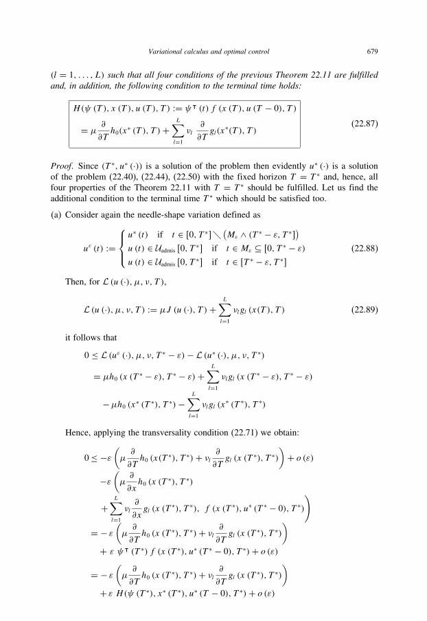
Variational calculus and optimal control 679
(l = 1, . . . , L) such that all four conditions of the previous Theorem 22.11 are fulfilledand, in addition, the following condition to the terminal time holds:
H(ψ (T ), x (T ), u (T ), T ) := ψᵀ (t) f (x (T ), u (T − 0), T )
= μ ∂∂Th0(x
∗ (T ), T )+L∑l=1
νl∂
∂Tgl(x
∗(T ), T )(22.87)
Proof. Since (T ∗, u∗ (·)) is a solution of the problem then evidently u∗ (·) is a solution
of the problem (22.40), (22.44), (22.50) with the fixed horizon T = T ∗ and, hence, all
four properties of the Theorem 22.11 with T = T ∗ should be fulfilled. Let us find the
additional condition to the terminal time T ∗ which should be satisfied too.
(a) Consider again the needle-shape variation defined as
uε (t) :=
⎧⎪⎨⎪⎩u∗ (t) if t ∈ [0, T ∗]�
(Mε ∧ (T ∗ − ε, T ∗]
)u (t) ∈ Uadmis [0, T
∗] if t ∈ Mε ⊆ [0, T ∗ − ε)u (t) ∈ Uadmis [0, T
∗] if t ∈ [T ∗ − ε, T ∗](22.88)
Then, for L (u (·), μ, ν, T ),
L (u (·), μ, ν, T ) := μJ (u (·), T )+L∑l=1
νlgl (x(T ), T ) (22.89)
it follows that
0 ≤ L (uε (·), μ, ν, T ∗ − ε)− L (u∗ (·), μ, ν, T ∗)
= μh0 (x (T ∗ − ε), T ∗ − ε)+L∑l=1
νlgl (x (T∗ − ε), T ∗ − ε)
−μh0 (x∗ (T ∗), T ∗)−L∑l=1
νlgl (x∗ (T ∗), T ∗)
Hence, applying the transversality condition (22.71) we obtain:
0≤ −ε(μ∂
∂Th0 (x(T
∗), T ∗)+ νl ∂∂Tgl (x (T
∗), T ∗))+ o (ε)
−ε(μ∂
∂xh0 (x (T
∗), T ∗)
+L∑l=1
νl∂
∂xgl (x (T
∗), T ∗), f (x (T ∗), u∗ (T ∗ − 0), T ∗)
)
= − ε(μ∂
∂Th0 (x (T
∗), T ∗)+ νl ∂∂Tgl (x (T
∗), T ∗))
+ ε ψᵀ (T ∗) f (x (T ∗), u∗ (T ∗ − 0), T ∗)+ o (ε)
= − ε(μ∂
∂Th0 (x (T
∗), T ∗)+ νl ∂∂Tgl (x (T
∗), T ∗))
+ ε H(ψ (T ∗), x∗ (T ∗), u∗ (T − 0), T ∗)+ o (ε)
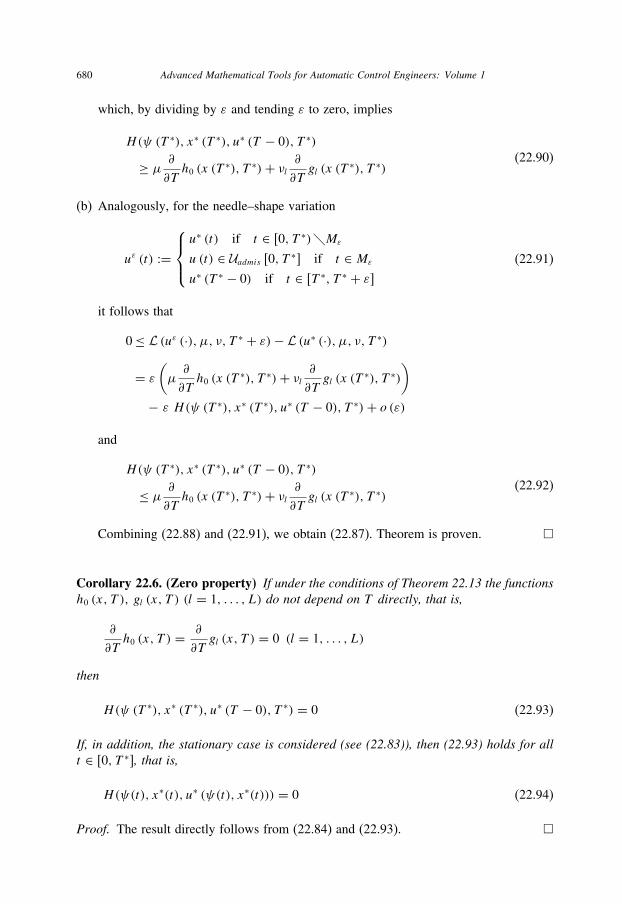
680 Advanced Mathematical Tools for Automatic Control Engineers: Volume 1
which, by dividing by ε and tending ε to zero, implies
H(ψ (T ∗), x∗ (T ∗), u∗ (T − 0), T ∗)
≥ μ ∂∂Th0 (x (T
∗), T ∗)+ νl ∂∂Tgl (x (T
∗), T ∗)(22.90)
(b) Analogously, for the needle–shape variation
uε (t) :=
⎧⎪⎨⎪⎩u∗ (t) if t ∈ [0, T ∗)�Mε
u (t) ∈ Uadmis [0, T ∗] if t ∈ Mε
u∗ (T ∗ − 0) if t ∈ [T ∗, T ∗ + ε](22.91)
it follows that
0≤ L (uε (·), μ, ν, T ∗ + ε)− L (u∗ (·), μ, ν, T ∗)
= ε(μ∂
∂Th0 (x (T
∗), T ∗)+ νl ∂∂Tgl (x (T
∗), T ∗))
− ε H(ψ (T ∗), x∗ (T ∗), u∗ (T − 0), T ∗)+ o (ε)
and
H(ψ (T ∗), x∗ (T ∗), u∗ (T − 0), T ∗)
≤ μ ∂∂Th0 (x (T
∗), T ∗)+ νl ∂∂Tgl (x (T
∗), T ∗)(22.92)
Combining (22.88) and (22.91), we obtain (22.87). Theorem is proven. �
Corollary 22.6. (Zero property) If under the conditions of Theorem 22.13 the functionsh0 (x, T ), gl (x, T ) (l = 1, . . . , L) do not depend on T directly, that is,
∂
∂Th0 (x, T ) = ∂
∂Tgl (x, T ) = 0 (l = 1, . . . , L)
then
H(ψ (T ∗), x∗ (T ∗), u∗ (T − 0), T ∗) = 0 (22.93)
If, in addition, the stationary case is considered (see (22.83)), then (22.93) holds for allt ∈ [0, T ∗], that is,
H(ψ(t), x∗(t), u∗ (ψ(t), x∗(t))) = 0 (22.94)
Proof. The result directly follows from (22.84) and (22.93). �
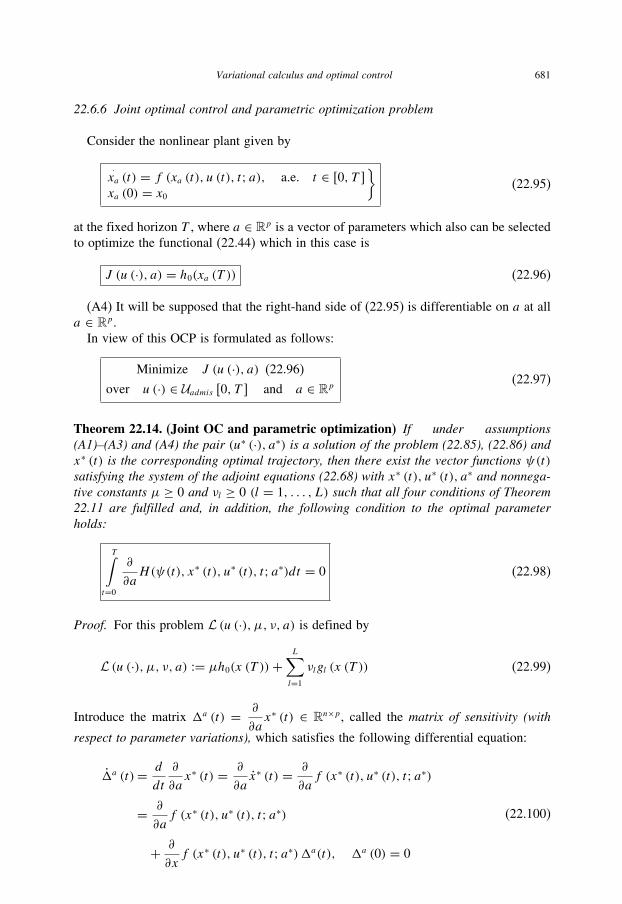
Variational calculus and optimal control 681
22.6.6 Joint optimal control and parametric optimization problem
Consider the nonlinear plant given by
·xa (t) = f (xa (t), u (t), t; a), a.e. t ∈ [0, T ]
xa (0) = x0}
(22.95)
at the fixed horizon T , where a ∈ Rp is a vector of parameters which also can be selected
to optimize the functional (22.44) which in this case is
J (u (·), a) = h0(xa (T )) (22.96)
(A4) It will be supposed that the right-hand side of (22.95) is differentiable on a at all
a ∈ Rp.
In view of this OCP is formulated as follows:
Minimize J (u (·), a) (22.96)
over u (·) ∈ Uadmis [0, T ] and a ∈ Rp(22.97)
Theorem 22.14. (Joint OC and parametric optimization) If under assumptions(A1)–(A3) and (A4) the pair (u∗ (·), a∗) is a solution of the problem (22.85), (22.86) andx∗ (t) is the corresponding optimal trajectory, then there exist the vector functions ψ(t)satisfying the system of the adjoint equations (22.68) with x∗ (t), u∗ (t), a∗ and nonnega-tive constants μ ≥ 0 and νl ≥ 0 (l = 1, . . . , L) such that all four conditions of Theorem22.11 are fulfilled and, in addition, the following condition to the optimal parameterholds:
T∫t=0
∂
∂aH(ψ(t), x∗ (t), u∗ (t), t; a∗)dt = 0 (22.98)
Proof. For this problem L (u (·), μ, ν, a) is defined by
L (u (·), μ, ν, a) := μh0(x (T ))+L∑l=1
νlgl (x (T )) (22.99)
Introduce the matrix �a (t) = ∂
∂ax∗ (t) ∈ Rn×p, called the matrix of sensitivity (with
respect to parameter variations), which satisfies the following differential equation:
�a (t)= d
dt
∂
∂ax∗ (t) = ∂
∂ax∗ (t) = ∂
∂af (x∗ (t), u∗ (t), t; a∗)
= ∂
∂af (x∗ (t), u∗ (t), t; a∗)
+ ∂
∂xf (x∗ (t), u∗ (t), t; a∗)�a(t), �a (0) = 0
(22.100)

682 Advanced Mathematical Tools for Automatic Control Engineers: Volume 1
In view of this and using (22.68), it follows that
0 ≤ L (u∗ (·), μ, ν, a)− L (u∗ (·), μ, ν, a∗)
= (a − a∗)ᵀ�a(T )ᵀ(μ∂
∂xh0 (x
∗ (T ))+L∑l=1
νl∂
∂xgl (x
∗ (T ))
)
+ o (‖a − a∗‖) = (a − a∗)ᵀ�a(T )ᵀψ(T )+ o (‖a − a∗‖)= (a − a∗)ᵀ [�a(T )ᵀψ(T )−�a(0)ᵀψ(0)]+ o (‖a − a∗‖)
= (a − a∗)ᵀT∫
t=0
d [�a(t)ᵀψ(t)]+ o (‖a − a∗‖)
= (a − a∗)ᵀT∫
t=0
[−�a (t)ᵀ ∂
∂xf (x∗ (t), u∗ (t), t; a∗)ᵀ ψ(t)
+�a (t)ᵀ ∂
∂xf (x∗ (t), u∗ (t), t; a∗)ᵀ ψ(t)
+ ∂
∂af (x∗ (t), u∗ (t), t; a∗)ᵀ ψ(t)
]dt + o (‖a − a∗‖)
= (a − a∗)ᵀT∫
t=0
∂
∂af (x∗ (t), u∗ (t), t; a∗)ᵀ ψ(t)dt + o (‖a − a∗‖)
But this inequality is possible for any a ∈ Rp in a small neighborhood of a∗ if and
only if the relation (22.98) holds (which may be proved by contradiction). Theorem is
proven. �
22.6.7 Sufficient conditions of optimality
The necessary and sufficient conditions of the constrained concave optimization
problem on x ∈ X ⊆ Rn is (see (21.80))
(∂f (x∗), x − x∗) ≤ 0
which should be valid for all x ∈ X (X is supposed to be a convex set and f (x) is
concave on X).
Here we will also need an additional assumption concerning the control region.
(A4) The control domain U is supposed to be a convex body (i.e., it is convex and has a
nonempty interior).
Lemma 22.9. (on a mixed subgradient) Let ϕ be a convex (or concave) function onRn × U where U is a convex body. Assuming that ϕ (x, u) is differentiable in x and

Variational calculus and optimal control 683
is continuous in (x, u), the following inclusion turns out to be valid for any (x∗, u∗) ∈Rn × U:
{(ϕx (x∗, u∗), r) | r ∈ ∂uϕ (x∗, u∗)} ⊆ ∂x,uϕ (x∗, u∗) (22.101)
Proof. For any y ∈ Rn, in view of the convexity of ϕ and its differentiability on x, it
follows that
ϕ (x∗ + y, u∗)− ϕ (x∗, u∗) ≥ (ϕx (x∗, u∗), y) (22.102)
Similarly, in view of the convexity of ϕ in u, there exists a vector r ∈ Rr such that for
any x∗, y ∈ Rn and any u ∈ U
ϕ (x∗ + y, u∗ + u)− ϕ (x∗ + y, u∗) ≥ (r, u) (22.103)
So, taking into account the previous inequalities (22.102)–(22.103), we derive
ϕ (x∗ + y, u∗ + u)− ϕ (x∗, u∗)= [ϕ (x∗ + y, u∗ + u)− ϕ (x∗ + y, u∗)]+ [ϕ (x∗ + y, u∗)− ϕ (x∗, u∗)] ≥ (r, u)+ (ϕx(x∗, u∗), y)
(22.104)
Then, by the definition of subgradient (21.69), it means that
(ϕx (x∗, u∗); r) ⊆ ∂dx,uϕ (x∗, u∗)
The concavity case is very similar if we note that (−ϕ) is convex. �
Now we are ready to formulate the central result of this subsection.
Theorem 22.15. (Sufficient condition of optimality) Let, under assumptions (A1)–(A4),the pair (x∗ (·), u∗ (·)) be an admissible pair and ψ (t) be the corresponding adjointvariable satisfying (22.68). Assume that
1. h0(x) and gl (x) (l = 1, . . . , L) are convex;2. H(ψ(t), x, u, t) is concave in (x, u) for any fixed t ∈ [0, T ] and any ψ(t) ∈ Rn.
Then this pair (x∗ (·), u∗ (·)) is optimal in the sense of the cost functional J (u (·)) =h0(x (T )) (22.44) if
H(ψ(t), x∗(t), u∗(t), t) = maxu∈U H(ψ(t), x∗(t), u, t) (22.105)
at almost all t ∈ [0, T ].
Proof. By (22.105) and in view of the criterion of optimality (21.80), it follows for any
u ∈ U that
(∂uH(ψ(t), x∗(t), u∗(t), t), u− u∗(t)) ≤ 0 (22.106)

684 Advanced Mathematical Tools for Automatic Control Engineers: Volume 1
Then, by concavity of H(ψ(t), x, u, t) in (x, u), for any admissible pair (x, u) and
applying the integration operation, in view of (22.106) we get
T∫t=0
H(ψ(t), x(t), u, t)dt −T∫
t=0
H(ψ(t), x∗(t), u∗(t), t)dt
≤T∫
t=0
[(∂
∂xH(ψ(t), x∗(t), u∗(t), t), x(t)− x∗(t)
)
+ (∂uH(ψ(t), x∗(t), u∗(t), t), u− u∗(t))] dt
≤T∫
t=0
(∂
∂xH(ψ(t), x∗(t), u∗(t), t), x(t)− x∗(t)
)dt
(22.107)
Let us introduce the “sensitivity” process δ (t) := x (t) − x∗ (t) which evidently
satisfies
δ (t) = η (t) a.e. t ∈ [0, T ], δ (0) = 0
η (t) := f (x(t), u(t), t)− f (x∗(t), u∗(t), t)(22.108)
Then, in view of (22.68) and (22.107), it follows that
∂
∂xh0 (x
∗(T ))ᵀ δ (T ) = − [ψ (T )ᵀ δ (T )− ψ (0)ᵀ δ (0)]
= −T∫
t=0
d [ψ (t)ᵀ δ (t)] =T∫
t=0
∂
∂xH(ψ(t), x∗(t), u∗(t), t)ᵀδ (t) dt
−T∫
t=0
ψ (t)ᵀ (f (x(t), u(t), t)− f (x∗(t), u∗(t), t)) dt
≥T∫
t=0
[H(ψ(t), x(t), u, t)−H(ψ(t), x∗(t), u∗, t)] dt(22.109)
−T∫
t=0
ψ (t)ᵀ (f (x(t), u(t), t)− f (x∗(t), u∗(t), t)) dt = 0
The convexity of h0 (x) and gl (x) (l = 1, . . . , L) and the complementary slackness
condition yield
(∂
∂xgl (x
∗(T )), δ (T ))≥ 0 and, hence,

Variational calculus and optimal control 685
∂
∂xh0 (x
∗(T )) δ (T )
≤[∂
∂xh0 (x
∗(T ))+L∑l=1
νl∂
∂xgl (x
∗(T ))
]ᵀ
δ (T )
≤ h0 (x(T ))− h0 (x∗(T ))+L∑l=1
νlgl (x∗(T ))
= h0 (x(T ))− h0 (x∗(T ))
(22.110)
Combining (22.109) with (22.110), we derive
J (u(·))− J (u∗(·))= h0 (x(T ))− h0 (x∗(T )) ≥ ∂
∂xh0 (x
∗(T )) δ (T ) ≥ 0
and, since u(·) is arbitrarily admissible, the desired result follows. �
Remark 22.3. Notice that to check the concavity property of H(ψ(t), x, u, t) (22.70) in(x, u) for any fixed t ∈ [0, T ] and any ψ(t) ∈ Rn is not a simple task since it depends onthe sign of the ψi(t) components. So, the theorem given above may be applied directlypractically only for a very narrow class of particular problems where the concavityproperty may be analytically checked.
Example 22.5. Consider the following variation calculus problem:
T∫t=0
|x (t)| dt → infx∈C1[0,T ]
x (t) ≥ a > 0, x (0) = 0, x (T ) = ξ(22.111)
It can be represented as an optimal control problem. Indeed, denoting x := u, the initialproblem (22.111) can be represented as
T∫t=0
|u (t)| dt → infu∈C[0,T ]
x (t) = u (t), u (t) ≥ a > 0, x (0) = 0, x (T ) = ξ(22.112)
According to (22.81), the corresponding Hamiltonian function is
H(ψ, x, u, t) := ψu− μ |u (t)|where ψ = ψ (t) satisfies the following adjoint ODE (22.68) ψ (t) = 0 with the transver-sality condition ψ(T ) = 0, which gives ψ (t) = 0 for all t ∈ [0, T ]. The nontrivialitycondition (22.73) implies μ > 0. So, by the maximality condition (22.80), it follows that
argmaxu≥a H(ψ, x, u, t) = argmin
u≥a μ|u (t)| = a

686 Advanced Mathematical Tools for Automatic Control Engineers: Volume 1
This leads to the following form for the optimal control: u (t) = a. The correspondingoptimal curve is x(t) = at + c. The boundary conditions imply c = 0, aT = ξ .So, finally, we may conclude that the initial problem (22.111) has the unique solutionx (t) = at if and only if the terminal value x (T ) = ξ > 0 is equal to ξ = aT . In anyother cases the solution does not exist.
Example 22.6. Consider the following variation calculus problem
T → infx∈C2[0,T ]
|x (t)| ≤ 2
x (0) = 1, x (T ) = −1, x (0) = x (T ) = 0
(22.113)
Let us introduce u (t) := x (t) ∈ C[−1, T ], x1 (t) := x (t) and x2 (t) := x (t). Then theinitial problem (22.113) can be represented as the following optimal control problem:
T → infu∈C[0,T ]
x1 = x2, x2 = u, |u (t)| ≤ 2
x1 (0) = 1, x1 (T ) = −1, x2 (0) = x2 (T ) = 0
(22.114)
By (22.81), the corresponding Hamiltonian function is
H(ψ, x, u, t) := ψ1x2 + ψ2u− μ, μ ≥ 0
since T = ∫ Tt=0h dt with h = 1. Here ψ = ψ (t) satisfies the following system of the
adjoint ODE (22.68)
ψ1 (t) = 0, ψ2 (t) = −ψ1
which solution is a ramp function
ψ1 (t) = c1ψ2 (t) = −c1t + c2, c1, c2 = const
So, by the maximality condition (22.80), it follows that
u∗ (t)= argmax|u|≤2H(ψ, x, u, t)
= argmax|u|≤2H(ψ2u) = 2 signψ2 = 2 sign (c2 − c1t)
The corresponding optimal curve is
x1 (t) = 2
t∫s=0
s∫τ=0
sign (c2 − c1τ) dτ ds + c3t + c4
x2 (t) =t∫
τ=0
sign (c2 − c1τ) dτ + c3
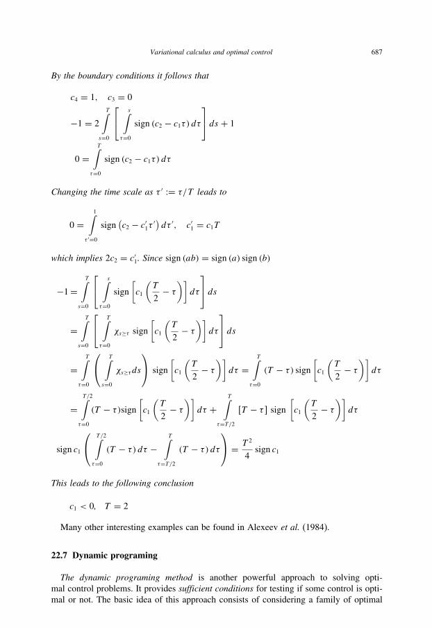
Variational calculus and optimal control 687
By the boundary conditions it follows that
c4 = 1, c3 = 0
−1 = 2
T∫s=0
⎡⎣ s∫τ=0
sign (c2 − c1τ) dτ⎤⎦ ds + 1
0 =T∫
τ=0
sign (c2 − c1τ) dτ
Changing the time scale as τ ′ := τ/T leads to
0 =1∫
τ ′=0
sign(c2 − c′1τ ′
)dτ ′, c′1 = c1T
which implies 2c2 = c′1. Since sign (ab) = sign (a) sign (b)
−1=T∫
s=0
⎡⎣ s∫τ=0
sign
[c1
(T
2− τ
)]dτ
⎤⎦ ds
=T∫
s=0
⎡⎣ T∫τ=0
χs≥τ sign[c1
(T
2− τ
)]dτ
⎤⎦ ds
=T∫
τ=0
⎛⎝ T∫s=0
χs≥τ ds
⎞⎠ sign
[c1
(T
2− τ
)]dτ =
T∫τ=0
(T − τ) sign[c1
(T
2− τ
)]dτ
=T/2∫τ=0
(T − τ)sign[c1
(T
2− τ
)]dτ +
T∫τ=T/2
[T − τ ] sign[c1
(T
2− τ
)]dτ
sign c1
⎛⎝ T/2∫τ=0
(T − τ) dτ −T∫
τ=T/2(T − τ) dτ
⎞⎠ = T
2
4sign c1
This leads to the following conclusion
c1 < 0, T = 2
Many other interesting examples can be found in Alexeev et al. (1984).
22.7 Dynamic programing
The dynamic programing method is another powerful approach to solving opti-
mal control problems. It provides sufficient conditions for testing if some control is opti-
mal or not. The basic idea of this approach consists of considering a family of optimal

688 Advanced Mathematical Tools for Automatic Control Engineers: Volume 1
control problems with different initial conditions (times and states) and of obtaining some
relationships among them via the, so-called, Hamilton–Jacoby–Bellman equation (HJB)
which is a nonlinear first-order partial differential equation. The optimal control can be
designed by maximization (or minimization) of the generalized Hamiltonian involved in
this equation. If this HJB equation is solvable (analytically or even numerically) then the
corresponding optimal controllers turn out to be given by a nonlinear feedback depending
on the optimized plant nonlinearity as well as the solution of the corresponding HJB equa-
tion. Such approach actually provides the solutions to the whole family of optimization
problems, and, in particular, to the original problem. Such a technique is called “invariant
embedding”. The major drawback of the classical HJB method is that it requires that
this partial differential equation admits a smooth enough solution. Unfortunately this is
not the case even for some very simple situations. To overcome this problem the so-
called viscosity solutions have been introduced (Crandall & Lions 1983). These solutions
are some sort of nonsmooth solutions with a key function to replace the conventional
derivatives by set-valued super/sub-differentials maintaining the uniqueness of solutions
under very mild conditions. These approaches not only save the DPM as a mathematical
method, but make it a powerful tool in tackling optimal control. In this section we do
not touch on this approach. But we will discuss the gap between necessary (MP) and
sufficient (DPM) conditions.
22.7.1 Bellman’s principle of optimality
Claim 22.1. (Bellman’s principle (BP) of optimality) “Any tail of an optimal trajec-tory is optimal too.”2
In other words, if some trajectory in the phase space connects the initial x (0) and terminal
x (T ) points and is optimal in the sense of some cost functional, then the sub-trajectory,
connecting any intermediate point x (t ′) of the same trajectory with the same terminal
point x (T ), should also be optimal (see Fig. 22.2).
22.7.2 Sufficient conditions for BP fulfilling
Theorem 22.16. (Sufficient condition for BP fulfilling) Let
1. the performance index (a cost functional) J (u (·)) with u (·) ∈ Uadmis [0, T ] be sepa-rable for any time t ′ ∈ (0, T ) such that
J (u (·)) = J1 (u1 (·), J2 (u2 (·))) (22.115)
where u1 (·) is the control within the time interval [0, t ′) called the initial controlstrategy and u2 (·) is the control within the time interval [t ′, T ] called the terminalcontrol strategy;
2 Bellman’s principle of optimality, formulated in Bellman (1960), is as follows: “An optimal policy has the
property that whatever the initial state and the initial decisions it must constitute an optimal policy with regards
to the state resulting from the first decision.”

Variational calculus and optimal control 689
0
x(0)
x1
x(t')
x(T)
x2
Fig. 22.2. Illustration of Bellman’s principle of optimality.
2. the functional J1 (u1 (·), J2 (u2 (·))) is monotonically nondecreasing with respect toits second argument J2 (u2 (·)), that is,
J1 (u1 (·), J2 (u2 (·))) ≥ J1(u1 (·), J2
(u′2 (·)
))if J2 (u2 (·)) ≥ J2
(u′2 (·)
) (22.116)
Then Bellman’s principle of optimality takes place for this functional.
Proof. For any admissible control strategies u1 (·), u2 (·) the following inequality holds
J ∗ := infu∈Uadmis[0,T ]
J (u (·))= infu1∈Uadmis[0,t
′), u2∈Uadmis[t′,T ]J1 (u1 (·), J2 (u2 (·)))
≤ J1 (u1 (·), J2 (u2 (·)))(22.117)
Select
u2 (·) = arg infu2∈Uadmis[t
′,T ]J2 (u2 (·)) (22.118)
Then (22.117) and (22.118) imply
J ∗ ≤ J1(u1 (·), inf
u2∈Uadmis[t′,T ]J2 (u2 (·))
)(22.119)
So,
u1 (·) = arg infu1∈Uadmis[t
′,T ]J1
(u1 (·), inf
u2∈Uadmis[t′,T ]J2 (u2 (·))
)(22.120)
leads to
J ∗ ≤ infu1∈Uadmis[t
′,T ]J1
(u1 (·), inf
u2∈Uadmis[t′,T ]J2 (u2 (·))
)(22.121)

690 Advanced Mathematical Tools for Automatic Control Engineers: Volume 1
Since J1 (u1 (·), J2 (u2 (·))) is monotonically nondecreasing with respect to the second
argument, from (22.121) we obtain
infu1∈Uadmis [t ′,T ]
J1
(u1(·), inf
u2∈Uadmis [t ′,T ]J2 (u2 (·))
)≤ infu1∈Uadmis [t ′,T ]
infu2∈Uadmis [t ′,T ]
J1 (u1(·), J2 (u2 (·)))= infu∈Uadmis [0,T ]
J (u (·)) = J ∗(22.122)
Combining (22.121) and (22.122), we finally derive that
J ∗ = infu1∈Uadmis [t ′,T ]
J1
(u1 (·), inf
u2∈Uadmis [t ′,T ]J2 (u2 (·))
)(22.123)
This proves the desired result. �
Summary 22.3. In strict mathematical form this fact may be expressed as follows: underthe assumptions of the theorem above for any time t ′ ∈ (0, T )
infu∈Uadmis [0,T ]
J (u (·))
= infu1∈Uadmis [t ′,T ]
J1
(u1 (·), inf
u2∈Uadmis [t ′,T ]J2 (u2 (·))
)(22.124)
Corollary 22.7. For the cost functional
J (u (·)) := h0 (x (T ))+T∫
t=0
h (x (t), u (t), t) dt
given in the Bolza form (22.41) Bellman’s principle holds.
Proof. For any t ′ ∈ (0, T ) from (22.41) obviously it follows that
J (u (·)) = J1 (u1 (·))+ J2 (u2 (·)) (22.125)
where
J1 (u1 (·)) :=t ′∫
t=0
h (x (t), u1 (t), t) dt
J2 (u2 (·)) := h0 (x (T ))+T∫
t=t ′h (x (t), u2 (t), t) dt
(22.126)
The representation (22.125) evidently yields the validity (22.115) and (22.116) for this
functional. �
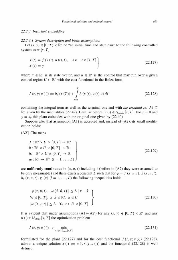
Variational calculus and optimal control 691
22.7.3 Invariant embedding
22.7.3.1 System description and basic assumptionsLet (s, y) ∈ [0, T )× Rn be “an initial time and state pair” to the following controlled
system over [s, T ]:
·x (t) = f (x (t), u (t), t), a.e. t ∈ [s, T ]
x (s) = y
}(22.127)
where x ∈ Rn is its state vector, and u ∈ Rr is the control that may run over a given
control region U ⊂ Rr with the cost functional in the Bolza form
J (s, y; u (·)) := h0 (x (T ))+T∫
t=sh (x (t), u (t), t) dt (22.128)
containing the integral term as well as the terminal one and with the terminal set M ⊆Rn given by the inequalities (22.42). Here, as before, u (·) ∈ Uadmis [s, T ]. For s = 0 and
y = x0 this plant coincides with the original one given by (22.40).
Suppose also that assumption (A1) is accepted and, instead of (A2), its small modifi-
cation holds:
(A2′) The maps
f : Rn × U × [0, T ]→ Rn
h : Rn × U × [0, T ]→ R
h0 : Rn × U × [0, T ]→ R
gl : Rn → Rn (l = 1, . . . , L)
⎫⎪⎪⎪⎬⎪⎪⎪⎭ (22.129)
are uniformly continuous in (x, u, t) including t (before in (A2) they were assumed to
be only measurable) and there exists a constant L such that for ϕ = f (x, u, t), h (x, u, t),h0 (x, u, t), gl (x) (l = 1, . . . , L) the following inequalities hold:
∥∥ϕ (x, u, t)− ϕ (x, u, t)∥∥ ≤ L∥∥x − x∥∥∀t ∈ [0, T ], x, x ∈ Rn, u ∈ U‖ϕ (0, u, t)‖ ≤ L ∀u, t ∈ U × [0, T ]
⎫⎪⎬⎪⎭ (22.130)
It is evident that under assumptions (A1)–(A2′) for any (s, y) ∈ [0, T ) × Rn and any
u (·) ∈ Uadmis [s, T ] the optimization problem
J (s, y; u (·))→ minu(·)∈Uadmis[s,T ]
(22.131)
formulated for the plant (22.127) and for the cost functional J (s, y; u (·)) (22.128),
admits a unique solution x (·) := x (·, s, y, u (·)) and the functional (22.128) is well
defined.

692 Advanced Mathematical Tools for Automatic Control Engineers: Volume 1
Definition 22.8. (The value function) The function V (s, y) defined for any (s, y) ∈[0, T )× Rn as
V (s, y) := infu(·)∈Uadmis[s,T ]
J (s, y; u (·))V (T , y) = h0(y)
}(22.132)
is called the value function of the optimization problem (22.131).
22.7.3.2 Dynamic programing equation in the integral formTheorem 22.17. Under assumptions (A1)–(A2′) for any (s, y) ∈ [0, T )×Rn the followingrelation holds
V (s, y)= infu(·)∈Uadmis[s,T ]
{ s∫t=sh (x (t, s, y, u (·)), u (t), t) dt
+ V (s, x
(s, s, y, u (·)))} ∀s ∈ [s, T ]
(22.133)
Proof. The result follows directly from BP of optimality (22.124), but, in view of the
great importance of this result, we present the proof again, using the concrete form of the
Bolza cost functional (22.128). Denoting the right-hand side of (22.133) by V (s, y) and
taking into account the definition (22.132), for any u (·) ∈ Uadmis [s, T ] we have
V (s, y) ≤ J (s, y; u (·))
=s∫
t=sh (x (t, s, y, u (·)), u (t), t) dt + J (s, x(s); u (·))
and, taking infimum over u (·) ∈ Uadmis [s, T ], it follows that
V (s, y) ≤ V (s, y) (22.134)
Hence, for any ε > 0 there exists a control uε (·) ∈ Uadmis [s, T ] such that for xε (·) :=x (·, s, y, uε (·))
V (s, y) + ε ≥ J (s, y; uε (·))
≥s∫
t=sh (x (t, s, y, uε (·)), uε (t), t) dt + V
(s, xε
(s)) ≥ V (s, y) (22.135)
Tending ε → 0 the inequalities (22.134), (22.135) imply the result (22.133) of this
theorem. �
Finding a solution V (s, y) to equation (22.133), we would be able to solve the origin
optimal control problem putting s = 0 and y = x0. Unfortunately, this equation is very
difficult to handle because of overcomplicated operations involved on its right-hand side.
That’s why in the next subsection we will explore this equation further, trying to get
another equation for the function V (s, y) with a simpler and more practically used form.

Variational calculus and optimal control 693
22.7.4 Hamilton–Jacoby–Bellman equation
To simplify the sequent calculations and following Young & Zhou (1999) we will
consider the original optimization problem without any terminal set, that is, M = Rn.
This may be expressed with the constraint function equal to
g (x) := 0 · ‖x‖2 − ε ≤ 0 (ε > 0) (22.136)
which is true for any x ∈ Rn. Slater’s condition (21.88) is evidently valid (also for any
x ∈ Rn). So, we deal here with the regular case. Denote by C1([0, T )× Rn
)the set of
all continuously differentiable functions v : [0, T )× Rn → R.
Theorem 22.18. (The HJB equation) Suppose that under assumptions (A1)–(A2′)the value function V (s, y) (22.132) is continuously differentiable, that is, V ∈C1
([0, T )× Rn
). Then V (s, y) is a solution to the following terminal value problem of
a first-order partial differential equation, named below the Hamilton–Jacoby–Bellman(HJB) equation associated with the original optimization problem (22.131) withoutterminal set (M = Rn):
− ∂∂tV (t, x)+ sup
u∈UH(− ∂
∂xV (t, x), x(t), u(t), t) = 0
(t, x) ∈ [0, T )× Rn, V (T , x) = h0 (x), x ∈ Rn
⎫⎬⎭ (22.137)
where
H(ψ, x, u, t) := ψᵀf (x, u, t)− h (x (t), u (t), t)t, x, u, ψ ∈ [0, T ]× Rn × Rr × Rn
(22.138)
is the same as in (22.81) with μ = 1 corresponding to the regular optimization problem.
Proof. Fixing u (t) ≡ u ∈ U , by (22.133) with s ↓ s we obtain
V (s, y)− V(s, x
(s, s, y, u (·)))
s − s
− 1
s − ss∫
t=sh (x (t, s, y, u (·)), u (t), t) dt ≤ 0
which implies
− ∂∂tV (s, y)− ∂
∂xV (s, y)ᵀ f (s, y, u)− h (s, u, t) ≤ 0
resulting in the following inequality
0 ≥ − ∂∂tV (s, y)+ sup
u∈UH(− ∂
∂xV (t, x), x(t), u(t), t) (22.139)
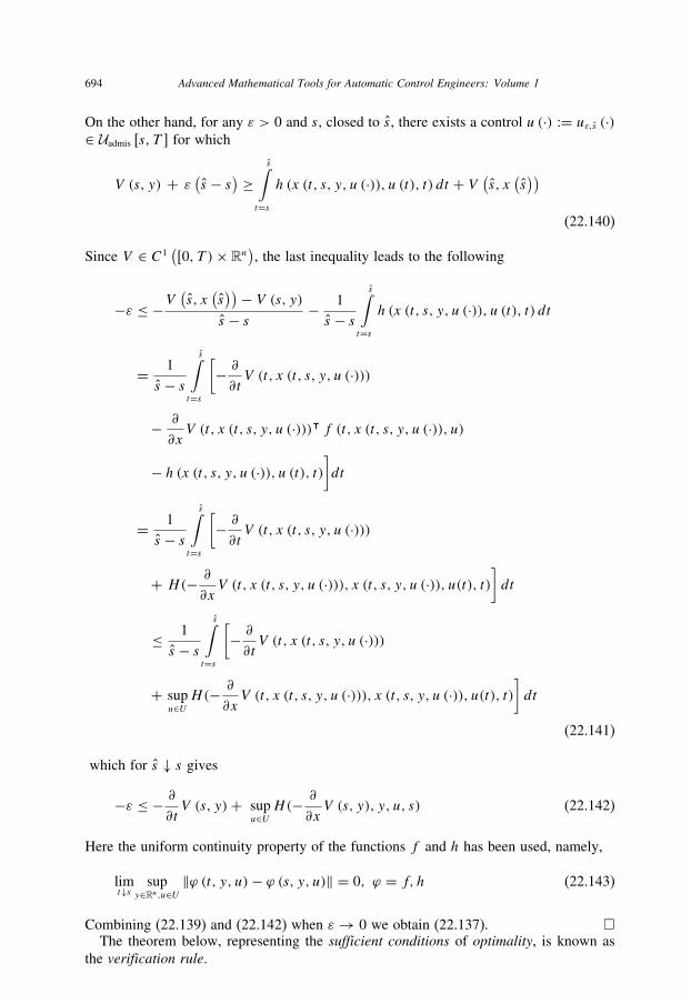
694 Advanced Mathematical Tools for Automatic Control Engineers: Volume 1
On the other hand, for any ε > 0 and s, closed to s, there exists a control u (·) := uε,s (·)∈ Uadmis [s, T ] for which
V (s, y) + ε (s − s) ≥ s∫t=sh (x (t, s, y, u (·)), u (t), t) dt + V (
s, x(s))
(22.140)
Since V ∈ C1([0, T )× Rn
), the last inequality leads to the following
−ε ≤ −V(s, x
(s))− V (s, y)s − s − 1
s − ss∫
t=sh (x (t, s, y, u (·)), u (t), t) dt
= 1
s − ss∫
t=s
[− ∂∂tV (t, x (t, s, y, u (·)))
− ∂
∂xV (t, x (t, s, y, u (·)))ᵀ f (t, x (t, s, y, u (·)), u)
− h (x (t, s, y, u (·)), u (t), t)]dt
= 1
s − ss∫
t=s
[− ∂∂tV (t, x (t, s, y, u (·)))
+ H(− ∂∂xV (t, x (t, s, y, u (·))), x (t, s, y, u (·)), u(t), t)
]dt
≤ 1
s − ss∫
t=s
[− ∂∂tV (t, x (t, s, y, u (·)))
+ supu∈UH(− ∂
∂xV (t, x (t, s, y, u (·))), x (t, s, y, u (·)), u(t), t)
]dt
(22.141)
which for s ↓ s gives
−ε ≤ − ∂∂tV (s, y)+ sup
u∈UH(− ∂
∂xV (s, y), y, u, s) (22.142)
Here the uniform continuity property of the functions f and h has been used, namely,
limt↓s sup
y∈Rn,u∈U‖ϕ (t, y, u)− ϕ (s, y, u)‖ = 0, ϕ = f, h (22.143)
Combining (22.139) and (22.142) when ε→ 0 we obtain (22.137). �The theorem below, representing the sufficient conditions of optimality, is known as
the verification rule.

Variational calculus and optimal control 695
Theorem 22.19. (The verification rule) Accept the following assumptions:
1. Let u∗(·) := u∗(t, x,
∂
∂xV (t, x)
)be a solution to the following optimization problem
H(− ∂∂xV (t, x), x, u, t)→ sup
u∈U(22.144)
with fixed values x, t and∂
∂xV (t, x);
2. Suppose that we can obtain the solution V (t, x) to the HJB equation
− ∂∂tV (t, x)+H(− ∂
∂xV (t, x), x, u∗ (·), t) = 0
V (T , x) = h0 (x), (t, x) ∈ [0, T )× Rn
⎫⎪⎬⎪⎭ (22.145)
which for any (t, x) ∈ [0, T ) × Rn is unique and smooth, that is, V ∈C1
([0, T )× Rn
);
3. Suppose that for any (s, x) ∈ [0, T ) × Rn there exists (a.e. t ∈ [s, T ]) a solutionx∗ (s, x) to the following ODE (ordinary differential equation)
·x∗(t) = f
(x∗ (t), u∗
(t, x∗ (t),
∂
∂xV (t, x∗ (t))
), t
)x∗ (s) = x
(22.146)
Then with (s, x) = (0, x0) the pair(x∗ (t), u∗
(t, x∗ (t),
∂
∂xV (t, x∗ (t))
))(22.147)
is optimal, that is, u∗(t, x∗ (t),
∂
∂xV (t, x∗ (t))
)is an optimal control.
Proof. The relations (22.138) and (22.145) imply
d
dtV (t, x∗ (t)) = − ∂
∂tV (t, x∗ (t))
+ ∂
∂xV (t, x∗ (t))ᵀ f
(x∗ (t), u∗
(t, x∗ (t),
∂
∂xV (t, x∗ (t))
), t
)
= −h(x∗ (t), u∗
(t, x∗ (t),
∂
∂xV (t, x∗ (t))
), t
)(22.148)
Integrating this equality by t within [s, T ] leads to the following relation
V (T , x∗ (T ))− V (s, x∗ (s))
= −T∫
t=sh
(x∗ (t), u∗
(t, x∗ (t),
∂
∂xV (t, x∗ (t))
), t
)dt

696 Advanced Mathematical Tools for Automatic Control Engineers: Volume 1
which, in view of the identity V (T , x∗ (T )) = h0 (x∗ (T )), is equal to the following one
V (s, x∗ (s)) = h0 (x∗ (T ))
+T∫
t=sh
(x∗ (t), u∗
(t, x∗ (t),
∂
∂xV (t, x∗ (t))
), t
)dt
(22.149)
By (22.133), this last equation means exactly that(x∗ (t), u∗
(t, x∗ (t),
∂
∂xV (t, x∗ (t))
))
is an optimal pair and u∗(t, x∗ (t),
∂
∂xV (t, x∗ (t))
)is an optimal control. �
22.8 Linear quadratic optimal control
22.8.1 Nonstationary linear systems and quadratic criterion
Consider in this section the dynamic plants (22.40) in their partial representation when
at each time t ∈ [0, T ] the right-hand side of the mathematical model is a linear function
with respect to the state vector x (t) and the control action u (t) as well, namely, for
almost all t ∈ [0, T ]
·x (t) = A (t) x (t)+ B (t) u (t)+ d (t)x (0) = x0
}(22.150)
Here the functional matrices A (t) ∈ Rn×n and B (t) ∈ Rn×r are supposed to be bounded
almost everywhere and the shifting vector function d (t) ∈ Rn is quadratically integrable,
that is,
A (·) ∈ L∞ (0, T ;Rn×n), B (·) ∈ L∞ (
0, T ;Rn×r), d (·) ∈ L2 (0, T ;Rn)(22.151)
The admissible control is assumed to be quadratically integrable on [0, T ] and the terminal
set M coincides with all space Rn (no terminal constraints), i.e.,
Uadmis [0, T ] :={u (·) : u (·) ∈ L2 (0, T ;Rr ), M = Rn
}(22.152)
The cost functional is considered in the form (22.41) with quadratic functions inside,
that is,
J (u (·))= 1
2xᵀ (T )Gx (T )+ 1
2
T∫t=0
[xᵀ (t)Q (t) x (t)
+ 2uᵀ (t) S (t) x (t)+ uᵀ (t) R (t) u (t)] dt
(22.153)

Variational calculus and optimal control 697
where
G ∈ Rn×n, Q (·) ∈ L∞ (0, T ;Rn×n)
S (·) ∈ L∞ (0, T ;Rn×r), R (·) ∈ L∞ (
0, T ;Rr×r) (22.154)
such that for almost all t ∈ [0, T ]
G ≥ 0, Q (t) ≥ 0, R (t) ≥ δI, δ > 0 (22.155)
Note that all coefficients (except G) in (22.150) and (22.153) are dependent on time t .
22.8.2 Linear quadratic problem
Problem 22.3. (Linear quadratic (LQ) problem) For the dynamic model (22.150) findan admissible control u∗ (·) ∈ Uadmis [0, T ] such that
J (u∗ (·)) = infu(·)∈Uadmis [0,T ]
J (u (·)) (22.156)
where the cost function J (u (·)) is given by (22.153).
We will refer to this problem as the linear quadratic optimal control problem (LQ).
22.8.3 Maximum principle for LQ problem
22.8.3.1 MP formulationTheorem 22.20. (Maximum principle for LQ problem) If a pair (x∗(t), u∗ (·)) is opti-mal, then
1. there exists a solution ψ (t) to the following ODE on [0, T ]
ψ (t) = −Aᵀ (t) ψ(t)+Q(t) x∗ (t)+ Sᵀ (t) u∗ (t)
ψ(T ) = −Gx∗ (T )
⎫⎬⎭ (22.157)
2. the optimal control u∗ (·) ∈ Uadmis [0, T ] is as follows
u∗ (t) = R−1 (t) [Bᵀ (t) ψ(t)− S (t) x∗ (t)] (22.158)
Proof. Since in this problem we have no terminal conditions, we deal with the regular
case and may take μ = 1. Then by (22.81) and (22.82) it follows that
H(ψ, x, u, t) := ψᵀ [A (t) x + B (t) u+ d (t)]
− 1
2xᵀ (t)Q (t) x (t)− uᵀ (t) S (t) x (t)− 1
2uᵀ (t) R (t) u (t)
(22.159)

698 Advanced Mathematical Tools for Automatic Control Engineers: Volume 1
So,
ψ(t)= − ∂∂xH(ψ(t), x∗(t), u∗ (t), t)
= −Aᵀ (t) ψ(t)+Q(t) x∗ (t)+ Sᵀ (t) u∗ (t)
ψ(T )= − ∂∂xh0 (x
∗ (T )) = −Gx∗ (T )
which proves claim (1) (22.157) of this theorem. Besides, by MP implementation,
we have
u∗ (t) ∈ Argminu∈Rr
H (ψ, x∗, u, t)
or, equivalently,
∂
∂uH(ψ, x∗, u∗, t) = Bᵀ (t) ψ(t)− R (t) u∗ (t)− S (t) x∗ (t) = 0 (22.160)
which leads to claim (2) (22.158). �
22.8.4 Sufficiency condition
Theorem 22.21. (on the sufficiency of MP) If the control u∗ (t) is as in (22.158) and
Q(t)− S (t) R−1 (t) Sᵀ (t) ≥ 0 (22.161)
then it is a unique optimal one.
Proof. It follows directly from Theorem 22.15 on the sufficient conditions of optimality.
The uniqueness is the result of equation (22.160) which has a unique solution if R (t) ≥ δIa.e. t ∈ [0, T ], δ > 0 (22.155). Besides, the Hessian of the functionH(ψ, x, u, t) (22.159)
is as follows∥∥∥∥∥∥∥∥∂2
∂x2H(ψ, x, u, t)
∂2
∂x∂uH(ψ, x, u, t)
∂2
∂u∂xH(ψ, x, u, t)
∂2
∂u2H(ψ, x, u, t)
∥∥∥∥∥∥∥∥ = −∥∥∥∥ Q(t) S (t)
Sᵀ (t) R (t)
∥∥∥∥
Let us show that
∥∥∥∥ Q(t) S (t)
Sᵀ (t) R (t)
∥∥∥∥ ≥ 0. A symmetric block-matrix
[M11 M12
Mᵀ12 M22
]with
M22 > 0 is nonnegative definite, that is,[M11 M12
Mᵀ12 M22
]≥ 0
if and only if
M11 ≥ 0, M11 −M12M−122 M
ᵀ12 ≥ 0

Variational calculus and optimal control 699
So, by the assumption (22.161) of the theorem we have that∥∥∥∥∥∥∥∥∂2
∂x2H(ψ, x, u, t)
∂2
∂x∂uH(ψ, x, u, t)
∂2
∂u∂xH(ψ, x, u, t)
∂2
∂u2H(ψ, x, u, t)
∥∥∥∥∥∥∥∥ ≤ 0
This means that the function H(ψ, x, u, t) is concave (not obligatory strictly) on (x, u)
for any fixed ψ(t) and any t ∈ [0, T ]. �
Corollary 22.8. If S (t) ≡ 0, then the control u∗ (t) (22.158) is always uniquely optimal.
Proof. Under this assumption the inequality (22.161) always holds. �
22.8.5 Riccati differential equation and feedback optimal control
22.8.5.1 Riccati differential equationLet us introduce the symmetric matrix function P (t) = Pᵀ (t) ∈ C1
(0, T ;Rn×n) and
the vector function p (t) ∈C1 (0, T ;Rn)which satisfy (a.e. t ∈ [0, T ]) the following ODE:
−P (t) = P (t)A (t)+ Aᵀ (t) P (t)+Q(t)− [Bᵀ (t) P (t)+ S (t)]ᵀ R−1 (t) [Bᵀ (t) P (t)+ S (t)]
= P (t) A (t)+ A (t)ᵀ P (t)− P (t) [B (t) R−1 (t) Bᵀ (t)]P (t)+ Q (t)
P (T ) =G
⎫⎪⎪⎪⎪⎪⎪⎬⎪⎪⎪⎪⎪⎪⎭
(22.162)
with
A (t) = A (t)− B (t) R−1 (t) S (t)
Q (t)= Q(t)− Sᵀ (t) R−1 (t) S (t)(22.163)
and
−p (t) = [(A (t)− B (t) R−1 (t) S (t)
)ᵀ
− P (t) B (t) R−1 (t) Bᵀ (t)]p (t) + P (t) d (t)
p (T ) = 0
⎫⎪⎪⎬⎪⎪⎭ (22.164)
Definition 22.9. We refer to ODE (22.162) as the Riccati differential equation and p (t)is referred to as the shifting vector associated with the problem (22.156).
22.8.6 Linear feedback control
Theorem 22.22. (on a linear feedback control) Assume that
P (t) = Pᵀ (t) ∈ C1(0, T ;Rn×n)

700 Advanced Mathematical Tools for Automatic Control Engineers: Volume 1
is a solution of (22.162) and
p (t) ∈ C1 (0, T ;Rn)
verifies (22.164). Then the optimal control u∗ (·) ∈ Uadmis [0, T ] for the problem (22.156)has the linear feedback form
u∗ (t) = −R−1 (t) [(Bᵀ (t) P (t)+ S (t)) x∗ (t)+ Bᵀ (t) p (t)] (22.165)
and the optimal cost function J (u∗ (·)) is as follows
J (u∗ (·)) = 1
2x
ᵀ0 P (0) x0 + pᵀ (0) x0
+ 1
2
T∫t=0
[2pᵀ (t) d (t)− ∥∥R−1/2 (t) Bᵀ (t) p (t)
∥∥2]dt
(22.166)
Proof.
1. Let us try to find the solution of ODE (22.157) in the form
ψ (t) = −P (t) x∗ (t)− p (t) (22.167)
The direct substitution of (22.167) into (22.157) leads to the following identity (t will
be suppressed for simplicity):(Q− SᵀR−1S
)x∗ − (
Aᵀ − SᵀR−1Bᵀ) [−P (t) x∗ − p] = ψ= −P x∗ − P [Ax∗ + B (u∗)+ d]− p = −P x∗−P [
Ax∗ + BR−1 [Bᵀ (−Px∗ − p)− Sx∗]+ d]− p= −P x∗ − P (
A− BR−1 [BᵀP + S]) x∗ + PBR−1p − Pd − p
This yields
0= (P (t)+ P (t)A (t)+ Aᵀ (t) P (t)+Q(t)− [Bᵀ (t) P (t)+ S (t)]ᵀ R−1 (t) [Bᵀ (t) P (t)+ S (t)]) x∗
p (t)+ [(A (t)− B (t) R−1 (t) S (t)
)ᵀ
−P (t) B (t) R−1 (t) Bᵀ (t)]p (t)+ P (t) d (t)
(22.168)
But, in view of (22.162) and (22.164), the right-hand side of (22.168) is identically
zero. The transversality condition ψ(T ) = −Gx∗ (T ) in (22.162) implies
ψ(T ) = −P (T ) x∗ (T )− p (T ) = −Gx∗ (T )
which holds for any x∗ (T ) if P (T ) = G and p (T ) = 0.

Variational calculus and optimal control 701
2. To prove (22.166) let us apply the chain integration rule for xᵀ (t) P (t) x (t) and for
pᵀ (t) x (t), respectively. In view of (22.150) and (22.162) we obtain
xᵀ (T ) P (T ) x (T )− xᵀ (s) P (s) x (s)
= x∗ᵀ (T )Gx∗ (T )− x∗ᵀ (s) P (s) x∗ (s)
=T∫
t=s
d
dt[xᵀ (t) P (t) x (t)] dt =
T∫t=s
[2xᵀ (t) P (t) x (t)+ xᵀ (t) P (t) x (t)
]dt
=T∫
t=s
{xᵀ (t)
([P (t) B (t)+ Sᵀ (t)]R−1 (t) [P (t) B (t)+ Sᵀ (t)]ᵀ
−Q(t)) x (t)+ 2u∗ᵀ (t) Bᵀ (t) P (t) x (t)+ 2dᵀ (t) P (t) x (t)} dt(22.169)
and, applying (22.164),
pᵀ (T ) x (T )− pᵀ (s) x (s) = −pᵀ (s) x (s)
=T∫
t=s
d
dt[pᵀ (t) x (t)] dt =
T∫t=s
[pᵀ (t) x (t)+ pᵀ (t) x (t)] dt
=T∫
t=s
{xᵀ (t)
([P (t) B (t)+ Sᵀ (t)]R−1 (t) B (t) p (t)− P (t) d (t))
+ pᵀ (t) [B (t) u∗ (t)+ d (t)]} dt(22.170)
Summing (22.169) and (22.170) and denoting
J ∗ (s, x (s)) := 1
2xᵀ (s) P (s) x (s)
+ 1
2
T∫t=s
[xᵀ (t)Q (t) x (t)+ u∗ᵀ (t) R (t) u∗ (t)+ 2u∗ᵀ (t) S (t) x (t)]
we get
J ∗ (s, x (s))− 1
2xᵀ (s) P (s) x (s)− pᵀ (s) x (s)
= 1
2
T∫t=s
{u∗ᵀ (t) R (t) u∗ (t)
+ xᵀ (t) [P (t) B (t)+ Sᵀ (t)]R−1 (t) [P (t) B (t)+ Sᵀ (t)]ᵀ x (t)
+ 2xᵀ (t) [P (t) B (t)+ Sᵀ (t)]ᵀ u∗ (t)
+ 2xᵀ (t) [P (t) B (t)+ Sᵀ (t)]ᵀ R−1 (t) Bᵀ (t) p (t)

702 Advanced Mathematical Tools for Automatic Control Engineers: Volume 1
+ 2u∗ᵀ(t) Bᵀ (t) p (t)+ 2pᵀ (t) d (t)
}dt
= 1
2
T∫t=s
{∥∥R−1/2 (t) [R (t) u∗ (t)+ [P (t) B (t)+ Sᵀ (t)]ᵀ xᵀ (t)]
+ Bᵀ (t) p (t)‖2 − ∥∥R−1/2 (t) Bᵀ (t) p (t)∥∥2 + 2pᵀ (t) d (t)
}dt
(22.171)
which, taking s = 0, x (s) = x0, and in view of
R (t) u∗ (t)+ [P (t) B (t)+ Sᵀ (t)]ᵀ xᵀ (t) = 0
yields (22.166). Theorem is proven. �
Theorem 22.23. (on the uniqueness of the optimal control) The optimal control u∗ (·)∈ Uadmis [0, T ] is unique if and only if the corresponding Riccati differential equation(22.162) has a unique solution P (t) ≥ 0 on [0, T ].
Proof.
1. Necessity. Assume that u∗ (·) ∈ Uadmis [0, T ] is unique and is given by (22.165). But
this is possible only if P (t) is uniquely defined (p (t) will be uniquely defined
automatically). So, the corresponding Riccati differential equation (22.162) should
have a unique solution P (t) ≥ 0 on [0, T ].
2. Sufficiency. If the corresponding Riccati differential equation (22.162) has a unique
solution P (t) ≥ 0 on [0, T ], then, by the previous theorem, u∗ (·) is uniquely defined
by (22.165) and the dynamics x∗ (t) is given by
x∗ (t)= [A (t)− B (t) R−1 (t) (Bᵀ (t) P (t)+ S (t))] x∗ (t)−B (t) R−1 (t) Bᵀ (t) p (t)+ d (t)
(22.172)
So, the uniqueness of (22.165) follows from the uniqueness of the solution of
ODE (22.172). �
22.8.7 Stationary systems on the infinite horizon
22.8.7.1 Stationary systems and the infinite horizon cost functionLet us consider a stationary linear plant given by the following ODE
·x (t) = Ax (t)+ Bu (t), t ∈ [0,∞]
x (0) = x0, A ∈ Rn×n, B ∈ Rn×r
}(22.173)
supplied by the quadratic cost function in the Lagrange form, namely,
J (u (·)) =∞∫
t=0
[xᵀ (t)Qx (t)+ uᵀ (t) Ru (t)] dt (22.174)
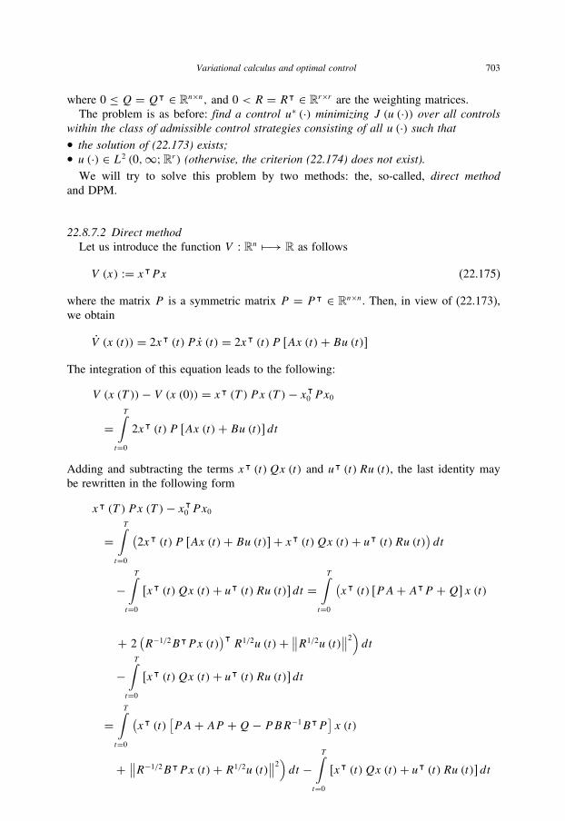
Variational calculus and optimal control 703
where 0 ≤ Q = Qᵀ ∈ Rn×n, and 0 < R = Rᵀ ∈ Rr×r are the weighting matrices.
The problem is as before: find a control u∗ (·) minimizing J (u (·)) over all controlswithin the class of admissible control strategies consisting of all u (·) such that• the solution of (22.173) exists;• u (·) ∈ L2 (0,∞;Rr ) (otherwise, the criterion (22.174) does not exist).
We will try to solve this problem by two methods: the, so-called, direct methodand DPM.
22.8.7.2 Direct methodLet us introduce the function V : Rn −→ R as follows
V (x) := xᵀPx (22.175)
where the matrix P is a symmetric matrix P = Pᵀ ∈ Rn×n. Then, in view of (22.173),
we obtain
V (x (t)) = 2xᵀ (t) P x (t) = 2xᵀ (t) P [Ax (t)+ Bu (t)]The integration of this equation leads to the following:
V (x (T ))− V (x (0)) = xᵀ (T ) Px (T )− xᵀ0 Px0
=T∫
t=0
2xᵀ (t) P [Ax (t)+ Bu (t)] dt
Adding and subtracting the terms xᵀ (t)Qx (t) and uᵀ (t) Ru (t), the last identity may
be rewritten in the following form
xᵀ (T ) Px (T )− xᵀ0 Px0
=T∫
t=0
(2xᵀ (t) P [Ax (t)+ Bu (t)]+ xᵀ (t)Qx (t)+ uᵀ (t) Ru (t)
)dt
−T∫
t=0
[xᵀ (t)Qx (t)+ uᵀ (t) Ru (t)] dt =T∫
t=0
(xᵀ (t) [PA+ AᵀP +Q] x (t)
+ 2(R−1/2BᵀPx (t)
)ᵀR1/2u (t)+ ∥∥R1/2u (t)
∥∥2)dt
−T∫
t=0
[xᵀ (t)Qx (t)+ uᵀ (t) Ru (t)] dt
=T∫
t=0
(xᵀ (t)
[PA+ AP +Q− PBR−1BᵀP
]x (t)
+ ∥∥R−1/2BᵀPx (t)+ R1/2u (t)∥∥2)dt −
T∫t=0
[xᵀ (t)Qx (t)+ uᵀ (t) Ru (t)] dt

704 Advanced Mathematical Tools for Automatic Control Engineers: Volume 1
which implies
T∫t=0
[xᵀ (t)Qx (t)+ uᵀ (t) Ru (t)] dt = xᵀ0 Px0 − xᵀ (T ) Px (T )
+T∫
t=0
∥∥R−1/2BᵀPx (t)+ R1/2u (t)∥∥2dt
+T∫
t=0
xᵀ (t)[PA+ AᵀP +Q− PBR−1BᵀP
]x (t) dt
(22.176)
Selecting (if it is possible) the matrix P as a solution to the following matrix Riccatiequation
PA+ AᵀP +Q− PBR−1BᵀP = 0 (22.177)
from (22.176) we get
T∫t=0
[xᵀ (t)Qx (t)+ uᵀ (t) Ru (t)] dt = xᵀ0 Px0 − xᵀ (T ) Px (T )
+T∫
t=0
∥∥R−1/2BᵀPx (t)+ R1/2u (t)∥∥2dt
≥ xᵀ0 Px0 − xᵀ (T ) Px (T )
(22.178)
Theorem 22.24. If for the system (22.173) the pair (A,B) is stabilizable and the pair(Q1/2, A
)is observable then the optimal control u∗ (t) minimizing (22.174) is given by
u∗ (t) = −R−1BᵀPx (t) (22.179)
where P is the unique positive definite solution of (22.177) making the closed-loop systemasymptotically stable. Moreover, the minimal value of the cost functional is
J (u (·)) =∞∫
t=0
[xᵀ (t)Qx (t)+ uᵀ (t) Ru (t)] dt = xᵀ0 Px0 (22.180)
Proof. First, notice that the dynamic system (22.173) closed by an optimal control should
be stable. Indeed, suppose that there exists at least one unstable mode of the controlled sys-
tem. Then, by the observability of the pair (C,A), it follows that the vector y (t) = Cx (t)

Variational calculus and optimal control 705
(Q := CᵀC) should tend to infinity and, hence,∫ Tt=0xᵀ (t)Qx (t) dt tends to infinity
with T → ∞ that cannot correspond to an optimal control. So, the term xᵀ (T ) Px (T )has to tend to zero and can be disregarded. By Theorem 10.8 there exists the unique
positive definite solution P of (22.177) which makes the closed-loop system stable since
x (t) = Ax (t)+ Bu∗ (t) = (A− BR−1BᵀP
)x (t) = Aclosedx (t)
where Aclosed is defined in (10.26). Taking this P in (22.179) and in view of (22.178)
under u (·) = u∗ (·) the equality (22.180) holds. Theorem is proven. �
Does the optimal control stabilize nonobservable systems?Proposition 22.1. The optimal control does not necessarily stabilize a nonobservablelinear stationary system.
The next simple example illustrates the statement given above.
Example 22.7. Consider the following linear second-order controllable time invariantsystem
x1 (t) = x2 (t), x2 (t) = x1 (t)+ u, x1 (0) = x10, x2 (0) = x20
Let the cost functional be J (u (·))= ∫∞t=0
[xᵀ (t)Qx (t)+ u2 (t)] dt with x (t) := [
x1 (t)
x2 (t)
]and Q :=
[1 −1
−1 1
]≥ 0. In our case this system can be represented in the form
(22.173) with A =[0 1
1 0
]and B =
[0
1
]. Notice that this system is unobservable since
the column rank of the observability matrix O =[C
CA
]=
[1 −1
−1 1
]is incomplete
and equal to 1. The statement of the proposition becomes evident if we define y (t) :=x1 (t) − x2 (t) and represent this system as
y (t) = −y (t)− u
J (u (·)) =∞∫
t=0
[y2 (t)+ u2 (t)] dt (22.181)
with
x2 (t) = y (t)+ x2 (t)+ u
According to Theorem 22.24 the optimal control in (22.181) is u∗ (t) = py (t) wherep = √
2− 1. As it is expected, in the optimal system y (t)→ 0 as t →∞. Evidently, thesecond component x2 (t)→∞, and, hence, the optimal system is unstable which provesthe above proposition. This effect appears due to instability of the unobservable statecomponent x2 (t)!

706 Advanced Mathematical Tools for Automatic Control Engineers: Volume 1
The revealed fact permits to indicate the class of stable unobservable optimal systems.
If the pair (C,A) is unobservable then there exists a nonsingular linear transformation
T x =(x1x2
)such that the system (22.173) can be represented in the, so-called, canonical
observability form
x1 = A11 + B1u, x2 = A21x1 + A22x2 + B2u
y = C1x1(22.182)
with x1 and x2 being the observable and unobservable state components. Let us show
how this transformation can be found. Select T in the form T =(v
w
)where the matrix
v ∈ Rk×n consists of k basis row vectors of the observability matrix (9.63)
O :=
⎡⎢⎢⎢⎢⎢⎣
C
CA
CA2
...
CAn−1
⎤⎥⎥⎥⎥⎥⎦
Since the system is unobservable then k < n. The matrix w ∈ R(n−k)×n is an arbitrary
one such that det T �= 0. Denote
T −1 := (N1 N2
), N1 ∈ Rn×k
The identity T T −1 = I implies
I =(v
w
)(N1 N2
) = (vN1 vN2
wN1 wN2
)
and
vN2 = 0 (22.183)
Since vA and vC are in the same basis there exist matrices LA and LC such that
vA = LAv, C = LCv
Then(x1x2
)= TAT −1
(x1x2
)+ T Bu
y = CT −1
(x1x2
)

Variational calculus and optimal control 707
In view of (22.183) and the relations
TAT −1 =(v
w
)A(N1 N2
)
=⎛⎝LAvwA
⎞⎠(N1 N2
) = (LAvN1 0
wAN1 wAN2
)
CT −1 = (LCvN1 LCvN2
) = (CN1 0
)we finally get (22.182) and the cost functional (22.174) becomes
J (u (·)) =∞∫
t=0
[xᵀ1 (t)Q1x1 (t)+ uᵀ (t) Ru (t)] dt
where Q1 = Cᵀ1 C1 and the pair (C1, A11) is observable. Then, by Theorem 22.24, the
optimal control is
u∗ (t) = −R−1Bᵀ1 P1x1 (t)
with P1 being the positive-definite solution to the reduced order Riccati equation
P1A11 + Aᵀ11P1 +Q− P1B1R
−1Bᵀ1 P1 = 0
which makes the first subsystem (with respect to x1) stable. It is evident that the optimal
system (22.173) is stable if the matrix A22 is Hurwitz (stable). According to the PBH test
9.1, such systems are called detectable. Finally we may formulate the following claim.
Claim 22.2. The linear time invariant system (22.173) optimal in the sense of the costfunctional (22.174) is stable if and only if this system is stabilizable and detectable.
22.8.7.3 DPM approachConsider the following HBJ equation (22.137):
−h+ supu∈UH(− ∂
∂xV (x), x, u) = 0
x ∈ Rn, h = const, V (0) = 0
⎫⎬⎭ (22.184a)
with
H(ψ, x, u) := ψᵀ (Ax + Bu)− xᵀQx − uᵀRu
x, u,ψ ∈ [0,∞]× Rn × Rr × Rn(22.185)
Theorem 22.25. (Verification rule for LQ-problem) If the control u∗ is a maximizingvector for (22.185) with some h = const, that is,
u∗ = −1
2R−1Bᵀ ∂
∂xV (x)

708 Advanced Mathematical Tools for Automatic Control Engineers: Volume 1
where V (x) is a solution to the following HJ equation:
− ∂∂xV ᵀ (x)Ax − xᵀQx + 1
4
∂
∂xV ᵀ (x) BR−1Bᵀ ∂
∂xV (x) = h
and the closed-loop system is stable, then such u∗ is an optimal control.
Proof. It is evident that only admissible control may be stabilizing (if not, the cost
function does not exist). By (22.185) for any stabilizing u (·) it follows that
H(− ∂∂xV (x∗), x∗, u∗) = h, H(− ∂
∂xV (x), x, u) ≤ h
and, hence,
H(− ∂∂xV (x), x, u) ≤ H(− ∂
∂xV (x∗), x∗, u∗)
which, after integration, leads to the following inequality
∞∫t=0
[− ∂∂xV ᵀ (x) (Ax + Bu)− xᵀQx − uᵀRu
]dt
≤∞∫
t=0
[− ∂∂xV ᵀ (x∗) (Ax∗ + Bu∗)− x∗ᵀQx∗ − u∗ᵀRu∗
]dt
or, equivalently,
T∫t=0
[x∗ᵀQx∗ + u∗ᵀRu∗] dt ≤T∫
t=0
[xᵀQx + uᵀRu] dt +∞∫
t=0
d (V (x)− V (x∗))
V (x(0))=Vᵀ(x∗(0))=T∫
t=0
[xᵀQx + uᵀRu] dt + V (x (T ))− V ᵀ (x∗ (T ))
Within the class of stabilizing strategies we have
V (x (T ))− V ᵀ (x∗ (T )) →T→∞ 0
which, in view of the last inequality, shows that u∗ (·) is an optimal control. �
Try to find the solution to (22.185) as V (x) = xᵀPx with P = Pᵀ ≥ 0. This implies∂
∂xV (x) = 2Px, and, hence,
−2xᵀP(Ax − BR−1BᵀPx
)− xᵀQx − xᵀPBR−1BᵀPx
= xᵀ (−PA− AᵀP −Q+ PBR−1BᵀP)x = 0
The last equation is identically fulfilled for any x ∈ Rn if P is the solution to the same
Riccati matrix equation as in (22.177) for a stabilizable and observable system. So, finally,
the optimal control is u∗ (t) = −R−1BᵀPx (t) which naturally coincides with (22.179).

Variational calculus and optimal control 709
22.9 Linear-time optimization
22.9.1 General result
For this problem the cost functional is
J (u (·)) = T (22.186)
It can be obtained from the Bolza form functional
J (u (·)) := h0(x (T ))+T∫
t=0
h (x (t), u (t), t) dt
if we put h0(x) ≡ 0, h (x, u, t) ≡ 1. Then for a linear plant, given by (22.150), the
Hamiltonian (22.81) is
H(ψ, x, u, t) := ψᵀ [A (t) x + B (t) u+ d (t)]− μ (22.187)
and, hence, the maximality condition (22.69) becomes as follows:
u∗ (t) ∈ Argmaxu∈U ψ
ᵀ (t) [A (t) x (t)+ B (t) u (t)+ d (t)]= Argmax
u∈U ψᵀ (t) B (t) u (t) = Argmax
u∈U [Bᵀ (t) ψ (t)]ᵀ u (t)
= Argmaxu∈U
r∑k=1
[Bᵀ (t) ψ (t)]k uk (t)
(22.188)
Theorem 22.26. (on linear time-optimal control) If the set U of the admissible controlvalues is a polytope defined by
U := {u ∈ Rr : u−k ≤ uk (t) ≤ u+k , k = 1, . . . , r
}(22.189)
then the optimal control (22.188) is as follows
u∗k (t) =⎧⎨⎩
u+k if [Bᵀ (t) ψ (t)]k > 0
u−k if [Bᵀ (t) ψ (t)]k < 0
any u ∈ U if [Bᵀ (t) ψ (t)]k = 0
(22.190)
and it is unique.
Proof. Formula (22.190) follows directly from (22.188), (22.189) and the uniqueness
is the consequence of the theorem on the sufficient condition of the optimality which
demands the concavity (and not obligatory strict) of the Hamiltonian with respect to
(x, u) for any fixed ψ , which is evidently fulfilled for the Hamiltonian function (22.187)
which is linear on x and u. �

710 Advanced Mathematical Tools for Automatic Control Engineers: Volume 1
22.9.2 Theorem on n-intervals for stationary linear systems
Consider in detail the partial case of linear systems (22.150) when the matrices of the
system are constant, that is, A (t) = A, B (t) = B. For this case the result below has
been obtained in Feldbaum (1953) and is known as the theorem on n-intervals. But first,let us prove an axillary lemma.
Lemma 22.10. If λ1, λ2, . . . , λm are real numbers and f1 (t), . . . , fm (t) are the polyno-mials with real coefficients and having the orders k1, . . . , km, correspondingly. Then thefunction
ϕ (t) =m∑i=1
fi (t) eλi t (22.191)
has a number of real roots which does not exceed
n0 := k1 + . . .+ km +m− 1 (22.192)
Proof. To prove this result let us use the induction method.
1. For m = 1 the lemma is true. Indeed, in this case the function ϕ (t) = f1 (t) eλ1t hasthe number of roots coinciding with k1 since e
λ1t > 0 for any t .
2. Suppose that this lemma is valid for m− 1 > 0. Then let us prove that it holds for m.
Multiplying (22.191) by e−λmt we obtain
ϕ (t) e−λmt =m−1∑i=1
fi (t) e(λi−λm)t + fm (t) (22.193)
Differentiation by t the relation (22.193) (km + 1)-times implies
d(km+1)
dt (km+1)
(ϕ (t) e−λmt
) = m−1∑i=1
fi (t) e(λi−λm)t := ϕkm+1 (t)
where fi (t) are the polynomials of the same order as fi (t). By the supposition before,
the function ϕ1 (t) has a number of roots which do not exceed
nkm+1 := k1 + . . .+ km−1 +m− 2
Since between two roots of continuously differentiable function, there is at least one
root of its derivative, then the function ϕkm (t) :=dkm
dtkm
(ϕ (t) e−λmt
)will have nkm =
nkm+1+1. Continuing this process, finally we get that the function ϕ0 (t) := ϕ (t) e−λmtwill have
n0 = n1 + 1 = n2 + 2 = . . . = nkm+1 + (km + 1)
= (k1 + . . .+ km−1 +m− 2)+ (km + 1) = k1 + . . .+ km +m− 1

Variational calculus and optimal control 711
And, since e−λmt > 0 always, we may conclude that ϕ (t) has the same number of roots
as ϕ0 (t). Lemma is proven. �
Now we are ready to prove the main result of this section.
Theorem 22.27. (Feldbaum 1953) If the matrix A ∈ Rn×n has only real eigenvalues,then the number of switches of any component of the optimal control (22.190) does notexceed (n− 1), that is, a number of the intervals, where each component of the optimalprogram (22.190) is constant, does not exceed n.
Proof. Let λ1, λ2, . . . , λm be the different eigenvalues of the matrix A and r1, r2, . . . , rmare their multiplicity numbers, correspondingly. Then a general solution of the adjoint
system of equations ψ(t) = −Aᵀψ(t) may be represented as
ψi(t) =m∑j=1
pij (t) e−λj t , i = 1, . . . , n (22.194)
where pij (t) are polynomials on t whose order does not exceed(rj − 1
). Substituting
(22.194) into (22.188) implies
u∗k (t)=u+k2
[1+ sign
(n∑i=1
bikψi (t)
)]+ u
−k
2
[1− sign
(n∑i=1
bikψi (t)
)]
= u+k
2
[1+ sign
(n∑i=1
bik
m∑j=1
pij (t) e−λj t
)]
+ u−k
2
[1− sign
(n∑i=1
bik
m∑j=1
pij (t) e−λj t
)]
= u+k
2
[1+ sign
(m∑j=1
pkj (t) e−λj t
)]+ u
−k
2
[1− sign
(m∑j=1
pkj (t) e−λj t
)]
where pkj (t) are the polynomials on t , whose order does not exceed(rj − 1
), equal to
pkj (t) :=n∑i=1
bikpij (t) (22.195)
Now the number of switches is defined by the number of the roots of the polynomials
(22.195). Applying directly the lemma above, we obtain that the polynomial function∑m
j=1 pkj (t) e−λj t has a number of real roots which do not exceed
(r1 − 1)+ (r2 − 1)+ . . .+ (rk − 1)+ (k − 1) = r1 + . . .+ rk − 1 = n− 1
Theorem is proven. �

This page intentionally left blank
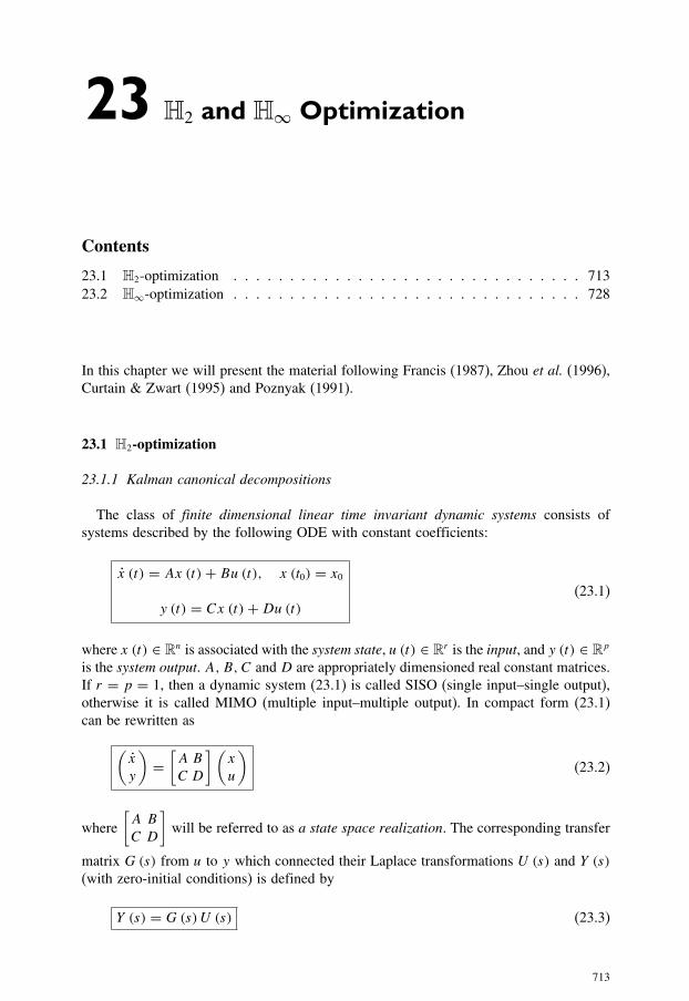
23 H2 and H∞ Optimization
Contents
23.1 H2-optimization . . . . . . . . . . . . . . . . . . . . . . . . . . . . . . . 713
23.2 H∞-optimization . . . . . . . . . . . . . . . . . . . . . . . . . . . . . . . 728
In this chapter we will present the material following Francis (1987), Zhou et al. (1996),Curtain & Zwart (1995) and Poznyak (1991).
23.1 H2-optimization
23.1.1 Kalman canonical decompositions
The class of finite dimensional linear time invariant dynamic systems consists of
systems described by the following ODE with constant coefficients:
x (t) = Ax (t)+ Bu (t), x (t0) = x0y (t) = Cx (t)+Du (t)
(23.1)
where x (t) ∈ Rn is associated with the system state, u (t) ∈ Rr is the input, and y (t) ∈ Rp
is the system output. A,B,C and D are appropriately dimensioned real constant matrices.
If r = p = 1, then a dynamic system (23.1) is called SISO (single input–single output),
otherwise it is called MIMO (multiple input–multiple output). In compact form (23.1)
can be rewritten as
(x
y
)=
[A B
C D
](x
u
)(23.2)
where
[A B
C D
]will be referred to as a state space realization. The corresponding transfer
matrix G(s) from u to y which connected their Laplace transformations U (s) and Y (s)
(with zero-initial conditions) is defined by
Y (s) = G(s)U (s) (23.3)
713
714 Advanced Mathematical Tools for Automatic Control Engineers: Volume 1
and is equal to
G(s) = C (sI − A)−1 B +D (23.4)
Proposition 23.1. The transfer matrix G(s) is not changed under any nonsingular coor-dinate transformation x = T x (det T �= 0) which converts (23.1) into
d
dtx (t)= TAT −1x (t)+ T Bu (t)
y (t)= CT −1x (t)+Du (t)(23.5)
Proof. Evidently,
G(s) = C (sI − A)−1 B +D = CT −1(sI − TAT −1
)−1T B +D �
Proposition 23.2. The corresponding controllability C and observability∼O matrices are
related to the original ones C (9.55) and O (9.63) by
C =T C,∼O = OT (23.6)
This implies that the controllability and observability properties are invariant under thesimilarity (nonsingular) coordinate transformations.
Proof. It follows directly from the definitions (9.55) and (9.63). �
The next theorems, known as the Kalman decompositions, show (see the details in
Zhou et al. (1996)) that any linear system (23.1) can be transformed by a similarity
transformation into a system having two groups of the coordinates such that one of them
is obligatory controllable, or observable, or both properties hold simultaneously.
Theorem 23.1. (on the controllable canonical form) If the controllability matrix hasrank kc < n, then there exists a similarity transformation
x =(xcxunc
)= T x
such that
d
dt
(xcxunc
)=
[Ac A12
0 Aunc
](xcxunc
)+[Bc0
]u
y = [Cc Cunc
]( xcxunc
)+Du
where Ac ∈ Rkc×kc and the pair(Ac, Bc
)is controllable (see Criteria 9.8). Moreover,
G(s) = C (sI − A)−1 B +D = Cc(sI − Ac
)−1
Bc +D

H2 and H∞ optimization 715
Proof. Since the pair (A,B) is uncontrollable and the rank of the controllability matrix
C is equal to kc < n, there exist kc linearly independent columns, say,(v1, . . . , vkc
)of C such that vi := BAji
(ji ∈ [0, n− 1]
). Adding any linearly independent (among
themselves and with(v1, . . . , vkc
) )vectors
(vkc+1, . . . , vn
)one can form the matrix
Q := [v1 · · · vkc vkc+1 · · · vn
](23.7)
which is nonsingular by the construction. Then the matrix
T = Q−1 (23.8)
will give the desired decomposition. Indeed, since by the Cayley–Hamilton theorem 3.1
any vector vi can be represented as a linear combination of the columns of C, whichimplies
AT −1 = [Av1 · · ·Avkc Avkc+1 · · ·Avn
]= [v1 · · · vkc vkc+1 · · · vn
] [Ac A12
0 Aunc
]= Q
[Ac A12
0 Aunc
]
By the same way, each column of the matrix B is a linear combination of vectors(v1, . . . , vkc
), which also leads to the following relation
B = Q[Bc0
]= T −1
[Bc0
]
Notice also that C can be represented as
C = T −1
[Bc AcBc · · ·
(Ac
)kc−1
Bc · · ·(Ac
)n−1
Bc
0 0 · · · 0 · · · 0
]
Again, by the Cayley–Hamilton theorem 3.1 any matrix(Ac
)iwith i > kc can be
represented as a linear combination of the matrices(Ac
)j(j = 1, . . . , kc), which
is why
rank[Bc AcBc · · ·
(Ac
)kc−1
Bc
]= kc
So, the pair(Ac, Bc
)is controllable. Theorem is proven. �
Corollary 23.1. According to Theorem 23.1 the state space {x} may be partitioned in
two orthogonal subspaces
{(xc0
)}and
(0
xunc
)where the first subspace is controllable

716 Advanced Mathematical Tools for Automatic Control Engineers: Volume 1
from the input and the second one is completely uncontrollable from the input. Moreover,since
x = T −1x = [v1 · · · vkc vkc+1 · · · vn
]( xcxunc
)
it follows that the controllable subspace is the span of the vectors vi (i = 1, . . . , kc), orequivalently Im C.
Theorem 23.2. (on the observable canonical form) If the observability matrix has rankko < n, then there exists a similarity transformation
x =(xoxuno
)= T x
such that
d
dt
(x0xuno
)=
[Ao 0
A21 Auno
](xoxuno
)+[Bo
Buno
]u
y = [Co 0
]( xoxuno
)+Du
where Ao ∈ Rko×ko and the pair(Co, Ao
)is observable (see Criteria 9.10). Moreover,
G(s) = C (sI − A)−1 B +D = Co(sI − Ao
)−1
Bo +D
Proof. By duality of the controllability and observability properties (see Criterion 6
in Theorem 9.10) the proof of this theorem can be converted to the proof of the
previous one. �
Combining the two above theorems one can get the following joint result.
Theorem 23.3. (The Kalman canonical decomposition) The state vector x of any finitedimensional linear time invariant dynamic system, given by (23.1), may be transformedby a nonsingular transformation T (det T �= 0) into the new states
x =
⎛⎜⎜⎝
xc,oxc,unoxunc,oxunc,uno
⎞⎟⎟⎠ = T x

H2 and H∞ optimization 717
such that
d
dt
⎛⎜⎜⎝
xc,oxc,unoxunc,oxunc,uno
⎞⎟⎟⎠
=
⎡⎢⎢⎣Ac,o 0 A13 0
A21 Ac,uno A23 A24
0 0 Aunc,o 0
0 0 A43 Aunc,uno
⎤⎥⎥⎦⎛⎜⎜⎝
xc,oxc,unoxunc,oxunc,uno
⎞⎟⎟⎠+
⎡⎢⎢⎣Bc,o
Bc,uno0
0
⎤⎥⎥⎦ u
y = [Co 0
] [Cc,o 0 Cunc,o 0
]⎛⎜⎜⎝
xc,oxc,unoxunc,oxunc,uno
⎞⎟⎟⎠+Du
where the vector xc,o is controllable and observable, xc,uno is controllable but unobserv-able, xunc,o is uncontrollable but observable, and, finally, xunc,uno is both uncontrollableand unobservable. Moreover,
G(s) = C (sI − A)−1 B +D = Cc,o(sI − Aco
)−1
Bco +D
23.1.2 Minimal and balanced realizations
Criteria for the minimality of transfer matrix realizations
Definition 23.1. A state space realization
[A B
C D
]of the transfer matrix function G(s)
is said to be a minimal realization of G(s) if the matrix A has the smallest possibledimension. Sometimes, this minimal dimension of A is called the McMillan degreeof G(s).
Lemma 23.1. (The criterion of minimality of a realization) A state space realization[A B
C D
]of the transfer matrix function G(s) is minimal if and only if the pair (A,B)
is controllable and the pair (C,A) is observable.
Proof.
1. Necessity. First, show that if
[A B
C D
]is minimal then the pair (A,B) is controllable
and the pair (C,A) is observable. On the contrary, supposing that (A,B) is uncontrol-
lable and/or (C,A) is unobservable, by Theorem 23.3 there exists another realization
with a smaller McMillan degree that contradicts the minimality of the considered
realization. This fact proves necessity.

718 Advanced Mathematical Tools for Automatic Control Engineers: Volume 1
2. Sufficiency. Let now the pair (A,B) be controllable and the pair (C,A) be observ-
able. Suppose that the given realization is not minimal and there exists another real-
ization
[A B
C D
]which is minimal with order nmin < n. Since by Theorem 23.3
G(s) = C (sI − A)−1 B +D = C(sI − A
)−1
B +D
for any i = 0, 1, . . . one has CAiB = CAiB which implies
OC = ∼O
∼C (23.9)
By the controllability and observability assumptions
rank (O) = rank (O) = n
and, hence, by the Sylvester inequality (2.24) we also have that rank (OC) = n. Bythe same reasons,
rank
( ∼O)= rank
(∼C)= k = rank
( ∼O
∼C)
which contradicts the identity rank(OC) = rank
( ∼O
∼C)resulting from (23.9). Suffi-
ciency is proven. �
Corollary 23.2. If
[Ai BiCi Di
](i = 1, 2) are two minimal realizations with the
controllability Ci and observability Oi matrices respectively, then there exists the uniquenonsingular coordinate transformation
x(2) = T x(1)
T = (Oᵀ
2 O2
)−1 Oᵀ2 O1 or T −1 = C1Cᵀ
2
(C2Cᵀ
2
)−1(23.10)
such that in the compact forms presentation (23.2) the corresponding matrices arerelated as
A2 = TA1T−1, B2 = T B1, C2 = C1T
−1 (23.11)
Proof. It directly follows from (23.9) and (23.5). �
Balanced realization for a transfer matrixIn spite of the fact that there are infinitely many different state space realizations
for a given transfer matrix, some particular realizations turn out to be very useful for
control engineering practice. First, let us prove the following lemma on the relation of
the structure of a state space realization with the solutions of the corresponding matrix
Riccati equations.

H2 and H∞ optimization 719
Lemma 23.2. Let
[A B
C D
]be a state space realization of a (not necessarily stable)
transfer matrix G(s). Suppose that there exists symmetric matrices
P =[P1 0
0 0
]and Q =
[Q1 0
0 0
](23.12)
with P1, Q1 nonsingular, that is, P1 > 0 and Q1 > 0, such that
AP + PAᵀ + BBᵀ = 0
AQ+QAᵀ + CᵀC = 0
(23.13)
(in fact, P and Q are the controllability (9.54) and observability (9.62) grammians,respectively).
1. If the partition of the state space realization, compatible with P , is
⎡⎣A11 A12
A21 A22
B1
B2
C1 C2 D
⎤⎦,
then
[A11 B1
C1 D
]is also the realization of G(s), and, moreover, the pair (A11, B1) is
controllable, A11 is stable and P1 > 0 satisfies the following matrix Lyapunov equation
A11P1 + P1Aᵀ11 + B1B
ᵀ1 = 0 (23.14)
2. If the partition of the state space realization, compatible with Q, is
⎡⎣A11 A12
A21 A22
B1
B2
C1 C2 D
⎤⎦,
then
[A11 B1
C1 D
]is also the realization of G(s), and, moreover, the pair (C1, A11, ) is
observable, A11 is stable and Q1 > 0 satisfies the following matrix Lyapunov equation
Aᵀ11Q1 +Q1A11 + Cᵀ
1 C1 = 0 (23.15)
Proof.
1. Substituting (23.12) into (23.13) implies
0 = AP + PAᵀ + BBᵀ =[A11P1 + P1A
ᵀ11 + B1B
ᵀ1 P1A
ᵀ21 + B1B
ᵀ2
A21P1 + B2Bᵀ1 B2B
ᵀ2
]
which, since P1 is nonsingular, gives B2 = 0 and A21 = 0. Hence,⎡⎣A11 A12 B1
A21 A22 B2
C1 C2 D
⎤⎦ =
⎡⎣A11 A12 B1
0 A22 0
C1 C2 D
⎤⎦

720 Advanced Mathematical Tools for Automatic Control Engineers: Volume 1
and, by Lemma 2.2, one has
G(s) = C (sI − A)−1 B +D
= [C1 C2
] [(sI − A11)−1 − (sI − A)−1A12 (sI − A22)
−1
0 (sI − A22)−1
] [B1
0
]
= [C1 C2
] [(sI − A11)−1 B1
0
]= C1 (sI − A11)
−1 B1
and, hence,
[A11 B1
C1 D
]is also a realization. From Lemma 9.1, it follows that the pair
(A11, B1) is controllable and A11 is stable if and only if P1 > 0.
2. The second part of the theorem results from duality and can be proven following the
analogous procedure. �
Definition 23.2. A minimal
[A B
C D
]state space realization of a transfer matrix G(s) is
said to be balanced, if two grammians P and Q are equal, that is,
P = Q (23.16)
Proposition 23.3. (The construction of a balanced realization) Let
[A B
C D
]be a min-
imal realization of G(s). Then the following procedure leads to a balanced realization:
1. Using (23.13), compute the controllability P > 0 and the observability grammiansQ > 0.
2. Using the Cholesky factorization (4.31), find matrix R such that
P = RᵀR
3. Diagonalize RQRᵀ getting
RQRᵀ = U!2Uᵀ
4. Let T = RᵀU!−1/2 and obtain new Pbal and Qbal as
Pbal := T PT ᵀ = (T ᵀ)−1QT −1 := Qbal = ! (23.17)
Proof. The validity of this construction follows from Theorem (7.4) ifA = P and B = Q.
Taking into account that for minimal realization A > 0 and B > 0, we get (23.17). �
Corollary 23.3.
PbalQbal = !2 = diag(σ 21 , . . . , σ
2n
)(23.18)

H2 and H∞ optimization 721
where, with the decreasing order number, σ1 ≥ . . . ≥ σn are called the Hankel singularvalues of a time invariant linear system with transfer matrix G(s).
23.1.3 H2 norm and its computing
It was mentioned in sections 18.1.8 and 18.1.9 that the Lebesgue space Lm×k2 (or
simply L2) consists of all quadratically integrable complex (m× k) matrices, i.e.,
Lm×k2 := {F : C → Cm×k |
‖F‖2Lm×k2
:= 1
2π
∞∫ω=−∞
tr {F (jω) F∼ (jω)} dω <∞⎫⎬⎭
(with F∼(jω) := Fᵀ (−jω))
(23.19)
L2 space is (see (18.18)) a Hilbert space with the scalar (inner) product defined by
〈X, Y 〉L2:= 1
2π
∞∫ω=−∞
tr{X (jω) Y
∼(jω)
}dω (23.20)
The Hardy space Hm×k2 (or, simply, H2) is the subspace of Lm×kp consisting of all
quadratically integrable complex (m× k) matrices with only regular (holomorphic)
(see Definition 17.2) elements on the open half-plane Re s > 0. Evidently, H2 is also a
Hilbert space with the same scalar product (23.20).
Lemma 23.3.
L2 = H2 ⊕H⊥2 (23.21)
such that if X ∈ H2 and Y ∈ H⊥2 then
〈X, Y 〉L2= 0 (23.22)
Proof. It is a direct consequence from Lemma 18.1 on the orthogonal complement of a
subset of a Hilbert space. �
The next theorems state the relation between Lm×k2 [0,∞) and Hm×k2 .

722 Advanced Mathematical Tools for Automatic Control Engineers: Volume 1
Theorem 23.4. If f (t), g (t) ∈ Lm×k2 [0,∞) and their Laplace transformation (17.73)are F (p),G(p) ∈ Hm×k
2 , then the following identities hold:
1.
〈f, g〉L2:=
∞∫t=0
tr {f (t) gᵀ (t)} dt
= 〈F,G〉H2:= 1
2π
∞∫ω=−∞
tr{F (jω)G
∼(jω)
}dω
(23.23)
where
G∼(jω) := Gᵀ (−jω) (23.24)
2.
‖f ‖L2:=
⎛⎝ ∞∫
t=0
tr {f (t) f ᵀ (t)} dt⎞⎠1/2
= ‖F‖H2:=
⎛⎝ 1
2π
∞∫ω=−∞
tr{F (jω)G
∼(jω)
}dω
⎞⎠1/2
(23.25)
The identities (23.23) and (23.25) will be referred to as the generalized Parseval’sidentities.
Proof. It is a direct consequence of the Plancherel theorem 17.18 and its Corollary
17.14. �
Remark 23.1. It is obvious from the manipulations above that L2-norm ‖f ‖L2is finite if
and only if the corresponding transfer matrix F (p) is strictly proper, i.e., F (∞) = 0.
Sure, ‖F‖H2can be computed, in principle, directly from its definition (23.25). But there
exist two other possibilities to realize this computation.
1. The first computational methodBy the residue Theorem 17.5, ‖F‖2
H2is equal to the sum of the residues of
tr{F (jω)G
∼(jω)
}at its poles ak (k = 1, . . . , n) in the left half-plane of the complex
plane C, i.e.,

H2 and H∞ optimization 723
‖F‖2H2= 1
2π
∞∫ω=−∞
tr{F (jω)G
∼(jω)
}dω
= in∑k=1
res(tr{FG
∼})(ak)
(23.26)
2. The second computational methodIt turns out to be useful in many applications to have an alternative characterization
of ‖F‖2H2
using the advantages of the state space representation.
Theorem 23.5. Let a transfer matrix G(s) have a state space realization
[A B
C 0
]with
the matrix A stable (Hurwitz). Then ‖G‖2H2
can be computed as follows:
‖G‖2H2= tr {BᵀQB} = tr {CPCᵀ} (23.27)
where P is the controllability (9.54) and Q is the observability (9.62) grammians,respectively, which can be obtained from the following matrix Lyapunov equations
AP + PAᵀ + BBᵀ = 0
AᵀQ+QA+ CᵀC = 0(23.28)
Proof. Since A is stable it follows that
g (t) = L−1 (G) ={CeAtB if t ≥ 0
0 if t < 0
and, by Parseval’s identity (23.25) and the Lyapunov Lemma 9.1, we have
‖G‖2H2= ‖g‖2L2
=∞∫
t=0
tr {g (t) gᵀ (t)} dt
=∞∫
t=0
tr{BᵀeA
ᵀtCᵀCeAtB}dt
= tr
⎧⎨⎩Bᵀ
⎛⎝ ∞∫
t=0
eAᵀtCᵀCeAtdt
⎞⎠B
⎫⎬⎭ = tr {BᵀPB}
=∞∫
t=0
tr{CeAtBBᵀeA
ᵀtCᵀ} dt= tr
⎧⎨⎩C
⎛⎝ ∞∫
t=0
eAtBBᵀeAᵀt dt
⎞⎠Cᵀ
⎫⎬⎭ = tr {CQCᵀ}
which proves the theorem. �

724 Advanced Mathematical Tools for Automatic Control Engineers: Volume 1
Example 23.1. If the state space realization ofG(p) is
[−1 1
2 0
]then by (23.28) P = 1/2
and Q = 2. So, by (23.27), ‖G‖2H2= 2.
Remark 23.2. To compute the norm ‖G‖2RL2
it is possible to use the following procedure:
1. Separation: represent G(p) as
G(p) = G+ (p)+G− (p) (23.29)
where G+ (p) ∈ RH2, i.e., it contains only stable elements, and G− (p) ∈ RH⊥2 .
2. Representation:
‖G‖2RL2
= ‖G+‖2H2+ ‖G−‖2H2
(23.30)
3. Calculation: using state space representations of G+ (s) and G− (−s) (which corre-spond to a stable system) calculate ‖G+‖2H2
, ‖G− (s)‖2H2= ‖G− (−s)‖2H2
and, finally,‖G‖2
RL2applying (23.30).
23.1.4 H2 optimal control problem and its solution
Consider a linear dynamic system given by
x (t) = Ax (t)+ Bu (t), x (0) = x0A ∈ Rn×n, B ∈ Rn×r
(23.31)
Problem 23.1. The problem, called LQR (linear quadratic regulation), consists of findinga feedback control u (t) = Kx (t) ∈ Lr2 [0,∞) which1. provides the property x (t) ∈ Ln2 [0,∞);2. minimizes the quadratic performance index
J (u (·)) :=∞∫
t=0
(x (t)
u (t)
)ᵀ (Q S
Sᵀ R
)(x (t)
u (t)
)dt (23.32)
where it is supposed that
(Q S
Sᵀ R
)≥ 0, Q = Qᵀ ≥ 0, R = Rᵀ > 0 (23.33)
Denote
u (t) := R1/2u (t) (23.34)

H2 and H∞ optimization 725
permits to represent (23.32) as follows
J (u (·)) =∞∫
t=0
(x (t)
u (t)
)ᵀ (Q S
Sᵀ I
)(x (t)
u (t)
)dt, S = SR−1/2
and the factorization(Q S
Sᵀ I
)=
(C
D
)(C D
)Q = CᵀC, I = DᵀD, S = CᵀD
leads to(x
u
)ᵀ (Q S
Sᵀ I
)(x
u
)= ‖Cx +Du‖2
Defining
z (t) := Cx (t)+Du (t) (23.35)
we can reformulate Problem 23.1 as the following L2 problem:
Problem 23.2. (LQR-L2 optimization)
‖z‖2L2→ min
u∈Ln2 [0,∞)
x = Ax + Buz = Cx +Duu = Kx
(23.36)
Under a fixed feedback u = Kx the given linear controlled system can be representedas an uncontrolled system with a singular input:
x = AKx + x0δ (t), x (0) = 0
z = CKxAK := A+ BK, CK := C +DK
(23.37)
The associated transfer matrix GK (s) from the singular input x0δ (t) to the “output” z is
GK (s) = CK (Is − AK)−1 (23.38)
with the state space realization
[AK I
CK 0
].
726 Advanced Mathematical Tools for Automatic Control Engineers: Volume 1
Theorem 23.6. (Zhou et al. 1996) If the pair (A,B) is controllable and (C,A) isdetectable, then the solution of the LQR problem is given by
K = K∗ := − (BᵀX +DᵀC) (23.39)
and the corresponding optimal performance index J (u (·)) (23.32) is
J (u (·)) = ‖z‖2L2= ‖GK∗ (s) x0‖2H2
= xᵀ0 Xx0 (23.40)
where X is the stabilizing solution of the following matrix Riccati equation
(A− BDᵀC)X +X (A− BDᵀC)ᵀ
−XBBᵀX + (DᵀC)ᵀ (DᵀC) = 0
(23.41)
(In fact, X is the observability grammian of (CK∗ , AK∗) satisfying the matrix Lyapunovequation
AᵀK∗X +XAK∗ − Cᵀ
K∗CK∗ = 0 (23.42)
coinciding with (23.41)).
Proof. First, notice that under the conditions of this theorem and by Theorem 10.7 the
Riccati equation (23.41) has the unique stabilizing nonnegative definite solution X. If
K = K∗ is fixed, then the relation (23.40) results from the Plancherel theorem 17.18 and
the formula (23.27) if B = I . To prove the inequality ‖GK (s) x0‖2L2≥ ‖GK∗ (s) x0‖2L2
for any stabilizing feedback u = Kx, let us consider in (23.36)
u (t) = K∗x (t)+ v (t)
which gives
x =AK∗x + Bv, x (0) = x0z =CK∗x +Dv
or, equivalently,
x =AKx + x0δ (t)+ Bv, x (0) = 0
z =CK∗x +DvApplying the Laplace transformation to this relation, in the frequency domain we have
Z (s)=CK∗ (I s − AK∗)−1 [x0 + BV (s)]+DV (s)
=GK∗ (s) x0 + U (s) V (s)(23.43)
where
V (s) := L {v}, U (s) := [GK∗ (s) B +D] ∈ RH∞

H2 and H∞ optimization 727
(since AK∗ is a stable matrix). Using (23.42) it is not difficult to check that
U∼(s) U (s) = I, U
∼(s)GK∼ (s) ∈ RH⊥
∞
Indeed, the space realizations of U (s) and U∼(s) are
U (s) =⇒[AK∼ B
CK∗ D
], U
∼(s) =⇒
[−AᵀK∗ −Cᵀ
K∗
Bᵀ Dᵀ
]
So,
U∼(s) U (s) =⇒
⎡⎣−Aᵀ
K∗ −CᵀK∗CK∗
0 AK∗
−CᵀK∗D
B
Bᵀ DᵀCK∗ I
⎤⎦
Define the matrix
T :=[I −X0 I
]
which is nonsingular for any X ≥ 0. Then, the application of this similarity state trans-
formation (which does not change U (s)) to the state vector leads to the following state
space realization:⎡⎣−Aᵀ
K∗ −CᵀK∗CK∗
0 AK∗
−CᵀK∗D
B
Bᵀ DᵀCK∗ I
⎤⎦ T=⇒
⎡⎣−Aᵀ
K∗ 0
0 AK∗
0
B
Bᵀ 0 I
⎤⎦
which gives U∼(s) U (s) = I . Also
U∼(s)GK∗ (s) =⇒
⎡⎣−Aᵀ
K∗ 0
0 AK∗
−XI
Bᵀ 0 0
⎤⎦ T=⇒
[−AᵀK∗ −X
Bᵀ 0
]
which is equivalent to U∼(s)GK∗ (s) ∈ RH⊥
∞. Taking these properties into account and
in view of (23.43) we obtain
Z (s) = GK∗ (s) x0 + U (s) V (s)
and
‖Z (s)‖2L2= ‖GK∗ (s) x0 + U (s) V (s)‖2L2
= ‖GK∗ (s) x0‖2L2+ ‖U (s) V (s)‖2
L2+ 2 〈GK∗ (s) x0, U (s) V (s)〉L2
= ‖GK∗ (s) x0‖2L2+ ‖U (s) V (s)‖2
L2+ 2 〈U ∗ (s)GK∗ (s) x0, V (s)〉L2
= ‖GK∗ (s) x0‖2L2+ ‖U (s) V (s)‖2
L2≥ ‖GK∗ (s) x0‖2L2

728 Advanced Mathematical Tools for Automatic Control Engineers: Volume 1
where the equality is attained when U (s) V (s) = 0 for any V (s) which is possible if and
only if U (s) ≡ 0. By the stability ofGK∗ (s) we get that ‖GK∗ (s) x0‖2L2= ‖GK∗ (s) x0‖2H2
.
Theorem is proven. �
23.2 H∞-optimization
23.2.1 L∞, H∞ norms
As it has already been mentioned in section 18.1,
1. the Lebesgue space Lm×k∞ is the space of all complex matrices bounded (almost
everywhere) on the imaginary axis elements, i.e.,
Lm×k∞ := {F : C → Cm×k |
‖F‖Lm×k∞ := ess sup
ω∈(−∞,∞)σ (F (iω)) <∞
}(23.44)
where
σ (F (iω)) := λ1/2max {F (iω) F ∗ (iω)}
= λ1/2max {F ∗ (iω) F (iω)}(23.45)
is the largest singular value of the matrix F (iω). The space Lm×k∞ with the norm
‖F‖Lm×k∞ (23.44) is a Banach space;
2. the rational subspace of Lm×k∞ , denoted by RLm×k∞ , consists of all proper and (with real
coefficients) rational transfer matrices, defined on C, with no poles on the imaginary
axis;
3. theHardy spaces Hm×k∞ and RHm×k
∞ are closed subspaces of the corresponding Lebesgue
spaces Lm×k∞ and RLm×k∞ containing complex matrices with only regular (holomorphic)
(see Definition 17.2) elements on the open half-plane Re s > 0. The Hm×k∞ norm is
defined as
Hm×k∞ := {
F : C → Cm×k |‖F‖
Hm×k∞ := ess sup
ω∈(−∞,∞)σ (F (iω)) <∞
}(23.46)
4. the rational subspace of Hm×k∞ , denoted by RHm×k
∞ , consists of all proper and rationalstable transfer matrices with real coefficients.
An engineering interpretation of theH∞ norm ‖F‖Hm×k∞ (23.46) of a scalar transfer function
is the distance in the complex plane C from the origin to the farthest point on the Nyquist
plot (x := ReF (iω), y := ImF (iω)) of F , and it also appears as the peak value in the
Bode magnitude plot of |F(iω|.Example 23.2. For
F (s) = 1− s(1+ s) (1+ 2s)

H2 and H∞ optimization 729
(in fact, F (s) ∈ RH2 ⊂ RH∞) we have
F (iω) = ReF (iω)+ iImF (iω)
ReF (iω) = 1+ 3ω2(1+ ω2
) (1+ 4ω2
)ImF (iω) = −2ω
(2− ω2
)(1+ ω2
) (1+ 4ω2
)
|F (iω)| =√(
1+ 3ω2)2 + 4ω2
(2− ω2
)2(1+ ω2
) (1+ 4ω2
)
The Nyquist plot is given in Fig. 23.1, and the Bode magnitude plot is depicted in
Fig. 23.2.
Example 23.3. For
F (s) = s − 1
s + 1∈ RH∞
it follows that
F (iω) F∼(iω) = iω − 1
iω + 1
−iω − 1
−iω + 1= 1 = σ 2 (F (iω))
‖F‖H∞ = ess supω∈(−∞,∞)
σ (F (iω)) = 1
0.0
20.1
20.2
20.3
20.4
20.5
20.6
20.7
0.2 0.3 0.4 0.5 0.6 0.7 0.8 0.9 1.0Re F (i �)
Im F (i �) ��F ��H`51,22
� 5 0
Fig. 23.1. The Nyquist plot of F (iω).

730 Advanced Mathematical Tools for Automatic Control Engineers: Volume 1
1.1
1.0
0.8
0.9
0.7
0.6
0.5
0.4
0.3
0.20.0 0.2 0.4 0.6 0.8 1.0 1.2 1.4 1.6 1.8 2.0
�
�F (i �)���F ��H`
5 1,22
Fig. 23.2. The Bode magnitude plot |F (iω)|.
Example 23.4. For
F (s) = 1
s + 1
(s −s0 1
)∈ RH∞
we have
F (iω) F∼(iω)= 1
1+ ω2
(iω −iω0 1
)(−iω 0
iω 1
)
= 1
1+ ω2
(2ω2 −iωiω 1
)
and
σ 2 (F (iω)) = 1+ 2ω2 +√1+ 4ω4
2 [1+ ω2]= 1/2+ ω2 +√
1/4+ ω4
1+ ω2
So,
‖F‖2H∞ = ess sup
ω∈(−∞,∞)σ 2 (F (iω))
= 1+ maxω∈(−∞,∞)
√1/4+ ω4 − 1/2
1+ ω2= 2
The following inequality turns out to be important in the considerations below.

H2 and H∞ optimization 731
Lemma 23.4. [on a relation between L2 and L∞ norms] For any g(s) ∈ Lk2 and anyG(s) ∈ Lm×k∞
‖G(s) g(s)‖Lm2≤ ‖G(s)‖
Lm×k∞ ‖g(s)‖
Lk2
(23.47)
Proof. By the definition (23.19) it follows that
‖G(s) g(s)‖2Lm2:= 1
2π
∞∫ω=−∞
[g∼(iω)G
∼(iω)G (iω) g(iω)
]dω
≤ 1
2π
∞∫ω=−∞
[g∼(iω)λ
(maxG
∼(iω)G (iω)
)g(iω)
]dω
≤ 1
2π
∞∫ω=−∞
tr{G
∼(iω)G (iω)
}g∼(iω) g(iω)dω
≤ 1
2π
∞∫ω=−∞
[ess supω∈(−∞,∞)
tr{G
∼(iω)G (iω)
}]g∼(iω) g(iω)dω
≤ 1
2π
∞∫ω=−∞
‖G(s)‖Lm×k∞ g
∼(iω)g(iω)dω
which proves the lemma. �
23.2.2 Laurent, Toeplitz and Hankel operators
Main definitionsDefinition 23.3. For G ∈ Lm×k∞ we may define the Laurent (or, multiplication) operator
�G : Lk2 → Lm2 (23.48)
acting as
�GF := GF ∈ Lm2 if F ∈ Lk2
Lemma 23.5. �G is a linear bounded operator, that is,
‖�GF‖Lm2≤ ‖G‖
Lm×k∞ ‖F‖L
k2
(23.49)
732 Advanced Mathematical Tools for Automatic Control Engineers: Volume 1
Proof. Directly, by the definition (23.19) and in view of (18.32), characterizing the
operator norm, it follows that
‖�GF‖Lm2:=
∞∫ω=−∞
‖�GF (jω)‖2 dω
=∞∫
ω=−∞‖F (jω)‖2
‖�GF (jω)‖2‖F (jω)‖2
dω
≤∞∫
ω=−∞‖F (jω)‖2
(ess supω∈(−∞,∞)
‖�GF (jω)‖2‖F (jω)‖2
)dω
=(ess supω∈(−∞,∞)
‖�GF (jω)‖2‖F (jω)‖2
) ∞∫ω=−∞
‖F (jω)‖2 dω = ‖G‖Lm×k∞ ‖F‖L
m2
which completes the proof. �
By the orthogonal decomposition of the Hilbert space Lk2 (see (18.23)) it follows that
Lk2 =(Hk
2
)⊥ ⊕ Hk2 (23.50)
where(Hk
2
)⊥is the orthogonal completion in Lk2 of Hk
2, that is,(Hk
2
)⊥is given by
(Hk
2
)⊥ := {F : C− → Ck, F is holomorphic (see Definition 17.2)
and ‖F‖2Lm×kp
:= supζ<0
∞∫ω=−∞
‖F (ζ + jω)‖2 dω} (23.51)
In view of the decomposition (23.50) the Laurent operator �G (23.48) can be represented
in the “block form”
�G =[�11G �12
G
�21G �22
G
](23.52)
where its “projections” �ij
G (i, j = 1, 2) act as
�11G : (Hk
2
)⊥ → (Hm
2
)⊥�12G : Hk
2 →(Hm
2
)⊥�21G : (Hk
2
)⊥ → Hm2
�22G : Hk
2 → Hm2
(23.53)
so that((Hm
2
)⊥Hm
2
)⇐=
[�11G �
12G
�21G �
22G
]((Hk
2
)⊥Hk
2
)
H2 and H∞ optimization 733
Definition 23.4.(a) The Hankel operator �G associated with G ∈ Lm×k∞ is defined by
�G := �21G : (Hk
2
)⊥ → Hm2 (23.54)
that is,
�GF = (�GF (−s)) ∈ Hm2 for F (s) ∈ Hk
2 (23.55)
where is the orthogonal projection operator from Lm2 onto Hm2 .
(b) The Toeplitz operator TG associated with G ∈ Lm×k∞ is defined by
�G := �22G : Hk
2 → Hm2 (23.56)
that is,
�GF = (�GF (s)) ∈ Hm2 for F (s) ∈ Hk
2 (23.57)
Example 23.5. (See Curtain & Zwart (1995)) Consider G(s) = 1
s + a with Re a > 0.
Any F ∈ H2 can be represented as
F(s) = F(a)+ (s − a)X (s) for any s ∈ C+ := {s ∈ C |Re s > 0}
where X (s) ∈ H2. So, we have
�GF = (�GF (−s)) = (
1
s + aF (−s))
= (
1
s + a [F (a)+ (−s − a)X (−s)])= F (a)s + a
Properties of Hankel operator �GProposition 23.4. The Hankel operator �G (23.54) associated with G ∈ Lm×k∞ has thefollowing properties:1.
‖�G‖ ≤ ‖G‖Lm×k∞ (23.58)
2. if G1,G2 ∈ Lm×k∞ then
�G1+G2= �G1
+ �G2 (23.59)

734 Advanced Mathematical Tools for Automatic Control Engineers: Volume 1
Proof.
1. By (23.55) and (23.49) it follows that
‖�GF‖Hm2= ‖ (�GF (−s))‖H
m2
≤ ‖�GF (−s)‖Hm2≤ ‖G‖
Lm×k∞ ‖F‖L
k2
which implies
‖�G‖ = supF∈
Lk2
‖�GF‖Hm2
‖F‖Lk2
≤ ‖G‖Lm×k∞
2. The property (23.59) easily follows from the fact that the Laurent (multiplication)
operator �G (23.48) satisfies a similar relation, namely,
�G1+G2= �G1
+�G2
Proposition is proven. �
Remark 23.3. If G(s) ∈ RLm×k∞ then G(s) can be decomposed into a “strictly causalpart” Gc (s) ∈ RHm×k
2 and an “anticausal part” Guntc (s), where Guntc (s) ∈(RHm×k
2
)⊥,
such that for all s ∈ C
G(s) = Gc (s)+Guntc (s)+G(∞) (23.60)
Hence, one can check that if F ∈ (Hk
2
)⊥then
�GF = (�GF (−s)) = ([Gc (s)+Guntc (s)+G(∞)]F (−s)
)= (Gc (s) F (−s))+
([Guntc (s)+G(∞)]F (−s)
) = (Gc (s) F (−s))or, shortly,
�GF = (Gc (s) F (−s)) = �GcF (23.61)
that is, the Hankel operator �G associated with G(s) ∈ RLm×k∞ depends only on thestrictly causal part Gc(s) of G(s).
Remark 23.4. Particularly, if G(s) is antistable, i.e., G∼(s) ∈ RHm×k
∞ , then Gc (s) = 0
and
�G = 0 (23.62)

H2 and H∞ optimization 735
Hankel operator in the time domainHere we will introduce the time domain Hankel operator which has a natural relation
with the corresponding Hankel operator �G (23.54) defined in the frequency domain.
Definition 23.5. Let g (t) ∈ Lm×k1 [0,∞). Then the time domain Hankel operator �g isdefined by
�g : Lk2 [0,∞)→ Lm2 [0,∞)
(�gu
)(t) :=
∞∫τ=0
g (t + τ) u (τ) dτ, t ≥ 0
(23.63)
Proposition 23.5. 1. For t ≥ 0
(�gu
)(t)=
∞∫τ=−∞
g (τ ) u (t − τ) dτ
=0∫
τ=−∞g (t − τ) u (τ ) dτ
(23.64)
where
g (τ ) :={g (τ) if τ ≥ 0
0 if τ < 0
u (τ ) ={
0 if τ ≥ 0
u (−τ) if τ < 0
2.
∥∥�g∥∥ ≤∞∫
τ=0
‖g (τ)‖ dτ (23.65)
736 Advanced Mathematical Tools for Automatic Control Engineers: Volume 1
Proof.
1. Indeed,
(�gu
)(t)=
∞∫τ=0
g (t + τ) u (τ) dτ =∞∫
s=tg (s) u (s − t) ds
=∞∫
s=tg (s) u (t − s) ds =
∞∫s=0
g (s) u (t − s) ds
=∞∫
s=0
g (s) u (t − s) ds =∞∫
s=−∞g (s) u (t − s) ds
t−s=τ=∞∫
s=−∞g (t − τ) u (τ ) dτ =
0∫s=−∞
g (t − τ) u (τ ) dτ
2. Define the operator �g : Lk2 [0,∞)→ Lm2 (−∞,∞) by the relation
(�gu
)(t) :=
∞∫s=−∞
g (s) u (t − s) ds
Then∥∥∥�gu∥∥∥2
Lm2 (−∞,∞)=
∞∫t=−∞
∥∥∥(�gu) (t)∥∥∥2
dt
=∞∫
t=−∞
∥∥∥∥∥∥∞∫
s=0
g (s) u (t − s) ds∥∥∥∥∥∥2
dt ≤∞∫
t=−∞
⎛⎝ ∞∫s=0
‖g (s)‖ ‖u (s − t)‖ ds⎞⎠2
dt
=∞∫
t=−∞
∞∫s=0
∞∫s′=0
‖g (s)‖∥∥g (s ′)∥∥ ‖u (s − t)‖∥∥u (s ′ − t)∥∥ ds ds ′ dt=
∞∫s=0
∞∫s′=0
‖g (s)‖∥∥g (s ′)∥∥⎡⎣ ∞∫t=−∞
‖u (s − t)‖∥∥u (s ′ − t)∥∥ dt⎤⎦ ds ds ′
=∞∫
s=0
∞∫s′=0
‖g (s)‖∥∥g (s ′)∥∥ ‖u‖2Lk2[0,∞) ds ds
′ = ‖g‖2Lm×k1 [0,∞) ‖u‖2Lk2[0,∞)
The result (23.65) follows then from the inequalities
∞∫t=0
∥∥(�gu) (t)∥∥2dt ≤
∞∫t=−∞
∥∥∥(�gu) (t)∥∥∥2
dt ≤ ‖g‖2Lm×k1 [0,∞) ‖u‖2Lk2[0,∞)
The proposition is proven. �The relation (23.64) permits to interpret the Hankel operator �g , associated with the
transition function g, as the map from the past inputs u (t) |t<0 to the further output
y (t) |y≥0, that is,(y (t) |y≥0
) = �g (u (t) |t<0) (see Fig. 23.3).

H2 and H∞ optimization 737
u(t) y(t)
t t
�g
Fig. 23.3. Time domain interpreation of the Hankel operator.
Lemma 23.6. The frequency domain Hankel operator �G (23.54) is the Laplace-transformed version of the time domain operator �g (23.63) where g (t) is the inverse(bilateral) Laplace transformation of G(s), that is, if U (s) = L {u} (s) then
L{�gu
} = �GU (23.66)
and
∥∥�g∥∥ = ‖�G‖ (23.67)
Proof. From (23.64) by the property (17.95) we have
(�gu
)(t) =
∞∫τ=−∞
g (τ ) u (t − τ) dτ =∞∫
s=−∞g (t − s) u (s) ds
and, hence,
L{�gu
}= L
⎧⎨⎩
∞∫τ=−∞
g (τ ) u (t − τ) dτ⎫⎬⎭
= L {g}L {u} = (�GU (−s)) = �GU
The equality (23.67) is true because of the isomorphism property between L2 and L2
spaces (see the Plancherel theorem 17.18). �

738 Advanced Mathematical Tools for Automatic Control Engineers: Volume 1
The norm of Hankel operator �G acting from(RHk
2
)⊥onto RHm
2
Suppose that G(s) ∈ RHm×k∞ has a minimal state space realization
[A B
C 0
]with A
stable. Then, according to (9.54), (9.62) and Lemma 9.1, the controllability Gc and
observability Go grammians are given by
Gc :=∞∫
τ=0
eAτBBᵀeAᵀτ dτ, Go :=
∞∫τ=0
eAᵀτCᵀCeAτdτ (23.68)
and satisfy the matrix Lyapunov equations
AGc +GcAᵀ = −BB ,T AᵀGo +GoA = −CᵀC (23.69)
Let us define also the controllability �c and the observability �o operators which are
defined, respectively, as
�c : Lk2 (−∞, 0]→ Cn
�cu (t) :=0∫
τ=−∞e−AτBu (τ) dτ
(23.70)
and
�0 : Cn → Lm2 [0,∞)
�ox0 := CeAtx0, t ≥ 0
(23.71)
Lemma 23.7. For any G(s) ∈ RHm×k∞ with a minimal state space realization
[A B
C 0
]we have
�g = �o�c (23.72)
and for any z ∈ Cm
�c�∗c z = Gcz
�∗o�oz = Goz
(23.73)

H2 and H∞ optimization 739
Proof. This fact can be easily checked directly using the representation of �g in the form
(23.64). Indeed, assuming that x (−∞) = 0 and in view of (23.64), we get
(�o�cu) (t)= CeAt0∫
τ=−∞e−AτBu (τ) dτ
=0∫
τ=−∞CeA(t−τ)Bu (τ) dτ =
0∫τ=−∞
g (t − τ) u (τ ) dτ = (�gu
)(t)
The relation (23.73) results from the definitions (23.68), (23.70) and (23.71) which
completes the proof. �
Theorem 23.7. (on the norm of the Hankel operator) For any G(s) ∈ RHm×k∞ with a
minimal state space realization
[A B
C 0
]1. the operators �∗g�g , �
∗G�G and the matrix GcGo have the same positive eigenvalues;
2.
∥∥�g∥∥ = ‖�G‖ = √λmax (GcGo) (23.74)
Proof.
1(a) If σ 2 is an eigenvalue of �∗g�g corresponding to an eigenvector (function) 0 �= u ∈Lk2 (−∞, 0], then by definition
�∗g�gu = �∗c �
∗o�o�cu = σ 2u
and in view of (23.73), after the pre-multiplication of the last identity by �c and defining
z := �cu, it follows that
�c�∗g�gu = �c�∗
c �∗o�oz = GcGoz = σ 2�cu = σ 2z
So, σ 2 is an eigenvalue of GcGo. Since both matrices Gc and Go are strictly positive it
follows that σ 2 > 0.
1(b) To show that the operator �∗G�G has the same eigenvalues let us rewrite equations
(23.69) in the following form
− (sI − A)Gc +Gc (sI + Aᵀ) = −BBᵀ
(sI + Aᵀ)Go −Go (sI − A) = −CᵀC(23.75)
Pre- and post-multiplying the first equation in (23.75) byC (sI − A)−1 and (sI + Aᵀ)−1 v,
respectively, where
v := 1√λmax (GcGo)
Gow (23.76)

740 Advanced Mathematical Tools for Automatic Control Engineers: Volume 1
and w is an eigenvector corresponding to λmax (GcGo), namely,
GcGow = λmax (GcGo)w
we get
−CGc (sI + Aᵀ)−1 v + C (sI − A)−1Gcv
= −C (sI − A)−1 BBᵀ (sI + Aᵀ)−1 v
(23.77)
Notice that
−CGc (sI + Aᵀ)−1 v = −CGc (sI − (−A)ᵀ) v ∈(RHm
2
)⊥C (sI − A)−1Gcv ∈ RHm
2
Define two vector functions
f(s) := C (sI − A)−1w ∈ RHm2
g(s) := −Bᵀ (sI + Aᵀ)−1 v ∈ (RHk
2
)⊥ (23.78)
which will be referred to as the Schmidt pair of vectors corresponding to the transfer
matrix G(s) ∈ RHm×k∞ with a minimal state space realization
[A B
C 0
]. Then
Gcv =√λmax (GcGo)w
and
C (sI − A)−1Gcv =√λmax (GcGo)C (sI − A)−1w =√
λmax (GcGo)f(s)
Notice that the right-hand side in (23.77) is
−C (sI − A)−1 BBᵀ (sI + Aᵀ)−1 v = C (sI − A)−1 Bg(s) = G(s)g(s)
which implies
−CGc (sI + Aᵀ)−1 v +√λmax (GcGo)f(s) = G(s)g(s)
Projecting this equality to RHm2 and in view of (23.54) we get
√λmax (GcGo)f(s) = G(s)g(s) := �Gg(s) (23.79)

H2 and H∞ optimization 741
Analogously, pre- and post-multiplying the second equation in (23.75) bywᵀ (sI + Aᵀ)−1
and (sI − A)−1 B, respectively, we get
wᵀGo (sI − A)−1 B − wᵀ (sI + Aᵀ)−1GoB
= −wᵀ (sI + Aᵀ)−1 CᵀC (sI − A)−1 B = fᵀ(−s)G (s) = f∼(s)G (s)
Since by definition Gow = √λmax (GcGo)v the last equality becomes as follows√
λmax (GcGo)gᵀ(−s)− wᵀ (sI + Aᵀ)−1GoB = f∼(s)G (s)
Projecting this identity to RHm2 we obtain
√λmax (GcGo)gᵀ(−s)= √
λmax (GcGo)g∼(s)
= (f∼(s)G (s)
) := f∼(s)�G
Taking the conjugation operation from both sides of this equality we have
�∗Gf(s) = √λmax (GcGo)g(s) (23.80)
The relations (23.79) and (23.80) lead to the following identity
�∗G�Gg(s) =√λmax (GcGo)�
∗Gf(s) = λmax (GcGo)g(s) (23.81)
This means that g(s) is the eigenvector of �∗G�G corresponding to the eigenvalue
λmax (GcGo). Evidently, the other eigenvectors are
gi (s) := −Bᵀ (sI + Aᵀ)−1 vi, vi = 1√λmax (GcGo)
Gowi
GcGowi = λiwi (i = 1, . . . , n)
such that λi0 = λmax (GcGo) for an index i0. This shows that
λmax
(�∗G�G
) = λmax (GcGo)
and, hence,
∥∥�∗G�G∥∥ := supU∈(RH
k2)
⊥
U ∗�∗G�GUU
∼U
= λmax
(�∗G�G
) = λmax (GcGo) (23.82)
2. (23.74) follows from (23.82) and the relation (23.67). Theorem is proven. �
Corollary 23.4. For any s ∈ C
f∼(s)f(s) = g
∼(s)g(s) (23.83)

742 Advanced Mathematical Tools for Automatic Control Engineers: Volume 1
Proof. It results directly from (23.79) and (23.80) since
f∼(s)f(s)= 1√
λmax (GcGo)f∼(s) (�Gg(s))
= 1√λmax (GcGo)
(f∼(s)�G
)g(s) = g
∼(s)g(s)
Corollary is proven. �
Example 23.6. For
G(s) = 1− s1+ s = Gc (s)+G(∞)
Gc (s) = 2
1+ s , G (∞) = −1
in view of the relation (23.61) �G = �Gc it follows that the minimal state space realizationof Gc (s) is
[−1 1
2 0
]. So
A = −1, B = 1 and C = 2
and, hence, by (23.69)
Gc = B2
2 |A| =1
2, Go = C2
2 |A| = 2
Using (23.74) we get
‖�G‖ =∥∥�Gc∥∥ =√
GcGo = 1
23.2.3 Nehari problem in RLm×k∞
Nehari problem formulationThe Nehari problem deals with the approximation of a transfer matrix G(s) ∈ RLm×k∞
by an anticausal transfer matrix X ∈ (RHm×k
∞)⊥
where the approximation is done
with respect to L∞ norm. It is naturally formulated in frequency domain terms in the
following way:
Given a matrix-valued function G(s) ∈ RLm×k∞ , find the L∞ distance of G from the
set of unstable matrix valued functions X (s) ∈ (RHm×k
∞)⊥
and define one of X0 (s) ∈(RHm×k
∞)⊥
where this minimal distance is achieved, that is, for the given G(s) ∈ RLm×k∞calculate
γopt = dist(G,
(RHm×k
∞)⊥) := inf
X(s)∈(RHm×k∞ )
⊥‖G(s)−X (s)‖
Lm×k∞ (23.84)

H2 and H∞ optimization 743
and find any X0 (s) ∈(RHm×k
∞)⊥
, referred to as an optimal element, such that
‖G(s)−X0 (s)‖Lm×k∞ = γopt (23.85)
Even this problem is formulated in Banach space RLm×k∞ , it admits a precise and elegant
solution in terms of the Hankel operator �G of the matrix-valued function G(s).
Theorem 23.8. (Nehari 1957) Let G(s) ∈ RLm×k∞ . Then
γopt = infX(s)∈(RH
m×k∞ )⊥‖G(s)−X (s)‖
Lm×k∞ =
infX(s)∈(RH
m×k∞ )⊥‖Gc(s)−X (s)‖L
m×k∞ = ‖�G‖ =∥∥�Gc∥∥ (23.86)
where Gc ∈ RHm×k2 is the causal part G(s). If there exists an optimal element X0 (s) ∈(
RHm×k∞
)⊥such that (23.85) holds, then it should satisfy the identity
[G(s)−X0 (s)]g(s) = �Gcg(s) (23.87)
where g(s) is defined by (23.78) for a minimal state-space realization of Gc(s).
Proof. By (23.58), (23.59), (23.61) and (23.62) for any X (s) ∈ (RHm×k
∞)⊥
it follows that
‖G(s)−X (s)‖Lm×k∞ ≥ ‖�G−X‖ = ‖�G − �X‖ = ‖�G‖ =
∥∥�Gc∥∥which states the inequality
γopt = infX(s)∈(RH
m×k∞ )⊥‖G(s)−X (s)‖
Lm×k∞ ≥ ‖�G‖ (23.88)
Suppose that there exists X0 (s) ∈(RHm×k
∞)⊥
such that
‖G(s)−X0 (s)‖2Lm×k∞ = ‖�G‖2 =∥∥�Gc∥∥2 = sup
U∈(RHk2)
⊥
U∼�∗Gc�GcUU
∼U
= λmax
(�∗Gc�Gc
) (23.81)= g∼(s)�∗Gc�Gcg(s)g∼(s)g(s)
(23.89)
Denote
h (s) := [G(s)−X0 (s)]g(s)
744 Advanced Mathematical Tools for Automatic Control Engineers: Volume 1
and consider
∥∥h (s)− �Gcg(s)∥∥2
Lm2
= ‖h (s)‖2Lm2+ ∥∥�Gcg(s)∥∥2
Lm2
−2⟨h (s), �Gcg(s)
⟩2Lm2 L
m2
(23.90)
Using the presentation
h (s) = h (s)+ ⊥h (s) h (s) ∈ RHm
2 , ⊥h (s) ∈ (RHm
2
)⊥and remembering that
g(s) ∈ (RHk
2
)⊥, X0 (s) ∈
(RHm×k
∞)⊥, X0 (s)g(s) ∈
(RHm
∞)⊥
we derive⟨h(s), �Gcg(s)
⟩Lm2
= ⟨ h (s)+ ⊥h (s), �Gcg(s)
⟩Lm2
= ⟨ h (s), �Gcg(s)
⟩Lm2
= ⟨ [G(s)−X0 (s)]g(s), �Gcg(s)
⟩Lm2
= ⟨ [G(s)−X0 (s)]g(s), �Gcg(s)
⟩Lm2
= ⟨ G(s)g(s), �Gcg(s)
⟩Lm2
= ⟨�Gg(s), �Gcg(s)
⟩Lm2
= ∥∥�Gcg(s)∥∥2
Lm2
So, (23.90) becomes
∥∥h (s)− �Gcg(s)∥∥2
Lm2
= ‖h (s)‖2Lm2− ∥∥�Gcg(s)∥∥2
Lm2
which, by (23.47) and (23.89), implies
∥∥h (s)− �Gcg(s)∥∥2
Lm2
= ‖h (s)‖2Lm2− ∥∥�Gcg(s)∥∥2
Lm2
≤ ‖G(s)−X0 (s)‖2Lm×k∞
−‖�Gg(s)‖2Lm2≤ ‖�G‖2 −
∥∥�Gcg(s)∥∥2
Lm2
= λmax (GcGo)− λmax (GcGo) = 0
This means that if (23.89) holds then obligatory (23.87) holds too. Theorem is proven. �
Corollary 23.5. In a multidimensional case (when k+m > 2) the Nehari problem (23.84)has infinitely many solutions, and at least one of them, referred to as the central optimalelement, is given by
X0 (s) = G(s)−√λmax (GcGo)
f(s)g∼(s)
g∼(s)g(s)
(23.91)

H2 and H∞ optimization 745
Proof. The direct substitution of (23.91) into (23.87) and (23.86) shows that X0 (s) given
by (23.91) is a solution of the Nehari problem. Indeed,
[G(s)−X0 (s)]g(s)= √λmax (GcGo)
f(s)g∼(s)
g∼(s)g(s)
g(s)
= √λmax (GcGo)f(s) = �Gcg(s)
and, by (23.79) and (23.80),
‖G(s)−X0 (s)‖2Lm×k∞ = λmax (GcGo)
∥∥∥∥ f(s)g∼(s)
g∼(s)g(s)
∥∥∥∥2
Lm×k∞
= λmax (GcGo) ess supω∈(−∞,∞)
λmax
(f(s)g
∼(s)
g∼(s)g(s)
g(s)f∼(s)
g∼(s)g(s)
)
= λmax (GcGo) ess supω∈(−∞,∞)
λmax
(f(s)f
∼(s)
g∼(s)g(s)
)
λmax (GcGo) ess supω∈(−∞,∞)
(f∼(s)f(s)
g∼(s)g(s)
)= λmax (GcGo) =
∥∥�Gc∥∥2
which proves the desired result. �
Corollary 23.6. The transfer matrix [G(s)−X0 (s)] with X0 (s) given by (23.91) is anall-pass transfer matrix, that is,
tr([G(s)−X0 (s)]
∼[G(s)−X0 (s)]
)= const
s(23.92)
Proof. Indeed, by (23.91), we have
tr([G(s)−X0 (s)]
∼[G(s)−X0 (s)]
)
= λmax (GcGo) tr
(g(s)f
∼(s)
g∼(s)g(s)
f(s)g∼(s)
g∼(s)g(s)
)= λmax (GcGo)
�
Corollary 23.7. (Adamjan et al. 1971) In the scalar case (m = k = 1) the Nehariproblem (23.84) has the unique solution given by
X0 (s) = G(s)−√λmax (GcGo)
f(s)g(s)
(23.93)

746 Advanced Mathematical Tools for Automatic Control Engineers: Volume 1
Proof. This fact follows directly from (23.87) since it is the unique central element.
Indeed,
[G(s)−X0 (s)]g(s) = �Gcg(s) =√λmax (GcGo)f(s)
and in the scalar case
G(s)−X0 (s)g(s) = �Gcg(s)g(s)=√
λmax (GcGo)f(s)g(s)
�
Example 23.7. Let
G(s) = (1+ s)2 (5+ s)(1+ 10s) (s − 1) (s − 5)
It can be represented as
G(s) = Gc(s)+Guntc(s)+G(∞)
Gc(s) = a
1+ 10s, a = 0.70749
Guntc(s) = b + cs(s − 1) (s − 5)
, b = 0.96257, c = 1.2193
G(∞) = 0.1
The minimal state-space realization of Gc(s) is[A B
C 0
]=
[−0.1 0.1
a 0
]
which gives
Gc = 0.05, G0 = 5a2
∥∥�Gc(s)∥∥ = √GcG0 = 0.5a = 0.35375
w = 1, v = 10a, f(s) = a
s + 0.1, g(s) := − a
s − 0.1

H2 and H∞ optimization 747
and, finally,
X0 (s)= G(s)−√λmax (GcGo)
f(s)g(s)
= 0.45374+ b + cs(s − 1) (s − 5)
= 0.45374s2 − 1.5031s + 3.2313
(s − 1) (s − 5)
Remark 23.5. The problem dealing with the approximation of a transfer matrix G(s) ∈RLm×k∞ by a causal transfer matrix X (s) ∈ RHm×k
∞ , where the approximation is donewith respect to L∞ norm, is equivalent to the Nehari problem (23.84) where the giventransfer matrix G(s) ∈ RLm×k∞ is changed to
G(s) := G(−s) ∈ RLm×k∞ (23.94)
Indeed, changing variable s to (−s) it follows that
dist(G,RHm×k
∞) := inf
X(s)∈RHm×k∞
‖G(s)−X (s)‖Lm×k∞
= infX(−s)∈(RH
m×k∞ )⊥‖G(−s)−X (−s)‖
Lm×k∞
= infX(−s):=X(s)∈(RH
m×k∞ )⊥
∥∥G(s)− X (s)∥∥Lm×k∞
= dist(G,
(RHm×k
∞)⊥)
(23.95)
23.2.4 Model-matching (MMP) problem
A controlled system is said to be robust if it possesses a guaranteeing working quality
in spite of the presence of some uncertain factors (usually related to environment pertur-
bations) which may affect it during a normal regime. Formally, the problem of synthesis
of robust controlled systems belongs to the class of the, so-called, min–max optimization
problems where max is taken over the set of uncertainties or disturbances and min is
taken over the set of admissible controllers. In this subsection we will consider one of the
most important min–max control problems and show its close relationship to the Nehari
problem discussed above.

748 Advanced Mathematical Tools for Automatic Control Engineers: Volume 1
MMP problem formulationConsider a multi-connected linear system which block scheme is presented in Fig. 23.4.
Suppose that all blocks in Fig. 23.4 are stable, that is,
T1 ∈ RHm1×k1∞ , T2 ∈ RHm2×k2
∞ , T3 ∈ RHm3×k3∞ , Q ∈ RHmq×kq
∞
k1 = k2, m2 = kq, mq = k3, m3 = m1
Problem 23.3. (MMP) The model-matching problem (MMP) consists of finding a stableblock with the transfer matrix Q(s) which for the worst external perturbation ξ of abounded energy, i.e.,
ξ ∈ Lk12 :∞∫
t=0
‖ξ (t)‖2 dt ≤ C <∞ (23.96)
would provide the “best approximation” of the given plant with the transfer matrix T1 (s)by the model with the transfer function T2 (s)Q (s) T3(s), namely, the MMP problem is
J (Q) := sup
ξ∈Lk12 :
∞∫t=0
‖ξ (t)‖2 dt ≤ C
∞∫t=0
‖ε (t)‖2 dt → infQ∈RH
mq×kq∞
ε (t) := y (t)− y (t)
(23.97)
where
y (t) := L−1 {T1 (s)� (s)}
y (t) := L−1{[T2 (s)Q (s) T3 (s)]�(s)
}
Stable plant
Model
T2 Q
T1
T3
�e5 y 2y
y
e
y
Fig. 23.4. The block scheme for the MMP problem.
H2 and H∞ optimization 749
are the inverse Laplace transformations (17.79) of the corresponding vector functiondefined on C and
�(s) := L {ξ (t)}
is the Laplace transformation (17.74) of ξ (t).
One can see that it is a min–max optimization problem.
The equivalent MMP problem formulation in the frequency domainLemma 23.8. (on the equivalency) The MMP problem (23.97) in the time domain isequivalent to the following MMP problem in the frequency domain:
J (Q)= C ‖T1 (s)− T2 (s)Q (s) T3 (s)‖2RH
m1×k1∞
→ infQ∈RH
mq×kq∞
(23.98)
Proof. By Parseval’s identity (17.107) it follows that
J (Q)= sup
�: 12π
∞∫ω=−∞
‖�(iω)‖2dω≤C
1
2π
∞∫ω=−∞
‖E (iω)‖2 dω
= sup�:‖�‖2
Lk12
≤C‖E‖2
Lk12
= sup�:‖�‖2
Lk12
≤C
∥∥[T1 (s)− T2 (s)Q (s) T3 (s)]�(s)∥∥2
Lk12
= C ‖T1 (s)− T2 (s)Q (s) T3 (s)‖2RH
m1×k1∞
where E (iω) := L {ε (t)} is the Laplace transformation (17.74) of ε (t). But by (23.47)
∥∥[T1 (s)− T2 (s)Q (s) T3 (s)]�(s)∥∥2
Lk12≤ ‖T1 (s)− T2 (s)Q (s) T3 (s)‖2
RHm1×k1∞
‖�(s)‖2Lk12
(23.99)
and the equality is attained. Indeed, if
ω0 := argmax ess supω∈(−∞,∞)
σ (T1 (iω)− T2 (iω)Q (iω) T3 (iω))
is finite, then the equality in (23.99) is attained when
�(iω)�∼(iω) = 2πδ (ω − ω0) Ik1×k1

750 Advanced Mathematical Tools for Automatic Control Engineers: Volume 1
If |ω0| = ∞, then ess supω∈(−∞,∞)
σ (T1 (iω)− T2 (iω)Q (iω) T3 (iω)) can be approximated
with any desired accuracy since the functional
[T1 (s)− T2 (s)Q (s) T3 (s)]
is bounded everywhere in the right semi-plane of C. In view of this,
sup�:‖�‖2
Lk12
≤C
∥∥[T1 (s)− T2 (s)Q (s) T3 (s)]�(s)∥∥2
Lk12
= ess supω∈(−∞,∞)
σ (T1 (iω)− T2 (iω)Q (iω) T3 (iω)) sup�:‖�‖2
Lk12
≤C‖�(s)‖2
Lk12
= C ‖T1 (s)− T2 (s)Q (s) T3 (s)‖2RH
m1×k1∞(23.100)
which completes the proof. �
Inner–outer factorizationDefinition 23.6. A transfer (m× k) matrix N (s) is called1. inner if for all s ∈ C
N (s) ∈ RHm×k∞ (23.101)
i.e., N (s) is stable, and
N∼(s)N (s) = Nᵀ (−s)N (s) = Ik×k (23.102)
2. co-inner if for all s ∈ C
N (s) ∈ RHm×k∞ (23.103)
i.e., N (s) is stable, and
N (s)N∼(s) = N (s)Nᵀ (−s) = Im×m (23.104)
Remark 23.6. Observe that for N (s) to be inner it must be “tall”, i.e., the number ofrows should be more or equal to the number of columns. Sure that by duality, for N (s)to be co-inner (or, equivalently, for Nᵀ (−s) to be inner) the number of columns shouldbe more or equal to the number of rows.
Example 23.8. In the scalar case (m = k = 1) the following functions are inners:
1,a − sa + s ,
1− as + bs21+ as + bs2 (a is any real number)

H2 and H∞ optimization 751
Proposition 23.6. If N (s) is inner and F (s) ∈ Lk2 then
‖NF‖Lk2= ‖F‖L
k2
(23.105)
that is, the multiplication of any vector F (s) ∈ Lk2 by an inner N does not change theLk2 norm of F . Analogously, if N (s) is co-inner and F (s) ∈ Lk2 then
∥∥∥FN∥∥∥Lk2
= ‖F‖Lk2
(23.106)
Proof. Indeed,
‖NF‖2Lk2:= 1
2π
∞∫ω=−∞
tr{N (jω) F (jω) F
∼(jω)N
∼(jω)
}dω
= 1
2π
∞∫ω=−∞
tr{N
∼(jω)N (jω) F (jω) F
∼(jω)
}dω
= 1
2π
∞∫ω=−∞
tr{F (jω) F
∼(jω)
}dω = ‖F‖2
Lk2
For the co-inner case the proof is similar. �
The next lemma presents the state-space characterization of inner transfer functions.
Lemma 23.9. (Zhou et al. 1996) Suppose that a transfer matrix N (s) ∈ RHm×k∞ has a
state-space realization
[A B
C D
]and X = Xᵀ ≥ 0 satisfies the matrix Lyapunov equation
AᵀX +XᵀA+ CᵀC = 0 (23.107)
Then the following properties hold:(a) the relation
DᵀC + BᵀX = 0 (23.108)
implies
N∼(s)N (s) = DᵀD (23.109)
(b) if the pair (A,B) is controllable and (23.109) holds then (23.108) holds too.
752 Advanced Mathematical Tools for Automatic Control Engineers: Volume 1
Proof. Notice that the state-space realization of N∼(s)N (s) is⎡
⎣ A 0
−CᵀC −AᵀB
−CᵀDDᵀC Bᵀ DᵀD
⎤⎦ (23.110)
Define the matrix
T :=[I 0
−X I
]
which is nonsingular for any X ≥ 0. Notice that
T −1 =[I 0
X I
]
Then, the application of this similarity state transformation (which does not change
the corresponding transfer matrix) to the state vector leads to the following state-space
realization and corresponds to the multiplication of (23.110) by T and post-multiplication
by T −1 yields that N∼(s)N (s) also has the state-space realization⎡
⎣ A 0
− (AᵀX +XᵀA+ CᵀC) −AᵀB
− (XBᵀ + CᵀD)BᵀX +DᵀC Bᵀ DᵀD
⎤⎦
=⎡⎣ A 0
0 −AᵀB
− (XBᵀ + CᵀD)BᵀX +DᵀC Bᵀ DᵀD
⎤⎦
= [BᵀX +DᵀC Bᵀ ] [(sI−A 0
0 −Aᵀ
)]−1 (B
− (XBᵀ +CᵀD)
)
[BᵀX +DᵀC Bᵀ ]((sI − A)−1 0
0 (sI + Aᵀ)−1
)
×⎛⎝ B
− (XBᵀ +CᵀD)
⎞⎠+DᵀD
Then (a) and (b) follow easily. �
One can see that adding the simple conditionDᵀD = I provides that N∼(s)N (s) = I .
The next corollary of the theorem above evidently states the more exact result.
Corollary 23.8. Suppose N (s) has a state-space realization
[A B
C D
]which is minimal
and stable (A is Hurwitz). Let Go be the corresponding observability grammian. ThenN (s) is an inner if and only if
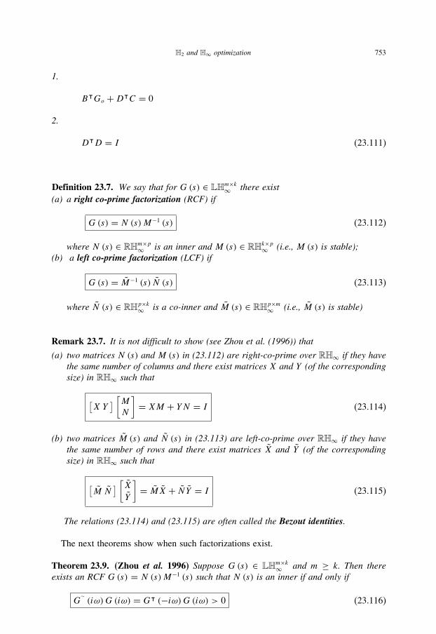
H2 and H∞ optimization 753
1.
BᵀGo +DᵀC = 0
2.
DᵀD = I (23.111)
Definition 23.7. We say that for G(s) ∈ LHm×k∞ there exist
(a) a right co-prime factorization (RCF) if
G(s) = N (s)M−1 (s) (23.112)
where N (s) ∈ RHm×p∞ is an inner and M (s) ∈ RHk×p
∞ (i.e., M (s) is stable);(b) a left co-prime factorization (LCF) if
G(s) = M−1 (s) N (s) (23.113)
where N (s) ∈ RHp×k∞ is a co-inner and M (s) ∈ RHp×m
∞ (i.e., M (s) is stable)
Remark 23.7. It is not difficult to show (see Zhou et al. (1996)) that
(a) two matrices N (s) and M (s) in (23.112) are right-co-prime over RH∞ if they havethe same number of columns and there exist matrices X and Y (of the correspondingsize) in RH∞ such that
[X Y
] [MN
]= XM + YN = I (23.114)
(b) two matrices M (s) and N (s) in (23.113) are left-co-prime over RH∞ if they havethe same number of rows and there exist matrices X and Y (of the correspondingsize) in RH∞ such that
[M N
] [XY
]= MX + N Y = I (23.115)
The relations (23.114) and (23.115) are often called the Bezout identities.
The next theorems show when such factorizations exist.
Theorem 23.9. (Zhou et al. 1996) Suppose G(s) ∈ LHm×k∞ and m ≥ k. Then there
exists an RCF G(s) = N (s)M−1 (s) such that N (s) is an inner if and only if
G∼(iω)G (iω) = Gᵀ (−iω)G (iω) > 0 (23.116)

754 Advanced Mathematical Tools for Automatic Control Engineers: Volume 1
for all ω ∈ [−∞,∞] (including at ±∞). Furthermore, if G(s) ∈ RHm×k∞ and its
state-space realization
[A B
C D
]has the stabilizable pair (A,B) such that the transfer
matrix G(iω) = C (iω − A)−1 B + D has the full column rank for all ω ∈ [−∞,∞],
then a particular state-space realization of the desired RCF
(M (s)
N (s)
)∈ RHk×p+m×p
∞ is
⎡⎣ A+ BF BR−1/2
F
C +DFR−1/2
DR−1/2
⎤⎦ (23.117)
where
R = DᵀD > 0
F = −R−1 (BᵀX +DᵀC)(23.118)
and X ≥ 0 is a solution of the following Riccati equation
(A− BR−1DᵀC
)X +X (
A− BR−1DᵀC)ᵀ
− XBR−1BᵀX − Cᵀ (I −DR−1Dᵀ)C = 0
(23.119)
Proof. (a) Necessity. Suppose G = NM−1 with N an inner and M (s) ∈ RHk×p∞ . Then
G∼(iω)G (iω)= (
M−1 (iω))∼N
∼(iω)N (iω)M−1 (iω)
= (M−1 (iω)
)∼M−1 (iω) > 0
for any ω ∈ [−∞,∞] since M (s) ∈ RHk×p∞ , that is, M (s) is “stable”.
(b) Sufficiency. First notice that if G = NM−1 is an RCF, then G = (NZ) (MZ)−1 is
also RCF for any nonsingular matrix Z ∈ Rp×p. Suppose now that N has its state-space
realization as[A+ BF BZ
C +DF DZ
]
For N to be an inner, as it follows from Corollary 23.8, we should have
(DZ)ᵀDZ = I
Select F in such a manner that the following matrix identities have been fulfilled:
(BZ)ᵀX + (DZ)ᵀ (C +DF) = 0
(A+ BF)ᵀX +X (A+ BF)+ (C +DF)ᵀ (C +DF) = 0
(23.120)

H2 and H∞ optimization 755
Take Z = R−1/2 where R := DᵀD > 0 by the assumption of the theorem. Then the first
equation in (23.120) becomes(BR−1/2
)ᵀX + (
DR−1/2)ᵀ(C +DF)
= R−1/2BᵀX + R−1/2Dᵀ (C +DF) = 0
which implies
R−1/2DᵀDF = −R−1/2 (BᵀX +DᵀC)
Then, pre-multiplication of the last equation by R−1/2 gives
F = −R−1 (BᵀX +DᵀC)
Substituting this F into the second equation in (23.120) gives exactly (23.119). The
existence of a nonnegative solution X ≥ 0 for (23.119) guarantees the fulfilling of
(23.116).1 �
Remark 23.8. Notice that if G(s) = N (s)M−1 (s) ∈ RHm×k∞ , then M−1 (s) ∈ RHp×k
∞and M−1 (s) is called an outer, so
G(s) = Ginn (s)Gout (s) (23.121)
where
Ginn (s) := N (s), Gout (s) = M−1 (s)
The factorization (23.121) is referred to as an inner–outer factorization. In an anal-ogous way the co-outer can be introduced such that the following co-inner–co-outerfactorization takes place:
G(s) = M−1 (s) N (s) = Gout (s) Ginn (s)
Ginn (s) := N (s), Gout (s) = M−1 (s)
(23.122)
Remark 23.9. The analogue result is valid for LCF (23.113), namely, supposing G(s) ∈LHm×k
∞ and m ≤ k, one concludes that there exists an RCF G(s) = M−1 (s) N (s) whereN (s) ∈ RHp×k
∞ is a co-inner and M (s) ∈ RHp×m∞ (i.e., M (s) is stable) if and only if
G(iω)G∼(iω) = G(iω)Gᵀ (−iω) > 0 (23.123)
for all ω ∈ [−∞,∞] (including at ±∞).
1 For details see Theorem 13.19 in Zhou et al. (1996).

756 Advanced Mathematical Tools for Automatic Control Engineers: Volume 1
Lemma 23.10. For any F (s) ∈ LHm×k∞ and any inner N (s) ∈ RHp×m
∞ (or any co-innerN (s) ∈ RHk×p
∞ )
‖F‖Lm×k∞ = ‖N (s) F‖
Lm×k∞ =
∥∥∥FN (s)∥∥∥Lm×k∞
(23.124)
that is, the pre-multiplication by an inner or the post-multiplication by a co-inner pre-serves the L∞ norm of any transfer matrix.
Proof. It follows directly from the definition (23.44) since
‖NF‖Lm×k∞ := ess sup
ω∈(−∞,∞)σ (N (iω) F (iω))
= ess supω∈(−∞,∞)
λ1/2max
{F
∼(iω)N
∼(iω)N (iω) F (iω)
}
= ess supω∈(−∞,∞)
λ1/2max
{F
∼(iω) F (iω)
} = ‖F‖Lm×k∞
and
∥∥∥FN∥∥∥Lm×k∞
:= ess supω∈(−∞,∞)
σ(F (iω) N (iω)
)
= ess supω∈(−∞,∞)
λ1/2max
{F (iω) N (iω) N
∼(iω) F
∼(iω)
}
= ess supω∈(−∞,∞)
λ1/2max
{F (iω) F
∼(iω)
} = ‖F‖Lm×k∞
�
Now we are ready to give the solution to the MMP problem (23.98) showing its
equivalence to the Nehari problem (23.95).
Theorem 23.10. The MMP problem (23.98) is equivalent to the Nehari problem(23.95) with
X (s) = M−12 (s)Q (s) M−1
3 (s) ∈ RHp2×p1∞
G(s) = N∼2 (s) T1 (s) N
∼3 (s)
(23.125)

H2 and H∞ optimization 757
and one of its solutions is
X (s) =M2 (s)
[N
∼2 (−s) T1 (−s) N∼
3 (−s)
−√λmax (GcGo)
f(−s)g∼(−s)
g∼(−s)g(−s)
]M3 (s)
(23.126)
where f(s) and g∼(s) is the Schmidt pair (23.78) for N
∼2 (s) T1 (s) N
∼3 (s) and Gc,Go its
grammians (23.68).
Proof. Using RCF and LCF for T2 (s) = N2 (s)M−12 (s) and for T3 (s) = M−1
3 (s) N3 (s),
respectively, and applying the property (23.124), we get
J (Q)= C ‖T1 (s)− T2 (s)Q (s) T3 (s)‖2RH
m1×k1∞
= C∥∥∥T1 (s)−N2 (s)M
−12 (s)Q (s) M−1
3 (s) N3 (s)
∥∥∥2
RHm1×k1∞
= C∥∥∥N∼
2 (s) T1 (s) N∼3 (s)−M−1
2 (s)Q (s) M−13 (s)
∥∥∥2
RHp2×p1∞
which is exactly (23.95) with (23.125). The solution (23.126) results from (23.126). �
23.2.5 Some control problems converted to MMP
H∞–control robust with respect to external perturbations–Problem formulationProblem 23.4. For the linear system given in the frequency domain by Fig. 23.5
G(s)
K(s)
w
u
z
y
Fig. 23.5. The block scheme of a linear system with an external input perturbation and an internal feedback.

758 Advanced Mathematical Tools for Automatic Control Engineers: Volume 1
G(s) :=[Gwz (s) Guz (s)
Gwy (s) Guy (s)
](Z (s)
Y (s)
)= G(s)
(W (s)
U (s)
)
U (s) := L {u}, Y (s) := L {y}Z (s) := L {z}, W (s) := L {w}
(23.127)
(z (t) ∈ Rn is associated with the part of coordinates forming a cost function, u (t) ∈ Rr
is the controlled input, y (t) ∈ Rp is the system output which may be used for feedbackdesigning and w (t) ∈ Rp is an external perturbation) design a feedback (dynamic)controller with a transfer matrix K (s) given by
U (s) = K (s) [Y (s)+W (s)] (23.128)
such that1. K (s) is proper and stable, i.e.,
K (s) ∈ RHr×p∞ (23.129)
2. it minimizes the following min–max criterion
J (K)→ minK(s)∈RH
r×p∞(23.130)
J (K) := supW∈L
n2 :‖W‖2
Ln2≤cw
‖Z‖2Hn+r2
where supremum is taken over all external perturbations of a bounded energy.Here the large symbols are the Laplace transformation of the small ones.
Notice that
Z (s)=Gwz (s)W (s)+Guz (s) U (s)=Gwz (s)W (s)+Guz (s)K (s) Y (s)
and
Y (s)=Gwy (s)W (s)+Guy (s) U (s)=Gwy (s)W (s)+Guy (s)K (s) Y (s)

H2 and H∞ optimization 759
which leads to the following relations
Y (s) = [I −Guy (s)K (s)]−1Gwy (s)W (s)
Z (s) =(Gwy (s)+Guy (s)K (s) [I −Guy (s)K (s)]−1
Gwy (s)
)W (s)
U (s) = K (s) [I −Guy (s)K (s)]−1Gwy (s)W (s)
Remark 23.10. 1. The cost functional J (K) (23.130) exists (finite) if and only if theclosed-loop system is stable, that is, when Z (s) ∈ L
n+r2 and Y (s) ∈ L
p
2 if W (s) ∈ Ln
2.2. By Lemma 23.4 it is possible if and only if the transfer functions from W (s) to Z (s)
and Y (s) are stable, namely when
Gwy (s)+Guy (s)K (s) [I −Guy (s)K (s)]−1Gwy (s) ∈ RH
(n+r)×n∞
[I −Guy (s)K (s)]−1Gwy (s) ∈ RH
p×n∞
Parametrization of all stabilizing stationary feedbacksProblem 23.5. Characterize the set of all stabilizing feedbacks K (s) which provides thestability for K (s) itself as well as for [I −Guy (s)K (s)]−1 supposing that the transfermatrices
Gwy (s) and Guy (s)
are stable, that is, we will try to find
K (s) ∈ RHr×p∞
such that
[I −Guy (s)K (s)]−1 ∈ RHp×p∞ (23.131)
providing
Gwy (s) ∈ RHp×p∞ , Guy (s) ∈ RHp×r
∞
Proposition 23.7. K (s) stabilizes G(s) if and only if it stabilizes Guy (s).
Proof. It follows directly from (23.131). �

760 Advanced Mathematical Tools for Automatic Control Engineers: Volume 1
Theorem 23.11. (Youla parametrization, 1961) The set of all (proper real rational)transfer matrices K (s) stabilizing Guy (s) is parametrized by the formula
K (s)= [Y (s)−M(s)Q(s)] [X(s)−N(s)Q(s)]−1
=[X(s)−Q(s)N(s)
]−1 [Y (s)−Q(s)M(s)
] (23.132)
where the matrix Q(s) ∈ RH∞ (provided that two inverted matrices exist) and all othermatrices are also from RH∞ and define the, so-called, double-co-prime factorization ofGuy (s), namely,
Guy (s) = N(s)M−1(s) = M−1(s)N(s)
[X(s) −Y (s)−N(s) M(s)
] [M(s) Y (s)
N(s) X(s)
]= I
(23.133)
Proof. It can be found in Francis (1987) as well as in Zhou et al. (1996). �
Corollary 23.9. If K (s) is as in (23.132), then
[I −Guy (s)K (s)]−1 = M (s)(X (s)−Q(s) N (s)
)K (s) [I −Guy (s)K (s)]−1 = N (s)
(X (s)−Q(s) N (s)
) (23.134)
Proof. Substituting Guy (s) = N(s)M−1(s) = M−1(s)N(s) and using the second identity
in (23.133) imply the desired relations (23.134). �
The solution of H∞ – linear robust control problemTheorem 23.12. The problem 23.4 is equivalent to the model matching problem (23.98)with
T1(s)= Gwy(s)+Guy(s)N(s)X(s)Gwy(s)
T2(s)= Guy(s)N(s)
T3(s)= N(s)Gwy(s)
(23.135)
Proof. The cost functional (23.130) can be represented as
J (K) := supW∈L
n2 :‖W‖2
Ln2≤cw
‖Z‖2Hn+r2
= supW∈L
n2 :‖W‖2
Ln2≤cw
‖TW‖2Hn+r2

H2 and H∞ optimization 761
where (omitting the argument)
T = Gwy +GuyK [I −GuyK]−1Gwy
which in view of (23.134) becomes
T = Gwy +GuyN(X −QN
)Gwy
=[Gwy +GuyNXGwy
]− [GuyN ]Q
[NGwy
]which completes the proof. �
Robust filtering problem: consider a linear system which block scheme is given at
Fig. 23.6.
Problem 23.6. Find a filter F (s) ∈ RHm×n∞ if it exists which minimizes
J (F ) := supw:‖w‖2
Lk2[0,∞)≤c
∥∥x − x∥∥2
Ln2 [0,∞)‖w‖2
Lk2[0,∞)(23.136)
Here w (t) ∈ Lk2 [0,∞) is an external noise, x (t) ∈ Ln2 [0,∞) is a state vector,y (t) ∈ Lm2 [0,∞) is an output of the system and x (t) ∈ Ln2 [0,∞) is a state estimate.For physical reasons it is supposed that all transfer matrices are stable, that is,
G(s) ∈ RHk×n∞ , F (s) ∈ RHn×m
∞ , H (s) ∈ RHn×m∞
F(s)
G(s)yxw
H(s)
x
e5 x 2x
Fig. 23.6. Filtering problem illustration.

762 Advanced Mathematical Tools for Automatic Control Engineers: Volume 1
As before, in view of (17.107) and (23.100), we have
J (F )= supW :‖W‖2
Lk2
≤c
∥∥∥X (s)− X (s)∥∥∥2
Ln2
‖W‖2Lk2
= supW :‖W‖2
Lk2
≤c‖X (s)− F (s) Y (s)‖2
Ln2
= supW :‖W‖2
Lk2
≤c
∥∥[G(s)− F (s)H (s)]W (s)∥∥2
Ln2
= c ‖G(s)− F (s)H (s)‖2RH
k×n∞
Using the left-co-prime factorization (23.113)
H (s) = M−1(s)N(s)
and applying the property (23.106), we derive
J (F )= c∥∥∥G(s)− F (s) M−1(s)N(s)
∥∥∥2
RHk×n∞
= c∥∥∥[G(s)− F (s) M−1(s)N(s)
]N∼(s)
∥∥∥2
RHk×n∞
= c∥∥∥G(s) N∼(s)− F (s) M−1(s)
∥∥∥2
RHk×n∞
(23.137)
which leads to the following result.
Theorem 23.13. The robust filtering problem (23.6) is equivalent to the model matchingproblem (23.98) with
T1(s) = G(s) N∼(s)
T2(s) = I, Q (s) = F (s)
T3(s) = M−1(s)
(23.138)
Proof. It results from (23.137). �

BIBLIOGRAPHY
Adamjan, V., Arov, D. & Krein, M. (1971), “Analytic properties of Schmidt pairs for a Hankel operator and
the generalized Schur-takagi problem”, Math. USSR Sbornik 15, 31–73 (in Russian).
Albert, A. (1972), Regression and Moore-Penrose Pseudoinverse, Vol. 94 of Mathematics in Science andEngineering, Academic Press, New York, London.
Alexeev, V., Galeev, E. & Tihomirov, V. (1984), Collection of Problems on Optimization, Nauka, Moscow
(in Russian).
Alexeev, V., Tikhomirov, V. & Fomin, S. (1979), Optimal Control, Nauka, Moscow (in Russian).
Antosiewicz, H. (1958), “A survey of Lyapunov’s second method”, Control of Nonlinear Oscillations 4,141–166.
Apostol, T. (1974), Mathematical Analysis, Addison-Wesley Series in Mathematics, 2nd edn, Addison-Wesley,
Massachusetts.
Arrow, K. J., Hurwics, L. & Uzawa, H. (1958), Studies in Linear and Non-linear Programming, StanfordUniversity Press.
Aubin, J. (1979), Mathematical Methods of Game and Economic Theory, North-Holland Publishing Company.
Barbashin, E. & Krasovskii, N. (1952), “On asymptotic global stability of motions”, Doklady Academy ofSciences, USSR 86(3), 453–458 (in Russian).
Bellman, R. (1957), Dynamic Programming, Princeton University Press, Princeton, New Jersey.
Bellman, R. (1960), Introduction to Matrix Analysis, McGraw-Hill Book Company, Inc., New York, USA.
Bihari, I. (1956), “A generalization of a lemma of Bellman and its applications to uniqueness problems of
differential equations”, Acta Math. Sci. Hungar. 4(7), 71–94.Boltyanski, V., Gamkrelidze, R. & Pontryagin, L. (1956), “On the theory of optimal processes”, Doklady AN
USSR 110(1), 7–10 (in Russian).
Boyd, S., El Chaoui, L., Feron, E. & Balakrishnan, V. (1994), Linear Matrix Inequalities in System and ControlTheory, Vol. 15 of SIAM Studies in Applied Mathematics, SIAM, Philadelphia, Pennsylvania, USA.
Chetaev, N. (1965), Stability of Motions, Nauka, Moscow (in Russian).
Chung, K. (1954), “On stochastic approximation method”, Annals of Mathematical Statistics 25(3), 463–483.Cline, R. (1964), “Representations for the generalized inverse of a partitioned matrix”, SIAM J. Applied
Mathematics 12, 588–600.Cline, R. (1965), “Representations for the generalized inverse of sums of matrices”, SIAM J. Applied Mathe-
matics 2, 99–114.Crandall, M. & Lions, P. (1983), “Viscosity solution of Hamilton–Jacobi equations”, Trans. Amer. Math. Soc.
277, 1–42.Curtain, R. & Zwart, H. (1995), An Introduction to Infinite-Dimensional Linear System Theory, Vol. 21 of Texts
in Applied Mathematics, Springer-Verlag, New York.
Danes, J. (1972), “A geometric theorem useful in nonlinear functional analysis”, Bulletino U.M.I. 6(4), MR
47:5678, 369–375.
Datta, B. N. (2004), Numerical Methods for Linear Control Systems (Design and Analysis), Elsevier Inc.
(Academic Press), San Diego, California, USA.
Dax, A. (1997), “An elementary proof of Farkas lemma”, SIAM Review 39(3), 503–507.El’sgol’ts, L. (1961), Differential Equations, International Monographs on Advanced Mathematics and Physics
(translated from Russian edition, 1957), Hindustan Publishing Corporation (India), Delhi.
Farkas, J. (1902), “Uber die Theorie der einfachen Ungleichungen”, J. Reine Angew. Math. 124, 1–24.Feldbaum, A. (1953), “Optimal processes in systems of automatic control”, Avtomatika i Telemehanika
14(6), 712–728 (in Russian).
Filippov, A. (1988), Differential Equations with Discontinuous Right-hand Sides, Kluwer Academic Publishers,
Dordrecht.
Finsler, P. (1937), “Uber das vorkommen definiter und semi-definiter formen in scharen quadratischer formen”,
Comentarii Mathematici Helvetici 9, 192–199.
763
764 Bibliography
Fuchs, B. & Shabat, B. (1964), Functions of a Complex Analysis, Pergamon Press (translated from Russian,
Fizmatgiz, Moscow, 1959), Oxford.
Gantmacher, F. (1990), The Theory of Matrices, 4th edn, Chelsea Publishing Company, New York.
Gel’fand, I. & Fomin, S. (1961), Variation Calculus, Fizmatgiz, Moscow, Russia (in Russian).
Gelig, A., Leonov, G. & Yakubovich, V. (1978), Stability of Nonlinear Systems with Nonunique Steady State,Nauka, Moscow, Russia (in Russian).
Greville, T. (1960), “Some applications of the pseudoinverse of a matrix”, SIAM Review 2, 15–22.Gronwall, T. (1919), “Note on the derivatives with respect to a parameter of the solutions of a system of
differential equations”, Ann. Math. 2(20), 292–296.Guillemin, E. (1949), The Mathematics of Circuit Analysis: Extensions to the Mathematical Training of Electrical
Engineers, John Wiley and Sons, New York.
Halanay, A. (1966), Differential Equations: Stability. Oscillations. Time Lag, Academic Press, New York.
Hartman, P. (2002), Ordinary Differential Equations, Vol. 38 of Classics in Applied Mathematics, 2nd edn,
SIAM, Philadelphia.
Hautus, M. & Silverman, L. (1983), “System structure and singular control”, System Structure and SingularControl 50, 369–402.
Highan, N. (1996), Accuracy and Stability of Numerical Algorithms, SIAM, Philadelphia.
Hinrichsen, D. & Pritchard, A. (2005), Mathematical Systems Theory I: Modelling, State Space Analysis,Stability and Robustness, Vol. 48 of Texts in Applied Mathematic, Springer, Berlin.
Ivanov, V. & Faldin, N. (1981), Theory of Optimal Automatic Control Systems, Nauka, Moscow, Russia
(in Russian).
Kharitonov, V. (1978), “Asymptotic stability of a family of linear differential equations”, Differential Equations14(11), 2086–2088 (in Russian).
Krasovskii, N. (1952), “On stability of dynamic motions”, Applied Mathematics and Mechanics 16(5), 3–24(in Russian).
Kuhn, H. & Tucker, A. (1951), “Nonlinear programming”, in University of California Press, ed., Proceedingsof the Second Berkeley Symposium on Math. Statistics and Probability, Berkeley, CA, pp. 481–492.
Lancaster, P. (1969), Theory of Matrices, Academic Press, New York.
Lankaster, P. & Tismenetsky, M. (1985), The Theory of Matrices, Computer Science and Applied Mathematics,
2nd edn, Academic Press, Inc., Orlando, Florida, 32887.
Lavrentiev, M. & Shabat, B. (1987), Methods of Theory of Functions of Complex Variables, Nauka, Moscow,
Russia (in Russian).
Lefschetz, S. (1965), Stability of Nonlinear Control Systems, Academic Press, New York.
Lurie, A. & Postnikov, V. (1944), “To the theory of control systems”, Problems of Mathematics and Mechanics(PMM) 8(3).
Lyapunov, A. (1892), General Problem of a Movement Stability, Doctor thesis, Leningrad-Moscow (in Russian)
(the original 1897).
Lyapunov, A. (1907), “Problèm Le général de la stabilité de mouvement” (translation of the paper published
in Comm. Soc. Math. Krakow 1893, reprinted in Ann. Math. Studies, 17, Princeton, 1949), Ann. Fac. Sci.,Toulose 2, 203–474.
Marcus, M. & Minc, H. (1992), A Survey of Matrix Theory and Matrix Inequality, 2nd edn, Dover Publications,
Inc., New York.
Nazin, A. & Poznyak, A. (1986), Adaptive Choice of Variants, Theoretical Backgrounds of Technical Cyber-netics, Nauka, Moscow, Russia (in Russian).
Nehari, Z. (1957), “On bounded bilinear forms”, Annals of Mathematics 15(1), 153–162.Nesterov, Y. & Nemirovsky, A. (1994), Interior-point Polynomial Methods in Convex Programming, Vol. 13
of Studies in Applied Mathematics, SIAM, Philadelphia, Pennsylvania, USA.
Pliss, V. (1964), Nonlocal Problems of Oscillation Theory, Nauka, Moscow-Leningrad (in Russian).
Polyak, B. (1987), Introduction to Optimization, Translations series in Mathematics and Engineering, Optimiza-
tion Software, Inc., Publications Division, New York.
Polyak, B. & Sherbakov, P. (2002), Robust Stability and Control, Nauka, Moscow, Russia.
Polyak, B. & Tsypkin, Y. Z. (1990), “Frequency-domain criteria for robust stability and aperiodicity of linear
systems”, Automation and Remote Control 51(9), 1192–1200. Translated from “Automaticay Telemechan-
ica” (in Russian), 1990, v.9, pp. 45–54.
Pontryagin, L. S., Boltyansky, V. G., Gamkrelidze, R. V. & Mishenko, E. F. (1969 (translated from Russian)),
Mathematical Theory of Optimal Processes, Interscience, New York.
Popov, V. (1961), “Global asymptotic stability of nonlinear systems of automatic control”, Automation andRemote Control (Translation from “Automatica i Telemechanica”) 22(8), 961–979.

Bibliography 765
Poznyak, A. (1991), Lectures on Basics of Robust Control (H-inf Theory), MPhTI (Moscow Physical Technical
Institute), Moscow (in Russian).
Rasvan, V. (1975), Absolute Stability of Time Lag Control Systems, Ed. Academiei, Bucharest (in Romanian,
Russian revised edition by Nauka, Moscow, 1983).
Riesz, F. & Nagy, B. (1978 (original in French, 1955)), Functional Analysis, Frederick Ungar, New York.
Rockafellar, R. (1970), Convex Analysis, Princeton University Press.
Royden, H. (1968), Real Analysis, 2nd edn, MacMillan Publishing Co., Inc., New York.
Rudin, W. (1973), Real and Complex Analysis, McGraw-Hill, New York.
Rudin, W. (1976), Principle of Mathematical Analysis, International Series in Pure and Applied Mathematics,
3rd edn, McGraw-Hill, New York.
Schlaepfer, F. & Schweppe, F. (1972), “Continuous-time state estimation under disturbances bounded by convex
sets”, IEEE Transactions on Automatic Control AC-17(2), 197–205.Trenogin, V. (1980), Functional Analysis, Nauka, Moscow, Russia (in Russian).
Troutman, J. (1996), Variation Calculus and Optimal Control (Optimization with Elementary Covexity), 2ndedn, Springer-Verlag, New York.
Utkin, V. (1992), Sliding Modes in Control and Optimization, Springer-Verlag.Utkin, V., Guldner, J. & Shi, J. (1999), Sliding Modes in Electromechanical Systems, Sliding Modes in
Electromechanical Systems, London.
Vidyasagar, M. (1993), Nonlinear Systems Analysis, Prentice Hall, Englewood Cliffs, New Jersey 07632.
Wintner, A. (1945), “The nonlocal existence problem of ordinary differential equations”, American Journal ofMathematics 67.
Yakubovich, V. (1973), “Auto-oscillation frequency conditions in nonlinear systems with a single stationary
nonlinearity”, Siberian Mathematical Journal 14(5), 1100–1129 (in Russian).
Yoshida, K. (1979), Functional Analysis, Narosa Publishing House, New Delhi.
Young, J. & Zhou, X. Y. (1999), Stochastic Controls: Hamiltonian Systems and HJB Equations, Springer-Verlag, New York.
Zeidler, E. (1986), Nonlinear Functional Analysis: Fixed-Point Theorems, Vol. 1, Springer-Verlag, New York.
Zeidler, E. (1995), Applied Functional Analysis, Vol. 108 of Applied Mathematical Sciences, Springer-Verlag,New York.
Zhou, et al., K., Doyle, J. & Glover, K. (1996), Robust and Optimal Control, Prentice Hall, Upper Saddle River,New Jersey.
Zubov, V. (1962), Mathematical Methods for the Study of Automatic Control Systems, Pergamon Press,
New York.
Zubov, V. (1964), Methods of A.M. Lyapunov and Their Applications, Noordhoff, Groningen.

This page intentionally left blank

INDEX
Adjoint equations, 673
Algebras, 294
sigma, 295
Algebraic complement, 11
Algebraic Riccati–Lurie’s matrix inequality,
195
All stabilizing feedbacks, 759
All-pass transfer matrix, 745
Almost everywhere concept, 311
Analytical center of the LMI, 210
Arc, 401
length, 402
simple (Jordan), 401
Arrow–Hurwicz–Uzawa method, 639
Axioms
field, 232
Barrier function, 210
Bellman’s principle of optimality, 688
Bezout identities, 753
Block-matrix
inversion, 31
Boundary of a set, 259
Bounded LS problem, 223
Bounded real condition, 199
Brachistochrone, 658
Canonical observability form, 706
Cauchy (fundamental) sequence, 263
Cauchy criterion, 264
for a series, 368
Cauchy formula, 410
Cauchy integral theorem, 87
Cauchy’s inequalities, 415
Cauchy’s integral formula, 410
Cauchy’s integral law, 406
Cauchy’s problem, 501
Cauchy’s residue theorem, 409
Cauchy–Adhamar formula, 421
Cauchy–Riemann conditions, 398
Cayley transformation, 52
Central optimal element, 744
Cesàro summability, 378
Chain rule, 317
Characteristic equation, 44
Characteristic polynomial, 44, 139
Cholesky factorization, 73
Circuit, 402
Cline’s formulas, 109
Co-inner, 750
Cofactor
complementary, 13
Cofactor of a matrix, 11
Commutation, 22
Companion matrix, 150
Complement of A relative to B, 253
Complementary slackness conditions, 677
Complete differential, 321
Completion, 457
Complex exponent, 248
Complex number, 239
Complex sines and cosines, 249
Condition
Euler–Lagrange, 657
Legandre, 657
maximality, 674, 677
nontriviality, 674
strong Legendre, 657
strong Legendre vector, 663
transversality, 674
Conditions
complementary slackness, 674
Euler–Poisson, 664
Weierstrass–Erdmann, 667
Congruent matrices, 70
Conjugate, 241
Conjugated symmetric, 186
Continuous dependence of the solutions of
ODE, 516
Contour
reducible, 406
Contraction, 273
Contraction principle, 273
Control
admissible, 669
feasible, 669

768 Index
Controllability, 165
Controllability grammian, 196
Controllable mode, 174
Convergence, 261
Convex body, 682
Convex hull, 130
Convex optimization problem, 191
Coordinate transformation, 352
Coordinate transformation in an integral, 352
Cost fucntional
in the Bolza form, 668
in the Lagrange form, 668
in the Mayer form, 668
Cramer’s rule, 18
Criterion
2k, 370
circle, 594
Kronecker–Capelli, 17
Criterion of polynomial robust stability, 160
Curve
piecewise smooth, 402
rectifiable, 401
Cutting plane, 207
D’Alembert–Euler conditions, 398
Damping factor, 211
Daneš’ theorem, 216
Darboux sums, 277
Decomposition
Kalman, 714
Kalman canonical, 716
polar, 63
singular-value, 66, 68
Def complete space, 455
Defect, 42
Deffeomorphism, 352
Delta-function, 42, 312
Derivative, 284, 315
directional, 320
Fréchet, 488
Gateaux, 490
mixed partial, 320
partial, 319
right, 512
Detectability, 173
Determinant, 4
homogeneous, 6
Vandermonde, 12
Wronsky, 473
Diagonal
main, 4
secondary, 4
Dichotomy, 576
Differential inclusion, 541
Disjoint sets, 253
Dissipation, 197
Distance function, 256, 299
Divergence, 332
Domain
simply-connected, 406
Dynamic Programming Method, 687
Eigenvalue, 44
Eigenvalue problem, 204
Eigenvector, 44
Eigenvectors
generalized, 54, 176
Elementary transformations, 32
Ellipsoid, 207
Ellipsoid algorithm, 207
Elliptic cylinder, 109
Equation
Hamilton–Jacobi–Bellman, 688
matrix Riccati, 704
Riccati, 598
Equivalent control, 552
Equivalent control method, 552
Euclidean k-space, 239
Euclidean, 89
Euler’s formula, 247
Expansion
Fourier, 460
Legendre, 111
Factorization
co-inner-co-outer, 755
double-co-prime, 760
inner-outer, 755
left co-prime, 753
polar, 63
right co-prime, 753
Farkaš’ lemma, 222
Feasible LMI, 193
Field, 232
ordered, 233
Finsler lemma, 216
First integral of ODE, 521
Fixed point, 491
Formula
Binet–Cauchy, 14
Cauchy, 518
Green, 524
Newton–Leibniz, 339
Schur’s, 30
Frequency inequality, 591

Index 769
Frequency theorem, 595
Function, 251
absolutely continuous, 533
analytic, 400
characteristic, 307
concave, 359, 606
continuous, 267, 542
convex, 359, 605
delta, 312
entire, 415
equicontinuous, 271
Hahn, 579
holomorphic, 400
integrable in the Lebesgue
sense, 309
Legendre, 111
Lipschitz continuous, 267
Lyapunov, 566
measurable, 304
meromorphic, 409
negative-definite, 563
of bounded variation, 290
piecewise continuous, 540
positive-definite, 562
quasi-convex, 621
regular, 400
semi-continuous, 542
simple, 307
spectral, 442
strictly convex, 605
strongly convex, 606
Functional
linear, 463
Lyapunov–Krasovski, 202
separable, 688
Functionals, 463
Functions of a matrix, 79
Fundamental theorem of algebra, 432
Gamma-entropy, 201
Gauss’s method, 16
Gauss’s method of determinant evaluation, 9
Gauss’s rule, 16
Godograph, 156
Gradient, 320, 332
Gradient method, 617, 619
Gram–Schmidt orthogonalization, 60
Grammian
controllability, 165, 719, 723
observability, 170, 719, 723
Greatest-integer function, 287
Greville’s formula, 106
Group property, 517
H-inf norm, 201
H2 norm, 196
H2 optimal control, 724
Hölder’s condition, 433
Hamilton–Jacoby–Bellman (HJB), 693
Hamiltonian, 523, 674, 677
Hamiltonian form, 677
Hamiltonian matrix, 175
Hankel singular values, 721
Hermitian form, 115
Homeomorphism, 273
Horizon, 668
Identity
Cauchy, 15
Image, 42, 165
Imaginary unit, 241
Inequality
Frobenius’s, 37
Popov’s, 591
Inertia of a square matrix, 70
Infeasible LMI, 193
Infimum, 232
essential, 311
Infinite products, 379
Inner, 750
Inner (scalar) product, 239
Inner–outer factorization, 755
Instability, 564, 570
Integer numbers, 233
Integral
contour, 403
Duhammel, 440
Lebesgue, 308
Lebesgue–Stieltjes, 308
Integral inequality
first Chebyshev, 356
second Chebyshev, 356
Cauchy–Bounyakovski–Schwartz, 358
generalized Chebyshev, 355
Hölder, 356
Jensen, 359
Kulbac, 364
Lyapunov, 363
Markov, 355
Minkowski, 366
Integral transformations, 433
kernel, 433
Integrand, 278
Integrator, 278
Interior point method, 191, 210
Interior point of a set, 257

770 Index
Internal points of a set, 259
Intersection of the sets, 253
Interval, 297
Invariant embedding, 688, 691
Inverse image of the function, 251
Isolated point, 257
Isometry, 273
Jordan
block, 62
chain, 56
form, 62
normal canonical representation, 62
Kantorovich’s matrix inequality, 226
Kernel, 42, 98, 171
Kharitonov’s theorem, 160
Kronecker product, 26
Kronecker sum,
Lagrange principle, 631
Laplace image, 434
Least square problem, 107
Lemma
Abel-Dini, 385
Bihari, 507
Du Bois–Reymond, 647
Fatou’s, 346
Gronwall, 510
Jordan, 418
KKM, 494
Kronecker, 384
Lagrange, 650
Mertens, 376
on a finite increment, 324
on quadratic functionals, 651
Schwartz, 416
Sperner, 493
Teöplitz, 382
Yakubovich–Klaman, 595
Liénard–Chipart criterion, 153
Limit point of a set, 257
Linear conbination, 41
Linear manifold, 97
Linear matrix inequalities, 191
Linear partial DE
method of characteristics, 529
Linear recurrent inequalities, 388
Linear stationary system, 196
Linear system
MIMO, 713
SISO, 713
Linear transformation, 42
Linearly dependent, 42
Linearly independent, 42
Liouville’s theorem, 415
Lipschitz condition, 324
LMI, 191
Low-pass filter, 555
Lower limit, 265
LQ problem, 697
Lyapunov equation
algebraic, 584
differential, 584
Lyapunov inequality, 195
Lyapunov order number, 524
Lyapunov stability, 566
Manifold, 541
Mapping, 251
Matrices
equivalent, 36
Matrix
adjoint, 21
block-diagonal, 30
companion, 10
controllability, 165
diagonal, 4, 182
difference, 20
fundamental, 517
Hautus, 165, 170
Hermitian, 21
Householder, 51
idempotent, 77
inverse, 21
Jacobi, 489
low triangular, 5
multiplication by scalar, 20
Newton’s bynom, 22
Nonnegative definite, 117
nonsingular, 21
normal, 21, 67
observability, 170
orthogonal, 21
partitioning, 29
Positive definite, 118
power, 22
product, 19
real normal, 21
rectangular, 3
simple, 36
singular, 21
skew-hermitian, 21
Square root, 118
Stable matrix, 139

Index 771
sum, 19
symmetric, 21
transpose, 6
transposed, 20
unitary, 21
upper triangular, 6
Matrix Abel identities, 214
Matrix exponent, 81
Frobenius (Euclidian), 91
Hölder, 91
induced matrix norm, 93
maximal singular-value, 92
spectral norm, 93
Trace, 91
Weighted Chebyshev, 91, 93
Matrix norm constraint, 194
Matrix or submultiplicative norm, 91
Matrix Riccati equation, 175, 188
Maximum modulus principle, 415
Maximum principle, 670
Maximum–minimum problem, 129
McMillan degree, 717
Mean-value theorem, 318, 322
Measure, 304
atomic, 312
countably additive, 303
Lebesque, 303
outer, 298
zero, 303
Method
Arrow–Hurwicz–Uzawa, 639
Galerkin, 485
Metric, 256
Chebyshev’s, 256
discrete, 256
Euclidian, 256
module, 256
Prokhorov’s, 257
weighted, 256
Metric space, 256
complete, 264
Mikhailov’s criterion, 156
Minimal ellipsoid, 206
Minimum
global, 611, 628
local, 611, 628
Minimum modulus principle, 416
Minimum point
locally unique, 613
nonsingular, 613
Minimum volume ellipsoid, 208
Minor
complementary, 13
leading principle, 13
of some order, 13
principle, 13
Minor of a matrix, 10
Mixed subgradient, 682
Mode, 174
Model-matching (MMP) problem, 747
Moivre–Laplace formula, 246
Monic polynomial, 139
Monotonic sequence, 265
Moore–Penrose pseudoinverse, 102
Multiplicity
algebraic, 54
geometric, 54
Necessary conditions of a matrix stability, 144
Nehari problem, 742
Nehari theorem, 743
Neighborhood of a point, 257
Newton’s method
modified, 617, 620
Nonexspansivity, 199
Nonlinear trace norm constraint, 194
Nonlinear weighted norm constraint, 194
Nonstrict LMI, 191
Norm, 88
Chebyshev, 89
Hölder, 89
Modul-sum, 89
weighted, 89
S-norm, 92
Norm equivalency, 89
Normal equations, 99
Normed linear space, 89
Compatible, 93
Null space, 42, 98, 171
Null space of an operator, 471
Number of inversions, 3
Observability, 170
Observable mode, 174
ODE, 501, 695
adjoint, 523, 676
Carathéodory’s type, 531
Jacobi, 657
Jacobi vector form, 663
singular perturbed, 534
variable structure, 533
with jumping parameters, 534
ODE solution
in Filippov’s sense, 541
maximal, 511
minimal, 511
772 Index
One-to-one mapping, 251
Open cover of a set, 260
Operator, 462
adjoint (dual), 477
coercive, 483
compact, 464, 469
continuously invertible, 472
differential, 463, 465
Hankel, 733
Hankel in the time domain, 735
Hermitian, 181
integral, 463, 465
invertible, 463
isomorphic, 471
Laplace, 333
Laurent, 731
linear continuous, 464
monotone, 482
monotone strictly, 483
monotone strongly, 483
nonnegative, 483
orthogonal projection, 480
positive, 483
self-adjoint (or Hermitian), 478
semi-continuous, 464
shift, 463
strongly continuous, 466
Toeplitz, 733
uniformly continuous, 466
weighting, 465
Operator nabla, 332
Optimal control, 670
Optimal control problem
in the Bolz form, 669
with a fixed terminal term,
670
Optimal pair, 670
Optimal state trajectory, 670
Optimality
sufficient conditions, 694
Order, 231
Order of a zero, 423
Ordered set, 231
Orlando’s formula, 146
Orthogonal complement, 460
Orthogonal completion, 42
Orthogonality, 42
Orthonormality, 42
Outer, 755
Pair
controllable, 165
detectable, 173
observable, 170
stabilizable, 170, 188
uncontrollable, 165
undetectable, 173
unobservable, 170
unstabilizable, 170
Parametric optimization, 681
Parseval’s identities
generalized, 722
Parseval’s identity, 423, 445
Passivity, 197
Permutation, 3
Pole, 409
Polyak–Tsypkin geometric criterion, 162
Polytope, 709
Popov’s line, 594
Popov–Belevitch–Hautus test, 174
Positive definiteness
strictly, 124
Principal value of the complex logarithm, 248
Principle of “zero-excluding”, 160
Principle of argument, 429
Principle of argument variation, 154
Problem
LQR, 724
Programming
dynamic, 671
Projection
orthogonal, 459
Projection to the manifold, 97
Projector, 77
complementary, 77
Pseudo-ellipsoid, 109
Pseudoinverse, 102
Quadratic form, 115
Quadratic stability degree, 205
Range, 42, 98
Range of function, 251
Rank, 17, 36
Ratio of two quadratic forms, 132
Rational numbers, 233
Rayleigh quotient, 129
Reaching phase, 539
Real-positiveness, 197
Realization
balanced, 720
minimal, 717
Refinement, 278
Residue, 410
Resolvent, 86
Index 773
Resolving Lourie’s equations, 596
Riccati differential equation, 699
Riccati matrix ODE, 525
Riemann integral, 277
Riemann–Stieltjes integral, 278
Riemann–Stieltjes sum, 278
Robust filtering problem, 761
Robust stability, 159
Rotor, 332
Rouché theorem, 431
Routh–Hurwitz criterion, 151
Row-echelon form, 16
Rule
Sylvester’s, 38
S-procedure, 195, 218
Saddle-point property, 634
Sarrius’s rule, 5
Scalar product, 41
Schmidt pair, 740
Schur’s complement, 120
Sensitivity matrix, 681
Sequence, 252
monotonically nondecreasing, 265
monotonically nonincreasing, 265
Series
alternating, 371
Fourier, 429
geometric, 372
Laurent, 425
nth partial sum, 368
sum, 368
Taylor, 420
telescopic, 369
Series convergence
Abel’s test, 375
Dirichlet’s test, 375
integral test, 373
Set
Borel, 303
bounded, 257
bounded above, 231
closed, 257
closure, 258
compact, 260
complement, 257
connected, 257
dense, 257
diameter, 263
elementary, 297
finitely μ-measurable, 300
low bound, 231
μ-measurable, 300
open, 257
relative compact, 469
separable, 625
strictly separable, 625
Set function
additive, 295
countably additive, 295
regular, 298
Shifting vector, 696, 699
Signature of a Hermitian matrix, 71
Simplex
Sperner, 493
Simultaneous reduction of more than two
quadratic forms, 128
Simultaneous transformation of pair of
quadratic forms, 125
Singular points, 409
Singular value, 67
Singularity
essential, 409
removable, 409
Slater’s condition, 631, 634
Sliding mode control, 554
Sliding mode equation, 552
Sliding motion, 545
Space
Banach, 455
bounded complex numbers, 452
continuous functions, 452
continuously differentiable functions, 452
dense, 451
dual, 475
frequency domain, 454
Hardy, 454
Hilbert, 457
homeomorphic, 273
Lebesgue, 453
measurable, 304
reflexive, 476
separable, 451
Sobolev, 453
summable complex sequences, 452
Span, 41
Spectral radius, 45, 92
Spectral theorem, 61
Spectrum, 45
of a unitary matrix, 51
Square root of a matrix, 84
Stability
absolute in the class, 588
asymptotic global, 576
asymptotically local, 564
774 Index
asymptotically uniformly local, 564
BIBO, 585
exponential, 569, 582, 584
exponential local, 564
Lyapunov (local), 563
uniformly local, 563
Stabilizability, 170
Stationary property, 131
Stationary time-delay system, 202
Steepest descent problem, 225
Stieltjes integral, 278
Stodola’s rule, 144
Subadditivity, 298
Subgradient, 626
Subsequence, 262
Subspace
A-invariant, 176
Support function, 111
Supremum, 232
essential, 311
Sylvester criterion, 124
Symbol
Kronecker, 42
Symmetric difference, 299
System
hybrid, 203
robust, 747
Systems
stationary, 678
Taylor’s formula, 318, 323
Terminal set, 668, 691
Theorem
first Lyapunov, 573
first mean-value, 337
second Lyapunov, 568
second mean-value, 337
Antosevitch, 579
Ascoli–Arzelà, 271
Bonnet’s, 338
Brouwer, 495
Cayley–Hamilton, 53
Chetaev, 580
Fermat, 611
fixed point, 273
Fubini’s, 348
Hahn–Banach, 467
Halanay, 580
implicit function, 327
inverse function, 325
Karush–John, 631
Krasovskii, 577
Kuhn–Tucker, 634
Laplace, 14
Lebesgue’s dominated convergence, 347
Lebesgue’s monotone convergence, 342
Leray–Schauder, 498
Liuoville, 517
on n-intervals, 710
on separation, 624
Peano, 506
Picard–Lindelöf, 504
Plancherel, 445
Rademacher, 607
Riesz, 479
Rolle’s, 318
Schauder, 496
Tonelli-Hobson, 351
Wintner, 515
Tolerance level optimization, 204
Topological mapping, 273
Topological properties, 274
Total variation, 291
Trace, 38
Transfer function, 196
Transformation
both-side Laplace, 448
Fourier, 442
Gladishev’s, 637
Hankel (Fourier–Bessel), 449
Laplace, 434, 435
Melline, 448
two-dimensional Fourier, 447
Transversality condition, 677
Transversality conditions, 666
Triangle inequality, 88
Uncontrollable mode, 174
Uniform continuity, 269
Union of the sets, 253
Unitary equivalentness, 69
Unobservable mode, 174
Upper function, 349
Upper limit, 265
Value function, 692
Variation
needle-shape
spike, 671
Variation principle, 491
Variation principle, 653
Verification rule, 694
Viscosity solutions, 688
Weierstrass theorem, 265, 268, 612
Winding number, 412