Advanced Full-Text Search Based on Synonyms in Postgres

Claremont Colleges Claremont Colleges

Scholarship @ Claremont Scholarship @ Claremont

CMC Senior Theses CMC Student Scholarship

2022

Advanced Full-Text Search Based on Synonyms in Postgres Advanced Full-Text Search Based on Synonyms in Postgres

Joey Bodoia

Follow this and additional works at: https://scholarship.claremont.edu/cmc_theses

Part of the Data Science Commons, and the Software Engineering Commons

Recommended Citation Recommended Citation Bodoia, Joey, "Advanced Full-Text Search Based on Synonyms in Postgres" (2022). CMC Senior Theses. 3070. https://scholarship.claremont.edu/cmc_theses/3070

This Open Access Senior Thesis is brought to you by Scholarship@Claremont. It has been accepted for inclusion in this collection by an authorized administrator. For more information, please contact [email protected].

https://scholarship.claremont.edu/

https://scholarship.claremont.edu/cmc_theses

https://scholarship.claremont.edu/cmc_student

https://scholarship.claremont.edu/cmc_theses?utm_source=scholarship.claremont.edu%2Fcmc_theses%2F3070&utm_medium=PDF&utm_campaign=PDFCoverPages

https://network.bepress.com/hgg/discipline/1429?utm_source=scholarship.claremont.edu%2Fcmc_theses%2F3070&utm_medium=PDF&utm_campaign=PDFCoverPages

https://network.bepress.com/hgg/discipline/150?utm_source=scholarship.claremont.edu%2Fcmc_theses%2F3070&utm_medium=PDF&utm_campaign=PDFCoverPages

https://scholarship.claremont.edu/cmc_theses/3070?utm_source=scholarship.claremont.edu%2Fcmc_theses%2F3070&utm_medium=PDF&utm_campaign=PDFCoverPages

mailto:[email protected]

Claremont McKenna College

Advanced Full-Text Search Based

on Synonyms in Postgres

submitted to

Professor Mike Izbicki

written by

Joey Bodoia

Senior Thesis

Spring 2022

April 25, 2022

Acknowledgements

I would like to extend my deepest gratitude to my thesis reader, Professor Mike Izbicki, for his time,

effort, patience, and thoughtful guidance throughout this project.

Contents

1 Abstract 1

2 Motivation 2

2.1 Synonyms . . . . . . . . . . . . . . . . . . . . . . . . . . . . . . . . . . . . . . . . . . 2

2.2 Typos . . . . . . . . . . . . . . . . . . . . . . . . . . . . . . . . . . . . . . . . . . . . 2

3 Examples 4

3.1 Example 1: Synonyms . . . . . . . . . . . . . . . . . . . . . . . . . . . . . . . . . . . 4

3.2 Example 2: Typos . . . . . . . . . . . . . . . . . . . . . . . . . . . . . . . . . . . . . 7

4 Limitations 11

5 Performance Testing/Issues 12

5.1 Test Design Overview . . . . . . . . . . . . . . . . . . . . . . . . . . . . . . . . . . . 12

5.2 Performance Issues . . . . . . . . . . . . . . . . . . . . . . . . . . . . . . . . . . . . . 14

6 Appendices 19

6.1 Appendix A: Python Code for augments fasttext function . . . . . . . . . . . . . . . 19

6.2 Appendix B: Python Script that runs Benchmark Testing . . . . . . . . . . . . . . . 25

6.3 Appendix C: Bash Script that Loads Data into Postgres and Runs the Testing Script

shown in Appendix B . . . . . . . . . . . . . . . . . . . . . . . . . . . . . . . . . . . 27

1 Abstract

This paper discusses the advanced full-text search queries based on synonyms that are supported in

Chajda [2], which is a postgres extension and corresponding python library for highly multi-lingual

full-text search in postgres. This discussion will include the motivations for using advanced queries

based on synonyms, examples of how to use these advanced queries in Chajda, current limitiations

of the advanced queries, and performance testing of the advanced queries.

1

2 Motivation

There are two motivating factors for supporting advanced full-text search queries based on synonyms:

capturing synonyms in query results, and handling typos.

2.1 Synonyms

The main motivation for supporting advanced queries based on synonyms is for more robust query

results that include synonyms of the word being searched for. For example, if you query for the word

scare, you might also be interested results that contain synonyms such as frighten or terrify.

Below is an example of a tsquery generated using the Chajda library that includes synonyms of the

word scare:

>>> tsq = to_tsquery("en", "scare", augment_with=lambda lang,word,config:

augments_fasttext(lang,word,config,10,False),weight=False)

>>> print(‘tsq = ’, tsq)

tsq = scare | frighten | unnerve | terrify | spook | bejabbers | beejesus

2.2 Typos

The other motivating factor for advanced queries based on synonyms is to provide a solution for

handling typos when performing a query. That is, returning results that are conceptually relevant

to your query word but contain a typo, and the reverse situation: returning the intended results

when the input word contains a typo.

Typos are extremely common, and when you’re executing a query on your database, you’d

like to get back all of the results that are conceptually relevant to your query, even if they contain

a typo. Consider a practical application of full-text search such as web search. The web is full of

misspelled words, and if we were to search for the word convenience, in addition to getting back

webpages containing the correct spelling of the word, we would also want to get webpages that

contain typos like convience, convienience, or convienence. The following example of a tsquery

that includes synonyms highlights this point:

>>> tsq = to_tsquery("en", "convenience", augment_with=lambda lang,word,config:



2

tsq = convenience | convience | convienience | convienence | convinience |

conveniece | conveniencethe

Chajda’s advanced queries based on synonyms are also useful in the reverse situation.

Although not as common, we also want to handle the event where the input word you’re querying

for contains a typo. For instance, if you intended on searching for the word business but accidentally

typed busines. If we look at the output below of a tsquery that includes synonyms, we see the

correct spelling, business, is returned as a “synonym” of the input word busines:

>>> tsq = to_tsquery("en", "busines", augment_with=lambda lang,word,config:



tsq = busines | busine | business | businees | buiness | busness | businesss

3

3 Examples

This section will walk the reader through two different examples demonstrating how to use advanced

queries based on synonyms in Chajda.

The first example highlights a situation where implementing advanced queries based on

synonyms helps capture synonyms of the word being queried for, and the second highlights a situation

where typos are captured by the advanced query.

3.1 Example 1: Synonyms

First, bring up the docker container in daemon mode by running the following:

$ docker-compose up -d

Next, connect to the database via psql:

$ docker-compose exec db psql

While connected to the database, load chajda into the database. It’s worth noting that the

plpython3u language must be installed before loading chajda.

root=# CREATE LANGUAGE plpython3u;

root=# CREATE EXTENSION chajda;

Next, create a table and populate it with some example documents.

root=# CREATE TABLE example1 (

id SERIAL PRIMARY KEY,

doc_id TEXT,

title TEXT,

content TEXT

);

INSERT INTO example1 (doc_id, title, content) VALUES

(1, ‘title1’, ‘I wish I could eat at Ichiraku Ramen, the food looks delicious.’),

(2, ‘title2’, ‘I wish I could eat at Ichiraku Ramen, the food looks so tasty.’ ),

(3, ‘title3’, ‘I wish I could eat at Ichiraku Ramen, the food looks scrumptious.’),

(4, ‘title4’, ‘I wish I could eat at Ichiraku Ramen, the food looks so yummy.’),

4

(5, ‘title5’, ‘I wish I could eat at Ichiraku Ramen, the food looks delectable.’),

(6, ‘title6’, ‘I wish I could eat at Ichiraku Ramen, the food looks mouthwatering.’),

(7, ‘title7’, ‘I wish I could eat at Ichiraku Ramen, the food looks so flavorful.’);

Note that the example1 table consists of 7 documents, one of which contains the word delicious

and six of which contain a synonym of the word delicious. This will be important to keep in mind

when considering the results of our advanced queries based on synonyms in this example.

Next, generate an index on the new table. It’s important to note that we’re using a GIN

index, which is commonly used for speeding up full-text search. We create this GIN index by running

the following:

root=# CREATE INDEX example_idx ON example1 USING GIN(chajda_tsvector(‘en’,content));

Now that we have a table consisting of some example text loaded into postgres, we can

execute some advanced queries based on synonyms. To demonstrate this, we first execute python3

in the container:

$ docker-compose exec db python3

From here, import the necessary packages:

>>> import psycopg2

>>> from chajda.tsquery.__init__ import to_tsquery

>>> from chajda.tsquery.augments import augments_fasttext

Next, connect to the database through psycopg2 and establish a cursor:

>>> connection = psycopg2.connect(database="root", user="root", password="pass")

>>> cursor = connection.cursor()

Finally, to demonstrate how to use Chajda’s advanced queries based on synonyms, we query for

the doc_id of all documents in example1 that contain the exact word delicious or synonyms. In

order to execute an advanced query based on synonyms, we use Chajda’s to_tsquery function, aug-

mented with the augments_fasttext(lang, word, config=Config(), n=5, annoy=True) func-

tion, to generate our tsquery that contains synonyms:

>>> tsq = to_tsquery("en", "delicious", augment_with=lambda lang,word,config:


5

There are two particularly important parameters of the augments_fasttext function to be

aware of when constructing queries. The first is the n parameter. This parameter denotes the desired

number of “similar” words to be included in the tsquery. That is, in the to_tsquery function call

above, we are specifying 4 as the number of “similar” words, resulting in the following tsquery:


tsq = delicious | tasty | scrumptious | yummy | delicous

The second important parameter is annoy. Setting this parameter to True will use the annoy library

[4] to retrieve “similar” words, while a parameter value of False will use the fasttext library [1].

Furthermore, it’s important to note that the first time calling the augments_fasttext function

with a new language will take longer to load because the language model from fasttext needs to

be downloaded. The code for augments_fasttext can be found in Appendix A.

Now that we have our tsquery generated, we can execute a query to find the doc_id of

all documents in example1 that contain the exact word delicious or synonyms:

>>> cursor.execute(f"SELECT doc_id FROM example1 WHERE chajda_tsvector(‘en’,

content) @@ CAST(‘{tsq}’ AS tsquery);")

>>> print(‘result = ’, cursor.fetchall())

result = [(‘1’,), (‘2’,), (‘3’,), (‘4’,)]

Note that with an n value of 4 passed into the augments_fasttext function, documents with ids

1,2,3,4 contain either the exact word delicious or a synonym. However, note also that not all of

the synonyms of the word delicious were captured in the query results. This is because of the n

value that we specified in the augments_fasttext function. Increasing this value of n will include

more synonyms in the tsquery, which will result in more synonyms being returned by the query.

To see how increasing the value of n changes the results of the query, let’s execute the same

query as above with an n value of 8:






result = [(‘1’,), (‘2’,), (‘3’,), (‘4’,), (‘5’,)]

6

We see that this captured one more document that contained a synonym of delicious, but there

are still two more documents that contain synonyms, so we’ll again increase the value of n to 16:






result = [(‘1’,), (‘2’,), (‘3’,), (‘4’,), (‘5’,), (‘6’,), (‘7’,)]

We see that with an n value of 16 we were able to capture all of the synonyms of delicious present

in the table.

3.2 Example 2: Typos

While connected to the database, create a new table and populate it with some new example

documents:

root=# CREATE TABLE example2 (


doc_id TEXT,

title TEXT,

content TEXT

);

root=# INSERT INTO example2 (doc_id, title, content) VALUES

(1, ‘title1’, ‘This is an example where the query word does not appear’),

(2, ‘title2’, ‘This is an example where the query word strength appears’ ),

(3, ‘title3’, ‘This is an example where the query word stength is misspelled’),

(4, ‘title4’, ‘This is an example where the query word strenght is misspelled’),

(5, ‘title5’, ‘This is an example where the query word strenth is misspelled’),

(6, ‘title6’, ‘This is an example where the query word stregnth is misspelled’),

(7, ‘title7’, ‘This is an example where the query word strengh is misspelled’),

(8, ‘title8’, ‘This is an example where the query word stregth is misspelled’),

7

(9, ‘title9’, ‘This is an example where the query word strenghth is misspelled’),

(10, ‘title10’, ‘This is an example that contains a typo. Look at the

strengththe person over there exhibits.’),

(11, ‘title11’, ‘This is an example that contains a typo. The strengthit has

is incredible.’),

(12, ‘title12’, ‘This is an example where the query word strentgh is misspelled’),

(13, ‘title13’, ‘This is an example that contains a typo. The strengththis person

has is incredible.’),

(14, ‘title14’, ‘This is an example that contains a typo. Consider strengthas a

function of something else.’);

Note that the example2 table consists of 14 documents, one of which doesn’t contain the word

strength or any common misspellings of strength, one of which contains the correct spelling of the

word strength, and 12 of which contain a common misspelling of the word strength. This will be

important to keep in mind when considering the results of our advanced queries based on synonyms.

After populating the example2 table with documents, we need to generate our index by

running the following:

root=# CREATE INDEX example2_idx ON example2 USING GIN(chajda_tsvector(‘en’,

content));

Next, execute python3 in the container:


Again, import the necessary packages, connect to the database through psycopg2 , and establish

our cursor:

>>> import psycopg2





Finally, query for the doc_id of all documents in the table that contain the word strength or

“synonyms” of the word:

8

>>> tsq = to_tsquery("en", "strength", augment_with=lambda lang,word,config:





result = [(‘2’,), (‘3’,), (‘4’,), (‘5’,), (‘6’,)]

We see from the result of this query that the documents with ids 2,3,4,5,6 contain either the exact

word strength or a word that is “similar”. However, we also see that not all of the misspellings/typos

of the word strength were captured in the query results. To see why this is the case, print out the

tsquery generated above:



tsq = strength | stength | strenght | strenth | stregnth

Again, we see that this is because of the n value that we specified in the augments_fasttext

function. Increasing this value of n will include more “similar” results in the query. To see how

increasing the value of n changes the results of the query, execute the same query as above with an

n value of 8:




tsq = strength | stength | strenght | strenth | stregnth | strengh | stregth |

strenghth | strengththe




result = [(‘2’,), (‘3’,), (‘4’,), (‘5’,), (‘6’,), (‘7’,), (‘8’,), (‘9’,), (‘10’,)]

We see that increasing the value of n to 8 captured four more documents that contained a ty-

po/mispelling of strength. However, because there are still four more documents that contain

typos/mispellings, let’s increase the value of n to 12:


9

4 Limitations

A major potential limitation of Chajda’s advanced queries based on synonyms is runtime. In order

to explore the extent of this potential limitation with regards to Chajda, benchmark tests are

currently under development to measure the runtime of queries based on synonyms, parametrized

by language, word chosen for query, and number of desired synonyms.

In addition to runtime limitations, it is also important to consider the difference in how

resources needed for using advanced queries based on synonyms are stored depending on how the

queries are executed. In order to execute advanced queries based on synonyms for a particular

language, a fasttext [3] language model containing pre-trained word vectors for that language

must be downloaded, which is typically multiple gigabytes in size. When executing the queries

directly from the postgres server, those resources are subsequently stored on the server. However,

if you were using python to connect to the server from a different service, e.g. web server, then the

aforementioned resources would be stored on the web server rather than the postgres server.

11

5 Performance Testing/Issues

In order to gain insight into the performance of the advanced queries based on synonyms, container-

ized tests were written which benchmarked the runtime of the queries based on synonyms. The goal

of these tests was to ensure that advanced queries based on synonyms were fast, and to measure how

the performance of advanced queries based on synonyms differed by language, number of synonyms

chosen, and word being queried for. The python script that executes these benchmark tests can be

found in Appendix B.

For each language tested, the entire Wikipedia data dump for that language was loaded

into postgres to act as the documents being queried over. The bash script that loads the wikipedia

data into postgres can be found in Appendix C.

5.1 Test Design Overview

In order to illustrate the issues encountered during performance testing, consider the English testing

suite. For these tests, the following table was created in a postgres container:

CREATE TABLE documents (


doc_id TEXT,

title TEXT,

content TEXT

);

This table was then populated with the entire English Wikipedia data dump, which con-

sisted of 6,425,694 Wikipedia articles. Each row of the documents table corresponded to one

Wikipedia article, where the doc_id column contained the id of the corresponding article, the

title column contained the title of the article, and the content column contained the actual text

of the article.

After populating the table, the following index on the documents table was created:

CREATE INDEX documents_idx ON documents USING GIN(chajda_tsvector(‘en’, content));

Note that because we’re working with full-text search, we are using a GIN index [3], which is com-

monly used for speeding up full-text search. This index will be important to keep in mind when

considering the performance issues discussed later on in this section.

12

After populating the documents table, runtime tests were executed which benchmarked the

performance of full-text searches using advanced queries based on synonyms with a different word

/number of synonyms combination specified for each query.

The runtime tests were written in python using the pytest library for testing, and psycopg2

to connect to the database. The framework of the benchmark tests consisted of first generating the

tsquery for the query. This is where the word / number of synonyms combination being queried

for was specified. The following is an example of a tsquery generated for the word page with the

number of synonyms specified as 4:

>>> tsq = to_tsquery("en", "page", augment_with=lambda lang, word, config:



tsq = ‘page | pagethe | pageit | pagethis’

For each tsquery that was generated, the runtime of the following query was measured:

SELECT count(*) FROM documents WHERE chajda_tsvector(‘en’, content)

@@ CAST(‘{tsq}’ AS tsquery);

This query uses the GIN index created on chajda_tsvector(‘en’, content) to retrieve all of the

rows from the documents table that contain a word from the above tsquery in the content column.

In this particular case, the result is the number of Wikipedia articles that contain page, pagethe,

pageit, or pagethis in the content of the article.

Note that chajda_tsvector was called on the content column of the documents table to

generate the tsvector utilized in the full-text search. That is, the actual text from the Wikipedia ar-

ticles, found in the content column of the documents table, represent the documents being searched

over.

In order to measure how performance of advanced queries based on synonyms differed

between number of synonyms chosen, as well as the word being queried for, we used 40 different

words, and n values of 2, 4, 8, 16, 32 to generate the tsquery being used in the full-text query

that was being tested. That is, the runtime of the above select count(*) query was measured 5

different times for each of the 40 different words: once for each of the 5 different n values.

13

5.2 Performance Issues

We encountered performance issues when running these tests. That is, full-text queries using a

tsquery generated from some words, e.g. google, were able to execute fast, while others were

executing extremely slow.

In order to investigate the cause(s) behind these performance discrepancies, we looked at

the query plan of queries that were able to execute quickly versus those that were not. First,

consider a tsquery that allows the above select count(*) full-text query to execute relatively

quickly. That is, a tsquery generated using the word google with 4 specified as the number of

synonyms. The following code will connect to the database and execute this query:


>>> import psycopg2





>>> tsq = to_tsquery(‘en’, ‘google’, augment_with=lambda lang,word,config:


>>> cursor.execute(f"SELECT count(*) FROM documents WHERE chajda_tsvector(‘en’,


In order to view the query plan for this query, we need to add the explain command to

the beginning of the query. We also need to add the analyze command in order to see the execution

time for the query:

>>> cursor.execute(f"explain analyze SELECT count(*) FROM documents

WHERE chajda_tsvector(‘en’, content) @@ CAST(‘{tsq}’ AS tsquery);")

This results in the following query plan:

QUERY PLAN

-----------------------------------------------------------------------------

Aggregate (cost=1634365.87..1634365.88 rows=1 width=8)

(actual time=172.585..172.587 rows=1 loops=1)

14

-> Bitmap Heap Scan on documents

(cost=1272.54..1634046.99 rows=127553 width=0)


Recheck Cond: ((chajda_lemmatize(‘en’::text, content, true, true, true,

true))::tsvector @@ ‘‘‘google’’ | ‘‘goolge’’ | ‘‘gooogle’’ | ‘‘goodle’’’

::tsquery)

Heap Blocks: exact=18425

-> Bitmap Index Scan on documents_idx

(cost=0.00..1240.65 rows=127553 width=0)


Index Cond: ((chajda_lemmatize(‘en’::text, content, true, true,

true, true))::tsvector @@ tsvector @@ ‘‘‘google’’ | ‘‘goolge’’

| ‘‘gooogle’’ | ‘‘goodle’’’::tsquery)

Planning Time: 2.428 ms

JIT:

Functions: 5

Options: Inlining true, Optimization true, Expressions true, Deforming true

Timing: Generation 0.862 ms, Inlining 84.598 ms, Optimization 41.021 ms,

Emission 26.725 ms, Total 153.207 ms

Execution Time: 219.182 ms

(8 rows)

Note that the query planner is correctly using the GIN index that was created on chajda_tsvector

(‘en’, content). This is demonstrated by the fact that a bitmap scan is being utilized, which

is the table scanning strategy that is supported by GIN indexes. Furthermore, we see that the

execution time of the query is 219.182 ms, and 18958 rows were returned by the query. This rules

out the possibility that the performance issues encountered were caused by not creating the index

on chajda_tsvector(‘en’, content) correctly because if that were the case, a sequential scan

would have been used.

The reason for the performance discrepancies becomes more clear when considering a query

that executed extremely slowly. Below is the query plan for the exact same select count(*) query

mentioned above with a tsquery generated using the word school and 4 specified as the number

15

of synonyms:

QUERY PLAN

-----------------------------------------------------------------------------




(cost=8884.69..2849643.52 rows=953380 width=0)


Recheck Cond: ((chajda_lemmatize(‘en’::text, content, true, true, true,

true))::tsvector @@ ‘‘‘school’’ | ‘‘schoo’’ | ‘‘schoolthe’’ | ‘‘schoool’’’

::tsquery)

Rows Removed by Index Recheck: 3006220

Heap Blocks: exact=50742 lossy=463343


(cost=0.00..8646.35 rows=953380 width=0)


Index Cond: ((chajda_lemmatize(‘en’::text, content, true, true,

true, true))::tsvector @@ ‘‘‘school’’ | ‘‘schoo’’ | ‘‘schoolthe’’ |

‘‘schoool’’’::tsquery)


JIT:

Functions: 5





(8 rows)

We see that the execution time for this query is tremendously slow at 18313649.496 ms, which

equates to roughly 5 hours. Comparing this to the first query plan, we see that both are using a

bitmap scan. However, there is one major difference: the number of rows being returned. That is,

the first query plan shows that 18958 rows were returned by the corresponding query, while this

16

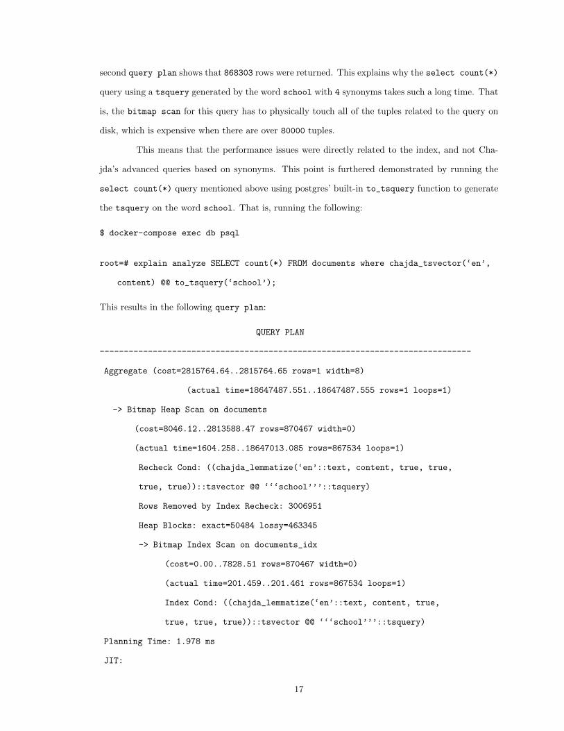
second query plan shows that 868303 rows were returned. This explains why the select count(*)

query using a tsquery generated by the word school with 4 synonyms takes such a long time. That

is, the bitmap scan for this query has to physically touch all of the tuples related to the query on

disk, which is expensive when there are over 80000 tuples.

This means that the performance issues were directly related to the index, and not Cha-

jda’s advanced queries based on synonyms. This point is furthered demonstrated by running the

select count(*) query mentioned above using postgres’ built-in to_tsquery function to generate

the tsquery on the word school. That is, running the following:

$ docker-compose exec db psql

root=# explain analyze SELECT count(*) FROM documents where chajda_tsvector(‘en’,

content) @@ to_tsquery(‘school’);

This results in the following query plan:

QUERY PLAN

-----------------------------------------------------------------------------




(cost=8046.12..2813588.47 rows=870467 width=0)


Recheck Cond: ((chajda_lemmatize(‘en’::text, content, true, true,

true, true))::tsvector @@ ‘‘‘school’’’::tsquery)

Rows Removed by Index Recheck: 3006951

Heap Blocks: exact=50484 lossy=463345


(cost=0.00..7828.51 rows=870467 width=0)


Index Cond: ((chajda_lemmatize(‘en’::text, content, true,

true, true, true))::tsvector @@ ‘‘‘school’’’::tsquery)


JIT:

17

Functions: 5





(13 rows)

We see that even when using the built-in to_tsquery function in postgres to generate the tsquery

for the word school, the execution time of the query is still tremendously slow at 18647538.022 ms

because of the number of rows being returned.

The difficulty revealed by the performance tests is that some words that were included

in the tests, e.g. school, returned far too many rows from the documents table to execute the

select count(*) query in a reasonable amount of time. A solution to this roadblock is to only

select words for benchmark testing that do not appear in hundreds of thousands of Wikipedia articles.

18

6 Appendices

6.1 Appendix A: Python Code for augments fasttext function

import os

import json

import fasttext

import fasttext.util

from annoy import AnnoyIndex

from collections import namedtuple

from chajda.tsvector import lemmatize, Config

from chajda.tsquery.__init__ import to_tsquery

################################################################################

# fasttext

################################################################################

# path used for storing/loading fasttext models and annoy indices

fasttext_annoy_data_path = os.path.dirname(__file__)

# dictionary whose key is a language and value is a fasttext model

fasttext_models = {}

def load_fasttext(lang):

‘‘‘

Downloads and loads a fasttext model for a particular language,

storing the fasttext model object in the fasttext_models dictionary.

Due to the size of fasttext models (>1gb), and the loading time,

we do not load all models on program startup.

Instead, this function is used to load them lazily as needed.

lang: language passed from augments_fasttext

NOTE:

The doctest below has been commented out due to requiring more memory

than github actions allows for.

# >>> load_fasttext(‘wa’) or fasttext_models[‘wa’] != None

# True

’’’

# suppress_stdout_stderr() is used for redirecting stdout and stderr

# when downloading and loading fasttext models.

# Without this, stdout and stderr from fasttext causes doctests to fail.

with suppress_stdout_stderr():

# fasttext downloads models to the current directory,

# but we want to store the model in chaja/tsquery/fasttext,

# so we change the working directory before downloading

working_dir = os.getcwd()

os.makedirs(f"{fasttext_annoy_data_path}/fasttext", exist_ok=True)

os.chdir(f"{fasttext_annoy_data_path}/fasttext")

# download and load fasttext model

19

fasttext.util.download_model(lang, if_exists=‘ignore’)

fasttext_models[lang] = fasttext.load_model(f"cc.{lang}.300.bin")

# fasttext downloads cc.{lang}.300.bin.gz and then decompresses the

# .gz file into cc.{lang}.300.bin.

# However, we only need cc.{lang}.300.bin,

# so we remove unneeded .gz file if exists

if os.path.isfile(f"{fasttext_annoy_data_path}/fasttext/cc.{lang}.300.bin.gz"):

os.remove(f"{fasttext_annoy_data_path}/fasttext/cc.{lang}.300.bin.gz")

# change working directory back

os.chdir(working_dir)

# Executing fasttext’s get_nearest_neighbor as well as accessing the words

# in the fasttext model both run significantly faster after they have been

# called once,

# so we call them once upon loading the model to ensure most efficient runtime

# for subsequent uses.

fasttext_models[lang].get_nearest_neighbors(‘google’, k=5)

fasttext_list = []

for word in fasttext_models[lang].get_words(on_unicode_error=‘replace’):

fasttext_list.append(word)

def destroy_fasttext(lang):

‘‘‘

removes fasttext model from disk and memory

’’’

# remove fasttext download from disk

if os.path.isfile(f"{fasttext_annoy_data_path}/fasttext/cc.{lang}.300.bin"):

os.remove(f"{fasttext_annoy_data_path}/fasttext/cc.{lang}.300.bin")

# remove fasttext model from memory

try:

del fasttext_models[lang]

except KeyError:

pass

################################################################################

# annoy

################################################################################

# stores all information needed for accessing the annoy index of a particular

# language

annoy_info = namedtuple(‘annoy_info’, [‘index’,‘pos_for_word’,‘word_at_pos’])

# dictionary with keys of language and values of annoy_info

annoy_indices = {}

# dictionaries for storing fasttext model words, and their corresponding indices;

# fasttext_pos_for_word stores fasttext words as keys, and corresponding indices

# as values;

20

# fasttext_word_at_pos stores fasttext word indices as keys, and corresponding

# words as values;

# both dictionaries are populated by the load_annoy_index function,

# and subsequently written to json files

# NOTE:

# these dictionaries are necessary for using annoy for nearest neighbor query

# after removing fasttext download

fasttext_pos_for_word = {}

fasttext_word_at_pos = {}

def load_annoy(lang, word=‘google’, n=5, seed=22, run_destroy_fasttext = True):

‘‘‘

Checks whether an annoy index has already been created for a specified language.

Populates an annoy index with vectors from the fasttext model that corresponds

to that language, builds the index, saves it to disk.

The annoy index is stored in the annoy dictionary.

lang: language passed from augments_fasttext

NOTE:

The doctest below has been commented out due to requiring more memory

than github actions allows for.

# >>> load_annoy(‘wa’) or annoy_indices[‘wa’] != None

# True

’’’

# create annoy index if not already created

try:

annoy_indices[lang]

except KeyError:

# download fasttext model if not already downloaded

try:

fasttext_models[lang]

except KeyError:

load_fasttext(lang)

# create annoy directory if needed

os.makedirs(f"{fasttext_annoy_data_path}/annoy", exist_ok=True)

index = AnnoyIndex(300, ‘angular’)

# populate fasttext_pos_for_word and fasttext_word_at_pos with words from

# fasttext model dictionary, as well as indices for each word

i=0

for word in fasttext_models[lang].get_words(on_unicode_error=‘replace’):

fasttext_pos_for_word[word] = i

fasttext_word_at_pos[i] = word

i += 1

# write fasttext_pos_for_word to json file

with open(

f"{fasttext_annoy_data_path}/annoy/fasttext_pos_for_word_{lang}_lookup.json",

"w") as outfile:

json.dump(fasttext_pos_for_word, outfile)

# write fasttext_word_at_pos to json file

21

with open(

f"{fasttext_annoy_data_path}/annoy/fasttext_word_at_pos_{lang}_lookup.json",

"w") as outfile:

json.dump(fasttext_word_at_pos, outfile)

json_pos_for_word = open(

f"{fasttext_annoy_data_path}/annoy/fasttext_pos_for_word_{lang}_lookup.json",

"r")

pos_for_word = json.load(json_pos_for_word)

json_word_at_pos = open(

f"{fasttext_annoy_data_path}/annoy/fasttext_word_at_pos_{lang}_lookup.json",

"r")

word_at_pos = json.load(json_word_at_pos)

annoy_indices[lang] = annoy_info(index, pos_for_word, word_at_pos)

# if annoy index has not been saved for this language yet,

# populate annoy index with vectors from corresponding fasttext model

try:

annoy_indices[lang].index

.load(f"{fasttext_annoy_data_path}/annoy/{lang}{seed}.ann")

# OSError occurs if index is not already saved to disk

except OSError:


try:


except KeyError:

load_fasttext(lang)

# The annoy library uses a random number genertor when building up

# the trees for an Annoy Index.

# In order to ensure that the output is deterministic, we specify the seed

# value for the random number generator.

annoy_indices[lang].index.set_seed(seed)

# Populate annoy index with vectors from corresponding fasttext model

i = 0

for j in fasttext_models[lang].get_words(on_unicode_error=‘replace’):

v = fasttext_models[lang][j]

annoy_indices[lang].index.add_item(i,v)

i += 1

# build the trees for the index

annoy_indices[lang].index.build(10)

# save the index to annoy directory

annoy_indices[lang].index

.save(f"{fasttext_annoy_data_path}/annoy/{lang}{seed}.ann")

# remove fasttext model from disk and memory

if run_destroy_fasttext:

22

destroy_fasttext(lang)

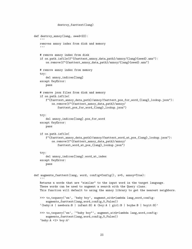
def destroy_annoy(lang, seed=22):

‘‘‘

removes annoy index from disk and memory

’’’

# remove annoy index from disk

if os.path.isfile(f"{fasttext_annoy_data_path}/annoy/{lang}{seed}.ann"):

os.remove(f"{fasttext_annoy_data_path}/annoy/{lang}{seed}.ann")

# remove annoy index from memory

try:

del annoy_indices[lang]

except KeyError:

pass

# remove json files from disk and memory

if os.path.isfile(

f"{fasttext_annoy_data_path}/annoy/fasttext_pos_for_word_{lang}_lookup.json"):

os.remove(f"{fasttext_annoy_data_path}/annoy/

fasttext_pos_for_word_{lang}_lookup.json")

try:

del annoy_indices[lang].pos_for_word

except KeyError:

pass

if os.path.isfile(

f"{fasttext_annoy_data_path}/annoy/fasttext_word_at_pos_{lang}_lookup.json"):

os.remove(f"{fasttext_annoy_data_path}/annoy/

fasttext_word_at_pos_{lang}_lookup.json")

try:

del annoy_indices[lang].word_at_index

except KeyError:

pass

def augments_fasttext(lang, word, config=Config(), n=5, annoy=True):

‘‘‘

Returns n words that are "similar" to the input word in the target language.

These words can be used to augment a search with the Query class.

This function will default to using the annoy library to get the nearest neighbors.

>>> to_tsquery(‘en’, ‘baby boy’, augment_with=lambda lang,word,config:

augments_fasttext(lang,word,config,5,False))

‘(baby:A | newborn:B | infant:B) & (boy:A | girl:B | boyhe:B | boyit:B)’

>>> to_tsquery(‘en’, ‘"baby boy"’, augment_with=lambda lang,word,config:

augments_fasttext(lang,word,config,5,False))

‘baby:A <1> boy:A’

23

>>> to_tsquery(‘en’, ‘"baby boy" (school | home) !weapon’, augment_with=

lambda lang,word,config: augments_fasttext(lang,word,config,5,False))

‘(baby:A <1> boy:A) & ((school:A | schoo:B | schoolthe:B | schoool:B |

kindergarten:B) | (home:A | house:B | homethe:B | homewhen:B |

homethis:B)) & !(weapon:A | weaponthe:B | weopon:B)’

>>> augments_fasttext(‘en’,‘weapon’, n=5, annoy=False)

[‘weaponthe’, ‘weopon’]

>>> augments_fasttext(‘en’,‘king’, n=5, annoy=False)

[‘queen’, ‘kingthe’]

NOTE:

Populating an AnnoyIndex with vectors from a major language fasttext model,

e.g. English, requires more memory than github actions allows for.

Therefore, the doctests involving the annoy library have been commented out below.

# >>> augments_fasttext(‘en’,‘weapon’, n=5)

# [‘nonweapon’, ‘loadout’, ‘dualwield’, ‘autogun’]

# >>> augments_fasttext(‘en’,‘king’, n=5)

# [‘kingthe’, ‘kingly’]

NOTE:

Due to the size of fasttext models (>1gb),

testing multiple languages in the doctest requires more space than github actions

allows for.

For this reason, tests involving languages other than English have been

commented out below.

# >>> augments_fasttext(‘es’,‘escuela’, n=5)

# [‘escuelala’, ‘academia’, ‘universidad’, ‘laescuela’]

’’’

# augments_fasttext defaults to using the annoy library to find nearest neighbors,

# if annoy==False is passed into the function, then the fasttext library will be used.

if annoy:

# populate and load AnnoyIndex with vectors from fasttext model if not

# already populated

load_annoy(lang)

# find the most similar words using annoy library

n_nearest_neighbor_indices =

annoy_indices[lang].index.get_nns_by_item(

annoy_indices[lang].pos_for_word[word], n)

n_nearest_neighbors =

[ annoy_indices[lang].word_at_pos[str(i)] for i in n_nearest_neighbor_indices ]

words = ‘ ’.join([ word for word in n_nearest_neighbors ])

else:


try:

24


except KeyError:

load_fasttext(lang)

# find the most similar words using fasttext library

topn = fasttext_models[lang].get_nearest_neighbors(word, k=n)

words = ‘ ’.join([ word for (rank, word) in topn ])

# lemmatize the results so that they’ll be in the search document’s vocabulary

words = lemmatize(lang, words, add_positions=False, config=config).split()

words = list(filter(lambda w: len(w)>1 and w != word, words))[:n]

return words

# The following imports as well as suppress_stdout_stderr() are taken from stackoverflow:

# stackoverflow.com/questions/11130156/suppress-stdout-stderr-print-from-python-functions

# In this project, suppress_stdout_stderr() is used for redirecting stdout

# and stderr when downloading gensim and fasttext models.

# Without this, the doctests fail due to stdout and stderr from fasttext model downloads.

from contextlib import contextmanager,redirect_stderr,redirect_stdout

from os import devnull

@contextmanager

def suppress_stdout_stderr():

"""Context manager that redirects stdout and stderr to devnull"""

with open(devnull, ‘w’) as fnull:

with redirect_stderr(fnull) as err, redirect_stdout(fnull) as out:

yield (err, out)

6.2 Appendix B: Python Script that runs Benchmark Testing

#!/usr/bin/python3

import psycopg2

from psycopg2 import Error

import os

import pytest

from chajda.tsvector import lemmatize

from chajda.tsquery.__init__ import to_tsquery

from chajda.tsquery.augments import load_fasttext, destroy_fasttext, load_annoy,

destroy_annoy, augments_fasttext

#######################################

# GLOBAL VARIABLE(s)

#######################################

# n values to be parametrized

nval = [2, 4, 8, 16, 32]

#######################################

# HELPER FUNCTIONS

25

#######################################

def execute_query_nval(cursor, tsq, lang):

cursor.execute(f"SELECT count(*) FROM documents WHERE chajda_tsvector(

‘{lang}’, content) @@ CAST(‘{tsq}’ AS tsquery);")

return cursor.fetchone()

def execute_query_nval_tsvector_preloaded(cursor, tsq):

cursor.execute(f"SELECT count(*) FROM documents WHERE tsvector_col

@@ CAST(‘{tsq}’ AS tsquery);")

return cursor.fetchone()

#######################################

# PYTEST FIXTURES

#######################################

@pytest.fixture(scope=‘module’, params=nval)

def req_param(request):

return request.param

@pytest.fixture(scope=‘module’)

def setup_teardown(req_param, pytestconfig):

param = req_param

lang = pytestconfig.getoption("lang")

# setup: preloading fasttext model before all tests

if param == nval[0]:

print(‘running setup’)

load_fasttext(lang)

# connect to db

connection = psycopg2.connect(database="root", user="root", password="pass")

cursor = connection.cursor()

test_info = {‘cursor’:cursor, ‘lang’:lang, ‘param’:param}

# running test

yield test_info

# teardown after all tests are completed

if param == nval[-1]:

print(‘running teardown’)

destroy_fasttext(lang)

#######################################

# TESTS

#######################################

def test_query_nval_fasttext(setup_teardown, benchmark, queryword):

tsq = to_tsquery(setup_teardown[‘lang’], queryword, augment_with=lambda

lang,word,config: augments_fasttext(lang,word,config,setup_teardown[‘param’],

False),weight=False)

benchmark(execute_query_nval, setup_teardown[‘cursor’], tsq, setup_teardown[‘lang’])

26

def test_query_nval_tsvector_preloaded_fasttext(setup_teardown, benchmark, queryword):



False),weight=False)

benchmark(execute_query_nval_tsvector_preloaded, setup_teardown[‘cursor’], tsq)

def test_query_nval_annoy(setup_teardown, benchmark, queryword):



True),weight=False)

benchmark(execute_query_nval, setup_teardown[‘cursor’], tsq, setup_teardown[‘lang’])

def test_query_nval_tsvector_preloaded_annoy(setup_teardown, benchmark, queryword):



True),weight=False)

benchmark(execute_query_nval_tsvector_preloaded, setup_teardown[‘cursor’], tsq)

6.3 Appendix C: Bash Script that Loads Data into Postgres and Runsthe Testing Script shown in Appendix B

#!/bin/bash

if [ $# -eq 0 ];

then

lang="en"

else

lang=$1

fi

echo ‘lang = ’ $lang

# check if json file exists for wiki data dump

if [ -f "/data/Sogou-QCL/wiki/json/wiki_${lang}" ];

then

echo "file exists"

else

echo "file does not exist"

echo "running wget"

# download wiki data dump

wget "http://download.wikimedia.org/${lang}wiki/latest

/${lang}wiki-latest-pages-articles.xml.bz2" -P "/data/Sogou-QCL/wiki/"

# use wikiextractor to clean the wiki data dump

python3 -m wikiextractor.WikiExtractor -o "/data/Sogou-QCL/wiki/extracted_${lang}"

--json "/data/Sogou-QCL/wiki/${lang}wiki-latest-pages-articles.xml.bz2"

# concatenate all json files returned by wikiextractor into one file

cat --squeeze-blank /data/Sogou-QCL/wiki/extracted_${lang}/*/* >

/data/Sogou-QCL/wiki/json/wiki_${lang}

27

fi

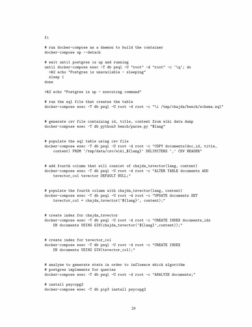
# run docker-compose as a daemon to build the container

docker-compose up --detach

# wait until postgres is up and running

until docker-compose exec -T db psql -U "root" -d "root" -c ‘\q’; do

>&2 echo "Postgres is unavailable - sleeping"

sleep 1

done

>&2 echo "Postgres is up - executing command"

# run the sql file that creates the table

docker-compose exec -T db psql -U root -d root -c "\i /tmp/chajda/bench/schema.sql"

# generate csv file containing id, title, content from wiki data dump

docker-compose exec -T db python3 bench/parse.py "$lang"

# populate the sql table using csv file

docker-compose exec -T db psql -U root -d root -c "COPY documents(doc_id, title,

content) FROM ‘/tmp/data/csv/wiki_${lang}’ DELIMITERS ‘,’ CSV HEADER"

# add fourth column that will consist of chajda_tsvector(lang, content)

docker-compose exec -T db psql -U root -d root -c "ALTER TABLE documents ADD

tsvector_col tsvector DEFAULT NULL;"

# populate the fourth column with chajda_tsvector(lang, content)

docker-compose exec -T db psql -U root -d root -c "UPDATE documents SET

tsvector_col = chajda_tsvector(‘${lang}’, content);"

# create index for chajda_tsvector

docker-compose exec -T db psql -U root -d root -c "CREATE INDEX documents_idx

ON documents USING GIN(chajda_tsvector(‘${lang}’,content));"

# create index for tsvector_col

docker-compose exec -T db psql -U root -d root -c "CREATE INDEX

ON documents USING GIN(tsvector_col);"

# analyze to generate stats in order to influence which algorithm

# postgres implements for queries

docker-compose exec -T db psql -U root -d root -c "ANALYZE documents;"

# install psycopg2

docker-compose exec -T db pip3 install psycopg2

28

# install pytest-postgresql

docker-compose exec -T db pip3 install pytest-postgresql

# run pytest benchmarks

docker-compose exec -T db python3 -m pytest bench/python_script2.py

--benchmark-json=benchmark_results/${lang}.json --lang ${lang} -s

docker-compose down

29

References

[1] Facebook. Fasttext. https://github.com/facebookresearch/fastText, 2018.

[2] Mike Izbicki. Chajda: multilingual full text search in postgres. https://github.com/

mikeizbicki/chajda/tree/notes, Dec 2021.

[3] Erop Porob. Indexes in postgresql — 7 (gin). https://habr.com/en/company/postgrespro/

blog/448746/, Apr 2019.

[4] Spotify. Annoy. https://github.com/spotify/annoy, 2021.

30

Advanced Full-Text Search Based on Synonyms in Postgres

Documents

Transcript of Advanced Full-Text Search Based on Synonyms in Postgres