For the full text of this licence, please go to

Loughborough UniversityInstitutional Repository

Influence of anti-dive andanti-squat geometry incombined vehicle bounce

and pitch dynamics

This item was submitted to Loughborough University’s Institutional Repositoryby the/an author.

Citation: AZMAN, M. ... et al., 2004. Influence of anti-dive and anti-squatgeometry in combined vehicle bounce and pitch dynamics. Proceedings of theInstitution of Mechanical Engineers, Part K: Journal of Multi-body Dynamics,218 (4), pp. 231-242

Additional Information:

• This article was published in the Journal, Proceedings of the Institutionof Mechanical Engineers, Part K: Journal of Multi-body Dynamics [ c©IMECHE]. The definitive version is available at: http://www.pepublishing.com/

Metadata Record: https://dspace.lboro.ac.uk/2134/4829

Version: Published

Publisher: Professional Engineering Publishing / c© IMECHE

Please cite the published version.

https://dspace.lboro.ac.uk/2134/4829

This item was submitted to Loughborough’s Institutional Repository (https://dspace.lboro.ac.uk/) by the author and is made available under the

following Creative Commons Licence conditions.

For the full text of this licence, please go to: http://creativecommons.org/licenses/by-nc-nd/2.5/

Influence of anti-dive and anti-squat geometry incombined vehicle bounce and pitch dynamics

M Azman1, H Rahnejat1�, P D King1 and T J Gordon2

1Wolfson School of Mechanical and Manufacturing Engineering, Loughborough University, Loughborough, UK2Transportation Research Institute, University of Michigan, Ann Arbor, Michigan, USA

Abstract: The paper presents a six-degree-of-freedom (6-DOF) multi-body vehicle model, including

realistic representation of suspension kinematics. The suspension system comprises anti-squat and anti-

dive element. The vehicle model is employed to study the effect of these features upon combined bounce

and pitch plane dynamics of the vehicle, when subjected to bump riding events. The investigations are con-

cerned with a real vehicle and the numerical predictions show reasonable agreement with measurements

obtained on an instrumented vehicle under the same manoeurves.

Keywords: vehicle dynamics, principle of virtual work, multi-body dynamics, anti-squat and anti-dive

characteristics

NOTATION

A1. . .4 matrices M2. . .5 multiplied by the inverse

of M1 respectively

B1,2,3 matrices M6, M7 and M8 multiplied by

the inverse of M1

e2 y axis base vector for the tyre coordinate

system

e3 unit vector (upward) normal to the road

surface at S

Fa actual tyre forces

Fx1,. . ., Fx4 longitudinal tyre forces

Fy1,. . ., Fy4 lateral tyre forces

Fz1,. . ., Fz4 vertical tyre forces

Ftmax nominal maximum ‘rim contact’ tyre force

Faero aerodynamic force

Ftyres tyre forces

Fweight vehicle weight

g gravity

G vehicle centre of gravity

Ixx,yy,zz roll, pitch and yaw moment of inertia

about the mass centre

Ixz product of inertia

IG inertia matrix of vehicle

I3 n � n identity matrix

kaero aerodynamic drag coefficient

k unit vector of the global z direction,

relative to the vehicle coordinates

KI, KP integral and proportional gains

M vehicle mass

Mtyres moment about G from the tyre forces

M1 generalized mass matrix

M2, M3, M4 matrix coefficients arising from the

bilinear gyroscopic terms

M5 matrix coefficient from aerodynamic drag

M6 matrix consisting of the sum of all the

applied forces and body dimensions and

giving the main contributions from the

tyre force inputs

M7 matrix containing the moment effect of

dynamic suspension deflections zM8 matrix containing the gravity term

nB unit vector in body z

nS unit vector (upward) normal to the road

surface at S

p, q, r angular velocity in the x, y and z axis

respectively

P nominal contact patch centre

Q new position of P obtained by translating

Q in the body z axes

rA(zsus) kinematics term accounting for the

steering torque

rG distance of the contact patches from the

centre of gravity

The MS was received on 2 February 2004 and was accepted after revisionfor publication on 6 September 2004.�Corresponding author: Wolfson School of Mechanical and ManufacturingEngineering, University of Loughborough, Loughborough, LeicestershireLE11 3TU, UK.

231

K00104 # IMechE 2004 Proc. Instn Mech. Engrs Vol. 218 Part K: J. Multi-body Dynamics

rp position of the nominal contact patch

centre in the global coordinates

rp{B} position of the nominal contact patch

centre in the vehicle body coordinates

based at G

rS position of the nominal contact patch on

the road surface

R actual vehicle orientation

R1,2,3 orientation matrix in the roll, pitch and

yaw axes

R fB!Gg passive rotation matrix that converts from

body to global coordinates, using Euler

angles

S, Sref actual and desired speed

Td drive torque (assumed to be generated

from an inboard differential)

U, V longitudinal and lateral velocity

v unit vector normal to the wheel plane

vG three components of translational

velocity

vQ velocity of point Q moving within the

plane (road surface)

x, x state and state derivative variables

xP, yP position of point P from the centre of

gravity in the x–y plane

x4 set of x coordinates at the four tyre

contact patches

y1 acceleration/brake command

y2 steering angle

zs suspension deflection

zt tyre deflection

ztmax loss of tyre contact, where Ft! 0

ztmin maximum tyre compression

z4 set of z coordinates at the four tyre

contact patches from the centre of gravity

~zz suspension deflections

b vehicle direction (yaw angle)

g lateral inclination angle

dx,dy contact patch forward progression and

lateral scrub respectively

dz suspension vertical changes

dv change in the caster angle

d static toe angle

dk(zsus) kinematics term accounting for bump-steer

11 deviation of actual speed from desired

speed

12 directional error between where the

car is pointing and where it should be

going

uv angle of the reference vector of the

vehicle in global coordinates

u1, u2, u3 roll angle, pitch angle and yaw angle

respectively

u1, u2, u3 derivative of roll angle, pitch angle and

yaw angle respectively

l sum of the suspension and tyre

deflections

m expansion velocity of the suspension–

tyre combination

n r caster and camber angle

r(zsus) kinematics term accounting for bump-

camber

f actual steer angle

w, u, c roll angle, pitch angle and yaw angle

respectively

v1, v2, v3 body angular velocity, roll, pitch and yaw

axis respectively

v three components of angular velocity

1 INTRODUCTION

During the last decade, improvements in computer capabili-

ties and commercial multi-body simulation software have

led to a tendency to develop detailed modelling of vehicle

systems. Such software is based on physical representations,

usually requiring large quantities of input data [1, 2]. These

are not always readily available to all engineering analysts.

Even when the full set of input parameters is available, the

simulation studies run considerably slower than the custo-

mized programs, which are less complex but adequate for

the purpose of investigation. The complexity of large

models can sometimes reduce the reliability of simulation,

especially when the model is constructed during the hectic

process of development and design [2]. Such circumstances

often result in simulation projects that can only confirm the

design and measurement but seldom contribute to a better

design before various test vehicles are built. As reported

in references [2] and [3], various problems concerning the

dynamics of a vehicle can be reliably solved with compara-

tively simple models of the real system. However, simple

models have their limits and are only suitable for certain

types of test. The work carried out in this paper is the initial

work to establish the limits of validity of a functional vehicle

model that is capable of evaluating handling analysis as well

as ride comfort, such as bump riding events. These simpler

multi-body models are regarded as intermediate [4].

The model reported here is used to investigate the effect

of anti-squat and anti-dive geometry in response to road pro-

file inputs. As Sharp [5] has already pointed out, transient

dynamics of vehicles is a non-trivial problem, even for a

standard road car, and a simple manoeuvre such as acceler-

ating or braking on a flat road, the so-called standard analy-

sis, therefore, is severely limited in its applicability. This

paper consisders a real-world scenario including both tran-

sient torque inputs and vertical road surface geometry.

One question addressed is the adequacy of a simplified

system model in predicting these effects. A second ques-

tion is the effectiveness of anti-squat and anti-dive geo-

metry on the pitch plane dynamics under such complex

real-world conditions. The model reported here has a

232 M AZMAN, H RAHNEJAT, P D KING AND T J GORDON

Proc. Instn Mech. Engrs Vol. 218 Part K: J. Multi-body Dynamics K00104 # IMechE 2004

six-degree-of-freedom (6-DOF) vehicle body with realistic

suspension kinematics and a non-linear load-dependent

tyre model. The results of the analysis for a given test are

compared with the measured performance data from the

actual vehicle.

2 DESCRIPTION OF AN INTERMEDIATEVEHICLE MODEL

The model can be divided into five main modules: rigid

body dynamics, vehicle kinematics, suspension and steering,

driveline and tyres and a driver model.

2.1 Rigid body dynamics

This module uses a body-centred coordinate system. The

inputs are the 12 tyre force components

Ftyres ¼ ½Fx1, . . . , Fx4, Fy1, . . . , Fy4, Fz1, . . . , Fz4�T

These are applied directly to the vehicle body. This is

justified because the unsprung mass is neglected and the

resultant forces and moments on the unsprung mass equili-

brate. Therefore, the forces and moments are directly ‘trans-

mitted’ to the vehicle body structure. The state variables are

the mass centre translational and rigid body angular velo-

cities using the body-fixed SAE (Society of Automotive

Engineers) frame of reference

x ¼ ½U,V ,W , p, q, r�T

Other inputs include the aerodynamic force (applied at the

centre of gravity of the sprung mass)

Faero ¼ �kaerovGvG (1)

(where vG ¼ [U, V, W]T) and the vehicle weight Fweight ¼

Mgk, where k is the unit vector of the global z direction

relative to the vehicle coordinates. Equations of motion

are based on the standard Newton–Euler form

M(_vvrelG þ v� vG) ¼ Faero þ SFtyres þ Fweight (2)

I G vrel þ v� (IGv) ¼ SMtyres (3)

Therefore, the intermediate model has six degrees of

freedom. They include vehicle translation along the x and

y directions, bounce the z direction and roll, pitch and yaw

about these axes respectively. The analysis carried out in

this paper is for straight-line motions involving the degrees

of freedom x, z and pitch motion. The model is, however,

generic and can be used for other manoeuvres such as com-

bined cornering and braking, and single-event bump riding;

involving appreciable vehicle roll.

The inertial matrix assumes lateral symmetry in the

vehicle model

IG ¼

Ixx 0 �1xz

0 Iyy 0

�Ixz 0 Izz

0@

1A

The equations of motion can be rewritten in terms of the

state variables in the following form

M1 _xx ¼ ( pM2 þ qM3 þ rM4 þM5jvGj)xþM6Ftyres

þM7~zz� Fxy þM8Fweight (4)

where, for example

M1 ¼MI3 03�3

03�3 IG

� �(5)

and M1 is a generalized mass matrix. Here, 0n�m is an n � m

matrix of zeros, ln�m similarly denotes a matrix of unity

values and I3 is an n � n identity matrix; M2, M3 and M4

contain coefficients arising from the bilinear gyroscopic

terms (those obtained from products of the form v � � � �

terms in the above equations of motion), with M2 picking

up all the terms in p, M3 picking up all the remaining

terms in q and M4 providing the remaining r terms (see

the Notation for full details); M5 relates to the aerodynamic

drag (and has zeros in rows 4 to 6, since no aerodynamic

moments are included) and M6 consists of ones (to sum

all the applied forces) and body dimensions (to evaluate

moments) and gives the main contributions from the tyre

force inputs

M6 ¼

14�1 04�1 04�1

04�1 14�1 14�1

04�1 04�1 14�1

04�1 �z4 y4

z4 04�1 �x4

�y4 x4 04�1

0BBBBBB@

1CCCCCCA

(6)

where x4 ¼ [a a 2b 2b] is the set of x coordinates at the

four tyre contact patches (see Fig. 1). The z coordinates

are all equal to the mass centre height of the vehicle in its

Fig. 1 A schematic representation of the intermediate vehicle

model

INFLUENCE OF ANTI-DIVE AND ANTI-SQUAT GEOMETRY IN COMBINED VEHICLE BOUNCE AND PITCH DYNAMICS 233


trim condition, z4 ¼ [hG hG hG hG], except for the moment

effect of dynamic suspension deflections z, which are

picked up by the M7 terms

M7 ¼

03�4 03�4

01�4 �11�4

11�4 01�4

01�4 01�4

0BB@

1CCA (7)

Also note that

~zz� Fxy ;½~zz1Fx1, ~zz2Fx2, ~zz3Fx3, ~zz4Fx4, ~zz1Fy1, ~zz2Fy2,

~zz3Fy3, ~zz4Fy4�T (8)

Finally, the gravity term is included by

M8 ¼I3

03�3

� �(9)

To evaluate state variable derivatives, the matrices on the

right-hand side of equation (4) are multiplied by M121 to

give the form

_xx ¼( pA1 þ qA2 þ rA3 þ A4jvGj)xþ B1FT

þ B2~zz� Fxy þ B3Fweight (10)

where A1 ¼M121 M2, etc.

2.2 Vehicle kinematics

The main purpose is to turn the local (i.e. the vehicle-based)

angular velocities into Euler angle derivatives and then inte-

grate these to find roll, pitch and yaw angles. Following the

equations given in references [6] and [7], the Euler angles

are u1 ¼ w, u2 ¼ u and u3 ¼ c (roll, pitch and yaw respect-

ively) and applied in the sequential order yaw, pitch and

roll in a body-fixed frame of reference to give the (active)

transformation matrix from reference to actual vehicle

orientation as

R ¼ R3(u3)R2(u2)R1(u1) (11)

Note that the order is reversed here since each matrix is

relative to the local body axes. Thus

R1(u1) ¼

1 0 0

0 cos u1 � sin u1

0 sin u1 cos u1

0B@

1CA,

R2(u2) ¼

cos u2 0 sin u2

0 1 0

� sin u2 0 cos u2

0B@

1CA,

R3(u3) ¼

cos u3 � sin u3 0

sin u3 cos u3 0

0 0 1

0B@

1CA

R is also the passive transformation from the body to the

global coordinates. Therefore, the Euler angle derivatives

are found as [6, 7]

_uu1 ¼ v1 þ (v2 sin u1 þ v3 cos u1) tan u2

_uu2 ¼ v2 cos u1 ¼ v3 sin u1

_uu3 ¼v2 sin u1 þ v3 cos u1

cos u2

(12)

Euler angles are used to rotate the local mass centre velocity

into globals, which are then integrated to find the global

x, y, z coordinates of G (vehicle centre of gravity). Vehicle

accelerations are also found in both local and global coordi-

nates, but only for post-processing purposes.

2.3 Suspension and steering

Nominal suspension deflections and velocities are found

(nominal because bump and rebound stop forces are ignored

in this analysis). This is non-trivial because of the large-

angle formulation highlighted here. There are three stages

(see Fig. 2).

1. Find P, the nominal contact patch centre that translates

and rotates with the vehicle body—based on the static

‘trim’ condition of the body, including static tyre deflec-

tion. Using the mass centre G as a reference point

rP ¼ rG þ R{B!G}r{B}P (13)

where the curly bracket superscripts denote the coordi-

nate system used: rPfBg is the position of the nominal con-

tact patch centre in the vehicle body coordinates, based at

G, and R fB!Gg is the (passive) rotation matrix that con-

verts from the body to the global coordinates using the

Euler angles. In the remainder of this section it is

assumed that similar transformations into globals have

been carried out as necessary.

2. Find Q, the new position of P obtained by translating Q

in body z axes (no account is taken here of the suspension

geometry at this point, to include scrub effects, etc., as

this has a negligible effect on the suspension vertical

travel). This defines the nominal suspension deflection.

Fig. 2 Representation of the point at the centre of the contact

patch



Except where the wheel is out of contact with the road,

the distance between P and Q can be expected to be small

compared with the typical wavelength of the surface. If

the surface is defined by z ¼ f (x, y), an initial approxi-

mation to Q is given by

rS ¼ ½xP, yP, f (xP, yP)�T (14)

The approximation will be poor unless both the vehicle

and the surface are considered to be close to horizontal.

S will be close in distance to the required point, so an

improved approximation can be found by a planar rep-

resentation of the road surface around S.

This is defined by nS, which is the unit (upward)

normal to the road surface at S

(r� rS) � nS ¼ 0 (15)

Since Q is obtained by translating P parallel to the body z

unit vector nB, then

rQ ¼ rP þ lnB (16)

Here, l is the sum of the suspension and tyre deflections

(relative to the static equilibrium position, ignoring the

actions of bump or rebound stops) and may be found

by solving the above two equations to give

l ¼(rS � rP) � nS

nB � nS

(17)

In the model this is calculated in the global coordinates.

Note that the estimation of suspension deflection can

be refined via an iteration process on the choice of

local surface normal, and, by including the suspension

geometry effects, the extra computational load is not

justified.

3. Analyse the velocity of Q to determine the suspension

velocity, and hence the overall velocity vector of the con-

tact patch. As Q moves on the surface, its velocity is

based on the rigid body motion of the vehicle, except

for the addition of suspension velocity

vQ ¼ vG þ v� (rQ � rG)þ mnB (18)

where m is the (expansion) velocity of the suspension–

tyre combination. Since Q is moving within the plane,

vQ. nS ¼ 0 and hence

m ¼nS � (vG þ v� (rQ � rG))

nS � nB

(19)

Tyre vertical compliance is included in the suspen-

sion model. The unsprung mass is considered to be

included in with the vehicle body, so the ‘massless’

wheel constitutes a ‘half degree of freedom’, involving

one state variable: the suspension deflection. In outline

this works as follows: as above, the combined tyre/

suspension displacement and velocities are known. The sus-

pension deflection state, zs, is used to determine the tyre

deflection as zt ¼ l 2 zs, and both ‘spring’ forces acting

on the wheel (see Fig. 3) are known. After taking into

account the geometry of the system and the in-plane

forces, this assumption implies a required damper force,

and (via an inverse damper map) the required suspen-

sion velocity is used to update the suspension deflection

state.

Limits on tyre and suspension travel are implemented as

simple modifications to the above

zmint 4 zt 4 zmax

t , zmins 4 zs 4 zmax

s (20)

Here, ztmin represents the maximum tyre compression and a

nominal maximum ‘rim contact’ tyre force Ftmax is applied.

Alternatively, ztmin represents loss of tyre contact, where

Ft! 0.

When suspension end-stops are exceeded, the damper

force is ‘overridden’ by virtual bump-stops; the calculated

velocity is modified to prevent an excursion beyond the

workspace limits as

_zzS ¼ max {_zzcalcS , _zzsmall

S } if zS , zminS (21)

_zzS ¼ min {_zzcalcS ,�_zzsmall

S } if zS . zmaxS (22)

Now, turning to the suspension geometry effects, such as

anti-dive characteristics and scrub effects, the balance is

obtained via application of the principle of virtual work in

the vehicle body coordinates. Considering the active

forces and moments acting on the wheel/hub assembly

when the body is fixed (see Fig. 4), the virtual work takes

the form

Fxdxþ Fydyþ Fzdzþ Fs(�dz)þ Tddn ¼ 0 (23)

Here, all the forces are acting on the wheel/hub assembly,

and link reaction forces (ball-joints at the body connections)

make no contribution. Force Fz increases with tyre exten-

sion but carries a large negative component owing to the

Fig. 3 Tyre and suspension travel



static load; overall it is negative, tending to zero as the

tyre lifts off the road surface. Similarly, Fs would usually

be negative but increases as the suspension is expanded.

The virtual work equation is based on the body-fixed coor-

dinates and z is the suspension deflection (vertical height

change of the contact patch centre) and is considered as

an independent variable. As the suspension is deflected, dx

and dy (contact patch forward progression and lateral

scrub respectively) follow from mapping the suspension

geometry as

dx ¼dx

dy

� �dz, dy ¼

dy

dz

� �dz (24)

where Fs is the net suspension force, based on the vertical

wheel travel. If the spring or damper is not directly aligned

with the wheel vertical motion (as is typically the case), then

the principle of virtual work can be used again to obtain

Fs(z) for example, if s is the spring deflection and Fs(s) is

the variation in the component of spring with deflection,

then

Fs(z) ¼ ~FFs(s)ds

dz

In the virtual work equation, Td is the drive torque (assumed

to be generated from an inboard differential) and dv is the

change in the caster angle. Brake torques do not contribute,

because they are considered as internal to the wheel–hub

assembly.

The virtual work equation can be written (in the body

coordinates) as

Fxdx þ Fydy þ Fz � Fs þ Tddv ¼ 0 (25)

where dx ¼ dx=dzð Þ etc. Then, defining

d ¼ ½dxdy1�T (26)

the virtual work equation becomes

F � d ¼ Fs � Tddv (27)

This must now be transformed to the ‘tyre’ coordinates in

order to find the unknown road normal force. Leaving

aside the details for now, let R fB ! Tg be the (passive)

rotation matrix that transforms vector components from

the body-fixed axes to the tyre axes. The dot product is

the same in any coordinate system, thus transforming to

tyre coordinates as

F{T} ¼ R{B!T}F{B}, d{T}¼ R{B!T}d{B} (28)

Making use of equation (27) yields

Fs ¼ F{T}x d{T}

x þ F{T}y d{T}

y þ F{T}z d{T}

z þ Tddv ¼ 0 (29)

With FzfTg known from the tyre deflection and Fx

fTg and FyfTg

obtained as output from the tyre model, this determines the

body vertical suspension force, Fs. Subtracting the spring

component (including static load) and inverting the

damper map gives the suspension velocity as required

above.

The transformation from body to tyre coordinates is now

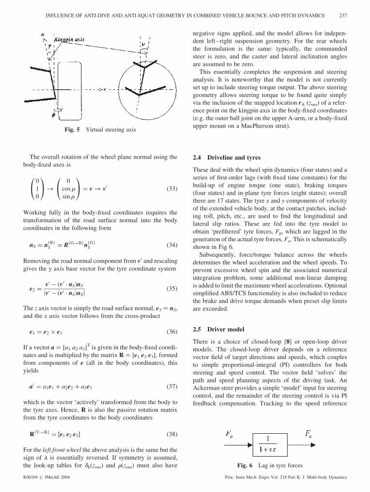
derived. In order to account for steering angle, the steering

axis geometry, toe, camber and caster change. The Euler

angles and road normal are also needed, because the tyre

Z axis is normal to the road. Consider a general rotation

through angle f about an axis defined by a unit vector n.

As an ‘active’ rotation, an arbitrary vector v is rotated and

the coordinates are fixed, so v! v0, with

v0 ¼ (v � n)n(1� cosf)þ v cosfþ (n� v) sinf (30)

Therefore, for steering rotation about the kingpin axis, for

example, for the right front wheel

n ¼cos g sin n

sin g

cos g sin n

0@

1A (31)

This is a unit vector pointing along the kingpin axis

(n ¼ caster angle, g ¼ lateral inclination angle), and

f ¼ dk(zsus)þ d (32)

This is the actual steer angle plus a kinematics term dk(zsus)

which accounts for bump-steer and the static toe angle. In

equation (30), v is a unit vector normal to the wheel

plane, and it is assumed that, starting from the reference

(trim) condition, the suspension is deflected first, inducing

bump-camber and bump-steer (these angles are small, so

the rotation sequence is unimportant and it is convenient

to effect the camber first), then rotated by angle d about

the kingpin axis (see Fig. 5). Note that both caster and lateral

inclination are considered constant in this model but can

easily be mapped as functions of suspension travel if

required.

Fig. 4 Forces and moments for the calculation of virtual work



The overall rotation of the wheel plane normal using the

body-fixed axes is

0

1

0

0@

1A!

0

cos r

sin r

0@

1A ¼ v! v0 (33)

Working fully in the body-fixed coordinates requires the

transformation of the road surface normal into the body

coordinates in the following form

nS ¼ n{B}S ¼ R{G!B}n{G}

S (34)

Removing the road normal component from v0 and rescaling

gives the y axis base vector for the tyre coordinate system

e2 ¼v0 � (v0 � nS)nS

jv0 � (v0 � nS)nSj(35)

The z axis vector is simply the road surface normal, e3 ¼ nS,

and the x axis vector follows from the cross-product

e1 ¼ e2 � e3 (36)

If a vector a ¼ [a1 a2 a3]T is given in the body-fixed coordi-

nates and is multiplied by the matrix R ¼ [e1 e2 e3], formed

from components of e (all in the body coordinates), this

yields

a0 ¼ a1e1 þ a2e2 þ a3e3 (37)

which is the vector ‘actively’ transformed from the body to

the tyre axes. Hence, R is also the passive rotation matrix

from the tyre coordinates to the body coordinates

R{T!B} ¼ ½e1 e2 e3� (38)

For the left front wheel the above analysis is the same but the

sign of l is essentially reversed. If symmetry is assumed,

the look-up tables for dk(zsus) and r(zsus) must also have

negative signs applied, and the model allows for indepen-

dent left–right suspension geometry. For the rear wheels

the formulation is the same: typically, the commanded

steer is zero, and the caster and lateral inclination angles

are assumed to be zero.

This essentially completes the suspension and steering

analysis. It is noteworthy that the model is not currently

set up to include steering torque output. The above steering

geometry allows steering torque to be found quite simply

via the inclusion of the mapped location rA (zsus) of a refer-

ence point on the kingpin axis in the body-fixed coordinates

(e.g. the outer ball joint on the upper A-arm, or a body-fixed

upper mount on a MacPherson strut).

2.4 Driveline and tyres

These deal with the wheel spin dynamics (four states) and a

series of first-order lags (with fixed time constants) for the

build-up of engine torque (one state), braking torques

(four states) and in-plane tyre forces (eight states); overall

there are 17 states. The tyre x and y components of velocity

of the extended vehicle body, at the contact patches, includ-

ing roll, pitch, etc., are used to find the longitudinal and

lateral slip ratios. These are fed into the tyre model to

obtain ‘prefiltered’ tyre forces, Fp, which are lagged in the

generation of the actual tyre forces, Fa. This is schematically

shown in Fig 6.

Subsequently, force/torque balance across the wheels

determines the wheel acceleration and the wheel speeds. To

prevent excessive wheel spin and the associated numerical

integration problem, some additional non-linear damping

is added to limit the maximum wheel accelerations. Optional

simplified ABS/TCS functionality is also included to reduce

the brake and drive torque demands when preset slip limits

are exceeded.

2.5 Driver model

There is a choice of closed-loop [8] or open-loop driver

models. The closed-loop driver depends on a reference

vector field of target directions and speeds, which couples

to simple proportional-integral (PI) controllers for both

steering and speed control. The vector field ‘solves’ the

path and speed planning aspects of the driving task. An

Ackerman steer provides a simple ‘model’ input for steering

control, and the remainder of the steering control is via PI

feedback compensation. Tracking to the speed reference

Fig. 6 Lag in tyre forces

Fig. 5 Virtual steering axis



control is entirely via the PI feedback. In more detail, for

speed control forward velocity is the key parameter as

y1 ¼ �KI1

ð11

|fflfflfflffl{zfflfflfflffl}integral

� KP111|fflffl{zfflffl}proportional

(39)

Deviation 11 ¼ (S� Sref) (40)

where the deviation 11 of the actual speed from its desired

value determines whether the output of the system would

provide acceleration or a braking command. The output of

the system y1 consists of two elements, integral and pro-

portional elements, where the integral gain is KI and the

proportional gain is KP.

The same approach is used for directional control, in

which case a three-element model of velocity is required:

the longitudinal, lateral and yaw components of velocity.

For directional control, uv, which is the angle (in the

global coordinates) of the reference vector field vector, b

is the yaw angle of the car, so 12 represents a directional

error between where the car is pointing and where it

should be heading

Deviation 12 ¼ (b� uv) (41)

Steering angle command y2 ¼ �KI2

ð12

|fflfflfflffl{zfflfflfflffl}integral

� KP212|fflffl{zfflffl}proportional

(42)

The ‘open-loop’ driver is specified by desired steer angle and

vehicle speed time histories, and once again the speed control

is feedback based. However, since the desired speed is pre-

computed, a desired acceleration time history is derived to

provide an approximate input into the vehicle (equivalent

torque demand), which is corrected by the PI feedback.

The entire intermediate model described above was

created in the environment of Matlab/Simulink.

3 EXPERIMENTAL AND SIMULATIONRESULTS

In order to validate the above model it was necessary to

compare it with the actual vehicle data. For this purpose,

five different types of test were conducted. These included:

(a) constant acceleration of 0.2g with an initial speed of

10 km/h;

(b) constant deceleration of 0.5g with an initial speed of

60 km/h;

(c) speed bump analysis—constant speed (10 km/h)

throughout negotiation of the speed bump;

(d) speed bump analysis—constant speed (20 km/h)

throughout traversal of the speed bump;

(e) speed bump analysis—the initial speed of 30 km/h is

given a deceleration of 0.15g before the vehicle nego-

tiates the speed bump.

3.1 Experimental procedure

A standard D class passenger car is used. The tests were

actual road manoeuvres as this is the most representative

of vehicle performance, rather than the usual chassis

dynamometer tests where the full effect of vehicle inertia

under various motions, particularly in combined bounce

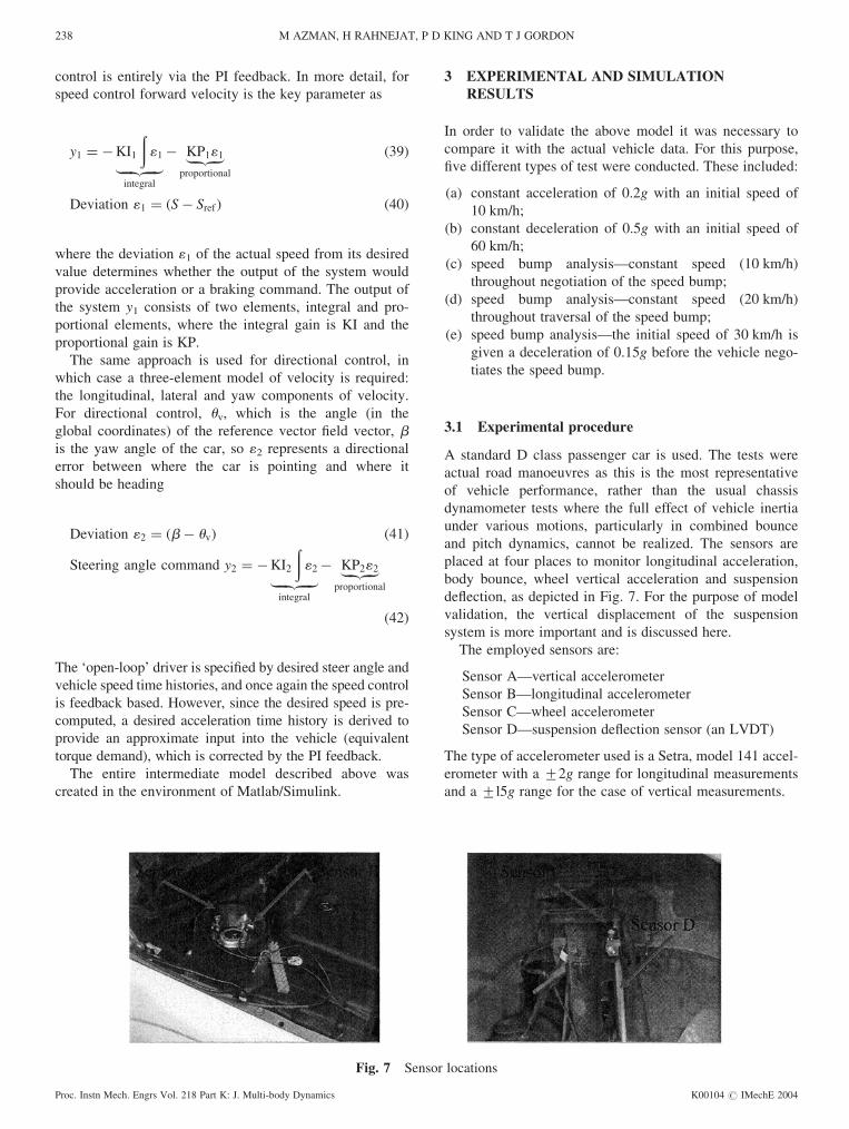
and pitch dynamics, cannot be realized. The sensors are

placed at four places to monitor longitudinal acceleration,

body bounce, wheel vertical acceleration and suspension

deflection, as depicted in Fig. 7. For the purpose of model

validation, the vertical displacement of the suspension

system is more important and is discussed here.

The employed sensors are:

Sensor A—vertical accelerometer

Sensor B—longitudinal accelerometer

Sensor C—wheel accelerometer

Sensor D—suspension deflection sensor (an LVDT)

The type of accelerometer used is a Setra, model 141 accel-

erometer with a +2g range for longitudinal measurements

and a +l5g range for the case of vertical measurements.

Fig. 7 Sensor locations



3.2 Experimental results and theoretical predictions

For the multi-body model, two types of suspension charac-

teristic are considered, one without anti-squat and anti-dive

features and the other with these characteristics provided by

the vehicle manufacturer. The current model uses linear

damping and does not include camber changes, kingpin

inclination and bump-steer effect. These features can be

included in the future developments of the reported model

for better representation of the suspension system. An

open-loop driver model is used.

3.2.1 Test 1: constant acceleration of 0.2g with an

initial speed of 10 km/h

Simulation models cannot exactly replicate the behaviour

of a vehicle in accelerated motion. This is because the rate

of change is driver dependent and in a simulation exercise

is usually considered to be ideally instantaneous. Figure 8

shows this difference. Owing to the step change caused by

the instantaneous application of throttle, the simulation

results tend to exhibit an initial rapid oscillatory behaviour.

Nevertheless, the conformity of model predictions to

experimental findings is remarkably good after this initial

anomaly.

To observe the effectiveness of the anti-squat and anti-

dive features, it is necessary to gauge vehicle performance,

when accelerated from coasting to drive condition (as

shown in Fig. 8), or in hard braking from coasting. The

result for the former case is shown in Fig. 9 for the front sus-

pension in this rear wheel drive vehicle. There are three

curves, one of which depicts the actual road data for suspen-

sion vertical deflection while the other two correspond to

numerical predictions: one for the suspension model with-

out the rear leading anti-squat arms and the other with this

feature included in the model. It can be observed that the

experimental results fall in between the two sets of numeri-

cal predictions. This is because, with the leading arms, the

rear suspension deflects less, and consequently the front sus-

pension carries a greater proportion of the inertial force than

would be expected. When the leading anti-squat arms are

removed, weight transfer to the rear under acceleration

takes place, as expected, and the front suspension vertical

travel is reduced. None of the predicted results totally con-

forms to the experiment. There are two possible reasons.

1. The anti-squat arm is considered without joint compli-

ance which would yield higher stiffness than that actually

existing in the vehicle (therefore less rear squat and

lower weight transfer to there).

2. Suspension deflection occurs in the real situation in both

vertical and horizontal directions, together with the

angular movement of the control arms as the result of

friction torque transfer. The models do not directly

obtain these. The predictions do, however, give fairly

good indications of vehicle dynamics.

3.2.2 Test 2: constant deceleration of 0.5g with an initial

speed of 60 km/h

A case of hard braking typical of an emergency stop was

investigated. In such cases a constant deceleration of 0.5g

may be considered as typical. However, in reality, the

driver does not maintain a constant brake pressure, because

under dive conditions the seating posture alters and conse-

quently there is some gradual loss of pedal brake force.

This can be observed in the experimental trace of Fig. 10

and accounts for the difference in the final portion of decel-

eration in the figure. Elsewhere, very good agreement is

observed between theory and experiment.

When considering vertical front suspension travel under

hard braking conditions (see Fig. 11), an opposite effect toFig. 8 Forward acceleration

Fig. 9 Front suspension deflection



that of Fig. 9 is observed, as would be expected. In this case,

the semi-trailing anti-dive arms resist inertial load transfer

to the front of the vehicle. Therefore, the suspension deflec-

tion is less than that predicted without this feature, which

conforms closer to the actual vehicle data. The discrepancy

is due to the effects of other resisting elements such as sus-

pension arm bushings and joints which are not included in

the simple suspension model described previously. Another

omission in the simulation model is the damping behaviour

of the suspension arm and trailing arm bushing mounts, this

being the reason for the lightly damped oscillatory charac-

teristics of both the numerical traces when compared with

the experimental curve in the same figure. Note, however,

that, owing to the generally underdamped nature of the

bushings, the frequency of oscillation is almost the same

in both cases. The results of the tests give an indication of

vehicle pitch plane dynamics. Another important consider-

ation is the combined effects of vehicle bounce and pitch

motions, increasingly encountered in today’s roads where

traffic calming measures invariably involve the use of

speed bumps. Ride comfort and handling, traditionally

kept apart in analysis work, combine in importance under

such manouevres.

3.2.3 Test 3: speed bump analysis—constant speed

(10 km/h) throughout negotiation of the

speed bump

Thus far the results presented are for accelerated motion

which in an ideal sense corresponds to vehicle pitch plane

dynamics. However, the vehicle body is often subject to

combined pitch, bounce and roll. In a straight-line motion

with both wheels going over a low-height barrier, the

effect of roll is diminished, but the individual contributions

of pitch and bounce cannot be isolated owing to the coupled

nature of the dynamics.

The first combined bounce and pitch dynamics test corre-

sponds to negotiating a speed bump of 4 m length and

110 mm height with a constant velocity of 10 km/h.

Figure 12 shows the monitored experimental data and the

corresponding numerical predictions with and without

anti-squat and anti-dive features. All the traces show

much more complex motions than the previous pitch

plane dynamics cases owing to the combined effect of this

motion with vertical bounce of the vehicle. The time

taken at a constant speed of 10 km/h to traverse the bump

Fig. 10 Forward deceleration


Fig. 12 Front suspension deflection with bounce and pitch

dynamics



is approximately 1.5 s. The front wheels reach the bump at

7 s after the commencement of the simulation or road test,

and finally the rear wheels leave the bump at t ¼ 8.5 s (as

shown in the figure). Following either of the three traces

(and note that both the numerical results almost coincide

with each other), the front suspension travel initially under-

goes an upward deflection (referred to as jounce), followed

by a return travel and rebound (an extended geometry due to

off-loading) as the front axle begins to fall off the bump.

This reaches a maximum float of front suspension (indicated

by the maximum positive deflection at around t ¼ 7.5 s). As

the front wheels fall off the bump, the extended (floating)

suspension begins to return to its equilibrium position,

while the rear wheels climb onto the bump, momentarily

carrying the major inertial load, and hence resulting in the

second less pronounced maximum in the vertical front sus-

pension travel. As the rear wheels reach the summit of the

bump, maximum load transfer to the front occurs, resulting

in maximum deflection (the second minima in any of the

traces in the figure). This is combined with the impact of

the front wheels onto the flat surface of the road. The load

almost instantaneously transfers to the rear thereafter, and,

after a few small oscillations, steady conditions are reached,

with the vehicle being on the flat road.

All the traces follow the same pattern and are reaso-

nably in accord with each other. The horizontal shifts in

time between the theoretical and experimental results are

due to omission of damping and non-linearity effects in

the former case, such as the elastokinetic effects in real sus-

pension systems caused by structural compliance. The lack

of a significant difference between the numerical results

with and without anti-dive and anti-squat characteristics is

due to lack of sufficient time for leading and trailing arms

to influence the vehicle dynamics, and in particular these

features have less effect with prounced vehicle bounce.

This point can be corroborated by further decrease in any

differences in the numerical results with increasing vehicle

speed.

3.2.4 Test 4: speed bump analysis—constant

speed (20 km/h) throughout traversal of the

speed bump

For this purpose the speed of the vehicle was doubled to

20 km/h and kept constant while negotiating the bump.

Monitoring the front suspension vertical travel, shown in

Fig. 13, indicates the same pattern of variation as in the pre-

vious case, with the exception that much greater deflection

and extension behaviour is observed, this being due to

increased inertial force and higher impact forces at the

tyres, transmitted to the suspension elements. The effect

of bounce motion has also become more dominant owing

to these increased vertical forces, as a result of which the

influence of anti-squat and anti-dive features has all but dis-

appeared. This results in almost coincident alternative

numerical predictions and a closer fit with the experimental

results.

3.2.5 Test 5: Speed bump analysis—the initial

speed of 30 km/h is given a deceleration

of 0.15g before the vehicle negotiates

the speed bump

A prior braking action, however, usually accompanies nego-

tiation of a speed bump. This represents a more realistic

scenario, particularly at a higher initial velocity, in this

case at 30 km/h. Figure 14 shows the front suspension beha-

viour under this condition for all three alternatives as in the

previous figures. A deceleration of 0.15g is typical of such a

braking action. It is clear that the results, obtained both from

road test data and through numerical simulations, are a com-

bination of characteristics already observed in Figs 10 and





12 or 13. The initial part of all the traces follows the charac-

teristics in Fig. 10, again indicating that in a real-life situ-

ation the driver does not maintain a constant braking

action (a natural reaction). Thus, the numerical results

correspond to a slightly higher forward speed than the

experimental value and, even given identical suspension

characteristics, would have less of a dive posture. As a

result, the suspension extension and deflection would be

larger owing to higher inertial force transfer even with the

same suspension characteristics. Furthermore, it is clear

that the numerical results would be greater than the road

test findings, although the total traverse time is very similar.

4 CONCLUSION

A number of conclusions can be made as a result of this

study. Firstly, a relatively simple 6-DOF model (referred

to as an intermediate model) can yield results of sufficient

accuracy (typically within 20 per cent, given that the current

intermediate model disregards the elastokinetics of the sus-

pension system) that conform closely to road test data. The

degree of conformity is clearly improved by the inclusion

of other features, but sufficiently reliable predictions do

not always require very sophisticated multi-body multi-

degree-of-freedom models

Secondly, pitch plane dynamics and pitch and bounce

motions are non-trivial problems that are often incorrectly

regarded as simple. Some driver behavioural characteristics

inhibit perceived ideal conditions such as maintaining a

constant braking action, which is often used in simulation

studies. It is noteworthy that anti-dive and anti-squat fea-

tures play a role in pitch plane dynamics, and their effect

diminishes with any additional vehicle bounce, particularly

at higher speeds. Increasing vehicle speed over a barrier

caused, greater inertial imbalance, thus reducing the effect

of anti-dive and anti-squat features which are designed

essentially for normal pitch plane dynamics with smaller

suspension vertical travel. This has been shown in the

results of negotiating bumps at progressively higher forward

speeds.

Finally, to replicate real-world conditions, attention

should be paid to the elastokinetic behaviour of suspension

systems which accounts for absorption of impact energies

by distortion of structural members, thus reducing the

observed differences between the ideal rigid-body simu-

lation conditions and those experienced in practice.

ACKNOWLEDGEMENTS

The authors would like to express their gratitude to SIRIM

BERHAD for the financial support it has extended to this

research project, and to Ford Motor Company for technical

and in-kind support. The effort of technical staff of the

School of Aeronautical and Automotive Engineering,

Loughborough University, is acknowledged.

REFERENCES

1 Dickinson, J. G. and Yardley, A. J. Development and appli-

cation of a functional model to vehicle development IMechE

Conference Transactions, 1993, Paper 930835.

2 Willumeit, H.-P., Neculau, M., Vikas, A. and Wohler, A.

Mathematical models for the computation of vehicle dynamics

behaviour during development. IMechE Conference Trans-

actions, 1992, Paper 925046.

3 Sayers, M. W. and Han, D. S. A generic multibody vehicle

model for simulating handling and braking. Veh. Syst.

Dynamics, 1996, 25, 599–613.

4 Azman, M., Rahnejat, H. and Gordon, T. J. Suspension and

road profile effects in vehicle pitch-plane response to transient

braking and throttle actions. Dynamics of Vehicle on Roads

and Track, 18th IAVSD, 2003.

5 Sharp, R. S. Influences of suspension kinematics on pitching

dynamics longitudinal maneuvering. Veh. Syst. Dynamics,

1999, 33.

6 Rahnejat, H. Multi-Body Dynamics: Vehicle. Machines and

Mechanisms, 1998 (Professional Engineering Publishing, Bury

St Edmunds; Society of automotive Engineers, Warrendale,

Pennsylvania).

7 Katz, A. Computational Rigid Vehicle Dynamics, 1997,

(Krieger, Melbourne, Florida).

8 Gordon, T. J., Best, M. C. and Dixon, P. J. An automated

driver based on convergent vector fields. Proc. Instn Mech.

Engrs, Part D: J Automobile Engineering, 2002, 216(D4),

329–347.



For the full text of this licence, please go to

Documents

Transcript of For the full text of this licence, please go to