Ai

Na

b

c

a

ARRA

KSSSGGCCSG

1

sa(tuce2iiecetot

i

0d

Forest Ecology and Management 260 (2010) 1198–1211

Contents lists available at ScienceDirect

Forest Ecology and Management

journa l homepage: www.e lsev ier .com/ locate / foreco

ddressing climate change in the forest vegetation simulator to assessmpacts on landscape forest dynamics

icholas L. Crookstona,∗, Gerald E. Rehfeldta, Gary E. Dixonb, Aaron R. Weiskittel c

Forest and Woodland Ecosystems, Rocky Mountain Research Station, US Forest Service, 1221 South Main, Moscow, ID 83843, United StatesForest Management Service Center, US Forest Service, Fort Collins, CO, United StatesSchool of Forest Resources, University of Maine, Orono, ME, United States

r t i c l e i n f o

rticle history:eceived 12 April 2010eceived in revised form 1 July 2010ccepted 5 July 2010

eywords:pecies–climate relationships

a b s t r a c t

To simulate stand-level impacts of climate change, predictors in the widely used Forest Vegetation Sim-ulator (FVS) were adjusted to account for expected climate effects. This was accomplished by: (1) addingfunctions that link mortality and regeneration of species to climate variables expressing climatic suit-ability, (2) constructing a function linking site index to climate and using it to modify growth rates, and(3) adding functions accounting for changing growth rates due to climate-induced genetic responses. Forthree climatically diverse landscapes, simulations were used to explore the change in species composi-tion and tree growth that should accompany climate change during the 21st century. The simulations

tand dynamicspecies compositionenetic adaptationeneral circulation modellimate changearbon loads

illustrated the changes in forest composition that could accompany climate change. Projections were themost sensitive to mortality, as the loss of trees of a dominant species heavily influenced stand dynamics.While additional work is needed on fundamental plant–climate relationships, this work incorporatesclimatic effects into FVS to produce a new model called Climate–FVS. This model provides for managersa tool that allows climate change impacts to be incorporated in forest plans.

ite indexrowth and yield

. Introduction

Climate change is expected to have pronounced ecological con-equences in forested ecosystems. Projected impacts encompassbroad range of effects: the evolution of novel plant associations

Jackson and Overpeck, 2000), shifts in the spatial distribution ofree species (e.g., Iverson and Prasad, 1998), redistribution of pop-lations adapted to local climates (e.g. Tchebakova et al., 2003), andhanges in site index (Monserud et al., 2008). Studies (e.g., Bachelett al., 2001b; Hansen et al., 2001; Melillo et al., 1995; Neilson et al.,005; Shafer et al., 2001), in fact, have been unanimous in predict-

ng widespread disruption of native ecosystems from the changen climate being portrayed by numerous General Circulation Mod-ls (GCM) (see IPCC, 2000). Many accounts illustrate the impact oflimate change on the vegetation (see Breshears et al., 2005; Jumpt al., 2009; Allen et al., 2010; Mátyás, 2010), such as the migra-ion at high altitudes and demise and replacement at low altitudes

f Fagus sylvatica (Penuelas et al., 2007), or the dieback of Populusremuloides due to a climate-induced stress (Rehfeldt et al., 2009).

Most forest managers use growth models to aid decision mak-ng. These models, like the widely used Forest Vegetation Simulator

∗ Corresponding author. Tel.: +1 208 883 2317; fax: +1 208 883 2318.E-mail address: ncrookston@fs.fed.us (N.L. Crookston).

378-1127/$ – see front matter. Published by Elsevier B.V.oi:10.1016/j.foreco.2010.07.013

Published by Elsevier B.V.

(FVS, Crookston and Dixon, 2005; Dixon, 2008; Stage, 1973), weredeveloped for use in a static climate. Because many componentfunctions describing stand dynamics are dependent on climate,growth models in general are incapable of reflecting impacts ofclimate change. In this paper, we describe adjustments to thepredictors in FVS to take into account the effects of climate onmortality, growth, and regeneration. The modified model, calledClimate–FVS, is used to simulate impacts of climate change on threeclimatically diverse landscapes.

FVS is an individual-tree, semi-distance-independent growthmodel. Inputs include an inventory of site conditions and a setof measurements on a sample of trees (e.g., tree size, species,crown ratio, recent growth and mortality rates). Outputs includesummaries of tree volume, species distributions, and growth andmortality rates that are often customized for specific user needs.The Fire and Fuels Extension of FVS (FFE-FVS, Rebain et al., 2009;Reinhardt and Crookston, 2003) outputs many indicators includ-ing a report on carbon loads used herein. FVS is used to supportan array of management issues spanning silviculture prescrip-tions, fuels management, insect and disease impacts, and wildlife

habitat management. Spatial scales range from a single stand tothousands of stands. The temporal scale has traditionally beenabout 200 years (400 years maximum), but here we limit our-selves to ∼100 years, the period covered the GCM used forsimulations.

and M

scuatv

2

fcasaidac

2

HotaegeDhgtdsg

ttSga4itmfip

TGu

N.L. Crookston et al. / Forest Ecology

FVS is widely used in North America for project-level analy-es and forest planning. Integrating climate change and species–limate relationships into FVS provides managers a familiar toolseful for addressing climate change issues. There are several vari-nts of FVS that share the same core technology but differ in theirreatment of growth and mortality. This paper deals only with thoseariants in use in the western United States.

. Methods

The components of FVS most subject to climate and there-ore needing adjustment are those dealing with mortality, carryingapacity, tree growth, and regeneration and establishment. Ourpproach to adjusting these components is to (1) define a species-pecific viability score as a function of climate and (2) developmeans to compute climatically induced changes in site qual-

ty. The final model must also recognize that stand dynamics willepend on the adaptedness of the genetic system (physiologicalttunement to the climate, see Rehfeldt et al., 1999) as the climatehanges.

.1. Climate estimates and projections

Our analyses use spline climate surfaces (ANUSPLIN,utchinson, 2004) for providing 1961–1990 monthly normalsf mean, maximum, and minimum temperature and precipita-ion for point locations (see Rehfeldt, 2006; Sáenz-Romero etl., 2010). The surfaces are indexed by latitude, longitude, andlevation, and because the splines are continuous rather thanrids, point estimates can be generated rather than griddedstimates available from raster cells in many climate models (e.g.,aly et al., 2008). The spline climate estimates, available at URLttp://forest.moscowfsl.wsu.edu/climate, include algorithms toenerate from monthly means 35 variables such as mean annualemperature and precipitation, degrees days above 5 ◦C, degreesays below 0 ◦C, and the length of the frost period, and interactionsuch as annual dryness index, which reflects the balance betweenrowing season warmth and precipitation.

To estimate future climates, weather data used in developinghe contemporary climate surfaces were updated using output fromhree GCM and three scenarios of the Special Report on Emissionscenarios (SRES, IPCC, 2000) (Table 1). Downscaling from the GCMrids to the point locations of the weather stations used a weightedverage of the monthly change for the GCM cell centers lying within00 km of a weather station (see Sáenz-Romero et al., 2010). The

nverse of the square of the distance from the station to the cell cen-er was used for weighting. Monthly climate surfaces for average,

inimum, and maximum temperature and precipitation were thent anew for each GCM and each scenario for each of three 10-yeareriods, nominally, 2030, 2060, and 2090.

able 1eneral circulation models (GCM) and special report on emission scenarios (SRES)sed herein.

GCM name Center name

CGCM3 Canadian Center of Climate Modeling and AnalysisHADMC3 Met Office Hadley Centre (UK)GFDLCM21 Geophysical Fluid Dynamics Laboratory (Princeton

University, NOAA Research)

SRES scenario Description

A2 High emissions, regionally diverse world, rapid growthA1B Intermediate emissions, homogeneous world, rapid

growthB2 Lower emissions, local environmental sustainabilityB1 Lowest emissions, global environmental sustainability

anagement 260 (2010) 1198–1211 1199

2.2. Species-specific viability scores

As an index to viability, we use a species-specific estimate of thelikelihood that the climate is suitable. The estimate is derived fromthe climate profile, a multivariate description of the climatic niche.The profiles are developed from bioclimate models, that is, regres-sions of the presence or absence of a species on climate variables.Modeling techniques generally follow Iverson and Prasad (1998)but most closely parallel Rehfeldt et al. (2006), described in detailin Rehfeldt et al. (2009).

To develop the climate profile, we used a data from perma-nent sample plots largely from Forest Inventory and Analysis (FIA,Bechtold and Patterson, 2005) but supplemented with researchplot data to provide about 117,000 observations (see Rehfeldt etal., 2006, 2009) describing the presence and absence of numerousspecies. The Random Forests classification tree of Breiman (2001),implemented in R by Liaw and Wiener (2002), was then used topredict the presence or absence of species from climate variables.The Random Forests algorithm outputs statistics (i.e., vote counts)that reflect the likelihood (proportion of the total votes cast) thatthe climate at a location would be suitable for a species. We inter-pret this likelihood as a viability score: values near zero indicatea low suitability while those near 1.0 indicate a suitability so highthat the species is nearly always present in that climate.

Random Forest classification trees were built for 74 tree speciesof the western United States (Table 2), about 70% of the species inthe FIA database. Although the culling of species was somewhatarbitrary, those eliminated generally occurred at fewer than 50plots. The statistical power of the analyses is reflected in the num-ber of available observations, as many as 39,000 for Pseudotsugamenziesii and as few as 76 for Populus deltoides ssp. monilifera.

The climate profile was built on 3–30 forests, each with 100trees. Protocols for selecting the sample of observations used ineach forest and the stepwise variable elimination process followedRehfeldt et al. (2006, 2009). The approach has been shown to berobust, working superbly for a variety of widely distributed speciesas well as the endangered spruce taxa of Mexico (Ledig et al., 2010).

2.3. Site Index and climate

Site index is a commonly used measure of the ability of a siteto produce wood (Monserud, 1984). Ideally, it is a species-specificheight at a base age reached by dominant trees that have alwaysgrown without competition. Site index is known to be a function ofclimate (see Monserud and Rehfeldt, 1990) which explained ∼25%of variation in site index of Pinus contorta var. latifolia in Alberta,Canada (Monserud et al., 2006, 2008). In general, high site indicesare correlated with long growing seasons and warm temperatures,provided that moisture is sufficient. The results show unequivocallythat P. contorta site indices are altered by a change in climate.

Because FVS uses site quality to estimate tree growth,Climate–FVS requires a function relating site quality to climateapplicable to all forest types and their ecotones to non-forest inall of western United States. This function, however, need not bespecies-specific because Climate–FVS used species viability scoresto judge site suitability. To provide such a function, we defined S tobe the proportionate change in site index caused by a change fromone climate (called C1) to another (called C2), where Ci is a vectorof climate metrics like those used to measure the viability scores.

Let f be a function of Ci that predicts the site index, or at leasta number that is proportional to the site index, then S = f(C2)/f(C1).

Note that f(C1) > 0 because FVS is initiated with sites that are suit-able for forests. To construct f, we used the FIA collection of sitetrees for the western United States, in which 82,649 observationsof height and age are spread over 21,553 plots in forested lands.Estimating site index for each tree, however, was hampered by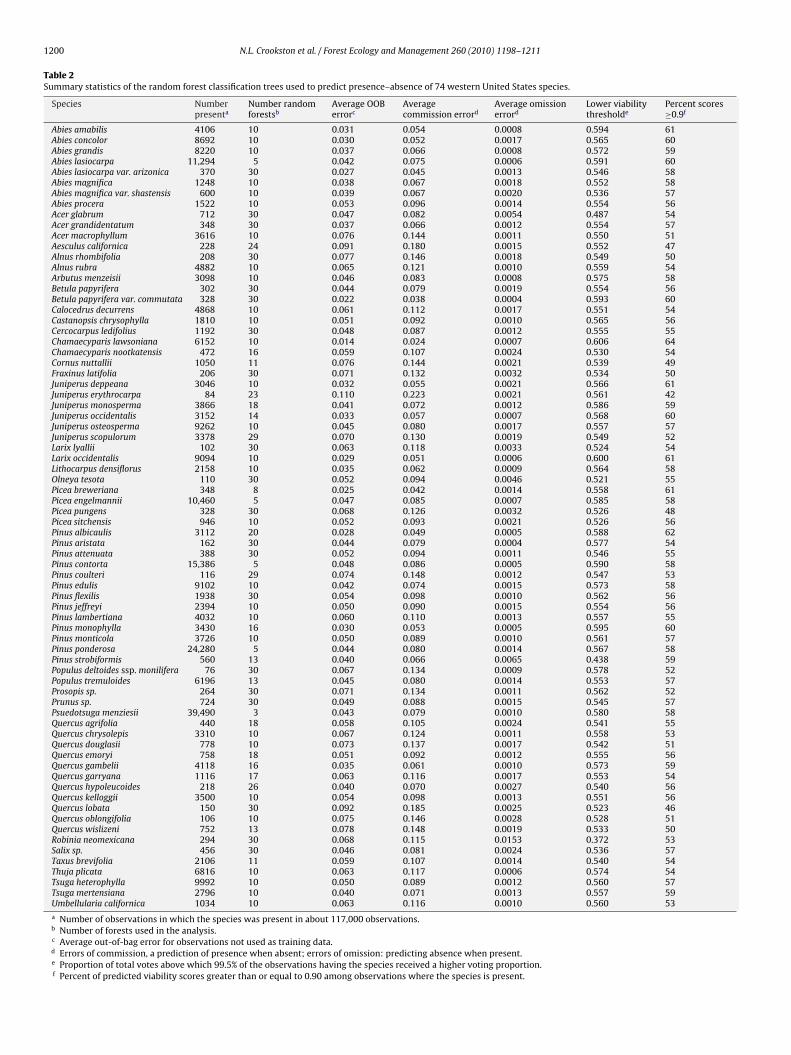

1200 N.L. Crookston et al. / Forest Ecology and Management 260 (2010) 1198–1211

Table 2Summary statistics of the random forest classification trees used to predict presence–absence of 74 western United States species.

Species Numberpresenta

Number randomforestsb

Average OOBerrorc

Averagecommission errord

Average omissionerrord

Lower viabilitythresholde

Percent scores≥0.9f

Abies amabilis 4106 10 0.031 0.054 0.0008 0.594 61Abies concolor 8692 10 0.030 0.052 0.0017 0.565 60Abies grandis 8220 10 0.037 0.066 0.0008 0.572 59Abies lasiocarpa 11,294 5 0.042 0.075 0.0006 0.591 60Abies lasiocarpa var. arizonica 370 30 0.027 0.045 0.0013 0.546 58Abies magnifica 1248 10 0.038 0.067 0.0018 0.552 58Abies magnifica var. shastensis 600 10 0.039 0.067 0.0020 0.536 57Abies procera 1522 10 0.053 0.096 0.0014 0.554 56Acer glabrum 712 30 0.047 0.082 0.0054 0.487 54Acer grandidentatum 348 30 0.037 0.066 0.0012 0.554 57Acer macrophyllum 3616 10 0.076 0.144 0.0011 0.550 51Aesculus californica 228 24 0.091 0.180 0.0015 0.552 47Alnus rhombifolia 208 30 0.077 0.146 0.0018 0.549 50Alnus rubra 4882 10 0.065 0.121 0.0010 0.559 54Arbutus menzeisii 3098 10 0.046 0.083 0.0008 0.575 58Betula papyrifera 302 30 0.044 0.079 0.0019 0.554 56Betula papyrifera var. commutata 328 30 0.022 0.038 0.0004 0.593 60Calocedrus decurrens 4868 10 0.061 0.112 0.0017 0.551 54Castanopsis chrysophylla 1810 10 0.051 0.092 0.0010 0.565 56Cercocarpus ledifolius 1192 30 0.048 0.087 0.0012 0.555 55Chamaecyparis lawsoniana 6152 10 0.014 0.024 0.0007 0.606 64Chamaecyparis nootkatensis 472 16 0.059 0.107 0.0024 0.530 54Cornus nuttallii 1050 11 0.076 0.144 0.0021 0.539 49Fraxinus latifolia 206 30 0.071 0.132 0.0032 0.534 50Juniperus deppeana 3046 10 0.032 0.055 0.0021 0.566 61Juniperus erythrocarpa 84 23 0.110 0.223 0.0021 0.561 42Juniperus monosperma 3866 18 0.041 0.072 0.0012 0.586 59Juniperus occidentalis 3152 14 0.033 0.057 0.0007 0.568 60Juniperus osteosperma 9262 10 0.045 0.080 0.0017 0.557 57Juniperus scopulorum 3378 29 0.070 0.130 0.0019 0.549 52Larix lyallii 102 30 0.063 0.118 0.0033 0.524 54Larix occidentalis 9094 10 0.029 0.051 0.0006 0.600 61Lithocarpus densiflorus 2158 10 0.035 0.062 0.0009 0.564 58Olneya tesota 110 30 0.052 0.094 0.0046 0.521 55Picea breweriana 348 8 0.025 0.042 0.0014 0.558 61Picea engelmannii 10,460 5 0.047 0.085 0.0007 0.585 58Picea pungens 328 30 0.068 0.126 0.0032 0.526 48Picea sitchensis 946 10 0.052 0.093 0.0021 0.526 56Pinus albicaulis 3112 20 0.028 0.049 0.0005 0.588 62Pinus aristata 162 30 0.044 0.079 0.0004 0.577 54Pinus attenuata 388 30 0.052 0.094 0.0011 0.546 55Pinus contorta 15,386 5 0.048 0.086 0.0005 0.590 58Pinus coulteri 116 29 0.074 0.148 0.0012 0.547 53Pinus edulis 9102 10 0.042 0.074 0.0015 0.573 58Pinus flexilis 1938 30 0.054 0.098 0.0010 0.562 56Pinus jeffreyi 2394 10 0.050 0.090 0.0015 0.554 56Pinus lambertiana 4032 10 0.060 0.110 0.0013 0.557 55Pinus monophylla 3430 16 0.030 0.053 0.0005 0.595 60Pinus monticola 3726 10 0.050 0.089 0.0010 0.561 57Pinus ponderosa 24,280 5 0.044 0.080 0.0014 0.567 58Pinus strobiformis 560 13 0.040 0.066 0.0065 0.438 59Populus deltoides ssp. monilifera 76 30 0.067 0.134 0.0009 0.578 52Populus tremuloides 6196 13 0.045 0.080 0.0014 0.553 57Prosopis sp. 264 30 0.071 0.134 0.0011 0.562 52Prunus sp. 724 30 0.049 0.088 0.0015 0.545 57Psuedotsuga menziesii 39,490 3 0.043 0.079 0.0010 0.580 58Quercus agrifolia 440 18 0.058 0.105 0.0024 0.541 55Quercus chrysolepis 3310 10 0.067 0.124 0.0011 0.558 53Quercus douglasii 778 10 0.073 0.137 0.0017 0.542 51Quercus emoryi 758 18 0.051 0.092 0.0012 0.555 56Quercus gambelii 4118 16 0.035 0.061 0.0010 0.573 59Quercus garryana 1116 17 0.063 0.116 0.0017 0.553 54Quercus hypoleucoides 218 26 0.040 0.070 0.0027 0.540 56Quercus kelloggii 3500 10 0.054 0.098 0.0013 0.551 56Quercus lobata 150 30 0.092 0.185 0.0025 0.523 46Quercus oblongifolia 106 10 0.075 0.146 0.0028 0.528 51Quercus wislizeni 752 13 0.078 0.148 0.0019 0.533 50Robinia neomexicana 294 30 0.068 0.115 0.0153 0.372 53Salix sp. 456 30 0.046 0.081 0.0024 0.536 57Taxus brevifolia 2106 11 0.059 0.107 0.0014 0.540 54Thuja plicata 6816 10 0.063 0.117 0.0006 0.574 54Tsuga heterophylla 9992 10 0.050 0.089 0.0012 0.560 57Tsuga mertensiana 2796 10 0.040 0.071 0.0013 0.557 59Umbellularia californica 1034 10 0.063 0.116 0.0010 0.560 53a Number of observations in which the species was present in about 117,000 observations.b Number of forests used in the analysis.c Average out-of-bag error for observations not used as training data.d Errors of commission, a prediction of presence when absent; errors of omission: predicting absence when present.e Proportion of total votes above which 99.5% of the observations having the species received a higher voting proportion.f Percent of predicted viability scores greater than or equal to 0.90 among observations where the species is present.

and Management 260 (2010) 1198–1211 1201

tuMadBbes3r

vr5tfm1(oepoc5t

sced

joc

2

2

bbsibERvottwov

smdpFafini

N.L. Crookston et al. / Forest Ecology

he several disparate regional models which, for instance, mayse different base ages. We circumvented this problem by usingonserud’s (1984) model calibrated for P. menziesii to estimatesite index for each tree. This equation was used for all species

espite the well known differences in growth rates among species.ecause Climate–FVS will use the ratio S instead of actual site index,ias introduced from using a single site curve for all species isxpected to be alleviated while the noise associated with disparateite curves and underlying techniques is avoided. Approximately9% of the observations in this dataset were P. menziesii, but theemainder included 61 other species.

Calibration data consisted of a random sample of 40,000 obser-ations drawn without replacement from the full data set. Toepresent climates where there are no trees, a random selection of000 points were selected from lands in the western United Stateshat are not capable of supporting forests. This sample was obtainedrom a systematic sampling of point locations within the digitized

ap of the Biotic Communities of North America (Brown et al.,998). Technical procedures, described in detail in Rehfeldt et al.2006), involved the use of ARCMAP software to procure the samplef point locations from each polygon on the file, and the digitizedlevation model of the GLOBE Task Team (1999) to associate eachoint sample with an elevation. Of the 24 biotic communities thatccur in western United States, 13 (e.g., desertscrub, grasslands,haparral) contained neither forests nor woodlands. Our sample of000 was drawn from the group of about 28,000 lacking trees ando them a site index of zero was assigned.

These 45,000 observations were used to build a series of regres-ion trees using the Random Forests algorithm and a set of 35andidate climate variables (see Section 2.1) to initiate a stepwiselimination process (see Section 2.2). The regression model waseveloped from one forest with 150 trees.

Observations not used in fitting the regression were used toudge the quality of the fit. This dataset consisted of about 65,700bservations, of which about 22,000 were from the sample of bioticommunities that contained no forests or woodlands.

.4. Conversion of FVS to Climate–FVS

.4.1. MortalityIn Climate–FVS, mortality is to be calibrated from species via-

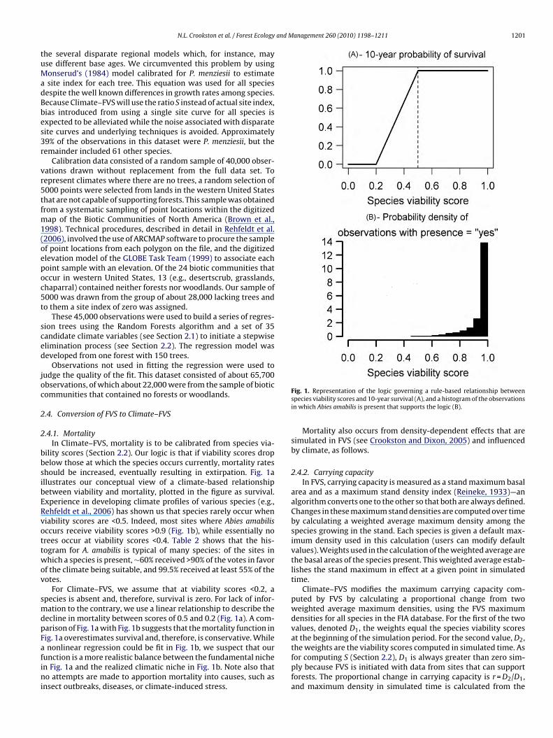
ility scores (Section 2.2). Our logic is that if viability scores dropelow those at which the species occurs currently, mortality rateshould be increased, eventually resulting in extirpation. Fig. 1allustrates our conceptual view of a climate-based relationshipetween viability and mortality, plotted in the figure as survival.xperience in developing climate profiles of various species (e.g.,ehfeldt et al., 2006) has shown us that species rarely occur wheniability scores are <0.5. Indeed, most sites where Abies amabilisccurs receive viability scores >0.9 (Fig. 1b), while essentially norees occur at viability scores <0.4. Table 2 shows that the his-ogram for A. amabilis is typical of many species: of the sites inhich a species is present, ∼60% received >90% of the votes in favor

f the climate being suitable, and 99.5% received at least 55% of theotes.

For Climate–FVS, we assume that at viability scores <0.2, apecies is absent and, therefore, survival is zero. For lack of infor-ation to the contrary, we use a linear relationship to describe the

ecline in mortality between scores of 0.5 and 0.2 (Fig. 1a). A com-arison of Fig. 1a with Fig. 1b suggests that the mortality function inig. 1a overestimates survival and, therefore, is conservative. While

nonlinear regression could be fit in Fig. 1b, we suspect that our

unction is a more realistic balance between the fundamental nichen Fig. 1a and the realized climatic niche in Fig. 1b. Note also thato attempts are made to apportion mortality into causes, such as

nsect outbreaks, diseases, or climate-induced stress.

Fig. 1. Representation of the logic governing a rule-based relationship betweenspecies viability scores and 10-year survival (A), and a histogram of the observationsin which Abies amabilis is present that supports the logic (B).

Mortality also occurs from density-dependent effects that aresimulated in FVS (see Crookston and Dixon, 2005) and influencedby climate, as follows.

2.4.2. Carrying capacityIn FVS, carrying capacity is measured as a stand maximum basal

area and as a maximum stand density index (Reineke, 1933)—analgorithm converts one to the other so that both are always defined.Changes in these maximum stand densities are computed over timeby calculating a weighted average maximum density among thespecies growing in the stand. Each species is given a default max-imum density used in this calculation (users can modify defaultvalues). Weights used in the calculation of the weighted average arethe basal areas of the species present. This weighted average estab-lishes the stand maximum in effect at a given point in simulatedtime.

Climate–FVS modifies the maximum carrying capacity com-puted by FVS by calculating a proportional change from twoweighted average maximum densities, using the FVS maximumdensities for all species in the FIA database. For the first of the twovalues, denoted D1, the weights equal the species viability scoresat the beginning of the simulation period. For the second value, D2,

the weights are the viability scores computed in simulated time. Asfor computing S (Section 2.2), D1 is always greater than zero sim-ply because FVS is initiated with data from sites that can supportforests. The proportional change in carrying capacity is r = D2/D1,and maximum density in simulated time is calculated from the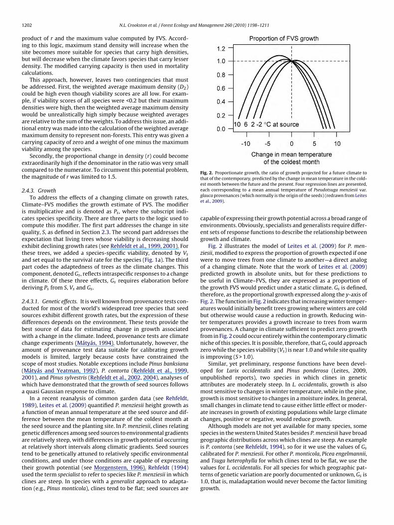

1 and Management 260 (2010) 1198–1211

pisbdc

bcpdwatmcv

ect

2

Ciccqeetapcid

2dsdbwcams(2wa

1aftgaatctuct

Fig. 2. Proportionate growth, the ratio of growth projected for a future climate tothat of the contemporary, predicted by the change in mean temperature in the cold-

202 N.L. Crookston et al. / Forest Ecology

roduct of r and the maximum value computed by FVS. Accord-ng to this logic, maximum stand density will increase when theite becomes more suitable for species that carry high densities,ut will decrease when the climate favors species that carry lesserensity. The modified carrying capacity is then used in mortalityalculations.

This approach, however, leaves two contingencies that muste addressed. First, the weighted average maximum density (D2)ould be high even though viability scores are all low. For exam-le, if viability scores of all species were <0.2 but their maximumensities were high, then the weighted average maximum densityould be unrealistically high simply because weighted averages

re relative to the sum of the weights. To address this issue, an addi-ional entry was made into the calculation of the weighted average

aximum density to represent non-forests. This entry was given aarrying capacity of zero and a weight of one minus the maximumiability among the species.

Secondly, the proportional change in density (r) could becomextraordinarily high if the denominator in the ratio was very smallompared to the numerator. To circumvent this potential problem,he magnitude of r was limited to 1.5.

.4.3. GrowthTo address the effects of a changing climate on growth rates,

limate–FVS modifies the growth estimate of FVS. The modifiers multiplicative and is denoted as Ps, where the subscript indi-ates species specificity. There are three parts to the logic used toompute this modifier. The first part addresses the change in siteuality, S, as defined in Section 2.3. The second part addresses thexpectation that living trees whose viability is decreasing shouldxhibit declining growth rates (see Rehfeldt et al., 1999, 2001). Forhese trees, we added a species-specific viability, denoted by Vs

nd set equal to the survival rate for the species (Fig. 1a). The thirdart codes the adaptedness of trees as the climate changes. Thisomponent, denoted Gs, reflects intraspecific responses to a changen climate. Of these three effects, Gs requires elaboration beforeeriving Ps from S, Vs and Gs.

.4.3.1. Genetic effects. It is well known from provenance tests con-ucted for most of the world’s widespread tree species that seedources exhibit different growth rates, but the expression of theseifferences depends on the environment. These tests provide theest source of data for estimating change in growth associatedith a change in the climate. Indeed, provenance tests are climate

hange experiments (Mátyás, 1994). Unfortunately, however, themount of provenance test data suitable for calibrating growthodels is limited, largely because costs have constrained the

cope of most studies. Notable exceptions include Pinus banksianaMátyás and Yeatman, 1992), P. contorta (Rehfeldt et al., 1999,001), and Pinus sylvestris (Rehfeldt et al., 2002, 2004), analyses ofhich have demonstrated that the growth of seed sources followsquasi Gaussian response to climate.

In a recent reanalysis of common garden data (see Rehfeldt,989), Leites et al. (2009) quantified P. menziesii height growth asfunction of mean annual temperature at the seed source and dif-

erence between the mean temperature of the coldest month athe seed source and the planting site. In P. menziesii, clines relatingenetic differences among seed sources to environmental gradientsre relatively steep, with differences in growth potential occurringt relatively short intervals along climatic gradients. Seed sourcesend to be genetically attuned to relatively specific environmental

onditions, and under those conditions are capable of expressingheir growth potential (see Morgenstern, 1996). Rehfeldt (1994)sed the term specialist to refer to species like P. menziesii in whichlines are steep. In species with a generalist approach to adapta-ion (e.g., Pinus monticola), clines tend to be flat; seed sources are

est month between the future and the present. Four regression lines are presented,each corresponding to a mean annual temperature of Pseudotsuga menziesii var.glauca provenances (which normally is the origin of the seeds) (redrawn from Leiteset al., 2009).

capable of expressing their growth potential across a broad range ofenvironments. Obviously, specialists and generalists require differ-ent sets of response functions to describe the relationship betweengrowth and climate.

Fig. 2 illustrates the model of Leites et al. (2009) for P. men-ziesii, modified to express the proportion of growth expected if onewere to move trees from one climate to another—a direct analogof a changing climate. Note that the work of Leites et al. (2009)predicted growth in absolute units, but for these predictions tobe useful in Climate–FVS, they are expressed as a proportion ofthe growth FVS would predict under a static climate. Gs is defined,therefore, as the proportional growth expressed along the y-axis ofFig. 2. The function in Fig. 2 indicates that increasing winter temper-atures would initially benefit trees growing where winters are coldbut otherwise would cause a reduction in growth. Reducing win-ter temperatures provides a growth increase to trees from warmprovenances. A change in climate sufficient to predict zero growthfrom in Fig. 2 could occur entirely within the contemporary climaticniche of this species. It is possible, therefore, that Gs could approachzero while the species viability (Vs) is near 1.0 and while site qualityis improving (S > 1.0).

Similar, yet preliminary, response functions have been devel-oped for Larix occidentalis and Pinus ponderosa (Leites, 2009,unpublished reports), two species in which clines in geneticattributes are moderately steep. In L. occidentalis, growth is alsomost sensitive to changes in winter temperature, while in the pine,growth is most sensitive to changes in a moisture index. In general,small changes in climate tend to cause either little effect or moder-ate increases in growth of existing populations while large climatechanges, positive or negative, would reduce growth.

Although models are not yet available for many species, somespecies in the western United States besides P. menziesii have broadgeographic distributions across which clines are steep. An exampleis P. contorta (see Rehfeldt, 1994), so for it we use the values of Gs

calibrated for P. menziesii. For other P. monticola, Picea engelmannii,

and Tsuga heterophylla for which clines tend to be flat, we use thevalues for L. occidentalis. For all species for which geographic pat-terns of genetic variation are poorly documented or unknown, Gs is1.0, that is, maladaptation would never become the factor limitinggrowth.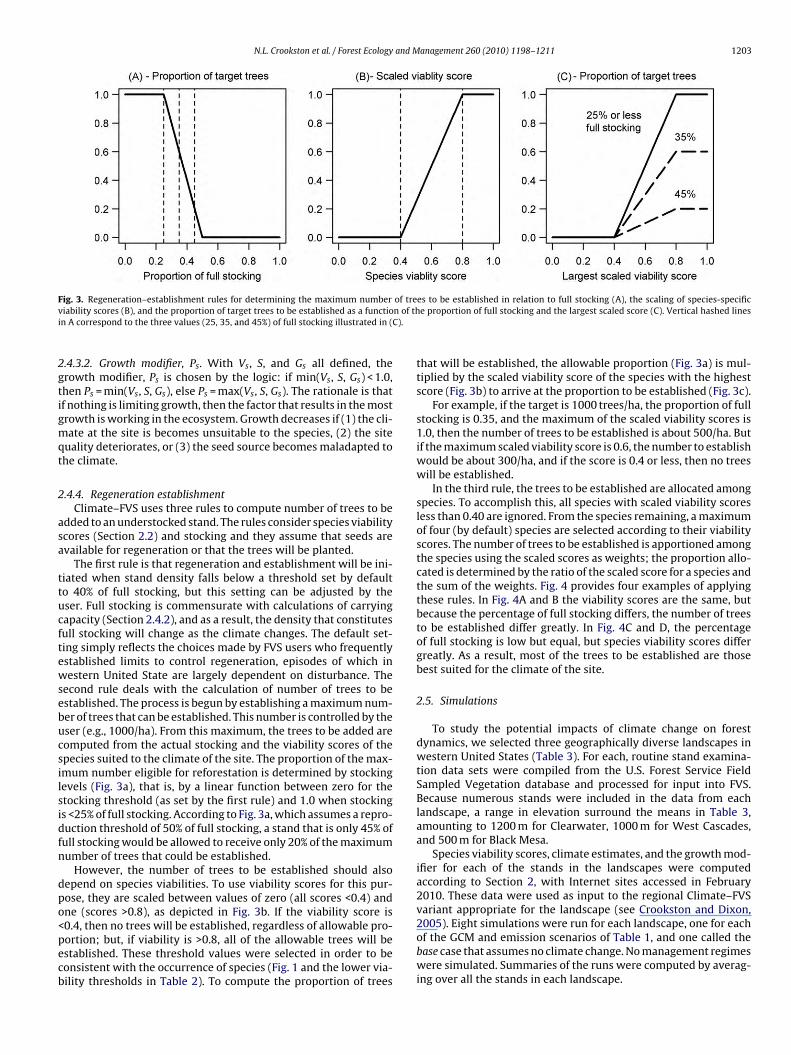

N.L. Crookston et al. / Forest Ecology and Management 260 (2010) 1198–1211 1203

F of trev n of thi C).

2gtigmqt

2

asa

ttucftewsebucsilsidfn

dpo<pecb

ig. 3. Regeneration–establishment rules for determining the maximum numberiability scores (B), and the proportion of target trees to be established as a function A correspond to the three values (25, 35, and 45%) of full stocking illustrated in (

.4.3.2. Growth modifier, Ps. With Vs, S, and Gs all defined, therowth modifier, Ps is chosen by the logic: if min(Vs, S, Gs) < 1.0,hen Ps = min(Vs, S, Gs), else Ps = max(Vs, S, Gs). The rationale is thatf nothing is limiting growth, then the factor that results in the mostrowth is working in the ecosystem. Growth decreases if (1) the cli-ate at the site is becomes unsuitable to the species, (2) the site

uality deteriorates, or (3) the seed source becomes maladapted tohe climate.

.4.4. Regeneration establishmentClimate–FVS uses three rules to compute number of trees to be

dded to an understocked stand. The rules consider species viabilitycores (Section 2.2) and stocking and they assume that seeds arevailable for regeneration or that the trees will be planted.

The first rule is that regeneration and establishment will be ini-iated when stand density falls below a threshold set by defaulto 40% of full stocking, but this setting can be adjusted by theser. Full stocking is commensurate with calculations of carryingapacity (Section 2.4.2), and as a result, the density that constitutesull stocking will change as the climate changes. The default set-ing simply reflects the choices made by FVS users who frequentlystablished limits to control regeneration, episodes of which inestern United State are largely dependent on disturbance. The

econd rule deals with the calculation of number of trees to bestablished. The process is begun by establishing a maximum num-er of trees that can be established. This number is controlled by theser (e.g., 1000/ha). From this maximum, the trees to be added areomputed from the actual stocking and the viability scores of thepecies suited to the climate of the site. The proportion of the max-mum number eligible for reforestation is determined by stockingevels (Fig. 3a), that is, by a linear function between zero for thetocking threshold (as set by the first rule) and 1.0 when stockings <25% of full stocking. According to Fig. 3a, which assumes a repro-uction threshold of 50% of full stocking, a stand that is only 45% ofull stocking would be allowed to receive only 20% of the maximumumber of trees that could be established.

However, the number of trees to be established should alsoepend on species viabilities. To use viability scores for this pur-ose, they are scaled between values of zero (all scores <0.4) andne (scores >0.8), as depicted in Fig. 3b. If the viability score is

0.4, then no trees will be established, regardless of allowable pro-ortion; but, if viability is >0.8, all of the allowable trees will bestablished. These threshold values were selected in order to beonsistent with the occurrence of species (Fig. 1 and the lower via-ility thresholds in Table 2). To compute the proportion of trees

es to be established in relation to full stocking (A), the scaling of species-specifice proportion of full stocking and the largest scaled score (C). Vertical hashed lines

that will be established, the allowable proportion (Fig. 3a) is mul-tiplied by the scaled viability score of the species with the highestscore (Fig. 3b) to arrive at the proportion to be established (Fig. 3c).

For example, if the target is 1000 trees/ha, the proportion of fullstocking is 0.35, and the maximum of the scaled viability scores is1.0, then the number of trees to be established is about 500/ha. Butif the maximum scaled viability score is 0.6, the number to establishwould be about 300/ha, and if the score is 0.4 or less, then no treeswill be established.

In the third rule, the trees to be established are allocated amongspecies. To accomplish this, all species with scaled viability scoresless than 0.40 are ignored. From the species remaining, a maximumof four (by default) species are selected according to their viabilityscores. The number of trees to be established is apportioned amongthe species using the scaled scores as weights; the proportion allo-cated is determined by the ratio of the scaled score for a species andthe sum of the weights. Fig. 4 provides four examples of applyingthese rules. In Fig. 4A and B the viability scores are the same, butbecause the percentage of full stocking differs, the number of treesto be established differ greatly. In Fig. 4C and D, the percentageof full stocking is low but equal, but species viability scores differgreatly. As a result, most of the trees to be established are thosebest suited for the climate of the site.

2.5. Simulations

To study the potential impacts of climate change on forestdynamics, we selected three geographically diverse landscapes inwestern United States (Table 3). For each, routine stand examina-tion data sets were compiled from the U.S. Forest Service FieldSampled Vegetation database and processed for input into FVS.Because numerous stands were included in the data from eachlandscape, a range in elevation surround the means in Table 3,amounting to 1200 m for Clearwater, 1000 m for West Cascades,and 500 m for Black Mesa.

Species viability scores, climate estimates, and the growth mod-ifier for each of the stands in the landscapes were computedaccording to Section 2, with Internet sites accessed in February2010. These data were used as input to the regional Climate–FVSvariant appropriate for the landscape (see Crookston and Dixon,

2005). Eight simulations were run for each landscape, one for eachof the GCM and emission scenarios of Table 1, and one called thebase case that assumes no climate change. No management regimeswere simulated. Summaries of the runs were computed by averag-ing over all the stands in each landscape.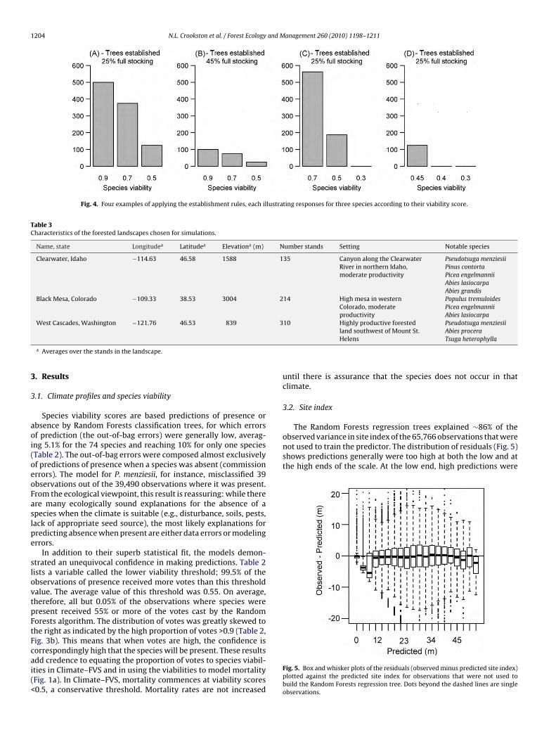

1204 N.L. Crookston et al. / Forest Ecology and Management 260 (2010) 1198–1211

Fig. 4. Four examples of applying the establishment rules, each illustrating responses for three species according to their viability score.

Table 3Characteristics of the forested landscapes chosen for simulations.

Name, state Longitudea Latitudea Elevationa (m) Number stands Setting Notable species

Clearwater, Idaho −114.63 46.58 1588 135 Canyon along the ClearwaterRiver in northern Idaho,moderate productivity

Pseudotsuga menziesiiPinus contortaPicea engelmanniiAbies lasiocarpaAbies grandis

Black Mesa, Colorado −109.33 38.53 3004 214 High mesa in westernColorado, moderateproductivity

Populus tremuloidesPicea engelmanniiAbies lasiocarpa

West Cascades, Washington −121.76 46.53 839 310 Highly productive forested Pseudotsuga menziesii

3

3

aoi(oeoFaslpe

slovtpFtFcai(<

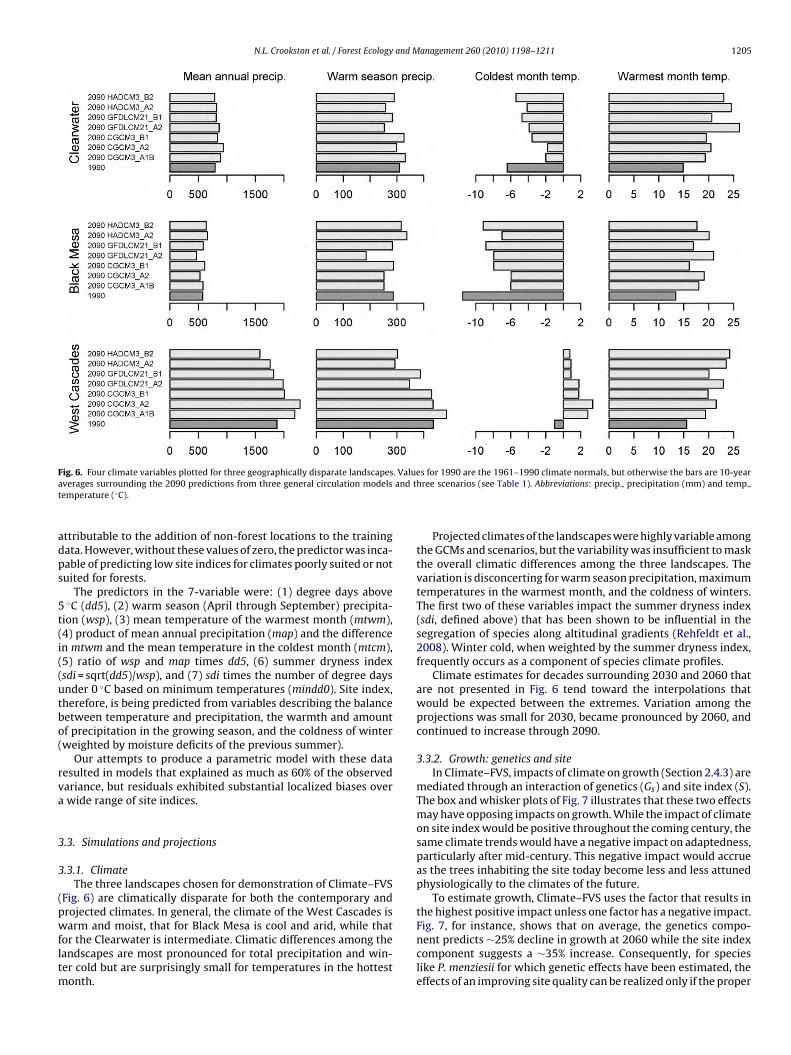
The Random Forests regression trees explained ∼86% of theobserved variance in site index of the 65,766 observations that werenot used to train the predictor. The distribution of residuals (Fig. 5)shows predictions generally were too high at both the low and atthe high ends of the scale. At the low end, high predictions were

a Averages over the stands in the landscape.

. Results

.1. Climate profiles and species viability

Species viability scores are based predictions of presence orbsence by Random Forests classification trees, for which errorsf prediction (the out-of-bag errors) were generally low, averag-ng 5.1% for the 74 species and reaching 10% for only one speciesTable 2). The out-of-bag errors were composed almost exclusivelyf predictions of presence when a species was absent (commissionrrors). The model for P. menziesii, for instance, misclassified 39bservations out of the 39,490 observations where it was present.rom the ecological viewpoint, this result is reassuring: while therere many ecologically sound explanations for the absence of apecies when the climate is suitable (e.g., disturbance, soils, pests,ack of appropriate seed source), the most likely explanations forredicting absence when present are either data errors or modelingrrors.

In addition to their superb statistical fit, the models demon-trated an unequivocal confidence in making predictions. Table 2ists a variable called the lower viability threshold; 99.5% of thebservations of presence received more votes than this thresholdalue. The average value of this threshold was 0.55. On average,herefore, all but 0.05% of the observations where species wereresent received 55% or more of the votes cast by the Randomorests algorithm. The distribution of votes was greatly skewed tohe right as indicated by the high proportion of votes >0.9 (Table 2,ig. 3b). This means that when votes are high, the confidence is

orrespondingly high that the species will be present. These resultsdd credence to equating the proportion of votes to species viabil-ties in Climate–FVS and in using the viabilities to model mortalityFig. 1a). In Climate–FVS, mortality commences at viability scores0.5, a conservative threshold. Mortality rates are not increased

land southwest of Mount St.Helens

Abies proceraTsuga heterophylla

until there is assurance that the species does not occur in thatclimate.

3.2. Site index

Fig. 5. Box and whisker plots of the residuals (observed minus predicted site index)plotted against the predicted site index for observations that were not used tobuild the Random Forests regression tree. Dots beyond the dashed lines are singleobservations.

N.L. Crookston et al. / Forest Ecology and Management 260 (2010) 1198–1211 1205

F . Valuea and tt

adps

5t(i((utbo(

rva

3

3

(pwfltm

ig. 6. Four climate variables plotted for three geographically disparate landscapesverages surrounding the 2090 predictions from three general circulation modelsemperature (◦C).

ttributable to the addition of non-forest locations to the trainingata. However, without these values of zero, the predictor was inca-able of predicting low site indices for climates poorly suited or notuited for forests.

The predictors in the 7-variable were: (1) degree days above◦C (dd5), (2) warm season (April through September) precipita-

ion (wsp), (3) mean temperature of the warmest month (mtwm),4) product of mean annual precipitation (map) and the differencen mtwm and the mean temperature in the coldest month (mtcm),5) ratio of wsp and map times dd5, (6) summer dryness indexsdi = sqrt(dd5)/wsp), and (7) sdi times the number of degree daysnder 0 ◦C based on minimum temperatures (mindd0). Site index,herefore, is being predicted from variables describing the balanceetween temperature and precipitation, the warmth and amountf precipitation in the growing season, and the coldness of winterweighted by moisture deficits of the previous summer).

Our attempts to produce a parametric model with these dataesulted in models that explained as much as 60% of the observedariance, but residuals exhibited substantial localized biases overwide range of site indices.

.3. Simulations and projections

.3.1. ClimateThe three landscapes chosen for demonstration of Climate–FVS

Fig. 6) are climatically disparate for both the contemporary androjected climates. In general, the climate of the West Cascades is

arm and moist, that for Black Mesa is cool and arid, while that

or the Clearwater is intermediate. Climatic differences among theandscapes are most pronounced for total precipitation and win-er cold but are surprisingly small for temperatures in the hottest

onth.

s for 1990 are the 1961–1990 climate normals, but otherwise the bars are 10-yearhree scenarios (see Table 1). Abbreviations: precip., precipitation (mm) and temp.,

Projected climates of the landscapes were highly variable amongthe GCMs and scenarios, but the variability was insufficient to maskthe overall climatic differences among the three landscapes. Thevariation is disconcerting for warm season precipitation, maximumtemperatures in the warmest month, and the coldness of winters.The first two of these variables impact the summer dryness index(sdi, defined above) that has been shown to be influential in thesegregation of species along altitudinal gradients (Rehfeldt et al.,2008). Winter cold, when weighted by the summer dryness index,frequently occurs as a component of species climate profiles.

Climate estimates for decades surrounding 2030 and 2060 thatare not presented in Fig. 6 tend toward the interpolations thatwould be expected between the extremes. Variation among theprojections was small for 2030, became pronounced by 2060, andcontinued to increase through 2090.

3.3.2. Growth: genetics and siteIn Climate–FVS, impacts of climate on growth (Section 2.4.3) are

mediated through an interaction of genetics (Gs) and site index (S).The box and whisker plots of Fig. 7 illustrates that these two effectsmay have opposing impacts on growth. While the impact of climateon site index would be positive throughout the coming century, thesame climate trends would have a negative impact on adaptedness,particularly after mid-century. This negative impact would accrueas the trees inhabiting the site today become less and less attunedphysiologically to the climates of the future.

To estimate growth, Climate–FVS uses the factor that results inthe highest positive impact unless one factor has a negative impact.

Fig. 7, for instance, shows that on average, the genetics compo-nent predicts ∼25% decline in growth at 2060 while the site indexcomponent suggests a ∼35% increase. Consequently, for specieslike P. menziesii for which genetic effects have been estimated, theeffects of an improving site quality can be realized only if the proper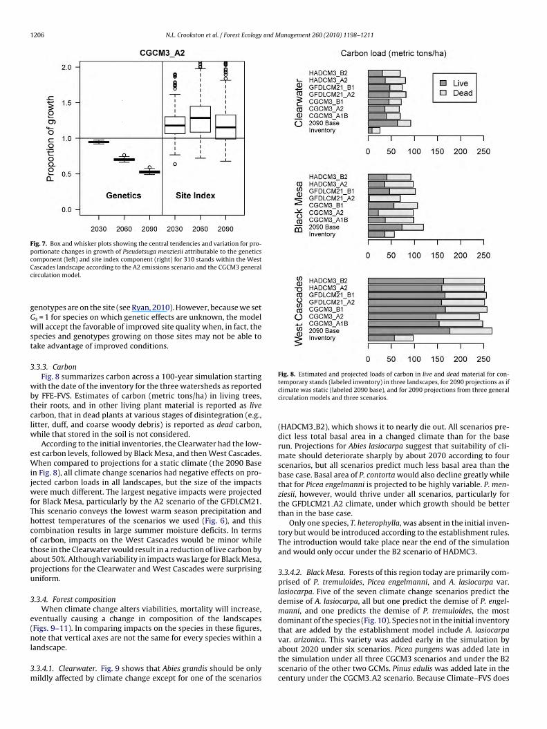

1206 N.L. Crookston et al. / Forest Ecology and Management 260 (2010) 1198–1211

Fig. 7. Box and whisker plots showing the central tendencies and variation for pro-portionate changes in growth of Pseudotsuga menziesii attributable to the geneticscCc

gGwst

3

wbtclw

eWijwfThcotapu

3

e(nl

3m

Fig. 8. Estimated and projected loads of carbon in live and dead material for con-

omponent (left) and site index component (right) for 310 stands within the Westascades landscape according to the A2 emissions scenario and the CGCM3 generalirculation model.

enotypes are on the site (see Ryan, 2010). However, because we sets = 1 for species on which genetic effects are unknown, the modelill accept the favorable of improved site quality when, in fact, the

pecies and genotypes growing on those sites may not be able toake advantage of improved conditions.

.3.3. CarbonFig. 8 summarizes carbon across a 100-year simulation starting

ith the date of the inventory for the three watersheds as reportedy FFE-FVS. Estimates of carbon (metric tons/ha) in living trees,heir roots, and in other living plant material is reported as livearbon, that in dead plants at various stages of disintegration (e.g.,itter, duff, and coarse woody debris) is reported as dead carbon,

hile that stored in the soil is not considered.According to the initial inventories, the Clearwater had the low-

st carbon levels, followed by Black Mesa, and then West Cascades.hen compared to projections for a static climate (the 2090 Base

n Fig. 8), all climate change scenarios had negative effects on pro-ected carbon loads in all landscapes, but the size of the impacts

ere much different. The largest negative impacts were projectedor Black Mesa, particularly by the A2 scenario of the GFDLCM21.his scenario conveys the lowest warm season precipitation andottest temperatures of the scenarios we used (Fig. 6), and thisombination results in large summer moisture deficits. In termsf carbon, impacts on the West Cascades would be minor whilehose in the Clearwater would result in a reduction of live carbon bybout 50%. Although variability in impacts was large for Black Mesa,rojections for the Clearwater and West Cascades were surprisingniform.

.3.4. Forest compositionWhen climate change alters viabilities, mortality will increase,

ventually causing a change in composition of the landscapesFigs. 9–11). In comparing impacts on the species in these figures,ote that vertical axes are not the same for every species within a

andscape.

.3.4.1. Clearwater. Fig. 9 shows that Abies grandis should be onlyildly affected by climate change except for one of the scenarios

temporary stands (labeled inventory) in three landscapes, for 2090 projections as ifclimate was static (labeled 2090 base), and for 2090 projections from three generalcirculation models and three scenarios.

(HADCM3 B2), which shows it to nearly die out. All scenarios pre-dict less total basal area in a changed climate than for the baserun. Projections for Abies lasiocarpa suggest that suitability of cli-mate should deteriorate sharply by about 2070 according to fourscenarios, but all scenarios predict much less basal area than thebase case. Basal area of P. contorta would also decline greatly whilethat for Picea engelmanni is projected to be highly variable. P. men-ziesii, however, would thrive under all scenarios, particularly forthe GFDLCM21 A2 climate, under which growth should be betterthan in the base case.

Only one species, T. heterophylla, was absent in the initial inven-tory but would be introduced according to the establishment rules.The introduction would take place near the end of the simulationand would only occur under the B2 scenario of HADMC3.

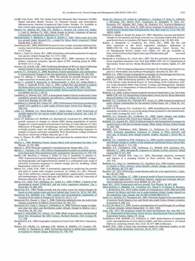
3.3.4.2. Black Mesa. Forests of this region today are primarily com-prised of P. tremuloides, Picea engelmanni, and A. lasiocarpa var.lasiocarpa. Five of the seven climate change scenarios predict thedemise of A. lasiocarpa, all but one predict the demise of P. engel-manni, and one predicts the demise of P. tremuloides, the mostdominant of the species (Fig. 10). Species not in the initial inventorythat are added by the establishment model include A. lasiocarpa

var. arizonica. This variety was added early in the simulation byabout 2020 under six scenarios. Picea pungens was added late inthe simulation under all three CGCM3 scenarios and under the B2scenario of the other two GCMs. Pinus edulis was added late in thecentury under the CGCM3 A2 scenario. Because Climate–FVS does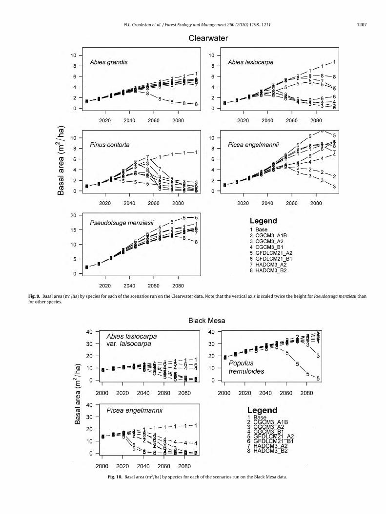

N.L. Crookston et al. / Forest Ecology and Management 260 (2010) 1198–1211 1207

Fig. 9. Basal area (m2/ha) by species for each of the scenarios run on the Clearwater data. Note that the vertical axis is scaled twice the height for Pseudotsuga menziesii thanfor other species.

Fig. 10. Basal area (m2/ha) by species for each of the scenarios run on the Black Mesa data.

1208 N.L. Crookston et al. / Forest Ecology and Management 260 (2010) 1198–1211

F ascadh rios an

na

3ccttgctat

4

4

tooifdtwwc

soatpwpact

ig. 11. Basal area (m2/ha) by species for each of the scenarios run on the West Cigher than for the other species and that the final differences in basal area a scena

ot consider migration rates, arrival of immigrant species at theppointed time likely would require planting.

.3.4.3. West Cascades. Most obvious predicted impacts of climatehange for the West Cascades (Fig. 11) are the losses of Abies pro-era (most scenarios) and T. heterophylla (four scenarios). Thesewo species currently represent small portions of the basal areahat is otherwise dominated by P. menziesii. The projections sug-est that the dominance of the latter species should continue, withhanges relative to the contemporary basal area ranging from −5%o +8%. A. grandis, P. monticola, Cornus nuttallii, Acer macrophyllum,nd Salix spp. are all predicted to be added to this landscape late inhe century.

. Discussion

.1. Mortality

Climate–FVS illustrates a potential impact of climate change onhe three landscapes chosen for simulations. For all locations, oner more of the scenarios we used would result in the demise of oner more species. Clearly, the mortality component of Climate–FVSs the most influential part of the model. It is unfortunate, there-ore, that there is little empirical evidence pertaining to rates ofemise as the climate becomes unfavorable (see Ryan, 2010). Ashe climate changes, mortality on the trailing edge (Mátyás, 2010)ill become better documented (e.g., Allen et al., 2010). These dataill be indispensable for calibrating mortality estimates driven by

limate effects.Our approach to estimating mortality used species viability

cores that were obtained from modeling presence and absencef species in contemporary climates. Because these viability scoresre based on the realized niche rather than the fundamental niche,he ability of species to survive a change in climate may not beroperly reflected by the scores. This argument is particularly valid

here distributions are limited by competition rather than by thehysical environment. Removal of the competition indeed mayllow a species to flourish. However, the climate profiles can beonsidered as indicators of those future climates that are beyondhe contemporary climatic niche. In the absence of data to the

es data. Note that for the Pseudotsuga menziesii plots, the vertical axis is six timesd the base case are tabulated for each projection.

contrary, Climate–FVS increases the mortality in such climatesso that over time the species would disappear in the simula-tion. This impact is demonstrated for P. tremuloides at Black Mesa(Fig. 9): the species is predicted to die out under HADCM3 A2and is headed toward demise under CGCM3 A2. The predictionsof Rehfeldt et al. (2009) for this species recur in Climate–FVSforecasts.

If future climates have contemporary analogs, one can expectcompetitive interactions to remain unchanged. Consequently,whether the realized niche remains of constant breadth depends onthe degree that future climates are novel (see Jackson and Overpeck,2000). Rehfeldt et al. (2006) show that novel climates in westernUnited States should increase in frequency as the current centuryadvances, occupying about 25% of the land at the end on the century.It is in these novel climates that one can anticipate competitive rela-tionships becoming re-assorted (see Jackson and Overpeck, 2000;Ibánez et al., 2009).

Our viability statistics are a conservative representation of therealized climatic niche. At viability scores below 0.5, there is littlechance of a species occurring (Table 2), and at scores between 0.0and 0.2, there is essentially no chance. The rate of mortality anddemise of stands after such scores are reached is a subject thatrequires a thorough assessment.

We recognize the importance of genetic effects on mortality (seeRehfeldt et al., 1999), but as of yet, these effects cannot be addressedby either statistical or mechanistic models. In the West Cascades,for example (Fig. 11), mortality of P. menziesii was projected to below. We suspect, however, that this estimate underestimates themortality rates that these forests will experience. The climate pro-files on which the viability scores are based were computed at thespecies level and do not account for intraspecific genetic variationHowever, for P. menziesii to maintain its current role in the ecosys-tem, that is, for the forecasted lack of mortality to be realized, theassortment of genotypes capable of thriving in the future climatewill need re-assorting across the landscape (see St. Clair and Howe,

2007) and may even be different from those occurring there today(see Rehfeldt et al., 1999, 2002, 2003). If replacing the genetic stockof the site is required for the species survival, then size distribu-tions and carbon loads would be greatly affected even if the speciescomposition were to remain the same.

and M

4

oioyFfs(ibt

iubdibios

gtnwsrttk

eetw(ewm1f

etadtApTiadt

Cgehbae

N.L. Crookston et al. / Forest Ecology

.2. Growth

Our approach to predicting growth in a changing climate reliesn results of ecological genetics studies in which trees were plantedn common gardens in climates different from those in which theyccur naturally. As a result these studies provide intraspecific anal-ses of growth as affected by a change in climate (Mátyás, 1994,ig. 2). While of potential use in calibrating growth and mortalityunctions intraspecifically, suitable data are available for only a fewpecies. However, Fig. 7 illustrates why genetics-related functionssensu Fig. 2) are needed for many more species; quite simply, antic-pated gains in growth resulting from improved site index cannote realized if these are becoming less well attuned physiologicallyo the climate of the site (see Ryan, 2010).

Fig. 7 also suggests that field-collected measurements of growthn a changing climate may show, for instance, growth increasesnder moderate climate change at some sites and for some speciesut decreases for others; or increases in growth followed byecreases even when the climate seemingly appears to be improv-

ng for tree growth in general. Understanding the relationshipetween genetic variation and site index and thereby improv-

ng growth estimators in Climate–FVS would benefit greatly frombservations across a wide range of conditions for a variety ofpecies.

For present applications, we do not believe our treatment ofenetic and site effects to be egregious. The simulations showhat the model is much more sensitive to the mortality compo-ent than to the growth component. Also, the growth modifiere compute is applied to the FVS growth estimate which repre-

ents an expected realized growth under contemporary conditionsather than a potential growth. Climate–FVS focuses on the depar-ure from these contemporary conditions to provide a frameworkhat takes utmost advantage of current models and their embeddednowledge.

Nonetheless, we considered several other approaches to mod-ling growth. Perhaps most relevant is the approach of Milnert al. (2003) who developed FVSBGC, a model that linked FVS tohe physiology-based model Stand-BGC (Milner and Coble, 1995),hich in turn is based on the stand-level model FOREST-BGC

Running and Coughlan, 1988). We found, however, that geneticffects and species viabilities could be incorporated easily into FVSithout resorting to the detail needed for FVSBGC. The mechanisticodel MC1 (Bachelet et al., 2001a) and 3PG (Landsberg and Waring,

997; Landsberg, 2003; Landsberg et al., 2003) also proved difficultor addressing the type of modifications we envisioned.

ForClim (Bugmann, 1996; Bugmann and Solomon, 2000) is a for-st gap model that computes a potential growth and scales it withhe product of two modifiers. One of the modifiers scales growtht the leading edge by equating a growth modifier to zero whenegree days above 5 ◦C is zero and increases as this value increaseso an asymptote index value of 1.0 when site conditions are optimal.

second modifier is used to reflect drying conditions and is com-uted as a ratio of actual water use to potentially available water.he product of these two indices scales potential growth. Althoughntriguing, the approach also requires soils data as additional input,nd it is unclear to us how the strongly empirically based FVS pre-ictions which operate at the species level can take advantage ofhis formulation.

We considered and rejected constructing a module dealing withO2 fertilization. Elevated concentrations of CO2 have boostedrowth in some situations, species, and age classes (Hättenschwiler

t al., 1997), but Körner et al. (2005) suggest that positive effectsave not been conclusively shown. Others (e.g., Norby et al., 2005)elieve that forests will respond positively to increased CO2 acrossbroad range of productivities. We prefer to procrastinate until theffects of CO2 fertilization are unambiguous. In fact, FVS contains

anagement 260 (2010) 1198–1211 1209

options that would allow model users to posit these effects at theirdiscretion. At present, we also are uncertain in which module CO2fertilization would be best expressed. If it is shown, for instance,that changes in atmospheric gas concentrations directly influ-ence species–climate relationships, then CO2 fertilization couldalter the impact of a changing temperature and precipitation onmortality.

Another tempting approach to modeling growth responses toclimate would involve re-fitting FVS component modules ratherthan provide adjustments to the algorithms already present. Ina previous attempt to estimate climate impacts on basal area ofP. menziesii, Crookston et al. (2007) re-fit Wykoff’s (1990) diam-eter growth equations by substituting climate variables for thesite descriptors used originally while retaining predictors relat-ing to tree size and competition. The best fitting regression modeldescribed a general increase in growth with increasing meanannual temperature and precipitation, but also suggested an absurdinteraction whereby the negative impact of reduced precipitationwould be offset by increasing temperatures. These results werelargely due to the climatic distribution of data points. Highestgrowth rates occur in warm and moist conditions, but no datapoints exist where it is equally warm but dry or equally wet butcold. The results demonstrate the care that must be taken to assurethat empirically based models are intuitively sensible as well asbeing of good statistical fit. The approach, therefore, was rejected.

4.3. Regeneration and establishment

For the regeneration and establishment module of Climate–FVS,we used a series of rules for controlling number of trees to beadded to a site from a list of the species best suited for the cli-mate. Absent in this approach were the modules accounting foreffects of disturbance (e.g., time since disturbance, disturbancetype) and composition of the previous stand that appear in someof the variants of FVS (Ferguson and Carlson, 1993; Ferguson etal., 1986). However, FVS and its regeneration component assumea static climate during the simulation period. Adding the effects ofdisturbance would require an establishment module that accountsnot only for a change in species viability scores but also the impactof climate on the agents of disturbance, the latter of which is onlybeginning to be understood (see Morgan et al., 2008).

Also absent in Climate–FVS are effects such as migration ratesthat would attempt to account for the arrival (by natural means) ofthe seeds from species and seed sources that are suited to the newclimate. Although ecological modelers currently are attempting toincorporate migration rates into the prediction of future distri-butions (e.g., Ibánez et al., 2009), accounting for these effects inClimate–FVS output temporarily will remain the responsibility ofmodel users.

The regeneration component of Climate–FVS provides man-agers a means of choosing among those species suitable to futureclimates. Selecting the appropriate seed source requires in-depthanalyses such as that for L. occidentalis (Rehfeldt and Jaquish, 2010)and for now also will remain a responsibility of the users.

4.4. Variation among projections

The seven projections of climate we used produced consistentpredictions for some species but highly variable projections for oth-ers. Fig. 9, for instance, suggests that Clearwater sites of today thatcontain P. contorta and P. engelmannii should continue to be cli-

matically suited to them until mid century. Consequently, currenttimber management plans for the first half of the century may needlittle adjustment. In the long run, however, the simulations areunanimous in predicting a loss of climates suitable to P. contorta.A decision to regenerate this species today carries the expectation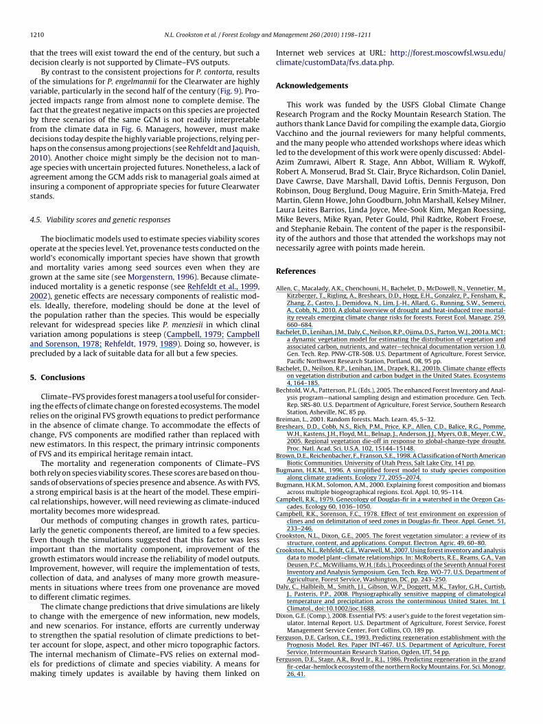

1 and M

td

ovjfbfdh2aais

4

owagi2etrvap

5

iricno

bsacm

lEigIcmt

tattTem

210 N.L. Crookston et al. / Forest Ecology

hat the trees will exist toward the end of the century, but such aecision clearly is not supported by Climate–FVS outputs.

By contrast to the consistent projections for P. contorta, resultsf the simulations for P. engelmannii for the Clearwater are highlyariable, particularly in the second half of the century (Fig. 9). Pro-ected impacts range from almost none to complete demise. Theact that the greatest negative impacts on this species are projectedy three scenarios of the same GCM is not readily interpretablerom the climate data in Fig. 6. Managers, however, must makeecisions today despite the highly variable projections, relying per-aps on the consensus among projections (see Rehfeldt and Jaquish,010). Another choice might simply be the decision not to man-ge species with uncertain projected futures. Nonetheless, a lack ofgreement among the GCM adds risk to managerial goals aimed atnsuring a component of appropriate species for future Clearwatertands.

.5. Viability scores and genetic responses

The bioclimatic models used to estimate species viability scoresperate at the species level. Yet, provenance tests conducted on theorld’s economically important species have shown that growth

nd mortality varies among seed sources even when they arerown at the same site (see Morgenstern, 1996). Because climate-nduced mortality is a genetic response (see Rehfeldt et al., 1999,002), genetic effects are necessary components of realistic mod-ls. Ideally, therefore, modeling should be done at the level ofhe population rather than the species. This would be especiallyelevant for widespread species like P. menziesii in which clinalariation among populations is steep (Campbell, 1979; Campbellnd Sorenson, 1978; Rehfeldt, 1979, 1989). Doing so, however, isrecluded by a lack of suitable data for all but a few species.

. Conclusions

Climate–FVS provides forest managers a tool useful for consider-ng the effects of climate change on forested ecosystems. The modelelies on the original FVS growth equations to predict performancen the absence of climate change. To accommodate the effects ofhange, FVS components are modified rather than replaced withew estimators. In this respect, the primary intrinsic componentsf FVS and its empirical heritage remain intact.

The mortality and regeneration components of Climate–FVSoth rely on species viability scores. These scores are based on thou-ands of observations of species presence and absence. As with FVS,strong empirical basis is at the heart of the model. These empiri-

al relationships, however, will need reviewing as climate-inducedortality becomes more widespread.Our methods of computing changes in growth rates, particu-

arly the genetic components thereof, are limited to a few species.ven though the simulations suggested that this factor was lessmportant than the mortality component, improvement of therowth estimators would increase the reliability of model outputs.mprovement, however, will require the implementation of tests,ollection of data, and analyses of many more growth measure-ents in situations where trees from one provenance are moved

o different climatic regimes.The climate change predictions that drive simulations are likely

o change with the emergence of new information, new models,nd new scenarios. For instance, efforts are currently underway

o strengthen the spatial resolution of climate predictions to bet-er account for slope, aspect, and other micro topographic factors.he internal mechanism of Climate–FVS relies on external mod-ls for predictions of climate and species viability. A means foraking timely updates is available by having them linked on

anagement 260 (2010) 1198–1211

Internet web services at URL: http://forest.moscowfsl.wsu.edu/climate/customData/fvs data.php.

Acknowledgements

This work was funded by the USFS Global Climate ChangeResearch Program and the Rocky Mountain Research Station. Theauthors thank Lance David for compiling the example data, GiorgioVacchino and the journal reviewers for many helpful comments,and the many people who attended workshops where ideas whichled to the development of this work were openly discussed: Abdel-Azim Zumrawi, Albert R. Stage, Ann Abbot, William R. Wykoff,Robert A. Monserud, Brad St. Clair, Bryce Richardson, Colin Daniel,Dave Cawrse, Dave Marshall, David Loftis, Dennis Ferguson, DonRobinson, Doug Berglund, Doug Maguire, Erin Smith-Mateja, FredMartin, Glenn Howe, John Goodburn, John Marshall, Kelsey Milner,Laura Leites Barrios, Linda Joyce, Mee-Sook Kim, Megan Roessing,Mike Bevers, Mike Ryan, Peter Gould, Phil Radtke, Robert Froese,and Stephanie Rebain. The content of the paper is the responsibil-ity of the authors and those that attended the workshops may notnecessarily agree with points made herein.

References

Allen, C., Macalady, A.K., Chenchouni, H., Bachelet, D., McDowell, N., Vennetier, M.,Kitzberger, T., Rigling, A., Breshears, D.D., Hogg, E.H., Gonzalez, P., Fensham, R.,Zhang, Z., Castro, J., Demidova, N., Lim, J.-H., Allard, G., Running, S.W., Semerci,A., Cobb, N., 2010. A global overview of drought and heat-induced tree mortal-ity reveals emerging climate change risks for forests. Forest Ecol. Manage. 259,660–684.

Bachelet, D., Lenihan, J.M., Daly, C., Neilson, R.P., Ojima, D.S., Parton, W.J., 2001a. MC1:a dynamic vegetation model for estimating the distribution of vegetation andassociated carbon, nutrients, and water—technical documentation version 1.0.Gen. Tech. Rep. PNW-GTR-508. U.S. Department of Agriculture, Forest Service,Pacific Northwest Research Station, Portland, OR, 95 pp.

Bachelet, D., Neilson, R.P., Lenihan, J.M., Drapek, R.J., 2001b. Climate change effectson vegetation distribution and carbon budget in the United States. Ecosystems4, 164–185.

Bechtold, W.A., Patterson, P.L. (Eds.), 2005. The enhanced Forest Inventory and Anal-ysis program—national sampling design and estimation procedure. Gen. Tech.Rep. SRS-80. U.S. Department of Agriculture, Forest Service, Southern ResearchStation, Asheville, NC, 85 pp.

Breiman, L., 2001. Random forests. Mach. Learn. 45, 5–32.Breshears, D.D., Cobb, N.S., Rich, P.M., Price, K.P., Allen, C.D., Balice, R.G., Pomme,

W.H., Kastens, J.H., Floyd, M.L., Belnap, J., Anderson, J.J., Myers, O.B., Meyer, C.W.,2005. Regional vegetation die-off in response to global-change-type drought.Proc. Natl. Acad. Sci. U.S.A. 102, 15144–15148.

Brown, D.E., Reichenbacher, F., Franson, S.E., 1998. A Classification of North AmericanBiotic Communities. University of Utah Press, Salt Lake City, 141 pp.

Bugmann, H.K.M., 1996. A simplified forest model to study species compositionalong climate gradients. Ecology 77, 2055–2074.

Bugmann, H.K.M., Solomon, A.M., 2000. Explaining forest composition and biomassacross multiple biogeographical regions. Ecol. Appl. 10, 95–114.

Campbell, R.K., 1979. Genecology of Douglas-fir in a watershed in the Oregon Cas-cades. Ecology 60, 1036–1050.

Campbell, R.K., Sorenson, F.C., 1978. Effect of test environment on expression ofclines and on delimitation of seed zones in Douglas-fir. Theor. Appl. Genet. 51,233–246.

Crookston, N.L., Dixon, G.E., 2005. The forest vegetation simulator: a review of itsstructure, content, and applications. Comput. Electron. Agric. 49, 60–80.

Crookston, N.L., Rehfeldt, G.E., Warwell, M., 2007. Using forest inventory and analysisdata to model plant–climate relationships. In: McRoberts, R.E., Reams, G.A., VanDeusen, P.C., McWilliams, W.H. (Eds.), Proceedings of the Seventh Annual ForestInventory and Analysis Symposium. Gen. Tech. Rep. WO-77. U.S. Department ofAgriculture, Forest Service, Washington, DC, pp. 243–250.

Daly, C., Halbleib, M., Smith, J.I., Gibson, W.P., Doggett, M.K., Taylor, G.H., Curtisb,J., Pasteris, P.P., 2008. Physiographically sensitive mapping of climatologicaltemperature and precipitation across the conterminous United States. Int. J.Climatol., doi:10.1002/joc.1688.

Dixon, G.E. (Comp.), 2008. Essential FVS: a user’s guide to the forest vegetation sim-ulator. Internal Report. U.S. Department of Agriculture, Forest Service, ForestManagement Service Center, Fort Collins, CO, 189 pp.

Ferguson, D.E. Carlson, C.E., 1993. Predicting regeneration establishment with thePrognosis Model. Res. Paper INT-467. U.S. Department of Agriculture, ForestService, Intermountain Research Station, Ogden, UT, 54 pp.

Ferguson, D.E., Stage, A.R., Boyd Jr., R.J., 1986. Predicting regeneration in the grandfir-cedar-hemlock ecosystem of the northern Rocky Mountains. For. Sci. Monogr.26, 41.

and M

G

H

H

H

I

I

I

J

J

K

L

L

L

L

L

L

M

MM

M

M

M

M

M

M

M

M

M

N

Experiment Station, Ogden, UT, 32 pp.

N.L. Crookston et al. / Forest Ecology

LOBE Task Team, 1999. The Global Land One-kilometer Base Elevation (GLOBE)Digital Elevation Model, Version 1.0. National Oceanic and AtmosphericAdministration, National Geophysical Data Center, Boulder, CO. Available athttp://www.ngdc.noaa.gov/mgg/topo/globe.html (accessed June 2010).

ansen, A.J., Neilson, R.P., Dale, V.H., Flather, C., Iverson, L.R., Currie, D.J., Shafer,S., Cook, R., Bartlein, P.J., 2001. Global change in forests: responses of species,communities, and biomes. BioScience 51, 765–779.

ättenschwiler, S., Miglietta, F., Raschi, A., Körner, C., 1997. Thirty years of in situtree growth under elevated CO2: a model for future forest responses? GlobalChange Biol. 3, 463–471.

utchinson, M.F., 2004. ANUSPLIN Version 4.3 User’s Guide. Australian National Uni-versity, Centre for Resource and Environmental Studies, Canberra, ISBN: 086740512 0, 54 pp.

bánez, I., Clark, J.S., Dietze, M.C., 2009. Estimating colonization potential of migranttree species. Global Change Biol. 15, 1173–1188.

ntergovernmental Panel on Climate Change (IPCC), 2000. Summary for policy-makers: emissions scenarios. Special report of IPCC working group III. ISBN:92-9169-113-5, 21 pp.

verson, L.R., Prasad, A.M., 1998. Predicting abundance of 80 tree species followingclimate change in the eastern United States. Ecol. Monogr. 68, 465–485.

ackson, S.T., Overpeck, J.T., 2000. Responses of plant populations and communitiesto environmental changes of the late Quaternary. Paleobiology 26, 194–220.

ump, A.S., Mátyás, C., Penuelas, J., 2009. The altitude-for-latitude disparity in therange retractions of woody species. Trends Ecol. Evol. 24 (12), 694–701.

örner, C., Asshoff, R., Bignucolo, O., Hättenschwiler, S., Keel, S.G., Peláez-Riedl, S.,Pepin, S., Siegwolf, R.T.W., Zotz, G., 2005. Carbon flux and growth in maturedeciduous forest trees exposed to elevated CO2. Science 309, 1360–1362.

andsberg, J., 2003. Physiology in forest models: history and the future. Forest Biom-etry Modell. Inf. Sci. 1, 49–63.

andsberg, J.J., Waring, R.H., 1997. A generalised model of forest productivity usingsimplified concepts of radiation-use efficiency, carbon balance and partitioning.Forest Ecol. Manage. 95, 209–228.

andsberg, J.J., Waring, R.H., Coops, N.C., 2003. Performance of the forest productivitymodel 3-PG applied to a wide range of forest types. Forest Ecol. Manage. 172,199–214.

edig, T.L., Rehfeldt, G.E., Sáenz-Romero, C., Flores-López, C., 2010. Projections ofsuitable habitat for rare species under global warming scenarios. Am. J. Bot. 97(6), 970–987.

eites, L.P., Robinson, A.P., Rehfeldt, G.E., Marshall, J.D., Crookston, N.L., 2009. Height-growth response to changes in climate differ among populations of interiorDouglas-fir: a novel analysis of provenance test data. in: Leites Barrios, L.P. (Ed.)Differences of Douglas-fir (Pseudotsuga menziessi (Mirb.) Franco) populationsin height growth, water use efficiency, and carbon partitioning responses tochanges in climate and water availability. Ph.D. Dissertation. College of NaturalResources, University of Idaho, Moscow, pp. 5–26.

iaw, A., Wiener, M., 2002. Classification and regression by random forest. R News2, 18–22.

átyás, C., 1994. Modeling climate change effects with provenance test data. TreePhysiol. 14, 797–804.

átyás, C., 2010. Forecasts needed for retreating forests. Nature 464, 1271.átyás, C., Yeatman, C.W., 1992. Effects of geographical transfer on growth and sur-

vival of jack pine (Pinus banksiana Lamb.) populations. Silvae Genet. 41, 370–376.elillo, J.M., Borchers, J., Chaney, J., Fisher, H., Fox, S., Haxeltine, A., Janetos, A.,

1995. Vegetation/Ecosystem Modeling and Analysis Project (VEMAP): compar-ing biogeography and biogeochemistry models in a continental-scale study ofterrestrial ecosystem responses to climate change and CO2 doubling. GlobalBiogeochem. Cycles 9, 407–437.

ilner, K.S., Coble, D.W., 1995. A mechanistic approach to predicting the growthand yield of stands with complex structures. In: O’Hara, K.S. (Ed.), Proceed-ings of the conference: uneven-aged management: opportunities, constraints,and methodologies, 29 April, Missoula, MT. MFCES Misc. Publ. 56. University ofMontana, Missoula, MT, pp. 144–166.

ilner, K.S., Coble, D.W., McMahan, D.J., Smith, E.L., 2003. FVSBGC: a hybrid of thephysiological model STAND-BGC and the forest vegetation simulator. Can. J.Forest Res. 33, 466–479.

onserud, R.A., 1984. Height growth and site index curves for inland Douglas-firbased on stem analysis data and forest habitat type. Forest Sci. 30 (4), 943–965.

onserud, R.A., Rehfeldt, G.E., 1990. Genetic and environmental components ofvariation of site index in Douglas-fir. Forest Sci. 36 (1), 1–9.

onserud, R.A., Huang, S., Yang, Y., 2006. Predicting lodgepole pine site index fromclimatic parameters in Alberta. Forest Chron. 82, 562–571.

onserud, R.A., Yang, Y., Huang, S., Tchebakova, N., 2008. Potential change in lodge-pole pine site index and distribution under climatic change in Alberta. Can. J.Forest Res. 38, 343–352.

organ, P., Heyerdahl, E.K., Gibson, C.E., 2008. Multi-season climate synchronizedforest fires throughout the 20th Century, Northern Rockies, USA. Ecology 89,

717–728.

orgenstern, E.K., 1996. Geographic Variation in Forest Trees. UBC Press, Vancouver,BC.

eilson, R.P., Pitelka, L.F., Solomon, A.M., Nathan, R., Midgley, G.F., Fragoso, J.M.,Lischke, H., Thompson, K., 2005. Forecasting regional to global plant migrationin response to climate change. BioScience 55, 749–759.

anagement 260 (2010) 1198–1211 1211

Norby, R.J., DeLucia, E.H., Gielen, B., Calfapietra, C., Giardina, C.P., King, J.S., Ledforda,J., McCarthy, H.R., Moore, D.J.P., Ceulemans, R., DeAngelis, P., Finzi, A.C.,Karnosky, D.F., Kubiske, M.E., Lukac, M., Pregitzer, K.S., Scarascia-Mugnozza,G.E., Schlesinger, W.H., Oren, R., 2005. Forest response to elevated CO2 is con-served across a broad range of productivity. Proc. Natl. Acad. Sci. U.S.A. 102 (50),18052–18056.

Penuelas, J., Ogaya, R., Boada, M., Jump, A.S., 2007. Migration, invasion and decline:changes in recruitment and forest structure in a warming-linked shift of Euro-pean beech forest in Catalonia (NE Spain). Ecography (Cop.) 30, 830–838.

Rebain, S., Reinhardt, E., Crookston, N.L. (Tech. Eds.), 2009. The fire andfuels extension to the forest vegetation simulator: addendum toRMRS-GTR-116. U.S. Department of Agriculture, Forest Service, For-est Management Service Center, Fort Collins, CO, 243 pp. Available at:http://www.fs.fed.us/fmsc/ftp/fvs/docs/gtr/FFEaddendum.pdf (accessedOctober 2009).

Reinhardt, E. Crookston, N.L. (Tech. Eds.), 2003. The fire and fuels extension to theforest vegetation simulator. Gen. Tech. Rep. RMRS-GTR-116. U.S. Department ofAgriculture, Forest Service, Rocky Mountain Research Station, Ogden, UT, 209pp.

Rehfeldt, G.E., 1979. Ecological adaptations in Douglas-fir (Pseudotsuga menziesii var.glauca) I. North Idaho and northeast Washington. Heredity 43, 383–397.

Rehfeldt, G.E., 1989. Ecological adaptations in Douglas-fir (Pseudotsuga menziesii var.glauca): a synthesis. Forest Ecol. Manage. 28, 203–215.

Rehfeldt, G.E., 1994. Evolutionary genetics, the biological species, and the ecologyof the interior cedar-hemlock forests. In: Proceedings of the Conference: Inte-rior Cedar-Hemlock-White Pine Forests: Ecology and Management, Spokane,WA, March 2–4. Department of Natural Resource Sciences, Washington StateUniversity, Pullman, WA.

Rehfeldt, G.E., 2006. A spline climate model for western United States. Gen. Tech. Rep.RMRS-GTR-165. U.S. Department of Agriculture, Forest Service, Rocky MountainResearch Station, Fort Collins, CO, 21 pp.

Rehfeldt, G.E., Crookston, N.L., Warwell, M.V., Evans, J.S., 2006. Empirical analyses ofplant–climate relationships for the western United States. Int. J. Plant Sci. 167,1123–1150.

Rehfeldt, G.E., Ferguson, D.E., Crookston, N.L., 2008. Quantifying the occurrence andabundance of conifers co-occurring along climate gradients in the Inland North-west (USA). Ecology 89, 2127–2139.

Rehfeldt, G.E., Ferguson, D.E., Crookston, N.L., 2009. Aspen, climate, and suddendieback in western USA. Forest Ecol. Manage. 258 (11), 2353–2364.

Rehfeldt, G.E., Jaquish, B.C., 2010. Ecological impacts and management strategies forwestern larch in the face of climate change. Mitig. Adapt. Strateg. Global Change15, 283–306.

Rehfeldt, G.E., Tchebakova, N.M., Milyutin, L.I., Parfenova, E.I., Wykoff, W.R.,2003. Assessing population responses to climate in Pinus sylvestris andLarix spp. of Eurasia with climate-transfer models. Eurasian J. Forest Res. 6,82–93.

Rehfeldt, G.E., Tchebakova, N.M., Parfenova, E.I., 2004. Genetic responses to climateand climate change in conifers of the temperate and boreal forests. Recent Res.Dev. Genet. Breed. 1, 113–130.

Rehfeldt, G.E., Tchebakova, N.M., Parfenova, Y.I., Wykoff, W.R., Kuzmina, N.A.,Milyutin, L.I., 2002. Intraspecific responses to climate in Pinus sylvestris. GlobalChange Biol. 8, 912–929.

Rehfeldt, G.E., Wykoff, W.R., Ying, C.C., 2001. Physiologic plasticity, evolution,and impacts of a changing climate in Piuns contorta. Clim. Change 50,355–376.

Rehfeldt, G.E., Ying, C.C., Spittlehouse, D.L., Hamilton, D.A., 1999. Genetic responsesto climate in Pinus contorta: niche breadth, climate change, and reforestation.Ecol. Monogr. 69, 375–407.

Reineke, L.H., 1933. Perfecting a stand-density index for even-aged forests. J. Agric.Res. 46, 627–638.

Running, S.W., Coughlan, J.C., 1988. A general model of forest ecosystem processesfor regional applications. I. Hydrologic balance, canopy gas exchange and pri-mary production processes. Ecol. Modell. 42, 125–154.

Ryan, M.G., 2010. Temperature and tree growth. Tree Physiol. 30, 667–668.Sáenz-Romero, C., Rehfeldt, G.E., Crookston, N.L., Duval, P., St-Amant, R., Beaulieu,

J., Richardson, B.A., 2010. Spline models of contemporary, 2030, 2060 and 2090climates for Mexico and their use in understanding climate change impacts onthe vegetation. Clim. Change, doi:10.1007/s10584-009-9753-5.

Shafer, S.L., Bartlein, P.J., Thompson, R.S., 2001. Potential changes in the distributionsof western North America tree and shrub taxa under future climate scenarios.Ecosystems 4, 200–215.

St. Clair, J.B., Howe, G.T., 2007. Genetic maladaptation of coastal Douglas-fir seedlingsto future climates. Global Change Biol. 13, 1441–1454.

Stage, A.R., 1973. The prognosis model for stand development. Res. Pap. INT-137.U.S. Department of Agriculture, Forest Service, Intermountain Forest and Range

Tchebakova, N.M., Rehfeldt, G.E., Parfenova, E., 2003. Redistribution of vegetationzones and populations of Larix sibirica Ledeb., and Pinus sylvestris L. in CentralSiberia in a winning climate. Sib. J. Ecol. 10, 677–686 (in Russian).

Wykoff, W.R., 1990. A basal area increment model for individual conifers in thenorthern Rocky Mountains. Forest Sci. 36 (4), 1077–1104.