Addressing One-Dimensional Protein Structure Prediction ...
79
Addressing One-Dimensional Protein Structure Prediction Problems with Machine Learning Techniques Author Heffernan, Rhys Published 2018-11-17 Thesis Type Thesis (PhD Doctorate) School School of Eng & Built Env DOI https://doi.org/10.25904/1912/3298 Copyright Statement The author owns the copyright in this thesis, unless stated otherwise. Downloaded from http://hdl.handle.net/10072/381401 Griffith Research Online https://research-repository.griffith.edu.au
-
Upload
khangminh22 -
Category
Documents
-
view
2 -
download
0
Transcript of Addressing One-Dimensional Protein Structure Prediction ...
Addressing One-Dimensional Protein Structure PredictionProblems with Machine Learning Techniques
Author
Heffernan, Rhys
Published
2018-11-17
Thesis Type
Thesis (PhD Doctorate)
School
School of Eng & Built Env
DOI
https://doi.org/10.25904/1912/3298
Copyright Statement
The author owns the copyright in this thesis, unless stated otherwise.
Downloaded from
http://hdl.handle.net/10072/381401
Griffith Research Online
https://research-repository.griffith.edu.au
Addressing One-Dimensional Protein StructurePrediction Problems with Machine Learning
Techniques
Rhys Heffernan, BEng (Hons)
School of Engineering and Built Environment
Griffith University, Brisbane, Australia
November 17, 2018
Dissertation submitted in fulfillment
of the requirements of the degree of
Doctor of Philosophy

Addressing One-Dimensional Protein StructurePrediction Problems with Machine Learning
Techniques
GUID: 2608017
Date of Submission: 6th August 2018
Principal Supervisor: Professor Kuldip K. Paliwal
iii

Acknowledgments
I would like to thank Professor Kuldip Paliwal for offering me the opportunity to
undertake, and then subsequently complete, this research. Without his patience, this
thesis would not exist. I also would like to thank Professor Yaoqi Zhou whose exceedingly
generous guidance has allowed me to achieve the success that I have.
A big thanks goes out to all members of the Signal Processing Laboratory, both past
and present, whose friendships have made this experience an enjoyable one. Special men-
tion must be made to James Lyons for always being there to discuss ideas, and to Abdollah
’Iman’ Dehzangi for reasons too numerous to list.
Finally I would like to thank all of my family and friends. If it wasn’t for all of their
support and love over the years, I would be neither where I am nor who I am today.
iv

v

vi

Statement of Originality
This work has not been previously submitted for a degree or diploma in any university.
To the best of my knowledge and belief, the thesis contains no material previously
published or written by another person except where due reference is made in the thesis
itself.
Rhys Heffernan
vii

viii
Contents
Statement of Originality vii
1 Introduction 1
1.1 Thesis Outline . . . . . . . . . . . . . . . . . . . . . . . . . . . . . . . . . . 3
1.2 Research Contributions . . . . . . . . . . . . . . . . . . . . . . . . . . . . . 4
References 7
2 SPIDER - Predicting Backbone Cα Angles and Dihedrals from ProteinSequences by Stacked Sparse Auto-Encoder Deep Neural Network 9
3 SPIDER2 - Improving prediction of secondary structure, local backboneangles, and solvent accessible surface area of proteins by iterative deeplearning 19
4 SPIDER2 HSE - Highly accurate sequence-based prediction of half-sphere exposures of amino acid residues in proteins 33
5 SPIDER3 - Capturing non-local interactions by long short-term memorybidirectional recurrent neural networks for improving prediction of pro-tein secondary structure, backbone angles, contact numbers and solventaccessibility 43
6 SPIDER3 Single - Single-Sequence-Based Prediction of Protein Sec-ondary Structures and Solvent Accessibility by Deep Whole-SequenceLearning. 53
7 Conclusions and Future Directions 63
7.1 Conclusions . . . . . . . . . . . . . . . . . . . . . . . . . . . . . . . . . . . . 63
7.2 Recommendations for Future Work . . . . . . . . . . . . . . . . . . . . . . . 64

x CONTENTS
Addressing One-Dimensional Protein Structure
Prediction Problems with Machine Learning
Techniques
xi

Chapter 1
Introduction
Proteins are important to all forms of life and are among the most abundant biological
macromolecules. The functions performed by proteins span almost all biological processes.
The range of those functions is enormous and include acting as structural elements in
cells, contracting and expanding as muscle fibres, enzymes acting as catalysts in biological
processes, and hormones used to send messages throughout the body. Due to the low
cost of genome sequencing, a huge number of protein sequences are known, with over 200
million collected in Genebank [1]. The specific function of a given protein is performed
by its structure, and as such to fully understand the action of a protein, one must know
its structure. While a number of experimental methods exist for finding the structure of
a protein, including X-ray crystallography, nuclear magnetic resonance, and cryo-electron
microscopy, they are not only time consuming, but also cost in the region of $100000 [2]
per protein. Because of this imbalance between the rate at which we discover new protein
sequences, and the rate that we are able to experimentally find their structure, having a
computational method for finding protein structure is highly desirable.
Since the classic work of Christian Anfinsen, we have known that a protein’s structure
is determined exclusively by its sequence alone. This fact has facilitated the research in
using computational methods to predict protein structure from sequence, which began
more than half a century ago [3]. Despite the significant time and effort dedicated to this
problem, we have still not found a solution. The difficulty of this problem is due to both
the astronomical number of possible conformations for even relatively short proteins, and
the lack of an accurate energy function to assess those conformations [4]. In response to
1
2 Chapter 1 Introduction
this difficulty, the structure prediction problem is divided into smaller subproblems. Not
only are many of these subproblems are defined in such a way that they are biologically
meaningful and insightful in their own right, but it is also hoped that solving them will
lead to the eventual solution of the larger structure prediction problem.
The most well known, and commonly predicted, of those subproblems is protein sec-
ondary structure. Secondary structure is a coarse-grained descriptor of the local structure
of the polypeptide backbone. It dates back to 1951 when Pauling and Corey analysed
possible hydrogen bonding patterns within proteins and proposed helical and sheet con-
formations [5]. Work on secondary structure prediction continues despite over five decades
of active research. In that time, the accuracy of three-state prediction has increased from
<70%, to around 80%, a small step away from the theoretical limit in the range of 88 -
90% [6, 7].
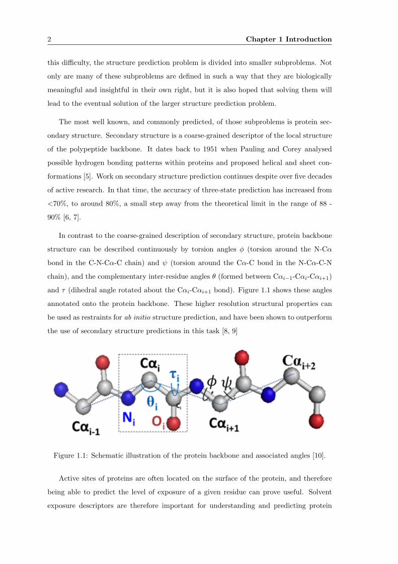
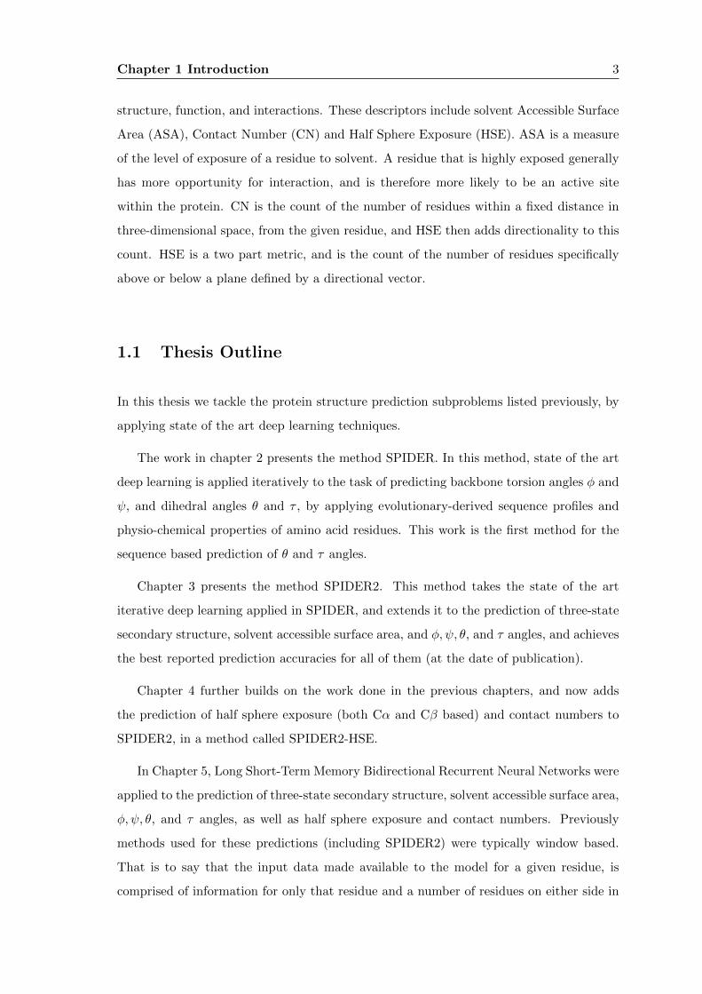
In contrast to the coarse-grained description of secondary structure, protein backbone
structure can be described continuously by torsion angles φ (torsion around the N-Cα
bond in the C-N-Cα-C chain) and ψ (torsion around the Cα-C bond in the N-Cα-C-N
chain), and the complementary inter-residue angles θ (formed between Cαi−1-Cαi-Cαi+1)
and τ (dihedral angle rotated about the Cαi-Cαi+1 bond). Figure 1.1 shows these angles
annotated onto the protein backbone. These higher resolution structural properties can
be used as restraints for ab initio structure prediction, and have been shown to outperform
the use of secondary structure predictions in this task [8, 9]
Figure 1.1: Schematic illustration of the protein backbone and associated angles [10].
Active sites of proteins are often located on the surface of the protein, and therefore
being able to predict the level of exposure of a given residue can prove useful. Solvent
exposure descriptors are therefore important for understanding and predicting protein
Chapter 1 Introduction 3
structure, function, and interactions. These descriptors include solvent Accessible Surface
Area (ASA), Contact Number (CN) and Half Sphere Exposure (HSE). ASA is a measure
of the level of exposure of a residue to solvent. A residue that is highly exposed generally
has more opportunity for interaction, and is therefore more likely to be an active site
within the protein. CN is the count of the number of residues within a fixed distance in
three-dimensional space, from the given residue, and HSE then adds directionality to this
count. HSE is a two part metric, and is the count of the number of residues specifically
above or below a plane defined by a directional vector.
1.1 Thesis Outline
In this thesis we tackle the protein structure prediction subproblems listed previously, by
applying state of the art deep learning techniques.
The work in chapter 2 presents the method SPIDER. In this method, state of the art
deep learning is applied iteratively to the task of predicting backbone torsion angles φ and
ψ, and dihedral angles θ and τ , by applying evolutionary-derived sequence profiles and
physio-chemical properties of amino acid residues. This work is the first method for the
sequence based prediction of θ and τ angles.
Chapter 3 presents the method SPIDER2. This method takes the state of the art
iterative deep learning applied in SPIDER, and extends it to the prediction of three-state
secondary structure, solvent accessible surface area, and φ, ψ, θ, and τ angles, and achieves
the best reported prediction accuracies for all of them (at the date of publication).
Chapter 4 further builds on the work done in the previous chapters, and now adds
the prediction of half sphere exposure (both Cα and Cβ based) and contact numbers to
SPIDER2, in a method called SPIDER2-HSE.
In Chapter 5, Long Short-Term Memory Bidirectional Recurrent Neural Networks were
applied to the prediction of three-state secondary structure, solvent accessible surface area,
φ, ψ, θ, and τ angles, as well as half sphere exposure and contact numbers. Previously
methods used for these predictions (including SPIDER2) were typically window based.
That is to say that the input data made available to the model for a given residue, is
comprised of information for only that residue and a number of residues on either side in
4 Chapter 1 Introduction
the sequence (in the range of 10-20 residues on each side). The use of LSTM-BRNNs in
this method allows SPIDER3 to better learn both long and short term interactions within
proteins. This advancement again lead to the best reported accuracies for all predicted
structural properties.
In Chapter 6, the LSTM-BRNN model used in SPIDER3 is applied to the prediction
of the same structural property predictions, plus the prediction of eight-state secondary
structure, using only single-sequence inputs. That is, structural properties were predicted
without using any evolutionary information. This provides a method that provides not
only the best reported single-sequence secondary structure and solvent accessible surface
area predictions, but the first reported method for the single-sequence based prediction of
half sphere exposure, contact numbers, and φ, ψ, θ, and τ angles. This study is important
as most proteins have few homologous sequences and their evolutionary profiles are inac-
curate and time-consuming to calculate. This single-sequence-based technique allows for
fast genome-scale screening analysis of protein one-dimensional structural properties.
1.2 Research Contributions
The research reported in this thesis (in order of chapters) appeared in the following pub-
lications
J. Lyons, A. Dehzangi, R. Heffernan, A. Sharma, K. Paliwal, A. Sattar, Y. Zhou, and Y. Yang,
“Predicting backbone Cα angles and dihedrals from protein sequences by stacked sparse auto-
encoder deep neural network,” Journal of Computational Chemistry, vol. 35, no. 28, pp. 2040–
2046, 2014.
R. Heffernan, K. Paliwal, J. Lyons, A. Dehzangi, A. Sharma, J. Wang, A. Sattar, Y. Yang,
and Y. Zhou, “Improving prediction of secondary structure, local backbone angles, and solvent
accessible surface area of proteins by iterative deep learning,” Scientific Reports, vol. 5, no. 11476,
p. 11476, 2015.
R. Heffernan, A. Dehzangi, J. Lyons, K. Paliwal, A. Sharma, J. Wang, A. Sattar, Y. Zhou,
and Y. Yang, “Highly accurate sequence-based prediction of half-sphere exposures of amino acid
residues in proteins,” Bioinformatics, vol. 32, no. 6, pp. 843–849, 2016.
R. Heffernan, Y. Yang, K. Paliwal, and Y. Zhou, “Capturing non-local interactions by long
short-term memory bidirectional recurrent neural networks for improving prediction of protein
Chapter 1 Introduction 5
secondary structure, backbone angles, contact numbers and solvent accessibility,” Bioinformatics,
vol. 33, no. 18, pp. 2842–2849, 2017.
R. Heffernan, K. Paliwal, J. Lyons, J. Singh, Y. Yang, and Y. Zhou, “Single-sequence-based pre-
diction of protein secondary structures and solvent accessibility by deep whole-sequence learning,”
Journal of Computational Chemistry, vol. 0, no. 0, pp. 1–7, 2018.
The publications resulting from the PhD that are not included in the scope of this
thesis are
A. Dehzangi, R. Heffernan , A. Sharma, J. Lyons, K. Paliwal, and A. Sattar, “Gram-positive and
gram-negative protein subcellular localization by incorporating evolutionary-based descriptors
into chous general pseaac,” Journal of Theoretical Biology, vol. 364, pp. 284 – 294, 2015.
K. Paliwal, J. Lyons, and R. Heffernan, “A short review of deep learning neural networks in
protein structure prediction problems,” Advanced Techniques in Biology & Medicine, pp. 1–2,
2015.
J. Lyons, A. Dehzangi, R. Heffernan, Y. Yang, Y. Zhou, A. Sharma, and K. Paliwal, “Advancing
the accuracy of protein fold recognition by utilizing profiles from hidden markov models,” IEEE
Transactions on NanoBioscience, vol. 14, no. 7, pp. 761–772, 2015.
A. Dehzangi, S. Sohrabi, R. Heffernan, A. Sharma, J. Lyons, K. Paliwal, and A. Sattar, “Gram-
positive and gram-negative subcellular localization using rotation forest and physicochemical-
based features,” BMC Bioinformatics, vol. 16, no. 4, p. S1, 2015.
J. Lyons, K. Paliwal, A. Dehzangi, R. Heffernan, T. Tsunoda, and A. Sharma, “Protein fold
recognition using hmmhmm alignment and dynamic programming,” Journal of Theoretical Biol-
ogy, vol. 393, pp. 67 – 74, 2016.
Y. Yang, R. Heffernan, K. Paliwal, J. Lyons, A. Dehzangi, A. Sharma, J. Wang, A. Sattar,
and Y. Zhou, SPIDER2: A Package to Predict Secondary Structure, Accessible Surface Area, and
Main-Chain Torsional Angles by Deep Neural Networks, pp. 55–63. New York, NY: Springer New
York, 2017.
Y. Yang, J. Gao, J. Wang, R. Heffernan, J. Hanson, K. Paliwal, and Y. Zhou, “Sixty-five
years of long march in protein secondary structure prediction: the final stretch?,” Briefings in
Bioinformatics, 2017.
J. O’Connell, Z. Li, J. Hanson, R. Heffernan, J. Lyons, K. Paliwal, A. Dehzangi, Y. Yang,
and Y. Zhou, “SPIN2: Predicting sequence profiles from protein structures using deep neural
networks,” Proteins: Structure, Function, and Bioinformatics, vol. 86, no. 6, pp. 629–633, 2018.

6 Chapter 1 Introduction
References
[1] D. Benson, K. Clark, I. Karsch-Mizrachi, D. Lipman, J. Ostell, and E. Sayers, “Gen-
bank,” Nucleic Acids Research, vol. 42, no. D1, pp. D32–D37, 2014.
[2] T. Terwilliger, D. Stuart, and S. Yokoyama, “Lessons from structural genomics,”
Annual Review of Biophysics, vol. 38, pp. 371–383, 2009.
[3] K. Gibson and H. Scheraga, “Minimization of polypeptide energy. I. Preliminary
structures of bovine pancreatic ribonuclease S-peptide,” Proceedings of the National
Academy of Sciences, vol. 58, no. 2, pp. 420–427, 1967.
[4] Y. Zhou, Y. Duan, Y. Yang, E. Faraggi, and H. Lei, “Trends in template/fragment-
free protein structure prediction,” Theoretical Chemistry Accounts, vol. 128, no. 1,
pp. 3–16, 2011.
[5] L. Pauling, R. Corey, and H. Branson, “The structure of proteins: two hydrogen-
bonded helical configurations of the polypeptide chain,” Proceedings of the National
Academy of Sciences, vol. 37, no. 4, pp. 205–211, 1951.
[6] B. Rost, “Review: protein secondary structure prediction continues to rise,” Journal
of Structural Biology, vol. 134, no. 2, pp. 204–218, 2001.
[7] Y. Yang, J. Gao, J. Wang, R. Heffernan, J. Hanson, K. Paliwal, and Y. Zhou, “Sixty-
five years of long march in protein secondary structure prediction: the final stretch?,”
Briefings in Bioinformatics, 2016.
[8] E. Faraggi, B. Xue, and Y. Zhou, “Improving the prediction accuracy of residue
solvent accessibility and real-value backbone torsion angles of proteins by guided-
learning through a two-layer neural network,” Proteins: Structure, Function, and
Bioinformatics, vol. 74, no. 4, pp. 847–856, 2009.
7

8 REFERENCES
[9] K. Simons, I. Ruczinski, C. Kooperberg, B. Fox, C. Bystroff, and D. Baker, “Im-
proved recognition of native-like protein structures using a combination of sequence-
dependent and sequence-independent features of proteins,” Proteins: Structure, Func-
tion, and Bioinformatics, vol. 34, no. 1, pp. 82–95, 1999.
[10] J. Lyons, A. Dehzangi, R. Heffernan, A. Sharma, K. Paliwal, A. Sattar, Y. Zhou, and
Y. Yang, “Predicting backbone Cα angles and dihedrals from protein sequences by
stacked sparse auto-encoder deep neural network,” J. Comput. Chem., vol. 35, no. 28,
pp. 2040–2046, 2014.
Chapter 2
SPIDER - Predicting Backbone
Cα Angles and Dihedrals from
Protein Sequences by Stacked
Sparse Auto-Encoder Deep Neural
Network
9

STATEMENT OF CONTRIBUTION TO CO-AUTHORED PUBLISHED PAPER
This chapter includes a co-authored paper. The bibliographic details of the co-authored paper, including all authors, are:
J. Lyons, A. Dehzangi, R. Heffernan, A. Sharma, K. Paliwal, A. Sattar, Y. Zhou, and Y.Yang, “Predicting backbone Cα angles and dihedrals from protein sequences bystacked sparse auto-encoder deep neural network,” Journal of ComputationalChemistry, vol. 35, no. 28, pp. 2040–2046, 2014.
My contribution to the paper involved:
Most of the computer programming and analysis of results. Co-wrote the manuscript.
(Signed) _________________________________ (Date)______________Rhys Heffernan
(Countersigned) ___________________________ (Date)______________Corresponding author of paper: Yaoqi Zhou
(Countersigned) ___________________________ (Date)______________Supervisor: Kuldip Paliwal
Predicting Backbone Ca Angles and Dihedralsfrom Protein Sequences by Stacked SparseAuto-Encoder Deep Neural Network
James Lyons,[a] Abdollah Dehzangi,[a,b] Rhys Heffernan,[a] Alok Sharma,[a,c]
Kuldip Paliwal,[a] Abdul Sattar,[a,b] Yaoqi Zhou,*[d] and Yuedong Yang*[d]
Because a nearly constant distance between two neighbouring
Ca atoms, local backbone structure of proteins can be repre-
sented accurately by the angle between Cai21ACaiACai11 (h)
and a dihedral angle rotated about the CaiACai11 bond (s). hand s angles, as the representative of structural properties of
three to four amino-acid residues, offer a description of back-
bone conformations that is complementary to u and w angles
(single residue) and secondary structures (>3 residues). Here,
we report the first machine-learning technique for sequence-
based prediction of h and s angles. Predicted angles based on
an independent test have a mean absolute error of 9� for h and
34� for s with a distribution on the h-s plane close to that of
native values. The average root-mean-square distance of 10-
residue fragment structures constructed from predicted h and sangles is only 1.9A from their corresponding native structures.
Predicted h and s angles are expected to be complementary to
predicted / and w angles and secondary structures for using in
model validation and template-based as well as template-free
structure prediction. The deep neural network learning tech-
nique is available as an on-line server called Structural Property
prediction with Integrated DEep neuRal network (SPIDER) at
http://sparks-lab.org. VC 2014 Wiley Periodicals, Inc.
DOI: 10.1002/jcc.23718
Introduction
Template-based and template-free protein-structure prediction
relies strongly on prediction of local backbone structures.[1,2]
Protein local structure prediction is dominated by secondary
structure prediction with its accuracy stagnant around 80% for
more than a decade.[3,4] However, secondary structures are
only a coarse-grained description of protein local structures in
three states (helices, sheets, and coils) that are somewhat arbi-
trarily defined because helices and sheets are often not in
their ideal shapes in protein structures. This arbitrariness has
limited the theoretically achievable accuracy of three-state pre-
diction to 88–90%.[4,5] Moreover, predicted coil residues do not
have a well-defined structure.
An alternative approach to characterize the local backbone
structure of a protein is to use three dihedral or rotational
angles about the NACa bond (u), the CaAC bond (w), and the
CAN bond (x). A schematic illustration is shown in Figure 1.
Because x angles are restricted to 180� (the majority) or 0�
due to rigid planar peptide bonds, two dihedral angles (/ and
w) essentially determine the overall backbone structure. Unlike
secondary structures, these dihedral angles (/ and w) can be
predicted as continuous variables and their predicted accuracy
has been improved over the years[6–8] so that it is closer to
dihedral angles estimated according to NMR chemical shifts.[9]
Predicted backbone dihedral angles were found to be more
useful than predicted secondary structure as restrains for ab
initio structure prediction.[9,10] It has also been utilized for
improving sequence alignment,[11] secondary structure predic-
tion,[3,12,13] and template-based structure prediction and fold
recognition.[14–16] However, unlike the secondary structure of
proteins, u and w are limited to the conformation of a single
residue.
Two different angles can also be used for representing pro-
tein backbones. As shown in Figure 1, they are the angle
between Cai21ACaiACai11 (hi) and a dihedral angle rotated
about the CaiACai11 bond (si). This two-angle representation
is possible because neighbouring Ca atoms mostly have a
fixed distance (3.8A) due to the fixed plane in
Cai21ACANACai. These two inter-residue angles (h and s)
reflect the conformation of four connected, neighbouring resi-
dues that is longer than a single-residue conformation repre-
sented by u and w angles. By comparison, a conformation
represented by helical or sheet residues involves in an
[a] J. Lyons, A. Dehzangi, R. Heffernan, A. Sharma,
K. Paliwal, A. Sattar
Institute for Integrated and Intelligent Systems, Griffith University, Brisbane,
Australia
[b] A. Dehzangi, A. Sattar
National ICT Australia (NICTA), Brisbane, Australia
[c] A. Sharma
School of Engineering and Physics, University of the South Pacific, Private
Mail Bag, Laucala Campus, Suva, Fiji
[d] Y. Zhou, Y. Yang
Institute for Glycomics and School of Information and Communication
Technique, Griffith University, Parklands Dr. Southport, QLD 4222,
Australia.
E-mail: [email protected] or [email protected]
Contract/grant sponsor: National Health and Medical Research Council of
Australia (to Y.Z.); contract/grant number: 1059775
VC 2014 Wiley Periodicals, Inc.
2040 Journal of Computational Chemistry 2014, 35, 2040–2046 WWW.CHEMISTRYVIEWS.COM
FULL PAPER WWW.C-CHEM.ORG
undefined number of residues (4 for 310 helix, 5 for a-helix,
and an undefined number of residues for sheet residues).
Thus, secondary structure, //w and h/s provide complimentary
local structural information along the backbone. Indeed, both
predicted //w and secondary structure are useful for
template-based structure prediction.[14]
In this article, we will develop the first machine-learning
technique to predict h and s from protein sequences. This tool
is needed not only because these two angles yield local struc-
tural information complementary to secondary structure and
//w angles but also because they have been widely used in
coarse-grained models for protein dynamics,[17] folding,[18]
structure prediction,[19,20] conformational analysis,[21] and
model validation.[22] That is, accurate prediction of h and s will
be useful for template or template-free structure prediction as
well as validation of predicted models. Using 4590 proteins for
training and cross validation and 1199 proteins for an inde-
pendent test, we have developed a deep-learning neural-net-
work-based method that achieved h and s angles within 9 and
34 degrees, in average, of their native values.
Method
Datasets
In this study, we obtained a dataset of 5840 proteins with less
than 25% sequence identity and X-ray resolution better than
2 A from the protein sequence culling server PISCES.[23] After
removing 51 proteins with obsolete IDs or missing data, the
final dataset consists of 5789 proteins with 1,246,420 residues.
We randomly selected 4590 proteins from this dataset for
training and cross-validation (TR4590) and used the remaining
1199 proteins for an independent test (TS1199).
Deep neural-network learning
An Artificial Neural Network (ANN) consists of highly intercon-
nected, multilayer processing units called neurons. Each neu-
ron combines its inputs with a nonlinear sigmoid activation
function to produce an output. Deep neural networks refer to
feed-forward ANNs with three or more hidden layers. Multi-
layer networks were not widely used because of the difficulty
to train neural-network weights. This has changed due to
recent advances through unsupervised weight initialization,
followed by fine-tuned supervised training.[24,25] In this study,
unsupervised weight initialization was done by stacked sparse
auto-encoder. A stacked auto-encoder treats each layer as an
auto-encoder that maps the layer’s inputs back to themselves.
During training auto-encoders a sparsity penalty was utilized
to prevent learning of the identity function.[26] Initialised
weights were then refined by standard back propagation. The
stacked sparse auto-encoder used in this study consists of
three hidden layers with 150 hidden nodes in each layer
(Fig. 2). The input data was normalised so that each feature is
in the range of 0 to 1. For residues near the ends of a protein,
the features of the amino acid residue at the other end of the
protein were duplicated so that a full window could be used.
The learning rate was initialised to start at 0.5 and was then
decreased as training progressed. In this study, we used the
deep neural network MATLAB toolbox implemented by
Palm.[27]
Input features
Each amino acid was described by a vector of input features
that include 20 values from the Position Specific Scoring
Matrix generated by PSI-BLAST[28] with three iterations of
searching against nonredundant sequence database with an E-
value cut off of 0.001. We also used seven representative
amino-acid properties: a steric parameter (graph shape index),
hydrophobicity, volume, polarizability, isoelectric point, helix
probability, and sheet probability.[29] In addition, we used pre-
dicted secondary structures (three probability values for helix,
sheet, and coils) and predicted solvent accessible surface area
(one value) from SPINE-X.[3] That is, this is a vector of 31
dimensions per amino acid residue. As before, we also used a
window size of 21 amino acids (10 amino acids at each side of
the target amino acid). This led to a total of 651 input features
(21 3 31) for a given amino acid residue.
Output
Here, we attempt to predict two angles. One is h, the angle
between three consecutive Ca atoms of a protein backbone.
The other one is s, the dihedral angle between four consecu-
tive Ca atoms of protein backbone. Two angles are predicted
at the same time. To remove the effect of periodicity, we used
four output nodes that correspond to Sin(h), Cos(h), Sin(s), and
Cos(s), respectively. Predicted sine and cosine values were con-
verted back to angles by using h5tan21½sin hð Þ=cos hð Þ� and
s5tan21½sin sð Þ=cos sð Þ�. Such transformation is widely used in
signal processing and speech recognition.[30]
Figure 1. The schematic illustration of the protein backbone and associated
angles. [Color figure can be viewed in the online issue, which is available
at wileyonlinelibrary.com.]
Figure 2. The general architecture of the stacked sparse auto-encoder
deep neural network. Four output nodes are Sin(h), Cos(h), Sin(s), and
Cos(s), respectively. [Color figure can be viewed in the online issue, which
is available at wileyonlinelibrary.com.]
FULL PAPERWWW.C-CHEM.ORG
Journal of Computational Chemistry 2014, 35, 2040–2046 2041
Evaluation methods
We investigated the effectiveness of our proposed method
using tenfold cross validation (TR4590) and independent test
sets (TS1199). In tenfold cross validation, TR4590 was divided
into 10 groups. Nine groups were used as a training dataset
while the remaining group was used for test. This process was
repeated 10 times until all the 10 groups were used once as
the test dataset. In addition to tenfold cross validation, TR4590
was used as the training set and TS1199 was used as an inde-
pendent test set. Comparison between tenfold cross validation
and the test gives an indicator for the generality of the predic-
tion tool. We evaluated the accuracy of our prediction by
mean absolute error (MAE), the average absolute difference
between predicted and experimentally determined angles. The
periodicity of s angles was taken care of by utilizing the
smaller value of the absolute difference di ð5jsPredi 2sExpt
i jÞ and
3602di for average.
Result
Table 1 compares the results of tenfold cross validation based
on TR4590 and the independent test (TS1199). h angles with a
range of 0 to 180� were predicted significantly more accurate
than s angles with a range of 2180� to 180�. The MAE is <9�
for h but 33–34� for s. This level of accuracy can be compared
to the baseline MAE values of 18.8� for h and 86.2� for s if hand s are assigned randomly according to their respective dis-
tributions. Accuracy for angles differs significantly in secondary
structure types. The angles for helical residues have the high-
est accuracy (MAE<5� for h and 17� for s. The MAE for sheet
residues is about twice larger than that for helical residues.
Angles for coil residues have the largest error (s in particular).
Different levels of accuracy in different secondary structural
types reflect the fact that helical structures are more locally
stabilized than sheet structures while coil residues do not have
a well-defined conformation. Similar trends were observed for
prediction of backbone / and w angles.[6–9] We also noted
that MAEs from tenfold cross validation and from the inde-
pendent test are essentially the same. This indicates the
robustness of the method trained. Thus, here and hereafter,
we will present the result based on the independent test only.
Actual and predicted distributions of h and s for TS1199 are
shown in Figure 3. Predicted and actual distributions agree
with each other very well. Both predicted and actual peaks for
h angles are located at 92� and 119�, respectively. Actual peaks
for s angles are also in good agreement with those predicted
ones at 50� and 2164�, respectively. Predicted peaks, however,
are slightly narrowly than native peaks for all cases. Predicted
and actual angle distributions also agree in a two-dimensional
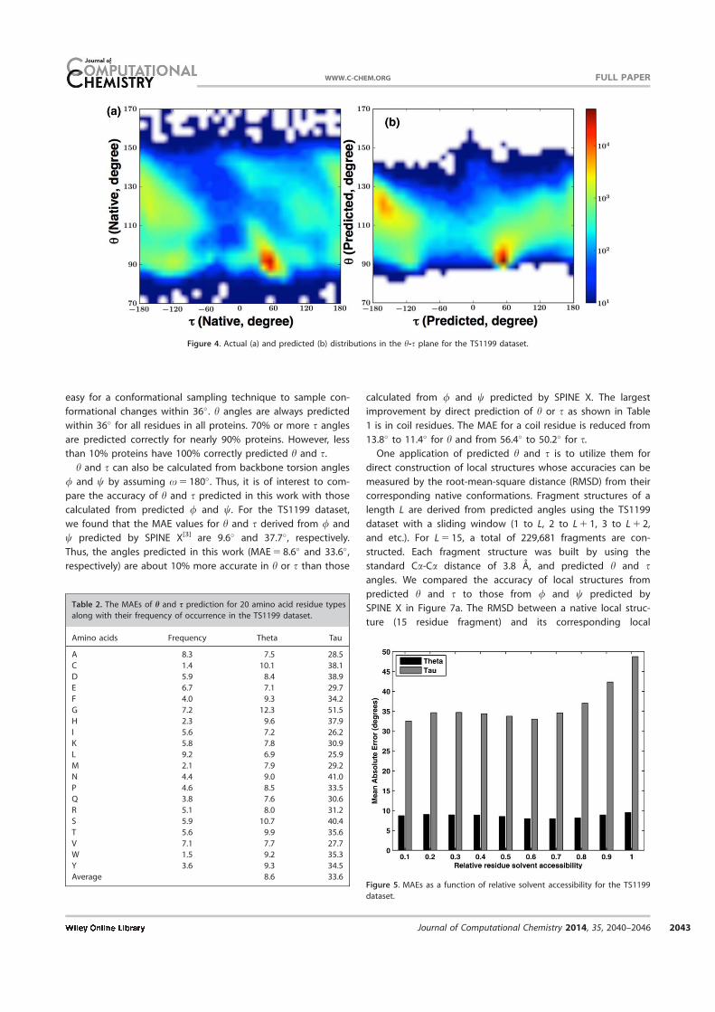
plane of h and s in Figure 4, the locations of three major popu-
lations were well captured by predicted distributions.
Table 2 lists the MAEs for 20 individual residue types along
with their frequencies of occurrence in the TS1199 dataset.
Glycine (G) has the largest MAE, corresponding to the fact that
it is the most flexible residue due to lack of a side chain. Leu-
cine (L), has the smallest MAE and interestingly also the most
frequently occurred residue (9.2%). The angles for several other
small hydrophobic residues [isoleucine (I), valine (V), and ala-
nine (A)] are also in the pack of residues with smallest errors.
There is no strong correlation between the MAE of an amino
acid residue type and its frequency of occurrence.
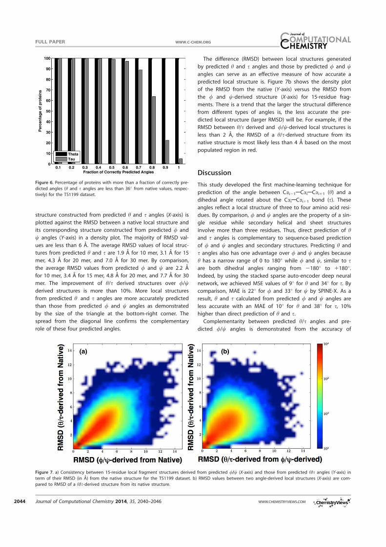
In Figure 5, MAEs for predicted angles are shown as a func-
tion of relative solvent accessible surface area. MAEs for h and
s have similar trend: two peaks separated by a valley (although
in a smaller magnitude for h). Both angles have the highest
accuracy (the smallest error) at an intermediate range of sol-
vent accessibility and the lowest accuracy (the largest error) at
90–100% solvent accessibility. The lowest accuracy at 90–100%
solvent accessibility is likely due to the smallest number of res-
idues at 90–100% solvent-accessible and 20% more coil resi-
dues in fully exposed residues.[3]
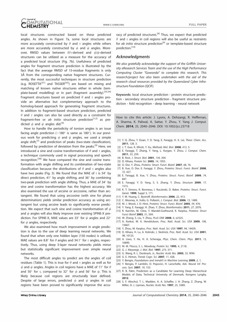
Figure 6 displays the fraction of proteins with more than a
given fraction of correctly predicted angles (h and s). Here, a
correct prediction is defined as 36� or less from the actual
angle. We use 36� as a cut off value because it is relatively
Table 1. Performance of h and s angle prediction based on the MAE as
compared to h and s angles calculated from / and w angles predicted
by SPINE-X for two datasets (tenfold cross validation for TR4590 and
independent test for TS1199).
MAE TR4590(�) TS1199(�)
TS1199(�)from
predicted / and w
h2All 8.57 6 0.01 8.6 9.6
h2Helix 4.50 6 0.02 4.5 4.5
h2Sheet 10.45 6 0.02 10.6 11.3
h2Coil 11.437 6 0.01 11.4 13.8
s 33.4 6 0.3 33.6 37.7
s2Helix 17.1 6 0.9 16.9 17.8
s2Sheet 32.4 6 0.1 33.1 39.1
s2Coil 50.1 6 0.3 50.2 56.4
Figure 3. Predicted and actual distributions of h (a) and s (b) angles for the
TS1199 dataset.
FULL PAPER WWW.C-CHEM.ORG
2042 Journal of Computational Chemistry 2014, 35, 2040–2046 WWW.CHEMISTRYVIEWS.COM
easy for a conformational sampling technique to sample con-
formational changes within 36�. h angles are always predicted
within 36� for all residues in all proteins. 70% or more s angles
are predicted correctly for nearly 90% proteins. However, less
than 10% proteins have 100% correctly predicted h and s.
h and s can also be calculated from backbone torsion angles
/ and w by assuming x 5 180�. Thus, it is of interest to com-
pare the accuracy of h and s predicted in this work with those
calculated from predicted / and w. For the TS1199 dataset,
we found that the MAE values for h and s derived from / and
w predicted by SPINE X[3] are 9.6� and 37.7�, respectively.
Thus, the angles predicted in this work (MAE 5 8.6� and 33.6�,
respectively) are about 10% more accurate in h or s than those
calculated from / and w predicted by SPINE X. The largest
improvement by direct prediction of h or s as shown in Table
1 is in coil residues. The MAE for a coil residue is reduced from
13.8� to 11.4� for h and from 56.4� to 50.2� for s.
One application of predicted h and s is to utilize them for
direct construction of local structures whose accuracies can be
measured by the root-mean-square distance (RMSD) from their
corresponding native conformations. Fragment structures of a
length L are derived from predicted angles using the TS1199
dataset with a sliding window (1 to L, 2 to L 1 1, 3 to L 1 2,
and etc.). For L 5 15, a total of 229,681 fragments are con-
structed. Each fragment structure was built by using the
standard Ca-Ca distance of 3.8 A, and predicted h and sangles. We compared the accuracy of local structures from
predicted h and s to those from / and w predicted by
SPINE X in Figure 7a. The RMSD between a native local struc-
ture (15 residue fragment) and its corresponding local
Figure 4. Actual (a) and predicted (b) distributions in the h-s plane for the TS1199 dataset.
Table 2. The MAEs of h and s prediction for 20 amino acid residue types
along with their frequency of occurrence in the TS1199 dataset.
Amino acids Frequency Theta Tau
A 8.3 7.5 28.5
C 1.4 10.1 38.1
D 5.9 8.4 38.9
E 6.7 7.1 29.7
F 4.0 9.3 34.2
G 7.2 12.3 51.5
H 2.3 9.6 37.9
I 5.6 7.2 26.2
K 5.8 7.8 30.9
L 9.2 6.9 25.9
M 2.1 7.9 29.2
N 4.4 9.0 41.0
P 4.6 8.5 33.5
Q 3.8 7.6 30.6
R 5.1 8.0 31.2
S 5.9 10.7 40.4
T 5.6 9.9 35.6
V 7.1 7.7 27.7
W 1.5 9.2 35.3
Y 3.6 9.3 34.5
Average 8.6 33.6Figure 5. MAEs as a function of relative solvent accessibility for the TS1199
dataset.
FULL PAPERWWW.C-CHEM.ORG
Journal of Computational Chemistry 2014, 35, 2040–2046 2043
structure constructed from predicted h and s angles (X-axis) is
plotted against the RMSD between a native local structure and
its corresponding structure constructed from predicted / and
w angles (Y-axis) in a density plot. The majority of RMSD val-
ues are less than 6 A. The average RMSD values of local struc-
tures from predicted h and s are 1.9 A for 10 mer, 3.1 A for 15
mer, 4.3 A for 20 mer, and 7.0 A for 30 mer. By comparison,
the average RMSD values from predicted / and w are 2.2 A
for 10 mer, 3.4 A for 15 mer, 4.8 A for 20 mer, and 7.7 A for 30
mer. The improvement of h/s derived structures over //wderived structures is more than 10%. More local structures
from predicted h and s angles are more accurately predicted
than those from predicted / and w angles as demonstrated
by the size of the triangle at the bottom-right corner. The
spread from the diagonal line confirms the complementary
role of these four predicted angles.
The difference (RMSD) between local structures generated
by predicted h and s angles and those by predicted / and wangles can serve as an effective measure of how accurate a
predicted local structure is. Figure 7b shows the density plot
of the RMSD from the native (Y-axis) versus the RMSD from
the / and w-derived structure (X-axis) for 15-residue frag-
ments. There is a trend that the larger the structural difference
from different types of angles is, the less accurate the pre-
dicted local structure (larger RMSD) will be. For example, if the
RMSD between h/s derived and //w-derived local structures is
less than 2 A, the RMSD of a h/s-derived structure from its
native structure is most likely less than 4 A based on the most
populated region in red.
Discussion
This study developed the first machine-learning technique for
prediction of the angle between Cai21ACaiACai11 (h) and a
dihedral angle rotated about the CaiACai11 bond (s). These
angles reflect a local structure of three to four amino acid resi-
dues. By comparison, / and w angles are the property of a sin-
gle residue while secondary helical and sheet structures
involve more than three residues. Thus, direct prediction of hand s angles is complementary to sequence-based prediction
of / and w angles and secondary structures. Predicting h and
s angles also has one advantage over / and w angles because
h has a narrow range of 0 to 180� while / and w, similar to sare both dihedral angles ranging from 2180� to 1180�.
Indeed, by using the stacked sparse auto-encoder deep neural
network, we achieved MSE values of 9� for h and 34� for s. By
comparison, MAE is 22� for / and 33� for w by SPINE-X. As a
result, h and s calculated from predicted / and w angles are
less accurate with an MAE of 10� for h and 38� for s, 10%
higher than direct prediction of h and s.
Complementarity between predicted h/s angles and pre-
dicted //w angles is demonstrated from the accuracy of
Figure 6. Percentage of proteins with more than a fraction of correctly pre-
dicted angles (h and s angles are less than 36� from native values, respec-
tively) for the TS1199 dataset.
Figure 7. a) Consistency between 15-residue local fragment structures derived from predicted //w (X-axis) and those from predicted h/s angles (Y-axis) in
term of their RMSD (in A) from the native structure for the TS1199 dataset. b) RMSD values between two angle-derived local structures (X-axis) are com-
pared to RMSD of a h/s-derived structure from its native structure.
FULL PAPER WWW.C-CHEM.ORG
2044 Journal of Computational Chemistry 2014, 35, 2040–2046 WWW.CHEMISTRYVIEWS.COM
local structures constructed based on these predicted
angles. As shown in Figure 7a, some local structures are
more accurately constructed by h and s angles while others
are more accurately constructed by / and w angles. More-
over, RMSD values between h/s-derived and //w-derived
structures can be utilized as a measure for the accuracy of
a predicted local structure (Fig. 7b). Usefulness of predicted
angles for fragment structure prediction is illustrated by the
fact that the average RMSD of 15-residue fragments is only
3A from the corresponding native fragment structures. Cur-
rently, the most successful techniques in structure prediction
(e.g. ROSETTA[31] and TASSER[32]) are based on mixing and
matching of known native structures either in whole (tem-
plate-based modelling) or in part (fragment assembly).[33,34]
Fragment structures based on predicted h and s angles pro-
vide an alternative but complementary approach to the
homolog-based approach for generating fragment structures.
In addition to fragment-based structure prediction, predicted
h and s angles can also be used directly as a constraint for
fragment-free or ab initio structure prediction[1,2] as pre-
dicted / and w angles did.[9]
How to handle the periodicity of torsion angles is an issue
facing angle prediction (2180� is same as 180�). In our previ-
ous work for predicting / and w angles, we used a simple
angle shift,[7] and prediction of peaks (two-state classification),
followed by prediction of deviation from the peaks.[9] Here, we
introduced a sine and cosine transformation of h and s angles,
a technique commonly used in signal processing and speech
recognition.[30] We have compared the sine and cosine trans-
formation with angle shifting and its combination of two-state
classification because the distributions of h and s angles also
have two peaks (Fig. 3). We found that the MAE of s is 54� by
direct prediction, 41� by angle shifting, and 36� by combining
two-peak prediction with angle shifting. Thus, a MAE of 34� by
sine and cosine transformation has the highest accuracy. We
also examined the use of arcsine or arccosine, rather than arc-
tangent. We found that using arccosine (with sine for phase
determination) yields similar prediction accuracy as using arc-
tangent but using arcsine leads to significantly worse predic-
tion. We expect that such sine and cosine transformation of /and w angles will also likely improve over existing SPINE-X pre-
diction. For SPINE-X, MAE values are 33� for w angles and 22�
for / angles, respectively.
We also examined how much improvement in angle predic-
tion is due to the use of deep learning neural networks. We
found that when only one hidden layer (150 nodes) is utilised,
MAE values are 8.8� for h angles and 34.1� for s angles, respec-
tively. Thus, using deep 3-layer neural networks yields minor
but statistically significant improvement over simple neural
networks.
The most difficult angles to predict are the angles of coil
residues (Table 1). This is true for h and s angles as well as for
/ and w angles. Angles in coil regions have a MAE of 11� for hand 50� for s, compared to 32� for / and 56� for w. This is
likely because coil regions are structurally least defined.
Despite of large errors, predicted / and w angles in coil
regions have been proved to significantly improve the accu-
racy of predicted structures.[9] Thus, we expect that predicted
h and s angles in coil regions will also be useful as restraints
for ab initio structure prediction[9] or template-based structure
prediction.[14]
Acknowledgments
We also gratefully acknowledge the support of the Griffith Univer-
sity eResearch Services Team and the use of the High Performance
Computing Cluster "Gowonda" to complete this research. This
research/project has also been undertaken with the aid of the
research cloud resources provided by the Queensland Cyber Infra-
structure Foundation (QCIF).
Keywords: local structure prediction � protein structure predic-
tion � secondary structure prediction � fragment structure pre-
diction � fold recognition � deep learning � neural network
How to cite this article: J. Lyons, A. Dehzangi, R. Heffernan,
A. Sharma, K. Paliwal, A. Sattar, Y. Zhou, Y. Yang J. Comput.
Chem. 2014, 35, 2040–2046. DOI: 10.1002/jcc.23718
[1] Y. Q. Zhou, Y. Duan, Y. D. Yang, E. Faraggi, H. X. Lei, Theor. Chem. Acc.
2011, 128, 3.
[2] J. T. Guo, K. Ellrott, Y. Xu, Methods Mol. Biol. 2008, 413, 3.
[3] E. Faraggi, T. Zhang, Y. Yang, L. Kurgan, Y. Zhou, J. Comput. Chem.
2011, 33, 259.
[4] B. Rost, J. Struct. Biol. 2001, 134, 204.
[5] D. Kihara, Protein Sci. 2005, 14, 1955.
[6] O. Dor, Y. Zhou, Proteins: Struct. Funct. Bioinf. 2007, 68, 76.
[7] B. Xue, O. Dor, E. Faraggi, Y. Zhou, Proteins: Struct. Funct. Bioinf. 2008,
72, 427.
[8] E. Faraggi, B. Xue, Y. Zhou, Proteins: Struct. Funct. Bioinf. 2009, 74,
847.
[9] E. Faraggi, Y. D. Yang, S. S. Zhang, Y. Zhou, Structure 2009, 17,
1515.
[10] K. T. Simons, R. Bonneau, I. Ruczinski, D. Baker, Proteins: Struct. Funct.
Genet. 1999, Suppl 3, 171.
[11] Y. M. Huang, C. Bystroff, Bioinformatics 2006, 22, 413.
[12] C. Mooney, A. Vullo, G. Pollastri, J. Comput. Biol. 2006, 13, 1489.
[13] M. J. Wood, J. D. Hirst, Proteins: Struct. Funct. Bioinf. 2005, 59, 476.
[14] Y. Yang, E. Faraggi, H. Zhao, Y. Zhou, Bioinformatics 2011, 27, 2076.
[15] R. Karchin, M. Cline, Y. Mandel-Gutfreund, K. Karplus, Proteins: Struct
Funct Bioinf 2003, 51, 504.
[16] W. Zhang, S. Liu, Y. Zhou, PLoS ONE 2008, 6, e2325.
[17] A. Korkut, W. A. Hendrickson, Proc. Natl. Acad. Sci. USA 2009, 106,
15667.
[18] Y. Zhou, M. Karplus, Proc. Natl. Acad. Sci. USA 1997, 94, 14429.
[19] D. Kihara, H. Lu, A. Kolinski, J. Skolnick, Proc. Natl. Acad. Sci. USA 2001,
98, 10125.
[20] A. Liwo, Y. He, H. A. Scheraga, Phys. Chem. Chem. Phys. 2011, 13,
16890.
[21] M. M. Flocco, S. L. Mowbray, Protein Sci. 1995, 4, 2118.
[22] G. J. Kleywegt, J. Mol. Biol. 1997, 273, 371.
[23] G. Wang, R. L. Dunbrack, Jr., Nucleic Acids Res. 2005, 33, W94.
[24] G. E. Hinton, Trends Cogn. Sci. 2007, 11, 428.
[25] Y. Bengio, Foundations and trendsVR in Machine Learning 2009, 2, 1.
[26] Y. Bengio, P. Lamblin, D. Popovici, H. Larochelle, Adv. Neural Inf. Pro-
cess. Syst. 2007, 19, 153.
[27] R. B. Palm, Prediction as a Candidate for Learning Deep Hierarchical
Models of Data; Technical University of Denmark, Kongens Lyngby,
2012.
[28] S. F. Altschul, T. L. Madden, A. A. Schaffer, J. H. Zhang, Z. Zhang, W.
Miller, D. J. Lipman, Nucleic Acids Res. 1997, 25, 3389.
FULL PAPERWWW.C-CHEM.ORG
Journal of Computational Chemistry 2014, 35, 2040–2046 2045

[29] J. Meiler, M. M€uller, A. Zeidler, F. Schm€aschke, J. Mol. Model. 2001, 7,
360.
[30] B. Bozkurt, L. Couvreur, T. Dutoit, Speech Commun. 2007, 49, 159.
[31] K. T. Simons, C. Kooperberg, E. Huang, D. Baker, J. Mol. Biol. 1997, 268,
209.
[32] Y. Zhang, J. Skolnick, Proc. Natl. Acad. Sci. USA 2004, 101, 7594.
[33] J. M. Bujnicki, Chembiochem 2006, 7, 19.
[34] Y. Zhang, Curr. Opin. Struct. Biol. 2009, 19, 145.
Received: 5 June 2014Revised: 12 July 2014Accepted: 9 August 2014Published online on 12 September 2014
FULL PAPER WWW.C-CHEM.ORG
2046 Journal of Computational Chemistry 2014, 35, 2040–2046 WWW.CHEMISTRYVIEWS.COM

18Chapter 2 SPIDER - Predicting Backbone Cα Angles and Dihedrals from
Protein Sequences by Stacked Sparse Auto-Encoder Deep Neural Network
Chapter 3
SPIDER2 - Improving prediction
of secondary structure, local
backbone angles, and solvent
accessible surface area of proteins
by iterative deep learning
19

STATEMENT OF CONTRIBUTION TO CO-AUTHORED PUBLISHED PAPER
This chapter includes a co-authored paper. The bibliographic details of the co-authored paper, including all authors, are:
R. Heffernan, K. Paliwal, J. Lyons, A. Dehzangi, A. Sharma, J. Wang, A. Sattar, Y.Yang, and Y. Zhou, “Improving prediction of secondary structure, local backboneangles, and solvent accessible surface area of proteins by iterative deep learning,”Scientific Reports, vol. 5, no. 11476, p. 11476, 2015.
My contribution to the paper involved:
Co-designed the method. Wrote all the code for the method. Produced and co-analyised results. Co-wrote the manuscript.
(Signed) _________________________________ (Date)______________Rhys Heffernan
(Countersigned) ___________________________ (Date)______________Corresponding author of paper: Yaoqi Zhou
(Countersigned) ___________________________ (Date)______________Supervisor: Kuldip Paliwal
1Scientific RepoRts | 5:11476 | DOi: 10.1038/srep11476
www.nature.com/scientificreports
Improving prediction of secondary structure, local backbone angles, and solvent accessible surface area of proteins by iterative deep learningRhys Heffernan1, Kuldip Paliwal1, James Lyons1, Abdollah Dehzangi1,2, Alok Sharma2,3, Jihua Wang4, Abdul Sattar2,5, Yuedong Yang6 & Yaoqi Zhou4,6
Direct prediction of protein structure from sequence is a challenging problem. An effective approach is to break it up into independent sub-problems. These sub-problems such as prediction of protein secondary structure can then be solved independently. In a previous study, we found that an iterative use of predicted secondary structure and backbone torsion angles can further improve secondary structure and torsion angle prediction. In this study, we expand the iterative features to include solvent accessible surface area and backbone angles and dihedrals based on Cα atoms. By using a deep learning neural network in three iterations, we achieved 82% accuracy for secondary structure prediction, 0.76 for the correlation coefficient between predicted and actual solvent accessible surface area, 19° and 30° for mean absolute errors of backbone ϕ and ψ angles, respectively, and 8° and 32° for mean absolute errors of Cα-based θ and τ angles, respectively, for an independent test dataset of 1199 proteins. The accuracy of the method is slightly lower for 72 CASP 11 targets but much higher than those of model structures from current state-of-the-art techniques. This suggests the potentially beneficial use of these predicted properties for model assessment and ranking.
Three-dimensional structures for most proteins are determined by their one-dimensional sequences of amino acid residues. How to predict three-dimensional structures from one-dimensional sequences has been an unsolved problem for the last half century1. This problem is challenging because it demands an efficient technique to search in astronomically large conformational space and a highly accurate energy function to rank and guide the conformational search, both of which are not yet available2. As a result, it is necessary to divide the structure prediction problem into many smaller problems with the hope that solving smaller problems will ultimately lead to the solution of the big problem.
One of those smaller or sub-problems is the prediction of one-dimensional structural properties of proteins from their sequences. The most commonly predicted one-dimensional structural property of a protein is secondary structure. Secondary structure describes each amino residue in a number of discrete states3 for which three state description (helix, sheet and coil) is the most common. In recent years, there
1Signal Processing Laboratory, School of Engineering, Griffith University, Brisbane, Australia. 2Institute for Integrated and Intelligent Systems, Griffith University, Brisbane, Australia. 3School of Engineering and Physics, University of the South Pacific, Private Mail Bag, Laucala Campus, Suva, Fiji. 4Shandong Provincial Key Laboratory of Functional Macromolecular Biophysics, Dezhou University, Dezhou, Shandong, China. 5National ICT Australia (NICTA), Brisbane, Australia. 6Institute for Glycomics and School of Information and Communication Technique, Griffith University, Parklands Dr. Southport, QLD 4222, Australia. Correspondence and requests for materials should be addressed to Y.Y. (email: [email protected]) or Y.Z. (email: [email protected])
received: 04 March 2015
Accepted: 19 May 2015
Published: 22 June 2015
OPEN
www.nature.com/scientificreports/
2Scientific RepoRts | 5:11476 | DOi: 10.1038/srep11476
has been a slow but steady improvement of secondary structure prediction to above 81% when homolo-gous sequences are not utilised for training (ab initio prediction)4,5. The steady improvement is due to a combination of improved machine-learning algorithms, improved features and larger training datasets. Other methods have also been developed to go beyond 81% by including homologous sequences in train-ing6–9. Secondary structure directly predicted from sequence was shown more accurate than secondary structure of the models predicted by protein structure prediction techniques for template-free modelling targets in critical assessment of structure prediction (CASP 9)4.
Secondary structure, however, is a coarse-grained description of local backbone structure because ideal helical and strand conformations do not exist in protein structures and the boundary between coil states and helical/strand states is not well defined10. This leads to development of backbone torsion angle prediction (φ and ψ ) in discontinuous11,12 and in real, continuous values13–15. More recently, a method for predicting angles based on Cα atoms (the angle between Cα i−1− Cα i− Cα i+1 (θ ) and a dihedral angle rotated about the Cα i− Cα i+1 bond (τ)) was also developed16. These local structure descriptors are complementary with each other because torsion angles (φ and ψ ), Cα − atom based angles (θ and τ), and secondary structure involve amino acid residues at different sequence separation: neighbouring residues for φ and ψ , 3–4 residues for θ and τ, and 4 for 310 helix, 5 for α -helix, and an undefined number of residues for sheet residues.
Another important one-dimensional structure property is solvent Accessible Surface Area (ASA). ASA measures the level of exposure of an amino acid residue to solvent (water) in a protein. This is an important structural property as active sites of proteins are often located on their surfaces. Multistate prediction of earlier methods17–19 have been replaced by continuous real value prediction14,20–23.
One interesting observation is that predicted secondary structure is often utilized to predict other one-dimensional structural properties but rarely the other way around. Several studies, however, indi-cated that other predicted structural properties can be utilized to improve secondary structure predic-tion such as predicted torsion angles4,13 and predicted solvent accessible surface area24. In particular, we have shown that the accuracy of secondary structure and torsion angle prediction can be substantially improved by iteratively adding improved prediction of torsion angles and secondary structure4.
Artificial neural networks have been widely employed in predicting structural properties of proteins due to the availability of large datasets25. Deep neural networks26, referring to artificial neural networks with more than two hidden layers, have been explored in prediction of local and nonlocal structural properties of proteins27–30. For example, Qi et al.29 developed a unified multi-task, local-structure pre-dictor of proteins using deep neural networks as a classifier. They trained a single neural network using sequential and evolutionary features to predict a number of protein properties including protein sec-ondary structure and solvent accessibility. Spencer et al.30 developed an iterative deep neural network for protein secondary structure prediction. The method utilized one deep neural network to predict sec-ondary structure by using physicochemical and evolutionary information in their first step and another deep neural network to predict their final secondary structure prediction based on predicted secondary structures in addition to the same input used in the first step. These methods achieved secondary struc-ture prediction with accuracy that is slightly higher than 80%.
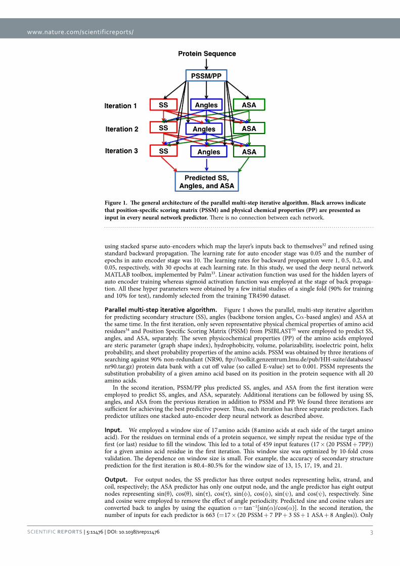
The goal of this paper is to develop an iterative method that predicts four different sets of structural properties: secondary structure, torsion angles, Cα − atom based angles and dihedral angles, and solvent accessible surface area. That is, both local and nonlocal structural information were utilized in iterations. At each iteration, a deep-learning neural network is employed to predict a structural property based on structural properties predicted in the previous iteration. We showed that all structural properties can be improved during the iteration process. The resulting method provides state-of-the-art, all-in-one accu-rate prediction of local structure and solvent accessible surface area. The method (named SPIDER2) is available as an on-line server at http://sparks-lab.org.
MethodsThis section describes the dataset employed and parametric details of the algorithm used as follows:
Datasets. We employed the same training and independent test datasets developed for the prediction of Cα based angles (θ ) and dihedral angles (τ)16. Briefly, a non-redundant (25% cutoff), high resolution (< 2.0 Å) structures of 5789 proteins were obtained from the sequence culling server PISCES31 and fol-lowed by removing obsolete structures. We then randomly selected 4590 proteins as the training set (TR4590) and the remaining 1199 proteins as an independent test (TS1199). In addition, we downloaded the targets from critical assessment of structure prediction technique (CASP 11, 2014, http://www.pre-dictioncenter.org/casp11/index.cgi). After removing the proteins with inconsistent sequences and the proteins with > 30% sequence identities between each other and to the training and test sets (TR4590 and TS1199), we obtained a set of 72 proteins (CASP11) out of original 99 proteins. This set contains 17382 amino acid residues. A list of 72 proteins is provided in the Supplementary material.
Deep neural-network learning. Here, we employed the same deep learning neural network as we have employed for prediction of Cα -based θ and τ angles prediction by SPIDER16. Briefly, the deep artificial Neural Network (ANN) consists of three hidden layers, each with 150 nodes. Input data was normalized to the range of 0 to 1. Weights for each layer were initialized in a greedy layer-wise manner,
www.nature.com/scientificreports/
3Scientific RepoRts | 5:11476 | DOi: 10.1038/srep11476
using stacked sparse auto-encoders which map the layer’s inputs back to themselves32 and refined using standard backward propagation. The learning rate for auto encoder stage was 0.05 and the number of epochs in auto encoder stage was 10. The learning rates for backward propagation were 1, 0.5, 0.2, and 0.05, respectively, with 30 epochs at each learning rate. In this study, we used the deep neural network MATLAB toolbox, implemented by Palm33. Linear activation function was used for the hidden layers of auto encoder training whereas sigmoid activation function was employed at the stage of back propaga-tion. All these hyper parameters were obtained by a few initial studies of a single fold (90% for training and 10% for test), randomly selected from the training TR4590 dataset.
Parallel multi-step iterative algorithm. Figure 1 shows the parallel, multi-step iterative algorithm for predicting secondary structure (SS), angles (backbone torsion angles, Cα -based angles) and ASA at the same time. In the first iteration, only seven representative physical chemical properties of amino acid residues34 and Position Specific Scoring Matrix (PSSM) from PSIBLAST35 were employed to predict SS, angles, and ASA, separately. The seven physicochemical properties (PP) of the amino acids employed are steric parameter (graph shape index), hydrophobicity, volume, polarizability, isoelectric point, helix probability, and sheet probability properties of the amino acids. PSSM was obtained by three iterations of searching against 90% non-redundant (NR90, ftp://toolkit.genzentrum.lmu.de/pub/HH-suite/databases/nr90.tar.gz) protein data bank with a cut off value (so called E-value) set to 0.001. PSSM represents the substitution probability of a given amino acid based on its position in the protein sequence with all 20 amino acids.
In the second iteration, PSSM/PP plus predicted SS, angles, and ASA from the first iteration were employed to predict SS, angles, and ASA, separately. Additional iterations can be followed by using SS, angles, and ASA from the previous iteration in addition to PSSM and PP. We found three iterations are sufficient for achieving the best predictive power. Thus, each iteration has three separate predictors. Each predictor utilizes one stacked auto-encoder deep neural network as described above.
Input. We employed a window size of 17 amino acids (8 amino acids at each side of the target amino acid). For the residues on terminal ends of a protein sequence, we simply repeat the residue type of the first (or last) residue to fill the window. This led to a total of 459 input features (17 × (20 PSSM + 7PP)) for a given amino acid residue in the first iteration. This window size was optimized by 10-fold cross validation. The dependence on window size is small. For example, the accuracy of secondary structure prediction for the first iteration is 80.4–80.5% for the window size of 13, 15, 17, 19, and 21.
Output. For output nodes, the SS predictor has three output nodes representing helix, strand, and coil, respectively; the ASA predictor has only one output node, and the angle predictor has eight output nodes representing sin(θ ), cos(θ ), sin(τ), cos(τ), sin(φ ), cos(φ ), sin(ψ ), and cos(ψ ), respectively. Sine and cosine were employed to remove the effect of angle periodicity. Predicted sine and cosine values are converted back to angles by using the equation α = tan−1[sin(α)/cos(α)]. In the second iteration, the number of inputs for each predictor is 663 (= 17 × (20 PSSM + 7 PP + 3 SS + 1 ASA + 8 Angles)). Only
Figure 1. The general architecture of the parallel multi-step iterative algorithm. Black arrows indicate that position-specific scoring matrix (PSSM) and physical chemical properties (PP) are presented as input in every neural network predictor. There is no connection between each network.
www.nature.com/scientificreports/
4Scientific RepoRts | 5:11476 | DOi: 10.1038/srep11476
sin(θ ), cos(θ ), sin(τ), cos(τ), sin(φ ), cos(φ ), sin(ψ ), and cos(ψ ) are utilised in the input for angles. The same number of inputs was employed for additional iterations.
Ten-fold cross validation and independent test. The method was first examined using ten-fold cross validation where TR4590 was randomly divided into 10 folds. Nine folds were used in turn for training and the remaining one for test until all 10 folds were tested. In addition, we tested our method for the independent test sets TS1199 and CASP11 by using TR4590 as the training set.
Performance measure. For secondary structure, we use the fraction of correctly predicted secondary structure elements for accuracy measurement (Q3)3. The accuracy of predicted angles was measured by a Mean Absolute Error (MAE), the average absolute difference between predicted and experimentally determined angles. The periodicity of an angle was taken care of by utilizing the smaller value of the absolute difference d A Ai i i
Pred Expt(= − ) and 360 − di for average. For ASA, we report both MAE and
the Pearson correlation coefficient between predicted and actual ASA.
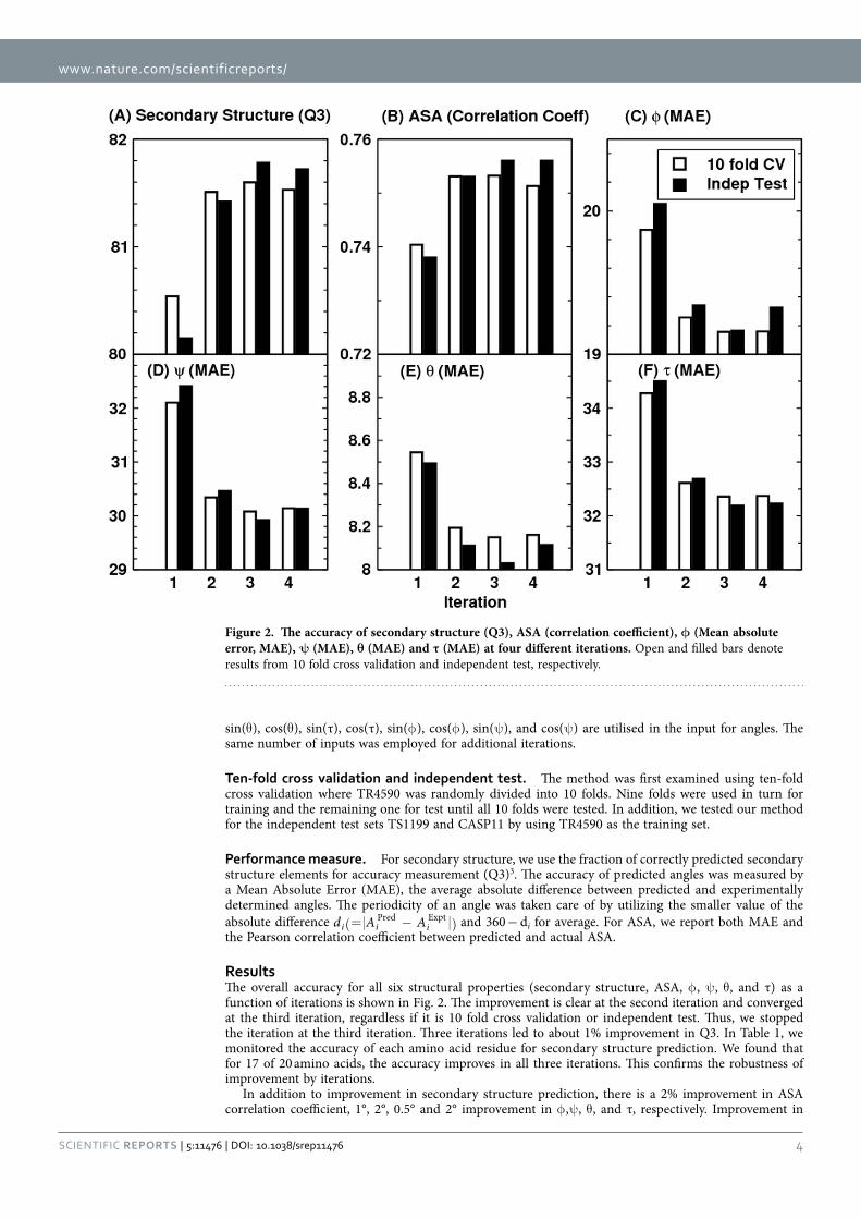
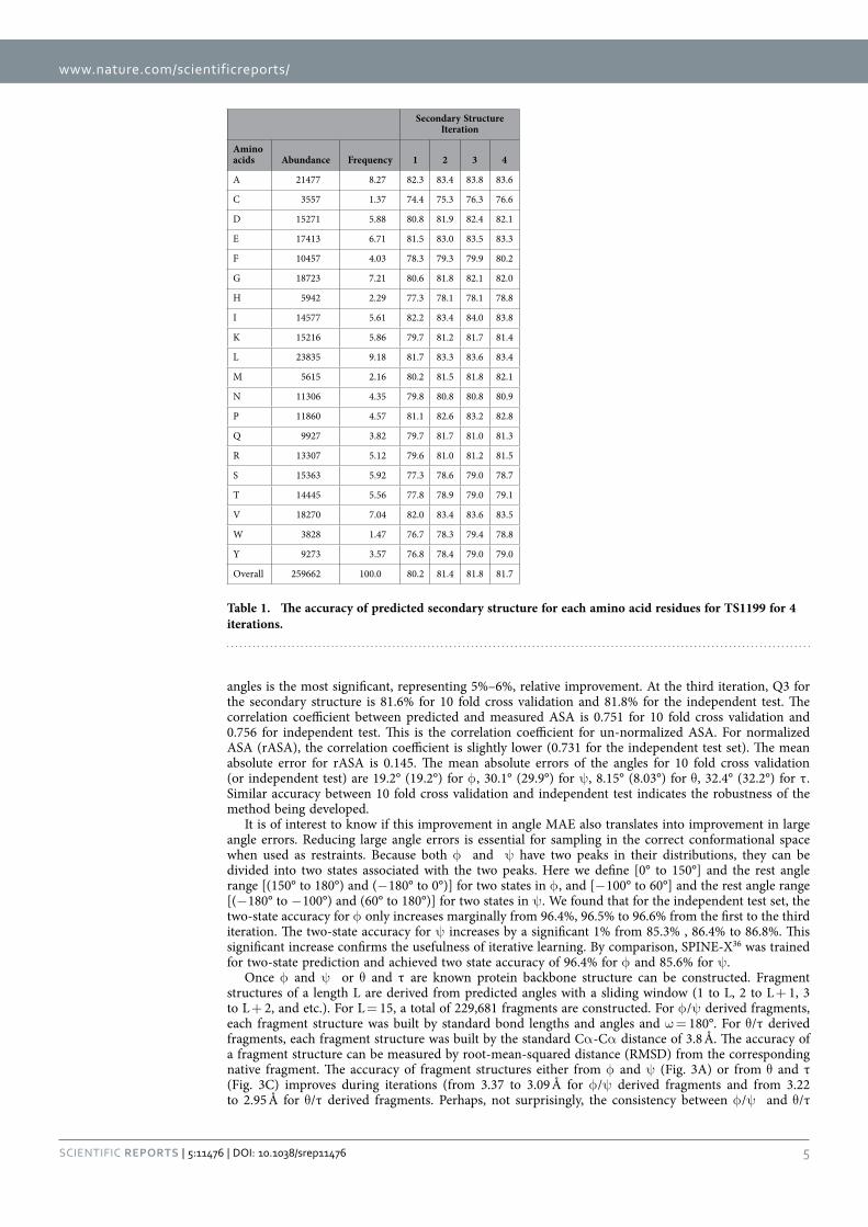
ResultsThe overall accuracy for all six structural properties (secondary structure, ASA, φ , ψ , θ , and τ) as a function of iterations is shown in Fig. 2. The improvement is clear at the second iteration and converged at the third iteration, regardless if it is 10 fold cross validation or independent test. Thus, we stopped the iteration at the third iteration. Three iterations led to about 1% improvement in Q3. In Table 1, we monitored the accuracy of each amino acid residue for secondary structure prediction. We found that for 17 of 20 amino acids, the accuracy improves in all three iterations. This confirms the robustness of improvement by iterations.
In addition to improvement in secondary structure prediction, there is a 2% improvement in ASA correlation coefficient, 1°, 2°, 0.5° and 2° improvement in φ ,ψ , θ , and τ, respectively. Improvement in
Figure 2. The accuracy of secondary structure (Q3), ASA (correlation coefficient), φ (Mean absolute error, MAE), ψ (MAE), θ (MAE) and τ (MAE) at four different iterations. Open and filled bars denote results from 10 fold cross validation and independent test, respectively.
www.nature.com/scientificreports/
5Scientific RepoRts | 5:11476 | DOi: 10.1038/srep11476
angles is the most significant, representing 5%–6%, relative improvement. At the third iteration, Q3 for the secondary structure is 81.6% for 10 fold cross validation and 81.8% for the independent test. The correlation coefficient between predicted and measured ASA is 0.751 for 10 fold cross validation and 0.756 for independent test. This is the correlation coefficient for un-normalized ASA. For normalized ASA (rASA), the correlation coefficient is slightly lower (0.731 for the independent test set). The mean absolute error for rASA is 0.145. The mean absolute errors of the angles for 10 fold cross validation (or independent test) are 19.2° (19.2°) for φ , 30.1° (29.9°) for ψ , 8.15° (8.03°) for θ , 32.4° (32.2°) for τ . Similar accuracy between 10 fold cross validation and independent test indicates the robustness of the method being developed.
It is of interest to know if this improvement in angle MAE also translates into improvement in large angle errors. Reducing large angle errors is essential for sampling in the correct conformational space when used as restraints. Because both φ and ψ have two peaks in their distributions, they can be divided into two states associated with the two peaks. Here we define [0° to 150°] and the rest angle range [(150° to 180°) and (− 180° to 0°)] for two states in φ , and [− 100° to 60°] and the rest angle range [(− 180° to − 100°) and (60° to 180°)] for two states in ψ . We found that for the independent test set, the two-state accuracy for φ only increases marginally from 96.4%, 96.5% to 96.6% from the first to the third iteration. The two-state accuracy for ψ increases by a significant 1% from 85.3% , 86.4% to 86.8%. This significant increase confirms the usefulness of iterative learning. By comparison, SPINE-X36 was trained for two-state prediction and achieved two state accuracy of 96.4% for φ and 85.6% for ψ .
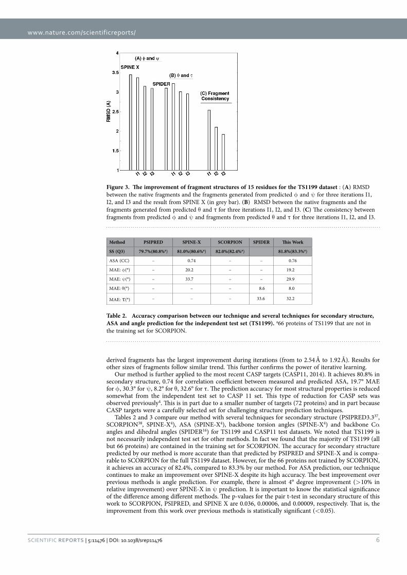
Once φ and ψ or θ and τ are known protein backbone structure can be constructed. Fragment structures of a length L are derived from predicted angles with a sliding window (1 to L, 2 to L + 1, 3 to L + 2, and etc.). For L = 15, a total of 229,681 fragments are constructed. For φ /ψ derived fragments, each fragment structure was built by standard bond lengths and angles and ω = 180°. For θ /τ derived fragments, each fragment structure was built by the standard Cα -Cα distance of 3.8 Å. The accuracy of a fragment structure can be measured by root-mean-squared distance (RMSD) from the corresponding native fragment. The accuracy of fragment structures either from φ and ψ (Fig. 3A) or from θ and τ (Fig. 3C) improves during iterations (from 3.37 to 3.09 Å for φ /ψ derived fragments and from 3.22 to 2.95 Å for θ /τ derived fragments. Perhaps, not surprisingly, the consistency between φ /ψ and θ /τ
Secondary Structure Iteration
Amino acids Abundance Frequency 1 2 3 4
A 21477 8.27 82.3 83.4 83.8 83.6
C 3557 1.37 74.4 75.3 76.3 76.6
D 15271 5.88 80.8 81.9 82.4 82.1
E 17413 6.71 81.5 83.0 83.5 83.3
F 10457 4.03 78.3 79.3 79.9 80.2
G 18723 7.21 80.6 81.8 82.1 82.0
H 5942 2.29 77.3 78.1 78.1 78.8
I 14577 5.61 82.2 83.4 84.0 83.8
K 15216 5.86 79.7 81.2 81.7 81.4
L 23835 9.18 81.7 83.3 83.6 83.4
M 5615 2.16 80.2 81.5 81.8 82.1
N 11306 4.35 79.8 80.8 80.8 80.9
P 11860 4.57 81.1 82.6 83.2 82.8
Q 9927 3.82 79.7 81.7 81.0 81.3
R 13307 5.12 79.6 81.0 81.2 81.5
S 15363 5.92 77.3 78.6 79.0 78.7
T 14445 5.56 77.8 78.9 79.0 79.1
V 18270 7.04 82.0 83.4 83.6 83.5
W 3828 1.47 76.7 78.3 79.4 78.8
Y 9273 3.57 76.8 78.4 79.0 79.0
Overall 259662 100.0 80.2 81.4 81.8 81.7
Table 1. The accuracy of predicted secondary structure for each amino acid residues for TS1199 for 4 iterations.
www.nature.com/scientificreports/
6Scientific RepoRts | 5:11476 | DOi: 10.1038/srep11476
derived fragments has the largest improvement during iterations (from to 2.54 Å to 1.92 Å). Results for other sizes of fragments follow similar trend. This further confirms the power of iterative learning.
Our method is further applied to the most recent CASP targets (CASP11, 2014). It achieves 80.8% in secondary structure, 0.74 for correlation coefficient between measured and predicted ASA, 19.7° MAE for φ , 30.3° for ψ , 8.2° for θ , 32.6° for τ . The prediction accuracy for most structural properties is reduced somewhat from the independent test set to CASP 11 set. This type of reduction for CASP sets was observed previously4. This is in part due to a smaller number of targets (72 proteins) and in part because CASP targets were a carefully selected set for challenging structure prediction techniques.
Tables 2 and 3 compare our method with several techniques for secondary structure (PSIPRED3.337, SCORPION38, SPINE-X4), ASA (SPINE-X4), backbone torsion angles (SPINE-X4) and backbone Cα angles and dihedral angles (SPIDER16) for TS1199 and CASP11 test datasets. We noted that TS1199 is not necessarily independent test set for other methods. In fact we found that the majority of TS1199 (all but 66 proteins) are contained in the training set for SCORPION. The accuracy for secondary structure predicted by our method is more accurate than that predicted by PSIPRED and SPINE-X and is compa-rable to SCORPION for the full TS1199 dataset. However, for the 66 proteins not trained by SCORPION, it achieves an accuracy of 82.4%, compared to 83.3% by our method. For ASA prediction, our technique continues to make an improvement over SPINE-X despite its high accuracy. The best improvement over previous methods is angle prediction. For example, there is almost 4° degree improvement (> 10% in relative improvement) over SPINE-X in ψ prediction. It is important to know the statistical significance of the difference among different methods. The p-values for the pair t-test in secondary structure of this work to SCORPION, PSIPRED, and SPINE X are 0.036, 0.00006, and 0.00009, respectively. That is, the improvement from this work over previous methods is statistically significant (< 0.05).
Figure 3. The improvement of fragment structures of 15 residues for the TS1199 dataset : (A) RMSD between the native fragments and the fragments generated from predicted φ and ψ for three iterations I1, I2, and I3 and the result from SPINE X (in grey bar). (B) RMSD between the native fragments and the fragments generated from predicted θ and τ for three iterations I1, I2, and I3. (C) The consistency between fragments from predicted φ and ψ and fragments from predicted θ and τ for three iterations I1, I2, and I3.
Method PSIPRED SPINE-X SCORPION SPIDER This Work
SS (Q3) 79.7%(80.8%a) 81.0%(80.6%a) 82.0%(82.4%a) 81.8%(83.3%a)
ASA (CC) – 0.74 – – 0.76
MAE: φ (°) – 20.2 – – 19.2
MAE: ψ (°) – 33.7 – – 29.9
MAE: θ (°) – – – 8.6 8.0
MAE: τ (°) – – – 33.6 32.2
Table 2. Accuracy comparison between our technique and several techniques for secondary structure, ASA and angle prediction for the independent test set (TS1199). a66 proteins of TS1199 that are not in the training set for SCORPION.
www.nature.com/scientificreports/
7Scientific RepoRts | 5:11476 | DOi: 10.1038/srep11476
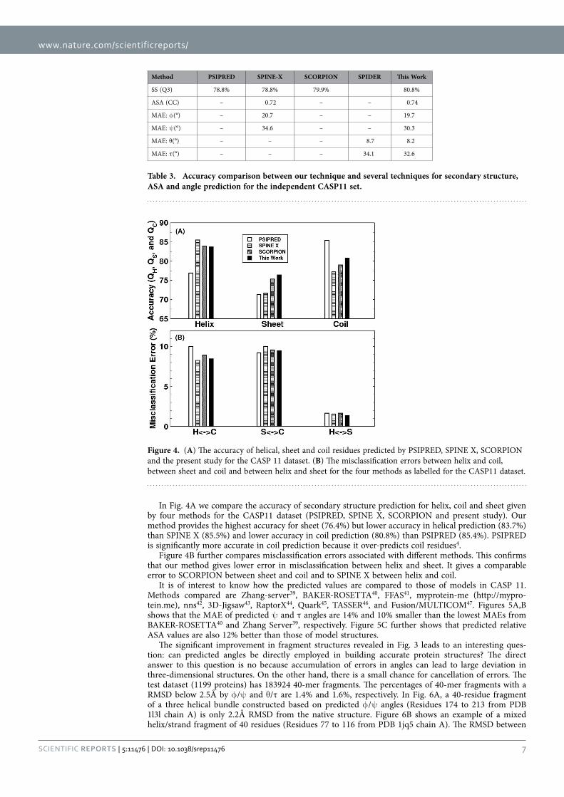
In Fig. 4A we compare the accuracy of secondary structure prediction for helix, coil and sheet given by four methods for the CASP11 dataset (PSIPRED, SPINE X, SCORPION and present study). Our method provides the highest accuracy for sheet (76.4%) but lower accuracy in helical prediction (83.7%) than SPINE X (85.5%) and lower accuracy in coil prediction (80.8%) than PSIPRED (85.4%). PSIPRED is significantly more accurate in coil prediction because it over-predicts coil residues4.
Figure 4B further compares misclassification errors associated with different methods. This confirms that our method gives lower error in misclassification between helix and sheet. It gives a comparable error to SCORPION between sheet and coil and to SPINE X between helix and coil.
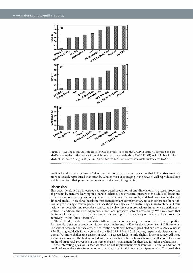
It is of interest to know how the predicted values are compared to those of models in CASP 11. Methods compared are Zhang-server39, BAKER-ROSETTA40, FFAS41, myprotein-me (http://mypro-tein.me), nns42, 3D-Jigsaw43, RaptorX44, Quark45, TASSER46, and Fusion/MULTICOM47. Figures 5A,B shows that the MAE of predicted ψ and τ angles are 14% and 10% smaller than the lowest MAEs from BAKER-ROSETTA40 and Zhang Server39, respectively. Figure 5C further shows that predicted relative ASA values are also 12% better than those of model structures.
The significant improvement in fragment structures revealed in Fig. 3 leads to an interesting ques-tion: can predicted angles be directly employed in building accurate protein structures? The direct answer to this question is no because accumulation of errors in angles can lead to large deviation in three-dimensional structures. On the other hand, there is a small chance for cancellation of errors. The test dataset (1199 proteins) has 183924 40-mer fragments. The percentages of 40-mer fragments with a RMSD below 2.5Å by φ /ψ and θ /τ are 1.4% and 1.6%, respectively. In Fig. 6A, a 40-residue fragment of a three helical bundle constructed based on predicted φ /ψ angles (Residues 174 to 213 from PDB 1l3l chain A) is only 2.2Å RMSD from the native structure. Figure 6B shows an example of a mixed helix/strand fragment of 40 residues (Residues 77 to 116 from PDB 1jq5 chain A). The RMSD between
Method PSIPRED SPINE-X SCORPION SPIDER This Work
SS (Q3) 78.8% 78.8% 79.9% 80.8%
ASA (CC) – 0.72 – – 0.74
MAE: φ (°) – 20.7 – – 19.7
MAE: ψ (°) – 34.6 – – 30.3
MAE: θ (°) – – – 8.7 8.2
MAE: τ (°) – – – 34.1 32.6
Table 3. Accuracy comparison between our technique and several techniques for secondary structure, ASA and angle prediction for the independent CASP11 set.
Figure 4. (A) The accuracy of helical, sheet and coil residues predicted by PSIPRED, SPINE X, SCORPION and the present study for the CASP 11 dataset. (B) The misclassification errors between helix and coil, between sheet and coil and between helix and sheet for the four methods as labelled for the CASP11 dataset.
www.nature.com/scientificreports/
8Scientific RepoRts | 5:11476 | DOi: 10.1038/srep11476
predicted and native structure is 2.4 Å. The two constructed structures show that helical structures are more accurately reproduced than strands. What is most encouraging in Fig. 6A,B is well reproduced loop and turn regions that permitted accurate reproduction of fragments.
DiscussionThis paper developed an integrated sequence-based prediction of one-dimensional structural properties of proteins by iterative learning in a parallel scheme. The structural properties include local backbone structures represented by secondary structure, backbone torsion angle, and backbone Cα angles and dihedral angles. These three backbone representations are complementary to each other: backbone tor-sion angles are single residue properties, backbone Cα angles and dihedral angles involve three and four residues, respectively, and secondary structures involve three or more residues in sequence-position sep-aration. In addition, the method predicts a non-local property: solvent accessibility. We have shown that the input of these predicted structural properties can improve the accuracy of these structural properties iteratively (within three iterations).
The method provides current state-of-the-art prediction accuracy for various structural properties. For secondary structure prediction, its accuracy reaches nearly 82% for the large test set of 1199 proteins. For solvent accessible surface area, the correlation coefficient between predicted and actual ASA values is 0.76. For angles, MAEs for φ , ψ , θ , and τ are 19.2, 29.9, 8.0 and 32.2 degrees, respectively. Application to a small but more challenging dataset of CASP 11 targets leads to only slightly lower accuracy. All these accuracies above are the best reported accuracies for test sets. Such an integrated collection of various predicted structural properties in one server makes it convenient for their use for other applications.
One interesting question is that whether or not improvement from iterations is due to addition of predicted secondary structures or other predicted structural information. Spencer et al.30 showed that
Figure 5. (A) The mean absolute error (MAE) of predicted ψ for the CASP 11 dataset compared to best MAEs of ψ angles in the models from eight most accurate methods in CASP 11. (B) as in (A) but for the MAE of Cα based τ angles. (C) as in (A) but for the MAE of relative assessable surface area (rASA).
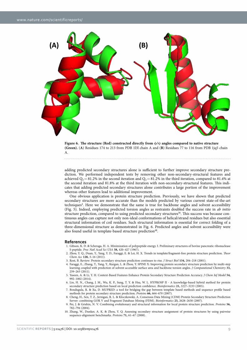
www.nature.com/scientificreports/
9Scientific RepoRts | 5:11476 | DOi: 10.1038/srep11476
adding predicted secondary structures alone is sufficient to further improve secondary structure pre-diction. We performed independent tests by removing other non-secondary-structural features and achieved Q3 = 81.2% in the second iteration and Q3 = 81.2% in the third iteration, compared to 81.4% at the second iteration and 81.8% at the third iteration with non-secondary-structural features. This indi-cates that adding predicted secondary structures alone contributes a large portion of the improvement whereas other features lead to additional improvement.
One obvious application is protein structure prediction. Previously, we have shown that predicted secondary structures are more accurate than the models predicted by various current state-of-the-art techniques4. Here we demonstrate that the same is true for backbone angles and solvent accessibility (Fig. 5). Indeed, employing predicted torsion angles as restraints doubled the success rate in ab initio structure prediction, compared to using predicted secondary structures36. This success was because con-tinuous angles can capture not only non-ideal conformations of helical/strand residues but also essential structural information of coil residues. Such structural information is essential for correct folding of a three-dimensional structure as demonstrated in Fig. 6. Predicted angles and solvent accessibility were also found useful in template-based structure prediction48.
References1. Gibson, K. D. & Scheraga, H. A. Minimization of polypeptide energy. I. Preliminary structures of bovine pancreatic ribonuclease
S-peptide. Proc Natl Acad Sci USA 58, 420–427 (1967).2. Zhou, Y. Q., Duan, Y., Yang, Y. D., Faraggi, E. & Lei, H. X. Trends in template/fragment-free protein structure prediction. Theor
Chem Acc 128, 3–16 (2011).3. Rost, B. Review: Protein secondary structure prediction continues to rise. J Struct Biol 134, 204–218 (2001).4. Faraggi, E., Zhang, T., Yang, Y., Kurgan, L. & Zhou, Y. SPINE X: Improving protein secondary structure prediction by multi-step
learning coupled with prediction of solvent accessible surface area and backbone torsion angles. J Computational Chemistry 33, 259–263 (2011).
5. Yaseen, A. & Li, Y. H. Context-Based Features Enhance Protein Secondary Structure Prediction Accuracy. J Chem Inf Model 54, 992–1002 (2014).
6. Lin, H. N., Chang, J. M., Wu, K. P., Sung, T. Y. & Hsu, W. L. HYPROSP II - A knowledge-based hybrid method for protein secondary structure prediction based on local prediction confidence. Bioinformatics 21, 3227–3233 (2005).
7. Bondugula, R. & Xu, D. MUPRED: a tool for bridging the gap between template based methods and sequence profile based methods for protein secondary structure prediction. Proteins 66, 664–670 (2007).
8. Cheng, H., Sen, T. Z., Jernigan, R. L. & Kloczkowski, A. Consensus Data Mining (CDM) Protein Secondary Structure Prediction Server: combining GOR V and Fragment Database Mining (FDM). Bioinformatics 23, 2628–2630 (2007).
9. Pei, J. & Grishin, N. V. Combining evolutionary and structural information for local protein structure prediction. Proteins 56, 782–794 (2004).
10. Zhang, W., Dunker, A. K. & Zhou, Y. Q. Assessing secondary structure assignment of protein structures by using pairwise sequence-alignment benchmarks. Proteins 71, 61–67 (2008).
Figure 6. The structure (Red) constructed directly from φ/ψ angles compared to native structure (Green). (A) Residues 174 to 213 from PDB 1l3l chain A and (B) Residues 77 to 116 from PDB 1jq5 chain A.
www.nature.com/scientificreports/
1 0Scientific RepoRts | 5:11476 | DOi: 10.1038/srep11476
11. Kuang, R., Leslie, C. S. & Yang, A. S. Protein backbone angle prediction with machine learning approaches. Bioinformatics 20, 1612–1621 (2004).
12. Kang, H. S., Kurochkina, N. A. & Lee, B. Estimation and Use of Protein Backbone Angle Probabilities. J Mol Biol 229, 448–460 (1993).
13. Wood, M. J. & Hirst, J. D. Protein secondary structure prediction with dihedral angles. Proteins 59, 476–481 (2005).14. Dor, O. & Zhou, Y. Real-SPINE: an integrated system of neural networks for real-value prediction of protein structural properties.
Proteins 68, 76–81 (2007).15. Xue, B., Dor, O., Faraggi, E. & Zhou, Y. Real-value prediction of backbone torsion angles. Proteins 72, 427–433 (2008).16. Lyons, J. et al. Predicting backbone Calpha angles and dihedrals from protein sequences by stacked sparse auto-encoder deep
neural network. J Comput Chem 35, 2040–2046 (2014).17. Holbrook, S. R., Muskal, S. M. & Kim, S. H. Predicting surface exposure of amino acids from protein sequence. Protein Eng 3,
659–665 (1990).18. Rost, B. & Sander, C. Conservation and prediction of solvent accessibility in protein families. Proteins 20, 216–226 (1994).19. Pollastri, G., Baldi, P., Fariselli, P. & Casadio, R. Prediction of coordination number and relative solvent accessibility in proteins.
Proteins 47, 142–153 (2002).20. Garg, A., Kaur, H. & Raghava, G. P. Real value prediction of solvent accessibility in proteins using multiple sequence alignment
and secondary structure. Proteins 61, 318–324 (2005).21. Yuan, Z. & Huang, B. Prediction of protein accessible surface areas by support vector regression. Proteins 57, 558–564 (2004).22. Ahmad, S., Gromiha, M. M. & Sarai, A. Real value prediction of solvent accessibility from amino acid sequence. Proteins 50,
629–635 (2003).23. Adamczak, R., Porollo, A. & Meller, J. Accurate prediction of solvent accessibility using neural networks-based regression.
Proteins 56, 753–767 (2004).24. Adamczak, R., Porollo, A. & Meller, J. Combining prediction of secondary structure and solvent accessibility in proteins. Proteins
59, 467–475 (2005).25. Zhou, Y. & Faraggi, E. Prediction of one-dimensional structural properties of proteins by integrated neural network. In: Protein
Structure Prediction: Method and Algorithms ((ed^(eds Rangwala H., Karypis G.). Wiley (2010).26. Hinton, G. E. Learning multiple layers of representation. Trends Cogn Sci 11, 428–434 (2007).27. Di Lena, P., Nagata, K. & Baldi, P. Deep architectures for protein contact map prediction. Bioinformatics 28, 2449–2457 (2012).28. Eickholt, J. & Cheng, J. L. DNdisorder: predicting protein disorder using boosting and deep networks. Bmc Bioinformatics 14,
88 (2013).29. Qi, Y. J., Oja, M., Weston, J. & Noble, W. S. A Unified Multitask Architecture for Predicting Local Protein Properties. Plos One
7, e32235 (2012).30. Spencer, M., Eickholt, J. & Cheng, J. L. A Deep Learning Network Approach to ab initio Protein Secondary Structure Prediction.
Ieee Acm T Comput Bi 12, 103–112 (2015).31. Wang, G. & Dunbrack, R. L., Jr. PISCES: recent improvements to a PDB sequence culling server. Nucleic Acids Res 33, W94–98
(2005).32. Bengio, Y., Lamblin, P., Popovici, D. & Larochelle, H. Greedy layer-wise training of deep networks. Advances in neural information
processing systems 19, 153 (2007).33. Palm, R. B. Prediction as a candidate for learning deep hierarchical models of data. M.Sc Thesis, Technical University of
Denmark, Denmark (2012).34. Meiler, J., Müller, M., Zeidler, A. & Schmäschke, F. Generation and evaluation of dimension-reduced amino acid parameter
representations by artificial neural networks. J Mol Model 7, 360–369 (2001).35. Altschul, S. F. et al. Gapped BLAST and PSI-BLAST: a new generation of protein database search programs. Nucleic Acids
Research 25, 3389–3402 (1997).36. Faraggi, E., Yang, Y. D., Zhang, S. S. & Zhou, Y. Predicting Continuous Local Structure and the Effect of Its Substitution for
Secondary Structure in Fragment-Free Protein Structure Prediction. Structure 17, 1515–1527 (2009).37. Jones, D. T. Protein secondary structure prediction based on position-specific scoring matrices. J Mol Biol 292, 195–202 (1999).38. Yaseen, A. & Li, Y. Context-based features enhance protein secondary structure prediction accuracy. J Chem Inf Model 54,
992–1002 (2014).39. Roy, A., Kucukural, A. & Zhang, Y. I-TASSER: a unified platform for automated protein structure and function prediction. Nat
Protoc 5, 725–738 (2010).40. Rohl, C. A., Strauss, C. E. M., Misura, K. M. S. & Baker, D. Protein structure prediction using Rosetta. Method Enzymol 383,
66–93 (2004).41. Jaroszewski, L., Rychlewski, L., Li, Z., Li, W. & Godzik, A. FFAS03: a server for profile--profile sequence alignments. Nucleic Acids
Res 33, W284–288 (2005).42. Joo, K., Lee, J., Lee, S., Seo, J. H., Lee, S. J. & Lee, J. High accuracy template based modeling by global optimization. Proteins 69
Suppl 8, 83–89 (2007).43. Offman, M. N., Tournier, A. L. & Bates, P. A. Alternating evolutionary pressure in a genetic algorithm facilitates protein model
selection. Bmc Struct Biol 8, 34 (2008).44. Ma, J. Z., Wang, S., Zhao, F. & Xu, J. B. Protein threading using context-specific alignment potential. Bioinformatics 29, 257–265
(2013).45. Zhang, Y. Interplay of I-TASSER and QUARK for template-based and ab initio protein structure prediction in CASP10. Proteins
82, 175–187 (2014).46. Zhou, H. Y. & Skolnick, J. Template-based protein structure modeling using TASSERVMT. Proteins 80, 352–361 (2012).47. Bhattacharya, D. & Cheng, J. L. i3Drefine Software for Protein 3D Structure Refinement and Its Assessment in CASP10. Plos One
8, e69648 (2013).48. Yang, Y., Faraggi, E., Zhao, H. & Zhou, Y. Improving protein fold recognition and template-based modeling by employing
probabilistic-based matching between predicted one-dimensional structural properties of the query and corresponding native properties of templates. Bioinformatics 27, 2076–2082 (2011).
AcknowledgementsThis work was supported in part by National Health and Medical Research Council (1059775) of Australia and Australian Research Council’s Linkage Infrastructure, Equipment and Facilities funding scheme (project number LE150100161) to Y.Z., National Science Foundation of China 61271378 to J. W. and Y. Y., and the Microsoft Azure for Research Awarded to Y.Y. We also gratefully acknowledge the support of the Griffith University eResearch Services Team and the use of the High Performance Computing
www.nature.com/scientificreports/
1 1Scientific RepoRts | 5:11476 | DOi: 10.1038/srep11476
Cluster “Gowonda” to complete this research. This research/project has also been undertaken with the aid of the research cloud resources provided by the Queensland Cyber Infrastructure Foundation (QCIF).
Author ContributionsR.H., K.P., J.L., A.D., A.S. J.W., A.S., Y.Y. and Y.Z. designed the method; R.H., J.L., A.D. and Y.Y. developed and implemented methods and produced results; R.H., J.L., A.D., Y.Y. and Y.Z. wrote the manuscript; all authors reviewed the manuscript.
Additional InformationSupplementary information accompanies this paper at http://www.nature.com/srepCompeting financial interests: The authors declare no competing financial interests.How to cite this article: Heffernan, R. et al. Improving prediction of secondary structure, local backbone angles, and solvent accessible surface area of proteins by iterative deep learning. Sci. Rep. 5, 11476; doi: 10.1038/srep11476 (2015).
This work is licensed under a Creative Commons Attribution 4.0 International License. The images or other third party material in this article are included in the article’s Creative Com-
mons license, unless indicated otherwise in the credit line; if the material is not included under the Creative Commons license, users will need to obtain permission from the license holder to reproduce the material. To view a copy of this license, visit http://creativecommons.org/licenses/by/4.0/

32
Chapter 3 SPIDER2 - Improving prediction of secondary structure, localbackbone angles, and solvent accessible surface area of proteins by iterative
deep learning
Chapter 4
SPIDER2 HSE - Highly accurate
sequence-based prediction of
half-sphere exposures of amino
acid residues in proteins
33

STATEMENT OF CONTRIBUTION TO CO-AUTHORED PUBLISHED PAPER
This chapter includes a co-authored paper. The bibliographic details of the co-authored paper, including all authors, are:
R. Heffernan, A. Dehzangi, J. Lyons, K. Paliwal, A. Sharma, J. Wang, A. Sattar, Y.Zhou, and Y. Yang, “Highly accurate sequence-based prediction of half-sphereexposures of amino acid residues in proteins,” Bioinformatics, vol. 32, no. 6, pp. 843–849, 2016.
My contribution to the paper involved:
Co-designed the method. Wrote all the code for the method. Produced and co-analyised results. Co-wrote the manuscript. .
(Signed) _________________________________ (Date)______________Rhys Heffernan
(Countersigned) ___________________________ (Date)______________Corresponding author of paper: Yaoqi Zhou
(Countersigned) ___________________________ (Date)______________Supervisor: Kuldip Paliwal
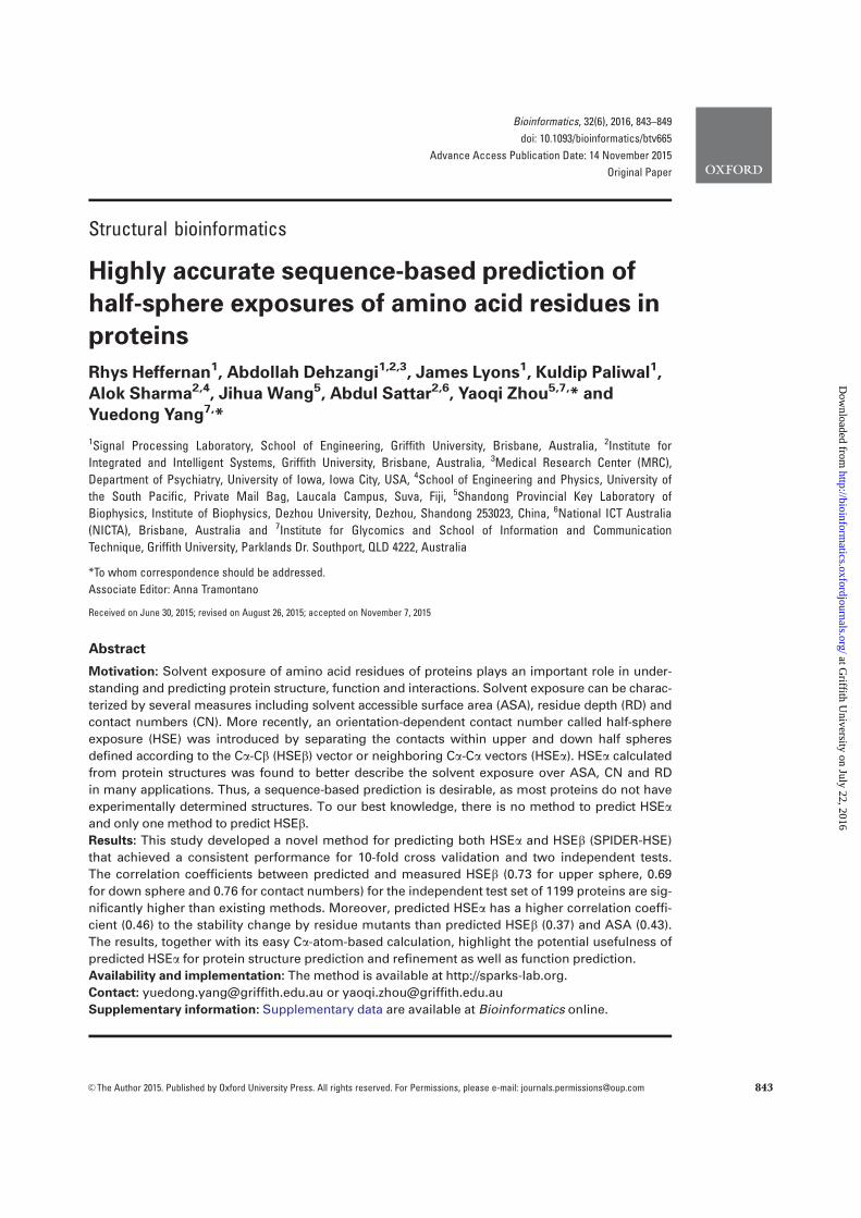
Structural bioinformatics
Highly accurate sequence-based prediction of
half-sphere exposures of amino acid residues in
proteins
Rhys Heffernan1, Abdollah Dehzangi1,2,3, James Lyons1, Kuldip Paliwal1,
Alok Sharma2,4, Jihua Wang5, Abdul Sattar2,6, Yaoqi Zhou5,7,* and
Yuedong Yang7,*
1Signal Processing Laboratory, School of Engineering, Griffith University, Brisbane, Australia, 2Institute for
Integrated and Intelligent Systems, Griffith University, Brisbane, Australia, 3Medical Research Center (MRC),
Department of Psychiatry, University of Iowa, Iowa City, USA, 4School of Engineering and Physics, University of
the South Pacific, Private Mail Bag, Laucala Campus, Suva, Fiji, 5Shandong Provincial Key Laboratory of
Biophysics, Institute of Biophysics, Dezhou University, Dezhou, Shandong 253023, China, 6National ICT Australia
(NICTA), Brisbane, Australia and 7Institute for Glycomics and School of Information and Communication
Technique, Griffith University, Parklands Dr. Southport, QLD 4222, Australia
*To whom correspondence should be addressed.
Associate Editor: Anna Tramontano
Received on June 30, 2015; revised on August 26, 2015; accepted on November 7, 2015
Abstract
Motivation: Solvent exposure of amino acid residues of proteins plays an important role in under-
standing and predicting protein structure, function and interactions. Solvent exposure can be charac-
terized by several measures including solvent accessible surface area (ASA), residue depth (RD) and
contact numbers (CN). More recently, an orientation-dependent contact number called half-sphere
exposure (HSE) was introduced by separating the contacts within upper and down half spheres
defined according to the Ca-Cb (HSEb) vector or neighboring Ca-Ca vectors (HSEa). HSEa calculated
from protein structures was found to better describe the solvent exposure over ASA, CN and RD
in many applications. Thus, a sequence-based prediction is desirable, as most proteins do not have
experimentally determined structures. To our best knowledge, there is no method to predict HSEaand only one method to predict HSEb.
Results: This study developed a novel method for predicting both HSEa and HSEb (SPIDER-HSE)
that achieved a consistent performance for 10-fold cross validation and two independent tests.
The correlation coefficients between predicted and measured HSEb (0.73 for upper sphere, 0.69
for down sphere and 0.76 for contact numbers) for the independent test set of 1199 proteins are sig-
nificantly higher than existing methods. Moreover, predicted HSEa has a higher correlation coeffi-
cient (0.46) to the stability change by residue mutants than predicted HSEb (0.37) and ASA (0.43).
The results, together with its easy Ca-atom-based calculation, highlight the potential usefulness of
predicted HSEa for protein structure prediction and refinement as well as function prediction.
Availability and implementation: The method is available at http://sparks-lab.org.
Contact: [email protected] or [email protected]
Supplementary information: Supplementary data are available at Bioinformatics online.
VC The Author 2015. Published by Oxford University Press. All rights reserved. For Permissions, please e-mail: [email protected] 843
Bioinformatics, 32(6), 2016, 843–849
doi: 10.1093/bioinformatics/btv665
Advance Access Publication Date: 14 November 2015
Original Paper
at Griffith U
niversity on July 22, 2016http://bioinform
atics.oxfordjournals.org/D
ownloaded from
1 Introduction
Measuring exposure of amino acid residues of proteins to solvent is
important for understanding and predicting protein structure, func-
tion and interactions (Gilis and Rooman, 1997; Lee and Richards,
1971; Rost and Sander, 1994; Tuncbag et al., 2009). The most com-
mon measure is solvent accessible surface area (ASA) (Connolly,
1983) with applications ranging from protein structure prediction
(Bennett-Lovsey et al., 2008; Wu and Zhang, 2008; Yang et al.,
2011) to protein function prediction (Lou et al., 2014; Zhang et al.,
2010; Zhang et al., 2008; Zhao et al., 2013; Zhao et al., 2011). The
inability of ASA to discriminate deeply buried residues from those
buried just beneath the surface leads to development of residue
depth (Chakravarty and Varadarajan, 1999) by averaging the dis-
tance to the nearest atom on the protein surface. Both ASA and resi-
due depth, however, require precise evaluation of the protein
surface in full atomic details that is time consuming. Having a time-
consuming calculation and requiring an all-atomic model limited the
usefulness of ASA and residue depth in the ab initio prediction of
protein structure where protein conformation is often represented
by main-chain atoms (Bradley et al., 2003; Faraggi et al., 2009) or
only Ca atoms (Kihara et al., 2001; Yang and Liu, 2006) in initial
conformational sampling.
Another measure of residue exposure to solvent is contact num-
ber (CN), which counts the number of residues within specific dis-
tance cut offs. The distances are based on the positions of Ca or Cbatoms. Thus, unlike ASA and residue depth, only a coarse-grained
model is needed for evaluating CNs. Different distance cut offs have
been used in earlier studies (Pollastri et al., 2002; Yuan, 2005). It
was shown that CN with a distance cut off between 12 and 14 A is
the best for protein fold recognition (Karchin et al., 2004).
All above-mentioned solvent-exposure measures, however, do not
contain explicit information regarding the orientation of side chains
that are important for functional and structural studies. Hamelryck
designed a new measure by splitting the sphere around the Ca atom
into two half spheres along the vector of Ca-Cb atoms (Hamelryck,
2005). The half sphere containing the Cb atom was defined as upper
and the other as down half spheres. The numbers of Ca atoms
enclosed in these two half-spheres were named as Half-Sphere
Exposure (HSE)-up and HSE-down, respectively. In addition, he has
substituted the vector Ca-Cb with a pseudo vector generated from the
sum of vectors Cai-1-Cai and Caiþ1-Cai. This HSE is denoted as
HSEa (-up and -down) to distinguish from the HSE calculated based
on the Ca-Cb vector (here and hereafter, it will be annotated as
HSEb). HSEa does not require the positions of Cb-atoms. One advan-
tage of HSE is that its value is independent of amino acid type because
it describes a residue’s coordination environment rather than a quan-
tity related to its size such as ASA and RD. Interestingly, HSEa-up
outperforms other solvent exposure measures including CN, ASA,
relative ASA, residue depth and the other three HSE definitions
(HSEb-up, HSEb-down and HSEa-down) in correlation to changes in
protein stability due to mutations and to conservation of amino acid
residues (Hamelryck, 2005). More recently, HSE was found to be bet-
ter than ASA for prediction of B cell epitopes of proteins from their
three dimensional structures (Kringelum et al., 2012). HSE has also
been found useful in many other applications (Franzosa and Xia,
2009; Kringelum et al., 2012; Sweredoski and Baldi, 2008). Most of
these applications obtained HSE based on known protein structures.
Because the structures for most proteins are not known experimen-
tally, a sequence-based prediction is desirable.
Many sequence-based methods were developed for predicting
ASA (Adamczak et al., 2004; Ahmad et al., 2003; Cheng et al.,
2005; Dor and Zhou, 2007; Garg et al., 2005; Yuan and Huang,
2004) and CN (Kinjo and Nishikawa, 2006; Pollastri et al., 2002;
Yuan, 2005). However, there is no method available for prediction
of HSEa and only one (HSEpred) for the prediction of HSEb (Song
et al., 2008). We found that the correlation coefficients between ac-
tual HSEb and those predicted by HSEpred (up and down, respect-
ively) are less than 0.43 for our dataset of 1199 proteins. One
possible factor is that HSEpred was trained on a small dataset of
632 proteins and was not tested on independent datasets. Therefore,
a more accurate method is clearly needed.
Recently, we developed a method called SPIDER 2 (Heffernan
et al., 2015) that utilized predicted secondary structures, backbone
torsion angles and ASA, iteratively, in order to improve their accura-
cies. The method achieved 82% accuracy for secondary structure
prediction, 0.76 for the correlation coefficient between predicted
and actual solvent accessible surface area, 19� and 30� for mean ab-
solute errors of backbone u and w angles, respectively, and 8� and
32� for mean absolute errors of Ca-based h and s angles, respect-
ively, for an independent test dataset of 1199 proteins. Here, we
expand the iterative technique to the prediction of HSEa (-up and -
down), HSEb (-up and -down) and CN by employing a large dataset
containing 4590 protein chains. The method was independently
tested in a dataset of 1199 proteins and a dataset of 69 proteins
from the Critical Assessment of Structure Prediction technique
(CASP 11, 2014). As a result, highly accurate and robust prediction
was obtained (e.g. a correlation coefficient of 0.73 for HSEb-up,
0.69 for HSEb-down and 0.76 for contact number on the independ-
ent test set). Comparison to two previous methods for contact pre-
diction and HSEb confirmed the superior performance of the
method obtained. The HSEa and HSEb predictors are incorporated
as a package in SPIDER 2 available at http://sparks-lab.org or down-
loadable as a standalone package.
2 Methods
2.1 DatasetsWe have employed the same dataset as used in our previous study
(Lyons et al., 2014), which consists of 5789 proteins (1 246 420 resi-
dues). This dataset was generated by the sequence culling server
PISCES (< 25% pairwise sequence identity and <2.0 A resolution)
(Wang and Dunbrack, 2003). From this dataset, 4590 proteins were
randomly selected as training set (TR4590) and the remaining 1199
proteins were utilized as an independent test set (TS1199). In add-
ition, we downloaded the targets from critical assessment of structure
prediction technique (CASP 11, 2014, http://www.predictioncenter.
org/casp11/). After removing redundant sequences (30% in between
or to the training set), we obtained a set of 69 proteins (CASP11) out
of original 99 proteins. This set contains 18 617 residues.
2.2 Input featuresFor each amino acid, we have extracted 69 input features. The first
20 features are substitution probabilities of amino acids from the
PSSM matrix. The PSSM is generated by PSI-BLAST (Altschul et al.,
1997) with three iterations of searching against 90% non-redundant
protein database (downloaded from ftp://toolkit.genzentrum.lmu.
de/pub/HH-suite/databases/). The next 30 features are extracted
from the HMM-profile generated by HHblits with default param-
eters against Uniprot20 protein database (Remmert et al., 2011).
The HMM profile includes 10 transition probabilities between
matching, insertion and deletion states in addition to 20 substitution
probabilities. The additional 12 features represent predicted
844 R.Heffernan et al.
at Griffith U
niversity on July 22, 2016http://bioinform
atics.oxfordjournals.org/D
ownloaded from
structural properties of amino acids by SPIDER 2 that include pre-
dicted probabilities in three secondary structure states (Helix, Sheet
and Coil), ASA, and sine and cosine values of the main chain tor-
sional angles (u and w) and main chain angles between Ca atoms (hand s). Here, sine and cosine of angles were employed to remove the
effect of angle periodicity (Lyons et al., 2014). The last seven fea-
tures are physicochemical representatives (PP7) of twenty standard
amino acids, namely, a steric parameter (graph shape index), hydro-
phobicity, volume, polarizability, isoelectric point, helix probability
and sheet probability. Additionally, we utilized a window size of 17
amino acids (8 amino acids at each side of the target amino acid).
Together with a global feature of the protein length, this led to a
total of 1174 input features (17�69þ1¼1174). The window size
was taken from SPIDER 2 (Heffernan et al., 2015) without further
optimization.
2.3 Parallel multiple-step iterative deep neural-network
learningHere, we implemented the same learning scheme as previously used in
SPIDER 2. As shown in Figure 1, the features were input into the
deep learning neural network to obtain an initial prediction of HSEs
(HSE-up, HSE-down and CN). The deep artificial neural network
consists of three hidden layers, each with 150 nodes. The input data
was normalized to the range of 0–1. The weights were initialized by
unsupervised learning from stacked sparse auto-encoders, and then
refined by using standard back propagation. In this study, we em-
ployed the deep neural network from the MATLAB toolbox, imple-
mented by Palm (2012). Deep neural networks have been widely
implemented in the prediction of protein structure (Nguyen et al.,
2014). In the second iteration, the predicted values from the first iter-
ation were added into the input features to predict HSEs. This process
iterated with updated predicted values until convergence. We found
that the prediction accuracy did not increase after two iterations. The
training process was performed separately for HSEa (HSEa-up,
HSEa-down and CN) and HSEb (HSEb-up, HSEb-down and CN).
All contacts are defined with 13 A distance cut off.
2.4 Evaluation methodThe method was first examined by 10-fold cross validation where
the training set TR4590 was randomly divided into 10-folds. Nine
folds were used in turn for training and the remaining one for testing
until all 10-folds were tested. As SPIDER 2 has been trained in the
same training set, we avoided over-training by following the same
10-folds and utilizing the 10-fold cross validation results during the
training of SPIDER 2 as input features. Moreover, we tested our
method in the independent test sets TS1199 and CASP11 dataset by
using TR4590 as the training set. The prediction performance of
CN, HSEa and HSEb was measured by Pearson correlation coeffi-
cient (PCC) as used in previous studies (Song et al., 2008; Yuan,
2005).
3 Results and discussions
3.1 Overall prediction performanceFigure 2 and Table 1 show the results of 10-fold cross validation
and independent test in the first four iterations for prediction of CN,
HSEb-up and HSEb-down. For the independent test, PCCs achieve
the highest value at the second iteration with 0.734, 0.693 and
0.756 for HSEb-up, HSEb-down and CN, respectively. The same is
true for 10-fold cross valuation. Thus additional iterations are un-
necessary. We also noted that the correlation coefficients from the
10-fold cross validation and from the independent test set are essen-
tially the same. For example, PCCs for CN at the second iteration
are 0.757 and 0.756 for 10-fold cross validation and independent
test, respectively. PCC for HSEb up at the second iteration are 0.733
and 0.734 for 10-fold cross validation and independent test, respect-
ively. High consistency between 10-fold cross validation and inde-
pendent test indicates the robustness of our trained method. The
small standard deviations between ten subsets from 10-fold cross
validation further confirm a stable performance.
We further found that the accuracy for HSEa is similar to that of
HSEb. For example, The PCCs of HSEa-up and HSEb-up at the se-
cond iteration for independent test are 0.729 and 0.734, respect-
ively. The PCCs of HSEa-down and HSEb-down at the second
iteration for independent test are 0.717 and 0.693, respectively.
Because of similarity between HSEa and HSEb, here and hereafter,
we will only present the results for HSEb from the second iteration
based on the independent test unless specifically mentioned.
Fig. 1. The general flowchart for the multiple-step iterative algorithm imple-
mented for training of SPIDER-HSE
1 2 3 4Iteration
0.684
0.687
0.69
0.693
PC
C
HSEβ-down
1 2 3 4Iteration
0.744
0.747
0.75
0.753
0.756
PC
C
10 fold CVIndep Test
CN
1 2 3 4Iteration
0.726
0.728
0.73
0.732
0.734
PC
C
HSEβ-up
Fig. 2. The Pearson Correlation Coefficients achieved for HSEb-up, HSEb-down and contact number by 10-fold cross validation (open bar) and on the independent
dataset TS1199 (filled bar) in different iterations
Highly accurate sequence-based prediction 845
at Griffith U
niversity on July 22, 2016http://bioinform
atics.oxfordjournals.org/D
ownloaded from
3.2 The contribution from each feature groupIt is of interest to know the contribution of each feature group to the
overall prediction performance of SPIDER-HSE. Table 2 compares
PCCs by utilizing a single feature group or by removing them indi-
vidually from SPIDER-HSE. In the first test, predicted ASA is the
single best feature as it achieved the highest PCC of 0.72, 0.69 and
0.64 for CN, HSE-up and HSE-down, respectively. This is under-
standable because ASA and CN both describe the level of solvent ex-
posure. Such high correlation confirms the suitability to substitute
ASA by the simpler representation of solvent exposure by HSE. The
performance of two conservation profiles HMM and PSSM is only
slightly worse than ASA with HMM marginally better than PSSM.
The physical parameters alone without sequence conservation infor-
mation can make a decent prediction with PCC around 0.5 for CN
and HSE-up.
One interesting observation is that predicted angles are more
useful than predicted secondary structure in predicting HSE-up
(0.58 versus 0.50) and HSE-down (0.54 versus 0.48) although they
contribute similarly in predicting CN (0.584 versus 0.586). This sug-
gests that continuous main-chain torsion angles have more orienta-
tion information than discrete states of secondary structure.
Another interesting observation is that protein length itself as a
single feature is not very useful in predicting HSE. Its combination
with other features, however, proved useful. Removing protein
length will reduce the correlation coefficient in the independent test
from 0.756 for CN to 0.740. This is the largest reduction, compared
to removing other feature groups. The relatively small change by
removing other feature groups is partly due to high redundancies be-
tween these feature groups.
For example, HHM and PSSM describe residue conservation
during evolution, whereas secondary structure and main-chain
angles both represent the main-chain conformations. In addition,
ASA, SS and main-chain angles have been obtained from PSSM and
PP7 feature groups for their prediction. Nonetheless, a drop in per-
formance by removing any single feature group indicates usefulness
of all these features for the overall performance.
3.3 Comparison to previous methodsTo compare our results with previously reported methods, we repro-
duced the results of HSEpred by both its locally running version and
online server (http://sunflower.kuicr.kyoto-u.ac.jp/�sjn/hse/links.
html) on test sets TS1199 and CASP 11. In addition, we compared
with a contact number prediction method CRNpred (Kinjo and
Nishikawa, 2006) (http://ipr.pdbj.org/crnpred/). As shown in Table
3, the PCC values for HSE are less than 0.5, compared to 0.7 from
our method for both test sets. Our predicted CN (PCC¼0.76 for
the independent test set) are also significantly more accurate than ei-
ther HSEpred (PCC¼0.56) or CRNpred (PCC¼0.70). A similar
Table 1. Pearson Correlation Coefficients of CN, HSEb-up and
HSEb-down in iterations for 10-fold cross validation and independ-
ent test set TS1199
Parameter Dataset 1 2 3 4
HSEb-up 10-folda 0.731 0.733 0.731 0.730
SDb 0.009 0.008 0.008 0.008
Test 0.730 0.734 0.734 0.733
HSEb-down 10-folda 0.686 0.693 0.692 0.690
SDb 0.007 0.008 0.008 0.008
Test 0.685 0.693 0.695 0.694
CN 10-folda 0.752 0.757 0.755 0.752
SDb 0.010 0.011 0.011 0.011
Test 0.751 0.756 0.754 0.754
a The average and b the standard deviation of PCCs from the 10-fold cross
validation.
Table 2. Pearson correlation coefficients (PCCs) of predicted CN, HSEb-up and HSEb-down by using single feature group or by removing it
from SPIDER-HSE for independent test set TS1199
CN HSEb-up HSEb-down CN HSEb-up HSEb-down
– – – – SP-HSEb 0.756 0.734 0.693
ASAa 0.721 0.689 0.637 �ASAc 0.746 0.728 0.680
HMM 0.709 0.682 0.620 �HHM 0.742 0.724 0.676
PSSM 0.694 0.683 0.607 �PSSM 0.751 0.730 0.684
SS 0.586 0.495 0.477 �SS 0.751 0.729 0.685
Angles 0.584 0.584 0.536 �Angles 0.752 0.729 0.681
PP7 0.523 0.520 0.436 �PP7 0.748 0.729 0.683
Length 0.013 0.006 0.006 �Length 0.740 0.725 0.679
aPredicting by using only individual feature group.bSPIDER2-HSE by using full features.cPredicting by excluding one feature group.
Table 3. Comparison to HSEpred and CRNpred in the independent dataset TS1199 and CASP11
Methods TS1199 CASP11
CN HSEb-up HSEb-down CN HSEb-up HSEb-down
CRNpred 0.697 a – – 0.691 a – –
HSEpred (Local) 0.624 0.490 0.398 0.590 0.467 0.394
HSEpred (Online) 0.555 0.429 0.326 0.527 0.427 0.331
1st Iteration (This work) 0.751 0.7301 0.685 0.766 0.749 0.692
2nd Iteration (This work) 0.756 0.7343 0.693 0.770 0.751 0.699
a The contact number based on 12 A.
846 R.Heffernan et al.
at Griffith U
niversity on July 22, 2016http://bioinform
atics.oxfordjournals.org/D
ownloaded from
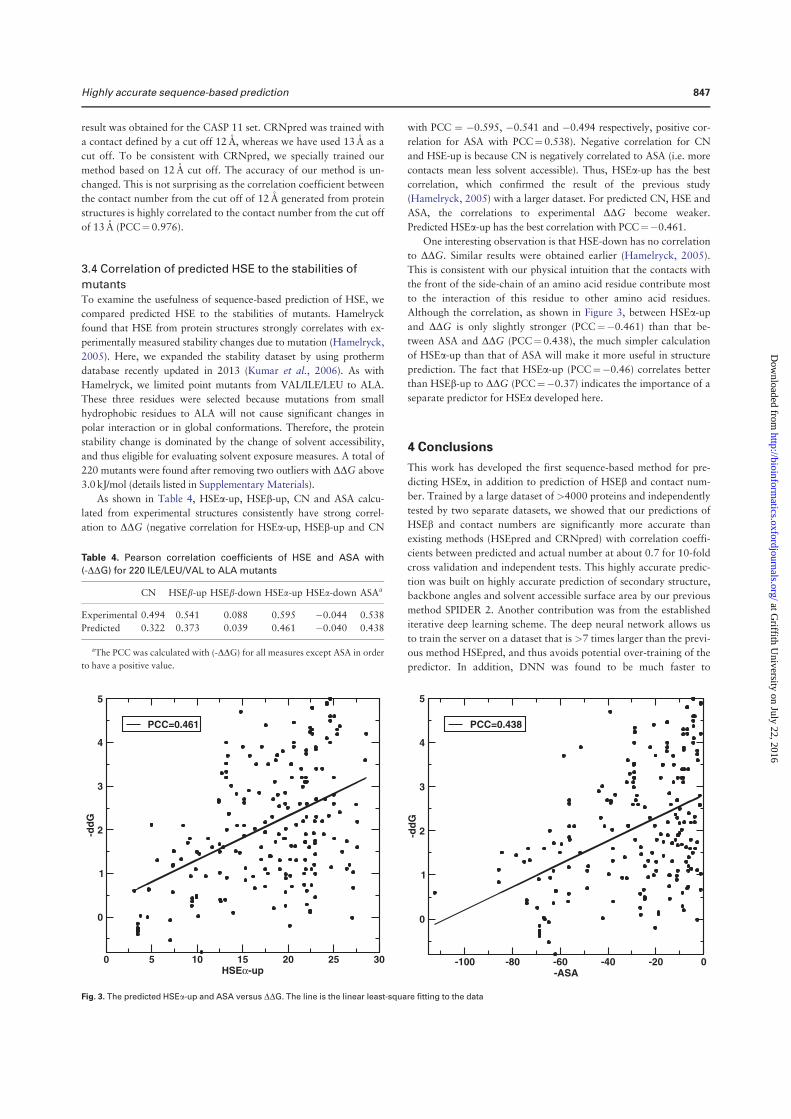
result was obtained for the CASP 11 set. CRNpred was trained with
a contact defined by a cut off 12 A, whereas we have used 13 A as a
cut off. To be consistent with CRNpred, we specially trained our
method based on 12 A cut off. The accuracy of our method is un-
changed. This is not surprising as the correlation coefficient between
the contact number from the cut off of 12 A generated from protein
structures is highly correlated to the contact number from the cut off
of 13 A (PCC¼0.976).
3.4 Correlation of predicted HSE to the stabilities of
mutantsTo examine the usefulness of sequence-based prediction of HSE, we
compared predicted HSE to the stabilities of mutants. Hamelryck
found that HSE from protein structures strongly correlates with ex-
perimentally measured stability changes due to mutation (Hamelryck,
2005). Here, we expanded the stability dataset by using protherm
database recently updated in 2013 (Kumar et al., 2006). As with
Hamelryck, we limited point mutants from VAL/ILE/LEU to ALA.
These three residues were selected because mutations from small
hydrophobic residues to ALA will not cause significant changes in
polar interaction or in global conformations. Therefore, the protein
stability change is dominated by the change of solvent accessibility,
and thus eligible for evaluating solvent exposure measures. A total of
220 mutants were found after removing two outliers with DDG above
3.0 kJ/mol (details listed in Supplementary Materials).
As shown in Table 4, HSEa-up, HSEb-up, CN and ASA calcu-
lated from experimental structures consistently have strong correl-
ation to DDG (negative correlation for HSEa-up, HSEb-up and CN
with PCC ¼ �0.595, �0.541 and �0.494 respectively, positive cor-
relation for ASA with PCC¼0.538). Negative correlation for CN
and HSE-up is because CN is negatively correlated to ASA (i.e. more
contacts mean less solvent accessible). Thus, HSEa-up has the best
correlation, which confirmed the result of the previous study
(Hamelryck, 2005) with a larger dataset. For predicted CN, HSE and
ASA, the correlations to experimental DDG become weaker.
Predicted HSEa-up has the best correlation with PCC¼�0.461.
One interesting observation is that HSE-down has no correlation
to DDG. Similar results were obtained earlier (Hamelryck, 2005).
This is consistent with our physical intuition that the contacts with
the front of the side-chain of an amino acid residue contribute most
to the interaction of this residue to other amino acid residues.
Although the correlation, as shown in Figure 3, between HSEa-up
and DDG is only slightly stronger (PCC¼�0.461) than that be-
tween ASA and DDG (PCC¼0.438), the much simpler calculation
of HSEa-up than that of ASA will make it more useful in structure
prediction. The fact that HSEa-up (PCC¼�0.46) correlates better
than HSEb-up to DDG (PCC¼�0.37) indicates the importance of a
separate predictor for HSEa developed here.
4 Conclusions
This work has developed the first sequence-based method for pre-
dicting HSEa, in addition to prediction of HSEb and contact num-
ber. Trained by a large dataset of >4000 proteins and independently
tested by two separate datasets, we showed that our predictions of
HSEb and contact numbers are significantly more accurate than
existing methods (HSEpred and CRNpred) with correlation coeffi-
cients between predicted and actual number at about 0.7 for 10-fold
cross validation and independent tests. This highly accurate predic-
tion was built on highly accurate prediction of secondary structure,
backbone angles and solvent accessible surface area by our previous
method SPIDER 2. Another contribution was from the established
iterative deep learning scheme. The deep neural network allows us
to train the server on a dataset that is >7 times larger than the previ-
ous method HSEpred, and thus avoids potential over-training of the
predictor. In addition, DNN was found to be much faster to
0 5 10 15 20 25 30HSEα-up
0
1
2
3
4
5
-dd
G
PCC=0.461
-100 -80 -60 -40 -20 0-ASA
0
1
2
3
4
5
-dd
G
PCC=0.438
Fig. 3. The predicted HSEa-up and ASA versus DDG. The line is the linear least-square fitting to the data
Table 4. Pearson correlation coefficients of HSE and ASA with
(-DDG) for 220 ILE/LEU/VAL to ALA mutants
CN HSEb-up HSEb-down HSEa-up HSEa-down ASAa
Experimental 0.494 0.541 0.088 0.595 �0.044 0.538
Predicted 0.322 0.373 0.039 0.461 �0.040 0.438
aThe PCC was calculated with (-DDG) for all measures except ASA in order
to have a positive value.
Highly accurate sequence-based prediction 847
at Griffith U
niversity on July 22, 2016http://bioinform
atics.oxfordjournals.org/D
ownloaded from
converge with better performance than SVM and random forest
methods in training big datasets with a large number of features
(Bengio and LeCun, 2007; Schmidhuber, 2015). The usefulness
of predicted HSEa is demonstrated by its improved correlation to ex-
perimentally measured stability change due to mutation, over pre-
dicted ASA.
Fast calculation of HSEa that requires the positions of Ca atoms
only makes it an ideal sequence-specific restraint for coarse-grained
modeling, protein structure prediction and refinement. The HSEaand HSEb predictors are incorporated as a package in SPIDER 2
available at http://sparks-lab.org. To speed up calculations, we pro-
vide another version by using all features except HMM profile. This
version leads to a slight reduction in PCCs but cuts the total running
time by half because it requires to prepare only one of the two se-
quence profiles that are the most time-consuming.
Acknowledgements
We also gratefully acknowledge the support of the Griffith University
eResearch Services Team and the use of the High Performance Computing
Cluster ‘Gowonda’ to complete this research.
Funding
This work was supported in part by National Health and Medical Research
Council (1059775 and 1083450) of Australia and Australian Research
Council’s Linkage Infrastructure, Equipment and Facilities funding scheme
(project number LE150100161) to Y.Z., National Natural Science
Foundation of China (61271378) to J.W. and Y.Y., the Taishan Scholar
Program of Shandong to Y.Z., and the Microsoft Azure for
Research Awarded to Y. Y. This research/project has also been undertaken
with the aid of the research cloud resources provided by the Queensland
Cyber Infrastructure Foundation (QCIF).
Conflict of Interest: none declared.
References
Adamczak,R. et al. (2004) Accurate prediction of solvent accessibility using
neural networks-based regression. Proteins, 56, 753–767.
Ahmad,S. et al. (2003) Real value prediction of solvent accessibility from
amino acid sequence. Proteins, 50, 629–635.
Altschul,S.F. et al. (1997) Gapped BLAST and PSI-BLAST: a new generation
of protein database search programs. Nucleic Acids Res., 25, 3389–3402.
Bengio,Y. and LeCun,Y. (2007) Scaling learning algorithms towards AI.
Large-Scale Kernel Mach., 34, 321–359.
Bennett-Lovsey,R.M. et al. (2008) Exploring the extremes of sequence/struc-
ture space with ensemble fold recognition in the program Phyre. Proteins,
70, 611–625.
Bradley,P. et al. (2003) Rosetta predictions in CASP5: successes, failures, and
prospects for complete automation. Proteins, 53, 457–468.
Chakravarty,S. and Varadarajan,R. (1999) Residue depth: a novel parameter
for the analysis of protein structure and stability. Structure, 7, 723–732.
Cheng,J. et al. (2005) SCRATCH: a protein structure and structural feature
prediction server. Nucleic Acids Res., 33, W72–W76.
Connolly,M.L. (1983) Solvent-accessible surfaces of proteins and nucleic
acids. Science, 221, 709–713.
Dor,O. and Zhou,Y. (2007) Real-SPINE: an integrated system of neural net-
works for real-value prediction of protein structural properties. Proteins:
Struct. Funct. Bioinf., 68, 76–81.
Faraggi,E. et al. (2009) Predicting continuous local structure and the effect of
its substitution for secondary structure in fragment-free protein structure
prediction. Structure, 17, 1515–1527.
Franzosa,E.A. and Xia,Y. (2009) Structural determinants of protein evolution
are context-sensitive at the residue level. Mol. Biol. Evol., 26, 2387–2395.
Garg,A. et al. (2005) Real value prediction of solvent accessibility in proteins
using multiple sequence alignment and secondary structure. Proteins, 61,
318–324.
Gilis,D. and Rooman,M. (1997) Predicting protein stability changes upon mu-
tation using database-derived potentials: solvent accessibility determines the
importance of local versus non-local interactions along the sequence. J. Mol.
Biol., 272, 276–290.
Hamelryck,T. (2005) An amino acid has two sides: a new 2D measure pro-
vides a different view of solvent exposure. Proteins: Struct. Funct. Bioinf.,
59, 38–48.
Heffernan,R. et al. (2015) Improving prediction of secondary structure, local
backbone angles, and solvent accessible surface area of proteins by iterative
deep learning. Sci. Rep., 5, 11476.
Karchin,R. et al. (2004) Evaluation of local structure alphabets based on resi-
due burial. Proteins: Struct. Funct. Bioinf., 55, 508–518.
Kihara,D. et al. (2001) TOUCHSTONE: an ab initio protein structure predic-
tion method that uses threading-based tertiary restraints. Proc. Natl. Acad.
Sci. U. S. A., 98, 10125–10130.
Kinjo,A.R. and Nishikawa,K. (2006) CRNPRED: highly accurate prediction
of one-dimensional protein structures by large-scale critical random net-
works. BMC Bioinformatics, 7, 401.
Kringelum,J.V. et al. (2012) Reliable B cell epitope predictions: impacts of
method development and improved benchmarking. PLoS Comput. Biol., 8,
e1002829.
Kumar,M.S. et al. (2006) ProTherm and ProNIT: thermodynamic databases
for proteins and protein–nucleic acid interactions. Nucleic Acids Res., 34,
D204–D206.
Lee,B. and Richards,F.M. (1971) The interpretation of protein structures: esti-
mation of static accessibility. J. Mol. Biol., 55, 379–400.
Lou,W. et al. (2014) Sequence based prediction of DNA-binding proteins
based on hybrid feature selection using random forest and Gaussian naıve
Bayes. PloS One, 9, e86703.
Lyons,J. et al. (2014) Predicting backbone Ca angles and dihedrals from pro-
tein sequences by stacked sparse auto-encoder deep neural network.
J. Comput. Chem., 35, 2040–2046.
Nguyen,S.P. et al. (2014) DL-PRO: A novel deep learning method for protein
model quality assessment. In: Neural Networks (IJCNN), 2014
International Joint Conference on. IEEE, pp. 2071–2078.
Palm,R.B. (2012) Prediction as a candidate for learning deep hierarchical mod-
els of data. Master Thesis, Technical University of Denmark, Palm, 24–25.
Pollastri,G. et al. (2002) Prediction of coordination number and relative solv-
ent accessibility in proteins. Proteins: Struct. Funct. Bioinf., 47, 142–153.
Remmert,M. et al. (2011) HHblits: lightning-fast iterative protein sequence
searching by HMM-HMM alignment. Nat. Methods, 9, 173–175.
Rost,B. and Sander,C. (1994) Conservation and prediction of solvent accessi-
bility in protein families. Proteins: Struct. Funct. Bioinf., 20, 216–226.
Schmidhuber,J. (2015) Deep learning in neural networks: an overview. Neural
Networks, 61, 85–117.
Song,J. et al. (2008) HSEpred: predict half-sphere exposure from protein se-
quences. Bioinformatics, 24, 1489–1497.
Sweredoski,M.J. and Baldi,P. (2008) PEPITO: improved discontinuous B-cell
epitope prediction using multiple distance thresholds and half sphere expos-
ure. Bioinformatics, 24, 1459–1460.
Tuncbag,N. et al. (2009) Identification of computational hot spots in protein
interfaces: combining solvent accessibility and inter-residue potentials im-
proves the accuracy. Bioinformatics, 25, 1513–1520.
Wang,G. and Dunbrack,R.L. (2003) PISCES: a protein sequence culling ser-
ver. Bioinformatics, 19, 1589–1591.
Wu,S. and Zhang,Y. (2008) MUSTER: Improving protein sequence profile-
profile alignments by using multiple sources of structure information.
Proteins, 72, 547–556.
Yang,Y. et al. (2011) Improving protein fold recognition and template-based
modeling by employing probabilistic-based matching between predicted
one-dimensional structural properties of query and corresponding native
properties of templates. Bioinformatics, 27, 2076–2082.
Yang,Y. and Liu,H. (2006) Genetic algorithms for protein conformation sam-
pling and optimization in a discrete backbone dihedral angle space.
J. Comput. Chem., 27, 1593–1602.
848 R.Heffernan et al.
at Griffith U
niversity on July 22, 2016http://bioinform
atics.oxfordjournals.org/D
ownloaded from

Yuan,Z. (2005) Better prediction of protein contact number using a support vec-
tor regression analysis of amino acid sequence. BMC Bioinformatics, 6, 248.
Yuan,Z. and Huang,B. (2004) Prediction of protein accessible surface areas by
support vector regression. Proteins, 57, 558–564.
Zhang,T. et al. (2010) Analysis and prediction of RNA-binding residues using
sequence, evolutionary conservation, and predicted secondary structure and
solvent accessibility. Curr. Protein Peptide Sci., 11, 609–628.
Zhang,T. et al. (2008) Accurate sequence-based prediction of catalytic resi-
dues. Bioinformatics, 24, 2329–2338.
Zhao,H. et al. (2013) DDIG-in: discriminating between disease-associated
and neutral non-frameshifting micro-indels. Genome Biol., 14, R23.
Zhao,H. et al. (2011) Highly accurate and high-resolution function prediction
of RNA binding proteins by fold recognition and binding affinity prediction.
RNA Biol., 8, 988–996.
Highly accurate sequence-based prediction 849
at Griffith U
niversity on July 22, 2016http://bioinform
atics.oxfordjournals.org/D
ownloaded from

42Chapter 4 SPIDER2 HSE - Highly accurate sequence-based prediction of
half-sphere exposures of amino acid residues in proteins
Chapter 5
SPIDER3 - Capturing non-local
interactions by long short-term
memory bidirectional recurrent
neural networks for improving
prediction of protein secondary
structure, backbone angles,
contact numbers and solvent
accessibility
43

STATEMENT OF CONTRIBUTION TO CO-AUTHORED PUBLISHED PAPER
This chapter includes a co-authored paper. The bibliographic details of the co-authored paper, including all authors, are:
R. Heffernan, Y. Yang, K. Paliwal, and Y. Zhou, “Capturing non-local interactions bylong short-term memory bidirectional recurrent neural networks for improvingprediction of protein secondary structure, backbone angles, contact numbers andsolvent accessibility,” Bioinformatics, vol. 33, no. 18, pp. 2842–2849, 2017.
My contribution to the paper involved:
Designed the method. Wrote all the code for the method. Produced and co-analyisedresults. Co-wrote the manuscript.
(Signed) _________________________________ (Date)______________Rhys Heffernan
(Countersigned) ___________________________ (Date)______________Corresponding author of paper: Yaoqi Zhou
(Countersigned) ___________________________ (Date)______________Supervisor: Kuldip Paliwal
Structural bioinformatics
Capturing non-local interactions by long
short-term memory bidirectional recurrent
neural networks for improving prediction of
protein secondary structure, backbone angles,
contact numbers and solvent accessibility
Rhys Heffernan1, Yuedong Yang2,*, Kuldip Paliwal1 and Yaoqi Zhou2,*
1Signal Processing Laboratory, Griffith University, Brisbane, QLD 4111, Australia and 2Institute for Glycomics and
School of Information and Communication Technology, Griffith University, Southport, QLD 4222, Australia
*To whom correspondence should be addressed.
Associate Editor: Alfonso Valencia
Received on October 27, 2016; revised on January 20, 2017; editorial decision on April 8, 2017; accepted on April 15, 2017
Abstract
Motivation: The accuracy of predicting protein local and global structural properties such as sec-
ondary structure and solvent accessible surface area has been stagnant for many years because of
the challenge of accounting for non-local interactions between amino acid residues that are close
in three-dimensional structural space but far from each other in their sequence positions. All exist-
ing machine-learning techniques relied on a sliding window of 10–20 amino acid residues to cap-
ture some ‘short to intermediate’ non-local interactions. Here, we employed Long Short-Term
Memory (LSTM) Bidirectional Recurrent Neural Networks (BRNNs) which are capable of capturing
long range interactions without using a window.
Results: We showed that the application of LSTM-BRNN to the prediction of protein structural
properties makes the most significant improvement for residues with the most long-range contacts
(ji-jj>19) over a previous window-based, deep-learning method SPIDER2. Capturing long-range
interactions allows the accuracy of three-state secondary structure prediction to reach 84% and the
correlation coefficient between predicted and actual solvent accessible surface areas to reach 0.80,
plus a reduction of 5%, 10%, 5% and 10% in the mean absolute error for backbone /, w, h and sangles, respectively, from SPIDER2. More significantly, 27% of 182724 40-residue models directly
constructed from predicted Ca atom-based h and s have similar structures to their corresponding
native structures (6A RMSD or less), which is 3% better than models built by / and w angles. We
expect the method to be useful for assisting protein structure and function prediction.
Availability and implementation: The method is available as a SPIDER3 server and standalone
package at http://sparks-lab.org.
Contact: [email protected] or [email protected]
Supplementary information: Supplementary data are available at Bioinformatics online.
VC The Author 2017. Published by Oxford University Press. All rights reserved. For Permissions, please e-mail: [email protected] 2842
Bioinformatics, 33(18), 2017, 2842–2849
doi: 10.1093/bioinformatics/btx218
Advance Access Publication Date: 18 April 2017
Original Paper
Downloaded from https://academic.oup.com/bioinformatics/article-abstract/33/18/2842/3738544by Griffith University useron 21 January 2018
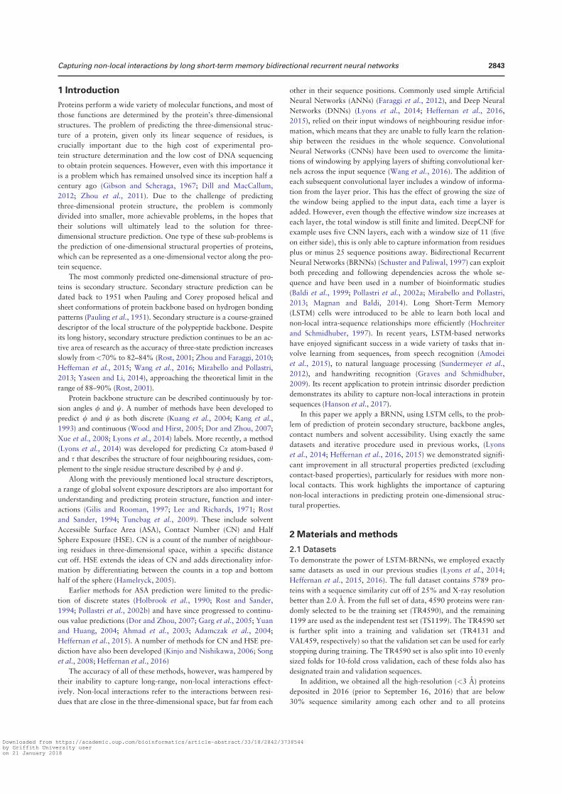
1 Introduction
Proteins perform a wide variety of molecular functions, and most of
those functions are determined by the protein’s three-dimensional
structures. The problem of predicting the three-dimensional struc-
ture of a protein, given only its linear sequence of residues, is
crucially important due to the high cost of experimental pro-
tein structure determination and the low cost of DNA sequencing
to obtain protein sequences. However, even with this importance it
is a problem which has remained unsolved since its inception half a
century ago (Gibson and Scheraga, 1967; Dill and MacCallum,
2012; Zhou et al., 2011). Due to the challenge of predicting
three-dimensional protein structure, the problem is commonly
divided into smaller, more achievable problems, in the hopes that
their solutions will ultimately lead to the solution for three-
dimensional structure prediction. One type of these sub-problems is
the prediction of one-dimensional structural properties of proteins,
which can be represented as a one-dimensional vector along the pro-
tein sequence.
The most commonly predicted one-dimensional structure of pro-
teins is secondary structure. Secondary structure prediction can be
dated back to 1951 when Pauling and Corey proposed helical and
sheet conformations of protein backbone based on hydrogen bonding
patterns (Pauling et al., 1951). Secondary structure is a course-grained
descriptor of the local structure of the polypeptide backbone. Despite
its long history, secondary structure prediction continues to be an ac-
tive area of research as the accuracy of three-state prediction increases
slowly from<70% to 82–84% (Rost, 2001; Zhou and Faraggi, 2010;
Heffernan et al., 2015; Wang et al., 2016; Mirabello and Pollastri,
2013; Yaseen and Li, 2014), approaching the theoretical limit in the
range of 88–90% (Rost, 2001).
Protein backbone structure can be described continuously by tor-
sion angles / and w. A number of methods have been developed to
predict / and w as both discrete (Kuang et al., 2004; Kang et al.,
1993) and continuous (Wood and Hirst, 2005; Dor and Zhou, 2007;
Xue et al., 2008; Lyons et al., 2014) labels. More recently, a method
(Lyons et al., 2014) was developed for predicting Ca atom-based hand s that describes the structure of four neighbouring residues, com-
plement to the single residue structure described by / and w.
Along with the previously mentioned local structure descriptors,
a range of global solvent exposure descriptors are also important for
understanding and predicting protein structure, function and inter-
actions (Gilis and Rooman, 1997; Lee and Richards, 1971; Rost
and Sander, 1994; Tuncbag et al., 2009). These include solvent
Accessible Surface Area (ASA), Contact Number (CN) and Half
Sphere Exposure (HSE). CN is a count of the number of neighbour-
ing residues in three-dimensional space, within a specific distance
cut off. HSE extends the ideas of CN and adds directionality infor-
mation by differentiating between the counts in a top and bottom
half of the sphere (Hamelryck, 2005).
Earlier methods for ASA prediction were limited to the predic-
tion of discrete states (Holbrook et al., 1990; Rost and Sander,
1994; Pollastri et al., 2002b) and have since progressed to continu-
ous value predictions (Dor and Zhou, 2007; Garg et al., 2005; Yuan
and Huang, 2004; Ahmad et al., 2003; Adamczak et al., 2004;
Heffernan et al., 2015). A number of methods for CN and HSE pre-
diction have also been developed (Kinjo and Nishikawa, 2006; Song
et al., 2008; Heffernan et al., 2016)
The accuracy of all of these methods, however, was hampered by
their inability to capture long-range, non-local interactions effect-
ively. Non-local interactions refer to the interactions between resi-
dues that are close in the three-dimensional space, but far from each
other in their sequence positions. Commonly used simple Artificial
Neural Networks (ANNs) (Faraggi et al., 2012), and Deep Neural
Networks (DNNs) (Lyons et al., 2014; Heffernan et al., 2016,
2015), relied on their input windows of neighbouring residue infor-
mation, which means that they are unable to fully learn the relation-
ship between the residues in the whole sequence. Convolutional
Neural Networks (CNNs) have been used to overcome the limita-
tions of windowing by applying layers of shifting convolutional ker-
nels across the input sequence (Wang et al., 2016). The addition of
each subsequent convolutional layer includes a window of informa-
tion from the layer prior. This has the effect of growing the size of
the window being applied to the input data, each time a layer is
added. However, even though the effective window size increases at
each layer, the total window is still finite and limited. DeepCNF for
example uses five CNN layers, each with a window size of 11 (five
on either side), this is only able to capture information from residues
plus or minus 25 sequence positions away. Bidirectional Recurrent
Neural Networks (BRNNs) (Schuster and Paliwal, 1997) can exploit
both preceding and following dependencies across the whole se-
quence and have been used in a number of bioinformatic studies
(Baldi et al., 1999; Pollastri et al., 2002a; Mirabello and Pollastri,
2013; Magnan and Baldi, 2014). Long Short-Term Memory
(LSTM) cells were introduced to be able to learn both local and
non-local intra-sequence relationships more efficiently (Hochreiter
and Schmidhuber, 1997). In recent years, LSTM-based networks
have enjoyed significant success in a wide variety of tasks that in-
volve learning from sequences, from speech recognition (Amodei
et al., 2015), to natural language processing (Sundermeyer et al.,
2012), and handwriting recognition (Graves and Schmidhuber,
2009). Its recent application to protein intrinsic disorder prediction
demonstrates its ability to capture non-local interactions in protein
sequences (Hanson et al., 2017).
In this paper we apply a BRNN, using LSTM cells, to the prob-
lem of prediction of protein secondary structure, backbone angles,
contact numbers and solvent accessibility. Using exactly the same
datasets and iterative procedure used in previous works, (Lyons
et al., 2014; Heffernan et al., 2016, 2015) we demonstrated signifi-
cant improvement in all structural properties predicted (excluding
contact-based properties), particularly for residues with more non-
local contacts. This work highlights the importance of capturing
non-local interactions in predicting protein one-dimensional struc-
tural properties.
2 Materials and methods
2.1 DatasetsTo demonstrate the power of LSTM-BRNNs, we employed exactly
same datasets as used in our previous studies (Lyons et al., 2014;
Heffernan et al., 2015, 2016). The full dataset contains 5789 pro-
teins with a sequence similarity cut off of 25% and X-ray resolution
better than 2.0 A. From the full set of data, 4590 proteins were ran-
domly selected to be the training set (TR4590), and the remaining
1199 are used as the independent test set (TS1199). The TR4590 set
is further split into a training and validation set (TR4131 and
VAL459, respectively) so that the validation set can be used for early
stopping during training. The TR4590 set is also split into 10 evenly
sized folds for 10-fold cross validation, each of these folds also has
designated train and validation sequences.
In addition, we obtained all the high-resolution (<3 A) proteins
deposited in 2016 (prior to September 16, 2016) that are below
30% sequence similarity among each other and to all proteins
Capturing non-local interactions by long short-term memory bidirectional recurrent neural networks 2843
Downloaded from https://academic.oup.com/bioinformatics/article-abstract/33/18/2842/3738544by Griffith University useron 21 January 2018
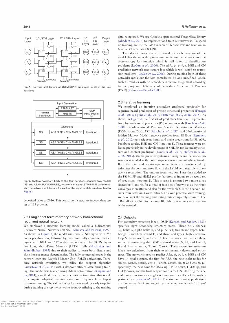
deposited prior to 2016. This constitutes a separate independent test
set of 115 proteins.
2.2 Long short-term memory network bidirectional
recurrent neural networkWe employed a machine learning model called a Bidirectional
Recurrent Neural Network (BRNN) (Schuster and Paliwal, 1997).
As shown in Figure 1, the model uses two BRNN layers with 256
nodes per direction, followed by two more fully connected hidden
layers with 1024 and 512 nodes, respectively. The BRNN layers
use Long Short-Term Memory (LSTM) cells (Hochreiter and
Schmidhuber, 1997) due to their ability to learn both distant and
close intra-sequence dependencies. The fully connected nodes in the
network each use Rectified Linear Unit (ReLU) activations. To re-
duce network overfitting, we utilize the dropout algorithm
(Srivastava et al., 2014) with a dropout ratio of 50% during train-
ing. The model was trained using Adam optimization (Kingma and
Ba, 2014), a method for efficient stochastic optimization that is able
to compute adaptive learning rates and requires little hyper-
parameter tuning. The validation set loss was used for early stopping
during training to stop the networks from overfitting to the training
data being used. We use Google’s open-sourced TensorFlow library
(Abadi et al., 2016) to implement and train our networks. To speed
up training, we use the GPU version of TensorFlow and train on an
Nvidia GeForce Titan X GPU.
Two distinct networks are trained for each iteration of the
model. For the secondary structure prediction the network uses the
cross-entropy loss function which is well suited to classification
problems (LeCun et al., 2006). The ASA, /, w, h, s, HSE and CN
prediction network uses square loss which is well suited to regres-
sion problems (LeCun et al., 2006). During training both of these
networks mask out the loss contributed by any undefined labels,
such as residues with no secondary structure assignment according
to the program Dictionary of Secondary Structure of Proteins
(DSSP) (Kabsch and Sander 1983).
2.3 Iterative learningWe employed an iterative procedure employed previously for
sequence-based prediction of protein structural properties (Faraggi
et al., 2012; Lyons et al., 2014; Heffernan et al., 2016, 2015). As
shown in Figure 2, the first set of predictors take seven representa-
tive physio-chemical properties (PP) of amino acids (Fauchere et al.,
1988), 20-dimensional Position Specific Substitution Matrices
(PSSM) from PSI-BLAST (Altschul et al., 1997), and 30-dimensional
hidden Markov Model sequence profiles from HHBlits (Remmert
et al., 2012) per residue as input, and make predictions for SS, ASA,
backbone angles, HSE and CN (iteration 1). These features were se-
lected previously in the development of SPIDER for secondary struc-
ture and contact prediction (Lyons et al., 2014; Heffernan et al.,
2016, 2015). Unlike previous systems utilizing neural networks, no
window is needed as the entire sequence was input into the network.
Both the long and short-range interactions are remembered by
enforcing the constant error flow in the LSTM cell, regardless of se-
quence separation. The outputs from iteration 1 are then added to
the PSSM, PP and HMM profile features, as inputs to a second set
of predictors (iteration 2). This process is repeated two more times
(iterations 3 and 4), for a total of four sets of networks as the result
converges. Hereafter (and also for the available SPIDER3 server), re-
sults from iteration 4 were utilized. To avoid potential over training,
we have kept the training and testing data completely separate. The
TR4950 set is split into the same 10 folds for training every iteration
of the network.
2.4 OutputsFor secondary structure labels, DSSP (Kabsch and Sander, 1983)
specifies eight secondary structure states. Three helix shapes:
310-helix G, alpha-helix H, and pi-helix I; two strand types: beta-
bridge B and beta-strand E; and three coil types: high curvature
loop S, beta-turn T, and coil C. For this work, we predict three
states by converting the DSSP assigned states G, H, and I to H;
B and E to E; and S, T, and C to C. These secondary structure
labels are calculated from their experimentally determined struc-
tures. The networks used to predict ASA, /, w, h, s, HSE and CN
have 14 total outputs, the first for ASA; the next eight nodes for
sin(/), cos(/), sin(w), cos(w), sin(h), cos(h), sin(s) and cos(s), re-
spectively; the next four for HSEa-up, HSEa-down, HSEb-up, and
HSEb-down; and the final output node is for CN. Utilizing the sine
and cosine functions for angles is to remove the effect of the angle’s
periodicity (Lyons et al., 2014). The sine and cosine predictions
are converted back to angles by the equation a¼ tan�1[sin(a)/
cos(a)].
Fig. 1. Network architecture of LSTM-BRNN employed in all of the four
iterations
Fig. 2. System flowchart. Each of the four iterations contains two models
(SS, and ASA/HSE/CN/ANGLES), for a total of eight LSTM-BRNN based mod-
els. The network architecture for each of the eight models are described by
Figure 1
2844 R.Heffernan et al.
Downloaded from https://academic.oup.com/bioinformatics/article-abstract/33/18/2842/3738544by Griffith University useron 21 January 2018
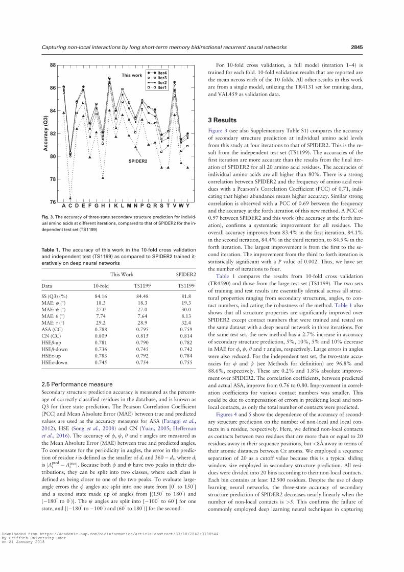
2.5 Performance measureSecondary structure prediction accuracy is measured as the percent-
age of correctly classified residues in the database, and is known as
Q3 for three state prediction. The Pearson Correlation Coefficient
(PCC) and Mean Absolute Error (MAE) between true and predicted
values are used as the accuracy measures for ASA (Faraggi et al.,
2012), HSE (Song et al., 2008) and CN (Yuan, 2005; Heffernan
et al., 2016). The accuracy of /, w, h and s angles are measured as
the Mean Absolute Error (MAE) between true and predicted angles.
To compensate for the periodicity in angles, the error in the predic-
tion of residue i is defined as the smaller of di and 360� di, where di
is jApredi � Atrue
i j. Because both / and w have two peaks in their dis-
tributions, they can be split into two classes, where each class is
defined as being closer to one of the two peaks. To evaluate large-
angle errors the / angles are split into one state from [08 to 1508]
and a second state made up of angles from [(1508 to 1808) and
(�1808 to 08)]. The w angles are split into [�1008 to 608] for one
state, and [(�1808 to �1008) and (608 to 1808)] for the second.
For 10-fold cross validation, a full model (iteration 1–4) is
trained for each fold. 10-fold validation results that are reported are
the mean across each of the 10-folds. All other results in this work
are from a single model, utilizing the TR4131 set for training data,
and VAL459 as validation data.
3 Results
Figure 3 (see also Supplementary Table S1) compares the accuracy
of secondary structure prediction at individual amino acid levels
from this study at four iterations to that of SPIDER2. This is the re-
sult from the independent test set (TS1199). The accuracies of the
first iteration are more accurate than the results from the final iter-
ation of SPIDER2 for all 20 amino acid residues. The accuracies of
individual amino acids are all higher than 80%. There is a strong
correlation between SPIDER2 and the frequency of amino acid resi-
dues with a Pearson’s Correlation Coefficient (PCC) of 0.71, indi-
cating that higher abundance means higher accuracy. Similar strong
correlation is observed with a PCC of 0.69 between the frequency
and the accuracy at the forth iteration of this new method. A PCC of
0.97 between SPIDER2 and this work (the accuracy at the forth iter-
ation), confirms a systematic improvement for all residues. The
overall accuracy improves from 83.4% in the first iteration, 84.1%
in the second iteration, 84.4% in the third iteration, to 84.5% in the
forth iteration. The largest improvement is from the first to the se-
cond iteration. The improvement from the third to forth iteration is
statistically significant with a P value of 0.002. Thus, we have set
the number of iterations to four.
Table 1 compares the results from 10-fold cross validation
(TR4590) and those from the large test set (TS1199). The two sets
of training and test results are essentially identical across all struc-
tural properties ranging from secondary structures, angles, to con-
tact numbers, indicating the robustness of the method. Table 1 also
shows that all structure properties are significantly improved over
SPIDER2 except contact numbers that were trained and tested on
the same dataset with a deep neural network in three iterations. For
the same test set, the new method has a 2.7% increase in accuracy
of secondary structure prediction, 5%, 10%, 5% and 10% decrease
in MAE for /, w, h and s angles, respectively. Large errors in angles
were also reduced. For the independent test set, the two-state accu-
racies for / and w (see Methods for definition) are 96.8% and
88.6%, respectively. These are 0.2% and 1.8% absolute improve-
ment over SPIDER2. The correlation coefficients, between predicted
and actual ASA, improve from 0.76 to 0.80. Improvement in correl-
ation coefficients for various contact numbers was smaller. This
could be due to compensation of errors in predicting local and non-
local contacts, as only the total number of contacts were predicted.
Figures 4 and 5 show the dependence of the accuracy of second-
ary structure prediction on the number of non-local and local con-
tacts in a residue, respectively. Here, we defined non-local contacts
as contacts between two residues that are more than or equal to 20
residues away in their sequence positions, but <8A away in terms of
their atomic distances between Ca atoms. We employed a sequence
separation of 20 as a cutoff value because this is a typical sliding
window size employed in secondary structure prediction. All resi-
dues were divided into 20 bins according to their non-local contacts.
Each bin contains at least 12 500 residues. Despite the use of deep
learning neural networks, the three-state accuracy of secondary
structure prediction of SPIDER2 decreases nearly linearly when the
number of non-local contacts is >5. This confirms the failure of
commonly employed deep learning neural techniques in capturing
Fig. 3. The accuracy of three-state secondary structure prediction for individ-
ual amino acids at different iterations, compared to that of SPIDER2 for the in-
dependent test set (TS1199)
Table 1. The accuracy of this work in the 10-fold cross validation
and independent test (TS1199) as compared to SPIDER2 trained it-
eratively on deep neural networks
This Work SPIDER2
Data 10-fold TS1199 TS1199
SS (Q3) (%) 84.16 84.48 81.8
MAE: / (8) 18.3 18.3 19.3
MAE: w (8) 27.0 27.0 30.0
MAE: h (8) 7.74 7.64 8.13
MAE: s (8) 29.2 28.9 32.4
ASA (CC) 0.788 0.795 0.759
CN (CC) 0.809 0.815 0.814
HSEb-up 0.781 0.790 0.782
HSEb-down 0.736 0.745 0.742
HSEa-up 0.783 0.792 0.784
HSEa-down 0.745 0.754 0.755
Capturing non-local interactions by long short-term memory bidirectional recurrent neural networks 2845
Downloaded from https://academic.oup.com/bioinformatics/article-abstract/33/18/2842/3738544by Griffith University useron 21 January 2018
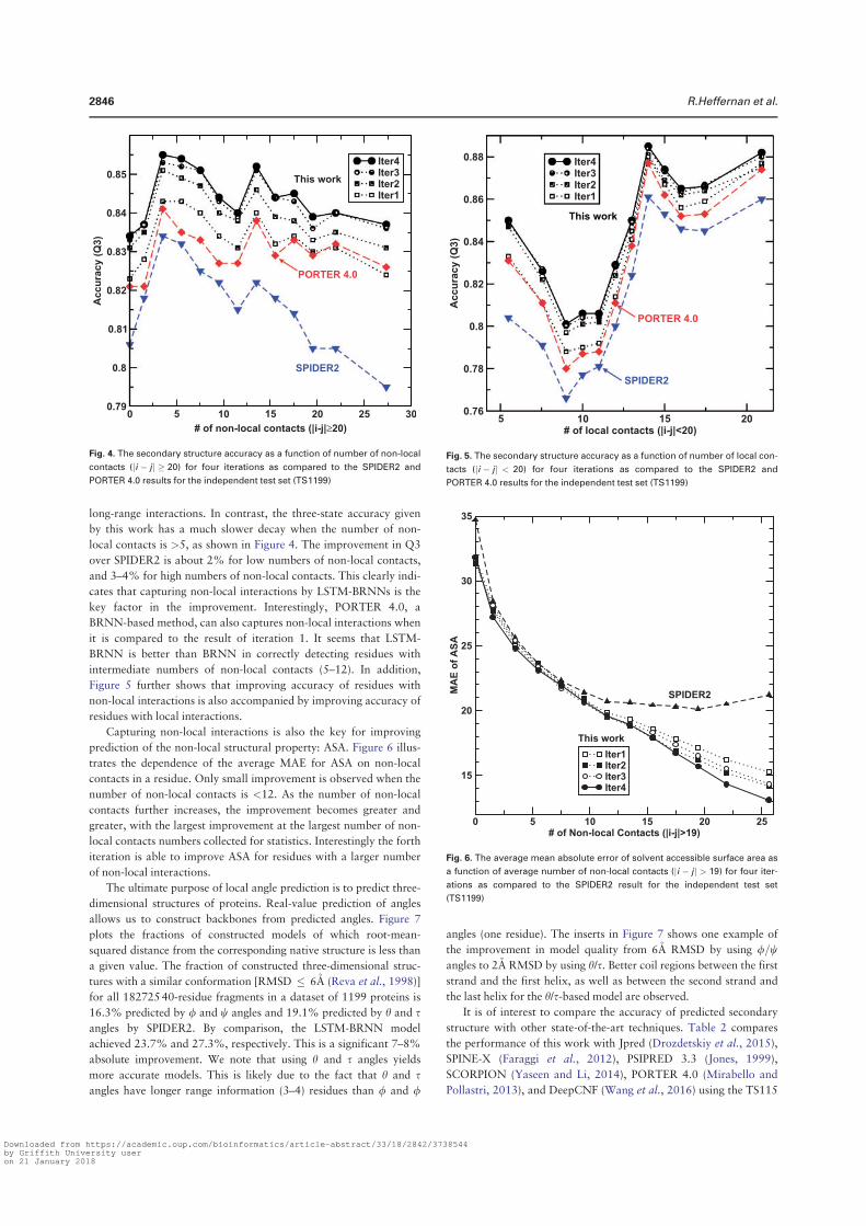
long-range interactions. In contrast, the three-state accuracy given
by this work has a much slower decay when the number of non-
local contacts is >5, as shown in Figure 4. The improvement in Q3
over SPIDER2 is about 2% for low numbers of non-local contacts,
and 3–4% for high numbers of non-local contacts. This clearly indi-
cates that capturing non-local interactions by LSTM-BRNNs is the
key factor in the improvement. Interestingly, PORTER 4.0, a
BRNN-based method, can also captures non-local interactions when
it is compared to the result of iteration 1. It seems that LSTM-
BRNN is better than BRNN in correctly detecting residues with
intermediate numbers of non-local contacts (5–12). In addition,
Figure 5 further shows that improving accuracy of residues with
non-local interactions is also accompanied by improving accuracy of
residues with local interactions.
Capturing non-local interactions is also the key for improving
prediction of the non-local structural property: ASA. Figure 6 illus-
trates the dependence of the average MAE for ASA on non-local
contacts in a residue. Only small improvement is observed when the
number of non-local contacts is <12. As the number of non-local
contacts further increases, the improvement becomes greater and
greater, with the largest improvement at the largest number of non-
local contacts numbers collected for statistics. Interestingly the forth
iteration is able to improve ASA for residues with a larger number
of non-local interactions.
The ultimate purpose of local angle prediction is to predict three-
dimensional structures of proteins. Real-value prediction of angles
allows us to construct backbones from predicted angles. Figure 7
plots the fractions of constructed models of which root-mean-
squared distance from the corresponding native structure is less than
a given value. The fraction of constructed three-dimensional struc-
tures with a similar conformation [RMSD � 6A (Reva et al., 1998)]
for all 182725 40-residue fragments in a dataset of 1199 proteins is
16.3% predicted by / and w angles and 19.1% predicted by h and sangles by SPIDER2. By comparison, the LSTM-BRNN model
achieved 23.7% and 27.3%, respectively. This is a significant 7–8%
absolute improvement. We note that using h and s angles yields
more accurate models. This is likely due to the fact that h and sangles have longer range information (3–4) residues than / and /
angles (one residue). The inserts in Figure 7 shows one example of
the improvement in model quality from 6A RMSD by using /=wangles to 2A RMSD by using h/s. Better coil regions between the first
strand and the first helix, as well as between the second strand and
the last helix for the h/s-based model are observed.
It is of interest to compare the accuracy of predicted secondary
structure with other state-of-the-art techniques. Table 2 compares
the performance of this work with Jpred (Drozdetskiy et al., 2015),
SPINE-X (Faraggi et al., 2012), PSIPRED 3.3 (Jones, 1999),
SCORPION (Yaseen and Li, 2014), PORTER 4.0 (Mirabello and
Pollastri, 2013), and DeepCNF (Wang et al., 2016) using the TS115
Fig. 4. The secondary structure accuracy as a function of number of non-local
contacts (ji � j j � 20) for four iterations as compared to the SPIDER2 and
PORTER 4.0 results for the independent test set (TS1199)
Fig. 5. The secondary structure accuracy as a function of number of local con-
tacts (ji � j j < 20) for four iterations as compared to the SPIDER2 and
PORTER 4.0 results for the independent test set (TS1199)
Fig. 6. The average mean absolute error of solvent accessible surface area as
a function of average number of non-local contacts (ji � jj > 19) for four iter-
ations as compared to the SPIDER2 result for the independent test set
(TS1199)
2846 R.Heffernan et al.
Downloaded from https://academic.oup.com/bioinformatics/article-abstract/33/18/2842/3738544by Griffith University useron 21 January 2018
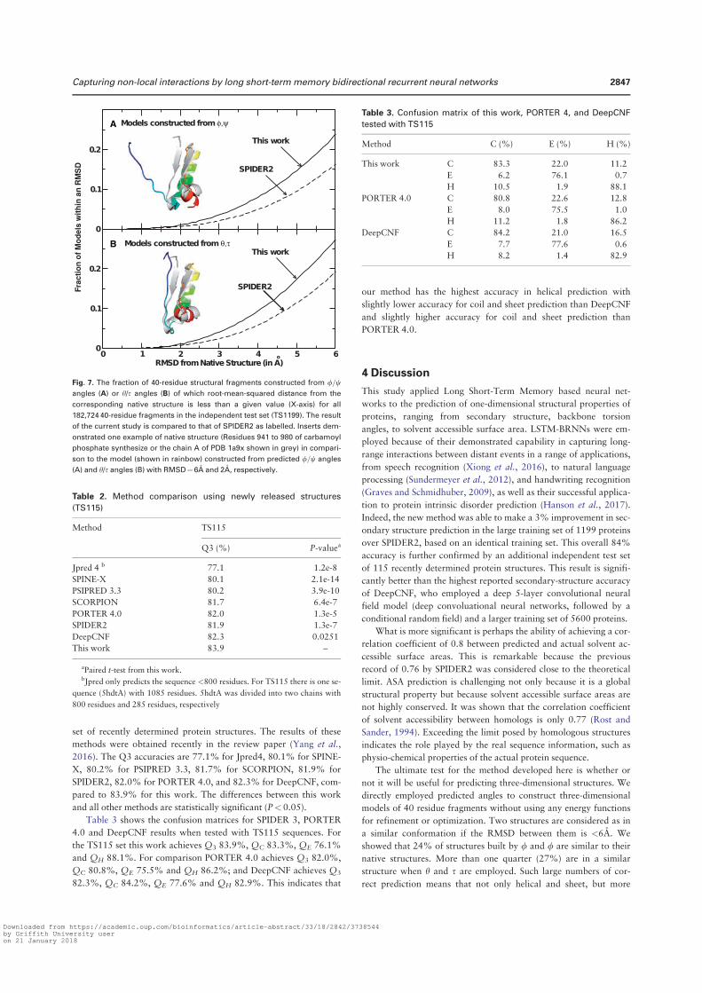
set of recently determined protein structures. The results of these
methods were obtained recently in the review paper (Yang et al.,
2016). The Q3 accuracies are 77.1% for Jpred4, 80.1% for SPINE-
X, 80.2% for PSIPRED 3.3, 81.7% for SCORPION, 81.9% for
SPIDER2, 82.0% for PORTER 4.0, and 82.3% for DeepCNF, com-
pared to 83.9% for this work. The differences between this work
and all other methods are statistically significant (P<0.05).
Table 3 shows the confusion matrices for SPIDER 3, PORTER
4.0 and DeepCNF results when tested with TS115 sequences. For
the TS115 set this work achieves Q3 83.9%, QC 83.3%, QE 76.1%
and QH 88.1%. For comparison PORTER 4.0 achieves Q3 82.0%,
QC 80.8%, QE 75.5% and QH 86.2%; and DeepCNF achieves Q3
82.3%, QC 84.2%, QE 77.6% and QH 82.9%. This indicates that
our method has the highest accuracy in helical prediction with
slightly lower accuracy for coil and sheet prediction than DeepCNF
and slightly higher accuracy for coil and sheet prediction than
PORTER 4.0.
4 Discussion
This study applied Long Short-Term Memory based neural net-
works to the prediction of one-dimensional structural properties of
proteins, ranging from secondary structure, backbone torsion
angles, to solvent accessible surface area. LSTM-BRNNs were em-
ployed because of their demonstrated capability in capturing long-
range interactions between distant events in a range of applications,
from speech recognition (Xiong et al., 2016), to natural language
processing (Sundermeyer et al., 2012), and handwriting recognition
(Graves and Schmidhuber, 2009), as well as their successful applica-
tion to protein intrinsic disorder prediction (Hanson et al., 2017).
Indeed, the new method was able to make a 3% improvement in sec-
ondary structure prediction in the large training set of 1199 proteins
over SPIDER2, based on an identical training set. This overall 84%
accuracy is further confirmed by an additional independent test set
of 115 recently determined protein structures. This result is signifi-
cantly better than the highest reported secondary-structure accuracy
of DeepCNF, who employed a deep 5-layer convolutional neural
field model (deep convoluational neural networks, followed by a
conditional random field) and a larger training set of 5600 proteins.
What is more significant is perhaps the ability of achieving a cor-
relation coefficient of 0.8 between predicted and actual solvent ac-
cessible surface areas. This is remarkable because the previous
record of 0.76 by SPIDER2 was considered close to the theoretical
limit. ASA prediction is challenging not only because it is a global
structural property but because solvent accessible surface areas are
not highly conserved. It was shown that the correlation coefficient
of solvent accessibility between homologs is only 0.77 (Rost and
Sander, 1994). Exceeding the limit posed by homologous structures
indicates the role played by the real sequence information, such as
physio-chemical properties of the actual protein sequence.
The ultimate test for the method developed here is whether or
not it will be useful for predicting three-dimensional structures. We
directly employed predicted angles to construct three-dimensional
models of 40 residue fragments without using any energy functions
for refinement or optimization. Two structures are considered as in
a similar conformation if the RMSD between them is <6A. We
showed that 24% of structures built by / and / are similar to their
native structures. More than one quarter (27%) are in a similar
structure when h and s are employed. Such large numbers of cor-
rect prediction means that not only helical and sheet, but more
A
B
Fig. 7. The fraction of 40-residue structural fragments constructed from /=w
angles (A) or h/s angles (B) of which root-mean-squared distance from the
corresponding native structure is less than a given value (X-axis) for all
182,724 40-residue fragments in the independent test set (TS1199). The result
of the current study is compared to that of SPIDER2 as labelled. Inserts dem-
onstrated one example of native structure (Residues 941 to 980 of carbamoyl
phosphate synthesize or the chain A of PDB 1a9x shown in grey) in compari-
son to the model (shown in rainbow) constructed from predicted /=w angles
(A) and h/s angles (B) with RMSD¼6A and 2A, respectively.
Table 2. Method comparison using newly released structures
(TS115)
Method TS115
Q3 (%) P-valuea
Jpred 4 b 77.1 1.2e-8
SPINE-X 80.1 2.1e-14
PSIPRED 3.3 80.2 3.9e-10
SCORPION 81.7 6.4e-7
PORTER 4.0 82.0 1.3e-5
SPIDER2 81.9 1.3e-7
DeepCNF 82.3 0.0251
This work 83.9 –
aPaired t-test from this work.bJpred only predicts the sequence <800 residues. For TS115 there is one se-
quence (5hdtA) with 1085 residues. 5hdtA was divided into two chains with
800 residues and 285 residues, respectively
Table 3. Confusion matrix of this work, PORTER 4, and DeepCNF
tested with TS115
Method C (%) E (%) H (%)
This work C 83.3 22.0 11.2
E 6.2 76.1 0.7
H 10.5 1.9 88.1
PORTER 4.0 C 80.8 22.6 12.8
E 8.0 75.5 1.0
H 11.2 1.8 86.2
DeepCNF C 84.2 21.0 16.5
E 7.7 77.6 0.6
H 8.2 1.4 82.9
Capturing non-local interactions by long short-term memory bidirectional recurrent neural networks 2847
Downloaded from https://academic.oup.com/bioinformatics/article-abstract/33/18/2842/3738544by Griffith University useron 21 January 2018
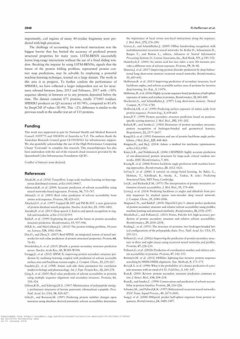
importantly, coil regions of many 40-residue fragments were pre-
dicted with high precision.
The challenge of accounting for non-local interactions was the
biggest barrier that has limited the accuracy of predicted protein
structural properties for many years. LSTM-BRNN successfully
learns long-range interactions without the use of a fixed sliding win-
dow. Breaking the impasse by using LSTM-BRNNs, signals that the
future of the protein folding problem, represented protein con-
tact map predictions, may be solvable by employing a powerful
machine-learning technique, trained on a large dataset. The work in
this area is in progress. To further confirm the performance of
SPIDER3, we have collected a larger independent test set for struc-
tures released between June, 2015 and February, 2017 with <30%
sequence identity in between or to any proteins deposited before the
time. The dataset contains 673 proteins, totally 171003 residues.
SPIDER3 produces an Q3 accuracy of 83.74%, compared to 81.6%
by DeepCNF (P-value<1E-99). This >2% difference is similar to the
previous result in the smaller test set of 115 proteins.
Funding
This work was supported in part by National Health and Medical Research
Council (1059775 and 1083450) of Australia to Y.Z. The authors thank the
Australian Research Council grant LE150100161 for infrastructure support.
We also gratefully acknowledge the use of the High Performance Computing
Cluster ‘Gowonda’ to complete this research. This research/project has also
been undertaken with the aid of the research cloud resources provided by the
Queensland Cyber Infrastructure Foundation (QCIF).
Conflict of Interest: none declared.
References
Abadi,M. et al. (2016) Tensorflow: Large-scale machine learning on heteroge-
neous distributed systems. arXiv:1603.04467.
Adamczak,R. et al. (2004) Accurate prediction of solvent accessibility using
neural networks-based regression. Proteins, 56, 753–767.
Ahmad,S. et al. (2003) Real value prediction of solvent accessibility from
amino acid sequence. Proteins, 50, 629–635.
Altschul,S.F. et al. (1997) Gapped BLAST and PSI-BLAST: a new generation
of protein database search programs. Nucleic Acids Res, 25, 3389–3402.
Amodei,D. et al. (2015) Deep speech 2: End-to-end speech recognition in eng-
lish and mandarin. arXiv:1512.02595.
Baldi,P. et al. (1999) Exploiting the past and the future in protein secondary
structure prediction. Bioinformatics, 15, 937–946.
Dill,K.A., and MacCallum,J.L. (2012) The protein-folding problem, 50 years
on. Science, 338, 1042–1046.
Dor,O., and Zhou,Y. (2007) Real-SPINE: an integrated system of neural net-
works for real-value prediction of protein structural properties. Protein, 68,
76–81.
Drozdetskiy,A. et al. (2015) JPred4: a protein secondary structure prediction
server. Nucleic Acids Res., 43, W389–W394.
Faraggi,E. et al. (2012) SPINE X: improving protein secondary structure pre-
diction by multistep learning coupled with prediction of solvent accessible
surface area and backbone torsion angles. J. Comput. Chem., 33, 259–267.
Fauchere,J.L. et al. (1988) Amino acid side chain parameters for correlation
studies in biology and pharmacology. Int. J. Pept. Protein Res., 32, 269–278.
Garg,A. et al. (2005) Real value prediction of solvent accessibility in proteins
using multiple sequence alignment and secondary structure. Proteins, 61,
318–324.
Gibson,K.D., and Scheraga,H.A. (1967) Minimization of polypeptide energy.
i. preliminary structures of bovine pancreatic ribonuclease s-peptide. Proc.
Natl. Acad. Sci. USA, 58, 420–427.
Gilis,D., and Rooman,M. (1997) Predicting protein stability changes upon
mutation using database-derived potentials: solvent accessibility determines
the importance of local versus non-local interactions along the sequence.
J. Mol. Biol., 272, 276–290.
Graves,A., and Schmidhuber,J. (2009) Offline handwriting recognition with
multidimensional recurrent neural networks. In: Koller D., Schuurmans D.,
Bengio Y., and Bottou L., editors, Advances in Neural Information
Processing Systems 21. Curran Associates, Inc., Red Hook, NY, p.545–552.
Hamelryck,T. (2005) An amino acid has two sides: a new 2D measure pro-
vides a different view of solvent exposure. Proteins, 59, 38–48.
Hanson,J. et al. (2017) Improving protein disorder prediction by deep bidirec-
tional long short-term memory recurrent neural networks. Bioinformatics,
33, 685–692.
Heffernan,R. et al. (2015) Improving prediction of secondary structure, local
backbone angles, and solvent accessible surface area of proteins by iterative
deep learning. Sci. Rep., 5, 11476.
Heffernan, R. et al. (2016) Highly accurate sequence-based prediction of half-sphere
exposures of amino acid residues in proteins. Bioinformatics, 32, 843–849.
Hochreiter,S., and Schmidhuber,J. (1997) Long short-term memory. Neural
Comput., 9, 1735–1780.
Holbrook,S.R. et al. (1990) Predicting surface exposure of amino acids from
protein sequence. Protein Eng., 3, 659–665.
Jones,D.T. (1999) Protein secondary structure prediction based on position-
specific scoring matrices. J. Mol. Biol., 292, 195–202.
Kabsch,W., and Sander,C. (1983) Dictionary of protein secondary structure:
pattern recognition of hydrogen-bonded and geometrical features.
Biopolymers, 22, 2577–2637.
Kang,H.S. et al. (1993) Estimation and use of protein backbone angle proba-
bilities. J Mol. Biol., 229, 448–460.
Kingma,D., and Ba,J. (2014) Adam: a method for stochastic optimization.
arXiv:1412.6980.
Kinjo,A.R., and Nishikawa,K. (2006) CRNPRED: highly accurate prediction
of one-dimensional protein structures by large-scale critical random net-
works. BMC Bioinformatics, 7, 401.
Kuang,R. et al. (2004) Protein backbone angle prediction with machine learn-
ing approaches. Bioinformatics, 20, 1612–1621.
LeCun,Y. et al. (2006) A tutorial on energy-based learning. In: Bakir, G.,
Hofman, T., Scholkopf, B., Smola, A., Taskar, B. (eds.) Predicting
Structured Data. MIT Press, Cambridge.
Lee,B., and Richards,F.M. (1971) The interpretation of protein structures: es-
timation of static accessibility. J. Mol. Biol., 55, 379–400.
Lyons,J. et al. (2014) Predicting backbone ca angles and dihedrals from pro-
tein sequences by stacked sparse auto-encoder deep neural network.
J. Comput. Chem., 35, 2040–2046.
Magnan,C.N., and Baldi,P. (2014) SSpro/ACCpro 5: almost perfect prediction
of protein secondary structure and relative solvent accessibility using profiles,
machine learning and structural similarity. Bioinformatics, 30, 2592–2597.
Mirabello,C., and Pollastri,G. (2013) Porter, PaleAle 4.0: high-accuracy pre-
diction of protein secondary structure and relative solvent accessibility.
Bioinformatics, 29, 2056–2058.
Pauling,L. et al. (1951) The structure of proteins: two hydrogen-bonded hel-
ical configurations of the polypeptide chain. Proc. Natl. Acad. Sci. USA, 37,
205–211.
Pollastri,G. et al. (2002a) Improving the prediction of protein secondary struc-
ture in three and eight classes using recurrent neural networks and profiles.
Proteins, 47, 228–235.
Pollastri,G. et al. (2002b) Prediction of coordination number and relative solv-
ent accessibility in proteins. Proteins, 47, 142–153.
Remmert,M. et al. (2012) HHblits: lightning-fast iterative protein sequence
searching by HMM-HMM alignment. Nat. Methods, 9, 173–175.
Reva,B.A. et al. (1998) What is the probability of a chance prediction of a pro-
tein structure with an rmsd of 6 A?. Fold Des., 3, 141–147.
Rost,B. (2001) Review: protein secondary structure prediction continues to
rise. J. Struct. Biol., 134, 204–218.
Rost,B., and Sander,C. (1994) Conservation and prediction of solvent accessi-
bility in protein families. Proteins, 20, 216–226.
Schuster,M., and Paliwal,K.K. (1997) Bidirectional recurrent neural networks.
IEEE Trans. Signal Process., 45, 2673–2681.
Song,J. et al. (2008) HSEpred: predict half-sphere exposure from protein se-
quences. Bioinformatics, 24, 1489–1497.
2848 R.Heffernan et al.
Downloaded from https://academic.oup.com/bioinformatics/article-abstract/33/18/2842/3738544by Griffith University useron 21 January 2018
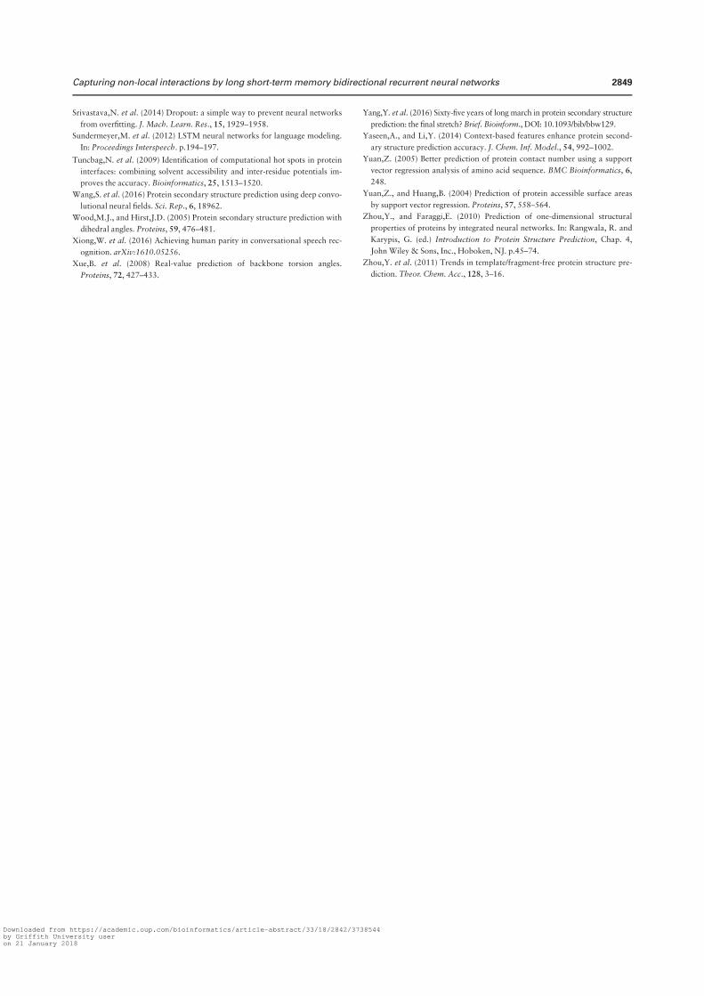
Srivastava,N. et al. (2014) Dropout: a simple way to prevent neural networks
from overfitting. J. Mach. Learn. Res., 15, 1929–1958.
Sundermeyer,M. et al. (2012) LSTM neural networks for language modeling.
In: Proceedings Interspeech. p.194–197.
Tuncbag,N. et al. (2009) Identification of computational hot spots in protein
interfaces: combining solvent accessibility and inter-residue potentials im-
proves the accuracy. Bioinformatics, 25, 1513–1520.
Wang,S. et al. (2016) Protein secondary structure prediction using deep convo-
lutional neural fields. Sci. Rep., 6, 18962.
Wood,M.J., and Hirst,J.D. (2005) Protein secondary structure prediction with
dihedral angles. Proteins, 59, 476–481.
Xiong,W. et al. (2016) Achieving human parity in conversational speech rec-
ognition. arXiv:1610.05256.
Xue,B. et al. (2008) Real-value prediction of backbone torsion angles.
Proteins, 72, 427–433.
Yang,Y. et al. (2016) Sixty-five years of long march in protein secondary structure
prediction: the final stretch? Brief. Bioinform., DOI: 10.1093/bib/bbw129.
Yaseen,A., and Li,Y. (2014) Context-based features enhance protein second-
ary structure prediction accuracy. J. Chem. Inf. Model., 54, 992–1002.
Yuan,Z. (2005) Better prediction of protein contact number using a support
vector regression analysis of amino acid sequence. BMC Bioinformatics, 6,
248.
Yuan,Z., and Huang,B. (2004) Prediction of protein accessible surface areas
by support vector regression. Proteins, 57, 558–564.
Zhou,Y., and Faraggi,E. (2010) Prediction of one-dimensional structural
properties of proteins by integrated neural networks. In: Rangwala, R. and
Karypis, G. (ed.) Introduction to Protein Structure Prediction, Chap. 4,
John Wiley & Sons, Inc., Hoboken, NJ. p.45–74.
Zhou,Y. et al. (2011) Trends in template/fragment-free protein structure pre-
diction. Theor. Chem. Acc., 128, 3–16.
Capturing non-local interactions by long short-term memory bidirectional recurrent neural networks 2849
Downloaded from https://academic.oup.com/bioinformatics/article-abstract/33/18/2842/3738544by Griffith University useron 21 January 2018
Chapter 6
SPIDER3 Single -
Single-Sequence-Based Prediction
of Protein Secondary Structures
and Solvent Accessibility by Deep
Whole-Sequence Learning.
53

STATEMENT OF CONTRIBUTION TO CO-AUTHORED PUBLISHED PAPER
This chapter includes a co-authored paper. The bibliographic details of the co-authored paper, including all authors, are:
R. Heffernan, K. Paliwal, J. Lyons, J. Singh, Y. Yang, and Y. Zhou, “Single-sequence-based prediction of protein secondary structures and solvent accessibility by deepwhole-sequence learning,” Journal of Computational Chemistry, in press.
My contribution to the paper involved:
Designed the method. Wrote all the code for the method. Produced and co-analyisedresults. Co-wrote the manuscript.
(Signed) _________________________________ (Date)______________Rhys Heffernan
(Countersigned) ___________________________ (Date)______________Corresponding author of paper: Yaoqi Zhou
(Countersigned) ___________________________ (Date)______________Supervisor: Kuldip Paliwal
Single-Sequence-Based Prediction of Protein SecondaryStructures and Solvent Accessibility by Deep Whole-Sequence LearningRhys Heffernan ,[a] Kuldip Paliwal,[a] James Lyons,[a] Jaswinder Singh,[a] Yuedong Yang,[b]
and Yaoqi Zhou ,*[c]
Predicting protein structure from sequence alone is challenging.Thus, the majority of methods for protein structure predictionrely on evolutionary information from multiple sequence align-ments. In previous work we showed that Long Short-Term Bidi-rectional Recurrent Neural Networks (LSTM-BRNNs) improvedover regular neural networks by better capturing intra-sequencedependencies. Here we show a single-sequence-based predic-tion method employing LSTM-BRNNs (SPIDER3-Single), thatconsistently achieves Q3 accuracy of 72.5%, and correlationcoefficient of 0.67 between predicted and actual solvent acces-sible surface area. Moreover, it yields reasonably accurate
prediction of eight-state secondary structure, main-chainangles (backbone ϕ and ψ torsion angles and Cα-atom-basedθ and τ angles), half-sphere exposure, and contact number.The method is more accurate than the correspondingevolutionary-based method for proteins with few sequencehomologs, and computationally efficient for large-scale screen-ing of protein-structural properties. It is available as an optionin the SPIDER3 server, and a standalone version for download,at http://sparks-lab.org. © 2018 Wiley Periodicals, Inc.
DOI:10.1002/jcc.25534
Introduction
The protein folding paradigm states that a protein’s structure isdetermined solely by its sequence. This is a fundamentallyimportant concept, as protein structures provide the key to theirfunctional mechanisms. Experimental techniques for solving pro-tein structures, such as X-ray crystallography, nuclear magneticresonance, and cryo-electron microscopy are time-consuming,labor-intensive, and costly; leading to a situation where the rateat which new proteins are discovered far outpaces our ability toexperimentally determine their structures. This adds an urgencyto finding a method to computationally predict a protein’s struc-ture, from its primary sequence alone. Despite its importance,the protein folding problem has remained unsolved[1–3] since itsinception over half a century ago[4]. This is due to the difficultyin formulating an accurate energy function for the solvent-mediated interaction between amino acid residues.[2]
While it is challenging to predict a protein’s structure directlyfrom its sequence alone, accurate structure prediction cannow be made using restraints derived from correlated muta-tions located from Multiple Sequence Alignments (MSAs) ofhomologous sequences, if a large number of homologoussequences are known.[5] Similarly, the accuracy of predictingprotein secondary structure, an important subproblem of pro-tein structure prediction, increased from approximately 60% byearly single-sequence-based techniques[6] to beyond 70% withthe introduction of evolutionary information from MSA,[7] and to82%–84% with the latest deep long-range learning techniquesalso with evolutionary information as the key input.[3,8–10]
However, the majority of proteins (>90%) have few, if any,known homologous sequences.[5] In these cases, evolutionary
information is limited or non-existent, and poor prediction accu-racy is expected. It is quite possible that inaccurate evolutionaryinformation might reduce the accuracy of prediction. Indeed, arecent single-sequence-based prediction of solvent AccessibleSurface Area (ASA by ASAquick) is more accurate thanevolution-profile trained methods for those proteins with fewhomologous sequences.[11] Thus, it is possible that one can sim-ply improve prediction accuracy by the alternative use of single-sequence and evolution-based methods, depending on the sizeof the homologous sequence cluster for a given protein.
Moreover, such single-sequence-based prediction is compu-tationally efficient because greater than 99% of the computa-tional time is spent on generating evolutionary sequenceprofiles. Increasingly inexpensive sequencing techniques haveled to an exponential increase in the number of knownsequences. As a result, the computational time requirement forfinding sequence profiles is continuing to increase. For
[a] R. Heffernan, K. Paliwal, J. Lyons, J. SinghSignal Processing Laboratory, Griffith University, Brisbane, QLD, 4111,Australia
[b] Y. YangSchool of Data and Computer Science, Sun Yet-Sen University, Guangzhou,China
[c] Y. ZhouInstitute for Glycomics and School of Information and CommunicationTechnology, Griffith University, Southport, QLD, 4222, AustraliaE-mail: [email protected]
Contract grant sponsor: This work was supported by Australian ResearchCouncil DP180102060 to Y.Z. and K. P. and in part by National Health andMedical Research Council (1121629) of Australia to Y.Z.
© 2018 Wiley Periodicals, Inc.
WWW.C-CHEM.ORG FULL PAPER
Wiley Online Library Journal of Computational Chemistry 2018 1
example, PSSM generation, by PSI-BLAST,[12] can take in theregion of 30 min for a short protein (around 100 resides) up tomultiple hours for a longer sequence (around 1000 residues).More importantly, a single-sequence-based prediction directlyaddresses the original subproblem of protein structure predic-tion: how far can we push the accuracy of predicting proteinsecondary structure from its sequence alone?
Although secondary structure prediction is dominated bymethods based on evolutionary information, progress has beenmake in single-sequence-based prediction. SIMPA is a methodemploying a nearest neighbor model, which reported a Q3 of67.7%.[13] BSPSS is a Bayesian solution which succeeds in incor-porating non local information and reports a Q3 of 68.8%.[14]
Kloczkowshi et al. presented a single sequence version of theGOR V method which reports a Q3 accuracy of 67.5%.[15] IPSSPextends upon BSPSS with a number of changes including itera-tive training and improved residue dependency model report-ing a Q3 of 70.3%.[16] Bidargaddi et al. combined BSPSS with aNeural Network (NN) to reach a Q3 of 71%.[17] Bouzianeet al. used an ensemble of Support Vector Machine (SVM) andNN models to achieve Q3 results around 66%.[18] The popularPSIpred also maintains a single sequence version (hereonreferred to as PSIpred-Single) which achieves results around70%.[19] All of these methods, however, have not yet takenadvantage of recent computational advancements in deeplearning.[20–22]
Recently, we employed Long Short-Term Memory (LSTM)Bidirectional Recurrent Neural Networks (BRNNs) to predict sev-eral one-dimensional structural properties of proteins by itera-tive learning.[9] LSTM networks take the whole proteinsequence as input, rather than a sliding window, to capturelong-range interactions between residues that are close inthree-dimensional space, but far from each other in sequencepositions. This allows the method (SPIDER3) to achieve thehighest reported accuracy for several one-dimensional struc-tural properties such as secondary structure (~84% Q3), solventaccessibility (with a correlation coefficient between predictedand actual solvent accessibility at 0.8), and backbone torsionangles (e.g., a mean absolute error of 27� for ψ ).
In this article, we examine if LSTM-BRNNs can make moreaccurate single-sequence prediction of secondary structurethan existing techniques, by using the same iterative deeplearning technique as SPIDER3. Unlike previous single-sequence-based methods, this method (named SPIDER3-Single)will not only predict secondary structure in three states, butalso in all eight states. Moreover, we will predict four backbonetorsion angles (ϕ, ψ , θ, and τ), solvent accessibility, Half SphereExposure (HSE), and Contact Number (CN). We show thatSPIDER3-Single is able to achieve reasonably accurate predic-tion for all structural properties predicted.
MethodologyDatasets
Our dataset was obtained by downloading 30% non-redundantsequences from cullpdb in February 2017, with a resolution of
less than 2.5 Å, and R-factor less than 1.0. Of these, we removedsequences with a length of less than 30 residues, a similaritygreater than 25% according to BlastClust,[12] and any sequenceswith incomplete information. This resulted in 12,442 sequences,which were split into 11192 submitted before and 1250 afterJune 2015 (TS1250). The 11,192 sequences submitted beforeJune 2015 were used for training and evaluation by separatinginto a training set of 9993 proteins called TR9993, and a test setof 1199 proteins called TS1199. The TR9993 set was used for10-fold cross validation, in which the set was divided into10 sets with each employed in turn as the test set and theremainder as the training set. We obtained a more difficult sub-set from TS1250 by further excluding potential homologousproteins from the training set with a PSI-Blast E-value cutoff of0.1. This subset, labeled TS-Hard, has 280 sequence.
Input features
Each single sequence is represented by a one-hot vector of size20 × L, where L is the length of the protein chain. Althoughsingle-sequence derived features such as physiochemical prop-erties[8,9] and the BLOSUM matrix[23] can also be used, we foundthat these did not offer any improvement. This is likely becausethese features are simply linear weight matrices that are learn-able by the neural network employed here. Thus, only the one-hot vector is employed.
Outputs
The secondary structure assignment program Define SecondaryStructure of Proteins (DSSP) specifies eight secondary structurestates, comprised of two helix, two strand, and three coilstates.[24] The three helix states are: 310-helix (G), alpha-helix(H), and pi-helix (I); the strand states are: beta-bridge (B) andbeta-strand (E); and the three coil types are high curvature loop(S), beta-turn (T), and coil (C). These eight states are convertedinto a three-state problem using the following conversion: G, H,and I to H; B and E to E; and S, T, and C to C. We designed ournetwork to independently predict 8 and 3 state secondarystructure for a total of 11 output nodes.
In addition to secondary structure, our method also predictsAccessible Surface Area (ASA), ϕ, ψ , θ, τ, Half Sphere Exposure(HSE), and Contact Number (CN). ASA is a measure of the levelof exposure of each residue within the protein to solvent(water). Active sites of proteins are often located on their sur-face, therefore knowing the level of exposure of each residuecan provide insight as to where that activity might occur. ϕ andψ are two of the backbone torsion angles, along with ω, thatdescribe a protein’s local backbone structure. ω is not predictedhere because it is usually at 180 due to the planarity of the pep-tide bond. θ and τ angles describe the orientation betweenneighboring residues according to Cα atoms. Specifically θ isthe angle between Cαi − 1 − Cαi − Cαi + 1, and τ is the dihedralangle rotated about the Cαi − Cαi + 1 vector.
[25] CN is the countof the number of residues within a distance cutoff, in three-dimensional space, of a given residue. HSE extends the idea ofCN by adding directionality information and differentiating
FULL PAPER WWW.C-CHEM.ORG
Journal of Computational Chemistry 2018 WWW.CHEMISTRYVIEWS.COM2
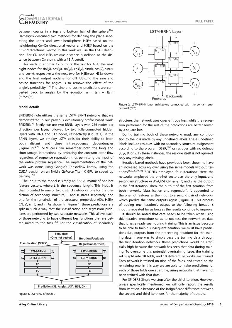
between counts in a top and bottom half of the sphere.[26]
Hamelryck described two methods for defining the plane sepa-rating the upper and lower hemisphere, HSEα based on theneighboring Cα–Cα directional vector and HSEβ based on theCα−Cβ directional vector. In this work we use the HSEα defini-tion. For CN and HSE, residue distance is defined as the dis-tance between Cα atoms with a 13 Å cutoff.
This leads to another 12 outputs: the first for ASA; the nexteight nodes for sin(ϕ), cos(ϕ), sin(ψ ), cos(ψ ), sin(θ), cos(θ), sin(τ),and cos(τ), respectively; the next two for HSEα-up, HSEα-down;and the final output node is for CN. Utilizing the sine andcosine functions for angles is to remove the effect of theangle’s periodicity.[25] The sine and cosine predictions are con-verted back to angles by the equation α = tan − 1[sin(α)/cos(α)].
Model details
SPIDER3-Single utilizes the same LSTM-BRNN networks that wedemonstrated in our previous evolutionary-profile based work,SPIDER3.[9] Briefly, we use two BRNN layers with 256 nodes perdirection, per layer; followed by two fully-connected hiddenlayers with 1024 and 512 nodes, respectively (Figure 1). In theBRNN layers, we employ LSTM cells for their ability to learnboth distant and close intra-sequence dependencies(Figure 2).[27] LSTM cells can remember both the long andshort-ranage interactions by enforcing the constant error flowregardless of sequence seperation, thus permitting the input ofthe entire protein sequence. The implementation of the net-work was done using Google’s Tensorflow library, using theCUDA version on an Nvidia GeForce Titan X GPU to speed uptraining.[28]
The input to the model is simply an L × 20 matrix of one-hotfeature vectors, where L is the sequence length. This input isthen provided to one of two distinct networks, one for the pre-diction of secondary structure, 3 and 8 states separately, andone for the remainder of the structural properties: ASA, HSEα,CN, ϕ, ψ , θ, and τ. As shown in Figure 1, these predictions aresplit in such a way that the classification and regression prob-lems are performed by two separate networks. This allows eachof those networks to have different loss functions that are bet-ter suited to the task.[29] For the classification of secondary
structure, the network uses cross-entropy loss, while the regres-sion performed for the rest of the predictions are better servedby a square loss.
During training both of these networks mask any contribu-tion to the loss made by any undefined labels. These undefinedlabels include residues with no secondary structure assignmentaccording to the program DSSP,[24] or residues with no definedϕ, ψ , θ, or τ. In these instances, the residue itself is not ignored,only any missing labels.
Iterative based methods have previously been shown to havean increased accuracy over using the same models without iter-ations.[8,9,25,30,31] SPIDER3 employed four iterations. Here thenetworks employed the one-hot vectors as the only input, andsecondary structure or ASA,HSE,CN, ϕ, ψ , θ, and τ as the outputin the first iteration. Then, the output of the first iteration, fromboth networks (classification and regression), is appended tothe one-hot features as the input to a second pair of networks,which predict the same outputs again (Figure 1). This processof adding one iteration’s output to the following iteration’sinput is repeated for as long as the results continue to improve.
It should be noted that care needs to be taken when usingthis iterative procedure so as to not test the network on datathat it has already seen during training. This is an issue becauseto be able to train a subsequent iteration, we must have predic-tions (i.e., outputs from the proceeding iteration) for the train-ing data. If one was to simply pass the training data throughthe first iteration networks, those predictions would be artifi-cially high because the network has seen that data during train-ing. To overcome this potential overtraining issue, the trainingset is split into 10 folds, and 10 different networks are trained.Each network is trained on nine of the folds, and tested on theremaining one. In this way we are able to make predictions foreach of those folds one at a time, using networks that have notbeen trained with that data.
For SPIDER3-Single we stop after the third iteration. However,unless specifically mentioned we will only report the resultsfrom iteration 2 because of the insignificant difference betweenthe second and third iterations for the majority of outputs.Figure 1. Overview of model.
Figure 2. LSTM-BRNN layer architecture connected with the contant errorcarousel (CEC).
WWW.C-CHEM.ORG FULL PAPER
Wiley Online Library Journal of Computational Chemistry 2018 3
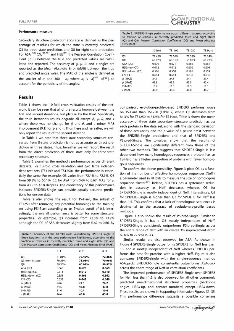
Performance measure
Secondary structure prediction accuracy is defined as the per-centage of residues for which the state is correctly predicted;Q3 for three state prediction, and Q8 for eight state prediction.For ASA,[30] CN,[31,32] and HSE[33] the Pearson Correlation Coeffi-cient (PCC) between the true and predicted values are calcu-lated and reported. The accuracy of ϕ, ψ , θ, and τ angles arereported as the Mean Absolute Error (MAE) between the trueand predicted angle vales. The MAE of the angles is defined as
the smaller of αi and 360 − αi, where αi is j αpredi −αtruei j, toaccount for the periodicity of the angles.
Results
Table 1 shows the 10-fold cross validation results of the net-work. It can be seen that all of the results improve between thefirst and second iterations, but plateau by the third. Specificallythe third iteration’s results degrade all except ϕ, ψ , θ, and τ
where there was no change for ϕ and θ, and a minor MAEimprovement (0.1) for ϕ and τ. Thus, here and hereafter, we willonly report the result of the second iteration.
In Table 1 we note that three-state secondary structure con-verted from 8-state prediction is not as accurate as direct pre-diction in three states. Thus, hereafter we will report the resultfrom the direct prediction of three state only for three-statesecondary structure.
Table 2 examines the method’s performance across differentdatasets. For 10-fold cross validation and two large indepen-dent test sets (TS1199 and TS1250), the performance is essen-tially the same. For example, Q3 varies from 72.4% to 72.6%, Q8from 59.8% to 60.1%, CC for ASA from 0.66 to 0.67, MAE for ψfrom 43.5 to 43.8 degrees. The consistency of this performanceindicates SPIDER3-Single can provide equally accurate predic-tions for unseen data.
Table 2 also shows the result for TS-Hard, the subset ofTS1250 after removing any potential homologs to the trainingset using PSI-Blast according to an E-value cutoff of 0.1. Inter-estingly, the overall performance is better for some structuralproperties. For example, Q3 increases from 72.5% to 73.2%although the CC of ASA decreases slightly from 0.67 to 0.66. By
comparison, evolution-profile-based SPIDER3 performs worseon TS-Hard than TS1250 (Table 2) where Q3 decreases from84.3% for TS1250 to 81.9% for TS-Hard. Table 3 shows the meanaccuracy of three state secondary structure prediction acrosseach protein in the data set, along with the standard deviationof those accuracies, and the p-value of a paired t-test betweenthe SPIDER3-Single predictions and that of SPIDER3 andPSIpred-Single. The p-values show that the results ofSPIDER3-Single are significantly different from those of theother two methods. This suggests that SPIDER3-Single is lessdependent how many homologous sequences a protein has, asTS-Hard has a higher proportion of proteins with fewer homolo-gous sequences.
To confirm the above possibility, Figure 3 plots Q3 as a func-tion of the number of effective homologous sequences (Neff ),a parameter used in HHblits to measure the size of homologoussequence cluster.[34] Indeed, SPIDER3 has a systematic reduc-tion in accuracy as Neff decreases whereas Q3 forSPIDER3-Single is mostly independent of Neff. Interestingly, Q3for SPIDER3-Single is higher than Q3 for SPIDER3 for Neff lessthan 1.5. This confirms that a lack of homologous sequences isdetrimental to the accuracy of evolutionary-profile basedmethods.
Figure 3 also shows the result of PSIpred-Single. Similar toSPIDER3-Single, it has a Q3 mostly independent of Neff.SPIDER3-Single consistently outperforms PSIpred-Single acrossthe entire range of Neff with an overall 3% improvement (from69.6% to 72.5%) in Q3.
Similar results are also observed for ASA. As shown inFigure 4 SPIDER3-Single outperforms SPIDER3 for Neff less than1.5 and is mostly independent of Neff whereas SPIDER3 per-forms the best for proteins with a higher Neff. Figure 4 alsocompares SPIDER3-single with the single-sequence methodASAquick. SPIDER3-Single consistently outperforms ASAquickacross the entire range of Neff in correlation coefficients.
The improved performance of SPIDER3-Single over SPIDER3for Neff less than 1.5 is also observed for all other commonlypredicted one-dimensional structural properties (backboneangles, HSEα-up, and contact numbers) except HSEα-down.These results are shown in Supporting Information Figures S1–S5.This performance difference suggests a possible consensus
Table 1. Accuracy of the 10-fold cross validation by SPIDER3-Single inthree iterations with the best performance highlighted, according to thefraction of residues in correctly predicted three and eight state (Q3 andQ8), Pearson Correlation Coefficients (CC), and Mean Absolute Error (MAE).
it. 1 it. 2 it. 3
Q3 71.81% 72.42% 72.36%Q3 from 8 state 70.28% 71.08% 70.96%Q8 59.30% 60.07% 59.97%ASA (CC) 0.666 0.670 0.669HSEα-up (CC) 0.611 0.612 0.610HSEα-down (CC) 0.551 0.566 0.562CN (CC) 0.638 0.643 0.640ϕ (MAE) 24.6 24.3 24.2ψ (MAE) 44.5 43.8 43.8θ (MAE) 11.0 10.7 10.6τ (MAE) 46.6 45.8 45.8
Table 2. SPIDER3-Single performance across different datasets accordingto fraction of residues in correctly predicted three and eight states(Q3 and Q8), Pearson Correlation Coefficients (CC), and Mean AbsoluteError (MAE).
10-fold TS1199 TS1250 TS-Hard
Q3 72.42% 72.56% 72.52% 73.24%Q8 60.07% 60.11% 59.80% 61.72%ASA (CC) 0.670 0.671 0.666 0.661HSEα-up (CC) 0.612 0.612 0.606 0.604HSEα-down (CC) 0.566 0.568 0.565 0.559CN (CC) 0.644 0.643 0.638 0.636ϕ (MAE) 24.3 24.5 24.1 23.4ψ (MAE) 43.8 43.5 43.5 42.4θ (MAE) 10.7 11.3 11.3 11.1τ (MAE) 45.8 45.8 46.0 44.7
FULL PAPER WWW.C-CHEM.ORG
Journal of Computational Chemistry 2018 WWW.CHEMISTRYVIEWS.COM4
prediction technique: employing SPIDER3 for Neff greater than1.5 and SPIDER3-Single for Neff ≤ 1.5. This method combinationleads a minor improvement of Q3 from 84.3 from SPIDER3 to84.4% by the consensus for TS1250 but a larger improvementfrom 81.9% to 82.1% for TS-Hard. Obviously, the level ofimprovement strongly depends on the fraction of sequenceswith Neff ≤ 1.5.
The significant improvement of SPIDER3-Single over previoussingle-sequence methods observed in Figures 3 and 4 is likelydue to the ability of LSTM-BRNN to better account for inter-residue dependencies between sequentially close and distantresidues. To confirm this hypothesis, Figures 5 and 6 comparethe performance of secondary structure prediction bySPIDER3-Single and by PSIpred-Single as a function of numberof local (j(i–j)j< 20) and long-range (j(i–j)j≥ 20) contacts, respec-tively, of a residue. For surface residues with few contacts (shortor long-range), SPIDER3-Single and PSIpred-Single have a smal-ler performance difference (~2%). As the number of contactsbetween short and long-range sequentially separated residuesincreases, the difference in performance increases to 5%–6%.
These results demonstrate the power of LSTM-BRNN over theregular NN used in PSIpred-Single.
Figure 7 compares SPIDER3-Single and SPIDER3 in accuracyof the secondary structure prediction for each residue type. Theoverall accuracy of SPIDER3 is higher than that ofSPIDER3-Single for all residue types. There is a strong correla-tion (CC = 0.98) between two sets of the accuracy. This
Table 3. Performance of secondary structure prediction by SPIDER3,PSIpred-Single, and SPIDER3-Single, on two datasets at the residue level.
TS1250 TS-Hard
SPIDER3 84.31% 81.87%PSIpred-Single 69.61% 70.21%SPIDER3-Single 72.52% 73.24%
1 2 3 4 5 6 7 8 9 10
NEFF
0.65
0.7
0.75
0.8
0.85
0.9
Q3
SPIDER3-Single
SPIDER3
PSIpred-Single
Figure 3. Accuracy of predicted secondary structure (Q3) given by SPIDER3,SPIDER3-Single, and PSIpred-Single as labeled as a function of the numberof effective homologous sequences (Neff ). Neff values were binned byrounding to their nearest integer value.
Table 4. Performance in secondary structure prediction by SPIDER3, PSIpred-Single, and SPIDER3-Single, on two datasets according to mean and standarddevation at the protein level.
TS1250 TS-Hard
Mean Std p-value Mean Std p-value
SPIDER3 84.74% 0.0717 2.67e-201 82.19% 0.0874 5.75e-21PSIpred-Single 70.78% 0.0901 7.65e-15 71.36% 0.0955 3.55e-04SPIDER3-Single 73.65% 0.0935 74.36% 0.1015
1 2 3 4 5 6 7 8 9 10
NEFF
0.55
0.6
0.65
0.7
0.75
0.8
AS
A (
CC
)
SPIDER3-Single
SPIDER3
ASAquick
Figure 4. Accuracy of predicted ASA (measured by correlation coefficientsbetween predicted and actual ASA) given by SPIIDER3, SPIDER3-Single, andASAquick as labeled as a function of the number of effective homologoussequences (Neff ). Neff values were binned by rounding to their nearestinteger value.
0 2 4 6 8 10
# of non-local contacts (|i-j|>19)
62
64
66
68
70
72
74
76
Accura
cy (
Q3)
0
1
2
3
4
5
6
7
Diffe
rence in Q
3
SPIDER3-Single
PSIpred-Single
Difference
Figure 5. Performance comparison between SPIDER3-Single and PSIpred-Single for secondary structure prediction (Q3) on TS1250, as a function ofresidues with different number of non-local (long-range) contacts, alongwith the difference in Q3 (SPIDER3-Single minus PSIpred-Single) with itsy-axis to the right.
WWW.C-CHEM.ORG FULL PAPER
Wiley Online Library Journal of Computational Chemistry 2018 5
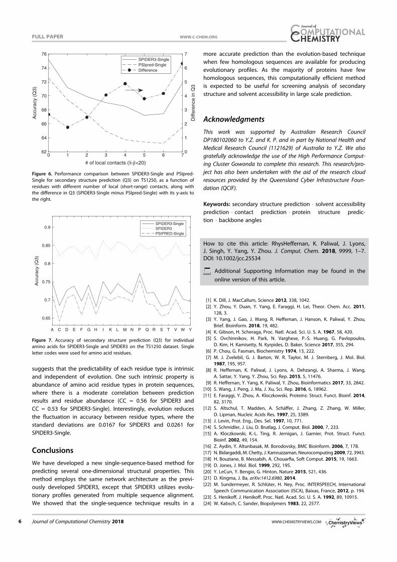
suggests that the predictability of each residue type is intrinsicand independent of evolution. One such intrinsic property isabundance of amino acid residue types in protein sequences,where there is a moderate correlation between predictionresults and residue abundance (CC = 0.56 for SPIDER3 andCC = 0.53 for SPIDER3-Single). Interestingly, evolution reducesthe fluctuation in accuracy between residue types, where thestandard deviations are 0.0167 for SPIDER3 and 0.0261 forSPIDER3-Single.
Conclusions
We have developed a new single-sequence-based method forpredicting several one-dimensional structural properties. Thismethod employs the same network architecture as the previ-ously developed SPIDER3, except that SPIDER3 utilizes evolu-tionary profiles generated from multiple sequence alignment.We showed that the single-sequence technique results in a
more accurate prediction than the evolution-based techniquewhen few homologous sequences are available for producingevolutionary profiles. As the majority of proteins have fewhomologous sequences, this computationally efficient methodis expected to be useful for screening analysis of secondarystructure and solvent accessibility in large scale prediction.
Acknowledgments
This work was supported by Australian Research CouncilDP180102060 to Y.Z. and K. P. and in part by National Health andMedical Research Council (1121629) of Australia to Y.Z. We alsogratefully acknowledge the use of the High Performance Comput-ing Cluster Gowonda to complete this research. This research/pro-ject has also been undertaken with the aid of the research cloudresources provided by the Queensland Cyber Infrastructure Foun-dation (QCIF).
Keywords: secondary structure prediction � solvent accessibilityprediction � contact prediction � protein structure predic-tion � backbone angles
How to cite this article: RhysHeffernan, K. Paliwal, J. Lyons,J. Singh, Y. Yang, Y. Zhou. J. Comput. Chem. 2018, 9999, 1–7.DOI: 10.1002/jcc.25534
Additional Supporting Information may be found in the
online version of this article.
[1] K. Dill, J. MacCallum, Science 2012, 338, 1042.[2] Y. Zhou, Y. Duan, Y. Yang, E. Faraggi, H. Lei, Theor. Chem. Acc. 2011,
128, 3.[3] Y. Yang, J. Gao, J. Wang, R. Heffernan, J. Hanson, K. Paliwal, Y. Zhou,
Brief. Bioinform. 2018, 19, 482.[4] K. Gibson, H. Scheraga, Proc. Natl. Acad. Sci. U. S. A. 1967, 58, 420.[5] S. Ovchinnikov, H. Park, N. Varghese, P.-S. Huang, G. Pavlopoulos,
D. Kim, H. Kamisetty, N. Kyrpides, D. Baker, Science 2017, 355, 294.[6] P. Chou, G. Fasman, Biochemistry 1974, 13, 222.[7] M. J. Zvelebil, G. J. Barton, W. R. Taylor, M. J. Sternberg, J. Mol. Biol.
1987, 195, 957.[8] R. Heffernan, K. Paliwal, J. Lyons, A. Dehzangi, A. Sharma, J. Wang,
A. Sattar, Y. Yang, Y. Zhou, Sci. Rep. 2015, 5, 11476.[9] R. Heffernan, Y. Yang, K. Paliwal, Y. Zhou, Bioinformatics 2017, 33, 2842.
[10] S. Wang, J. Peng, J. Ma, J. Xu, Sci. Rep. 2016, 6, 18962.[11] E. Faraggi, Y. Zhou, A. Kloczkowski, Proteins: Struct. Funct. Bioinf. 2014,
82, 3170.[12] S. Altschul, T. Madden, A. Schäffer, J. Zhang, Z. Zhang, W. Miller,
D. Lipman, Nucleic Acids Res. 1997, 25, 3389.[13] J. Levin, Prot. Eng., Des. Sel. 1997, 10, 771.[14] S. Schmidler, J. Liu, D. Brutlag, J. Comput. Biol. 2000, 7, 233.[15] A. Kloczkowski, K.-L. Ting, R. Jernigan, J. Garnier, Prot. Struct. Funct.
Bioinf. 2002, 49, 154.[16] Z. Aydin, Y. Altunbasak, M. Borodovsky, BMC Bioinform. 2006, 7, 178.[17] N. Bidargaddi, M. Chetty, J. Kamruzzaman, Neurocomputing 2009, 72, 3943.[18] H. Bouziane, B. Messabih, A. Chouarfia, Soft Comput. 2015, 19, 1663.[19] D. Jones, J. Mol. Biol. 1999, 292, 195.[20] Y. LeCun, Y. Bengio, G. Hinton, Nature 2015, 521, 436.[21] D. Kingma, J. Ba, arXiv:1412.6980, 2014.[22] M. Sundermeyer, R. Schlüter, H. Ney, Proc. INTERSPEECH, International
Speech Communication Association (ISCA), Baixas, France, 2012, p. 194.[23] S. Henikoff, J. Henikoff, Proc. Natl. Acad. Sci. U. S. A. 1992, 89, 10915.[24] W. Kabsch, C. Sander, Biopolymers 1983, 22, 2577.
0 1 2 3 4 5 6 7
# of local contacts (|i-j|<20)
62
64
66
68
70
72
74
76
Accura
cy (
Q3)
0
1
2
3
4
5
6
7
Diffe
rence in Q
3
SPIDER3-Single
PSIpred-Single
Difference
Figure 6. Performance comparison between SPIDER3-Single and PSIpred-Single for secondary structure prediction (Q3) on TS1250, as a function ofresidues with different number of local (short-range) contacts, along withthe difference in Q3 (SPIDER3-Single minus PSIpred-Single) with its y-axis tothe right.
A C D E F G H I K L M N P Q R S T V W Y
0.65
0.7
0.75
0.8
0.85
0.9
Accu
racy (
Q3
)
SPIDER3-Single
SPIDER3
PSIPRED-Single
Figure 7. Accuracy of secondary structure prediction (Q3) for individualamino acids for SPIDER3-Single and SPIDER3 on the TS1250 dataset. Singleletter codes were used for amino acid residues.
FULL PAPER WWW.C-CHEM.ORG
Journal of Computational Chemistry 2018 WWW.CHEMISTRYVIEWS.COM6
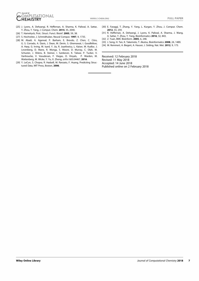
[25] J. Lyons, A. Dehzangi, R. Heffernan, A. Sharma, K. Paliwal, A. Sattar,Y. Zhou, Y. Yang, J. Comput. Chem. 2014, 35, 2040.
[26] T. Hamelryck, Prot.: Struct. Funct. Bioinf. 2005, 59, 38.[27] S. Hochreiter, J. Schmidhuber, Neural Comput. 1997, 9, 1735.[28] M. Abadi, A. Agarwal, P. Barham, E. Brevdo, Z. Chen, C. Citro,
G. S. Corrado, A. Davis, J. Dean, M. Devin, S. Ghemawat, I. Goodfellow,A. Harp, G. Irving, M. Isard, Y. Jia, R. Jozefowicz, L. Kaiser, M. Kudlur, J.Levenberg, D. Mane, R. Monga, S. Moore, D. Murray, C. Olah, M.Schuster, J. Shlens, B. Steiner, I. Sutskever, K. Talwar, P. Tucker, V.Vanhoucke, V. Vasudevan, F. Viegas, O. Vinyals, P. Warden, M.Wattenberg, M. Wicke, Y. Yu, X. Zheng, arXiv:1603.04467, 2016.
[29] Y. LeCun, S. Chopra, R. Hadsell, M. Ranzato, F. Huang, Predicting Struc-tured Data, MIT Press, Boston, 2006.
[30] E. Faraggi, T. Zhang, Y. Yang, L. Kurgan, Y. Zhou, J. Comput. Chem.2012, 33, 259.
[31] R. Heffernan, A. Dehzangi, J. Lyons, K. Paliwal, A. Sharma, J. Wang,A. Sattar, Y. Zhou, Y. Yang, Bioinformatics 2016, 32, 843.
[32] Z. Yuan, BMC Bioinform. 2005, 6, 248.[33] J. Song, H. Tan, K. Takemoto, T. Akutsu, Bioinformatics 2008, 24, 1489.[34] M. Remmert, A. Biegert, A. Hauser, J. Söding, Nat. Met. 2012, 9, 173.
Received: 12 February 2018Revised: 11 May 2018Accepted: 14 June 2018Published online on 2 February 2018
WWW.C-CHEM.ORG FULL PAPER
Wiley Online Library Journal of Computational Chemistry 2018 7

62
Chapter 6 SPIDER3 Single - Single-Sequence-Based Prediction of ProteinSecondary Structures and Solvent Accessibility by Deep Whole-Sequence
Learning.
Chapter 7
Conclusions and Future Directions
7.1 Conclusions
With the high cost of experimental methods for finding protein structure, and the low cost
of genome sequencing, it is necessary to find computational methods for the prediction of
those structures. Despite over half a century of research into this problem, there is still
work to be done. This thesis presented a body of work which furthers the prediction of a
range of one-dimensional structural properties of proteins.
We presented SPIDER, the first method for the direct prediction of the angle between
Cαi−1-Cαi-Cαi+1, and dihedral angle rotated about the Cαi-Cαi+1 bond, θ and τ re-
spectively. For this, we used an iterative deep-learning based method, based on stacked
auto-encoders. We showed that this method could be used to create low RMSD recon-
structions of the local backbone structure of short regions of proteins. Based on the
success of this iterative deep-learning method, we extended the method and applied it to
a range of one-dimensional protein structure predictions. In this new method, SPIDER2,
we predicted θ, τ, φ and ψ angles, along with three-state secondary structure, and solvent
accessible surface area. SPIDER2 was able to achieve the best reported results for all
of its predictions. The addition of these extra properties during the iterative learning
process also improved upon the θ and τ angles over SPIDER. We further extended the
solvent exposure descriptors predicted by the SPIDER2 method, by adding state-of-the-
art prediction of half sphere exposures (both Cα and Cβ based) and contact numbers.
In predicting these new half sphere exposure and contact number values, we also began
63
64 Chapter 7 Conclusions and Future Directions
to utilise the evolutionary information provided by the HMM profiles of HHBlits. With
SPIDER2 in its current state, we have provided a tool for the prediction of secondary
structure, solvent exposure, and backbone angles, is both highly accurate and easy to use.
We then utilised Long Short-Term Memory Bidirectional Recurrent Neural Networks
(LSTM-BRNNs) for the prediction of one-dimensional structural properties, in a method
called SPIDER3. This LSTM-BRNNs model was able to learn both local and non-local
dependencies, and again produced the best reported accuracies for all of its predictions.
Another method, based on the SPIDER3 model, was then developed. In this new method,
SPIDER3-Single, the evolutionary based features used previously were replaced by single
sequence features. Along with this change, we also added eight-state secondary structure
prediction to model. In this method, we achieve the best reported results for the single-
sequence prediction of three and eight-state secondary structure predictions, solvent acces-
sible surface area, half sphere exposures, contact numbers, and θ, τ, ψ, and ψ angles. Not
only that, but the method out performed the evolutionary based SPIDER3, when applied
to sequences with a limited number of homologous sequences. With SPIDER3-Single,
we provided a tool that can be used to both quickly assess massive numbers of protein
sequences without having to wait for evolutionary profiles to be calculated, and also more
accurately make predictions for sequences with little or no evolutionary information.
The methods presented in this thesis are all available as online servers, or downloadable
packages, on the spark-labs website http://sparks-lab.org/.
7.2 Recommendations for Future Work
The most significant limiting factor for the methods employed in this thesis, is the avail-
ability of usable data with known structure. When making predictions in the field of
structural bioinformatics, we typically use datasets where homologous sequences are re-
moved from both training and testing data. While it is important to have a testing set
that is as independent as possible, the removal of these homologous sequences from the
training data is potentially (and unnecessarily) removing key information that our models
could be learning. State-of-the-art image recognition tasks, for example, will often apply
a number of random distortions (shifting, scaling, rotation, etc.) to their training data
so as to expose their models to as much varied input as possible in the hopes of making
Chapter 7 Conclusions and Future Directions 65
those models more robust. When we discard training data that is homologous to other
training data, we are doing the exact opposite, and removing the biological equivalent
of those those random distortions. For example, if two sequences are 90% homologous,
we currently select one of those to keep and one to ignore; however if those two similar
sequences result in similar structure (or even very different structure) then that is key
information that our model should be exposed to, and currently isn’t. While employing
multiple sequence alignments to find the evolutionary profiles does help to reintroduce
that information from sequences that were removed, simply not removing it in the first
place is worth exploring, particularly for single-sequence based methods.
Many of the driving forces in the machine learning field are problems where there is an
abundance of data availability, for example image recognition with millions of images or
speech recognition with thousands of hours of speech. This has lead to a situation where
many of the most impressive techniques currently available (including those used in the
research presented here), are designed to be able to fully utilise this huge amount of data.
Using multiple sequence alignments as a preprocessing or feature generation step has served
the field of protein structure prediction well. However in recent years significant research
has been done on harnessing huge amount of data to perform unsupervised learning, ie.
learning from massive amounts of unlabeled data. The exact driving force behind the
search for computational methods of protein structure prediction, that being the high rate
of protein sequence discovery versus low rate of protein structure discovery, makes for
a situation that is well placed to be able to benefit in potentially significant ways from
these unsupervised learning ideas. If one could find a way to utilise all of the available
information in the body of known sequences with no structural information, it seems
possible that we could see results for single-sequence based methods which at least match
those of evolutionary-information-based methods.

66 Chapter 7 Conclusions and Future Directions