Adaptive backstepping type control for electrohydraulic servos

Felicia Ursu*, Ioan Ursu*, Eliza Munteanu**

* “Elie Carafoli” National Institute for Aerospace Research, Bucharest, ROMANIA **Advanced Studies and Research Center, Bucharest, ROMANIA

Abstract -The work considers the control synthesis in the presence of a parametric uncertainty, with application to electrohydraulic servos actuating primary flight controls. The obtained control law, containing a dynamic updating of uncertain parameter, renders the closed loop system stable and guarantees asymptotic tracking of position references. The uncertain parameter is on line adjusted, using in synthesis the methods of Control Lyapunov Functions and backstepping. Numerical simulations are reported from viewpoint of the servo time constant performance.

I. INTRODUCTION The present paper continues the theme of recent

researches of the authors [1-4], by considering now a problem of adaptive backstepping control synthesis for the Electrohydraulic Servos (EHSs). This procedure of adaptive backstepping for systems with uncertain (unknown) parameters is introduced avant la lettre by Kanellakopoulos et al [5], where a characterization of the class of nonlinear systems to which the new adaptive scheme is applicable is achieved. In our paper, two are the main aims: a) to propose an alternative adaptive backstepping, for an EHS with unknown or uncertain parameters, versus the general sophisticated scheme described in Kanellakopoulos et al. [5]; and b) to illustrate the working of the synthesized control by numerical simulations. More specifically, instead of Kanellakopoulos’s adaptive scheme, herein a dynamic update for an uncertain parameter can be performed during the controlled proces – in other words, on line – in the framework of a recurrent control law based on the Control Lyapunov Functions (CLFs) and backstepping synthesis. The estimation error is proved to be asymptotically stable. The obtained control law renders the closed loop stable and ensures the regulation of the desired output.

Remembering [5], [1], the key idea of backstepping is simple. At every step of backstepping, a new Control Lyapunov Function is constructed by augmentation of the CLF from the previous step by a term which penalizes the error between a state variable and its desired value. A major advantage of backstepping is the construction of a Lyapunov function whose derivative can be made negative definite by a variety of control laws rather than a specific control law. It is obviously that the easy of incorporating uncertainties and unknown parameters with each

backstepping contributed to its instant popularity and rapid acceptance.

II. BACKSTEPPING ADAPTIVE CONTROL SYNTHESIS

FOR AN ELECTROHYDRAULIC SERVO

In the work [4], by using a backstepping technique, position and force control laws were synthesised for a five-dimensional mathematical model of EHS (see modelling aspects in [6], [7] and the physical model in Fig. 1)

( )[ ]( )

( )

1 2 2 1 2 3 4

3 5 3 2 3 41

4 5 4 2 3 41

55

1,

2,

a

vd

x x x k x fx S x xmBx cx p x Sx k x x

V SxBx cx x Sx k x x

V Sxx k ux c c w

= = − − + −

= − − − − += − + + − −

− += =

τ ρ

(1)

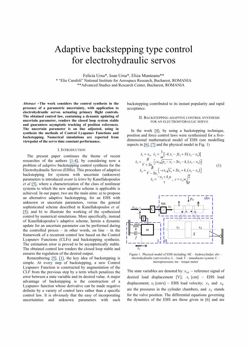
Figure 1. Physical model of EHS including: HC – hydrocylinder; ehv – electrohydraulic (servo)valve; L – load; T – transducers system; C –

microprocessor; tm – torque motor The state variables are denoted by: dx1 − reference signal of desired load displacement [V]; 1x [cm] − EHS load displacement; x2 [cm/s] − EHS load velocity; 3x and 4x are the pressures in the cylinder chambers, and 5x stands for the valve position. The differential equations governing the dynamics of the EHS are those given in [6] and are

ehv

x3 x4

L

pa

S m

x1

k

f

x5 tm

T–

x1d C u

H

Proceedings of the 15th Mediterranean Conference onControl & Automation, July 27 - 29, 2007, Athens - Greece

T01-024

reported having as a reference point the hydromechanical servomechanism SMHR included in the aileron control chain of military jet IAR 99. The nominal values of the parameters appearing in the equations (1) are: m = 0.033 daNs2/cm − equivalent inertial load of primary control surface reduced at the EHS’s rod; S = 10 cm2 − EHS’s piston area; f = 3 daNs/cm − equivalent viscous friction force coefficient; k = 100 daN/cm − equivalent aerodynamic elastic force coefficient; w = 0.05 cm − valve-port width; pa = 210 daN/cm2 − supply pressure; 0≈Tp − tank pressure; k = 5/210 cm5/(daN×s) − internal leakage cylinder’s coefficient; ρ = 85/(981×105) daNs2/cm4 − volumetric density of oil; cd = 0.63 − volumetric flow coefficient of the valve port; B = 6000 daN/cm2 − the bulk modulus B of the oil used; V = 30 cm2 − the EHS’s cylinder semivolume V; τ = 1/573 s − time constant of the (servo)valve. kv = 0.0085/(0.05×10) cm/V is taken as a proportionality coefficient valve displacement 5x -control (voltage) u.

The following result [2], [4] describes the structure of the backstepping position control law:

Proposition 1. Let 1 20 0k , k> > be tuning parameters. Under the (rather physical) assumptions

3 4 10 , 0 ,a ax p x p x V S< < < < < , the control u given by

( )5 5 2 21

d d pv

u x x k g ek

= + τ − (2)

( )5 1 12

1d p dx k e p G

G= − − + (3)

( ) ( )

( )

21 1 1 2 2 2 2

1

3 42 2 1 2 3

1 1

2,

, , a

BV Sx k pG G x xV S xp x xG G x x x Bc

V Sx V Sx

− += =

− −

= = + + −

(4)

3 4,p de p p p x x= − = −

( ) ( ) ( )1/1 1 1 rt t

d d sk kp t x t x eS S

−= = −

15 5 5 cosde x x −= − θ

(5)

when applied to (1), guarantees asymptotic stability for the position tracking error 1 1 1de x x= − ; more precisely,

( )1lim 0t

e t→∞

= .

The basic backstepping assumes the knowledge of the system parameters. In fact, frequently it may be necessary to identify some of these parameters off line or estimate them using on-line adaptive schemes. The essence of adaptive control is that, by learning from the past information through this parameter adaptation mechanism,

the real parametric uncertainty can be handled. In the following, the adaptive backstepping machinery is illustrated by considering the mathematical model (1). In these equations it is assumed the uncertainty of the coefficient c enclosed in the mixed parameter Bc

Bcα = (6)

So, the geometric and flow uncertainties in the electrohydraulic servovalve are concerned.

For the sake of simplicity in the treatment of the problem, one neglects the coefficient k of internal leakage. Thus, the pressure equations will be rewritten as

5 33 2

1 1

5 44 2

1 1

ax p x BSx xV Sx V Sx

x x BSx xV Sx V Sx

α −= −

+ +−α

= +− −

(1′)

and will be added to the other equations of the system (1)

( )[ ]1 2 2 1 2 3 4

55

1,

v

x x x k x fx S x xm

x k ux

= = − − + −

− +=

τ

(1″)

to define a system whose equations belong to a general class of nonlinear systems treated in [5]

( ) ( ) ( ) ( )( )0 01 1

p p

i i i ii i

x x g x u= =

= + θ + + θ∑ ∑x f f g x (7)

where n∈x is the state vector, u ∈ is the control vector, 0 0 i if , g , f , g are smooth vector fields of appropriate

dimensions and T

1, ... , pθ θ is the vector of unknown (uncertain) constant parameters. Two geometric conditions, so called: a) feedback linearization condition and b) parametric-pure-feedback condition must be fulfilled by the vector fields 0 0 i if , g , f , g . This geometric approach therein developed, not very familiar to most control engineers, is avoided in the present paper, instead using a simple, intuitive scheme of adaptive backstepping having as object the system (1'), (1''), (6), which represents the electrohydraulic servo as a tracking system. Therefore, for this system the aim of control synthesis is to have a good tracking by the state variable x1 of the specified x1d desired position references. The closed loop performance of the system can be measured by the actual (realised) servo time constant sτ . Thus, a good tracking system is characterised by fast (little) time constant sτ . Both servo time constant and position reference signal are in connection with the response of a first order system to step inputs xis

( )11 1 1 rt td sx x e−= − (8)

x1s stands for stationary value of the state x1, and t1r stands

Proceedings of the 15th Mediterranean Conference onControl & Automation, July 27 - 29, 2007, Athens - Greece

T01-024

for associated desired time constants. The main result of this work is given by the following

Proposition 2. Consider the uncertain parameter α for the EHS mathematical model (1'), (1''), (6). Let

1 2 30, 0, 0, 0k k k α> > > ρ > be tuning parameters and ˆ 0α ≠ the notation for the estimate of the uncertain

parameter α . Define the learning error ˆα = α − α . Under the rather physical assumptions 1 ,x V S< 30 ,ax p< <

40 ax p< < , the control u given by

( )5 5 2 21 ˆd d pu x x k g ek

′= + τ − α v

(9)

( )5 1 12

1ˆd p dx k e p gg

= − − +′α

(10)

( )2 5 31ˆ pg x e k

α

′α = + αρ

, ( )2 5 31

pg x e kα

′α = − + αρ

(11)

3 4,p de p p p x x= − = −

( ) ( ) ( )1/1 1: : 1 rt t

d d sk kp t x t x eS S

−= = − , 5 5 5de x x= − (12)

( )

( )

21 1 2 2 2 2

1

3 42 1 3 4

1 1

2,

, , a

BSVxg x xV S xp x xg x x x

V Sx V Sx

−=

− −

= α + + −

(13)

( ) ( )2 1 3 42 1 3 4

, ,, , g x x xg x x x′ =α

when applied to (1'), (1''), (6), guarantees asymptotic stability for the learning error α and the position tracking error 1 1 1de x x= − ; more precisely, ( )lim 0

tt

→∞α = ,

( )1lim 0t

e t→∞

= .

Proof: By inspecting the system (1'), (1''), (6), it follows that the internal states x1 and x2 are stable; indeed, the roots of the characteristic equation

2 0m f kλ + λ + = (14)

are stable roots − negative real, or complex with negative real parts − due to the viscous friction force in hydraulic cylinder. Therefore, a special care to stabilise the states x1, x2 is not necessary. Thus, evading the equations for the states x1, x2 in the backstepping procedure, this technique will be applied only with regard to the variables x3 − x4 and x5. Consider now the Lyapunov like function

2 2 21 5

2

1 1 12 2 2pV e e

k α= + + ρ α (15)

Then, its derivative along the system (1'), (1'') is

( ) 5 51 2 5 1 5

2ˆ.

p d de x k uV e g x g p xk

α

− + = + − + − − τ − ρ αα

v

Now, by using (12), (13), (10), (11), we have

( ) ( )[ ]( )

( )

( )

( )

2 5 1 2 5 5 1

2 5 2 5 1

2 5 1 1 1

2 5 1 1 1

2 5 1 1 1

21 2 5

ˆ1

ˆ

ˆ

p d p d d

p d d

p d d p

p d d p

p p d p

p p

e g x g p e g e x g pe g e g x g p

e g e g p g p k e

e g e g p g p k e

e g e k e g p k e

k e g e e

+ − = + + − =′ ′= α +α + − =

α ′= α + − + − + − = α α ′= α + − + + − + − = α

α ′= α − + − + − = α ′= − +α + ( )1 1ˆ

pd p

eg p k e α − + − α

Thus

( )21 1 2 5 1 1

5 55

2

ˆˆ.

pp p d p

d

eV k e g e e g p k e

e x k u xk α

′= − + α + α − + − + α − + + − − ρ αα τ

v

By substituting (11)−(13), one gets

( )2 21 1 5 1 1

22 2 2

2 5 1 5 32

1ˆ

1ˆ

pp d p

p p

eV k e e g p k e

kg e e k e e k

kα

= − − + α − + − +τ α′ + + − ρ α = − − − α τ

(16)

The equations for the errors ep, e5 can be written as

( )( )

1 2 5 1 1

55 2 2 3 2 5

ˆ1ˆ ,

p p d p

p p

e k e g e g p k eee k g e k g x e

α

α= − + + − + −

α′ ′= − − α α = − α +

τ ρ

(17)

A tedious way to continue the proof is that of checking the asymptotic stability of the errors 5, ,pe e α by using the second method of Lyapunov for systems with variable coefficients (see [8], Theorem 1). As in [4], an alternative and very efficient procedure will be further used: that of Barbalat's Lemma [9]. The reasoning is as follows. Making use of the definitions (11)−(13) for 5,pe e and α , we have

( )1 0 0V > when 0t → (see 5 0dx ≠ ). Since 1 0V ≤ , it is obvious that ( ) ( )1 10 0V t V≤ ≤ , ( ) 0t∀ > , hence the positive function ( )1V t is bounded and consequently 5,pe e and α are bounded; so, ( )p p t= is also bounded in the interval

[ )0,+ = ∞ . Now, taking the derivative of (16) yields

( ) ( )

2 2 21 1 5 1 2 5 2 52

2

1 31 1 2 5 3

1 2 ˆ2 2

2 2ˆ

p p p

p p d p

V k e e k g e e g e ek

k ke k e p g g x e kα

′= + − + α + τ τ α ′ + − + + α + α

α ρ

Furthermore, 1V is bounded, provided that 1 2 ˆ, ,g g α remain bounded during the dynamical process; this condition holds, having in view the assumptions involving the

Proceedings of the 15th Mediterranean Conference onControl & Automation, July 27 - 29, 2007, Athens - Greece

T01-024

variables 1 3 4, ,x x x . So, 1V is uniformly continuous (as having a bounded derivative). Let us now consider Barbalat's Lemma:

If the function f(t) is differentiable and has a finite limit ( )

tlim f t→∞

, and if f is uniformly continuous, then ( )lim 0t

f t→∞

= .

Thus, Barbalat’s Lemma will be applied to show that the errors pe and 5e tend to zero as time tends to infinity.

Indeed, applying Barbalat's Lemma, 1 0V → . Hence, pe

and 5 e tend to zero. Now, let's look at the second equation in (1''), which can be rewritten as follows

21 1 1 1 12 , , ,

2f k Sx hx r x p h r p pm m m

+ + = = = = (18)

and p is now seen as a bounded function of ( ) ( ) ( )3 4, :t p p t x t x t= = − . The most usual case is that of

complex roots with negative real parts, considered in the precedent works [1-4]. But, the occurrence of negative real roots is not excluded. With initial conditions

( ) ( )1 10 0 0x x= = , the solution of (18) in this aperiodic case is

( ) ( ) ( ) ( ) ( ) ( ) ( )1 1 10 01 1d d2 2

t tq h t h q u q h t h q ux t e e p u u e e p u uq q

− − − + += −∫ ∫ (19)

with 2 2 2 0, , , ,q r h q h r h q= − > − positive. This variant is inherent to hydraulic servo systems owing to small viscous friction in cylinder. Define

( ) ( )1d dSp t p tm

= (20)

and let us also consider

( ) ( ) ( ) ( )

( ) ( ) ( )

1 10

10

1212

tq h t h q ud d

tq h t h q ud

x t e e p u duq

e e p u duq

− −

− + +

= −∫

− ∫ (21)

Since 0pe → when t → ∞ , it is clear that ( ) ( )1 1dp t p t→ , as t → ∞ ; this means: ( ) 0∀ ε > , (∃) ( )δ ε such that for

( )t > δ ε we have ( ) ( )1 1dp t p t− < ε . Then, if ( )t > δ ε

( ) ( ) ( ) ( ) ( ) ( )

( ) ( ) ( ) ( )

1 1 1 10

1 10

1 d2

1 d2

tq h t h q ud d

tq h t h q ud

x t x t e e p t p t uq

e e p t p t uq

− −

− + +

− ≤ − +∫

+ − ≤∫

( ) ( ) ( ) ( )( )( ) ( )

0 0d d2

1 12

t tq h t h q u q h t h q u

q h t q h t

e e u e e uq

e eq h q h q

− − − + +

− − +

ε+ =∫ ∫

ε − −= + − +

Therefore

( ) ( )1 1 as dx t x t t→ → ∞ (22)

Then:

( ) ( )

( ) ( )

1

1

11 0

0

1 d2

1 d

r

r

utq h t h q u ts

d

utq h t h q u t

kxx e e e uqm

e e e u

−− −

−− + +

= − −∫ − −∫

and, based on definition relations

2 2 2 2, ,2f kq h r h rm m= − = =

simple, successive calculations finally give

( )1 1 as d sx t x t→ → ∞ (23)

Thus, from (22) and (23), a standard proceeding gives

( )1 1 as sx t x t→ → ∞

and so ends the proof. ♦

Let notice that if 0α = , the control (9) is identical with the “nonadaptive” control given in [2], [4].

III. SIMULATION RESULTS AND CONCLUDING REMARKS It is was mentioned in Section 2 that the goal of the control is to ensure a good tracking of the specified x1d desired position references, for instance as given in (8). Simulations are used to illustrate the theoretical findings. Thus, fourth order Runge-Kutta integrations of the tandem controlled system (1'), (1''), (6) – compensator (9)-(13) were performed considering a succession of time intervals of length T = 0.002 s and “zero order hold control” (which means that the control variable is kept constant during the time period T). Numerical data are those already given in Section 2. For the simulations, a set of values of the tuning parameters were selected, in a trial and error process, as suitable (these values are naturally related to the system of units chosen in Section 2): 1 25k = , 2 0.00004k = ,

3 0.0000005k = , 30.04 kαρ = × , with a medium reference signal 1 0.255 cmsx = (Figs. 2, 3, 6), a small reference signal 1 0.115 cmsx = (Fig. 4) and a great reference signal

1 0.5 cmsx = (Fig. 5) and a desired time constant

1 0.018 srt = . Thus, the presented plots, considered as representative for simulations, show a good working of the proposed adaptive backstepping controller (9). Due to different key parameter scheme, the nominal actual servo time constant 0.037ssτ = (i.e., corresponding to

1 0.255 cmsx = ; see [4], where 1 0.002 srt = was considered) of the ideal “nonadaptive” system (i.e., for total parameter

Proceedings of the 15th Mediterranean Conference onControl & Automation, July 27 - 29, 2007, Athens - Greece

T01-024

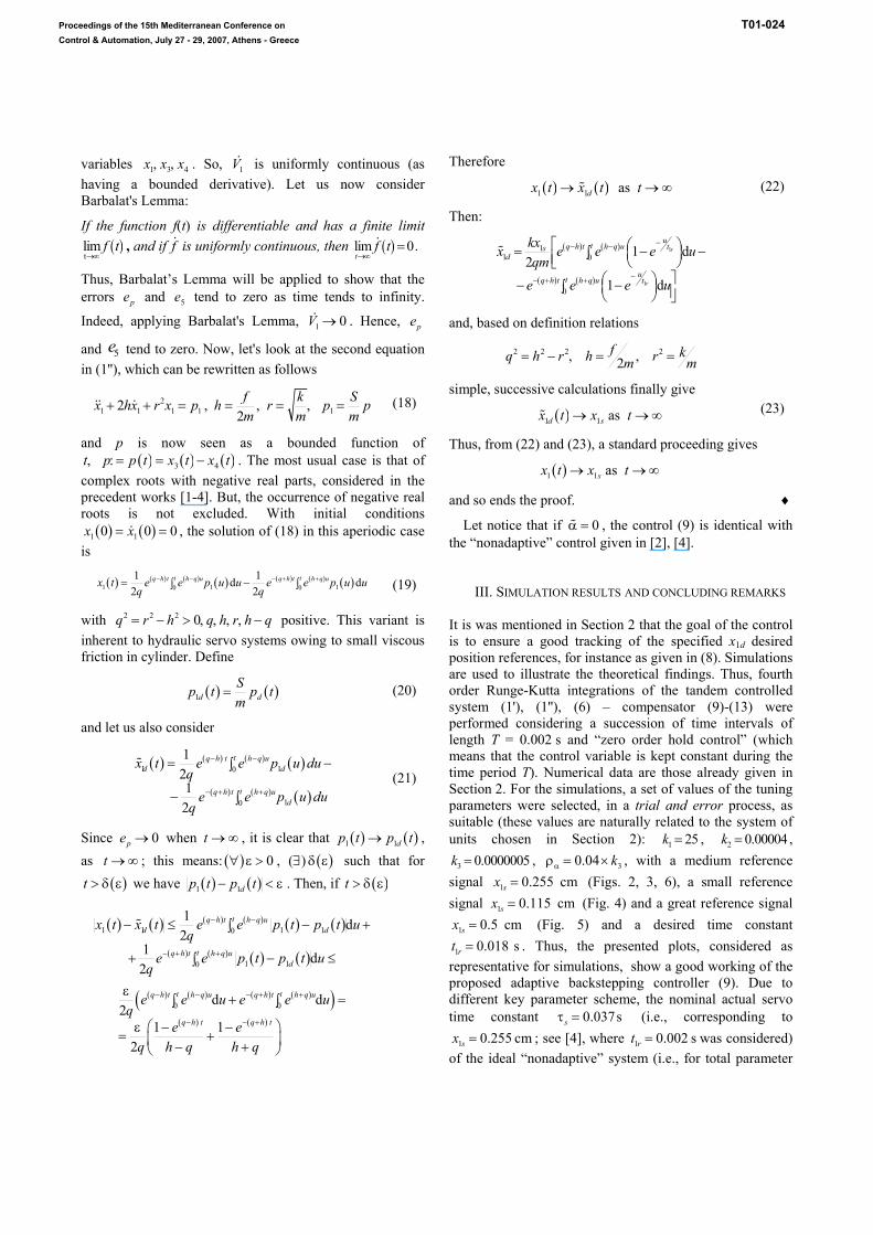
knowledge) can be slower than the actual servo time constant 0.026ssτ = , in an adaptive framework, see Fig. 2.

Figure 2. Case of initial estimate of uncertain parameter ( )ˆ 0 0.1Bcα =

Evolutions of the variables 1 ,x u and / Bα . The result: actual servo

performance τs ≅ 0.026 s

Figure 3. Case of initial estimate of uncertain parameter ( )ˆ 0 1.2 .Bcα =

Evolutions of the variables 1 ,x u and / Bα . The result: actual servo

performance τs ≅ 0.062 s

The Figures 2-6 show that the estimation error converges to zero. Performing various numerical simulations demonstrated that the initial parameter estimate ( )ˆ 0α doesn’t affect the estimation process. Given the selected configuration of key parameters, the servo time constants – the main performance criterion of the system – are more or less maintained even when the uncertain parameter c was changed from the decreased value 4.785 cm3s-1daN-1/2 (Fig.

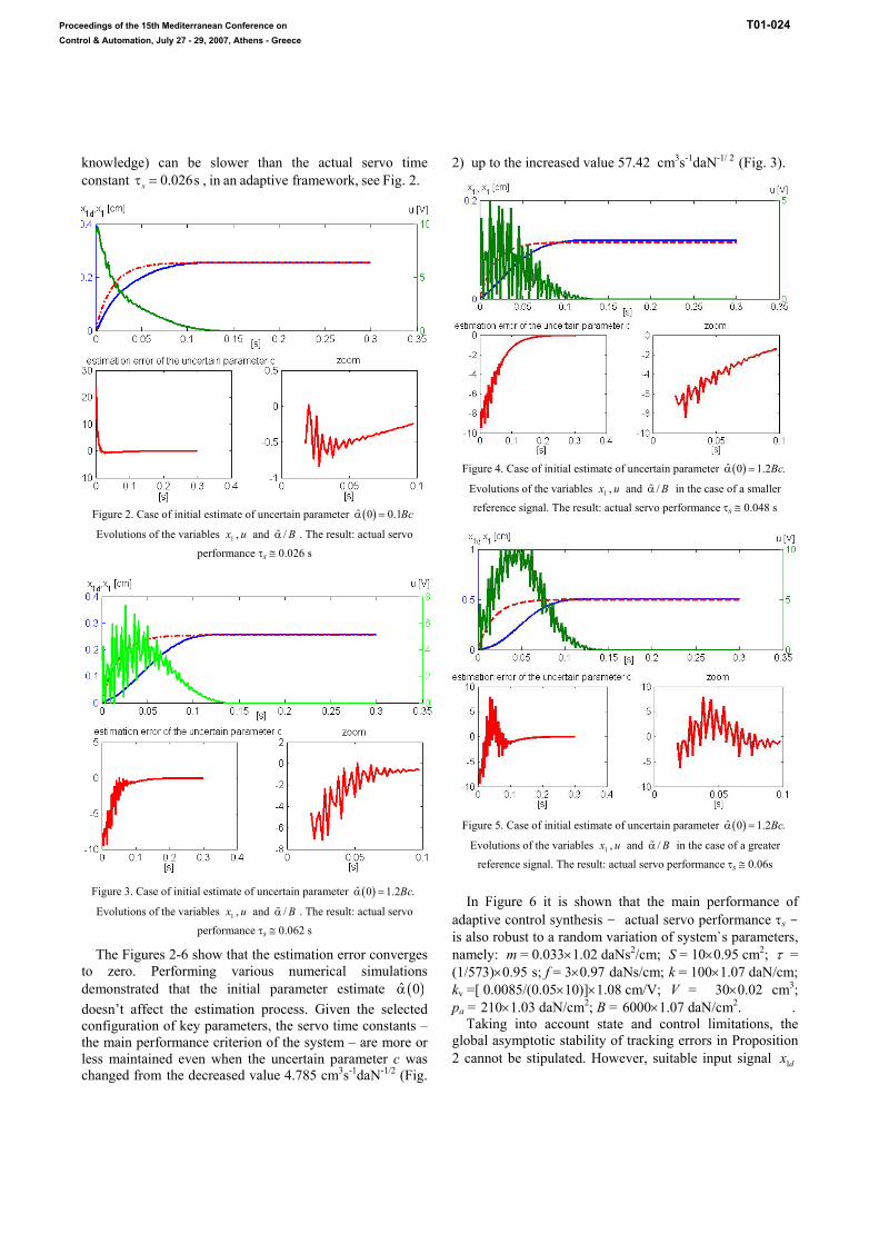
2) up to the increased value 57.42 cm3s-1daN-1/ 2 (Fig. 3).

Figure 4. Case of initial estimate of uncertain parameter ( )ˆ 0 1.2 .Bcα =

Evolutions of the variables 1 ,x u and / Bα in the case of a smaller

reference signal. The result: actual servo performance τs ≅ 0.048 s

Figure 5. Case of initial estimate of uncertain parameter ( )ˆ 0 1.2 .Bcα =

Evolutions of the variables 1 ,x u and / Bα in the case of a greater

reference signal. The result: actual servo performance τs ≅ 0.06s

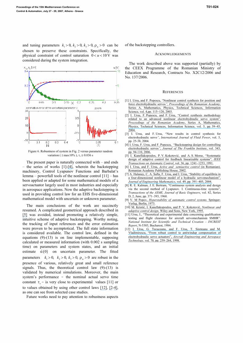
In Figure 6 it is shown that the main performance of adaptive control synthesis – actual servo performance τs - is also robust to a random variation of system`s parameters, namely: m = 0.033×1.02 daNs2/cm; S = 10×0.95 cm2; τ = (1/573)×0.95 s; f = 3×0.97 daNs/cm; k = 100×1.07 daN/cm; kv =[ 0.0085/(0.05×10)]×1.08 cm/V; V = 30×0.02 cm3; pa = 210×1.03 daN/cm2; B = 6000×1.07 daN/cm2. .

Taking into account state and control limitations, the global asymptotic stability of tracking errors in Proposition 2 cannot be stipulated. However, suitable input signal 1dx

Proceedings of the 15th Mediterranean Conference onControl & Automation, July 27 - 29, 2007, Athens - Greece

T01-024

and tuning parameters 1 0,k > 2 0,k > 3 0,k > 0αρ > can be chosen to preserve these constraints. Specifically, the physical constraint of control saturation 0 10u< < V was considered during the system integration.

Figure 6. Robustness of system in Fig. 2 versus parameter random

variation ( max10%± ), τs ≅ 0.036 s

The present paper is naturally connected with – and ends – the series of works [1]-[4], wherein the backstepping machinery, Control Lyapunov Functions and Barbalat’s lemma – powerfull tools of the nonlinear control [11] – has been applied or adapted for some mathematical models of a servoactuator largely used in most industries and especially in aerospace applications. Now the adaptive backstepping is used in providing control law for an EHS five-dimensional mathematical model with uncertain or unknown parameter.

The main conclusions of the work are succinctly resumed. A complicated geometrical approach described in [5] was avoided, instead promoting a relatively simple, intuitive scheme of adaptive backstepping. Worthy noting, the tracking of input references and the error estimation were proven to be asymptotical. The full state information is considered available. The control law, defined in the equations (9)-(13) is on line implementable, supposing calculated or measured information (with 0.002 s sampling time) on parameters and system states, and an initial estimate ( )0α̂ on uncertain parameter. The fitted parameters 1 2 30, 0, 0, 0k k k α> > > ρ > are robust in the presence of various, relatively great and small reference signals. Thus, the theoretical control law (9)-(13) is validated by numerical simulations. Moreover, the main system’s performance - the nominal actual servo time constant sτ - is very close to experimental values [11] or to values obtained by using other control laws [12], [2-4], as one can see from selected case studies.

Future works need to pay attention to robustness aspects

of the backstepping controllers.

ACKNOWLEDGEMENTS

The work described above was supported (partially) by the CEEX Programme of the Romanian Ministry of Education and Research, Contracts No. X2C12/2006 and No. 137/2006.

REFERENCES [1] I. Ursu, and F. Popescu, “Nonlinear control synthesis for position and

force electrohydraulic servos”, Proceedings of the Romanian Academy, Series A, Mathematics, Physics, Technical Sciences, Information Science, vol. 4,pp. 115−120, 2003.

[2] I. Ursu, F. Popescu, and F. Ursu, “Control synthesis methodology related to an advanced nonlinear electrohydraulic servo system”, Proceedings of the Romanian Academy, Series A, Mathematics, Physics, Technical Sciences, Information Science, vol. 5, pp. 39−45, 2004.

[3] I. Ursu, and F. Ursu, “New results in control synthesis for electrohydraulic servo”, International Journal of Fluid Power, vol. 5, pp. 25-38, 2004.

[4] I. Ursu, F. Ursu, and F. Popescu, “Backstepping design for controlling electrohydraulic servos”, Journal of The Franklin Institute, vol. 343, pp. 94-110, 2006.

[5] I. Kanellakopoulos, P. V. Kokotović, and A. S. Morse, “Systematic design of adaptive control for feedback linearizable systems”, IEEE Transactions on Automatic Control, vol. 36, pp. 1241−1253, 1991.

[6] I. Ursu, and F. Ursu, Active and semiactive control (in Romanian). Romanian Academy Publishing House, 2002.

[7] A. Halanay, C. A. Safta, F. Ursu, and I. Ursu, “Stability of equilibria in a four-dimensional nonlinear model of a hydraulic servomechanism”, Journal of Engineering Mathematics, vol. 49, pp. 391−405, 2004.

[8] R. E. Kalman, J. E. Bertram, “Continuous system analysis and design via the second method of Lyapunov. I. Continuous-time systems”, Transactions of the ASME, Journal of Basic Engineers, vol. 82, Series D, 2, June, pp. 371–393, 1960.

[9] V. M Popov, Hyperstability of automatic control systems. Springer-Verlag, Berlin, 1973.

[10] M. Kristić, I. Kanellakopoulos, and P. V. Kokotović, Nonlinear and adaptive control design, Wiley and Sons, New York, 1995.

[11] Ursu, I., “Theoretical and experimental data concerning qualification testing and flight clearance for aircraft servomechanism SMHR”. National Institute for Scientific and Technical Creation – INCREST Report, N-5303, Bucharest, 1984.

[12] I. Ursu, G. Tecuceanu, and F. Ursu, T. Sireteanu and M. Vladimirescu, “From robust control to antiwindup compensation of electrohydraulic servo actuators”, Aircraft Engineering and Aerospace Technology, vol. 70, pp. 259–264, 1998.

Proceedings of the 15th Mediterranean Conference onControl & Automation, July 27 - 29, 2007, Athens - Greece

T01-024