sustainability

Article

Cascade Adaptive MPC with Type 2 Fuzzy System for Safetyand Energy Management in Autonomous Vehicles:A Sustainable Approach for Future of Transportation

Duong Phan 1, Ali Moradi Amani 2, Mirhamed Mola 3, Ahmad Asgharian Rezaei 2, Mojgan Fayyazi 2 ,Mahdi Jalili 2, Dinh Ba Pham 1 , Reza Langari 4 and Hamid Khayyam 2,*

�����������������

Citation: Phan, D.; Amani, A.M.;

Mola, M.; Rezaei, A.A.; Fayyazi, M.;

Jalili, M.; Ba Pham, D.; Langari, R.;

Khayyam, H. Cascade Adaptive MPC

with Type 2 Fuzzy System for Safety

and Energy Management in

Autonomous Vehicles: A Sustainable

Approach for Future of

Transportation. Sustainability 2021, 13,

10113. https://doi.org/10.3390/

su131810113

Academic Editor: Bilal Farooq

Received: 14 July 2021

Accepted: 2 September 2021

Published: 9 September 2021

Publisher’s Note: MDPI stays neutral

with regard to jurisdictional claims in

published maps and institutional affil-

iations.

Copyright: © 2021 by the authors.

Licensee MDPI, Basel, Switzerland.

This article is an open access article

distributed under the terms and

conditions of the Creative Commons

Attribution (CC BY) license (https://

creativecommons.org/licenses/by/

4.0/).

1 Division of Mechatronics, Mechanical Engineering Institute, Vietnam Maritime University,Haiphong 180000, Vietnam; duongpv.vck@vimaru.edu.vn (D.P.); bapd.vck@vimaru.edu.vn (D.B.P.)

2 School of Engineering, RMIT University, Melbourne, VIC 3083, Australia;ali.moradiamani@rmit.edu.au (A.M.A.); S3813083@student.rmit.edu.au (A.A.R.);s3694457@student.rmit.edu.au (M.F.); mahdi.jalili@rmit.edu.au (M.J.)

3 School of Electrical and Computer Engineering, Shiraz University, Shiraz 71348, Iran;mirhamed.mola@gmail.com

4 Engineering Technology and Industrial Distribution (ETID), Texas A&M University (TAMU),College Station, TX 77843, USA; rlangari@tamu.edu

* Correspondence: hamid.khayyam@rmit.edu.au

Abstract: A sustainable circular economy involves designing and promoting new products with theleast environmental impact through increasing efficiency. The emergence of autonomous vehicles(AVs) has been a revolution in the automobile industry and a breakthrough opportunity to createmore sustainable transportation in the future. Autonomous vehicles are supposed to provide a safe,easy-to-use and environmentally friendly means of transport. To this end, improving AVs’ safetyand energy efficiency by using advanced control and optimization algorithms has become an activeresearch topic to deliver on new commitments: carbon reduction and responsible innovation. Thefocus of this study is to improve the energy consumption of an AV in a vehicle-following processwhile safe driving is satisfied. We propose a cascade control system in which an autonomouscruise controller (ACC) is integrated with an energy management system (EMS) to reduce energyconsumption. An adaptive model predictive control (AMPC) is proposed as the ACC to control theacceleration of the ego vehicle (the following vehicle) in a vehicle-following scenario, such that itcan safely follow the lead vehicle in the same lane on a highway. The proposed ACC appropriatelyswitches between speed and distance control systems to follow the lead vehicle safely and precisely.The computed acceleration is then used in the EMS component to find the optimal engine torquethat minimizes the fuel consumption of the ego vehicle. EMS is designed based on two methods:type 1 fuzzy logic system (T1FLS) and interval type 2 fuzzy logic system (IT2FLS). Results show thatthe combination of AMPC and IT2FLS significantly reduces fuel consumption while the ego vehiclefollows the lead vehicle safely and with a minimum spacing error. The proposed controller facilitatessmarter energy use in AVs and supports safer transportation.

Keywords: autonomous vehicle; cascade control; adaptive model predictive control; interval type 2fuzzy logic; autonomous cruise control; sustainable circular economy; complex system

1. Introduction

Greenhouse gas emission is the greatest concern of our future life [1]. Despite socialand political movements towards electrification, transportation is still responsible for 24%of CO2 emissions [2]. This means that we need a deep restructure in the transport sectorin order to achieve the goals of the Paris Climate Accords. To address these concerns,some transportation researchers have begun to align their R&D efforts with the sustainable

Sustainability 2021, 13, 10113. https://doi.org/10.3390/su131810113 https://www.mdpi.com/journal/sustainability

Sustainability 2021, 13, 10113 2 of 17

circular economy principles: reduce, reuse, recycle and replace (RRRR) [3,4]. In this context,the autonomous vehicle (AV) is a promising technology [5].

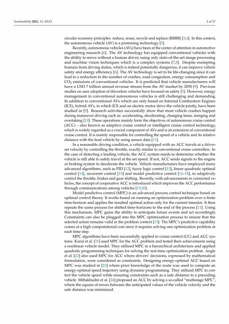
Recently, autonomous vehicles (AVs) have been at the center of attention in automotiveengineering research [6]. The AV technology has equipped conventional vehicles withthe ability to move without a human driver, using only state-of-the-art image processingand machine vision techniques which is a complex systems [7,8]. Despite exemptinghumans from driving duties, which is indeed potentially dangerous, it can improve vehiclesafety and energy efficiency [6]. The AV technology is set to be life-changing since it canlead to a reduction in the number of crashes, road congestion, energy consumption andCO2 emissions of conventional vehicles. It is predicted that vehicle manufacturers willhave a USD 7 trillion annual revenue stream from the AV market by 2050 [9]. Previousstudies on user adoption of driverless vehicles have focused on safety [5]. However, energymanagement in conventional autonomous vehicles is still challenging and demanding.In addition to conventional AVs which are only based on Internal Combustion Engines(ICE), hybrid AVs, in which ICE and an electric motor drive the vehicle jointly, have beenstudied in [9]. Research activities successfully show that most vehicle crashes happenduring maneuver driving such as: accelerating, decelerating, changing lanes, merging andovertaking [10]. These operations mainly form the objectives of autonomous cruise control(ACC) – also known as adaptive cruise control or intelligent cruise control technology,which is widely regarded as a crucial component of AVs and is an extension of conventionalcruise control. It is mainly responsible for controlling the speed of a vehicle and its relativedistance with the lead vehicle by using sensor data [11].

In a reasonable driving condition, a vehicle equipped with an ACC travels at a driver-set velocity by controlling the throttle, exactly similar to conventional cruise controllers. Inthe case of detecting a leading vehicle, the ACC system needs to determine whether thevehicle is still able to safely travel at the set speed. If not, ACC sends signals to the engineor braking system to decelerate the vehicle. Vehicle manufacturers have employed manyadvanced algorithms, such as PID [12], fuzzy logic control [13], linear quadratic optimalcontrol [14], recurrent control [15] and model predictive control [16–18], to adaptivelycontrol the throttle, brakes and gear shifting. Recently, with advancements in connected ve-hicles, the concept of cooperative ACC is introduced which improves the ACC performancethrough communications among vehicles [19,20].

Model predictive control (MPC) is an advanced process control technique based onoptimal control theory. It works based on running an optimization problem over a finitetime-horizon and applies the resulted optimal action only for the current timeslot. It thenrepeats the same process for shifted time-horizons to the end of the process [11]. Usingthis mechanism, MPC gains the ability to anticipate future events and act accordingly.Constraints can also be plugged into the MPC optimization process to ensure that theselected action remains valid in the problem context [13]. The MPC’s predictive capabilitycomes at a high computational cost since it requires solving one optimization problem ateach time step.

MPC algorithms have been successfully applied to cruise control (CC) and ACC sys-tems. Kural et al. [21] used MPC for the ACC problem and tested their achievements usinga nonlinear vehicle model. They utilized MPC in a hierarchical architecture and appliedquadratic programming techniques for solving the real-time optimization problem. Angleet al. [22] also used MPC for ACC where drivers’ decisions, expressed by mathematicalformulation, were considered as constraints. Designing energy-optimal ACC based onMPC was studied in [23] where prior knowledge of the route was used to compute anenergy-optimal speed trajectory using dynamic programming. They utilized MPC to con-trol the vehicle speed while ensuring constraints such as a safe distance to a precedingvehicle. Miftakhudin et al. [24] proposed an ACC by solving a so-called “multistage MPC”,where the square of errors between the anticipated values of the vehicle velocity and thesafe distance was minimized.

Sustainability 2021, 13, 10113 3 of 17

Adaptive model predictive control (AMPC) is a type of MPC where the controlalgorithm is re-tuned based on the behavior of the system, such as variation of the vehiclemodel. This feature helps ACC designers to accommodate a vehicle lateral dynamicsmodel [25] or the road condition [26]. As the control system is adapted to current systemconditions, AMPC performance is robust against uncertainties.

Despite the aforementioned advances in ACC to improve safety, it is not the onlyconcern about AVs from a sustainability perspective. Transportation, as a complex system,has challenges such as capacity, transfer, reliability, integration to reduce time and energyconsumption [27]. Energy management systems (EMSs) are control systems aiming forenergy efficiency in AVs. Numerous methods have been proposed to improve engineefficiency, such as regenerative braking protocols [28], rule-based reduction of energyconsumption [29,30] and intelligent approaches [31–33]. Among these approaches, intel-ligent control algorithms, such as fuzzy systems, show a great potential to deal with thenonlinearities of this problem in vehicles [31]. Many of the existing fuzzy logic-based EMShas been designed based on a type 1 fuzzy logic system (T1FLS) [29,34–36]. The set ofrules and membership functions of a T1FLS are formulated based on the knowledge ofhuman beings. However, the linguistic and numerical uncertainties, inherited from thedriving conditions, could not be solved and addressed comprehensively by using explicitmembership functions in a T1FLS [37–39]. To overcome these disadvantages, interval type2 fuzzy logic systems (IT2FLS) have been introduced [40]. By offering fuzzy member-ship functions (MFs), they can accommodate the insufficiency related to the changes ofthe driving conditions. The MFs of IT2FLS are three-dimensional, in opposition to thetwo-dimension MFs in T1FLS, and therefore offering one additional degree of freedom.IT2FLS can precisely achieve membership grades in practical problems with high levels ofuncertainty [41]. Our recent research [42] showed that IT2FLS is more effective than T1FLSin reducing energy consumption in an autonomous vehicle.

In this paper, we integrate an AMPC-based ACC with an IT2FLS fuzzy logic-basedEMS to achieve a cascade control system. It has two different objectives simultaneously:obtaining a safe distance with the lead vehicle and reducing the energy consumption ofthe ego vehicle. A lead-ego vehicle-following scenario (see Figure 1), which is when a leadvehicle is being followed by an ego vehicle in the same lane, is considered. The ego vehicleis appropriately equipped with a combining radar measurement using an extended objecttracker, and the LiDAR measurements using a joint probabilistic data association trackerare used. Then these tracks are fused by using a track-level fusion algorithm to measurethe distance and velocity relative to the lead vehicle.

Sustainability 2021, 13, x FOR PEER REVIEW 4 of 17

Figure 1. The lead-ego scenario to keep a safe distance between the lead and ego vehicles.

2. Vehicle Dynamics and Require Power In this article, a longitudinal model is considered for the ego vehicle as shown in

Figure 2. Using Newton’s law, the total driving force of a vehicle is: 𝑚𝑎 = 𝐹 − 𝐹 − 𝐹 − 𝐹 (1)

where 𝐹 , 𝐹 , 𝐹 and 𝐹 are the total driving force, the rolling resistance force, the aerodynamic resistance force, and the component of gravity along the road surface, respectively, m is the mass of the vehicle and a shows its acceleration. Forces are calculated using the following formulas: 𝐹 = 𝜇 . 𝑚𝑔𝑐𝑜𝑠𝜃 (2)

𝐹 = 𝑐 . 12 𝜌. 𝐴. (𝑣 + 𝑣 ) (3)

𝐹 = 𝑚𝑔𝑠𝑖𝑛𝜃 (4)

where 𝜇 is the road friction coefficient, 𝜃 is the slope of the road, ca is the aerodynamic resistance coefficient, 𝜌 is the air density, A is the cross-sectional area, vt is the velocity of the vehicle, vw is the velocity of the wind, g is gravity, and a is the acceleration of the vehicle. By Substituting (2), (3) and (4) into (1), the total driving force is 𝐹 = 𝜇 𝑚𝑔 𝑐𝑜𝑠 𝜃 + 𝑐 . 12 𝜌. 𝐴. (𝑣 + 𝑣 ) + 𝑚𝑔 𝑠𝑖𝑛 𝜃 + 𝑚𝑎 (5)

Using 𝐹 , we can define the required power of the vehicle as, 𝑃 = 𝐹 . 𝑣 + 𝑃 (6)

where 𝑃 is the air conditioning (AC) power consumption. In this paper, the AC model, introduced in [43], is considered. As the vehicle travels along the road, the power consumption exploited by an AC system changes dynamically. It can increase the power usage of the vehicle by 12–17% [44]. Other supplementary powers are quite modest in comparison with the overall power consumption of the vehicle. Thus, in this work, only the AC’s power consumption is considered, and the rest are consolidated in the mechanical losses. For the AC power we have: 𝑃 = 𝑑𝑊𝑑𝑡 = 𝑀𝐶 𝑑𝑇𝑑𝑡 (7)

where M is the air mass in the cabin, Troom and Croom are the cabin temperature and the temperature constant.

To achieve the vehicle power (𝑃) in Equation (6) and considering the power train model explained in [45], the following fuel consumption rate is required 𝑚 = 𝑃𝑞 . 𝜂 . 𝜂 (8)

where 𝑞 is the combustion energy, 𝜂 = 0.9 [46] is the mechanical efficiency and 𝜂 is the engine efficiency. The engine efficiency graph (see Figure 3) is normally illustrated by a contour plot as a function of torque [Nm] and the engine speed [rpm]. These contours are derived using the experimental characterization of the engine

Figure 1. The lead-ego scenario to keep a safe distance between the lead and ego vehicles.

We show that by using this combination, the distance between two vehicles is kept safewhile energy consumption is reduced. The main contributions impact on implementationof the technology of this study are useful for the future of transportation and can behighlighted as follows:

An AMPC algorithm is applied as ACC to control the safe operation of the ego vehicleunder combined loads. In this algorithm, the objective function of the MPC algorithm isadapted based on ego-lead distance.

Energy management of vehicles in cascade with the AMPC is established based onthe IT2FLS method which can handle the uncertainties of driving conditions.

Prediction safety control is used to control a vehicle while satisfying a set of vehicleand road geometry constraints.

Sustainability 2021, 13, 10113 4 of 17

The rest of the paper is organized as follows: Section 2 illustrates the vehicle dynamicsand power model required for the ego vehicle. Our integrated control system is presentedin Section 3. Section 4 illustrates simulation results, including a discussion. Finally, thework is concluded in Section 5.

2. Vehicle Dynamics and Require Power

In this article, a longitudinal model is considered for the ego vehicle as shown inFigure 2. Using Newton’s law, the total driving force of a vehicle is:

ma = Ft − Fr − Fw − Fg (1)

where Ft, Fr, Fw and Fg are the total driving force, the rolling resistance force, the aerody-namic resistance force, and the component of gravity along the road surface, respectively,m is the mass of the vehicle and a shows its acceleration. Forces are calculated using thefollowing formulas:

Fr = µr.mgcosθ (2)

Fw = ca.12

ρ.A.(vt + vw)2 (3)

Fg = mgsinθ (4)

where µr is the road friction coefficient, θ is the slope of the road, ca is the aerodynamicresistance coefficient, ρ is the air density, A is the cross-sectional area, vt is the velocityof the vehicle, vw is the velocity of the wind, g is gravity, and a is the acceleration of thevehicle. By Substituting (2), (3) and (4) into (1), the total driving force is

Ft = µrmg cos θ + ca.12

ρ.A.(vw + vt)2 + mg sin θ + ma (5)

Sustainability 2021, 13, x FOR PEER REVIEW 5 of 17

in real performing conditions. The highest obtainable efficiency for an ICE is 34%, due to thermodynamic limitations.

Figure 2. Longitudinal dynamics of the ego vehicle.

Figure 3. Engine efficiency map of Honda Insight (2004) 1.01 VTEC-E SI from ANL test data.

3. Proposed Control System for the Ego Vehicle The block diagram of the control system for the ego vehicle is shown in Figure 4. This

is a cascade control structure, including an ACC in series with an EMS. The control objectives are as follows. • The spacing error between two vehicles, i.e., Δ𝑑 = 𝑑 − 𝑑 is always maintained

greater than zero, where d and dsafe are the actual and safe distances between the lead and ego vehicles, respectively.

• The energy consumption for the ego vehicle is optimized using an EMS.

Figure 4. Integrated control system architecture.

Figure 2. Longitudinal dynamics of the ego vehicle.

Using Ft, we can define the required power of the vehicle as,

P = Ft.vt + Paccessory (6)

where Paccessory is the air conditioning (AC) power consumption. In this paper, the ACmodel, introduced in [43], is considered. As the vehicle travels along the road, the powerconsumption exploited by an AC system changes dynamically. It can increase the powerusage of the vehicle by 12–17% [44]. Other supplementary powers are quite modest incomparison with the overall power consumption of the vehicle. Thus, in this work, onlythe AC’s power consumption is considered, and the rest are consolidated in the mechanicallosses. For the AC power we have:

Paccessory =dWac

dt= MCroom

dTroom

dt(7)

where M is the air mass in the cabin, Troom and Croom are the cabin temperature and thetemperature constant.

Sustainability 2021, 13, 10113 5 of 17

To achieve the vehicle power (P) in Equation (6) and considering the power trainmodel explained in [45], the following fuel consumption rate is required

.m f uel =

Pqcombustion.ηmechanical .ηengine

(8)

where qcombustion is the combustion energy, ηmechanical = 0.9 [46] is the mechanical efficiencyand ηengine is the engine efficiency. The engine efficiency graph (see Figure 3) is nor-mally illustrated by a contour plot as a function of torque [Nm] and the engine speed[rpm]. These contours are derived using the experimental characterization of the enginein real performing conditions. The highest obtainable efficiency for an ICE is 34%, due tothermodynamic limitations.

Sustainability 2021, 13, x FOR PEER REVIEW 5 of 17

in real performing conditions. The highest obtainable efficiency for an ICE is 34%, due to thermodynamic limitations.

Figure 2. Longitudinal dynamics of the ego vehicle.

Figure 3. Engine efficiency map of Honda Insight (2004) 1.01 VTEC-E SI from ANL test data.

3. Proposed Control System for the Ego Vehicle The block diagram of the control system for the ego vehicle is shown in Figure 4. This

is a cascade control structure, including an ACC in series with an EMS. The control objectives are as follows. • The spacing error between two vehicles, i.e., Δ𝑑 = 𝑑 − 𝑑 is always maintained

greater than zero, where d and dsafe are the actual and safe distances between the lead and ego vehicles, respectively.

• The energy consumption for the ego vehicle is optimized using an EMS.

Figure 4. Integrated control system architecture.

Figure 3. Engine efficiency map of Honda Insight (2004) 1.01 VTEC-E SI from ANL test data.

3. Proposed Control System for the Ego Vehicle

The block diagram of the control system for the ego vehicle is shown in Figure 4.This is a cascade control structure, including an ACC in series with an EMS. The controlobjectives are as follows.

Sustainability 2021, 13, x FOR PEER REVIEW 5 of 17

in real performing conditions. The highest obtainable efficiency for an ICE is 34%, due to thermodynamic limitations.

Figure 2. Longitudinal dynamics of the ego vehicle.

Figure 3. Engine efficiency map of Honda Insight (2004) 1.01 VTEC-E SI from ANL test data.

3. Proposed Control System for the Ego Vehicle The block diagram of the control system for the ego vehicle is shown in Figure 4. This

is a cascade control structure, including an ACC in series with an EMS. The control objectives are as follows. • The spacing error between two vehicles, i.e., Δ𝑑 = 𝑑 − 𝑑 is always maintained

greater than zero, where d and dsafe are the actual and safe distances between the lead and ego vehicles, respectively.

• The energy consumption for the ego vehicle is optimized using an EMS.

Figure 4. Integrated control system architecture.

Figure 4. Integrated control system architecture.

• The spacing error between two vehicles, i.e., ∆d = d− dsa f e is always maintainedgreater than zero, where d and dsafe are the actual and safe distances between the leadand ego vehicles, respectively.

• The energy consumption for the ego vehicle is optimized using an EMS.

Sustainability 2021, 13, 10113 6 of 17

3.1. Adaptive Cruise Control

Generally, an ACC controller has a hierarchical structure, including an upper-levelcontroller and a lower-level controller [47]. The upper-level controller typically determinesthe desired acceleration for the ego vehicle based on the relative speed and the relativedistance from the lead vehicle. The lower-level controller determines the throttle and brakeactions to follow the acceleration/deceleration commands from the upper-level controller.In this paper, by assuming that the lower-level controller is well-designed, our focus ismore on the design of the upper-level controller. The ACC model of the vehicle can bedefined as follows [16].

τd

..x(t)dt

+..x(t) = u(t) (9)

where τ refers to the time lag corresponding to the finite bandwidth of the lower-levelcontroller and u depicts the acceleration command applied by the upper-level controller. x,.x, a =

..x are the position, speed and acceleration of the ego vehicle, respectively. Using a

first-order approximation, the discrete-time expression of (9) can be shown as,

a(k + 1) =(

1− Ts

τ

)a(k) +

Ts

τu(k) (10)

where Ts refers to the sampling period, a(k) is the acceleration of the ego vehicle at thesampling time k. The safe distance between the lead vehicle and ego vehicle can becalculated based on the velocity of the ego vehicle, shown below.

dsa f e = dde f ault + tgap.ve(k) (11)

where tgap is the constant time headway. dde f ault is a safe distance and is fixed when thevehicle travels at a low speed or is completely stopped. In other words, dsa f e is adjustedbased on the speed of the ego vehicle ve(k). The relative speed between the lead and theego vehicle v is,

v(k) = vl(k)− ve(k) (12)

where vl(k) is the speed of the lead vehicle at sampling time k. Therefore, equations ofmotion of the ego vehicle can be represented using the following state-space model:

x(k + 1) =

1 Ts − 12 T2

s0 1 −Ts0 0 1− Ts

τ

x(k) +

00Tsτ

u(k)

y =

1 0 00 1 00 0 1

x(k) +

−dde f ault00

(13)

where x = [∆d, v, a]T is the state vector of the system.Despite these linear equations, ACC deals with the strongly nonlinear powertrain

system, for which equations will come later. The control objective for the ego vehicleis to maintain its speed close to the lead vehicle while their relative distance is safe, i.e.,∆d→ 0 and v(k)→ 0 as k reaches to infinity. To achieve this objective, an adaptive modelpredictive control (AMPC) is used. Acceleration of the ego vehicle should be adaptivelychanged in order to regulate ∆d. The acceleration command is calculated by solving thefollowing constrained optimization problem during each sampling period.

minJu

=p

∑k=1{zT

t+kQtzt+k + ∆uTt+kR∆u

t ∆ut+k + uTt+kRu

t ut+k} (14)

Sustainability 2021, 13, 10113 7 of 17

s.t.

∆d ≥ 0

vmin ≤ ve(k) ≤ vmaxamin ≤ a(k) ≤ amaxumin ≤ u(k) ≤ umax

(15)

where t is the current time, p is the prediction horizon and ∆u is the increment of the controlinput. Qt, R∆u

t , and Rut refer to the weight matrices for the following error, change rate and

magnitude of the control input, respectively.As a normal ACC, the MPC control objective should be distance control, i.e., z = ∆d

in Equation (15). However, we will show in simulations that the performance of such acontroller is poor when the ego vehicle falls behind for any reason. To solve this issue,an AMPC is considered in which the control objective is adaptively changed based onthe distance ∆d between ego and lead vehicles. When ∆d is large, i.e., the ego vehicle isfar behind the lead one, AMPC switches to speed control system. Therefore, z = v inthe optimization problem (15) which results in accelerating the ego vehicle to fill its gapwith the lead. However, when ∆d becomes reasonably close to dde f ault, the control systemswitches to distance control and z = ∆d. In this case, the ego vehicle follows the drivingprofile of the lead by increasing and decreasing longitudinal acceleration such that ∆d→ 0 .It is worth noting that if the relative speed between the lead and the ego vehicle is notprecisely measurable, the controller goes to the distance control mode to preserve safety.

This adaptive behavior makes the control algorithm robust against undesired distur-bances. For example, if the ego vehicle fails in achieving ∆d→ 0 for any reason, such assudden action of the lead driver or loss of sensor signals, it will be easily compensated byswitching to the speed control mode for a while.

3.2. Energy Management System

In this work, an EMS is integrated with ACC to reduce fuel consumption while thevehicle performance is kept satisfactory. The EMS system has two main components: Afuzzy logic system (FLS) and a PID controller. FLS is employed to generate the optimaltorque by considering the required power for the vehicle. A PID controller is exploited togovern the engine to follow the optimal torque created by FLS.

3.2.1. Fuzzy Logic System

The FLS uses the required power of the vehicle as input and generates the optimaltorque for the engine. To calculate the required power, described in Equation (6), alldata about the behavior of the driver (e.g., the speed of the vehicle using data fusion),environmental conditions and vehicle specification are collected and passed through theenergy calculation unit (ECU) in Figure 4.

The environmental conditions, such as road and wind profiles, vary during the drivingprocess. Road profiles are generated with statistical characteristics of real roads using themethod presented in [48]. A Poisson distribution is used to create the number of roadsegments. The length of each road segment is obtained by using an exponential distribution.Rayleigh distribution is employed to model the height of up and down hills of the road.The left and the right bend of the road are acquired using Gaussian distribution. A windprofile is also obtained from the model in [48]. It is a collection of regions of differentlengths, the speed of the wind and its direction. The length, wind speed and direction aremodelled using the exponential, Weibull and uniform distributions, respectively. All theparameters used to calculate the required power of the vehicle are shown in Table 1.

Sustainability 2021, 13, 10113 8 of 17

Table 1. Inputs used to calculate the required power of the vehicle.

Description Symbol Value

Coefficient of road friction µr 0.015Gravity acceleration g 9.81 [m/s2]

Velocity of the vehicle v ACC commandMass (vehicle + equivalent rotating parts + passengers) m 1280 [kg]

Aerodynamic resistance coefficient ca 0.335A cross-sectional area A 1.9 ∗ 1/ cos(φ)

Air density ρ 1.225 [kg/m3]Combustion energy qcombustion 38,017 [kJ/kg]

After achieving the required power of the vehicle, FLS is used to produce the desiredengine torque. FLS is considered a reasoning method which resembles human reasoning.FLS is designed based on two methods: T1FLS and IT2FLS.

Part I. Type 1 Fuzzy Logic System

The membership functions of T1FLS are designed based on our previous work [34].Five membership functions for the input (the required power of the vehicle) are formulated,including L, LN, N, NH, H (Figure 5). The membership function of the output (the enginetorque) is split into three groups: LO, O, RO (Figure 6). Fuzzy rules are constructed sothat the engine state is regulated to operate on its optimal area to elevate energy efficiency.These rules cover five different conditions and are shown in Table 2. In summary, if therequired power is in L or H range of Figure 5, the T1FLS generates LO and RO signalsrelated to low and high torque values, respectively. Otherwise, it generates an O signal.

Sustainability 2021, 13, x FOR PEER REVIEW 8 of 17

Table 1. Inputs used to calculate the required power of the vehicle.

Description Symbol Value Coefficient of road friction 𝜇 0.015

Gravity acceleration g 9.81 [m/s2] Velocity of the vehicle v ACC command

Mass (vehicle + equivalent rotating parts + passengers) m 1280 [kg] Aerodynamic resistance coefficient 𝑐 0.335

A cross-sectional area 𝐴 1.9 ∗ 1/cos (𝜙) Air density 𝜌 1.225 [kg/m3]

Combustion energy qcombustion 38,017 [kJ/kg]

After achieving the required power of the vehicle, FLS is used to produce the desired engine torque. FLS is considered a reasoning method which resembles human reasoning. FLS is designed based on two methods: T1FLS and IT2FLS.

Part I. Type 1 Fuzzy Logic System The membership functions of T1FLS are designed based on our previous work [34].

Five membership functions for the input (the required power of the vehicle) are formulated, including L, LN, N, NH, H (Figure 5). The membership function of the output (the engine torque) is split into three groups: LO, O, RO (Figure 6). Fuzzy rules are constructed so that the engine state is regulated to operate on its optimal area to elevate energy efficiency. These rules cover five different conditions and are shown in Table 2. In summary, if the required power is in L or H range of Figure 5, the T1FLS generates LO and RO signals related to low and high torque values, respectively. Otherwise, it generates an O signal.

00.20.40.60.81

0.5 1 1.5 2 2.5 3 3.5 4 4.5 5

L LN N NH H

P [W]X 104

Figure 5. T1FLS membership functions for the input, the required power of the vehicle.

Figure 6. T1FLS membership function of the output, the engine torque.

Part II. Interval Type 2 Fuzzy Logic System The IT2FLS is a new algorithm that accommodates unique characteristics to

overcome the limitations of T1FLS in coping with the uncertainties. An IT2FLS is represented in Figure 7, including five components: fuzzifier, rule-based, fuzzy inference, type-reducer and defuzzifier.

Figure 5. T1FLS membership functions for the input, the required power of the vehicle.

Sustainability 2021, 13, x FOR PEER REVIEW 8 of 17

Table 1. Inputs used to calculate the required power of the vehicle.

Description Symbol Value Coefficient of road friction 𝜇 0.015

Gravity acceleration g 9.81 [m/s2] Velocity of the vehicle v ACC command

Mass (vehicle + equivalent rotating parts + passengers) m 1280 [kg] Aerodynamic resistance coefficient 𝑐 0.335

A cross-sectional area 𝐴 1.9 ∗ 1/cos (𝜙) Air density 𝜌 1.225 [kg/m3]

Combustion energy qcombustion 38,017 [kJ/kg]

After achieving the required power of the vehicle, FLS is used to produce the desired engine torque. FLS is considered a reasoning method which resembles human reasoning. FLS is designed based on two methods: T1FLS and IT2FLS.

Part I. Type 1 Fuzzy Logic System The membership functions of T1FLS are designed based on our previous work [34].

Five membership functions for the input (the required power of the vehicle) are formulated, including L, LN, N, NH, H (Figure 5). The membership function of the output (the engine torque) is split into three groups: LO, O, RO (Figure 6). Fuzzy rules are constructed so that the engine state is regulated to operate on its optimal area to elevate energy efficiency. These rules cover five different conditions and are shown in Table 2. In summary, if the required power is in L or H range of Figure 5, the T1FLS generates LO and RO signals related to low and high torque values, respectively. Otherwise, it generates an O signal.

00.20.40.60.81

0.5 1 1.5 2 2.5 3 3.5 4 4.5 5

L LN N NH H

P [W]X 104

Figure 5. T1FLS membership functions for the input, the required power of the vehicle.

Figure 6. T1FLS membership function of the output, the engine torque.

Part II. Interval Type 2 Fuzzy Logic System The IT2FLS is a new algorithm that accommodates unique characteristics to

overcome the limitations of T1FLS in coping with the uncertainties. An IT2FLS is represented in Figure 7, including five components: fuzzifier, rule-based, fuzzy inference, type-reducer and defuzzifier.

Figure 6. T1FLS membership function of the output, the engine torque.

Table 2. Fuzzy logic system rules.

Condition Number IfRequired Power

ThenEngine Torque

1 L LO2 LN O3 N O4 NH O5 H RO

Sustainability 2021, 13, 10113 9 of 17

Part II. Interval Type 2 Fuzzy Logic System

The IT2FLS is a new algorithm that accommodates unique characteristics to overcomethe limitations of T1FLS in coping with the uncertainties. An IT2FLS is represented inFigure 7, including five components: fuzzifier, rule-based, fuzzy inference, type-reducerand defuzzifier.

Sustainability 2021, 13, x FOR PEER REVIEW 9 of 17

Table 2. Fuzzy logic system rules.

Condition Number If

Required Power Then

Engine Torque 1 L LO 2 LN O 3 N O 4 NH O 5 H RO

Figure 7. Block diagram of a type 2 fuzzy logic system.

The notable discrepancies between IT2FLS and the type 1 counterpart are that interval type 2 fuzzy sets are exploited and used in IT2FLS. Therefore, the IT2FLS has an extra process that is known as the type reduction [37,49,50]. An interval type 2 set (𝐴) is determined with a type 2 membership function 𝜇 (𝑥, 𝑢) as below. 𝐴 = 𝜇 (𝑥, 𝑢)(𝑥, 𝑢)∈∈ (16)

where Jx is the primary membership of x, while 𝜇 (𝑥, 𝑢) is a type 1 fuzzy set known as the secondary set [37,49,50]. 𝜇 (𝑥 = 𝑥 , 𝑢) ≡ 𝜇 (𝑥 ) = 𝑓 (𝑢)𝑢∈ (17)

0 ≤ 𝑓 (𝑢) ≤ 1 (18)

A region called footprint of uncertainty (FOU) is formulated to evaluate the uncertainty in the primary membership of an interval type 2 fuzzy set 𝐴, as depicted in Figure 8. It can be defined as follows. FOU 𝐴 = 𝐽 = {(𝑥, 𝑢)| 𝑢 ∈ 𝐽 ⊆ 0,1 }∈ (19)

where 𝐽 presents the primary membership of 𝐴. An upper membership function (UMF) and a lower membership function (LMF) are

also introduced to represent the FOU. They can be represented as below. 𝜇 (𝑥) = LMF 𝐴 = 𝑖𝑛𝑓{𝑢 | 𝑢 ∈ 0,1 , 𝜇 (𝑥, 𝑢) > 0} (20)�� (𝑥) = UMF 𝐴 = 𝑠𝑢𝑝{𝑢 | 𝑢 ∈ 0,1 , 𝜇 (𝑥, 𝑢) > 0} (21)

The uncertainty of driving conditions is handled by the antecedents and consequents interval type 2 fuzzy sets, which utilize FOUs to cover the linguistic and numerical uncertainties associated with changing unstructured environments. The interval type 2 fuzzy sets compound a huge amount of embedded type 1 fuzzy sets to solve the various uncertainties as well [51].

Figure 7. Block diagram of a type 2 fuzzy logic system.

The notable discrepancies between IT2FLS and the type 1 counterpart are that intervaltype 2 fuzzy sets are exploited and used in IT2FLS. Therefore, the IT2FLS has an extraprocess that is known as the type reduction [37,49,50]. An interval type 2 set (A) isdetermined with a type 2 membership function µA(x, u) as below.

A =∫

x∈DA

∫u∈Jx

µA(x, u)(x, u)

(16)

where Jx is the primary membership of x, while µA(x, u) is a type 1 fuzzy set known as thesecondary set [37,49,50].

µA

(x = x′, u

)≡ µA

(x′)=∫

u∈Jx′

fx′(u)u

(17)

0 ≤ fx′(u) ≤ 1 (18)

A region called footprint of uncertainty (FOU) is formulated to evaluate the uncer-tainty in the primary membership of an interval type 2 fuzzy set A, as depicted in Figure 8.It can be defined as follows.

FOU(

A)=⋃

x∈XJx = {(x, u)| u ∈ Jx ⊆ [0, 1]} (19)

where Jx presents the primary membership of A.

Sustainability 2021, 13, x FOR PEER REVIEW 10 of 17

x

( )A xμ

Upper membership function

Lower membership function

FOU

Figure 8. The FOU (shaded area), UMF and LMF of IT2FLS.

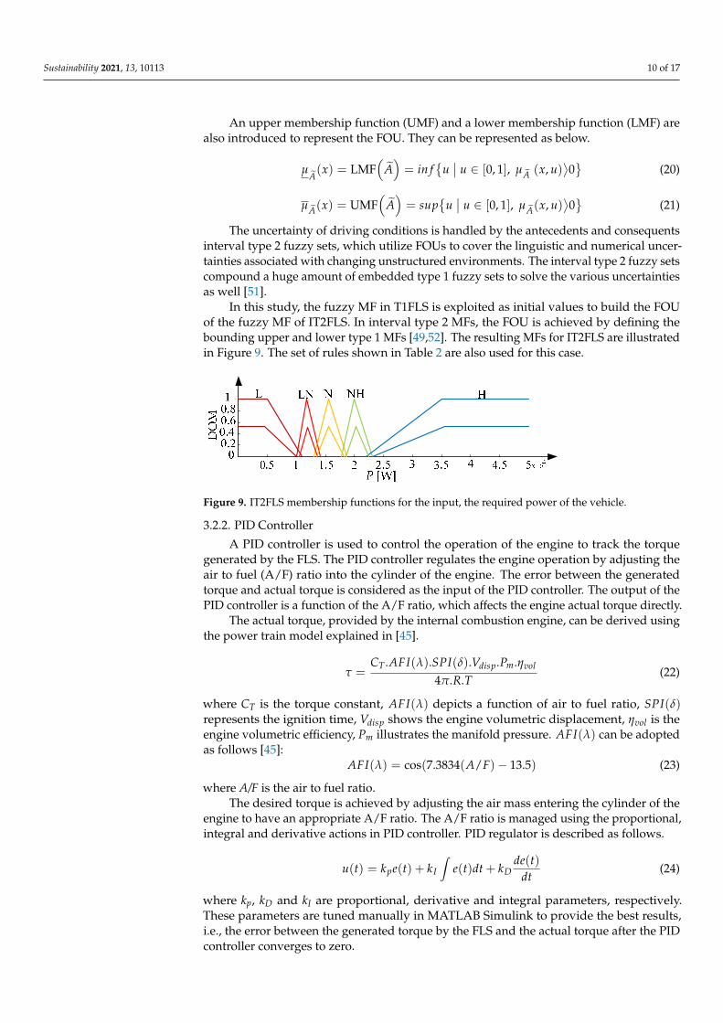
In this study, the fuzzy MF in T1FLS is exploited as initial values to build the FOU of the fuzzy MF of IT2FLS. In interval type 2 MFs, the FOU is achieved by defining the bounding upper and lower type 1 MFs [49,52]. The resulting MFs for IT2FLS are illustrated in Figure 9. The set of rules shown in Table 2 are also used for this case.

Figure 9. IT2FLS membership functions for the input, the required power of the vehicle.

3.2.2. PID Controller A PID controller is used to control the operation of the engine to track the torque

generated by the FLS. The PID controller regulates the engine operation by adjusting the air to fuel (A/F) ratio into the cylinder of the engine. The error between the generated torque and actual torque is considered as the input of the PID controller. The output of the PID controller is a function of the A/F ratio, which affects the engine actual torque directly.

The actual torque, provided by the internal combustion engine, can be derived using the power train model explained in [45]. 𝜏 = 𝐶 . 𝐴𝐹𝐼(𝜆). 𝑆𝑃𝐼(𝛿). 𝑉 . 𝑃 . 𝜂4𝜋. 𝑅. 𝑇 (22)

where CT is the torque constant, 𝐴𝐹𝐼(𝜆) depicts a function of air to fuel ratio, 𝑆𝑃𝐼(𝛿) represents the ignition time, 𝑉 shows the engine volumetric displacement, 𝜂 is the engine volumetric efficiency, Pm illustrates the manifold pressure. 𝐴𝐹𝐼(𝜆) can be adopted as follows [45]: 𝐴𝐹𝐼(𝜆) = cos (7.3834(𝐴/𝐹) − 13.5) (23)

where A/F is the air to fuel ratio. The desired torque is achieved by adjusting the air mass entering the cylinder of the

engine to have an appropriate A/F ratio. The A/F ratio is managed using the proportional, integral and derivative actions in PID controller. PID regulator is described as follows. 𝑢(𝑡) = 𝑘 𝑒(𝑡) + 𝑘 𝑒(𝑡)𝑑𝑡 + 𝑘 𝑑𝑒(𝑡)𝑑𝑡 (24)

where kp, kD and kI are proportional, derivative and integral parameters, respectively. These parameters are tuned manually in MATLAB Simulink to provide the best results,

Figure 8. The FOU (shaded area), UMF and LMF of IT2FLS.

Sustainability 2021, 13, 10113 10 of 17

An upper membership function (UMF) and a lower membership function (LMF) arealso introduced to represent the FOU. They can be represented as below.

µA(x) = LMF

(A)= in f

{u∣∣ u ∈ [0, 1], µA (x, u)

⟩0}

(20)

µA(x) = UMF(

A)= sup

{u∣∣ u ∈ [0, 1], µA(x, u)

⟩0}

(21)

The uncertainty of driving conditions is handled by the antecedents and consequentsinterval type 2 fuzzy sets, which utilize FOUs to cover the linguistic and numerical uncer-tainties associated with changing unstructured environments. The interval type 2 fuzzy setscompound a huge amount of embedded type 1 fuzzy sets to solve the various uncertaintiesas well [51].

In this study, the fuzzy MF in T1FLS is exploited as initial values to build the FOUof the fuzzy MF of IT2FLS. In interval type 2 MFs, the FOU is achieved by defining thebounding upper and lower type 1 MFs [49,52]. The resulting MFs for IT2FLS are illustratedin Figure 9. The set of rules shown in Table 2 are also used for this case.

Sustainability 2021, 13, x FOR PEER REVIEW 10 of 17

x

( )A xμ

Upper membership function

Lower membership function

FOU

Figure 8. The FOU (shaded area), UMF and LMF of IT2FLS.

In this study, the fuzzy MF in T1FLS is exploited as initial values to build the FOU of the fuzzy MF of IT2FLS. In interval type 2 MFs, the FOU is achieved by defining the bounding upper and lower type 1 MFs [49,52]. The resulting MFs for IT2FLS are illustrated in Figure 9. The set of rules shown in Table 2 are also used for this case.

Figure 9. IT2FLS membership functions for the input, the required power of the vehicle.

3.2.2. PID Controller A PID controller is used to control the operation of the engine to track the torque

generated by the FLS. The PID controller regulates the engine operation by adjusting the air to fuel (A/F) ratio into the cylinder of the engine. The error between the generated torque and actual torque is considered as the input of the PID controller. The output of the PID controller is a function of the A/F ratio, which affects the engine actual torque directly.

The actual torque, provided by the internal combustion engine, can be derived using the power train model explained in [45]. 𝜏 = 𝐶 . 𝐴𝐹𝐼(𝜆). 𝑆𝑃𝐼(𝛿). 𝑉 . 𝑃 . 𝜂4𝜋. 𝑅. 𝑇 (22)

where CT is the torque constant, 𝐴𝐹𝐼(𝜆) depicts a function of air to fuel ratio, 𝑆𝑃𝐼(𝛿) represents the ignition time, 𝑉 shows the engine volumetric displacement, 𝜂 is the engine volumetric efficiency, Pm illustrates the manifold pressure. 𝐴𝐹𝐼(𝜆) can be adopted as follows [45]: 𝐴𝐹𝐼(𝜆) = cos (7.3834(𝐴/𝐹) − 13.5) (23)

where A/F is the air to fuel ratio. The desired torque is achieved by adjusting the air mass entering the cylinder of the

engine to have an appropriate A/F ratio. The A/F ratio is managed using the proportional, integral and derivative actions in PID controller. PID regulator is described as follows. 𝑢(𝑡) = 𝑘 𝑒(𝑡) + 𝑘 𝑒(𝑡)𝑑𝑡 + 𝑘 𝑑𝑒(𝑡)𝑑𝑡 (24)

where kp, kD and kI are proportional, derivative and integral parameters, respectively. These parameters are tuned manually in MATLAB Simulink to provide the best results,

Figure 9. IT2FLS membership functions for the input, the required power of the vehicle.

3.2.2. PID Controller

A PID controller is used to control the operation of the engine to track the torquegenerated by the FLS. The PID controller regulates the engine operation by adjusting theair to fuel (A/F) ratio into the cylinder of the engine. The error between the generatedtorque and actual torque is considered as the input of the PID controller. The output of thePID controller is a function of the A/F ratio, which affects the engine actual torque directly.

The actual torque, provided by the internal combustion engine, can be derived usingthe power train model explained in [45].

τ =CT .AFI(λ).SPI(δ).Vdisp.Pm.ηvol

4π.R.T(22)

where CT is the torque constant, AFI(λ) depicts a function of air to fuel ratio, SPI(δ)represents the ignition time, Vdisp shows the engine volumetric displacement, ηvol is theengine volumetric efficiency, Pm illustrates the manifold pressure. AFI(λ) can be adoptedas follows [45]:

AFI(λ) = cos(7.3834(A/F)− 13.5) (23)

where A/F is the air to fuel ratio.The desired torque is achieved by adjusting the air mass entering the cylinder of the

engine to have an appropriate A/F ratio. The A/F ratio is managed using the proportional,integral and derivative actions in PID controller. PID regulator is described as follows.

u(t) = kpe(t) + kI

∫e(t)dt + kD

de(t)dt

(24)

where kp, kD and kI are proportional, derivative and integral parameters, respectively.These parameters are tuned manually in MATLAB Simulink to provide the best results,i.e., the error between the generated torque by the FLS and the actual torque after the PIDcontroller converges to zero.

Sustainability 2021, 13, 10113 11 of 17

4. Simulations and Discussion4.1. Simulations

In this section, for the ego vehicle, we compare the performance of three differentalternatives for the control structure, mentioned in Table 3. The powertrain model whichhas been introduced in [45], is summarized by Equations (23) and (24). This model is usedduring all scenarios in these simulations. It assumes a continuously variable transmis-sion (CVT) system as an automatic transmission that can change seamlessly through acontinuous range of gear ratios.

Table 3. Structures of the control system compared in this paper.

ACC EMS

Alternative 1 AMPC -Alternative 2 AMPC T1FLSAlternative 3 AMPC T2FLS

Alternative 1: For this structure, the EMS block in the model of Figure 4 is bypassed.The ego vehicle follows the lead vehicle for a period of 766 s, equal to 16.5 km of traveldistance using an ACC. Through this journey, the lead vehicle follows a standard drivingcycle (HWFET). The ego vehicle, equipped with ACC based on AMPC, travels with theinitial velocity of 0 m/s. The relative distance between the two vehicles at the beginningis 200 m. In the simulation, the controller’s sampling time is 0.1 s, the constant timeheadway is 1.4 s, the prediction horizon p = 30 and the standstill default spacing is 10 m.MATLAB Simulink and model predictive control toolbox [53] are used in the simulations.The required power of the ego vehicle is produced by the energy calculation unit.

Alternative 2: This simulation is conducted under the same conditions as the Alter-native 1. However, the EMS block is activated and works based on the T1FLS, which isintroduced in Section 3.2.1 Part I.

Alternative 3: This simulation is conducted under the same conditions as the Alter-native 1. However, an EMS based on IT2FLS is considered. This allows to evaluate thecontroller’s performance in handling enormous uncertainties of driving conditions, espe-cially in the vehicle-following process. The IT2FLS MATLAB/Simulink toolbox designedby [54] is applied to execute the third simulation.

4.2. Discussion4.2.1. Safety

Figures 10 and 11 compare the performance of our proposed AMPC with the con-ventional MPC which focuses only on the distance control, i.e., z = v in Equation (15).Figure 10 shows how switching between speed and distance control mode happens basedon ∆d. When ∆d > 0, i.e., when the distance between the lead and ego cars is largerthan the safe threshold, the controller switches to speed control to compensate for the gapbetween vehicles. However, it activates the distance control mode when ∆d < 0, i.e., whenthe distance between vehicles is not safe. In Figure 11, it is assumed that the ego car startsfalling behind the lead vehicle at T = 200 s. It can be seen in Figure 11a that the normalMPC algorithm fails to bring the distance between two vehicles in an acceptable region. Itmeans that, using this control technique, the gap between cars cannot be compensated if∆d becomes too large for any reason. However, our proposed AMPC successfully controlsthe distance and keeps it in a safe range (Figure 11b). In addition, our study shows thatthe normal MPC consumes about 0.2 L/100 km more fuel than the proposed AMPC inthis maneuver. In other words, the AMPC works more robustly against any uncertaintieswhich results in increasing ∆d. Figure 11b also shows a smooth variation of the spacing∆d during the whole scenario which means that excessive high braking and acceleratingare avoided. Consequently, not only the risk of crashes is reduced, but also the comfort ofdriving is improved significantly.

Sustainability 2021, 13, 10113 12 of 17Sustainability 2021, 13, x FOR PEER REVIEW 13 of 17

Figure 10. Switching between speed and distance control systems.

(a)

(b)

Figure 11. Distance variation between ego and lead cars in the presence of (a) MPC for distance control only and (b) the AMPC.

Figure 12. The A/F ration of the engine.

Figure 10. Switching between speed and distance control systems.

Sustainability 2021, 13, x FOR PEER REVIEW 13 of 17

Figure 10. Switching between speed and distance control systems.

(a)

(b)

Figure 11. Distance variation between ego and lead cars in the presence of (a) MPC for distance control only and (b) the AMPC.

Figure 12. The A/F ration of the engine.

Figure 11. Distance variation between ego and lead cars in the presence of (a) MPC for distance control only and(b) the AMPC.

4.2.2. Fuel Economy

In this section, performances of three alternatives for the ACC+EMS control structure,introduced in Table 3, are compared. Results of comparing A/F ratio, revolutions perminute, torque of the engine, fuel efficiency and fuel consumption rate in these three controlstructures are compared in Figures 12–16, respectively.

Sustainability 2021, 13, x FOR PEER REVIEW 13 of 17

Figure 10. Switching between speed and distance control systems.

(a)

(b)

Figure 11. Distance variation between ego and lead cars in the presence of (a) MPC for distance control only and (b) the AMPC.

Figure 12. The A/F ration of the engine. Figure 12. The A/F ration of the engine.

Sustainability 2021, 13, 10113 13 of 17

Sustainability 2021, 13, x FOR PEER REVIEW 14 of 17

ωICE

[rpm

]

Figure 13. The revolutions per minute of the engine.

τICE

[Nm

]

Figure 14. The torque of the engine.

Figure 15. The efficiency of the engine.

Figure 16. The fuel consumption rate of the engine.

Figure 13. The revolutions per minute of the engine.

Sustainability 2021, 13, x FOR PEER REVIEW 14 of 17

ωICE

[rpm

]

Figure 13. The revolutions per minute of the engine.

τICE

[Nm

]

Figure 14. The torque of the engine.

Figure 15. The efficiency of the engine.

Figure 16. The fuel consumption rate of the engine.

Figure 14. The torque of the engine.

Sustainability 2021, 13, x FOR PEER REVIEW 14 of 17

ωICE

[rpm

]

Figure 13. The revolutions per minute of the engine.

τICE

[Nm

]

Figure 14. The torque of the engine.

Figure 15. The efficiency of the engine.

Figure 16. The fuel consumption rate of the engine.

Figure 15. The efficiency of the engine.

Sustainability 2021, 13, x FOR PEER REVIEW 14 of 17

ωICE

[rpm

]

Figure 13. The revolutions per minute of the engine.

τICE

[Nm

]

Figure 14. The torque of the engine.

Figure 15. The efficiency of the engine.

Figure 16. The fuel consumption rate of the engine.

Figure 16. The fuel consumption rate of the engine.

Alternative 1: In this case, the engine operates in a region that has low energy ef-ficiency as the engine torque is elevated and the RPM is low (compare blue lines in

Sustainability 2021, 13, 10113 14 of 17

Figures 13 and 14). The average proficiency of the engine in this control structure is 25.31%.Therefore, the fuel usage of the vehicle can be estimated as 7.21 L/100 km.

Alternative 2: In this simulation, the EMS based on T1FLS is applied to save the fuelconsumed by the ego vehicle. Figure 14 shows that with the proposed system, the engineis regulated to produce a torque within the range of 35–65 [Nm]. In this case, a suboptimalrange of engine torque is considered, referring to Figure 3. Thus, the efficiency of theengine increases to 29% on average (see Figure 15). Consequently, the vehicle consumes6.88 L/100 km which is less than Alternative 1.

Alternative 3: In this structure, the engine is controlled to supply the torque and the speedwithin ranges 40–75 [Nm] and 1000–3800 [rpm], respectively, based on Figures 13 and 14.Therefore, the working area of the engine shifts to a more optimal regime, referring to Figure 3.The engine efficiency is escalated to 29.78% on average (see Figure 15), which is the result ofa reduction in fuel consumption to 6.68 L/100 km.

These results are also compared with the adaptive cruise control look ahead (ACC(LA))system [13] in Table 4. The ACC(LA) was designed based on the adaptive neuro-fuzzyinference system. The system calculated the fuel usage of the vehicle under combineddynamic loads as well. A look-ahead approach was involved in the model to anticipate theslope of the road in the future.

Table 4. Fuel consumption of different ACC system.

Model Average Efficiency mfuel (L/100 km)

ACC (LA) - 7.95ACC (AMPC) 25.31% 7.21

ACC (AMPC) + EMS (T1FLS) 29.00% 6.88ACC (AMPC) + EMS (T2FLS) 29.78% 6.68

A comparison of these three alternatives shows that the combination of AMPC asACC and T2FLS as EMS provide the best engine performance for the vehicles and resultsin less fuel consumption. It also inherits robustness of MPC, which is a crucial requirementin the uncertain environment of AVs. We see an example of this robustness in Figure 11when uncertainty in ∆d happens.

5. Conclusions

Unlike previous research activities which were mainly focused on the autonomouscruise control (ACC) – also known as adaptive cruise control or intelligent cruise controlof autonomous vehicles (AVs), this paper considered the joint ACC-energy managementsystems (EMS) problem to address both safety and energy management simultaneously,thus providing a sustainable solution for AVs. We proposed integrated adaptive modelpredictive control (AMPC) and interval type 2 fuzzy logic systems (IT2FLS)-based EMS forimproving energy efficiency in conventional vehicles in a vehicle-following scenario whilea safe driving condition is achieved. To this end, we utilized a cascade control structurewith an ACC on the outer loop and an EMS on the inner one. An AMPC approach wasused to design ACC in which the control objective was appropriately switched betweenspeed and distance. This resulted in compensation for the gap between vehicles in areasonable amount of time if the ego vehicle fell behind for any reason. The AMPC isaccompanied by an IT2FLS-based EMS, which was originally proposed to manage modeluncertainties. The control system was conducted in a MATLAB/Simulink environmentto empirically test the performance in a lead-ego vehicle-following scenario. Simulationresults for an HWFET drive cycle showed safe driving in a vehicle-following process in allscenarios. Meanwhile, the fuel consumption per hundred kilometres for the ego vehiclewas improved by 13.45% using the T1LFS-based system and by 15.97% using an IT2FLSEMS. That means by applying advanced EMS algorithms, robust against nonlinearities ofthe energy efficiency problem, and combining them with advanced ACC, can result in asignificant energy saving and emission reduction toward a sustainable circular economy.

Sustainability 2021, 13, 10113 15 of 17

Moreover, the AMPC+IT2FLS method assists AVs to make a smarter use of energy andsupport a safer transportation.

Author Contributions: Conceptualization, Ideas, Methodology, Management, Conducting, D.P. andH.K.; Software and Development and Data Curation, A.M.A., M.M., A.A.R., M.F., M.J. and R.L.Conducting a research and Investigation process supervision D.B.P.; Project administration H.K. Allauthors have read and agreed to the published version of the manuscript.

Funding: This research received no external funding.

Data Availability Statement: Not applicable.

Conflicts of Interest: The authors declare no conflict of interest.

References1. The Sustainable Development Goals Report; United Nations: New York, NY, USA, 2019.2. Tracking Transport 2020; International Energy Agency: Paris, France, 2020.3. Khayyam, H.; Naebe, M.; Milani, A.S.; Fakhrhoseini, S.M.; Date, A.; Shabani, B.; Atkiss, S.; Ramakrishna, S.; Fox, B.; Jazar, R.N.

Improving energy efficiency of carbon fiber manufacturing through waste heat recovery: A circular economy approach withmachine learning. Energy 2021, 225, 120113. [CrossRef]

4. Cugurullo, F.; Acheampong, R.A.; Gueriau, M.; Dusparic, I. The transition to autonomous cars, the redesign of cities and thefuture of urban sustainability. Urban Geogr. 2020, 1–27. [CrossRef]

5. Acheampong, R.A.; Cugurullo, F.; Gueriau, M.; Dusparic, I. Can autonomous vehicles enable sustainable mobility in future cities?Insights and policy challenges from user preferences over different urban transport options. Cities 2021, 112, 103134. [CrossRef]

6. Xie, J.; Xu, X.; Wang, F.; Tang, Z.; Chen, L. Coordinated control based path following of distributed drive autonomous electricvehicles with yaw-moment control. Control. Eng. Pract. 2021, 106, 104659. [CrossRef]

7. Khayyam, H.; Javadi, B.; Jalili, M.; Jazar, R.N. Artificial Intelligence and Internet of Things for Autonomous Vehicles. In NonlinearApproaches in Engineering Applications; Springer: Basingstoke, UK, 2020; pp. 39–68. [CrossRef]

8. Marzbani, H.; Khayyam, H.; To, C.N.; Quoc, D.V.; Jazar, R.N. Autonomous Vehicles: Autodriver Algorithm and Vehicle Dynamics.IEEE Trans. Veh. Technol. 2019, 68, 3201–3211. [CrossRef]

9. Lanctot, R. Accelerating the future: The economic impact of the emerging passenger economy. Strategy Anal. 2017, 5.10. Noh, S. Decision-Making Framework for Autonomous Driving at Road Intersections: Safeguarding Against Collision, Overly

Conservative Behavior, and Violation Vehicles. IEEE Trans. Ind. Electron. 2018, 66, 3275–3286. [CrossRef]11. Duraisamy, B.; Schwarz, T.; Wöhler, C. Track level fusion algorithms for automotive safety applications. In Proceedings of

the 2013 International Conference on Signal Processing, Image Processing & Pattern Recognition, Innsbruck, Australia, 12–14February 2013; pp. 179–184.

12. Milanes, V.; Villagra, J.; Godoy, J.; Gonzalez, C. Comparing Fuzzy and Intelligent PI Controllers in Stop-and-Go Manoeuvres.IEEE Trans. Control. Syst. Technol. 2011, 20, 770–778. [CrossRef]

13. Khayyam, H.; Nahavandi, S.; Davis, S. Adaptive cruise control look-ahead system for energy management of vehicles. ExpertSyst. Appl. 2012, 39, 3874–3885. [CrossRef]

14. Liang, Z.; Ren, Z.; Shao, X. Decoupling trajectory tracking for gliding reentry vehicles. IEEE/CAA J. Autom. Sin. 2015, 2, 115–120.[CrossRef]

15. Lin, C.-M.; Chen, C.-H. Car-Following Control Using Recurrent Cerebellar Model Articulation Controller. IEEE Trans. Veh. Technol.2007, 56, 3660–3673. [CrossRef]

16. Bageshwar, V.; Garrard, W.; Rajamani, R. Model Predictive Control of Transitional Maneuvers for Adaptive Cruise ControlVehicles. IEEE Trans. Veh. Technol. 2004, 53, 1573–1585. [CrossRef]

17. Magdici, S.; Althoff, M. Adaptive Cruise Control with Safety Guarantees for Autonomous Vehicles. IFAC-PapersOnLine 2017, 50,5774–5781. [CrossRef]

18. Takahama, T.; Akasaka, D. Model Predictive Control Approach to Design Practical Adaptive Cruise Control for Traffic Jam. Int. J.Automot. Eng. 2018, 9, 99–104. [CrossRef]

19. Mahdinia, I.; Arvin, R.; Khattak, A.J.; Ghiasi, A. Safety, Energy, and Emissions Impacts of Adaptive Cruise Control andCooperative Adaptive Cruise Control. Transp. Res. Rec. J. Transp. Res. Board 2020, 2674, 253–267. [CrossRef]

20. Shladover, S.E.; Nowakowski, C.; Lu, X.-Y.; Ferlis, R. Cooperative adaptive cruise control: Definitions and operating concepts.Transp. Res. Record 2015, 2489, 145–152. [CrossRef]

21. Kural, E.; Güvenç, B.A. Model Predictive Adaptive Cruise Control. In Proceedings of the 2010 IEEE International Conference onSystems, Man and Cybernetics, Cordoba, Spain, 1–4 June 2010; pp. 1455–1461.

22. De Madrid, A.P.; Mañoso, C.; Romero, M. Fundamentals of the MPC approach to stop-and-go Adaptive Cruise Control. InProceedings of the 2014 13th International Conference on Control Automation Robotics & Vision (ICARCV), Singapore, Singapore,10–12 December 2014; pp. 175–180.

Sustainability 2021, 13, 10113 16 of 17

23. Weißmann, A.; Görges, D.; Lin, X. Energy-Optimal Adaptive Cruise Control based on Model Predictive Control. IFAC-PapersOnLine 2017, 50, 12563–12568. [CrossRef]

24. Miftakhudin, M.I.; Subiantoro, A.; Yusivar, F. Adaptive Cruise Control by Considering Control Decision as Multistage MPCConstraints. In Proceedings of the 2019 IEEE Conference on Energy Conversion (CENCON), Yogyakarta, Indonesia, 16–17December 2019; pp. 171–176.

25. Bujarbaruah, M.; Zhang, X.; Borrelli, F. Adaptive MPC for Autonomous Lane Keeping. In Proceedings of the 14th InternationalSymposium on Advanced Vehicle Control (AVEC), Beijing, China, 16–20 July 2018.

26. Wang, X.; Guo, L.; Jia, Y. Road Condition Based Adaptive Model Predictive Control for Autonomous Vehicles. In Proceedings ofthe Dynamic Systems and Control Conference (DSCC), Atlanta, GA, USA, 30 September–3 October 2018.

27. Khayyam, H. Automation, Control and Energy Efficiency in Complex Systems; MDPI Books: Belgrade, Switzerland, 2020; p. 245.28. Koot, M.; Kessels, J.J.; De Jager, A.B.; Bosch, P.P.V.D. Fuel reduction potential of energy management for vehicular electric power

systems. Int. J. Altern. Propuls. 2006, 1, 112. [CrossRef]29. Khayyam, H.; Kouzani, A.Z.; Khoshmanesh, K.; Hu, E.J. A.Z.; Khoshmanesh, K.; Hu, E.J. A rule-based intelligent energy

management system for an internal combustion engine vehicle. In TENCON 2008-2008 IEEE Region 10 Conference; Institute ofElectrical and Electronics Engineers (IEEE): Piscataway, NJ, USA, 2008; pp. 1–5.

30. Khayyam, H.; Kouzani, A.Z.; Hu, E.J.; Nahavandi, S. Coordinated energy management of vehicle air conditioning system. Appl.Therm. Eng. 2011, 31, 750–764. [CrossRef]

31. Phan, D.; Bab-Hadiashar, A.; Lai, C.Y.; Crawford, B.; Hoseinnezhad, R.; Jazar, R.N.; Khayyam, H. Intelligent energy managementsystem for conventional autonomous vehicles. Energy 2020, 191, 116476. [CrossRef]

32. Won, J.-S.; Langari, R. Intelligent Energy Management Agent for a Parallel Hybrid Vehicle—Part II: Torque Distribution, ChargeSustenance Strategies, and Performance Results. IEEE Trans. Veh. Technol. 2005, 54, 935–953. [CrossRef]

33. Khayyam, H.; Nahavandi, S.; Hu, E.; Kouzani, A.; Chonka, A.; Abawajy, J.; Marano, V.; Davis, S. Intelligent energy managementcontrol of vehicle air conditioning via look-ahead system. Appl. Therm. Eng. 2011, 31, 3147–3160. [CrossRef]

34. Marano, V.; Rizzoni, G.; Tulpule, P.; Gong, Q.; Khayyam, H. Intelligent energy management for plug-in hybrid electric vehicles:The role of ITS infrastructure in vehicle electrification. Oil Gas Sci. Technol. Rev. d’IFP Energies Nouv. 2012, 67, 575–587. [CrossRef]

35. Phan, D.; Bab-Hadiashar, A.; Hoseinnezhad, R.; Jazar, R.N.; Date, A.; Jamali, A.; Pham, D.B.; Khayyam, H. Neuro-Fuzzy Systemfor Energy Management of Conventional Autonomous Vehicles. Energies 2020, 13, 1745. [CrossRef]

36. Naranjo, J.E.; Sotelo, M.A.; Gonzalez, C.; Garcia, R.; De Pedro, T. Using Fuzzy Logic in Automated Vehicle Control. IEEE Intell.Syst. 2007, 22, 36–45. [CrossRef]

37. Tan, W.W.; Chua, T.W. Uncertain Rule-Based Fuzzy Logic Systems: Introduction and New Directions. IEEE Comput. Intell. Mag.2007, 2, 72–73. [CrossRef]

38. John, R. Type 2 Fuzzy Sets: An Appraisal of Theory and Applications. Int. J. Uncertain. Fuzziness Knowl. Based Syst. 1998, 6,563–576. [CrossRef]

39. Bi, Y.; Lu, X.; Sun, Z.; Srinivasan, D.; Sun, Z. Optimal Type-2 Fuzzy System for Arterial Traffic Signal Control. IEEE Trans. Intell.Transp. Syst. 2017, 19, 3009–3027. [CrossRef]

40. Vaezipour, A.; Rakotonirainy, A.; Haworth, N. Reviewing In-vehicle Systems to Improve Fuel Efficiency and Road Safety. ProcediaManuf. 2015, 3, 3192–3199. [CrossRef]

41. Khooban, M.-H.; Gheisarnejad, M.; Vafamand, N.; Boudjadar, J. Electric Vehicle Power Propulsion System Control Basedon Time-Varying Fractional Calculus: Implementation and Experimental Results. IEEE Trans. Intell. Veh. 2019, 4, 255–264.[CrossRef]

42. Phan, D.; Bab-Hadiashar, A.; Fayyazi, M.; Hoseinnezhad, R.; Jazar, R.N.; Khayyam, H. Interval Type 2 Fuzzy Logic Control forEnergy Management of Hybrid Electric Autonomous Vehicles. IEEE Trans. Intell. Veh. 2021, 6, 210–220. [CrossRef]

43. Khayyam, H. Adaptive intelligent control of vehicle air conditioning system. Appl. Therm. Eng. 2013, 51, 1154–1161. [CrossRef]44. A Lambert, M.; Jones, B.J. Automotive Adsorption Air Conditioner Powered by Exhaust Heat. Part 1: Conceptual and

Embodiment Design. Proc. Inst. Mech. Eng. Part D 2006, 220, 959–972. [CrossRef]45. Cho, D.-I.; Hedrick, J.K. Automotive Powertrain Modeling for Control. J. Dyn. Syst. Meas. Control. 1989, 111, 568–576.

[CrossRef]46. Michael, P.; Anthony, M. Engine Testing Theory and Practice; SAE International: Warrendale, PA, USA, 1999.47. Rajamani, R.; Zhu, C. Semi-autonomous adaptive cruise control systems. IEEE Trans. Veh. Technol. 2002, 51, 1186–1192.

[CrossRef]48. Khayyam, H. Stochastic Models of Road Geometry and Wind Condition for Vehicle Energy Management and Control. IEEE

Trans. Veh. Technol. 2012, 62, 61–68. [CrossRef]49. Liang, Q.; Mendel, J.M. Interval type-2 fuzzy logic systems: theory and design. IEEE Trans. Fuzzy Syst. 2000, 8, 535–550.

[CrossRef]50. Mendel, J.M.; Liu, X. Simplified Interval Type-2 Fuzzy Logic Systems. IEEE Trans. Fuzzy Syst. 2013, 21, 1056–1069. [CrossRef]51. Karnik, N.N.; Mendel, J.M.; Liang, Q. Type-2 Fuzzy Logic Systems. IEEE Trans. Fuzzy Syst. 1999, 7, 643–658. [CrossRef]52. Mendel, J.; Karnik, N.; Liang, Q. Connection admission control in ATM networks using survey-based type-2 fuzzy logic systems.

IEEE Trans. Syst. Man Cybern. Part C 2000, 30, 329–339. [CrossRef]

Sustainability 2021, 13, 10113 17 of 17

53. Bemporad, A.; Morari, M.; Ricker, N.L. Model Predictive Control Toolbox User’s Guide; The Mathworks: Portola Valley, CA,USA, 2010.

54. Taskin, A.; Kumbasar, T. An open source Matlab/Simulink toolbox for interval type-2 fuzzy logic systems. In Proceedings of the2015 IEEE Symposium Series on Computational Intelligence, Cape Town, South Africa, 8–10 December 2015; pp. 1561–1568.