Adapting Experimental and Monitoring Methods for ...

Adapting Experimental and Monitoring Methods for Continuous Processes under

Feedback ControlChallenges, Examples, and Tools

Francesca Capaci

Quality Technology and Management

Department of Business Administration, Technology and Social ScienceDivision of Business Administration and Industrial Engineering

ISSN 1402-1544ISBN 978-91-7790-411-3 (print)ISBN 978-91-7790-412-0 (pdf)

Luleå University of Technology 2019

DOCTORA L T H E S I S

Francesca Capaci A

dapting Experim

ental and Monitoring M

ethods for Continuous Processes under Feedback C

ontrol

27 September, 2019 DOCTORAL THESIS

Luleå University of Technology

Department of Business Administration, Technology and Social Science

Division of Business Administration and Industrial Engineering

Quality Technology and Logistics

Adapting Experimental and Monitoring Methods for Continuous Processes under Feedback Control

Challenges, Examples, and Tools

Francesca Capaci

Main Supervisor: Erik Vanhatalo

Assistant Supervisors: Bjarne Bergquist and Murat Kulahci

Printed by Luleå University of Technology, Graphic Production 2019

ISSN 1402-1544 ISBN 978-91-7790-411-3 (print)ISBN 978-91-7790-412-0 (pdf)

Luleå 2019

www.ltu.se

I

ABSTRACT

Continuous production covers a significant part of today’s industrial manufacturing. Consumer

goods purchased on a frequent basis, such as food, drugs, and cosmetics, and capital goods such

as iron, chemicals, oil, and ore come through continuous processes. Statistical process control

(SPC) and design of experiments (DoE) play important roles as quality control and product and

process improvement methods. SPC reduces product and process variation by eliminating

assignable causes, while DoE shows how products and processes may be improved through

systematic experimentation and analysis. Special issues emerge when applying these methods to

continuous process settings, such as the need to simultaneously analyze massive time series of

autocorrelated and cross-correlated data. Another important characteristic of most continuous

processes is that they operate under engineering process control (EPC), as in the case of feedback

controllers. Feedback controllers transform processes into closed-loop systems and thereby

increase the process and analysis complexity and application of SPC and DoE methods that need

to be adapted accordingly. For example, the quality characteristics or process variables to be

monitored in a control chart or the experimental factors in an experiment need to be chosen

considering the presence of feedback controllers.

The main objective of this thesis is to suggest adapted strategies for applying experimental

and monitoring methods (namely, DoE and SPC) to continuous processes under feedback

control. Specifically, this research aims to [1] identify, explore, and describe the potential

challenges when applying SPC and DoE to continuous processes; [2] propose and illustrate new

or adapted SPC and DoE methods to address some of the issues raised by the presence of

feedback controllers; and [3] suggest potential simulation tools that may be instrumental in SPC

and DoE methods development.

The results are summarized in five appended papers. Through a literature review, Paper

A outlines the SPC and DoE implementation challenges for managers, researchers, and

practitioners. For example, the problems due to process transitions, the multivariate nature of

data, serial correlation, and the presence of EPC are discussed. Paper B describes the issues and

potential strategies in designing and analyzing experiments on processes operating under closed-

loop control. Two simulated examples in the Tennessee Eastman (TE) process simulator show

the benefits of using DoE methods to improve these industrial processes. Paper C provides

guidelines on how to use the revised TE process simulator under a decentralized control strategy

as a testbed for SPC and DoE methods development in continuous processes. Papers D and E

discuss the concurrent use of SPC in processes under feedback control. Paper D further illustrates

how step and ramp disturbances manifest themselves in single-input single-output processes

controlled by variations in the proportional-integral-derivative control and discusses the

implications for process monitoring. Paper E describes a two-step monitoring procedure for

multivariate processes and explains the process and controller performance when out-of-control

process conditions occur.

Keywords: Continuous process; Statistical process control; Design of experiments; Engineering

process control; Quality improvement; Simulation tools.

III

CONTENTS

ABSTRACT ........................................................................................................... I

APPENDED PAPERS ........................................................................................... V

THESIS STRUCTURE ..................................................................................... VII

PART I: THEORETICAL FOUNDATIONS

1. INTRODUCTION ....................................................................... 3

1.1. Statistical process control and Design of experiments for quality control and

improvement ...................................................................................................3

1.2. Continuous processes ......................................................................................5

1.3. The need for engineering process control ........................................................7

1.4. Monitoring and experimental challenges in processes under feedback control

………………………………………………………………………………...9

1.5. Problem statement, scope, and research objective .......................................... 11

1.6. Additional SPC and DoE challenges in continuous processes ......................... 12

1.7. Introduction and authors’ contributions to appended papers .......................... 17

PART II: EMPIRICAL WORK AND FINDINGS

2. RESEARCH METHOD .............................................................. 23

2.1. Research design ............................................................................................. 23

2.2. Aim I: SPC and DoE challenges for improving continuous processes ............ 26

2.3. Aim II: applying SPC and DoE to continuous processes under feedback control

……………………………………………………………………………….28

2.4. Aim III: a simulator for SPC and DoE methods development ....................... 31

2.5. Summary of methods used in appended papers .............................................. 32

3. RESULTS AND DISCUSSION .................................................... 34

3.1. Aim I: SPC and DoE challenges for improving continuous processes ............ 34

3.2. Aim II: applying SPC and DoE to continuous processes under feedback control

……………………………………………………………………………….38

3.3. Aim III: the TE simulator for SPC and DoE methods development .............. 45

3.4. Research limitations ...................................................................................... 48

3.5. Main contributions ........................................................................................ 49

PART III: FUTURE RESEARCH

4. FUTURE RESEARCH DIRECTIONS ......................................... 55

APPENDIX – Research Process............................................................................ 57

REFERENCES .................................................................................. 59

PART IV: APPENDED PAPERS (A-E)

V

APPENDED PAPERS

This doctoral thesis summarizes and discusses the following five appended papers.

A1 Capaci, F., Vanhatalo, E., Bergquist, B., and Kulahci, M. (2017). Managerial

Implications for Improving Continuous Production Processes. Conference

Proceedings, 24th International Annual EurOMA Conference: Inspiring Operations

Management, July 1-5, 2017, Edinburgh (Scotland).

B2 Capaci, F., Bergquist, B., Kulahci, M., and Vanhatalo, E. (2017). Exploring

the Use of Design of Experiments in Industrial Processes Operating under

Closed-Loop Control. Quality and Reliability Engineering International, 33 (7):

1601-1614. DOI: 10.1002/qre.2128.

C3 Capaci, F., Vanhatalo, E., Kulahci, M., and Bergquist, B. (2019). The

Revised Tennessee Eastman Process Simulator as Testbed for SPC and DoE

Methods. Quality Engineering, 31(2): 212-229. DOI: 10.1080/08982112.

2018.1461905

D Capaci, F., Vanhatalo, E., Palazoglu, A., Bergquist, B., and Kulahci, M.

(2019). On Monitoring Industrial Processes under Feedback Control. To Be

Submitted for Publication.

E4 Capaci, F. (2019). A Two-Step Monitoring Procedure for Knowledge

Discovery in Industrial Processes under Feedback Control. Submitted for

Publication.

1 Paper A was presented by Francesca Capaci on July 4, 2017, at the 24th International Annual EurOMA Conference:

Inspiring Operations Management in Edinburgh, Scotland.

2 An early version of paper B was presented by Francesca Capaci on September 13, 2016, at the 16th International

Annual Conference of the European Network for Business and Industrial Statistics (ENBIS-16) in Sheffield, United

Kingdom.

3 An early version of paper C was presented by Francesca Capaci on September 7, 2015, at the 15th International

Annual Conference of the European Network for Business and Industrial Statistics (ENBIS-15) in Prague, Czech Republic.

4 Paper E is the development of a research idea presented by Francesca Capaci on June 21, 2016, at the 4th

International Conference on the Interface Between Statistics and Engineering (ICISE-2016) in Palermo, Italy.

VII

THESIS STRUCTURE

This thesis is organized in four parts: theoretical foundations, empirical work and

findings, future research, and appended papers. Figure I illustrates the chapters

included in parts I–III. The type and order of the appended papers are given in part

IV.

Figure I. Structure of thesis showing its four parts; the chapters are in parts I–III, and the papers

appended are in part IV. The type and order of the appended papers are also shown.

Chapter 1 (Introduction) provides an introduction and theoretical foundation to the

research area. The problem statement, research objective, and scope are outlined. The

chapter also briefly describes the authors’ contributions to the appended papers.

Chapter 2 (Research Method) summarizes the method chosen for the research. Chapter

3 (Results) outlines the main results and discusses the main contributions, implications,

and limitations of the research. Chapter 4 (Future Research Directions) presents new

ideas and the future research questions that emerged during the research process.

Adapting Experimental and Monitoring Methods for

Continuous Processes under Feedback Control(Challenges, Examples, and Tools)


CHAPTER 1:Introduction

PART II: EMPIRICAL WORK AND FINDINGS

CHAPTER 2:Research Method

CHAPTER 3:Results and Discussion


CHAPTER 4:Future Research Directions

PART IV: APPENDED PAPERS

Conference paper (paper A), Journal papers (papers B, C, D, and E)


“He who loves practice without theory is

like the sailor who boards ship without a rudder and

compass and never knows where he may cast.”

Leonardo da Vinci

3

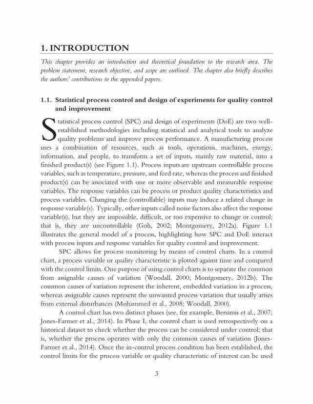
1. INTRODUCTION

This chapter provides an introduction and theoretical foundation to the research area. The

problem statement, research objective, and scope are outlined. The chapter also briefly describes

the authors’ contributions to the appended papers.

1.1. Statistical process control and design of experiments for quality control

and improvement

tatistical process control (SPC) and design of experiments (DoE) are two well-

established methodologies including statistical and analytical tools to analyze

quality problems and improve process performance. A manufacturing process

uses a combination of resources, such as tools, operations, machines, energy,

information, and people, to transform a set of inputs, mainly raw material, into a

finished product(s) (see Figure 1.1). Process inputs are upstream controllable process

variables, such as temperature, pressure, and feed rate, whereas the process and finished

product(s) can be associated with one or more observable and measurable response

variables. The response variables can be process or product quality characteristics and

process variables. Changing the (controllable) inputs may induce a related change in

response variable(s). Typically, other inputs called noise factors also affect the response

variable(s), but they are impossible, difficult, or too expensive to change or control;

that is, they are uncontrollable (Goh, 2002; Montgomery, 2012a). Figure 1.1

illustrates the general model of a process, highlighting how SPC and DoE interact

with process inputs and response variables for quality control and improvement.

SPC allows for process monitoring by means of control charts. In a control

chart, a process variable or quality characteristic is plotted against time and compared

with the control limits. One purpose of using control charts is to separate the common

from assignable causes of variation (Woodall, 2000; Montgomery, 2012b). The

common causes of variation represent the inherent, embedded variation in a process,

whereas assignable causes represent the unwanted process variation that usually arises

from external disturbances (Mohammed et al., 2008; Woodall, 2000).

A control chart has two distinct phases (see, for example, Bersimis et al., 2007;

Jones-Farmer et al., 2014). In Phase I, the control chart is used retrospectively on a

historical dataset to check whether the process can be considered under control; that

is, whether the process operates with only the common causes of variation (Jones-

Farmer et al., 2014). Once the in-control process condition has been established, the

control limits for the process variable or quality characteristic of interest can be used

S

THEORETICAL FOUNDATIONS

4

for Phase II (Jensen et al., 2006; Vining, 2009). In Phase II, the control chart is used

prospectively on new collected values to monitor deviations from the in-control

condition (Wells et al., 2012). Whenever new collected values of the monitored

variable fall outside the control limits, the control chart issues an out-of-control signal

(Jensen et al., 2006). In this case, corrective action on the process may be needed to

uncover and remove the assignable causes and reduce unwanted process variation

(Jensen et al., 2006; Montgomery, 2012b).

Figure 1.1. General model of a process highlighting how SPC and DoE interact with process

inputs and response variables. Adapted from Montgomery (2012a).

A designed experiment allows for systematically changing the controllable

process inputs to study their effects on the response variable(s) (Mason et al., 2003;

Box et al., 2005; Antony et al., 2011; Montgomery, 2012a). Factorial and fractional

factorial designs are two major types of designed experiments in which the

experimental factors (that is, all or a subset of controllable process inputs) are varied

together in such manner that all or a subset of factor-level combinations are tested.

Controllable inputs (Xs)

Process

Inputs

(Raw materials,

information,

machines…)

Uncontrollable inputs (Zs)

Experimentation

How can the process be improved?

What should be monitored?

Monitoring & Control

How does the process perform?

Finished product(s)

SPC DoE

Res

ponse

vari

able

(s)

Ys

INTRODUCTION

5

DoE mainly uses offline quality improvement tools to find the potential causal

relationships between the process inputs and response variable(s). Knowledge of the

crucial process inputs is essential to understand and characterize a process and improve

its performance by steering it toward a target value and/or reducing the process

variability (Montgomery, 2012a). When the key factors are identified and the nature

of relationship between the factors and response variable(s) established, an online

process control chart for process monitoring can be routinely employed to promptly

adjust the process whenever unforeseen events drive the process toward out-of-

control situations.

1.2. Continuous processes

Reid and Sanders (2012) classify production processes into two fundamental

categories of operations: intermittent and repetitive operations. Depending on the

product volume and degree of product customization, the intermittent operations can

be further divided into project and batch processes and repetitive operations can be

divided into line and continuous processes (ibid.). Figure 1.2 presents the product-

process matrix for production processes, and their main characteristics and

management challenges.

Figure 1.2. Product-process matrix for production processes, and their main characteristics and

management challenges. Adapted from Reid and Sanders (2012).

Product Mix

Process

PatternOne of a kind

Custom

products

Standard

products

Capital and

consumer goods

Management

challenges

Very jumbled

flow with process

operations loosely

linked

Fast reaction,

loading plant,

Estimating

capacity, costs, and

delivery times

Jumbled flow

with dominant

line

Worker

motivation,

maintaining

capacity, balance

and flexibilityPacing line

Highly

automated,

uninterrupted

flow with tightly

linked and

controlled

operations

Capital intensive,

technological

change,

vertical

integration,

running

equipment at peak

efficiency

BATCH

PROJECT

LINE

CONTINUOUS

HighLow

High LowCustomization

Volume

Les

s in

term

itte

nt

and m

ore

rep

etitiv

e oper

atio

ns


6

New achievements in information and communication technologies are now

leading to Industry 4.0, the new industrial revolution. Among others, the key

technologies and features of this ongoing revolution include faster sensing technology,

Internet of Things (IoT), cloud services, embedded systems, robotics, real-time

analysis and decision-making, and connectivity (Santos et al., 2017). Industry 4.0 has

the potential to disrupt the entire traditional approaches to manufacturing processes,

posing new significant challenges at, among others, the scientific, technological,

managerial, and organizational levels (Zhou et al., 2015; Santos et al., 2017). Thus,

researchers are working on refining the product-process matrix (Ariss and Zhang,

2002; Schroeder and Ahmad, 2002; Bello-Pintado et al., 2019). Wagner et al. (2017)

argue that the full impact of this revolution on production processes is not clearly

defined as yet. Nevertheless, the ongoing challenges include implementation of digital

manufacturing, big data analysis and processing, the management of cooperation

between different systems, and enhanced knowledge management (Zhou et al., 2015;

Wagner et al., 2017; Preuveneers and Ilie-Zudor, 2017).

Continuous and batch productions represent the main process technologies in

the process industry, which is responsible for about 25% of production worldwide

and involves industries such as pulp and paper, oil and gas, food and beverage, steel,

mining, and material (Lager et al., 2013). A common misconception is that “process

industry” and “continuous processes” are interchangeable terms, although in fact they

differ in meaning (Abdulmalek et al., 2006). This study uses the definitions of the

American Production and Inventory Control Society (APICS dictionary, 2019) as

follows. They define the process industry as

“a production that adds value by mixing, separating, forming and/or performing

chemical reactions by either batch or continuous mode,”

and a continuous process as

“a production system in which the productive equipment is organized and sequenced

according to the steps involved to produce the product. The material flow is continuous

during the production process. The routing of the jobs is fixed and setups are seldom

changed.”

Continuous processes differ from other types of manufacturing processes in three main

features: types of incoming materials, transformation processes, and outgoing materials

(Lager, 2010). The incoming materials in continuous processes are usually raw

INTRODUCTION

7

materials, often stemming directly from natural resources and showing inherent

characteristics that may vary substantially (Fransoo and Rutten, 1994; Abdulmalek et

al., 2006; Kvarnström and Oghazi, 2008). The transformation process includes several

operational units, such as tanks, reactors, mixing units working in a continuous flow,

and the relationship between process inputs and response variables that might not be

immediately clear (Hild et al., 2001; Vanhatalo, 2009; Lee, S. L. et al., 2015). Finally,

the outgoing materials (often also incoming materials) are non-discrete products; for

example, liquids, pulp, slurries, gases, and powders that evaporate, expand, contract,

settle out, absorb moisture, or dry out (Dennis and Meredith, 2000; Frishammar et

al., 2012; Lyons et al., 2013). The nature of the handled materials makes these

processes more sensitive to stoppages and interruptions owing to the loss in

production quality and long lead times for startups (Duchesne et al., 2002;

Abdulmalek et al., 2006; Lager, 2010; Krajewski et al., 2013).

1.3. The need for engineering process control

The dimensions and characteristics of continuous processes often make it unavoidable

to implement engineering process control (EPC) to stabilize the quality characteristics

and process variables (Lyons et al., 2013; Lee, S. L. et al., 2015; Peterson et al., 2019).

One of the most common control structures used in industry is feedback control

(Akram et al., 2012; Saif, 2019). Feedback controllers transform processes from open-

loop into closed-loop systems5, thus increasing the process complexity.

Figure 1.3 provides a schematic representation of an (a) open-loop and (b)

closed-loop system. Ogata (2010, p. 7) defines an open-loop system as one

“where the output (i.e., the response variable) is neither measured nor fed back for

comparison with the desired target,”

and a closed-loop system as one

“that maintains a prescribed relationship between the output (i.e, the response

variable) and the desired target by comparing them and using the difference as a means

of control.”

5 In control theory, a “system” is a combination of components acting together and performing a certain objective (Ogata, 2010). In the DoE and SPC literature, a “process” is a system with a set of inputs and outputs (Montgomery,

2012a; Montgomery, 2012b). In this thesis, the terms “process” and “system” are used interchangeably.


8

In an open-loop system, a fixed operating condition corresponds to the desired target

of the response variable, and the accuracy of the system depends on calibration (Ogata,

2010). Conversely, in a closed-loop system, an automatic controller continuously

compares the controlled (response) variables to a set-point value (i.e, the target value)

and adjusts the measured deviation, regulating a manipulated variable, that is, a

(controllable) process input (ibid.). The required adjustments can be determined

because the causal relationship between the manipulated and controlled variables is

often already established and known (Dorf and Bishop, 2011; Romagnoli and

Palazoglu, 2012).

(a) Open-loop system

(b) Closed-loop system

Figure 1.3. Schematic representation of an (a) open-loop and (b) closed-loop system

Disturbance(s)

Process input(s) Response variable(s)Process or

subprocesses

Disturbance(s)

+

Controller(s)

++Process

or subprocesses

Manipulated variable(s)

Controlled (response)

variable(s)

Measurement(s)

-

Set-point(s)

INTRODUCTION

9

1.4. Monitoring and experimental challenges in processes under feedback

control

For decades, management improvement programs such as Total Quality Management

and Six Sigma have been promoting the use of statistical improvement methods such

as SPC and DoE to improve process and product quality (Bergquist and Albing, 2006;

Bergman and Klefsjö, 2010). Although these methods are well established in the

statistics and quality engineering literature, their application has been found to be

relatively sparse in industry (Tanco et al., 2010; Bergquist, 2015b; Lundkvist et al.,

2018). The use of SPC and DoE in industrial applications in discrete manufacturing

production environments faces barriers such as lack of theoretical knowledge, change

management, practical problems, and lack of resources for internal training (Tanco et

al., 2009; Žmuk, 2015a; 2015b). In addition to these barriers, the implementation of

SPC and DoE methods in continuous processes is further complicated by the need to

promote and adapt the use of such methods to continuous production environments

(Bergquist, 2015b).

The need to run continuous processes under feedback control represents one of

these challenges, as explained in the two following sub-sections.

1.4.1. SPC challenges in processes under feedback control

Feedback controllers make a process insensitive to disturbances and maintain crucial

quality characteristics or process variables around their target values or set-points

(Romagnoli and Palazoglu, 2012). The control action stems from upstream process

inputs (or manipulated variables) transferring the short-term variability from

controlled responses to manipulated variables (MacGregor and Harris, 1990; Hild et

al., 2001; Akram et al., 2012).

The concurrent use of SPC and EPC has been widely recognized in the

literature (see, for example, Box and MacGregor, 1976; Faltin and Tucker, 1991; Box

and Kramer, 1992; Box and Luceño, 1997; Del Castillo, 2002; Del Castillo, 2006;

Woodall and Del Castillo, 2014). Statistical process control charts should be applied

to engineering controlled processes to detect and remove assignable causes of variation

rather than compensating for them. Thus, an overall process improvement can be

achieved by using the complementary capabilities of SPC and EPC to reduce the

long-term and short-term process variability (MacGregor, 1992; Tsung, 2001). In line

with these views, Box and Luceño (1997) suggest SPC for process monitoring and

EPC for process adjustments.


10

When a process involves EPC, monitoring only the controlled variable may be

ineffective owing to the controllers’ potential masking of process disturbances (Wang

and Tsung, 2007; Reynolds Jr and Park, 2010). The SPC literature outlines two

approaches to monitor processes under EPC. The first recommends monitoring the

difference between the controlled variable and set-point value, or the control error

(Montgomery et al., 1994; Keats et al., 1996; Montgomery et al., 2000). The second

approach is to monitor the manipulated variable (Faltin et al., 1993; Montgomery et

al., 1994). Sometimes, monitoring the control error or manipulated variable alone

might be ineffective (Tsung and Tsui, 2003). Therefore, a combined approach of

jointly monitoring the control error and manipulated variable (or the controlled and

manipulated variables) using a bivariate control chart has also been proposed (Tsung,

1999; Tsung et al., 1999; Jiang, 2004; Siddiqui et al., 2015; Du and Zhang, 2016).

The combined approach increases the chances of the control chart issuing an out-of-

control signal when either the controller fails to compensate for the disturbance

completely or the manipulated variable deviates from its normal operating condition.

The combined approach of monitoring the controlled and manipulated

variables in the same multivariate chart(s) can also be extended to multivariate

processes (Tsung et al., 1999; Tsung, 2000; John and Singhal, 2019). In multivariate

processes (with multiple inputs and response variables), several response variables

usually need to be maintained at their target values and several manipulated variables

may have to be adjusted. Consequently, the concurrent use of SPC and EPC becomes

further complicated in multivariate processes (Faltin et al., 1993; Akram et al., 2012).

The complexity of the problem mainly arises from the need to simultaneously

monitor a large number of variables and understand the information dispersion among

process variables due to engineering control (Yoon and MacGregor, 2001; Akram et

al., 2012).

1.4.2. DoE challenges in processes under feedback control

Conventional applications of DoE methods implicitly assume open-loop operations.

In this configuration, the potential effects of changes in process inputs on the response

variables can be observed directly (Hild et al., 2001; Goh, 2002; Montgomery, 2012a).

Under closed-loop operations, variables that might be interesting responses are usually

maintained around desired target values (i.e., set-points). The potential effects of

changes in process inputs are displaced from response variables to other process

streams. Thus, the relationships between process inputs and response variables might

be difficult to understand (Lee, S. L. et al., 2015). Closed-loop operations require a

INTRODUCTION

11

different experimental strategy based on further research to better understand the

experimental results (Hild et al., 2001; Vanhatalo and Bergquist, 2007; Vanhatalo,

2009).

The response surface methodology (RSM) (Box and Wilson, 1951) and

evolutionary operations (EVOP) (Box, 1957) are sequential in nature and hence

appealing strategies in experiments involving continuous processes. However, the

application of RSM and EVOP may have to be adjusted for closed-loop operations

because, for example, the variables to be optimized might not be immediately clear.

1.5. Problem statement, scope, and research objective

As with other types of manufacturing processes, one of the major concerns with

continuous processes is the inherent variation exhibited during production. SPC and

DoE methods can play important roles in quality control and product and process

improvement strategies. The conventional SPC and DoE methods and applications

assume open-loop operations. However, continuous processes often operate under

EPC as in the case of feedback controllers (Lee, S. L. et al., 2015; Peterson et al.,

2019). The presence of feedback controllers challenges the conventional open-loop

assumption of SPC and DoE methods.

Despite the abundant literature on the concurrent use of SPC and EPC, more

research is needed to develop an integrated framework simultaneously studying

controller and process performance to better understand the process disturbances in

out-of-control conditions (Siddiqui et al., 2015). Moreover, how DoE can contribute

to improving industrial processes operating under feedback control is not clearly

defined in the literature (Vanhatalo, 2009). How closed-loop operations affect

experimental procedures, analyses, and results is an open research question. To gain

access to processes allowing for full-scale SPC and DoE methods development is

challenging. SPC method development requires datasets with given characteristics,

such as sampling time, sample size, and occurrence of specific faults, while DoE

method development in full-scale industrial plants is costly and time-consuming.

The main objective of this thesis is to suggest adapted strategies for applying

experimental and monitoring methods (namely, DoE and SPC) to continuous

processes under feedback control. Specifically, this research aims

I. to identify, explore, and describe the potential challenges when applying

SPC and DoE to continuous processes,


12

II. to propose and illustrate new or adapted SPC and DoE methods to address

some of the issues raised by one of the identified challenges, the presence

of feedback controllers, and

III. to suggest potential simulation tools that may be instrumental in SPC and

DoE methods development.

This research is framed into the quality engineering field and builds on a framework

broader than from an exclusive statistical standpoint. The study does not focus on

theoretical development of the applied SPC and DoE analysis methods per se, but

instead develops the suggested solutions and methods considering the adapted

methods and analysis procedures to apply SPC and DoE and improve continuous

processes under feedback control. Besides academics and researchers in the quality

engineering field, this study is directed to quality managers, industrial practitioners,

and engineers interested in quality control and improvement of continuous processes.

By illustrating the potential SPC and DoE challenges in continuous processes, this

study can reinforce or broaden the knowledge of SPC and DoE methods development

needs. Moreover, implementation of the adapted SPC and DoE methods is expected

to contribute to improving the continuous processes under closed-loop control.

Finally, the promotion of simulators to test new or adapted SPC and DoE methods is

expected to provide tools and aids supporting the development of these methods.

1.6. Additional SPC and DoE challenges in continuous processes

Beyond the challenges due to the presence of feedback controllers, the literature

highlights those that may arise when applying SPC and DoE methods to continuous

processes. For a broader perspective of the research field, the following sub-sections

briefly summarize these challenges. While the issues due to these challenges are not

the main focus of this research, they have been encountered during the course of the

studies and overcome using existing solutions in the literature. Thus, the following

sub-sections also provide theoretical foundations for some of the method chosen for

the research.

1.6.1. SPC challenges in continuous processes

This sub-section summarizes the additional challenges that may emerge when

applying SPC methods to continuous processes.

INTRODUCTION

13

Multivariate nature of process data

Researchers in different areas are increasingly focusing on issues related to managing

big data. The accelerated advancement of sensing technology, such as IoT and high-

throughput instruments, and the increasing availability of storage capacity allow for

taking process measurements at multiple locations and with high sampling frequency

(Woodall and Montgomery, 2014; Ferrer, 2014; Peterson et al., 2019). The

uninterrupted flow of continuous processes can produce massive datasets of both

variables and observations exhibiting varying degrees of autocorrelation and cross-

correlation (Saunders and Eccleston, 1992; Hild et al., 2001; Vanhatalo, 2010; He, Q.

P. and Wang, 2018). Vining et al. (2016) claim that any process and product

improvement attempt should consider the complexity of the problem due to the new

data-rich environment. SPC (and DoE) methods require more application-oriented

and methodological studies to handle this modern challenge and meet the growing

industry demand (Vining et al., 2016; Steinberg, 2016; Peterson et al., 2019).

The earliest SPC research and industrial applications focused mainly on

univariate control charts, with the product quality characteristics monitored

individually. In data-rich environments, such as those of continuous processes, the

univariate monitoring of each process variable in separate control charts is often

inefficient and misleading (Kourti and MacGregor, 1995; Bersimis et al., 2007; He,

Q. P. and Wang, 2018). In 1997, MacGregor (cited in Ferrer, 2014) argued that

monitoring a multivariate process using univariate charts is analogous to using one-

factor-at-a-time experimentation: while the correlation of variables makes it difficult

to interpret univariate SPC charts, factor interactions make it difficult to interpret the

results obtained from one-factor-at-a-time experimentation. To overcome this

problem, researchers have adopted multivariate SPC allowing for the simultaneous

monitoring of multiple process variables.

Multivariate monitoring charts based on latent variable techniques, such as

principal component analysis (PCA) and partial least squares (PLS), have been used in

industrial applications successfully (see, for example, Kourti et al., 1996; Qin, 2012;

Ferrer, 2014; Zhang et al., 2014; Silva et al., 2017; Silva et al., 2019). The strength of

latent variable techniques relies on their dimensionality reduction properties. Through

the cross-correlation of process variables, these techniques can reduce an original

dataset to a few linear process variable combinations (or principal components), which

can be considered the main drivers of the process events (MacGregor and Kourti,

1995; Yoon and MacGregor, 2001; Kourti, 2005; De Ketelaere et al., 2015; Rato et

al., 2016). Typically, two control charts are commonly used for process monitoring,


14

a Hotelling T2 control chart on the first retained principal components of the

PCA/PLS model, and the squared prediction error (SPE or Q) chart on the model

residuals.

Autocorrelated data

Control charts based on PCA are well equipped to handle cross-correlation, but not

autocorrelation (Vanhatalo and Kulahci, 2015). Autocorrelation is an inherent

characteristic of continuous processes due to process inertia, continuous flow of

material, EPC, and high sampling frequencies (Atienza et al., 1998; Noorossana et al.,

2003; Prajapati and Singh, 2012). Autocorrelation in data violates the basic assumption

of time-independent observations that the SPC methods rely on, affecting both

univariate and multivariate SPC techniques (Mastrangelo and Forrest, 2002; Woodall

and Montgomery, 2014). According to Prapajati and Singh (2012), in practice,

positive autocorrelation is more often encountered than negative autocorrelation,

leading to deflated control limits in control charts and increased false alarm rates

(Mastrangelo and Montgomery, 1995; Runger, 1996; Woodall, 2000; Bisgaard and

Kulahci, 2005; Vanhatalo et al., 2017).

The literature describes two main solutions to dealing with autocorrelated data

(Prajapati and Singh, 2012). The first is to use a standard control chart and adjust the

control limits to achieve the desired false alarm rate (Russell et al., 2000; Vermaat et

al., 2008; Rato and Reis, 2013b; Vanhatalo and Kulahci, 2015; Vanhatalo et al.,

2017). This approach requires an ad-hoc adjustment to each case, which is

cumbersome and time-consuming. The second solution requires “filtering out the

autocorrelation” using a time series model and then applying a control chart to the

model residuals (Harris and Ross, 1991; Kruger et al., 2004; Pacella and Semeraro,

2007; Rato and Reis, 2013a; Reis and Gins, 2017). Most of the studies using this

approach are based on the assumption of a known time series model (Woodall and

Montgomery, 2014). Furthermore, fitting a time series model for many variables is

challenging because a large number of parameters must be estimated (Rato and Reis,

2013a).

To monitor autocorrelated large-scale processes, Ku et al. (1995) proposed a

modified version of the PCA framework, known as dynamic PCA (DPCA). The

DPCA approach suggests applying the usual PCA method to an augmented data

matrix obtained by appending its time-shifted duplicates to the original dataset. The

Hotelling T2 and Q charts based on dynamic principal components can then be used

to monitor the process.

INTRODUCTION

15

1.6.2. DoE challenges in continuous processes

This sub-section summarizes the additional challenges that may emerge when

applying DoE methods to continuous processes.

Large-scale and costly experimentation

Continuous process plants are usually spread out over a large area and operate around

the clock. Experimentation in full-scale continuous processes may involve the

majority of production staff, making coordination and information flows essential

(Vanhatalo and Bergquist, 2007). Experimental campaigns can continue for a long

time, jeopardizing the production plans and leading to off-grade products. Time and

cost are often significant constraints (Kvist and Thyregod, 2005; Bergquist, 2015b).

Continuous production process characteristics unavoidably affect the

experimentation strategy. Planning, conducting, and analyzing experiments require

proper adjustments in continuous process settings (Vanhatalo and Vännman, 2008).

An experimental campaign should always begin with careful planning because

planning is critical to successfully solving the experimenters’ problem (Coleman and

Montgomery, 1993; Box et al., 2005; Freeman et al., 2013). Vanhatalo and Bergquist

(2007) provide a checklist for planning experiments in continuous process settings,

where limited number of experimental runs, easy-/hard-to-change factors,

randomization restrictions, and design preferences are particularly relevant. Time

restrictions and budget constraints force the analyst to consider experiments with few

factors and runs. Thus, two-level (fractional) factorial designs are important, but

replicates of the experiments may not always be possible (Bergquist, 2015a). Analyzing

unreplicated designs might not always be easy because of the impossibility of

estimating experimental random variations and lack of degrees of freedom when

calculating the model unknowns (i.e., the factors’ effects). When split-plot designs are

needed, for example, to reduce the transition times between runs, the analysis might

become further complicated (see, for example, Vanhatalo and Vännman, 2008;

Vanhatalo et al., 2010)

Time series nature of process data and process dynamics

Random process disturbances and unforeseen control action seldom let the

experimental factors remain constant during experimentation in a continuous process

(Vining et al., 2016). Moreover, high sampling frequencies produce a chronological

sequence of observations. Thus, both experimental factors and response variables

should be viewed as time series (Storm et al., 2013; He, Z. et al., 2015). Production


16

steps such as mixing, melting, reflux flows, or product state changes make the process

dynamic (Lundkvist and Vanhatalo, 2014). In a dynamic process, changed process

inputs affect the response variables gradually, and the process stabilizes to a new steady

state (Nembhard and Valverde-Ventura, 2003; Vanhatalo et al., 2010; Bisgaard and

Khachatryan, 2011; Lundkvist and Vanhatalo, 2014). Vanhatalo et al. (2010) defined

the time taken for a response to reach a new steady state as transition time, arguing

that its characterization is crucial when experimenting in continuous processes.

To correctly estimate the factors’ effects on the response variables, the process

needs to reach a steady-state condition. That is, the transition times affect the run

length of the experiments (Vanhatalo and Vännman, 2008; Vanhatalo et al., 2010).

By knowing the transition times, the experimenter can avoid unnecessary long and

costly or too short run lengths that yield misleading estimates of the effects. However,

to determine the transition times in continuous processes is not easy for several

reasons. Factors’ levels change often affects the response variables in several ways, and

the transition times may vary for different responses in terms of both length and

behavior. For example, Vanhatalo et al. (2010) developed a method to estimate the

transition times in dynamic processes by combining PCA and transfer-function noise

modeling. However, the method is an offline method that has to determine the

transition times a priori during the planning phase of the experiment. Methodological

research on online estimation of transition times in continuous processes can help

solve the aforementioned experimentation challenges in such production

environments.

Autocorrelated and cross-correlated responses

In continuous processes, high sampling frequency induces a positive correlation in the

response variables (Hild et al., 2001; Prajapati and Singh, 2012). Ignoring the

autocorrelation in responses might lead to ineffective or erroneous analysis of the

experimental results. For example, using the run averages of responses might be a poor

alternative and can lead to incorrect estimation of the effects. Time series analysis

could be a useful tool to analyze the experimental results because both the time series

nature and autocorrelation of data can be taken into account. However, few attempts

have been made to combine the benefits of DoE and time series analysis. As shown

in Vanhatalo et al. (2010), the dynamic relationships between process inputs and

response variables can be modeled using transfer-function noise modeling and

intervention analysis to improve the efficiency of the results (Bisgaard and Kulahci,

2011; Vanhatalo et al., 2013; Lundkvist and Vanhatalo, 2014).

INTRODUCTION

17

In continuous processes, the response variables are often related to each other,

making it difficult to identify the process inputs that can be changed independently

from one another and used as experimental factors (Hild et al., 2001). A change in

one experimental factor often affects several response variables because they are simply

reflections of the same underlying event (Kourti and MacGregor, 1995; Kourti and

MacGregor, 1996; Kourti, 2005). Moreover, small changes in a factor might lead to

unacceptable changes in process operating conditions and exorbitant production costs

of a large volume of off-spec products (Kvist and Thyregod, 2005). A multivariate

analysis approach using latent variable techniques, such as PCA and PLS, should be

preferred to a univariate approach. Moreover, in many experimental situations, the

main interest might be to characterize how a function (a surface or profile) changes

over time within an experimental design region (see, for example, Storm et al., 2013;

He, Z. et al., 2015). However, existing methods do not allow for designing and

analyzing these experimental scenarios, and further research is needed to address these

challenges (Vining et al., 2016).

1.7. Introduction and authors’ contributions to appended papers

This section introduces the appended papers and highlights the relationship between

them and their connection with the research aims. The authors’ contributions to the

appended papers are also presented.

Paper A: “Managerial Implications for Improving Continuous Production

Processes.” Capaci, F., Vanhatalo, E., Bergquist, B., and Kulahci, M.

(2017).

Paper A outlines the SPC and DoE implementation challenges described in the

literature for managers, researchers, and practitioners interested in continuous

production process improvement. Besides the research gaps and state-of-the-art

solutions, the paper illustrates the current challenges. This is the first appended paper

since it introduces the research topic and relates to aim I of the research.

This paper was conceived by Francesca Capaci when an opportunity arose to submit a

contribution to the 24th International Annual EurOMA Conference. Francesca Capaci

carried out the four phases and eight stages of the literature review process including searches

for data collection, screening steps, and analysis of data. The co-authors provided support

throughout the emerging analysis steps. Francesca Capaci wrote the paper, with

contributions from all co-authors.


18

Paper B: “Exploring the Use of Design of Experiments in Industrial

Processes Operating Under Closed-Loop Control.” Capaci, F., Bergquist,

B., Kulahci, M., and Vanhatalo, E. (2017).

Paper B conceptually explores issues of the experimental design and analysis in

processes operating under closed-loop control, and illustrates how DoE can help

in improving and optimizing such processes. The Tennessee Eastman (TE) process

simulator is used to illustrate two experimental scenarios. Paper B relates to aim II

of the research.

All the authors jointly developed the idea of exploring the use of DoE in processes

operating under closed-loop control. Francesca Capaci tried to understand the TE process

simulator in order to find viable scenarios for conducting the experiments. Francesca Capaci

planned, simulated, and analyzed the experimental scenarios, while all authors were

involved in the discussions leading up to the results. Francesca Capaci wrote the paper,

with contributions from all co-authors.

Paper C: “The Revised Tennessee Eastman Process Simulator as Testbed

for SPC and DoE Methods.” Capaci, F., Vanhatalo, E., Kulahci, M., and

Bergquist, B. (2019).

Paper C provides guidelines on how to use the revised TE process simulator, run with

a decentralized control strategy, as testbed for SPC and DoE methods in continuous

processes. Flowcharts detail the necessary steps to initiate the Matlab/Simulink®

framework. The paper also explains how to create random variation in the simulator,

with two examples illustrating two potential applications in the SPC and DoE

contexts. Paper C mainly relates to aim III of the research.

The proposal to use the revised TE process as testbed for SPC and DoE methods

development for continuous processes was jointly developed by all the authors. Francesca

Capaci located the revised simulator, performed all work required to understand the details

of the simulator, and developed the idea on how to create random variation in the

simulator. Francesca Capaci also designed the illustrated examples, and was responsible

for all simulations and analyses. All the authors were involved in the discussions leading

up to the results. Francesca Capaci wrote the paper, with contributions from all co-authors.

INTRODUCTION

19

Paper D: “On Monitoring Industrial Processes under Feedback Control.”

Capaci, F., Vanhatalo, E., Palazoglu A., Bergquist, B., and Kulahci, M.,

(2019).

Paper D explores the use of SPC in single-input single-output6 processes controlled

by variations in the proportional-integral-derivative (PID) control scheme, illustrating

whether and how common disturbances (i.e., mean shifts or trends) manifest

themselves on the controlled and manipulated variables. The implications of process

monitoring for these scenarios are discussed. Two simulated examples in

Matlab/Simulink® illustrate two industrial applications. Paper D relates to aim II of

the research.

The proposal to study the signatures of step and ramp disturbances in single-input single-

output processes came from Francesca Capaci while taking a course in “Basics of Control

Theory.” Francesca Capaci had to understand how step and ramp disturbances are

handled by variations in the PID control scheme and how they manifest themselves on

the controlled and manipulated variables. Francesca Capaci also developed the simulators

used in the two examples, performed the simulations, and analyzed the results. Ahmet

Palazoglu provided support to properly set up the control scheme in the simulated

examples. Francesca Capaci wrote the paper, with contributions from all co-authors.

Paper E: “A Two-Step Monitoring Procedure for Knowledge Discovery in

Industrial Processes under Feedback Control.” Capaci, F. (2019).

Paper E explores the use of SPC in multiple-inputs multiple-outputs7 processes under

feedback control, illustrating a two-step monitoring procedure in which the process

variables are classified prior to the analysis and then monitored separately by means of

a multivariate monitoring scheme. The revised TE process simulator under a

decentralized feedback control strategy is used to apply the two-step monitoring

procedure. The results of the two simulated scenarios are compared with the approach

of monitoring the variables simultaneously in the same multivariate chart(s). Paper E

relates to aim II of the research.

6 In this thesis, the term “single-input single-output process” refers to a process with one process input and one

response variable. 7 In this thesis, the term “multiple-inputs multiple-outputs process” refers to a process with several process inputs and several response variables.


20

As the sole author, Francesca Capaci designed the study, carried out the simulations,

analyzed the data, and wrote the paper. Erik Vanhatalo, Bjarne Bergquist, and Murat

Kulahci contributed with valuable feedback.

PART II: EMPIRICAL WORK AND

FINDINGS

“If we knew what it was we were doing,

it would not be called research, would it?”

Albert Einstein

23

2. RESEARCH METHOD This chapter outlines the research design and describes the tools and methods used for data

collection and analysis in the research. The chapter provides the relationships between the studies

and frames them in the research aims. The studies are presented in relation to the research aims

and do not follow their chronological development (i.e., the order of the appended papers).

2.1. Research design

o fulfill the overall research objective, the research was organized around

three topics, one for each research aim. To reach the research aims, five

studies were totally conducted, as illustrated in Figure 2.1.

Figure 2.1. Design of research and studies conducted.

A literature review is summarized in Paper A. This was required to achieve aim I of

the research objective. The review was motivated by the need for a theoretical

foundation for the research and to summarize the results of the searches and readings

in a systematic manner. This is an essential step in the research. A knowledge of the

existing literature would help, for example, to determine what researchers already

know about the research topic, summarize the research evidence from high-quality

studies, identify the research gaps, and generate new ideas to fill those gaps (Tranfield

et al., 2003; Briner and Denyer, 2012).

T Adapting Experimental and Monitoring Methods for

Continuous processes under Feedback Control

Research Objective

SPC and DoE Challenges for

Improving Continuous Processes

Aim I

Literature Review

Study 1

Applying SPC and DoE in Continuous Processes under

Feedback Control

Aim II

Monitoring Processes under

Feedback Control

Study 2, Study 3

Experimentation in Processes under

Feedback Control

Study 4

Simulator for SPC and DoE methods

development

Aim III

Tennesse Eastman Process

Study 5

Paper A Paper BPaper D

Paper E

Paper CStudy 2

Study 3

Univariate case

Multivariate case

EMPIRICAL WORK AND FINDINGS

24

Aim II of the research objective was defined on the basis of the literature

review. The review highlighted several challenges faced when applying SPC and DoE

to continuous processes. Among them, the need for more research to adapt

experimental and monitoring methods for processes under feedback control emerged.

This became the focus of aim II of the research objective. Three studies were

conducted to achieve aim II of the research objective. The first and second studies

(studies 2 and 3 in Figure 2.1) investigated the use of SPC methods in processes under

feedback control; this led to the development of Papers D and E. Study 2 focused on

the application of SPC methods to single-input single-output processes under

feedback control, while study 3 investigated the use of SPC methods in multiple-

inputs multiple-outputs processes under feedback control. The third study (study 4 in

Figure 2.1) delved into the problem of adapting DoE methods for processes under

feedback control, leading to the development of Paper B.

The research strategy relating to aim II of the research objective was based on

simulations. The main reason for choosing this approach was that the project did not

involve industrial collaborators where SPC and DoE methods could be studied. Even

with access to industrial processes, it would have been difficult to obtain processes

allowing for full-scale methods developments. To develop and test SPC methods,

datasets with specific characteristics such as sample size, sampling time, and the

occurrence of known faults are required. Furthermore, DoE applications in full-scale

industrial processes may unavoidably jeopardize the production plants and thus affect

the production goals. This could make it difficult to convince top management to

adopt large and costly experimental campaigns.

Finding a realistic simulator for SPC and DoE methods development was a

priority, and led to the definition of aim III of the research objective. This simulator

needed to offer a good balance between realistic simulation of a continuous process

and flexibility necessary for testing new SPC and DoE methods. To achieve aim III,

the research strategy was to search the literature for available simulators that can mimic

the features of continuous processes. A literature search highlighted that many

published studies in chemometrics, an important field of research connected to

continuous processes, used the TE process as testbed for new methods developed (see,

for example, Lee et al., 2004; Liu et al., 2015; Rato et al., 2016). Downs and Vogel

(1993) originally proposed the TE process as a test problem, providing a list of

potential applications in a wide variety of topics such as plant control, optimization,

education, and non-linear control. In addition, Reis and Kenett (2017) classified the

TE simulator as one of the more complex simulators (medium-/large-scale nonlinear

RESEARCH METHOD

25

dynamic simulator), suggesting its use for advanced applications in high-level statistical

courses. The TE process simulator can emulate many of the challenges frequently

found in continuous processes, such as multivariate nature of the data, process

dynamics, and autocorrelated and cross-correlated responses. The process operating

conditions can be disturbed activating 21 pre-programmed process disturbances of

different types, such as step and random variation. Most importantly, the TE process

simulator has to be run with an implemented control strategy to overcome its open-

loop instability.

The above-mentioned features and the need to run the TE process simulator

under a designed control strategy supported an in-depth study of the simulator, since

it could allow for the development of studies 3, 4, and 5. Numerous control strategies

were available to control for and stabilize the TE process. Among them, the

decentralized control strategy proposed by Ricker (1996; 2005) was the most suitable

for this research, with the following advantages:

the set-points of the controlled variables and process inputs (not involved in

control loops) can be modified as long as they are maintained within the process

operations constraints,

the analyst can specify the characteristics of the simulated data (e.g., length of

experiment, sampling frequency, types of process disturbances), and

the simulator is free to access.

Building on this knowledge, study 5 of the research aimed to make an in-depth study

of the TE process simulator and investigate its suitability for SPC and DoE methods

development in continuous process settings.

The decentralized TE simulator devised by Ricker (2005) was first used to run

the experiments for study 4. The analyses made during this study highlighted an

important limitation of the decentralized TE process simulator, that is, it is almost

deterministic in nature. Measurements of the decentralized TE process variables were

affected only by white Gaussian noise, with standard deviation typical of the

measurement type and thus mimicking a measurement error. Repeated simulations

with the same starting conditions and setup produced the same results, except for

measurements errors. The impossibility to simulate replicated experiments did not

allow for estimating the experimental error and determining whether the observed

differences in data were really statistically different. Moreover, the value of a model

containing only measurement noise is limited when running repeated simulations to

assess the performance of an SPC method.


26

The knowledge gained during study 4 called for revision of the research design.

Additional research was needed to understand whether the limitations of the

decentralized TE process simulator of Ricker (2005) could be overcome to make it

suitable for studies 3 and 5. A literature search led to the release of the decentralized

TE process simulator, known as the revised TE process model, implemented in

Matlab/Simulink® (Bathelt et al., 2015a; 2015b). Among other possibilities, the

revised simulator allowed for scaling the disturbances introduced to the process and

changing the seed of each simulation. Scaling the random variation disturbances

allowed for adding variability to the simulation results without overly distorting them.

Moreover, the seed change of random numbers could force the simulator to generate

different results for repeated simulations with the same starting conditions. Combining

these two features, the deterministic nature and limitations of the simulator could be

overcome, making the revised TE model suitable for testing the SPC and DoE

methods in continuous process settings. The revised TE process was then used for

studies 3 and 5.

2.2. Aim I: SPC and DoE challenges for improving continuous processes

This section highlights the tools and methods used for data collection and analysis in

study 1 related to aim I of the research objective.

2.2.1. Study 1: Literature review

The literature review highlighted the SPC and DoE implementation challenges for

managers, researchers, and practitioners interested in improving continuous

production processes. It was conducted in four phases based on the eight review stages

suggested by Briner and Denyer (2012), as shown in Table 2.1.

The review stages of the “to plan” phase were outlined using Cooper’s

literature review taxonomy (Randolph, 2009) as follows:

Review stage 1:

o Focus: to identify methods for SPC and DoE in continuous processes;

o Goal: to identify and classify central issues related to the identified methods;

o Perspective: to present the review findings assuming a neutral position (i.e.,

reporting the results).

Review stage 2

o Coverage: a representative sample of publications central or pivotal to

achieving the goal.

RESEARCH METHOD

27

Review stage 3

o Organization: to be structured around concepts (i.e., around the central

issues identified by the literature review);

o Audience: researchers and practitioners in the field, as well as top

management.

Table 2.1. Four phases and eight review stages of the literature review process [adapted

from Briner and Denyer (2012)].

Phase Review stage

To plan 1. Identify and clarify the question(s) to be addressed 2. Determine the types of studies that will answer the question(s)

3. Establish the audience

To conduct 4. Search the literature to locate relevant studies 5. Sift through the studies and include or exclude following predefined criteria

To analyze 6. Extract the relevant information from the studies 7. Classify the findings from the studies

To remember 8. Synthesize and disseminate the findings from the studies

The other phases shown in Table 2.1 were conducted twice in five review stages, first

for the SPC field, and then for the DoE field. Review stage 4 of the “to conduct”

phase was realized in April 2017 using the Scopus database, limiting the search to

publications in English during the past 30 years. Sequential searches were conducted

using keywords and combined queries such as “statistical process control” AND

“continuous process” OR “continuous production” for the SPC literature searches,

and “design of experiments” AND “continuous process” OR “continuous

production” for the DoE literature searches. Starting from the search results, the items

were sequentially screened (review stage 5), excluding all items not related to SPC

and DoE applications to continuous processes, and those that did not highlight the

potential challenges in applying SPC and DoE methods to continuous processes.

Conference articles were excluded if a later journal article by the same authors and

with the same title was found. In review stages 6 and 7 (the “to analyze” phase in

Table 2.1), the relevant information from the remaining publications was extracted

and classified to identify the challenges or development needs of SPC and DoE

methods in continuous processes. The classification stage was conducted using a

Microsoft Excel® worksheet. Then, relevant publications not found by searches were

added to the classified publications. The reference lists of the classified publications

were also examined to minimize the risk of missing out other important publications.

This final step provided the pivotal or central publications making up the


28

representative sample which the results of Paper A were based on (review stage 8 of

the “to remember” phase in Table 2.1).

2.3. Aim II: applying SPC and DoE to continuous processes under feedback

control

The following sections explain the tools and methods used for data collection and

analysis used in studies 2, 3, and 4 related to aim II of the research objective.

2.3.1. Study 2: monitoring univariate processes under closed-loop control

Study 2 focused on the use of statistical process control charts in univariate processes

(single-input single-output processes) controlled by variations in the proportional-

integral-derivative (PID) control scheme. The study explored how commonly

occurring disturbances (step and ramp) manifest themselves in univariate processes by

studying their signatures on the controlled and manipulated variables. Moreover,

monitoring the controlled and manipulated variables separately helps in better

understanding the process and controller performance in cases of out-of-control

conditions. Formulas to quantify the steady-state values of controlled and manipulated

variables were also derived. These formulas were based on mathematical derivations

applying the principles and theorems used in control theory, such as the superposition

principle and final value theorem (for further details, see Ogata, 2010; Romagnoli and

Palazoglu, 2012). Two common textbook industrial applications were used to

exemplify the theoretical results and illustrate the implications for process monitoring.

For further information, the reader can refer to Paper D, which also provides all the

details of the simulators employed for the study. These simulators can be used as

testbeds for SPC methods in univariate processes under closed-loop control. Hence,

study 2 relates to aim II and, to a lesser extent, aim III of the research objective.

The two simulated examples were implemented in Matlab/Simulink®. The

first example simulates a heat-exchanger controlled by a proportional (P) controller.

The proportional gain of the controller was tuned using the Ziegler-Nichols

technique (see, Ogata, 2010; Romagnoli and Palazoglu, 2012). The second example

simulates a steel rolling mill with a proportional-integral (PI) controller. In this case,

the proportional and integral gains of the controller were tuned using the internal

model control rule (see, for example, Romagnoli and Palazoglu, 2012). In both

examples, the controlled and manipulated variable values were collected twice during

the continuous process operations. The processes were upset the first time by a step

RESEARCH METHOD

29

disturbance and the second time by a ramp disturbance. Prior to data analysis, the

observations collected during the process startup were discarded to allow for a more

stable estimation of the process parameters in Phase I.

The simulated data were analyzed using Matlab® scripts and the free R statistics

software. In the heat-exchanger example, time series plots of the controlled and

manipulated variables were used to analyze the results. In the steel rolling mill

example, standardized CUSUM charts applied separately to the controlled and

manipulated variables were used to analyze the results. Step and ramp disturbances do

not typically result in large shifts of the process variables in the presence of the PI

controller. Thus, CUSUM charts were considered a good alternative to detect

potential out-of-control signals. Of course, other control charts with comparable

detection abilities, such as the exponentially weighted moving average (EWMA)

chart, could have been used. However, a different choice of control chart would not

have changed the final conclusions of the study.

2.3.2. Study 3: monitoring multivariate processes under closed-loop control

Study 3 explored the use of control charts in multivariate processes (multiple-inputs

multiple-outputs processes) under feedback control. The study focused on a two-step

monitoring procedure for multivariate processes, first [1] classifying the process

variables into groups as controlled, manipulated, and measured variables, and then [2]

monitoring each group of variables separately using a multivariate monitoring scheme.

The two-step monitoring procedure was adopted to better understand the process

and the controllers’ performance in multivariate processes in case of out-of-control

signals. From this perspective, study 3 can be considered an extension of study 2. The

results of study 3 are reported in Paper E.

The revised TE process under a decentralized feedback control strategy (Bathelt

et al., 2015b) was used as a testbed for the two step-monitoring procedure, as advised

in Paper C. Two simulated scenarios were illustrated and discussed. The results were

also compared with the commonly used approach of monitoring the process variables

together in the same multivariate control charts.

In the first step of the two-step monitoring procedure, the TE process variables

were classified as controlled, manipulated, and measured variables using a qualitative

approach. The information for classification was mainly extracted from the work by

Ricker (1996), who explained the design phases of the TE process decentralized

control strategy. The knowledge gained during the development of study 5


30

(conducted prior to study 3) also supported the TE process variables classification. The

support tool for the classification was a Microsoft Excel® sheet.

In the second step of the two-step monitoring procedure, the controlled,

manipulated, and measured variables were monitored separately using a multivariate

monitoring scheme. The revised TE simulator (Matlab/Simulink®) was run twice to

collect two datasets, one for each illustrated example. Throughout the simulations, a

step-change disturbance was introduced into the process to collect the faulty datasets

(for details, see Paper E). Using a Matlab® script, the phase I samples of the controlled,

manipulated, and measured variables were produced by removing the observations

during the transition time on process startup. Steady-state values of the variables

provide a more stable estimation of the covariance matrices and hence of the in-

control models. The TE process variables exhibit moderate to high autocorrelation

coefficients. Thus, a multivariate monitoring scheme based on DPCA was applied to

each group of variables.

Hotelling T2 and Q charts built on the basis of DPCA models in phase I were

used to monitor separately the controlled, manipulated, and measured variables in

phase II. For comparative purposes, the phase I and phase II samples consisting of

controlled, manipulated, and measured variables were used for monitoring all the

variables simultaneously. The data analysis was conducted using the free R statistics

software.

2.3.3. Study 4: experimentation in processes under closed-loop control

Study 4 relates to aim II of the research objective. The study explored the

experimental design and analysis issues to explain to researchers and practitioners how

DoE can add value to the processes under closed-loop. Two experimental scenarios

were designed to exemplify the study’s conceptual ideas.

Design Expert® (version 9) was used to generate the experimental designs and

analyze the experimental results, and the experiments were simulated using the

decentralized TE process simulator implemented in Matlab/Simulink® as a testbed

(Ricker, 1996; 2005).

The first scenario illustrated an experiment in which the control strategy is

disturbed by level change of process inputs not involved in control loops. Process

inputs not involved in control loops can be considered as disturbances in closed-loop

systems and thus viewed as experimental factors. The TE process has three inputs not

involved in any control loop that can be used as experimental factors. However, even

a small factor-levels change can be exaggerated to unacceptable effects that lead to a

RESEARCH METHOD

31

process shutdown. A 22 randomized factorial design with three replicates was

generated to estimate the location effects (main effects and interactions) of two inputs

not involved in control loops on the controlled and associated manipulated variables.

The second scenario exemplified a screening design using the set-points of controlled

variables as experimental factors. In this case, a factor-level change will move the process

from one operating region to another. A two-step sequential experiment estimated the

set-points’ impact on the process operating cost. A 2𝐼𝐼𝐼9−5 fully randomized fractional

factorial design with four additional central points was followed by a full fold-over in

a new block to explain some aliased effects. The final design was of resolution IV.

In both experimental scenarios, the analysis of experimental results for analysis

of variance (ANOVA) was based on the averages of each experimental run. Matlab

scripts and Microsoft Excel® sheets were used for extracting averages and saving results.

Vanhatalo et al. (2013) recommend removing apparent dynamic behavior at the

beginning of each run to avoid the biased estimation of effects. Nevertheless, in the

first experimental scenario, the initial observations were included in calculating the

run averages since an effective control action should be able to remove the impact of

the factors’ level change on the controlled variables. In the second experimental

scenario, a transition time of 24 hours was removed prior to the calculation of the run

averages. In this case, the response variables were not involved in control loops and

the factors’ level changes can take time before reaching its full effect.

2.4. Aim III: a simulator for SPC and DoE methods development

The following section highlights the tools and methods used for data collection and

analyses in study 5 related to aim III of the research objective.

2.4.1. Study 5: the Tennessee Eastman (TE) process simulator

Study 5 examines how to use the revised TE process simulator (Bathelt et al., 2015b)

run under a decentralized control strategy as testbed for SPC and DoE methods.

During the study, the guidelines on the required steps to initialize the revised TE

process simulator and simulate data for SPC and DoE applications were formulated

and illustrated by means of flow charts. The flow charts were created using Bizagi

modeler® based on the business process modeling notation (BPMN) (see, for

example, Chinosi and Trombetta, 2012; the BPMN archive, 2011). Furthermore,

two simulated examples were conducted to demonstrate the strategy for creating

random variability in the simulator and potential SPC and DoE applications. For


32

further details, see Paper C, which mainly relates to aim III and, to a lesser extent,

aim I of the research objective. The revised TE simulator can in fact simulate most of

the challenges described in Paper A.

The first example demonstrates how closed-loop operations affect the shift-

detection ability of control charts. The revised TE process simulator was used to

simulate Phase I and Phase II data. The free R statistics software was used to analyze

the collected data, that is, to build a Hotelling T2 control chart on the controlled and

manipulated variables. The second example employs a response surface methodology

approach. The levels change of five controlled variables’ set-points were analyzed

through sequential experimentation to improve the process operating cost of the TE

process. While the revised TE simulator, Microsoft Excel®, and Matlab Scripts were

used to simulate the experiments, Design Expert® (version 10) was used to generate

the experimental designs and analyze the experimental results.

The sequential experimentation started with a 2𝑉5−1

fully randomized fractional

factorial design, with four additional center points to screen the set-points of five

controllers. Then, a central composite design was created by augmenting the

resolution V fractional factorial design with ten additional axial points run in a new

block, allowing for estimation of a second-order model. The numerical optimization

tool in Design Expert® (version 10) was used to search for design space and find the

settings for the set-points that would produce the lowest predicted cost. Three

additional runs were simulated for confirmation. During the sequential stages, the

experimental results were analyzed using ANOVA tests based on the averages of each

run after removing 24 hours of transition time, as suggested by Vanhatalo et al. (2013).

2.5. Summary of methods used in appended papers

Table 2.2 provides an overview of the methods chosen for the studies connected to

the five appended papers and the papers’ relationship with the aims of the research

objective.

33

Table

2.2

. O

ver

vie

w o

f th

e m

ethods

choic

es m

ade

in t

he

studie

s re

port

ed in t

he

appen

ded

pap

ers.

Paper

A

Paper

B

Paper

C

Paper

D

Paper

E

Aim

of th

e

rese

arc

h o

bje

ctive

I II

I,

III

II

, II

I II

Type o

f paper

Liter

ature

rev

iew

R

esea

rch

Res

earc

h

Res

earc

h

Res

earc

h

Targ

et

audie

nce

Qual

ity m

anag

ers,

rese

arch

ers,

and

pra

ctitio

ner

s

Res

earc

her

s an

d

pra

ctitio

ner

s R

esea

rcher

s an

d

pra

ctitio

ner

s R

esea

rcher

s an

d

pra

ctitio

ner

s R

esea

rcher

s an

d

pra

ctitio

ner

s

Data

collection

(tools)

Sco

pus

TE

pro

cess

R

evised

TE

pro

cess

Hea

t ex

chan

ger

Ste

el r

ollin

g m

ill

Rev

ised

TE

pro

cess

Data

collection

(meth

ods)

Sea

rches

using

key

word

s an

d q

uer

ies

D

oE

Sim

ula

tions

D

oE

SP

C

S

imula

tions

M

athem

atic

al

der

ivat

ions

S

PC

Sim

ula

tions

A

rtic

le b

y R

icker

(1996)

S

PC

S

imula

tions

Data

analy

sis

(tools/m

eth

ods)

Seq

uen

tial

scr

eenin

g

and c

lass

ific

atio

n o

f publica

tions

iden

tified

duri

ng the

sear

ches

AN

OV

A

A

NO

VA

T

ime

seri

es p

lots

Hote

llin

g T

2 c

har

t

T

ime

seri

es p

lots

CU

SU

M c

har

t

Q

ual

itat

ive

clas

sifica

tion o

f th

e T

E p

roce

ss v

aria

ble

s

DP

CA

Hote

llin

g T

2 a

nd Q

char

ts

Illu

stra

tion o

f t

he r

esu

lts

Conce

ptu

al

clas

sifica

tion o

f SP

C a

nd D

oE

ch

alle

nges

in

continuous

pro

cess

es

Tw

o s

imula

ted

exam

ple

s

B

PM

N flo

w c

har

ts

T

wo s

imula

ted

exam

ple

s

M

athem

atic

al

form

ula

s;

T

wo s

imula

ted

exam

ple

s;

Tw

o s

imula

ted e

xam

ple

s

Softw

are

M

icro

soft

Exce

l®

D

esig

n E

xper

t 9

M

atla

b/Sim

ulink

M

atla

b

M

icro

soft

Exce

l

B

izag

i M

odel

er

D

esig

n E

xper

t 10

M

atla

b/Sim

ulink

M

atla

b

M

icro

soft

Exce

l

R

M

atla

b/Sim

ulink

M

atla

b

M

icro

soft

Exce

l

R

M

atla

b/Sim

ulink

M

atla

b

M

icro

soft

Exce

l

R

34

3. RESULTS AND DISCUSSION This chapter summarizes the results of the studies presented in the five appended papers and

discusses the main contributions, implications, and limitations of the research. The results are

conceptually organized in relation to the research aims (i.e., around related topics) and therefore

do not necessarily follow the order of the appended papers.

3.1. Aim I: SPC and DoE challenges for improving continuous processes

The literature review highlighted several challenges that may arise when applying SPC

and DoE methods to continuous processes. As explained in section 2.2.1, these

challenges were classified in categories. Figure 3.1 illustrates the categories of SPC and

DoE challenges identified during the classification procedure of the literature review

and the following sections summarize the main findings. Further details are provided

in Paper A.

Figure 3.1. SPC and DoE challenges for improving continuous processes identified during the

literature review.

SPC in continuous processes

In continuous processes, operating conditions frequently change owing to grade

changes, restarts, or process adjustments and process inertia leads to transition phases.

Data storage should be designed to preserve the history of transition phases and the

interrelation of variables during transitions (Kourti, 2003). The monitoring phase in

SPC should begin after the transition is complete (Duchesne et al., 2002). The existing

SPC literature recognizes the need for multivariate control charts to monitor multiple

quality characteristics or process variables simultaneously as in continuous processes

(Ferrer, 2014). Several options need to be considered here. The Hotelling T2 control

chart is commonly used for monitoring up to ten variables exhibiting moderate cross-

SPC

Process Transitions &

Data Acquisition

Multivariate Nature of

Process DataAutocorrelation

Engineering Process Control

DoE

Large and Costly

Experiments

Process Transitions & Time Series

Analysis

Multivariate

Nature of

Process Data

Engineering Process Control


35

correlation. When the number of variables is larger, other multivariate SPC methods

are available (Shi and MacGregor, 2000; Qin, 2012; Ge et al., 2013). Ge et al. (2013)

classify the available process monitoring methods into five categories:

1. Gaussian process monitoring methods (e.g., latent structure variable techniques

such as PCA/PLS),

2. Non-Gaussian process monitoring methods (e.g., independent component

analysis),

3. Non-linear process monitoring methods (e.g., neural networks),

4. Time-varying and multimode process monitoring (e.g., adaptive/recursive

methods), and

5. Dynamic process monitoring (e.g., dynamic multivariate SPC methods).

In these cases, the choice of multivariate SPC methods should depend on the process

characteristics (for example, Gaussian/non-Gaussian, stationary/non-stationary, and

linear/non-linear) and level of data autocorrelation.

Among the above-mentioned methods, process monitoring based on

PCA/PLS is an important quality improvement tool for data-rich environments

already used successfully in the process industry (see, for example, Ferrer, 2014; Zhang

et al., 2014; Silva et al., 2019). Using PCA/PLS reduces the high-dimensional

monitoring problems to a few orthogonal principal components, which can be

monitored either individually or simultaneously. Control charts based on PCA/PLS

are well equipped to deal with cross-correlated, independent, and stationary data, but

autocorrelation and non-stationarity affect their performance (De Ketelaere et al.,

2015). To cope with autocorrelation or non-stationarity, certain extensions of the

PCA/PLS monitoring methods are also available in the literature. For autocorrelated

data and stationary processes, Ku et al. (1995) suggest expanding the original data

matrix by adding time-lagged versions of the original variables and transforming the

autocorrelation into cross-correlation. The performance of PCA on this extended data

matrix is referred to as DPCA. For independent data and non-stationary processes,

recursive and adaptive methods are available (see, for example, Li et al., 2000; De

Ketelaere et al., 2015). Figure 3.2 illustrates the PCA/PLS methods available for

process and data challenges.

The literature review presented in Paper A also highlight some technical issues and

development needs to improve the applicability of these methods. While knowledge

of the above-mentioned solutions support the adoption of these methods, researchers

RESULTS AND DISCUSSION

36

and practitioners should be aware of the following issues that need to be overcome.

Among others, the relevant problems include the following:

How to simultaneously handle autocorrelation and non-stationarity? (De

Ketelaere et al., 2015),

How to select the number of latent variables to retain and lags to add in DPCA?

(Himes et al., 1994; Ku et al., 1995; De Ketelaere et al., 2015; Vanhatalo et al.,

2017),

Fault detection and isolation (Kourti and MacGregor, 1996; Dunia et al., 1996;

Yoon and MacGregor, 2001), and

Handling of outliers in the data (Stanimirova et al., 2007; Serneels and

Verdonck, 2008).

Figure 3.2. Process and data challenges, and available PCA/PLS methods.

Another important SPC challenge that emerged during the literature review is the

need to run continuous processes under EPC, such as for feedback controllers.

Feedback controllers mitigate unwanted deviations of controlled variables through

continuous adjustment of related manipulated variables (see, for example, Ogata,

2010; Romagnoli and Palazoglu, 2012). The propagation of a disturbance through

the process might not always be visible in the controlled response variable, but may

be displaced to the related manipulated variable (Akram et al., 2012; Siddiqui et al.,

2015). The SPC examples simulated in the revised TE process presented in Papers C

DynamicPCA/PLS

?

StaticPCA/PLS

Adaptive/ RecursivePCA/PLS

Stationary process Non-stationary process

Autocorrelated data

Independent data


37

and E and in the heat exchanger and steel rolling mill simulators presented in Paper

D illustrate this behavior.

To detect out-of-control process conditions, the traditional approach of

applying a control chart to controlled variable(s) is often replaced with a control chart

applied to manipulated variable(s) or a multivariate control chart monitoring the

controlled and manipulated variables together (Montgomery et al., 1994; Tsung,

1999). However, the study results presented in Papers D and E show that these

approaches might hinder deeper process insight and understanding of out-of-control

process conditions. Further details on the implications of monitoring either the

manipulated or controlled and manipulated variables in the same multivariate chart(s)

will be discussed in section 3.2.1.

DoE in continuous processes

The literature review highlighted both the challenges and existing solutions when

conducting experiments in continuous processes. While the challenges affect all the

experimental phases (i.e., planning, conducting, and analysis of experiments), the

literature review shows that related solutions are not always available, and if available,

need to be developed further.

Following the recommendations of Coleman and Montgomery (1993), who

highlight the critical importance of the planning phase, Vanhatalo and Bergquist

(2007) provide a systematic approach to planning an industrial experiment in

continuous processes. The authors present twelve steps for the planning phase, which

need to have both technical and organizational choices due to the complexity of large-

scale experimentation. The choice of design preferences and factor levels and need

for restricted randomization are as critical as the requirement for assigning

responsibilities in coordinating the experiment or collecting relevant background

information. Vanhatalo and Bergquist (2007) also recommend identifying the

presence of controlled variables in the planning phase, suggesting that closed-loop

operations affect the entire experimental strategy. Paper A classifies the

experimentation in processes under closed-loop control as one of the important issues

in continuous process experiments, as conventional DoE methods implicitly assume

open-loop operations (Montgomery, 2012a). For further details, see section 3.2.2 and

Paper B summarizing the results of study 4, which focuses on the use of DoE in

processes under closed-loop.

Planning and conducting experiments in continuous processes also imply

unavoidable cost and time constraints (Vanhatalo, 2010). The often lengthy


38

experimental campaigns jeopardize the production plan since the production plant

could be unavailable during an experimental campaign or produce off-spec products

(Bergquist, 2015b). Nevertheless, the need for improvement often calls for

experimentation. The use of simulators to test methodological ideas prior to

implementation might be helpful to improve continuous processes. The results of

study 5 are presented assuming this perspective (see section 3.3 and Paper C).

Moreover, two best practices need to be promoted: [1] support and allocate resources

to the planning phase, and [2] create awareness of experimental strategies suitable for

large-scale experimentation (Vanhatalo and Bergquist, 2007).

Paper A presents the potential issues that emerge when analyzing experiments

conducted in continuous processes. The experimental factors and responses from

continuous processes can typically be represented as time series (Vining et al., 2016).

In these cases, the existing methods are inadequate to design the experiments and

properly analyze them. The literature review highlights that analytical methods such

as functional data analysis, shape analysis, and time series analysis receive increasing

attention from both academia and industry owing to their considerable importance

(He, Z. et al., 2015; Vining et al., 2016). Moreover, continuous processes are dynamic

systems with inertia, meaning that the impact of factors’ level changes on responses

can take time to reach its full impact (Nembhard and Valverde-Ventura, 2003;

Vanhatalo et al., 2010; Lundkvist and Vanhatalo, 2014). These transition times need

to be considered in the planning and analysis phases because they might affect, for

example, the length of experimental runs or estimation of effects.

Other challenges in the analysis phase relate to the use of multivariate methods

to analyze the experimental results. In continuous processes, the presence of several

cross-correlated responses suggests that a univariate approach to analyses might be

ineffective (Ferrer, 2014; Vanhatalo and Vännman, 2008). Latent variable techniques

can be used to summarize the information in experimental response variables. The

latent variables can then be used as new responses to test the statistical significance of

the experimental factors effects. El-Hagrasy et al. (2006), Vanhatalo and Vännman

(2008), Baldinger (2012), Souihi et al. (2013), and Storm et al. (2013), among others,

provide examples of multivariate analysis combined with DoE.

3.2. Aim II: applying SPC and DoE to continuous processes under feedback

control

The following sub-sections summarize the results of studies 2, 3, and 4 in terms of

aim II of the research objective, that is, to propose new or adapted SPC and DoE


39

methods to overcome some of the issues due to the presence of feedback controllers.

For more details, see Papers B, D, and E.

3.2.1. Monitoring processes under closed-loop control

In a closed-loop system, quality characteristics or process variables that might be

interesting to monitor are usually controlled for and kept around desired target values

(i.e., set-points). Monitoring only the controlled variables in a control chart will often

be unsuccessful because of the controllers’ potential masking effect of external

disturbances. The literature recommends two basic approaches to monitor a process

under feedback control: [1] monitoring the control error, that is, the difference

between the controlled variable and set-point value (see, for example, Faltin et al.,

1993; Montgomery et al., 1994) and [2] monitoring the manipulated variable

(MacGregor, 1991; Faltin et al., 1993). To maximize the chances of detecting out-

of-control process conditions, a combined approach of monitoring the controlled

variable (or control error) and the manipulated variable in the same bivariate control

chart has also been proposed (Tsung, 1999). The same approaches can also be

extended to monitor multivariate processes. For further details, see section 1.4.1.

The results of studies 2 and 3, summarized in Paper D and E, indicate that the

above-mentioned approaches are valuable for detecting out-of-control process

conditions, but might hinder deeper process insight. Instead, as will be explained later,

monitoring both controlled and manipulated variables in separate charts might

increase the knowledge of the process and controller performance when out-of-

control situations occur.

Study 2 deals with single-input single-output processes and illustrates whether

and how step and ramp disturbances manifesting themselves on the controlled and

manipulated variables depend on the control mode used [proportional (P),

proportional-integral (PI), or proportional-integral-derivative (PID)]. The study

shows that the ongoing disturbance (step or ramp) and control mode used (P, PI, or

PID) determine the pattern (mean shift or trend) of the disturbance signatures on the

controlled and manipulated variables. The upper part of Table 3.1 shows on which

variables (manipulated and/or controlled) the signature of a step or ramp disturbance

manifest itself depending on the control mode used (P, PI, or PID) and the pattern

(mean shift or trend) of the signatures. Assuming a set-point equal to zero, the lower

part of Table 3.1 provides the formulas for calculating the steady-state values of the

controlled and manipulated variables, knowing the step magnitude (�̅�) or slope of the

ramp (�̂�) and the process (kp) and controller parameters (kc, and τI). Generally,


40

knowing the magnitude or slope of a disturbance is not a realistic situation. However,

using the true steady-state values of the controlled and manipulated variables

calculated from the process data, the inverse formulas can be useful to calculate, for

example, the magnitude or slope of a disturbance.

Table 3.1. (Upper part) Signatures of step and ramp disturbances on the controlled and

manipulated variables depending on the control mode (P, PI, or PID). (Lower part) Steady-state values of the controlled and manipulated variables as functions of the step

magnitude (�̅�) or slope of the ramp (�̂�) and the process (kp) and controller parameters (kc,

and τI).

Control Mode

Step Disturbance Ramp Disturbance

Controlled variable

Manipulated variable

Controlled variable


P Mean shift Mean shift Trend Trend

PI, PID No signature Mean shift Mean shift Trend

Control Mode Steady-state values Steady-state values

P �̅�

1 + 𝑘𝑐𝑘𝑝 −

𝑘𝑐 �̅�

1 + 𝑘𝑐𝑘𝑝 + ∞ −∞

PI, PID 0 (= set-point) −�̅�

𝑘𝑝

𝜏𝐼

𝑘𝑐𝑘𝑝�̂� −∞

As an illustration of the results in Table 3.1, Figure 3.3 displays the time series plot

and CUSUM chart of the controlled (a-b) and manipulated (c-d) variables of a steel

rolling mill under a PI controller. Paper D provides full details on this example. A

disturbance occurs around the 500th observation. An analysis of the CUSUM charts

on the controlled and manipulated variables indicates that the controller is active

(manipulated variable out-of-control), but unable to fully remove the disturbance

effect on the controlled variable (i.e., the controlled variable is out-of-control and the

process is not performing satisfactorily). Moreover, the (slight) mean shift of the

controlled variable and trend pattern of the manipulated variable shown in the time

series plots might be a hint of an ongoing ramp disturbance (see Table 3.1).


41

(a) Controlled variable – time series plot (c) Manipulated variable – time series plot

(b) Controlled variable – CUSUM chart (c) Manipulated variable – CUSUM chart

Figure 3.3. Time series plot and CUSUM chart of the controlled (a-b) and manipulated (c-d) variables of a steel rolling mill under a PI controller. The vertical dotted lines divide Phase I and

Phase II data. A disturbance occurs around the 500th observation.

The general implication of the results in Table 3.1 is that the P, PI, and PID control

modes have limitations on the type of disturbances they can handle. Moreover, the

results in Table 3.1 imply that monitoring the steady-state error, manipulated variable,

and controlled and manipulated variables together in the same control chart (in this

case, a bivariate chart) should enable detection of an out-of-control situation when a

step or ramp disturbance occurs. However, none of the approaches illustrated in the

literature can provide information on the process and controller performance

simultaneously. This process insight can be gained when controlled and manipulated

variables are monitored using separate charts.

Study 3 summarized in Paper E can be considered, to some extent, as an

extension of study 2 to multivariate processes. In multivariate processes (with multiple

inputs and several response variables), feedback controllers need to keep several

controlled variables at their set-point values and several manipulated variables are


42

likely to be adjusted. Typically, control loops involve crucial quality characteristics or

process variables that need to be kept around target values, for example, to ensure

product quality specifications or stable process conditions within equipment

constraints. Other response variables related to process performance indicators, such

as energy consumption or product waste, might be more difficult or too expensive to

control for and are not usually involved in any control loop. These additional response

variables (called measured variables here) are generally affected by the process

operating conditions and hence assess the overall process performance.

The author of this thesis argues that in a multivariate process (with multiple

inputs and several response variables), the response variables can be classified into at

least three categories: controlled, manipulated, and measured variables. Akin to study

2 in Paper D, grouping these response variables (the controlled, manipulated, and

measured variables) and monitoring them in separate multivariate charts, rather than

jointly, might improve the process knowledge as well as controllers’ performance

when out-of-control conditions occur.

In general, a combined study of the control charts applied to controlled and

measured variables provides information on process performance. As mentioned

earlier, controlled variables usually relate to the quality characteristics of a product or

the process producing it. Out-of-control signals in control chart(s) on the controlled

variables might indicate that the process performance and hence product quality are

most likely critically affected. However, out-of-control signals in control chart(s) on

the measured variables might indicate that the process performance is compromised,

even though the product quality might most likely be unaffected.

As in the univariate case, the combined study of the control charts on the

controlled and manipulated variables would show the controllers’ performance. An

analyst can check whether the control action is active or inactive (manipulated

variables out-of-control or in control) and its ability or inability to partially or fully

compensate for the disturbance (controlled variables out-of-control or in-control).

More details on the potential scenarios that an analyst might encounter are provided

in Paper E.

The approach often used to monitor all the variables together in the same

multivariate chart(s) is valuable to detect out-of-control process conditions. However,

this approach does not directly provide the process insight gained by monitoring the

variables in groups as illustrated above. Moreover, in case of an out-of-control signal,

the suggested approach might support the search of disturbance. When an out-of-

control situation occurs, the controllers’ action propagates the effect of a disturbance


43

to several process variables, making the contribution plots difficult to interpret (Yoon

and MacGregor, 2001; Qin, 2003). Classifying the process variables in “blocks” (or

groups) can reduce the “smearing effect” of the contribution plots on non-faulty

variables (see, for example, MacGregor and Kourti, 1995; Qin et al., 2001), as the

analyst will have to analyze the contribution plots for groups of variables rather than

all the variables together.

3.2.2. Experimentation in processes under closed-loop control

Designed experiments imply deliberately changing a set of experimental factors in

order to study how important process variables or quality characteristics react. In an

open-loop process, the experimenter can discover the potential impact of factor-level

changes in the process response(s). In this case, the purpose of DoE is essentially to

reveal the potential causal relationships between the experimental factors and process

response(s). Typically, in a closed-loop system, the causal relationships between the

process inputs (or manipulated variables) and controlled response variables are already

established and known, and are normally not the focus of the designed experiment.

Generally, the existing relationships between process inputs and response variables are

discovered using system identification methods dealing with building dynamic models

(usually a set of differential equations) based on observed data from the system (Ljung,

2007). In system identification, experimental data are used to find the optimal input

signals and model the system to ensure stability. However, as Paper B shows, designed

experiments can improve industrial processes under feedback control supporting in

factor screening, factor characterization, or process improvement and optimization.

Closed-loop operations affect all the experimental phases; that is, planning,

conducting, and analyzing. Continuous interference by controllers makes the

experimentation challenging, as the control action might neutralize the factors’ level

change impact on the response variables. Moreover, if the experimental factors are

not properly chosen in the planning phase, all attempts to change the experimental

factors’ levels may prove futile because the feedback controllers might counteract their

deliberate changes. That is, the input variables involved in control loops (or

manipulated variables) cannot be considered as potential experimental factors since

they are not free to vary independently.

Study 4, summarized in Paper B, illustrates two potential scenarios for

experiments in processes under closed-loops (see Table 3.2). In the first scenario, the

experimenter can consider any set of inputs not involved in control loops as potential

experimental factors. In a closed-loop system, input variables not involved in control


44

loops behave as disturbances and thus can be viewed as experimental factors. In this

case, both the controlled and manipulated variables are interesting response variables.

An analysis of the controlled variables will provide information on the presence of

controllers if in doubt, and their performance. An analysis of the manipulated variables

will reveal whether experimental factors affect the important process phenomena

controlled in the loops. To better clarify this concept, consider Figure 3.4.

Table 3.2. Potential experimental scenarios to conduct designed experiments in processes under closed-loop control.

Experimental scenario Experimental factors Response variable(s)

1 Process inputs not involved

in control loops Controlled and manipulated

variables

2 Controlled variables’ set-points Process performance indicators

(e.g., operating cost, energy consumption and, product waste)

Figure 3.4 shows the behavior of the manipulated and controlled variables of the TE

process control loop 16 when two inputs not involved in control loops are used as

experimental factors. The charts show (a) the controlled variable XMEAS(9), and (b)

the manipulated variable XMV(10). The coded levels of the experimental factors

XMV(9) and XMV(12) are superimposed in both charts. A simple visual inspection

of the charts reveals that the controlled variable is insensitive to the factors’ level

changes, suggesting the presence of a full-operational controller. Moreover, an analysis

of the manipulated variable’s chart suggests that the factors’ level changes affect the

process phenomena controlled in the loop.

In the second scenario, the experimenter can change the controlled variables’

set-points to study their effect on process performance indicators, such as cost, product

waste, and energy consumption (experimental scenario 2 in Table 3.2). In this case,

the change in the set-points’ levels is equivalent to moving the process from an

operating condition to another. The process performance indicators can be improved

by finding “better” set-points-level settings.


45

(a) Controlled variable - XMEAS(9)

(b) Manipulated variable – XMV (10)

Figure 3.4. Impact of inputs not involved in control loops on the (a) controlled and (b) manipulated variables of the TE process loop 16.

The suggested experimental scenarios for experiments in closed-loop systems can

generate knowledge and contribute to process improvement, making it possible to

study

the presence of controllers if in doubt,

the performance of controllers, that is, whether they are functioning well,


46

the impact of experimental factors on process phenomena, and

how the controlled variables’ set-points affect the process performance

indicators.

3.3. Aim III: the TE simulator for SPC and DoE methods development

New SPC or DoE methods development is generally difficult to test in real

continuous process plants. SPC method development does not usually affect the

production plant, but the need for datasets with specific characteristics, such as sample

size, sampling time, and occurrence of a known fault, could limit or slow down the

testing process. Conversely, DoE method development may jeopardize the

production plant and affect the production goals. Production engineers and managers

may find it inconvenient to invest time and money on lengthy experimental

campaigns. Simulation tools can thus be instrumental in SPC and DoE method

development.

Reis and Kennet (2017) map a wide variety of resources and simulators that

can be used to teach statistical methods, such as Rice Virtual Lab in Statistics, StatLab,

and PenSim8. The authors classify the simulators based on three characteristics: [1]

linear/non-linear elements in the simulation model, [2] time-independent/time-

dependent behavior, and [3] size of simulator. In this classification, the TE process is

considered one of the most complex and realistic simulators since it mimics a large-

scale, non-linear, and dynamic process. Moreover, the TE process simulator has to be

run with an implemented control strategy to overcome its open-loop instability

(Downs and Vogel, 1993).

The decentralized control strategy of the TE process (Ricker, 1996) is attractive

from an SPC and DoE methods development perspective because it can mimic the

challenges frequently found in continuous processes (see sections 1.4 and 1.6). Ricker

(1996) devised the decentralized control strategy of the TE process and implemented

a simulator in Matlab/Simulink® (Ricker, 2005). Recently, Bathelt et al. (2015a;

2015b) implemented an upgraded version of Ricker’s simulator, the revised TE

process simulator, in Matlab/Simulink®. Table 3.3 compares the main characteristics

8 Rice Virtual Lab in Statistics offer an online statistics open textbook and additional resources to assist students in

understanding statistical concepts (http://onlinestatbook.com/rvls.html). StatLab is a free web-based application for supporting teaching the basics of DoE (https://www.win.tue.nl/statlab/). PenSim is a web-based simulator designed

for students’ education that simulates a fed-batch penicillin production (http://simulator.iit.edu/web/pensim/).


47

of the decentralized TE process simulator strategy of Ricker (2005) and the revised

TE process simulator strategy of Bathelt et al. (2015b).

From Table 3.3., the revised TE process simulator offers more flexibility than

the simulator originally developed by Ricker (2005). These new possibilities

discovered while developing study 5 and summarized in Paper C widen the usability

of the revised TE process simulator, making it more suitable for testing the SPC and

DoE methods. The illustrated examples in Papers B and C simulated using Ricker’s

simulator and the revised TE process, respectively, highlight this concept as well.

Among the most relevant features, the possibility of changing the seed of each

simulation and scaling random disturbances allows for introducing random variation

in the simulation results, which is essential for testing SPC and DoE methods.

Moreover, from an SPC perspective, the possibility of scaling process disturbances

allows for testing the sensitivity of SPC methods. However, the revised TE process

lacks a graphical user interface (GUI). New users might find it challenging to

understand the details of the revised TE process and to run it. Thus, the results of

Paper C are illustrated in order to support the interaction between a new user and the

simulator. Flowcharts using the Business Process Modelling Notation (BPMN)

provide a step-by-step description of how to use the simulator, and simulate data for

SPC and DoE applications.

Table 3.3. Comparison of the main characteristics of the decentralized TE process of Ricker (2005) and the revised TE process of Bathelt et al. (2015b).

Characteristic

Decentralized

TE process

(Ricker, 2005)

Revised

TE process

(Bathelt et al., 2015b)

Set simulation seed No Yes

Set simulation length and sampling frequency Yes Yes

Introduce process disturbances Yes Yes

Scale process disturbances No Yes

Monitor output of the disturbances No Yes

The random generator uses different state variables for process disturbances and measurements noise

No Yes

Possibility to pause and resume the simulation using final process conditions

Yes Yes

Repeatability of simulation results No Yes

Graphical user interface (GUI) No No


48

3.4. Research limitations

The conclusions and recommendations drawn from the studies related to aim II of

this thesis are based on data collected through simulations. Papers B and E used the

TE process as testbed for the adapted SPC and DoE methods. The data for Paper D

were collected using simulators of two common industrial applications, that is, a heat

exchanger and a steel rolling mill.

The method chosen for data collection via simulations has both advantages and

disadvantages. From an SPC perspective, the use of simulators implies the immediate

availability of datasets with the desired characteristics (sampling time, number of

observations, type of process disturbance, and so on). From a DoE perspective, the

use of TE simulators implies the availability of a realistic process to test new

experimental methods. Finding industrial partners willing to share their production

data for SPC methods development is potentially easier than finding those willing to

share their production plants for conducting lengthy and costly experimental

campaigns. Testing new DoE methods would be feasible if the company is proposing

to run experiments with the sole aim of improving the production process. Thus,

DoE methods development might be limited due to the lack of available industrial

partners willing to support the research ideas.

The main drawback of working with simulators is that the SPC analyst or

experimenter cannot consider the challenges that would emerge when working in

real environments. Among them, in SPC applications, the collection of data from

multiple and interconnected sources and massive datasets is common for continuous

processes. Thus, what data and how to handle them properly will become crucial in

addressing questions of interest. In DoE applications, planning, conducting, and

analyzing experiments would need a transversal organization in real processes.

Moreover, replicates of experiments will most likely not be possible. Unforeseen

events, unexpected complications during experimental runs, or lack of coordination

and information might also affect the experimental results, thus further challenging

the testing process of the methods.

The suggested SPC and DoE methods in the research tested on simulated data

can be applied to real continuous processes. However, one can fairly expect these

methods to be implemented considering the needs of the production environments.


49

3.5. Main contributions

This research explored the challenges usually encountered when applying SPC and

DoE methods to continuous processes, with focus on the adapted strategies to

overcome some of the issues due to one of the identified challenges, the presence of

feedback controllers. This research also proposed simulation tools that can be used in

SPC and DoE methods development.

Creating awareness of potential challenges when applying SPC and DoE

methods to continuous processes is an essential step supporting the development of

these methods. This research reinforces the knowledge of SPC and DoE methods

development needs and suggests the current remedies found in the literature to

overcome these challenges. A first contribution of this research is to show the

researchers the SPC and DoE challenges that need to be overcome and to encourage

practitioners and quality engineers to adopt these methods and benefit from them.

Other contributions of this research come from the SPC and DoE methods

suggested for application to continuous processes under feedback control. Feedback

controllers challenge the implicit SPC and DoE assumption of open-loop operations.

From an SPC perspective, feedback controllers imply that the quality characteristics

or process variables potentially interesting to be monitored are controlled for and kept

around desired target values. Generally, the impact of external process disturbances

are displaced from the controlled to manipulated variables. Monitoring only the

controlled variables might be futile. The approaches suggested in the literature for

monitoring processes under feedback control mainly focus on detecting out-of-

control process conditions (see section 1.4.1). Certainly, the detection of out-of-

control conditions is a key aspect of an effective process monitoring procedure.

However, this research assumes a broader perspective. The suggested SPC methods

for monitoring under feedback control emphasize how the process knowledge and

understanding can improve when an out-of-control situation occurs. Another

contribution of this research is to suggest a monitoring procedure for processes under

feedback control that jointly uses the information from the control charts and

controllers to improve the process knowledge and the controllers’ performance when

out-of-control situations occur. This enhanced knowledge can be achieved

monitoring the controlled, manipulated, and measured variables (if they exist)

simultaneously, but in separate charts. The following questions can be answered

simultaneously using the suggested approach: Is the compensatory control action

active? Is the controller able to fully remove the impact of a disturbance on the


50

controlled variables? Is the disturbance affecting the process phenomena controlled

for in a closed-loop? Is the controller in place able to handle the ongoing disturbance?

A direct implication of this enhanced knowledge is to provide support to search

and identify the disturbance. In single-input single-output processes controlled for by

varying the PID controllers, step and ramp disturbances leave distinctive signatures on

the controlled and manipulated variables. Thus, monitoring the controlled and

manipulated variables simultaneously and in separate charts provides information on

process and controller performance and indicates the potential disturbances affecting

the process.

As in single-input single-output processes, an SPC analyst can monitor the

controlled, manipulated, and measured variables of a multivariate process under

feedback control in separate control charts. This will show the SPC analyst whether

the control action is active, its ability or inability to deal with the ongoing disturbance,

and whether an out-of-control condition is affecting the process phenomena

controlled for in a loop. Although it is more challenging to understand the disturbance

signature in a multivariate process than in a univariate process, the suggested approach

can support the search and identification of an ongoing disturbance. As for an out-of-

control condition, identification of the disturbance might be easier because the analyst

will have to analyze the contribution plots for groups of variables rather than for all

the variables at once. The suggested approach can thus mitigate the so-called smearing

effect (Yoon and MacGregor, 2001; Qin, 2003), that is, the spreading of disturbance

on the non-faulty variables.

From a DoE perspective, the main contribution of this research pertains to the

benefits of using experimental methods in process under closed-loop, a different

framework compared to the one usually found in textbooks or traditional DoE

applications. The research provides an adapted framework to widen the applicability

of DoE methods to industrial processes under feedback control. The traditional open-

loop experimental framework is adjusted to the closed-loop framework and the

implications are discussed. In this adjustment, the two suggested experimental

scenarios classify the potential experimental factors as either a set of inputs not

involved in the control loops, or the set-points of the controlled variables (see Table

3.2). In the former case, the manipulated and controlled variables become the

responses. In the latter case, the typical responses include process performance

indicators such as cost, product waste, or energy consumption.

The adapted SPC and DoE methods for application to processes under

feedback control constitute a contribution to the quality engineering field, and also


51

provide useful suggestions to industrial practitioners and engineers interested in quality

control and improvement of continuous processes.

The last main contribution of this study is to provide detailed guidelines on how

to use the TE process, a flexible simulation tool, to further develop SPC and DoE

methods and overcome the challenges presented by continuous processes. The TE

process has been used for methodological work especially in the SPC field for a long

time. However, the previous simulator’s deterministic nature has most likely

hampered the researchers in choosing development work and making fair comparison

of methods. This study promotes the use of the TE process simulator widely used in

the control theory field for SPC and DoE methods development. Following the ideas

and recommendations presented in this study, the deterministic nature of the TE

process can be overcome and the simulator can become a valuable tool for SPC and

DoE methods development. Moreover, the TE simulator can play a key role in

teaching SPC and DoE concepts in statistical and quality engineering courses in

academia. Thus, this last contribution of the study is undoubtedly the most valuable

one for researchers interested in SPC and DoE methods development and academics

interested in teaching SPC and DoE concepts.


“Somewhere, something incredible is

waiting to be known.”

Carl Sagan

55

4. FUTURE RESEARCH DIRECTIONS This chapter presents ideas and new questions for future research that emerged during the Ph.D.

research education and that I would like to pursue in the future.

PC and DoE methods can be valuable to support product and process quality

improvement, but companies will not gain full advantage without adjusting

these statistical methods to the new production environments. In later years,

the research community can reasonably be assumed to focus increasingly on the

challenges offered by data-rich manufacturing environments. Moreover, SPC and

DoE methods and their implementation can be affected by the new industrial

revolution, Industry 4.0. SPC and DoE methods will most likely be increasingly used

along with machine learning and artificial intelligent to gain full advantage from

simultaneous application. Nevertheless, both methodological and application-

oriented SPC and DoE research will still be needed to solve problems arising from

the process industry.

Considering the background and development of this research, future studies

can explore both methodological and applied directions. The availability of the revised

TE process as flexible simulator and testbed for method development allows for

undertaking more theory-oriented studies of the challenges described in the thesis,

such as the multivariate nature of process data, process dynamics, and closed-loop

operations. Moreover, thus far, most of the multivariate SPC methods suggested in

the literature have been tested using pre-simulated training and testing datasets from

the TE process. The characteristics of the revised TE simulator make it possible to

revisit the suggested multivariate SPC methods and perform improved and more

realistic comparative studies between existing methods or between existing and new

methods.

The research related to the challenge of applying SPC and DoE methods in

continuous processes under EPC is a very recent topic, and could offer a rich research

path to explore in the future. A natural continuation of the research undertaken in

Paper D could be, for example, to run extensive simulations and study the sensitivity

of commonly used control charts in processes governed by variations of PID

controllers in relation to the controllers’ parameters. This type of studies could benefit

both univariate and multivariate processes. Further development of the research in

Paper E could investigate how different types of disturbances manifest themselves on

the controlled, manipulated, and measured variables of a multivariate process. The

results could be valuable to support the search and identification of process

S

FUTURE RESEARCH

56

disturbances. More research related to fault identification and isolation tasks in

processes under EPC is also needed. In the future, an integrated framework that helps

in understanding controller and process performances simultaneously can provide

more powerful tools for improved disturbance diagnosis.

More research to develop the adapted or new DoE methods for processes

operating under EPC can provide useful contributions to the DoE field. For example,

analysis methods to model the dynamic relations between several experimental factors

and the time series response(s) would be interesting to explore. From this perspective,

the first experimental scenario described in Paper B is of special interest (see Table

3.2). A more in-depth study of the process control theory could lead to more

advanced analysis methods of experimental results, where a closed-loop system could

be transformed into its relative open-loop system. If the effect of control action could

be filtered back from the controlled variable, the experimental factors change effects

on the “back-filtered” variables could be analyzed and compared with those on the

manipulated and controlled variables.

Further interesting research relates to how to adapt and apply sequential

experimentation methods such as response surface methodology (RSM) and

evolutionary operations (EVOP), to processes under feedback control. Adjustments

of the experimentation strategies may be needed in this framework because, for

example, the response variable(s) to be optimized may not be immediately clear.

A more in-depth study of the process control and system identification theory

is therefore crucial and highly necessary to develop the above-mentioned ideas and

nurture further research in developing SPC and DoE methods.

57

APPENDIX – Research Process

Figure A.1 illustrates a Gantt chart showing the main research activities of this doctoral

study that led to the five appended papers. The authors’ contributions to the appended

papers are also highlighted (for more information refer back to section 1.5). In the

chart, upside down triangles mark the beginning of a research study, circles indicate

conference presentations for the appended papers, and triangles and diamonds indicate

the papers that have been submitted or accepted for publication, respectively.

58

Fig

ure

A.1

. G

antt

char

t sh

ow

ing t

he

mai

n r

esea

rch a

ctiv

itie

s fr

om

the

beg

innin

g o

f m

y r

esea

rch e

duca

tion u

ntil

the

doct

ora

l def

ense

sem

inar

. T

he

auth

ors

’

contr

ibutions

to t

he

appen

ded

pap

ers

are

also

hig

hlighte

d (

FC

= F

rance

sca

Cap

aci; E

V =

Eri

k V

anhat

alo; B

B =

Bja

rne

Ber

gquis

t; M

K =

Mura

t K

ula

hci

; A

P =

A

hm

et P

alaz

oglu

) Act

ivit

iy2016

Q4

2E

nhan

cing s

tatist

ical

, an

alytica

l, a

nd p

rogra

mm

ing

skills a

tten

din

g c

ours

es

4Paper

A

5Liter

ature

res

earc

h a

nd c

lass

ific

atio

n o

f th

e re

sults

6P

aper

wri

ting a

nd s

ubm

issi

on

Q4

Q3

Q1

Q3

2017

Q2

2014

Q4

Q1

Q4

Q1

Q3

Q4

Rea

din

g a

nd d

iscu

ssin

g liter

arure

1

Pre

senta

tion a

t E

UR

om

a 2017

7

11

8Paper

B

Stu

dyin

g t

he

TE

pro

cess

sim

ula

tor

9

Rea

din

g a

nd d

iscu

ssin

g liter

ature

Sim

ula

ting&

anal

yzi

ng e

xper

imen

ts in c

lose

d-l

oop

envir

onm

ents

Pap

er w

riting a

nd s

ubm

issi

on

17

10

Pre

senta

tion a

t E

NB

IS-2

016

16

12

Paper

C

Stu

dyin

g t

he

revis

ed T

E s

imula

tor

14

15

Sta

rtin

g p

aper

wri

ting

Fin

ishin

g p

aper

wri

ting a

nd s

ubm

issi

on

Wri

ting lic

entiate

thesi

s 18

Con

trib

uti

ons

FC

;EV

;BB

;MK

FC

FC

FC

;EV

;BB

;MK

FC

FC

;EV

;BB

;MK

FC

FC

FC

;BB

;MK

;EV

FC

FC

;EV

;MK

;BB

FC

FC

;EV

;MK

;BB

FC

2018

Q2

Q1

2015

Q2

3

20

Paper

D

Q1

21

2019

Q4

Q2

22

19

FC

Skills e

nhan

cem

ent

atte

ndin

g c

ours

es, lite

ratu

re

read

ing

FC

Dev

elopin

g t

heo

retica

l re

sults

and s

imula

tion

model

s

FC

Sim

ula

ting&

anal

yzi

ng d

ata

23

FC

;EV

;AP

;BB

;MK

Pap

er w

riting a

nd s

ubm

issi

on

Q3

Q2

24

Paper

E

26

FC

Sim

ula

ting d

ata

and a

nal

yzi

ng r

esults

FC

Pap

er w

ritn

g a

nd s

ubm

issi

on

Q3

282

7

FC

Wri

ting D

octo

ral th

esi

s

13

FC

Pre

senta

tion a

t E

NB

IS-2

015 (

earl

y v

ersi

on)

25

FC

Pre

senta

tion a

t IC

ISE

-2016 (

earl

y v

ersi

on)

59

REFERENCES

Abdulmalek, F.A., Rajgopal, J. and Needy, K.L., (2006). A Classification Scheme for the Process Industry to Guide the Implementation of Lean. Engineering Management

Journal, 18(2): 15-25.

Akram, M.A., Saif, A.A. and Rahim, M.A., (2012). Quality Monitoring and Process Adjustment by Integrating SPC and APC: A Review. International Journal of Industrial

and Systems Engineering, 11(4): 375-405.

Antony, J., Coleman, S., Montgomery, D.C., Anderson, M.J. and Silvestrini, R.T., (2011). Design of Experiments for Non-Manufacturing Processes: Benefits,

Challenges and some Examples. Proceedings of the Institution of Mechanical Engineers, Part B: Journal of Engineering Manufacture, 225(11): 2078-2087.

Ariss, S.S. and Zhang, Q., (2002). The Impact of Flexible Process Capability on the Product – Process Matrix: An Empirical Examination. International Journal of Production Economics 76 (2): 135-145.

Atienza, O.O., Tang, L.C. and Ang, B.W., (1998). A SPC Procedure for Detecting Level Shifts of Autocorrelated Processes. Journal of Quality Technology, 30(4): 340-351.

Baldinger, A., Clerdent, L., Rantanen, J., Yang, M. and Grohganz, H., (2012). Quality by Design Approach in the Optimization of the Spray-Drying Process.

Pharmaceutical development and technology, 17(4): 389-397.

Bathelt, A., Ricker, N.L. and Jelali, M., (2015a). Revision of the Tennessee Eastman Process Model. IFAC-PapersOnLine, 48(8): 309-314.

Bathelt, A., Ricker, N.L. and Jelali, M., (2015b). Tennessee Eastman Challenge Archive. Available: http://depts.washington.edu/control/LARRY/TE/# download.html.

Bello-Pintado, A., García Marco, T. and Zouaghi, F., (2019). Product/Process Definition, Technology Adoption and Workforce Qualification: Impact on Performance. International Journal of Production Research, 57(1): 200-215.

Bergman, B. and Klefsjö, B., (2010). Quality from Customer Needs to Customer Satisfaction. Lund, Studentlitteratur AB.

REFERENCES

60

Bergquist, B., (2015a). Analysis of an Unreplicated 22 Factorial Experiment Performed in a Continuous Process. Total Quality Management & Business Excellence, 26(9-10):

1083-1094.

Bergquist, B., (2015b). Some Ideas on Why Factorial Designs are Seldom Used for Full-Scale Experiments in Continuous Production Processes. Total Quality

Management & Business Excellence, 26(11-12): 1242-1254.

Bergquist, B. and Albing, M., (2006). Statistical Methods–Does Anyone Really Use Them? Total Quality Management, 17(8): 961-972.

Bersimis, S., Psarakis, S. and Panaretos, J., (2007). Multivariate Statistical Process Control Charts: An Overview. Quality and Reliability Engineering International, 23(5): 517-543.

Bisgaard, S. and Khachatryan, D., (2011). Quasi‐experiments on Process Dynamics. Journal of the Royal Statistical Society: Series C (Applied Statistics), 60(4): 497-517.

Bisgaard, S. and Kulahci, M., (2011). Time Series Analysis and Forecasting by Example. Hoboken, New Jersey, John Wiley & Sons.

Bisgaard, S. and Kulahci, M., (2005). Quality Quandaries: The Effect of Autocorrelation on Statistical Process Control Procedures. Quality Engineering, 17(3):

481-489.

Box, G.E.P., (1957). Evolutionary Operation: A Method for Increasing Industrial Productivity. Journal of the Royal Statistical Society. Series C (Applied Statistics), 6(2): 81-

101.

Box, G.E.P., Hunter, J.S. and Hunter, W.G., (2005). Statistics for Experimenters: Design, Innovation, and Discovery. New York, Wiley.

Box, G.E.P. and Kramer, T., (1992). Statistical Process Monitoring and Feedback Adjustment: A Discussion. Technometrics, 34(3): 251-267.

Box, G.E.P. and Luceño, A., (1997). Statistical Control by Monitoring and Feedback

Adjustment. New York, Wiley.

Box, G.E.P. and MacGregor, J.F., (1976). Parameter Estimation with Closed-Loop Operating Data. Technometrics, 18(4): 371-380.

REFERENCES

61

Briner, R.B. and Denyer, D., (2012). Systematic Review and Evidence Synthesis as a Practice and Scholarship Tool. Handbook of Evidence-Based Management: Companies,

Classrooms and Research: 112-129.

Chinosi, M. and Trombetta, A., (2012). BPMN: An Introduction to the Standard. Computer Standards & Interfaces, 34(1): 124-134.

Coleman, D.E. and Montgomery, D.C., (1993). A Systematic Approach to Planning for a Designed Industrial Experiment. Technometrics, 35(1): 1-12.

De Ketelaere, B., Hubert, M. and Schimitt, E., (2015). Overview of PCA-Based Statistical Process-Monitoring Methods for Time Dependent, High Dimensional

Data. Journal of Quality Technology, 47(4): 318-335.

Del Castillo, E., (2006). Statistical Process Adjustment: A Brief Retrospective, Current Status, and some Opportunities for further Work. Statistica Neerlandica, 60(3):

309-326.

Del Castillo, E., (2002). Statistical Process Adjustment for Quality Control. Wiley-Interscience.

Dennis, D. and Meredith, J., (2000). An Empirical Analysis of Process Industry Transformation Systems. Management Science, 46(8): 1058-1099.

Dorf, R.C. and Bishop, R.H., (2011). Modern Control Systems. New Jersey, Pearson.

Downs, J.J. and Vogel, E.F., (1993). A Plant Wide Industrial Process Control Problem. Computers & Chemical Engineering, 17(3): 245-255.

Du, S. and Zhang, R., (2016). Modelling and Joint Monitoring of Input and Output of Systems with Arbitrary Order Autoregressive Disturbance. International Journal of Production Research, 54(6): 1822-1838.

Duchesne, C., Kourti, T. and MacGregor, J.F., (2002). Multivariate SPC for Startups and Grade Transitions. AIChE Journal, 48(12): 2890-2901.

Dunia, R., Qin, S.J., Edgar, T.F. and McAvoy, T.J., (1996). Identification of Faulty

Sensors using Principal Component Analysis. AIChE Journal, 42(10): 2797-2812.

El‐Hagrasy, A.S., D'Amico, F. and Drennen, J.K., (2006). A Process Analytical

Technology Approach to Near‐infrared Process Control of Pharmaceutical Powder

REFERENCES

62

Blending. Part I: D‐optimal Design for Characterization of Powder Mixing and Preliminary Spectral Data Evaluation. Journal of pharmaceutical sciences, 95(2): 392-406.

Faltin, F.W., Hahn, G.J., Tucker, W.T. and Vander Wiel, S.A., (1993). Algorithmic Statistical Process Control: Some Practical Observations. International Statistical

Review/Revue Internationale de Statistique, 60(1): 67-80.

Faltin, F.W. and Tucker, W.T., (1991). On-Line Quality Control for the Factory of the 1990s and Beyond. Statistical Process Control in Manufacturing: 14-28.

Ferrer, A., (2014). Latent Structures-Based Multivariate Statistical Process Control: A Paradigm Shift. Quality Engineering, 26(1): 72-91.

Fransoo, J.C. and Rutten, W.G., (1994). A Typology of Production Control Situations in Process Industries. International Journal of Operations & Production

Management, 14(12): 47-57.

Freeman, L.J., Ryan, A.G., Kensler, J.L.K., Dickinson, R.M. and Vining, G., (2013). A Tutorial on the Planning of Experiments. Quality Engineering, 25(4): 315-332.

Frishammar, J., Lichtenthaler, U. and Kurkkio, M., 2012. The Front End in Non-Assembled Product Development: A Multiple Case Study of Mineral-and Metal Firms. Journal of Engineering and Technology Management, 29(4): 468-488.

Ge, Z., Song, Z. and Gao, F., (2013). Review of Recent Research on Data-Based Process Monitoring. Industrial & Engineering Chemistry Research, 52(10): 3543-3562.

Goh, T.N., (2002). The Role of Statistical Design of Experiments in Six Sigma:

Perspectives of a Practitioner. Quality Engineering, 14(4): 659-671.

Harris, T.J. and Ross, W.H., (1991). Statistical Process Control Procedures for Correlated Observations. The Canadian Journal of Chemical Engineering, 69(1): 48-57.

He, Q.P. and Wang, J., (2018). Statistical Process Monitoring as a Big Data Analytics Tool for Smart Manufacturing. Journal of Process Control, 67: 35-43.

He, Z., Zhou, P., Zhang, M. and Goh, T.N., (2015). A Review of Analysis of Dynamic Response in Design of Experiments. Quality and Reliability Engineering

International, 31(4): 535-542.

REFERENCES

63

Hild, C., Sanders, D. and Cooper, T., (2001). Six Sigma* on Continuous Processes: How and Why it Differs. Quality Engineering, 13(1): 1-9.

Himes, D.M., Storer, R.H. and Georgakis, C., (1994). Determination of the Number of Principal Components for Disturbance Detection and Isolation. Proceedings of the American Control Conference, 2: 1279-1283.

Jensen, W.A., Jones-Farmer, L., Champ, C.W. and Woodall, W.H., (2006). Effects of Parameter Estimation on Control Chart Properties: A Literature Review. Journal of Quality Technology, 38(4): 349-364.

Jiang, W., (2004). A Joint Monitoring Scheme for Automatically Controlled Processes. IIE Transactions, 36(12): 1201-1210.

John, B. and Singhal, S., (2019). An Application of Integrated EPC–SPC Methodology for Simultaneously Monitoring Multiple Output Characteristics.

International Journal of Quality & Reliability Management, 36(5): 669-685.

Jones-Farmer, L., Woodall, W.H., Steiner, S.H. and Champ, C.W., (2014). An Overview of Phase I Analysis for Process Improvement and Monitoring. Journal of

Quality Technology, 46(3): 265-280.

Keats, J.B., Montgomery, D.C., Runger, G.C. and Messina, W., (1996). Feedback Control and Statistical Process Monitoring. International Journal of Reliability, Quality

and Safety Engineering, 03(03): 231-241.

Kourti, T., (2005). Application of Latent Variable Methods to Process Control and Multivariate Statistical Process Control in Industry. International Journal of Adaptive

Control and Signal Processing, 19(4): 213-246.

Kourti, T., (2003). Abnormal Situation Detection, Three-Way Data and Projection Methods; Robust Data Archiving and Modeling for Industrial Applications. Annual

Reviews in Control, 27(2): 131-139.

Kourti, T., Lee, J.H. and Macgregor, J.F., (1996). Experiences with Industrial Applications of Projection Methods for Multivariate Statistical Process Control.

Computers and Chemical Engineering, 20: S74-S750.

Kourti, T. and MacGregor, J.F., (1996). Multivariate SPC Methods for Process and Product Monitoring. Journal of Quality Technology, 28(4): 409-428.

REFERENCES

64

Kourti, T. and MacGregor, J.F., (1995). Process Analysis, Monitoring and Diagnosis, using Multivariate Projection Methods. Chemometrics and Intelligent Laboratory Systems,

28: 3-21.

Krajewski, L.J., Ritzman, L.P. and Malhotra, M.K., (2013). Operations Management. Processes and Supply Chains (9th Edition). Global Edition. Pearson Prentice Hall, Upper

Saddle River, New Jersey.

Kruger, U., Zhou, Y. and Irwin, G.W., (2004). Improved Principal Component Monitoring of Large-Scale Processes. Journal of Process Control, 14(8): 879-888.

Ku, W., Storer, R.H. and Georgakis, C., (1995). Disturbance Detection and Isolation by Dynamic Principal Component Analysis. Chemometrics and Intelligent Laboratory Systems, 30(1): 179-196.

Kvarnström, B. and Oghazi, P., (2008). Methods for Traceability in Continuous Processes–Experience from an Iron Ore Refinement Process. Minerals Engineering, 21(10), 720-730.

Kvist, T. and Thyregod, P., (2005a). Using Evolutionary Operation to Improve Yield in Biotechnological Processes. Quality and Reliability Engineering International, 21(5): 457-463.

Lager, T., (2010). Series On Technology Management-Vol. 17. Managing Process Innovation: From Idea Generation to Implementation. London, Imperial College Press.

Lager, T., Blanco, S. and Frishammar, J., (2013). Managing R&D and Innovation in the Process Industries. R&D Management, 43(3): 189-195.

Lee, G., Han, C. and Yoon, E.S., (2004). Multiple-Fault Diagnosis of the Tennessee Eastman Process Based on System Decomposition and Dynamic PLS. Industrial & Engineering Chemistry Research, 43(25): 8037-8048.

Lee, S.L., O’Connor, T.F., Yang, X., Cruz, C.N., Chatterjee, S., Madurawe, R.D., Moore, C.M.V., Yu, L.X. and Woodcock, J., (2015). Modernizing Pharmaceutical Manufacturing: From Batch to Continuous Production. Journal of Pharmaceutical

Innovation, 10(3): 191-199.

Li, W., Yue, H.H., Valle-Cervantes, S. and Qin, S.J., (2000). Recursive PCA for Adaptive Process Monitoring. Journal of Process Control, 10(5): 471-486.

REFERENCES

65

Liu, K., Fei, Z., Yue, B., Liang, J. and Lin, H., (2015). Adaptive Sparse Principal Component Analysis for Enhanced Process Monitoring and Fault Isolation.

Chemometrics and Intelligent Laboratory Systems, 146: 426-436.

Ljung, L., 2007. System Identification. Wiley Encyclopedia of Electrical and Electronics Engineering.

Lundkvist, P., Bergquist, B. and Vanhatalo, E., (2018). Statistical Methods–still Ignored? The Testimony of Swedish Alumni. Total Quality Management & Business Excellence, 1-18.

Lundkvist, P. and Vanhatalo, E., (2014). Identifying Process Dynamics through a Two-Level Factorial Experiment. Quality Engineering, 26(2): 154-167.

Lyons, A.C., Vidamour, K., Jain, R. and Sutherland, M., (2013). Developing an Understanding of Lean Thinking in Process Industries. Production Planning & Control,

24(6): 475-494.

MacGregor, J.F., (1997). Using On-Line Process Data to Improve Quality: Challenges for Statisticians. International Statistical Review / Revue Internationale de

Statistique, 65(3): 309-323.

MacGregor, J.F., (1992). Statistical Process Monitoring and Feedback Adjustment: Discussion. Technometrics, 34(3): 273-275.

MacGregor, J.F. and Harris, T.J., (1990). Exponentially Moving Average Control Schemes: Properties and Enhancements – Discussion. Technometrics, 32(1): 23-26.

MacGregor, J.F. and Kourti, T., (1995). Statistical Process Control of Multivariate Processes. Control Engineering Practice, 3(3): 403-414.

Mason, R.L., Gunst, R.F. and Hess, J.L., (2003). Statistical Design and Analysis of Experiments: With Applications to Engineering and Science. John Wiley & Sons.

Mastrangelo, C.M. and Forrest, D.R., (2002). Multivariate Autocorrelated Processes: Data and Shift Generation. Journal of Quality Technology, 34(2): 216-220.

Mastrangelo, C.M. and Montgomery, D.C., (1995). SPC with Correlated Observations for the Chemical and Process Industries. Quality and Reliability Engineering International, 11(2): 79-89.

REFERENCES

66

Mohammed, M.A., Worthington, P. and Woodall, W.H., (2008). Plotting Basic Control Charts: Tutorial Notes for Healthcare Practitioners. BMJ Quality & Safety,

17(2): 137-145.

Montgomery, D.C., (2012a). Design and Analysis of Experiments.Wiley, New York.

Montgomery, D.C., (2012b). Statistical Process Control: A Modern Introduction. Wiley, Hoboken, New Jersey.

Montgomery, D.C., Keats, J.B., Yatskievitch, M. and Messina, W.S., (2000). Integrating Statistical Process Monitoring with Feedforward Control. Quality and Reliability Engineering International, 16(6): 515-525.

Montgomery, D.C., Keats, J.B., Runger, G.C. and Messina, W.S., (1994). Integrating Statistical Process Control and Engineering Process Control. Journal of Quality Technology, 26(2): 79-87.

Nembhard, H.B. and Valverde-Ventura, R., (2003). Integrating Experimental Design and Statistical Control for Quality Improvement. Journal of Quality Technology, 35(4): 406-423.

Noorossana, R., Farrokhi, M. and Saghaei, A., (2003). Using Neural Networks to

Detect and Classify Out‐of‐Control Signals in Autocorrelated Processes. Quality and Reliability Engineering International, 19(6): 493-504.

Object Management Group Inc., (2011). Documents Associated with Business Process Model and Notation™ (BPMN™)

Version 2.0. Available: http://www.omg.org/spec/BPMN/2.0/.

Ogata, K., (2010). Modern Control Engineering (5th Edition). International Edition. Pearson, Boston.

Pacella, M. and Semeraro, Q., (2007). Using Recurrent Neural Networks to Detect Changes in Autocorrelated Processes for Quality Monitoring. Computers & Industrial Engineering, 52(4), 502-520.

Peterson, J.J., Kramer, T.T., Hofer, J.D. and Atkins, G., (2019). Opportunities and Challenges for Statisticians in Advanced Pharmaceutical Manufacturing. Statistics in Biopharmaceutical Research, 11(2): 152-161.

REFERENCES

67

Prajapati, D.R. and Singh, S., (2012). Control Charts for Monitoring the Autocorrelated Process Parameters: A Literature Review. International Journal of

Productivity and Quality Management, 10(2): 207-249.

Preuveneers, D. and Ilie-Zudor, E., (2017). The Intelligent Industry of the Future: A Survey on Emerging Trends, Research Challenges and Opportunities in Industry 4.0.

Journal of Ambient Intelligence and Smart Environments, 9(3): 287-298.

Qin, S.J., (2012). Survey on Data-Driven Industrial Process Monitoring and Diagnosis. Annual Reviews in Control, 36(2): 220-234.

Qin, S.J., (2003). Statistical Process Monitoring: Basics and Beyond. Journal of

Chemometrics, 17(8‐9): 480-502.

Randolph, J.J., (2009). A Guide to Writing the Dissertation Literature Review. Practical Assessment, Research & Evaluation, 14(13): 1-13.

Rato, T.J. and Reis, M., (2013a). Advantage of using Decorrelated Residuals in Dynamic Principal Component Analysis for Monitoring Large-Scale Systems.

Industrial & Engineering Chemistry Research, 52(38): 13685-13698.

Rato, T.J. and Reis, M., (2013b). Defining the Structure of DPCA Models and its Impact on Process Monitoring and Prediction Activities. Chemometrics and Intelligent

Laboratory Systems, (125): 74-86.

Rato, T.J., Reis, M., Schmitt, E., Hubert, M. and De Ketelaere, B., (2016). A

Systematic Comparison of PCA‐based Statistical Process Monitoring Methods for

High‐dimensional, Time‐dependent Processes. AIChE Journal, 62(5): 1478-1493.

Reid, R.D. and Sanders, N.R., (2012). Operations Management: an Integrated Approach. Wiley, Hoboken, New Jersey.

Reis, M. and Gins, G., (2017). Industrial Process Monitoring in the Big Data/Industry 4.0 Era: From Detection, to Diagnosis, to Prognosis. Processes, 5(3): 35.

Reis, M. and Kenett, R.S., (2017). A Structured Overview on the use of Computational Simulators for Teaching Statistical Methods. Quality Engineering, 29(4): 730-744.

REFERENCES

68

Reynolds Jr, M.R. and Park, C., (2010). CUSUM Charts for Detecting Special Causes in Integrated Process Control. Quality and Reliability Engineering International,

26(3): 199-221.

Ricker, L.N., (2005). Tennessee Eastman Challenge Archive. Available: http://depts.washington.edu/control/LARRY/TE/download.html.

Ricker, L.N., (1996). Decentralized Control of the Tennessee Eastman Challenge Process. Journal of Process Control, 6(4): 205-221.

Romagnoli, J.A. and Palazoglu, A., (2012). Introduction to Process Control. CRC press, Taylor & Francis Group, New York.

Runger, G.C., (1996). Multivariate Statistical Process Control for Autocorrelated Processes. International Journal of Production Research, 34(6): 1715-1724.

Russell, E.L., Chiang, L.H. and Braatz, R.D., (2000). Fault Detection in Industrial Processes using Canonical Variate Analysis and Dynamic Principal Component

Analysis. Chemometrics and intelligent laboratory systems, 51(1), 81-93.

Saif, A., (2019). A Frame Work for the Integration of Statistical Process Control and Engineering Process Control. 2019, Industrial & Systems Engineering Conference (ISEC),

1-4.

Santos, C., Mehrsai, A., Barros, A.C., Araújo, M. and Ares, E., (2017). Towards Industry 4.0: An Overview of European Strategic Roadmaps. Procedia Manufacturing,

13: 972-979.

Saunders, I.W. and Eccleston, J.A., (1992). Experimental Design for Continuous Processes. Australian Journal of Statistics, 34(1): 77-89.

Schroeder, R.G. and Ahmad, S., (2002). Refining the Product‐process Matrix.

International Journal of Operations & Production Management, 22(1): 103-124.

Serneels, S. and Verdonck, T., (2008). Principal Component Analysis for Data Containing Outliers and Missing Elements. Computational Statistics & Data Analysis,

52(3): 1712-1727.

Shi, R. and MacGregor, J.F., (2000). Modeling of Dynamic Systems using Latent Variable and Subspace Methods. Journal of Chemometrics, 14(5-6): 423-439.

REFERENCES

69

Siddiqui, Y.A., Saif, A.A., Cheded, L., Elshafei, M. and Rahim, A., (2015). Integration of Multivariate Statistical Process Control and Engineering Process

Control: A Novel Framework. The International Journal of Advanced Manufacturing Technology, 78(1): 259-268.

Silva, A.F., Vercruysse, J., Vervaet, C., Remon, J.P., Lopes, J.A., De Beer, T. and Sarraguça, M.C., (2019). In-Depth Evaluation of Data Collected during a Continuous Pharmaceutical Manufacturing Process: A Multivariate Statistical Process Monitoring

Approach. International Journal of Pharmaceutical Sciences, 108(1): 439-450

Silva, A.F., Sarraguça, M.C., Fonteyne, M., Vercruysse, J., De Leersnyder, F., Vanhoorne, V., Bostijn, N., Verstraeten, M., Vervaet, C., Remon, J.P., De Beer, T. and Lopes, J.A., (2017). Multivariate Statistical Process Control of a Continuous

Pharmaceutical Twin-Screw Granulation and Fluid Bed Drying Process. International Journal of Pharmaceutical Sciences, 528(1): 242-252

Souihi, N., Dumarey, M., Wikström, H., Tajarobi, P., Fransson, M., Svensson, O., Josefson, M. and Trygg, J., (2013). A Quality by Design Approach to Investigate the Effect of Mannitol and Dicalcium Phosphate Qualities on Roll Compaction.

International Journal of Pharmaceutics, 447(1): 47-61.

Stanimirova, I., Daszykowski, M. and Walczak, B., (2007). Dealing with Missing Values and Outliers in Principal Component Analysis. Talanta, 72(1): 172-178.

Steinberg, D.M., (2016). Industrial Statistics: The Challenges and the Research. Quality Engineering, 28(1): 45-59.

Storm, S.M., Hill, R.R. and Pignatiello Jr, J.J., (2013). A Response Surface Methodology for Modeling Time Series Response Data. Quality and Reliability

Engineering International, 29(5): 771-778.

Tanco, M., Viles, E., Ilzarbe, L. and Jesus Alvarez, M., (2009). Barriers Faced by Engineers when Applying Design of Experiments. The Total Quality Management

Journal, 21(6): 565-575.

Tanco, M., Viles, E., Jesus Alvarez, M. and Ilzarbe, L., (2010). Why is Not Design of Experiments Widely used by Engineers in Europe? Journal of Applied Statistics, 37(12):

1961-1977.

REFERENCES

70

Tranfield, D., Denyer, D. and Smart, P., (2003). Towards a Methodology for Developing Evidence-Informed Management Knowledge by Means of Systematic

Review. British Journal of Management, 14(3): 207-222.

Tsung, F., (2001). A Note on Statistical Monitoring of Engineering Controlled Processes. International Journal of Reliability, Quality & Safety Engineering, 8(1): 1.

Tsung, F., (2000). Statistical Monitoring and Diagnosis of Automatic Controlled Processes using Dynamic PCA. International Journal of Production Research, 38(3): 625-637.

Tsung, F., (1999). Improving Automatic‐controlled Process Quality using Adaptive Principal Component Monitoring. Quality and Reliability Engineering International,

15(2): 135-142.

Tsung, F., Shi, J. and Wu, C.F.J., (1999). Joint Monitoring of PID-Controlled Processes. Journal of Quality Technology, 31(3): 275-285.

Tsung, F. and Tsui, K.L., (2003). A Mean-Shift Pattern Study on Integration of SPC and APC for Process Monitoring. IIE Transactions, 35(3): 231-242.

Vanhatalo, E., (2010). Multivariate Process Monitoring of an Experimental Blast Furnace. Quality and Reliability Engineering International, 26(5): 495-508.

Vanhatalo, E., (2009). On Design of Experiments in Continuous Processes. Luleå Tekniska Universitet.

Vanhatalo, E. and Bergquist, B., (2007). Special Considerations when Planning

Experiments in a Continuous Process. Quality Engineering, 19(3): 155-169.

Vanhatalo, E., Bergquist, B. and Vännman, K., (2013). Towards Improved Analysis Methods for Two-Level Factorial Experiment with Time Series Responses. Quality

and Reliability Engineering International, 29(5): 725-741.

Vanhatalo, E. and Kulahci, M., (2015). Impact of Autocorrelation on Principal Components and their use in Statistical Process Control. Quality and Reliability


Vanhatalo, E., Kulahci, M. and Bergquist, B., (2017). On the Structure of Dynamic Principal Component Analysis used in Statistical Process Monitoring. Chemometrics and Intelligent Laboratory Systems, 167: 1-11.

REFERENCES

71

Vanhatalo, E., Kvarnström, B., Bergquist, B. and Vännman, K., (2010). A Method to Determine Transition Time for Experiments in Dynamic Processes. Quality

Engineering, 23(1): 30-45.

Vanhatalo, E. and Vännman, K., (2008). Using Factorial Design and Multivariate Analysis when Experimenting in a Continuous Process. Quality and Reliability


Vermaat, M.B., Does, R. J. M. M. and Bisgaard, S., (2008). EWMA Control Chart

Limits for First‐and Second‐order Autoregressive Processes. Quality and Reliability Engineering International, 24(5): 573-584.

Vining, G., (2009). Technical Advice: Phase I and Phase II Control Charts. Quality Engineering, 21(4): 478-479.

Vining, G., Kulahci, M. and Pedersen, S., (2016). Recent Advances and Future Directions for Quality Engineering. Quality and Reliability Engineering International,

32(3): 863-875.

Wagner, T., Herrmann, C. and Thiede, S., (2017). Industry 4.0 Impacts on Lean Production Systems. Procedia CIRP, 63: 125-131.

Wang, K. and Tsung, F., (2007). Monitoring Feedback-Controlled Processes using Adaptive T 2 Schemes. International Journal of Production Research, 45(23): 5601-5619.

Wells, L.J., Megahed, F.M., Camelio, J.A. and Woodall, W.H., (2012). A Framework for Variation Visualization and Understanding in Complex Manufacturing Systems.

Journal of Intelligent Manufacturing, 23(5): 2025-2036.

Woodall, W.H., (2000). Controversies and Contradictions in Statistical Process Control. Journal of Quality Technology, 32(4): 341-350.

Woodall, W.H. and Del Castillo, E., (2014). An Overview of George Box's Contributions to Process Monitoring and Feedback Adjustment. Applied Stochastic Models in Business and Industry, 30(1): 53-61.

Woodall, W.H. and Montgomery, D.C., (2014). Some Current Directions in the Theory and Application of Statistical Process Monitoring. Journal of Quality Technology, 46(1): 78-94.

REFERENCES

72

Yoon, S. and MacGregor, J.F., (2001). Fault Diagnosis with Multivariate Statistical Models Part I: Using Steady State Fault Signatures. Journal of Process Control, 11(4):

387-400.

Zhang, T., Ye, H., Wang, W. and Zhang, H., (2014). Fault Diagnosis for Blast Furnace Ironmaking Process Based on Two-Stage Principal Component Analysis. The

Iron and Steel Institute of Japan International, 54(10): 2334-2341.

Zhou, K., Liu, T. and Zhou, L., (2015). Industry 4.0: Towards Future Industrial Opportunities and Challenges. 2015, 12th International Conference on Fuzzy Systems

and Knowledge Discovery (FSKD), 2147-2152.

Žmuk, B., (2015a). Adoption and Benefits of Statistical Methods in Enterprises: Differences between Croatian Regions. South East European Journal of Economics and

Business, 10(1): 55-65.

Žmuk, B., (2015b). Business Sample Survey Measurement on Statistical Thinking and Methods Adoption: The Case of Croatian Small Enterprises. Interdisciplinary Description

of Complex Systems: INDECS, 13(1): 154-166.

PART IV: APPENDED PAPERS

“It always seems impossible

until it’s done.”

Nelson Mandela

PAPER A

Managerial Implications for Improving Continuous Production Processes

Capaci, F., Vanhatalo, E., Bergquist, B., and Kulahci, M. (2017)

Published as:

Capaci, F., Vanhatalo, E., Bergquist, B., and Kulahci, M. (2017). Managerial Implications for Improving Continuous Production Processes. Conference Proceedings, 24th International Annual EurOMA Conference: Inspiring Operations Management, July 1-5, 2017, Edinburgh (Scotland).

1

Managerial implications for improving continuous production processes

Francesca Capaci ([email protected]) Luleå University of Technology, Luleå, Sweden

Erik Vanhatalo

Luleå University of Technology, Luleå, Sweden

Bjarne Bergquist Luleå University of Technology, Luleå, Sweden

Murat Kulahci

Luleå University of Technology, Luleå, Sweden and, Technical University of Denmark, Kongens Lyngby, Denmark

Abstract Data analytics remains essential for process improvement and optimization. Statistical process control and design of experiments are among the most powerful process and product improvement methods available. However, continuous process environments challenge the application of these methods. In this article, we highlight SPC and DoE implementation challenges described in the literature for managers, researchers and practitioners interested in continuous production process improvement. The results may help managers support the implementation of these methods and make researchers and practitioners aware of methodological challenges in continuous process environments. Keywords: Productivity, Statistical tools, Continuous processes Introduction Continuous production processes (CPPs), often found in, e.g., pulp and paper, chemical, steel, or other process industries, constitute a significant part of goods production. In a CPP, the product is gradually and often with minimal interruption refined through different process steps (Dennis and Meredith, 2000). Raw materials in these processes often stem directly from natural resources and characteristics of inputs such as ores or wood will therefore vary substantially. CPPs are often large-scale and tend to include interconnected process steps and complex flows. Continuous production environments are typically inflexible producing only one or a few products, require large investments, and occupy a large area. Wear and varying raw material characteristics are examples of frequent disturbances, making engineering process control (EPC) necessary to stabilize product quality and process characteristics (Montgomery et al., 1994; Box and Luceño, 1997). Although EPC keeps quality characteristics on target, CPPs require continuous improvements to remain competitive (Hild et al., 2001).

2

The main possibilities to learn and improve any process come from the analysis of observational and experimental process data. While first principles support correlations among observational data, process analyst usually needs experiments to discover causal relationships in industrial processes (Montgomery, 2012).

In this article, we focus on statistical process control (SPC) and design of experiments (DoE) since they constitute two fundamental process improvement methodologies. The purpose of SPC is to monitor the process and reduce process variation through identification and elimination of assignable causes of variation. In the SPC field univariate and multivariate control charts constitute the most important improvement tools. Alarms issued by control charts indicate the presence of potential assignable causes (i.e., unusual events). Root-cause analysis is the next step to uncover reasons for these events and if possible, to eliminate their causes. SPC is a long-term improvement methodology, while EPC is a short-term control strategy that transfers variability from the controlled variable to manipulated variables (MacGregor and Harris, 1990). The purpose of DoE is to plan, conduct and analyse experiments to improve products and processes in a systematic and statistically sound manner.

Since their introduction in the early twentieth century, management controlled improvement programs such as Robust Design, Total Quality Management, and Six Sigma have been promoting these methodologies. Their apparent omission from the currently popular lean program descriptions, as well as methods within popular data analytics and machine learning, indicate that textbook implementation of these methods may be ill-suited for today’s production environment. It is becoming increasingly apparent that standard SPC and DoE methods need to be adapted to challenges such as rapid data collection from multiple and interconnected sources and massive datasets (Vining et al., 2015), which are common for CPPs. We argue that DoE and SPC are far from obsolete and that companies will not take full advantage of the big data transition without such proper statistically based methodologies for learning and improvements. However, practitioners must be aware of the challenges that this data rich environment brings to SPC and DoE.

McAfee et al. (2012) highlight leadership and decision-making as important management challenges in the big data era. If managers of CPPs understand SPC and DOE challenges, they can support pairing their data with effective improvement methods. Hild et al. (1999) suggest using thought maps to promote improvement methods and critical thinking. While managers need to be aware of techniques such as DoE and SPC to reduce resources, to meet customer requirements and, perhaps most important, they should also promote their use (Lendrem et al., 2001; Bergquist and Albing, 2006; Tanco et al., 2010).

The purpose of this article is to highlight challenges and development needs described in the literature for SPC and DoE in CPPs. We also provide some examples of state-of-the-art solutions to current challenges.

Method Literature searches were conducted in April 2017 using the Scopus database, limited to publications in English in the last 30 years (1987->). Table 2 and 3 show sequential search steps and keywords used. We examined reference lists of selected publications in Search 4 to minimize the risk of missing relevant publications, following recommendation by Randolph (2009).

3

Table 2 – Search terms and number of publications in each step in the SPC search. Search # Search terms and queries Step 1 Step 2 Step 3 Step 4 Step 5

Search 1 (“statistical process control”) AND

(“continuous process” OR “continuous production”)

136 32 14

Cla

ssifi

catio

n

23 (7)

Search 2 (“statistical process monitoring”) AND (“continuous process” OR “continuous

production”) 16 2 0

Search 3 (“statistical process monitoring”) AND (“process industry”) 9 4 3

Search 4 References of selected publications in Search 1, 2 and 3 436 64 35

The initial sample from Step 1 is the number of publications found using the keywords

in Scopus. Duplicates were deleted in each search. In Step 2, the initial sample was reduced by screening titles, author keywords, and sources. Conference articles were excluded if a later journal article of the same authors and with the same title was found. Many publications were rejected after abstracts were read in Step 3. We then classified challenges or development needs for DoE and SPC in CPPs in Step 4. Publications were further analysed in Step 5 to identify the central or pivotal publications on which our results are mainly based. Additional relevant publications known by the authors (indicated in brackets at Step 5 in Tables 2 and 3) were also added and analysed.

Table 3 – Search terms and number of publications in each step in the DoE search.

Search # Search terms and queries Step 1 Step 2 Step 3 Step 4 Step 5

Search 1 (“design of experiments”) AND (“continuous process” OR “continuous production”) 49 27 8

Cla

ssifi

catio

n

20 (11)

Search 2 (“experimental design”) AND (“continuous process” OR “continuous production”) 50 25 15

Search 3 (“experimental design”) AND (“process industry”) 12 7 2

Search 4 References of selected publications in Search 1, 2 and 3 877 66 40

SPC challenges in continuous production processes The literature review revealed many technical solutions to challenges arising when using SPC in continuous processes. The aim of this section is to provide an overview of challenges and potential strategies that managers can promote. Technical details are therefore not be completely covered in this article. Process transitions and data acquisition Operating conditions frequently change due to grade changes, restarts or process adjustments and process inertia leads to transition phases. Data storage should be designed as to preserve the history of transitions phases and interrelation of process variables during transitions (Kourti, 2003). Process transitions may involve loss of production time and increased costs due to produced sub-grade products. The monitoring phase in SPC should begin after the transition is complete (Duchesne et al., 2002). Moreover, properly stored historical data is crucial to gain process knowledge. Multivariate nature of process data Important reactions such as phase changes from ore to metal are difficult to measure accurately. Instead, engineers try to measure a multitude of secondary variables such as temperatures and pressures as proxies to the real, hidden process events. Technological development continuously reduces sensor costs and increases data storage capacity.

4

Today measuring, e.g., a reactor temperature at multiple locations is easily achieved. With many underlying phenomena, the analyst soon has hundreds of cross-correlated variables that need simultaneous monitoring. A univariate approach with each variable in separate control charts is inefficient and often misleading.

Fortunately, there are many multivariate SPC tools available (see, e.g., Shi and MacGregor, 2000; Qin, 2012, and Ge et al., 2013). These methods can be classified in five categories: Gaussian process monitoring methods (e.g. latent structure variable methods), non-Gaussian process monitoring methods (e.g. independent component analysis), non-linear process monitoring methods (e.g. neural networks), time varying and multimode process monitoring (e.g. adaptive/recursive methods), and dynamic process monitoring (e.g. dynamic multivariate SPC methods). The choice of multivariate SPC method depends on assumed process characteristics: Gaussian/non-Gaussian, static/dynamic, and linear/non-linear. Data characteristics such as if data are two or multidimensional or if data can be assumed to be time independent also affect the choice. An important multivariate process monitoring technique is to use a few linear combinations of the process variables (the so-called latent variables). Multivariate monitoring based on latent variables such as Principal Component Analysis (PCA) and Partial Least Square (PLS) are popular and important especially due to their dimensionality reduction properties (Frank and Friedman, 1993; MacGregor and Kourti, 1995). Kourti et al. (1996) provide a review of examples with industrial applications of latent variable monitoring techniques in process plants such as a chemical smelter, a polymerization process, a pulp digester, and others. Ferrer (2014) illustrates how latent variable methods for process understanding, monitoring and improvement can be used effectively in a petrochemical CPP. Latent variable techniques use the process variables’ cross-correlation. Process monitoring uses a few linear combinations of the process variables (the so-called latent variables). Commonly, a Hotelling T2 control chart simultaneously monitors the retained latent variables from the PCA/PLS model whereas the squared prediction error (Q) chart monitors the model’s residuals. When the charts signal an out-of-control observation, these composite statistics are often decomposed into the original variables for fault identification (Himes et al., 1994; Ku et al., 1995; Kourti and MacGregor, 1996; Yoon and MacGregor, 2001; De Ketelaere et al., 2015)

Serial correlation (autocorrelation) Process variables in CPPs are often highly (and positively) autocorrelated due to high sampling rates and process dynamics. This challenge is increasing due to sensor development and availability of almost unlimited data storages. Serial correlation usually means that the current observation is similar to the previous one. Since autocorrelation affects the estimation of the process’ variability, autocorrelation can lead to increased false alarm rates in both univariate and multivariate control charts or incorrectly estimated process capability indices (Tracy et al., 1992; Runger, 1996; Mastrangelo et al., 1996; Bisgaard and Kulahci, 2005; Jarrett and Pan, 2007).

Two ways to handle SPC of multivariate, autocorrelated data have been suggested. The first employs a standard univariate or multivariate control chart but with adjusted control limits to achieve the desired in-control alarm rate. The second requires ‘filtering out the autocorrelation’ through a univariate or multivariate time series model and applying a control chart to the residuals from this model. However, fitting a multivariate time series model with many variables is difficult.

Latent variables based SPC is recommended for cases with multiple and highly cross-correlated process variables. Vanhatalo and Kulahci (2015) show that autocorrelated process variables still affect the monitoring performance of PCA based control charts

5

since the principal components also are autocorrelated. Control charts based on PCA/PLS are well equipped to deal with cross-correlated, independent, and stationary data but will be affected by autocorrelation. De Ketelaere et al. (2015) review extensions of PCA/PLS based monitoring methods available for more complex process and data characteristics, see Figure 1. Specifically, dynamic PCA/PLS have been promoted for handling the autocorrelation by adding time-lagged variables (Ku et al., 1995) to transform autocorrelation into the cross-correlation that is suitable for PCA/PLS.

Figure 1 – Process and data challenges and available PCA/PLS methods.

Process capability analyses are important and popular for assessing process performance, frequently used in six sigma companies and promoted by various management and industrial systems standards. However, positive autocorrelation would lead to an overestimation of process capability indices (Shore, 1997; Zhang, 1998; Sun et al., 2010; Lundkvist et al., 2012).

The literature seems to lack a comprehensive solution to assessing process capability from processes with autocorrelated and multivariate data. Pan and Huang (2015) develop two multivariate process capability indices for autocorrelated data and compare their performance via a simulation study and, Mignoti and Oliveira (2011) propose an adjustment of multivariate capability indices to handle autocorrelation.

Presence of engineering process control Fault detection using SPC control charts could fail when EPC is applied. Integrating SPC and EPC requires applying control charts to manipulated and not to controlled process variables. Box and Kramer (1992) provide a comprehensive discussion on the interface between EPC and SPC and Montgomery et al. (1994) demonstrate the effectiveness of integrating SPC and EPC in process surveillance. Contributions related to this challenge for most CPPs can also be found in Box and Luceño (1997), Janakiram and Keats (1998), Capilla et al. (1999), Tsung (2000) and in Huang and Lin (2002). DoE challenges in continuous production processes The literature seems unanimous on the benefits of using DoE but also on the need of managerial support for increased use of DoE in industry (Tanco et al., 2009; Bergquist, 2015b). In this section, we describe specific challenges when applying DoE in CPPs but also suggest remedies.

6

Large scale and costly experimentation Operations in CPP plants typically occur around the clock with few operators in charge. Full-scale experiments may thus involve the majority of the production staff, making managerial support, coordination, and information flow essential. Moreover, the often lengthy experimental campaigns can jeopardize the production plan. Previously unexplored factor settings may lead to production of low-grade products. Time and costs are therefore unavoidable constraints. Nevertheless, the need for improvements often make experimentation necessary. Relevant examples include Wormbs et al (2004) who describe experimentation to evaluate production methods of milk using a three factors, two-levels full factorial design in a dairy company and, Gonnissen et al. (2008) who show how a continuously produced powder mixture can be optimized using DoE.

We have found two best practices that managers can promote: (i) support and allocate resources to the planning phase of the experiment and (ii) create awareness of experimental strategies suitable for large scale experimentation.

Montgomery (2012) and Box et al. (2005) highlight the planning activities preceding the actual experiments. However, recognizing that the planning phase is seldom a taught skill, Coleman and Montgomery (1993) provide a systematic approach to plan an industrial experiment. Later, Vanhatalo and Bergquist (2007) adapt this approach to CPPs. Beside a well-chosen design, the planning phase should include, e.g., a clear problem statement, background such as expert knowledge or previous experiments, and someone responsible for coordination and information flow. Of special importance for CPPs is a list of experimental restrictions such as the number of possible experimental runs, easy/hard-to-change factors, randomization restrictions and design preferences.

Due to restrictions, cost, and time constraints, experiments in CPPs typically involve few factors, runs and replicates (Vanhatalo and Bergquist, 2007). Two-level (fractional) factorial designs are especially important to reduce the number of runs and factor level changes (Bergquist, 2015a). Box-Behnken designs also require few runs and are particularly suitable when extreme regions of the experimental space need to be avoided (Stazi et al., 2005; Kamath et al., 2011; Iyyaswami et al., 2013). Needs for restricted randomization, for instance to minimize transition times, may require split-plot designs (Sanders and Coleman, 1999; Bjerke et al., 2008; Vanhatalo and Vännman, 2008).

Response surface methodology (Box and Wilson, 1951; Myers et al., 2004) and evolutionary operation (Box, 1957) are two useful sequential experimental strategies when the goal is process optimization. Kvist and Thyregod (2005) demonstrate evolutionary operation for optimizing an industrial enzyme fermentation process.

Closed loop process operation Applying EPC means running CPPs under closed-loop control, which complicates experimental design and analysis. Conventional DoE methods make the implicit assumption of open-loop operation in which effects of changes of experimental factors on responses may be studied directly. In closed-loop, many potentially interesting variables are kept around a certain values (set-points) to achieve desired product quality and/or for plant safety reasons. Potential effects of experimental factors on controlled variables are masked when manipulated variables are adjusted to counteract their deviations from set-points (Figure 2).

Capaci et al. (2017) suggest two closed-loop experimental strategies that classify the potential experimental factors as either a set of system inputs not involved in control loops or the actual control loop set-points, see Figure 2. In the former case, the manipulated

7

variables become the responses. The experimenter can also use controlled variables as responses to study controller effectiveness. In the latter case, typical responses include overall process performance indicators such as cost and/or quality.

Figure 2. Schematic overview of process operating under closed-loop control

Process transitions and time series responses High sampling frequencies in CPPs produce time series responses. Moreover, process dynamics often cause effects of experimental factors to develop gradually and then stabilize (Nembhard and Valverde-Ventura, 2003; Bisgaard and Khachatryan, 2011). These process transitions need consideration. Vanhatalo et al. (2013) develop possible analysis methods for experiments with time series responses. If the analyst can estimate the transition time (see for example Vanhatalo et al., 2010), the analyst can (i) use averages of the response in each run after eliminating transition time or (ii) use transfer function-noise modelling. However, transition times may prolong experimentation since it may be unclear when the process reaches steady state. Lundkvist and Vanhatalo (2014) apply a version of the second method to model time series of factors and responses of a full-scale blast furnace experiment. He et al. (2015) provide a recent review of additional available methods to analyse dynamic process responses in DoE. Multivariate responses Cross-correlations among responses often make multivariate analysis methods effective. Applications of multivariate projection methods such as PCA and PLS have been used to reduce the dimensionality and restrict the loss of information compared to univariate response analysis. A multivariate analysis approach also controls the Type I error rate. Vanhatalo and Vännman (2008) use principal components as new responses for a blast furnace experiment. El-Hagrasy et al. (2006), Baldinger (2012) and Souihi et al., (2013) provide additional multivariate analysis examples in DoE. Conclusions and discussions In this article, we focus our attention on discussing challenges of employing SPC and DoE for improving CPPs. Existing challenges do not mean that these methods cannot be used or should be discouraged. Similar or other challenges will be encountered also in other data analytics methods as in machine learning or neural networks. Managers of CPPs environments need to be aware that data-rich environments produce challenges for most employed methods. This is true also in applying SPC and DoE. We are aware that many of the mentioned challenges are not unique for CPPs and lie outside of the general managerial knowledge domain. A managerial implication is thus to guide analysts to a proper choice of tools by posing questions of how to address these challenges. We recommend that managers should solicit the competence of a statistically trained data

8

analyst until process engineers gain such competence. This is especially true during SPC method selection, or when designing and analysing experiments.

Our literature review has revealed challenges in using SPC and DoE in CPPs, but also many remedies to overcome those challenges. Applications of SPC in CPPs are often multivariate, need to deal with autocorrelation and process transitions, as well as to work alongside EPC procedures. DoE may need to deal with the large-scale, closed-loop operation and multivariate time series responses. An important message is also that SPC and DoE methods can be applied readily using proper adjustments presented in the literature. We also recommend managers to make sufficient resources available to engineers and analysts to adapt methods and to acquire software that can support application. Software are continuously developing to meet some of the challenges we highlight in this article. Examples of commercial software that can aid the application of SPC in CPPs are Prosensus® (www.prosensus.com), Simca® (www.umetrics.com), and Unscrambler X® (www.camo.com). Available DoE software include JMP® (www.jmp.com), Design Expert® (www.statease.com), and Modde® (www.umetrics.com). For the more experienced analyst free software such as the R statistics software are interesting alternatives. Acknowledgments The authors gratefully acknowledge the financial support from the Swedish Research Council under grant number 340-2013-5108. References

Baldinger, A., Clerdent, L., Rantanen, J., Yang, M. and Grohganz, H., (2012), "Quality by design approach in the optimization of the spray-drying process", Pharm. Dev. Technol., (17): 389-397.

Bergquist, B., (2015a), "Analysis of an unreplicated 22 factorial experiment performed in a continuous process", Total Qual. Manage. & Bus. Excel., (26): 1083-1094.

Bergquist, B., (2015b), "Some ideas on why factorial designs are seldom used for full-scale experiments in continuous production processes", Total Qual. Manage & Bus. Excel., (26): 1242-1254.

Bergquist, B. and Albing, M., (2006), "Statistical methods–does anyone really use them?", Total Qual.Manage., (17): 961-972.

Bisgaard, S. and Khachatryan, D., (2011), "Quasi-experiments on process dynamics", J. of the Royal Stat. Soc.: Series C (Applied Statistics), (60): 497-517.

Bisgaard, S. and Kulahci, M., (2005), "Quality quandaries: the effect of autocorrelation on statistical process control procedures", Qual. Engng., (17): 481-489.

Bjerke, F., Langsrud, Ø and Aastveit, A.H., (2008), "Restricted randomization and multiple responses in industrial experiments", Qual. Reliab. Engng. Int., (24): 167-181.

Box, G.E., Hunter, J.S. and Hunter, W.G., (2005), Statistics for experimenters: design, innovation, and discovery, Wiley: New York.

Box, G.E.P., (1957), "Evolutionary Operation: a method for increasing industrial productivity", J. of the Royal Stat. Soc.: Series C (Applied Statistics), (6): 81-101.

Box, G.E.P. and Luceño, A., (1997), Statistical Control By Monitoring and Feedback Adjustment, Wiley: New York.

Box, G.E.P. and Wilson, K.B., (1951), "On the experimental attainment of optimum conditions", J. of the Royal Stat. Soc.: Series B (Methodological), (13): 1-45.

Box, G.E.P. and Kramer, T., (1992), "Statistical process monitoring and feedback adjustment: a discussion", Technometrics, (34): 251-267.

Capaci, F., Bergquist, B., Kulahci, M. and Vanhatalo, E., (2017), "Exploring the use of design of experiments in industrial processes operating under closed‐loop control", Qual. Reliab. Engng. Int., (In Press).

Capilla, C., Ferrer, A., Romero, R. and Hualda, A., (1999), "Integration of statistical and engineering process control in a continuous polymerization process", Technometrics, (41): 14-28.

Coleman, D.E. and Montgomery, D.C., (1993), "A systematic approach to planning for a designed industrial experiment", Technometrics, (35): 1-12.

9

De Ketelaere, B., Hubert, M. and Schimitt, E., (2015), "Overview of PCA-based statistical process-monitoring methods for time dependent, high dimensional data", J. of Qual. Tech., (4): 318-334.

Dennis, D. and Meredith, J., (2000), "An empirical analysis of process industry transformation systems", Management Science, (46): 1058-1099.

Duchesne, C., Kourti, T. and MacGregor, J.F., (2002), "Multivariate SPC for startups and grade transitions", AIChE J., (48): 2890-2901.

El-Hagrasy, A.S., D'Amico, F. and Drennen, J.K., (2006), "A Process Analytical Technology approach to near‐infrared process control of pharmaceutical powder blending. Part I: D-optimal design for characterization of powder mixing and preliminary spectral data evaluation", J. Pharm. Sci., (95): 392-406.

Ferrer, A., (2014), "Latent structures-based multivariate statistical process control: A paradigm shift", Qual. Engng., (26): 72-91.

Frank, I.E. and Friedman, J.H., (1993), "A statistical view of some chemometrics regression tools", Technometrics, (35): 109-135.

Ge, Z., Song, Z. and Gao, F., (2013), "Review of recent research on data-based process monitoring", Ind. Engng. Chem. Res., (52): 3543-3562.

Gonnissen, Y., Goncalves, S., De Geest, B., Remon, J. P. and Vervaet, C., (2008), "Process design applied to optimise a directly compressible powder produced via a continuous manufacturing process", European J. of Pharm. and Biopharm., (68): 760-770.

He, Z., Zhou, P., Zhang, M. and Goh, T.N., (2015), "A review of analysis of dynamic response in design of experiments", Qual. Reliab. Engng. Int., (31): 535-542.

Hild, C., Sanders, D. and Ross, B., (1999), "The thought map", Qual. Engng., (12): 21-27. Hild, C., Sanders, D. and Cooper, T., (2001), "Six Sigma* on continuous processes: how and why it

differs", Qual. Engng., (13): 1-9. Himes, D.M., Storer, R.H. and Georgakis, C., (1994), "Determination of the number of principal

components for disturbance detection and isolation", Proc. of the Am. Control Conf.: 1279-1283. Huang, C. and Lin, Y., (2002), "Decision rule of assignable causes removal under an SPC-EPC integration

system", Int. J. Syst. Sci., (33): 855-867. Iyyaswami, R., Halladi, V.K., Yarramreddy, S.R. and Bharathaiyengar, S.M., (2013), "Microwave-assisted

batch and continuous transesterification of karanja oil: process variables optimization and effectiveness of irradiation", Biomass Conv. and Bioref., (3): 305-317.

Janakiram, M. and Keats, J.B., (1998), "Combining SPC and EPC in a hybrid industry", J. of Qual. Tech., (30): 189-200.

Jarrett, J. E. and Pan, X., (2007), "The quality control chart for monitoring multivariate autocorrelated processes", Comput. Stat. Data Anal., (51): 3862-3870.

Kamath, H.V., Regupathi, I. and Saidutta, M., (2011), "Optimization of two step karanja biodiesel synthesis under microwave irradiation", Fuel Process Tech., (92): 100-105.

Kourti, T., (2003), "Abnormal situation detection, three-way data and projection methods; robust data archiving and modeling for industrial applications", Annual Reviews in Control, (27): 131-139.

Kourti, T., Lee, J. and Macgregor, J.F., (1996), "Experiences with industrial applications of projection methods for multivariate statistical process control", Comput. Chem. Engng., (20): S745-S750.

Kourti, T. and MacGregor, J.F., (1996), "Multivariate SPC methods for process and product monitoring", J. Qual. Tech., (28): 409-428.

Ku, W., Storer, R.H. and Georgakis, C., (1995), "Disturbance detection and isolation by dynamic principal component analysis", Chem. and Intel. Lab. Syst., (30): 179-196.

Kvist, T. and Thyregod, P., (2005), "Using Evolutionary Operation to improve yield in biotechnological processes", Qual. Reliab. Engng .Int., (21): 457-463.

Lendrem, D., Owen, M. and Godbert, S., (2001), "DOE (design of experiments) in development chemistry: potential obstacles", Organic Process Res. & Devel., (5): 324-327.

Lundkvist, P. and Vanhatalo, E., (2014), "Identyfying process dynamics through a two-level factorial experiment", Qual. Engng., (26): 154-167.

Lundkvist, P., Vännman, K. and Kulahci, M., (2012), "A comparison of decision methods for Cpk when data are autocorrelated", Qual. Engng., (24): 460-472.

MacGregor, J.F. and Harris, T.J., (1990), "Discussion", Technometrics, (32): 23-26. MacGregor, J.F. and Kourti, T., (1995), "Statistical process control of multivariate processes", Control

Engng. Pract., (3): 403-414. Mastrangelo, C. M., Runger, G. C. and Montgomery, D. C., (1996), "Statistical process monitoring with

principal components", Qual. Reliab. Eng. Int., (12): 203-210. McAfee, A., Brynjolfsson, E., Davenport, T.H., Patil, D. and Barton, D., (2012), "Big data: the management

revolution”, Harvard Bus. Rev., (90): 61-67.

10

Mingoti, S.A. and Oliveira, Fernando Luiz Pereira de, (2011), "On capability indices for multivariate autocorrelated processes", Brazilian J. of Op. & Prod. Manage., (8): 133-152.

Montgomery, D.C., (2012), Design and analysis of experiments, Wiley: New York. Montgomery, D.C., Keats, J.B., Runger, G.C. and Messina, W.S., (1994), "Integrating statistical process

control and engineering process control", J. of Qual. Tech., (26): 79-87. Myers, R.H., Montgomery, D.C., Vining, G.G., Borror, C.M. and Kowalski, S.M., (2004), "Response

Surface Methodology: a retrospective and literature survey", J. of Qual. Tech., (36): 53-77. Nembhard, H.B. and Valverde-Ventura, R., (2003), "Integrating experimental design and statistical control

for quality improvement", J. of Qual. Tech., (35): 406-423. Pan, J. and Huang, W.K., (2015), "Developing new multivariate process capability indices for

autocorrelated data", Qual. Reliab. Engng. Int., (31): 431-444. Qin, S.J., (2012), "Survey on data-driven industrial process monitoring and diagnosis", Annual Rev. in

Control, (36): 220-234. Randolph, J.J., (2009), "A guide to writing the dissertation literature review", Pract. Assess. Res. & Eval.,

(14): 1-13. Runger, G., (1996), "Multivariate statistical process control for autocorrelated processes", Int. J. Prod. Res.,

(34): 1715-1724. Sanders, D. and Coleman, J., (1999), "Considerations associated with restrictions on randomization in

industrial experimentation", Qual. Engng, (12): 57-64. Shi, R. and MacGregor, J.F., (2000), "Modeling of dynamic systems using latent variable and subspace

methods", J. of Chem., (14): 423-439. Shore, H., (1997), "Process capability analysis when data are autocorrelated", Qual. Engng., (9): 615-626. Souihi, N., Dumarey, M., Wikström, H., Tajarobi, P., Fransson, M., Svensson, O., Josefson, M. and Trygg,

J., (2013), "A quality by design approach to investigate the effect of mannitol and dicalcium phosphate qualities on roll compaction", Int. J. Pharm., (447): 47-61.

Stazi, F., Palmisano, G., Turconi, M. and Santagostino, M., (2005), "Statistical experimental design-driven discovery of room-temperature conditions for palladium-catalyzed cyanation of aryl bromides", Tetrahedron Lett., (46): 1815-1818.

Sun, J., Wang, S. and Fu, Z., (2010), "Process capability analysis and estimation scheme for autocorrelated data", J. of Syst. Sc. and Syst. Engng., (19): 105-127.

Tanco, M., Viles, E., Ilzarbe, L. and Jesus Alvarez, M., (2009), "Barriers faced by engineers when applying design of experiments", The TQM J., (21): 565-575.

Tanco, M., Viles, E., Jesus Alvarez, M. and Ilzarbe, L., (2010), "Why is not design of experiments widely used by engineers in Europe?", J. of Appl. Stat., (37): 1961-1977.

Tracy, N.D., Young, J.C. and Mason, R.L., (1992), "Multivariate control charts for individual observations", J. of Qual. Tech., (24): 88-95.

Tsung, F., (2000), "Statistical monitoring and diagnosis of automatic controlled processes using dynamic PCA", Int. J. Prod. Res., (38): 625-637.

Vanhatalo, E., Bergquist, B. and Vännman, K., (2013), "Towards improved analysis methods for two-level factorial experiment with time series responses", Qual. and Rel. Engng. Int., (29): 725-741.

Vanhatalo, E., Kvarnström, B., Bergquist, B. and Vännman, K., (2010), "A method to determine transition time for experiments in dynamic processes", Qual. Engng., (23): 30-45.

Vanhatalo, E. and Vännman, K., (2008), "Using factorial design and multivariate analysis when experimenting in a continuous process", Qual. Reliab. Engng. Int., (24): 983-995.

Vanhatalo, E. and Bergquist, B., (2007), "Special considerations when planning experiments in a continuous process", Qual. Engng., (19): 155-169.

Vanhatalo, E. and Kulahci, M., (2015), "Impact of autocorrelation on principal components and their use in statistical process control", Qual. Reliab. Engng. Int., (32): 1483-1503.

Vining, G., Kulahci, M. and Pedersen, S., (2015), "Recent advances and future directions for quality engineering", Qual. Reliab. Engng. Int., (32): 863–875.

Wormbs, G., Larsson, A., Alm, J., Tunklint-Aspelin, C., Strinning, O., Danielsson, E. and Larsson, H., (2004), "The use of Design of Experiment and sensory analysis as tools for the evaluation of production methods for milk", Chem. and Intel. Lab. Syst., (73): 67-71.

Yoon, S. and MacGregor, J.F., (2001), "Fault diagnosis with multivariate statistical models part I: using steady state fault signatures", J. of Process Control, (11): 387-400.

Zhang, N.F., (1998), "Estimating process capability indexes for autocorrelated data", J. of Appl. Stat., (25): 559-574.

PAPER B

Exploring the Use of Design of Experiments in Industrial Processes Operating Under

Closed-Loop Control

Capaci, F., Bergquist, B., Kulahci, M., and Vanhatalo, E. (2017).

Published as:

Capaci, F., Bergquist, B., Kulahci, M., and Vanhatalo, E. (2017). Exploring the Use of Design of Experiments in Industrial Processes Operating Under Closed-Loop Control. Quality and Reliability Engineering International, 33(7): 1601-1614. DOI: 10.1002/qre.2128.

Exploring the Use of Design of Experiments inIndustrial Processes Operating Under Closed-Loop ControlFrancesca Capaci,a*† Bjarne Bergquist,a Murat Kulahcia,b andErik Vanhataloa

Industrial manufacturing processes often operate under closed-loop control, where automation aims to keep importantprocess variables at their set-points. In process industries such as pulp, paper, chemical and steel plants, it is often hard tofind production processes operating in open loop. Instead, closed-loop control systems will actively attempt to minimizethe impact of process disturbances. However, we argue that an implicit assumption in most experimental investigations isthat the studied system is open loop, allowing the experimental factors to freely affect the important system responses. Thisscenario is typically not found in process industries. The purpose of this article is therefore to explore issues of experimentaldesign and analysis in processes operating under closed-loop control and to illustrate how Design of Experiments can help inimproving and optimizing such processes. The Tennessee Eastman challenge process simulator is used as a test-bed tohighlight two experimental scenarios. The first scenario explores the impact of experimental factors that may be consideredas disturbances in the closed-loop system. The second scenario exemplifies a screening design using the set-points ofcontrollers as experimental factors. We provide examples of how to analyze the two scenarios. © 2017 The Authors Qualityand Reliability Engineering International Published by John Wiley & Sons Ltd

Keywords: Design of Experiments; engineering control; feedback adjustment; simulation; Tennessee Eastman process

1. Introduction

Industrial processes often involve automated control systems to reduce variation of quality characteristics or variables affectingplant safety. Sometimes, the control relies on human intervention, such as subjective evaluation of the process state followedby an operator’s control action. Processes operating under such control regimes are operating under some form of closed-loop

control. Experimenting in these processes will be challenging due to controllers’ continuous interference, see Box and MacGregor.1,2

Because the control action will potentially eliminate the impact of experimental factor changes, experimentation in closed-loopsystems may be seen as futile. However, we argue that well designed and properly analyzed experiments run under such conditionscan yield valuable information.

This article relates to system identification, which aims at building mathematical models of dynamic systems based on observeddata from the system, see Ljung.3 Experimental design in that sense typically concerns the selection of a proper input signaldisturbance to discover the causal relationships between the disturbance and the responses or manipulated variables. This way,system identification allows for the estimation of model parameters to optimize a feedback controller, see, e.g. Jansson.4 Typically,experimental design research in the system identification field studies ‘optimal’ input signals to model the system.

In this article, we are primarily concerned with factor screening, factor characterization or process improvement and optimizationrather than modeling process dynamics through factors that are already known to affect the response. Similar to system identificationexperiments, allowable factor ranges are usually restricted, the experiments could be run in full-scale production and the number ofexperimental runs are limited. However, compared to system identification, the experiments we consider are run for longer periods oftime and, most importantly, they have a more overarching purpose of improving or optimizing a process rather than to guaranteestability of a control loop.

aLuleå University of Technology, Luleå, SwedenbTechnical University of Denmark, Kongens Lyngby, Denmark*Correspondence to: Francesca Capaci, Luleå University of Technology, Luleå, Sweden.†E-mail: [email protected] is an open access article under the terms of the Creative Commons Attribution-NonCommercial-NoDerivs License, which permits use and distribution in anymedium, provided the original work is properly cited, the use is non-commercial and no modifications or adaptations are made.

© 2017 The Authors Quality and Reliability Engineering International Published by John Wiley & Sons Ltd Qual. Reliab. Engng. Int. 2017

Research Article

(wileyonlinelibrary.com) DOI: 10.1002/qre.2128 Published online in Wiley Online Library

Closed-loop environments add complexity to experimental design and analysis because the control strategy affects the choice ofexperimental factors. For example, some input variables are manipulated within control loops and therefore may not be suitable asexperimental factors. Moreover, even though closed-loop operation is common, we argue that Design of Experiments (DoE) literaturetypically rests on the implicit assumption that the studied system is operating in open loop, hence allowing the experimental factorsto freely affect the response(s). However, as pointed out by, e.g. Vanhatalo and Bergquist5 and Hild et al.,6 process control systems aredesigned to maintain the important process variables at their set-points with low variability. Hence, control loops may counteractdeliberate changes of experimental factors and thereby displace the effect from typical responses to manipulated variables. Ananalysis implication is that these manipulated variables instead may have to be used as responses to understand the experimentalfactors’ impact on the system.

The purpose of this article is therefore to explore experimental design and analysis issues in processes operating under closed-loopcontrol and to illustrate how DoE can add value in improving or optimizing such processes. We will pursue this through the help of aprocess simulator. Process simulators in general have limitations in mimicking the behavior of a real process, but they also offer theflexibility required for methodological developments without jeopardizing plant safety or product quality.

A well-known simulator in the engineering control community is the Tennessee Eastman (TE) challenge chemical process simulatorfirst described by Downs and Vogel.7 The TE simulator has been primarily used in the development of different process controlstrategies and for the development of statistical process monitoring methods mainly in chemometrics literature, see for exampleKruger et al.8 In this article, we run the TE process with a decentralized control strategy to simulate and illustrate experiments in aclosed-loop system.

The remainder of this article is organized as follows: Section 2 establishes important concepts and provides a general comparisonof open loop and closed-loop systems from a DoE perspective. Section 3 provides a general description of the TE process simulatorand the chosen control strategy. Section 3 also outlines the two experimental scenarios we illustrate in closed-loop operation of theprocess. The experimental scenarios are elaborated and analyzed in Sections 4 and 5, respectively. Finally, conclusions and discussionare provided in Section 6.

2. Experiments run in open vs. closed-loop systems

Experiments imply that one or many input variables (experimental factors) are allowed to vary to affect the output (response(s)) withthe aim of revealing potential causal relationships (effects) between factors and responses, and providing estimates of these effects.The response could be also affected by random disturbances, see Figure 1.

In a process operating under closed-loop control, unwanted variable deviations are mitigated by adjusting a manipulated variable,see Figure 2.

From an experimental perspective, the manipulated variables involved in control loops are not potential experimental factors. Infact, because manipulated variables are involved in control loops, the control engineers have an idea, e.g., from a past experiment,how the manipulated variables affect the response. In relation to Figure 2, the experimental factors in a closed-loop setting shouldbe viewed as disturbances to the system operating under closed-loop control. The potential effects of a disturbance on the controlledvariable(s) are therefore typically masked and displaced to one or several manipulated variables if the control system is working

Figure 1. Experimental paradigm for open-loop operation. Figure inspired by Montgomery.9

Figure 2. Schematic overview of a process under closed-loop control.

F. CAPACI ET AL.


properly. This constitutes the first message we would like to convey in this article. That is, if the control action is ignored, theexperimental factor changes will likely not affect the response (the controlled variable) significantly. An erroneous conclusion fromthe lack of detectable reaction would then be, depending on the effectiveness of the control action, that the factor is unimportant.However, if the presence of the controller is suspected or known, controlled variables may be used as responses primarily to testthe presence and the effectiveness of the controllers. Manipulated variables may thus be considered as responses to study the impactof the experimental factors on the system and its dynamics due to the displacement of the potential effects from controlled tomanipulated variables.

We classify experimental factors for processes operating under closed-loop control as (i) either a set of system inputs not involvedin any control loop (should be viewed as disturbances in Figure 2) or (ii) the actual set-point values in the control loops. In the formerscenario, both the manipulated and controlled variables can be used as experimental responses, while in the latter case more naturalresponses may be overall process performance indicators such as cost and/or product quality.

3. The Tennessee Eastman process simulator

Downs and Vogel7 introduced the TE chemical process simulator for studying and developing engineering control design. Theprocess is open loop unstable meaning that it will deviate and stop after a certain time period without any active control. With anappropriate control strategy, however, the process will remain stable. Several different control strategies for the TE process have beenproposed; see for example McAvoy,10 Lyman and Georgakis,11 and Ricker.12 The TE process has also been used as a test-bed formethodological development of multivariate statistical process monitoring.8,13–16

In the remainder of this section, we will describe some of the details of the TE process to facilitate the understanding of theexperimental scenarios we use.

3.1. Process description

The TE process is a chemical process for which the components, kinetics, processing and operating conditions have been modified forproprietary reasons, see Downs and Vogel.7 Following four irreversible and exothermic reactions, the process produces two liquidproducts from four gaseous reactants. With an additional byproduct and an inert product, eight components are present in theprocess. The process has five major unit operations: a reactor, a product condenser, a vapor–liquid separator, a recycle compressorand a product stripper as shown in a simplified process overview in Figure 3. A more detailed process map is given in the originalreference.7

The physical inputs to the process consist of four gaseous streams, out of which three are fed to a reactor. After the reaction, theproduct mixture flows into a condenser, in which most of the gas is condensed. Some non-condensable components remain asvapors and the two phases are separated in the vapor–liquid separator. Vapor is partially recycled and purged together with the inertproduct and the byproduct. The product stripper separates remaining reactants from the products. The reactants are recycled, andthe products exit the process from the stripper.

The TE process simulator has 12 manipulated variables (XMVs) and 41 measured variables (XMEASs). Out of 41 measured variables,22 are measured directly while the remaining 19 variables can be calculated by the composition of the directly measured streams. Inaddition to XMVs and XMEASs, operating costs, production and product quality data are also recorded.

Figure 3. A schematic overview of the TE process.

F. CAPACI ET AL.


The TE process has six different operating modes based on the production ratio of the two products and the production rate. Mode1 is the most commonly used base case in research articles, which we also employ in this article. Five operating constraints need to befulfilled to avoid process shutdown. There is also a possibility to activate 20 pre-set process disturbances (IDVs) during processoperation. Downs and Vogel7 provide more information on manipulated and measured variables, operating constraints, disturbancesand the different operating modes.

3.2. Implemented process control strategy

A control strategy is a prerequisite for experimentation in the TE process because it is open loop unstable. Ricker12 developed adecentralized control strategy for the TE process for improved performance, especially for the maximization of the production rate.The decentralized approach partitions the TE plant into 19 sub-units to each of which a controller is added. Tables I and II list thecontrol loops, controlled variables, their set-points and manipulated variables. Note that we also provide XMV(i) and XMEAS(j); theith manipulated variable and the jth measured variable given in Tables III and IV of the original article by Downs and Vogel7 for easeof comparison. The manipulated variables listed with different codes, such as Fp, r7 etc. come from the decentralized control strategysettings given in Ricker.12

We use a Matlab/Simulink decentralized control simulator (available at: http://depts.washington.edu/control/LARRY/TE/download.html#MATLAB_5x). In this configuration, all constraints are satisfied and the process can operate without undesired shutdowns.Moreover, the set-point values for some controlled variables and the values of inputs (XMVs) not involved in control loops may bevaried, thereby allowing for experimentation.

The override loops 18 and 19 are exceptions to the control procedure described in Section 2. These control loops are only activewhen abnormal conditions occur that require an operating strategy change. Severe disturbances such as an introduction of the feedloss of A (IDV 6) activate the override loops. The production index Fp and the compressor recycle valve XMV(5) are not manipulatedwhen the process operates without disturbances. All variables that can be manipulated except for the stripper steam valve XMV(9)and the agitator speed XMV(12) are involved in control loops in the decentralized control strategy. Consequently, XMV(9) andXMV(12) may be varied during experimentation and should then be viewed as disturbances in Figure 2.

3.3. Chosen experimental scenarios in the TE process

Two experimental scenarios in the TE process will illustrate experimentation in a process under closed-loop control. The first scenariowill demonstrate an experiment when the system is disturbed by experimental factors. Input variables not involved in control loopscan act as such disturbances and therefore be defined as experimental factors. The second scenario will demonstrate the use of theset-points of the control loops as experimental factors.

3.3.1. Scenario 1. The aim of this scenario is to demonstrate and visualize how experimental factor variation effects are distributedamong the controlled and manipulated variables and how these effects can be analyzed. Recall that the stripper steam valve XMV(9)

Table I. Control loops for the decentralized control strategy (Ricker12)

Loop

Controlled variable Manipulated variable

Name Code Name Code

1 A feed rate (stream 1) XMEAS(1) A feed flow XMV(3)2 D feed rate (stream 2) XMEAS(2) D feed flow XMV(1)3 E feed rate (stream 3) XMEAS(3) E feed flow XMV(2)4 C feed rate (stream 4) XMEAS(4) A and C feed flow XMV(4)5 Purge rate (stream 9) XMEAS(10) Purge valve XMV(6)6 Separator liquid rate (stream 10) XMEAS(14) Separator pot liquid flow XMV(7)7 Stripper liquid rate (stream 11) XMEAS(17) Stripper liquid product flow XMV(8)8 Production rate (stream 11) XMEAS(41) Production index Fp9 Stripper liquid level XMEAS(15) Ratio in loop 7 r710 Separator liquid level XMEAS(12) Ratio in loop 6 r611 Reactor liquid level XMEAS(8) Set-point of loop 17 s.p. 1712 Reactor pressure XMEAS(7) Ratio in loop 5 r513 Mol % G (stream 11) XMEAS(40) Adjustment to the molar feed rate of E Eadj14 Amount of A in reactor feed, yA(stream 6) XMEAS(6) Ratio in loop 1 r115 Amount of A + C in reactor feed, yAC (stream 6) XMEAS(6) Sum of ratio in loop 1 and 4 r1 + r416 Reactor temperature XMEAS(9) Reactor cooling water flow XMV(10)17 Separator temperature XMEAS(11) Condenser cooling water flow XMV(11)18 Maximum reactor pressure XMEAS(7) Production index Fp19 Reactor level override XMEAS(8) Compressor recycle valve XMV(5)

F. CAPACI ET AL.


and the agitator speed XMV(12) are the only two manipulated variables not involved in control loops. Moreover, if the process is runwithout introducing any of the pre-set disturbances (IDVs), the compressor recycle valve XMV(5) is not manipulated and can beconsidered as another possible experimental factor. Because the TE simulator is designed the way it is, these factors not involvedin control loops can be seen as potential experimental factors (disturbances), and an experiment can be designed to evaluate theirimpact on the system. We would like to note that in a real process the experimental factors need not only come from a list of numericinput variables not involved in control loops but can rather be drawn from a variety of potential disturbances to the system, such asdifferent raw materials, methods of operation etc. Our choice here is convenient because XMV(5, 9, and 12) can be changed rathereasily in the simulation model.

Three experimental factors are thus available in this scenario. Response variables will be the controlled variables as well as themanipulated variables in the control loops (see Section 2). Table III presents base case values of XMV(5, 9 and 12) and their allowedranges in operating Mode 1 of the TE process.

Table II. Set-point values in the control loops for the decentralized control strategy (Ricker12)

Loop Controlled variable

Set-point

Base case values Units

1 A feed rate (stream 1) 0.2505 kscmh2 D feed rate (stream 2) 3664.0 kg h�1

3 E feed rate (stream 3) 4509.3 kg h�1

4 C feed rate (stream 4) 9.3477 kscmh5 Purge rate (stream 9) 0.3371 kscmh6 Separator liquid rate (stream 10) 25.160 m3 h�1

7 Stripper liquid rate (stream 11) 22.949 m3 h�1

8 Production rate (stream 11) 100 %9 Stripper liquid level 50 %10 Separator liquid level 50 %11 Reactor liquid level 75 %12 Reactor pressure 2705 kPa13 Mol % G (stream 11) 53.724 mol%14 Amount of A in reactor feed, yA (stream 6) 54.95 %15 Amount of A + C in reactor feed, yAC (stream 6) 58.57 %16 Reactor temperature 120.40 °C17 Separator temperature 80.109 °C18 Maximum reactor pressure 2950 kPa19 Reactor level override 95 %

Table III. Potential experimental factors in scenario 1. Input variables not involved in control loops

Variable name Code Base case value (%) Low limit (%) High limit (%)

Compressor recycle valve XMV(5) 22.210 0 100Stripper steam valve XMV(9) 47.446 0 100Agitator speed XMV(12) 50.000 0 100

Table IV. Potential experimental factors of the TE process: set-point values of the control loops

Loop Controlled variable Base set-point

7 Stripper liquid rate (production) 22.949 m3 h�1

9 Stripper liquid level 50%10 Separator liquid level 50%11 Reactor liquid level 75%12 Reactor pressure 2705 kPa13 Mole % G 53.724 mol%14 Amount of A in reactor feed (yA) 54.95%15 Amount of A + C in reactor feed (yAC) 58.57%16 Reactor temperature 120.40 °C

F. CAPACI ET AL.


3.3.2. Scenario 2. The aim of this scenario in the TE process is to explore the set-points of the controllers to reveal their potentialimpact on the process operating cost. That is, to see causal relationships between the process’ operating conditions and an importantprocess performance indicator. By changing the set-points, the second experimental scenario indirectly uses the levels of thecontrolled variables as experimental factors. However, some of the set-points are actually controlled in a cascaded procedure basedon directives generated by other controllers. Thus, only a subset of the controlled variables may be considered potential experimentalfactors. Table IV lists the controlled variables that may be used as potential experimental factors and their set-point values foroperating Mode 1.

4. Scenario 1: design and analysis

This section and Section 5 through examples illustrate the two experimental scenarios explained above. We would like to clarify thatthe aim of these examples is not to show the ‘best’ experimental designs or analysis procedures but rather to illustrate issues relatedto experimentation in closed-loop operation.

4.1. A two-level factorial design

Scenario 1 involves a 22 randomized factorial design with three replicates with the aim of estimating location effects (main effects andinteraction) of the stripper steam valve XMV(9) and of the agitator speed XMV(12) on controlled variables and associated manipulatedvariables. Control loops 9, 10, 11, 12 and 16 (see Table I) include constraints implemented for securing plant safety and adequatecontrol actions to avoid shutdown.

The run-order of the experiments and the averages of the controlled and manipulated variables are given in Table V. The TEprocess was run for 36 h under normal operating conditions, i.e., the base case values for operating Mode 1, before starting the firstexperimental run. This ‘warm-up phase’ allows for the process to reach a steady-state condition before the manipulated variables arechanged. Thereafter, every run lasted 50 h, and all 12 runs were run in sequence during continuous operation of the process. We didnot apply any of the possible pre-set disturbances (IDVs) during experimentation. Including the warm-up phase, the entire experimentcontained 636 h of simulated operation (real simulation time is only 115 s on a computer using an Intel® Core™ i5-4310 U processorrunning at 2.0 GHz with 16 GB of RAM.) The controlled and manipulated variables were sampled every 12 min.

Due to the process’ continuous nature, the experimental factors and responses need to be viewed as time series. For example,Figure 4 illustrates the impact of the experimental factors on the controlled and manipulated variables in Loop 16 which controlsthe reactor temperature, XMEAS(9), by adjusting the reactor cooling water flow, XMV(10).

As seen in Figure 4, the experiment has a substantial impact on the manipulated variable – reactor cooling water flow, XMV(10).However, even though the levels of the experimental factors are changing, the controlled reactor temperature XMEAS(9) exhibits arandom variation around its set-point value, indicating that the impact on this controlled variable is small or non-existent. A similarbehavior has been observed also for loops 9, 10 and 11.

4.2. Statistical analysis

In the first scenario, the manipulated variables of loops 9, 10, 11, 12 and 16 are considered as the main response variables. A simplebut reasonable way to analyze the experiments with time series responses is to ignore the time series aspect of the responses and tocalculate the average value for each run in Table V, see Vanhatalo et al.17. Vanhatalo et al.18 recommend removing apparent dynamicbehavior at the beginning of each run. However, the initial observations are here included to investigate if the control loops areeffective because the control action may not succeed to remove the impact on the controlled variable instantly. The run averagescan be used to perform analysis of variance (ANOVA). Table VI presents a summary of the ANOVA based on the averages inTable V. The analysis was performed using the software Design-Expert® version 9.

Based on the high p-values for the controlled variables in Loops 11, 12 and 16, the results do not indicate that the experimentalfactors affect their related controlled variables. However, as revealed by the low p-values for the manipulated variables in Loops 12and 16 in Table VI, the experimental factors affect process phenomena controlled by these loops. Furthermore, Loops 9 and 10 failto remove the full impact of the experimental factor variation on the controlled variables as indicated by the low p-values on thecontrolled variables. There is no evidence that the experimental factors are affecting process phenomena controlled by Loop 12.Furthermore, the low p-value of the main effect of the stripper steam valve XMV(9) on the stripper liquid level in Loop 9, XMEAS(15),is explained by the inclusion of the transition time. The run averages are affected because the control action of Loop 9 is delayed.

4.3. Concluding remarks for scenario 1

When experimenting in a closed-loop system, the analyst should expect that the impact of the experimental factors could be partly orcompletely displaced from the controlled variables to manipulated variables. This is true despite using inputs not involved in controlloops as experimental factors, if the experimental factors affect the phenomena controlled in the loops. However, as illustrated, theanalysis may reveal potential ineffectiveness of the controllers to completely or instantly remove disturbances acting on controlledvariables. We therefore recommend viewing the responses as two important and closely related groups: [1] controlled variablesand [2] manipulated variables when analyzing an experiment in a closed-loop system as illustrated above.

F. CAPACI ET AL.


Table

V.Ru

norder

andaverag

esoftheobservationsfortheman

ipulatedan

dcontrolledvariab

lesin

the22

factorial

experim

ent

Run

Experim

entalfactors

Man

ipulatedvariab

les(XMVs)

Controlledvariab

les(XMEA

Ss)

XMV(9)%

XMV(12)

%Lo

op9

Loop10

Loop11

Loop12

Loop16

Loop9

Loop10

Loop11

Loop12

Loop16

r 7r 6

s.p.1

7r 5

XMV(10)

j=15

j=12

j=8

j=7

j=9

140

400.22

730.24

8980

.324

70.00

3442

.597

049

.97

49.97

74.98

2705

.03

120.40

260

600.22

810.25

0080

.253

60.00

3439

.790

050

.34

50.09

74.94

2705

.04

120.40

360

400.22

810.25

0080

.275

40.00

3442

.482

550

.06

49.97

75.01

2705

.03

120.40

440

600.22

720.24

8980

.375

50.00

3439

.880

949

.62

50.00

75.02

2704

.99

120.40

560

600.22

810.25

0180

.290

90.00

3339

.786

250

.37

50.19

74.99

2704

.95

120.40

640

400.22

720.24

8880

.379

50.00

3342

.609

049

.62

50.02

74.98

2705

.02

120.40

740

400.22

720.24

8980

.330

60.00

3342

.596

949

.92

50.04

74.99

2705

.00

120.40

860

400.22

810.25

0180

.254

10.00

3342

.496

150

.16

50.04

74.98

2704

.99

120.40

960

400.22

810.25

0180

.246

90.00

3342

.505

749

.98

49.97

75.02

2705

.01

120.40

1040

600.22

720.24

8780

.385

80.00

3339

.884

249

.81

49.93

74.99

2705

.05

120.40

1140

600.22

720.24

8980

.331

50.00

3339

.897

049

.97

49.83

74.96

2704

.95

120.40

1260

600.22

810.25

0080

.233

50.00

3339

.806

550

.36

50.00

75.06

2705

.01

120.40

F. CAPACI ET AL.


5. Scenario 2: design and analysis

The second scenario illustrates a different way of running experiments in closed-loop controlled processes. Now, we consider the set-points of the control loops as experimental factors. Our major concern is no longer to reveal cause and effect relationships betweeninputs and important measured variables in the process. These should have been identified already in the engineering control designphase. Instead, we are exploring the set-points of the controllers to see causal relationships between the process operating conditionsand process performance indicators with the aim of optimizing the process.

5.1. A screening experiment

In this case, we focus on the process operating cost as an important response. We have nine possible set-points to change (seeTable IV), and we wish to test their impact on the process operating cost using a two-step sequential experiment. The starting point

Figure 4. Overview of experimental factors’ impact on variables related to control loop 16. The manipulated variable, XMV(10), is given in the top chart and controlledvariable, XMEAS(9), in the bottom chart. The levels, in coded units, of the experimental factors XMV(9) and XMV(12) are superimposed on the plots. The duration of each

experiment is 50 h.

F. CAPACI ET AL.


Table

VI.Th

ep-values

oftheestimated

effectsbased

onANOVA.C

ellswithbold

text

indicatethesignificanteffectsbased

onasignificance

levelo

f5%

Maineffects

andinteraction

Man

ipulatedvariab

les

Controlledvariab

lesXMEA

S(j)

Loop9

Loop10

Loop11

Loop12

Loop16

Loop9

Loop10

Loop11

Loop12

Loop16

r 7r 6

sp17

r 5XMV(10)

j=15

j=12

j=8

j=7

j=9

XMV(9)

<0.0001

<0.0001

<0.0002

0.70

11<0.0001

0.001

0.09

370.49

970.90

310.95

88XM

V(12)

0.99

580.37

440.53

510.40

29<0.0001

0.14

140.87

360.85

670.46

680.13

63XM

V(9)*XMV(12)

0.27

540.98

650.55

640.99

970.27

590.06

920.0412

0.70

480.83

900.68

49

F. CAPACI ET AL.


is a 29�5III fully randomized fractional factorial design with four additional center points. This resolution III design is then followed by a

full fold-over in a new block to entangle some aliased effects. The final design, i.e., the original plus the fold-over, is of resolution IV.Some factor setting combinations will invoke a process shutdown and some shutdown limits are also given in the Downs and

Vogel7 paper. The base case value of each factor (rounded to the nearest integer) was chosen as either the low or high factor levelin the design. The other level of each variable was defined by trial and error by either adding to or subtracting from the base casevalue while trying to keep the process from shutting down. Table VII provides the low and high levels of each experimental factor(set-point) used in the experiment.

Furthermore, we chose to keep XMVs (5, 9 and 12) fixed at their base case values given in Table III during the experiment becausethey are not involved in the loops but do affect the process behavior.

A ‘warm-up phase’ of 36 h was once again used before the start of the first run of the experiment. During this phase, theexperimental factors (set-points) were fixed to their base case values for operating Mode 1. The 40 runs of the experiment are givenin Table VIII. Each experimental run lasted 50 h. Including the warm-up phase, the entire experiment contained 2036 h of operation(simulation time was 147 s for all runs). From the TE simulator, the process operating cost ($/h) can be extracted, and we have theoperating cost for every 12 min. Figure 5 illustrates the impact of the experimental factors on the process operating cost duringthe first three experiments in run order.

Table VII. Low and high level of the set-points used as experimental factors

Loop Controlled variable Base set-point Low level High level

7 Stripper liquid rate (production) 22.949 m3 h�1 21 m3 h�1 23 m3 h�1

9 Stripper liquid level 50% 50% 60%10 Separator liquid level 50% 35% 50%11 Reactor liquid level 75% 70% 75%12 Reactor pressure 2705 kPa 2600 kPa 2705 kPa13 Mole % G 53.724 mol% 54 mol% 62 mol%14 Amount of A in reactor feed (yA) 54.95% 55% 65%15 Amount of A + C in reactor feed (yAC) 58.57% 50% 59%16 Reactor temperature 120.40 °C 120 °C 127 °C

Table VIII. Run order, standard order of the runs and average operating cost both before and after removal of transition time atthe beginning of each run

Block 1: 29�5III experimental design Block 2: Full fold-over

Runorder

Standardorder

Operatingcost ($/h)

Operating cost ($/h)(after removingtransition time)

Runorder

Standardorder

Operatingcost ($/h)

Operating cost ($/h)(after removingtransition time)

1 14 201.11 201.68 21 38 139.46 130.842 2 156.51 154.51 22 26 130.55 131.723 9 148.60 143.56 23 34 152.75 146.084 4 127.37 140.00 24 27 156.25 157.615 6 185.37 172.01 25 35 182.89 170.586 20 124.19 129.89 26 22 125.28 126.767 1 139.87 141.24 27 30 175.37 157.198 17 133.27 131.09 28 39 120.70 131.029 11 123.56 129.74 29 33 151.78 150.6610 12 255.76 215.15 30 24 166.46 155.2011 8 175.52 187.61 31 29 129.43 142.9112 16 164.44 160.05 32 31 186.93 167.8413 18 127.84 130.15 33 28 166.30 167.9414 15 147.23 142.59 34 36 164.98 165.4115 19 130.64 132.81 35 37 128.14 132.7216 5 104.70 109.27 36 21 145.67 140.7017 13 181.27 161.61 37 32 104.34 115.4618 3 128.85 127.87 38 23 174.01 166.6919 7 182.26 177.45 39 25 213.02 198.8820 10 117.49 127.62 40 40 127.23 135.06

F. CAPACI ET AL.


5.2. Statistical analysis

The aim of the experiment is to find set-points which reduce the long-term operating cost. In contrast to scenario 1, it makes sense toremove transition time from the runs and then use the remaining observations to calculate run averages. To keep the observationsduring the transition time in the calculation of run averages will lead to an underestimation of the location effect of the factors andinteractions, see Vanhatalo et al.17 The process operating cost exhibits some transition time before reaching the steady state asillustrated in Figure 5. A visual inspection of the operating cost reveals that 24 h can be considered as a reasonable transition time(grey shaded area in Figure 5), and thus the observations obtained during the first 24 h of all runs were removed before calculatingthe run averages, see Table VIII.

Table IX presents an ANOVA table of the 40-run experimental design in Table VIII based on a significance level of 5%. We have alsorepeated the analysis including the transition time. The results of that analysis are not reported in this article, but with the transitiontime included, the same main effects turn out to be active, but the significant interaction effects differ. As seen in Table IX, seven maineffects and eight two-factor interaction alias strings are active (interactions of order three or higher are ignored). It is perhaps notsurprising that most factors affect the operating cost because control loops aim to control important process phenomena which tendto affect the production cost. Moreover, the interconnectedness of the different control loops is demonstrated by the manysignificant interactions.

Note that the curvature test is significant and that the model exhibits significant lack of fit, suggesting that a higher order model isappropriate. The fitted model in Table IX is thus ill-suited for optimization and prediction but provides a starting point for futureresponse surface experimentation. The many significant two-factor interaction alias strings would need further investigation to decidewhich among the aliases are actually active. However, as we mentioned earlier, the main purpose of this article is not necessarily toprovide an optimization procedure on a simulated process but rather to draw attention to possibilities and pitfalls in experimentationunder closed-loop operation. Hence, for demonstration purposes, we simply assume that the first interactions of the interactionstrings in Table IX are the important ones, ignoring the interactions in brackets. We proceed to use the estimated model to providesuggested factor settings for the lowest operating cost within the experimental region. In this case, the lowest cost will be at a cornerpoint on the multidimensional hyperplane. The settings of the factors and the predicted operating cost at this point (104.5 $/h) areprovided in Table X. The significant curvature, the lack of fit tests and the R2 for prediction indicate that the predictive ability of themodel is poor. A confirmation run in the TE process simulator using the suggested factors settings gives the long-term averageoperating cost 109.1 $/h. The 4.6 $/h discrepancy between the predicted cost and the confirmation run is likely due to the models’poor predictive ability. Nevertheless, this rough analysis provides a significant improvement of the process operating cost. Asimulation of the process keeping the factors settings at the base set-points values given in Table VII gives a long-term averageoperating cost of 170.2 $/h. Hence, running the process at the suggested factors settings leads to a substantial cost reduction of61.1 $/h. Further reduction of the operating cost is likely possible but outside the scope of this article.

5.3. Concluding remarks for scenario 2

The second scenario illustrates how designed experiments can be used to improve process performance indicators using the set-points of variables controlled in closed-loop. This scenario also exemplifies the importance of considering, and here removing, thetransition time during analysis. We want to point out that the set-points of the controllers in this example and in real life in generalaffect important process operating conditions. The experimenter should therefore expect that improper choices of factor levels of the

Figure 5. The operating cost during the first three runs of the experiment. Note the dynamic behavior of the response during the first part of each run. The shaded areashighlight the removed observations before calculating the run averages. The duration of each experiment is 50 h.

F. CAPACI ET AL.


set-points may lead to unexpected process behavior or even shutdown. Special care should be taken in choosing the levels becausethe window of operability may be irregular or unknown.

6. Conclusion and discussion

This article explores important issues in designing and analyzing experiments in the presence of engineering process control. Theclosed-loop operation increases process complexity and influences the strategy of experimentation. Two experimental scenarios

Table X. Suggested settings of the set-points of the control loops to provide the lowest operating cost of the estimated modelwithin the experimental region

Loop Set-point Suggested setting

7 Stripper liquid rate (production) 21 m3 h�1

9 Stripper liquid level Not in model, use base case10 Separator liquid level Not in model, use base case11 Reactor liquid level 70%12 Reactor pressure 2705 kPa13 Mole % G 62 mol%14 Amount of A in reactor feed (yA) 65%15 Amount of A + C in reactor feed (yAC) 50%16 Reactor temperature 120 °C

Resulting predicted process operating cost: 104.5 $/h

Table IX. ANOVA and estimated effects based on the averages of the response after removing the transition time. The modelincludes only terms significant at 5% level. Aliased two-factor interaction aliases that based on the heredity principle are less likelygiven in italic text within brackets. The control loop numbers are indicated by (#) in the factor names

SourceSum ofsquares df

Meansquare F value Prob > F

Estimated standardizedeffects

Block 15.11 1 15.11Model 18 431.18 15 1228.75 83.97 <0.0001A: #7—Production 3946.30 1 3946.30 269.68 <0.0001 11.11D: #11—Reactor level 321.10 1 321.10 21.94 0.0001 3.17E: #12—Reactorpressure

3131.68 1 3131.68 214.01 <0.0001 �9.89

F: #13—Mole %G 4085.75 1 4085.75 279.21 <0.0001 �11.30G: #14—yA 443.48 1 443.48 30.31 <0.0001 �3.72H: #15—yAC 2444.72 1 2444.72 167.07 <0.0001 8.74J: #16—Reactor temp 126.25 1 126.25 8.63 0.0076 �1.99AD (BH CG FG) 124.36 1 124.36 8.50 0.0080 1.97AF (BG CH DE) 207.73 1 207.73 14.20 0.0011 �2.55AG (BF CD EH) 78.98 1 78.98 5.40 0.0298 �1.57AH (BD CF EG) 151.98 1 151.98 10.39 0.0039 �2.18AJ 532.42 1 532.42 36.38 <0.0001 �4.08FJ 282.93 1 282.93 19.34 0.0002 2.97GJ 619.92 1 619.92 42.36 <0.0001 4.40HJ 1933.59 1 1933.59 132.14 <0.0001 7.77Curvature 3415.43 1 3415.43 233.40 <0.0001Residual 321.93 22 14.63Lack of Fit 305.16 16 19.07 6.82 0.0129Pure Error 16.77 6 2.80Cor Total 22 183.66 39

R2 83.1%Adjusted R2 72.1%R2 prediction 67.2%

F. CAPACI ET AL.


based on the TE process simulator are used to answer the questions why and how to conduct and analyze experiments in closed-loopsystems.

Even though we have prior experience with experiments lasting several weeks in continuous processes, the 2038 h ofexperimentation we use in our examples may admittedly be considered unrealistically long in practice. This is, however, beside thepoint because the examples we provide are for demonstration purposes, and we did not necessarily focus on shortening the durationof the experiments.

The first experimental scenario illustrates how the experimental factors not directly involved in control loops impact the closed-loop system and how the controllers affect the analysis. The controllers adjust manipulated variables to limit or eliminate theexperimental factor effects on the controlled variable(s). We note that this will only occur if the experimental factors affectphenomena/variables governed by the closed-loop system. The effect on the controlled variables is partly or fully transferred tothe manipulated variables depending on the effectiveness of the controllers. Hence, both the controlled and manipulated variablesshould be used as responses. Analyzing the effects of experimental factors on controlled variables may give important informationabout the effectiveness of the engineering process control. The effects on the manipulated variables instead reveal whether theexperimental factors affect important process behavior.

In the second scenario, the experimental factors are the set-points of the controlled variables. The set-points are target values forthe controlled variables and are typically closely tied to important process operating conditions. A level change of the set-points cantherefore be considered equivalent to shifting the location of the process. Overall process performance indicators such as operatingcost or product quality may then be suitable responses.

Using two scenarios we have illustrated that DoE can generate knowledge and aid process improvement in closed-loop systems.More specifically, DoE can be used to study:

• if the engineering process control is efficient and cost effective;• if experimental factors affect important process phenomena; and• how controlled variable set-points affect important process performance indicators.

We believe simulation software like the TE process offer great opportunities for methodology development in experimentation inclosed-loop systems. In this article, we simply provide some basic ideas and approaches, but more research is needed for furtherdevelopment of experimentation and analysis methods for better process understanding and optimization in closed-loop systems.

Acknowledgments

The authors gratefully acknowledge the financial support from the Swedish Research Council under grant number 340-2013-5108.

References1. Box GEP, MacGregor JF. The analysis of closed-loop dynamic-stochastic systems. Technometrics 1974; 16(3):391–398.2. Box GEP, MacGregor JF. Parameter estimation with closed-loop operating data. Technometrics 1976; 18(4):371–380.3. Ljung L. System Identification: Theory for the User (2nd. edn). Prentice-Hall: Upper Saddle River, NJ, 1999.4. Jansson H. Experiment design with applications in identification for control. Department of Signals, Sensors, and Systems, Royal Institute of

Technology (KTH), Stockholm, Sweden, 2004. Doctoral Thesis.5. Vanhatalo E, Bergquist B. Special considerations when planning experiments in a continuous process. Quality Engineering 2007; 19(3):155–169.

doi:10.1080/08982110701474100.6. Hild C, Sanders D, Cooper T. Six Sigma* on continuous processes: how and why it differs. Quality Engineering 2001; 13(1):1–9. doi:10.1080/

08982110108918618.7. Downs JJ, Vogel EF. A plant wide industrial process control problem. Computers & Chemical Engineering 1993; 17(3):245–255.8. Kruger U, Zhou Y, Irwin GW. Improved principal component monitoring of large-scale processes. Journal of Process Control 2004; 14(8):879–888.

doi:10.1016/j.jprocont.2004.02.002.9. Montgomery DC. Design and Analysis of Experiments (8th. edn). Wiley: New York, 2012.10. McAvoy TJ, Ye N. Base control for the Tennessee Eastman problem. Computers & Chemical Engineering 1994; 18(5):383–413. doi:10.1016/0098-

1354(94)88019-0.11. Lyman PR, Georgakis C. Plant-wide control of the Tennessee Eastman problem. Computers & Chemical Engineering 1995; 19(3):321–331.

doi:10.1016/0098-1354(94)00057-U.12. Ricker LN. Decentralized control of the Tennessee Eastman challenge process. Journal of Process Control 1996; 6(4):205–221. doi:10.1016/0959-

1524(96)00031-5.13. Ku W, Storer RH, Georgakis C. Disturbance detection and isolation by dynamic principal component analysis. Chemometrics and Intelligent

Laboratory Systems 1995; 30(1):179–196. doi:10.1016/0169-7439(95)00076-3.14. Lee G, Han C, Yoon ES. Multiple-fault diagnosis of the Tennessee Eastman process based on system decomposition and dynamic PLS. Industrial &

Engineering Chemistry Research 2004; 43(25):8037–8048. doi:10.1021/ie049624u.15. Hsu C, Chen M, Chen L. A novel process monitoring approach with dynamic independent component analysis. Control Engineering Practice 2010;

18:242–253. doi:10.1016/j.conengprac.2009.11.002.16. Liu K, Fei Z, Yue B, Liang J, Lin H. Adaptive sparse principal component analysis for enhanced process monitoring and fault isolation. Chemometrics

and Intelligent Laboratory Systems 2015; 146:426–436. doi:10.1016/j.chemolab.2015.06.014.17. Vanhatalo E, Bergquist B, Vännman K. Towards improved analysis methods for two-level factorial experiment with time series responses. Quality

and Reliability Engineering International 2013; 29(5):725–741. doi:10.1002/qre.1424.

F. CAPACI ET AL.


18. Vanhatalo E, Kvarnström B, Bergquist B, Vännman K. A method to determine transition time for experiments in dynamic processes. QualityEngineering 2010; 23(1):30–45. doi:10.1080/08982112.2010.495099.

Authors' biographies

Francesca Capaci is a doctoral candidate in Quality Technology at the Department of Business Administration and Social Sciences atLuleå University of Technology (LTU) in Sweden. She received her Master’s degree in Industrial Engineering and Management atUniversitá Degli Studi di Palermo (Italy) in 2014. Her research area is focused around experimental strategies and statistical processcontrol for continuous processes. Since 2014, she has also been teaching Design of Experiment and Statistical Process Control atLTU. She is a member of the European Network for Business and Industrial Statistics (ENBIS).

Bjarne Bergquist is Professor and Chair of Quality Technology and Management at Luleå University of Technology, Sweden. Hiscurrent research interests are focused on the use of statistically based methods and tools for improvements, particularly in thecontinuous process industries, as well as on statistically based railway maintenance. He has a background in Materials Science buthas lately mainly published the field of operations management, quality technology and quality improvements.

Murat Kulahci is a professor in the Department of Business Administration, Technology and Social Sciences at Luleå University ofTechnology in Sweden and an associate professor in the Department of Applied Mathematics and Computer Science, at the TechnicalUniversity of Denmark. His research focuses on design of physical and computer experiments, statistical process control, time seriesanalysis and forecasting, and financial engineering. He has presented his work in international conferences, and published over 70articles in archival journals. He is the co-author of two books on time series analysis and forecasting.

Erik Vanhatalo is an assistant professor and senior lecturer of quality technology and management at Luleå University of Technology(LTU). He holds an MSc degree in industrial and management engineering from LTU and a PhD in quality technology andmanagement from LTU. His current research is focused on the use of statistical process control, experimental design, time seriesanalysis and multivariate statistical methods, especially in process industry. He is a member of the European Network for Businessand Industrial Statistics (ENBIS).

F. CAPACI ET AL.


PAPER C

The Revised Tennessee Eastman Process Simulator as Testbed for SPC and DoE Methods

Capaci, F., Vanhatalo, E., Kulahci, M., and Bergquist, B. (2019).

Published as:

Capaci, F., Vanhatalo, E., Kulahci, M., and Bergquist, B. (2019). The Revised Tennessee Eastman Process Simulator as Testbed for SPC and DoE Methods. Quality Engineering, 31(2): 212-229. DOI: 10.1080/08982112. 2018.1461905

The revised Tennessee Eastman process simulator as testbed for SPCand DoE methods

Francesca Capacia, Erik Vanhataloa, Murat Kulahcia,b, and Bjarne Bergquista

aLuleå University of Technology, Luleå, Sweden; bTechnical University of Denmark, Kongens Lyngby, Denmark

ABSTRACTEngineering process control and high-dimensional, time-dependent data present greatmethodological challenges when applying statistical process control (SPC) and design ofexperiments (DoE) in continuous industrial processes. Process simulators with an ability tomimic these challenges are instrumental in research and education. This article focuses onthe revised Tennessee Eastman process simulator providing guidelines for its use as atestbed for SPC and DoE methods. We provide flowcharts that can support new users toget started in the Simulink/Matlab framework, and illustrate how to run stochastic simula-tions for SPC and DoE applications using the Tennessee Eastman process.

KEYWORDSclosed-loop; design ofexperiments; engineeringprocess control; simulation;statistical processcontrol; tutorial

Introduction

Continuous production during which the product isgradually refined through different process steps andwith minimal interruptions (Dennis and Meredith 2000)is common across different industries. Today these proc-esses manufacture both consumption goods such asfood, drugs, and cosmetics, and industrial goods such assteel, chemicals, oil, and ore. Full-scale continuous pro-duction plants present analytical challenges since theyare characterized by, for example, high-technologicaland complex production machinery, low flexibility,engineering process control (closed-loop operations) andhigh production volume. Automated data collectionschemes producing multi-dimensional and high-fre-quency data generate additional analytical challenges.However, these processes still need to be improved con-tinuously to remain competitive. Statistical process con-trol (SPC) and design of experiments (DoE) techniquesare essential in these improvement efforts.

The main challenge of applying SPC and DoE incontinuous process settings comes from that these proc-esses are run under engineering process control (EPC).EPC works by adjusting process outputs through manip-ulated variables. This autonomous control implies thatwhen EPC is in place, the traditional SPC paradigm tomonitor the process outputs needs to be adjusted to beeffective since the process output(s) most likely follows

the set-point(s) closely. However, the primary goals ofEPC and SPC differ. SPC as a methodology is not aimedto produce feedback-controlled stability, but to help theanalyst detect and eliminate unexpected sources ofvariation and disturbances that otherwise may goundetected. Also, while EPC can be used to compensatefor a process disturbance, it has limits to what disturb-ance types and sizes it can handle. However, delvingdeep into the possibilities and obstacles of EPC in thesesettings goes beyond the scope of this article, as we wishto study the place for SPC and DoE in an environmentcontaining EPC.

DoE involves deliberately disturbing the process tostudy how the process reacts, and traditionally, thisinvolves studying an important response such as aproduct quality characteristics or a process outputsuch as the yield. In the process industrial contextwhere processes are run under EPC, such efforts maybe futile as EPC may counteract any deliberatechanges. However, better process conditions may befound by changing set-points or studying manipulatedvariables. Adding SPC and working with improve-ments using DoE to a process already operating underEPC may thus help improve processes, as we furtherdemonstrate in this article.

The literature on the use of SPC and DoE in pro-cess industrial applications is extensive. However, a

CONTACT Francesca Capaci [email protected] Luleå University of Technology, Quality Technology, Luleå, 97187, SwedenColor versions of one or more of the figures in the article can be found online at www.tandfonline.com/lqen.� 2018 Lulea University of Technology. Published with license by Taylor & Francis Group, LLCThis is an Open Access article distributed under the terms of the Creative Commons Attribution License (http://creativecommons.org/licenses/by/4.0/), which permitsunrestricted use, distribution, and reproduction in any medium, provided the original work is properly cited.

QUALITY ENGINEERING2019, VOL. 31, NO. 2, 212–229https://doi.org/10.1080/08982112.2018.1461905

majority of these examples fail to capture essentialchallenges that analysts face when applying thesemethods in modern continuous processes. Recent SPCliterature highlights the need to adapt SPC practicesto the new manufacturing environments with massivedatasets, multistep production processes, or greatercomputing capabilities (Ge et al. 2013, Ferrer 2014,Vining et al. 2015). Similarly, features of continuousprocesses unavoidably affect experiments and howexperimental design strategies should be adapted, see,e.g., Vanhatalo and Bergquist (2007) and Capaci etal. (2017).

Methodological work to upgrade current SPC andDoE methods to address the continuous productionchallenges is needed, but it is often overly complicatedto do methodological development using real proc-esses. Tests of SPC or DoE methods in full-scaleplants tend to require considerable resources and mayjeopardize the production goals. Simulators may offera reasonable trade-off between the required flexibilityto perform tests and the limitations in mimicking thebehavior of a real process.

Reis and Kenett (2017) map a wide range of simu-lators that can be used to aid the teaching of statisticalmethods to reduce the gap between theory and prac-tice. They classify existing simulators based on variouslevels of complexity and guide educators to choose aproper simulator depending on the needed sophistica-tion. Reis and Kenett (2017) classify the TennesseeEastman (TE) process simulator (Downs and Vogel1993) as one of the more complex simulators(medium-/large-scale nonlinear dynamic simulator)suggesting its use for advanced applications in gradu-ate or high-level statistical courses. Downs and Vogel(1993) originally proposed the TE process as a testproblem providing a list of potential applications in awide variety of topics such as plant control, optimiza-tion, education, non-linear control and, many others.However, older implementations of the TE processthat we have come across have a fundamental draw-back in that the simulations are deterministic, apartfrom the added measurement error. An almost deter-ministic simulator is of limited value in statisticalmethodological development, since random replica-tions as in Monte Carlo simulations are not possible.

The revised TE process by Bathelt et al. (2015a)does provide sufficient flexibility to create randomerrors in simulations. Especially after this latest revi-sion, we believe that the TE process simulator canhelp bridge the gap between theory and practice aswell as provide a valuable tool for teaching. However,as argued by Reis and Kenett (2017), the TE process

simulator together with other advanced simulatorslack an interactive graphical user interface (GUI),which means that the methodological developer stillneeds some programming skills.

In this article, we aim to provide guidelines forhow to use the TE process simulator as a testbed forSPC and DoE methods. We use the revised TE pro-cess presented in Bathelt et al. (2015a) run with adecentralized control strategy (Ricker 1996).Flowcharts based on the Business Process ModellingNotation (BPMN) illustrate the required steps toimplement the simulations (Chinosi and Trombetta2012). Finally, we provide examples of SPC and DoEapplications using the TE process.

The next section of this article provides a generaldescription of the revised TE process simulator andthe chosen control strategy. Sections 3 and 4 describehow to run simulations for SPC and DoE applications,respectively. We then present two simulated SPC andDOE examples in the TE process (Sections 5 and 6).Conclusions and discussion are provided in thelast section.

The Tennessee Eastman process simulator

The TE process simulator emulates a continuouschemical process originally developed for studies anddevelopment of engineering control and control strat-egy design. See, for instance, plant-wide strategies(Lyman and Georgakis 1995), or model predictivecontrol strategies (Ricker and Lee 1995).Independently of the chosen control strategy, the TEprocess mimics most of the challenges continuousprocesses present. The TE process has also been popu-lar within the chemometrics community. SimulatedTE process data have been used extensively for meth-odological development of multivariate statistical pro-cess control methods. For instance, the TE processsimulator has been used for work on integratingdynamic principal component analysis (DPCA) intoprocess monitoring, see Ku et al. (1995), Rato andReis (2013), and Vanhatalo et al. (2017). Other TEprocess simulator examples for multivariate monitor-ing include Kruger et al. (2004), Lee et al., (2004),Hsu et al., (2010), and Liu et al., (2015). However,examples of DoE applications using the TE processare limited. Capaci et al. (2017) illustrate the use oftwo-level factorial designs using the TE process rununder closed-loop control. Likely, methodologicalwork has been hampered by the previous TE processsimulator’s deterministic nature.

QUALITY ENGINEERING 213

From an SPC and DoE method development per-spective, the decentralized control strategy proposedby Ricker (1996) and later revised by Bathelt et al.(2015a) is attractive because of the characteristics ofthe simulator under this strategy. Therefore, we intendto illustrate how the new revised simulation model ofthe decentralized TE process implemented by Batheltet al. (2015b) can be adjusted to allow stochastic sim-ulations and replications. The simulator has the fol-lowing additional advantages:

� the simulator is implemented in the Simulink/MatlabVR interface and can be obtained for free,

� the set-points of the controlled variables and theprocess inputs can be modified as long as they aremaintained within the restrictions of the decentral-ized control strategy,

� the analyst can specify the characteristics of thesimulated data as, for example, length of experi-mentation, sampling frequency, type and magni-tude of process disturbances, and

� the simulation speed is fast. For example, to simu-late the SPC example in this article with 252 hoursof operation in the TE process takes less than aminute (56.26 seconds) on a computer using anIntelVR CoreTM i5-4310U processor running at2.0 GHz with 16 GB of RAM.

Process description

The TE process plant involves five major units: areactor, a condenser, a vapor-liquid separator, a prod-uct stripper and a recycle compressor (Downs andVogel 1993). The plant produces two liquid products(G and H) from four gaseous reactants through areaction system composed of four irreversible andexothermic reactions. It also produces an inert prod-uct and a byproduct purged as vapors from the sys-tem through the vapor-liquid separator (Figure 1).

Reactants A, D and E flow into a reactor where thereaction takes place. The output from the reactor isfed to a condenser. Some non-condensable vaporsjoin the liquid products, but the following vapor-liquid separator again splits the substances into separ-ate flows. Vapor is partially recycled and partiallypurged together with the inert product and thebyproduct. The stripper separates the remaining A, Dand E reactants from the liquid and another reactant,C, is added to the product. The final products thenexit the process and the remaining reactantsare recycled.

The TE process has 12 manipulated variables(XMVs) and 41 measured variables (XMEAs). Tablesin Downs and Vogel (1993) provide detailed informa-tion about all the process variables and the cost func-tion that provides the process operating cost in $/h.The combination of three G/H mass ratios and fourproduction rates of the final products define six differ-ent operating modes of the process. The user can alsochoose to activate 20 preset process disturban-ces (IDVs).

The TE process is open-loop unstable and it willrapidly leave the allowed process operations windowand then shut down if it is run without engineeringprocess control. Therefore, a control strategy is neces-sary for process stability. To avoid shutdowns and forsecuring plant safety, the control strategy should abideby five operating constraints related to the reactorpressure, level and temperature, the product separatorlevel, and the stripper base level. Even with controllersworking correctly, the TE process is sensitive and mayshut down depending on the controller tuning andthe set-points of the controlled variables.

Decentralized control strategy

The decentralized control strategy partitions the plantinto sub-units and designs a controller for each one,with the intent of maximizing the production rate.Ricker (1996) identified nineteen feedback controlloops to stabilize the process. Table 1 provides thecontrol loops and the related controlled and manipu-lated variables. The original article by Ricker (1996)provides detailed information about the design phasesof the decentralized control strategy.

The revised TE simulation model

Ricker (2005) devised the decentralized TE controlstrategy as a Simulink/MatlabVR code. Bathelt et al.(2015b) recently developed a revised version of the

Figure 1. A simplified overview of the TE process flow.

214 F. CAPACI ET AL.

simulation model. The revision is an update ofRicker’s (2005) code that widens its usability by allow-ing for customization of the simulation by modifyinga list of parameters in the process model function.Below we describe how to initialize the revised TEsimulator and how to use the model function parame-ters to achieve intended simulator characteristics.

Initialization of the revised TE modelThe files of the revised model are available as aSimulink/MatlabVR code at the Tennessee EastmanArchive (Updated TE code by Bathelt et al. (2015b)).Figure 2 illustrates the workflow to initialize the simu-lator through a simulation test, using the BPMNstandard (Chinosi and Trombetta 2012). The simula-tor requires three phases to be initialized: installation,test, and use. The installation mainly consists ofdownloading the files and setting them in the samecomputer directory. Then a simulation test can belaunched to check if the installation has been success-ful. During the simulation test, four online plots dis-play the reactor pressure, process operating cost,production flow, and product quality trend. When thesimulation ends, the simulator provides datasets ofXMVs and XMEAs as well as the related plots. Thecorrect completion of the installation and test phasesensures that the simulator works properly and it isready to be used. Initialization is then completed.

The simulator can be run in both operating Mode1 and 3. Operating Mode 1, which we use in this art-icle, seems to be the most commonly used in the lit-erature. The model “MultiLoop_mode1” runs theprocess at Mode 1 when the set-points of the inputvariables not involved in control loops and of the

controlled variables are set up according to the basecase values given in Tables 2 and 3.

In Figure 2, “DoE applications” and “SPCapplications” consist of different compound activities,expanded later, that the user must follow dependingon which method is being applied. The definition ofthe model function parameters is one of these activ-ities and can be done following the instruc-tions below.

Using the model function parameters to customizethe simulationThe model function “temexd_mod” contains the “TEcode” and it is located in the “TE Plant” block of theSimulink model. A double-click on “temexd_mod”opens a dialog window. In the field “S-functionparameters,” the user can define three model functionparameters separated by commas. Square brackets areused for undefined parameters. The simulation can becustomized to fit different needs by changing theseparameters. Table 4 provides more details of themodel function parameters.

Parameter 1 relates to the initial values of themodel states. Since we wish to run the process inMode 1, we hereafter assume that this parameter isset as empty unless otherwise specified. Therefore, thedefault “xInitial” array is used when we launch thesimulator. Parameters 2 and 3 enable the customiza-tions introduced in the revised TE code.

The possibility to change the seed of each simula-tion (parameter 2) creates the opportunity to avoiddeterministic simulations, but only when the user acti-vates process disturbances (IDVs) of the type randomvariation in the model, see Table 5. Parameter 3

Table 1. Controlled and manipulated variables in the 19 loops of the decentralized control strategy. The manipulated variableswith codes such as Fp and r7 come from the decentralized control strategy settings (Ricker 1996). XMV(i) and XMEAS(j) are num-bered according to the original article by Downs and Vogel (1993).Loop Controlled variable Code Manipulated variable Code

1 A feed rate (stream 1) XMEAS(1) A feed flow XMV(3)2 D feed rate (stream 2) XMEAS(2) D feed flow XMV(1)3 E feed rate (stream 3) XMEAS(3) E feed flow XMV(2)4 C feed rate (stream 4) XMEAS(4) A and C feed flow XMV(4)5 Purge rate (stream 9) XMEAS(10) Purge valve XMV(6)6 Separator liquid rate (stream 10) XMEAS(14) Separator pot liquid flow XMV(7)7 Stripper liquid rate (stream 11) XMEAS(17) Stripper liquid product flow XMV(8)8 Production rate (stream 11) XMEAS(41) Production index Fp9 Stripper liquid level XMEAS(15) Ratio in loop 7 r710 Separator liquid level XMEAS(12) Ratio in loop 6 r611 Reactor liquid level XMEAS(8) Set-point of loop 17 s.p. 1712 Reactor pressure XMEAS(7) Ratio in loop 5 r513 Mol % G (stream 11) XMEAS(40) Adjustment of the molar feed rate of E Eadj14 Amount of A in reactor feed, yA(stream 6) XMEAS(6) Ratio in loop 1 r115 Amount of AþC in reactor feed, yAC(stream 6) XMEAS(6) Sum of loops 1 and 4 ratio r1þ r416 Reactor temperature XMEAS(9) Reactor cooling water flow XMV(10)17 Separator temperature XMEAS(11) Condenser cooling water flow XMV(11)18 Maximum reactor pressure XMEAS(7) Production index Fp19 Reactor level override XMEAS(8) Compressor recycle valve XMV(5)


Figu

re2.

Maintasksrequiredto

initializethesimulator

forop

eratingMode1.

Notethat

somesymbo

lsin

thelegend

might

beun

used

inthisflowchart.Legend

inspiredby

http://

resources.b

izagi.com

/docs/BPMN_Q

uick_Reference_G

uide_ENG.pdf


allows for activating/deactivating the model flags listedin Table 4. Each model flag corresponds to a bit thatcan be switched using the binary notation. The valueof parameter 3 corresponds to the decimal integer ofthe binary number obtained after setting the value ofeach bit. For example, the binary number (11100010)2is equivalent to the parameter value of (226)10, whichproduces the exemplified model structure given inTable 4. Note that for the right conversion from abinary to a decimal number, the binary number mustbe written starting from the highest to the lowest bitposition (from 15 to 0).

As a rule of thumb, model flags 5 and 6 should beactive during the simulation while the user can set the

other model flags to adjust the model to the simula-tion needs. Further details of the model flag structureare given in Bathelt et al. (2015a).

Creating random simulations in the revised TEprocess simulator

The TE process is complex and in that sense mimics areal chemical process. While the high degree of com-plexity makes it useful as a testbed for methodologicaldevelopment, the same complexity imposes some limi-tations. As already stated, without customization, theTE simulator provides an output that does not differmuch from a deterministic simulation where all meas-urement error is set to zero.

Figure 3 shows a schematic overview of the revisedTE simulation model highlighting potential sources ofrandom variation. Note that the TE process variablesare only affected by white Gaussian noise mimickingtypical measurement noise when random disturbancesof type “random variation” are turned off. Thus,repeated simulations with the same setup will produceidentical results, except for measurement error, whichlimit the model’s value when running repeated simu-lations. Repeated simulations are for instance usedwhen assessing the performance of an SPC method orwhen replicates of experimental runs are needed.

To overcome this limitation, we suggest runningthe simulator with added measurement noise andone or more of the random disturbances (IDVs)listed in Table 5 activated. Indeed, the possibility toscale random variation disturbances allows the userto add variability without overly distorting theresults. The possibility to change the seed is also

Table 4. Description and settings of the parameter list for the process model function “temexd_mod” (Bathelt et al. 2015a). Anexample of settings for parameter 3 is given.Parameter list of“temexd_mod” Description Setting

1 An array of the initial values of the 50 states of the model.The user can specify a vector of 50 states of the model torun the simulator in a specific operating mode

Empty: default values of process operatingMode 1 are used (Downs and Vogel 1993).

2 Initial value (seed) of the random generator Every integer number greater than 0 is valid.

Model structure flag

3 Bit Description Example (11100010)2¼ (226)100 Additional measurements points 0 Integer value equivalent to the binary

number activating/deactivating the bitof the model structure flag

1 Monitoring outputs of the disturbances 12 Monitoring outputs of the reaction and process 03 Monitoring outputs of the component’s concentration 04 Deactivation of measurement noise 05 Random generator uses different state variables for

process disturbances and measurements noise1

6 Solver-independent calculations of the process disturbances 17 Disturbances are scaled by the value of the activation flags 115 Reset model structure to original structure of Ricker (2005) 0

Table 2. Base case set-points of the input variables notinvolved in control loops for operating Mode 1.

Variable name CodeBase casevalue (%)

Lowlimit (%)

Highlimit (%)

Compressor Recycle Valve XMV(5) 22.210 0 100Stripper Steam Valve XMV(9) 47.446 0 100Agitator Speed XMV(12) 50.000 0 100

Table 3. Base case set-points of the controlled variables(available experimental factors) in the TE process for operatingMode 1.Loop Controlled variable Base set-point

7 Stripper liquid rate (production) 22.949 m3 h�1

9 Stripper liquid level 50%10 Separator liquid level 50%11 Reactor liquid level 75%12 Reactor pressure 2705 kPa13 Mole % G 53.724 mol%14 Amount of A in reactor feed (yA) 54.95%15 Amount of AþC in reactor feed (yAC) 58.57%16 Reactor temperature 120.40 oC


important for our conclusion that the revised TEmodel is suitable for methodological tests of SPC andDoE methods.

It should be noted that the choice of the scale factor(s)to adjust the random variation depends on the randomdisturbance(s) introduced in the simulation model andthe aim of the simulation study. The random disturban-ces vary in both magnitude and dynamics and henceimpact the process differently. Therefore, we leave thechoice of disturbances and the scale factor(s) to the userbut explain the ideas behind our choices in our examples.

The TE process simulator in the SPC context

SPC applications require historical in-control data(Phase I dataset) and an online collection of data to

perform Phase II analysis. Samples from Phase I andPhase II are typically collected in one shot in the TEprocess simulator. Using the BPMN standard, theupper half of Figure 4 presents the tasks required tosimulate Phase I and Phase II data. Table 5 lists pos-sible process disturbances (IDVs) that can be used asfaults in Phase II. Note that the revised TE modeladds eight “random variation” disturbances to thesimulator, IDV(21)-IDV(28). A valuable characteristicof the revised simulator for SPC applications is thepossibility to scale all process disturbances by settingtheir disturbance activation parameter values between0 and 1.

Before we highlight three important SPC challengesthat frequently occur in continuous processes and thatthe TE process simulator can emulate.

TE Model (Equations, Derivatives)

Set-Points

Input Variables

Not Involved in

Control Loops

Controlled/

Measured Variables

Measurements Noise (White Gaussian Noise)

Process Disturbances (IDVs)(Random Variation)

ONON/OFF

(if ON: 0 < Scale Factor ≤ 1)

Seed/Generator of the Random Numbers

Figure 3. Schematic overview of the revised TE simulation model with a focus on potential sources of random variation.

Table 5. The 28 process disturbances available (Downs and Vogel 1993, Bathelt et al. 2015a).Variable Number Process Variable Type

IDV(1) A/C feed ratio, B composition constant (stream 4) StepIDV(2) B composition, A/C ratio constant (stream 4) StepIDV(3) D feed temperature (stream 2) StepIDV(4) Water inlet temperature for reactor cooling StepIDV(5) Water inlet temperature for condenser cooling StepIDV(6) A feed loss (stream 1) StepIDV(7) C header pressure loss- reduced availability (stream 4) StepIDV(8) A,B,C proportion in stream 4 Random variationIDV(9) D feed temperature (stream 2) Random variationIDV(10) A and C feed temperature(stream 4) Random variationIDV(11) Water inlet temperature for reactor cooling Random variationIDV(12) Ater inlet temperatur for condenser cooling Random variationIDV(13) Variation coefficients of reaction kinetics Random variationIDV(14) Reactor cooling water valve StickingIDV(15) Condenser cooling water valve StickingIDV(16) Variation coefficient of the steam supply of the heat exchanger of the stripper Random variationIDV(17) Variation coefficient of heat transfer in reactor Random variationIDV(18) Variation coefficient of heat transfer in condenser Random variationIDV(19) Unknown UnknownIDV(20) Unknown Random variationIDV(21) A feed temperature (stream 1) Random variationIDV(22) E feed temperature (stream 3) Random variationIDV(23) A feed flow (stream 1) Random variationIDV(24) D feed flow (stream 2) Random variationIDV(25) E feed flow (stream 3) Random variationIDV(26) A and C feed flow (stream 4) Random variationIDV(27) Reactor cooling water flow Random variationIDV(28) Condenser cooling water flow Random variation


Figu

re4.

Overview

oftasksrequ

iredto

simulatedata

forSPC(upp

er)andDoE

(bottom)applications.Sym

bolsareexplainedin

Figu

re2.


Multivariate data

The 53 variables available in the TE process (12XMVs and 41 XMEAs), some of which are highlycross-correlated, allow for studies of multivariatemonitoring methods. The TE process has been usedextensively within the chemometrics literature to testmonitoring applications and fault detection/isolationmethods based on latent structures techniques such asprincipal component analysis (PCA) and partial leastsquares (PLS). The simulator does not produce miss-ing data, but the analyst may remove data manuallyif needed.

Autocorrelated data

The user can choose the variables’ sampling rate inthe TE process, but for most choices, the resultingdata will be serially correlated (autocorrelated).Autocorrelation will require adjustment of the controllimits of control charts since the theoretical limits willnot be valid. This faulty estimation will affect in-con-trol and out-of-control alarm rates (Bisgaard andKulahci 2005, Kulahci and Bisgaard 2006), and thisalso extends to process capability analysis affectingboth univariate and multivariate techniques.

Closed-Loop Operation

Closed-loop engineering process control is constantlyworking to adjust process outputs through manipu-lated variables, which represents an interesting SPCchallenge. Control charts applied to controlled outputscould fail to detect a fault and might erroneously indi-cate an in-control situation. The traditional SPC para-digm to monitor the process output when engineeringprocess control is in place requires proper adjustmentsand the TE process simulator provides a good testbedfor this.

The TE process simulator in DoE context

The lower part of Figure 4 provides a guide on howto simulate data in using the TE process for testingDoE methods for continuous processes operatingunder closed-loop control. Note that one of the earlytasks is to activate one or more process disturbancesof type “random variation,” see Table 5, to overcomethe deterministic nature of the simulator. Two experi-mental scenarios can, for example, be simulated usingthe TE process simulator (Capaci et al. 2017). In thefirst scenario, the experimental factors can include thethree manipulated variables not involved in control

loops, XMV(5), XMV(9), and XMV(12), see alsoTable 2, while the responses can include both manipu-lated and controlled variables. In the second scenario,the experimenter can use the set-point values of thecontrol variables as experimental factors and the oper-ating cost function as a response. However, a cascadedprocedure based on directives generated by the decen-tralized control strategy will make some set-pointsdependent. Therefore, the experimenter only has thesubset of the nine set-points given in Table 3 availableas experimental factors in the second scenario.

The TE process simulator allows the user to pause,analyze the experiment, and make new choices basedon the results. Thus, sequential experimentation, acornerstone in experimental studies, is possible tosimulate. The experimenter can repeat the experimen-tal runs and expand the experiment with an aug-mented design since the seeds for the randomdisturbances can be changed. Hence, TE processsimulator can emulate potential experimentation strat-egies such as response surface methodology (Box andWilson 1951) and evolutionary operation (Box 1957).Even though cost and time concerns are irrelevantwhen experiments are run in a simulator and thenumber of experimental factor levels and replicatesare practically limitless compared to a real-life experi-ment, there are only a few potential experimental fac-tors available. The simulator may aid studies on therobustness and the analysis of an experiment wherethe number of experimental runs is limited, such asunreplicated designs with a minimum numberof runs.

Below we highlight three challenges for the analystwhen applying DoE in the TE process. These chal-lenges are also commonly found in full-scale experi-mentation in continuous processes:

The closed-loop environment

The TE process experimenter must select experimentalfactors and analyze process responses while takinginto account the presence of feedback control systems(Capaci et al. 2017). The decentralized control of theTE process will mask relationships between processinput and output (see also McGregor and Harris1990), and feedback control loops will limit the possi-bility to vary all the process inputs freely.Furthermore, the experimenter must restrict potentialexperimental factor changes within constrained oper-ating regions to avoid any process shutdowns. As inopen-loop systems, the choice of the experimental fac-tor levels becomes crucial to assure the closed-loop


process stability. However, one cannot expect theexperimenter, new to the TE process, to predict theprocess behavior due to experimental factor changes.Instead, we have found that a trial-and-error approachof sufficiently stable operating regions has given suffi-cient a-priori knowledge of potentially feasible operat-ing regions (such an approach is, of course, unfeasiblein the real process case as it potentially involves mul-tiple process shutdowns.) Later, results of the experi-mentation can provide an improved posterioriknowledge of actual feasible operating regions.Therefore, DoE methods can be used for factorscreening, factor characterization, or process improve-ment and optimization in these processes. Moreover,it is fair to assume that a subsequent re-tuning of thecontrol parameters at different sub-regions within thewhole tolerable experimental region might lead to afurther improvement of the process and an expansionof the region of tolerable operating conditions.

Transition times between runs

The time required for different responses to reach anew steady state in the TE process will differ depend-ing on the factors and the magnitude of the change.The characterization of transition times is crucial tominimize their effect on the experimental results aswell as to allocate the time needed for the treatmentsto take full effect (Vanhatalo et al. 2010). Long transi-tion times between steady-state conditions add to thecosts of randomizing the runs in a real experiment.The literature suggests using split-plot designs torestrict factor changes in this situation. Moreover, it iscommon to avoid resetting the levels of factorsbetween consecutive runs where the factors are to beheld at the same level for time and cost concerns.However, maintaining the factor level settings betweenadjacent runs and disregarding resetting lead to a cor-relation between neighboring runs and todesigns called randomized-not-reset (RNR) designs(Webb et al. 2004). These can also be studied in theTE process.

Time series data for factors and responses

The continuous nature, the dynamic behavior, and thetransition times of the TE process make it necessaryto view experimental factors and responses as timeseries. The analysis of the experiments from the TEprocess allows for considering the time series natureof factors and responses. The response time seriesneed to be summarized in averages or standard

deviations to fit in a standard analysis such as theanalysis of variance (ANOVA). Transfer function-noise modeling may be used to model the dynamicrelations between experimental factors and theresponse(s) (Lundkvist and Vanhatalo 2014).

Example 1: The TE process simulator and SPC

Note that the aim of the example provided here (andin Section 6) is not to describe the most complexscenario available nor is it to suggest the “best sol-ution” to the illustrated challenges. The examples areprovided to show how the TE process can act as atestbed for developing and testing methodologicalideas. In the first example, we illustrate how closed-loop operation can affect the shift detection ability ofcontrol charts. In particular, this example demon-strates how control charts applied to the (controlled)output could fail to detect a fault and, therefore,might erroneously indicate an in-control situation. Itshould be noted that this issue has been alreadyhandled in other research articles, see, for example,Rato and Reis 2014, 2015, and here we make use of itfor illustration purposes.

The example focuses on control loops 9–12 and 16(Table 1). These loops regulate the process operatingconstraints needed to secure plant safety and to avoidunwanted shutdowns. Five process inputs (r5, s.p.17,XMV(10), r6, and r7), i.e., the manipulated variables,control the related TE process outputs (XMEAS 7–9,12 and 15). We here refer to control loops 9–12 and16, and their related variables as critical control loops,critical controlled variables (C-XMEAS) and criticalmanipulated variables (C-XMVs) respectively.

Selecting and scaling disturbances

After a preliminary study of the process disturbancesof type random variation (Table 5) available in the TEprocess, we further analyzed the behavior of IDV(8)and IDV(13). IDV(8) varies the proportion of thechemical agents (A, B, C) in stream 4 of the process,mimicking a reasonably realistic situation, whereasIDV(13) adds random variation to the coefficients ofreaction kinetics, propagating its impact through thewhole process. We performed 4 sets of 20 simulationseach with a scale factor of the disturbances equal to0.25, 0.5, 0.75 and 1 to understand the impact ofIDV(8) and IDV(13) on process behavior. Each simu-lation, run with a randomly selected seed, lasted200 hours in the TE process and the outputs of therandom disturbances were collected with a sampling


interval of 12 minutes. We kept constant the set-points of the inputs not involved in control loops andof the controlled variables at the base case values ofoperating Mode 1 (Tables 2 and 3).

Based on the averages and standard deviations pre-sented in Table 6, to achieve random variation in theTE process, we ran Phase I and Phase II data collec-tion with both IDV(8) and IDV(13) active, with ran-domly selected scale factors between 0 and 0.25 and, 0and 0.5 respectively.

We then performed a preliminary simulation withthe same simulator settings for the random disturban-ces to select the magnitude of the step size (fault) forPhase II. Table 6 shows the magnitude of the step sizefor the scale factor equal to 0.25, 0.5, 0.75 and, 1. We,therefore, introduced a step change in the coolingwater inlet temperature of the reactor in Phase II, i.e.,IDV(4), with a randomly selected scale factor between0.25 and 0.5.

Data collection

The TE process was first run for 144 hours at normaloperating conditions (Phase I), i.e., base case valuesfor operating Mode 1. A step change in the coolingwater inlet temperature of the reactor (IDV4) wasthen introduced in the process for 108 hours (PhaseII). The randomly selected scale factors of disturban-ces IDV(4), IDV(8) and IDV(13) in this simulationwere 0.32, 0.1 and 0.25 respectively. Values on C-XMEAS and C-XMVs were collected in sequence dur-ing continuous operation of the process with a sam-pling time of 12 minutes.

Multivariate process monitoring

For illustration purposes, consider a standardHotelling T2 multivariate control chart for individualobservations for the five critical controlled variables ofthe TE process (C-XMEAS). The Phase I sample wasproduced by excluding the start-up phase of the

process. The critical controlled variables exhibit adynamic behavior for about 36 hours or 180 samplesat the start of the simulation. After this “warm-upphase,” the TE process was deemed to have reachedsteady-state.

Samples of C-XMEAS collected during steady-stateoperation provide a more stable estimation of thesample covariance matrix, S, and thus of the T2 val-ues. We discarded the first 180 observations and useddatasets of 540 samples both in Phase I and Phase IIto build the Hotelling T2 chart, see Figure 5. Thestandard sample covariance matrix was used to formthe T2 chart. The theoretical Phase I and Phase IIupper control limits were based on the b and F distri-butions and on the assumption that observations aretime-independent (Montgomery 2012). This assump-tion is unrealistic because of the observed positiveautocorrelation in the critical controlled variables (andas a result also in the T2 values), and consequently,the upper control limits should be adjusted, seeVanhatalo and Kulahci (2015). However, the point wewant to make here will still be evident from theappearance of Figure 5 using the theoretical controllimits and we here intentionally avoid a detailed dis-cussion on adjusted control limits.

There are a few T2 observations above the controllimit in the Phase II sample based on C-XMEAS (toppanel in Figure 5), but an analyst might as well con-clude that there is little evidence to deem the processout-of-control. Moreover, a visual inspection of the C-XMEAS univariate plots in Figure 6 seems to supportthis conclusion, as the critical controlled variablesappear to be insensitive to the step change in thecooling water inlet temperature of the reactor (IDV4).However, this conclusion is incorrect. Since the TEprocess is run in closed-loop operations, the analystshould know that the engineering process controlseeks to displace most of the variability induced bythe step change (fault) to some manipulated varia-ble(s). In fact, the correct conclusion in this scenariois that the process is still working at the desired

Table 6. Averages and standard deviations of IDV(8) and IDV(13) based on 20 simulations. Step size of IDV(4) for different scalefactor values.Variable number Process variable Scale factor Average Step size Standard deviation

IDV(4) Cooling water inlet temperatureof reactor

0.25nn¼ 0,1,… ,4

35 þ1.25n -

n¼ 1 n¼ 2 n¼ 3 n¼ 4IDV(8) Proportion of A in stream 4 0.25n 48.51 0.372 0.748 1.126 1.50

Proportion of B in stream 4 0.25n 0.50 0.038 0.074 0.110 0.15Proportion of C in stream 4 0.25n 50.99 0.374 0.751 1.130 1.51

IDV(13) Variation coefficient of reactionkinetics Aþ CþD ! G

0.25n 1 0.03n

Variation coefficient of reactionkinetics Aþ CþD ! G

1


targets thanks to the feedback control loops. If the C-XMVs are studied, the analyst would probably deemthe process to be out-of-control. That the process isdisturbed becomes evident by studying the HotellingT2 chart based only on the five C-XMVs (bottompanel in Figure 5). While one may consider the pro-cess in control during Phase I, it is out-of-control inPhase II. Moreover, a visual inspection of the univari-ate C-XMVs plots in Figure 6 suggests that anincrease in the flow of the reactor cooling water,XMV(10) compensates for the effect of the introducedfault in the inlet temperature. Such a control actioncould, of course, increase waste of water and/orenergy while trying to maintain product propertieson target.

Closing remarks

The example above shows a possible application ofhow to use the TE process as a testbed for SPC meth-ods. As the TE process is run in closed-loop oper-ation, control actions may partly or entirely displacethe impact of a disturbance from the controlled varia-bles to manipulated variables. The traditionalapproach of applying a control chart on the (con-trolled) process output then needs to be supplemented

with a control chart on the manipulated variables.The concurrent use of both of these control chartsallows for [1] confirming the presence and effective-ness of the controller by analyzing the control chartfor the controlled variables and [2] identifying poten-tial assignable causes by analyzing the control chartfor the manipulated variables.

Example 2: DoE in TE process simulator

This example illustrates a response surface method-ology approach based on sequential experimentationusing a subset of the set-points of the control loops inthe TE process. The example starts with a two-levelfractional factorial design, which is augmented to acentral composite design, followed by confirmationruns in the simulator. The example describes how touse the TE process for experimentation. Hence, weconduct a simplified analysis of the experimentalresults applying ANOVA on the average values of thetime series of the factors and the response of eachexperimental run, as suggested by Vanhatalo etal. (2013).

Closed-loop process performance may improve byexploring the relationships between the set-points ofthe controlled variables and an overall performance

Figure 5. Hotelling T2 chart based on individual observations for the C-XMEAS (top) C-XMVs (bottom). The vertical line dividesPhase I and Phase II data.


indicator such as production cost. Consider an experi-ment where we first want to identify reactor set-pointsthat affect the operating cost and then aim to minim-ize this cost. Our experimental factors are in this casethe five set-points of the controlled variables in loops11, 12, 14, 15 and 16. The response is the processoperating cost ($/h). Table 7 presents the set-points ofthe starting condition, the average operating cost(long-term value) given these set-points, and thechosen levels of the set-points in the two-level experi-mental design. Note that the choices of experimental

factor levels were found using trial-and-error bychanging the base case values, testing that these valuesyield a stable process. The input variables that werenot involved in control loops were set at operatingMode 1 values (Table 2) in all simulations.

Selecting and scaling disturbances

Real processes are often disturbed by unknown sour-ces. The random process variation in the simulatorneeds to be comparable to disturbances affecting a

Figure 6. Univariate time series plots for C-XMEAS (left column) and C-XMVs (right column) during both Phase I and II.


real process. We used the random disturbancesIDV(8) and IDV(13) to add random disturbances tothe process. The impact of IDV(8) on the operatingcosts of the process was studied using ten simulationswith the starting set-points given in Table 7. The scalefactor of IDV(8) was then increased in increments of0.1 in each run. Each simulation, run with a randomseed, lasted 200 hours (simulation time, not real time)and the operating cost was sampled every 12 minutes(simulation time). We repeated the procedure forIDV(13), increasing the scale factor in increments of0.1 in each run. Visual inspection of the resulting costtime series led us to the conclusion that the scale fac-tors for both IDV(8) and IDV(13) should be setbetween 0.1 and 0.4 to produce reasonable randomvariability.

The scale factors of IDV(8) and IDV(13) were setto 0.31 and 0.1 respectively throughout the simula-tions after drawing random numbers from a uniformdistribution between 0.1 and 0.4. From another set of20 simulations with these selected scale factors, theaverage (long-term) operating costs were 147.60 $/hwith a standard deviation of 36.75 $/h. Visual inspec-tion shows that the process operating cost exhibits atransition time of approximately 24 hours beforereaching the steady state. Therefore, we removedobservations of the cost function during the first24 hours before calculating the average and standarddeviation of the time series of the process operat-ing cost.

Experimental design and analysis

Analyses reported in this section were all made usingDesign ExpertVR version 10.

Phase I: ScreeningWe chose a 25� 1

V fully randomized fractional factorialdesign with four additional center runs to screen the fivefactors (reactor set-points) in Table 7. The experiment

started by a “warm-up phase” where the TE process wasrun for 36 hours (180 samples) using the starting set-point settings in Table 7. After these 36 hours, the TEprocess was deemed to have reached steady-state. Atsteady-state, all runs were conducted in sequence accord-ing to their run order during continuous process oper-ation. The simulation runs lasted 50 hours each (250samples) and the simulation seed was randomly changedbefore each run. The operating cost was sampled every12 minutes.

We calculated response averages for each run toanalyze the response time series of the cost. Weremoved the observations of the transition time beforecalculating the run averages to avoid a biased estima-tion of the main effects and their interactions(Vanhatalo et al. 2013). The transition time duringsome runs was determined to be approximately24 hours through visual inspection. Some settingsthus affected process stability, which meant that therun averages were based on the run’s last 26 hours(130 samples). Table 8 shows the run order duringthe experiment and the averages of the process operat-ing cost for each run.

Table 9 presents an ANOVA table of active effects(at 5% significance level) based on the first 20 experi-mental runs of Table 8. Four main effects and twotwo-factor interactions have statistically significanteffects on the operating cost. We also included themain effect of factor E in the model due to effect her-edity. However, the significant curvature suggests thata higher order model may be needed.

Phase 2: Second-order modelAugmenting the resolution V fractional factorialdesign with ten additional axial points run in a newblock produced a central composite design, allowingfor estimation of a second-order model. We simulatedthe second block of experimental runs in sequence asa continuation of the first 20 runs and used the sameprocedure to calculate run averages as in the first

Table 7. Long-term average operating cost at the set-points of the starting condition. Low and high level of the set-points usedas experimental factors.Loop Controlled variable Set-points of the starting condition Low level High level

7 Stripper liquid rate (production) 22.949 m3 h�1 - -9 Stripper liquid level 50% - -10 Separator liquid level 50% - -11 Reactor liquid level 75% 70% 75%12 Reactor pressure 2705 kPa 2600 kPa 2705 Kpa13 Mole % G (product quality) 62 mol% - -14 Amount of A in reactor feed (yA) 54.95% 55% 65%15 Amount of AþC in reactor feed (yAC) 58.57% 50% 59%16 Reactor temperature 120.40 oC 120 oC 127 oCLong-term average operating cost 147.60 $/h


block. We did not impose any blocking effect in thesimulations. The analysis of the 30-run augmenteddesign gives the second-order model shown in theANOVA table (Table 10). The residual analysis indi-cated that the 15th run (standard order #2) could be

an outlier. However, since we did not find a reason-able explanation for this outlier, we chose to includeit in the model despite a slight decrease in the R2, R2

adjusted, and R2 predicted statistics. Table 10 thuspresents the ANOVA table of the augmented design

Table 8. Run order, standard order of the runs, and average operating cost after removing the transition time at the beginningof each run. The “c” in standard order marks the center points.

Block 1: 25� 1V Block 2: Augmented plan

Runorder

Standardorder

OperatingCost ($/h)

Run order Standardorder

OperatingCost ($/h)

Run order Standardorder

OperatingCost ($/h)

1 9 163.66 11 17c 128.83 21 27 147.822 14 162.79 12 19c 126.96 22 22 135.913 12 155.84 13 3 144.00 23 21 126.964 10 175.84 14 13 175.24 24 28 189.135 7 127.38 15 2 180.51 25 29 168.996 18c 131.29 16 1 140.62 26 26 136.397 20c 123.26 17 16 159.84 27 24 117.518 6 145.13 18 8 136.36 28 30 163.259 5 151.53 19 11 158.39 29 23 147.9510 4 129.90 20 15 136.09 30 25 140.13

Table 9. ANOVA and estimated effects based on the first 20 runs in Table 8. Third order and higher interactions are ignored.Source Sum of Squares df Mean Square F Value Prob> F Estimated Standardized Effects ($/h)

Model 3941.46 7 563.07 29.65 < 0.0001A: Reactor Liquid Level 151.89 1 151.89 8.00 0.0164 3.08B: Reactor Pressure 1360.21 1 1360.21 71.64 < 0.0001 -9.22C: Amount of A in the reactor feed (yA) 184.90 1 184.90 9.74 0.0097 -3.40D: Amount of AþC in the reactor feed (yAC) 1093.39 1 1093.39 57.58 < 0.0001 8.27E: Reactor Temperature 21.22 1 21.22 1.12 0.3131 -1.15CE 225.63 1 225.63 11.88 0.0055 3.76DE 904.21 1 904.21 47.62 < 0.0001 7.52Curvature 2017.86 1 2017.86 106.27 < 0.0001 3.08Residual 208.87 11 18.99Lack of Fit 174.46 8 21.81 1.90 0.3234Pure Error 34.41 3 11.47Cor Total 6168.18 19


Table 10. ANOVA and estimated effects for the augmented design using observations in both blocks. The model includes onlythose terms significant on a 5% significance level. Third order and higher interactions are ignored.

Source Sum of Squares df Mean Square F Value Prob> FEstimated

Standardized Effects ($/h)

Block 0.49 1 0.49Model 9896.57 10 989.66 51.10 < 0.0001A: Reactor Liquid Level 188.15 1 188.15 9.72 0.0060 2.80B: Reactor Pressure 1809.73 1 1809.73 93.45 < 0.0001 -8.68C: Amount of A in the reactor feed (yA) 159.56 1 159.56 8.24 0.0102 -2.58D: Amount of AþC in the reactor feed (yAC) 1924.18 1 1924.18 99.36 < 0.0001 8.95E: Reactor Temperature 37.30 1 37.30 1.93 0.1821 -1.25CE 225.63 1 225.63 11.65 0.0031 3.76DE 904.21 1 904.21 46.69 < 0.0001 7.52C2 160.68 1 160.68 8.30 0.0100 2.40D2 2772.06 1 2772.06 143.14 < 0.0001 9.95E2 2453.31 1 2453.31 126.68 < 0.0001 9.36Residual 348.58 18 19.37Lack of Fit 314.17 15 20.94Pure Error 34.41 3 11.47Cor Total 10245.64 29



in Table 8 (5% significance level). The non-significantlack of fit and the high values of the R2 statistics indi-cate that the model fits the data well and has goodpredictive ability.

We then minimized the operating cost within theexperimental design region spanned by the low andhigh levels of the factors in Table 7 based on themodel in Table 10. The numerical optimization toolin the Design ExpertVR was used to search the designspace, and Table 11 presents the settings of the reactorset-points that result in the lowest predicted cost.

Phase 3: Confirmation runsThree additional confirmation runs were simulated inthe TE process using the suggested set-points(Table 11). The average cost of these runs was 117.16$/h. An average operating cost of 117.16 $/h repre-sents a reduction of 30.44 $/h compared to the oper-ating cost when starting set-point values are used, areduction that we assume most production engineerswould deem considerable.

Closing remarks

The sequential experimentation example illustrateshow DoE methodologies can be explored in processeswhere engineering process control is present using theTE process simulator as a testbed. The example showshow a continuous process operating in closed-loopcan be improved by shifting the set-points of the con-trolled variables. Experimental plans can help toexplore the relationship between set-points and overallprocess performance indicators such as process costor product quality. Note that the change in operatingconditions invoked by the recommended change ofthe set-points may require re-tuning of the controllersin the system. We have not done that. That is, weassume that the control configuration and settings canstill maintain the stability of the system in the newoperating condition based on the new set-points. Inour approach, we use DoE as a systematic solution to

reduce the cost of the TE process based on an existingcontrol system without redesigning it. As such, itresembles ideas in the so-called retrofit self-optimizingcontrol approach from the engineering controldomain described by Ye et al. (2017).

Conclusions and discussion

The TE process simulator is one of the more complexsimulators available that offers possibilities to simulatea nonlinear, dynamic process and operates in closed-loop useful for both methodological research andteaching. In this article, we provide guidelines forusing the revised TE process simulator, run with adecentralized control strategy, as a testbed for newSPC and DoE methods. In our experience, under-standing the details of the TE process simulator andgetting it to run may be challenging for novice users.The main contribution of this article is the flowchartscoupled with recommended settings of the TE processthat will help a novice user of the simulator to getstarted. Another contribution is the suggestedapproach of how to induce random variation in thesimulator. The possibility of introducing random vari-ability in the simulator improves the usability of theTE process simulator in SPC and DoE contexts. Thisway, independent simulations can now be producedfor SPC applications and independent replicates canbe run in an experimental application.

In the two examples provided, we illustrate some ofthe challenges that an analyst normally faces whenapplying SPC and DoE in continuous processes oper-ating under closed-loop control. We would like toreiterate that the illustrated examples are only exam-ples of applications for which the TE process simula-tor can be used. We believe that the revised TEprocess simulator offers ample opportunities forstudying other and more complicated scenarios thatwill mimic real-life applications.

SPC methods do not jeopardize the production orthe product quality since these methods use

Table 11. The suggested setting of the reactor set-points to obtain lowest operating cost.Loop Controlled variable Suggested set-points setting

7 Stripper liquid rate (production) Not in model (refer to Table 7)9 Stripper liquid level Not in model (refer to Table 7)10 Separator liquid level Not in model (refer to Table 7)11 Reactor liquid level 70.37%12 Reactor pressure 2701.30 kPa13 Mole % G (product quality) Not in model (refer to Table 7)14 Amount of A in reactor feed (yA) 63.67%15 Amount of AþC in reactor feed (yAC) 52.25%16 Reactor temperature 124.25 oC

Estimated process operating cost 117.07 $/h


observational data and require human intervention ifout-of-control situations are indicated. For instance,in a real scenario, the process engineer may deem thatthe out-of-control situation is too marginal to stopthe process for corrective actions but keep the disturb-ance in mind the next time the process is overhauled.However, when developing and testing SPC methods,the revised TE process simulator can quickly providedatasets with the desired characteristics as, forexample, sample size, sampling time, or occurrence ofa specific fault.

Unlike SPC methods, developing of DoE methodsrequires data from a process that was deliberately dis-turbed and getting access to such data could meanloss of product quality or risking the plant integrity.Consequently, the method developer will have troublegetting production managers to accommodate requestsfor disturbing the processes, just for the sake of devel-oping new methods. Experimental campaigns in con-tinuous processes tend to be lengthy and expensive.Therefore, simulators are particularly useful for devel-oping DoE methods in such environments.

As a suggestion for further research, the possibilityto develop other statistically based methods such astimes series modelling or predictive analytics to beuseful for a continuous process environment using therevised TE process in other applications on a widevariety of topics should of course be possible.

About the authors

Francesca Capaci is a doctoral candidate in QualityTechnology at Luleå University of Technology (LTU) inSweden. She has a Master’s degree in Industrial andManagement Engineering from the University of Palermo,Italy. Her research is focused on experimental design andstatistical process control for continuous processes. She is amember of the European Network for Business andIndustrial Statistics (ENBIS).

Erik Vanhatalo is associate professor of QualityTechnology at LTU. He holds an MSc degree in Industrialand Management Engineering and Ph.D. in QualityTechnology from LTU. His research is mainly focused onthe use of statistical process control, experimental design,time series analysis, and multivariate statistical methods,especially in the process industry. He is a member ENBIS.

Murat Kulahci is a professor of Quality Technology atLTU and Associate Professor in theDepartment of AppliedMathematics and Computer Science, at the TechnicalUniversity of Denmark. His research focuses on the designof physical and computer experiments, statistical processcontrol, time series analysis and forecasting, and financialengineering. He has presented his work in internationalconferences, and published over 70 articles in archival jour-nals. He is the co-author of two books on time series ana-lysis and forecasting.

Bjarne Bergquist is Professor and Chair of QualityTechnology LTU. His current research interests are focusedon the use of statistically based methods and tools forimprovements, particularly in the continuous process indus-tries, as well as on statistically based railway maintenance.He has a background in Materials Science but lately hasmainly published in the field of operations management,quality technology, and quality improvements.

Acknowledgements

We gratefully acknowledge the constructive suggestionsmade by the two reviewers of the paper.

Funding

The authors gratefully acknowledge the financial supportfrom the Swedish Research Council under grant number340-2013-5108.

References

Bathelt, A., Ricker, N.L., and Jelali, M. (2015a). Revision ofthe Tennessee Eastman Process Model. IFAC-PapersOnLine, 48(8):309–314.

Bathelt, A., Ricker, N.L., and Jelali, M. (2015b). TennesseeEastman Challenge Archive. http://depts.washington.edu/control/LARRY/TE/down-load.html#Updated_TE_Code.(accessed 2017 May).

Bisgaard, S., and Kulahci, M. (2005). Quality Quandaries:The Effect of Autocorrelation on Statistical ProcessControl Procedures. Quality Engineering, 17(3):481–489.

Box, G.E.P. (1957). Evolutionary Operation: A Method forIncreasing Industrial Productivity. Journal of the RoyalStatistical Society. Series C (Applied Statistics), 6(2):81–101.

Box, G.E.P., and Wilson, K.B. (1951). On the ExperimentalAttainment of Optimum Conditions. Journal of the RoyalStatistical Society, Series B (Methodological) 13(1):1–45.

Capaci, F., Bergquist, B., Kulahci, M., and Vanhatalo, E.(2017). Exploring the use of design of experiments inindustrial processes operating under closed-loop control.Quality and Reliability Engineering International. 33:1601–1614. doi:10.1002/qre.2128.

Chinosi, M., and Trombetta, A. (2012). BPMN: AnIntroduction to the Standard. Computer Standards &Interfaces, 34(1):124–134.

Dennis, D., and Meredith, J. (2000). An Empirical Analysisof Process Industry Transformation Systems.Management Science, 46 (8):1058–1099.

Downs, J.J., and Vogel, E.F. (1993). A Plant Wide IndustrialProcess Control Problem. Computers & ChemicalEngineering, 17(3):245–255.

Ferrer, A. (2014). Latent Structures-Based MultivariateStatistical Process Control: A Paradigm Shift. QualityEngineering, 26(1):72–91.

Ge, Z., Song, Z., and Gao, F. (2013). Review of RecentResearch on Data-Based Process Monitoring. Industrial &Engineering Chemistry Research, 52(10):3543–3562.

Hsu, C., Chen, M., and Chen, L. (2010). A Novel ProcessMonitoring Approach with Dynamic Independent


Component Analysis. Control Engineering Practice, 18(3):242–253.

Kruger, U., Zhou, Y., and Irwin, G.W. (2004). ImprovedPrincipal Component Monitoring of Large-ScaleProcesses. Journal of Process Control, 14(8):879–888.

Ku, W., Storer, R.H., and Georgakis, C. (1995). DisturbanceDetection and Isolation by Dynamic PrincipalComponent Analysis. Chemometrics and IntelligentLaboratory Systems, 30(1):179–196.

Kulahci, M., and S. Bisgaard. (2006). Challenges inMultivariate Control Charts with Autocorrelated Data.Proceedings to the 12th ISSAT International Conferenceon Reliability and Quality in Design, Chicago, IL.

Lee, G., Han, C., and Yoon, E.S. (2004). Multiple-FaultDiagnosis of the Tennessee Eastman Process Based onSystem Decomposition and Dynamic PLS. Industrial &Engineering Chemistry Research, 43(25):8037–8048.

Liu, K., Fei, Z., Yue, B., Liang, J., and Lin, H. (2015).Adaptive Sparse Principal Component Analysis forEnhanced Process Monitoring and Fault Isolation.Chemometrics and Intelligent Laboratory Systems, 146:426–436.

Lundkvist, P., and Vanhatalo, E. (2014). Identifying ProcessDynamics through a Two-Level Factorial Experiment.Quality Engineering, 26(2):154–167.

Lyman, P.R., and Georgakis, C. (1995). Plant-Wide Controlof the Tennessee Eastman Problem. Computers &Chemical Engineering, 19(3): 321–331.

McGregor, J., and Harris, T.J. (1990). Exponentially MovingAverage Control Schemes: Properties and Enhancements– Discussion. Technometrics, 32(1): 23–26.

Montgomery, D. (2012). Statistical process control: A mod-ern introduction. 7th ed., Hoboken (NJ): Wiley.

Rato, T.J., and Reis, M.S. (2013). Fault Detection in theTennessee Eastman Benchmark Process using DynamicPrincipal Components Analysis Based on DecorrelatedResiduals (DPCA-DR). Chemometrics and IntelligentLaboratory Systems, 125:101–108.

Rato, T.J., and Reis, M.S. (2014). Sensitivity enhancingtransformations for monitoring the process correlationstructure. Journal of Process Control, 24:905–915.

Rato, T.J., and Reis, M.S. (2015). On-line process monitoringusing local measures of association: Part I – Detection per-formance. Chemometrics and Intelligent LaboratorySystems, 142: 255–264.

Reis, M., and Kenett, R.S. (2017). A Structured Overview onthe use of Computational Simulators for TeachingStatistical Methods. Quality Engineering, 29(4):730–744.

Ricker, L.N. (1996). Decentralized Control of the TennesseeEastman Challenge Process. Journal of Process Control,6(4):205–221.

Ricker, L.N. (2005). Tennessee Eastman Challenge Archive.http://depts.washington.edu/control/LARRY/TE/download.html#Decentralized_control (accessed 2017 May).

Ricker, L.N., and Lee, J.H. (1995). Non-Linear ModelPredictive Control of the Tennessee Eastman ChallengeProcess. Computers & Chemical Engineering, 19(9):961–981.

Vanhatalo, E., Bergquist, B., and V€annman, K. (2013).Towards Improved Analysis Methods for Two-LevelFactorial Experiment with Time Series Responses. Qualityand Reliability Engineering International, 29(5):725–741.

Vanhatalo, E., Kvarnstr€om, B., Bergquist, B., and V€annman,K. (2010). A Method to Determine Transition Time forExperiments in Dynamic Processes. Quality Engineering,23(1):30–45.

Vanhatalo, E., and Bergquist, B. (2007). SpecialConsiderations when Planning Experiments in aContinuous Process. Quality Engineering, 19(3):155–169.

Vanhatalo, E., Kulahci, M., and Bergquist, B. (2017). On theStructure of Dynamic Principal Component Analysisused in Statistical Process Monitoring. Chemometrics andIntelligent Laboratory Systems, 167:1–11.

Vanhatalo, E. and Kulahci, M. (2015). The Effect ofAutocorrelation on the Hotelling T2 Control Chart.Quality and Reliability Engineering International, 31(8):1779–1796.

Vining, G., Kulahci, M., and Pedersen, S. (2015). RecentAdvances and Future Directions for Quality Engineering.Quality and Reliability Engineering International, 32(3):11–21.

Webb, D.F., Lucas, J.M., and Borkowski, J.J. (2004).Factorial Experiments when Factor Levels are NotNecessarily Reset. Journal of Quality Technology, 36(1):1–11.

Ye, L., Cao, Y., Yuan, X., and Song, Z. (2016). Retrofit self-optimizing control of Tennessee Eastman Process.Industrial Electronics IEEE Transactions 64:4662–4670.ISSN 0278-0046.


PAPER D

On Monitoring Industrial Processes under Feedback Control

Capaci, F., Vanhatalo, E., Palazoglu, A., Bergquist, B., and Kulahci, M. (2019).

To Be Submitted for Publication

1

On Monitoring Industrial Processes under Feedback Control

F. Capaci1, E. Vanhatalo,1 A. Palazoglu2, B. Bergquist1, and M. Kulahci1,3

1Luleå University of Technology, 97187, Luleå, Sweden 2University of California, Davis, CA 95616, USA

3Technical University of Denmark, 2800, Kongens Lyngby, Denmark

Abstract

The concurrent use of statistical process control and engineering process control involves

monitoring manipulated and controlled variables. One multivariate control chart may

handle the statistical monitoring of all variables, but observing the manipulated and

controlled variables in separate control charts may improve understanding of how

disturbances and the controller performance affect the process. In this article, we illustrate

how step and ramp disturbances manifest themselves in a single-input–single-output

system by studying their resulting signatures in the controlled and manipulated variables.

The system is controlled by variations of the widely used proportional-integral-derivative

(PID) control scheme. Implications for applying control charts for these scenarios are

discussed.

Keywords: engineering process control (EPC), statistical process control (SPC), control

charts, proportional-integral-derivative (PID), disturbance signatures.

1. Introduction

Statistical process control (SPC) and engineering process control (EPC) have developed

more or less independently, but with the same overarching goal of reducing process

2

variability. SPC methods typically employ control charts to monitor that a product quality

characteristic or important process variable remains close to a nominal value. If control

charts signal a statistically significant change in the process mean and/or variability, the

SPC methodology assumes that off-line process analysis will be able to identify sources of

variation, so-called assignable causes. Given that the root-cause can be identified, problem-

solving methods can then be used to remove or reduce effects of the variation sources.

EPC, conversely, attempts to make a process insensitive to external disturbances by

continuously adjusting a process input (manipulated variable) to ensure that an output

variable (controlled variable) remains on target (the controller set-point).

The assignable causes in SPC usually arise from external disturbances. Such

disturbances will increase probabilities for out-of-control signals in control charts. An out-

of-control signal should trigger further investigation and corrective action and, given a

successful remedial action, the reduced variability improves the process performance. The

EPC controllers continuously adjust the process to minimize deviations of a controlled

variable from its set-point due to various unexpected and/or unplanned external

phenomena. The control action stems from the manipulation of a related and less sensitive

variable thereby transferring the variability from the controlled variable to the manipulated

variable. Knowledge of the causal relationships between such manipulated and controlled

variables and of the process dynamics is therefore important to determine the required EPC

adjustments. Athough the continuous adjustments of the manipulated variable may be able

to keep the controlled variable at its set-point they may come at some increased cost that

we would like to avoid.

3

The currently high and increasing level of automation leads to complex production

environments where a combination of EPC and SPC may be needed to improve the

processes, as for example, in semiconductor manufacturing (Janakiram and Keats 1998).

Accordingly, there have been attempts to develop a unified tool for process improvement

that concurrently uses EPC for process adjustments and SPC for process monitoring (Box

and Kramer 1992; Box and Luceño 1997). MacGregor (1988) suggested that engineers

could use control charts to monitor a process that was already under feedback control. For

additional background and discussions, see, for example, Vander Wiel (1992), MacGregor

(1992), Tucker et al. (1993), Fultin et al. (1993), Del Castillo (2002), and Vining (2010).

To apply SPC naïvely in a process under feedback control without considering how

the implemented feedback control should affect the choice of variables to monitor is risky.

A control chart applied to a tightly controlled variable in an EPC scheme will often result

in a small “window of opportunity” or in a failure to detect out-of-control situations due to

the continuous adjustments of the manipulated variable (Vander Wiel 1996). In the SPC

literature, there are two basic recommended approaches to deal the potential masking effect

that EPC may have on process disturbances. The first approach suggests monitoring the

difference between the controlled variable and set-point value, i.e., the control error

(Montgomery et al. 1994; Keats et al. 1996; Montgomery et al. 2000). Keats et al. (1996)

showed that a control chart that monitors the control error detects sources of variation for

which the feedback controller does not compensate. The study included integral (I),

proportional-integral (PI), and proportional-integral-derivative (PID) control schemes.

Montgomery et al. (1994; 2000) drew similar conclusions for feedforward control schemes.

4

The second approach is to monitor the manipulated variable itself (Box and Kramer 1992;

Capilla et al. 1999; Capaci et al. 2018). Tsung and Tsui (2003) demonstrate that monitoring

the manipulated variable may be more appropriate than monitoring the controlled variable

for some processes and vice versa for others. Therefore, a combined approach that jointly

monitors the control error and the manipulated variable (or the controlled and the

manipulated variables) using a multivariate control chart is also possible (Tsung, Shi, and

Wu 1999; Tsung 1999). A combined approach increases the chances that the control chart

will issue an out-of-control signal. The out-of-control signal may be issued either when the

controller fails to compensate for the disturbance completely or when the manipulated

variable deviates from its normal (expected) operating condition.

The main aim of this article is to provide further insight and guidelines to an analyst

who wants to apply SPC on a system under feedback control. We focus on outlining and

illustrating what we in this article will call ‘disturbance signatures’ (e.g., mean shifts or

trends) and how these will manifest themselves in the controlled and/or manipulated

variables at steady-state for step and ramp disturbances. We limit our study to a single-

input–single-output (SISO) system controlled by variations of the widely used

proportional-integral-derivative (PID) control scheme. Step and ramp disturbances

represent two general classes of disturbances and control engineers often use such

disturbances to quantify feedback control systems in practice. The controlled and

manipulated variables are also monitored using control charts. We argue that monitoring

both the manipulated and controlled variables in separate univariate charts instead of using

a combined, multivariate chart may increase understanding of the out-of-control condition

5

of the process and also makes it possible to evaluate controller performance. We use two

simulated examples of SISO systems in Matlab/Simulink® to illustrate the disturbance

signatures in the controlled and manipulated variables and the implications for process

monitoring.

2. Preliminaries on Engineering Process Control

Feedback control schemes mitigate unwanted deviations of a process variable by adjusting

a related manipulated variable, i.e., a process input. These adjustments (the actuator

signals) depend on the implemented control scheme and the output error fed back to the

controller. The output error is the difference between the actual measured value of the

process variable and its set-point. Feedback control systems are also referred to as closed-

loop systems. Figure 1 shows a general block diagram of a closed-loop system (Romagnoli

and Palazoglu 2012). Conventionally, the variables are expressed in the frequency domain

through their Laplace transformed quantities:

• 𝑦𝑦(𝑠𝑠) is the controlled variable to be kept at its set-point value 𝑦𝑦𝑠𝑠𝑠𝑠(𝑠𝑠),

• 𝑢𝑢(𝑠𝑠) is the actuator signal of the controller, i.e., the manipulated variable,

• 𝑦𝑦𝑚𝑚(𝑠𝑠) is the measured output variable,

• 𝑒𝑒(𝑠𝑠) is the output error, i.e., 𝑒𝑒(𝑠𝑠) = 𝑦𝑦𝑠𝑠𝑠𝑠(𝑠𝑠) − 𝑦𝑦𝑚𝑚(𝑠𝑠), and

• 𝑑𝑑(𝑠𝑠) is the disturbance signal affecting the process.

By definition, all Laplace transformed variables are also in deviation form, i.e., each

variable represents its deviation from a corresponding steady-state value.

6

The dynamics of the various elements in the feedback loop are defined through their

transfer function models as,

• 𝑔𝑔𝑠𝑠(𝑠𝑠) is the transfer function of the process plant,

• 𝑔𝑔𝑐𝑐(𝑠𝑠) is the transfer function of the controller,

• 𝑔𝑔𝑚𝑚(𝑠𝑠) is the transfer function of the measuring element (e.g., a sensor) and,

• 𝑔𝑔𝑑𝑑(𝑠𝑠) is the transfer function describing how the disturbance influences the output.

Figure 1. Block diagram of a closed-loop system subject to a disturbance.

2.1. Transfer Function of the Controller

The implemented EPC action defines the controller model (e.g., a transfer function model,

𝑔𝑔𝑐𝑐(𝑠𝑠)). The outcome of the EPC action is evaluated considering several criteria such as

closed-loop stability and performance. The speed of the response, the degree of overshoot

and damping, as well as the ability of the control system to eliminate the steady-state error

are often important aspects of controller performance evaluation (Romagnoli and

Palazoglu 2012). Below, we briefly discuss the properties of the common PID controller.

7

The PID controller is typically deployed in one of three control modes - P, PI, or PID -

depending on the system requirements. For convenience and ease of exposition, we will

assume that the transfer function of the measuring element, 𝑔𝑔𝑚𝑚(𝑠𝑠) = 1. We will thus have

𝑦𝑦𝑚𝑚(𝑠𝑠) = 𝑦𝑦(𝑠𝑠).

Proportional (P) controller

The P mode is the simplest form of a feedback controller. The relationship between the

manipulated variable and the control error is expressed proportionally as,

𝑔𝑔c(𝑠𝑠) = 𝑢𝑢(𝑠𝑠)𝑒𝑒(𝑠𝑠) = 𝑘𝑘𝑐𝑐 (1)

where the constant 𝑘𝑘𝑐𝑐 denotes the proportional gain. The P controller has the main

advantage of having only one parameter (𝑘𝑘𝑐𝑐) to tune. However, the P controller can

produce a steady-state error. That is, a non-zero difference, 𝑒𝑒(𝑠𝑠) ≠ 0, between the set-point

and measured output will remain indefinitely as long as the disturbance persists.

Proportional-Integral (PI) controller

The PI controller combines the proportional and integral control actions according to the

transfer function:

𝑔𝑔c(𝑠𝑠) = 𝑢𝑢(𝑠𝑠)𝑒𝑒(𝑠𝑠) = 𝑘𝑘𝑐𝑐 � 1 + 1

𝜏𝜏𝐼𝐼𝑠𝑠� (2)

where 𝜏𝜏𝐼𝐼 is the integral time. In the PI control mode, the integral part of the control action

works to eliminate the steady-state error. However, tuning of 𝜏𝜏𝐼𝐼 is critical, as a too large

value can lead to long settling times and a too small value can produce an oscillatory

response of the controlled variable.

8

Proportional-Integral-Derivative (PID) controller

A PID controller combines the proportional, integral, and derivative control actions. The

transfer function of this combined control action is given by,

𝑔𝑔c(𝑠𝑠) = 𝑢𝑢(𝑠𝑠)𝑒𝑒(𝑠𝑠) = 𝑘𝑘𝑐𝑐 �1 + 1

𝜏𝜏𝐼𝐼𝑠𝑠 + 𝜏𝜏𝐷𝐷𝑠𝑠� (3)

where 𝜏𝜏𝐷𝐷 represents the derivative time. A PID controller has the added advantage of

balancing the aggressive integral action by providing an anticipatory element through the

derivative action (Romagnoli and Palazoglu 2012).

2.2. Transfer Function Model of the Process Plant

One of the core components of a controlled system is the process plant model, representing

the dynamic behavior of the controlled variable of interest in response to a specific input

(manipulated) variable. The model of the process plant is usually expressed in the following

general form,

𝑔𝑔𝑠𝑠(𝑠𝑠) = 𝑘𝑘𝑝𝑝 (𝑏𝑏0𝑠𝑠+1)(𝑏𝑏1𝑠𝑠+1)…(𝑏𝑏𝑚𝑚𝑠𝑠+ 1)(𝑎𝑎0𝑠𝑠+1)(𝑎𝑎1𝑠𝑠+1)…(𝑎𝑎𝑛𝑛𝑠𝑠+ 1) (4)

where 𝑘𝑘𝑠𝑠 is the process gain and the a’s and b’s can be viewed as time constants associated

with the underlying physical phenomena. The constants m and n represent the order of the

numerator and denominator polynomials and their difference denotes the relative order of

the model. For causal systems, 𝑚𝑚 ≤ 𝑛𝑛.

9

2.3. Closed-Loop Systems Subject to a Disturbance

Closed-loop systems are designed to satisfy particular control objectives such as stability

and performance while addressing two specific problems: set-point tracking and

disturbance rejection. In this article, our focus will be on the disturbance rejection problem,

and we will thus assume that the set-point is held constant. We will study the effect of

external disturbances on systems controlled by variations of PID control modes and show

that in some cases, even though the controller attempts to mitigate unwanted variations by

adjusting the manipulated variable, the controlled variable may have a resulting steady-

state error depending on the disturbance type. Therefore, steady-state analysis of both the

controlled and manipulated variables in systems where EPC is implemented is relevant for

understanding how SPC will work if applied to that system. Specifically, the steady-state

analysis is important to understand how SPC can help detect the out-of-control signals that

may result from disturbance signatures in the controlled and manipulated variables. In what

follows, we focus on analyzing the steady-state behavior of the controlled and manipulated

variables in closed-loop systems subject to a disturbance. We examine the effects of using

P, PI, and PID controllers on the behavior of the controlled and manipulated variables for

step and ramp disturbances. As most textbooks on process control provide the

mathematical background, we give here only essential concepts for purposes of

completeness. Appendix A provides a more detailed derivation.

2.4. Steady-State Response of Controlled and Manipulated Variables

The following assumptions are made:

10

• the set-point 𝑦𝑦𝑠𝑠𝑠𝑠(𝑠𝑠) is constant over time, that is, 𝑦𝑦𝑠𝑠𝑠𝑠(𝑠𝑠) = 0,

• the set-point 𝑦𝑦𝑠𝑠𝑠𝑠(𝑠𝑠) and the disturbance 𝑑𝑑(𝑠𝑠) are handled independently, and

• the closed-loop system is stable.

As shown in Appendix A, using the Final Value Theorem, the steady-state error 𝑒𝑒𝑠𝑠𝑠𝑠 and

the steady-state values (the long-term value after the transient dynamics have settled) of

the controlled and manipulated variables, 𝑦𝑦𝑠𝑠𝑠𝑠 and 𝑢𝑢𝑠𝑠𝑠𝑠, are determined to be:

𝑒𝑒𝑠𝑠𝑠𝑠 = lim𝑠𝑠→0

𝑠𝑠𝑒𝑒(𝑠𝑠) = lim𝑠𝑠→0

𝑠𝑠 �− 𝑔𝑔𝑑𝑑(𝑠𝑠)1+ 𝑔𝑔𝑝𝑝(𝑠𝑠)𝑔𝑔𝑐𝑐(𝑠𝑠) 𝑑𝑑(𝑠𝑠)� (5)

𝑦𝑦𝑠𝑠𝑠𝑠 = lim𝑠𝑠→0

𝑠𝑠𝑦𝑦(𝑠𝑠) = lim𝑠𝑠→0

𝑠𝑠 � 𝑔𝑔𝑑𝑑(𝑠𝑠)1+ 𝑔𝑔𝑝𝑝(𝑠𝑠)𝑔𝑔𝑐𝑐(𝑠𝑠) 𝑑𝑑(𝑠𝑠)� = −𝑒𝑒𝑠𝑠𝑠𝑠 (6)

𝑢𝑢𝑠𝑠𝑠𝑠 = lim𝑠𝑠→0

𝑠𝑠𝑢𝑢(𝑠𝑠) = lim𝑠𝑠→0

𝑠𝑠 �− 𝑔𝑔𝑑𝑑(𝑠𝑠)𝑔𝑔𝑐𝑐(𝑠𝑠)1+ 𝑔𝑔𝑝𝑝(𝑠𝑠)𝑔𝑔𝑐𝑐(𝑠𝑠) 𝑑𝑑(𝑠𝑠)� (7)

The steady-state values of the controlled and manipulated variables of a closed-loop system

can be determined using Equations (5)-(7) if the implemented controller 𝑔𝑔𝑐𝑐(𝑠𝑠), the process

plant model 𝑔𝑔𝑠𝑠(𝑠𝑠), the disturbance model 𝑔𝑔𝑑𝑑(𝑠𝑠), and the disturbance signal 𝑑𝑑(𝑠𝑠) are

known. Again, for convenience, and without loss of generalization, we assume that

𝑔𝑔𝑑𝑑(𝑠𝑠) = 1.

Scenario I: Step disturbance

In this first scenario, suppose that a step disturbance of magnitude �̅�𝑑 affects the system in

Figure 1, that is, 𝑑𝑑(𝑠𝑠) = �̅�𝑑/𝑠𝑠. The steady-state values of the controlled and manipulated

variables can now be determined for a given control mode - P, PI, or PID - using the process

11

plant model in Equation (4) and Equations (5-7). Table 1 presents the steady-state error ess,

and the steady-state values of the controlled and manipulated variables, yss and uss, when a

P, PI, or PID control mode is in place and a step disturbance of magnitude �̅�𝑑 affects the

system.

Table 1 shows that a P control mode produces a steady-state error ess proportional to

�̅�𝑑 (magnitude of the disturbance) and inversely proportional to kc (proportional gain). Even

though the controller adjusts the manipulated variable continuously, (uss ≠ 0), the controller

cannot keep the controlled variable at the set-point.

Table 1. Steady-state error (ess) and steady-state values of the controlled variable (yss) and manipulated variable (uss) of a closed-loop system subject to a step disturbance when a P, PI, or PID control mode is in place.

Control Mode Steady-state error Controlled Variable Manipulated Variable ess yss uss

P −�̅�𝑑

1 + 𝑘𝑘𝑐𝑐𝑘𝑘𝑠𝑠

�̅�𝑑1 + 𝑘𝑘𝑐𝑐𝑘𝑘𝑠𝑠

−𝑘𝑘𝑐𝑐 �̅�𝑑

1 + 𝑘𝑘𝑐𝑐𝑘𝑘𝑠𝑠

PI, PID 0 0 (= 𝑦𝑦𝑠𝑠𝑠𝑠) −�̅�𝑑𝑘𝑘𝑠𝑠

On the contrary, both the PI and PID control modes produce a steady-state error ess = 0,

which means that both control modes are able to remove the step disturbance effect from

the controlled variable by adjusting the manipulated variable (uss ≠ 0). Note that for ease of

discussion, we intentionally avoided adding a random component to the system. In the

presence of a small amount of random noise, ess, yss, and uss also show the presence of

noise, slightly fluctuating around their steady-state values. However, when the amount of

random noise is not negligible, the control action design should also consider noise

12

attenuation. Hereafter, we assume that the random noise affecting the system is small and

that the controller can cope with it.

Scenario II: Ramp disturbance

In this second scenario, suppose that a ramp disturbance of a slope �̂�𝑑 affects the system,

that is, 𝑑𝑑(𝑠𝑠) = �̂�𝑑/𝑠𝑠2. Similar to the step disturbance scenario, the steady-state values ess,

yss, and uss (given in Table 2) can be determined for the P, PI, and PID control actions when

a ramp disturbance affects the system. Note that when a P action is in place, the steady-

state values ess, yss, and uss do not converge to a finite value. It is thus evident that a P

control mode is not suitable if ramp disturbances are expected. When a PI or a PID control

action is in place, the steady-state value of the controlled variable yss converges to a constant

finite value, although different from the set-point value ysp, proportional to �̂�𝑑 (slope of the

ramp) and 𝜏𝜏𝐼𝐼 (the integral time constant) and inversely proportional to kc (the proportional

gain of the controller). In summary, a PID control scheme cannot remove the steady-state

error for a ramp disturbance.

13

Table 2. Steady-state error (ess) and steady-state values of the controlled variable (yss) and manipulated variable (uss) of a closed-loop system subject to a ramp disturbance when a P, PI, or PID is in place. Note that the signs of ∞ need to be changed to the opposite signs if �̂�𝑑 < 0.

Control Mode Steady-state error Controlled Variable Manipulated Variable ess yss uss

P −∞ + ∞ −∞

PI, PID −𝜏𝜏𝐼𝐼

𝐾𝐾𝑐𝑐𝐾𝐾𝑠𝑠�̂�𝑑

𝜏𝜏𝐼𝐼𝐾𝐾𝑐𝑐𝐾𝐾𝑠𝑠

�̂�𝑑 −∞

3. SPC and EPC Used Concurrently

As mentioned earlier, the aim of EPC is to reduce variation by keeping the variable of

interest around a set-point through continuous adjustments of another variable. SPC also

aims at reducing variation, but in this case, the aim is the detection and subsequently the

removal of the disturbance from the system that causes more than an expected amount of

variation. In that regard, EPC can be seen as relieving the symptom (i.e., excessive

variation) without necessarily identifying and removing the cause of the problem. Its

prevalence has primarily been due to its ease of application at a low cost. However,

continuous monitoring of the process via SPC can be more effective than EPC alone when

the disturbance is persistent, for example when the resulting disturbance signature in the

manipulated variable is a mean shift and adjustments are relatively costly.

SPC is by nature a real-time scheme. That is, process surveillance is performed as

an on-going process. The idea is to focus on a variable of interest or a statistic directly

related to the state of the process and based on its current value declare the process in-

control or out-of-control. Hence, SPC can ultimately be seen as a decision-making scheme

and as is the case with any decision made, two potential errors can occur: labelling a process

out-of-control when in fact it is in-control (false alarm) and vice versa (delay in detection).

14

The probability of these errors happening can be calculated if the distribution of the statistic

being monitored is known. In most cases, even if the distribution is identified, its

parameter(s) needs to be estimated. For that, an off-line study (also called Phase I study) is

performed where the data is collected following the data collection scheme set for the real-

time monitoring and parameter estimates are estimated accordingly. These estimates can

be used to calculate the probabilities of a false alarm or delay in detection for a given

change in the distribution parameters. The uncertainties associated with the parameter

estimation also affect the calculation of these probabilities, but this is beyond the scope of

this article.

In SPC, the primary decision-making tool is a control chart on which the statistic

of interest is plotted along with a threshold(s) (also called the control limits) within which

the statistic is expected to be for an in-control process. The threshold is obtained through

the probability distribution of the statistic. Akin to Type I and Type II errors in hypothesis

testing, the decision errors (false alarm and delay in detection) compete leading to a choice

of threshold where a balance between the probabilities of these two errors is established.

Similarly, the commonly used performance measure for a control chart is its average run

length (ARL), the expected amount of observations collected before an out-of-control

signal is seen. For an in-control process (and assuming that the observations are

independent), the ARL is the inverse of the false alarm rate, and for an out-of-control

process, it is the inverse of the probability of detection. For further details on control charts,

we refer the reader to Montgomery (2012).

15

3.1. Control Charts for Individual Observations

The Shewhart chart and the time-weighted control charts, such as the cumulative sum

(CUSUM) control chart (Page 1954) or the exponentially weighted moving average

(EWMA) control chart (Roberts 1959), are commonly applied univariate control charts for

individual observations. In this article we elaborate on the CUSUM chart in somewhat

more detail below as it performs well in detecting small shifts in the mean of a process,

which we will encounter in the upcoming examples.

As the name indicates, the statistic for the CUSUM chart is obtained through the

accumulated deviation from the expectation. Since in this work we mainly focus on the

shift in the process mean, we apply CUSUM on the deviations of the observations from

their expectation. To avoid scaling issues, we standardize the variable by taking its average

out and dividing it by the sample standard deviation both obtained from the Phase I study.

For the standardized CUSUM chart, the following two statistics are recorded for upward

and downward shifts in the mean, respectively:

𝐶𝐶𝑖𝑖+ = 𝑚𝑚𝑚𝑚𝑚𝑚 �0, 𝑥𝑥𝑖𝑖−µ0𝜎𝜎

− 𝑘𝑘 + 𝐶𝐶𝑖𝑖−1+ �

𝐶𝐶𝑖𝑖− = 𝑚𝑚𝑚𝑚𝑛𝑛 �0, 𝑥𝑥𝑖𝑖−µ0𝜎𝜎

+ 𝑘𝑘 + 𝐶𝐶𝑖𝑖−1− � (9)

where µ0 is the target value and σ is the standard deviation of the process variable x

estimated, respectively, using the average and the sample standard deviation, and k is the

reference or slack variable. The slack variable is used to avoid excessive false alarms and

often chosen to be halfway between the target mean (µ0) and out-of-control mean (µ1) that

is of interest for fast detection. The shift is often given in standard deviation units

16

µ1=µ0+δσ. For the standardized variable, we then have k = δ/2. Furthermore, the starting

values are 𝐶𝐶0+ = 𝐶𝐶0− = 0.

The process is deemed out-of-control if either 𝐶𝐶𝑖𝑖+or 𝐶𝐶𝑖𝑖−exceeds a critical value h.

In most practical applications, h = 5 is often recommended as it provides a good average

run length (ARL) to detect shifts of 1σ in the process mean. The reader is referred to

Montgomery (2012) for further details about the CUSUM chart.

3.2. Disturbance Signatures in the Controlled and Manipulated Variables

Depending on the applied control mode, (P, PI, or PID), the steady-state error in the

controlled variable due to a step disturbance can be eliminated partially or completely

through continuous adjustments of the manipulated variable (see Table 1). Moreover, Table

2 shows that variations of the PID control scheme, at best, only reduces the steady-state

error in the controlled variable that a ramp disturbance induces. Consequently, there are

circumstances where the disturbance signature appears in both the controlled and

manipulated variables. If control charts are applied to both the controlled and manipulated

variables, then both may issue an out-of-control signal, albeit for different reasons. The

choice of control mode will also influence how the two charts will signal for different types

of disturbances. Moreover, the disturbance types and magnitudes, and the control chart and

its parameters influence the charts’ detection abilities. General recommendations of which

control charts and control chart parameter settings are most appropriate for each variable

in a process under feedback control are hard to give. However, if we know which control

action is in place (P, PI, or PID), we would know a-priori in which variables a step or a

17

ramp disturbance will manifest itself and what kind of signature to expect (mean shift or

trend). Such knowledge can guide the choice of a control chart and eventually the

disturbance identification during the monitoring phase (Phase II).

Table 3 indicates on which variables (manipulated and/or controlled) the signature

of a step or ramp disturbance can be found depending on the control mode used (P, PI, or

PID) and if this signature is of the type ‘mean shift’ or ‘trend’.

Table 3. Signatures of step and ramp disturbances on the controlled and manipulated variables depending on the control mode (P, PI, or PID).

Control Mode Step Disturbance Ramp Disturbance

Controlled variable


Controlled variable


P Mean shift Mean shift Trend Trend PI, PID No signature Mean shift Mean shift Trend

As shown in Table 3, the signature of a step disturbance can be found as a mean shift solely

in the manipulated variable when the PI or PID control modes are used, whereas the

signature of a step or ramp disturbance will be visible as mean shifts or trends in both the

controlled and manipulated variables in the remaining cases. In the former case, a properly

chosen and parameterized control chart applied to the manipulated variable should issue an

out-of-control signal if the controller is working properly. In latter cases, control charts on

both the controlled and manipulated variables can be expected to issue out-of-control

signals. Consequently, the typical approaches of monitoring either only the manipulated

variable or both the manipulated and controlled variables in one multivariate control chart

are expected to result in an out-of-control signal for all cases in Table 3. However, it should

be underscored that the multivariate chart in itself would be less informative as monitoring

18

the controlled and manipulated variables separately allows for more insight, e.g., regarding

how well the controller is performing, or if the controllers are malfunctioning as well as to

offering clues of what type of disturbance may be affecting the system.

4. Example 1 – Heat-Exchanger with a proportional (P) controller

In this example, we will study how the disturbance signatures manifest themselves in the

controlled and manipulated variables of a simulated SISO system controlled by a

proportional (P) controller to exemplify some of the theoretical results presented in Tables

1-3.

4.1. Heat-Exchanger and Controller Transfer Functions

The model of the process plant, gp(s), obtained empirically by Romagnoli and Palazoglu

(2012), represents a heat-exchanger where the input-output relationship between the exit

temperature (oC) of the process stream and the steam flow rate (ml/s) is expressed as

𝑔𝑔𝑠𝑠(𝑠𝑠) = TemperatureSteam Flow Rate

= 2.58e−14.61s

33.73s + 1 (10)

Here it is assumed that the heat-exchanger is operating in closed-loop with a P controller:

𝑔𝑔𝑐𝑐(𝑠𝑠) = 𝑢𝑢(𝑠𝑠)𝑒𝑒(𝑠𝑠) = 𝑘𝑘𝑐𝑐 = 0.8315 (11)

where the proportional gain, kc, was tuned using the Ziegler-Nichols technique. The system

was simulated in Matlab/Simulink® adding a random, normally distributed noise with zero

mean and constant variance, σ2 = 0.002.

19

4.2. Scenario I: Step Disturbance

A dataset including 840 samples of the controlled and manipulated variables was produced

through simulation. A step-change disturbance of magnitude �̅�𝑑 = 0.25 was introduced at

the 440th observation and onwards.

Disturbance signatures in the controlled and manipulated variables

The left half of Table 4 provides the mean, standard deviation, and steady-state values of

the temperature (controlled variable) and steam flow rate (manipulated variable) when no

disturbance is present, �̅�𝑑 = 0. The mean and the standard deviation were calculated by

removing the start-up phase of the process that was deemed to be completed after 40

samples, creating a Phase I data set consisting of 400 observations. All theoretical steady-

state values, yss and uss, were calculated using the formulas in Table 1.

As shown in the left half of Table 4, the theoretical steady-state values yss and uss

are similar to the respective mean values of the controlled and manipulated variables.

Differences from the theoretical steady-state values are due to the added random noise. As

the mean temperature is close to zero, it is clear that the P controller is able to keep the

controlled variable at its set-point when the process is running without any disturbance

(�̅�𝑑 = 0).

The right half of Table 4 provides the theoretical steady-state values yss and uss when

the process is affected by a step disturbance of magnitude �̅�𝑑 = 0.25 as well as the estimated

means and standard deviations of the controlled and manipulated variables. The P

controller is no longer able to maintain the temperature at the desired set-point value. The

20

mean of the controlled variable when the disturbance is active is 0.090, close to the

theoretical steady-state value. As outlined in Table 3, when a P controller is used a step

disturbance results in a mean shift on both the controlled and manipulated variables.

Table 4. Mean, standard deviation, and steady-state values of the controlled and manipulated variables when �̅�𝑑 = 0 and �̅�𝑑 = 0.25 (step disturbance).

Variable

Phase I: 𝒅𝒅� = 𝟎𝟎

Phase II: Step disturbance 𝒅𝒅� = 𝟎𝟎.𝟐𝟐𝟐𝟐

Mean Sd Steady-state value Mean Sd Steady-state

value Temperature [oC]:controlled 0.001 0.047 yss 0 0.090 0.045 yss 0.080

Steam flow rate [ml/s]:manipulated -1.066 38.87 uss 0 -74.937 37.74 uss -66.109

Figures 2 (a-b) provide the time series plots of the 800 observations of the temperature

(controlled variable) and steam flow rate (manipulated variable). Both variables show a

transient and then a clear, sustained shift after the introduction of the step disturbance.

Hence, we do not provide control charts as any univariate control chart would be able to

detect these apparent mean shifts in the variables quickly.

Figure 2. Time series plots of the controlled (a) and manipulated (b) variables. The step disturbance of magnitude �̅�𝑑 = 0.25 occurs at the 400th observation as indicated by the vertical dotted line. The horizontal lines in the time series plots indicate the mean values of the controlled and manipulated variables in Phase I and Phase II (after the introduction of the disturbance).

21

4.3. Scenario II: Ramp Disturbance

A new dataset with 840 observations of the controlled and manipulated variables from the

heat-exchanger example was generated. This time, a ramp disturbance with a slope �̂�𝑑 =

0.01 was introduced at the 440th observation and onwards.


Table 5 shows the mean, standard deviation, and the theoretical steady-state values of the

controlled and manipulated variable without the disturbance (�̂�𝑑 = 0) and after the

disturbance is introduced (�̂�𝑑 = 0.01). Again, the mean and the standard deviation when

there is no active disturbance were calculated by removing the first 40 observations of the

start-up phase. The theoretical steady-state values yss and uss are zero when �̂�𝑑 = 0 (see Table

1) and drawn from Table 2 when �̂�𝑑 = 0.01.

Table 5. Mean, standard deviation, and steady-state values of the controlled and manipulated variables when �̂�𝑑 = 0 and �̂�𝑑 = 0.01 (ramp disturbance).

Variable


Phase II: Ramp disturbance 𝒅𝒅� = 𝟎𝟎.𝟎𝟎𝟎𝟎


value Temperature [oC]: controlled 0.0004 0.045 yss 0 0.4244 0.044 yss +∞

Steam Flow Rate [ml/s]: manipulated -0.3322 37.695 uss 0 -352.873 37.196 uss -∞

As expected, the simulation results summarized in Table 5 confirm those presented in Table

3. The P controller cannot keep the temperature at its set-point when the ramp disturbance

is introduced, and the disturbance signature is visible on the mean values of both the

controlled and manipulated variables in Phase II. Note that the theoretical steady-state

values of the controlled and manipulated variables approach infinity as the ramp

disturbance approaches infinity. That is, the values of the controlled (manipulated) variable

22

keep increasing (decreasing) as long as the ramp disturbance continues to increase

(decrease). Figures 3 (a-b) provide a graphical representation of this behavior where the

temperature continues to increase and move away from its set-point while the steam flow

rate keeps decreasing to counteract the disturbance. Similar to the previous case, these

trends in both variables are apparent, so we do not provide control charts. Any univariate

control chart would be able to signal an out-of-control situation in these variables quickly.

Figure 3. Time series plots of the controlled (a) and manipulated (b) variables. A ramp disturbance of a slope �̂�𝑑= 0.01 occurs at 400th observation as indicated by the vertical dotted lines.

4.4. Remarks on the Heat-Exchanger Example

The heat-exchanger example illustrates that for the P control mode, the adjustments of the

manipulated variable at best reduces the effect of a step disturbance on the controlled

variable while a ramp disturbance will affect the controlled variable with a continuously

increasing difference between the controlled variable and its set-point over time.

Consequently, the signatures of a step or ramp disturbance are present on both the

controlled and manipulated variables for the P control mode. When introducing control

charts to monitor a process controlled by the P control mode, it may suffice just to monitor

the controlled variable in a univariate chart. Since the disturbance signal in the controlled

23

variable may be a small mean shift, a robust choice may be to use a time-weighted control

chart, such as a CUSUM chart to increase detection capability. Regarding diagnosing

disturbances, note that the disturbance signatures on the controlled and manipulated

variables keep their step and ramp characteristics in both cases. As we have illustrated, a

step disturbance induces mean level shifts on both the controlled and manipulated variables

for the P control mode whereas a ramp disturbance induces an increasing/decreasing trend

in both variables. The analyst can thus use these known patterns to classify which type of

disturbance is affecting the process, knowing that a P controller is governing it.

5. Example 2 – Steel Rolling Mill with a Proportional-Integral (PI) Controller

In this second example, we further illustrate the theoretical results presented in Tables 1-3

but now with a different example using the PI control mode.

5.1. Steel Rolling Mill and Controller Transfer Functions

Figure 4 depicts a steel rolling mill where steel bars pass through a pair of rolls to reduce

their thickness. Each time a new bar engages the rolls, the load change produces a torque

on the rolls that reduces their speed. This unwanted speed reduction can be avoided by

designing a feedback control scheme that keeps the roll speed (the controlled variable) at

the desired set-point (Dorf and Bishop 2011). The steel rolling mills are usually equipped

with a DC motor and a speed controller to maintain the speed of the rolls. That way, the

DC motor can convert the electromotive force (the manipulated variable) into rotational

energy according to the error fed back to the controller. The resulting feedback control

24

scheme has a block diagram like the one shown in Figure 1, where the torque on the rolls

due to the load change can be interpreted as a (known) constant disturbance.

Figure 4. Steel rolling mill. Figure inspired by Dorf and Bishop (2011).

The described system was implemented in Matlab/Simulink®, introducing a normally

distributed random noise with zero mean and constant variance σ2 = 6 x 10-5 chosen

subjectively to provide a realistic simulation. The variance level was picked by trial and

error. The employed DC motor has the following transfer function,

𝑔𝑔p(𝑠𝑠) = SpeedVoltage

= 2.857(𝜏𝜏𝑠𝑠+1) = 2.857

(0.086𝑠𝑠+1) (12)

A Matlab model of the DC motor by Elshamy (2006) is available in the Matlab central file

repository. For additional information about the transfer function and typical constants of

the DC motor, see Dorf and Bishop (2011, pp.70-73).

A PI controller with the following transfer function

𝑔𝑔c(𝑠𝑠) = 𝑘𝑘𝑐𝑐 �1 + 1𝜏𝜏𝐼𝐼𝑠𝑠

� = 0.175 (1 + 10.086𝑠𝑠

) (13)

was implemented to keep the roll speed at the set-point value. The controller parameters

were tuned using the internal model control (IMC) rule by setting λ = τ/2, which indicates

25

a twice as fast closed-loop response time compared to the open-loop. The reader is referred

to Romagnoli and Palazoglu (2012) for additional information about the IMC rules for

tuning PID controllers.

5.2. Scenario I: Step Disturbance

Observations of the roll speed (controlled variable) and the voltage (manipulated variable)

were collected in sequence during a continuous simulation of the process. Again, 840

observations were generated. The first 440 observations were collected under normal

operating conditions, that is, �̅�𝑑 = 0. The first 40 observations were excluded to remove the

start-up phase thus creating a Phase I data set of 400 observations. The last 400

observations constitute the Phase II dataset. A step disturbance in the torque of magnitude

�̅�𝑑 = −0.0025 was introduced at observation 100 in the Phase II dataset.


Table 6 shows the mean, standard deviation, and theoretical steady-state values of the

controlled and manipulated variables in Phase I and Phase II. The theoretical steady-state

values yss and uss were calculated based on formulas in Table 1.

Table 6. Mean, standard deviation, and steady-state values of the rolls’ speed and voltage in Phase I and Phase II (step disturbance of magnitude �̅�𝑑 = − 0.0025).

Variable


Phase II: Step disturbance 𝒅𝒅� = − 𝟎𝟎.𝟎𝟎𝟎𝟎𝟐𝟐𝟐𝟐


value Speed [rad/s]: controlled 0.000 0.0079 yss 0 0.000 0.0082 yss 0

Voltage [mV]: manipulated -0.093 1.380 uss 0 0.585 1.431 uss 0.875

26

From Table 6 we see that mean values of the controlled and manipulated variables in Phase

I are the same or similar to the theoretical steady-state values yss and uss indicating stable

process operation during which the PI controller is able to keep the controlled variable at

the set-point. The mean value of the manipulated variable is close to the theoretical value,

uss, and the small difference is due to the random noise. Table 6 also provides the theoretical

steady-state values yss and uss in Phase II. Note that in a real process, these values are not

known in advance since the disturbance types and magnitudes are unknown beforehand.

However, in the specific situation that the analyst can assume that the disturbance is a step-

change, formulas in Table 1 may actually be used to estimate the magnitude of the

disturbance �̅�𝑑 using the mean of the controlled (or manipulated) variable in Phase II as an

estimate of the steady-state value yss (or uss).

Table 3 as well as the mean values of Phase II in Table 6 suggest that for the PI

control mode, the signature of a step-change disturbance should only be visible as a mean

shift in the manipulated variable. This means that the PI controller is able to keep the

disturbance from affecting the controlled variable and the disturbance signature is only

identifiable in the manipulated variable.

Monitoring the controlled and manipulated variables in control charts

Figures 5 (a-b) show the time-series plots of the controlled and manipulated variables in

both Phase I and II. A visual inspection of the time-series plots shows that the controlled

variable does not exhibit a clear shift when the step disturbance is introduced. However,

27

the time series plot of the manipulated variable seems to exhibit a slightly higher mean

value after the step disturbance is introduced.

The Phase I and Phase II datasets with 400 observations each of the controlled and

manipulated variables were used to create the control charts. Two CUSUM charts were

applied to monitor the controlled and manipulated variables in Phase II, see Figures 5 (c-

d). Note that in this example (as well as in the previous one) the observations in Phase I

(no disturbance) are independent and normally distributed. Without active disturbances,

the random variability of the controlled and manipulated variables comes from the added

random, normally distributed noise. Throughout this example, we used the common

choices of k = 0.5 and h = 5 for the CUSUM charts (Montgomery 2012). Other choices are

possible, but here we are mainly interested in illustrating how commonly used univariate

control charts can be applied to the controlled and manipulated variables, and not in

optimizing the sensitivity of the charts. Under the assumption of time-independent

observations, the selected CUSUM charts’ parameters would result in an in-control average

run length (ARL0) of 465 observations (Montgomery 2012).

From Figure 5 (c), we see that the CUSUM chart for the controlled variable does

not issue any out-of-control signal. However, the CUSUM chart for the manipulated

variable issues an out-of-control signal as the CUSUM passes the control limit at the 543rd

observation in Figure 5 (d). From the analysis of the control charts, it is possible to conclude

that the controlled variable is in control operating close to or at its desired set-point and

that the PI controller prevents the disturbance from affecting the controlled variable. The

signature of the disturbance is instead displaced to the manipulated variable. The engineer

28

may at this point undertake a root cause search for the disturbance if the sustained control

action is causing unwanted costs or other negative consequences.

Figure 5. Time series plots of the speed (a) and voltage (b) variables. A step-change disturbance of magnitude �̅�𝑑 =−0.0025 occurs at the 500th observation. The vertical dotted lines divides observations in Phase I and Phase II. (c) CUSUM chart for the controlled variable. (d) CUSUM chart for the manipulated variable. The vertical solid line indicates the out-of-control signal at the 543rd observation.

5.3. Scenario II: Ramp Disturbance

Another dataset of 840 observations was once again produced for both the controlled and

manipulated variables following the same criteria of the previous step disturbance scenario.

Again, the first 40 observations were removed and the Phase I dataset includes 400

observations. This time, a ramp disturbance with a slope �̂�𝑑 = −0.025 was introduced at

observation 100 in the Phase II dataset.

29


Table 7 shows the mean, standard deviation, and theoretical steady-state values of the

controlled and manipulated variables in Phase I (�̂�𝑑 = 0) and in Phase II (�̂�𝑑 = - 0.025). The

theoretical steady-state values, yss and uss, are zero in Phase I whereas their values in Phase

II were obtained using the formulas in Table 2.

Table 7. Mean, standard deviation, and steady-state values of the rolls’ speed and voltage in Phase I and Phase II (ramp disturbance with a slope �̂�𝑑 = − 0.025).

Variable


Phase II: Ramp disturbance 𝒅𝒅� = −𝟎𝟎.𝟎𝟎𝟐𝟐𝟐𝟐


value Speed [rad/s]: Controlled -0.000 0.0074 yss 0 -0.003 0.0077 yss -0.004

Voltage [mV]: Manipulated 0.029 1.2948 uss 0 4.478 1.3330 uss + ∞

Monitoring the controlled and manipulated variables in control charts

Figures 6 (a-b) show the time-series plots of the controlled and manipulated variables. A

visual inspection of the time-series plots shows that after the disturbance introduction

(500th observation) there is an obvious increasing trend in the manipulated variable and a

slight decrease in the mean of the controlled variable. In this example, the PI controller

does a fair job of keeping the roll speed close to its set-point by rapidly increasing the

voltage. Based on theoretical results summarized in Tables 2-3, the signature of a ramp

disturbance should remain on both the controlled and manipulated variables, but a signature

in the controlled variable is perhaps not evident from a visual inspection of Figure 6 (a).

Therefore, we move on to analyze the control charts for the controlled and manipulated

variables. Again, we used a CUSUM chart for both the controlled and the manipulated

variables using the same control chart parameters as in the previous step disturbance

scenario, see Figures 6 (c-d).

30

Figure 6. Time series plots of the speed (a) and voltage (b) variables. A ramp disturbance with a slope �̂�𝑑 = −0.025 is introduced at the 500th observation. The vertical dotted lines divide Phase I and Phase II data. (c) and (d) are CUSUM charts for the controlled and manipulated variables, respectively. The vertical solid lines indicate the out-of-control signal at the 542nd observation for the controlled variable and at 537th observation for the manipulated variable.

The CUSUM chart for the controlled variable issues an out-of-control signal indicating a

decrease in the mean of the controlled variable; see Figure 6 (c). Not surprisingly, the

CUSUM chart in Figure 6 (d) for the manipulated variable also issues an out-of-control

signal with an ever-increasing voltage. In a real-life scenario, however, the voltage would

only be allowed to increase to a certain limit before the process would be shut down.

5.4. Remarks on the Steel Rolling Mill Example

The steel rolling mill example shows how for a given implemented control scheme and

process plant, monitoring the controlled and manipulated variables separately may be

31

crucial for understanding and interpreting out-of-control situations in a closed-loop system.

Monitoring both the controlled and the manipulated variables in separate charts allows the

analyst to evaluate the performance of the controller but also to develop an increased

understanding of which type of disturbance is active in the system (step or ramp). For the

PI (or PID) control mode, a step disturbance results in a mean shift signature in the

manipulated variable only. However, a ramp disturbance induces a mean level shift in the

controlled variable and an increasing or decreasing trend in the manipulated variable. In

which of the variables a disturbance signal can be detected depends on the control mode

used, the type of disturbance affecting the system, and the choice of control chart, as we

have illustrated in the examples above and in Tables 1-3.

A generalization on the proper choice of control chart for a general EPC application

is not self-evident. The Shewhart chart for individual observations would be fast to signal

when a large shift occurs, such as a dramatic step-change. However, at times the remaining

signals in the controlled and/or manipulated variables may be much smaller and time-

weighted control charts, such as the CUSUM chart, would be needed for fast and effective

shift detection.

6. Conclusions and Discussion

This article explores and discusses the concurrent use of EPC and SPC and more

specifically the implications of monitoring variables from a system under feedback control

through control charts. From an SPC perspective, the control action increases complexity

and influences the behavior of the process variables when a disturbance affects the process.

32

The analyst may even fail to detect a disturbance affecting the system when monitoring

only the controlled variable in an EPC scheme. This mistake may occur since the controlled

variable in a feedback controller usually is “the” important process output that the naïve

analyst may think warrants monitoring through SPC.

In this article, we provide formulas for calculating the theoretical steady-state values

of the controlled and manipulated variables in a SISO system for the P, PI, and PID control

modes, given that the system is affected by step or ramp disturbances. In the two simulated

examples, we illustrate how step and ramp disturbance signatures manifest themselves in

the controlled and manipulated variables for the above-mentioned control modes. The

control mode used, the disturbance type, and the choice of control chart determine whether

the disturbance signature can be detected in the controlled and/or manipulated variables.

For step disturbances, PI and PID controllers can maintain the controlled variable on target

by adjusting the manipulated variable thereby displacing the disturbance signature to the

manipulated variable. For P controllers and for ramp disturbances combined with all tested

control modes, the disturbance affects both the controlled and the manipulated variables.

Consequently, irrespective of the control mode applied, properly chosen and

parameterized control charts monitoring the controlled and/or the manipulated variables

should be able to signal out-of-control situations for step and ramp disturbances affecting

the system. Our recommendation is to monitor both the controlled and manipulated

variables when applying SPC on a process under feedback control. A combined study of

the disturbance signatures in both control charts can also give important information on

how well the controller is performing in terms of disturbance elimination as well as clues

33

of what type of disturbance is affecting the system (step or ramp). Indeed, for the P, PI, and

PID control modes, univariate control charts monitoring only the manipulated variable may

also issue out-of-control signals for step and ramp disturbances. Another alternative is to

use a bivariate chart based on both the controlled and manipulated variables. However,

these choices would potentially be at the expense of gaining a deeper process insight. For

example, if the control chart for the controlled variable is in control and the control chart

for the manipulated variable is out-of-control, one can infer that the controller is performing

satisfactorily in keeping the controlled variable at its set-point by transferring the

disturbance (variability) from the controlled variable to the manipulated variable. The

disturbance signature in the manipulated variable may, of course, be a lingering problem if

the sustained adjustment incurs increased costs or other negative consequences. The goal

of SPC in this case is to eliminate the assignable cause to cut potential unwanted costs of

corrective adjustments by the controller. Moreover, if the control charts for both

manipulated and controlled variables are out-of-control, we may conclude either that the

controller is not working or that the controller is working but unable to counteract the

disturbance completely. In this case, understanding and eliminating the assignable cause is

even more important to reduce unwanted costs of waste, resource consumption, production

of off-spec products, safety risk, or to consider potential changes on the controller design

if, for example, the assignable cause occurs frequently.

This article focuses on SISO systems. Future research will explore multivariate

systems and the potential of dividing controlled and manipulated variables in separate

multivariate control charts for increased process insight.

34

References Box, G. E. P. and Alberto Luceño. 1997. Statistical Control by Monitoring and Feedback Adjustment. New

York: Wiley. Box, George E. P. and Tim Kramer. 1992. "Statistical Process Monitoring and Feedback Adjustment: A

Discussion." Technometrics 34 (3): 251-267. doi:10.2307/1270028. http://www.jstor.org/stable/1270028.

Capaci, Francesca, Erik Vanhatalo, Murat Kulahci, and Bjarne Bergquist. 2018. "The Revised Tennessee Eastman Process Simulator as Testbed for SPC and DoE Methods." Quality Engineering (just-accepted).

Capilla, C., A. Ferrer, R. Romero, and A. Hualda. 1999. "Integration of Statistical and Engineering Process Control in a Continuous Polymerization Process." Technometrics 41 (1): 14-28. https://www.scopus.com/inward/record.uri?eid=2-s2.0-0033080104&partnerID=40&md5=af38a26559849b6fbf58e22401749298.

Del Castillo, Enrique. 2002. Statistical Process Adjustment for Quality Control. Vol. 369 Wiley-Interscience. Dorf, Richard C. and Robert H. Bishop. 2011. Modern Control Systems. 12th ed. New Jersey: Pearson. Elshamy, Wesam. "DC Motor Model (Simulink) - File Exchange - MATLAB Central.", accessed Jul 12,

2018, https://se.mathworks.com/matlabcentral/fileexchange/11587. Faltin, Frederick W., Gerald J. Hahn, William T. Tucker, and Scott A. Vander Wiel. 1993. "Algorithmic

Statistical Process Control: Some Practical Observations." International Statistical Review/Revue Internationale De Statistique: 67-80.

Janakiram, Mani and J. Bert Keats. 1998. "Combining SPC and EPC in a Hybrid Industry." Journal of Quality Technology 30 (3): 189-200.

Keats, J. Bert, Douglas C. Montgomery, George C. Runger, and WillIams Messina. 1996. "Feedback Control and Statistical Process Monitoring." International Journal of Reliability, Quality and Safety Engineering 03 (03): 231-241. doi:10.1142/S0218539396000168. http://dx.doi.org/10.1142/S0218539396000168.

MacGregor, John F. 1988. "On-Line Statistical Process Control." Chemical Engineering Progress 84 (10): 21-31.

———. 1992. "Statistical Process Monitoring and Feedback Adjustment: Discussion." Technometrics 34 (3): 273-275. doi:10.2307/1270030. http://www.jstor.org/stable/1270030.

Montgomery, Douglas. 2012. Statistical Process Control: A Modern Introduction. 7th ed. Hoboken, New Jersey: Wiley.

Montgomery, Douglas C., J. B. Keats, Mark Yatskievitch, and William S. Messina. 2000. "Integrating Statistical Process Monitoring with Feedforward Control." Quality and Reliability Engineering International 16 (6): 515-525. doi:AID-QRE359>3.0.CO;2-I. http://dx.doi.org/10.1002/1099-1638(200011/12)16:63.0.CO;2-I.

Montgomery, Douglas C., J. Bert Keats, George C. Runger, and William S. Messina. 1994. "Integrating Statistical Process Control and Engineering Process Control." Journal of Quality Technology 26 (2): 79-87.

Page, Ewan S. 1954. "Continuous Inspection Schemes." Biometrika 41 (1/2): 100-115. Roberts, S. W. 1959. "Control Chart Tests Based on Geometric Moving Averages." Technometrics 1 (3):

239-250. Romagnoli, Jose A. and Ahmet Palazoglu. 2012. Introduction to Process Control. 2nd ed. New York: CRC

press, Taylor & Francis Group. Tsung, Fugee. 1999. "Improving Automatic‐controlled Process Quality using Adaptive Principal Component

Monitoring." Quality and Reliability Engineering International 15 (2): 135-142. Tsung, Fugee, Jianjun Shi, and CFJ Wu. 1999. "Joint Monitoring of PID-Controlled Processes." Journal of

Quality Technology 31 (3): 275-285.

35

Tsung, Fugee and Kwok-Leung Tsui. 2003. "A Mean-Shift Pattern Study on Integration of SPC and APC for Process Monitoring." IIE Transactions 35 (3): 231-242. doi:10.1080/07408170304365. https://doi.org/10.1080/07408170304365.

Tucker, William T., Frederick W. Faltin, and Scott A. Vander Wiel. 1993. "Algorithmic Statistical Process Control: An Elaboration." Technometrics 35 (4): 363-375.

Vander Wiel, S. A. 1996. "Monitoring Processes that Wander using Integrated Moving Average Models." Technometrics 38 (2): 139-151.

Vander Wiel, Scott A., Wlliam T. Tucker, Frederick W. Faltin, and Necip Doganaksoy. 1992. "Algorithmic Statistical Process Control: Concepts and an Application." Technometrics 34 (3): 286-297.

Vining, Geoff. 2010. "Technical Advice: Statistical Process Control and Automatic/Engineering Process Control." Quality Engineering 22 (3): 222-224.

Appendix A

As shown in the block diagram of Figure 1, the effect of 𝑦𝑦𝑠𝑠𝑠𝑠(𝑠𝑠) and 𝑑𝑑(𝑠𝑠) on the controlled

variable can be expressed through the representation of the set-point tracking and

disturbance rejection problems. This yields the additive output response as,

𝑦𝑦(𝑠𝑠) = 𝑔𝑔𝑝𝑝(𝑠𝑠)𝑔𝑔𝑐𝑐(𝑠𝑠)

1+ 𝑔𝑔𝑝𝑝(𝑠𝑠)𝑔𝑔𝑐𝑐(𝑠𝑠) 𝑦𝑦𝑠𝑠𝑠𝑠(𝑠𝑠) + 𝑔𝑔𝑑𝑑(𝑠𝑠)1+ 𝑔𝑔𝑝𝑝(𝑠𝑠)𝑔𝑔𝑐𝑐(𝑠𝑠) 𝑑𝑑(𝑠𝑠) (A.1)

𝑦𝑦(𝑠𝑠) = 𝑔𝑔𝑆𝑆𝑆𝑆(𝑠𝑠)𝑦𝑦𝑠𝑠𝑠𝑠(𝑠𝑠) + 𝑔𝑔𝐷𝐷(𝑠𝑠)𝑑𝑑(𝑠𝑠)

where 𝑔𝑔𝑆𝑆𝑆𝑆(𝑠𝑠) and 𝑔𝑔𝐷𝐷(𝑠𝑠) are the closed-loop transfer functions for the set-point response

and the disturbance response, respectively. Since the set-point is assumed to be constant

(𝑦𝑦𝑠𝑠𝑠𝑠(𝑠𝑠) = 0), we are left with the expression,

𝑦𝑦(𝑠𝑠) = 𝑔𝑔𝑑𝑑(𝑠𝑠)1+ 𝑔𝑔𝑝𝑝(𝑠𝑠)𝑔𝑔𝑐𝑐(𝑠𝑠) 𝑑𝑑(𝑠𝑠) (A.2)

The steady-state value of the controlled variable 𝑦𝑦𝑠𝑠𝑠𝑠 can then be determined using the Final

Value Theorem:

𝑦𝑦𝑠𝑠𝑠𝑠 = lim𝑡𝑡→+∞

𝑦𝑦(𝑡𝑡) = lim𝑠𝑠→0

𝑠𝑠[𝑦𝑦(𝑠𝑠)] = lim𝑠𝑠→0

𝑠𝑠[𝑔𝑔𝐷𝐷(𝑠𝑠)𝑑𝑑(𝑠𝑠)] (A.3)

or, incorporating Equation (A.2) in Equation (A.3):

𝑦𝑦𝑠𝑠𝑠𝑠 = lim𝑠𝑠→0

𝑠𝑠 � 𝑔𝑔𝑑𝑑(𝑠𝑠)1+ 𝑔𝑔𝑝𝑝(𝑠𝑠)𝑔𝑔𝑐𝑐(𝑠𝑠) 𝑑𝑑(𝑠𝑠)� (A.4)

where the steady-state value of the controlled variable 𝑦𝑦𝑠𝑠𝑠𝑠 becomes a function of the

controller, 𝑔𝑔𝑐𝑐(𝑠𝑠), the process model 𝑔𝑔𝑠𝑠(𝑠𝑠), and the disturbance model, 𝑔𝑔𝑑𝑑(𝑠𝑠) as well as

36

the disturbance signal. If 𝑦𝑦𝑠𝑠𝑠𝑠 is non-zero, it represents the steady-state error. Similarly, the

steady-state value of the manipulated variable is calculated as,

𝑢𝑢𝑠𝑠𝑠𝑠 = lim𝑡𝑡→+∞

𝑢𝑢(𝑡𝑡) = lim𝑠𝑠→0

𝑠𝑠[𝑢𝑢(𝑠𝑠)] = lim𝑠𝑠→0

𝑠𝑠[𝑒𝑒(𝑠𝑠)𝑔𝑔𝑐𝑐(𝑠𝑠)]

Since the error term is expressed as,

𝑒𝑒(𝑠𝑠) = 𝑦𝑦𝑠𝑠𝑠𝑠(𝑠𝑠) − 𝑦𝑦(𝑠𝑠)

This yields,

𝑢𝑢𝑠𝑠𝑠𝑠 = lim𝑠𝑠→0

𝑠𝑠 � −𝑔𝑔𝑑𝑑(𝑠𝑠)1+ 𝑔𝑔𝑝𝑝(𝑠𝑠)𝑔𝑔𝑐𝑐(𝑠𝑠) 𝑑𝑑(𝑠𝑠)� [𝑔𝑔𝑐𝑐(𝑠𝑠)] = lim

𝑠𝑠→0𝑠𝑠 � −𝑔𝑔𝑑𝑑(𝑠𝑠)𝑔𝑔𝑐𝑐(𝑠𝑠)

1+ 𝑔𝑔𝑝𝑝(𝑠𝑠)𝑔𝑔𝑐𝑐(𝑠𝑠) 𝑑𝑑(𝑠𝑠)� (A.6)

PAPER E

A Two-Step Monitoring Procedure for Knowledge Discovery in Industrial Processes

under Feedback Control

Capaci, F. (2019).

Submitted for Publication

1

A Two-Step Monitoring Procedure for Knowledge Discovery

in Industrial Processes under Feedback Control

F. Capaci

Luleå University of Technology, Luleå, Sweden

ABSTRACT

Many modern production processes involve engineering process control as in the case of

feedback controllers. Nonetheless, statistical process control remains valuable for detecting

and eliminating assignable causes of variation. As feedback controllers continuously adjust

manipulated variables to keep critical process outputs on set-points, monitoring only the

controlled outputs may be ineffective. Controlled and manipulated variables can be also

jointly monitored in the same multivariate chart(s) such as a Hotelling T2 chart. However,

this approach might hinder deeper process insight.

The aim of this article is to explore multivariate processes under feedback control,

and to describe and illustrate a two-step monitoring procedure in which [1] the variables

are pre-classified as controlled, manipulated, and measured variables and [2] a multivariate

monitoring scheme is applied to each group of variables. Potential scenarios an analyst

might encounter when applying the illustrated procedure are presented and knowledge

discovery in terms of process and controller performance is discussed. The two-step

monitoring procedure is applied using the Tennessee Eastman process simulator under a

decentralized feedback control strategy. The results of two simulated examples are

compared with the approach of monitoring the variables together in the same multivariate

chart(s.)

Keywords: multivariate processes, multivariate statistical process control, engineering

process control, latent structure methods, enhanced process understanding.

1. Introduction

Statistical process control (SPC) is a well-known, established methodology that uses

control charts as the main tool to monitor whether a specified product quality characteristic

or an important process variable remains near a nominal value. Many modern industrial

processes currently operate under engineering process control (EPC), as in the case of

2

feedback controllers. In industrial operations, EPC contributes to production plant safety,

environmental impact reduction, and process and product optimization by keeping process

variables of interest near desired target values.[1] Even though SPC and EPC appear to

chase the same goal of reducing process variability, these methodologies rely on methods

and concepts that are fundamentally different.

The core idea of the SPC methodology is to declare a process as in control, or out-

of-control, by monitoring the process mean and/or variability with a real-time scheme,

namely, a control chart.[2] A shift of the process parameters usually arises from external

disturbances, responsible for unwanted sources of variability so-called assignable causes

of variation. When a shift of the process parameters occurs, a control chart should give an

out-of-control signal and analysts can seek ways to isolate assignable causes of variation.

A reduction of the long-term process variability is thus achievable once the assignable

cause(s) has been detected and removed. Additionally, feedback controllers attempt to

make a process insensitive to external disturbances by continuously adjusting a process

input (manipulated variable) to ensure that a process output (controlled variable) remains

on target (set-point.) The control action stems from the manipulation of a process input,

thereby transferring the short-term variability from the controlled to the manipulated

variable. Typically, feedback controllers are utilized to keep critical process outputs on

target. On the contrary, other outputs that might be difficult to adjust are not governed by

feedback controllers, but are still measured and analyzed to assess the overall process

performance. Such measured outputs are called measured variables.

Over the years, the concurrent use of SPC and EPC has been widely recognized and

there is abundant research on the topic.[3,4,5,6,7] Statistical process control charts should be

applied to an engineering controlled process to detect and remove assignable causes of

variation rather than continuously compensating for them.[8] This way, an overall process

improvement is achievable using the complementary capabilities of SPC and EPC to reduce

long-term and short-term process variability, respectively.[9]

Naïvely applying a control chart to a tightly controlled variable in an EPC scheme

will often fail to detect out-of-control situations due to the continuous adjustments of the

manipulated variable [10,11]. SPC literature recommends two basic approaches to deal with

EPC’s potential masking of process disturbances. The first approach suggests monitoring

3

the difference between the controlled variable and set-point value, (i.e., the control

error.)[12,13,14] The second approach is to monitor the manipulated variable.[15,16] Monitoring

the control error (controlled variable) or the manipulated variable alone might be

ineffective.[17,18,19] Therefore, a combined approach that jointly monitors the control error

and the manipulated variable (or the controlled and the manipulated variables), using a

bivariate control chart is also used.[17,18] A combined approach increases the chances that

the control chart issues an out-of-control signal when either the controller fails to

compensate for the disturbance completely or the manipulated variable deviates from its

normal (expected) operating condition[20].

The combined approach of monitoring the controlled and manipulated variables in

the same multivariate chart(s) can be also extended to multivariate processes.[18,21] In this

case, when an out-of-control situation occurs, the faulty variables need to be isolated to

diagnose the assignable cause of the disturbance. Contribution plots are commonly used to

identify which variables make the greatest contributions to push the monitored statistic(s)

above the control limits.[8] However, in case of complex faults or complex processes,

contribution plots suffer from a ‘smearing effect’ on non-faulty variables, which might

make the isolation of the faulty variables challenging.[22,23,24] Classifying the process

variables in ‘blocks’, representing for example a process unit or a section of a unit, might

make the fault isolation task easier, as the process variables are analyzed in groups rather

than all at once.[8,25] As alternative, the analyst can resort to the analysis of the univariate

control charts but, treating the variables one at a time, as they were independent, often

makes the interpretation and diagnosis difficult.[8] Although monitoring the controlled

and manipulated variables in the same multivariate chart(s) usually allows detecting out-

of-control process conditions, this approach might hinder deeper process insight.

Monitoring the controlled and manipulated variables separately might be crucial for

understanding out-of-control process conditions and controller performance. For example,

Capaci et al.[26] explore single-input single-output systems under variations of the

proportional-integral-derivative control scheme, and illustrate if and how frequently

occurring disturbances (i.e., step and ramp disturbances) manifest themselves in the

controlled and manipulated variables at a steady state. Capaci et al.[26] argue in favor of

4

monitoring the manipulated and controlled variables in separate charts because the

understanding of out-of-control conditions and controller performance might be improved.

The aim of this article is to explore multivariate processes (with multiple inputs and

outputs) under feedback control and to describe and illustrate a two-step monitoring

procedure in which [1] the variables are pre-classified as controlled, manipulated, and

measured variables and [2] a multivariate monitoring scheme is applied to each group of

variables. Potential scenarios an analyst might encounter when applying the illustrated

procedure are presented and the gained knowledge of process and controller performance

is discussed. The two-step monitoring procedure is applied using the Tennessee Eastman

process simulator under a decentralized feedback control strategy. The results of two

simulated scenarios are compared with the approach of monitoring all the variables

together in the same multivariate chart(s.)

2. Statistical Process Control Charts for Multivariate Processes

This section provides a short theoretical background on multivariate control charts based

on principal component analysis (PCA.) In section 4, Hotelling T2 and Q charts based on

dynamic PCA are utilized to present the results from the application of the two-step

monitoring procedure to the Tennessee Eastman (TE) process.

2.1. Control Charts Based on Principal Components

When the number of variables, k, to monitor is large and the level of cross-correlation

among the variables is high, a common approach for reducing the dimensionality of the

variable space is to apply PCA.[27,28] PCA transforms a set of correlated variables into a

new set of uncorrelated latent variables, principal components (PCs), or scores that are

linear combinations of the original variables defined as

𝒕𝑖 = 𝒑𝑖′𝒙 (𝑖 = 1, 2, … , 𝑘) (1)

where 𝒙 is an observations vector on k variables, and 𝒑𝑖′ is the ith eigenvector of the

covariance matrix of 𝑿 subject to ‖𝒑𝑖′‖ = 1. The variance of the ith PC is the eigenvalue 𝜆𝑖

or 𝑣𝑎𝑟(𝒕𝑖) = 𝜆𝑖 and the PCs are defined so that 𝜆1 ≥ 𝜆2 ≥ ⋯ ≥ 𝜆𝑘 ≥ 0. Thus, the

proportion of variability in the original data explained by the ith PC is given by

𝜆𝑖

𝜆1+𝜆2+…+𝜆𝑘 (2)

5

One can determine how much variability is explained by retaining the first few r < k PCs.

Retaining only the first r PCs, a data matrix 𝑿 of m observations on k variables can be

decomposed as

𝑿 = 𝑻𝑷′ + 𝑬 = ∑ 𝒕𝒊𝒓𝒊=𝟏 𝒑𝒊

′ + ∑ 𝒕𝒊𝒌𝒊=𝒓+𝟏 𝒑𝒊

′ (3)

where the first r PCs are assumed to represent variation of underlying events driving the

process phenomena, while the last k-r PCs are representative of the noise and can be

summed up in a matrix of residuals E. Note that PCA is scale-dependent and the variables

are often mean-centered and scaled to unit variance prior to PCA implementation. A

complete explanation of PCA is available, for example, in Jolliffe [27] and Jackson [28].

Akin to other SPC procedures, a PCA-based monitoring scheme involves two

phases. In Phase I, a process dataset representing normal operating conditions is used to

estimate the in-control PCA model. In Phase II, new multivariate observations are

monitored online based on the in-control model from Phase I. The process-monitoring

scheme requires two complementary control charts that rely on the assumption of time-

independent observations.[29] The first is a Hotelling T2 chart based on the r first retained

PCs (rather than the k original process variables) to monitor the variability in the PCA

model space. The second is a Q control chart on the last k-r PCs to monitor the squared

prediction error (SPE) of the residuals of the new observations, that is, the residual

variability not captured by the PCA model.

In Phase II, the T2 statistic is plotted against time along with the lower and upper control

limits

𝐿𝐶𝐿𝑇2 = 0 (4)

𝑈𝐶𝐿𝑇2 =𝑟 (𝑚 − 1)(𝑚 + 1)

𝑚2 − 𝑚𝑟 𝐹 𝛼,𝑟,𝑚−𝑟

where 𝐹 𝛼,𝑟,𝑚−𝑟 is the upper α percentile of the F distribution with r and m-r degrees of

freedom. Note that in Phase I, the upper control limit for the T2 statistic is based on the beta

distribution and is provided by Tracy et al. [30]

In both Phase I and Phase II, the Q statistic is plotted against time, along with the upper

control limit provided by Jackson and Mudholkar [31]

𝑈𝐶𝐿𝑄 = 𝜃1 [𝑧𝛼√2𝜃2ℎ0

2

𝜃1+ 1 +

𝜃2ℎ0(ℎ0−1)

𝜃12 ]

1

ℎ0

(5)

6

where 𝑧𝛼 is the 100(1 − 𝛼) percentile of the standardized normal distribution, 𝜃𝑗=1,2,3 =

∑ 𝜆𝑖𝑗𝑘

𝑖=𝑟+1 , and ℎ0 = 1 −2𝜃1𝜃3

3𝜃32 . The lower control limit is 0 in Phase I and in Phase II. For

further details on control charts based on PCA, see MacGregor and Kourti[8], and Kourti[32].

2.2. Control Charts Based on Dynamic Principal Components

Frequently, process data exhibit a high level of both cross-correlation and autocorrelation.

To account for static and dynamic relationships in the data, Ku et al.[33] suggest applying

dynamic PCA (DPCA), that is, applying the usual PCA method to an augmented data

matrix 𝑿𝑙𝑎𝑔obtained by appending to the original matrix 𝑿 its l time-shifted duplicates.

Table 1 illustrates the procedure to determine the time-shifts or number of lags l.

Alternative approaches are discussed in Rato and Reis [34], and Vanhatalo and Kulahci[35].

Table 1. Ku et al.’s procedure to select the number of lags (l) in DPCA.[33] 1. Set l = 0.

2. Form data matrix 𝑿𝑙𝑎𝑔 = 𝑿(𝑚−𝑙) x 𝑘(𝑙+1) = [𝑿𝑚 x 𝑘 𝑿(𝑚−1) x 𝑘,1 … 𝑿(𝑚−𝑙) x 𝑘,𝑙].

3. Perform PCA on Xlag and calculate all the scores.

4. Set d = kⅹ(l+1) and number of linear relations c(l) = 0

5. Determine if the jth component represents a linear relation. If yes, go to 6; if no, go to 7.

6. Set d = d - 1 and c(l) = c(l) +1; repeat 5.

7. Calculate the number of new linear relations cnew (l) = c(l) - ∑ (𝑙 − ℎ + 1) 𝑐𝑛𝑒𝑤𝑙−1ℎ=0 (ℎ)

8. If cnew (l) ≤ 0, go to 10; otherwise, go to 9.

9. Set l = l + 1; go to 2.

10. Stop.

After applying DPCA on an in-control process dataset, Hotelling T2 and Q charts based on

dynamic PCs can be used to monitor the process. Since the DPCA residual space is

composed of PCs with small eigenvalues, the linear relationships among the process

variables should be weak in the DPCA residual space. Consequently, the Q statistic, applied

to residuals, assumed to be independent, can primarily monitor the process dynamics. Refer

to De Ketelaere[36] for further details on PCA-based monitoring schemes for time-

dependent data.

Note that in case of strongly auto-correlated data, DPCA still produces auto-

correlated PCs and the control limits of the Hotelling T2 and Q charts might need to be

adjusted.[37]

7

3. A Two-Step Monitoring Procedure for Processes under Feedback

Control

Engineering process control is extensively used in modern industrial processes to satisfy

particular control objectives such as process stability and performance. In a process under

feedback control, potential unwanted effects of external disturbances on a process variable

(i.e., a process output) are mitigated by adjusting a related manipulated variable (i.e., a

process input); see Figure 1. The required adjustments depend on the implemented control

scheme (variations of the proportional-integral-derivative schemes) and the output error

fed back to the controller. The output error measures the difference between the actual

process output and the desired target value or set-point. Therefore, feedback controllers are

also referred to as closed-loop systems.

Figure 1. Compact representation of a process under feedback control subject to a disturbance.

The next section describes a two-step monitoring procedure for multivariate processes

under feedback control in which [1] the variables are pre-classified qualitatively or

quantitatively as controlled, manipulated, and measured and [2] a multivariate monitoring

scheme is applied to each group of variables. Additionally, the next section presents

potential scenarios an analyst might encounter when applying the suggested procedure,

along with an understanding of process and controllers’ performance.

3.1. Step 1: Classification of Process Variables

The first step of the suggested two-step monitoring procedure is to pre-classify the

variables of a multivariate process under feedback control as controlled, manipulated, and

measured variables. In processes with many inputs and outputs, the same set of control

objectives can often be achieved via several control strategies. To determine the most

Controlled

variable(s)

Output

error(s)Set-point(s)Controller(s)

Process or

sub-processes

Manipulated

variable(s)

Measurement of the controlled variable(s)

-

++

+

Disturbance(s)

8

appropriate control strategy, one of the most challenging tasks is the pairing between the

(output) variables to be controlled and the (input) variables to be adjusted so that each

controlled variable can approach the desired set-point.[1] Accordingly, control engineers

first search for answers regarding potential causal relationships among process inputs and

outputs, process dynamics, possible cross effects that the change of a process input might

have on more outputs, and the interaction effects that the simultaneous change of more

inputs might have on one output. Then, the pairing between the controlled and manipulated

variables requires design decisions.[1] Control loops typically involve crucial process

outputs that need to remain at the target values, for example, to maintain stable process

operating conditions within equipment constraints for securing plant and personnel safety,

and within quality-specification constraints.[1] On the contrary, other process outputs such

as process operating costs, energy consumption, or product waste, are not usually involved

in any control loop as they might be more difficult to adjust. These outputs are generally

affected by the process operating conditions and are thus measured for assessing the overall

process performance. The process outputs not involved in any control loop are called

measured variables.

A qualitative or a quantitative approach can be used to classify the process variables

as controlled, manipulated, or measured variables. A qualitative approach is feasible when

existing knowledge about the variables’ pairing of the process under feedback control and

the implemented control strategy are known. For example, in a multi-loop strategy,

multiple controllers are designed to control the whole process and each controller adjusts

one manipulated variable to regulate one controlled variable. Other times, all or a subset of

the manipulated variables can be used to govern simultaneously all or a subset of the

controlled variables using a multivariable control strategy.[1] It is reasonable to assume that

process engineers possess this kind of knowledge. Hence, a qualitative approach could

often be pursued. Conversely, a quantitative approach is also possible. In this case,

historical data and all the methodologies taking advantage of correlation and regression

methods, such as partial least squares[32] or regression regularization methods[38,39,40], can

be used to discover the hidden relationships among the process variables. An application

of this approach can be found in Gao et al.,[41] who show how sparse principal component

9

analysis regularized with a LASSO penalty can be used to discover the relationships among

the process variables using simulated data from the TE process.

3.2. Step 2: Monitoring Each Group of Variables Separately

The second step of the suggested two-step monitoring procedure is to apply a multivariate

monitoring scheme to each group of variables separately.

Monitoring controlled, manipulated, and measured variables in separate control

charts provide additional knowledge on the process and controllers’ performance.

Specifically, the knowledge on where (on which group of variables) the disturbances

manifest themselves supports understanding the severity of the out-of-control condition

and the functioning of the controllers. Table 2 shows potential scenarios an analyst might

encounter when monitoring the controlled, manipulated, and measured variables in

separate multivariate control charts and summarizes the knowledge gained by analyzing

the control charts.

Table 2. Potential scenarios and knowledge discovery regarding process and controller performance.

Scenario Controlled

Variables

Manipulated

Variables

Measured

Variables

Knowledge Discovery

Process

Performance

Controller

Active

compensatory

control action?

Performance

1

In-Control

In-Control

In-Control ‘Ideal’

condition No N.A.

2 Out-of-

Control

Not critically

affected No N.A.

3 Out-of-

Control

In-Control Not critically

affected Yes

Well-

functioning/full

compensation

for the

disturbance 4

Out-of-

Control

Not critically

affected Yes

5

Out-of-

Control

In-Control

In-Control Critically

affected No

Malfunctioning

and/or unable to

counteract the

disturbance

6 Out-of-

Control

Critically

affected No

7 Out-of-

Control

In-Control Critically

affected Yes

8 Out-of-

Control

Worst

condition Yes

10

Note that the information in Table 2 should be thought from an SPC perspective. For

example, in scenarios 3-4, the process is out-of-control although a fully operational control

strategy that keeps the controlled variables on target is an in-control process from an EPC

perspective. Moreover, the severity of the disturbance effect on the process performance

(critically/not critically affected) is considered from a product quality standpoint. Since the

controlled variables usually relate to quality characteristics of a product or of a process

producing it, the process performance is deemed as critically affected by the disturbance if

the controlled variables are out-of-control.

In scenario 1, the process operates at the ‘ideal’ condition as no disturbances affect

the process. In scenarios 2–4, the process performance is not critically affected by the

disturbance, as the controlled variables are in control. Conversely, in scenarios 5–8, the

process performance is critically affected, as the controlled variables are out-of-control.

Moreover, in scenarios 1 and 2, no relevant information about the controllers’ performance

is available, but for different underlying reasons. In scenario 1, the process is not subject

to disturbances and the analyst cannot make considerations about the controllers’

performance. In scenario 2, the process is subject to a disturbance but because this

disturbance does not affect the implemented control strategy, no information is available

to draw conclusions on the controllers’ performance. In scenarios 3 and 4, a compensatory

control action successfully eliminates the effect of the disturbance on the controlled

variables; hence, the controllers perform satisfactorily. Finally, in scenarios 5–8, the

controllers are not performing satisfactorily as they are malfunctioning and/or unable to

counteract the disturbance. Among the illustrated scenarios, scenario 8, in which all the

variables are out-of-control, illustrates the worst process operating condition.

4. Two-Step Monitoring Procedure in the Tennessee Eastman Process

In this section, the two-step monitoring procedure is applied using the TE process under a

decentralized control strategy.[42,43] The results of two simulated examples are illustrated

and compared with the approach of monitoring all variables in the same multivariate

chart(s.)

Data were simulated using the most recent version of the decentralized control

strategy of the TE process simulator implemented by Bathelt et al.[43], as it allows for

11

stochastic simulations, replications, and adjustments of the disturbances’ magnitude. The

simulator works in Matlab/Simulink® and is available for download from the Tennessee

Eastman Challenge Archive. [44] The analysis of the TE process data was conducted using

the free R statistics software (the R Foundation for Statistical Computing) and the code is

available upon request.

4.1. Step 1: Classification of Variables in Tennessee Eastman Process

The TE process simulator emulates a continuous chemical process composed of five major

units: a reactor, a condenser, a vapor-liquid separator, a product stripper, and a recycle

compressor. [45] The plant produces two liquid products from four gaseous reactants through

four irreversible and exothermic reactions. It also produces an inert product and a byproduct

purged as vapors from the system through the vapor-liquid separator. The TE process consists

of 41 process outputs (XMEAS) and 12 process inputs (XMV) and can work in three operating

modes (mode 1-3). In addition, the user can choose to activate 21 process disturbances (IDVs).

Ricker[42] devised the decentralized control strategy of the TE process. The decentralized

control strategy partitions the plant into sub-units and designs a controller for each, with the

intent of maximizing the production rate. Ricker identifies nineteen feedback control loops to

stabilize the process and provides a comprehensive explanation of the implemented control

strategy (control loops and pairing between the controlled and manipulated variables) and its

design phases. Therefore, the classification of the TE process variables as controlled,

manipulated, and measured variables can be accomplished using a qualitative approach.

Table 3 provides the control loops, the pairing between controlled and manipulated

variables, and the measured variables for the decentralized control strategy of the TE process.

As shown in Table 3, the classification has led to 16 controlled variables, 18 manipulated

variables, and 25 measured variables.

12

Table 3. Controlled and manipulated variables in the 19 loops, and measured variables of the TE decentralized control

strategy. The manipulated variables with codes such as Fp and r7 come from the decentralized control strategy settings.[42]

XMV(i) and XMEAS(j) are numbered according to the original article by Downs and Vogel.[45]

Loop Controlled variable Code Manipulated variable Code

1 A feed rate (stream 1) XMEAS(1) A feed flow XMV(3)

2 D feed rate (stream 2) XMEAS(2) D feed flow XMV(1)

3 E feed rate (stream 3) XMEAS(3) E feed flow XMV(2)

4 C feed rate (stream 4) XMEAS(4) A and C feed flow XMV(4)

5 Purge rate (stream 9) XMEAS(10) Purge valve XMV(6)

6 Separator liquid rate (stream 10) XMEAS(14) Separator pot liquid flow XMV(7)

7 Stripper liquid rate (stream 11) XMEAS(17) Stripper liquid product flow XMV(8)

8 Production rate (stream 11) XMEAS(41) Production index Fp

9 Stripper liquid level XMEAS(15) Ratio in loop 7 r7

10 Separator liquid level XMEAS(12) Ratio in loop 6 r6

11 Reactor liquid level XMEAS(8) Set-point of Loop 17 s.p. 17

12 Reactor pressure XMEAS(7) Ratio in loop 5 r5

13 Mol % G (stream 11) XMEAS(40) Adjustment of the molar

feed rate of E Eadj

14 Amount of A in reactor feed, yA(stream 6) XMEAS(6) Ratio in loop 1 r1

15 Amount of A+C in reactor feed, yAC (stream 6) XMEAS(6) Sum of loops 1 and 4 ratio r1 + r4

16 Reactor temperature XMEAS(9) Reactor cooling water flow XMV(10)

17 Separator temperature XMEAS(11) Condenser cooling water

flow XMV(11)

18 Maximum reactor pressure XMEAS(7) Production index Fp

19 Reactor level override XMEAS(8) Compressor recycle valve XMV(5)

Total 16 18

Measured Variables Code

Recycle flow XMEAS(5)

Product separator pressure XMEAS(13)

Stripper pressure XMEAS(16)

Stripper temperature XMEAS(18)

Stripper steam flow XMEAS(19)

Compressor work XMEAS(20)

Reactor cooling water outlet temperature XMEAS(21)

Separator cooling water outlet temperature XMEAS(22)

Reactor feed analysis (Component A, B, C, D, E, F) XMEAS(23)-XMEAS(28)

Purge gas analysis (Component A, B, C, D, E, F, G, H) XMEAS(29)-XMEAS(36)

Product analysis (Component D, E, F) XMEAS(37)-XMEAS(39)

Total 25

4.2. Step 2: Separate Monitoring of the Controlled, Manipulated, and Measured

Variables of the Tennessee Eastman process

In the second step of the illustrated procedure, controlled, manipulated, and measured

variables of the TE process are monitored using a DPCA-based multivariate SPC scheme

for each group of variables. First, data were collected by running the decentralized TE

process simulator.

13

Data collection

The TE simulator was run twice to collect two datasets, one for each example. Values of

the controlled, manipulated, and measured variables were collected in sequence during

continuous simulation of the TE process and using the base-case values for operating mode

1. To realize the process dynamics and the full effect of the disturbances, Downs and

Vogel[45] suggest a simulation time of 24–48 hours. The process exhibits a transition time

of about 36 hours on startup. Thus, in both simulations, the process was run for 84 hours

at normal operating conditions and then for further 48 hours, introducing a disturbance at

92 hours (see Table 4.) In the first simulation, the normal operating conditions were upset

activating IDV(1), whereas in the second simulation activating IDV(4). IDV(1) mimics a

step-change disturbance in the ratio between the chemical reactants A and C, that is, a quite

realistic situation caused by substandard raw materials. IDV(4) emulates a step-change

disturbance in the reactor cooling water inlet temperature, thus upsetting the process

operational constraints.[45] Both disturbances were introduced with a scale factor of 0.50,

that is, half of the maximum magnitude of the disturbance value. There are other possible

choices, but in what follows, the focus is on the overall behavior of the controlled,

manipulated, and measured TE process variables subject to a disturbance. Because the scale

factor gives a scale replication of the variables’ behavior, other choices of the scale factor

are not expected to affect the points made here.

To create random simulations without overly distorting the results, the TE process

was run with two active random disturbances, IDV(8) and IDV(13) with a scale factor of

0.10 and 0.25 respectively.[46] IDV(8) varies the composition of the components in stream

4 of the process whereas, IDV(13) deviates the coefficients of reaction kinetics. Moreover,

the seed of the random numbers (second parameter of the TE model) was randomly selected

and changed at the beginning of each simulation. That way, repeated simulations with the

same starting conditions generate different values providing more realistic process data.

Specifically, in the following examples, changing the seed of each simulation implies

dealing with two different Phase I samples.

Table 4 summarizes the settings of the simulations and of the TE model parameters

to produce the datasets for the two examples. Capaci et al.[46] include further details on

how to use the decentralized TE simulator as a testbed for SPC methods, and Capaci et

14

al.[46] and Bathelt et al.[43] provide information on the parameters’ settings of the

decentralized TE model.

Table 4. Settings of the simulations and of the TE model parameters to produce the datasets of example

1 and example 2.

Settings Example 1 Example 2

Simulation:

Sampling time 3 minutes

Simulation time of which:

Transition time on process startup

Phase I

Phase II

132 hours:

36 hours (720 observations)



Step-change introduction at (from the simulation start) 92 hours (1840 observations)

Step-change disturbance in Phase II, magnitude IDV(1), 0.50 IDV(4), 0.50

Random disturbance 1 in Phase I and Phase II, magnitude IDV(8), 0.10

Random disturbance 2 in Phase I and Phase II, magnitude IDV(13), 0.25

Parameters of TE model:

Parameter 1 (Initial conditions) Default values for Mode 1

Parameter 2 (Seed of the random generator) 8686 7746

Parameter 3 (Model structure flag) 194

Example 1: IDV(1), Step-Change in the A/C Feed Ratio, B Composition Constant

The Phase I samples of the controlled, manipulated, and measured variables were produced

by removing the observations during the transition time on process startup (see, Table 4.)

Samples of the process variables during steady-state operations provide a more stable

estimation of the covariance matrices and thus of the in-control models. Therefore, Phase

I samples of the controlled, manipulated, and measured variables collected during 48 hours

(960 observations) of normal operating conditions at steady state were used to estimate the

in-control model for each group of variables. In addition, the Phase I sample composed by

the controlled, manipulated, and measured variables was used to estimate the in-control

model for all the variables together. The compressor recycle valve XMV(5) was excluded

from the monitoring scheme of the manipulated variables as it had a constant value

throughout the simulations. Thus, the group of manipulated variables resulted in 17

variables used for process monitoring.

Table 5 shows the minimum and maximum values of the autocorrelation coefficients

at lag 1 for each group of variables in Phase I. Because the TE process variables exhibit

moderate to high autocorrelation coefficients, a multivariate monitoring scheme based on

DPCA was applied to monitor the controlled, manipulated, and measured variables, and

the controlled, manipulated, and measured variables together.

15

Table 5. Minimum and maximum values of the autocorrelation coefficients at lag 1 for the controlled,

manipulated, and measured variables, and for all the variables together in Phase I. Autocorrelation

coefficients at lag 1 of the T2 and Q statistics for each group of variables in Phase I.

Group of variables Autocorrelation coefficients at lag 1 in Phase I

[Min, Max] T2 statistic Q statistic

Controlled variables [0.2833, 0.9966] 0.8367 0.3981

Manipulated variables [0.1389, 0.9979] 0.9837 0.7907

Measured variables [0.5394, 0.9976] 0.8911 0.6819

Controlled, manipulated, and measured variables [0.1389, 0.9979] 0.8988 0.5452

Table 6 shows the number of lags (l), of variables, and of retained PCs, and percent of

explained variance of the in-control DPCA models for the controlled, manipulated, and

measured variables, and for the controlled, manipulated, and measured variables together.

In each estimated model, the number of lags added to each group of variables was

determined by applying the method by Ku et al.[33] (Table 1.) The retained PCs correspond

to the number of PCs that provides the minimum absolute value of the difference between

the cumulative variance explained by the PCs and the cumulative variance threshold value

of 80%.

Table 6. Number of lags (l), of variables, and of retained PCs, and percent of explained variance of the in-control

DPCA models for the controlled, manipulated, and measured variables, and for the controlled, manipulated, and

measured variables together. Group of variables No. of lags (l) No. of variables No. of retained PCs Explained variance

Controlled variables 1 32 9 80.29%

Manipulated variables 1 34 4 80.03%

Measured variables 1 50 6 79.26%

Controlled, manipulated,

and measured variables 1 116 10 80.13%

The Phase II sample of each group of variables, 960 observations collected during 48 hours

of simulation, was then used to build the Hotelling T2 and Q charts based on DPCA for the

controlled, manipulated, and measured variables (Figure 2 [a-f].) Moreover, the Phase II

sample composed by the controlled, manipulated, and measured variables was used to build

the Hotelling T2 and Q charts based on DPCA for all the variables together (Figure 2 [g-

h].) The theoretical upper control limits were based on the 99.73% confidence level. Under

the assumption of time-independent and normally distributed observations, this choice of

the confidence level generates only 27 false alarms out of 10,000 observations and

corresponds to the typically used 3-sigma control limits.[2] The theoretical control limits

could be adjusted due to the observed autocorrelation in both the T2 and Q statistics (see

16

Table 5.) However, an adjustment procedure of the control limits is intentionally avoided

here because the message to convey is still relevant using the theoretical limits.

The out-of-control signals issued by the Hotelling T2 and Q charts applied to the

controlled (Figure 2 [a-b]) and manipulated (Figure 2 [c-d]) variables indicate that the

control action is not able to fully remove the effect of the disturbance on the controlled

variables despite the compensatory control action of the manipulated variables.

Furthermore, the control charts on the measured variables first issue an out-of-control

signal near the disturbance introduction and then approach an in-control situation (Figure

2 [e-f].) The behavior of the measured variables might be most likely due to a cascade

effect based on the directives generated by the controllers that indirectly affect the process

variables not involved in control loops.

The illustrated example matches scenario 7 in Table 2. Hence, an analyst might draw

the conclusion that some controllers are malfunctioning or that the implemented control

strategy is unable to handle the disturbance. Because the controlled variables are out-of-

control, the process performance is critically affected. Process engineers should

immediately seek ways to remove the root cause of the disturbance to keep the production

plant and the personnel safe, to avoid unwanted disruptions in the production plan, and to

cut extra costs of the (in vain) control action. Note that the Hotelling T2 and the Q control

charts applied to the controlled, manipulated, and measured variables all together (Figure

2 [g-h]) promptly signal an out-of-control process condition, but do not provide any further

insight on the process and controllers’ performance.

17

Only Controlled Variables

Only Manipulated Variables

Only Measured Variables

Controlled, Manipulated, and Measured Variables All Together

Figure 2. DPCA based Hotelling T2 and Q charts in Phase II for the [a-b] controlled variables, [c-d] manipulated

variables, [e-f] measured variables, and for the [g-h] controlled, manipulated, and measured variables together.

18

Example 2: IDV(4), Step-Change in the Reactor Cooling Water Inlet Temperature

Following the same criteria described above, the second simulated dataset was used to build

the Hotelling T2 and Q charts based on DPCA when IDV(4), a step change in the reactor

cooling water inlet temperature, affects the TE process. Table 7 shows the minimum and

maximum values of the autocorrelation coefficients at lag 1 for each group of variables in

Phase I. Table 8 provides the number of lags (l), of variables, and of retained PCs, and

percent of explained variance of the in-control DPCA model for each group of variables.

Table 7. Minimum and maximum values of the autocorrelation coefficients at lag 1 in Phase I and

autocorrelation coefficients at lag 1 in Phase I of the T2 and Q statistics for the controlled, manipulated, and

measured variables, and for all the variables together.

Group of variables Autocorrelation coefficients at lag 1 in Phase I

[Min, Max] T2 statistics Q statistics

Controlled variables [0.2691, 0.9968] 0.6312 0.3176

Manipulated variables [0.1530, 0.9976] 0.9348 0.6822

Measured variables [0.5257, 0.9968] 0.8394 0.5227

Controlled, manipulated, and measured variables [0.1530, 0.9976] 0.8521 0.6600

Table 8. Number of lags (l), of variables, and of retained PCs, and explained variance of the in-control DPCA

models for the controlled, manipulated, and measured variables, and for the controlled, manipulated, and

measured variables together. Group of variables No. of lags (l) No. of variables No. of retained PCs Explained variance

Controlled variables 1 32 9 79.49%

Manipulated variables 1 34 4 80.14%

Measured variables 1 50 7 79.44%

Controlled, manipulated,

and measured variables 2 174 13 79.99%

Figure 3 [a-h] shows the Hotelling T2 and Q charts based on DPCA for each group of

variables in Phase II. As shown in Figure 3 [c-d], the Q control chart on the manipulated

variables issues an out-of-control signal indicating that a compensatory control action is

working to counteract the disturbance. The prompt reaction of the controllers is also made

apparent by the isolated out-of-control signals (indicated by the arrows in Figure 3 [a-b])

issued by the control charts applied to the controlled variables near to the disturbance

introduction. The disturbance variability is then fully displaced from the controlled to the

manipulated variables and both the Hotelling T2 and Q charts on the controlled variables

exhibit an in-control situation (Figure 3 [a-b].)

19

Only Controlled Variables

Only Manipulated Variables

Only Measured Variables

Controlled, Manipulated, and Measured Variables All Together

Figure 3. DPCA based Hotelling T2 and Q charts in Phase II for the [a-b] controlled variables, [c-d] manipulated

variables, [e-f] measured variables, and for the [g-h] controlled, manipulated, and measured variables together.

20

The measured variables are insensitive to the disturbance: both the Hotelling T2 and Q

charts seem to be in-control (Figures 3 [g-h]), except for a few sparse out-of-control signals

issued by the Q chart that could most likely be explained with the underestimation of the

control limits due to the autocorrelation of the Q statistic (see Table 7.).

The illustrated case matches scenario 3 in Table 2. Hence, a reasonable conclusion

is that the control action is well designed to remove the effect of a disturbance, IDV(4),

that could affect the process operational constraints. However, although the controlled and

measured variables are on-target, an SPC analyst cannot deem the process to be in control.

A more appropriate conclusion is that the process performance is not critically affected, as

the controllers are fully compensating for the disturbance. Therefore, an overall

improvement of the process performance can be achieved by detecting and removing the

assignable cause that generates the unwanted costs of the compensatory control action. As

in the previous example, it should be underscored that the Hotelling T2 and Q charts applied

to the controlled, manipulated, and measured variables all together clearly detect an out-

of-control process condition (Figure 3 [g-h]), but once again at the expense of a more

thorough understanding of the out-of-control situation.

4.3. Remarks

As many modern industrial processes operate under EPC, the usual approach of applying

a control chart only on the process outputs might be ineffective because of the potential

masking action of the controllers. Sometimes, a multivariate scheme that monitors process

outputs and manipulated variables together in the same multivariate chart(s) is used.

However, as shown in the above examples, this approach allows detecting out-of-control

process conditions but does not provide additional knowledge on process and controllers’

performance. On the contrary, monitoring controlled, manipulated, and measured variables

in separate multivariate charts makes available information on process performance

(severity of out-of-control process conditions) and controllers’ performance

(ability/inability to handle a disturbance or controllers’ malfunctions) when a disturbance

occurs.

21

5. Conclusions and Discussion

Due to the ease of application at low cost, many modern industrial processes involve EPC,

as in the case of feedback controllers. Nevertheless, SPC remains valuable for detecting

and eliminating assignable causes of variation.

This article explores the concurrent use of EPC and SPC in multivariate processes

and illustrates how an analyst can use the information provided by the two complementary

approaches in quality improvement efforts. EPC increases the process complexity and

affects the process variables’ behavior in different ways. Thus, an SPC analyst could

enhance the understanding of the process and controllers’ performance by classifying and

monitoring the process variables in groups. This article illustrates a two-step monitoring

procedure in which [1] the variables are pre-classified as controlled, manipulated, and

measured variables, and [2] a multivariate monitoring scheme is applied to each group of

variables separately. Potential scenarios an analyst might encounter when applying the

illustrated procedure and the additional knowledge gained regarding process and

controllers’ performance is discussed. In general, the combined study of control charts on

the controlled and measured variables provides information on process performance,

whereas the combined study of control charts on the controlled and manipulated variables

gives information on controllers’ performance.

Through two simulated examples, the application of the two-step monitoring

procedure to the TE process explores two potential (faulty) scenarios. In the first example,

a disturbance critically affects the process performance. The compensatory control action

of the manipulated variables is unable to remove the effect of the disturbance on the

controlled variables. Thus, the critical nature of the out-of-control situation should trigger

an immediate search of the assignable cause(s) and the implemented control strategy should

be inspected. In the second example, a disturbance does not affect the process performance

critically. The underlying assignable cause(s) will jeopardize neither the production plan

nor the production plant, as the manipulated variables fully counteract the effect of the

disturbance on the controlled variables. Hence, the control strategy is working properly but

the elimination of the assignable cause might still be relevant to reduce the cost of

continuous corrective adjustments.

22

It is worth emphasizing that the approach to analyze all the process variables in the

same multivariate chart(s) still allows detecting out-of-control process conditions but at the

expense of gaining deeper process insight. By contrast, the two-step monitoring procedure

allows for knowledge discovery and deeper process understanding but with some added

complexity in the analysis process. In the first step of the suggested procedure, experts’

knowledge might play a crucial role, as the existing causal relationships among the process

variables must be known or estimated. Furthermore, the second step of the procedure

requires the concurrent building and monitoring of several control charts compared to the

approach of monitoring the variables all together in one multivariate chart. However, when

an out-of-control situation occurs, knowing on which group of variables (controlled,

manipulated, and/or measured variables) the disturbances manifest themselves provides the

analyst with a hint of the severity of the out-of-control situation and hence of the degree of

urgency to search and remove the assignable cause of the disturbance. Moreover, the fault

isolation task might be easier, as the analyst will need to analyze contribution plots for

groups of variables rather than for all the variables together. Finally, the choice regarding

the most suitable approach for monitoring a multivariate process should be left to the

analyst who understands the process features and the consequences of frequently occurring

disturbances on the process under study.

Future research on the topic should explore multivariate processes under feedback

control to understand the ‘signatures’ or ‘signals’ that different disturbances (e.g. step and

ramp disturbances) leave on the controlled, manipulated, and measured variables.

References

1. Romagnoli JA, Palazoglu A. Introduction to Process Control. (2nd. ed.). CRC press, Taylor & Francis

Group: New York, 2012.

2. Montgomery D. Statistical Process Control: A Modern Introduction. (7th. ed.). Wiley: Hoboken, New

Jersey, 2012.

3. Box GEP, Kramer T. Statistical Process Monitoring and Feedback Adjustment: A Discussion.

Technometrics 1992; 34(3): 251-267. DOI: 10.2307/1270028.

4. Tucker WT, Faltin FW, Vander Wiel SA. Algorithmic Statistical Process Control: An Elaboration.

Technometrics 1993; 35(4): 363-375.

5. Box GEP, Luceño A. Statistical Control by Monitoring and Feedback Adjustment. Wiley: New York,

1997.

6. Del Castillo E. Statistical Process Adjustment for Quality Control. Vol. 369. Wiley-Interscience: 2002.

7. Del Castillo E. Statistical Process Adjustment: A Brief Retrospective, Current Status, and some

Opportunities for further Work. Statistica Neerlandica 2006; 60(3): 309-326.

8. MacGregor JF, Kourti T. Statistical Process Control of Multivariate Processes. Control Engineering

Practice 1995; 3(3): 403-414. DOI: 10.1016/0967-0661(95)00014-L.

23

9. MacGregor JF. Statistical Process Monitoring and Feedback Adjustment: Discussion. Technometrics 1992;

34(3): 273-275. DOI: 10.2307/1270030.

10. Vander Wiel SA, Tucker WT, Faltin FW, Doganaksoy N. Algorithmic Statistical Process Control:

Concepts and an Application. Technometrics 1992; 34(3): 286-297.

11. Faltin FW, Hahn GJ, Tucker WT, Vander Wiel SA. Algorithmic Statistical Process Control: Some

Practical Observations. International Statistical Review/Revue Internationale De Statistique 1993;

61(1): 67-80.

12. Montgomery DC, Keats JB, Runger GC, Messina WS. Integrating Statistical Process Control and

Engineering Process Control. Journal of Quality Technology 1994; 26(2): 79-87.

13. Keats JB, Montgomery DC, Runger GC, Messina WS. Feedback Control and Statistical Process

Monitoring. International Journal of Reliability, Quality and Safety Engineering 1996; 03(03): 231-

241. DOI: 10.1142/S0218539396000168.

14. Montgomery DC, Keats JB, Yatskievitch M, Messina WS. Integrating Statistical Process Monitoring with

Feedforward Control. Quality and Reliability Engineering International 2000; 16(6): 515-525. DOI:

AID-QRE359>3.0.CO;2-I.

15. MacGregor JF. Some Statistical Process-Control Methods for Autocorrelated Data. Journal of Quality

Technology 1991; 23(3): 198-199.

16. Capilla C, Ferrer A, Romero R, Hualda A. Integration of Statistical and Engineering Process Control in

a Continuous Polymerization Process. Technometrics 1999; 41(1): 14-28.

17. Tsung F. Improving Automatic‐controlled Process Quality using Adaptive Principal Component

Monitoring. Quality and Reliability Engineering International 1999; 15(2): 135-142.

18. Tsung F, Shi J, Wu C. Joint Monitoring of PID-Controlled Processes. Journal of Quality Technology

1999; 31(3): 275-285.

19. Tsung F, Tsui K. A Mean-Shift Pattern Study on Integration of SPC and APC for Process Monitoring.

IIE Transactions 2003; 35(3): 231-242. DOI: 10.1080/07408170304365.

20. Jiang W. A Joint Monitoring Scheme for Automatically Controlled Processes. IIE Transactions 2004;

36(12): 1201-1210. DOI: 10.1080/07408170490507828.

21. Tsung F. Statistical Monitoring and Diagnosis of Automatic Controlled Processes using Dynamic PCA.

International Journal of Production Research 2000; 38(3): 625-637.

22. Kourti T, MacGregor JF. Multivariate SPC Methods for Process and Product Monitoring. Journal of

Quality Technology 1996; 28(4): 409-428.

23. Yoon S, MacGregor JF. Fault Diagnosis with Multivariate Statistical Models Part I: Using Steady State

Fault Signatures. Journal of Process Control 2001; 11(4): 387-400.

24. Qin SJ. Statistical Process Monitoring: Basics and Beyond. Journal of Chemometrics 2003; 17(8‐9): 480-

502.

25. Qin SJ, Valle S, Piovoso MJ. On Unifying Multiblock Analysis with Application to Decentralized Process

Monitoring. Journal of Chemometrics 2001; 15(9): 715-742. DOI: 10.1002/cem.667.

26. Capaci F, Vanhatalo E, Palazoglu A, Bergquist B, Kulahci M. On Monitoring Industrial Processes Under

Feedback Control. Submitted for Publication 2019;.

27. Joliffe IT. Principal Component Analysis. (2nd. ed.). New York, NY, 2002.

28. Jackson JE. A User's Guide to Principal Components. Vol. 587. John Wiley & Sons, 2005.

29. Kourti T, MacGregor JF. Process Analysis, Monitoring and Diagnosis, using Multivariate Projection

Methods. Chemometrics and Intelligent Laboratory Systems 1995; 28: 3-21.

30. Tracy ND, Young JC, Mason RL. Multivariate Control Charts for Individual Observations. Journal of

Quality Technology 1992; 24(2): 88-95.

31. Jackson JE, Mudholkar GS. Control Procedures for Residuals Associated with Principal Component

Analysis. Technometrics 1979; 21(3): 341-349. DOI: 10.2307/1267757.

32. Kourti T. Application of Latent Variable Methods to Process Control and Multivariate Statistical Process

Control in Industry. International Journal of Adaptive Control and Signal Processing 2005; 19(4): 213-

246. DOI: 10.1002/acs.859.

33. Ku W, Storer RH, Georgakis C. Disturbance Detection and Isolation by Dynamic Principal Component

Analysis. Chemometrics and Intelligent Laboratory Systems 1995; 30(1): 179-196. DOI: 10.1016/0169-

7439(95)00076-3.

34. Rato TJ, Reis MS. Fault Detection in the Tennessee Eastman Benchmark Process using Dynamic

Principal Components Analysis Based on Decorrelated Residuals (DPCA-DR). Chemometrics and

Intelligent Laboratory Systems 2013; 125: 101-108.

24

35. Vanhatalo E, Kulahci M, Bergquist B. On the Structure of Dynamic Principal Component Analysis used

in Statistical Process Monitoring. Chemometrics and Intelligent Laboratory Systems 2017; 167: 1-11.

DOI: //doi.org/10.1016/j.chemolab.2017.05.016.

36. De Ketelaere B, Hubert M, Schimitt E. Overview of PCA-Based Statistical Process-Monitoring Methods

for Time Dependent, High Dimensional Data. Journal of Quality Technology 2015; 47(4): 318-335.

37. Kruger U, Zhou Y, Irwin GW. Improved Principal Component Monitoring of Large-Scale Processes.

Journal of Process Control 2004; 14(8): 879-888. DOI: 10.1016/j.jprocont.2004.02.002.

38. Hoerl AE, Kennard RW. Ridge Regression: Biased Estimation for Nonorthogonal Problems.

Technometrics 1970; 12(1): 55-67.

39. Tibshirani R. Regression Shrinkage and Selection Via the Lasso. Journal of the Royal Statistical Society:

Series B (Methodological) 1996; 58(1): 267-288.

40. Zou H, Hastie T. Regularization and Variable Selection Via the Elastic Net. Journal of the Royal

Statistical Society: Series B (Statistical Methodology) 2005; 67(2): 301-320.

41. Gao H, Gajjar S, Kulahci M, Zhu Q, Palazoglu A. Process Knowledge Discovery using Sparse Principal

Component Analysis. Industrial & Engineering Chemistry Research 2016; 55(46): 12046-12059.

42. Ricker LN. Decentralized Control of the Tennessee Eastman Challenge Process. Journal of Process

Control 1996; 6(4): 205-221. DOI: 10.1016/0959-1524(96)00031-5.

43. Bathelt A, Ricker NL, Jelali M. Revision of the Tennessee Eastman Process Model. IFAC-PapersOnLine

2015; 48(8): 309-314. DOI: 10.1016/j.ifacol.2015.08.199.

44. Bathelt, A, Ricker, NL and Jelali, M. Tennessee Eastman Challenge Archive. 2015. Available from

http://depts.washington.edu/control/LARRY/TE/download.html (accessed July, 2017).

45. Downs JJ, Vogel EF. A Plant Wide Industrial Process Control Problem. Computers & Chemical

Engineering 1993; 17(3): 245-255.

46. Capaci F, Vanhatalo E, Kulahci M, Bergquist B. The Revised Tennessee Eastman Process Simulator as

Testbed for SPC and DoE Methods. Quality Engineering 2019; 31(2): 212-229. DOI:

10.1080/08982112.2018.1461905

About the author

Francesca Capaci is a doctoral candidate in Quality Technology at Luleå University of

Technology (LTU) in Sweden. She holds an MSc degree in Industrial and Management

Engineering at “University degli Studi di Palermo”, Italy. Her research is focused on

experimental design and statistical process control for continuous processes. She is a

member of the European Network for Business and Industrial Statistics (ENBIS).

Adapting Experimental and Monitoring Methods for Continuous Processes under

Feedback ControlChallenges, Examples, and Tools

Francesca Capaci

Quality Technology and Management

Department of Business Administration, Technology and Social ScienceDivision of Business Administration and Industrial Engineering

ISSN 1402-1544ISBN 978-91-7790-411-3 (print)ISBN 978-91-7790-412-0 (pdf)

Luleå University of Technology 2019

DOCTORA L T H E S I S

Francesca Capaci A

dapting Experim

ental and Monitoring M

ethods for Continuous Processes under Feedback C

ontrol

Adapting Experimental and Monitoring Methods for ...

Documents

Transcript of Adapting Experimental and Monitoring Methods for ...