Self Adapting Numerical Software (SANS) Effort

George Bosilca, Zizhong Chen, Jack Dongarra, Victor Eijkhout, Graham E. Fagg,Erika Fuentes, Julien Langou, Piotr Luszczek, Jelena Pjesivac-Grbovic,Keith Seymour, Haihang You, Sathish S. VadhiyarUniversity of Tennessee and Oak Ridge National Laboratory; Indian Institute of Science

June 2005

AbstractThe challenge for the development of next generationsoftware is the successful management of the complexcomputational environment while delivering to the sci-entist the full power of flexible compositions of theavailable algorithmic alternatives. Self-Adapting Nu-merical Software (SANS) systems are intended to meetthis significant challenge.

The process of arriving at an efficient numerical solu-tion of problems in computational science involves nu-merous decisions by a numerical expert. Attempts to au-tomate such decisions distinguish three levels:

• Algorithmic decision;• Management of the parallel environment;• Processor-specific tuning of kernels.

Additionally, at any of these levels we can decide torearrange the user’s data.

In this paper we look at a number of efforts at the Uni-versity of Tennessee that are investigating these areas.

1 IntroductionThe increasing availability of advanced-architecturecomputers is having a very significant effect on allspheres of scientific computation, including algorithmresearch and software development. In numerous areasof computational science, such as aerodynamics (ve-hicle design), electrodynamics (semiconductor devicedesign), magnetohydrodynamics (fusion energy devicedesign), and porous media (petroleum recovery), pro-duction runs on expensive, high-end systems last forhours or days, and a major portion of the execution timeis usually spent inside of numerical routines, such as forthe solution of large-scale nonlinear and linear systems

that derive from discretized systems of nonlinear par-tial differential equations. Driven by the desire of sci-entists for ever higher levels of detail and accuracy intheir simulations, the size and complexity of requiredcomputations is growing at least as fast as the improve-ments in processor technology. Unfortunately it is get-ting more difficult to achieve the necessary high per-formance from available platforms, because of the spe-cialized knowledge in numerical analysis, mathematicalsoftware, compilers and computer architecture required,and because rapid innovation in hardware and systemssoftware rapidly makes performance tuning efforts ob-solete. Additionally, an optimal scientific environmentwould have to adapt itself dynamically to changes in thecomputational platform – for instance, network condi-tions – and the developing characteristics of the prob-lem to be solve – for instance, during a time-evolutionsimulation.

With good reason scientists expect their computingtools to serve them and not the other way around. Itis not uncommon for applications that involve a largeamount of communication or a large number of irreg-ular memory accesses to run at 10% of peak or less.If this gap were fixed then we could simply wait forMoore’s Law to solve our problems, but the gap isgrowing. The challenge of closing this gap is exacer-bated by four factors.

Scientific applications need to be tuned to extract nearpeak performance even as hardware platforms changeunderneath them. Unfortunately, tuning even the sim-plest real-world operations for high performance usu-ally requires an intense and sustained effort, stretch-ing over a period of weeks or months, from the mosttechnically advanced programmers, who are inevitablyin very scarce supply. While access to necessary com-puting and information technology has improved dra-

1

matically over the past decade, the efficient applicationof scientific computing techniques still requires levelsof specialized knowledge in numerical analysis, mathe-matical software, computer architectures, and program-ming languages that many working researchers do nothave the time, the energy, or the inclination to acquire.

Our goal in the SANS projects are to address the widen-ing gap between peak performance of computers andattained performance of real applications in scientificcomputing.

Challenge 1: The complexity of modern machines andcompilers is so great that very few people know enough,or should be expected to know enough, to predict theperformance of an algorithm expressed in a high levellanguage: There are too many layers of translationfrom the source code to the hardware. Seemingly smallchanges in the source code can change performancegreatly. In particular, where a datum resides in a deepmemory hierarchy is both hard to predict and critical toperformance.

Challenge 2: The speed of innovation in hardware andcompilers is so great that even if one knew enough totune an algorithm for high performance on a particu-lar machine and with a particular compiler, that workwould soon be obsolete. Also, platform specific tuningimpedes the portability of the code.

Challenge 3: The number of algorithms, or even algo-rithmic kernels in standard libraries [41] is large andgrowing, too fast for the few experts to keep up withtuning or even knowing about them all.

Challenge 4: The need for tuning cannot be restrictedto problems that can be solved by libraries where alloptimization is done at design time, installation time, oreven compile time. In particular sparse matrix computa-tions require information about matrix structure for tun-ing, while interprocessor communication routines re-quire information about machine size and configurationused for a particular program run. It may be critical touse tuning information captured in prior runs to tunefuture runs.

A SANS system comprises intelligent next generationnumerical software that domain scientists – with dis-parate levels of knowledge of algorithmic and program-matic complexities of the underlying numerical soft-ware – can use to easily express and efficiently solvetheir problem.

The following sections describe the various facets of

our effort.

• Generic Code Optimization GCO: a system forautomatically generating optimized kernels.

• LFC: software that manages parallelism of denselinear algebra, transparently to the user.

• SALSA: a system for picking optimal algorithmsbased on statistical analysis of the user problem.

• FT-LA: a linear algebra approach to fault toler-ance and error recovery.

• Optimized Communication Library: optimal im-plementations of MPI collective primitives thatadapt to the network properties and topology aswell as the characteristics (such as message size)of the user data.

2 Structure of a SANS systemA SANS system has the following large scale buildingblocks:

• Application• Analysis Modules• Intelligent switch• Lower level libraries• Database• Modeler

We will give a brief discussion of each of these, andthe interfaces needed. Note that not all of the adaptivesystems in this paper have all of the above components.

2.1 The Application

The problem to be solved by a SANS system typicallyderives from a physics, chemistry, et cetera application.This application would normally call a library routine,picked and parametrized by an application expert. Ab-sent such an expert, the application calls the SANS rou-tine that solves the problem.

For maximum ease of use, then, the API of the SANSroutine should be largely similar to the library call itreplaces. However, this ignores the issue that we maywant the application to pass application metadata to theSANS system. Other application questions to be ad-dressed relate to the fact that we may call the SANSsystem repeatedly on data that varies only a little be-tween instances. In such cases we want to limit the ef-fort expended by the Analysis Modules.

2

2.2 Analysis Modules

Certain kinds of SANS systems, for instance the onesthat govern optimized kernels or communication opera-tions, need little dynamic, runtime, analysis of the userdata. On the other hand, a SANS system for numeri-cal algorithms operates largely at runtime. For this dy-namic analysis we introduce Analysis Modules into thegeneral structure of a SANS system.

Analysis modules have a two-level structure of cate-gories and elements inside the categories. Categoriesare mostly intended to be conceptual, but they can alsobe dictated by practical considerations. An analysis ele-ment can either be computed exactly or approximately.

2.3 Intelligent Switch

The intelligent switch determines which algorithm orlibrary code to apply to the problem. On different lev-els, different amounts of intelligence are needed. For in-stance, dense kernels such as in ATLAS [66] make es-sentially no runtime decisions; software for optimizedcommunication primitives typically chooses between asmall number of schemes based on only a few charac-teristics of the data; systems such as Salsa have a com-plicated decision making process based on dozens offeatures, some of which can be relatively expensive tocompute.

2.4 Numerical Components

In order to make numerical library routines more man-agable, we embed them in a component framework.This will also introduce a level of abstraction, as thereneed not be a one-to-one relation between library rou-tines and components. In fact, we will define two kindsof components:

• ‘library components’ are uniquely based on li-brary routines, but they carry a specification inthe numerical adaptivity language that describestheir applicability;

• ‘numerical components’ are based on one ormore library routines, and having an extendedinterface that accomodates passing numericalmetadata.

This distinction allows us to make components cor-responding to the specific algorithm level (‘Incom-plete LU with drop tolerance’) and generic (‘precondi-tioner’).

2.5 Database

The database of a SANS system contains informationthat couples problem features to method performance.While problem features can be standardized (this is nu-merical metadata), method performance is very muchdependent on the problem area and the actual algorithm.

As an indication of some of the problems in definingmethod performance, consider linear system solvers.The performance of a direct solver can be character-ized by the amount of memory and the time it takes,and one can aim to optimize for either or both of them.The amount of memory here is strongly variable be-tween methods, and should perhaps be normalized bythe memory needed to store the problem. For iterativesolvers, the amount of memory is usually limited to asmall multiple of the problem memory, and thereforeof less concern. However, in addition to the time to so-lution, one could here add a measure such as ”time toa certain accuracy”, which is interesting if the linearsolver is used in a nonlinear solver context.

2.6 Modeler

The intelligence in a SANS system resides in two com-ponents: the intelligent switch which makes the deci-sions, and the modeler which draws up the rules thatthe switch applies. The modeler draws on the databaseof problem characteristics (as laid down in the meta-data) to make rules.

3 Empirical Code OptimizationAs CPU speeds double every 18 months followingMoore’s law[47], memory speed lags behind. Becauseof this increasing gap between the speeds of proces-sors and memory, in order to achieve high perfor-mance on modern systems new techniques such aslonger pipeline, deeper memory hierarchy, and hy-per threading have been introduced into the hardwaredesign. Meanwhile, compiler optimization techniqueshave been developed to transform programs writtenin high-level languages to run efficiently on modernarchitectures[2, 50]. These program transformations in-clude loop blocking[68, 61], loop unrolling[2], looppermutation, fusion and distribution[45, 5]. To selectoptimal parameters such as block size, unrolling factor,and loop order, most compilers would compute these

3

values with analytical models referred to as model-driven optimization. In contrast, empirical optimizationtechniques generate a large number of code variantswith different parameter values for an algorithm, forexample matrix mulplication. All these candidates runon the target machine, and the one that gives the bestperformance is picked. With this empirical optimizationapproach ATLAS[67, 18], PHiPAC[8], and FFTW[29]successfully generate highly optimized libraries fordense, sparse linear algebra kernels and FFT respec-tively. It has been shown that empirical optimization ismore effective than model-driven optimization[70].

One requirement of empirical optimization methodolo-gies is an appropriate search heuristic, which automatesthe search for the most optimal available implementa-tion [67, 18]. Theoretically, the search space is infinite,but in practice it can be limited based on specific in-formation about the hardware for which the software isbeing tuned. For example, ATLAS bounds NB (block-ing size) such that 16 ≤ NB ≤ min(

√L1,80), where

L1 represents the L1 cache size, detected by a micro-benchmark. Usually the bounded search space is stillvery large and it grows exponentially as the dimensionof the search space increases. In order to find optimalcases quickly, certain search heuristics need to be em-ployed. The goal of our research is to provide a generalsearch method that can apply to any empirical optimiza-tion system. The Nelder-Mead simplex method[49] is awell-known and successful non-derivative direct searchmethod for optimization. We have applied this methodto ATLAS, replacing the global search of ATLAS withthe simplex method. This section will show experimen-tal results on four different architectures to compare thissearch technique with the original ATLAS search bothin terms of the performance of the resulting library andthe time required to perform the search.

3.1 Modified Simplex Search Algorithm

Empirical optimization requires a search heuristic forselecting the most highly optimized code from the largenumber of code variants generated during the search.Because there are a number of different tuning param-eters, such as blocking size, unrolling factor and com-putational latency, the resulting search space is multi-dimensional. The direct search method, namely Nelder-Mead simplex method [49], fits in the role perfectly.

The Nelder-Mead simplex method is a direct searchmethod for minimizing a real-valued function f (x) for

x∈Rn. It assumes the function f (x) is continuously dif-ferentiable. We modify the search method according tothe nature of the empirical optimization technique:• In a multi-dimensional discrete space, the value

of each vertex coordinate is cast from double pre-cision to integer.

• The search space is bounded by setting f (x) =∞ where x < l, x > u and l, u, and x ∈ Rn. Thelower and upper bounds are determined based onhardware information.

• The simplex is initialized along the diagonal ofthe search space. The size of the simplex is cho-sen randomly.

• User defined restriction conditions: If a point vi-olates the condition, we can simply set f (x) = ∞,which saves search time by skipping code gener-ation and execution of this code variant.

• Create a searchable record of previous execu-tion timing at each eligible point. Since executiontimes would not be identical at the same searchpoint on a real machine, it is very important tobe able to retrieve the same function value at thesame point. It also saves search time by not hav-ing to re-run the code variant for this point.

• As the search can only find the local optimal per-formance, multiple runs are conducted. In searchspace of Rn, we start n+1 searches. The ini-tial simplexes are uniformly distributed along thediagonal of the search space. With the initialsimplex of the n+1 result vertices of previoussearches, we conduct the final search with thesimplex method.

• After every search with the simplex method, weapply a local search by comparing performancewith neighbor vertices, and if a better one isfound the local search continues recursively.

3.2 Experiments with ATLAS

In this section, we briefly describe the structure of AT-LAS and then compare the effectiveness of its searchtechnique to the simplex search method.

3.2.1 Structure of ATLAS

By running a set of benchmarks, ATLAS [67, 18] de-tects hardware information such as L1 cache size, la-tency for computation scheduling, number of registersand existence of fused floating-point multiply add in-struction. The search heuristics of ATLAS bound the

4

global search of optimal parameters with detected hard-ware information. For example, NB (blocking size) isone of ATLAS’s optimization parameters. ATLAS setsNB’s upper bound to be the minimum of 80 and squareroot of L1 cache size, and lower bound as 16, and NB isa composite of 4. The optimization parameters are gen-erated and fed into the ATLAS code generator, whichgenerates matrix multiply source code. The code is thencompiled and executed on the target machine. Perfor-mance data is returned to the search manager and com-pared with previous executions.

ATLAS uses an orthogonal search [70]. For an opti-mization problem:

min f (x1,x2, · · · ,xn)

Parameters xi (where 1 ≤ i ≤ n) are initialized with ref-erence values. From x1 to xn, orthogonal search doesa linear one-dimensional search for the optimal valueof xi and it uses previously found optimal values forx1,x2, · · · ,xn−1.

3.2.2 Applying Simplex Search to ATLAS

We have replaced the ATLAS global search with themodified Nelder-Mead simplex search and conductedexperiments on four different architectures: 2.4 GHzPentium 4, 900 MHz Itanium 2, 1.3 GHz Power 4, and900 MHz Sparc Ultra.

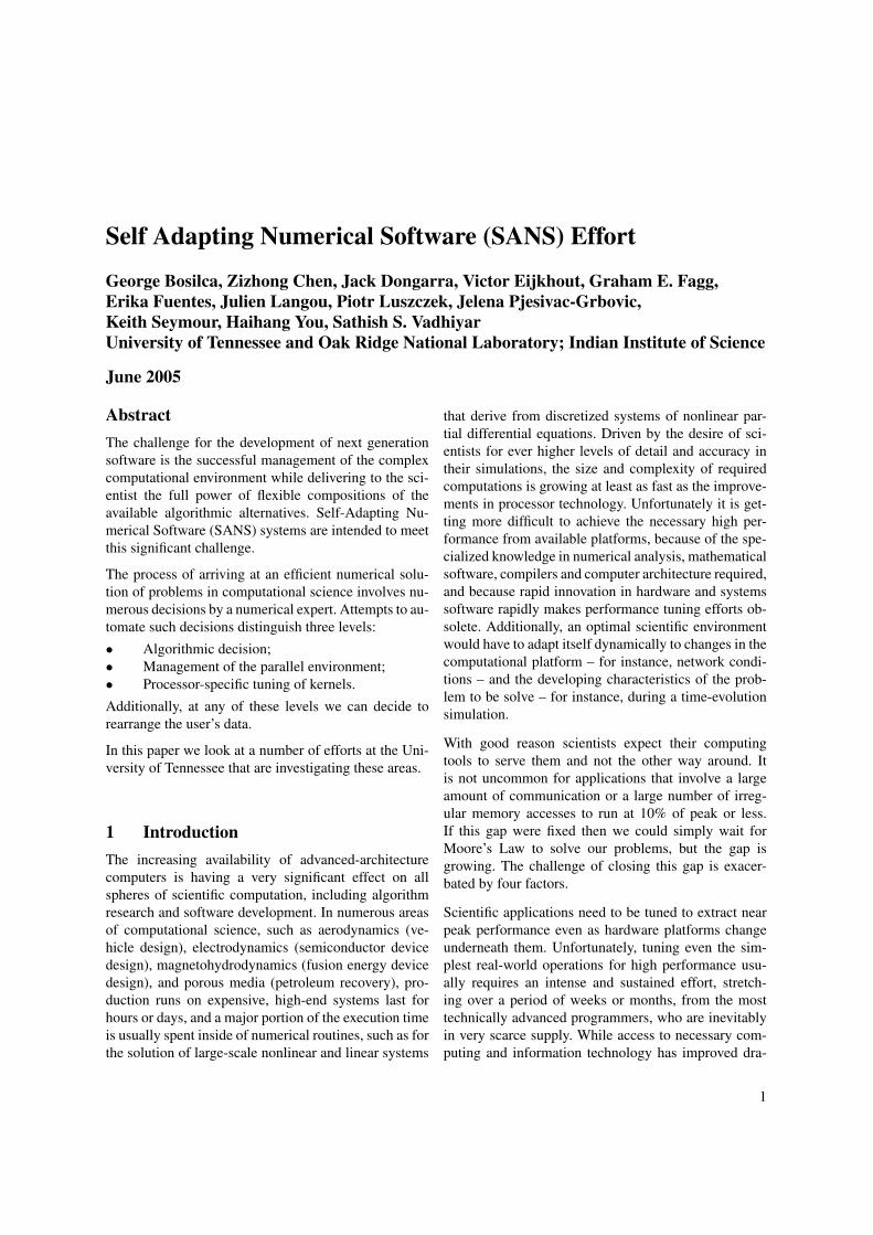
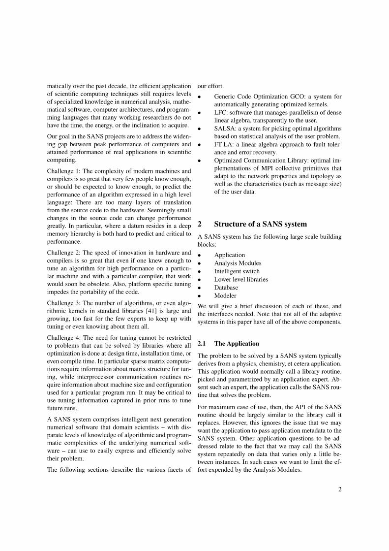
Given values for a set of parameters, the ATLAS codegenerator generates a code variant of matrix multi-ply. The code gets executed with randomly generated1000x1000 dense matrices as input. After executing thesearch heuristic, the output is a set of parameters thatgives the best performance for that platform. Figure 1compares the total time spent by each of the searchmethods on the search itself. The Itanium2 search time(for all search techniques) is much longer than theother platforms because we are using the Intel com-piler, which in our experience takes longer to compilethe same piece of code than the compiler used on theother platforms (gcc). Figure 2 shows the comparisionof the performance of matrix multiply on different sizesof matrices using the ATLAS libraries generated by theSimplex search and the original ATLAS search.

3.3 Generic Code Optimization

Current empirical optimization techniques such as AT-LAS and FFTW can achieve good performance because

Figure 1: Search time

the algorithms to be optimized are known ahead of time.We are addressing this limitation by extending the tech-niques used in ATLAS to the optimization of arbitrarycode. Since the algorithm to be optimized is not knownin advance, it will require compiler technology to ana-lyze the source code and generate the candidate imple-mentations. The ROSE project[69, 54] from LawrenceLivermore National Laboratory provides, among otherthings, a source-to-source code transformation tool thatcan produce blocked and unrolled versions of the inputcode. Combined with our search heuristic and hardwareinformation, we can use ROSE to perform empiricalcode optimization. For example, based on an automaticcharacterization of the hardware, we will direct theircompiler to perform automatic loop blocking at varyingsizes, which we can then evaluate to find the best blocksize for that loop. To perform the evaulations, we havedeveloped a test infrastructure that automatically gener-ates a timing driver for the optimized routine based ona simple description of the arguments.

The Generic Code Optimization system is structured asa feedback loop. The code is fed into the loop proces-sor for optimization and separately fed into the timingdriver generator which generates the code that actuallyruns the optimized code variant to determine its execu-tion time. The results of the timing are fed back intothe search engine. Based on these results, the search en-gine may adjust the parameters used to generate the next

5

1000

1050

1100

1150

1200

1250

1300

1000 2000 3000 4000

mflo

ps

Matrix Size

ATLAS dgemm -- SparcUltra(900MHZ)

ATLASSimplex

2600

2650

2700

2750

2800

2850

2900

2950

3000

1000 2000 3000 4000 5000

mflo

ps

Matrix Size

ATLAS dgemm -- Itanium2(900MHZ)

ATLASSimplex

1600

1700

1800

1900

2000

2100

2200

1000 2000 3000 4000

mflo

ps

Matrix Size

ATLAS dgemm -- Pentium4(2.4GMHZ)

ATLASSimplex

2000

2200

2400

2600

2800

3000

1000 2000 3000

mflo

ps

Matrix Size

ATLAS dgemm -- power4(1.3 GHZ)

ATLASSimplex

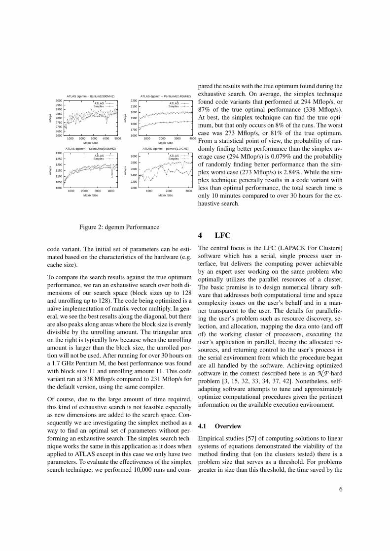
Figure 2: dgemm Performance

code variant. The initial set of parameters can be esti-mated based on the characteristics of the hardware (e.g.cache size).

To compare the search results against the true optimumperformance, we ran an exhaustive search over both di-mensions of our search space (block sizes up to 128and unrolling up to 128). The code being optimized is anaıve implementation of matrix-vector multiply. In gen-eral, we see the best results along the diagonal, but thereare also peaks along areas where the block size is evenlydivisible by the unrolling amount. The triangular areaon the right is typically low because when the unrollingamount is larger than the block size, the unrolled por-tion will not be used. After running for over 30 hours ona 1.7 GHz Pentium M, the best performance was foundwith block size 11 and unrolling amount 11. This codevariant ran at 338 Mflop/s compared to 231 Mflop/s forthe default version, using the same compiler.

Of course, due to the large amount of time required,this kind of exhaustive search is not feasible especiallyas new dimensions are added to the search space. Con-sequently we are investigating the simplex method as away to find an optimal set of parameters without per-forming an exhaustive search. The simplex search tech-nique works the same in this application as it does whenapplied to ATLAS except in this case we only have twoparameters. To evaluate the effectiveness of the simplexsearch technique, we performed 10,000 runs and com-

pared the results with the true optimum found during theexhaustive search. On average, the simplex techniquefound code variants that performed at 294 Mflop/s, or87% of the true optimal performance (338 Mflop/s).At best, the simplex technique can find the true opti-mum, but that only occurs on 8% of the runs. The worstcase was 273 Mflop/s, or 81% of the true optimum.From a statistical point of view, the probability of ran-domly finding better performance than the simplex av-erage case (294 Mflop/s) is 0.079% and the probabilityof randomly finding better performance than the sim-plex worst case (273 Mflop/s) is 2.84%. While the sim-plex technique generally results in a code variant withless than optimal performance, the total search time isonly 10 minutes compared to over 30 hours for the ex-haustive search.

4 LFCThe central focus is the LFC (LAPACK For Clusters)software which has a serial, single process user in-terface, but delivers the computing power achievableby an expert user working on the same problem whooptimally utilizes the parallel resources of a cluster.The basic premise is to design numerical library soft-ware that addresses both computational time and spacecomplexity issues on the user’s behalf and in a man-ner transparent to the user. The details for paralleliz-ing the user’s problem such as resource discovery, se-lection, and allocation, mapping the data onto (and offof) the working cluster of processors, executing theuser’s application in parallel, freeing the allocated re-sources, and returning control to the user’s process inthe serial environment from which the procedure beganare all handled by the software. Achieving optimizedsoftware in the context described here is an N P -hardproblem [3, 15, 32, 33, 34, 37, 42]. Nonetheless, self-adapting software attempts to tune and approximatelyoptimize computational procedures given the pertinentinformation on the available execution environment.

4.1 Overview

Empirical studies [57] of computing solutions to linearsystems of equations demonstrated the viability of themethod finding that (on the clusters tested) there is aproblem size that serves as a threshold. For problemsgreater in size than this threshold, the time saved by the

6

self-adaptive method scales with the parallel applicationjustifying the approach.

LFC addresses user’s problems that may be stated interms of numerical linear algebra. The problem mayotherwise be dealt with one of the LAPACK [4] and/orScaLAPACK [9] routines supported in LFC. In partic-ular, suppose that the user has a system of m linearequations with n unknowns, Ax = b. Three commonfactorizations (LU, Cholesky-LLT, and QR) apply forsuch a system depending on properties and dimensionsof A. All three decompositions are currently supportedby LFC.

LFC assumes that only a C compiler, a Message Pass-ing Interface (MPI) [26, 27, 28] implementation suchas MPICH [48] or LAM MPI [40], and some variant ofthe BLAS routines, be it ATLAS or a vendor suppliedimplementation, is installed on the target system. Targetsystems are intended to be “Beowulf-like” [62].

4.2 Algorithm Selection Processes

ScaLAPACK Users’ Guide [9] provides the followingequation for predicting the total time T spent in one ofits linear solvers (LLT, LU, or QR) on matrix of size nin NP processes [14]:

T (n,NP) =C f n3

NPt f +

Cvn2√

NPtv +

CmnNB

tm (1)

where:

• NP number of processes• NB blocking factor for both computation and

communication• t f time per floating-point operation (matrix-

matrix multiplication flop rate is a good startingapproximation)

• tm corresponds to latency• 1/tv corresponds to bandwidth• C f corresponds to number of floating-point oper-

ations• Cv and Cm correspond to communication costs

The constands C f Cv and Cm should be taken from thefollwing table:

Driver C f Cv CmLU 2/3 3+1/4log2 NP NB(6+ log2 NP)LLT 1/3 2+1/2log2 NP 4+ log2 NPQR 4/3 3+ log2 NP 2(NB log2 NP +1)

The hard part in using the above equation is obtainingthe system-related parameters t f , tm, and tv indepentlyof each other and without performing costly parametersweep. At the moment we are not aware of any reli-able way of acquiring those parameters and thus we relyon parameter fitting approach that uses timing informa-tion from previous runs. Furthermore, with respect toruntime software parameters the equation includes onlythe process count NP and blocking factor NB. However,the key to good performance is the right aspect ratioof the logical process grid: the number of process rowsdivided by the number of process columns. In heterge-neous environments (for which the equation doesn’t ac-count at all), choosing the right subset of processor iscrucial as well.

Lastly, the decision making process is influenced by thefollwing factors directly related to system policies thatdefine what is the goal of the optimal selection:• resource utilization (throughput),• time to solution (response time),• per-processor performance (parallel efficiency).Trivially, the owner (or manager) of the system is in-terested in optimal resource utilization while the userexpects the shortest time to obtain the solution. Insteadof aiming at optimization of either the former (by max-imizing memory utilization and sacrificing the total so-lution time by minimizing the number of processes in-volved) or the latter (by using all the available proces-sors) a benchmarking engineer would be interested inbest floating-point performance.

4.3 Experimental Results

Figure 3 illustrates how the time to solution is influ-enced by the aspect ratio of the logical process grid fora range of process counts. It is clear that sometimes itmight be beneficial not to use all the available proces-sors for computation (the idle processors might be usedfor example for fault-tolerance purposes). This is espe-cially true if the number of processors is a prime num-ber which leads to a one-dimensional process grid andthus very poor performance on many systems. It is un-realistic to expect that non-expert users will correctlymake the right decisions in every such case. It is ei-ther a matter of having expertise or relevant experimen-tal data to guide the choice and our experiences sug-gest that perhaps a combination of both is required tomake good decisions consistently. As a side note, withrespect to the experimental data, it is worth mentioning

7

5000

6000

7000

8000

9000

10000

11000

30 35 40 45 50 55 60 65

Wal

l clo

ck ti

me

[s]

Number of processors

Best process gridWorst process grid

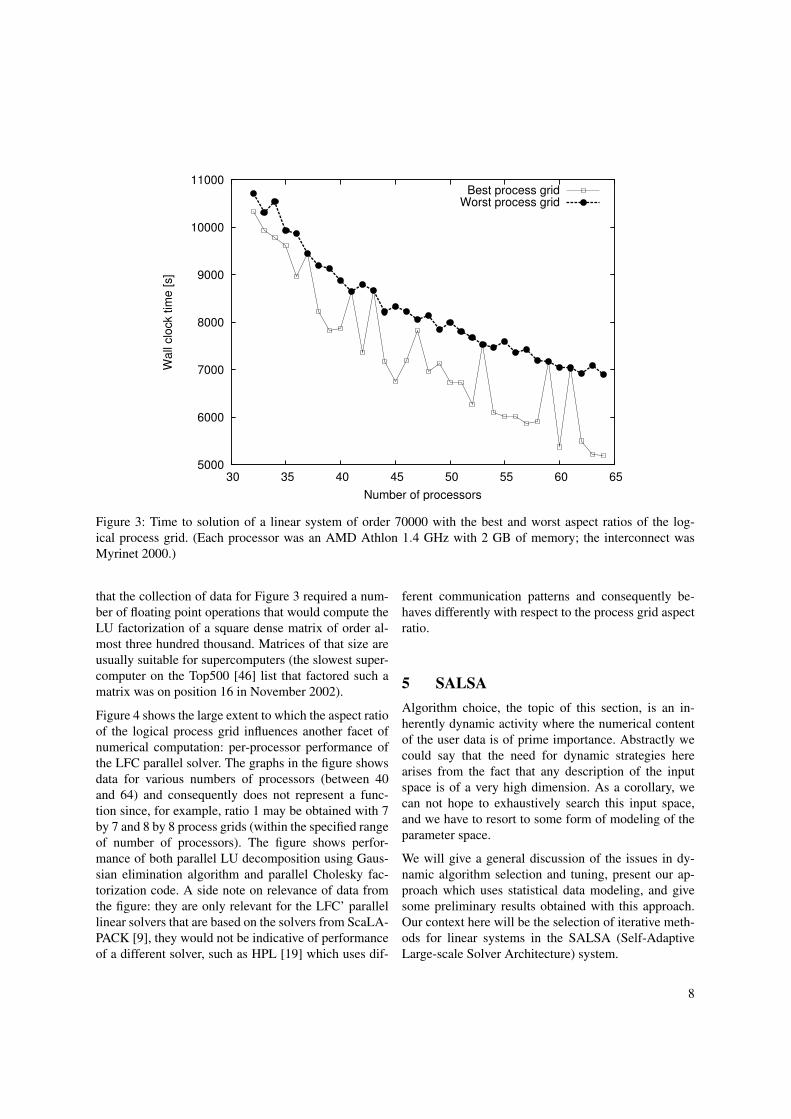
Figure 3: Time to solution of a linear system of order 70000 with the best and worst aspect ratios of the log-ical process grid. (Each processor was an AMD Athlon 1.4 GHz with 2 GB of memory; the interconnect wasMyrinet 2000.)

that the collection of data for Figure 3 required a num-ber of floating point operations that would compute theLU factorization of a square dense matrix of order al-most three hundred thousand. Matrices of that size areusually suitable for supercomputers (the slowest super-computer on the Top500 [46] list that factored such amatrix was on position 16 in November 2002).

Figure 4 shows the large extent to which the aspect ratioof the logical process grid influences another facet ofnumerical computation: per-processor performance ofthe LFC parallel solver. The graphs in the figure showsdata for various numbers of processors (between 40and 64) and consequently does not represent a func-tion since, for example, ratio 1 may be obtained with 7by 7 and 8 by 8 process grids (within the specified rangeof number of processors). The figure shows perfor-mance of both parallel LU decomposition using Gaus-sian elimination algorithm and parallel Cholesky fac-torization code. A side note on relevance of data fromthe figure: they are only relevant for the LFC’ parallellinear solvers that are based on the solvers from ScaLA-PACK [9], they would not be indicative of performanceof a different solver, such as HPL [19] which uses dif-

ferent communication patterns and consequently be-haves differently with respect to the process grid aspectratio.

5 SALSAAlgorithm choice, the topic of this section, is an in-herently dynamic activity where the numerical contentof the user data is of prime importance. Abstractly wecould say that the need for dynamic strategies herearises from the fact that any description of the inputspace is of a very high dimension. As a corollary, wecan not hope to exhaustively search this input space,and we have to resort to some form of modeling of theparameter space.

We will give a general discussion of the issues in dy-namic algorithm selection and tuning, present our ap-proach which uses statistical data modeling, and givesome preliminary results obtained with this approach.Our context here will be the selection of iterative meth-ods for linear systems in the SALSA (Self-AdaptiveLarge-scale Solver Architecture) system.

8

0

0.5

1

1.5

2

2.5

3

3.5

4

0 0.1 0.2 0.3 0.4 0.5 0.6 0.7 0.8 0.9 1

Per

-pro

cess

per

form

ance

[Gflo

p/s]

Logical processor grid aspect ratio

LUCholesky

Figure 4: Per-processor performance of the LFC parallel linear LU and parallel Cholesky solvers on the Pentium 4cluster as a function of the aspect ratio of the logical process grid (matrix size was 72000 and the number of CPUsvaried between 40 and 64).

5.1 Dynamic Algorithm Determination

In finding the appropriate numerical algorithm for aproblem we are faced with two issues:

1. There are often several algorithms that, poten-tially, solve the problem, and

2. Algorithms often have one or more parameters ofsome sort.

Thus, given user data, we have to choose an algorithm,and choose a proper parameter setting for it.

Our strategy in determining numerical algorithms bystatistical techniques is globally as follows.

• We solve a large collection of test problems byevery available method, that is, every choice ofalgorithm, and a suitable ‘binning’ of algorithmparameters.

• Each problem is assigned to a class correspond-ing to the method that gave the fastest solution.

• We also draw up a list of characteristics of eachproblem.

• We then compute a probability density functionfor each class.

As a result of this process we find a function pi(x)where i ranges over all classes, that is, all methods, andx is in the space of the vectors of features of the inputproblems. Given a new problem and its feature vector x,we then decide to solve the problem with the method ifor which pi(x) is maximised.

We will now discuss the details of this statistical analy-sis, and we will present some proof-of-concept numer-ical results evincing the potential usefulness of this ap-proach.

5.2 Statistical analysis

In this section we give a short overview of the way amulti-variate Bayesian decision rule can be used in nu-merical decision making. We stress that statistical tech-niques are merely one of the possible ways of usingnon-numerical techniques for algorithm selection andparameterization, and in fact, the technique we describehere is only one among many possible statistical tech-niques. We will describe here the use of parametricmodels, a technique with obvious implicit assumptionsthat very likely will not hold overall, but, as we shall

9

show in the next section, they have surprising applica-bility.

5.2.1 Feature extraction

The basis of the statistical decision process is the ex-traction of features from the application problem, andthe characterization of algorithms in terms of these fea-tures. In [21] we have given examples of relevant fea-tures of application problems. In the context of lin-ear/nonlinear system solving we can identify at leastthe following categories of features: structural features,pertaining to the nonzero structure; simple quantitiesthat can be computed exactly and cheaply; spectralproperties, which have to be approximated; measuresof the variance of the matrix.

5.2.2 Training stage

Based on the feature set described above, we now en-gage in an – expensive and time-consuming – train-ing phase, where a large number of problems is solvedwith every available method. For linear system solving,methods can be described as an orthogonal combinationof several choices: the iterative method, the precondi-tioner, and preprocessing steps such as scaling or per-muting the system. Several of these choices involve nu-merical parameters, such as the GMRES restart length,or the number of ILU fill levels.

In spite of this multi-dimensional characterization of it-erative solvers, we will for the purpose of this exposi-tion consider methods as a singly-indexed set.

The essential step in the training process is that each nu-merical problem is assigned to a class, where the classescorrespond to the solvers, and the problem is assignedto the class of the method that gave the fastest solution.As a result of this, we find for each method (class) amultivariate density function:

p j(x) =1

2π|Σ|1/2 e−(1/2)(x−µ)Σ−1(x−µ)

where x are the features, µ the means, and Σ the covari-ance matrix.

Having computed these density functions, we can com-pute the a posteriori probability of a class (‘given asample x, what is the probability that it belongs inclass j’) as

P(wi|x) =p(x|w j)P(w j)

p(x).

We then select the numerical method for which thisquantity is maximised.

5.3 Numerical test

To study the behavior and performance of the statisticaltechniques described in the previous section, we per-form several tests on a number of matrices from dif-ferent sets from the Matrix Market [44]. To collect thedata, we generate matrix statistics by running an ex-haustive test of the different coded methods and precon-ditioners; for each of the matrices we collect statisticsfor each possible existing combination of: permutation,scaling, preconditioner and iterative method.

From this data we select those combinations that con-verged and had the minimum solving time (those com-binations that didn’t converge are discarded). Each pos-sible combination corresponds to a class, but since thenumber of these combination is too large, we reduce thescope of the analysis and concentrate only on the behav-ior of the possible permutation choices. Thus, we havethree classes corresponding to the partitioning types:Induced the default Petsc distribution induced by the

matrix ordering and the number of processors,Parmetis , using the Parmetis [60, 51] package,Icmk a heuristic [20] that, without permuting the sys-

tem, tries to find meaningful split points based onthe sparsity structure.

Our test is to see if the predicted class (method) is in-deed the one that yields minimum solving time for eachcase.

5.4 Results

These results were obtained using the following ap-proach for both training and testing the classifier: con-sidering that Induced and Icmk are the same except forthe Block-Jacobi case, if a given sample is not usingBlock-Jacobi it is classified as both Induced and Icmk,and if it is using Block-Jacobi then the distinction ismade and it is classified as Induced or Icmk. For thetesting set, the verification is performed with same cri-teria, for instance, if a sample from the class Inducedis not using Block-Jacobi and is classified as Icmk bythe classifier, is still counted as a correct classification(same for the inverse case of Icmk classified as In-duced), however, if a sample from the Induced class isclassified as Induced and was using block-jacobi, it iscounted as a misclassification.

10

The results for the different sets of features tested, areas follows:

Features: non-zeros, bandwidth left and right,splits number, ellipse axes

ParametricNon-ParametricInduced Class: 70% 60%Parmetis Class: 98% 73%Icmk Class: 93% 82%

Features: diagonal, non-zeros, bandwidth left and right,splits number, ellipse axes and center

Parametric Non-ParametricInduced Class: 70% 80%Parmetis Class: 95% 76%Icmk Class: 90% 90%

It is important to note that although we have many pos-sible features to choose from, there might not be enoughdegrees of freedom (i.e. some of these features mightbe corelated), so it is important to continue experimen-tation with other sets of features. The results of thesetests might give some lead for further experimentationand understanding of the application of statistical meth-ods on numerical data.

These tests and results are a first glance at the behaviorof the statistical methods presented, and there is plentyof information that can be extracted and explored inother experiments and perhaps using other methods.

6 FT-LAAs the number of processors in today’s high perfor-mance computers continue to grow, the mean-time-to-failure of these computers is becoming significantlyshorter than the execution time of many current highperformance applications. Consequently, failures of anode or a process becomes events to which numericalsoftware needs to adapt, preferably in an automatic way.

FT-LA stands for Fault Tolerant Linear Algebra andaims at exploring parallel distributed numerical linearalgebra algorithms in the context of volatile resources.The parent of FT-LA is FT-MPI [24, 31]. FT-MPI en-ables an implementer to write fault tolerant code whileproviding the maximum of freedom to the user. Basedon this library, it becomes possible to create more andmore fault-tolerant algorithms and software without theneed for specialized hardware; thus providing us theability to explore new areas for implementation and de-velopment.

In this section, we only focus on the solution of sparselinear systems of equations using iterative methods.(For the dense case, we refer to [52], for eigenvaluecomputation [11].) We assume that a failure of one ofthe processors (nodes) results in the lost of all the datastored in its memory (local data). After the failure, theremaining processors are still active, another processoris added to the communicator to replace the failed oneand the MPI environenment is sane. These assumptionsare true in the FT-MPI context. In the context of itera-tive methods, once the MPI environment and the initialdata (matrix, right-hand sides) are recovered, the nextissue, which is our main concern, is to recover the datacreated by the iterative method.

Diskless Checkpoint-Restart Technique

In order to recover the data from any of the processorswhile maintaining a low storage overhead, we are usinga checksum approach to checkpointing.

Our checkpoints are diskless, in the sense that thecheckpoint is stored in memory of a processor and noton a disk. To achieve this, an additional processor isadded to the environment. It will be referred as thecheckpoint processor and its role is to store the check-sum. The checkpoint processor can be viewed as a diskbut with low latency and high bandwidth since it is lo-cated in the network of processors. For more informa-tion, we refer the reader to [13, 52] where special in-terests are given on simultaneous failures and the scala-bility of diskless checkpointing (the first reference usesPVM, the second one FT-MPI).

The information is encoded in the following trivial way:if there are n processors for each of which we wantto save the vector xk (for simplicity, we assume thatthe size of xk is the same on all the processors), thenthe checkpoint unit stores the checksum xn+1 such thatxn+1 = ∑i=1,...,n xi. If processor f fails, we can restore x fvia x f = xn+1 −∑i=1,...,n;i6= f xi. The arithmetic used forthe operations + and − can either be binary or floating-point arithmetic.

When the size of the information is pretty large (ourcase), a pipelined broadcasting algorithm enables thecomputation of checksum to have almost perfect scal-ing with respect to constant charge of the processors(see [58] for a theoretical bound). For example, in Ta-ble 1, we report experimental data on two different plat-forms at the University of Tennessee: the boba Linux

11

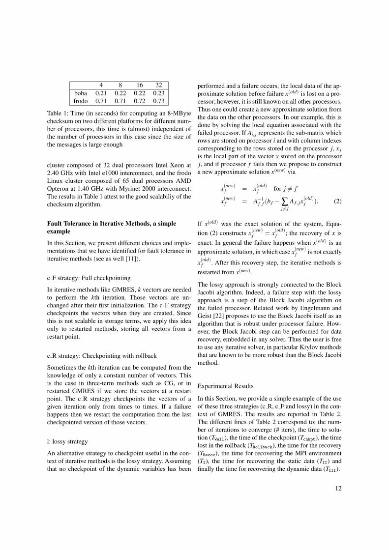
4 8 16 32boba 0.21 0.22 0.22 0.23frodo 0.71 0.71 0.72 0.73

Table 1: Time (in seconds) for computing an 8-MBytechecksum on two different platforms for different num-ber of processors, this time is (almost) independent ofthe number of processors in this case since the size ofthe messages is large enough

cluster composed of 32 dual processors Intel Xeon at2.40 GHz with Intel e1000 interconnect, and the frodoLinux cluster composed of 65 dual processors AMDOpteron at 1.40 GHz with Myrinet 2000 interconnect.The results in Table 1 attest to the good scalabiliy of thechecksum algorithm.

Fault Tolerance in Iterative Methods, a simpleexample

In this Section, we present different choices and imple-mentations that we have identified for fault tolerance initerative methods (see as well [11]).

c F strategy: Full checkpointing

In iterative methods like GMRES, k vectors are neededto perform the kth iteration. Those vectors are un-changed after their first initialization. The c F strategycheckpoints the vectors when they are created. Sincethis is not scalable in storage terms, we apply this ideaonly to restarted methods, storing all vectors from arestart point.

c R strategy: Checkpointing with rollback

Sometimes the kth iteration can be computed from theknowledge of only a constant number of vectors. Thisis the case in three-term methods such as CG, or inrestarted GMRES if we store the vectors at a restartpoint. The c R strategy checkpoints the vectors of agiven iteration only from times to times. If a failurehappens then we restart the computation from the lastcheckpointed version of those vectors.

l: lossy strategy

An alternative strategy to checkpoint useful in the con-text of iterative methods is the lossy strategy. Assumingthat no checkpoint of the dynamic variables has been

performed and a failure occurs, the local data of the ap-proximate solution before failure x(old) is lost on a pro-cessor; however, it is still known on all other processors.Thus one could create a new approximate solution fromthe data on the other processors. In our example, this isdone by solving the local equation associated with thefailed processor. If Ai, j represents the sub-matrix whichrows are stored on processor i and with column indexescorresponding to the rows stored on the processor j, x jis the local part of the vector x stored on the processorj, and if processor f fails then we propose to constructa new approximate solution x(new) via

x(new)j = x(old)

j for j 6= f

x(new)f = A−1

f , f (b f − ∑j 6= f

A f , jx(old)j ). (2)

If x(old) was the exact solution of the system, Equa-tion (2) constructs x(new)

f = x(old)f ; the recovery of x is

exact. In general the failure happens when x(old) is anapproximate solution, in which case x(new)

f is not exactly

x(old)f . After this recovery step, the iterative methods is

restarted from x(new).

The lossy approach is strongly connected to the BlockJacobi algorithm. Indeed, a failure step with the lossyapproach is a step of the Block Jacobi algorithm onthe failed processor. Related work by Engelmann andGeist [22] proposes to use the Block Jacobi itself as analgorithm that is robust under processor failure. How-ever, the Block Jacobi step can be performed for datarecovery, embedded in any solver. Thus the user is freeto use any iterative solver, in particular Krylov methodsthat are known to be more robust than the Block Jacobimethod.

Experimental Results

In this Section, we provide a simple example of the useof these three strategies (c R, c F and lossy) in the con-text of GMRES. The results are reported in Table 2.The different lines of Table 2 correspond to: the num-ber of iterations to converge (# iters), the time to solu-tion (TWall), the time of the checkpoint (Tchkpt), the timelost in the rollback (TRollback), the time for the recovery(TRecov), the time for recovering the MPI environment(TI), the time for recovering the static data (TII) andfinally the time for recovering the dynamic data (TIII).

12

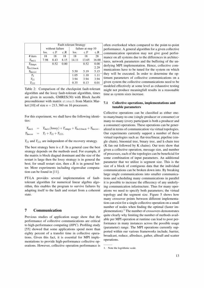
Fault-tolerant Strategywithout failure failure at step 10

los. c F c R los. c F c R# iters 18 18 18 18 18 28TWall 7.98 8.43 8.15 14.11 13.65 16.00TChkpt 0.52 0.00 0.52 0.00

TRollback 2.29TRecov 5.50 5.19 5.15

TI 1.05 1.10 1.11TII 3.94 3.94 3.94TIII 0.35 0.13 0.01

Table 2: Comparison of the checkpoint fault-tolerantalgorithm and the lossy fault-tolerant algorithm, timesare given in seconds, GMRES(30) with Block Jacobipreconditioner with matrix stomach from Matrix Mar-ket [10] of size n = 213,360 on 16 processors.

For this experiment, we shall have the following identi-ties:

TWall = TWall(lossy)+Tchkpt +TRollback +TRecov,

TRecov = TI +TII +TIII,

TII and TIII are independent of the recovery strategy.

The best strategy here is c F. In a general case the beststrategy depends on the methods used. For example, ifthe matrix is block diagnal dominant and the size of therestart is large then the lossy strategy is in general thebest; for small restart size, then c R is in general bet-ter. More experiments including eigenvalue computa-tion can be found in [11].

FT-LA provides several implementation of fault-tolerant algorithm for numerical linear algebra algo-rithm, this enables the program to survive failures byadapting itself to the fault and restart from a coherentstate.

7 CommunicationPrevious studies of application usage show that theperformance of collective communications are criticalto high-performance computing (HPC). Profiling study[55] showed that some applications spend more thaneighty percent of a transfer time in collective opera-tions. Given this fact, it is essential for MPI imple-mentations to provide high-performance collective op-erations. However, collective operation performance is

often overlooked when compared to the point-to-pointperformance. A general algorithm for a given collectivecommunication operation may not give good perfor-mance on all systems due to the differences in architec-tures, network parameters and the buffering of the un-derlying MPI implementation. Hence, collective com-munications have to be tuned for the system on whichthey will be executed. In order to determine the op-timum parameters of collective communications on agiven system the collective communications need to bemodeled effectively at some level as exhaustive testingmight not produce meaningfull results in a reasonabletime as system sizes increase.

7.1 Collective operations, implementations andtunable parameters

Collective operations can be classified as either one-to-many/many-to-one (single producer or consumer) ormany-to-many (every participant is both a producer anda consumer) operations. These operations can be gener-alized in terms of communication via virtual topologies.Our experiments currently support a number of thesevirtual topologies such as: flat-tree/linear, pipeline (sin-gle chain), binomial tree, binary tree, and k-chain tree(K fan out followed by K chains). Our tests show thatgiven a collective operation, message size, and numberof processes, each of the topologies can be beneficial forsome combination of input parameters. An additionalparameter that we utilize is segment size. This is thesize of a block of contiguous data that the individualcommunications can be broken down into. By breakinglarge single communications into smaller communica-tions and scheduling many communications in parallelit is possible to increase the effiecency of any underly-ing communication infastructure. Thus for many oper-ations we need to specify both parameters; the virtualtopology and the segment size. Figure 5 shows howmany crossover points between different implementa-tion can exist for a single collective operation on a smallnumber of nodes when finding the optimal (faster im-plementation).1 The number of crossovers demonstratesquite clearly why limiting the number of methods avail-able per MPI operation at runtime can lead to poor per-formance in many instances across the possible usage(parameter) range. The MPI operations currently sup-ported within our various frameworks include; barrier,broadcast, reduce, allreduce, gather, alltoall and scatteroperations.

1. Note the logrithmic scale.

13

Figure 5: Multiple Implementations of the MPI ReduceOperation on 16 nodes

7.2 Exhaustive and directed searching

Simple, yet time consuming method to find an optimalimplementation of an individual collective operation isto run an extensive set of tests over a parameter spacefor the collective on a dedicated system. However, run-ning such detailed tests even on relatively small clus-ters, can take a substantial amount of time [65]. Tuningexhaustively for eight MPI collectives on a small (40node) IBM SP-2 upto message sizes of one MegaByteinvolved approximately 13000 individual experiments,and took 50 hours to complete. Even though this onlyneeded to occur once, tuning all of the MPI collectivesin a similar manner would take days for a modaratlysized system or weeks for a larger system.

Finding the optimal implementation of any given col-lective can be broken down into a number of stages. Thefirst stage being dependent on message size, number ofprocessors and MPI collective operation. The secondarystage is an optimization at these parameters for the cor-rect method (topology-algorithm pair) and segmenta-tion size. Reducing the time needed for running the ac-tual experiments can be achieved at many different lev-els, such as not testing at every point and interpolat-ing results. i.e. testing 8, 32, 128 processes rather than8, 16, 32, 64, 128 etc. Additionally using instrumentedapplication runs to build a table of only those collectiveoperations that are required, i.e. not tuning operationsthat will never be called, or are called infrequently. Weare currently testing this instrumentation method via anewly developed profiling interface known as the Scal-

Figure 6: Multiple Implementations of the MPI Scatteroperation on 8 nodes for various segmentation sizes

able Application Instrumention System (SAIS).

Another method used to reduce the search space inan intelligent manner is to use traditional optimizationtechniques such as gradient decent with domain knowl-edge. Figure 6 shows the performance of four differentmethods for implementing an 8 processor MPI Scatterfor 128 KBytes of data on the UltraSPARC cluster whenvarying the segmentation size. From the resulting shapeof the performance data we can see that the optimal seg-mentation size occurs for larger sizes, and that tests ofvery small segmentation sizes are very expensive. Byusing various gradient decent methods to control run-time tests we can reduce the time to find the optimalsegmentation size from 12613 seconds and 600 tests to40 seconds and just 90 tests [59]. Thus simple methodscan still allow semi-exhaustive testing in a reasonabletime.

7.3 Communication modelling

There are many parallel communicational models thatpredict performance of any given collective operationbased on standardizing network and system parame-ters. Hockney [35], LogP [17], LogGP [1], and PLogP[38] models are frequently used to analyze parallelalgorithm performance. Assessing the parameters forthese models within local area network is relativelystraightforward and the methods to approximate themhave already been established and are well understood[16][38]. Thakur et al. [63] and Rabenseifner et al.[56] use Hockney model to analyze the performanceof different collective operation algorithms. Kielmann

14

et al. [39] use PLogP model to find optimal algorithmand parameters for topology-aware collective opera-tions incorporated in the MagPIe library. Bell et al. [6]use extensions of LogP and LogGP models to evaluatehigh performance networks. Bernaschi et al. [7] analyzethe efficiency of reduce-scatter collective using LogGPmodel. Vadhiyar et al. [65][59] used a modified LogPmodel which took into account the number of pendingrequests that had been queued. The most important fac-tor concerning communication modelling is that the ini-tial collection of (point to point communication) param-eters is usually performed by executing a microbench-mark that takes seconds to run followed by some com-putation to calculate the time per collective operationand thus is much faster than exhaustive testing. Once asystem has been parameterized in terms of a communi-cation model we then can build a mathematical modelof a particular collective operation as shown in [36].

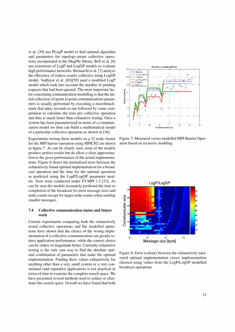
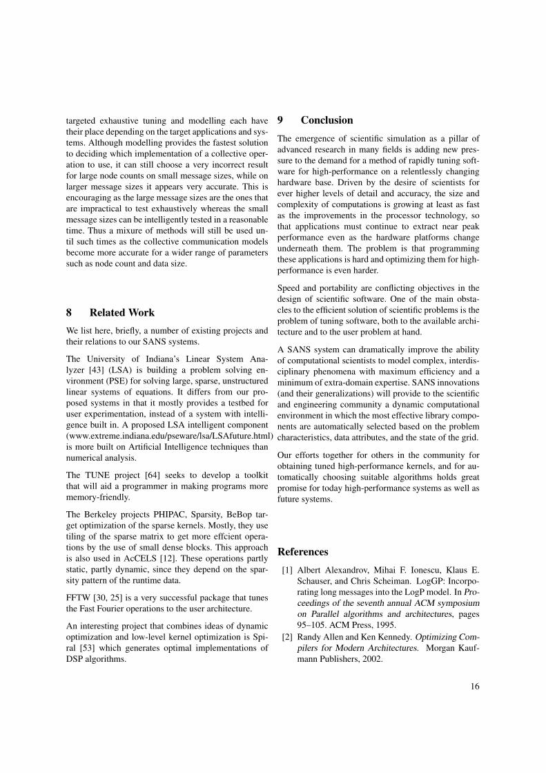
Experiments testing these models on a 32 node clusterfor the MPI barrier operation using MPICH2 are shownin figure 7. As can be clearly seen, none of the modelsproduce perfect results but do allow a close approxima-tion to the gross performance of the actual implementa-tions. Figure 8 shows the normalised error between theexhaustively found optimal implementation for a broad-cast operation and the time for the optimal operationas predicted using the LogP/LogGP parameter mod-els. Tests were conducted under FT-MPI 1.2 [23]. Ascan be seen the models accurately predicted the time tocompletion of the broadcast for most message sizes andnode counts except for larger node counts when sendingsmaller measages.

7.4 Collective communication status and futurework

Current experiments comparing both the exhaustivelytested collective operations and the modelled opera-tions have shown that the choice of the wrong imple-mentation of a collective communication can greatly re-duce application performance, while the correct choicecan be orders of magnitude better. Currently exhaustivetesting is the only sure way to find the absolute opti-mal combination of parameters that make the optimalimplementation. Finding these values exhaustively foranything other than a very small system or a very con-strained (and repetative application) is not practical interms of time to examine the complete search space. Wehave presented several methods used to reduce or elim-inate this search space. Overall we have found that both

Figure 7: Measured verses modelled MPI Barrier Oper-ation based on recursive doubling

Figure 8: Error (colour) between the exhaustively mea-sured optimal implementation verses implementationchoosen using values from the LogP/LogGP modelledbroadcast operations

15

targeted exhaustive tuning and modelling each havetheir place depending on the target applications and sys-tems. Although modelling provides the fastest solutionto deciding which implementation of a collective oper-ation to use, it can still choose a very incorrect resultfor large node counts on small message sizes, while onlarger message sizes it appears very accurate. This isencouraging as the large message sizes are the ones thatare impractical to test exhaustively whereas the smallmessage sizes can be intelligently tested in a reasonabletime. Thus a mixure of methods will still be used un-til such times as the collective communication modelsbecome more accurate for a wider range of parameterssuch as node count and data size.

8 Related WorkWe list here, briefly, a number of existing projects andtheir relations to our SANS systems.

The University of Indiana’s Linear System Ana-lyzer [43] (LSA) is building a problem solving en-vironment (PSE) for solving large, sparse, unstructuredlinear systems of equations. It differs from our pro-posed systems in that it mostly provides a testbed foruser experimentation, instead of a system with intelli-gence built in. A proposed LSA intelligent component(www.extreme.indiana.edu/pseware/lsa/LSAfuture.html)is more built on Artificial Intelligence techniques thannumerical analysis.

The TUNE project [64] seeks to develop a toolkitthat will aid a programmer in making programs morememory-friendly.

The Berkeley projects PHIPAC, Sparsity, BeBop tar-get optimization of the sparse kernels. Mostly, they usetiling of the sparse matrix to get more effcient opera-tions by the use of small dense blocks. This approachis also used in AcCELS [12]. These operations partlystatic, partly dynamic, since they depend on the spar-sity pattern of the runtime data.

FFTW [30, 25] is a very successful package that tunesthe Fast Fourier operations to the user architecture.

An interesting project that combines ideas of dynamicoptimization and low-level kernel optimization is Spi-ral [53] which generates optimal implementations ofDSP algorithms.

9 ConclusionThe emergence of scientific simulation as a pillar ofadvanced research in many fields is adding new pres-sure to the demand for a method of rapidly tuning soft-ware for high-performance on a relentlessly changinghardware base. Driven by the desire of scientists forever higher levels of detail and accuracy, the size andcomplexity of computations is growing at least as fastas the improvements in the processor technology, sothat applications must continue to extract near peakperformance even as the hardware platforms changeunderneath them. The problem is that programmingthese applications is hard and optimizing them for high-performance is even harder.

Speed and portability are conflicting objectives in thedesign of scientific software. One of the main obsta-cles to the efficient solution of scientific problems is theproblem of tuning software, both to the available archi-tecture and to the user problem at hand.

A SANS system can dramatically improve the abilityof computational scientists to model complex, interdis-ciplinary phenomena with maximum efficiency and aminimum of extra-domain expertise. SANS innovations(and their generalizations) will provide to the scientificand engineering community a dynamic computationalenvironment in which the most effective library compo-nents are automatically selected based on the problemcharacteristics, data attributes, and the state of the grid.

Our efforts together for others in the community forobtaining tuned high-performance kernels, and for au-tomatically choosing suitable algorithms holds greatpromise for today high-performance systems as well asfuture systems.

References[1] Albert Alexandrov, Mihai F. Ionescu, Klaus E.

Schauser, and Chris Scheiman. LogGP: Incorpo-rating long messages into the LogP model. In Pro-ceedings of the seventh annual ACM symposiumon Parallel algorithms and architectures, pages95–105. ACM Press, 1995.

[2] Randy Allen and Ken Kennedy. Optimizing Com-pilers for Modern Architectures. Morgan Kauf-mann Publishers, 2002.

16

[3] E. Amaldi and V. Kann. On the approximabilityof minimizing nonzero variables or unsatisfied re-lations in linear systems. Theoretical ComputerScience, 209:237–260, 1998.

[4] E. Anderson, Z. Bai, C. Bischof, Suzan L. Black-ford, James W. Demmel, Jack J. Dongarra, J. DuCroz, A. Greenbaum, S. Hammarling, A. McKen-ney, and Danny C. Sorensen. LAPACK User’sGuide. Society for Industrial and Applied Mathe-matics, Philadelphia, Third edition, 1999.

[5] Utpal Banerjee. A Theory of Loop Permutations.In Selected Papers of the Second Workshop onLanguages and Compilers for Parallel Computing,pages 54–74. Pitman Publishing, 1990.

[6] Christian Bell, Dan Bonachea, Yannick Cote, Ja-son Duell, Paul Hargrove, Parry Husbands, CostinIancu, Michael Welcome, and Katherine Yelick.An evaluation of current high-performance net-works. In Proceedings of the 17th InternationalSymposium on Parallel and Distributed Process-ing, page 28.1. IEEE Computer Society, 2003.

[7] Massimo Bernaschi, Giulio Iannello, and MarioLauria. Efficient implementation of reduce-scatterin MPI. J. Syst. Archit., 49(3):89–108, 2003.

[8] Jeff Bilmes, Krste Asanovic, Chee-Whye Chin,and James Demmel. Optimizing Matrix MultiplyUsing PHiPAC: A Portable, High-Performance,ANSI C Coding Methodology. In InternationalConference on Supercomputing, pages 340–347,1997.

[9] L. Suzan Blackford, J. Choi, Andy Cleary, Ed-uardo F. D’Azevedo, James W. Demmel, Inder-jit S. Dhillon, Jack J. Dongarra, Sven Hammar-ling, Greg Henry, Antoine Petitet, Ken Stanley,David W. Walker, and R. Clint Whaley. ScaLA-PACK Users’ Guide. Society for Industrial andApplied Mathematics, Philadelphia, 1997.

[10] Ronald Boisvert, Roldan Pozo, Karin Remington,Richard Barrett, and Jack Dongarra. Matrix Mar-ket : a web resource for test matrix collections.In R. Boisvert, editor, The Quality of NumericalSoftware: Assessment and Enhancement, pages125–137, Chapman and Hall, London, 1997.

[11] George Bosilca, Zizhong Chen, Jack Dongarra,and Julien Langou. Recovery patterns for iterativemethods in a parallel unstable environment. Tech-nical Report UT-CS-04-538, University of Ten-nessee Computer Science Department, 2004.

[12] Alfredo Buttari, Victor Eijkhout, Julien Langou,and Salvatore Filippone. Performance optimiza-

tion and modeling of blocked sparse kernels.Technical Report ICL-UT-04-05, ICL, Depart-ment of Computer Science, University of Ten-nessee, 2004.

[13] Zizhong Chen, Graham E. Fagg, Edgar Gabriel,Julien Langou, Thara Angskun, George Bosilca,and Jack Dongarra. Building fault surviv-able mpi programs with ft-mpi using diskless-checkpointing. In Proceedings for ACM SIG-PLAN Symposium on Principles and Practice ofParallel Programming, 2005.

[14] J. Choi, Jack J. Dongarra, Susan Ostrouchov, An-toine Petitet, David W. Walker, and R. Clint Wha-ley. The design and implementation of the ScaLA-PACK LU, QR, and Cholesky factorization rou-tines. Scientific Programming, 5:173–184, 1996.

[15] Pierluigi Crescenzi and Viggo Kann (edi-tors). A compendium of NP optimizationproblems. http://www.nada.kth.se/theory/problemlist.html.

[16] D. Culler, L. T. Liu, R. P. Martin, andC. Yoshikawa. Assessing fast network interfaces.IEEE Micro, 16:35–43, 1996.

[17] David Culler, Richard Karp, David Patterson, Ab-hijit Sahay, Klaus Erik Schauser, Eunice Santos,Ramesh Subramonian, and Thorsten von Eicken.LogP: Towards a realistic model of parallel com-putation. In Proceedings of the fourth ACM SIG-PLAN symposium on Principles and practice ofparallel programming, pages 1–12. ACM Press,1993.

[18] Jim Demmel, Jack Dongarra, Victor Eijkhout,Erika Fuentes, Antoine Petitet, Rich Vuduc, ClintWhaley, and Katherine Yelick. Self adapting lin-ear algebra algorithms and software. Proceedingsof the IEEE, 93(2), 2005. special issue on ”Pro-gram Generation, Optimization, and Adaptation”.

[19] Jack J. Dongarra, Piotr Luszczek, and Antoine Pe-titet. The LINPACK benchmark: Past, present,and future. Concurrency and Computation: Prac-tice and Experience, 15:1–18, 2003.

[20] Victor Eijkhout. Automatic determination of ma-trix blocks. Technical Report ut-cs-01-458, De-partment of Computer Science, University of Ten-nessee, 2001. Lapack Working Note 151.

[21] Victor Eijkhout and Erika Fuentes. A proposedstandard for numerical metadata. Technical Re-port ICL-UT-03-02, Innovative Computing Labo-ratory, University of Tennessee, 2003. Poster pre-sentation at Supercomputing 2003.

17

[22] Christian Engelmann and G. Al Geist. De-velopment of naturally fault tolerant algo-rithms for computing on 100,000 processors.http://www.csm.ornl.gov/˜geist.

[23] G. E. Fagg, A. Bukovsky, and J. J. Dongarra.HARNESS and Fault Tolerant MPI. Journal ofParallel Computing, 27(11), 2001.

[24] Graham E. Fagg, Edgar Gabriel, George Bosilca,Thara Angskun, Zizhong Chen, Jelena Pjesivac-Grbovic, Kevin London, and Jack J. Dongarra.Extending the MPI specification for process faulttolerance on high performance computing sys-tems. In Proceedings of the International Super-computer Conference, June 2004.

[25] http://www.fftw.org.[26] Message Passing Interface Forum. MPI: A

Message-Passing Interface Standard. The Interna-tional Journal of Supercomputer Applications andHigh Performance Computing, 8, 1994.

[27] Message Passing Interface Forum. MPI: AMessage-Passing Interface Standard (version 1.1),1995. Available at: http://www.mpi-forum.org/.

[28] Message Passing Interface Forum. MPI-2: Exten-sions to the Message-Passing Interface, 18 July1997. Available at http://www.mpi-forum.org/docs/mpi-20.ps.

[29] Matteo Frigo and Steven G. Johnson. FFTW: AnAdaptive Software Architecture for the FFT. InProc. 1998 IEEE Intl. Conf. Acoustics Speech andSignal Processing, volume 3, pages 1381–1384.IEEE, 1998.

[30] Matteo Frigo and Steven G. Johnson. FFTW: Anadaptive software architecture for the FFT. InProc. 1998 IEEE Intl. Conf. Acoustics Speech andSignal Processing, volume 3, pages 1381–1384.IEEE, 1998.

[31] Edgar Gabriel, Graham E. Fagg, AntoninBukovsky, Thara Angskun, and Jack J. Dongarra.A fault-tolerant communication library for gridenvironments. In Proceedings of the 17th AnnualACM International Conference on Supercomput-ing (ICS’03), International Workshop on GridComputing, 2003.

[32] M. Garey and D. Johnson. Computers andIntractability: A Guide to the Theory of NP-Completeness. W.H. Freeman and Company, NewYork, 1979.

[33] J. Gergov. Approximation algorithms for dynamicstorage allocation. In Proceedings of the 4th An-

nual European Symposium on Algorithms, pages52–56. Springer-Verlag, 1996. Lecture Notes inComputer Science 1136.

[34] D. Hochbaum and D. Shmoys. A polynomialapproximation scheme for machine schedulingon uniform processors: using the dual approach.SIAM Journal of Computing, 17:539–551, 1988.

[35] R.W. Hockney. The communication challenge forMPP: Intel Paragon and Meiko CS-2. ParallelComputing, 20(3):389–398, March 1994.

[36] George Bosilca Graham E. Fagg Edgar Gabriel Je-lena Pjesivac-Grbovic, Thara Angskun and Jack J.Dongarra. Performance analysis of mpi collec-tive operations. In Proceedings 4th InternationalWorkshop on Performance Modeling, Evaluation,and Optimization of Parallel and Distributed Sys-tems PMEO-PDS’05, 2005.

[37] V. Kann. Strong lower bounds on the approx-imability of some NPO PB-complete maximiza-tion problems. In Proceedings of the 20th Interna-tional Symposium on Mathematical Foundationsof Computer Science, pages 227–236. Springer-Verlag, 1995. Lecture Notes in Computer Sci-ence 969.

[38] T. Kielmann, H.E. Bal, and K. Verstoep. Fastmeasurement of LogP parameters for messagepassing platforms. In Jose D. P. Rolim, editor,IPDPS Workshops, volume 1800 of Lecture Notesin Computer Science, pages 1176–1183, Cancun,Mexico, May 2000. Springer-Verlag.

[39] Thilo Kielmann, Rutger F. H. Hofman, Henri E.Bal, Aske Plaat, and Raoul A. F. Bhoedjang. Mag-PIe: MPI’s collective communication operationsfor clustered wide area systems. In Proceedings ofthe seventh ACM SIGPLAN symposium on Prin-ciples and practice of parallel programming, pages131–140. ACM Press, 1999.

[40] LAM/MPI parallel computing. http://www.mpi.nd.edu/lam/.

[41] C. Lawson, R. Hanson, D. Kincaid, and F. Krogh.Basic linear algebra subprograms for FORTRANusage. Transactions on Mathematical Software,5:308–323, 1979.

[42] J. Lenstra, D. Shmoys, and E. Tardos. Approxima-tion algorithms for scheduling unrelated parallelmachines. Mathematical Programming, 46:259–271, 1990.

[43] http://www.extreme.indiana.edu/pseware/lsa/index.html.

[44] http://math.nist.gov/MatrixMarket.

18

[45] Kathryn S. McKinley, Steve Carr, and Chau-WenTseng. Improving Data Locality with Loop Trans-formations. ACM Trans. Program. Lang. Syst.,18(4):424–453, 1996.

[46] Hans W. Meuer, Erich Strohmaier, Jack J. Don-garra, and Horst D. Simon. Top500 Supercom-puter Sites, 20th edition edition, November 2002.(The report can be downloaded from http://www.netlib.org/benchmark/top500.html).

[47] Gordon E. Moore. Cramming More Componentsonto Integrated Circuits. Electronics, 38(8):114–117, 19 April 1965.

[48] MPICH. http://www.mcs.anl.gov/mpi/mpich/.

[49] J. A. Nelder and R. Mead. A Simplex Method forFunction Minimization. The Computer Journal,8:308–313, 1965.

[50] David A. Padua and Michael Wolfe. Ad-vanced Compiler Optimizations for Supercomput-ers. Commun. ACM, 29(12):1184–1201, 1986.

[51] http://www-users.cs.umn.edu/˜karypis/metis/parmetis/index.html.

[52] James S. Plank, Youngbae Kim, and Jack Don-garra. Fault tolerant matrix operations for net-works of workstations using diskless checkpoint-ing. Journal of Parallel and Distributed Comput-ing, 43:125–138, 1997.

[53] M. Puschel, B. Singer, J. Xiong, J. M. F. Moura,J. Johnson, D. Padua, M. Veloso, and R. W. John-son. SPIRAL: A generator for platform-adaptedlibraries of signal processing algorithms. Int’lJournal of High Performance Computing Appli-cations, 18(1):21–45, 2004.

[54] Dan Quinlan, Markus Schordan, Qing Yi, and An-dreas Saebjornsen. Classification and untilizationof abstractions for optimization. In Ths First Inter-national Symposium on Leveraging Applicationsof Formal Methods, Paphos, Cyprus, Oct 2004.

[55] Rolf Rabenseifner. Automatic MPI counter profil-ing of all users: First results on a CRAY T3E 900-512. In Proceedings of the Message Passing In-terface Developer’s and User’s Conference, pages77–85, 1999.

[56] Rolf Rabenseifner and Jesper Larsson Traff. Moreefficient reduction algorithms for non-power-of-two number of processors in message-passing par-allel systems. In Proceedings of EuroPVM/MPI,Lecture Notes in Computer Science. Springer-Verlag, 2004.

[57] Kenneth J. Roche and Jack J. Dongarra. Deploy-ing parallel numerical library routines to clustercomputing in a self adapting fashion. In ParallelComputing: Advances and Current Issues. Impe-rial College Press, London, 2002.

[58] Peter Sanders and Jop F. Sibeyn. A bandwidthlatency tradeoff for broadcast and reduction. In-formation Processing Letters, 86(1):33–38, 2003.

[59] Graham E. Fagg Sathish S. Vadhiyar and Jack J.Dongarra. Towards an accurate model for collec-tive communications, 2005.

[60] K. Schloegel, G. Karypis, and V. Kumar. Parallelmultilevel algorithms for multi-constraint graphpartitioning. In Proceedings of EuroPar-2000,2000.

[61] Robert Schreiber and Jack Dongarra. AutomaticBlocking of Nested Loops. Technical Report CS-90-108, Knoxville, TN 37996, USA, 1990.

[62] Thomas Sterling. Beowulf Cluster Computingwith Linux (Scientific and Engineering Computa-tion). MIT Press, October 2001.

[63] Rajeev Thakur and William Gropp. Improving theperformance of collective operations in MPICH.In Jack Dongarra, Domenico Laforenza, and Sal-vatore Orlando, editors, Recent Advances in Par-allel Virtual Machine and Message Passing In-terface, number 2840 in LNCS, pages 257–267.Springer Verlag, 2003. 10th European PVM/MPIUser’s Group Meeting, Venice, Italy.

[64] http://www.cs.unc.edu/Research/TUNE/.[65] Sathish S. Vadhiyar, Graham E. Fagg, and

Jack J. Dongarra. Automatically tuned collec-tive communications. In Proceedings of the2000 ACM/IEEE conference on Supercomputing(CDROM), page 3. IEEE Computer Society, 2000.

[66] R. Clint Whaley, Antoine Petitet, and Jack J.Dongarra. Automated empirical optimizationof software and the ATLAS project. Paral-lel Computing, 27(1–2):3–35, 2001. Alsoavailable as University of Tennessee LA-PACK Working Note #147, UT-CS-00-448, 2000(www.netlib.org/lapack/lawns/lawn147.ps).

[67] R. Clinton Whaley, Antoine Petitet, and Jack Don-garra. Automated Empirical Optimizations ofSoftware and the ATLAS Project. Parallel Com-puting, 27(1-2):3–35, January 2001.

[68] Qing Yi, Ken Kennedy, Haihang You, Keith Sey-mour, and Jack Dongarra. Automatic Blocking ofQR and LU Factorizations for Locality. In 2nd

19

ACM SIGPLAN Workshop on Memory SystemPerformance (MSP 2004), 2004.

[69] Qing Yi and Dan Quinlan. Applying loop opti-mizations to object-oriented abstractions throughgeneral classification of array semantics. InThe 17th International Workshop on Languagesand Compilers for Parallel Computing, WestLafayette, Indiana, USA, Sep 2004.

[70] Kamen Yotov, Xiaoming Li, Gang Ren, MichaelCibulskis, Gerald DeJong, Maria Garzaran, DavidPadua, Keshav Pingali, Paul Stodghill, and PengWu. A Comparison of Empirical and Model-driven Optimization. In PLDI ’03: Proceedingsof the ACM SIGPLAN 2003 Conference on Pro-gramming Language Design and Implementation,pages 63–76. ACM Press, 2003.

20