Adapting behaviors through a learning process

Journal of Economic Behavior & OrganizationVol. xxx (2005) xxx–xxx

Adapting behaviors through a learning process

Alain Jean-Mariea, Mabel Tidballb,∗a LIRMM, University of Montpellier 2, 161 Rue Ada, 34392 Montpellier Cedex 5, France

b INRA-LAMETA, 2 Place Viala, 34060 Montpellier Cedex 1, France

Received 23 April 2002; accepted 17 February 2004

Abstract

This paper concerns the concepts of conjectures and reactions of agents in a dynamic context, aframework where agents form conjectures on how the other agents (would) react to their actions andupdate this belief according to observations. They decide based on this conjecture without knowingprofit functions of other agents. Agents somehow “learn” about the behavior (including the conjec-tures) of the other agents. We show that some type of “consistency” of these conjectures spontaneouslyappears. We discuss the Pareto-optimality and the local stability of the strategies obtained in the longrun and analyze the example of Cournot’s oligopoly.© 2005 Elsevier B.V. All rights reserved.

JEL classification:D83; D84; C61; C62; C73; D43

Keywords:Conjectures; Learning; Dynamic games; Bounded rationality

1. Introduction

The topic of this paper is the analysis of a dynamic interaction between economic agentsformingconjectureson the behavior of other agents.

The notion of conjectures has a long history in the theory of Games, since the intro-duction ofconjectural variation equilibriaby Bowley (1924), Frisch (1933)and others.According to this behavioral model, a player conjectures a reaction of the rivals in response

∗ Corresponding author. Tel.: +33 4 99 61 22 45; fax: +33 4 67 54 58 05.E-mail addresses:[email protected] (M. Tidball), [email protected] (A. Jean-Marie).

0167-2681/$ – see front matter © 2005 Elsevier B.V. All rights reserved.doi:10.1016/j.jebo.2004.02.007

JEBO-1810; No. of Pages 24

2 A. Jean-Marie, M. Tidball / J. of Economic Behavior & Org. xxx (2005) xxx–xxx

to a modification of his own actions. This amounts to saying that each player believesthat other players are somehow “constrained” to play on specific sets of the space ofstrategies.

The notion of conjectural variation equilibrium in a static game has prompted the interestof numerous researchers but has met no success in theoretical economics. Indeed, in a staticsetting, this concept describes an inconsistent, not fullyrational behavior of agents. Anattempt to improve this notion was to endogeneize the conjecture mechanism by requiringa certainconsistencyamong these conjectures (Bresnahan, 1981among other proposals),unsuccessfully; see for instanceLindh (1992).

On the other hand, conjectural variations models have found more success in empiricaleconomics, in the sense that they sometimes match the observed behaviors of firms betterthan does the standard Nash equilibrium; seeSlade (1995). It is “as if” firms had conjecturesabout other firms, despite the lack of complete rationality of this behavior. The literature onstatic conjectural variations does not explain why, most likely for lack of a dynamic aspect.

Several papers are devoted to conjectural variations in a dynamic setting. Some of themshow that the steady state of the Nash-feedback equilibria of a certain dynamic game isthe conjectural variations equilibrium of the associated static game. This is the case forWorthington (1969), Dockner (1992)andCabral (1995).

Other works define consistency in particular dynamic games involving some form ofconjectures: for instanceFriedman (1977), Laitner (1980), Fershtman and Kamien (1985)andBasar et al. (1986). Their definitions lead to technical difficulties for the existence ofequilibria, and for their computation.

Finally, some approaches use the ideas of conjectures in the definition of a dynamicoptimization process, as inItaya and Dasgupta (1995)andFriedman and Mezzetti (2002).In the latter paper, economic agents are assumed to have a limited rationality and, in par-ticular, do not know the profit functions of the other agents and do, however, observe theoutcomes of past actions and form conjectures about other players, and this is captured ina belief function, which they use for optimizing their profit. These beliefs may be revisedaccording to observations leading to a learning process. Friedman and Mezzetti show, for theoligopoly, that steady state equilibria of their process can range from complete cooperationto fully noncooperative play, depending on the values of the conjecture and of the discountrate. In addition, when this discount parameter approaches 1, the limiting price profileapproaches the conjectural variations equilibrium of the static game with the correspondingconjectures.

The model we study in this paper has many similarities to that of Mezzetti, but is differentin the modeling of the “rationality” of agents. While they analyze a discounted discrete-time,infinite-horizon oligopoly game with conjectures, we propose alearningmodel bearingon conjectures with a step-by-step optimization. This makes the model closer to Controltheory than to Game theory; in particular, we do not assume that agents look for some sortof equilibrium.

First, as in Mezzetti, we assume that agents have beliefs about other agents that lead themto think that they will play in a certain subset of the space of strategies. We shall assumethe simplest of sets: straight lines. Second, the agents maximize their immediate profit inthe spirit of the best response dynamics of the learning models in games; see, for example,Fudenberg and Levine (1998). A motivation for this behavior on part of our agents would

A. Jean-Marie, M. Tidball / J. of Economic Behavior & Org. xxx (2005) xxx–xxx 3

be that the absence of knowledge on their opponents’ abilities and motivations leads themto distrust the future.

Third, since agents are nevertheless repeating the game, we shall endow them with thepossibility of revising their beliefs according to observations. This will result in a “learning”process where agents, at each step of the game, update the ideas they have about the behaviorof other agents (their “conjecture”).

The result of these modeling assumptions is a dynamic system on conjectures. We shallconsider that the conjecture mechanism possesses, from the point of view of the agents, areasonable “consistency” if the conjectures converge over time, thereby convincing themthat they were somehow right in their beliefs.

In the literature, one often reads a justification of the static Nash equilibrium in a dynamiccontext based on the fact that dynamic reactions converge to this outcome in a stable manner(the “Cobweb”). Our process is based on the same idea, except that instead of reactingdirectly to the strategy they have observed and pretending that the other player will keepto this strategy, players try to anticipate by applying some conjectured linear rule. Thus,the “zeroth-order” Nash reaction is replaced by a “first-order” reaction. The anticipation ofagents does not go beyond this since we assume that they ignore profit functions of theiropponents.

We are interested in the convergence of this scheme and in the properties of the limitingstrategies. In particular, we shall consider the efficiency of the solution and see whether itis possible by this mechanism that agents reach a Pareto solution.

The paper is organized as follows. In Section2, we describe the learning scheme formallyand set up the basic recurrence mechanism. In Section3, we derive general conclusions onthe properties of the limits of the learning process. We exhibit the ties that exist betweenthe limiting strategies and Pareto-efficient outcomes. We then turn to the study of thelocal stability of the adaptive scheme (Section4) and provide general conditions for itsconvergence. Section5 is devoted to the application of the learning process to the classicalcase of Cournot’s oligopoly. In this example, we obtain that agents move to Pareto optimalityin the steady state of the processes, provided certain conditions are met on profit functionsand on learning parameters. Section6 is devoted to preliminary considerations on moreelaborate belief adaptation models. We conclude in Section7.

2. Learning processes

In the model, we propose here, economic agents have a limited knowledge and a limitedrationality. In particular, they do not know the payoff functions of the other agents. They do,however, observe the outcomes of past actions. As in the papers ofItaya and Dasgupta (1995)andFriedman and Mezzetti (2002), we use the idea of “dynamic conjectures”: agents formconjectures on variations of the opponent, and they have the ability torevisetheir beliefsas a function of the discrepancy between the actual conjectural variation deduced from theobservedactions of the opponents and their current conjectural variations

Agents are involved in repeated interactions. At timet, agenti forms a conjecture aboutagentj, captured by the valueAij(t). Based on the observed behavior of the opponent, agenti will revise this conjecture over time.


Let A′ij(t) denote in general the conjecture thati thinks she should have used, based on

her observations up to timet. She then updates her conjecture based on the discrepancybetween the current valueAij(t) and this ideal valueA′

ij(t). In continuous time, this leadsto a differential equation of the form proposed in Dasgupta:

Aij(t) = ρi

(A′ij(t) − Aij(t)

),

with ρi > 0, the speed of adjustment. In discrete time, this principle leads to a recurrenceof the form:

Aij(t + 1) = Aij(t) + ρi(A′ij(t) − Aij(t)).

Now, the issue is to specify the valueA′ij(t) and to identify precisely what information

is needed by agenti to compute it. This requires making precise predictions about whatstrategies are played (and observed) at each point in timet, given the conjectures. In otherwords, what is the individual optimization process involved?

Among various possibilities, we select one that we describe in the next section. Wethen discuss the specificities of its assumptions (Section2.2). Alternatives will be brieflyexplored in Section6 and the conclusion.

2.1. Principle

The process is described in two steps. First, we precisely define the behavior of anindividual learning agent at one time step. Second, we join the behaviors to obtain theglobal evolution process.

We assume that there areN agents, and that

• xi is the strategy of agenti and• Πi(x1, . . . , xN ) is the profit function of agenti.

2.1.1. Individual behavior and evolutionAgenti seeks to maximize her instantaneous profitΠi(·), not knowing what the strategies

of the other agents are, nor even what their profit functions are. For the purpose of hermaximization, she makes the conjecture about the behavior of playerj that

xj = xj + Aij(xi − xi), Aij ∈ R. (1)

For eachi = 1,. . ., N, the value ¯xi is a given strategy called thereference point. In otherwords, agenti assumes that other agents will observe her deviation from her referencepoint xi and deviate from their own reference point ¯xj by a quantity proportional to thisdeviation.

Among the different possibilities for capturing the move of the opponent as a functionof one’s own move, this is the simplest form one can think of. The strictly proportional ruledoes not make much sense in economic situations, so we use anaffineform. Any affine rulecan always be written as in(1), that is, as a variation with respect to some reference point.


In this paper, the reference point is considered as exogenously given and of commonknowledge. The only adjustable quantities will be the coefficientsAij of the affine conjec-ture.

The goal of agenti is to maximize her profit function taking into account the conjecturesthat she has made about the other agents. She, therefore, solves the maximization problem:

maxxi

Πi(xi, (xj + Aij(xi − xi))j =i). (2)

If the solution of this problem exists and is unique, this results in aconjectured reactionfunctionxi = ri(x;Ai), whereAi = (Aij)j =i ∈ R

N−1 is the vector of the conjectures thatimakes aboutotheragents1 andx = (x1 . . . , xN ) is the profile of reference strategies.

For instance,ri may be obtained by solving the first-order conditions

∂Πi

∂xi(xi, (xj + Aij(xi − xi))j =i) +

∑j =i

Aij

∂Πi

∂xj(xi, (xj + Aij(xi − xi))j =i) = 0 (3)

if these happen to be sufficient conditions for optimality.After the play, the moves of the players are observed by everyone. In particular, agenti

observes that agentj has playedxj. She concludes that if her conjectural scheme has anyreality, her conjecture should have beenA′

ij, such that

xj = xj + A′ij(xi − xi), that is, A′

ij = xj − xj

xi − xi.

If the interaction between actors is to be repeated, agenti should revise her conjecture. Inorder not to trust too much the observed values (this information may be noisy, agentjmay have cheated/made mistakes. . .), the update of the conjectureAij is done through astandard smoothing:

(1 − ρi)Aij + ρiA′ij

where the learning parameterρi belongs to the interval (0,1].Observe here that the behavior of these economic agents is similar to that of Stackelberg

leaders. Indeed, if Eq.(1) was the reaction function of playerj, then(3) would be the first-order condition of a leader assuming thatj is a follower with this reaction function. In thisinterpretation, modifying the coefficientAij while keeping ¯xi andxj constant amounts tochanging both the slope and the intercept of this reaction function.

2.1.2. Global evolutionWe now embed the individual optimization scheme in a dynamic process. Letxj(t),

1 ≤ j ≤ N, be the values played at staget, andAij(t) be the values of conjectures justbefore playing staget.

1 We shall occasionally use the conventionAii = 1 to extend this vector toRN .


Since agenti revises her conjectures at each step, we have

Aij(t + 1) = (1 − ρi)Aij(t) + ρixj(t) − xj

xi(t) − xi

with xi(t) = ri(x;Ai(t)).Assume that some agentj = i actually observes playersi’s strategyxi(t) and plays

according to the proportional reaction rule(1) with a fixedproportionAij. Then, the con-jecture ofi on j will evolve as

Aij(t + 1) = (1 − ρi)Aij(t) + ρiAij.

This recurrence converges toAij for any initial conditionAij(0). In that sense,i will actuallylearn the proportionality constant.

What is more interesting to study is what happens if all players apply the same rulesimultaneously. In that case, the set of all conjectures will evolve according to the recurrence:

Aij(t + 1) = (1 − ρi)Aij(t) + ρirj(x;Aj(t)) − xj

ri(x;Ai(t)) − xi. (4)

Clearly, this is defined only whenri andrj have a value and ifri(x;Ai(t)) = xi. In othercases, the new conjecture is undefined.

2.1.3. ConsistencyAlthough boundedly rational, the agents should wonder whether their beliefs have any

substance. Our model assumes that errors in the conjectures are part of the game and thatagents use observations to “try to do better next time,” yet this optimism would not last ifthe observed errors were too large in magnitude and too frequent. For this reason, we shallassume that the dynamics of the system will appear “reasonably consistent” to the agentsif the values of the conjectures stabilize (that is, converge) when time passes.

The study of the convergence and stability of Recurrence(4), as well as of the propertiesof the limits, is the purpose of this paper.

2.2. Discussion

Our model has obvious limitations that we discuss now.The most questionable issue is the origin of the reference point, given a priori. This

reference point is made necessary by the “variational” choice of the conjecture. One maythink of it as fixed by some authority, as for instance the initial value of some pricing process,or as a regulation from which unruly players try to depart. The reference point may also bethe outcome of some internal analysis of the firms, for instance a Nash equilibrium. Also,firms may have announced objectives some time in advance, and comparisons are made withrespect to this plan. If the recurrence exhibits some instability, this should make it clear toplayers that their reference point is not adequate. Also, the results developed below showthat the outcome of the learning process (existence and value of limits) generally dependson the value of the reference point. The choice of a proper one is therefore important,


and alternatives to a fixed reference point will have to be explored. For instance, in theirbelief adaptation scheme, Friedman and Mezzetti use the last observed value as referencepoint.

Concerning the optimization problem, and from an economic standpoint, we shouldrather set aconstrainedmaximization problem in order to ensure that conjectured valueslie in a reasonable domain and that the individual optimization program always results in awell defined value. Since our results will concentrate on thelocal stability of limits of thelearning process, they should apply to interior solutions obtained when adding constraintsto the recurrence or the optimization problem anyway.

Finally, there is the problem that Recurrence(4) is not always defined, either because thefunctionsri andrj have a restricted domain of definition (this may be corrected, see above)or whenri(x;Ai(t)) = xi. In this last case, if at the same timerj(x;Aj(t)) = xj, playeri hasto conclude that her conjecture mechanism fails and must choose a value by other means.Among the ideas for correcting this problem, one may add a rule by which conjecturesdo not change ifri(x;Ai(t)) is too close to ¯xi. This convention is used in Friedman andMezzetti. It has the advantage of making the reference point a fixed point of the processthat remains stable as long as no player wanders too far from it. Another possibility is tochange the reference point; see above.

We shall not pursue these ideas in this paper in order to keep the model simple withthe possibility of obtaining an extensive analytical solution. Nevertheless, some possibleextensions will be discussed in Sections6 and 7.

3. Properties of fixed points: consistency and Pareto efficiency

The fixed points of Recurrence(4) turn out to have a consistency property and exhibit aclose relationship with Pareto optima of the problem.

We shall state these results in a framework slightly more general than that of the previoussection. Consider that each playeri holds beliefs about the behavior of her opponents thatare captured in a reference point ¯xi and proportionality factorsAij. Assume that these valuesevolve in time, according to learning schemes of the form:

Aij(t + 1) = (1 − ρi)Aij(t) + ρihj(xj(t), Aj(t))

hi(xi(t), Ai(t)), xi(t + 1) = gi(xi(t), Ai(t)),(5)

for some continuous functionshi andgi and some learning parametersρi ∈ (0,1]. Accord-ing to Eq.(4), the learning scheme constructed in the previous section is indeed of thisform, with hi(x, A) = ri(x;A) − xi, andgi a constant function, since the reference pointis not allowed to move. The functionshi will be continuous if the functionsri(x;A) arecontinuous.

3.1. Consistency

For learning schemes of the form(5), playeri is assumed to choose her strategy on aline of the space of strategies, passing through the reference point ¯x with directionAi(t). Itturns out that in the limit, the vectors of proportionality factorsAi correspond to acommon


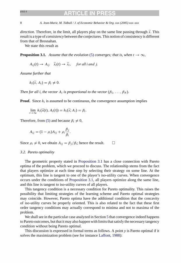
direction. Therefore, in the limit, all players play on the same line passing through ¯x. Thisresult is a type ofconsistencybetween the conjectures. This notion of consistency is differentfrom that of Bresnahan.

We state this result as

Proposition 3.1. Assume that the evolution(5) converges; that is, whent → ∞,

Aij(t) → Aij xi(t) → xi, for all i and j.

Assume further that

hi(x, Ai) = βi = 0.

Then for all i, the vectorAi is proportional to the vector(β1, . . . , βN ).

Proof. Sincehi is assumed to be continuous, the convergence assumption implies

limt→∞hi(x(t), Ai(t)) = hi(x;Ai) = βi.

Therefore, from(5) and becauseβi = 0,

Aij = (1 − ρi)Aij + ρiβj

βi.

Sinceρi = 0, we obtainAij = βj/βi; hence the result. �

3.2. Pareto optimality

The geometric property stated inProposition 3.1has a close connection with Paretooptima of the problem, which we proceed to discuss. The relationship stems from the factthat players optimize at each time step by selecting their strategy on some line. At theoptimum, this line is tangent to one of the player’s iso-utility curves. When convergenceoccurs under the conditions ofProposition 3.1, all players optimize along the same line,and this line is tangent to iso-utility curves of all players.

This tangency condition is a necessary condition for Pareto optimality. This raises thepossibility that limiting strategies of the learning scheme and Pareto optimal strategiesmay coincide. However, Pareto optima have the additional condition that the concavityof iso-utility curves be properly oriented. This is also related to the fact that these firstorder tangency conditions may actually correspond to minima and not to maxima of theproblem.

We shall see in the particular case analyzed in Section5 that convergence indeed happensto Pareto outcomes, but that it may also happen with limits that satisfy the necessary tangencycondition without being Pareto optimal.

This discussion is expressed in formal terms as follows. A pointy is Pareto optimal if itsolves the maximization problem (see for instanceLaffont, 1988):


maxx

∑j

λjΠj(x), (6)

for some numbersλj ≥ 0. A necessary condition for the Pareto optimality of pointy is thenthat there exist numbersλj ≥ 0 such that the first-order condition,

∑j

λj∂Πj

∂xi(y) = 0, (7)

holds for all i. Introduce the gradient matrix∇Π(y) = (∂Πi/∂xj(y))i,j. Then, the vectorλ = (λ1, . . . , λN ) is such thatλ∇Π(y) = 0. This implies that the matrix∇Π(y) is singular.

Let us now assume that players select, at each step of time, their strategy by solvingthe optimization problem(2). Assume that Recurrence(5) converges, resulting in a limitreference point ¯x, limit proportionality factorsAij and a limit strategy profilex. If the first-order derivatives ofΠi are continuous,x satisfies Eq.(3) for all i. Equivalently, multiplyingby βi and using the fact thatAij = βj/βi, for all i,

0 = βi∂Πi

∂xi(x) +

∑j =i

βj∂Πi

∂xj(x) =

∑j

βj∂Πi

∂xj(x).

This amounts to say that the (column) vectorβ is such that∇Π(x)β = 0. Again, this impliesthat∇Π(x) is singular.

We conclude that both the limits of the learning scheme and the Pareto optima are suchthat∇Π(x) is singular, making them “likely” to coincide. Concretely, ifx is a limit pointobtained by the convergence of the learning scheme(5), then∇Π(x) is singular, and thereexists a row vectorµ such thatµ∇Π(x) = 0. If this vector happens to be positive, thenx isa candidate solution for the maximization problem(6). In any case, the fact thatx realizesa maximum must also be checked.

4. Local stability

Our analysis will concentrate on the values of the fixed points of the Recurrence(4)and the stability of these fixed points. Numerical experiments not reported here show thatthe attraction basins of the fixed points have complicated boundaries. Obtaining a simpledescription of these basins seems hopeless. We shall therefore investigate mostly thelocalstability of the fixed points. The question will be given some fixed point of(4), what is theset of learning parameters (ρ1, . . . , ρN ) for which the recurrence converges to this pointwhen initial values are close enough to it.

For two-player games, we give a simple characterization for this set (Proposition 4.1),and we discuss precisely its geometry (Corollaries 4.2 and 4.3). ForN players, a generalresult is that this set is star-shaped (Proposition A.1). We discuss symmetric cases (forNplayers) and provide a sufficient condition for local stability with any value of (ρ1, . . . , ρN )(Proposition 4.4). When there is a complete symmetry for parameters, we show that globalconvergence occurs (Proposition 4.5).


4.1. Results for two players

When there areN = 2 players, it is possible to obtain precise structural properties onthe local stability of the learning procedure. We summarize them inProposition 4.1andCorollaries 4.2 and 4.3below. The analysis holds for the slightly generalized setting(5)for the iterations on conjectures (but with a fixed reference point ¯x). For two players, theconjectureAi that playeri makes about other players is reduced to a single number notedai.

Let f (a1, a2) be a function fromR2 to R. Consider the mapΦ from R

2 to R2 given by

Φ1(a1, a2) = (1 − ρ1)a1 + ρ1f (a1, a2) (8)

Φ2(a1, a2) = (1 − ρ2)a2 + ρ21

f (a1, a2). (9)

In the learning procedure described in Section2.1, the functionf is given by

f (a1, a2) = r2(x; a2) − x2

r1(x; a1) − x1

with two functionsr1(x; a) and r2(x; a) describing the response of players who have aconjecturea. Typically, ri(x; a) will be the result of some optimization problem, as above,but this need not be so for the argument below. In the remaining of this paper, we shall dropthe mention to ¯x in functionsri.

Define the values

S1 = − ∂f

∂a1, T1 = ∂f

∂a2, T2 = − ∂f

∂a1

1

f 2 , S2 = ∂f

∂a2

1

f 2 (10)

evaluated at point (a1, a2). In our particular learning scheme, we have the specific form:

Si = r′i(ai)rj(aj) − xj

(ri(ai) − xi)2= r′i(ai)

ai

ri(ai) − xi, Ti = r′j(aj)

1

ri(ai) − xi. (11)

The analysis reveals that the stability depends on the four valuesS1, S2, ρ1 andρ2.

Proposition 4.1. The recurrence is locally stable if and only if the following conditionshold:

ρ1ρ2(1 + S1 + S2) > 0 (12)

4 − 2(ρ1(1 + S1) + ρ2(1 + S2)) + ρ1ρ2(1 + S1 + S2) > 0 (13)

ρ1(1 + S1) + ρ2(1 + S2) − ρ1ρ2(1 + S1 + S2) > 0. (14)

The proofs of this result and of the following ones are given inAppendix A.2(availableon the JEBO Web Site).

In order to gain some insight on the extent of this domain of stability, two complementaryinvestigations are useful. First, we shall assume thatS1 andS2 (which are determined by themodel structure) are given, and we then look for which values of the learning parameters(ρ1, ρ2) the steady state is locally stable. The same analysis may be performed the otherway round: for given values (ρ1, ρ2), what is the set of values of (S1, S2) that yield a stablerecurrence?


Table 1Types of stability of the recurrence

Type Description

I All valuesII All values near (0,0), but not near (0,1), (1,0) or (1,1). Limiting condition:(13).III Some values near (0,0) in certain directions but not all Limiting conditions:(14)and(13).IV No values

For the first point of view, we are led to defining four types of situations describing thevalues of (ρ1, ρ2) for which local convergence is ensured. These are qualitatively describedin Table 1and represented inFig. 1. The convergence area is the dashed area.

The different situations can then be classified according to

Corollary 4.2. Considering the numbersS1 andS2 given by(10)evaluated at a fixed pointof the recurrence.

(a) If 1 + S1 + S2 ≤ 0, the recurrence is locally unstable for any values ofρ1 andρ2 (typeIV).

(b) If 1 + S1 + S2 > 0, S1S2 ≥ 0 andS1 + S2 < 1, then the recurrence is locally stablefor any values ofρ1, ρ2 (type I).

(c) If 1 + S1 + S2 > 0, S1S2 ≥ 0 andS1 + S2 ≥ 1, then the recurrence is of type II. Thecurve limiting the region is thehyperbolaofequation4 − 2(ρ1(1 + S1) + ρ2(1 + S2)) +ρ1ρ2(1 + S1 + S2) = 0.This region includes the points(1,0) and(0,1) , respectively,if and only ifS1 < 1 andS2 < 1.

(d) If 1 + S1 + S2 > 0, S1S2 < 0, −1 ≤ S1 < 1 and−1 ≤ S2 < 1, the recurrence is oftype I.

(e) If 1 + S1 + S2 > 0, S1 ≥ 1 and−1 ≤ S2 < 0 or S2 ≥ 1 and−1 ≤ S1 < 0, the recur-rence is of type II. The region includes the point (1,1) if and only ifS1 + S2 < 1.

Fig. 1. Types of stability used in the classification. The grey area represents the values of (ρ1, ρ2) for which localconvergence occurs.


(f) If 1 + S1 + S2 > 0, S1S2 < 0 andS1 ≤ −1 or S2 ≤ −1, the recurrence is type III. Itis defined by both inequalities(13)and(14). The point(1,1) belongs to this set if andonly if S1 + S2 < 1.

For the second point of view, consider (ρ1, ρ2) as given, the domain of values of (S1, S2)for which local stability holds can be described as follows.

Corollary 4.3. For given (ρ1, ρ2) ∈ (0,1]2, with ρ1 = ρ2, the set of(S1, S2) for whichlocal stability holds is the interior of a triangle with vertices

(2 − ρ1

ρ1 − ρ2,

2 − ρ2

ρ2 − ρ1

),

(ρ1

ρ2 − ρ1,

ρ2

ρ1 − ρ2

),

((2 − ρ1)2

ρ1(ρ2 − ρ1),

(2 − ρ2)2

ρ2(ρ1 − ρ2)

).

This nonempty triangle contains(0,0). If ρ1 = ρ2, this set is the half-plane defined byS1 + S2 > −1.

4.2. The symmetric case

In this section, we assume that there areN ≥ 2 players who have the same utility functionand, therefore, the same conjectured reactionri(x; a) = r(x; a). This situation will be calledsymmetric.

If, in addition, players share the same reference point ¯xi = x, then

Aij = 1, ∀i = j (15)

is a fixed point of the recurrence. The following proposition gives conditions for this solutionto be locally stable.

Proposition 4.4. Assume that players have the same utility function and the same referencepoint x. If x and the function r satisfy the following condition,

2N−1∑k=1

∣∣∣∣ ∂r∂ak (1, . . . ,1)

∣∣∣∣ < |r(1, . . . ,1) − x|, (16)

then, the recurrence is locally stable around the point(1, . . . ,1) for any value ofρi, i =1, . . . , N.In the case of two players, the condition is

2|r′(1)| < |r(1) − x|. (17)

The proof of this result is deferred toAppendix A.3(available on the JEBO Web Site).

Remark 4.1. The valuer(1, . . . ,1) is independent from the reference point ¯x. Indeed, it isobtained by solving the maximization problem

maxxi

Πi(xi, (x + (xi − x))j =i) = maxxi

Πi(xi, (xi)j =i)


that yields the same value for alli due to the assumed symmetry. Any symmetric Paretooutcome that maximizes the joint profit

∑i Πi(x1, . . . , xN ) has this property.

Therefore, Eq.(17) of Proposition 4.4leads to conclusion that choosing the referencepoint x at a Pareto outcome does not lead to a locally stable recurrence unless the derivativeof r vanishes ata = 1.

This will be verified in the example of Cournot’s duopoly studied later on. Similar resultshave been found for Bertrand’s duopoly (seeJean-Marie and Tidball, 2002for details).The completely symmetric case.Assume that in addition to the current assumptions, the

initial valuesAij(0) are identical. Assume also thatρi = ρ for all i. We call this situation“completely symmetric.” Then, we have a stronger result.

Proposition 4.5. In the completely symmetric case, the recurrence converges to1 for any0 < ρ < 1 and any (common) initial condition.

Proof. By recurrence,Aij(t) is the same valuea(t) for all i and j. Indeed, this is true fort = 0 by the symmetry assumptions, and if it holds fort, then

Aij(t + 1) = (1 − ρ)Aij(t) + ρ × 1 = (1 − ρ)a(t) + ρ.

The sequencea(t + 1) = (1 − ρ)a(t) + ρ clearly converges to 1 for all values ofa(0) pro-vided that|ρ| < 1 andρ = 0. �

Observe that there are cases where the use ofProposition 4.1may conclude to the lackof local stability, whereas the above proposition concludes to global convergence. This isnot a contradiction because local “instability” means that the matrix∇Φ has an eigenvaluelarger than 1. However the other eigenvalue may be less than 1, and only this one happensto have an influence in the completely symmetric case.

5. Cournot’s oligopoly

Consider the symmetric Cournot oligopoly with linear inverse demand function andconstant marginal costs. The profit function of firmi is therefore of the form

Πi(q1, . . . , qN ) =α − β

N∑j=1

qj

qi − (bqi + c)

for some positiveα, β, b andcwith qj denoting the quantity produced by firmj.We have applied the conjecture-learning scheme of Section2 to this situation. The

issue is then to find for all possible locations of the reference strategy profile whetherthere exist fixed points of Recurrence(4) and whether those fixed points are stableor not.


The details of the analysis are provided inAppendix B(available on the JEBO Web Site).The principal results obtained for this example can be summarized as follows:

• There always exists one unique fixed point to Recurrence(4) and the limiting strategiesare always Pareto optima of the problem (Proposition B.2). The quantities obtained bythe different firms in the long run areproportional to those assumed by the referencepoint. In other words, the firms obtain in the steady state the same shares as specified bythe reference quantity profile.

• In the duopoly, the local stability of the learning scheme depends on the location ofthe reference quantity profile ¯q. If the corresponding total quantityQ is larger than thequantity of the CartelQc, then the scheme is locally stable. This is the case when thereference quantity is the Nash equilibrium or a Bertrand outcome of the game. The set ofvalues of the learning parametersρi for which local stability holds shrinks as the quantityQ approaches that of the Cartel.

WhenQ is smaller thanQc, then the recurrence is structurally unstable, whatever thevalues given to the learning parameters. Convergence may occur nevertheless in partic-ular cases such as the symmetric setting of identical learning parameters and identicalreference quantities for all players.

An interesting parallel can be drawn between this situation and the one reported inOsborne (1976). Osborne analyses in which situations a Cartel solution may have somestability although it is not a Nash equilibrium. He considers the situation where oligopolistsloyal to the Cartel apply a rule by which they retaliate to a deviation of some cheating playerwith a change of her production levels. The change should be such that all firms keep thesame share of the total production. If there is a Cartel point such that the line tangent to allplayer’s isoprofits passes through the origin, then this point is stable in the sense that noplayer has an incentive to deviate from it.

One may wonder whether players may reach this Cartel solution through an adjustmentprocess. If the learning scheme is the one studied in this paper, we conclude that the Cartelmay indeed emerge, but this depends on the selected reference point. In particular, if thispoint is the Cartel point itself, convergence does not occur. If the point corresponds to alarger quantity than that of the Cartel, convergence does occur.

6. Adapting the reference point

In this section, we briefly investigate other conjecture adjustment schemes, with thepurpose of quickly assessing whether some features of the learning scheme of Section2may be retained.

6.1. Adapting the conjecture and the reference point

Since the conjectural mechanism of the agents involves a reference strategy profile ¯x andproportionality factorsAij, a general adjustment procedure should bear both ¯x and theAijs.The resulting dynamical system will now involve sequences ¯x(t), Aij(t), and effectively


played strategiesx(t). Since players optimize using the conjectural variations principle, wehave

xi(t + 1) = ri(x(t);Ai(t)).

Concerning the conjectural variations, the principle of Section2 yields

Aij(t + 1) = (1 − ρi)Aij(t) + ρixj(t) − xj(t)

xi(t) − xi(t).

For the adjustment of the reference point ¯x(t), several ideas can be explored.Following Friedman and Mezzetti (2002), one may consider using the last observed

strategy profile as a reference point for the next time period. This amounts to assumingthatx(t + 1) = x(t). More generally, if agents are somewhat cautious and prefer not to trustobserved values too much, we would have, for someµi ≥ 0,

x(t + 1) = (1 − µi)x(t) + µix(t). (18)

Alternatively, the last observationsxi(t) may be used to update the idea that playeri has ofthe reference point in the following way:

x(t + 1) = (1 − µi)x(t) + µix0, (19)

wherex0 = x(0) is the initial reference strategy profile, in which playeri stills places sometrust, measured by the weightµi. Observe that if the parametersµi are distinct, which islikely if decisions are private, then each player will have her own idea of the reference point.

Assume first that the believed reference point evolves according to(19). If the sequencesAij(t), xi(t) converge whent tends to infinity, ifri(x;A) is a continuous function in (x,A)and if µi > 0, the properties of Section3 hold. Here, the functiongi(x,A) is given by(19) andhi(x,A) = ri(x,A) − x. Indeed, we haveβi = hi(x, Ai) = 0 unless ¯x = ri(x, A)which would occur, according to the discussion of Section3.2, when the reference pointis a Pareto outcome. Convergence therefore still occurs in general to strategies that can bePareto-efficient.

On the other hand, whenµi = 0, or if the believed reference point evolves accordingto (18), Proposition 3.1does not apply anymore sinceβi = 0. Actually, the ratio (xj(t) −xj(t))/(xi(t) − xi(t)) is indeterminate in the limit, and a more refined analysis is necessary.

6.2. Adapting the reference point alone

We assume that playeri has a conjectureAij about playerj and that this conjecture doesnot change over time. On the other hand, the reference point is assumed to be updated byall players following the last observed play, as in Friedman and Mezzetti.

The resulting dynamical system bears on the reference strategy profile ¯x(t) and thestrategy profile playedx(t), but since ¯x(t) = x(t), it reduces to a recurrence on the referenceprofile:

xi(t + 1) = ri(x(t);Ai).


If this recurrence converges, its limit ¯x satisfies the fixed point equations

xi = ri(x;Ai).

Let us examine what happens in the specific context of Cournot’s duopoly, with theassumptions of Section5. In that case, the functionri is given by (see Eq.(22) in AppendixB)

ri(xi, xj;Ai) = Γ − (x1 + x2)

2(1+ Aij)+ xi

2.

Accordingly, the recurrence to study is

xi(t + 1) = Γ − (xi(t) + xj(t))

2(1+ Aij)+ xi(t)

2,

which is a linear recurrence. Its fixed point quantities are

x1 = (1 + A12)Γ

(2 + A12)(2 + A21) − 1, x2 = (1 + A21)Γ

(2 + A12)(2 + A21) − 1.

The strategy profile (x1, x2) lies on the Pareto frontier of equation{x1 + x2 = Γ/2} if andonly if A12A21 = 1. In other words, if the conjectures of both players are fixed butconsistentin the sense used in Section3.1, then stable reference strategy profiles (and also, outcomes)are Pareto-efficient.

In addition, the eigenvalues of the linear operator are readily found to be 1/2 and

λ = A12A21 − 1

2(1+ A12)(1 + A21).

One concludes that global convergence occurs when the conjecturesAij are such that thisvalue lies in the interval (−1,1). This is the case in particular for “Nash” conjectures(A12 = A21 = 0), as well as for “Pareto” conjectures such thatA12A21 = 1.

To conclude this brief analysis, we see that when the reference point of conjectures istaken as the last observed play, convergence of the profile of played strategies may or maynot occur, depending on the values of the conjectures (whether|λ| < 1 or not). When itdoes occur, this may still be to a Pareto-efficient outcome. However, for this to happen, itis necessary that the conjectures (which are now fixed) be compatible with the geometricproperty of Section3.2.

7. Conclusion and extensions

We have proposed a simple dynamic model with linear conjectures. Players anticipateproportional reactions with respect to some reference strategies (e.g. Nash strategies), they


base their choice of actions on this anticipation, and then they revise the proportionalityfactor according to observations. This mechanism has the advantage of not assuming thatplayers have the knowledge of their opponent’s payoffs, since they act only according toobservations.

This model, like the model of Friedman and Mezzetti, is an attempt to fulfill the needfor models embedding the notion of conjectures in a dynamic setting. This need has beenexpressed by many authors commenting on the concept of static conjectural variationsequilibria.

We have shown that Pareto optima are among the possible limiting strategies of theprocess. In Cournot’s oligopoly, convergence can indeed occur to Pareto optima. The anal-ysis of Bertrand’s duopoly, which is reported in Jean-Marie and Tidball, leads to similarconclusions. We have here an example in which a cooperative behavior emerges out ofa distributed individual optimization procedure when player interactions are modeled bysimple linear conjectures.

However, we have also shown that the convergence to efficient outcomes dependsstrongly on the value of the reference strategy of the linear conjecture: convergence mayoccur with a limit strategy that is not a Pareto optimum, or not occur at all. In addition, ourresults are mostly restricted tolocal convergence. Still, among this variety of behaviors, wehave observed for both Cournot’s and Bertrand’s duopolies, that taking as reference pointthe Nash equilibrium yields a local convergence towards a Pareto solution.

A future direction will be to investigate further the conjecture updating schemes intro-duced in Section6 in order to improve the stability of the convergence and avoid thedrawbacks attached to the fixed reference point. Finally, it will be interesting to endow theprocess with a more complex cost structure and study it as a real dynamic game, as in themodel of Friedman and Mezzetti. Their results allow for stronger stability properties in sucha model.

Acknowledgements

The authors wish to thank Charles Figuieres and Denis Claude for their helpful commentson this research. They also thank Claudio Mezzetti for useful pieces of advice. Credits aredue to an anonymous referee for improvements in the analysis of Section4.1.

Appendix A. Proofs of general stability results

A.1. Preliminaries

In order to characterize the stability of fixed points, we use the following well knowntheorem. The notation sp(A) stands for the spectral radius of a matrixA.

Theorem 1. Consider a mapΦ fromRN toR

N with a fixed point a such thatΦ is C2 in thevicinity of a. Let∇Φ(a) be the linearized map around this fixed point. Ifsp(∇Φ) < 1, thenthe recurrencea(t + 1) = Φ(a(t)) is locally stable around point a, in the sense that thereexists a neighborhood N of a such thata(t) converges to a for anya(0) in N.


Conversely, if this spectral radius is larger than 1, we call the recurrence “locally unstable”in the (weak) sense that the sequence of iterates will move away for almost all initialconditions. We include the limit case sp(∇Φ) = 1 in which any behavior may occur apriori.

If all eigenvalues of∇Φ are strictly larger than 1 in modulus, then the fixed point isrepulsive; the iterates will move away from it for all initial conditions excepta itself.

A simple geometric property may be deduced from the structure of the matrix∇Φ:

Proposition A.1. The set of values ofρ = (ρ1, . . . , ρN ) for which local stability occursis star shaped with respect to(0, . . . ,0): if a ρ belongs to this set, then anytρ does, for0 < t ≤ 1.

Proof. From(4), it easy to see that∇Φ = Id + DF , where Id is the identity matrix,D =diag(ρ1, . . . , ρN ) andF is a matrix independent ofρ. Let zi be eigenvalues of∇Φ forcertain values of theρj. There are the roots of the characteristic polynomialχ∇Φ(z) =det(∇Φ − zId) = χDF (z − 1). Consider nowzti, eigenvalues of∇Φ for valuestρi. Theseare the roots ofχtDF (z − 1) = χDF ((z − 1)/t). Therefore, we havezti = 1 − t + tzi, and ifall zi are inside the unit disc, so are thezti, for any 0< t ≤ 1.

A.2. Proof of Proposition 4.1 and Corollaries 4.2 and 4.3

According toTheorem 1, local stability depends on the spectral radius of the Jacobian

matrix∇Φ =[∂Φi

∂ak

]k=1,2,i=1,2

. We, therefore, proceed to compute this matrix and its char-

acteristic polynomial.From Eqs.(8) and (9), the matrix has the form

∇Φ =(

1 − ρ1(1 + S1) ρ1T1

ρ2T2 1 − ρ2(1 + S2)

),

with

S1 = − ∂f

∂a1, T1 = ∂f

∂a2, T2 = − ∂f

∂a1

1

f 2 , S2 = ∂f

∂a2

1

f 2 (10)

evaluated at some fixed point (a1, a2). Clearly,S1S2 = T1T2. Using this identity, the char-acteristic polynomial of∇Φ has the form

χ(z) = (1 − z)2 − (1 − z)(ρ1(1 + S1) + ρ2(1 + S2)) + ρ1ρ2(1 + S1 + S2). (20)

The problem is to identify the setS of values of (ρ1, ρ2) ∈ (0,1]2 for which this polynomialhas both rootsz1 andz2 strictly inside the unit disk.

Consider a polynomial of the formP(z) = z2 + bz + c. It is readily verified that bothof its roots have a modulus strictly less than one if and only ifP(−1) > 0, P(1) > 0 andP(0) = c < 1 (the product of both roots is less than one). Writing down these conditionsfor the polynomialχ(z) gives Inequalities(13), (14), and (12), respectively. This provesProposition 4.1.


Next, assume thatS1 andS2 are given. Since(12) is necessary for local stability, andsince theρi are assumed to be different from 0, we haveCorollary 4.2(a). We shall assume1 + S1 + S2 > 0 in the rest of the proof. Inequalities(13) and (14)define domains delimitedby hyperbolas of respective equations:

(H−1) ρ2 = 2ρ1(1 + S1) − 4

ρ1(1 + S1 + S2) − 2(1+ S2)

(H1) ρ2 = ρ1(1 + S1)

ρ1(1 + S1 + S2) − (1 + S2).

In the case whereS1S2 ≥ 0, then Inequality(14) is always satisfied. The setS is thereforedefined by Inequality(13). It is nonempty since this inequality clearly holds for small valuesof ρ1 andρ2. The points (1,0), (0,1) or (1,1) satisfy condition(13) if and only if S1 < 1,S2 < 1 andS1 + S2 < 1, respectively, but if this last condition is satisfied withS1S2 ≥ 0,it implies the two first ones. This leads to cases (b and c) ofCorollary 4.2.

We now proceed to cases (d–f). WhenS1S2 < 0, the hyperbola (H−1) is increasing. Itpasses through the points (0,2/(1 + S2)) and (2/(1 + S1),0). If |S1| < 1 and|S2| < 1, then(H−1) does not intersect the square (0,1]2.

On the other hand, the hyperbola (H1) passes through point (0,0). When (1+ S1)(1 +S2) ≤ 0, it is decreasing and concave (or is degenerate and constant ifS1 or S2 equals−1),and does not intersect the square domain (ρ1, ρ2) ∈ (0,1]2. This leads to case (d), wherenone of these curves enters this domain, and (e) where (H−1) only enters it.

Finally, when (1+ S1)(1 + S2) > 0, (H1) does intersect the square (0,1]2, and we havecase (f).

This concludes the proof ofCorollary 4.2. The proof ofCorollary 4.3results fromelementary geometric calculations. Since Conditions(12)–(14)are linear inS1 andS2, thedomainS is the interior of a triangle.

A.3. Proof of Proposition 4.4

According toTheorem 1, the spectral radius of the Jacobian matrix∇Φ should be lessthan 1. A sufficient condition for this is that∑

k,.

∣∣∣∣∂Φi,j

∂Ak.

∣∣∣∣ < 1, (21)

for all i, j. We shall use this condition.SinceΦi,j depends only on the variablesAi. andAj., we have

∑k,.

∣∣∣∣∂Φi,j

∂Akl

∣∣∣∣ =∑.=i

∣∣∣∣∂Φi,j

∂Ai.

∣∣∣∣+∑.=j

∣∣∣∣∂Φi,j

∂Aj.

∣∣∣∣ =∣∣∣∣1 − ρi − ρi

∂r(Ai)

∂Aij

r(Aj) − x

(r(Ai) − x)2

∣∣∣∣+ρi

∑i=.,j =.

∣∣∣∣∂r(Ai)

∂Ai.

r(A.) − x

(r(Ai) − x)2

∣∣∣∣+ ρi∑.=j

∣∣∣∣∂r(Aj)

∂Aj.

1

r(Aj) − xj

∣∣∣∣ .


When evaluated atAi = Aj = 1= (1, . . . ,1), there remains

∑k,.

∣∣∣∣∂Φi,j

∂Akl

∣∣∣∣ ≤ 1 − ρi + ρi

N−1∑k=1

∣∣∣∣ ∂r∂ak (1)

∣∣∣∣ 1

|r(1) − x| + ρi∑k =j

∣∣∣∣ ∂r∂ak (1)

∣∣∣∣ 1

|r(1) − x|

= 1 − ρi + 2ρi

N−1∑k=1

∣∣∣∣ ∂r∂ak (1)

∣∣∣∣ 1

|r(1) − x| .

If Condition (16)holds, then Condition(21)holds for allρi > 0.

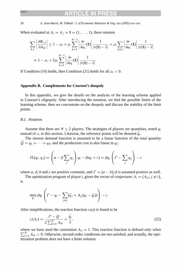
Appendix B. Complements for Cournot’s duopoly

In this appendix, we give the details on the analysis of the learning scheme appliedto Cournot’s oligopoly. After introducing the notation, we find the possible limits of thelearning scheme, then we concentrate on the duopoly and discuss the stability of the limitpoints.

B.1. Notation

Assume that there areN ≥ 2 players. The strategies of players are quantities, notedqiinstead ofxi in this section. Likewise, the reference points will be denoted ¯qi.

The inverse demand function is assumed to be a linear function of the total quantityQ = q1 + · · · + qN and the production cost is also linear inqi:

Πi(qi, qj) =α − β

∑j

qj

qi − (bqi + c) = βqi

Γ −

∑j

qj

− c

whereα, β, b andc are positive constants, andΓ = (α − b)/β is assumed positive as well.The optimization program of playeri, given the vector of conjecturesAi = (Aij; j = i),

is

maxqi

βqi

Γ − qi −

∑j =i

(qj + Aij(qi − qi))

− c.

After simplifications, the reaction functionri(a) is found to be

ri(Ai) = Γ − Q

2∑N

k=1Aik

+ qi

2, (22)

where we have used the conventionAii = 1. This reaction function is defined only when∑Ni=1Aik > 0. Otherwise, second-order conditions are not satisfied, and actually, the opti-

mization problem does not have a finite solution.


B.2. Existence and Pareto optimality of fixed points

We prove in this section the following proposition.

Proposition B.2. The unique fixed points of Recurrence(4) areAij = qj/qi. The corre-sponding strategies are Pareto efficient.

Proof. According to Section3, possible limits of(4) are of the formAij = βj/βi, withβi = ri(Ai) − qi. Using Eq.(22), we obtain that

βj = βjΓ − Q

2∑

i βi− qj

2,

and then by adding these equations, that∑

j βj = (Γ − 2Q)/2, so that

βj = qi

2

Γ − 2Q

Q.

Finally, the only fixed point of the recurrence on conjectures isAij = βj/βi = qj/qi. Usingthese values in the reaction, function gives the steady state quantities

qi = Γ

2

qi

Q.

These verify

N∑i=1

qi = Γ/2.

It is well known that for this symmetric oligopoly, the set of Pareto solutionsqi is preciselygiven by this equation. Therefore, the steady state quantities are always Pareto efficient. Thelearning procedure selects among the Pareto outcomes the only one with both quantitiesproportional to that of the reference point.

B.3. Local stability in the symmetric case with identical reference points

In the symmetric case ¯qi = q = Q/N. Proposition 4.4provides a necessary conditionfor the local stability of the recurrence around the fixed point (1, . . . ,1) for any valueof (ρ1, . . . , ρN ). Since the reaction function is given by Eq.(22), Condition(16) is, aftersimplifications,

2N − 1

N|Γ − Q| < |Γ − 2Q|.


Fig. B.1. Zones of stability in the Cournot case (Γ = 1).

This is never satisfied for 0≤ Q ≤ Γ/2. For Γ/2 ≤ Q ≤ Γ , this is equivalent toQ >

(3N − 2)Γ/(4N − 2). ForN = 2 players, this givesQ > 2Γ/3, but the detailed analysisbelow shows that actually,Q > Γ/2 ensures the local convergence; seeFig. B.1.

B.4. Local stability for two players

We now turn to the local stability issue for a two-players game. As before, we simplifythe notation for the conjecture of playeri to a single number notedai.

According to the analysis of Section4, we need the values of

Si = r′i(ai)rj(aj) − qj

(ri(ai) − qi)2,

evaluated at the fixed point (a∗1, a

∗2) = (q2/q1, q1/q2). Here,ri is given by Eq.(22):

ri(a) = Γ − qj + aqi

2(a + 1), r′i(a) = − Γ − Q

2(a + 1)2.

After simplifications,

Si = − qi

Q

Γ − Q

Γ − 2Q,

whereQ = q1 + q2. Looking at the discussion ofCorollary 4.2, we see that sinceS1S2 ≥ 0,only cases (a–c) may occur. For a detailed analysis of the convergence, the limiting casesto consider areS1 + S2 = −1, S1 + S2 = 1, S1 = 1 andS2 = 1. Expressed as conditions


on (q1, q2), the interesting sets turn out to be

{S1 + S2 > −1} = {q1 + q2 > Γ2 }

{S1 + S2 = 1} = {q1 + q2 = 2Γ3 }

{S1 = 1} = {2q21 + 5q1q2 + 3q2

2 − Γ (q1 + 2q2) = 0}{S2 = 1} = {2q2

2 + 5q1q2 + 3q21 − Γ (q1 + 2q2) = 0},

with q1 > 0,q2 > 0 andq1 + q2 ≤ Γ . The two curves{S1 = 1} and{S2 = 1} intersect at thepoint (3Γ/10,3Γ/10) (seeFig. B.1). The line{S1 + S2 = 1} contains the Nash equilibrium(Γ/3, Γ/3).

According toProposition 4.2, it is necessary for local stability that 1+ S1 + S2 > 0,that is to say,Q > Γ/2. Under this condition, we haveS1 ≥ 0 andS2 ≥ 0. In particular,S1S2 ≥ 0.

Next, assume that 1− S1 − S2 > 0; that turns out to be equivalent toQ > 2Γ/3. Then,1 − S1 > S2 > 0 and 1− S2 > 0. Therefore,Proposition 4.2(b) applies, and the recurrenceis always stable. Finally, in the case 1− S1 − S2 < 0, the recurrence is unstable for somevalues ofρ1 or/andρ2.

The result of this analysis is depicted inFig. B.1. Between the linesQ = Γ/2 andQ = 2Γ/3, the recurrence is of type II with different variants according to whether points(1,0) and (0,1) give stability or not.

The case where the reference point is the Nash equilibrium is a limit case since this pointlies on the line that separates the zone of stability of type I (stability for allρi) and that oftype II (stability away from (1,1)). Therefore, the recurrence is locally convergent exceptwhen (ρ1 = ρ2 = 1).

The case where the reference point is a Pareto outcome (the line ¯q1 + q2 = Γ/2) is alsoa limiting case. In this case, the matrix∇Φ is not even defined since theSi are infinite. Thisconfirms the observations ofRemark 4.1this case.

B.5. Particular cases

According toProposition 4.5, the completely symmetric case exhibits a particular con-vergence property. Indeed, assume thatq1 = q2, ρ1 = ρ2 and a1(0) = a2(0). Then, theconvergence is global in this case. Note that when ¯q1 + q2 < Γ/2, we have concluded thatthe limit is locally unstable in general. As noted earlier, this is not a contradiction becauseparticular sets of initial values may nevertheless exhibit an attraction behavior; this is pre-cisely the case here. Any perturbation in the process may destroy this convergence.

A second interesting case is whenQ = q1 + q2 = Γ . Then,(22)becomes

ri(a) = qi

2,

independently ofa. The learning scheme(4) becomes

ai(t + 1) = (1 − ρi)ai(t) + ρiqj

qi.


Therefore, the convergence is global in this case also. We already knew that it was locallyconvergent usingProposition 4.4, becauser′(1) = 0. Of course, such a value for ¯q is nota reasonable economic situation, but the result is that maximizing players will move awayfrom it and end up playing a Pareto-efficient outcome.

References

Bowley, A.L., 1924. The Mathematical Groundwork of Economics. Oxford University Press, Oxford.Basar, T., Turnovsky, S.J., d’Orey, V., 1986. Optimal strategic monetary policies in dynamic interdependent

economies. Springer Lecture Notes on Economics and Management Science, vol. 265, pp. 134–178.Bresnahan, T.F., 1981. Duopoly models with consistent conjectures. American Economic Review 71, 934–945.Cabral, L.M.B., 1995. Conjectural variations as a reduced form. Economics Letters 49, 397–402.Dockner, E.J., 1992. A dynamic theory of conjectural variations. The Journal of Industrial Economics 40, 377–395.Fershtman, C., Kamien, M.I., 1985. Conjectural equilibrium and strategy spaces in differential games. Optimal

Control Theory and Economic Analysis 2, 569–579.Friedman, J.W. (1977). Oligopoly and the Theory of Games, North-Holland, Amsterdam.Friedman, J.W., Mezzetti, C., 2002. Bounded rationality, dynamic oligopoly, and conjectural variations. Journal

of Economic Behavior and Organization 49, 287–306.Frisch, R.(1951). Monopoly, polypoly: the concept of force in the economy, International Economic Papers, 1,

23–36. Reprinted from: Monopole, polypole: La notion de force enEconomie, Nationaløkonomisk Tidsskrift,71 (1933) 241–259.

Fudenberg, D., Levine, D.K., 1998. The Theory of Learning in Games. MIT Press, Boston.Itaya, J.-I., Dasgupta, D., 1995. Dynamics, consistent conjectures, and heterogeneous agents in the private provision

of public goods. Public Finance/Finances Publiques 50, 371–389.Jean-Marie, A., Tidball, M., 2002. Adapting Behaviors through a Learning Process, Working Paper LAMETA DT

2002-10, University of Montpellier 1.Laitner, J., 1980. Rational duopoly equilibria. The Quarterly Journal of Economics, 641–662.Laffont, J.-J., 1988. Fundamentals of Public Economics. MIT Press.Lindh, T., 1992. The Inconsistency of consistent conjectures. Coming back to cournot. Journal of Economic

Behavior and Organization 18, 69–90.Osborne, D.K., 1976. Cartel problems. American Economic Review 66, 835–844.Slade, M., 1995. Empirical games: the oligopoly case. Revue Canadienne d’Economique 28, 368–402.Worthington, P.R., 1969. Strategic investment and conjectural variations. International Journal of Industrial Orga-

nization 8, 315–328.

Adapting behaviors through a learning process

Documents

Transcript of Adapting behaviors through a learning process