Adapting Materialized Views after Redefinitions

Ashish Gupta* Inderpal S. Mumick Kenneth A. Rossl

IBM Almaden Research Center AT&T Bell Laboratories Columbia University

ashish@almaden. ibm.com mumick@lresearch. att. com kar@cs.columbia. edu

Abstract

We consider a variant of the view maintenance problem:

How does one keep a materialized view up-to-date when

the view definition itself changes? Can one do better

than recomputing the view from the base relations?

Traditional view maintenance tries to maintain the

materialized view in response to modifications to the

base relations; we try to “adapt” the view in response

to changes in the view definition.

Such techniques are needed for applications where the

user can change queries dynamically and see the changes

in the results fast. Data archaeology, data visualization,

and dynamic queries are examples of such applications.

We consider all possible redefinitions of SQL SELECT-

FROM-UHERE-GROUPBY, UNION, and EXCEPT views, and

show how these views can be adapted using the old

materialization for the cases where it is possible to do

so. We identify extra information that can be kept with

a materialization to facilitate redefinition. Multiple

simultaneous changes to a view can be handled without

necessarily materializing intermediate results. We iden-

tify guidelines for users and database administrators

that can be used to facilitate efficient view adaptation.

1 Introduction

Visualization applications try to visualize views

over the data stored in a database. The view is

materialized, and a graphical display program may

*Research supported by NSF grants IRI–91–16646 andIRI-92-23405.

t Research supported by a grant from the AT8zT Founda-tion, by a David and Lucile Packard Foundation Fellowshipin Science and Engineering, by a Sloan Foundation Fellow-ship, by NSF grants IRI-9209029, CDA-90-24735, and by anNSF Young Investigator award.

Permission to copy without fee all or part of this material isgranted provided that the copies are not made or distributed fordirect commercial advantage, the ACM copyright notice and thetitle of the publication and Its date appear, and notice is giventhat copying is by permission of the Association of ComputingMachinery.To copy otherwise, or to republish, requiresa fee andlor s~ecific ~ermission.._—._,..SIGMOD ‘ 95;San Jcke , CA USA@ 1995 ACM 0-89791-731 -6/95/0005 ..$3.50

present the data in the view visually, If the user

changes the view definition, the system must be

able to recompute the view fast in order to keep

the application interactive. An interface for such

queries in a real estate system is reported in [WS93],

where they are called dynamic queries [AWS93].

Data archaeology [BST+ 92, BST+ 93] is another

application where an archaeologist tries to discover

rules about data by formulating queries, looking

at the results of the query, and then changing the

query iteratively as the archaeologist’s understand-

ing improves.

We consider the problem of recomputing a ma-

terialized view in response to changes made to the

view definition, that is, in response to redefinition of

the view. We call this problem the “view adaptation

problem.”

l.l Motivating Example

Example 1.1: Consider the following relations E (em-

ployees), W (works), and P (projects):

E(Ernp#, Name, Address, Age, Salary).

W(Emp#, Proj#, Hours).——P(Proj#, Projname, Leader#, Location, Budget).

The key of each relation is underlined. Consider a

graphical interface used to pose queries on the above

relations using SELECT, FROM, WHERE,GROUPBY,and

other SQL constructs. For instance, consider the

following view defined by query Q1.

CREATE VIEW V AS

SELECT Emp#, Proj#, Salary

FROM E & W

WHERE Salary >20000 AND Hours >20

The natural join between relations E and W on

attribute Emp# is specified as a part of the FROM

clause using the “&” sign. Query QI might be

specified graphically using a slider for the Salary

attribute and another slider for the Hours attribute.

As the position of these sliders is changed, the

display is updated to reflect the new answer.

211

Say the user shifts the slider for the Salary

attribute making the first condition Sa/ary >25000.

The answer to this new query can be computed

easily from the answer already displayed on the

screen. All those tuples that have Salary more

than 20000 but not more than 25000, are removed

from the display. This incremental computation is

much more efficient than recomputing the view from

scratch.

Not all changes to the view definition are so

easily computable. For instance, if the slider for

Sa/ary is moved to lower the threshold of interest

to Salary > 15000, then the above computation is

not possible. However, we can still infer that (a)

the old tuples still need to be displayed and (b)

some more tuples need to be added, namely, those

tuples that have salary more than 15000 but not

more than 20000. Thus, even though the new query

is not entirely computable using the answer to the

old query, it is possible to substantially reduce the

amount of recomputation.

Now, say the user decides to change Q1 by joining

it with relation P and then computing an aggregate.

That is view V now is defined by a new query Qz:

CREATE VIEW V AS

SELECT Proj#, Location, SU1.f($alary)

FROM E&W&P

WHERE Salary >20000 AND Hours >20

GROUPBY proj#, Location

Thus QZ requires that Q1 be joined with relation

P on attribute Proj# and the resulting view be

grouped by Proj# and Location. Note that the

key for relation P is Proj# and Proj# is already

in the answer to query Q1. Thus, to compute Q2

we need only look up the Location attribute from

the relation P using the value of Proj# for each

tuple in the current answer set. (To avoid having

to materialize Q2 separately from Q1, we could

reserve in advance free space in each record of Q1

so that answering Q2 consists of a simple in place

append of an extra attribute to each existing tuple.)

The resulting set of tuples is aggregated over the

required attributes to compute the answer to query

Q2

Finally, say the user changes view V to compute

the sum of salaries for each Location that appears

in Q2. The answer to this query (call it Q3) is

computable using only the result of Q2. Because

the grouping attributes of Q2 are a superset of the

grouping attributes of Q3, each group of Q2 is a

subgroup of a group in Q3. Thus, multiple tuples in

the result of Q2 are combined together to compute

the answer to Q3. ❑

We focus on changing a single materialized view,

and on recomputing the new materialization using

the old materialization and the base relations.

In this paper we do not consider how multiple

materialized views may be used to further assist the

adapt ation process.

1,2 Results

WJe define the process of redefining a view as a

sequence of local changes in the view definition, The

adaptation is expressed as an additional query or

update upon the old view and the base relations

that needs to be executed to adapt the view

in response to the redefinition. We identify a

basic set of local changes so that a sequence of

local changes can be maintained by concatenating

the maintenance process for each local change.

In almost all cases, this concatenation can be

performed without materializing the intermediate

results, yielding a single adaptation method for

arbitrary changes to a view definition.

We present a comprehensive study of different

types of local changes that can be. made to a view,

and present algorithms to maintain the views in re-

sponse to these changes. These algorithms integrate

smoothly with a cost-based query optimizer, The

optimizer considers the additional plans provided

by the algorithms and uses one of them if its cost is

lower than the cost of rematerializing the view.

We show that the maintenance in response to a

redefinition is facilitated by keeping a small amount

of extra information (beyond the view definition’s

attributes themselves). We only consider informa-

tion that can be maintained efficiently, and show

how the adaptation process can be made far more

efficient with this information.

Our work shows that (a) it is often significantly

better to use previously materialized views, and

(b) if you know in advance that you might change

the views in certain ways, then you can include

appropriate kinds of additional information in theviews.

1.3 Related Work

The problem of redefining materialized views is

related to the problem of optimizing an arbitrary

query given that the database has materialized aview V, The query can be considered to be a redefi-

nition of the view V and one may compute the query

by changing the materialization of V. However,

there is an important difference. Consider a query

that returns all the tuples in the view except one.

When framed as a query optimization problem, the

complexity of using the view is 0( IVI), where IVI is

the cardinality of the materialization of V. When

framed as a view maintenance problem, the com-

plexity of the maintenance process is O(log(lVl)).

This will impact the choice of the strategies for

212

query answering and view maintenance differently.

Further, the view adaptation approach loses the

old materialized view, while the querying approach

keeps the old view in storage.

View adaptation differs from the problem of

using materialized views to answer queries also in

that adaptation assumes the new view definition

is “close” to the old view definition, in the sense

that the view changes via a small set of local

changes. There is no such assumption in the

query-answering problem, which means that a

query compilerioptimizer would have to spend

a considerable time determining how to use the

existing views to correctly answer a given query,

Thus, adaptation considers a smaller search space

and yields a smaller but more efficient set of

standard techniques that are easily incorporated in

relational systems.

Classic [BBMR89] is a system developed at

AT&T Bell Laboratories that allows users to define

new concepts and optimizes the evaluation of their

extents by classifying the concepts in a concept hi-

erarchy, and then computing them starting with the

parent concepts. This corresponds to evaluating a

new Classic query (the new concept), using informa-

tion in several materialized views (the old concepts).

Classic has been used for data archaeology,

[LY85, YL87] look at the question of answering

queries using cached results or materialized views.

[LY85, YL87] show how to transform an SPJ (select-

project-join) query so that it is expressed com-

pletely using a given set of views, without any

reference to the base relations. They also have

the idea of augmented views where each view is

extended with keys of the underlying base relations,

[CKPS95] tackle the broader problem of trying to

answer any query given any set of view definitions.

Because they look at this more general problem,

they have a much larger search space (exponential

size) in their optimization algorithm. We have a

simple small set of extra plans to check. For the

less general problem we can do more, and do it more

efficiently.

[RSU95, LMSS95] also tackle the problem of

answering a query given any set of view definitions.

They do not consider aggregate queries.

[TS194] focuses on the broader issue of enhancing

physical data independence using “gmaps.” They

use a logical schema and then specify the underlying

physical storage structures as results of “gmap”

queries on the logical schema. User queries on

the logical schema are rewritten using one or more

gmap queries that each correspond an to access to

a physical structures. The gmap and user queries

are SPJ expressions. Query translation is similar to

using only existing views (gmaps) to compute new

213

views (user queries).

2 The System Model

2.1 Notation

We consider simple SQL SELECT-FROM-WHERE views,

in addition to views definable using UNION, differ-

ence (EXCEPT) and aggregation (GROUPBY). We use

a syntactic shorthand to avoid having to write down

all the equality conditions in a natural join.

SELECT Al, . . . . An

FROM RI&...&h

WHERE c1 Am).- ANDCj.When the relations in the FROM clause are separated

by ampersands rather than commas, we mean that

the relations RI, . . . . R. are combined by a natural

join over all attributes that are mentioned in more

than one relation. If we want an equijoin that is not

a natural join, we shall specify the equijoin condi-

tion in the FROM clause rather than in the WHERE

clause, inside square brackets. Join conditions that

are not equijoins or natural joins will be specified

in the WHERE clause. The conditions C’l,

basic, i.e., non-conjunctive conditions.

When we perform schema changes,

shorthand of the form

UPDATE V IN V SET Ai = . . .

UPDATE V IN V DROP Ai

. . . ek are

we use a

The second of these can be expressed alternatively

as an SQL2 “ALTER TABLE” statement. The first of

these can be expressed as a combination of an SQL2

ALTER TABLE statement and UPDATE statement.

Relations will be of two types - base relations and

view relations. Base relations are physically stored

by the system, and are updated directly. The view

relations are defined as views (i.e, queries) over base

relations and other view relations. A materialized

view relation has its extension physically stored by

the system. Materialized views are not updated

directly; updates on the base relations and other

view relations are translated by a view maintenance

algorithm into updates to the materialized view.

Adaptation and Recomputation When view

V is redefined, let the new definition be called

V’. When the extent of V’ is obtained utilizing

the previously materialized extent of view V, the

process will be called adapting view V. When

the extent of V’ is obtained by evaluating the

view definition, without utilizing the previously

materialized extent of view V, the process will be

called recomputing view V. We can look upon a

recomputation as a special case of adaptation where

the previously materialized extent of view V is not

used profitably.

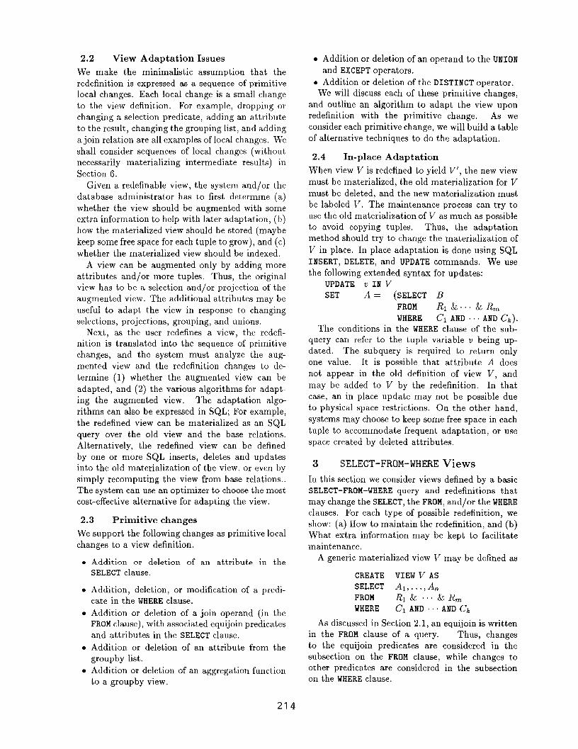
2.2 View Adaptation Issues

We make the minimalistic assumption that the

redefinition is expressed as a sequence of primitive

local changes. Each local change is a small change

to the view definition. For example, dropping or

changing a selection predicate, adding an attribute

to the result, changing the grouping list, and adding

a join relation are all examples of local changes. We

shall consider sequences of local changes (without

necessarily materializing intermediate results) in

Section 6.

Given a redefinable view, the system andlor the

database administrator has to first determine (a)

whether the view should be augmented with some

extra information to help with later adaptation, (b)

how the materialized view should be stored (maybe

keep some free space for each tuple to grow), and (c)

whether the materialized view should be indexed.

A view can be augmented only by adding more

attributes and/or more tuples. Thus, the originalview has to be a selection and/or projection of the

augmented view. The additional attributes may be

useful to adapt the view in response to changing

selections, projections, grouping, and unions.

Next, as the user redefines a view, the redefi-

nition is translated into the sequence of primitive

changes, and the system must analyze the aug-

mented view and the redefinition changes to de-

termine (1) whether the augmented view can be

adapted, and (2) the various algorithms for adapt-

ing the augmented view. The adaptation algo-

rithms can also be expressed in SQL; For example,

the redefined view can be materialized as an SQL

query over the old view and the base relations.

Alternatively, the redefined view can be defined

by one or more SQL inserts, deletes and updates

into the old materialization of the view, or even by

simply recomputing the view from base relations..

The system can use an optimizer to choose the most

cost-effective alternative for adapting the view.

2.3 Primitive changes

We support the following changes as primitive local

changes to a view definition.

0

●

●

●

●

Addition or deletion of an attribute in the

SELECT clause.

Addition, deletion, or modification of a predi-

cate in the WHERE clause.

Addition or deletion of a join operand (in the

FROM clause), with associated equijoin predicates

and attributes in the SELECT clause.

Addition or deletion of an attribute from the

groupby list.

Addition or deletion of an aggregation function

to a groupby view.

● Addition or deletion of an operand to the UNION

and EXCEPT operators.

● Addition or deletion of the DISTINCT operator.

We will discuss each of these primitive changes,

and outline an algorithm to adapt the view upon

redefinition with the primitive change. As we

consider each primitive change, we will build a table

of alternative techniques to do the adaptation.

2.4 In-place Adaptation

When view V is redefined to yield V’, the new view

must be materialized, the old materialization for V

must be deleted! and the new materialization must

be labeled V, The maintenance process can try to

use the old materialization of V as much as possible

to avoid copying tuples, Thus, the adaptation

method should try to change the materialization of

V in place. In place adaptation is done using SQL

INSERT, DELETE, and UPDATE commands. we use

the following extended syntax for updates:

UPDATE V IN V

SET A = (SELECT 1?

FROM R1&.. &Rm

WHERE CI AND... AND Ck).

The conditions in the WHERE clause of the sub-

query can refer to the tuple variable w being up-

dated. The subquery is required to return only

one value. It is possible that attribute A does

not appear in the old definition of view V, and

may be added to V by the redefinition. In that

case, an in place update may not be possible due

to physical space restrictions. On the other hand,

systems may choose to keep some free space in each

tuple to accommodate frequent adaptation, or use

space created by deleted attributes.

3 SELECT-FROM-WHERE Views

In this section we consider views defined by a basic

SELECT-FROM-WHERE query and redefinitions that

may change the SELECT, the FROM, and/or the WHERE

clauses. For each type of possible redefinition, we

show: (a) How to maintain the redefinition, and (b)

What extra information may be kept to facilitate

maintenance.

A generic materialized view V may be defined as

CREATE VIEW V AS

SELECT Al, . . . . An

FROM R1&... iURmWHERE c1 AND ~. . AND ck

AS discussed in Section 2.1, an equijoin is written

in the FROM clause of a query.

to the equijoin predicates are

subsection on the FROM clause,

other predicates are considered

on the WHERE clause.

Thus, changes

considered in the

while changes to

in the subsection

214

3.1 Changing the SELECT Clause

Reducing the set of attributes that define a view V

is straightforward: In one pass of the old view we

can project out the unneeded attributes to get the

new view. Alternatively, one could simply keep the

old view V, and make sure that accesses to the new

view V’ are obtained by pipelining a projection at

the end of an access to V.

Adding attributes to a view is more difficult.

One solution, is to keep more attributes than those

needed for V in an augmented relation W, and to

perform the projection only when references to V

occur. In that case, we can add attributes to the

view easily if they are attributes of W.

The solution mentioned above may be appropri-

ate for a small number of attributes. However, when

there are several base relations and many attributes,

keeping a copy of all of the attributes may not

be feasible. In such cases, we shall prefer where

possible to keep ~oreign keys into the base relations.

Example 3.1: Suppose our database consists of

three relations E, W, and P as in Example 1.1,

Define a view V as

CREATE VIEW V AS

SELECT Name, Projname

FROM E& W’&P

WHERE Location= New- York

Keeping all of the attributes in an augmented re-

lation would require maintaining eleven additional

attributes. Alternatively, we could just keep Emp#

and Proj# in addition to Name and Projname in an

augmented relation, say G.

Suppose we wished to add the Address attribute

to the view. We could do this addition incremen-

tally by scanning once through relation G, and

doing an indexed lookup on the E relation based

on Emp#. This can be expressed as:

UPDATE g IN G

SET Address = (SELECT Address

FROM E

WHERE E.Emp# = g, Emp#).

The update could be done in place, or it could

be done by copying the result into a new version

of G. A query optimizer could also rewrite the

update statement into a join between E and G

and modify the tuples of G as they participate in

the join. In either case, the cost of updating

G is easily estimated using standard cost-based

optimization techniques, and is likely to be far less

than recomputing the entire three-way join. O

Often the original view itself keeps the key

columns for one of the base relations. Thus, if view

V includes the key for a base relation Ii, or the key

of R is equated to a constant in the view definition,

and a redefinition requires additional columns of R,

then the view can be adapted by using the keys

present in the old materialization of the view to pick

the appropriate tuples from relation R. Sometimes,

adaptation can be done even in the absence of a

key for R in the view. A sound and complete test

for adaptation can be constructed using conjunc-

tive query containment [U11$9, GSUW94], and is

discussed in the full version of this paper.

Changing the DISTINCT Qualifier. Suppose

that a user adds a DISTINCT qualifier to the

definition of a view that did not previously have one.

Thus we have to delete duplicate entries from the

old view to obtain the new view. This adaptation is

fairly simply expressed as a SELECT DISTINCT over

the old view to obtain the new view. Deleting a

DISTINCT qualifier is more difficult, since it is not

clear how many duplicates of each tuple should be

in the new view. Techniques to do so are discussed

in the full version of this paper [G MR95].

An alternative is to augment the view so as to

always keep a count of the number of derivations

for each tuple in the view. In this case, changes

to the DISTINCT Qualifier can be handled easily by

either presenting the count to the user, or by hiding

the count.

3.2 Changes in the WHERE Clause

In this section we discuss changes to a condition in

the WHERE clause. We do not distinguish between

conditions on a single relation and conditions on

multiple relations (i.e., ‘join conditions” ) in the

WHERE clause.

Let C! be a new condition. (Without loss of

generality, we assume we are changing C’l to C’{ in

our generic view. ) We want to efficiently materialize

V’, which could be defined as

CREATE VIEW V’ AS

SELECT Al, . . . . An

FROM RI&... &Rm

WHERE C; AND . . . AND ck

by taking advantage of the fact that V has already

been materialized.

Algebraically, V’ = V U V+ – V- where

SELECT Al, . . . . An

V+= FROM RI&...&Rm

WHERE c{ AND NOT Cl AND . . . AND C~

SELECT Al, . . . . An

V-= FROM R1&... &Rm

WHERE NOT C{ AND Cl AND . . ~ AND Ck

If the attributes mentioned by C~ are a subset of

{Al,..., An}, then

215

V- = SELECT Al, . . . . An FROM V WHERE NOT Cj

or

P’ - v- = sELECT AI ,.. ., An FROM V WHERE c!

V can thus be adapted as follows:

DELETE FROM V WHERE NOT ~{

INSERT INTO V

(sELECT A1, . . ..An

FROM RI&. &Rm

WHERE c; AND NOT c1 AND . . ~ AND c~ )

Alternatively, if the attributes of C{ are not

available in the view, the view adaptation algorithm

for the SELECT clause could have materialized

some extra attributes in an augmented relation W’,

or obtained these attributes using joins with the

relation containing the attribute as discussed in

Section 3.1. In this case, even if C! mentioned an

attribute not in {AI, . . . . An}, we could write V- as

above as long as all the attributes mentioned by C!

were obtainable using the techniques of the previous

section.

Thus we can see that the cost of adapting V in

either of the cases above is (at most) one selection

on V (or on the augmentation G) to adapt V into

V- V-, plus the cost of computing V+ for insertion

into V. As we shall see, in many examples the cost

of computing V+ will be small compared with the

cost of recomputing V.

Example 3.2: Let E and W be as defined in

Example 1.1. Consider a view V defined by

CREATE VIEW V AS

SELECT * FROM E & W WHERE salary> 50000

Suppose that we wish to adapt V to

SELECT * FROM E & W WHERE Saiary >60000

Let us refer to the new expression as V’. Using

the terminology above, we see that Cl is “Salary >

50000” and C{ is “Salary> 60000.” Hence V- and

P’+ can be defined as

V- = SELECT * FROM v WHERE

,$’alary <60000 AND salary >50000V+ = SELECT * FROM E & W WHERE

salary >60000 AND Salary ~ 50000

V+ is empty, since its conditions in the WHERE

clause are inconsistent with each other. Hence, the

cost of recomputing the view is (at most) one pass

over V. Now suppose that V’ is defined by

SELECT * FROM ~ & W WHERE Saiary >49000.

Then V- is empty, and V+ is given by

-..

SELECT * FROM E & W WHERE salary> 49000 AND

Salary <50000.

If there is an index on salary in E, then (with a

reasonable distribution of salary values) V U V+

might be computed much more efficiently than

recomputing V’ from scratch. The query optimizer

would have enough information to decide which is

the better strategy. ❑

Most queries that involve multiple relations use

either equijoins or use single table selection condi-

tions. For example, in one of our application envi-

ronments, making efficient visual tools for browsing

data, users are known to refine queries by changing

the selection conditions on a relation interactively.

Thus, it is likely that both the old condition Cl

and the new condition C{ are single table selection

conditions on the same attributes. Thus, the condi-

tion NOT Cl AND C; can be pushed down to a single

base relation, making the computation of V+ more

efficient.

Adding or Deleting a Condition We can

express the addition of a condition C’ in the

WHERE clause as a change of condition by adding

some tautologically true selection to the old view

definition V, then changing it to C’. The analysis

above then means that V+ is empty, and the new

view can be computed as V – V–, i.e., as a filter on

the extension of V.

Similarly, the deletion of a condition is equivalent

to replacing that condition by a tautologically true

condition. In this case, V- is empty, and the

optimizer needs to compare the cost of computing

V+’ with the cost of computing the view from

scratch.

3.3 Changing the FROM Clause

If we change an equijoin condition, then it is

not clear that V+ is efficiently evaluable. This

corresponds to our intuition, which states that if

an equijoin condition changes then there will be a

dramatic change in the result of the join, and so

the old view definition will not be much help in

computing the new join result. We note that it

is unlikely that the users will change the equijoin

predicates [G. Lehman, personal communication].

Nevertheless, there are situations where we can

make use of the old view to efficiently compute a

new view in which we have either added or deleted

relations from the FROM clause,

Adding a join relation Suppose that we add

a new relation Rm+l to the FROM clause, with

an equijoin condition equating some attribute Aof Rm+l to another attribute 1? in Ri for some

Z-lb

1 < i < m. Suppose also that we want to add

some attributes Dl, . . . . DJ from Rm+l to the view.

If B is part of the view, then the new view can

be computed as

SELECT A1, . . .. Afi. D1, Dj. ,Dj FROM V, Rm+l

WHERE A = B.

If the joining attribute A is a key for relation

Rm+l, or we can otherwise guarantee that A values

are all distinct, then we can express the adaptation

as an update (we generalize SQL syntax to assign

values to a list of attributes from the result of a

subquery that returns exactly one tuple) :

UPDATE v IN V

SET D1, . . .. Dj=(SELECT ill. Dj., Dj

FROM &z+l

WHERE Rm+l.A = v.B)

If B is not part of the view, then it still may be

possible to obtain B by joining V with Ri (assuming

that V contains a key K for Ri) and hence compute

the new view either as

UPDATE v IN V

SET D1, ..., Dj = (SELECT Dl,..., Dj

FROM Rm+l, Ri

WHERE &+l .A = Ri.B

AND V.K = Ri.K).

if A is a key in Rm+l, or as

SELECT A1, . . .. An. D1, DjFROMV,Ri,R m+l Rm+l

WHERE A = B AND V.11 = Ri.K.

if A is not guaranteed to be distinct in Rm+l.

Example 3.3: For example, suppose we have a

materialized view of customers with their customer

data, including their zip-codes. If we want to also

know their cities, we can take the old materialized

view and join it with our zip-code/city relation to

get the city information as an extra attribute. ❑

Deleting a join relation When deleting a join

operand, one has to make sure that the number of

duplicates is maintained correctly, and also allow

for dangling tuples. For R N S LX! T, when the

join with T is dropped, the system (1) needs to

go back and find R cu S tuples that did not join

with T, and (2) figure out the exact multiplicity of

tuples in the new view. The former can be avoided

if the join with T is lossless, a condition that might

be observed by the database system if the join is

on a key of T and if the system enforces referential

integrity. The latter can be avoided if the view does

not care about duplicates (SELECT DISTINCT), or if

T is being joined on its key attributes, and the key

of T is in the old view.

1. Attribute A is from relation S and the key K for Sis in view V.

2. An augmented view that keeps a count of number ofderivations of each tuple is used.

3. Attribute of condition is either an attribute of theview, or of a wider augmented stored view.

4. Dl, ..., Dj and A are attributes of Rm+I, and thejoin condition is A = B.

5. B is an attribute of V.

6. A is a key for relation 11~+1.

7. B is an attribute of R~, K is a key of R,, and X isan attribute of V.

8. Join with Rm is known to be lossless.

9. Either V contains a SELECT DISTI~CT, or the join ofRm is on a key attribute that is also present in V.

Table 1: Assumptions for the Adaptation Tech-

niques in Table 2

3.4 Summary: SELECT-FROM-WHERE views

Table 2 summarizes our adaptation techniques for

SELECT-FROM-WHERE queries. we assume that the

initial view definition is as stated at the begin-

ning of Section 3. For each possible redefinition,

we give the possible adaptations along with the

assumptions needed for the adaptation to work.

The assumptions are listed separately in Table 1.

In the full version of this paper [GMR95] we also

discuss adaptation of SELECT-FROM-WHERE queries

that originally use the DISTINCT qualifier.

Table 2 can be used in three ways. Firstly, the

query optimizer would use this table to find the

adaptation technique (and compute its cost esti-

mate) given the properties of the current schema

vis-a-vis the assumptions stated in the table. Sec-

ondly, a database administrator or user would use

this table to see what assumptions need to hold in

order to make incremental view adaptation possible

at the most efficient level. Given this information,

the views can be defined with enough extra infor-

mation so that view changes can be computed most

efficiently. Note that different collections of as-

sumptions make different types of incremental com-

putation possible, so that different “menus” of extra

information stored should be considered. Thirdly,

the database administrator could interact with the

query optimizer to see which access methods and

indexes should be built, on the base relations and on

the materialized views, in order to facilitate efficient

adaptation.

Recommendations for Augment at ion. Keep

the keys of referenced relations from which at-

tributes may be added. Store the view with padding

in each tuple for future in-place expansion. Keep

attributes referenced by the selection conditions

217

Redefined View Adaptation Technique Assumptions

SELECT A, Al, ..)AnUPDATE tIINV

FROM R1&&RtnSET A= (SELECT A

FROM(1)

WHEREs

Cl AND AND C~ WHERE S.K = u K)

SELECT A2, . . ..A*FROM Rl&. .&Rm

UPDATE uINV

WHERE Cl AND AND ilkDROP Al

SELECT DISTINCT Al, , An INSERT INTO New. VFROM RI & &Rm SELECT DISTINCT *

~ WHERE FROM VSELECT DISTINCT Al) ... A.FROM R1&&Rm Mark view as being distinct. (2)

WHERE Cl AND AND CkSELECT Al, ,Am DELETEFROM R1 &.. &Rm FROM v c; a cl, (3)

W HERE C; AND AND Ck WHERE NOT C{INSERT INTO V

SELECT A1, . . ..An DELETE SELECT AI, ,AnFROM R1&. ..&Rm FROM v FROM RI & &Rm Cj * cl, (3)

WHERE C! AND AND C. WHERE NOT C: W HERE C; AND NOT Cl. .AhD . . . AND C~

SELECT A1, . . ..An DELETEFROM R1&. .&Rm FROM v (3)

WHERE Co AND Cl AND AND C~ WHERE NOT CO

SELECT Al, ,AnINSERT INTO V

FROM R1&. &RmSELECT Al, ,AmFROM RI & &Rm

(3)

WHERE C2 AND AND C~ WHERE NOT Cl AND C2 AND AND C~

SELEC - ‘ ‘ - -UPDATE vINV

I 17DnR,f

,1,AI, . . .. An. UI, JJJ, JJJ

. &vu ,“, RI & . ..& Rm&Rm+lSET D1,..., DJ= (SELECT Dl, ,Dj (4,5,6)

WHERE Cl AND AND C~FROM Rm+]WHERE Rm+l A = u. B).

SELECT A1, . . .. An) D1. D3. ,D3INSERT INTO New-V

FROM R1&&Rm&Rm+ISELECT AI, . . ,An, DI, . . ,DjFROM V, Rm+l

(4,5)

WHERE Cl AND AND C~ WHERE A=BUPDATE wINV

SELECT A1, .,. ,An, D1, . . ..DjSET D1, .,DJ=

FROM RI & & Rrn & Rm+l(SELECT Dl, ... D3FROM Rm+l , R,

(4,6,7)

WHERE Cl AND AND C~ WHERE R-+1 A = R,.B ANDuK’= R,. K),

SELECT Al, . ., An, DI, . , DjINSERT INTO New. V

FROM RI & & Rm & Rm+lSELECT Al, , Ar., D1, . . ..D1FROM V, R,, Rm+l

(4,7)WHERE Cl AND AND Ch W HERE A= BAND VK=R, K

SELECT A1, . . ..A~FROM R1&. .& Rm_l No adaptation needed, (8,9)WHERE Cl AND AND C~SELECT A1>. ... AJFROM R1& & Rm.l

UPDATE uINVDROP A,+I, .,An

j < n, (8,9)

W HERE Cl AND AND C~

Table 2: Adaptation Techniques for SELECT-FROM-WHERE views

in the view definition, or at least keep the keys

of referenced relations from which these attributes

may be added. Keep the count of the number of

derivations for each tuple.

4 Aggregation Views

In this section, we show how to adapt views when

grouping columns and the aggregate functions used

in a materialized SQL aggregation view change.

Example 4.1: Consider again the relations of Ex-

ample 1.1. We could express the total salaries

charged to a project with the following materialized

view: We assume that an employee is nominally

employed for 40 hours per week, and that if an

employee works more or less, a proportional salary

218

is paid. Thus the charge to a project for an em-

ployee is obtained by multiplying the salary by the

fraction of the 40 hour week the employee works on

the project.

CREATE VIEW V(F’roj#, Locat,on, Proj+$a/) AS

SELECT Proj#, Location, SUM((Sal x Hours)/40)

FROM E&W&P

GROUPBY proj#, Location

Suppose we want to modify V so that it gives

a location-by-location sum of charged salaries.

This modification corresponds to removing the

Proj# attribute from the list of grouping variables

and output variables, to give the following view

definition:

CREATE VIEW V’(Location, proj~al) AS

SELECT Location, SUM((Saiary x Hours)/40)

FROM E&W&P

GROUPBY Location

Using the commutativity properties of SUM, the

query optimizer can observe that V’ can be mate-

rialized as

SELECT Location, SUM(Proj-Sal)

FROM vGROUPBY Location

In this way we can use the original view to redefine

the materialized view more efficiently.

Next, suppose we want to modify V to compute

the sum of charged salaries for each Proj#. We can

adapt V simply by dropping the Location attribute

because Proj# is the key for relation P and

functionally determines Location. The redefined

groups are the same as before. ❑

4.1 Dropping GROUPBY columns

Given an aggregation view, the set of tuples in the

grouped relation that have the same values for all

the grouping attributes is called a group. Thus, for

the original view in Example 4.1, there is one group

of tuples for each pair of (Proj#, Location) values.

For the redefined view, there is one group of tuples

for each (Location) value.

When a grouping attribute is dropped, each

redefined group can be obtained by combining

one or more original groups, so we can try to

get the aggregation function over the redefined

groups by combining the aggregation values from

the combined groups. For instance, in Example 4.1,

after dropping the Proj# attribute, the sum for the

group for a particular (Location) value was obtained

from the sum Proj-Sal of all the groups with this

Location. When we dropped the Location attribute,

we inferred that each redefined group was obtained

from a single original group. So no new aggregation

was needed

A materialized view can be adapted when group-

ing columns are dropped if

● The dropped column is functionally determined

by the remaining grouping columns, or

The aggregate functions in the redefined view

are expressible as a computation over one or

more of the original aggregation functions and

grouping attributes. Table 3 lists a few aggre-

gation functions that can be computed in such

a manner.

Table 3 is meant to be illustrative,

exhaustive. Several other aggregation

may be decomposed in this manner.

and not

functions

4.2 Adding GROUPBY Columns

In general, when adding a groupby column, we

would need to go back to the base relations since

we are looking to aggregate data at a finer level of

granularity. However, in case the added attribute

is functionally determined by the original grouping

attributes, we can add it just like we add a new

projection column (Section 3.1).

Another situation where we can add GROUPBY

columns is when there was no grouping or aggre-

gation before, In that case, the new view is formed

simply by applying the grouping and aggregation

over the old view, assuming that the attributes

needed for the grouping and aggregation are present

in the old view. Even if the needed attributes are

not present, they can be added in many cases, as

discussed previously.

4.3 Dropping/Adding Aggregation

Functions

Adapting a view to drop an aggregation function

is straightforward, similar to the case where a

column is projected out (Section 3.1). However,

it is not possible to adapt to most additions of

aggregation functions, unless the new function can

be expressed in terms of existing functions, or unless

the aggregation view is significantly augmented.

One type of augmentation requires storing the key

values of all tuples in a group in the view. This

augmentation is discussed in the full version of this

paper.

4.4 Summary: GROUPBY views

In this section we have seen several techniques

for adapting views with aggregation. A more

complete list is available in the full version of this

paper [GMR95].

Recommendations for Augmentation. Table 3

illustrates that redefinition can be helped tremen-

dously if the views are augmented with a G’01-IN~*)

aggregation fUnction.

5 Union and Difference Views

5.1 UNION

A view V maybe defined as the union of sub queries,

say VI and V2. If the definition of V changes by a

local change in either VI or V2 but not both, then

it would be advantageous to apply the techniques

developed in the previous sections to incrementally

update either the materialization of VI or V2 while

lea~ing the other unchanged.

In order to do this, we need to know which tuples

in V came from V1 and which from V2. With this

knowledge, we can simply keep the tuples from the

unchanged part of the view, and update the changed

219

Redefined Aggregation Adaptation using Original View

MIN(X) MIN(M) where Al= MIN(X) was an original aggregation column.

MAX(X) MAX(M) where M = MAX(X) was an original aggregation column.

MN(X) MIN(X), where X waa an original grouping column.

MAX(X) MAX(X), where X was an original grouping column.

Sufkf(x) SUM(S) where S = SUM(X) was an original aggregation column.

SUM(X) SUM(X x C), where C = CO i7N~*) was an original aggregation

column, and X was an original grouping column.

COUN~*) SUM(C) where C = CO UN~*) was an original aggregation

column.

A VG(X) SUM(A x C)/SUM(C) where C = COUN~*) and A = AVG(X)

were original aggregation columns.

A VG(X) SUM(X x C)/SUM( C) where C = CO UN~*) was an original

aggregation columns, and X was an original grouping column.

Table 3: Aggregate functions for a group defined as functions of subgroup aggregates.

part of the view. Thus it would be beneficial to

store with each tuple an indication of whether it

came from VI or V2. Alternatively, one could store

VI and V2 separately, and form the union only when

the whole view V is accessed.

Example 5.1: Consider the schema from Exam-

ple 1.1. Suppose we want the names of employees

who either work on a project located in New York,

or who manage a project located in New York. We

can write this view V as VI UNION V2 where VI and

Va are as follows.

VI = SELECT Name, SubQ=<’Vl” FROM E & W & P

WHERE Locatton=New- York

Va = SELECT Name, SubQ= “V2”FROM E, P [E. Emp# = P. Leader~

WHERE Location= New- York

(We would probably choose not to display the

SubQ field to the user, but to keep it as an attribute

of a larger augmented relation.) If we wanted to

change V1 so that we get only employees working

more than 20 hours per week, then we could do so

using techniques developed in the previous sections

for tuples in V with SubQ= “Vl” , and leave the other

tuples unchanged. ❑

It is easy to delete a UNION operand if we keep

track of which tuples came from which subqueries.

We simply remove from V all tuples with the

SubQ attribute matching that of the sub query being

deleted.

Adding a union operand is also straightforward:

The old union is unchanged, and the new operand

is evaluated to generate the new tuples.

5.2 EXCEPT

Example 5.2: Consider again the schema from

Example 1.1. Suppose we want the names of

employees who work on a project located in New

York, but who are not managers, We can write this

view as V1 EXCEPT V2 where V1 and V2 are defined

as follows.

CREATE

SELECT

CREATE

SELECT

c!

VIEW V1 AS

Name FROM E & W & P

WHERE Location= New- York

VIEW V2 AS

Name FROM E, P [E.Emp# = P. Leader#l

WHERE Locatton=New- York

Unlike the case for unions, the extension of

V could conceivably be much smaller than the

extensions of either V1 or Vz. Thus, we cannot argue

that in general we should keep all of the VI and Vz

tuples with an identification of whether they came

from VI or Va.

However, in two cases we can still use information

in the old view to compute the new view more

efficiently.

1.

2.

If V2 is replaced by a view V; that is strictly

weaker (i.e., contains more tuples) than V2, then

we can observe that V2– is empty, and V’ = V

EXCEPT Vz+

If V1 is replaced by a view V( that is strictly

stronger (i.e., contains fewer tuples) than V1,

then we can observe that VI+ is empty, and

V’ = V EXCEPT V1- .

If we want to subtract a new subquery V2 from

an existing materialized view V, then we can do so

220

efficiently using the first observation above. In that

case, the new view V’ is V EXCEPT V, and we can

make use of the old extension of V.

In the general case, there is another possibility

that the optimizer can consider for computing V’.

Suppose that V2 changes with both Vz+ and V2-

nonempt y. The new answer is V EXCEPT Vz+ UNION

U where U is VI n Vz-. While we probably have

not materialized V1, we can still evaluate U by

considering each tuple in Vz- and checking that it

satisfies the conditions defining VI. If V2+ and V2–

are small, then this strategy will still be better than

recomputing V’ from scratch. A symmetric case

holds if VI changes rather than V2. In order for this

strategy to be effective, the query optimizer needs

to estimate the sizes of Vz+ and VQ-. For simple

views V2 this may be achieved using selectivity

information and information about the domains of

the attributes. For complicated queries, it may be

hard to estimate these sizes.

5.3 Summary: Views with Union and

Difference

In this section we have seen several techniques for

adapting views with union and difference. A more

complete list is available in the full version of this

paper [GMR95].

Recommendations for Augmentation. Keep

an attribute identifying which subquery in a union

each tuple came from.

6 Multiple Changes to a View

Definition

So far we have considered single local changes to a

view definition. However, a user might make several

simultaneous local changes to a view definition. The

new view may easily be obtained by concatenating

the adaptations from each local change, but this

approach would materialize all of the intermediate

results, which may not be necessary.

For example, if more than one condition in the

WHERE clause is simultaneously changed, then the

analysis of Section 3.2 still applies by thinking of

Cl and C{ as conjunctions of conditions. Simi-

larly, multiple attributes may be added or deleted

from a view simultaneously using the techniques

of Section 3.1 without materializing intermediate

results. Several relations may be added to the FROM

clause using the techniques of Section 3.3 without

materializing the intermediate results.

If the new view is obtained by making changes

of different types, then we can avoid materializing

intermediate results by pipelining the results of ap-

plying one change into the computation of the next

change. Pipelining is possible if each of the basic

adaptation techniques can be applied in a single

pass over the materialized view. It turns out that,

with one exception, all techniques described in this

paper can be done in a single pass. The exception is

the use of a previously materialized view V within

an aggregation that is grouped on an attribute that

is not the (physical) ordering attribute of V. Thus,

for changes other than this one exception, it is pos-

sible in principle to cascade multiple local changes

without materializing intermediate results. Note,

if updates are done in-place, then there is little

choice but to perform the individual adaptations

sequentially.

Thus the optimizer can choose the best of

the following three choices for adaptation: (a)

applying successive in-place updates, (b) csscading

the adaptations as above, or (c) recomputing the

view from base relations.

7 Conclusions

When the definition of a materialized view changes

we need to bring the materialization up-to-date. In

this paper we focus on adapting a materialized view,

i.e., using the old materialization to help in the

materialization of the new view. The alternative to

adaptation is to recompute the view from scratch,

making no use of the old materialization. Often,

it is more efficient to adapt a view rather than

recompute it, sometimes by an order of magnitude;

a number of examples have been described in this

paper.

A number of applications, like data-archaeology

and visualization, require interactive, and thus

quick, response to changes in the definition of a

materialized view.

We have provided a comprehensive list of view

adaptation techniques that can be applied for basic

view definition changes. Each of these adaptation

techniques is itself expressed as an SQL query or

update that makes use of the old materialization.

Because the adaptation is itself expressed in SQL, it

is possible for the query optimizer to estimate the

cost of these techniques using standard cost-based

optimization. In some cases there may be several

adaptation alternatives, and each of the alternatives

would be considered in turn.

Our basic adaptation techniques correspond to lo-

cal changes in the view definition. We also describe

how multiple local changes can be combined to give

an adaptation technique for changes to several parts

of a view definition. All, but one, techniques for

adapting a view in response to a local change can

be pipelined thereby eliminating the need to store

intermediate adapted views when multiple local

changes are combined.

221

Often it is easier to adapt a view if certain ad-

ditional information is kept in the view. Such ad-

ditional information includes keys of base relations,

attributes involved in selection conditions, counts of

the number of derivations of each tuple, additional

aggregate functions beyond those requested, and

identifiers indicating which subquery in a union

each tuple came from. Depending on the type of an-

ticipated change, the view can be defined to contain

the appropriate additional information. Addition-

ally, it can be beneficial to reserve some physical

space in each record to allow in-place adaptation

involving addition of attributes,

We have derived tables of adaptation techniques

(see [GMR95] for a complete list) that can be

used in three important ways. Firstly, the query

optimizer can use the tables to find the adaptation

technique (and compute its cost estimate) given

the properties of the current schema vis-a-vis the

assumptions stated in the table. Secondly, a

database administrator or user can use the tables

to see what assumptions would need to be satisfied

in order to make view adaptation possible at the

most efficient level, and define the view accordingly.

Thirdly, the database administrator can interact

with the query optimizer to build appropriate access

methods and indexes on the base relations and on

the materialized views, in order to facilitate efficient

adaptation.

The main contributions of this paper are (a) the

derivation of a comprehensive set of view adapta-

tion techniques, (b) the smooth integration of such

techniques into the framework of current relational

database systems using existing optimization tech-

nology, and (c) the identification of guidelines that

can be provided to users and database administra-

tors in order to facilitate view adaptation.

Acknowledgments

We thank Arun Netravali for pointing out the

importance of redefinition to data visualization,

and Shaul Dar and Tom Funkhouser for discussions

of the relationship between view maintenance and

data visualization.

References

[AWS93]

[BBMR89]

[BST+ 92]

Christopher Ahlberg, Christopher Williamson,and Ben Shneidermam Dynamic Queries forinformation exploration: an implementation andevaluation. In Ben Shneiderman, editor, Sparks

of Innovation in Human-Computer Interaction.

Ablex Publishing Corp, 1993.

Alex Borgida, et al. CLASSIC: A structural data

model for objects. In A CM- SIGMOD, pages 59–

67, June 1989.

Ronald J. Brachnmn, et al. Knowledge rep-

resentation support for data archaeology. In

[BST+93]

[CKPS95]

[GMR95]

[GMS93]

[GSUW94]

[LMS94]

[LMSS95]

[LY85]

[MPR90]

[RSU95]

[TS194]

[U1189]

[WS93]

[YL87]

First International Conference On InjoTmation

and Knowledge Management, pages 457–464,

November 1992.

Ronald J. Brachman, et al. Integrated sup.

port for data archaeology. International JOUT-

nal o.f Intelligent and Cooperative Information

Systems, 2:159–185, 1993.

Surajit Chaudhuri, Ravi Krishnamurthy, Spyros

Potarnianos, and Kyuseok Shim. Optimizing

queries with materialized views. To appem in

Proceedings of International Conference on Data

Engineering, 1995.

Ashish Gupta, Inderpal Singh Mumick, and Ken-

neth A. Ross. Adapting materialized views after

redefinitions. Columbia University Technical Re-

port number CUCS-O1O-95, March 1995.

Ashish Gupta, Inderpaf Singh Mumick, and V. S.

Subrahmanian. Maintaining views incremen-tally. In SIGMOD, pages 157–167, 1993,

Ashish Gupta, Yehoshua Sagiv, Jeffrey D. Unm-

an, and Jennifer Widom. Constraint Checking

with Partiaf Information, In PODS, pages 45–55,

1994.

Alon Levy, Inderprsf Singh Mumick, and

Yehoshua Sagiv. Query optimization by predi-

cate movearonnd. In Bocca et al. VLDB, pages

96-107, 1994.

Alon Y. Levy, Alberto O. Mendelzon, Yehoshua

Sagiv, and Divesh Srivastava. Answering queries

using views. To appear in PODS, 1995.

P. A. Larson and H.Z. Yang. Computing queries

from derived relations. In VLDB , pages 259-

269, 1985.

I. S. Mumick, H. Pirahesh, and R. Ramakrkh-

ns,n. The magic of duplicates and aggregates. In

VLDB, 1990.

Anand Rajaraman, Yehoshua Sagiv, and Jeffrey

Unman. Answering queries using templates with

binding patterns. To appear in PODS, 1995.

Odysseas G. Tsatalos, Marvin H. Solomon, and

Yaunis E. Ioannidis. The GMAP: A versatile tool

for physical data independence. In Bocca et al.

VLDB, pages 367–378, 1994.

Jeffrey D. Unman, Principles of Database and

Ii_nowledge-Base Systems, Volume 2. Computer

Science Press, 1989.

Christopher Williamson and Ben Shneiderman.

The Dynamic HomeFinder: evaluating Dynamic

Queries in a real- estate information exploration

system. Iu Ben Shneiderman, editor, Sparks

o~ Innovation in Human -Computev Interaction.Ablex Publishing Corp, 1993,

H. Z. Yang and P, A. Larson. Query transforma-

tion for PSJ-queries. In VLDB, pages 245–254,

1987.