Acrobat Distiller, Job 64
319
-
Upload
khangminh22 -
Category
Documents
-
view
1 -
download
0
Transcript of Acrobat Distiller, Job 64


New Zealand MunicipalWastewater Monitoring
Guidelines
NZ Water Environment ResearchFoundation
Edited by David Ray (NIWA)
October 2002

ISBN 1-877134-40-6
Published by the New Zealand Water Environment Research Foundation, October 2002
These Guidelines were funded principally through the Minister for the Environment’sSustainable Management Fund, administered by the Ministry for the Environment.
SMF No. 4173
© The Crown (acting through the Minister for the Environment), 2002.
Copyright exists in this work in accordance with the Copyright Act 1994. However, theCrown authorises and grants a licence for the copying, adaptation and issuing of this
work for any non-profit purpose. All applications for reproduction of this work for anyother purpose should be made to the Ministry for the Environment.
Citation:NZWERF (2002). New Zealand Municipal Wastewater Monitoring Guidelines.
(Edited by D.E. Ray). NZ Water Environment Research Foundation. Wellington, NewZealand.
Copies of this publication can be obtained from:NZ Water Environment Research Foundation
PO Box 1301Wellington
www.nzwerf.org

i
FOREWORD
Discharges from wastewater treatment plants have a significant impact on theenvironment. Effective monitoring is vital to ensure that discharges from wastewatertreatment plants are not resulting in adverse environmental or health effects.
Designing wastewater monitoring programmes can be complex. Wastewater treatmentplants discharge into a range of receiving environments, including into rivers, estuaries,streams, lakes, and on to land. And the discharges vary in nature depending on the levelof industrial input and the type of treatment process.
The purpose of the Ministry for the Environment’s Sustainable Management Fund is tosupport the community, industry, iwi, and local government in a wide range of practicalenvironmental management initiatives. I am pleased that the fund has been able tosupport the development of these guidelines to assist in the development of monitoringprogrammes for municipal wastewater discharges.
The core principle of these guidelines is that the higher the potential risks of thedischarge to the receiving environment, the greater the level of monitoring that will berequired. This approach works best if the experience of the treatment plant operator,regulator and local knowledge and values are incorporated into the design of themonitoring programme.
These guidelines provide a framework for councils and their communities to workcollectively through a risk-based process, prior to a resource consent renewal or review,to develop an appropriate environmental monitoring programme.
Hon Marian L Hobbs
Minister for the Environment

ii
PREFACE
The Wastewater Monitoring Guidelines were developed under a Ministry for the Environmentinitiative, in response to the demand from local authorities and consultants for a consistentapproach to setting wastewater monitoring requirements under resource consent conditions. Thedevelopment of the scope of the Guidelines involved extensive consultation with interestedparties, including four workshops around New Zealand.
During the consultation process there was considerable debate about the scope and content of theGuidelines. Like many resource management issues, the setting of monitoring programmes can becontentious. These Guidelines will not prevent debate during the development of a monitoringprogramme, but they should provide a coherent framework within which that debate takes place.
These Guidelines should be regarded as a ‘living document’, subject to continual revision andimprovement. Readers are encouraged to submit their comments to the NZ Water EnvironmentResearch Foundation. It is hoped that future versions will address more fully the monitoringrequirements for wastewater discharges onto land. More detailed comment on air and biosolidsdischarges should also be considered. Detailed reference to these topics was not possible in thisversion of the Guidelines.
David RayEditor

iii
ACKNOWLEDGEMENTSThe Steering Group for the consultation phase of the Wastewater Monitoring Guidelines projectcomprised the following people:
Lisa Sheppard (Ministry for the Environment) Brian Turner (Dunedin City Council)James Holloway (Southland Regional Council) John Goldsmith (Hutt City Council)Ken Becker (Auckland Regional Council) Bob McWilliams (Hastings District Council)Martin King (Tasman District Council) Paul Prendergast (Ministry of Health)Simon Matthews (Watercare Service Ltd) Tim Charleson (Rotorua District Council)Urlwyn Trebilco (Environment Waikato)
The Steering Group membership was altered slightly for the Guidelines preparation phase of theproject, and comprised the following people:
Glenn Wigley (Ministry for the Environment) Brian Turner (Dunedin City Council)Bob McWilliams (Hastings District Council) Martin King (Tasman District Council)Urlwyn Trebilco (Environment Waikato) William Kapea (Te Hao o Ngati Whatua)Eric Pyle (Forest and Bird Society)
The Steering Group members played a pivotal role in the development of the Guidelines, anddonated many hours to the project.
The Guidelines have been co-authored and reviewed by a number of people from severalorganisations. Their names are cited at the beginning of their respective chapters. Other peoplewho contributed to reviewing the document (apart from the preparation phase Steering Group)included Juliet Milne (Otago Regional Council) and Andrew Ball (ESR). A number of peoplealso made valuable submissions on the draft Guidelines (released in June 2002).
The Guidelines were funded principally through the Minister for the Environment’s SustainableManagement Fund, administered by the Ministry for the Environment. However, funds for theproject were boosted substantially by individual contributions from the following localauthorities with the assistance of New Zealand Water and Wastes Association. Thesecontributions enabled the scope and content of the Guidelines to be significantly expanded.
Buller District Council Clutha District CouncilEnvironment Canterbury Environment WaikatoFar North District Council Franklin District CouncilGisborne District Council Hauraki District CouncilHutt City Council Kapiti Coast District CouncilManukau City Council Marlborough District CouncilMasterton District Council Matamata Piako District CouncilNapier District Council Rodney District CouncilRuapehu District Council Selwyn District CouncilSouth Taranaki District Council Tasman District CouncilTaupo District Council Timaru District CouncilWaimate District Council Wanganui District CouncilWestern Bay of Plenty District Council Westland District Council


v
September 2002New Zealand Municipal Wastewater Monitoring Guidelines
EXECUTIVE SUMMARYDavid Ray (NIWA)
This document provides guidance to developing monitoring programmes for municipalwastewater discharges. The Guidelines use a risk-based approach. The guiding principle is thatthe higher the risk to the environment from the discharge, the greater the required scale ofmonitoring.
Although the principles of these Guidelines can be applied to many types of monitoringprogrammes (e.g., investigative monitoring for consent applications), the primary focus ismonitoring required for resource consent conditions.
Preliminary (Part One)
The Guidelines are divided into four Parts. Part One provides an introduction to the scope andstructure of the Guidelines (Chapter 1), the statutory requirements for wastewater monitoring(Chapter 2), and links to other relevant guidelines (Chapter 3).
Risk analysis (Part Two)
The process of developing the monitoring programme is shown in Figure 1 (note that Figure 1 isalso included in a laminated sheet contained in the rear pocket of the Guidelines). The first phaseis to identify the hazards and analyse the risks of the discharge to the receiving environment,including people (Chapter 4). This phase is termed the HIAMP process (Hazard Identification,Analysis, and Monitoring Plan – refer to Figure 2). The steps to completing the HIAMP processare set out in Sections 4.3.2 to 4.3.4, and summarised in Section 4.3.5 (included on the laminatedsheet in the rear pocket).
Firstly, the characteristics of the discharge are identified by characterising the untreatedwastewater and the performance of the wastewater treatment system (Chapter 5). Thischaracterisation process is documented in Table 5.5 (page 47). Secondly, the characteristics of thereceiving environment are assessed (Chapter 6) and documented in Table 6.2 (page 54). Thistakes into account the sensitivity and assimilative capacity of the receiving environment inrelation to the discharge. Thirdly, the values of the community (including the Tangata Whenua,the ‘host’ community, and the wider affected community) need to be taken into account (Chapter7). This ensures that the risk analysis is not a purely technical assessment, but also recognises theeffects of the discharge on the community’s values.
Once this characterisation is completed, the risks of the discharge are analysed (Chapter 4). Thisis done in a detailed manner, addressing each constituent of the wastewater (e.g., suspendedsolids, nutrients, pathogens). The different types of impact (public health, ecological, social,economic, aesthetics and odour) are identified for each constituent. For each of these impacttypes, the level of impact is assessed. The level of impact takes into account the characteristics ofthe discharge and receiving environment and the community values in an integrated manner. Thelikelihood of each of these impacts is then assessed. Finally, the level of impact and the likelihoodof that impact are combined to identify the appropriate level of monitoring resources for each

vi EXECUTIVE SUMMARY
September 2002New Zealand Municipal Wastewater Monitoring Guidelines
constituent of the wastewater. This ‘appropriate resources’ designation is ranked on a scale from1 to 3, plus a further option of ‘none’ (i.e., no monitoring required for the constituent).
The risk analysis process is documented on two Worksheets (Appendix 3). The first, WorksheetA, addresses the ‘normal’ situation – i.e., that which is normally expected to occur. Note that thisincludes normally expected variations in wastewater characteristics and environmental conditions– for example, it might include the 5-year low flow in a receiving river. The second, WorksheetB, addresses ‘abnormal’ situations – i.e., those that are not normally expected to occur, but areconsidered possible. Examples are major treatment plant failures and extreme environmentalconditions (e.g., extreme low flows in rivers).
Design of monitoring programme (Part Three)
Designing the monitoring programme begins with developing a conceptual plan (Chapter 8). Thisinvolves defining the objectives of the programme and its intended end uses, and then consideringthe appropriate mix of monitoring options, based on the outcomes of the risk analysis processfrom Part Two. The development of the conceptual plan is an iterative process, as indicated inFigure 1. Once an initial concept programme is prepared, the monitoring options are consideredin detail (Chapters 9 to 12), and the concept plan revised if necessary. These monitoring optionsare divided into four general types; sewerage network and treatment plant monitoring (Chapter 9),discharge monitoring (Chapter 10), receiving environment monitoring (Chapter 11), andmonitoring effects on community values (Chapter 12).
There is considerable debate as to whether sewerage network and/or treatment plant monitoringshould be required in resource consent conditions. It is beyond the scope of these Guidelines toprovide guidance on this issue. However, an understanding of the characteristics of thewastewater within the sewerage network and wastewater treatment plant can help with diagnosingproblems with the effluent discharge quality, as well as providing valuable information ontreatment plant management. Therefore an overview of such monitoring is provided in Chapter 9.
Chapter 10 addresses discharge monitoring options. Guidance is provided on what to monitor(Table 10.1 on page 86) and how often (Table 10.4 on page 96), based on the ‘appropriateresources’ designations in Worksheets A and B. Details on each monitoring parameter areprovided, as well as integrated monitoring options such as whole effluent toxicity testing.
Chapter 11 addresses receiving environment monitoring options. It is more difficult to provide adirect link to the risk analysis process for this chapter, because of the complex nature of receivingenvironment monitoring. However, the ‘appropriate resources’ designations should be used tohelp judge the appropriate scale of monitoring, and Table 11.1 (page 104) presents a guide tochoosing the wastewater characteristics to be monitored. Chapter 11 also provides detailedinformation on receiving environment monitoring methods.
The community can be involved in effects monitoring in a variety of ways, although this is stillsomewhat of an emerging practice (Chapter 12). Community involvement options includeevaluation by the community of technical monitoring results, involvement of communityrepresentatives in monitoring activities, and monitoring effects on people’s values, usually bysurveys (e.g., impacts from odour, noise, litter, etc.).

EXECUTIVE SUMMARY vii
September 2002New Zealand Municipal Wastewater Monitoring Guidelines
Once the conceptual monitoring programme has been refined and the appropriate mix ofmonitoring options determined, the details of the monitoring programme should be confirmed(Chapter 13). Issues to be addressed include: spatial and temporal scale of monitoring; location ofsampling sites; monitoring frequency and timing; how data is interpreted (statistical designcriteria); how compliance consent conditions are written; and what actions are taken on the basisof the results.
Detailed sampling and analytical methods are addressed in Chapter 14. Finally, Chapter 15 dealswith the review procedures for the monitoring programme.
Case Studies (Part Four)
In addition to the numerous brief examples that are given in Chapters 4 to 15, three hypotheticalcase studies are provided in Part Four, based on the Martinborough (Wairarapa), Cooks Beach(Coromandel), and Green Island (Dunedin) wastewater discharges.

viii EXECUTIVE SUMMARY
September 2002New Zealand Municipal Wastewater Monitoring Guidelines
Identify hazards and analyse risks (Ch. 4)
Scope of Guidelines (Ch. 1)
Statutory requirements (Ch. 2)
Links to other guidelines (Ch. 3)
Characterisedischarge (Ch. 5)
Characterise receivingenvironment (Ch. 6)
Characterise community values (Ch. 7)
Develop conceptualmonitoring programme (Ch. 8)
Evaluate sewerage system monitoring options (Ch. 9)
Evaluate discharge monitoring options (Ch. 10)Evaluate receiving environment
monitoring options (Ch. 11)
Evaluate community values monitoring options (Ch. 12)
Complete detailed design (Ch. 13)
Define sampling and analytical methods (Ch. 14)
Identify review procedures (Ch. 15)
PAR
T O
NE
PREL
IMIN
ARY
PAR
T TW
OR
ISK
AN
ALY
SIS
PART
THR
EEDE
SIG
N O
F M
ON
ITO
RIN
G P
RO
GR
AMM
E
Figure 1: The process of designing the wastewater monitoring programme

EXECUTIVE SUMMARY ix
September 2002New Zealand Municipal Wastewater Monitoring Guidelines
The HIAMP Process
Characterise thedischarge (by
consideration of theinfluent and treatment
process)(Table 5.5)
Characterise localcommunity values
(Chp 7)
Characterise theenvironment
(under normal andsensitive conditions)
(Table 6.2)
Identify 'normaloperation' hazards
(Chp 4 Table A)
Identify 'abnormalcondition' hazards(Chp 4 Table B)
Classify Hazardsby Type
(Chp 4 Table C)
Assign "level ofimpact" for each
hazard(Chp 4 Table D)
Identify expectedfrequency
(Chp 4 Table E)
Identify appropriatemonitoringresources
(Chp 4 Table F)
Design monitoring plan(Part 3)
Review plan
Human HealthEcologySocial ValueEconomic UtilityAestheticsOdour(Chp 4 Table C)
Record onW orksheets A and B
Record onW orksheets A and B
Record onW orksheets A and B
Step 1:Characterisationand HazardIdentification
Step 2:Risk Analysis
Step 3:DevelopMonitoringPlan
Repeat forabnormalconditions
ImpactInformation
.
Figure 2: The HIAMP process (flow diagram by Geraint Bermingham, URS).


ContentsAcknowledgements iii
Executive Summary v
PART ONE: PRELIMINARY 1
Chapter 1: Introduction 31.1 Why monitor? 31.2 Development of the Guidelines 31.3 Objectives 41.4 Scope 41.5 Structure of the Guidelines 51.6 Statutory Status of the Guidelines 71.7 Management of the Guidelines 7
Chapter 2: Statutory Requirements 102.1 Introduction 102.2 Resource Management Act 1991 102.3 Regional Plans 102.4 Resource consents 10
Chapter 3: Links to Other Guidelines 123.1 Introduction 123.2 Australian and New Zealand Guidelines for Fresh and Marine Water Quality 123.3 Australian Guidelines for Water Quality Monitoring and Reporting 133.4 Guidelines for the Application of Biosolids to Land in New Zealand 133.5 New Zealand Guidelines for Utilisation of Sewage Effluent on Land 133.6 Manual for Wastewater Odour Management 133.7 Model General Bylaw - Trade Waste 143.8 Drinking Water Standards for New Zealand 143.9 Guidelines for Drinking Water Quality Management for New Zealand 143.10 Microbiological Water Quality Guidelines 143.11 USEPA NPDES Permit Writers’ Manual 153.12 The New Zealand Waste Strategy 15
PART TWO: RISK ANALYSIS 17
Chapter 4: The Risk Analysis Process 194.1 Introduction 194.2 The risk-based approach 19
4.2.1 The concept of risk and risk-based management 194.2.2 Aim of the risk-based approach 194.2.3 Terminology 20
4.3 The HIAMP risk analysis process 204.3.1 Overview of the HIAMP risk model 204.3.2 Step 1: Characterisation and Hazard Identification 214.3.3 Step 2: Risk Analysis 254.3.4 Step 3: Developing the monitoring plan 274.3.5 Summary of instructions 27
4.4 Look-Up tables 29

Chapter 5: Risk Analysis: Characterising the Discharge 385.1 Introduction 385.2 Influent wastewater characterisation 38
5.2.1 Flow volume 385.2.2 Temperature 395.2.3 pH 405.2.4 Suspended solids 405.2.5 Biochemical oxygen demand (BOD) 405.2.6 Fats, oils and greases 405.2.7 Nutrients and ammonia 405.2.8 Cations and anions 415.2.9 Pathogens 415.2.10 Heavy metals 425.2.11 Persistent organic pollutants (POPs) 425.2.12 Characterising the influent wastewater 43
5.3 Treatment processes 435.3.1 Primary treatment 435.3.2 Secondary treatment 445.3.3 Tertiary treatment 465.3.4 Characterising the treatment system 48
5.4 Characterising the discharge 48
Chapter 6: Risk Analysis: Characterising The Receiving Environment 586.1 Introduction 586.2 Types of receiving environments 60
6.2.1 Water 606.2.2 Soil 626.2.3 Air 62
6.3 Receiving environment hazard identification 626.4 Characteristics of receiving environment 66
Chapter 7: Recognising Community Values 747.1 Why recognise community values? 747.2 Which values? 75
7.2.1 What do we mean by values? 757.2.2 Community values 767.2.3 Recognising well-established bodies of knowledge and value bases 777.2.4 Examples of community values relevant to wastewater discharge monitoring 78
7.3 The impact of community values on risk perceptions 797.4 Using qualitative risk assessment to help include values 807.5 Putting these ideas into practice 80
PART THREE: DESIGN 83
Chapter 8: Conceptual design of the monitoring programme 858.1 Introduction 85
8.1.1 Design of the monitoring programme - overview 858.1.2 Conceptual design 85
8.2 Setting monitoring objectives 868.2.1 Identifying end-use expectations 868.2.2 Generic approach to setting objectives 878.2.3 Setting objectives for specific types of monitoring 888.2.4 Integrated approach to monitoring 908.2.5 Writing objectives 91
8.3 Scale of monitoring 91

Chapter 9: Sewerage Network and Treatment Plant Monitoring 939.1 Introduction 939.2 Monitoring within the sewerage system 939.3 Trade waste management and trade waste by-laws 979.4 Monitoring within the treatment plant 97
Chapter 10: Discharge Monitoring 9910.1 Introduction 9910.2 What should be monitored in the wastewater discharge? 10010.3 Flow monitoring 101
10.3.1 Why measure flow? 10110.3.2 What do consent conditions typically require? 10210.3.3 How is flow measured? 102
10.4 Physical characteristics 10210.4.1 Temperature 10310.4.2 pH 10310.4.3 Particulates (suspended solids, turbidity) 10310.4.4 Colour 10310.4.4 Electrical conductivity 10310.4.5 Alkalinity and hardness 103
10.5 Chemical characteristics 10410.5.1 Oxygen demand (BOD and COD) 10410.5.2 Fats, oils and greases 10410.5.3 Nutrients and ammonia 10510.5.4 Cations and anions 10510.5.5 Metal contaminants 10610.5.6 Persistent organic pollutants (POPs) 107
10.6 Microbiological characteristics 11110.6.1 Indicator bacteria 11110.6.2 Pathogens 112
10.7 Monitoring frequency 11210.8 Toxicity monitoring 113
10.8.1 Why carry out toxicity testing? 11310.8.2 Whole Effluent Toxicity (WET) Testing 11410.8.3 Direct toxicity assessment 11610.8.4 Conditions modifying toxicity 116
10.9 Mixing zone characterisation 11710.10 Monitoring of sewage sludge quality (biosolids) 11910.11 Monitoring of discharges to air (odour, aerosols) 119
10.11.1 Why monitor air quality? 11910.11.2 Monitoring of pathogens 11910.11.3 Assessment of odour 119
Chapter 11: Monitoring receiving environment effects 12111.1 Introduction 121
11.1.1 Why monitor the receiving environment? 12111.1.2 How is the HIAMP process used? 122
11.2 Key considerations for receiving environment effects monitoring 12311.2.1 Water column 12411.2.2 Substratum 12511.2.3 Standard approach 125
11.3 Effluent dilution and dispersion 12911.3.1 Computer models 12911.3.2 Drogue studies 130

11.3.3 Dye studies 13111.3.4 Current meters 132
11.4 Monitoring water column effects 13211.4.1 Background 13211.4.2 Colour and clarity 13311.4.3 Floatables (scums, films, other floatables) 13711.4.4 Electrical conductivity 13911.4.5 Temperature, pH, dissolved oxygen 14011.4.6 Nutrients 14211.4.7 Phytoplankton, zooplankton and fish 143
11.5 Effects on sediments and biology: marine environment 14411.5.1 Assessing effects on sediment quality 14411.5.2 Enrichment 14411.5.3 Contaminants 14511.5.4 Assessing ecological effects 147
11.6 Effects on sediments and biology: freshwater environment 15111.6.1 Overview 15111.6.2 Ecological effects in hard-bottomed riffle habitats 15211.6.3 Ecological effects in soft-sediment habitats 153
11.7 Bioaccumulation and transplanted biota 15311.7.1 Bioaccumulation 15311.7.2 Transplanted biota 154
11.8 Monitoring human health issues 15511.9 Other monitoring tools 156
11.9.1 Stable isotopes as tracers 15611.9.2 Semi permeable membrane devices (SPMDs) 15711.9.3 Fluorescent whitening agents (FWAs) 15711.9.4 Sterols 157
11.10 Mixing zones 15811.11 Air and land discharges 159
11.11.1 Air 15911.11.2 Land 160
Chapter 12: Monitoring effects on community values 16212.1 Levels of community involvement 162
12.1.1 Evaluation by the community of technical monitoring results 16212.1.2 Involvement of community representatives in monitoring activities 16212.1.3 Social monitoring activities (impact monitoring) 163
12.2 Why monitor effects on community values? 16312.3 Approaches to monitoring effects on community values 164
12.3.1 Choosing how to incorporate monitoring of effects on community values 16412.3.2 Evaluation by the community of technical monitoring results 16412.3.3 Two examples of involvement 16412.3.4 Social monitoring activities (impact monitoring) 166
Chapter 13: Detailed design of monitoring programme 16913.1 Introduction 16913.2 Key requirements 17013.3 Statistical sampling design criteria 171
13.3.1 Representing wastewater in the presence of variability 17113.3.2 Have potential sources of variability been identified? 17113.3.3 Selection of sampling sites and sampling frequency 17213.3.4 Selection of compliance period and sampling numbers 17513.3.5 Statistical approaches for designing compliance rules 178
13.4 Sampling techniques and times 182

13.5 Design of data processing steps 18413.6 Cost 18513.7 Monitoring management plan 187
Chapter 14: Sampling and analytical methods 18814.1 Methods for sampling and sample handling 188
14.1.1 Introduction 18814.1.2 Composite sampling methods 18814.1.3 Sample collection equipment 18914.1.4 Sample containers 19114.1.5 Sample preservation 19114.1.6 Microbiological samples 19214.1.7 Chemical samples 194
14.2 Analytical methods 19414.2.1 Standard analytical texts 19414.2.2 Categories of analytical methods 19514.2.3 Sewerage network 19514.2.4 Influent 19514.2.5 Within the plant 19614.2.6 Effluent 19714.2.7 Receiving environment 19814.2.8 Emerging issues 19914.2.9 Precision versus accuracy 20014.2.10 Analysis costs 20214.2.11 Dealing with data 202
14.3 Quality control and assurance 20414.3.1 Prior to sampling 20414.3.2 During sampling 20414.3.3 Post-sampling 20514.3.4 Auditing 206
Chapter 15: Review of monitoring programme 21015.1 Introduction 21015.2 Review/audit objectives 21015.3 Review mechanisms 211
PART FOUR: CASE STUDIES 212
CASE STUDY 1: MARTINBOROUGH SEWAGE TREATMENT POND 214
CASE STUDY 2: COOKS BEACH SEWAGE TREATMENT PLANT 225
CASE STUDY 3: GREEN ISLAND (DUNEDIN) EFFLUENT OUTFALL 247
ABBREVIATIONS 261GLOSSARY 262REFERENCES 268APPENDIX 1: Calculating sample percentiles 275APPENDIX 2: Monitoring parameters for discharge monitoring 279APPENDIX 3: Worksheets for Chapter 4 (use to document HIAMP process) 294APPENDIX 4: Example of use of Worksheets for Chapter 4 296


PART ONE:PRELIMINARY

September 2002New Zealand Municipal Wastewater Monitoring Guidelines
CHAPTER 1INTRODUCTION
David Ray (NIWA)
1.1 Why monitor?
The main reason for monitoring wastewater discharges and their effects on the environmentis to help us manage our activities and water resources in an effective and sustainablemanner. Like many areas of resource management, “we cannot manage what we do notmeasure”. Monitoring is also required explicitly under the Resource Management Act 1991,as discussed in Chapter 2 of these Guidelines.
However, monitoring can be expensive, and there must be a sound rationale supporting anymonitoring programme. Above all, the scale of monitoring should be appropriate to thepotential for, and severity of, adverse effects on the environment. For this reason, theseGuidelines follow a ‘risk-based’ approach. The risk-based approach takes into account thecharacteristics of the discharge (e.g., its volume and contaminant concentrations) and thesensitivity of the receiving environment. The details of this risk-based approach aredescribed in detail in Chapter 4, but the guiding principle is that, the higher the potential riskof the discharge to the receiving environment, the greater the scale of monitoring.
1.2 Development of the Guidelines
The Ministry for the Environment (MfE) has been aware for some years of the difficultiesthat have been faced by territorial and regulatory authorities in setting wastewatermonitoring programmes that are consistent and appropriate. In 2000 the Ministrycommissioned a consultation process with affected parties (including local authorities,Tangata Whenua and consultants) to confirm whether Wastewater Monitoring Guidelineswere required, what the scope and content of the Guidelines should be, and whether a risk-based approach was appropriate. This consultation process was overseen by a SteeringGroup comprising representatives from MfE, territorial authorities, regional councils, and theMinistry of Health. Four workshops were held around the country, and questionnaires weresent to all members of the New Zealand Water and Wastes Association (NZWWA). Theconsultation process demonstrated strong support for development of the Guidelines, as wellas adopting a risk-based approach, provided that this approach was not overly complex. Thescope and content of these Guidelines follows closely that agreed to through the consultationprocess.
The writing of the Guidelines was carried out by a team of specialists from several differentorganisations, overseen by a Steering Group comprising representatives from MfE and localgovernment, plus two people bringing Maori and environmental non-governmentorganisation perspectives, respectively.
4 Chapter 1 - Introduction
September 2002New Zealand Municipal Wastewater Monitoring Guidelines
1.3 Objectives
The objectives of these guidelines are:
‘To assist with determining monitoring requirements for municipal wastewater discharges,that are appropriate to the environmental and public health risks presented by the discharge.’
1.4 Scope
These Guidelines address monitoring requirements for municipal wastewater discharges,including discharges with trade waste inputs. Stand-alone industrial wastewater dischargesand stormwater discharges are not specifically included. However, the framework andapproach of the Guidelines should be applicable to these other discharges.
The Guidelines do not provide guidance on how to set compliance limits in resource consentconditions; they are purely aimed at designing a monitoring programme.
Monitoring of sewer overflows is not addressed in these Guidelines. This does not imply thatsewer overflows are of less concern than discharges from wastewater treatment plants; on thecontrary, overflows can result in much more serious (albeit infrequent) impacts than thosefrom treatment plant discharges. However, monitoring requirements for sewer overflows arevery site-specific, since overflows occur intermittently and with little warning. Thedescription of some of the receiving environment monitoring methods in Chapter 11 may beuseful if monitoring the effects of sewer overflows is being considered.
Liquid, solid (including biosolids) and gaseous discharges are covered, but, to keep theGuidelines manageable, the focus is mainly on liquid discharges. Monitoring requirementsfor biosolids are to be addressed in the New Zealand Water Environment ResearchFoundation (NZWERF) Biosolids guidelines. Discharges to water, land and air will beaddressed, but only discharges to surface waters are covered in detail. Monitoringrequirements for discharges to land are addressed in the NZ Guidelines for Utilisation ofSewage Effluent on Land (NZLTC 2000). If there is a demand for more detail on solid andgaseous discharges, and discharges onto land or into the air, extra detail may be added insubsequent versions of the Guidelines.
These Guidelines are deliberately aimed at small to medium sized discharges, since this iswhere there is the greatest need for guidance. Large discharges (e.g., the Watercare ServicesWastewater Treatment Plant at Mangere and the Christchurch Wastewater Treatment Plant)will involve one-off, specialised approaches to developing monitoring programmes.However, these Guidelines should provide some assistance even with these large discharges.
The Guidelines address even the smallest reticulated wastewater systems, but are notintended for single dwellings served by an on-site system. Reference should be made to the‘On-site domestic wastewater management’ guidelines, AS/NZS 1547 2000 (Standards NZ2000).

Chapter 1 – Introduction 5
September 2002New Zealand Municipal Wastewater Monitoring Guidelines
It is important to note that these Guidelines will not provide an exact ‘answer’ for aparticular wastewater discharge situation. The intention is to provide a framework fordesigning monitoring programmes, and to provide some robust and easy-to-follow guidanceon what monitoring is appropriate for different situations.
Types of monitoring programmes
These Guidelines are pertinent to four generic types of monitoring programmes.
• Baseline monitoring - measuring the state of the receiving environment beforecommencement of discharge. This is often carried out as part of an Assessment ofEffects on the Environment (AEE), and is usually more detailed than monitoringrequired under the resource consent conditions.
• Compliance monitoring - checking compliance with numeric limits in resourceconsent conditions (usually discharge monitoring and/or receiving environmentmonitoring).
• Trend monitoring - documenting general trends over time in the characteristics ofthe receiving environment. This is usually not associated with resource consentcompliance limits.
• Investigative monitoring - facilitating investigative monitoring that is activated ondefined trigger-levels being exceeded, or when non-compliance occurs, to determinemore precisely the nature and cause of the problem.
The main focus of the Guidelines is on the second and third types of monitoring programme,but the framework should also assist with the other types of monitoring.
1.5 Structure of the Guidelines
The Guidelines are divided into four parts. The first three of these Parts, which describe theprocess of developing the monitoring programme, are shown in the flowchart in Figure 1.1.The fourth Part comprises case studies.
Part One – Preliminary
Part One provides an introduction to the development of a monitoring programme. Chapter 1sets the scope and structure of the Guidelines. Chapter 2 briefly describes the statutoryrequirements for monitoring. Chapter 3 explains the relevance of other guidelines andstandards to these Guidelines.
Part Two – Risk Analysis
Part Two sets out the risk analysis process. At the end of Part Two, the user will havedeveloped a ‘risk profile’ for the discharge, which will provide clear guidance on what levelof monitoring is appropriate, and which components of the discharge and receivingenvironment have the highest priority for monitoring. As with any ‘new’ approach, the risk-based approach may appear somewhat daunting at first. However, the reader is urged topersevere with the process, as there are significant benefits to be gained, and the procedureshould lead to a common basis for defining monitoring requirements.

6 Chapter 1 - Introduction
September 2002New Zealand Municipal Wastewater Monitoring Guidelines
Chapter 4 sets out the principles of the risk analysis process. It then sets out a step-by-stepprocess for analysing the risks, using a series of ‘look-up’ tables and a worksheet todocument the risk analysis. A worked example is also provided, to assist the reader withunderstanding the process.
The risk analysis is based on the characteristics of the discharge and the receivingenvironment. Chapter 5 provides a system of characterising the discharge, firstly bycharacterising the untreated wastewater, then characterising the effectiveness of thewastewater treatment plant (WWTP). Chapter 6 describes the characterisation of thereceiving environment, addressing in particular the sensitivity of the receiving environmentto the discharge.
Chapter 7 discusses the consideration of community values in the risk analysis process.
The intention with Part Two is that the reader will not follow the Part in a purely sequentialmanner. Instead, an iterative process between Chapter 4 and the following three chapters willbe required (refer to Figure 1.1).
Part Three – Design of the Monitoring Programme
Part Three describes the design of the monitoring programme, based on the risk analysiscompleted in Part Two. Again, the process is an iterative one, rather than purely sequential(refer to Figure 1.1).
Chapter 8 sets out the conceptual design of the monitoring programme. Central to this is thesetting of the programme’s objectives and defining the proposed end uses of the monitoringresults. This leads to a concept plan for the programme, considering the appropriate mix ofmonitoring options.
Chapters 9 to 12 describe the monitoring options in detail. Chapter 9 describes briefly theoptions for monitoring of the sewage network system and in-plant monitoring. This is aimedmainly at operational-type monitoring.
Chapter 10 describes options for effluent discharge monitoring, which will be the central‘plank’ for most monitoring programmes. Chapter 11 sets out options for receivingenvironment effects monitoring, focusing on surface water receiving environments.
Chapter 12 discusses the emerging options for monitoring the effects of wastewaterdischarges on community values. Three main themes are addressed – evaluation by thecommunity of technical monitoring results, involvement of community representatives inmonitoring activities, and ways of monitoring effects on people’s values (e.g. impacts fromodour, noise, litter, etc.).
Chapter 13 describes the detailed design of the monitoring programme, once the skeleton ofthe monitoring programme has been confirmed. Considerable attention is paid to howmonitoring programmes must be essentially statistical in nature, given the very tiny fractionof the waste stream or receiving environment that is being monitored.
Chapter 14 addresses methods to be used for sampling and analytical procedures, as well asquality control measures. Finally, Chapter 15 considers briefly the review procedures for

Chapter 1 – Introduction 7
September 2002New Zealand Municipal Wastewater Monitoring Guidelines
monitoring programmes, including in particular the selection of the duration of theprogramme.
Part Four – Case Studies
Prior to finalisation, these Guidelines were trialed under three ‘real-life’ situations.Wastewater discharges at Cooks Beach (a land disposal system on the CoromandelPeninsula), Martinborough (an oxidation pond discharge into the Ruamahanga River in theWairarapa) and Green Island (a relatively large ocean outfall at Dunedin) were chosen forthe trial. District and regional council staff and one consultant used the draft Guidelines todevelop a monitoring programme, and to provide the authors with feedback on the draftGuidelines. The trials were written up as Case Studies, with the intention of providing thereader with examples of how the Guidelines can be applied.
1.6 Statutory Status of the Guidelines
These Guidelines have no statutory status, and are therefore not legally binding on any party.They are intended purely as a guide for consent applicants, regulatory authorities, andinterested parties. Furthermore, these Guidelines should in no way override the resourceconsent process defined by the RMA.
1.7 Management of the Guidelines
These Guidelines are intended to be a ‘living document’, administered by NZWERF under acontract to MfE. One of NZWERF’s responsibilities is to manage any updates to theGuidelines. Recommendations for minor amendments to the Guidelines should be made tothe NZWERF Chief Executive, PO Box 1301, Wellington. Amendments are to be made onlywith the approval of the NZWERF Board and the MfE.
A complete review of the Guidelines is to be conducted in 2007. This will be initiated byNZWERF, and will involve consultation with affected parties.

8 Chapter 1 - Introduction
September 2002New Zealand Municipal Wastewater Monitoring Guidelines
Identify hazards and analyse risks (Ch. 4)
Scope of Guidelines (Ch. 1)
Statutory requirements (Ch. 2)
Links to other guidelines (Ch. 3)
Characterisedischarge (Ch. 5)
Characterise receivingenvironment (Ch. 6)
Characterise community values (Ch. 7)
Develop conceptualmonitoring programme (Ch. 8)
Evaluate sewerage system monitoring options (Ch. 9)
Evaluate discharge monitoring options (Ch. 10)Evaluate receiving environment
monitoring options (Ch. 11)
Evaluate community values monitoring options (Ch. 12)
Complete detailed design (Ch. 13)
Define sampling and analytical methods (Ch. 14)
Identify review procedures (Ch. 15)
PAR
T O
NE
PREL
IMIN
ARY
PAR
T TW
OR
ISK
AN
ALY
SIS
PAR
T TH
REE
DES
IGN
OF
MO
NIT
OR
ING
PR
OG
RA
MM
E

Chapter 1 – Introduction 9
September 2002New Zealand Municipal Wastewater Monitoring Guidelines
Figure 1.1 The process of developing a monitoring programme using these Guidelines.

September 2002New Zealand Municipal Wastewater Monitoring Guidelines
CHAPTER 2STATUTORY REQUIREMENTS
Laurence Dolan (URS (New Zealand) Ltd)
2.1 Introduction
This section describes the legislative requirements relating to wastewater treatment plants,specific to monitoring. It addresses the requirements of the Resource Management Act 1991.
2.2 Resource Management Act 1991
The Resource Management Act 1991 (RMA) is the legislation controlling the use of naturalresources in New Zealand. Part II of the RMA sets out the purpose and principles. Thepurpose of the Act is:
“To promote the sustainable management of natural and physical resources”.
The RMA provides a definition of ‘sustainable management’ in section 5. Essentially, theterm means communities managing resources to provide for their social, economic, andcultural well being and for their health and safety while meeting certain environmentalimperatives. The potential of natural and physical resources to meet the reasonablyforeseeable needs of future generations must be sustained, the life-supporting capacity ofresources must be safeguarded and adverse effects of activities on the environment must beavoided, remedied or mitigated. This last focus upon the effects of activities is a key feature ofthe Act.
MfE (1999) provides useful guidance to the Act.
2.3 Regional Plans
Section 64 of the RMA requires regional councils to prepare a regional coastal plan. Section63 allows regional councils to prepare plans in respect of other resources or activities. Allregional plans must be prepared in the manner set out in the First Schedule.
Individual regional coastal plans and regional plans may contain requirements with respectto the quality of discharges and/or receiving environments and associated monitoring.Consent applicants need to consult the relevant regional plans in detail when preparing amonitoring programme. In many cases, the requirements of the regional plan will have morebearing on the monitoring programme than the RMA.
2.4 Resource consents
The owners of wastewater treatment plants are required to obtain resource consents under theRMA for discharges to the environment, unless these discharges are expressly allowed in a

11 Chapter 2 – Statutory requirements
September 2002New Zealand Municipal Wastewater Monitoring Guidelines
regional plan or proposed regional plan. In general a wastewater treatment plant wouldrequire the following consents:
• Discharge permit for contaminant discharges to water, for the discharge of effluentto a water body (section 15(1)(a)).
• Discharge permit for contaminants onto or into land in circumstances where it mayresult in a contaminant entering water, eg for disposal of biosolids onto land,irrigation of effluent to land, or for discharges through the base of oxidation ponds(section 15(1)(b)).
• Discharge permit for contaminants into air for odour or aerosol discharges (section15(1)(c)).
An application for a resource consent requires the preparation of an assessment of effects onthe environment, in accordance with section 88 and the Fourth Schedule. The FourthSchedule sets out matters that should be included in an assessment of effects on theenvironment, including clause 1(i):
“Where the scale or significance of the activity’s effect are such thatmonitoring is required, a description of how, once the proposal is approved,effects will be monitored and by whom.”
Section 108 of the RMA authorises the imposition of conditions on a resource consent. Inaccordance with sections 108(3) and (4), conditions may require the consent holder tocollect, at its own expense, information relating to the exercise of the resource consent, andrelevant to the effects of the activity, and provide it to the consent authority, including:
• The making and recording of measurements.
• The taking and supplying of samples.
• Carrying out analyses, surveys, investigations, inspections, or other specified tests.
• Carrying out and analysing measurements, samples, analyses, surveys,investigations, inspections, or other specified tests in a specified manner;
• Provision of information to the consent authority at a specified time, or times.
• Provision of information to the consent authority in a specified manner.
• Compliance with the condition at the consent holder’s expense.
September 2002New Zealand Municipal Wastewater Monitoring Guidelines
CHAPTER 3LINKS TO OTHER GUIDELINES
Laurence Dolan (URS (New Zealand) Ltd)
3.1 Introduction
These monitoring Guidelines are not intended to be a stand-alone document. There are arange of other guidelines that have direct relevance to the development of wastewatermonitoring programmes. Each of these needs to be considered in conjunction with theWastewater Monitoring Guidelines. The following is a list of other relevant guidelines:
• Australian and New Zealand Guidelines for Fresh and Marine Water Quality(ANZECC 2000a).
• Australian Guidelines for Water Quality Monitoring and Reporting (ANZECC2000b).
• Guidelines for the Application of Biosolids to Land in New Zealand (due forcompletion late in 2002).
• New Zealand Guidelines for Utilisation of Sewage Effluent on Land (NZLTC 2000).
• Manual for Wastewater Odour Management, Second Edition (NZWWA 2000).
• NZS 9201 Model General Bylaws, Part 23 - Trade Waste.
• Drinking Water Standards for New Zealand (MoH 2000).
• Guidelines for Drinking Water Quality Management for New Zealand (MoH 1995).
• Microbiological Water Quality Guidelines (MfE 2002a).
• USEPA NPDES Permit Writers’ Manual (USEPA 1996).
• The New Zealand Waste Strategy (MfE 2002b).
The scope of each of these guidelines is discussed briefly below.
3.2 Australian and New Zealand Guidelines for Fresh and Marine Water Quality
These guidelines are an update of the 1992 Australian Water Quality Guidelines for Freshand Marine Waters. They provide quality management guidelines to protect and manage theenvironmental values related to the following fresh and marine water resources:
• Aquatic ecosystems.
• Primary industries.
• Recreation and aesthetics.

Chapter 3 – Links to other guidelines 13
September 2002New Zealand Municipal Wastewater Monitoring Guidelines
• Drinking water.
• Industrial water.
The guidelines are not mandatory standards that set maximum limits for contaminants, butrather are intended to be used to trigger action.
3.3 Australian Guidelines for Water Quality Monitoring and Reporting
These guidelines are related to the Australian and New Zealand Guidelines for Fresh andMarine Water Quality (2000a). They provide the guidance necessary for designingmonitoring programmes with which to assess receiving water quality in freshwater, marinewaters and groundwaters. There is some overlap between the Wastewater MonitoringGuidelines and the ANZECC Monitoring Guidelines. The ANZECC Guidelines are moredetailed in some of the issues they address with respect to receiving environment monitoring.The user of Part Three of this document is strongly advised to consult Australian Guidelinesfor Water Quality Monitoring and Reporting.
3.4 Guidelines for the Application of Biosolids to Land in New Zealand
The NZWERF Biosolids Guidelines (currently in draft form) will address monitoring ofbiosolids and the receiving environment.
3.5 New Zealand Guidelines for Utilisation of Sewage Effluent on Land
These are guidelines for the land treatment of municipal and domestic effluents. They consistof two documents. Part 1 provides a guide to the overall process involved in designing asystem, gaining resource consents and setting up management systems. Part 2 providessupporting information on key issues relating to designing, operating and monitoring landtreatment systems. Part 2 is most relevant to wastewater monitoring.
3.6 Manual for Wastewater Odour Management
This Manual contains information on procedures and processes for the management of odourfrom wastewater facilities. It addresses the regulatory and legislative issues, methods ofquantifying odour, dispersion modelling and standards, and techniques for assessing thepotential for odour problems to occur.
Methods of odour control, such as prevention, use of buffer zones, chemical scrubbers andbiofilters, are outlined.
In addition, case studies and process guidelines offer examples for practical application toreal situations.

14 Chapter 3 – Links to other guidelines
September 2002New Zealand Municipal Wastewater Monitoring Guidelines
3.7 Model General Bylaw - Trade Waste
This model general bylaw addresses, among other things, acceptable dischargecharacteristics for discharges of trade waste into sewerage systems. It provides guidelinevalues for maximum concentrations of general chemical characteristics, heavy metals andorganic compounds and pesticides. Note that many local bodies have their own trade wastebylaws; not all of these follow the Model General Bylaw.
3.8 Drinking Water Standards for New Zealand
The drinking water standards list the maximum acceptable values (MAVs) for concentrationsof chemical, radiological and microbiological contaminants for public health in drinkingwater for community water supplies. Also specified are sampling frequencies and testingprocedures that must be used to demonstrate that the water complies with the standards.
3.9 Guidelines for Drinking Water Quality Management for New Zealand
These guidelines form a companion volume to the Drinking Water Standards for NewZealand. They explain the principles the standards were based on, how the MAVs werederived and the part aesthetic quality plays in producing a safe, wholesome and acceptablecommunity drinking water.
3.10 Microbiological Water Quality Guidelines
These guidelines cover three categories of water use:
• Marine bathing and other contact recreation activities.
• Fresh water bathing and other contact recreation activities.
• Recreational shellfish gathering.
Note that the MfE (2002a) microbiological guidelines are interim, and will be revised in2003.
Note also that these guidelines should not be directly used to determine water quality criteriafor wastewater discharges, because there is the potential for the relationship betweenindicators and pathogens to be altered by the treatment process (refer to Section 10.6). Theguidelines should also not be directly applied to assess the microbiological quality of waterthat is impacted by a nearby point source discharge of treated effluent (particularlydisinfected effluent and including waste stabilisation pond effluent) without first confirmingthat they are appropriate (refer to Section 11.8).

Chapter 3 – Links to other guidelines 15
September 2002New Zealand Municipal Wastewater Monitoring Guidelines
3.11 USEPA NPDES Permit Writers’ Manual
This document provides detailed guidance to discharge monitoring. It is available on the webat http://www.epa.gov/owm/sectper.htm.
The USEPA has many other relevant guidelines too numerous to describe in this document.These can be accessed via USEPA’s website at http://www.epa.gov/clariton/.
3.12 The New Zealand Waste Strategy
This document sets out New Zealand’s strategy for waste minimisation and management,and as such is an overarching strategy for management of wastewater discharges. It isavailable on the web at http://www.mfe.govt.nz/.


PART TWO:RISK ANALYSIS


September 2002New Zealand Municipal Wastewater Monitoring Guidelines
CHAPTER 4THE RISK ANALYSIS PROCESS
Geraint Bermingham (URS (New Zealand) Ltd)
4.1 Introduction
As discussed in Chapter 1, these Guidelines use a risk-based approach as a basis fordeveloping monitoring programmes. This chapter describes how to carry out the risk analysisprocess.
Although in many cases the risk analysis process will be co-ordinated by one person, it isstrongly recommended that the analysis is carried out by a team with between them theknowledge of the receiving environment, the waste stream and the waste process. This teammight include the plant operator, the asset manager, wastewater treatment specialist(s),specialists in assessing environmental impacts, and representatives of the community.
Section 4.2 summarises the principles of the risk-based approach. Section 4.3 sets out therisk analysis process in a step-by-step manner. It is necessary to refer to Chapters 5, 6 and 7whilst carrying out the risk analysis; this is explained fully in Section 4.3.
Those users new to risk-based analysis may initially find the process complex. However, therisk process instructions are set out in a straightforward way, and provide users with a clear,step-by-step methodology. First time users should refer to the example provided in Appendix4 to assist with the understanding of the risk analysis process.
4.2 The risk-based approach
4.2.1 The concept of risk and risk-based management
Risk-based management offers the ability to systematically manage unplanned or unintendedfuture events and the associated uncertainties. The process used for the risk-baseddevelopment of a monitoring programme in these Guidelines is termed the ‘HIAMP’ process(Hazard Identification, Analysis, and Monitoring Plan).
4.2.2 Aim of the risk-based approach
The aim of the risk-based approach adopted by these Guidelines is to ensure that amonitoring programme devised for any given situation:
• Reflects the true risks faced by the receiving environment.
• Is efficient in terms of resources expended.
• Aids the control of the risks.

20 Chapter 4 – The risk analysis process
September 2002New Zealand Municipal Wastewater Monitoring Guidelines
The risk analysis process is designed to identify the level of risk associated with eachindividual hazard posed by the wastewater discharge. This in turn provides clear guidance onwhich constituents represent the highest priority for monitoring.
4.2.3 Terminology
Risk
The term ‘risk’ as used in these Guidelines is defined as a function of both the likelihood andimpact of an untoward event. This definition is consistent with the relevant New ZealandStandard on Risk Management, AS/NZS4360.
Hazard
The term ‘hazard’ as used in these Guidelines is defined as a source of potential harm. Thisdefinition is consistent with the relevant New Zealand Standard on Risk Management,AS/NZS4360.
Impact
The term ‘impact’ as used within the HIAMP process is defined as an adverse effect on theenvironment (including the human environment).
4.3 The HIAMP risk analysis process
4.3.1 Overview of the HIAMP risk model
The HIAMP process is summarised in Figure 4.1. The process is designed as a series ofdiscrete steps, as follows (full details in Section 4.3.2):
Step 1: Characterisation and Hazard Identification
This step enables an understanding of the main factors that influence the risksassociated with discharge to the local environment to be developed. It involves thecharacterisation of the discharge (the untreated waste stream and treatment process)and the receiving environment, as well as the associated community values.
Each source of risk (hazard) associated with the waste stream, the treatmentprocess and the receiving environment is then identified.
Step 2: Risk Analysis
The impacts resulting from each source of risk are assessed against a ‘consequencescale’. The anticipated likelihood of occurrence is also recorded. This informationis then used to establish the appropriate level of monitoring resources.
Step 3: Monitoring Plan Development
Chapter 4 – The risk analysis process 21
September 2002New Zealand Municipal Wastewater Monitoring Guidelines
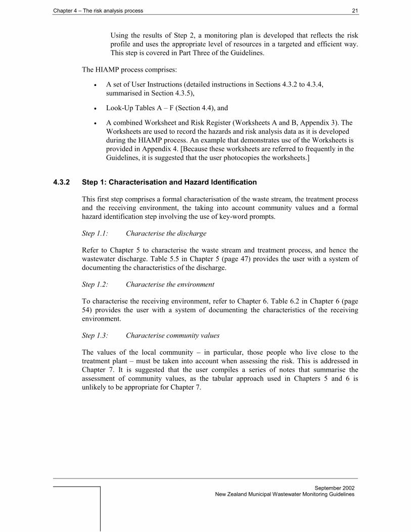
Using the results of Step 2, a monitoring plan is developed that reflects the riskprofile and uses the appropriate level of resources in a targeted and efficient way.This step is covered in Part Three of the Guidelines.
The HIAMP process comprises:
• A set of User Instructions (detailed instructions in Sections 4.3.2 to 4.3.4,summarised in Section 4.3.5),
• Look-Up Tables A – F (Section 4.4), and
• A combined Worksheet and Risk Register (Worksheets A and B, Appendix 3). TheWorksheets are used to record the hazards and risk analysis data as it is developedduring the HIAMP process. An example that demonstrates use of the Worksheets isprovided in Appendix 4. [Because these worksheets are referred to frequently in theGuidelines, it is suggested that the user photocopies the worksheets.]
4.3.2 Step 1: Characterisation and Hazard Identification
This first step comprises a formal characterisation of the waste stream, the treatment processand the receiving environment, the taking into account community values and a formalhazard identification step involving the use of key-word prompts.
Step 1.1: Characterise the discharge
Refer to Chapter 5 to characterise the waste stream and treatment process, and hence thewastewater discharge. Table 5.5 in Chapter 5 (page 47) provides the user with a system ofdocumenting the characteristics of the discharge.
Step 1.2: Characterise the environment
To characterise the receiving environment, refer to Chapter 6. Table 6.2 in Chapter 6 (page54) provides the user with a system of documenting the characteristics of the receivingenvironment.
Step 1.3: Characterise community values
The values of the local community – in particular, those people who live close to thetreatment plant – must be taken into account when assessing the risk. This is addressed inChapter 7. It is suggested that the user compiles a series of notes that summarise theassessment of community values, as the tabular approach used in Chapters 5 and 6 isunlikely to be appropriate for Chapter 7.

22 Chapter 4 – The risk analysis process
September 2002New Zealand Municipal Wastewater Monitoring Guidelines
Figure 4.1: The HIAMP process.
The HIAMP Process
Characterise thedischarge (by
consideration of theinfluent and treatment
process)(Table 5.5)
Characterise localcommunity values
(Chp 7)
Characterise theenvironment
(under normal andsensitive conditions)
(Table 6.2)
Identify 'normaloperation' hazards
(Chp 4 Table A)
Identify 'abnormalcondition' hazards(Chp 4 Table B)
Classify Hazardsby Type
(Chp 4 Table C)
Assign "level ofimpact" for each
hazard(Chp 4 Table D)
Identify expectedfrequency
(Chp 4 Table E)
Identify appropriatemonitoringresources
(Chp 4 Table F)
Design monitoring plan(Part 3)
Review plan
Human HealthEcologySocial ValueEconomic UtilityAestheticsOdour(Chp 4 Table C)
Record onW orksheets A and B
Record onW orksheets A and B
Record onW orksheets A and B
Step 1:Characterisationand HazardIdentification
Step 2:Risk Analysis
Step 3:DevelopMonitoringPlan
Repeat forabnormalconditions
ImpactInformation
.

Chapter 4 – The risk analysis process 23
September 2002New Zealand Municipal Wastewater Monitoring Guidelines

24 Chapter 4 – The risk analysis process
September 2002New Zealand Municipal Wastewater Monitoring Guidelines
Step 1.4: Hazard Identification
Ideally, a group working within a workshop environment will carry out the hazardidentification process. This will ensure that all required knowledge is available to identify allrisks. Alternatively, the process can be carried out by a series of people with between themthe knowledge of the receiving environment, the waste stream and the waste process.
When characterising the wastewater discharge and receiving environment, the user needs toconsider risks associated with both ‘normal’ conditions and ‘abnormal’ conditions. These aredescribed as follows.
Risk related to ‘normal’ conditions
This refers to the sources of risk associated with the waste stream, the plant and the receivingenvironment during ‘normal’ conditions. Normal conditions are those that are expected tooccur. Table A in Section 4.4 provides a list of key-words that are designed to prompt theuser to identify the ‘normal’ hazards. Note that natural fluctuations in contaminantconcentrations, wastewater flow rate and environmental conditions are part of the normalcondition. For example, the 5-year low flow in a receiving river would be considered part ofthe ‘normal’ conditions. Tables 5.5 and 6.2 should document the characteristics of thedischarge and receiving environment under normal conditions.
Risks related to ‘abnormal’ conditions and gross uncertainty
This refers to hazards associated with the waste stream, the plant and the receivingenvironment that arise due to gross uncertainty and abnormal conditions. Abnormalconditions refer to those events that result from faults, failures and untoward events that arenot normally expected or repeating, but are considered possible and credible as well asunusually sensitive environmental conditions. Examples include major plant failures, processupsets and toxic shock incidents, and unusual long-term weather conditions (e.g., a 50-yeardrought). Gross uncertainty may be present in cases where there is some uncertaintyregarding the capability or suitability of a given process, or the dynamics of the environmentin response to the discharge inflows. This type of gross uncertainty is over and above thenormal levels expected when predicting discharge impacts.
Table B (Section 4.4) provides a list of key-words that are designed to prompt the user toidentify ‘abnormal’ sources of risk.
Users may find that the same hazard will be identified more than once by the use of key-word prompts. Where this occurs, the duplication is simply removed before the ‘Analysis’step (see Step 2 below).
At completion of Steps 1.1 to 1.4, the user should have completed:
• Tables 5.5 and 6.2 (discharge and receiving environment characteristics undernormal conditions).
• Notes on abnormal conditions for the influent wastewater, treatment plant andreceiving environment.
• Notes on community values relevant to the discharge and receiving environment.

Chapter 4 – The risk analysis process 25
September 2002New Zealand Municipal Wastewater Monitoring Guidelines
4.3.3 Step 2: Risk Analysis
Step 2 involves analysing the impact and likelihood of each of the hazards identified in Step1. Use Worksheets A and B in Appendix 3 to document this analysis.
Step 2.1: Identifying the Type of Impact
Use the information gathered in Step 1 to provide a brief description of the nature of theimpacts under normal conditions in the first empty column in Worksheet A. Refer to theexample worksheet in Appendix 4 for guidance.
Identified risks need to be assigned to a given type, or types, of impact to enable the level ofimpact to be ascribed. Six distinct types of impact are used:
• Human health and safety.
• Ecology.
• Community Values.
• Economic Utility.
• Aesthetics.
• Odour.
A description of each of these impact types is given in Table C (Section 4.4). ‘Odour’ and‘aesthetics’ have been ascribed separate impact types to ‘community values’, in the view ofthe prominence these two issues have with wastewater discharge issues.
Step 2.2: Rating the Level of Impact
This step involves identifying the anticipated level of impact. The general description of theimpact scale is given in Table 4.1 below. Each step on the scale is intended to represent an‘order of magnitude’ increase in impact. The detailed impact scales for each type of impact(i.e., human health and safety, ecology, etc) is described in Tables D1 to D6 (Section 4.4).
Each impact scale is based upon a 6 step scale denoted ‘A’ to ‘F’, with a consistentdescriptor term used for all types of risk. The scale for each type of impact ranges from an‘F’ rating that denotes ‘insignificant impact’, to a level commensurate with the maximumpotential impact. As human health is considered to carry most importance by society, thehighest level for human health (only) is rated ‘A’. Other types of impact have differentmaximum ratings (for example, Aesthetics scale ranges from D to F only).
When assessing the level of impact, it is clearly necessary to account for the relative volumeof the discharge (i.e. the flow rate) to the characteristics of the receiving environment (e.g.,degree of dilution), as these will have a significant bearing on the level of impact.
Use the first column of the paired columns in Worksheet A to document the assessed level ofimpact (refer to example in Appendix 4 for guidance). Reasonable assumptions are to bemade when identifying the anticipated level of impact. Use separate lines where there isclearly more than one type of event of discrete level of impact resulting from one ‘prompt’.Normal levels of uncertainty regarding discharge constituents and anticipated sensitivity of

26 Chapter 4 – The risk analysis process
September 2002New Zealand Municipal Wastewater Monitoring Guidelines
the receiving environment should be considered, and a reasonably precautionary approachtaken.
Table 4.1: Impact Designations (see Tables D1 - 6 for specific descriptions for each separate ‘type’of impact – Section 4.4).
Term General Description and Notes Designation
HighlyInjurious
Most serious consequence. Public illness or injury that could involvedeath. This level only applies to ‘Human Health and Safety’ type ofimpact
A
Critical Very serious impact involving permanent or long-term damage B
Major Partial or temporary but significant damage C
Moderate Clear stress noted and intervention expected to be required to limitimpacts
D
Slight Measurable or notable impact but intervention unlikely to be called for E
Insignificant Impact expected but may not be measurable or of concern F
Step 2.3: Identifying the Likelihood
For each hazardous event identified, a judgement must be made as to the frequency orlikelihood of it occurring. The frequency or likelihood scale used is described qualitativelyusing a 5-step scale. This is given in Table E in Section 4.4.
Note that the first three terms in Table E relate to essentially routine or normal events, whilstthe last two describe unexpected or abnormal conditions.
The appropriate likelihood is recorded on the worksheet for each identified hazardous event.
It may be that for any one type of hazardous event there are a number of possible likelihoodsfor different impacts. For example, the likelihood of ‘slight’ odour may be ‘frequent’, whilethe likelihood of ‘moderate’ odour might be ‘occasional’ (refer also to the example inAppendix 4). It is normal to describe similar combinations of impact and likelihood as oneevent with representative values, using reasonable assumptions (i.e. using highest realisticlikelihood). However, it is sometimes necessary to describe two or possibly more events tocover all important scenarios.
Step 2.4: Assigning the Appropriate Level of Monitoring Resources
The final step in the analysis process is to identify the level of resources appropriate formonitoring. This is accomplished by using Table F, which draws on the worst-casecombinations of the scale of impact with the likelihood.
Step 2.5: Risk Analysis for abnormal risks
Chapter 4 – The risk analysis process 27
September 2002New Zealand Municipal Wastewater Monitoring Guidelines
Repeat steps 2.1 to 2.4 for abnormal condition risks. Fill in Worksheet B at each step.
At the completion of Steps 2.1 to 2.5, the user should have completed Worksheets A and B.The user should then proceed to Chapter 8 to complete Step 3.
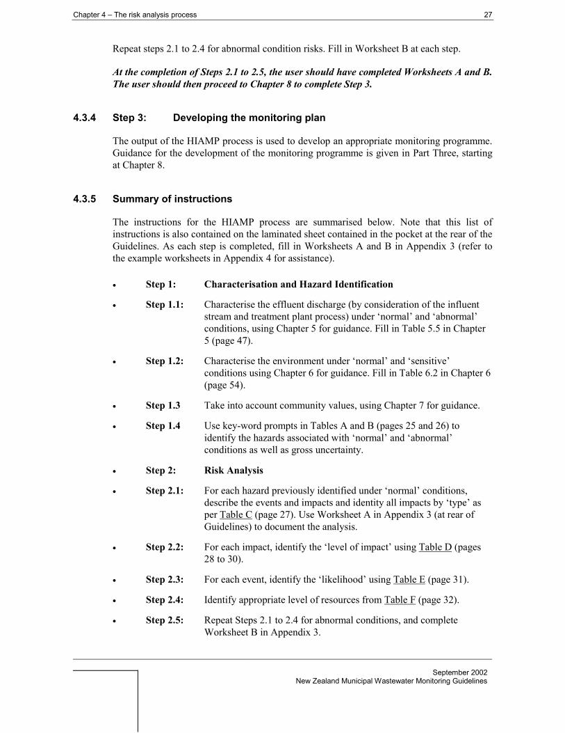
4.3.4 Step 3: Developing the monitoring plan
The output of the HIAMP process is used to develop an appropriate monitoring programme.Guidance for the development of the monitoring programme is given in Part Three, startingat Chapter 8.
4.3.5 Summary of instructions
The instructions for the HIAMP process are summarised below. Note that this list ofinstructions is also contained on the laminated sheet contained in the pocket at the rear of theGuidelines. As each step is completed, fill in Worksheets A and B in Appendix 3 (refer tothe example worksheets in Appendix 4 for assistance).
• Step 1: Characterisation and Hazard Identification
• Step 1.1: Characterise the effluent discharge (by consideration of the influentstream and treatment plant process) under ‘normal’ and ‘abnormal’conditions, using Chapter 5 for guidance. Fill in Table 5.5 in Chapter5 (page 47).
• Step 1.2: Characterise the environment under ‘normal’ and ‘sensitive’conditions using Chapter 6 for guidance. Fill in Table 6.2 in Chapter 6(page 54).
• Step 1.3 Take into account community values, using Chapter 7 for guidance.
• Step 1.4 Use key-word prompts in Tables A and B (pages 25 and 26) toidentify the hazards associated with ‘normal’ and ‘abnormal’conditions as well as gross uncertainty.
• Step 2: Risk Analysis
• Step 2.1: For each hazard previously identified under ‘normal’ conditions,describe the events and impacts and identity all impacts by ‘type’ asper Table C (page 27). Use Worksheet A in Appendix 3 (at rear ofGuidelines) to document the analysis.
• Step 2.2: For each impact, identify the ‘level of impact’ using Table D (pages28 to 30).
• Step 2.3: For each event, identify the ‘likelihood’ using Table E (page 31).
• Step 2.4: Identify appropriate level of resources from Table F (page 32).
• Step 2.5: Repeat Steps 2.1 to 2.4 for abnormal conditions, and completeWorksheet B in Appendix 3.

28 Chapter 4 – The risk analysis process
September 2002New Zealand Municipal Wastewater Monitoring Guidelines
• Step 3: Monitoring Programme
Using results of risk analysis, develop monitoring programme – referto Part 3 of Guidelines, beginning at Chapter 8.

Chapter 4 – The risk analysis process 29
September 2002New Zealand Municipal Wastewater Monitoring Guidelines
4.4 Look-Up tables
Table A: Sources of Risk (Normal Conditions)
Key Word Comment Reference
NormalConstituents
Consider the risks created by the constituentsexpected to be in the waste stream (mostprobably chronic impacts)
Chapter 5Section 5.2Table 5.2
Volume Slug Is the nature of the catchment such that suddenwastewater volume changes can occur?
Chapter 5Section 5.2.1
Contaminant orWaste Slug
Is the nature of the catchment such thatcontaminant or waste slugs can or do occur?
Chapter 5Table 5.3
Odour Does the treatment process create odour thatcould be detected at or beyond the plantboundary?
Chapter 5Table 5.3
Trade Waste(normalconstituents)
Are there potential sources of trade waste thatroutinely discharge contaminants that will passthrough the treatment process and cause chronicimpacts of any kind?
Chapter 5Table 5.2
Solids Disposal Are there any issues or risks associated withsludge or other process-generated solidsdisposal?
Chapter 5Section 5.3
Other Sources ofRisk
Any other sources of risk under normal conditions Chapter 5Tables 5.2, 5.3

30 Chapter 4 – The risk analysis process
September 2002New Zealand Municipal Wastewater Monitoring Guidelines
Table B: Sources of Risk (Abnormal Conditions and Gross Uncertainty)
Key Word Comment Reference
Process fault orupset conditions
Is the process potentially unreliable or could itbecome unstable? If so what would be the effectof changes to the effluent composition?
Chapter 5Section 5.3Table 5.4
Extreme weatherrelated upset ofprocess
Could the process be upset by extreme weatherconditions? If so what would be the effect ofchanges to the effluent composition as well as theweather-related sensitivities of the receivingenvironment?
Chapter 5Table 5.4
Trade Waste(abnormalconstituents)
Are there any potential sources of trade wastethat could lead to unintended contaminantspassing through treatment process from time totime and cause acute impacts of any kind?
Chapter 5Tables 5.2, 5.4
Toxic Shock/Slug(constituents thatcould cause anupset withinprocess)
Are there industries or any other potential sourcesof waste that could lead to unintendedcontaminant load that could de-stabilise thetreatment process? (acute impacts)
Chapter 5Tables 5.2, 5.4
Is there acharacteristic of theenvironment thatmay result inunusual sensitivityunder specificunusual conditions
Some conditions or events not related to thedischarge stream may result in unusualenvironmental sensitivity at times – e.g., low flowsin streams.
Chapter 6Section 6.4
Contaminantcompositionuncertainty
Is there materially significant uncertaintyregarding the composition of the influent wastestream?
Chapter 5Section 5.2
Uncertainty(volume)
Normal volume and seasonal profile not fullyquantified
Chapter 5
Lack ofenvironmentalknowledge(uncertainty)
Is there significant uncertainty regarding theenvironmental impact from the discharge?
Chapter 6
Uncertainty(ecosystemdynamics)
Is there any uncertainty regarding the ecosystemdynamics?
Chapter 6
Other sources ofrisk
Any other sources of process related risk (seechapter text for identification methodology)?
Chapters 5, 6, 7

Chapter 4 – The risk analysis process 31
September 2002New Zealand Municipal Wastewater Monitoring Guidelines

32 Chapter 4 – The risk analysis process
September 2002New Zealand Municipal Wastewater Monitoring Guidelines
Table C: Type of Impact
Type of Impact Example Reference
Human Health andSafety
Pathogens or other health-affecting agent in zone ofinfluence where people swim, undertake watersports, fish or collect shellfish, or where water isabstracted for drinking water. Reduced water clarityor slime build up on rocks that presents a potentialhazard to bathers.
Chapter 6Section 6.4
Ecology Any species, communities, or ecosystemsadversely affected by the waste stream.
Chapter 6
Community Value Any cultural or social aspect impacted directly orindirectly by the waste stream.
Chapter 7
Economic Utility Any current or anticipated economic use of theenvironment that is adversely impacted by thewaste – e.g., downstream abstractions for watersupply; commercial fishing
Chapter 7
Aesthetics Any aesthetic impact caused by the waste or thephysical effects of the waste stream.
Chapter 6Section 6.4Chapter 7
Odour Any impact caused by unpleasant odour eventsoutside the waste facility boundaries.
Chapter 5Chapter 7

Chapter 4 – The risk analysis process 33
September 2002New Zealand Municipal Wastewater Monitoring Guidelines
Table D1: Level of Impact (Human Health and Safety)
Level of Impact Example Designation
Highly Injurious Illness anticipated in large numbers of people, someserious
A
Critical Illness anticipated in the community B
Major Isolated illnesses anticipated; significant hazard tobathers from poor water clarity or slimes on substrates
C
Moderate Precautions in place to protect the public (e.g., beachclosures); possibility of hazard to bathers from poorwater clarity or slimes on substrates
D
Slight Concern leading to call for increased monitoring;compromised water clarity and/or evidence of slimebuild up on substrates
E
Insignificant No measurable decrease in community well-being oreffects on water clarity or slimes
F
Table D2: Level of Impact (Ecology)
Level of Impact Example Designation
Highly Injurious Not applicable X
Critical Severe impact over wide area; medium to long termeffects
B
Major Severe impact over small area or moderate impactover large area; medium to long term effects
C
Moderate Moderate impact over small area or minor impactover wide area; short term effects
D
Slight Minor short term impact over small area E
Insignificant No discernible impact on any ecosystem or species F

34 Chapter 4 – The risk analysis process
September 2002New Zealand Municipal Wastewater Monitoring Guidelines
Table D3: Level of Impact (Community Value)
Level of Impact Example Designation
Highly Injurious Not applicable X
Critical Concern at regional or national level. B
Major Intense concern from local community; somedistrict-wide concern.
C
Moderate Widespread local community/tangata whenuaconcern.
D
Slight Minor concern from tangata whenua or specialinterest groups (e.g. Fish & Game)
E
Insignificant Minor concern expressed by a few individuals only F
Table D4: Level of Impact (Economic Utility)
Level of Impact Example Designation
Highly Injurious Not applicable X
Critical Existing local uses of environment prevented forextended time periods
B
Major Existing local uses of environment prevented forshort periods
C
Moderate Restrictions on local activities of environment D
Slight Advice issued of potential impact E
Insignificant No noticeable effect F

Chapter 4 – The risk analysis process 35
September 2002New Zealand Municipal Wastewater Monitoring Guidelines
Table D5: Level of Impact (Aesthetics)
Level of Impact Example Designation
Highly Injurious Not applicable X
Critical Not applicable X
Major Obvious effect to large number of people C
Moderate Effect visible to casual observer; visible from publicareas
D
Slight Effect visible only when observed closely from astationary position, or visible effect from little visitedareas
E
Insignificant Very limited visual effect F
Table D6: Level of Impact (Odour)
Level of Impact Example Designation
Highly Injurious Not applicable X
Critical Not applicable X
Major Offensive, objectionable odour in local communityareas. Many complaints expected.
C
Moderate Objectionable odour noticeable by community.Complaints expected from ‘reasonable’ people
D
Slight Inoffensive odour in public areas. A few complaintspossible
E
Insignificant No odour beyond boundaries. No odour complaintswould be expected
F

36 Chapter 4 – The risk analysis process
September 2002New Zealand Municipal Wastewater Monitoring Guidelines
Table E: Likelihood Categories
Likelihood Typical Frequency Designation Note
Continuous Is expected to be the normal condition ordiurnal in nature
I
Frequent Although not the normal condition – canbe expected to be seen every few daysor weeks
II
Seasonal Can be expect more than once per year III
Representtypicallynormalconditions
Occasional Expected to occur in some years IV
Possible Conceivable during the life of the plant V
Typicallyabnormalconditions
Table F: Appropriate Resources (applies to each type of impact).
Likelihood (refer Table E)Level of impact(refer Tables
D1-6)I II III IV V
A 1 1 1 1 1
B 1 1 1 1 3
C 2 2 2 2 None
D 2 2 2 3 None
E 3 3 3 3 None
F 3 3 3 None None
Typically normal conditions Typically abnormal conditions
Key: 1 = Detailed management plan and employment of dedicated resources2 = Standard monitoring regime appropriate to the type of hazard, within capacity of normallevel of resources3 = Incidental, implied from other monitored constituents or indicatorsNone = Monitoring not appropriate


September 2002New Zealand Municipal Wastewater Monitoring Guidelines
CHAPTER 5RISK ANALYSIS: CHARACTERISING THE DISCHARGE
Rob Potts, Sarah Smith (Glasson Potts Fowler Limited)
5.1 Introduction
This chapter assists the reader in characterising the wastewater discharge, as required in Step1.1 in the HIAMP process (refer to Section 4.3). The discharge characterisation process is asfollows:
• The untreated wastewater is characterised using Section 5.2 and Table 5.2.
• The efficiency and effectiveness of the wastewater treatment process ischaracterised, using Section 5.3 and Tables 5.3 and 5.4.
• By integrating the first two steps, the wastewater discharge to the receivingenvironment is characterised. This information is then used in Section 4.3 to assessthe risk presented by the discharge.
The key points in the text are summarised at the rear of the chapter in the following:
Table 5.2 - untreated wastewater characteristics;
Table 5.3 - wastewater treatment plant performance – normal conditions; and
Table 5.4 - treatment plant performance – vulnerability to ‘upset’.
The reader may choose to refer to these tables in the first instance, then refer to the chaptertext for more detail.
The output from this chapter for use in Step 1.1 in the HIAMP process is the completion ofTable 5.5 (page 47, at the end of the chapter). Table 5.5 helps the reader to build up anddocument the profile of the influent wastewater, the treatment process, and finally theeffluent discharge. An example of how to fill in Table 5.5 is provided in Table 5.6.
5.2 Influent wastewater characterisation
5.2.1 Flow volume
Flow volume is an important factor in discharge characterisation. Generally, a largedischarge has a higher risk of adverse environmental effects than a smaller discharge withthe same contaminant concentrations into the same receiving environment. If available, goodhistoric flow records should be used and be taken into account with the risk assessment. Ifflow records are not available, the following can be used as a guide for assessing flows.
Flow varies between communities, and is influenced by many factors. Flow volume variesover a typical day, and throughout any year depending on the type of dwelling, its occupants

Chapter 5 – Risk analysis: characterising the discharge 39
September 2002New Zealand Municipal Wastewater Monitoring Guidelines
and their habits, and the influence of any industrial trade waste contributions. Severalmeasures are important:
• Average dry weather flow (ADWF) which is the wastewater flow taken after threeconsecutive days without rainfall, or with rainfall less than one millimetre.
• Peaking factors are applied to the ADWF to obtain the peak daily flow (PDF).
• Peak wet weather flow (PWWF) – includes additional flow from stormwater cross-connections and groundwater infiltration.
Typical New Zealand values for ADWF are as follows:
140 - 180 L/person/day - on-site systems
270 - community systems
150 - summer holiday house
360 - luxury home with modern conveniences
Peaks in daily flow occur mid to late morning and early evening. Peaking factors can becalculated by analysing community flow data. If there is no data, published values can beused (based on ADWF and connected population, ranging from 2 - 6).
Infiltration can occur even in new reticulation systems and can vary, depending on theseason and local groundwater levels. Infiltration calculations are usually based oncommunity area, with New Zealand values in the range 0.05 - 0.07 L/s/ha. Stormwaterinflow depends on the number of connections from roof downpipes, manhole covers, yarddrains and pipe cross connections. New Zealand values are generally in the range 0.15 - 0.19L/s/ha, with 30% allowance for extreme conditions. Some older wastewater treatment plants(WWTPs) were designed for flows up to six times ADWF to accommodate large inflowsfrom groundwater and stormwater.
The trade waste component of any wastewater will have a significant impact on the flow rateand volume depending on the type of industry and its size in relationship to the size of thecommunity.
Certain trade wastes can produce high loadings of various constituents in wastewater, forexample, industrial processes are responsible for 30 - 85% of metals in New Zealandmunicipal wastewaters (NZLTC, 2000). So the proportion of the wastewater that comes fromtrade and industrial sources (known as trade waste) is a significant factor when assessing andcharacterising any wastewater discharge.
5.2.2 Temperature
The temperature of wastewater in domestic sewage is slightly higher than the incomingwater supply due to the addition of warm water. Depending on location, the mean annualtemperature of wastewater varies from about 10 to 21o C, with 15.6 oC taken as a

40 Chapter 5 – Risk analysis: characterising the discharge
September 2002New Zealand Municipal Wastewater Monitoring Guidelines
representative value. The variation is greater in areas with high trade waste inputs due to hotinputs from cleaning and cooking and chilled water being added with some food processingindustries.
5.2.3 pH
This is the concentration of hydrogen ions (H+) in the wastewater, and measures how acidicor alkaline the wastewater is. If extreme pH is not adjusted prior to discharge, toxic effectscan result such as salt precipitation or some compounds becoming more toxic (e.g.ammonia).
The average pH of New Zealand untreated wastewater pH is 7.5, depending on thecontributing flows.
5.2.4 Suspended solids
High suspended solids (SS) levels can result in overloading of some treatment processes, andcan also impact on receiving environments. Typical influent SS levels in New Zealand are inthe range 50-800 g m-3 with an average of 300 g m-3.
5.2.5 Biochemical oxygen demand (BOD)
This measures the oxygen required by micro-organisms to degrade organic matter, usuallyover five days (BOD5). It is the most common measure of organic pollution.
BOD can be critical as it can cause organic enrichment, bacterial growths on aquatic surfacesand dissolved oxygen depletion. BOD is the preferred organic strength measurement in NewZealand. Typical influent BOD concentrations in New Zealand domestic wastewater rangebetween 150 - 450 g m-3, with an average value of 250 g m-3 (Hauber, 1995).
5.2.6 Fats, oils and greases
Fats and oils are contributed to domestic wastewater in butter, lard, margarine and vegetableoils and fats. Fats are also found in meats, parts of cereals, seeds, nuts, milk and certainfruits. Kerosene, lubricating and road oils also reach the sewers from garages, shops and carsale yards. Trade wastes with high levels are animal and dairy processing wastes. Fats, oiland grease are similar chemically. They are relatively stable compounds and are not easilydecomposed by bacteria. Fats and greases can cause problems in both sewers and at thetreatment plant. Trade wastes usually have stringent limits so that these are removed prior tothe sewer.
5.2.7 Nutrients and ammonia
The main nutrients of interest in wastewater are nitrogen and phosphorus.
Nitrogen
Chapter 5 – Risk analysis: characterising the discharge 41
September 2002New Zealand Municipal Wastewater Monitoring Guidelines
Nitrogen is found in untreated wastewater mainly in two forms – ammoniacal (NH4 andNH3) (about 60%) and organic (about 40%) forms. High nitrogen levels in receiving surfacewaters can result in micro and macro-scale plant growth (algal blooms, excessive aquaticweed growth) and toxic effects on aquatic organisms.
Typical New Zealand untreated wastewater total nitrogen concentrations are in the range 7 -60 g m-3, with an average concentration of 35 g m-3 (Hauber, 1995).
Ammoniacal nitrogen is an important nitrogen compound. It exists in two forms, ionised(NH4
+) and unionised (NH3). The unionised form is toxic to aquatic organisms, in both freshand marine waters. Receiving water pH and temperature both influence ammonia toxicity.
Phosphorus
Phosphorus (P) in wastewater comes from sources such as detergents and organic matterbreakdown. It is found in inorganic and organic forms.
Elevated phosphorus in wastewater discharges can cause excessive plant growth in surfacewaters. Typical untreated wastewater total phosphorus (TP) concentrations in New Zealandare between 3.3 - 13 g m-3, with an average concentration (across the WWTPs surveyed) of 7g m-3 (Hauber 1995).
5.2.8 Cations and anions
Cations and anions found in wastewater include sodium, potassium, calcium and chloride. Ingeneral, these are not routinely monitored in New Zealand domestic wastewater, since theydo not usually result in adverse environmental effects. In some cases, they may be monitoredfor specific reasons (e.g., ion build up in soils used for land disposal).
5.2.9 Pathogens
Many different micro-organisms are found in untreated wastewater, including bacteria,viruses, helminths and protozoa. Many of these are relied on in WWTPs for biologicalwastewater treatment. Disease causing micro-organisms are called pathogens.
Pathogenic bacteria found in wastewater include Yersinia, Shigella (bacterial dysentery),Vibrio (cholera), Salmonella (typhoid) and Escherichia. Most enteric bacteria die offquickly outside the gut, but some can persist in water or soil.
Viruses found in wastewater include enteroviruses, rotaviruses and hepatitis. Most viruses donot survive well outside their host and numbers decrease rapidly, depending on the treatmentmethod used.
Helminths include threadworms, nematodes (roundworms, hookworms), cestodes(tapeworms) and trematodes (flukes). These organisms are parasitic, and can be easilypassed on through wastewater. Eggs and larvae are stable in soil environments and can beviable for a long time. Helminths from wastewater discharges are not normally a risk toreceiving environments in New Zealand.
Protozoa found in wastewater include Giardia and Cryptosporidium, which can causedisease. These organisms are difficult to remove from wastewater, as their reproductive cysts

42 Chapter 5 – Risk analysis: characterising the discharge
September 2002New Zealand Municipal Wastewater Monitoring Guidelines
and oocysts are able to pass through most treatment processes, although recent developmentsin ultra violet light treatment are addressing this problem. Protozoa are able to persist onvegetation (via applied wastewater) for a short period and can survive for days in soil. Someprotozoa can survive for several months in water, particularly intermediate stages (likeGiardia cysts).
Human infection potential determines the required treatment level for pathogen removal. If awastewater with a high pathogen level is discharged, health effects can occur in peoplecontacting with the discharge, either water-borne (swimming, drinking, eating shellfish orplants growing in the water) or land (direct contact with wet surfaces, aerosols fromirrigation being ingested).
Bacterial indicators that are usually used for wastewater in New Zealand are E. coli, faecalcoliforms and enterococci. Values in untreated wastewater for the selected organisms areshown in Table 5.1.
Table 5.1: Typical range for selected micro-organisms in untreated wastewater (number/100 mL).From Metcalfe and Eddy (1991).
Organism FaecalColiforms
Enterococci Giardiacysts
Cryptosporidiumoocysts
Helminthova
EntericViruses
Range ofValues 106-107 104-105 101-105 101-103 1-103 103-104
5.2.10 Heavy metals
High levels of heavy metals can be toxic to biota and people. There are also severalmetalloid compounds (like aluminium, boron and arsenic) which have similar properties andeffects. Metal solubility is generally low and is influenced by pH (as pH increases, solubilitydecreases).
Industrial trade waste sources contribute a large proportion of metals and metalloids in NewZealand wastewater. Industry-specific metals and metalloids include chromium (tanning),arsenic, copper, zinc/ nickel (metal plating), aluminium (metal smelting) and boron.
Metals contributed from domestic sources come from water treatment, detergents, soap,cosmetics, household dust, medicines, toilet paper and pipework (copper). Metalconcentrations from domestic sources are usually low compared to industrial sources andgenerally do not pose significant environmental effects. However, in some systems (such aslow flows and older pipes), household sources cannot be completely ruled out ascontaminant mass loading is concentration and flow dependent.
5.2.11 Persistent organic pollutants (POPs)
Persistent organic pollutants (POPs) are defined as organic substances that are persistent andpossess toxic characteristics. There is a wide range of compounds that fall into this category,including phenols, chlorinated hydrocarbons (DDT, PCP, PCBs), pesticides and herbicides(2,4,5T; 2,4D), PAHs (polycyclic aromatic hydrocarbons), large organic molecules andBTEX (benzene, toluene, ethylbenzene, xylenes). Concentrations should be below levels of

Chapter 5 – Risk analysis: characterising the discharge 43
September 2002New Zealand Municipal Wastewater Monitoring Guidelines
concern unless there is a significant point-source discharge into the sewerage system, e.g.,from a primary industry such as a woolscour.
5.2.12 Characterising the influent wastewater
Table 5.2 provides a comparative guide to the levels of common constituents in NewZealand wastewater, for domestic and typical industrial wastewater components. Anindicative assessment of the relevant characteristics of a wastewater can be made using thistable, taking into account both domestic and industrial components.
More specific information is difficult to provide, given the wide variability of New Zealandwastewaters. Where possible, monitoring records should be used to assess the potentialhazard for the wastewater constituents. Alternatively, screening sample analyses should becarried out to better assess the influent wastewater characteristics, the results of which can becompared to the values in Section 5.2.
At this stage, the reader should be able to fill in the first two columns in Table 5.5. Anexample of how to use Table 5.5 is provided in Table 5.6.
The reader should also make notes on the possible large changes to the wastewatercharacteristics under ‘abnormal’ conditions. For example, certain industrial practices mightlead to occasional peaks in toxic elements being discharged to the sewer. Obviously thisrequires a degree of judgement, based on past experience. Further examples of abnormalconditions are given in Table B in Chapter 4.
5.3 Treatment processes
The treatment processes described below are divided into primary, secondary and tertiarytreatment components for convenience. There can be debate over whether a treatmentprocess should be considered secondary or tertiary, or a combination of the two. Thedivisions used below are not definitive.
5.3.1 Primary treatment
These are physical unit operations to remove large solids and floatable material. Typical unitprocesses include:
• Screening and grit removal - usually the first process at a WWTP. Removing largeparticles will prevent blockages downstream.
• Sedimentation – used to remove further larger particles as settled sludge.Sedimentation can also remove some heavy metals and POPs (persistent organicpollutants) which adsorb onto the settled particulate matter and are removed with thesludge.
• Further improvements include using chemical additives to improve solids removaland to precipitate out heavy metals (the Advanced Primary Treatment system).

44 Chapter 5 – Risk analysis: characterising the discharge
September 2002New Zealand Municipal Wastewater Monitoring Guidelines
5.3.2 Secondary treatment
There are two types of secondary processes: aerobic and anaerobic. Within each category,there are suspended growth and attached growth processes. In New Zealand, aerobicprocesses used are:
• Suspended growth: activated sludge (AS), high-rate activated sludge (HRAS), pondsystems (aerated and passive), sequencing batch reactors (SBRs), and advancedintegrated pond systems.
• Fixed growth: trickling filters, rotating biological contactors, packed bed reactors.
In New Zealand, anaerobic processes in use are:
• Suspended growth: pond systems, sludge digestion, upflow anaerobic sludge blanketreactors.
• Fixed growth: anaerobic filters, expanded bed reactors.
For specific details on how each of the treatment processes operate, refer to relevantliterature (e.g., Metcalf and Eddy (1990); NZLTC (2000)).
Common suspended growth aerobic systems
Activated sludge (AS)
Bacteria are kept in suspension in wastewater via aeration for a set time inside a tank. Excesscells are settled out in a separate clarifier unit.
BOD and SS removal rates are good, but limited nutrient removal occurs. Pathogen removalis poor. Heavy metal removal is moderate, through adsorption and settling as per primarytreatment. POPs and hydrocarbons removal is low to moderate by bio-oxidation, air strippingand floc adsorption (providing the concentration of POPs is not lethal to the treatingmicrobes).
AS systems can have problems handling volume slug loads, due to insufficient freeboard orvolume available. Toxic slugs can cause biomass die off within the activated sludge tank,with a consequent large sludge volume increase and possible overloading of the clarifierunit. Toxic slugs can also result in excess growth of filamentous organisms, causing‘bulking’ of the reactor contents and reducing settle ability in the clarifier.
There are several variations of AS possible. High Rate Activated Sludge (HRAS) involveshigher loadings with a shorter retention time and some solids recycle. Extended Aeration(EA) uses a longer retention time, with high levels of oxygen being diffused into thewastewater.
Another variation is the Sequencing Batch Reactor (SBR). This variant of AS involves thesame processes, but they occur sequentially within the same tank. All SBRs have a five stepoperating sequence, and sludge wasting occurs to improve performance. Well designed andoperated SBRs can substantially reduce nitrogen and phosphorus concentrations.
Pond systems
Chapter 5 – Risk analysis: characterising the discharge 45
September 2002New Zealand Municipal Wastewater Monitoring Guidelines
These use the action of bacteria, algae and climate (sun, wind) to reduce organic andpathogenic loading. Ponds can be aerobic (shallow, oxygenated) or facultative (mediumdepth, areas of high and low oxygenation).
Pond systems usually have multiple ponds in series or parallel, to improve treatment. Ponds(especially two pond systems) are a very common wastewater treatment process.
BOD and SS removal rates are reasonable, but limited nutrient and ammonia removal occurs.Pathogen removal in conventional pond systems is relatively good, due to microbialpredation and the action of UV light (in sunlight). Ponds provide flow buffering, whichmeans their response to sudden volume slugs is good. Toxic slugs may result in the killing ofpond microbial populations which will reduce treatment and disinfection performance.Adding internal rock filters and baffles can improve performance by removing suspendedsolids and promoting better mixing. Additional aeration can be provided via mechanicalaerators to increase dissolved oxygen.
Heavy metal removal is moderate, primarily through adsorption and settling. POPs andhydrocarbons removal will be low.
A recent development has been the Advanced Integrated Ponds (AIPS) concept. It usesseveral ponds, the first being an advanced facultative pond which reduces the organicloading of the wastewater. The next pond is a ‘high rate’ algal pond, which is shallow andpaddlewheel-mixed. It promotes algal cell growth to take up nutrients. An algal settling pondis then used, to harvest algal cells (and hence nutrients). Final maturation ponds are used todisinfect the wastewater before discharge. BOD, SS, pathogen and nutrient removal(particularly nitrogen) are good for this system.
Common fixed growth aerobic systems
Trickling filter
This system consists of a tank filled with media (covered in a microbial biofilm), over whichthe wastewater trickles. The biofilm takes up nutrients and organic matter from the passingwastewater flow. Collected percolate flows into a clarifier to settle out sloughed biofilmbefore being discharged.
Trickling filters are good at removing BOD and SS. Nutrient removal is poor to moderate,with limited ability to remove ammoniacal nitrogen and phosphorus. Pathogen removal isgenerally not high. Trickling filters deal poorly with toxic slugs, which can kill micro-organisms in the biofilm layer and cause excessive sloughing (heavily loading the clarifierunit). Volume slugs can be dealt with reasonably well, but high shear velocities can alsoresult in biofilm sloughing and overloading of the clarifier unit.
Heavy metal removal is low to moderate, primarily through adsorption and settling. POPsand hydrocarbons removal will be low.
Performance can be improved by recycling some of the sloughed biofilm into the inflow(solids contact process), which improves organics and nutrient removal.

46 Chapter 5 – Risk analysis: characterising the discharge
September 2002New Zealand Municipal Wastewater Monitoring Guidelines
5.3.3 Tertiary treatment
These processes involve wastewater polishing and/or disinfection from secondary treatmentprocesses.
Wetlands
Constructed wetlands can be used as secondary or tertiary treatment units. They are anestablished treatment technology in New Zealand. There are two types:
Surface flow (SF)
Semi-aquatic/aquatic plants grow in a soil or gravel media base with the wastewater passingthrough in a free manner, with open water areas. The plants filter out solids and removenutrients. Biofilms growing on the media and the plants also remove organic compounds andnutrients.
SF wetlands remove BOD and SS well, but have limited ability to remove nitrogen.Pathogen removal is moderate to good (due to the action of UV in sunlight, and predation).Toxic slug handling is not good, with possible plant and microbial death occurring. Heavymetal removal is low to moderate, primarily through adsorption and filtering/settling. POPsand hydrocarbons removal will be low.
Sub-surface flow (SSF)
Semi-aquatic plants grow in a gravel media base and the wastewater flows through the mediaand plant roots without reaching the surface.
BOD and SS removal in SSF wetlands is good. Nitrogen removal is average. Phosphorusremoval depends on the media’s adsorption properties, which can decrease over time.Volume slugs are handled moderately, as excess flow may break through and pond on themedia surface. Toxic slug handling is not good, as the microbial population in the media andthe plants can be killed, reducing treatment levels. Influent SS needs to be low to avoidclogging the media bed. Heavy metal removal is moderate through adsorption andfiltering/settling.
The performance of both SF and SSF wetlands is dependent on the level of pre-treatmentprior to discharge into the wetlands. Wetlands generally perform well when locateddownstream from a well designed and maintained oxidation pond system.
Overland flow (OLF)
Pre-treated wastewater is distributed across the upper portions of graded, vegetated slopesand allowed to flow over the surface to collection drains at the slope bottom.
BOD and SS removal is relatively good. Pathogen removal is good, primarily due to theaction of UV light in sunlight. Nutrient removal is good, due to uptake by vegetation andabsorption by the soil, although performance can reduce over time. Volume slugs are poorlyhandled, as excess flow will move quickly downslope, and will result in reduced removal ofcontaminants, particularly SS. Some shearing of slope material can also occur. Toxic slugswill also be poorly handled, as die-off of vegetation can occur.

Chapter 5 – Risk analysis: characterising the discharge 47
September 2002New Zealand Municipal Wastewater Monitoring Guidelines
Heavy metal removal is good through adsorption and filtration in the soil.
The performance of overland flow systems is highly dependent on good design andoperation/maintenance. If there is insufficient contact time with the soil surface, wastewatertreatment can be negligible.
Slow rate land treatment systems
Pre-treated wastewater is applied via sprinklers or drip irrigation onto land, which isvegetated. The applied wastewater either percolates through the soil or is taken up via plants.Treatment occurs as the wastewater passes through the soil.
BOD and SS removals are good. Nutrient removal is generally good, due to soil absorptionand plant uptake, but can vary depending on soil type and whether the plant crop is harvestedto remove nutrients from the site. Pathogen removal is relatively good, as most pathogens areretained and die off within the soil profile, depending on the soil type. Volume slugs arehandled poorly, as the sprinklers can only deliver a set amount, resulting in backing upthrough the system. Toxic slugs are also handled poorly as this may cause vegetation die-offand microbial die-off within the soil in the disposal area. Heavy metal removal is good,through adsorption and filtration in the soil.
Rapid infiltration land treatment systems (RI)
Pre-treated wastewater is applied intermittently, at high volume loadings, to shallow basins.Applied wastewater percolates through the soil profile where treatment occurs.
BOD and SS removal is generally good. Pathogen removal can be good if pathogens areretained within the soil profile, but this depends on the soil type, loading rate and depth ofunsaturated soil (i.e., distance to the water table). Nutrient removal will generally bemoderate, due to soil absorption and microbial action, but can vary depending on soil type.Nutrient (especially phosphorus) removal generally reduces over time. Volume slugs can behandled depending on freeboard available in the basins. Toxic loadings may cause microbialpopulations present in the soil profile to be killed, reducing treatment effectiveness.
Heavy metal removal is moderate to good, through adsorption and filtration in the soil, butthis can decrease over time. POPs and hydrocarbons removal will generally be low throughbio-oxidation (providing the concentration of POPs is not fatal for the treating microbes).
RI system treatment is generally less effective than that of slow rate systems.
Disinfection
Chlorination
Chlorine compounds have good kill rates for some micro-organisms during and afterapplication (due to a chlorine residual forming). It is effective against most bacteria, but isless effective against viruses and protozoa.
Chlorine-based compounds can interact with organic material present in the wastewater toform trihalomethanes (THMs) and other organic chlorines, which are toxic.
Ultraviolet light (UV)

48 Chapter 5 – Risk analysis: characterising the discharge
September 2002New Zealand Municipal Wastewater Monitoring Guidelines
UV light is used to disinfect wastewater, by exposing wastewater to UV light from an arrayof quartz light tubes. The UV light penetrates the bacterial cell wall and kills the cell ordisrupts its DNA. Newer UV systems are effective against all pathogens, including virusesand protozoa, but older systems are less effective against viruses and protozoa. It has noresidual effect, and some bacteria can repair the UV-induced damage, although newersystems are becoming more effective in avoiding this problem. A high clarity wastewater isrequired, although the UV is effective in lower clarity wastewater when the suspended solidsare mainly algal cells (e.g., pond discharges). Significant advances have been made with UVin recent years, and UV is becoming an accepted wastewater disinfection method in NewZealand.
Ozone
Ozone gas is passed through the wastewater inside a tall contact tank. The bacteria are killedby cell wall disintegration. Ozone can produce toxic residuals but these are very short-lived,dissipating rapidly. Ozone is effective against bacteria, protozoa and viruses. Ozone is notcommonly used in New Zealand.
5.3.4 Characterising the treatment system
Tables 5.3 and 5.4 summarise process unit removals for typical constituents and performanceof process units under abnormal conditions. A general characterisation of the overalltreatment plant can be made from the information contained in the two tables.
When characterising the performance of a treatment system, the operation of the treatmentunits in combination must be considered. For example, a well designed UV disinfectionsystem will still produce an effluent with high pathogen levels if there is not sufficient pre-treatment to reduce SS concentrations to acceptable levels.
At this stage, the reader should be able to fill in the columns in Table 5.5 that relate to thetreatment process units. An example of how to use these tables is provided in Table 5.6. Thereader should also make notes on the vulnerability of the plant to ‘upset’ conditions, i.e.,under abnormal conditions. These notes can be drawn on in the HIAMP process in Chapter4.
5.4 Characterising the discharge
To characterise the discharge, the outcomes of Sections 5.2 (untreated wastewatercharacterisation) and 5.3 (treatment plant characterisation) need to be integrated. This can bedone by completing Table 5.5. This will result in a ‘low’, ‘medium’ or ‘high’ potentialhazard rating for each of the constituents in the discharge. An example of how to completethe table is provided in Table 5.6.
Table 5.5 should be seen as a guide only. It may be necessary to modify the table, dependingon the situation. In particular, it may be necessary to add further wastewater constituents tothe table – for example, if POPs or hydrogen sulphide are considered to be importantwastewater constituents.

Chapter 5 – Risk analysis: characterising the discharge 49
September 2002New Zealand Municipal Wastewater Monitoring Guidelines
Note that if monitoring records are available for the effluent discharge, these should be usedto assist with the discharge characterisation. Care will be required in the interpretation ofthese records if modifications to the treatment plant are planned.
Once Table 5.5 is completed (complete with the notes made on abnormal conditions – referto Sections 5.2.12 and 5.3.4), Step 1.1 in the risk analysis process in Chapter 4 is completed.

50C
hapt
er 5
– R
isk
anal
ysis
: cha
ract
eris
ing
the
disc
harg
e
Sept
embe
r 200
2N
ew Z
eala
nd M
unic
ipal
Was
tew
ater
Mon
itorin
g G
uide
lines
Tabl
e 5.
2:Ty
pica
l inf
luen
t con
cent
ratio
ns o
r val
ues
in w
aste
wat
er (g
uide
onl
y –
use
mon
itorin
g da
ta if
pos
sibl
e)
Was
tew
ater
Sou
rce
Addi
tiona
l Ind
ustr
ial
Con
stitu
ent
Dom
estic
(with
out
sign
ifica
nt tr
ade
was
tes)
Food
Pro
duct
ion/
Proc
essi
ngM
eat
Proc
essi
ngTa
nnin
g/H
ide
Proc
essi
ngM
etal
wor
king
Dai
ryPr
oces
sing
Anim
al B
y-Pr
oduc
tsPr
oces
sing
Tem
pera
ture
LL-
HL-
MM
-HL-
HL-
MM
-H
pHM
L-H
(pro
cess
dep
ende
nt)
MM
L-H
M-H
(pro
cess
depe
nden
t)L-
M (p
roce
ssde
pend
ent)
BOD
MH
HM
-HL
HH
Susp
ende
dSo
lids
MH
HM
-HL
HH
Fats
, Oil
and
Gre
ase,
float
able
sM
M-H
HM
L-M
HH
Nut
rient
s-n
itrog
en-p
hosp
horu
sM M
M-H M
H M-H
L-M
L-M
L LM
-HL-
MM
-HM
-H
Amm
onia
MM
HL-
HL
MM
-H
Path
ogen
sH
L-M
HL
LL-
MM
-H
Hea
vy m
etal
sL
(dep
ends
on
indu
stry
inca
tchm
ent)
LL
L-H
HL
L
Spec
ific
com
poun
ds o
fno
tePa
thog
ens
BOD
, SS,
pH
BOD
, SS,
Fat
sO
il an
d G
reas
eC
hrom
ium
Cya
nide
, nic
kel,
zinc
, cop
per,
chro
miu
m
Fats
, Oil
and
Gre
ase,
BO
D, S
S
BOD
, SS,
Fats
, Oil
and
Gre
ase
Not
e:H
= H
igh
conc
entra
tion
or h
azar
d po
tent
ial;
M =
Med
ium
con
cent
ratio
n or
haz
ard
pote
ntia
l; L
= Lo
w c
once
ntra
tion
or h
azar
d po
tent
ial
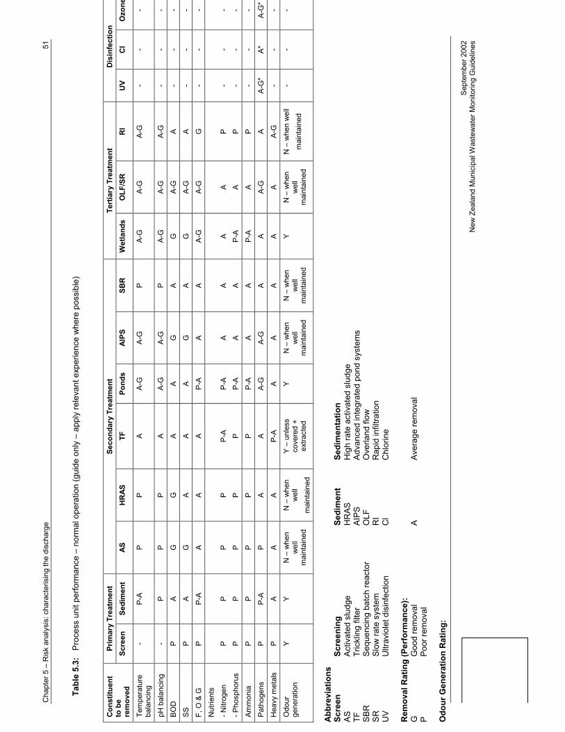
Cha
pter
5 –
Ris
k an
alys
is: c
hara
cter
isin
g th
e di
scha
rge
51
Sept
embe
r 200
2N
ew Z
eala
nd M
unic
ipal
Was
tew
ater
Mon
itorin
g G
uide
lines
Tabl
e 5.
3:
Proc
ess
unit
perfo
rman
ce –
nor
mal
ope
ratio
n (g
uide
onl
y –
appl
y re
leva
nt e
xper
ienc
e w
here
pos
sibl
e)
Prim
ary
Trea
tmen
tSe
cond
ary
Trea
tmen
tTe
rtia
ry T
reat
men
tD
isin
fect
ion
Con
stitu
ent
to b
ere
mov
edSc
reen
Sedi
men
tAS
HR
ASTF
Pond
sAI
PSSB
RW
etla
nds
OLF
/SR
RI
UV
Cl
Ozo
ne
Tem
pera
ture
bala
ncin
g-
P-A
PP
AA-
GA-
GP
A-G
A-G
A-G
--
-
pH b
alan
cing
-P
PP
AA-
GA-
GP
A-G
A-G
A-G
--
-BO
DP
AG
GA
AG
AG
A-G
A-
--
SSP
AG
AA
AG
AG
A-G
A-
--
F, O
& G
PP-
AA
AA
P-A
AA
A-G
A-G
G-
--
Nut
rient
s- N
itrog
en- P
hosp
horu
sP P
P PP P
P PP-
A PP-
AP-
AA A
A AA P-A
A AP P
- -- -
- -Am
mon
iaP
PP
PP
P-A
AA
P-A
AP
--
-Pa
thog
ens
PP-
AP
AA
A-G
A-G
AA
A-G
AA-
G*
A*A-
G*
Hea
vy m
etal
sP
AA
AP-
AA
AA
AA
A-G
--
-O
dour
gene
ratio
nY
YN
– w
hen
wel
lm
aint
aine
d
N –
whe
nw
ell
mai
ntai
ned
Y –
unle
ssco
vere
d +
extra
cted
YN
– w
hen
wel
lm
aint
aine
d
N –
whe
nw
ell
mai
ntai
ned
YN
– w
hen
wel
lm
aint
aine
d
N –
whe
n w
ell
mai
ntai
ned
--
-
Abbr
evia
tions
Scre
enSc
reen
ing
Sedi
men
tSe
dim
enta
tion
ASAc
tivat
ed s
ludg
eH
RAS
Hig
h ra
te a
ctiv
ated
slu
dge
TFTr
ickl
ing
filte
rAI
PSAd
vanc
ed in
tegr
ated
pon
d sy
stem
sSB
RSe
quen
cing
bat
ch re
acto
rO
LF
O
verla
nd fl
owSR
Slow
rate
sys
tem
RI
Rap
id in
filtra
tion
UV
Ultr
avio
let d
isin
fect
ion
Cl
Chl
orin
e
Rem
oval
Rat
ing
(Per
form
ance
):G
Goo
d re
mov
alA
Aver
age
rem
oval
PPo
or re
mov
al
Odo
ur G
ener
atio
n Ra
ting:

52C
hapt
er 5
– R
isk
anal
ysis
: cha
ract
eris
ing
the
disc
harg
e
Sept
embe
r 200
2N
ew Z
eala
nd M
unic
ipal
Was
tew
ater
Mon
itorin
g G
uide
lines
YYe
sN
No
* Dis
infe
ctio
n ca
pabi
lity
depe
nden
t on
rem
oval
cap
abilit
y of
trea
tmen
t uni
ts p
rior t
o di
sinf
ectio
n pr
oces
s.

Cha
pter
5 –
Ris
k an
alys
is: c
hara
cter
isin
g th
e di
scha
rge
53
Sept
embe
r 200
2N
ew Z
eala
nd M
unic
ipal
Was
tew
ater
Mon
itorin
g G
uide
lines
Tabl
e 5.
4: P
roce
ss u
nit p
erfo
rman
ce –
vul
nera
bilit
y to
‘ups
et’ c
ondi
tions
(gui
de o
nly
– ap
ply
rele
vant
exp
erie
nce
whe
re p
ossi
ble)
Prim
ary
Trea
tmen
tSe
cond
ary
Trea
tmen
tTe
rtia
ry T
reat
men
tD
isin
fect
ion
Con
ditio
nSc
reen
Sedi
men
tAS
HR
ASTF
Pond
sAI
PSSB
RW
etla
nds
OLF
/SR
RI
UV
Cl
Ozo
neH
andl
es p
roce
ss u
pset
chan
ge?
AA
P-A
P-A
PA
P-A
AP-
AA
A-
--
Han
dles
sud
den
volu
me
chan
ges?
AA
AA
AA*
AP
A*A
A*-
--
Han
dles
toxi
c sh
ock/
slug
?A
AP-
AP-
AP
P-A
P-A
PP-
AP-
AA
--
-R
elia
bilit
yA
AP-
AA
AA
AA
AA
AA
AA
Ease
of o
pera
tion?
GA-
GA
AA
GA
AA
AA
AA
A
Abbr
evia
tions
:
Scre
enSc
reen
ing
Sedi
men
t Se
dim
enta
tion
ASAc
tivat
ed s
ludg
eH
RAS
Hig
h ra
te a
ctiv
ated
slu
dge
TFTr
ickl
ing
filte
rAI
PS
Adva
nced
inte
grat
ed p
ond
syst
ems
SBR
Sequ
enci
ng b
atch
reac
tor
OLF
O
verla
nd fl
owSR
Slow
rate
sys
tem
RI
Rap
id in
filtra
tion
UV
Ultr
avio
let d
isin
fect
ion
Cl
Chl
orin
e
Perf
orm
ance
Rat
ing
(relia
bilit
y an
d/or
‘rob
ustn
ess’
)
GG
ood
AAv
erag
eP
Poor
* Dep
ende
nt o
n th
e am
ount
of f
reeb
oard
ava
ilabl
e w
ithin
the
treat
men
t uni
t(s).

54C
hapt
er 5
– R
isk
anal
ysis
: cha
ract
eris
ing
the
disc
harg
e
Sept
embe
r 200
2N
ew Z
eala
nd M
unic
ipal
Was
tew
ater
Mon
itorin
g G
uide
lines
Tab
le 5
.5:
D
isch
arge
cha
ract
eris
atio
n sh
eet.
Fill
this
she
et in
for S
tep
1.1
in ri
sk a
naly
sis
in C
hapt
er 4
. See
als
o ex
ampl
e in
Tab
le 5
.6.
Add
othe
r con
stitu
ents
and
mak
e ot
her a
dapt
ions
to th
is ta
ble
if re
quire
d.
Was
tew
ater
sou
rces
:…
……
……
……
……
……
……
……
……
……
……
……
….
Flow
(bes
t est
imat
e):
ADW
F:…
……
……
……
……
……
…PW
WF:
……
……
……
……
……
……
..C
onst
ituen
tIn
fluen
t cha
ract
eris
tics
Trea
tmen
t pla
nt p
roce
ss u
nit p
erfo
rman
ce, n
orm
al o
pera
tion
(giv
e ra
ting
of P
, A o
r G fo
r eac
h un
it fo
r eac
h co
nstit
uent
, fro
mTa
bles
5.3
& 5
.4)
Kno
wn
data
on in
fluen
tw
/w (N
ote
1)
Influ
ent
char
acte
ristic
ratin
g(L
, M o
r H –
from
Tab
le5.
2)
Kno
wn
data
on
w/w
effl
uent
(Not
e 1)
Asse
ssed
haz
ard
pote
ntia
l of
disc
harg
eco
nstit
uent
(giv
e ra
ting
of L
,M
or H
) (N
ote
2)
Tem
pera
ture
pH BOD
, CO
DSu
spen
ded
solid
sFa
ts, o
il &
grea
se,
float
able
sN
utrie
nts
-nitr
ogen
-pho
spho
rus
Amm
onia
Path
ogen
s(in
dica
tors
)H
eavy
met
als
Odo
ur
Not
e 1:
En
ter a
ny k
now
n da
ta, e
.g.,
mea
n an
d 95
%ile
con
cent
ratio
ns, d
aily
load
s, e
tc. R
efer
to a
noth
er s
heet
if n
eces
sary
.

Cha
pter
5 –
Ris
k an
alys
is: c
hara
cter
isin
g th
e di
scha
rge
55
Sept
embe
r 200
2N
ew Z
eala
nd M
unic
ipal
Was
tew
ater
Mon
itorin
g G
uide
lines
Not
e 2:
As
sess
the
char
acte
ristic
s of
the
disc
harg
e (fi
nal c
olum
n) b
y co
mbi
ning
the
influ
ent c
hara
cter
istic
ratin
g w
ith th
e tre
atm
ent p
roce
ss u
nit r
atin
gs. T
he L
, M &
H ra
tings
in th
e fin
al c
olum
n sh
ould
repr
esen
t the
ass
esse
d po
tent
ial h
azar
d ra
ting
of e
ach
disc
harg
e co
nstit
uent
. Kno
wn
data
on
the
efflu
ent d
isch
arge
(pen
ultim
ate
colu
mn)
shou
ld b
e ta
ken
into
acc
ount
if th
is is
ava
ilabl
e.
L =
low
pot
entia
l haz
ard,
M =
med
ium
pot
entia
l haz
ard,
H =
hig
h po
tent
ial h
azar
d (re
fer t
o Ta
bles
5.2
to 5
.4).
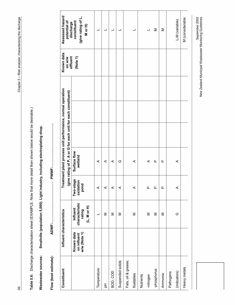
56C
hapt
er 5
– R
isk
anal
ysis
: cha
ract
eris
ing
the
disc
harg
e
Sept
embe
r 200
2N
ew Z
eala
nd M
unic
ipal
Was
tew
ater
Mon
itorin
g G
uide
lines
Tabl
e 5.
6:
Dis
char
ge c
hara
cter
isat
ion
shee
t (EX
AMPL
E. N
ote
that
mor
e de
tail
than
sho
wn
belo
w w
ould
be
desi
rabl
e.)
Was
tew
ater
sou
rces
:Sm
allv
ille
(pop
ulat
ion
5,00
0). L
ight
indu
stry
, inc
ludi
ng e
lect
ropl
atin
g sh
op.
Flow
(bes
t est
imat
e):
ADW
F:…
……
……
……
……
……
…PW
WF:
……
……
……
……
……
……
..
Con
stitu
ent
Influ
ent c
hara
cter
istic
sTr
eatm
ent p
lant
pro
cess
uni
t per
form
ance
, nor
mal
ope
ratio
n(g
ive
ratin
g of
P, A
or G
for e
ach
unit
for e
ach
cons
titue
nt)
Kno
wn
data
on in
fluen
tw
/w (N
ote
1)
Influ
ent
char
acte
ristic
ratin
g(L
, M o
r H)
Two-
stag
eox
idat
ion
pond
Surf
ace
flow
wet
land
Kno
wn
data
on w
/wef
fluen
t(N
ote
1)
Asse
ssed
haz
ard
pote
ntia
l of
disc
harg
eco
nstit
uent
(giv
e ra
ting
of L
,M
or H
)
Tem
pera
ture
LA
AL
pHM
AA
L
BOD
, CO
DM
AA
L
Susp
ende
d so
lids
MA
GL
Fats
, oil
& gr
ease
,
float
able
sM
AA
L
Nut
rient
s
-nitr
ogen
-pho
spho
rus
M M
P P
A P
L M
Amm
onia
MP
PM
Path
ogen
s
(indi
cato
rs)
GA
AL-
M (v
aria
ble)
Hea
vy m
etal
sM
(con
side
rabl
e

Cha
pter
5 –
Ris
k an
alys
is: c
hara
cter
isin
g th
e di
scha
rge
57
Sept
embe
r 200
2N
ew Z
eala
nd M
unic
ipal
Was
tew
ater
Mon
itorin
g G
uide
lines
(mai
nly
zinc
)G
AA
unce
rtain
ty)
Odo
urM
YY
M
September 2002New Zealand Municipal Wastewater Monitoring Guidelines
CHAPTER 6RISK ANALYSIS: CHARACTERISING THERECEIVING ENVIRONMENT
Paul Barter, Barry Robertson (Cawthron Institute)
6.1 Introduction
The purpose of this chapter is to assist the reader with characterising the receivingenvironment, as required in Step 1.2 in the risk analysis process (refer to Section 4.3.1). Thekey points are summarised in Table 6.2 (page 54), with a worked example in Table 6.3.
Classification of the receiving environment is a fundamental step in the HIAMP process.Since the receiving environment represents the final step in any wastewater treatment anddischarge process, the way in which an effluent is incorporated into the receivingenvironment is of critical importance in determining the extent and degree of adverse effectsto that environment. Receiving environment classification can take many forms and can bevery complex or very general, depending on the desired outcome. For example, physicalfactors such as climate, geography and biology are often used to ‘ecotype’ an environment,but social and cultural values are also important and might be incorporated under certaincircumstances. In general, characterisation of the receiving environment allows for thecreation of groups, or types of environments, which will react in a different fashion whenexposed to a wastewater discharge. For the purposes of these Guidelines, receivingenvironment classification will focus solely on physical, chemical and biological factors andwill not try to fully incorporate social and cultural aspects, as these are covered separately inChapter 7.
Receiving environment characterisation has been divided into two primary categories: (i)type of environment (e.g., lake, estuary etc.) and (ii) characteristics within each environmentthat affect the extent to which wastewater components will be assimilated (called‘assimilative capacity’). The types of environment have been deliberately modelled after theecosystem classifications used in the recent ANZECC guidelines (ANZECC 2000a) andreflect the broad categories of different receiving environments (i.e., Water, Soil, Air).Within each of these broad categories are additional divisions (e.g., lakes, rivers, estuaries),which reflect easily discernible differences in the individual category.
The characteristics of each of these receiving environment types (e.g., substrate, ecologyetc.) are used to derive which constituents of the wastewater (e.g., pH, nutrients, etc.) aremost important for consideration in the risk assessment (HIAMP) process in Chapter 4, andduring the design of the monitoring programme.
In this chapter, the broad categories that make up each of the types of receivingenvironments will be discussed first with some guidance on how the categories are defined.
From this, the wastewater and receiving environment components that may present a hazard(e.g., nutrients, odour, flow etc) are outlined in a matrix against the types of environments tohelp the reader short-list which factors have the highest priority (see section 6.4.1). Fromthis, the applicable constituents can be compared against the primary factors affecting

Chapter 6 – Risk analysis: characterising the receiving environment 59
September 2002New Zealand Municipal Wastewater Monitoring Guidelines
assimilative capacity and sensitivity for the particular receiving environment. The outputfrom this table can then be used to generate a list for inclusion in the HIAMP model.

60 Chapter 6 – Risk analysis: characterising the receiving environment
September 2002New Zealand Municipal Wastewater Monitoring Guidelines
6.2 Types of receiving environments
6.2.1 Water
Surface waters are the primary receiving environment for almost all wastewater dischargesin New Zealand (Table 6.1). As such, the focus of the guidelines and particularly this chapterwill be on surface waters, with far less emphasis placed on air and soil discharges, althoughthese will be addressed.
Table 6.1: Summary of wastewater plants and flow into different receiving environments in NewZealand (from Macdonald et al. 2001).
Receiving Environment Number of WastewaterPlants Average Daily Flow
Count (%) Sum (%)Freshwater<50% of stream/river flow 133 47.00 159,198 21.26>50% of stream/river flow 14 4.95 12,787 1.71Lake 4 1.41 2,868 0.38MarineEstuarine 7 2.47 146,487 19.57Harbour 13 4.59 10,314 1.38Shoreline 6 2.12 8,587 1.15Off-shore outfall 29 10.25 325,289 43.45Land & otherTotal flow to land 59 20.85 46,716 6.24Land, excess flow to surface water 17 6.01 35,553 4.75Piped to another plant 1 0.35 888 0.12Total 283 100 748,687 100
Table 6.1 shows that almost two-thirds (65.5%) of the average daily volume of wastewater inNew Zealand is discharged to a marine receiving environment. The majority of theremainder is discharged to a freshwater environment (23.4%), while only 6% is dischargedentirely to land.
However, when comparing numbers of wastewater plants producing these volumes, theproportions are very different, with roughly half (53%) of the total WWTPs discharging to afreshwater environment while roughly 20% of the WWTPs discharge to a marineenvironment. This distribution demonstrates that the freshwater discharges tend to be fromsmaller plants, while the marine discharges are from much larger facilities. This ratio is notunexpected, given that most of the major urban centres are situated on the coast.

Chapter 6 – Risk analysis: characterising the receiving environment 61
September 2002New Zealand Municipal Wastewater Monitoring Guidelines
Freshwater
The freshwater receiving environments have been divided into four main categories (refer toFigure 6.1):
(i) Lakes & Reservoirs.
(ii) Rivers/streams where wastewater input is <50% of normal base flow.
(iii) Rivers/streams where wastewater input is >50% of normal base flow.
(iv) Groundwater.
These categories are fairly self-explanatory and will not be discussed in detail. There arenumerous references that cover the hydrology of New Zealand (e.g., Mosley 1992, Viner1987 etc.) for those interested in obtaining more detail. There is also a reasonable summaryof New Zealand’s freshwater environments in Appendix 2, Volume 2 of the ANZECC(2000a) guidelines.
The majority of existing discharges to freshwater in New Zealand are to rivers or streamswhere the wastewater input represents less than 50% of the normal base flow (Table 6.1).
MarineFreshwater
Standing Waters Flowing WatersRivers & Streams Groundwater
Estuarine Harbours &Sheltered
Embayments
LakesReservoirs Wetlands Discharge is
<50% Base FlowDischarge is
>50% Base Flow
Soils
ref: Sewage Effluent toLand Guidelines
Air
ExposedNearshore Coastal
Offshore Coastal
Figure 6.1: Receiving Environment Categories.
Marine waters
The marine receiving environments have been divided into four main categories:
(i) Estuarine.
(ii) Harbours and Sheltered enclosed embayments.
(ii) Exposed Nearshore Coastal (shoreline).
(iii) Exposed Offshore coastal.
As was the case with freshwater, these categories are self-explanatory and will not bediscussed in detail. Unlike the freshwater environments in New Zealand, general texts on thecoastal waters are not readily available and tend to be more specific to individual disciplines.For example, physical oceanography (Heath 1985), ecology (Morton & Miller 1968; Jones1983), fish life (Francis 1988; Doak 1984), botany (Adams 1994), etc. There is also a

62 Chapter 6 – Risk analysis: characterising the receiving environment
September 2002New Zealand Municipal Wastewater Monitoring Guidelines
cursory summary of the New Zealand coastal environment in Appendix 2 (Volume 2) of thenew ANZECC guidelines.
Many people view ports and harbours as analogous to nearshore coastal. However, ports andharbours differ from coastal environments in that they are generally subject to a lesseramount of mixing and dispersion, which is a fundamental component of receivingenvironment characterisation.
6.2.2 Soil
Like water, the soil environment that receives wastewater discharges can be divided intovarious categories based on such parameters as soil type, existing land uses, proximity toground and surface waters, size of site, slope and various physical and chemical parameters.Although this chapter includes soil as a receiving environment, the primary purpose is tooffer guidance on discharges to surface waters, since the guidelines for disposal of sewageonto land (NZLTC 2000) address the soil receiving environment. The land disposalguidelines include sections on wastewater characteristics, site selection, soil treatmentprocesses, environmental effects, application methods, and crop selection. If soil disposal isa primary component of the wastewater discharge scenario being evaluated, it isrecommended that these other guidelines be used in conjunction with these wastewatermonitoring guidelines.
6.2.3 Air
In a similar vein to water and soil, the air environment receiving secondary emissions from awastewater plant can be divided into categories based on such parameters as land use,meteorology and topography. However, because air emission problems (particularly odours)can arise in most, if not all, of the different air environments (e.g., low or high windvelocities) air is considered as a single category in this chapter. In many areas air emissionsare a major concern for environmental assessment, particularly in relation to odour.Pathogens contained in discharged aerosols can also be of concern. Generally, however, theisolation from most public activity and the short distances travelled by most aerosols makesall but odour issues insignificant.
6.3 Receiving environment hazard identification
In order to develop the list of hazards needed for the HIAMP framework, the followingsection uses a two-part approach to narrow down the possible wastewater constituents thatare of concern. The process is set out in Table 6.2, with an example provided in Table 6.3.The process for filling in Table 6.2 is as follows:
1. From the first part of the table, select the relevant receiving environment and tick theshaded boxes for this receiving environment.
2. For each characteristic (i.e., Dilution, Substrate etc) in the second half of the Table,cross out the descriptions that don’t apply (i.e., if Dilution is poor, cross out‘moderate’ and ‘excellent’).

Chapter 6 – Risk analysis: characterising the receiving environment 63
September 2002New Zealand Municipal Wastewater Monitoring Guidelines
3. For each characteristic (i.e., Dilution, Substrate etc) tick the shaded boxes relating tothe description not crossed out.
4. Bring the ticks down to the row titled ‘Include in HIAMP’ to identify which issuesshould be identified in the worksheet in Appendix 3.
By selecting a particular receiving environment in the first half of Table 6.2, the list ofconstituents will be shortened (see estuary example, Table 6.3). For example, pH will neverbe an issue for a wastewater discharge into the marine environment. This shortened list isthen transferred to the second part of the table where each of these constituents is comparedagainst the assimilative characteristics and sensitivity for that particular environment. Fromthis second table, the list of hazards for the HIAMP model may be further reduced. However,any hazard checked in the bottom half of the table should be added to the HIAMP worksheet.
On completion, this process will result in a list of general wastewater constituents that maybe of concern for the given receiving environment and will therefore need to be consideredin the development of a monitoring programme. These general categories of constituentswill, in many cases, need to be refined to fit a targeted monitoring programme. For example,the wastewater characterisation (Chapter 5) may identify specific toxic compounds ornutrients to address. If a complete list of target metals is identified when the discharge ischaracterised, this list should be used in place of the more generic ‘Toxic compounds’ whenfilling in the HIAMP worksheet(s). On the other hand, if pH is highlighted as a factor in thedischarge characterisation in Chapter 5, but the receiving environment is a marine outfall,there is no rationale for including it in the HIAMP worksheet as an ecosystem risk.

64 Chapter 6 – Risk analysis: characterising the receiving environment
September 2002New Zealand Municipal Wastewater Monitoring Guidelines
Table 6.2: Receiving environments, constituents of concern, and assimilative capacity. Shadedboxes = potentially of concern. Refer to Section 6.4 for explanation of assimilativecapacity terms.
Receiving Environment Tem
pera
ture
Oxy
gen/
BOD
pH Sedi
men
tatio
n/sm
oth
erin
g (S
S)
Odo
ur/T
aint
ing
Floa
tabl
es/
scum
s
Col
our /
cla
rity
(SS)
Nut
rient
s/ e
nric
hmen
t
Toxi
c co
mpo
unds
Path
ogen
s
Lake/Reservoir - -River/ Stream (>50% base flow)River/ Stream (<50% base flow) - -Estuary - -Harbours & Sheltered Embayments - -Nearshore Marine (shoreline) - - - -Offshore Marine - - - -Groundwater - -Air - - - - - - - -Soils - - - -
Assimilative Capacity/SensitivityOf Te
mpe
ratu
re
Oxy
gen/
BOD
pH Sedi
men
tatio
n/sm
oth
erin
g (S
S)
Odo
ur/T
aint
ing
Floa
tabl
es/
scum
s
Col
our /
cla
rity
(SS)
Nut
rient
s/ e
nric
hmen
t
Toxi
c co
mpo
unds
Path
ogen
s
PoorModerate - - - DilutionExcellent - - - - - - - - - -
Mud - - - - -Sand - - - - - - - Substrate (s)Rock - - - - - - - - -
Unenriched - - - - - -Mod Enrichment - - - - - - Enrichment status
Enriched - - - - - - - - -High - - - -
Moderate - - - - - Sensitivity of Ecological Values Low - - - - - - - - - -
Yes Significant other Inputs No - - - - - - - - - -
Important - - - - - - Aesthetics Not so Important - - - - - - - - - -Yes - - - - - Contact
Recreation No - - - - - - - - - -Drinking - - -Irrigation - - - - Water Supply
(Economic Utility) Industrial - - - - - Food gathering Yes - - - - - - - -

Chapter 6 – Risk analysis: characterising the receiving environment 65
September 2002New Zealand Municipal Wastewater Monitoring Guidelines
No - - - - - - - - - -
YesInclude in HIAMP No
Table 6.3: Worked example of estuary receiving environment.
Receiving Environment Tem
pera
ture
Oxy
gen/
BOD
pH Sedi
men
tatio
n/sm
oth
erin
g (S
S)
Odo
ur/T
aint
ing
Floa
tabl
es/
scum
s
Col
our /
cla
rity
(SS)
Nut
rient
s/ e
nric
hmen
t
Toxi
c co
mpo
unds
Path
ogen
s
Lake/Reservoir - -River/ Stream (>50% base flow)River/ Stream (<50% base flow) - -Estuary - -Harbours & Sheltered Embayments -Nearshore Marine (shoreline) - - - -Offshore Marine - - - -Groundwater - -Air - - - - - - - -Soils - - -
Assimilative Capacity/SensitivityOf Te
mpe
ratu
re
Oxy
gen/
BOD
pH Sedi
men
tatio
n/sm
oth
erin
g (S
S)
Odo
ur/T
aint
ing
Floa
tabl
es/
scum
s
Col
our /
cla
rity
(SS)
Nut
rient
s/ e
nric
hmen
t
Toxi
c co
mpo
unds
Path
ogen
s
EstuaryPoor
Moderate - - - DilutionExcellent - - - - - - - - -
Mud - - - - - -Sand - - - - - - - Substrate (s)Rock - - - - - - - - -
Unenriched - - - - - -Mod Enrichment - - - - - - Enrichment status
Enriched - - - - - - - - - -Low - - - -
Moderate - - - - - Sensitivity of Ecological Values High - - - - - - - - -
Yes Significant other Inputs No - - - - - - - - - -
Important - - - - - - Aesthetics Not so Important - - - - - - - - - -Yes - - - - - Contact
Recreation No - - - - - - - - - -Drinking - - - Water Supply
(Economic Utility) Irrigation - - - -
TransferDown

66 Chapter 6 – Risk analysis: characterising the receiving environment
September 2002New Zealand Municipal Wastewater Monitoring Guidelines
Industrial - - - - -Yes - - - - - - - -
Food gathering No - - - - - - - - - -
YesInclude in HIAMP No
6.4 Characteristics of receiving environment
The remainder of this chapter defines the various categories of assimilative capacity andsensitivity listed in Table 6.2. It should be noted that these are not absolute measures and areonly intended to help provide a relative scale to prioritise the constituents in the wastewaterfor inclusion in the HIAMP model. If in doubt about which option within a category to use, itwould be prudent to choose the more conservative value. For example, choose moderatedilution over excellent dilution.
Dilution
Although fully understanding all the parameters that influence dilution and dispersion can bequite complicated, for the purposes of this chapter they have been simplified into the primaryfactors driving wastewater dilution. Namely, the configuration of the outfall (e.g., diffuservs. end of pipe), relative volumes of wastewater versus receiving water, and velocity of thereceiving water. By looking at these three factors, the relative dilution (i.e. poor, moderate,excellent) can be determined. As guidance, each of these three scenarios is discussed briefly.
Poor dilution (generally less than 50 fold dilution at 100m from outfall)
Poor dilution usually occurs when an effluent is piped directly onto the surface of a slowmoving receiving water. This category is characterised by a conspicuous and persistentplume in the receiving water under all discharge flows and receiving environmentconditions. This is most pronounced when effluents are discharged to an estuarine or coastalenvironment where the lighter, freshwater effluent sits atop the heavier saline receivingwater or in lakes or rivers where available dilution is low. Although poor dilution is mostobvious for poorly treated effluents, the level of treatment has little effect on dilution.
Moderate dilution (generally between 50 & 250 fold dilution at 100m from outfall)
Most wastewater outfalls in New Zealand currently fall under this category. This category ischaracterised by a noticeable, but perhaps intermittent plume in the vicinity of the dischargethat may or may not dissipate fairly quickly. This plume might show up as a discolourationin the receiving water or just as likely as a ‘boil’ or ‘slick’ representing a change in thesurface tension of the receiving water. Moderate dilution can cover a wide range ofscenarios. For example, a low volume discharge into a fast moving, large river might achievemoderate dilution regardless of whether the effluent is diffused or not. Similarly, a largevolume discharge into a slow moving coastal environment might also achieve moderatedilution if the effluent is sufficiently diffused and submerged.
Excellent dilution (generally >250 fold dilution at 100m from the outfall)

Chapter 6 – Risk analysis: characterising the receiving environment 67
September 2002New Zealand Municipal Wastewater Monitoring Guidelines
Very few wastewater outfalls in New Zealand have excellent dilution. This category ischaracterised by an absence of a visible plume under all operating and receiving environmentconditions. It also applies almost exclusively to multiport, submerged diffusers into fastmoving or large volume receiving waters.

68 Chapter 6 – Risk analysis: characterising the receiving environment
September 2002New Zealand Municipal Wastewater Monitoring Guidelines
Substrate
Substrate has been broken into three categories: Mud, Sand and Rock. It is loosely defined asthe bottom type in the vicinity of the outfall that is likely to be impacted by the discharge. Avariety of substrates can exist, so multiple selections can be made. Substrate is an importantfactor for determining receiving environment sensitivity, particularly with regard to nutrientenrichment and sedimentation/smothering.
Enrichment status
The trophic state of an aquatic receiving environment refers to the nutritional level of thatwaterbody and is generally determined by measuring the nutrients or organic primaryproductivity of that body. Commonly, there are three trophic states (unenriched, moderatelyenriched, and enriched) for marine and fresh waterbodies. Their general characteristics aredescribed in Table 6.4 but it must be borne in mind that additional baseline data may berequired to define appropriate categories.
Table 6.4: Categories of trophic status and the likely response of various waterbodies.
TrophicCategory
Lake or Reservoir(see Cooke et al. 1986)
Rivers and Streams(see Biggs 2000)
Coastal and Estuarine
UnenrichedLow innutrients andorganicproduction.
Usually deep withnutrient-poor sediments,few macrophytes andhigh dissolved oxygen inthe deepest water (e.g.Lake Manapouri).Diversity ofphytoplankton can behigh.
Usually few macrophytesor periphyton growth.
Low production andabundance of fast-growingalgae, such as phytoplankton,attached algae and short-livedmacroalgae (e.g. sea lettuce).
ModeratelyenrichedModeratenutrients andorganicproduction
Moderate nutrient levelsin sediments, somemacrophytes andmoderate dissolvedoxygen in deepestwater(e.g., LakeTarawera)
Moderate macrophyteand periphyton growth.
Moderate production andabundance of fast-growingalgae, such as phytoplankton,attached algae and short-livedmacroalgae (e.g. sea lettuce).Many New Zealand estuariesfit this category.
EnrichedHighnutrients andorganicproduction.
Often shallow tomoderately deep,nutrient-rich sediments,low oxygen in deepestwater (e.g. Lake Hayes.Lake Rotorua). Water isoften coloured andphytoplanktonpopulations are nearlymonospecific.
High periphyton, andmacrophyte growth.Sometimes, lowdissolved oxygenparticularly in earlymorning.
High production andabundance of fast-growingalgae, such as phytoplankton,attached algae and short-livedmacroalgae (e.g. sea lettuce).Shading by these plantsreduces the abundance ofslow-growing benthicmacrophytes such asseagrasses and kelps.Sometimes low dissolved

Chapter 6 – Risk analysis: characterising the receiving environment 69
September 2002New Zealand Municipal Wastewater Monitoring Guidelines
oxygen in poorly flushedwaters.

70 Chapter 6 – Risk analysis: characterising the receiving environment
September 2002New Zealand Municipal Wastewater Monitoring Guidelines
Sensitivity of ecological values
Impacts of wastewater on marine and freshwater ecology is a complex issue but is mostfrequently addressed by considering effects at the community level. Such impacts include:
• Loss of rare or sensitive species.
• Quantitative changes (e.g., in age structure) of longer-lived species.
• Decreased species diversity.
• Dominance of opportunistic species.
Although impacts can occur to most members of an aquatic community, the effect on thebenthic (bottom-dwelling) community, in particular, is often used as an indicator of thelikely worst case overall ecological impact of a particular discharge. This is because variouscontaminants, including nutrients, organic matter, metals, synthetic organic toxicants andpathogens, accumulate in marine and freshwater sediments at greater concentrations than theoverlying water. As such, aquatic sediments serve as ‘sinks’ for contaminants, with thepotential to affect benthic communities and overlying water quality. In addition, comparedwith overlying water, which exhibits large short term fluctuations in physical, chemical andbiological characteristics, the benthic environment is much more stable as it effectively‘integrates’ these fluctuations over time.
Given that the benthic community is likely to be a good indicator of wastewater impacts, thesensitivity of that community (plus any other more sensitive individuals or communities) canbe categorised into low, moderate and high sensitivity groupings as follows:
High sensitivity: This category implies that there are communities, habitats or species in thevicinity of the outfall that are especially sensitive to wastewater contaminants. As aconsequence, avoiding adverse effects to these groups is of paramount importance. Examplesinclude the presence of rare, threatened or endangered species; direct proximity to reserveareas; or the presence of species that are particularly sensitive to wastewater dischargerelated effects (e.g., smothering, enrichment etc.) It also includes communities or species thatare very slow to recover from a disturbance. An example of this category would be a lakethat is completely contained within an unmodified catchment.
Low sensitivity: This category is characterised by a relative lack of biota or an environmentthat is impoverished, homogeneous, or ubiquitous. Ubiquitous communities/species,although not without ecological merit, can be considered of lower ecological sensitivity forsmall scale disturbance if they are common enough on local, regional, national scales. Anexample of this type of community would be a coastal environment dominated by highenergy, mobile coarse sediments where physical disturbance is the dominating force.
Moderate Sensitivity: This category, as the name implies, falls somewhere in between thetwo extremes of low and high sensitivity, and under most circumstances will be valuejudgement based. It includes areas where loss of, or adverse effects to, a part of thecommunity might be an issue, but not to such an extent that it should be completely avoided.It includes areas that might already be slightly compromised, from either other inputs orperiodic natural disturbance.

Chapter 6 – Risk analysis: characterising the receiving environment 71
September 2002New Zealand Municipal Wastewater Monitoring Guidelines
Significant other inputs to the environment
Other inputs (e.g., wastewater sources, septic runoff, industrial discharges, stormwater, solidwaste disposal, aquaculture, and dredge disposal) can have a dramatic effect on theassimilative capacity of a receiving environment. If these other inputs are not taken intoaccount, it might erroneously be assumed that the assimilative capacity is much higher thanit actually is because the bulk of the capacity has already been expended.
Ideally, the condition of any given receiving environment will be the result of thecombination of inputs it already receives. As such, the effects of other inputs on theassimilation of wastewater constituents will already be adequately accounted for by the othercategories, e.g., enrichment status, contact recreation etc. However, for the sake of ensuringa more holistic assessment, the category of ‘other inputs’ has been included in the hazardidentification procedure. The category has been divided into two groupings, significant otherinputs and no significant other inputs.
Whether any of these other inputs represents a significant contribution is again a judgement-based decision, but generally if the activity requires a resource consent it should beconsidered a significant input. Additionally, significant inputs of contaminants may beentering a receiving environment via non-point sources that do not require a consent (e.g.,during flooding in a river, agricultural runoff and construction site runoff).
Aesthetics
This is a somewhat subjective category, but in general, more pristine areas are considered ofhigher aesthetic value than areas that are subject to a high degree of development ormodification. There are numerous items to consider when assessing the aesthetic nature of areceiving environment. These include but are by no means limited to: proximity to parks &reserves, amount of tourist activity, level of industrial development, colour of the receivingwater (deep blue waters are inherently more aesthetically valued than brown or greenwaters), adjoining beaches etc. Again, if in doubt, choose the more conservative value of‘high importance’.
Human health and safety via contact recreation
There are at least two aspects to consider with contact recreation: firstly, the potential forinfection from pathogens; and secondly, physical hazards caused by poor water clarity and/orbuild up of slimes on substrate (refer to MfE 1994a and MfE 1992, respectively).
At one time contact recreation activities were primarily restricted to swimming and bathingbut that is no longer the case. Therefore, when interpreting this category, it is important toconsider not just whether the given receiving environment is as suitable swimming/bathingarea but the myriad other activities that could be taking place e.g., surfing, boardsailing,kayaking, personal watercraft (e.g., Jet ski), snorkelling, SCUBA diving, etc. If it issuspected that any of these activities are conducted on a regular basis, then the contactrecreation ‘Yes’ box should be selected.
Water supply

72 Chapter 6 – Risk analysis: characterising the receiving environment
September 2002New Zealand Municipal Wastewater Monitoring Guidelines
Some receiving waters may be taken for community water supplies, irrigation and industrialpurposes. These are classified under ‘economic utility’ in the HIAMP process. If so, therewill be a need to ensure that any risk of contamination to these supplies is adequately takeninto account and appropriate monitoring undertaken. The quality of water required for watersupply will vary depending on the type of supply. The ANZECC (2000b) water qualityguidelines provide direction on the appropriate parameters to monitor for various types ofwater supply, and the NZ Drinking Water Standards (MOH 2000) set compliance limits forthe protection of human health.

Chapter 6 – Risk analysis: characterising the receiving environment 73
September 2002New Zealand Municipal Wastewater Monitoring Guidelines
Food gathering
This category can include either community-based (community value) or commercialactivities (economic utility). Given the potential human risks associated with all but the moststringent wastewater treatment processes, any amount of food gathering should beconsidered significant, even if the food source is not commonly thought to retaincontaminants. This includes everything from small amounts of plants collected for cultural orspiritual reasons, up to large commercial fishing activities. Common examples includecollection of watercress, shellfish (e.g., mussels, pipis, cockles, scallops, koura, etc.), fishing,whitebaiting etc.
Cultural or spiritual value
Under the Third Schedule to the RMA, waters may be managed for Cultural Purposes andwaters may be classified for such purposes where cultural or spiritual values are specified forthat area. Such values, including burial sites and traditional food gathering areas, are ofparticular significance to Maori, but other groups may also consider an area to have culturalor spiritual values. This aspect is covered in greater detail in Chapter 7, but is also includedhere as it has bearing on the receiving environment sensitivity in a similar manner toaesthetic values.

September 2002New Zealand Municipal Wastewater Monitoring Guidelines
CHAPTER 7RECOGNISING COMMUNITY VALUES
James Baines, Janet Gough (Taylor Baines Associates)Donald Couch (Lincoln University)
7.1 Why recognise community values?
Community values are an important driver for establishing priorities under a risk-basedapproach to setting priorities for wastewater monitoring. Ideally, consistent with theAustralian and New Zealand Risk Management Standard (AS/NZS 4360), adopting a riskmanagement framework should involve explicit consideration of both review andmonitoring, and communication and consultation with affected parties. In addition, whilerisk is a function of likelihood and magnitude of effect, the context of the activity is animportant component of any risk analysis.
Monitoring programmes for wastewater discharges are instituted in conjunction with settingconditions for resource consents (both new consents and renewals). At the present time veryfew consents include requirements for recognising community values, though this may bebecoming more common. However, there can be significant benefits gained by recognisingand taking account of community values.
These include:
• A broader understanding of the effects of discharge on the receiving environmentand the host communities (i.e., those communities affected by the wastewatersystem) by capturing well established bodies of knowledge that might reflect localknowledge, but also more general social and cultural information.
• Understanding of the factors that influence community priorities, thus providing away of determining where emphasis should be placed.
• A process for engaging the community and gaining their understanding and support.
• A process for meeting legislative requirements.
The effects of wastewater treatment processes have both physical and value components.Thus there are a number of community-based factors that influence both the level of risk,and the available (acceptable) processes for reducing those risks. These physical and socialfactors, which include perceptions of risk, affect the priorities resulting from adopting a risk-based approach.

Chapter 7 – Recognising community values 75
September 2002New Zealand Municipal Wastewater Monitoring Guidelines
7.2 Which values?
7.2.1 What do we mean by values?
Values are basic principles, which are reflected in our cultures and help us in a variety ofways; to understand and give meaning and significance to our world, and to say what isimportant. Specifically, they assist us to -
• Understand our place in the world (e.g., “we should treat other species with the samelevel of respect we treat people”, or “people are more important than other species”).
• Identify desirable goals and situations, and choose among alternatives (e.g.,“protecting water quality for human consumption is important”, or “taking the long-term view is important”, or “using resources sustainably is essential”).
• Develop a basis for relating to the environment (physical, social and spiritualenvironment) to maximise the achievement of desirable goals (e.g., “rivers can nolonger be treated as convenient dumping grounds for waste”, or “discharge ofwastewater into rivers is acceptable provided that certain environmental standardsare met”).
• Set social norms and determine appropriate behaviours (e.g., “respect for others isimportant”, or “wastefulness should be discouraged”).
From the Maori perspective this can be portrayed by a proverb: -
Toi tu te marae o Tane
Toi tu te marae o Tangaroa
Toi tu te iwi …
If the marae of Tane (Deity of the Forest) survives
If the marae of Tangaroa (Deity of the Sea) survives
The people live on …
Whilst some values can be very closely linked to the survival of communities and cultures,they are not easily scientifically testable propositions; they reflect fundamental beliefs.
Values are basic principles that are usually shared widely in common with others but notnecessarily universally by everyone in the community. Not everyone will express similarvalues in the same way or hold the same attitudes to everything. Therefore, the concept ofvalues encompasses both the idea of community norms and the idea that there will bedifferences in values held by different groups within a community, or different individualswithin a group.
Maori values do not differ essentially from Pakeha values when looking at our naturalenvironment and the effects of wastewater discharges.

76 Chapter 7 – Recognising community values
September 2002New Zealand Municipal Wastewater Monitoring Guidelines
Values are expressed in attitudes and the way people behave to other people, and to theenvironment. However, even if values remain fairly constant over time, the interpretation ofthose values in determining appropriate behaviour (tikanga) can change over time in newand evolving social and technological contexts. This means that certain cultural values donot necessarily prescribe the same behaviours for all time. For example, the values of tapuand noa are still important to preserving both spiritual and physical well being in the Maoricommunity. The relationship of Maori communities with their taonga and their waahi tapu isstill important. What has changed is the way these values are implemented, the modern-daytikanga. Tikanga may change over time. It is not necessarily applicable everywhere in thecountry. It is important to remember that iwi in different areas have their own tikanga fordealing with these matters.
Technical understanding and good information can influence how values are re-interpretedinto behaviour. For example, the repugnance for Maori to the discharge of sewage into watercan be resolved using the belief that materials can be cleansed by recycling them throughwhenua, the land. Knowledge of the cleansing effects of passage through the soil has enabledmodern arrangements for sewage effluent to be designed to take advantage of this withoutcausing offence to Maori in the modern world (e.g., effluent irrigation to land).
7.2.2 Community values
Values are diverse; they may relate to many different aspects of people’s lives. The phrase‘community values’ is intended to describe the mix of social, community and spiritualvalues; to be inclusive of the diversity of values which people in the community hold.
It is likely that certain values will generally be applicable to thinking about the operation ofwastewater treatment plants, such as, for example -
1. The discharge of effluent containing significant residues of human wastes to water willalways be offensive to local communities.
2. Protecting water quality in neighbouring water bodies is important.
3. The ability of neighbours to live in healthy conditions or neighbouring businesses tomaintain the health of the natural environment should not be compromised by theoperations of a WWTP.
4. The operations of a WWTP should not create significant offence to other parties,beyond the boundary of the plant.
This cluster of value statements describes various things which communities value - ahealthy environment (2), healthy people (3), opportunities for people to enjoy naturalenvironmental amenities (4) - all linked to a basic moral position (1).
However, the expression of values may differ for different interest groups in the community,or for communities in different geographical locations. For example, if a WWTP is locatedin a totally rural community, with predominantly productive agricultural businessneighbours, these neighbours are likely to place considerable importance on controlling risksfrom aerosols, preventing contamination of surface water by sewage effluent or bio-solids, or

Chapter 7 – Recognising community values 77
September 2002New Zealand Municipal Wastewater Monitoring Guidelines
ensuring that weeds are well controlled on land within the plant boundary so that they cannotpose a threat to neighbouring farmers. In contrast, if the locality has a significant rural-residential lifestyle presence, neighbours are likely to put greater emphasis on the possibilityof off-site odour, visual and noise effects.
As a result, what is important may vary from group to group or place to place. This hasimplications for how to go about ‘recognising community values’ in monitoring activities.Ideally, the approach to working out what is appropriate should involve face-to-facediscussion - kanohi ki kanohi.
7.2.3 Recognising well-established bodies of knowledge and value bases
Because of the multi-cultural make-up of New Zealand’s population, we have a diversity ofvalues. There are two dominant, well-established bodies of knowledge and understanding -the values and knowledge of Maori as long-standing indigenous people of the land, and thevalues and knowledge of Pakeha as the more recent arrivals, with more techno-centricapproaches. These two cultural strands display some values that are very similar and somethat are contrasting.
There are undoubtedly comparable and parallel ideas between the two dominant strands,even if the ‘point of entry’ into a discussion may appear conflicting. For example, askingPakeha about a proposal for sewage effluent discharge into a river is most likely to evoke aresponse which discusses water quality in terms of faecal contamination, nutrient andturbidity levels, and the potential effects on recreational use of the water or on abstraction forcommercial use. In contrast, asking Maori the same question is most likely to evoke aresponse which challenges the whole idea of discharge to the river, raises issues of waahitapu, kaitiakitanga and whakapapa and then examines potential effects on customary rightsto gather food nearby. Different values means that different issues may take on greaterimportance. But are the sets of underlying values really so different?
In fact, the two responses differ most in their initial ‘point of entry’ to the discussion andrange of issues. Maori and Pakeha may not be so different in some of the importantunderlying values. However, they may choose to express them in different ways, or not toarticulate some values at all. Furthermore, there are many very similar concepts that arerelevant to managing and monitoring the effects of waste water treatment plants:
kaitiakitanga responsibility to look after the land, the water and the people in theirrohe, that is, the environment and the people who live in thatenvironment
rangatiratanga the right to make rules governing the use of resources
whakapapa interconnectedness; linking people to nature by tracing back to Ranginuiand Papatuanuku
Maori classify water according to a number of different states, including:

78 Chapter 7 – Recognising community values
September 2002New Zealand Municipal Wastewater Monitoring Guidelines
• Waiora which is the purest form of water and has the potential to give life, tosustain well being and to counteract evil. Waiora is used in sacred ritualsto purify and sanctify.
• Waikino is water that is polluted, debased and spoilt. Water in this polluted formhas the potential to cause harm to all life forms including humans.
• Waimate is water that is so polluted that its life-force has expired. The mauri hasleft the water. Waimate has lost its power to regenerate itself and otherliving things.
Practical implications of water management associated with these categories link to thenotion of sustainability. The brief descriptions of some Maori concepts provided above arenot comprehensive. They are provided for the reader as examples of different butcomparable forms of expression. Details may vary in different parts of the country, and thereader should engage local iwi representatives in a dialogue to achieve better mutualunderstanding.
Many Maori are increasingly comfortable with the concept of sustainability, interpreted inthe sense of ‘managed use’ of resources. Sustainability has undoubtedly gained widespreadcurrency in pakeha discussions on resource management.
It makes sense to recognise both Maori and Pakeha values and knowledge not only becauseof what can be learnt from being open to various sources of knowledge in our communities.In this particular instance it is reinforced by the partnership obligations flowing from theTreaty of Waitangi, now required under the RMA and several other recent pieces oflegislation.
The significance of this discussion, in the context of a risk-based approach to monitoringwastewater treatment plants, can be summed up as follows:
• Recognising community values is important to implementing a risk-based approachto monitoring.
• Since communities are not homogenous in the values they subscribe to, it isnecessary to draw on the well-established value bases and bodies of knowledge.
• Acceptance of this has practical implications for the way local authorities approachthe need for community input into monitoring programmes - whom to work with inestablishing community priorities, and deciding what to monitor.
7.2.4 Examples of community values relevant to wastewater discharge monitoring
The community values as presented in Section 7.3.2 point to a range of possible issues andeffects which help to explain why monitoring is important, and also indicate what to monitorfor. These include:
• Risk to spiritual well-being or aesthetics from inappropriate discharge practices.
• Risk of causing undesirable changes in natural systems (e.g., loss of fish species,algal blooms, etc.) from bio-chemical contaminants in the discharge.
Chapter 7 – Recognising community values 79
September 2002New Zealand Municipal Wastewater Monitoring Guidelines
• Risks to human health from bio-chemical contaminants in the discharge.
• Risks of reducing or losing natural environmental amenities from intrusive odours,aerosols, noise or water contamination.
• Derived risks to property values in the neighbourhood.
If monitoring is not effective in avoiding these risks, or in maintaining them at levelsacceptable to the community, then monitoring and management has failed.
7.3 The impact of community values on risk perceptions
Values inform perceptions. Perceived risk is a judgement or valuation by individuals orgroups of people. Whether estimates of risk are made by technical experts or by the generalpublic, they cannot avoid containing elements of perception. This derives from the way inwhich people design models or experiments, the weighting that they give to socialimportance, the way in which they select or derive data and even in the risks they choose tostudy.
However, perceived risk estimates differ from technical assessments because they take intoaccount a wider range of factors or attributes of the risk and general context of the situation.Risk perceptions are often more to do with the acceptability of the risk than the level of therisk, and typically factors such as the type of harm, the number of people affected, whetherexposure to the risk is voluntary, and how much is known about the risk dominate the wayrisks are perceived. Thus risk perceptions are founded on value systems.
There is no general method for dealing with the differences between perceptions andtechnological judgements. Sometimes communities estimate risk as being lower thantechnical experts and sometimes they estimate it as being higher. Society's inputs areperceptions, deriving from values, and to adequately include these in decision processesways of measuring (or at least eliciting) community values are needed. Communityperceptions of risk are informed by local knowledge, written and verbal history, and socialand cultural customs, and evaluation of the magnitude of effect component of risk requiresconsideration of human values and emotions.
Interaction between technical experts and communities is a useful way of developing mutualunderstanding and respect. The term ‘risk communication’ is used in a technical sense tomean the development of communication channels that are used to transmit informationbetween different parties such as council staff and communities. It is essential that all theparties involved in communicating risk recognise that they should listen, ask questions,provide responses and be prepared to acknowledge uncertainty. Effective riskcommunication depends on trust and credibility and two-way communication.
An important aspect of risk communication is deciding who should be involved. Thisrequires identifying a community of interest that might not necessarily be defined solely ongeographical factors. Individuals and groups from outside the local area may have links withthe area that mean that they also need to be considered. In many cases the local communitywill be able to advise as to who might need to be consulted.

80 Chapter 7 – Recognising community values
September 2002New Zealand Municipal Wastewater Monitoring Guidelines
Another aspect of risk communication is ensuring that all parties have a commonunderstanding of the language being used. While technical experts should avoid ‘talkingdown’ to individuals and community groups, they should at the same time make sure that theterms they use are simple, clear and consistent.
7.4 Using qualitative risk assessment to help include values
Qualitative risk assessment can be used to prioritise risks where quantitative information isnot available. It uses words to describe the probability or likelihood of the effect occurringand the magnitude of that effect, and then combines these to form a qualitative estimate ofthe level of risk. The benefit of using qualitative risk assessment to elicit communityestimates of risk levels is that the descriptors used to describe likelihood and magnitude (seebelow) can incorporate values.
Qualitative analysis requires three sets of word scales that should be constructed individuallyfor each situation. The first of these is the likelihood of the event occurring. This is describedin Table E in Chapter 4. The second word scale is the magnitude of the event. This isdescribed in Table D3 in Chapter 4 (aesthetics and odour and also described in Tables D5and D6, respectively). The likelihood and magnitude tables can be combined in a matrix thatis used to develop a ‘level of risk’ designation that is used to group and rank risks (see TableF in Chapter 4).
Recognising community values in risk assessment (i.e. in the process of determining thelikelihood and magnitude components as above) can be done through a range of ways ofallowing community input to monitoring and evaluation of WWTP performance, all ofwhich depend on effective risk communication. Some particular ways of doing this aredescribed in Chapter 13. It is the process of community assessment and judgment thatenables communities to express their values in relation to managing the effects of WWTPs.
Therefore, critical questions to think about are:
• Who/which groups should you try to involve (who are the affected parties andinterested parties).
• How often.
• How should this be done (this may differ from group to group).
• What are the prior information needs of the community and what are the feedbackrequirements for the operators.
7.5 Putting these ideas into practice
Community values can be recognised explicitly through the consultation processessurrounding the applications for resource consents. However, even if consents have beengranted for long periods (e.g., 35 years), it should not be assumed that it might be severaldecades before such an opportunity arises again. Other opportunities will arise from time totime during periodic reviews of monitoring results by the consent authority. These are

Chapter 7 – Recognising community values 81
September 2002New Zealand Municipal Wastewater Monitoring Guidelines
usually stipulated in consent conditions. The consent authority may review monitoringreports for reasons that may include community concerns, as a reflection of their values.


PART THREE:DESIGN


September 2002New Zealand Municipal Wastewater Monitoring Guidelines
CHAPTER 8CONCEPTUAL DESIGN OF THEMONITORING PROGRAMME
Rob Bell, David Ray, Chris Hickey, Graham McBride (NIWA)
8.1 Introduction
8.1.1 Design of the monitoring programme - overview
The risk analysis completed in Part Two (summarised on Worksheets A and B in Appendix3) provides the starting point for the design of the monitoring programme. The final columnin Worksheets A and B identifies the level of resources appropriate for monitoring of each ofthe identified risks in the discharge.
The final output from Part Three of the Guidelines should be a detailed monitoringprogramme. The process of arriving at this monitoring programme is summarised as follows:
1. Define the objectives and end uses of the monitoring programme, and design theconceptual form of the monitoring programme (Chapter 8).
2. Review the monitoring options in Chapters 9 to 12 to determine which options are mostrelevant in terms of the risks identified in Part Two and the objectives and end usesdefined in Chapter 8.
3. For each monitoring option chosen in step 2 above, use Chapters 13 (detailed design)and 14 (sampling and analytical methods) to determine the details of the monitoringprogramme.
4. Determine the review procedures for the monitoring programme (Chapter 15).
This process is shown diagrammatically in Figure 1.1 (Chapter 1 – also presented on thelaminated sheet at the rear of the document).
8.1.2 Conceptual design
Developing a conceptual design for a monitoring programme is not a simple step-by-stepprocess; rather, it is an iterative process, as shown in Figure 1.1. An initial concept isdeveloped based on the knowledge gained in Part Two, and then the concept is refined oncethe range of different monitoring options in Chapters 9 to 12 is considered in more detail.
One of the key elements in developing the conceptual programme is clearly identifying itsobjectives. If the purpose of the monitoring programme is not clarified and agreed to by allrelevant parties, it is unlikely to be effective or cost-efficient. As part of this process, the enduses of the programme must be identified and clearly stated.

86 Chapter 8 – Conceptual design of the monitoring programme
September 2002New Zealand Municipal Wastewater Monitoring Guidelines
By the end of Chapters 8 to 12, the user should have prepared a conceptual monitoringprogramme that identifies the objectives and proposed end uses of the programme, the keyconstituents in the effluent that need to be addressed by the monitoring programme, and theappropriate mix of sewerage network, discharge, receiving environment, and communityeffects monitoring. The exact constituents to be monitored and the frequency and location ofsampling will not be finalised; this is completed in Chapter 13.
8.2 Setting monitoring objectives
8.2.1 Identifying end-use expectations
One of the key considerations when setting the objectives for a monitoring programme is theproposed end use of the monitoring results. Is the intended use of the results to test andreport on consent compliance? Or is it for trigger-level monitoring using indicators to detectsymptomatic plant performance? Is a widely-disseminated report or Web page tostakeholders and the local community required? After the monitoring programme has beenrunning for some time, regulatory authorities and the public are likely to ask questions suchas “are we achieving the water quality objectives for this receiving environment?” If amonitoring programme has not been specifically designed to answer such questions, then itis unlikely that a satisfactory answer can be given. Also, by identifying the type ofinformation that can be produced, it is less likely that stakeholders will place unrealisticexpectations on a monitoring programme (Ward et al. 1990). Information types can beclassified as:
• Narrative information—that describes the result e.g., “the water surface was freefrom visible discoloration and slicks”.
• Numerical information—numerical presentation of monitoring observations. Thisshould not simply comprise a compilation of tables of numbers, with the readers leftto draw their own conclusions. If the expectation is for a trend assessment over time,then the monitoring data needs to be appropriate for use in a trend analysis softwarepackage.
• Graphical Information—visual presentation of results, which can be a usefulapproach to conveying information.
• Statistical information—this is an important consideration, especially where a smallnumber of samples are being used to represent the entire ‘population’ of the wastestream. Statistical summaries can provide an understanding of the average, changingand extreme water quality conditions. This issue is addressed in more detail inChapter 13.
• Indices—producing an index that combines information from several variables into asingle number. This is mainly used for environmental effects monitoring, andsometimes in local community surveys of the effects on people.
If the HIAMP process in Part Two highlights areas where there is uncertainty or a majorpublic issue, one of the objectives may relate to allaying public concerns through monitoring

Chapter 8 – Conceptual design of the monitoring programme 87
September 2002New Zealand Municipal Wastewater Monitoring Guidelines
for a defined period, in which case that objective should be written with a duration clause atan early stage.
8.2.2 Generic approach to setting objectives
The process of setting objectives is summarised in Figure 8.1. The output from the HIAMPprocess should underpin the formulation of monitoring objectives.
Figure 8.1: Process leading up to setting monitoring programme objectives.
The two ‘side inputs’ in Figure 8.1 are important contributors to the process of settingobjectives. The importance of considering the intended use of the results has already beenaddressed in Section 8.2.1. In addition, statutory rules (e.g., in regional plans) can requirespecific elements in the monitoring programme. For example, there might be narrative ornumeric water quality standards or rules that are required to be met for the particularreceiving environment. This is separate from the HIAMP process, being an imposedcondition where the discharge may have special restrictions under statutory Coastal orRegional Plans, or any future changes to a National Policy Statement, the NZ Coastal PolicyStatement, or the Hazardous Substances and New Organisms (HSNO) Act. Monitoringrequirements may also need to be revised following the release of statutory environmentalstandards through the RMA or HSNO Act.
Generic objectives for monitoring
General objectives for a monitoring programme might include:
• Provide assurance that compliance with numeric limits in resource consentconditions is being achieved (compliance monitoring);
HIAMP process (Part Two):• Identify hazards• Analyse risks
Intended use(s) ofmonitoring information
Statutory rules orstandards to comply with
Setmonitoringobjectives

88 Chapter 8 – Conceptual design of the monitoring programme
September 2002New Zealand Municipal Wastewater Monitoring Guidelines
• Measure the state of the receiving environment before and after commencement ofdischarge (baseline monitoring);
• Document general trends over time in the quality of the waters, sediments, biota orair in the receiving environment (trend assessment);
• Assess the overall loads of material discharged to the environment e.g., nutrients,toxicants (contaminant loads);
• Alleviate uncertainty over an initial review period that a specific constituent ofpublic concern is posing a low risk to the environment — also for a new plant, orwhere monitoring data is not available;
• Develop an understanding of how the environmental system functions and respondsto impacts, by measuring processes and their responses. Mostly used for scientificstudies, but may be appropriate for AEE-type investigations;
• Facilitate investigative monitoring that is activated on defined trigger-levels beingexceeded, or when non-compliance occurs, to determine more precisely the natureand cause of the problem, e.g., repeat sampling with replicates, or analysing otherbacterial or viral indicator groups to clarify an anomalous faecal indicator result(investigative monitoring).
Given the expense of routine monitoring, programmes should comprise components that aredirectly targeted at the most important of the above objectives, rather than try to accomplisha mix of several objectives. Guidance with more specific objectives for the various types ofmonitoring programme is provided in Section 8.2.3.
8.2.3 Setting objectives for specific types of monitoring
Baseline or AEE monitoring
In most situations, monitoring data should be gathered prior to a resource consentapplication, for the following reasons:
• The presence or absence, or relative importance of a pollutant can be more clearlyestablished or refuted.
• Effluent variability can be more clearly defined.
• To assess the state of the receiving environment, as defined by a variety ofenvironmental variables or indicators.
Effluent discharge monitoring
Effluent monitoring usually has the objective of checking compliance with a set of resourceconsent conditions. However, a secondary objective is to collect sufficient data as supportinginformation to help interpret measurements of the selected effluent constituents e.g., watertemperature, effluent flow, winds (for odour monitoring). Some constituents may also bemeasured to check the plant operation from an operator’s viewpoint, but may not necessarily

Chapter 8 – Conceptual design of the monitoring programme 89
September 2002New Zealand Municipal Wastewater Monitoring Guidelines
be required for compliance, e.g., BOD and DO, which are not normally required for coastaland open harbour discharges.
Important issues to address when setting objectives for discharges into surface waters are thedilution and dispersion of the discharge, and the characteristics of the mixing zone. Theseissues are covered in Sections 11.3 and 11.10.
Environmental effects monitoring
Guidance is given in Chapter 2 of the ANZECC (2000b) guidelines for setting objectives formonitoring different types of aquatic environment effects. For land disposal of wastewater,the purpose and objectives for monitoring and management programmes are discussed inChapter 7 of the Guidelines for Utilisation of Sewage Effluent on Land (NZLTC 2000).Some background guidance for developing objectives to monitor discharges to air isprovided in the Manual for Wastewater Odour Management (NZWWA 2000).
There are special issues to consider when setting objectives for effects monitoring. Naturalenvironmental variability and multiple diffuse sources of pollutants from the catchmentthrow up confounding processes that can severely limit the resolving power ofenvironmental monitoring programmes. The ability of a monitoring programme to clearlyidentify the effects of a discharge becomes increasingly difficult with distance from thedischarge point. This monitoring conundrum is exacerbated by the modern trend towardshigher effluent quality and increased public expectations to demonstrate no environmentallysignificant effect on ecosystems or public health. Consequently, over the last few years therehas been a trend towards testing the compliance of discharges by tightly monitoring theeffluent. However, an effluent monitoring plan for a significant discharge is usuallysupported by a less frequent environmental monitoring programme, with the objective of‘trend assessment’ or checking environment loading. Even then, it is difficult to isolate theeffects of a discharge into a large receiving environment unless sufficient monitoring effortis applied to determine effects over and above natural variability and the confounding effectsof other discharges.
Careful attention is therefore required to set very specific objectives for an environmentaleffects monitoring programme. Environmental monitoring is generally more expensive thaneffluent monitoring, which means the scope and frequency of sampling must be modest. Thisraises the question about how well trends can be assessed with only one or two samples peryear. Monitoring that is able to integrate effects over time should be the prime focus, e.g.,sediment quality, or sentinel shellfish. This is discussed further in Chapter 11.
For discharges into streams and small rivers the receiving environment is less complex. Forexample, upstream control sites can provide a more robust comparison of effects in anenvironmental monitoring plan.
There are a number of other aspects that could be considered in developing specificobjectives to monitor aquatic environments (refer also to Chapter 11):
• Upstream ‘control’ sites vs. downstream comparisons (only for uni-directional riversystems–not estuaries, lakes or coastal waters); ‘reference’ sites with comparablephysical habitats are required for other environments.

90 Chapter 8 – Conceptual design of the monitoring programme
September 2002New Zealand Municipal Wastewater Monitoring Guidelines
• The RMA requires that water quality standards be met after ‘reasonable mixing’.This zone around a discharge, often called a mixing zone or non-compliance zone,needs to be considered when setting monitoring objectives. For example, theobjectives could be to sample at the edge of the zone, or to monitor the dischargeand calculate the diluted contaminant concentration beyond the mixing zone dilution(or possibly a combination of the two methods). Refer also to Section 11.10 andChapter 13.
• Detecting any environmental-effect ‘gradient’ (including within the mixing zone)with distance from the discharge.
• Key species or sensitive species that can be monitored as an indicator of ecosystemfunctioning and health.
• The important role fine sediments play in the functioning of benthic ecosystems, andtheir role in transporting contaminants. The ability of sediments to integrate effectsmeans that infrequent sediment quality monitoring can sometimes be used for effectsmonitoring. Refer also to Sections 11.5 and 11.6.
8.2.4 Integrated approach to monitoring
Increasingly, an integrated, multi-pronged approach to monitoring is being used forsignificant discharges. Traditionally, monitoring only involved the measurement of severalindividual effluent components or environmental variables. Judgements were then made onecological or environmental effects by comparing the sample concentrations againstestablished guideline values. For significant discharges, it is now more common to use acombination of the following four approaches:
Specific physico-chemical and microbiological controls
Determine what individual effluent constituents or receiving environment variables need tobe controlled and hence monitored:
• Physico-chemical constituents (e.g., pH, temperature, suspended sediments, DO,BOD5, nutrients, metals, POPs).
• Microbiological indicators for public health (e.g., faecal coliforms, E. coli,enterococci, possibly even viruses and protozoa for large discharges).
Community monitoring and surveys
Examples include odour monitoring (e.g., surveys or diaries), effects on other resource users,and aesthetics (e.g., visual observations of a plume by the public). Refer also to Chapter 12.
Toxicological approach
Protects the environment from the aggregated toxic effect of the mixture of pollutants in theeffluent by checking the response of organisms to exposure to the whole effluent. This isoften referred to as Whole Effluent Toxicity (WET) testing. Refer also to Section 10.8.

Chapter 8 – Conceptual design of the monitoring programme 91
September 2002New Zealand Municipal Wastewater Monitoring Guidelines
Biomonitoring approach
Use of biological indicators or an ecosystem condition index, where appropriate species aremonitored directly for stress e.g., use of caged mussels. Alternatively, monitor an index ofecosystem structure e.g., abundance or presence/absence of a key species in the receivingenvironment. Guidance documents are available for toxics bio-indicators (e.g., MfE 1998)and community biomonitoring e.g., Section 3.2, Vol. 4, ANZECC(2000a). Refer also toChapter 11.
This suite of monitoring is then drawn together to provide a ‘weight of evidence’ assessmentof the effects of the discharge on the environment. However, for lower risk, smallerdischarges, the first of these approaches is still likely to be adequate (e.g., monitoringeffluent characteristics only). Guidance is given in Chapters 9 to 12 on the merits of eachapproach to monitoring, and when a combination of approaches might be used.
8.2.5 Writing objectives
A set of monitoring objectives must be specific, measurable, result-orientated, realistic andattainable. The key questions to address when writing monitoring objectives are:
• Do the objectives specify what is to be achieved, and indicate when each stage iscomplete?
• Are the monitoring objectives clear and concisely defined?
Two examples of monitoring objectives are provided below:
1. To determine if a sewage discharge is causing contaminant concentrations in a river toexceed water quality guidelines beyond the initial mixing zone, under base flowconditions.
2. To determine whether the annual load of phosphorus and nitrogen from the dischargeexceeds a pre-determined level (where the HIAMP process, public concerns and asynthesis of the environmental effects has highlighted the potential for nuisance algalgrowths).
Note that the objectives do not specify details of sampling frequency, compliance period,how the samples are measured, where to sample, or how big the mixing zone is, and how theconsent conditions are written. These matters are decided during the detailed design phase,discussed in Chapters 9 to 13.
8.3 Scale of monitoring
Having set the monitoring objectives, the next step is mapping out the scale of a monitoringprogramme. This involves determining the geographic spread and length of time over whicha system is monitored. These issues are addressed in Chapters 10 and 11, but are introducedbriefly below.

92 Chapter 8 – Conceptual design of the monitoring programme
September 2002New Zealand Municipal Wastewater Monitoring Guidelines
Geographic spread and time scales to ‘capture’ information
For an effluent discharge, monitoring must occur as close to the discharge point as possibleto include any post-treatment changes in the composition of the effluent, e.g., faecalcontamination by water fowl or photo-reactivation of faecal indicator bacteria by sunlight-induced processes. For example, the discharge permit for Project Manukau requiresmeasurement at the point of discharge, even though the final effluent is stored in a holdingpond until the next high tide.
In addition to direct wastewater monitoring, the effects of a discharge to water or air mayalso be monitored at the edge of that discharge’s mixing or non-compliance zone, afterallowing for reasonable mixing. The size of the non-compliance zone should be determinedfrom desk-top studies of the receiving environment or field studies on mixing behaviour.Guidance on mixing zones can be found in Rutherford et al. (1994).
For environmental effects monitoring, the appropriate geographical spread, resolution ofsampling effort and deciding what time scales to ‘capture’ becomes more difficult,depending on how simple or complex the monitoring objectives are. For instance, if seasonalvariability in the discharge (e.g., summer holiday influx) and the associated environmentalresponse is a key issue, then sampling twice per year will not be adequate to detect aseasonal signal. Guidance is given on establishing spatial spread and appropriate time scalesin Chapter 3 of ANZECC (2000b). For a preliminary assessment of the requiredgeographical spread, number of sites and time scales, the following questions should beasked:
• How much will the monitoring cost to cover the selected geographical and timescales?
• Is the level of resolution (time and space) of the monitoring programme fine enoughto satisfy the programme objectives?
Duration of monitoring
Usually monitoring is required regularly throughout the fixed term of a resource consent, setby the regulatory authority. However, there are situations where other monitoring durationsshould be considered, such as AEE investigations, community surveys, and any interimmonitoring of the influent, effluent, or receiving environment that is done to reduceuncertainty in the public’s mind. Selecting the duration of the compliance or reporting periodis described in Chapter 13.

September 2002New Zealand Municipal Wastewater Monitoring Guidelines
CHAPTER 9SEWERAGE NETWORK AND TREATMENTPLANT MONITORING
Paul Kennedy, Jennifer Gadd (Kingett Mitchell Ltd)
9.1 Introduction
The need to monitor wastewater treatment plant effluent quality is influenced by both thenature of the influent to the treatment plant and the effectiveness of the treatment process.Having an understanding of the nature of the sewerage catchment and the quality of theinfluent provides valuable information on treatment plant management. It can also assist withissues that might arise in relation to sludge quality and discharge and receiving environmentmonitoring (discussed in Chapters 10 and 11).
There is considerable debate as to whether sewerage network and/or treatment plantmonitoring should be required in resource consent conditions. It is beyond the scope of theseGuidelines to provide guidance on this issue. However, some guidance is provided in thischapter on how to go about such monitoring if it is deemed to be of benefit.
Contaminants are derived from a wide variety of sources in the reticulation system (refer toChapter 5). In addition to wastes derived from larger identifiable industries (tanneries, meatworks, food processors, metal finishers, wool scourers), there are contributions from smallerindustrial and commercial contributors (e.g., photographic developers, restaurants, butchers,dentists) and household sources (e.g., discarded paints and solvents, general householdcleaning products, cosmetics).
9.2 Monitoring within the sewerage system
Monitoring within the sewerage system typically takes two forms:
1. Monitoring of wastewater influent quality to the treatment plant. This providesinformation on influent quality, but also allows assessments of plant treatmentefficiency through the treatment plant and of the overall plant efficiency.
2. Monitoring of wastewater quality within the sewerage system network.
Monitoring of wastewater influent quality can be carried out using manually collected grabsamples or automated sampling equipment (to collect composite samples or systematic pointin time samples). AS/NZS 5667/10 provides guidance on sampling of waste waters. Referalso to Chapter 14.
Both methods of sampling have disadvantages and no one single sampling method is alwaysideal. Grab sampling for influent quality has one significant drawback - the influent qualityto treatment plants is highly variable and diurnally variable. The within-day variation arises

94 Chapter 9 – Sewerage network and treatment plant monitoring
September 2002New Zealand Municipal Wastewater Monitoring Guidelines
mainly from the timing of different activities associated with sources delivering to thereticulation. As such, single grab samples taken at the same time of day may result inmisleading information on influent quality (the inset box shows the variation during the dayof the quality of wastewater entering the treatment plant). Such variation means that thecalculation of constituent loads (e.g., BOD, suspended solids, phosphorus) based on grabsamples of influent can be quite erroneous.
Example – Diurnal variation in zinc in wastewater discharged from the historic Moa Pointwastewater outfall (zinc concentration in g m-3).
Treatment plants typically compare measured influent quality with expected quality andloads based on standard equivalent person loads. If the measured load significantly exceedsthe estimated loads then evaluation of known contributor loads may be required.Montgomery Watson (1999) reported that wastewater treatment plant operators at largerplants have found that influent loads often exceeded predictions. This is not surprising, asunknown additions will result in increases in loadings. If there are uncertainties in influentquality, or differences between estimated and measured loads are significant, it may benecessary to actively assess wastewater quality within the reticulation system. As is the casewith influent quality assessment, different sampling may be required to answer differentquestions.
Sampling of average wastewater quality at key points in the network (e.g., branches) willprovide information on sub-catchment contributions, which may narrow down the locationof unidentified contributors. Grab sampling (or sequential auto-sampling) will assist inidentifying intermittent contributors (e.g., of metals such as chromium, nickel and zinc).Investigations of network and influent quality assist in ensuring that the contributors to thetreatment plant are well understood.
As identified above, the examination of influent composition is dependent upon theobjectives of the monitoring. For the purposes of assessing treatment efficiency in relation todischarge quality, the monitored constituents should match those monitored in the discharge.
x
xx
x
xx
x
xx
x
x x
xx
x x x x x x x xx
x
x
3
2
1
0800 1200 1600 2000 2400 0400 0800TIME IN HOURS
3-4/12/75
3/3/76

Chapter 9 – Sewerage network and treatment plant monitoring 95
September 2002New Zealand Municipal Wastewater Monitoring Guidelines
For the assessment of contributions from particular industries, some knowledge of the keyconstituents contributed by the particular industry is required.
Examination of the types of waste streams derived from commercial and industrial activitiesin the sewerage catchment provides the first means of assessing unusual contributions to thetreatment plant. A range of waste streams have the potential to contain potentially hazardousconstituents. Examples include:
• Inks, dyes, pigments, paints, lacquers and varnishes from a variety of commercialand industrial processes.
• Oil and oil-water mixes and emulsions, vegetable oils from garages, recycling depotsand food manufacturers.
• Resins, latex, adhesives and glues from a variety of manufacturers.
• Photographic chemicals.
• Solvents used in a variety of industrial and commercial activities and processes.
• Animal and vegetable fats and waxes from animal and vegetable processing.
• A wide range of contaminants from industrial processes involving cleaning of tanks,traps, factory equipment and floors.
Table 9.1 provides a summary of the types of constituents that could be included in anyinfluent or network monitoring programme involving particular industry/trade sectors orindustries. A good source of information regarding what is in various waste streams enteringtreatment plants is the Ministry for the Environments “What’s in your waste” web-site. Theweb site can be found at http://www.mfe.govt.nz. The site provides considerable informationon likely contaminants in a wide range of industries classified by ANSIC categories.

96 Chapter 9 – Sewerage network and treatment plant monitoring
September 2002New Zealand Municipal Wastewater Monitoring Guidelines
Table 9.1: Examples of key influent monitoring parameters by contributing industry sector (for moredetail refer to “What’s in my waste” – www.mfe.govt.nz).
Industry General Organic Nutrients Metal Other Organiccompounds
Meat works,rendering etc.,
SS BOD, N, P NH4-N,sulphides
Dairy factories pH BOD N, P Biocides
Vegetableprocessors
SS BOD
Food industry pH BOD surfactants
Brewers pH
Tanneries SS, pH Ammonia Mn,Cr
Boron,sulphide
Solvents,variouscompounds
Metal finishing,electroplaters
pH Cd, Cr,Ni, Zn
CN
Dry cleaners detergents solvents
Photographers Ag Variousinorganiccompounds,CN
Various
Paint, printers etc., BOD Various Solvents
Battery manufacture pH Pb, Sb
Textile SS BOD SurfactantsSulphites,peroxides,chlorites,grease
Dyes, organicacids
Laundries surfactants

Chapter 9 – Sewerage network and treatment plant monitoring 97
September 2002New Zealand Municipal Wastewater Monitoring Guidelines
9.3 Trade waste management and trade waste by-laws
Most territorial authorities operating wastewater treatment plants in New Zealand receivesome type of trade waste into their treatment plant. Accepting and removing hazardousconstituents from wastewater entering a treatment plant has several implications to theCouncil or operator of the treatment plant. These are:
• Risk to the functioning of the treatment plant.
• Risk in terms of discharge of unknown hazardous constituents.
• Risk in terms of the quality of biosolids produced at the treatment plant.
Trade waste by-laws are the key mechanism that is used to manage the entry of trade wastesinto wastewater treatment plants in New Zealand. Tonkin & Taylor (1998) identified that asurvey of larger wastewater treatment plants in New Zealand (>20,000 m3/day) showed thatall operated under a trade waste by-law and that 55% of those had updated their trade wasteby-law in relation to the 1995 model by-law. Montgomery Watson (1999) noted that itappeared that at that time about 20% of territorial authorities did not operate under tradewaste by-laws.
Montgomery Watson (1999) noted that “Proper management of WWTFs requiresowners/operators to have a thorough knowledge of trade waste discharges to sewers and theissuing of trade waste permits by territorial local authorities is currently the only means ofcontrolling the toxicant load arriving at the WWTF”.
9.4 Monitoring within the treatment plant
Monitoring within treatment plants is a treatment plant-specific matter (i.e., dependent upontreatment plant process, treatment components etc). Monitoring is typically carried out toprovide information on within-plant treatment processes and the efficiency of treatmentassociated with different components at different points in the plant. These might include:
• Performance of clarifiers.
• Performance of an ultraviolet disinfection system.
• Performance of a maturation section within an oxidation pond.
This type of monitoring should be designed around specific objectives and must meetspecific constituent/sampling requirements by a suitably trained person. Constituents,number of samples and method of sampling are the key considerations. Monitoring typicallyinvolves one or more of the following key groups of constituents shown in Table 9.2.

98 Chapter 9 – Sewerage network and treatment plant monitoring
September 2002New Zealand Municipal Wastewater Monitoring Guidelines
Table 9.2: Examples of key within-plant performance monitoring.
Constituent Treatment Plant component
Microbiological removal • Effectiveness of Ultraviolet or other disinfection units• Effectiveness of oxidation/maturation ponds
Suspended solids • Operation of clarifiers, sand filters
Biological oxygen demand • Effectiveness of digesters.
Dissolved reactive andtotal phosphorus
• Operation of biological nutrient removal (BNR)components of plant.
Ammoniacal-nitrogen • Operation of oxidation ponds• Operation of BNR components of plant

September 2002New Zealand Municipal Wastewater Monitoring Guidelines
CHAPTER 10DISCHARGE MONITORING
Paul Kennedy, Jennifer Gadd (Kingett Mitchell Ltd)
10.1 Introduction
This chapter addresses the monitoring of discharges from the WWTP. The main focus is onselecting the ‘traditional’ characteristics to be monitored in the wastewater discharge. Someguidance is also given on choosing the monitoring frequency for each of thesecharacteristics, although this is site-specific, and is addressed in more detail in Section13.3.3.
Other discharge monitoring issues addressed include toxicity testing, mixing zones, sludge‘discharge’, and air discharges.
Design of discharge monitoring must not be made in isolation of other monitoring (e.g.,receiving environment monitoring). Before embarking on this chapter, reference must firstbe made to Chapter 8, regarding the conceptual design of the monitoring programme.
Further detailed guidance to discharge monitoring can also be found in the USEPA ‘PermitWriters’ Manual’ (USEPA 1996), available on the web at www.epa.gov/owm/sectper.htm.
Structure of chapter
Section 10.2 provides a guide to selecting the discharge characteristics to be monitored,based on the outcomes of the risk analysis in Chapter 4.
Sections 10.3 to 10.6 address monitoring options for the traditional characteristics of thewastewater discharge, namely:
• Flow
• Physical characteristics
• Chemical characteristics
• Microbiological characteristics
Note that further details on these wastewater characteristics can be found in Section 5.2.
Section 10.7 provides guidance on determining the frequency of monitoring for theparameters described in Sections 10.3 to 10.6.
Sections 10.8 and 10.9 address toxicity testing and mixing zones, respectively.
Sections 10.10 and 10.11 briefly address monitoring of sewage sludge and air discharges,respectively.

100 Chapter 10 – Discharge monitoring
September 2002New Zealand Municipal Wastewater Monitoring Guidelines
A summary of the relevance of the range of constituents that can be monitored in a dischargeis provided in Tables 10.A to 10.H, contained in Appendix 2.
10.2 What should be monitored in the wastewater discharge?
The parameters to be monitored in the wastewater discharge should be determined by theoutcomes of the risk analysis process in Chapter 4. A ‘designation’ for appropriate resourceswill have been assigned to each characteristic of the wastewater in Worksheets A and B(Appendix 3). This designation provides a guide as to whether or not each of the wastewatercharacteristics requires monitoring, as set out in Table 10.1. Note that Table 10.1 relates tomonitoring required under resource consent conditions. A larger range of monitoringparameters might be appropriate for investigative monitoring for a resource consentapplication, for example.
Table 10.1: Guide to choice of monitoring parameters in wastewater discharge, using risk analysisresults from Chapter 4. Apply this guide to each of the wastewater characteristics listedin Worksheets A & B (Appendix 3).
Appropriate resourcesdesignation (from lastcolumn in WorksheetsA & B)
Description of appropriateresources (as defined inTable F, Section 4.4)
Requirements for dischargemonitoring for relevantcharacteristic
1 ‘Detailed management planand employment of dedicatedresources’
Monitoring of characteristic definitelyrequired, unless monitoring analternative indicator will achieve samelevel of information.
2 ‘Standard monitoring regimeappropriate to the type ofhazard, within capacity ofnormal level of resources’
Monitoring of characteristic probablyrequired, but an indicator could beused if appropriate.
3 ‘Incidental, implied from othermonitored constituents orindicators’
Monitoring of characteristic probablynot required, but monitoring anappropriate indicator should beconsidered.
None Monitoring not appropriate Monitoring of the characteristic notrequired.
Table 10.1 makes frequent reference to the use of indicators as options to monitoring aparticular characteristic. The purpose of indicators is to provide a lower cost for routinemonitoring that can be used instead of the actual characteristic of interest. Should athreshold be reached, the programme then defaults to a wider range of pre-definedconstituents or a greater frequency, depending upon the programme. The most commonexample of an indicator is the use of indicator bacteria such as faecal coliforms or E. coli to

Chapter 10 – Discharge monitoring 101
September 2002New Zealand Municipal Wastewater Monitoring Guidelines
indicate the overall microbiological quality of the wastewater (i.e., the likelihood of thewastewater sample containing pathogens).
There are few widely recognised indicators used for routine wastewater dischargemonitoring. However, it is possible to use one parameter to monitor for others if there is arelationship between their presence. For example:
• Suspended solids or turbidity to represent all particulate emissions (rather than bothand/or volatile solids).
• Zinc to represent all metals in situations where only household sources of waste areinvolved (instead of copper, zinc, cadmium and lead).
Common sense needs to be used in the final selection of the monitoring parameters. Forexample, there are few monitoring programmes that would not require some form ofindicator bacteria monitoring, in view of the universal concerns regarding public healthissues for wastewater discharges.
Sections 10.3 to 10.7 provide details on each of the characteristics that can be monitored, andshould be used to help confirm which characteristics to monitor. Further details are alsocontained in Section 5.2.
10.3 Flow monitoring
10.3.1 Why measure flow?
Flow is one of the most important parts of discharge monitoring. Flow needs to be measuredto ensure that consent conditions on flow rate, volume and contaminant loadings arecomplied with. Flow and volume measurements are also used in combination with dischargequality data to calculate the loads of contaminants discharged into a waterbody. Consentauthorities may specify limits as loads rather than concentrations. This is particularly thecase for nutrients and persistent contaminants such as heavy metals, where the total amountdischarged is more important environmentally than the concentration.
Dilution and dispersion calculations also require accurate discharge flows. Flow data can beused with discharge quality data to predict contaminant concentrations in the receivingenvironment.
Finally, flow monitoring data can be used to detect leaks from and inflows into thewastewater treatment system, when the inflow from the sewerage system is also measured.When discharge flows are less than the inflows, and cannot be accounted for by evaporation,there may be some loss to the ground (and potentially groundwater) or other leaks in thesystem. If discharge flows are consistently greater than flows in, this indicates further inputssuch as rainwater or groundwater infiltration.
Daily flow should be measured for most wastewater discharges, as a minimum.

102 Chapter 10 – Discharge monitoring
September 2002New Zealand Municipal Wastewater Monitoring Guidelines
10.3.2 What do consent conditions typically require?
Resource consents almost always specify a maximum volume that can be discharged. Forexample:
At a rate of up to 18,600 m3/day, seven days a week, 52 weeks a year.
The maximum discharge rate of treated effluent shall be 6m3/s.
There is no standardised approach to identifying flow limitations within consent conditionsgranted by Regional Councils. Typically, the consent requires that daily records of flowthrough the treatment plant are maintained and that these are made available to the RegionalCouncil that granted the consent, for the purposes of verifying that flow consent conditionsare met.
10.3.3 How is flow measured?
Flow measurement of discharge at treatment plants may be required in open channels andwithin pipes. In open channels, flow is often measured by assessing flow through flumes orweirs and measuring the water level. Closed pipe measurements can be undertaken using avariety of methods. These include mechanical methods, magnetic flow meters, ultrasonicflow meters and acoustic meters. The inset box below provides some examples of the typesof flow measurements devices used at some treatment plants in New Zealand.
Examples of flow measurement at treatment plants around New Zealand
10.4 Physical characteristics
To avoid repetition, the reader is referred to the description of the various wastewatercharacteristics in Chapter 5. The comments below relate more to the relevance of thesecharacteristics to discharge monitoring.
Treatment Plant Operating Council Flow MeasurementRosedale North Shore City Magflow, continuous recorder
Warkworth Rodney District Magflow, continuous recorder
Wellsford Rodney District Ultrasonic meter at the inflow
Omaha Rodney District Propeller flow meter, counter on top
Ngaruawahia Waikato District Magflow, continuous recorder
Hamilton Hamilton City Was a Wesmar flow meter
Now Magflow, continuous recorder, between
1° and 2° plants.

Chapter 10 – Discharge monitoring 103
September 2002New Zealand Municipal Wastewater Monitoring Guidelines
10.4.1 Temperature
Increases in temperature can have a range of effects in receiving waters, as discussed inChapter 11. Temperature is easily measured in situ with a thermometer or thermistor,sometimes combined with meters that measure oxygen or conductivity. Because of its easeof measurement, temperature monitoring is commonly monitored in discharges, particularlywhere there are significant trade waste inputs. However, in most treatment plants thedischarge has a temperature similar to the receiving environment and as such it is not acritical monitoring parameter. Temperature influences mixing properties when wastewaterdischarges to coastal waters.
10.4.2 pH
pH is an important characteristic, as it affects chemical reactions and toxicity of ammonia,sulphide and most metals. As such it is a key monitoring parameter.
10.4.3 Particulates (suspended solids, turbidity)
Particulates can be measured directly by weight of particulate matter in water, or indirectlyas turbidity or clarity. Suspended solids is a relatively inexpensive test that provides a usefulindication of overall wastewater quality, and hence should be included in most monitoringprogrammes.
10.4.4 Colour and clarity
MfE (1994a) provides information on the optical characteristics of wastewaters. Colour israrely measured for treatment plant discharges, although guidance is given in MfE (1994a)on predicting the likely impacts on receiving waters, e.g., by measuring light absorbance ofthe effluent using a spectrophotometer.
Clarity can be assessed indirectly through measurement of suspended solids or turbidity(Section 10.4.3). The effects of the discharge on receiving water clarity can also be predictedby measuring the clarity of diluted effluent (refer to MfE 1994a). Measurement of bothcolour and clarity is discussed in more detail in Section 11.4.2 (page 114).
10.4.4 Electrical conductivity
Electrical conductivity indicates the amount of dissolved ions in a water sample. It can beused as a very general (and inexpensive) indicator of water quality, as it reflects thecombined effects of dissolved constituents. However, conductivity is not a criticalmeasurement in terms of environmental effects.
10.4.5 Alkalinity and hardness
Alkalinity is the acid-neutralising capacity of a water sample. It is typically reported as theconcentration of CaCO3. Hardness refers to the amount of calcium and magnesium in the

104 Chapter 10 – Discharge monitoring
September 2002New Zealand Municipal Wastewater Monitoring Guidelines
water. Hardness information of discharges to freshwaters may be required if toxicity ofdissolved metals in the discharge is being assessed.
10.5 Chemical characteristics
There is a wide range of chemical constituents present in wastewater, as discussed inChapter 5. However, monitoring all constituents in wastewater is rarely necessary, as manyparameters are not environmentally relevant. This section identifies chemical parameters thatcan be monitored in wastewater discharges and why they would be included in a monitoringprogramme.
10.5.1 Oxygen demand (BOD and COD)
Five day biochemical oxygen demand (BOD5) is a common monitoring requirement forconsent conditions, although this should depend on the type of receiving environment. BOD5is an empirical test that measures the oxygen utilised during a specific incubation period forthe biochemical degradation of organic material and the oxygen consumed by the oxidationof reduced inorganic constituents in the wastewater such as sulphides and ferrous iron.
Oxygen demand is also exerted by reduced forms of nitrogen in the wastewater whenmediated by micro organisms. Many biological treatment plants contain these types ofnitrifying organisms and they can oxidise nitrogenous compounds in a wastewater samplecollected in the plant or downstream. This increases the BOD. Adding an inhibitory chemicalcan inhibit this interference and the BOD measured is reported as carbonaceous BOD, orcBOD5.
Chemical oxygen demand (COD) is another measure of oxygen demand. COD represents theoxygen equivalent of the organic matter content of a sample that is susceptible to oxidationby a strong chemical oxidant. COD can be related to BOD or other constituents such as totalorganic carbon in a particular discharge through analysis of paired samples.
Typically BOD is measured as a gauge of potential oxygen demand in wastewaterdischarges. In some situations it may also be important to measure the soluble BOD todetermine the proportion of BOD attributable to particulate matter in the wastewater. Highparticulate BOD has the potential to increase benthic oxygen demand in streams or coastalsediments where it is deposited (leading to anaerobic conditions in sediments and in smallerwaterways). BOD monitoring typically becomes more important in discharges to smallerfreshwater streams and rivers.
10.5.2 Fats, oils and greases
Fats, oils and greases discharged in large quantities with the final effluent can result insurface slicks that are obvious to the public. Aquatic biota can also be adversely affected.Where primary processing industries such as abattoirs or fellmongeries discharge to thesewer, these compounds should normally be monitored in the discharge.

Chapter 10 – Discharge monitoring 105
September 2002New Zealand Municipal Wastewater Monitoring Guidelines
10.5.3 Nutrients and ammonia
Nitrogen is mainly found in two forms in wastewater discharges; as ammoniacal nitrogen(NH4-N) and as organic nitrogen, in the form of amino acids and within particulate matter. Inmost situations it is best to measure both forms, by measuring TKN (total kjeldahl nitrogen –a measure of organic nitrogen plus NH4-N) and NH4-N. If cost is an important issue,consideration could be given to measuring NH4-N only. Nitrate nitrogen (NO3-N) and nitritenitrogen (NO2-N) should also be monitored if these forms are likely to be present in highconcentrations in the discharge (most analytical methods measure nitrate plus nitritesimultaneously).
Phosphorus is present in wastewaters as phosphate (PO43-); either dissolved (dissolved
reactive phosphorus, DRP) or within particulate matter (total phosphorus, TP). It is best tomeasure both forms if possible. DRP is the best indicator for short term effects on receivingwaters, while TP gives a better indication of long term loads on the environment.
Identification of the need to monitor particular forms of nitrogen and phosphorus will dependupon the nutrient sensitivity of the receiving environment.
10.5.4 Cations and anions
There are a range of general cations and anions that are present in treated wastewater. Table10.2 provides a summary of the key anions and cations. Many are insignificant, as they areeither environmentally benign and present at low concentrations in the wastewater (e.g., K+)or are present in high concentration in the receiving water (e.g., B, Na+ and Cl- in coastalwaters).
Table 10.2: Summary of cations and anions commonly found in wastewater, and their relevance formonitoring.
Measure in wastewater discharging to:Significance ofEnvironmentaleffects/environmentalrelevance
Freshwaterreceivingenvironment
Marine receivingenvironment
AnionsFluoride (F-) Insignificant No NoChloride (Cl-) Insignificant No NoBromide (Br -) Insignificant No NoSulphate (SO4
2-) Moderate Possibly NoCarbonate (CO3
2-) Moderate Rarely NoBicarbonate(HCO3-)
Moderate Rarely No
CationsSodium (Na+) Insignificant1 No NoPotassium (K+) Insignificant No NoMagnesium Moderate Rarely No
106 Chapter 10 – Discharge monitoring
September 2002New Zealand Municipal Wastewater Monitoring Guidelines
(Mg2+)Calcium (Ca2+) Moderate Rarely No
1except for land disposal
10.5.5 Metal contaminants
Metals (e.g., lead, copper) and semi-metallic elements (e.g., arsenic) are present inwastewaters from domestic and industrial sources. In fact, there are suggestions that thedomestic sources of some elements (e.g., copper) are more important than the industrialsources, and so even small WWTPs treating small communities may have significantamounts of metals in the wastewater effluent. During wastewater treatment, a proportion ofthe metals will settle into the sludge. However, some will remain in the liquid effluent,depending on the treatment processes and the characteristics of the individual elements.
Many of the metals found in wastewater effluents are toxic to aquatic organisms, dependingon the concentration. ANZECC (2000a) and USEPA (1999b) provide guidelineconcentrations for toxicity of individual metals in aquatic environments. Table 10.3 providesa summary of metals in wastewater and their significance in fresh and coastal waters.
Although a number of the metals listed in Table 10.3 are likely to be present in toxicconcentrations in the discharge (copper, lead, zinc and nickel), this does not mean that thesemetals always need to be monitored. Whether monitoring is required (and whether dissolvedor total metal concentrations are measured) will often depend on the nature of the receivingenvironment, and in particular the level of dilution.

Chapter 10 – Discharge monitoring 107
September 2002New Zealand Municipal Wastewater Monitoring Guidelines
Table 10.3: Summary of metals found in wastewater and their relevance for monitoring.
Measure in wastewater discharging to:
Metal ormetalloid
Likelihood of presence inwastewater at toxicconcentrations1 Freshwater receiving
environmentMarine receivingenvironment
Aluminium Possibly Rarely RarelyAntimony Unlikely No NoArsenic Unlikely Rarely RarelyBeryllium Extremely Unlikely No NoBismuth Extremely Unlikely No NoBoron Possibly Rarely NoCadmium Possibly Possibly PossiblyCaesium Extremely Unlikely No NoChromium Possibly Possibly PossiblyCobalt Unlikely No NoCopper Likely Probably ProbablyGold Extremely Unlikely No NoIron Unlikely Rarely NoLanthanum Extremely Unlikely No NoLead Likely Possibly PossiblyLithium Extremely Unlikely No NoManganese Unlikely Rarely NoMercury Possibly Possibly PossiblyMolybdenum Extremely Unlikely No NoNickel Likely Possibly PossiblyRubidium Extremely Unlikely No NoSelenium Unlikely No NoStrontium Extremely Unlikely No NoThallium Extremely Unlikely No NoTin Unlikely Rarely RarelyUranium Extremely Unlikely No NoVanadium Unlikely No NoZinc Likely Probably Probably
1The likelihood of these elements is obviously dependent on the types of trade waste inputs to thewastewater stream.
10.5.6 Persistent organic pollutants (POPs)
POPs (refer to description in Section 5.2.11) are currently not routinely monitored inwastewaters in New Zealand, but there may be situations where occasional screening testsshould be performed where the risk analysis process has identified potential sources (e.g.,industry).
The inset box on the following page provides further information on the complex nature oftrace organics in wastewater, and in particular provides comments on endocrine disrupters.

108 Chapter 10 – Discharge monitoring
September 2002New Zealand Municipal Wastewater Monitoring Guidelines

Chapter 10 – Discharge monitoring 109
September 2002New Zealand Municipal Wastewater Monitoring Guidelines
Trace organic compounds in wastewater
Our society uses a vast array of materials and chemical compounds in its everyday life. Many of these end up inthe wastewater system through use by industry, use in the home through cleaning and by being washed off ourbodies during bathing and showering. In recent years there has been increasing focus on one specific group ofsubstances which are referred to as ‘endocrine disrupting substances’ (EDS). The USEPA has identified a widerange of organic compounds (e.g., polychlorinated biphenyls, organochlorine insecticides, polyaromatichydrocarbons and others) as priority pollutants. Stubin et al. (1996) provided a summary of the detection oforganic priority pollutants in New York wastewater up to 1993. This list of chemicals has not changedsubstantially over the last decade but our awareness of the significance of persistent organic pollutants (POPs)has. This is evident by the extensive work undertaken on organochlorine chemicals in the New Zealandenvironment by the Ministry for the Environment (seehttp://www.mfe.govt.nz/issues/waste/organochlorines/organo.htm)
EDS are “exogenous substances that cause adverse health effects in an intact organism, or its progeny,consequent to changes in endocrine function”. A potential EDS is “a substance that possesses properties thatmight lead to endocrine disruption in an intact organism” (EUR 1996 in Olsson et al. 1998). Persistent organicpollutants have been identified as potential EDS for many years. Their key effect lies in their interaction withhormone receptors, transport proteins, have toxic effects on gonads, the hypothalamus, the pituitary or endocrineglands (Olsson et al. 1998). Olsson et al. (1998) describe a wide range of global EDS effects. The authors alsoprovide background information on a number of key groups of organic chemicals that are implicated as EDS.These include the range of organochlorine compounds, polybrominated diphenyl ethers, polychlorinated diphenylethers, chlorinated paraffins, halogenated phenols, polychlorinated naphthalene’s, alkyl phenols, phthalates,bisphenol A, tetrabromobisphenol A amongst others.
EDS are not sourced just from industrial sources. Boronti et al. (2000) examined the presence of a number ofEDS in Italian wastewater treatment plants. Treatment plants where the contribution was predominantly domesticin origin were identified as contributors of EDS. Ternes et al. (1999) and Johnson & Sumpter (2001) reviewed theeffectiveness of treatment works at removing EDS. Field data indicates that the activated sludge treatmentprocess consistently removes over 85% of compounds such as estradiol, estriol and ethinylestradiol. Compoundssuch as alkylphenol accumulate in sludge because of its hydrophobicity. Some EDS are removed through theaction of micro-organims in the treatment process. The estrogenic alkylphenols and steroid estrogens in treatedwastewater are the incomplete breakdown products of their parent compounds.
Surfactants are an important group of compounds entering treatment plants. Alkylphenol polyethoxylates (APE)are important non-ionic surfactants. Activated sludge plants effectively remove it from the waste stream.However during the treatment process incomplete biodegradation releases products into the wastewater that arereleased to the environment in the discharge. The breakdown products include compounds such as nonylphenoland short chained ethoxylates. These compounds are hydrophobic and tend to increase in concentrationthrough the treatment plant to discharge.
There have been a number of studies undertaken to show the significant range of human-derived compounds inthe wastewater entering treatment plants. These include early work by authors including Shiraishi et al. (1985)who examined organic compounds in wastewater from a Japanese treatment plant. That study identified a rangeof halogenated organic compounds and alkylphenyl compounds amongst others. Paxeus (1996), Paxeus &Schroder (1996) and Hirsch et al. (1999) reported on organic compounds and antibiotics in municipal wastewaterin Europe. The former authors identified over 50 organic compounds in influent and effluent (alcohols, ethers,acids and esters, dioxanes and dioxolanes, odorants (e.g., citronellol, terpinolene), nitrogen and phosphoruscontaining compounds, phenols and ketones. The fate of the compounds identified differed significantlydepending upon their properties (e.g., volatilisation, octonol/carbon partition coefficient etc,.,). Compounds suchas perfume additives (including polycyclic musks used in household fragrances, cleaners etc. - refer Verbruggenet al. 1999), washing powders, cleaning agents and solvents are significantly removed through volatilisation;partial removal of less volatile compounds occurs (e.g., benzothiazole, dimethyl-quinine etc.). Overviews of theprocesses involved/contributing to the fate of organic compounds in treatment plants can be found in referencessuch as WPCF (1990).
The complexity of the nature of organic chemicals in treatment plant wastewaters is illustrated well through thepresence of a large range of man-made drugs/pharmaceuticals in wastewater (used for both humans and

110 Chapter 10 – Discharge monitoring
September 2002New Zealand Municipal Wastewater Monitoring Guidelines
animals). Klummerer.(2001) provides a review of drugs, antibiotics (e.g., ibruprofen – see also Stumpf et al.1999), anaesthetics, disinfectants, x-ray contrast chemicals and also the trace elements such platinum,gadolinium and osmium etc., which are used in a variety of medical procedures. Further information can be foundin EU (2001)

Chapter 10 – Discharge monitoring 111
September 2002New Zealand Municipal Wastewater Monitoring Guidelines
10.6 Microbiological characteristics
Public health protection is one of the key reasons that wastewater discharges are monitored.There are a wide variety of potentially disease-causing organisms (i.e., pathogens) inwastewater. These pathogens fall into three major groups: bacterial (e.g., Campylobacter,Salmonella, Yersinia, enteropathogenic E. coli), viral (e.g., poliovirus, hepatitis A,coxsachievirus, echovirus, human calicivirus, reovirus, adenovirus), and protozoan (e.g.,Giardia, Cryptosporidium). The actual organisms present is dependent upon the prevalenceor the incidence of disease within the community.
Most resource consents for wastewater discharges specify conditions that limit theconcentration of indicator bacteria in the final effluent. Most consents also require the finaleffluent to be monitored for the indicator bacteria.
10.6.1 Indicator bacteria
Indicator bacteria have been used for many years as a relatively inexpensive means ofassessing human health risks for recreational waters. Indicator bacteria themselves aregenerally not disease-causing, but they are found in large numbers in the gut of warm-blooded animals, including people; hence their usefulness as indicators of faecal pollution. Ifindicator bacteria are used, the appropriate types to use are as follows:
• Escherichia coli (E. coli)for fresh waters.
• Enterococci for contact recreation in marine waters (including estuaries).
• Faecal coliforms for marine shellfish-gathering waters.
Although a useful monitoring tool, it must be recognised that indicator bacteria have somesignificant weaknesses as indicators of risk to human health. In some circumstances indicatororganisms may not reflect the risk from pathogens, e.g.:
• If the treatment system removes indicator bacteria in preference to viruses andprotozoa (e.g., chlorination). The relationship between indicator bacteria andpathogens should be established for the effluent discharge if possible.
• If there is an outbreak of disease in the community (e.g. virus) the increasedconcentration of viruses may not be reflected by an increased concentration of theindicator bacteria, which generally occur at fairly consistent concentrations.
• Where the water quality of the receiving water is greatly influenced by faecal pointsource.
Under these circumstances pathogens should be considered (Section 10.6.2).

112 Chapter 10 – Discharge monitoring
September 2002New Zealand Municipal Wastewater Monitoring Guidelines
10.6.2 Pathogens
Testing can be carried out for a range of pathogenic organisms, depending upon the specificneed of the testing programme. Three groups of organisms may be included in monitoring.These are:
• Protozoans such as Giardia and Cryptosporidium.
• Viruses such as human enteric viruses.
• Bacterial pathogens such as Salmonella and Campylobacter.
However, there are a number of problems with monitoring such pathogens, especially forsmall community WWTPs. For example, the pathogens may only be present in thewastewater when there is a disease outbreak in the community – thus a non-detect resultmight not provide a true indication of the potential risk to the receiving environment. Alsothere are considerable costs involved in analysing for pathogens. Before embarking onmonitoring pathogens, specialist site-specific advice should be sought (often this is availablefrom laboratories specialising in pathogen analyses). It is usually worthwhile monitoringindicator bacteria in conjunction with any pathogen monitoring.
10.7 Monitoring frequency
Table 10.4 provides guidance on the appropriate monitoring frequency for the characteristicsdiscussed in Sections 10.3 to 10.6. However, required monitoring frequency varies on a case-by-case basis, and depends on a number of factors, not all of which are obvious. Monitoringfrequency should not be confirmed until after consulting Section 13.3.3, ‘Selection ofsampling sites and sampling frequency’.

Chapter 10 – Discharge monitoring 113
September 2002New Zealand Municipal Wastewater Monitoring Guidelines
Table 10.4: Guide to monitoring frequency for various discharge characteristics. Refer also toSection 13.3.3. Note that characteristics to be monitored should be determined beforeconsulting this table.
Parameter Appropriate resources designation (from Worksheets A & B)
3 2 1
Temperature Nil – weekly Weekly - daily Daily – continuously
pH Nil – monthly Weekly – daily Daily – continuously
Total suspended solids Monthly – fortnightly Fortnightly – weekly Daily
Turbidity Monthly Fortnightly – weekly Daily
Volatile suspended solids – Nil to Annually Quarterly
Biochemical Oxygen Demand Monthly Fortnightly – weekly Weekly – daily
Chemical Oxygen Demand Nil – monthly Monthly – weekly Weekly – daily
Foam & Scum Daily checks Daily checks Daily checks
Fats, oils and greases Nil – monthly Monthly – weekly Weekly – daily
Total Nitrogen or TKN Quarterly Monthly Weekly
Ammoniacal–N Quarterly – monthly Monthly – weekly Weekly – daily
Nitrate–N & Nitrite–N Nil – quarterly Quarterly – monthly Weekly
Total Phosphorus Quarterly Monthly Weekly
Dissolved ReactivePhosphorus
Nil – quarterly Quarterly – monthly Weekly
E. coli, enterococci, &/or faecalcoliforms
Monthly Weekly Daily
Pathogens – Quarterly Monthly - weekly
Cd, Cu, Ni, Pb, Zn Nil – annually Annually – quarterly Quarterly - monthly
Hg, As, Ag, Cr – Annually Quarterly
Hardness or Alkalinity – Annually Quarterly
POPs – Annually Quarterly
– = Non-routine monitoring. However, monitoring may be required during extreme events such as lowflows in receiving environments, accidental overflows or for resource consent applications etc.
10.8 Toxicity monitoring
10.8.1 Why carry out toxicity testing?
Comparison of contaminant concentrations in discharged wastewater with receivingenvironment guidelines (after mixing) does not always provide a clear indication of thepotential for adverse effects. Toxicity to biota in the receiving environment may arise due toa combination of contaminants in discharged wastewater. Toxicity testing of wastewater

114 Chapter 10 – Discharge monitoring
September 2002New Zealand Municipal Wastewater Monitoring Guidelines
provides a means of looking at the combined effects of the wastewater on biota. A number ofcouncils (e.g., Hastings District Council) undertake toxicity testing as a requirement ofcurrent discharge consents. Toxicity testing can comprise Whole Effluent Toxicity (WET)testing or Direct Toxicity Assessment (DTA). WET testing is now fairly commonplace inNew Zealand, but DTA is much less common at present.
10.8.2 Whole Effluent Toxicity (WET) Testing
WET testing has been used in New Zealand since the mid 1980’s, initially using speciesimported from overseas or using New Zealand species with protocols developed for similarspecies overseas (Hickey 1995). A WET test measures the response of a test organism to thewastewater, or dilutions of it, under controlled laboratory conditions. The response of theorganism in the test is measured using a defined ‘endpoint’. The endpoints typically involveeffects on reproduction, growth and survival.
WET tests can be carried out using dilution series to assess the response, using a range ofstatistical measures. Examples include the no observable effects concentration (NOEC), thelowest observed effect concentration (LOEC), the EC50 (the concentration affecting 50% ofthe test organisms) and the LC50 (the concentration causing mortality to 50% of the testorganisms).
Most tests undertaken are acute tests because they are short term (48 or 96 hour). Chronictests are typically longer, as they measure well-being in terms of factors such as reproductivesuccess. Chronic tests form the toxicity basis for water quality guidelines derived in theANZECC (2000a) water quality guidelines.
Testing used in New Zealand follows procedures based upon international standards (e.g.,those of ASTM, APHA and USEPA). Tests may be undertaken using internationallyrecognised benchmark species or native species for which test protocols have beendeveloped. ANZECC (2000a) recommends running tests using an invertebrate, vertebrateand a plant to identify the most sensitive species for developing WET permit limits or testingrequirements.
For effective use of WET testing as conditions on resource consents, it is important to haveavailable a set of standardised protocols with native species that can be used throughout NewZealand for routine testing. Reference should be made to ‘Standard Methods for WholeEffluent Toxicity Testing: Development and Application’ (Hall and Golding 1998).
A tiered approach is recommended for implementation of effluent toxicity monitoringprogrammes (Table 10.5). The type of assessment regime follows a risk-based approach thatis influenced by the nature of the discharge and the risk level in the receiving environment.Factors that influence the risk level include: available effluent dilution, diversity of valuednative species and the presence of culturally sensitive species. Together, these factors willdictate both the type and frequency of testing undertaken.

Chapter 10 – Discharge monitoring 115
September 2002New Zealand Municipal Wastewater Monitoring Guidelines
Table 10.5: Selection of toxicity test types and applications (after Martin et al. 1998).
Type of assessment Species Selection Applications/risk level
Effluent Screening • 1-3 ‘benchmark’ species• acute endpoints• 1 sample• toxicity present/absent
• Preliminary investigations
Definitive Testing • 3 species• acute and chronic tests• possibly native species• 1 or more samples
• Consent applications• Consent monitoring• Process efficiency• Effluent characterisation• Low risk environment• Large dilution factor and mixing
zone• Includes some chemical
analysis
Site-specific Investigations • Multiple species• Native species• Acute and chronic tests• Multiple sampling dates
• Consent applications• High risk fragile environment• Low dilution and small mixing
zones• Extensive concurrent chemical
analyses• Biological monitoring of
receiving site (s)
To carry out effective toxicity testing of wastewater, it is recommended that multipleindicator species be used (USEPA 1991, ANZECC 2000a). A first priority is to test diversetypes of organisms, using a battery of standardized methods and associated organisms (e.g.,microbes, plants, terrestrial and/or aquatic invertebrates, and fish). Beyond that, suitablelocal species might be used if site-specific information is required, but parallel tests with astandard species should also be done. The standard species used in routine toxicityassessment programmes are limited in number, but now represent a broad spectrum of typesof organisms, including native species (Hall and Golding 1998; Hickey 2000). Studies withreference toxicants (e.g., ammonia, zinc) have enabled the sensitivity of native species to beestablished and compared with international species used for guideline derivation (Hickey2000).
Standard test species should be chosen for their adaptability to laboratory conditions, andalso as representatives of sensitive species in the environment. More methods are becomingavailable for smaller organisms with short life cycles, allowing tests of reproductiveperformance within a reasonable time.

116 Chapter 10 – Discharge monitoring
September 2002New Zealand Municipal Wastewater Monitoring Guidelines
Information on the likely chemical nature of the effluent may be useful in choosing the testspecies. For example, while cladocerans are sensitive to metals, they have low sensitivity toammonia. Amphipods may be more suitable species for detection of ammonia toxicity.
Freshwater toxicity testing is typically carried out using organisms such as water fleas(Daphnia carinata and D. magna), which are common in lakes and ponds, and the green algaSelenastrum capricornutum. These species are sensitive to many toxicants and are usedinternationally in toxicity tests. Daphnia are commonly used for chronic tests in whichreproductive success is measured (the number of young produced).
Marine toxicity testing in New Zealand typically involves testing with species such as micro-organisms (bacteria and alga) and invertebrates such as amphipods (Chaetocorophium sp.),sand dollar embryos, and Pacific oyster larvae.
Once the toxicity of the discharge has been established using a suite of WET tests, any futuremonitoring programmes could revert to testing using fewer species based on measuredsensitivity. For this role, a sufficiently sensitive standard species might be used as asurrogate for protection of the local community. For example, rainbow trout might be usedas a surrogate for the protection of native New Zealand fish species, since they are generallymore sensitive to toxicants.
Example: Hastings District Council undertake toxicity assessment at a 1:200 dilution (the compliancereceiving water dilution at the Hastings outfall) using alga, Microtox, and sand dollar embryo.Compliance is assessed by determining the threshold effects concentration (TEC) value for each of thetest species used. The TEC is the geometric mean of the no observed effect concentration (NOEC)and the lowest observed effects concentration (LOEC).
Toxicity testing can be followed up if required with toxicity identification evaluation (TIE)to try to identify the cause of the observed toxicity.
10.8.3 Direct toxicity assessment
Direct toxicity assessment (DTA) involves measuring the toxicity of receiving watersamples, or testing in the receiving environment itself, as opposed to testing in dilutions ofthe wastewater. This approach is described in ANZECC (2000a).
10.8.4 Conditions modifying toxicity
Ambient conditions and biotic factors can modify the effects of toxicants in nature. Thesemodifiers must be taken into account when extrapolating results of toxicity tests to the field.
The major physicochemical factors influencing toxicity in aquatic environments aretemperature, pH, light, hardness, and dissolved and suspended organic matter. pH isprobably the most important physicochemical modifier, especially for metals, but also forammonia, hydrogen sulphide and other ionisable substances for which the undissociatedform is more toxic. Higher temperature often increases toxicity, but this is not universal.Light can degrade toxicants or, for some PAHs, stimulate higher potency.

Chapter 10 – Discharge monitoring 117
September 2002New Zealand Municipal Wastewater Monitoring Guidelines
Oxidation-reduction potential is important in sediments, where toxic forms of substancesoften prevail under reduced conditions (anoxia). Hard water decreases the toxicity of mostmetals. Organic matter can adsorb and reduce the toxicity of some substances, whether theorganic matter is dissolved, suspended, or a component of sediment or soil.
Important biotic modifiers include organism behaviour, life cycles, body size, nutrition,adaptation, interactions between species and the possibility of multiple stressors. Behaviourof toxicant-exposed organisms can be important, especially avoidance reactions. Early lifestages in plants and animals generally include the most sensitive stages, which is the mainreason they are used in toxicity tests. Aside from that, body size has a variable role intolerance of toxicants. Poor-quality nutrition can increase toxic effects. Adaptation totoxicants generally increases tolerance two- or three-fold.
Multiple sources of stress can combine in the organism to make it more sensitive. Stressorscould include adverse natural conditions such as high temperature, human activities such asdredging, or the presence of toxic substances.
10.9 Mixing zone characterisation
When discharges to receiving environments occur, the nature of the receiving environmentdetermines the fate of the wastewater discharged and therefore the effects that might arisefrom the discharge. Understanding the physical properties of the treatment plant discharge(the structure and manner of discharge) and the nature of the initial mixing zone providesvaluable information for determining whether the discharge has potential to have effects. Toassist in determining what monitoring should be undertaken on the discharge, two keyapproaches to understanding the discharge environment are noted briefly below. These aredescribed more fully in Chapter 11 (receiving environment monitoring). See also Rutherfordet al. (1992).
Modelling
Initial dilution from discharges can be predicted using computer models (see Williams1985). Hydrodynamic models such as the USEPA model CORMIX version 3.0 (CornellMixing Zone Expert System, Jerka et al. 1996) can be used to examine and predict the fate ofpollutants discharged into water bodies such as rivers, lakes and the sea. The main focus ofthe model is on the nature of the initial mixing zone around the discharge point. Output fromthe model in relation to initial mixing can be used to assist in justifying the need forparticular parameters within the discharge monitoring programme where water columnchemistry, toxicity or other issues are at question. It should be noted that if other concernsexist (e.g., benthic bioaccumulation, total loading conditions on consent), then there may stillbe a need for discharge monitoring of a particular constituent.
Use of field measurements to assess dispersion and dilution
Information can be obtained from field studies of the environment around the dischargepoint. Basic physical information can assist in assessing the nature of the likely dispersionand dilution of discharged wastewater. Information can also be collected on water columnphysical and chemical properties and quality that also provides information on the nature of

118 Chapter 10 – Discharge monitoring
September 2002New Zealand Municipal Wastewater Monitoring Guidelines
dispersion and dilution. Techniques include measurement of conductivity (salinity),temperature, water depth, and current velocity.
Use of dye to assess dilution
Dye can be injected into discharge outfalls (e.g., at the final pump station) at a known rate. Afield fluorometer is used to detect the concentration of dye and the dilution calculated for thesampling point. With multiple measurement, the dispersion of the dye can be examined.

Chapter 10 – Discharge monitoring 119
September 2002New Zealand Municipal Wastewater Monitoring Guidelines
10.10 Monitoring of sewage sludge quality (biosolids)
Monitoring requirements for biosolids are addressed in the NZWERF Biosolids guidelines,so are only covered briefly in this section. Reference should be made to the Biosolidsguidelines for monitoring requirements.
The main reason that biosolids should be monitored is to safeguard public and environmentalhealth. If biosolids are being removed from the WWTP to a disposal site, or for beneficialuse, the biosolids have the potential to come into contact with people, plants and animals. Asbiosolids contain pathogens, there is potential for this contact to result in disease or illness.
Biosolids can also contain inorganic contaminants such as heavy metals and toxic organiccompounds. Typically 50-95% of the metals in sewage are removed during treatment and aredeposited with the biosolids. The chemical and biological characteristics of biosolids dependon the composition of the wastewater entering the WWTP and the treatment processes.Elevated concentrations of metals or toxic organics in sludge may have implications for itsuse and disposal. Some sludges from WWTPs treating large amounts of industrial waste maybe classed as hazardous waste, whereas other sludges have beneficial uses.
10.11 Monitoring of discharges to air (odour, aerosols)
10.11.1 Why monitor air quality?
Wastewater treatment facilities commonly discharge to air in the form of odour and aerosols.WWTPs with oxidation ponds and aeration lagoons can be particularly odorous if poorlymanaged. Odour can be obnoxious to WWTP neighbours. Any process at WWTPs involvingaeration facilities have the potential to generate aerosols that can be distributed within thesite (requiring consideration of worker health and safety) and beyond the site boundary.
10.11.2 Monitoring of pathogens
Assessment of airborne pathogens requires collection of air samples for testing. This iscarried out by obtaining samples of a known volume of air in a downwind direction from thesource under scrutiny (e.g., oxidation pond, aeration lagoon) and testing for indicatorbacteria (usually faecal coliforms) to see whether bacteria are being transported with waterdroplets derived from the activity on-site.
Monitoring of airborne pathogens is a specialist field, and is beyond the scope of theseGuidelines.
10.11.3 Assessment of odour
Odour emissions from WWTPs are complex in nature. Odour is derived from a variety ofsources within treatment plants. These include inlet chambers, open transport channels, weirs

120 Chapter 10 – Discharge monitoring
September 2002New Zealand Municipal Wastewater Monitoring Guidelines
and drop structures, trickling filters, aerated lagoon and other aerated ponds, non-aeratedponds and sludge stockpiles and ponds.
Due to the sensitivities of the human olfactory system, odour associated with manycompounds is detectable at very low concentrations. Assessment of odour generated atWWTPs is a complex subject due primarily to the variation in sensitivity to odours ofdifferent people (Van Harreveld 2001, Sucker et al. 2001).
MfE (1994b) and NZWWA (2000) discuss the measurement and management of odours atWWTPs. Typically, odour in WWTP resource consents is limited in terms of its potentialeffects on a geographical basis. Usually this is achieved through the inclusion in thetreatment plant’s discharge to air permit of a condition requiring “no odour beyond theboundary of the treatment plant”. An example of such a condition is:
“There shall be no discharges to air from any facility at the wastewater treatment plant thatare noxious, dangerous or offensive or objectionable at or beyond the boundary of that landowned by the permit holder.”
The identification and confirmation of a breach in this consent condition is often achievedthrough the opinion of an officer of the Regional Council.
However, apart from the identification of off-site odours it is often necessary to monitorcomponents of the treatment plant that contribute to the overall odour generated. On-siteodour monitoring can be carried out in three main ways. The first is the use of humanolfactory assessment (using individuals such as Council staff to make observations as to thenature of odour or using human panels and olfactometers). The second is using chemicalcompound specific monitoring/measuring devices, and the third is through the use ofelectrochemical measures of odour.
Jiang (2001) reviewed sampling methods for odour, including sampling of point sources(using isokinetic sampling) and sampling of area sources using isolation chambers (fluxhoods – these were used to determine odour from point sources at the Mangere treatmentplant), and portable wind tunnels. Both methods are used in Australia for collecting samplesfor measuring odour emission rates from area sources (Jiang 2001).
Nimmermark (2001) reviewed the use of ‘electronic noses’ for the detection of odour.Electronic noses are capable of detecting some compounds at concentrations in air lowerthan human noses are able. However, a number of compounds that are offensive to thehuman nose are not detected. Nimmermark (2001) summarises the available equipment onthe market as at March 2001.

September 2002New Zealand Municipal Wastewater Monitoring Guidelines
CHAPTER 11MONITORING RECEIVING ENVIRONMENT EFFECTS
Paul Barter, Barrie Forrest (Cawthron Institute)
11.1 Introduction
11.1.1 Why monitor the receiving environment?
The purpose of this chapter is to describe a range of options commonly used in monitoringwastewater effects on the receiving environment so that those involved in setting consentmonitoring conditions, or designing receiving environment surveys, can avoid some of thecommon pitfalls. Monitoring receiving environment effects will usually be carried out tofulfil conditions stipulated in a resource consent, or less commonly, in response to triggerssuch as a significant deterioration in effluent or receiving water quality. Resource consentmonitoring conditions are usually imposed where there are concerns about actual orperceived impacts, for example effects on ecological values or human health. These concernsmay arise because:
• Adverse impacts have already been documented, and it is necessary to check thatreceiving environment quality doesn’t deteriorate.
• There is uncertainty regarding the nature and severity of impacts – for example, inthe case of a new discharge.
• Existing monitoring data indicates water and/or sediment quality criteria have beenexceeded.
• There is recognition that the level of impact may change over time, because ofchanges in the nature of the discharge or the characteristics of the receivingenvironment. For example, a river may experience an extended and unprecedentedlow flow period, making it more vulnerable to discharge impacts.
Not all discharges will require receiving environment monitoring. The extent of routinemonitoring required for a discharge consent is often not as comprehensive as that of anAssessment of Environmental Effects (AEE), and where it has been convincinglydemonstrated that actual and potential receiving environment effects are negligible, it isoften appropriate not to impose any receiving environment monitoring conditions.
Cumulative environmental change is another issue often addressed by effects monitoring.This could be a cumulative temporal effect, for example a build-up of wastewatercontaminants in sediments around an outfall following many years of discharge; orcumulative spatial effects, where ambient environmental quality deteriorates because of theoccurrence of other diffuse or point source discharges that affect the same receivingenvironment.

122 Chapter 11 – Monitoring receiving environment effects
September 2002New Zealand Municipal Wastewater Monitoring Guidelines
11.1.2 How is the HIAMP process used?
It is more difficult to provide a direct link between the risk analysis process in Chapter 4 andreceiving environment monitoring, because of the complex nature of receiving environmentmonitoring. However, the outputs of the risk analysis process in Chapter 4 (i.e., the‘appropriate resources’ designations summarised in Worksheets A and B) should be used tohelp judge the appropriate scale of receiving environment monitoring. Table 11.1 provides aguide as to whether or not the various wastewater characteristics require monitoring in thereceiving environment.
Table 11.1: Guide to choice of monitoring parameters in the receiving environment, using riskanalysis results from Chapter 4. Apply this guide to each of the wastewatercharacteristics listed in Worksheets A & B (Appendix 3).
Appropriateresourcesdesignation (fromlast column inWorksheets A & B)
Description of appropriateresources (as defined in Table F,Section 4.4)
Requirements for receivingenvironment monitoring forrelevant characteristic
1 ‘Detailed management plan andemployment of dedicated resources’
Monitoring of characteristic probablyrequired.
2 ‘Standard monitoring regimeappropriate to the type of hazard,within capacity of normal level ofresources’
Monitoring of characteristic shouldbe considered. Use an indicator ifappropriate.
3 ‘Incidental, implied from othermonitored constituents or indicators’
Monitoring of characteristic notrequired unless unusualcircumstances prevail.
None Monitoring not appropriate Monitoring of the characteristic notrequired.
This chapter builds on previous chapters, specifically Chapter 6 (characterising the receivingenvironment) and Chapter 10 (discharge monitoring). The discussion focuses almostexclusively on discharges to aquatic environments, which represent the vast majority ofwastewater discharges in New Zealand (MacDonald et al. 2001), but considerations fordischarge to air and land are also addressed briefly at the end of this Chapter.
The general hazard categories listed in the HIAMP worksheet(s) and their relationship to thesection(s) within this Chapter are listed in Table 11.2. Reference should also be made toChapter 8, regarding the conceptual design of the monitoring programme.
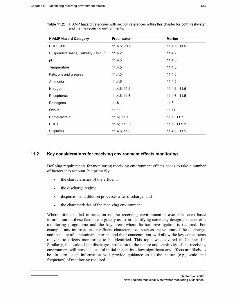
Chapter 11 – Monitoring receiving environment effects 123
September 2002New Zealand Municipal Wastewater Monitoring Guidelines
Table 11.2: HIAMP hazard categories with section references within this chapter for both freshwaterand marine receiving environments.
HIAMP Hazard Category Freshwater Marine
BOD, COD 11.4.5; 11.6 11.4.5; 11.5
Suspended Solids, Turbidity, Colour 11.4.2 11.4.2
pH 11.4.5 11.4.5
Temperature 11.4.5 11.4.5
Fats, oils and greases 11.4.3 11.4.3
Ammonia 11.4.6 11.4.6
Nitrogen 11.4.6; 11.6 11.4.6; 11.5
Phosphorus 11.4.6; 11.6 11.4.6; 11.5
Pathogens 11.8 11.8
Odour 11.11 11.11
Heavy metals 11.6; 11.7 11.5; 11.7
POPs 11.6; 11.9.2 11.5; 11.9.2
Sulphides 11.4.6; 11.6 11.4.6; 11.5
11.2 Key considerations for receiving environment effects monitoring
Defining requirements for monitoring receiving environment effects needs to take a numberof factors into account, but primarily:
• the characteristics of the effluent;
• the discharge regime;
• dispersion and dilution processes after discharge; and
• the characteristics of the receiving environment.
Where little detailed information on the receiving environment is available, even basicinformation on these factors can greatly assist in identifying some key design elements of amonitoring programme and the key areas where further investigation is required. Forexample, any information on effluent characteristics, such as the volume of the discharge,and the suite of contaminants present and their concentration, will allow the key constituentsrelevant to effects monitoring to be identified. This topic was covered in Chapter 10.Similarly, the scale of the discharge in relation to the nature and sensitivity of the receivingenvironment will provide a useful initial insight into how significant any effects are likely tobe. In turn, such information will provide guidance as to the nature (e.g., scale andfrequency) of monitoring required.

124 Chapter 11 – Monitoring receiving environment effects
September 2002New Zealand Municipal Wastewater Monitoring Guidelines
In any monitoring programme, it will usually be desirable to at least identify the directionand characteristics of effluent dispersion after discharge, since this will assist with theselection of receiving environment monitoring sites and sampling methods. In somecircumstances it may also be necessary to quantify effluent dilution, for example where it isnecessary to assess potential water quality impacts on human health. When assessing what,where, and how to monitor effects, it is useful to recognise the water column and thesubstratum as the two main components of the receiving environment in all aquatic systems.The substratum may be the bed of river, lake or coastal area, and may consist of both hard(e.g., rock, cobble etc.) and soft-sediment (e.g., mud, sand) types. The water column andsubstratum have markedly different intrinsic characteristics, and are also subject to differentinfluences from wastewater discharges, as described below.
11.2.1 Water column
The water column is subject primarily to dissolved contaminants and, to a lesser extent,particulates from the wastewater discharge. Background environmental conditions tend to behighly transient. Background water quality, for example, changes diurnally, seasonally, andinter-annually, as well as in relation to climatic events like storms. Such changes couldreflect both external and intrinsic processes. For example, external forces such as changingstates of the tide may bring about diurnal changes in a coastal or estuarine system (e.g.,increased freshwater influence in an estuary during the ebb tide). In a freshwater system,diurnal changes may be the result of intrinsic factors such as the activity of plant life, whichproduce oxygen in the day-time via photosynthesis and deplete it during night-timerespiration (MfE 1992). Furthermore, water quality effects from wastewater discharges mayalso be transient, for example where discharges are intermittent. Similarly, the biologicalcomponents of the water column – plant plankton (phytoplankton), animal plankton(zooplankton), and fish - are also relatively transient. When effects monitoring programmesare being designed, it is particularly important to recognise and account for variability inbackground water quality and wastewater discharge effects in terms of when and where tomonitor, and how often (see Chapter 8 – Concept design; and Chapter 14 – Methods).
Basic questions and answers for receiving environment effects monitoring:
Q: Is receiving environment monitoring warranted?A: The HIAMP output will help to answer this based on treatment level, receiving environment
characterisation, and what’s in the discharge, to name a few. In some circumstances a good discharge-monitoring programme can be used in lieu of receiving environment effects monitoring.
Q: Is dilution and dispersion of the effluent well understood?A: If it isn’t, then running a simple computer model (e.g. Cormix) and/or conducting dilution/dispersion studies
(e.g. dye dispersion and/or drogue tracking) should be considered as a first step. If you don’t know whereyour effluent is going and at what concentrations, it is difficult to conduct meaningful effects monitoring.Dilution and dispersion monitoring generally only needs to be conducted once, and can save both timeand effort on subsequent effects monitoring.
Q: What are the substrate(s) in the vicinity of the outfall?A: Fine muddy sediments are susceptible to nutrient enrichment and contaminant loading, causing adverse
biological effects to benthic macrofauna. If the discharge is likely to contribute to such parameters,monitoring may be necessary. Coarse, mobile sandy sediments or rocky substrates, may be lesssusceptible to nutrient enrichment or contaminant loading, but may be highly sensitive to sedimentaccumulation.
Q: Is there a visible plume under most discharge scenarios?A: If so, then receiving environment water quality monitoring (for clarity, temperature, dissolved oxygen,
floatables etc.) should be seriously considered. If there is no visible plume then there might be strongjustification for conducting only discharge monitoring, or focusing on sediments.
Q: To what extent is contact recreation or shellfish gathering/food gathering taking place in the receivingenvironment?
A: If either of these activities takes place on a regular basis then monitoring for human health indicators maybe warranted. The simplest of these is the collection of water samples for indicator bacteria; however,collection of indigenous biota known to bioconcentrate indicator bacteria (e.g. shellfish) or transplantedbiota (e.g. caged eels or bivalves) could also be considered.

Chapter 11 – Monitoring receiving environment effects 125
September 2002New Zealand Municipal Wastewater Monitoring Guidelines
11.2.2 Substratum
In contrast to the water column, the substratum is a relatively stable medium in which toassess receiving environment effects. The physical, chemical and biological characteristicsof the substratum may integrate transient changes of a wastewater outfall from bothdissolved contaminants in the water column and deposited organic-rich or contaminatedparticulate material (e.g., sewage solids). While substratum characteristics (e.g., sedimentcontaminants, ecological communities) will change over scales of months (e.g., seasonally)and years, they remain relatively stable over smaller time scales, and provide a good way ofdetecting impacts. For example, elevated, variable nutrient inputs may be determined fromthe proliferation of stream periphyton communities. However, care must be taken as thesubstratum can be sensitive to short duration, event-related change such as storms or floods(e.g., hydraulic effects from high stream flows removing periphyton). Biggs (2000)recommends at least three weeks of low flow prior to conducting bio-assessments ofperiphyton communities.
The influence of dissolved or deposited contaminants on the substratum will depend on thedischarge configuration and the characteristics of the receiving environment. Shallowfreshwater streams may experience both water column and depositional effects where thereis complete vertical mixing of the effluent and the receiving water. At submarine outfalls, thesubstratum in the immediate vicinity will primarily be exposed to depositional impacts ratherthan water column effects. In coastal and estuarine situations, wastewater effluents generallyform buoyant surface plumes, limiting depositional effects. The main exceptions are forintertidal discharges or where the plume from a subtidal discharge impinges on the intertidalzone.
The episodic nature of water column effects compared to the more stable, cumulative natureof substratum effects mean that water column monitoring may need to be repeated manytimes in order to obtain representative information about the effects of a discharge. Incontrast the substratum may be reliably characterised with fewer surveys. In fact, substratumimpacts can often be adequately assessed by a one-off ‘snap shot’ survey; an approach thatwould probably be highly misleading in the case of water column monitoring. A furtherimportant difference between the water column and substratum monitoring is the spatialscale over which impacts may occur. While it is typical to measure a gradient of decreasingeffects from the point of discharge in both cases, measurable effects on water quality mayextend much further than substratum effects. Barter & Forrest (1999a), for example, describewater quality and potential human health effects from a subtidal coastal wastewaterdischarge extending for hundreds of metres to kilometres from the outfall, in the absence ofany discernible effects on the substratum.
11.2.3 Standard approach
In this Chapter we propose a standardised framework to wastewater discharge effectsmonitoring, based on the following key elements:
• An assessment of effluent dispersion characteristics and, where necessary, effluentdilution.

126 Chapter 11 – Monitoring receiving environment effects
September 2002New Zealand Municipal Wastewater Monitoring Guidelines
• Water column sampling for: key physical parameters (temperature, clarity, andfloatables); key chemical constituents (pH, dissolved oxygen, nutrients); and keyindicators of potential risks to human health (indicator bacteria).
• Substratum investigations to assess effects from the deposition of sewage-derivedparticulates in terms of: trace contaminants and sediment enrichment (where fine-grained soft-sediments are present); and effects on ecological communities.
These basic elements will apply to many wastewater discharge scenarios. While there will besome instances where only a low level of monitoring effort is appropriate for any one ofthese components, we would generally advocate that receiving environment impacts from awastewater discharge are assessed using a range of complementary approaches. Thisrecognises the many examples, especially in coastal and estuarine systems, where thereceiving environment is highly complex, and cause-effect links between a wastewaterdischarge and a degraded environment may not be clear. In such situations, the extent ofadverse effects from a wastewater discharge usually needs to be assessed using a ‘weight ofevidence’ approach, in which a range of different measures are used to paint a picture of the‘true’ extent of effects, within the framework of a well-designed survey (see Chapter 13).
Clearly, a ‘recipe’ approach will not apply to every situation, and the approach taken needsto be tailored to fit specific circumstances. Hence, a degree of caution should be exercisedwhen using these Guidelines. Note that this Chapter provides only a cursory overview ofapproaches to receiving environment monitoring, in order to highlight key aspects of therecommended approach. Other reference material is referred to, since there is a wealth ofinformation on receiving environment monitoring, from collection and sampling methods, toquality assurance quality control objectives. Some of the most frequently referencedmaterials currently available and relevant to New Zealand are listed in Table 11.3.
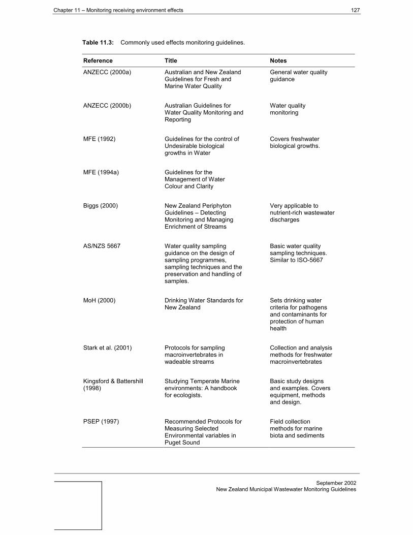
Chapter 11 – Monitoring receiving environment effects 127
September 2002New Zealand Municipal Wastewater Monitoring Guidelines
Table 11.3: Commonly used effects monitoring guidelines.
Reference Title Notes
ANZECC (2000a) Australian and New ZealandGuidelines for Fresh andMarine Water Quality
General water qualityguidance
ANZECC (2000b) Australian Guidelines forWater Quality Monitoring andReporting
Water qualitymonitoring
MFE (1992) Guidelines for the control ofUndesirable biologicalgrowths in Water
Covers freshwaterbiological growths.
MFE (1994a) Guidelines for theManagement of WaterColour and Clarity
Biggs (2000) New Zealand PeriphytonGuidelines – DetectingMonitoring and ManagingEnrichment of Streams
Very applicable tonutrient-rich wastewaterdischarges
AS/NZS 5667 Water quality samplingguidance on the design ofsampling programmes,sampling techniques and thepreservation and handling ofsamples.
Basic water qualitysampling techniques.Similar to ISO-5667
MoH (2000) Drinking Water Standards forNew Zealand
Sets drinking watercriteria for pathogensand contaminants forprotection of humanhealth
Stark et al. (2001) Protocols for samplingmacroinvertebrates inwadeable streams
Collection and analysismethods for freshwatermacroinvertebrates
Kingsford & Battershill(1998)
Studying Temperate Marineenvironments: A handbookfor ecologists.
Basic study designsand examples. Coversequipment, methodsand design.
PSEP (1997) Recommended Protocols forMeasuring SelectedEnvironmental variables inPuget Sound
Field collectionmethods for marinebiota and sediments

128 Chapter 11 – Monitoring receiving environment effects
September 2002New Zealand Municipal Wastewater Monitoring Guidelines

Chapter 11 – Monitoring receiving environment effects 129
September 2002New Zealand Municipal Wastewater Monitoring Guidelines
11.3 Effluent dilution and dispersion
Effluent dispersion and dilution are not technically effects monitoring components, nor arethey discharge monitoring components, but instead fall somewhere in between. However,since any effects will be determined, in part, by the direction and strength of the effluentplume, they require consideration prior to initiating a monitoring programme. Withoutknowledge about where the effluent is likely to end up, it is meaningless to try to selectmonitoring sites and/or sampling and analysis methods. For new discharges, thesecomponents will almost certainly be considered as part of an AEE. However, many existingdischarges either preceded the standard compilation of this information, or the information isno longer available and requires re-collecting.
As mentioned previously, determination of effluent dispersion and/or dilution is generallyonly required once, unless there are changes in either the discharge (e.g., quality, quantity,location, diffuser type) or the receiving environment (e.g., changes in flow direction and/orvolume). Dispersion and dilution can be assessed as a desktop exercise through the use ofcomputer models (e.g., Cormix) and/or using a variety of different field methods (e.g.,drogues, dye, current meters). These two different approaches are often used in conjunction,especially where field data like current measurements are required to validate computermodels.
11.3.1 Computer models
The use of hydrodynamic computer models for determining dilution and dispersion hasgrown appreciably over the last decade due to the rise in computing power and developmentof affordable ‘off-the-shelf’ packages. Previously this type of evaluation was limited tomunicipalities with large outfalls and even larger budgets, whereas the use of this technologyis now within the reach of the majority of dischargers. While evaluation of the data stillrequires some basic understanding of hydrodynamic processes, there are numerousorganisations within New Zealand qualified to offer assistance or conduct this type of study.
The number of different commercially available computer models and the continuousdevelopment of new products precludes the description of all but a few selected examples.The examples listed have been chosen because they have a proven track record in NewZealand, and are directly applicable to wastewater discharges. This list is by no meanscomprehensive and direct endorsement of these particular products should not be inferred.

130 Chapter 11 – Monitoring receiving environment effects
September 2002New Zealand Municipal Wastewater Monitoring Guidelines
Examples of wastewater computer models:
A US EPA’s CORMIX: a hydrodynamic mixing zone model for discharges into riverine, lake and marine receivingwaters including subsurface single- and multi-port diffusers as well as buoyant surface discharges. A fulldescription of the CORMIX model and its underlying assumptions is given in the users manual (Jerka, et al.1996). Although the primary use of the model is for pre-construction design purposes under varying flow anddischarge configurations, it can also be used to verify field data and extrapolate near-field mixing under varyingflow regimes for existing outfalls.
Danish Hydraulic Institute’s Mike series: Mike 21 is an example of the range of different modelling packagesproduced by the DHI. It is a 2D engineering modelling tool for rivers, estuaries and coastal waters. MIKE 21consists of more than twenty modules covering areas including, coastal hydrodynamics, environmentalhydraulics, sediment processes, and wave processes. This group also produces 3D hydrodynamic models andmodels for treatment plants and reticulation systems including wastewater and stormwater. In general, the DHImodels are much more expensive than the Cormix model and require a better understanding of hydrodynamics,but also are much more flexible than the Cormix system.
Puffin: A locally developed model for evaluating far-field dispersion of effluent plumes based on in situ currentmeter data. Puffin is a simpler version of many 2D and 3D models and requires less field verification. Puffin hasbeen used recently to evaluate the upgraded Green Island outfall in Dunedin (Papps 1998) and is currentlybeing used for other proposed outfall extensions.
11.3.2 Drogue studies
A drogue is a device that drifts along with water currents without being influenced bysurface winds, and thus provides a measure of the direction and speed of water movement(hence effluent plume movement) in the vicinity of a discharge. Tracking of drogues isusually accomplished by taking position readings (e.g., GPS fixes) at regular intervals. Onecommon drogue configuration is the holey-sock drogue, consisting of a cylindrical nylontube reinforced with stainless steel rings (Figure 11.1). The holey-sock drogue is preferredover the window-shade style outlined in the New Zealand Water and Soil ConservationAuthority’s Ocean Outfall Handbook (Williams 1985). Studies have shown that current flowaround a window-shade drogue may cause lift, similar to air flow for a sail boat, and thatcylindrical drogue designs that enclose a parcel of water (like the holey-sock) have beenfound to more accurately follow the ambient current patterns (Sombardier & Niiler 1994).

Chapter 11 – Monitoring receiving environment effects 131
September 2002New Zealand Municipal Wastewater Monitoring Guidelines
DRIFTDIRECTION
WATER LEVEL
SPHERICAL FLOAT
CONNECTING LINE
TRACKING SPAR
IDENTIFICATION PENNANT
BALLAST
2 Metres
Figure 11.1: Holey sock drogue
Drogues do not necessarily have to be complicated, however, and tracking a surface plumein low wind situations can be accomplished using very cost-effective means. For example,oranges have been used in many situations to serve as inexpensive (and biodegradable)drogues.
11.3.3 Dye studies
Fluorescent dyes are often used to track effluent plumes either visually or quantitativelyusing a field fluorometer. The two most frequently used dyes are Rhodamine WT andFluoroscein. Rhodamine is a red dye while Fluoroscein is green. Both readily disperse inwater and can easily be injected into an effluent discharge to track the plume as it dispersesin the receiving environment. Rhodamine is the preferred dye for wastewater studies forseveral reasons: it disperses readily in receiving waters, is easily detected (visible to thenaked eye to 1 g m-3 and by fluorometer to as low as 0.01 mg m-3), is very stable, and is non-toxic. Although Fluoroscein shares some of these attributes, it is less stable and tends tobreak down under UV light more quickly than Rhodamine. It also tends to adhere toparticulate matter more readily than Rhodamine. For batch releases where the dye will betracked visually, Fluoroscein is sometimes preferred as many people see green as a lessoffensive colour than red. Use of dye often requires a resource consent (which is normallygranted very quickly by the regulatory authority, provided that affected parties are notified ofthe planned use of the dye).
Dye studies fall into two categories, (i) Qualitative: where a large slug of dye is trackedvisually; and (ii) Quantitative: where the dye is injected at a known rate and tracked belowthe visible range using a field fluorometer. Qualitative studies tend to involve less equipmentand are used to get an idea of the large scale dispersion of the surface effluent plume but will

132 Chapter 11 – Monitoring receiving environment effects
September 2002New Zealand Municipal Wastewater Monitoring Guidelines
not generally yield dilution ratios. Visual tracking of the plume can be accomplished eitherfrom shore surface observations or through the use of aerial photography.
Quantitative studies involve more equipment, but provide dilution estimates. The equipmentincludes a metering pump that can inject the dye at a constant rate and a field fluorometercalibrated to measure the specific dye being used. Grab samples of the receiving water canbe analysed individually, or alternatively the fluorometer can be run in flow-through mode ortowed in-situ where continuous readings are collected. A modification of this approach is tolink a field fluorometer with a datalogger and GPS to collect real-time concentrations as wellas positions to map the effluent plume.
11.3.4 Current meters
Current meters are used to measure the current velocity and direction that can be used toextrapolate dispersion and dilution in the vicinity of a discharge. These measurements aretypically used to feed into or validate the computer models mentioned previously. There is ahuge range of instrumentation available from older mechanical meters to modern profilingmeters that can collect simultaneous readings from various depths (or bins) within the watercolumn. The most widely used meters calculate velocity and direction using eitherelectromagnetic (e.g. InterOcean S4 meter) or Doppler sound shift technology (e.g., RDInstruments ADCP, Sontek ADCP, Falmouth Scientific ACM, Marsh McBirney Dopplermeter etc.) Meters can be moored in a single position for an extended period, used to collectin situ velocity measurements in rivers/streams, or vessel mounted for collection of datafrom multiple positions. A good basic summary of marine current meters is presented inKingsford & Battershill (1998).
11.4 Monitoring water column effects
11.4.1 Background
In most situations, the water column should only require monitoring for a subset of the keydischarge constituents identified in Chapter 10, along with some basic receiving environmentconstituents. These include:
• Most of the key physical parameters, especially temperature, clarity, and aestheticparameters (i.e. floatables).
• Only a few chemical constituents, especially pH, dissolved oxygen, and nutrients.
• Human health constituents (usually indicator bacteria).
The rationale for these choices lies primarily in the ‘best bang for the buck’ approach. Whileit is perfectly feasible to sample the water column for trace contaminants such as heavymetals, such constituents are closely associated with particulate matter. Since particulatematerial tends to settle out of the water column, trace contaminants in the receivingenvironment are usually more of an issue in sediments than in the water column itself.Additionally, while measuring contaminants in the water column only gives a ‘snap shot’ atone particular instance, measuring these constituents in the sediments can show historic or

Chapter 11 – Monitoring receiving environment effects 133
September 2002New Zealand Municipal Wastewater Monitoring Guidelines
chronic inputs. An exception to this approach is fast flowing rivers/streams where stonyhabitats predominate. In these areas alternative approaches are often required (see section11.6.2).
In most wastewater discharge situations, grab samples taken at the water surface will besufficient for receiving environment monitoring, since buoyant effluent plumes will usuallymix with surface waters. An important exception can occur in stratified freshwater-dominated estuarine systems, where subtidal effluent discharges can be trapped beneathsurface freshwater layers (e.g., Sherwin, et al 1997, Roberts 1998) and water column profilesneed to be established for key parameters. Water column profiling may also be undertaken asa component of effluent plume studies, for example to validate dispersion and dilutionmodels (see section 11.3.1).
Similarly, water column effects monitoring would not normally involve an assessment ofphytoplankton, zooplankton or fish. Since these groups are usually transient, cause and effectrelationships are difficult to ascertain without undertaking extensive research. Some of thepotential effects on water column biology can be addressed theoretically, however. Forexample, potential enrichment effects on phytoplankton (e.g., the potential for bloomformation) can be dealt with via nutrient mass load approaches. Similarly, a number ofstudies have described the sensitivity or avoidance behaviour of fish in relation to effluentplumes, especially for heat and ammonia (e.g., Beitinger and Freeman 1983).
A further rationale for the selection of water column constituents is that many are specifiedin the various water quality classes in the Third Schedule of the RMA, hence compliancewith such classes in relation to mixing zone characteristics can be determined (see section11.10). For example, temperature, pH and dissolved oxygen have specific numerical limitsfor 5 of the 11 RMA water quality classes. Additionally, some of the key constituents (e.g.,colour/clarity, floatables) are given narrative limits in Sections 70 and 107 of the RMA, andcompliance with these limits is often incorporated into discharge permits. Furtherinformation on receiving environment effects monitoring using these key water columnconstituents is given below. Note that monitoring of public health constituents (pathogensand indicator bacteria) is addressed in Section 11.8.
11.4.2 Colour and clarity
Optical measurements of a receiving water are carried out as changes in colour and/or claritycan reduce photosynthesis, alter predator/prey dynamics, cause hazards to bathers (from lackof visibility of swimming hazards), and/or reduce aesthetic values. There is a wealth ofbackground information on colour and clarity measurements in both the ANZECC waterquality guidelines (ANZECC 2000a) and the MfE colour and clarity guidelines (MfE 1994a),which will not be repeated here. The latter of these guidelines was developed to help addressthe narrative limits in sections 70 and 107 of the RMA, namely, “there shall be noconspicuous change in colour or visual clarity”. These same narrative standards for colourand clarity are usually either included verbatim in individual discharge consents or areinferred by their inclusion in the RMA. As such it is expected that a majority of wastewatermonitoring programmes will include some sort of colour and/or clarity component. Althoughnumerous methods exist for measuring colour and clarity, only those most frequentlyemployed for addressing these narrative standards in wastewater programmes are discussed.

134 Chapter 11 – Monitoring receiving environment effects
September 2002New Zealand Municipal Wastewater Monitoring Guidelines
General tips on deciding which colour/clarity methods to use:
• Black disk is suited to all water types, although it can be difficult to use from a small boat.
• Secchi disk is generally suitable only for lakes, estuarine and marine waters.
• Turbidity (NTU) lacks a direct relationship to other clarity measures, and has inter-instrumentvariability, but can still be used for relative measures both spatially and temporally.
• Transmissivity has a better relationship to other clarity measures but is not as widely used asturbidity, most likely due to cost factors and historical precedent.
• Transparency tubes (e.g., SHMAK tube) work only for very turbid waters, where visibility is lessthan the tube length.
Before going into the individual methods, however, some background information onassessing these narrative standards is worth considering. Firstly, the bulk of the underlyingscientific data used to support the MfE (1994a) guidelines was conducted in freshwaterenvironments, and therefore the approach is more focused toward freshwater rather thanmarine or estuarine waters. This is not to imply that the guidelines are inappropriate formarine environments, merely that careful site-specific consideration should be used whentrying to apply the guidelines to either marine or estuarine environments. Secondly, althoughcolour and clarity are both specified in the limits, colour is rarely assessed and claritymeasures are usually solely used (rightly or wrongly) to assess the standards. This is mostlikely due to the relative ease of conducting clarity measures compared with colourmeasures. Finally, while there are no ‘hard and fast’ rules on which methods to use, there aresome general tips that may help to make a decision as listed in the following text box:
Colour (Munsell scale)
The Munsell Scale is basically a set of colour patches that are used to match the colour of thereceiving water against a set of standards. The patches are very similar in style to the sheetsof paint colours available from paint shops. Without going into detail on how the scale isused, its primary advantage is that a quantitative difference in colour can be ascertained,which can subsequently be used for regulatory purposes. The Munsell scale can be likened toa 100 point compass rosette, which is divided equally by the colours Red, Yellow, Green,Blue, and Purple (see Figure 11.2). The MfE colour and clarity guidelines (MfE 1994a)recommend no greater than a 5 to 10 point change in Munsell colour, depending on waterquality class as a suitable limit. At the time of writing, charts cost approximately $100 USDand are available through the Munsell Color Company Incorporated.
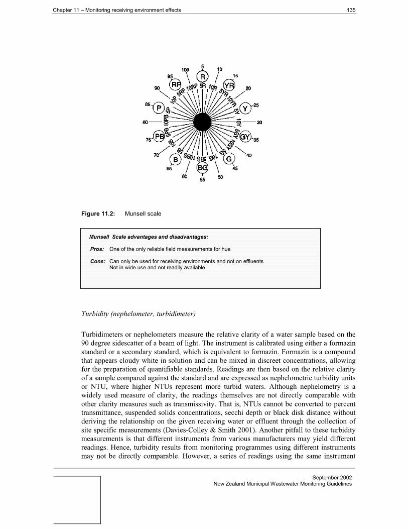
Chapter 11 – Monitoring receiving environment effects 135
September 2002New Zealand Municipal Wastewater Monitoring Guidelines
Figure 11.2: Munsell scale
Turbidity (nephelometer, turbidimeter)
Turbidimeters or nephelometers measure the relative clarity of a water sample based on the90 degree sidescatter of a beam of light. The instrument is calibrated using either a formazinstandard or a secondary standard, which is equivalent to formazin. Formazin is a compoundthat appears cloudy white in solution and can be mixed in discreet concentrations, allowingfor the preparation of quantifiable standards. Readings are then based on the relative clarityof a sample compared against the standard and are expressed as nephelometric turbidity unitsor NTU, where higher NTUs represent more turbid waters. Although nephelometry is awidely used measure of clarity, the readings themselves are not directly comparable withother clarity measures such as transmissivity. That is, NTUs cannot be converted to percenttransmittance, suspended solids concentrations, secchi depth or black disk distance withoutderiving the relationship on the given receiving water or effluent through the collection ofsite specific measurements (Davies-Colley & Smith 2001). Another pitfall to these turbiditymeasurements is that different instruments from various manufacturers may yield differentreadings. Hence, turbidity results from monitoring programmes using different instrumentsmay not be directly comparable. However, a series of readings using the same instrument
Munsell Scale advantages and disadvantages:
Pros: One of the only reliable field measurements for hue
Cons: Can only be used for receiving environments and not on effluentsNot in wide use and not readily available
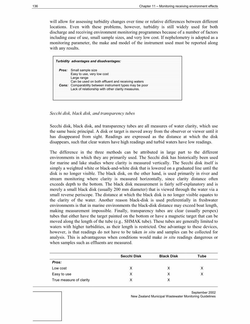
136 Chapter 11 – Monitoring receiving environment effects
September 2002New Zealand Municipal Wastewater Monitoring Guidelines
will allow for assessing turbidity changes over time or relative differences between differentlocations. Even with these problems, however, turbidity is still widely used for bothdischarge and receiving environment monitoring programmes because of a number of factorsincluding ease of use, small sample sizes, and very low cost. If nephelometry is adopted as amonitoring parameter, the make and model of the instrument used must be reported alongwith any results.
Secchi disk, black disk, and transparency tubes
Secchi disk, black disk, and transparency tubes are all measures of water clarity, which usethe same basic principal. A disk or target is moved away from the observer or viewer until ithas disappeared from sight. Readings are expressed as the distance at which the diskdisappears, such that clear waters have high readings and turbid waters have low readings.
The difference in the three methods can be attributed in large part to the differentenvironments in which they are primarily used. The Secchi disk has historically been usedfor marine and lake studies where clarity is measured vertically. The Secchi disk itself issimply a weighted white or black-and-white disk that is lowered on a graduated line until thedisk is no longer visible. The black disk, on the other hand, is used primarily in river andstream monitoring where clarity is measured horizontally, since clarity distance oftenexceeds depth to the bottom. The black disk measurement is fairly self-explanatory and ismerely a small black disk (usually 200 mm diameter) that is viewed through the water via asmall reverse periscope. The distance at which the black disk is no longer visible equates tothe clarity of the water. Another reason black-disk is used preferentially in freshwaterenvironments is that in marine environments the black-disk distance may exceed boat length,making measurement impossible. Finally, transparency tubes are clear (usually perspex)tubes that either have the target painted on the bottom or have a magnetic target that can bemoved along the length of the tube (e.g., SHMAK tube). These tubes are generally limited towaters with higher turbidities, as their length is restricted. One advantage to these devices,however, is that readings do not have to be taken in situ and samples can be collected foranalysis. This is advantageous when conditions would make in situ readings dangerous orwhen samples such as effluents are measured.
Secchi Disk Black Disk TubePros:Low cost X X XEasy to use X X XTrue measure of clarity X X
Turbidity advantages and disadvantages:
Pros: Small sample sizeEasy to use, very low costLarge rangeCan be used on both effluent and receiving waters
Cons: Comparability between instrument types may be poorLack of relationship with other clarity measures.

Chapter 11 – Monitoring receiving environment effects 137
September 2002New Zealand Municipal Wastewater Monitoring Guidelines
Lots of historic data X Xa
Can be used on effluents Xb XCons:Receiving water only XLimited range Xa Very little historic marine datab Only with modified trough
Transmissivity
The final clarity measure discussed is transmissometry. A transmissometer is akin to anephelometer in that it measures the attenuation of a beam of light passed through a samplebut with some fundamental differences. Firstly, a transmissometer, unlike a nephelometer,measures the amount of light passing directly through the sample and not the amountdeflected at 90 degrees. As such, these instruments are measuring clarity in the same fashionas Secchi disks or black disks, only on a much smaller scale. Readings are presented aspercent transmittance over a given path length (e.g., 25 cm) and can therefore be adjusted toa standardised length (e.g., % transmittance m-1), regardless of the instrument. This alsomakes them directly comparable to other clarity readings like Secchi disk or black disk.However, transmissometers tend to be more expensive than nephelometers, which isprobably why they are not more widely used for effects monitoring.
11.4.3 Floatables (scums, films, other floatables)
For the purposes of these guidelines, the term ‘floatables’ refers to scums, slicks, films,foam, floating particulate matter or any other floating debris (e.g., plastics) associated with awastewater discharge. For domestic wastewater, slicks and films are typically caused by thedischarge of oil and grease in the form of salts and esters of fatty acids (Williams 1985),while foams are caused by methyl blue active substances (e.g., detergents) or proteins.Depending on the level of treatment, particulates in the form of paper, plastics and othersolids can also form conspicuous amounts of floatable material.
The primary reason for including floatables as part of a receiving environment monitoringprogramme is because they are included in sections 70 and 107 of the RMA. These sectionsstate that, after reasonable mixing, a wastewater discharge should not give rise to: “Theproduction of conspicuous oil or grease films, scums or foams, or floatable or suspendedmaterials”. However, unlike the colour and clarity limits that are listed in the same sectionsof the RMA, there are no existing guidelines for interpreting what would constitute aconspicuous discharge.
Transmissivity advantages and disadvantages:
Pros: Can measure the direct transmittance of light and can be compared with Secchi disk or black diskCan be used on effluent samplesEasy to use and interpret
Cons: Expensive compared with other clarity measures

138 Chapter 11 – Monitoring receiving environment effects
September 2002New Zealand Municipal Wastewater Monitoring Guidelines
Monitoring for floatables is perhaps the most subjective measure included in water qualityeffects monitoring, as it relies solely on personal observation. While it can be assessednarratively, comparisons over time are difficult using this method and some sort ofquantitative approach is often required. One approach is to assign a relative scale of theconspicuousness of the visual effect so that comparison between sites and/or surveys can beperformed. An example of this type of relative scale, from Forrest and Brown (1996), ispresented in Table 11.4. This scale was accompanied by criteria for assessing how theobservations were made (e.g., from a passing vessel at a certain speed).

Chapter 11 – Monitoring receiving environment effects 139
September 2002New Zealand Municipal Wastewater Monitoring Guidelines
Table 11.4: Scales used for assessment of the conspicuousness of visual effects
Rank Description
0 Visual effect absent
1 Effect visible only when observed closely from a stationary position.
2 Effect visible to a passer-by or casual observer but effect not grossly visible.
3 Effect grossly visible or ‘eye-catching’ to a passer-by or casual observer
11.4.4 Electrical conductivity
Conductivity is the capacity of a substance (the receiving water) to conduct an electricalcurrent, and is usually expressed in micro-siemens per centimetre (µS cm-1). In simple terms,the more ions present in the water, the higher the conductivity. As such, marine and estuarinewaters have much higher conductivities than freshwaters. For example, freshwaters rarelyexceed 500 µS cm-1 while coastal seawater (with a salinity of 33) would have a conductivityof roughly 27,500 µS cm-1. Conductivity and salinity are often used interchangeably, andeven though this is not technically correct it is beyond the scope of these Guidelines to delveinto the differences. Readers are directed to ANZECC (2000a) or other basic water qualitytexts for clarification. Since freshwater conductivities can vary widely (i.e., 20 - 2000 µScm-1) depending on the receiving environment, it is imperative that levels and variation ofthe receiving environment be determined if conductivity is included in a monitoringprogramme. If, however, the conductivity of the receiving environment is known along withthe conductivity of the effluent, and the two are disparate enough, this measure can be asimple and inexpensive way of tracking effluent presence in a receiving environment.
In marine situations, conductivity measurements are often made through the water column todetermine if a density layer exists of lighter less saline waters over heavier more salinewaters (a halocline). Determination of this halocline is important, because distinct densityboundaries can trap a submerged discharge and prevent it from rising to the surface. It is alsoimportant to identify this type of stratification if any receiving water column monitoring isbeing conducted. Otherwise, sampling may not be taking place in the effluent plume, butrather in a water layer overlying the trapped plume. Trapped layers are often subject to farless efficient dilution and dispersion, and evaluation of this reduced mixing is important. Asimilar, and more common, density gradient occurs when two distinct temperature regimesexist, a warmer lighter layer on top of a colder denser layer (thermocline).
Floatables observations advantages and disadvantages:
Pros: Simple low cost methodDoes not require training
Cons: Subjective to individual making observationRelative scale needs to be adopted for quantitative measurement
140 Chapter 11 – Monitoring receiving environment effects
September 2002New Zealand Municipal Wastewater Monitoring Guidelines
11.4.5 Temperature, pH, dissolved oxygen
Temperature, pH and dissolved oxygen (DO) have been included together since they are allessentially physical characteristics of the water column that directly affect aquatic life, andall three are specified in the various water quality classes in the Third schedule of the RMA.By having RMA-stipulated limits for the various water quality classes, compliance with suchclasses in relation to mixing zone characteristics can be determined. For example,temperature, pH and dissolved oxygen have specific numerical limits for 5 of the 11 RMAwater quality classes (see Table 11.5).
Temperature criteria are generally limited to not more than a 3° C temperature change awayfrom ambient conditions. Changes in temperature can have direct impacts on thermallysensitive organisms or indirect impacts through decreased oxygen saturation. Temperature isalso important in that it can cause water column stratification (see above). Temperaturereadings are easy and very inexpensive and are therefore included in many monitoringprogrammes. Similarly, pH changes can have both direct and indirect effects on receivingwater biota, and the most frequent criteria is a range of between 6 and 9. Direct effects occur,as most biota can only tolerate a specific pH range, and indirect effects involve the increasedtoxicity of some metals (e.g., aluminium) and ammonia at different pH ranges. Given thebuffering capacity of seawater, pH is not a parameter that is likely to be an issue in eithermarine or estuarine monitoring programmes. However, it is often included since it isinexpensive and easy to measure in-situ.
Note: It is worth remembering that pH is a logarithmic scale from 0 to 14, with values less than 7 being acidicand greater than 7 being basic, or alkaline. As such, monitoring programmes should report minima, maxima andmedian values rather than mean or averaged values, as arithmetic means of logarithmic values are incorrect andmisleading.
Dissolved oxygen criteria for various water quality classes are generally greater than 80%saturation, as values below this percentage can have direct effects on respiration of aquaticbiota, among other factors. Wastewater discharges are often high in biochemical oxygendemand (BOD), which directly reduces oxygen concentrations in receiving waters. The 80%saturation criteria should, however, be used carefully, as many natural systems undergo widechanges in DO levels on a diurnal basis. If DO is considered as a constituent for effectsmonitoring, sufficient readings must be collected to determine any natural variation inreceiving environment concentrations before attempting comparison with DO criteria. Inmost circumstances reduction in DO is not an issue for wastewater discharged to marineenvironments and does not require inclusion in a monitoring programme. However, therelative ease of measuring DO, coupled with the receiving water criteria, often leads to theinclusion of this parameter regardless.
Conductivity advantages and disadvantages:
Pros: Low cost in-situ method which can sometimes be used to track effluent plumes.Can be used to document stratified water bodies ( i.e. haloclines).
Cons: Freshwater conductivities have high natural variability and site specific information is crucial.Often confused with salinity.

Chapter 11 – Monitoring receiving environment effects 141
September 2002New Zealand Municipal Wastewater Monitoring Guidelines
Table 11.5: Water quality classes and criteria from Third Schedule of RMA.
RMA Water QualityClass Temperature pH DO Other
Aquatic Ecosystems(AE) ± 3 °C Change
No changecausingadverseeffect onaquatic life
> 80%saturation
• No adverse effect on aquaticlife from:• Contaminant discharge• Depositional matter
Fishery (F)± 3 °C Change< 25°C
> 80%saturation
• No tainting of fish for humanconsumption
Fish Spawning (FS) ± 3 °C Change > 80%saturation
• No undesirable biologicalgrowths
Shellfish Gathering(SG) ± 3 °C Change > 80%
saturation
• Aquatic organisms shall notbe rendered unsuitable forhuman consumption by thepresence of contaminants.
Water Supply (WS) 6.0 - 9.0 > 5g m-3
• The water shall not berendered unsuitable fortreatment for humanconsumption.
• The water shall not betainted or contaminated soas to make it unpalatable orunsuitable for consumptionby humans after treatment orunsuitable for irrigation.
• No undesirable biologicalgrowths
Contact Recreation(CR)
• Water should not be rendered unsuitable for bathing from:• Reduction in visual clarity• Presence of contaminants• No undesirable biological growths
Irrigation (I) • The water shall not be tainted or contaminated so as to make it unsuitable forthe irrigation of crops growing or likely to be grown in the area to be irrigated.
• No undesirable biological growths
Industrial Abstraction(IA)
• The quality of the water shall not be altered in those characteristics which havea direct bearing upon its suitability for the specified industrial abstraction.
• No undesirable biological growths
Natural State (NS) • The natural quality of the water shall not be altered.
Aesthetics (A) • The quality of the water shall not be altered in those characteristics which havea direct bearing upon the specified aesthetic values.
Cultural (C) • The quality of the water shall not be altered in those characteristics which havea direct bearing upon the specified cultural or spiritual values.
142 Chapter 11 – Monitoring receiving environment effects
September 2002New Zealand Municipal Wastewater Monitoring Guidelines
11.4.6 Nutrients
Nutrients are an important component of receiving environment monitoring, especially insituations where the ratio of discharge volume to receiving environment volume is high (e.g.,small streams/rivers), or where the receiving environment is sensitive to increased nutrientinputs (e.g., spring-fed stream with relatively stable flows). High concentrations of nutrientsin the water can result in excessive growth of aquatic plants such as phytoplankton,cyanobacteria, macrophytes, seagrasses, and filamentous and attached algae.
Key nutrients in wastewater discharges are nitrogen and phosphorus, which come in manydifferent chemical forms. Nitrogen is generally regarded as a limiting nutrient in estuarineand marine systems, hence can promote adverse effects through the stimulation of excessivealgal growth. The forms of nitrogen that are most readily available (i.e., bioavailable) arenitrate, nitrite and ammonia, which are collectively referred to as dissolved inorganicnitrogen (DIN). Total nitrogen (TN) is the sum of organic nitrogen plus DIN and, as thename implies, provides a measures of the total pool of nitrogen in the system, recognisingthat organic nitrogen can be converted to the more bioavailable forms by sediment microbialprocesses. TN should not be confused with total Kjeldahl nitrogen (TKN), which is the sumof organic N and ammonia. For effects monitoring purposes it is usually sufficient to have ameasure of the bioavailable nitrogen pool (DIN) and the total pool (TN).
Like nitrogen in marine systems, phosphorus is often the limiting nutrient in freshwatersystems or the upper reaches of estuaries. It can exist in the water in organic phosphate,orthophosphate (inorganic, dissolved phosphorus), total phosphorous (dissolved andparticulate), and polyphosphate (from detergents) forms. Phosphorous is constantly cycledfrom one biogeochemical form to another within an ecosystem, but not all are available fornuisance plant growth (i.e., bioavailable). The most bioavailable form of phosphorous isconsidered to be orthophosphate (PO4
3-). Bioavailable phosphorous is comprised of solublereactive phosphorous (SRP – equivalent to dissolved reactive phosphorus, DRP) andbioavailable particulate phosphorus (BPP). For effects monitoring purposes it is usuallysufficient to have a measure of the bioavailable phosphorous (SRP/DRP) and the total pool(TP).
Measuring each of the nutrient species (both N and P) in receiving water is generallyrecommended even though it is only one of the species that is likely to be limiting to plantgrowth. In most situations limiting the analysis to nitrate, ammonia and SRP/DRP issufficient, however discharge considerations may warrant analysing additional parameters(see Section 10.4). It is also important to remember that natural variations are likely to takeplace and multiple samples over an extended time frame (e.g., monthly samples over thecourse of a year) may be required to ascertain natural temporal variation in a receiving water.Understanding the extent of this natural variation is critical prior to attempting to draw anyrelationship between discharge and ambient receiving water concentrations. Furtherinformation regarding freshwater nutrients and their capacity to promote eutrophication arepresented in the MfE water quality guidelines No. 1 (MfE 1992) and the periphytonguidelines (Biggs 2000). The latter of these also contains recommended nutrientconcentrations for freshwater environments along with some of the important caveats toconsider when attempting to apply the limits specified.
Chapter 11 – Monitoring receiving environment effects 143
September 2002New Zealand Municipal Wastewater Monitoring Guidelines
11.4.7 Phytoplankton, zooplankton and fish
As mentioned previously in section 11.4.1 an assessment of phytoplankton, zooplankton orfish is not normally included in water column effects monitoring. This is because thesegroups are primarily mobile or transient, and cause and effect relationships are difficult toascertain without undertaking extensive research. Generally the potential effects on watercolumn biology can be addressed theoretically. For example, potential enrichment effects onphytoplankton (e.g., the potential for bloom formation) can be dealt with via nutrient massload approaches. The potential effects on fish populations can vary widely depending on thequality of the effluent and are not as easily addressed in a theoretical sense. For example,Beitinger & Freeman (1983) have shown fish avoidance behaviour from wastewater effluentwhile in other cases (e.g., Barter & Forrest 1999b) nutrient rich effluent appears to supportfish aggregation.
Due to the cost of conducting and analysing this type of data in conjunction with the lack ofdirect cause and effect relationship, inclusion of phytoplankton and or zooplanktonmonitoring should only be considered if certain conditions apply. These are listed in thefollowing text box.Only consider conducting phytoplankton or zooplankton monitoring if:• Nutrient levels are very high in the discharge• Dilution and dispersion are low enough that nutrient rich waters persist in the vicinity of the discharge.• Blooms have been documented or observed previously.
Likewise, monitoring bioaccumulation, histopathology (presence of disease/lesions), habitatmodification, or behavioural changes in fish can be an expensive exercise, which may ormay not yield meaningful results. Again, this approach should only be considered in specialcircumstances like those listed in the text box.
Only consider conducting bioaccumulation monitoring if:• There is a contaminant in the discharge (e.g., mercury) which is known to have high bioaccumulation or
bioconcentration factors in fish• The discharge is into a high profile trout fishing river/stream.
Summary of N and P Nutrient Species:
• DIN (Dissolved Inorganic Nitrogen) = Combination of Nitrate, Nitrite, and Ammonia. These representthe most readily bioavailable forms of nitrogen.
• TN (Total Nitrogen) = Organic nitrogen plus inorganic nitrogen (DIN).• TKN (Total Kjeldahl nitrogen) = Organic nitrogen plus ammonia.
• DRP (Dissolved Reactive Phosphorus) = Also called soluble reactive phosphorus (SRP). Onebioavailable form of Phosphorus (see BPP). Most commonly measured form.
• BPP (Bioavailable Particulate Phosphorus) = Second bioavailable form of phosphorus. BPP + SRPmakes up total bioavailable phosphorus.
• TP (Total Phosphorus) = Combination of both bioavailable and other forms of phosphorus.
144 Chapter 11 – Monitoring receiving environment effects
September 2002New Zealand Municipal Wastewater Monitoring Guidelines
• There is commercial or recreational fishing activity in the immediate vicinity of the discharge, and there arehuman health implications.
Sampling methods for these parameters are covered in detail in either the Puget SoundMonitoring Protocols (PSEP 1997) or studying temperate marine environments (Kingsford& Battershill 1998).
11.5 Effects on sediments and biology: marine environment
For various reasons, effects monitoring requirements for marine and freshwaterenvironments have been presented separately, although cross-referencing is used where thereare similarities between the two. In this section, the requirements for the marine environmentare discussed.
The data of MacDonald et al. (2001) indicate that, by volume, about 66% of New Zealand’spresent-day wastewater discharges are into the marine environment. Many of thesedischarges are into areas characterised by soft-sediment habitats. It is logical, therefore, thata discussion of effects monitoring requirements for marine systems should focus mainly onsuch areas. While effects monitoring in rocky habitats is referred to at times, morecomprehensive discussions can be found elsewhere (e.g., Kingsford and Battershill 1998).
11.5.1 Assessing effects on sediment quality
Except where buoyant effluent plumes affect intertidal areas, the substratum in marinesystems will primarily be exposed to the impacts of sewage-derived solids that are depositedin the vicinity of the outfall. Enhanced deposition of organic-rich solids can result in a rangeof effects in marine systems.
As a measure of depositional impacts, it is important to assess the severity and extent oforganic enrichment of the seabed in the case of all wastewater discharges. For dischargeswhere toxic contaminants have been identified, it will also be important to assess sediment-associated contaminant levels and their implications.
11.5.2 Enrichment
There are a number of key indicators of changes in sediment quality under different levels ofenrichment that are reasonably easy to measure. These are outlined below.
Sediment organic content: this can be measured either as percent ash free dry weight (%AFDW) or percent total organic carbon (% TOC). These are relatively inexpensive lab-basedanalyses of sediment samples that provide a direct measure of sediment organic content.They are not identical measures, however, but can be roughly related by using the formulafrom Craft, et al. (1991) where TOC% = 0.4(AFDW) + 0.0025(AFDW)2.
Sediment nutrient content: as discussed in section 11.4.6, nitrogen is the key nutrient thatlimits algal growth in estuarine and marine systems. Sediments can be measured for DIN asan indication of the bioavailable forms and TN as an indication of the total nitrogen pool.

Chapter 11 – Monitoring receiving environment effects 145
September 2002New Zealand Municipal Wastewater Monitoring Guidelines
Sediment redox status: whereas unenriched sediments are typically grey/brown, excessivelyenriched and anoxic (oxygen-depleted) sediments can be black. As the level of enrichmentincreases, and the sediment becomes increasingly anoxic, the black zone moves closertowards the sediment surface. While this change can be quantified by measuring redoxpotential in sediment cores, the technique is difficult and results are often equivocal (e.g.,Pearson & Stanley 1979). A somewhat crude yet widely used alternative is to measure thedepth of transition between ‘clean’ surface sediments and the anoxic ‘black zone’. Thisapproach has limitations in the case of muddy estuarine sediments where sediments may benaturally anoxic in all but the very surface of a core profile.
Sediment odour: unenriched sediments are typically relatively odourless or ‘muddy’-smelling, whereas excessively enriched and anoxic sediments have a strong ‘rotten egg’smell of hydrogen sulphide. While this is a highly subjective ‘measure’ it can nonethelessadd to the overall weight of evidence regarding the severity of impacts. As above, thisapproach has limitations in the case of muddy estuarine sediments that are naturally anoxic.
11.5.3 Contaminants
The term ‘contaminant’ as used in this Chapter, refers to all of the toxic wastewaterconstituents listed in Chapter 10, such as metals and metalloids (e.g., copper, mercury, zinc,and arsenic), as well as organic compounds (e.g., PAHs, PCBs and pesticides). There may besignificant differences between each contaminant in their nature and effect. For example,some contaminants will be more toxic than others or have a relatively greater capacity forbioaccumulation and biomagnification through the food chain (e.g., mercury). Despite suchdifferences, effects monitoring requirements for contaminants can be discussed collectivelysince: (i) all of them are primarily sediment-associated; (ii) all are usually measured via coresampling of surficial sediments; and (iii) their environmental significance can usually beevaluated against sediment quality guidelines or the state of the biological community.
When making a decision on whether or not to conduct sediment contaminant analyses, atleast two important factors need consideration:
• Which contaminants should be tested for?
• Are the sediments likely to accumulate contaminants?
Contaminant analyses can be very expensive. Given the usual complexity of receivingenvironment sampling (e.g., multiple sampling sites or replicate samples), only thosecontaminants identified as problematic in the discharge monitoring (Chapter 10) should beconsidered for effects monitoring.
Furthermore, coarse sediments like gravel and sand are not likely to accumulate particulate-bound contaminants nearly as readily as fine muddy sediments. Also, sediments subject toregular disturbance and redistribution or resuspension are less likely to accumulatecontaminants. In such situations, the analysis of multiple sediment samples for a suite ofcontaminants may be expensive, yet reveal nothing about wastewater-related effects.
There are a couple of approaches that can be taken where there is doubt about the likelyextent of sediment contamination. One is to have only a few samples analysed, to seewhether there is an obvious impact that needs more detailed evaluation. The other is to

146 Chapter 11 – Monitoring receiving environment effects
September 2002New Zealand Municipal Wastewater Monitoring Guidelines
initially have samples analysed for a subset of the contaminants, before deciding whetheranalysis of all contaminants of concern is required. One strategy commonly employed is tofirst analyse selected samples for key trace metal contaminants, since the cost per analysis isconsiderably less than for organic contaminants like pesticides.
Sediment grain size analyses should also be considered for assessing wastewater impacts onsoft-sediment communities. A full break down by standard grain size classes is generally notnecessary, but analyses should at least differentiate between mud (silt/clay particles < 63µm), sand (> 63 µm – 2 mm) and larger size classes. This requirement is a reflection of twokey influences of sediment grain size characteristics.
First, chemical contaminants are associated mainly with the fine muddy sediment fraction. Avalid comparison of contaminant levels at different sites (e.g., control vs impact sites) willneed to recognise any major differences in sediment grain size characteristics. Where thesediffer greatly, it may be necessary to normalise the contaminant data (e.g., expresscontaminant concentrations per gram of mud) or analyse the data in such a way that grainsize differences are taken into account. Second, sediment grain size characteristics cangreatly influence the ecological community present. As was the case for contaminants,biological differences between samples or sites will need to recognise any differences insediment grain size.
Interpretation of the potential ecological implications of sediment contaminant results isusually done on an individual constituent basis, where a single parameter is tested against asediment quality guideline level. Sediment quality guidelines aim to predict ‘acceptable’levels of contaminants in sediment, based on ecological effects criteria. New Zealand hasrecently published national guidelines for sediment quality (ANZECC 2000a) based oninternational guidelines (e.g., PSDDA & U.S. Army Corps of Engineers 1989, Long &Morgan 1991). The ANZECC (2000a) guidelines specify, for individual contaminants, alower threshold (ISQC-Low) that indicates a possible biological effect, and an upperthreshold (ISQC-High) that indicates a probable biological effect.
Note:
Sediment grain size and organic content are both important factors when assessing contaminant levels in sediments.Grain Size: At a minimum analysis should include gravel, sand and mud:
Grain size class Particle size rangemm Phi units
Gravel 2.0 - 4096 -1.0 to -12Sand 0.0625 (63 µm) – 2.0 4.0 to -1.0
Silt 0.0039 – 0.0625 8.0 to 4.0Mud Clay < 0.0039 14.0 to 8.0
Organic content: Use either ash free dry weight (AFDW) or percent total organic carbon (TOC).TOC% = 0.4(AFDW ) + 0.0025(AFDW)2 [Craft 1991]

Chapter 11 – Monitoring receiving environment effects 147
September 2002New Zealand Municipal Wastewater Monitoring Guidelines
It should be recognised that because the guidelines are limited to individual analytes, they donot take into account the synergistic, antagonistic or additive effects of combinedcontaminants within a sediment, nor the extent to which the contaminants are bioavailable.Experience has shown such guidelines are usually conservative in that values for a range ofconstituents may be exceeded in the absence of discernible ecological effects.
Sampling
For an assessment of contaminant levels, and for direct measures of the level of enrichment(e.g., % TOC), sampling of surficial sediments will be adequate for most wastewatermonitoring studies. Furthermore, since sediment-dwelling fauna (see section 11.5.4)generally inhabit surficial sediments (e.g., the surface 50-100 mm of a muddy sediment), it ismost relevant in ecological terms to target surface sediments during sampling. In this way,relationships between contaminant/enrichment levels and biological effects can be examined.
Collection of surficial sediments can be accomplished using a variety of methods. The mostcommon of these, however, are manual collection with hand corers or remote sampling fromthe water surface using a grab or coring device. The small volume of material generallyrequired for most analyses means that simple gravity cores can often be used for this type ofremote sampling.
11.5.4 Assessing ecological effects
Background
Monitoring ecological effects on the seabed is perhaps one of the most importantcomponents of an effects monitoring programme in a marine system. Although othercomponents (e.g., contaminant monitoring) provide a picture of the potential to cause effects,ecological monitoring allows for direct assessment.
There are a number of studies from New Zealand (e.g., Roper 1990, Barter and Forrest1999b) and overseas (e.g., Chapman, et al 1995, Koop & Hutchings 1996, Smith 1996,Underwood & Chapman 1996) that describe large subtidal wastewater discharges that havehad little discernible ecological impact on soft sediment or rocky habitats. Koop &Hutchings (1996), for example, note that most of the studies of impacts from Sydney’sdeepwater outfall have been unable to detect environmental impacts. The study of ecologicaleffects from Tauranga’s wastewater discharge by Roper (1990) indicates that even in an
Contaminant analysis advantages and disadvantages:
Pros: Gives direct measure of concentrations in the receiving environmentCan be easily checked against guideline levels to determine potential effectsMay not require lots of replication and multiple samples to elucidate trends
Cons: Does not apply to all sediments. Not much value for coarse sandy and/or mobile sediments.Can be expensive, especially organic analysesConcentrations might not be bioavailable and may give a misleading picture of potential effects

148 Chapter 11 – Monitoring receiving environment effects
September 2002New Zealand Municipal Wastewater Monitoring Guidelines
estuarine environment with adequate flushing, seabed impacts can be limited to within tensof metres from the outfall.
In contrast, a number of other studies in New Zealand (e.g., Roper et al. 1989, Anderlini &Wear 1992) and overseas (e.g., Chapman et al. 1995) have revealed sediment contaminationand ecological impacts over scales of hundreds of metres, even in relatively exposed coastalareas. The more significant effects are described for discharges which are large, receiveminimal treatment, or consist of industrial as well as domestic wastewater. As a generaltrend, the effect of discharges to intertidal areas, which would be exposed to buoyant effluentplumes, appear far greater than for the subtidal (Fairweather 1990, Smith 1996, May 1985).Clearly, the impacts of wastewater discharges can be variable and depend on a combinationof wastewater treatment, contaminant loading, and a range of site-specific environmentalfactors.

Chapter 11 – Monitoring receiving environment effects 149
September 2002New Zealand Municipal Wastewater Monitoring Guidelines
A discussion of effects monitoring requirements needs to recognise two main ecologicalcomponents of the seabed environment: (i) infauna, which is the assemblage of animals(often microscopic) that live buried or partially buried with the sediment matrix (e.g., worms,bivalve shellfish); and (ii) epibiota, which refers to the animals and plants (e.g., sea stars,urchins, seaweeds) that inhabit the surface of the seabed. Epibiotic assemblages may be asignificant feature of both rocky and soft-sediment habitats, although epibiota can berelatively impoverished in both. Infaunal assemblages, on the other hand, are a uniquefeature of soft-sediment habitats.
Effects on sediment-dwelling infauna
Many wastewater monitoring studies target the infaunal assemblage. This in part reflects thefact that a large proportion of wastewater outfalls are situated on soft muddy sediments. Anadvantage of infaunal sampling in such situations is that results can be interpreted in light ofany sediment quality data from the same sampling stations.
In addition, infauna, and especially macrofauna (by definition infaunal animals that areretained on a 0.5 mm mesh screen), have been used for several decades as sensitiveindicators of the effects of wastewater discharges, and are suitable for quantitative studies.For example, the composition of the macrofaunal community, the number of differentspecies, and the number of individuals of a given species, all provide a valuable indication ofthe quality of soft-sediment habitats.
The enrichment effects from wastewater and other organic-rich discharges are particularlywell documented and understood. A generalised model for the effects of organic enrichmentis provided in Table 11.6. This model shows that significant organic enrichment is typicallyaccompanied by a proliferation of one or a few macrofaunal species, and a decrease inspecies richness (the number of different species present).
Table 11.6. Generalised model of the effects of organic enrichment. (adapted from Pearson &Rosenberg 1978).
Level of enrichment Macrofaunal Response
Unenriched Moderate species richness with a moderate abundance distributed evenlyamong species
Low Transition zone: abundance and species richness may be higher than‘normal’
Moderate Moderate-low species richness with a few ‘opportunist’ species occurringin high abundance
High Low species richness consisting of one or a few opportunist specieswhich reach very high abundance levels. [e.g. Very high capitellid levelsare defined as > 1,000/m2 (ANZECC 2000a)]
Extreme Anoxic, sulphide-rich conditions either devoid of macrofauna or havingvery few species in very low abundance

150 Chapter 11 – Monitoring receiving environment effects
September 2002New Zealand Municipal Wastewater Monitoring Guidelines
Seabed macrofauna can be collected through a variety of methods, however, the two mostcommon are manual methods (large hand cores) or grab sampling methods. Sample volumeshould be consistent between sites and surveys to allow cross comparison. As a rule ofthumb, samples should be at least 10 cm depth and have a minimum surface area of at least125 square centimetres. Because macrofaunal communities may be variable or patchy, it isstandard practice to take replicate samples from any one site in order to provide an average
picture of species richness and abundance, and provide a representative sample of the speciespresent. The identification and enumeration of seabed macrofauna is usually performed onpreserved samples in the laboratory with the aid of a binocular microscope, and requiresspecialist expertise.
Effects on epibiota
The wastewater impact studies that have described effects on epibiota tend to be thoseconducted in environments where rocky habitats were dominant (e.g., May 1985, Chapmanet al. 1995, Smith 1996, Underwood & Chapman 1996). Generally, however, less attentionhas been paid to sampling epibiota in either rocky or soft-sediment communities, than theinfaunal community. This reflects a number of factors as follows:
• The sensitivity of most epibiotic assemblages to wastewater-related impacts ispoorly understood.
• Sampling methods (especially quantitative sampling) for epibiota tend be morelabour intensive than for infauna.
• Epibiota can be highly variable spatially and over time, meaning that it can berelatively difficult to separate background variation from wastewater impacts.
• The taxonomy of epibiota, especially in rocky habitats, is generally less wellunderstood than for infaunal assemblages.
Hence, it is suggested that wastewater effects monitoring programmes should targetsediment quality and infaunal sampling where possible. Nevertheless, in soft-sedimenthabitats where epibiota are a conspicuous feature (but not dominant), it is desirable todocument any major effects if they are present. A reasonable approach in such situationswould be to undertake a quantitative programme to sample infauna and sediment quality,supported by semi-quantitative sampling of epibiota. This could involve, for example,recording the conspicuous species present and whether they were rare, common, or abundantaccording to defined density categories; or making percent cover estimates of sessile(attached or encrusting) species (e.g., seaweeds). In exclusively soft-sediment areas,dredging may also be a useful tool, since it provides a broad-scale semi-quantitative sample
Sediment infauna monitoring advantages and disadvantages:
Pros: Lots of historical data for comparative purposesGood relationship between enrichment level and effects on biota.
Cons: Analysis and taxonomic identification requires specialised expertiseNot as valuable in sandy coarse sediments.Can be expensive, particularly since replicates and multiple samples are required.

Chapter 11 – Monitoring receiving environment effects 151
September 2002New Zealand Municipal Wastewater Monitoring Guidelines
of epibiota and shallow infauna that are large, sparse, or patchy, and that cannot easily besampled by other methods.
Where epibiota are dominant, and especially if rocky habitat is dominant, it may benecessary to undertake quantitative sampling. Most of the common quantitative methods arenon-destructive and involve sampling along transects or within quadrats. A transect isusually a straight line of a few metres to tens of metres long and perhaps 1-2 m wide, and issuited to the sampling of large, sparsely populated, or patchy epibiota. A quadrat is a smallrectangular or square frame (usually 1 m2 or less) that is suited to sampling small andcommon epibiota.
Sampling in transects or quadrats will usually require making counts of target species, orobtaining percent cover estimates of target species or entire assemblages. Percent coverestimates can be derived from the ‘point count’ method conducted in situ, or usingphotoquadrats. A photoquadrat consists of a camera and frame designed to take a photo of asmall quadrat area. Photoquadrats are often used for deeper subtidal outfalls where timeconstraints placed on divers do not allow for in situ sampling. In addition to sampling thespecies present, such methods can also be used to quantify the nature of the substratum. In arocky habitat subject to wastewater discharge effects, for example, it may be of interest toknow whether depositional impacts have resulted in an increase in bare rock substratum, oran increase in sediment cover, relative to control areas or baseline conditions. Acomprehensive account of appropriate methods for sampling epibiota is provided inKingsford and Battershill (1998), and is not further discussed here.
11.6 Effects on sediments and biology: freshwater environment
11.6.1 Overview
While the marine environment receives approximately two thirds of New Zealand’swastewater discharges by volume, the greatest number of discharges (∼ 53 %) are intofreshwater environments, primarily rivers and streams (MacDonald et al. 2000). Sincedischarges to lakes are insignificant in the New Zealand context both in terms of volume (< 1%) and number of discharges (< 2%), it is only effects monitoring requirements for riversand streams that are considered here.
The evolution and general approach to ecological effects monitoring in rivers and streamsprovides an interesting contrast with the marine environment. Whereas ecologicalassessment studies in marine systems have focussed primarily on soft-sediment habitats, thefocus in rivers and streams has primarily been on monitoring wadeable hard-bottomedhabitats, in particular faster-flowing ‘riffle’ areas. Such areas are readily accessible and havemacrofaunal communities that include the most pollution-sensitive of the streaminvertebrates. A knowledge of pollution effects on this community has lead to thedevelopment of a number of community-based environmental health indices, including thewell known macroinvertebrate community index (MCI) and its derivatives (Stark 1993,Boothroyd & Stark 2000).
In contrast, the soft-sediment habitats characteristic of relatively slow-flowing streams andrivers are less well understood, and less favoured in environmental assessment studies. In

152 Chapter 11 – Monitoring receiving environment effects
September 2002New Zealand Municipal Wastewater Monitoring Guidelines
part this reflects the fact that it may be relatively difficult to obtain ‘representative’ samplesfrom such habitats. It also recognises that the macrofaunal communities of soft-sedimentareas are relatively impoverished and species-poor, do not contain the pollution-sensitivespecies characteristic of riffle areas, and are less amenable to comparative quantitativesampling than riffles (Stark, et al 2001).
This contrast between hard-bottomed and soft-sediment habitats creates an interestingdilemma for wastewater monitoring. On the one hand, ecologically sensitive riffles are thelogical habitats in which to assess ecological effects, while soft-sediment habitats, are anobvious focal point for targeting sediment-associated contaminants. Since these two habitattypes may not coincide in terms of proximity to the wastewater discharge, drawing linksbetween environmental quality and ecological effects can be more difficult than in marinesediments. Hence it is useful to consider approaches to effects monitoring in hard-bottomedvs soft-sediment habitats separately.
11.6.2 Ecological effects in hard-bottomed riffle habitats
Since muddy sediments may be difficult to find in fast-flowing streams, sampling forsediment-associated contaminants is not often carried out in wastewater monitoring studiesin these systems. Instead, inference about environmental effects often relies heavily on rifflesampling of macroinvertebrates and biological growths (e.g., Harding 2000). Stark et al.(2001) recommend two sampling protocols for macroinvertebrates in such habitats and theyare not further discussed here. Biological growths include autotrophic growths likeperiphyton, whose proliferation may indicate nutrient enrichment. Visual scales for assessingperiphyton are provided in Biggs (2000). Other potentially nuisance biological growths areheterotrophic slimes collectively referred to as sewage fungus, discussed in MfE (1992). Theoccurrence of such growths has been described for untreated wastewater discharges, but nowgenerally appears uncommon with the move to improved effluent treatment.
Where potentially toxic contaminants or high nutrient concentrations have been identified asan environmental concern, but cannot be sampled in sediments, some assessment of risk todownstream ecological communities is still desirable. While direct sampling and analysis ofreceiving waters can be carried out, the limitations of ‘snap-shot’ water quality samplingdescribed in Section 11.4.1 need to be recognised. Furthermore, it is usually desirable toconsider potential ecological effects under a ‘worst-case’ scenario. This is usually assumedto be where a high (e.g., 95th percentile) concentration of each contaminant is discharged atmaximum effluent flow during low-flow conditions in the receiving environment. In themost simplistic approach, where complete mixing of the effluent and receiving water isassumed, the downstream concentration of a contaminant can be calculated as follows:
Concentrationds = [Concentrationeff x Peff] + [(Concentrationus x (1-Peff)].
where ds = downstream, us = upstream, eff = effluent, Peff = effluent volume as a proportionof downstream flow.
The predicted downstream concentration can then be compared to appropriate water qualityguidelines (e.g. ANZECC 2000a) to provide some indication of potential effects.
Riffle Habitat monitoring advantages and disadvantages:
Pros:Lots of historical data for comparative purposesWell developed indices for evaluating effects (e.g. MCI, SQMCI)
Cons:Direct relationship to sediment contaminant/enrichment level and biota does not exist like in marinesituations due to spatial separation of the two environmentsAnalysis and taxonomic identification of macrofauna requires specialised expertise

Chapter 11 – Monitoring receiving environment effects 153
September 2002New Zealand Municipal Wastewater Monitoring Guidelines
11.6.3 Ecological effects in soft-sediment habitats
The general approach to sampling freshwater soft-sediments, and interpretation of results, islargely the same as for marine sediments (section 11.5.1). While assessment of effects on theecological communities of soft-sediment habitats provides the opportunity for exploringrelationships between contaminant concentrations and ecological effects, the lack ofpollution-sensitive macroinvertebrates in freshwater soft-sediments means that it can bedifficult to detect effects, or that only gross effects may be detected.
Unlike riffle habitats, therefore, ecological communities in soft-sediment habitats mayprovide a poor basis for assessing the ecological effects of wastewater discharges. This is notalways the case, however, since many of the community-based ecological changes describedfor marine sediments are similar for freshwater sediments. For example, while enrichment inmarine sediments may lead to a proliferation of polycheate or nematode worms, enrichmentin freshwater soft-sediments may lead to a proliferation of oligochaete worms andchironomid larvae (Biggs 2000).
Rather than focus macroinvertebrate sampling on soft-sediments alone, Stark et al. (2001)suggest that sampling in soft-bottomed streams should comprise a semi-quantitative ‘multi-habitat’ approach that targets, for example, bank margins, aquatic macrophytes, and woodydebris. The latter can be an important substrate for pollution sensitive groups ofmacroinvertebrates. The need for a semi-quantitative rather than quantitative approach stemsfrom the fact that there may be inter-site variability due to differing proportions of thehabitats sampled. However, they also provide a quantitative protocol for sampling themacroinvertebrates communities of macrophytes alone. Such an approach wouldconceivably be useful for assessing the effects of dissolved contaminants or nutrients (andtheir effects) in the water column, rather than sediment-associated contaminants.
11.7 Bioaccumulation and transplanted biota
11.7.1 Bioaccumulation
Bioaccumulation is, as the name implies, the build-up or increase of contaminants within aliving organism due to the presence of that contaminant in the environment.Bioaccumulation studies generally involve the collection and analysis of native populationsof organisms (usually sedentary) which are utilised as bioindicators of chemical orbacteriological contamination. The most widely used organisms for these types of studies arebivalves. Bivalves such as the blue mussel (Mytilus edulis galloprovincialis) or green-lip
Soft sediment monitoring advantages and disadvantages:
Pros: Direct relationship to sediment contaminant/enrichment level and biota is possible
Cons: Often requires multi-habitat approachSoft muddy substratum for sampling not as prevalent as in marine situations.Relative lack of macrofauna compared to other environments.
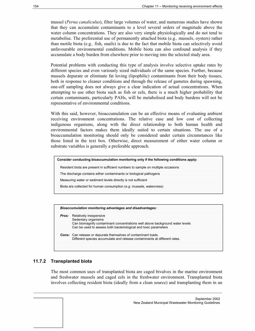
154 Chapter 11 – Monitoring receiving environment effects
September 2002New Zealand Municipal Wastewater Monitoring Guidelines
mussel (Perna canaliculus), filter large volumes of water, and numerous studies have shownthat they can accumulate contaminants to a level several orders of magnitude above thewater column concentrations. They are also very simple physiologically and do not tend tometabolise. The preferential use of permanently attached biota (e.g., mussels, oysters) ratherthan motile biota (e.g., fish, snails) is due to the fact that mobile biota can selectively avoidunfavourable environmental conditions. Mobile biota can also confound analysis if theyaccumulate a body burden from elsewhere prior to moving into the selected study area.
Potential problems with conducting this type of analysis involve selective uptake rates bydifferent species and even variously sized individuals of the same species. Further, becausemussels depurate or eliminate fat loving (lipophilic) contaminants from their body tissues,both in response to cleaner conditions and through the release of gametes during spawning,one-off sampling does not always give a clear indication of actual concentrations. Whenattempting to use other biota such as fish or eels, there is a much higher probability thatcertain contaminants, particularly PAHs, will be metabolised and body burdens will not berepresentative of environmental conditions.
With this said, however, bioaccumulation can be an effective means of evaluating ambientreceiving environment concentrations. The relative ease and low cost of collectingindigenous organisms, along with the direct relationship to both human health andenvironmental factors makes them ideally suited to certain situations. The use of abioaccumulation monitoring should only be considered under certain circumstances likethose listed in the text box. Otherwise, direct measurement of either water column orsubstrate variables is generally a preferable approach.
11.7.2 Transplanted biota
The most common uses of transplanted biota are caged bivalves in the marine environmentand freshwater mussels and caged eels in the freshwater environment. Transplanted biotainvolves collecting resident biota (ideally from a clean source) and transplanting them in an
Consider conducting bioaccumulation monitoring only if the following conditions apply:
Resident biota are present in sufficient numbers to sample on multiple occasions
The discharge contains either contaminants or biological pathogens
Measuring water or sediment levels directly is not sufficient
Biota are collected for human consumption (e.g. mussels, watercress)
Bioaccumulation monitoring advantages and disadvantages:
Pros: Relatively inexpensiveSedentary organismsCan biomagnify contaminant concentrations well above background water levelsCan be used to assess both bacteriological and toxic parameters
Cons: Can release or depurate themselves of contaminant loads.Different species accumulate and release contaminants at different rates.

Chapter 11 – Monitoring receiving environment effects 155
September 2002New Zealand Municipal Wastewater Monitoring Guidelines
area where they are subject to effluent exposure in the receiving environment. The samegeneral considerations that applied to resident bioaccumulation hold true for transplantedbiota. For example, selective uptake rates, depuration, and metabolism of contaminants.
One real advantage to transplanted biota over resident bioaccumulation studies is thattransplanted organisms can be positioned exactly where they are wanted and not where theyhappen to reside. The downside to this is that artificial structures like moorings are usuallyrequired to suspend the biota within the water column at the proper level. Other problemsoften arise in that the transplanted organisms cannot survive in the new environment or arestressed to different degrees depending on the contaminant gradient and thereby filter or feedselectively which varies uptake rates. In addition finding a resident population in a pristineenvironment is not always possible. It is often necessary to either transplant the biota to aclean environment, so they can depurate any existing body burdens prior to initiating thestudy, or have a control population in a clean environment during the course of the study forcomparative purposes. As was the case with resident biota, the same general considerationsneed to be addressed prior to choosing this method as a monitoring approach.
11.8 Monitoring human health issues
Since domestic wastewater can contain high concentrations of disease-causing pathogens,the potential for adverse human health effects resulting from wastewater discharges needsaddressing. Health risks associated with activities in sewage-contaminated waters ariseprimarily from water ingestion during contact recreation (e.g., swimming, surfing) and fromeating filter-feeding shellfish (e.g., oysters & mussels) which have accumulated bacteria andother pathogens in their bodies. However, contact through inhalation or direct contact withears, nasal passages, and cuts or abrasions are also potential entry points for pathogens.
Monitoring of receiving waters for human health risks can be done by monitoring either orboth of indicator bacteria or pathogens. The advantages and disadvantages of these methodsis described in Section 10.6. It should be noted that, in most circumstances, it will be verydifficult to find evidence of pathogens at any distance from the wastewater outfall, unlessthere are large numbers of such pathogens in the discharge. On the other hand, if indicatorbacteria are to be used in receiving environment monitoring, the relationship betweenindicator bacteria and pathogens should be established for the effluent discharge if possible.
The Ministry of Health (MoH) and MfE released guideline values for indicator bacteriaconcentrations for contact recreation and shellfish harvesting waters in August 2002 (MfE2002a). However, these guidelines should not be directly applied to assess themicrobiological quality of water that is impacted by a nearby discharge of treated effluent(particularly disinfected effluent and including waste stabilisation pond effluent) without
Transplanted biota monitoring advantages and disadvantages:
Pros: Can be used when resident organisms are not presentCan be placed in exact locationsCan be used to determine exposure rates and not just body burdens
Cons: High costUsually requires mooring or other attachment device for deployment

156 Chapter 11 – Monitoring receiving environment effects
September 2002New Zealand Municipal Wastewater Monitoring Guidelines
first confirming that they are appropriate. While it is correct to infer that water exceeding theguideline values poses an unacceptable health risk, the converse is not necessarily true; watercontaining less than the guideline indicator bacteria values does not necessarily correspondto an acceptable health risk. This is because effluent may be treated to a level where theindicator bacteria concentrations are very low, but pathogens such as viruses and protozoamay still be present at substantial concentrations, effectively changing the indicator/pathogenratio.
11.9 Other monitoring tools
11.9.1 Stable isotopes as tracers
In simple terms an isotope is one of two or more elements, of which the individual atomshave the same atomic number but different atomic weights based on the number of neutronsin the nucleus. For example 13C and 14C are both isotopes of Carbon, each with 6 protons butwith 7 and 8 neutrons respectively. The latter of these, carbon-14 is very well known becauseit is a radioactive isotope of carbon that decays at a known rate and has been usedextensively in geology and archaeology to date artefacts. On the other hand, carbon-13 is notradioactive and is therefore referred to as a stable isotope of carbon.
Analysis of the stable isotopes of carbon and nitrogen (13C and 15N) for tracking terrestrialinputs of particulate organic matter (POM) into marine systems is an emerging science inNew Zealand. Although the use of these isotopes for tracking wastewater inputs into marinesystems has been well understood for more than twenty years (Rau, et al 1981, Sweeney, etal 1980), recent advancements in analytical instrumentation have brought down the cost ofconducting these tests to the point where they can be considered for routine effectsmonitoring and not merely as an interesting research topic.
In simple terms, the analysis involves comparing the ratio of the stable isotopes of carbonand nitrogen (13C and 15N) against the parent forms of each atom (12C and 14N). Marineorganisms and sediments tend to have different sources of carbon of nitrogen than theirterrestrial counterparts and therefore have been shown to have markedly different isotopicsignatures. However, marine organisms and sediments in the vicinity of wastewater outfallsare subjected to terrestrial sources of carbon and nitrogen and show an isotopic shift towardsthis terrestrial signature.
The use of this technique for helping to elucidate any outfall-derived organic enrichment hasbeen used recently on several studies (e.g., Rogers 1999, Barter 2000) and is showingpromise as routine monitoring tool.
Stable isotope analysis advantages and disadvantages:
Pros: Can show a direct link between enrichment and wastewater outfallLow cost (about the same price as other nutrient methods).Analytical results include total organic carbon (TOC) and total organic nitrogen (TON).
Cons: Not yet widely used in New ZealandLack of historical data for comparison
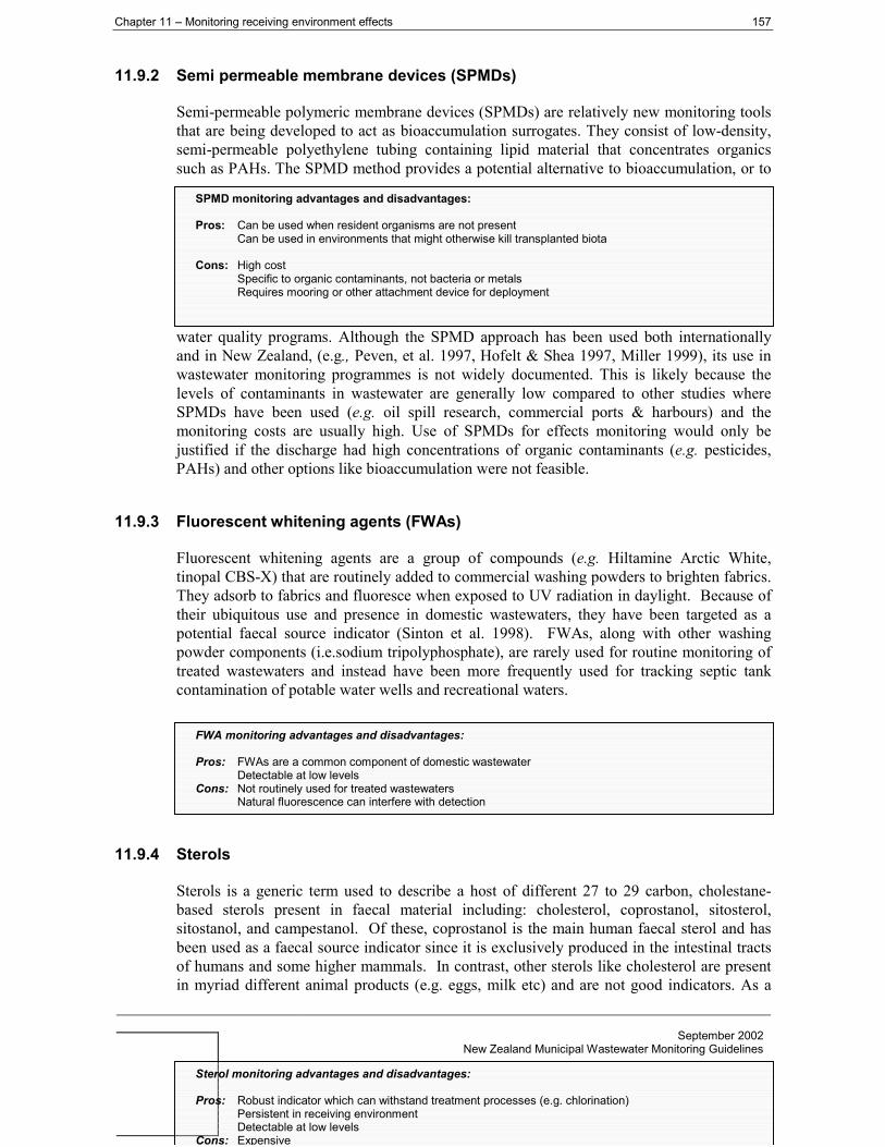
Chapter 11 – Monitoring receiving environment effects 157
September 2002New Zealand Municipal Wastewater Monitoring Guidelines
11.9.2 Semi permeable membrane devices (SPMDs)
Semi-permeable polymeric membrane devices (SPMDs) are relatively new monitoring toolsthat are being developed to act as bioaccumulation surrogates. They consist of low-density,semi-permeable polyethylene tubing containing lipid material that concentrates organicssuch as PAHs. The SPMD method provides a potential alternative to bioaccumulation, or to
water quality programs. Although the SPMD approach has been used both internationallyand in New Zealand, (e.g., Peven, et al. 1997, Hofelt & Shea 1997, Miller 1999), its use inwastewater monitoring programmes is not widely documented. This is likely because thelevels of contaminants in wastewater are generally low compared to other studies whereSPMDs have been used (e.g. oil spill research, commercial ports & harbours) and themonitoring costs are usually high. Use of SPMDs for effects monitoring would only bejustified if the discharge had high concentrations of organic contaminants (e.g. pesticides,PAHs) and other options like bioaccumulation were not feasible.
11.9.3 Fluorescent whitening agents (FWAs)
Fluorescent whitening agents are a group of compounds (e.g. Hiltamine Arctic White,tinopal CBS-X) that are routinely added to commercial washing powders to brighten fabrics.They adsorb to fabrics and fluoresce when exposed to UV radiation in daylight. Because oftheir ubiquitous use and presence in domestic wastewaters, they have been targeted as apotential faecal source indicator (Sinton et al. 1998). FWAs, along with other washingpowder components (i.e.sodium tripolyphosphate), are rarely used for routine monitoring oftreated wastewaters and instead have been more frequently used for tracking septic tankcontamination of potable water wells and recreational waters.
11.9.4 Sterols
Sterols is a generic term used to describe a host of different 27 to 29 carbon, cholestane-based sterols present in faecal material including: cholesterol, coprostanol, sitosterol,sitostanol, and campestanol. Of these, coprostanol is the main human faecal sterol and hasbeen used as a faecal source indicator since it is exclusively produced in the intestinal tractsof humans and some higher mammals. In contrast, other sterols like cholesterol are presentin myriad different animal products (e.g. eggs, milk etc) and are not good indicators. As a
SPMD monitoring advantages and disadvantages:
Pros: Can be used when resident organisms are not presentCan be used in environments that might otherwise kill transplanted biota
Cons: High costSpecific to organic contaminants, not bacteria or metalsRequires mooring or other attachment device for deployment
Sterol monitoring advantages and disadvantages:
Pros: Robust indicator which can withstand treatment processes (e.g. chlorination)Persistent in receiving environmentDetectable at low levels
Cons: Expensive
FWA monitoring advantages and disadvantages:
Pros: FWAs are a common component of domestic wastewaterDetectable at low levels
Cons: Not routinely used for treated wastewatersNatural fluorescence can interfere with detection

158 Chapter 11 – Monitoring receiving environment effects
September 2002New Zealand Municipal Wastewater Monitoring Guidelines
biological indicator sterols are very robust and generally have a much longer environmentalfate than other routine indicators such as coliform bacteria. However, even though the use ofsterols as a wastewater monitoring tool has been well documented (Brown & Wade 1984,Dureth et al. 1986) they are not routinely used. This is primarily due to cost sincedetermination of sterols requires gas chromatography/mass spectrometry methods, which areinherently more expensive than other analytical techniques used for alternative indicators.
11.10 Mixing zones
The RMA requires that any standards imposed through classification or section 107 is metafter ‘reasonable mixing’. Zones of reasonable mixing are areas of transition within whichclassifications do not apply. They are effectively zones of non-compliance. From a practicalviewpoint standards can only apply after reasonable mixing of any contaminant or waterwith the receiving water, disregarding the effect of any natural perturbation. The area withinwhich this mixing occurs is called a ‘zone of reasonable mixing’. This ‘zone of reasonablemixing’ provides for the mixing of discharges with receiving waters. Some further mixingcould still occur outside of the zone as long as the effects in section 107(1) of the RMA donot occur and the relevant water quality classification standards are met.
In general, it is not intended that the size of a zone of reasonable mixing be tailored to thevolume and nature of a discharge, but rather that the volume and nature of a discharge fit thestandards and criteria in accordance with regulatory framework (e.g., Regional Council’sCoastal Plan). The zone of reasonable mixing depends on:
• The rate of discharge and concentrations.
• The physical configuration of the outfall or structure from which the discharge isemitted.
• The depth, current velocity and direction, and the rate of turbulent mixing of thereceiving water.
• Ambient concentrations in the receiving water.
The general requirements for the zone of reasonable mixing are outlined in “ResourceManagement Ideas No 10 – A discussion on reasonable mixing in water qualitymanagement.” (Rutherford, et al. 1994) as follows:
• The size of the zone of reasonable mixing should be minimised.
• Any adverse effects should be confined to within the zone of reasonable mixing.
• Any adverse effects within the zone of reasonable mixing should be no more thanminor.
It is anticipated that a discharger, altering the extent to which contaminants or water aredischarged into the receiving environment, can control the size of the zone of reasonablemixing. For example, lowering the volume or improving the level of treatment or mixingcharacteristics, even by a small degree, can produce marked changes in mixing zonespecification.

Chapter 11 – Monitoring receiving environment effects 159
September 2002New Zealand Municipal Wastewater Monitoring Guidelines
It is also important to appreciate that a single discharge may have more than one zone ofreasonable mixing. For example, a coastal outfall may have one zone of reasonable mixingfor seabed impacts and another for water column impacts. The location of the zone ofreasonable mixing should also take into account the nature and degree of uses in that area.Data from other areas can help clarify a likely zone of reasonable mixing.
11.11 Air and land discharges
11.11.1 Air
As mentioned previously, discharges to air from wastewater plants are of a secondary nature.This is because the overwhelming majority of the emissions from a plant are either in theform of biosolids or liquid effluent, with any discharges to air being either incidental releaseof spray or aerosols or through the treatment process. They are also being treated as asecondary concern given the focus of these guidelines, which concentrate on discharge toaquatic environments.
With these caveats in mind, discharges to air can be divided into three main categories: (i)aerosols, (ii) odour, and (iii) treatment related contaminants. The latter of these is a verybroad term that is used to describe all other discharges to air and can include sludgeincineration stack gases, anaerobic digestion gas exhaust, and sludge drier emissions to namea few. While these processes have the potential to emit considerable amounts of methane,nitrogen oxides, sulphur oxides, and particulates to the air; it is not within the scope of theseguidelines to address these issues. These issues are generally specific to individual treatmentplants and mitigative action to reduce emissions is almost always employed to the pointwhere odour, and to a much lesser degree, aerosols become the primary air emissionconcerns.
Aerosols
Aerosols are small air-bound particles of water. These particles are only visible to the nakedeye in high concentration and large volumes. For example, the haze that is often observedalong the surf zone of beaches is made up of aerosols. The diminutive size of individualaerosols, however, does not mean that they cannot act as vectors for the microscopicpathogens that are present in wastewater effluent. Wastewater aerosols have the potential ofcontaining not only pathogenic micro-organisms but also minute organic and inorganicparticulates. In almost all circumstances, though, the isolation from most public activitysurrounding wastewater facilities and the short distances travelled by high concentrations ofaerosols makes all but odour issues insignificant.
If it is expected that exposure to aerosols might be an issue there are several good referencesavailable, although specialist advice will probably be required. A general discussion of thetypes of pathogens present in wastewater is covered in section 11.8 and more detaileddiscussions are available in most wastewater engineering texts. In addition, the recentsewage effluent to land guidelines (NZLTC 2000) discusses the emission rates, exposureroutes and mitigative measures for controlling aerosols from irrigation equipment.

160 Chapter 11 – Monitoring receiving environment effects
September 2002New Zealand Municipal Wastewater Monitoring Guidelines
Odour
Without question, public perception places odours as the most significant air relateddischarge from wastewater plants. Reactions to odour are as variable as the people thatencounter them, and range from ambivalence to physical effects like nausea. Generally, thereaction to wastewater odours is a negative one, but it is not within the scope of theseguidelines to discuss odour assessment methods. Odour effects monitoring and assessmentmethods are covered in the sewage effluent to land guidelines (NZ Land TreatmentCollective 2000).
11.11.2 Land
Discharge of wastewater directly to land constituents a small percentage (roughly 6%) of thetotal daily effluent volumes in New Zealand (Macdonald, et al 2001). This, coupled with therecent release of guidelines specifically designed to address the discharge of wastewater toland (NZLTC 2000), are the two main reasons why discharge to land is not being covered indetail in this Chapter.
The recent land disposal guidelines include sections on wastewater characteristics, siteselection, soil treatment processes, environmental effects, application methods, and cropselection. With respect to effects monitoring the land disposal guidelines outline approachesfor monitoring:
• Soil, surface and ground waters.
• Soil quality.
• Climate and air quality.
• Vegetation.


September 2002New Zealand Municipal Wastewater Monitoring Guidelines
CHAPTER 12MONITORING EFFECTS ON COMMUNITY VALUES
James Baines, Janet Gough (Taylor Baines Associates)Donald Couch (Lincoln University)
12.1 Levels of community involvement
The community can be involved in the effects monitoring process in a variety of ways. Atdiffering levels of community involvement, they include -
1. Evaluation by the community of technical monitoring results.
2. Involvement of community representatives in monitoring activities, including datagathering.
3. Monitoring effects on people’s values (e.g., impacts from odour, noise, litter, etc.).
12.1.1 Evaluation by the community of technical monitoring results
This is common practice with many Councils, and occurs when small groups of communityrepresentatives are sent periodically the results of technical monitoring activities (e.g., waterquality test results) and invited to review and comment on the results. The approach, whichserves as a mechanism for communicating information on certain aspects of the WWTP’sperformance to interested community participants, requires the existence of appropriatecommunity groups or groups of representatives and tends to be targeted at groups with astatutory basis (e.g., Runanga or Community Boards) or groups which are part of a largerorganisational network (e.g., Fish & Game Council). Providing this information increases thecommunities’ knowledge and understanding and typically the information is fed back to thelarger community as well as other community groups, and friends and neighbours.
At this level of involvement, the community is unlikely to have had any input to settingpriorities for monitoring; they simply receive information deemed important by technicalexperts.
12.1.2 Involvement of community representatives in monitoring activities
This is when small groups of community representatives commit themselves to gatheringinformation in a systematic and agreed way (e.g., water samples at bathing beaches),delivering the samples for analysis and then meeting to review and interpret the results. Suchan arrangement implies a focus on a particular type of risk factor (e.g., the risk of watercontamination). Because of the greater level of community participation, it is likely that thecommunity representatives have had an opportunity to discuss and negotiate priorities forsuch monitoring with the WWTP operators and administrators.

Chapter 12 – Monitoring Effects on Community Values 163
September 2002New Zealand Municipal Wastewater Monitoring Guidelines
Another example might be the establishment of a community liaison group with neighboursof the WWTP as a mechanism for channelling and reviewing observations and complaintsabout the effects of the WWTP’s operations that come to the attention of people nearby. Thiswould usually go hand in hand with an agreed response procedure. While such anarrangement might involve regular review meetings, the intervening activities may beanything but regular. The purpose of such a community liaison group is to support amechanism for anyone in the neighbouring community to relay observations or complaintsdirectly to the plant’s operators. Depending on the performance of the plant, suchobservations may be very rare or very frequent.
These arrangements provide good examples of risk communication mechanisms – channelsof communication between the community and the plant operators are maintained on an ‘asrequired’ basis.
12.1.3 Social monitoring activities (impact monitoring)
Social monitoring occurs when neighbours of the WWTP are systematically surveyed abouttheir experience of the plant’s operations over the preceding time period. It is likely to occurat time intervals related to any formal review of consent conditions and plant performance(say every 3-5 years). The focus is on assessing the impacts that the WWTP’s operationshave had on its neighbours. An assessment of impacts enables individuals to relate anyeffects they might experience to the environmental qualities they value. Effects are thusrelated to values.
If motivation and effective participation are considered important, then it is likely that modesof involvement which allow community members to make input to setting priorities as wellas evaluating results will be favoured (i.e., the second and third categories above).
12.2 Why monitor effects on community values?
Monitoring activities allow, at the very least, for information on the performance of WWTPsto be made available to members of the community. With higher levels of involvement,community members have greater knowledge and understanding of the significance of theinformation. Over a period of time, this allows the community to learn more about theoperation of the plant. Community members may then be in a position to re-assess the risks,the need for particular monitoring, the level of monitoring effort that is appropriate, and thepriorities for monitoring effort.
If a risk-based monitoring regime changes over time, then the community should beprovided with the opportunity to review its priorities.
Consent conditions embody protection for neighbours and other parties who have a stake inthe quality of the environment. Community involvement in monitoring effects can provideinput to the review processes for consent conditions. Social monitoring may identify issuesand effects not previously considered in the setting of consent conditions and the design ofmonitoring regimes. It can also provide a channel for community input to future consentconditions, complementary to the input of technical experts.

164 Chapter 12 – Monitoring Effects on Community Values
September 2002New Zealand Municipal Wastewater Monitoring Guidelines
12.3 Approaches to monitoring effects on community values
12.3.1 Choosing how to incorporate monitoring of effects on community values
The approach chosen will reflect the scale of the system, and the size and sensitivity of localcommunities. There will be costs involved with monitoring community values (as formonitoring technical aspects) and these costs will fall on the community involved.Therefore, before deciding on what form of community involvement there should be in themonitoring programme, the community should be consulted so that members of thecommunity are aware of what has been proposed, understand the costs involved and whowill have to pay, and know the expected benefits. These costs and benefits include costs interms of people’s valuable time. Such contributions will in most cases reduce the dollar costof administering consents (see 12.3.3).
The remainder of this section contains examples of each level of community involvement inmonitoring.
12.3.2 Evaluation by the community of technical monitoring results
This involves use of established community representative groups (e.g., Runanga,Community Boards or Ratepayer Associations in urban centres, or established residentsgroups) or the formation of groups representing neighbours interests and the interests ofother immediate stakeholders in the locality (e.g., user groups of a river being used to receiveeffluent discharge - ‘Friends of the ......River’).
Several questions to think about here are:
• Which groups should be sent the monitoring results and invited to comment?
• What criteria are used in identifying such groups?
• Are any of the existing groups actually well placed in order to make sensibleevaluation of the results? In other words, do members of the group have first-handexperience - residential occupancy, workplace or recreational location - whichenables them to make sense of the results?
• (How) will groups be able to ask questions about the monitoring activities? Ofwhom?
12.3.3 Two examples of involvement
A formalised monitoring group - the Lyttelton Harbour Basin Issues Group
The Lyttelton Harbour Basin Issues Group was established by Environment Canterbury andthe Banks Peninsula District Council as a means of establishing a communication channelbetween the councils and the communities of the harbour basin. Representatives of eachcommunity attend regular meetings every six weeks and report back to their communities.

Chapter 12 – Monitoring Effects on Community Values 165
September 2002New Zealand Municipal Wastewater Monitoring Guidelines
A key activity of this group has been to design and implement a water-monitoringprogramme. Members of the group collect water samples on a weekly basis from eight localbathing beaches, and these samples are analysed by Environment Canterbury. Initiallyeighteen months of continuous sampling was undertaken to obtain baseline data. This hasnow been replaced by monitoring over the summer months only (November to April). Inaddition, Rapaki has been taking shellfish samples from six sites around the harbour foranalysis on a monthly basis.
The group has designed a notice that is placed at each site being monitored, explaining theprogramme. If the sample for a particular beach reaches the bathing water trigger level, thena ‘don’t swim’ sign can be placed while additional sampling is undertaken.
The water monitoring programme has been designed by the group with expert assistanceprovided by the two councils, Health Authorities, and other invited experts. An importantaspect is that the group retains ownership and drives the process. Results to date havedemonstrated that the highest enterococci readings occur after heavy rain, and the group isconsidering how to establish a monitoring programme for peak flows on some of the mainstreams entering the harbour.
Another important aspect is that while the initial focus has been on water quality, the group’smandate is not limited to water monitoring. Currently the Lyttelton group is concerned aboutissues relating to multiple use of the harbour. Some aspects of this impinge on water quality,but other aspects are related to community integrity and amenity values.
Resources to support the activities of this group have come from various sources andindividuals on the group have given their time for free, both in attending meetings, andundertaking the monitoring programme. Environment Canterbury has funded the laboratoryanalyses of water samples. They have a statutory obligation to monitor and the free samplecollection means that they are able to monitor a larger number of areas than they wouldotherwise. Rapaki and Crown Public Health have paid for shell fish testing at various times.Several community organisations have made contributions in kind - meeting venues,collection and delivery of samples.
For further information, contact John Porter at the Banks Peninsula District Council.
A formalised neighbours liaison group - Redvale Landfill Community Liaison Committee
[Note: while this example is associated with a solid waste facility, the rationale for itsestablishment is consistent with the focus of these guidelines for WWTPs. Other groups existfor WWTPs as in the case of Moa Point, in Wellington]
The Redvale Landfill Community Liaison Committee was established as a condition of theresource consents for operating the landfill. It comprises twelve members and meetsquarterly. Membership of the committee is predominantly (more than half) from those withinthe immediate host community of Dairy Flat, while the Auckland Regional Council, theRodney District Council and the facility’s technical Peer Review Committee are eachrepresented and the facility’s manager is a member (as well as being a neighbour).
The Committee’s role is to allow issues and concerns relating to the operation of the landfillto be debated and negotiated. At least one local resident is designated Resident Liaison

166 Chapter 12 – Monitoring Effects on Community Values
September 2002New Zealand Municipal Wastewater Monitoring Guidelines
Officer, a neighbour to whom complaints can be lodged. However, neighbours are activelyencouraged to report any off-site effects directly to the facility manager. A recording andresponse procedure is in place. The Community Liaison Committee supports this mechanismfor direct communication between operator and neighbours by regular reviews of thecomplaints register, evaluating patterns of effects and assessing whether the operator’sresponses have been reasonable and effective. Through the Liaison Committee, complaintscan be de-personalised, and legitimate community interests advocated.
Such Liaison Committees can instigate ‘open days’ or tours of the facility, so that neighbourscan be informed about the operations and understand likely sources of risk. With amechanism such as this, it is more likely that priorities for attention and discussion will beset by members of the community rather than technical experts.
For further information, contact the Manager, Redvale Landfill, Dairy Flat.
Some such groups are set up with independent facilitators, although with goodwill and goodintentions by all parties, this should not be a requirement.
12.3.4 Social monitoring activities (impact monitoring)
The emphasis in social monitoring should be on making a realistic assessment of thecommunity’s experience, from the community’s point of view. In the specific context ofodour monitoring, Lincoln Ventures (1997) distinguish between an ‘indicative survey’, themain focus of which is to improve management of the plant for odour effects, and a‘definitive survey’ where the immediate objective is to provide information for legalproceedings (e.g., consent hearings, enforcement orders, abatement notices).
The nature of monitoring is that it is a systematic and repeated activity. Therefore, to beuseful, social monitoring needs to be as practical and affordable as possible, in terms of time,financial and human resources. One approach to this is the recent case study survey workcarried out for eight case studies as part of a research programme commissioned by theFoundation for Research, Science & Technology (Taylor Baines & Associates, 2001).
Key aspects of this survey approach involve:
• Purposive sampling of neighbours, in terms of proximity, topography and windpattern;
• Sampling for representative coverage rather than statistical analysis;
• Use of unprompted and prompted questions, to allow respondent experience andpriorities to determine emphasis;
• Systematic assessment of respondent experience, to elicit overall patterns and trendsin effects and impacts;
• A risk-based approach to assessment (i.e., covering both frequency of effect andseverity of impact, and the use of word scales);
• Supplementing individual survey interviews (i.e., precisely replicated structure) withsemi-structured key informant interviews to incorporate the experience of organised

Chapter 12 – Monitoring Effects on Community Values 167
September 2002New Zealand Municipal Wastewater Monitoring Guidelines
community groups as appropriate, and to access secondary data sets that assist in theoverall assessment;
• Providing feedback to those who have been surveyed, prior to finalising the surveyresults - for validation.
This method of surveying may be applied in a completely open-ended way, covering allpotential aspects of community experience of the plant’s operations, or in a more targetedway, where the focus is on one specific type of effect.


September 2002New Zealand Municipal Wastewater Monitoring Guidelines
CHAPTER 13DETAILED DESIGN OF MONITORING PROGRAMME
Rob Bell, Graham McBride, David Ray, Chris Hickey (NIWA)
13.1 Introduction
Having developed a conceptual monitoring programme from the HIAMP process (Chapters 4and 8) and chosen which monitoring options to adopt (Chapters 9 to 12), the details of themonitoring programme need to be determined. Certain fundamental questions need to beanswered when considering the detailed design of a monitoring programme and howcompliance is to be tested. For example:
• What are the objectives of the monitoring programme? (Chapter 8)
• What scale (duration and extent) is appropriate?
• What variables or components should be measured? (see Chapters 9 to 12)
• What sampling site(s) should be used?
• What are the practical consequences of various sampling frequencies, complianceperiods, sampling time (time of day or week)?
• Should grab samples be used, or bulking methods to obtain a composite sample?
• How should data problems be handled, e.g., ‘outliers’, ‘less-than’ or ‘greater-than’values, ‘non-detect’ results, missing data?
• How should compliance consent conditions be written?
• What decisions and actions should be made on the evidence of the sample results?
• Will the monitoring programme be cost-effective and is it affordable?
The detailed design of the various components of a monitoring programme is summarised inFigure 13.1.

170 Chapter 13 – Detailed design of monitoring programme
September 2002New Zealand Municipal Wastewater Monitoring Guidelines
Define purposes of monitoring: specific objectives (Ch. 8)
Determine scope in terms of duration:AEE (baseline), consent period, reviews
Sampling design issues
Samplingtechniques
Specific data handling and statistical analysis routines
Complianceperiod Frequency
Select samplingsites
Variables tomeasure
Cost effectiveness
Determine scope in terms of scale:in-plant?, effluent?, environment?, community?
Timing
Compliance testing, reports and dissemination
Consent conditions
Figure 13.1: Framework for the detailed design of a monitoring programme
13.2 Key requirements
A useful checklist of key questions to ask before finally deciding on monitoringmeasurements is provided in Table 13.1 (adapted from ANZECC 2000b).
Table 13.1: Checklist for the selection of monitoring options
Relevance Does the measured variable reflect directly on the main risks andissues of concern?
Validity Does the measured variable respond to changes in the discharge orenvironment and have some explanatory power?
Diagnostic value The measured variable must be able to detect changes and trends inconditions or discharge characteristics for the specified monitoringduration or compliance period. Can the amount of change beassessed quantitatively or qualitatively?
Responsiveness Does the measured variable detect changes early enough to allow amanagement response, and will it reflect changes due to theintervention by management?
Reliability The measured variable must be measurable in a reliable,reproducible and cost-effective way.
Chapter 13 – Detailed design of monitoring programme 171
September 2002New Zealand Municipal Wastewater Monitoring Guidelines
For most situations where the wastewater comprises sewage, effects on public health (e.g.,water-contact recreation and shellfish gathering) will invariably be identified as one of themain public and cultural issues. Consequently, monitoring an appropriate faecal indicator inthe effluent will usually be required as a minimum, and possibly at some receivingenvironment sites where recreational activities might be compromised.
The other critical physical variables to measure are the discharge flow rate (to gain anestimate of environmental loadings) and temperature (for interpretation purposes).
13.3 Statistical sampling design criteria
13.3.1 Representing wastewater in the presence of variability
Monitoring can only hope to sample a very tiny fraction of a waste stream or a snapshot ofthe receiving environment quality. For example, if 6 one-litre grab samples are taken perannum from an average effluent flow of 10 L s-1, these samples will represent only0.000002% of the total effluent volume over a year. Yet we are hoping to use these tinysamples to represent the wastewater. Furthermore, intensive monitoring of wastewaterstreams has demonstrated that there can be substantial variability of its components. Forexample, it is not uncommon for faecal indicators to vary over orders of magnitude. Some ofthis variability is ‘natural’–all natural processes exhibit some variability, after all. But somemay be a pattern, e.g., caused by plant overloading or equipment malfunctioning. Ananalysis of monitoring results seeks to separate such pattern from inherent randomness, andthat is the fundamental task of statistics.
The ecological community’s response to effluent loadings may also be variable. Forexample, the input of inorganic nitrogen to an estuary may stimulate the growth ofphytoplankton during warm periods only when conditions are optimal.
Environmental and effluent variability, both with time and space, is the most importantaspect to be considered in the detailed design of monitoring programmes. Consequently,monitoring design and interpretation is essentially statistical in nature, to move beyond a fewsample results through to inferring knowledge about the total ‘population’ or quality of acontinuous waste stream or receiving environment.
In those situations where high variability exists together with financial constraints on theextent of monitoring, it is vital that monitoring targets the key issues and risks. Otherwise theall too common scenario occurs where a monitoring dataset is too variable to reveal anyimpact or trend, or adequately describe the discharge.
13.3.2 Have potential sources of variability been identified?
If possible, the variability in the treatment plant performance or in the receiving environmentshould be gleaned from pilot studies, AEE studies, consulting other plant operators or from

172 Chapter 13 – Detailed design of monitoring programme
September 2002New Zealand Municipal Wastewater Monitoring Guidelines
the literature. An example is oxidation pond effluent, where the DO varies diurnally (i.e.,throughout a day/night cycle). Knowing this variability will help with deciding when thesample of the effluent should be taken or when a river reach is most stressed on a daily basis.For example, dissolved oxygen is often lowest in a river in the early morning.
Variability may also be important at seasonal timescales. For example, suspended sedimentconcentrations and chlorophyll a from oxidation pond systems tends to peak over late springand summer.
Disruptive processes that might occur in the effluent treatment system or receivingenvironment should also be considered – refer to the risk-assessment process for ‘abnormal’conditions in Chapter 4.
13.3.3 Selection of sampling sites and sampling frequency
How many sites should be sampled? How many samples are needed for measuring eacheffluent constituent or environmental variable at each site? How many samples can beafforded? Answers to these questions depend on the outcomes of the HIAMP risk analysis inChapter 4, anticipated variability, the ability to compute robust sample statistics (e.g.,median, 90%ile, 95%ile) to compare with consent conditions, and the costs of sampling.
Sampling Locations (effluent and influent monitoring)
Specifying the appropriate monitoring location for effluent compliance may seem obvious,but is critical to producing valid compliance data. Some considerations are:
• The wastewater or odour flow should be measurable at the monitoring location.
• The location should be easily and safely accessible.
• The sample must be representative of the discharge during the time period it ismonitored.
Expanding on the last point, the discharge must be as well-mixed as possible, where the flowhas experienced hydraulic turbulence. Logically, the monitoring location should be just priorto discharge or at the entry point to an outfall pipe. This will also ensure measurements offaecal indicator bacteria include the effects of water-fowl contamination in oxidation ponds,chlorine-residual effects (if chlorine is used for disinfection), and any photo-reactivation offaecal-indicator bacteria that might have taken place after treatment with UV-disinfection.
In some instances, a monitoring location may be required well before the discharge point.Such circumstances can include compliance of multiple waste streams from differenttreatment plants and industries in an area that are served by a common outfall, or where thedetection of a pollutant is required in the influent before treatment and dilution occurs withinthe plant, e.g., if a certain percentage or log-order removal is specified in a consent.
Sampling a waste stream at a weir is not recommended, as solids settle behind a weir andfloating oil and grease tend to accumulate immediately downstream of a weir.

Chapter 13 – Detailed design of monitoring programme 173
September 2002New Zealand Municipal Wastewater Monitoring Guidelines
Sampling locations (receiving-environment monitoring)
Specifying locations for environmental-effects monitoring is more complex, and specialistadvice should be sought. Some guidance is provided in Chapter 3 of the ANZECC (2000b)guidelines. The three approaches to sample site selection are:
• Random sampling–randomly selected sites. This may not be the most cost-efficientpattern because of variation within the site.
• Stratified random sampling–system is divided into parts (strata) in each of which thevariable of interest is as uniform as possible, either in space (one or more samplesper strata) or with time (e.g., may sample more often in a season that shows morevariability). This is more efficient than using simple random sample sites.
• Systematic sampling–samples are collected at regular intervals in space (or time),but care is needed to avoid bias, e.g., discharge impact may be routinely lower in themorning than afternoon, and tides are not synchronous with a 24-hour solar day.
Selected sites must be accurately defined and fixed to ensure they can be sampled repeatedly.Archiving site photographs can be an important feature, to guide future samplers to collectfrom the defined site. Such care with fixing sampling locations is highlighted whencompliance is required by way of sampling around the edge of a mixing zone. GPS can be auseful tool for this, but the accuracy of the instrument should be checked carefully.
Finally, sampling sites must be accessible and safe under most conditions, especially iflocated in lakes, large rivers, estuaries, harbours or open coastal waters.
Sampling frequency (effluent and influent monitoring)
Specifying the frequency of sampling for discharge monitoring is an interactive process thatincludes the duration over which compliance is to be tested or results reported, and thesample statistics that will be used, as determined by the planning for the end-use of themonitoring information (Chapter 8). For instance, calculating a 95-percentile sample statisticrequires between 10 and 19 samples, depending on the method used to calculate it (seeSection 13.4.5), so if a 3-month compliance or report period were deemed necessary, thesampling frequency would have to be approximately weekly to extract a 95%ile. If costfactors and the level of risk meant that monthly sampling was sufficient, then the complianceperiod would need to be annually if a 95%ile was one of the consent conditions imposed.
For variables that are associated with a lower concern or risk, the sampling frequency isoften set much lower than high-risk variables. But cognisance must be given to seasonalvariability (e.g., summer vs winter), rather than simply measuring it once a year, whichprovides very limited explanatory power.
Sampling frequency (receiving environment monitoring)
Specifying sampling frequency for receiving environments is much more difficult. Thereader is once again referred to Chapter 3 of the ANZECC (2000b) guidelines. Considerationof all the key timescales that naturally occur in environmental systems is required to ensurethe sampling frequency is sufficient to capture natural ‘cycles’. The Nyquist fundamentalfrequency states that to resolve any time cycle ∆t, you need to sample at least morefrequently than ∆t/2. For example, to resolve an annual cycle, you would need to sample at

174 Chapter 13 – Detailed design of monitoring programme
September 2002New Zealand Municipal Wastewater Monitoring Guidelines
least at 6-monthly intervals, and preferably 3- to 4-month intervals for better resolution. Toresolve a cycle over a single season, at least monthly sampling is required.

Chapter 13 – Detailed design of monitoring programme 175
September 2002New Zealand Municipal Wastewater Monitoring Guidelines
Other timescales to consider are:
• Impact of episodic events, such as storms or river floods, on natural disturbance tothe receiving environment or contamination by catchment run-off (e.g., faecalindicator bacteria from farmland). Equally, summer low-flows or droughts caninduce highly variable natural impacts on a freshwater system.
• Tidal cycles for lowland rivers, estuaries and coastal waters. Tides occur at regularcycles of 12.4 hours, which means the following high water on the next day isapproximately one hour later. Salinity and current velocity change dramaticallyduring a tide cycle, so monitoring of intra-tidal effects means several samples maybe required during a tide cycle. Low-frequency monitoring also needs to allow fortides to ensure there is no bias e.g., six-monthly sampling should be done at the sametide state (high, mid-ebb, low water, or mid flood) and tide range (spring, mean orneap).
• Interannual cycles of 2 to 5 years, generated by the El Niño–Southern Oscillationsystem, can produce high variability in rainfall, river run-off, water temperatures,and winds, which need to be taken into account in selecting a sampling frequencyand duration when embarking on trend-type monitoring objectives.
13.3.4 Selection of compliance period and sampling numbers
Setting a compliance or reporting period is a crucial decision, as it determines the overallnumber of samples (n) used to test compliance against a numeric standard for a selectedsampling frequency. Settling on a compliance period needs to take into account: medium tolong-term variability; minimum number of samples needed for calculating percentile limits;and public expectations or activities that dictate the duration of a compliance period, e.g.,summer bathing season.
Situations have occurred where the compliance period was set without due cognisance ofmonthly and seasonal (annual) cycles in the discharge. For example, a typical oxidation ponddischarge has higher concentrations of suspended solids over summer months than at othertimes during the year. These solids are largely algal cells from summer blooms rather thansewage-derived particles. If a 3-month compliance period is required, then this type ofvariability needs to be taken into account, with perhaps setting a different summer medianand say 90%ile, than those that would apply for the rest of the year (or by adopting adifferent variable, e.g., filtered BOD5).
Calendar vs rolling period
The other issue to resolve is whether the compliance period is based on consecutive calendar(fixed) periods or a rolling period.
A ‘calendar’ or fixed compliance period simply uses the n samples collected over a definedcalendar period (e.g., a 6-month or 12-month period) to test compliance. In the followingcalendar period, a completely new batch of n samples is analysed. Only one report oncompliance determination is required for each elapsed calendar period.
Period 1 Period 2 Period 3 ‘calendar’ compliance period

176 Chapter 13 – Detailed design of monitoring programme
September 2002New Zealand Municipal Wastewater Monitoring Guidelines

Chapter 13 – Detailed design of monitoring programme 177
September 2002New Zealand Municipal Wastewater Monitoring Guidelines
A ‘rolling’ compliance period also uses n successive samples to test compliance. But therollover is accomplished by dropping the x oldest sample(s), and introducing the samenumber (x) of the latest sample(s) taken, to make up a new batch of n samples to testcompliance. Effectively, this is a sliding or overlapping window of n samples. For a givenelapsed calendar period, n/x compliance reports will be required.
Consider a discharge for which compliance with certain limits is required over a six-monthperiod, based on weekly sampling, and that the discharge impacts upon recreational waters.The question then is: should compliance be assessed on a rolling six-month basis or on afixed (calendar) six-month basis?
In the former case, compliance could be assessed each week, by dropping off the datum forthe oldest week and adding in the latest value, and then re-assessing compliance. That is, 26times per six-month period. In the latter case, compliance would be assessed and reportedjust once every six months.
A problem with the former is that the applicant can be found to be in breach of a compliancerule on many occasions, with each occasion being the result of the same data or event! Forexample, imagine that there have been 4 exceedances of a 95%ile enterococci concentrationlimit in a 26-week period from October to March (encompassing most of the bathing season).In this case the 95%ile standard for that period has been breached (because the consent onlyallows 3 exceedances in a six-month period). Now also imagine the (quite plausible) scenariothat all of these 4 exceedances occurred in the weeks of March. Then under a rollingcompliance assessment basis, there would be 22 weekly compliance assessments in whichthe effluent would be declared to be in breach of its standard. These 22 ‘fail’ assessmentswould include all the new data from weeks in April to August (inclusive). But all of thesedeclarations would be attributable to data from the same ‘event’, being the exceedances ofenterococci in March. Consequently, the same reasons for a given breach of the standard willhave to be re-iterated to the regulatory authority many times over and probably explained tothe public. The process of operating a ‘rolling’ compliance period is also more difficult toexplain.
Note that it usually will not be necessary to wait until the end of the compliance period todetermine that there has been non-compliance for the ‘calendar’ compliance approach. In theexample used above, if the compliance period had been January to June (inclusive), non-compliance would have been determined at the end of March – there would be no need towait until the end of June.
Accordingly, it seems sensible in most cases to use calendar (fixed-period) complianceassessments rather than rolling assessments.
Period 1
Period 2
Period 3
‘rolling’ compliance period

178 Chapter 13 – Detailed design of monitoring programme
September 2002New Zealand Municipal Wastewater Monitoring Guidelines
13.3.5 Statistical approaches for designing compliance rules
Sampling error
The heterogeneous nature of the sampled wastewater means that small and infrequentsamples of the discharge will exhibit variability. Statisticians call this ‘sampling error’ – butthat does not mean that an error has been made in sampling! If an error is made in thesampling or in analysing the sample’s contents this is known as ‘measurement error’.
Percentile standards or maximum limits?
In setting a discharge monitoring standard one is interested in some critical concentration ofa contaminant (e.g., nitrogen, suspended solids, a bacterial indicator) derived from toxicity,ecological or epidemiological studies. These critical values are never known precisely – theirderivation always calls for an element of value-judgement, and recognition that the scientificstudies upon which they are based are not absolute in their findings. Because of this, there isincreasing use of percentile standards, in which concentrations may exceed the critical valuefor some proportion of the time (typically 5%, in which case we have a 95%ile standard,and/or 50% for a median standard). The case for percentile standards, rather than maximumstandards, is made stronger when one recognises two mechanisms that may give rise toresults that are too high (rather than too low):
• The occasional presence of sample contamination or laboratory error.
• The at-times heterogeneous nature of effluent treatment processes and thereforeeffluent quality (e.g., some parcels of an effluent stream may not have been aseffectively sterilised by UV lamps, and so are rather higher in their concentration ofa bacterial indicator than is the bulk of the fluid).
When we consider the statistical ‘sampling error’ along with percentile standards we mustconsider ‘burden-of-proof’ issues. For example, see Figure 13.2, showing a hypotheticalsituation in which we actually know the true 95%ile concentration (i.e., 60 units – we neverdo know it of course, but the Figure will be instructive). Figure 13.2a shows a situationwhere the sample 95%ile (63.5 concentration units), calculated using some standard formula(see Appendix 1) is greater than this true value of the continuous discharge. But for anotherdetermination as shown in Figure 13.2b the sample 95%ile (58.2 concentration units) islower than the true value. Either situation can occur. And because in practice we do not everknow the true value, we always are uncertain about whether the true value is above or belowour sample-statistic value. This is where the burden-of-proof issue arises, in which either the‘producer’s’ risk (i.e., discharger’s risk) or the ‘consumer’s’ risk (i.e., environment’s risk)may be kept small. They cannot both be made small. These two approaches are characterisedas the ‘benefit-of-doubt’ and ‘fail-safe’ approaches respectively (Ellis 1989; McBride 2000a;McBride et al. 2000).

Chapter 13 – Detailed design of monitoring programme 179
September 2002New Zealand Municipal Wastewater Monitoring Guidelines
Effluent Concentration
0
10
20
30
40
50
60
70
80
0 100 200 300 400 500
Time
Con
cent
ratio
n ContinuousSamples
(a)
Effluent Concentration
0
10
20
30
40
50
60
70
80
0 100 200 300 400 500
Time
Con
cent
ratio
n
ContinuousSamples
(b)
Figure 13.2: Two scenarios of a ‘continuous’ time series of a discharge concentration with a true95-percentile concentration of 60 units, but have then been grab-sampled at a timespacing of 10 time units, where: (a) the 95-percentile of sample concentrations is >60(i.e., 63.5); and (b) the 95-percentile of sample concentrations is <60 (i.e., 58.2). (fromMcBride et al. 2000).
If one or the other risk is desired to be kept small – where the discharger or the environmentis given the benefit-of-doubt – some calculation procedures are available. These may besomewhat complicated and require certain assumptions to be made about the statisticaldistribution of the effluent quality, posing further difficulties – especially when littleprevious monitoring data is available. A third approach is to ignore ‘sampling error’ andassume the samples measured completely represent the characteristics of the continuouswaste stream. Sometimes the sample statistic will be below the true value and sometimes itwill be above the true value (as in Figure 13.2). This is called the ‘even-handed’ approach,because it treats both risks equally. It leads to discharge monitoring compliance conditionscouched in terms of sample percentiles. For example:

180 Chapter 13 – Detailed design of monitoring programme
September 2002New Zealand Municipal Wastewater Monitoring Guidelines
Based on no fewer than 20 samples on separate days over 3 months, the medianconcentration of faecal coliform bacteria of the samples shall not exceed 2000MPN per 100 mL, and no more than 10% of samples shall exceed 8000 MPN per100 mL.
Proportional compliance conditions
A simpler approach to operate with is to consider instead the permissible proportion ofexceedances of a percentile limit in a batch of samples. This is much more easily understoodby all parties (public included), as it lends itself to simple tabulation. There are two furtheradvantages:
1. No assumptions about the distribution of the effluent quality data are needed (becausethe probability of pass or fail in a fixed number of random samples always follows thebinomial distribution i.e., a ‘heads or tails’ situation discussed in most elementarystatistics texts);
2. It is immediately obvious when the standard has been breached (i.e., more than thepermissible number of exceedances have occurred); there is no need to wait until theend of the compliance assessment period to make that decision and to seek to mitigatethe problem.
Often, discharge monitoring conditions are based on a mixture of a 50%ile concentrationlimit (i.e., median) and an upper-percentile limit (80%ile, 90%ile, or 95%ile). Look-up tables(such as Table 13.2) allow one to determine the permissible number of sample exceedances(e) in a compliance period comprising n samples, based on keeping the discharger’s risk1 atno more than 10%. For calculation of other values of the number of samples (n) or thedischarger’s risk, refer to McBride et al. (2000) and McBride & Ellis (2001).
1 This is the risk that at some future time the discharger will in breach of the consent conditions, by way of the measuredsamples, when in fact the true ‘continuous’ effluent concentration is below the percentile limit.

Chapter 13 – Detailed design of monitoring programme 181
September 2002New Zealand Municipal Wastewater Monitoring Guidelines
Table 13.2: Number of exceedances (e) out of n samples permitted to meet percentile dischargecompliance standards based on a discharger’s risk of no more than 10%.
Number ofsamplestaken in
monitoringperiod (n)
Number of permitted exceedances (e) for a 10% discharger's risk to meetthe performance standards listed.
Median (50%ile) 80%ile 90%ile 95%ile5 4 2 1 16 5 2 2 17 5 3 2 18 6 3 2 19 6 3 2 1
10 7 4 2 111 8 4 2 212 8 4 3 213 9 4 3 214 9 5 3 215 10 5 3 216 11 5 3 217 11 6 3 218 12 6 3 219 12 6 4 220 13 6 4 221 13 7 4 222 14 7 4 223 15 7 4 324 15 7 4 325 16 8 4 326 16 8 5 327 17 8 5 328 17 8 5 329 18 9 5 330 19 9 5 331 19 9 5 332 20 9 5 333 20 10 6 334 21 10 6 335 21 10 6 336 22 10 6 440 24 11 6 450 30 14 8 5
100 56 25 14 8
Note: These numbers are in fact pessimistic because their calculation is based on the assumption thatthe effluent is in fact always borderline for compliance. Such an assumption is necessary usingstandard statistical methods. But in general this assumption is not true An alternative (Bayesian)approach to the calculations does not make this assumption and so results in smaller numbers ofsamples being required (McBride & Ellis 2001). Note that this alternative approach has alreadybeen used in the compliance rules in new drinking-water standards (MoH 2000), and will beexplained in some detail in the Ministry of Health’s forthcoming Guidelines for Drinking-WaterManagement.
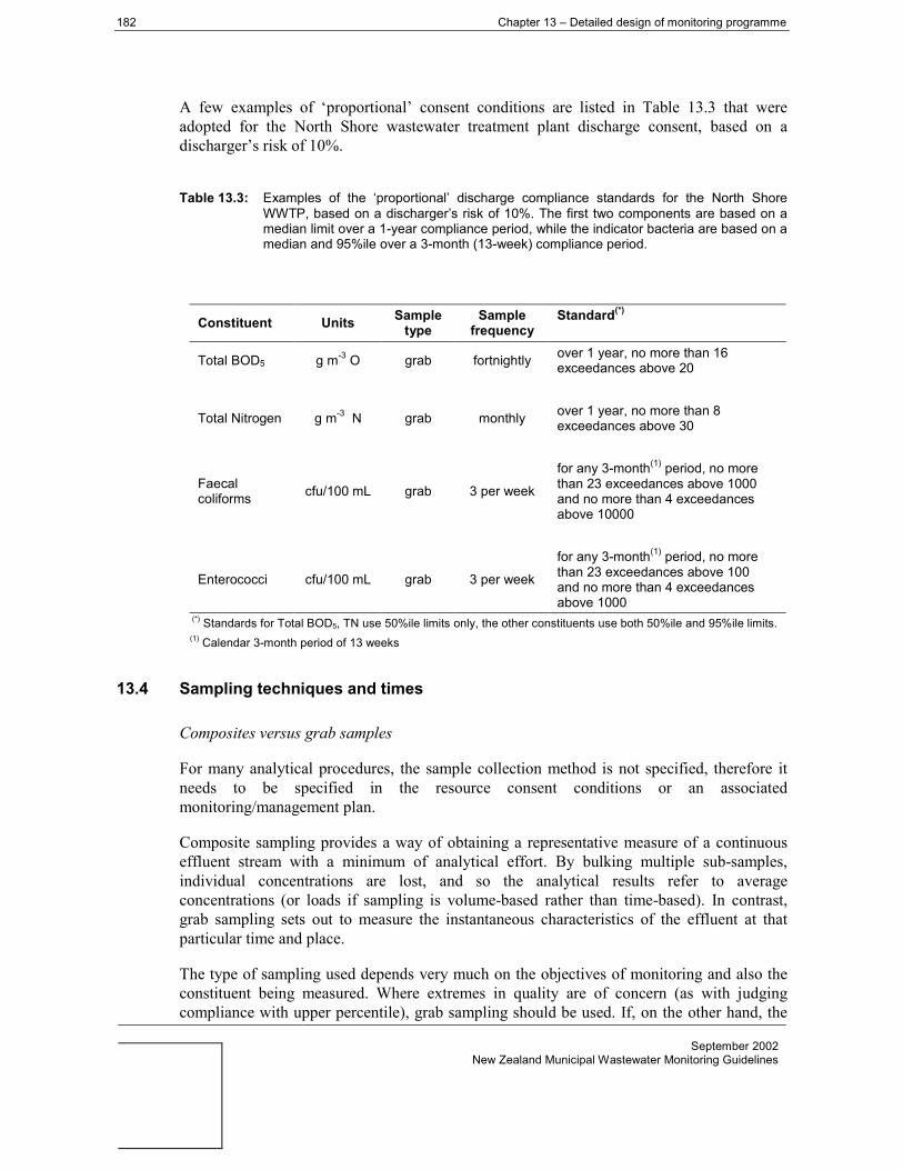
182 Chapter 13 – Detailed design of monitoring programme
September 2002New Zealand Municipal Wastewater Monitoring Guidelines
A few examples of ‘proportional’ consent conditions are listed in Table 13.3 that wereadopted for the North Shore wastewater treatment plant discharge consent, based on adischarger’s risk of 10%.
Table 13.3: Examples of the ‘proportional’ discharge compliance standards for the North ShoreWWTP, based on a discharger’s risk of 10%. The first two components are based on amedian limit over a 1-year compliance period, while the indicator bacteria are based on amedian and 95%ile over a 3-month (13-week) compliance period.
Constituent Units Sampletype
Samplefrequency
Standard(*)
Total BOD5 g m-3 O grab fortnightly over 1 year, no more than 16exceedances above 20
Total Nitrogen g m-3 N grab monthly over 1 year, no more than 8exceedances above 30
Faecalcoliforms cfu/100 mL grab 3 per week
for any 3-month(1) period, no morethan 23 exceedances above 1000and no more than 4 exceedancesabove 10000
Enterococci cfu/100 mL grab 3 per week
for any 3-month(1) period, no morethan 23 exceedances above 100and no more than 4 exceedancesabove 1000
(*) Standards for Total BOD5, TN use 50%ile limits only, the other constituents use both 50%ile and 95%ile limits.(1) Calendar 3-month period of 13 weeks
13.4 Sampling techniques and times
Composites versus grab samples
For many analytical procedures, the sample collection method is not specified, therefore itneeds to be specified in the resource consent conditions or an associatedmonitoring/management plan.
Composite sampling provides a way of obtaining a representative measure of a continuouseffluent stream with a minimum of analytical effort. By bulking multiple sub-samples,individual concentrations are lost, and so the analytical results refer to averageconcentrations (or loads if sampling is volume-based rather than time-based). In contrast,grab sampling sets out to measure the instantaneous characteristics of the effluent at thatparticular time and place.
The type of sampling used depends very much on the objectives of monitoring and also theconstituent being measured. Where extremes in quality are of concern (as with judgingcompliance with upper percentile), grab sampling should be used. If, on the other hand, the
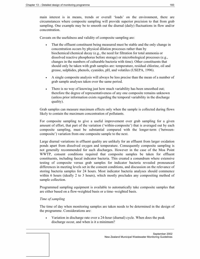
Chapter 13 – Detailed design of monitoring programme 183
September 2002New Zealand Municipal Wastewater Monitoring Guidelines
main interest is in means, trends or overall ‘loads’ on the environment, there arecircumstances where composite sampling will provide superior precision to that from grabsampling. One example may be to smooth out the diurnal (daily) fluctuations in flow and/orconcentration.
Caveats on the usefulness and validity of composite sampling are:
• That the effluent constituent being measured must be stable and the only change inconcentration occurs by physical dilution processes rather than bybiochemical/chemical decay (e.g., the need for filtration for total ammonia ordissolved reactive phosphorus before storage) or microbiological processes (e.g.,changes in the numbers of culturable bacteria with time). Other constituents thatshould only be taken with grab samples are: temperature, residual chlorine, oil andgrease, sulphides, phenols, cyanides, pH, and volatiles (USEPA, 1996).
• A single composite analysis will always be less precise than the mean of a number ofgrab sample analyses taken over the same period.
• There is no way of knowing just how much variability has been smoothed out;therefore the degree of representativeness of any one composite remains unknown(unless prior information exists regarding the temporal variability in the dischargequality).
Grab samples can measure maximum effects only when the sample is collected during flowslikely to contain the maximum concentration of pollutants.
For composite sampling to give a useful improvement over grab sampling for a givenamount of effort, that part of the variation (‘within-composite’) that is averaged out by eachcomposite sampling, must be substantial compared with the longer-term (‘between-composite’) variation from one composite sample to the next.
Large diurnal variations in effluent quality are unlikely for an effluent from larger oxidationponds apart from dissolved oxygen and temperature. Consequently composite sampling isnot generally recommended for such discharges. However in the case of the Moa PointWWTP, consent conditions required that composite samples be taken for effluentconstituents, including faecal indicator bacteria. This created a conundrum where extensivetesting of composite versus grab samples for indicator bacteria revealed pronounceddifferences in meeting levels set in the consent conditions, and discussion on the relevance ofstoring bacteria samples for 24 hours. Most indicator bacteria analyses should commencewithin 6 hours (ideally 2 to 3 hours), which mostly precludes any compositing method ofsample collection.
Programmed sampling equipment is available to automatically take composite samples thatare either based on a flow-weighted basis or a time–weighted basis.
Time of sampling
The time of day when monitoring samples are taken needs to be determined in the design ofthe programme. Considerations are:
• Variation in discharge rate over a 24-hour (diurnal) cycle. When does the peakdischarge occur, and when is it a minimum?

184 Chapter 13 – Detailed design of monitoring programme
September 2002New Zealand Municipal Wastewater Monitoring Guidelines
• Variation in concentrations over a 24-hour (diurnal) cycle. Is there a daily peak forany constituents being monitored? For example with oxidation ponds, dissolvedoxygen will be minimum around sunrise, while faecal indicator bacteria may belowest towards mid-afternoon after a decent dose of solar radiation.
• Variation in discharge rate and concentrations during a typical week (e.g., week daydischarge versus weekend).
13.5 Design of data processing steps
While often forgotten, it is essential that the data handling protocols right through to theproduction of the final report are designed beforehand and included in the monitoringbudget. Some steps along the way should include:
• Pre-processing procedures for adjusting measurements (if not already done by thelaboratory) e.g., adjusting ammoniacal nitrogen or %DO saturation for temperature,pH or salinity.
• Plotting software package and procedures to view and plot monitoring data.
• Develop checks for outliers, missing data, non-detects, ‘greater-than’ or ‘less-than’data and process according to preset protocols. (See section on special data handlingtechniques).
• Specify the methods to be used for calculating required sample statistics e.g.,median, 90-percentile, range, number of exceedances (e) of a specifiedconcentration. (See section on methods to compute percentiles).
• Set up milestones when a statistical analysis of environmental and communitymonitoring data is to be carried out, against a hypothesis or objective such as: thereis no significant change or trend with time, or there is no significant differencebetween upstream and downstream of the discharge (see Chapter 11).
• Design a clear and concise presentation layout for results.
• Protocols for dissemination to the Regional Council, stakeholders, and the public,including any Web page display.
• Design archive and back-up system for the monitoring data.
Special data handling problems
One should always be seeking to interpret data into information. In doing so, water-qualitydata can pose some special problems:
• ‘Non-detects’, or ‘less-thans’, where the result is less than a detection limit.
• Skewness, where very high values may occasionally be present (especially formicrobiological analyses).
• ‘Outliers’, where the data seem inexplicably large or small.

Chapter 13 – Detailed design of monitoring programme 185
September 2002New Zealand Municipal Wastewater Monitoring Guidelines
• ‘Greater-thans’, where the test's upper detection limit is less than the actualconcentration (for example, this would be reported for E. coli if all wells in a Colilerttray were positive for presence of that organism).
The first two problems are easily handled using standard statistical analyses. Thus means andstandard deviations would be calculated, maybe adopting the non-detect limit as the numericvalue (or half of its value) or using logarithms to remove the skewness in the data. The lasttwo problems are much more problematical using such standard (i.e., ‘parametric’)techniques. However, if we use methods that use only the ranks of the data (i.e., ‘non-parametric’ techniques), rather than the actual data values, most of the last two issues areresolved. One does not need to consider whether the outlier is an artefact or is real, it merelybecomes a datum with high rank, as does a ‘greater than’.
Note: common use of Microsoft EXCEL® often results in the ‘<‘ or ‘>‘ qualifiers onmonitoring data becoming divorced from the numerical value. It is important they are storedwith the value.
Calculating percentiles from sample data
It is often a surprise to people that there are several methods that can be used to calculatepercentiles (e.g., medians, 95%iles) from sample data, and they produce different results.While it is often thought that there is always one ‘statistically correct’ way to proceed, oftenthere are several – calculation of percentiles being a case in point. Consequently, the designof the data analysis routines needs to specify a method to consistently calculate samplepercentiles. The most common methods are Weibull, Hazen and the procedure embedded inMicrosoft Excel® (and also in the statistics package S-Plus). This is no trivial matter: resultsfor 95%iles of bathing beach enterococci data using Weibull and the Excel method canproduce results that differ four-fold in value (McBride 2000b). The same may well be truefor effluent microbiological variables.
The Hazen method is generally preferred, as it provides an answer about half-way betweenthe other two methods. Also the Weibull convention, although used widely in the UK waterindustry (Ellis 1989), requires 19 samples before a 95%ile can be calculated, whereas only10 are required for the Hazen procedure. Microsoft Excel® produces an answer for anynumber of samples (even just 1!), which is very misleading for small sample sizes. Formulaeare given in Appendix 1. Note however that while the Excel method does pose someconceptual difficulties (in particular, in being able to calculate any percentile given just onedatum), at least it is ubiquitous, whereas special procedures need to be available forcomputation of the Hazen method (which can be done as a macro in Excel).
13.6 Cost
Now that the monitoring programme has been designed, it should be fully costed, includingsample collection (labour and capital items), sample preparation, delivery to laboratory,laboratory analyses, processing monitoring data and disseminating reports to regulatoryagencies and the public. Any additional monitoring that might be required when triggerlevels are exceeded should also be estimated.

186 Chapter 13 – Detailed design of monitoring programme
September 2002New Zealand Municipal Wastewater Monitoring Guidelines
If the total ongoing cost cannot be afforded, then further iterations of the monitoringprogramme design will be required e.g., reducing sampling frequency, increasing complianceor reporting period, reducing the scale of any environmental-effects monitoring, orinvestigating a different mix of monitoring approaches. For the latter, a few toxicity tests peryear for a lower-risk discharge may be more cost-effective than measuring several dischargeconstituents more frequently.
If further cost reductions are required, there is the option of reducing the number ofconstituents, tests or variables measured. However, this would necessitate returning toChapter 8 and redefining the objectives of the monitoring programme, in the context of theHIAMP process.

Chapter 13 – Detailed design of monitoring programme 187
September 2002New Zealand Municipal Wastewater Monitoring Guidelines
13.7 Monitoring management plan
The preparation of a monitoring management plan is becoming a commonplace procedure,and is frequently required as a requirement of a resource consent condition. The mainadvantage of such a plan is that it can be picked up and implemented by a person who is newto the monitoring programme. This is particularly useful when monitoring personnel havenot been involved in the development of the programme, or when there is a change inpersonnel. Another advantage is that the plan can include minor items that are not deemednecessary to be included as a consent condition, and hence can be changed more readily,provided there is agreement between the regulatory authority and the consent holder.
The monitoring plan will often form a part of a wastewater management plan for the WWTP.Issues that might be covered include:
• Maps showing sampling locations.
• Sampling methods (timing, frequency, volumes, sampling equipment, preservation).
• Laboratory delivery details, analytical procedures (see Chapter 14).
• Description of other monitoring procedures, e.g., surveys of biota, communitysurveys.
• QA procedures (see Chapter 14).
• Data interpretation protocols, including statistical analyses.
• Response procedures in the event of non-compliance or treatment plant breakdown.
• Reporting and information dissemination protocols.
• Names and contact details of key personnel (consent holder, WWTP personnel,regional council staff, Medical Officer of Health, key interest groups, localresidents).
• Copy of the resource consent conditions.

September 2002New Zealand Municipal Wastewater Monitoring Guidelines
CHAPTER 14SAMPLING AND ANALYTICAL METHODS
Luci Ryan (CH2M Beca Ltd)Rob Fullerton (Envirolab Geotest Ltd)
14.1 Methods for sampling and sample handling
14.1.1 Introduction
Obtaining representative samples and maintaining their integrity are critical parts of anymonitoring programme. Analytical methods have been standardised but the results are onlyas good as the sample collection and preservation methods.
In sampling, the objective is to collect a small portion of an environment that isrepresentative of the whole body. Once the sample is taken the constituents of the samplemust stay in the same condition as when collected.
The US Environmental Protection agency (EPA) has estimated that 95% of the totalvariability in environmental measurements is due to sample collection and handling and thatonly 5% is due to variability during laboratory analysis. The 95% can be further brokendown into 85% of variability from sample collection and 10% from sub-sampling in thelaboratory (Rosecrance & Adolfo 1996). This gives some indication as to the importance ofusing correct sampling procedure at all times.
Analytical laboratory personnel are usually a valuable source of knowledge for sampling andsample handling methods. The reader is strongly advised to consult laboratory personnelbefore embarking on a sampling programme.
14.1.2 Composite sampling methods
The advantages and disadvantages of using composite versus grab sampling are described inSection 13.4. If composite sampling is to be used, there are four methods to be considered.Smoley (1993) describes these as follows:
a) Constant time – constant volume: Samples of equal volume are taken at equalincrements of time and composited to make an average sample.
b) Constant time – volume proportional to flow increment: Samples are taken atequal increments of time and are composited proportional to the volume of theflow since the last sample was taken.
c) Constant time – volume proportional to flow rate: Samples are taken at equalincrements of time and are composited proportional to the flow rate at the timeeach sample was taken.

Chapter 14 – Sampling and analytical methods 189
September 2002New Zealand Municipal Wastewater Monitoring Guidelines
d) Constant volume – time proportional to flow volume increment: Samples ofequal volume are taken at equal increments of flow volume and composited.
The most common form of composite collected by automatic sampler is d), whereby thesampler is triggered to take an incremental constant volume sample each time a givenvolume of flow has passed through the measuring point. A flow meter is not required forcomposite sample type a). Note that a flow proportional composite can be manually preparedfrom individual grab samples if flow data is available. Samples b) and c) are also usuallycollected and composited manually.
Guidance to the most appropriate type of composite method to use can be found in ISO5667/10 5.3.1.2.
It is also possible to take composite samples manually, but the volume of the bucket, ladle orbottle should be well defined and known to a precision of ±5%.
Discrete samples that make up a composite sample can be stored in individual containers andthen mixed proportionally when the sampling period is complete. However, it is morecommon for the discrete samples to be collected in one sample container, so that no furthermixing is required.
14.1.3 Sample collection equipment
Manual sampling
A grab sample can be taken manually using a scoop, pump, vacuum or other suitable devicethat will collect a sample from the intended location. Samples of influent wastewater or fromwithin the process are often taken from flow channels. The simplest sampler is a pole with aclamp for a sample container to dip into the channel. Many WWTPs use a ‘Mighty Gripper’,a stainless steel spring loaded clamp which securely fastens around the sample container.Sample volumes are typically about one litre.
The collection of environmental samples from the receiving waters requires a diverse rangeequipment, depending on the parameters being monitored. Grab samples from surface watercan be effectively carried out with a ‘sample container on a pole’ technique, either from theshore or from a boat. If subsurface samples are required, submersible pumps can be used orspecialised water column samplers are available.
Automatic Samplers
Automatic samplers allow the collection of multiple samples or composite samples overextended periods. They are most applicable to sewer and treatment plant sampling and areavailable in widely varying levels of sophistication, performance, mechanical reliability andcost. Samplers are available with inputs for triggering from a flow meter to enable automaticflow compositing. Bottle samplers (usually 24 bottles) are available to collect individualsamples on a time or flow basis
Auto samplers are not usually considered appropriate for microbiological sampling as thesample tube is not sterilised between samples and therefore contamination of subsequentsamples could occur. Other constituents can also change in concentration with time – for

190 Chapter 14 – Sampling and analytical methods
September 2002New Zealand Municipal Wastewater Monitoring Guidelines
example, ammonia can be converted to nitrate. If in doubt, consult with the analyticallaboratory prior to sampling.

Chapter 14 – Sampling and analytical methods 191
September 2002New Zealand Municipal Wastewater Monitoring Guidelines
14.1.4 Sample containers
ISO 5667 – 10:1992 lists the following factors to be considered when choosing a samplecontainer:
• High resistance to breakage.
• Good sealing efficiency.
• Ease of reopening.
• Good resistance to temperature extremes.
• Practicable size, shape and mass.
• Good potential for cleaning and re-use.
• Availability and cost.
Sample containers are generally made out of glass or plastic. The type of determinand thesample is to be analysed for often controls the type of material the container is made from, assome containers will react with the determinands and give false results when the sample isanalysed. If you require a sample to be analysed for more than one determinand, it ispossible that you may have to use more than one type of sample container.
Plastic containers are commonly used for sampling wastewater, although glass containersmust be used if the sample is to be analysed for oils and grease, hydrocarbons, detergentsand pesticides. If you are not sure which type of container you require, the laboratory that iscarrying out the analysis will be able to advise you.
Containers must be cleaned before sampling commences in order to reduce the risk of thesample being contaminated. Containers must be thoroughly rinsed with water after cleaningto minimise risk of the sample being contaminated. This is particularly important if thesample taken is to be analysed for detergents.
Please note that sampling lines should also be considered as containers, and therefore themethod of selection of materials for containers should also apply to sampling lines.
14.1.5 Sample preservation
If a sample is to remain representative of the water sampled when it is analysed, it is usuallynecessary to preserve the sample to prevent changes taking place. This is particularlyimportant with regard to composite samples, which could be collected over a period of a dayor more.
The most common way of preserving wastewater samples is with ice, to cool the sample tobetween 0 ºC and 4 ºC. If the sample is being collected over an extended period of time thepreservation of the sample should form an integral part of the collection procedure. Keepingthe samples in the dark can enhance preservation further.

192 Chapter 14 – Sampling and analytical methods
September 2002New Zealand Municipal Wastewater Monitoring Guidelines
There are other limited methods of chemical preservation that are applicable to specific typesof samples. For example, sulphuric acid (H2SO4) can be added to ammonia samples to lowerthe pH if the sample is not to be analysed immediately. Sodium thiosulphate is added towater samples for bacteriological analysis to nullify the disinfecting effect of chlorine. If youare unsure as to how to preserve your samples, contact the laboratory that will analyse themfor advice. A summary table of sample preservation and minimum sample size is given inAPHA Standard Methods 20th Ed. (Table 1060-I) (APHA 1998).
14.1.6 Microbiological samples
Special attention must be given to microbiological samples, because they are verysusceptible to being contaminated by poor sampling technique. When taking amicrobiological sample, keep the following issues in mind:
• Automatic composite samplers used for general wastewater sample collection areinappropriate for microbiological sample collection due to sample tubecontamination. Specialist microbiological samplers are available but are rarely usedin the field due to cost and availability. Microbiological samples are usually taken bymeans of grab samples.
• Bottles for collecting microbiological samples will have been sterilised before use.The lids may have a seal over them, which has to be broken before you take thesample. If this seal is damaged in any way, do not use this bottle to take the sample,as it may not be sterile.
• Never rinse out the bottle that the sample is to be collected in. Bottles for finaleffluent microbiological samples may contain the sodium thiosulphate, whichinactivates any chlorine disinfectant present, and therefore reduces the risks of all themicro-organisms in the water dying before analysis takes place.
• The bottle may have a ‘use by’ date on it. If it has and the date is in the past, do notuse this bottle to collect samples, as it may not be sterile.
• When taking the sample do not touch the neck of the bottle, or the inside of the lid.The lid must not be put down on any surfaces as this can contaminate the sample. Ifsampling in channels use a dip bottle holder to prevent accidental contamination ofthe sample.
• When transporting bacteriological samples, keep them separate from other non-sterile samples and cool with ice. The freezer blocks used in chilly bins are mostsuitable for this purpose, as they will not leak when they melt. If regular ice has to beused take care not to let melted ice come into contact with the bottle lids (this is bestachieved by keeping the ice inside a plastic bag, separate from the sample bottles). Ifmelted ice does come into contact with the bottles the samples may have to bethrown away.
• Remember that even if the outside of the bottle is dirty, whilst it may not directlyaffect your sample it could contaminate the laboratory. Samples must not be exposedto direct sunlight and must reach the laboratory within the specified time limit at theappropriate temperature (not frozen).

Chapter 14 – Sampling and analytical methods 193
September 2002New Zealand Municipal Wastewater Monitoring Guidelines
If you have to take samples for microbiological analysis and you are unfamiliar with aseptictechnique, you must contact the laboratory for advice before collecting any samples.

194 Chapter 14 – Sampling and analytical methods
September 2002New Zealand Municipal Wastewater Monitoring Guidelines
14.1.7 Chemical samples
Special attention may need to be given to samples that are taken for the following types ofanalyses:
• Low level metals/trace organics.
• Dissolved metals.
• Dissolved gases.
These types of parameters can be affected by physical changes that occur after the samplehas been taken, such as the loss of gases from the sample or change in pH, which has theeffect of altering the result to one that is not representative of the water being sampled.Samples that are being analysed for metals/organics that may be present in very lowquantities may also be adversely affected by very low levels of contamination introduced atthe time of sampling as the result of poor collection technique.
14.2 Analytical methods
14.2.1 Standard analytical texts
The most widely utilised text of standardised analytical procedures for wastewater andenvironmental samples is Standard Methods for the Examination of Water and Wastewater,20th Edition, 1998. APHA, AWWA, WEF Washington, DC. This text covers a wide range ofparameters applicable to the majority of wastewater monitoring programmes.
The USEPA has developed a large number of standard analytical procedures, many of whichparallel the APHA Standard Methods. USEPA have a large number of standard methods forenvironmental monitoring. The list of standard USEPA methodologies can be found on thewebsite: http://www.epa.gov/epahome/index/
Additional test methods can be found in:
Official Methods of Analysis of the Association of Official Analytical Chemists. 1990. 15thEd. Volumes 1-2 & Supplement, published by the Association of Official AnalyticalChemists (AOAC);
Annual Book of ASTM Standards. 1997. Volumes 11.01-11.04 (Water Methods,Atmospheric Analysis, Hazardous Substances), published by the American Society forTesting and Materials (ASTM).
International and country specific standards (ISO, NZS etc.) are also available which coverprocedures and methods for sample collection and analysis for many of the parametersidentified in this chapter.

Chapter 14 – Sampling and analytical methods 195
September 2002New Zealand Municipal Wastewater Monitoring Guidelines
14.2.2 Categories of analytical methods
Constituents of wastewater can be divided broadly into three categories; chemical, physicaland biological. However, in order to make this chapter more usable in the field, theconstituents of wastewater that are commonly investigated have been associated withdifferent points in the wastewater treatment and disposal cycle.
14.2.3 Sewerage network
Samples may be taken in the sewerage network for a number of reasons:
• Trade effluent monitoring
• Monitoring discharges from Combined Sewer Overflows
• Monitor infiltration
• Characterise sewage before treatment
Determinant Analysis Reference Comments
Total Suspended Solids (TSS) APHA 2540D
Biochemical Oxygen Demand(BOD)
APHA 5210B
Chemical Oxygen Demand(COD)
APHA 5220C,D
Total Kjeldahl Nitrogen (TKN) APHA 4500-Norg
Ammonia (NH3) APHA 4500-NH3
Conductivity APHA 2510
Fats, Oil & grease APHA 5520
Temperature APHA 2550
pH APHA 4500-H+
Sulphide APHA 4500-S2-
Chloride APHA 4500-Cl-
Trade waste specificconstituents
Tests specific to particular tradewaste discharges, could includeheavy metals, organics,solvents
14.2.4 Influent
Samples may be taken of wastewater influent for the following reasons:
• Characterise the influent to determine treatment required
• To calculate load to the plant for operational control

196 Chapter 14 – Sampling and analytical methods
September 2002New Zealand Municipal Wastewater Monitoring Guidelines
• Consent requirements
• Contractual requirements
In addition to the above analyses, it is often useful to further characterise the influentfractions in terms of soluble and particulate fractions. This information is necessary if awastewater treatment simulation model is to be used for design or performance optimisation.The data is obtained by filtering the wastewater sample and determining the appropriateparameters on the filtrate. A satisfactory filtered sample is produced by using a GF/C gradefilter. The parameters generally required are soluble COD, BOD, TKN and phosphorus.
Determinant Analysis Reference Comments
Temperature APHA 2550
pH APHA 4500-H+
Total Suspended Solids (TSS) APHA 2540D
Biochemical Oxygen Demand (BOD) APHA 5210B
Chemical Oxygen Demand (COD) APHA 5220C,D
Total Kjeldahl Nitrogen (TKN) APHA 4500-Norg
Ammonia (NH3) APHA 4500-NH3
Total Phosphorus APHA 4500-P
Microbiological APHA Part 9000 Includes faecal indicatorbacteria (E. coli, enterococci,faecal coliforms), virus, protozoa
Fats/Grease/Oils APHA 5520
Total Organic Carbon (TOC) APHA 5310
Volatile Organic Compounds (VOC) APHA 6200
Alkalinity APHA 2320
Chloride APHA 4500-Cl-
14.2.5 Within the plant
Samples may be taken at various locations around a wastewater treatment plant for a numberof reasons (refer also to Chapter 9):
• To assess performance of a particular process.
• To compare performance of different processes.
• To characterise return effluent streams within the plant.
• Process control.

Chapter 14 – Sampling and analytical methods 197
September 2002New Zealand Municipal Wastewater Monitoring Guidelines
Determinant Analysis Reference Comments
Biochemical Oxygen Demand(BOD)
APHA 5210B If nitrification is known to occuracross the plant carbonaceousBOD should be measured, ratherthan BOD5.
Chemical Oxygen Demand(COD)
APHA 5220C,D
Total Suspended Solids (TSS) APHA 2540D MLSS for activated sludge plants
Total Kjeldahl Nitrogen (TKN) APHA 4500-Norg
Ammonia (NH3) APHA 4500-NH3
Microbiological APHA Part 9000 Includes faecal indicator bacteria(E. coli, enterococci), virus,protozoa
Nitrate, nitrite NO3, NO2 APHA 4500 – NO2/3 For BNR plant control
Soluble phosphorus APHA 4500 -P
Alkalinity APHA 2320 For BNR plant control
pH APHA 4500-H+
Dissolved oxygen APHA 4500-O Aeration tanks in activated sludgeplants, oxidation ponds
Odour Dynamic olfactometry Specialist odour lab required forquantification of odours
Algal analysis, chlorophyll A APHA Part 1000 Oxidation ponds
14.2.6 Effluent
The effluent may be sampled for a number of different reasons as follows:
• Consent compliance.
• To calculate load to the receiving water.
• To determine efficiency of the plant.
Determinant Analysis Reference Comments
BiochemicalOxygen Demand(BOD)
APHA 5210B If nitrification is known to occur acrossthe plant, carbonaceous BOD shouldbe measured, rather than BOD5.
Chemical OxygenDemand (COD)
APHA 5220C,D
Total SuspendedSolids (TSS)
APHA 2540D
Ammonia (NH3) APHA 4500-NH3

198 Chapter 14 – Sampling and analytical methods
September 2002New Zealand Municipal Wastewater Monitoring Guidelines
Determinant Analysis Reference Comments
Microbiological APHA Part 9000 Faecal indicator bacteria (E. coli,enterococci), virus, protozoa
pH APHA 4500-H+
Metals APHA Part 3000 Analyse for total metals.
Pesticides/Herbicides/Insecticides
APHA 6610, 6630, 6640,6651.
USEPA methods
Specialist laboratory requirements –consult laboratory for samplingcontainers etc.
Nutrients APHA Will include nitrogen and phosphorus
OrganicCompounds
APHA Part 6000 Could include wide range of organiccompounds dependent on receivingenvironment – VOC, extractablebase/neutrals and acids, PAH
Temperature APHA 2550
Surfactants APHA 5540
HalogenatedCompounds
Could be required if effluent ischlorinated
Sulphide APHA 4500 – S2-
14.2.7 Receiving environment
The environment that receives the effluent discharge may be sampled for a number ofreasons as follows:
• To determine the impact of an effluent discharge.
• To create a state of the environment baseline prior to a new discharge being created.
• Consent compliance.
• To determine sources of pollution.
Water receiving environments can be freshwater, estuarine or marine. The range ofappropriate analyses will depend on the specific discharge location and the nature of thereceiving water. Some guidance as to where sampling should take place is provided inChapters 12 and 14. It is not possible to give a definitive list of determinants in thisGuideline, however the following may be typical of the parameters required:
Determinant Comments
Physical and Chemical
Dissolved Oxygen
Temperature
pH
Physical and chemical parameters of receivingenvironments often show short term variability related tothe variability of the effluent quality and the degree ofdilution of the discharge. Sampling is often in the vicinity ofthe discharge and at some point remote from the dischargeto determine the significance of the discharge impact.

Chapter 14 – Sampling and analytical methods 199
September 2002New Zealand Municipal Wastewater Monitoring Guidelines
Determinant Comments
Turbidity
Nitrogen
Phosphorus
Heavy Metals (dissolved)
Organics
Microbiological
Faecal bacteria
Viruses
Protozoa
Microbiological parameters are usually sampled for publichealth reasons. Sampling could relate to recreational watercontact or food gathering and consumption
Biology
Plankton:
Phytoplankton = plants
Zooplankton = animals
Algae
Fish
Amphibians/Birds/Reptiles/Mammals
Benthic Macroinvertebrates
Periphyton cover
Biological monitoring can be directed at acute and chronicimpacts. Time frames for monitoring can extend overseveral years.
Results are often evaluated in terms of comparativeresponses observed in the discharge area and in a controlarea remote from the discharge.
Biological monitoring is usually a multi-disciplinaryapproach covering a number of scientific fields. Expertadvice on monitoring programmes should be sought
Detailed advice on sampling and analytical approaches, particularly for biota samples, isprovided in the ANZECC (2000b) water quality monitoring guidelines.
14.2.8 Emerging issues
WET testing
Until recently, effluent monitoring programmes for the control of toxic substances have beenbased largely on effluent limitations for individual chemicals. Data on the toxicity ofsubstances to aquatic organisms, however, are available for only a limited number ofcompounds. Effluent limitations on specific compounds, therefore, do not necessarilyprovide adequate protection for aquatic life when the toxicity of all effluent components isnot known. Whole Effluent Toxicity (WET) testing is a biological procedure whereby theaggregate toxicity of an effluent is measured as a pollutant parameter. Test methods havebeen developed to measure the toxicity of effluents to freshwater and marine organisms.

200 Chapter 14 – Sampling and analytical methods
September 2002New Zealand Municipal Wastewater Monitoring Guidelines
In the WET procedure test organisms are exposed to five effluent concentrations and acontrol water. The tests determine the effluent concentration, expressed as a volume, thatcauses death in 50% of the organisms (LC50) within the prescribed test period, or whethersurvival in a given effluent concentration is significantly different than the controls. Theeffluent toxicity data are then used to predict potential acute and chronic toxicity of theeffluent in receiving water, based on the LC50 and appropriate dilution.
The selection of the appropriate test organisms is important as they have to be representativeof the flora and fauna of the discharge environment. It is recommended that specialist advicefrom a laboratory with WET test experience be engaged to carry out the testing or to provideadvice. NIWA has developed expertise in this test with New Zealand organisms.
Pathogen monitoring
Improved analytical techniques for the detection and enumeration of pathogens and agrowing focus on issues of human health associated with wastewater discharges into theenvironment has seen an increased requirement for pathogen monitoring in treatment planteffluent consents. The three main groups of pathogens of concern are bacteria (e.g.,Campylobacter, Salmonella, pathogenic E. coli), viruses (e.g., enteroviruses, hepatitis Avirus and Norwalk-like viruses) and protozoa (e.g., Giardia and Cryptosporidium). Pathogenanalysis involves specialised sampling and laboratory procedures and it is recommended thatexpert advice is obtained from the laboratory before a sampling programme is commenced.
Endocrine disrupters
Endocrine disrupters are synthetic chemicals that mimic hormones that regulate theendocrine system in humans and animals. The endocrine system regulates an organismsgrowth, development and behaviour, and so impairment of this by endocrine disrupters canhave serious ramifications. Feminisation of fish downstream of sewage discharges is just oneof the phenomena that have been linked with the presence of endocrine disrupters inwastewater. Currently the technology to analyses wastewater discharges for the presence ofsuch chemicals is in its infancy. However, operators of wastewater treatment plants shouldbe aware that the debate over endocrine disrupters is increasing and it is likely that this willbecome a bigger issue in the future.
14.2.9 Precision versus accuracy
A common mistake many people make is to assume that sample results are 100% accurateand base their interpretation of the data on this premise. It is extremely unlikely that this isever true, even if the sampling programme has been conducted in the most thorough manner.In particular the heterogeneous nature of wastewater means that sample results will bevariable, even if sampling technique is perfect.
Accuracy is a function of high precision and low bias. Sample results with a high precision(i.e. the results are all close to one another), should not be assumed to be accurate, as theymay be subject to high bias. For sample results to be accurate the measured value must beclose to the true value, and this is achieved by a combination of high precision coupled withlow bias. The diagram over best represents this relationship between bias and precision.

Chapter 14 – Sampling and analytical methods 201
September 2002New Zealand Municipal Wastewater Monitoring Guidelines
In the context of these Guidelines, accuracy and precision are defined as follows:
Accuracy: how close a measurement is to the ‘true’ value. In practice the ‘true’ value isnever known, so accuracy of measurement is determined by laboratories using spikedsamples and/or interlabarotory comparisons.
Precision: how repeatable a measurement is.

202 Chapter 14 – Sampling and analytical methods
September 2002New Zealand Municipal Wastewater Monitoring Guidelines
14.2.10 Analysis costs
The costs for sample analysis will generally fall into two broad classes; the standardlaboratory charges for routine and high volume analyses and the more expensive chargesassociated with technically specialised tests or analysis at lower concentrations.
The range of costs for routine influent/effluent tests, such as TSS, BOD, COD, nitrogen,phosphorus etc., is typically $20 - $50 per determinand, depending on the nature of thesample. Charges for microbiological samples are typically <$50 for bacterial analyses butcan extent to around $500 per sample for pathogen testing (virus, protozoa).
Monitoring of the receiving environment generally involves a more diverse range ofdeterminands and analysis at concentrations several orders of magnitude less than may befound in typical effluents. Analytical costs are therefore proportionately higher. It is beyondthe scope of this document to identify these costs.
14.2.11 Dealing with data
Units and definitions
The key to dealing with data successfully is to get the units of measurement right and toensure that the numbers to be manipulated are in compatible units of measure.
Some useful equivalents to common units of measurement are tabulated over.
BIAS
PRECISION
Accurate Inaccurate
InaccurateInaccurate

Chapter 14 – Sampling and analytical methods 203
September 2002New Zealand Municipal Wastewater Monitoring Guidelines
Unit in Words Abbreviation Equivalent
Megalitre ML 1000 m3
Litre L 1000 mL
Gram g
Milligram mg 10–3 x g
Microgram µg 10–6 x g
Grams per litre g L-1
Grams per metre cubed g m-3 1 part per million (ppm); mg L-1
Milligrams per meter cubed mg m-3 1 part per billion (ppb); µg L-1
Metre m
Cubic metre m3 1000 L
Most probable number MPN/100 mL Bacterial count per 100 mL
Colony-forming units cfu/100 mL Bacterial count per 100 mL
Plaque-forming units pfu/L Virus count per litre
Cubic metres per second m3 s-1 Cumec
Expression of results
This Guideline uses the standard negative exponent system for representing units ofmeasurement. For example, using this system, milligrams per litre are represented as g m-3
rather than g/m3.
Figures should only be reported to the accuracy of the equipment or method used todetermine them. For example, if the method is only accurate to one decimal place, secondand third decimal places should not be reported. Similarly, the appropriate number ofsignificant figures only should be reported.
If a sample has not been collected or analysed for whatever reason, a result of zero shouldnot be shown when the results are tabulated, as this is very misleading.
Data handling
There are many different ways of handling data collected from a sampling programme.Spreadsheet programs can be used to handle large amounts of data and can produce usefulcharts and provide some statistical analysis.
Statistical analysis is useful as it can simplify data with the detection and definition of trendsand relationships. However, there are many different types of statistical analysis availableand unless you understand the inputs and outputs of the statistical method chosen it can bevery difficult to interpret a data set meaningfully. It is also necessary to understand why the

204 Chapter 14 – Sampling and analytical methods
September 2002New Zealand Municipal Wastewater Monitoring Guidelines
data is being analysed. If you are unsure as to how to analyse a data set specialist statisticaladvice should be sought. (Refer also to Chapter 13).
14.3 Quality control and assurance
14.3.1 Prior to sampling
There are a number of activities that should be carried out prior to the commencement of asampling programme in order to ensure that the results obtained are as accurate as possible.It should be recognised that the aim of these activities is to reduce the amount of error causedin the field. A well documented, but badly executed sample programme is just as ineffectiveas a poorly documented one.
The following activities should be completed before any samples are taken:
• Engage a laboratory to analyse the samples and inform them when to expect thesamples and what sort of analysis is required. The limit of detection required and thetype of sample that is to be tested may influence the selection of the analyticalmethod. It is important therefore to make sure the laboratory is aware of what typeof water the sample is from (i.e. untreated wastewater, treated wastewater, riverwater etc), and what limit of detection is required for each parameter.
• Arrange transport for the samples from the field to the laboratory.
• Determine how many samples need to be taken and document reasons why thisnumber was selected if setting up a new sampling programme. It is wise to discussthe project with a statistician before undertaking any sampling.
• Make sure personnel taking the samples have been thoroughly trained in using therelevant equipment for both taking samples and undertaking any on-site analysis.
• Select the sample point/s and label clearly. It is also advisable to create a mapidentifying the location of each sample site.
• Create any documentation that is required, such as chain of custody sheets, sampleanalysis request sheets etc.
Document all standard operating procedures for collecting samples and make sure allrelevant personnel have copies.
14.3.2 During sampling
A carefully written, fully documented sampling programme can be ruined if the method ofsample collection is poor. The wrong type of bottle, incorrect storage, dirty equipment,poorly labelled sampling points, unrepresentative sampling points, badly labelled samplesetc. can all contribute to sample results that are not representative of the wastewater streambeing investigated.
Blank samples

Chapter 14 – Sampling and analytical methods 205
September 2002New Zealand Municipal Wastewater Monitoring Guidelines
A blank sample is a sample that is taken in exactly the same way as the other samples, exceptdeionised water is used instead. The blank sample is the analysed for the same determinandsas the actual samples. Blank samples are used as a method of determining if the sample isbeing contaminated at specific points in the sampling procedure. Blank samples are ofparticular importance when the determinands of interest in the actual samples are present intrace quantities. ISO 5667-1 identifies the following types of blanks that can be taken:
• Transport blank – This blank is used to estimate the amount of contaminationintroduced during the transport and storage of samples from the time of sampling,until the time of analysis. Ideally at least one transport blank should be allowed pergroup of samples.
• Field blank – This blank is used to estimate contamination of a sample during thecollection procedure. Ideally at least one field blank should be taken per samplingteam, per trip, per collection apparatus. Once knowledge of the homogeneity ofsampling collections is established, it may be possible to reduce the collection offield blanks.
• Container blank – Container blanks should be carried out on all new batches ofcontainers.
Consult ISO 5667-1 5.2.2 for instructions on how to prepare blank samples.
On-site analysis
Certain parameters such as pH, temperature and dissolved oxygen have to be monitored on-site. This is because they can deteriorate quickly and if they were analysed in a laboratoryseveral hours after sampling the results are unlikely to be representative of the true valuesseen in the field. Personnel taking these type of samples need to be adequately trained in theuse of the equipment in the field in order to minimise ‘measurement error’. As measurementequipment used in the field is often moved around and stored in different places it is muchmore prone to damage than equipment that remains in a fixed position in the laboratory. Thiscan also contribute to measurement error. Anybody using measurement equipment in thefield should not only follow the manufacturers instructions with regard to usage, but shouldpay particular attention to storage and cleaning requirements as well as frequency ofequipment calibration.
Whilst not an actual analysis procedure, it may also be necessary to filter a sample in thefield before sending it to a laboratory for analysis. This is an unusual requirement forwastewater samples, but may be necessary if investigating dissolved metals or nutrients inthe receiving environment. The laboratory analysing the samples should advise you if thistype of procedure is necessary. Field filtering should only be carried out by a suitablyqualified person, as it is easy to contaminate the sample.
14.3.3 Post-sampling
Transportation

206 Chapter 14 – Sampling and analytical methods
September 2002New Zealand Municipal Wastewater Monitoring Guidelines
Samples should be transported to the laboratory as soon as possible after they have beentaken. This is because the characteristics of the sample may start to alter after collection,making the sample unrepresentative of the wastewater being investigated.
All samples should be transported to the laboratory within 24 hours of being taken, althoughthe shorter the time elapsed between collection and analysis the more reliable the result.Preservation of the sample also applies during transportation and every effort should bemade to keep the sample cool and dark.
Microbiological samples should arrive at the laboratory within 6 hours of being taken, as thelikelihood of the microorganisms dying off after this time greatly increases. Samples thatcannot be tested within 24 hours of sampling are invalid samples and must not be tested.
Containers that the samples are transported in should be clean to further reduce risk ofcontamination of the samples.
Laboratory accreditation
In New Zealand the primary accreditation agency for laboratories associated with water andwastewater testing is International Accreditation New Zealand (IANZ). This agency wasformerly known as TELARC, and is governed by an act of parliament. Generallylaboratories with IANZ accreditation should be selected for analysis of samples becausethese laboratories will have quality assurance programmes in place to maintain analyticalperformance. Effluent resource consents may specify the tests are to be carried out by anIANZ accredited laboratory. However you should note that IANZ accreditation is testspecific and therefore not all IANZ laboratories may be accredited for the particular test youwish to use. Confirm the status of test (i.e. analyte and method) accreditation with thelaboratory.
There may be tests, particularly some environmental or biological tests, where no laboratoryhas the specific accreditation. In this case you should choose a competent laboratory anddiscuss the selection of an appropriate standard test method. In these circumstances it is wiseto take a few split samples that can be analysed independently and/or spike some sampleswith a known amount of the material being tested.
14.3.4 Auditing
It is advisable to audit any sample programme, no matter how well prepared in order toensure that samples are being collected, transported and analysed correctly. If any problemsare identified they should be resolved immediately to reduce the amount of error introducedin the field.
So that it is possible to audit sampling procedure a chain of custody form should be usedthroughout the sampling process. This should record the following information:
• Name and signature of person collecting sample.
• Date and time sample collected.
• Purpose of the sample.
• Analysis required.

Chapter 14 – Sampling and analytical methods 207
September 2002New Zealand Municipal Wastewater Monitoring Guidelines
What is the aim of thesampling programme?
Who will do the analysis?
Where will the samples betaken from?
What types of sample/s needto be taken?
What types of samplecontainers are required?
Who will take the samples?
Who will analyse & collate theresults?
Collect & preserve samples
Review progress regularlyand make adjustments as
necessary
PRE-SA
MPL
ING
AC
TIV
ITIESC
OLL
ECTIO
NPO
ST-SAMPLIN
GAC
TIVITIES
COMMENTS
It is important that the activities inthe pre-sampling stage are givendue consideration and attention, asa badly designed samplingprogramme will producemeaningless results.
Remember to document conditionson the day of sampling.
If sampling programme is beingconducted over a period of months,changes at the WWTP may meanthat the sample programme has tobe revised. Likewise preliminarysample results may indicatechanges are needed.
• Location of sample point and unique reference number if one has been assigned.
• Sampling method (i.e. spot, composite).
• Preservation method.
• Name of person receiving the sample for analysis.
• Date analysed.
• Results and whether these have been confirmed.
Other information can be collected and Annex A of ISO 5667 – 10: 1992 contains a goodexample of what a sampling report should contain. The general rule is to collect as muchinformation as possible. This includes recording times, dates and results from any sampleblanks taken. On-site sampling operation audits should also be conducted to ensure samplesare being taken correctly. This applies to both manual and automatic collected samples.
The diagram below provides a schematic of the sampling process from start to finish, whichcould be used as an aid when auditing a sampling programme.

208 Chapter 14 – Sampling and analytical methods
September 2002New Zealand Municipal Wastewater Monitoring Guidelines

September 2002New Zealand Municipal Wastewater Monitoring Guidelines
CHAPTER 15REVIEW OF MONITORING PROGRAMME
Rob Bell (NIWA)
15.1 Introduction
Reviews and audits of monitoring programmes should be planned and undertaken for avariety of reasons, such as: checking compliance; peer-review of results and analysis;periodic investigations and possible redesign of the scope and scale of the monitoring;statutory consented reviews; and revisiting the cost-effectiveness of the monitoringapproach.
It is generally recognised that, as time passes, it may be necessary for a consent holder orconsent authority to revisit a previously granted consent and review any conditions attachedto it. Provisions in the RMA provide this mechanism, to ensure that monitoring conditionsdo not become outdated, irrelevant or inadequate, while still allowing long-term consents tobe granted.
Review mechanisms should be planned into a monitoring plan right from the conceptualdesign and setting of objectives (Chapter 8). Then the how, when, by whom and the cost ofreviews need to be factored into the detailed design of the programme at pre-determinedmilestones (Chapter 13). This Chapter briefly describes some of the reasons and mechanismsfor reviews of monitoring programmes.
15.2 Review/audit objectives
Objectives should be set for the review or audits of various components of a monitoringprogramme. For example:
• Interim monitoring could be put in place with a dated review clause to coveruncertainties in the level of discharge impacts or to establish treatment plantperformance after commissioning.
• Establishing milestones for an overall review of monitoring plan objectives and howwell they are being met; asking questions such as “are some variables or constituentsborderline or conversely very low, requiring changes to say the monitoringfrequency?”
• Periodic technical reviews analysing trends and variability in monitoring data orupstream versus downstream differences – the methodologies are described inAppendix 5 of the ANZECC Water Quality Monitoring Guidelines (ANZECC2000b), Ellis (1989), Ward et al. (1990), Gilbert (1987), and Zar (1984).
• Occasional reviews of data analysis techniques, software and reporting format,bearing in mind that any mid-course change in statistical techniques or software will

Chapter 14 – Sampling and analytical methods 211
September 2002New Zealand Municipal Wastewater Monitoring Guidelines
mean previous results may be different (e.g., calculation of percentiles – Chapter13). Consequently, the entire dataset to the present should be re-analysed.
• Community surveys on best methods and media for dissemination and assimilationof monitoring information, which can be combined with some public awareness ofthe level of impacts.
15.3 Review mechanisms
For reviews of statutory consent conditions, the two main questions are “when?” and“how?”.
The key is to design flexible consent conditions (and supporting monitoring plans – seeChapter 13) at the outset, with review clauses built in at pre-determined milestones. Forexample, a review after the first one or two years of monitoring can be done in the light ofthe results to date since commissioning, and then perhaps another review after 5 to 10 years.The discharger then has an opportunity to decrease the monitoring intensity as uncertainty ofparticular impacts improves to the satisfaction of the community, or where environmental orwastewater quality stabilises to low-risk levels. Conversely, a higher monitoring frequencymay be required if the results are borderline or demonstrate adverse impacts.
For example, an extensive monitoring programme might be set up initially if there is publicconcern and technical uncertainty regarding the effectiveness of an upgrade to a treatmentplant or where a new discharge commences into a sensitive environment. If a monitoringreview demonstrates that the plant is consistently achieving the predicted level of treatment,or better, it may be appropriate to reduce the extent of monitoring.
Section 127 of the RMA provides a mechanism for the consent holder to apply to cancel orchange permit conditions, which can include modification of any monitoring requirement.The procedure for the review is similar to an application for a resource consent [S. 127(3)].Commonly, much of the detailed design and operation of the agreed monitoring programmesare contained in separate Management or Monitoring Plans that are then referred to in theresource consent.
Sections 128 to 133 of the RMA prescribe the mechanisms whereby the consenting authoritycan review a resource consent, especially if adverse effects occur on the receivingenvironment. They may then require the discharger to adopt the best practicable option toremove or reduce any adverse effect. However many permits also provide a clause for thealteration or ‘fine-tuning’ of monitoring requirements, including further monitoring, orincreasing or reducing the frequency of monitoring. A further reason why the consentingauthority may require a review is to implement rules of any relevant regional plan that isproposed or becomes operative, or the release of any national guidelines or regulations.Again the procedure is similar to an application for a resource consent.

PART FOUR:CASE STUDIES

September 2002New Zealand Municipal Wastewater Monitoring Guidelines
CASE STUDY 1:MARTINBOROUGH SEWAGE TREATMENT POND
Stephen Yeats (Wellington Regional Council)
Editor’s note
The following is a case study where the Wastewater Monitoring Guidelines were used to helpdevelop a monitoring programme for the Martinborough wastewater treatment plant discharge.Note that this case study is the author’s interpretation of the use of the Guidelines. Otherinterpretations are possible.
Description
Martinborough is a small town in the Wairarapa with a growing reputation for producing finewine. It is about an hour’s drive from the Wellington urban area. The population of the townswells during weekends as Wellingtonians travel over to spend time in their holiday homes orcasual accommodation.
The Martinborough sewage oxidation pond is located approximately 1 km southwest of thetownship, and was constructed in 1975. Raw, unscreened sewage is pumped to this pond. Twomechanical aerators were installed in August 1998. The pond is approximately 23 000 m3 involume, with a surface area of approximately 16 300 m2. The average daily flow, based on datafrom the AEE is 440 m3/ day, giving a residence time within the pond of 52 days. The peak flowis 1460 m3/ day.
The discharge was operating under a resource consent granted in 1986 (WAR860077 01). Thisconsent allowed a discharge of up to 1464 m3/day. There are five conditions attached to theconsent, all of which have been complied with.
The treated effluent is discharged from the pond by gravity feeding through a weir and bafflearrangement to a single 300 mm diameter pipeline which terminates immediately beside theRuamahanga river. The terminal end of the pipe is set in a concrete structure above the normalriver water level. Effluent flows from the pipe, down the river bank and into the edge of theriver.
The pond treats the effluent from a 2001 census night population of 1356 “usual residents”.Projections provided in the AEE estimate a population of 1592 by the year 2011. The applicanthas based the figures provided in the AEE on a projected estimate of 6% growth rate. Thecensus figures do not reflect higher population during weekends and other holidays. TheCouncil estimates a 20% increase in weekends.
The Ruamahanga river at Waihenga bridge, 2.2 km upstream of the discharge, has a meanannual low flow of 9152 litres a second. Based on the dry weather influent flow of 340 m3 /day

Part 4 – Case Studies 215
September 2002New Zealand Municipal Wastewater Monitoring Guidelines
(3.93 L/s), if the effluent being discharged was equal to the influent flow, it would be diluted2329 times in the river during low flow conditions. Similarly, based on the average dailyinfluent flow stated in the AEE of 440 m3 / day, the effluent would be diluted 1797 times insummer.
The river downstream of the discharge is widely used for recreational, commercial andagricultural purposes. There are 11 resource consents totalling 850 L/s to take water from theriver for irrigation below the pond. Wellington Regional Council monitored the Bentleys Beachsite for contact recreation in the mid-nineties, and dropped this site after a survey found littlerecreational use.
Monitoring of the effluent from the pond has been undertaken for a considerable number ofyears. There are currently two effluent monitoring programmes in place – the WRC sewageprogramme and the SWDC’s own monitoring. Both of these programmes sample the effluentonce a month – one within the pond and one at the outfall.
Monitoring of the receiving river was started in 1994. Both the effluent and the river (upstreamand downstream) have been monitored by WRC on a monthly basis for a varied suite ofparameters since 1994. There is also a biological assessment using a macroinvertebratecommunity index score once per year both up and downstream.
WRC monitors the water quality at Waihenga bridge once per month as part of the ambientwater monitoring study. Monitoring at an ambient site at Tuhitarata was discontinued becauselittle change in water quality was found downstream of Waihenga. The Regional Council alsomonitors bacteria levels at Waihenga bridge once per week during the swimming season.
The Consent Renewal Process
South Wairarapa District Council applied to the Wellington Regional Council to renew aresource consent to continue discharging sewage to the Ruamahanga river. The previous consentwas granted in 1986, and expired in 1997. A final application to renew the consent was made inJanuary 2002.
Thirty four submissions were received. Almost all of them were from landowners downstreamof the discharge, and 32 out of the 34 opposed the application. Two were neutral and nonesupported the application.
In the application, the District Council proposed to continue the discharge as usual until somepoint in the future, when unspecified improvements would be made to the plant.
In an unorthodox move, the Hearings Committee adjourned the Hearing and instructed allparties to attempt to reach agreement on a satisfactory programme of upgrading the plant.Through further negotiation, agreement was reached to upgrade the plant over a two- stageprocess within 7 years of commencement of the consent.

216 Part 4 – Case Studies
September 2002New Zealand Municipal Wastewater Monitoring Guidelines
The conditions on the granted consent set effluent limits on E. Coli, BOD, SS, Oil and Grease,TN, Ammonia N, TP, pH. There are no limits set on the receiving water.
The monitoring condition on the consent states The consent holder shall, in consultation withthe Wellington Regional Council, submit a monitoring programme for the sewage treatment,discharge and receiving water. The monitoring programme is to be confirmed to the satisfactionof the Manager, Planning and Resources, Wellington Regional Council and implemented withintwo months of the commencement of this consent.
As a result, staff from both the District Council and the Regional Council have been workingtogether using a draft of the guidelines to agree on a suitable monitoring programme. Theworked examples to date are included:

217
Part
4 –
Cas
e St
udie
s
Sept
embe
r 200
2N
ew Z
eala
nd M
unic
ipal
Was
tew
ater
Mon
itorin
g G
uide
lines
Tabl
e 5.
5:
Dis
char
ge c
hara
cter
isat
ion
shee
t. Fi
ll th
is s
heet
in fo
r Ste
p 1.
1 in
risk
ana
lysi
s in
Cha
pter
4. S
ee a
lso
exam
ple
in T
able
5.6
.Ad
d ot
her c
onst
ituen
ts a
nd m
ake
othe
r ada
ptio
ns to
this
tabl
e if
requ
ired.
Was
tew
ater
sou
rces
: Mar
tinbo
roug
h U
rban
, Per
man
ent P
opul
atio
n 12
00…
……
……
……
……
……
……
……
……
….
Flow
(bes
t est
imat
e):
ADW
F:34
0 m
3 / da
y……
……
…PW
WF:
……
……
……
……
……
……
..
Con
stitu
ent
Influ
ent c
hara
cter
istic
sTr
eatm
ent p
lant
pro
cess
uni
t per
form
ance
, nor
mal
ope
ratio
n(g
ive
ratin
g of
L, M
or H
of e
ach
unit
for e
ach
cons
titue
nt)
Kno
wn
data
on in
fluen
tw
/w (N
ote
1)
Influ
ent
char
acte
ristic
ratin
g(L
, M o
r H)
Sing
lePo
nd
Kno
wn
data
on
w/w
effl
uent
(Not
e 1)
Asse
ssed
char
acte
ristic
sof
dis
char
ge(g
ive
ratin
g of
L,
M o
r H) (
Not
e 2)
Tem
pera
ture
LM
15 d
egre
esL
PHM
M8
L
BOD
, CO
DM
MBO
D 4
1 g/
m3
L
Susp
ende
d so
lids
HM
73M
Fats
, oil
& gr
ease
,flo
atab
les
Not
mea
sure
d
Nut
rient
s
-nitr
ogen
-pho
spho
rus
M-H
M
L L
TN 2
1,86
4m
g/m
3
TPP
8419
mg/
m3
M M
Amm
onia
ML
10,5
17 m
g/m
3M
Path
ogen
s(in
dica
tors
)M
-HM
FC’s
224
00
E. C
oli 1
1000
Ente
roco
cci
M

218
Part
4 –
Cas
e St
udie
s
Sept
embe
r 200
2N
ew Z
eala
nd M
unic
ipal
Was
tew
ater
Mon
itorin
g G
uide
lines
7000
Hea
vy m
etal
sL
MN
ot m
easu
red
L

Part 4 – Case Studies 219
September 2002New Zealand Municipal Wastewater Monitoring Guidelines
Characterisation of the Environment
Table 6.2: Receiving environments, constituents of concern, and assimilative capacity. Shadedboxes = of concern. Refer to Section 6.4 for explanation of assimilative capacity terms.
Receiving Environment Tem
pera
ture
Oxy
gen/
BOD
pH Sedi
men
tatio
n/sm
oth
erin
g (S
S)
Odo
ur/T
aint
ing
Floa
tabl
es/
scum
s
Col
our /
cla
rity
(SS)
Nut
rient
s/ e
nric
hmen
t
Toxi
c co
mpo
unds
Path
ogen
s
River/ Stream (<50% base flow) x x - - x x x x x x
Assimilative Capacity/SensitivityOf Te
mpe
ratu
re
Oxy
gen/
BOD
pH Sedi
men
tatio
n/sm
oth
erin
g (S
S)
Odo
ur/T
aint
ing
Floa
tabl
es/
scum
s
Col
our /
cla
rity
(SS)
Nut
rient
s/ e
nric
hmen
t
Toxi
c co
mpo
unds
Path
ogen
s
River x x x x x x x xPoor
Moderate - - - DilutionExcellent - - - - - - - - - -
Mud - x - - - - x x xSand - - - - - - x x - Substrate (s)Rock - - - - - - - - -
Unenriched - - - - - -Mod Enrichment - x - x - - x - - Enrichment status
Enriched - - - - - - - - -High - - - -
Moderate - x - - - x x - Sensitivity of Ecological Values Low - - - - - - - - - -
Yes x x x x x x x x Significant other Inputs No - - - - - - - - - -
Important - - - x x x - - - Aesthetics Not so Important - - - - - - - - - -Yes - - - x x x - - x Contact
Recreation No - - - - - - - - - -Drinking - - -Irrigation - - - x - x x x - Water Supply
(Economic Utility) Industrial - - - x x - - x -Yes - - - - - - - - x Food gathering No - - - - - - - - - -
Yes x x x x x x x xInclude in HIAMP No x x

220 Part 4 – Case Studies
September 2002New Zealand Municipal Wastewater Monitoring Guidelines
Community Values
Through the consent process, 34 submitters provided a reasonable overview of the valuesthey wished to be taken into account:
• Use of the receiving river for recreation
• The importance of the river for tourism
• The use of the river for agricultural. Specifically irrigation and water supply.
• Issues of specific relevance to tangata whenua.
• The principle that the rural sector is withdrawing effluent discharges to water, but notthe urban centres.
[Editors note: consultation with the community would normally be undertaken prior tolodging the consent application, and this would provide information for the hazardassessment in addition to submissions on the application.]
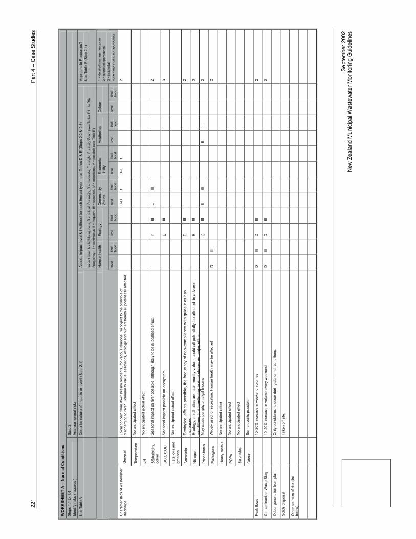
221
Part
4 –
Cas
e St
udie
s
Sept
embe
r 200
2N
ew Z
eala
nd M
unic
ipal
Was
tew
ater
Mon
itorin
g G
uide
lines
WO
RK
SHEE
T A
– N
orm
al C
ondi
tions
St
eps
1.1
to 1
.4
Iden
tify
risks
(haz
ards
) St
ep 2
A
naly
se n
orm
al ri
sks
Use
Tab
le A
D
escr
ibe
natu
re o
f im
pact
s or
eve
nt (S
tep
2.1)
A
sses
s im
pact
leve
l & li
kelih
ood
for e
ach
impa
ct ty
pe –
use
Tab
les
D &
E (S
teps
2.2
& 2
.3)
Impa
ct le
vel:
A =
high
ly in
jurio
us, B
= c
ritic
al, C
= m
ajor
, D =
mod
erat
e, E
= s
light
, F =
insi
gnifi
cant
(see
Tab
les
D1
to D
6)
Freq
uenc
y:
I = c
ontin
uous
, II =
freq
uent
, III
= se
ason
al, I
V =
occa
sion
al, V
= p
ossi
ble
(see
Tab
le E
)
App
ropr
iate
Res
ourc
es?
U
se T
able
F (S
tep
2.4)
Hum
an h
ealth
E
colo
gy
Com
mun
ity
Valu
es
Eco
nom
ic
Util
ity
Aes
thet
ics
Odo
ur
leve
l lik
eli-
hood
le
vel
likel
i-ho
od
leve
l lik
eli-
hood
le
vel
likel
i-ho
od
leve
l lik
eli-
hood
le
vel
likel
i-ho
od
1 =
deta
iled
man
agem
ent p
lan
2 =
stan
dard
app
roac
hes
3 =
inci
dent
al
none
= m
onito
ring
not a
ppro
pria
te
Gen
eral
Lo
cal c
once
rn fr
om d
owns
tream
resi
dent
s, fo
r var
ious
reas
ons.
Iwi o
bjec
t to
the
prin
cipl
e of
di
scha
rgin
g to
rive
r. C
omm
unity
val
ue, a
esth
etic
s, e
colo
gy a
nd h
uman
hea
lth a
ll po
tent
ially
affe
cted
.
C-D
l
D-E
I
2
Tem
pera
ture
N
o an
ticip
ated
effe
ct
pH
No
antic
ipat
ed a
ctua
l effe
ct
SS/
turb
idity
, co
lour
S
easo
nal i
mpa
ct o
n riv
er p
ossi
ble,
alth
ough
like
ly to
be
a lo
calis
ed e
ffect
.
D
III
E
III
2
BO
D, C
OD
S
easo
nal i
mpa
ct p
ossi
ble
on e
cosy
stem
E III
3
Fats
, oils
and
gr
ease
s N
o an
ticip
ated
act
ual e
ffect
Am
mon
ia
Ecol
ogic
al e
ffect
s po
ssib
le, t
he fr
eque
ncy
of n
on-c
ompl
ianc
e w
ith g
uide
lines
has
in
crea
sed.
D
III
2
Nitr
ogen
Ec
olog
y, a
esth
etic
s an
d co
mm
unity
val
ues
coul
d al
l pot
entia
lly b
e af
fect
ed in
adv
erse
co
nditi
ons,
but
mon
itorin
g to
dat
e sh
ows
no m
ajor
effe
ct.
E III
3
Pho
spho
rus
May
cau
se p
erip
hyto
n al
gal b
loom
s
C
III
E
III
E III
2
Pat
hoge
ns
Wid
ely
used
for r
ecre
atio
n. H
uman
hea
lth m
ay b
e af
fect
ed
D
III
2
Hea
vy m
etal
s N
o an
ticip
ated
effe
ct
PO
Ps
No
antic
ipat
ed e
ffect
Sul
phid
es
No
antic
ipat
ed e
ffect
Cha
ract
eris
tics
of w
aste
wat
er
disc
harg
e
Odo
ur
Som
e ev
ents
pos
sibl
e.
Peak
flow
s
10-2
0% in
crea
se in
wee
kend
vol
umes
D
III
D
III
2
Con
tam
inan
t or W
aste
Slu
g
10-2
0% in
crea
se in
vol
ume
ever
y w
eeke
nd
D
III
D
III
2
Odo
ur g
ener
atio
n fro
m p
lant
Onl
y co
nsid
ered
to o
ccur
dur
ing
abno
rmal
con
ditio
ns.
Solid
s di
spos
al
Ta
ken
off s
ite.
Oth
er s
ourc
es o
f ris
k (li
st
belo
w)

222
Part
4 –
Cas
e St
udie
s
Sept
embe
r 200
2N
ew Z
eala
nd M
unic
ipal
Was
tew
ater
Mon
itorin
g G
uide
lines
WO
RK
SHEE
T B
– A
bnor
mal
Con
ditio
ns a
nd e
ffect
of g
ross
unc
erta
inty
St
eps
1.1
to 1
.4
Iden
tify
haza
rds
St
ep 2
.5
Ana
lyse
abn
orm
al ri
sks
(rep
eat s
teps
2.1
to 2
.4 fo
r abn
orm
al ri
sks)
Use
Tab
le B
D
escr
ibe
natu
re o
f im
pact
s or
eve
nt (S
tep
2.1)
A
sses
s im
pact
leve
l & li
kelih
ood
for e
ach
impa
ct ty
pe –
use
Tab
les
D &
E (S
teps
2.2
& 2
.3)
Impa
ct le
vel:
A =
high
ly in
jurio
us, B
= c
ritic
al, C
= m
ajor
, D =
mod
erat
e, E
= s
light
, F =
insi
gnifi
cant
(see
Tab
les
D1
to D
6)
Freq
uenc
y:
I = c
ontin
uous
, II =
freq
uent
, III
= se
ason
al, I
V =
occa
sion
al, V
= p
ossi
ble
(see
Tab
le E
)
App
ropr
iate
Res
ourc
es?
U
se T
able
F (S
tep
2.4)
Hum
an h
ealth
Ec
olog
y C
omm
unity
Va
lues
E
cono
mic
U
tility
A
esth
etic
s O
dour
leve
l lik
eli-
hood
le
vel
likel
i-ho
od
leve
l lik
eli-
hood
le
vel
likel
i-ho
od
leve
l lik
eli-
hood
le
vel
likel
i-ho
od
1 =
deta
iled
man
agem
ent p
lan
2 =
stan
dard
app
roac
hes
3 =
inci
dent
al
none
= m
onito
ring
not
appr
opria
te
(see
Tab
le F
)
Po
ssib
ility
of p
ond
turn
ing
anae
robi
c du
ring
certa
in w
eath
er p
atte
rns.
Res
ult –
odo
ur, h
igh
SS
, BO
D,
disc
olou
ratio
n
D
V
2
Con
stitu
ents
of c
once
rn fo
r tre
atm
ent p
lant
faul
t co
nditi
ons
P
ossi
bilit
y of
trad
e w
aste
che
mic
al e
mer
genc
y. R
isk
too
slig
ht to
con
side
r
Con
stitu
ents
of c
once
rn fo
r tre
atm
ent p
lant
ups
et
cond
ition
(e.g
., fro
m t
oxic
sh
ocks
)
Ups
et o
f pla
nt re
late
d to
ex
trem
e w
eath
er
P
ossi
bilit
y of
pon
d tu
rnin
g an
aero
bic,
ext
rem
e lo
w fl
ow c
ondi
tions
in th
e re
ceiv
ing
wat
er
C
V
C
V
C
V
C
V
C
V
C
V
2
Abno
rmal
con
stitu
ents
in
trade
was
tes
Tr
ade
was
te w
ell u
nder
stoo
d, n
ot c
onsi
dere
d a
sign
ifica
nt ri
sk
Is th
ere
a ch
arac
teris
tic o
f the
en
viro
nmen
t tha
t may
resu
lt in
pa
rticu
lar
sen
sitiv
ity u
nder
sp
ecifi
c un
usua
l con
ditio
ns?
Lo
w fl
ows
in ri
ver
C
V
C
V
C
V
C
V
C
V
C
V
2
Proc
ess
unce
rtain
ty (i
s th
ere
a si
gnifi
cant
asp
ect o
f the
pr
oces
s be
havi
our t
hat
is
unce
rtain
?)
P
ond
very
sim
ple,
reas
onab
ly w
ell u
nder
stoo
d
Con
tam
inan
t com
posi
tion
unce
rtain
ty
Ve
ry u
nifo
rm w
aste
stre
am
Sign
ifica
nt la
ck o
f kno
wle
dge
of
envi
ronm
enta
l beh
avio
ur
(unc
erta
inty
rega
rdin
g ec
osys
tem
dyn
amic
s et
c)
W
ell u
nder
stoo
d re
ceiv
ing
envi
ronm
ent
Oth
er c
ause
s of
risk
(lis
t be
low
)

223 Part 4 – Case Studies
September 2002New Zealand Municipal Wastewater Monitoring Guidelines
The Objectives of Monitoring
Compliance monitoring for the resource consents is considered important for the followingreasons;
• To provide assurance to the community that the treatment plant is producing areasonable quality effluent
• To demonstrate the level of impact on the receiving waters
• To detect or identify any trends in water quality in the discharge and/or receivingwaters.
• To measure the effects of improvements from the proposed upgrading of the plant.
• To demonstrate that the pond is being maintained in an aerobic state, and is notcausing nuisance conditions.
The Agreed Monitoring of the Effluent
Three staff from the District Council and the Regional Council met and went through therelevant sections of the guidelines. Agreement was reached on the monitoring of the effluent.
Parameter Appropriate resources(from Worksheet A)
Monitoring Frequency
BOD 3 MonthlySS 2 MonthlyAmmonia 2 FortnightlyTotal Nitrogen 3 MonthlyPhosphorus 2 MonthlyE. coli 2 3 times per monthVolume 2 Continuous
The monitoring of the receiving water is still being negotiated at the time of writing. TheRegional Council experienced considerable difficulty in establishing the zone of reasonablemixing. Improved guidance on this matter would be desirable.


September 2002New Zealand Municipal Wastewater Monitoring Guidelines
CASE STUDY 2:COOKS BEACH SEWAGE TREATMENT PLANT
Chris Stumbles and Rob Docherty (Pattle Delamore Partners)
Editor's note
The following is a case study that uses the Wastewater Monitoring Guidelines to develop ahypothetical monitoring programme for the Cooks Beach wastewater treatment plantdischarge. Note that this case study is the authors' interpretation of the use of the Guidelines.Other interpretations are possible. Note also that the following does not necessarily reflectthe views of the Thames-Coromandel District Council (who are responsible for the CooksBeach WWTP).
Description
The Cooks Beach WWTP has been designed to serve the greater Cooks Beach community.Cooks Beach is a small coastal settlement on the Coromandel Peninsula popular with holidaymakers. It has a population that varies between 300 in winter and 6,000 during the summerpeaks, with the peak summer population projected to increase to around 8,500 at some stagein the future. There is currently 3 km of reticulation with 2 sewage pumpstations and thisnetwork is currently being expanded to serve the greater Cooks Beach area. The seweragenetwork will increase to approximately 10 km of reticulation with 8 sewage pumpstations by2003.
The WWTP and disposal area are situated on a 40 ha site approximately 1 km south ofCooks Beach with the nearest habitable building located approximately 500 m from the site.There is a small stream with two of its tributaries crossing the site and these could potentiallybe susceptible to contamination. The stream flows into Cook Stream which discharges intoCooks Bay.
The sewage reticulation catchment contributing to the Cooks Beach WWTP is residentialand there is no industry in the area and no trade wastes discharge into the sewerage system,so the plant only treats sewage of a domestic origin apart from about 10 commercialproperties including restaurants, dairies and a fast food outlet.
The treatment system consists of a single step screen followed by two Aerated Lagoonswhich operate in series. Treated effluent is stored in a 35,000 m3 storage pond and appliedto 24 ha of forest by means of slow rate spray irrigation (SRI) when conditions are suitable.The system has an ultimate treatment capacity of approximately 1,200 m3/d. There is nodisinfection of the effluent before irrigation and the land that is used for irrigation isrelatively steep and consists mainly of clay or silty clay soils. Relatively low applicationrates (35 mm/wk summer and 24 mm/wk winter) have been consented based on detailedhydraulic modelling of the irrigation site.

226 Part 4 – Case Studies
September 2002New Zealand Municipal Wastewater Monitoring Guidelines
The treated effluent is applied to land (soil), but there is a possibility of contaminationreaching the groundwater after an extended period of application to the land, and also apossibility of contamination of the stream due to overland flow caused by extreme rainfallevents, pipe bursts or poor operation of the irrigation system. A resource consent has beengranted (20 year term, expiry in 30 June 2019) which requires, inter alia, that soil,groundwater and stream water quality are all monitored on a periodic basis. The system isoperated in accordance with a detailed Operation and Maintenance manual.
The HIAMP Evaluation:
Step 1.1: Characterisation of the Effluent Discharge
Refer to completed Table 5.5 below.
Step 1.2: Characterisation of the Environment
This was undertaken for all three receiving environments at Cooks Beach (i.e. Soils,Groundwater and the Stream) using Table 6.2, as they are all potentially affected.
Step 1.3: Community Values
• The following community values were identified and have been considered:
• Maori Issues - protecting the spiritual well being of the streams etc.
• Aesthetic Values - are there any aesthetic problems caused by the WWTP.
• Odour Problems - how are the community affected by odours from the WWTP.
• Food Gathering - are any areas at risk, or perceived to be at risk.
• Property Values - how are these affected by the existence or proximity to theWWTP.
• Use of Amenities - how are the use of amenities eg. stream & beach affected.
• Restricted Access - loss of access to the irrigation area etc.
• Perceived health risks - the perceived health risk is often far greater than theactual risk.
• Community participation - in the current consent there is only a requirement tokeep a complaints register at the plant, no other community input into themonitoring of the plant is required.
Step 1.4: Hazard Identification
Items identified in Table 6.2 were transferred to Worksheets A & B. Once again a separateworksheet was prepared for each of the three receiving environments. (i.e. Soils,Groundwater and the Stream)

Part 4 – Case Studies 227
September 2002New Zealand Municipal Wastewater Monitoring Guidelines
Step 2: Risk Analysis
The risk analysis steps 2.1 to 2.5 were carried out using Worksheets A & B for each of thereceiving environments.

228 Part 4 – Case Studies
September 2002New Zealand Municipal Wastewater Monitoring Guidelines
Step 3: Monitoring Programme
A table has been prepared comparing the proposed monitoring requirements, as obtainedusing the appropriate resource designation (Worksheets A & B) and suggested monitoringfrequency (Table 10.4), and the current resource consent monitoring requirements. We havealso commented on what we regard as the appropriate level of monitoring.
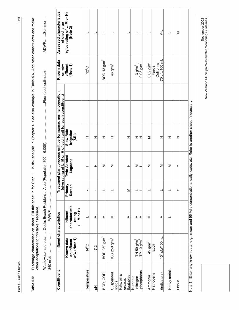
Part
4 –
Cas
e St
udie
s22
9
Sept
embe
r 200
2N
ew Z
eala
nd M
unic
ipal
Was
tew
ater
Mon
itorin
g G
uide
lines
Tabl
e 5.
5:
Dis
char
ge c
hara
cter
isat
ion
shee
t. Fi
ll th
is s
heet
in fo
r St
ep 1
.1 in
ris
k an
alys
is in
Cha
pter
4. S
ee a
lso
exam
ple
in T
able
5.6
. Add
oth
er c
onst
ituen
ts a
nd m
ake
othe
r ada
ptat
ions
to th
is ta
ble
if re
quire
d.
Was
tew
ater
sou
rces
:… C
ooks
Bea
ch R
esid
entia
l Are
a (P
opul
atio
n 30
0 –
6,00
0)…
……
……
……
……
……
.Flo
w (b
est e
stim
ate)
:AD
WF:
……
Sum
mer
-84
0 m
3 /d…
……
……
…PW
WF:
……
……
……
……
……
……
..
Con
stitu
ent
Influ
ent c
hara
cter
istic
sTr
eatm
ent p
lant
pro
cess
uni
t per
form
ance
, nor
mal
ope
ratio
n(g
ive
ratin
g of
L, M
or H
of e
ach
unit
for e
ach
cons
titue
nt)
Kno
wn
data
on in
fluen
tw
/w (N
ote
1)
Influ
ent
char
acte
ristic
ratin
g(L
, M o
r H)
Prim
ary
Scre
enTw
in A
erat
edLa
goon
sSl
ow R
ate
Irrig
atio
n(S
RI)
Kno
wn
data
on w
/wef
fluen
t(N
ote
1)
Asse
ssed
cha
ract
eris
tics
of d
isch
arge
(giv
e ra
ting
of L
, M o
r H)
(Not
e 2)
Tem
pera
ture
14o C
L-
HH
12o C
L
pH7.
2M
-H
HL
BOD
, CO
DBO
D 2
50 g
/m3
ML
MH
BOD
13
g/m
3L
Susp
ende
dso
lids
TSS
250
g/m
3M
LM
H46
g/m
3L
Fats
, oil
&gr
ease
,flo
atab
les
MM
HH
LN
utrie
nts
-nitr
ogen
-pho
spho
rus
TN 5
0 g/
m3
TP 1
0 g/
m3
M ML L
M LH H
3 g/
m3
0.98
g/m
3L L
Amm
onia
45 g
/m3
ML
MM
0.02
g/m
3L
Path
ogen
sEc
oli
Faec
alC
olifo
rms
(indi
cato
rs)
106 c
fu/1
00m
LM
LM
H70
cfu
/100
mL
M-L
Hea
vy m
etal
sL
LM
HL
Odo
urY
YN
M
Not
e 1:
Ent
er a
ny k
now
n da
ta, e
.g.,
mea
n an
d 95
%ile
con
cent
ratio
ns, d
aily
load
s, e
tc. R
efer
to a
noth
er s
heet
if n
eces
sary
.

Sept
embe
r 200
2N
ew Z
eala
nd M
unic
ipal
Was
tew
ater
Mon
itorin
g G
uide
lines
Not
e 2:
Ass
ess
the
char
acte
ristic
s of
the
disc
harg
e (fi
nal c
olum
n) b
y co
mbi
ning
the
influ
ent c
hara
cter
istic
ratin
g w
ith th
e tre
atm
ent p
roce
ss u
nit r
atin
gs. K
now
n da
ta o
n th
eef
fluen
t dis
char
ge (c
olum
n 4)
sho
uld
be ta
ken
into
acc
ount
if th
is is
ava
ilabl
e.L
= lo
w, M
= m
ediu
m, H
= h
igh
N
otes
: Ef
fluen
t sam
pled
bef
ore
SRI,
Flow
s ext
rem
ely
varia
ble
due
to la
rge
popu
latio
n flu
ctua
tions
.

Part 4 – Case Studies 231
September 2002New Zealand Municipal Wastewater Monitoring Guidelines
Table 6.2: Receiving environments, constituents of concern, and assimilative capacity.(Groundwater)
Receiving Environment Tem
pera
ture
Oxy
gen/
BOD
pH Sedi
men
tatio
n/sm
oth
erin
g (S
S)
Odo
ur/T
aint
ing
Floa
tabl
es/
scum
s
Col
our /
cla
rity
(SS)
Nut
rient
s/ e
nric
hmen
t
Toxi
c co
mpo
unds
Path
ogen
s
Lake/Reservoir - -River/ Stream (>50% base flow)River/ Stream (<50% base flow) - -Estuary - -Harbours & Sheltered Embayments - -Nearshore Marine (shoreline) - - - -Offshore Marine - - - -Groundwater - X X - X X X X X XAir - - - - - - - -Soils - - - -
Assimilative Capacity/SensitivityOf Te
mpe
ratu
re
Oxy
gen/
BOD
pH Sedi
men
tatio
n/sm
oth
erin
g (S
S)
Odo
ur/T
aint
ing
Floa
tabl
es/
scum
s
Col
our /
cla
rity
(SS)
Nut
rient
s/ e
nric
hmen
t
Toxi
c co
mpo
unds
Path
ogen
s
Groundwater X X X X X X X XPoor
Moderate - - - DilutionExcellent - - - - - - - - -
Mud - - - - - -Sand - - - - - - - Substrate (s)Rock - - - - - - - - -
Unenriched - X - X - - X - -Mod Enrichment - - - - - - Enrichment status
Enriched - - - - - - - - - -High - - - -
Moderate - X X - - - X X - Sensitivity of Ecological Values Low - - - - - - - - -
Yes Significant other Inputs No - - - - - - - - - -
Important - - - - - - Aesthetics Not so Important - - - - - - - - - -Yes - - - - - Contact
Recreation No - - - - - - - - - -Drinking - - X - X X X X X XIrrigation - - - - - Water Supply
(Economic Utility) Industrial - - - - - -Yes - - - - - - - -
Food gathering No - - - - - - - - - -
Include in HIAMP Yes X X X X X X X X

232 Part 4 – Case Studies
September 2002New Zealand Municipal Wastewater Monitoring Guidelines
No X X
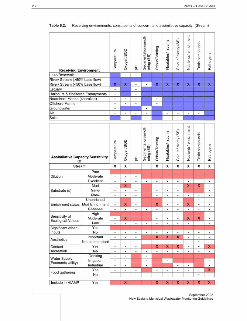
233 Part 4 – Case Studies
September 2002New Zealand Municipal Wastewater Monitoring Guidelines
Table 6.2: Receiving environments, constituents of concern, and assimilative capacity. (Stream)
Receiving Environment Tem
pera
ture
Oxy
gen/
BOD
pH Sedi
men
tatio
n/sm
oth
erin
g (S
S)
Odo
ur/T
aint
ing
Floa
tabl
es/
scum
s
Col
our /
cla
rity
(SS)
Nut
rient
s/ e
nric
hmen
t
Toxi
c co
mpo
unds
Path
ogen
s
Lake/Reservoir - -River/ Stream (>50% base flow)River/ Stream (<50% base flow) X X - - X X X X X XEstuary - -Harbours & Sheltered Embayments - -Nearshore Marine (shoreline) - - - -Offshore Marine - - - -Groundwater - -Air - - - - - - - -Soils - - - -
Assimilative Capacity/SensitivityOf Te
mpe
ratu
re
Oxy
gen/
BOD
pH Sedi
men
tatio
n/sm
oth
erin
g (S
S)
Odo
ur/T
aint
ing
Floa
tabl
es/
scum
s
Col
our /
cla
rity
(SS)
Nut
rient
s/ e
nric
hmen
t
Toxi
c co
mpo
unds
Path
ogen
s
Stream X X X X X X X XPoor
Moderate - - - DilutionExcellent - - - - - - - - -
Mud - X - - - - X X -Sand - - - - - - - Substrate (s)Rock - - - - - - - - -
Unenriched - - - - - -Mod Enrichment - X - X - - X - - Enrichment status
Enriched - - - - - - - - - -High - - - -
Moderate - X - - - X X - Sensitivity of Ecological Values Low - - - - - - - - -
Yes Significant other Inputs No - - - - - - - - - -
Important - - - X X X - - - Aesthetics Not so Important - - - - - - - - - -Yes - - - X X X - - X Contact
Recreation No - - - - - - - - - -Drinking - - -Irrigation - - - - - Water Supply
(Economic Utility) Industrial - - - - - -Yes - - - - - - - - X Food gathering No - - - - - - - - - -
Include in HIAMP Yes X X X X X X X

234 Part 4 – Case Studies
September 2002New Zealand Municipal Wastewater Monitoring Guidelines
No X X X

Part
4 –
Cas
e St
udie
s23
5
Sept
embe
r 200
2N
ew Z
eala
nd M
unic
ipal
Was
tew
ater
Mon
itorin
g G
uide
lines
WO
RKS
HEE
T A
– N
orm
al C
ondi
tions
– S
OIL
S St
eps
1.1
to 1
.4
Iden
tify
risks
(haz
ards
) St
ep 2
An
alys
e no
rmal
risk
s
Use
Tab
le A
D
escr
ibe
natu
re o
f im
pact
s or
eve
nt (S
tep
2.1)
As
sess
impa
ct le
vel &
like
lihoo
d fo
r eac
h im
pact
type
– u
se T
able
s D
& E
(Ste
ps 2
.2 &
2.3
) Im
pact
leve
l: A
= hi
ghly
inju
rious
, B =
crit
ical
, C =
maj
or, D
= m
oder
ate,
E =
slig
ht, F
= in
sign
ifica
nt (s
ee T
able
s D
1 to
D6)
Fr
eque
ncy:
I =
con
tinuo
us, I
I = fr
eque
nt, I
II =
seas
onal
, IV
= oc
casi
onal
, V =
pos
sibl
e (s
ee T
able
E)
Appr
opria
te R
esou
rces
?
Use
Tab
le F
(Ste
p 2.
4)
Hum
an h
ealth
Ec
olog
y C
omm
unity
Va
lues
Ec
onom
ic
Util
ity
Aest
hetic
s
Odo
ur
leve
l lik
eli-
hood
le
vel
likel
i-ho
od
leve
l lik
eli-
hood
le
vel
likel
i-ho
od
leve
l lik
eli-
hood
le
vel
likel
i-ho
od
1 =
deta
iled
man
agem
ent p
lan
2 =
stan
dard
app
roac
hes
3 =
inci
dent
al
none
= m
onito
ring
not a
ppro
pria
te
(see
Tab
le F
)
Gen
eral
La
rge
fluct
uatio
ns in
flow
& lo
ad e
xper
ienc
ed o
ver w
eeke
nds
and
holid
ay p
erio
ds
F
II F
II F
II F
II F
II F
II 3
Tem
pera
ture
N
ot R
equi
red
in H
IAM
P
-
pH
Long
term
app
licat
ion
coul
d m
odify
soi
l cha
ract
eriti
cs
B
V
3
SS/tu
rbid
ity,
colo
ur
Not
Req
uire
d in
HIA
MP
-
BOD
, CO
D
Not
Req
uire
d in
HIA
MP
-
Fats
, oils
and
gr
ease
s N
ot R
equi
red
in H
IAM
P
-
Amm
onia
Se
ason
al fl
uctu
atio
ns –
Pos
sibl
e da
mag
e to
soi
l bio
ta if
not
man
aged
cor
rect
ly
B
V
3
Nitr
ogen
Se
ason
al fl
uctu
atio
ns –
Pos
sibl
e ov
erlo
adin
g of
soi
ls if
not
man
aged
cor
rect
ly
B
V
3
Phos
phor
us
Seas
onal
fluc
tuat
ions
– P
ossi
ble
over
load
ing
of s
oils
if n
ot m
anag
ed c
orre
ctly
B V
3
Path
ogen
s N
ot R
equi
red
in H
IAM
P
-
Hea
vy m
etal
s N
o in
dust
ry th
eref
ore
Hea
vy m
etal
s no
t exp
ecte
d to
be
a pr
oble
m
Non
e
POPs
N
o in
dust
ry th
eref
ore
POP’
s no
t exp
ecte
d to
be
a pr
oble
m
Non
e
Sulp
hide
s Lo
w le
vels
of s
ulph
ides
pos
sibl
e bu
t the
se a
re n
ot e
xpec
ted
to c
ause
any
sig
nific
ant i
mpa
ct
N
one
Cha
ract
eris
tics
of
was
tew
ater
dis
char
ge
Odo
ur
Lim
ited
odou
r pos
sibl
e at
WW
TP b
ut n
ot e
xpec
ted
to h
ave
any
sign
ifica
nt im
pact
Non
e
Peak
flow
s
Hig
h flo
ws
likel
y du
ring
peak
per
iods
. The
se a
re o
f sho
rt du
ratio
n an
d ar
e no
t lik
ely
to h
ave
any
long
term
effe
ct.
F V
D
V F
V F
V F
V E
V N
one
Con
tam
inan
t or W
aste
Sl
ug
W
WTP
is re
silie
nt to
was
te s
lugs
and
has
larg
e st
orag
e ca
paci
ty
Non
e
Odo
ur g
ener
atio
n fro
m
plan
t
Odo
ur p
ossi
ble
durin
g de
slud
ging
pro
cess
D
V N
one
Solid
s di
spos
al
N
o pr
oced
ure
deriv
ed y
et.
Oth
er s
ourc
es o
f ris
k (li
st b
elow
)
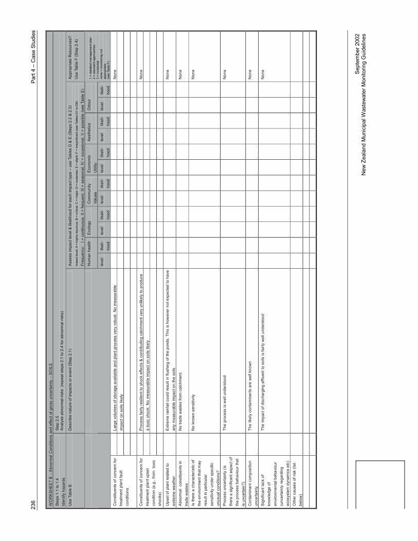
236
Part
4 –
Cas
e St
udie
s
Sept
embe
r 200
2N
ew Z
eala
nd M
unic
ipal
Was
tew
ater
Mon
itorin
g G
uide
lines
WO
RK
SH
EE
T B
– A
bnor
mal
Con
ditio
ns a
nd e
ffect
of g
ross
unc
erta
inty
– S
OIL
S
Step
s 1.
1 to
1.4
Id
entif
y ha
zard
s
Step
2.5
A
naly
se a
bnor
mal
risk
s (r
epea
t ste
ps 2
.1 to
2.4
for a
bnor
mal
risk
s)
Use
Tab
le B
D
escr
ibe
natu
re o
f im
pact
s or
eve
nt (S
tep
2.1)
A
sses
s im
pact
leve
l & li
kelih
ood
for e
ach
impa
ct ty
pe –
use
Tab
les
D &
E (S
teps
2.2
& 2
.3)
Impa
ct le
vel:
A =
high
ly in
jurio
us, B
= c
ritic
al, C
= m
ajor
, D =
mod
erat
e, E
= s
light
, F =
insi
gnifi
cant
(see
Tab
les
D1
to D
6)
Freq
uenc
y:
I = c
ontin
uous
, II =
freq
uent
, III
= se
ason
al, I
V =
occa
sion
al, V
= p
ossi
ble
(see
Tab
le E
)
Appr
opria
te R
esou
rces
?
Use
Tab
le F
(Ste
p 2.
4)
Hum
an h
ealth
E
colo
gy
Com
mun
ity
Valu
es
Eco
nom
ic
Util
ity
Aest
hetic
s O
dour
leve
l lik
eli-
hood
le
vel
likel
i-ho
od
leve
l lik
eli-
hood
le
vel
likel
i-ho
od
leve
l lik
eli-
hood
le
vel
likel
i-ho
od
1 =
deta
iled
man
agem
ent p
lan
2 =
stan
dard
app
roac
hes
3 =
inci
dent
al
none
= m
onito
ring
not
appr
opria
te
(see
Tab
le F
)
La
rge
volu
mes
of s
tora
ge a
vaila
ble
and
plan
t pro
cess
ver
y ro
bust
. No
mea
sura
ble
N
one
im
pact
on
soils
like
ly
Con
stitu
ents
of c
once
rn fo
r tre
atm
ent p
lant
faul
t co
nditi
ons
Pro
cess
fairl
y re
silie
nt to
sho
ck e
ffect
s &
cont
ribut
ing
catc
hmen
t ver
y un
likel
y to
pro
duce
N
one
a
toxi
c sh
ock.
No
mea
sura
ble
impa
ct o
n so
ils li
kely
Con
stitu
ents
of c
once
rn fo
r tre
atm
ent p
lant
ups
et
cond
ition
(e.g
., fro
m t
oxic
sh
ocks
)
Ups
et o
f pla
nt re
late
d to
ex
trem
e w
eath
er
E
xtre
me
rain
fall
coul
d re
sult
in fl
ushi
ng o
f the
pon
ds. T
his
is h
owev
er n
ot e
xpec
ted
to h
ave
any
mea
sura
ble
impa
ct o
n th
e so
ils
Non
e
Abn
orm
al c
onst
ituen
ts in
tra
de w
aste
s
No
trade
was
tes
from
cat
chm
ent.
Non
e
Is th
ere
a ch
arac
teris
tic o
f th
e en
viro
nmen
t tha
t may
re
sult
in p
artic
ular
se
nsiti
vity
und
er s
peci
fic
unus
ual c
ondi
tions
?
N
o kn
own
sens
itivi
ty
Non
e
Pro
cess
unc
erta
inty
(is
th
ere
a si
gnifi
cant
asp
ect o
f th
e pr
oces
s be
havi
our t
hat
is u
ncer
tain
?)
Th
e pr
oces
s is
wel
l und
erst
ood
Non
e
Con
tam
inan
t com
posi
tion
unce
rtain
ty
Th
e lik
ely
cont
amin
ants
are
wel
l kno
wn
Non
e
Sign
ifica
nt la
ck o
f kn
owle
dge
of
envi
ronm
enta
l beh
avio
ur
(unc
erta
inty
rega
rdin
g ec
osys
tem
dyn
amic
s et
c)
Th
e im
pact
of d
isch
argi
ng e
fflue
nt to
soi
ls is
fairl
y w
ell u
nder
stoo
d
N
one
Oth
er c
ause
s of
risk
(lis
t be
low
)

Part
4 –
Cas
e St
udie
s23
7
Sept
embe
r 200
2N
ew Z
eala
nd M
unic
ipal
Was
tew
ater
Mon
itorin
g G
uide
lines
WO
RKS
HE
ET
A –
Nor
mal
Con
ditio
ns –
GR
OU
ND
WAT
ER
Step
s 1.
1 to
1.4
Id
entif
y ris
ks (h
azar
ds )
Step
2
Anal
yse
norm
al ri
sks
Use
Tab
le A
D
escr
ibe
natu
re o
f im
pact
s or
eve
nt (S
tep
2.1)
A
sses
s im
pact
leve
l & li
kelih
ood
for e
ach
impa
ct ty
pe –
use
Tab
les
D &
E (S
teps
2.2
& 2
.3)
Impa
ct le
vel: A
= h
ighl
y in
jurio
us, B
= c
ritic
al, C
= m
ajor
, D =
mod
erat
e, E
= s
light
, F =
insi
gnifi
cant
(se
e Ta
bles
D1
to D
6)
Freq
uenc
y:
I = c
ontin
uous
, II =
freq
uent
, III
= se
ason
al, I
V =
occa
sion
al, V
= p
ossi
ble
(see
Tab
le E
)
App
ropr
iate
Res
ourc
es?
U
se T
able
F (S
tep
2.4)
Hum
an h
ealth
E
colo
gy
Com
mun
ity
Valu
es
Eco
nom
ic
Util
ity
Aest
hetic
s
Odo
ur
leve
l lik
eli-
hood
le
vel
likel
i-ho
od
leve
l lik
eli-
hood
le
vel
likel
i-ho
od
leve
l lik
eli-
hood
le
vel
likel
i-ho
od
1 =
deta
iled
man
agem
ent p
lan
2 =
stan
dard
app
roac
hes
3 =
inci
dent
al
none
= m
onito
ring
not a
ppro
pria
te
(see
Tab
le F
)
Gen
eral
La
rge
fluct
uatio
ns in
flow
& lo
ad e
xper
ienc
ed o
ver w
eeke
nds
and
holid
ay p
erio
ds
F
II F
II F
II F
II F
II F
II 3
Tem
pera
ture
N
ot R
equi
red
in H
IAM
P
-
pH
Long
term
app
licat
ion
coul
d al
ter g
roun
dwat
er p
H
E
V
B
V
E
V
3
SS
/turb
idity
, co
lour
N
o ef
fect
on
grou
ndw
ater
exp
ecte
d
Non
e
BO
D, C
OD
Po
ssib
le c
onta
min
atio
n of
gro
undw
ater
afte
r ext
ende
d ap
plic
atio
n
E
V F
II
B
V
3
Fats
, oils
and
gr
ease
s N
o an
ticip
ated
mea
sura
ble
effe
ct
Non
e
Am
mon
ia
Poss
ible
con
tam
inat
ion
of g
roun
dwat
er a
fter e
xten
ded
appl
icat
ion
B
V
B
V
C
V
B
V
3
Nitr
ogen
Po
ssib
le c
onta
min
atio
n of
gro
undw
ater
afte
r ext
ende
d ap
plic
atio
n
B
V
C
V
B
V
3
Pho
spho
rus
Poss
ible
con
tam
inat
ion
of g
roun
dwat
er a
fter e
xten
ded
appl
icat
ion
B
V
C
V
B
V
3
Pat
hoge
ns
Poss
ible
con
tam
inat
ion
of g
roun
dwat
er a
fter e
xten
ded
appl
icat
ion
B
V
C
V
B
V
3
Hea
vy m
etal
s N
o in
dust
ry th
eref
ore
Hea
vy m
etal
s no
t exp
ecte
d to
be
a pr
oble
m
Non
e
PO
Ps
No
indu
stry
ther
efor
e P
OP’
s no
t exp
ecte
d to
be
a pr
oble
m
Non
e
Sul
phid
es
Low
leve
ls o
f sul
phid
es p
ossi
ble
but t
hese
are
not
exp
ecte
d to
cau
se a
ny s
igni
fican
t im
pact
Non
e
Cha
ract
eris
tics
of
was
tew
ater
dis
char
ge
Odo
ur
Lim
ited
odou
r pos
sibl
e at
WW
TP b
ut n
ot e
xpec
ted
to h
ave
any
sign
ifica
nt im
pact
Non
e
Pea
k flo
ws
N
ot li
kely
to h
ave
any
impa
ct o
n gr
ound
wat
er
Non
e
Con
tam
inan
t or W
aste
S
lug
W
WTP
resi
lient
to w
aste
slu
gs
Non
e
Odo
ur g
ener
atio
n fro
m
plan
t
Odo
ur p
ossi
ble
durin
g de
slud
ging
pro
cess
Sol
ids
disp
osal
No
proc
edur
e de
rived
yet
– O
n-si
te d
ispo
sal c
ould
con
tam
inat
e gr
ound
wat
er
Oth
er s
ourc
es o
f ris
k (li
st b
elow
)

238
Part
4 –
Cas
e St
udie
s
Sept
embe
r 200
2N
ew Z
eala
nd M
unic
ipal
Was
tew
ater
Mon
itorin
g G
uide
lines
WO
RKS
HEE
T B
– A
bnor
mal
Con
ditio
ns a
nd e
ffect
of g
ross
unc
erta
inty
– G
RO
UN
DW
ATE
R
Step
s 1.
1 to
1.4
Id
entif
y ha
zard
s
Step
2.5
A
naly
se a
bnor
mal
risk
s (r
epea
t ste
ps 2
.1 to
2.4
for a
bnor
mal
risk
s)
Use
Tab
le B
D
escr
ibe
natu
re o
f im
pact
s or
eve
nt (S
tep
2.1)
A
sses
s im
pact
leve
l & li
kelih
ood
for e
ach
impa
ct ty
pe –
use
Tab
les
D &
E (S
teps
2.2
& 2
.3)
Impa
ct le
vel:
A =
high
ly in
jurio
us, B
= c
ritic
al, C
= m
ajor
, D =
mod
erat
e, E
= s
light
, F =
insi
gnifi
cant
(see
Tab
les
D1
to D
6)
Freq
uenc
y:
I = c
ontin
uous
, II =
freq
uent
, III
= se
ason
al, I
V =
occ
asio
nal,
V =
pos
sibl
e (s
ee T
able
E)
App
ropr
iate
Res
ourc
es?
U
se T
able
F (S
tep
2.4)
Hum
an h
ealth
Ec
olog
y C
omm
unity
Va
lues
E
cono
mic
U
tility
A
esth
etic
s
Odo
ur
leve
l lik
eli-
hood
le
vel
likel
i-ho
od
leve
l lik
eli-
hood
le
vel
likel
i-ho
od
leve
l lik
eli-
hood
le
vel
likel
i-ho
od
1 =
deta
iled
man
agem
ent p
lan
2
= st
anda
rd a
ppro
ache
s 3
= in
cide
ntal
no
ne =
mon
itorin
g no
t ap
prop
riate
(s
ee T
able
F)
La
rge
volu
mes
of s
tora
ge a
vaila
ble
and
plan
t pro
cess
ver
y ro
bust
. No
mea
sura
ble
Non
e
Impa
ct o
n gr
ound
wat
er li
kely
Con
stitu
ents
of c
once
rn fo
r tre
atm
ent p
lant
faul
t co
nditi
ons
Pro
cess
fairl
y re
silie
nt to
sho
ck e
ffect
s &
con
tribu
ting
catc
hem
nt v
ery
unlik
ely
to p
rodu
ce
Non
e
A to
xic
shoc
k. N
o m
easu
rabl
e im
pact
on
grou
ndw
ater
like
ly
Con
stitu
ents
of c
once
rn fo
r tre
atm
ent p
lant
ups
et
cond
ition
(e.g
., fro
m t
oxic
sh
ocks
)
Ups
et o
f pla
nt re
late
d to
ex
trem
e w
eath
er
E
xtre
me
rain
fall
coul
d re
sult
in fl
ushi
ng o
f the
pon
ds. T
his
is h
owev
er n
ot e
xpec
ted
to h
ave
any
mea
sure
ble
impa
ct o
n th
e gr
ound
wat
er
Non
e
Abn
orm
al c
onst
ituen
ts in
tra
de w
aste
s
No
trade
was
tes
from
the
catc
hmen
t
N
one
Is th
ere
a ch
arac
teris
tic o
f th
e en
viro
nmen
t tha
t may
re
sult
in p
artic
ular
se
nsiti
vity
und
er s
peci
fic
unus
ual c
ondi
tions
?
N
o kn
own
sens
itivi
ty
Non
e
Pro
cess
unc
erta
inty
(is
th
ere
a si
gnifi
cant
asp
ect o
f th
e pr
oces
s be
havi
our t
hat
is u
ncer
tain
?)
R
ate
of in
filtra
tion
of c
onta
min
ants
into
gro
undw
ater
not
wel
l und
erst
ood
Con
tam
inan
t com
posi
tion
unce
rtain
ty
Th
e lik
ely
cont
amin
ants
are
wel
l kno
wn
Non
e
Sig
nific
ant l
ack
of
know
ledg
e of
en
viro
nmen
tal b
ehav
iour
(u
ncer
tain
ty re
gard
ing
ecos
yste
m d
ynam
ics
etc)
E
cosy
stem
reas
onab
ly w
ell u
nder
stoo
d
N
one
Oth
er c
ause
s of
risk
(lis
t be
low
)

Part
4 –
Cas
e St
udie
s23
9
Sept
embe
r 200
2N
ew Z
eala
nd M
unic
ipal
Was
tew
ater
Mon
itorin
g G
uide
lines
WO
RKS
HEE
T A
– N
orm
al C
ondi
tions
– S
TREA
M
Step
s 1.
1 to
1.4
Id
entif
y ris
ks (h
azar
ds )
Step
2
Anal
yse
norm
al ri
sks
Use
Tab
le A
D
escr
ibe
natu
re o
f im
pact
s or
eve
nt (S
tep
2.1)
As
sess
impa
ct le
vel &
like
lihoo
d fo
r eac
h im
pact
type
– u
se T
able
s D
& E
(Ste
ps 2
.2 &
2.3
) Im
pact
leve
l: A
= hi
ghly
inju
rious
, B =
crit
ical
, C =
maj
or, D
= m
oder
ate,
E =
slig
ht, F
= in
sign
ifica
nt (s
ee T
able
s D
1 to
D6)
Fr
eque
ncy:
I =
con
tinuo
us, I
I = fr
eque
nt, I
II =
seas
onal
, IV
= o
ccas
iona
l, V
= po
ssib
le (s
ee T
able
E)
Appr
opria
te R
esou
rces
?
Use
Tab
le F
(Ste
p 2.
4)
Hum
an h
ealth
Ec
olog
y C
omm
unity
Va
lues
Ec
onom
ic
Util
ity
Aest
hetic
s
Odo
ur
leve
l lik
eli-
hood
le
vel
likel
i-ho
od
leve
l lik
eli-
hood
le
vel
likel
i-ho
od
leve
l lik
eli-
hood
le
vel
likel
i-ho
od
1 =
deta
iled
man
agem
ent p
lan
2 =
stan
dard
app
roac
hes
3 =
inci
dent
al
none
= m
onito
ring
not a
ppro
pria
te
(see
Tab
le F
)
Gen
eral
La
rge
fluct
uatio
ns in
flow
& lo
ad e
xper
ienc
ed o
ver w
eeke
nds
and
holid
ay p
erio
ds, b
ut th
is is
no
t exp
ecte
d to
hav
e an
y im
pact
on
the
stre
am
Non
e
Tem
pera
ture
N
ot R
equi
red
in H
IAM
P
-
pH
Not
Req
uire
d in
HIA
MP
-
SS/tu
rbid
ity,
colo
ur
Failu
re to
ope
rate
the
irrig
atio
n sy
stem
cor
rect
ly c
ould
resu
lt in
ove
rland
flow
into
the
stre
am
whi
ch fl
ows
thro
ugh
Coo
ks B
each
and
out
nea
r the
bat
hing
bea
ch
E V
Non
e
BOD
, CO
D
Failu
re to
ope
rate
the
irrig
atio
n sy
stem
cor
rect
ly c
ould
resu
lt in
ove
rland
flow
into
the
stre
am
whi
ch fl
ows
thro
ugh
Coo
ks B
each
and
out
nea
r the
bat
hing
bea
ch
D
V
N
one
Fats
, oils
and
gr
ease
s N
o im
pact
on
stre
am li
kely
N
one
Amm
onia
Fa
ilure
to o
pera
te th
e irr
igat
ion
syst
em c
orre
ctly
cou
ld re
sult
in o
verla
nd fl
ow in
to th
e st
ream
w
hich
cou
ld a
ffect
cer
tain
org
enis
ms
B V
D
V D
V
E V
3
Nitr
ogen
Fa
ilure
to o
pera
te th
e irr
igat
ion
syst
em c
orre
ctly
cou
ld re
sult
in o
verla
nd fl
ow in
to th
e st
ream
re
sulti
ng in
incr
ease
d pl
ant g
row
th
B V
D
V D
V
E V
3
Phos
phor
us
Failu
re to
ope
rate
the
irrig
atio
n sy
stem
cor
rect
ly c
ould
resu
lt in
ove
rland
flow
into
the
stre
am
resu
lting
in in
crea
sed
plan
t gro
wth
B
V D
V
D
V E
V
3
Path
ogen
s Fa
ilure
to o
pera
te th
e irr
igat
ion
syst
em c
orre
ctly
cou
ld re
sult
in o
verla
nd fl
ow in
to th
e st
ream
w
hich
flow
s th
roug
h C
ooks
Bea
ch a
nd o
ut n
ear t
he b
athi
ng b
each
B
V
D
V D
V
3
Hea
vy m
etal
s N
o in
dust
ry th
eref
ore
Hea
vy m
etal
s no
t exp
ecte
d to
be
a pr
oble
m
Non
e
POPs
N
o in
dust
ry th
eref
ore
POP’
s no
t exp
ecte
d to
be
a pr
oble
m
Non
e
Sulp
hide
s Lo
w le
vels
of s
ulph
ides
pos
sibl
e bu
t the
se a
re n
ot e
xpec
ted
to c
ause
any
sig
nific
ant i
mpa
ct
N
one
Cha
ract
eris
tics
of
was
tew
ater
dis
char
ge
Odo
ur
Incr
ease
d BO
D &
nut
rient
leve
ls in
stre
am c
ause
d by
failu
re o
f the
irrig
atio
n sy
stem
cou
ld
resu
lt in
odo
urs
from
the
stre
am
E V
E V
E V
Non
e
Peak
flow
s
Hig
h flo
ws
likel
y du
ring
peak
per
iods
or d
urin
g ex
trem
e ra
infa
ll ev
ents
cou
ld re
sult
in
over
land
flow
of c
onta
min
ants
into
wat
erco
urse
s or
floo
ding
of s
ewag
e pu
mps
tatio
ns
resu
lting
in c
onta
min
atio
n of
the
stre
am
B V
D
V
D
V D
V
E V
E
V 3
Con
tam
inan
t or W
aste
Sl
ug
W
WTP
resi
lient
to w
aste
slu
gs
Odo
ur g
ener
atio
n fro
m
plan
t
Odo
ur p
ossi
ble
durin
g de
slud
ging
D
V N
one
Solid
s di
spos
al
N
o pr
oced
ure
deriv
ed y
et. O
n-si
te d
ispo
sal c
ould
lead
to c
onta
min
atio
n of
the
stre
am.
Oth
er s
ourc
es o
f ris
k (li
st b
elow
)

240
Part
4 –
Cas
e St
udie
s
Sept
embe
r 200
2N
ew Z
eala
nd M
unic
ipal
Was
tew
ater
Mon
itorin
g G
uide
lines

Part
4 –
Cas
e St
udie
s24
1
Sept
embe
r 200
2N
ew Z
eala
nd M
unic
ipal
Was
tew
ater
Mon
itorin
g G
uide
lines
WO
RKS
HEE
T B
– A
bnor
mal
Con
ditio
ns a
nd e
ffect
of g
ross
unc
erta
inty
– S
TRE
AM
St
eps
1.1
to 1
.4
Iden
tify
haza
rds
St
ep 2
.5
Ana
lyse
abn
orm
al ri
sks
(rep
eat s
teps
2.1
to 2
.4 fo
r abn
orm
al ri
sks)
Use
Tab
le B
D
escr
ibe
natu
re o
f im
pact
s or
eve
nt (S
tep
2.1)
A
sses
s im
pact
leve
l & li
kelih
ood
for e
ach
impa
ct ty
pe –
use
Tab
les
D &
E (S
teps
2.2
& 2
.3)
Impa
ct le
vel:
A =
high
ly in
jurio
us, B
= c
ritic
al, C
= m
ajor
, D =
mod
erat
e, E
= s
light
, F =
insi
gnifi
cant
(see
Tab
les
D1
to D
6)
Freq
uenc
y:
I = c
ontin
uous
, II =
freq
uent
, III
= se
ason
al, I
V =
occa
sion
al, V
= p
ossi
ble
(see
Tab
le E
)
App
ropr
iate
Res
ourc
es?
U
se T
able
F (S
tep
2.4)
Hum
an h
ealth
Ec
olog
y C
omm
unity
Va
lues
E
cono
mic
U
tility
A
esth
etic
s O
dour
leve
l lik
eli-
hood
le
vel
likel
i-ho
od
leve
l lik
eli-
hood
le
vel
likel
i-ho
od
leve
l lik
eli-
hood
le
vel
likel
i-ho
od
1 =
deta
iled
man
agem
ent p
lan
2 =
stan
dard
app
roac
hes
3 =
inci
dent
al
none
= m
onito
ring
not
appr
opria
te
(see
Tab
le F
)
SS
Ove
rland
flow
s in
to s
tream
cou
ld re
sult
from
pip
e bu
rsts
/blo
ckag
es
D
V E
V
E V
Non
e P
ath
Ove
rland
flow
s in
to s
tream
cou
ld re
sult
from
pip
e bu
rsts
/blo
ckag
es
B
V
C
V D
V
3 N
H4+
Ove
rland
flow
s in
to s
tream
cou
ld re
sult
from
pip
e bu
rsts
/blo
ckag
es
D
V
D
V
N
one
Con
stitu
ents
of c
once
rn fo
r tre
atm
ent p
lant
faul
t co
nditi
ons
BO
D
Ove
rland
flow
s in
to s
tream
cou
ld re
sult
from
pip
e bu
rsts
/blo
ckag
es
D
V
E
V
Non
e
Pro
cess
fairl
y re
silie
nt to
sho
ck e
ffect
s &
cont
ribut
ing
catc
hem
nt v
ery
unlik
ely
to p
rodu
ce
Non
e
A to
xic
shoc
k. N
o m
easu
rabl
e im
pact
on
grou
ndw
ater
like
ly
Con
stitu
ents
of c
once
rn fo
r tre
atm
ent p
lant
ups
et
cond
ition
(e.g
., fro
m t
oxic
sh
ocks
)
Ups
et o
f pla
nt re
late
d to
ex
trem
e w
eath
er
E
xtre
me
rain
fall
coul
d re
sult
in fl
ushi
ng o
f th
e po
nd a
s w
ell a
s ru
noff
of ir
rigat
ed e
fflue
nt
into
the
stre
ams,
or f
lood
ing
of s
ewag
e pu
mps
tatio
ns
B
V
D
V C
V
D
V E
V E
V
3
Abn
orm
al c
onst
ituen
ts in
tra
de w
aste
s
No
trade
was
tes
from
the
catc
hmen
t
N
one
Is th
ere
a ch
arac
teris
tic o
f th
e en
viro
nmen
t tha
t may
re
sult
in p
artic
ular
se
nsiti
vity
und
er s
peci
fic
unus
ual c
ondi
tions
?
N
o kn
own
sens
itivi
ty
Non
e
Pro
cess
unc
erta
inty
(is
th
ere
a si
gnifi
cant
asp
ect o
f th
e pr
oces
s be
havi
our t
hat
is u
ncer
tain
?)
P
roce
ss w
ell u
nder
stoo
d
N
one
Con
tam
inan
t com
posi
tion
unce
rtain
ty
Th
e lik
ely
cont
amin
ants
are
wel
l kno
wn
Non
e
Sig
nific
ant l
ack
of
know
ledg
e of
en
viro
nmen
tal b
ehav
iour
(u
ncer
tain
ty re
gard
ing
ecos
yste
m d
ynam
ics
etc)
E
cosy
stem
reas
onab
ly w
ell u
nder
stoo
d
N
one
Oth
er c
ause
s of
risk
(lis
t be
low
)
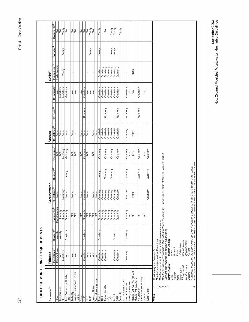
242
Part
4 –
Cas
e St
udie
s
Sept
embe
r 200
2N
ew Z
eala
nd M
unic
ipal
Was
tew
ater
Mon
itorin
g G
uide
lines
TAB
LE O
F M
ON
ITO
RIN
G R
EQU
IREM
ENTS
Efflu
ent
Gro
undw
ater
St
ream
So
ils(5
) Pa
ram
eter
(4)
G
uide
lines
(1)
Cons
ent(2
) Co
mm
ents
(3)
Gui
delin
es (1
) Co
nsen
t(2)
Com
men
ts(3
) G
uide
lines
(1)
Cons
ent(2
) Co
mm
ents
(3)
Gui
delin
es (1
) Co
nsen
t(2)
Com
men
ts(3
)
Flow
Dai
ly V
olum
e W
eekl
y D
aily
Sum
mer
N
one
N
/A
Non
e
N/A
D
aily
Vol
ume
N
/A
Tem
pera
ture
Non
e W
eekl
y Q
uarte
rly
-
N/A
N
one
Q
uarte
rly
-
N/A
pH
Qua
rterly
Qua
rterly
Q
uarte
rly
Q
uarte
rly
Non
e
Qua
rterly
Ye
arly
Ye
arly
Ye
arly
To
tal S
uspe
nded
Sol
ids
(TSS
)
Non
e Q
uarte
rly
Qua
rterly
N
one
Year
ly
Qua
rterly
N
one
Q
uarte
rly
-
N/A
Turb
idity
N/A
N/A
N
one
N
/A
Non
e
N/A
-
N
/A
Vola
tile
Susp
ende
d So
lids
(VSS
)
N/A
N/A
-
N
/A
-
N/A
-
N
/A
Col
our
N
one
N
/A
Non
e
N/A
N
one
N
/A
-
N/A
BO
D
Q
uarte
rly
Qua
rterly
Q
uarte
rly
Qua
rterly
Qua
rterly
N
one
Qua
rterly
Q
uarte
rly
-
N/A
C
OD
Non
e
N/A
N
one
N
/A
Non
e
N/A
-
N
/A
TOC
Non
e
N/A
N/A
Year
ly
Year
ly
Foam
& S
cum
Non
e
N/A
N
one
N
/A
Non
e
N/A
-
N
/A
Fats
, oils
and
gre
ases
Non
e
N/A
N
one
Non
e
-
Tota
l N
Q
uarte
rly
Qua
rterly
Q
uarte
rly
Qua
rterly
Ye
arly
Q
uarte
rly
Qua
rterly
Qua
rterly
Q
uarte
rly
Year
ly
Year
ly
TKN
Qua
rterly
Qua
rterly
Q
uarte
rly
Qua
rterly
Qua
rterly
Q
uarte
rly
Amm
onia
cal-N
Qua
rterly
Qua
rterly
Q
uarte
rly
Qua
rterly
Q
uarte
rly
Qua
rterly
Q
uarte
rly
Qua
rterly
Q
uarte
rly
N
/A
NO
2
Qua
rterly
Q
uarte
rly
Qua
rterly
Qua
rterly
Q
uarte
rly
NO
3-
Qua
rterly
Q
uarte
rly
Qua
rterly
Q
uarte
rly
Qua
rterly
Qua
rterly
Q
uarte
rly
Year
ly
Year
ly
Tota
l P
Q
uarte
rly
Qua
rterly
Q
uarte
rly
Qua
rterly
Q
uarte
rly
Q
uarte
rly
Qua
rterly
Ye
arly
Ye
arly
D
RP
Q
uarte
rly
Q
uarte
rly
Qua
rterly
Qua
rterly
Q
uarte
rly
Qua
rterly
Q
uarte
rly
Qua
rterly
O
lsen
P
Year
ly
E. c
oli,
Ente
roco
cci,
Fa
ecal
col
iform
s
Mon
thly
Q
uarte
rly
Qua
rterly
M
onth
ly
Qua
rterly
Q
uarte
rly
Mon
thly
Q
uarte
rly
Qua
rterly
-
HEV
s, P
atho
gens
N/A
-
N
/A
-
N/A
-
Met
als
(Cd,
Cu,
Ni,
Pb, Z
n)
N
/A
Non
e
N/A
N
one
N
/A
Non
e
M
etal
s (H
g, A
s, A
g, C
r)
-
-
-
H
ardn
ess
or
Alka
linity
/Con
duct
ivity
*
N/A
-
Qua
rterly
Q
uarte
rly
- Q
uarte
rly
Qua
rterly
-
POP’
s
N/A
-
N
/A
-
N/A
-
Wat
er L
evel
Qua
rterly
Q
uarte
rly
Qua
rterly
No
tes:
*
C
ondu
ctiv
ity h
as b
een
adde
d.
Mon
itorin
g as
requ
ired
by G
uide
lines
.
Mon
itorin
g re
quire
d by
exi
stin
g C
ooks
Bea
ch c
onse
nt.
M
onito
ring
cons
ider
ed d
esira
ble
(but
not
alto
geth
er n
eces
sary
) by
R. D
oche
rty o
f Pat
tle D
elam
ore
Partn
ers
Lim
ited.
C
onse
nt a
lso
requ
ires
the
follo
win
g m
onito
ring
Su
mm
er D
aily
Win
ter W
eekl
y
Win
d
Win
d
Rai
nfal
l
Rai
nfal
l
Fros
t
Fros
t
Wat
er le
vel
W
ater
leve
l DO
/A/L
hea
lth
DO
/A/L
hea
lth
Aera
tor h
ours
Ae
rato
r hou
rs
Odo
urs
O
dour
s
Addi
tiona
l ins
pect
ion
are
also
car
ried
out b
y th
e O
pera
tor a
s de
taile
d in
the
Coo
ks B
each
O&M
man
ual
Th
e co
nsen
t req
uire
s th
at s
oils
are
mon
itore
d at
5 s
ites
and
2 de
pths
at e
ach
site
for t
he p
aram
eter
s no
ted.
1. 2. 3. 4. 5.

Part 4 – Case Studies 243
September 2002New Zealand Municipal Wastewater Monitoring Guidelines
Discussion on decisions made for monitoring
Cooks Beach has four situations that require monitoring. There is the effluent stream and threereceiving environments that could be affected by the disposal of effluent from the WWTP(excluding the future disposal of sludge, as the receiving environment has not yet beendetermined at this stage). The table above compares the current monitoring requirements withthose determined using the Guidelines. Some monitoring of the influent and the conditions inthe ponds should also be carried out for operational reasons. The reason for each decision isdiscussed below.
Flow
The volume of effluent applied to the irrigation area (soils) needs to be monitored as well as therainfall on the site to ensure the soils do not become saturated. In addition to this thegroundwater level needs to be monitored to determine what impact the application of effluent tothe irrigation area is having on the groundwater table (not identified by the Guidelines).Monitoring of flow into the plant would be useful from an operational point of view.
Temperature
Temperature of the effluent is unlikely to impact on any of the receiving environments, butambient temperature and wind will affect the rate of evaporation/evapotranspiration from theirrigation area. However, the temperature of the water in the ponds will affect the quality ofeffluent produced by the plant. Temperature is required to be monitored by the consent, but wasnot identified by the Guidelines, and in our opinion should only be monitored as an operationalrequirement.
pH
The current consent only requires monitoring of the pH in the soils on an annual basis. Howeverthe Guidelines require the monitoring of pH in the groundwater as well. In our opinion, both soil& groundwater pH require monitoring.
Suspended Solids
Following the Guidelines did not identify the need for any monitoring of Suspended Solids. Thecurrent consent however requires the monitoring of TSS in the effluent on a quarterly basis, andthe groundwater on an annual basis.
Carbon
The Guidelines suggest monitoring of BOD5/COD in the groundwater because of the possibilityof it being used for potable purposes, but does not identify the stream as requiring monitoring.The current consent on the other hand requires monitoring of the stream but not thegroundwater. One area that the Guidelines did not identify, is the possible build up of carbon in

244 Part 4 – Case Studies
September 2002New Zealand Municipal Wastewater Monitoring Guidelines
the soils. The existing consent requires monitoring of Organic Carbon in the soil on an annualbasis. We believe that both the effluent & soils require monitoring.
Floatables
Floatables (foam, scum, fats, oils & greases) should not reach or affect any of the receivingenvironments as the treatment process should capture all of them, and therefore floatables do notrequire monitoring. Some monitoring of the build up of floatables on the ponds is required onthe operational side.
Nitrogen
Nitrogen in its various forms is one of the most important elements that requires monitoring onthis site. Monitoring is required for all three receiving environments. Only Total N, TKN andAmmoniacal-N require monitoring, as the other N species can be derived from these monitoringresults.
Phosphorus
The current consent only requires monitoring of Total P in the effluent on a quarterly basis andthe soil on an annual basis, while the Guidelines suggest monitoring of both Total P & DRP on aquarterly basis. We believe all 3 receiving environments should be monitored and that soilsshould also be monitored for Olsen Phosphorus.
Pathogens
The consent requires the monitoring of faecal coliforms on a quarterly basis in the effluent,stream and groundwater. The Guidelines on the other hand require monitoring on a monthlybasis. We believe that monitoring should take place on a quarterly basis to coincide with othermonitoring frequency.
Metals
Because of the nature of the catchment, it is very unlikely that metals will be a problem, and thishas been confirmed by both the Guidelines and the current consent. Some monitoring of theeffluent should probably take place every 5 years or so to confirm that this is still the case.
Sampling Frequency
We suggest that sampling of effluent, groundwater and stream water be carried out quarterly,and soil samples be taken on an annual basis. Measurement of flow on the other hand needs tobe recorded daily. Although the Guidelines suggest monthly monitoring of BOD5 and Faecalcoliforms, we recommend that this only be monitored quarterly to fit in with the other sampling.

Part 4 – Case Studies 245
September 2002New Zealand Municipal Wastewater Monitoring Guidelines
Note that with all the above sampling, if a problem is detected then additional sampling shouldbe undertaken if considered necessary to check the previous result.


September 2002New Zealand Municipal Wastewater Monitoring Guidelines
CASE STUDY 3GREEN ISLAND (DUNEDIN) EFFLUENT OUTFALL
Brian Turner (Dunedin City Council)
Editor’s note
The following is a case study where the Wastewater Monitoring Guidelines were used to helpdevelop a monitoring programme for the Green Island wastewater outfall. Note that this casestudy is the author’s interpretation of the use of the Guidelines. Other interpretations arepossible.
Description
The Green Island wastewater treatment plant is situated adjacent to the Kaikorai Estuary withinthe boundary of Dunedin City. The treatment plant services a catchment of some 11,000population for full treatment and the Mosgiel catchment of 10,000 for disinfection only as wellas a significant industrial load from Green Island and Mosgiel. The plant is fed by wastewaterpumped into the Green Island plant through 4 separate pumping systems (all about 11kms. long)and a gravity sewerage system from Green Island and Burnside.
The catchment includes the Green Island and Concord domestic suburbs and the Burnsideindustrial area, Brighton and Waldronville domestic sewage from ribbon coastal development,waste from Mosgiel’s Wingatui area and the suburbs of Fairfield and Abbotsford, DAF(dissolved air flotation) treated and disinfected industrial primary wastewater and secondarytreated wastewater from the Mosgiel trickling filter plant. The Mosgiel treated wastewater is UVdisinfected at the Green Island plant.
Once the wastewater has been treated and disinfected it normally gravitates (but can be pumped)some 3kms. to the offshore marine outfall at Waldronville. The outfall is 850m long.
The wastewater treatment plant consists of 1mm rotary screens, a high rate activated sludgeplant (HRAS) with ultraviolet (UV) disinfection of the treated wastewater. The sludge processincludes thermophilic/mesophilic anaerobic digesters whilst final dewatering is carried out usingcentrifuges. The sludge, at this stage, is disposed of into the adjacent Green Island landfill.
There is approximately 4 hours storage (a second balancing clarifier) within the plant and afurther 12 hours emergency storage in a pond area to prevent any discharge to the KaikoraiEstuary.
Site odour control is achieved by full covering of the plant and venting through biofilters.

248 Part 4 – Case Studies
September 2002New Zealand Municipal Wastewater Monitoring Guidelines
A diesel generator will produce sufficient power to operate the majority of the plant during apower outage. The plant operating control system is protected from power surges by lightningconductors and a UPS (uninterruptible power supply) of appropriate capacity.
All chemical and diesel storage and sludge processing areas are bunded or controlled to preventsuch materials from entering the Kaikorai Estuary. The site stormwater flows through a largeoil/solids separator prior to discharge to drain.
The site is fully sealed to assist with keeping the plant and site clean. The surrounding sitebuffer land is planted out in pine, eucalypts and native trees and shrubs.
The various plant flows are indicated on Table 5.5.
The HIAMP Evaluation
Step 1.1: Characterisation of the Treated Wastewater Discharge
Refer to the completed Table 5.5 attached.
Step 1.2: Characterisation of the Environment
Refer to the completed Table 6.2 attached.
Step 1.3: Community Values
The following community values were identified and considered:
• Cultural and Social Issues – a Working Party was set up consisting of Iwi, potentialneighbours, industry, user groups e.g. Fishing Co-operative, Surf Lifesaving, specialinterest groups, government departments e.g. DOC, MoF, environmental health e.g.Public Health South and Dunedin Ratepayers.
• Aesthetic Issues – improve the appearance of plant by extensive tree planting, low profilebuildings, building colours to blend into the landscape.
• Odour Issues – undertake extensive odour control works, reply immediately to odourcomplaints and rectify.
• Food Gathering /Spiritual well being of Water Issues – address by involving Iwi in theprocess right from the beginning.
• Property Value Issues – work with neighbours with respect to odour issues and plantvisibility. Plant screening belts early if possible.

Part 4 – Case Studies 249
September 2002New Zealand Municipal Wastewater Monitoring Guidelines
• Perceived Health Risk Issues – fully explain treatment processes to the various HealthAuthorities and Health Professionals.
Step 1.4: Hazard Identification
Items identified in Table 6.2 were transferred to Worksheets A and B.
Step 2: Risk Analysis
The risk analysis steps 2.1 to 2.5 were carried out using Worksheets A and B.
Step 3: Monitoring Programme
A table has been prepared from the resource designations on Worksheets A and B and thesuggested monitoring frequencies in Table 10.4. Some comments have been made on therecommended monitoring requirements including a fairly extensive effects-based ecologicalmonitoring programme.
Discussion on Monitoring Decisions
The Green Island High Rate Activated Sludge plant ‘in-season’ is very much an industrial plantwith minimal dilution from domestic sources. The ‘Monitoring Requirements’ table relatesmostly to monitoring of discharges to the environment. Some of this monitoring is also used forprocess control. However there is as much monitoring carried out for process control as for theactual discharge monitoring. This is particularly so during the primary processing peak season.Monitoring industrial trade waste discharges is often carried out daily at this stage.
As the treated wastewater is discharged to an offshore marine environment the dilution isconsiderable. Certain parameters e.g. ammonia relate to the ZIFID (zone of inner field initialdilution – acute toxicity conditions), others relate to the ZID (chronic toxicity conditions) whilstmicro-organisms relate to the far-field dilution. The dilutions relate to certain conditions e.g.flow, current speed and the probability of the occurrence – Green Island uses a 90%ile basecase.
Environmental monitoring of the ‘ecosystem’ is also used extensively as a tool to ensure that ona long term sustainable basis the ‘ecosystem’ is not degenerating. The ‘ecosystem’ we monitoris some 60kms along the coastline and includes control sites at either end. The Green Islandtreated wastewater (secondary with disinfection) discharges into the monitored ‘ecosystem’ asdoes the larger Tahuna treated wastewater (primary).
A discussion of the parameters is given below:
Flow

250 Part 4 – Case Studies
September 2002New Zealand Municipal Wastewater Monitoring Guidelines
Flow is measured daily for a number of operational reasons including trade waste charging,calculating plant performance, plant capacity and mass of contaminants into and out of thetreatment system. Flow meters should be appropriately calibrated at least annually.
Temperature
Largely monitored for operational reasons. It has little impact on the marine environment fromthe HRAS plant.

Part 4 – Case Studies 251
September 2002New Zealand Municipal Wastewater Monitoring Guidelines
pH
This is probably our most critical monitoring parameter with respect to plant operation. Thelevel of pH is related to the plant operation and the quality of the incoming industrial effluent.The pH is monitored continuously with alarms at high and low set-points both on and off thesite. If the pH falls outside the limits we can divert flow to a holding clarifier for later bleedback. If the pH is not within our operational limits the plant becomes unstable.
Suspended Solids
We can readily meet consent levels for SS. However we operate the plant to a UVT (ultra violet% transmission) of >8% to achieve the microbiological indicator consent levels required. TheSS is a quick indicator of what the UVT could be.
Carbon
The BOD is not critical to an offshore marine discharge and hence is used for plant operationsonly and does give a good indication of how effective the HRAS process is at reducing BOD.
Floatables
This parameter is really included in the O&G and is not an issue of note with the HRAS processon the resultant discharge.
Ammonia
We currently exceed our consent. Any effect on the environment does not appear to be an issuealthough we clearly exceed USEPA acute toxicity guidelines. The level of ammonia is industrysourced and is being reduced by industry using different process chemicals not includingammonia.
Pathogens
We monitor for indicator species at the plant discharge, close proximity beaches to the outfall(weekly in the swimming season and monthly outside this time) and bioaccumulation inshellfish along 60kms of the coastline. Enterovirus testing is also carried out on mussels on a6monthly basis (this is not a consent condition at this stage). The Guidelines indicate monthlyplant testing for indicator organisms. However the Consent requires weekly testing – in futurethe in-plant testing may match the weekly and monthly beach testing.
Nutrients
Nitrogen and phosphorous are unlikely to be an issue with an offshore marine outfall in a highenergy coastal area. We review the nutrient data annually and can ascertain that the nutrients are

252 Part 4 – Case Studies
September 2002New Zealand Municipal Wastewater Monitoring Guidelines
unlikely to affect any nuisance phytoplankton dynamics in the area. This is one area where wewill seek to reduce the testing with the consenting authority.

Part 4 – Case Studies 253
September 2002New Zealand Municipal Wastewater Monitoring Guidelines
Metals
Industry in the catchment is mostly primary industry. The metals are very low and could well betested annually especially if we test 6 monthly for the bioaccumulation of metals in mussels.The metals in the mussels are also low.
Ecological Monitoring
The RMA is effects based. Thus extensive ecological monitoring is carried out as follows (asalso indicated above in some sections):
• WET (Whole Effluent Toxicity) testing on 3 species carried out annually – this is not aconsent requirement at this frequency.
• Faecal coliforms in mussels and the adjacent water column. Tested quarterly at some 13sites over 60kms of coastline including control sites.
• Enteroviruses and metals in mussels are tested 6 monthly at sites adjacent to the marineoutfalls (Green Island and Tahuna) as well as the two control sites.
• Mussels tested weekly over a 6 week period (January to March) at the closest mussel bedsite to the Green Island outfall.
• Rocky shoreline ecological monitoring at the appropriate locations over the 60kms ofcoastline – this is carried out annually and compares the biodiversity and health ofecological communities at the control sites with the sites adjacent to the outfalls.
Sampling Frequency and Monitoring Parameters
By formalising ‘Monitoring Requirements’ a sound basis can be developed so that meaningfuldiscussions can be undertaken with ‘interested parties’ and the consenting authority. Differentanswers can be arrived at but agreement will be more readily and understandably achieved bycarrying out the HIAMP discipline.

254
Part
4 –
Cas
e St
udie
s
Sept
embe
r 200
2N
ew Z
eala
nd M
unic
ipal
Was
tew
ater
Mon
itorin
g G
uide
lines
Tabl
e 5.
5:
Dis
char
ge c
hara
cter
isat
ion
shee
t.
Was
tew
ater
sou
rces
: Fin
al tr
eate
d w
aste
wat
er: I
ndus
trial
& D
omes
tic G
reen
Isla
nd; S
econ
dary
Tre
ated
Dom
estic
with
som
e In
dust
ry, M
osgi
el; D
AF
treat
edpr
imar
y in
dust
ry M
osgi
el.
Flow
(bes
t est
imat
e): A
DW
F: 7
,000
m3 /d
ay G
reen
Isla
nd, M
osgi
el 5
,000
m3 /d
ay, P
rimar
y in
dust
ry 1
,000
m3 /d
ay =
Tot
al 1
3,00
0m3 /d
ay P
WW
F: 2
2,00
0m3 /d
ay
Con
stitu
ent
Influ
ent c
hara
cter
istic
sTr
eatm
ent p
lant
pro
cess
uni
t per
form
ance
, nor
mal
ope
ratio
n(g
ive
ratin
g of
L, M
or H
of e
ach
unit
for e
ach
cons
titue
nt)
Kno
wn
data
on in
fluen
tw
/w (N
ote
1)
Influ
ent
char
acte
ristic
ratin
g(L
, M o
r H)
Fine
Scre
ens
(1m
m)
HR
ASH
igh
Rat
eAc
tivat
edSl
udge
Dis
infe
ctio
nU
VSl
udge
Trea
tmen
t
Kno
wn
data
on
w/w
effl
uent
(Not
e 1)
Asse
ssed
char
acte
ristic
sof
dis
char
ge(g
ive
ratin
g of
L,
M o
r H)
(Not
e 2)
Tem
pera
ture
16OC
L-
L-
-17
OC
L
pH7.
8M
(4)
-L
--
8.2
M
BOD
, CO
D77
0H
LH
--
125
MSu
spen
ded
solid
s59
0H
LM
--
74M
Fats
, oil
& gr
ease
,flo
atab
les
180
MM
H-
-11
MN
utrie
nts
-nitr
ogen
-pho
spho
rus
-H
LL
--
TN 8
1TP
6H
Amm
onia
Mon
itor I
ndus
tryH
LL
--
78H
Path
ogen
s(in
dica
tors
)10
6M
LM
M-
As e
nter
ococ
ci2.
7E+0
3M
Hea
vy m
etal
s-
LL
M-
-Pb
– 0
.02
Cu
– 0.
03Zn
– 0
.06
L
Odo
urY-
N-
NN
-Y
-Y-
NN
ote
3:
Uni
ts g
/m3 un
less
oth
erw
ise
stat
ed.
Not
e 4:
Pr
oces
s ca
n be
con
side
rabl
y af
fect
ed b
y ve
ry lo
w/h
igh
pH fr
om in
dust
ry. T
rade
Was
te C
onse
nt ra
nge
5.8
to 8
.5.
Not
e 5:
Ef
fluen
t dat
a is
repo
rted
as a
med
ian
and
over
the
seas
onal
pea
k (J
an to
Jun
e). F
or th
e ou
t of s
easo
n pe
riod
(Jul
y to
Dec
) BO
D(3
8), S
S (2
9), O
&G (7
), A
mm
onia
(45)
, Ent
eroc
occi
(0.6
5E+0
3).

Part 4 – Case Studies 255
September 2002New Zealand Municipal Wastewater Monitoring Guidelines
Table 6.2: Receiving environments, constituents of concern, and assimilative capacity. Shadedboxes = of concern.
Receiving Environment Tem
pera
ture
Oxy
gen/
BOD
pH Sedi
men
tatio
n/sm
oth
erin
g (S
S)
Odo
ur/T
aint
ing
Floa
tabl
es/
scum
s
Col
our /
cla
rity
(SS)
Nut
rient
s/ e
nric
hmen
t
Toxi
c co
mpo
unds
Path
ogen
s
Lake/Reservoir - -River/ Stream (>50% base flow)River/ Stream (<50% base flow) - -Estuary - -Harbours & Sheltered Embayments - -Nearshore Marine (shoreline) - - - -Offshore Marine - - - X - X X X X XGroundwater - -Air - - - - - - - -Soils - - - -
Assimilative Capacity/SensitivityOf Te
mpe
ratu
re
Oxy
gen/
BOD
pH Sedi
men
tatio
n/sm
oth
erin
g (S
S)
Odo
ur/T
aint
ing
Floa
tabl
es/
scum
s
Col
our /
cla
rity
(SS)
Nut
rient
s/ e
nric
hmen
t
Toxi
c co
mpo
unds
Path
ogen
s
Offshore marine environment X X X X X XPoor
Moderate - - - X X X X X X At ZID DilutionExcellent - - - - - - - - -
Mud - - - - - -Sand - - - X - - - X X - Substrate (s)Rock - - - - - - - - -
Unenriched - - X - - X - -Mod Enrichment - - - - - - Enrichment status
Enriched - - - - - - - - - -High - - - -
Moderate - X - - - X X - Sensitivity of Ecological Values Low - - - - - - - - -
Yes Significant other Inputs No - - - - - - - - - -
Important - - - - - - Aesthetics Not so Important - - - - - - - - - -Yes - - - X x x - - X Contact
Recreation No - - - - - - - - - -Drinking - - -Irrigation - - - - - Water Supply
(Economic Utility) Industrial - - - - - -Yes - - - X - - - - - X Food gathering No - - - - - - - - - -
Yes X X X X X XInclude in HIAMP No X X X X

256 Part 4 – Case Studies
September 2002New Zealand Municipal Wastewater Monitoring Guidelines
Location: Green Island (Dunedin City Council) Offshore Marine Outfall: 850m long,860mm ID. Dilution Zones, ZIFID 17:1, ZID 170:1, Farfield 1000:1

Part
4 –
Cas
e St
udie
s25
7
Sept
embe
r 200
2N
ew Z
eala
nd M
unic
ipal
Was
tew
ater
Mon
itorin
g G
uide
lines
WO
RKS
HEE
T A
– N
orm
al C
ondi
tions
– O
ffsho
re M
arin
e Di
scha
rge:
Gre
en Is
land
St
eps
1.1
to 1
.4
Iden
tify
risks
(haz
ards
) St
ep 2
An
alys
e no
rmal
risk
s
Use
Tab
le A
D
escr
ibe
natu
re o
f im
pact
s or
eve
nt (S
tep
2.1)
– o
n th
e of
fsho
re m
arin
e re
ceiv
ing
envi
ronm
ent.
Asse
ss im
pact
leve
l & li
kelih
ood
for e
ach
impa
ct ty
pe –
use
Tab
les
D &
E (S
teps
2.2
& 2
.3)
Appr
opria
te R
esou
rces
?
Use
Tab
le F
(Ste
p 2.
4)
Hum
an h
ealth
Ec
olog
y C
omm
unity
Va
lues
Ec
onom
ic
Util
ity
Aest
hetic
s O
dour
leve
l lik
eli-
hood
le
vel
likel
i-ho
od
leve
l lik
eli-
hood
le
vel
likel
i-ho
od
leve
l lik
eli-
hood
le
vel
likel
i-ho
od
Gen
eral
Sm
all d
omes
tic lo
ad c
ompa
red
to in
dust
ry. P
rimar
y in
dust
ry s
easo
nal.
Larg
e in
ustri
al
load
ing
Oct
ober
to J
une.
N
one
Tem
pera
ture
N
ot re
quire
d in
HIA
MP(2
) - pr
oces
s co
ntro
l.
2
– Pr
oces
s M
onito
ring
pH
Not
requ
ired
in H
IAM
P - p
roce
ss c
ontro
l.
1 –
Proc
ess
& In
dust
ry
Mon
itorin
g.
SS/tu
rbid
ity,
colo
ur
Dis
char
ge <
con
sent
, but
the
high
er th
e SS
(up
to s
ay 8
0glm
3 ) t
he lo
wer
the
UVT
(1) . A
im
for U
VT >
8%.
F V
F V
F V
1 - P
roce
ss M
onito
ring
BOD,
CO
D
Not
requ
ired
in H
IAM
P - p
roce
ss c
ontro
l.
Non
e –
Proc
ess
Mon
itorin
g.
Fats
, oils
and
gr
ease
s N
ot n
orm
ally
an is
sue,
con
trol in
dust
ry th
roug
h Tr
ade
Was
te B
y la
ws.
E
V
F
V F
V
N
one
– Pr
oces
s M
onito
ring.
Amm
onia
U
pstre
am in
dust
rial p
roce
sses
usi
ng a
mm
oniu
m c
hlor
ide
for d
elim
min
g. B
reak
ing
dow
n of
pr
imar
y in
dust
ry p
rote
in.
D
II F
II E
II F
II
2
- Pro
cess
& In
dust
ry
Mon
itorin
g N
itrog
en
TN m
ostly
rela
tes
to a
mm
onia
.
F
II F
II F
II F
II
3
Phos
phor
us
Not
requ
ired
in H
IAM
P
Non
e
Path
ogen
s O
pera
tion
of a
ppro
piat
e U
V di
sinf
ectio
n re
late
s to
UVT
& S
S.
E
V
E
V F
V F
V
N
one
– Pr
oces
s M
onito
ring.
Hea
vy m
etal
s Lo
w le
vels
- m
ainl
y pr
imar
y in
dust
ry in
cat
chm
ents
.
F
V
N
one
POPs
M
inim
al le
vels
in c
atch
men
ts.
F V
Non
e
Sulp
hide
s If
ups
tream
indu
stria
l pro
cess
es fa
il hi
gh le
vels
of S
ent
er p
lant
. The
trea
tmen
t pl
ant a
cts
as a
filte
r so
min
imal
effe
ct o
n en
viro
nmen
t.
E
V
2
- Pro
cess
Mon
itorin
g
Cha
ract
eris
tics
of
was
tew
ater
dis
char
ge
Odo
ur
Not
requ
ired
in H
IAM
P –
som
e lim
ited
mon
itorin
g.
N
one
Peak
flow
s
Tend
s to
dilu
te in
com
min
g w
aste
wat
er.
F V
E V
F V
Non
e
Con
tam
inan
t or W
aste
Sl
ug
W
aste
slu
g w
ill da
mag
e H
RAS
but
pro
cess
resi
lient
. Pro
cess
effe
cted
. Env
ironm
ent
prot
ecte
d to
a c
onsi
dera
ble
degr
ee. A
tmos
pher
ic o
dour
rele
ase
as H
2S.
D III
2
– In
dust
ry M
onito
ring
Odo
ur g
ener
atio
n fro
m
plan
t
Som
e od
our i
f was
te s
lug
ente
rs p
lant
from
indu
stry
that
can
not b
e ‘a
bsor
bed’
by
proc
ess.
E III
3
Solid
s di
spos
al
C
an b
e so
me
odou
r par
ticul
arly
follo
win
g w
aste
slu
g ev
ent.
D III
2
Oth
er s
ourc
es o
f ris
k (li
st b
elow
)

258
Part
4 –
Cas
e St
udie
s
Sept
embe
r 200
2N
ew Z
eala
nd M
unic
ipal
Was
tew
ater
Mon
itorin
g G
uide
lines
Not
e 1
: UVT
– U
ltra
viol
et %
tran
smis
sion
at 2
54nm
rela
tes
to e
ffect
iven
ess
of U
V in
activ
atio
n of
mic
ro- o
rgan
ism
s.N
ote
2 : W
here
a p
aram
eter
is ‘n
ot re
quire
d in
HIA
MP’
– s
ee ta
ble
6.2
& di
scha
rge
to th
e en
viro
nmen
t.

Part
4 –
Cas
e St
udie
s25
9
Sept
embe
r 200
2N
ew Z
eala
nd M
unic
ipal
Was
tew
ater
Mon
itorin
g G
uide
lines
WO
RK
SHEE
T B
– A
bnor
mal
Con
ditio
ns a
nd e
ffect
of g
ross
unc
erta
inty
– O
ffsho
re M
arin
e D
isch
arge
at G
reen
Isla
nd
Step
s 1.
1 to
1.4
Id
entif
y ha
zard
s
Step
2.5
An
alys
e ab
norm
al ri
sks
(rep
eat s
teps
2.1
to 2
.4 fo
r abn
orm
al ri
sks)
Use
Tab
le B
D
escr
ibe
natu
re o
f im
pact
s or
eve
nt (S
tep
2.1)
– o
n th
e of
fsho
re m
arin
e re
ceiv
ing
envi
ronm
ent.
Asse
ss im
pact
leve
l & li
kelih
ood
for e
ach
impa
ct ty
pe –
use
Tab
les
D &
E (S
teps
2.2
& 2
.3)
Appr
opria
te R
esou
rces
?
Use
Tab
le F
(Ste
p 2.
4)
Hum
an h
ealth
Ec
olog
y C
omm
unity
Va
lues
E
cono
mic
U
tility
A
esth
etic
s
Odo
ur
leve
l lik
eli-
hood
le
vel
likel
i-ho
od
leve
l lik
eli-
hood
le
vel
likel
i-ho
od
leve
l lik
eli-
hood
le
vel
likel
i-ho
od
Pr
oces
s ge
nera
lly re
liabl
e an
d st
able
.
SS
Aera
tion
tank
s, lo
ss o
f air,
hig
h SS
resu
lting
in lo
w U
VT, d
ecre
ased
dis
infe
ctio
n an
d le
ss
inac
tivat
ion
of m
icro
-org
anis
ms
in th
e w
aste
wat
er d
isch
arge
. E
V
E
V
3
–Mai
nten
ance
MP
2
Con
stitu
ents
of c
once
rn fo
r tre
atm
ent p
lant
faul
t co
nditi
ons
pH
Hig
h or
low
pH
will
inac
tivat
e ae
robi
c/an
aero
bic
proc
ess
bact
eria
. Thi
s in
turn
lead
s to
hig
h SS
& lo
w U
VT
E II
E II
F II
F II
3 –
Indu
stry
Mon
itorin
g
S At
low
er le
vel e
ncou
rage
fila
men
tous
bac
eria
l gro
wth
(thio
thrix
), at
hig
her l
evel
s w
ill in
activ
ate
aero
bic/
anae
robi
c pr
oces
s ba
cter
ia.
E II
F II
E II
F II
3 –
Indu
stry
Mon
itorin
g
Con
stitu
ents
of c
once
rn fo
r tre
atm
ent p
lant
ups
et
cond
ition
(e.g
., fro
m t
oxic
sh
ocks
)
U
pset
of p
lant
rela
ted
to
extre
me
wea
ther
Plan
t cou
ld ‘w
asho
ut’ u
nder
hig
h flo
w c
ondi
tions
but
des
igne
d to
par
tially
sav
e bi
o-m
ass.
F
V
E
V F
V
N
one
Abno
rmal
con
stitu
ents
in
trade
was
tes
Amm
onia
U
se o
f am
mon
ium
chl
orid
e in
indu
stry
. Cha
ngin
g to
alte
rnat
ives
for d
elim
ing.
D
I
2 - I
ndus
try M
onito
ring
Is th
ere
a ch
arac
teris
tic o
f th
e en
viro
nmen
t tha
t may
re
sult
in p
artic
ular
se
nsiti
vity
und
er s
peci
fic
unus
ual c
ondi
tions
?
No
know
n se
nsiti
vity
. The
trea
ted
was
tew
ater
dis
char
ge is
loca
ted
in a
hig
h en
ergy
o
ffsho
re m
arin
e ar
ea.
Proc
ess
unce
rtain
ty (i
s
ther
e a
sign
ifica
nt a
spec
t of
the
proc
ess
beha
viou
r tha
t is
unc
erta
in?)
Proc
ess
reas
onab
ly w
ell u
nder
stoo
d.
Con
tam
inan
t com
posi
tion
unce
rtain
ty
C
onta
min
ants
wel
l kno
wn
– th
e tim
ing
is n
ot, d
ue to
indu
stria
l hum
an, p
roce
ss a
nd p
lant
fa
ilure
with
in in
dust
ry.
Sign
ifica
nt la
ck o
f kn
owle
dge
of
envi
ronm
enta
l beh
avio
ur
(unc
erta
inty
rega
rdin
g ec
osys
tem
dyn
amic
s et
c)
Ecos
yste
m re
ason
ably
wel
l und
erst
ood.
The
env
ironm
enta
l mon
itorin
g is
ext
ensi
ve. T
he
bio-
accu
mul
atio
n of
indi
cato
r org
anis
ms
& m
etal
s in
mus
sels
is u
sed
to d
eter
min
e th
e lo
ng
term
effe
cts
of t
he tr
eate
d w
aste
wae
r dis
char
ge a
s w
ell a
s co
ntam
inat
ion
from
non
-poi
nt
sour
ce c
onta
min
atio
n.
Oth
er c
ause
s of
risk
(lis
t be
low
)

260 Part 4 – Case Studies
September 2002New Zealand Municipal Wastewater Monitoring Guidelines
TABLE OF MONITORING REQUIREMENTS - Green Island: HRAS Activated Sludge :UV Disinifection : Thermophilic / Mesophilic Sludge Digestion.
Effluent Parameter Guidelines(2) Consent(3) Comments
Flow Daily Volume Daily Temperature Daily - Process Control pH Daily - Process & Industry Control, continuous record. UV % Transmission Daily Nil Process Control Total Suspended Solids (TSS) Daily Weekly Process Control, continuous record. Turbidity - - Volatile Suspended Solids (VSS)
- -
Colour - - BOD Nil Weekly Process Control COD - - TOC - - Foam & Scum - - Fats, oils and greases Nil Weekly Sulphide Weekly Weekly Total N Quarterly Monthly TKN - Monthly Ammoniacal-N Weekly Monthly NO2 Nil Monthly NO3
- Nil Monthly Total P Nil Monthly DRP Nil Monthly Olsen P - - Enterococci Monthly Weekly Consent considers ‘swimming season’. Faecal coliforms Weekly HEVs, Pathogens Nil - Metals (Cd, Cu, Ni, Pb, Zn) Annually Monthly Metals (Hg, As, Ag, Cr) Annually Monthly Hardness or Alkalinity/Conductivity*
- -
POP’s Nil - Ecological Monitoring Quarterly Quarterly Mussel enterovirus & metal testing is carried out 6
monthly. Notes:
• The Guideline Monitoring parameters are determined from Tab le 10.4 & Worksheets A&B
• Monitoring as developed from the Guidelines. • Monitoring as per existing consent.

ABBREVIATIONS 261
September 2002New Zealand Municipal Wastewater Monitoring Guidelines
ABBREVIATIONS
%ile Percentile
AEE Assessment of Effects on theEnvironment (as required under Part Fourof the Resource Management Act 1991)
ANZECC Australian and New Zealand Environmentand Conservation Council
BOD Biochemical oxygen demand
BOD5 5-day biochemical oxygen demand
cBOD carbonaceous BOD
COD Chemical oxygen demand
DIN Dissolved inorganic nitrogen (NH4 + NO2
+ NO3)
DO Dissolved oxygen
DRP Dissolved reactive phosphorus
DTA Direct toxicity assessment
HIAMP Hazard Identification, Analysis, andMonitoring Plan (refer to Chapter 4)
ISO International Standards Authority
MfE Ministry for the Environment
MoH Ministry of Health
N Nitrogen
NH3 Free ammonia gas
NH4-N Ammoniacal nitrogen
NO2-N Nitrite nitrogen
NO3-N Nitrate nitrogen
NTU Nephelometric turbidity units
NZCPS New Zealand Coastal Policy Statement
NZWWA New Zealand Water and WastesAssociation
NZWERF New Zealand Water EnvironmentResearch Foundation
P Phosphorus
POP Persistent organic pollutant
ppb 1 part per billion = 1 mg m–3 = 1 µg L-1.
ppm 1 part per million = 1 g m–3 = 1 mg L-1.
QA Quality assurance
QC Quality control
RMA Resource Management Act 1991
SS Suspended solids
TKN Total Kjeldahl nitrogen
TN Total nitrogen
TP Total phosphorus
TPH Total petroleum hydrocarbons
USEPA United States Environmental ProtectionAgency
UV Ultra-violet (light)
VOC Volatile aromatic compounds (e.g.,benzene, toluene, xylene)
WETT Whole effluent toxicity testing
WWTP Wastewater treatment plant
ZID Zone of initial dilution

262 GLOSSARY
September 2002New Zealand Municipal Wastewater Monitoring Guidelines
GLOSSARY
Accuracy The extent to which a measurementapproaches the true value of themeasured quantity. See alsoprecision.
Acute Occurring over a short period of time;used to describe brief exposures andeffects that appear promptly afterexposure.
Acute toxicity Rapid adverse effect (e.g., death)caused by a substance in a livingorganism. Can be used to defineeither the exposure or the responseto an exposure (effect).
Aerobic A condition in which ‘free’(atmospheric) or dissolved oxygen ispresent in the water.
Algae A large group of mainly aquatic one-celled or multi-celled plants, lackingtrue stems, roots and leaves.
Algal bloom Sudden, massive growths ofmicroscopic and macroscopic plantlife, such as green or blue-greenalgae, which develop in lakes andreservoirs.
Alkalinity The total measurable bases (OH,HCO3, CO3) in a volume of water; ameasure of a material’s capacity toneutralise acids; pH 7.0.
Ammonia Unionised ammonia gas (NH3). Toxicto many aquatic animals. Alsoreferred to as free ammonia.
(This term should not be usedto describe ammoniacal nitrogen –see below).
Ammoniacal nitrogen The sum of unionised ammonia gas(NH3) and ionised ammonia (NH4).
Ammonium Ionised ammonium (NH4). Does notinclude ammonia gas (NH3).
Anaerobic A condition in which ‘free’(atmospheric) or dissolved oxygen isnot present in water or sediment.
Aseptic technique Method of collecting samples formicrobiological analysis free fromunwanted microbial contamination
Assimilative capacity The capacity of a natural system toassimilate contaminants withoutadverse effects on biota.
Baseline monitoring Refers to a monitoring programmethat sets a baseline measurement ofenvironmental conditions, from whichfuture measurements can becompared to assess changes.
Benthic Associated with the river bed, seabed or lake bed
Bioaccumulation A process by which substances areingested and retained by organisms,either from the environment directlyor through the consumption of foodcontaining the chemicals.
Bioavailable Elements or compounds that can betaken up in their present form bybiota. For example, dissolved metalsare generally bioavailable, whilemetals bound to particulates (e.g.,sediment) are usually not bioavailableuntil they are dissociated from theparticulate matter. There is a widerange of methods for measuringbioavailability of contaminants, andspecialist advice should be sought.
Biochemical Oxygen An indirect measure of thedemand concentration of biologically
degradable material present inorganic wastes. It usually reflects theamount of oxygen consumed bybiological processes breaking downorganic waste. See also BOD5.
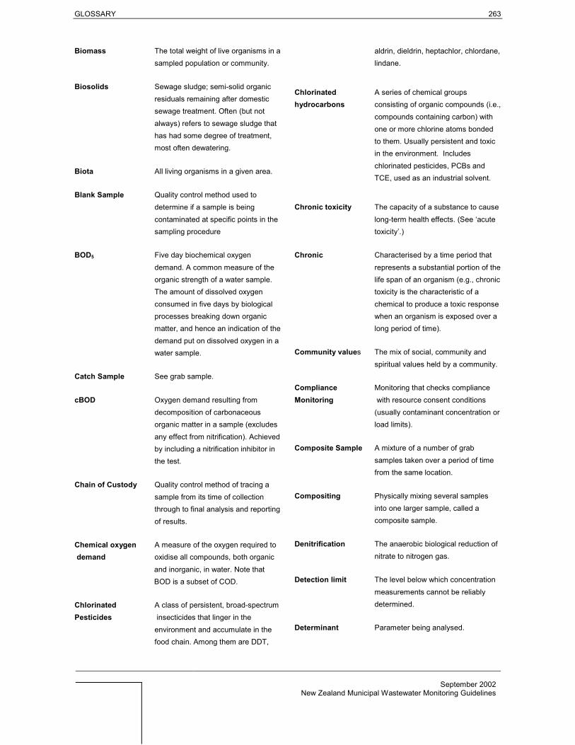
GLOSSARY 263
September 2002New Zealand Municipal Wastewater Monitoring Guidelines
Biomass The total weight of live organisms in asampled population or community.
Biosolids Sewage sludge; semi-solid organicresiduals remaining after domesticsewage treatment. Often (but notalways) refers to sewage sludge thathas had some degree of treatment,most often dewatering.
Biota All living organisms in a given area.
Blank Sample Quality control method used todetermine if a sample is beingcontaminated at specific points in thesampling procedure
BOD5 Five day biochemical oxygendemand. A common measure of theorganic strength of a water sample.The amount of dissolved oxygenconsumed in five days by biologicalprocesses breaking down organicmatter, and hence an indication of thedemand put on dissolved oxygen in awater sample.
Catch Sample See grab sample.
cBOD Oxygen demand resulting fromdecomposition of carbonaceousorganic matter in a sample (excludesany effect from nitrification). Achievedby including a nitrification inhibitor inthe test.
Chain of Custody Quality control method of tracing asample from its time of collectionthrough to final analysis and reportingof results.
Chemical oxygen A measure of the oxygen required to demand oxidise all compounds, both organic
and inorganic, in water. Note thatBOD is a subset of COD.
Chlorinated A class of persistent, broad-spectrumPesticides insecticides that linger in the
environment and accumulate in thefood chain. Among them are DDT,
aldrin, dieldrin, heptachlor, chlordane,lindane.
Chlorinated A series of chemical groupshydrocarbons consisting of organic compounds (i.e.,
compounds containing carbon) withone or more chlorine atoms bondedto them. Usually persistent and toxicin the environment. Includeschlorinated pesticides, PCBs andTCE, used as an industrial solvent.
Chronic toxicity The capacity of a substance to causelong-term health effects. (See ‘acutetoxicity’.)
Chronic Characterised by a time period thatrepresents a substantial portion of thelife span of an organism (e.g., chronictoxicity is the characteristic of achemical to produce a toxic responsewhen an organism is exposed over along period of time).
Community values The mix of social, community andspiritual values held by a community.
Compliance Monitoring that checks complianceMonitoring with resource consent conditions
(usually contaminant concentration orload limits).
Composite Sample A mixture of a number of grabsamples taken over a period of timefrom the same location.
Compositing Physically mixing several samplesinto one larger sample, called acomposite sample.
Denitrification The anaerobic biological reduction ofnitrate to nitrogen gas.
Detection limit The level below which concentrationmeasurements cannot be reliablydetermined.
Determinant Parameter being analysed.

264 GLOSSARY
September 2002New Zealand Municipal Wastewater Monitoring Guidelines
Diffuser Structure designed to enhance thedispersion of the effluent as it isdischarged into the receivingenvironment.
Discharge Monitoring of the effluent as it ismonitoring discharged into the receiving
environment.
Disinfection Inactivation of micro-organisms byaddition of a chemical (such aschlorine), boiling, or irradiation withultra-violet light.
Dissolved oxygen Oxygen gas that is freely available inwater to sustain the lives of fish andother aquatic organisms.
Dissolved The sum of ammoniacal nitrogen,inorganic nitrogen nitrate and nitrite. The portion of total
nitrogen that is readily available asnutrients to aquatic plants.
Dissolved metal Metals in a water sample that pass a0.45 micron filter. Often used as ameasure of the portion of total metalsthat are bioavailable (and hence toxicto biota).
Dissolved Phosphorus in a water sample thatreactive phosphorus passes a 0.45 micron filter. Used as
a measure of the phosphorus that isreadily available as nutrients toaquatic plants.
Diurnal 24-hour or daily cycle.
Domestic sewage Sewage containing only householdwastewater, i.e., no commercial orindustrial wastewater.
Duplicate samples Two samples taken from andrepresentative of the same populationand carried through all steps of thesampling and analytical procedures inan identical manner. Duplicatesamples are used to assess varianceof the total method, includingsampling and analysis.
E. coli Escherichia coli. A subgroup of faecalcoliforms that are used as indicator
for the presence of pathogens infresh water.
Effects monitoring Monitoring that assesses the effectsof an activity (in this case awastewater discharge) on thereceiving environment.
Enriched Generally refers to an aquaticenvironment that has an abundanceof nutrients. Often implies a eutrophicstatus.
Enterococci A subgroup of faecal streptococci thatare used as indicator for the presenceof pathogens in marine waters andestuaries.
Enteroviruses A sub-group of viruses that arederived from human sources (e.g.sewage effluent). Humanenteroviruses are indicators of thepresence of domestic sewage inwater, but can vary markedlydepending on the disease burden inthe community.
Estuaries Areas where fresh water meets andmixes with salt water. For example,mouths of rivers, salt marshes, andlagoons. Estuaries serve asnurseries, spawning and feedinggrounds for a large group of marinelife and provide shelter and food forbirds and wildlife.
Eutrophic Abundant in nutrients and having highrates of productivity, frequentlyresulting in algal blooms and oxygendepletion below the surface layer of awaterbody. In general, an undesirablestate for natural water bodies.
Faecal coliforms Thermo-tolerant bacteria from thecoliform group found in the intestinaltracts of mammals (includinghumans). Used as indicator for thepossible presence of pathogens inwastewater, receiving waters, andshellfish.

GLOSSARY 265
September 2002New Zealand Municipal Wastewater Monitoring Guidelines
Far-field The area that is not in the closevicinity of the discharge beingconsidered.
Flocculation The process by which suspendedcolloidal or very fine particlescoalesce and agglomerate into well-defined flocs of sufficient size to settlerapidly.
Grab Sample A sample collected in one go at aparticular point in space and time.Also known as a spot or catchsample.
Heavy metals High atomic weight metals, includingcopper, lead, zinc, chromium,cadmium, mercury. Toxic to biota athigh concentrations.
Heterogeneous Being composed of diverse elements
Homogenous Having a uniform consistency
Indicator organisms A group of micro-organisms that areused to indicate the risk of pathogensoccurring in a wastewater or receivingwater sample. The most commonexamples are faecal coliforms, E. coli,and enterococci.
Influent Wastewater flowing into a treatmentplant.
Inorganic nitrogen Non-organic nitrogen (i.e., NH4-N,NO3-N and NO2-N).
Integrated Sample A mixture of a number of grabsamples taken at the same time, butfrom different locations.
Macrophyte Aquatic plant, individually visible tothe naked eye.
Mesotrophic Mildly nutrient enriched.
Mixing zone Zone in which mixing of the effluentdischarge takes place in the receivingenvironment. An allowance forreasonable mixing is made in theRMA (1991) (S 69,70, Schedule 3)
before water quality standards arerequired to be met. The extent of themixing zone will vary on a case-by-case basis. Refer to Rutherford et al.(1994).
Non-compliance A zone around a discharge wherezone water quality standards or guidelines
are not likely to be met.
NTU A standard unit of turbiditymeasurement. Relates to the side-scatterance (usually 90°) of light byparticles in the water.
Nutrient Any substance assimilated by livingthings that promotes growth. Theterm is generally applied to nitrogenand phosphorus in wastewater, but isalso applied to other essential andtrace elements such as potassium.
Oligotrophic Waters with a low supply of nutrients.Usually indicates high quality lakesand streams.
Organic nitrogen Nitrogen bound with organiccompounds; generally not readilyavailable to plants. Can bemineralised to NH4-N.
Pathogens Disease-causing organisms. Includeviruses, bacteria, protozoa andhelminths (worms).
Percentile (%ile) The value of a variable that is notexceeded for a stated percentage ofan assessment period.
Periphyton Plants, usually algae, which grow onstones, logs and other plants.
Persistent A general term for all organicorganic pollutants compounds (referred to as POPs)
that are resistant to degradation in theenvironment, and are potentially toxicto biota. Includes phenols, chlorinatedhydrocarbons (DDT, PCP, PCBs),pesticides and herbicides (2,4,5 T;2,4D).

266 GLOSSARY
September 2002New Zealand Municipal Wastewater Monitoring Guidelines
pH A measure of the acidity or alkalinityof a solution (defined as the negativelogarithm, to base 10, of thehydrogen ion).
Phenols A class of aromatic organiccompounds contain one or morehydroxyl groups attached directly to abenzene ring. Toxic to aquatic biota.
Phytoplankton Small, free-floating usuallymicroscopic plants (such as algae),found in rivers lakes and the sea.They include diatoms, desmids, anddinoflagellates.
Precision Precision refers to the degree towhich repeated measurements aresimilar to one another. It measuresthe agreement (reproducibility)among individual measurements,obtained under prescribed similarconditions. To use an analogy,precise archers have all of theirarrows land very close together.However, the arrows of a precisearcher may or may not land on (oreven near) the bull's-eye. See alsoaccuracy.
Protozoa Single-celled parasites that producecysts that are able to survive outsidetheir hosts under adverseenvironmental conditions. Examplesare Giardia and Cryptosporidium.
Reasonable mixing The term used in Sections 69, 70,107 and Schedule 3 of the RMA(1991) to define the area beyondwhich a range of minimum standardsmust be met. The boundaries of thearea of ‘reasonable mixing’ will varyon a case-by-case basis, and is notsynonymous with the ‘mixing zone’.Refer to Rutherford et al. (1994).
Salinity The degree of saltiness in seawateras measured by conductivity at agiven temperature e.g. offshoreseawater has a salinity of ~35.
Sewage Wastewater that contains acomponent of human faeces andurine, as well as other householdwastewater (e.g., from showers, sinksand washing machines). Often alsocontains a proportion of commercialand industrial wastewater (see tradewastes).
Sewer A pipe or conduit that carrieswastewater to a treatment plant orreceiving waters. ‘Sanitary’ sewerscarry household, industrial, andcommercial waste. ‘Storm’ sewerscarry runoff from rain.
Sewerage system Network of pipes, pumps andchannels conveying sewage.
Soluble Fraction of material that passesthough a filter (internationalconvention uses a 0.45 micronmembrane filter).
Split Sample A sample that is divided into 2 ormore portions after collection, witheach portion being analysedseparately either in the samelaboratory or different laboratories.
Spot Sample See grab sample.
Standard For water quality, a limit that must becomplied with under law.
Stormwater Flow of water from urban surfaceareas after rainfall.
Stratification Horizontal layering of a water body,caused by layers of water withdiffering densities (due to verticalchanges in temperature and/orsalinity).
Suspended solids Solid particles suspended in water.Some of these particles may settleout in quiescent conditions, but afraction of the (smaller) suspendedsolids will always remain insuspension.
Temporal Varying over time.

GLOSSARY 267
September 2002New Zealand Municipal Wastewater Monitoring Guidelines
TKN See total Kjeldahl nitrogen.
Total ammonia See ammoniacal nitrogen (thepreferred term).
Total Kjeldahl An analytical method that provides anitrogen (TKN) measure of the sum of all nitrogen
forms except nitrate and nitrite (i.e.,includes organic N and ammoniacalN).
Total metal The concentration of a metal in anunfiltered sample. Note that only aportion of the total metal is usuallybioavailable (and hence toxic) tobiota. Measurement typically involvessample digestion in a strong acid(usually nitric acid).
Total nitrogen The sum of all forms of nitrogen in asample, i.e., organic N + ammoniacalN + nitrate N + nitrite N, expressed inmass of nitrogen.
Total phosphorus The sum of all forms of phosphorus ina sample, i.e., dissolved reactivephosphorus + particulate phosphorus,expressed in mass of phosphorus.
Toxic substance A material able to cause adverseeffects in living organisms.
Toxicity The inherent potential or capacity of amaterial to cause adverse effects inliving organisms.
Trade waste Definition in NZS 9201:1999 ModelGeneral Bylaws Part 23 - TradeWaste is: ‘any liquid, with or withoutmatter in suspension or solution, thatis or may be discharged from a tradepremises in the course of any trade orindustrial process or operation, or inthe course of any activity or operationof a like nature; but does not includecondensing or cooling waters; stormwater, or domestic sewage.’
Trend monitoring Monitoring designed to assesstrends, or changes, in wastewater orthe receiving environment over time.Refer also to baseline monitoring.
Trophic state or level In the context of receiving waters,refers to the nutrient status of thewater body. Eutrophic, mesotrophicand oligotrophic are typical examplesof trophic levels, ranging fromnutrient-enriched (i.e., degradedwater quality) to low nutrient (i.e.,high water quality), respectively.
Turbidity A measure of water clarity - thecloudiness in a fluid caused by thepresence of finely divided, suspendedmaterial. Usually measured using aturbidity meter. Turbidity is related(but not directly proportional) to theamount of suspended solids in thewater.
Volatile Readily vaporisable at a relatively lowtemperature.
Wastewater Facility where contaminants in waterTreatment Plant or wastewater are substantially
removed.
Zone of initial Zone in which the initial dilution of theDilution wastewater effluent discharge takes
place. Should not be confused withthe area in which ‘reasonable mixing’occurs. The extent of the zone ofinitial dilution will vary on a case-by-case basis. Refer to Rutherford et al.(1994).
Zooplankton Microscopic animals in aquaticsystems. Unlike phytoplankton,zooplankton cannot produce theirown food, and so are consumers.

268
September 2002New Zealand Municipal Wastewater Monitoring Guidelines
REFERENCES
Adams, N. (1994). Seaweeds of New Zealand - An Illustrated Guide. Christchurch, NZ:Canterbury University Press.
Anderlini, V.C.; Wear, R.G. (1992). The effect of sewage and natural seasonal disturbances onbenthic macrofaunal communities in Fitzroy Bay, Wellington, New Zealand. MarinePollution Bulletin 24: 21-26.
ANZECC (2000a). Australian and New Zealand guidelines for fresh and marine water quality,Vol. 4. Published by Australian & New Zealand Environment and Conservation Council.
ANZECC (2000b). Australian guidelines for water quality monitoring and reporting, Vol. 7.Published by Australian & New Zealand Environment and Conservation Council.
APHA (1998). Standard methods for the examination of water and wastewater. 20th edition.Edited by Lenore S. Clesceri, Arnold E. Greenberg, and Andrew D. Eaton. Published bythe American Public Health Association, the American Water Works Association and theWater Environment Federation. Available for purchase on the web at www.apha.org.
AS/NZS 1998: Australia/New Zealand Standard. Water Quality – Sampling. Part 10:Guidance on sampling of waste waters. AS/NZS 5667.10: 1998.
Barter, P. (2000). Benthic ecological monitoring of the Picton sewage outfall. CawthronReport No. 558 ii. 16 p.
Barter, P.; Forrest, B. (1999a). Wakapuaka Sewage Outfall Emergency Discharge EIA.Cawthron Report No. 499. Prepared for Nelson City Council. 26 p.
Barter, P.; Forrest, B. (1999b). Effluent mixing and environmental impacts at the Wakapuakasewage outfall. Cawthron Report No. 420. 48 p.
Beitinger, T.L.; Freeman, L. (1983). Behavioural avoidance and selection responses of fishes tochemicals. Residue Reviews 90: 35-53.
Biggs, B.J.F. (2000). New Zealand periphyton guideline: detecting, monitoring and managingenrichment of streams. Ministry for the Environment. Wellington. 122 p.
Boothroyd, I.K.G.; Stark, J. D. (2000). Use of invertebrates in Monitoring. In: New ZealandStream Invertebrates: Ecology and implications for management. Collier K. &Winterbourn, M. J. eds. New Zealand Limnological Society, Hamilton. pp. 344-373.
Boronti, C.; Curini, R.; D’Ascenzo, G.; Di Corcia, A.; Gentili, A.; Samperi, R. (2000).Monitoring natural and synthetic estrogens at activated sludge sewage treatment plantsand in a receiving river water. Environmental science and technology 34 (24).
Brown, R.C.; Wade, T.L. (1984). Sedimentary coprostanol and hydrocarbon distributionadjacent to a sewage outfall. Water Research 18: 621-632
Cabelli,V.J.; Dufour, A.P.; McCabe, L.J.; Levin, M.A. (1983). A marine recreational waterquality criterion consistent with indicator concepts and risk analysis. Journal of theWater Pollution Control Federation 55: 1306-1314.
Chapman, M.G.; Underwood, A.J.; Skilleter, G.A. (1995). Variability at different spatial scalesbetween a subtidal assemblage exposed to the discharge of sewage and two controlassemblages. Journal of Experimental Marine Biology and Ecology 189: 103-122.
Christchurch City Council (1986): Design Manual. Drainage and Waste Management Unit.Cooke, G.D.; Welch, E.B.; Peterson, S.A.; Newroth, P.R. (1986). Lake and Reservoir
Restoration. Stoneham, MA: Butterworths Publishers 391 p.Craft, C.B.; Seneca, E.D.; Broome, S.W. (1991). Loss on ignition and Kjeldahl digestion for
estimating organic carbon and total nitrogen in estuarine marsh soils: calibration with drycombustion. Estuaries 14: 175-179.
Davies-Colley, R.J.; Smith, D.G. (2001). Turbidity, suspended sediment and water clarity: areview. Journal of the American Water Resources Association 37: 1-17.

269
September 2002New Zealand Municipal Wastewater Monitoring Guidelines
Department of Health (1992). Public Health Guidelines for the Safe Use of Sewage Effluent andSewage Sludge on Land. Public Health Services.
Doak, W. (1984). Fishes of the New Zealand region. Auckland, NZ: Hodder and Stoughton.Düreth, S.; Reimer, H.; Pecher, K. (1986). Tracing faecal pollution by coprostanol and
intestinal bacteria in an ice covered Finnish lake loaded with both industrial and domesticsewage. Water, air, soil pollution 28:131-149.
Eaton, A.D.; Clesceri, L.S.; Greenberg, A.E. (1998) Standard Methods for the Examination ofWater and Wastewater, 20th Edition, 1998. American Public Health Association,American Water Works Association, Water Environment Federation, Washington, DC
Ellis, J.C. (1989). Handbook on the design and interpretation of monitoring programmes. ReportNS29, Water Research Centre (WRC Environment), Medmenham, UK.
EU (2001). Pollutants in urban waste water and sewage sludge. Final report prepared by ICONfor Directorate-general Environment, European Communities. February 2001.
EUR 17549, (1996). European workshop on the impact of endocrine disrupters on humanhealth and wildlife. Report of Proceedings. p 125.
Fairweather, P.G. (1990). Sewage and the biota on seashores: assessment of impact in relationto natural variability. Environmental Monitoring and Assessment 14: 197-210.
Forrest, B.; Brown, S. (1996). Determination of effluent standards to avoid conspicuous visualeffects from the Tasman Bay fisheries outfall discharge (interim report). Cawthron ReportNo. 329: 43 p.
Francis, M. (1988). Coastal Fishes of New Zealand - A diver's identification guide. HeinemannReed.
Gilbert, R.O. (1987). Statistical methods for environmental pollution monitoring. Van NostrandReinhold Co. Inc., New York, USA. 320 p.
Hall, J.A.; Golding, L.A. (1998). Standard methods for whole effluent toxicity testing:development and application. Report no. MFE80205. NIWA report for the Ministry forthe Environment, Wellington, New Zealand.
Harding, J. (2000). Impacts of the Reefton sewage outfall on the ecology of Cemetery Creekand the Inangahua River. Cawthron Report No. 543
Hauber, G. (1995). Wastewater Treatment in NZ: Evaluation of 1992/93 Performance Data –ORGD. Water and Wastes in N.Z. May 1995. pp. 28-34.
Heath, R.A. (1985). A review of the physical oceanography of the seas around New Zealand.New Zealand Journal of Marine and Freshwater Research 19: 79-124.
Hickey, C. W. (1995). Ecotoxicity in New Zealand. Australian journal of ecotoxicology 1: 43-50.
Hickey, C.W. (2000). Ecotoxicology: laboratory and field approaches. In: Collier, K.C.;Winterbourn, M. (eds). New Zealand stream invertebrates: Ecology and implications formanagement, pp. 313-343, New Zealand Limnological Society, Christchurch, NewZealand.
Hirsch, R.; Ternes, T.; Haberer, K.; Kratz, K-L. (1999). Occurrence of antibiotics in the aquaticenvironment. The science of the total environment 225: 109-118.
Hofelt, C.S.; Shea, D. (1997). Accumulation of organochlorine pesticides and PCBs by seemipermeable membrane devices and mytilus edulis in New Bedford harbor.
Environmental Science and Technology 31: 154-159.ISO 5667 – 1: 1980 Water Quality – Sampling Part 1: Guidance on the design of sampling
techniques and the preservation and handling of samples.ISO 5667 – 10: 1992 Water Quality – Sampling Part 10: Guidance on sampling of wastewaters.ISO 5667 – 11: 1993 Water Quality – Sampling Part 11: Guidance on sampling of
groundwaters.

270
September 2002New Zealand Municipal Wastewater Monitoring Guidelines
ISO 5667 – 14: 1998 Water Quality – Sampling Part 14: Guidance on quality assurance ofenvironmental water sampling and handling.
ISO 5667 – 2: 1991 Water Quality – Sampling Part 2: Guidance on sampling techniques.ISO 5667 – 3: 1994 Water Quality – Sampling Part 3: Guidance on the preservation and
handling of samples.ISO 5667 – 4: 1987 Water Quality – Sampling Part 4: Guidance on sampling from lakes, natural
and man-made.ISO 5667 – 5: 1991 Water Quality – Sampling Part 5: Guidance on sampling of drinking water
and water used for food and beverage processing.ISO 5667 – 6: 1990 Water Quality – Sampling Part 6: Guidance on sampling of rivers and
streams.ISO 5667 – 9: 1992 Water Quality – Sampling Part 9: Guidance on sampling from marine
waters.Jerka, G. H.; Donekar, R. L.; Hinton, S. W. (1996). Users manual for CORMIX: A
hydrodynamic mixing zone model and decision support system for pollutant dischargesinto surface waters. USEPA Office of Science and Technology. Washington DC.
Jiang, J. (2001). What are the areas for further research? Water Science and Technology 44(9).Johnson, A. C.; Sumpter, J. P. (2001). Removal of endocrine-disrupting chemicals in activated
sludge treatment works. Environmental science and technology 35(24) 4697-4703.Jones, M.B. (1983). Animals of the estuary shore - Illustrated guide and ecology. Christchurch,
NZ: University of Canterbury.Kingsford, M.; Battershill, C. (1998). Studying Temperate Marine Environments; A handbook
for ecologists. Canterbury University Press.Klummerer, K. (2001). Drugs in the environment: emission of drugs, diagnostic aids and
disinfectants into wastewater by hospitals in relation to other sources – a review.Chemosphere 45: 957-968.
Koop, K.; Hutchings, P. (1996). Disposal of sewage to the ocean - a sustainable solution?Marine Pollution Bulletin 33: 121-123.
Lincoln Ventures (1997). Guidelines for Community Odour Assessment. Ministry for theEnvironment SMF report No 2706/1. March 1997. Lincoln Ventures Ltd, Lincoln.
Long, E.R.; Morgan, L.G. (1991). The potential for biological effects of sediment-sorbedcontaminants tested in the National Status and Trends Program. NOAA TechnicalMemorandum NOS OMA 52
Macdonald, G.; Lewis, C.; Gregor, J.; Mattingly, B.; Prendergast, P. (2001). Communitysewerage information database for New Zealand. In New Zealand Water & WastesAssociation - 43rd Annual Conference and Expo. (1-10). Wellington, New Zealand.
McBride, G.B. (2000a). Environmental statistics and the precautionary principle: room formanoeuvre? Proceedings of Water 2000, New Zealand Water & Wastes Assoc.,Institution of Professional Engineers of New Zealand, Royal Society of New Zealand,Water Environment Federation (USA), Auckland, March (proceedings available on CD-Rom from NZWWA).
McBride, G.B. (2000b). Quantitative interpretation of the WHO ‘Annapolis Protocol’ usingenterococci data from New Zealand beaches’. NIWA Client Report: MFE01228. Report toMinistry for the Environment 82 pp.
McBride, G.B.; Bell, R.G.; Ellis, J.C. (2000). Some issues in setting effluent monitoringstandards. NZWWA Annual Conference & Expo (New Zealand Water & WastesAssociation), Rotorua, September 26–29.
McBride, G.B.; Ellis, J.C. (2001). Confidence of Compliance: a Bayesian approach forpercentile standards. Water Research 35(5): 1117–1124.

271
September 2002New Zealand Municipal Wastewater Monitoring Guidelines
Martin, M.; Hickey, C.; Hall, J. (1998). Assessment of environmental effects using toxicitytesting. Water and Wastes in New Zealand March: 35-37.
May, V. (1985). Observations on algal floras close to two sewerage outlets. Cunninghamia 1:385-394.
Metcalf and Eddy (1991): Wastewater Engineering Treatment, Disposal, and Reuse. ThirdEdition. Revised by F Burton and G Tchobanoglous. McGraw-Hill Book Co., Singapore.
MfE. (1992). Water Quality Guidelines No. 1. Anonymous. Guidelines for the Control ofUndesirable Biological Growths in Water. Ministry for the Environment, Wellington. 1-60.
MfE (1994a). Resource Management Water quality guidelines No. 2 Guidelines for theManagement of Water Colour and Clarity. Ministry for the Environment, Wellington. pp.77. June 1994.
MfE (1994b). Odour measurement and management. Discussion document. Ministry for theEnvironment, Wellington. July 1994
MfE (1998). Environmental performance indicators: Technical Paper No. 37. Review ofEnvironmental Performance Indicators for Toxic Contaminants in the environment–air,water and land. Technical Paper No. 37. Ministry for the Environment, Wellington. 105pp.+ App.
MfE (1999). Your guide to the Resource Management Act. Draft. Ministry for the Environment,Wellington. January 1999.
MfE (2002a). Microbiological water quality guidelines for marine and freshwater recreationalareas. Published by the Ministry for the Environment, Wellington on behalf of theMinistry of Health and the Ministry for the Environment. Available on the MfE web site:http://www.mfe.govt.nz..
MfE (2002b). The New Zealand Waste Strategy: Towards zero waste and a sustainable NewZealand. ME 422. Ministry for the Environment, Wellington, March 2002. Available onthe web athttp://www.mfe.govt.nz/.
Miller, C. (1999). Monitoring polycyclic aromatic hydrocarbons in the Auckland marineenvironment using SPMDs and mussels. New Zealand Water and Wastes Association,annual conference and expo: 311-316.
MoH (1995). Guidelines for drinking water quality management for New Zealand. Ministry ofHealth, Wellington.
MoH (2000). Drinking-Water Standards for New Zealand 2000. Ministry of Health, Wellington.Martin, M.; Hickey, C.; Hall, J. (1998). Assessment of environmental effects using toxicity
testing. Water and Wastes in New Zealand, March 1998: 35-37.Montgomery Watson. (1999). Monitoring protocols for hazardous constituents in wastewater
treatment facility effluents. Report prepared for Ministry for the Environment, November1999.
Morton, J.; Miller, M. (1968) The New Zealand Sea Shore. Auckland, NZ: Collins.Mosley, M.P. (1992). Waters of New Zealand. Wellington, NZ: New Zealand Hydrological
Society.Nimmermark, S. (2001). Use of electronic noses for detection of odour from animal production
facilities: a review. Water Science and Technology 44(9): 33-42.NZLTC (2000): New Zealand Guidelines for Utilisation of Sewage Effluent on Land, Part Two:
Issues for Design and Management. New Zealand Land Treatment Collective and ForestResearch, New Zealand.
NZWWA (2000). Manual for wastewater odour management. A manual prepared for the NZWater & Wastes Association, Auckland.

272
September 2002New Zealand Municipal Wastewater Monitoring Guidelines
Olsson, P.E.; Borg, B.; Brunstrom, B.; Hakansson, H.; Klasson-Wehler, E. (1998). Endocrinedisrupting substances – impairment of reproduction and development. SwedishEnvironmental Protection Agency. Report 4859
Papps, D. (1998). Puffin: A simple but effective model for outfall plume dispersion. In:NZWWA 40th Annual conference and expo, Wellington 1998, New Zealand Water &Wastes Association, p. 123-130.
Paxeus, N. (1996). Organic pollutants in the effluents of large wastewater treatment plants inSweden. Water Research 30(5): 1115-1122.
Paxeus, N.; Schroder, H. F. (1996). Screening for non-regulated organic compounds inmunicipal wastewater in Goteborg, Sweden. Water Science and Technology 33(6): 9-15.
Pearson, T.H.; Rosenberg, R. (1978). Macrobenthic succession in relation to organicenrichment and pollution of the marine environment. Oceanogr Mar Biol Annu Rev 16:229-311.
Pearson, T.H.; Stanley, S.O. (1979). Comparative measurement of the redox potential ofmarine sediments as a rapid means of assessing the effect of organic pollution. MarineBiology 53: 371-379.
Peven, C.S.; Uhler, A.D.; Querzoli, F.J. (1997). Caged mussels and semipermeable membranedevices as indicators of organic contaminant uptake in Dorchester and Duxbury Bays,Massachusetts. Environmental Toxicology and Chemistry 15: 144-149.
PSDDA; U.S Army Corps of Engineers. (1989). Unconfined open water disposal of dredgedmaterial, phase II. Anonymous. AD-A213 372
PSEP. (1997). Recommended protocols for measuring selected environmental variables inPuget Sound.
Rau, G.H.; Sweeney, R.E.; Kaplan, I.R.; Mearns, A.J.; Young, D.R. (1981). Differences inanimal 13C, 15N and D abundance between a polluted and an unpolluted coastal site: likelyindicators of sewage uptake by a marine food web. Estuarine, Coastal and Shelf Science13: 701-707.
Roberts, P.J. (1998). Dispersion from ocean outfalls. Water Quality International : 43-48.Rogers, K.M. (1999). Effects of sewage contamination on macro-algae and shellfish at Moa
Point, New Zealand using stable carbon and nitrogen isotopes. New Zealand Journal ofMarine and Freshwater Research 33: 181-188.
Roper, D. (1990). Benthos associated with an estuarine outfall, Tauranga Harbour, NewZealand. New Zealand Journal of Marine and Freshwater Research 24: 487-498.
Rosecrance A. & Adolfo N.C. (1996). Quality Assurance Guidance for EnvironmentalSampling. Water Environment Federation Technical Library.
Rutherford, J.C.; Zuur, B.; Race, P. (1994). ‘Reasonable Mixing’: a discussion of reasonablemixing in water quality management. Resources Management Ideas No. 10. Ministry forthe Environment, Wellington, August.
Sherwin, T.J.; Jonas, P.J.C.; Sharp, C. (1997). Subduction and dispersion of a buoyant effluentplume in a stratified English Bay. Marine Pollution Bulletin 34: 827-839.
Shiraishi, H.; Otsuki, A.; Fuwa, K.; (1985). Identification of extractable organic chemicals insewage effluent by gas-chromatography/mass spectrometry. Biomedical massspectrometry 12(2): 86-94.
Sinton, L.W.; Finlay, R.K.; Hannah, D.J. (1998). Distinguishing human from animal faecalcontamination in water: A review. NZ Journal of Marine and Freshwater Research 32.
Smith, S.D.A. (1996). The effects of domestic sewage effluent on marine communities at CoffsHarbour, New South Wales, Australia. Marine Pollution Bulletin 33: 309-316.
Smoley, C.K. (1993). NPDES Storm Water Sampling Guidance Manual, USEPA Office ofWater, CRN Press Inc.

273
September 2002New Zealand Municipal Wastewater Monitoring Guidelines
Sombardier, L.; Niiler, P.P. (1994). Global surface circulation measured by langrangiandrifters. Sea Technology 35: 21-24.
Standards NZ (2000). On-site domestic wastewater management. AS/NZS 1547/2000.Standards New Zealand, Wellington. 167 pp.
Stark, J. D. (1993). Performance of the Macroinvertebrate Community Index: effects ofsampling method, sample replication, water depth, current velocity and substratum onindex values. N Z Journal of Marine and Freshwater Research 27:463-478
Stark, J. D.; Boothroyd, I.K.G; Harding, J. S.; Maxted, J. R.; Scarsbrook, M. R. (2001).Protocols for sampling macroinvertebrates in wadeable streams. New ZealandMacroinvertebrate Working Group Report No. 1. Prepared for the Ministry for theEnvironment. Sustainable Management Fund Project No. 5103. 57pp.
Stubin, A. I.; Brosnan, T. M.; Porter, K. D.; Jimenez, L.; Lochan, H. (1996). Organic prioritypollutants in New York wastewaters: 1989-1993. Water Environment Research 68(Sept/Oct): 137-1044.
Stumpf, M.; Ternes, T. A.; Wilken, R-D.; Rodrigues, S. V.; Braumann, W. (1999). Polar drugresidues in sewage and natural waters in the state of Rio de Janeiro, Brazil. The Scienceof the Total Environment 225: 135-141.
Sucker, K.; Both, R.; Winneke, G. (2001). Adverse effects of environmental odours: reviewingstudies on annoyance responses and symptom reporting. Water Science and Technology44(9): 43-52.
Sweeney, R.E.; Kalil, E.K.; Kaplan, I.R. (1980). Characterisation of domestic and industrialsewage in southern California coastal sediments using nitrogen, carbon, sulphur anduranium tracers. Marine Environmental Research 3: 225-243.
Taylor Baines & Associates (2001). Contemporary Host Community experience of WWTPfacilities in New Zealand. Working Paper FS19. Public Good Science Fund ContractTBA X0002. November 2001.
Ternes, T.A.; Stumpf, M.; Mueller, J.; Haberer, K.; Wilken, R-D.; Servos, M. (1999). Behaviourand occurrence of estrogens in municipal sewage treatment plants – 1. Investigations inGermany, Canada and Brazil. The Science of the Total Environment 225: 81-90.
Tonkin & Taylor (1998). Identification of hazardous waste in New Zealand. Report forMinistry for the Environment, June 1998.
Underwood, A.J.; Chapman, M.G. (1996). Subtidal assemblages on rocky reefs at a cliff-facesewage outfall (North Head, Sydney, Australia): What happened when the outfall wasturned off? Marine Pollution Bulletin 33: 293-302.
USEPA (1991). Technical support document for water quality–based toxics control. EPA/505/2-90/001. United States Environmental Protection Agency, Criteria and StandardsDivision, Washington D.C.
USEPA (1996). U.S. EPA NPDES Permit Writers’ Manual. Report No. EPA-833-B-96-003,published by the US Environmental Protection Agency, Office of WastewaterManagement, Washington DC. At Web site: http://www.epa.gov/owm/sectper.htm
USEPA (1999a). 1999 update of ambient water quality criteria for ammonia. Office of Water,United States Environmental Protection Agency. EPA-822-R-99-014. December 1999.
USEPA (1999b). National recommended water quality criteria - correction. Office of Water,United States Environmental Protection Agency. EPA-822-Z-99-001. April 1999.
Van Harreveld, A. P. (2001). From odorant formation to odour nuisance: new definitions fordiscussing a complex process. Water Science and Technology 44(9): 9-16.
Verbruggen, E. M. J.; Van Loon, W.M.G.M.; Tonkes, M.; Van Duijn, P.; Seinen, W.; Hermens,J.L.M. (1999). Biomimetic extraction as a tool to identify chemicals with highbioconcentration potential: An illustration by two fragrances in sewage treatment planteffluents and surface waters. Environmental science & technology 33: 801-806.

274
September 2002New Zealand Municipal Wastewater Monitoring Guidelines
Viner, A.B. (1987). Inland Waters of New Zealand. Wellington, NZ: Science InformationPublishing Centre.
Ward, R.C.; Loftis, J.C.; McBride, G.B. (1990). Design of water quality monitoring systems.Van Nostrand Reinhold, New York. 231 pp.
Williams, ed. (1985). Ocean outfall handbook. Water and soil miscellaneous publication No 76.Ministry of Works and Development.
Wood, I.R.; Bell, R.G.; Wilkinson, D.L. (1993). Ocean Disposal of Wastewater. Singapore:World Scientific Publishing Co. 425 pp.
WPCF, (1990). Critical evaluation of the state of technologies for predicting the transport andfate of toxic compounds in wastewater facilities. WPCF Research Foundation Project90-1. Water Pollution Control Federation, December 1990.
Zar, J.H. (1996). Biostatistical analysis. Third edition. Prentice Hall.

275
September 2002New Zealand Municipal Wastewater Monitoring Guidelines
APPENDIX 1: Calculating sample percentiles
A sample percentile, denoted as ‘P%ile’, of a set of sample data is the value that is exceeded by (1–P)% of the sample values. For example, a sample median (which is a 50%ile), is the estimated valueexceeded exactly as often as not. A sample 95%ile is the estimated value exceeded by 5% of thesamples.
There is no one ‘statistically-correct’ way to calculate sample percentiles.
Three percentile calculatorsTo illustrate procedures, let’s examine the simplest and most commonly used percentile, i.e., themedian. For example, it is often quoted in the news media in respect of house prices. Half the data areabove the median value and half are below it. Now consider the following small set of nine numbers:8, 4, 12, 10, 34, 5, 47, 7, 9. The median of these data is in fact the last value in this list, i.e., 9. This isobtained by first sorting (‘ranking’) the data in ascending order (i.e., 4, 5, 7, 8, 9, 10, 12, 34, 47) andpicking out the middle value, that is the fifth value ‘9’ – there are four numbers below this value andfour numbers above it. If there were an even number of numbers in this list, we would have to take thearithmetic average of the middle two number as the median. This average ‘collapses’ the list into anodd number of numbers, and so the middle value (the average of the middle two) will have the samenumber of values above it as lie below it.
In principle, this ordering concept is easily generalised to other percentiles. For example, an 80percentile has 80% of data below its value, and therefore 20% above it. But this poses a problem as20% of 9 samples is not a whole number. This difficulty is avoided by using a formula2 to calculate anon-integer value of the rank of the percentile data and then interpolating between the adjacent rankeddata. An example appears below, but first we will define three formulae for the percentile’s rank (r).
Weibull: ( )1+= npr
Hazen: pnr += ½
Excel:3 ( )11 −+= npr
wherein p = P/100 (so for an 80%ile p = 0.8) and n is the number of samples available.
In the simple example in the previous paragraph the Weibull equation happens to give an integer valuefor r, i.e., r = 8. Accordingly the 80%ile of the 9 samples, as calculated by the Weibull formula, is the8th ranked value, i.e., ‘34’. But the Hazen formula gives r = 7.7. So we must interpolate between the 7th
and 8th ranked data to get the 80%ile by the Hazen method, i.e., between ‘12’ and ‘34’. Using linear
2 Note: most software packages don’t tell you how they calculate percentiles.3 This formula is not defined in Excel’s Help files or manuals, but it may be simply adduced.

276
September 2002New Zealand Municipal Wastewater Monitoring Guidelines
interpolation (as is usual) we get the 80%ile of the 9 samples, as calculated by the Hazen formula as27.4. The Excel formula gives r = 7.4 and so the 80%ile of the 9 samples, as calculated by the Excelformula is 20.8. In summary, the three methods give an 80%ile of 34, 27.4 and 20.8 respectively.
This simple example shows that if the numbers surrounding the computed rank are very different (i.e.,12 and 34 in the above example), then the computed percentiles will be very different also. It alsodemonstrates the general result that the three formula span the range of results that may be obtainedusing other formulae,4 with the Excel estimator always giving the lowest value.
Now note that a certain minimum number of samples (nmin) is needed before these formulae can beused, which is important to realise when setting compliance periods and percentile limits. Theseminimum numbers for a percentile ratio p are:
Weibull:p
pnpp
pn −≥≥−
≥ 1 otherwise ,5.0 if 1 minmin
Hazen: ( ) pnp
pn
21 otherwise ,5.0 if
121
minmin ≥≥−
≥
Excel:5 pn allfor 1min ≥
In the case of the increasingly used 95%iles (p= 0.95) the Weibull formula requires 19 (not 20)samples to be at hand before a 95%ile can be calculated, whereas only 10 are required for the Hazenformula. Microsoft Excel® only ever requires one sample, and there is a conceptual difficulty with thatproperty.
Formalising the interpolationPut sample data {Xj ; j = 1, n} into ascending order. Call this dataset {Yj ; j = 1, n}. Using one of theequations given above calculate r, then break it down to its integer and decimal parts:
r = rint + rrem
Then the Pth percentile is calculated from the ascending-ordered data as
( )( ) ( )1remrem intint1 ++−= rrP YrYrX
As a further example, say that we want to calculate the 95%ile from a dataset Xj (j = 1,…, 50). Wetherefore have n = 50 samples and P = 95, so that p = 0.95. Say the four largest sample values forsuspended solids are 59, 63, 67 and 75 g m-3.
From the ordering of the data we know that Y47 = 59, Y48 = 63, Y49 = 67, Y50 = 75. So to calculate the95%ile from the Weibull formula we have r = 0.95x51= 48.45, so rint = 48 and rrem = 0.45. Then usingthe above equation we obtain X95 = 0.55x63 + 0.45x67 = 64.8.
To calculate the 95%ile from the Hazen formula we have r = 0.5 + 0.95x50 = 48.0, so rint = 48 and rrem= 0.0. Then using we obtain X95 = 1.0x63 + 0.0x67 = 63. 4 For example the Tukey and Blom estimators given in Ellis 1989.5 This formula is not defined in Excel’s Help files or manuals, but it may be simply adduced.

277
September 2002New Zealand Municipal Wastewater Monitoring Guidelines
Using the Excel estimator we have r = 1 + 0.95x49 = 47.55, so rint = 47 and rrem = 0.55. Then weobtain X95 = 0.45x59 + 0.55x63 = 61.2.

278 APPENDIX 2
September 2002New Zealand Municipal Wastewater Monitoring Guidelines

APPENDIX 2 279
September 2002New Zealand Municipal Wastewater Monitoring Guidelines
APPENDIX 2: Monitoring parameters for discharge monitoring
(Refer to Chapter 10).

280
APPE
ND
IX 2
Sept
embe
r 200
2N
ew Z
eala
nd M
unic
ipal
Was
tew
ater
Mon
itorin
g G
uide
lines
Tabl
e 10
.A:
Mon
itorin
g pa
ram
eter
s - p
hysi
co-c
hem
ical
.
Para
met
erD
escr
iptio
n an
d us
esEn
viro
nmen
tal R
elev
ance
Fres
hwat
erR
ecei
ving
Envi
ronm
ent
Coa
stal
Rec
eivi
ngEn
viro
nmen
tTe
mpe
ratu
reW
aste
wat
er te
mpe
ratu
re, m
easu
red
in d
egre
es C
elsi
usD
irect
impa
cts
on a
quat
ic li
fe w
hich
hav
ea
tem
pera
ture
tole
ranc
e ra
nge.
Indi
rect
impa
cts
as h
igh
wat
er te
mpe
ratu
res
redu
ce th
e am
ount
of d
isso
lved
gas
es,
incr
ease
rate
of c
hem
ical
reac
tions
and
incr
ease
gro
wth
rate
s, in
crea
sing
the
risk
of a
lgal
blo
oms.
Yes
Yes
pHpH
is a
mea
sure
of t
he w
ater
sac
idity
or a
lkal
inity
.Aq
uatic
life
hav
e a
tole
ranc
e ra
nge
for
pH (u
sual
ly p
H 6
- 9)
. pH
can
hav
ein
dire
ct im
pact
s on
aqu
atic
life
by
affe
ctin
g th
e sp
ecia
tion
and
toxi
city
of
met
als
and
amm
onia
.
Yes
No
Elec
trica
lC
ondu
ctiv
ity (E
C)
EC is
a m
easu
re o
f the
abi
lity
ofw
ater
to c
ondu
ct a
n el
ectri
cal
curre
nt.
It pr
ovid
es a
n in
dica
tion
ofth
e am
ount
of d
isso
lved
ions
in th
ew
ater
.
Con
duct
ivity
can
be
used
to in
dica
teio
nic
pollu
tion
but i
s no
t typ
ical
ly a
nen
viro
nmen
tal i
ssue
.
Yes
No
Col
our
Col
our c
an b
e de
scrib
ed in
refe
renc
e to
Mun
sell
stan
dard
s or
by
abso
rptio
n of
ligh
t at a
par
ticul
arw
avel
engt
h.
Col
our a
ffect
s th
e ae
sthe
tics
of a
wat
erbo
dy.
Som
e co
lour
s ca
n re
duce
light
pen
etra
tion.
Yes
Typi
cally
No
Cla
rity
Cla
rity
is th
e lim
it of
vis
ibilit
y in
wat
er.
Poor
cla
rity
redu
ces
aest
hetic
val
ues,
light
pen
etra
tion
and
phot
osyn
thes
is.
Poor
cla
rity
can
also
affe
ct th
epr
edat
or/p
rey
activ
ities
of a
quat
ic b
iota
.
Yes
Yes

APPE
ND
IX 2
281
Sept
embe
r 200
2N
ew Z
eala
nd M
unic
ipal
Was
tew
ater
Mon
itorin
g G
uide
lines
Para
met
erD
escr
iptio
n an
d us
esEn
viro
nmen
tal R
elev
ance
Fres
hwat
erR
ecei
ving
Envi
ronm
ent
Coa
stal
Rec
eivi
ngEn
viro
nmen
tTu
rbid
ityTu
rbid
ity is
the
scat
terin
g of
ligh
t by
parti
cles
in th
e w
ater
.H
igh
turb
idity
affe
cts
light
pen
etra
tion
and
can
redu
ce p
hoto
synt
hesi
s fo
r alg
ae a
ndm
acro
phyt
es.
Yes
Yes
Susp
ende
d So
lids
Susp
ende
d so
lids
are
parti
cula
tem
atte
r tha
t can
be
rem
oved
by
filtra
tion
with
a 0
.45
�m
filte
r. It
incl
udes
cla
y, s
ilt, f
ine
parti
cles
of
orga
nic
and
inor
gani
c m
atte
r and
mic
rosc
opic
and
sm
all o
rgan
ism
s.
Susp
ende
d so
lids
affe
ct li
ght p
enet
ratio
nan
d ae
sthe
tics.
The
re c
an b
e di
rect
effe
cts
on a
quat
ic b
iota
. H
igh
susp
ende
d so
lids
can
lead
tose
dim
enta
tion
in d
epos
ition
are
as.
Yes
Yes
Odo
urO
dour
is a
ny a
ppar
ent o
dour
,ca
used
by
the
pres
ence
of v
olat
ileco
mpo
unds
in th
e ai
r.
Odo
ur h
as th
e po
tent
ial t
o re
duce
the
aest
hetic
s of
a w
ater
bod
y.Ye
sYe
s
Har
dnes
sTh
e ha
rdne
ss o
f wat
er d
epen
ds o
nth
e ca
lciu
m a
nd m
agne
sium
con
tent
.It
is u
sual
ly m
easu
red
as c
arbo
nate
hard
ness
(as
CaC
O3)
.
The
hard
ness
of a
wat
er b
ody
affe
cts
the
toxi
city
of s
ome
met
als.
Yes
No
Alka
linity
Alka
linity
is c
apac
ity o
f a w
ater
bod
yto
neu
tralis
e ac
id a
nd is
gen
eral
lyre
porte
d as
g m
-3 o
f CaC
O3.
Alka
linity
affe
cts
hard
ness
and
toxi
city
of s
ome
met
als.
Yes
No

282
APPE
ND
IX 2
Sept
embe
r 200
2N
ew Z
eala
nd M
unic
ipal
Was
tew
ater
Mon
itorin
g G
uide
lines
Tabl
e 10
.B:
Mon
itorin
g pa
ram
eter
s - c
omm
on io
ns.
Para
met
erD
escr
iptio
n an
d us
esEn
viro
nmen
tal R
elev
ance
Fres
hwat
erR
ecei
ving
Envi
ronm
ent
Coa
stal
Rec
eivi
ngEn
viro
nmen
tSo
dium
Sodi
um is
a c
omm
on c
atio
n an
d th
e m
ajor
cat
ion
inse
awat
er (f
rom
sal
t), fo
und
as N
a+ .So
dium
is n
atur
ally
hig
h in
sea
wat
eran
d in
est
uarie
s.N
oN
o
Pota
ssiu
mPo
tass
ium
is a
com
mon
cat
ion,
whi
ch is
read
ily s
olub
lein
wat
er a
nd fo
und
as K
+ .Po
tass
ium
is a
n es
sent
ial n
utrit
iona
lel
emen
t for
aqu
atic
bio
ta.
No
No
Mag
nesi
umM
agne
sium
is a
com
mon
cat
ion
foun
d as
Mg2+
and
is
rele
ased
into
fres
hwat
er fr
om th
e w
eath
erin
g of
rock
s.M
agne
sium
is a
maj
or s
ourc
e of
wat
erha
rdne
ss.
Yes
No
Cal
cium
Cal
cium
is p
rese
nt in
all
wat
ers
as C
a2+. C
alci
um is
read
ily d
isso
lved
from
rock
s su
ch a
s lim
esto
ne.
Cal
cium
is a
n es
sent
ial e
lem
ent f
oraq
uatic
ver
tebr
ates
and
inve
rtebr
ates
.C
alci
um is
a m
ajor
sou
rce
of w
ater
hard
ness
and
is p
rese
nt in
bot
hfre
shw
ater
and
sea
wat
er.
Yes
No
Fluo
ride
Fluo
ride
is a
com
mon
ani
on, p
rese
nt a
s F- .
Yes
No
Chl
orid
eC
hlor
ide
is th
e do
min
ant a
nion
foun
d in
sea
wat
er a
nd is
pres
ent a
s C
l- in b
oth
fresh
wat
er a
nd s
eaw
ater
.C
hlor
ide
is h
igh
in s
ea w
ater
and
ines
tuar
ies.
No
No
Sulp
hate
Sulp
hate
is n
atur
ally
pre
sent
in s
urfa
ce w
ater
s as
the
anio
n SO
42-.
Sulp
hate
can
be
redu
ced
unde
r ana
erob
icco
nditi
ons
to h
ydro
gen
sulp
hide
(H2S
, HS- ).
Hyd
roge
n su
lphi
de is
the
sour
ce o
f'ro
tten
egg'
odo
urs.
Yes
Yes
Car
bona
te a
ndBi
carb
onat
eC
arbo
nate
(CO
32-) a
nd b
icar
bona
te (H
CO
3- ) inf
luen
ceth
e al
kalin
ity o
f wat
er.
Car
bona
te a
nd b
icar
bona
te c
an fo
rmco
mpl
exes
with
met
als,
rem
ovin
gYe
sN
o

APPE
ND
IX 2
283
Sept
embe
r 200
2N
ew Z
eala
nd M
unic
ipal
Was
tew
ater
Mon
itorin
g G
uide
lines
them
from
the
wat
er c
olum
n an
dlo
wer
ing
toxi
city
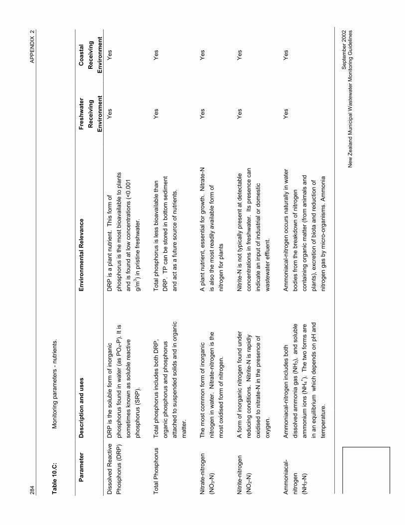
284
APPE
ND
IX 2
Sept
embe
r 200
2N
ew Z
eala
nd M
unic
ipal
Was
tew
ater
Mon
itorin
g G
uide
lines
Tabl
e 10
.C:
Mon
itorin
g pa
ram
eter
s - n
utrie
nts.
Para
met
erD
escr
iptio
n an
d us
esEn
viro
nmen
tal R
elev
ance
Fres
hwat
erR
ecei
ving
Envi
ronm
ent
Coa
stal
Rec
eivi
ngEn
viro
nmen
tD
isso
lved
Rea
ctiv
ePh
osph
orus
(DR
P)D
RP
is th
e so
lubl
e fo
rm o
f ino
rgan
icph
osph
orus
foun
d in
wat
er (a
s PO
4-P)
. It i
sso
met
imes
kno
wn
as s
olub
le re
activ
eph
osph
orus
(SR
P).
DR
P is
a p
lant
nut
rient
. Th
is fo
rm o
fph
osph
orus
is th
e m
ost b
ioav
aila
ble
to p
lant
san
d is
foun
d at
low
con
cent
ratio
ns (<
0.00
1g/
m3 ) i
n pr
istin
e fre
shw
ater
.
Yes
Yes
Tota
l Pho
spho
rus
Tota
l pho
spho
rus
incl
udes
bot
h D
RP,
orga
nic
phos
phor
us a
nd p
hosp
horu
sat
tach
ed to
sus
pend
ed s
olid
s an
d in
org
anic
mat
ter.
Tota
l pho
spho
rus
is le
ss b
ioav
aila
ble
than
DR
P. T
P ca
n be
sto
red
in b
otto
m s
edim
ent
and
act a
s a
futu
re s
ourc
e of
nut
rient
s.
Yes
Yes
Nitr
ate-
nitro
gen
(NO
3-N
)Th
e m
ost c
omm
on fo
rm o
f ino
rgan
icni
troge
n in
wat
er.
Nitr
ate-
nitro
gen
is th
em
ost o
xidi
sed
form
of n
itrog
en.
A pl
ant n
utrie
nt, e
ssen
tial f
or g
row
th.
Nitr
ate-
Nis
als
o th
e m
ost r
eadi
ly a
vaila
ble
form
of
nitro
gen
for p
lant
s
Yes
Yes
Nitr
ite-n
itrog
en(N
O2-
N)
A fo
rm o
f ino
rgan
ic n
itrog
en fo
und
unde
rre
duci
ng c
ondi
tions
. N
itrite
-N is
rapi
dly
oxid
ised
to n
itrat
e-N
in th
e pr
esen
ce o
fox
ygen
.
Nitr
ite-N
is n
ot ty
pica
lly p
rese
nt a
t det
ecta
ble
conc
entra
tions
in fr
eshw
ater
. Its
pre
senc
e ca
nin
dica
te a
n in
put o
f ind
ustri
al o
r dom
estic
was
tew
ater
effl
uent
.
Yes
Yes
Amm
onia
cal-
nitro
gen
(NH
3-N
)
Amm
onia
cal-n
itrog
en in
clud
es b
oth
diss
olve
d am
mon
ia g
as (N
H3)
, an
d so
lubl
eam
mon
ium
ions
(NH
4+ ). T
he tw
o fo
rms
are
in a
n eq
uilib
rium
whi
ch d
epen
ds o
n pH
and
tem
pera
ture
.
Amm
onia
cal-n
itrog
en o
ccur
s na
tura
lly in
wat
erbo
dies
from
the
brea
kdow
n of
nitr
ogen
cont
aini
ng o
rgan
ic m
atte
r (fro
m a
nim
als
and
plan
ts),
excr
etio
n of
bio
ta a
nd re
duct
ion
ofni
troge
n ga
s by
mic
ro-o
rgan
ism
s. A
mm
onia
Yes
Yes

APPE
ND
IX 2
285
Sept
embe
r 200
2N
ew Z
eala
nd M
unic
ipal
Was
tew
ater
Mon
itorin
g G
uide
lines
Para
met
erD
escr
iptio
n an
d us
esEn
viro
nmen
tal R
elev
ance
Fres
hwat
erR
ecei
ving
Envi
ronm
ent
Coa
stal
Rec
eivi
ngEn
viro
nmen
tga
s is
toxi
c at
hig
h co
ncen
tratio
ns (a
nd a
tce
rtain
pH
). A
mm
onia
cal-N
is o
xidi
sed
toni
trite
-N a
nd n
itrat
e-N
.
Tota
l Kje
ldah
lN
itrog
en (T
KN)
TKN
incl
udes
org
anic
nitr
ogen
, bot
hdi
ssol
ved
and
parti
cula
te, a
nd a
mm
onia
cal-
nitro
gen.
TKN
incl
udes
livi
ng fo
rms
of n
itrog
en s
uch
asal
gae,
that
may
be
in th
e w
ater
.Ye
sYe
s
Org
anic
nitr
ogen
(tota
l org
anic
nitro
gen)
Nitr
ogen
in th
e fo
rm o
f pro
tein
or
trans
form
atio
n pr
oduc
ts, b
oth
diss
olve
d an
dpa
rticu
late
.
Org
anic
nitr
ogen
com
es fr
om p
lant
and
ani
mal
mat
ter a
nd th
eir d
egra
datio
n pr
oduc
ts.
Nitr
ogen
with
in a
lgae
is a
lso
incl
uded
in o
rgan
icni
troge
n m
easu
rem
ents
Yes
Yes
Tota
l Nitr
ogen
Tota
l nitr
ogen
incl
udes
all
of th
e ab
ove
form
s of
nitr
ogen
, org
anic
and
inor
gani
c,di
ssol
ved
and
parti
cula
te.
Som
e of
thes
e fo
rms
of n
itrog
en a
re n
otre
adily
bio
avai
labl
e as
pla
nt n
utrie
nts.
Yes
Yes
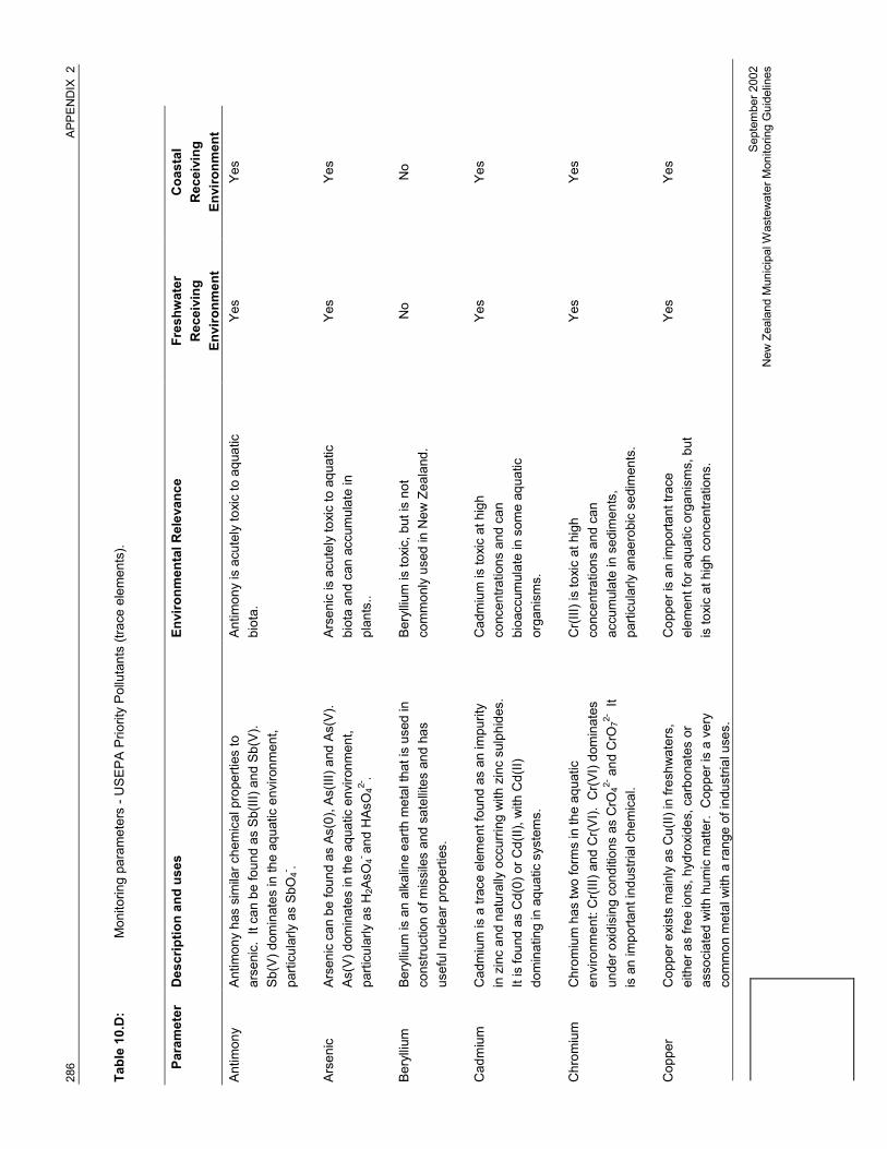
286
APPE
ND
IX 2
Sept
embe
r 200
2N
ew Z
eala
nd M
unic
ipal
Was
tew
ater
Mon
itorin
g G
uide
lines
Tabl
e 10
.D:
Mon
itorin
g pa
ram
eter
s - U
SEPA
Prio
rity
Pollu
tant
s (tr
ace
elem
ents
).
Para
met
erD
escr
iptio
n an
d us
esEn
viro
nmen
tal R
elev
ance
Fres
hwat
erR
ecei
ving
Envi
ronm
ent
Coa
stal
Rec
eivi
ngEn
viro
nmen
tAn
timon
yAn
timon
y ha
s si
mila
r che
mic
al p
rope
rties
toar
seni
c. I
t can
be
foun
d as
Sb(
III) a
nd S
b(V)
.Sb
(V) d
omin
ates
in th
e aq
uatic
env
ironm
ent,
parti
cula
rly a
s Sb
O4- .
Antim
ony
is a
cute
ly to
xic
to a
quat
icbi
ota.
Yes
Yes
Arse
nic
Arse
nic
can
be fo
und
as A
s(0)
, As(
III) a
nd A
s(V)
.As
(V) d
omin
ates
in th
e aq
uatic
env
ironm
ent,
parti
cula
rly a
s H
2AsO
4- and
HAs
O42-
.
Arse
nic
is a
cute
ly to
xic
to a
quat
icbi
ota
and
can
accu
mul
ate
inpl
ants
..
Yes
Yes
Bery
llium
Bery
llium
is a
n al
kalin
e ea
rth m
etal
that
is u
sed
inco
nstru
ctio
n of
mis
sile
s an
d sa
tellit
es a
nd h
asus
eful
nuc
lear
pro
perti
es.
Bery
llium
is to
xic,
but
is n
otco
mm
only
use
d in
New
Zea
land
.N
oN
o
Cad
miu
mC
adm
ium
is a
trac
e el
emen
t fou
nd a
s an
impu
rity
in z
inc
and
natu
rally
occ
urrin
g w
ith z
inc
sulp
hide
s.It
is fo
und
as C
d(0)
or C
d(II)
, with
Cd(
II)do
min
atin
g in
aqu
atic
sys
tem
s.
Cad
miu
m is
toxi
c at
hig
hco
ncen
tratio
ns a
nd c
anbi
oacc
umul
ate
in s
ome
aqua
ticor
gani
sms.
Yes
Yes
Chr
omiu
mC
hrom
ium
has
two
form
s in
the
aqua
ticen
viro
nmen
t: C
r(III)
and
Cr(V
I). C
r(VI)
dom
inat
esun
der o
xidi
sing
con
ditio
ns a
s C
rO42-
and
CrO
72- I
tis
an
impo
rtant
indu
stria
l che
mic
al.
Cr(I
II) is
toxi
c at
hig
hco
ncen
tratio
ns a
nd c
anac
cum
ulat
e in
sed
imen
ts,
parti
cula
rly a
naer
obic
sed
imen
ts.
Yes
Yes
Cop
per
Cop
per e
xist
s m
ainl
y as
Cu(
II) in
fres
hwat
ers,
eith
er a
s fre
e io
ns, h
ydro
xide
s, c
arbo
nate
s or
asso
ciat
ed w
ith h
umic
mat
ter.
Cop
per i
s a
very
com
mon
met
al w
ith a
rang
e of
indu
stria
l use
s.
Cop
per i
s an
impo
rtant
trac
eel
emen
t for
aqu
atic
org
anis
ms,
but
is to
xic
at h
igh
conc
entra
tions
.
Yes
Yes

APPE
ND
IX 2
287
Sept
embe
r 200
2N
ew Z
eala
nd M
unic
ipal
Was
tew
ater
Mon
itorin
g G
uide
lines
Para
met
erD
escr
iptio
n an
d us
esEn
viro
nmen
tal R
elev
ance
Fres
hwat
erR
ecei
ving
Envi
ronm
ent
Coa
stal
Rec
eivi
ngEn
viro
nmen
t
Lead
Lead
is fo
und
in tw
o ox
idat
ion
stat
es, P
b(II)
and
Pb(IV
). In
nat
ural
wat
ers
,Pb(
II) d
omin
ates
, mai
nly
as o
rgan
ic c
ompl
exes
. Le
ad is
a d
ense
met
al w
itha
wid
e ra
nge
of u
ses,
com
mon
ly u
sed
in in
dust
ryan
d fo
r pip
es.
Lead
is to
xic
to a
quat
ic o
rgan
ism
sat
hig
h co
ncen
tratio
ns.
Yes
Yes
Mer
cury
Mer
cury
has
thre
e ox
idat
ion
stat
es, H
g(0)
, Hg(
I)an
d H
g(II)
. Mer
cury
met
al is
liqu
id a
t roo
mte
mpe
ratu
re.
All f
orm
s of
mer
cury
are
hig
hly
toxi
c to
aqu
atic
org
anis
ms.
An
orga
nic
form
(met
hyl m
ercu
ry) i
sal
so b
ioac
cum
ulat
ive.
Yes
Yes
Nic
kel
Nic
kel i
s a
har
d m
etal
use
d in
allo
ys, e
lect
rical
good
s an
d ni
ckel
-cad
miu
m b
atte
ries.
Nic
kel i
spr
esen
t as
free
Ni(I
I) an
d ca
rbon
ate
com
plex
es in
aqua
tic e
nviro
nmen
ts.
Nic
kel i
s an
ess
entia
l tra
ceel
emen
t for
pla
nts
and
anim
als
but
is to
xic
at h
igh
conc
entra
tions
.
Yes
Yes
Sele
nium
Sele
nium
is s
emi-m
etal
lic a
nd it
s us
es in
clud
epa
ints
, ele
ctro
nics
and
pho
toel
ectri
c ce
lls.
Sele
nium
is e
ssen
tial a
t tra
ceco
ncen
tratio
ns fo
r ani
mal
s, b
ut a
thi
gh c
once
ntra
tions
it is
toxi
c.
No
No
Silv
erSi
lver
is a
har
d m
etal
with
dec
orat
ive
and
indu
stria
lus
es.
Silv
er h
alid
es a
re u
sed
in p
hoto
grap
hy.
Silv
er is
acu
tely
toxi
c to
aqu
atic
biot
a (h
ardn
ess
depe
nden
t).Ye
sYe
s
Thal
lium
Thal
lium
is a
met
allic
ele
men
t use
d in
lead
allo
ys,
phot
ocel
ls a
nd g
lass
man
ufac
ture
.Th
alliu
m is
not
requ
ired
as a
nutri
ent f
or p
lant
s or
ani
mal
s.N
oN
o
Zinc
Zinc
met
al is
com
mon
ly u
sed
for a
wid
e ra
nge
ofin
dust
rial a
nd d
omes
tic u
ses.
Zin
c is
foun
d as
Zn(II
) in
aqua
tic e
nviro
nmen
ts, a
s fre
e io
ns in
Zinc
is a
n im
porta
nt tr
ace
elem
ent
for
aqua
tic p
lant
s an
d an
imal
s, b
utis
toxi
c at
hig
h co
ncen
tratio
ns
Yes
Yes

288
APPE
ND
IX 2
Sept
embe
r 200
2N
ew Z
eala
nd M
unic
ipal
Was
tew
ater
Mon
itorin
g G
uide
lines
Para
met
erD
escr
iptio
n an
d us
esEn
viro
nmen
tal R
elev
ance
Fres
hwat
erR
ecei
ving
Envi
ronm
ent
Coa
stal
Rec
eivi
ngEn
viro
nmen
tfre
shw
ater
and
as
ZnC
l 2 in
sea
wat
er.
(har
dnes
s de
pend
ent).
Not
es :
No
– El
emen
ts th
at a
re n
ot k
now
n to
be
pres
ent i
n si
gnifi
cant
con
cent
ratio
ns o
r use
d by
indu
stry
in N
ew Z
eala
nd.

APPE
ND
IX 2
289
Sept
embe
r 200
2N
ew Z
eala
nd M
unic
ipal
Was
tew
ater
Mon
itorin
g G
uide
lines
Tabl
e 10
.E:
Mon
itorin
g pa
ram
eter
s - O
ther
ele
men
ts.
Para
met
erD
escr
iptio
n an
d us
esEn
viro
nmen
tal R
elev
ance
Fres
hwat
erR
ecei
ving
Envi
ronm
ent
Coa
stal
Rec
eivi
ngEn
viro
nmen
tAl
umin
ium
Alum
iniu
m is
com
mon
ly fo
und
as A
l(III)
oxi
des
and
hydr
oxid
es a
nd a
ttach
ed to
sol
ids
in th
eaq
uatic
env
ironm
ent.
Alum
iniu
m is
an
impo
rtant
trac
e el
emen
tfo
r aq
uatic
org
anis
ms,
but
is to
xic
athi
gh c
once
ntra
tions
.
Yes
Yes
Boro
nBo
ron
is a
non
-met
al w
hich
is p
rese
nt in
geot
herm
al w
ater
s an
d as
soci
ated
with
coa
lde
posi
ts.
Boro
n co
ncen
tratio
ns a
re n
atur
ally
hig
hin
sea
wat
er.
Yes
No
Iron
Iron
is ty
pica
lly fo
und
as s
peci
es o
f Fe(
III),
(ferri
cox
ides
and
hyd
roxi
des)
in th
e aq
uatic
envi
ronm
ent.
The
redu
ced
form
, Fe(
II), i
s pr
esen
tin
redu
cing
con
ditio
ns.
Iron
is a
n im
porta
nt tr
ace
elem
ent f
oraq
uatic
org
anis
ms.
Ver
y hi
ghco
ncen
tratio
ns o
f iro
n ca
n ca
use
the
form
atio
n of
iron
floc
(iro
n ox
ides
and
hydr
oxid
es) i
n st
ream
s.
Yes
No
Man
gane
seM
anga
nese
is a
met
al re
sem
blin
g iro
n an
d of
ten
used
with
iron.
Per
man
gana
te (M
nO4- ) i
s so
met
imes
use
das
a m
ild d
isin
fect
ant.
Man
gane
se is
a v
ital e
lem
ent f
or a
quat
icor
gani
sms
at tr
ace
conc
entra
tions
.Ye
sN
o
Tin
Tin
is a
com
mon
met
al u
sed
in s
olde
r allo
ys a
ndco
rrosi
on-re
sist
ant c
oatin
gs.
Tin
is to
xic
to a
quat
ic o
rgan
ism
s at
hig
hco
ncen
tratio
ns.
Yes
Yes

290
APPE
ND
IX 2
Sept
embe
r 200
2N
ew Z
eala
nd M
unic
ipal
Was
tew
ater
Mon
itorin
g G
uide
lines
Tabl
e 10
.F:
Mon
itorin
g pa
ram
eter
s - O
ther
Par
amet
ers.
Para
met
erD
escr
iptio
n an
d us
esEn
viro
nmen
tal R
elev
ance
Fres
hwat
erR
ecei
ving
Envi
ronm
ent
Coa
stal
Rec
eivi
ngEn
viro
nmen
tC
hlor
ine
(FAC
)Fr
ee a
vaila
ble
chlo
rine
(FAC
) inc
lude
sch
lorin
e an
d hy
poch
lorit
e fro
m w
aste
wat
ertre
atm
ent.
Res
idua
l chl
orin
e, if
pre
sent
in w
aste
wat
ers,
can
be to
xic
to a
quat
ic o
rgan
ism
s.Ye
sYe
s
Bioc
hem
ical
oxy
gen
dem
and
BOD
is th
e qu
antit
y of
oxy
gen
requ
ired
bym
icro
-org
anis
ms
to s
tabi
lise
deco
mpo
sabl
eor
gani
c m
atte
r und
er a
erob
ic c
ondi
tions
.Th
is is
usu
ally
test
ed a
s th
e 5
day
BOD
(BO
D5)
.
Was
tes
with
hig
h ox
ygen
dem
and
can
depl
ete
the
conc
entra
tion
of d
isso
lved
oxy
gen
in a
wat
er b
ody.
Yes
Yes
CO
DC
hem
ical
oxy
gen
dem
and
is th
e am
ount
of a
chem
ical
oxi
dant
(pot
assi
um c
hrom
ate)
requ
ired
to o
xidi
se th
e or
gani
c ca
rbon
in a
sam
ple.
CO
D c
an b
e us
ed a
s a
subs
titut
e fo
r BO
Dan
alys
is fo
r pre
dict
ing
depl
etio
n of
dis
solv
edox
ygen
in a
wat
er b
ody.
Yes
Yes
Cya
nide
Cya
nide
(CN
- ) is
used
in th
e m
inin
g in
dust
ry.
Cya
nide
is to
xic
to a
quat
ic o
rgan
ism
s.Ye
sYe
s
Fats
, Oil
and
Gre
ase
Fats
, oil
and
grea
se in
clud
es a
nim
al a
ndve
geta
ble
oils
and
pet
role
um h
ydro
carb
ons.
Oil
and
grea
se c
an fo
rm s
urfa
ce la
yers
acro
ss a
wat
erbo
dy, r
educ
ing
aest
hetic
s an
daf
fect
ing
diffu
sion
of g
ases
into
and
out
of t
hew
ater
.
Yes
Yes
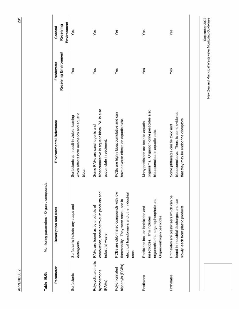
APPE
ND
IX 2
291
Sept
embe
r 200
2N
ew Z
eala
nd M
unic
ipal
Was
tew
ater
Mon
itorin
g G
uide
lines
Tabl
e 10
.G:
Mon
itorin
g pa
ram
eter
s - O
rgan
ic c
ompo
unds
.
Para
met
erD
escr
iptio
n an
d us
esEn
viro
nmen
tal R
elev
ance
Fres
hwat
erR
ecei
ving
Env
ironm
ent
Coa
stal
Rec
eivi
ngEn
viro
nmen
tSu
rfact
ants
Surfa
ctan
ts in
clud
e an
y so
aps
and
dete
rgen
ts.
Surfa
ctan
ts c
an re
sult
in v
isib
le fo
amin
gw
hich
affe
cts
both
aes
thet
ics
and
aqua
ticbi
ota.
Yes
Yes
Poly
cycl
ic a
rom
atic
hydr
ocar
bons
(PAH
s)
PAH
s ar
e fo
und
as b
y-pr
oduc
ts o
fco
mbu
stio
n, s
ome
petro
leum
pro
duct
s an
din
dust
rial w
aste
.
Som
e PA
Hs
are
carc
inog
enic
and
bioa
ccum
ulat
ive
in a
quat
ic b
iota
. PAH
s al
soac
cum
ulat
e in
sed
imen
t.
Yes
Yes
Poly
chlo
rinat
edbi
phen
yls
(PC
Bs)
PCBs
are
chl
orin
ated
com
poun
ds w
ith lo
wfla
mm
abilit
y. T
hey
wer
e on
ce u
sed
inel
ectri
cal t
rans
form
ers
and
othe
r ind
ustri
alus
es.
PCBs
are
hig
hly
bioa
ccum
ulat
ive
and
can
have
adv
erse
effe
cts
on a
quat
ic b
iota
.Ye
sYe
s
Pest
icid
esPe
stic
ides
incl
ude
herb
icid
es a
ndin
sect
icid
es.
This
incl
udes
orga
noch
lorin
e, o
rgan
opho
spha
te a
ndO
rgan
o-ni
troge
n pe
stic
ides
.
Man
y pe
stic
ides
are
toxi
c to
aqu
atic
orga
nism
s. O
rgan
ochl
orin
e pe
stic
ides
als
obi
oacc
umul
ate
in a
quat
ic b
iota
.
Yes
Yes
Phth
alat
esPh
thal
ates
are
pla
stic
iser
s w
hich
can
be
foun
d in
indu
stria
l dis
char
ges
and
can
slow
ly le
ach
from
pla
stic
pro
duct
s.
Som
e ph
thal
ates
can
be
toxi
c an
dbi
oacc
umul
ativ
e. T
here
is s
ome
evid
ence
that
they
may
be
endo
crin
e di
srup
tors
.
Yes
Yes

292
APPE
ND
IX 2
Sept
embe
r 200
2N
ew Z
eala
nd M
unic
ipal
Was
tew
ater
Mon
itorin
g G
uide
lines

APPE
ND
IX 2
293
Sept
embe
r 200
2N
ew Z
eala
nd M
unic
ipal
Was
tew
ater
Mon
itorin
g G
uide
lines
Tabl
e 10
.H:
Mon
itorin
g pa
ram
eter
s - B
acte
ria a
nd p
atho
gens
.
Para
met
erD
escr
iptio
n an
d us
esEn
viro
nmen
tal R
elev
ance
Fres
hwat
erR
ecei
ving
Envi
ronm
ent
Coa
stal
Rec
eivi
ngEn
viro
nmen
tE.
Col
iE.
Col
i is
a st
rain
of f
aeca
l bac
teria
, fou
nd in
gast
roin
test
inal
trac
ts o
f mam
mal
s.E.
Col
i is
the
indi
cato
r for
fres
h w
ater
use
d fo
rco
ntac
t rec
reat
ion
in th
e M
fE (2
002)
mic
robi
olog
ical
gui
delin
es.
Yes
No
Faec
al C
olifo
rms
Faec
al c
olifo
rms
are
bact
eria
foun
d in
hig
hnu
mbe
rs in
hum
an a
nd a
nim
al fa
eces
.Fa
ecal
col
iform
s ar
e th
e in
dica
tor f
or m
arin
ew
ater
use
d fo
r she
llfis
h ga
ther
ing
in th
e M
fE(2
002)
mic
robi
olog
ical
gui
delin
es.
No
Yes
Ente
roco
cci
Ente
roco
cci a
re a
stra
in o
f fae
cal b
acte
ria,
foun
d in
gas
troin
test
inal
trac
ts o
f mam
mal
s.En
tero
cocc
i are
the
indi
cato
r for
mar
ine
wat
erus
ed fo
r con
tact
recr
eatio
n in
the
MfE
(200
2)m
icro
biol
ogic
al g
uide
lines
.
No
Yes
Cam
pylo
bact
erC
ampy
loba
cter
are
pat
hoge
nic
bact
eria
.C
ampy
loba
cter
wer
e fo
und
at m
ore
than
hal
f the
site
s in
a re
cent
, ext
ensi
ve s
tudy
of r
ecre
atio
nal
fresh
wat
er s
ites
in N
Z (T
ill et
al.
2002
).
Yes
Yes
Prot
ozoa
Prot
ozoa
are
sin
gle-
cell
anim
als
and
incl
ude
Gia
rdia
and
Cry
ptos
porid
ium
.So
me
prot
ozoa
are
pat
hoge
nic
and
can
caus
ega
stro
-inte
stin
al d
isea
ses
Yes
Yes
Viru
ses
Viru
ses
are
para
sitic
org
anis
ms
cont
aini
ngD
NA
or R
NA
insi
de a
pro
tein
coa
ting.
Com
mon
wat
erbo
rne
viru
ses
can
caus
e he
patit
isan
d ga
stro
ente
ritis
.Ye
sYe
s

294
APPE
ND
IX 3
Sept
embe
r 200
2N
ew Z
eala
nd M
unic
ipal
Was
tew
ater
Mon
itorin
g G
uide
lines
APPE
ND
IX 3
:W
orks
heet
s fo
r Cha
pter
4 (u
se to
doc
umen
t HIA
MP
proc
ess)
WO
RK
SHEE
T A
– N
orm
al C
ondi
tions
Step
s 1.
1 to
1.4
Iden
tify
risks
(haz
ards
)St
ep 2
Anal
yse
norm
al ri
sks
Use
Tab
le A
Des
crib
e na
ture
of i
mpa
cts
or e
vent
(Ste
p 2.
1)As
sess
impa
ct le
vel &
like
lihoo
d fo
r eac
h im
pact
type
– u
se T
able
s D
& E
(Ste
ps 2
.2 &
2.3
)
Impa
ct le
vel:
A =
high
ly in
jurio
us, B
= c
ritic
al, C
= m
ajor
, D =
mod
erat
e, E
= s
light
, F =
insi
gnifi
cant
(see
Tab
les
D1
to D
6)
Freq
uenc
y:
I = c
ontin
uous
, II =
freq
uent
, III
= se
ason
al, I
V =
occ
asio
nal,
V =
poss
ible
(see
Tab
le E
)
Appr
opria
te R
esou
rces
?U
se T
able
F (S
tep
2.4)
Hum
an h
ealth
and
safe
tyEc
olog
yC
omm
unity
Valu
esEc
onom
icU
tility
Aest
hetic
sO
dour
leve
llik
eli-
hood
leve
llik
eli-
hood
leve
llik
eli-
hood
leve
llik
eli-
hood
leve
llik
eli-
hood
leve
llik
eli-
hood
1 =
deta
iled
man
agem
ent p
lan
2 =
stan
dard
app
roac
hes
3 =
inci
dent
al
none
= m
onito
ring
not a
ppro
pria
te
Gen
eral
Tem
pera
ture
pH SS/tu
rbid
ity,
colo
ur
BOD
, CO
D
Fats
, oils
and
grea
ses
Amm
onia
Nitr
ogen
Phos
phor
us
Path
ogen
s
Hea
vy m
etal
s
POPs
Sulp
hide
s
Cha
ract
eris
tics
of w
aste
wat
erdi
scha
rge
Odo
ur
Peak
flow
s
Con
tam
inan
t or W
aste
Slu
g
Odo
ur g
ener
atio
n fro
m p
lant
Solid
s di
spos
al
Oth
er s
ourc
es o
f ris
k (li
stbe
low
)

APPE
ND
IX 3
295
Sept
embe
r 200
2N
ew Z
eala
nd M
unic
ipal
Was
tew
ater
Mon
itorin
g G
uide
lines
WO
RK
SHEE
T B
– A
bnor
mal
Con
ditio
ns a
nd e
ffect
of g
ross
unc
erta
inty
Step
s 1.
1 to
1.4
Iden
tify
haza
rds
Step
2.5
Anal
yse
abno
rmal
risk
s (r
epea
t ste
ps 2
.1 to
2.4
for a
bnor
mal
risk
s)
Use
Tab
le B
Des
crib
e na
ture
of i
mpa
cts
or e
vent
(Ste
p 2.
1)As
sess
impa
ct le
vel &
like
lihoo
d fo
r eac
h im
pact
type
– u
se T
able
s D
& E
(Ste
ps 2
.2 &
2.3
)
Impa
ct le
vel:
A =
high
ly in
jurio
us, B
= c
ritic
al, C
= m
ajor
, D =
mod
erat
e, E
= s
light
, F =
insi
gnifi
cant
(see
Tab
les
D1
to D
6)
Freq
uenc
y:
I = c
ontin
uous
, II =
freq
uent
, III
= se
ason
al, I
V =
occ
asio
nal,
V =
poss
ible
(see
Tab
le E
)
Appr
opria
te R
esou
rces
?U
se T
able
F (S
tep
2.4)
Hum
an h
ealth
and
safe
tyEc
olog
yC
omm
unity
Valu
esEc
onom
icU
tility
Aest
hetic
sO
dour
leve
llik
eli-
hood
leve
llik
eli-
hood
leve
llik
eli-
hood
leve
llik
eli-
hood
leve
llik
eli-
hood
leve
llik
eli-
hood
1 =
deta
iled
man
agem
ent p
lan
2 =
stan
dard
app
roac
hes
3 =
inci
dent
al
none
= m
onito
ring
not
appr
opria
te
(see
Tab
le F
)
Con
stitu
ents
of c
once
rn fo
rtre
atm
ent p
lant
faul
tco
nditi
ons
Con
stitu
ents
of c
once
rn fo
rtre
atm
ent p
lant
ups
etco
nditi
on (e
.g.,
from
tox
icsh
ocks
)
Ups
et o
f pla
nt re
late
d to
extre
me
wea
ther
Abno
rmal
con
stitu
ents
intra
de w
aste
s
Is th
ere
a ch
arac
teris
tic o
f the
envi
ronm
ent t
hat m
ay re
sult
inpa
rticu
lar
sen
sitiv
ity u
nder
spec
ific
unus
ual c
ondi
tions
?
Proc
ess
unce
rtain
ty (i
s th
ere
a si
gnifi
cant
asp
ect o
f the
proc
ess
beha
viou
r tha
t is
unce
rtain
?)
Con
tam
inan
t com
posi
tion
unce
rtain
ty
Sign
ifica
nt la
ck o
f kno
wle
dge
of
envi
ronm
enta
l beh
avio
ur(u
ncer
tain
ty re
gard
ing
ecos
yste
m d
ynam
ics
etc)
Oth
er c
ause
s of
risk
(lis
tbe
low
)

296
APPE
ND
IX 4
Sept
embe
r 200
2N
ew Z
eala
nd M
unic
ipal
Was
tew
ater
Mon
itorin
g G
uide
lines
APPE
ND
IX 4
:Exa
mpl
e of
use
of W
orks
heet
s fo
r Cha
pter
4
The
follo
win
g is
an
exam
ple
usin
g th
e H
IAM
P pr
oces
s. R
efer
als
o to
exa
mpl
e W
orks
heet
s A a
nd B
on
follo
win
g pa
ges.
The
exam
ple
uses
the
follo
win
g sc
enar
io:
• Pl
ant s
erve
s sm
all t
owns
hip
of a
pop
ulat
ion
of a
ppro
xim
atel
y 50
00
• Li
ght i
ndus
try in
clud
ing
a pl
ate
shop
is si
ted
near
by.
The
asso
ciat
ed tr
ade
was
te is
wel
l
cont
rolle
d bu
t som
e ch
emic
als t
hat c
ould
be
spilt
wou
ld b
e ex
pect
ed to
cau
se p
robl
ems.
• Th
e pl
ant u
ses e
stab
lishe
d te
chno
logy
• A
smal
l loc
al c
omm
unity
is si
ted
near
to th
e pl
ant b
ound
ary
• Th
e sh
ort o
utfa
ll di
scha
rges
into
a lo
cal m
arin
e ba
y
• Th
ere
is a
smal
l sw
imm
ing
beac
h on
the
bay
and
shel
lfish
and
oth
er re
crea
tiona
l fis
hing
take
s
plac
e so
me
dist
ance
from
the
outfa
ll.
• Th
e ba
y ex
hibi
ts m
oder
atel
y go
od fl
ushi
ng
The
risk
anal
ysis
(see
wor
kshe
ets o
n fo
llow
ing
page
s) d
emon
stra
tes t
hat s
tand
ard
mon
itorin
g re
gim
es a
re d
eem
ed a
ppro
pria
te e
xcep
t for
pat
hoge
ns a
nd m
etal
s fro
m lo
cal t
rade
pro
cess
es, w
here
a d
etai
led
man
agem
ent p
lan
and
dedi
cate
d
reso
urce
s sho
uld
be c
onsi
dere
d.

APPE
ND
IX 4
297
Sept
embe
r 200
2N
ew Z
eala
nd M
unic
ipal
Was
tew
ater
Mon
itorin
g G
uide
lines
WO
RK
SHEE
T A
– N
orm
al C
ondi
tions
– E
XAM
PLE
Step
s 1.
1 to
1.4
Iden
tify
risks
(haz
ards
)St
ep 2
Anal
yse
norm
al ri
sks
Use
Tab
le A
Des
crib
e na
ture
of i
mpa
cts
or e
vent
(Ste
p 2.
1)As
sess
impa
ct le
vel &
like
lihoo
d fo
r eac
h im
pact
type
– u
se T
able
s D
& E
(Ste
ps 2
.2 &
2.3
)
Impa
ct le
vel:
A =
high
ly in
jurio
us, B
= c
ritic
al, C
= m
ajor
, D =
mod
erat
e, E
= s
light
, F =
insi
gnifi
cant
(see
Tab
les
D1
to D
6)
Freq
uenc
y:
I = c
ontin
uous
, II =
freq
uent
, III
= se
ason
al, I
V =
occ
asio
nal,
V =
poss
ible
(see
Tab
le E
)
Appr
opria
te R
esou
rces
?U
se T
able
F (S
tep
2.4)
Hum
an h
ealth
and
safe
tyEc
olog
yC
omm
unity
Valu
esEc
onom
icU
tility
Aest
hetic
sO
dour
leve
llik
eli-
hood
leve
llik
eli-
hood
leve
llik
eli-
hood
leve
llik
eli-
hood
leve
llik
eli-
hood
leve
llik
eli-
hood
1 =
deta
iled
man
agem
ent p
lan
2 =
stan
dard
app
roac
hes
3 =
inci
dent
al
none
= m
onito
ring
not a
ppro
pria
te
Gen
eral
Som
e lo
cal c
once
rns
rega
rdin
g w
aste
dis
char
ge to
the
sea
due
to s
trong
cul
tura
l ide
ntity
with
bay
.C
once
rns
may
als
o af
fect
pos
sibl
e us
e of
bay
for f
ish
farm
ing
CI
DI
2
Tem
pera
ture
No
antic
ipat
ed m
easu
rabl
e ad
vers
e im
pact
FI
3
pHN
o an
ticip
ated
mea
sura
ble
adve
rse
impa
ctF
I3
SS/tu
rbid
ity,
colo
urPo
ssib
le lo
calis
ed im
pact
cau
sing
vis
ible
col
our c
hang
eE
IV3
BOD
, CO
DPo
ssib
le s
easo
nal i
mpa
ct b
ut li
kely
to b
e m
inor
DIV
DIV
2
Fats
, oils
and
grea
ses
No
antic
ipat
ed m
easu
rabl
e ad
vers
e im
pact
FI
3
Amm
onia
Nitr
ogen
Phos
phor
us
Path
ogen
sSw
imm
ing
beac
h is
not
exp
ecte
d to
be
affe
cted
. H
owev
er, s
hellf
ish
colle
ctio
n ta
kes
plac
e ne
ar to
disc
harg
e. S
ome
fishi
ng ta
kes
plac
e in
bay
.B
IIID
III1
Hea
vy m
etal
sLi
mite
d lo
calis
ed o
dour
pos
sibl
e at
dis
char
ge lo
catio
nC
IV2
POPs
Sulp
hide
s
Cha
ract
eris
tics
ofw
aste
wat
er d
isch
arge
Odo
urLi
mite
d lo
calis
ed o
dour
pos
sibl
e at
dis
char
ge lo
catio
nE
II3
Peak
flow
sSo
me
scou
ring
of m
ud c
hann
el e
xpec
ted
durin
g hi
gh ra
in e
vent
s du
e to
sto
rmw
ater
in
gres
s to
sew
age
syst
emE
IV3
Con
tam
inan
t or W
aste
Slug
Loca
l pla
te s
hop
flush
es v
ats
ever
y fe
w m
onth
s –
Not
toxi
c to
pro
cess
but
hig
her t
han
norm
al m
etal
sle
vels
exp
ecte
d at
tim
es.
This
cou
ld a
ccum
ulat
e in
she
ll fis
hB
IIID
IIIC
IIIB
III1
Odo
ur g
ener
atio
n fro
mpl
ant
Proc
ess
know
n to
cau
se o
dour
if n
ot o
pera
ting
at o
ptim
um c
ondi
tion
CIV
2
Solid
s di
spos
alSo
lids
will
be tr
ucke
d aw
ay v
ia m
ain
road
thro
ugh
loca
l com
mun
ity to
new
land
fill.
Som
e un
certa
inty
rega
rdin
g gr
ound
wat
er u
nder
land
fill.
Com
mun
ity e
xpre
ssed
wis
h fo
r com
post
ing.
Som
e od
our,
seag
ulls
and
rest
ricte
d us
e of
sur
roun
ding
land
.
FI
DI
DI
DI
EI
2

298
APPE
ND
IX 4
Sept
embe
r 200
2N
ew Z
eala
nd M
unic
ipal
Was
tew
ater
Mon
itorin
g G
uide
lines
Oth
er s
ourc
es o
f ris
k (li
stbe
low
)N
one
iden
tifie
d
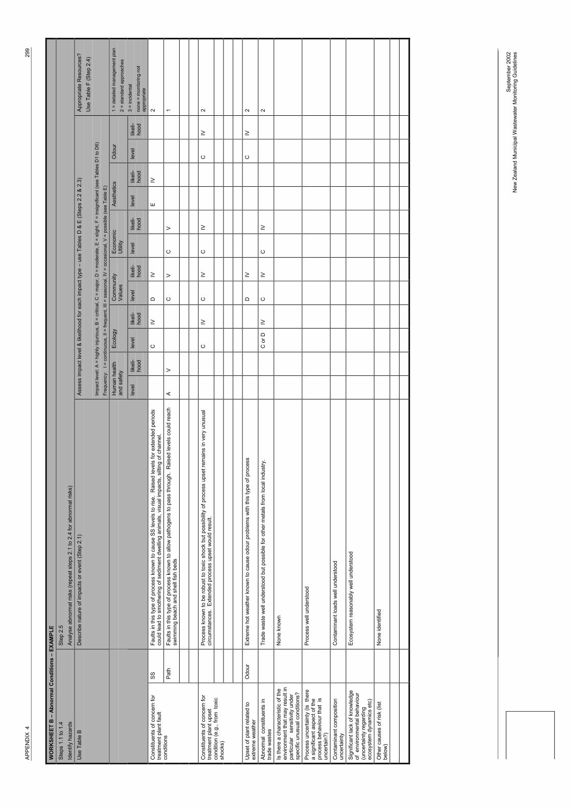
APPE
ND
IX 4
299
Sept
embe
r 200
2N
ew Z
eala
nd M
unic
ipal
Was
tew
ater
Mon
itorin
g G
uide
lines
WO
RK
SHEE
T B
– A
bnor
mal
Con
ditio
ns –
EXA
MPL
ESt
eps
1.1
to 1
.4Id
entif
y ha
zard
sSt
ep 2
.5An
alys
e ab
norm
al ri
sks
(repe
at s
teps
2.1
to 2
.4 fo
r abn
orm
al ri
sks)
Use
Tab
le B
Des
crib
e na
ture
of i
mpa
cts
or e
vent
(Ste
p 2.
1)As
sess
impa
ct le
vel &
like
lihoo
d fo
r eac
h im
pact
type
– u
se T
able
s D
& E
(Ste
ps 2
.2 &
2.3
)
Impa
ct le
vel:
A =
high
ly in
jurio
us, B
= c
ritic
al, C
= m
ajor
, D =
mod
erat
e, E
= s
light
, F =
insi
gnifi
cant
(see
Tab
les
D1
to D
6)
Freq
uenc
y:
I = c
ontin
uous
, II =
freq
uent
, III
= se
ason
al, I
V =
occ
asio
nal,
V =
poss
ible
(see
Tab
le E
)
Appr
opria
te R
esou
rces
?U
se T
able
F (S
tep
2.4)
Hum
an h
ealth
and
safe
tyEc
olog
yC
omm
unity
Valu
esEc
onom
icU
tility
Aest
hetic
sO
dour
leve
llik
eli-
hood
leve
llik
eli-
hood
leve
llik
eli-
hood
leve
llik
eli-
hood
leve
llik
eli-
hood
leve
llik
eli-
hood
1 =
deta
iled
man
agem
ent p
lan
2 =
stan
dard
app
roac
hes
3 =
inci
dent
al
none
= m
onito
ring
not
appr
opria
te
SSFa
ults
in th
is ty
pe o
f pro
cess
kno
wn
to c
ause
SS
leve
ls to
rise
. R
aise
d le
vels
for e
xten
ded
perio
dsco
uld
lead
to s
mot
herin
g of
sed
imen
t dw
ellin
g an
imal
s, v
isua
l im
pact
s, s
iltin
g of
cha
nnel
.C
IVD
IVE
IV2
Path
Faul
ts in
this
type
of p
roce
ss k
now
n to
allo
w p
atho
gens
to p
ass
thro
ugh.
Rai
sed
leve
ls c
ould
reac
hsw
imm
ing
beac
h an
d sh
ell f
ish
beds
AV
CV
CV
1
Con
stitu
ents
of c
once
rn fo
rtre
atm
ent p
lant
faul
tco
nditi
ons
Proc
ess
know
n to
be
robu
st to
toxi
c sh
ock
but p
ossi
bilit
y of
pro
cess
ups
et re
mai
ns in
ver
y un
usua
lci
rcum
stan
ces.
Ext
ende
d pr
oces
s up
set w
ould
resu
lt.C
IVC
IVC
IVC
IV2
Con
stitu
ents
of c
once
rn fo
rtre
atm
ent p
lant
ups
etco
nditi
on (e
.g.,
from
tox
icsh
ocks
)
Ups
et o
f pla
nt re
late
d to
extre
me
wea
ther
Odo
urEx
trem
e ho
t wea
ther
kno
wn
to c
ause
odo
ur p
robl
ems
with
this
type
of p
roce
ssD
IVC
IV2
Abno
rmal
con
stitu
ents
intra
de w
aste
sTr
ade
was
te w
ell u
nder
stoo
d bu
t pos
sibl
e fo
r oth
er m
etal
s fro
m lo
cal i
ndus
try.
C o
r DIV
CIV
CIV
2
Is th
ere
a ch
arac
teris
tic o
f the
envi
ronm
ent t
hat m
ay re
sult
inpa
rticu
lar
sen
sitiv
ity u
nder
spec
ific
unus
ual c
ondi
tions
?
Non
e kn
own
Proc
ess
unce
rtain
ty (i
s th
ere
a si
gnifi
cant
asp
ect o
f the
proc
ess
beha
viou
r tha
t is
unce
rtain
?)
Proc
ess
wel
l und
erst
ood
Con
tam
inan
t com
posi
tion
unce
rtain
tyC
onta
min
ant l
oads
wel
l und
erst
ood
Sign
ifica
nt la
ck o
f kno
wle
dge
of e
nviro
nmen
tal b
ehav
iour
(unc
erta
inty
rega
rdin
gec
osys
tem
dyn
amic
s et
c)
Ecos
yste
m re
ason
ably
wel
l und
erst
ood
Oth
er c
ause
s of
risk
(lis
tbe
low
)N
one
iden
tifie
d