Florida International UniversityFIU Digital Commons

FIU Electronic Theses and Dissertations University Graduate School

3-17-2015

Acoustic Manipulation and Alignment of Particlesfor Applications in Separation, Micro-Templating,and Device FabricationKAMRAN MORADIFlorida International University, kmora019@fiu.edu

DOI: 10.25148/etd.FI15032198Follow this and additional works at: https://digitalcommons.fiu.edu/etd

Part of the Acoustics, Dynamics, and Controls Commons, Applied Mechanics Commons,Electro-Mechanical Systems Commons, Energy Systems Commons, and the Semiconductor andOptical Materials Commons

This work is brought to you for free and open access by the University Graduate School at FIU Digital Commons. It has been accepted for inclusion inFIU Electronic Theses and Dissertations by an authorized administrator of FIU Digital Commons. For more information, please contact dcc@fiu.edu.

Recommended CitationMORADI, KAMRAN, "Acoustic Manipulation and Alignment of Particles for Applications in Separation, Micro-Templating, andDevice Fabrication" (2015). FIU Electronic Theses and Dissertations. 1753.https://digitalcommons.fiu.edu/etd/1753

FLORIDA INTERNATIONAL UNIVERSITY

Miami, Florida

ACOUSTIC MANIPULATION AND ALIGNMENT OF PARTICLES FOR

APPLICATIONS IN SEPARATION, MICRO-TEMPLATING AND DEVICE

FABRICATION

A dissertation submitted in partial fulfillment of

the requirements for the degree of

DOCTOR OF PHILOSOPHY

in

MECHANICAL ENGINEERING

by

Kamran Moradi

2015

ii

To: Dean Amir Mirmiran College of Engineering and Computing

This dissertation, written by Kamran Moradi, and entitled Acoustic Manipulation and Alignment of Particles for Applications in Separation, Micro-Templating, and Device Fabrication, having been approved in respect to style and intellectual content, is referred to you for judgment.

We have read this dissertation and recommend that it be approved.

_______________________________________ George S. Dulikravich

_______________________________________

Ibrahim Nur Tansel

_______________________________________ Nezih Pala

_______________________________________

Na Li

_______________________________________ Bilal El-Zahab, Major Professor

Date of Defense: March 17, 2015

The dissertation of Kamran Moradi is approved.

_______________________________________ Dean Amir Mirmiran

College of Engineering and Computing

_______________________________________ Dean Lakshmi N. Reddi

University Graduate School

Florida International University, 2015

iii

© Copyright 2015 by Kamran Moradi

All rights reserved.

iv

DEDICATION

To the last moment of my life.

v

ACKNOWLEDGMENTS

First and foremost, I want to thank my advisor Bilal El-Zahab. It has been an honor to be

his first graduated Ph.D. student. He has taught me, both consciously and unconsciously,

how good experimental mechanics can be done. I appreciate all his contributions of time,

idea, and funding to make my Ph.D. experience productive and stimulating. The joy and

enthusiasm he has for his research was contagious and motivational for me, even during

tough times in the Ph.D. pursuit. I am also thankful for the excellent example he has

provided as a successful researcher.

The members of energy and microfluidic group have contributed immensely to my

personal and professional time at FIU. The group has been a source of friendships as well

as good advice and collaboration. I would also like to acknowledge the Advanced

Materials Engineering Research Institute (AMERI) and in particular Mr. Neal Ricks who

helped me during my Ph.D. research to learn and accomplish microfabrication processes.

My gratitude is also extended to the members of my dissertation committee for their

support, patience and valuable discussions, in particular, Dr. George S. Dulikravich, Dr.

Ibrahim Nur Tansel, Dr. Nezih Pala, and Dr. Na Li. I would like to acknowledge the

Mechanical and Materials engineering department funding assistantships, dissertation

year fellowship from the FIU graduate school during the last year of dissertation research,

and NSF funding during my PhD.

My time at Florida International University was made enjoyable in large part due to the

many friends and groups that became a part of my life. I am grateful for time spent with

my roommates and friends, for our memorable activities experiencing beautiful city

Miami and great country, the United States of America.

vi

Lastly, I would like to thank my family for all their love and encouragement. For my

parents, Khosrow and Mastoureh who raised me with love, supported me in all my

pursuits, and were able to tolerate the hardship of being far from me for all my Ph.D.

period from thousands miles away. For my brother, Shahram, who has been my light to

truth, which always delivers me towards peace and confidence. And most of all for my

loving, supportive, encouraging, and patient wife Banessa whose faithful support during

the final stages of this Ph.D. is so appreciated. Thank you.

vii

ABSTRACT OF THE DISSERTATION

ACOUSTIC MANIPULATION AND ALIGNMENT OF PARTICLES FOR

APPLICATIONS IN SEPARATION, MICRO-TEMPLATING, AND DEVICE

FABRICATION

by

Kamran Moradi

Florida International University, 2015

Miami, Florida

Professor Bilal El-Zahab, Major Professor

This dissertation studies the manipulation of particles using acoustic stimulation for

applications in microfluidics and templating of devices. The term particle is used here to

denote any solid, liquid or gaseous material that has properties, which are distinct from

the fluid in which it is suspended. Manipulation means to take over the movements of the

particles and to position them in specified locations.

Using devices, microfabricated out of silicon, the behavior of particles under the acoustic

stimulation was studied with the main purpose of aligning the particles at either low-

pressure zones, known as the nodes or high-pressure zones, known as anti-nodes. By

aligning particles at the nodes in a flow system, these particles can be focused at the

center or walls of a microchannel in order to ultimately separate them. These separations

are of high scientific importance, especially in the biomedical domain, since

acoustopheresis provides a unique approach to separate based on density and

compressibility, unparalleled by other techniques. The study of controlling and aligning

viii

the particles in various geometries and configurations was successfully achieved by

controlling the acoustic waves.

Apart from their use in flow systems, a stationary suspended-particle device was

developed to provide controllable light transmittance based on acoustic stimuli. Using a

glass compartment and a carbon-particle suspension in an organic solvent, the device

responded to acoustic stimulation by aligning the particles. The alignment of light-

absorbing carbon particles afforded an increase in visible light transmittance as high as

84.5%, and it was controlled by adjusting the frequency and amplitude of the acoustic

wave. The device also demonstrated alignment memory rendering it energy-efficient. A

similar device for suspended-particles in a monomer enabled the development of

electrically conductive films. These films were based on networks of conductive

particles. Elastomers doped with conductive metal particles were rendered surface

conductive at particle loadings as low as 1% by weight using acoustic focusing. The

resulting films were flexible and had transparencies exceeding 80% in the visible

spectrum (400-800 nm) These films had electrical bulk conductivities exceeding 50 S/cm.

ix

TABLE OF CONTENTS

CHAPTER PAGE

1 Introduction ................................................................................................................... 11.1 Background ................................................................................................................. 11.2 Particle Manipulations Methods ................................................................................. 11.2.1 Acoustophoresis ....................................................................................................... 21.2.2 Inertial .................................................................................................................... 141.2.3 Magnetophoresis .................................................................................................... 161.2.4 Electrophoresis and Di-Electrophoresis ................................................................. 181.2.5 Comparison of Particle Manipulation Methods ..................................................... 21

2 Chip Microfabrication Processes ................................................................................ 232.1 Introduction .............................................................................................................. 232.1.1 Pattern Generation ................................................................................................. 232.1.2 Photomask .............................................................................................................. 262.1.3 Photomask Inspection ............................................................................................ 282.2 Photolithography ...................................................................................................... 342.2.1 Lithography Instrument (Alignment and Exposure) .............................................. 352.2.2 Lithography Inspection .......................................................................................... 372.3 Photoresists and Coating .......................................................................................... 392.4 Developing ................................................................................................................ 412.5 Etching ...................................................................................................................... 432.5.1 Wet Etching ........................................................................................................... 432.5.2 Dry Etching: ........................................................................................................... 472.6 Anodic Bonding: ....................................................................................................... 50

3 Acoustic Focusing in Flow Systems ........................................................................... 53Abstract ............................................................................................................................. 533.1 Introduction .............................................................................................................. 533.2 Device Design and Fabrication ................................................................................. 573.3 Results and Conclusion ............................................................................................ 66

4 Novel Optical Switchable Transparency driven by Acoustophoresis ........................ 72Abstract ............................................................................................................................. 724.1 Introduction .............................................................................................................. 724.2 Experimental Procedure: .......................................................................................... 734.3 Results and Discussion: ............................................................................................ 744.4 Conclusions .............................................................................................................. 80

5 Transparent and Anisotropic Conductive Film Templated Using Acoustic Focusing 81Abstract ............................................................................................................................. 815.1 Introduction .............................................................................................................. 815.2 I-V experiment .......................................................................................................... 89

x

5.3 Transparency Analysis ............................................................................................. 915.4 Experimental Section ................................................................................................ 95

6 Conclusions and future works ..................................................................................... 97

7 References ................................................................................................................. 100

8 VITA ......................................................................................................................... 110

xi

LIST OF TABLES

TABLE PAGE

Table 1.1. Density, speed of sound and acoustic impedance of some materials [16] ........13

Table 1.2. Summary of particle manipulation methods, features, and limitations. ...........21

Table 2.1. Chromium etchant 1010 specifications. ............................................................33

Table 2.2. AZ-4620 spin-coating and lithography recipe. .................................................41

Table 2.3. Wet etching rate of Si with different KOH concentrations. .............................44

Table 2.4. Specification of silicon etchants [66] ................................................................45

Table 2.5. RIE etching parameters for LSN and photoresist etching. ..............................49

Table 2.6. List of common plasma and wet etchants in microfabrication. ........................50

Table 3.1. Experiments of medium density variation to find the sign changing point for acoustic contrast factor. ..............................................................................................70

Table 5.1. Summary of the resistances in the X and Y-directions of the films for 1%, 2%, 5%, and 10% particle loading and films prepared using no acoustic stimulation, 150 kHz frequency, and 2 MHz frequencies. .........................................88

xii

LIST OF FIGURES

FIGURES PAGES

Figure 1.1. Schematic of acoustophoresis phenomena with a single transducer and one reflector or two transducers acting in opposite directions. ...........................................3

Figure 1.2. Schematic of standing-wave adaption to a microchannel. ................................4

Figure 1.3. Cross-sectional sketch of a straight, silicon walls (gray) fluid-filled. microchannel of width w with a transverse, standing, ultrasound λ/2 -pressure resonance pin(z)=Pacos(kz), wavenumber k= π/w , in physical (0<z<w)and frequency domain (0<z<π . .........................................................................................5

Figure 1.4. Transverse and layered resonator device schematics ......................................12

Figure 1.5. Layered resonator device to generate transverse wave. ..................................12

Figure 1.6. Schematic of microparticles migration locations in inertia method. ...............15

Figure 1.7. Schematic of a charged particle experiencing electrophoresis. .......................18

Figure 1.8. a) Negative DEP force and Re[fCM(w)]<0, b) positive DEP force and Re[fCM(w)] > 0 ............................................................................................................20

Figure 2.1. Example of exposure energy amount on the uPG 101 instrument software. ..24

Figure 2.2. CAD light field sample channel. ....................................................................25

Figure 2.3. a) exposing the pattern on the resist, b) removing the resist from exposed parts, c) removing the chrome from the open area, d) striping the photomask ..........27

Figure 2.4. Optical microscopy inspection of photomask before chrome etching. ...........28

Figure 2.5. Underexposed mask (black dash line is the boundary of the pattern, red strips are the resist residue) ........................................................................................29

Figure 2.6. Underexposed mask (black dash line is the boundary of the pattern). ............30

Figure 2.7. Inadequately focused result in mask making process (black line is the boundary of the pattern). ............................................................................................31

Figure 2.8. Photomask after patterning and before chrome etching. .................................32

Figure 2.9. Final dark field photomask that can be used in photolithography. ..................33

Figure 2.10. Final bright field photomask that can be used in photolithography. .............34

Figure 2.11. Photolithography process flowchart. .............................................................35

xiii

Figure 2.12. Wafer alignment using three pins (inside of yellow circles) on the mask aligner. ........................................................................................................................36

Figure 2.13. Mask aligner demonstration. .........................................................................37

Figure 2.14. Possible lithography patterning defects, a) underexposed type one, b) underexposed type two. ..............................................................................................38

Figure 2.15. Possible lithography patterning defects, a) over-exposed, b) over-developed. ...................................................................................................................39

Figure 2.16. Spin coating process, a) photoresist deposition, b) low speed circulation, c) high speed circulation. ................................................................................................40

Figure 2.17. Photoresist exposure on, a) positive photoresist, b) negative photoresist - grey: substrate, red: photoresist. .................................................................................42

Figure 2.18. a) Isometric scanning electron microscopy of the microchannel with vertical walls and etched with PSE-200, b) cross section of the microchannel. ........46

Figure 2.19. Microchannel after wet etching. left) microchannel, middle) the fork, right) bottom of the microchannel. .......................................................................................47

Figure 2.20. Reactive ion etching schematics. ...................................................................48

Figure 2.21. Plasma etching process parameters. .............................................................49

Figure 2.22. Standard anodic bonding setup. .....................................................................51

Figure 3.1. Schematic of acoustic device and acoustic zone for focusing the microparticles in the center. .......................................................................................54

Figure 3.2. Microfluific patterning on parafilm sheet using digital cutting. ......................58

Figure 3.3. Microfluidic patterning on parafilm sheet using laser. ....................................59

Figure 3.4. Microfluidic patterning on plastic slides using laser. ......................................60

Figure 3.5. Microfluidic patterning on glass using high speed driller. .............................60

Figure 3.6. Schematic of silicon etching process and related parameters. .......................61

Figure 3.7. Schematic of patterning the microchannel on silicon wafer substrate using photolithography method............................................................................................62

Figure 3.8. Schematic of mask making process. ................................................................63

Figure 3.9. Exploded view of device schematic. ...............................................................64

Figure 3.10. Assembled view of device schematic. ...........................................................64

xiv

Figure 3.11. Assembled acoustic focusing device .............................................................65

Figure 3.13. Results in different frequencies and Vpp=10 volt, a) suspension with no acoustic energy, b) frequency= 1.305 MHz, c) frequency = 2.649 MHz, d) frequency 3,992 MHz, e) frequency = 5.435 MHz, f) frequency = 6.778 MHz. .......67

Figure 3.14. Separation of glass gel microparticles at 1.305 MHz and 20 Vpp. ...............67

Figure 3.15. Separation of glass gel microparticles at 4.051 MHz and 20 Vpp. ...............68

Figure 3.16. Separation of glass gel microparticles at 5.365 MHz and 20 Vpp. ...............69

Figure 4.1. Schematic presentation of the experimental setup used in the device transmittance study. ....................................................................................................74

Figure 4.2. Schematic of the direction of the acoustic radiation force for rigid (black) and flexible (blue) particle/droplet in an acoustic standing wave. Black arrows denote the direction of the momentum transfer and the green arrows denote the direction of the net force and thus the resulting motion. ............................................75

Figure 4.3. Comparison of the randomly disperse (left) versus the aligned particles (right) caused by switching on the acoustic radiation. ...............................................75

Figure 4.4 - Spectrophotometric analysis of the device filled with acetone (triangles) and 10% suspended-particles (circles) between 400 and 800 nm. .............................76

Figure 4.5- Image processing approach used to determine the percent light transmittance applied for (1) the original images at various frequencies of 222 kHz, 757 kHz, and 1.51 MHz, (2) after application of red filter, (3) after application of grayscale filter, (4) after application of monochrome filter. ......................................77

Figure 4.6. Light transmittance of the device at frequencies of 222 kHz, 757 kHz, and 1.51 MHz. The asterisk marked data point corresponds to no acoustic stimulation. .78

Figure 4.7. Transmittance memory of the device operated at 2 MHz and 20 Vpp showing the retention of transmittance after the acoustic stimulation was switched off. The asterisk marked data point corresponds to no acoustic stimulation. The insets correspond to optical micrographs of the device at each of the corresponding times. ..........................................................................................................................80

Figure 5.1. Schematic of the steady-state particles’ assembly in a half wavelength resonator compartments for: gravity-dominated mode (left), acoustics-dominated mode (middle), and mixed gravity-acoustics mode (right), which is observed in this paper ....................................................................................................................85

Figure 5.2. UV exposure process .......................................................................................86

Figure 5.3. Optical micrographs in transmission mode of: (a) 10% suspension of the particles in the compartment fully dispersed, (b) 10% suspension of the particles

xv

after acoustic alignment at 2 MHz and 16 Vpp, (c) 2% suspension of the particles fully dispersed, and (d) 2% suspension of the particles after acoustic alignment at 2 MHz and 16 Vpp ........................................................................................................87

Figure 5.4. Schematic presentation of the setup used for testing the surface resistivity of the films. The setup used two gold electrode plates with adjustable spacing that were connected to an Ohmmeter. ...............................................................................88

Figure 5.5. Circuit schematic to measure the V- I experiment ..........................................89

Figure 5.6. I-V curve (current vs. voltage), when the measured resistance of the film is 1.01 ohm .....................................................................................................................90

Figure 5.7. Anisotropic conductive film experimental setup .............................................90

Figure 5.8. Flexibility demonstration of the cured polymer while the conductive particles are aligned acoustically and embedded on one side ....................................91

Figure 5.9. Transmittance of the films prepared using (Δ) 2% particles, () 5% particles, and () 10% particles for randomly suspended particles with no acoustic stimulation ..................................................................................................................92

Figure 5.10. Transmittance of the films prepared using (Δ) 2% particles, () 5% particles, and () 10% particles for randomly suspended particles with acoustically aligned particles using 150 kHz .................................................................................93

Figure 5.11. Transmittance of the films prepared using (Δ) 2% particles, () 5% particles, and () 10% particles for randomly suspended particles with acoustically aligned particles using 2 MHz. ...................................................................................94

1

1 Introduction

1.1 Background

Miniaturization has progressed considerably in the last decade. It has found utility in

many systems, including mechanical, electrical, biological, and others. The science that

deals with the flow of fluids and suspensions in channels with less than millimeter-sized

cross-sections under the influence of external forces is called microfluidics. External

forces could be acoustic, magnetic, or electric, among others. Microfluidic devices have

been extensively developed because of their usefulness in analytical sciences and bio-

analysis [1]. The separation and sorting of biological cells is critical to a variety of

biomedical applications, including diagnostics, therapeutics and fundamental cell biology

[2]. The microfluidic platform technology has been fast progressing towards the

miniaturization, integration, and automation of biological and chemical assays [3], [4].

One of the representative output technologies in this trend is lab-on-a-chip (LOC)

devices, also known as micro total analysis systems, which combine lab-scale tasks on a

single mini-scale chip [5], [6]. They have two main significances, first, they require small

volume of sample size, which increases the synthesis and analysis process speed, and

reduces the consumption of reagent and cost. On the other hand, these devices are

compact, which allows multiple analyses and process parallelization to occur

simultaneously, yielding high throughput analyses [7], [8].

1.2 Particle Manipulations Methods

Manipulating and separating particles is a critical activity in a variety of engineering,

medical, and biochemical applications. However, LOCs have several advantages over

traditional large-scale methods, which are often labor intensive and require multiple tags

2

or labels to identify target particles. One of the most traditional and still promising

methods that is used to separate particles based on their density is centrifugation [9].

Centrifugation is a manual and macroscale technique, which requires labor dedication,

long operation times, large sample sizes, and is prone to contamination [10]. There is

significant interest in the manipulation of particles using label-free methods that utilize

their intrinsic properties, such as size, density, shape, and electrical polarizability.

Extrinsic properties, such as magnetization to execute manipulation or separation from

fluidic media, are also of interest. Acoustic, optical, magnetic, electrical, inertial, and

hydrodynamic approaches have been developed and implemented in different biological

and engineering applications. Some basics and definitions of these methodologies are

discussed and compared in the next sections.

1.2.1 Acoustophoresis

Acoustic waves carry pressure profiles, which generate acoustic forces. Particles exposed

to this force will be affected and consequently displaced, either to pressure nodes or

pressure anti-nodes, depending on the physical properties of the particles and the

suspending medium. The process of manipulating particles using such acoustic forces is

called acoustophoresis [11], [12]. A very general way of designing an acoustic resonator

for manipulation purposes includes a cavity or a microchannel in which both walls are

smooth and parallel to each other to promote efficient focusing. In the simplest design,

one wall acts as a resonator while the opposite wall acts as a passive/active resonator

(Figure 1.1).

3

Figure 1.1. Schematic of acoustophoresis phenomena with a single transducer and one reflector or two transducers acting in opposite directions.

A modern microfabrication method is required that will be discussed in the next chapter.

The acoustic wave is either generated by piezoelectric transducers, which is most

commonly composed of lead zirconate titanate (PZT), or inter-digitated transducers

(IDT) [13]–[15]. These transducers should be able to act in different resonance modes,

depending on the application. However, there is a material limitation in PZT

manufacturing. The possibility of generating very high frequencies in higher voltages is

challenging. The standing wave has two main parameters: frequency and amplitude.

Every standing wave has a node and an anti-node, as shown in Figure 1.2. In order to

have a single node in the microchannel, the microchannel can be designed to have the

same width as the length of half a standing-wavelength. This is the main relationship

between physical and frequency domain. Travelling acoustic waves have two parameters,

wavelength and frequency. Their multiplication yields the speed of that acoustic wave in

4

that media. Having the width of the cavity or microchannel and the frequency can give us

the speed of travelling standing wave into suspension.

Figure 1.2. Schematic of standing-wave adaption to a microchannel.

To quantify the acoustic force on the particles in a suspension, a mathematical model was

developed to justify the physics of the acoustophoresis. To find the one-dimensional

transverse, standing, ultrasound, /2 pressure resonance is defined in Equation 1.1 as:

Equation 1.1

1 cos cos2

2

2 cos

2

2

cos

where w is the width of microchannel and is equal to the half of wavelength ( . k is the

wavenumber which maps the frequency domain ( ) to the physical domain (z

direction 0 ). (Figure 1.3)

5

Figure 1.3. Cross-sectional sketch of a straight, silicon walls (gray) fluid-filled. microchannel of width w with a transverse, standing, ultrasound /2-pressure resonance

pin(z)=Pacos(kz), wavenumber k= / , in physical (0<z<w)and frequency domain (0<z< .

The first order incoming acoustic field are given by:

Equation 1.2 , cos

cos

Acoustic pressure:

Equation 1.3 , cos sin

Density field:

Equation 1.4 ,

02 cos sin

Velocity field:

Equation 1.5 ,

0 0sin cos

From these equations, the time average of the functions can be calculated, as shown

below:

6

Equation 1.6

cos121 cos 2

12

12cos 2

12

12∆

cos 2 12

Equation 1.7

sin121 cos 2

12

12cos 2

12

12∆

cos 2 12

Based on the time average values, it can be concluded that:

Equation 1.8

⟨ 2 ⟩ ⟨ cos sin 2⟩

cos 2⟨sin2 ⟩

1

2cos 2

Equation 1.9

⟨ 2 ⟩ ⟨0sin cos 2⟩

0sin

2

⟨cos2 ⟩

1

2 0sin

2

7

For a small, spherical particles (a<<λ), acoustic radiation potential will be:

Equation 1.10 4

33

1

1

2 0⟨2 ⟩

2

3

4 0⟨2 ⟩

43

12

12

cos 34

12

sin

3cos

2sin

Equation 1.11 01

0 02

3 20

1

3cos2 2

2sin2

The subsequent radiation force Frad on a small, spherical particle (a<<λ) in a fluid is the

gradient of an acoustic potential Urad,

Equation 1.12

All terms of acoustic potential Urad are independent of the z-direction, but the

trigonometric terms are dependent. Therefore, deriving the trigonometric terms in the z

direction (Equation 1.11) and applying proper trigonometric conversions will result in a

common term [sin(2kz)] that allows the super-positioning in Equation 1.15.

Equation 1.13

cos22 sin cos

2

Equation 1.14

sin22 cos sin

2

8

Equation 1.15

3 20

13 cos2 2

2 sin2

3 20

1

32 2

22

Equation 1.16 2

03 2 1

32

2

Defining acoustic energy density as /4 and substituting it in Equation 1.16

will result in Equation 1.17.

Equation 1.17 2

0/4 3 2 1

32

2

Separating the terms representing relative density ( and relative compressibility ),

and showing their relationship known as acoustic contrast factor Φ , , will simplify

the acoustic radiation force in Equation 1.18.

Equation 1.18 ∴ Φ , 1

322 3 2 Φ

The monopole coefficient is related to the relative compressibility of particles and the

fluid medium (Equation 1.19). The dipole coefficient is related to the transitional

motion of the particle in the media, which represents the relative density relationship

between particles and fluid medium (Equation 1.20).

Equation 1.19 1 1 10

9

Equation 1.20 2

2 1

2 1

20

1

20

1

Substituting the monopole and dipole coefficients in the acoustic contract factor results in

Equation 1.21 to Equation 1.24. The value of the acoustic contrast factor defines the

direction of acoustic radiation force (Equation 1.25). If the sign of the acoustic contrast

factor is negative, the force will be towards anti-node and the particles will migrate to

walls. However, if the sign is positive, the acoustic force will be positive and the particles

will focus in the center of the microchannel.

Equation 1.21

Φ ,3 2

13

32

131

32

2 12 1

Equation 1.22 Φ ,

13

5 22 1

Equation 1.23

0

0

⟹ Φ ,1

35

02

20

1 0

Equation 1.24 ∴ Φ

13

5 22

10

In summary, the acoustic one-dimensional transverse, standing, ultrasound /2 acoustic

force, the acoustic contrast factor, and the acoustic energy density are shown in Equation

1.26.

∴

2 Φ Acoustic radiation force

Φ135 22

4 4

Equation 1.25

Equation 1.26

Equation 1.25 shows the amount of the acoustic radiation force, which depends on the

geometry of particles, geometry of microchannel, physics of the acoustic wave

(frequency, amplitude and wavelength) and physical properties of medium and particles

(density and compressibility). Some facts that can be derived from the Equation 1.24,

Equation 1.25, and Equation 1.26 are as followings:

Increasing (decreasing) the size of particles will significantly increase (decrease)

the acoustic radiation force with the order of 3 ( ∝ ).

Decreasing (increasing) of media fluid density will increase (decrease) the

acoustic energy density E ∝ .

Increasing (decreasing) the acoustic amplitude of the wave will increase

(decrease) the acoustic energy density with order of 2. E ∝ .

If density of particles are chosen less than 0.4 times of fluid media

density , the acoustic contrast factor will be negative and the particles will go

to the walls 0.4 .

11

If the density of media and particles are almost identical, so acoustic contrast

factor can be reduced to Φ 1 .

If the particles and fluid media are considered as incompressible, so acoustic

contrast factor can be simplified to Φ .

If the particles and fluid media are considered as incompressible and the density

of media is greater (smaller) than the density of particles, Φwill be negative

(positive).

This method of manipulating particles is label free, non-contact in a continuous flow

mode. Acoustic properties of the compartment, substrate, and the reflector are very

important. There are three types of resonators, transverse, layered, and surface acoustic

waves (SAW) [16]. In order to have high acoustic efficiency in acoustophoresis, the

geometry of the compartment and the material of choice need to be under control. For

example, in layered resonator, the thickness of each layer and overall device Q-value are

very important, but in transverse resonators only the material of choice needs to own high

Q-value and the thickness does not come to consideration. The shape of the standing

wave is also different in these two types of resonator (Figure 1.4).

12

Figure 1.4. Transverse and layered resonator device schematics

In transverse resonator, all layers need to own high Q-values, but in layered resonator the

intermediate layer could be some material, such as polymers [16]. In order to have a

transverse wave in the compartment, but using a layered resonator another arrangement

can be proposed (Figure 1.5).

Figure 1.5. Layered resonator device to generate transverse wave.

13

We will use this arrangement in the chapters 4 and 5 in building a novel optical smart

window and anisotropic conductive thin film. To select a right material, which has better

acoustic properties, new parameters can be compromised to tabulate the acoustic

properties of different materials, such as acoustic impedance. This parameter can be

formulated as Equation 1.27 and represents the attenuation magnitude of the material.

Equation 1.27 .

The acoustic impedance of the materials is the result of multiplication of the density and

the speed of sound in that material. Therefore, increasing the density of the material will

result in high acoustic impedance. However, higher values of impedance mean having

lower attenuations, therefore higher Q-value will be obtained. Impedance parameter is

tabulated as Table 1.1:

Table 1.1. Density, speed of sound and acoustic impedance of some materials [16]

Material Speed of Sound (m/s) Density (kg/m-3) Acoustic Impedance(kg/ m2s) *106

Silicon 8490 2331 19.79 Pyrex 5647 2230 12.59 Polydimethylsiloxane (PDMS)

1076 (10:1)1119 (5:1)

965 1.04

1.08 H2O (25oC) 1497 997 1.5 PZT transducer 4000 7700 30.8 Air 343 1 0.000343

Table 1.1 shows that air has the biggest attenuation and silicon and Pyrex glass are better

options to fabricate acoustic resonator device.

14

1.2.2 Inertial

Microfluidic is the combination of two main concepts, micro that refers to the size and

fluidics that refers to any analysis or process with fluids; thus, analyzing fluids in a scale

of micro will be called microfluidics. Traditionally, inertia was considered as a

insignificant parameter in microfluidics governing equations [17]. Fluid flow in

microfluidics is considered dominantly laminar regime due to the definition of

dimensionless parameter Reynolds number, which refers to the ratio of inertia forces to

viscous forces ( ⁄ . , U, H and are density, mean velocity, channel

dimension and dynamic viscosity, respectively) [18]. Based on this principle, inertia was

ignored in most microfluidic researches and basically momentum terms of fluid

governing equations (Navier Stokes equations) was ignored to have a linear equation of

motion in Newtonian fluids. Without any external forces neutrally buoyant particles

flowing through the microchannel are migrating across the flow streamlines and allocate

at equilibrium positions close to the wall. Inertial manipulation of particles is a passive

technique and has high throughput [19][20]. Like the other methods of particle

manipulations, applications, such as filtration [21][22] and separation [23] [24] are

expected.

The geometry of the channel, particle size, and flow rate are three main parameters that

are critical in inertial manipulation. The geometry of the microchannel will define the

fluid flow streams and the consequent forces. Four types of microchannels have been

used in inertial particle manipulation: straight [25][26], expansion-contraction [27], [28],

spiral [29][30], and serpentine microchannels [31]. Some researches prefer to combine

these types and use them in different stages of manipulation[32].

15

It is required to have profound understanding of fluid flow dynamics in laminar flow

regime. Particle moving in a fluid stream are under influence of two types of forces

imposed by fluid and particles interactions: lift and drag. Drag force is in opposite

direction of particle movement direction and it is because of viscosity. Lift is another

type of force, which makes particles to migrate across the streamlines. Forces implied by

fluid flow will put the particles in an equilibrium positions in which their pattern is

depending on the shape of the microchannel cross-section. Different number of

dynamical equilibrium positions has been reported in square cross-sections, such as two,

four and eight.

Channel length required for focusing to equilibrium positions [17]:

Equation 1.28

2

2

Figure 1.6. Schematic of microparticles migration locations in inertia method.

0.02 0.05 for 2 ⁄ 0.5

Where H is channel width in the direction of particle migration, W is channel width in the

perpendicular direction). Flowrate(Q)requiredforfocusingtoequilibriumpositions

forachanneloflength(L)[17]:

16

Equation 1.29 23

Inertial manipulation is one type of hydrodynamic manipulation method. In

hydrodynamic manipulation, there are no external forces on particles, while moving

along microchannel or cavity. Hydrodynamic manipulation some times uses another

fluid, which is called sheath flow to focus the particles of main suspension [33]. Drag

force is the only significant force in hydrodynamic manipulation method. Inertial

manipulation is a hydrodynamic sheathless focusing [34].

1.2.3 Magnetophoresis

A magnetic field can be originated by two methods: permanent magnets or electric

currents. Permanent magnet materials, such as neodymium (NdFeB), which is one of the

strongest ones, are favorable, when they have strong magnetic properties with a low

mass. On the other hand, electric current also can induce magnetic field also, but it needs

a huge electric energy. The magnetic field can have a lot of applications in medical and

clinical fields, such as magnetic resonance imaging (MRI) and also other industrial fields.

Magnetic behavior is dependent on the magnetic field and magnetic properties of the

material to be exposed to that field. Based on the reaction to magnetic field and the type

of the material, magnetic behaviors of materials can be classified into three categories:

ferromagnetic, paramagnetic, and diamagnetic. Paramagnetic materials respond weakly

to a magnet but if they are exposed to an external magnetic field, they can be magnetized

and once the magnetic field is removed, their magnetic properties will practically vanish.

Ferromagnetic materials attract to magnets intensely and retain magnetization.

17

Diamagnetic materials are considered to be completely non-magnetic, such as water or

wood.

The different reactions and susceptibilities of magnetic or magnetically tagged

microparticles to an applied magnetic field usually in aqueous solution will rise to the

magnetophoresis phenomenon. A general magnetophoresis force for a particle is [35]:

Equation 1.30 0 ∙

Where is the volume of the particle, 4 10 / is the permeability of free

space, and are the effective magnetization of the particle and ferrofluid,

respectively, and H is the magnetic field at the particle center. As it is clear on Equation

1.30, the magnetophoretic force can have negative or positive sign depending on the

value of - . If values are larger than , magnetophoresis force will have

positive sign and positive magnetophoresis will happen. For example, if magnetically

tagged particles or magnetic particles are suspended in diamagnetic aqueous solution (for

example: red blood cells in water), they will be attracted and travel towards the magnetic

field source. In contrast, once the term - results in a negative value, the

magnetophoretic force will also be negative. For biological cells, which are mostly

composed of water, they will be repelled from the magnetic field source if they are

suspended in a ferrofluid or paramagnetic salts, such as ionic liquids. Magnetophoresis is

a non-invasive method of separation or manipulation because there little heat generation

as a result, thus making it fit for biological applications [36]. In addition, magnetic fields

can penetrate different materials, such as glass and plastics [36] and there is less

limitations in material of choice for device fabrication. However, magnetophoresis cannot

18

be utilized to manipulate materials with no magnetic properties and magnetic

functionalization is often a complex process, which has to be done prior to manipulations.

1.2.4 Electrophoresis and Di-Electrophoresis

Electrophoresis is a blend of two words: electro and phoresis. Phoresis is Greek for

migration which refers to the charged particles movements relative to the suspension

fluid and electro represents the external force implied by an electric field [37]. The net

electric charge of the particle determines the migration direction of the particles. Usually,

one pair of direct current (DC) electrodes can create an electric field. Charged particles

are suspended in an ionic solution, and exposed to those electrodes. The particles will

experience an electrophoresis force Fel, which causes the migration of charged particles

towards opposite charge polarity of that the particles (Figure 1.7) [38].

Figure 1.7. Schematic of a charged particle experiencing electrophoresis.

19

There are two more forces that are exerted on the particles. Both of them are in opposite

direction of particles’ movement, drag force and electrophoretic retardation. Drag force

or fluid friction refers to the forces acting against particles movement with respect to a

surrounding fluid. Drag force is depends on the velocity, size and shape of the particles

and viscosity of the fluid since in microfluidics fluid flow is dominantly laminar [39].

The electrophoretic retardation force Fret, refers to the force exerted on the diffuse cloud

of ions surrounding the particles known as the “Debye layer”, and the length associated

with that is show as . The ions in Debye layer has opposite charge polarity to the

particles so the fluid around the particle is forces by electric field to move opposite

direction which causes retardation force which tends to move particles in opposite

direction of their own direction.

Multiple applications of electrophoresis manipulation have been reported in

biotechnology field, such as preparation of samples and their analysis, such as proteins,

DNA and RNA [40]. Researchers also have reported to utilize electrophoresis liquid

purification processes in non-biological field [41].

The migration of neutral or semi-conducting particles by polarization effects in a non-

uniform electric field is known as dielectrophoresis (DEP) [42]. A pair of not necessarily

identical electrodes is needed to generate a non-uniform electric field. These electrodes

are connected to an alternating current (AC) power supplier which the magnitude and

frequency of the AC signal will control the motion of the particles in the suspension. A

neutral particle will be polarized and charged dipoles internally. Net dielectrophoresis

force will be defined based on the geometry of electrodes and the non-uniformity of the

electric field. For a spherical particles, the DEP force is given by [42]:

20

Equation 1.31 2 3

02

Where r is the radius of the particles, is the permittivity of the suspending medium,

is the Clausius-Mossotti (CM) factor, and is the root mean square (rms) of

the applied electric field. The sign of will define the behavior of particles in

response to an applied DEP force such that if negative they will experience repelling

from the region of high electric field gradient (Figure 1.8-a) and if positive, they will

experience attraction to the region of high electric field gradient (Figure 1.8-b).

(a)

(b)

Figure 1.8. a) Negative DEP force and Re[fCM(w)]<0, b) positive DEP force and Re[fCM(w)] > 0

Different researchers have reported utilization of DEP in particle separation [43],

transport [44], and sorting [45]. The magnitude of the DEP force is changing with and

the design of electrodes are very critical in the accuracy of the results, therefore DEP

manipulation method will be not so much efficient, when the particle size is deep-

submicron. However, the application of dielectrophoresis in microfluidics and nano-scale

have been reported [46]–[48].

21

1.2.5 Comparison of Particle Manipulation Methods

Beside inertial, acoustophoresis, magnetophoresis, EP and DEP that has been mentioned

in the previous sections, there are also other methods of particle manipulation methods,

such as thermal[49], optical [50], etc. Thermal method has some difficulties in

controlling the particles, heat convection rate and comparing to other methods stopping

the process in a desired situation is sometimes inevitable. However, thermal properties of

media and particles, temperature gradients are key control parameters [49]. Optical

manipulation is also another method that generates heat during the process, therefore is

not suitable for biological applications. However, it has been used extensively in particle

sorting and characterization [51]. Particle volume and permittivity of suspension and

particles are playing a big role in optical manipulation. Two key parameters that are

controlling the optical manipulation process are optical wavelength and intensity [52],

[53]. A summary of particle manipulation methods, features, and limitations can be

tabulated as below:

Table 1.2. Summary of particle manipulation methods, features, and limitations.

Method Features Limitations References

Aco

usto

phor

esis

Acoustic waves generate acoustic forces

Separation based on Size, Density and Compressibility

Amplitude and frequency of acoustic wave are controlling parameters

Not efficient in nano-scale particle sizes

Heating problems during a long term process

[54], [55], [56], [57]

Mag

neto

phor

esis

Magnetic field generates magnetic force

Minimally invasive and generally safe for bio-particles

The magnitude of magnetic field, particle size and magnetic susceptibilities of the particles and suspension media are key parameters

Limited to the magnetic particles

Chemically magnetic tagging is required if the particles are not magnetic which is complex

Agglomeration of magnetic particles in on/off magnetization sequence

[36],[58], [35], [57]

22

Ele

ctro

phor

esis

Uniform electric field generates electrophoretic force

Electrophoretic force pushes the charged particles towards opposite charge

Viscosity of media, particle sizes and permittivity of the particles are key parameters

Limited to charged particles

Slow particle migration times

Limited to purification and separation applications

[40], [41], [37], [57]

Die

lect

roph

ores

is

Non-uniform electric field generates the force

Particles are neutral or semiconductor

Motion depends on relative polarizability of the particle with respect to the suspension media

Particles size, permittivity, and conductivity of particles and suspension media are the key parameters

Efficiency and precision of the process is depending on electrodes fabrication and geometry

Not recommended for bio applications because of high electric field gradients

DEP force decreases extremely with particles size

[46], [48], [57]

Iner

tial

Drag force in laminar regime will control the particles

Flow rate, particle size and density are key parameters

Other side fluid flow other than suspension media can be used to help focusing

Microchannel geometry and fabrication plays a big roll

Very sensitive for flow rates Not proper for biological

applications Purification is the best

application

[59], [30], [29], [57]

23

2 Chip Microfabrication Processes

2.1 Introduction

Lithography generally includes the transfer of a pattern from a mask into a pattern

transfer layer, the resist, which is then used for subsequent pattern transfer onto a

working surface, e.g. silicon [60]. Microfabrication uses a variety of patterning

techniques [61]; as the standard method of defining geometric features and shaped

boundaries between materials, photolithography is regularly the most essential phase in

the microfabrication process. The specific role of photo-patterning differs depending not

only on the type of material that is meant to be patterned (silicon, glass, metals and

polymers), but also on dimensional necessities, such as depth, thickness, resolution and

aspect ration [62]. The basic process that has been used in engraving the patterns, such as

microchannels onto the substrate, such as silicon wafer includes, CAD designing of the

features, mask making, resist coating, baking, lithography, developing, reactive ion

etching and wet etching. Inspection is definitely a part of each section to insure the

precision.

2.1.1 Pattern Generation

The standard photolithography process starts with designing a pattern using a

computer aided design (CAD) software. It is recommended to choose this software with

reference to the instrument’s manual or associated manufacturer company, which can

generate the pattern CAD file compatible to the instrument. The instrument that was used

in this research work was Heidelberg μPG 101 laser pattern generator (direct write mask

maker) and a recommended CAD designing software was LayoutEditorTM v. 9.0 licensed

by Florida International University. The files should be exported in CIF or DXF format

24

so the instrument can read them. Then, the exposure process will start which could take

hours (between 1.5 to 4 hours), depending on the design complexity. The optimal energy

for the laser exposure rate could be estimated 23 mW. For example, considering the hours

that the instrument will work, which is 3 hours and 37 minutes, the total energy will be

299.46 joules. Figure 2.1 shows the rate of laser exposure, which includes the energy

amount, and its percentage, which finally will define the exposure rate.

Figure 2.1. Example of exposure energy amount on the uPG 101 instrument software.

A sample design that has been used in this research work is shown in Figure 2.2. The

yellow color shows the area that will be exposed, therefore, if the yellow area is the

inside of the pattern, then the mask will be called light field photomask and if the outside

of the pattern is yellow and the inside is black, it is called dark field photomask.

25

Figure 2.2. CAD light field sample channel.

After designing the CAD file of the feature on layout editor, the file should be transferred

to the instrument to be patterned on a photomask. Several points that should be

considered while using this instrument are as follow:

Stage should be out of the way, when loading the mask hitting the lens while

loading the mask is one the most harmful things, which can happen to this

instrument.

When the stage is in the proper position for loading, it is better to put the mask in

and lock it in place with the vacuum.

The software divides the design into pixels based on the CAD file.

The instrument can make direct exposures if different exposure energies are

needed.

26

The laser size is around 4μ, but using proper optics it will be reduced to 1μ.

The instrument can reach up to 20nm precision in positioning.

In the observable black and white pattern the black part is the part, which is going

to be exposed.

Unless the “Automatic Centering” has been unchecked, the file will assume the

exposure center in the middle of the wafer.

It should be confirmed that the head comes down to focus, when the “Load

Substrate” has been activated.

2.1.2 Photomask

Photomask, for optical lithography are conventionally made of transparent

substrates coated with opaque metal films, most commonly chromium. The chrome

represents opaque areas on the photomask, which are responsible for the casting of

shadow during exposure of the silicon wafers. The transparent substrate can be fused

silica or quartz because of their excellent transmission characteristics, even in the low UV

range. Resist layer, which is sensitive to electron beams or laser beams exposure, be

transferred into the chrome layer using the etch process. The difference between electron

beam exposures with laser beam exposure is that electron beam exposure needs to be

done under a vacuum but laser beams exposure does not require a vacuum. Also,

submicron features are possible only via electron beam exposure. Figure 2.3 (a~d) shows

the standard mask making steps, including laser patterning, resist developing, chrome

etching and resist striping.

27

(a)

(b)

(c)

(d)

Figure 2.3. a) exposing the pattern on the resist, b) removing the resist from exposed parts, c) removing the chrome from the open area, d) striping the photomask

Two types of photomask can be developed, bright and dark. If the pattern is the area of

interest to create an opening on the photomask, it is called dark photomask, and if all area

other than the pattern needs to be removed, it is called bright photomask. There are a lot

of references explaining the different types of photomasks for different feature sizes in

various applications, but the materials of this part were essentially from the book

Microfabrication for microfluidics [62].

After chemically etching the chrome and developing the photoresist on photomask, it is

ready to be used in transferring the pattern onto a silicon wafer every time in a standard

photolithography instrument. The details of each step will be discussed in the next

sections.

28

2.1.3 Photomask Inspection

After exposing the pattern on the resist and removing the exposed resist area, inspection

needs to be carried out to see if the exposure was done correctly. It is better to do the

inspection process before chrome etching. An inspection of a mask before chrome

etching is shown in Figure 2.4. The size of CAD design of main microchannel was

considered 100 micrometer but inspection shows that it is 101.33 micrometer which is in

the range of the instrument tolerance 1 .

Figure 2.4. Optical microscopy inspection of photomask before chrome etching.

There are three major problems that can happen in the photomask process: underexposed,

overexposed and not-focused conditions. If the photomask was inspected underexposed,

29

it means exposure energy intensity was not enough; thus, the features are not patterned

completely. If there is insufficient light energy reaching the photoresist, the chemical

reaction will be incomplete, and the photoresist will not become completely soluble.

When this happens, the pattern will not develop, or will only partially develop. The

common effect of underexposure is that pattern will have residue of resist strips after

developing or it will be impossible to remove resist (Figure 2.5).

Figure 2.5. Underexposed mask (black dash line is the boundary of the pattern, red strips are the resist residue)

If too much light energy reaches the photoresist, the chemical reaction can extend outside

of the bounds of the exposed area. This is partially due to chemical transport within the

photoresist, but is mostly caused by random light reaching areas, which are supposed to

be masked. If the mask is not truly opaque, the random light can reach the photoresist

30

from the edges of patterns and after developing, the result pattern will be bigger than the

CAD file pattern and the edges and corners will not be sharp (Figure 2.6).

Figure 2.6. Underexposed mask (black dash line is the boundary of the pattern).

Both underexposing and overexposing are advised to be taken seriously in the process of

photolithography, but sometimes the overexposed mask will still be useable, but when

underexposed, it cannot be used whatsoever. For the same reason, if the user is not sure

about the amount of energy, more energy is better than less. Optical microscopy is the

instrument of choice in inspection of photomask making. The numbers about the

exposure amount are mostly available in a logbook associated with the mask maker. It is

advised to check the energy amount for previous works and read their comments to

prevent any repeating mistakes.

31

Another problem that can happen during photomask making is that the mask was not

initialized with full focus. Therefore, there will be two outputs: no patterning or patterns

with gradient edges. Gradient edges will be seen under a microscope, like in Figure 2.7.

Figure 2.7. Inadequately focused result in mask making process (black line is the boundary of the pattern).

After exposure and developing the mask and final inspections in every step, the final

result after developing the photoresist is shown in Figure 2.8. The reflection of the light

in the gaps is due to the layer of chrome. Chrome should be removed via the wet etching

process.

32

Figure 2.8. Photomask after patterning and before chrome etching.

Chrome-etchant was used to remove the chrome layer from the openings in room

temperature for 90 seconds. After chrome was etched out, the photo resist is not needed

anymore, so using a remover could remove the remaining resist. The final photomask that

is ready to be used in photolithography will be ready after these steps. Inspection should

be done using optical microscopy after removing the resist to make sure that there is no

defect on the photomask. Table 2.1. Chromium etchant 1010 specifications shows the

specifications of the chromium etchant 1010 that was used:

33

Table 2.1. Chromium etchant 1010 specifications.

Chromium Etchant 1020 Appearance Clear, orange

Specific gravity 1.127-1.130 Filtration 0.2 Micron

Operating Temperature Variable Etch rate, 40oC 40 Å/sec

Storage Room Temperature Rinse Deionized water

Two samples of final dark field masks that have been developed for various purposes in

this project are shown in Figure 2.9:

Figure 2.9. Final dark field photomask that can be used in photolithography.

A sample of bright field mask is shown in Figure 2.10.

34

Figure 2.10. Final bright field photomask that can be used in photolithography.

2.2 Photolithography

After making the photomask, it was used for transferring the pattern onto photoresist

coated on the substrate, such as silicon wafer. Standard photolithography process has

three main steps: coating appropriate photoresist on the substrate, selectively exposing

the areas to UV radiation through a photomask, and finally removing the areas that are

still soluble by developing (Figure 2.11). Baking is another optional step that can be in

between these fundamental steps to stabilize the process, if needed. Baking is to

evaporate the solvent and to help curing. Three types of baking processes can be

intermixed: pre, post, and hard exposing. Pre-exposed baking is before the UV exposing

process to evaporate the solvent and make it possible to put the substrate in contact mode.

Post-expose baking is after the UV exposure process to complete the curing process

before developing. Hard baking is after developing to increase resistance to following

processes, such as etching [62].

35

Figure 2.11. Photolithography process flowchart.

2.2.1 Lithography Instrument (Alignment and Exposure)

Photolithography is going to utilize photomask to transfer pattern onto the resist that pre-

coated on the silicon wafer. The exposure source is an ultra violate (UV) mercury-based

lamp. The associated instrument for photolithography is called aligner or mask aligner.

Basically this instrument has two main parameters: exposure intensity and exposure time.

Because every lamp has a lifetime, so the lamp exposure intensity can decrease as time

goes on. So it is advisable to measure the intensity of the lamp before use. The exposure

intensity will be measured in terms of power per unit area (e.g. mW/cm2). The exposure

dose comes with the process recipe of the resist that was coated on the silicon wafer,

which is in terms of energy per unit area (e.g. mJ/cm2). In order to calculate the required

exposure time (seconds) for the photolithography process, the amount of dose (mJ/cm2)

should be divided by the lamp power (mW/cm2).

36

The calculated process time was entered using the instrument interface along with

alignment afterwards. After fixing the photomask on the aligner part of the instrument, it

should be connected to the vacuum system to prevent the photomask to move to any

misalignment. Wafer needs to be placed on the stage of mask aligner, which has three

pins (Figure 2.12). After adjusting the wafer in the right place, vacuum needs to be

activated to prevent any movement towards misalignment. Alignment refers to the

important task of positioning existing features on a wafer respect to features on a

photomask, after which the exposure step is performed [62]. Alignment is a vital process

for multilayer features, which allows the features perfectly align, but the exposure

process can be done with no need for alignment for the mono-layer features. Basically

there are three types of movements in aligner stage that helps accomplishing perfect

alignment: x-directional aligner, y-directional aligner, and rotational aligner.

Figure 2.12. Wafer alignment using three pins (inside of yellow circles) on the mask aligner.

The process of alignment can be done manually or automatic. Using monitors and

cameras as it is shown in Figure 2.13, will help very precise alignment automatically or

37

manually. After figuring out the process time and programming the instrument, a leveling

process should be carried out as it is shown on the interface. The leveling process will

transfer the wafer close to the photomask, then the full contact mode will start which

allows the photomask and silicon wafer to be in a very intimate contact mode. This

eliminates any air between mask and wafer and therefore improves optical resolution at

the risk of minor surface damage.

Figure 2.13. Mask aligner demonstration.

2.2.2 Lithography Inspection

After the exposure process, a developing process will be carried out. The recipe for

developing for each resist can be found on the information package that comes with the

resist. A logbook is available to see what other users have used and how was their results.

38

After the developing and drying process, an inspection can start using optical microscope.

There could be two main problems that can happen during lithography: underexposing or

overexposing. If underexposed happens, the feature will develop partially (underexposed

type one – Figure 2.14-a) or the developed pattern will be smaller with dull corners and

edges (underexposed type two – Figure 2.14-b) respect to the photomask pattern.

(a)

(b)

Figure 2.14. Possible lithography patterning defects, a) underexposed type one, b) underexposed type two.

If overexposure happens the developed pattern will have defects at the edges and it will

look bigger that the actual pattern with rough boundaries (Figure 2.15-a). Beside this

other parts of resist also might start chemically react to the light and some parts in outside

of the pattern might etch out (Figure 2.15-b).

39

(a)

(b)

Figure 2.15. Possible lithography patterning defects, a) over-exposed, b) over-developed.

A useful diagram exist which plots the optimal exposure dose for a given

photoresist, which is called contrast curve [62]. The amount of solubility of the resist

versus amount of exposure dose can help the user to figure out how much energy is

required to remove target thickness. This thickness could be all removal or some or

nothing. This plot is based on experimental information that the resist manufacturer

publishes.

2.3 Photoresists and Coating

Photoresists are fluidic and light-sensitive materials used in photolithography to

form a patterned coating on a substrate surface, such as silicon wafer. Depending on their

reaction to the UV light, they are categorized into two major tones: negative and positive.

Negative resist will start polymerizing (cross-linking/curing) once it is exposed to the UV

light. The positive resist acts opposite and once it is exposed to the UV light, chemical

reaction happens and turns the photoresist to a very soluble material. Thickness of these

photoresist on the substrate is very important as it was explained in contrast curve from

40

exposure section. Uniformity in thickness all over the coating is very important. Coating

thin-layer and uniform photoresist on a flat substrate is to be done by spin coating. Faster

spin coating will result in thin layer coating and lower spin coating will result in thicker

coating. Spray coating [63] and electrodeposition [64] of photoresist are replacements to

spin coating that are especially useful for substrates that have moderately extreme

changes in three dimensional topography. Spin coater is an instrument, which has three

parameters mainly: circular speed (rpm), circular ramp (rpm/sec) and time (sec). Spin

coating can happen in several steps, which each step individually includes those three

parameters. Manufacturers, based on the final coating thickness, develop these recipes

experimentally.

(a) (b) (c)

Figure 2.16. Spin coating process, a) photoresist deposition, b) low speed circulation, c) high speed circulation.

After selecting right recipes, resist will be deposited on the substrate that has already

been aligned and fixed in the place by turning on the vacuum, (Figure 2.16-a) and then

once you run the recipe, it starts with lower speed rotation which is basically for

spreading purpose of the resist on all parts of substrate, (Figure 2.16-b). After specific

time with reference to the recipe, spin coater will ramp to higher circular speeds to insure

existing of uniform thickness of the resist in all parts of the substrate, (Figure 2.16-c).

41

Baking after the spin coating process will cause evaporation of the solvent and will dry

out the resist so it won’t stick to the photomask in the lithography step under high

vacuum. A sample recipe for positive photoresist (AZ-4620) that has been used in this

project is as Table 2.2.

Table 2.2. AZ-4620 spin-coating and lithography recipe.

Spin Coating Step 1 Time (sec) 9 Speed (rpm) 1790

Ramp (rpm/sec) 350 Step 2 Time (sec) 60

Speed (rpm) 3000 Ramp (rpm/sec) 350

Step 3 Time (sec) 10 Speed (rpm) 7000

Ramp (rpm/sec) 350 Pre-Baking Time (min) 45

Temperature (oC) 90 (oC) Mask aligner

OAI Dose mJ/cm2 800

Develop Developer AZ400K Time (sec) 180

Concentration (volume Developer/DI-water) 3:1

2.4 Developing

Developing process is the step in which the uncured regions of photoresist are going to be

removed [62]. Figure 2.17 demonstrates the exposure and the developing process of

negative (Figure 2.17-b) and positive (Figure 2.17-a) photoresists.

42

Exp

osur

e st

ep

Aft

er d

evel

opin

g

a) Positive resist

b) Negative resist

Figure 2.17. Photoresist exposure on, a) positive photoresist, b) negative photoresist - grey: substrate, red: photoresist.

Dilute solutions of tetramethyl ammonium hydroxide (TMAH, N(CH)+ OH−) are

effective for a wide variety of positive photoresists, and they are preferred in many

facilities over alkaline chemicals, such as potassium hydroxide (KOH) because latter may

introduce ions that can contaminate semiconductor device. Developers for negative

photoresists are less universal, and are typically based on organic solvents. For higher

aspect ratios ultrasonic agitation are recommended to assist material displacement and

43

removal. Three main parameters are important in the developing process: developer type,

dilution concentration with DI water, and successful developing time.

2.5 Etching

The pattern transfer process consists of two steps: lithographic resist patterning and the

subsequent etching of the underlying material. The resist pattern can always be removed

if found faulty on inspection, but once the pattern has been transferred on to solid

material by etching, rework is much more difficult, and often impossible and reversible.

Etching is often divided into two classes, wet etching and plasma etching. Wet etching

equipment consists of a heated quartz bath, and plasma-etch equipment is a vacuum

chamber with an RF-generator and a gas system. The basic reactions in etching are as

follows:

Wet etching: Solid + liquid etchant → soluble products

Plasma etching:

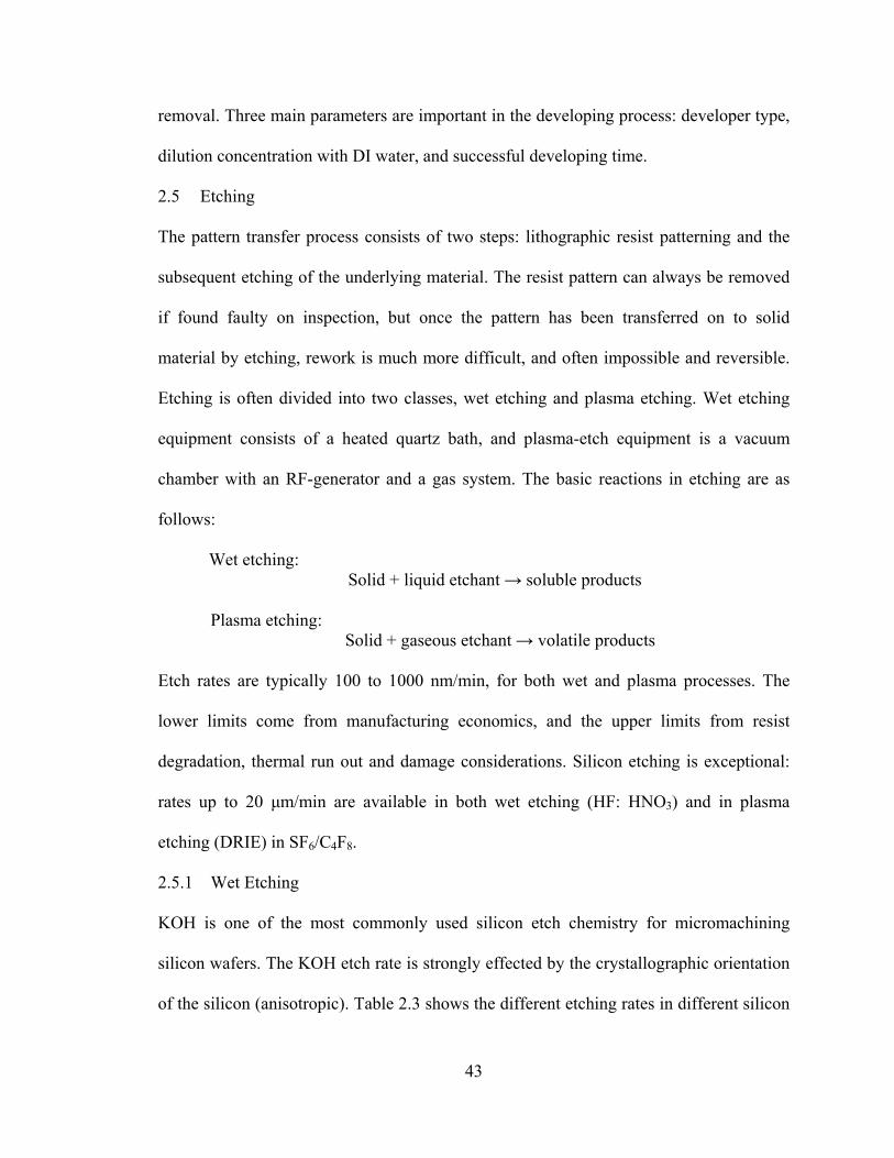
Solid + gaseous etchant → volatile products Etch rates are typically 100 to 1000 nm/min, for both wet and plasma processes. The

lower limits come from manufacturing economics, and the upper limits from resist

degradation, thermal run out and damage considerations. Silicon etching is exceptional:

rates up to 20 μm/min are available in both wet etching (HF: HNO3) and in plasma

etching (DRIE) in SF6/C4F8.

2.5.1 Wet Etching

KOH is one of the most commonly used silicon etch chemistry for micromachining

silicon wafers. The KOH etch rate is strongly effected by the crystallographic orientation

of the silicon (anisotropic). Table 2.3 shows the different etching rates in different silicon

44

crystallographic orientations in different concentration of KOH. The parenthesis shows

the ratio of etching in different orientations versus (110) orientation [65].

Table 2.3. Wet etching rate of Si with different KOH concentrations.

Crystallographic orientation Rates at different KOH concentration 30% 40% 50%

<100> 0.797 (0.548) 0599 (0463) 0.539 (0.619) <110> 1.455 (1) 1.294 (1) 0.87 (1) <111> 0.005 (0.004) 0.009 (0.007) 0.009 (0.10)

The <110> plane is the fastest etching primary surface. The ideal <110> surface has a

more corrugated atomic structure than the <100> and <111> primary surfaces. The

<111> plane is an extremely slow etching plane that is tightly packed, has a single

dangling-bond per atom, and is overall atomically flat.

In this project because of the nature of acoustophoresis, having vertical walls to create a

better standing wave is critical. Therefore, selecting an etchant that is anisotropic that

etches one plane more than the others will be desirable. Preferential Silicon Etchants are

preparations, which have the greatest etch rate on a specific plane of orientation. These

anisotropic etchants are used in lead beam technology to separate silicon chips and a

technique to obtain electrical isolation within integrated circuit chips. The etching

systems may also be used for chemical shaping of silicon and as etchants with photomask

of Ag, Au, Ta, or SiO2 as these materials are not etched.

Two etching systems from Transene Co. (Danvers, MA) are commercially available:

PSE-200 is alkali-based, is safe to use and has a fast etch rate. It is used to etch deep-wall

patterns in silicon. PSE-300 is ethylenediamine-based and has a moderate etch rate [66].

Table 2.4 shows the physical properties of PSE-200 and PSE-300 silicon etchants.

45

Table 2.4. Specification of silicon etchants [66]

Property PSE 200 PSE 300 Appearance Odorless, colorless liquid Clear liquid Composition Alkali-based Ethylenediamine-based Boiling Point >100 oC 118 oC Oper. Temp 75-100 oC 100 oC

Preferred operation <110> direction <100> direction Other common orientations

<111> plane - <110> can be used

<111> negligible Etch Rate 25 mil/3 min @ 100oC 25 mil/hr <100> Etch rinse Water Water

Metallization SiO2 Attacks Al; does not attach Au; mild attack on Ag

Will not attack – use as mask

No attack on Au, Ta; attacks Al, Cu; mild

attack on Ag Negligible

PSE 200 was selected to be used as an etchant in our fabrication methodology. The depth

and undercut-etching rate was 0.75 u/min and 0.6 u/min respectively, when the

temperature of the etchant is stable on 90 degree Celsius. The ration of etching through

depth and undercut is close it 0.9 meaning that undercut grows slightly slower than depth.

For the same reason, to hit the final desired design, undercut needs to be considered and

CAD design should be much smaller than what exists as final design. In our experiment

the least feature size we considered in CAD design was 22 micrometer. It has also seen

that the etching ratio is varying in different opening sizes. The smaller the opening is, the

lower the etching rate will be. Figure 2.18 shows the scanning electron microscopy graph

of the microchannel etched:

46

(a)

(b)

Figure 2.18. a) Isometric scanning electron microscopy of the microchannel with vertical walls and etched with PSE-200, b) cross section of the microchannel.

The microchannel pattern after wet etching is shown in Figure 2.19. The yellow color

shows the overhang happens during the silicon wet etching. Low stress nitride layer is

resisting against silicon etchant but after the etching of silicon from substrate, it looks

yellow color under optical microscope. Branches at the fork (Figure 2.19-middle) has a

47

black color at the edges that shows that because of crystal orientation of Si <100>, the

angle will not have vertical walls.

Figure 2.19. Microchannel after wet etching. left) microchannel, middle) the fork, right) bottom of the microchannel.

2.5.2 Dry Etching:

Dry etching mostly is used to remove selected areas from the surface layers. Dry etch can

be chemical etch, physical etch, or combination of chemical and physical etch. Physical

etching is similar to sandblasting process, in which high velocity sand is used to etch

away selected layers of glass, which is exposed. The dry etching technology that has been

mostly used in here is reactive ion etching (RIE). In RIE, the substrate is placed inside a

reactor in which several gases are introduced. Plasma hits into the gas mixture using an

RF power source, breaking the gas molecules into ions. (Figure 2.20)

48

Figure 2.20. Reactive ion etching schematics.

The ions are accelerated and reacted at the surface of the material being etched, forming

another gaseous material. This is known as the chemical part of reactive ion etching.

There is also a physical part, which is similar in nature to the sputtering deposition

process. If the ions have high enough energy, they can knock atoms out of the material to

be etched without a chemical reaction. It is a very complex task to develop dry etches

processes that balance chemical and physical etching, since there are many parameters to

adjust. By changing the balance it is possible to influence the anisotropy of the etching,

since the chemical part is isotropic and the physical part highly anisotropic the

combination can form sidewalls that have shapes from rounded to vertical. A schematic

of a typical reactive ion etching system is shown in the Figure 2.21.

49

Figure 2.21. Plasma etching process parameters.

The material of the gases is also important parameter. It needs to be selected properly in

order to have a right chemical reaction on the surface. The gases that are used in this

project to etch off low stress nitride (LSN) and photoresist layer from the surface of the

silicon wafer are CF4 and O2, respectively. The parameters to have both chemical and

physical etch at the same time in this project is as Table 2.5:

Table 2.5. RIE etching parameters for LSN and photoresist etching.

Purpose Pressure (mTorr) RF Power

(Watts)

Gas used Flow (sccm) Time

(sec)

Photoresist Etch 400 100 O2 60 600

LSN Etch 110 80 CF4 10 660

Some of the common wet and plasma etchants that are mostly used in different

microfabrication projects are listed in Table 2.6:

50

Table 2.6. List of common plasma and wet etchants in microfabrication.

Material to be etched Wet etchants Plasma etchants

Aluminum (Al)

80% phosphoric acid (H3PO4) + 5% acetic acid + 5% nitric acid (HNO3) + 10% water (H2O)

temp: 40-50 oC rate: 2000 Å/min [67]

Cl2, CCI4, SiCl4, BCl3

[67]

Chromium (Cr) “Chrome etch”: citric ammonium nitrate

((NH4)2Ce(NO3)6) + nitric acid (HNO3) [7] Hydrochloric acid (HCL) [7]

Gold (Au) Aqua regia, Iodine and Potassium Iodide

solution

Organic residues and photoresist Piranha etch: sulfuric acid (H2SO4) + hydrogen

peroxide (H2O2) O2 (Ashing)

Silicon (Si)

Nitric acid (HNO3) + hydrofluoric acid (HF)[4] Potassium hydroxide (KOH)

Ethylenediamine pyrocatechol (EDP) Tetramethylammonium hydroxide (TMAH)

CF4, SF4, SF6

[67] Cl2, CCl4,

BCl3, SiCl4 [67]

Silicon dioxide (SiO2)

Buffered oxide etch [BOE]: Ammonium fluoride (NH4F) and hydrofluoric

acid (HF) (8:1) temp: 40 - 50 oC

rate: 700 Å/min [67]

CF4, SF6, NF3, CHF3, C2F6,

C3F8 [67]

Silicon nitride (Si3N4) 85% Phosphoric acid (H3PO4)

temp: 150 - 180 °C rate: 80 Å/min [67]

CF4, SF6, NF3,[5] CHF3

Titanium (Ti)

Diluted Hydrofluoric acid (HF) 0.4 mol/l – room temp – Rate: 100 nm/s @ Room

Rate: 200 nm/s @ 32oC Salpetric acid-fluoric acid solution HF (2.6 ml/l) + HNO3 (2.6 ml/l) Rate: 200 nm/s @ 32oC [68]

BCl3[8]

2.6 Anodic Bonding:

Anodic bonding, also known as glass-silicon sealing, is a process of bonding a

silicon wafer to glass under the influence of high temperature and an externally applied

DC electric voltage. The materials required were Si wafer, 7740 Pyrex glass wafers, and

piranha cleaning solution. The equipment that is required for this step is a hot plate with

51

non-conductive ceramic top, high voltage power supplier, probes stand, aluminum plates,

electrical connectors, and thermometer. In order for good contact to occur, the two

surfaces to be bonded must be quite smooth with microscale roughness. In a typical

anodic bonding procedure, the wafers to be bonded are assembled together and heated on

a hotplate to about 500oC. A DC power supply connected to the assembly such that the

positive terminal is connected to the silicon wafer and the negative terminal is connected

to the Pyrex glass wafer is then turned on. When an electric field of several hundred to a

thousand volts is applied across the assembly, the glass seals to the silicon wafer. The

bonded areas initially appear as dark marks starting in the area where the voltage is

directly applied. Eventually these marks grow and cover the entire surface. The resulting

bond is essentially irreversible. Figure 2.22 gives a schematic drawing of a standard

anodic bonding setup.

Figure 2.22. Standard anodic bonding setup.

The success of the anodic bonding process depends heavily on the cleanliness of the

surfaces involved. Without clean surfaces, adequate contact cannot be made. The Si and

Pyrex wafers are cleaned in a solution known as Piranha clean consisting of a 3:1 ratio of

H2SO4: H2O2. After placing 30 ml of H2SO4 in a petri dish, both the silicon and Pyrex

wafers immersed in the dish. Then 10 ml of H2O2 were added and allowed the wafers to

52

clean for ten minuets. After cleaning the wafers, they should be rinsed with de-ionized

(DI) water and dried thoroughly using nitrogen gas. Pyrex or sodium rich glass, such as

soda lime is proper choice for bonding or sealing the microchannels on the silicon wafer

because during the process of anodic bonding, Na+ ions will migrate to negative electrode

and O- ions will move to the interface between silicon and glass and creates an

intermediate layer made of SiO2 which bonds glass to silicon. Mechanical properties of

glass are also important, because after bonding process, cooling will create cracks on the

glass with lower mechanical properties. But utilizing sodium rich glasses with better

mechanical properties, such as Pyrex is recommended.

53

3 Acoustic Focusing in Flow Systems

Abstract

Acoustic focusing and separations is a growing field of research since it is an efficient

and continuous method for particle manipulation in microfluidic systems. Using

microfabrication, microfluidic devices driven by an acoustic resonator were used to focus

various microparticle suspensions. By simple tuning of frequency, amplitude, and

channel geometry, controllable focusing patterns and alignments were obtained. This

approach afforded the separation of particles of contrasting sizes, shapes, densities,

porosities, and compressibilities. In this study we present the method for the fabrication

of these lab-on-chip devices and report on their performance in the manipulation of

microsized particles.

3.1 Introduction

Microfluidic separations hold a great promise especially in biosample analyses due

their ability to perform a sequence of analyses quickly [69]. A microfluidic lab-on-chip

device can perform a sequence of analyses on less than a microliter of a fluid that may

include filtration, mixing, concentrating, heating, reacting, and detection with similar

accuracy compared to a full-size laboratory. The science that deals with the flow of fluids

and suspensions in channels with less than millimeter-sized cross-sections under

influence of external forces is called microfluidics [70]–[75]. In microfluidics, viscosity

dominates over inertia and ensures the presence of laminar flow. Having laminar flow

and combining it with external forces results in particle controlling methods which are

useful in analytical sciences, based on different physical mechanisms including

54

inertial[21], electrokinetics[76], dielectrophoretics[77], magneto-phoretics[78], as well as

mechanical contact forces [79]. Acoustic focusing is a science, which utilizes the ultra

sound external forces to handle microparticles in microchannels.

Figure 3.1 shows the concept of acoustic focusing in a microfluidic device.

Figure 3.1. Schematic of acoustic device and acoustic zone for focusing the microparticles in the center.

Advantages like gentle and label free separations based on purely mechanical properties:

size, shape, density and compressibility have garnered a lot of excitement and attention to

this science [80]. However, one of the most common laboratory processes, centrifugation,

cannot be easily miniaturized or integrated in a continuous-flow microfluidic device and

filtration often suffers from limitations due to blockage. Centrifugation relies on

separating analyses based on their densities. Acoustic focusing solves this problem by

providing high and low attractive inter-droplet forces in ultrasonic standing waves. The

forces on particles in a standing wave have been utilized to develop continuous focusing,

55

and consequently, separation in lab-on-chip devices to separate red blood cells and fats

from whole blood samples. The standing wave is the combination of two counter waves

from either two transducers or from one transducer and a reflector. The transducers are

lead zirconate titanate (Pb[Zr(x)Ti(1-x)]O3) (PZT) devices [54], [81]–[83] or have

interdigitated transducers (IDT) [84]. The pressure is maximum at the antinode and

minimum at the node. Due to this pressure differential, solid particles tend to reassemble

and concentrate in zones of minimum acoustic potential energy, which is typically at the

nodes [14]. In a microchannel multiple nodes could exist depending on the

wavelength/frequency of the wave. If multiple nodes are present, they would be half a

wavelength (λ/2) apart from each other the flowing particle suspension will be under the

influence of four different forces each acting in a different direction. The acoustic force

mentioned above is depending on the physical properties of particles/ cells. The most

important parameters, which affect the magnitude of this axial radiation force, Fax, the

major force component in acoustic standing wave manipulation, are density ρ, speed of

sound c, and the radius R. These properties, the corresponding data for the suspending

medium and the parameters of the sound field compose the equation, Fax. Equation 3.1 is

a special case of the primary acoustic radiation force as obtained in a one-dimensional

plane acoustic standing wave [85]. The acoustic force mentioned above will be in the

direction of the width of the channel either left or right depending on the sign of the

primary radiation force which is defined by the material properties of the particle/cell

relative to the suspending medium and is formulated by the acoustic contrast factor (Φ),

Equation 3.2. Therefore, the contrast factor is defining whether a particle will move

toward the pressure node or the antinode in the acoustic standing wave field. A positive

56

contrast factor results in movement toward the pressure node while a negative contrast

factor results in a movement to the antinode [85].

Equation 3.1 F

4πR E ksin 2kz Φ

where Fax is the acoustic radiation force, Eac is the acoustic energy density, R is the

particle radius and z is the distance from pressure anti-node in the wave propagation axis.

Equation 3.2

Φρ 2

3 ρ ρ

2ρ ρ

13ρ cρ c

where and are density of particle and fluid, respectively, cp and c0 are speed of

sound in particle material and fluid, respectively, k is the wavenumber (2πf/c0) and ᴪ is

the acoustic contrast factor. The gravitational force for a device laid flat will be in the

direction of the depth of the channel and pulling downward. The buoyant force will be

acting opposite to the gravitational force. And the viscous drag force will be acting in the

channel length direction opposite to the flow. To accurately predict this required channel

dimensions, a quantitative force analysis can be performed considering these four forces.

Typically, larger particles would be easier to concentrate at the pressure nodes [86]. To

increase the force acting on a particle higher frequencies (> 1 MHz) would be needed.

However, if only one acoustic pressure node is desired, the wavelength has to be half of

width of the microchannel [87]. Acoustic standing wave aggregation in microfluidic

components is typically used in half wavelength resonators where the primary acoustic

radiation force levitates the cells/particles into the nodal plane and subsequently the

57

lateral gradient of the primary radiation force drives the cells into a dense cluster in the

nodal plane. The other harmonics can be used if several nodal points are desired

depending on the application.

Acoustic focusing is not mostly applicable to particles with nanosizes. A lot of solid

particles focusing have been done on micro-size particles. This can have a plethora of

applications in bioanalyses, e.g. drug delivery. In this article we focus on focusing latex

particles and their match with governing equations.

3.2 Device Design and Fabrication

Device design must be precisely controlled to satisfy fabrication limitations. Specific

features are wanted in the device, such as, smooth vertical microchannel walls or

adjusting the aspect ratio of height per width of microchannel. Speed of sound in the

media which is carrying the particles has a relationship with imposed wavelength and

frequency Equation 3.3. On the other hand, microchannel width should be the half size of

wavelength Equation 3.3, so a standing wave can happen inside of fluid compartment.

Equation 3.3

2⁄

.

Assuming the media carrying the particles is aqueous and the speed of sound in water is

1480 m/s. If the width of a channel is wanted, depending on the first or second harmonic

frequency of piezoelectric, can be found. The width of channel will be two times of .

Although the most commonly reported microfluidic methods are PDMS stamping and

silicon etching, in this work various methods of fabrication were attempted. Firstly, using

simple layering of a parafilm layer between two glass-slides, the desired patterns were

58

first mechanical cut on the parafilm layer using a digital cutter. The method was both

rapid and low-cost and microchannels were reproducible and with controllable (Figure

3.2). These devices were unsuccessful in acoustopheretic application primarily since the

middle layer had poor acoustic impedance properties and therefore transforming the

mode of operation of the device from transversal to layered which distorted the

alignments. In addition, these channels were heat treated after preparation, which also

distorted the channel wall properties. Similar behavior was observed for channel

patterned using a CO2 laser. Although the laser afforded pattern dimension significantly

smaller and with sharper corners (Figure 3.3), the devices did not perform in

acoustophortic applications. This method was not investigated beyond this point.

250 micron 300 micron

400 micron 800 micron

Figure 3.2. Microfluific patterning on parafilm sheet using digital cutting.

59

1-80-10-500 1-80-10-500

1-80-20-500 1-80-20-500

Figure 3.3. Microfluidic patterning on parafilm sheet using laser.

The poor acoustic impedance of parafilm due to its soft and low melting nature suggested

that harder and better acoustic impedance materials were suitable. Based on that,

polyethylene films (500 microns thick) were used and similarly to the method used about

for parafilm, were patterned using CO2 laser. Several experiments were carried out and

all experiments are various cutting rates, laser energy, and number of passes yielded

various degrees of charring of the plastic films (Figure 3.4). This charring resulted in

carbonated materials, which was highly rough, when observed under the microscope. In

addition, a device layered using these plastic films suffered from leaking problems and

heat treatment wasn’t effective due to the high melting properties of polyethylene.

60

Figure 3.4. Microfluidic patterning on plastic slides using laser.

Glass slides were also cut using high-speed driller and although visible clean cut, these

channels were rough. (Figure3.5).

Figure 3.5. Microfluidic patterning on glass using high speed driller.

It was due to the above described attempts that channels presented in this work were

fabricated using silicon and etched using standard wet etching procedures. In these

procedures, the width of the microchannel is determined after undercut calculations, a

61

common phenomenon in silicon wet etching. The final width of channel will therefore be

the designed width plus twice the width of the undercut (Figure 3.6). Etching ratio in

depth-wise and sidewise of the channel per minute will be important.

Figure 3.6. Schematic of silicon etching process and related parameters.

Different instruments, methods, materials and fabrication processes are available in

microfabrication of acoustic focusing devices design. The selection of material,

geometry, instrumentation, fabrication, and monitoring are very important characteristics

that must be considered beforehand. For transversal resonators, silicon is a suitable

choice due to its low acoustic energy attenuation. The first concern in transversal

resonators is having vertical sidewalls in order to accomplish standing waves inside of

fluid suspension. Wet chemical anisotropic etching is restricted to crystallographic

orientations, while dry etching is not. Dry etching however is more difficult to control

and the equipment is more costly [88]. Forty-five degree rotation in wet etching of the

<100 >Si-wafer is needed to have parallel vertical walls in main channel ( Figure 3.7).

62

Figure 3.7. Schematic of patterning the microchannel on silicon wafer substrate using photolithography method.

Silicon wafer was selected with low stress nitride (LSN) layer pre-coated, because it is

needed to protect silicon wafer in step 7 of fabrication in Figure 3.7. In step 2, AZ4620

photoresist is spin coated on silicon wafer in two steps, 500 rpm @100 rpm/s ramp for 5

seconds and then 2500 rpm @ 300 rpm/s for 30 seconds. It should be softly baked in

110oC for 2 minutes. 400 mJ/cm2 exposure energy is needed in the third step. Mask must

be already fabricated and ready for this step. Removal of the negative photoresist was

performed using AZ400K with 1:3 concentrations with DI water for 90 seconds.

Unexposed photoresist will protect LSN layer in CF4 plasma etching. In step six, the

photoresist was removed by acetone and methanol rinsing on spin coater. Based on the

ratio for sidewise (~1.26 / ) and depth wise (~1.42 / ), silicon wafer was soaked into

preferred silicon etchant (PSE-200 TRANSENE COMPANY, INC. DANVERS, MA

63

01923) for 89 minutes in 100oC. 500±5 microchannel width with 130 ±5 can

be fabricated. For removing LSN layer in step eight, it was soaked into Aluminum

etchant (potassium Hydroxide solution) for 240 minutes in 180oC. A mask, which is

chrome-on-quartz one and pre-coated by positive photoresist was used. Based on

lithography instrument (µPG 101, Heidelberg Instruments Mikrotechnik GmbH)

logbook, 12 mW power with 100% exposure for 187 minutes was set. Figure 3.8 shows

the steps for mask fabrication. In step 3, chrome etchant 1020 (Transene Co., Danvers,

MA) was used for 60 seconds at room temperature. Photoresist removed using O2 in

100mTorr pressure, 400 Watt power with 60 sccm flow rate for 660 seconds by reactive

ion etcher instrument March cs-1701.

Figure 3.8. Schematic of mask making process.

Pyrex was selected as the reflector layer because of lower thermal expansion and

transparency properties. After drilling holes using diamond driller at inlets and outlet

64

ports, the Pyrex was be bonded to silicon using anodic bonding method at 500V and

500oC for 6 minutes). Cylindrical shaped PZT (APC 850) with 0.25 inch diameter was

installed on the back side of silicon wafer underneath the microchannel. Figure 3.9

demonstrates the exploded view of device parts and their arrangement.

Figure 3.9. Exploded view of device schematic.

Figure 3.10 demonstrates the assembled and three-dimensional view of the device.

Figure 3.10. Assembled view of device schematic.

65

Figure 3.11 shows a complete acoustic focusing device fabricated utilizing rectangular

PZT.

Figure 3.11. Assembled acoustic focusing device Experimental Setup.

An aqueous suspension of latex particles with 10 µm average diameter were used as

model particles. Optical analysis was carried out using an optical microscope to screen

the particle focusing inside of microchannel. An AC sinusoidal signal was generated by a

(RIGOL DG4062 function generator. A representative experimental setup is shown in

Figure 3.12.

Figure 3.12. Experimental setup for acoustic focusing experiment.

PZT

66

The flow rate range was controlled between 0.1-0.5 µL/min, and the acoustic power used

to do particle focusing (10 Vpp and 1.4 MHz and 2.8 MHz).

3.3 Results and Conclusion

A microfabrication method was used to fabricate a microfluidic channel on silicon wafer.

Fabrication a microchannel with smooth walls was target so <100> crystal orientation

was selected and 45o rotation while patterning is applied. Anodic bonding is used to make

a strong bonding between reflector and silicon wafer. Pyrex was used as a reflector

because of its strong mechanical properties while anodic bonding and transparency for

monitoring. Changing the frequency by function generator in the highest possible

amplitude that instrument can provide we get different focusing of microparticles as can

be seen in Figure 3.13.

(a) (b) (c)

(d) (e) (f)

67

Figure 3.13. Results in different frequencies and Vpp=10 volt, a) suspension with no acoustic energy, b) frequency= 1.305 MHz, c) frequency = 2.649 MHz, d) frequency

3,992 MHz, e) frequency = 5.435 MHz, f) frequency = 6.778 MHz.

Images in Figure 3.13 demonstrate a successful focusing of particles into 1, 2, 3 or more

lines, controlled by the frequency of the acoustic waves. Based on this behavior a method

is currently being devised to separate these particles, based on the acoustic force acting

on them and their response time. It is also noteworthy that based on the mathematics of

acoustofluidics we can conclude that the speed of sound in this suspension is 1435.5 m/s.

which is close to the speed of sound in the water. We were expecting that for the width of

microchannel to get the first focusing in 1.305 MHz, which is showing another physical

and mathematical compatibility in this experiment. Clear microscopic images of glass gel

microparticles focusing driven by acoustic forces are shown in Figure 3.14 to Figure

3.16. The first resonance is happening at 1.305 MHz and one focusing alignment is

expected which is shown in Figure 3.14.

Figure 3.14. Separation of glass gel microparticles at 1.305 MHz and 20 Vpp.

68

The experimental observation (Figure 3.15) of three lines alignments was accomplished,

when the frequency is three times greater than the frequency in the first resonance mode.

This confirms the linear relationship between frequency and number of alignments.

Figure 3.15. Separation of glass gel microparticles at 4.051 MHz and 20 Vpp.

Thus, to obtain four lines of alignments, setting the frequency on four times of the one in

the first resonance is necessary. Clear four lines of alignment was observed

experimentally on fourth resonance mode (Figure 3.16).

69

Figure 3.16. Separation of glass gel microparticles at 5.365 MHz and 20 Vpp.

Amplitude changes were affecting directly the acoustic forces so the more amplitude is

causing the particles to move faster.

Other particle materials beside glass microparticles were also explored to push the

limited of acoustophoresis. While most particles would mathematically have positive

contrast factors, this factor depended on both the density and compressiblities of particles

and media. In some of our studies materials, such as the silicone rubber PDMS migrated

toward to the antinodes due to their negative contrast factor number afforded by high

compressibility. Similarly, liquids, such as mineral oil migrated to the antinodes. The

density effect was observed to be dominated by the compressibility effect. Therefore we

performed a systematic experiment to uncover this role. In this study were selected glass

shells/air core glass bubbles (density of 0.6 g/cc) as the particle model. The media was

70

aqueous solution of calcium nitrate with various concentrations in order to vary the

density of the media. Media densities ranging from 1.0 to 1.6 g/cc were studied and

experiments were setup to determine the direction of particle migration, i.e. nodal or anti-

nodal. The results of this study are summarized in table 1.1. Based on the calculation and

by assuming that full glass particles and hollow glass particles have the same

compressibility, the density of the media which would have yield negative contrast factor

would be > 1.52 g/cc. Instead, experimental, it was observed that this density was ~ 1.32

g/cc. This discrepancy has two indications, first that the equation report for the contrast

factors were applicable all particles system, e.g. core-shell particles; or that the

assumption of same compressibility of glass particles system was inaccurate. While the

determination of the compressibility of the glass bubbles is possible and it is a daunting

task that is in turn an approximation. We therefore proposed for this chapter a set of

future works which can utilize this phenomena to determine the compressibility of the

particle systems. By using the set of variable density media and pinpointing the turning

point density above which the contrast factor is negative and below which the contrast

factor is positive, using the equation for Phi (Equation 3.4), one can solve for beta of the

particle.

Equation 3.4 Φ Φ ρ Φ β5ρ 2ρ2ρ ρ

β

β

Table 3.1. Experiments of medium density variation to find the sign changing point for acoustic contrast factor.

Experiment Number

1 2 3 4 5 6 7 8

Density of particles

0.6 0.6 0.6 0.6 0.6 0.6 0.6 0.6

Density of 1.05 1.1 1.125 1.15 1.25 1.3 1.35 1.47

71

Media

Sign of Contrast Factor

(+:P, -:N) P P P P P P N N

Φ ρ 0.4 0.35 0.32 0.30 0.20 0.16 0.12 0.02

Correction 0.140.019

0.140.019

0.140.019

0.140.019

0.140.019

0.140.019

0.140.019

0.140.019

Equation 3.5 Φ βββ

0.14 0.019

72

4 Novel Optical Switchable Transparency driven by Acoustophoresis

Abstract

In this chapter, a suspended-particle device with controllable light transmittance was

developed based on the acoustic stimuli. Using a glass compartment and carbon particle

suspension in an organic solvent, the device responded to acoustic stimulation by

alignment of particles. The alignment of light-absorbing carbon particles afforded in

increasing light transmittance was as high as 84.5% and was controllable based on the

control of the frequency of the acoustic waves. The device also demonstrated alignment

memory rendering it energy-efficient.

4.1 Introduction

Materials with switchable transparency have found numerous applications, especially in

dynamics tintable or smart windows. These materials have found utility in applications

in agriculture [89], automobile sunroofs [90], personal privacy [91], photovoltaics [92],

[93], and energy-efficient buildings [94]. Switchable transparency is achievable

following various techniques, all of which utilize external stimuli or triggers. The most

common are chromic materials, liquid crystals, and suspended-particle devices. The

chromic materials are most commonly photochromic, in which case the external stimulus

is light, e.g. photochromic lenses. However, other types of stimuli for chromic materials

have been developed, namely, electricity (electrochromic), gases (gasochromic), and heat

(thermochromic) [89]. Liquid crystal devices while they shares the same stimulus with

electrochromic, are fundamentally different since they rely on changes in the orientation

of the liquid crystal molecules rather than through ion insertion/extraction. Suspended-

73

particle devices that exist today also rely on electrical stimuli to create an electronic field

to align light-absorbing particles suspended in a fluid or gel between two transparent and

conductive surfaces. The alignment of the particles yields a rapid increase in

transmittance that was reported to reach as high as 79% [95]–[97].

In this work, a suspended-particle device that has switchable transmittance using sound

waves was developed. Similar to previously reported suspended-particles devices, our

light-absorbing particles are aligned using an external stimulus to allow light

transmittance. However, instead of using electrophoretic alignment, the presented device

utilizes acousticphoretic alignment. The working principles of acoustophoresis has been well

exploited in previous studies for microfluidic applications [54], [98]. This alignment approach

is rapid, low-energy, and can be applied to virtually any particle type not restricted by

electrical, magnetic, or chemical reactivity. The acoustophoretic alignment presented in

this work is tested on label-free carbon particles. Random suspensions of the carbon

particles are practically opaque, while aligned particles of various frequencies afforded

higher light transmittance.

4.2 Experimental Procedure:

Particle suspensions (1-10% by weight) were prepared using graphitized carbon

particles 0.5-5 µm in diameter obtained from MTI Corporation (Richmond, CA) in

anhydrous acetone obtained from Sigma-Aldrich (St. Louis, MO). Stable

suspensions were obtained by vortex mixing followed by sonicating the particles in

an ultrasonication bath (100 W) for 30 minutes. The particles were then syringe

injected into a custom-made glass compartment 10mm x 15mm x 1mm in

74

dimension with one of its sides as a Teflon cap. A piezoceramic transducer PZ-26

obtained from Ferroperm (Denmark) was affixed to this compartment and was

wired to a function generator Rigol DG4062 (Beavertown, OR). The experiments

were conducted using the setup schematically presented in Figure 4.1. In the

figure, the device was placed under a stereo microscope with a working distance of

10-20 cm focused on a 10mm x 15mm window with the light source placed either

under or above the device.

Figure 4.1. Schematic presentation of the experimental setup used in the device transmittance study.

4.3 Results and Discussion:

In a symmetric compartment, such as the one described in this work, a transducer produced an

acoustic radiation that was reflected from the opposite wall, creating a standing-wave. An

acoustic force is then imposed on the particles by the standing-wave based on their spatial

coordinates and the size of the particles, and the density and acoustic compressibility of both the

particle and the media [55]. Rigid and dense particles often migrate toward the nodal zones while

flexible and lighter particles migrate toward the anti-nodal zones shown in Figure 4.2.

75

Figure 4.2. Schematic of the direction of the acoustic radiation force for rigid (black) and flexible (blue) particle/droplet in an acoustic standing wave. Black arrows denote the

direction of the momentum transfer and the green arrows denote the direction of the net force and thus the resulting motion.

In this study, carbon had instantaneous nodal migrations and aligned into lines across the device

with spacing depending on the frequency of the sound wave controlled by the function generator.

Since the carbon particles are light-absorbing, when aligned, no-particle gaps, develop allowing

light transmittance through the device, as shown in Figure 4.3

Figure 4.3. Comparison of the randomly disperse (left) versus the aligned particles (right) caused by switching on the acoustic radiation.

The device itself with no particles was shown to be highly transparent, when filled only with fluid

with transmittance of 99.3%. The device with 10% carbon particles randomly suspended with no

acoustic stimulation, was show to have 1.5% light transmittance in the visible 400 – 800 nm

76

range (Figure 4.4). This shows that the material selection for this device to use a glass

compartment and carbon particles at the chosen concentration is suitable for complete

transparency and opacity of the device.

Figure 4.4 - Spectrophotometric analysis of the device filled with acetone (triangles) and 10% suspended-particles (circles) between 400 and 800 nm.

The experimental setup described in Figure 4.1 was used to determine the controllable

optical properties of the device. Using a printed text placed underneath the device,

various images were taken for a 1mm x 15mm window at various acoustic frequencies.

Then, an image-processing approach was used to measure the global transparency. The

image-processing approach consisted of the successive application of three digital filters,

red, greyscale, and monochrome, using the software Matlab, as shown in Figure 4.5.

After these digital filters were applied, the ratio of white to total pixels was calculated.

77

This ratio was a close match to the transmittance percentage obtained using

spectrophotometric analysis in the 400–800 nm range.

(1) (2) (3) (4)

Figure 4.5- Image processing approach used to determine the percent light transmittance applied for (1) the original images at various frequencies of 222 kHz, 757 kHz, and 1.51 MHz, (2) after application of red filter, (3) after application of grayscale filter, (4) after

application of monochrome filter.

The error is attributed to the more localized analysis for the spectrophotometer due to its

small spot size (~ 1.5 mm). The image-processing approach was a global one that can be

applied to the whole surface. Figure 4.6 compares the transmittance percentages for the

device at various frequencies to the transmittance percentage prior to switching on the

acoustic stimulation. The device with random dispersed particles was black with light

78

transmittances of 1.5% using the spectral analysis and 0% image-processing approach.

The transmittance increases immediately to 85.8% upon stimulation with 222 kHz.

Figure 4.6. Light transmittance of the device at frequencies of 222 kHz, 757 kHz, and 1.51 MHz. The asterisk marked data point corresponds to no acoustic stimulation.

This was possible since most particles in the analysis window of 10mm x 15mm migrated

out of the window. At higher frequencies, where particles aligned in the analysis window

transmittance percentages were 57.5% for 757 kHz, and 63.9% for 1.51 MHz. All wave

amplitudes were set to 20 Vpp throughout this experiment. The relationship between

frequency and transparency was therefore only predictable for wavelengths significantly

shorter than the width of the analysis window. Above this threshold, the transmittance

was consistently increasing with increasing frequency, which afforded thinner and

narrowly spaced lines of particles. The upper limit in this instance is determined by both

79

the selection of an effective transducer capable of resonating efficiently in a wide range

of frequencies, since most piezoceramic materials, such as PZT used in this study, peak

in performance around few hundred kHz. The choice of compartment materials, medium,

and particles are also crucial to minimize acoustic radiation losses and attenuation [16]

and maximize the sensitivity of the particles to acoustic stimulation.

One of the major pros of this approach is the low power requirement of the

studied device. The device not only requires low power (less than 150 mW), but also

acoustic stimulation was only essential for an initial alignment while the alignment was

relatively stable afterwards. This device’s memory property was investigated for a given

device stimulated at 2 MHz and 20 Vpp, which had a light transmittance rise from 0% to

81.5% in less than 3 seconds. Afterwards, the function generator was switch off while the

transmittance was monitored as a function of time. Figure 4.7 summarizes the memory

effect for the described device. After power was switched off, the transmittance

instantaneously (less than 10 seconds) dropped to 70% and remained at that range a few

minutes. The steady state transparency reached 55.9% after 30 minutes. It is noteworthy

that this drop was partly due to acetone evaporation, which occurred at a slow rate.

80

Figure 4.7. Transmittance memory of the device operated at 2 MHz and 20 Vpp showing the retention of transmittance after the acoustic stimulation was switched off. The asterisk

marked data point corresponds to no acoustic stimulation. The insets correspond to optical micrographs of the device at each of the corresponding times.

4.4 Conclusions

A switchable and controllable light transmittance device was developed in this study. To

our knowledge, this is the first report on switchable or controllable transparency using

acoustic stimulation of suspended particle device. The method was simple, rapid, and

energy-efficient. Transmittance as high as 84.5% was achieved and steady-state

transmittance retention of 55.9% was observed after switching off acoustic stimulation.

This technique could have a plethora of applications, especially in low-power devices.

81

5 Transparent and Anisotropic Conductive Film Templated Using Acoustic Focusing

Abstract

Elastomers doped with conductive metal particles were rendered surface

conductive at particle loadings as low as 1% by weight using acoustic focusing.

The resulting films were flexible and had transparencies exceeding 80% in the

visible spectrum and with electrical bulk conductivities exceeding 50 S/cm.

5.1 Introduction

Transparent conducting oxides, such as indium tin oxide (ITO) and fluorine tin

oxide (FTO), have been standardized optoelectronic electrode materials due to

their electrical conductivity and optical transparency. However, with the

emergence of new transparent electronic materials, these materials have

shortcomings that became apparent. Some of these shortcomings are their limited

worldwide resources of indium, acid/base instability, and limited transparency in

the near-IR region. Therefore, highly stable, transparent, and flexible electrically

conductive materials are in high demand.

Advances in flexible organic electronics enabled great developments in

research areas, such as light-emitting-diodes (LED) [99], transistors [100], solar

cells [101], [102], and wearable devices [103]. These organic electronics

distinguish themselves from their inorganic counterparts by possessing superior

physical properties, such as flexibility, gravimetric density, and corrosion

resistance, while being generally low-cost [104]–[107] .Several research studies

82

reported on thin layers with optical transparencies exceeding 70% and, in one case

reaching 98% using carbon nanotubes [108], and electrical conductivities

exceeding 50 S/cm [109]. Optoelectronic devices require conductive electrodes,

which are flexible, cheap and compatible with large-scale manufacturing methods

[110].

The focus of this research work is to develop a thin, transparent, flexible,

and at the same time highly anisotropically conductive film templated using

acoustic focusing. Particle manipulation using external stimuli acting on particles

in suspensions has attracted attention in different fields, especially in lab-on-chip

applications [16], [111]–[113]. Different techniques for particle manipulation have

been previously reported for electronic materials, including electrokinetic [76],

inertial [17], [21], [29], magnetophoretic [58], [114], optical [115],

[116]dielectrophoretic [77], [117], [118]. Acoustic methods however, have been

limited to flow systems and have not been previously used for the templating of

electronic materials. Acoustic stimuli allow rapid, gentle, label-free particle

manipulation based on physical properties, such as size, density, and

compressibility. Cell trapping [119]–[121], cell sorting[122], plasmaphoresis [56]

are some of the biotechnical applications of acoustophoresis. In this study we

report on the utilization of acoustic standing waves for optoelectronic applications.

The manipulation of conductive microparticles and sub-micron particles enabled

the migration and subsequent alignment of particles into continuous networks that

afforded both conductivity and optical transparency. The morphology and

orientation of these networks were tailored by controlling the acoustic wave’s

83

frequency and amplitude generated by the transducer. Since freestanding and

flexible films were favoured, the conductive particles were suspended in a liquid

monomer or acetonic solution of the monomer during the focusing studies. To our

knowledge, no prior research reported the production of optically transparent and

anisotropically conductive films using our approach.

A standing-wave can be generated by two acoustic waves in opposite direction

which makes acoustic standing waves [55]. These waves can be produced by a transducer

and a reflector or by two transducers in a compartment that is made of good acoustic

conducting materials, such as glass or silicon. The particles’ response to the standing

wave is largely dependent on their spatial coordinates, size, compressibility, and density.

The principles of acoustic radiation force for particle manipulation has been well-studied

in the past, chiefly for lab-on-chip applications [54], [98]. In its simplest configuration, an

acoustic radiation force will cause a certain particle to migrate at a force given by

Equation 5.1 either towards the closest node or anti-node of the standing-wave

depending on the sign of the acoustic contrast factor given in Equation 5.2

Equation 5.1

Where Fax is the acoustic radiation force, is pressure amplitude; is the

volume of microparticle. Φis the acoustic contrast factor which is depending on

the physical properties of fluid and

Equation 5.2

84

where ρp and ρ0 are the bulk densities of the particles and media, respectively.

Whereas, βp and β0 are the acoustic compressibilities of the particles and media,

respectively. The term k designates the wave number while λ is the wavelength

[123]. Most aqueous suspensions of solid particles have positive acoustic contrast

factor, thus often migrate towards the nodes. The observed behavior in this study

for silver-coated nickel particles was not different

In the glass compartment, the particles are constantly subjected to four

forces namely, gravitational, buoyant, drag, and acoustic. The introduction of

acetone was intended to reduce the viscosity of the suspension and thus reduce the

drag force resisting the acoustic focusing. Due to the high density of the particles

relative to the media and the spherical nature of the particles, the gravitational

force was dominant in its direction (Z-direction). Therefore, considering these two

forces, gravitational and acoustic, the resulting arrangement of the particles within

the films was similar to the arrangement schematically presented in Figure 5.1.

This arrangement affords anisotropic surface conductivity, on the bottom surface

of the film possible only in the Y-direction. It is imaginable that conductivity in the

Z-direction can be obtained if lower density and smaller particles, higher viscosity

media, and thinner films are used such that to allow the acoustic force to be the

dominant force acting on the particles (Figure 5.1). Factors that cause losses of the

acoustic force and thus reducing its effect on the particle include propagation

through poor sound conductors, geometry on the compartment, and the roughness

of the walls of the compartment. Considering the first factor, the materials

85

selection for the compartment is of paramount importance for acoustic focusing

studies.

Figure 5.1. Schematic of the steady-state particles’ assembly in a half wavelength resonator compartments for: gravity-dominated mode (left), acoustics-dominated mode

(middle), and mixed gravity-acoustics mode (right), which is observed in this paper

The loss of energy due to attenuation and deformation of material can lead to

inefficient alignment in which the particles do not come in physical contact,

causing discontinuity in the electron pathway rendering the film non-conductive.

In this study, glass was used. While glass, is not the most ideal of acoustic

conductors, its visible light transparency in this study was important since it

permitted constant monitoring of the alignment throughout the experiments and

ultimately external polymerization of the film using UV light. Figure 5.2

demonstrates the UV exposure process after alignment driven by acoustics.

z

x

y

Gravity‐dominated Acoustics‐dominated Mixed gravity‐acoustics

86

Figure 5.2. UV exposure process

The second factor is also important for the macroscopic properties of the particle

alignment and the viability of the acoustic focusing. Since in this study one was

used as a resonator and the other was used as a reflector, for the standing wave

formation to be possible, the walls have to be perfectly parallel. These walls also

need to be as smooth as possible to minimize scattering and absorption and reflect

the acoustic radiation efficiently.

In this work an elastomer film was rendered conductive by doping it with

conductive particles at lower than theoretical thresholds. By acoustically aligning

the particles, continuous electron conduction pathways were constructed which

also allowed the films to remain partially transparent. The alignments were

controlled in spacing by controlling the frequency of the acoustic stimulus.

According to Equation 5.2, the positive contrast factor indicates nodal focusing.

And based on the number of nodes of the standing-wave, the number of alignments

in the film were controlled. Figure 5.3 shows an optical micrograph in

87

transmission mode detailing the morphology of a representative spot on films

prepared using 10% and 2% by weight of particles to polymer.

Figure 5.3. Optical micrographs in transmission mode of: (a) 10% suspension of the particles in the compartment fully dispersed, (b) 10% suspension of the particles after

acoustic alignment at 2 MHz and 16 Vpp, (c) 2% suspension of the particles fully dispersed, and (d) 2% suspension of the particles after acoustic alignment at 2 MHz and

16 Vpp

At 2 MHz, these lines were dense and continuous and provided very little

resistance, i.e. less than 1 using the apparatus show in Figure 5.4.

88

Figure 5.4. Schematic presentation of the setup used for testing the surface resistivity of the films. The setup used two gold electrode plates with adjustable spacing that were

connected to an Ohmmeter.

The film prepared using unaligned suspensions was poorly conductive with

resistances in the M range. While the anisotropic ratio (RX/RY) of resistance in

X-direction (RX) to the resistance in the Y-direction (RY) exceeded 106-fold at

certain conditions, demonstrating conductivity only in one direction. The data are

summarized in Table 5.1.

Table 5.1. Summary of the resistances in the X and Y-directions of the films for 1%, 2%, 5%, and 10% particle loading and films prepared using no acoustic stimulation, 150 kHz

frequency, and 2 MHz frequencies.

Loading Percentage No Acoustics 150 kHz 2 MHz RX RY RX RY RX RY

10% 1.2 1.2 > 106 0.8 > 106 1.0 5% > 106 > 106 > 106 2.1 > 106 6.9 2% > 106 > 106 > 106 3.8 > 106 10.1

1% > 106 > 106 > 106 6.0 > 106 > 106

Gold electrodes

Prepared film

Glass cover slip

Ohmmeter

89

The optical transparency in the visible range (400–800 nm) of a 1 mm thick

cured polymer film with 0% particle loading averaged 86%.

5.2 I-V experiment

Using the same setup sketched in Figure 5.4 , a direct current (DC) voltage

was applied in two sides of anisotropic film to measure the amount of current

passing through the network created by the particles. After aligning the particles

using acoustic forces in the media a UV exposure carried out and a resistivity

measurement was carried out on the resulted film that was 1.01 ohm. Figure 5.5

shows the circuit schematic that was used to acquire the current variation via

voltage changes.

Figure 5.5. Circuit schematic to measure the V- I experiment

An I-V graph of the measurement is shown in Figure 5.6, which shows a good

compatibility with the electronic Ohm’s law, and the variation of current versus

voltage changes is linear. Nonlinearity of the experimental data is because of the

temperature and material characteristics of the resistor and environment.

90

Figure 5.6. I-V curve (current vs. voltage), when the measured resistance of the film is 1.01 ohm

The film was tested in a real circuit as a resistor. Figure 5.7 demonstrates the

electrical conductivity and optical transparency of the film by connecting the

prepared film in series with a CR2032 3V lithium-ion battery and a red light

emitting diode.

Figure 5.7. Anisotropic conductive film experimental setup

91

The film is flexible and its flexibility is depending on its thickness. The flexibility

of the film is increasing, when the thickness of the film decreases. The thinner the

film is, the more flexible and the more transparent it will be. Figure 5.8 shows that

film is very flexible and bendable.

Figure 5.8. Flexibility demonstration of the cured polymer while the conductive particles are aligned acoustically and embedded on one side

5.3 Transparency Analysis

The same film with different particle loadings has different transparencies,

when the particles are fully dispersed; the variation of light transmittance versus

the emitted light wavelength is shown in Figure 5.9. The average light

transparencies of the films in the 400–800 nm wavelength range are displayed on

the charts. Higher particle loads will decrease the light transmittance to lower than

5% and decreasing the particle loads will increase the light transmittance.

92

Figure 5.9. Transmittance of the films prepared using (Δ) 2% particles, () 5% particles, and () 10% particles for randomly suspended particles with no acoustic stimulation

The same film with 10% particle loading was less than 5% transparent, while the

same film’s transparency increased to 22% after acoustic focusing at 2 MHz for 10

seconds followed by UV curing for 2 minutes as shown in Figure 5.10 and Figure

5.11. When the particles were stimulated with 150 kHz, the transparency

increased to 63% while the film’s resistance remained largely unchanged. This

93

difference is attributed to particles focusing in the thickness Z-direction and thus

blocking less light, while maintaining continuous electron conduction pathways.

Figure 5.10. Transmittance of the films prepared using (Δ) 2% particles, () 5% particles, and () 10% particles for randomly suspended particles with acoustically aligned

particles using 150 kHz

Due to the choice of the piezoelectric device, wave amplitudes were more

pronounced at 150 kHz than at 2 MHz causing stronger acoustic forces, which led

to more acoustic force dominance as previously shown in Figure 5.1. Expectedly,

94

the transparency for lower particle loading were improved and films using 2%

loading acoustically aligned at 150 kHz exceeding 80%.

Figure 5.11. Transmittance of the films prepared using (Δ) 2% particles, () 5% particles, and () 10% particles for randomly suspended particles with acoustically aligned

particles using 2 MHz.

In summary, a transparent, anisotropically conductive, and flexible film was

prepared using widely available conductive particles and elastomers with

95

conductive materials loading as low as 1%. The film’s preparation was simple,

rapid, and at ambient conditions using no additives.

5.4 Experimental Section

The particles used in this study are silver-coated nickel quasi-spherical particles

with average diameter of 6 μm and were obtained from Sigma–Aldrich (St. Louis,

MO). The elastomer used for the preparation of the films was prepared using the

monomer trimethylolpropane ethoxylate triacrylate (TMEP-ETA) and the photo-

initiator 2-hydroxy-2-methylpropiophenone (HMPP) were obtained from Sigma-

Aldrich. The compartment in which in the acoustic focusing studies were

performed was 10x10x1 mm and was made from glass. A piezoceramic actuator

PZ26 (FerroPerm, Denmark) was affixed on one of the sides parallel to the shallow

coordinate (Y-axis shown in Figure 5.1).

In a typical preparation, a TMEP-ETA:HMPP solution in a 100:1 weight ratio

was prepared by dissolving the HMPP in TMEP-ETA under gentle stirring

conditions. In some studies acetone was added to up to 3:1 volume ratio to reduce

the viscosity of the suspension. To the monomer solution, the appropriate amount

of conductive particles was added (0–10% by weight). The particles were

suspended by rigorous mixing and sonication for 5 and 10 minutes, respectively.

Due to their high density and depending on the viscosity of the media, the particles

rapidly begin to precipitate in the compartment prior to the alignment. The

alignment was initiated by switching on the frequency generator and selecting the

desired amplitude (1–25 Vpp) and frequency (100 kHz–2 MHz). The particles’

96

response was typically instantaneous, taking only few seconds to reach steady

state. After steady state is reached, the film was cured by illumination from the top,

using a low-power (6 W) 365 nm handheld UV lamp for 2 minutes. After curing

the film, the film was recovered from the compartment by removing the side caps

and sliding out. The films that contained acetone were left on a Petri dish to

completely evaporate. The films were then stored under inert and dry environment

until tested for transparency, electrical conductivity, and mechanical properties

analyses.

The surface electrical resistance was measured using a Hewlett Packard

34401A multimeter with maximum resolution of 100 mΩ using two gold

electrodes with adjustable spacing. The bulk conductivity was calculated using the

Equation 5.3:

= L/ZA Equation 5.3

where is the bulk electronic conductivity in S.cm-1, L is the spacing between the

electrodes in cm, A is the cross-sectional area of the film in cm2, and Z is the

electrical resistance of the film in .

Optical transparency test were performed using a Gamry Spectro-115E

spectrophotometer with deuterium/tungsten light source set to operate in the

visible wavelength range of 400 – 800 nm. The film transparency was calculated

from averaging the transmittance percentages over the above range. The 100%

reference was air set for an empty cell with only air inside, while the 0% reference

was set with the light source shutter switched off.

97

6 Conclusions and future works

The combination of microfluidic and external stimuli, such as acoustic radiation to

produce a standing-wave has generated a unique, label-free, and integrated method for

the manipulation of particles [16]. This thesis presents the implementation and fabrication

process of an acoustic focusing device. The results demonstrated that particles (500 nm to

10 µm) can be manipulated by acoustic forces in a microscale cavity made of materials

with high acoustic properties. Beside all advantages of acoustic focusing, such as label-

free manipulation, simple control, and high throughput, its ability in manipulation in

submicron microparticles becomes limited and heat generation during the process can

occur at higher powers. Different particle materials were explored to push the limits of

acoustophoresis. In some materials, such as the elastomer PDMS and liquid mineral oil,

density effect was dominated by the compressibility effect. The discrepancy of

experimental and mathematical observations in core air/shell glass microparticles had two

indications, first that the equation report for acoustic contrast factors were not equally

applicable to all particle systems, e.g. core-shell particles; or that the assumption of same

compressibility was not only a surface phenomenon. With this approach, the

determination of the compressibility of the glass bubbles is possible if the compressibility

of the media is known. Media density variation to hit a specific threshold in which the

behavior of microparticles changes and the contrast factor become negative, is a tool to

separate two microparticles with the same buoyancy behavior, which was explored in this

98

thesis. However, this solution has also limitation, such as pushing the density of media to

certain ranges.

Aligning the light blocking/absorbing particles in a transparent compartment can generate

a controllable transparency. A switchable and controllable light transmittance device was

developed in this study. To our knowledge, this is the first report on switchable or

controllable transparency using acoustic stimulation of a suspended-particle device. The

method was simple, rapid, and energy-efficient. Transmittance values as high as 84.5%

were achieved and steady-state transmittance retention of 55.9% was observed 30

minutes after switching off acoustic stimulation. This technique could have a plethora of

application, especially in low-power devices. Applying the same concept to electrically

conductive particles (e.g. silver, nickel, etc.) induced particle alignments of microscale

electric network capable of conducting electrons. Locking these network in place by

curing the media produced thin films with conductive surfaces. These lines on the surface

have one direction so an anisotropic conductive surface was expected. These materials

can have abundant applications in flexible electronics.

The studies and applications developed in this thesis open up various future applications.

Some of these applications are listed as possible future directions:

• Conducting switchable transparency in nano scale.

• Conducting anisotropic electronically conductive thin film utilizing nanoparticles.

• Using much powerful transducers which works on more than 10 MHz to generate

thinner alignment for better transparency.

• Developing other optical patterns, such as dots and matrices using the switchable

optical transparency method.

99

• Developing the same applications utilizing surface acoustic waves (SAW) .

• Investigating thermal analysis after preparing the film for better electric

properties.

• Investigating mechanical properties such flexibility and stretchability.

• Computer modeling and simulating of each application using computational

software, such as Comsol and comparing the results with experimental data.

100

7 References

[1] G. M. Whitesides, “The origins and the future of microfluidics.,” Nature, vol. 442, no. 7101, pp. 368–73, Jul. 2006.

[2] B. D. Plouffe, S. K. Murthy, and L. H. Lewis, “Fundamentals and application of magnetic particles in cell isolation and enrichment: a review.,” Rep. Prog. Phys., vol. 78, no. 1, p. 016601, Dec. 2014.

[3] S. Haeberle and R. Zengerle, “Microfluidic platforms for lab-on-a-chip applications.,” Lab Chip, vol. 7, no. 9, pp. 1094–110, Sep. 2007.

[4] D. Mark, S. Haeberle, G. Roth, F. von Stetten, and R. Zengerle, “Microfluidic lab-on-a-chip platforms: requirements, characteristics and applications.,” Chem. Soc. Rev., vol. 39, no. 3, pp. 1153–82, Mar. 2010.

[5] Y. C. Lim, A. Z. Kouzani, and W. Duan, “Lab-on-a-chip: a component view,” Microsyst. Technol., vol. 16, no. 12, pp. 1995–2015, Sep. 2010.

[6] D. Figeys and D. Pinto, “Lab-on-a-chip: a revolution in biological and medical sciences,” Anal. Chem., vol. 72, no. 9, p. 330A–335A, May 2000.

[7] M. T. Guo, A. Rotem, J. A. Heyman, and D. A. Weitz, “Droplet microfluidics for high-throughput biological assays.,” Lab Chip, vol. 12, no. 12, pp. 2146–55, Jun. 2012.

[8] S. J. Trietsch, T. Hankemeier, and H. J. van der Linden, “Lab-on-a-chip technologies for massive parallel data generation in the life sciences: A review,” Chemom. Intell. Lab. Syst., vol. 108, no. 1, pp. 64–75, Aug. 2011.

[9] W. W.-F. Leung, Centrifugal Separations in Biotechnology. Academic Press, 2007, p. 312.

[10] E. Sollier, H. Rostaing, P. Pouteau, Y. Fouillet, and J.-L. Achard, “Passive microfluidic devices for plasma extraction from whole human blood,” Sensors Actuators B Chem., vol. 141, no. 2, pp. 617–624, Sep. 2009.

[11] T. Laurell, F. Petersson, and A. Nilsson, “Chip integrated strategies for acoustic separation and manipulation of cells and particles.,” Chem. Soc. Rev., vol. 36, no. 3, pp. 492–506, Mar. 2007.

[12] F. Petersson, L. Aberg, A.-M. Swärd-Nilsson, and T. Laurell, “Free flow acoustophoresis: microfluidic-based mode of particle and cell separation.,” Anal. Chem., vol. 79, no. 14, pp. 5117–23, Jul. 2007.

101

[13] D. a. Johnson and D. L. Feke, “Methodology for fractionating suspended particles using ultrasonic standing wave and divided flow fields,” Sep. Technol., vol. 5, no. 4, pp. 251–258, Nov. 1995.

[14] R. Guldiken, M. C. Jo, N. D. Gallant, U. Demirci, and J. Zhe, “Sheathless size-based acoustic particle separation.,” Sensors (Basel)., vol. 12, no. 1, pp. 905–22, Jan. 2012.

[15] T. Lilliehorn, U. Simu, M. Nilsson, M. Almqvist, T. Stepinski, T. Laurell, J. Nilsson, and S. Johansson, “Trapping of microparticles in the near field of an ultrasonic transducer.,” Ultrasonics, vol. 43, no. 5, pp. 293–303, Mar. 2005.

[16] a Lenshof, M. Evander, T. Laurell, and J. Nilsson, “Acoustofluidics 5: Building microfluidic acoustic resonators.,” Lab Chip, vol. 12, no. 4, pp. 684–95, Feb. 2012.

[17] D. Di Carlo, “Inertial microfluidics.,” Lab Chip, vol. 9, no. 21, pp. 3038–46, Nov. 2009.

[18] H. Amini, W. Lee, and D. Di Carlo, “Inertial microfluidic physics.,” Lab Chip, vol. 14, no. 15, pp. 2739–61, Aug. 2014.

[19] J. Hansson, J. M. Karlsson, T. Haraldsson, H. Brismar, W. van der Wijngaart, and A. Russom, “Inertial microfluidics in parallel channels for high-throughput applications.,” Lab Chip, vol. 12, no. 22, pp. 4644–50, Nov. 2012.

[20] J. M. Burke, R. E. Zubajlo, E. Smela, and I. M. White, “High-throughput particle separation and concentration using spiral inertial filtration.,” Biomicrofluidics, vol. 8, no. 2, p. 024105, Mar. 2014.

[21] A. J. Mach and D. Di Carlo, “Continuous scalable blood filtration device using inertial microfluidics.,” Biotechnol. Bioeng., vol. 107, no. 2, pp. 302–11, Oct. 2010.

[22] J. Zhou, P. V. Giridhar, S. Kasper, and I. Papautsky, “Modulation of rotation-induced lift force for cell filtration in a low aspect ratio microchannel,” Biomicrofluidics, vol. 8, no. 4, p. 044112, Jul. 2014.

[23] J. Zhang, S. Yan, R. Sluyter, W. Li, G. Alici, and N.-T. Nguyen, “Inertial particle separation by differential equilibrium positions in a symmetrical serpentine micro-channel.,” Sci. Rep., vol. 4, no. ii, p. 4527, Jan. 2014.

[24] C. Prohm, F. Tröltzsch, and H. Stark, “Optimal control of particle separation in inertial microfluidics.,” Eur. Phys. J. E. Soft Matter, vol. 36, no. 10, p. 118, Oct. 2013.

102

[25] J. Zeng, C. Chen, P. Vedantam, V. Brown, T.-R. J. Tzeng, and X. Xuan, “Three-dimensional magnetic focusing of particles and cells in ferrofluid flow through a straight microchannel,” J. Micromechanics Microengineering, vol. 22, no. 10, p. 105018, Oct. 2012.

[26] A. T. Ciftlik, M. A. M. Gijs, E. Polytechnique, F. De Lausanne, and C.- Lausanne, “DEMONSTRATION OF INERTIAL FOCUSING IN STRAIGHT MICROFLUIDIC CHANNELS WITH HIGH REYNOLDS NUMBERS UP TO TURBULENCE ONSET Pyrex &,” no. June, pp. 1468–1471, 2013.

[27] M. G. Lee, S. Choi, H.-J. Kim, H. K. Lim, J.-H. Kim, N. Huh, and J.-K. Park, “Inertial blood plasma separation in a contraction–expansion array microchannel,” Appl. Phys. Lett., vol. 98, no. 25, p. 253702, Jun. 2011.

[28] R. Wang, “Hydrodynamic Trapping of Particles in an Expansion-Contraction Microfluidic Device,” Abstr. Appl. Anal., vol. 2013, pp. 1–6, 2013.

[29] S. S. Kuntaegowdanahalli, A. A. S. Bhagat, G. Kumar, and I. Papautsky, “Inertial microfluidics for continuous particle separation in spiral microchannels.,” Lab Chip, vol. 9, no. 20, pp. 2973–80, Oct. 2009.

[30] J. M. Martel and M. Toner, “Inertial focusing dynamics in spiral microchannels.,” Phys. Fluids (1994)., vol. 24, no. 3, p. 32001, Mar. 2012.

[31] A. Afzal and K.-Y. Kim, “Flow and mixing analysis of non-Newtonian fluids in straight and serpentine microchannels,” Chem. Eng. Sci., vol. 116, pp. 263–274, Sep. 2014.

[32] J. Zhang, M. Li, W. H. Li, and G. Alici, “Inertial focusing in a straight channel with asymmetrical expansion–contraction cavity arrays using two secondary flows,” J. Micromechanics Microengineering, vol. 23, no. 8, p. 085023, Aug. 2013.

[33] X. Xuan, J. Zhu, and C. Church, “Particle focusing in microfluidic devices,” Microfluid. Nanofluidics, vol. 9, no. 1, pp. 1–16, Mar. 2010.

[34] S. Yang, J. Y. Kim, S. J. Lee, S. S. Lee, and J. M. Kim, “Sheathless elasto-inertial particle focusing and continuous separation in a straight rectangular microchannel.,” Lab Chip, vol. 11, no. 2, pp. 266–73, Jan. 2011.

[35] A. I. Rodríguez-Villarreal, M. D. Tarn, L. a Madden, J. B. Lutz, J. Greenman, J. Samitier, and N. Pamme, “Flow focussing of particles and cells based on their intrinsic properties using a simple diamagnetic repulsion setup.,” Lab Chip, vol. 11, no. 7, pp. 1240–8, Apr. 2011.

103

[36] M. Suwa and H. Watarai, “Magnetoanalysis of micro/nanoparticles: a review.,” Anal. Chim. Acta, vol. 690, no. 2, pp. 137–47, Apr. 2011.

[37] B. Gas, “Theory of electrophoresis: fate of one equation.,” Electrophoresis, vol. 30 Suppl 1, no. 1, pp. S7–15, Jun. 2009.

[38] Z. Deyl, “Electrophoresis, A Survey of Techniques and Applications,” Elsevier, 1979.

[39] F. M. White, Fluid mechanics. McGraw-Hill Ryerson, Limited, 1986, p. 732.

[40] K. Klepárník and P. Bocek, “Electrophoresis today and tomorrow: Helping biologists’ dreams come true.,” Bioessays, vol. 32, no. 3, pp. 218–26, Mar. 2010.

[41] M. Melvin, ELectrophoresis. Chichester: John Wiley & Sons, 1979.

[42] H. A. Pohl, Dielectrophoresis: The behavior of neutral matter in nonuniform electric field. New York: Cambridge University Press, 1978.

[43] E. Morganti, C. Collini, R. Cunaccia, A. Gianfelice, L. Odorizzi, A. Adami, L. Lorenzelli, E. Jacchetti, A. Podestà, C. Lenardi, and P. Milani, “A dielectrophoresis-based microdevice coated with nanostructured TiO2 for separation of particles and cells,” Microfluid. Nanofluidics, vol. 10, no. 6, pp. 1211–1221, Dec. 2010.

[44] E. Choi, B. Kim, and J. Park, “High-throughput microparticle separation using gradient traveling wave dielectrophoresis,” J. Micromechanics Microengineering, vol. 19, no. 12, p. 125014, Dec. 2009.

[45] M. D. Vahey and J. Voldman, “An equilibrium method for continuous-flow cell sorting using dielectrophoresis.,” Anal. Chem., vol. 80, no. 9, pp. 3135–43, May 2008.

[46] A. Kuzyk, “Dielectrophoresis at the nanoscale.,” Electrophoresis, vol. 32, no. 17, pp. 2307–13, Sep. 2011.

[47] B. Cetin and D. Li, “Dielectrophoresis in microfluidics technology.,” Electrophoresis, vol. 32, no. 18, pp. 2410–27, Sep. 2011.

[48] K. Khoshmanesh, S. Nahavandi, S. Baratchi, A. Mitchell, and K. Kalantar-zadeh, “Dielectrophoretic platforms for bio-microfluidic systems.,” Biosens. Bioelectron., vol. 26, no. 5, pp. 1800–14, Jan. 2011.

[49] R. Piazza, “Thermophoresis: moving particles with thermal gradients,” Soft Matter, vol. 4, no. 9, p. 1740, Aug. 2008.

104

[50] D. G. Grier, “A revolution in optical manipulation,” vol. 424, no. August, 2003.

[51] H. Tsutsui and C.-M. Ho, “Cell Separation by Non-Inertial Force Fields in Microfluidic Systems.,” Mech. Res. Commun., vol. 36, no. 1, pp. 92–103, Jan. 2009.

[52] A. Ashkin, “Optical trapping and manipulation of neutral particles using lasers,” Proc. Natl. Acad. Sci., vol. 94, no. 10, pp. 4853–4860, May 1997.

[53] U. Levy and R. Shamai, “Tunable optofluidic devices,” Microfluid. Nanofluidics, vol. 4, no. 1–2, pp. 97–105, Sep. 2007.

[54] A. Nilsson, F. Petersson, H. Jönsson, and T. Laurell, “Acoustic control of suspended particles in micro fluidic chips.,” Lab Chip, vol. 4, no. 2, pp. 131–5, Apr. 2004.

[55] H. Bruus, “Acoustofluidics 7: The acoustic radiation force on small particles.,” Lab Chip, vol. 12, no. 6, pp. 1014–21, Mar. 2012.

[56] A. Lenshof, A. Ahmad-Tajudin, K. Järås, A.-M. Swärd-Nilsson, L. Aberg, G. Marko-Varga, J. Malm, H. Lilja, and T. Laurell, “Acoustic whole blood plasmapheresis chip for prostate specific antigen microarray diagnostics.,” Anal. Chem., vol. 81, no. 15, pp. 6030–7, Aug. 2009.

[57] A. a Kayani, K. Khoshmanesh, S. a Ward, A. Mitchell, and K. Kalantar-Zadeh, “Optofluidics incorporating actively controlled micro- and nano-particles.,” Biomicrofluidics, vol. 6, no. 3, p. 31501, Sep. 2012.

[58] J. Jung and K.-H. Han, “Lateral-driven continuous magnetophoretic separation of blood cells,” Appl. Phys. Lett., vol. 93, no. 22, p. 223902, 2008.

[59] M. G. Lee, S. Choi, H.-J. Kim, H. K. Lim, J.-H. Kim, N. Huh, and J.-K. Park, “Inertial blood plasma separation in a contraction–expansion array microchannel,” Appl. Phys. Lett., vol. 98, no. 25, p. 253702, Jun. 2011.

[60] R. Luttge, Micro and Nano Technologies : Microfabrication for Industrial Applications. William Andrew, 2011.

[61] D. Brambley, B. Martin, and P. D. Prewett, “Microlithography: An overview,” Adv. Mater. Opt. Electron., vol. 4, no. 2, pp. 55–74, Mar. 1994.

[62] S. john Lee and N. Sundararajan, Microfabrication for microfluidics. 2010.

105

[63] N. P. Pham, T. L. Scholtes, R. Klerk, B. Wieder, P. M. Sarro, and J. N. Burghartz, “Direct spray coating of photoresist for MEMS application,” in Micromachining and Microfabrication, 2001, pp. 312–319.

[64] P. Kersten, S. Boustra, and J. W. Petersen, “Photolithography on micromachined 3D surfaces using electrodeposited photoresists,” Sensors Actuators A Phys., vol. 51, no. 1, pp. 51–54, Oct. 1995.

[65] K. Sat, M. Shikida, Y. Matsushima, T. Yamashiro, K. Asaumi, Y. Iriye, and M. Yamamoto, “Characterization of orientation-dependent etching properties of single-crystal silicon : effects of KOH concentration,” vol. 61, pp. 87–93, 1998.

[66] “http://transene.com/si/.” .

[67] P. VanZant, Microchip Fabrication, Five., vol. 35, no. 10. McGraw-Hill Professional, 2004, p. 642.

[68] M. Kohler, Etching in Microsystem Technology. 1999.

[69] P. Abgrall and a-M. Gué, “Lab-on-chip technologies: making a microfluidic network and coupling it into a complete microsystem—a review,” J. Micromechanics Microengineering, vol. 17, no. 5, pp. R15–R49, May 2007.

[70] P. Tabeling, Introduction to Microfluidics. Oxford University Press, 2006.

[71] N. Karniadakis, George, Beskok, Ali, Aluru, Microflows and Nanoflows. Springer, 2005.

[72] N. Nam-Trung and S. T. Wereley, Fundamentals And Applications of Microfluidics, Second Edition (Integrated Microsystems). Artech Print on Demand, 2006.

[73] H. Bruus, Theoretical Microfluidics. Oxford University Press, 2007.

[74] B. Jean and P. Silberzan, Microfluidics for Biotechnology, 2nd ed. Artech House, 2009.

[75] B. J. Kirby, Micro- and Nanoscale Fluid Mechanics: Transport in Microfluidic Devices. Cambridge University Press, 2010.

[76] S. C. Jacobson, R. Hergenroder, L. B. Koutny, and J. M. Ramsey, “High-Speed Separations on a Microchip,” Anal. Chem., vol. 66, no. 7, pp. 1114–1118, Apr. 1994.

106

[77] P. R. C. Gascoyne, J. Noshari, T. J. Anderson, and F. F. Becker, “Isolation of rare cells from cell mixtures by dielectrophoresis.,” Electrophoresis, vol. 30, no. 8, pp. 1388–98, Apr. 2009.

[78] M. a. M. Gijs, “Magnetic bead handling on-chip: new opportunities for analytical applications,” Microfluid. Nanofluidics, pp. 22–40, Oct. 2004.

[79] L. R. Huang, E. C. Cox, R. H. Austin, and J. C. Sturm, “Continuous particle separation through deterministic lateral displacement.,” Science, vol. 304, no. 5673, pp. 987–90, May 2004.

[80] H. Bruus, “Acoustofluidics 1: Governing equations in microfluidics.,” Lab Chip, vol. 11, no. 22, pp. 3742–51, Nov. 2011.

[81] W. T. Coakley, D. W. Bardsley, M. A. Grundy, F. Zamani, and D. J. Clarke, “Cell Manipulation in Ultrasonic Standing Wave Fields,” 1989.

[82] N. R. Harris, M. Hill, S. Beeby, Y. Shen, N. M. White, J. J. Hawkes, and W. T. Coakley, “A silicon microfluidic ultrasonic separator,” Sensors Actuators B Chem., vol. 95, no. 1–3, pp. 425–434, Oct. 2003.

[83] a Haake and J. Dual, “Positioning of small particles by an ultrasound field excited by surface waves.,” Ultrasonics, vol. 42, no. 1–9, pp. 75–80, Apr. 2004.

[84] J. Friend and L. Y. Yeo, “Microscale acoustofluidics: Microfluidics driven via acoustics and ultrasonics,” Rev. Mod. Phys., vol. 83, no. 2, pp. 647–704, Jun. 2011.

[85] A. Lenshof, C. Magnusson, and T. Laurell, “Acoustofluidics 8: applications of acoustophoresis in continuous flow microsystems.,” Lab Chip, vol. 12, no. 7, pp. 1210–23, Apr. 2012.

[86] S. Kapishnikov, V. Kantsler, and V. Steinberg, “Continuous particle size separation and size sorting using ultrasound in a microchannel,” J. Stat. Mech. Theory Exp., vol. 2006, no. 01, pp. P01012–P01012, Jan. 2006.

[87] M. Grösch, W. Burger, B. Handl, O. Doblhoff-Dier, T. Gaida, and C. Schmatz, “Ultrasonic Separation of Suspended Particles - Part III: Application in Biotechnology.”

[88] M. Elwenspoek and H. V. Jansen, Silicon Micromachining (Cambridge Studies in Semiconductor Physics and Microelectronic Engineering). Cambridge University Press, 2004.

107

[89] J. Zhang, G. Pu, M. R. Dubay, Y. Zhao, and S. J. Severtson, “Repositionable pressure-sensitive adhesive possessing thermal-stimuli switchable transparency,” J. Mater. Chem. C, vol. 1, no. 6, p. 1080, 2013.

[90] C. H. Lee, H. S. Lim, J. Kim, and J. H. Cho, “Counterion-induced reversibly switchable transparency in smart windows.,” ACS Nano, vol. 5, no. 9, pp. 7397–403, Sep. 2011.

[91] S. Science, “Chromogenic smart materials,” no. March, pp. 28–35, 2004.

[92] C. M. Lampert, “Large-area smart glass and integrated photovoltaics,” Sol. Energy Mater. Sol. Cells, vol. 76, no. 4, pp. 489–499, Apr. 2003.

[93] K. Moradi, M. Ali Ebadian, and C.-X. Lin, “A review of PV/T technologies: Effects of control parameters,” Int. J. Heat Mass Transf., vol. 64, pp. 483–500, Sep. 2013.

[94] S. G. Lee, D. Y. Lee, H. S. Lim, D. H. Lee, S. Lee, and K. Cho, “Switchable transparency and wetting of elastomeric smart windows.,” Adv. Mater., vol. 22, no. 44, pp. 5013–7, Nov. 2010.

[95] C. G. Granqvist, “Oxide electrochromics: An introduction to devices and materials,” Sol. Energy Mater. Sol. Cells, vol. 99, pp. 1–13, Apr. 2012.

[96] A. Šutka, K. Saal, V. Kisand, R. Lõhmus, U. Joost, and M. Timusk, “TiO nanowire dispersions in viscous polymer matrix: electrophoretic alignment and optical properties.,” Nanotechnology, vol. 25, no. 41, p. 415703, Oct. 2014.

[97] R. Vergaz, J.-M. Sánchez-Pena, D. Barrios, C. Vázquez, and P. Contreras-Lallana, “Modelling and electro-optical testing of suspended particle devices,” Sol. Energy Mater. Sol. Cells, vol. 92, no. 11, pp. 1483–1487, Nov. 2008.

[98] R. Barnkob, P. Augustsson, T. Laurell, and H. Bruus, “Measuring the local pressure amplitude in microchannel acoustophoresis.,” Lab Chip, vol. 10, no. 5, pp. 563–70, Mar. 2010.

[99] X. Gong, D. Moses, A. J. Heeger, S. Liu, and A. K.-Y. Jen, “High-performance polymer light-emitting diodes fabricated with a polymer hole injection layer,” Appl. Phys. Lett., vol. 83, no. 1, p. 183, Jun. 2003.

[100] N. Stutzmann, R. H. Friend, and H. Sirringhaus, “Self-aligned, vertical-channel, polymer field-effect transistors.,” Science, vol. 299, no. 5614, pp. 1881–4, Mar. 2003.

108

[101] D. M. Russell, A. C. Arias, R. H. Friend, C. Silva, C. Ego, A. C. Grimsdale, and K. Müllen, “Efficient light harvesting in a photovoltaic diode composed of a semiconductor conjugated copolymer blend,” Appl. Phys. Lett., vol. 80, no. 12, p. 2204, Mar. 2002.

[102] F. Padinger, R. S. Rittberger, and N. S. Sariciftci, “Effects of Postproduction Treatment on Plastic Solar Cells,” Adv. Funct. Mater., vol. 13, no. 1, pp. 85–88, Jan. 2003.

[103] S. Pan, H. Lin, J. Deng, P. Chen, X. Chen, Z. Yang, and H. Peng, “Novel Wearable Energy Devices Based on Aligned Carbon Nanotube Fiber Textiles,” Adv. Energy Mater., p. n/a–n/a, Oct. 2014.

[104] O. Zhang, Fengling, Inganas, Organic Photovoltaics: Mechanism, Materials, and Devices. CRC Press, 2005, pp. 479–494.

[105] F. Garnier, R. Hajlaoui, A. Yassar, and P. Srivastava, “All-polymer field-effect transistor realized by printing techniques.,” Science, vol. 265, no. 5179, pp. 1684–6, Sep. 1994.

[106] B. Crone, A. Dodabalapur, Y. Lin, R. Filas, Z. Bao, A. LaDuca, R. Sarpeshkar, H. Katz, and W. Li, “Large-scale complementary integrated circuits based on organic transistors,” Nature, vol. 403, no. 6769, pp. 521–3, Feb. 2000.

[107] N. Stutzmann, R. H. Friend, and H. Sirringhaus, “Self-aligned, vertical-channel, polymer field-effect transistors.,” Science, vol. 299, no. 5614, pp. 1881–4, Mar. 2003.

[108] F. Mirri, A. W. K. Ma, T. T. Hsu, N. Behabtu, S. L. Eichmann, C. C. Young, D. E. Tsentalovich, and M. Pasquali, “High-performance carbon nanotube transparent conductive films by scalable dip coating.,” ACS Nano, vol. 6, no. 11, pp. 9737–44, Nov. 2012.

[109] D. Langley, C. Celle, D. Bellet, and J. Simonato, “Flexible transparent conductive materials based on silver nanowire networks : a review,” vol. 452001.

[110] A. Kumar and C. Zhou, “The race to replace tin-doped indium oxide: which material will win?,” ACS Nano, vol. 4, no. 1, pp. 11–4, Jan. 2010.

[111] V. Parichehreh and P. Sethu, “Lab on a Chip Inertial lift enhanced phase partitioning for continuous microfluidic surface,” pp. 1296–1301, 2012.

[112] J. Lim, C. Lanni, E. R. Evarts, F. Lanni, R. D. Tilton, and S. a Majetich, “Magnetophoresis of nanoparticles.,” ACS Nano, vol. 5, no. 1, pp. 217–26, Jan. 2011.

109

[113] C. D. García, K. Y. Chumbimuni-Torres, and E. Carrilho, Capillary Electrophoresis and Microchip Capillary Electrophoresis: Principles, Applications, and Limitations. John Wiley & Sons, 2013, p. 416.

[114] K.-H. Han and a B. Frazier, “Paramagnetic capture mode magnetophoretic microseparator for high efficiency blood cell separations.,” Lab Chip, vol. 6, no. 2, pp. 265–73, Feb. 2006.

[115] G. J. Shah, A. T. Ohta, E. P.-Y. Chiou, M. C. Wu, and C.-J. C. J. Kim, “EWOD-driven droplet microfluidic device integrated with optoelectronic tweezers as an automated platform for cellular isolation and analysis.,” Lab Chip, vol. 9, no. 12, pp. 1732–9, Jun. 2009.

[116] M. P. MacDonald, G. C. Spalding, and K. Dholakia, “Microfluidic sorting in an optical lattice.,” Nature, vol. 426, no. 6965, pp. 421–4, Nov. 2003.

[117] D. F. Chen, H. Du, and W. H. Li, “A 3D paired microelectrode array for accumulation and separation of microparticles,” J. Micromechanics Microengineering, vol. 16, no. 7, pp. 1162–1169, Jul. 2006.

[118] P. R. C. Gascoyne, “Review Particle separation by dielectrophoresis,” pp. 1973–1983, 2002.

[119] Y. Xie, C. Zhao, Y. Zhao, S. Li, J. Rufo, S. Yang, F. Guo, and T. J. Huang, “Optoacoustic tweezers: a programmable, localized cell concentrator based on opto-thermally generated, acoustically activated, surface bubbles.,” Lab Chip, vol. 13, no. 9, pp. 1772–9, May 2013.

[120] J. Hultström, O. Manneberg, K. Dopf, H. M. Hertz, H. Brismar, and M. Wiklund, “Proliferation and viability of adherent cells manipulated by standing-wave ultrasound in a microfluidic chip.,” Ultrasound Med. Biol., vol. 33, no. 1, pp. 145–51, Jan. 2007.

[121] J. Svennebring, O. Manneberg, P. Skafte-Pedersen, H. Bruus, and M. Wiklund, “Selective bioparticle retention and characterization in a chip-integrated confocal ultrasonic cavity.,” Biotechnol. Bioeng., vol. 103, no. 2, pp. 323–8, Jun. 2009.

[122] T. Franke, S. Braunmüller, L. Schmid, a Wixforth, and D. a Weitz, “Surface acoustic wave actuated cell sorting (SAWACS).,” Lab Chip, vol. 10, no. 6, pp. 789–94, Mar. 2010.

[123] K. Moradi and B. El-zahab, “Silicon Based Lab-on-Chip Device for Acoustic Focusing Applications,” in Proceedings of the ASME 2014 12th International Conference on Nanochannels, Microchannels, and Minichannels ICNMM2014 August 3-7, 2014, Chicago, Illinois, USA, 2014, no. 1, pp. 1–4.

110

8 VITA

1982 Born, Urmia, Iran. 2000-2005 Bachelor of Science, Mechanical Engineering Urmia University, Urmia, Iran. 2005-2008 Master of Science, Mechanical Engineering Shahrood University of Technology, Shahrood, Iran. 2010-2015 Doctorate of Philosophy, Mechanical Engineering Florida International University, Miami, Florida, USA. Journal Papers (Since 2013):

Kamran Moradi, M.A. Ebadian, C.X. Lin, “A review of PV/T technologies: Effects of control parameters”, International Journal of Heat and Mass Transfer Volume 64, September 2013, Pages 483-500.

Kamran Moradi, Bilal El-Zahab, “Novel Optical Switchable Transparency driven by Acoustophoresis”, under review.

Kamran Moradi, Bilal El-Zahab, “Transparent and anisotropic conductive film templated, using Acoustic Focusing”, under review.

Conferences & Presentations (Since 2013):

Kamran Moradi, Bilal El-Zahab, “Blood lipid profiling using a lab-on-chip device powered by acoustic sound waves”, 36th Annual International Conference of the IEEE Engineering in Medicine and Biology Society (EMBC), Chicago, IL, August 2014.

Kamran Moradi, Bilal El-Zahab, “Silicon Based Lab-On-Chip Device for Acoustic Focusing Applications”, the 12th International Conference on Nanochannels, Microchannels and Minichannels, American Society of Mechanical Engineers (ASME), Chicago, IL, August 2014.

Kamran Moradi, Bilal El-Zahab, “Particle Separation in a lab-on-chip Using Ultrasonic Waves”, Florida International University graduate school appreciation week poster competition, March 2014.

Kamran Moradi, Bilal El-Zahab, "Blood Lipid Profiling using a LOC Driven by UltraSound Radiation", the 2nd Annual State of Florida Healthcare Innovation Pitch Competition, University of South Florida, Tampa, April, 2014.

111

Honors and Awards:

Statewide award, top 12 finalists, the 2nd Annual State of Florida Healthcare Innovation Pitch Competition, April 2014.

National award ($10,000), top 10 finalists, the sixth annual round national prize competition for primary healthcare (CIMIT), August 2014.

Research Travel Fund Award from CIMIT to attend to 2014 Engineering for Medicine & Biology Society conference (EMB-IEEE), August 2014.

2014 Florida International University Graduate Student Spotlight, http://goo.gl/PA7eyf, September 2014.

Fellowship:

Dissertation Year Fellowship, Florida International University Graduate School, February 2014.

Student involvements:

Florida International University Engineering Expo Project and Lab Demonstrator, Feb. 2015.

Florida International University Engineering Expo Project and Lab Demonstrator, Feb. 2014.

Active student member of American Society of Mechanical Engineers (ASME), FIU chapter.

Active student member of Institute of Electrical and Electronics Engineers (IEEE), FIU Chapter.

Active student member of Engineering in Medicine and Biology Society (EMBC).

Active student member of American Institute of Aeronautics and Astronautics (AIAA).

Patent: Kamran Moradi and Bilal El-Zahab, “Anisotropic Films Templated Using

Ultrasonic Focusing”, US 14/692255, filed on 21-April 2015