Acoustic bed velocity and bed load dynamics in a large sand bed river

David Gaeuman1 and Robert B. Jacobson1

Received 19 September 2005; revised 24 January 2006; accepted 17 February 2006; published 4 May 2006.

[1] Development of a practical technology for rapid quantification of bed load transport inlarge rivers would represent a revolutionary advance for sediment monitoring and theinvestigation of fluvial dynamics. Measurement of bed load motion with acoustic Dopplercurrent profilers (ADCPs) has emerged as a promising approach for evaluating bed loadtransport. However, a better understanding of how ADCP data relate to conditionsnear the stream bed is necessary to make the method practical for quantitative applications.In this paper, we discuss the response of ADCP bed velocity measurements, defined as thenear-bed sediment velocity detected by the instrument’s bottom-tracking feature, tochanging sediment-transporting conditions in the lower Missouri River. Bed velocityrepresents a weighted average of backscatter from moving bed load particles and spectralreflections from the immobile bed. The ratio of bed velocity to mean bed load particlevelocity depends on the concentration of the particles moving in the bed load layer, thebed load layer thickness, and the backscatter strength from a unit area of moving particlesrelative to the echo strength from a unit area of unobstructed bed. A model based onexisting bed load transport theory predicted measured bed velocities from hydraulic andgrain size measurements with reasonable success. Bed velocities become more variableand increase more rapidly with shear stress when the transport stage, defined as the ratio ofskin friction to the critical shear stress for particle entrainment, exceeds a threshold ofabout 17. This transition in bed velocity response appears to be associated with theappearance of longer, flatter bed forms at high transport stages.

Citation: Gaeuman, D., and R. B. Jacobson (2006), Acoustic bed velocity and bed load dynamics in a large sand bed river,

J. Geophys. Res., 111, F02005, doi:10.1029/2005JF000411.

1. Introduction

[2] Form and morphologic adjustment in alluvial streamsare determined by the transport and redistribution of thesediments that compose the bed and banks of the stream.Quantifying bed material fluxes is therefore a key compo-nent of managing, engineering, and predicting the physicalstructure of streams and stream ecosystems [Engelund andHansen, 1967; Andrews and Nankervis, 1995; Lane et al.,1996; Milhous, 1998]. Despite their importance, reliableestimates of bed material transport rates are seldom avail-able. Bed load, which is defined for present purposes as theportion of the sediment load captured in a bed load sedimentsampler, can comprise a significant proportion of the bedmaterial in transport in many systems. Direct sampling ofbed load transport is expensive, time consuming, andsometimes dangerous. Bed load transport is characterizedby high spatial and temporal variability related to fluctua-tions in fluid turbulence and heterogeneous flow over bedforms [Gray et al., 1991; Kleinhans and Ten Brinke, 2001],whilst properly positioning a bed load sampler in deep,

swift, or turbid water can present substantial logisticalchallenges.[3] Previous studies [Rennie et al., 2002; Rennie and

Villard, 2004; Rennie and Millar, 2004] suggest that it maybe practical to measure bed load transport rates usingmeasurements obtained with an acoustic Doppler currentprofiler (ADCP). Such an approach potentially offers sev-eral distinct advantages over traditional methods. An ADCPtransect at a stream cross section can be completed in amatter of minutes, while the large number of samples andspatial averaging inherent in ADCP data tend to smooth outfine-scale spatial and temporal variability. Since no instru-mentation is placed on the stream bed, measurements can beconducted at locations and in hydraulic conditions whereconventional sampling is impractical. Acoustic techniquesare also nonintrusive, and so do not directly interfere withthe transport processes being measured.[4] ADCP measurement of bed load transport is based on

the instrument’s bottom-tracking capacity, which measuresthe velocity of the ADCP relative to the stream bed. Thisrelative velocity may include a component caused by themotion of bed sediment particles in transport near the bed,as well as a component caused by motion of the instrument.Subtracting the velocity component representing actualinstrument motion from the total bottom track velocityyields a velocity measure derived from the motion of thenear-bed sediments. This measure is referred to as the

JOURNAL OF GEOPHYSICAL RESEARCH, VOL. 111, F02005, doi:10.1029/2005JF000411, 2006

1Columbia Environmental Research Center, U.S. Geological Survey,Columbia, Missouri, USA.

This paper is not subject to U.S. copyright.Published in 2006 by the American Geophysical Union.

F02005 1 of 14

acoustic bed velocity. However, the precise nature of theinformation contained in bed velocity measurementsremains unclear. All ADCP measurements are derived fromthe received echoes of acoustic pulses transmitted into thewater by the instrument. In the case of bottom tracking, thereceived echoes are potentially reflected from one of threetypes of objects: stationary bed material, bed materialmoving in a mobile bed load layer, or suspended particlesin the water column some unspecified distance above thebed. Varying proportions of echoes from each source areaare incorporated into the bottom track signal, depending onthe prevailing sediment-transporting conditions. It is im-practical to determine the effects of those changes analyt-ically because dynamic near-bed environmental conditionscan be known only approximately, and important instrumentresponse characteristics may depend on proprietary signal-processing algorithms or hardware design details that equip-ment manufacturers are reluctant to share.[5] Attempts to understand the relationship between

acoustic bed velocity and bed load sediment transport havethus far focused on empirical correlations with bed loadsediment samples [Rennie et al., 2002; Rennie and Villard,2004; this study]. Rennie et al. [2002] reported a strongcorrelation between bed velocities and bed load sedimentsamples obtained in a gravel bed stream, but results fromsand bed reaches have been less successful. Previous studiesin sand bed reaches [Rennie and Villard, 2004] have eitherproduced rather poor correlations or been limited to con-ditions in which sediment transport rates were relativelylow. No such efforts have yielded a reliable calibration thatcan be applied to conditions of high excess shear stresswhen most sediment transport occurs, nor have these effortsestablished the general form of the relationship. Empiricalcorrelation alone is unlikely to provide an effective basis forinvestigating bed sediment dynamics with acoustic Dopplerinstruments.[6] Further progress toward that end seems to require a

better understanding of how bed velocities relate to physicalconditions in the near-bed environment. Rennie et al. [2002]assumed that acoustic bed velocity (na) is equal to theaverage velocity of particles moving within the bed loadlayer (np), and hypothesized that the bed load transport rateis equal to the product of na, the particle concentration in thebed load layer, and the thickness of the bed load layer:

gb ¼ npd 1� lð Þrs ¼ nad 1� lð Þrs ð1Þ

where gb is the bed load mass transport rate, d is thethickness of the bed load layer, l is the porosity of the bedload layer, and rs is the density of the sediment particles.The necessary assumption for this description, i.e., that na isequivalent to the mean velocity of bed load particles, has nophysical basis and is unlikely to be true in general.Alternatively, Rennie et al. [2002] pointed out that gb isequal to the product of the average bed load particle velocityand the mass of bed load particles per unit bed area:

gb ¼ 4=3rsXi

npifi Di=2ð Þ ð2Þ

where fi is the fraction of the bed surface occupied byspherical particles of diameter Di. In deriving (2), they

explicitly recognized that echoes from immobile portions ofthe bed are incorporated into the acoustic signal used tocalculate na, and indicated that immobile areas can berepresented by particle-size fractions for which np = 0.Later, Rennie and Villard [2004] extended this concept toequation (1):

gb ¼Xi

npi di 1� lið ÞAi

Ars

� �ð3Þ

where Ai is the fraction of the bed surface occupied byparticles of size class i and A is the total area of bedsampled. However, it is unclear how parameters such as fi orAi might be evaluated. As implemented by Rennie andVillard [2004], the quantity inside the braces in (3) wasassumed constant, so that the model reduced to:

gb /Xi

npi / np ð4Þ

[7] Our objective for this paper is to move toward a morecomplete physical interpretation of bed velocity by investi-gating how acoustic bed velocity measurements respond tochanging flow and sediment-transporting conditions in alarge sand bed river. When combined with basic principlesgoverning acoustic backscatter response, hydraulic andsediment transport theory provides a means for formulatinghypotheses regarding the information content of bed veloc-ity measurements. These hypotheses carry implicationsregarding expected bed velocity response characteristicsthat can be evaluated by comparison with response charac-teristics observed in the field. We applied this approach toinfer the probable source areas of the acoustic echoescomprising the bed velocity measurements, and to evaluatethe form of the relation between na and np as a function ofshear stress at the bed. Results of these comparisons aresummarized in terms of a physically based model. Inaddition, evidence that na is responsive to changes in bedform morphology is discussed.

2. ADCP Operation and Bottom Tracking

[8] ADCP-type instruments are designed to simulta-neously measure the flow velocity at several heights inthe water column, primarily for the purpose of measuringwater discharge. These instruments emit acoustic pulses, orpings, and record the echoes reflected back to the instru-ment by particles carried in the water. The velocities of theparticles reflecting the signal at various distances from theinstruments are calculated from shifts in the frequency(Doppler shift) and/or phase (time dilation) of the echoes[RD Instruments, Inc., 1996; Simpson, 2001]. Velocitiescomputed in this manner are relative to the instrument, suchthat calculating the actual flow velocity requires that theinstrument velocity be known. Instrument velocity is nor-mally determined either through the use of integrated GPSor by bottom tracking.[9] Bottom tracking is accomplished using a different

type of acoustic ping whose echoes return informationregarding the velocity of the bed with respect to the

F02005 GAEUMAN AND JACOBSON: ACOUSTIC BED VELOCITY AND BED LOAD DYNAMICS

2 of 14

F02005

instrument. If the bed is assumed to be stationary, thebottom track velocity vector is equal in magnitude to thevelocity of the instrument, but in the opposite direction.Thus the velocity and direction of instrument movement canbe determined while traversing a stream cross section duringa discharge measurement.[10] In cases where sediment is moving on or near the

stream bed, bottom track echoes may incorporate velocityinformation related to the motion of sediment particles nearthe bed. This additional velocity information can cause theADCP to record apparent instrument motion when theinstrument is, in fact, stationary. Standard stream gaugingprotocols [U.S. Geological Survey, 2001] include tests todetect bed sediment motion, or moving-bed conditions. Themoving-bed velocity itself can be isolated if the instrumentis held stationary, or if all actual instrument motion issubtracted from the apparent instrument motion determinedfrom the bottom track measurements. When isolated in thismanner, the moving-bed velocity may prove useful forestimating bed load sediment transport, provided uncertain-ties regarding how ADCPs respond to various environmen-tal conditions can be accommodated.[11] Consideration of bottom track response requires a

basic familiarity with the acoustic principles governing theproblem. The strength of the acoustic signal backscatteredfrom suspended sediment particles in a volume of waterlocated at a distance R from the instrument is proportional tothe square root of particle concentration, according to[Thorne and Hanes, 2002]:

Vrms ¼kskt

RC0:5 exp �2R aw þ asð Þ½ � ð5Þ

where Vrms is the strength of the signal received at theinstrument transducer in root-mean-square voltage, C is theparticle concentration in the sampled volume of water, andkt is a constant describing instrument transmit power andother aspects of instrument electronics. ks is the normalizedbackscattering cross section, which scales backscatterstrength as a function of instrument frequency and severalparticle characteristics, including size, shape, density, andelasticity. aw and as are attenuation coefficients thatquantify the rates at which a propagating acoustic signalis absorbed by water and absorbed or scattered by particlesin the water column, respectively. as increases linearly withparticle concentration, and like ks, also depends on particlesize, shape, and composition. Clearly, the concentration andphysical attributes of particles moving in the near-bedregion of a natural stream are difficult to measure orestimate with confidence.[12] A perhaps greater impediment to a fundamental

understanding of bottom track response is that the back-scattered signal from the near-bed sediment layer is mixedwith the signal reflected from the bed itself. Equation (5)describes backscatter from a population of particles whosediameters are smaller than or similar to the wavelength ofthe acoustic signal, and does not apply to objects that areconsiderably larger than the acoustic wavelength. In addi-tion, bed load or highly concentrated suspended sedimentmoving near the bed can be expected to attenuate bedechoes to some extent. Although bed echoes are usuallystronger than backscatter from particles in the water col-umn [RD Instruments, Inc., 1996], instrument manufacturesare unable to provide practical guidance for quantifying therelative strengths of the two signal types. In fairness to themanufacturers, it must be pointed out that ADCP bottom

Figure 1. Air photo of the study reach. Stream flow is from left to right. Hashes on the navigation lineused for longitudinal profiles indicate distance downstream from an arbitrary starting point. 2005 acousticsamples were located along the longitudinal navigation line, predominantly in the upstream crossing.Most 2004 samples were located in the upstream crossing or near 7000 m on the profile line.

F02005 GAEUMAN AND JACOBSON: ACOUSTIC BED VELOCITY AND BED LOAD DYNAMICS

3 of 14

F02005

tracking is intended only to track instrument movementsduring water discharge measurements, and was notdesigned to measure bed load sediment fluxes (R. Marsden,RD Instruments, personal communication, 2005). Indirectmeans are therefore necessary to infer the transport con-ditions under which immobile areas of the bed are acous-tically visible, and the degree to which they influencebottom track velocities.

3. Study Area

[13] This study was conducted in a bend of the lowerMissouri River located between about 0.5 and 5 kmupstream from the U.S. Interstate 70 bridge in centralMissouri (Figure 1). A U.S. Geological Survey stream flowgauging station (USGS 06909000, Missouri River at Boon-ville) is about 15 km upstream from the site. Nearly all ofthe lower Missouri River (downstream from Gavins PointDam near Yankton, SD) has been engineered for navigation,with continuously reveted banks and frequent wing dikestructures designed to maintain a deep, narrow navigationchannel for about 1210 km upstream from Saint Louis.Flow in the lower river is therefore deep and swift, andchannel geometry is relatively simple.[14] The width of the navigation channel in the study area

is about 200 m between wing-dike tips, and the totalchannel width between the outer banks is 350–400 m.Thalweg depths range between about 7–10 m when theriver is at flood stage at the Boonville gauge. The desig-nated flood stage at Boonville corresponds to a discharge of4,670 m3/s, and the 2-year annual peak discharge is5,747 m3/s [U.S. Army Corps of Engineers, 2003]. Reach-averaged water surface slope in the study area is consis-tently about 0.00016 over a wide range of discharges. Bedmaterial in the navigation channel is primarily fine tomedium sand with small amounts of fine gravel.

4. Methods

4.1. ADCP Data Acquisition and Processing

[15] A total of 205 time-averaged ADCP samples ofdepth, water velocity, and bed velocity was obtained

between April 2004 and June 2005 (Figure 2 and Table 1)using a broadband 600 kHz Workhorse Rio Grande ADCPmanufactured by RD Instruments, Inc. (Trade names areused for information purposes only and do not constitute anendorsement by the U.S. Geological Survey.) The ADCPwas configured to record bottom track measurements andwater column velocity profiles at a rate of about 2 samplesper second, and deployed from a boat equipped with real-time kinematic (RTK) GPS with an update rate of5 positions per second and horizontal positional accuracyof about 0.03 m. Water column pings were configured toreport water column velocities with a vertical spacing (binsize) of 0.25 m. Each sample consists of a large number ofindividual pings collected for periods ranging from2 minutes up to about 10 minutes while the boat was heldin approximately the same location. Sampling position wasmaintained using the boat motors and navigation softwareor by anchoring, depending on flow conditions and theabundance of floating debris. Minor boat movements awayfrom the initial sampling positions were allowed or inten-tionally produced during sampling to enhance the spatialaveraging inherent in the ADCP data. These movementsranged from about 3 m to more than 10 m, depending onflow conditions, the scale of the bed forms in the area, andsampling duration. In the absence of instrument movement,bed velocities computed by our instrument are based on thevelocities recorded in each of 4 acoustic beams evenlyspaced around the perimeter of a circular domain with adiameter of roughly 2hd tan b, where hd is the flow depthminus the instrument draft and b is the angle of theinstrument’s acoustic beams from vertical. For flow depthstypical of this study and our instrument beam angle (20�),the instrument footprint is in the vicinity of 6 m indiameter.[16] Bed velocities were calculated for each acoustic

sample by subtracting the GPS velocity for each ping fromthe bottom track velocity. The north-south and east-westbed velocity components were averaged over all pings foreach sample, then combined via the Pythagorean theoremto yield an average bed velocity vector. Depth-averagedflow velocities (U) for each sample were computed bydepth averaging each horizontal water velocity component

Figure 2. Daily mean stream flow at the Boonville gauging station during sampling periods in 2004 and2005. Sequentially numbered vertical lines indicate days on which sampling was conducted.

F02005 GAEUMAN AND JACOBSON: ACOUSTIC BED VELOCITY AND BED LOAD DYNAMICS

4 of 14

F02005

for each ping, then averaging the depth-averaged watervelocity components over all pings before combining viathe Pythagorean theorem. To evaluate the effect of theaveraging scheme on the depth-averaged velocity results,velocity components were also averaged across pings first,then averaged vertically. Velocity magnitudes computed bythis method were typically 2–5% less than those calculatedby averaging vertically first.[17] The shape of the velocity profiles for each sample

was parameterized by fitting all water velocity data recordedin all bins within 40% of the flow depth above the bed to thestandard logarithmic velocity profile:

u yð Þ ¼ uv*=k ln y=y0ð Þ ð6Þ

where u(y) is the downstream flow velocity at height yabove the bed, y0 is the height above the bed where u(y)goes to zero, uv* is the shear velocity estimated from thevelocity profile, and k is the von Karman constant, taken tobe 0.4. As estimated from ADCP data, uv* and y0 should beregarded simply as fitted parameters that describe theapproximate shape of the velocity profiles. Accurateestimates of the shear velocity or the height of zero-velocityflow cannot be obtained from ADCP data because ADCPsare inherently incapable of measuring water velocities in thenear bed region. All water velocity data received from aheight above the bed of less than (hd � hd cos b) are

contaminated with echoes from the bed. For our instrument,water velocity readings nearer to the bed than about 6% ofthe flow depth are unreliable.[18] Analyses presented later will require estimates of the

fluid shear stresses responsible for sediment motion (tsk).Although a number of approaches for estimating tsk havebeen suggested, none is unequivocally reliable. A methodsuggested by Van Rijn [1984] makes use of depth, velocity,and bed material grain size information, all of which areavailable in this study. The Chezy roughness coefficient dueto grain roughness is first computed according to theempirical relation [Van Rijn,1984]:

C0 ¼ 18 log12h

3D90

� �ð7Þ

where h is the flow depth and D90 is the 90th-percentile bedmaterial particle diameter. tsk then follows directly from:

tsk ¼ rg0:5U

C0

� �2

ð8Þ

We also estimated tsk by first computing the total boundaryshear stress (t) as rghS, where r is the density of water andS is the water surface slope. After calculating t in itsdimensionless form (t* = t/[g(rs � r)D]), where D is themedian particle size of the bed material, we applied arelation proposed by Wright and Parker [2004]:

tsk* ¼ 0:05þ 0:7 t * F0:7R

� �0:8 ð9Þ

where FR is the flow Froude number, equal to U/(gh)0.5.Values of tsk estimated by the two methods show reasonablecorrespondence (r2 = 0.87), with (7) and (8) yielding valuesabout 30% larger on average. Only those results based on(7) and (8) are reported below.

4.2. Bathymetric Profiles and Mapping

[19] A precision echo sounder and navigation softwarewith integrated RTK-GPS was used to record longitudinalprofiles of bed topography along a navigation line extend-ing through the study area on each day in 2005 when ADCPsamples were collected (Figure 1 and Table 1). Nearly all ofthose ADCP samples were obtained within a few meters ofthe navigation line, which roughly coincides with thechannel thalweg. Short profiles extending about 200 mthrough the upstream crossover area were used to charac-terize bed form morphology on 8 days of data collection in2004. Also in 2004, a few high-resolution ADCP surveys ofa small patch of bed in the upstream crossover area wereconducted along transects with 3-m spacing. These datawere subsequently gridded using commercial software toproduce detailed maps of the bed velocity distribution overindividual bed forms.

4.3. Bed Load Sampling

[20] A total of 187 bed load samples was collected usingcable-suspended bed load samplers deployed from a boatwhile concurrently recording ADCP bed velocity and watervelocity data. Of these, 107 samples were collected in 2005

Table 1. Dates of Data Collection and Data Types Reported for

This Studya

Date,m/d/yr

Dischargem3/s

DataCollected

4/14/04 1110 AS,HS4/26/04 1135 AS,HS5/03/04 1440 AS,HS5/07/04 1150 AS,HS,DT5/21/04 3340 AS,HS5/28/04 3935 AS,HS6/02/04 4275 AS,HS,PM6/03/04 3710 AS,HS6/16/04 3965 AS,HS,SP,PM6/18/04 3680 SP,PM7/15/05 2615 SP,PM7/27/04 2475 AS,HS,SP,PM8/26/04 2540 AS,HS8/27/04 2830 AS,HS8/30/04 4275 AS,HS,SP,PM4/25/05 2165 AS,BL,BP,DT5/02/05 1355 AS,BL,BP,DT5/05/05 1250 AS,BL,BP,DT5/09/05 1170 AS,BL,BP5/14/05 2250 AS,BL,BP,BM,DT5/15/05 3935 AS,BL,BP,BM5/16/05 3765 AS,BL,BP,BM5/17/05 3170 AS,BL,BP,BM5/20/05 2110 AS,BL,BP,BM,DT6/06/05 4220 AS,BL,BP6/07/05 4245 AS,BL,BP,BM6/08/05 3625 AS,BL,BP,BM,DT6/14/05 5380 AS,BL,BP

aAS, acoustic samples; HS, Helley-Smith bed load samples; BL, BL-84bed load samples; BP, bed form profiles through reach; SP, short bed formprofiles in upstream crossing; PM, bed form patch maps; BM, bed materialsamples; DT, dredge tests with bed load samplers.

F02005 GAEUMAN AND JACOBSON: ACOUSTIC BED VELOCITY AND BED LOAD DYNAMICS

5 of 14

F02005

using a US BL-84 bed load sampler, and 80 samples werecollected in 2004 using a Helley-Smith bed load sampler.Both are pressure difference bag sampler with a 0.076-mintake nozzle, and both were deployed with a 0.25 mmmesh bag. The samplers are similar in design, except thatthe Helley-Smith has a nozzle expansion ratio of 3.2,whereas the BL-84 expansion ration is 1.4 [Edwards andGlysson, 1999]. At 28.5 kg, the Helley-Smith is alsoapproximately twice as massive as the BL-84. Samplingwas conducted at a variety of locations in the study area in2004, including along the channel margins, whereas all2005 samples were obtained in the navigation channel atthe upstream crossover area (Figure 1). Sampler time on thebed ranged from 30 seconds to about 4 minutes, dependingon flow conditions. Once in 2004 and on 6 days in 2005, thesampler was repeatedly lowered to the bed and immediatelyraised to evaluate the quantity of sediment mechanicallyscooped into the sampler or otherwise introduced duringsampler emplacement and retrieval. In all cases, the amountof sediment dredged per emplacement was an order ofmagnitude smaller than the larger bed load samplesobtained on the same day. Bed material samples werecollected with a pipe dredge at the upstream crossover areaon 7 days in 2005. Substrate particle-size parametersrepresentative of the navigation channel (D50 = 0.55 mm,D90 = 2.2 mm) were estimated by averaging the bedmaterial sampling results.

5. Bed Load Sampling Results

[21] Bed load sampling results are described first becausecomparison with physical sampling is probably the mostcommon and fundamental approach to testing alternative

techniques for measuring sediment transport. It is thusworthwhile to consider the effectiveness of conventionalbed load sampling for evaluating the quality of bed velocitymeasurements obtained in large rivers.[22] Functional relations [Mark and Church, 1977] be-

tween bed velocity measurements and the rate of sedimentcapture in the bed load sediment samplers (cB) are verynearly linear for both types of samplers used in this study(Figure 3). Although this could perhaps be interpreted asevidence of a 1:1 correspondence between the acoustic andphysical samples, the relationships are relatively weak. Thecomparatively high r2 shown for the BL-84 data is mislead-ing, as the statistical fit is heavily influenced by the clusterof 12 BL-84 samples in the lower left corner of the graph.These samples were collected near the channel marginwhere flow velocities, bed velocities, and sediment capturerates were all relatively low. When these 12 samples areremoved, r2 for the remaining data is 0.18. The Helley-Smith results presented here are comparable to thosereported by Rennie and Villard [2004] for one of their sandbed study reaches (r2 = 0.4). Although Rennie and Villard[2004] obtained a considerably higher r2 (0.76) for datacollected in another sand bedded study area, those data werelimited to flow conditions near the threshold for entrain-ment. The maximum range of the data used to define thatrelationship is indicated by the dashed box at the bottom ofthe graph in Figure 3.[23] Much of the difficulty in attaining a convincing

correlation between cB and na can be attributed to bed loadsampling variability. To some extent, bed load samplingvariability is attributed to real fluctuations in the transportprocess related to various forms of flow turbulence and tobed form dynamics [Gomez, 1991]. However, bed loadsampling is also subject to large errors that can makeunbiased bed load transport estimates extremely difficultto obtain. For example, horizontal movements upon sampleremplacement or retrieval can cause the sampler to dredgebed material [Childers, 1999]. It has also been observed thatthe presence of a sampler on a sand bed frequently producesscour that can result in either oversampling or undersam-pling, or even cause the sampler to literally sink into the bed[Gaweesh and Van Rijn, 1994]. Hence bed load samplingmay not provide a reliable test of the quality of hydro-acoustic methods.[24] It must also be acknowledged that bed velocity

data are subject to several sources of error. In particular,bottom track measurements are sensitive to errors related tothe heterogeneous character of the near-bed flow field[Gaeuman and Jacobson, 2005]. If one is to continue topursue the use of ADCP technology to measure bed loadtransport in sand bed systems, it must be assumed thatunsatisfactory correlations with bed load samples are causedby the difficulty in obtaining accurate bed load samplesmore so than by deficiencies in the acoustic data.

6. Quality of Bed Velocity Measurements

[25] One approach to evaluating the quality of bedvelocity measurements is to consider the variability in nameasured under similar hydraulic circumstances. Compar-isons of na with t*sk show that bed velocity response tohydraulic forcing is reasonably predictable, and consistent

Figure 3. Graph showing bed velocity plotted against thebed load sediment capture rate using a BL-84 or a Helley-Smith sampler. The dashed boxed indicates the range ofdata reported by Rennie and Villard [2004]. The equationsshown are functional relations based on the assumption thatthe measurement errors associated with each variable areproportional to their variances [Mark and Church, 1977].The r2 values are squared product-moment correlationcoefficients, and so are independent of the equations used tofit the data.

F02005 GAEUMAN AND JACOBSON: ACOUSTIC BED VELOCITY AND BED LOAD DYNAMICS

6 of 14

F02005

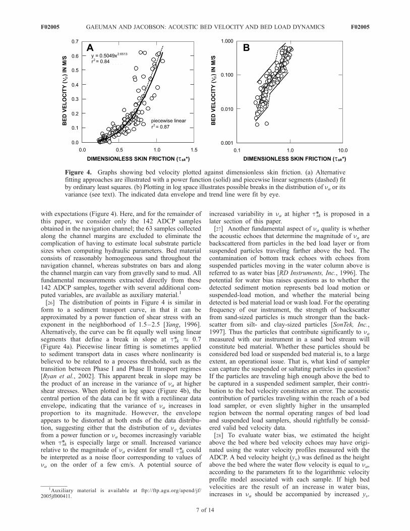
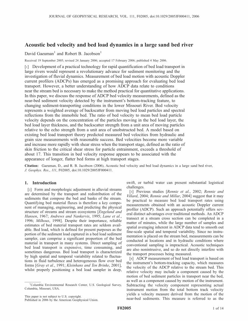
with expectations (Figure 4). Here, and for the remainder ofthis paper, we consider only the 142 ADCP samplesobtained in the navigation channel; the 63 samples collectedalong the channel margins are excluded to eliminate thecomplication of having to estimate local substrate particlesizes when computing hydraulic parameters. Bed materialconsists of reasonably homogeneous sand throughout thenavigation channel, whereas substrates on bars and alongthe channel margin can vary from gravelly sand to mud. Allfundamental measurements extracted directly from these142 ADCP samples, together with several additional com-puted variables, are available as auxiliary material.1

[26] The distribution of points in Figure 4 is similar inform to a sediment transport curve, in that it can beapproximated by a power function of shear stress with anexponent in the neighborhood of 1.5–2.5 [Yang, 1996].Alternatively, the curve can be fit equally well using linearsegments that define a break in slope at t*sk 0.7(Figure 4a). Piecewise linear fitting is sometimes appliedto sediment transport data in cases where nonlinearity isbelieved to be related to a process threshold, such as thetransition between Phase I and Phase II transport regimes[Ryan et al., 2002]. This apparent break in slope may bethe product of an increase in the variance of na at highershear stresses. When plotted in log space (Figure 4b), thecentral portion of the data can be fit with a rectilinear dataenvelope, indicating that the variance of na increases inproportion to its magnitude. However, the envelopeappears to be distorted at both ends of the data distribu-tion, suggesting either that the distribution of na deviatesfrom a power function or na becomes increasingly variablewhen t*sk is especially large or small. Increased variancerelative to the magnitude of na evident for small t*sk couldbe interpreted as a noise floor corresponding to values ofna on the order of a few cm/s. A potential source of

increased variability in na at higher t*sk is proposed in alater section of this paper.[27] Another fundamental aspect of na quality is whether

the acoustic echoes that determine the magnitude of na arebackscattered from particles in the bed load layer or fromsuspended particles traveling farther above the bed. Thecontamination of bottom track echoes with echoes fromsuspended particles moving in the water column above isreferred to as water bias [RD Instruments, Inc., 1996]. Thepotential for water bias raises questions as to whether thedetected sediment motion represents bed load motion orsuspended-load motion, and whether the material beingdetected is bed material load or wash load. For the operatingfrequency of our instrument, the strength of backscatterfrom sand-sized particles is much stronger than the back-scatter from silt- and clay-sized particles [SonTek, Inc.,1997]. Thus the particles that contribute significantly to nameasured with our instrument in a sand bed stream willconstitute bed material. Whether these particles should beconsidered bed load or suspended bed material is, to a largeextent, an operational issue. That is, what kind of samplercan capture the suspended or saltating particles in question?If the particles are traveling high enough above the bed tobe captured in a suspended sediment sampler, their contri-bution to the bed velocity constitutes an error. The acousticcontribution of particles traveling within the reach of a bedload sampler, or even slightly higher in the unsampledregion between the normal operating ranges of bed loadand suspended load samplers, should rightfully be consid-ered valid bed velocity data.[28] To evaluate water bias, we estimated the height

above the bed where bed velocity echoes may have origi-nated using the water velocity profiles measured with theADCP. A bed velocity height (yn) was defined as the heightabove the bed where the water flow velocity is equal to na,according to the parameters fit to the logarithmic velocityprofile model associated with each sample. If high bedvelocities are the result of an increase in water bias,increases in na should be accompanied by increased yn.

Figure 4. Graphs showing bed velocity plotted against dimensionless skin friction. (a) Alternativefitting approaches are illustrated with a power function (solid) and piecewise linear segments (dashed) fitby ordinary least squares. (b) Plotting in log space illustrates possible breaks in the distribution of na or itsvariance (see text). The indicated data envelope and trend line were fit by eye.

1Auxiliary material is available at ftp://ftp.agu.org/apend/jf/2005jf000411.

F02005 GAEUMAN AND JACOBSON: ACOUSTIC BED VELOCITY AND BED LOAD DYNAMICS

7 of 14

F02005

Instead, yn is either constant or decreases with increasing na(Figure 5). The average value of yn for the sample data is0.045 m, which is within the vertical reach of a conven-tional bed load sampler and thus within the bed loadtransport region for practical purposes. Most heights greaterthan about 0.05 m correspond to relatively low na, and mayreflect the incorporation of separated flow in the velocityprofiles data. According to Smith and McLean [1977], theslopes of spatially averaged velocity gradients normallydecrease near the bed when bed forms are present. Errorsin the fitted parameters due to the lack of flow-velocity datanear the bed should therefore tend to underestimate theactual near-bed velocities, so that the measured bed veloc-ities are likely to correspond to locations closer to the bedthan estimated here. To the extent that na is influenced bywater bias, the effect appears to be essentially constant overa wide range of flow conditions. This result is to someextent instrument- and site-specific. However, becausesuspended sediment loads are relatively high in the lowerMissouri River [Keown et al., 1986], the conclusion that thisinstrument is rather insensitive to water bias may beregarded to be generally valid.

7. Bed Velocity and Bed Load Particle Velocity

7.1. Model Development

[29] A better understanding of the relationship between naand np would represent a fundamental step toward improvedphysical descriptions of both na and the bed load transportprocess in general. We explore this relationship by compar-ing na to np estimated with published bed load saltationmodels. According to Van Rijn [1984], the velocity ofparticles in the bed load layer is:

np ¼ 9þ 2:6 logD*� 8tctsk

� �0:5 !

tskrs

� �0:5

ð10aÞ

D* ¼ Drs=r�1� �

g

m=r� �2

!13

ð10bÞ

The viscosity term in (10b) is expressed in terms of dynamicviscosity (m) to avoid confusion with na.[30] To ensure that estimates of np are not unduly influ-

enced by the approximations contained within the particularmodel employed, a separate set of np estimates werecomputed according to the method of Mohrig and Smith[1996]. In this model, the flow velocity distribution is givenby:

u yð Þ ¼ u*2

Zyy0

1� y=hð ÞKm yð Þ dy ð11aÞ

Km yð Þ ¼ ku*y exp �y=h� 3:2 y=hð Þ2þ2:1 y=hð Þ3h i

ð11bÞ

where u(y) is the water flow velocity at height y above thebed and u* = (ghS)0.5. Mohrig and Smith [1996] estimatedy0 as 0.056d [Wiberg and Rubin, 1989], where d is theheight above the bed of the top of the bed load layer,computed as:

d ¼ 0:68T*

1þ aT*

� �D ð12aÞ

a ¼ 0:0204 ln 100Dð Þ2 þ 0:0220 ln 100Dð Þ þ 0:0709 ð12bÞ

Equation (12a) was originally developed by Dietrich[1982], whereas the coefficients 0.68 and equation (12b)are from Wiberg and Smith [1985]. T* is a transport stageparameter, defined as t*sk/t*c, where tc is the critical shearstress for grain entrainment. Results reported below werecalculated using t*c = 0.04. The mean velocity of aparticular particle-size class in the bed load layer is thenassumed equal to the mean flow velocity in the bed loadlayer, so that:

np ¼1

d

Zdy0

u yð Þdy ¼u*2

d

Zdy0

Zyy0

1� y=hð ÞKm yð Þ dydy ð13Þ

[31] Although np computed with (10) are about 20%larger on average than those computed with (11) through(13), the two sets of estimates exhibit qualitatively similarbehavior with respect to np and hydraulic forcing. Thedynamics of these interactions are conveniently expressedby plotting the ratio na/np as a function of T* (Figure 6).Given the uncertainties associated with the modeled valuesof np used to generate Figure 6, it is encouraging that theestimated values of na/np scale from near zero to approxi-mately 1 with increasing T*. This is to be expected if oneaccepts the hypothesis introduced in (2) that na incorporateszero-velocity echoes from the immobile bed, such that na isalways less than or equal to np, and the magnitude of theeffect depends on the fraction of the bed occupied bymoving particles. In simplest terms, the hypothesis can beexpressed as:

na ¼ npwb ð14Þ

Figure 5. Graphs of heights in the water column where theestimated water velocity is equal to the bed velocity. Dashedline indicates the height of the nozzle opening of the bedload samplers used in this study (0.076 m).

F02005 GAEUMAN AND JACOBSON: ACOUSTIC BED VELOCITY AND BED LOAD DYNAMICS

8 of 14

F02005

where wb is a weighting function that presumably dependson the particle concentration and thickness of the bed loadlayer.[32] Further development along these lines requires an

expression quantifying wb. We begin by defining bp as thefraction of the bed area that is occupied by moving bed loadparticles. Assuming, for the moment, that the moving bedload particles are acoustically opaque, no echoes from thebed itself are received from that fraction. The remainder ofthe bed area, denoted bb, is the fraction of the bed fromwhich bed echoes propagate freely. By definition, bb = (1 �bp). These fractions can be estimated from the volumetricsediment concentration in the bed load layer (Cb) and thethickness of the bed load layer. Assuming that bed loadparticles are spherical, the particle cross sectional areapresented by a slice of the bed load layer 1 particle diameterin thickness is:

ap ¼Cb

4=3p D=2ð Þ3p D=2� �2 !

D ¼ 1:5Cb ð15Þ

The bed load layer contains (d/D) such slices, and thefraction of area within each slice through which bed echoescan propagate is (1 � ap). The probable fraction of bed areathat remains uncovered by a particle cross section whenoverlain by (d/D) slices is:

bb ¼ 1� ap� � d

Dð Þ ð16Þ

[33] The ratio of bp to the sum of bb and bp is equivalentto the fraction of the bed occupied by moving particles.However, because reflections from a solid bed are strongerthan backscatter from suspended particles, it is necessary toadjust this simple area ratio by including a factor (F)quantifying the relative strengths of echoes reflected fromimmobile and mobile areas:

wb ¼bp

bp þ bbF

� �ð17Þ

[34] Evaluation of (17) requires estimates for Cb, d, and F.Although many models have been proposed for estimating

Cb and d, their results vary widely and their accuracy isuncertain [Cao, 1999]. Differences in estimated values of Cb

and d commensurate with the variability among differentsediment entrainment models were found to have largeeffects on computed values of wb. In particular, relativelymodest changes in d can produce changes in parts of the wb-response curve that span the bulk of the response domain(Figure 7). For this study, we estimated the particle con-centration in the bed load layer and the height of the top ofthe bed load layer according to [Van Rijn, 1984]:

Cb

C0

¼ 0:18tsk=tc þ 1ð Þ

D*ð18aÞ

dD¼ 0:3D*

0:7 tsktc

þ 1

� �0:5

ð18bÞ

Figure 6. Graphs of the ratio of na/np versus T*. Normalization by np should theoretically cause theordinate to approach unity at sufficiently large values of excess shear stress. Estimates for np wereobtained from (a) equation (10) and (b) equations (11)–(13). Note that the range of the ordinate scale isgreater in Figure 6b.

Figure 7. Graph showing values of the weighting factorwb as a function of sediment concentration in the bed loadlayer and layer thickness. Solid circles show wb correspond-ing to concentration-thickness combinations calculated forADCP samples according to the Van Rijn method. Solidlines indicate the shape of the relation for bed load layerthicknesses ranging between about D90 (0.0022 m) and3D90.

F02005 GAEUMAN AND JACOBSON: ACOUSTIC BED VELOCITY AND BED LOAD DYNAMICS

9 of 14

F02005

where C0 is the maximum volumetric concentration of thebed, assumed equal to 0.65. Use of these equations isjustified because they are components of an internallyconsistent bed load transport formula that was explicitlyformulated as the product of Cb, d, and np as computed with(10). Values of Cb and d predicted by (18) are inapproximate agreement with graphs of laboratory datapresented by Cao [1999] for the grain sizes and shearstresses considered here.[35] The value of F depends on characteristics of the

instrument, the bed, and the bed load particles, for whichdetailed information is generally unavailable. However,backscatter profiles collected in the field suggest that Fmay be in the neighborhood of 101 for our instrument andfield conditions (analysis of a representative backscatterprofile is presented in Appendix A). We therefore assignF a nominal value of 10 for the modeling experimentsreported below. We emphasize that this choice of F repre-sents a rough approximation based on noisy, low-resolutionfield data confounded by the presence of bed topography. Inaddition, the analysis requires the approximation of numer-ous unknown environmental parameters. Precise measure-ments under controlled conditions will ultimately benecessary if F is to be accurately determined. Fortunately,the qualitative behavior of wb is not strongly dependent onthe precise value assigned to F. Plotting wb versus bp forvalues of F ranging from 5 to 50 yields a family of concave-up curves (Figure 8). Increasing F produces a sharper curveand shifts the region of maximum curvature to larger bp. Ingeneral, most of the curvature occurs when bp > 0.5, suchthat the function is approximately linear for small bp.

7.2. Model Performance

[36] The complete model relating na to np is obtained byinserting (17) into (14) and estimating the required inputvariables with (10), (15), (16), and (18). As F has beenassigned a constant value of 10, this implementation of themodel contains no adjustable parameters. The resultingpredicted bed velocities plot along an approximately linear

trend reasonably near the line of 1:1 correspondence withrespect to the measured bed velocities (Figure 9). Theseresults suggest that the concavity in the distribution of na/npwith respect to T* (Figure 6) primarily reflects the nonlinearform of wb shown in Figures 7 and 8. The extent to whichwb will reproduce the observed concavity in na/np dependsmainly on the values of Cb and d input to the model, as thesedetermine bp and the portion of the wb-response curve(Figure 8) from which wb values will be drawn. Largerinput values of either Cb or d would produce a set of wb

values and hence a set of predicted na with a steeper slopeand greater curvature with respect to the forcing hydraulicvariables. Inaccuracies in the specification of Cb or d couldbe compensated to some extent by allowing F to be adjustedas a free parameter. However, F has relatively little effect onthe shape of the model output curve, so that the primaryconsequence of making modest changes to its value is ageneral scaling of the output. The fact that bed velocitiesmodeled with F = 10 are similar in magnitude to themeasured values suggests that this estimate for F is nottoo far off the mark.

7.3. Influence of Bed Forms

[37] Although the model described above is capable ofreproducing some general aspects of how na/np changeswith T*, additional effects independent of wb no doubtinfluence the magnitude of na. In particular, wb containsno provision to account for the substantial increase invariability observed at larger values of T* (Figure 6). Asin Figure 4, increased scatter appears in the na/np � T*relation at approximately the point of maximum concavityin the curve, suggesting that some portion of the apparentcurvature may be related to a shift in the processes thatdetermine the magnitude or variance of na.[38] As the phenomenon depicted in Figure 6 incorporates

poorly understood interactions between acoustic energyand moving sediment, we refrain from specifying a pre-ferred functional form for these relations. Regardless of thestatistical model chosen to describe the data, the region ofgreatest curvature (if a curve is assumed), break in slope (if

Figure 8. Graph showing the effect of the value of F onthe shape of the response curve of the weighting factor wb

as a function of the fraction of bed area occupied by movingparticles (bp).

Figure 9. Graph of measured na versus modeled na forinput variables estimated with the Van Rijn equations. Thedashed line indicates 1:1 correspondence.

F02005 GAEUMAN AND JACOBSON: ACOUSTIC BED VELOCITY AND BED LOAD DYNAMICS

10 of 14

F02005

a piecewise linear description is chosen), or increasedvariance occurs in the neighborhood of T* 17. Fieldobservations suggest that the somewhat erratic increases inna observed when T* > 17 are associated with changes in themorphology of bed forms where the measurements wereobtained. Conventional estimates of np are derived with theassumption of a fully developed boundary layer, and so arestrictly applicable only to uniform flow conditions or in thevicinity of bed form crests [Mohrig and Smith, 1996;McLean et al., 1999]. More realistically, bed load particlevelocity is a spatially distributed continuous variable with aspatial average less than np. The relationship between localnp, i.e., the velocity computed for bed form crests, to spatiallyaveraged np is unlikely to be constant with changing T*. It iswell established that both bed form morphology [Yalin andKarahan, 1979; Karim, 1995; Julien and Klaassen, 1995]and the degree of flow separation associated with bed forms[Smith and McLean, 1977] change with flow conditions.Because na is inherently a spatially averaged measurement, itshould be expected to respond to these changes.[39] The effect of bed form morphology on na can be

illustrated by comparing samples with large na with samplesfor which na is relatively small, but T* is comparable. Wechose to compare the 15 samples with the largest na(average T* = 21.7 and average na = 0.51 m/s) with10 samples whose average T* is comparable (18.6) butwhose average na is substantially less (0.15 m/s). Of these25 samples, 17 were obtained near the longitudinal naviga-tion line established in 2005, so na can be compared withbed form morphology at the same location. Samples with

relatively low na were found to be associated with small,often irregular bed forms with an average wavelength of16 m, whereas samples with high na were obtained in areaswhere bed forms were more than twice as long, with anaverage of about 35 m (Figure 10). Unfortunately, we didnot collect spatially explicit profile data for the subset ofhigh-na samples recorded in 2004. These samples wereobtained in early to mid June in the downstream part ofthe bend near the 7000 m hash on Figure 1. Bed formprofiles were not conducted in 2004 until mid-June, andthen only in the upstream crossing. However, these surveysdocumented the presence of bed forms up to 60 m inwavelength at the time (Figure 10). Bed forms wereobserved to increase in size with increased stream dischargein both years, and, according to the 2005 profiles, areconsistently larger in the bend than in the crossing. Thusit is probable that large bed forms were present in the bendthrough most of June 2004, when large forms evolved in thecrossing and discharge was relatively high (Figure 2).[40] Noticeable differences in the distribution of na

over smaller and larger bed forms were observed in high-resolution maps of bed topography and bed velocitiesobtained in 2004 (Figure 11). All the maps indicate thathigh na occurs in topographically high areas and low naoccurs in troughs where separated flow is presumed to occur.However, the areas of relatively low na aremore extensive forsmaller bed forms, so that higher-than-average na is restrictedto small areas near the bed form crests. The result is thatthe frequency distribution of na is strongly skewed.In contrast, na is more evenly distributed in the vicinity of

Figure 10. Bed form profiles indicating the magnitudes and locations of bed velocity and transport-stage measurements. (a and b) Smaller bed forms associated with low na. (c and d) Larger bed formsassociated with high na. Figure 10c includes examples of the large bed forms surveyed in the upstreamcrossing in June 2004. Horizontal axis indicates downstream position on the longitudinal navigation line.

F02005 GAEUMAN AND JACOBSON: ACOUSTIC BED VELOCITY AND BED LOAD DYNAMICS

11 of 14

F02005

larger bed forms where areas of separated flow appear to beconfined to the deepest part of the troughs.[41] These linkages between dune morphology, bed load

velocity, and changes in the bed velocity field suggest that ageneralized expression for na requires an additional scalingfactor (wf) to account for differences between the spatiallyaveraged bed load particle velocity and np, so that (14)becomes:

na ¼ npwbwf ð19Þ

Development of a quantitative model for wf is beyond thescope of the present study. The precise spatially distributedmeasurements of bed load/bed form dynamics needed todefine and validate suitable equations are currentlyunavailable.

8. Conclusions

[42] Comparisons between 142 time-averaged ADCP bedvelocity measurements (na) and mean bed load particle

velocities (np) estimated from existing sediment transportequations demonstrate that the ratio na/np scales from zeroto approximately 1 with increasing sediment transport stage(T*). This result is consistent with the hypothesis that nameasurements represent a weighted average of the acousticbackscatter from moving bed load particles and spectralreflections from the immobile bed. As T* increases, thefraction of the bed occupied by moving particles becomeslarger, so that more acoustic energy is backscattered fromthe moving bed load, less energy penetrates to and reflectsfrom the bed, and the ratio na/np increases. The observedrelation between measured na and estimated np is formalizedin a physically based model composed of a weightingfunction (wb), where na = npwb. The value of wb dependson the size and concentration of the particles moving in thebed load layer, the bed load layer thickness, and a parameter(F) that represents the ratio of the echo strength from a unitarea of unobstructed bed to the backscatter strength from aunit cross sectional area of moving particles. The modelreplicates measured values of na from hydraulic and grainsize measurements with reasonable success. However, pre-dicted na are on average about 50% larger than measured na.This bias may reflect the fact that the equations used topredict bed load particle velocities are strictly applicableonly in the vicinity of bed forms crests, whereas the acousticmeasurements represent spatial averages over both crestsand lower-velocity trough areas.[43] When plotted as a function of T*, the ratio na/np was

found to increase relatively gradually up to a threshold T*of about 17. As T* exceeds about 17, the rate of increase inna/np increases sharply. The form of the na/np responsecurve is at least partially due to the presence of similarcurvature in wb when plotted versus the fraction of bed areaoccupied by moving bed load. The amount of curvature inthe relation depends primarily on the model parameter F,which in this study was set equal to 10 on the basis of semi-quantitative evaluation of ADCP backscatter profilesrecorded in the field. Model results are also sensitive tothe methods used to estimate the bed load particle concen-tration and layer thickness, parameters for which no gener-ally accepted predictive equations exist. Therefore theapparent success of the present model must be regardedwith caution. The detailed measurements of bed loadtransport parameters necessary for a rigorous evaluation ofmodel performance are likely obtainable only in a controlledlaboratory setting. The minimum data requirement includessimultaneous measurement of na, the actual bed loadtransport rate, the mean bed load particle velocity, and thethickness of the bed load saltation layer. The mean particleconcentration in the saltation layer can be determined fromthe measured data, and F can be treated as a parameterwhose range of possible values can be constrained byindependent measurements or theoretical expectations.[44] The increased slope of the na/np response curve at

higher transport stages may be partially due to the appear-ance of considerable variability in na/np when T* exceeds17. The increased scatter at higher T* appears to be relatedto changes in bed form morphology that produce an abruptthreshold-like shift in the na response. Particularly largevalues of na/np were recorded in areas where bed formwavelengths were approximately twice the wavelengths ofbed forms located in areas where T* was similar, but na/np

Figure 11. Map of bed topography and the distribution ofna over the same patch of bed on (a) 27 July 2004 and on(b) 18 June 2004. Contours indicated flow depth andshading indicates the normalized Z scores for na [(na �mean(na))/standard deviation (na)]. Histograms show rangesand frequency distributions of the na measurements for eachdate.

F02005 GAEUMAN AND JACOBSON: ACOUSTIC BED VELOCITY AND BED LOAD DYNAMICS

12 of 14

F02005

was comparatively small. High-resolution maps suggest thatregions of near-bed flow separation and near-zero bed loadparticle velocities comprise a smaller fraction of the largerbed forms, such that spatially averaged bed load velocitiesmore closely approximate velocities near the bed formcrests. However, insufficient data are presently availableto validate this hypothesis.[45] Prerequisite to any meaningful interpretation of bed

velocity data, it is necessary to confirm the general precisionand accuracy of these acoustic measurements. The emer-gence of consistent and physically realistic trends whencompared to other hydraulic measurements indicate that theprecision of na measured with the instrument and methodsemployed here is similar to that of other basic measure-ments routinely used to characterize streams. Analysis ofthe vertical velocity profile suggests that the measurementsreported here are essentially unaffected by water bias, eventhough this study was conducted in a river carrying rela-tively high suspended sediment loads. An instrument thatoperates at a higher frequency or makes use of a narrowerfrequency bandwidth may not perform as well under theenvironmental conditions encountered in the lower MissouriRiver.

Appendix A: Evaluation of F From BackscatterProfiles

[46] Figure A1 shows representative water column back-scatter profiles for a single ping, as recorded in 0.25-m binsby each of the ADCP’s 4 transducers. These data wereobtained in 9.84 m of water under conditions of high na(0.44 m/s) and T* (23). The greatest backscatter intensityfor each of the 4 profiles corresponds to the bin containingthe bed, and is about 14 dB greater on average than thebackscatter recorded for the water column bin immediatelyabove the bed. As each difference of 3 dB corresponds to adoubling of signal strength, a difference of 14 dB corre-sponds to more than a 25-fold difference in signal strength(i.e., wb = 1/25). Although the bin immediately above bedlevel may not contain the bed load layer, it does occupy aregion of the water column in which suspended sandconcentrations are relatively high. Thus an approximationof F can be obtained by inverting (17) if the distribution ofsuspended bed material in the bin immediately above thebed can be estimated.[47] The mean concentration of suspended bed material at

specific distances above the bed can be estimated with theRouse equation [Raudkivi, 1998]:

Cy

Ca

¼ h� y

h� a

a

y

� �Z

ðA1Þ

where Cy is the bed material concentration at height y abovethe bed, Ca is the concentration at height a above the bed, ais the height above the bed of the top of the bed load layer, Zis the Rouse number (w/ku*), and w is the particle fallvelocity. According to the method of Rubey [1933], w forthe bed particle D50 in the study reach is approximately0.07 m/s. u* is defined as (ghS)0.5, whereas a and Ca areequivalent to d and Cb, as estimated by (18). For the flowconditions associated with Figure A1, Cb is approximately0.2 and d is 0.0047.

[48] For the present analysis, (A1) was evaluated for eachof 0.25/D50 discrete layers from y1 to y2, where y1 corre-sponds to the bottom of the lowest water column bin abovethe bed, y2 corresponds to the top of the same bin (y1 +0.25), and each layer is one particle diameter in thickness.An individual ap was obtained for each of the 0.25/D50

layers according to (15), and bb was then computed as theproduct of all ap values. However, the spatial resolution ofthe ADCP data does not permit precise specification of y1and y2, so that it is necessary to consider a range of possiblevalues. By definition, the maximum value of y1 is 1 bin, or0.25 m. When evaluated over the interval y = 0.25 to 0.5 m,this analysis yields F = 8.3. Conversely, the minimum valueof y1 approaches zero. Arbitrarily choosing a small y1 of0.01 m yields F = 692. On average, y1 will fall at 0.125 m(half a bin), which yields F = 19.2. We therefore tentativelyconclude that the actual value of F is probably near 10, orperhaps somewhat larger than 10.

[49] Acknowledgment. This paper benefited immensely from thethorough review and numerous helpful suggestions provided by twoanonymous reviewers and an anonymous Associate Editor.

ReferencesAndrews, E. D., and J. M. Nankervis (1995), Effective discharge and thedesign of channel maintenance flows for gravel-bed rivers, in Naturaland Anthropomorphic Influences in Fluvial Geomorphology, Geophys.Monogr. Ser., vol. 89, edited by J. E. Costa et al., pp. 151–164, AGU,Washington, D. C.

Cao, Z. (1999), Equilibrium near-bed concentration of suspended sediment,J. Hydraul. Eng., 125, 1270–1278.

Childers, D. (1999), Field comparisons of six pressure-difference bedloadsamplers in high-energy flow, U.S. Geol. Surv. Water Resour. Invest.Rep., 92-4068.

Dietrich, W. E. (1982), Flow, boundary shear stress, and sediment transportin a river meander, Ph.D. dissertation, Univ. of Wash., Seattle.

Figure A1. Graph showing backscatter profiles recordedby each of the 4 instrument transducers for a representativewater column ping. Backscatter intensities recorded in thebin containing the bed are about 25 times stronger thanbackscatter recorded in the bin immediately above the bed.Bins are 0.25 m in vertical extent.

F02005 GAEUMAN AND JACOBSON: ACOUSTIC BED VELOCITY AND BED LOAD DYNAMICS

13 of 14

F02005

Edwards, T. E., and G. D. Glysson (1999), Field methods for measurementof fluvial sediment, U.S. Geol. Surv. Tech. Water Resour. Invest., Book 3,Chap. C2.

Engelund, F., and E. Hansen (1967), A Monograph on Sediment Transportin Alluvial Streams, Teknisk Forlag, Copenhagen.

Gaeuman, D., and R. B. Jacobson (2005), Aquatic habitat mapping with anacoustic Doppler current profiler: Considerations for data quality, U.S.Geol. Surv. Open File Rep., 2005-1163.

Gaweesh, M. T. K., and L. C. Van Rijn (1994), Bed-load sampling in sandbed rivers, J. Hydraul. Eng., 120, 1365–1384.

Gomez, B. (1991), Bedload transport, Earth Sci. Rev., 31, 89–132.Gray, J. R., R. H. Webb, and D. W. Hyndmann (1991), Low-flow sedimenttransport in the Colorado River, in Proceedings of the Fifth FederalInteragency Sedimentation Conference, vol. 4, edited by S.-S. Fan andY.-H. Kuo, pp. 63–71, U.S. Subcomm. on Sedimentation, Washington,D.C.

Julien, P. Y., and G. J. Klaassen (1995), Sand-dune geometry of large riversduring floods, J. Hydraul. Eng., 121, 657–663.

Karim, F. (1995), Bed configuration and hydraulic resistance in alluvial-channel flows, J. Hydraul. Eng., 121, 15–25.

Keown, M. P., E. A. Dardeau Jr., and E. M. Causey (1986), Historic trendsin the sediment flow regime of the Mississippi River, Water Resour. Res.,22, 1555–1564.

Kleinhans, M. G., and W. B. M. Ten Brinke (2001), Accuracy of cross-channel sampled sediment transport in large sand-gravel-bed rivers,J. Hydraul. Eng., 127, 258–269.

Lane, S. N., K. S. Richards, and J. H. Chandler (1996), Discharge andsediment supply controls on erosion and deposition in a dynamic alluvialchannel, Geomorphology, 15, 1–15.

Mark, D. M., and M. Church (1977), On the use and misuse of regression inEarth science, Math. Geol., 9, 63–75.

McLean, S. R., S. R. Wolfe, and J. M. Nelson (1999), Predicting boundaryshear stress and sediment transport over bed forms, J. Hydraul. Eng.,127, 725–736.

Milhous, R. T. (1998), Modelling of instream flow needs: The link betweensediment and aquatic habitat, Reg. Rivers Res. Manage., 14, 79–94.

Mohrig, D., and J. D. Smith (1996), Predicting the migration rates ofsubaqueous dunes, Water Resour. Res., 32, 3207–3217.

Raudkivi, A. J. (1998), Loose Boundary Hydraulics, A. A. Balkema,Brookfield, Vt.

RD Instruments, Inc. (1996), Principles of operation: A practical primer,2nd edition for broadband ADCPs, report, San Diego, Calif.

Rennie, C. D., and R. G. Millar (2004), Measurement of the spatial dis-tribution of fluvial bedload transport velocity in both sand and gravel,Earth Surf. Processes Landforms, 29, 1173–1193, doi:10.1002/esp1074.

Rennie, C. D., and P. V. Villard (2004), Site specificity of bed load mea-

surement using an acoustic Doppler current profiler, J. Geophys. Res.,109, F03003, doi:10.1029/2003JF000106.

Rennie, C. D., R. G. Millar, and M. A. Church (2002), Measurement of bedload velocity using an acoustic Doppler current profiler, J. Hydraul. Eng.,128, 473–483.

Rubey, W. W. (1933), Settling velocities of gravel, sand, and silt particles,Am. J. Sci., 25, 325–338.

Ryan, S. E., L. S. Porth, and C. A. Troendle (2002), Defining phases of bedload transport using piecewise regression, Earth Surf. Processes Land-forms, 27, 971–990.

Simpson, M. R. (2001), Discharge measurements using a broadband acousticDoppler current profiler, U.S. Geol. Surv. Open File Rep., 01-1.

Smith, J. D., and S. R. McLean (1977), Spatially averaged flow over awavy surface, J. Geophys. Res., 82, 1735–1746.

SonTek, Inc. (1997), SonTek Doppler current meters—Using signalstrength data to monitor suspended sediment concentrations, SonTekapplication notes, report, San Diego, Calif.

Thorne, P. D., and D. M. Hanes (2002), A review of acoustic measurementof small-scale sediment processes, Cont. Shelf Res., 22, 603–632.

U.S. Army Corps of Engineers (2003), Appendix E: Missouri River hydrol-ogy and hydraulic analysis, in Upper Mississippi River System FlowFrequency Study, report, Kansas City Dist., Kansas City, Mo. (Availableat http://www.mvr.usace.army.mil/pdw/pdf/FlowFrequency/Documents/FinalReport/default.asp)

U.S. Geological Survey (2001), Policy and technical guidance on dischargemeasurements using acoustic Doppler current profilers, Tech. Memo.2002.02, Off. of Surf. Water, Water Resour. Div., Washington, D. C.

Van Rijn, L. C. (1984), Sediment transport, part I: Bed load transport,J. Hydraul. Eng., 110, 1431–1456.

Wiberg, P. L., and D. M. Rubin (1989), Bed roughness produced by salt-ating sediment, J. Geophys. Res., 94, 5011–5016.

Wiberg, P. L., and J. D. Smith (1985), A theoretical model for saltatinggrains in water, J. Geophys. Res., 90, 7341–7354.

Wright, S., and G. Parker (2004), Flow resistance and suspended load insand-bed rivers: Simplified stratification model, J. Hydraul. Eng., 130,796–805.

Yalin, M. S., and E. Karahan (1979), Steepness of sedimentary dunes,J. Hydraul. Div. Am. Soc. Civ. Eng., 105, 381–392.

Yang, C. T. (1996), Sediment Transport: Theory and Practice, McGraw-Hill, New York.

�����������������������D. Gaeuman and R. B. Jacobson, Columbia Environmental Research

Center, USGS, 4200 New Haven Road, Columbia, MO 65201, USA.(dgaeuman@mp.usbr.gov; rjacobson@usgs.gov)

F02005 GAEUMAN AND JACOBSON: ACOUSTIC BED VELOCITY AND BED LOAD DYNAMICS

14 of 14

F02005