Accuracy of activity quantitation of F-18 fluorodeoxyglucose (FDG ...
140
Florida International University FIU Digital Commons FIU Electronic eses and Dissertations University Graduate School 7-24-2003 Accuracy of activity quantitation of F-18 fluorodeoxyglucose (FDG) Positron Emission Tomography (PET) imaging using simulated malignant tumors Madhu Durai Florida International University DOI: 10.25148/etd.FI15101249 Follow this and additional works at: hps://digitalcommons.fiu.edu/etd Part of the Biomedical Engineering and Bioengineering Commons is work is brought to you for free and open access by the University Graduate School at FIU Digital Commons. It has been accepted for inclusion in FIU Electronic eses and Dissertations by an authorized administrator of FIU Digital Commons. For more information, please contact dcc@fiu.edu. Recommended Citation Durai, Madhu, "Accuracy of activity quantitation of F-18 fluorodeoxyglucose (FDG) Positron Emission Tomography (PET) imaging using simulated malignant tumors" (2003). FIU Electronic eses and Dissertations. 3102. hps://digitalcommons.fiu.edu/etd/3102
-
Upload
khangminh22 -
Category
Documents
-
view
1 -
download
0
Transcript of Accuracy of activity quantitation of F-18 fluorodeoxyglucose (FDG ...
Florida International UniversityFIU Digital Commons
FIU Electronic Theses and Dissertations University Graduate School
7-24-2003
Accuracy of activity quantitation of F-18fluorodeoxyglucose (FDG) Positron EmissionTomography (PET) imaging using simulatedmalignant tumorsMadhu DuraiFlorida International University
DOI: 10.25148/etd.FI15101249Follow this and additional works at: https://digitalcommons.fiu.edu/etd
Part of the Biomedical Engineering and Bioengineering Commons
This work is brought to you for free and open access by the University Graduate School at FIU Digital Commons. It has been accepted for inclusion inFIU Electronic Theses and Dissertations by an authorized administrator of FIU Digital Commons. For more information, please contact [email protected].
Recommended CitationDurai, Madhu, "Accuracy of activity quantitation of F-18 fluorodeoxyglucose (FDG) Positron Emission Tomography (PET) imagingusing simulated malignant tumors" (2003). FIU Electronic Theses and Dissertations. 3102.https://digitalcommons.fiu.edu/etd/3102
FLORIDA INTERNATIONAL UNIVERSITY
Miami, Florida
ACCURACY OF ACTIVITY QUANTITATION OF F-18 FLUORODEOXYGLUCOSE
(FDG) POSITRON EMISSION TOMOGRAPHY (PET) IMAGING USING
SIMULATED MALIGNANT TUMORS
A thesis submitted in partial fulfillment of the
requirements for the degree of
MASTER OF SCIENCE
in
BIOMEDICAL ENGINEERING
by
Madhu Durai
2003
To: Dean Vish PrasadCollege of Engineering
This thesis, written by Madhu Durai, and entitled Accuracy of Activity Quantitation OFF-18 Fluorodeoxyglucose (FDG) Positron Emission Tomography (PET) Imaging UsingSimulated Malignant Tumors, having been approved in respect to style and intellectualcontent, is referred to you for judgment.
We have read this thesis and recommend that it be approved.
Eric T. Crumpler
Anthony J. McGoron
Juan Franquiz, Major Professor
Date of Defense: July 24, 2003
The thesis of Madhu Durai is approved.
Dean Vish PrasadCollege of Engineering
Dean Douglas WartzokUniversity Graduate School
Florida International University, 2003
ii

ACKNOWLEDGMENTS
I express a sincere gratitude to my committee members, Dr. Juan Franquiz, Dr. Anthony
McGoron and Dr.Eric Crumpler for their invaluable comments, assistance and interests
in the completion of this thesis. I am particularly grateful to Dr. Juan Franquiz for the
advice, guidance and patience that he exhibited through out this project and this
research would not have been possible without his support. I would also thank the
Department of Radiology and Nuclear Medicine of Baptist hospital for providing their
instrumentation and time.
iii
ABSTRACT OF THE THESIS
ACCURACY OF ACTIVITY QUANTITATION OF F-18 FLUORO-
DEOXYGLUCOSE (FDG) POSITRON EMISSION TOMOGRAPHY (PET) IMAGING
USING SIMULATED TUMORS
by
Madhu Durai
Florida International University, 2003
Miami, Florida
Professor Juan Franquiz, Major Professor
This thesis involves a procedure, which calculated and compared the sum of all the pixel
counts, threshold pixel counts sum of a 3D PET image and mean and maximum pixel
count of one single transaxial slice (2D) of simulated tumors for a chosen region of
interest (ROI). A calibration factor was multiplied by the sum of the pixel counts,
threshold pixel counts sum of all the transaxial slices, and the mean, and maximum pixel
counts of one single transaxial slice in an ROI to calculate for the activity of the tumor.
This activity calculated was compared with the real activity values. The results showed
that the sum of all the pixel counts with applied threshold is better to calculate the activity
of tumor with greater accuracy.
These findings suggest that a 3D distribution of sum of all the pixel counts was able to
calculate the activity of malignant tumors and lung lesions with better accuracy.
iv

TABLE OF CONTENTS
CHAPTER PAGE
1. INTRODUCTION .......................................................................................................... 1
1.1 18- FDG 21.2. PET/CT Hybrid Scanner .............................. 31.3. Objective ................................................................................................................. 51.4. Hypothesis ............................................................................................................... 61.5 Significance of the Research.........,. ,. . , . ,, ,, . . ...... 6
2. BACKGROUND 9...f..he .Res.ar.. .............................................................
2 .1 BAC ton UND............................................................................................................. 9
2.2. Detection of positrons ............................................................................................ 11
2.3. Positron detectors .................................................................................................. 132.4. Production of positron emitters ......... ......... ... ..... ..... ..... ......................... 132.5. Positron emitting radio pharmaceuticals ........... ................................ 142.6. Reconstruction of PET imaging . 172.7. Attenuation of PET imaging ...................................................................... .. 18
3. M ATERIALS A M ETHODS ............................................................................... 22
3.1. PET-CT Scanner.................................................................................................233.2. Radioisotope Calibrator ......................................................... ... ...... 243.3. Radio Pharmaceutical ............................................................................................ 253.4. ET Calibration ..................................................................................................... 253.5 Decay correction of PET calibration method ........................................................ 27
3. . Uniformity calculation. .......................................................................................... 27
3.7 Experiment with simulated tumors ........................................................................ 28
3.8 Experiment with simulated lung lesions................................................................. 293.9 Region of Interest (ROI) and Threshold method.................................................... 313.10. Linear Regression Analysis ................................................................................. 32
3.11. Drawing Histograms ............................................................................................ 333.12 Comparison of activity.......................................................................................... 333.13 Errors in the calculation........................................................................................ 343.14 t-test analysis: ........................................................................................... .... 34
4. .................................................................................................................. 36
4.1. Data Analysis of PET calibration method ............................................................ 36
4.2. Data Analysis of Attenuation corrected simulated tumor PET images ................ 424.3 Data Analysis of Simulated Lung Lesion............................................................ 86
V

5. DISCUSSION ............................................................................................................. 101
. CONCLUSIONS ......................................................................................................... 106
REFERENCES ............ .................................................................................................... 109
APPENDIX ...................................................................................................................... 112
vi
LIST OF TABLES
TABLE PAGE
1. PET CALIBRATION DATA ............................................................................................... 37
2. PET CALIBRATION PIXEL COUNT VALUES ................................... 39
3. CALCULATION OF CALIBRATION FACTOR ......................................... ........................... 40
4. SIMULATED TUMOR EXPERIMENT DATA .............................................................. . 43
5. 3D PIXEL COUNT VALUES OF SPHERE 1 OF ATTENUATION CORRECTED IMAGES ............ 44
6. 10 % THRESHOLD VALUE PIXEL COUNT VALUES OF SPHERE 1 ........................................ 45
7. 20 % THRESHOLD VALUE PIXEL COUNT VALUES OF SPHERE 1 ..................................... 46
8.30 % THRESHOLD VALUE PIXEL COUNT VALUES OF SPHERE 1 ...................................... 47
9.40 % AND 50 % THRESHOLD PIXEL COUNTS VALUE OF SPHERE 1 .................................. 48
10. 3D PIXEL COUNT VALUES OF SPHERE 2 OF ATTENUATION CORRECTED IMAGES ......... 49
11. 10 % THRESHOLD VALUE PIXEL COUNT VALUES OF SPHERE 2 ...................................... 51
12. 20 % AND 30% THRESHOLD VALUE PIXEL COUNT VALUES OF SPHERE 2 ...................... 52
13. 40 % AND 50% THRESHOLD VALUE PIXEL COUNT VALUES OF SPHERE 2 ...................... 53
14. 3D PIXEL COUNT VALUES OF SPHERE 3 OF ATTENUATION CORRECTED IMAGES ............ 54
15. 10 % THRESHOLD VALUE PIXEL COUNT VALUES OF SPHERE 3...................................... 56
16. 20 % THRESHOLD VALUE PIXEL COUNT VALUES OF SPHERE 3 .................................... 57
17. 30 % THRESHOLD VALUE PIXEL COUNT VALUES OF SPHERE 3 ...................................... 58
18.40 % AND 50% THRESHOLD VALUE PIXEL COUNT VALUES OF SPHERE 3 ...................... 59
19. 3D PIXEL COUNT VALUES OF ATTENUATION CORRECTED IMAGES OF SPHERE 4 ............ 60
20. 10% THRESHOLD VALUE PIXEL COUNT VALUES OF SPHERE 4................................... 62
21. 20% AND 30% THRESHOLD VALUE PIXEL COUNT VALUES OF SPHERE 4 ...................... 63
vii
22.40% AND 50% THRESHOLD VALUE PIXEL COUNT VALUES OF SPHERE 4 ....................... 64
23. 3D PIXEL COUNT VALUES OF ATTENUATION CORRECTED IMAGES OF SPHERE 5 ............ 65
24. 10% THRESHOLD VALUE PIXEL COUNT VALUES OF SPHERE 5....................................... 66
25.20% AND 30% THRESHOLD VALUE PIXEL COUNT VALUES OF SPHERE 5....................... 67
26.40% AND 50% THRESHOLD VALUE PIXEL COUNT VALUES OF SPHERE 5 ...................... 68
27. 3D PIXEL COUNT VALUES OF ATTENUATION CORRECTED IMAGES OF SPHERE 6 ............ 69
28. 10% THRESHOLD VALUE PIXEL COUNT VALUES OF SPHERE 6................................... 71
29. 20% AND 30% THRESHOLD VALUE PIXEL COUNT VALUES OF SPHERE 6 ...................... 72
30.40% AND 50% THRESHOLD VALUE PIXEL COUNT VALUES OF SPHERE 6 ...................... 73
31. LINEAR REGRESSION ANALYSIS OF SPHERE ACTIVITY(gCI) VS PIXEL COUNTS MEAN.... 75
32. LINEAR REGRESSION ANALYSIS OF SPHERE ACTIVITY( CI) VS PIXEL COUNTS MAX...... 76
33. LINEAR REGRESSION ANALYSIS OF SPHERE ACTIVITY(pCI) VS PIXEL COUNTS SUM ...... 77
34. 10% THRESHOLD LINEAR REGRESSION ANALYSIS OF SPHERE ACTIVITY (pCI) VS PIXELCOUNTS SUM .................................................................................... 78
35. 20% THRESHOLD LINEAR REGRESSION ANALYSIS OF SPHERE ACTIVITY (pCI) VS PIXEL
COUNTS SUM ............................................................................................................... 79
36. 30% THRESHOLD LINEAR REGRESSION ANALYSIS OF SPHERE ACTIVITY (pCI) VS PIXEL
COUNTS SUM ................................................................................................................ 80
37.40% THRESHOLD LINEAR REGRESSION ANALYSIS OF SPHERE ACTIVITY (PCI) VS PIXEL
COUNTS SUM ................................................................................................................ 81
38. 50% THRESHOLD LINEAR REGRESSION ANALYSIS OF SPHERE ACTIVITY (pCI) VS PIXEL
COUNTS SUM ............................................................................................................... 82
39. PIXEL COUNT VALUES OF SIMULATED LUNG LESION 1 WITH 10% AND 20% THRESHOLD
.................................................................................................................................. 88
40. PIXEL COUNT VALUES OF SIMULATED LUNG LESION 2.................................................. 89
41. 10% THRESHOLD PIXEL COUNT VALUES OF SIMULATED LUNG LESION 2..................... 90
Viii

42. 20% AND 30% THRESHOLD PIXEL COUNT VALUES OF SIMULATED LUNG LESION 2 ..... 91
43.40% AND 50% THRESHOLD PIXEL COUNT VALUES OF SIMULATED LUNG LESION 2...... 92
44. ERROR PERCENTAGE CALCULATION OF PIXEL COUNTS MEAN PER MINUTE FOR ALL THESIX SPHERES. ................................................................................................................ 94
45. ERROR PERCENTAGE CALCULATION OF PIXEL COUNTS MAXIMUM PER MINUTE FOR ALLTHE SIX SPHERES. ......................................................................................................... 94
46. ERROR PERCENTAGE CALCULATION OF PIXEL COUNTS SUM PER MINUTE FOR ALL THE SIXSPHERES ....................................................................................................................... 95
47. ERROR PERCENTAGE CALCULATION OF 10% THRESHOLD PIXEL COUNTS SUM PERMINUTE FOR L THE SIX SPHERES............................................................................. 95
48. ERROR PERCENTAGE CALCULATION OF 20% THRESHOLD PIXEL COUNTS SUM PERMINUTE FOR ALL THE SIX SPHERES ............................................................................ 96
49. ERROR PERCENTAGE CALCULATION OF 30% THRESHOLD PIXEL COUNTS SUM PERMINUTE FOR ALL THE SIX SPHERES .............................................................................. 96
50. ERROR PERCENTAGE CALCULATION OF 40% THRESHOLD PIXEL COUNTS SUM PERMINUTE FOR ALL THE SIX SPHERES............................................................................. 9
51. ERROR PERCENTAGE CALCULATION OF 50% THRESHOLD PIXEL COUNTS SUM PERMINUTE FOR ALL THE SIX SPHERES .............................................................................. 97
52. ERROR PERCENTAGE CALCULATION OF PIXEL COUNTS MEAN PER MINUTE FOR
SIMULATED LUNG LESIONS 1 AND 2 ............................................. ........... 98
53. ERROR PERCENTAGE CALCULATION OF PIXEL COUNTS MAXIMUM PER MINUTE FOR
SIMULATED LUNG LESIONS 1 AND 2 .............................................................................. 98
54. ERROR PERCENTAGE CALCULATION OF PIXEL COUNTS SUM PER MINUTE AND
THRESHOLD PIXEL COUNTS SUM PER MINUTE FOR SIMULATED LUNG LESIONS 1 AND 2. 98
55. T-TEST ANALYSIS OF LINEAR REGRESSION GRAPHS ................................................. 99
56. HISTOGRAM ANALYSIS OF SIMULATED TUMORS AND SIMULATED LUNG LESION ........ 100
iX
LIST OF FIGURES
FIGURE PAGE
1. STRUCTURE OF 1 8-FDG ................................................................................................... 3
2. PET-CT SCANNER ........................................................................................................... 4
3. THE POSITRON ELECTRON ANNIHILATION PROCESS ................................ 11
4. COINCIDENCE DETECTION ................................................ 12
5. PHOTOELECTRIC EFFECT . 19
6. COMPTON EFFECT. .......................................................................................................... 19
7. CALCULATION OF ATTENUATION COEFFICIENT ............................................................. 21
8. RADIOISOTOPE CALIBRATOR ............................................. 24
9. JASZCZAK PHANTOM ..................................................................................................... 25
10. DATA SPECTRUM LUNG PHANTOM ............................................................................... 30
11. PET CALIBRATION IMAGES .......................................................................................... 38
12. SLICE NUMBER VS UNIFORMITY(% .......................................................................... 41
13. SLICE NUMBER VS CPM PER PIXEL ................................................................ 41
14. TRANSAXIAL SLICES 28-34 OF ATTENUATION CORRECTED PET IMAGE .................... 43
15. LINEAR REGRESSION ANALYSIS OF SPHERE ACTIVITY(pCI) VS PIXEL COUNTS MEAN.. 75
16. LINEAR REGRESSION ANALYSIS OF SPHERE ACTIVITY (JCI) VS PIXEL COUNTS MAXIMUM
.................................................. 7.................................................................................. 76
17. LINEAR REGRESSION ANALYSIS OF SPHERE ACTIVITY (pCI) VS PIXEL COUNTS SUM ..... 77
18. 10% THRESHOLD LINEAR REGRESSION ANALYSIS OF SPHERE ACTIVITY (pCI) VS PIXEL
COUNTS SUM ............................................................................................................... 78
19. 20 % THRESHOLD LINEAR REGRESSION ANALYSIS PF SPHERE ACTIVITY(pCI) VS PIXEL
COUTS SUM. .............................................................................................................. 79

20.30 % THRESHOLD LINEAR REGRESSION ANALYSIS OF SPHERE ACTIVITY (SCI) VS PIXEL
COUNTS SUM ................................................................................................................ 80
21.40 % THRESHOLD LINEAR REGRESSION ANALYSIS OF SPHERE ACTIVITY (P CI) VS PIXELCOUNTS SUM ................................................................................................................ 81
22. 50 % THRESHOLD LINEAR REGRESSION ANALYSIS OF SPHERE ACTIVITY (pCI) VS PIXELCOUNTS SUM ............................................................................................................... 82
23. HISTOGRAM OF PIXEL COUNTS VS FREQUENCY OF SPHERE 1 ........................................ 83
24. HISTOGRAM OF PIXEL COUNTS VS FREQUENCY OF SPHERE 2........................................ 83
25. HISTOGRAM OF PIXEL COUNTS VS FREQUENCY OF SPHERE 3 ....................................... 84
26. HISTOGRAM OF PIXEL COUNTS VS FREQUENCY OF SPHERE 4........................................ 84
27. HISTOGRAM OF PIXEL COUNTS VS FREQUENCY OF SPHERE 5........................................ 85
28. HISTOGRAM OF PIXEL COUNTS VS FREQUENCY OF SPHERE 6........................................ 85
29. PET-CT IMAGE OF SIMULATE LUNG LESIONS ............................................................ .... 87
30. HISTOGRAM OF PIXEL COUNTS VS FREQUENCY OF LUNG 1 ........................................... 93
31. HISTOGRAM OF PIXEL COUNTS VS FREQUENCY OF LUNG 2 ........................................... 93
X1
1. INTRODUCTION
Positron Emission Tomography (PET) is a three-dimensional (3D) imaging
technique, which can be used to measure the level of metabolic activity within the cell.
The process of measuring begins when a radiopharmaceutical is injected into a vein of
the patient, carried to the site of interest, and undergoes radioactive decay. PETs'
measurement of this decay is based upon the annihilation reaction between a positron and
a tissue electron. Two photons created in the annihilation reaction travel away from each
other at a 180-degree angle, and are simultaneously sensed by opposing detectors. This
detection reveals their line of origin (Turkington et al., 2001). A computer then constructs
a transaxial image according to standard back projection or iterative reconstruction
methods. The most commonly used radiotracer for PET oncologic imaging is fluorine-18-
labeled fluorodeoxyglucose (Hani et al. 2002).
PET provides the means for imaging the rates of biologic processes in vivo.
Imaging is accomplished through the tracer kinetic assay method. The tracer kinetic assay
method employs a radiolabeled biologically active compound (tracer) and a mathematical
model that describes the kinetics of the tracer as it participates in a biological process.
The model permits the calculation of the rate of the biological process. The PET scanner
provides the tissue tracer concentration measurement required by the tracer kinetic
model, with the final result being a 3D image of the anatomic distribution of the
biological process under study (Graham et al., 2000). The tracer technique continues to
be one of the most sensitive and widely used methodologies for performing assays of
1

biological systems. PET allows the transfer of the tracer assay methodology to the living
subject, particularly humans. PET builds a bridge of communication and investigation
between the basic and clinical sciences, based upon a commonality of methods used and
problems studied.
The transfer of tracer methods from the basic biological sciences to humans using
PET is made possible by the unique nature of the radioisotopes used in PET to label
compounds: 11-C, 13-N, 15-0, and 18-F. These are the only radioactive forms of the
natural elements (18-F is used as a substitute for hydrogen) that emit radiation that will
pass through the body for external detection. Natural substrates, substrate analogs, and
drugs can be labeled with these radioisotopes without altering their chemical or biological
properties. This allows the methods, knowledge, and interpretation of results from tracer
kinetic assays used in the basic biological sciences to be applied to humans by the
quantitative measurement abilities of the PET scanner (Phelps et al, 1992).
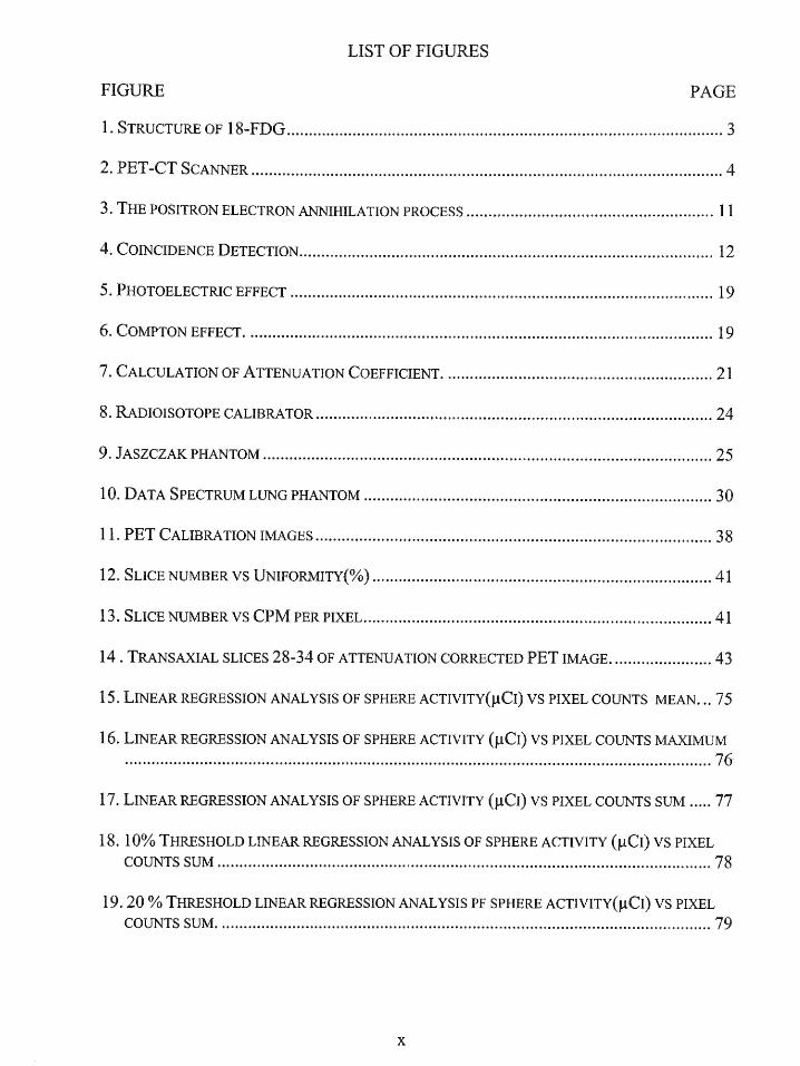
1.1 18- FDG
1 8F-labeled 2-deoxyglucose (FDG) is used in neurology, cardiology and
oncology to study glucose metabolism. In cardiology, [18F]-labeled FDG can be used to
measure regional myocardial glucose metabolism. Although glucose is not the primary
metabolic fuel of the myocardium, glucose utilization has been extensively studied as a
metabolic marker in both diseased and normal myocardium. Since [18F]-labeled FDG
measures glucose metabolism it is also useful for tumor localization and quantitation. 18-
FDG is potentially useful in differentiating benign from malignant lesions because of the
high metabolic activity of many types of aggressive tumors (Schulte et al., 1999). The
2
development of 18-FDG has been the major factor in expanding the clinical role of PET
imaging. The development of PET instrumentation, FDA approval of 18-FDG, and its
advantages compared to other radiopharmaceutical favors the use of 18-FDG in PET
imaging.
HO
\ OH
Figure1. Structure of 18-FDG
1.2 PET/CT Hybrid Scanner
A number of computer algorithms are available to register image sets from
different modalities, such as CT and PET retrospectively (Marguire et al., 1991).
Retrospective image alignment works best for a rigid organ such as the brain. Success in
other regions of the body is less certain since, in most cases, the patient must be moved
between the two machines and repositioned on different beds, with the two scans perhaps
even being performed on different days. This inevitably leads to mis-registration due to
differences in patient position, physiological state, scanner bed profile, and the
uncontrollable movement of internal organs. Even with the use of reference markers
3
retrospective alignment procedures can be labor-intensive (Tai et al., 1997) making them
less attractive for routine clinical use in high-throughput scenarios.
Cm
Figure 2. Combination of GE Discovery LS (GEMS) Light speed plus CT scanner andGE Advance Nxi PET scanner. (Courtesy of GE medical systems).
The advantages with the PET/CT Hybrid Scanner are:
1. Combining a PET and a CT, transmission images are used to construct an
attenuation correction map scaled to 51 lkeV.
2. The attenuation map is noise-free, thus a practical solution is obtained for the
need of a very rapid, low-noise and quantitatively correct method of PET
attenuation correction.
3. The automatic registration of PET and CT images with sub-millimeter accuracy.
4. CT provides the anatomic framework needed for PET images.
5. Clinical diagnostic quality CT images are obtained.
4

The disadvantages of the PET/CT Hybrid scanner are:
1. The array of detectors surrounding the patient detect two gamma rays having an
energy of 511 keV for PET imaging, whereas for CT imaging, the transmission
energy is 140 keV (Efficient energy is around 80 keV). Since the attenuation
coefficients are energy dependent, coefficients measured at CT energies must be
converted to the appropriate values at 511 keV if they are to be used to correct
PET emission data.
2. Though the same gantry is used for both CT and PET imaging, involuntary patient
motion in the form of respiratory motion or cardiac motion might not produce the
desired result after image registration. Other motions during the study can also
affect the automatic registration of PET and CT images.
1.3. OBJECTIVE OF THIS RESEARCH
The main objective of this research is to determine the most accurate method for
quantitation of activity of 18-FDG in simulated lesion.
The specific aims are:
1. To calculate a voxel calibration factor for activity quantitation of PET images.
2. To compare the accuracy of activity quantitation of PET images by using different
methods: mean and maximum voxel activity in a single transaxial slice and sum
of voxel activity in a stack of transaxial slices. Measurements in a single
transaxial slice were considered as 2D methods and measurements including
complete stack of transaxial slices were considered as 3D methods.
5
3. Since the hybrid PET/CT scanner used in this study is a new instrument (the 3'rd
installed in the US and the fifth installed in the world), the results of this research
were used to partially validate the performance of the PET-CT scanner.
1.4. HYPOTHESIS
The basic hypothesis of this research is that the 3D quantitation of activity of 18-
FDG uptake in simulated tumors provides a more accurate description of the uptake than
simple measurements in one plane.
1.5 Significance of the Research
The primary goal of 1 8-FDG PET imaging is to determine if a tumor is
present and to determine if a known tumor is responding to treatment. A quantitative
study of 18-FDG PET imaging will determine the uptake of the tumor. One of the most
popular and commonly used method for quantitation in clinical 1 8-FDG PET imaging is
Standardized uptake value (SUV) method. SUV, a practical way to quantify glucose
metabolism in tumors, is basically the ratio of two specific activities: that of a tumor at
the study's end and a temporally constant entire body average. SUV is mathematically
shown as:
voxel concentration (pCi/ml)SUV=
injected dose (pCi)/ body weight (g)
Its clinical appeal, compared with various other quantitative approaches, lies in its
simplicity. SUV is very commonly used as an adjunct to visual interpretation (Joseph et
6
al., 2000) (SUV = 1 would be obtained if the entire dose distributes uniformly throughout
the body).
The SUV explicitly corrects for the variable distribution volume of the tracer, via
measurement of the patient's weight, to provide an index that is much more uniform
among patients than the earlier measure, with higher SUV's indicating increased 1 8-FDG
uptakes and presumably, increased glucose metabolic rates. Hence there is a direct
relationship between tumor growth rate and SUV (Miller et al., 1998). SUV has been
calculated by commercial software, by choosing a region of interest (ROI) and
calculating the mean or maximum pixel value in that ROI. However only one SUV value,
either the average or the maximum value, is not enough to characterize the tumor. This is
the main disadvantage of SUV.
The various advantages of SUV- PET imaging are (Schulte et al., 2000):
1. Can monitor cancer therapeutic efficiency.
2. Can differentiate scar lesions from recurrent or new malignant lesions.
3. Can reduce the number of invasive procedures.
4. Improves cancer staging and consequently the therapeutic choices.
5. Increases accuracy of radiation treatment planning (IMRT) treating the most
active tumoral cells with the highest radiation dose.
The disadvantages of SUV- PET imaging are:
1. The need to standardize the time between the tracer administration and data
acquisition (Kole et al., 1997)
2. SUV is reduced to only one value in one pixel, in one transaxial slice, while the
malignant lesion is 3-D and occupies several slices.
7

3. SUV is affected by various factors like statistical noise, partial volume effect and
recovery coefficients.
The method we are proposing is an extension of classical SUV values by
including all the pixels, and our study is 3D as we are including all the tumor pixels in all
the transaxial slices. SUV is a method which is used to determine the uptake of
radiopharmaceutical by the human body and our method is based upon the phantom
studies. Here we know the activity of the simulated tumor and we verify the accuracy of
this activity in 1 8-FDG PET imaging by calculating all the pixel count values for a region
of interest(ROI) of the simulated tumor and finding the activity of the simulated tumors
by using either the sum, mean or maximum pixel counts per minute and multiplying the
pixel counts per minute with a calibration factor and determining which method gives
better accuracy by comparing the calculated activity with real activity. The calibration
factor is found to determine how many pixel counts per minute is equivalent to one micro
curie, which is the activity units of 1 8-FDG. The linear regression analysis is also applied
between sum, mean and maximum pixel counts and activities in simulated tumors to
determine which among these three pixel counts have better relation with the activity.
PET quantitation with 18-FDG is usually done by 2D methods in which we have only
one transaxial slice and either the mean or maximum pixel count is used to determine the
activity of the tumor. Our method is 3D in which we use all the transaxial slices and draw
the same ROI in all the transaxial slices and include all the pixels that corresponds to
tumor activity. We are trying to determine the accuracy of the uptake by applying
threshold values and eliminating the pixel counts that do not correspond to the activity of
the tumor in the chosen ROI.
8

2. BACKGROUND
Positron Emission tomography (PET) is a diagnostic method that creates high
resolution, 3D tomographic images of the distribution of positron emitting radionuclides
in the human body. The radiolabeled compounds used include substrates, ligands, drugs,
antibodies, neurotransmitters and other biomolecules that are tracers for specific
biological processes. Thus the resulting PET images can be considered images of these
biochemical or physiological processes (Hoffman et al., 1992). The images produced are
functional indexes of blood flow, glucose metabolism, amino acids transport, protein
metabolism, neuroreceptor status, oxygen consumption and even cell division (Degrado
et al., 1994).
The ability to study biochemical processes in vivo and to quantify and
characterize these processes by a functional parameter has become possible in the second
half of the 20th century. The conceptual idea of measuring in vivo biochemistry
originates from around 1930 when many new discoveries in nuclear physics were made.
The first artificial radioisotopes were produced and almost immediately it was realized
that the possibility of in vivo biochemistry was within reach. Reality, however, was long
in coming because scintillation detectors and their appropriate electronics, the required
computers for data acquisition and image reconstruction, were nonexistent at that time.
The first scintillation crystals were discovered around 1950, computers came into use
somewhat later, so the first positron camera was not constructed until the 1960s (Paans et
al., 2002).
9
In 1978 the first commercial PET scanner based on Nal (TI) crystals became
available. A breakthrough in detector technology was accomplished with implementation
of the BGO (bismuth germanate) block-structure detector. Compared with Nal (TI), a
higher spatial resolution and larger axial length were obtained, as was a much higher
sensitivity due to the density and larger atomic number of BGO (Paans et al., 2002). With
the development of scatter correction techniques, three-dimensional (3D) data acquisition
with its high sensitivity became possible. At present, the whole-body mode is the most
frequently used acquisition mode in clinical oncological studies. In the whole-body mode
the total body is scanned in steps and afterward these consecutive studies are put together
as a total body overview. Especially in the 3D mode, the total body can be scanned and
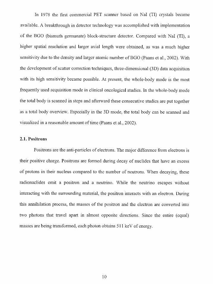
visualized in a reasonable amount of time (Paans et al., 2002).
2.1. Positrons
Positrons are the anti-particles of electrons. The major difference from electrons is
their positive charge. Positrons are formed during decay of nuclides that have an excess
of protons in their nucleus compared to the number of neutrons. When decaying, these
radionuclides emit a positron and a neutrino. While the neutrino escapes without
interacting with the surrounding material, the positron interacts with an electron. During
this annihilation process, the masses of the positron and the electron are converted into
two photons that travel apart in almost opposite directions. Since the entire (equal)
masses are being transformed, each photon obtains 511 keV of energy.
10
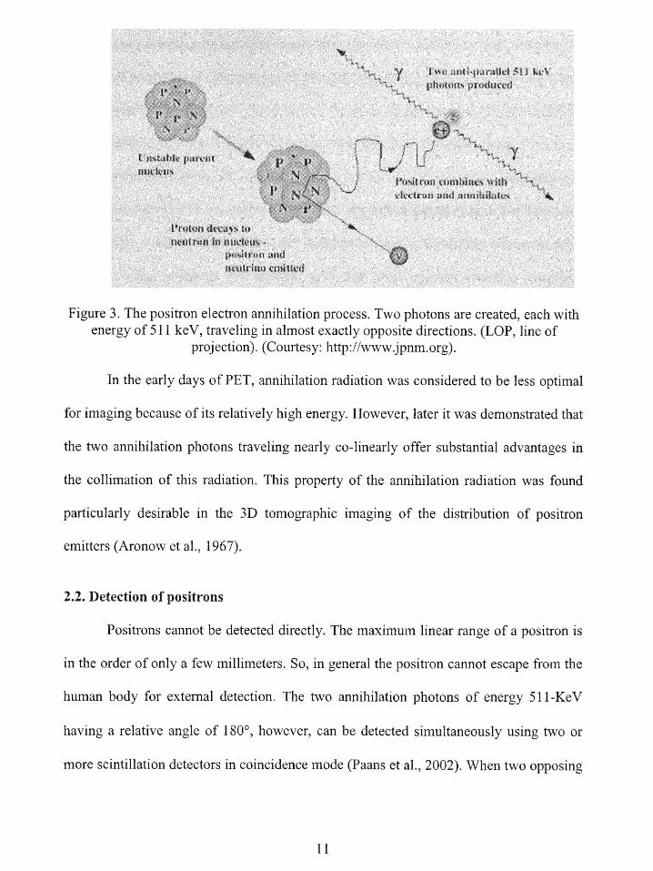
Figure 3. The positron electron annihilation process. Two photons are created, each with
energy of 511 keV, traveling in almost exactly opposite directions. (LOP, line of
projection). (Courtesy: http://www.jpnm.org).
In the early days of :PET, annihilation radiation was considered to be less optimal
for imaging because of its relatively high energy. However, later it was demonstrated that
the two annihilation photons traveling nearly co-linearly offer substantial advantages in
the collimation of this radiation. This property of the annihilation radiation was found
particularly desirable in the 3D tomographic imaging of the distribution of positron
emitters (Aronow et al., 1967).
2.2. Detection of positrons
Positrons cannot be detected directly. The maximum linear range of a positron is
in the order of only a few millimeters. So, in general the positron cannot escape from the
human body for external detection. The two annihilation photons of energy 511-Ke
having a relative angle of 180 , however, can be detected simultaneously using tw o or
more scintillation detectors in coincidence mode (Paans et al., 2002). When two opposing
II
detectors are detecting the annihilation photons, the site of annihilation will be a point on
the line of projection (LOP), connecting the detectors. If two photons are detected within
a very small coincidence time window (15 ns), they are assumed to originate from the
same annihilation event. The place where the positron was emitted is close to or on the
LOP, the distance to the LOP depends on the energy of the positron. Integrated data of a
pair of detectors in a PET camera having two to several thousands of detectors result into
tomographic images. These images are reconstructed using algorithms similar to those
used in X-ray computed tomography (CT) and single photon emission computed
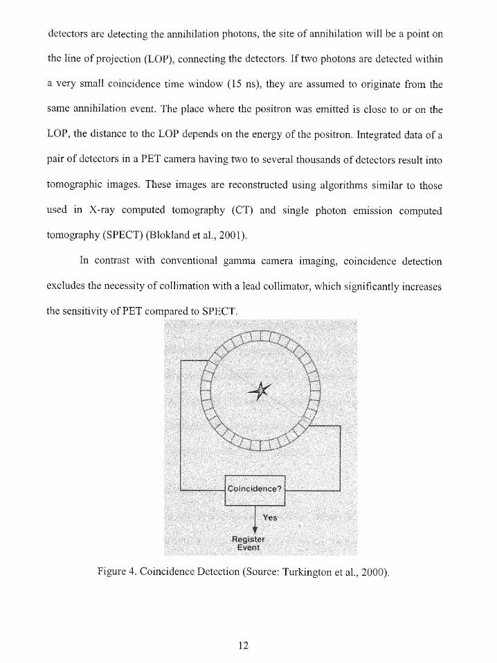
tomography (SPECT) (Blokland et al., 2001).
In contrast with conventional gamma camera imaging, coincidence detection
excludes the necessity of collimation with a lead collimator, which significantly increases
the sensitivity of PET compared to SPECT.
Even
Figure 4. Coincidence Detection (Source: Turkington et al., 2000).
12

In Figure 4, the location of the annihilation is determined by detection of
the two 511 keV photons by a pair of photon detectors using coincidence detection. If the
two detectors records two 511 keV photons simultaneously, the position of the
annihilation must have occurred somewhere along the line connecting the two detectors,
since the annihilation photons are emitted 1800 apart. A modem PET system typically
has more than 10,000 detector elements arranged in rings surrounding the patient. These
detector elements form over 20,000,000 possible coincidence combinations.
2.3. Positron detectors
Radiation detectors for use in PET must be optimized over several physical
characteristics of the detectors, including detection efficiency, output signal strength,
signal decay time, coincidence timing characteristics, and certain physical properties. In
conventional PET, the scintillator of choice is bismuth germanate (Bi 4Ge3O12; BGO),
which has a very high detection efficiency for high energetic photons. Thallium-activated
sodium iodine (Nal (Tl))--the detector material used in ordinary single photon gamma
cameras, has been applied as well. Nal (Tl) offers a better energy resolution than BGO.
The choice of the detector material affects the important parameters of a PET scanner,
including spatial resolution, sensitivity, noise and count rate.
2.4. Production of positron emitters
Due to the short half-life of most positron emitters, these radionuclides must be
produced close to the place where they are going to be used. Transport times must be
reduced to a minimum. Two basic approaches for preparing these radionuclides can be
used. First, the isotopes can be produced in a nuclear generator-using the
13
parent/daughter radionuclide approach. Unfortunately, only a few useful short-living
radionuclides can be prepared by this method (e.g. 82Rb for cardiac PET imaging)
(Blokland et al., 2001).
The second approach is to use cyclotrons to produce artificial radioisotopes,
including carbon-11 (11-C), nitrogen-13 (13-N), oxygen-15 (15-0) and fluorine-18 (18-
F). Several commercial companies offer small reliable cyclotrons specifically designed to
produce radionuclides for PET imaging that are relatively easy to operate (Blokland et
al., 2001).
2.5. Positron emitting radio pharmaceuticals
Shortly after the development of the cyclotron, the usefulness of 1 -C, 13-N, 15-
0, and 18-F as radioactive tracers for biological studies was recognized. Carbon, nitrogen
and oxygen are atoms essential to most physiological processes. Fluorine has been found
a useful radionuclide to label biologically important molecules. These nuclides most
generally exhibit properties that render them particularly desirable in physiological
studies. They provide an ideal starting point for the production of a variety of tracers that
are either natural substances, such as 11-C-labelled methionine, or analogues, such as 18-
FDG. Of course it is necessary to match the half-life of the nuclide to the phenomenon
being studied.
One of the challenging problems was the labeling of pharmaceuticals for medical
use with positron emitting nuclides. Chemists became interested, which led to the
development of fast and automated labeling procedures. In 1980, a list of approximately
30 compounds labeled with positron emitting radionuclides was published (Pogossian et
14
al., 1980). Since then, the list has increased to several hundreds of compounds (Blokland
et al., 2001).
Carbon-11
Carbon-labeled carbon monoxide (11-CO) provides an excellent and simple way
to label red blood cells for localizing blood pools by external scanning. 11-CO and 11-
CO 2 have been used to study pulmonary function (Blokland et al., 2001).
Nitrogen-13
Nitrogen-13 (13-N) is mainly applied as 13-N-amonia to study perfusion. It has
been used extensively to assess myocardial perfusion. In oncology, studies have been
carried out with 13-N-labelled amino acids, as 13-N-methionin, to investigate tumor
growth and viability (Blokland et al., 2001).
Oxygen-15
Oxygen-15 (15-0) is a very valuable tracer in biology. Oxidation is a fundamental
phenomenon in the life of higher organisms. Probably, the most reliable index of tissue
metabolism is its rate of oxidation. Metabolic oxidation is a process, which in most of its
phases is comparable in time scale to the half-life of oxygen. Therefore, 15-0 can indeed
be used to study many phases of metabolism. The combination of the need for a tracer of
oxygen and the fact that most phenomena studied that way are short in duration has made
15-0 a useful tracer in biological and medical studies. 15-0 can be used as a tracer for
oxygen, carbon monoxide, and carbon dioxide and as water (Blokland et al, 2001).
Fluorine-18
Among all the positron emitting radiopharmaceuticals Fluorine-18 is the most
popular and widely used radiopharmaceutical in PET imaging. Cyclotron-produced
15
radionuclides are generally produced and used at a single site. Due to the relatively short
half-life of the radionuclides, these radiopharmaceuticals are not suitable for distribution
over longer distances. The one exception is 18-F, which has a 110 min half-life. Thus,
1 8-FDG and other 18-F-radiopharmaceuticals can be distributed commercially over
regions extending at least several hundred kilometers from the site of production. 18-
FDG is especially valuable in detecting primary tumors and metastatic disease (staging).
It has been shown to be highly useful clinically especially in oncology (McCready et al,
2000). The ability to perform whole body imaging of cancer patients at high risk of both
primary and metastatic recurrence is helpful in diagnosis and staging. In total, PET
provides a better selection of patients for specific therapies, whether it is surgery,
radiation therapy or chemotherapy. It has also shown to be able to monitor the effect of
therapy, which has significant clinical implications (Blokland et al., 2001). The various
advantages of fluorine based 1 8-FDG compared to other positron emitting
radiopharmaceutical are listed below.
Advantages of 18-FDG:
1. Relatively long half-life for a positron emitter of 110 minutes.
2. It can be produced in large quantities by small hospital based cyclotrons.
3. Commercial distribution of F-18 has become relatively widespread.
4. Most common cancers can be easily imaged and detected with F-18.
. The biochemical basis for FDG uptake is firmly linked to glycolysis, and the
pharmacology of this substrate is well understood.
16
2.6. Reconstruction of PET imaging
In the past, filter back projection was used, but a newer technique called iterative
reconstruction is favored because it eliminates some of the artifacts generated with
filtered back projection. The reconstructed data can be displayed in a three-dimensional
rotating volume as well as standard tomographic slices in the transaxial, coronal, and
sagittal planes, Iterative reconstruction methods applied to image reconstruction in three-
dimensional (3D) positron emission tomography (PET) should result in possibly better
images than analytical reconstruction algorithms. However, the long reconstruction time
has remained an obstacle to their development and, moreover, their clinical routine use.
Together with the constant increase in performances of the computing platforms, recent
developments in parallel processing techniques offer practical ways to speed up the
calculations and attain clinically viable processing rates (Barrett T et al., 1997).
Various analytical (exact and approximate) and iterative algorithms have been
proposed for 3D reconstruction in PET. The reconstruction algorithms already
implemented or under development includes: The reprojection algorithm (PROMIS), the
Fourier rebinning algorithm (FORE), the maximum likelihood by expectation
maximisation (ML-EM) algorithm, the ordered subsets, expectation maximisation
(OSEM) algorithm, the maximum a posteriori, expectation maximisation (MAP-EM)
algorithm, the least squares (LSQ) algorithm and variants of it including the image space
reconstruction algorithm (ISRA) and ordered subsets ISRA (OSISRA), the ordered
subsets, Mirror (OS-MIRROR) algorithm, the algebraic reconstruction technique (ART)
(labbe et al, 1999).
17

2.7. Attenuation of PET imaging
Attenuation is the inevitable loss of information in an image due to the interaction
of emitted photons with matter, through the photoelectric effect (photon absorption), and
the Compton effect (photon scatter). Attenuation, caused by scatter and absorption
photons, causes pronounced effects in coincidence imaging. In addition to general loss of
counts and quantitative accuracy, nonuniformity and distortions are introduced in
reconstructed images when attenuation is not corrected (Turkington et al., 2000).
In photoelectric absorption an atom absorbs a photon and in the process electron
is ejected from one of its bound shells. The probability of photoelectric absorption
increases rapidly with increasing atomic number of the absorber atom, and decreases
rapidly with increasing photon energy (Evans et al., 1955).
In water, the probability of photoelectric absorption decreases with roughly the 3rd
power of photon energy and is negligible at 511 keV (Johns et al., 1983). In theory the
attenuation effects in PET radionuclide imaging method can be exactly compensated
before image reconstruction. If 511 keV annihilation gamma rays were made to travel
through a substance with a very high atomic number, such as lead brick, only a few of the
photons would pass completely through brick unaltered. Most of the photons would
interact with the atoms of lead and may undergo photoelectric effect, which involves an
atomic electron and the nucleus of the lead atom. The photon completely disappears in
this process. It is totally absorbed by the lead, its energy transferred to the nucleus and a
fast moving atomic electron. Other gamma rays passing through the lead brick would
interact by a process called scattering.
18

Ie r ay h ee nXy
Ejeted Photn
Figure 5. Photoelectric effect. Radiation impinges on the electron within an inner shelland ejects from the atom. (Source: http://www.eee.ntu.ac.uk)
electron Sore t//weenuack) 1eE r ray
Mnd fedb Phtn
Figure 6. Comnpton effect. It takes place when high X-ray energy photons collide with anelectron. (Source: http://www.eee.ntu.ac.uk).
19
In soft tissue, complete absorption almost never occurs. Instead, essentially all
interactions result in the photon scattering. Even in bone, 511 keV photons are absorbed
only rarely. Instead they simply scatter. In regions with an appreciable concentration of
radiotracer, many annihilation gamma ray pairs are emitted in all directions. Some small
fraction of these photons will be headed in a direction such that both photons would
strike a detector in the ring. These photons must pass through the tissue of the body as
they travel toward the detector. If either of the photon scatters, it will no longer be headed
toward the detector. It will miss the ring entirely, or on those rare occasions that it does
not, its energy will be too reduced to be detected.
A coincidence event that would have occurred in the absence of intervening tissue
now does not occur. The photons emanating from this small section of the body have
been attenuated, and the loss of detected events due to interactions with atoms of the
intervening tissue is termed as attenuation. The constant t is the attenuation coefficient,
which has a value 0.096 cm 1 for 511 keV photons in soft tissue. The number of photons
that make it through unscathed decrease exponentially with the thickness of interposed
tissue. Lower energy photons are attenuated more easily, because is higher at lower
energies (Botker et al., 1998). The number of photons reaching a detector is equal to the
number of photons headed for the detector multiplied by e- where 'a' is the distance
traveled by photons (Figure 7). The attenuation occurring for a pair of photons
(coincidences) can be calculated by the equation:
20
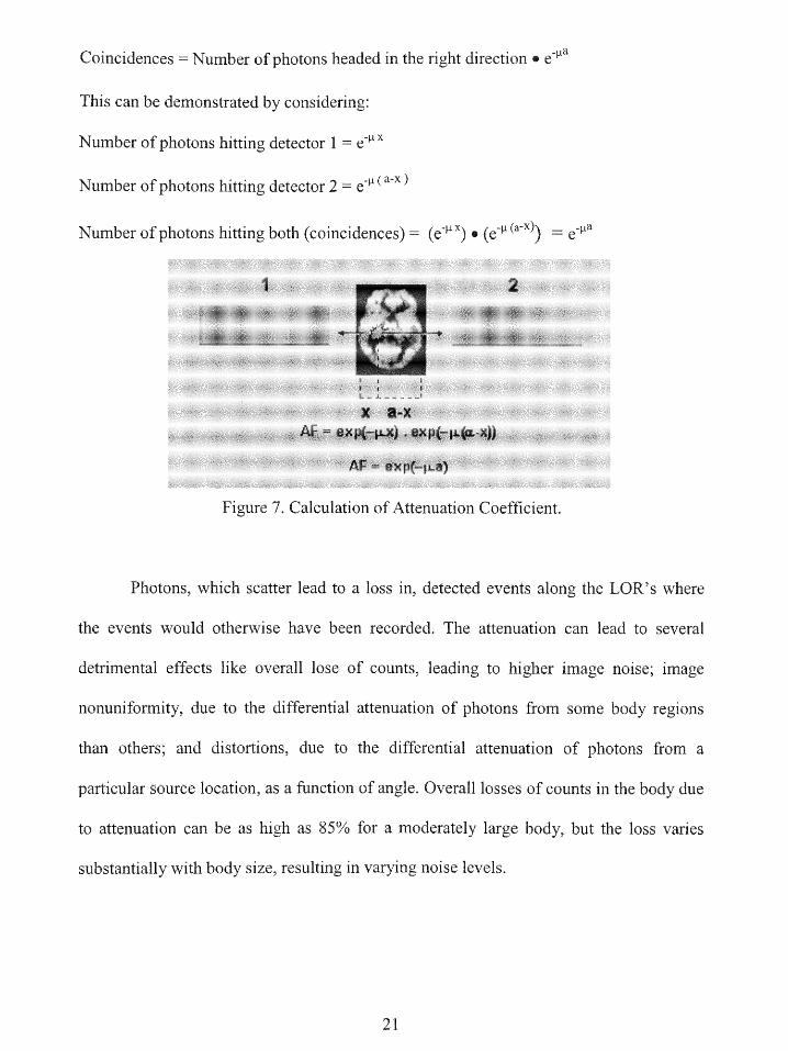
Coincidences = Number of photons headed in the right direction e-e
This can be demonstrated by considering:
Number of photons hitting detector 1 e- x
Number of photons hitting detector 2= e,( a-x )
Number of photons hitting both (coincidences)= (e X) (e (a-x)) e-a
Pt )
Figure 7. Calculation of Attenuation Coefficient.
Photons, which scatter lead to a loss in, detected events along the LOR's where
the events would otherwise have been recorded. The attenuation can lead to several
detrimental effects like overall lose of counts, leading to higher image noise; image
nonuniformity, due to the differential attenuation of photons from some body regions
than others; and distortions, due to the differential attenuation of photons from a
particular source location, as a function of angle. Overall losses of counts in the body due
to attenuation can be as high as 85% for a moderately large body, but the loss varies
substantially with body size, resulting in varying noise levels.
21
3. MATERIALS AND METHODS
The accuracy of activity quantitation of 1 8-FDG in simulated tumors and
simulated lung lesions was performed by calculating the 3D pixel counts of the simulated
tumors and lung lesions and comparing the calculated activities of sum of pixel count of
all the transaxial slices, mean and maximum pixel count of one single transaxial slice
with the real activity that we have taken. The various experiments performed wee,
1. PET calibration method
2. Experiment with simulated tumors
3. Experiment with simulated lung lesions
Jaszczak phantom and Data Spectrum lung phantom wass used for processing
with the hybrid PET/CT scanner for all the above three methods. The experiments were
conducted at the Baptist Hospital of Miami, using the Hybrid PET/CT system (Discovery
LS, GE Medical Systems). The images were acquired in the DICOM format. DICOM is a
standard file format used in storing and transferring medical data. The initial goal in
developing a standard for the transmission of digital images was to enable users to
retrieve images and associated information from various digital imaging equipment.
The DICOM standard is extremely adaptable, a planned feature that has led to the
adoption of DICOM by other specialties that generate images. The fact that many of the
medical imaging equipment manufacturers are global corporations has sparked
considerable international interest in DICOM (DICOM, 2000). The DICOM standard has
become the predominant standard for the communication of medical images. DICOM
also provides a means by which users of imaging equipment may assess whether two
22
devices claiming conformance will be able to exchange meaningful information. The
software for processing the images and calculating the pixel count was developed using
MATLAB (Mathworks Inc., Natick MA).
3.1. PET-CT Scanner
A Hybrid PET/CT with a whole-body positron emission tomograph with 2 ring
detectors was used to perform positron emission tomography. It has two detector rings
and each ring has 4096 detectors (8192 total detectors) with bismuth germanate (BGO)
crystal. The LightSpeed (LS) portion of the system provides cubic CT data sets with the
smallest practical volume, delivering superior image quality in 3D and multi-planar
reformatting. The reconstruction of the PET image is done by a filter back projection
method by built in software on the PET-CT scanner computer.
Attenuation Correction of PET Emission Scans
CT images have been used to calculate attenuation values for radiotherapy
treatment and for PET values (Blankespoor et al., 1996). In order to use the CT values for
attenuation correction, an attenuation map was constructed by converting the CT values
into attenuation coefficients at the required energy of 511 keV for coincidence imaging.
The attenuation correction was done automatically by the built in software on the PET-
CT scanner.
23

3.2. Radioisotope Calibrator
A radioisotope Calibrator was used to deterrmine the activity of radionuclide 18-
FDG directly. It provides fast, accurate radionuclide activity measurements with
performance that easily surpasses the most stringent regulatory requirements. The
radioisotope calibrator used in our experiment is CRC-I5R calibrator (Radiation Products
Design, Inc. Albertville, MN). It has various features like,
1. On screen display of Nuclide, Activity, Unit of Measure and Calibration Number.
2. Large character, high visibility display with automatic backlighting.
3. Over 80 Nuclides with half-lives in memory.
4. Built-in dose calibration, quality control and self-diagnostics
5. Resolution of 0.01 pCi.
Figure 8. Radioisotope calibrator (Source: www.biodex.com).
24
To the right of the Activity Display were the units of measure, e.g., micro curies
(pCi) or Becquerel (Bq). We can select the required units of activity. Then an isotope is
selected, and the atom lab dose calibrator was automatically calibrated to display the
activity of that isotope. Press the 18-FDG as Isotope Selection key and observe the LED
on the key to come on. Then the 18-FDG source is placed into chamber well and the
corresponding activity is found directly from the LED display unit.
3.3. Radio Pharmaceutical
The radioisotope we used was 18-FDG. The isotope 18-F is a positron emitter
with a half-life period of 110 minute, bound to deoxyglucose.
3.4. PET Calibration
The phantom we used for the PET calibration is the Jaszczak Phantom (Figure 9),
which is cylindrical in shape with interior dimensions 21.6cm * 18.6cm, with the rods
and spheres removed.
Figure 9. Jaszczak phantom with the rods and spheres installed (Source:http://www.biodex.com).
25
The specifications of the Jaszczak phantom are:
1. Cylinder Interior Dimensions: 8.5" dia x 7.32" h (21.6 x 18.6 cm)
2. Cylinder Wall Thickness: 0.125" (3.2 mm)
3. Volume: 6.75 L
4. Volume With Inserts: 6.1 L
(All the above information is provided, courtesy www.biodex.com).
In the PET calibration method, we were calibrating for the activity of the injected
dose (pCi/ml) in terms of (counts/mi/pixel). The concentration values we obtain from
the PET images are in terms of counts/pixel. But we need activity values in terms of
Ci/ml, which is the unit for activity. Here, in PET calibration method, we are trying to
find how many counts per minute are equivalent to 1p Ci. A typical PET calibration
experiment was performed with the phantom filled with water, and a specific dose of a
known amount of activity of 18-FDG is injected into the phantom. The activity of FDG
(2.487mCi) was measured, before injecting into the phantom, using the radioisotope dose
calibrator. Then the Jaszczak phantom is mounted on the patient table of the Hybrid PET-
CT and a projection set is taken for 30 min. Transaxial slices (2D PET images) were
obtained by Filter back projection (FBP) reconstruction of the projections. Totally, there
were 35 PET transaxial slices obtained and each slice is a 128 * 128 matrix. Attenuation
correction of the PET images wass derived following CT imaging.
In our PET calibration method, we were including a spread sheet which has all the
important parameters, like name of the phantom, volume of the phantom in L', activity
of Phantom in 'mCi', average scanning time, decay correction time, decay corrected
activity. A typical spreadsheet is shown in chapter 4.
26
From the transaxial slices obtained, we can choose region of interest (ROI) and
the mean pixel values for each ROI are calculated with the help of suitable software.
Matlab software was used in our experiment for calculating minimum, mean and
maximum pixel counts in PET calibration method and description of calculation is added
in the appendix.
3.5 Decay correction of PET calibration method
In our PET calibration method there is a time difference between the
radiopharmaceutical injected and PET image acquisition and the radiopharmaceutical
will undergo radioactive decay and we need to correct the activity for this decay. The
formula used to correct the radioactive decay is,
Decay corrected activity of scan, A = A0 * exp(-0.693* t/T1/2).
where,
A,= initial activity of phantom at the time of injection, in pCi.
t = decay correction time, which is the difference between average scanning time and the
time at the activity of injecting the radiopharmaceutical in the phantom, in mi.
T12= half life time of 1 8-FDG which is 110 min.
The decay corrected activity of scan is shown in chapter 4.
3.6. Uniformity calculation:
The purpose of calculating uniformity is to determine, how good is the
distribution of the pixel counts uniformly in the image so that we can determine whether
27
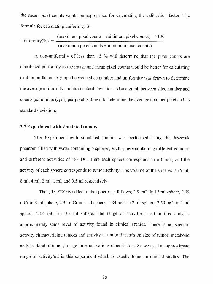
the mean pixel counts would be appropriate for calculating the calibration factor. The
formula for calculating uniformity is,
(maximum pixel counts - minimum pixel counts) * 100Uniformity(%)
(maximum pixel counts + minimum pixel counts)
A non-uniformity of less than 15 % will determine that the pixel counts are
distributed uniformly in the image and mean pixel counts would be better for calculating
calibration factor. A graph between slice number and uniformity was drawn to determine
the average uniformity and its standard deviation. Also a graph between slice number and
counts per minute (cpm) per pixel is drawn to determine the average cpm per pixel and its
standard deviation.
3.7 Experiment with simulated tumors
The Experiment with simulated tumors was performed using the Jaszczak
phantom filled with water containing 6 spheres, each sphere containing different volumes
and different activities of 1 8-FDG. Here each sphere corresponds to a tumor, and the
activity of each sphere corresponds to tumor activity. The volume of the spheres is 15 ml,
8 ml, 4 ml, 2 ml, 1 ml, and 0.5 ml respectively.
Then, 18-FDG is added to the spheres as follows; 2.9 mCi in 15 ml sphere, 2.69
mCi in 8 ml sphere, 2.36 mCi in 4 ml sphere, 1.84 mCi in 2 ml sphere, 2.59 mCi in 1 ml
sphere, 2.04 mCi in 0.5 ml sphere. The range of activities used in this study is
approximately same level of activity found in clinical studies. There is no specific
activity characterizing tumors and activity in tumor depends on size of tumor, metabolic
activity, kind of tumor, image time and various other factors. So we used an approximate
range of activity/ml in this experiment which is usually found in clinical studies. The
28

phantom containing simulated tumors was then mounted on the patient table of the PET-
CT scanner and projection set was taken for 5 min. Transaxial slices (2D PET images)
were obtained by FBP reconstruction of the projections. Totally there are 60 transaxial
slices in which we have seven transaxial slices containing simulated tumors. Attenuation
correction of PET imaging is derived following CT imaging. A typical table showing all
the values of the simulated tumor experiment and the images containing simulated tumors
are shown in chapter 4.
3.8 Experiment with simulated lung lesions
A lung lesion is something in the lung that can be inflammatory, a benign
tumor or a malignant tumor. Simulated lung lesion can be approximated by a sphere with
higher uptake of the radiotracer 18-FDG. The experiment with simulated lung lesion was
performed with Data Spectrum lung phantom with elliptical cylinder. The Data spectrum
lung phantom consists of two chambers that are shaped to simulate the lungs. The
chambers can be filled with material that mimics the lung tissue. For example, when
packed with styrofoam beads and filled with a radioactive solution, lung chambers
simulate lung tissue with density of ~0.3 gm/cm 3 and with any desirable radioactivity
concentration.
29

Figure 10. Data Spectrum lung phantom with elliptical cylinder
The specifications of Data Spectrum lung phantom are :
Inside Diameter Elliptical Shape:
1. Diameter along major axis: 12.2" (30.5 cm)
2. Diameter along minor axis: 8.7" (22.1 cm)
3. Inside Height: 7.3" (18.6 cm)
Volume:
1 Empty cylinder: ~ 9.4 L
2. Right Lung (w/o Styrofoam beads): ~ 1.1 L
3. Left Lung (w/ Styrofoam beads): ~ 0.36 L
4. Right Lung (w/ Styrofoam beads): 0.44 L
Two small lung lesions containing "F were simulated, one in the right lung (0.34
ml and 0.8478 pCi) and the second one in the left lung (0.02 ml and 0.0981 pCi), in a
Data spectrum lung phantom. We mentioned left lung has lung 1 and right lung has lung
2.
30

We were doing our data analysis for the lung lesions and compare the results of
activity of surn of pixel counts of all the transaxial slices, mean and maximum pixel count
of one single transaxial slice with the real activity. A typical table showing all the values
of the simulated lung lesion and a PET image of a simulated lung lesion are shown in
chapter 4.
3.9 Region of Interest (ROI) and Threshold method
The software used for drawing ROIs is Matlab. The matlab program written for
this is included in the appendix. The ROI was drawn for a particular sphere in one of the
transaxial slice and this ROI is going to be the same for all the transaxial slices of that
particular sphere for the calculation of pixel counts. The ROI is drawn in such a way so
that we can eliminate the pixel counts having zero values using a command called
'sparse'. We can also calculate the sum, mean and maximum pixel counts of each
transaxial slices and also the overall pixel counts sum. Threshold values like 10%-50% of
the maximum pixel counts are found and the pixel counts which are less than this
threshold value are eliminated from the pixel count calculation. The basic purpose of
applying threshold values is to eliminate the pixel counts that are not really contributing
to the activity of the tumors and to increase the accuracy of the calculation of uptake.
Choosing the threshold value is arbitrary and from the threshold value pixel count we can
identify which threshold gives better accuracy for calculation of activity for particular
sphere.
The mean, maximum pixel counts of individual transaxial slices and overall sum
of all the transaxial slices for the threshold values were also detennined. ROI was also
31
chosen for other spheres using the same program. Images containing spheres are shown
in chapter 4. By using this matlab program code we can obtain all the pixel counts of all
the transaxial slices for one particular ROE In our experiment we assume that there is no
background activity for the tumors which will not be the case in clinical studies with
patients. So we need to include the background correction accordingly if we are going to
use this matlab program for calculating pixel counts for patient studies. The ROI on this
work has arbitrary size in which same ROI for all the transaxial slices will introduce an
error. Since we don't have background activity this error is negligible. But in clinical
studies, real background assists the ROI and the ROI must fit the image of the lesions in
each transaxial slice.
3.10. Linear Regression Analysis
The goal of linear regression analysis is to find the "best fit" straight line through
a set of y vs. x data.
The linear regression analysis was applied for sum of all the pixel counts, mean
and maximum pixel counts of individual transaxial slice for all the six spheres and from
the correlation coefficient values we are trying to determine which one among sum, mean
and maximum pixel count is better to calculate the activity of tumor. Calculation of pixel
counts is discussed in chapter 4. We have chosen threshold values like 10%-50% of
maximum pixel counts and the pixel counts, which are lesser than those threshold values,
are excluded from linear regression analysis. Threshold values are applied for all the six
spheres and their corresponding sum of all the pixel counts and mean pixel counts of
individual transaxial slice are found.
32

3.11. Drawing Histograms
In our Experiment with simulated tumors we draw histograms with horizontal (x)
axis corresponding to pixel counts, while the vertical axis (y) axis represents the
frequency of each class or category. Frequency is determined assuming 10 intervals
(bins) of pixel counts values. Histograms were drawn for all the six spheres and two
simulated lung lesions and is shown in chaper 4. Its distribution is discussed in chapter 5.
A table named histogram analysis is added in chapter 4 with all parameters like mean
(ptCi), median (pCi), kurtosis and skewness calculated for all the histograms. We are
trying to verify whether the distribution follows a normal gaussian distribution.
3.12 Comparison of activity
The activity of each sphere was calculated by dividing the sum of all pixel counts
by scanning time so that we can express pixel counts in terms of counts per minute
(CPM). Pixel counts per minute multiplied by the calibration factor will give the activity
in terms of tCi, which is the calculated activity of the tumor. This activity is compared to
the real activity. Comparison of activity is done for all the pixel counts and also for
threshold value pixel counts. We can similarly calculate the activity of mean and
maximum pixel counts of one particular transaxial slice. Comparison of activities will
determine which calculated activity among threshold sum of all pixel counts, mean and
maximum pixel counts of one single transaxial slice will give better accuracy with
respect to the real activity.
33
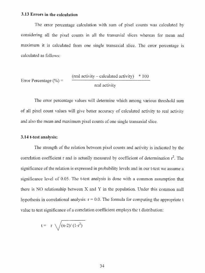
3.13 Errors in the calculation
The error percentage calculation with sum of pixel counts was calculated by
considering all the pixel counts in all the transaxial slices whereas for mean and
maximum it is calculated from one single transaxial slice. The error percentage is
calculated as follows:
(real activity - calculated activity) * 100Error Percentage (%)=
real activity
The error percentage values will determine which among various threshold sum
of all pixel count values will give better accuracy of calculated activity to real activity
and also the mean and maximum pixel counts of one single transaxial slice.
3.14 t-test analysis:
The strength of the relation between pixel counts and activity is indicated by the
correlation coefficient r and is actually measured by coefficient of determination r'. The
significance of the relation is expressed in probability levels and in our t-test we assume a
significance level of 0.05. The t-test analysis is done with a common assumption that
there is NO relationship between X and Y in the population. Under this common null
hypothesis in correlational analysis: r = 0.0. The formula for computing the appropriate t
value to test significance of a correlation coefficient employs the t distribution:
t = r (n-2)/ (1-r)
34

where,
n-2 = degrees of freedom
r = regression coefficient.
The critical 'r' for a 0.05 significance level is 2.132 and the calculated 'r' is
compared with this value to determine the significance of the relation. A table of t-test
analysis of linear regression graphs is shown in chapter 4.
35
4. RESULTS
4.1. Data Analysis of PET calibration method
The spread sheet used for PET calibration method with all the parameters is
shown in Table 1 and the images that we obtained in PET calibration method is shown in
Figure 10. Twelve images among 35 transaxial slices are shown in Figure 10. With the
help of the Matlab software we can choose a ROI in all 35 transaxial slices and calculate
the minimum, mean and maximum pixel counts in the ROE All these data are shown in
Table 2. The average counts per minute (cpm)/pixel in all the transaxial slices is found to
be 303.96 cpm/pixel. The volume of one pixel is 0.064 cm 3 and dividing cpm/pixel by
this amount will give the cpm/ml, which is 4745.94 cpm/ml. We already know the
concentration of 1 8-FDG in the phantom and the volume of the phantom, so we can
calculate the concentration in terms of the unit pCi/ml. The ratio of pCi /ml to that
cpm/ml gave the calibration factor. The calibration factor in our PET calibration method
is found to be 4.84*l10®5 pCi/CPM. We can use this value in finding the real activity of
the simulated tumors in our tumor experiment. The sequence of calculations used in
calculating calibration factor is shown in Table 3.
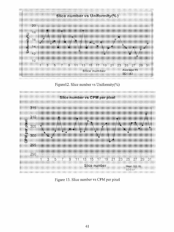
The uniformity in terms of percentage was calculated to determine the
significance of using the mean pixel counts per minute for calculating the calibration
factor. The uniformity percentage shows that the uniformity is less than 15% and the
distribution of pixel counts is even in the image. Hence we assume mean pixel counts per
minute for calculating the calibration factor instead of minimum or maximum pixel
counts in the chosen ROI. While doing uniformity calculations, the pixel counts of first
36
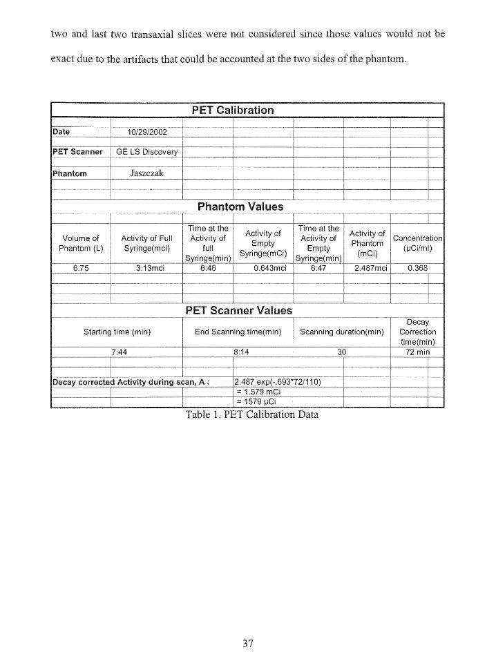
two and last two transaxial slices were not considered since those values would not be
exact due to the artifacts that could be accounted at the two sides of the phantom.
PET Calibration
Date 10/29/2002
PET Scanner GE LS Discovery
Phantom Jaszczak
Phantom Values
Time at the Time at theVolume of Activity of Full Activity of Activity of Activity of Concentration
Phantom (L) Syringe(mci) full EmI mt hno (pCi/mI)Syringe(min) Syinge(mCi) Syringe(min) (mCi)
6.75 313mci 6:46 0.643mci 6:47 2 487mci 0.368
PET Scanner ValuesDecay
Starting time (min) End Scanning time(min) Scanning duration(min) Correctiontime(min)
7:44 _____ :14 30 72min
Decay corrected Activity during scan, A: 2.487 exp(-.693*72/110)= 1.579 mCi= 1579 pCi
Table 1. PET Calibration Data
37

a
ti
b,_ aye L a 1
i
Vtz
y + yr. ss
.t , ell
Nie^+i-, .+. '
a
.?3 ;a ,.
"S
s. q g
Mil 3
F 1r
+
ONE!
e
+ e .,:A..ti.,sr :a?.a "ee , n,.v.. i G +4.w;. sod" =" t a'is bla ' ;' xko U'.a+srs. et. , 17a'aa
Figure 11. PET Calibration ages
38
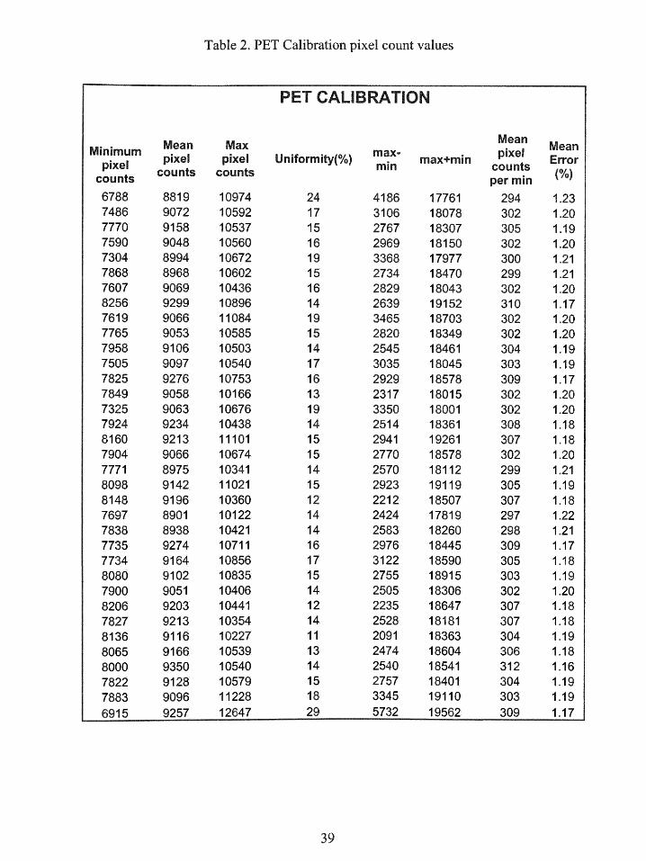
Table 2. PET Calibration pixel count values
PET CALIBRATION
Mean Max Mean MeanMinimum max-x pielnpixel pixel pixel Uniformity(%) max+min couns Error
counts counts counts mnper mn
6788 8819 10974 24 4186 17761 294 1.237486 9072 10592 17 3106 18078 302 1.207770 9158 10537 15 2767 18307 305 1.197590 9048 10560 16 2969 18150 302 1.207304 8994 10672 19 3368 17977 300 1.217868 8968 10602 15 2734 18470 299 1.217607 9069 10436 16 2829 18043 302 1.208256 9299 10896 14 2639 19152 310 1.177619 9066 11084 19 3465 18703 302 1.207765 9053 10585 15 2820 18349 302 1.207958 9106 10503 14 2545 18461 304 1.197505 9097 10540 17 3035 18045 303 1.197825 9276 10753 16 2929 18578 309 1.177849 9058 10166 13 2317 18015 302 1.207325 9063 10676 19 3350 18001 302 1.207924 9234 10438 14 2514 18361 308 1.188160 9213 11101 15 2941 19261 307 1.187904 9066 10674 15 2770 18578 302 1.207771 8975 10341 14 2570 18112 299 1.218098 9142 11021 15 2923 19119 305 1.198148 9196 10360 12 2212 18507 307 1.187697 8901 10122 14 2424 17819 297 1.227838 8938 10421 14 2583 18260 298 1.217735 9274 10711 16 2976 18445 309 1.177734 9164 10856 17 3122 18590 305 1.188080 9102 10835 15 2755 18915 303 1.197900 9051 10406 14 2505 18306 302 1.208206 9203 10441 12 2235 18647 307 1.187827 9213 10354 14 2528 18181 307 1.188136 9116 10227 11 2091 18363 304 1.198065 9166 10539 13 2474 18604 306 1.188000 9350 10540 14 2540 18541 312 1.167822 9128 10579 15 2757 18401 304 1.197883 9096 11228 18 3345 19110 303 1.196915 9257 12647 29 5732 19562 309 1.17
39
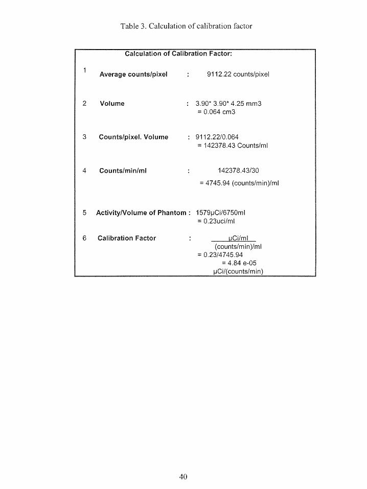
Table 3. Calculation of calibration factor
Calculation of Calibration Factor:
1 Average counts/pixel : 9112.22 counts/pixel
2 Volume 3.90* 3.90* 4.25 mm3= 0.064 cm3
3 Counts/pixel. Volume 9112.22/0.064= 142378.43 Counts/ml
4 Counts/min/mI 142378.43/30
= 4745,94 (counts/min)/ml
5 Activity/Volume of Phantom 1579pCi/6750ml= 0.23uci/ml
6 Calibration Factor UCi/mI(counts/min)/ml
= 0.23/4745.94= 4.84 e-05
pCi/(counts/min)
40
{
f
a {
2
fa ,
Slice number S ET
Figure12. Slice tiur ber vs Uniformity(%)
a C
315
fi
TO xf
i I+:as '3 vF 1_5 t \ r ?{, i
sue, ,'
2 r-5,
9 11 13 15 17 19 21 23 25 27 29 3 1
Figure 13. Slice number v P per pixel
1

4.2. Data Analysis of Attenuation corrected simulated tumor PET images
A typical table showing all the values used in simulated tumor experiment is
shown in Table 4. the table there are two columns containing activity corresponding to
two different time intervals. This is because to improve the accuracy of measuring low
activities of 18-FDG in pCi, high activities were drawn up and allowed to decay
approximately 22 hours so that low activity of 1 -FDG could be added to the spheres.
These low activation otherwise be very difficult to measure accurately with a dose
calibrator. The images containing simulated tumors are shown in Figure 14. The order of
spheres in each image is in the counterclockwise direction. The ROI for each sphere is
chosen in each of the seven slices and the entire pixel counts for all the ROI chosen are
found. ROI is drawn with a computer mouse along line segments around the
circumference of the sphere of interest. Opening the image, choosing the ROI for each
sphere in that particular transaxial slice and finding the pixel values of each sphere in all
transaxial slices is all done with the help of the software, Matlab. The program code
written for this is included in the Appendix. The pixel counts for all of the six spheres in
all of the 7 slices and their threshold value pixel counts are tabulated. The mean and
maximum pixel counts for all the six spheres and the over all sum for each sphere is also
calculated and shown.
42
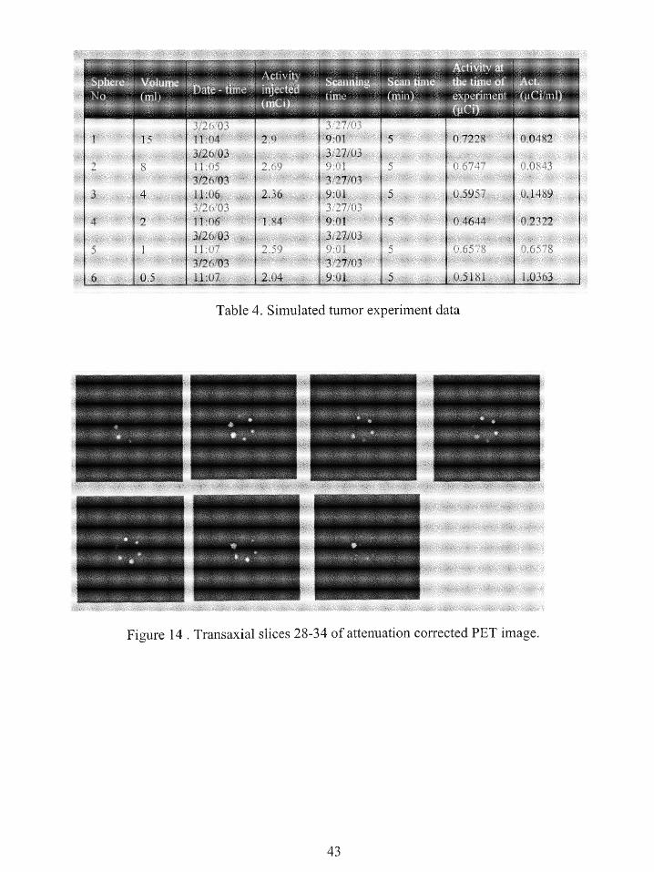
Is
4 25 11:06 2.9 9:01 5 0 7228 0.04823/26/03 3/27/032 8 11:07 2.69 9:01 5 0677 0.68
3/26/03 3/27/036 04 11:07 2034 9:01 5 0.5957 0348
Table 4. Simulated tumor experiment data
Figure 1 nsxa .sics283 of0 ateuto correcte PE image
34Tabg 4. Sm aedm reprmetdtFigure 14 . T'ransaxial slices 28-34 of attenuation corrected PET image.
43

Table 5. 3D pixel count values of sphere 1 of attenuation corrected images
SPHERE1:
Slice 28: Slice 29: Slice 30: Sldice 31: Slice 32: Slice 33: Slice 34:311 235 63 103 149 207 193136 619 222 149 503 611 17214 451 229 175 395 426 287495 108 117 153 237 251 131819 451 218 179 440 558 6641043 722 252 198 599 725 783825 826 302 236 627 884 699381 773 292_ 216 550 _ 759 629164 458 174 152 412 _ 589 241119 160 104 70 147 387 425287 20 75 230 340 110 1168
710 436 180 259 538 814 1573_1207 __712 262 285 mm603 _ 917 15981559 _889 260 E297 577 907 13811309 884 249 1237 578 988 709650 883 242 151 513 1044 226
227 669 216 92 238 933 208127 359 188 43 23 501 566334 192 85 198 435 76 1271761 726 212 268 591 647 1788....12 3 7 10 7 1.WW...__ 269.__... __.. 4 _......_.. 11...... .._......
7 ._..,... .1966 _.._.
1580 1140 258 279 577 921 17351372 1025 253 226 527 892 1062730 904 271 164 469 1026 403261 _ 678 292 143 296 989 _ 99864_ 461 287 257 560 422 1529
1061_ 1044 280 288 607_ 892 1665_
1348 1111 276 1 225 603 947 13561171 1008 289 182 474 916 34585 860 295 141 405 1037 742295 622 281 194 421 883 1195620 583 213 i 214 495 636 1160919 710 245 162 499 842 780765 697 _ _ 243 156 389 883 418252 635 202 109 330 905 541239 451 158 82 250 636 472420 301 134 83 242 532 244279 328 140 112 228 561 30173 319 82 28 15 526
69 63 229
ean: Mean: Mean: Mean: Mean: Mean: Mean:652 614 212 180 423 700 838
Max: Max: Max: Max: ax ax: ax:1580 1140 302 297 627 1044 1966
SUMLL141831
44
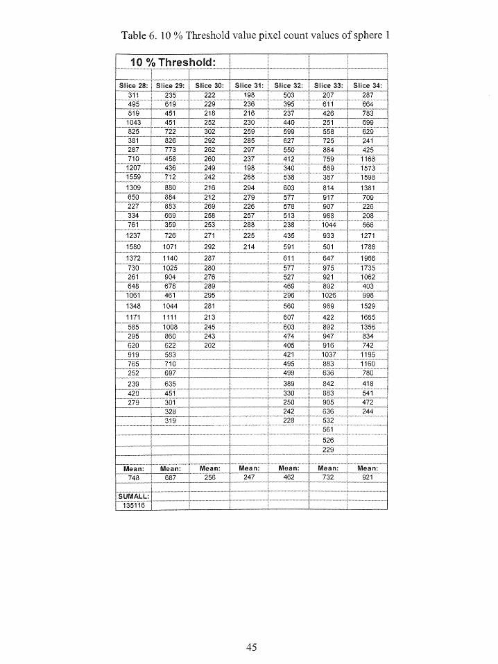
Table 6. 10 % Threshold value pixel count values of sphere 1
10 %Threshold:
Sice 28: Sli ce 29: Sice 30: S ice 31: Sice 32: Sice 33: Sice 34:311 235 222 198 503 207 287495 619 229 236 395 611 664819 451 218 216 237 426 7831043 451 252 230 440 251 699
.825 722 302 259 599 1 558 629381 826 292 285 627 725 241
1287 171 262 297 550 884 17425710 458 260 237 412 759 11686 259 40 89 1573
1559 712 242 268 538 387 1598
1309 880 __ 216 1 294 603 84 1381
3650 84 212 2 279 577 937 709227 883 269 226 578 907 226334 669 258 257 513 988 208761 359 253 288 238 1044 566
1237 726 271 1 225 435 p 933 1271 yW1580 m 1071 . 292 i 214 591 1 501 1788
1372 1140 287 611 647 1966730 1025 2805 1735261 904 276 527 921 1062648 678 1289 469 1 892 4031061 461 _1 295 f296 1026 998
1348 1044 281 560 989 1529
1171 1111 213 ! 607 422 1665585 1008 245 ; 603 892 1356295 860 243 E 474 947 - 834620 622 202 j 405 916 742919 583 421 1037 1195
252 697 1499 i 636 780
239 635 389 j 842 418420 45 30 83 4279 301 ¬ 250 905 472
328 244 2 1 636 244319 1 2-28 1 532
1 526
Mean: Mean: Mean: Mea n: Mean: Mean: Mean:748 687 256 247 462 732 921
45
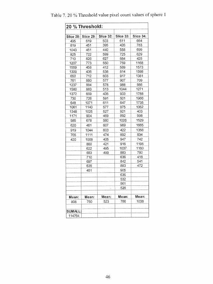
Table 7. 20 % Threshold value pixel count values of sphere 1
20 % Threshold:
Slice 28:~ Slc 9 Slice 32 Slice 33 Slice 34:495 619 503 __611 664819 451 395 426 783
1043 1 451 440 . 558 699
825 722 599 725 62971_0 826 627 E884 4251207 773 550 759 !11681559 _ 458 __412 589 1573_1309 436 538 814 1598650 712 603 917 1381761 880 577 1907_ 7091237 884_ 578 ( 988 5661580 883 513 1044 1271
1372 669 435 933 1788
730 726 591 501 1966648 1071 611 647 1735
1061 1140 . 577 975, 10621348 1025 527 921 4031171 904 469 892 998 _
585 678 ( 560 1026 1529
620 461 -.607 989 1665
919 1044 603 422 1356
_765 i1111j 474 892 834
_420 w_._..1008 ,.,...,405.,.,._..,w ..947 ....... 742860 4 421 916 1195622 495 ¬1037 1160583 499 1 883 780710 636 418
697 842 541635 4883 { 472451 905
636
532
Mean: Mean Mean: Mean: Mean:
808 _ 750 523 786 1038
SUM _114764 I ________
46
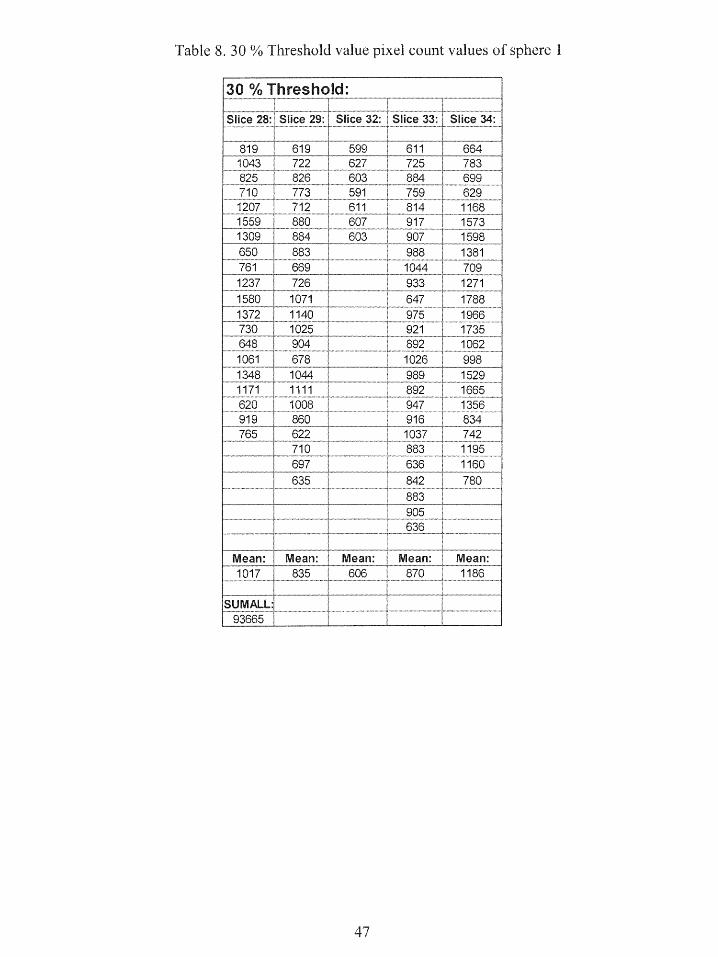
Table 8. 30 % Threshold value pixel count values of sphere 1
30 % Threshold:
Slice 28 Slice 29: Slice 32 Slice 33: Slice 34:
819 ..619 599 . 611 _ 6641043 722 4 627 725 ¬ 783825 826 _ 603 884 699710 773 591 759 629
1207 712 _ 611 814 11681559 j880 607 ¬ 917 [15731309 884 603 907 1598650 883 988 1381761 669 1044 7091237 726 933 12711580 1071 647 17881372 1140 975 1966730 1025 921 1735648 904 892 10621061 678 j1026 9981348 1044 ( 989_ 15291171 1111 4892 1665620 1008 947 1356919 860 916 834765 622 1037 742
710 883 1195697 636 1160635 842 780
883905636
Mean: Mean: Mean Mean: Mean:1017 835 606 870 1186
SUMALLI93665 _ __
47
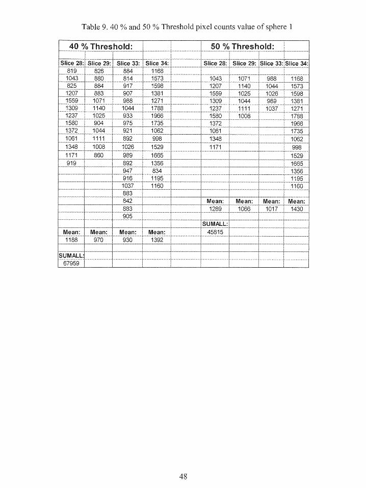
Table 9. 40 % and 50 % Threshold pixel counts value of sphere 1
40 % Theh¬ 50 % Thehl:
Slice 28: Slice 29: Slice 33: ;Slice 34: Slice 28 Slice 29 Slice 33: Slice:819 826 884 11681043 880 814 1573 1043 1071 988 1168825 884 917 1598 1207 1140 1044 15731207 883 907 E1381 1559 1025 1026 15981559 1071 _ 988 .._..,1271._... ........ 1309 1044 989 13811309 1140 1044 1788 1237 1111 1037 1271
1580 904 1 975 {1735 1372 19661372 1044 921 1062 1061 _ 1735
1061 1111 892 1 10621348 1008 1026 1529 1171 9981171 860 989j 1665 _ 1529919 892 1356 '665
916 1195 1195
_ __1037 1160 1 1160
905____UALL883:_..______ __._ _ _ _____
___842 Mean: Mean: Mean: Mean:883 1m m^ 1289 1066 1017 1430
6 SUM LL:
Mean: Mean: Mean: Mean: 458151188 970 930 1392 _ _
S
67959-1- t --
48
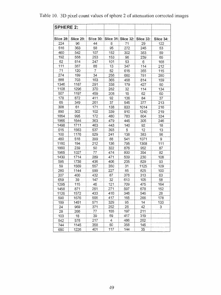
Table 10. 3D pixel count values of sphere 2 of attenuation corrected images
SP HE RE 2:
Slice 28:, Slice 29: Slice 30: Slice 31:1 Slice 32: Slice 33: Slice 34:224 96 . ,44 w. 8 71 29 122516 363 58 i 95 1 272 245 534601542 107 152 302 383 59192., 558 2 53 13 1 96 239 6562 514 247 101 53 6 168
111 387 88 13 347 114 21271 120 1 7 82 1 615 355 115274 199 1 34 = 256 660 781 280888 1 703 163 365 458 814 1591346 1187 1291 38 1 427 _._._501108 1296 370 282 172 1 134 _
507 1197 1 459 208 15 62 60178 872 1 411 92 136 84 3765 349 261 37 545 377 213308 61 171 138 833 1014 216890 302_ _ 102 339 910 1240 2191664 995 172 480 783 804 3341966 1644 363 479 1 445 305 2461498 1711 463 443 140 92 18615 1563 537 393 5 12 13100 _ 1176j 529 241 138 383 _ 56
480 518 399 88 541 1071 91160 194 212 j 136 795 1368 1111860 239 1 50 322 1;876 952 871965 1027 77 474 800 _,351 821430 1714 E289 471 E509 230 1 108_595 1738 436 406 205 829 9359 1569 557 350 31 1125 x 109280 1144 599 227 85 825 100207 400 1 432 87 378 313 63
659 39 1471 32 61 105 581295 115 46 121 709 475 1641458 1871_ 251 27 597 678 1521126 1572 433_ 410_ 348 545 28590 1676 556 1 417 j 165 ..266 .. 178189 1451 571 329 95 14 13324 969 371 252 28 4228 26 77 _ 155 197 211103 9 18 39 | 59 417 319542 578 217 4 486 262744 1145 358 50 358 145650 1226 401 117 144 35
49
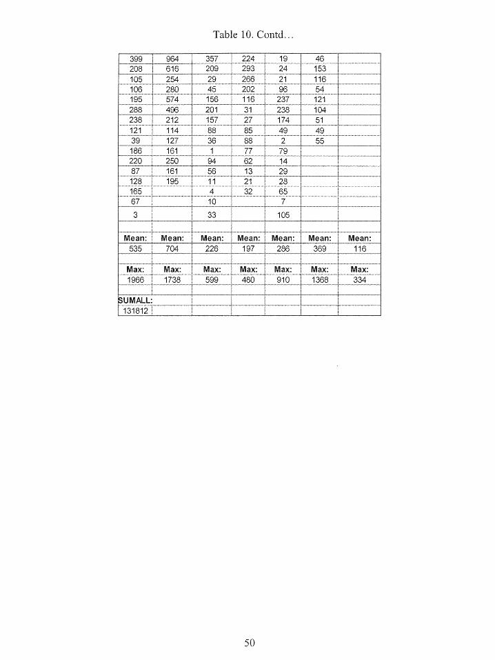
Table 10. Contd..
399 964 i 357 224 1 4
206 ; 616 209 293 24 153,
1.05...._._ 254 29 266 21 116
'106 n .,_nan_. n..._......._SA . ......
20 5 202 ._..,...,._...n..,. ..n.m...,_...
_.,__._..__._...._ .......... .............__... __...u....,..._._._........_...v........... ....... __y.........,_........_._..,......_...._.,.._.....v...__......W_...._._ .... ,.._._......__._......_..........._
195 574 56 116 E 27 121
::::2288 496 201-'--31 238 104
238 212 157 27 174 51
121 114 i 88 85 49 49
399 127 36 1 88 2 55
186 77 .__._.7 __
220 I 250 G 94 j 62 14
87 161 56 13 29
128 ....................... 195..........[ 11 21 2$.w._... _.m...
.....................65 .......... 32 65
_w.._.........._._..._..._..___.r._._. W ...__...._....,....__..,_ .................._._......_._..,...
67 1... . ...... 6 ,... .,,,,n .. ,,..
3 33
105.__, -. . ..__..._
Mean: Mean: .. Mean: ,. - Mean: Mean: Mean: T Mean:535 704 226 197 286 369 116
Max: ax: ax: Max: E ax: ax: Max:_..W..__,._._ ..._.._,._.._.__....._..,....._._.,W_.._._._..._ _.... _,.. _.. _.W__..._.W._._.,
1966 9 1738 599 480 .W_ ._910_..__,.. 1368 4 334
------------------l1 L
_._n._ n,._,... w .................
13 18 12 F ,.._.,m.. ..._._...¬.m,._.,n._..._,._P .... .,_ .,..rt..n.,
50

Table 11. 10 % Threshold value pixel count values of sphere 2
10 % Threshold:
Slice 28:[ Slice 29: Slice 29: Slice 30: Slice 31: Slice 32: Slice 33: Slice 34:224 363 964 23 256 272 245 212516 542 616 247 365 302 383 _ 280460 558 254 291 338 347__ 239 W 213274 514 280 X370 282 615 355 j 216888 387 574 459 208 660 781 2191346 199 _ 496 411 339 458 814 3341108 703 212 261 480 545 427 246507 1187 250 363 479 833 I 377308 1296 463 443 910 1014890 1197 537 393 783 12401664 872 529 241 445 8041966 349 399 322 541 _ 3051498 302 212 474 795 383
615 995 289 471 876 1071
480 31644 436 406 800 13681160 1711 557 350 509 9521860 1563 599 227 205 3541965 11176 432 271 378 2301430 518 251 410 613 829 _
595 _ 239 1 433 417 709 L 1125280 1027 _ 556 329 597 | 825 _
207 1 1714 571 252 348 313 __ _____
659 i 1738 371 224 197 _ 4751295 1569 217 293 417 6781458 1144 358 266 486 5451 12 6 ....._...4 0 0 ._._.. ,..._... ,.....__ .... 4 0 1 ....... 2..... 02 ._.... . ...3 5 8......_........._... 2 6.6 1.,....._..._......_.590 ;871 __1357 ___ 237 211 _____
542 1572 209 238 319744 1676 201 2626 5 0 14 5 1 . .. __._ ,._ rmw ..... H_..,.. n_.. , . .399 } 969...._..........._....208 266 717IS".
_.2 8 8 r.,. 5 7 8 _..__ r. ... w.._H n _ . ..,. , .. _.. . ._
238 1145220 1226 _ _
Mean: Mean. Mean: Mean: Mean: IMean: Mean:819 868 380 336 517 1 593 246
ssUM L: 5
119111~ _____
51
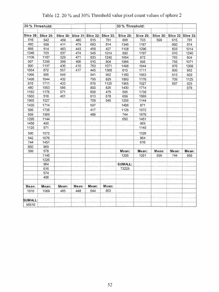
Table 12. 20 % and 30% Threshold value pixel count values of sphere 2
20 % Threshold: _30_ * Tihreshold:
Slice 28 Slice 29: Sice 30: Slice 31: Sice 32: S lice 33: Sice 28: Slice 29: Sice 30: Slice 32: Slice 33:56 52 49 480 615 1 781 _ 888 703 599 615 __ 781
460 558 411 479 660 814 1346 1187 660 814888 _514 _463 443 458 427 1108 1296 833 10141346 3 537 474 545 1014 890 _ 1197 910 12401108 1187 529 471 83 1240 1664 872 783 804507 1296 399 406 910 804 1966 995 795 1071890 1197 436 410 78 1071 1498 1644 876 13681664 872 557 417 445 1368 615 1711 800 9521966 995 599 541 952 1160 1563 613 8291498 1_1644 432 795 f829 1860 1176 709 1125
61 1 433 876 125 1965 1027 597 825_480 1563 556 800 825 1430 1714 6781160 1176 571 509 1475 595 1738 ______
1860 518 401 _ 613 678 659 15691965 1027 _709 545 1295 11441430 1714 597 1458 871
595 j 1738 417 1126 1572659 1569 486 _ 744 1676
1295_ _1144 650 1451
1458 3_...40_0 9691126 81-1145.__._-
590 1572 1226542 16_76 964744 _ 1451 616
399 578 Mean: Mean: Mean: Mean: Mean:1145 1206 1251 599 744 958
1226964 :UM L
616 ( 73228
496
Mean: Mean: Mean Mean: Mean: ean:1016 1069 485 448 644 863
UMALL:95516
52
Table 13. 40 o and 50% Threshold value pixel count values of sphere 2
40 % Threshold: _ 50 % Threshold:
Slice 28:1 Slice 29: Slice 32: ISlice 33:, Slice 28: Slice 29: Slice 33:
888 1 1187 . 833 814 1346 1187 10141346 1296 910 1014 1108 i 1296 12401108 1197 _ 795 _ 1240 _ 1664 1197 1 1071
890 872 . 876 804 1966 995 13681664 995 , 800 1071 _ 1498 1644 11251966 1644 ; 1368 _ 1160 17111498 1711 952 1860 1563
1160 1563; 829 1965 11761860 1176 ¬ 1125 - 1430 1027 _
1965 1027 825 _ _ 1295 1714
1430 1714 1458 h 17381295 1738 1126 15691458 15 69 11441126 1144 1572
871 16761572 1451
...... . 1 1676,__,____ __ 11 5
11451 1226969T
1145 Mean: Mean: Mean:1226 ..__-.1490 1391 1164
X964
SUMALL:Mean: Mean: ean: Mean: 487231404 1305 843 1004
SUMALL:62614 I
53
Table 14. 3D pixel count values of sphere 3 of attenuation corrected images
SPHERE 3:[
Slice 28: Slice 29: Slice 30: Slice 31: Slice 32: Slice 33: Slice 34:
6 114 39 18 31 1 w«126 4454 139 10 8 30 338 55
_ 53 73 92 188 9 312 471 183 108 113 106 7 7233 135 76 1 192 48 3163 9 20 35 177 321 148 75 ' 71 66 133 67 102103 216 159 2 3 5 106 595 72132 _ 190 274 , 392 130 328 17371 75 308 322 232 28 32379 71 254 134 447 188 335120 120 190 33 628 473 16897 20 114 1 41 549 1035 102112 07 5 42 284 . _1379 ,__37911 563 33 123 69 I 1164 545
111.._._ _....775._., ,._..206. ._.,.._ 241 «.._.........94 . 548_._..... 458192 716 411 427 415 144 132249 375 504 567 887 137 132167 110 553 562 1086 ~39 18038 40 479 383 930 234 36623 32 218 139 549 554 498
281 1030 507 29 59 1966 153394 1477 594 103 506 1680 67394 . 1253 635 297 1131 796 2205 .632 518 523 1319 197 91181 1 193 208 670 1146 117 174377 24 197 716 773 15 103436 35 499 542 289 117 131313 309 601 211 29 78 277104 855 543 38 39 205 2965 F1263 I354 1 32 49 940 259
164 1075 _ 113_[ 3 399 1669 247265 524 ___ 1 180 _ 979 1 1571 72 _
180 100 96 441 1229 776 42103 82 305 648 1141 148 7969 159 414 ]686 757 42 1718 358 322 486 231 30 4452 551 133 167 37 334 8680 532 44 17 50 828 16545 308 22 27 261 876 255
54
Table 14. Contd...
26 35 13 108 4 r 445 15553 17 17 290 161 72 19844 57 114 427 526 16 136
27 70 187 398 756 82 749 100 97 229 792 228 17338 195 14 47 507 276 1251 259 36 16 44 227 240
3 75 45 177 16 24 11618 75 95 170 150 11 123
__41 66 97 236 14 8
21 2 19 30 326 29 5835 138 76 47 __ 259 8191.. 96 ji 23.._.._ _ ----- ...... ....... 83 29 .... _...........200
70 154 22 79 25 _ 198
34 173 8 54 101 13
49 214 40 14 152 59
.28 4 55 184187 43 42 209151 2 96 49
___I__ - 9 96 136
35 37 22 11m 4 0__.. _..,. __ _. __ 4 1002,,....
4372__ 61 __ __ _ _ _
Mean: Mean: Mean: Mean: Mean: Mean: Mean:108 294 1 194 191 340 397 166
_..._. .,. ,.., ...,., .._ . _.__ .. I _ _
Max: Max: Max: Max Max: Max: Max:436 1477 635 716 1319 1966 545
SUMALL:1 _
103914 _
55

Table 15. 10 % Threshold value pixel count values of sphere 3
10 % Threshold:
Slice 28: S lice 29: S lice30: Slice 31: Slice 32: S lice 33: Slice 34:249 216 274 235 232 338 323281 307 308 392 447 312 335394 563 254 322 628 321 379394 775 206 241 549 567 545205 716 411 427 284 595 458377 375 . 4 567 415 1328 366
384 553 62 887 3313 1030 479 383 1086 1035 385265 1 1477~ 218 297 930 11379 277
_ 1253 228 523 549 1164 296632 507 670 506 ¬ 548 259309 1594 716 1131 234 247
855 635 542 1319 554 - 2551263 518 211 1146 _ 1374 1981075 208 m 441 773 1966 240
-524 197 648 289 180 221358 499 686 399 796
{ 551 _601 486 979 E197532 543 290 1229 205308 354 427 1141 940259 305 398 757 1669244 414 229 231 1571
__1 214 !322 526~ 776
______ ___________ __ 92 828 __
507 1 876_ __ 236 445
326 228259 276
+ 7x77~ 227200198209
-Mean: Mea: Mea Mean: Mean: Mean: Mean:324 618 397 441 666 692 330
SUMALL:83391 _ _
56
Table 16. 20 % Threshold value pixel count values of sphere 3
20 % Threshold:Slice 28: Sice 29: Sce 30 S ice 31: Slice 32: Slice 33: S lice 34:
394 563 411 427 447 567___ 545394 775 504 ! 567 628 595 458436 716 553 x.562 549 473 498
__ 1030 479 ; M523. 415 1035 ____
14771 507 670 887 ~ 1379 m1253__ 594 1 716 1086 1164632 m 635 , _542 _ 930 548855 ._518 _,441 .. 549 5541263 ; 499 648 506 13741075 _ 601 686 1131 1966524 543 486 1319 1680551 1_. _..414_....,, 427 1146 796 _ _ _ _
532 1 398 ~77 ; 940___ _____ ____ ____ 399 1669 ___
979 1571__ _ _ __ _ _ ......................... _ 1229 776 _ _ _
1 1 4 1 828
757_.......876 ,.,.
526 445
756
_ . . 507Mean: Mean: Mean: Mean: Mean: Mean: Mean:408 865 ¬ 521 546 793 1012 500
SUMALL 164009 I _________________
57
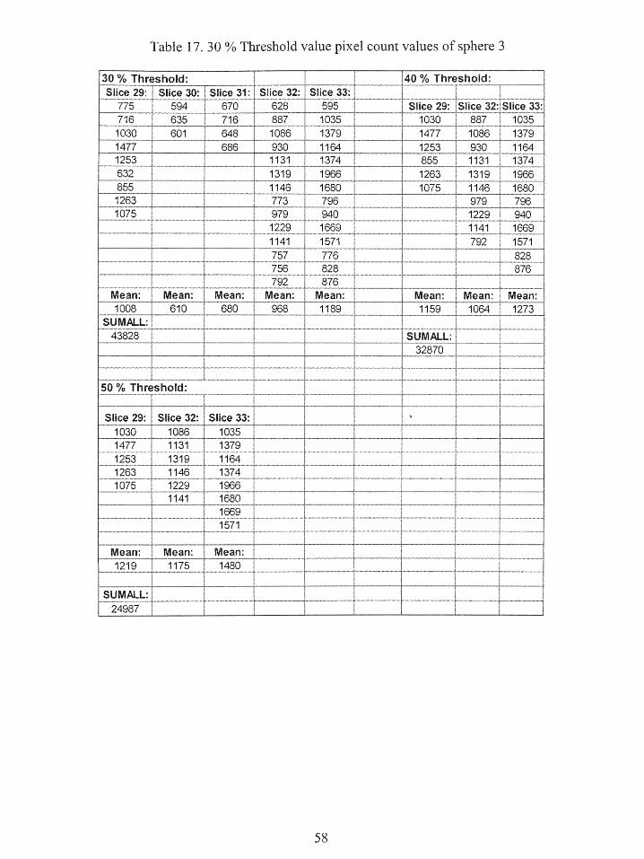
Table 17. 30 % Threshold value pixel count values of sphere 3
30 % Threshold: 4 % Threshold:Slice 29: Slice 30: Sldice 31: Slice 32: Slice 33: ;
775 594 670 628 595 Slice 29: Slice 32: Slice 33:716 635 716 887 1035 ( 1030 887 10351030 _ 601 I 648 1086 1379 1477 1086 13791477 _______ 686 930 1164 _ 1253 930 1164
1253 1 1131 1374 855 1131 T 1374632 1319 _ 1966 11263 1319 1966855 1146 1680 1075 11146 16801263 773 _ 796 979 796
. .5. 979 940 1229 940EE1229 1669 1141 I1669
_ 1 1141 1571 E 792 1571
756 828 1876792 876
Mean: Mean Mean: Mean: Mean __ Mean: Mean: Mean:1008 610 680 968 1189 1 1159 1064 1273
SUMALL:43828 _ SUMAL:
32870
--- - -+--- --4---IE50% Threshold:
Slice 29: Slice 32: Slice 3:1030_ 1086 1035-1477 1131 13791253 1319 1164 11263 1146 1374- - -- - t1075 1229 1966
1141_ 1680 T16694
1 1571
Mean: Mean: Mean)1219 1175 K 14 80
_- '4 --- - -4---SUMALLi._._,_...__ _ -__ -_t_ ____.__.___..__ _ _ _ _ _ _ _ _ _ _ _ _ _ _ _ _ _ _ _ _ _ _ _ _ _S_ _ _
24987 _
58

Table 18. 40 % and 50% o Threshold value pixel count values of sphere
40 % Threshold:
Slice 29: Slice32: S lice 33:1030 887 10351477 . .1086 . 1379
855 1131 13741263 1319 19661075 1146 1680
979 . 7961229 9401141 1669792 1571
828876
Mean: Mean: Mean:1159 1064 1273
SUM L:32870
50 % Threshold:
Slice 29: S ice 32: Slice 33:1030 1086 10351477 1131 13791253 1319 11641263 1146 13741075 1229 1966
1141 168016691571
Mean: Mean: Mean:1219 1175 1480
SUMALL24987 _
59

Table 19. 3D pixel count values of attenuation corrected images of sphere
SPHERE 4:-
Slice 28: Slice 29: Slice 30: Slice 31: Slice 32: Slice 33: Slice 4:
55 97 50 41 46 140 2911 221 115 57 19 61 8115 45 59 33 4 8 7976 138 41 74 46 88 5212 247 145 76 39 85 .153134 209 123 _ 65 64 47 11792 42 20 81 96 49 165152 83 64 69 30 16 20215 184 38 44 9 _24 79
255 48 275 103 1 143 50108 - 5 343 3320 149 145 3847 397 196 375 j 416 19 8939 594 59 _ 278 505 65 816 373 31 169 260 109 98
163 65 45 ..91 34 131 226321 85 20 30 463 243 263144 24 15 259 1156 473 16110w 193 223 727 1376® 548 _ 9843 725 573 912 910 ? 325 67102 1014 742 683 325 163 10224 712 549P 323 14 95 79128 308 218 98 127 92 14252 123 15 27 692 48 130108 50 48 8 I15681 96 131113 77 323 347 1880 298 113
81 219 963 1167 570 990 64128 621 735 859 149 702 p 49
101 866 309 353 24 394 24110 637 29 ; 56 1 184 161 41
76 320 19 15 1 506 2 44 _
99 187 53 23 1090 2 36155 79 226 248 1336 128 127201 80 561 678 938 r 587 180140 82 734 864 384 822 36124 123 554 607 105 5 06 227-11-1-1186 272 2411206 55 188
56 237 17 55 107 95
60
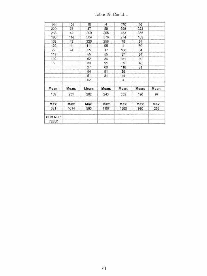
Table 19. Contd..
144 T 104 10 4 170 16220 75 37 59 398 223258 44 209 j 265 453 355190 118 304 378 . 274 109.103 _ 43 ~ 226 256 i 75 34120 4 111 95 4 8079 74 55 V 1 7 100 3 64119 55 55 37 84110 62 1 36 151 Ij 39
6 30 91 59 4027 66 116 31
n. .. .. m_. . . ._~_ _ , . .54 51 3 9 _._,..,._.._.. _ , ...
51 81 4452 4 '
Mean: Mean: Mean: Mean: Mean: Mean: Mean:
109 231 202 243 355 196 97
Max: Max: Max: Max: Max: Max: Max:321 1014 963 1167 1880 990 263
SUMALL __ ___ __ _ _72850
61
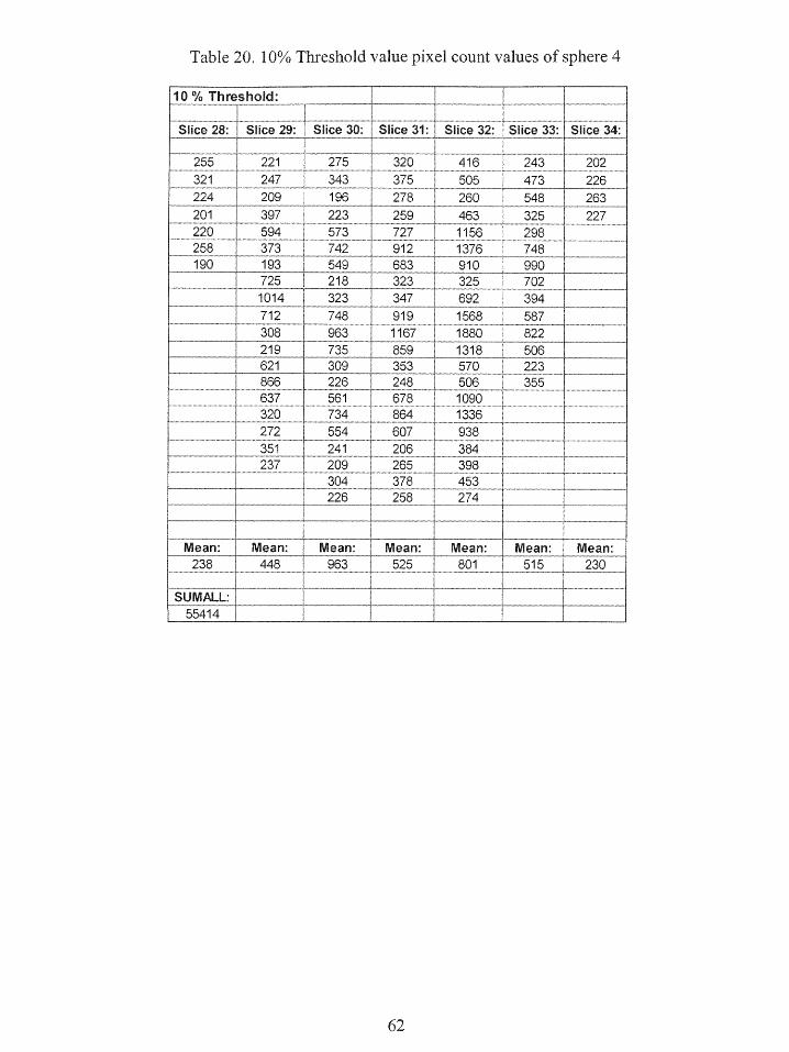
Table 20. 10% Threshold value pixel count values of sphere 4
10% Threshold: _
Slice 28: Slice 29: Slice 30: Slice 31: Slice 32 Slice 33: lice 34:
255 221 275 320 416 243 202
321 247 343 1 375 505 473 226
224 _ 209 196 3 278 260 548 263
201 397 223 259 463 325 227220 594 573 727 1156 298258 373 742 j 912 1376 748190 _ 193 549 1 683 910 990
_ 725 218 1323 325 7021014 323 347 692 394712 748 919 1568 587308 963 1167 1 1880 .. 822219 735 859 1318 506621 309 353 570 223
866 226 248 506 355637 561 678 1090320 734 864 1336272 554 607 938351 241 206 384
304 37 8 453
Mean: Mean: Mean: Mean: Mean: ] Mean: Mean:238 448 963 525 -801 m 515 230
SUMALL:55414
62
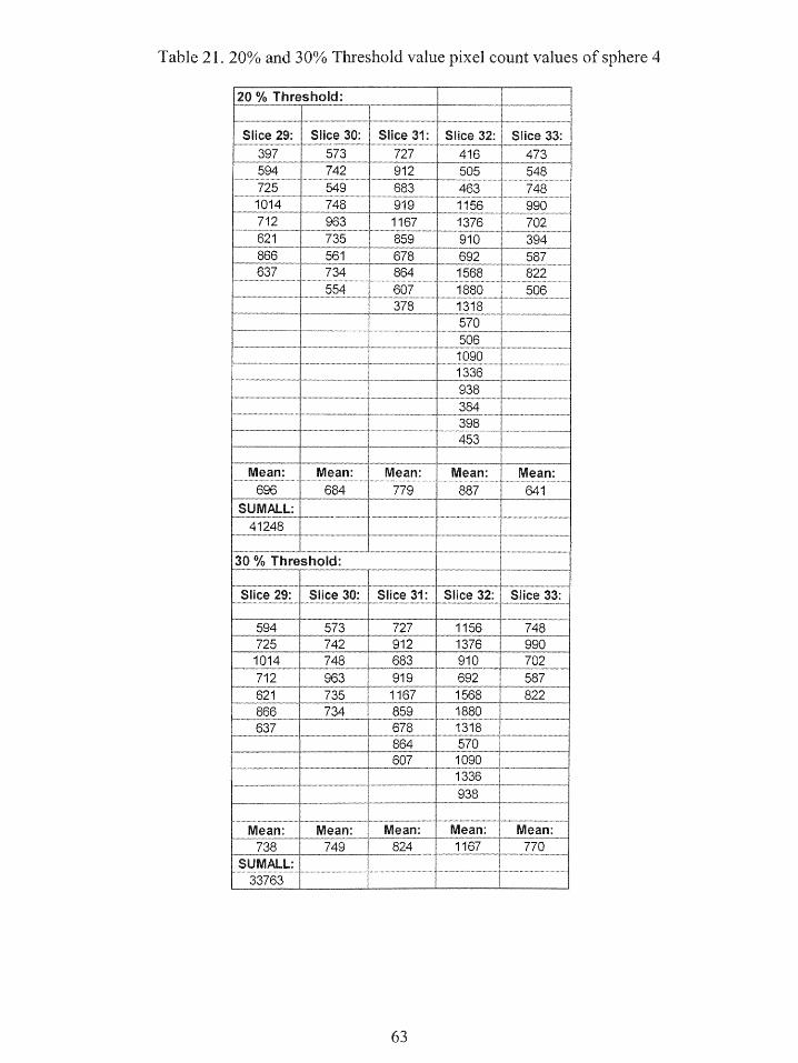
Table 21. 20% and 30% Threshold value pixel count values of sphere 4
20 % Threshold:
Slice 29: Slice 30: Slice 31: Slice 32: lice 33:397 573 727 416 473594 742 912 _ 505 548725 549 683 463 I 7481014 748 919 1156 990712 963 1167 1376 702621 735 859 910 394866 561 678 692 587637 734 864 1568 822
554 607 1880 506378 1318 j
570
10901336938
398
453
Mean: Mean: Mean: Mean: M an:696 684 779 887 641
41248
30 % Threshold: ___
Slice 29: Slice 30: Slice 31: Slice 32: Slice 33:
594 573 727 1156 748725 742 912 1376 9901014 748 683 910 702712 963 _919 692 .587.
621 735 1167 1568 1822866 __ 734 859 _1880
637 678 1318864 570607 _ _1090
1336938
Mean: Mean: Mean: Mean: Mean:738 749 824 1167 770
SUM 6L:33763 _____ ____ __________
63
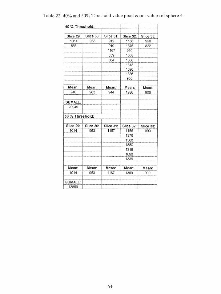
Table 22. 40% and 50% Threshold value pixel count values of sphere 4
40 % Threshold:
Slice 9: Slice 30: Slice 31: Slice 32: Slice :1014 963 912 1156 990866 919 1376 822
1167 910859 1568
864 1880
1090_____ ___ ______ 1336 __
26 938Mean: Mean: Mean: Mean: Mean:940 963 944 1286 _...,.906..._,.n
SUMALL:
50 % Threshold:
Slice 29: Slice 30: Slice 31: Slice 32: Slice 3:1014 963 1167 1156 990
13761568
_1880
1318
10901336
Mean: _Mean: -Mean: Mean: Mean:1014 963 1167 1389 990
13859
64
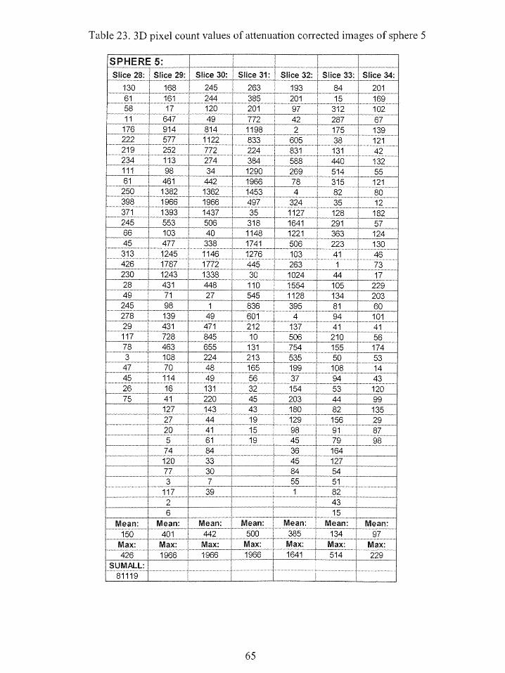
Table 23. 3D pixel count values of attenuation corrected images of sphere 5
SPHERE 5: _
Slice 28: Slice 29: Slice 30: Slice 31: Slice 32: Slice 33: Slice 34:
130 168 245 263 193 { 84 2016144161 201 169
58 17 120 201 97 312 10211 647 49 772 42 287 67176 914 814 1198 2 175 139222 577 1122 833 _ 605 38 121219 252 772 224 831 131 42234 113 274 384 588 440 132111 98 34 1290 269 514 5561 _ 461 442 1966 78 315 121250 1382 1362 1453 4 82 80398 1966 1966 497 324 35 12371 1393 1437 35 1127 128 182245 553 506 318 1641 291 5766 103 40 1148 1221 363 12445 4 338 1741 506 223 130313 1245 1146 1276 103 41 462 139 1772 445 263 1 4 1
230 1243 1338 30 1024 44 17.28 . 431 448 110 1554 105 22949 71 27 545 1128 134 203
245 98 1 836 395 _ 81 60
278 139 49 61 34 94 10129 431 471 212 137 _41 41117 728 845 10 _ 506 4 210. 56_78 _463 655 131 3 754 1 155j 1743 108 224 213 535 I 50 ' 53_
45 j 114 49 56 394 4326 16 131 32 154 53 12075 41 220 45 203 E 44 99
127 143 43 180 82 13527 44 19 129 156 1 2920 41 15 98 91 875 6 1 19 4 79 9874 84 36 164120 33 45 127
77 _ 30 84 543 7 55 51
117 39 1 822 _ 43
6 15Mean: Mean: Mean: Meean
150 401 442 500 385 134 97
Max: Max: Max: Max: Max Max: Max:426 1966 ._M W 1966~_ M N 1966 1641 514 229
SUML:11811196
65
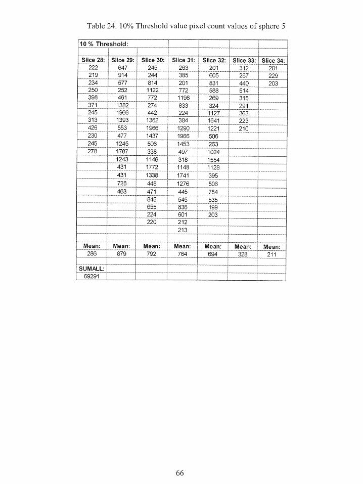
Table 24. 10% Threshold value pixel count values of sphere 5
10 % Threshold:
Slice 28: Slice 29: Slice 30: Slice 31: Slice 32: Slice 33: lice 34222 647 245 263 201 312 201219 914 244 385 605 287 229234 577 814 201 831 440 _ 203250 252 1122 772 588 514
398 461 772 11981 269 315371 1382 274 833 324 291245 ? 1966 442 224 1127 363313 1393 1362 384 1641 223426 ..553 1966 1290 1221 210230 [477 1437 1966 506245 1245 506 1453 263278 1787 338 497 1024
1243 1146 318 1554 -
431 1772 1148 1128431 1338 1741 395
728 448 1276 506463 471 445 754
845 , 545 535655 836 199_
__ _ _224 _ 601 ._2_.03 ._ _..«,_.._._._.___ _._.vN__ .___.__
220 212 2
213
Mean: Mean: Mean: Mean: Mean: EMean: Mean:286 j879 792 764 -694 328 _21.1__.
SUMALL:___{_______ __
69291
66
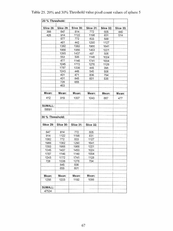
Table 25. 20% and 30% Threshold value pixel count values of sphere
20 % Threshold:
Slice 28: Slice 29: Slice 30: Slice 31: Slice 32: 1Slice 3:398 647 g 814 772 605 T 440426 914 1122 1198 831 514
577 772 833 588461 442 1290 11271382 1362 1966 T 16411966 J 1966 1453 12211393 1437 497 506553 506 1148 1024477 1146 1741k 1554 -
1245 1772 1276 11281787 1338 445 3951243 448 545 506
431 471 836 754431 845m 601 535728 655 - _463
Mean: Mean: Mean: Mean: Mean: Mean:412 919 1007 1043 887 477
SUMALL58591 ¬
30 % Threshold:
Slice 29: Slice 30: Slice 31: Slice 32:
647 814 772 605914 1122 1198 831382 { 772 833 11271966 1362 1290 16411393 11966 1966 1221 _
1245 1437 1453 10241787 1146 1148 1554 {____1243 1 1772 1741 1128728 1338 1276 754
845 836
655 601
Mean: Mean: Mean: Mean1256 ! 1203 1192 1098
SUMALL:647534
67

Table 26. 40% and 50% Threshold value pixel count values of sphere 5
40 % Threshold:
Slice 29: Slice 0: S lice 31: Slice 32:914 814 1198 8311382 1122 83_3 11271966 1362 1290 1641
1393 1966 1966 12211245 1437 1453 10241787 1146 1148 15541243 1772 1741 1128
1338 T 1276 ......_..m.......
~845 ._ 836 _ _
Mean: Mean: Mean: Mean:1419 1311 1305 1218
SUM LL:. .___ ... .m42000
50 % Threshold:
Slice 29: lice 30: Sice 31: Slice 32:
1382 1122 1198 11271966 t1362 1290 1641
33 96 966 12211245"-- -- 1437 _..1453._ ._m 10241787 1146 1148 15541243 1772 1741 1128
1338 1276 _
Mean: Mean: Mean: Mean:1503 1449 1439 1282
36926
68
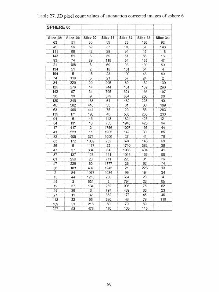
Table 27. 3D pixel count values of attenuation corrected images of sphere 6
SPHERES:
Slice 28: Slice 29: Slice 30 Slice 31: Slice 32: Slice 33: Slice 3463 51 35 59 33 . 126 92
w45 56 52 37 110 67 148111168 42 28 94 15 118143 51 3 59 51 56 1693 74 29 118 54 188 4721 108 3 69 93 139 59
134 51 2 18 161 54 4194 5 _ 15 23 100 48 _ 5074 116 3 21 57 24 234 329 20 295 89 132 130126 279 14 744 I 151 139 290142 97 34 795 621 186 19736 39 9_ L7 834 260 68139 349 138 61 482 225 4040 582 410 30 81 66 109
63 466 E441 75 20 55 283139 171 190 40 505 230 23394 6 45 143 1624 423 121
54 131 18 755 1943 425 9417j 417 _ 2 __ 1756 1)007 195 4441 523 11 1905 1 147 33 8582 405 371 _ 1006 _ 27 . 41 7683 172 1 1039 232 . 624 146 6986 9 1177 22 1710 382 3647 37 604 64 1966 404 41
_ 87 137 123 111 1013 166 6061 250 28 711 _ 228 31 ^26
47 1 228 60 1777 26 92 7456 183 407 1945 21 223 132 84 1077 1034 99 194 34
13 44 1210 235 354 23 4
44 3 631 2 79 4 _ 23 _ 6512 37 134 232 906 1 75 6224 36 6 797 489 83 2327 11 32 862 173 _ 45 46113 32 56 395 w 21V~1 79 118169 51 216 60 70 69227 53 478 170 108 115
69
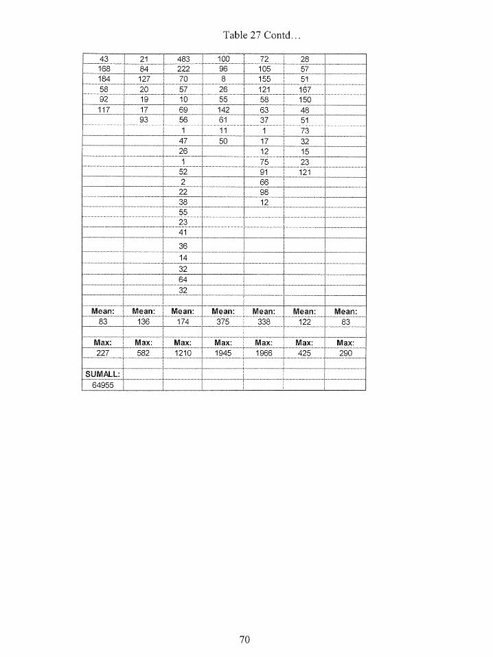
Table 27 Contd...
43 21 483 100 72 28__..222 96 105 1 7
184 __ 127 70 8 155 51_,._....,..._.....nn _,_. __.._..,.._ .... _., T ....... .............___..._,m __._... ..,,...,_._..._...,_.,.._.... ..... _ ._.._.,..n_..____,,....__....;..__,, ....... n_...._...._,._.....,..n...........,.,.....,..........,......_..__..,,8....._..,...._,' 20 _._._._...,7......_n... 26 121 167
........ .................. ,.._...._....,.......,............_....,...._.......... _.......__._..,..._..._ ._._......,................._,..,.._.,,..
92 19 10 _ 55 i 58 150 _
117 17 1 69 142 63 48
1 93 56 61 3 37 51..................................... _., _................,. .
i 1 11 i 1 7
47 50 17 32
26 i 12 15
_,__......,_,.__,_.,.,_..,._,_ ............. ....._,.......,..__..,.. =a._,,.............. _ u.._.....,......................,..._~_,._,._._...1............... 23.... ,.a,..,... ,._............ .......... ....................................? 52 91 _...,,,121
2 . 66
22 98
._._.,_ .,._...3 1 2
_,.._...._...__...__...,....___... ...... _ .................:................. ................. 2553......._.....,....,..,...........,......._.._........,...... ,....,......,.......,,....,....._........ ...,._,.....,......,......,..,._......._...................................,.............
y 41
3 36
14
323
E
6432
Mean: Mean: ! Mean: Mean: } Mean: Mean: Mean:_...__..,.... ._,....._...__._ ........ _ ..................._....__ _..._...,,......._.._...._,_.:._._..._..__._.,.....,_....,._....._,..............,. ._._.m..,....... _..... ... ,..,.. .. u._._83 136 174 375 338 122 83
Max: }3 f 3 - IM xa 3 a). a y ® Max: Max: 1 x: Max:227 582 1210 1945 1966 425 290
}SUMALL:_w_....._._...,..._..,...._ . .._ .............__..._.............,.,.n._._,.._ _.m,_.... _,.., ._....._u....,__ _......__.....,_.mr_.,.,. _,._._ _.,,........_...,_.,..._.__.., ..
64955
7

Table 28. 10% Threshold value pixel count values of sphere 6
10 % Threshold:
Sice 28: Slice 29: Slice 30: Slice 31: Slice 32: S lice 33: Slice34:227 329 410 295 621 260 290
__ 279 441 744 834 225 197349 371 795 482 230 283582 1039 379 505 423 233466 1177 755 1624 425417 604 1756 l 1943 382523 407 1905 | 1007 4047405 107 06 624 223250 1210 232 1710
228 631 711 1966
216 1777 1013478 1945 228483 1034 354222 235 i 794
232 906 797 489
862j_._.. . 9 ____ __._.__ _.... __.. _ ________.. __ ....... _.__.____ ..
Mean: I ean: Man: Mean: Mean: Mean: Mean:227 383 626 881 944 321 251
SUMAL v473481
71
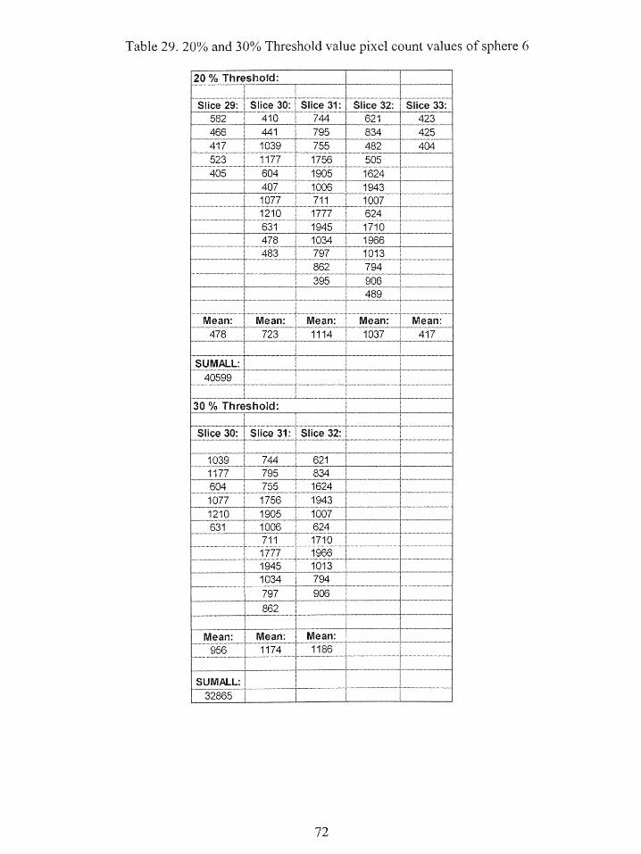
Table 29. 20% and 30% Threshold value pixel count values of sphere
20 % Threshold:
Slice 29: Slice 30: Slice 31: Slice 32: Slice 33:582 410 744 621 T423466 441 795 834 L 425417 1039 755 482 404523 1177 1756 505405 604 1905 1624 ___
407 <1006 19431077 ; 711 10071210 1777 624631 1945 1710
478 _11034 -_ 1966
862 794395 906T_489 __
I _
Mean: Mean: z Mean: Mean: Mean:478 1 723 1114 1037 417
SUMALL{40599
30 % Threshold:
Mica 30: Slice31: Slice 32
1039 744 621 -m
1177 795 834604 755 16241077 1756 31943
1210 1905 1007 ._.1
631 1006 624711 j17101777 19661945 10131034 794797 906862
Mean: Mean: Mean: 4
956 1174 1186
SUMALL:32865 _
72
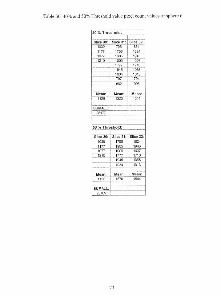
Table 30. 40% and 50% Threshold value pixel count values of sphere
40 % Threshold:
Slice 0 Slice 31: Slice 32:1039 795 8341177 1756 1624
.1077.. .. 1905 19431210 1006 1007
1777 17101945 19661034 _1013
797 794
862 1906Mean: Mean: Mean:1126 1320 1 111
SUM L:28177
50 % Threshold:
Slice 30: Slice 31: Sice 32:1039 1756 16241177 1905 19431077 1006] 10071210 1777 1710
1945 19661034 1013
Mean: Mean: Mean:1126 1570 1544
SUML _
23189 _ _ _ _
73
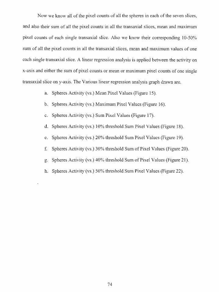
Now we know all of the pixel counts of all the spheres in each of the seven slices,
and also their sum of all the pixel counts in all the transaxial slices, mean and maximum
pixel counts of each single transaxial slice. Also we ow their corresponding 10-50%
sum of all the pixel counts in all the transaxial slices, mean and maximum values of one
each single transaxial slice. A linear regression analysis is applied between the activity on
x-axis and either the sum of pixel counts or mean or maximum pixel counts of one single
transaxial slice on y-axis. The Various linear regression analysis graph drawn are.
a. Spheres Activity (vs.) Mean Pixel Values (Figure 15).
b. Spheres Activity (vs.) Maximum Pixel Values (Figure 16).
c. Spheres Activity (vs.) Sum Pixel Values (Figure 17).
d. Spheres Activity (vs.) 10% threshold Sum Pixel Values (Figure 18).
e. Spheres Activity (vs.) 20% threshold Sum Pixel Values (Figure 19).
f. Spheres Activity (vs.) 30% threshold Sum of Pixel Values (Figure 20).
g. Spheres Activity (vs.) 40% threshold Sum of Pixel Values (Figure 21).
h. Spheres Activity (vs.) 50% threshold Sum Pixel Values (Figure 22).
74
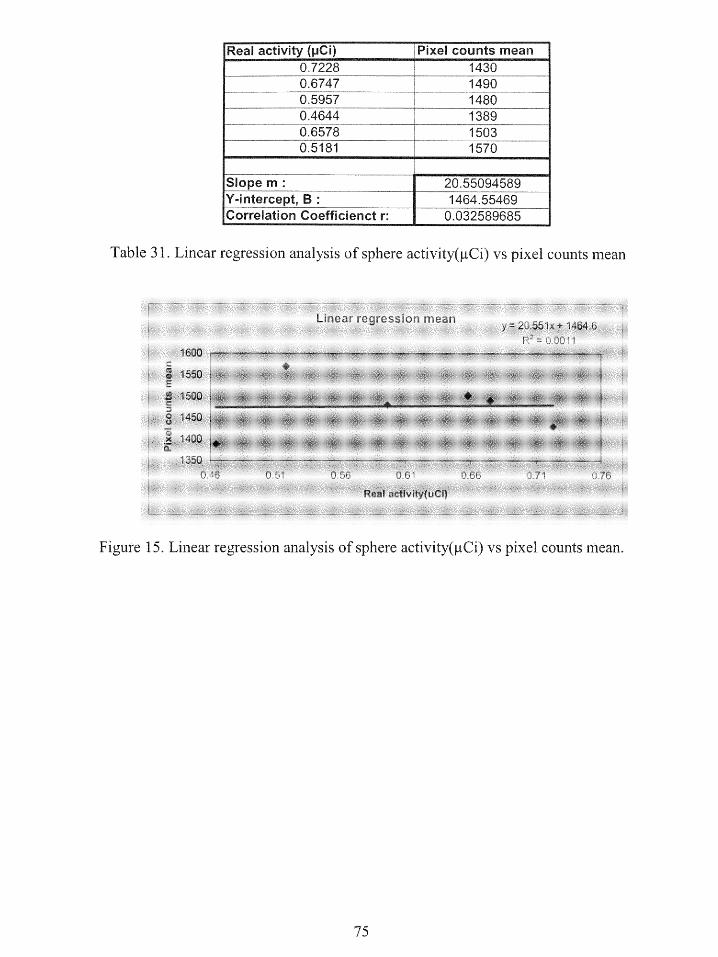
Real activity (pCi) Pixel counts mean0.7228 14300.6747 14900.5957 14800.4644 1389 _
0.6578 15030.5181 1570
Slope m: 20.55094589Y-intercept, B: 1464.55469lCorrelation Coefficienct r: 0.032589685
Table 31. Linear regression analysis of sphere activity(gCi) vs pixel counts mean
unear regression mean
j~ -1
160
Figure 15. Line-ar regression analysis of sphere activiy(pCi) -vs pixel counts rean.
15
Real activity (pCi) Pixel counts max0.7228 19660.6747 19660.5957 19660.4644 1880
0.6578 1966
0.5181 1966
Slope m: 248.1599103Y-intercept, B: 1801.385161Correlation Coefficienct r: 0.699195983
Table 32. Linear regression analysis of sphere activity(pCi) vs pixel counts max
Liear regression max
Figure 16. Linear regression analysis of sphere activity (pCi) vs pixel counts maximnum
76

Real activity (pCi) Pixel counts sum0.7228 1418310.6747 133580
___ 0.5957 _ 103_914
0.4644 _ 72850
0.6578 811190.5181 64955
Slope 267716.6451Y-intercept, B: -62416.57169Correlation Coefficienct r: 0.820094669
Table 33. Linear regression analysis of sphere activity(pCi) vs pixel counts sum
Linear regression sum 267x627s.R 2 =Q. 726
Figure 17. Linear regression analysis of sphere activity (pCi) vs pixel counts su
77

Real activity (pCi) Pixel counts sum0.7228 135116
0.6747 1191110.5957 833910.4644 554140.6578 69291
0.5181 _ 47348
Slope m:_304507.02Y-intercept, B: -99459.20953Correlation Coefficienct r: 0.854208287
Table 34. 10% Threshold linear regression analysis of sphere activity (pCi) vs pixelcounts sum
10 % Threshold lnear regression sum
Figure 18. 10% Threshold linear regression analysis of sphere activity (pCi) vs pixelcounts surn
78
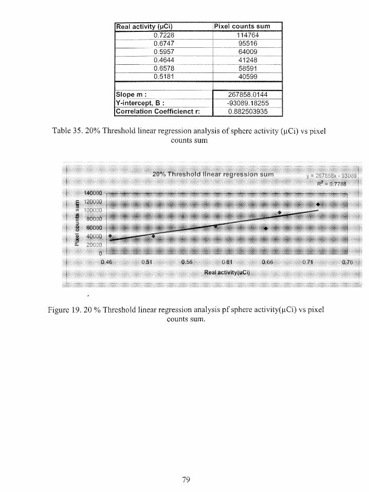
Real activity (pCi) Pixel counts sum0.7228 114764
0.6747 955160.5957 640090.4644 41248
0.6578 585910.5181 40599
Slope rn_ 267858.0144
Y-intercept, B: -93089.18255Correlation Coefficienct r: 0.882503935
Table 35. 20% Threshold linear regression analysis of sphere activity ( Ci) vs pixelcounts sum
20% Threshold linear regression sum 939
Figure 19. 20 % Threshold linear regression analysis pf sphere activity(pCi) vs pixel
counts sum.
79
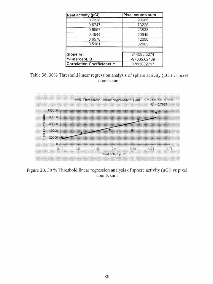
Real activity (p i) Pixel counts sum0.7228 936650.6747 732280.5957 438280.4644 209490.6578 420000.5181 32865
Slope m 244598.5274Y-intercept, B: -97035.62489Correlation Coefficienct r2032717
Table 36. 30% Threshold linear regression analysis of sphere activity (pCi) vs pixelcounts sum
30% Threshold linear regression sumy245x973
Figure 20. 30 % Threshold linear regression analysis of sphere activity (pCi) vs pixelcounts s0
60
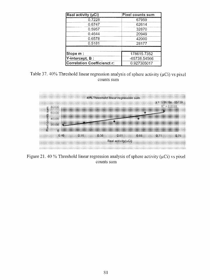
Real activity (pCi) !Pixel counts sum0.7228 679590.6747 62614
0.5957 328700.4644 209490.6578 420000.5181 28177
Slope m: 178615.7352
Y-intercept, B: -65738.54566Correlation Coefficienct r: 0.927305017
Table 37. 40% Threshold linear regression analysis of sphere activity (pCi) vs pixelcounts sum
40 Threshold near regresion sum
Figure 21. 40 % Threshold linear regression analysis of sphere activity (pCi) vs pixelcounts sum
81
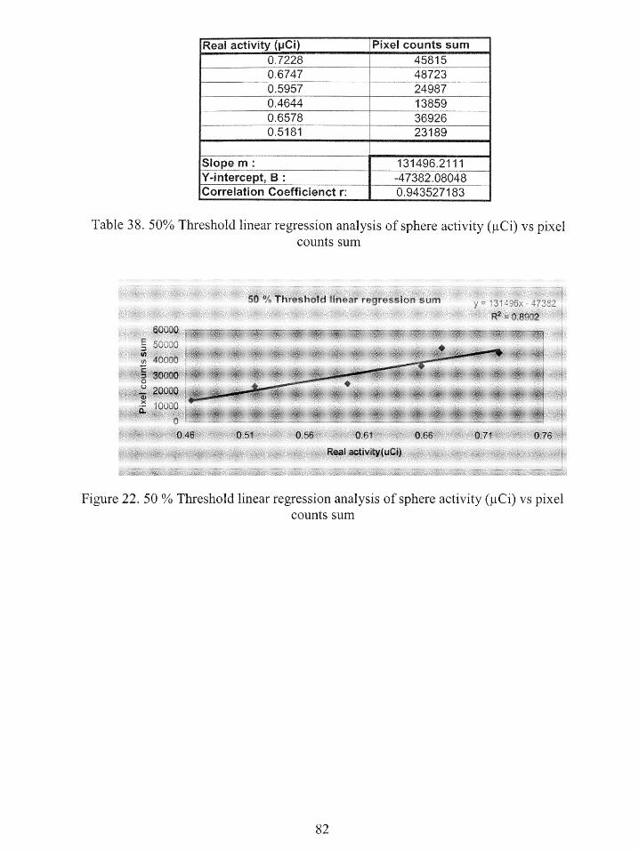
Real activity (pCi) Pixel counts sum0.7228 45815
0.6747 487230.5957 249870.4644 13859
0.6578 369260.5181 23189
Slope m 131496.2111Y-intercept, B -47382.08048Correlation Coefficienct r: 0.943527183
Table 38. 50% Threshold linear regression analysis of sphere activity (PCi) vs pixelcounts sum
50 Threshold lnear reression sum
Realatd yu i
Figure 22. 50 % Threshold linear regression analysis of sphere activity (pCi) vs pixelcounts s0
82

35j 3
30 -
25 21
15 12> < ~ >
591 727 863 999 1135 1271 1407 1543 1679 1815 19 6
Pixel count
Figure 23. Histogram of pixel counts vs frequency of sphere 1
Sphere 2
50 46V
45
0S25o2016 1
'15
10 - -K5 'K
399 592 785 978 1171 1364 1557 1750 1943 2136
Pixel count
Figure 24. Histogramn of pixel counts vs frequency of sphere 2
83

Fiue . itorm fpie cutsv feuecSo phere 330
~25 >
20 15
15 - -10 -, 85
5 5
394 551 708 865 1022 1179 1336 1493 1650 1807 1966
Pixel count
Figure 25. Histogram of pixel counts vs frequency of sphere 3
Sphere 4
60 5
50
-40
S30
i20 14141
10 2
0190 359 528 697 866 1035 1204 1373 1542 1711 80
Pixel count
Figure 26. Histogram of pixel counts vs frequency of sphere 4
84
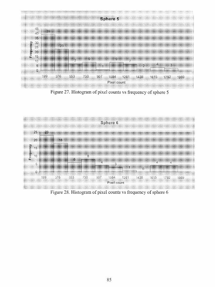
45 3403530
1510 77
199 376 553 730 907 1084 1261 1438 1615 1792 16
Pixel count
Figure 27. Histogram of pixel counts vs frequency of sphere 5
Sphere 6
25 2
10 1
15
199 376 553 730 907 1084 1261 1438 1615 1792 16Pixel count
Figure 28. Histogram of pixel counts vs frequency of sphere 6
85

4.3 Data Analysis of Simulated Lung Lesion
A PET image showing simulated lung lesion is in Figure 29. Now data analysis is
performed for simulated lung lesion experiment by calculating pixel counts for both the
left and right lung and histograms are drawn between various pixel counts and frequency.
The pixel counts values and threshold values of both the lungs are shown in Tables 39-43
and the corresponding histograms are shown in Figure 30 and 31.
86

Figure 29. Right-TOP: CT image of simulated lung lesions in which we seelung lesion 1 on Right lung and lung lesion 2 on left lung; Left-TOP:PET image of lung lesions 1 and 2; Left Bottom: Combined PET-CT
image of lung lesions 1 and 2
87
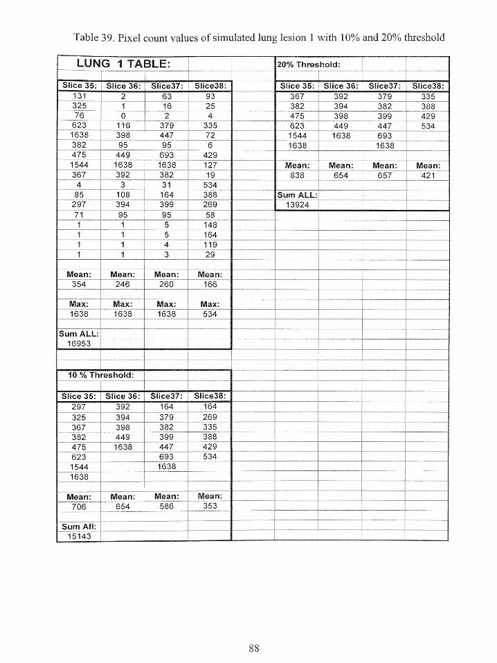
Table 39. Pixel count values of simulated lung lesion 1 with 10% and 20% threshold
LUNG 1 TABLE: 20% Threshold:
Slice 35: Slice 36: Slice37: Slice38: Slice 35: Slice 36: Slice37: Slice38:131 2 63 93 -- 367 392 379 335325 1 16 25 382 394 382 38876 0 2 4 475 398 399 429
623 116 379 335 623 449 447 5341638 398 447 72 1544 1638 693382 95 95 6 1638 1638475 449 693 4291544 1638 1638 127 Mean: Mean: Mean: Mean:367 392 382 19 838 654 657 421
4 3 31 .. 53485 108 164 388 Sum ALL:
297 394 399 269 1392471 95 95 58
1 1 5 1481 1 5 164 -
1 1 4 1 1191 1 3 - 29
_ ---. __-_
Mean: Mean: Mean: Mean:354 246 260 166 _
- - - - --- - _Max: Max: Max: Max:1638 1638 1638 534
Sum ALL:
16953 . ~41 91 5
10 % Threshold:
Slice 35: Slice 36: Slice37: Slice38:297 392 164 164-.
325 394 379 269 1367 398 382 335382 449 399 388
475 1638 447 429623 L 693 534 __-
1544 16381638
Mean: Mean: Mean: Mean:706 654 586 353 1 ---353
Sum All: 1-.
15143
88
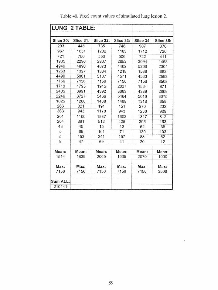
Table 40. Pixel count values of simulated lung lesion 2.
LUNG 2 TABLE:___
Slice 30: Slice 31: 1 Slice 32: Slice 33: Slice 34: S lice 35:293 448 735 746 907 376967 1051 1202 1183- 1712 - 720721 760 553 506 722 4111935 2296 2907 2852 3094 14684949 4890 4873 4402 5266 23041263 1327 1334 1218 1536 6824499 5001 5107 4571 4583 25937156 7156 7156 7156 7156 35081719 95 1945 2037 1884 8712405 3991 4392 3683 4339 28092246 3727 5466 5464 5616 30751025 ' 1260 1438 1489 1318 659266 321 191 151 270 232363 943 1170 943 1238 909201 1100 -1887 1602 1347 812204 391 512 1 425 305 163
45 15 12 52 38
5 69 101 71 130 1035 1 153 241 157 88 629 47 69 41 20 12
Mean: Mean: Mean: Mean: Mean: Mean:1514 1839 2065 1935 2079 1090
- + ------ -
Max: Max: Max Max Max: Max:7156 7156 7156 7156 1 7156_ 3508
Sum ALL:210441
89
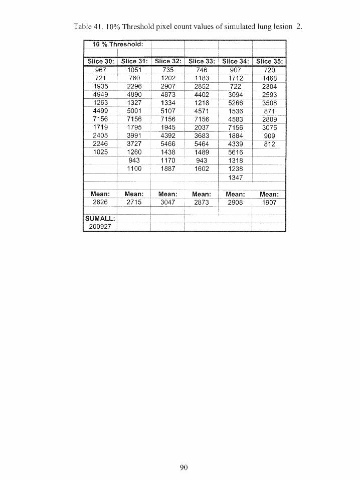
Table 41. 10% Threshold pixel count values of simulated lung lesion 2.
10 % Threshold:
Slice 30: Slice 31: Slice 32: Slice 33: Slice 34: Slice 35967 1051 735 746 907 720721 760 1202 1183 1712 14681935 2296 2907 2852 722 23044949 4890 4873 4402 3094 25931263 1327 1334 1218 5266 35084499 5001 5107 4571 1536 8717156 7156 7156 7156 4583 28091719 1795 1 1945 2037 7156 307545 39 392 3683 1884 909
2246 3727 5466 5464 4339 8121025 1260~ 1438 1489 5616
943 1170 943 -1318_1100 1887 1602 1238
1347
Mean: Mean: Mean: Mean: Mean: Mean:2626 2715 3047 2873 2908 1907
SUMALL:9200927
90
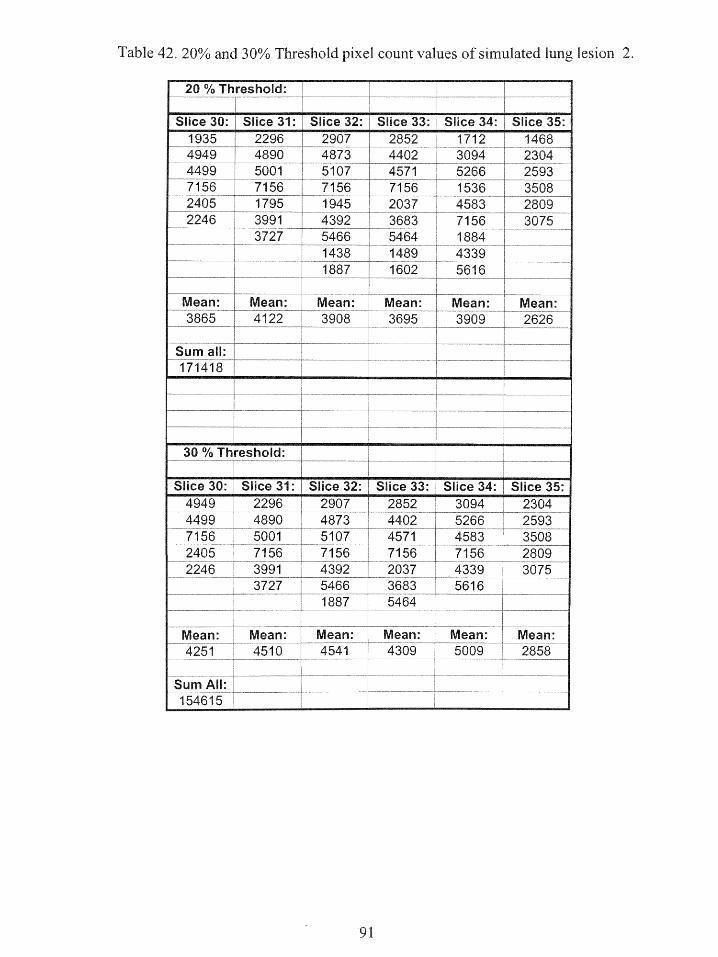
Table 42. 20% and 30o Threshold pixel count values of simulated lung lesion 2.
20 % Threshold:
Slice 30:' Slice 31: Slice 32: Slice 33: Slice 34: Slice 351935 2296 2907 2852 1712 14684949 4890 4873 4402 3094 23044499 5001 5107 4571 5266 25937156 7156 7156 7156 1536 35082405 1795 1945 2037 4583 _ 28092246 - 3991 4392 3683 7156 3075
3727 5466 5464 18841438 1489 43391887 1602 5616
Mean: Mean: Mean: Mean: Mean: Mean:3865 4122 3908 3695 3909 2626
Sum all:171418 I
30 % Threshold: .
Slice 30: Slice 31: Slice 32 Slice 33: Slice 34: Slice 35:4949 2296 2907 2852 3094 23044499 4890 4873 4402 5266 25937156 5001 5107 4571 4583 35082405 7156 7156 7156 7156 28092246 3991 4392 2037 4339 3075__ 2037 433 3075-
3727 5466 3683 56161887 _ 5464
Mean: Mean: Mean: Mean: Mean: Mean4251 4510 4541 4309 5009 2858
SumAll:154615
91
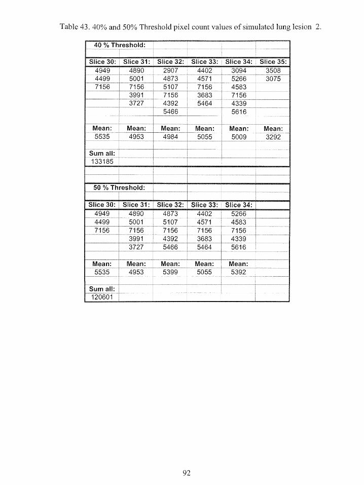
Table 43. 40% and 50% Threshold pixel count values of simulated lung lesion 2.
40 % Threshold:
Slice 30: Slice 31: Slice 32: Slice 33: Slice 34: Slice 35:4949 4890 2907 4402 3094 35084499 5001 473 14571 5266 30757156 7156 5107 7156 4583
- 3991 7156 3683 71563727 4392 5464 4339
5466 5616
Mean: Mean: Mean: Mean: Mean: Mean:5535 4953 4984 5055 5009 3292
Sum all:-133185
50 % Threshold:
Slice 30: Slice 31: Slice 32: Slice 33: Slice 34:4949 4890 4873 4402 52664499 5001 5107 4571 45837156 7156 L 7156 7156 7156
3991 4392 3683 43393727 5466 5464 5616
Mean: Mean: Mean: Mean: Mean:5535 4953 5399 5055 5392
Sum all:120601
92

16.
14
12
1078>9 4 222> ---- 10 0 >0 0>0
164 311 458 605 752 899 1046 1193 1340 1487 163
Pixel count
Figure 30. Histogram of pixel counts vs frequency of Lung 1
Lung lesion2
25
20
z 15 > 2
0
0 ~<720 1364 2008 2652 3296 3940 45&4 5225 5872 6516 716
Pixel count
Figure 31. Histogram of pixel counts vs frequency of Lung 2
93
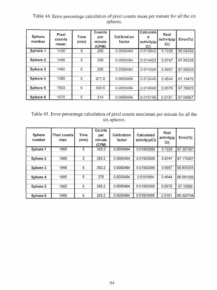
Table 44. Error percentage calculation of pixel counts mean per minute for all the sixspheres.
Shr Pie Tie Counts Calculate Raunts Time per Calibration d activity(p Error(%)
number cnts (mm) minute factor activity(p Ci)mean: CPM) Ci)
Sphere 1 1430 5 286 0.0000484 0.013842 0.7228 98.08489
Sphere 2 1490 5 298 0.0000484 0.014423 0.6747 97.86228
Sphere 3 1480 5 296 0.0000484 0.014326 0 5957 97.59503
Sphere 4 1389 5 277.8 0.0000484 0.013446 0.4644 97.10475
Sphere 5 1503 5 300.6 0.0000484 0.014549 0.6578 97.78823
Sphere 6 1570 5 314 0.0000484 0.015198 0.5181 97.06667
Table 45. Error percentage calculation of pixel counts maximum per minute for all thesix spheres.
Counts Real
Sphere Pixel counts Time per Calibration Calculatednumber max: (mm) minute factor activi(pi) Ci)
_ (CPM) _Sphere 1 1966 5 393.2 0.0000484 0.01903088 0.7228 97.367061
Sphere 2 1966 5 393.2 0.0000484 0.01903088 0.6747 97.179357
Sphere 3 1966 5 393.2 0.0000484 0.01903088 0.5957 96.805291
Sphere 1880 5 376 0 0000484 00181984 04644 96081309
Sphere 5 1966 5 393.2 0.0000484 0.01903088 0,6578 97.10689
Sphere 6 1966 5 393.2 0,0000484 0.01903088 0.5181 96.326794
94
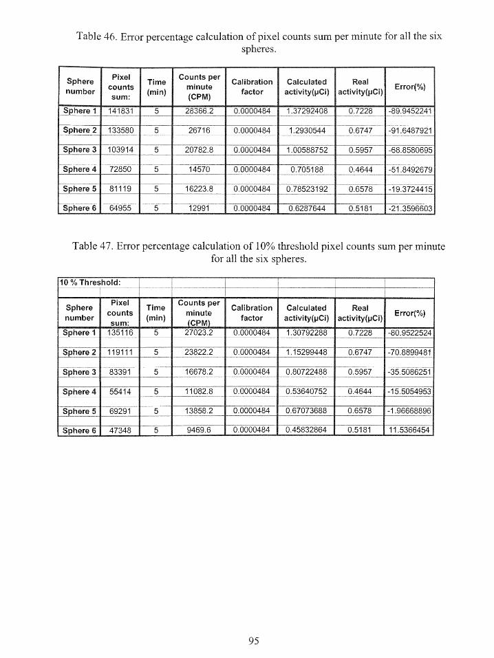
Table 46. Error percentage calculation of pixel counts sum per minute for all the sixspheres.
Sphere Time Counts per Calibration Calculated Realnumber cou ts min) minfactor activity(pCi) activity(pCi) Error(%)
sum:
Sphere 1 141831 5 28366.2 0.0000484 1.37292408 0.7228 -89.9452241
Sphere 2 133580 5 26716 0.0000484 1.2930544 0.6747 -91.6487921
Sphere 3 103914 5 20782.8 0.0000484 1.00588752 0.5957 -68.8580695
Sphere 4 72850 5 14570 0.0000484 0.705188 0.4644 -51.8492679
Sphere 5 81119 5 16223.8 0.0000484 0.78523192 0.6578 -19.3724415
Sphere 6 64955 5 12991 0.0000484 0.6287644 0.5181 -21,3596603
Table 47. Error percentage calculation of 10% threshold pixel counts sum per minutefor all the six spheres.
10 % Threshold:
Sphere Time Counts per Calibration Calculated Realnumber counts minute factor activity(pCi) activity(p ) Error(%)
sum: (CPM)
Sphere 1 135116 5 27023.2 0.0000484 1. 30792288 0.7228 -80.9522524
Sphere 2 119111 5 23822.2 0.0000484 1.15299448 0.6747 -70.8899481
Sphere 3 83391 5 16678.2 0.0000484 0.80722488 0.5957 -35.5086251
Sphere 4 55414 5 11082.8 0.0000484 0.53640752 0.4644 -15.5054953
Sphere 5 69291 5 138582 0.0000484 0.67073688 0.6578 -1.96668896
Sphere 6 47348 5 9469.6 0.0000484 0.45832864 0.5181 11.5366454
95
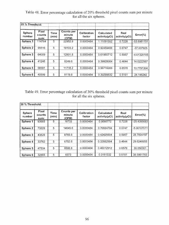
Table 48. Error percentage calculation of 20% threshold pixel counts sum per minutefor all the six spheres.
20 % Threshold:
Sphere Tie ounts per Calibration Calculated Realnuber counts in) minute factor activity(pCi) activity(pCi) Error(%)
Sphere 1 114764 5 22952.8 0,0000484 111091552 0.7228 -536961151
Sphere 2 95516 5 19103.2 0.0000484 0.92459488 0.6747 -37.037925
Sphere 3 64009 5 12801.8 0.0000484 061960712 0.5957 4.01328185
Sphere 4 41248 5 8249.6 0.0000484 039928064 0.4644 140222567
Sphere 5 58591 5 11718.2 0.0000484 0.56716088 0.6578 13.7791304
Sphere 6 40599 5 8119.8 0.0000484 0.39299832 0.5181 24.146242
Table 49. Error percentage calculation of 30% threshold pixel counts sum per minutefor all the six spheres.
30 % Threshold:
Sphere Time ounts per Calibration Calculated Realnumber counts mmin) factor activity(pCi) activity(pCi) Error(%)
Sphere 1 93665 5 18733 0.0000484 0.9066772 0.7228 -25.4395683
Sphere 2 73228 5 14645.6 0.0000484 070884704 0.6747 -5.06107011
Sphere 3 43828 5 8765.6 0.0000484 0.42425504 0.5957 28.7804197
Sphere 4 33763 5 6752.6 00000484 0.32682584 0.4644 29.6240655
Sphere 5 47534 5 9506.8 0.0000484 0.46012912 0.6578 30.050301
Sphere 6 32865 5 6573 0.0000484 0.3181332 0.5181 38.5961783
96
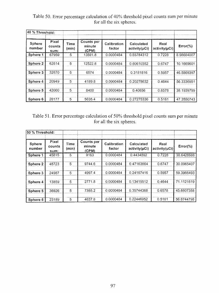
Table 50. Error percentage calculation of 40% threshold pixel counts sum per minutefor all the six spheres.
40 % Threshold: _____ _ _
Sphere Time ounts per Calibration Calculated Realnumber tcounts (rin) factor activity(pCi) activity(pCi) Error(%)
Sphere 1 67959 5 13591.8 0.0000484 0.65784312 0.7228 8.98684007
_ere 62614 5 12522.8 0.0000484 0.60610352 0.6747 101669601
Sphere 3 32870 5 6574 0.0000484 0.3181816 0.5957 46.5869397
Sphere 4 20949 5 4189.8 0.0000484 0.20278632 0.4644 56.3336951
Sphere 5 42000 5 8400 0.0000484 0.40656 0,6578 381939799
Sphere 6 28177 5 5635.4 0.0000484 027275336 0.5181 47.3550743
Table 51. Error percentage calculation of 50% threshold pixel counts sum per minutefor all the six spheres.
50 % Threshold: ]
Sphere Tie ounts per Calibration Calculated Realnumber counts (min) ute factor activity(pCi) activity(pCi) Error(%)
Sphere 1 45815 5 9163 0.0000484 0.4434892 0.7228 38.6428888
Sphere 2 48723 5 9744.6 0.0000484 0.47163864 0.6747 30.0965407
Sphere 3 24987 5 4997.4 0.0000484 0,24187416 0.5957 59.3966493
Sphere 4 13859 5 2771.8 _0.0000484 0,13415512 0.4644 71.1121619
phere 5 36926 5 7385.2 0.0000484 035744368 0,6578 45.6607358
Sphere 6 23189 5 4637.8 0.0000484 0.22446952 0.5181 56.6744798
97

Table 52. Error percentage calculation of pixel counts mean per minute for simulated
lung lesions 1 and 2.
Pixel Counts
Lung counts Time per Calibration Calculated Real(min) minute factor activity(pCi) activity(pCi)
an(CPM)
Lung 1 838 7 119.7143 0.0000484 0.005794171 0.09801 94.08818
Lung 2 5535 7 790.7143 0.0000484 0.038270571 0.8478 95.4859
Table 53. Error percentage calculation of pixel counts maximum per minute forsimulated lung lesions 1 and 2.
Pixel CountsTime per Calibration Calculated Real
Lung counts (min) minute factor activity(pCi) activity(pC i) Error(%)max
- _______ ~(CPM) ____
Lung 1 1638 7 234 0.0000484 0.0113256 0.09801 88.44444
Lung 2 7156 7 1022.286 0.0000484 0.049478629 0.8478 94.16388
Table 54. Error percentage calculation of pixel counts sum per minute and thresholdpixel counts sum per minute for simulated lung lesions 1 and 2.
Pixel CountsTime per Calibration Calculated Real
Lung coun (mm) minute factor activity(pCi) activity (Ci) rror(%)
sum(CPM)
Lung 1 16949 7 2421.286 0.0000484 0.117190229 0.09801 -19.569710 % Threshold Lung 1 15143 7 2163.286 0.0000484 0.104703029 0.09801 -6.8289220 % Threshold Lung 1 13924 7 1989.143 0.0000484 0.096274514 0_09801 1.770723
Lung 2 210441 7 30063 0.0000484 1.4550492 0.8478 -71.626510 % Threshold Lung 2 200927 7 28703.86 0.0000484 1389266686 0.8478 -63.867320 % Threshold Lung 2 171418 7 24488.29 0.0000484 1.185233029 0.8478 -39.80130% Threshold Lung2 154615 7 22087.86 0.0000484 1.069052286 0.8478 -26.097240 % Threshold Lung 2 133185 7 19026.43 0.0000484 0.920879143 0.8478 -8.61986
50 %o Threshodl Lung 2 120601 7 17228.71 0.0000484 0.833869771 0.8478 1.643103
98
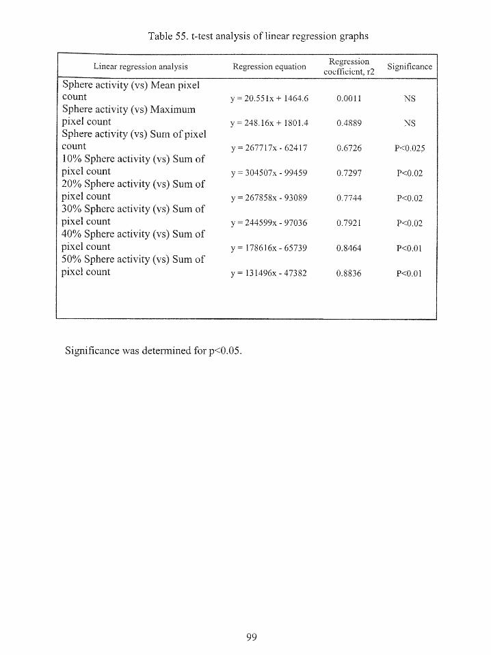
Table 55. t-test analysis of linear regression graphs
Linear regression analysis Regression equation Regression Significancecoefficient, r2
Sphere activity (vs) Mean pixelcount y = 20.551x + 1464.6 0.0011 NSSphere activity (vs) Maximumpixel count y = 248.16x + 1801.4 0.4889 NSSphere activity (vs) Sum of pixelcount y 267717x - 62417 0.6726 P<0.02510% Sphere activity (vs) Sum ofpixel count y = 304507x - 99459 0.7297 P<0.0220%0 Sphere activity (vs) Sum ofpixel count y = 267858x - 93089 0.7744 P<0.0230% Sphere activity (vs) Sum ofpixel count y = 244599x - 97036 0.7921 P<0.0240% Sphere activity (vs) Sum ofpixel count y = 178616x - 65739 0.8464 P<0.0150% Sphere activity (vs) Sum ofpixel count y = 131496x - 47382 0.8836 P<0.01
Significance was determined for p<0.05.
99
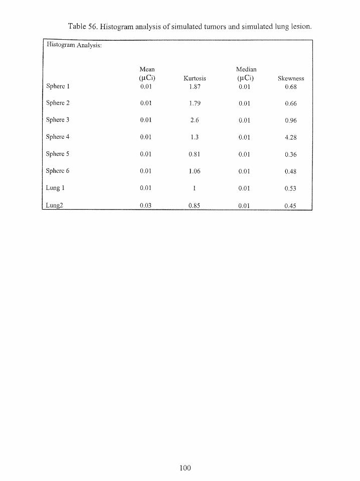
Table 56. Histogram analysis of simulated tumors and simulated lung lesion.
Histogram Analysis:
Mean Median
(pCi) Kurtosis ( Ci) SkewnessSphere 1 0.01 1.87 0.01 0.68
Sphere 2 0.01 1.79 0.01 0.66
Sphere 3 0.01 2.6 0.01 0.96
Sphere 4 0.01 1.3 0.01 4.28
Sphere 5 0.01 0.81 0.01 0.36
Sphere 6 0.01 1.06 0.01 0.48
Lung 1 0.01 1 0.01 0.53
Lung2 0.03 0.85 0.01 0.45
100
5. DISCUSSION
Quantitation of 18-FDG uptake is essential in oncologic PET studies in assessing
tumor response to radiotherapy or chemotherapy. The method we propose for the
accuracy of quantitation of 18-FDG uptake with simulated tumors correlates pixel count
values with the activity uptake by the tumor. We did three experiments, namely PET
calibration, experiment with simulated tumors and experiment with simulated lung
lesions. In the PET calibration method we found out how many counts per pixel per
minute are equal to one micro-curie of 18-FDG. In the experiment with simulated tumors
and simulated lung lesion we have measured the activity for all the spheres in all the
slices for images with attenuation correction.
Our method of choosing a ROI and calculating pixel counts differs from the
traditional quantitative uptake method in which the activity of only one 2D transaxial
slice is used to calculate either the mean or maximum pixel count to quantify the activity
uptake in the tumor. In this study, from a stack of transaxial slices we calculate all the
pixel counts that are distributed in a chosen ROI over a simulated lesion. The ROI chosen
for one transaxial slice will be same for all the transaxial slices. The mean, maximum of
one single transaxial slice and sum of all the pixel counts in all the transaxial slices were
also calculated. We applied threshold values like 10-50% of maximum pixel counts to
eliminate those pixel counts that really don't correspond to the activity and hence to
increase the accuracy of activity quantitation.
From all the correlation coefficients of sphere activity vs pixel counts we can
see that the sum of all pixel counts has the highest significance when compared to that of
101
mean pixel count and maximum pixel count. Thus we can say that there is a linear
relation between the sum of all pixel counts and the sphere activity in simulated tumors.
One can calculate the activity of the simulated tumor if we know the sum of all pixel
counts. It is also proved that the sum of all the pixel count is a better index to determine
the tumor's activity rather than mean pixel count or maximum pixel count. Thus sum of
all pixel counts is needed to get good accuracy in PET quantitation.
We are able to find the activity of a tumor if we know the sum of the entire pixel
counts per minute of all the transaxial slices and multiply it by the calibration factor. The
activity is calculated for both simulated tumors and simulated lung lesions for the sum of
pixel count values, threshold pixel count sum and also for the mean and maximum pixel
counts of one single transaxial slice and compared with real activity. The sum activity is
closer to that of the real activity whereas the activity calculated from the mean and
maximum pixel counts is lower compared to that of the real activity.
The error in calculation of activity is shown in terms of percentage. The error
percentage is high for the mean and maximum pixel count, greater than 96% in all the six
spheres. Also, the error value for simulated lung lesions for the mean and maximum pixel
count is greater than 88%.
From the error percentage values it is understood that the better accuracy for
activity for spheres of volume 15 ml and 8 ml occurs using 30% to 40% threshold pixel
counts sum. For sphere of volume 4 ml better accuracy occur using 20%o to 30%
threshold pixel counts sum. For sphere of volume 2 ml and 1 ml better accuracy occur
using 10% to 20% threshold pixel counts sum. For sphere of volume 0.5 ml better
accuracy occurred for 10% threshold pixel counts sum. Thus it is understood that
102
applying threshold values are important in activity quantitation for better accuracy of
uptake.
In the error percentage calculation for the sphere images with attenuation
correction, the percentage of error at 30-40% threshold for spheres of smaller volume are
higher compared to that of spheres of larger size. This may be due to the partial volume
effect in which the activity of the adjacent voxel may influence the activity of voxels of
interest in smaller volume spheres.
In the sum of pixel error percentage calculations the better accuracy in terms of
error percentage of attenuation corrected spheres 1-6 are 9% at 40 % threshold, -5% at
30% threshold, -4% at 20% threshold, 14% at 20%threshold, -2% at 10% threshold and
11% at 10% threshold respectively.
Better accuracy of activity for simulated lung lesions 1 and 2 were obtained at
10% and 5 0 % thresholds respectively. The error percentage was of 1.7% and 1.6%
respectively. Hence applying threshold values are important for calculating the uptake of
lung lesions.
Histograms were drawn between pixel count and frequency for images from
simulated tumor experiment and also for the lung lesion experiment. Histogram is drawn
for each sphere by taking 10 intervals of pixel count and finding the frequency or number
of pixel count in each interval. This is done for all the six spheres, with and without
attenuation correction and also for two simulated lung lesion. The mean, median,
skewness and kurtosis were found for all the 14 histograms.
Skewness is a measure of symmetry, or more precisely, the lack of symmetry. A
distribution, or data set, is symmetric if it looks the same to the left and right of the center
103
point. A normal distribution is symmetric about its mean, which indicates that there is an
equal probability of an outcome above or below the mean, or average. The skewness for a
Gaussian normal distribution is zero, and any symmetric data should have skewness near
zero. The skewness is greater than 0 in all the histograms thus showing positive skewness
and the distribution lean toward left and the right end of the distribution is trailing off.
Thus we can say the distribution does not follow Gaussian normal distribution and the
data here are skewed to the right. Thus the distribution of pixel count value does not
depend on the mean pixel count.
Kurtosis is a measure of whether the data are peaked or flat relative to a normal
distribution. That is, data sets with high kurtosis tend to have a distinct peak near the
mean, decline rather rapidly, and have heavy tails. Data sets with low kurtosis tend to
have a flat top near the mean rather than a sharp peak. From table 44 we have seen that
we have positive kurtosis values for all the spheres and have a flat distribution. The
kurtosis for a Gaussian normal distribution is 0 and we have values between 0.81-2.6
which are not close to 0. Thus we can predict from the kurtosis data that distribution of
activity does not follow Gaussian normal distribution. The distribution of pixel count
value does not depend on the mean pixel count and hence considering the mean pixel
counts for quantitation of uptake may lead to false results and hence the distribution of
entire pixel counts is necessary for better understanding of the uptake.
The errors percentages obtained in this experiment are unacceptable for clinical
studies. This demonstrates that the performance of instrument is not proper for
quantitative studies. The software initially used in this research has been changed by the
manufacturer with the new improved version in which the bugs have been eliminated.
104

The new experiment following the same methodology used in this study will be
undertaken in order to validate the new software. In other words the results of this
research are not satisfactory for clinical studies but the methodology are same for further
studies.
105

6. CONCLUSIONS
We have used a new procedure to calculate all the pixel counts in the chosen ROI in
all the 3D transaxial slices and their corresponding sum of all transaxial slices, mean and
maximum of each transaxial slices. We also applied threshold values and obtain their
corresponding sum pixel counts of all transaxial slices, mean and maximum pixel counts
of individual transaxial slice.
The results demonstrated that we can calculate the activity of the tumor if we know
the sum of all pixel counts with applied threshold and multiplying them by the calibration
factor. The importance of applying threshold is that we can eliminate pixel counts that
really don't contribute to the tumor activity and thus increase the accuracy of activity
quantitation of the tumor.
The linear regression analysis and error percentage values show that the sum of
the pixel counts of all the transaxial slices (3D) with applied threshold is better than mean
and maximum pixel counts of one single transaxial slice (2D) to calculate the activity of a
tumor. Better accuracy of error percentage of attenuation corrected spheres1-6 are 9% at
40 % threshold sum, -5% at 3 0% threshold sum, -4% at 20% threshold sum, 14% at 20%
threshold sum, -2% at 10% threshold sum and 11% at 10% threshold sum respectively.
The error percentage of mean and maximum of one single transaxial slice of all six
spheres are greater than 95%.
106

From the correlation coefficient values of the sum of pixel counts, mean pixel
counts and maximum pixel counts we have shown that the sum of the pixel counts varies
linearly with the activity of tumor compared to mean pixel count and maximum pixel
count values. The t-test analysis proved that the linear relation between sum of all the
pixel counts and activity is significant.
Comparing the calculated activity with the known real activity proves that a
threshold value around 20%-40% will yield better results for calculating activities in
bigger tumors of volume 15 ml, 8 ml, and 4 ml.
Similarly, this method proves effective to calculate the activity of a lung lesion if
we know the sum of the entire pixel counts and multiply by the calibration factor. A
40%-50% threshold value would be appropriate for the bigger lung lesion of volume 0.34
ml.
Skewness and kurtosis of histograms of pixel counts showed that the 3D
distribution of pixel count does not follow Gaussian normal distribution. This indicates
that the mean value is not a reliable parameter to correlate with the activity of tumor and
the knowledge of entire pixel counts is essential to characterize the uptake.
The calculated activity of smaller spheres at 20%-40% threshold is not close to the
real activity as compared to that of bigger spheres. This may be due to the partial volume
107
effect in which the activity of adjacent voxel may influence the activity of the voxels of
interest.
Finally, experimental errors in quantitation of the activity of the sources and their
dependence with threshold levels are unacceptable for clinical studies. This is probably
due to bugs and limitations of the first software version that was installed in a very new
instrument. A new software version has been installed and it will be validated by the
same methodology.
108
REFERENCES
1. Anne M J Paans, Aren van Waarde, Philip H. Elsinga, , Antoon T. M. Willemsenand Willem Vaalburg 2002. Positron Emission Tomography: the conceptual ideausing multidisciplinary approach. Methods Volume 27, Issue 3 , July 2002, Pages195-207. PET Center, Groningen University Hospital, P.O. Box 30.001, 9700 RB,Groningen, The Netherlands.
2. Annemeike C. kole, Omgo E. Nieweg, Jan Pruim, Anne M.J. Paans, John Th. MPlukker, Harald J. Hoekstra, Heimen Schraffordt Koops and Willem Vaalburg. "Standardized Uptake Value and Quantification of Metabolism for Breast CancerImaging with FDG and L-[1- 1 C] Tyrosine ". PET.J.Nucl Med 1997; 38:692-696.
3. C. Labbe, K. Thielemans, H. Zaidi C. Morell. An object-oriented libraryincorporating efficient projection/backprojection operators for volumereconstruction in 3D PET 1997. Division of Nuclear Medicine, Geneva UniversityHospital, CH-1211 Geneva 4, Switzerland.
4. C.S. Patlak, R.G. Blasberg and J.D. Fenstermacher, Graphical evaluation ofblood-to-brain transfer constants from multiple-time uptake data. J. Cereb. BloodFlow Metab. 3 (1983), pp. 1-7.
5. Dahlbom M, Hoffman EJ, Hoh CK et al. Whole- body positron emissiontomography: Part 1: Methods and performance characterstics. J.Nucl Med 1992;33:1191-1199.
6. Degrado TR, Turkington TG, Williams JJ et al. Performance characterstics ofwhole-body PET scanner. J.Nucl Med 1994;35 1398-1406.
7. Digital imaging and communications in medicine (Dicom), 2000. NationalElectrical Manufacturers Association 1300 N. 17 ' Street, Rosslyn, Virginia22209 USA.
8. Dominique Delbeke, D.Michael Rose, William Chapman, C.Wright Pinson.Optimal Interpretation of FDG PET in the Diagnosis, Staging and Management ofPancreatic Carcinoma. J Nucl Med 1999; 40: 1794-1791.
9. G. Friedlander, J.W. Kennedy, E.S. Macias and J.M. Miller , NuclearRadiochemistry. (third ed.),, Wiley, New York (1981).
10. G. Stocklin and V.W. Pike, Editors, Radiopharmaceuticals for Positron EmisssionTomography, Kluwer, Dordrecht/Norwell, MA (1993) ISBN 0-7923-2340-8.
109
11. Graham M.M, Peterson L.M, Hayward RM. Comparison of simplifiedquantitative analyses of FDG uptake. Journal of Nuclear Medicine and Biology2000.
12. Hamberg LM, Hunter GJ, Alpert NM, Choi NC, Babich JW, Fischman AJ. Thedose uptake ratio as an index of glucose metabolism: useful parameter oroversimplicification? J Nucl Med 1994; 35; 1308-1312.
13. Hani A. Nabi, MD, Phd and Jose M. Zubeldia, MD. Clinical Applications of 18-FDG in Oncology. J. Nucl Med 2002.
14. HE Johns and JR Cunningham 1983. The Physics of Radiology (fourth edition).Charles C Thomas, III. USA, ISBN 0-398-04669-7.
15. (Henry) Sung-Cheng Huang 2000. Anatomy of SUV. Division of Biophysics andNuclear Medicine, Department of Molecular and Medical Pharmacology, UCLASchool of Medicine, Los Angeles, California, USA. Nuclear Medicine andBiology Volume 27, Issue 7 , October 2000, Pages 643-646
16. J. Helus, Editor, Radionuclides Production vols. I & II, CRC Press, Boca Raton,FL (1983) ISBN 0-8493-6003-X & 0-8493-6004-8.
17. Jacobus A.K.Blokland Petar Trindev, Marcel P. M. Stokkel and Ernest K. J.Pauwels 2001. Positron emission tomography: a technical introduction forclinicans. Department of Radiology, Division of Nuclear Medicine, C4Q LeidenUniversity Medical Centre, Albinusdreef 2, 2333 ZA, Leiden, The NetherlandsMedical Faculty, Centre of Nuclear Medicine, Sofia, Bulgaria.
18. Joseph A. Thie, KarlnF.bHubner, Gary T. Smith. " The Diagnostic Utility of theLognormal Behavior of PET Standardized Uptake Values in Tumors". J NuclMed 2000; 41:1664-1672.
19. Keyes JW JR. SUV: standard uptake or silly useless value? J Nucl Med 1995; 36;1836-1839
20. M.M. Ter Pogossian, Positron-emission tomography. Sci. Am. 243 (1980), pp.171- 181.
21. Maguire, GQ., et al 1991: Graphics applied to medical image registration. IEEEComputer graphics and applications, (3): p 20-28.
22. Michael Schulte, Doris Brecht-Krauss, Berno Heymer, Albrecht Guhlmann, ErichHartwig. "Grading of Tumors and Tumor like Lesions of Bone: Evaluation byFDG PET". J Nucl Med 2000; 41:1695-1701.
110
23. Phelps, M.E., Positron Emission Tomography. In: Mazziotta, J. and Gilman, S.,Eds., Clinical Brain Imaging: Principles and Applications, 1992, F.A. DavisCompany, pp71-107.
24. S. Aronow , Positron scanning. In: G.J. Hine, Editor, Instrumentation in nuclearmedicine, Academic Press, New York (1967), pp. 461-483.
25. Tai, Y.C., et al. 1997: Utilization of 3-D elastic transformation in the registrationof chest X-ray CT and Whole Body PET. IEEE Transactions on Nuclear Science.,44(4): p. 1606-1612.
26. Timothy G. Turkington, Ph.d. 2001. Introduction to PET Instrumentation. Journalof nuclear medicine technology, Mar, 29(1): 4-11.
27. U.Bepler, A.Dimitrakopoulou-strauss, G.Kontaxakis, L.G.Strauss. "Functionalstudies of 18 F-Deoxyglucose (FDG) in small cell lung tumors using positronemission tomography (PET)". Greek J.Nucl Med, Volume 1 No 4, October-december 1998,1(4):231-239.
28. V.R. McCready. Milestones in nuclear medicine. Eur. J. Nucl. Med. 27 (2000),pp. S49-S79.
29. http://www.gemedicalsystems.com.
30. http://www.biodex.com.
31. http://www.eee.ntu.ac.uk
111

Appendix
112
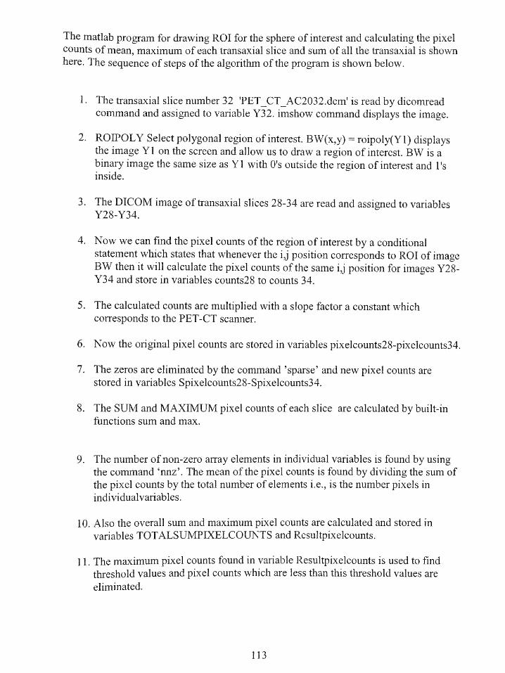
The matlab program for drawing ROI for the sphere of interest and calculating the pixelcounts of mean, maximum of each transaxial slice and sum of all the transaxial is shownhere. The sequence of steps of the algorithm of the program is shown below.
1. The transaxial slice number 32 'PET_CT_AC2032.dcm' is read by dicomreadcommand and assigned to variable Y32. imshow command displays the image.
2. ROIPOLY Select polygonal region of interest. BW(x,y) = roipoly(Y1) displaysthe image Y1 on the screen and allow us to draw a region of interest. BW is abinary image the same size as Yl with 0's outside the region of interest and l'sinside.
3. The DICOM image of transaxial slices 28-34 are read and assigned to variablesY28-Y34.
4. Now we can find the pixel counts of the region of interest by a conditionalstatement which states that whenever the ij position corresponds to ROI of imageBW then it will calculate the pixel counts of the same i,j position for images Y28-Y34 and store in variables counts28 to counts 34.
5. The calculated counts are multiplied with a slope factor a constant whichcorresponds to the PET-CT scanner.
6. Now the original pixel counts are stored in variables pixelcounts28-pixelcounts34.
7. The zeros are eliminated by the command 'sparse' and new pixel counts arestored in variables Spixelcounts28-Spixelcounts34.
8. The SUM and MAXIMUM pixel counts of each slice are calculated by built-infunctions sum and max.
9. The number of non-zero array elements in individual variables is found by usingthe command 'nnz'. The mean of the pixel counts is found by dividing the sum ofthe pixel counts by the total number of elements i.e., is the number pixels inindividualvariables.
10. Also the overall sum and maximum pixel counts are calculated and stored invariables TOTALSUMPIXELCOUNTS and Resultpixelcounts.
11. The maximum pixel counts found in variable Resultpixelcounts is used to findthreshold values and pixel counts which are less than this threshold values areeliminated.
113
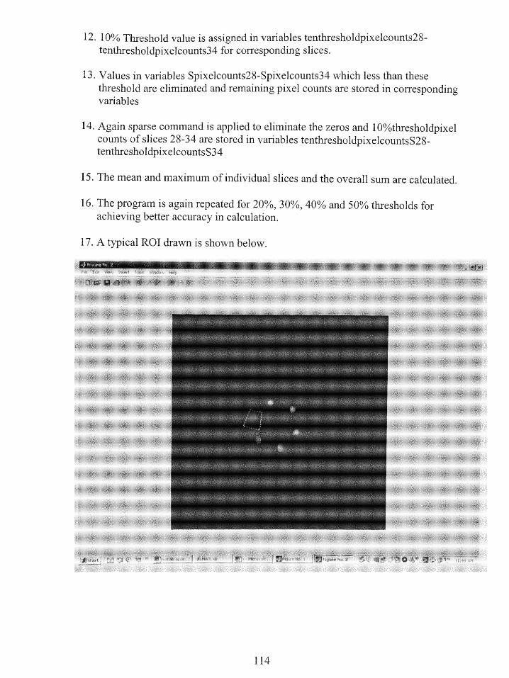
12. 10% Threshold value is assigned in variables tenthresholdpixelcounts28-tenthresholdpixelcounts34 for corresponding slices.
13. Values in variables Spixelcounts28-Spixelcounts34 which less than thesethreshold are eliminated and remaining pixel counts are stored in correspondingvariables
14. Again sparse command is applied to eliminate the zeros and 10%thresholdpixelcounts of slices 28-34 are stored in variables tenthresholdpixelcountsS28-tenthresholdpixelcountsS34
15. The mean and maximum of individual slices and the overall sum are calculated.
16. The program is again repeated for 20%, 30%, 40% and 50% thresholds forachieving better accuracy in calculation.
17. A typical ROI drawn is shown below.
LeT ~ emiel~zdaaa@5ih
t,4y0
114
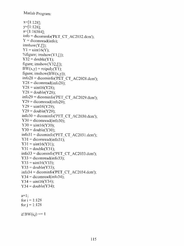
Matlab Program:
x=[1:128];
y-[1:128];a=[1:16384];info = dicominfo('PETCT_AC2032.dcm');Y = dicomread(info);imshow(Y,[]);Y1 uintl6(Y);%figure; imshow(Y1,[]);Y32 = double(Y1);figure; imshow(Y32,[]);BW(x,y) = roipoly(Yl);figure; imshow(BW(x,y));info28 = dicominfo('PET CTAC2028.dcm');Y28 = dicomread(info28);Y28 = uintl6(Y28);Y28 = double(Y28);info29 = dicominfo('PET CTAC2029.dcm');Y29 = dicomread(info29);Y29 = uintl6(Y29);Y29 = double(Y29);info30 = dicominfo('PETCT-AC2030.dcm');Y30 = dicomread(info30);Y30 = uintl6(Y30);Y30 = double(Y30);info31 1 dicominfo('PET CTAC2031.d m');Y31 = dicomread(info3 1);Y31 = uint16(Y31);Y31 = double(Y31);info33 = dicominfo('PETCT-AC2033.dcm);Y33 = dicomread(info33);Y33 = uintl6(Y33);Y33 = double(Y33);info34 = dicominfo('PETCTAC2034.dcm');Y34 = dicomread(info34);Y34 = uintl6(Y34);Y34 = double(Y34);
a= 1;fori= 1:128for j = 1:128
if BW(ij)== 1
115
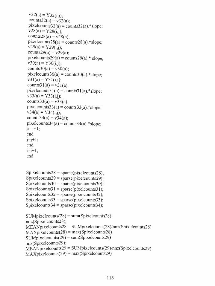
v32(a) = Y32(i,j);counts32(a) = v32(a);pixelcounts32(a) = counts32(a).*slope;v2 8(a) = Y28(i,j);counts28(a) = v28(a);pixelcounts28(a) = counts28(a).*slope;v29(a) = Y29(i,j);counts29(a) = v29(a);pixelcounts29(a) = counts29(a).* slope;v30(a) = Y30(ij);counts30(a) = v30(a);pixelcounts30(a) = counts30(a).*slope;v31(a) = Y31(i,j);counts31(a) = v31(a);pixelcounts3 1(a) = counts3 1(a).*slope;v33(a) = Y33(ij);counts33(a) = v33(a);pixelcounts33(a) = counts33(a).*slope;v34(a) = Y34(ij);counts34(a) = v34(a);pixelcounts34(a) = counts34(a).*slope;a=a+ 1;end
j j+1;endi=i+1;end
Spixelcounts28 = sparse(pixelcounts28);Spixelcounts29 = sparse(pixelcounts29);Spixelcounts30 = sparse(pixelcounts30);Spixelcounts3 1 = sparse(pixelcounts31);Spixelcounts32 = sparse(pixelcounts32);Spixelcounts33 = sparse(pixelcounts33);Spixelcounts34 = sparse(pixelcounts34);
SUMpixelcounts(28) = sum(Spixelcounts28)nnz(Spixelcounts28);MEANpixelcounts28 = SUMpixelcounts(28)/nnz(Spixelcounts28)MAXpixelcounts(28)= max(Spixelcounts28)SUMpixelcounts(29) = su(Spixelcounts29)nnz(Spixelcounts 2 9 );MEANpixelcounts29= SUMpixelcounts(29)/nnz(Spixelcounts29)MAXpixelcounts(29)= max(Spixelcounts29)
116
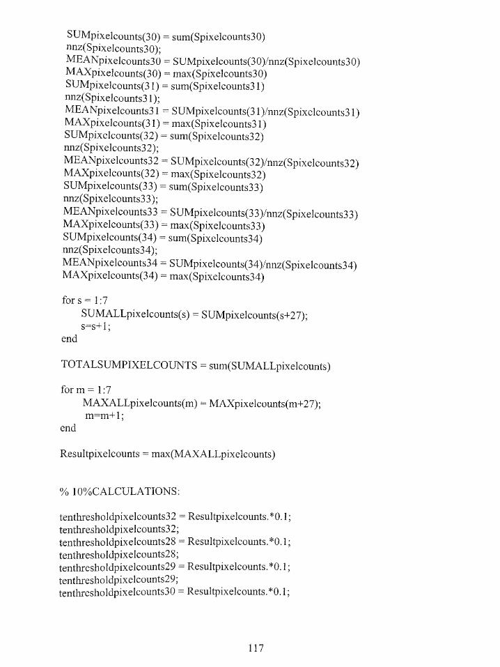
SUMpixelcounts(30) = sum(Spixelcounts30)ffz(Spixelcounts30);MEANpixelcounts30 = SUMpixelcounts(30)/nnz(Spixelcounts30)MAXpixelcounts(30) = max(Spixelcounts30)SUMpixelcounts(31) = sum(Spixelcounts31)nnz(Spixelcounts31);MEANpixelcounts3 1 = SUMpixelcounts(3 1)/nnz(Spixelcounts31)MAXpixelcounts(31) = max(Spixelcounts31)SUMpixelcounts(32) = sum(Spixelcounts32)nnz(Spixelcounts32);MEANpixelcounts32 = SUMpixelcounts(32)/nnz(Spixelcounts32)MAXpixelcounts(32) = max(Spixelcounts32)SUMpixelcounts(33) = sum(Spixelcounts33)nnz(Spixelcounts33);MEANpixelcounts33= SUMpixelcounts(33)/nnz(Spixelcounts33)MAXpixelcounts(33)= max(Spixelcounts33)SUMpixelcounts(34) = sum(Spixelcounts34)nnz(Spixelcounts34);MEANpixelcounts34 = SUMpixelcounts(34)/nnz(Spixelcounts34)MAXpixelcounts(34) = max(Spixelcounts34)
fors= 1:7SUMALLpixelcounts(s) = SUMpixelcounts(s+27);s=s+1;
end
TOTALSUMPIXELCOUNTS = sum(SUMALLpixelcounts)
form = 1:7MAXALLpixelcounts(m)= MAXpixelcounts(m+27);m=m+1;
end
Resultpixelcounts = max(MAXALLpixelcounts)
% 10%CALCULATIONS:
tenthresholdpixelcounts32 = Resultpixelcounts. *0.1;tenthresholdpixelcounts32;tenthresholdpixelcounts28 = Resultpixelcounts. 0.1;tenthresholdpixelcounts28;tenthresholdpixelcounts29 = Resultpixelcounts.*0.1;tenthresholdpixelcounts 2 9 ;tenthresholdpixelcounts3 0 = Resultpixelcounts. *0. 1;
117
tenthresholdpixelcounts30;tenthresholdpixelcounts31 = Resultpixelcounts.*0.1;tent esholdpixelcounts3 1;tenthresholdpixelcounts33 = Resultpixelcounts.*0.1;tenthresholdpixelcounts33tenthresholdpixelcounts34 = Resultpixelcounts. *0. 1;tenthresholdpixelcounts34;
n32 = numel(Spixelcounts32)for a= 1:n32
if Spixelcounts32(a) > tent esholdpixelcounts32tenanswerpixelcounts32(a) = Spixelcounts32(a);
endif Spixelcounts28(a) > tenthresholdpixelcounts28
tenanswerpixelcounts28(a)= Spixelcounts28(a);endif Spixelcounts29(a) > tent esholdpixelcounts29
tenanswerpixelcounts29(a)= Spixelcounts29(a);endif Spixelcounts30(a) > tenthresholdpixelcounts3
tenanswerpixelcounts30(a) = Spixelcounts30(a);endif Spixelcounts3 1(a) > tenthresholdpixelcounts3 1
tenanswerpixelcounts3 1(a) = Spixelcounts3 1(a);endif Spixelcounts33(a) > tenthresholdpixelcounts33
tenanswerpixelcounts33(a)= Spixelcounts33(a);endif Spixelcounts34(a) > tenthresholdpixelcounts34
tenanswerpixelcounts34(a) = Spixelcounts34(a);end
a=a+1;endtenanswerpixelcounts32(a);
%waming off MATLAB : waing _end-withoutblock
tenthresholdpixelcountsS32 = sparse(tenanswerpixelcounts32);SUMtent esholdpixelcounts(32) = surn(tenthresholdpixelcountsS32)MEANtenthresholdpixelcounts(32) = mean(tenthresholdpixelcountsS32)MAXtenthresholpixelcounts(32) = max(tenthresholdpixelcountsS32)tenthresholdpixelcountsS 2 8 = sparse(tenanswerpixelcounts28);SUMtent esholdpixelcounts(28)= sum(tenthresholdpixelcountsS28)
118
nnz(tenthresholdpixelcountsS28);
MEANtenthresholdpixelcounts28 = SUMtenthresholdpixelcounts(28)/nnz(tenthresholdpixelcountsS28)
MAXtenthresholdpixelcounts(28)= max(tenthresholdpixelcountsS28)tenthresholdpixelcountsS29= sparse(tenanswerpixelcounts29);SUMtenthresholdpixelcounts(29)= sum(tent esholdpixelcountsS29)nnz(tenthresholdpixelcountsS29);MEANtentiresholdpixelcounts29= SUMtenthresholdpixelcounts(29)/nnz(tent esholdpixelcountsS29)MAXtenthresholdpixelcounts(29) = max(tenthresholdpixelcountsS29)tenthresholdpixelcountsS30 = sparse(tenanswerpixelcounts30);SUMtenthresholdpixelcounts(30)= sum(tenthresholdpixelcountsS30)nnz(tenthresholdpixelcountsS30);MEANtenthresholdpixelcounts30 = SUMtenthresholdpixelcounts(3 0)/nnz(tenthresholdpixelcountsS30)MAXtenthresholdpixelcounts(30) = max(tent esholdpixelcountsS30)tenthresholdpixelcountsS31 = sparse(tenanswerpixelcounts31);SUMtenthresholdpixelcounts(31) = sum(tenthresholdpixelcountsS31)nnz(tenthresholdpixelcountsS31);MEANtenthresholdpixelcounts3 1 = SUMtenthresholdpixelcounts(3 1)/nnz(tenthresholdpixelcountsS31)MAXtenthresholdpixelcounts(31) = max(tenthresholdpixelcountsS31)tenthresholdpixelcountsS33 = sparse(tenanswerpixelcounts33);SUMtenthresholdpixelcounts(33) = sum(tenthresholdpixelcountsS33)nnz(tenthresholdpixelcountsS33);MEANtenthresholdpixelcounts33 = SUMtenthresholdpixelcounts(33)/nnz(tenthresholdpixelcountsS33)MAXtenthresholdpixelcounts(33) = max(tenthresholdpixelcountsS33)tenthresholdpixelcountsS34= sparse(tenanswerpixelcounts34);SUMtenthresholdpixelcounts(34) = sum(tenthresholdpixelcountsS34)nnz(tenthresholdpixelcountsS34);MEANtenthresholdpixelcounts34 = SUMtenthresholdpixelcounts(34)/nnz(tenthresholdpixelcountsS34)
MAXtenthresholdpixelcounts(34) = max(tenthresholdpixelcountsS34)
SUMALLtenthresholdpixelcounts = sum(SUMtenthresholdpixelcounts(28)+SUMtenthresholdpixelcounts(29)+ SUMtenthresholdpixelcounts(30)+SUMtent esholdpixelcounts(31)+ SUMtent esholdpixelcounts(32)+SUMtent esholdpixelcounts(3 3)+ SUMtent esholdpixelcounts(34))
119

00 20%CALCULATIONS:
twentythresholdpixelcounts32 = Resultpixelcounts.*0.2;twentythresholdpixelcounts32;
twentythresholdpixelcounts28 = Resultpixelcounts. *0.2;twentythresholdpixelcounts28;twentythresholdpixelcounts29 Resultpixelcounts. *0.2;twentythresholdpixelcounts29;twentythresholdpixelcounts30 = Resultpixelcounts.*0.2;twentythresholdpixelcounts30;twentythresholdpixelcounts31 = Resultpixelcounts.*0.2;twentythresholdpixelcounts3 1;twentythresholdpixelcounts33 = Resultpixelcounts.*0.2;twentythresholdpixelcounts33
entythresholdpixelcounts34 = Resultpixelcounts.*0.2;twentythresholdpixelcounts34;
n32 = numel(Spixelcounts32)for a= 1:n32
if Spixelcounts32(a) > twentyt esholdpixelcounts32entyanswerpixelcounts32(a) = Spixelcounts32(a);
endif Spixelcounts28(a) > twentythresholdpixelcounts28
twentyanswerpixelcounts28(a)= Spixelcounts28(a);endif Spixelcounts29(a) > twentythresholdpixelcounts29
twentyanswerpixelcounts29(a) = Spixelcounts29(a);endif Spixelcounts30(a) > twentythresholdpixelcounts30
twentyanswerpixelcounts30(a)= Spixelcounts30(a);endif Spixelcounts3 1(a) > twentythresholdpixelcounts31
twentyanswe ixelcounts3 1(a)= Spixelcounts3 1(a);endif Spixelcounts33(a) > twentythresholdpixelcounts33
twentyanswerpixelcounts33(a) = Spixelcounts33(a)endif Spixelcounts34(a) > twentythresholdpixelcounts34
twentyanswerpixelcounts34(a) = Spixelcounts34(a);end
a=a+1;endtwentyanswerpixelcounts 32 (a);
120

% warning off MATLAB:mwarningend withoutblock
twentythresholdpixelcountsS32 = sparse(twentyanswerpixelcounts32);SUMtwentythresholdpixelcounts(32) = sum(twentyt esholdpixelcountsS32)nnz(twentythresholdpixelcountsS32);MEANtwentythresholdpixelcounts32= SUMtwentythresholdpixelcounts(32)/nnz(twentythresholdpixelcountsS32)MAXtwentythresholdpixelcounts(32) = max(twentythresholdpixelcountsS32)twentythresholdpixelcountsS28 = sparse(twentyanswerpixelcounts28);SUMtwentythresholdpixelcounts(28) = sum(twentyt esholdpixelcountsS28)nnz(twentythresholdpixelcountsS28);MEANtwentythresholdpixelcounts28 = SUMtwentythresholdpixelcounts(28)/nnz(twentythresholdpixelcountsS28)MAXtwentythresholdpixelcounts(28)= rnax(twentythresholdpixelcountsS28)twentythresholdpixelcountsS29 = sparse(twentyanswerpixelcounts29);SUMtwentythresholdpixelcounts(29) = sum(twentythresholdpixelcountsS29)nnz(twentythresholdpixelcountsS29);MEANtwentythresholdpixelcounts29 = SUMtwentythresholdpixelcounts(29)/nnz(twentythresholdpixelcountsS29)MAXtwentythresholdpixelcounts(29) = max(twentythresholdpixelcountsS29)twentythresholdpixelcountsS30 = sparse(twentyanswerpixelcounts30);SUMtwentythresholdpixelcounts(30) = sum(twentythresholdpixelcountsS30)nnz(twentythresholdpixelcountsS30);MEANtwentythresholdpixelcounts3o = SUMtwentyt esholdpixelcounts(30)/nnz(twentythresholdpixelcountsS30)MAXtwentythresholdpixelcounts(30)= max(twentythresholdpixelcountsS30)twentythresholdpixelcountsS31 = sparse(twentyanswerpixelcounts31);SUMtwentythresholdpixelcounts(31)= sur(twentythresholdpixelcountsS31)nnz(twentythresholdpixelcountsS31);MEANtwentythresholdpixelcounts31 = SUMtwentythresholdpixelcounts(3 1)/nnz(twentyt esholdpixelcountsS31)MAXtwentythresholdpixelcounts(31) = max(twentythresholdpixelcountsS31)twentythresholdpixelcountsS33 = sparse(twentyanswerpixelcounts33);SUMtwentythresholdpixelcounts(33) = sum(twentythresholdpixelcountsS33)nnz(twentythresholdpixelcountsS33);MEANtwentythresholpixelcounts33 = SUMtwentythresholdpixelcounts(33)/nnz(twentythresholdpixelcountsS3 3 )MAXtwentytresholdpixelcounts(33) = max(twentythresholdpixelcountsS33)twentythresoldpixelcountsS 3 4 = sparse(twentyanswerpixelcounts34);SUM entythresholdpixelcounts(34) = sum(twentythresholdpixelcountsS34)nnz(twentyt esholdpixelcountsS34);MEANtwentyt hresholdpixelcounts34 = SUMtwentythresholdpixelcounts(34)/nnz(twentyt hresholdpixelcountsS34)MAXtwentythresholdpixelcounts(34) = max(twentythresholdpixelcountsS34)
121
SUMALLtwentythresholdpixelcounts = sum(SUMtwentythresholdpixelcounts(28)+SlMtwentythresholdpixelcounts(29)+ SUMtwentythresholdpixelcounts(30)+SUMtwentyt esholdpixelcounts(31)+ SUMtwentythresholdpixelcounts(32)+SUMtwentythresholdpixelcounts(33)+ SUMtwentyt esholdpixelcounts(34))
% 30%CALCULATIONS:
thirtythresholdpixelcounts32 = Resultpixelcounts.*0.3;thirtythresholdpixelcounts32;thirtythresholdpixelcounts28= Resultpixelcounts.*0.3;thirtythresholdpixelcounts28;thirtythresholdpixelcounts29 = Resultpixelcounts.*0.3;thirtythresholdpixelcounts29;thirtythresholdpixelcounts30 = Resultpixelcounts.*0.3;thirtythresholdpixelcounts3 0;thirtythresholdpixelcounts3I = Resultpixelcounts.*0.3;thirtythresholdpixelcounts31;thirtythresholdpixelcounts33 = Resultpixelcounts.*0.3;thirtythresholdpixelcounts33thirtythresholdpixelcounts34 = Resultpixelcounts.*0.3;thirtythresholdpixelcounts34;
n32 = numel(Spixelcounts32)for a= 1:n32
if Spixelcounts32(a) > thirtythresholdpixelcounts32thirtyanswerpixelcounts32(a) = Spixelcounts32(a);
endif Spixelcounts28(a) > thirtythresholdpixelcounts28
thirtyanswerpixelcounts28(a) = Spixelcounts28(a);endif Spixelcounts29(a) > thirtythresholdpixelcounts29
thirtyanswerpixelcounts29(a) = Spixelcounts29(a);endif Spixelcounts30(a) > thirtythresholdpixelcounts30
thirtyanswerpixelcounts30(a) = Spixelcounts30(a);endif Spixelcounts3 1(a) > thirtythresholdpixelcounts31
thirtyanswerpixelcounts3 1(a) = Spixelcounts3 1(a);endif Spixelcounts33(a) > thirtythresholdpixelcounts33
thirtyanswerpixelcounts 3 3 (a) = Spixelcounts33(a);
122
end
if Spixelcounts34(a) > thirtythresholdpixelcounts34thirtyanswerpixelcounts34(a) = Spixelcounts34(a);
end
a=a+ 1;endthirtyanswerpixelcounts32(a);
% warning off MATLAB:m warningend without block
thirtythresholdpixelcountsS32 = sparse(thirtyanswerpixelcounts32);SUMthirtythresholdpixelcounts(32) = sum(thirtythresholdpixelcountsS32)nnz(thirtythresholdpixelcountsS32);MEANthirtythresholdpixelcounts32= SUMthirtythresholdpixelcounts(32)/nnz(thirtythresholdpixelcountsS32)MAXthirtythresholdpixelcounts(32)= max(thirtythresholdpixelcountsS32)thirtythresholdpixelcountsS28 = sparse(thirtyanswerpixelcounts28);SUMthirtythresholdpixelcounts(28) = sum(thirtythresholdpixelcountsS28)nnz(thirtythresholdpixelcountsS28);MEANthirtythresholdpixelcounts28 = SUMthirtythresholdpixelcounts(28)/nnz(thirtythresholdpixelcountsS28)MAXthirtythresholdpixelcounts(28) = max(thirtythresholdpixelcountsS28)thirtythresholdpixelcountsS29 = sparse(thirtyanswerpixelcounts29);SUMthirtythresholdpixelcounts(29) = sum(thirtythresholdpixelcountsS29)nnz(thirtythresholdpixelcountsS29);MEANthirtythresholdpixelcounts29 = SUMthirtythresholdpixelcounts(29)/nnz(thirtyt esholdpixelcountsS29)MAXthirtythresholdpixelcounts(29)= max(thirtythresholdpixelcountsS29)thirtythresholdpixelcountsS30 = sparse(thirtyanswerpixelcounts30);SUMthirtythresholdpixelcounts(30) = sum(thirtythresholdpixelcountsS30)nnz(thirtythresholdpixelcountsS30);MEANthirtythresholdpixelcounts30 = SUMthirtythresholdpixelcounts(30)/nnz(thirtythresholdpixelcountsS30)MAXthirtythresholdpixelcounts(30) = max(thirtyt esholdpixelcountsS30)thirtythresholdpixelcountsS31 = sparse(thirtyanswerpixelcounts31);SUMthirtythresholdpixelcounts(31) = sum(thirtythresholdpixelcountsS31)nnz(thirtythresholdpixelcountsS31);MEANthirtythresholdpixelcounts31 = SUMthirtyt esholdpixelcounts(31)/nnz(twentythresholdpixelcountsS 3 1)MAXthirtythresholdpixelcounts(3 1) = ax(thirtyt esholdpixelcountsS31)thirtythresholdpixelcountsS 3 3 = sparse(thirtyanswerpixelcounts33);SUMthirtythresholdpixelcounts(33) = sum(thirtythresholdpixelcountsS33)nnz(thiyhresholdpixelcOuntS33);MEANthirtyt esholdpixelcounts33 = SUMthirtythresholdpixelcounts(33)/
123
nnz(twentythresholdpixelcountsS33)
MAXthirtythresholdpixelcounts(33) = max(thirtythresholdpixelcountsS33)thirtythresholdpixelcountsS34 = sparse(thirtyanswerpixelcounts34);SUMthirtythresholdpixelcounts(34) sum(thirtythresholdpixelcountsS34)nnz(thirtythresholdpixelcountsS34);
MEANthirtythresholdpixelcounts34 = SUMthirtythresholdpixelcounts(34)/nnz(twentythresholdpixelcountsS34)
MAXthirtythresholdpixelcounts(34) = max(thirtythresholdpixelcountsS34)
SUMALLthirtythresholdpixelcounts = sum(SUMthirtythresholdpixelcounts(28)+SUMthirtythresholdpixelcounts(29)+ SUMthirtythresholdpixelcounts(30)+SUMthirtythresholdpixelcounts(31)+ SUMthirtythresholdpixelcounts(32)+SUMthirtythresholdpixelcounts(33)+ SUMthirtythresholdpixelcounts(34))
% 40% CALCULATIONS:
fortythresholdpixelcounts32 = Resultpixelcounts.*0.4;fortythresholdpixelcounts32;fortythresholdpixelcounts28 = Resultpixelcounts.*04;fortythresholdpixelcounts28;fortythresholdpixelcounts29 = Resultpixelcounts.*0.4;fortythresholdpixelcounts29;fortythresholdpixelcounts30= Resultpixelcounts.*0.4;fortythresholdpixelcounts30;fortythresholdpixelcounts31 = Resultpixelcounts.*0.4;fortythresholdpixelcounts31;fortythresholdpixelcounts33 = Result ixelcounts.*0.4;fortythresholdpixelcounts33fortythresholdpixelcounts34 = Resultpixelcounts.*0.4;fortythresholdpixelcounts34;
n32 = numel(Spixelcounts32)for a= 1:n32
if Spixelcounts32(a)> fortythresholdpixelcounts32fortyanswerpixelcounts32(a)= Spixelcounts32(a);
endif Spixelcounts28(a) > fortyt esholdpixelcounts28
fortyanswerpixelcounts2 8 (a) = Spixelcounts28(a);endif Spixelcounts29(a) > fortythresholdpixelcounts29
fortyanswerpixelcounts 2 9 (a) = Spixelcounts29(a);end
124
if Spixelcounts30(a) > fortythresholdpixelcounts30fortyanswerpixelcounts30(a) = Spixelcounts3O(a);
endif Spixelcounts3 1(a) > fortythresholdpixelcounts31
fortyanswerpixelcounts3 1(a) = Spixelcounts3 1(a);endif Spixelcounts33(a) > fortythresholdpixelcounts33
fortyanswerpixelcounts33(a) = Spixelcounts33(a);endif Spixelcounts34(a) > fortythresholdpixelcounts34
fortyanswerpixelcounts34(a) = Spixelcounts34(a);enda=a+1;endfortyanswerpixelcounts32(a);
% warning off MATLAB:m warning _end without-block
fortythresholdpixelcountsS32 = sparse(fortyanswerpixelcounts32);SUMfortythresholdpixelcounts(32) = sum(fortythresholdpixelcountsS32)nnz(fortythresholdpixelcountsS32);MEANfortythresholdpixelcounts32 = SUMfortythresholdpixelcounts(32)/nnz(fortythresholdpixelcountsS32)MAXfortythresholdpixelcounts(32) = max(fortythresholdpixelcountsS32)fortythresholdpixelcountsS28 = sparse(fortyanswerpixelcounts28);SUMfortythresholdpixelcounts(28)= sum(fortythresholdpixelcountsS28)nnz(fortythresholdpixelcountsS28);MEANfortythresholdpixelcounts28= SUMfortythresholdpixelcounts(28)/nnz(fortythresholdpixelcountsS28)MAXfortythresholdpixelcounts(28) = ax(fortythresholdpixelcountsS28)fortythresholdpixelcountsS29 = sparse(fortyanswerpixelcounts29);SUMfortythresholdpixelcounts(29)= sum(fortythresholdpixelcountsS29)nnz(fortythresholdpixelcountsS29);MEANfortythresholdpixelcounts29= SUMfortyt esholdpixelcounts(29)/nnz(fortythresholdpixelcountsS29)MAXfortyt esholdpixelcounts(29) max(fortythresholdpixelcountsS29)fortythresholdpixelcountsS30 = sparse(fortyanswerpixelcounts30);SUMfortyt hresholdpixelcounts(30) = sum(fortythresholdpixelcountsS3)nnz(fortythresholdpixelcountsS30);MEANfortyt esholdpixelcounts30 = SUMfortythresholdpixelcounts(30)/nnz(fortythresholdpixelcountsS30)MAXfortythresholdpixelcounts(30) = mnax(fortythresholdpixelcountsS30)fortyt esholdpixelcountsS 3 1 = sparse(fortyanswerpixelcounts31);SUMfortyt esholdpixelcounts( 3 1)= sun(fortythresholdpixelcountsS31)nnz(fortythresholdpixelcountsS 3 1);
125
MEANfortythresholdpixelcounts31 = SUMfortythresholdpixelcounts(31)/nnz(fortythresholdpixelcountsS31)MAXfortythresholdpixelcounts(31)= max(fortythresholdpixelcountsS31)fortyt esholdpixelcountsS33 = sparse(fortyanswerpixelcounts33);SUMfortyt esholdpixelcounts(33) = sum(fortythresholdpixelcountsS33)nnz(fortythresholdpixelcountsS33);MEANfortythresholdpixelcounts3 = SUMfortythresholdpixelcounts(33)/nnz(fortythresholdpixelcountsS33)MAXfortythresholdpixelcounts(33) = max(fortythresholdpixelcountsS33)fortythresholdpixelcountsS34 = sparse(fortyanswerpixelcounts34);SUMfortythresholdpixelcounts(34)= sum(fortythresholdpixelcountsS34)nnz(fortythresholdpixelcountsS34);MEANfortythresholdpixelcounts34 = SUMfortythresholdpixelcounts(34)/nnz(fortythresholdpixelcountsS34)MAXfortyt esholdpixelcounts(34)= max(fortythresholdpixelcountsS34)
SUMALLfortythresholdpixelcounts = sum(SUMfortythresholdpixelcounts(28)+SUMfortythresholdpixelcounts(29)+ SUMfortythresholdpixelcounts(30)+SUMfortythresholdpixelcounts(31)+ SUMfortythresholdpixelcounts(32)+SUMfortythresholdpixelcounts(33)+ SUMfortythresholdpixelcounts(34))
% 50%CALCULATIONS:
fiftythresholdpixelcounts32 = Resultpixelcounts.*0,5;fiftythresholdpixelcounts32;fiftythresholdpixelcounts28 = Resultpixelcounts.*0.5;fiftythresholdpixelcounts28;fiftythresholdpixelcounts29 = Resultpixelcounts.*0,5;fiftythresholdpixelcounts29;fiftythresholdpixelcounts30 = Resul ixelcounts.*0.5;fiftythresholdpixelcounts3 ;fiftythresholdpixelcounts31 = Resultpixelcounts.*0.5;fiftythresholdpixelcounts3 1;fiftythresholdpixelcounts33 = Resultpixelcounts.*0.5;fiftythresholdpixelcounts33fiftythresholdpixelcounts34 = Resul ixelcounts.*0.5;fiftythresholdpixelcounts34;
n32 = numel(Spixelcounts3 2 )for a= 1:n32
if Spixelcounts3 2 (a) > fiftythresholdpixelcounts32fiftyanswerpixelcounts 32 (a) = Spixelcounts32(a);
endif Spixelcounts28(a) > fiftyt esholdpixelcounts28
126
fiftyanswerpixelcounts28(a) = Spixelcounts28(a);endif Spixelcounts29(a) > fiftythresholdpixelcounts29
fiftyanswerpixelcounts29(a) = Spixelcounts29(a);endif Spixelcounts30(a) > fiftythresholdpixelcounts30
fiftyanswerpixelcounts30(a) = Spixelcounts3O(a);endif Spixelcounts3 1(a) > fiftythresholdpixelcounts3 1
fiftyanswerpixelcounts3 1(a) = Spixelcounts3 1(a);endif Spixelcounts33(a) > fiftythresholdpixelcounts33
fiftyanswerpixelcounts33(a) = Spixelcounts33(a);endif Spixelcounts34(a) > fiftythresholdpixelcounts34
fiftyanswerpixelcounts34(a) = Spixelcounts34(a);end
a=a+1;
endfiftyanswerpixelcounts32(a);
% warning off MATLAB:m-warning _end without block
fiftythresholdpixelcountsS32 = sparse(fiftyanswerpixelcounts32);SUMfiftythresholdpixelcounts(32) = sum(fiftythresholdpixelcountsS32)nnz(fiftythresholdpixelcountsS32);MEANfiftythresholdpixelcounts32 = SUMfiftythresholdpixelcounts(32)/nnz(fiftyt esholdpixelcountsS32)MAXfiftythresholdpixelcounts(32) = max(fiftyt esholdpixelcountsS32)fiftythresholdpixelcountsS28 = sparse(fiftyanswerpixelcounts28);SUMfiftythresholdpixelcounts(28)= sum(fiftythresholdpixelcountsS28)nnz(fiftythresholdpixelcountsS28);MEANfiftythresholdpixelcounts28 = SUMfiftythresholdpixelcounts(28)/nnz(fiftythresholdpixelcountsS28)MAXfiftythresholdpixelcounts(28) max(fiftythresholdpixelcountsS28)fiftyt esholdpixelcountsS29 = sparse(fiftyanswerpixelcounts29);SUMfiftyt esholdpixelcounts(29) = sum(fiftythresholdpixelcountsS29)nnz(fiftythresholdpixelcountsS29);MEANfiftythresholdpixelcounts29= SUMfiftyt esholdpixelcounts(29)/nnz(fiftythresholdpixelcountsS 2 9 )MAXfiftythresholdpixelcounts( 2 9 )= max(fiftythresholdpixelcountsS29)fiftyt esholdpixelcountsS30 = sparse(fiftyanswerpixelcounts30);SUMfiftyt esholdpixelcounts(30)= sum(fiftythresholdpixelcountsS30)
127
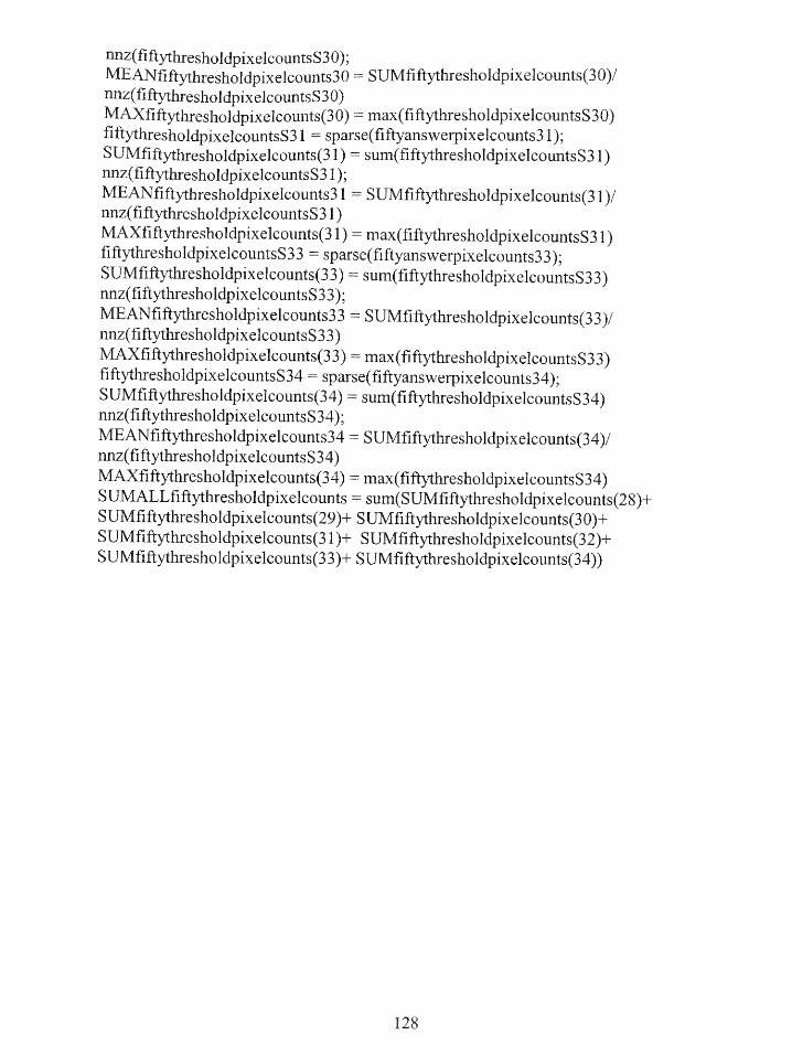
nnz(fiftythresholdpixelcountsS30);
MEANfiftythresholdpixelcounts30 = SUMfiftythresholdpixelcounts(30)/nnz(fiftythresholdpixelcountsS30)
MAXfiftyt esholdpixelcounts(30)= max(fiftythresholdpixelcountsS30)fiftythresholdpixelcountsS31 = sparse(fiftyanswerpixelcounts31);SUMfiftythresholdpixelcounts(31)= sum(fiftythresholdpixelcountsS31)nnz(fiftyt esholdpixelcountsS31);MEANfiftythresholdpixelcounts31 = SUMfiftythresholdpixelcounts(31)/nnz(fiftythresholdpixelcountsS31)MAXfiftythresholdpixelcounts(31) = max(fiftythresholdpixelcountsS31)fiftythresholdpixelcountsS33 = sparse(fiftyanswerpixelcounts33);SUMfiftythresholdpixelcounts(33)= sum(fiftythresholdpixelcountsS33)nnz(fiftythresholdpixelcountsS33);MEANfiftythresholdpixelcounts33 = SUMfiftythresholdpixelcounts(33)/nnz(fiftythresholdpixelcountsS33)MAXfiftythresholdpixelcounts(33)= max(fiftythresholdpixelcountsS33)fiftythresholdpixelcountsS34= sparse(fiftyanswerpixelcounts34);SUMfiftythresholdpixelcounts(34) = sum(fiftythresholdpixelcountsS34)nnz(fiftythresholdpixelcountsS34);MEANfiftythresholdpixelcounts34= SUMfiftythresholdpixelcounts(34)/nnz(fiftythresholdpixelcountsS34)MAXfiftythresholdpixelcounts(34)= max(fiftythresholdpixelcountsS34)SUMALLfiftythresholdpixelcounts = sum(SUMfiftythresholdpixelcounts(28)+SUMfiftythresholdpixelcounts(29)+ SUMfiftythresholdpixelcounts(30)+SUMfiftythresholdpixelcounts(31)+ SUMfiftythresholdpixelcounts(32)+SUMfiftythresholdpixelcounts(33)+ SUMfiftythresholdpixelcounts(34))
128


![CYCLOTRON PRODUCED RADIONUCLIDES:GUIDANCE ON FACILITY DESIGN AND PRODUCTION OF [18F]FLUORODEOXYGLUCOSE (FDG)](https://static.fdokumen.com/doc/165x107/631647d8c32ab5e46f0db468/cyclotron-produced-radionuclidesguidance-on-facility-design-and-production-of-18ffluorodeoxyglucose.jpg)