Accounting for growth: the role of physical work

Structural Change and Economic Dynamics16 (2005) 181–209

Accounting for growth: the role of physical work

Robert U. Ayres∗, Benjamin Warr1

Center for the Management of Environmental Resources, INSEAD, Boulevard de Constance,77305 Fontainebleau, France

Received 1 September 2002; received in revised form 1 August 2003; accepted 1 October 2003Available online 22 February 2004

Abstract

This paper tests several related hypothesis for explaining US economic growth since 1900. It be-gins from the belief that consumption of natural resources—especially energy (or, more precisely,exergy) has been, and still is, an important factor of production and driver of economic growth.However the major result of the paper is that it is not ‘raw’ energy (exergy) as an input, but exergyconverted to useful (physical) work that—along with capital and (human) labor—really explainsoutput and drives long-term economic growth. We develop a formal model (Resource-EXergy Ser-vice or REXS) based on these ideas. Using this model we demonstrate first that, if raw energyinputs are included with capital and labor in a Cobb–Douglas or any other production function sat-isfying the Euler (constant returns) condition, the 100-year growth history of the US cannot beexplained without introducing an exogenous ‘technical progress’ multiplier (the Solow residual) toexplain most of the growth. However, if we replace raw energy as an input by ‘useful work’ (thesum total of all types of physical work by animals, prime movers and heat transfer systems) as afactor of production, the historical growth path of the US is reproduced with high accuracy from1900 until the mid 1 970s, without any residual except during brief periods of economic dislo-cation, and with fairly high accuracy since then. (There are indications that an additional factor,possibly information technology, needs to be taken into account as a fourth input factor since the1970s.) Various hypotheses for explaining the latest period are discussed briefly, along with futureimplications.© 2004 Elsevier B.V. All rights reserved.

JEL classification: 011; 013; 014

Keywords: Exergy; Technology; Economy; Growth; Efficiency; Dematerialisation

∗ Corresponding author. Tel.:+33-160-72-4128; fax:+33-16-498-7672.E-mail address: [email protected] (R.U. Ayres).1 Research supported by institute for Advanced Study, UN University, Tokyo and The European Commission,

TERRA project.

0954-349X/$ – see front matter © 2004 Elsevier B.V. All rights reserved.doi:10.1016/j.strueco.2003.10.003

182 R.U. Ayres, B. Warr / Structural Change and Economic Dynamics 16 (2005) 181–209

1. Introduction

The primary motivation of this paper is to revisit the neoclassical theory of growth from thephysical (thermodynamic) perspective. The ‘standard’ growth theory, which was formulatedin its current production function form (independently) bySolow (1956, 1957)andSwan(1956). The standard theory assumes that production of goods and services (in monetaryterms) can be expressed as a function of capital and labor, yet the major contributionto growth had to be attributed to an unexplained exogenous driver called ‘technologicalprogress’.

Both casual observation and physical intuition have convinced many investigators sinceGeorgescu-Roegen first expounded on the subject, that production in the real world cannot beunderstood without taking into account the role of materials and energy (Oeorgescu-Roegen,1966). Our primary objective in this paper is to elaborate and quantify this intuition—whichwe share—and to simultaneously endogenize ‘technological progress’, insofar as possible.A further, though secondary, objective is to clarify the differences between our currentapproach and the several earlier attempts to incorporate resource flows explicitly into growthmodels (Jorgenson and Houthakker, 1973; Allen et al., 1976; Hannon and Joyce, 1981;Jorgenson, 1983, 1984). We attempt to explain, hereafter, why the several earlier attemptsdid not succeed and how—and why—the present approach differs from earlier ones.

Before passing on, we also emphasize that several features of our work follow (albeitindirectly) from our concept of growth dynamics as a positive feedback cycle. This maynot seem immediately relevant to our main results. But it is relevant to some of the choiceswe make later in formalizing the growth model. The generic positive feedback cycle, ineconomics, operates as follows: cheaper resource inputs, due to discoveries, economies ofscale and experience (or learning-by-doing) enable tangible goods and intangible servicesto be produced and delivered at ever lower cost. This is another way of saying that resourceflows are productive, which is our point of departure. Lower cost, m competitive markets,translates into lower prices for all products and services. Thanks to non-zero price elasticity,lower prices encourage higher demand. Since demand for final goods and services neces-sarily corresponds to the sum of factor payments, most of which go back to labor as wagesand salaries, it follows that wages of labor tend to increase as output rises.2 This, in turn,stimulates the further substitution of natural resources, especially fossil fuels, and mechan-ical power produced from resource inputs, for human (and animal) labor. This continuingsubstitution drives further increases in scale, experience, learning and still lower costs.

Based on both qualitative and quantitative evidence, the existence of the positive feedbackcycle sketched briefly above implies that physical resource flows must be a major factorof production. Indeed, including a fossil energy flow proxy in the neoclassical productionfunction, without any constraint on factor share, seems to account for economic growthquite accurately, at least for limited time periods, without any exogenous time-dependentterm (Hannon and Joyce, 1981; Kümmel, 1982, 1989; Cleveland et al., 1984, 1998; Kümmel

2 Marx believed (with some justification) that the gains would flow mainly to owners of capital rather than toworkers. Political developments have changed the balance of power since Marx’s time. However, in either case,returns to energy or physical resources tend to decline as output grows. This can be interpreted as a declining realprice.

R.U. Ayres, B. Warr / Structural Change and Economic Dynamics 16 (2005) 181–209 183

et al., 1985, 2000; Kaufmann, 1992; Beaudreau, 1998). It is important to note, however, thatincluding energy or exergy as a factor of production doesnot explain economic growth forperiods longer than two or three decades, without recalibration or without a time dependentmultiplier.3 The reason for this (negative) empirical result becomes clear hereafter.

The fact that economic growth tends to be very closely correlated with energy consump-tion, at least for short periods does not a priori mean that energy consumption is the causeof the growth. Indeed, many economic growth models still assume exactly the opposite:that economic growth (due to accumulation of capital, and labor, plus technical progress)is responsible for increasing energy and natural resource consumption. This automaticallyexplains (indeed, guarantees) high correlation. We argue, on the contrary, that decliningresource prices can have a direct impact on growth, via the positive feedback loop. The di-rection of causality must evidently be determined empirically by other means, either theorybased or empirical.4

The major new feature of our approach is that, in contrast to earlier treatments that in-troduced (commercial) energy (exergy), or energy (exergy) and materials separately, asfactors of production, we considerphysical work (or ‘exergy services’) as the appropriateindependent variable for the production function. The term exergy is introduced and ex-plained inSection 2which follows. It is important to emphasize here thatphysical work isa well-defined concept from thermodynamics and physics; it must be distinguished fromthe term as it is used in ordinary language, where ‘work’ is generally what people do toearn a living. The relationship between potential work (exergy) and actual work—or exergyservices—performed in the economy is explained inSection 3. In brief, the ratio of actualwork to potential work can be interpreted as thethermodynamic efficiency with which theeconomy converts resource inputs into finished materials and services.

To avoid confusion, it is important to note that term ‘thermodynamic efficiency’, intro-duced above, is not related to economic efficiency. Thermodynamic efficiency is a straight-forward ratio between (physical work) output and resource input. As will be seen, bothnumerator and denominator are measured in the same physical units (e.g. gigajoules or GJ).

3 For instance, for the years 1929–1969, one specification that gave good results without an exogenous termfor technical progress was the choice ofK andE as factors of production. In this case, the best fit (R2 = 0.99895)implied a capital share of only 0.031 and an energy share of 0.976 (which corresponds to very small increasingreturns) (Hannon and Joyce, 1981). Another formulation, involvingK and electricity, El, yielded very differentresults, namely (R2 = 0.99464) a capital share of 0.990 with only a tiny share for electricity [ibid]. Using factorsK,L only—as Solow did in his pathbreaking (Nobel Prizewinning) paper—but not including an exogenous technicalprogress factor (as he did) the best fit (R2 = 0.99495) was obtained with a capital share of 0.234 and a laborshare of 0.852. These shares add up to more than unity (1.086), which implies significantly increasing returns.Evidently, one cannot rely on econometrics to ascertain the “best” formulation of a Cobb–Douglas (or any other)production function.

4 There are statistical approaches to addressing the causality issue. For instance, Granger and others havedeveloped statistical tests that can provide some clues as to which is cause and which is effect (Granger, 1969;Sims, 1972). These tests have been applied to the present question (i.e. whether energy consumption is a cause or aneffect of economic growth) by Stern (Stern, 1993; Kaufmann, 1995). In brief, the conclusions depend upon whetherenergy is measured in terms of heat value of all fuels (in which case the direction of causation is ambiguous) orwhether the energy aggregate is adjusted to reflect the quality (or, more accurately, the price or productivity) ofeach fuel in the mix. In the latter case, the econometric evidence seem to confirm the qualitative conclusion thatenergy (exergy) consumption is a cause of growth. Both results are consistent with the notion of mutual causation.


Moreover, we are able to estimate both inputs and outputs, and the resulting ratio, withreasonable accuracy, from published empirical data (seeSections 2 and 3).

Introducing an additional factor creates certain conceptual problems that we must ac-knowledge from the outset. Suppose we had opted (as some modelers have) to chooseexergy inputs as a factor of production, measured in monetary terms. Payments for fossilfuels, minerals, ores, farm products and other forms of ‘raw’ exergy inputs are actuallypayments for ‘produced’ outputs of the extractive industries, agriculture and forest prod-ucts sectors. By convention, all of these are intermediates, accounting for a very smallpercentage of GDP—perhaps 4% without agriculture and less than 10% even if agricul-ture is included. Evidently, electric power, motive power, space heat and industrial heatare also produced outputs. Of course, some capital and labor are required to produce theseintermediate products.

However, among these exergy services only electric power is regarded as acommodityproduced and sold by a well-defined industrial sector for which financial accounts are kept.Motive power is produced and consumed (mostly) within the agriculture, transportationand construction sectors, while heat is produced and consumed within many other sectors,including households. They are not regarded as (or, accounted for) commodities, and theydo not have explicit market prices. If shadow prices for these kinds of exergy services (usefulwork) were available, it is likely that the corresponding payments would account—in toto—for a considerably greater share of the US GDP. But, needless to say, capital and labor, aswell as inputs from the extractive and farming sectors, are also required to produce theseintermediates, just as they, in turn, are required to produce other goods and services.

In short, to introduce either ‘raw’ exergy or exergy services as a third factor of productionalso forces us to think in terms of a multi-sector input-output structure with inter-industryfeedbacks. The two choices (exergy or exergy services) differ only in the magnitudes of thefeedbacks from downstream products and services back to extraction and primary process-ing. At first glance this might argue against introducing either of them as a third factor.

Note that capital goods are also produced intermediates. The inputs to capital goods pro-duction are—again—capital, labor and other intermediates (including exergy and/or exergyservices). The key conceptual difference is that capital goods and labor are not consumed inthe production process5 (although depreciation is almost a form of consumption), whencethey arecumulable, and capital and labor services are proportional to the correspondingstocks. On the other hand, resource (exergy) flows, or exergy service flows, are not cumu-lable; they are consumed immediately in the production process.

Furthermore, thanks to cumulability, capital services and labor services can be—withinlimits—regarded asindependent variables in the sense of being independent of currenteconomic conditions (i.e. demandvis a vis potential supply). Of course, the true relationshipbetween capital and output is one of mutual dependence, but with a time lag between theoutput level and the stock levels. It takes a few years for capital stocks to respond to currenteconomic conditions via the price mechanism. The potential labor supply responds throughdemographic feedbacks over an even longer time frame, whence adjustment of current laborsupply occurs mainly through the political process (i.e. laws regarding minimum schooling

5 Georgescu-Roegen was the first to have emphasized this crucial point (Georgescu-Roegen, 1971).


requirements, retirement ages, work-weeks, immigration, and so on). On the other hand,both resource (exergy) consumption, and exergy service (useful work) consumption levelsrespond rather quickly to economic conditions (via prices), whereas the forward impact ofchanges in prices on demand—up or down—driven by technological improvements and/orresource scarcity lags by several years.

Having acknowledged these points, the question arises: do they, taken together, precludethe use of exergy flows or exergy service flows as inputs to a formal production function?We think that the answer is ‘no’. We argue (Section 4) that the economic system shouldbe understood as a sequential materials processing system, converting raw materials (andfuels) by stages into final products and services. The existence of possibly lagged) feedbacksfrom downstream sectors to upstream sectors is understood. Capital services constitute onesuch lagged feedback. Exergy services can be regarded as a generic intermediate with bothfeedback and feed-forward. Whether it has explanatory power is then an empirical question.

Section 5presents the formal Resource-EXergy Service (REXS) model, which is mainlydefined by a choice of variables and production function.Section 6presents the main resultsandSection 7summarizes and discusses further implications.

2. The role of natural resources and energy (exergy)

An obvious implication of economic history—and one that is consistent with our view ofgrowth dynamics as a feedback cycle—it that important ‘engine of growth’ since the firstindustrial revolution has been the continuously declining real price of physical resources,especially energy (and power) delivered at a point of use. The tendency of virtually all rawmaterial and fuel costs to decline over time (lumber was the main exception) has been thor-oughly documented, especially by economists at Resources For the Future (RFF) (Barnettand Morse, 1962; Potter and Christy, 1968; Smith and Knitilla, 1979). The increasing avail-ability of energy from fossil fuels, and power from steam engines and internal combustionengines (ICEs), has clearly played a fundamental role in past economic growth. Machinespowered by fossil energy have gradually displaced animals, wind power, water power andhuman muscles and thus made human workers vastly more productive than they wouldotherwise have been. There is no dispute among economists on this point.

The termenergy as used above, and in most discussions (including the economics litera-ture) is actually technically incorrect. The reason is thatenergy is conserved in every activityor process and therefore cannot be ‘used up’—as most common usages of the term imply.But energy is not necessarily available to do useful work. The standard textbook example isthe heat energy in the ocean water, virtually none of which can be utilized fordoing usefulwork. As was discovered nearly two centuries ago by the French engineer Sadi Carnot,heat can only be converted into useful work if there is a temperaturegradient. Absolutetemperature does not matter. It is the temperature difference between two reservoirs thatdetermines the amount of work that can be extracted by a so-called heat engine. By thesame token, it is the temperature difference between the sun and the earth that drives mostnatural processes on earth, including the weather and photosynthesis.

Exergy is the correct thermodynamic term for ‘available energy’ or ‘useful energy’, orenergy capable of performing mechanical, chemical or thermal work. The distinction is


theoretically important because energy is a conserved quantity: this is the famous first lawof thermodynamics. Energy is not ‘used up’ in physical processes, it is merely degradedfrom available to less and less available forms. On the other hand, exergy is dissipated (usedand destroyed) in all transformation processes. The measure of exergy destruction is theproduction of a thermodynamic quantity calledentropy (second law of thermodynamics).

The formal definition of exergy is the maximum work that could theoretically be doneby a system as it approaches thermodynamic equilibrium with its surroundings, reversibly.Thus, exergy is effectively equivalent topotential work. There is an important distinctionbetweenpotential work and actual work done by animals or machines. Theconversionefficiency between exergy potential work), as an input, and actual work done, as an output,is also an important concept in thermodynamics. The notion of thermodynamic efficiencyplays a key role in this paper.

To summarize the technical definition of exergy is the maximum work that a subsystemcan do as it approaches thermodynamic equilibrium (reversibly) with its surroundings.Exergy is also measured in energy units, and exergy values are very nearly the same asenthalpy (heating values) for all ordinary fuels. So, effectively, it is what most people meanwhen they speak of ‘energy’, the major exception to this rule is that exergy is a measure thatis applicable, and can be estimated with acceptable accuracy, not only for traditional fuelsbut to all agricultural products and industrial materials, including minerals. This point isimportant because it enables us to construct an aggregate measure of all resource flows intothe economic system, as well as an aggregate measure of all processed intermediate flows.We have tabulated and published exergy values per kilogram for most common materialsand mixtures (such as ores) in (Ayres and Ayres, 1999). SeeAppendix Aof this paper formore details.

3. Physical work and thermodynamic conversion efficiency

As noted above, exergy is equivalent to maximumpotential work. There are several kindsof work, including mechanical work, electrical work and chemical work. For non-engineers,mechanical work can be exemplified in a variety of ways, such as lifting a weight againstgravity or compressing a fluid. The term horsepower was introduced in the context ofhorses pumping water from flooded 18th century British coal and tin mines. A more generaldefinition of work is movement against a potential gradient (or resistance) of some sort.A heat engine is a mechanical device to perform work from heat (though not all work isperformed by heat engines).

With this in mind, we can subdivide work into three broad categories, as follows: workdone by animal (or human) muscles, work done by heat engines or water or wind turbinesand work done in other ways (e.g. thermal or chemical work). Mechanical work can befurther subdivided into work done to generate electric power and work done to providemotive power (e.g. to drive motor vehicles). The power sources in this case are so-called‘prime movers’, including all kinds of internal and external combustion engines, from steamturbines to jet engines. So called ‘renewables, including hydraulic, nuclear, wind and solarpower sources for electric power generation are conventionally included. However electricmotors arenot prime movers, because electricity is generated by some other prime mover,


usually a steam or gas turbine. In fact, electricity can be defined (for purposes of this paper)as ‘pure’ work.

Chemical work is exemplified by the reduction of metal ores to obtain the pure metal, orindeed to drive any endothermic chemical synthesis process (ammonia synthesis is a goodexample). Thermal work is exemplified by the transfer of heat from its point of origin (e.g.a furnace) to its point of use, via one or more heat exchangers and a carrier (such as steam,hot water or hot air).

To measure the useful workU done by the economy, in practice, it is helpful to classifyfuels by use. The first category is muscle work, for which the fuel is food or feed. In the US,human muscle work was quantitatively insignificant by 1900 and can be neglected. Horsesand mules, which accounted for most animal work on US farms and urban transport, havenot changed significantly since then. Animal work was still significant up to the 1930s butmechanical and electrical work have since become far more important. The thermodynamicefficiency with which horses and mules convert feed energy to useful work is generallyreckoned at about 4% (i.e. one unit of work requires 25 units of feed).

The second category is fuel used by prime movers to do mechanical work. This consistsof fuel used by electric power generation equipment and fuel used by mobile power sourcessuch as motor vehicles, aircraft and so on. As regards mobile power sources, we definethermodynamic efficiency in terms of useful work performed by the whole vehicle, againstair resistance and rolling resistance of the wheels on the road, not just work done by theengine itself. Thus, the efficiency of an automobile is the ratio of work done by the vehicleto the total potential work (exergy content) of the fuel.

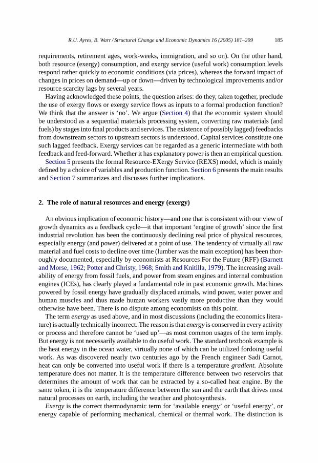
The third broad category is fuel used to generate heatas such, either for industry processheat to do chemical work) or space heat and domestic uses such as washing and cooking.The efficiency, in this case, refers to the delivery system. Lighting can be thought of asa special case of heating. Clearly, the efficiency of muscles as energy converters has notchanged during human history. But the conversion efficiency of heat engines, domestic andcommercial heating systems and industrial thermal processes has increased significantlyover the past 100 years. We have plotted these increasing conversion efficiencies, from1900 to 1998 inFig. 1. Detailed derivations of these curves involve extensive reviews ofthe engineering literature and technological history. Details, including data sources, can befound in another publication (Ayres and Warr, 2003).

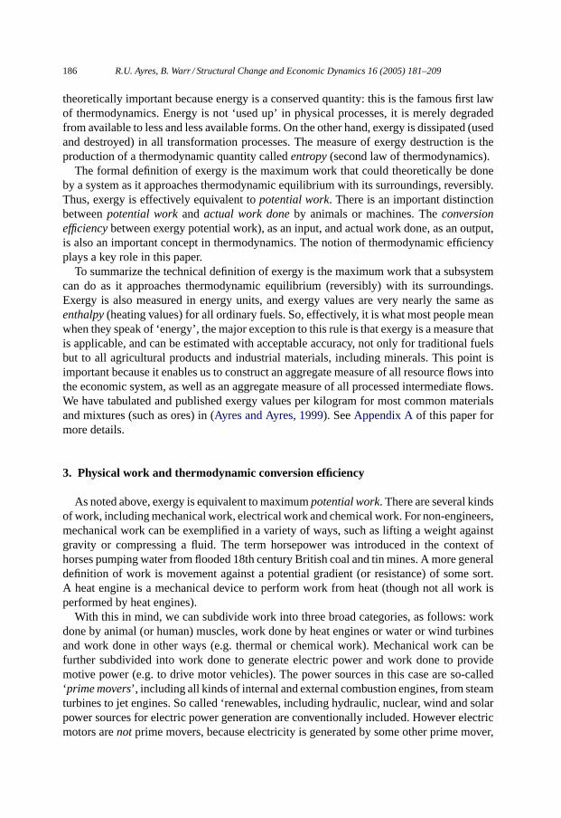
Electrical work output is measured directly in kilowatt-hours (kWh) generated. Data arepublished by the US Federal Power Commission and the US Department of Energy (seeAppendix A). Other types of work must be estimated from fuel inputs, multiplied by con-version efficiencies, as shown inFig. 1, over time. Allocations of fossil fuel exergy inputsto the economy by type of work are shown inFig. 2. Electrification has been perhaps thesingle most important source of useful work for production of goods and services, and(as will be seen later) the most important single driver of economic growth during thetwentieth century. The fuel exergy required to generate a kilowatt-hour of electric powerhas decreased by a factor of ten during the past century. This implies that the thermody-namic efficiency of conversion increased over that period by the same factor, as shownin Fig. 2.

Electricity prices fell correspondingly, especially during the first half of the century.However, the consumption of electricity in the US has increased over the same period by


Fig. 1. Energy (exergy) conversion efficiencies, USA, 1900–1998.

Fig. 2. Fossil fuel consumption exergy allocation, USA, 1900–1998.


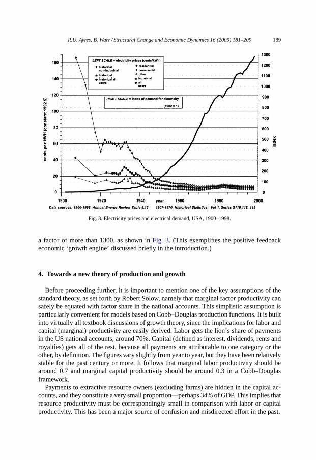
Fig. 3. Electricity prices and electrical demand, USA, 1900–1998.

a factor of more than 1300, as shown inFig. 3. (This exemplifies the positive feedbackeconomic ‘growth engine’ discussed briefly in the introduction.)

4. Towards a new theory of production and growth

Before proceeding further, it is important to mention one of the key assumptions of thestandard theory, as set forth by Robert Solow, namely that marginal factor productivity cansafely be equated with factor share in the national accounts. This simplistic assumption isparticularly convenient for models based on Cobb–Douglas production functions. It is builtinto virtually all textbook discussions of growth theory, since the implications for labor andcapital (marginal) productivity are easily derived. Labor gets the lion’s share of paymentsin the US national accounts, around 70%. Capital (defined as interest, dividends, rents androyalties) gets all of the rest, because all payments are attributable to one category or theother, by definition. The figures vary slightly from year to year, but they have been relativelystable for the past century or more. It follows that marginal labor productivity should bearound 0.7 and marginal capital productivity should be around 0.3 in a Cobb–Douglasframework.

Payments to extractive resource owners (excluding farms) are hidden in the capital ac-counts, and they constitute a very small proportion—perhaps 34% of GDP. This implies thatresource productivity must be correspondingly small in comparison with labor or capitalproductivity. This has been a major source of confusion and misdirected effort in the past.


We reject this simple assumption (along with most modern modelers) on the basis oftwo arguments. The first follows from our view of the growth process as a positive feed-back cycle, as discussed previously. This implies that resource (exergy) flows—or, moreprecisely, declining resource prices—arenot simply a consequence of growth. They arealso (and simultaneously) a cause of growth. This means that the marginal productivity ofresource flows should not be quantitatively insignificant compared to the marginal produc-tivities of other factors. Nor should it be constant over a long period of time. There is anapparent inconsistency between very small factor payments directly attributable to physicalresources—especially fossil fuels—and the obvious importance of energy (exergy) as afactor of production.

The second argument, which is more rigorous, is based on the fact that the identificationof marginal factor productivities with factor shares in the national accounts is based on anoversimplification of the neoclassical theory of optimal income allocation. If labor and capi-tal are the only two factors of production, neoclassical theory implies that the productivity ofa factor of production must be proportional to the share of that factor in the national income.This proposition is quite easy to prove in a hypothetical single sector economy consisting ofa large number of producers manufacturing a single all-purpose good using only labor andcapital services. The textbook example is usually bread, produced by bakeries that producebread from capital and labor, but without any inputs of flour or fuel (Mankiw, 1997).

The supposed link between factor payments and factor productivities gives the nationalaccounts a direct and fundamental (but spurious) role in production theory. In reality, how-ever (as noted in the introduction), the economy produces final products from a chain ofintermediates, not directly from raw materials or, still less, from labor and capital withoutmaterial inputs. In the simple single sector model used to ‘prove’ the relationship betweenfactor productivity and factor payments, this crucial fact is neglected. Allowing for theomission of intermediates (by introducing even a two- or three-sector production process)the picture changes completely. In effect, downstream value-added stages act as productiv-ity multipliers. This enables a factor receiving a very small share of the national incomedirectly, to contribute a much larger effective share of the value of aggregate production,i.e. to be much more productive than its share of overall labor and capital would seem toimply if the simple theory of income allocation were applicable (Ayres, 2001).

Our rejection of the simplistic identification of marginal productivities with factor shareshas two consequences. One is that we are free to depart from the Cobb–Douglas strait-jacket.The other is that we must determine the parameters of the chosen production function bymeans of statistical fitting procedures. These issues are discussed in the next section.

For clarity in further discussion, we use the conventional terminologyL for human labor,as indexed to man-hours employed, andK for produced capital (a construct of accumu-lated investment less depreciation), as compiled and published by the Bureau of EconomicAnalysis in the US Department of Commerce. We use the symbolE for the energy inputsto the economy, as traditionally defined and compiled by the US Department of Energy.This consists of the heat (actually,enthalpy) content of fossil fuels and fuelwood, plusthe nuclear heat used as an input to nuclear electric power generation, and the energy offlowing water harnessed for purposes of hydro-electric power production, plus small contri-butions from wind and solar heat. This variable has been used many times in the economicsliterature.


We use the symbolB for exergy inputs to the economy, which include the items above—allof which arepotential (but not actually performed) work—plus the potential work embod-ied in non-fuel wood and agricultural products and non-fuel minerals, such as sulfide ores.In practice, the mineral contribution to exergy is quite small (except in the metallurgicalindustry itself) and can be neglected without significant error. The major quantitative dif-ference betweenE andB nowadays is that the latter is slightly larger and more inclusive.However, in the 19th century and the early years of the 20th century (and in many developingcountries) the differences are significant.

We use the symbolU for work actually performed in the economy for economic purposes.The components of performed work include animal work (by horses and mules), work doneby prime movers (both electric power generated and motive power) and heat deliveredto a point of use, whether industrial or residential. The human contribution to physical(muscle) work can be neglected in comparison to other inputs as a first approximation.6

We distinguish two variants of performed work, namelyUE and UB where the secondvariant includes animal work, whereas the first variant does not. The distinction is nec-essary because animals consume feed produced by the agriculture sector, which is in-cluded in B but not included in the conventional measure of energy inputs tot heeconomy,E.

Given the assumed importance of resource (exergy) flows in the economy, one mightpostulate two simple linear relationships of the form:

Y = fEggE = gEUE (1a)

Y = fBgBB = gEUE (1b)

whereY is GDP, measured in dollars,E is a measure of commercial energy (mainly fossilfuels),B is a measure of all ‘raw’ physical resource inputs (technically, exergy), includingfuels, minerals and agricultural and forest products. Thenf is the thermodynamic efficiencydefined earlier, namely the ratio of ‘useful work performed’U done by the economy asa whole to ‘raw’ exergy input. Theng is the ratio of economic output in value terms touseful work performed. The variablesf, g andU have implicit subscriptsB or E, whichwe neglect hereafter where the choice is obvious from context. Since work appears in bothnumerator and denominator, its definition depends on whether we chooseB or E. Note thatEqs. (1a) and (1b)are essentially definitions of the two new variablesf andg. There isno theory or approximation involved at this stage, except for the implicit assumption oflinearity.

6 The US population in 1900 was 76 million, of which perhaps 50 million were of working age. but only 25million were men (women worked, without question, but their work did not contribute to GDP at the time), andat least half of the male workers were doing things other than chopping wood, shoveling coal or lifting bales ofcotton, which depended more on eye-hand coordination or intelligence than muscles. The minimum metabolicrequirement is of the order of 1500 cal per day (for men), whereas the average food consumption for a workingman was about 3000 cal per day, whence no more than 1500 cal per day was available for physical work. Thiscomes to 18 billion cal per day or about 0.16 EJ per year of food exergy inputs for work, compared to fossilfuel consumption of 8.9 EJ in that year. If muscles convert energy into work at about 15% efficiency, the overallfood-to-work conversion efficiency for the human population as a whole would also be roughly 2.4%. In recentyears, though most women have jobs, given the changing nature of work, and the much greater life expectancyand retirement time, the conversion efficiency has declined significantly.


There are two mathematical conditions that a production function must satisfy to beeconomically realistic. One is the condition of constant (or nearly constant) returns toscale. This implies that the function should be a first-order homogeneous function of itsvariables (known as the Euler condition). The other requirement is that the logarithmicderivatives (marginal productivities) of the factor variables should be non-negative—atleast on average—throughout the entire time period (1900–1998).

Subject to these requirements, we note that the expressions (1a) or (1b) can be convertedinto a production function in either of two ways. The first possibility is to specify eitherE orBas a plausible factor of production (along withK andL). Then the productfg with subscriptsE or B can be approximated by some first order homogeneous function of the three factors:laborL, capitalK andE orB. The second possibility is that useful workU is a more plausiblefactor of production (instead ofE or B) and the functiong can be expressed approximatelyby some first order homogeneous function ofK, L andU, again with appropriate subscriptsWe have tested these possibilities empirically, for several choices of production function,as noted hereafter.

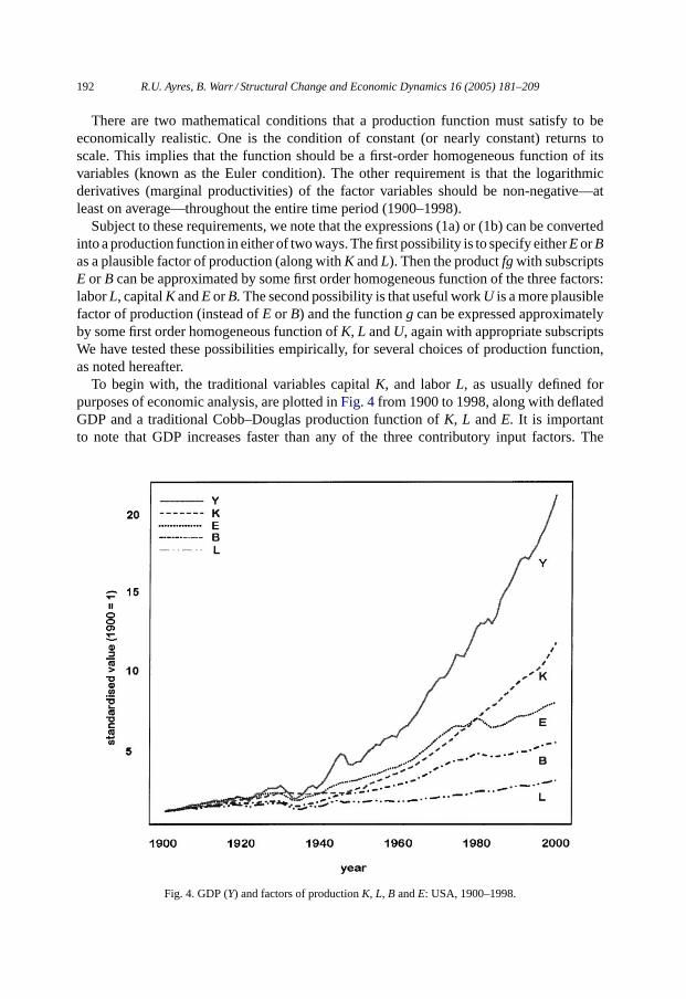
To begin with, the traditional variables capitalK, and laborL, as usually defined forpurposes of economic analysis, are plotted inFig. 4from 1900 to 1998, along with deflatedGDP and a traditional Cobb–Douglas production function ofK, L andE. It is importantto note that GDP increases faster than any of the three contributory input factors. The

Fig. 4. GDP (Y) and factors of productionK, L, B andE: USA, 1900–1998.


need for a time-dependent factor representing technical progress (i.e. the Solow residual) isevident as seen in the figure. ReplacingE by B (i.e. including biomass) does not affect thatqualitative conclusion. Substituting a more complex form of production function, whetherCES, trans-log or linear-exponential (LINEX) (introduced later) with the same variablesdoes not make a significant difference in the need for an exogenous multiplier, althoughthe unexplained residual can be reduced slightly. The problem is, simply, that US GDPsince 1900 has increased faster thanK andL or eitherE or B, and thereforefaster than anyhomogeneous first order combination of those variables. Thus, from here on, we drop thepossibility of using eitherE or B as a factor of production in a production function.

We now turn to the alternative possibility, namely to try useful workU (exergy services)as a factor of production instead ofE orB. The analogy with capital services seems apposite.Effectively there are two definitions of useful work to be considered hereafter, namely

UB = fBB (2a)

or

UE = fEE (2b)

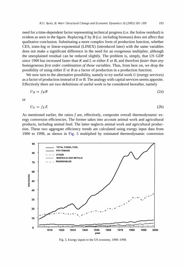
As mentioned earlier, the ratiosf are, effectively, composite overall thermodynamic ex-ergy conversion efficiencies. The former takes into account animal work and agriculturalproducts, including animal feed. The latter neglects animal work and agricultural produc-tion. These two aggregate efficiency trends are calculated using exergy input data from1900 to 1998, as shown inFig. 5 multiplied by estimated thermodynamic conversion

Fig. 5. Exergy inputs to the US economy, 1900–1998.


Fig. 6. Primary work and primary work/GDP ratio, USA, 1900–1998.

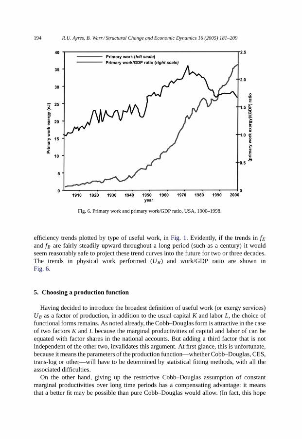
efficiency trends plotted by type of useful work, inFig. 1. Evidently, if the trends infEand fB are fairly steadily upward throughout a long period (such as a century) it wouldseem reasonably safe to project these trend curves into the future for two or three decades.The trends in physical work performed (UB) and work/GDP ratio are shown inFig. 6.

5. Choosing a production function

Having decided to introduce the broadest definition of useful work (or exergy services)UB as a factor of production, in addition to the usual capitalK and laborL, the choice offunctional forms remains. As noted already, the Cobb–Douglas form is attractive in the caseof two factorsK andL because the marginal productivities of capital and labor of can beequated with factor shares in the national accounts. But adding a third factor that is notindependent of the other two, invalidates this argument. At first glance, this is unfortunate,because it means the parameters of the production function—whether Cobb–Douglas, CES,trans-log or other—will have to be determined by statistical fitting methods, with all theassociated difficulties.

On the other hand, giving up the restrictive Cobb–Douglas assumption of constantmarginal productivities over long time periods has a compensating advantage: it meansthat a better fit may be possible than pure Cobb–Douglas would allow. (In fact, this hope


is realized). Actually, the form of production function we have used was originally derivedby reversing the usual logic (Kümmel et al., 1985): Instead of choosing a mathematicalproduction function and performing logarithmic differentiation, one can choose simplemathematical forms for the three marginal productivities (based on plausible assumptionsabout asymptotic behavior), and perform three partial integrations instead. The resultingLINEX form is given below. We have merely substitutedUB for E in Kümmel’s function,yielding

Y = AU exp

(aL

U− b(U + L)

K

)(3)

wherea andb are parameters to be chosen econometrically andA is a multiplier. If economicoutput and growth are fully explained by the three variables, then the multiplier A shouldbe independent of time. It can be verified without difficulty that the R.H.S. of (3) satisfiesthe Euler condition for constant returns-to-scale. It can also be shown that the requirementof non-negative marginal productivities can be met.

As a matter of fact, the LINEX function has another useful feature that is worthy ofmention. Namely, it does not imply (as does the Cobb–Douglas function) that the threefactors are all strict substitutes for each other in the sense that more of one factor impliesless of the other, or conversely. On the contrary, it implies a more complex and more realisticsubstitution–complement relationship among the variables.

The three factor productivities are easily derived by differentiation as follows:

∂Y

∂K

K

Y= bL

K(4a)

∂Y

∂L

L

Y= aL

U− bL

K(4b)

∂Y

∂U

U

Y= 1 − aL

U− bU

K(4c)

The requirement of non-negativity is equivalent to the following three inequalities:

b > 0 (5a)

aK > bU (5b)

1 >aL

U+ bU

K(5c)

The first condition (5a) is trivial. However, the second and third conditions are not auto-matically satisfied for all possible values of the variables. It is therefore necessary to dothe fitting by constrained non-linear optimization. The statistical procedures and qualitymeasures are discussed inAppendix B.7

7 In recent work subsequent to the submission of this paper, we have carried out a large number of statis-tical tests for both Cobb–Douglas and LINEX functions. The standard procedure is to carry out the OLS fitfor annual increments, to eliminate possible collinearity. The results are essentially the same as those presentedhere.


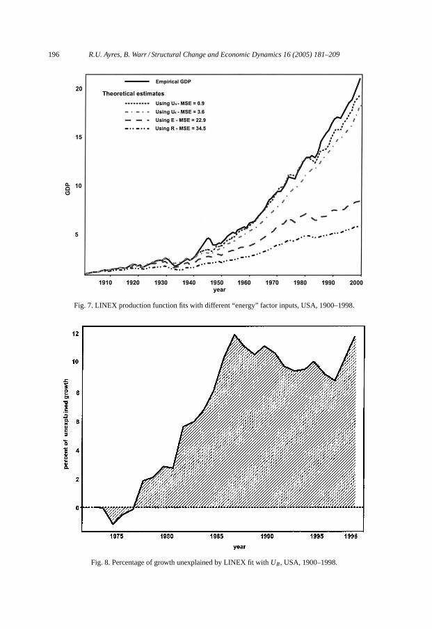
Fig. 7. LINEX production function fits with different “energy” factor inputs, USA, 1900–1998.

Fig. 8. Percentage of growth unexplained by LINEX fit withUB, USA, 1900–1998.


6. Results

The two curves inFig. 7 show the LINEX fit, with workUE andUB respectively, asfactors of production. In the first case, we consider physical work from commercial energysourcesUE (excluding animal work) as a factor. The second caseUB, reflects work derivedfrom all exergy inputs (B includes animal work derived from agricultural phytomass). Thebest fit, by far, is the latter. The unexplained residual has essentially disappeared, prior to1975 and remains small thereafter. In short, it would seem that ‘technical progress’—asdefined by the Solow residual—is almost entirely explained by historical improvements inexergy conversion (to physical work), as summarized inFig. 2, at least until recent times.The remaining unexplained residual, roughly 12% of recent economic growth (since 1975),is shown next inFig. 8.

We conjecture that a kind of phase-change or structural shift took place at that time, trig-gered perhaps by the so-called energy crisis, precipitated by the OPEC blockade. Higherenergy prices induced significant investments in energy conservation and systems optimiza-tion. For instance, the CAFE standards for automobile fuel economy, introduced in the late1970s, forced US motor vehicle manufacturers to redesign their vehicles. The result was todouble the vehicle miles obtained from a unit of motor fuel in the US between 1970 and1989. This was achieved mainly by weight reduction and improvements in aerodynamicsand tires. Comparable improvements have been achieved in air travel, rail freight and inmany manufacturing sectors, induced primarily by the sharp (though temporary) fuel priceincreases.

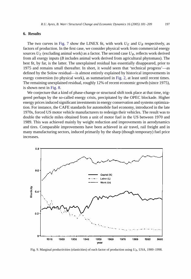
Fig. 9. Marginal productivities (elasticities) of each factor of production usingUB, USA, 1900–1998.


The marginal productivities of the factors can be calculated directly from Eq. (4).The three marginal productivities for the preferred case,UB are plotted inFig. 9. The

marginal productivity trends for capital and work, in both cases show a very slight directionalchange between 1970 and 1980. The marginal productivity of capital has started to increasewhereas the marginal productivity of physical work—resulting from increases in the effi-ciency of energy conversion—has declined slightly. This shift roughly coincides with thetwo so-called oil crisis, and may well have been triggered by the spike in energy (exergy)prices that occurred at that time.

7. Summary and conclusions

In the ‘standard’ model a forecast of GDP requires a forecast of laborL, capital stockKand the Solow multiplier—multifactor productivity or technical progress—A(t). We haveshown that introducing energy and/or material resource (i.e. exergy) inputs does not signifi-cantly improve the explanatory power of traditional production functions. A time-dependentSolow-multiplier is still needed.

However, a much better explanation of past economic growth can be obtained by in-troducing exergy services (useful work) as a factor of production, in place of exergyinputs.

Exergy services can be equated to exergy inputs multiplied by an overall conversion effi-ciency which, of course, corresponds to cumulative technological improvements over time.Based on this hypothesis economic growth from 1900 to 1975 or so is explained almost per-fectly, except for wartime perturbations. The results described above, the technical progressterm can be decomposed into two main contributions. The most important, historically, isfrom improved exergy conversion-to-work efficiency. This propagates, via cost and pricereductions, through the whole downstream value-added chain.

More recently, however, there is obviously some contribution from ‘other’ downstreamtechnical improvements. Evidently growth of GDP in the past quarter century has slightlyoutstripped growth of the three main input factors, capital, labor and physical work. Since1975 or so an additional source of value-added is involved. One possibility is energy con-servation and systems optimization triggered by the energy (exergy) price spike in the1973–1981 period. The other obvious candidate for this additional value creation is infor-mation and communications technology (ICT). However, in the spirit of some endogenousgrowth theories, it would be possible to interpret this additional productivity to some qual-itative improvement in either capital or labor.

It does appear that the marginal productivity of physical work is still by far the dominantdriver of past growth and will be for decades to come. This does not mean that human laboror capital are unimportant. As noted already, the three factors are not really independentof each other. Increasing exergy conversion efficiency requires investments of capital andlabor, while the creation of capital is highly dependent on the productivity of physical work.

It is tempting to argue that the observed shift starting in the 1970s reflects the influence ofinformation technology. Certainly, large scale systems optimization depends very stronglyon large data bases and information processing capability. The airline reservation systemsnow in use have achieved significant operational economies and productivity gains for


airlines by increasing capacity utilization. Manufacturing firms have achieved comparablegains in machine utilization and inventory control through computerized integration ofdifferent functions.

One of the more important implications of the foregoing is that some of the most dramaticand visible technological changes of the past century havenot contributed significantly tooverall economic growth. An example in point is medical progress. While infant mortalityhas declined dramatically and life expectancy has increased very significantly since 1900, itits hard to see any direct impact on economic growth, at least up to the 1970s. Neither of thetwo major benefits adds to labor productivity. The gain has been primarily in quality of life,not quantity of output. Although health services demand an increasing share of GDP, thereis no indication of a decline in prices, as implied by the positive feedback ‘growth engine’.

Changes in telecommunications technology since 1900 may constitute another example.New service industries, like moving pictures, radio and TV have been created, but if the netresult is new forms of entertainment, the gains in employment and output may have comelargely at the expense of earlier forms of public news and entertainment, such as the printmedia, live theater, circuses and vaudeville. Again, the net impact may have been primarilyon quality of life. While the changes have been spectacular, as measured in terms of infor-mation transmitted, the productivity gains may not have been especially large, at least untilrecently (the 1990s) when the internet began to have an impact on ways of doing business.

In any case, since economic growth for the past century can be explained with considerableaccuracy by three factorsK, L andUB, it is not unreasonable to expect that future growthfor some time to come will be explained quite well by these same variables, plus a smallbut growing contribution from ICT.

From a long-term sustainability viewpoint, this conclusion carries a powerful implication.If economic growth is to continue without proportional increases in fossil fuel consumption,it is vitally important to exploit new ways of generating value added without doing morework. But it is also essential to develop ways of reducing fossil fuel exergy inputs per unit ofphysical work output (i.e. increasing conversion efficiency). In other words, energy (exergy)conservation is probably the main key to long term environmental sustainability.

Appendix A. Data

We have compiled a number of historical data sets for the US from 1900 through 1995,indexed to 1900. All of the series are from standard sources. Both labor and capital seriesup to 1970 are found in (USDOCBEA, 1973) Long Term Economic Growth 1860–1970,US Department of Commerce, Bureau of Economic Analysis. Tables (Series A-68 andA-65, respectively). More recent data (1947–1995) came from (USCEA, 1996) EconomicReport of the President, 1996 (Tables B-32 and B-43). The earlier and later labor series arenot exactly the same, but the differences during the period of overlap (1949–1970) are veryminor. The capital series since 1929 comes from (USDOCBEA, monthly) Survey of CurrentBusiness, May 1997, and (USDOC, 1992) Business Statistics, also the US Department ofCommerce. Labor is counted as man-hours actually worked, and private reproducible capitalstock, adjusted by the fraction of the labor force actually employed. This same adjustmentwas also made bySolow (1957).


The exergy series are much more complicated. In brief, we have compiled historical dataon fuel consumption for all fuels, including wood, and for non-fuel material inputs withnon-trivial exergy content, including non-fuel wood, and major metal ores (iron, copper) andminerals (limestone). Data for 1900 to 1970 are mostly from (USCensus, 1975) HistoricalStatistics of the US from Colonial Times to 1970, various tables, with some interpolationsand estimates for missing numbers. More recent data on fuels—both raw and processed(including electricity)—are from (USDOEEIA, annual) US Department of Energy,AnnualReview of Energy Statistics. Data on other minerals and metal ores are from (USGS, 1999;USBuMines, annual) Minerals Yearbooks (US Bureau of Mines until 1995; US GeologicalSurvey since then). We have calculated the exergy for all fuels as a multiplier of heatcontent; exergy for other materials was calculated using standard methods (Szargut et al.,1988; Ayres et al., 1998).

Finished materials include coal consumed by industry other than electric utilities, gasconsumed by households or industry other than utilities, gasoline, heating oil, and residualoil (not consumed by utilities), plus electricity from all sources. Finished non-fuel mate-rials with significant exergy content include plastics, petrochemicals, asphalt, metals, andnon-fuel wood. Obviously, large quantities of finished fuels are consumed by industry, forthe manufacture of goods, and additional quantities are consumed in transporting thosegoods to final consumers (i.e. households).

Fig. A.1. Output and factors of production USA 1900–2000.


There are no precise statistics on fuels and materials consumed by ‘final’ usersvis avis that which is consumed by intermediates. We do have a breakdown of energy usagesince 1955, which distinguishes household use from industrial and commercial use. Buttransportation use is not subdivided in this way, either by the Department of Energy or theDepartment of Transportation. The best supplementary source for transportation energy useis Oak Ridge National Laboratory (ORNL). We have rather arbitrarily assigned all gasolineuse to households and all diesel fuel use to commercial establishments. This undoubtedlyoverestimates household use, especially during the early decades of the century before smalldiesel engines became competitive. There is a further ambiguity, arising from the fact that asmuch as 40% of all automobile travel is for the purpose of travel to work. It could be arguedthat this fraction properly belongs to the ‘commercial’ category rather than the ‘private’category, although we have not done so. Simply, we have calculated the household fractionof all fuels and assumed that the same percentage applies to the exergy content of all finalgoods.

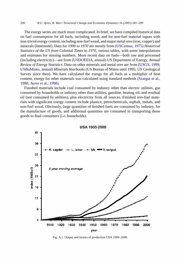
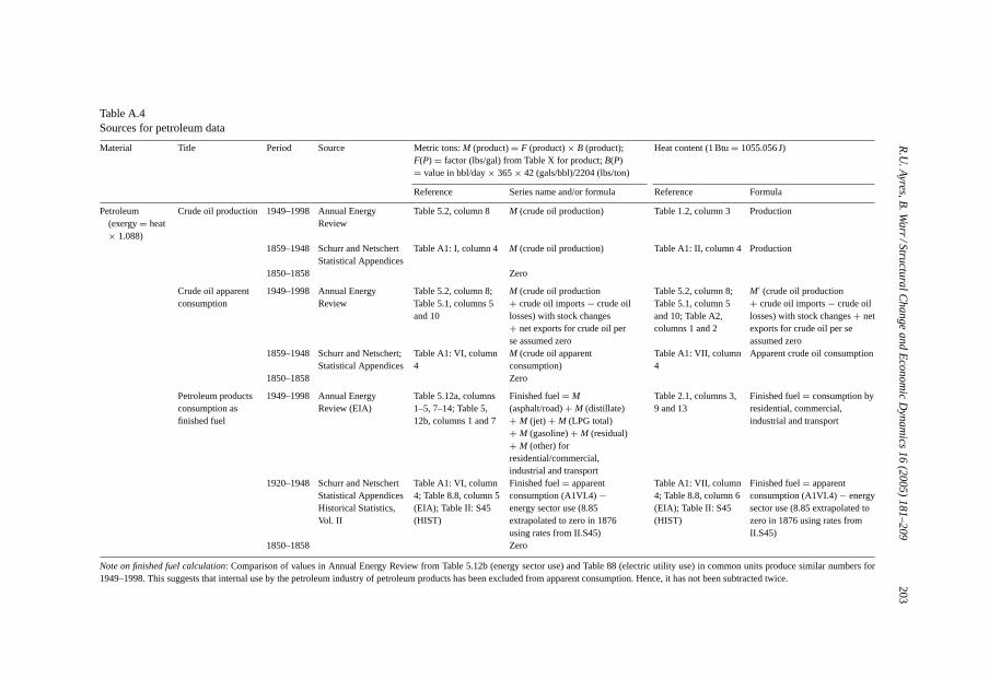
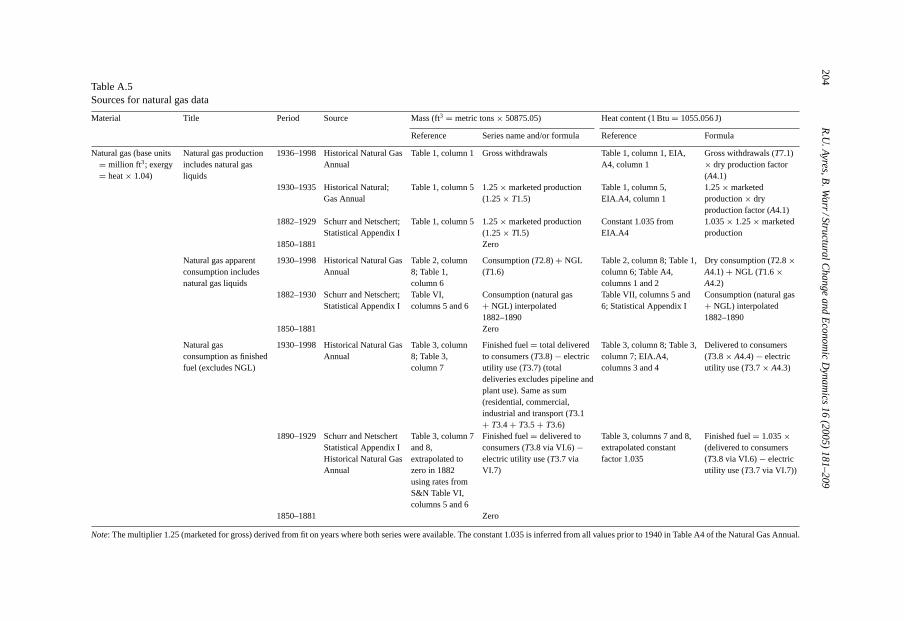
The major time series forK, L andE, expressed in index form normalized to 1900, areshown inFig. A.1. Conversion factors are given inTables A.1 and A.2. Tables A.3–A.6givethe original data sources.

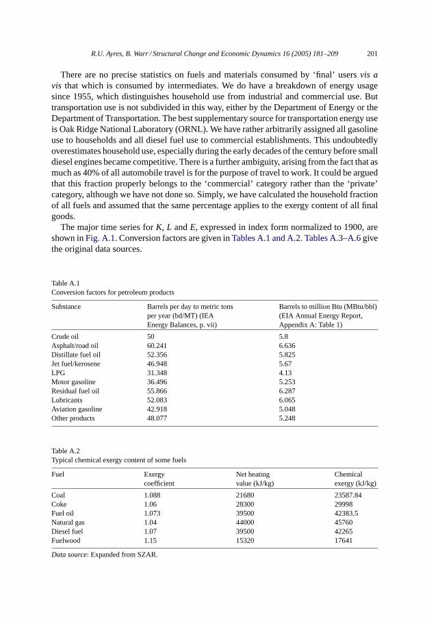
Table A.1Conversion factors for petroleum products

Substance Barrels per day to metric tonsper year (bd/MT) (IEAEnergy Balances, p. vii)

Barrels to million Btu (MBtu/bbl)(EIA Annual Energy Report,Appendix A: Table 1)

Crude oil 50 5.8Asphalt/road oil 60.241 6.636Distillate fuel oil 52.356 5.825Jet fuel/kerosene 46.948 5.67LPG 31.348 4.13Motor gasoline 36.496 5.253Residual fuel oil 55.866 6.287Lubricants 52.083 6.065Aviation gasoline 42.918 5.048Other products 48.077 5.248

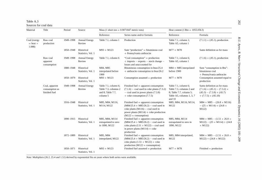
Table A.2Typical chemical exergy content of some fuels

Fuel Exergycoefficient

Net heatingvalue (kJ/kg)

Chemicalexergy (kJ/kg)

Coal 1.088 21680 23587.84Coke 1.06 28300 29998Fuel oil 1.073 39500 42383.5Natural gas 1.04 44000 45760Diesel fuel 1.07 39500 42265Fuelwood 1.15 15320 17641

Data source: Expanded from SZAR.

202R

.U.A

yres,B.W

arr/StructuralC

hangeand

Econom

icD

ynamics

16(2005)

181–209Table A.3Sources for coal data

Material Title Period Source Mass (1 short ton= 0.9071847 metric tons) Heat content (1 Btn= 1055.056 J)

Reference Series name and/or formula Reference Formula

Coal (exergy= heat×1.088)

Raw coalproduction

1949–1998 Annual EnergyReview

Table 7.1, column 1 Production Table 7.1, column 1;Table A5, column 1

(7.1.1)× (A5.1), production

1850–1948 HistoricalStatistics, Vol. 1

M93 + M123 Sum “production”= bituminous coal+ Pennsylvania anthracite

M77 + M78 Same definition as for mass

Raw coalapparentconsumption


Table 7.1, column 6 “Coal consumption”= production+ imports− exports− stock change−losses and unaccounted for

Table 7.1, column 6;Table A5, column 1

(7.1.6)× (A5.1), production


M84, M85interpolated before1900

Bituminous consumption in btus/25.4+ anthracite consumption in btus/26.2

M84 + M85 interpolatedbefore 1900

Sum “consumption in Btu”:bituminous coal+ Pennsylvania anthracite


M93 + M123 Consumption assumed= production M77+ M78 Consumption assumed equal toproduction

Coal, apparentconsumption asfinished fuel


Table 7.1, column 6;Table 7.3, columns 2and 8; Table 7.7,column 5

Finished fuel= apparent consumption(7.1.6)− coal used in coke plants (7.3.2)− coal used in power plants (7.3.8)+ coke consumption (7.7.5)

Table 7.1, column 6;Table 7.3, columns 2 and8; Table 7.7, column 5;Table A5, columns 1, 3, 7and 10

Same definition as for mass(7.1.6)× (A5.1)− (7.3.2)×(A5.3)− (7.3.8)× (A5.7)+ (7.7.5)× (A5.10)


M85, M84, M116,M114, M122

Finished fuel= apparent consumption(M84/25.4+ M85/26.2)− coal used incoke plants (M116)− coal used inpower plants (M114)+ coke production(M122= consumption)

M85, M84, M116, M114,M122

M84 + M85 − (26.8× M116)− (25× M114)+ (24.8×M122)


M85, M84, M114extrapolated to zeroin 1890, M122

Finished fuel= apparent consumption(M84/25.4+ M85/26.2)− coal used incoke plants (l.51× M122)− coal usedin power plants (M114)+ cokeproduction

M85, M84, M114extrapolated to zero in1890, M122

M84 + M85 − (1.51× 26.8×M122)− (25× M114)+ (24.8× M122)


M85, M84interpolated, M122

Finished fuel= apparent consumption(M84/25.4+ M85/26.2)− coal used incoke plants (1.51× M122)+ cokeproduction (M122= consumption)

M85, M84 interpolated,M122

M84 + M85 − (1.51× 26.8×M122)+ (24.8× M122)


M93 + M123 Finished fuel assumed= production M77+ M78 Finished= production

Note: Multipliers (26.2, 25.4 and 1.51) derived by exponential fits on years where both series were available.

R.U

.Ayres,B

.Warr

/StructuralChange

andE

conomic

Dynam

ics16

(2005)181–209

203

Table A.4Sources for petroleum data

Material Title Period Source Metric tons:M (product)= F (product)× B (product);F(P) = factor (lbs/gal) from Table X for product;B(P)= value in bbl/day× 365× 42 (gals/bbl)/2204 (lbs/ton)

Heat content (1 Btu= 1055.056 J)


Petroleum(exergy= heat× 1.088)

Crude oil production 1949–1998 Annual EnergyReview

Table 5.2, column 8 M (crude oil production) Table 1.2, column 3 Production

1859–1948 Schurr and NetschertStatistical Appendices

Table A1: I, column 4 M (crude oil production) Table A1: II, column 4 Production

1850–1858 Zero

Crude oil apparentconsumption


Table 5.2, column 8;Table 5.1, columns 5and 10

M (crude oil production+ crude oil imports− crude oillosses) with stock changes+ net exports for crude oil perse assumed zero

Table 5.2, column 8;Table 5.1, column 5and 10; Table A2,columns 1 and 2

M′ (crude oil production+ crude oil imports− crude oillosses) with stock changes+ netexports for crude oil per seassumed zero

1859–1948 Schurr and Netschert;Statistical Appendices

Table A1: VI, column4

M (crude oil apparentconsumption)

Table A1: VII, column4

Apparent crude oil consumption

1850–1858 Zero

Petroleum productsconsumption asfinished fuel

1949–1998 Annual EnergyReview (EIA)

Table 5.12a, columns1–5, 7–14; Table 5,12b, columns 1 and 7

Finished fuel= M(asphalt/road)+ M (distillate)+ M (jet) + M (LPG total)+ M (gasoline)+ M (residual)+ M (other) forresidential/commercial,industrial and transport

Table 2.1, columns 3,9 and 13

Finished fuel= consumption byresidential, commercial,industrial and transport

1920–1948 Schurr and NetschertStatistical AppendicesHistorical Statistics,Vol. II

Table A1: VI, column4; Table 8.8, column 5(EIA); Table II: S45(HIST)

Finished fuel= apparentconsumption (A1VI.4)−energy sector use (8.85extrapolated to zero in 1876using rates from II.S45)

Table A1: VII, column4; Table 8.8, column 6(EIA); Table II: S45(HIST)

Finished fuel= apparentconsumption (A1VI.4)− energysector use (8.85 extrapolated tozero in 1876 using rates fromII.S45)

1850–1858 Zero

Note on finished fuel calculation: Comparison of values in Annual Energy Review from Table 5.12b (energy sector use) and Table 88 (electric utility use) in common units produce similarnumbers for1949–1998. This suggests that internal use by the petroleum industry of petroleum products has been excluded from apparent consumption. Hence, it has not been subtracted twice.

204R

.U.A

yres,B.W

arr/StructuralC

hangeand

Econom

icD

ynamics

16(2005)

181–209Table A.5Sources for natural gas data

Material Title Period Source Mass (ft3 = metric tons× 50875.05) Heat content (1 Btu= 1055.056 J)


Natural gas (base units= million ft 3; exergy= heat× 1.04)

Natural gas productionincludes natural gasliquids

1936–1998 Historical Natural GasAnnual

Table 1, column 1 Gross withdrawals Table 1, column 1, EIA,A4, column 1

Gross withdrawals (T7.1)× dry production factor(A4.1)

1930–1935 Historical Natural;Gas Annual

Table 1, column 5 1.25× marketed production(1.25× T1.5)

Table 1, column 5,EIA.A4, column 1

1.25× marketedproduction× dryproduction factor (A4.1)

1882–1929 Schurr and Netschert;Statistical Appendix I

Table 1, column 5 1.25× marketed production(1.25× TI.5)

Constant 1.035 fromEIA.A4

1.035× 1.25× marketedproduction

1850–1881 Zero

Natural gas apparentconsumption includesnatural gas liquids


Table 2, column8; Table 1,column 6

Consumption (T2.8)+ NGL(T1.6)

Table 2, column 8; Table 1,column 6; Table A4,columns 1 and 2

Dry consumption (T2.8×A4.1)+ NGL (T1.6×A4.2)

1882–1930 Schurr and Netschert;Statistical Appendix I

Table VI,columns 5 and 6

Consumption (natural gas+ NGL) interpolated1882–1890

Table VII, columns 5 and6; Statistical Appendix I

Consumption (natural gas+ NGL) interpolated1882–1890

1850–1881 Zero

Natural gasconsumption as finishedfuel (excludes NGL)


Table 3, column8; Table 3,column 7

Finished fuel= total deliveredto consumers (T3.8)− electricutility use (T3.7) (totaldeliveries excludes pipeline andplant use). Same as sum(residential, commercial,industrial and transport (T3.1+ T3.4+ T3.5+ T3.6)

Table 3, column 8; Table 3,column 7; EIA.A4,columns 3 and 4

Delivered to consumers(T3.8× A4.4)− electricutility use (T3.7× A4.3)

1890–1929 Schurr and NetschertStatistical Appendix IHistorical Natural GasAnnual

Table 3, column 7and 8,extrapolated tozero in 1882using rates fromS&N Table VI,columns 5 and 6

Finished fuel= delivered toconsumers (T3.8 via VI.6)−electric utility use (T3.7 viaVI.7)

Table 3, columns 7 and 8,extrapolated constantfactor 1.035

Finished fuel= 1.035×(delivered to consumers(T3.8 via VI.6)− electricutility use (T3.7 via VI.7))

1850–1881 Zero

Note: The multiplier 1.25 (marketed for gross) derived from fit on years where both series were available. The constant 1.035 is inferred from all values prior to 1940 in Table A4 of the Natural Gas Annual.

R.U

.Ayres,B

.Warr

/StructuralChange

andE

conomic

Dynam

ics16

(2005)181–209

205

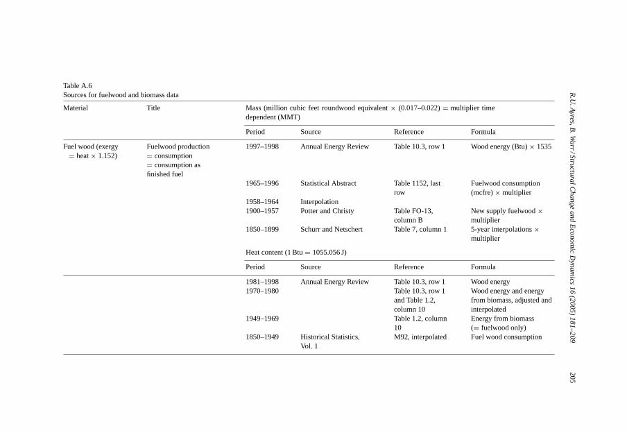
Table A.6Sources for fuelwood and biomass data

Material Title Mass (million cubic feet roundwood equivalent× (0.017–0.022)= multiplier timedependent (MMT)

Period Source Reference Formula

Fuel wood (exergy= heat× 1.152)

Fuelwood production= consumption= consumption asfinished fuel

1997–1998 Annual Energy Review Table 10.3, row 1 Wood energy (Btu)× 1535

1965–1996 Statistical Abstract Table 1152, lastrow

Fuelwood consumption(mcfre)× multiplier

1958–1964 Interpolation1900–1957 Potter and Christy Table FO-13,

column BNew supply fuelwood×multiplier

1850–1899 Schurr and Netschert Table 7, column 1 5-year interpolations×multiplier

Heat content (1 Btu= 1055.056 J)

Period Source Reference Formula

1981–1998 Annual Energy Review Table 10.3, row 1 Wood energy1970–1980 Table 10.3, row 1

and Table 1.2,column 10

Wood energy and energyfrom biomass, adjusted andinterpolated

1949–1969 Table 1.2, column10

Energy from biomass(= fuelwood only)

1850–1949 Historical Statistics,Vol. 1

M92, interpolated Fuel wood consumption


References:Sources have often been abbreviated in the tables—these abbreviations are shown in italic

capitals at the end of each relevant citation. Brackets indicate the main textualcitation.

ANNERO: Annual Energy Review (USDOEEIA, annual).BEA: Long Term Economic Growth 1860–1970 (USDOCBEA, 1973).BUSTAT: Business Statistics (USDOC, 1992).CEA: Economic Report of the President (USCEA, 1996).EIA = Annual Energy Review (USDOEEIA, annual).HISTAT: Historical Statistics of the United States: Colonial Times to 1970, 1975

(USCensus, 1975).HNGA: Historical Natural Gas Annual (USDOEEIA, 1999).IEA: Energy Balances of OECD Countries, annual (OECD/IEA, 1999).MINYB: Minerals Yearbooks, annual (USGS, 1999; USBuMines annual).P&C: Potter and Christy (Potter and Christy, 1968).S&N: Schurr and Netschert (Schurr and Netschert, 1960).SCB:Survey of Current Business, monthly (USDOCBEA).STATAB: Statistical Abstract of the United States (STATAB annual).Szar: Szargut (Szargut et al., 1988).

Appendix B

The LINEX function parameters were obtained by using a quasi-Newton non-linearoptimization method, with box-constraints. The objective function was simply the sum ofthe squared error. The constraints on the possible values of the parameters of the LINEXmodel were required to ensure that the factor marginal productivities (Eqs. (4a)–(4c)) werenon-negative. A statistical measure of the overall fit was provided by the mean squareerror

MSE =∑n

t=1(e2)

n − k(B.1)

The MSE is a measure of the absolute deviation of the theoretical fit from the empiricalcurve, wheren is the number of samples,k the number of parameters ande the residualfrom the fitted curve.

To compare the predictive power of raw exergy flows (B andE) vis a vis physical work(UB andUB) we calculated the correlation coefficients (R2) between the logarithms of theLINEX function of the variables and the actual GDP. We tested the significance of thecorrelations using a t-test with Welch modification for unequal variances (Table B.1). Theresults showed that the relationship of GDP with a LINEX function ofB or E was notsignificant. SubstitutingUE andUB the correlations were significant, and the latter choicewas by far the most significant, as indicated by the smallt-value.

The coefficient of determination is often reported as another measure of the goodnessof fit. To be valid the residuals should be identically and independently distributed. The


Table B.1Statistical measures of the quality and significance of fitted models

Variable used t-value Degrees of freedom P-value Correlation coefficient (R2)

B 5.74 158.4 4.5E−08 0.98E 3.09 174.3 0.002 0.97UE 0.51 194.8 0.604 0.99UB 0.19 195.9 0.845 0.99

Durbin–Watson statistic was used to check for the presence of correlated residual error. Itis calculated as

DW =∑n

t=2(et − et−1)2∑n

t=1(e2)

(B.2)

wheree is the residual error, calculated for each yeart, for a time period of lengthn, wherek is the number of independent variables. The DW statistic takes values between 0 and 4.The Null Hypothesis was that there was no significant correlation between the residual errorvalues for each year.

The DW statistic, calculated for each estimate using either definition of work input (UE orUB) for the entire period (1900–1998), provided evidence of strong residual autocorrelation(DW < 1.61,k = 3). The Null Hypothesis was therefore rejected.

References

Allen, E.L., et al., 1976. US energy and economic growth, 1975–2010. Oak Ridge, TN: Oak Ridge AssociatedUniversities, Institute for Energy Analysis (Publication: ORAU/IEA-76-7).

Ayres, R.U., 2001. The minimum complexity of endogenous growth models: The role of physical resource flows.Energy—The International Journal 28, 219–273.

Ayres, R.U., Ayres, L.W., 1999. Accounting for Resources. 2. The Life Cycle of Materials (Series). Edward Elgar,Cheltenham, UK/Lyme, MA, ISBN 1-85898-923-X.

Ayres, R.U., Warr, B., 2003. Exergy, power and work in the US economy 1900–1998. Energy—The InternationalJournal 28, 219–273.

Ayres, R.U., Martin, K., Ayres, L.W., 1998. Exergy waste accounting and life cycle analysis. Energy 23 (5),355–363.

Barnett, H.J., Morse, C., 1962. Scarcity and Growth: The Economics of Resource Scarcity (Series). Johns HopkinsUniversity Press, Baltimore, MD.

Beaudreau, B.C., 1998. Energy and Organization: Growth and Distribution Reexamined (Series). GreenwoodPress, Westwood, CT, ISBN 0-313-30580-3.

Cleveland, C.J., Costanza, R., Hall, C.A.S., Kauflnann, R.K., 1984. Energy and the US economy: a biophysicalperspective. Science 255, 890–897.

Cleveland, C.J., Kaufinann, R.K., Stern, D.I., 1998. The aggregation of energy and materials in economicindicators of sustainability: thermodynamic, biophysical and economic approaches. In: Proceedings of theInternational Workshop on Advances in Energy Studies: Energy Flows in Ecology and Economy, Porto Venere,Italy.

Georgescu-Roegen, N., 1971. The Entropy Law and the Economic Process (Series). Harvard University Press:Cambridge, MA.

Granger, C.W.J., 1969. Investigating causal relations by econometric models and cross-spectral methods.Econometrica 37, 424–438.


Hannon, B.M., Joyce, J., 1981. Energy and technical progress. Energy 6, 187–195.Jorgenson, D.W., 1983. Energy, prices and productivity growth. In: Schurr, S.H., Sonenblum, S., Woods,

D.O. (Eds.), Energy, Productivity and Economic Growth. Oelgeschlager, Gunn and Ham, Cambridge, MA,pp. 133–153.

Jorgenson, D.W., 1984. The role of energy in productivity growth. The Energy Journal 5 (3), 11–26.Jorgenson, D.W., Houthakker, H.S. (Eds.), 1973. US Energy Resources and Economic Growth (Series). Energy

Policy Project, Washington, DC.Kaufinann, R.K., 1992. A biophysical analysis of the energy/real GDP ratio: Implications for substitution and

technical change. Ecological Economics 6, 33–56.Kaufinami, R.K., 1995. The economic multiplier of environmental life support: can capital substitute for a degraded

environment. Ecological Economics 12 (1), 67–80.Kümmel, R., 1982. The impact of energy on industrial growth. Energy 7 (2), 189–201.Kümmel, R., 1989. Energy as a factor of production and entropy as a pollution indicator in macroeconomic

modeling. Ecological Economics 1, 161–180.Kümmel, R., Strassi, W., Gossner, A., Eichhorn, W., 1985. Technical progress and energy dependent production

functions. Journal of Economics 45 (3), 285–311.Kümmel, R., Lindenberger, D., Eichhom, W., 2000. The productive power of energy and economic evolution.

Indian Journal of Applied Economics, in press (special issue on Macro and Micro Economics).Mankiw, N.G., 1997. Macroeconomics. Worth Publishing.Oeorgescu-Roegen, N., 1966. Analytical Economics (Series). Harvard University Press, Cambridge, MA.Potter, N., Christy Jr., F.T., 1968. Trends in Natural Resource Commodities (Series). Johns Hopkins University

Press, Baltimore, MD.Sims, C.J.A., 1972. Money, income and causality. American Economic Review.Smith, V.K., Knitilla, J. (Eds.), 1979. Scarcity and Growth Revisited (Series). Johns Hopkins University Press,

Baltimore, MD.Solow, R.M., 1956. A contribution to the theory of economic growth. Quarterly Journal of Economics 70, 65–

94.Solow, R.M., 1957. Technical change and the aggregate production function. Review of Economics and Statistics

39, 312–320.Stern, D.I., 1993. Energy use and economic growth in the USA: a multivariate approach. Energy Economics 15,

137–150.Swan, T., 1956. Economic growth and capital accumulation. The Economic Record 32 (68), 334–361.Organization for Economic Cooperation and Development and International Energy Agency, 1999. Energy

Balances of OECD Countries 1960–1997 (Series). OECD, Paris.Schurr, S.H., Netschert, B.C., 1960. Energy in the American Economy, 1850–1975 (Series). Johns Hopkins

University Press, Baltimore, MD.Szargut, J., Morris, D.R., Steward, F.R., 1988. Exergy Analysis of Thermal, Chemical, and Metallurgical Processes

(Series). Hemisphere Publishing Corporation, New York, ISBN 0-89116-574-6.United States Bureau of the Census, annual. Statistical abstract of the United States (Series). United States

Government Printing Office, Washington, DC.United States Council of Economic Advisors, 1996. Economic report of the president together with the annual

report of the council of economic advisors (Series). United States Government Printing Office, WashingtonDC, ISBN 0-16-048501-0.

United States Bureau of the Census, 1975. Historical statistics of the United States, colonial times to 1970 (Series).United States Government Printing Office, Washington, DC.

United States Department of Commerce Bureau of Economic Analysis, 1992. Business Statistics, 1963–1991.United States Department of Commerce, Washington DC.

United States Department of Commerce Bureau of Economic Analysis, monthly. Survey of Current Business.United States Department of Commerce, Washington DC.

United States Department of Commerce Bureau of Economic Analysis, 1973. Long Term Economic Growth1860–1970 (Series). United States Government Printing Office, Washington, DC, LC 73-600130.

USBuMines, annual. United States Bureau of Mines, annual. Minerals Yearbook (Series). United StatesGovernment Printing Office, Washington, DC.


Energy Information Administration Office of Oil and Gas, 1999. Historical Natural Gas Annual 1930 through1998 (Series). United States Department of Energy, Energy Information Administration, Washington, DC.

United States Department of Energy, Energy Information Administration, annual. EJA Annual Energy Review(Series). United States Government Printing Office, Washington, DC.

United States Geological Survey, 1999. Minerals Yearbook: 1998. United States Geological Survey, Washington,DC.

Accounting for growth: the role of physical work

Documents

Transcript of Accounting for growth: the role of physical work