Accepted Manuscript - RSC Publishing

This is an Accepted Manuscript, which has been through the Royal Society of Chemistry peer review process and has been accepted for publication.

Accepted Manuscripts are published online shortly after acceptance, before technical editing, formatting and proof reading. Using this free service, authors can make their results available to the community, in citable form, before we publish the edited article. We will replace this Accepted Manuscript with the edited and formatted Advance Article as soon as it is available.

You can find more information about Accepted Manuscripts in the Information for Authors.

Please note that technical editing may introduce minor changes to the text and/or graphics, which may alter content. The journal’s standard Terms & Conditions and the Ethical guidelines still apply. In no event shall the Royal Society of Chemistry be held responsible for any errors or omissions in this Accepted Manuscript or any consequences arising from the use of any information it contains.

Accepted Manuscript

www.rsc.org/pccp

PCCP

http://www.rsc.org/Publishing/Journals/guidelines/AuthorGuidelines/JournalPolicy/accepted_manuscripts.asp

http://www.rsc.org/help/termsconditions.asp

http://www.rsc.org/publishing/journals/guidelines/

CREATED USING THE RSC ARTICLE TEMPLATE (VER. 3.0) - SEE WWW.RSC.ORG/ELECTRONICFILES FOR DETAILS

ARTICLE TYPE www.rsc.org/xxxxxx | XXXXXXXX

This journal is © The Royal Society of Chemistry [year] Journal Name, [year], [vol], 00–00 | 1

Dynamic and Static Behavior of Hydrogen Bonds of the X–H---π Type (X = F, Cl, Br, I, RO and RR'N; R, R' = H or Me) in Benzene π-System, Elucidated by QTAIM Dual Functional Analysis Yuji Sugibayashi,a Satoko Hayashia and Waro Nakanishi*,a

Received (in XXX, XXX) 1st May 2015, Accepted XXX YYY 2015 5

First published on the web 1st May 2015 DOI: 10.1039/b000000x

Dynamic and static behavior of the X–H-∗-π interactions in X–H-∗-π(C6H6) (X = F, Cl, Br, I, HO, MeO, H2N, MeHN and Me2N) is elucidated by QTAIM-DFA (QTAIM dual functional analysis), which we proposed recently, as the first step to clarify various types of X–H-∗-π interactions. The 10

asterisk ∗ emphasizes the existence of the bond critical point (BCP) on the interaction in question. Total electron energy densities (Hb(rc)) are plotted versus Hb(rc) – Vb(rc)/2 [= (ћ2/8m)∇2ρb(rc)] at BCPs in QTAIM-DFA, where Vb(rc) are potential energy densities at BCPs. In our treatment, data for the perturbed structures around the fully optimized ones are employed, in addition to those for the fully optimized structures. Data from the fully optimized structures are analyzed by the polar 15

(R, θ) coordinate representation. Each plot for an interaction, containing data from the perturbed structures, shows a specific curve, which provides important information. The plot is expressed by (θp, κp): θp corresponds to the tangent line of the plot and κp is the curvature. θ and θp are measured from the y-axis and y-direction, respectively. While (R, θ) correspond to the static nature, (θp, κp) represent the dynamic nature of interactions. The nature of the X–H-∗-π(C6H6) interactions 20

is well specified by (R, θ) and (θp, κp). All interactions, examined in this work, are classified by the pure closed shell interactions and predicted to have the van der Waals nature.

Introduction Hydrogen atom (H) forms two center–two electron bonds of the σ-type (σ(2c–2e)) with other atoms (X), where one 25

electron in σ(2c–2e) is supplied from the atomic 1s orbital of H and another one from the valence orbital of X. The H atom in H–X will be positively charged as in Hδ+–Xδ–, if the electronegativity of X (χX) is larger than that of H (χH) (χX > χH). Atoms of group 15, 16 and 17 elements, containing lone 30

pair electrons (Z: or n(Z)), tend to interact with the polarized bonds at the positively charged Hδ+ side of Hδ+–Xδ–, resulting in the formation of Z:---H–X. Such interactions are known as hydrogen bonds (HBs)1–6 of the shared proton interaction type.6,7 Conventional HBs of this type are formed with atoms 35

of main group elements, X and Z,6 which are usually not so strong in the neutral form (≤ 40 kJ mol–1),1,8 although they are usually stronger than the van der Waals (vdW) interactions. Attractive electrostatic interactions and the dispersion force mainly contribute to form vdW adducts. Contributions from 40

the CT (charge transfer) interaction of the n(Z)→σ*(Hδ+–Xδ–) type become more important as the strength of HBs increases, in addition to the vdW interactions. HBs with the unsymmetric σ(3c–4e) character of the n(Z)---σ*(Hδ+–Xδ–) type7,9 will control the orientations of the HB 45

adducts. Therefore, HBs play a very important role in all fields of chemical and biological sciences and they are fundamentally important by their ability of the molecular association due to the stabilization of the system in energy.1–16 HBs also control various chemical processes depending on the 50

strength. It must be a typical example that the duplex DNA structure once opens and then closes in active proliferation at around room temperature.17 HBs will also play an important role in the very specific conformation of hormones, containing those in dimers, which controls the characteristic biological 55

properties.18 It must be inevitable to clarify the nature of HBs, for the better understanding the chemistry controlled by the interactions. We reported the behavior in conventional HBs of the shared proton interaction type by applying the quantum theory of atoms-in-molecules dual functional analysis 60

(QTAIM-DFA), which we proposed recently.19–21 We also paid much attention to HBs of the X–H---π type, where π-electrons are supplied from acetylene,22 ethylene,23

Scheme 1 Some X–H---π interactions in benzene π-system. 65

H

Cl

H

X

X-H---π(C6H6)X-H = F-H, Cl-H, Br-H, I-H, HO-H, MeO-H,

H2N-H, MeHN-H and Me2N-H

H

O H

H

OH

H

N MeMeSome observed X-H---π(C6H6) adducts

Page 1 of 12 Physical Chemistry Chemical Physics

Phy

sica

lChe

mis

try

Che

mic

alP

hysi

csA

ccep

ted

Man

uscr

ipt

2 | Journal Name, [year], [vol], 00–00 This journal is © The Royal Society of Chemistry [year]

benzene23 and related species.25–27 Some structures of such adducts have been reported; the hydrogen chloride and hydrogen fluoride adducts of benzene and the derivatives by the microwave technics28 and the interactions in benzene adduct with water by jet cooled microwave spectra29 or 5

Raman multivariate curve resolution (Raman-MCR),30 and ammonia by microwave spectra31 or infrared spectroscopy.32–

34 The Cl–H---π(C6H6) adduct has the C1 symmetry close to Cs, where Cl–H is located near the D6h axis of the original benzene.28 Two types of H2O adducts with benzene were 10

reported, which would have the symmetries close to Cs and C2v.29 Scheme 1 illustrates the X–H---π interactions in X–H---π(C6H6) (X = F, Cl, Br, I, HO, MeO, H2N, MeHN and Me2N), to be elucidated in this work, together with some observed structures for the adducts. 15

QTAIM approach, introduced by Bader,35,36 enables us to analyze the nature of chemical bonds and interactions.35–39 Lots of QTAIM investigations have been reported so far,35–58 however, those from a viewpoint of experimental chemists seem not so many. We proposed QTAIM-DFA, recently,19–21 20

for experimental chemists, who are not so familiar with QTAIM, to analyze their own results, concerning chemical bonds and interactions, by their own image. QTAIM-DFA will provide an excellent possibility to evaluate, understand and classify weak to strong interactions in a unified form.59 25

Investigations on the X–H---π(C6H6) interactions have been growing successively.22–34,60–71 However, it must be of very importance to clarify the causality between the basic properties of the interactions and the phenomena controlled by them, with physical necessity. We consider QTAIM-DFA to 30

be well-suited to clarify the dynamic and static nature of the X–H---π(C6H6) interactions, in addition to the recent investigations on the behavior for conventional HBs of the shared proton interaction type.8 Here, we present the results of theoretical elucidation of the X–H---π(C6H6) interactions with 35

QTAIM-DFA, as the first step to clarify the behavior of various types of the X–H---π interactions.

QTAIM-DFA is surveyed next, together with the basic concept of the QTAIM approach.

QTAIM-DFA (QTAIM Dual Functional Analysis) 40

The bond critical point (BCP; rc, ∗72) is an important concept in QTAIM. BCP of (ω, σ) = (3, –1)35 is a point along the bond path (BP) at the interatomic surface, where charge density ρ(r) reaches a minimum. A chemical bond or an interaction between A and B is denoted by A–B, which corresponds to BP 45

between A and B in QTAIM. A-∗-B emphasizes the existence of BCP in A–B.35,72

The sign of ∇2ρb(rc) indicates that ρb(rc) is depleted or concentrated with respect to its surrounding, since ∇2ρb(rc) is the second derivative of ρ(r) at BCP. ρb(rc) is locally depleted 50

relative to the average distribution around rc if ∇2ρb(rc) > 0, but it is concentrated when ∇2ρb(rc) < 0. Total electron energy densities at BCPs (Hb(rc)) must be a more appropriate measure for weak interactions on the energy basis.19–21,35,36,73 Hb(rc) are the sum of kinetic energy densities (Gb(rc)) and potential 55

energy densities (Vb(rc)) at BCPs, as shown in eqn (1). Electrons at BCPs are stabilized when Hb(rc) < 0, therefore,

interactions exhibit the covalent nature in this region, whereas they exhibit no covalency if Hb(rc) > 0, due to the destabilization of electrons at BCPs under the conditions.35 60

Eqn (2) represents the relation between ∇2ρb(rc) and Hb(rc), together with Gb(rc) and Vb(rc), which is closely related to the Virial theorem. Hb(rc) = Gb(rc) + Vb(rc) (1) 65

(ћ2/8m)∇2ρb(rc) = Hb(rc) – Vb(rc)/2 = Gb(rc) + Vb(rc)/2 (2) Interactions are classified by the signs of ∇2ρb(rc) and Hb(rc). Interactions in the region of ∇2ρb(rc) < 0 are called shared-shell (SS) interactions and they are closed-shell (CS) 70

interactions for ∇2ρb(rc) > 0. Hb(rc) must be negative when ∇2ρb(rc) < 0, since Hb(rc) are larger than (ћ2/8m)∇2ρb(rc) by Vb(rc)/2, where Vb(rc) < 0 at all BCPs (eqn (2)). Consequently, ∇2ρb(rc) < 0 and Hb(rc) < 0 are for the SS interactions. The CS interactions are especially called pure CS interactions for 75

Hb(rc) > 0 and ∇2ρb(rc) > 0, since electrons at BCPs are depleted and destabilized under the conditions.35a Electrons in the intermediate region between SS and pure CS, which belong to CS, are locally depleted but stabilized at BCPs, since ∇2ρb(rc) > 0 but Hb(rc) < 0.35a We call the interactions in 80

this region regular CS,19–21 when it is necessary to distinguish from pure CS. The role of ∇2ρb(rc) in the classification of interactions can be replaced by Hb(rc) – Vb(rc)/2, since (ћ2/8m)∇2ρb(rc) = Hb(rc) – Vb(rc)/2 (eqn (2)). We proposed QTAIM-DFA by plotting Hb(rc) versus Hb(rc) 85

– Vb(rc)/2 [= (ћ2/8m)∇2ρb(rc)], after proposal of the plot of Hb(rc) versus ∇2ρb(rc).19–21 Both axes in the plot of the former are given in energy unit, therefore, distances on the (x, y) (= (Hb(rc) – Vb(rc)/2, Hb(rc)) plane can be expressed in the energy unit. QTAIM-DFA incorporates the classification of 90

interactions by the signs of ∇2ρb(rc) and Hb(rc) (cf: eqn (2)). Scheme 2 summarizes the proposal. Interactions of pure CS appear in the first quadrant, those of regular CS in the forth quadrant and data of SS drop in the third quadrant. No interactions appear in the second one. 95

Scheme 2 QTAIM-DFA: Plot of Hb(rc) versus Hb(rc) – Vb(rc)/2 for weak

to strong interactions.

In our treatment, data for perturbed structures around fully-optimized structures are employed for the plots, in addition to 100

the fully-optimized ones (see Fig. 1).19–21,73 The method to generate the perturbed structures will be explained later. The plots of Hb(rc) versus Hb(rc) – Vb(rc)/2 are analyzed employing the polar coordinate (R, θ) representation with the (θp, κp) parameters.19a,20,21 Fig. 1 explains the treatment. R in (R, θ) is 105

defined by eqn (3) and given in the energy unit. R corresponds

Hb(rc) = 0

Gb(rc) = –Vb(rc)

No reasonable relations

SS in third quadrant

pure CS in first quadrant

regular CS in forth quadrant

Gb(rc) < –Vb(rc)/2

–Vb(rc) < Gb(rc)

–Vb(rc)/2 < Gb(rc) < –Vb(rc)

Hb(rc) – Vb(rc)/2

Hb(rc)

Hb(rc) – Vb(rc)/2 = 0 Gb(rc) = –Vb(rc)/2

Page 2 of 12Physical Chemistry Chemical Physics

Phy

sica

lChe

mis

try

Che

mic

alP

hysi

csA

ccep

ted

Man

uscr

ipt


to the energy for an interaction at BCP. The plots show a spiral stream, as a whole.19a,20,21 θ is defined by eqn (4) and measured from the y-axis, which controls the spiral stream of the plot and classifies the interactions. Each plot for an interaction gives a specific curve with the data from the 5

perturbed structures and the fully-optimized one, which provides important information for the interaction. The curve is expressed by θp and κp. θp is defined by eqn (5) and measured from the y-direction, which corresponds to the tangent line of the plot. θp specifies the character of the 10

interaction. κp is the curvature (eqn (6)).19a We proposed the concept of "the dynamic nature of interactions" originated from the data containing the perturbed structures.19a,20,21,73 While (R, θ) for the fully optimized structures correspond to the static nature, (θp, κp) exhibit the 15

dynamic nature of interactions.74 While ρ(r), ∇2ρ(r), H(r) – V(r)/2, H(r), V(r) and G(r) are called QTAIM functions, (R, θ) and (θp, κp) are QTAIM-DFA parameters, here. kb(rc), defined by eqn (7), is also an important QTAIM function. However, it will be treated as if it was a parameter, if suitable. 20

Fig. 1 Application of QTAIM-DFA. Polar (R, θ) coordinate representation with (θp, κp) for the plot of Hb(rc) versus Hb(rc) – Vb(rc)/2.

R = (x2 + y2)1/2 (3) 25

θ = 90º – tan–1 (y/x) (4) θp = 90º – tan–1 (dy/dx) (5) κp = ⎜d2y/dx2⎜/[1 + (dy/dx)2]3/2 (6) kb(rc) = Vb(rc)/Gb(rc) (7) where (x, y) = (Hb(rc) – Vb(rc)/2, Hb(rc)) 30

Application of QTAIM-DFA to Typical Interactions: Criteria to Classify and Characterize Interactions

OTAIM-DFA is applied to typical interactions; vdW, HBs, molecular complexes formed through CT (CT-MC), trihalide 35

ions (X3–), trigonal bipyramidal adducts formed through CT

(CT-TBP), weak covalent bonds (Cov-w) and strong covalent bonds (Cov-s). Rough criteria are obtained, after analysis of the plots, according to eqns (3)–(6).19a,20,21 Scheme 3 shows

40

Scheme 3 Rough criteria to classify and characterize interactions by θ and θp. Values for kb(rc) are also given.

the rough criteria for the typical interactions.

Methodological Details in Calculations

Structures were optimized employing the Gaussian 09 45

program.75 Various types of basis set systems (BSSs: BSS-A, BSS-B, BSS-C, BSS-D, BSS-E and BSS-F) were examined for the evaluations. Table 1 summarizes the BSSs. The basis set for I of the 6-311G* type76 was obtained from EMSL Basis Set Exchange Library.77,78 Higher basis set for I of the 50

(7433211/743111/7411/2 + 1s1p1d1f) type was from Sapporo Basis Set Factory.79 The diffusion functions of the sp parts for I in (7433211/743111/7411/2 + 1s1p1d1f)80 were diverted as those of the sp type for the 6-311G* basis set of I, since the diffusion functions were not found for 6-311G* of I. The 55

Møller-Plesset second order energy correlation (MP2) level was applied to all calculations.81 Optimized structures were confirmed by the frequency analysis. QTAIM functions were calculated using the Gaussian 09 program packages75 with the same method of the 60

optimizations and the data were analyzed with the AIM2000 program.82 Normal coordinates of internal vibrations (NIV), obtained by the frequency analysis, were employed to generate the perturbed structures.21,73 We call this method to generate the perturbed structures NIV. The method is 65

explained in eqn (8). A k-th perturbed structure in question (Skw) is generated by the addition of the normal coordinates of the k-th internal vibration (Nk) to the standard orientation of a fully-optimized structure (So) in the matrix representation.21 The coefficient fkw in eqn (8) controls the difference in the 70

structures between Skw and So: fkw is determined to satisfy eqn (9) for the interaction distance in question (r) in a perturbed structure, where ro is the distance in the fully-optimized structure, with ao of Bohr radius (0.52918 Å).83 Nk of five digits are used to predict Skw, although only two digits are 75

usually printed out.84 Perturbed structures generated with NIV correspond to those with r in question being elongated or shortened by 0.05ao or 0.1ao, relative to ro, (eqn (9)). NIV may also correspond to the photographic survey of the structures over the instantaneous ones of the selected motion 80

in the zero-point internal vibrations by amplifying them to the extent where r in question satisfies eqn (9). The selected motion must be most effectively located on the interaction in question among the zero-point internal vibrations. 85

Skw = So + fkw•Nk (8) r = ro + wao (9) (w = (0), ±0.05 and ±0.1; ao = 0.52918 Å) y = ao + a1x + a2x2 + a3x3 (10) (Rc

2: square of correlation coefficient) 90

In the QTAIM-DFA treatment, Hb(rc) are plotted versus Hb(rc) – Vb(rc)/2 for data of five points, where w = 0, ±0.05 and ±0.1 in eqn (9). Each plot is analyzed using a regression curve assuming the cubic function as shown in eqn (10), 95

where (x, y) = (Hb(rc) – Vb(rc)/2, Hb(rc)) (Rc2 > 0.99999 in

usual).8,19–21,73 The nature of the X–H-∗-π(C6H6) interactions will be discussed employing the criteria in Scheme 3, as a reference.

P (Hb(rc) – Vb(rc)/2, Hb(rc)) (R, θ; θp, κp)

y: Hb(rc)

x: Hb(rc) – Vb(rc)/2

θ

θp

R

(Rκ = κp−1)

κp

45º 90º 180º 206.6ºθ

45º 90º 180ºθp

pure CS pure CS regular CS regular CS SS

206.6º

vdW HB-typical HB-typical CT-TBP + X3

– Cov-w + Cov-s

(≈ 125º) (≈ 190º)

(≈ 75º) (≈ 150º)

kb(rc)0 –1 –2 (–∞)

(Origin) (BD-1) (x-Intercept) (BD-2) (y-Intercept)Strong limit

(–0.9) (–1.4)

CT-MC

(≈ 115º)

(≈ 150º)

Weak limit Interactions


Phy

sica

lChe

mis

try

Che

mic

alP

hysi

csA

ccep

ted

Man

uscr

ipt


Table 1 Basis set systems employed for the calculations

BSS C, H F, Cl, Br I BSS-A 6-311G(d, p) 6-311G(d) (5211111111/411111111/31111)a BSS-B 6-311G(d, p) 6-311+G(d) (5211111111/411111111/31111 + 1s1p)b BSS-C 6-311G(d, p) 6-311G(3d) (7433211/743111/7411/2 + 1s1p1d1f)c BSS-D 6-311G(d, p) 6-311G(3df) (7433211/743111/7411/2 + 1s1p1d1f)c BSS-E 6-311G(d, p) 6-311+G(3df) (7433211/743111/7411/2 + 1s1p1d1f)c BSS-F 6-311++G(d, p) 6-311+G(3df) (7433211/743111/7411/2 + 1s1p1d1f)c a The basis set of the 6-311G* type for I was obtained from EMSL Basis Set Exchange Library.77,78 b Diffusion functions of the 1s1p parts in (7433211/743111/7411/2 + 1s1p1d1f)76 being employed as the diffusion functions of the 1s1p type for (5211111111/411111111/31111), which is called the 6-311G* basis set. c The higher basis set of the (7433211/743111/7411/2 + 1s1p1d1f) type for I was obtained from Sapporo Basis Set Factory.79

Table 2 Structural parameters for Cl–H---π(C6H6), evaluated with various basis set systems at the MP2 levela

BSSb

r(Cl, Mc)d

(Å) Δr(Cl, Mc)e

(Å) r(H, Mc)

(Å) r(H, Cl)

(Å) ∠ΜΗClc

(°) BSS-A 3.6285 –0.002 2.3705 1.2784 167.29 BSS-B 3.6053 –0.025 2.3320 1.2773 174.42 BSS-C 3.5659 –0.064 2.3292 1.2806 169.31 BSS-D 3.5516 –0.078 2.3178 1.2835 160.10 BSS-E 3.5470 –0.083 2.2778 1.2820 169.89 BSS-F 3.5740 –0.056 2.2924 1.2816 179.99 a The optimized structure was confirmed by all positive frequencies for each. b See Table 1 for BSSs. c A point M is placed at the center of C6H6 in Cl–H---π(C6H6). d The observed value for r(Cl, M) is 3.63 Å.85 e Δr(Cl, M) = rcalcd(Cl, M) – robsd(Cl, M).

Results and Discussion Optimization of Cl–H---π(C6H6) with Various BSSs

It must be important to employ such calculation method that 5

reproduces well the observed structures for the better understanding the real picture of the interactions, since the picture drawn with QTAIM-DFA will change depending on the predicted distances. How do the calculation methods affect on the H---π distances in X–H---π(C6H6)? Optimizations were 10

performed with BSS-X (X = A, B, C, D, E, and F) at the MP2 level, exemplified by Cl–H---π(C6H6) (see Table 1 for BSSs). The C1 symmetry is confirmed for the optimized structures of Cl–H---π(C6H6) by the frequency analysis. The structural parameters are measured from a point M placed at the center 15

of C6H6 in Cl–H---π(C6H6) (C1). Table 2 collects those for Cl–H---π(C6H6) optimized with various BSSs. The predicted r(Cl, M) distances become shorter in the order of BSS-A (3.629 Å) > BSS-B (3.605 Å) > BSS-F (3.574 Å) > BSS-C (3.566 Å) > BSS-D (3.552 Å) > BSS-E (3.547 Å) 20

at the MP2 level. The r(Cl, M) values, determined by the microwave technics, is 3.63 Å.85 The distances relative to the observed value, Δr(Cl, M) [= rcalcd(Cl, M) – robsd(Cl, M)], are also given in Table 2, which are –0.002, –0.025, –0.056, –0.064, –0.078 and –0.083 Å, respectively. The Δr(Cl, M) value seems 25

more negative as the BSS level becomes higher, except for BSS-F. One may image that BSS-A is most suitable for the optimization of Cl–H---π(C6H6), relative to others, at first glance, together with BSS-B. However, the r(Cl, M) value of 3.574 Å predicted with BSS-F is the intermediate value 30

between those predicted with BSS-C and BSS-B. Diffusion functions both on H and Cl would play an important role to reproduce the r(Cl, M) distances in the adduct. The observed (assumed) r(H, Cl) value of 1.284 Å85 is well reproduced by the predicted values of 1.277–1.284 Å. The 35

∠MHCl angles are predicted to be 160º–180º for Cl–H---π(C6H6), which are larger than the observed (estimated) value around 146º. The ∠MHCl angle must affect much on r(Cl, M) and r(H, M) in Cl–H---π(C6H6). The predicted r(H, M) values of 2.28–2.37 Å seem shorter than the observed value, which is 40

expected to be around 2.50 Å, although it is obtained with some assumptions in the structural parameters. The observed values would correspond to the averaged ones in the thermal processes, whereas the predicted values do to the minima on the energy surface at 0 K. The values change 45

depending on the methods employed for the evaluation. Therefore, we must be careful when the predicted values are compared with the observed (estimated) ones. The observed value would change depending on the conditions of the measurement. The r(Cl, M) value in Cl–H---π(C6H6) could be 50

shorter than that reported, since the temperature for the microwave measurements for Cl–H---π(C6H6) was around room temperature,28 as usually. Namely, the r(Cl, M) and/or r(H, M) values determined under the experimental conditions could be longer than the intrinsic values. 55

Therefore, data evaluated with BSS-F are mainly employed for the discussion, together with others.86 Data with BSS-A will cover the plausible range of the longer interaction distances, which could occur due to some unforeseen experimental conditions, such as strong solvent effect. On the 60

other hand, those with BSS-D would supply the shorter distances, which may correspond to the strong limit of the X–H---π(C6H6) interaction under our calculation conditions.

Structural Optimizations of X–H---π(C6H6)

Structures of X–H---π(C6H6) (X = F, Cl, Br, I, HO, MeO, H2N, 65

MeHN and Me2N) were optimized, employing BSS-A, BSS-B, BSS-D and/or BSS-F at the MP2 level. Optimized structures were confirmed by all positive frequencies through the frequency analysis. Scheme 4 summarizes the optimized


Phy

sica

lChe

mis

try

Che

mic

alP

hysi

csA

ccep

ted

Man

uscr

ipt


structures of X–H---π(C6H6). The structure will be called type IBzn, if only one X–H---π interaction is expected for each adduct, whereas the adduct will be type IIBzn, if the structure is expected to contain two H---π interactions. The types of the structures will be employed to organize the optimized 5

structures, therefore, they are independent from the molecular graphs constructed by BPs and BCPs. Type IBzn is sub- divided into type IBzn, type IaBzn and type IaaBzn for X in X–H of monovalent halogen, divalent oxygen and trivalent nitrogen

10

Scheme 4 Typical structures illustrated for X–H---π(C6H6).

atoms, respectively. While the type IBzn, type IaBzn and type IaaBzn structures will be denoted by X–H---π(C6H6), type IIBzn will be OH2---π(C6H6), where X–H = H–O–H. Table 3 collects the structural parameters, r1, r2, r3, r4, θ1, 15

θ2, θ3, θ4, φ1, φ2, φ3 and/or φ4 for X–H---π(C6H6), defined by Scheme 4, together with the symmetries and types. Optimized structures are not shown in a figure but some of them can be found in molecular graphs, since the molecular graphs are drawn on the optimized structures (see Fig. 3). 20

The optimized structures of X–H---π(C6H6) seem to change rather dramatically depending on the BSSs for X = F, Cl, Br and I, as shown in Table 3. The r1 value for X–H---π(C6H6) predicted with BSS-D seems shortest, relative to those evaluated with other BSSs in Table 3, if the values of the 25

same X (X = F, Cl, Br, and I) are compared. The results may show that r1 is easily affected from the surrounding. The relative stability of the species should be strongly correlated to the r1 values. On the other hand, the r2 values seem very close with each other even if evaluated with various BSSs. 30

The magnitudes of the differences are less than 0.01 Å, which shows that the X–H bonds would not be affected so easily in the formation of the adducts in benzene π-system. The C2 structure optimized for OH2---π(C6H6) is predicted to have one imaginary (negative) frequency, in our calculation 35

Table 3 Structural parameters for X–H---C6H6, optimized with BSS-A, BSS-B, BSS-D and BSS-F at the MP2 levela,b

Species r1 r2 r3 r4 θ1 θ2 θ3 φ1 φ2 φ3 ΔE (Symmetry: type) (Å) (Å) (Å) (Å) (°) (°) (°) (°) (°) (°) (kJ mol–1) BSS-A F–H---π(C6H6) (Cs: type IBzn) 2.2127 0.9170 78.8 155.3 -83.4 -149.3 -22.7 Cl–H---π(C6H6) (C1: type IBzn) 2.3705 1.2784 82.3 167.3 -88.3 -167.7 -18.2 Br–H---π(C6H6) (C1: type IBzn) 2.3466 1.4161 88.3 177.0 -90.0 -178.3 -18.7 I–H---π(C6H6) (Cs: type IBzn) 2.3754 1.6085 87.4 173.2 -88.5 -150.0 -18.1 BSS-B F–H---π(C6H6) (Cs: type IBzn) 2.3366 0.9219 76.1 165.5 -81.8 -149.0 -23.3 Cl–H---π(C6H6) (C1: type IBzn) 2.3320 1.2773 86.8 174.4 -89.4 -170.0 -20.7 Br–H---π(C6H6) (Cs: type IBzn) 2.3323 1.4120 87.7 175.0 -88.7 -150.0 -20.6 I–H---π(C6H6) (C1: type IBzn) 2.3740 1.6086 86.0 170.7 -89.8 -177.3 -19.2 HO–H---π(C6H6) (Cs: type IaBzn) 2.4124 0.9619 0.9594 80.8 163.0 102.8 -84.7 -149.6 0.0 -17.8 OH2---π(C6H6) (C2: type IIBzn)c 3.2961 0.9610 0.9610 90.0 50.8 101.5 90.0 -30.0 0.0 -16.8 MeO–H---π(C6H6) (C1: type IaBzn) 2.3150 0.9612 1.4178 82.7 166.8 106.9 85.8 149.7 0.0 -23.1 H2N–H---π(C6H6) (Cs: type IaaBzn)d 2.4703 1.0143 1.0138 1.0138 83.6 176.1 107.1 -90.0 180.0 -57.2 -13.6 MeHN–H---π(C6H6) (C1: type IaaBzn)e 2.3982 1.0142 1.4636 1.0144 84.5 162.0 109.8 87.1 117.4 -11.4 -18.9 Me2N–H---π(C6H6) (C1: type IaaBzn)f 2.3174 1.0140 1.4559 1.4559 85.2 158.3 108.9 87.2 149.9 -60.8 -25.5 BSS-D F–H---π(C6H6) (C1: type IBzn) 2.1638 0.9196 76.9 154.9 90.0 179.9 -25.1 Cl–H---π(C6H6) (C1: type IBzn) 2.3178 1.2835 80.0 160.1 -85.3 -154.6 -21.5 Br–H---π(C6H6) (C1: type IBzn) 2.3113 1.4201 83.0 165.4 -86.4 -152.4 -22.3 I–H---π(C6H6) (C1: type IBzn) 2.2871 1.6159 81.4 156.7 -89.8 -178.5 -27.9 BSS-F F–H---π(C6H6) (Cs: type IBzn) 2.2902 0.9252 78.1 165.0 -83.0 -149.2 -24.0 Cl–H---π(C6H6) (Cs: type IBzn) 2.2924 1.2816 90.0 180.0 -90.0 180.0 -24.0 Br–H---π(C6H6) (C6v: type IBzn) 2.3151 1.4193 90.0 180.0 -90.0 180.0 -23.8 I–H---π(C6H6) (Cs: type IBzn) 2.2934 1.6153 84.8 166.8 -90.0 180.0 -27.3 HO–H---π(C6H6) (Cs: type IaBzn) 2.3824 0.9635 0.9607 81.7 166.5 104.2 -85.1 -149.6 0.0 -18.7 OH2---π(C6H6) (C2: type IIBzn)c 3.3195 0.9623 0.9623 90.0 51.5 103.0 90.0 -30.0 0.0 -17.2 MeO–H---π(C6H6) (Cs: type IaBzn) 2.2771 0.9628 1.4200 83.3 167.3 108.3 -86.1 -149.8 0.0 -24.6 H2N–H---π(C6H6) (Cs: type IaaBzn)g 2.4375 1.0153 1.0145 1.0145 84.8 179.2 106.7 -90.0 180.0 -56.9 -14.9 MeHN–H---π(C6H6) (C1: type IaaBzn)h 2.3624 1.0144 1.4614 1.0144 84.9 163.2 110.0 -87.6 169.7 -14.1 -20.8 Me2N–H---π(C6H6) (C1: type IaaBzn)i 2.2792 1.0139 1.4526 1.4526 85.2 159.5 109.0 87.3 150.1 -61.2 -27.6 a See Table 1 for BSSs. b ΔE = E (X–H-∗-π(C6H6)) – (E (X–H) + E (C6H6)). c One imaginary frequency being predicted for the adduct. d (θ4, φ4) = (107.0º, 57.2º). e (θ4, φ4) = (110.0º, 107.7º). f (θ4, φ4) = (111.3º, 60.8º). g (θ4, φ4) = (106.6º, 56.9º). h (θ4, φ4) = (110.3º, 105.3º). i (θ4, φ4) = (111.8º, 61.2º).

θ1

r1

type IaBzn

1C2C

φ1(2C1CMH)φ2(1CMHO)φ3(MHOR)

H

O

θ2

r2

M

H'

O

θ1

r1θ2

type IIBzn

1C2C

r2

H

Rr3

θ3 r3θ3

M

φ1(2C1CMO)φ2(1CMOH)φ3(MOHH')

θ1

r1

type IBzn

1C2C

φ1(2C1CMH)φ2(1CMHX)

H

X

θ2

r2

M

θ1

r1

type IaaBzn

1C2C

φ1(2C1CMH)φ2(1CMHN)φ3(MHNR)φ4(MHNR')

H

N

θ2

r2

M

Rr3θ3

R'r4θ4

(R, R' = H and Me)(X = F, Cl, Br and I) (R = H and Me)


Phy

sica

lChe

mis

try

Che

mic

alP

hysi

csA

ccep

ted

Man

uscr

ipt


system. It should be assigned to a transition state (TS). A C1

structure very close to the C2 structure was also optimized, if the optimization is started assuming the C1 symmetry. One imaginary frequency was predicted again to the species. Very gradual energy surface around the motion would be 5

responsible for the imaginary frequency under the calculation conditions. All positive frequencies could be predicted for OH2---π(C6H6) (C2: type IIBzn), if the calculation system is suitably selected. Further investigations seem necessary, which will be discussed in the forthcoming paper. 10

How are the species stabilized? Table 3 also contains the stabilization energies ΔE in the formation of X–H---π(C6H6) [ΔE = E (X–H---π(C6H6)) – (E (X–H) + E (C6H6))), where the structures of the components, X–H and C6H6, are assumed to be the same as those in X–H---π(C6H6). The ΔE values 15

evaluated with BSS-A, BSS-D and BSS-F at the MP2 level (abbreviated by ΔEA, ΔED and ΔEF, respectively) are plotted versus ΔEB, separately by (X = F, Cl, Br and I) and (X = HO, MeO, H2N, MeHN and Me2N) to examine the trend in ΔE. Fig. 2 shows the results. The plots gave good correlations, which 20

were given in the figure with the square of the correlation coefficient (Rc

2). Data for I–H---π(C6H6) in ΔED and ΔEF deviated downward from the corresponding correlation lines. Higher basis set for I employed to evaluate ΔED and ΔEF would be responsible for the deviations, relative to the case of 25

ΔEB. The data were omitted in the correlations. While ΔEF for X–H---π(C6H6) (X = HO, MeO, H2N, MeHN and Me2N) correlated well with ΔEB, ΔEF for X–H---π(C6H6) (X = F, Cl and Br) were predicted to be very close values of about 24 kJ mol–1. The ΔE values must be mainly controlled by the r1 30

values, which would also be much affected from the surrounding in the formation of the adducts.

Fig. 2 Plots of ΔEA (●), ΔED (▲/△) and ΔEF (■/□) versus ΔEB for X–H---π(C6H6) (X = F, Cl, Br and I) with ΔEF (◆) versus ΔEB for X = HO, 35

MeO, H2N, MeHN and Me2N). Data for I–H---π(C6H6) deviated from the correlations in ΔED and ΔEF, which are shown by △ and □, respectively.

Before application of QTAIM-DFA to X–H---π(C6H6), molecular graphs, counter maps, negative Laplacians and trajectory plots were examined, first. 40

Molecular Graphs, Counter Maps, Negative Laplacians and Trajectory Plots for X–H-∗-π(C6H6)

Fig. 3 illustrates the molecular graphs for X–H-∗-π(C6H6) (X = F, Br, I, HO, MeO, H2N and Me2N) evaluated with BSS-F, together with Br–H-∗-π(C6H6) and MeO–H-∗-π(C6H6) 45

calculated with BSS-B, at the MP2 level. All BCPs expected are clearly detected, containing those for the X–H-∗-π(C6H6) interactions, together with ring critical points (RCPs) and cage critical points (CCPs). Each H of X–H in X–H-∗-π(C6H6) is connected to π(C6H6) by BP with BCP. Therefore, main 50

interactions in X–H-∗-π(C6H6) should be of the H-∗-π type, although additional interactions between C in Me and π(C6H6) are detected in MeO–H-∗-π(C6H6) (C1: type IaBzn), if evaluated with BSS-B. The molecular graphs of X–H---π(C6H6) may change topologically depending on BSSs 55

employed for the evaluations. The symmetry in the optimized structures must be an important factor for the change in molecular graphs of X–H---π(C6H6) (see, Figs. 3b and 3i for Br–H-∗-π(C6H6)). Fig. 4 draws the counter maps of ρ(r) drawn on the Cs 60

plane or that close to the plane of the adducts, exemplified by X–H-∗-π(C6H6) (X = Br, I, HO, MeO, H2N and Me2N) and OH2---π(C6H6) evaluated with BSS-F, together with MeO–H-∗-π(C6H6) calculated with BSS-B. BCPs are well located at the three-dimensional saddle points of ρ(r). Figs. 5 and 6 65

show the negative Laplacians and trajectory plots, respectively, for the same adducts drawn in Fig. 4. It is well visualized how BCPs are classified through ∇2ρ(r) (Fig. 5) and the space around the species is well divided into atoms in each adduct (Fig. 6). 70

QTAIM functions are calculated at BCPs of X–H-∗-π(C6H6) and QTAIM-DFA is applied to the interactions to clarify the behavior. The results are discussed next.

Survey of the X–H-∗-π(C6H6) Interactions.

Before discussion of the behavior of X–H-∗-π(C6H6), it is 75

instructive to examine BPs for the interactions, since some BPs are apparently curved, as shown in Fig. 3. Therefore, the lengths of BPs (rBP) will be substantially longer than the corresponding straight-line distances (RSL). The rBP values and the components (rBP1 and rBP2: rBP = rBP1 + rBP2) in question 80

are collected in Table S1 of the Supporting Information, together with the RSL values, where rBP1 and rBP2 are those between H in XH and BCP in question and between the BCP and a point in C6H6 in question, respectively. Fig. 7 shows the plot of rBP versus RSL for X–H-∗-π(C6H6), 85

evaluated with BSS-F at the MP2 level. It is demonstrated that rBP are very close to RSL (0.020 ≤ rBP – RSL ≤ 0.034 Å), except for MeHN–H-∗-π(C6H6) (C1: type IaaBzn) and Me2N–H-∗-π(C6H6) (C1: type IaaBzn) of which rBP – RSL values amount to 0.56–0.58 Å. Consequently, the X–H-∗-π(C6H6) interactions 90

can be described by the linear BPs, except for the two. In the case of MeHN–H-∗-π(C6H6) (C1: type IaaBzn) and Me2N–H-∗-π(C6H6) (C1: type IaaBzn), the BPs are expected to connect H in MeRN–H (R = H and Me) and BCP of C=C in C6H6, from the geometric feature, at first glance. However, it is 95

recognized that BPs connect H in MeRN–H (R = H and Me) and C in C6H6, after careful examination. The results must be

��

��

��

��

y = 5.84 + 1.21x Rc2 = 0.88 y = 2.82 + 1.20x Rc2 = 0.94y = -23.08 + 0.04x y = -0.28 + 1.06x Rc2 = 0.994I-H---π(C6H6)I-H---π(C6H6)

ΔE(kJ mol–1)

ΔEB (kJ mol–1)

F

Cl

Br

Me2NII

H2N

MeHN

ICl

Br

Br

Cl

MeO

F

F

HO (CS)


Phy

sica

lChe

mis

try

Che

mic

alP

hysi

csA

ccep

ted

Man

uscr

ipt


Fig. 3 Molecular graphs for F–H-∗-π(C6H6) (Cs: type IBzn) (a), Br–H-∗-π(C6H6) (C6v: type IBzn) (b), I–H-∗-π(C6H6) (Cs: type IBzn) (c), HO–H-∗-π(C6H6) (Cs: type IaBzn) (d), OH2-∗-π(C6H6) (C2: type IIBzn) (e), MeO–H-∗-π(C6H6) (Cs: type IBzn) (f), H2N–H-∗-π(C6H6) (Cs: type IaaBzn) (g) and Me2N–H-∗-π(C6H6) (C1: type IaaBzn) (h), evaluated with BSS-F, together with Br–H-∗-π(C6H6) (Cs: type IBzn) (i) and MeO–H-∗-π(C6H6) (C1: type IaBzn) (j) evaluated by BSS-B. BCPs are denoted by red dots (●), RCPs by yellow dots (●) and CCPs by green dots (●), together with BPs by pink line (-●-). Carbon atoms 5

are in black (●) and hydrogen atoms in gray (●), with fluorine, bromine and iodine atoms in dark gold (●), brown (●) and purple (●), respectively.

Fig. 4 Counter maps of ρb(rc) for Br–H-∗-π(C6H6) (C6v: type IBzn) (a), I–H-∗-π(C6H6) (Cs: type IBzn) (b), HO–H-∗-π(C6H6) (Cs: type IaBzn) (c), OH2-∗-π(C6H6) (C2: type IIBzn) (d), MeO–H-∗-π(C6H6) (Cs: type IaBzn) (e), H2N–H-∗-π(C6H6) (Cs: type IaaBzn) (f) and Me2N–H-∗-π(C6H6) (C1: type IaaBzn) (g) 10

evaluated with BSS-F, together with MeO–H-∗-π(C6H6) (C1: type IaBzn) (h) calculated by BSS-B. BCPs on the plane are denoted by red dots (●), those outside of the plane in pink dots (●), RCPs by blue squares (■), CCPs by green dots (■) and BPs on the plane by black lines and those outside of the plane are by gray lines. Carbon atoms are in black (●) and hydrogen atoms are in gray (●), with other atoms in black (●).


Phy

sica

lChe

mis

try

Che

mic

alP

hysi

csA

ccep

ted

Man

uscr

ipt


Fig. 5 Negative Laplacians for Br–H-∗-π(C6H6) (C6v: type IBzn) (a), I–H-∗-π(C6H6) (Cs: type IBzn) (b), HO–H-∗-π(C6H6) (Cs: type IaBzn) (c), OH2-∗-π(C6H6) (C2: type IIBzn) (d), MeO–H-∗-π(C6H6) (Cs: type IaBzn) (e), H2N–H-∗-π(C6H6) (Cs: type IaaBzn) (f) and Me2N–H-∗-π(C6H6) (C1: type IaaBzn) (g), evaluated with BSS-F, together with MeO–H-∗-π(C6H6) (C1: type IaBzn) (h) by BSS-B. Blue and red lines correspond to positive and negative areas, respectively.

5

Fig. 6 Trajectory plots for Br–H-∗-π(C6H6) (C6v: type IBzn) (a), I–H-∗-π(C6H6) (Cs: type IBzn) (b), HO–H-∗-π(C6H6) (Cs: type IaBzn) (c), OH2-∗-π(C6H6) (C2: type IIBzn) (d), MeO–H-∗-π(C6H6) (Cs: type IaBzn) (e), H2N–H-∗-π(C6H6) (Cs: type IaaBzn) (f) and Me2N–H-∗-π(C6H6) (C1: type IaaBzn) (g), evaluated with BSS-F, together with MeO–H-∗-π(C6H6) (C1: type IaBzn) (h) by BSS-B. Colors and marks are the same as those in Fig. 3.


Phy

sica

lChe

mis

try

Che

mic

alP

hysi

csA

ccep

ted

Man

uscr

ipt


Fig. 7 Plot of rBP versus RSL evaluated with BSS-F at the MP2 level. Correlation for type IBzn with X = F, Cl, Br, I, HO, MeO and H2N is given in the figure, together with Rc

2 (the square of the correlation coefficient).

5

Fig. 8 Plots of Hb(rc) versus Hb(rc) – Vb(rc)/2 for X–H-∗-π(C6H6), evaluated with BSS-F at the MP2 level. Colors and marks for the species are shown in the figure. Data with w = –0.1, –0.05, –0.025, (0) and 0.001 are employed for MeHN–H-∗-π(C6H6), in place of those with w = (0), ±0.05 and ±0.1, resulting in narrower intervals between the data points on 10

the regression curves for the species, relative to others.

responsible for the larger differences between rBP and RSL for the species. QTAIM-DFA is applied to X–H-∗-π(C6H6) (X–H = F, Cl, Br, I, HO, MeO, H2N, MeHN and Me2N). Fig. 8 shows the 15

plots of Hb(rc) versus Hb(rc) – Vb(rc)/2 for the X–H-∗-π(C6H6) interactions, evaluated with BSS-F. All data in Fig. 8 appear in the area of Hb(rc) – Vb(rc)/2 > 0 and Hb(rc) > 0, which belong to the pure CS region. Therefore, all H-∗-π interactions in X–H-∗-π(C6H6) should be classified by pure 20

CS interactions. The plots are analyzed according to eqns (3)–(6) by applying QTAIM-DFA. The results are discussed, next. Application of QTAIM-DFA to X–H-∗ -π (C6H6) Interactions 25

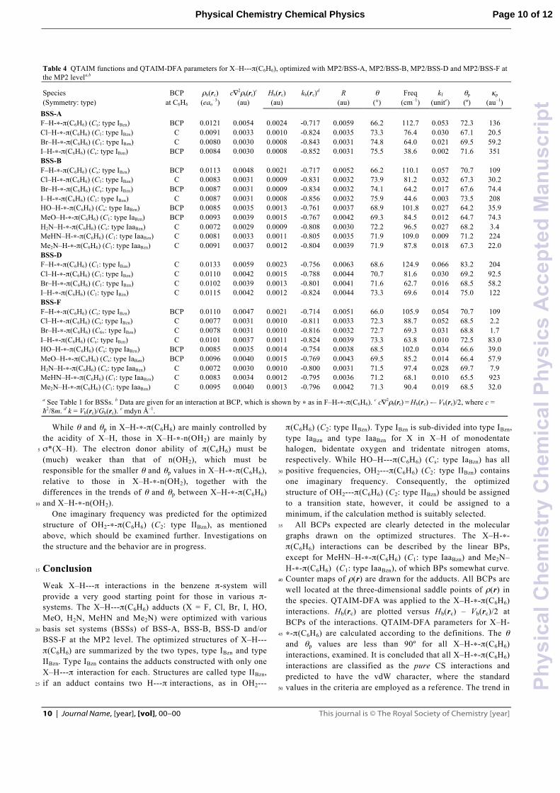
Table 4 collects the QTAIM-DFA parameters, evaluated with BSS-A, BSS-B, BSS-D and BSS-F at the MP2 level. The behavior of the X–H-∗-π(C6H6) interactions are classified and characterized based on the QTAIM-DFA parameters of θ and θp, respectively, employing the criteria in Scheme 3, as a 30

reference. The criteria tell us that the interactions will be classified by the pure CS interactions if 45º < θ < 90º and characterized as the vdW interactions for 45º ≤ θp < 90º. The θ and θp values are less than 90º for all X–H-∗-π(C6H6), examined in this work, as shown in Table 4. Consequently, all 35

X–H-∗-π(C6H6) interactions are classified as the pure CS interactions and they have the vdW-type character, where X = F, Cl, Br, I, HO, MeO, H2N, MeHN and Me2N. How are the trends in the behavior of θ and θp in X–H-∗-π(C6H6)? To clarify the trends, θ and θp in X–H-∗-π(C6H6) 40

and X–H-∗-n(OH2) are plotted versus X (= F, Cl, Br and I) in Fig. 9, evaluated with BSS-F at the MP2 level. While θ in X–H-∗-π(C6H6) become larger in the order of X = F < Cl < Br < I, θp increase in the order of X = Cl ≤ Br (< F) < I. The behavior seems inverse in the trend of X–H-∗-OH2, as a 45

whole.8,87

Fig. 9 Plots of θ versus X (= F, Cl, Br and I) for X–H-∗-π(C6H6) (●) and X–H-∗-n(OH2) (◯) and those of θp versus X for X–H-∗-π(C6H6) (●) and X–H-∗-n(OH2) (◯) evaluated with BSS-F at the MP2 level. 50

What factors control the trends? Acidity of H–X88 and MO energies of σ*(X–H) would be the candidates for the factors. The acidity of H–X in the gas phase and ε(LUMO) of H–X89 are given in eqns (11) and (12), respectively. The acidity becomes stronger in the order of X = F < Cl < Br < I, as 55

expected (eqn (11)). The θ and θp values in X–H-∗-π(C6H6) increase almost proportionally as the acidity of H–X becomes stronger. However, those in X–H-∗-n(OH2) change inversely proportional to the acidity of H–X, as visualized in Fig. 9. Instead, ε(LUMO) of H–X seems to explain the behavior of θ 60

and θp in X–H-∗-n(OH2), as a whole, although ε(LUMO) of H–Cl is predicted to be less than that of H–F. Acidity (ΔHº/kJ mol–1): HF (–1552) < HCl (–1396) < HBr (–1351) < HI (–1315) (11) 65

ε(LUMO) of H–X (eV): HCl (1.12) < HF (1.17) ≤ HBr (1.18) < HI (1.25) (12)

��

��

��

��

��π��π�� π��π��π��π��π��π��π��

Hb(rc) – Vb(rc)/2 (au)

Hb(rc)(au)

θ ) θ ( )

θ ) θ ( )

θ (º) θp (º)

X = F Cl Br I


Phy

sica

lChe

mis

try

Che

mic

alP

hysi

csA

ccep

ted

Man

uscr

ipt


Table 4 QTAIM functions and QTAIM-DFA parameters for X–H---π(C6H6), optimized with MP2/BSS-A, MP2/BSS-B, MP2/BSS-D and MP2/BSS-F at the MP2 levela,b

Species (Symmetry: type)

BCP at C6H6

ρb(rc) (eao

–3) c∇2ρb(rc)c

(au) Hb(rc) (au)

kb(rc)d

R

(au) θ

(°) Freq

(cm–1) kf

(unite) θp

(º) κp

(au–1) BSS-A F–H-∗-π(C6H6) (Cs: type IBzn) BCP 0.0121 0.0054 0.0024 -0.717 0.0059 66.2 112.7 0.053 72.3 136 Cl–H-∗-π(C6H6) (C1: type IBzn) C 0.0091 0.0033 0.0010 -0.824 0.0035 73.3 76.4 0.030 67.1 20.5 Br–H-∗-π(C6H6) (C1: type IBzn) C 0.0080 0.0030 0.0008 -0.843 0.0031 74.8 64.0 0.021 69.5 59.2 I–H-∗-π(C6H6) (Cs: type IBzn) BCP 0.0084 0.0030 0.0008 -0.852 0.0031 75.5 38.6 0.002 71.6 351 BSS-B F–H-∗-π(C6H6) (Cs: type IBzn) BCP 0.0113 0.0048 0.0021 -0.717 0.0052 66.2 110.1 0.057 70.7 109 Cl–H-∗-π(C6H6) (C1: type IBzn) C 0.0083 0.0031 0.0009 -0.831 0.0032 73.9 81.2 0.032 67.3 30.2 Br–H-∗-π(C6H6) (Cs: type IBzn) BCP 0.0087 0.0031 0.0009 -0.834 0.0032 74.1 64.2 0.017 67.6 74.4 I–H-∗-π(C6H6) (C1: type IBzn) C 0.0087 0.0031 0.0008 -0.856 0.0032 75.9 44.6 0.003 73.5 208 HO–H-∗-π(C6H6) (Cs: type IaBzn) BCP 0.0085 0.0035 0.0013 -0.761 0.0037 68.9 101.8 0.027 64.2 35.9 MeO–H-∗-π(C6H6) (C1: type IaBzn) BCP 0.0093 0.0039 0.0015 -0.767 0.0042 69.3 84.5 0.012 64.7 74.3 H2N–H-∗-π(C6H6) (Cs: type IaaBzn) C 0.0072 0.0029 0.0009 -0.808 0.0030 72.2 96.5 0.027 68.2 3.4 MeHN–H-∗-π(C6H6) (C1: type IaaBzn) C 0.0081 0.0033 0.0011 -0.805 0.0035 71.9 109.0 0.009 71.2 224 Me2N–H-∗-π(C6H6) (C1: type IaaBzn) C 0.0091 0.0037 0.0012 -0.804 0.0039 71.9 87.8 0.018 67.3 22.0 BSS-D F–H-∗-π(C6H6) (C1: type IBzn) C 0.0133 0.0059 0.0023 -0.756 0.0063 68.6 124.9 0.066 83.2 204 Cl–H-∗-π(C6H6) (C1: type IBzn) C 0.0110 0.0042 0.0015 -0.788 0.0044 70.7 81.6 0.030 69.2 92.5 Br–H-∗-π(C6H6) (C1: type IBzn) C 0.0102 0.0039 0.0013 -0.801 0.0041 71.6 62.7 0.016 68.5 58.2 I–H-∗-π(C6H6) (C1: type IBzn) C 0.0115 0.0042 0.0012 -0.824 0.0044 73.3 69.6 0.014 75.0 122 BSS-F F–H-∗-π(C6H6) (Cs: type IBzn) BCP 0.0110 0.0047 0.0021 -0.714 0.0051 66.0 105.9 0.054 70.7 109 Cl–H-∗-π(C6H6) (Cs: type IBzn) C 0.0077 0.0031 0.0010 -0.811 0.0033 72.3 88.7 0.052 68.5 2.2 Br–H-∗-π(C6H6) (C6v: type IBzn) C 0.0078 0.0031 0.0010 -0.816 0.0032 72.7 69.3 0.031 68.8 1.7 I–H-∗-π(C6H6) (Cs: type IBzn) C 0.0101 0.0037 0.0011 -0.824 0.0039 73.3 63.8 0.010 72.5 83.0 HO–H-∗-π(C6H6) (Cs: type IaBzn) BCP 0.0085 0.0035 0.0014 -0.754 0.0038 68.5 102.0 0.034 66.6 39.0 MeO–H-∗-π(C6H6) (Cs: type IaBzn) BCP 0.0096 0.0040 0.0015 -0.769 0.0043 69.5 85.2 0.014 66.4 57.9 H2N–H-∗-π(C6H6) (Cs: type IaaBzn) C 0.0072 0.0030 0.0010 -0.800 0.0031 71.5 97.4 0.028 69.7 7.9 MeHN–H-∗-π(C6H6) (C1: type IaaBzn) C 0.0083 0.0034 0.0012 -0.795 0.0036 71.2 68.1 0.010 65.5 923 Me2N–H-∗-π(C6H6) (C1: type IaaBzn) C 0.0095 0.0040 0.0013 -0.796 0.0042 71.3 90.4 0.019 68.5 32.0 a See Table 1 for BSSs. b Data are given for an interaction at BCP, which is shown by ∗ as in F–H-∗-π(C6H6). c c∇2ρb(rc) = Hb(rc) -– Vb(rc)/2, where c = ћ2/8m. d k = Vb(rc)/Gb(rc). e mdyn Å–1.

While θ and θp in X–H-∗-π(C6H6) are mainly controlled by the acidity of X–H, those in X–H-∗-n(OH2) are mainly by σ*(X–H). The electron donor ability of π(C6H6) must be 5

(much) weaker than that of n(OH2), which must be responsible for the smaller θ and θp values in X–H-∗-π(C6H6), relative to those in X–H-∗-n(OH2), together with the differences in the trends of θ and θp between X–H-∗-π(C6H6) and X–H-∗-n(OH2). 10

One imaginary frequency was predicted for the optimized structure of OH2-∗-π(C6H6) (C2: type IIBzn), as mentioned above, which should be examined further. Investigations on the structure and the behavior are in progress.

Conclusion 15

Weak X–H---π interactions in the benzene π-system will provide a very good starting point for those in various π-systems. The X–H---π(C6H6) adducts (X = F, Cl, Br, I, HO, MeO, H2N, MeHN and Me2N) were optimized with various basis set systems (BSSs) of BSS-A, BSS-B, BSS-D and/or 20

BSS-F at the MP2 level. The optimized structures of X–H---π(C6H6) are summarized by the two types, type IBzn and type IIBzn. Type IBzn contains the adducts constructed with only one X–H---π interaction for each. Structures are called type IIBzn, if an adduct contains two H---π interactions, as in OH2---25

π(C6H6) (C2: type IIBzn). Type IBzn is sub-divided into type IBzn, type IaBzn and type IaaBzn for X in X–H of monodentate halogen, bidentate oxygen and tridentate nitrogen atoms, respectively. While HO–H---π(C6H6) (Cs: type IaBzn) has all positive frequencies, OH2---π(C6H6) (C2: type IIBzn) contains 30

one imaginary frequency. Consequently, the optimized structure of OH2---π(C6H6) (C2: type IIBzn) should be assigned to a transition state, however, it could be assigned to a minimum, if the calculation method is suitably selected. All BCPs expected are clearly detected in the molecular 35

graphs drawn on the optimized structures. The X–H-∗-π(C6H6) interactions can be described by the linear BPs, except for MeHN–H-∗-π(C6H6) (C1: type IaaBzn) and Me2N–H-∗-π(C6H6) (C1: type IaaBzn), of which BPs somewhat curve. Counter maps of ρ(r) are drawn for the adducts. All BCPs are 40

well located at the three-dimensional saddle points of ρ(r) in the species. QTAIM-DFA was applied to the X–H-∗-π(C6H6) interactions. Hb(rc) are plotted versus Hb(rc) – Vb(rc)/2 at BCPs of the interactions. QTAIM-DFA parameters for X–H-∗-π(C6H6) are calculated according to the definitions. The θ 45

and θp values are less than 90º for all X–H-∗-π(C6H6) interactions, examined. It is concluded that all X–H-∗-π(C6H6) interactions are classified as the pure CS interactions and predicted to have the vdW character, where the standard values in the criteria are employed as a reference. The trend in 50


Phy

sica

lChe

mis

try

Che

mic

alP

hysi

csA

ccep

ted

Man

uscr

ipt


the θ and θp values for X–H-∗-π(C6H6) (X = F, Cl, Br and I) seems different from that for X–H-∗-n(OH2). Factors to control the trend are also examined.

Acknowledgements

This work was partially supported by a Grant-in-Aid for 5

Scientific Research (Nos. 23350019 and 26410050) from the Ministry of Education, Culture, Sports, Science and Technology, Japan. The support of the Wakayama University Original Research Support Project Grant and the Wakayama University Graduate School Project Research Grant is also 10

acknowledged.

Notes and references a Department of Material Science and Chemistry, Faculty of Systems Engineering, Wakayama University, 930 Sakaedani, Wakayama 640-8510, Japan. Fax: +81 73 457 8253; Tel: +81 73 457 8252; E-mail: 15

[email protected] † Electronic supplementary information (ESI) available: Cartesian coordinates for optimized structures of X–H---π(C6H6) (X = F, Cl, Br, I, HO, MeO, H2N, MeHN and Me2N). For ESI or other electronic format see DOI: 10.1039/b000000x. 20

1 L. Pauling, The Nature of the Chemical Bond, ed. L. Pauling, Cornell University Press, Ithaca, NY, 1960, 3rd ed., ch. 12, p. 449.

2 G. A. Jeffrey, An Introduction to Hydrogen Bonding, Oxford University Press: New York, 1997.

3 S. Scheiner, Hydrogen Bonding, Oxford University Press: New York, 25

1997. 4 G. R. Desiraju and T. Steiner, The Weak Hydrogen Bond: In

Structural Chemistry and Biology (IUCr Monographs on Crystallography), Oxford University Press: Oxford, 1999.

5 Hydrogen Bonding and Transfer in the Excited State, ed. K.-L. Han 30

and G.-J. Zhao, Wiley, Chichester, 2010, vol. I and II 6 G. Gilli and P. Gilli, The Nature of the Hydrogen Bond: Outline of a

Comprehensive Hydrogen Bond Theory (IUCr Monographs on Crystallography), Oxford University Press: Oxford, 2009.

7 G. Gilli and P. Gilli, The Nature of the Hydrogen Bond: Outline of a 35

Comprehensive Hydrogen Bond Theory (IUCr Monographs on Crystallography), Oxford University Press: Oxford, 2009, ch. 2.3, p. 28.

8 S. Hayashi, K. Matsuiwa, M. Kitamoto and W. Nakanishi, J. Phys. Chem. A, 2013, 117, 1804-1816. 40

9 S. N. Vinogradov and R. H. Linnell, Hydrogen Bonding, Van Nostrand Reinhold, New York, 1971.

10 G. R. Desiraju, Cryst. Growth Des., 2011, 11, 896-898. 11 C. B. Aakeroy and K. R. Seddon, Chem. Soc. Rev., 1993, 22, 397-407. 12 M. Meot-Ner (Mautner), Chem. Rev., 2005, 105, 213-284. 45

13 G. R. Desiraju, Mol. Cryst. Liq. Cryst., 1992, 211, 63-74. 14 P. Gilli and G. Gilli, J. Mol. Struct., 2010, 972, 2-10. 15 P. A. Kollman and L. C. Allen, Chem. Rev., 1972, 72, 283-303. 16 A. G. Slater, L. M. A. Perdigão, P. H. Beton and N. R. Champness,

Acc. Chem. Res., 2014, 47, 3417-3427. 50

17 C. Otto, G. A. Thomas, K. Rippe, T. M. Jovin and W. L. Peticolas, Biochemistry, 1991, 30, 3062-3069.

18 The temperature effect on the low frequency Raman spectra of hormones was investigated, which should be closely related to the specific conformation, together with the intra- and inter-molecular 55

interactions employing QTAIM. See, V. A. Minaeva, B. F. Minaev, G. V. Baryshnikov, N. V. Surovtsev, O. P. Cherkasova, L. I. Tkachenko, N. N. Karaush and E. V. Stromylo, Optics and Spectroscopy, 2015, 118, 214–223.

19 (a) W. Nakanishi, S. Hayashi and K. Narahara, J. Phys. Chem. A, 60

2009, 113, 10050-10057; (b) W. Nakanishi, S. Hayashi and K. Narahara, J. Phys. Chem. A, 2008, 112, 13593-13599.

20 W. Nakanishi and S. Hayashi, Curr. Org. Chem., 2010, 14, 181-197. 21 W. Nakanishi and S. Hayashi, J. Phys. Chem. A, 2010, 114, 7423-

7430. 65

22 A. C. Legon, P. D. Aldrich and W. H. Flygare, J. Chem. Phys., 1981, 75, 625-630.

23 P. D. Aldrich, A. C. Legon and W. H. Flygare, J. Chem. Phys., 1981, 75, 2126-2134.

24 W. G. Read, E. J. Campbell and G. Henderson, J. Chem. Phys., 1983, 70

78, 3501-3508. 25 J. A. Shea and S. G. Kukolich, J. Chem. Phys., 1983, 78, 3545-3551. 26 S. A. Cooke, G. K. Corlett, D. G. Lister and A. C. Legon, J. Chem.

Soc., Faraday Trans., 1998, 94, 837-841.; S. A. Cooke, G. K. Corlett and A. C. Legon, J. Chem. Soc., Faraday Trans., 1998, 94, 1565-75

1570. 27 M. E. Sanz, S. Antolînez, J. L. Alonso, J. C. Lôpez, R. L.

Kuczkowski, S. A. Peebles, R. A. Peebles, F. C. Boman, E. Kraka, D. Cremer, J. Chem. Phys., 2003, 118, 9278-9290.

28 W. G. Read, E. J. Campbell, G. Henderson and W. H. Flygare, J. Am. 80

Chem. Soc., 1981, 103, 7670-7672; W. G. Read, E. J. Campbell and G. Henderson, J. Chem. Phys., 1983, 78, 3501-3508. See also M. E. Sanz, S. Antolinez, J. L. Alonso and J. C. Lopez, J. Chem. Phys., 2003, 118, 9278-9290.

29 S. Furutaka and S. Ikawa, J. Chem. Phys., 2002, 117, 751-755. 85

30 K. P. Gierszal, J. G. Davis, M. D. Hands, D. S. Wilcox, L. V. Slipchenko and D. Ben-Amotz, J. Phys. Chem. Lett., 2011, 2, 2930-2933.

31 D. A. Rodham, S. Suzuki, R. D. Suenram, F. J. Lovas, S. Dasgupta, W. A. Goddard III and G. A. Blake, Nature, 1993, 362, 735-737. 90

32 M. Albertí, A. Aguilar, F. Huarte-Larrañaga, J. M. Lucas and F. Pirani, J. Phys. Chem. A, 2014, 118, 1651-1662.

33 S. Vaupel, B. Brutschy, P. Tarakeshwar and K. S. Kim, J. Am. Chem. Soc., 2006, 128, 5416-5426.

34 X. Wang and P. P. Power, Angew. Chem. Int. Ed., 2011, 50, 10965-95

10968. 35 (a) Atoms in Molecules. A Quantum Theory, ed. R. F. W. Bader,

Oxford University Press, Oxford, UK, 1990; (b) C. F. Matta and R. J. Boyd, An Introduction to the Quantum Theory of Atoms in Molecules In The Quantum Theory of Atoms in Molecules: From Solid State to 100

DNA and Drug Design, ed. C. F. Matta and R. J. Boyd, Wiley-VCH, Weinheim, Germany, 2007, ch. 1.

36 (a) R. F. W. Bader, T. S. Slee. D. Cremer and E. Kraka, J. Am. Chem. Soc., 1983, 105, 5061-5068; (b) R. F. W. Bader, Chem. Res., 1991, 91, 893-926; (c) R. F. W. Bader, J. Phys. Chem. A, 1998, 102, 7314-105

7323; (d) F. Biegler-König, R. F. W. Bader and T. H. Tang, J. Comput. Chem., 1982, 3, 317-328; (e) R. F. W. Bader, Acc. Chem. Res., 1985, 18, 9-15; (f) T. H. Tang, R. F. W. Bader and P. MacDougall, Inorg. Chem., 1985, 24, 2047-2053; (g) F. Biegler-König, J. Schönbohm and D. Bayles, J. Comput. Chem., 2001, 22, 110

545-559; (h) F. Biegler-König and J. Schönbohm, J. Comput. Chem., 2002, 23, 1489-1494.

37 J. Molina and J. A. Dobado, Theor. Chem. Acc., 2001, 105, 328-337. 38 J. A. Dobado, H. Martinez-Garcia, J. Molina and M. R. Sundberg, J.

Am. Chem. Soc., 2000, 122, 1144-1149. 115

39 Some specific interactions are tried to analyze employing QTAIM. See, I. S. Bushmarinov, M. Y. Antipin, V. R. Akhmetova, G. R. Nadyrgulova and K. A. Lyssenko, J. Phys. Chem. A, 2008, 112, 5017-5023, for an example.

40 R. J. Boyd and S. C. Choi, Chem. Phys. Lett., 1986, 129, 62-65. 120

41 M. T. Carroll and R. F. W. Bader, Mol. Phys., 1988, 65, 695-722. 42 S. J. Grabowski, J. Phys. Chem. A, 2001, 105, 10739-10746. 43 (a) E. Espinosa, I. Alkorta, J. Elguero and E. Molins, J. Chem. Phys.,

2002, 117, 5529-5542; (b) I. Rozas, I. Alkorta and J. Elguero, J. Am. Chem. Soc., 2000, 122, 11154-11161; (c) E. Espinosa, E. Molins and 125

C. Lecomte, Chem. Phys. Lett., 1998, 285, 170-173. 44 M. Domagala, S. Grabowski, K. Urbaniak and G. Mloston, J. Phys.

Chem. A, 2003, 107, 2730-2736. 45 S. K. Ignatov, N. H. Rees, B. R. Tyrrell, S. R. Dubberley, A. G.

Razuvaev, P. Mountford and G. I. Nikonov, Chem. Eur. J., 2004, 10, 130

4991-4999. 46 (a) M. Yamashita, Y. Yamamoto, K.-y. Akiba, D. Hashizume, F.

Iwasaki, N. Takagi and S. Nagase, J. Am. Chem. Soc., 2005, 127, 4354-4371; (b) Y. Yamamoto and K.-y. Akiba, J. Syn. Org. Chem. Jpn., 2004, 62, 1128-1137. 135


Phy

sica

lChe

mis

try

Che

mic

alP

hysi

csA

ccep

ted

Man

uscr

ipt


47 S. K. Tripathi, U. Patel, D. Roy, R. B. Sunoj, H. B. Singh, G. Wolmershäuser and R. J. Butcher, J. Org. Chem., 2005, 70, 9237-9247.

48 M. Domagala and S. Grabowski, J. Phys. Chem. A, 2005, 109, 5683-5688. 5

49 (a) P. Lipkowski, S. J. Grabowski and J. Leszczynski, J. Phys. Chem. A, 2006, 110, 10296-10302; (b) M. Ziôkowski, S. J. Grabowski and J. Leszczynski, J. Phys. Chem. A, 2006, 110, 6514-6521; (c) S. Grabowski, W. A. Sokalski and J. Leszczynski, J. Phys. Chem. A, 2005, 109, 4331-4341. 10

50 J. Poater, M. Solâ and F. M. Bickelhaupt, Chem. Eur. J., 2006, 12, 2889-2895.

51 R. Parthasarathi, V. Subramanian and N. Sathyamurthy, J. Phys. Chem. A, 2006, 110, 3349-3351.

52 D. Chopra, T. S. Cameron, J. D. Ferrara and T. N. Guru Row, J. Phys. 15

Chem. A, 2006, 110, 10465-10477. 53 W. Nakanishi, T. Nakamoto, S. Hayashi, T. Sasamori and N. Tokitoh,

Chem. Eur. J., 2007, 13, 255-268. 54 R. F. W. Bader, J. Phys. Chem. A, 2007, 111, 7966-7972. 55 I. S. Bushmarinov, M. Y. Antipin, V. R. Akhmetova, G. R. 20

Nadyrgulova and K. A. Lyssenko, J. Phys. Chem. A, 2008, 112, 5017-5023.

56 H. Szatylowicz, T. M. Krygowski, J. J. Panek and A. Jezierska, J. Phys. Chem. A, 2008, 112, 9895-9905.

57 I. Mata, E. Molins and I. Alkorta, J. Chem. Phys., 2009, 130, 044104. 25

58 E. Matito and M. Solâ, Coord. Chem. Rev., 2009, 253, 647-665. 59 QTAIM-DFA is successfully applied to analyze weak to strong

interactions in gas phase. It should also be applied to the interactions in crystals and to those in larger systems, containing bioactive materials, although the methodological improvement is inevitable to 30

generate the perturbed structures suitable for the systems. Such improvement is in progress, which will be reported elsewhere.

60 S. Scheiner, Acc. Chem. Res., 2013, 46, 280-288. 61 R. T. Myers, Inorg. Chem., 1977, 16, 2671-2674. 62 A. Mukherjee, S. Tothadi and G. R. Desiraju, Acc. Chem. Res., 2014, 35

47, 2514-2524. 63 C. Bissantz, B. Kuhn and M. Stahl, J. Med. Chem., 2010, 53, 5061-

5084. 64 Y. Umezawa, S. Tsuboyama, K. Honda, J. Uzawa and M. Nishio,

Bull. Chem. Soc. Jpn., 1998, 71, 1207-1213. 40

65 O. Takahashi, Y. Kohno, S. Iwasaki, K. Saito, M. Iwaoka, S. Tomoda, Y. Umezawa, S. Tsuboyama and M. Nishio, Bull. Chem. Soc. Jpn., 2001, 74, 2421-2430.

66 M. Albertí, A. Aguilar, J. M. Lucas and F. Pirani, J. Phys. Chem. A, 2012, 116, 5480-5490. 45

67 A. Jain, V. Ramanathan and R. Sankararamakrishnan, Protein Science, 2009, 18, 595-605.

68 S. Tsuzuki, K. Honda, T. Uchimaru, M. Mikami and K. Tanabe, J. Am. Chem. Soc., 2000, 122, 11450-11458.

69 J. P. M. Lommerse, A. J. Stone, R. Taylor and F. H. Allen, J. Am. 50

Chem. Soc., 1996, 118, 3108-3116. 70 J. W. G. Bloom, R. K. Raju and S. E. Wheeler, J. Chem. Theory

Comput., 2012, 8, 3167-3174. 71 N. J. Singh, S. K. Min, D. Y. Kim and K. S. Kim, J. Chem. Theor.

Comput., 2009, 5, 515-529. 55

72 Dots are usually employed to show BCPs in molecular graphs. Therefore, A-•-B would be more suitable to describe BP with BCP. Nevertheless, A-∗-B is employed to emphasize the existence of BCP on BP, in question, in our case.

73 W. Nakanishi, S. Hayashi, K. Matsuiwa and M. Kitamoto, Bull. 60

Chem. Soc. Jpn., 2012, 85, 1293-1305. 74 θp and κp for the major bonds/interactions seem to be affected by the

behavior of the bonds/interactions around those in question (minor bonds/interactions): The influence from the behavior of the minor bonds/interactions would not be so severe for usual cases. See ref 21. 65

75 Gaussian 09 (Revision D.01), M. J. Frisch, G. W. Trucks, H. B. Schlegel, G. E. Scuseria, M. A. Robb, J. R. Cheeseman, G. Scalmani, V. Barone, B. Mennucci, G. A. Petersson, H. Nakatsuji, M. Caricato, X. Li, H. P. Hratchian, A. F. Izmaylov, J. Bloino, G. Zheng, J. L. Sonnenberg, M. Hada, M. Ehara, K. Toyota, R. Fukuda, J. Hasegawa, 70

M. Ishida, T. Nakajima, Y. Honda, O. Kitao, H. Nakai, T. Vreven, J. A. Montgomery, Jr., J. E. Peralta, F. Ogliaro, M. Bearpark, J. J. Heyd, E. Brothers, K. N. Kudin, V. N. Staroverov, R. Kobayashi, J. Normand, K. Raghavachari, A. Rendell, J. C. Burant, S. S. Iyengar, J. Tomasi, M. Cossi, N. Rega, J. M. Millam, M. Klene, J. E. Knox, J. B. 75

Cross, V. Bakken, C. Adamo, J. Jaramillo, R. Gomperts, R. E. Stratmann, O. Yazyev, A. J. Austin, R. Cammi, C. Pomelli, J. W. Ochterski, R. L. Martin, K. Morokuma, V. G. Zakrzewski, G. A. Voth, P. Salvador, J. J. Dannenberg, S. Dapprich, A. D. Daniels, Ö. Farkas, J. B. Foresman, J. V. Ortiz, J. Cioslowski and D. J. Fox, 80

Gaussian, Inc.: Wallingford CT, 2009. 76 For the 6-311G(3d) basis sets, see: (a) R. C. Binning Jr. and L. A.

Curtiss, J. Comput. Chem., 1990, 11, 1206-1216; (b) L. A. Curtiss, M. P. McGrath, J.-P. Blaudeau, N. E. Davis, R. C. Binning Jr. and L. Radom, J. Chem. Phys., 1995, 103, 6104-6113; (c) M. P. McGrath 85

and L. Radom, J. Chem. Phys., 1991, 94, 511-516. For the diffuse functions (+ and ++), see: T. Clark, J. Chandrasekhar, G. W. Spitznagel and P. v. R. Schleyer, J. Comput. Chem., 1983, 4, 294-301.

77 D. Feller, J. Comp. Chem., 1996, 17, 1571-1586. 78 K. L. Schuchardt, B. T. Didier, T. Elsethagen, L. Sun, V. 90

Gurumoorthi, J. Chase, J. Li and T. L. Windus, J. Chem. Inf. Model., 2007, 47, 1045-1052.

79 T. Noro, M. Sekiya and T. Koga, Theoret. Chem. Acc., 2012, 131, 1124.

80 (a) For inner and valence shells: T. Koga, S. Yamamoto, T. 95

Shimazaki and H. Tatewaki, Theor. Chem. Acc., 2002, 108, 41-45; (b) For valence correlated set: M. Sekiya, T. Noro, Y. Osanai and T. Koga, Theor. Chem. Acc., 2001, 106, 297-300.

81 C. Møller and M. S. Plesset, Phys. Rev., 1934, 46, 618-622; J. Gauss, J. Chem. Phys., 1993, 99, 3629-3643; J. Gauss, Ber. Bunsen-Ges. 100

Phys. Chem., 1995, 99, 1001-1008. 82 The AIM2000 program (Version 2.0) is employed to analyze and

visualize atoms-in-molecules: F. Biegler-König, J. Comput. Chem., 2000, 21, 1040−1048. See also ref 36g.

83 The values of w = (0), ±0.1 and ±0.2 in r = ro + wao were employed 105

for the perturbed structures in POM (partial optimization method),18,19 since the bond orders becomes 2/3 and 3/2 times larger at w = +0.2 and –0.2 relative to the original value at w = 0, respectively. However, w = (0), ±0.05 and ±0.1 for r = ro + wao are applied in usual cases to reduce the calculation errors in the perturbed structures generated by 110

NIV and/or POM (see also refs 19–21). 84 It is achieved by changing the corresponding parameters in Gaussian

09 from the default values to print out the normal coordinates of five digits for the purpose.

85 W. G. Read, E. J. Campbell and G. Henderson, J. Chem. Phys., 1983, 115

78, 3501-3508. 86 The noncovalent distances would be better reproduced by considering

BSSE (basis set errors). However, optimizations are performed without considering BSSE, since the normal coordinates of internal vibrations are necessary to generate the perturbed structures in 120

QTAIM-DFA, which are obtained through the frequency analysis. 87 S. Hayashi, Y. Sugibayashi, and W. Nakanishi, unpublished work. 88 The Chemical Handbook (Kagaku-Binran), ed. Chemical Society of

Japan eds. 4th ed., Maruzen, Tokyo, in Japanese, 1993, II-315. 89 The MO energies of σ*(X–H) must be most suitable for the 125

discussion, however, the character of σ*(X–H) seems to spread over a few vacant orbitals such as LUMO, LUMO+1 and/or LUMO+2. Therefore, ε(LUMO) of H–X is employed for the discussion.

130


Phy

sica

lChe

mis

try

Che

mic

alP

hysi

csA

ccep

ted

Man

uscr

ipt

Accepted Manuscript - RSC Publishing

Documents

Transcript of Accepted Manuscript - RSC Publishing