ABSTRACT SAVAGE, DEBRA MACIVOR. The advantages ...
207
ABSTRACT SAVAGE, DEBRA MACIVOR. The advantages and disadvantages of three-dimensional maps for focused and integrative map analysis performance by novice and experienced users. (Under the direction of Hugh A. Devine.) The purpose of this study was to investigate the following questions: 1. Are 3D pictorial maps projected on the 2D computer display more effective than flat 2D topographic maps (i.e., contour maps) in supporting simple geographic problem solving? 2. Are different task types better supported by traditional 2D contour maps or 3D contour maps? 3. Does the map user’s previous experience with contour maps moderate any of the effects of map type and task type interactions? This study consisted of two parts. Part 1 was a 2x2x2 design, with dimension (2D or 3D), task type (focused or integrative) and elevation requirement (required or not required to perform the task)as the independent variables. Response time and accuracy were the dependent variables. Spatial ability as measured by a paper folding test was treated as a covariate. 2D representations showed a clear advantage only for focused, non-elevation tasks such as “Determine the longitude at point A.” 3D representations showed no clear advantage in any task condition. There were interactions between task type and both dimension and elevation. Integrative, elevation questions were clearly more difficult regardless of dimension. Part 2 of this study was similar to Part 1, except the additional variable of experience with topographic maps was added in order to examine potential interactions
-
Upload
khangminh22 -
Category
Documents
-
view
1 -
download
0
Transcript of ABSTRACT SAVAGE, DEBRA MACIVOR. The advantages ...

ABSTRACT
SAVAGE, DEBRA MACIVOR. The advantages and disadvantages of three-dimensional maps for focused and integrative map analysis performance by novice and experienced users. (Under the direction of Hugh A. Devine.)
The purpose of this study was to investigate the following questions:
1. Are 3D pictorial maps projected on the 2D computer display more
effective than flat 2D topographic maps (i.e., contour maps) in supporting
simple geographic problem solving?
2. Are different task types better supported by traditional 2D contour maps or
3D contour maps?
3. Does the map user’s previous experience with contour maps moderate any
of the effects of map type and task type interactions?
This study consisted of two parts. Part 1 was a 2x2x2 design, with dimension (2D or 3D),
task type (focused or integrative) and elevation requirement (required or not required to
perform the task)as the independent variables. Response time and accuracy were the
dependent variables. Spatial ability as measured by a paper folding test was treated as a
covariate.
2D representations showed a clear advantage only for focused, non-elevation
tasks such as “Determine the longitude at point A.” 3D representations showed no clear
advantage in any task condition. There were interactions between task type and both
dimension and elevation. Integrative, elevation questions were clearly more difficult
regardless of dimension.
Part 2 of this study was similar to Part 1, except the additional variable of
experience with topographic maps was added in order to examine potential interactions

with these tasks and topographic representation. Spatial ability proved significant, along
with experience and task type. Both experienced and inexperienced participants
performed better with the 2D maps across all tasks.
Study results showed that there is probably no single best map type that supports
all task requirements equally. Map format, including dimensions, should be decided
based on the task to be performed. Additionally, 3D maps should probably not be used
for tasks requiring extraction of simple values of latitude and longitude. Finally, if 3D
maps are to be used for instruction or problem solving, some training on their
interpretation may enhance their effectiveness.

THE ADVANTAGES AND DISADVANTAGES OF THREE-DIMENSIONAL MAPS
FOR FOCUSED AND INTEGRATIVE MAP ANALYSIS PERFORMANCE BY
NOVICE AND EXPERIENCED USERS
By
Debra MacIvor Savage
A dissertation submitted to the Graduate Faculty of North Carolina State University in partial fulfillment of the
requirements for the Degree of Doctor of Philosophy Parks, Recreation and Tourism Management
Raleigh, North Carolina
August 2006
Approved By:
_____________________________ _____________________________ Eric N Wiebe Harriett S Stubbs _____________________________ _____________________________ Hugh A. Devine Douglas Wellman Chair of Advisory Committee

ii
DEDICATION
To Dr. Hugh Devine who knew when to encourage and when to have faith,
thank you for your confidence and your outstanding example, and to my husband Rick
Savage, who has never stopped believing in me: You are the wind beneath my wings –
Thank you!

iii
BIOGRAPHY
Debra MacIvor Savage was born in Hartford Connecticut on July 5, 1954. She
has wanted to be a college professor since she knew what it was, which means since
about the age of 8. She graduated from Orange High School in June of 1972, and after
a series of jobs, started a job at IBM in Boston in December 1975. In 1979, she was
transferred to Tampa, Florida, where she completed her Bachelor of Arts degree in
Business Economics in 1982, the year her daughter Suzanna was born. In 1983 she
was transferred by IBM to Raleigh, North Carolina to a job in online computer-based
training. Since that time, Debra has had jobs in programming and Human Factors
Engineering, and has started degree programs in computer-based training at UNC
Chapel Hill, MS in Business at North Carolina State University, and Ergonomics at
North Carolina State University.
Finally, with support from her family (emotional) and the National Science
Foundation and the Parks and Recreation Department at North Carolina State
University (financial), she completed the requirements for the Doctor of Philosophy
program in August of 2006, with focus on Spatial Information Science.

iv
ACKNOWLEDGEMENTS
My research was supported by a research traineeship from the National
Science Foundation, as well as support as a Research Assistant from the department of
Parks, Recreation and Tourism Management. Without this support I could not have
completed my research.
I am grateful to my committee chair, Hugh Devine, without whose example
and encouragement I might not have completed my graduate work. Harriett Stubbs has
been an outstanding example of what can be accomplished by one person if she is very
determined. Doug Wellman has served as an intellectual and professional role model
to me as a person who has a diversity of interests, background and abilities. Eric
Wiebe has especially kept me going with kind words and encouragement, as well as
extreme patience. You are all professionals and friends. I could not have had a better
committee.
Beth Eastman, Harriett Stubbs and Eric Wiebe have all patiently read and
commented on my proposals and papers, making excellent and timely suggestions.
Beth additionally assisted in conducting study 1. Thank you so much for your help.
Thanks are also due to the Department of Landscape Architecture for
providing me with study participants and lab space to conduct study 2, especially
Achva Stein, Art Rice and Kofi Boone. Robert I. Bruck of the Environmental
Technology Program graciously gave me class time and access to his introductory
students for Study 2. Finally the following faculty members in Parks, Recreation and
Tourism kindly gave me access to their students to conduct study 1: Tricia Day,

v
Annette Moore and Phil Rea. Steven Jones and Scott Payne helped me set up the lab.
Thank you!

vi
TABLE OF CONTENTS
LIST OF FIGURES .............................................................................................................................viii LIST OF TABLES .................................................................................................................................xi DEFINITION OF QUESTION TYPES .............................................................................................xiv CHAPTER 1: INTRODUCTION .........................................................................................................1
GEOGRAPHIC INFORMATION SYSTEMS - OVERVIEW..............................................................................2 GIS in Community Planning ............................................................................................................3
TERMS AND DEFINITIONS ......................................................................................................................5 A USEFUL STRUCTURE FOR THINKING ABOUT MAPS ............................................................................6
Topographic Contour Maps.............................................................................................................7 SUMMARY AND RESEARCH QUESTIONS ..............................................................................................10
CHAPTER 2: REVIEW OF THE LITERATURE ...........................................................................12 INFORMATION PROCESSING IN EXPERIENCED AND NOVICE USERS ......................................................12
The Expert/Novice Paradigm and map-reading ............................................................................13 Difference in novice and experienced map-learning strategies.....................................................17 Perception of three dimensions from a two-dimensional display ..................................................22 Pictorial Cues ................................................................................................................................23
SEPARABILITY, INTEGRALITY AND CONFIGURABILITY OF PERCEPTUAL QUALITIES .............................30 Perceptual separability of qualities ...............................................................................................31 Perceptual integrality of qualities .................................................................................................32 Testing for integral and separable stimuli.....................................................................................33 Configural stimulus qualities.........................................................................................................36
CONFIGURAL DISPLAYS AND EMERGENT FEATURES............................................................................38 Focused and Integrative Tasks ......................................................................................................39 The Proximity Compatibility Principle ..........................................................................................44 The Semantic Mapping Model .......................................................................................................45 3D maps as configural displays.....................................................................................................45
ADVANTAGES AND DISADVANTAGES OF 3D GRAPHICS ON 2D DISPLAYS ............................................48 Advantages of a 3D display ...........................................................................................................48 Potential Advantages of a Flat Topographic Map.........................................................................49
SUMMARY ...........................................................................................................................................50 CHAPTER 3: OBJECTIVES AND HYPOTHESES .........................................................................52
Hypotheses for Study 1 ..................................................................................................................53 Hypothesis for Study 2 ...................................................................................................................59 Study Delimitations........................................................................................................................59
CHAPTER 4: METHODOLOGY ......................................................................................................60 RESEARCH DESIGN..............................................................................................................................60
Study 1 Design ...............................................................................................................................60 Study 2 Design ...............................................................................................................................62
PARTICIPANTS .....................................................................................................................................64 Study 1 Participants.......................................................................................................................64 Study 2 Participants.......................................................................................................................67
SETTING AND APPARATUS...................................................................................................................70 Computer Labs and displays..........................................................................................................70 Task Material Packets ...................................................................................................................71
MEASURES ..........................................................................................................................................84 PROCEDURE.........................................................................................................................................84
Study 1 Procedure..........................................................................................................................84 Study 2 Procedure..........................................................................................................................85

vii
DATA COLLECTION AND REDUCTION..................................................................................................86 Chapter 5: Analysis and Results ..........................................................................................................87
Introduction ...................................................................................................................................87 PARTICIPANT QUESTIONNAIRE AND SPATIAL ABILITY SCORES...........................................................87
Study 1 Participants.......................................................................................................................87 Study 2 Participants.......................................................................................................................91 Summary of Participant Questionnaire and Spatial Ability Scores ...............................................95
TEST FOR POTENTIAL COVARIATES......................................................................................................96 Study 1 Correlation Analysis .........................................................................................................96 Study 2 Correlation Analysis .........................................................................................................97 Summary ........................................................................................................................................97
TEST FOR QUESTION VALIDITY ...........................................................................................................97 TASK PERFORMANCE ........................................................................................................................101
Study 1 Accuracy .........................................................................................................................101 Study 1 Time ................................................................................................................................104 Study 2 Accuracy .........................................................................................................................106 Study 2 Speed...............................................................................................................................109
SUMMARY OF RESULTS .....................................................................................................................110 Study 1 .........................................................................................................................................110 Study 2 .........................................................................................................................................112
Chapter 6: Discussion .........................................................................................................................113 THE PROBLEM ...................................................................................................................................113 SUMMARY OF RESULTS......................................................................................................................113
Discussion of results ....................................................................................................................115 LIMITATIONS OF THIS STUDY.............................................................................................................116 RECOMMENDATIONS FOR FUTURE RESEARCH...................................................................................120 CONCLUSIONS ...................................................................................................................................120
References ............................................................................................................................................122 APPENDICES .....................................................................................................................................129
APPENDIX 1. INFORMED CONSENT FORM ..........................................................................................130 APPENDIX 2. SURVEY........................................................................................................................131 APPENDIX 3: THE QUESTIONS ..........................................................................................................132
Items 1-5 and 24: Focused, Elevation Inclusive ..........................................................................133 Items 6-10 and 21: Integrative, Elevation Inclusive ....................................................................145 Items 11-15 and 22: Integrative, Elevation Exclusive .................................................................157 Items 16-20 and 23: Focused, Elevation Exclusive .....................................................................169
APPENDIX 4. VISUAL BASIC CODE ....................................................................................................181 Study Code...................................................................................................................................181 Code to Read Diskette, Parse and Write Data.............................................................................189

viii
LIST OF FIGURES
Figure 1. Example of a planar contour map (Muehrcke & Muehrcke, 1998, Figure
5.20) ........................................................................................................................8
Figure 2. 3D perspective contour map, and its corresponding 2D (planar) contour map
(Feinstein & Krohelski, n.d., Ground Water Levels section, para. 5, figure 1) ......9
Figure 3. Information Processing Model (Ellis & Hunt, 1993) ...................................16
Figure 4. Perspective projection (Bertoline et al., 1997) ..............................................24
Figure 5. Parallel projection (Bertoline et al., 1977) ...................................................25
Figure 6. Size and Height in Field of View (Bertoline et al., 1997)............................26
Figure 7. Map illustration showing texture gradient....................................................27
Figure 8. Computer-shaded relief map (Muehrcke & Muehrcke, 1998) ......................28
Figure 9. Change of color and loss of detail at great distances.....................................29
Figure 10. Multivariate symbols - animal type and population levels..........................31
Figure 11.Hue and brightness as integral qualities .......................................................33
Figure 12. Divided attention task- color and size are varied independently.................35
Figure 13. A grid can be considered integral or separable- the red dot not clustered
with the others.......................................................................................................36
Figure 14. Plotted relationship between year and population variables .......................40
Figure 15. Emergent feature of trend line, which emerges from separate stimuli........41
Figure 16. Configural line display – trend lines configure to form polygons...............42
Figure 17. Separable rectangle display illustrating emergent trend line for mammals43
Figure 18. 2D topographic map with latitude and longitude lines and intersection
points.....................................................................................................................46

ix
Figure 19. Integrated Question: From which spot are you most likely to see your house
and all of the other points?....................................................................................47
Figure 20. Example of a focused question about a single value of latitude or longitude
(not elevation) at a single location – “Question: How far east is the blue point
(east from “zero” or 0 East)?”...............................................................................55
Figure 21. Example of a focused question about a single value of elevation at a single
location – “Question: Which point shown above represents the lowest lying area
(the lowest elevation)?” ........................................................................................56
Figure 22. Integrative task to determine distance relationships between three or more
points in a 2D space “Question: Which point is the farthest distance EAST from
the blue point?” .....................................................................................................57
Figure 23. Integrative task to determine terrain shape – “Question: From which spot
are you most likely to see your house and all of the other points?” .....................58
Figure 24. Self-assessed experience question...............................................................65
Figure 25.Thematic map- classified into 100 ft elevation changes ..............................75
Figure 26. Contour lines for map shown in Figure 25..................................................76
Figure 27. Latitude and longitude grid lines for map shown in Figure 25 ...................77
Figure 28. Finished 2D map from parts shown in Figure 25 through Figure 27 ..........78
Figure 29. Final 3D question from the 2D map shown in Figure 28 ............................79
Figure 30. Practice Question - 2D.................................................................................80
Figure 31. Practice Question - 3D.................................................................................81
Figure 32. Study task question example -2D................................................................82
x
Figure 33. Example of challenging questions: 2D question 6- 3 people on the panel
thought the answer was "B", the other three thought the answer was "E". The
correct answer is “E”.............................................................................................83
Figure 34. Self-assessed experience question on the survey. .......................................88
Figure 35. Survey question – types of experiences in map reading..............................90
Figure 36. 2DAccuracy scores for tasks requiring elevation knowledge and those
which do not........................................................................................................102
Figure 37. 3DAccuracy scores for tasks requiring elevation knowledge and those that
do not ..................................................................................................................103
Figure 38. Speed (in seconds) of 2D and 3D tasks for which elevation knowledge was
not required .........................................................................................................105
Figure 39. Speed (in seconds) —Task type/Elevation by Dimension ........................106
Figure 40. Scores of experienced subjects by task type..............................................108
Figure 41. Scores of novice subjects by task type ......................................................109
Figure 42.Example of an Integrative, Elevation knowledge not required question....119

xi
LIST OF TABLES
Table 1. Classification system of three-dimensional presentation techniques in
cartography. (Kraak, 1988) .....................................................................................7
Table 2. Integral, separable and configural stimulus qualities (Garner, 1976).............38
Table 3. Mapping of Focused and Integrative tasks to Relative Position (RP) and
Shape Understanding (SU) Tasks (St. John, Cowen et al., 2001). .......................52
Table 4. Study 1 Design................................................................................................60
Table 5. Study 2 design.................................................................................................63
Table 6. ANOVA summary table for study 1 novices – relationship between group and
experience level ....................................................................................................66
Table 7. ANOVA summary table for study 1 novices – relationship between group and
spatial ability .........................................................................................................66
Table 8. Study 2 novice participants.............................................................................67
Table 9. ANOVA summary table – relationship between Study 1 and Study 2 novices
in experience .........................................................................................................68
Table 10. ANOVA summary table – relationship between Study 1 and Study 2 novices
in spatial ability.....................................................................................................68
Table 11. ANOVA summary table for study 2 experienced groups – relationship
between group and self-assessed experience level ...............................................69
Table 12. ANOVA summary table for study 2 experienced groups – relationship
between group and spatial ability..........................................................................70
Table 13. Problem questions from preliminary study...................................................83
Table 14. Study 1 self-assessed level of experience .....................................................88
xii
Table 15. ANOVA and summary table for Study 1 novices – relationship between
group and experience level ...................................................................................89
Table 16. Study 1 types of map experiences (n=66).....................................................90
Table 17. ANOVA summary table for study 1 novices – relationship between group
and spatial ability ..................................................................................................90
Table 18. Gender of novice participants in Study 2......................................................91
Table 19. Gender of experienced participants in Study 2.............................................91
Table 20. Study 2 Novices self-assessed level of experience.......................................91
Table 21. Study 2 Experienced Participants’ Self-Assessed Level of Experience .......92
Table 22. ANOVA summary table for study 2 experienced groups – relationship
between group and self-assessed experience level ...............................................92
Table 23. Study 2 novices - types of map experiences (n=32) .....................................93
Table 24.Study 2 experts - types of map experiences (n=44).......................................93
Table 25.ANOVA summary table for study 2 experienced groups – relationship
between group and spatial ability..........................................................................94
Table 26. ANOVA summary table - comparison of self-assessed experience with maps
between Study 2 novice and experienced participants..........................................95
Table 27. ANOVA and summary table – comparison of spatial ability between Study
2 novice and experienced participants ..................................................................95
Table 28. Summary data for 2D task questions – all 2D participants...........................98
Table 29. Summary data for 3D task questions – all 3D participants.........................100
Table 30. Mean Accuracy Scores for Task Type/Elevation Pairs ..............................102

xiii
Table 31. Mean Speed (seconds) for Tasktype/Map type Pairs When Elevation
Knowledge is not required ..................................................................................104
Table 32: Study 2 Novice Participants........................................................................107
Table 33: Study 2 Expert Participants ........................................................................107
Table 34. Mean Scores for interaction of Task type x Elevation................................107
Table 35. Mean Scores for Interaction of Elevation x Experience .............................108
Table 36. Speed (in seconds) Means for Interaction of Elevation X Dimension .......110

xiv
DEFINITION OF QUESTION TYPES
Focused, Elevation-Exclusive tasks. These tasks require comparison of simple data values for latitude and/or longitude at different locations, but not elevation. Focused, Elevation-Inclusive Tasks. These tasks require comparison of simple elevation values at different locations. Integrative, Elevation- Exclusive Tasks. These tasks require understanding of overall terrain relationships that do not include elevation. Integrative, Elevation-Inclusive Tasks. These tasks require understanding of the overall terrain shape including fluctuations in elevation.

1
CHAPTER 1: INTRODUCTION
“Those who fail to plan, plan to fail” is an old proverb which still holds true
today, particularly in the arenas of natural resource and community planning. If all
stakeholders are not included in the formulation of plans, the risk is high of omitting
relevant information that could only be known by local residents. In addition, lack of
public participation in the planning process can result in a sense of futility,
marginalization and polarization on the part of the affected citizens (Al-Kodmany, 2001).
Stakeholder participation at the grassroots level can result in a synergy and consensus
that would be difficult to accomplish by any other means. Knowing this, planners are
incorporating formal and informal geographic information into public presentations of
what currently exists as well as in visualizations of possible future alternatives
(Obermeyer, 1998).
The need for accurate, easy to understand geographic information is increasing as
change accelerates and the public becomes more involved in planning. Computer
geographic technologies are beginning to replace traditional paper maps as
communication and collaboration vehicles to address this need.
Historically, geographical information has been most frequently illustrated on a
planar surface. The planar surface often took the form of a paper map. In order to show
the curved surface of the earth on a flat display, a transformation called a "projection" is
required. This transformation "flattens" the curved surface so it can be shown in two
dimensions on the map. To compensate for the resulting distortions, cartographers use a
variety of techniques to represent the 3-dimensional (3D) world as accurately as possible.
The time and skill required to create 3D spatial representations by hand, together with the

2
demand for rapid, dynamic data analysis and illustration for planning purposes, have led
to increasing dependence on Geographic Information Systems (GIS) to perform these
functions. (For examples, see Hicks and Hammond (2005), and Villa, Ceroni and Mazza,
(1996)).
Geographic Information Systems can product detailed 3D maps more quickly and
cost-effectively than in the past. The purpose of this study was to investigate the
effectiveness of 3D topographic maps for supporting data understanding and problem
solving.
Geographic Information Systems - Overview
A Geographic Information System is a computer system capable of capturing,
storing, distributing, analyzing, and displaying geographically-referenced information
(Clarke, 1997). Less formally, a Geographic Information System (GIS) stores geographic
data in a database. The GIS can then be used to analyze and manipulate the data, and is
capable of displaying a spatial data model of the data (a graphical representation, or
map.) Maps may take the form of computer displays or printed paper maps. The same
data can be used to create either traditional flat maps or "3D"-appearing perspective
maps. The spatial model can be analyzed or changed interactively, and the results
displayed dynamically. These capabilities allow GIS to play an important role in resource
planning and information dissemination.

3
GIS in Community Planning
The study of GIS (Geographic Information Systems) and its use in public
meetings and planning sessions has come to be called PPGIS (public participation GIS).
The focus of PPGIS research is to improve access of non-GIS professionals to geographic
information. In a history and review of the evolution of PPGIS, Obermeyer (1998)
describes the concern by planning and other government professionals that spatial tools
should be available to all stakeholders in the planning process.
If spatial data are not available to, and understandable by, the general public, then
stakeholders will be excluded from participating (Harris & Weiner, 1998). The following
are some examples of situations where stakeholders may be excluded:
1. Data used as sources for GIS are usually quantitative. Non-technical
people without access to and understanding of GIS will find it difficult to
argue with conclusions reached on the basis of the underlying quantitative
data.
2. Displays do not typically indicate how the data were analyzed, nor do
they illuminate any underlying assumptions of the data gatherers, such as
what data are relevant and what scale is appropriate. These may lead to
lack of understanding on the part of inexperienced users.
3. Qualitative aspects of land and neighborhood relationships which cannot
be captured through quantitative data gathering may end up being ignored
by GIS. These types of information could be gathered through public
forums, but stakeholders are not always present at these forums.

4
4. Displays produced using GIS and other computer-based presentation tools
are difficult to refute without access to the same type of data and polished
presentation tools (Obermeyer, 1998).
Since the mid-1990s there has been considerable research on methods for
enhancing public accessibility to spatial data. Al-Kodmany (2000; 2001) has
experimented with combinations of multimedia and GIS, using 3D GIS maps to spatially
anchor photographs, animations, and sketches. GIS maps have been used to develop and
present alternative school districting plans (Slagle, 2000), zoning alternatives (Craig &
Elwood, 1998; McGarigle, 2002; Snyder, 2001), and infrastructure (Liedke, 2003).
However, because of the steep technical learning curve required to use a GIS, the
effectiveness of these public outreach efforts has been mixed. For example, in his work
with urban planning meetings in a Chicago neighborhood, Al-Kodmany (2001) found
that some citizens with valuable local knowledge were intimidated by the GIS technology
and so were not comfortable asking questions or requesting additional displays. This
unfamiliarity with the technology can lead to frustration and feelings of helplessness and
exclusion (Al-Kodmany, 2001).
In a survey of the literature on public participation in planning (Ball, 2002), Ball
concluded that there are three key principles for using GIS to support public
participation:
• Accessibility – for example, on the web
• Accountability – information must be impartial and represent the interest
of all sectors of the public
• Understandability - understanding the interface as well as the display

5
Enhancing understandability includes making the interfaces intuitive to
understand and use (Longley, 2004; MacEachren & Kraak, 1997), as well ensuring
realistic appearance in the displays (A. M. MacEachren, 2000). An example of enhanced
realism would be providing 3D displays to simulate the actual appearance of the
neighborhood. The 3D display could be used to illustrate issues of size, shape, scale, and
density of urban environments (Longley, 2004).
This study focuses on the potential for 3D model displays to enhance
understandability for geographically unsophisticated users, without interfering with
functionality for expert users.
Terms and Definitions
Before continuing, a few definitions are needed in order to understand maps in a
GIS. A GIS contains data in the form of a spatial model, which is a generalized
representation of reality. The word "generalized" in this context means that every detail
of reality is not represented, but enough details are included to make the model useful as
a proxy for reality. A GIS is a generalized model of spatial reality that has been
structured and stored as discrete data points, but can be displayed as a more-or-less
continuous spatial surface.
An example of a GIS spatial model is a Digital Terrain Model (DTM) - a model
of a portion of the earth's surface. The actual surface of the earth is made up of an infinite
number of locations with unique sets of x, y and z coordinates. The DTM is a
generalized image - created from a representative set of coordinates (Kraak, 1988). A
DTM can be used as the basis for both 2D and 3D maps, and is the type of dataset of
interest in this study.

6
A Useful Structure for Thinking about Maps
The purpose of a map is to communicate spatial data so that the geographic
realities behind the data are understood by the end user. Cartographers have developed a
variety of methods to accomplish this task, as shown in Table 1 (Kraak, 1988). 3D maps
can communicate information by representing geographic reality in one of two ways:
1. Realistic or concrete representations. These are maps whose appearance
is similar to the shape or relief of the area represented. Examples of these
are globes (which simulate the shape of the earth) or at a more local level,
models or maps with the shape of the terrain tactually (by touch)
embedded in them.
2. Suggestive representations. Examples of these would include paper maps
or flat computer displays with graphical representations suggesting 3D
shape (e.g. topographic maps). Stereo pairs or images viewed through
stereo lenses can also be considered suggestive because they appear to
have three dimensions but do not have tactual reality. Additionally, maps
visualized in the mind with 3D representations can be considered
suggestive representations, because they do not have tactual shape.
Besides taking either realistic or suggestive form, a map display can be thought of
as having one of three states (Table 1):
• Permanent maps such as a paper map or a globe, which have concrete form.
Permanent images may also be electronically stored, but are considered
permanent when they are static – generated once and unchanged thereafter.

7
• Virtual maps which are created in the mind of the map user, either in memory or
via display techniques such as optical stereo or holographic.
• Temporary maps that are generated from a spatial database and displayed on a
computer display.
Each of the forms of map (realistic or suggestive) coupled with type of display
(permanent, temporary or virtual) represents a set of tradeoffs in usability, effectiveness
and efficiency.
Table 1. Classification system of three-dimensional presentation techniques in cartography. (Kraak, 1988)
Three-dimensional presentation technique
Image Type State of display
Realistic representations
Globe Relief model Tactual map
One image Images on 2D medium using graphic stimuli for 3D perception Mental maps Movement parallax
Two images Optical stereo Anaglyph polarization
Suggestive representations
More images holographics lenses vari-focal mirrors
virtual
temporary
permanent
Topographic Contour Maps
There are many types of problems that can be most effectively solved by
visualizing geographic (spatial) relationships. Such applications as zoning and land use

8
planning, natural resource planning, geographic education, park and recreation planning
(e.g. Hicks and Hammond (2005)) and maintenance, utility infrastructure maintenance
and repair, mining, transportation planning, and delivery route planning all require
visualizing the relationship between terrain (surface features of an area of land) and
features located at specific locations within the same in geographic space. Planar
topographic contour maps are typically used in these applications (planar maps are flat
and perpendicular to the line of sight – e.g. Figure 1). Topographic contour maps are
static displays or hardcopy maps used as geographic visualization tools. They include
rectangular grids of latitude and longitude, as well as contour lines (lines drawn through
points of equal elevation at regular intervals such as 10 meters of elevation change).
Contour maps may also be shaded into different elevation zones (Muehrcke & Muehrcke,
1998).
Figure 1. Example of a planar contour map (Muehrcke & Muehrcke, 1998, Figure 5.20)
Although traditionally displayed as planar with the line of sight perpendicular to
the map surface, topographic displays can also be drawn to show an oblique view. A 3D
oblique view shows the topography as it would appear from an angle neither parallel nor
perpendicular to the surface of the image (Bertoline, Wiebe, Miller, & Nasman, 1997),
typically from a 30-45 degree angle (e.g. Figure 2).
9
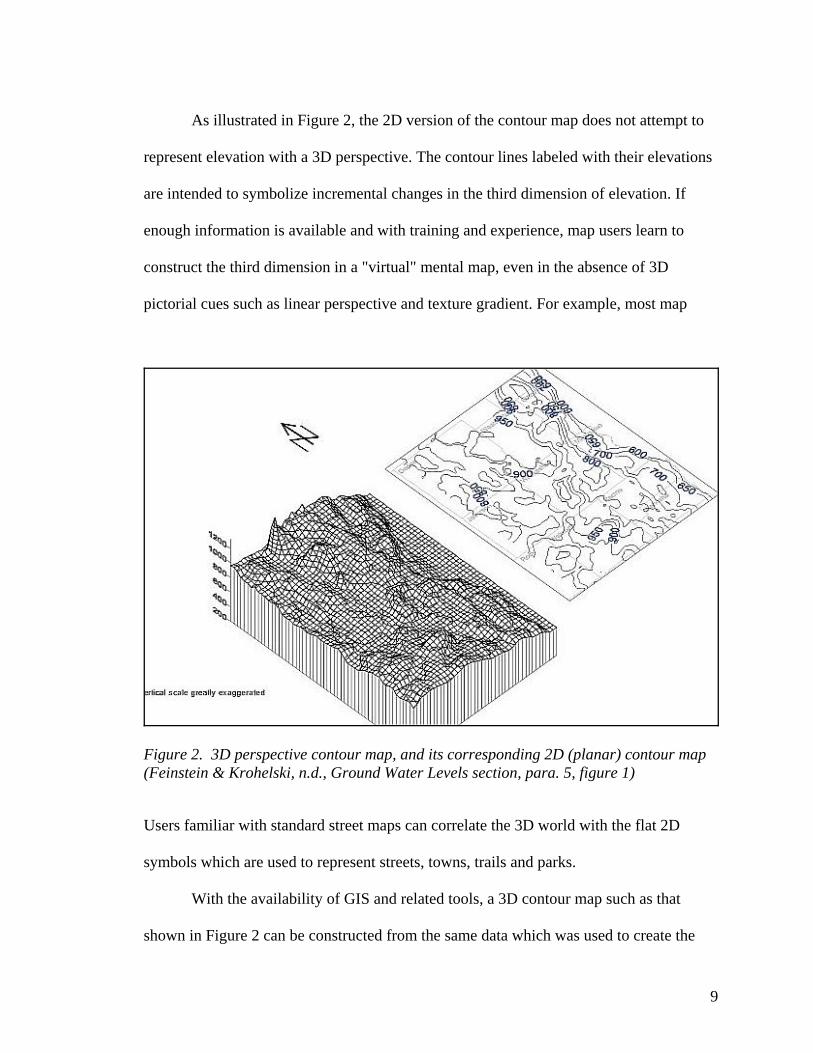
As illustrated in Figure 2, the 2D version of the contour map does not attempt to
represent elevation with a 3D perspective. The contour lines labeled with their elevations
are intended to symbolize incremental changes in the third dimension of elevation. If
enough information is available and with training and experience, map users learn to
construct the third dimension in a "virtual" mental map, even in the absence of 3D
pictorial cues such as linear perspective and texture gradient. For example, most map
Figure 2. 3D perspective contour map, and its corresponding 2D (planar) contour map (Feinstein & Krohelski, n.d., Ground Water Levels section, para. 5, figure 1)
Users familiar with standard street maps can correlate the 3D world with the flat 2D
symbols which are used to represent streets, towns, trails and parks.
With the availability of GIS and related tools, a 3D contour map such as that
shown in Figure 2 can be constructed from the same data which was used to create the

10
2D contour map. If a map with 3D pictorial cues is provided to the map user, the time and
effort required to construct the third dimension mentally may be reduced, thus making it
easier for the map user to visualize relationships between data dimensions, such as
elevation with latitude and longitude (Wickens, Todd and Seidler, 1989). Sometimes this
type of map display is called a 2.5 dimensional map since the third dimension can be
perceived but is not tangible (Kraak, 1988).
Summary and Research Questions
In some types of planning such as park management and park design, experienced
map users (professional planners and natural resource managers) and inexperienced map
users (some of the general public) work together to make decisions. The enhanced
realism of a 3D map may help inexperienced map users to better visualize the shape of
the terrain, and consequently make better, more informed decisions. Simple tasks that do
not require knowledge of terrain shape may be better facilitated by 2D maps. The
following questions were the focus of this study:
1. Are 3D topographic map displays more useful than traditional 2D
topographic maps for planning applications that involve people with a
variety of map experience levels, such as in a park planning public forum?
2. What types of tasks are facilitated by 3D maps, and what tasks are better
supported by 2D maps?
At this point, it is useful to review the literature surrounding displays, task types,
dimensionality and experience, in order to provide a context for understanding this
research. This requires an overview of the theory and recent research regarding task
type/display compatibility, advantages of 2D and 3D displays, and the effect of

11
geographic experience on map understanding and use, which will be provided in the next
chapter. Following the Review of the Literature, Chapter Three outlines the objectives
and hypotheses, Chapter 4 the methods and materials used to perform this study, Chapter
Five presents the results, and Chapter Six concludes with a discussion of the results and
their implications.

12
CHAPTER 2: REVIEW OF THE LITERATURE
This chapter examines the multidisciplinary scholarship and research
underpinning the question of 2D versus 3D map superiority. In order to provide a
necessarily broad foundation, the chapter will be divided into the following topics:
1. Information processing characteristics of experienced versus novice users
2. Perception of three dimensions from a 2D display
3. Separability and integrality of perceptual qualities
4. Display separability, integrality, configurability and emergent features
5. Advantages and disadvantages of a 3D graphical display - research
6. Summary and Hypotheses
Information Processing in Experienced and Novice users
The effectiveness of a specific map for a particular user depends upon the
stimulus characteristics of the map and the user’s interpretation of the map. Data can be
made available in a map, but the data need to be collected, remembered, and integrated
together in order to become information that can successfully be used to solve problems.
The ability to integrate data to create information requires knowledge in the form of
mental models, procedures and facts, as well as cognitive resources of short term memory
and mental processing (Ellis & Hunt, 1993). The users’ mental models, in turn, partially
depend upon their previous knowledge of and experience with maps (McGuinness,
1994).

13
The Expert/Novice Paradigm of map use (McGuinness, 1994) assumes a
distinction between inherent abilities or aptitudes (such as spatial ability, verbal ability,
and visual memory) and expertise. Expertise consists of acquired 1) knowledge about
maps, 2) training in using maps - skill (usually guided practice, especially including
metacognitive strategies for map reading), and 3) unguided practice (experience) –
repeated exposure to map-reading tasks until they become automatic. Consequently,
although spatial ability is assumed to be innate, expertise can presumably be gained
through training and experience. Experienced map users are likely to have more expertise
(i.e. have better knowledge, more efficient control processes (strategies for approaching
map reading) and make better use of personal memory than map users without
experience.
In order to understand why experience may aid in map problem solving, it is
useful to understand how memory, perception and problem-solving strategies work
together. The “information processing approach” to cognition is the metatheory, or
paradigm, currently used to guide research in cognition (Ashcraft, 1989). The
Information Processing Model, originally developed by Atkinson & Shiffrin, (1968), is
the basis for the information processing approach to cognition, and is described below.
The Expert/Novice Paradigm and map-reading
Individual differences in map-reading include ability and aptitudes, experience,
prior knowledge, and training. The Expert/Novice paradigm (McGuinness, 1994) used in
this study focuses on acquired knowledge in contrast to inherent abilities. The
measurement of specific abilities, and their influence on map problem-solving, will be
discussed in a future section.

14
In order to understand why experience might be important, a working concept of
expertise is necessary. The following sections describe the Information Processing
Model of memory, and how expert problem-solvers utilize memory more efficiently than
novices.
Memory and the Information Processing Model
The Information Processing Model of Cognition (Atkinson & Shiffrin, 1968)
illustrates the potential advantages of map-reading experience in geographic problem
solving. These authors conceptualize the human mind as computer: There is input in the
form of perception, attention and processing, storage and retrieval and output, the result
of cognition. The effective and efficient use of memory is important at each of these
stages of information processing.
Memory is where information is held when it is initially received, while it is being
processed, and after it is processed. Memory can be conceptualized as having three parts;
each part providing a different function, and requiring different processing:
1. The Sensory Register,
2. Short-term Store, and
3. Long-term Store.
Initially, a stimulus is received or “input” through one of the six senses and temporarily
held in a very short-term memory area called the “Sensory Register”. The Sensory
Register is where signals are transferred from external input. Attention to information in
the sensory register results in transfer to the Short-term Store (STS). If the stimulus is not
attended to, it will quickly be replaced by new incoming sensations. If this happens, the
stimulus will most likely be lost – the individual will not remember that it was ever

15
perceived (Figure 3.) An example of this would be not hearing someone calling when
focused on reading a book.
“Short-term Store” is also known as Short-term Memory. Information can be
maintained in short term memory by rehearsing (for example, repeating a phone number
in the mind while dialing). Information is lost from short term memory if it is not
subjected to control processes such as rehearsal. The control process of coding transfers
information into Long-term Store. Long-term Store is also known as long-term memory.
Information coded into long term memory does not need to be rehearsed, but does need to
be retrieved (remembered.)
Expert problem solvers use memory more efficiently
Information relevant to problem solving is stored in long-term semantic (factual)
memory, in the form of propositional knowledge and procedural knowledge (Tooling,
1983). Propositional knowledge is the knowledge of concepts and the relationships
between them (Ashcraft, 1989), such as the concepts of contour lines and elevation
changes, and how they relate to each other.
Procedural knowledge can be thought of as skill – knowing how to do something
such as ride a bicycle or read a map (J. R. Anderson, 1983). Reading a map is a skill, and
the expert map reader uses that skill to direct the use of specific information in short-term
memory.
Short-term memory has a limited capacity of between five and nine items (G. A.
Miller, 1956). This limitation implies a restriction on how many items of information can
be held in conscious memory and worked on simultaneously. The short-term memory
limitation can be partially overcome by learning to recognize patterns in information. The

16
larger more complex patterns can be treated as individual items, thus allowing more
information in short term memory. This recognition of information patterns is called
information “chunking” (Atkinson & Shiffrin, 1968). An example of chunking in
topographic map reading would be the ability to recognize the pattern of contour lines
which together indicate a river valley, rather than perceiving the individual lines.
Figure 3. Information Processing Model (Ellis & Hunt, 1993)
Propositional and procedural knowledge together comprise “expertise” as the
term is used in this study. The knowledge of patterns and relationships which is available
in the long-term memory of experienced users allows them to retain more information in
short-term memory. Continuing with the river valley example above, the experienced
user may be able to look at a contour map and see the relationship lines indicating hills
and lines indicating river valleys. Thus the hill and the river valley could be held together
17
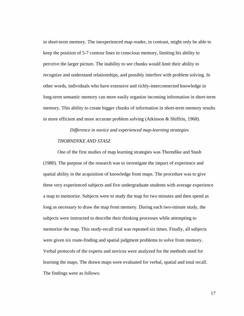
in short-term memory. The inexperienced map reader, in contrast, might only be able to
keep the position of 5-7 contour lines in conscious memory, limiting his ability to
perceive the larger picture. The inability to see chunks would limit their ability to
recognize and understand relationships, and possibly interfere with problem solving. In
other words, individuals who have extensive and richly-interconnected knowledge in
long-term semantic memory can more easily organize incoming information in short-term
memory. This ability to create bigger chunks of information in short-term memory results
in more efficient and more accurate problem solving (Atkinson & Shiffrin, 1968).
Difference in novice and experienced map-learning strategies
THORNDYKE AND STASZ
One of the first studies of map learning strategies was Thorndike and Stash
(1980). The purpose of the research was to investigate the impact of experience and
spatial ability in the acquisition of knowledge from maps. The procedure was to give
three very experienced subjects and five undergraduate students with average experience
a map to memorize. Subjects were to study the map for two minutes and then spend as
long as necessary to draw the map from memory. During each two-minute study, the
subjects were instructed to describe their thinking processes while attempting to
memorize the map. This study-recall trial was repeated six times. Finally, all subjects
were given six route-finding and spatial judgment problems to solve from memory.
Verbal protocols of the experts and novices were analyzed for the methods used for
learning the maps. The drawn maps were evaluated for verbal, spatial and total recall.
The findings were as follows:

18
• Map learning performance and map problem solving performance were
highly correlated, (r = .90, p < .001)
• The experienced users did not necessarily use the most effective map-
learning procedures
In a subsequent experiment to test the efficacy of the learning procedures
discovered in experiment 1, subjects were tested for visual memory aptitude using the
Building Memory test of the Kit of Factor-referenced Cognitive Tests (Ekstrom, French,
Harman, & Dermen, 1976). After being trained in using the effective map-learning
procedures, the improvement in problem-solving and map-memory performance was
higher for those subjects with higher visual memory aptitude as measured by the Ekstrom
test. Although this study was primarily about learning and memory and secondarily
about problem-solving, the implications are as follows:
• Experience may not be as important as training in appropriate map-
learning and map-comprehension procedures
• Visual memory ability interacts with knowledge and the use of appropriate
procedures: Those with lower visual memory aptitude may gain less from
using appropriate procedures than those with higher visual memory
aptitude
GILHOOLY, WOOD, KINNEAR AND GREEN
Two potential issues with Thorndyke and Stasz were noted in Gilhooly, Wood,
Kinnear and Green (1988): The sample size for experiment 1 was three experts and five
novices. This sample size may have been too small to pick up a relationship between
19
experience and performance. The second issue was that Thorndyke and Stasz used
planimetric (non-topographic) maps in their study, while the experienced subjects’
expertise was probably strongest with topographic maps.
In experiment 1 (Gilhooly et al., 1988), 262 undergraduates were tested for
topographic map ability and were given a biographical questionnaire regarding their
previous exposure to topographic maps. The results were used to select the top 30% to
represent the high-skill group, and the bottom 30% to represent the low-skill group in
their study.
The planimetric maps from Thorndyke and Stasz and two topographic maps with
20 foot contour intervals were used in a between subjects design (each subject studied
only one map). Subjects were allowed to study the map for five minutes and were given
ten minutes to draw the map from memory. Finally, each subject answered a 9-item
multiple-choice memory test.
The results indicated that
1. the subjects experienced with topographic maps recalled the topographic
maps better, both in drawing and answering questions
2. The experienced subjects did not recall the planimetric maps better than
the inexperienced subjects.
Experiment 2 of Gilhooly et al. was designed to discover the differences in
thought processes between the experienced and inexperienced subjects. It replicated
Experiment 1 with thinking out loud and a small pointer to indicate where their attention
was directed. The main difference between the experienced and inexperienced subjects’
approaches was that the experienced subjects focused on “specialist’s schemata” such as

20
map feature description and inferring height, both during study and recall. Inexperienced
subjects focused relatively more on place names during study and recall. In summary,
although rich in detailed geographic information, contour maps were found difficult to
read by inexperienced users. The same was not true for planimetric (flat) maps.
WILLIAMSON AND MCGUINNESS
Further evidence that experienced map readers use superior map schema is found
in Williamson and McGuinness (1990). Expert and novice map users were shown
topographic maps and asked to write a five minute description of each map. Most of the
novices listed the map elements by name, or described their color or sometimes their
shape. In contrast, the expert users typically named each element of the map such as a
small forest, a large city etc, described each element, then described the element’s
relationship to other map elements. Additionally, experts tended to identify geographic
locations and used geographic terms to describe map elements (e.g. city 1 is northwest of
a large forest).
A second task had expert and novice map readers sorting maps into categories.
Experienced map readers categorized maps based on their underlying geographic
structure (e.g. a mountainous region), while inexperienced readers chose more superficial
aspects to sort on such as a similar element (e.g. stream, forest) rather than overall
structure of the terrain.
One implication of Williamson and McGuinness is that the expert map readers
have a richer map schema (mental template used to organize information) than do novice
map readers. When asked to categorize a map, the expert’s map schema is activated and
the type of terrain is identified as the map category. Once the schema is triggered for each

21
map category, the map can be analyzed for expected relationships between map elements,
leading to a coherent and integrated map description, as in study 1.
Other studies suggest that a variety of geographic experts benefit from richer map
schema for geographic problem solving. Among these are orienteers (Crampton, 1992)
and advanced college geography students (K. C. Anderson & Leinhardt, 2002; Chang,
Antes, & Lenzen, 1985).
BARSAM & SIMUTIS
The difficulty of visualizing terrain by interpreting topographic maps may inhibit
all but the most spatially talented map readers (Barsam & Simutis, 1984). A group of 60
soldiers with little or no terrain visualization training were tested for spatial ability using
the Kit for Factor-Referenced Cognitive Tests (Ekstrom et al., 1976). The subjects with
spatial ability score .5 standard deviations from the mean of all scores were classified as
having Medium spatial ability; those more than .5 standard deviations above the mean
were classified as High spatial ability, and the rest were classified as Low spatial ability.
All soldiers were given the same one hour computer-based training course.
Following the training, another lesson on Interpretation of Contour Lines was
administered for either active or passive practice. The active practice allowed map
readers to choose contour maps and see the contours as a ground profile. The passive
version displayed random maps and locations, with equivalent ground profile. Finally, a
terrain visualization test was administered to all users.
The most interesting finding of this study was the interaction between spatial
ability and practice. The active practice subjects with high spatial ability had scores
almost double the scores of the high spatial ability subjects and passive practice. The

22
active practice had little or no effect on the performance of the low and medium ability
soldiers. There was no significant difference in performance between the low and
medium ability soldiers, either with or without active practice. That is, only the high-
ability soldiers benefited from the active practice.
From the previously discussed studies, it can be seen that map experience as a
variable appears to have mixed effects on spatial problem solving. Problem solving with
topographic maps is enhanced by both spatial ability and by previous experience with this
type of map. Problem solving with planimetric (flat) maps does not appear to be
influenced by previous map experience. Additionally, knowledgeable problem-solving
strategies appear to be an important factor in problem-solving effectiveness, especially
for those with higher spatial ability.
The next section is a review of the literature of three-dimensional (3D), or depth,
perception, and how a two-dimensional (2D) display can be made to appear three-
dimensional. Depth perception is a result of both pictorial cues such as perspective, and
physical cues such as movement of observer around an observed object. The focus of this
discussion is on pictorial cues, which can be used to enhance a flat display.
Perception of three dimensions from a two-dimensional display
The retina at the back of the eye is a two-dimensional surface, and all light
reflected is imaged there in two dimensions. Depth perception is the result of identifying
visual cues within the image which allow the observer to interpret the retinal image as
three-dimensional (Marr, 1982).

23
Depth cues are connections between the object viewed, the stimulus on the retina,
and the perceived depth of the scene (Goldstein, 1989). Depth cues can be divided into
three types (Goldstein, 1989; Alan. M. MacEachren, 1995; Marr, 1982):
1. Physiological cues, which include accommodation (changes in the thickness
of the eye’s lens resulting from focus on an object), convergence (the
movement of the eyes inward toward or away from each other to view objects
at different distances, and retinal (binocular) disparity. Physiological cues are
not typically helpful when interpreting static images on a flat screen at a fixed
distance from the viewer (the exception might be binocular disparity, which
can be artificially induced using a stereo display and special lenses).
2. Motion cues, which depend on movement on the part of the observer or the
object observed. Movement of the observer around an object, or spinning the
object, provides cues to the dimensionality of the object.
3. Pictorial cues, which include static perspective and non-perspective cues.
The focus of this review will be pictorial cues, as those are the cues which can be
most readily manipulated by altering the map image on the screen.
Pictorial Cues
Linear perspective
In order to display a 3D object on a flat page or display, the 3D object must be
projected onto the 2D surface. (Projection is the process of transforming 3D points into
2D points, to create a drawing or image.) A perspective projection distorts the drawn
object so it more closely matches its appearance in space. This type of projection creates

24
the depth cue of linear perspective, with parallel lines converging as depth along the line
of sight increases. This cue is the major determinant of effective monocular 3D
perspective of an oblique view (Gillam, 1995). One drawback of this type of projection
is the foreshortening of the dimension(s) along the line of sight in relation to the
dimension(s) perpendicular to the line of sight. Notice in Figure 4 that the width
dimension converges on the right vanishing point, while the depth dimension converges
on the left vanishing point. This distortion of the actual dimensions of an object can make
it difficult to evaluate the object’s measurements.
Figure 4. Perspective projection (Bertoline et al., 1997)
In contrast, a parallel projection (Figure 5) has no converging parallel lines,
meaning it preserves the true relationships of an object’s features and edges (Bertoline et
al., 1997).

25
Figure 5. Parallel projection (Bertoline et al., 1977)
With a parallel projection there is no foreshortening, but in a complex image, it
can be difficult to tell which is the foreground and which the background (Wanger,
Ferwerda, & Greenberg, 1992). For this reason, perspective projections are typically used
in oblique 3D map views, and other cues such as grids and overlap are used to
compensate for the resulting distortion.
Overlap and Size and height in the field of view
The size disparity of two or more objects serves as a cue to their relative distance
from the observer. In the absence of other cues, a larger object appears closer to the
observer while a smaller object appears farther away. A related cue is the relative height
of objects within the field of view. For example, if two objects appear on a display, but
one is vertically higher on the display than the other, then the higher object will be
perceived to be farther away.

26
Finally, if an object overlaps another in a display, the overlapping object is seen
as in front of the overlapped object. This relationship works in combination with the
other cues of relative size and relative height in the field of view. For example in Figure
6, the upright timber pointed to by the white arrow is lower and larger than that pointed to
by the black arrow. In addition, the upright timber in the foreground (white arrow)
overlaps the base supporting the rear timber (yellow diagonal arrow). These cues
together allow the perception of the larger lower timber as in front of the shorter, higher
timber in the back.
Figure 6. Size and Height in Field of View (Bertoline et al., 1997)

27
Texture gradient
Texture gradient as a depth cue means that the texture of objects is coarser in the
foreground and is smoother as objects recede (Kraak, 1988). One example of this type of
cue would be in a fishnet map (Alan. M. MacEachren, 1995), as illustrated in Figure 7.
Figure 7. Map illustration showing texture gradient
In a fishnet map at an oblique view, the squares appear larger in the foreground
(lower left) than they do in the background (upper right). This distortion of the mesh size
contributes to the perception that the map tilts forward to the bottom left, and that the top
right corner is more distant.

28
Non-perspective pictorial cues
Shading is a method whereby a map is differentially tinted to imply a light source.
Depending on the location of the light source, different parts of the surface are lightened
as if under direct light, or shaded as if lying in shadow.
Figure 8. Computer-shaded relief map (Muehrcke & Muehrcke, 1998)
In Figure 8, notice that the light source appears to be coming from the upper left – the
29
bright spots on the terrain are lit from the direction, while the areas lower and to the right
of the lit areas are in shadow.
The use of brightness variation and shadow can be useful for visualizing terrain
shape and volume. Many modern GIS can produce 2D or 3D maps with shading,
although it often requires additional processing steps beyond the creation of a typical
topographic map.
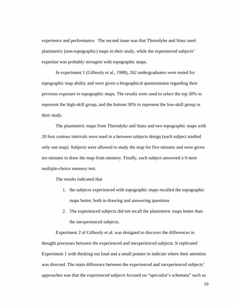
Change of color (Figure 9) toward the blue end of the spectrum is noticeable as
the eye moves from objects close to the observer to objects at great distances. This effect
is the result of atmospheric scattering of the shorter (red) wavelengths as distance
increases. Loss of detail as the eye moves from near objects to objects farther away can
also provide a depth cue (Figure 9). This reduction in detail is due to the limitations of the
human visual system (Kraak, 1988).
Figure 9. Change of color and loss of detail at great distances

30
Summary
The preceding section discussed the various depth cues available to support the
perception of depth in a map. Some or all of these cues can be used to create the
perception of depth in a 3D map on a flat display. The choice of depth cues to be is
dependent upon (Kraak, 1993; Wanger et al., 1992):
1. The effectiveness of the depth cues, separately and together, in
communicating the required information
2. The computational resources available to produce the map
3. The complexity of the information included in the map, and
4. The purpose of the map and the tasks for which it is being created.
Understanding the depth cues available and their various effects is only one aspect
of map design. In deciding what type of map to use to provide information, the map
producer must also take into consideration the type of task for which the map is intended.
The requirements of the tasks to be supported combined with the characteristics of
particular display formats (e.g. 2D versus 3D) determine the type of map to be used for a
specific purpose. The next section discusses the qualities of displays which potentially
contribute to, or interfere with, map usefulness for specific tasks.
Separability, integrality and configurability of perceptual qualities
Some visual displays are easier than others to use for focused tasks – e.g. the
extraction of individual data values – but interfere with being able to see patterns in the
data. Other displays facilitate integrated tasks – e.g. pattern visualization - but make
31
individual data value extraction difficult. The property of a display which facilitates
focused tasks is called separability; the property which facilitates pattern visualization is
called integrality (Garner, 1994).
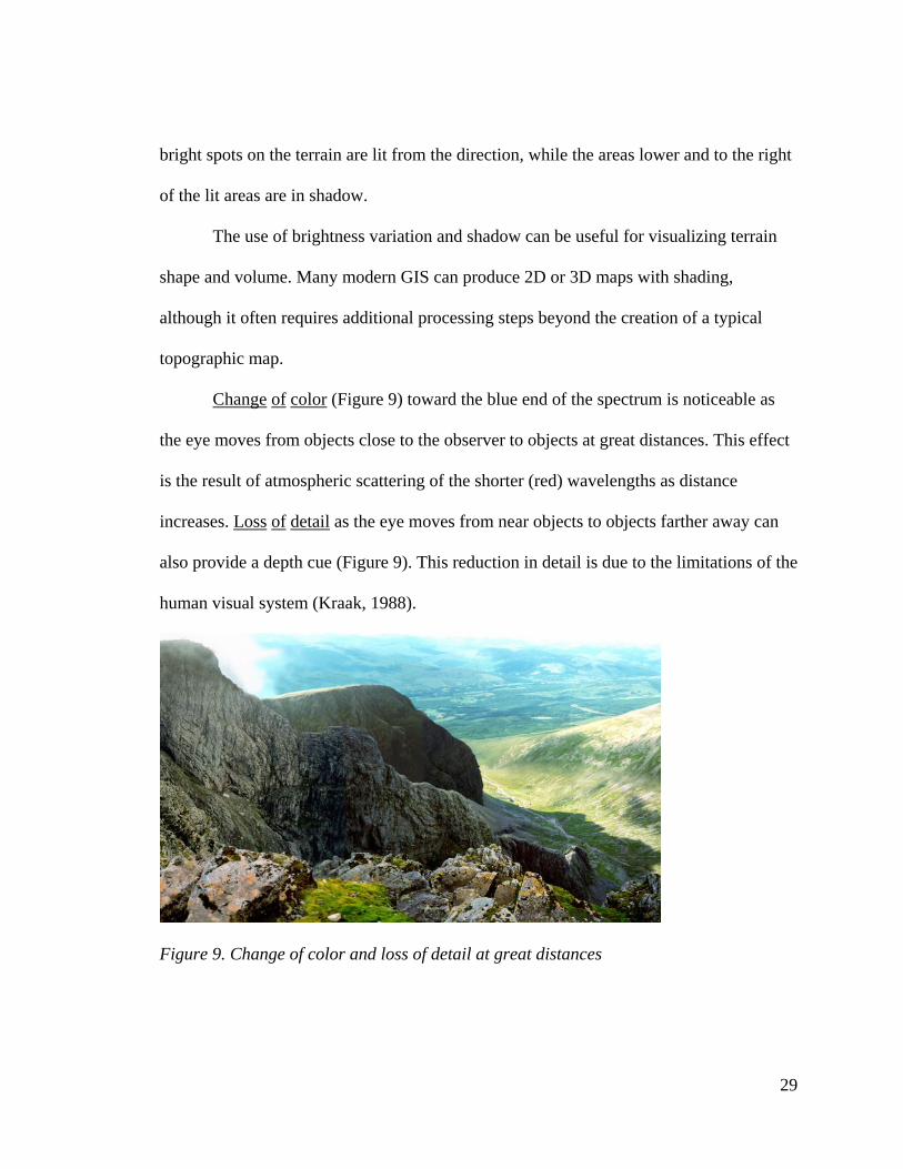
Perceptual separability of qualities
Population
0 100 200 300 400 500 600
Birds
Fish
Birds Fish
Figure 10. Multivariate symbols - animal type and population levels
A given stimulus can have multiple qualities such as color, shape, area and
orientation, each of which can represent a different variable. For example, graduated
symbols such as rectangles can be varied in size to represent differences in population
numbers, while different colored rectangles can represent different types of animals (e.g.
Birds and Fish in Figure 10). The same rectangle has two perceptual qualities, each of
which represents a different variable (number and type) of the same population. These
qualities are separable, because the dimensions of a rectangle are easy to perceive
without attending to the color, and vice versa. (Note: Garner and subsequent authors

32
referred to multiple perceptual qualities of stimuli as “dimensions.” The term “qualities”
is used here to avoid confusion with geographic or spatial dimensions.)
Multivariate symbols have different levels of each perceptual quality, and they
can be sorted into groups based on their varying levels of each quality. The ease with
which stimuli with multiple qualities can be classified into separate groups depends on
both the type of sorting task (sorting on single or multiple qualities) and the ease of
visually separating the qualities (Garner, 1974).
Perceptual integrality of qualities
Some stimuli can have multiple qualities which are difficult to separate perceptually,
such as hue, saturation and brightness. When comparing several circles of different
colors, it would be difficult for most users to quickly choose all the bright circles,
regardless of color. For this reason, these perceptual qualities are called integral qualities,
because they are difficult to separate. There is a time or accuracy penalty in a task that
requires attending to one integral quality while ignoring others. For example, in Figure
11, the circle on the right has the same brightness as the green circle on the left, but the
same hue as the yellow circle. If asked which circle on the left is most similar in hue to
the circle on the right, many observers would choose the green circle.

33
Figure 11.Hue and brightness as integral qualities
Testing for integral and separable stimuli
To determine whether perceptual qualities were integral or separable, Garner used
four different classification (sorting) tasks as benchmarks:
Control task – one quality of the stimulus is varied and the other(s) are held
constant. An example of a control task would be sorting squares by color when all the
squares are the same size.
Filtering (also called selective attention) task – one quality of the stimulus is
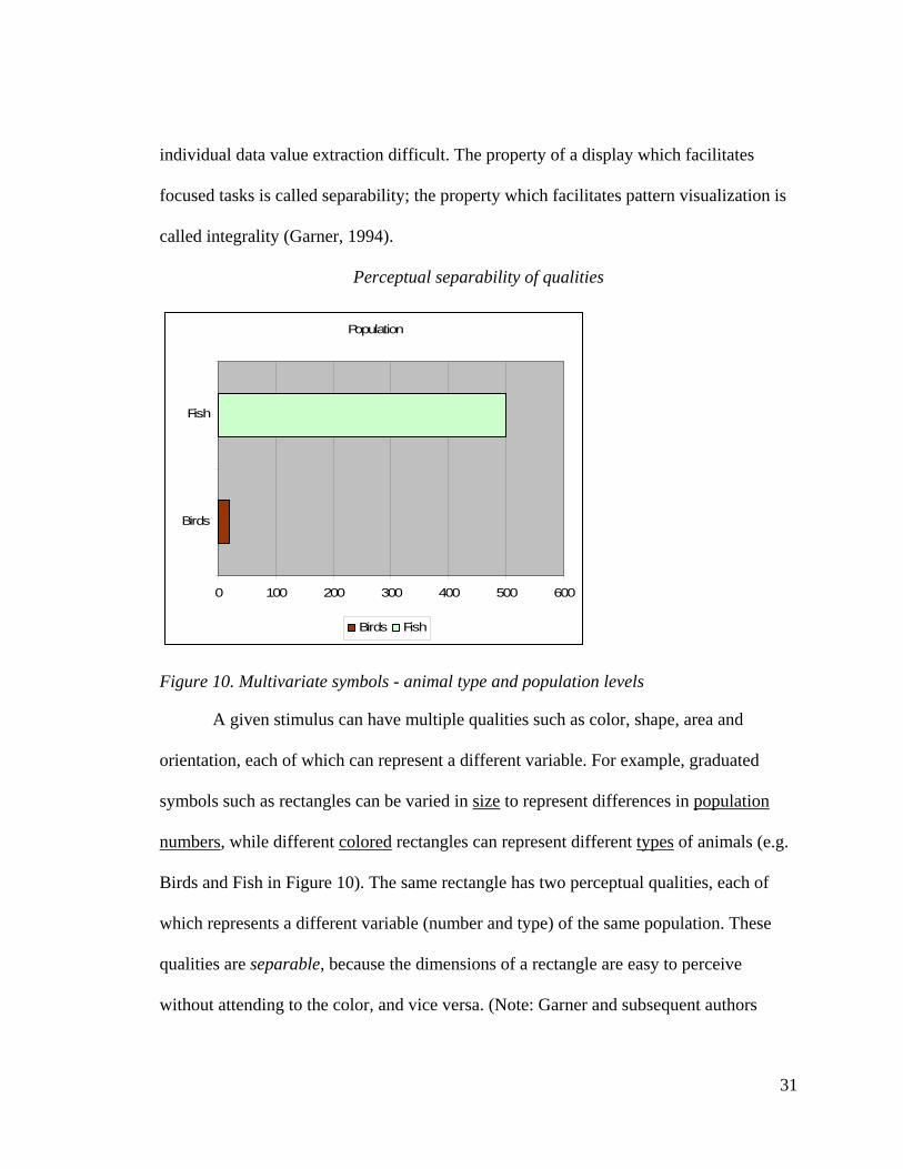
varied (and needs to be attended to) while the other(s) are varied independently. Again
using Figure 12, a filtering task might be sorting by the color of a square (white gray or
black) with the size of the square varying randomly. The quality of size would need to be
ignored in a selective attention task.

34
Redundant task – all qualities are varied in equal proportion, so that any quality
may be attended to. A redundant task using Figure 12 might be sorting squares into
groups of
• small and white
• medium and gray, or
• large and black,
so that either color or size (or both) may be used for sorting.
Divided attention (also called condensation) task – all stimulus qualities are varied
independently, and all must be attended to in order to perform the task (Bennett & Flach,
1992). Using Figure 12, a divided attention task might be a sorting task where the
squares must be sorted based on multiple qualities such as color and size. With three
variations of size and three of color, the stimuli would be sorted into 3x3 or nine groups
(e.g. in Figure 12 black, large squares are one group). The task requires attention to both
qualities at once, requiring the division of attention among qualities (Pomerantz, 1985).
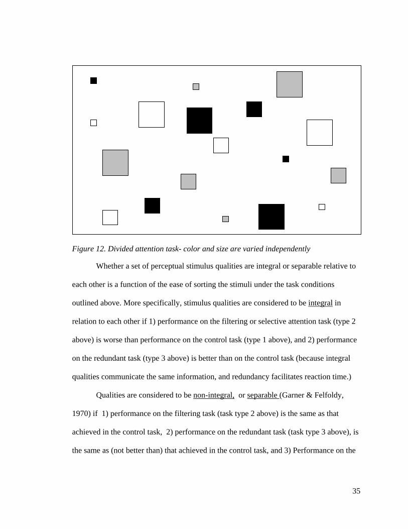
35
Figure 12. Divided attention task- color and size are varied independently
Whether a set of perceptual stimulus qualities are integral or separable relative to
each other is a function of the ease of sorting the stimuli under the task conditions
outlined above. More specifically, stimulus qualities are considered to be integral in
relation to each other if 1) performance on the filtering or selective attention task (type 2
above) is worse than performance on the control task (type 1 above), and 2) performance
on the redundant task (type 3 above) is better than on the control task (because integral
qualities communicate the same information, and redundancy facilitates reaction time.)
Qualities are considered to be non-integral, or separable (Garner & Felfoldy,
1970) if 1) performance on the filtering task (task type 2 above) is the same as that
achieved in the control task, 2) performance on the redundant task (task type 3 above), is
the same as (not better than) that achieved in the control task, and 3) Performance on the

36
divided attention task (type 4 above) is not worse than on the control task when sorting
on one stimulus quality.
Configural stimulus qualities
The classification of stimulus qualities as either integral or separable was a first
step in determining their usefulness for specific tasks. In reality, stimulus qualities are on
a scale between completely integral and completely separable (Garner, 1976). A
completely integral set of qualities could never be perceived as distinct from each other,
while a completely separable set of stimulus qualities would be perceived as separate
stimuli. In addition, Garner later acknowledged the likelihood that some types of
relationships between stimulus qualities could be perceived by subjects as either integral
or separable, depending on the demands of the task to be performed.
Figure 13. A grid can be considered integral or separable- the red dot not clustered with the others

37
A grid can be considered integral in that the crossing of lines forms points. Tasks that
require the recognition of point clusters, as in Figure 13, do not use the individual lines
but instead use relative positions of the dots to solve the problem. A separable task would
be one which requests the dot that is four units below the top of the grid. This task
requires separating the horizontal position from the vertical position, and results in the
choice of the blue dot.
In addition, Garner (1974) described the facilitation that can occur when two
qualities combine to form a new quality which makes the sorting task easier than either of
the intended two qualities alone. If the stimulus quality pairs configured in some way to
form a type of third quality, those pairs that configured had better reaction time on Type
3 tasks. The relationships between separable stimulus qualities which can combine to
form a new quality are called configural. Configural qualities effectively configure
together to add a new quality that facilitates discrimination. Qualities are considered to be
configural (Garner, 1976) if
• Reaction time on the filtering task (task type 2) is worse than that achieved
on the control task, and
• The reaction time on the redundant task (task type 3) is the same or worse
than that achieved in the control task.

38
Table 2. Integral, separable and configural stimulus qualities (Garner, 1976)
Types of Stimulus Quality Interaction
Integral Separable Configural
Reaction Time with orthogonal qualities (Task Type 2 compared to control task)
Worse Same Worse
Reaction Time with redundant qualities (Task Type 3 compared to control task)
Better Same Same
To summarize (Pomerantz & Garner, 1973):
“Separable” qualities do not interact: They can be attended to separately, and do
not incur a filtering cost.
“Integral” qualities strongly interact. When the dimensions must be attended to
separately, there is a cost in reaction time.
“Configural” qualities are related at an intermediate level between Separable and
Integral qualities. The cost of divided attention is sometimes smaller than for Separable
qualities and the cost of filtering is greater than for Separable qualities (Garner, 1976;
Bennett & Flach, 1992).
Configural Displays and emergent features
Garner’s research on perceptual processing of multidimensional stimuli provides
a foundation for research on effective methods for representing multidimensional data

39
(Garner, 1976). Multidimensional data are data that include several variables that are
related, and that need to be used together to perform a task. The effectiveness of the data
display is a function of not only the data dimensions but of the tasks that the data are
intended to support.
There is the potential for more efficient use of time and mental processing
resources when a single stimulus can communicate multiple data variables. Configural
displays are displays that contain stimuli with integral (Garner, 1976) or separable
(Bennett & Flach, 1992) dimensions which can be arranged so as to create emergent
features (Pomerantz & Pristach, 1989).
An emergent feature is the creation of a single feature by combining several
dimensions of the display. An example of an emergent feature might be the configuration
of latitude, longitude and elevation into the emergent feature of terrain shape. If the
display provides the data variables in an integrated form, or in the form of an emergent
feature, then it could provide a perceptual shortcut in performing the task (Pomerantz &
Pristach, 1989). If a task requires integration of information but the data are displayed
separately, information processing time and effort are necessary in order to perform the
integration mentally.
Focused and Integrative Tasks
Bennett and Flach (1992) used the terms “focused” and “integrative” to refer to
the spectrum of problem-solving tasks for which a configural display might be used.
These terms encompass the perceptual processes as well as information processing
requirements of a problem-solving task. The term “focused” is used to refer to tasks that
require extraction of a single value from a multidimensional data display. The term

40
“integrative” refers to tasks that require integration of values from multiple dimensions of
data types (Bennett & Flach, 1992), and is related to the Type 4 task described earlier
(Pomerantz, 1985).
Emergent features may enhance performance in integration tasks if the features
illustrate dimensions that are critical to task performance (Sanderson, Flach, Buttigieg, &
Casey, 1989). The advantage of a configural display is that it may provide support for
both focused and integrative tasks if both the emergent features and their component
dimensions remain perceptually accessible (Pomerantz & Pristach, 1989).
Population
0
10
20
30
40
50
60
70
80
90
1989 1990 1991 1992 1993 1994
Population
Figure 14. Plotted relationship between year and population variables
An example of this advantage is represented in Figure 14, which illustrates the
plotting of a series of x, y (year, population) variables. The chart contains a set of
detached points, but the chart user can easily see the downward trend in population. The

41
imaginary population trend line, shown in Figure 15 as a dotted line, illustrates an
emergent feature – the downward sloping trend of the data series.
Population
0
10
20
30
40
50
60
70
80
90
1989 1990 1991 1992 1993 1994
Population
Figure 15. Emergent feature of trend line, which emerges from separate stimuli
One of the pioneers in the research of emergent features was Christopher
Wickens. Wickens and Andre (1990) tested decision accuracy using 1) individual bar
graphs to represent individual data dimensions, 2) individual rectangles to represent sets
of data dimensions, and 3) integrated rectangle displays to represent all data dimensions
on the same display. The integrated rectangle display resulted in the best accuracy for
decisions requiring integration of cues. At the same time, the integrated rectangle display
did not diminish accuracy in retrospective memory probes of individual values. Other
studies using retrospective memory probes with emergent features (Barnett & Wickens,

42
1988; Bennett, Toms, & Woods, 1993) got similar results.
Shape as emergent feature
0
100
200
300
4001990
1991
1992
1993
BirdsInsectsMammals
Figure 16. Configural line display – trend lines configure to form polygons
As an example, In Figure 16, notice the pink lines representing the trends of insect
population levels between the year 1990 and 1993 (each year is represented by an axis in
the chart). The insect population remained steady between 1990 and 1993, so the four
trend lines form an emergent feature of a square. The square in this case indicates a
steady population level for 1990-1993.
The solid blue lines represent the trends in bird population between 1990 and
1993. The emergent feature created by the trend lines is not a square, because there were
changes in population in each of the years. If the user’s task was to scan a group of
population trend charts to find the ones which indicated decreases in population, the blue

43
figure representing birds can immediately be discriminated from figures indicating
unchanged populations (squares) and from figures representing increasing populations
Other studies have investigated the use of emergent features in a variety of task
types, including situation monitoring tasks, such as monitoring power plants or
manufacturing processes. Using a signal detection task, Buttigieg and Sanderson (1991)
used both global and local (individual sensor) failure indicators in configural and
separable displays similar to those in Figure 16 and Figure 17.
Bar graph with emergent features
0
50
100
150
200
250
300
350
400
450
1990 1991 1992 1993
Birds
Insects
Mammals
Linear(Mammals)
Figure 17. Separable rectangle display illustrating emergent trend line for mammals
Both types of displays were arranged in order to create, or avoid creating,
emergent features. Both configural and separable displays supported better reaction times
and lower probability of false alarms when they were arranged to create emergent
features (Buttigieg & Sanderson, 1991; Sanderson et al., 1989).

44
With tasks varying on a scale between focused and integrative, sets of guidelines
were developed to assist in matching the appropriate displays (integral, separable, or
configural) to each task. Two such related sets of guidelines are called the “Proximity
Compatibility Principle” and the “Semantic Mapping Model.” Both are discussed below.
The Proximity Compatibility Principle
The Proximity Compatibility Principle was originally proposed by Christopher
Wickens (1984) to describe the relationship between task characteristics and display
requirements:
• If a task is integrative (i.e. it requires integration of data dimensions,) then
the display should have integral stimulus dimensions
• If a task is focused (i.e. it requires separate attention to individual data
dimensions,) then stimulus (display) dimensions should be separable
• If a task has both focused and integrative elements and requires both
separate attention to individual data dimensions as well as integration of
data dimensions, then configural display dimensions might be an
appropriate tradeoff. With configural displays, cost of divided attention is
sometimes smaller than for separable dimensions and the cost of filtering
is greater than for separable dimensions.
Although some evidence has been found to support the superiority of 3D integral
displays for integrated tasks, less support has been found for the premise that focused
tasks are better supported by separable displays. For example, referring to Figure 16 and
Figure 17, the focused task of determining bird population in 1992 might be as easily

45
accomplished using the configural line display as the separable bar graph display. Goettl,
Wickens and Kramer (1991) examined focused tasks, and found a slight but significant
advantage for the separable format over the integral format, but Danek and Roubek
(1995) found no difference in error rate between tasks performed with separate bar
graphs and those performed with four-sided geometric figures representing the same
variables.
The Semantic Mapping Model
Rasmussen and Vicente’s Semantic Mapping Model is similar to the Wickens’
Proximity Compatibility Principle, in that it focuses on using the right display for the
right task. The Semantic Mapping Model prescribes compatibility between the salient
features (including emergent features) of the display and the underlying information
requirements of the task (Rasmussen & Vicente, 1989; Vicente & Rasmussen, 1992). It is
not enough for the structure of the task and the dimensions of the display to match. The
task information requirements (including requirements for both integrated and separate
data dimensions) must be specifically met by features in the display. In order to support
task information requirements, integrated displays need to be designed specifically to
support emergent features reflecting information needs, while at the same time supporting
focused task information extraction.
3D maps as configural displays
Horizontal and vertical coordinates of points on a chart were defined as integral
qualities of a single point by Garner and Felfoldy (1970). However, a 2D topographic
map that includes a series of latitude and longitude lines in a grid actually forms a set of

46
points at the intersection of the grid lines, for example, in Figure 18. The grid lines
configure to form a set of regularly spaced points indicating the line intersections, but the
constituent x and y variables can still be processed independently as one of the
intersecting lines.
A single map may be required to support focused tasks such as the extraction of a
single coordinate at a particular location, and it may also be used to determine the terrain
shape in a region surrounding a landmark.
Figure 18. 2D topographic map with latitude and longitude lines and intersection points
According to the Proximity Compatibility Principle and the Semantic Mapping
Model, the best type of map display to support both types of tasks would be a configural
display. In a typical contour map, the z dimension (elevation or altitude) is represented
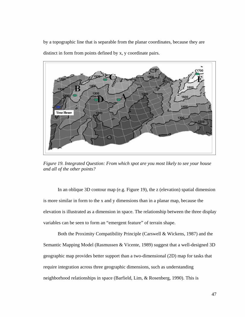
47
by a topographic line that is separable from the planar coordinates, because they are
distinct in form from points defined by x, y coordinate pairs.
Figure 19. Integrated Question: From which spot are you most likely to see your house and all of the other points?
In an oblique 3D contour map (e.g. Figure 19), the z (elevation) spatial dimension
is more similar in form to the x and y dimensions than in a planar map, because the
elevation is illustrated as a dimension in space. The relationship between the three display
variables can be seen to form an “emergent feature” of terrain shape.
Both the Proximity Compatibility Principle (Carswell & Wickens, 1987) and the
Semantic Mapping Model (Rasmussen & Vicente, 1989) suggest that a well-designed 3D
geographic map provides better support than a two-dimensional (2D) map for tasks that
require integration across three geographic dimensions, such as understanding
neighborhood relationships in space (Barfield, Lim, & Rosenberg, 1990). This is

48
illustrated by Figure 19. It is less clear whether a 3D map or a 2D map would provide an
advantage for focused tasks, which require the extraction of a single data value in one
geographic dimension.
Some evidence for 2D map superiority for both focused and integrative tasks has
been found in Hollands, Pierce, & Magee (1995), which showed an accuracy advantage
for 2D graph displays, even for Integrative tasks. Although the Proximity Compatibility
Principle predicts that focused attention tasks are better performed with separable
displays (Goettl, Wickens, & Kramer, 1991, for example), other studies have found no
advantage for 2D over 3D displays when scales and tick marks were used to facilitate
data extraction (Bennett, Payne, Calcaterra, & Nittoli, 2000; Dolan, 1991); Meserth &
Hollands, 1999).
Advantages and disadvantages of 3D graphics on 2D displays
Advantages of a 3D display
Maps can provide three possible types of information (A. M. MacEachren, 1991):
• Declarative – facts about locations
• Procedural – how-to information regarding navigation, e.g. how to get
from one place to another
• Configurational – relative locations, geographic patterns, relationships
The requirements of the tasks to be supported by the map determine the type and
complexity of information which must be extractable, which in turn determines the
potential usefulness of 3D depth cues (Kraak, 1993). In a report on the use of 3D
displays, Wickens, Todd and Seidler (1989) outlined three arguments for their use:

49
1. 3D images are more interesting and aesthetically appealing than 2D images
2. The 3D representation may be more “natural” than the 2D representation, since its
appearance more closely resembles 3D reality.
3. The 3D representation, to the extent that it resembles reality, requires less human
information processing, since the user does not need to construct the third
dimension in order to have an accurate mental model.
Orthographic views of 3D objects were displayed and used to solve problems.
Participants were able to choose isometric views of those objects whose problems they
had solved correctly. This implies that the participants were creating 3D mental models to
correctly solve problems (Cooper, 1990).
Potential Advantages of a Flat Topographic Map
Some evidence for 2D map superiority for both focused attention and integrative
tasks has been found (Hollands et al., 1995). In fact, 3D perspective displays can
introduce problems due to foreshortening of the depth (y) of maps when they are tilted at
an oblique angle (Smallman, St. John, & Cowen, 2002).
Other studies have found little or no advantage for 2D over 3D displays when
scales and tick marks were used to facilitate data extraction (Bennett et al., 2000; Meserth
& Hollands, 1999). Haskell and Wickens (1993) found that for integrative 3D spatial
tasks, a 3D perspective (oblique) display may be preferable to a 2D display, and for tasks
requiring focused attention, 2D separable or separate displays may be better.
Experience with 2D maps may reduce or eliminate any advantages to be gained
from the 3D maps. Experienced users were found to be more accurate in judgment of

50
relative elevation, and appeared to recognize landscape patterns (because of “chunking”)
(Chang et al., 1985)
A series of studies attempting to design more effective aviation navigation
displays found that experienced flight controllers did better with 2D than 3D in
navigation tasks (Boyer, Campbell, May, Merwin, & Wickens, 1995). In contrast,
previous experience with 3D maps can improve performance with 2D maps. The reverse
was not found to be true - prior experience with 2D maps did not facilitate the use of 3D
maps (Campbell, May, & Wickens, 1995). In the same study (Campbell et al., 1995),
navigation judgments were found to require more time with 3D maps than with 2D. In
addition, research has shown that 2D can be superior to 3D topographic maps for precise
relative positioning tasks, but not for shape understanding. (St. John, Cowen, Smallman,
& Oonk, 2001; St. John & Smallman, 2000)
Finally, the potential exists for a 3D topographic map to interfere with the
extraction of data values in a simple focused task. Carswell, Frankenberger and Bernard
(1991) investigated the effect of the third dimension in a line, bar or pie graph when it
was superfluous to the task – i.e. it was not used to display a task variable. They found
that using 3D graphs resulted in time and accuracy decrements when the third dimension
did not represent required data.
Summary
There is much interest in the potential for use of 3D topographic representations
to enhance terrain shape visualization. Among the areas of interest for 3D topographic
maps are planning functions such as natural resource management and park design. 2D

51
topographic maps are currently the most popular products used for these types of
functions.
Could the simple projection of the traditional topographic map into a 3D image
enhance visualization in planning functions? This question is the focus of the following
chapters.

52
CHAPTER 3: OBJECTIVES AND HYPOTHESES
The objectives of this study were the following:
1. To investigate whether the addition of shape (but no other 3D cues
such as shadows) to the traditional 2D topographic maps is enough to
gain the advantages of 3D for shape understanding, while retaining
the relative positioning advantage of the 2D map.
For this purpose, all of the traditional characteristics of the 2D topographic maps were retained: equally spaced latitude and longitude lines with numeric labels, elevation measured in isolines with numeric labels, and graduated shading from dark (low elevations) to light (high elevations). In addition, the 3D representations consisted of the 2D maps “draped” over the terrain.
2. To evaluate whether task type affects the relative advantages of 2D
versus 3D.
Tasks were of two types: • Focused Tasks – which require specific/focused information to
perform. These tasks are similar to the relative position tasks in St. John , Cowen et al. (2001) and
• Integrative Tasks – which require holistic/integrative information to perform. These tasks are similar to the shape understanding tasks used in St. John, Cowen et al. (2001).
Table 3. Mapping of Focused and Integrative tasks to Relative Position (RP) and Shape Understanding (SU) Tasks (St. John, Cowen et al., 2001).
Elevation Non-Elevation
Focused A-high-B (RP)
A-to-B (RP)
Task Type
Integrative A-see-B (SU) ----------

53
3. To analyze the effect of task requirements (whether the task requires
information about the third dimension) on the effectiveness of 2D
versus 3D maps, and
4. To examine the effect that experience with topographic 2D maps has
on the relationships between map dimensions, elevation relevance
(whether knowing elevation information is required to perform the
task) and task type.
The research is divided into two studies:
1. Study 1 investigates the effects of dimensionality, task requirements, and
task type on the effectiveness of 2D versus 3D displays with novice
participants, addressing objectives 1-3.
2. Study 2 is a repetition of Study 1, but with the addition of experience level
as an independent variable, and addressing objective 4.
Hypotheses for Study 1
Hypothesis 1:
For focused questions about a single value of latitude or longitude (not
elevation) at a single location, the flat 2D map and the 3D map are equally effective.
In this study the grid marks should support the separability of the spatial dimensions of latitude, longitude, and elevation (see Figure 20).

54
Hypothesis 2:
For Focused questions of a single value of elevation at a single location, the
3D map is more effective.
Additional cognitive processing effort is required to extract the third dimension of elevation from a 2D topographic map (see Figure 21).
Hypothesis 3:
For Integrative tasks to determine distance relationships between three or
more points in a 2D space, the 2D map is more effective than the 3D map (see Figure
22).
Because elevation information is not required for these tasks, the simplicity of the 2D map better supports the 2D task.
Hypothesis 4:
For terrain shape integrative tasks, the 3D map is most effective.
Additional information processing is required in order to project a 2D map into a 3D mental image in order to solve the problem (see Figure 23).

55
Figure 20. Example of a focused question about a single value of latitude or longitude (not elevation) at a single location – “Question: How far east is the blue point (east from “zero” or 0 East)?”

56
Figure 21. Example of a focused question about a single value of elevation at a single location – “Question: Which point shown above represents the lowest lying area (the lowest elevation)?”

57
Figure 22. Integrative task to determine distance relationships between three or more points in a 2D space “Question: Which point is the farthest distance EAST from the blue point?”

58
Figure 23. Integrative task to determine terrain shape – “Question: From which spot are you most likely to see your house and all of the other points?”
59
Hypothesis for Study 2
Hypothesis 5: For experienced users, the advantage of a 3D map will be less than
for novice users.
Experienced topographic map users should easily visualize the relative elevation
information contained in a 2D topographic line map.
Study Delimitations
In order to isolate dimensionality from the effects of color and shading, this
research intentionally omitted those. Shading of different elevations was done in
grayscale for both types of maps, and no light source shading or textures were used to
enhance the dimensional appearance of the displays. In addition, 3D maps were created
by extruding the 2D versions of the maps, in an attempt to reduce the differences between
them that might be due to factors other than dimensionality. Consequently, the results of
this research are limited in application to those situations were light shading; texture and
color are not used to enhance 3D appearance.
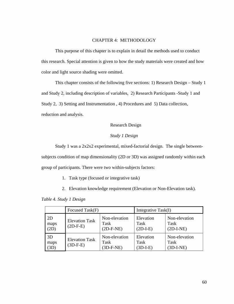
60
CHAPTER 4: METHODOLOGY
This purpose of this chapter is to explain in detail the methods used to conduct
this research. Special attention is given to how the study materials were created and how
color and light source shading were omitted.
This chapter consists of the following five sections: 1) Research Design – Study 1
and Study 2, including description of variables, 2) Research Participants -Study 1 and
Study 2, 3) Setting and Instrumentation , 4) Procedures and 5) Data collection,
reduction and analysis.
Research Design
Study 1 Design
Study 1 was a 2x2x2 experimental, mixed-factorial design. The single between-
subjects condition of map dimensionality (2D or 3D) was assigned randomly within each
group of participants. There were two within-subjects factors:
1. Task type (focused or integrative task)
2. Elevation knowledge requirement (Elevation or Non-Elevation task).
Table 4. Study 1 Design
Focused Task(F) Integrative Task(I)
2D maps (2D)
Elevation Task (2D-F-E)
Non-elevation Task (2D-F-NE)
Elevation Task (2D-I-E)
Non-elevation Task (2D-I-NE)
3D maps (3D)
Elevation Task (3D-F-E)
Non-elevation Task (3D-F-NE)
Elevation Task (3D-I-E)
Non-elevation Task (3D-I-NE)

61
Table 4 shows the eight cells of the design. The two rows illustrate the between-
subjects variable of map dimensionality:
• 2D or
• 3D
.
The first within-subjects variable was task type, represented by the two main
columns in Table 4, were:
1. Focused task (F) – a task requiring the extraction of a single data value
from a single geographic object. An example might be to report the
latitude of point “A”.
2. Integrative task (I) – a task requiring the integration of information about
several geographic objects and their relationships with each other in order
to perform the task, for example, “Which point shown is the farthest from
point A?”
Within each task type (focused or integrative) there were two levels of elevation
knowledge requirement:
1. Elevation task (E) – a task requiring knowledge of elevation of a point or
points in order to perform the task.
2. Non-elevation task (NE) – a task that does not require the knowledge of
elevations in order to successfully perform it.

62
Consequently, there are four question types, resulting from the crossing of the
above levels of variables:
1. An F-E task requires extraction of the elevation value at a point.
2. An F-NE task requires extraction of a latitude or longitude (not elevation)
value at a point.
3. An I-E task requires solving a problem involving integration of latitude,
longitude and elevation over several points; in other words, understanding
of terrain shape.
4. An I-NE task requires solving a problem involving relative position of
several points within 2D space, i.e. does not involve elevation.
There were five questions in each cell, for a total of twenty questions per
participant.
Study 2 Design
The design for Study 2 was similar to study 1, but included the additional between
subjects factor of experience with topographic maps. The design was a 2x2x2x2 mixed
factorial design, with 2 types of maps (2D and 3D) and two levels of experience: Low
(LE) and High (HE) between subjects. The within-subjects factors were task type (F or I)
and elevation requirement of task (E or NE), as in study 1.

63
Table 5. Study 2 design
Focused Task(F) Integrative Task(I) 2D maps (LE-2D) Elevation Task
(LE-2D-F-E)
Non-elevation Task (LE-2D-F-NE)
Elevation Task (LE-2D-I-E)
Non-elevation Task (LE-2D-I-NE) Low
Experience (LE) 3D maps
(LE-3D) Elevation Task (LE-3D-F-E)
Non-elevation Task (LE-3D-F-NE)
Elevation Task (LE-3D-I-E)
Non-elevation Task (LE-3D-I-NE)
2D maps (HE-2D) Elevation Task
(HE-2D-F-E)
Non-elevation Task (HE-2D-F-NE)
Elevation Task (HE-2D-I-E)
Non-elevation Task (HE-2D-I-NE) High
Experience (HE) 3D maps
(HE-3D) Elevation Task (HE-3D-F-E)
Non-elevation Task (HE-3D-F-NE)
Elevation Task (HE-3D-I-E)
Non-elevation Task (HE-3D-I-NE)
Table 5 shows the sixteen cells of the design. The four rows illustrate the
between-subjects variables of map dimensionality and experience:
1. Low Experience 2D (LE-2D)
2. Low Experience 3D (LE-3D)
3. High Experience 2D (HE-2D)
4. High Experience 3D (HE-3D)
.
The within-subjects variables were task type and elevation knowledge
requirement, represented by the four columns in Table 5 as:
5. An F-E task requires extraction of the elevation value at a point.
6. An F-NE task requires extraction of a latitude or longitude (not elevation)
value at a point.

64
7. An I-E task requires solving a problem involving integration of latitude,
longitude and elevation over several points; in other words, understanding
of terrain shape.
8. An I-NE task requires solving a problem involving relative position of
several points within 2D space, i.e. does not involve elevation.
There were six questions in each cell, for a total of twenty –four questions per participant.
The dependent variables for both studies were speed and accuracy. Participants
were instructed to proceed as quickly but as accurately as possible through the tasks, and
the average time and percent correct was calculated for each cell of the design.
Participants
The study participants came from a convenience sample of college classes whose
professors were willing to give up a class period for this study. For each study, the level
and type of classes are described, and the students’ genders are noted. The students’ self-
description on an ordinal scale as shown in Figure 24 (1=no experience, 5=highly
experienced) of their own contour map experience, as well as their spatial ability, was
analyzed using a one-way ANOVA, in order to determine if the classroom groups could
be treated as coming from a single population.
Study 1 Participants
The Study 1 participants were undergraduates taking freshman/sophomore level
introductory Parks and Recreation courses. A total of three groups were used, one class
taught by Professor ‘1’ (Group A) and two taught by Professor ‘2’ (Groups B and C).
This convenience sample was selected because it represented the majority of underclass
students in the PRTM program, and because permission from the professors was readily

65
obtained. Group A had 5 females and 23 males for a total of 28 participants, Group B had
3 females and 11 males for a total of 14 participants, and Group C had 4 females and 20
males for a total of 24 participants.
The short survey given to all participants included the following question to
provide a rough idea of the participants’ previous experience with contour maps:
Figure 24. Self-assessed experience question
The self-assessed experience levels of the three groups were analyzed using a
one-way ANOVA. This analysis failed to show a significant difference in self-assessed
experience level between groups, F(2,63) = 1.47, p= .24.
Which of the following statements best characterizes your experience with contour maps (circle 1):
1. I don’t know what they are, or I have not used contour maps in any context (classwork, professional work, orienteering, etc.).
2. I have used a contour map either in a class or in my work, but only once or twice.
3. I have used a contour map more than once or twice, but I would not consider myself an experienced user.
4. I consider myself an experienced user of contour maps, but not an expert 5. I consider myself an expert in using contour maps ( As good as or better
than 95% of the general population).

66
Table 6. ANOVA summary table for study 1 novices – relationship between group and experience level
SUMMARY Groups N Female Male Sum Mean Variance Group A 28 5 23 66 2.36 1.05 Group B 14 3 11 29 2.07 0.69 Group C 24 4 20 46 1.92 0.775 ANOVA – Experience Level Source SS df MS F P-value F crit Between Groups 2.58 2 1.29 1.47 0.24 3.14 Within Groups 55.19 63 0.88 Total 57.77 65 __________________________________________________________________
The Spatial Ability of the three groups was measured using the Factor VZ:
Visualization - Paper Folding Test -- VZ-2, in Kit of Factor-Referenced Cognitive Tests
(R. B. Ekstrom et al., 1976). The resulting scores for the three groups were analyzed
using a one-way ANOVA. No significant difference was found between groups, F(2,63)
= .47, p=.63.
Table 7. ANOVA summary table for study 1 novices – relationship between group and spatial ability
SUMMARY __________________________________________ Groups N Sum Mean Variance Group A 28 314 11.21 8.40 Group B 14 146 10.43 7.65 Group C 24 276 11.50 16 ANOVA – Spatial Ability Source SS df MS F P-value F crit Between Groups 10.34 2 5.17 0.47 0.63 3.14 Within Groups 694.14 63 11.02 Total 704.48 65

67
Study 2 Participants
Participants in study 2 were of two types: Novice and Experienced. The novice
group was a convenience sample, consisting of an undergraduate class of environmental
science majors, mostly freshmen and sophomores, all with one professor.
Study 2 novices
The self-assessed experience levels of the novices in study 1 and study 2 were
compared using a one-way ANOVA. This analysis revealed a significant difference in
self-assessed experience level between novices in the two studies, F(1,96) = 8.88, p=
.004, with study 2 novices assessing themselves as more experienced than the study 1
novices.
Table 8. Study 2 novice participants
N Females Males
Experience- Scale of 1 (none) to 5 (high)
Spatial Ability (Out of 20)
32 14 18 2.75 14.03

68
Table 9. ANOVA summary table – relationship between Study 1 and Study 2 novices in experience
SUMMARY Groups N Sum Average Variance Study 1 66 141 2.14 0.89 Study 2 32 88 2.75 0.97 ANOVA – Experience Level Source SS df MS F P-value F crit Between Groups 8.11 1 8.11 8.88 0.0037 3.94 Within Groups 87.77 96 0.91 Total 95.89 97
The Spatial Ability of the participants in study 2 was assessed using the Factor
VZ: Visualization - Paper Folding Test -- VZ-2, in Kit of Factor-Referenced Cognitive
Tests (R. B. Ekstrom et al., 1976). The spatial ability of the novices in the two studies
was analyzed for differences using a one-way ANOVA. There was a significant
difference in spatial ability between novices in the two studies, F(1,96) = 16.70,
p=.00009, with study 2 novices scoring higher in spatial ability.
Table 10. ANOVA summary table – relationship between Study 1 and Study 2 novices in spatial ability
SUMMARY Groups N Sum Mean Variance Study 1 66 736 11.15 10.84 Study 2 32 449 14.03125 10.42 ANOVA – Spatial ability Source SS df MS F P-value F crit Between Groups 178.72 1 178.72 16.70 .00009 3.94 Within Groups 1027.45 96 10.70 Total 1206.17 97

69
Study 2 experienced participants
The Study 2 experienced participant group was also a convenience sample from a
selection of professors in the department of Landscape Architecture who volunteered
their classes. There were four classroom groups. Group A was a group of junior and
senior undergraduates taking an intermediate level class in Landscape Architecture.
Groups B and C were first year graduate students taking a more advanced level
laboratory in Landscape Architecture. Group D were graduating Landscape Architecture
graduate students working on their final project, plus one interested professor (AR).
The self-assessed experience levels of the four groups were analyzed using a one-
way ANOVA. A significant difference was found between groups, F(3,40)=3.33, p=.03,
with Group D (the most advanced group) having the most self-assessed experience.
Table 11. ANOVA summary table for study 2 experienced groups – relationship between group and self-assessed experience level
SUMMARY Groups N Females Males Sum Average Variance Group A 12 3 9 48 4 0 Group B 11 7 4 39 3.55 0.27 Group C 12 5 7 48 4 0.55 Group D 9 4 5 39 4.33 0.5 ANOVA – Experience Level Source SS df MS F P-value F crit Between Groups 3.18 3 1.06 3.33 0.03 2.84 Within Groups 12.72 40 0.32 Total 15.91 43
The spatial ability of the four experienced groups as measured by the paper-
folding test was also analyzed using a one-way ANOVA. This analysis showed no
significant difference in spatial ability between groups, F(3,40) = .72, p= .54.

70
Table 12. ANOVA summary table for study 2 experienced groups – relationship between group and spatial ability
SUMMARY Groups N Females Males Sum Mean Variance Group A 12 3 9 161 13.42 10.08 Group B 11 7 4 144 13.09 7.29 Group C 12 5 7 144 12 10.54 Group D 9 4 5 126 14 15.5 ANOVA – Spatial Ability Source SS df MS F P-value F crit Between Groups 22.97 3 7.66 .72 0.54 2.84 Within Groups 423.83 40 10.60 Total 446.80 43
The gender data within each group is provided as part of the background
information about the participants. Because gender is not a variable controllable by the
map maker, gender was not a specific variable of interest in this study, and so was not
analyzed as a variable.
Setting and Apparatus
Computer Labs and displays
Study 1 was conducted in two computer labs within the College of Natural
Resources. Each lab was equipped with Dell Optiplex ™ GX110 Pentium III 800Mhz
computers with 512Mb of Memory and 19” color displays. All questions were displayed
at 800x600 resolution.
Study 2 novices used the same computer labs as the study 1 participants, while
Study 2 experienced participants used the same computer setup in the College of Design,
except the lab was smaller (two rows of four computers each, and two rows of five
computers each.)

71
Task Material Packets
The study packets consisted of the informed consent form (Appendix 1), a brief
survey (Appendix 2), the paper folding test (R. B. Ekstrom, French, & Harmon, 1976)
and a diskette with the Visual Basic program that administered the tasks. The details and
creation of the study packet components are outlined below.
Informed Consent
A brief description of this study, its requirements, and its purpose was read to the
group of participants, and included in the informed consent form. Participants were
reminded that the data were to be kept confidential, that they could stop their
participation without penalty, and that they could receive their results upon request. The
name and phone number of the researcher were given, and a duplicate copy was provided
for the benefit of the participants.
Survey
The survey was very brief and consisted of four questions: 1) The participant’s
gender 2) their evaluation of their own experience level (from A – don’t know what a
contour map is, to E – I consider myself an expert on contour maps) 3) Do you have any
type of color blindness?, and 4) what types of previous experiences you have had with
map reading (orienteering, Boy or Girl Scout instruction, Geography, GIS or other class,
and other map-reading experiences).
Spatial ability (paper-folding) test
The spatial ability test is more explicitly a spatial visualization test. Its purpose is
to examine the ability to mentally manipulate objects, and choose the appearance of the
end result from a sequence of figures (R. B. Ekstrom, French, & Harman, 1979). Since it

72
is unclear whether this is an innate ability or one which grows with experience, it was
decided to treat spatial ability as a covariate in this study.
The Factor VZ: Visualization - Paper Folding Test -- VZ-2. In Kit of Factor-
Referenced Cognitive Tests (R. B. Ekstrom et al., 1976) was used to assess spatial ability
in the participants. The test consisted of 2 sets of 10 problems each. Three minutes was
allowed for the completion of each section. Each problem on the paper folding test
consists of a series of images representing paper being folded, and a hole being punched
somewhere in the folded paper. The participant was to select the figure on the right which
represented the paper after it had been punched and unfolded again. The score for each
participant is the sum of correct answers on both sections of the test. Sample results are
provided in manual for the test (Ruth B. Ekstrom et al., 1976). (Note: The test materials
are copyrighted: Please reference the Kit of Factor-Referenced Cognitive Tests for the
actual paper folding test items.)
Maps
The purpose of this research was to determine under what conditions 3D maps are
superior to 2D maps in supporting task performance. One enhancement commonly made
to 3D representations is to add hill shading. Hill shading is the creation of shadows in the
image based on a model of illumination, in order to enhance the realism of its 3D
appearance (Weibel & Heller, 1992) e.g. Figure 8. However, hill shading provides clues
to terrain shape that would not necessarily be available in a 2D topographic map.
In order to isolate the effects of dimensionality from other potentially
confounding effects, the decision was made to eliminate color variation and hill shading

73
from the list of potential confounds. Instead, simple graduated grayscale shading (e.g.
Figure 1 and Figure 18) was used to emphasize the elevation changes between contour
lines and both the 2D and 3D maps.
MAP CREATION OVERVIEW
The task maps were created from USGS Digital Elevation Maps (DEMs) of
Western North Carolina counties (see “Appendix 3: The Questions” for the actual source
DEMs and the resulting maps). Contour lines were created from elevation data, shaded,
labeled, and then “draped” over a terrain image derived from elevation (Z) values at
regular intervals. Each 3D image was tilted to an angle which would allow the correct
answer to be perceived. Five tasks of each type were created (e.g. Figure 20 through
Figure 23):
1. Focused, elevation - 5 questions – images and questions in “Appendix 3,
Items 1-5 and 24: Focused, Elevation Inclusive”
2. Focused, no elevation - 5 questions – images and questions in “Appendix
3, Items 16-20 and 23: Focused, Elevation Exclusive”
3. Integrative, elevation - 5 questions – images and questions in “Appendix
3, Items 6-10 and 24: Integrative, Elevation Inclusive”
4. Integrative, no elevation - 5 questions – images and questions in
“Appendix 3, Items 11-15 and 22: Integrative, Elevation Exclusive”
Each of the maps used in this experiment was created in both 2D and 3D from the
same source dataset. The 2D and 3D maps consisted of four layers: 1) a TIN
(Triangulated Irregular Network), which provided the shape of the 3D maps (2D maps
were flat, meaning the Z or elevation dimension of the TIN was not used in map

74
creation), 2) A thematic map layer, where grayscale shading is from low(black) to
high(white), 3) a contour line layer, which provided the contour lines and shading, and 4)
an XY grid used to mark units of distance on the map. The details for creating each
layer of map are described below, and were derived from an article on DEM use in
ArcUser Journal (D. Miller, 1999).
THEMATIC MAP AND CONTOUR LINE CREATION
The maps were created from USGS 1:24,000 DEMs (Digital Elevation Model)
(USGS, 2000) of Counties in Western North Carolina in 30 meter resolution. (See
Appendix 3 for the exact coordinates of each task’s map.)

75
Projection: State Plane 1983
Map Units: meters
Datum: NAD 83
The DEMs were downloaded in ESRI ArcInfo™ interchange (.e00) format, and
converted to coverages using the ESRI ArcView™ Import71 utility. Each coverage was
opened in ArcView 3.2 ™ with Spatial Analyst extension, USGS DEM file type, and
then saved as an ArcView project. The grayscale shading was created by selecting the
elevation value as the classification field, and specifying a range size of 100 (as shown in
Figure 25).
Figure 25.Thematic map- classified into 100 ft elevation changes
The contour lines were created by selecting contour maps from the Spatial
Analyst surface menu, and selecting a contour interval of 100 (see Figure 26 for an
example).

76
Figure 26. Contour lines for map shown in Figure 25
TIN CREATION
The TIN (Triangulated Irregular Network) is a data model for storing surfaces as
triangles with varying orientations (Price, 2004). In this study, a TIN was used as the
definition of the surface over which the contour map and coordinate grid were draped.
The TIN was created by selecting “Features” from the “Surface” menu in Spatial Analyst,
then selecting “Create TIN,” with the contour layer specified as the height source.
COORDINATE GRID CREATION
Using the Coordinate Grid Maker Extension (Feldkotter, 2003) for ArcView,
several coordinate grids were created for each county. The grids were created over the
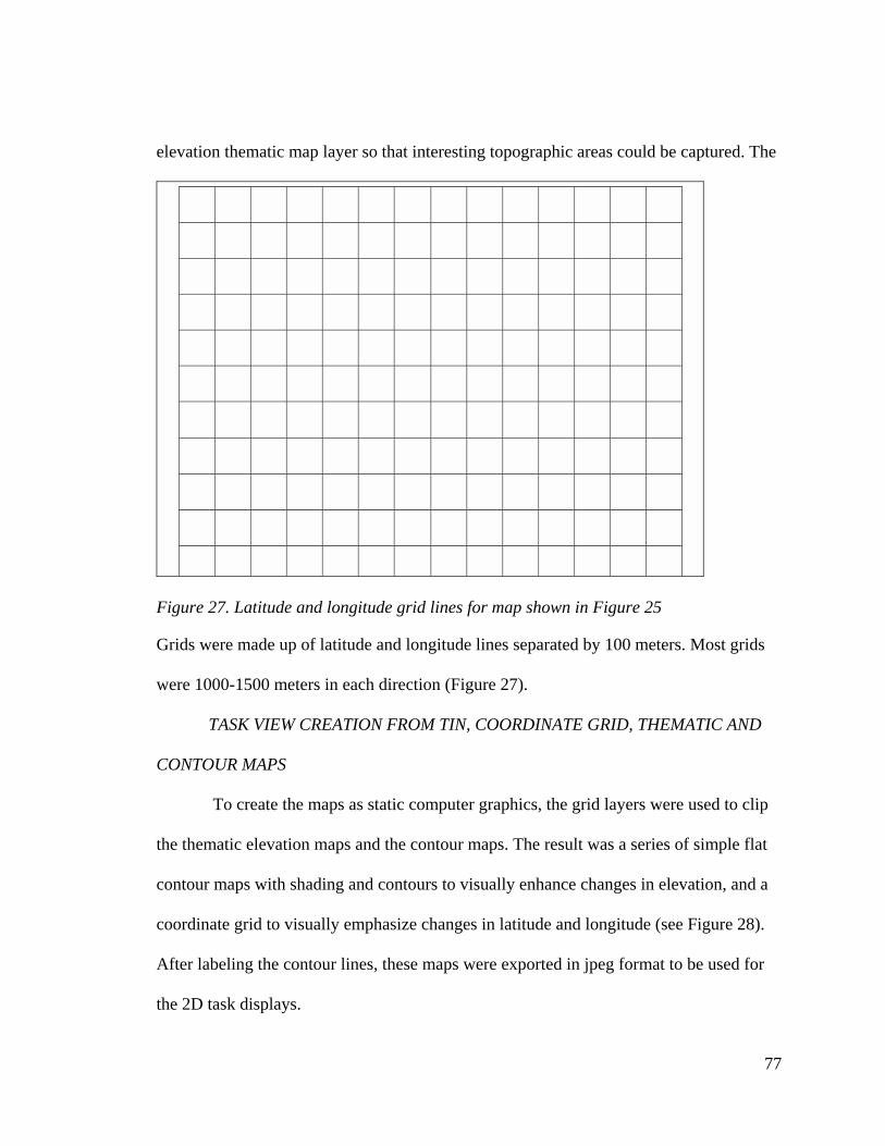
77
elevation thematic map layer so that interesting topographic areas could be captured. The
Figure 27. Latitude and longitude grid lines for map shown in Figure 25
Grids were made up of latitude and longitude lines separated by 100 meters. Most grids
were 1000-1500 meters in each direction (Figure 27).
TASK VIEW CREATION FROM TIN, COORDINATE GRID, THEMATIC AND
CONTOUR MAPS
To create the maps as static computer graphics, the grid layers were used to clip
the thematic elevation maps and the contour maps. The result was a series of simple flat
contour maps with shading and contours to visually enhance changes in elevation, and a
coordinate grid to visually emphasize changes in latitude and longitude (see Figure 28).
After labeling the contour lines, these maps were exported in jpeg format to be used for
the 2D task displays.

78
Figure 28. Finished 2D map from parts shown in Figure 25 through Figure 27
To create the 3D version of each map, the grid, contour and thematic maps were
“draped” on the TINs in 3D Analyst. After shifting the viewing angle (the acute angle
between the line of sight and the horizontal or ground elevation surface) to enhance
visibility of appropriate details, the 3D “Scenes” were exported to create images in jpeg
format for use in 3D task displays. PaintShop Pro™ was used to add the text of the task
questions to the bottom of each graphic (Figure 29).

79
Figure 29. Final 3D question from the 2D map shown in Figure 28
Visual Basic Program
A Visual Basic 6™ compiled application was designed to administer the tasks in
a random sequence (see Appendix 4. Visual Basic Code). Four practice questions were
displayed to make sure that the participants understood what they were supposed to do
and how to do it. (For examples, see Figure 30 for a 2D example and Figure 31 for a 3D
example.)

80
Figure 30. Practice Question - 2D
During the practice, each participant had an opportunity to respond by selecting a
letter between “A” and “E” representing a point on the map. Following the pressing of
the ‘Enter’ key, the correct answer was displayed. Participants were encouraged to ask
questions if they did not understand the task. After all practice questions were answered,
a screen was displayed saying practice was finished, and the next screen displayed would
be the first research task.

81
Figure 31. Practice Question - 3D
The tasks were selected for display by the Visual Basic program, which used a
random number function to choose the next task. After displaying each task, a timer was
started to measure the duration of the task.

82
Figure 32. Study task question example -2D
The program would accept a, b, c, d or e, and when the enter key was pressed, the
timer for that task was stopped, and the results written to the diskette. After each answer
was entered, the next screen was displayed and the timer was started for the next task.
Task/Question design and Validation
The task materials can be found in Appendix 3. The questions were generated to
create a scope of difficulty in answering correctly. The questions were tested by
administering the study with 6 individuals with varying experience levels (two were
beginning students in GIS, two were graduate students in GIS, and two were GIS
faculty). All tasks were answered correctly by one or more of the individuals. It was

83
decided that all tasks were representative of varying levels of difficulty, and should be
retained.
Figure 33. Example of challenging questions: 2D question 6- 3 people on the panel thought the answer was "B", the other three thought the answer was "E". The correct answer is “E”.
Three 2D tasks/questions and three 3D tasks/questions were found to be
challenging by the panel, as shown in table 13. Four of those questions were subsequently
eliminated by a post-study item analysis, which is detailed in the next chapter in the
section entitled “Test for Question Validity”.
Table 13. Problem questions from preliminary study
Question % Wrong Eliminated by post-study item analysis 2D Q6 50% Yes 2D Q9 83% No 2D Q14 83% Yes 3D Q9 17% Yes 3D Q14 83% Yes 3D Q18 67% No
84
Measures
There were two independent measures in this research: time and accuracy. Time
was measured as the number of seconds required to answer each question. The time in
seconds was measured between the display of the map and the pressing of the enter key
with an acceptable answer (a, b, c, d, or e). The time was computed by the administering
Visual Basic program and recorded on the diskette with the answer to the question.
Accuracy was simply the percent correct, not including the practice questions.
Procedure
Study 1 Procedure
The time period used for this study replaced a regular class period (approximately
75 minutes). Participants were given the choice of whether to participate or not after
receiving their packets and reading the informed consent, but before starting the
procedure. Those students who chose not to participate could study quietly but not leave
the classroom. Most students (95%) chose to participate.
The treatment of 2D versus 3D was distributed by alternate distribution between
2D and 3D test packet (2D-3D-2D-3D etc). Subjects were not aware which treatment
they were getting, or even that there was more than one treatment. See Appendix 2 for the
description of the study that was given to the students.
The purpose of the study was read to all participants, and they were given the
opportunity to sign the informed consent and remove a copy to take with them. They

85
were told that there was no penalty for non-participation, and that they could get their
results if they requested them on the informed consent, or by telephoning or e-mailing the
researcher.
The informed consent form, survey, spatial abilities test and diskette all had the
subject number on it. Participants were given five minutes to fill out the survey, and an
opportunity was given for any questions. The only question was whether they could ask
questions during the study, to which the answer was “no”. Next, participants were told
that the spatial ability test was used so that the effectiveness of the maps could be
separated statistically from their overall ability. Each section of the spatial ability test
consisted of 10 questions, and each section was limited to three minutes.
Finally, participants were told to insert the diskettes into the computers, and the
Visual Basic administering program was started by double-clicking on it in the MS
Windows directory. An opportunity for practice (four practice questions) was given. A
final opportunity for questions was offered. Participants were told to "work as quickly
and as accurately as possible."
Study 2 Procedure
Study 2 protocol was similar to Study 1 for the novices. The experts performed
their tasks in a smaller computer lab but with the same type of computers. The study was
administered in groups of 3-5 participants. (Participants were taking an open lab and
participated when convenient for them.) There were 4 practice questions and 24 task
questions in Study 2.

86
Data Collection and Reduction
A second Visual Basic program (see Appendix 4. Visual Basic Code) was written
to read the diskettes, rearrange the data into an array, and write them out to a text file in a
format readable by SAS™. A SAS™ program was used to read in the data, interpret the
answers as ‘0’ for incorrect answers and ‘1’ for correct answers, calculate the percent
correct and the paper fold score, and write the results into a SAS™ dataset.
An item analysis was performed on all the questions to determine if any question
had results more than two standard deviations below the mean results for all questions.
The correlation between paper fold test scores and the between subject variables of
dimension and experience was found to be positive, so ANCOVA was necessary to
control for the covariate of spatial ability. ANCOVA analysis was done for both studies,
with Tukey’s post hoc test. The results of the analysis can be found in the next chapter.

87
CHAPTER 5: ANALYSIS AND RESULTS
Introduction
This chapter describes the results of the participant questionnaire and spatial
ability test, the item analysis performed on the task items, and the analysis and results of
the task performance. The first section includes a summary of the questionnaire results
and the spatial ability test results. The second section analyzes correlations between
potential covariates of gender and spatial ability and the dependent variables time and
accuracy for Study 1 and Study 2.
The third section reports the results of the task item analysis. This includes the
discussion of specific issues with some of the tasks, and the criteria used to determine
whether to keep the tasks.
The fourth and final section describes the task performance analysis and discusses
the results. The time and accuracy data were analyzed using an ANCOVA to assess the
significance of main affects and interactions of the independent variables for task type,
elevation requirement, dimension and (in Study 2) experience. ANCOVA was used rather
than ANOVA, in order to control the variability which may have resulted from
differences in spatial ability (as represented by the spatial ability test).
Participant Questionnaire and Spatial Ability Scores
Study 1 Participants
Prior to performing the tasks, the participants were asked to fill out a very brief
survey and take a spatial visualization test (R. B. Ekstrom et al., 1976). The first question
on the survey was whether the participant was male or female. The participants were in

88
groups by college class, and were all taking an introductory course in Parks, Recreation
and Tourism Management. Group A had 5 females and 23 males for a total of 28
participants. Group B had 3 females and 11 males for a total of 14 participants. Group C
had 4 females and 20 males for a total of 24 participants.
The purpose of the second question on the survey was to estimate the self-
assessed experience level of each participant. The question and possible answers are in
Figure 34.
Figure 34. Self-assessed experience question on the survey.
The answers were recoded into numbers (1 for A, 5 for E, etc.) The number of
participants who assessed themselves at each level of experience is shown in Table 14.
Table 14. Study 1 self-assessed level of experience
Exp. Level 1 2 3 4 5 Group A 8 5 12 3 0 Group B 4 5 5 0 0 Group C 9 9 5 1 0 Totals 21 19 22 4 0
Which of the following statements best characterizes your experience with
contour maps (circle 1)?
1. I don’t know what they are, or I have not used contour maps in any context (class work, professional work, orienteering, etc.).
2. I have used a contour map either in a class or in my work, but only once or twice.
3. I have used a contour map more than once or twice, but I would not consider myself an experienced user.
4. I consider myself an experienced user of contour maps, but not an expert
5. I consider myself an expert in using contour maps (As good as or better than 95% of the general population).

89
The self-assessed experience levels of the three groups were analyzed using a
one-way ANOVA, to see if there was a significant difference between classroom groups
in self-assessed experience level. This analysis failed to show a significant difference in
self-assessed experience level between classroom groups, F(2,63) = 1.47, p= .24, so the
classroom groups can be treated as coming from a single group.
Table 15. ANOVA and summary table for Study 1 novices – relationship between group and experience level
SUMMARY Groups Sum Mean Variance Group A 66 2.36 1.05 Group B 29 2.07 0.69 Group C 46 1.92 0.775 ANOVA – Experience Level Source SS df MS F P-value F crit Between Groups 2.58 2 1.29 1.47 0.24 3.14 Within Groups 55.19 63 0.88 Total 57.77 65 __________________________________________________________________
The third question on the survey was qualitative; it requested the types of
experiences the participants had previously had with maps. The question is shown in
Figure 35. The results showed that about 25% of the participants had had map reading
instruction in Boy or Girl Scouts. A few had work-related experience such as
construction work. One participant had had an orienteering class. The majority of the
participants wrote “None” in the description of their map reading experience.

90
Figure 35. Survey question – types of experiences in map reading
Table 16. Study 1 types of map experiences (n=66)
Type of Experiences Number Reported Orienteering class (formal or informal) 14 Map reading instruction in Boy or Girl Scouts 11 Map reading in a Geography class, Geographic Information System (GIS) class, or other high school or college class
41
Other map reading experiences 21 None or blank 6
Spatial ability
After the survey was completed, the participants were given the spatial ability test
(R. B. Ekstrom et al., 1976). The spatial ability of the three groups was analyzed using a
one-way ANOVA. No significant difference was found between groups, F(2,63) = .47,
p=.63 (Table 17).
Table 17. ANOVA summary table for study 1 novices – relationship between group and spatial ability
SUMMARY Groups N Sum Mean Variance Group A 28 314 11.21 8.40 Group B 14 146 10.43 7.65 Group C 24 276 11.50 16 ANOVA – Spatial Ability Source SS df MS F P-value F crit Between Groups 10.34 2 5.17 0.47 0.63 3.14 Within Groups 694.14 63 11.02 Total 704.48 65
I have had the following experiences in map reading (check all that apply): ( ) Orienteering class (formal or informal) ( ) Map reading instruction in Boy or Girl Scouts ( ) Map reading in a Geography class, Geographic Information System (GIS) class, or other high school or college class ( ) Other map reading experiences (please describe in a few words):

91
Study 2 Participants
Similar to Study 1, in Study 2 there was one novice classroom group (study 2
novice - 2N) and four experienced classroom groups (2A, 2B, 2C and 2D). Table 18
details the number in the novice group by gender and total, and Table 19 details the
numbers in the experienced groups 2A through 2D by gender and total.
Gender
Table 18. Gender of novice participants in Study 2
Group N Female Male 2N 32 14 18
Table 19. Gender of experienced participants in Study 2
Groups N Female Male 2A 12 5 7 2B 11 7 4 2C 12 3 9 2D 9 4 5 Total Exp. 44 19 25 Self-Assessed Experience
The number of participants who assessed themselves at each experience level is
shown in Table 20 and Table 211.
Table 20. Study 2 Novices self-assessed level of experience
Exp. Level 1 2 3 4 5 Group 2N 4 7 15 5 1
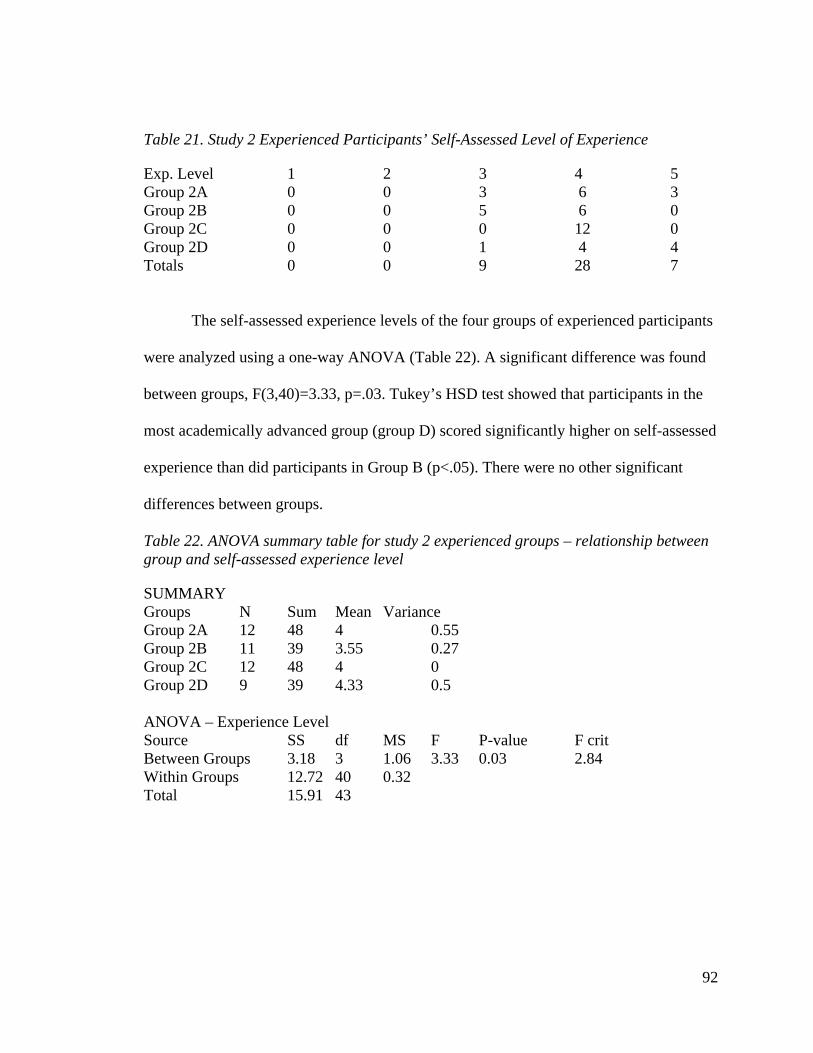
92
Table 21. Study 2 Experienced Participants’ Self-Assessed Level of Experience
Exp. Level 1 2 3 4 5 Group 2A 0 0 3 6 3 Group 2B 0 0 5 6 0 Group 2C 0 0 0 12 0 Group 2D 0 0 1 4 4 Totals 0 0 9 28 7
The self-assessed experience levels of the four groups of experienced participants
were analyzed using a one-way ANOVA (Table 22). A significant difference was found
between groups, F(3,40)=3.33, p=.03. Tukey’s HSD test showed that participants in the
most academically advanced group (group D) scored significantly higher on self-assessed
experience than did participants in Group B (p<.05). There were no other significant
differences between groups.
Table 22. ANOVA summary table for study 2 experienced groups – relationship between group and self-assessed experience level
SUMMARY Groups N Sum Mean Variance Group 2A 12 48 4 0.55 Group 2B 11 39 3.55 0.27 Group 2C 12 48 4 0 Group 2D 9 39 4.33 0.5 ANOVA – Experience Level Source SS df MS F P-value F crit Between Groups 3.18 3 1.06 3.33 0.03 2.84 Within Groups 12.72 40 0.32 Total 15.91 43

93
Table 23. Study 2 novices - types of map experiences (n=32)
Type of Experiences Number Reported Orienteering class (formal or informal) 10 Map reading instruction in Boy or Girl Scouts 6 Map reading in a Geography class, Geographic Information System (GIS) class, or other high school or college class
18
Other map reading experiences 7 None or blank 4
Table 24.Study 2 experts - types of map experiences (n=44)
Type of Experiences Number Reported Orienteering class (formal or informal) 15 Map reading instruction in Boy or Girl Scouts 6 Map reading in a Geography class, Geographic Information System (GIS) class, or other high school or college class
28
Other map reading experiences 31 None or blank 3
Spatial ability
The Spatial Ability of the four experienced groups was also analyzed using a one-
way ANOVA (Table 25). This analysis showed no significant difference in spatial ability
between experienced groups, F(3,40) = .72, p= .54. This indicates that the groups came
from a single population regarding self-assessed experience.

94
Table 25.ANOVA summary table for study 2 experienced groups – relationship between group and spatial ability
SUMMARY Groups N Sum Mean Variance Group 2A 12 144 12 10.54 Group 2B 11 144 13.09 7.29 Group 2C 12 161 13.42 10.08 Group 2D 9 126 14 15.5 ANOVA – Spatial Ability Source SS df MS F P-value F crit Between Groups 22.97 3 7.66 .72 0.54 2.84 Within Groups 423.83 40 10.60 Total 446.80 43
Once the expert classroom groups were determined to be from the same
population with regard to self-assessed experience level, the expert group was compared
to the novice group. The self-assessed experience level of the experienced groups taken
together, and the novice group was analyzed using a one-way ANOVA (Table 26). This
analysis showed a significant difference in self-assessed experience between experienced
and novice participants, F(1,74) = 43.33, p= <.0001, with the experienced group having a
mean experience level of 3.95 out of 5, and the novice group having a mean experience
level of 2.75.

95
Table 26. ANOVA summary table - comparison of self-assessed experience with maps between Study 2 novice and experienced participants
SUMMARY Groups N Sum Mean Variance Experienced 44 174 3.95 .37 Novices 32 88 2.75 .97 ANOVA – Spatial Ability Source SS df MS F P-value F crit Between Groups 26.88 1 26.88 43.33 .000 3.97 Within Groups 45.91 74 0.62 Total 72.79 75
Next, the expert group was compared to the novice group in spatial ability as
measured by the paper folding test. The spatial ability of the experienced groups taken
together, and the novice group was analyzed using a one-way ANOVA (Table 27). This
analysis showed no significant difference in spatial ability between experienced and
novice participants.
Table 27. ANOVA and summary table – comparison of spatial ability between Study 2 novice and experienced participants
SUMMARY Groups N Sum Mean Variance Experienced 44 575 13.07 10.39 Novices 32 449 14.03 10.42 ANOVA – Spatial Ability Source SS df MS F P-value F crit Between Groups 17.18 1 17.18 1.65 0.20 3.97 Within Groups 769.76 74 10.40 Total 786.95 75
Summary of Participant Questionnaire and Spatial Ability Scores
The analysis of self-assessed experience and spatial ability are summarized by the
following:

96
1. There was no significant difference between groups in Study 1 in either self-
assessed experience or spatial ability as measured by the visualization test.
2. In Study 2, there was no significant difference between the four experienced
groups in spatial ability as measured by the visualization test.
3. In study 2, there was a significant difference between group 2D (the most
experienced) and 2B in self-assessed experience. All other comparisons were
insignificant.
4. In study 2, there was a significant difference between the novice and experienced
participants in self-assessed experience, but not in spatial ability as measured by
the visualization test.
5. There was no significant difference between groups in Study 2 in spatial ability as
measured by the visualization test.
Test for potential covariates
Although this study was mainly interested in the effects of map dimensionality,
task type and experience levels on map task performance, there are other variables which
may influence map task performance, such as spatial ability or gender. Since those
variables were not of interest in this study, a test was done to determine if gender or
ability should be treated as covariates in analysis.
Study 1 Correlation Analysis
In order to determine whether there were any independent factors which should be
considered covariates, the Pearson’s Correlation was calculated between the dependent
variables of speed and accuracy with spatial ability test score and gender. In Study 1, the

97
correlation between average time to solve a task and spatial ability was -.26, p=.04, and
the correlation of average score (accuracy) with spatial ability was .33, p=.007. The
relationships between speed and gender, and accuracy and gender were not significant, so
spatial ability was the only factor treated as a covariate.
Study 2 Correlation Analysis
In a similar manner, Pearson’s Correlations were computed for spatial ability and
gender (independent factors) with time and accuracy (dependent variables). The
correlation between spatial ability and average score (accuracy) was significant at p=.002
with a value of .455. None of the other correlations were significant. The relationships
between speed and gender, and accuracy and gender were not significant, so spatial
ability (but not gender) was treated as a covariate.
Summary
In summary, groups in both studies showed no significant differences in spatial
ability scores between groups, and only one group in Study 2 showed a significant
difference in self-assessed ability. For this reason, groups in Study 1 will be analyzed as a
single group, and the experienced participants in Study 2 will be analyzed as a single
group (novices in Study 2 were all from a single group.) In addition, the spatial ability
test score, but not gender, will be treated as a covariate in subsequent analysis.
The next section describes the analysis of the task/question results to determine if
there were any invalid tasks/questions.
Test for Question Validity
Due to the results of the pilot study of the task materials described on page 82,
there was some concern about construct validity of the tasks – did all of the tasks measure

98
the same relationships between task type, elevation knowledge requirement, map type
and experience? A conservative measure of validity was chosen in order to preserve tasks
which were challenging but valid, and remove outlier tasks (H. A. Devine and E. N.
Wiebe, personal communication, September, 2003).
Table 28. Summary data for 2D task questions – all 2D participants
Mean of all 2D questions .798 s if all 2D Questions: .216 Range +/- 1 s from the mean: 0.58 1.01 Range +/- 2 s from the mean: 0.37 1.23 Question N mean s 1 71 0.97 0.167 2 71 0.94 0.232 3 71 0.94 0.232 4 71 0.92 0.280 5 71 0.86 0.350 6 71 0.23** 0.420 7 71 0.56* 0.499 8 71 0.79 0.411 9 71 0.41* 0.495 10 71 0.87 0.335 11 71 0.94 0.232 12 71 0.94 0.232 13 71 0.77 0.421 14 71 0.27** 0.446 15 71 0.75 0.438 16 71 0.92 0.280 17 71 0.87 0.335 18 71 0.90 0.300 19 71 0.90 0.300 20 71 0.93 0.258 21 39 0.72 0.456 22 39 1.00 0.0 23 39 0.90 0.307 24 39 0.85 0.365 * More than one s from the mean ** More than two s from the mean

99
For this analysis, the participants’ answers were coded as either ‘0’ for incorrect
answers, or ‘1’ for correct answers. The questions results were analyzed and compared
with the overall results within each dimension, that is, each 2D question result was
compared with results of all 2D questions, and each 3D question result was compared to
results of all 3D questions.
Table 28 shows the mean score and standard deviation (s) of each 2D question,
and compares that with the mean and standard deviation of all 2D questions. Any
question mean more than two standard deviations below the overall 2D mean is flagged
with a double asterisk (**).
The results of this analysis show that questions 6 (m=.23) and 14 (m=.27) of the
2D group had results lower than two standard deviations below the overall 2D mean.
Consequently, the results of these two questions were deleted from future analyses.
Table 29 shows the mean score and standard deviation of each 3D question, and
compares that mean with the mean of all 3D questions. Any question mean more than
two standard deviations below the overall 3D mean is flagged with a double asterisk (**).

100
Table 29. Summary data for 3D task questions – all 3D participants
Mean of all 3D questions .737 s if all 3D Questions: .221 Range +/- 1 s from the mean 0.516 .958 Range +/- 2 s from the mean 0.295 1.18 Question N mean s 1 71 0.90 0.302 2 71 0.91 0.280 3 71 0.93 0.258 4 71 0.76 0.430 5 71 0.70 0.460 6 71 0.45* 0.501 7 71 0.59 0.490 8 71 0.46* 0.502 9 71 0.11** 0.318 10 71 0.86 0.350 11 71 0.93 0.258 12 71 0.93 0.258 13 71 0.74 0.438 14 71 0.24** 0.430 15 71 0.80 0.400 16 71 0.92 0.280 17 71 0.86 0.350 18 71 0.61 0.492 19 71 0.83 0.377 20 71 0.83 0.377 21 37 0.81 0.397 22 37 0.89 0.315 23 37 0.81 0.397 24 37 0.78 0.417 * More than one s from the mean ** More than two s from the mean

101
The results of this analysis show that questions 9 (m=.11) and 14 (m=.27) of the
2D group had results lower than two standard deviations below the overall 3D mean.
Consequently, the results of these two questions were deleted from future analyses.
Task Performance
Study 1 Accuracy
Accuracy results were analyzed using a three-way ANCOVA with repeated
measures in two factors:
1) Task type (repeated measures)
• Focused
• Integrative
2) Elevation (repeated measures)
• task requires knowledge of elevation to solve (elev_Yes) or
• does not (elev_No)
3) Map dimension
• 2D
• 3D
The main effect of the covariate (Paper fold score) was significant, F(1,63) =
6.45, p =.014. The main effect of Dimension was also significant, F(1,63) = 4.47, p
=.038. Additionally, the Task type x Elevation interaction was significant, F(1,63) = 5.08,
p=.028. The Task type x Elevation x Dimension interaction was not significant. For the
focused, non-elevation task, post-hoc analysis showed a significant difference between

102
the 2D and 3D groups in their mean accuracy scores (Mean 2D=.87, Mean 3D=.73,
p=.023). Table 30 also shows significantly lower scores for the integrative elevation task
in both 2D and 3D conditions (p < .001) than for the other task type/elevation cells.
Table 30. Mean Accuracy Scores for Task Type/Elevation Pairs
Elevation Non-Elevation Focused M=.83, SD=.24 M=.80, SD=.25 Task Type Integrative M=.45, SD=.18 M=.71, SD=.20
2D Scores for tasks requiring elevation knowledge (elev_Yes) and tasks which do not require elevation
(elev_no)
0
0.1
0.2
0.3
0.4
0.5
0.6
0.7
0.8
0.9
1
Focused IntegrativeTask Type
Scor
e
elev_No elev_Yes Linear (elev_Yes) Linear (elev_No)
Figure 36. 2DAccuracy scores for tasks requiring elevation knowledge and those which do not

103
Figure 36 illustrates the difference in 2D accuracy scores between tasks that
require elevation knowledge and those which do not. The interaction of task type
(focused or integrative) with elevation knowledge requirement (elev_yes or elev_no) is
shown by the intersection of the broken trend lines (the lines do not indicate a continuous
variable and are provided solely to indicate the interaction).
3D Scores for tasks requiring elevation knowledge (elev_yes) and tasks which do not require elevation
(elev_no)
0
0.1
0.2
0.3
0.4
0.5
0.6
0.7
0.8
0.9
Focused IntegrativeTask Type
Scor
e
elev_No elev_Yes
Linear (elev_Yes) Linear (elev_No)
Figure 37. 3DAccuracy scores for tasks requiring elevation knowledge and those that do not
Figure 37 illustrates the difference in 3D accuracy scores between tasks that
require elevation knowledge and those which do not. The interaction of task type
(focused or integrative) with elevation knowledge requirement (elev_yes or elev_no) is

104
shown by the intersection of the broken trend lines (the lines do not indicate a continuous
variable, and are provided solely to indicate the interaction).
Study 1 Time
Time results were analyzed using a three-way ANCOVA with repeated measures
in two factors (Tasktype and Elevation). The main effect of the covariate was significant,
F(1,63) = 4.69, p =.034. The main effect of Dimension was not significant in this
analysis, F(1,63) = .22, p =.64. The main effect for Elevation was significant, F(1,63) =
11.35, p =.0013. Additionally, the Tasktype x Dimension interaction was significant,
F(1,63) = 5.05, p =.028. The Tasktype x Elevation x Dimension interaction was not
significant. For focused, non-elevation tasks, post-hoc analysis showed a significant
difference between the 2D and 3D groups in their mean speed in seconds (2D m=13.6,
3D m=16.6, p =.012).
Table 31. Mean Speed (seconds) for Tasktype/Map type Pairs When Elevation Knowledge is not required
2D 3D
Focused m=19.7, s=4.6
m=21.3, s=6.0 Task Type
Integrative m=27.2, s=6.4 m=25.2, s=5.7
Table 31 illustrates the difference in speed on Elevation-knowledge-not-required
tasks, between 2D maps and 3D maps. The interaction of task type (focused or
integrative) with map type (2D and 3D) is shown by the intersection of the broken trend
lines (the lines do not indicate a continuous variable and is solely to indicate the
interaction).

105
Speed on elevation knowledge not required tasks
0
5
10
15
20
25
Integrative FocusedTask type
Tim
e
2D Map 3D Map Linear (2D Map) Linear (3D Map)
Figure 38. Speed (in seconds) of 2D and 3D tasks for which elevation knowledge was not required
Figure 39 illustrates the difference in speed on Elevation-knowledge-required tasks,
between 2D maps and 3D maps. The interaction of task type (Focused or Integrative)
with map type (2D and 3D) is shown by the intersection of the broken trend lines (the
lines do not indicate a continuous variable and are solely provided to indicate the
interaction).

106
Speed on elevation required tasks
0
5
10
15
20
25
30
35
Integrative FocusedTask Type
Tim
e (s
econ
ds)
2D Map 3D Map Linear (3D Map) Linear (2D Map)
Figure 39. Speed (in seconds) —Task type/Elevation by Dimension
Study 2 Accuracy
Study 2 included 76 subjects, 18 novices and 21 experienced in the 2D between-subjects
treatment, 14 novices and 23 experienced in the 3D treatment. Accuracy scores are
average scores for each task/elevation combination. Accuracy results were analyzed
using a four-way ANCOVA with repeated measures in two factors (Task type and
Elevation). The main effect of the covariate (Paper fold score) was significant, F (1, 71) =
9.65, p=.0027. The main effect of Dimension was also significant, F (1, 71) = 4.25,
p=.0428. The Paper fold score did not significantly interact with dimension, so that
interaction was not included in the model. Additionally, there was a main effect of
experience, F(1,71) = 10.10, p=.0022, and a main effect of task type, F(1,71) = 5.17,
p=.0260.
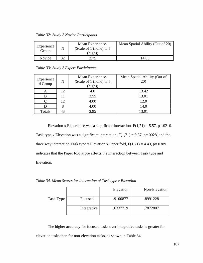
107
Table 32: Study 2 Novice Participants
Experience Group N
Mean Experience- (Scale of 1 (none) to 5
(high))
Mean Spatial Ability (Out of 20)
Novice 32 2.75 14.03 Table 33: Study 2 Expert Participants
Experienced Group N
Mean Experience- (Scale of 1 (none) to 5
(high))
Mean Spatial Ability (Out of 20)
A 12 4.0 13.42 B 11 3.55 13.01 C 12 4.00 12.0 D 8 4.00 14.0
Totals 43 3.95 13.01
Elevation x Experience was a significant interaction, F(1,71) = 5.57, p=.0210.
Task type x Elevation was a significant interaction, F(1,71) = 9.57, p=.0028, and the
three way interaction Task type x Elevation x Paper fold, F(1,71) = 4.43, p=.0389
indicates that the Paper fold score affects the interaction between Task type and
Elevation.
Table 34. Mean Scores for interaction of Task type x Elevation
Elevation Non-Elevation
Focused .9100877 .8991228 Task Type
Integrative .6337719 .7872807
The higher accuracy for focused tasks over integrative tasks is greater for
elevation tasks than for non-elevation tasks, as shown in Table 34.

108
Table 35. Mean Scores for Interaction of Elevation x Experience
Experienced Novice Elevation .81250000 0.71614585Task Type
Non-Elevation 0.85227275 0.8307292
There is a larger difference in scores for novice users between elevation and non-
elevation tasks than there is for experienced users, as shown in Table 35.
Dimension x Experience was not a significant interaction, F(1,73) = .45, p=.5057.
Scores by Experienced Subjects on Various Tasktypes with 2D and 3D Treatments
00.20.40.60.8
11.2
Focusednon-
elevation
FocusedElevation
Integratednon-
elevation
Integratedelevation
Task types - Elevation and non-elevation
Mea
n s
core
s
2D-exp3D-exp
Figure 40. Scores of experienced subjects by task type

109
Scores by Novice Subjects on Various Tasktypes with 2D and 3D Treatments
00.20.40.60.8
1
Focusednon-
elevation
FocusedElevation
Integratednon-
elevation
Integratedelevation
Tasktypes - Elevation and non-Elevation
Mea
n S
core
s
2D-nov3D-nov
Figure 41. Scores of novice subjects by task type
Study 2 Speed
Speed results are the average number of seconds taken to answer each type of task
(task type/elevation combination). Speed results were analyzed using a four-way
ANCOVA with repeated measures in two factors (task type and elevation). The main
effect of the covariate (paper fold score) was significant, F(1,71) = 5.14, p=.0265. The
main effect of Dimension was not significant in this analysis, F(1,71) = .66, p=.4193.
(The paper fold score did not significantly interact with Dimension, so that interaction
was not included in the model.)
There was a significant main effect for elevation, F(1,71) = 13.97, p=.0004, and a
significant interaction of Elevation X Dimension, F(1,71) = 16.18, p=.0001.

110
Table 36. Speed (in seconds) Means for Interaction of Elevation X Dimension
2D 3D Elevation 29.01923075 27.76801805Non-Elevation 18.27564105 22.15316715
The faster speed for non-elevation as compared to elevation tasks was larger for
the 2D than for the 3D treatment, as shown in Table 36.
Summary of Results
Study 1
Hypothesis 1: For focused questions of a single value of latitude or longitude
at a single location, the flat 2D map and the 3D map will be equally effective (no
significant difference in speed or accuracy).
Result: This hypothesis was not supported.
For the focused, non-elevation task, post-hoc analysis showed a significant
difference between the 2D and 3D groups in their mean accuracy scores (Mean 2D=.87,
Mean 3D=.73, p=.023). The participants that used the 2D maps were significantly more
accurate than the 3D map users. In addition, post-hoc analysis showed a significant
difference between the 2D and 3D groups in their mean times (Mean 2D=13.6, Mean
3D=16.6, p =.012). Not only were the 3D map users less accurate, but their mean time to
perform the tasks was greater than the 2D map users.
Hypothesis 2: For separate (focused) questions of a single value of Altitude at
a single location, the 3D map will be more effective.
Result: This hypothesis was not supported

111
One might assume that for focused tasks requiring elevation (similar to St. John et
al. 2001 A-high-B tasks); scores would be better and times would be reduced for those
participants using the 3D maps. This is because the third dimension of elevation is added
to the 3D maps as a redundant cue. However, there was no significant difference in
accuracy and time between 2D and 3D for this task type, in contrast to St. John et al. (St.
John, Cowen et al., 2001) who found a difference in accuracy but not time. This result is
puzzling, but could be due to the simplicity of the tasks in the current study: The
elevation lines were clearly marked, there were redundant shading cues indicating high
and low elevations, and the tasks were to compare elevations at two points or extract the
elevation value at a single point.
Hypothesis 3: For integrative tasks in a 2D space not requiring elevation
data, the 2D map will be more effective than the 3D map.
Result: This hypothesis was not supported
Hypothesis 3 predicted that for integrative tasks not requiring elevation data,
scores would be better and times would be less for those using 2D maps, due to the
misunderstanding of the effects of foreshortening in 3D maps (Smallman et al., 2002). No
significant difference was found in accuracy and time between 2D and 3D for this task
type.
Hypothesis 4: For integrative tasks requiring elevation data (shape
understanding tasks), there would be an advantage to using 3D maps.
Results: This hypothesis was not supported

112
Hypothesis 4 predicted that for integrative tasks which require elevation data,
scores would be better and times would be less for those using 3D maps, due to the
similarity between the task and the mental image required to perform the task. (Smallman
et al., 2001; Haskell & Wickens, 1993). No significant difference between 2D and 3D in
either accuracy or time was found for this task type.
Study 2
Hypothesis 5 – Study 2 Experienced Users: Experienced topographic map
users will more easily be able to mentally transform the 3D information contained in
a 2D topographic line map, and the advantage of a 3D map will be less for
experienced users than for novice users.
Result: This hypothesis was not supported
Dimension x Experience was not a significant interaction in the ANCOVA in
Study 2, F(1,73) = .45, p = .5057.

113
CHAPTER 6: DISCUSSION
The Problem
Traditional topographic maps provide detailed information on landscape shape in
an information-dense package. Despite their efficiency, topographic maps can be difficult
for inexperienced readers to interpret. A potential solution to this difficulty is offered by
the new technology for creating 3D maps from the same data. However, 3D maps
displayed on 2D surfaces such as computer displays can create ambiguity and are subject
to distortion. Task type, user experience and data dimensionality can all be expected to
influence the relative effectiveness of two-dimensional versus three-dimensional
topographic maps.
This study examined the advantages and disadvantages of 3D topographic contour
maps as compared to 2D topographic contour maps under a variety of conditions. The
conditions of interest in this study were:
• 2D versus 3D contour maps
• Focused versus Integrative task types
• Elevation knowledge required versus not required for task type
• Experience level (novice or experienced) with map reading
Summary of results
Although none of the working hypotheses was supported by this research, some
interesting effects were found.

114
1. The covariate of spatial ability (represented by Paper fold score in this
study) was significant for both speed and accuracy in both novice and
experienced participants. This is consistent with the findings of Thorndyke
and Stasz (1980). In addition, Barsam and Simutis (1984) found that
active practice (experience) only helped participants with high spatial
ability. The implication is that those with moderate or low spatial ability
may be limited in map-reading achievement.
2. The main effect of dimension was significant for accuracy in both studies,
but not significant for speed in either study. This means the 3D
participants took generally as long as the 2D participants to perform the
same tasks, but those with 2D maps were significantly more accurate. The
implication is that the distortion introduced by projecting the 3D map onto
a 2D surface interfered with accuracy.
3. In Study 1, for tasks which required elevation knowledge, participants
with 2D maps as well as participants with 3D maps had more difficulty
with Integrative questions than they did with focused questions. For tasks
not requiring elevation knowledge, the difference between focused and
integrative task accuracy was not significant. In other words, Integrative
tasks were more difficult when elevation knowledge was required to solve
them, regardless of map dimensionality.
4. In Study 1, the main effect of Elevation knowledge requirement was
significant for speed for both types of maps, indicating that elevation is

115
more time-consuming to extract than the other two dimensions of latitude
and longitude.
5. In Study 1, the interaction of Task Type x Dimension was significant for
speed. The Integrative task took longer to complete than the focused task,
especially using the 2D map. Integrative tasks require more analysis and
should be expected to take longer, but the focused tasks were more
quickly performed with 2D maps than 3D maps, and the integrative tasks
took longer using the 2D maps than the 3D maps.
6. In Study 2, the Elevation Knowledge Requirement x Experience level
interaction was significant for accuracy. Novices did much better on tasks
requiring elevation knowledge than did experienced participants. This is a
puzzling result, but could be partially due to the fact that there was no
significant difference in spatial ability (Novice m=14.03, Experienced
m=13.07).
7. In Study 2, there was a significant main effect of Elevation knowledge
requirement, and of Elevation knowledge x Dimension on speed. The
Elevation knowledge required tasks took significantly longer with the 2D
maps than with the 3D maps.
Discussion of results
This analysis revealed a significant advantage for 2D maps in both accuracy and
time for simple tasks that do not require elevation data. This implies that the 3D map
representation used in this study may interfere with task performance, which is consistent
with the research of others (St. John, Cowen et al., 2001) (Haskell & Wickens, 1993).

116
In addition, there was no apparent advantage of 3D maps for those tasks
requiring elevation information, nor was there a disadvantage for integrative tasks which
did not require elevation information. Finally, experience was not significant with regard
to speed or accuracy when using 3D maps. These results are probably due to most or all
previous experience with topographic maps having been with 2D maps.
It is worth noting that spatial visualization ability, as measured by the Paper
Folding Test seemed to be a strong indicator as to how individuals would perform on
these types of tasks. In addition, shape understanding tasks showed themselves to be the
most difficult—whether they were paired with 2D or 3D maps. On the other hand,
focused, non-elevation questions were the easiest, with an advantage going to the 2D
maps, as predicted by St. John et al. (2001). This would be expected, since individual
coordinate values are most likely easier to read from planar maps than from 3D maps.
Finally, it should be noted that the experienced participants were not necessarily
experienced with 3D maps. 3D visualization ability is most likely a different skill than
strictly 2D map reading skill. Perhaps metacognitive skills need to be learned in order to
take advantage of the benefits of 3D topographic maps. Future research could investigate
whether the teaching of 3D visualization skills would change the outcomes encountered
here.
Limitations of this study
None of the working hypotheses of this study was supported, although several
variables approached significance. The conclusions that can be drawn from this study are
limited by the following:

117
1. There was a significant difference between both the spatial ability (Table
10. ANOVA summary table – relationship between Study 1 and Study 2
novices in spatial ability) and the self-assessed experience of the novices
in Study 1 and those in Study 2 (Table 9. ANOVA summary table –
relationship between Study 1 and Study 2 novices in experience). One
possible interpretation of this is that the Novices in Study 2 were not really
novices for the purposes of this study. The concept of “experience” was
not as effectively operationalized as it might have been if a test of contour
map-reading skills had been used to partition the participants.
2. Two 2D (Table 28) and two 3D (Table 29) question results were excluded
from analysis due to evidence that they were not valid. One Integrative
Elevation-knowledge-required question and one Integrative, Elevation-
knowledge- not-required question was eliminated from both Study 1 and
Study 2. This made the number of questions in each experimental cell
unequal in both studies. Statistical tests for significance tend to be more
conservative when unequal cell sizes are used. Consequently, there were
several failures to achieve significant results.
3. Because the samples (groups) used were opportunistic, the between-
subjects variable of experience in Study 2 had unequal cell sizes (unequal
participant numbers). In addition, the option to opt out was given after the
materials were randomly distributed, resulting in the number of
participants in the between-subjects variable of map dimensionality being

118
unequal. This resulted in a weaker statistical test for significance. Using
equal cell sizes might have resulted more statistically significant results.
4. Developing Integrative, Elevation-knowledge-not-required questions was
very difficult. A realistic question requires integration of several point
locations in 2 dimensions, but illustration on a 3D surface, without the task
requiring knowledge of the elevation e.g. Figure 42. This was the weakest
question type, and more preliminary research on this type of task might
have resulted in a more rigorous study.

119
Figure 42.Example of an Integrative, Elevation knowledge not required question
The pale gray grid marks above mark the number of miles north and east on the map. Question: Which point is the closest IN EASTERLY DIRECTION to the blue point, WHILE STILL IN THE SAME SHADED AREA . A) B) C) D) E)

120
Recommendations for Future Research
The following recommendations emerge from this study as areas in need of
future investigation:
1. The research of Barsam & Simutis (1984) found that the effects of practice
appear to be limited by spatial ability. These findings have interesting
implications for the results of this study. It would be informative to
operationalize experience in contour-map reading, and then investigate the
relationship between experience and spatial ability.
2. The wire frame version of the 3D maps used in the study did not appear to
aid in map problem solving. Perhaps a repetition of this research with a
hill shaded version of contour maps, both 2D (for example as shown in
Figure 8) and 3D would make it easier to visualize the shape of the terrain.
3. As described on the previous page, integrative non-elevation problems
were difficult to develop. Research might be done to determine if this is a
valid problem type i.e. what type of problems would measure integration
over a terrain without requiring knowledge of elevation?
Conclusions
This study was undertaken with the belief that 3D maps would be more effective
for integrative tasks - those that require understanding of terrain shape, including
elevation variation. That belief was not borne out by the results. This might have been
because of the participants’ general lack of experience with 3D projections on 2D
surfaces, or the limited use of depth cues (hillshading, color and motion). Further, results

121
may have been influenced by the unequal study cell size, or the difficulty in delimiting
experts from novices. However, the following are indicated by the results:
1. There is probably no single best map type that supports all task requirements
equally. Map format, including dimensions, should be decided based on the task
to be performed.
2. If 3D maps are to be used for instruction or problem solving, some training on
their interpretation may enhance their effectiveness.
3. For tasks requiring extraction of simple data values such as latitude and longitude,
3D maps should probably not be used.
4. Light shading, color and motion to enhance depth perception need to be
investigated.

122
REFERENCES
Al-Kodmany, K. (2000). GIS in the urban landscape: Reconfiguring neighborhood planning and design processes. Landscape Research, 25(1), 5-28.
Al-Kodmany, K. (2001). Bridging the gap between technical and local knowledge: Tools for promoting community-based planning and design. Journal of Architectural and Planning Research, 18(2), 110-130.
Anderson, J. R. (1983). The architecture of cognition. Cambridge, MA: Harvard University Press.
Anderson, K. C., & Leinhardt, G. (2002). Maps as representations: Expert novice comparison of projection understanding. Cognition and Instruction, 20(3), 283-321.
Ashcraft, M. H. (1989). Human Memory and Cognition. New York: HarperCollins Publishers.
Atkinson, R. C., & Shiffrin, R. M. (1968). Human Memory: A proposed system and its control processes. The Psychology of Learning and Motivation: Advances in Theory and Research, 2, 89-95.
Ball, J. (2002). Towards a methodology for mapping 'regions of sustainability' using PPGIS. Progress in Planning, 58(2), 81-140.
Barfield, W., Lim, R., & Rosenberg, C. (1990). Visual enhancements and geometric field of view as factors in the design of a 3D perspective display. Paper presented at the Human Factors Society - 34th Annual Meeting.
Barnett, B. J., & Wickens, C. D. (1988). Display Proximity in Multicue Information Integration - the Benefits of Boxes. Human Factors, 30(1), 15-24.
Barsam, H. F., & Simutis, Z. M. (1984). Computer-based graphics for terrain visualization training. Human-Factors, 26(6), 659-665.
Bennett, K. B., & Flach, J. M. (1992). Graphical Displays - Implications for Divided Attention, Focused Attention, and Problem-Solving. Human Factors, 34(5), 513-533.
Bennett, K. B., Payne, M., Calcaterra, J., & Nittoli, B. (2000). An empirical comparison of alternative methodologies for the evaluation of configural displays. Human Factors, 42(2), 287-298.
123
Bennett, K. B., Toms, M. L., & Woods, D. D. (1993). Emergent Features and Graphical Elements - Designing More Effective Configural Displays. Human Factors, 35(1), 71-97.
Bertoline, G. R., Wiebe, E. N., Miller, C. L., & Nasman, L. O. (1997). Fundamentals of graphics communication (1st ed. ed.). Boston, MA: WCB/McGraw-Hill.
Boyer, B., Campbell, M., May, P., Merwin, D., & Wickens, C. D. (1995). Three-Dimensional Display for Terrain and Weather Awareness in the National Airspace System. In Designing for the Global Village. Proceedings of the Human Factors and Ergonomics Society 39th Annual Meeting (Vol. 1, pp. 6-10). Santa Monica, California: The Human Factors and Ergonomics Society.
Buttigieg, M. A., & Sanderson, P. M. (1991). Emergent Features in Visual-Display Design for 2 Types of Failure-Detection Tasks. Human Factors, 33(6), 631-651.
Campbell, M., May, P. A., & Wickens, C. D. (1995). Perspective Displays for Air Traffic Control: Display of Terrain and Weather. In R. S. J. a. L. A. Rakovan (Ed.), Proceedings of the Eighth International Symposium on Aviation Psychology, April 24-27, 1995 (Vol. 1).
Carswell, C. M., Frankenberger, S., & Bernhard, D. (1991). Graphing in depth: Perspectives on the use of three-dimensional graphs to represent lower-dimensional data. Behaviour and Information Technology, 10(6), 459-474.
Carswell, C. M., & Wickens, C. D. (1987). Information Integration and the Object Display - an Interaction of Task Demands and Display Superiority. Ergonomics, 30(3), 511-527.
Chang, K., Antes, J., & Lenzen, T. (1985). The effect of experience on reading topographic relief information: analysis of performance and eye movements. The Cartographic Journal, 22, 88-94.
Clarke, K. C. (1999). Getting Started with Geographic Information Systems (Second Edition). Upper Saddle River, N.J.: Prentice Hall..
Cooper, L. A. (1990). Mental Representation of Three-Dimensional Objects in Visual Problem Solving and Recognition. Journal of Experimental Psychology: Learning, Memory, and Cognition, 16(6), 1097-1106.
Craig, W. J., & Elwood, S. A. (1998). How and why community groups use maps and geographic information. Cartography and Geographic Information Systems, 25(2), 95-111.
Crampton, J. (1992). A cognitive analysis of wayfinding expertise. Cartographica, 29, 46-55.

124
Dolan, N. J., Elvers, G. C., and Schmidt, J. (1991). Measurement Scale and Zero Point Indicators affect object display separate and integral task performance. Paper presented at the Human Factors Society 35th Annual Meeting, Santa Monica, CA.
Ekstrom, R. B., French, J. W., & Harman, H. H. (1979). Cognitive factors: Their identification and replication. (Vol. 79(2)).
Ekstrom, R. B., French, J. W., Harman, H. H., & Dermen, D. (1976). Manual for Kit of Factor-Referenced Cognitive Tests. Princeton, NJ: Educational Testing Service.
Ekstrom, R. B., French, W., & Harmon, H. (1976). Factor VZ: Visualization - Paper Folding Test -- VZ-2. In Kit of Factor-Referenced Cognitive Tests. Princeton: Educational Testing Service.
Ellis, H. C., & Hunt, R. R. (1993). Fundamentals of Cognitive Psychology (5th Edition). Boston: McGraw-Hill.
Feinstein, D. T., & Krohelski, J. T. Ground water in the Great Lakes Basin: The case of southeastern Wisconsin (n.d.). Retrieved March 9, 2006, from US Geological Survey, Wisconsin Water Science Center Web Site: http://wi.water.usgs.gov/glpf/cn_pmp_wls.htm.
Feldkotter, C. (2003). Coordinate Grid Maker Extension (Version 2.290) [ArcView GIS Extension]: ESRI.
Garner, W. R. (1974). The processing of information and structure. Potomac, Md: L. Erlbaum Associates.
Garner, W. R. (1976). Interaction of Stimulus Dimensions in Concept and Choice Processes. Cognitive Psychology, 8(1), 98-123.
Garner, W. R., & Felfoldy, G. L. (1970). Integrality of Stimulus Dimensions in Various Types of Information Processing. Cognitive Psychology, 1(3), 225-241.
Gilhooly, K. J., Wood, M., Kinnear, P. R., & Green, C. (1988). Skill in Map Reading and Memory for Maps. Quarterly Journal of Experimental Psychology Section a-Human Experimental Psychology, 40(1), 87-107.
Gillam, B. (1995). The Perception of spatial layout from static optical Information. In W. Epstein & S. J. Rogers (Eds.), Perception of Space and Motion (2nd ed., pp. 23-67). San Diego: Academic Press.
Goettl, B. P., Wickens, C. D., & Kramer, A. F. (1991). Integrated Displays and the Perception of Graphical Data. Ergonomics, 34(8), 1047-1063.
125
Goldstein, E. B. (1989). Sensation and Perception. Belmont, California: Wadsworth Publishing Company.
Harris, T., & Weiner, D. (1998). Empowerment, marginalization, and "Community-integrated" GIS. Cartography and Geographic Information Systems, 25(2), 67-83.
Haskell, I. D., & Wickens, C. D. (1993). Two- and three-dimensional displays for aviation: A theoretical and empirical comparison. International-Journal-of-Aviation-Psychology, 3(2), 87-109.
Hicks, J., & Hammond, R. (2005). No more guess with GIS. Parks and Recreation 40(6), 52-54.
Hollands, J. G., Pierce, B. J., & Magee, L. E. (1995). Displaying quantitative information in two and three dimensions. Paper presented at the Human Factors and Ergonomics Society 39th Annual Meeting, San Diego, CA.
Kraak, M. J. (1988). Computer-assisted cartographical three-dimensional imaging techniques. Delft: Netherlands: Delft University Press.
Kraak, M. J. (1993). Three-dimensional map design. The Cartographic Journal, 30, 188-194.
Liedke, J. (2003). From 3D urban modeling to fire safety. Planning, 69(2), 22-24.
Longley, P. A. (2004). Geographic Information Systems: On modelling and representation. Progress in Human Geography, 28(1), 108-116.
MacEachren, A. M. (1991). The role of maps in spatial knowledge acquisition. The Cartographic Journal, 28, 152-161.
MacEachren, A. M. (1995). How Maps Work: Representation, Visualization and Design. New York: The Guilford Press.
MacEachren, A. M. (2000). Cartography and GIS: Facilitating collaboration. Progress in Human Geography, 24(3), 445-456.
MacEachren, A. M., & Kraak, M. J. (1997). Exploratory cartographic visualization: Advancing the agenda. Computers and Geosciences, 23(4), 335-343.
Marr, D. (1982). Vision. San Francisco: W. H. Freeman.
McGarigle, B. (2002). Mapping places and spaces. Architectural Record, 190(6), 180-185.

126
McGuinness, C. (1994). Expert/novice use of visualization Tools. In A. M. Maceachren & D. R. F. Taylor (Eds.), Visualization in Modern Cartography (pp. 185-199). New York: Elsevier Science Inc.
Meserth, T. A., & Hollands, J. G. (1999). Comparing 2D and 3D Displays for Trend Estimation: The Effects of Display Augmentation. In Proceedings of the Human Factors and Ergonomics Society 43rd Annual Meeting, Houston, Texas, September 27-October 1, 1999. (Vol. 2, pp. 1308-1312). Santa Monica, California: The Human Factors and Ergonomics Society.
Miller, D. (1999, July 2, 1999). DEM-Based terrain Modeling with ArcView GIS. Retrieved January, 2005, from http://www.esri.com/news/arcuser/0799/demdemo.html
Miller, G. A. (1956). The magical number seven, plus or minus two: Some limits on our capacity for processing information. Psychological Review, 63, 81-97.
Muehrcke, P. C., & Muehrcke, J. O. (1998). Map Use: Reading, Analysis and Interpretation (Fourth ed.). Madison, WI: JP Publications.
Obermeyer, N. G. (1998). The Evolution of public participation GIS. Cartography and Geographic Information Systems, 25(2), 65.
Pomerantz, J. R. (1985). Perceptual organization in information processing. In A. M. A. a. J. M. Slack (Ed.), Issues in cognitive modeling : a reader. London ; Hillsdale, N.J.: Erlbaum in association with the Open University.
Pomerantz, J. R., & Garner, W. R. (1973). Stimulus Configuration in Selective Attention Tasks. Perception & Psychophysics, 14(3), 565-569.
Pomerantz, J. R., & Pristach, E. A. (1989). Emergent Features, Attention, and Perceptual Glue in Visual Form Perception. Journal of Experimental Psychology-Human Perception and Performance, 15(4), 635-649.
Price, M. (2004). Mastering ArcGIS. Boston: McGraw-Hill.
Rasmussen, J., & Vicente, K. J. (1989). Coping with Human Errors through System-Design - Implications for Ecological Interface Design. International Journal of Man-Machine Studies, 31(5), 517-534.
Sanderson, P. M., Flach, J. M., Buttigieg, M. A., & Casey, E. J. (1989). Object Displays Do Not Always Support Better Integrated Task- Performance. Human Factors, 31(2), 183-198.

127
Slagle, M. (2000). GIS in community-based school planning: A tool to enhance decision making, cooperation and democratization in the planning process. ERIC, number ED452686.
Smallman, H. S., St.John, M., & Cowen, M. B. (2002). Use and Misuse of Linear Perspective in the Perceptual Reconstruction of 3-D Perspective View Displays. In Proceedings of the 46th Annual Meeting of the Human Factors and Ergonomics Society (pp. 1560-1564). Santa Monica, California: Human Factors and Ergonomics Society.
Snyder, K. (2001). Decision support tools for community planning. Public Management, 4-8.
St. John, M., Cowen, M. B., Smallman, H. S., & Oonk, H. M. (2001). The Use of 2D and 3D Displays for Shape-Understanding versus Relative-Position. Human Factors, 43(1), 79-98.
St. John, M., & Smallman, H. S. (2000). Designing for the Task: Sometimes 2-D Is Just Plane Better. In Ergonomics for the New Millennium. Proceedings of the XIVth Triennial Congress of the International Ergonomics Association and 44th Annual Meeting of the Human Factors and Ergonomics Society, San Diego, California, USA, July 29-August 4, 2000 (Vol. 3, pp. 407-410). Santa Monica, California: Human Factors and Ergonomics Society.
St. John, M., Smallman, H. S., Bank, T. E., & Cowen, M. B. (2001). Tactical Routing Using Two-Dimensional and Three-Dimensional Views of Terrain. In Human Factors/Ergonomics: It Works. Proceedings of the Human Factors and Ergonomics Society 45th Annual Meeting, Minneapolis/St Paul, Minnesota, October 8-12, 2001 (Vol. 2). Santa Monica, California: The Human Factors and Ergonomics Society.
Thorndyke, P. W., & Stasz, C. (1980). Individual differences in procedures for knowledge acquisition from maps. Cognitive Psychology, 12(1), 137-175.
Tulving, E. (1983). Elements of Episodic Memory. New York: Oxford University Press.
USGS. (2000, 2000). National Elevation Dataset: County. 2000. Retrieved August 10, 2002, 2002, from http://www.lib.ncsu.edu/stacks/gis/data17/data1714.html
Vicente, K. J., & Rasmussen, J. (1992). Ecological Interface Design - Theoretical Foundations. Ieee Transactions on Systems Man and Cybernetics, 22(4), 589-606.
Villa, F., Ceroni, M., & Mazza, A. (1996). A GIS-based method for multi-objective evaluation of park vegetation. Landscape and Urban Planning, 35(4), 203-212.

128
Wanger, L. R., Ferwerda, J. A., & Greenberg, D. P. (1992). Perceiving spatial relationships in computer-generated images. IEEE Computer Graphics and Applications, 12(3), 44-58.
Weibel, R., & Heller, H. (1992). Digital Terrain Modelling. In D. J. MaGuire, M. F. Goodchild & D. W. Rhind (Eds.), Geographical Information Systems: Principles and Applications (Vol. 1, pp. 269-297). New York: John Wiley & Sons, Inc.
Wickens, C. D. (1984). Engineering Psychology and Human Performance (Second ed.). New York: HarperCollins Publishers, Inc.
Wickens, C. D., & Andre, A. D. (1990). Proximity Compatibility and Information Display - Effects of Color, Space, and Objectness on Information Integration. Human Factors, 32(1), 61-77.
Wickens, C. D., & Carswell, C. M. (1995). The proximity compatibility principle: its psychological foundation and relevance to display design. Human Factors, 37(3), 473-495.
Wickens, C. D., Todd, S., & Seidler, K. (1989). Three-Dimensional Displays: Perception, Implementation, and Applications: Aviation Research Laboratory, University of Illinois.
Williamson, J., & McGuinness, C. (1990). The role of schemata in the comprehension of maps. In K. J. Gilhooly, M. T. G. Keane, R. H. Logie & G. Erdos (Eds.), Lines of Thinking (Vol. 2, pp. 29-40). London: Wiley.

129
APPENDICES

130
Appendix 1. Informed Consent Form

131
Appendix 2. Survey
Participant #: _________ (Please Print Clearly) Sex (Circle 1): Male Female We’d like to ask you a few questions in order to understand your previous background in working with contour maps. This will help us analyze which kinds of experiences, if any, influence their ease of use. Which of the following statements best characterizes your experience with contour maps (circle 1)?
1. I don’t know what they are, or I have not used contour maps in any context (class work, professional work, orienteering, etc.).
2. I have used a contour map either in a class or in my work, but only once or twice. 3. I have used a contour map more than once or twice, but I would not consider
myself an experienced user. 4. I consider myself an experienced user of contour maps, but not an expert 5. I consider myself an expert in using contour maps (As good as or better than 95%
of the general population). I have had the following experiences in map reading (check all that apply): ( ) Orienteering class (formal or informal) ( ) Map reading instruction in Boy or Girl Scouts
( ) Map reading in a Geography class, Geographic Information System (GIS) class, or other high school or college class
( ) Other map reading experiences (please describe in a few words):

132
Appendix 3: The Questions
The following maps were derived from North Carolina County DEMs, assembled by the
NC State University Spatial Information Research Lab (SIRL) from NED DEMs. Each
grid (DEM) consisted of one county of DEM data at 1:24,000 30 meter resolution, in
decimal degrees. Each DEM was named “countyname.e00”, which means it was an
ArcInfo Grid in archive (.e00) format.
The data are no longer online, but the reference page at the NC State Library that
describes these data is:
http://www.lib.ncsu.edu/gis//search/datainfo.php?datasetid=1714_NED00&rk=1&s=

133
Items 1-5 and 24: Focused, Elevation Inclusive
Question Number: 1 Source: Buncombe County, NC (1) Bounding Coordinates NAD 83 North Carolina State Plane Meters: Top: 208500.00 Bottom: 202491.00 Left: 303500.00 Right: 312500.00
Type: Focused, Elevation Inclusive
Description: Choose the point with the highest elevation. Requires determination of a single value at each point, and choice of the highest one.
Correct Answer: C
Mean Score 2D: Study 1 (Novices): .97 Study 2 Novices: .94 Study 2 Experts: 1.0 Overall Mean: .96 Mean Score 3D: Study 1 (Novices): .79 Study 2 Novices: 1.0 Study 2 Experts: 1.0 Overall Mean: .90

134
Question Number 1 - Focused, Elevation Inclusive
The numbers above represent the elevation (high or height) at the line to which the bottom of the number points. Lighter areas are higher than the line, darker areas are lower than the line. Question: Which point has the highest elevation? A) B) C) D) E)

135
Question Number: 2 Source: Buncombe County, NC (2) Bounding Coordinates NAD 83 North Carolina State Plane Meters: Top: 214000.00 Bottom: 206475.00 Left: 271500.00 Right: 281000.00
Type: Focused, Elevation Inclusive
Description: Choose the point with the lowest elevation. Requires determination of a single value at each point, and choice of the lowest one.
Correct Answer: E
Mean Score 2D: Study 1 (Novices): .84 Study 2 Novices: 1.0 Study 2 Experts: .95 Overall Mean: .93
Mean Score 3D: Study 1 (Novices): .88 Study 2 Novices:.93 Study 2 Experts: .98 Overall Mean: .91

136
Question Number 2 - Focused, Elevation Inclusive
The numbers above represent the elevation (high or height) at the line to which the bottom of the number points. Lighter areas are higher than the line, darker areas are lower than the line. Botanists are looking for the lowest lying area (elevation) in the area above, in order to check for rare wetland species, which are more likely to grow, at low elevations. Question: Which point shown above represents the lowest lying area (the lowest elevation)? A) B) C) D) E)
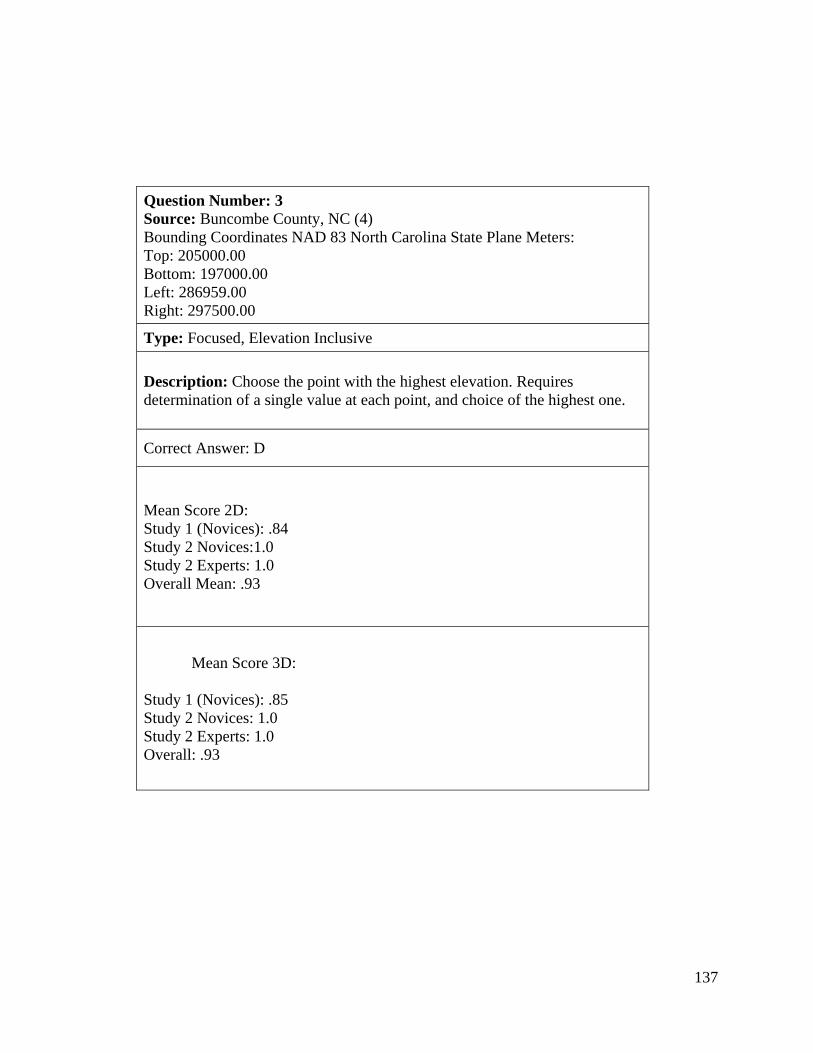
137
Question Number: 3 Source: Buncombe County, NC (4) Bounding Coordinates NAD 83 North Carolina State Plane Meters: Top: 205000.00 Bottom: 197000.00 Left: 286959.00 Right: 297500.00
Type: Focused, Elevation Inclusive
Description: Choose the point with the highest elevation. Requires determination of a single value at each point, and choice of the highest one.
Correct Answer: D
Mean Score 2D: Study 1 (Novices): .84 Study 2 Novices:1.0 Study 2 Experts: 1.0 Overall Mean: .93
Mean Score 3D:
Study 1 (Novices): .85 Study 2 Novices: 1.0 Study 2 Experts: 1.0 Overall: .93

138
Question Number 3 - Focused, Elevation Inclusive
The numbers above represent the elevation (high or height) at the line to which the bottom of the number points. Lighter areas are higher than the line, darker areas are lower than the line. State Government would like to build a monument at the highest elevation in this area so that it can be seen for long distances. Question: Which point shown above represents the highest elevation? A) B) C) D) E)

139
Question Number: 4 Source: Burke County, NC (4) Bounding Coordinates NAD 83 North Carolina State Plane Meters: Top: 239160.00 Bottom: 232200.00 Left: 346946.00 Right: 356000.00
Type: Focused, Elevation Inclusive
Description: Choose the point with the medium elevation. Requires determination of a single value at each point, and choice of the one which is not high or low.
Correct Answer: B
Mean Score 2D: Study 1 (Novices): .84 Study 2 Novices:1.0 Study 2 Experts: .95 Overall Mean: .92
Mean Score 3D: Study 1 (Novices): .74 Study 2 Novices:0.50 Study 2 Experts: .95 Overall Mean: .76

140
Question Number 4 - Focused, Elevation Inclusive
The numbers above represent the elevation (high or height) at the line to which the bottom of the number points. Lighter areas are higher than the line, darker areas are lower than the line. .You would like to build a cabin on a hillside, neither at the highest point nor at the lowest point, but at a point in between. Question: Which point shown above best represents a medium (neither high nor low) elevation? A) B) C) D) E)

141
Question Number: 5 Source: Burke County, NC (2) Bounding Coordinates NAD 83 North Carolina State Plane Meters: Top: 217487.00 Bottom: 209991.00 Left: 362508.00 Right: 371508.00
Type: Focused, Elevation Inclusive
Description: Choose the point with the medium elevation. Requires determination of a single value at each point, and choice of the one which is not high or low.
Correct Answer: C
Mean Score 2D: Study 1 Novices: .87 Study 2 Novices: .78 Study 2 Experts: .81 Overall Mean: .83
Mean Score 3D: Study 1 Novices: .65 Study 2 Novices: .93 Study 2 Experts: .72 Overall Mean: .73

142
Question Number 5 - Focused, Elevation Inclusive
The numbers above represent the elevation (high or height) at the line to which the bottom of the number points. Lighter areas are higher than the line, darker areas are lower than the line. Question: What is the elevation at the point shown? A) 300 B) 400 C) 500 D) 600 E) 700

143
Question Number: 24 Source: Burke County, NC (1) Bounding Coordinates NAD 83 North Carolina State Plane Meters: Top: 223976.00 Bottom: 216480.00 Left: 371503.00 Right: 380996.00
Type: Focused, Elevation Inclusive
Description: Choose the point with the medium elevation. Requires determination of a single value at each point, and choice of the one which is not high or low.
Correct Answer: B
Mean Score 2D: Study 2 Novices:.72 Study 2 Experts: .95 Overall Mean: .85
Mean Score 3D: Study 2 Novices: .64 Study 2 Experts: .77 Overall Mean: .72

144
Question Number 24 - Focused, Elevation Inclusive
The numbers above represent the elevation (high or height) at the line to which the bottom of the number points. Lighter areas are higher than the line, darker areas are lower than the line. .You would like to build a cabin on a hillside, neither at the highest point nor at the lowest point, but at a point in between. Question: Which point shown above best represents a medium (neither high nor low) elevation? A) B) C) D) E)

145
Items 6-10 and 21: Integrative, Elevation Inclusive
Question Number: 6 Source: Avery County, NC (2) Bounding Coordinates NAD 83 North Carolina State Plane Meters: Top: 268043 Bottom: 261963 Left: 347968 Right: 356529
Type: Integrative, Elevation Inclusive
Description: Choose the point with the highest elevation. Requires determination of a single value at each point, and choice of the highest one.
Correct Answer: B
Mean Score 2D: Study 1 Novices: .09 Study 2 Novices:.17 Study 2 Experts: 1.0 Overall Mean: .24 Mean Score 3D: Study 1 Novices: .38 Study 2 Novices: .36 Study 2 Experts: 1.0 Overall Mean: .43

146
Question Number 6 - Integrative, Elevation Inclusive
Question: From which spot are you most likely to see your house and all of the other points? A) B) C) D) E)

147
Question Number: 7 Source: Avery County, NC (3) Bounding Coordinates NAD 83 North Carolina State Plane Meters: Top: 257990 Bottom: 252494 Left: 348999 Right: 356505
Type: Integrative, Elevation Inclusive
Description: Choose the point that is upstream from the selected point. Requires eliminating those points which are not at a higher elevation than the selected point.
Correct Answer: C
Mean Score 2D: Study 1 Novices: .41 Study 2 Novices: .61 Study 2 Experts: .96 Overall Mean: .57 Mean Score 3D: Study 1 Novices: .47 Study 2 Novices: .71 Study 2 Experts: .95 Overall Mean: .57

148
Question Number 7 - Integrative, Elevation Inclusive
Well water pollution was found at the location labeled “Contamination”. Question: Given that water and water pollutants usually flow downhill, which point is the most likely source of the pollution (contamination)?
A) B) C) D) E)

149
Question Number: 8 Source: Source: Avery County, NC (4) Bounding Coordinates NAD 83 North Carolina State Plane Meters: Top: 257008 Bottom: 251500 Left: 335999 Right: 344008
Type: Integrative, Elevation Inclusive
Description: Choose the point which is not at the lowest elevation, and is also on the Southwest slope of an elevated area.
Correct Answer: B
Mean Score 2D: Study 1 Novices: .63 Study 2 Novices: .78 Study 2 Experts: .82 Overall Mean: .73 Mean Score 3D: Study 1 Novices: .41 Study 2 Novices: .50 Study 2 Experts: .73 Overall Mean: .50

150
Question Number 8 - Integrative, Elevation Inclusive
You are looking for a rare plant that only grows in areas protected from exposure to the cold winds coming from the Northeast. The plant enjoys lower altitudes, but will not grow in wetland areas. The lowest area of this map represents a riverbed and wetland. Question: Where would you start looking for this rare plant? A) B) C) D) E)

151
Question Number: 9 Source: Source: Buncombe County, NC (3) Bounding Coordinates NAD 83 North Carolina State Plane Meters: Top: 222498 Bottom: 214982 Left: 297497 Right: 306511
Type: Integrative, Elevation Inclusive
Description: Determine the end point which represents the most rapid change in elevation per distance traveled from the beginning point.
Correct Answer: B
Mean Score 2D: Study 1 Novices: .16 Study 2 Novices: .44 Study 2 Experts: .55 Overall Mean: .28 Mean Score 3D: Study 1 Novices: .18 Study 2 Novices: .14 Study 2 Experts: .55 Overall Mean: .25

152
Question Number 9 - Integrative, Elevation Inclusive
The park manager is trying to decide where to build an “advanced” trail down from the peak of the hill. Advanced trails are usually steep and challenging for even experienced hikers. Trails have been proposed from the point labeled “Trail Head” to each proposed end point (A, B, C, D or E.) Question: Which of the proposed trail routes is the steepest. A) B) C) D) E)

153
Question Number: 10 Source: Burke County, NC (3) Bounding Coordinates NAD 83 North Carolina State Plane Meters: Top: 24698 Bottom: 238992 Left: 350488 Right: 359011
Type: Integrative, Elevation Inclusive
Description: Find the lowest point at a continuous downward slope from the origin point.
Correct Answer: C
Mean Score 2D: Study 1 Novices: .84 Study 2 Novices: .78 Study 2 Experts: .91 Overall Mean: .84 Mean Score 3D: Study 1 Novices: .82 Study 2 Novices: .93 Study 2 Experts: .91 Overall Mean: .87

154
Question Number 10 - Integrative, Elevation Inclusive
Question: If you dropped a ball at the blue point labeled “Ball Dropped Here”, and it kept rolling downhill until it reached the lowest point, where would the ball stop? A) B) C) D) E)

155
Question Number: 21 Source: Avery County, NC (1) Bounding Coordinates NAD 83 North Carolina State Plane Meters: Top: 276503 Bottom: 271003 Left: 342012 Right: 348998
Type: Integrative, Elevation Inclusive
Description: Determine the point least likely to be seen from the target point. Requires visualization of terrain and line of sight.
Correct Answer: C
Mean Score 2D: Study 2 Novices: .50 Study 2 Experts: .91 Overall Mean: .72 Mean Score 3D: Study 2 Novices: .79 Study 2 Experts: .86 Overall Mean: .83

156
Question Number 21 - Integrative, Elevation Inclusive
The blue point shows where the State Park’s “Visitor’s Center” is. Question: Where should we build the dump so it cannot be seen from the visitor’s Center? A) B) C) D) E)
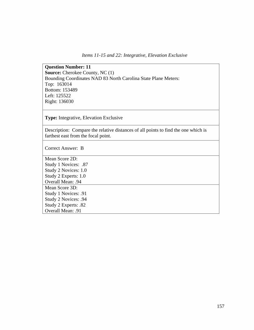
157
Items 11-15 and 22: Integrative, Elevation Exclusive
Question Number: 11 Source: Cherokee County, NC (1) Bounding Coordinates NAD 83 North Carolina State Plane Meters: Top: 163014 Bottom: 153489 Left: 125522 Right: 136030
Type: Integrative, Elevation Exclusive
Description: Compare the relative distances of all points to find the one which is farthest east from the focal point.
Correct Answer: B
Mean Score 2D: Study 1 Novices: .87 Study 2 Novices: 1.0 Study 2 Experts: 1.0 Overall Mean: .94 Mean Score 3D: Study 1 Novices: .91 Study 2 Novices: .94 Study 2 Experts: .82 Overall Mean: .91

158
Question Number 11 - Integrative, Elevation Exclusive
The pale gray grid marks above mark the number of miles north and east on the map. Question: Which point is the farthest distance EAST from the blue point. A) B) C) D) E)
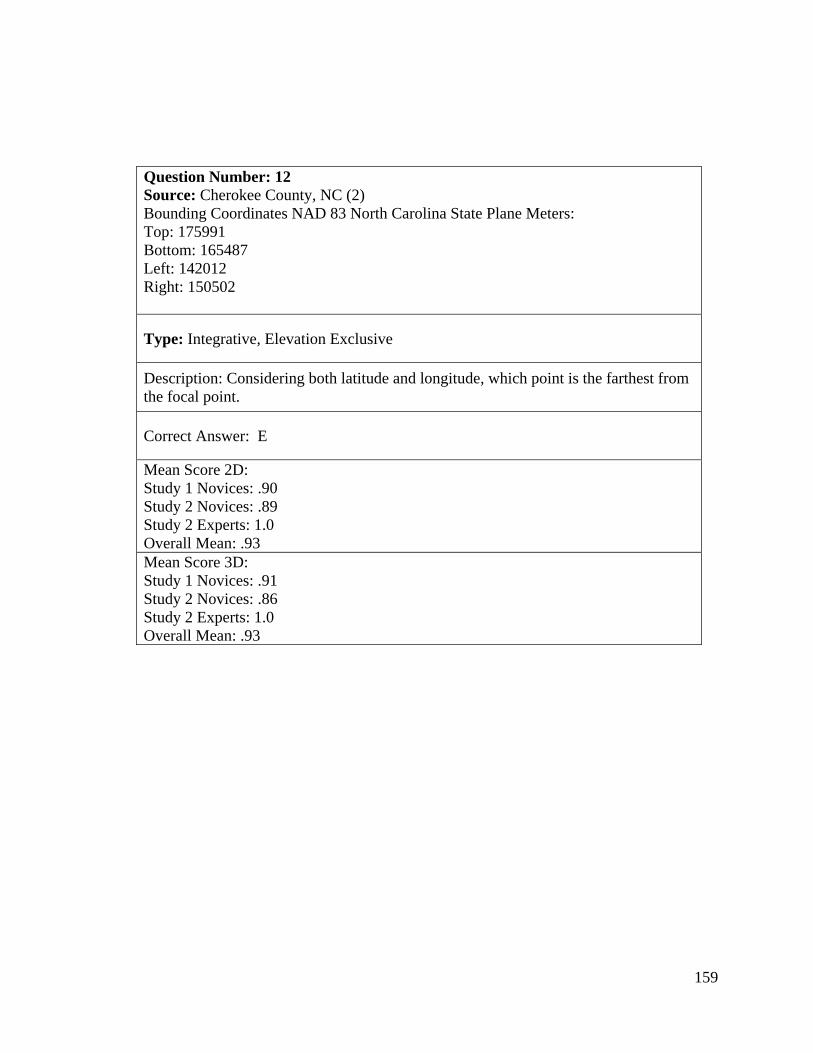
159
Question Number: 12 Source: Cherokee County, NC (2) Bounding Coordinates NAD 83 North Carolina State Plane Meters: Top: 175991 Bottom: 165487 Left: 142012 Right: 150502
Type: Integrative, Elevation Exclusive
Description: Considering both latitude and longitude, which point is the farthest from the focal point.
Correct Answer: E
Mean Score 2D: Study 1 Novices: .90 Study 2 Novices: .89 Study 2 Experts: 1.0 Overall Mean: .93 Mean Score 3D: Study 1 Novices: .91 Study 2 Novices: .86 Study 2 Experts: 1.0 Overall Mean: .93

160
Question Number 12 - Integrative, Elevation Exclusive
The pale gray grid marks above mark the number of miles north and east on the map. Question: Which point is the farthest in BOTH EAST AND NORTH directions from the blue point. A) B) C) D) E

161
Question Number: 13 Source: Cherokee County, NC (3) Bounding Coordinates NAD 83 North Carolina State Plane Meters: Top: 174011 Bottom: 167007 Left: 153488 Right: 162533
Type: Integrative, Elevation Exclusive
Description: Considering both latitude and longitude, which point is the farthest from the focal point.
Correct Answer: B
Mean Score 2D: Study 1 Novices: .69 Study 2 Novices: .83 Study 2 Experts: .77 Overall Mean: .75 Mean Score 3D: Study 1 (Novices): .71 Study 2 Novices: .71 Study 2 Experts: .86 Overall Mean: .76

162
Question Number 13 - Integrative, Elevation Exclusive
The pale gray grid marks above mark the number of miles north and east on the map. Question: Which point is the closest (IN BOTH DIRECTIONS, EAST AND NORTH) to the blue point.
A) B) C) D) E)

163
Question Number: 14 Source: Cherokee County, NC (4) Bounding Coordinates NAD 83 North Carolina State Plane Meters: Top: 176490 Bottom: 168987 Left: 170009 Right: 178535
Type: Integrative, Elevation Exclusive
Description: This question asks for the closest point in the easterly direction that is at the same elevation.
Correct Answer: E
Mean Score 2D: Study 1 Novices: .19 Study 2 Novices: .22 Study 2 Experts: .23 Overall Mean: .21 Mean Score 3D: Study 1 Novices: .26 Study 2 Novices: .21 Study 2 Experts: .41 Overall Mean: .30
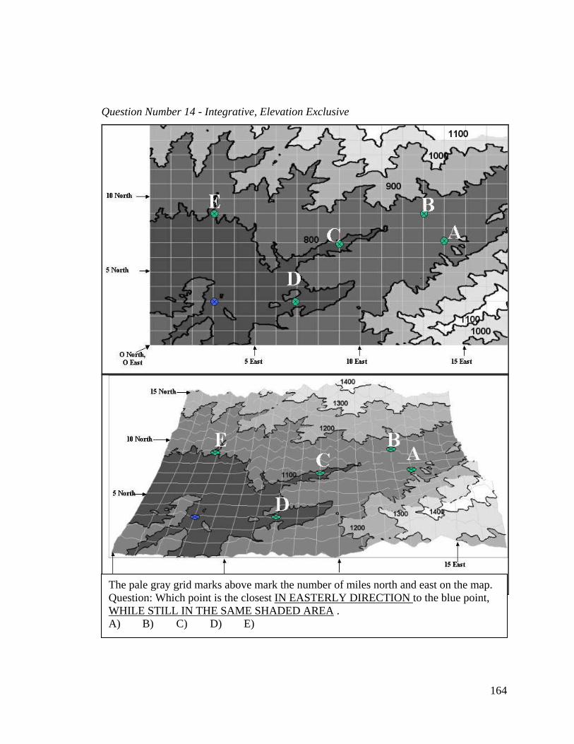
164
Question Number 14 - Integrative, Elevation Exclusive
The pale gray grid marks above mark the number of miles north and east on the map. Question: Which point is the closest IN EASTERLY DIRECTION to the blue point, WHILE STILL IN THE SAME SHADED AREA . A) B) C) D) E)

165
Question Number: 15 Source: Clay County, NC (4) Bounding Coordinates NAD 83 North Carolina State Plane Meters: Top: 152493 Bottom: 147490 Left: 187486 Right: 194518
Type: Integrative, Elevation Exclusive
This question asks for the closest point in the northerly direction that is at the same elevation.
Correct Answer: C
Mean Score 2D: Study 1 Novices: .72 Study 2 Novices: .72 Study 2 Experts: .82 Overall Mean: .75 Mean Score 3D: Study 1 Novices: .74 Study 2 Novices: .71 Study 2 Experts: .91 Overall Mean: .79

166
Question Number 15 - Integrative, Elevation Exclusive
The pale gray grid marks above mark the number of miles north and east on the map. Question: Which point is the closest IN NORTHERLY DIRECTION to the blue point, WHILE STILL IN THE SAME SHADED AREA . A) B) C) D) E)

167
Question Number: 22 Source: Caldwell County, NC (4) Bounding Coordinates NAD 83 North Carolina State Plane Meters: Top: 263500 Bottom: 256981 Left: 376513 Right: 384520
Type: Integrative, Elevation Exclusive
Description: Considering all points, which is the farthest north from the focal point?
Correct Answer: A
Mean Score 2D: Study 2 Novices: 1.0 Study 2 Experts: .95 Overall Mean: .98 Mean Score 3D: Study 2 Novices: .93 Study 2 Experts: .82 Overall Mean: .86

168
Question Number 22 - Integrative, Elevation Exclusive
The pale gray grid above marks the number of miles north and east on the map. Question: Which point is the furthest distance North from the blue point? A) B) C) D) E)

169
Items 16-20 and 23: Focused, Elevation Exclusive
Question Number: 16 Source: Caldwell County, NC (2) Bounding Coordinates NAD 83 North Carolina State Plane Meters: Top: 240003 Bottom: 232673 Left: 374996 Right: 384042
Type: Focused, Elevation Exclusive
Description: This question asks for the easterly coordinate of the focal point (starting from zero).
Correct Answer: D
Mean Score 2D: Study 1 Novices: .75 Study 2 Novices: 1.0 Study 2 Experts: .95 Overall Mean: .87 Mean Score 3D: Study 1 Novices: .94 Study 2 Novices: 1.0 Study 2 Experts: .91 Overall Mean: .94

170
Question Number 16 - Focused, Elevation Exclusive
Question: How far East is the blue point (East from “zero” or 0 East)? A) 9 B) 11 C) 14 D) 7 E) 15

171
Question Number: 17 Source: Caldwell County, NC (3) Bounding Coordinates NAD 83 North Carolina State Plane Meters: Top: 265995 Bottom: 259977 Left: 362506 Right: 371497
Type: Focused, Elevation Exclusive
Description: How far east of the focal point is the other point?
Correct Answer: B
Mean Score 2D: Study 1 Novices: .78 Study 2 Novices: 1.0 Study 2 Experts: .95 Overall Mean: .89 Mean Score 3D: Study 1 Novices: .79 Study 2 Novices: .86 Study 2 Experts: .86 Overall Mean: .83
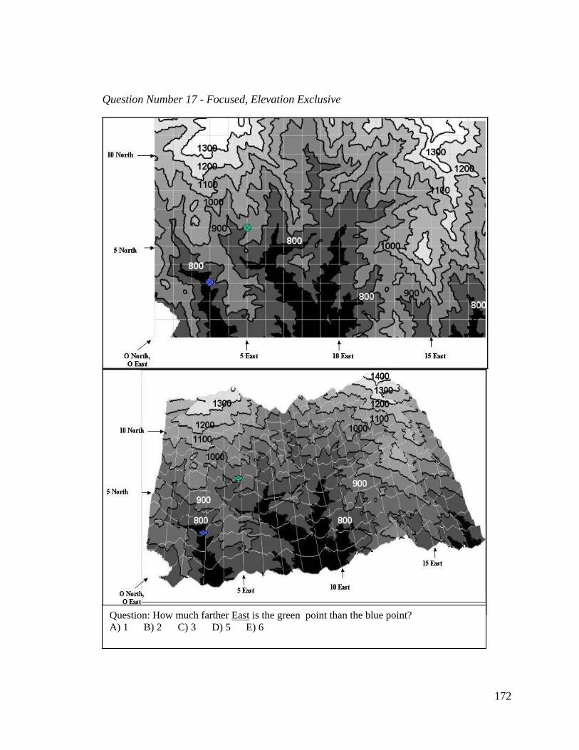
172
Question Number 17 - Focused, Elevation Exclusive
Question: How much farther East is the green point than the blue point? A) 1 B) 2 C) 3 D) 5 E) 6

173
Question Number: 18 Source: Clay County, NC (1) Bounding Coordinates NAD 83 North Carolina State Plane Meters: Top: 164997 Bottom: 159992 Left: 171519 Right: 180004
Type: Focused, Elevation Exclusive
Description: How far north of the focal point is the other point?
Correct Answer: C
Mean Score 2D: Study 1 Novices: .91 Study 2 Novices: .78 Study 2 Experts: .91 Overall Mean: .87 Mean Score 3D: Study 1 Novices: .35 Study 2 Novices: .86 Study 2 Experts: .86 Overall Mean: .62

174
Question Number 18 - Focused, Elevation Exclusive
Question: How much farther North is the green point than the blue point? A) 1 B) 2 C) 3 D) 5 E) 6

175
Question Number: 19 Source: Clay County, NC (2) Bounding Coordinates NAD 83 North Carolina State Plane Meters: Top: 158000 Bottom: 152494 Left: 180524 Right: 187507
Type: Focused, Elevation Exclusive
Description: Pick the most easterly point
Correct Answer: D
Mean Score 2D: Study 1 Novices: .78 Study 2 Novices: 1.0 Study 2 Experts: .95 Overall Mean: .89 Mean Score 3D: Study 1 Novices: .82 Study 2 Novices: .86 Study 2 Experts: .82 Overall Mean: .83
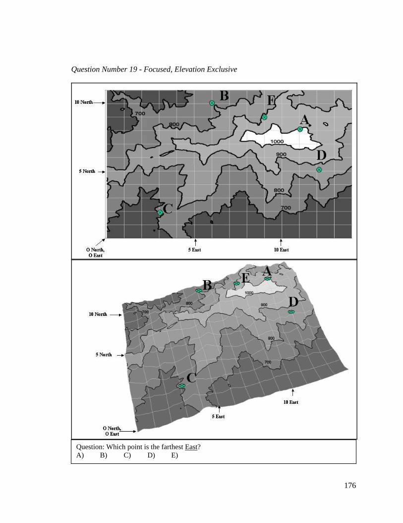
176
Question Number 19 - Focused, Elevation Exclusive
Question: Which point is the farthest East?
A) B) C) D) E)

177
Question Number: 20 Source: Clay County, NC (3) Bounding Coordinates NAD 83 North Carolina State Plane Meters: Top: 162004 Bottom: 157995 Left: 181022 Right: 187509
Type: Focused, Elevation Exclusive
Description: pick the most northerly point
Correct Answer: B
Mean Score 2D: Study 1 Novices: .78 Study 2 Novices: .89 Study 2 Experts: .95 Overall Mean: .89 Mean Score 3D: Study 1 Novices: .82 Study 2 Novices: .86 Study 2 Experts: .86 Overall Mean: .86

178
Question Number 20 - Focused, Elevation Exclusive
Question: Which point is the farthest North? A) B) C) D) E

179
Question Number: 23 Source: Caldwell County, NC (1) Bounding Coordinates NAD 83 North Carolina State Plane Meters: Top: 254493 Bottom: 246481 Left: 379506 Right: 389502
Type: Focused, Elevation Exclusive
Description: This question asks for the northerly coordinate of the focal point (starting from zero).
Correct Answer: B
Mean Score 2D: Study 2 Novices: .89 Study 2 Experts: .91 Overall Mean: .90 Mean Score 3D: Study 2 Novices: .79 Study 2 Experts: .91 Overall Mean: .86
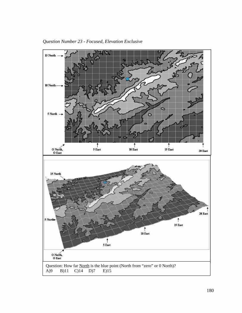
180
Question Number 23 - Focused, Elevation Exclusive
Question: How far North is the blue point (North from “zero” or 0 North)?
A)9 B)11 C)14 D)7 E)15

181
Appendix 4. Visual Basic Code
Study Code
Form 4 - get subject number and current directory, and launch practice intro
Form 2 – “practice” intro then launch practice
Form 3 – Ask Practice questions in random order, and give feedback
Form 1 – start timer and display task, receive and write answer and time

182
Form 4 Code
Public basepath As String, subjectnum As String, subjectfile As String Private Sub continue_Click() If File1.FileName = "studyProject.exe" Then basepath = File1.Path & "\" Form4.Hide subjectnum = InputBox("Please change the number below to your survey number: ", "Survey Number", "S001G12Z") subjectfile = "a:\" & subjectnum & ".txt" Open subjectfile For Output As #1 Print #1, subjectnum 'save string to file Close #1 'close file Form2.Show Else i% = MsgBox("Please choose the location of 'studyProject.exe'", vbOKOnly, "wrong File location") End If End Sub Private Sub Dir1_Change() File1.Path = Dir1.Path End Sub Private Sub Drive1_Change() Dir1.Path = Drive1.Drive End Sub Private Sub Form_Load() Label1.Caption = "Find the program file 'studyProject.exe' which runs the study, and click on it. When the " _ & "correct file is selected, click the 'Continue' button" End Sub

183
Form 2 Code
Private Sub Form_Load() Text1.Text = "When you click the button below, you will get four practice questions. A picture will be displayed," _ & "and a question will be asked. Select an answer between A and E and click the 'Next Question' Button. " _ & "Please answer the questions as quickly and accurately as you can. Click the button when you are ready " _ & "to start." End Sub Private Sub start_Click() Form2.Hide Form3.Show End Sub
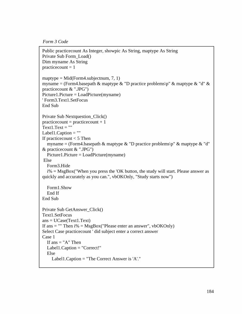
184
Form 3 Code
Public practicecount As Integer, showpic As String, maptype As String Private Sub Form_Load() Dim myname As String practicecount = 1 maptype = Mid(Form4.subjectnum, 7, 1) myname = (Form4.basepath & maptype & "D practice problems\p" & maptype & "d" & practicecount & ".JPG") Picture1.Picture = LoadPicture(myname) ' Form3.Text1.SetFocus End Sub Private Sub Nextquestion_Click() practicecount = practicecount + 1 Text1.Text = "" Label1.Caption = "" If practicecount < 5 Then myname = (Form4.basepath & maptype & "D practice problems\p" & maptype & "d" & practicecount & ".JPG") Picture1.Picture = LoadPicture(myname) Else Form3.Hide i% = MsgBox("When you press the 'OK button, the study will start. Please answer as quickly and accurately as you can.", vbOKOnly, "Study starts now") Form1.Show End If End Sub Private Sub GetAnswer_Click() Text1.SetFocus ans = UCase(Text1.Text) If ans = "" Then i% = MsgBox("Please enter an answer", vbOKOnly) Select Case practicecount ' did subject enter a correct answer Case 1 If ans = "A" Then Label1.Caption = "Correct!" Else Label1.Caption = "The Correct Answer is 'A'."

185
End If Case 2 If ans = "A" Then Label1.Caption = "Correct!" Else Label1.Caption = "The Correct Answer is 'A'." End If Text1.Text = "" Case 3 If ans = "B" Then Label1.Caption = "Correct!" Else Label1.Caption = "The Correct Answer is 'B'." End If Text1.Text = "" Case 4 If ans = "B" Then Label1.Caption = "Correct!" Else Label1.Caption = "The Correct Answer is 'B'." End If End Select ' end answer processing End Sub

186
Form 1 Code
Public curcount As Integer, showpic As String, subjectfile As String, starttime As Variant Private Sub Form_Load() Dim myname, temparray() As String, searchpath ' Returns filename with specified extension. If more than one *.jpg ' file exists, the first file found is returned. ' subjectnum = InputBox("Please change the number below to your survey number: ", "Survey Number", "S001G12Z") ' subjectfile = "a:\" & form4.subjectnum & ".txt" ' Open subjectfile For Output As #1 ' Print #1, subjectnum 'save string to file ' Close #1 'close file curcount = 0 Form1.Timer1.Enabled = True Form1.starttime = Time searchpath = Form4.basepath & Mid(Form4.subjectnum, 7, 1) & "D Study Problems\*.JPG" myname = Dir(searchpath) Do While myname <> "" ' Start the loop. curcount = curcount + 1 myname = Dir ' Get next entry. Loop myname = Dir(searchpath) ReDim PicFileNames(1 To curcount) For i% = 1 To curcount PicFileNames(i%) = myname myname = Dir Next i% ReDim temparray(1 To (curcount - 1)) Randomize whichpic = (Int(curcount * Rnd) + 1) showpic = PicFileNames(whichpic) Picture1.Picture = LoadPicture(Form4.basepath & Mid(Form4.subjectnum, 7, 1) & "D Study Problems\" & showpic) For i% = 1 To (whichpic - 1) temparray(i%) = PicFileNames(i%) Next i% If (whichpic) <> curcount Then For i% = (whichpic + 1) To curcount temparray(i% - 1) = PicFileNames(i%) Next i%
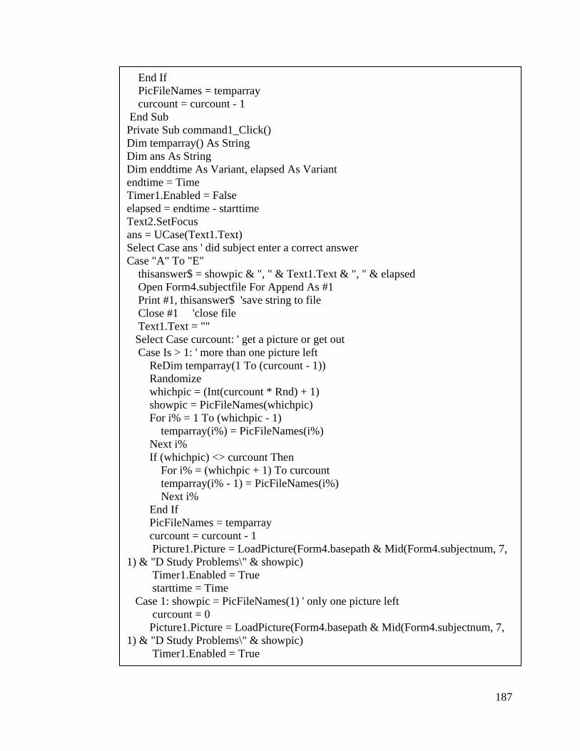
187
End If PicFileNames = temparray curcount = curcount - 1 End Sub Private Sub command1_Click() Dim temparray() As String Dim ans As String Dim enddtime As Variant, elapsed As Variant endtime = Time Timer1.Enabled = False elapsed = endtime - starttime Text2.SetFocus ans = UCase(Text1.Text) Select Case ans ' did subject enter a correct answer Case "A" To "E" thisanswer$ = showpic & ", " & Text1.Text & ", " & elapsed Open Form4.subjectfile For Append As #1 Print #1, thisanswer$ 'save string to file Close #1 'close file Text1.Text = "" Select Case curcount: ' get a picture or get out Case Is > 1: ' more than one picture left ReDim temparray(1 To (curcount - 1)) Randomize whichpic = (Int(curcount * Rnd) + 1) showpic = PicFileNames(whichpic) For i% = 1 To (whichpic - 1) temparray(i%) = PicFileNames(i%) Next i% If (whichpic) <> curcount Then For i% = (whichpic + 1) To curcount temparray(i% - 1) = PicFileNames(i%) Next i% End If PicFileNames = temparray curcount = curcount - 1 Picture1.Picture = LoadPicture(Form4.basepath & Mid(Form4.subjectnum, 7, 1) & "D Study Problems\" & showpic) Timer1.Enabled = True starttime = Time Case 1: showpic = PicFileNames(1) ' only one picture left curcount = 0 Picture1.Picture = LoadPicture(Form4.basepath & Mid(Form4.subjectnum, 7, 1) & "D Study Problems\" & showpic) Timer1.Enabled = True

188
starttime = Time Case Else: ' no pictures left Form1.Hide i% = MsgBox("That's the Last question. Thanks for participating in this study! Click 'OK' to exit.", vbOKOnly, "Thank You...") End End Select ' end picture processing Case Else ' wrong or no answer entered i% = MsgBox("Please type an answer between A and E, and then click the 'Next Answer' key", vbOKOnly, "Please enter A, B, C, D or E") End Select ' end answer processing End Sub Private Sub Text2_KeyPress(KeyAscii As Integer) Nextpic.SetFocus End Sub

189
Code to Read Diskette, Parse and Write Data
_________________________________ ______________________________
Public subjectfile As String, astring As String, bstring As String Private Sub Form_Load() myname = Dir("a:\*.txt") subjectfile = "a:\" & myname Open subjectfile For Input As #1 Line Input #1, astring subjectcode.Text = astring End Sub Private Sub proceed_Click() Dim counterindex(1 To 24) As Integer, subjanswers(1 To 24) As String, subjtimes(1 To 24) As String, lines() As String Dim summfile As String Dim subjectnum As String, numdims As String ' define subject number and dimensions 2 or 3 Dim subjanswer As String, questionnum As Integer ' define answer a, b,c,d,e and question number Dim subjtime As String ' define time in miliseconds Dim NoExchange As Boolean 'sort Dim Temp Dim powr As Integer Dim mynum As Single astring = subjectcode.Text summfile = "C:\project2asumm.txt" ' define name of summary file subjectnum = Mid(astring, 2, 3) ' parse subject number numdims = Mid(astring, 7, 1) ' parse dims For I% = 1 To 24 'read 24 lines on first diskette Line Input #1, astring questionnum = Mid(astring, 4, 2) counterindex(I) = questionnum ' read and store question number in its place within the array subjanswer = Mid(astring, 12, 1) subjanswers(questionnum) = subjanswer ' read and store answer subjtime = Mid(astring, 15)

190
subjtime = subjtime * 86400 subjtimes(questionnum) = FormatNumber(subjtime, 1) ' read and store time Next I% Close #1 ' close diskette file astring = numdims & ", " & subjectnum & ", " ' start the string with the number of dims and subject number For I = 1 To 24 astring = astring & subjanswers(I) & ", " ' append answers to the subject number Next I For I = 1 To 23 astring = astring & subjtimes(I) & ", " ' append times to the string Next I astring = astring & subjtimes(24) Open summfile For Append As #2 ' open output file and write the line Print #2, astring Close #2 Response = MsgBox("another diskette", vbYesNo, Title, Help, Ctxt) If Response = vbYes Then ' User chose Yes. myname = Dir("a:\*.txt") subjectfile = "a:\" & myname Open subjectfile For Input As #1 Line Input #1, astring subjectcode.Text = astring Else ' User chose No. Open summfile For Input As #2 I = 0 Do Until EOF(2) Line Input #2, nextline I = I + 1 Loop Close #2 j = I ReDim lines(1 To I) As String Open summfile For Input As #2 I = 0 Do Until EOF(2) Line Input #2, nextline I = I + 1 lines(I) = nextline Loop Close #2 ' bubble sort

191
Do NoExchange = True I = j - 1 For l = 1 To (I) If Mid(lines(l), 4, 3) > Mid(lines(l + 1), 4, 3) Then Temp = lines(l) lines(l) = lines(l + 1) lines(l + 1) = Temp NoExchange = False End If Next Loop Until NoExchange Open summfile For Output As #2 For I = 1 To j Print #2, lines(I) Next Do ' sort by dimension, then subject number NoExchange = True I = j - 1 For l = 1 To (I) If Left(lines(l), 6) > Left(lines(l + 1), 6) Then Temp = lines(l) lines(l) = lines(l + 1) lines(l + 1) = Temp NoExchange = False End If Next Loop Until NoExchange Open "C:\summdim.txt" For Output As #3 For I = 1 To j Print #3, lines(I) Next Close #3 End End If End Sub