ABSTRACT OVERBY, DAVID THOMAS. Stress-Strain ...

ABSTRACT

OVERBY, DAVID THOMAS. Stress-Strain Behavior of ASTM A706 Grade 80

Reinforcement. (Under the direction of Dr. Mervyn Kowalsky and Dr. Rudolf Seracino)

In the seismic design of reinforced concrete structures, the overstrength of the steel

reinforcement plays a critical role in the structure’s ability to dissipate energy inelastically as

unaccounted for strength could lead to sudden, non-ductile modes of failure. Thus,

knowledge of the expected mechanical properties of the reinforcement being used is

extremely important. The current availability of ASTM A706 grade 80 rebar material test

results is very limited in regards to both strength and strain parameters. In response to this

issue, a research program was developed to determine the stress-strain behavior of ASTM

A706 grade 80 high strength steel reinforcement.

Three types of tests were performed in pursuit of this objective: monotonic tensile

tests, cyclic tests, and strain age tests. A total of 788 tensile tests of A706 grade 80 rebar

were performed on all bar sizes No. 4 through No. 18 in the as-rolled condition. Additional

tests of No. 5 and No. 7 bars were used to investigate the strain aging and cyclic performance

of the steel. Steel was provided by three producing mills and multiple heats were tested from

each mill. A non-contact 3D position measurement system was used to simultaneously

evaluating strains over multiple gage lengths for the full duration of each test, including

fracture of the bar.

Results generated by the tensile tests are used to develop recommendations for the

yield strength, yield strain, strain at onset of strain hardening, tensile strength, and ultimate

tensile strain based on the mean values obtained across all bar sizes. The Kolmogorov-

Smirnov goodness-of-fit test is used to identify the underlying probability distributions of the

material properties which have been presented graphically with the empirical cumulative

distribution functions in order to illustrate the variability in the data. The A706 grade 80

monotonic stress-strain curve is shown to have a proportionally consistent shape to the A706

grade 60 rebar and may be characterized by existing reinforcing steel models. No consistent

trend related to strain aging was observed for any of the experimental treatments. An existing

reinforcing steel model was shown to successfully characterize the shape of the cyclic stress-

strain curve. Limitations of the testing equipment precluded identification of any specific

relationship between cyclic load history and ultimate tensile strain.

Stress-Strain Behavior of ASTM A706 Grade 80 Reinforcement

by

David Thomas Overby

A thesis submitted to the Graduate Faculty of

North Carolina State University

in partial fulfillment of the

requirements for the degree of

Master of Science

Civil Engineering

Raleigh, North Carolina

2016

APPROVED BY:

_______________________________ _______________________________

Rudolf Seracino, Ph.D. James M. Nau, Ph.D.

_____________________________

Mervyn J. Kowalsky, Ph.D.

Committee Chair

ii

BIOGRAPHY

David Thomas Overby was born in Merrillville, IN; however, much of his early years

were spent in the mountains of Pennsylvania where he developed a love for the outdoors and

a fascination with knowing how things worked. Coupled with a desire to be continually

learning, his interest in science and math ultimately led him to pursue a degree in Civil

Engineering following graduation from Gospel Light Christian School in Walkertown, NC in

May, 2010. Four years later, he received a Bachelor of Science in Civil Engineering from

North Carolina State University. Desiring to expand on his knowledge, David continued his

education into graduate school at North Carolina State University where he received a Master

of Science in Civil Engineering with an emphasis on Structural Engineering in 2016. David

intends to bring the experience and knowledge gained from his education with him into a

career in structural engineering.

iii

ACKNOWLEDGMENTS

I would very much like to thank my advisor, Dr. Mervyn Kowalsky, for his

enthusiasm in structural and earthquake engineering and his willingness to be so engaged

with his students in the projects that they pursue together. I appreciate his high standard of

achievement and desire to do things both well and thoroughly. I would additionally like to

thank Drs. Rudi Seracino and James Nau for being members of my committee and for the

real-world perspective they are able to bring both to the classroom and the research to which

they contribute.

I would be remiss not to gratefully acknowledge the faithful support of the staff and

students at the CFL who contributed so extensively to the completion of this project. In

particular, I would like to extend a hearty thanks to Greg Lucier, Jerry Atkinson, and

Johnathan McEntire for constantly providing advice on how to use the equipment at the lab,

fixing things when they broke, and their patience through numerous hours of performing the

tensile tests. I am further indebted to Emrah Tasdemir for assisting in the design of the large

bar test setup, Aaron Stroud for his efforts in helping test the large diameter bars, and

Grayson Fulp for helping prepare the rebar specimens for testing.

Additional thanks go to the California Department of Transportation for their

financial support and interest in the project, to the three producing mills (Cascade, Gerdau,

and Nucor) who graciously donated reinforcing bars for this research, and the Concrete

Reinforcing Steel Institute (CRSI) and Bethany Hennings who coordinated with the mills to

acquire the steel and provided special access to the CRSI database of mill tensile test results.

Above all, I thank God who has given my life a purpose and meaning beyond itself.

iv

TABLE OF CONTENTS

LIST OF TABLES .................................................................................................................... x

LIST OF FIGURES ................................................................................................................ xii

1. INTRODUCTION ............................................................................................................. 1

1.1. Background ................................................................................................................ 1

1.2. Research Objective ..................................................................................................... 4

1.3. Scope .......................................................................................................................... 6

1.3.1. Tensile Tests ....................................................................................................... 6

1.3.2. Strain Age Tests .................................................................................................. 6

1.3.3. Cyclic Tests ......................................................................................................... 7

1.4. Overview of Report Contents ..................................................................................... 7

2. LITERATURE REVIEW ................................................................................................ 10

2.1. A706 Grade 80 Rebar in Design Standards ............................................................. 10

2.1.1. ACI 318-14 ....................................................................................................... 10

2.1.2. Caltrans Seismic Design Criteria ...................................................................... 10

2.1.3. AASHTO LRFD Bridge Design Specification ................................................. 11

2.1.4. AASHTO Guide Specification for LRFD Seismic Bridge Design ................... 11

2.1.5. WSDOT Bridge Design Manual ....................................................................... 12

2.1.6. ODOT Bridge Design and Drafting Manual ..................................................... 12

2.1.7. Alaska DOT ...................................................................................................... 12

2.2. Existing A706 Grade 80 Experimental Data ............................................................ 12

2.2.1. Research Data ................................................................................................... 14

2.2.1.1. Rautenberg et al. (2013) ............................................................................ 14

2.2.1.2. WJE RGA 04-13 Report (2013) ................................................................ 15

2.2.1.3. GCR 14-917-30 (2014) .............................................................................. 19

2.2.1.4. Trejo, Barbosa, and Link. (2014) .............................................................. 21

2.2.2. Mill and CRSI Data .......................................................................................... 23

2.3. Statistical Studies of Rebar Test Results .................................................................. 27

v

2.3.1. Allen (1972) ...................................................................................................... 27

2.3.2. Mirza and MacGregor (1979) ........................................................................... 28

2.3.3. Nowak and Szerszen (2003) ............................................................................. 29

2.3.4. Bournonville et al. (2004) ................................................................................. 29

2.4. Strain Aging Literature............................................................................................. 31

2.4.1. Introduction to Strain Aging ............................................................................. 31

2.4.2. Relevant Papers on Strain Aging ...................................................................... 34

2.4.2.1. Pussegoda (1978) ....................................................................................... 34

2.4.2.2. Lim (1991) ................................................................................................. 36

2.4.2.3. Restrepo-Posada et al. (1994) .................................................................... 38

2.4.2.4. Momtahan et al. (2009) ............................................................................. 39

2.4.2.5. Summary of Strain Aging Literature ......................................................... 41

2.5. Cyclic Testing Literature .......................................................................................... 43

2.5.1. Existing Material Models .................................................................................. 45

2.5.1.1. Giuffre-Pinto (1970); Menegotto-Pinto (1973) ......................................... 45

2.5.1.2. Filippou et al. (1983) ................................................................................. 47

2.5.1.3. Monti-Nuti (1992) ..................................................................................... 48

2.5.1.4. Chang and Mander (1994) ......................................................................... 49

2.5.1.5. Dhakal and Maekawa (2002) ..................................................................... 50

2.5.2. Summary of Cyclic Testing Literature ............................................................. 51

3. EXPERIMENTAL PROGRAM ...................................................................................... 53

3.1. Chapter Overview .................................................................................................... 53

3.2. Materials ................................................................................................................... 53

3.3. Equipment ................................................................................................................ 56

3.3.1. Testing Equipment ............................................................................................ 56

3.3.2. Instrumentation ................................................................................................. 60

3.4. Tensile Testing ......................................................................................................... 63

3.4.1. Test Matrix ........................................................................................................ 63

3.4.2. Specimen Preparation ....................................................................................... 65

vi

3.4.3. Test Parameters ................................................................................................. 67

3.4.4. Calibration of Custom Testing Rig ................................................................... 72

3.5. Strain Age Testing .................................................................................................... 76

3.5.1. Test matrix ........................................................................................................ 76


3.5.3. Testing Parameters ............................................................................................ 78

3.6. Cyclic Testing .......................................................................................................... 79

3.6.1. Test Matrix ........................................................................................................ 79


3.6.3. Test Parameters ................................................................................................. 81

4. RESULTS ........................................................................................................................ 83

4.1. Chapter Overview .................................................................................................... 83

4.2. Tensile Testing ......................................................................................................... 84

4.2.1. Determination of Stress-Strain Parameters ....................................................... 84

4.2.1.1. Modulus of Elasticity................................................................................. 85

4.2.1.2. Yield Strength ............................................................................................ 85

4.2.1.3. Yield Strain ................................................................................................ 86

4.2.1.4. Onset of Strain Hardening ......................................................................... 86

4.2.1.5. Tensile Strength and Ultimate Tensile Strain ............................................ 87

4.2.2. Statistical Methods ............................................................................................ 87

4.2.3. Expected Mechanical Properties ....................................................................... 92

4.2.3.1. Modulus of Elasticity................................................................................. 92

4.2.3.2. ADM Yield Strength ................................................................................. 94

4.2.3.3. EUL Yield Strength ................................................................................... 97

4.2.3.4. OM Yield Strength .................................................................................. 100

4.2.3.5. Yield Strain .............................................................................................. 103

4.2.3.6. Strain at Onset of Strain Hardening ......................................................... 106

4.2.3.7. Tensile Strength ....................................................................................... 109

4.2.3.8. Ultimate Tensile Strain ............................................................................ 112

4.2.3.9. Tensile to Yield Ratio .............................................................................. 115

vii

4.2.3.10. Summary of Tensile Test Results ........................................................... 118

4.2.4. Shape of the Strain Hardening Curve ............................................................. 119

4.3. Strain Age Testing .................................................................................................. 124

4.3.1. Impact of Aging Period ................................................................................... 125

4.3.2. Impact of Pre-Strain Level .............................................................................. 129

4.3.3. Impact of Bar Size .......................................................................................... 133

4.3.4. Impact of Temperature .................................................................................... 136

4.4. Cyclic Testing ........................................................................................................ 139

4.4.1. Model Comparison.......................................................................................... 140

4.4.2. Effects of Load History on Ultimate Tensile Strain ....................................... 141

4.4.2.1. Test ID: 12544 ......................................................................................... 145

4.4.2.2. Test ID: 12547 ......................................................................................... 146

4.4.2.3. Test ID: 12548 ......................................................................................... 147

4.4.2.4. Test ID: 12549 ......................................................................................... 148

4.4.2.5. Test ID: 125410 ....................................................................................... 150

4.4.2.6. Test ID: 125411 ....................................................................................... 151

4.4.2.7. Test ID: 12746 ......................................................................................... 152

4.4.2.8. Summary Table........................................................................................ 154

5. DISCUSSION ................................................................................................................ 155

5.1. Tensile Tests ........................................................................................................... 155

5.1.1. Comparison with Literature Results ............................................................... 155

5.1.2. Comparison with Mill and CRSI Data ............................................................ 158

5.1.2.1. Yield Strength .......................................................................................... 158

5.1.2.2. Tensile Strength ....................................................................................... 159

5.1.2.3. Percent Elongation at Fracture ................................................................ 160

5.1.2.4. Tensile-to-Yield Ratio ............................................................................. 161

5.1.3. Analysis of Variabilities ................................................................................. 163

5.1.3.1. Mills ......................................................................................................... 163

5.1.3.2. Heats ........................................................................................................ 165

5.1.3.3. Twenty-foot Bars ..................................................................................... 165

viii

5.1.3.4. Heats by Bar Size .................................................................................... 166

5.1.3.5. Summary .................................................................................................. 167

5.1.4. Parameter Interactions .................................................................................... 168

5.1.4.1. fye vs sh .................................................................................................... 169

5.1.4.2. fye vs fue .................................................................................................... 170

5.1.4.3. fye vs su .................................................................................................... 171

5.1.4.4. fue vs su .................................................................................................... 172

5.1.4.5. sh vs su ................................................................................................... 173

5.1.4.6. percent elongation vs su .......................................................................... 174

5.1.5. Yield Strengths Falling Below 80 ksi ............................................................. 177

5.1.6. Variability in Strain Over Bar Length ............................................................ 178

5.1.7. Future Tensile Testing .................................................................................... 181

5.1.7.1. Effect of Testing 1 Specimen per Bar ..................................................... 181

5.1.7.2. Effect of Testing 1 Specimen per Bar per Heat ....................................... 182

5.2. Strain Age Tests ..................................................................................................... 183

5.2.1. Comparison with Literature Results ............................................................... 183

5.2.2. Future Strain Age Testing ............................................................................... 184

5.3. Cyclic Tests ............................................................................................................ 185

5.3.1. Future Cyclic Testing ...................................................................................... 185

6. CONCLUSIONS ........................................................................................................... 187

6.1. Summary ................................................................................................................ 187

6.2. Recommendations .................................................................................................. 189

7. REFERENCES .............................................................................................................. 190

APPENDICES ...................................................................................................................... 197

8. Appendix A: Summary of Bar Sizes by Heat and Mill ................................................. 198

8.1. Mill 1 ...................................................................................................................... 198

8.2. Mill 2 ...................................................................................................................... 198

8.3. Mill 3 ...................................................................................................................... 198

ix

9. Appendix B: Determination of Stress-Strain Parameters .............................................. 199

9.1. Modulus of Elasticity ............................................................................................. 199

9.2. Yield Strength ........................................................................................................ 200

9.3. Onset of Strain Hardening ...................................................................................... 200

10. Appendix C: Mill Cumulative Distribution Functions ............................................. 201

10.1. ADM Yield Strength .......................................................................................... 201

10.2. Yield Strain ......................................................................................................... 202

10.3. Onset of Strain Hardening .................................................................................. 203

10.4. Tensile Strength .................................................................................................. 204

10.5. Ultimate Tensile Strain ....................................................................................... 205

10.6. Tensile-to-Yield Ratio ........................................................................................ 206

11. Appendix D: Heat Cumulative Distribution Functions ............................................ 207

11.1. Yield Strength ..................................................................................................... 207

11.2. Yield Strain ......................................................................................................... 209


11.4. Tensile Strength .................................................................................................. 213


12. Appendix E: 2” vs 8” Gage Length Comparison ...................................................... 217

12.1. Yield Strain ......................................................................................................... 217



13. Appendix F: Comparison of Yield Strength Determination Methods ...................... 219

14. Appendix G: Summary of Yield Behaviors .............................................................. 220

15. Appendix H: Strain-aging Stress-strain Curves ........................................................ 221

16. Appendix I: Additional No. 7 bar cyclic test ............................................................ 235

17. Appendix J: Test Photos ........................................................................................... 236

x

LIST OF TABLES

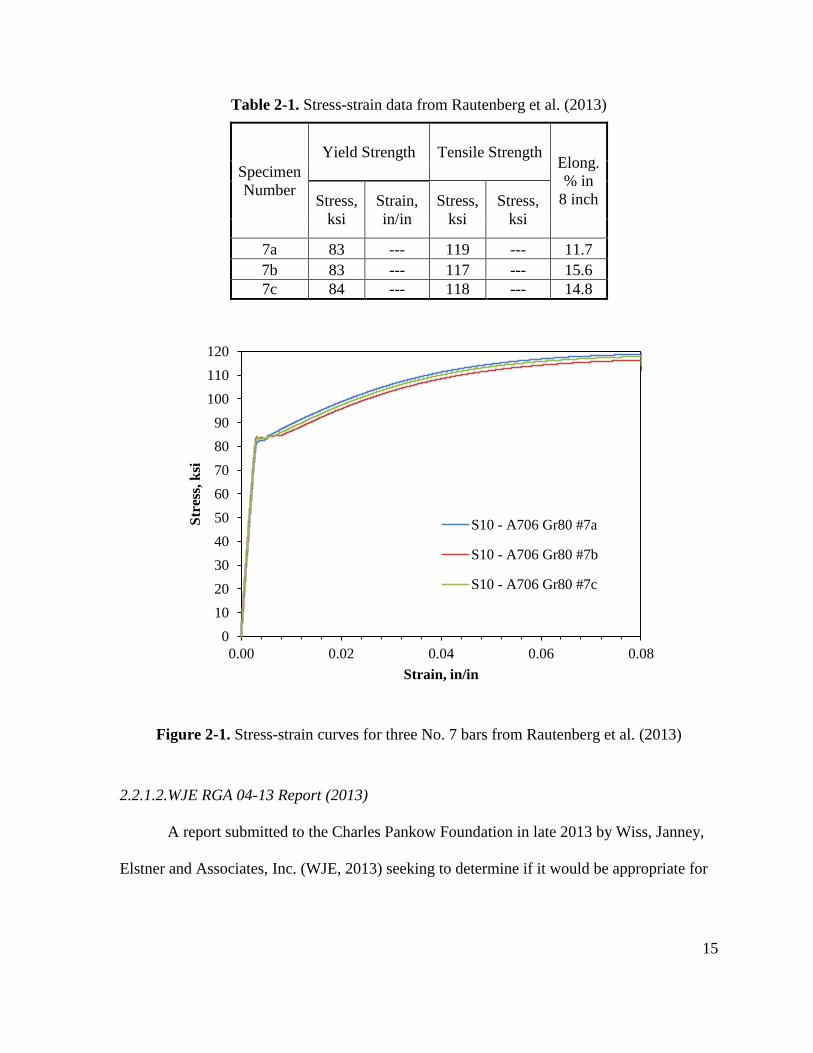
Table 2-1. Stress-strain data from Rautenberg et al. (2013) ................................................... 15

Table 2-2. Stress-strain data provided in NIST GCR Report (2014) ...................................... 20

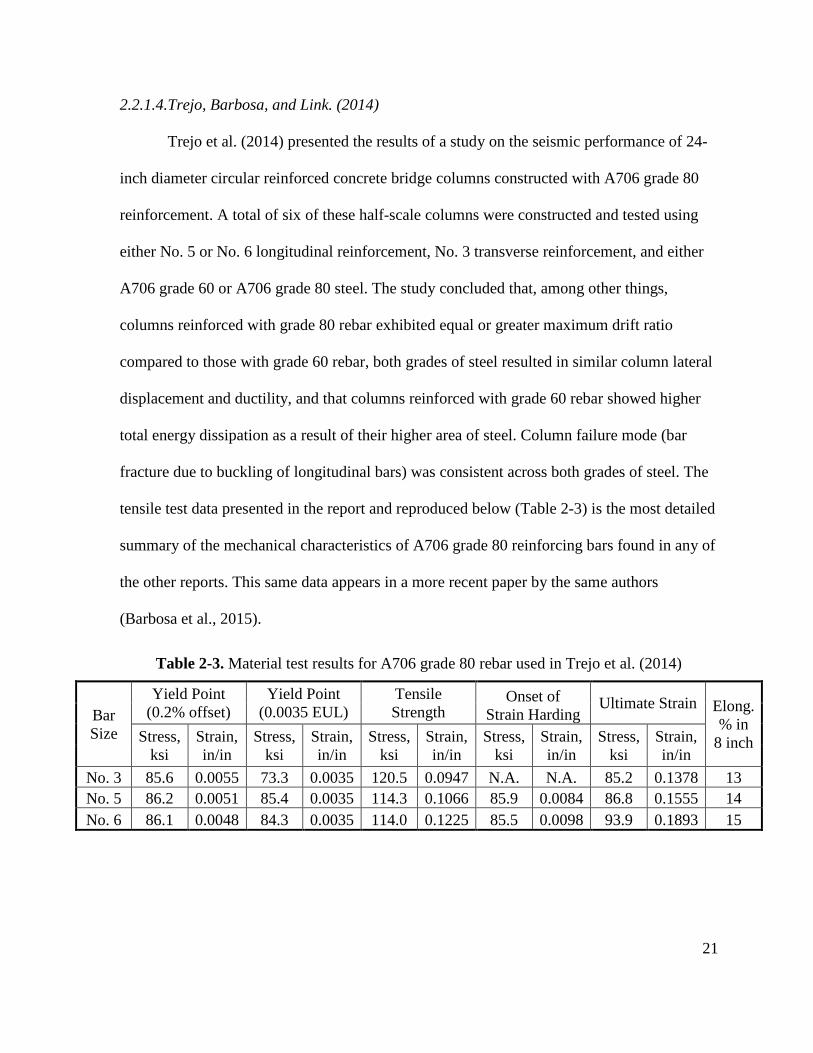
Table 2-3. Material test results for A706 grade 80 rebar used in Trejo et al. (2014) ............. 21

Table 2-4. Statistical summary of stress data for all A706 grade 80 and Dual A615/A706

grade 80 rebar (CRSI, 2013) ................................................................................................... 24

Table 2-5. Cascade Steel mill data referenced in Trejo et al. (2014) ...................................... 27 Table 2-6. Impact of vanadium content on strain aging susceptibility of mild (grade 275)

New Zealand bars (Pussegoda, 1978) ..................................................................................... 35 Table 2-7. Impact of titanium content on strain aging susceptibility of mild (grade 275) New

Zealand bars for a range of pre-strain levels (Pussegoda, 1978) ............................................ 36

Table 2-8. Extent of strain-aging following a 5% pre-strain as presented in Lim (1991) ...... 37 Table 2-9. Percent increase in yield strength of New Zealand grade 300 reinforcing steel as a

function of pre-strain level and duration of aging period (Momtahan et al., 2009) ............... 41

Table 2-10. Cyclical load history used in Monti and Nuti (1992) .......................................... 49 Table 3-1 Partial mill chemical compositions (including vanadium content) demonstrating

conformity with ASTM requirements ..................................................................................... 55 Table 3-2. As-stamped type and grade of steel by producing mill and bar size ..................... 56 Table 3-3. Tensile test matrix illustrating number of tests performed .................................... 64 Table 3-4. Results from the additional 9 No. 11 and 9 No. 14 bar tests used to develop

adjustment factors ................................................................................................................... 76 Table 3-5. Number of strain age tests by bar size and aging period. Three pre-strain levels

were evaluated for each category: 0.0075, 0.0150, and 0.0300 .............................................. 76

Table 3-6. Cyclic test matrix ................................................................................................... 80

Table 4-1. Complete list of parameters determined for each tensile test ................................ 85 Table 4-2. Probability distributions found to be acceptable fits to each parameter from the KS

test at a 5% significance level in order of accuracy ................................................................ 89 Table 4-3. Shape parameter values used to define the fitted probability distributions ........... 90 Table 4-4. Summary of tensile testing results and design recommendations by parameter (1

ksi = 6.9 MPa). ...................................................................................................................... 119 Table 4-5. Summary of tensile testing means and standard deviations by bar size (1 ksi = 6.9

MPa). ..................................................................................................................................... 119 Table 4-6. Ultimate tensile strain occurring during tensile test following cyclic loading .... 154 Table 5-1. Percent difference between experimental and mill-based data ........................... 162 Table 5-2. Mill averages and variability between mills ........................................................ 164

Table 5-3. Mill coefficients of variation and average CV across the mills .......................... 164 Table 5-4. Coefficients of variation of averages - variability "between" (heats from a

common mill for each bar size) ............................................................................................ 167

Table 5-5. Averages of coefficient of variation - variability "within" (a heat for a given bar

size) ....................................................................................................................................... 167 Table 5-6. Coefficients of variation of averages - variability "between” ............................. 168 Table 5-7. Averages of coefficient of variation - variability "within" .................................. 168

xi

Table 5-8. Mill 3 Heat 7 mean yield strengths by bar size ................................................... 178

Table 5-9. Average variabilities in the six strain values recorded for each parameter from

each test ................................................................................................................................. 180 Table 5-10. Impact on recommendations considering only 1 specimen per 20' bar ............. 182

Table 5-11. Impact on recommendations considering only 1 specimen per 20’ bar and 1 20’

bar per heat ............................................................................................................................ 183 Table 6-1. Recommendations for A706 grade 80 monotonic stress-strain parameters ........ 189

xii

LIST OF FIGURES

Figure 1-1. Illustration of trend for increased steel strength to associate with reduced ductility

................................................................................................................................................... 2

Figure 1-2. Illustration of need for manufactures to produce steel with yield strength well

above the minimum allowable .................................................................................................. 4

Figure 1-3. Explanation of monotonic stress-strain parameters ............................................... 5 Figure 2-1. Stress-strain curves for three No. 7 bars from Rautenberg et al. (2013) .............. 15

Figure 2-2. Grades 60 and 80 stress-strain curves for ASTM A615 and A706 reinforcing steel

from WJE (2013) report having distinct yield plateaus .......................................................... 17 Figure 2-3. A615 and A706 grade 80 stress-strain curves from WJE (2013) report exhibiting

a “roundhouse” curve .............................................................................................................. 18 Figure 2-4. Dual A615/A706 grade 80 coiled rebar stress-strain curve from WJE (2013)

report exhibiting a "roundhouse" curve .................................................................................. 18

Figure 2-5. Stress-strain curves of No. 8 and No. 18 bars referenced in NIST GCR Report

(2014). Original source: Nucor Steel Seattle, Inc. .................................................................. 20

Figure 2-6. Stress-strain curves of three No. 3 bars (Trejo et al. 2014) .................................. 22 Figure 2-7. Stress-strain curves of three No. 5 bars (Trejo et al. 2014) .................................. 23 Figure 2-8. Stress-strain curves of three No. 6 bars (Trejo et al. 2014) .................................. 23

Figure 2-9. Distribution of all A706 grade 80 and Dual A615/A706 grade 80 test results by

bar size (CRSI, 2013) .............................................................................................................. 25


production year (CRSI, 2013) ................................................................................................. 25

Figure 2-11. Yield strength normal distribution for all A706 grade 80 and Dual A615/A706

grade 80 rebar (CRSI, 2013) ................................................................................................... 26

Figure 2-12. Tensile strength normal distribution for all A706 grade 80 and Dual A615/A706

grade 80 rebar (CRSI, 2013) ................................................................................................... 26

Figure 2-13. Schematic illustration of strain aging showing increased yield strength (Y),

increased tensile strength (U), reduced ductility (), and reemergence of the yield plateau.

Adapted from Lim (1991). ...................................................................................................... 32 Figure 2-14. Illustration of strain aging effect on yield strength and the Bauschinger effect

(Restrepo-Posada, 1994) ......................................................................................................... 39

Figure 2-15. Impact of aging period on yield strength resulting from a pre-strain of 10y

(Momtahan et al., 2009) .......................................................................................................... 41 Figure 2-16. Coupon test of 10 mm diameter bar having symmetric tension/compression

cycles used to calibrate Giuffre-Pinto (1970) material model ................................................ 47

Figure 2-17. Comparison of Dhakal and Maekawa (2002) model, including buckling, with

test data from Monti and Nuti (1992) ..................................................................................... 51 Figure 3-1. Relative sizes of No. 4 (left) through No. 18 bars (right) provided by mills ....... 54 Figure 3-2. Single 30" test specimen cut from one of three 20-foot straight bars (No. 7

shown) and labelled according to developed numbering scheme. .......................................... 54

xiii

Figure 3-3. Crossheads of MTS machine used to test No. 4 through No. 10 bars (No. 10 bar

shown) ..................................................................................................................................... 57 Figure 3-4. Custom testing rig designed to test No. 11, 14, and 18 bars ................................ 59 Figure 3-5. Wedge-chuck system used to anchor No. 11, 14, and 18 bars (tested No. 18 bar

shown) ..................................................................................................................................... 59 Figure 3-6. Interface between bar and wedge grips ................................................................ 59 Figure 3-7. Epsilon class B1 2” gage length extensometer used to record strains during No. 4

through No. 10 bar tests (No. 4 bar shown) ............................................................................ 60 Figure 3-8. Single gage length of Optotrak markers on a No. 7 bar ....................................... 61

Figure 3-9. Test setup showing MTS machine, extensometer, and Optotrak camera aimed at

test specimen ........................................................................................................................... 62 Figure 3-10. Illustration of 3 heats, 3 20-foot bars, and 3 individual test specimens from a

single mill (No. 7 bars shown) ................................................................................................ 63

Figure 3-11. No. 18 bar wedges undamaged (left) and after testing Mill 1 bars (right) ......... 64 Figure 3-12. Numbering scheme used to uniquely identify each test specimen ..................... 66

Figure 3-13. Location and spacing of Optotrak markers on a No. 4 bar and illustration of six

2" and three overlapping 8" gage lengths ............................................................................... 67

Figure 3-14. Back-calculated load rate of a No. 8 bar tested in the MTS machine confirming

the specified 1 in/min displacement rate ................................................................................. 69 Figure 3-15. Wedge-seating phenomenon observed in No. 11-No. 18 bar tests .................... 71

Figure 3-16. Results of single No. 11 bar test showing impact of neglecting losses resulting

from location the load cell away from the test specimen ........................................................ 73

Figure 3-17. Modified test setup with one 200-kip load cell in-line with the test specimen and

another 200-kip load cell on a separate jack connected to the same hydraulic source ........... 74 Figure 3-18. Relationship between the on-bar load cell and the off-bar load cell forces for 9

No. 11 and 9 No. 14 bar tests .................................................................................................. 75

Figure 3-19. No. 7 strain-age test bars returning to ambient temperatures after removing from

the freezer. Visible ice formation from moisture in the laboratory air. .................................. 78 Figure 3-20. No. 7 bar in MTS machine prior to testing ........................................................ 82

Figure 4-1. Partially plotted stress-strain curve (left) and distribution of strain over

instrumented region at that instant (right) ............................................................................... 91

Figure 4-2. Modulus of elasticity empirical CDFs including all bar sizes ............................. 93 Figure 4-3. Modulus of elasticity empirical CDFs for individual bar sizes............................ 94

Figure 4-4. ADM yield strength beta and empirical CDFs including all bar sizes ................. 96 Figure 4-5. ADM yield strength empirical CDFs for individual bar sizes ............................. 97 Figure 4-6. EUL yield strength empirical CDFs including all bar sizes ................................. 99 Figure 4-7. EUL yield strength empirical CDFs for individual bar sizes ............................. 100

Figure 4-8. OM yield strength empirical CDFs including all bar sizes ................................ 102 Figure 4-9. OM yield strength empirical CDFs for individual bar sizes .............................. 103 Figure 4-10. Yield strain gamma and empirical CDFs including all bar sizes ..................... 105

Figure 4-11. Yield strain empirical CDFs for individual bar sizes ....................................... 106 Figure 4-12. Strain at onset of strain hardening empirical CDFs including all bar sizes

(lognormal distribution shown for reference purposes only) ................................................ 108

xiv

Figure 4-13. Strain at onset of strain hardening empirical CDFs for individual bar sizes ... 109

Figure 4-14. Tensile strength lognormal and empirical CDFs including all bar sizes ......... 111 Figure 4-15. Tensile strength empirical CDFS for individual bar sizes ............................... 112 Figure 4-16. Ultimate tensile strain Weibull and empirical CDFs including all bar sizes ... 114

Figure 4-17. Ultimate tensile strain empirical CDFs for individual bar sizes ...................... 115 Figure 4-18. Tensile-to-yield ratio gamma and empirical CDFs including all bar sizes ...... 117 Figure 4-19. Tensile-to-yield ratio empirical CDFs for individual bar sizes ........................ 118 Figure 4-20. A706 grade 80 stress-strain curves for all tensile tests .................................... 121 Figure 4-21. Overlay of King Model on all stress-strain curves using recommended

parameter values (King et al., 1986) ..................................................................................... 122 Figure 4-22. Overlay of Raynor Model on all stress-strain curves using recommended

parameter values (Raynor et al., 2002) ................................................................................. 123 Figure 4-23. Overlay of an A706 grade 60 curve on all experimental stress-strain curves .. 124

Figure 4-24. Impact of aging period on tensile strength of No. 5 bars ................................. 126 Figure 4-25. Impact of aging period on tensile strength of No. 7 bars ................................. 127

Figure 4-26. Impact of aging period on ultimate tensile strain of No. 5 bars ....................... 128 Figure 4-27. Impact of aging period on ultimate tensile strain of No. 7 bars ....................... 129

Figure 4-28. Impact of pre-strain level on tensile strength of No. 5 bars ............................. 130 Figure 4-29. Impact of pre-strain level on tensile strength of No. 7 bars ............................. 131 Figure 4-30. Impact of pre-strain on ultimate tensile strain of No. 5 bars ............................ 132

Figure 4-31. Impact of pre-strain on ultimate tensile strain of No. 7 bars ............................ 133 Figure 4-32. Impact of bar size on tensile strength after strain aging ................................... 135

Figure 4-33. Impact of bar size on ultimate tensile strain after strain aging ........................ 136 Figure 4-34. Impact of temperature on tensile strength of No. 7 bars .................................. 138 Figure 4-35. Impact of temperature on ultimate tensile strain of No. 7 bars ........................ 139

Figure 4-36. Comparison of cyclic test of No. 7 bar with OpenSees Reinforcing Steel

Material (Mazzoni et al. 2007) model ................................................................................... 141 Figure 4-37. Strain history of a No. 5 bar (12547) tested in force-control mode showing

obvious strain "drifting" ........................................................................................................ 142

Figure 4-38. Stress history of the same No. 5 bar tested in force-control mode showing

constant stress while strains “drifted” ................................................................................... 143

Figure 4-39. Unexpected buckled shape of a No. 7 bar tested in pure compression (L/dbl = 5)

............................................................................................................................................... 144

Figure 4-40. Buckled shapes of No. 7 bars tested in pure compression (L/dbl = 8 to L/dbl = 4)

indicating poor fixity of the boundary conditions (MTS machine grips) ............................. 145 Figure 4-41. Cyclic test of a No. 5 bar (12544) followed by tensile test to failure .............. 146 Figure 4-42. Cyclic test of a No. 5 bar (12547) followed by tensile test to failure .............. 147

Figure 4-43. Cyclic test of a No. 5 bar (12548) followed by tensile test to failure .............. 148 Figure 4-44. Cyclic test of a No. 5 bar (12549) followed by tensile test to failure .............. 149 Figure 4-45. Cyclic test of a No. 5 bar (125410) followed by tensile test to failure ............ 150

Figure 4-46. Cyclic test of a No. 5 bar (125411) followed by tensile test to failure ............ 152 Figure 4-47.Cyclic test of a No. 7 bar (12746) followed by tensile test to failure ............... 153 Figure 5-1. WJE (2013) stress-strain curves superimposed over project data ...................... 156

xv

Figure 5-2. GCR (2014) stress-strain curves superimposed over project data (plotted up to

su) ......................................................................................................................................... 157 Figure 5-3. Trejo et al. (2014) stress-strain curves superimposed over project data (plotted up

to su) ..................................................................................................................................... 157 Figure 5-4. Empirical CDFs comparing project, CRSI, and mill certificate yield strength data

............................................................................................................................................... 159 Figure 5-5. Empirical CDFs comparing project, CRSI, and mill certificate tensile strength

data ........................................................................................................................................ 160

Figure 5-6. Empirical CDFs comparing project, CRSI, and mill certificate elongation at

fracture data .......................................................................................................................... 161 Figure 5-7. Empirical CDFs comparing project, CRSI, and mill certificate tensile-to-yield

ratio data................................................................................................................................ 162 Figure 5-8. Interaction between yield strength and onset of strain hardening strain ............ 170

Figure 5-9. Interaction between yield strength and tensile strength ..................................... 171 Figure 5-10. Interaction between yield strength and ultimate tensile strain ......................... 172

Figure 5-11. Interaction between tensile strength and ultimate tensile strain ....................... 173

Figure 5-12. Interaction between strain at the onset of strain hardening and ultimate tensile

strain ...................................................................................................................................... 174 Figure 5-13. Interaction between Optotrak-based percent elongation at fracture and ultimate

tensile strain measurements .................................................................................................. 175 Figure 5-14. Change in variation between gage lengths with increasing strain ................... 180

1

1. INTRODUCTION

1.1. Background

The basic principles of seismic design follow the capacity design philosophy as

outlined by Paulay and Priestley (1992) that consists of three steps: (1) Locations of inelastic

action are chosen; (2) The chosen locations are detailed to sustain the deformation demands

expected during the design basis earthquake; and (3) All other elements of the system are

protected against inelastic action. In the case of seismic design of reinforced concrete

bridges, locations of inelastic action occur in the columns, while all other actions in the

column (i.e. shear), and all other elements in the bridge (i.e., footing, cap-beams, joints,

superstructure) are protected against failure. This role is switched in the case of reinforced

concrete frames such that the columns are designed to remain elastic while the beams

dissipate energy though plastic hinge formation. In all cases, it is the reinforcing steel that

acts as the critical link between a ductile response and a brittle failure. As a consequence,

reinforcing steel used in seismic applications must possess large inelastic strain capacity

(ductility) as well as sufficient strain hardening to ensure the spread of plasticity over the

plastic hinge and reduce the maximum strains occurring at a given point. Furthermore,

strength properties should be tightly controlled to ensure efficiency in design by limiting the

overstrength factor for the design of capacity protected members and actions.

In regions where high seismicity requires large quantities of reinforcing steel to

ensure adequate ductility, congestion at joints is a major problem. The use of high strength

reinforcing steel in these cases offers a potential solution to this problem; however, as

2

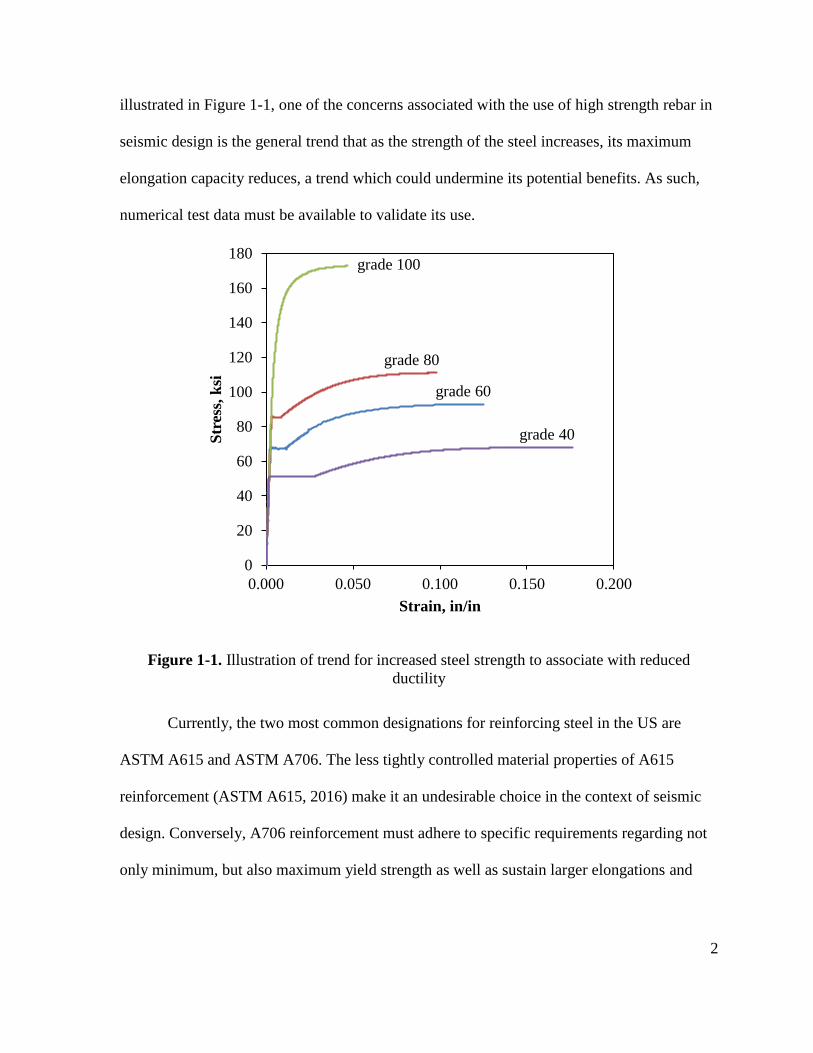
illustrated in Figure 1-1, one of the concerns associated with the use of high strength rebar in

seismic design is the general trend that as the strength of the steel increases, its maximum

elongation capacity reduces, a trend which could undermine its potential benefits. As such,

numerical test data must be available to validate its use.

Figure 1-1. Illustration of trend for increased steel strength to associate with reduced

ductility

Currently, the two most common designations for reinforcing steel in the US are

ASTM A615 and ASTM A706. The less tightly controlled material properties of A615

reinforcement (ASTM A615, 2016) make it an undesirable choice in the context of seismic

design. Conversely, A706 reinforcement must adhere to specific requirements regarding not

only minimum, but also maximum yield strength as well as sustain larger elongations and

0

20

40

60

80

100

120

140

160

180

0.000 0.050 0.100 0.150 0.200

Str

ess,

ksi

Strain, in/in

grade 80

grade 60

grade 40

grade 100

3

meet specific chemical composition requirements (ASTM A706, 2016). As a consequence,

ASTM A706 steel is routinely specified for members expected to form plastic hinges, and is

often used for all reinforcing steel in high seismic regions.

Prior to December 2009, the only grade of rebar available in the A706 specification

was grade 60. Since that time, ASTM has included requirements for an 80 ksi (550 MPa)

steel (A706 grade 80) in the A706 specification. The grade designation denotes the minimum

allowable yield strength of the steel.

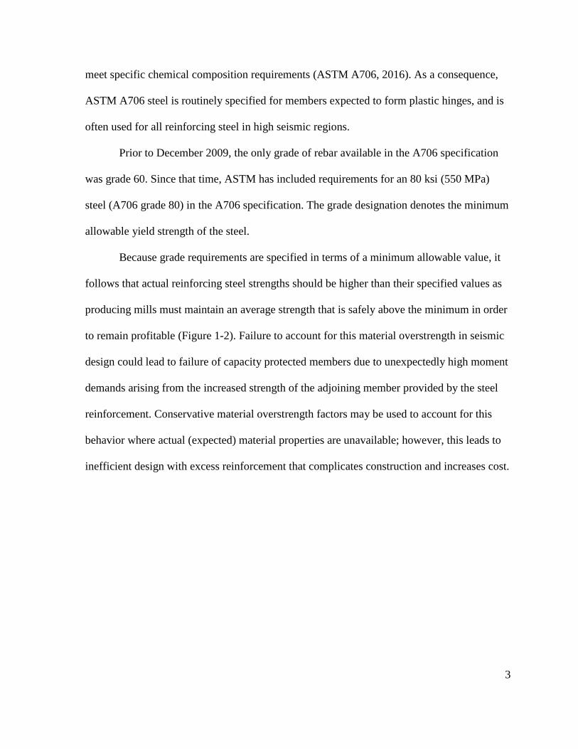
Because grade requirements are specified in terms of a minimum allowable value, it

follows that actual reinforcing steel strengths should be higher than their specified values as

producing mills must maintain an average strength that is safely above the minimum in order

to remain profitable (Figure 1-2). Failure to account for this material overstrength in seismic

design could lead to failure of capacity protected members due to unexpectedly high moment

demands arising from the increased strength of the adjoining member provided by the steel

reinforcement. Conservative material overstrength factors may be used to account for this

behavior where actual (expected) material properties are unavailable; however, this leads to

inefficient design with excess reinforcement that complicates construction and increases cost.

4

Figure 1-2. Illustration of need for manufactures to produce steel with yield strength well

above the minimum allowable

1.2. Research Objective

Given the potential benefits of using A706 grade 80 rebar in seismic design, and

considering the current limitations hindering its ready use in this context, the research

presented in this paper aims to expand the existing knowledge base on the stress-strain

behavior of A706 grade 80 rebar. The following items are identified as critical elements to be

addressed in fulfilment of this task:

1. Determine the expected (mean) values of all parameters necessary to define the

monotonic stress-strain curve (Fig. 1-3):

modulus of elasticity

yield strength

0.00

0.05

0.10

0.15

0.20

0.25

70 75 80 85 90 95 100

Pro

bab

ilit

y

Yield Strength, ksi

s = ?

95th

percentile = ?

min

. all

ow

ab

le

= ?

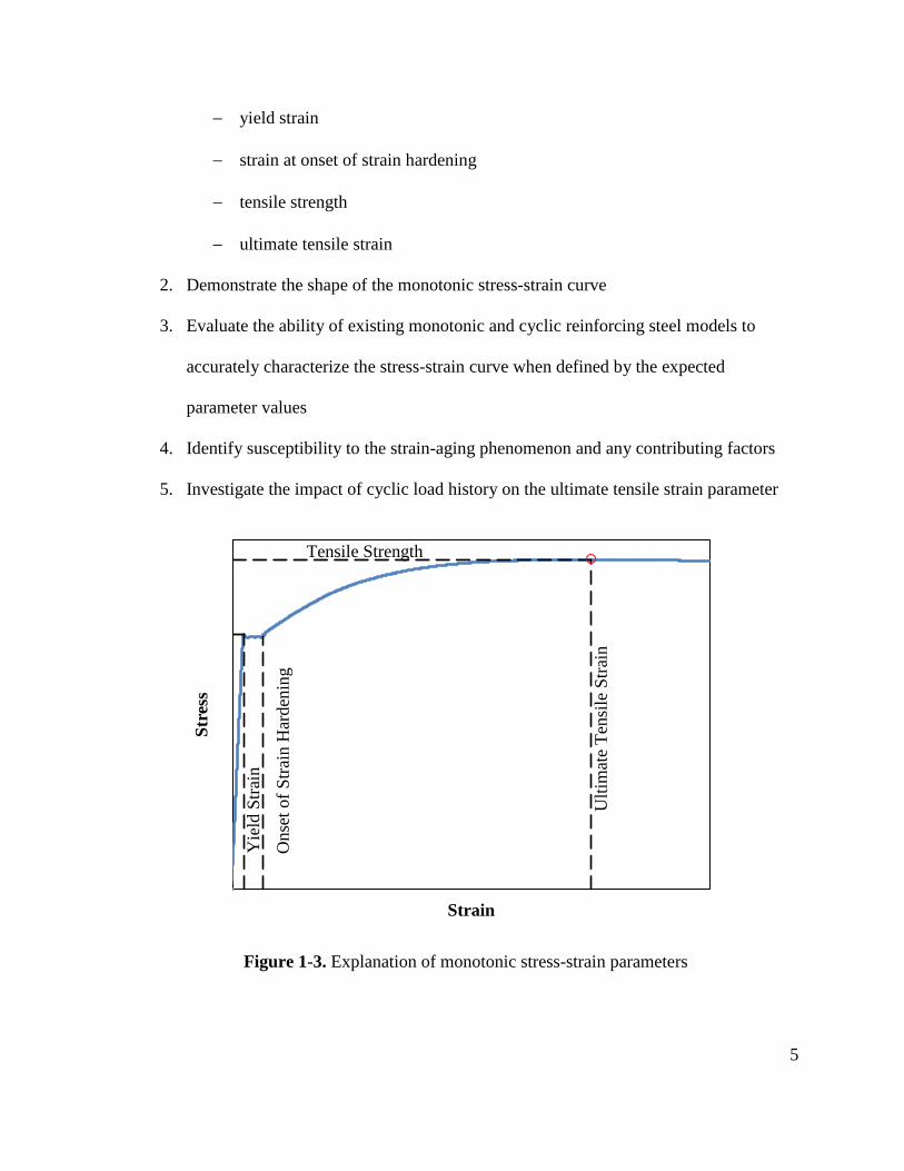
5

yield strain

strain at onset of strain hardening

tensile strength

ultimate tensile strain

2. Demonstrate the shape of the monotonic stress-strain curve

3. Evaluate the ability of existing monotonic and cyclic reinforcing steel models to

accurately characterize the stress-strain curve when defined by the expected

parameter values

4. Identify susceptibility to the strain-aging phenomenon and any contributing factors

5. Investigate the impact of cyclic load history on the ultimate tensile strain parameter

Figure 1-3. Explanation of monotonic stress-strain parameters

0

10

20

30

40

50

60

70

80

90

100

110

120

0.0000 0.0200 0.0400 0.0600 0.0800 0.1000 0.1200 0.1400

Str

ess

Strain

Ult

imat

eT

ensi

le S

trai

n

Onse

tof

Str

ain H

arden

ing

Yie

ld S

trai

n

Tensile Strength

6

1.3. Scope

The research objectives presented above are addressed through the experimental

testing and post-processing statistical analysis of A706 grade 80 rebar in the as-rolled

condition at North Carolina State University Constructed Facilities laboratory. The

reinforcing steel used in the research originated from three west coast producing mills:

Cascade Steel Rolling Mills (McMinnville, OR), Gerdau Ameristeel (Rancho Cucamonga,

CA), and Nucor Steel Seattle (Seattle, WA). Each mill provided three heats (batches) of bars

for each of the ten major bar sizes: No. 4 through No. 18. Three types of tests were

performed in pursuit of the research objectives: monotonic tensile tests, cyclic tests, and

strain age tests.

1.3.1. Tensile Tests

The tensile testing program constituted the majority of the research effort in terms of

number of tests and level of analysis of the findings. A total of 788 tests were performed in

order to represent a statistically-defendable sampling from all of the mills, heats, and bar

sizes provided. This portion of the research served to address objectives 1, 2, and 3.

1.3.2. Strain Age Tests

A subset of the reinforcing bars was used to evaluate the strain aging performance of

the steel. In total, 39 tests were performed on No. 5 and No. 7 bars in order to evaluate the

effect of bar size, pre-strain level, aging period, and temperature on the strain aging behavior

of A706 grade 80 rebar. This portion of the research served to address objective 4.

7

1.3.3. Cyclic Tests

An additional subset of bars was used to evaluate the cyclic stress-strain behavior of

the steel. A total of 13 tests were performed on No. 5 and No. 7 bars in order to address

objectives 3 and 5.

1.4. Overview of Report Contents

Chapter 1 introduces the subject of A706 grade 80 rebar and gives context to the

research presented in the following chapters. Specifically, it describes the role of reinforcing

steel in seismic design, the advantages of using high strength rebar, the history of A706 grade

80 rebar, and its current place in the role of seismic design. Also presented are the research

objectives and scope of the project.

Chapter 2 summarizes relevant background literature used to substantiate the research

effort, direct its approach, and evaluate its findings. First, a review of the limitations on A706

grade 80 rebar in current design standards is used to illustrate the need for the present

research. Following this, an overview of the existing papers, reports, and databases

containing A706 grade 80 experimental data is presented to further demonstrate the need for

the current research as well as provide a point of reference for evaluating the experimental

findings. A third section focuses on previous approaches to the statistical analysis of rebar

tensile test data. The literature findings presented in this section are used to direct the

methods employed in evaluating the data generated from the experimental tests and

evaluating it for anomalies. The chapter concludes with an introduction to strain aging and

how it has been previously studied with regards to reinforcing steel as well as an overview of

8

currently available cyclic material models, how they were defined, and which parameters are

necessary to defining each one.

Chapter 3 covers all aspects of the experimental testing portions of the project.

Included in this chapter is a detailed presentation of the material that was tested as well as a

thorough description of the equipment and instrumentation used in the testing. Procedures

specific to each of the three types of tests (tensile, strain age, and cyclic) are described in

their own section. These sections each contain details such as test matrix, parameters

investigated, specimen preparation, and testing procedure.

Chapter 4 presents the results of the experimental testing portions of the project

broken down according to the three types of tests performed. Included is a description of how

each of the tensile test parameters where determined and what statistical methods were

employed in aggregating and evaluating the test results which have been presented as

empirical and best-fit cumulative distribution functions to demonstrate the variability in the

data. The shape of the monotonic stress-strain curve is presented graphically and compared

with existing material models calibrated with the test results. The impact of aging period,

pre-strain level, bar size, and temperature on the strain aging performance is also presented

graphically. The chapter concludes with a section addressing the cyclic behavior of the steel.

Chapter 5 discusses the results presented in Chapter 4 in the context of existing test

data found in the literature and additionally explores trends and anomalies observed in the

test results. Specifically, this includes a comparison of the literature monotonic stress-strain

curves with those obtained from the tensile tests, a comparison of the tensile test results with

available mill certificate reports, an assessment of the variability in test results occurring

9

between the three mills, the heats within a mill, and the individual lengths of bar within a

heat. Also included is an investigation of the correlation between monotonic stress-strain

parameters, a summary of test results failing to meet the ASTM requirements, and an

observation on how strains vary over the length of bar in a tensile test. A few comments are

offered based on the results of the strain aging and cyclic test results in order to relate them

back to the literature review findings. The chapter closes with a proposal for future work in

the areas of tensile testing, strain age testing, and cyclic testing of A706 grade 80 rebar based

on the research findings.

Chapter 6 summarizes the conclusions from the research, including final

recommendations on the monotonic stress-strain curve parameter values, and relates the

findings back to the initial research objectives.

10

2. LITERATURE REVIEW

2.1. A706 Grade 80 Rebar in Design Standards

The overall lack of experimental data on A706 grade 80 rebar in the literature is

reflected in the hesitancy of design codes to allow its use in regions expected to form plastic

hinges. In some cases, the use of A706 grade 80 reinforcement is directly restricted while in

others it is passively restricted by setting upper limits on yield strength that are below 80 ksi

(550 MPa). A brief summary of the guidelines (or lack thereof) for use of A706 grade 80

steel in design codes is presented below.

2.1.1. ACI 318-14

ACI 318-14 Section 20.2.2 limits deformed reinforcement used in special seismic

systems to be of grade 60 or lower “because of insufficient data to confirm applicability of

existing code provisions for structures using the higher grade [A706 grade 80]” (ACI 318-

14). However, the commentary to Section 18.2.6 makes provision for higher grades where

sufficient test data is available to support their use: “Section 18.2.1.7 permits alternative

material such as ASTM A706 Grade 80 if results of tests and analytical studies are presented

in support of its use” (ACI 318-14).

2.1.2. Caltrans Seismic Design Criteria

Section 3.2 of the Caltrans SDC 1.7 limits the range in yield stress of ASTM A706

reinforcement to between 60 ksi and 78 ksi. The use of ASTM A706 grade 80 reinforcing

steel is not directly addressed.

11

2.1.3. AASHTO LRFD Bridge Design Specification

Based on research by Shahrooz et al. (2011), the AASHTO LRFD Bridge Design

Specification (AASHTO 2014) permits the use of reinforcing steel with specified minimum

yield strength of up to 100 ksi (690 MPa) for all elements and connections in Seismic Zone 1

where permitted by specific articles. Section C5.4.3.3 states that “Reinforcing steels with a

minimum specified yield strength between 75.0 and 100 ksi may be used in seismic

applications, with the Owner’s approval, only as permitted in the AASHTO Guide

Specifications for LRFD Seismic Bridge Design” (AASHTO 2014). This implies that A706

grade 80 reinforcing steel is permissible, subject to specific constraints.

2.1.4. AASHTO Guide Specification for LRFD Seismic Bridge Design

Section 8.4.1 of the AASHTO Guide Spec. for LRFD Seismic Bridge Design

(AASHTO 2011) states that “ASTM A 706 Grade 80 reinforcing steel may be used in

capacity-protected members as specified in Article 8.5 but shall not be used in members

where plastic hinging is expected”. It is further stated in the accompanying commentary that

this allowance was made due to the strength control and elongation characteristics of A706

grade 80 reinforcement, and that it has not been permitted on plastic hinge regions due, in

part, to a lack of stress-strain data. Only ASTM A615 grade 60 (in seismic design categories

B and C, with the owner’s approval) or A706 grade 60 reinforcing steel is allowed in

members expected to form a plastic hinge.

12

2.1.5. WSDOT Bridge Design Manual

The Washington Department of Transportation Bridge Design Manual (WSDOT

2015) Section 5.1.2 permits the unrestricted use of A706 grade 80 reinforcement in regions

having Seismic Design Category (SDC) A, but limits its use to only capacity protected

members for SDCs B, C, and D.

2.1.6. ODOT Bridge Design and Drafting Manual

Section 1.5.5.1.17 of the Oregon Department of Transportation Bridge Design and

Drafting Manual is specifically devoted to the use of ASTM A706 grade 80 reinforcement

(ODOT 2015). The manual states that A706 grade 80 reinforcement may not be used in

members designed for plastic seismic performance such as bridge columns due to limited

experimental testing.

2.1.7. Alaska DOT

The Alaska DOT currently uses A706 grade 60 rebar for the design of members

expected to form a plastic hinge; however, A706 grade 80 has been specified for capacity

protected members in accordance with the AASHTO specifications (Elmer Marx, AKDOT,

personal communication, April 1, 2016).

2.2. Existing A706 Grade 80 Experimental Data

Just five reports were found to include material test results on A706 grade 80 steel

either in tabulated or graphical form. Of the five reports, only two unique datasets could be

confirmed: one consisting of three No. 7 bar tests (Rautenberg et al., 2013) and one

consisting of three No. 3, three No. 5, and three No. 6 bar tests (Trejo et al., 2014). The

13

earliest of the five reports was completed in 2013, two were completed in March of 2014,

and the most recent paper was published in June of 2015. This is not surprising considering

the relatively recent introduction of grade 80 rebar into the ASTM A706/A706M

specification in 2009.

The available experimental data is further limited in that only a few bar sizes have

been considered and that strains have generally not been provided to accompany the included

yield and tensile strength data. This is particularly true with data provided by the producing

mills as they generally lack the necessary equipment required to capture strains. It should

also be considered that because data obtained from producing mills does not necessarily stem

from ideal laboratory conditions using appropriate, carefully calibrated measurement

equipment and trained personnel, it should not be used for design purposes. This limitation

extends to the Concrete Reinforcing Steel Institute (CRSI) Mill Databases which, while

offering insight into the increased use and testing of A706 grade 80 rebar between 2011 and

2013, are composed of submitted mill test results.

By consequence of the extremely limited amount of data found in the available

literature, what does exist is not sufficient to generate recommendations on the material

properties of A706 grade 80 rebar. Rather, these findings simply served as reference points to

validate trends and identify anomalies arising during the testing phase of the project. A

graphical comparison of the literature-based stress-strain curves with the experimental curves

generated through this project is presented in Chapter 5.

14

2.2.1. Research Data

2.2.1.1.Rautenberg et al. (2013)

Rautenberg et al. (2013) presented the findings of a study on the applicability of high-

strength reinforcement in reinforced concrete columns resisting lateral earthquake loads. The

primary goal of the research, which was based on testing conducted as part of Rautenberg’s

PhD dissertation at Purdue in 2011 (Rautenberg, 2011), was to evaluate the 60 ksi limit

imposed by the American Concrete Institute (ACI) on the yield strength of rebar used in

regions expected to form plastic hinges (ACI 318-11). A total of 8 columns consisting of

either ASTM A706 grade 60, A706 grade 80, or A1035 grade 120 longitudinal reinforcement

were considered in the analysis. Material testing was conducted for the purpose of calibrating

numerical models of full-scale buildings subjected to strong ground motions. Of particular

interest are the tensile tests that were performed on three A706 grade 80 No. 7 bars. The test

specimens all originated from the same heat and were tested in a Baldwin 120-kip capacity

universal testing machine upgraded with Instron control and data acquisition equipment. An

Instron extensometer having two inch gauge length was used to acquire the strains. Tests

were performed in compliance with ASTM A370 (2009). Data from the tests, which is

publicly available on the NEES website (NEES, 2009), is presented in Table 2-1.

15

Table 2-1. Stress-strain data from Rautenberg et al. (2013)

Specimen

Number

Yield Strength Tensile Strength Elong.

% in

8 inch Stress,

ksi

Strain,

in/in

Stress,

ksi

Stress,

ksi

7a 83 --- 119 --- 11.7

7b 83 --- 117 --- 15.6

7c 84 --- 118 --- 14.8

Figure 2-1. Stress-strain curves for three No. 7 bars from Rautenberg et al. (2013)

2.2.1.2.WJE RGA 04-13 Report (2013)

A report submitted to the Charles Pankow Foundation in late 2013 by Wiss, Janney,

Elstner and Associates, Inc. (WJE, 2013) seeking to determine if it would be appropriate for

0

10

20

30

40

50

60

70

80

90

100

110

120

0.00 0.02 0.04 0.06 0.08

Str

ess,

ksi

Strain, in/in

S10 - A706 Gr80 #7a

S10 - A706 Gr80 #7b

S10 - A706 Gr80 #7c

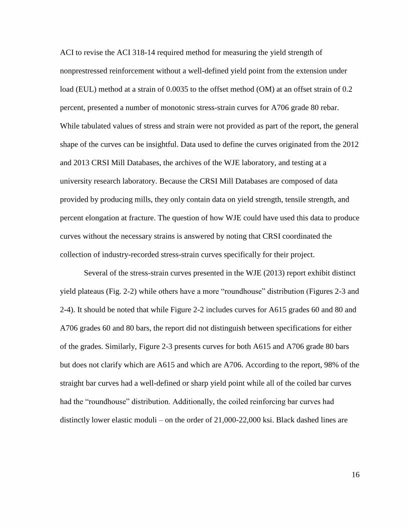
16

ACI to revise the ACI 318-14 required method for measuring the yield strength of

nonprestressed reinforcement without a well-defined yield point from the extension under

load (EUL) method at a strain of 0.0035 to the offset method (OM) at an offset strain of 0.2

percent, presented a number of monotonic stress-strain curves for A706 grade 80 rebar.

While tabulated values of stress and strain were not provided as part of the report, the general

shape of the curves can be insightful. Data used to define the curves originated from the 2012

and 2013 CRSI Mill Databases, the archives of the WJE laboratory, and testing at a

university research laboratory. Because the CRSI Mill Databases are composed of data

provided by producing mills, they only contain data on yield strength, tensile strength, and

percent elongation at fracture. The question of how WJE could have used this data to produce

curves without the necessary strains is answered by noting that CRSI coordinated the

collection of industry-recorded stress-strain curves specifically for their project.

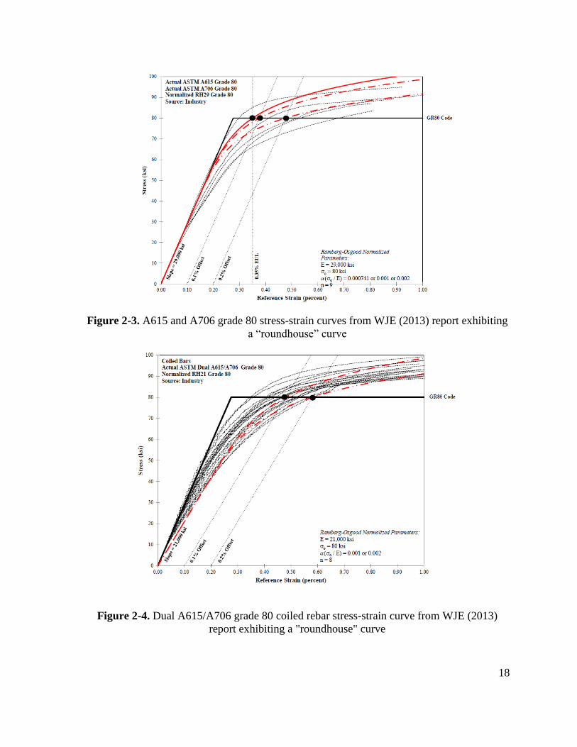
Several of the stress-strain curves presented in the WJE (2013) report exhibit distinct

yield plateaus (Fig. 2-2) while others have a more “roundhouse” distribution (Figures 2-3 and

2-4). It should be noted that while Figure 2-2 includes curves for A615 grades 60 and 80 and

A706 grades 60 and 80 bars, the report did not distinguish between specifications for either

of the grades. Similarly, Figure 2-3 presents curves for both A615 and A706 grade 80 bars

but does not clarify which are A615 and which are A706. According to the report, 98% of the

straight bar curves had a well-defined or sharp yield point while all of the coiled bar curves

had the “roundhouse” distribution. Additionally, the coiled reinforcing bar curves had

distinctly lower elastic moduli – on the order of 21,000-22,000 ksi. Black dashed lines are

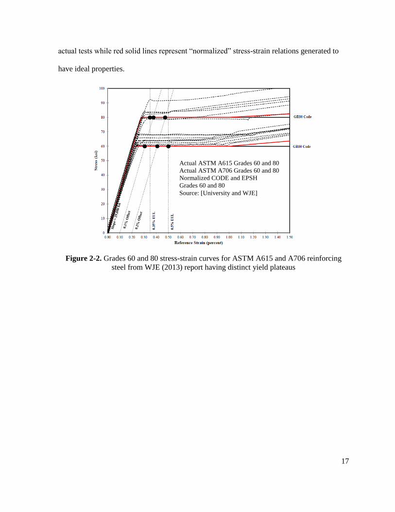
17

actual tests while red solid lines represent “normalized” stress-strain relations generated to

have ideal properties.

Figure 2-2. Grades 60 and 80 stress-strain curves for ASTM A615 and A706 reinforcing

steel from WJE (2013) report having distinct yield plateaus

Actual ASTM A615 Grades 60 and 80

Actual ASTM A706 Grades 60 and 80

Normalized CODE and EPSH

Grades 60 and 80

Source: [University and WJE]

18

Figure 2-3. A615 and A706 grade 80 stress-strain curves from WJE (2013) report exhibiting

a “roundhouse” curve

Figure 2-4. Dual A615/A706 grade 80 coiled rebar stress-strain curve from WJE (2013)

report exhibiting a "roundhouse" curve

19

2.2.1.3.GCR 14-917-30 (2014)

A detailed report produced by the National Earthquake Hazards Reduction Program

(NEHRP) Consultants Joint Venture (GCR, 2014) in March 2014 focused on the use of high-

strength reinforcement (fy greater than 60 ksi) in special moment frames and special

structural walls. A parametric study of four building models reinforced with grades 60, 80,

and 100 longitudinal reinforcement subjected to actual recorded ground motions revealed

that the different grades offered comparable performance in the considered earthquakes.

Results from the study were used to validate a proposal to ACI recommending A706 Grade

80 reinforcement be allowed in special moment frames and structural walls. Reinforcing steel

data was provided by Nucor Steel Seattle, Inc. and the 2011 and 2012 CRSI Mill Databases.

While no numerical stress-strain data was provided in the report, the stress-strain

curve of a No. 8 and a No. 18 bar was provided courtesy of the steel mill (Fig. 2-5). Based on

the graph, the No. 18 bar barely meets the minimum allowable yield strength of 80 ksi when

a 2% offset line is used to define the yield point. Past research has indicated a possibility for

larger diameter bars to have lower strengths, presumably due to factors associated with the

manufacturing process such as reduced grain refinement and different cooling rates and times

(Lim, 1991); however, other research suggests that this is not the case (Mirza and

MacGregor, 1979; Nowak and Szerszen, 2003). It is unclear whether such factors influenced

the results of the present research. Nonetheless, the nature of the curves offers an interesting

point of comparison with test results obtained during the experimental phase of the current

project (Section 5.1.1.). Despite their differences in yield and tensile strength, both bars

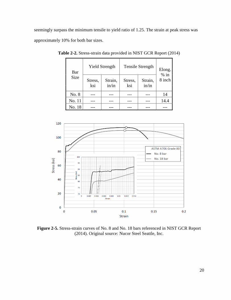
20

seemingly surpass the minimum tensile to yield ratio of 1.25. The strain at peak stress was

approximately 10% for both bar sizes.

Table 2-2. Stress-strain data provided in NIST GCR Report (2014)

Bar

Size


% in

8 inch Stress,

ksi

Strain,

in/in

Stress,

ksi

Strain,

in/in

No. 8 --- --- --- --- 14

No. 11 --- --- --- --- 14.4

No. 18 --- --- --- --- ---

Figure 2-5. Stress-strain curves of No. 8 and No. 18 bars referenced in NIST GCR Report

(2014). Original source: Nucor Steel Seattle, Inc.

21

2.2.1.4.Trejo, Barbosa, and Link. (2014)

Trejo et al. (2014) presented the results of a study on the seismic performance of 24-

inch diameter circular reinforced concrete bridge columns constructed with A706 grade 80

reinforcement. A total of six of these half-scale columns were constructed and tested using

either No. 5 or No. 6 longitudinal reinforcement, No. 3 transverse reinforcement, and either

A706 grade 60 or A706 grade 80 steel. The study concluded that, among other things,

columns reinforced with grade 80 rebar exhibited equal or greater maximum drift ratio

compared to those with grade 60 rebar, both grades of steel resulted in similar column lateral

displacement and ductility, and that columns reinforced with grade 60 rebar showed higher

total energy dissipation as a result of their higher area of steel. Column failure mode (bar

fracture due to buckling of longitudinal bars) was consistent across both grades of steel. The

tensile test data presented in the report and reproduced below (Table 2-3) is the most detailed

summary of the mechanical characteristics of A706 grade 80 reinforcing bars found in any of

the other reports. This same data appears in a more recent paper by the same authors

(Barbosa et al., 2015).

Table 2-3. Material test results for A706 grade 80 rebar used in Trejo et al. (2014)

Bar

Size

Yield Point

(0.2% offset)

Yield Point

(0.0035 EUL)

Tensile

Strength Onset of

Strain Harding Ultimate Strain Elong.

% in

8 inch Stress,

ksi

Strain,

in/in

Stress,

ksi

Strain,

in/in

Stress,

ksi

Strain,

in/in

Stress,

ksi

Strain,

in/in

Stress,

ksi

Strain,

in/in

No. 3 85.6 0.0055 73.3 0.0035 120.5 0.0947 N.A. N.A. 85.2 0.1378 13

No. 5 86.2 0.0051 85.4 0.0035 114.3 0.1066 85.9 0.0084 86.8 0.1555 14

No. 6 86.1 0.0048 84.3 0.0035 114.0 0.1225 85.5 0.0098 93.9 0.1893 15

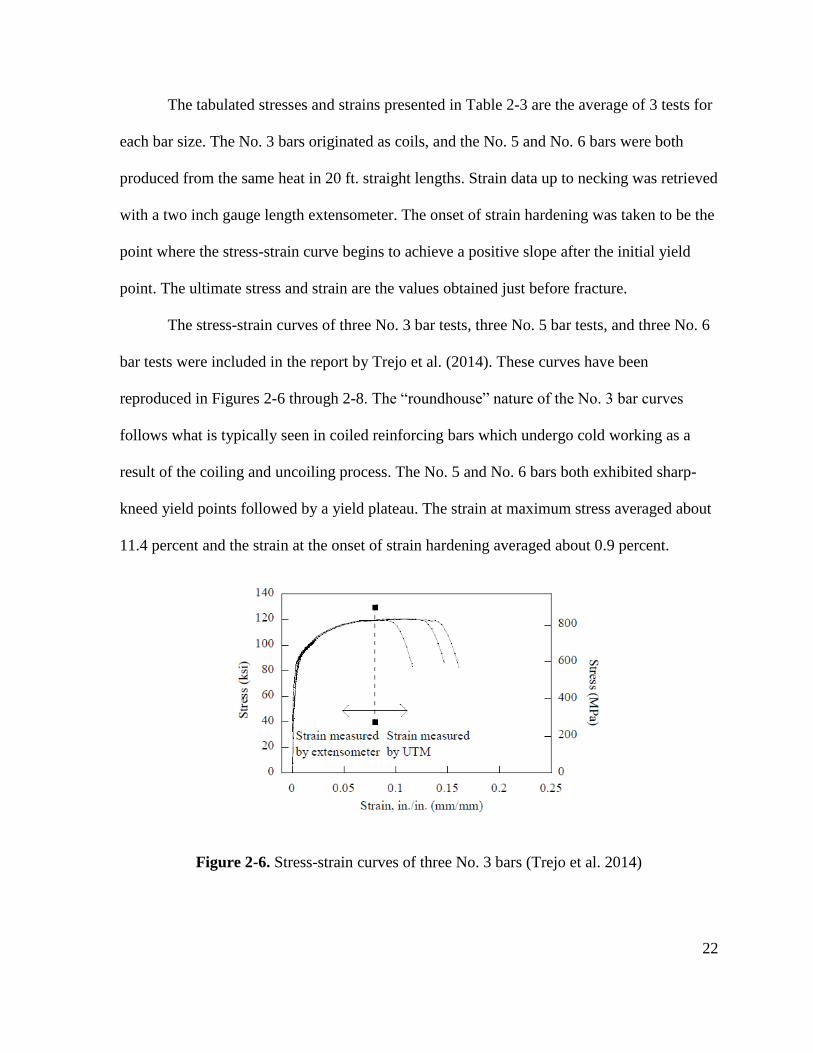
22

The tabulated stresses and strains presented in Table 2-3 are the average of 3 tests for

each bar size. The No. 3 bars originated as coils, and the No. 5 and No. 6 bars were both

produced from the same heat in 20 ft. straight lengths. Strain data up to necking was retrieved

with a two inch gauge length extensometer. The onset of strain hardening was taken to be the

point where the stress-strain curve begins to achieve a positive slope after the initial yield

point. The ultimate stress and strain are the values obtained just before fracture.

The stress-strain curves of three No. 3 bar tests, three No. 5 bar tests, and three No. 6

bar tests were included in the report by Trejo et al. (2014). These curves have been

reproduced in Figures 2-6 through 2-8. The “roundhouse” nature of the No. 3 bar curves

follows what is typically seen in coiled reinforcing bars which undergo cold working as a

result of the coiling and uncoiling process. The No. 5 and No. 6 bars both exhibited sharp-

kneed yield points followed by a yield plateau. The strain at maximum stress averaged about

11.4 percent and the strain at the onset of strain hardening averaged about 0.9 percent.

Figure 2-6. Stress-strain curves of three No. 3 bars (Trejo et al. 2014)

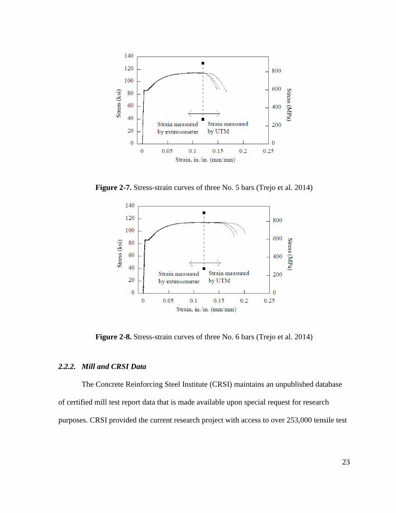
23



2.2.2. Mill and CRSI Data

The Concrete Reinforcing Steel Institute (CRSI) maintains an unpublished database

of certified mill test report data that is made available upon special request for research

purposes. CRSI provided the current research project with access to over 253,000 tensile test

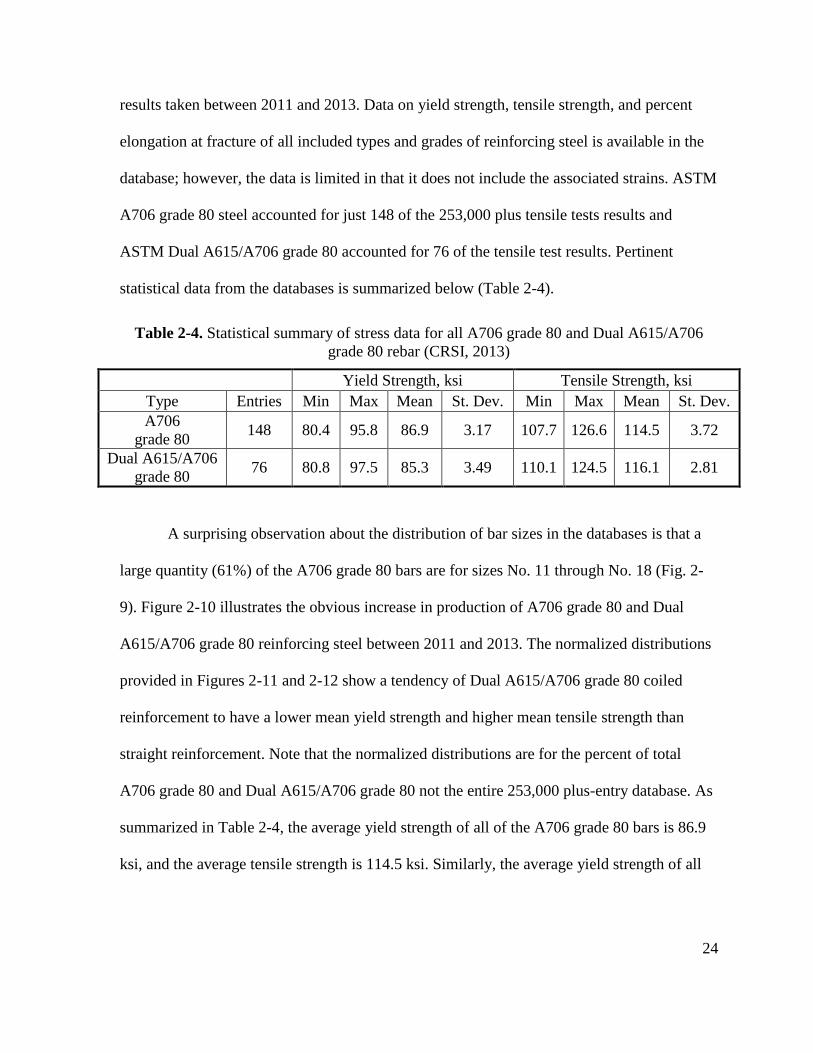
24

results taken between 2011 and 2013. Data on yield strength, tensile strength, and percent

elongation at fracture of all included types and grades of reinforcing steel is available in the

database; however, the data is limited in that it does not include the associated strains. ASTM

A706 grade 80 steel accounted for just 148 of the 253,000 plus tensile tests results and

ASTM Dual A615/A706 grade 80 accounted for 76 of the tensile test results. Pertinent

statistical data from the databases is summarized below (Table 2-4).

Table 2-4. Statistical summary of stress data for all A706 grade 80 and Dual A615/A706

grade 80 rebar (CRSI, 2013)

Yield Strength, ksi Tensile Strength, ksi

Type Entries Min Max Mean St. Dev. Min Max Mean St. Dev.

A706

grade 80 148 80.4 95.8 86.9 3.17 107.7 126.6 114.5 3.72

Dual A615/A706

grade 80 76 80.8 97.5 85.3 3.49 110.1 124.5 116.1 2.81

A surprising observation about the distribution of bar sizes in the databases is that a

large quantity (61%) of the A706 grade 80 bars are for sizes No. 11 through No. 18 (Fig. 2-

9). Figure 2-10 illustrates the obvious increase in production of A706 grade 80 and Dual

A615/A706 grade 80 reinforcing steel between 2011 and 2013. The normalized distributions

provided in Figures 2-11 and 2-12 show a tendency of Dual A615/A706 grade 80 coiled

reinforcement to have a lower mean yield strength and higher mean tensile strength than

straight reinforcement. Note that the normalized distributions are for the percent of total

A706 grade 80 and Dual A615/A706 grade 80 not the entire 253,000 plus-entry database. As

summarized in Table 2-4, the average yield strength of all of the A706 grade 80 bars is 86.9

ksi, and the average tensile strength is 114.5 ksi. Similarly, the average yield strength of all

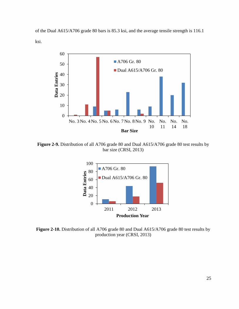
25

of the Dual A615/A706 grade 80 bars is 85.3 ksi, and the average tensile strength is 116.1

ksi.


bar size (CRSI, 2013)


production year (CRSI, 2013)

0

10

20

30

40

50

60

No. 3 No. 4 No. 5 No. 6 No. 7 No. 8 No. 9 No.

10

No.

11

No.

14

No.

18

Data

En

trie

s

Bar Size

A706 Gr. 80

Dual A615/A706 Gr. 80

0

20

40

60

80

100

2011 2012 2013

Data

En

trie

s

Production Year

A706 Gr. 80

Dual A615/A706 Gr. 80

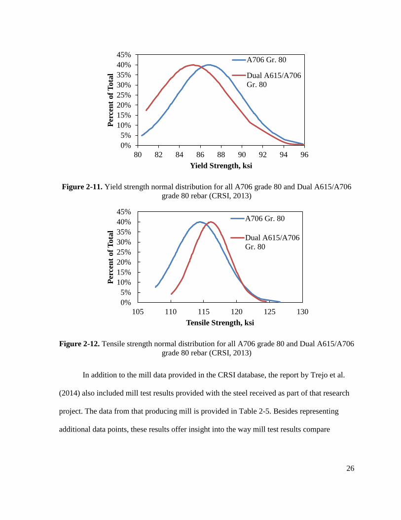
26

Figure 2-11. Yield strength normal distribution for all A706 grade 80 and Dual A615/A706


Figure 2-12. Tensile strength normal distribution for all A706 grade 80 and Dual A615/A706


In addition to the mill data provided in the CRSI database, the report by Trejo et al.

(2014) also included mill test results provided with the steel received as part of that research

project. The data from that producing mill is provided in Table 2-5. Besides representing

additional data points, these results offer insight into the way mill test results compare

0%

5%

10%

15%

20%

25%

30%

35%

40%

45%

80 82 84 86 88 90 92 94 96

Per

cen

t of

Tota

l

Yield Strength, ksi

A706 Gr. 80

Dual A615/A706

Gr. 80

0%

5%

10%

15%

20%

25%

30%

35%

40%

45%

105 110 115 120 125 130

Per

cen

t of

Tota

l

Tensile Strength, ksi

A706 Gr. 80

Dual A615/A706

Gr. 80

27

against laboratory test results. A comparison of Tables 2-3 and 2-5 illustrates the trend for

mill-measured strength values to be higher and percent elongation at fracture values to be

lower than research laboratory test results. As will be seen in Chapter 5, this trend also held

true for the results obtained as part of the current research project. Note that the method by

which the producing mill obtained the yield strength data was not clarified in the report.

Table 2-5. Cascade Steel mill data referenced in Trejo et al. (2014)

Bar

Size


% in

8 inch Stress,

ksi

Strain,

in/in

Stress,

ksi

Strain,

in/in

#3 96.5 --- 124.0 --- 23

#5 87.5 --- 114.0 --- 13

#6 88.0 --- 115.0 --- 14

2.3. Statistical Studies of Rebar Test Results

2.3.1. Allen (1972)

Allen (1972) conducted a statistical analysis of reinforcing bar mechanical properties

based on two samples of Canadian-manufactured rebar test results. The smaller sample

originated from a research facility and consisted of 102 tests on No. 3, 5, 8, 11, and 14 grade

40 bars representing 5 different heats. The larger sample originated from a Canadian

manufacturing plant and consisted of 132 tests on No. 5 through No. 14 grade 60 bars where

each test represented a different heat. Relevant findings from the paper were the distribution

of the test results and the variability between and within heats. Specifically, it was noted that

28

the ultimate tensile strength was approximately normally distributed. The coefficient of

variation (COV) for bars tested within a heat ranged from 2-3% for the yield strength and

about 1% for the ultimate tensile strength. The variation across heats within a mill was noted

to be higher with COV’s of 7-8% for the yield strength and around 3% for the ultimate

tensile strength.

2.3.2. Mirza and MacGregor (1979)

Mirza and MacGregor (1979) compiled nearly 4000 tensile test results from over 13

sources (mill and laboratory), including three different grades (40, 50, and 60) and nine

different bar sizes (No. 3, 4, 5, 6, 8, 10, 11, 14, and 18) in order to investigate the variability

in reinforcing steel mechanical properties, specifically the yield strength, tensile strength, and

modulus of elasticity. While a number of sources of variability were considered, the two that

are most relevant to this paper are the variability in the strength of the material and the effect

of bar diameter. It was shown that the yield strength COV’s ranged from 1-4% for individual

bar sizes from a single source and from 5-8% for individual bar sizes considering all sources.

Similarly, the yield strength COV’s ranged from 4-7% considering all bar sized from a single

source, and from 8-12% considering all bars sizes across all the supports. They concluded

that, at least for grade 60 steel, the larger diameter bars (No. 14 and 18) did not show lower

yield strength than the smaller bars.

In addition to presenting their findings in terms of the means and coefficients of

variation, the authors also evaluated the ability of a number of probability distributions to

characterize the spread of the data. More specifically, they investigated normal, lognormal,

29

modified lognormal, beta, and Pearson system distributions. The general conclusion was that

the yield strength and tensile strength could be described by a normal distribution between

the 5th and 95th percentile, but that the beta distribution offered the most comprehensive fit

to the data. The authors noted that a likely reason for the non-normal behavior at the lower

probabilities could be attributed to mill test results not including tests that failed to meet the

minimum grade requirement, therefore, in a sense, biasing the available data. A normal

distribution was used to characterize the modulus of elasticity data. It should be noted that

there was no indication given as to how the different probability distributions were evaluated

other than through visual inspection.

2.3.3. Nowak and Szerszen (2003)

As part of an effort to develop appropriate resistance models for calibration of the

ACI 318 Code, Nowak and Szerszen (2003) assembled the results of 416 industry-based

tensile test results of grade 60 rebar ranging in size from No. 3 to No. 11. A component of the

investigation was to identify a suitable probability distribution to characterize the yield

strength of the data in order to run Monte Carlo simulations to develop the resistance models.

The authors concluded that a normal distribution suitably described the yield strength data.

The COV’s varied from 3.5 to 6.5 percent. The only technique described in the paper for

evaluating the probability distribution fits was the use of normal probability paper.

2.3.4. Bournonville et al. (2004)

Bournonville et al. (2004) performed a statistical evaluation of the mechanical

properties and weight of reinforcing bars produced by twenty-nine United States mills in the

30

year 1997. A total of 23,768 heats of bars were represented in the analysis. The study

included bar sizes No. 3 through No. 18 and specifications A615 grades 40, 60, and 75, A616

grade 60, and A706 grade 60. Of interest to the present research on A706 grade 80 rebar are

the findings related to the A706 bars and the grade 75 bars.

The authors concluded that less than 0.1% of heats failed to meet the minimum

ASTM standards for both yield strength and tensile strength. They also concluded that the

normal and beta distributions could be used to characterize the yield and tensile strengths of

A615 grade 75, A616 grade 60, and A706 grade 60 rebar. It should be noted, however, that

while the report clarified the method of fitting the beta distribution to the test data, it did not

indicate how the distributions were deemed reliable fits to the data other than through visual

inspection using normal probability plots. A more robust approach would have used an

appropriate goodness-of-fit test and a desired significance level.

Other relevant findings from the report where that the A615 grade 60 bars showed an

increase in yield strength with an increase in bar size but a general decrease in tensile

strength with increasing bar size. No such trend was observed in either the A706 grade 60

bars or higher strength A615 grade 75 bars. The overall (across all the mills) coefficients of

variation for the A706 grade 60 bar yield and tensile strengths were 4 to 6 percent and 3 to 6

percent respectively.

31

2.4. Strain Aging Literature

2.4.1. Introduction to Strain Aging

Strain aging can be defined as the process by which a reinforcing bar develops

increased strength and reduced ductility over time following inelastic deformation. This

behavior arises as a result of dislocation pinning at the molecular level in which small,

interstitial atoms like carbon and nitrogen are freed through plastic deformation of the

material and allowed to migrate through the crystal structure until they accumulate at

dislocation sites (irregularities in the molecular structure), preventing further slipping of the

crystal planes (Cottrell and Bilby, 1949). The increased resistance to sliding of the crystal

planes is seen as an increase in strength (both yield and ultimate) and reduction in ductility of

the material (Figure 2-13). As illustrated in the figure, an additional indicator of strain aging

is the reemergence of the yield plateau.

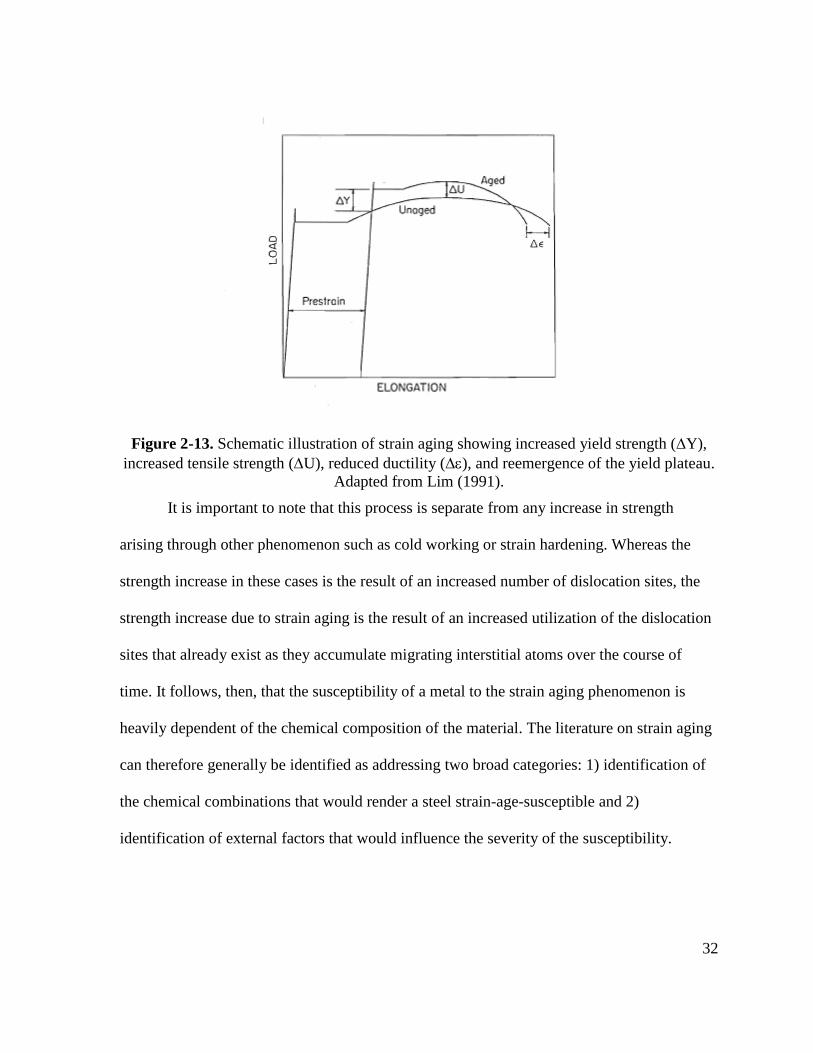
32

Figure 2-13. Schematic illustration of strain aging showing increased yield strength (Y),

increased tensile strength (U), reduced ductility (), and reemergence of the yield plateau.

Adapted from Lim (1991).

It is important to note that this process is separate from any increase in strength

arising through other phenomenon such as cold working or strain hardening. Whereas the

strength increase in these cases is the result of an increased number of dislocation sites, the

strength increase due to strain aging is the result of an increased utilization of the dislocation

sites that already exist as they accumulate migrating interstitial atoms over the course of

time. It follows, then, that the susceptibility of a metal to the strain aging phenomenon is

heavily dependent of the chemical composition of the material. The literature on strain aging

can therefore generally be identified as addressing two broad categories: 1) identification of

the chemical combinations that would render a steel strain-age-susceptible and 2)

identification of external factors that would influence the severity of the susceptibility.

33

Strain aging has been previously studied in the context of earthquake structural

engineering as its ability to impact reinforcing steel strength and ductility over time could

have significant implications on the capacity design philosophy in which the ability of a

structure to dissipate energy through inelastic deformation (plastic hinge formation) is reliant

on a specified hierarchy of strength. Within this approach, locations of inelastic action are

specifically chosen and detailed to ensure ductile response while other members are chosen

to remain elastic to protect against brittle failure modes such as shear failure. These capacity

protected members are designed for the maximum overstrength moments from the adjacent

beams (in frames) or columns (in bridges).

As a primary goal of this methodology is to prevent collapse of the structure, it is

often possible that repair methods may be implemented to restore the function of the

structure following a seismic event inducing damage. Should the calculated capacity of the

repaired structure neglect the increased strength and reduced ductility of the plastically-

strained reinforcing steel, a subsequent seismic event may lead to unanticipated failure of

capacity protected members due to strain aging of the reinforcing steel. One examples of this

would include shear failure of columns in frames or bent caps in bridges as a result of higher

input moments from the adjoining members arising from an increase in the rebar strength.

Another example of the negative impacts of strain aging on the capacity design philosophy

would include loss of confinement due to reduced ductility and subsequent early fracture of

the transverse reinforcing steel.

As illustrated in Chapter 1, there is a general trend for increased steel strength to be

accompanied by reduced steel ductility (as part of the metallurgical process). As such, the

34

anticipated reduced ductility of A706 grade 80 rebar as compared to A706 grade 60 rebar

means that its susceptibility to strain aging must be investigated and understood prior to its

use in members expected to dissipate energy through inelastic deformation (or at least before

repair of such members following a seismic event).

2.4.2. Relevant Papers on Strain Aging

2.4.2.1.Pussegoda (1978)

Pussegoda (1978) conducted a detailed investigation on the impact of chemical

composition on strain aging susceptibility of steel reinforcing bars. In particular, the study

specifically focused on the use of two alloying elements, titanium and vanadium, to mitigate

strain aging effects as these elements were established to be strong nitride forming

compounds. Fourteen New Zealand grade 275 bars were manufactured with varying

percentages of vanadium (approx. 0 to 0.1%), tested to 5% pre-strain (36y, assuming

Es=200000 MPa), and then artificially aged at 100⁰ C for 3 hours in order to determine the

quantity of vanadium needed to prevent strain aging. The temperature and duration of the

artificial aging period were derived using Hundy’s equation (Hundy, 1954) to simulate the

effects of natural aging at 15⁰ C for 9 months. An additional set of 15 grade 275 bars, 6

having no titanium and 9 having 0.03% titanium, were tested to varying levels of pre-strain

(2.5 to 15%) to simultaneously investigate the effect of pre-strain level on degree of strain

aging as well as the ability of titanium to hinder strain aging. Artificial aging at 100⁰ C for 3

hours was again used to simulate natural strain aging over 9 months.

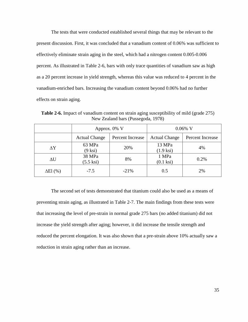
35

The tests that were conducted established several things that may be relevant to the

present discussion. First, it was concluded that a vanadium content of 0.06% was sufficient to

effectively eliminate strain aging in the steel, which had a nitrogen content 0.005-0.006

percent. As illustrated in Table 2-6, bars with only trace quantities of vanadium saw as high

as a 20 percent increase in yield strength, whereas this value was reduced to 4 percent in the

vanadium-enriched bars. Increasing the vanadium content beyond 0.06% had no further

effects on strain aging.

Table 2-6. Impact of vanadium content on strain aging susceptibility of mild (grade 275)

New Zealand bars (Pussegoda, 1978)

Approx. 0% V 0.06% V

Actual Change Percent Increase Actual Change Percent Increase

Y 63 MPa

(9 ksi) 20%

13 MPa

(1.9 ksi) 4%

U 38 MPa

(5.5 ksi) 8%

1 MPa

(0.1 ksi) 0.2%

El (%) -7.5 -21% 0.5 2%

The second set of tests demonstrated that titanium could also be used as a means of

preventing strain aging, as illustrated in Table 2-7. The main findings from these tests were

that increasing the level of pre-strain in normal grade 275 bars (no added titanium) did not

increase the yield strength after aging; however, it did increase the tensile strength and

reduced the percent elongation. It was also shown that a pre-strain above 10% actually saw a

reduction in strain aging rather than an increase.

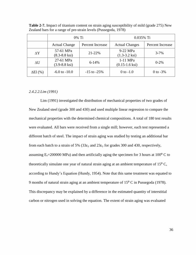
36

Table 2-7. Impact of titanium content on strain aging susceptibility of mild (grade 275) New

Zealand bars for a range of pre-strain levels (Pussegoda, 1978)

0% Ti 0.035% Ti

Actual Change Percent Increase Actual Changes Percent Increase

Y 57-61 MPa

(8.3-8.8 ksi) 21-22%

9-22 MPa

(1.3-3.2 ksi) 3-7%

U 27-61 MPa

(3.9-8.8 ksi) 6-14%

1-11 MPa

(0.15-1.6 ksi) 0-2%

El (%) -6.0 to -10.0 -15 to -25% 0 to -1.0 0 to -3%

2.4.2.2.Lim (1991)

Lim (1991) investigated the distribution of mechanical properties of two grades of

New Zealand steel (grade 300 and 430) and used multiple linear regression to compare the

mechanical properties with the determined chemical compositions. A total of 180 test results

were evaluated. All bars were received from a single mill; however, each test represented a

different batch of steel. The impact of strain aging was studied by testing an additional bar

from each batch to a strain of 5% (33y and 23y for grades 300 and 430, respectively,

assuming Es=200000 MPa) and then artificially aging the specimen for 3 hours at 100⁰ C to

theoretically simulate one year of natural strain aging at an ambient temperature of 15⁰ C,

according to Hundy’s Equation (Hundy, 1954). Note that this same treatment was equated to

9 months of natural strain aging at an ambient temperature of 15⁰ C in Pussegoda (1978).

This discrepancy may be explained by a difference in the estimated quantity of interstitial

carbon or nitrogen used in solving the equation. The extent of strain aging was evaluated

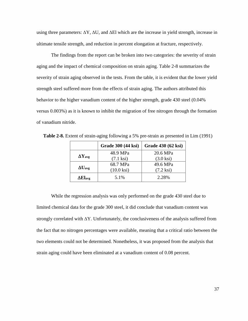
37

using three parameters: Y, U, and El which are the increase in yield strength, increase in

ultimate tensile strength, and reduction in percent elongation at fracture, respectively.

The findings from the report can be broken into two categories: the severity of strain

aging and the impact of chemical composition on strain aging. Table 2-8 summarizes the

severity of strain aging observed in the tests. From the table, it is evident that the lower yield

strength steel suffered more from the effects of strain aging. The authors attributed this

behavior to the higher vanadium content of the higher strength, grade 430 steel (0.04%

versus 0.003%) as it is known to inhibit the migration of free nitrogen through the formation

of vanadium nitride.

Table 2-8. Extent of strain-aging following a 5% pre-strain as presented in Lim (1991)

Grade 300 (44 ksi) Grade 430 (62 ksi)

Yavg 48.9 MPa

(7.1 ksi)

20.6 MPa

(3.0 ksi)

Uavg 68.7 MPa

(10.0 ksi)

49.6 MPa

(7.2 ksi)

Elavg 5.1% 2.28%

While the regression analysis was only performed on the grade 430 steel due to

limited chemical data for the grade 300 steel, it did conclude that vanadium content was

strongly correlated with Y. Unfortunately, the conclusiveness of the analysis suffered from

the fact that no nitrogen percentages were available, meaning that a critical ratio between the

two elements could not be determined. Nonetheless, it was proposed from the analysis that

strain aging could have been eliminated at a vanadium content of 0.08 percent.

38

Several other observations from the report are relevant to the present research. A

comparison of the tensile test results from the producing mill with laboratory results of the

same steel showed that mill tests consistently demonstrated higher yield and tensile strengths

of 20-30 MPa (2.9-4.4 ksi) and 33 MPa (4.8 ksi), respectively. This variation was largely

attributed to differences in strain rates. Also observed was the trend for larger diameter bars

to have reduced strength and ductility as compared to smaller diameter bars, which is thought

to arise from the finer grain size of the smaller diameter bars that results from additional

rolling at the mill and faster cooling .

2.4.2.3.Restrepo-Posada et al. (1994)

As part of an investigation into the effects of cyclic loading, bar deformation, and

strain rate on the stress-strain behavior of two grades of New Zealand reinforcing steel

(grades 300 and 430), Restrepo-Posada et al. (1994) also studied the strain aging behavior of

both grades of rebar. In total, four strain-age tests were conducted for each grade, two having

the pre-strain within the yield plateau, and two with the pre-strain point at the onset of strain

hardening. Each set of two was composed of one uniaxial test and one cyclic test having a

single reversal loop following the pre-strain. Two aging periods were evaluated: 37 days and

147 days. The bars were naturally aged at an ambient 68⁰ F (20⁰ C).

The tests concluded that the grade 300 steel was susceptible to strain aging while the

grade 430 steel was not. This matches the findings by Lim (1991). The difference was

attributed to the respective vanadium contents of the two steels which were zero and 0.04

percent, respectively. Observed signs of strain aging in the grade 300 steel included increased

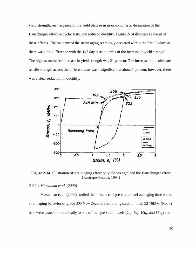
39

yield strength, reemergence of the yield plateau in monotonic tests, dissipation of the

Bauschinger effect in cyclic tests, and reduced ductility. Figure 2-14 illustrates several of

these effects. The majority of the strain aging seemingly occurred within the first 37 days as

there was little difference with the 147 day tests in terms of the increase in yield strength.

The highest measured increase in yield strength was 21 percent. The increase in the ultimate

tensile strength across the different tests was insignificant at about 1 percent; however, there

was a clear reduction in ductility.

Figure 2-14. Illustration of strain aging effect on yield strength and the Bauschinger effect

(Restrepo-Posada, 1994)

2.4.2.4.Momtahan et al. (2009)

Momtahan et al. (2009) studied the influence of pre-strain level and aging time on the

strain aging behavior of grade 300 New Zealand reinforcing steel. In total, 53 16MM (No. 5)

bars were tested monotonically to one of four pre-strain levels (2y, 5y, 10y, and 15y) and

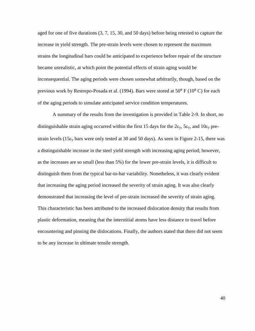
40

aged for one of five durations (3, 7, 15, 30, and 50 days) before being retested to capture the

increase in yield strength. The pre-strain levels were chosen to represent the maximum

strains the longitudinal bars could be anticipated to experience before repair of the structure

became unrealistic, at which point the potential effects of strain aging would be

inconsequential. The aging periods were chosen somewhat arbitrarily, though, based on the

previous work by Restrepo-Posada et al. (1994). Bars were stored at 50⁰ F (10⁰ C) for each

of the aging periods to simulate anticipated service condition temperatures.

A summary of the results from the investigation is provided in Table 2-9. In short, no

distinguishable strain aging occurred within the first 15 days for the 2y, 5y, and 10y pre-

strain levels (15y bars were only tested at 30 and 50 days). As seen in Figure 2-15, there was

a distinguishable increase in the steel yield strength with increasing aging period; however,

as the increases are so small (less than 5%) for the lower pre-strain levels, it is difficult to

distinguish them from the typical bar-to-bar variability. Nonetheless, it was clearly evident

that increasing the aging period increased the severity of strain aging. It was also clearly

demonstrated that increasing the level of pre-strain increased the severity of strain aging.

This characteristic has been attributed to the increased dislocation density that results from

plastic deformation, meaning that the interstitial atoms have less distance to travel before

encountering and pinning the dislocations. Finally, the authors stated that there did not seem

to be any increase in ultimate tensile strength.

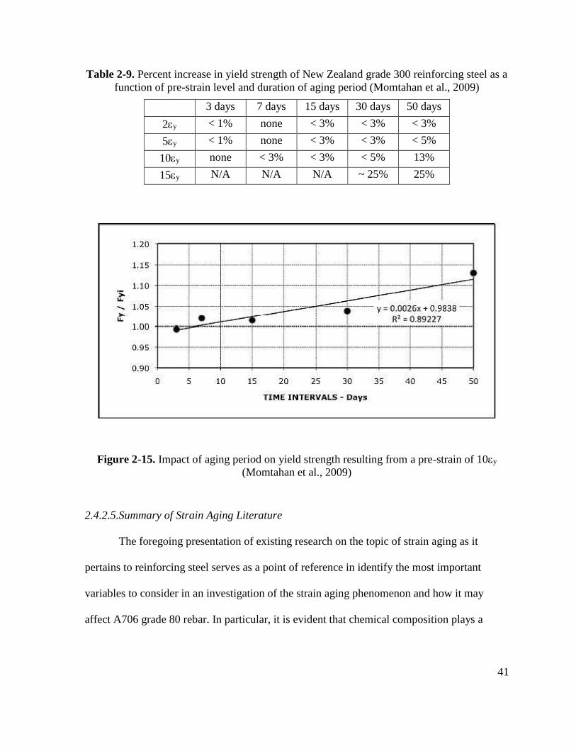
41

Table 2-9. Percent increase in yield strength of New Zealand grade 300 reinforcing steel as a

function of pre-strain level and duration of aging period (Momtahan et al., 2009)

3 days 7 days 15 days 30 days 50 days

2y < 1% none < 3% < 3% < 3%

5y < 1% none < 3% < 3% < 5%

10y none < 3% < 3% < 5% 13%

15y N/A N/A N/A ~ 25% 25%

Figure 2-15. Impact of aging period on yield strength resulting from a pre-strain of 10y

(Momtahan et al., 2009)

2.4.2.5.Summary of Strain Aging Literature

The foregoing presentation of existing research on the topic of strain aging as it

pertains to reinforcing steel serves as a point of reference in identify the most important

variables to consider in an investigation of the strain aging phenomenon and how it may

affect A706 grade 80 rebar. In particular, it is evident that chemical composition plays a

42

significant role in the ability of a given type of steel to be affected by strain aging. As was

described at the beginning of this section, strain aging takes place through the pinning of

molecular slip planes by small, interstitial elements such as nitrogen and carbon. It has been

explained in Pussegoda (1978) that nitrogen is the main participant in strain aging below

100⁰ C while carbon assumes this role at higher temperatures. The process of diffusion and

pinning can be hindered through the addition of nitride forming elements to the steel. While

numerous elements are capable of performing this function, the research consistently points

towards vanadium as the element of choice as it not only reduces strain aging but also

contributes to higher yield strength, lower variability in yield strength, and acceptably high

ductility (Milbourn and Yu, 2010) without the adverse side effects and production costs of

many of the other nitride forming elements (Pussegoda, 1978) which make it ideal for use in

a seismic steel such as A706 grade 80.

While there seems to be a consensus on which elements affect strain aging, the

literature was somewhat divided on the relative proportions of those elements. Pussegoda

(1978) demonstrated that a vanadium content of 0.04-0.06% was sufficient to reduced strain

aging to negligible levels in a grade 275 reinforcing steel having 0.0056% nitrogen. This

would suggest a V/N ratio between 7:1 and 10:1. Lim (1991) speculated that a vanadium

content of 0.08% would have prevented strain aging in a grade 430 steel; however, a V/N

ratio could not be established as the nitrogen content of the steel was unknown. It has

elsewhere been suggested that a V/N ratio of 4:1 is sufficient to reduce strain aging to

insignificant levels (Russwurm and Wille, 1995).

43

The impact of external variables such as aging time and level of pre-strain on the

extent of strain aging has also been investigated though the results are more difficult to

interpret. Some studies relied on artificial aging through a sustained heat treatment after

plastic deformation, while others allowed the steel to age naturally at ambient temperatures.

Furthermore, the grades of steel evaluated ranged from 275 MPa (40 ksi) to 430 MPa (63 ksi)

which, in addition to being varied, all fall below the 550 MPa limit of A706 grade 80 rebar.

Nonetheless, Pussegoda (1978) and Momtahan et al. (2009) concluded that increasing the

level of pre-strain increased the extent of strain aging in the steel they studied. Further,

Restrepo-Posada et al. (1994) and Momtahan et al. (2009) demonstrated that the impact of

strain aging increased with increased aging time (up until a point).

2.5. Cyclic Testing Literature

As described at the beginning of this chapter, a limited number of papers have

presented experimental findings related to the monotonic stress-strain behavior of A706

grade 80 rebar. While this information is extremely useful, actual reinforcing bars in a

reinforced concrete member will experience cyclical demands during an earthquake attack.

As these demands expose unique characteristics of the steel such as fatigue and buckling

behavior, it is necessary to investigate the cyclic performance of A706 grade 80 rebar in

order to more fully complete the picture of its stress-strain behavior. At the time of this

research, there does not appear to be anything in the literature specifically investigating the

cyclic stress-strain behavior of A706 grade 80 rebar.

44

As such, the literature presented in this section does not relate directly to A706 grade

80 rebar, but rather serves to support the two objectives of the cyclic testing program outlined

in Chapter 1 and summarized below:

Identify if there is anything unique about the A706 grade 80 cyclic stress-strain

behavior that would not be captured by existing material models

Investigate the effect of inelastic cycling on the tensile ductility of the steel

The first objective requires both knowledge of existing material models and

availability of A706 grade 80 cyclic test data. The second objective simply requires cyclic

and monotonic experimental test data. While knowledge of existing material models

currently being used in computational programs is easily obtained, acquisition of the

necessary experimental test data is not as readily obtainable as there is currently no standard

in place for cyclic testing of reinforcing bars. As such, the cyclic testing program must draw

on the work of previous researchers studying other grades of steel as well as a rational

understanding of the demands experienced by a reinforcing bar in a concrete member during

an earthquake.

Based on the foregoing discussion, the following papers have been presented as they

represent currently available cyclic material models and modifications to those models to

include additional features such as low cycle fatigue and buckling. Emphasis is placed on the

parameters necessary to define the models, the purpose of those parameters, the intuition

behind the model, and the experimental procedures used in obtaining the test data used to

calibrate the models.

45

2.5.1. Existing Material Models

2.5.1.1.Giuffre-Pinto (1970); Menegotto-Pinto (1973)

Many of the modern cyclic reinforcing steel models can be identified as modifications

of the Giuffre-Pinto (1970) cyclic steel model. For this reason, a brief overview of their

model is presented as foundational to understanding the abilities and limitations of the more

recent models. The Giuffre-Pinto cyclic steel model can be seen as an extension of the

monotonic material model developed by Goldberg and Richard (1963) to cyclic applications

by redefining the stress and strain variables according to the Ramberg-Osgood (1943)

approach. Despite drawing on the Ramberg-Osgood model, which is a =f(s) model, the

Giuffre-Pinto model is defined as a s=f() cyclic model, which makes it preferable for

implementation in displacement-based methods – a characteristic that explains its widespread

presence in modern computational programs. The model proposed by Giuffre and Pinto

offered an improvement over existing models in that it could be used to characterize features

such as the Bauschinger effect, impact of plastic excursion on the shape of the cyclic loops,

and hardening and softening behavior. The generalized equation is presented below as Eqn.

2-1. The parameter R varies as a function of the plastic excursion () and may be modified

by the input parameters A1 and A2 in order to define the curvature of the reversals as well as

account for the Bauschinger effect. The parameter A may be used to define the rate of

softening or hardening of the steel. Thus there are six parameters necessary to define this

model: s0, 0, R0, A1, A2, and A. A coupon test of a mild steel bar (d=10 mm) undergoing

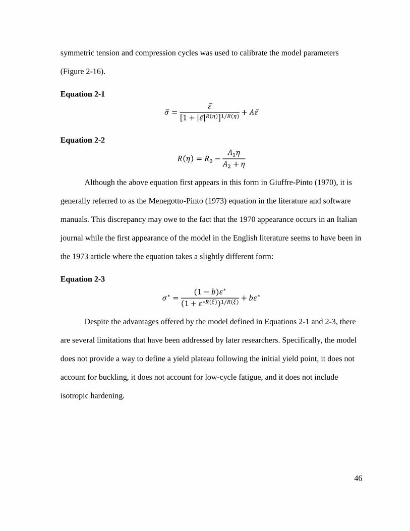
46

symmetric tension and compression cycles was used to calibrate the model parameters

(Figure 2-16).

Equation 2-1

𝜎 =𝜀̅

[1 + |𝜀|̅𝑅(𝜂)]1/𝑅(𝜂)+ 𝐴𝜀 ̅

Equation 2-2

𝑅(𝜂) = 𝑅0 −𝐴1𝜂

𝐴2 + 𝜂

Although the above equation first appears in this form in Giuffre-Pinto (1970), it is

generally referred to as the Menegotto-Pinto (1973) equation in the literature and software

manuals. This discrepancy may owe to the fact that the 1970 appearance occurs in an Italian

journal while the first appearance of the model in the English literature seems to have been in

the 1973 article where the equation takes a slightly different form:

Equation 2-3

𝜎∗ =(1 − 𝑏)𝜀∗

(1 + 𝜀∗𝑅(𝜉))1/𝑅(𝜉)+ 𝑏𝜀∗

Despite the advantages offered by the model defined in Equations 2-1 and 2-3, there

are several limitations that have been addressed by later researchers. Specifically, the model

does not provide a way to define a yield plateau following the initial yield point, it does not

account for buckling, it does not account for low-cycle fatigue, and it does not include

isotropic hardening.

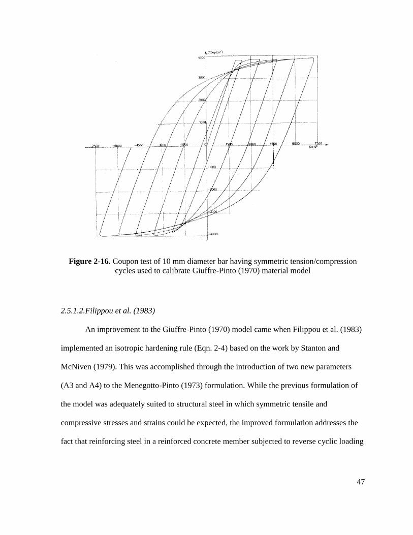
47

Figure 2-16. Coupon test of 10 mm diameter bar having symmetric tension/compression

cycles used to calibrate Giuffre-Pinto (1970) material model

2.5.1.2.Filippou et al. (1983)

An improvement to the Giuffre-Pinto (1970) model came when Filippou et al. (1983)

implemented an isotropic hardening rule (Eqn. 2-4) based on the work by Stanton and

McNiven (1979). This was accomplished through the introduction of two new parameters

(A3 and A4) to the Menegotto-Pinto (1973) formulation. While the previous formulation of

the model was adequately suited to structural steel in which symmetric tensile and

compressive stresses and strains could be expected, the improved formulation addresses the

fact that reinforcing steel in a reinforced concrete member subjected to reverse cyclic loading

48

will experience unbalanced tension and compression strain histories due to the presence of

the concrete and closure of the cracks. This is accomplished by allowing for a shift in the

yield asymptote as a function of the maximum achieved plastic strain – a feature which gives

the model the ability to properly characterize reversals from partial unloading as well as

prediction of isotopic hardening.

Equation 2-4

𝜎𝑠𝑡𝜎𝑦

= 𝑎3 (𝜖𝑚𝑎𝑥

𝜖𝑦− 𝑎4)

Calibration of the model was achieved through comparison with the cyclic rebar test

results presented in Ma et al. (1976). The tests consisted of six machined No. 5 and No. 6

bars (grade 60) tested using load histories representative of what would be experienced in the

top and bottom bars in actual reinforced concrete beams. One of the rebar specimens was

tested using an arbitrary load history. While this addition to the Menegotto-Pinto model does

not account for buckling or low-cycle fatigue, it does appear as an option in many of the later

modifications to the model.

2.5.1.3.Monti-Nuti (1992)

The modification of the Menegotto-Pinto (1973) model to include an isotropic

hardening rule by Filippou et al. (1983) was expanded on by Monti and Nuti (1992) to

include two additional hardening rules as well as the ability to capture post-buckling

softening. The improved model retained the Menegotto-Pinto model parameters R0, A1, A2,

and b+ while replacing the added parameters A3 and A4 with a single new parameter, P,

which is calibrated based on cyclic test results. Calibration of the model was based on tests of

49

16, 20, and 24 mm diameter rebar (approximately No. 5, 6, and 7) of grade 440 MPa having

L/D ratios of 5, 8, and 11. Five different load histories were evaluated (Table 2-10): two

random, one symmetrical, and two nonsymmetrical. The paper did not clarify how the

specific tension-compression strain pairs were selected.

Table 2-10. Cyclical load history used in Monti and Nuti (1992)

Test Strain History (percent strain)

A1, C1

A2, C2

A3, C3

A4, C4

C5

+0.5 -0.5; +2.5 -1; +2 +0.4; +4 +1; +3 +1.5; +4

+1 0; +1.5 -0.5; +2 -0.5; +4 +1.5; +3 +0.5; +4

3(+1 -1); 2(+2 -1); 4(+2 -2)

2(+3 -1); 2(+2 -1); 4(+3 -1)

+1 -1; +2 -1; +3 -1; +4 -3

2.5.1.4.Chang and Mander (1994)

Chang and Mander (1994) presented another modification of the Menegotto-Pinto

(1973) model, based on the work by Mander (1983), in which the Coffin-Manson (1955)

fatigue life model was incorporated to predict bar fracture. Other features of their formulation

included modeling of the monotonic envelope branch to include a yield plateau defined

between the yield strain (y) and the strain at the onset of strain hardening (sh). An implicitly

defined scaling factor allowed the envelope branch to be adjusted in order to account for

strength degradation after each reversal based on the plastic deformation, similar to the

shifting approach used by Filippou et al. (1983).

Despite the fact that ten different rules are used to define the loop shapes, depending

on whether the reversal took place from the envelope curve or part way through a returning

branch, the model benefits from the fact that it may be completely defined using parameters

50

obtained from a monotonic tensile test: fy, Es, sh, Esh, fsu, and su. This feature is achieved

through implicit formulation of many of the cyclic parameters. Cyclic test results available in

Kent and Park (1973), Ma et al. (1976), and Panthaki (1991) were used to calibrate the

model. While the Chang and Mander (1994) model does not include buckling, it is available

in current analysis programs.

2.5.1.5.Dhakal and Maekawa (2002)

A more recent modification of the Menegotto-Pinto (1973) model to include post-

buckling behavior has been proposed by Dhakal and Maekawa (2002). The proposed model

combines the Mander (1983) tension envelope curve formulation and the Menegotto-Pinto

(1973) reversal rules with a post-buckling softening formulation developed by the authors to

form a path-dependent cyclic material model. The aim of the new model was to address the

limited scope of the existing models, such as the one proposed by Monti and Nuti (1992),

which had been calibrated based on limited tests of only a few L/D ratios and steel strengths.

A defining feature of the proposed model was the ability to predict the post-buckling

softening curve as a function of just the bar free length (L), the bar diameter (D), and the

square root of the yield strength (fy). Verification of the final model was performed using the

experimental cyclic tests presented in Monti and Nuti (1992).

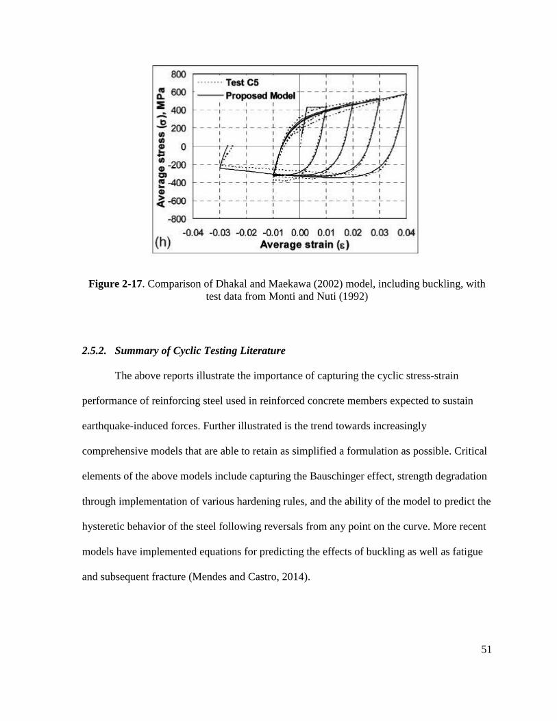
51

Figure 2-17. Comparison of Dhakal and Maekawa (2002) model, including buckling, with

test data from Monti and Nuti (1992)

2.5.2. Summary of Cyclic Testing Literature

The above reports illustrate the importance of capturing the cyclic stress-strain

performance of reinforcing steel used in reinforced concrete members expected to sustain

earthquake-induced forces. Further illustrated is the trend towards increasingly

comprehensive models that are able to retain as simplified a formulation as possible. Critical

elements of the above models include capturing the Bauschinger effect, strength degradation

through implementation of various hardening rules, and the ability of the model to predict the

hysteretic behavior of the steel following reversals from any point on the curve. More recent

models have implemented equations for predicting the effects of buckling as well as fatigue

and subsequent fracture (Mendes and Castro, 2014).

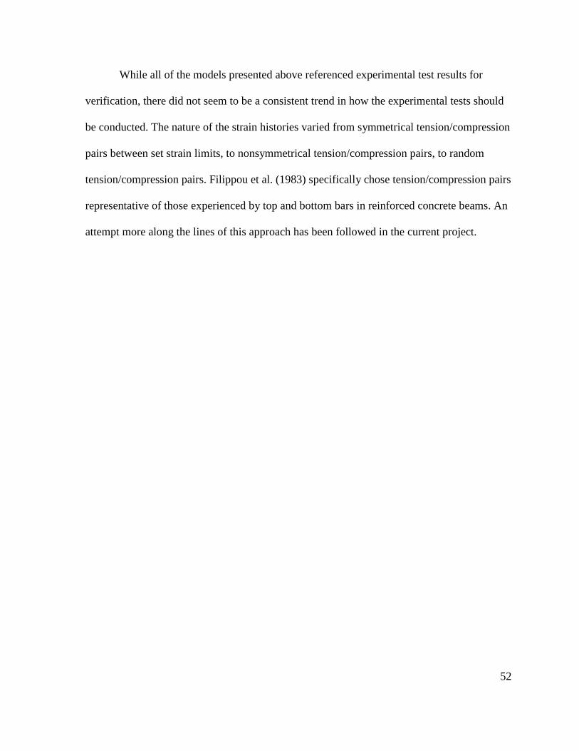
52

While all of the models presented above referenced experimental test results for

verification, there did not seem to be a consistent trend in how the experimental tests should

be conducted. The nature of the strain histories varied from symmetrical tension/compression

pairs between set strain limits, to nonsymmetrical tension/compression pairs, to random

tension/compression pairs. Filippou et al. (1983) specifically chose tension/compression pairs

representative of those experienced by top and bottom bars in reinforced concrete beams. An

attempt more along the lines of this approach has been followed in the current project.

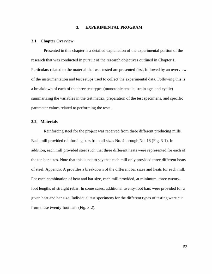
53

3. EXPERIMENTAL PROGRAM

3.1. Chapter Overview

Presented in this chapter is a detailed explanation of the experimental portion of the

research that was conducted in pursuit of the research objectives outlined in Chapter 1.

Particulars related to the material that was tested are presented first, followed by an overview

of the instrumentation and test setups used to collect the experimental data. Following this is

a breakdown of each of the three test types (monotonic tensile, strain age, and cyclic)

summarizing the variables in the test matrix, preparation of the test specimens, and specific

parameter values related to performing the tests.

3.2. Materials

Reinforcing steel for the project was received from three different producing mills.

Each mill provided reinforcing bars from all sizes No. 4 through No. 18 (Fig. 3-1). In

addition, each mill provided steel such that three different heats were represented for each of

the ten bar sizes. Note that this is not to say that each mill only provided three different heats

of steel. Appendix A provides a breakdown of the different bar sizes and heats for each mill.

For each combination of heat and bar size, each mill provided, at minimum, three twenty-

foot lengths of straight rebar. In some cases, additional twenty-foot bars were provided for a

given heat and bar size. Individual test specimens for the different types of testing were cut

from these twenty-foot bars (Fig. 3-2).

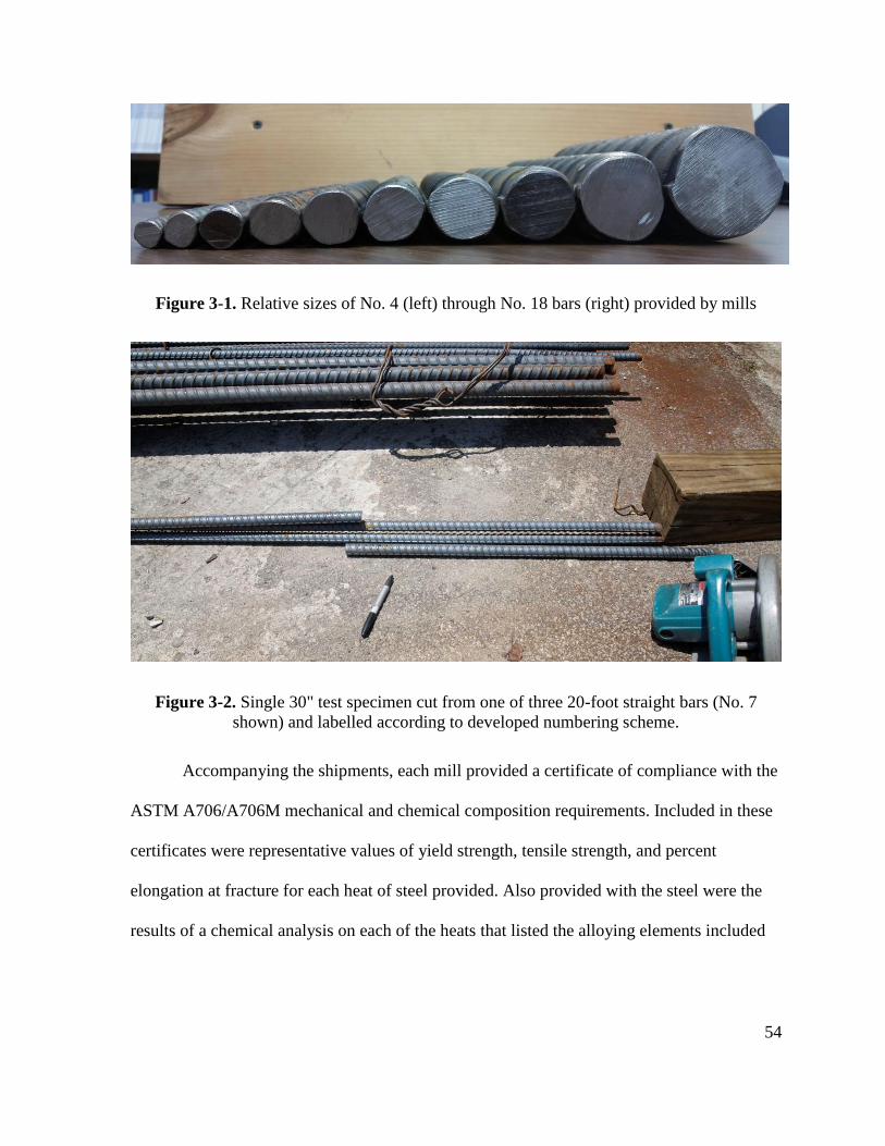
54

Figure 3-1. Relative sizes of No. 4 (left) through No. 18 bars (right) provided by mills

Figure 3-2. Single 30" test specimen cut from one of three 20-foot straight bars (No. 7

shown) and labelled according to developed numbering scheme.

Accompanying the shipments, each mill provided a certificate of compliance with the

ASTM A706/A706M mechanical and chemical composition requirements. Included in these

certificates were representative values of yield strength, tensile strength, and percent

elongation at fracture for each heat of steel provided. Also provided with the steel were the

results of a chemical analysis on each of the heats that listed the alloying elements included

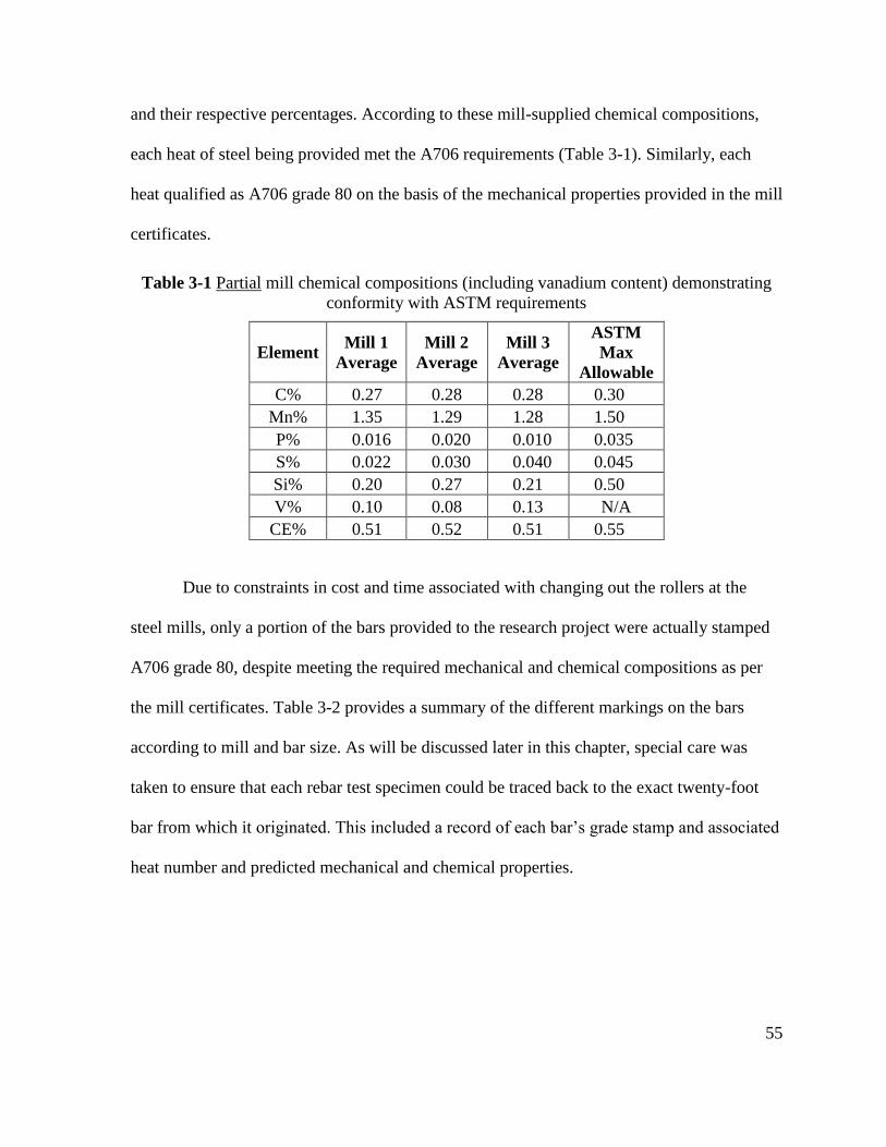
55

and their respective percentages. According to these mill-supplied chemical compositions,

each heat of steel being provided met the A706 requirements (Table 3-1). Similarly, each

heat qualified as A706 grade 80 on the basis of the mechanical properties provided in the mill

certificates.

Table 3-1 Partial mill chemical compositions (including vanadium content) demonstrating

conformity with ASTM requirements

Element Mill 1

Average

Mill 2

Average

Mill 3

Average

ASTM

Max

Allowable

C% 0.27 0.28 0.28 0.30

Mn% 1.35 1.29 1.28 1.50

P% 0.016 0.020 0.010 0.035

S% 0.022 0.030 0.040 0.045

Si% 0.20 0.27 0.21 0.50

V% 0.10 0.08 0.13 N/A

CE% 0.51 0.52 0.51 0.55

Due to constraints in cost and time associated with changing out the rollers at the

steel mills, only a portion of the bars provided to the research project were actually stamped

A706 grade 80, despite meeting the required mechanical and chemical compositions as per

the mill certificates. Table 3-2 provides a summary of the different markings on the bars

according to mill and bar size. As will be discussed later in this chapter, special care was

taken to ensure that each rebar test specimen could be traced back to the exact twenty-foot

bar from which it originated. This included a record of each bar’s grade stamp and associated

heat number and predicted mechanical and chemical properties.

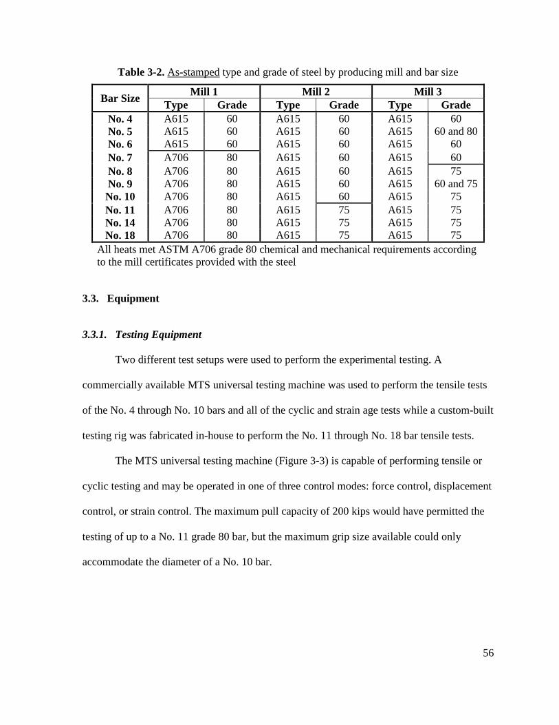
56

Table 3-2. As-stamped type and grade of steel by producing mill and bar size

Bar Size Mill 1 Mill 2 Mill 3

Type Grade Type Grade Type Grade

No. 4 A615 60 A615 60 A615 60

No. 5 A615 60 A615 60 A615 60 and 80

No. 6 A615 60 A615 60 A615 60

No. 7 A706 80 A615 60 A615 60

No. 8 A706 80 A615 60 A615 75

No. 9 A706 80 A615 60 A615 60 and 75

No. 10 A706 80 A615 60 A615 75

No. 11 A706 80 A615 75 A615 75

No. 14 A706 80 A615 75 A615 75

No. 18 A706 80 A615 75 A615 75

All heats met ASTM A706 grade 80 chemical and mechanical requirements according

to the mill certificates provided with the steel

3.3. Equipment

3.3.1. Testing Equipment

Two different test setups were used to perform the experimental testing. A

commercially available MTS universal testing machine was used to perform the tensile tests

of the No. 4 through No. 10 bars and all of the cyclic and strain age tests while a custom-built

testing rig was fabricated in-house to perform the No. 11 through No. 18 bar tensile tests.

The MTS universal testing machine (Figure 3-3) is capable of performing tensile or

cyclic testing and may be operated in one of three control modes: force control, displacement

control, or strain control. The maximum pull capacity of 200 kips would have permitted the

testing of up to a No. 11 grade 80 bar, but the maximum grip size available could only

accommodate the diameter of a No. 10 bar.

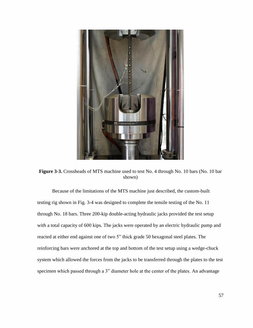
57

Figure 3-3. Crossheads of MTS machine used to test No. 4 through No. 10 bars (No. 10 bar

shown)

Because of the limitations of the MTS machine just described, the custom-built

testing rig shown in Fig. 3-4 was designed to complete the tensile testing of the No. 11

through No. 18 bars. Three 200-kip double-acting hydraulic jacks provided the test setup

with a total capacity of 600 kips. The jacks were operated by an electric hydraulic pump and

reacted at either end against one of two 5” thick grade 50 hexagonal steel plates. The

reinforcing bars were anchored at the top and bottom of the test setup using a wedge-chuck

system which allowed the forces from the jacks to be transferred through the plates to the test

specimen which passed through a 3” diameter hole at the center of the plates. An advantage

58

of this system is that the entire test setup was self-reacting and able to simple sit on the

laboratory floor. A disadvantage was that only tensile tests could be performed.

Forces were obtained by a single 200 kip load cell located separate from the main

setup on a fourth 200-kip jack. This configuration resulted from the need to record forces in

excess of 480 kips with a 200-kip cell which would be damaged if placed directly in line with

a No. 14 or 18 bar. Rather than place the load cell on one of the three jacks surrounding the

bar, which would require equal-height spacers on the other two jacks, it was placed on a

fourth jack physically separated from the setup but still connected to the hydraulic pump.

This fourth jack reacted against a high-strength threaded rod sized to take the full capacity of

the jack. Theoretically, the fourth jack would produce the same force as the other three jacks

as a consequence of being the same size and connected to the same hydraulic source;

however, complicating issues of frictional losses caused this theory to break down. As a

result, the force readings from the load cell had to be artificially reduced to account for losses

between the two systems. This is described in further detail in Section 3.4.4.

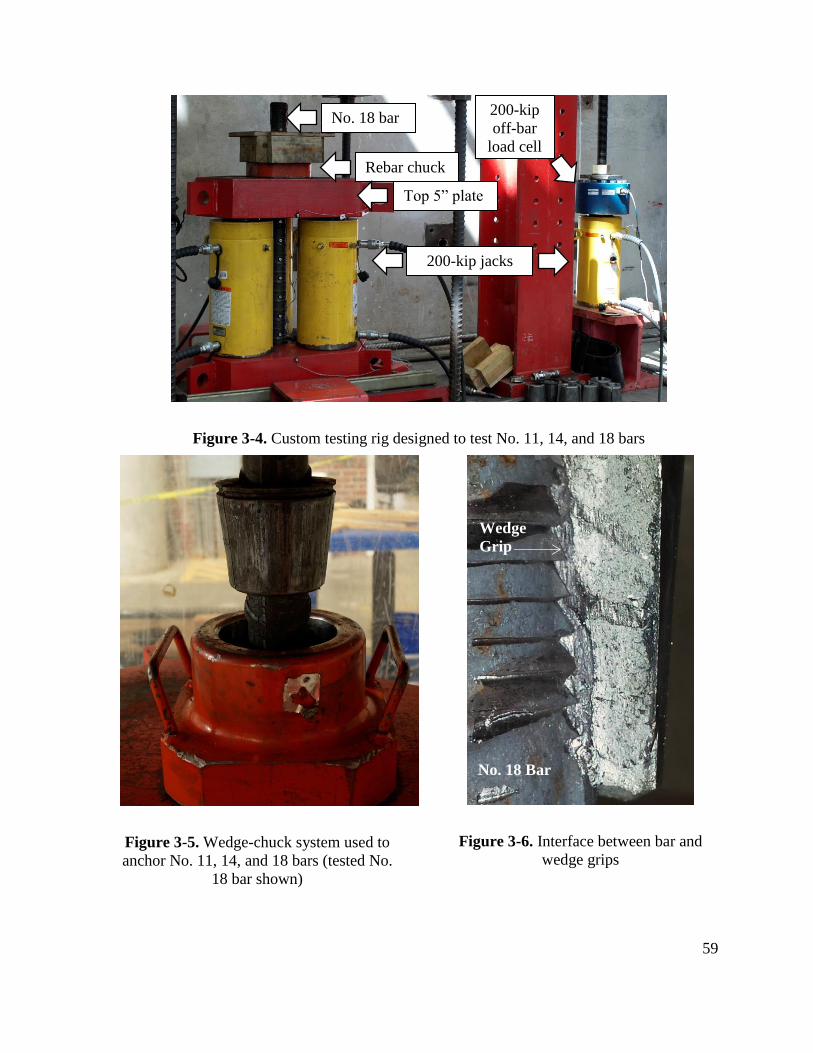
59

Figure 3-4. Custom testing rig designed to test No. 11, 14, and 18 bars

Figure 3-5. Wedge-chuck system used to

anchor No. 11, 14, and 18 bars (tested No.

18 bar shown)

Figure 3-6. Interface between bar and

wedge grips

200-kip

off-bar

load cell

No. 18 bar

Rebar chuck

Top 5” plate

200-kip jacks

Wedge

Grip

No. 18 Bar

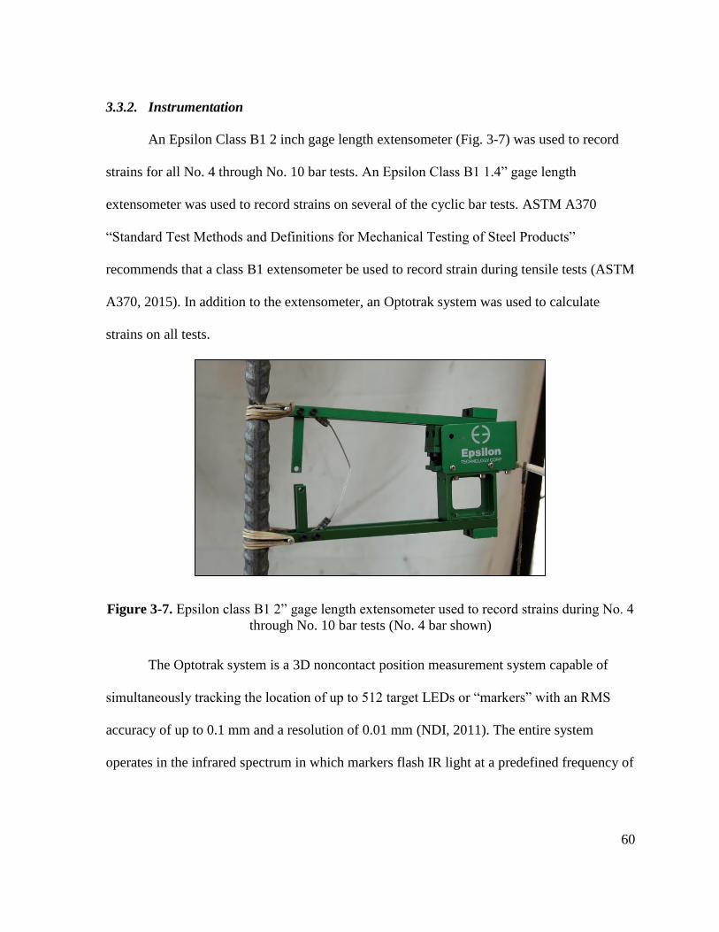
60

3.3.2. Instrumentation

An Epsilon Class B1 2 inch gage length extensometer (Fig. 3-7) was used to record

strains for all No. 4 through No. 10 bar tests. An Epsilon Class B1 1.4” gage length

extensometer was used to record strains on several of the cyclic bar tests. ASTM A370

“Standard Test Methods and Definitions for Mechanical Testing of Steel Products”

recommends that a class B1 extensometer be used to record strain during tensile tests (ASTM

A370, 2015). In addition to the extensometer, an Optotrak system was used to calculate

strains on all tests.

Figure 3-7. Epsilon class B1 2” gage length extensometer used to record strains during No. 4

through No. 10 bar tests (No. 4 bar shown)

The Optotrak system is a 3D noncontact position measurement system capable of

simultaneously tracking the location of up to 512 target LEDs or “markers” with an RMS

accuracy of up to 0.1 mm and a resolution of 0.01 mm (NDI, 2011). The entire system

operates in the infrared spectrum in which markers flash IR light at a predefined frequency of

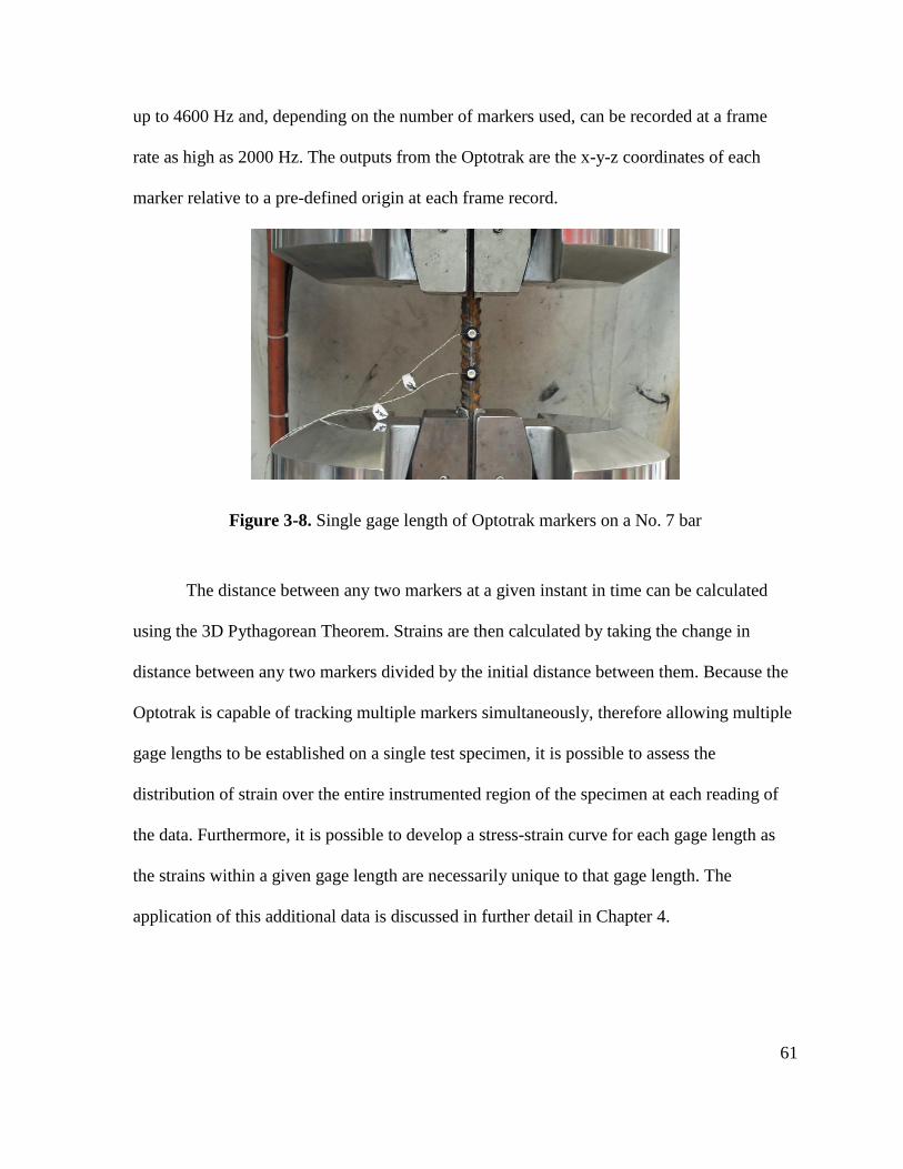
61

up to 4600 Hz and, depending on the number of markers used, can be recorded at a frame

rate as high as 2000 Hz. The outputs from the Optotrak are the x-y-z coordinates of each

marker relative to a pre-defined origin at each frame record.

Figure 3-8. Single gage length of Optotrak markers on a No. 7 bar

The distance between any two markers at a given instant in time can be calculated

using the 3D Pythagorean Theorem. Strains are then calculated by taking the change in

distance between any two markers divided by the initial distance between them. Because the

Optotrak is capable of tracking multiple markers simultaneously, therefore allowing multiple

gage lengths to be established on a single test specimen, it is possible to assess the

distribution of strain over the entire instrumented region of the specimen at each reading of

the data. Furthermore, it is possible to develop a stress-strain curve for each gage length as

the strains within a given gage length are necessarily unique to that gage length. The

application of this additional data is discussed in further detail in Chapter 4.

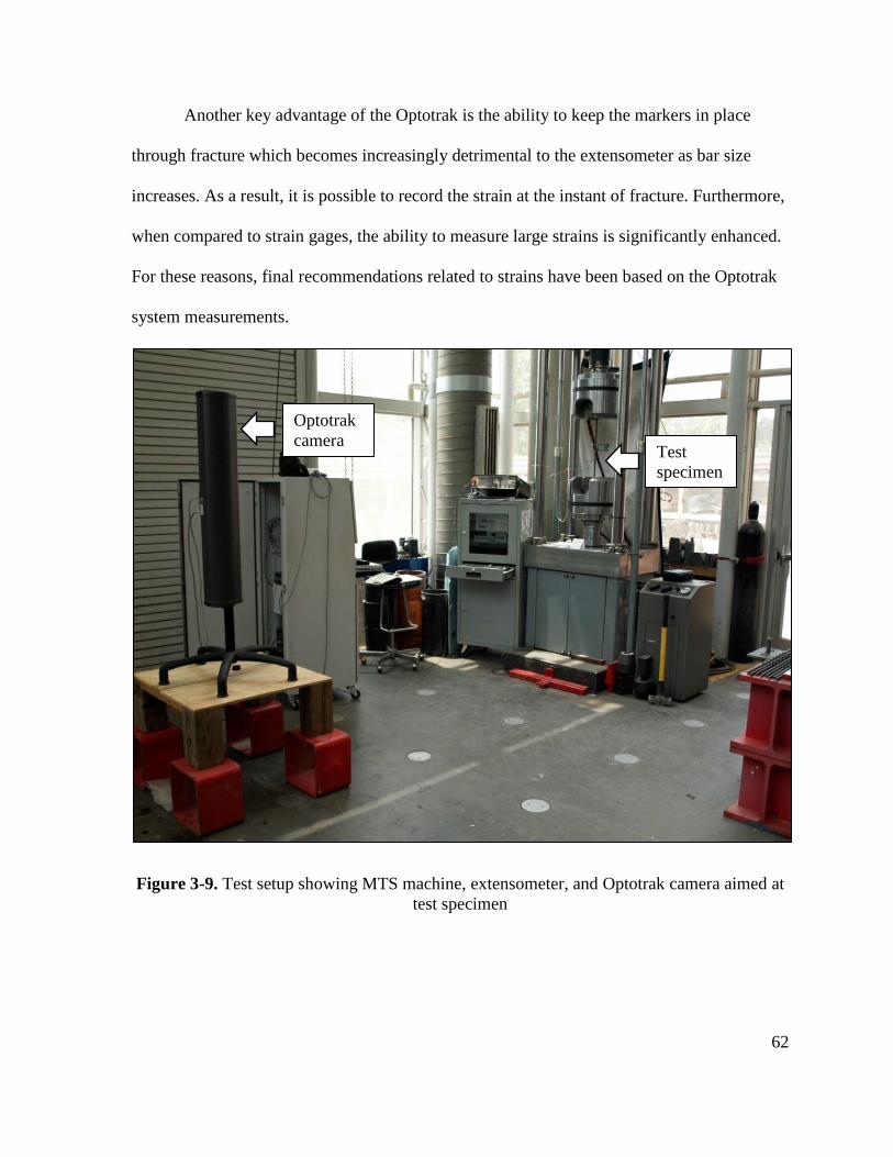
62

Another key advantage of the Optotrak is the ability to keep the markers in place

through fracture which becomes increasingly detrimental to the extensometer as bar size

increases. As a result, it is possible to record the strain at the instant of fracture. Furthermore,

when compared to strain gages, the ability to measure large strains is significantly enhanced.

For these reasons, final recommendations related to strains have been based on the Optotrak

system measurements.

Figure 3-9. Test setup showing MTS machine, extensometer, and Optotrak camera aimed at

test specimen

Optotrak

camera Test

specimen

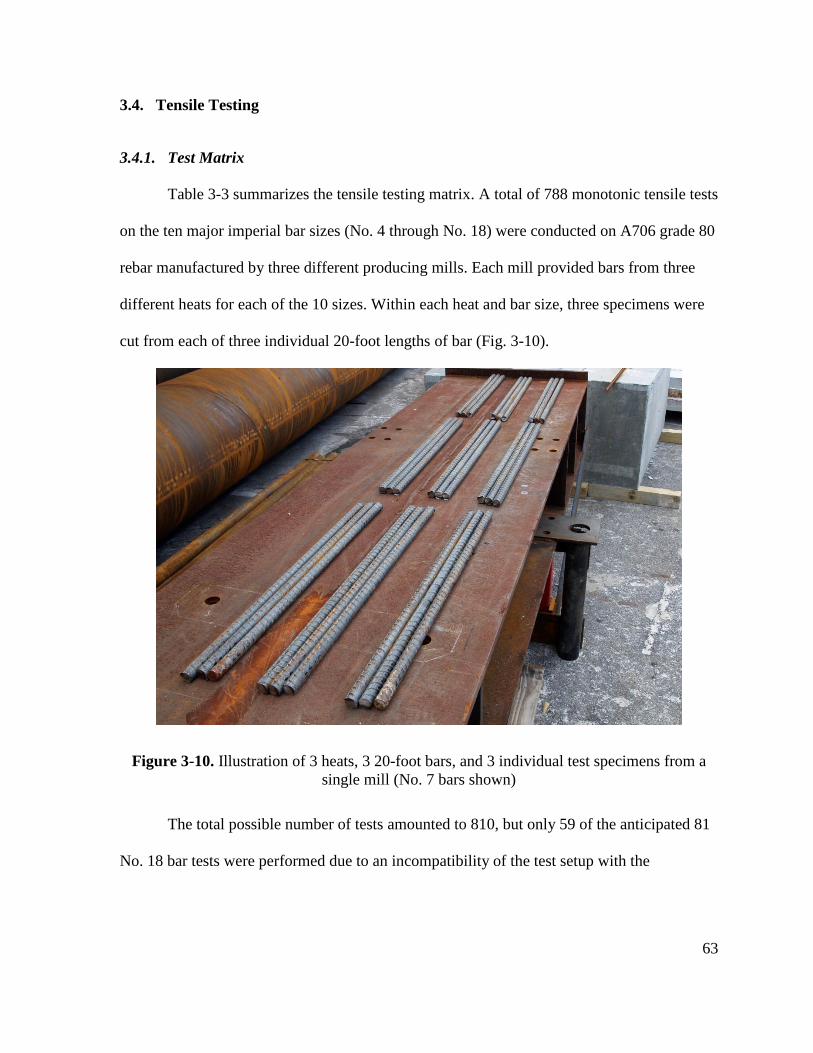
63

3.4. Tensile Testing

3.4.1. Test Matrix

Table 3-3 summarizes the tensile testing matrix. A total of 788 monotonic tensile tests

on the ten major imperial bar sizes (No. 4 through No. 18) were conducted on A706 grade 80

rebar manufactured by three different producing mills. Each mill provided bars from three

different heats for each of the 10 sizes. Within each heat and bar size, three specimens were

cut from each of three individual 20-foot lengths of bar (Fig. 3-10).

Figure 3-10. Illustration of 3 heats, 3 20-foot bars, and 3 individual test specimens from a

single mill (No. 7 bars shown)

The total possible number of tests amounted to 810, but only 59 of the anticipated 81

No. 18 bar tests were performed due to an incompatibility of the test setup with the

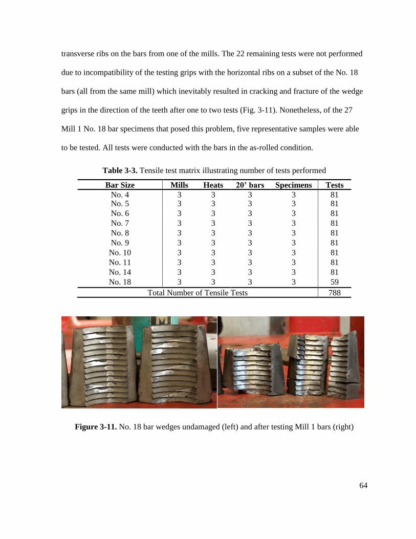
64

transverse ribs on the bars from one of the mills. The 22 remaining tests were not performed

due to incompatibility of the testing grips with the horizontal ribs on a subset of the No. 18

bars (all from the same mill) which inevitably resulted in cracking and fracture of the wedge

grips in the direction of the teeth after one to two tests (Fig. 3-11). Nonetheless, of the 27

Mill 1 No. 18 bar specimens that posed this problem, five representative samples were able

to be tested. All tests were conducted with the bars in the as-rolled condition.

Table 3-3. Tensile test matrix illustrating number of tests performed

Bar Size Mills Heats 20’ bars Specimens Tests

No. 4 3 3 3 3 81 No. 5 3 3 3 3 81

No. 6 3 3 3 3 81

No. 7 3 3 3 3 81

No. 8 3 3 3 3 81

No. 9 3 3 3 3 81

No. 10 3 3 3 3 81

No. 11 3 3 3 3 81

No. 14 3 3 3 3 81

No. 18 3 3 3 3 59

Total Number of Tensile Tests

788

Figure 3-11. No. 18 bar wedges undamaged (left) and after testing Mill 1 bars (right)

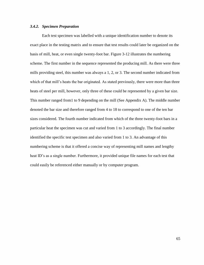
65

3.4.2. Specimen Preparation

Each test specimen was labelled with a unique identification number to denote its

exact place in the testing matrix and to ensure that test results could later be organized on the

basis of mill, heat, or even single twenty-foot bar. Figure 3-12 illustrates the numbering

scheme. The first number in the sequence represented the producing mill. As there were three

mills providing steel, this number was always a 1, 2, or 3. The second number indicated from

which of that mill’s heats the bar originated. As stated previously, there were more than three

heats of steel per mill, however, only three of these could be represented by a given bar size.

This number ranged from1 to 9 depending on the mill (See Appendix A). The middle number

denoted the bar size and therefore ranged from 4 to 18 to correspond to one of the ten bar

sizes considered. The fourth number indicated from which of the three twenty-foot bars in a

particular heat the specimen was cut and varied from 1 to 3 accordingly. The final number

identified the specific test specimen and also varied from 1 to 3. An advantage of this

numbering scheme is that it offered a concise way of representing mill names and lengthy

heat ID’s as a single number. Furthermore, it provided unique file names for each test that

could easily be referenced either manually or by computer program.

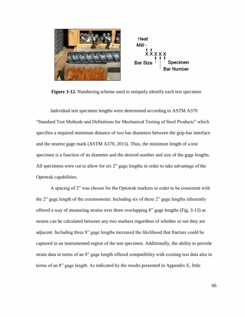
66

Figure 3-12. Numbering scheme used to uniquely identify each test specimen

Individual test specimen lengths were determined according to ASTM A370

“Standard Test Methods and Definitions for Mechanical Testing of Steel Products” which

specifies a required minimum distance of two bar diameters between the grip-bar interface

and the nearest gage mark (ASTM A370, 2015). Thus, the minimum length of a test

specimen is a function of its diameter and the desired number and size of the gage lengths.

All specimens were cut to allow for six 2” gage lengths in order to take advantage of the

Optotrak capabilities.

A spacing of 2” was chosen for the Optotrak markers in order to be consistent with

the 2” gage length of the extensometer. Including six of these 2” gage lengths inherently

offered a way of measuring strains over three overlapping 8” gage lengths (Fig. 3-13) as

strains can be calculated between any two markers regardless of whether or not they are

adjacent. Including three 8” gage lengths increased the likelihood that fracture could be

captured in an instrumented region of the test specimen. Additionally, the ability to provide

strain data in terms of an 8” gage length offered compatibility with existing test data also in

terms of an 8” gage length. As indicated by the results presented in Appendix E, little

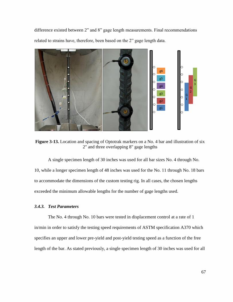
67

difference existed between 2” and 8” gage length measurements. Final recommendations

related to strains have, therefore, been based on the 2” gage length data.

Figure 3-13. Location and spacing of Optotrak markers on a No. 4 bar and illustration of six

2" and three overlapping 8" gage lengths

A single specimen length of 30 inches was used for all bar sizes No. 4 through No.

10, while a longer specimen length of 48 inches was used for the No. 11 through No. 18 bars

to accommodate the dimensions of the custom testing rig. In all cases, the chosen lengths

exceeded the minimum allowable lengths for the number of gage lengths used.

3.4.3. Test Parameters

The No. 4 through No. 10 bars were tested in displacement control at a rate of 1

in/min in order to satisfy the testing speed requirements of ASTM specification A370 which

specifies an upper and lower pre-yield and post-yield testing speed as a function of the free

length of the bar. As stated previously, a single specimen length of 30 inches was used for all

68

No. 4 through No. 10 tests. This corresponded to a bar free length of approximately 20

inches. Rather than select a single pre-yield speed and a different post-yield speed, which

causes a momentary fluctuation in the force-displacement response at the change in load rate

and necessarily adds a level of subjectivity to the test, the constant displacement rate of 1

in/min was applied for the full duration of each test. Initially, all tests were taken until

fracture of the bar; however, tests conducted later in the testing program were stopped prior

to fracture if necking occurred outside of the instrumented region. This prevented

unnecessary wear on the testing equipment as no further useable data would have been

acquired in these cases. A compilation of fractured and necked bar photos is included in

Appendix J.

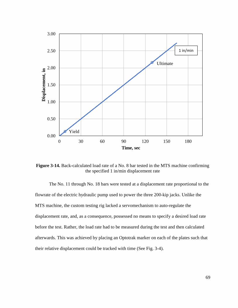
69

Figure 3-14. Back-calculated load rate of a No. 8 bar tested in the MTS machine confirming

the specified 1 in/min displacement rate

The No. 11 through No. 18 bars were tested at a displacement rate proportional to the

flowrate of the electric hydraulic pump used to power the three 200-kip jacks. Unlike the

MTS machine, the custom testing rig lacked a servomechanism to auto-regulate the

displacement rate, and, as a consequence, possessed no means to specify a desired load rate

before the test. Rather, the load rate had to be measured during the test and then calculated

afterwards. This was achieved by placing an Optotrak marker on each of the plates such that

their relative displacement could be tracked with time (See Fig. 3-4).

0.00

0.50

1.00

1.50

2.00

2.50

3.00

0 30 60 90 120 150 180

Dis

pla

cem

ent,

in

Time, sec

1 in/min

Ultimate

Yield

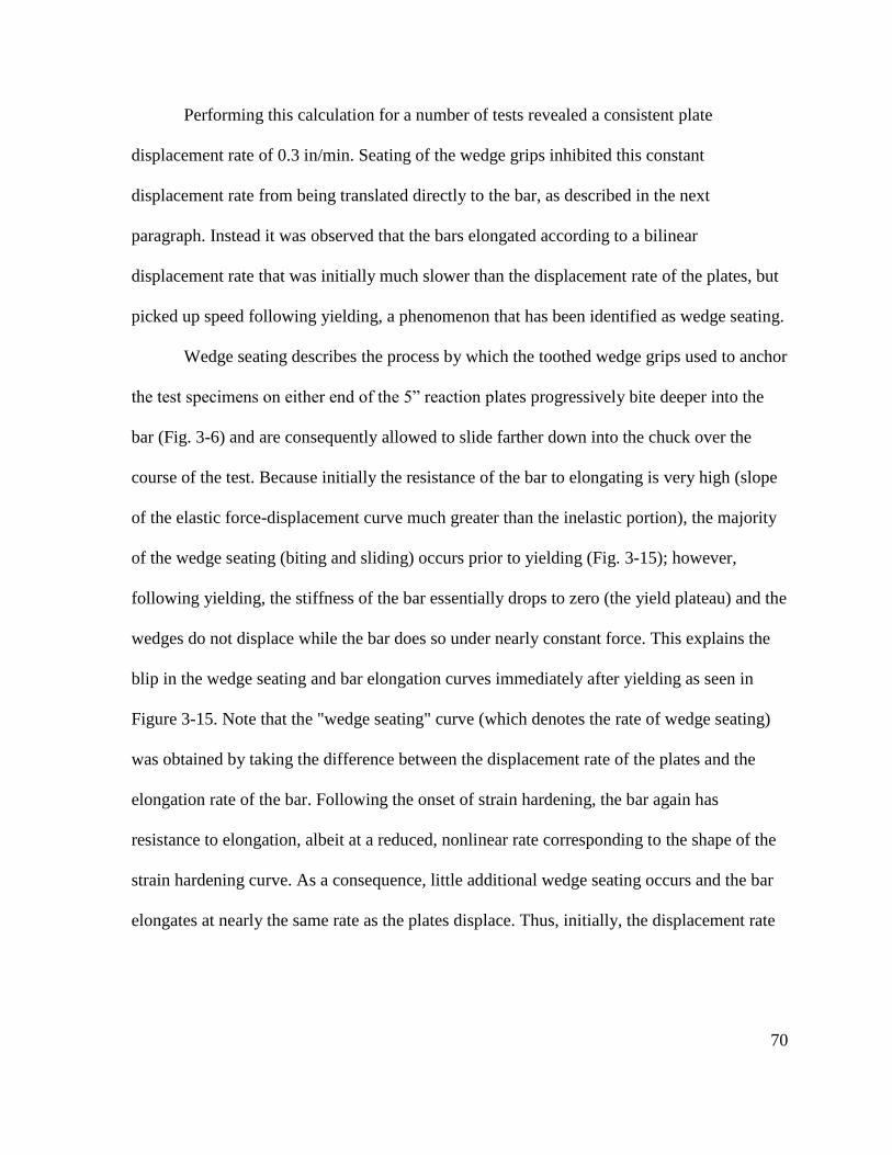
70

Performing this calculation for a number of tests revealed a consistent plate

displacement rate of 0.3 in/min. Seating of the wedge grips inhibited this constant

displacement rate from being translated directly to the bar, as described in the next

paragraph. Instead it was observed that the bars elongated according to a bilinear

displacement rate that was initially much slower than the displacement rate of the plates, but

picked up speed following yielding, a phenomenon that has been identified as wedge seating.

Wedge seating describes the process by which the toothed wedge grips used to anchor

the test specimens on either end of the 5” reaction plates progressively bite deeper into the

bar (Fig. 3-6) and are consequently allowed to slide farther down into the chuck over the

course of the test. Because initially the resistance of the bar to elongating is very high (slope

of the elastic force-displacement curve much greater than the inelastic portion), the majority

of the wedge seating (biting and sliding) occurs prior to yielding (Fig. 3-15); however,

following yielding, the stiffness of the bar essentially drops to zero (the yield plateau) and the

wedges do not displace while the bar does so under nearly constant force. This explains the

blip in the wedge seating and bar elongation curves immediately after yielding as seen in

Figure 3-15. Note that the "wedge seating" curve (which denotes the rate of wedge seating)

was obtained by taking the difference between the displacement rate of the plates and the

elongation rate of the bar. Following the onset of strain hardening, the bar again has

resistance to elongation, albeit at a reduced, nonlinear rate corresponding to the shape of the

strain hardening curve. As a consequence, little additional wedge seating occurs and the bar

elongates at nearly the same rate as the plates displace. Thus, initially, the displacement rate

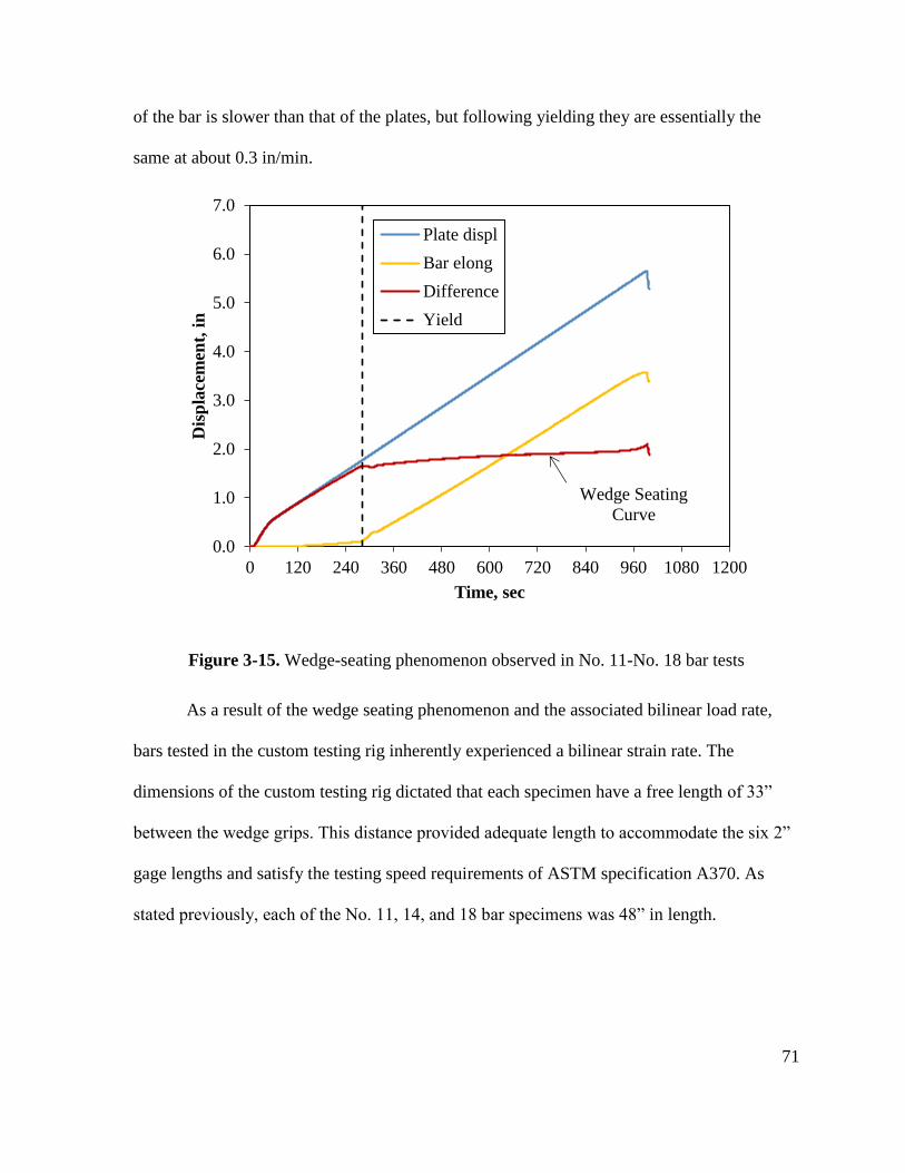
71

of the bar is slower than that of the plates, but following yielding they are essentially the

same at about 0.3 in/min.

Figure 3-15. Wedge-seating phenomenon observed in No. 11-No. 18 bar tests

As a result of the wedge seating phenomenon and the associated bilinear load rate,

bars tested in the custom testing rig inherently experienced a bilinear strain rate. The

dimensions of the custom testing rig dictated that each specimen have a free length of 33”

between the wedge grips. This distance provided adequate length to accommodate the six 2”

gage lengths and satisfy the testing speed requirements of ASTM specification A370. As

stated previously, each of the No. 11, 14, and 18 bar specimens was 48” in length.

0.0

1.0

2.0

3.0

4.0

5.0

6.0

7.0

0 120 240 360 480 600 720 840 960 1080 1200

Dis

pla

cem

ent,

in

Time, sec

Plate displ

Bar elong

Difference

Yield

Wedge Seating

Curve

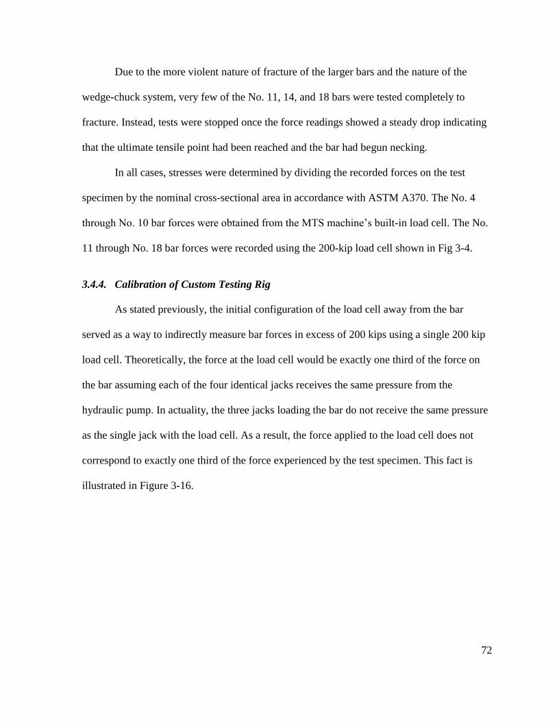
72

Due to the more violent nature of fracture of the larger bars and the nature of the

wedge-chuck system, very few of the No. 11, 14, and 18 bars were tested completely to

fracture. Instead, tests were stopped once the force readings showed a steady drop indicating

that the ultimate tensile point had been reached and the bar had begun necking.

In all cases, stresses were determined by dividing the recorded forces on the test

specimen by the nominal cross-sectional area in accordance with ASTM A370. The No. 4

through No. 10 bar forces were obtained from the MTS machine’s built-in load cell. The No.

11 through No. 18 bar forces were recorded using the 200-kip load cell shown in Fig 3-4.

3.4.4. Calibration of Custom Testing Rig

As stated previously, the initial configuration of the load cell away from the bar

served as a way to indirectly measure bar forces in excess of 200 kips using a single 200 kip

load cell. Theoretically, the force at the load cell would be exactly one third of the force on

the bar assuming each of the four identical jacks receives the same pressure from the

hydraulic pump. In actuality, the three jacks loading the bar do not receive the same pressure

as the single jack with the load cell. As a result, the force applied to the load cell does not

correspond to exactly one third of the force experienced by the test specimen. This fact is

illustrated in Figure 3-16.

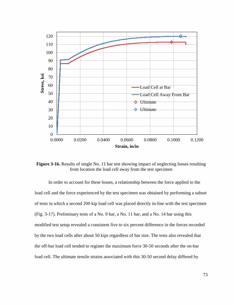
73

Figure 3-16. Results of single No. 11 bar test showing impact of neglecting losses resulting

from location the load cell away from the test specimen

In order to account for these losses, a relationship between the force applied to the

load cell and the force experienced by the test specimen was obtained by performing a subset

of tests in which a second 200 kip load cell was placed directly in-line with the test specimen

(Fig. 3-17). Preliminary tests of a No. 9 bar, a No. 11 bar, and a No. 14 bar using this

modified test setup revealed a consistent five to six percent difference in the forces recorded

by the two load cells after about 50 kips regardless of bar size. The tests also revealed that

the off-bar load cell tended to register the maximum force 30-50 seconds after the on-bar

load cell. The ultimate tensile strains associated with this 30-50 second delay differed by

0

10

20

30

40

50

60

70

80

90

100

110

120

0.0000 0.0200 0.0400 0.0600 0.0800 0.1000 0.1200

Str

ess,

ksi

Strain, in/in

Load Cell at Bar

Load Cell Away From Bar

Ultimate

Ultimate

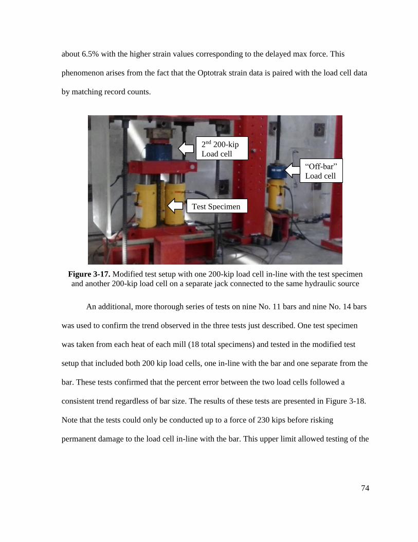
74

about 6.5% with the higher strain values corresponding to the delayed max force. This

phenomenon arises from the fact that the Optotrak strain data is paired with the load cell data

by matching record counts.

Figure 3-17. Modified test setup with one 200-kip load cell in-line with the test specimen

and another 200-kip load cell on a separate jack connected to the same hydraulic source

An additional, more thorough series of tests on nine No. 11 bars and nine No. 14 bars

was used to confirm the trend observed in the three tests just described. One test specimen

was taken from each heat of each mill (18 total specimens) and tested in the modified test

setup that included both 200 kip load cells, one in-line with the bar and one separate from the

bar. These tests confirmed that the percent error between the two load cells followed a

consistent trend regardless of bar size. The results of these tests are presented in Figure 3-18.

Note that the tests could only be conducted up to a force of 230 kips before risking

permanent damage to the load cell in-line with the bar. This upper limit allowed testing of the

2nd 200-kip

Load cell

Test Specimen

“Off-bar”

Load cell

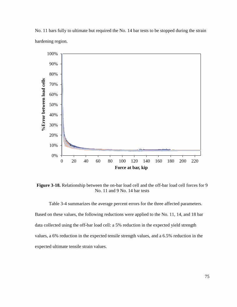
75

No. 11 bars fully to ultimate but required the No. 14 bar tests to be stopped during the strain

hardening region.

Figure 3-18. Relationship between the on-bar load cell and the off-bar load cell forces for 9

No. 11 and 9 No. 14 bar tests

Table 3-4 summarizes the average percent errors for the three affected parameters.

Based on these values, the following reductions were applied to the No. 11, 14, and 18 bar

data collected using the off-bar load cell: a 5% reduction in the expected yield strength

values, a 6% reduction in the expected tensile strength values, and a 6.5% reduction in the

expected ultimate tensile strain values.

0%

10%

20%

30%

40%

50%

60%

70%

80%

90%

100%

0 20 40 60 80 100 120 140 160 180 200 220

%E

rror

bet

wee

n l

oad

cel

ls

Force at bar, kip

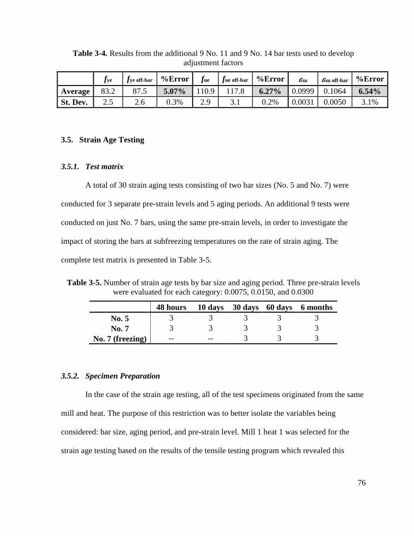
76

Table 3-4. Results from the additional 9 No. 11 and 9 No. 14 bar tests used to develop

adjustment factors

fye fye off-bar %Error fue fue off-bar %Error su su off-bar %Error

Average 83.2 87.5 5.07% 110.9 117.8 6.27% 0.0999 0.1064 6.54%

St. Dev. 2.5 2.6 0.3% 2.9 3.1 0.2% 0.0031 0.0050 3.1%

3.5. Strain Age Testing

3.5.1. Test matrix

A total of 30 strain aging tests consisting of two bar sizes (No. 5 and No. 7) were

conducted for 3 separate pre-strain levels and 5 aging periods. An additional 9 tests were

conducted on just No. 7 bars, using the same pre-strain levels, in order to investigate the

impact of storing the bars at subfreezing temperatures on the rate of strain aging. The

complete test matrix is presented in Table 3-5.

Table 3-5. Number of strain age tests by bar size and aging period. Three pre-strain levels

were evaluated for each category: 0.0075, 0.0150, and 0.0300

48 hours 10 days 30 days 60 days 6 months

No. 5 3 3 3 3 3

No. 7 3 3 3 3 3

No. 7 (freezing) -- -- 3 3 3


In the case of the strain age testing, all of the test specimens originated from the same

mill and heat. The purpose of this restriction was to better isolate the variables being

considered: bar size, aging period, and pre-strain level. Mill 1 heat 1 was selected for the

strain age testing based on the results of the tensile testing program which revealed this

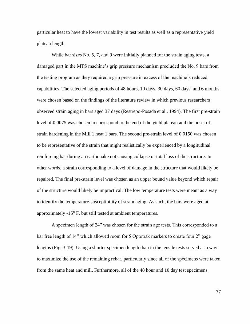
77

particular heat to have the lowest variability in test results as well as a representative yield

plateau length.

While bar sizes No. 5, 7, and 9 were initially planned for the strain aging tests, a

damaged part in the MTS machine’s grip pressure mechanism precluded the No. 9 bars from

the testing program as they required a grip pressure in excess of the machine’s reduced

capabilities. The selected aging periods of 48 hours, 10 days, 30 days, 60 days, and 6 months

were chosen based on the findings of the literature review in which previous researchers

observed strain aging in bars aged 37 days (Restrepo-Posada et al., 1994). The first pre-strain

level of 0.0075 was chosen to correspond to the end of the yield plateau and the onset of

strain hardening in the Mill 1 heat 1 bars. The second pre-strain level of 0.0150 was chosen

to be representative of the strain that might realistically be experienced by a longitudinal

reinforcing bar during an earthquake not causing collapse or total loss of the structure. In

other words, a strain corresponding to a level of damage in the structure that would likely be

repaired. The final pre-strain level was chosen as an upper bound value beyond which repair

of the structure would likely be impractical. The low temperature tests were meant as a way

to identify the temperature-susceptibility of strain aging. As such, the bars were aged at

approximately -15⁰ F, but still tested at ambient temperatures.

A specimen length of 24” was chosen for the strain age tests. This corresponded to a

bar free length of 14” which allowed room for 5 Optotrak markers to create four 2” gage

lengths (Fig. 3-19). Using a shorter specimen length than in the tensile tests served as a way

to maximize the use of the remaining rebar, particularly since all of the specimens were taken

from the same heat and mill. Furthermore, all of the 48 hour and 10 day test specimens

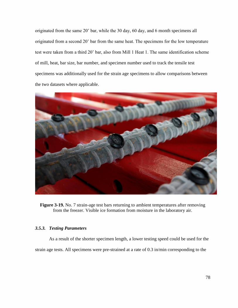
78

originated from the same 20’ bar, while the 30 day, 60 day, and 6 month specimens all

originated from a second 20’ bar from the same heat. The specimens for the low temperature

test were taken from a third 20’ bar, also from Mill 1 Heat 1. The same identification scheme

of mill, heat, bar size, bar number, and specimen number used to track the tensile test

specimens was additionally used for the strain age specimens to allow comparisons between

the two datasets where applicable.

Figure 3-19. No. 7 strain-age test bars returning to ambient temperatures after removing

from the freezer. Visible ice formation from moisture in the laboratory air.

3.5.3. Testing Parameters

As a result of the shorter specimen length, a lower testing speed could be used for the

strain age tests. All specimens were pre-strained at a rate of 0.3 in/min corresponding to the

79

upper bound pre-yield strain rate permitted by ASTM A370. A load rate of 0.7 in/min was

used to re-test the specimens at the conclusion of the aging period.

The procedure for conducting the strain age tests was to initially test the bar to the

desired pre-strain, pause the test, and then gradually release the force on the bar until it could

be removed from the grips of the MTS machine. Following this, the bars were stored at

ambient laboratory temperatures for the duration of the desired aging period. In the case of

the low temperature tests, the bars were placed into a freezer upon completion of the pre-

strain testing where they remained until the end of the aging period. At the conclusion of this

period, the bars were again loaded into the testing machine and tested until failure. The low

temperature bars where allowed a minimum of 1 hour to return to ambient temperatures

before being retested. Chapter 4 presents the results from the tests.

3.6. Cyclic Testing

A limited number of cyclic tests on No. 5 and No. 7 bars were conducted with the

primary purpose of evaluating the capability of existing rebar models to characterize the

cyclic material behavior. A further intent of the cyclic testing program was to investigate the

effect of cyclic load history on the ultimate tensile strain (strain at max stress). While

difficulties with the gripping mechanism of the MTS machine greatly limited the scope of

this portion of the research, informative results were still able to be obtained.

3.6.1. Test Matrix

Table 3-6 summarizes the cyclic tests that were performed. A total of ten No. 5 bars

and three No. 7 bars were tested in the as-rolled condition using varying load histories and

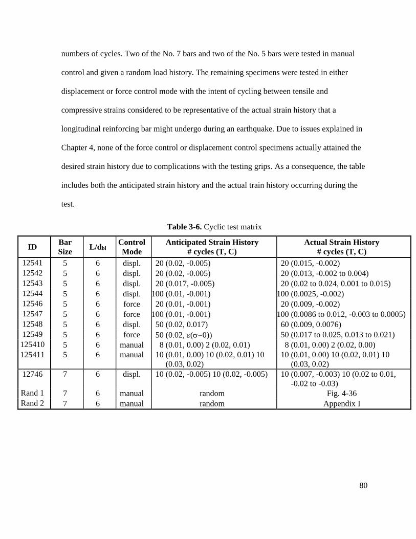
80

numbers of cycles. Two of the No. 7 bars and two of the No. 5 bars were tested in manual

control and given a random load history. The remaining specimens were tested in either

displacement or force control mode with the intent of cycling between tensile and

compressive strains considered to be representative of the actual strain history that a

longitudinal reinforcing bar might undergo during an earthquake. Due to issues explained in

Chapter 4, none of the force control or displacement control specimens actually attained the

desired strain history due to complications with the testing grips. As a consequence, the table

includes both the anticipated strain history and the actual train history occurring during the

test.

Table 3-6. Cyclic test matrix

ID Bar

Size L/dbl

Control

Mode

Anticipated Strain History

# cycles (T, C)

Actual Strain History

# cycles (T, C)

12541 5 6 displ. 20 (0.02, -0.005) 20 (0.015, -0.002)

12542 5 6 displ. 20 (0.02, -0.005) 20 (0.013, -0.002 to 0.004)

12543 5 6 displ. 20 (0.017, -0.005) 20 (0.02 to 0.024, 0.001 to 0.015)

12544 5 6 displ. 100 (0.01, -0.001) 100 (0.0025, -0.002)

12546 5 6 force 20 (0.01, -0.001) 20 (0.009, -0.002)

12547 5 6 force 100 (0.01, -0.001) 100 (0.0086 to 0.012, -0.003 to 0.0005)

12548 5 6 displ. 50 (0.02, 0.017) 60 (0.009, 0.0076)

12549 5 6 force 50 (0.02, (s=0)) 50 (0.017 to 0.025, 0.013 to 0.021)

125410 5 6 manual 8 (0.01, 0.00) 2 (0.02, 0.01) 8 (0.01, 0.00) 2 (0.02, 0.00)

125411 5 6 manual 10 (0.01, 0.00) 10 (0.02, 0.01) 10

(0.03, 0.02)

10 (0.01, 0.00) 10 (0.02, 0.01) 10

(0.03, 0.02)

12746 7 6 displ. 10 (0.02, -0.005) 10 (0.02, -0.005) 10 (0.007, -0.003) 10 (0.02 to 0.01,

-0.02 to -0.03)

Rand 1 7 6 manual random Fig. 4-36

Rand 2 7 6 manual random Appendix I

81


Save for the two No. 7 bars tested manually, test specimens used to perform the

cyclic tests were taken from the remaining Mill 1 heat 2 bars as this mill provided extra steel

and the tensile tests showed comparatively low variability within this heat. Furthermore, each

of the No. 5 bar test specimens originated from the same 20’ length. Two of the No. 7 bar

specimens originated from a common 20’ length of bar. The test specimens were cut to

provide an unbraced length between the MTS machine crossheads of 6 bar diameters. The

same identification scheme of mill, heat, bar size, bar number, and specimen number used to

track the tensile and strain age test specimens was used for the cyclic test specimens to allow

for close comparison with the tensile test results.

3.6.3. Test Parameters

Due to the lack of requirements for performing tensile tests, as discussed in Chapter

2, the tensile testing speed requirements of ASTM A370 were translated into cycle frequency

based on an equivalent monotonic rate of 0.7 in/min. While the majority of the tests were

conducted for just 20 cycles, a few tests were performed for a greater number of cycles, as

indicated in Table 3-6, as part of the effort to identify the effect of cycling on the monotonic

strain at max stress.

Initially, all of the tests were conducted using the MTS machine’s displacement

control mode in which the desired strain history was first transformed into displacement

limits based on the expected unbraced length of the bar. The bar was then tested between

these displacement limits using a sinusoidal wave form at a cycle rate defined by the

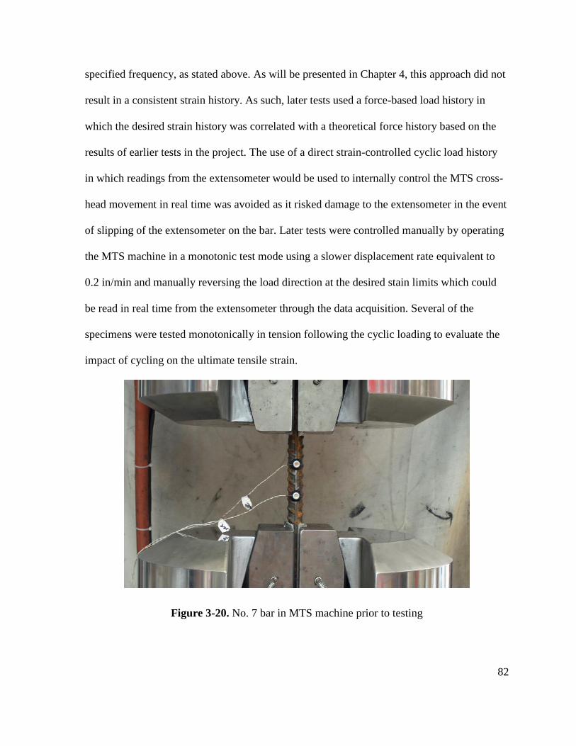
82

specified frequency, as stated above. As will be presented in Chapter 4, this approach did not

result in a consistent strain history. As such, later tests used a force-based load history in

which the desired strain history was correlated with a theoretical force history based on the

results of earlier tests in the project. The use of a direct strain-controlled cyclic load history

in which readings from the extensometer would be used to internally control the MTS cross-

head movement in real time was avoided as it risked damage to the extensometer in the event

of slipping of the extensometer on the bar. Later tests were controlled manually by operating

the MTS machine in a monotonic test mode using a slower displacement rate equivalent to

0.2 in/min and manually reversing the load direction at the desired stain limits which could

be read in real time from the extensometer through the data acquisition. Several of the

specimens were tested monotonically in tension following the cyclic loading to evaluate the

impact of cycling on the ultimate tensile strain.

Figure 3-20. No. 7 bar in MTS machine prior to testing

83

4. RESULTS

4.1. Chapter Overview

Presented in this chapter are the findings of the experimental program just described.

As with the previous chapter, each of the three types of tests are addressed independently.

The presentation of the tensile test results opens with an explanation of which stress-strain

parameters were evaluated and how they were determined. Following this is an overview of

the statistical methods used in interpreting the findings and then a presentation of each of the

stress-strain parameters in terms of the identified cumulative distribution functions including

best-fit probability distributions. Relevant summary statistics of the tensile tests are provided

in Section 4.2.3.10.

The strain aging section of this chapter presents the results of the 30 tests that were

described in Chapter 3. A subsection is devoted to each of the four variables investigated for

impact on strain-aging: impact of aging period, impact of pre-strain, impact of bar size, and

impact of low temperature. Stress-strain curves from the tests have been located in Appendix

H.

The chapter concludes with a presentation of the results of the cyclic testing program.

Included in this is a presentation of a cyclic material model that has been fitted to one of the

experimental stress-strain curves. Also included in the cyclic test results section is a

presentation of the tests used to identify the impact of cyclic load history on the monotonic

strain at max stress.

84

4.2. Tensile Testing

4.2.1. Determination of Stress-Strain Parameters

Each test generated two raw data files: one text file containing force data and one

CSV file containing the Optotrak marker x-y-z coordinate data. Data was collected at a

frequency of 8 Hz for the No. 4 through No. 10 bar tests and 2 Hz for the No. 11 through No.

18 bar tests. A slower recording rate was chosen for the large bar tests to account for the

slower displacement rate produced by the electric hydraulic pump.

The two raw data files were compiled and processed in a single macro-enabled Excel

workbook unique to each test in which forces were converted to stresses based on the

nominal cross-sectional area of the bar and Optotrak marker coordinate data was converted to

strain data using the procedure described in Chapter 3. A combination of VBA programs and

Excel worksheet functions was used in these compiled individual test files to identify the

values of the six parameters needed to define the monotonic stress-strain curve, as indicated

in Section 1.2, within each gage length for each test. Table 4-1 provides a list of all the

parameters for which values were determined for each test. These parameters were

specifically selected as they correspond to transitional points on the monotonic stress strain

curve, and many of them are necessary to defining existing material models. Parameters

highlighted in bold were used to define the recommendations for the A706 grade 80 stress-

strain curve presented in Chapter 5. The remainder of this section describes each of the

parameters and how they were determined.

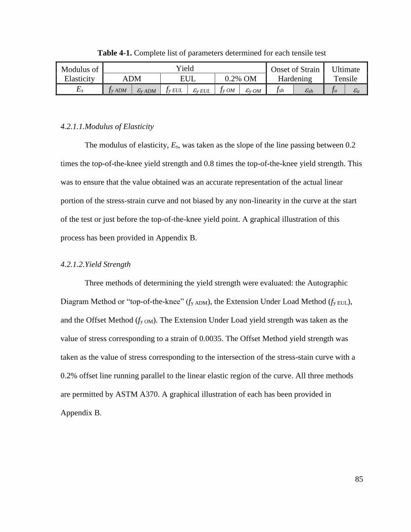
85

Table 4-1. Complete list of parameters determined for each tensile test

Modulus of

Elasticity

Yield Onset of Strain

Hardening

Ultimate

Tensile ADM EUL 0.2% OM

Es fy ADM y ADM fy EUL y EUL fy OM y OM fsh sh fu u

4.2.1.1.Modulus of Elasticity

The modulus of elasticity, Es, was taken as the slope of the line passing between 0.2

times the top-of-the-knee yield strength and 0.8 times the top-of-the-knee yield strength. This

was to ensure that the value obtained was an accurate representation of the actual linear

portion of the stress-strain curve and not biased by any non-linearity in the curve at the start

of the test or just before the top-of-the-knee yield point. A graphical illustration of this

process has been provided in Appendix B.

4.2.1.2.Yield Strength

Three methods of determining the yield strength were evaluated: the Autographic

Diagram Method or “top-of-the-knee” (fy ADM), the Extension Under Load Method (fy EUL),

and the Offset Method (fy OM). The Extension Under Load yield strength was taken as the

value of stress corresponding to a strain of 0.0035. The Offset Method yield strength was

taken as the value of stress corresponding to the intersection of the stress-stain curve with a

0.2% offset line running parallel to the linear elastic region of the curve. All three methods

are permitted by ASTM A370. A graphical illustration of each has been provided in

Appendix B.

86

4.2.1.3.Yield Strain

Three individual yield strains were identified for each test, one corresponding to each

of the three determined yield strengths: the Autographic Diagram Method yield strain (y

ADM), the Extension Under Load yield strain (y EUL), and the Offset Method yield strain (y

OM). The ADM yield strain was taken as the strain corresponding to the top-of-the-knee yield

strength (fy ADM). The EUL yield strain simply equaled 0.0035 by definition. The OM yield

strain was identified as the value of strain corresponding to the intersection of the stress-

strain curve with a 0.2% offset line running parallel to the linear elastic region of the curve.

4.2.1.4.Onset of Strain Hardening

The strain at the onset of strain hardening, sh, was determined as the point at which a

horizontal line passing through the 0.2% offset stress intersected a line tangent to the initial

portion of the strain hardening curve. Specifically, the tangent line to the strain hardening

curve was defined as the line passing between 1.02 times the 0.2% offset yield strength and

1.05 times the 0.2% offset yield strength. In specimens exhibiting well-defined yield

plateaus, the 0.2% offset line consistently intersected the yield plateau thus making the

horizontal line passing through this point analogous to the slope of the yield plateau. The

stress at the onset of strain hardening was taken as the point on the actual stress-stain curve

corresponding to the strain at the onset of strain hardening using interpolation as necessary.

This approach was designed to reduce subjectivity in determining when the yield plateau

ceased and when the strain hardening curve commenced as well as to speed up the processing

of the data. A graphical illustration of this process has been provided in Appendix B.

87

4.2.1.5.Tensile Strength and Ultimate Tensile Strain

The tensile strength, fu, was identified as the maximum value of stress occurring

during the test; in other words, the point at which strain hardening ceased and necking

initiated. The ultimate tensile strain, u, was identified as the value of strain corresponding to

the point of maximum stress. This is not to be confused with the value of strain at fracture.

4.2.2. Statistical Methods

Two primary approaches were taken to interpreting the body of data generated during

the tensile testing program. The first approach was to describe the combined results for each

of the parameters in terms of its summary statistics, specifically: mean, standard deviation,

coefficient of variation, 5th percentile, and 95th percentile. A summary of these results is

presented in Section 4.2.3.10. The second approach was to plot the cumulative distribution

curves for each parameter and then evaluate the underlying probability distributions. This

method accomplished several things: it provided a graphical means of illustrating the spread

of the data, it provided a graphical way to identify trends or anomalies in the data, and most

significantly it provided a resource for other researchers to use in the future. The remainder

of this section expands on the latter of these two approaches.

Quantitatively, a cumulative distribution function (CDF) describes the percentage of

data in a dataset that exists at or below a given value. Qualitatively, it serves as a graphical

means of illustrating the distribution of the data in a dataset about its median. CDFs that are

short and steep imply less variability in the data while CDFs that are long and sweeping

imply higher variability in the data. It should be noted that this interpretation can be biased

88

by the scale used in generating the graph. The term empirical distribution function is used to

describe the arrangement of the actual, raw measurements according to probability of

exceedance. Several methods of organizing the empirical distribution of a dataset have been

proposed; however, the method followed in this paper is presented in Equation 4-1. The

equation was implemented indirectly through the PERCENTRANK.EXC function in

EXCEL.

Equation 4-1

𝑃𝑖 =𝑖

(𝑁 + 1)

Knowledge of the underlying distribution of a dataset is beneficial in that it permits

the dataset to be defined by a mathematical function that can be used to approximate values

from the global dataset (in this case, all A706 grade 80 bars in existence) which is typically

impossible to completely test. An example of where such findings are useful is in the area of

probabilistic seismic risk assessment in which sampling techniques such as Latin Hypercube

sampling are used within a Monte Carlo simulation to develop seismic fragility curves that

take into consideration the expected material properties and their associated distributions.

Thus, the ability to define the constitutive properties of the material as mathematical

expressions is extremely useful.

Five probability distributions were analyzed for each of the primary monotonic stress-

strain parameters in an effort to identify which underlying distributions described their

empirical distributions. Specifically, the normal distribution, lognormal distribution, and beta

distribution were selected based on the literature findings presented in Chapter 2. The gamma

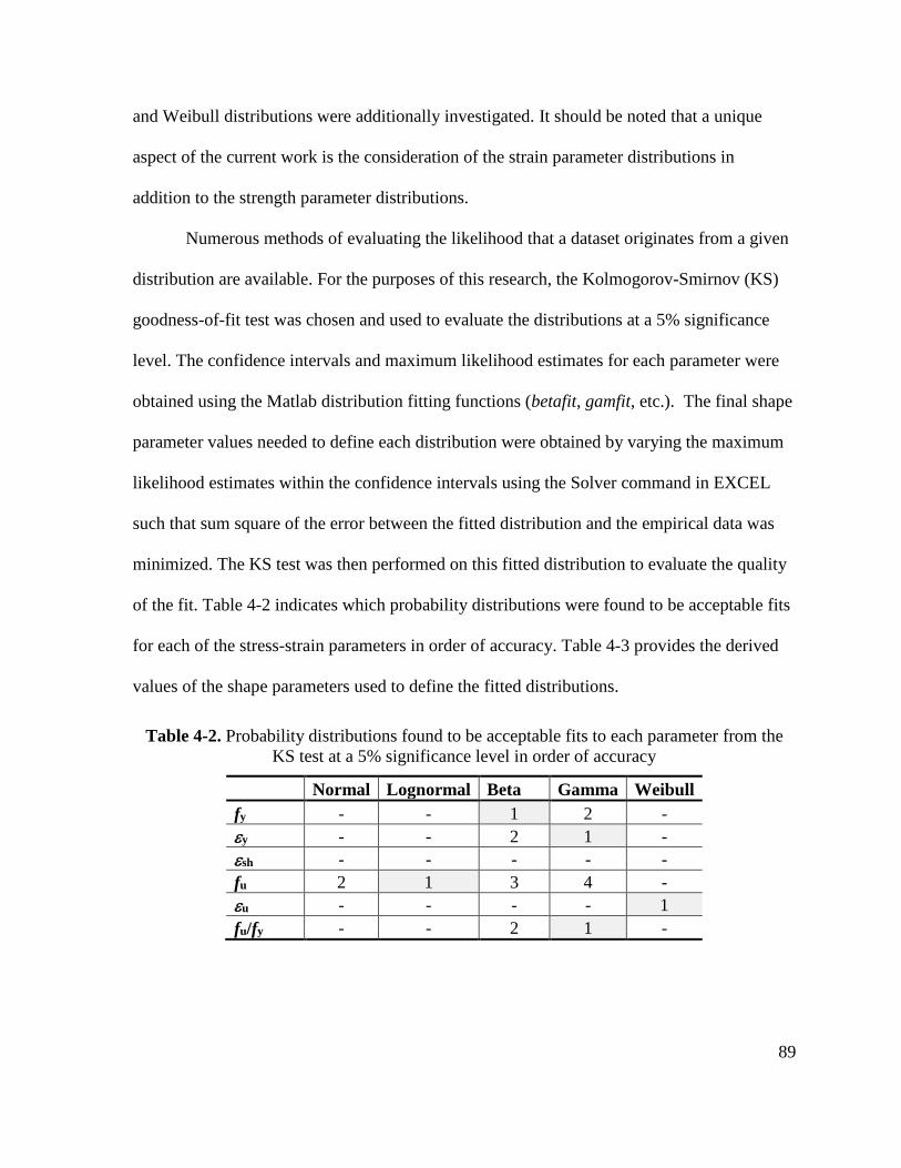
89

and Weibull distributions were additionally investigated. It should be noted that a unique

aspect of the current work is the consideration of the strain parameter distributions in

addition to the strength parameter distributions.

Numerous methods of evaluating the likelihood that a dataset originates from a given

distribution are available. For the purposes of this research, the Kolmogorov-Smirnov (KS)

goodness-of-fit test was chosen and used to evaluate the distributions at a 5% significance

level. The confidence intervals and maximum likelihood estimates for each parameter were

obtained using the Matlab distribution fitting functions (betafit, gamfit, etc.). The final shape

parameter values needed to define each distribution were obtained by varying the maximum

likelihood estimates within the confidence intervals using the Solver command in EXCEL

such that sum square of the error between the fitted distribution and the empirical data was

minimized. The KS test was then performed on this fitted distribution to evaluate the quality

of the fit. Table 4-2 indicates which probability distributions were found to be acceptable fits

for each of the stress-strain parameters in order of accuracy. Table 4-3 provides the derived

values of the shape parameters used to define the fitted distributions.

Table 4-2. Probability distributions found to be acceptable fits to each parameter from the

KS test at a 5% significance level in order of accuracy

Normal Lognormal Beta Gamma Weibull

fy - - 1 2 -

y - - 2 1 -

sh - - - - -

fu 2 1 3 4 -

u - - - - 1

fu/fy - - 2 1 -

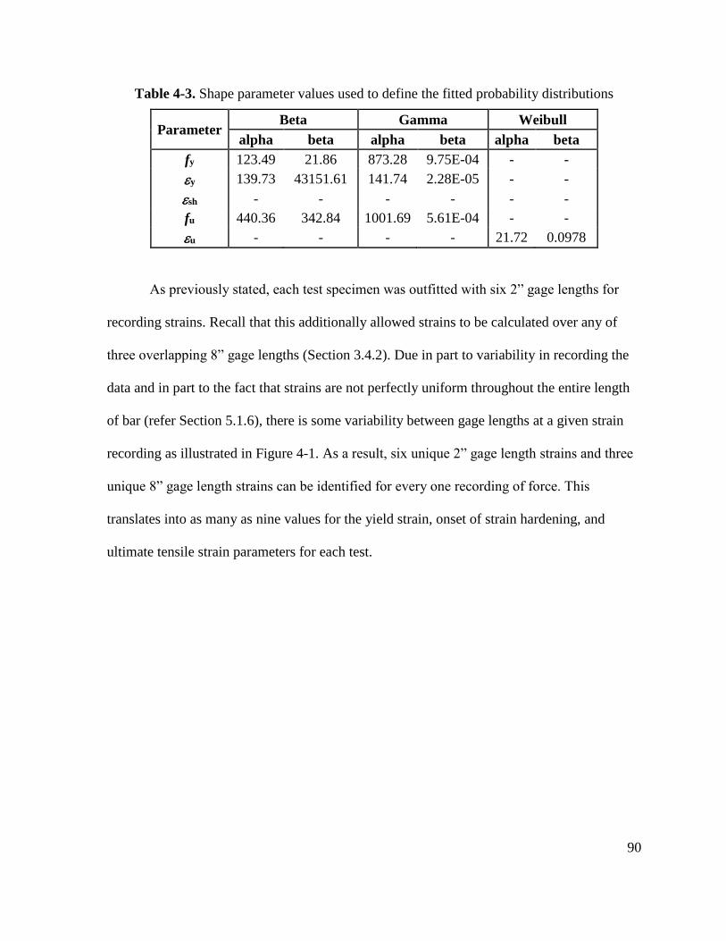
90

Table 4-3. Shape parameter values used to define the fitted probability distributions

Parameter Beta Gamma Weibull

alpha beta alpha beta alpha beta

fy 123.49 21.86 873.28 9.75E-04 - -

y 139.73 43151.61 141.74 2.28E-05 - -

sh - - - - - -

fu 440.36 342.84 1001.69 5.61E-04 - -

u - - - - 21.72 0.0978

As previously stated, each test specimen was outfitted with six 2” gage lengths for

recording strains. Recall that this additionally allowed strains to be calculated over any of

three overlapping 8” gage lengths (Section 3.4.2). Due in part to variability in recording the

data and in part to the fact that strains are not perfectly uniform throughout the entire length

of bar (refer Section 5.1.6), there is some variability between gage lengths at a given strain

recording as illustrated in Figure 4-1. As a result, six unique 2” gage length strains and three

unique 8” gage length strains can be identified for every one recording of force. This

translates into as many as nine values for the yield strain, onset of strain hardening, and

ultimate tensile strain parameters for each test.

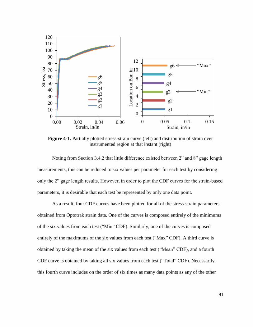
91

Figure 4-1. Partially plotted stress-strain curve (left) and distribution of strain over

instrumented region at that instant (right)

Noting from Section 3.4.2 that little difference existed between 2” and 8” gage length

measurements, this can be reduced to six values per parameter for each test by considering

only the 2” gage length results. However, in order to plot the CDF curves for the strain-based

parameters, it is desirable that each test be represented by only one data point.

As a result, four CDF curves have been plotted for all of the stress-strain parameters

obtained from Optotrak strain data. One of the curves is composed entirely of the minimums

of the six values from each test (“Min” CDF). Similarly, one of the curves is composed

entirely of the maximums of the six values from each test (“Max” CDF). A third curve is

obtained by taking the mean of the six values from each test (“Mean” CDF), and a fourth

CDF curve is obtained by taking all six values from each test (“Total” CDF). Necessarily,

this fourth curve includes on the order of six times as many data points as any of the other

0

10

20

30

40

50

60

70

80

90

100

110

120

0.00 0.02 0.04 0.06

Str

ess,

ksi

Strain, in/in

g6

g5

g4

g3

g2

g1g1

g2

g3

g4

g5

g6

0 0.05 0.1 0.15

0

2

4

6

8

10

12

Strain, in/inL

oca

tion o

n B

ar,

in

“Min”

“Max”

92

three curves. As will be seen, the recommended values were ultimately taken from the CDF

curves of the means and the min, max, and total CDF curves left for illustrative purposes

only.

4.2.3. Expected Mechanical Properties

4.2.3.1.Modulus of Elasticity

As described in Section 4.2.1, the modulus of elasticity was defined as the slope of

the linear elastic region of the stress-strain curve between 0.2 times the top-of-the-knee yield

strength and 0.8 times the top-of-the-knee yield strength. This parameter was not evaluated

for a best-fit probability distribution.

Figure 4-2 presents the empirical CDF curves for the modulus of elasticity

considering all bar sizes. Because this parameter is indirectly based on Optotrak readings,

there are four empirical distributions, as described in Section 4.2.2. The mean value of the

empirical data is 27,888 ksi. The standard deviation and coefficient of variation are 1,601 ksi

and 5.7% respectively. Also included in the graph is a modulus of elasticity value of 29,000

ksi for reference.

Figure 4-3 illustrates the breakdown of the modulus of elasticity data according to the

mean CDFs for each bar size. The mean values ranged from 26,143 ksi to 28,894 ksi with the

No. 14 bars having the lowest mean value and the No. 4 bars having the highest. There was

no indication that the modulus of elasticity was influenced by bar size. Table 4-5 summarizes

the mean values of each parameter according to bar size.

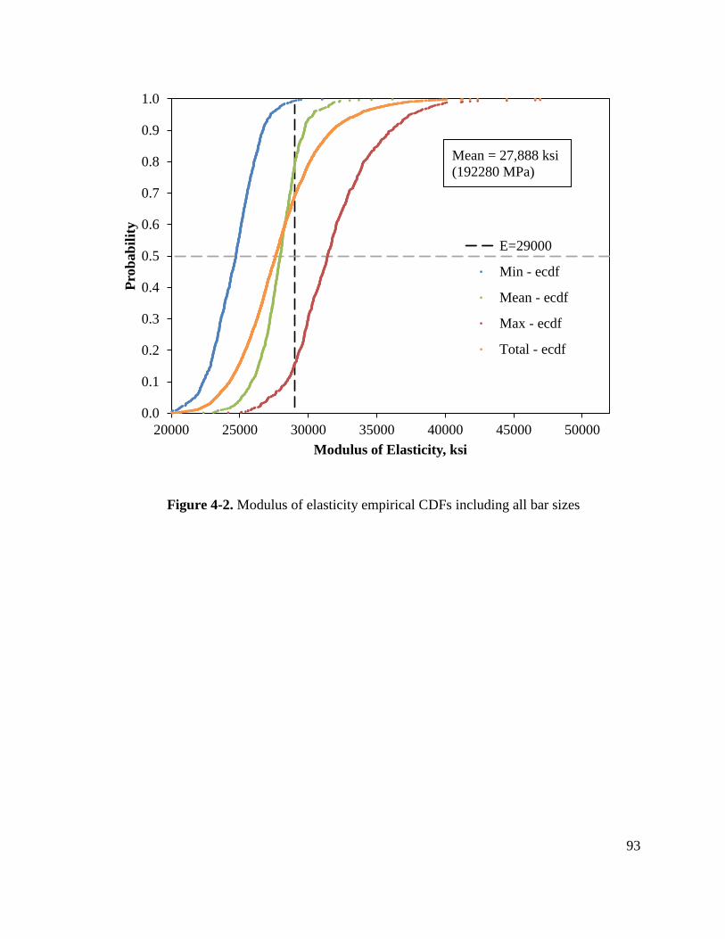
93

Figure 4-2. Modulus of elasticity empirical CDFs including all bar sizes

0.0

0.1

0.2

0.3

0.4

0.5

0.6

0.7

0.8

0.9

1.0

20000 25000 30000 35000 40000 45000 50000

Pro

bab

ilit

y

Modulus of Elasticity, ksi

E=29000

Min - ecdf

Mean - ecdf

Max - ecdf

Total - ecdf

Mean = 27,888 ksi

(192280 MPa)

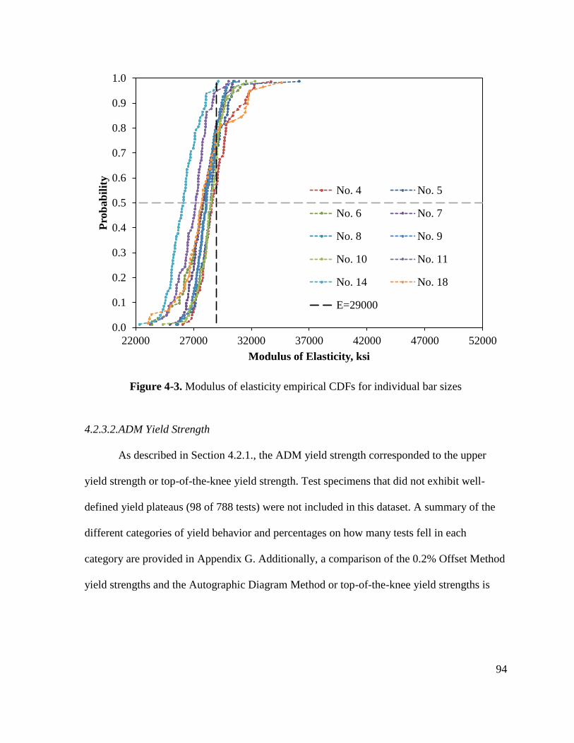
94

Figure 4-3. Modulus of elasticity empirical CDFs for individual bar sizes

4.2.3.2.ADM Yield Strength

As described in Section 4.2.1., the ADM yield strength corresponded to the upper

yield strength or top-of-the-knee yield strength. Test specimens that did not exhibit well-

defined yield plateaus (98 of 788 tests) were not included in this dataset. A summary of the

different categories of yield behavior and percentages on how many tests fell in each

category are provided in Appendix G. Additionally, a comparison of the 0.2% Offset Method

yield strengths and the Autographic Diagram Method or top-of-the-knee yield strengths is

0.0

0.1

0.2

0.3

0.4

0.5

0.6

0.7

0.8

0.9

1.0

22000 27000 32000 37000 42000 47000 52000

Pro

bab

ilit

y

Modulus of Elasticity, ksi

No. 4 No. 5

No. 6 No. 7

No. 8 No. 9

No. 10 No. 11

No. 14 No. 18

E=29000

95

provided in Appendix F. As stated in Chapter 3, a 5% reduction was applied to the No. 11,

14, and 18 bar yield strengths to account for the losses occurring in the custom testing rig.

The beta and empirical CDF curves for the ADM yield strength considering all bar

sizes are presented in Figure 4-4. The gamma and beta distributions were found to be

acceptable fits to the yield strength data at a 5 percent significance level; however, the beta

distribution was identified as the best fitting distribution based on the Kolmogorov-Smirnov

statistic. This observation is consistent with the work by Bournonville et al. (2004) who

found the beta distribution to be an acceptable fit for A706 grade 60 rebar.

The mean value of the empirical data is 85.0 ksi. The standard deviation and

coefficient of variation are 3.0 ksi and 3.6% respectively. Also included in the graph are the

ASTM minimum and maximum allowable yield strengths of 80 ksi and 98 ksi respectively

(ASTM, 2016). Because this parameter is determined based on load cell readings as opposed

to Optotrak readings, there is only one fitted and one empirical distribution.

From the figure, it is immediately apparent that several of the tests (48 out of 690

tests) fell below the ASTM lower limit of 80 ksi. While this behavior was limited solely to

the No. 11, 14, and 18 bars (see Figure 4-5), it was demonstrated through additional testing

that this was not a result of the adjustment factor previously described. A further observation

of the testing was that different bar sizes originating from the same heat could have distinctly

different yield strengths. This observation is presented in further detail in Chapter 5.

Figure 4-5 illustrates the breakdown of the ADM yield strength data according to bar

size. These curves were not evaluated for best-fit probability distributions. The mean values

ranged from 80.7 ksi to 88.0 ksi (556 MPa to 607 MPa) with the No. 18 bars having the

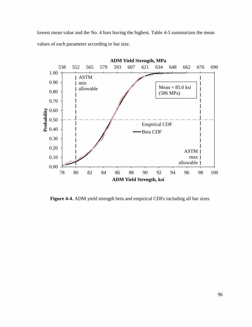
96

lowest mean value and the No. 4 bars having the highest. Table 4-5 summarizes the mean

values of each parameter according to bar size.

Figure 4-4. ADM yield strength beta and empirical CDFs including all bar sizes

538 552 565 579 593 607 621 634 648 662 676 690

0.00

0.10

0.20

0.30

0.40

0.50

0.60

0.70

0.80

0.90

1.00

78 80 82 84 86 88 90 92 94 96 98 100

ADM Yield Strength, MPa

Pro

bab

ilit

y

ADM Yield Strength, ksi

Empirical CDF

Beta CDF

Mean = 85.0 ksi

(586 MPa)

ASTM

max

allowable

ASTM

min

allowable

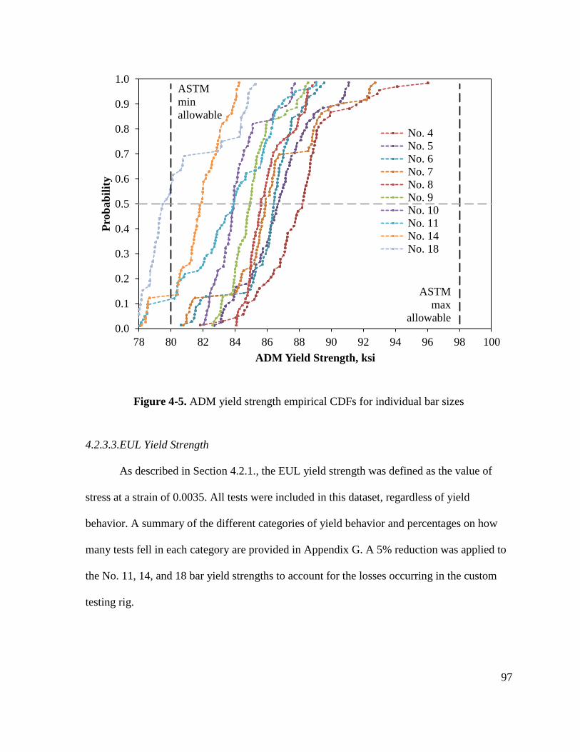
97

Figure 4-5. ADM yield strength empirical CDFs for individual bar sizes

4.2.3.3.EUL Yield Strength

As described in Section 4.2.1., the EUL yield strength was defined as the value of

stress at a strain of 0.0035. All tests were included in this dataset, regardless of yield

behavior. A summary of the different categories of yield behavior and percentages on how

many tests fell in each category are provided in Appendix G. A 5% reduction was applied to

the No. 11, 14, and 18 bar yield strengths to account for the losses occurring in the custom

testing rig.

0.0

0.1

0.2

0.3

0.4

0.5

0.6

0.7

0.8

0.9

1.0

78 80 82 84 86 88 90 92 94 96 98 100

Pro

bab

ilit

y


No. 4No. 5No. 6No. 7No. 8No. 9No. 10No. 11No. 14No. 18

ASTM

min

allowable

ASTM

max

allowable

98

As this parameter was not used to prescribe recommendations for the yield strength, it

was not evaluated for a best-fit probability distribution.

Figure 4-6 presents the empirical CDF curves for the EUL yield strength considering

all bar sizes. Because this parameter is indirectly based on Optotrak readings, there are four

empirical distributions, as described in Section 4.2.2. The mean value of the empirical data is

84.3 ksi. The standard deviation and coefficient of variation are 3.2 ksi and 3.8%

respectively. Also included in the graph are the ASTM minimum and maximum allowable

yield strengths of 80 ksi and 98 ksi respectively (ASTM, 2016).

As with the ADM yield strength CDF’s, it is immediately apparent that several tests

failed to meet the ASTM minimum yield strength requirements. This observation is

presented in further detail in Chapter 5.

Figure 4-7 illustrates the breakdown of the EUL yield strength data according to bar

size. Only the mean empirical CDF for each bar size is presented. The mean values of the

mean empirical data, based on a 2” gage length, ranged from 80.5 ksi to 86.6 ksi with the No.

18 bars having the lowest mean value and the No. 4 bars having the highest. The general

trend from the empirical CDF is that there is a decrease in median yield strength with

increasing bar size. Table 4-5 summarizes the mean values of each parameter according to

bar size.

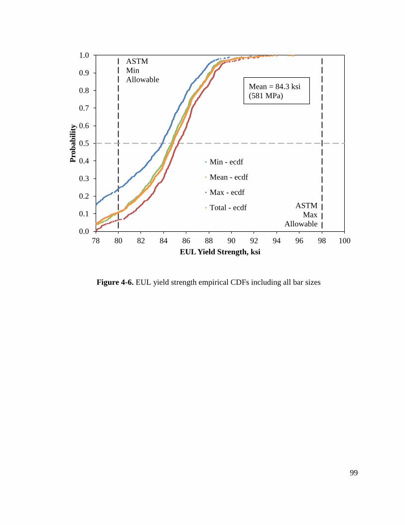
99

Figure 4-6. EUL yield strength empirical CDFs including all bar sizes

0.0

0.1

0.2

0.3

0.4

0.5

0.6

0.7

0.8

0.9

1.0

78 80 82 84 86 88 90 92 94 96 98 100

Pro

bab

ilit

y

EUL Yield Strength, ksi

Min - ecdf

Mean - ecdf

Max - ecdf

Total - ecdf

Mean = 84.3 ksi

(581 MPa)

ASTM

Max

Allowable

ASTM

Min

Allowable

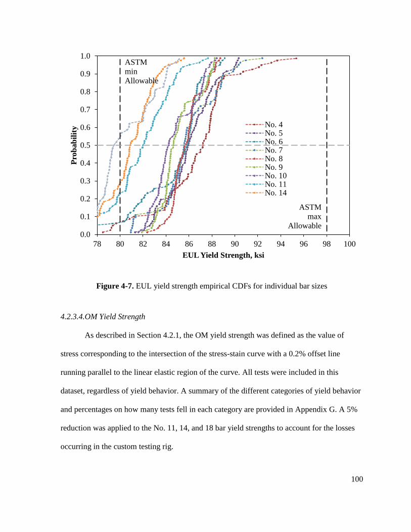
100

Figure 4-7. EUL yield strength empirical CDFs for individual bar sizes

4.2.3.4.OM Yield Strength

As described in Section 4.2.1, the OM yield strength was defined as the value of

stress corresponding to the intersection of the stress-stain curve with a 0.2% offset line

running parallel to the linear elastic region of the curve. All tests were included in this

dataset, regardless of yield behavior. A summary of the different categories of yield behavior

and percentages on how many tests fell in each category are provided in Appendix G. A 5%

reduction was applied to the No. 11, 14, and 18 bar yield strengths to account for the losses

occurring in the custom testing rig.

0.0

0.1

0.2

0.3

0.4

0.5

0.6

0.7

0.8

0.9

1.0

78 80 82 84 86 88 90 92 94 96 98 100

Pro

bab

ilit

y

EUL Yield Strength, ksi

No. 4No. 5No. 6No. 7No. 8No. 9No. 10No. 11No. 14

ASTM

max

Allowable

ASTM

min

Allowable

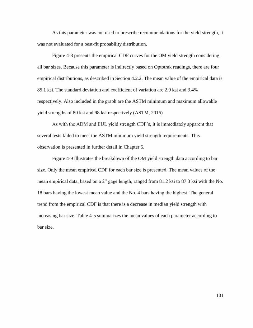
101

As this parameter was not used to prescribe recommendations for the yield strength, it

was not evaluated for a best-fit probability distribution.

Figure 4-8 presents the empirical CDF curves for the OM yield strength considering

all bar sizes. Because this parameter is indirectly based on Optotrak readings, there are four

empirical distributions, as described in Section 4.2.2. The mean value of the empirical data is

85.1 ksi. The standard deviation and coefficient of variation are 2.9 ksi and 3.4%

respectively. Also included in the graph are the ASTM minimum and maximum allowable

yield strengths of 80 ksi and 98 ksi respectively (ASTM, 2016).

As with the ADM and EUL yield strength CDF’s, it is immediately apparent that

several tests failed to meet the ASTM minimum yield strength requirements. This

observation is presented in further detail in Chapter 5.

Figure 4-9 illustrates the breakdown of the OM yield strength data according to bar

size. Only the mean empirical CDF for each bar size is presented. The mean values of the

mean empirical data, based on a 2” gage length, ranged from 81.2 ksi to 87.3 ksi with the No.

18 bars having the lowest mean value and the No. 4 bars having the highest. The general

trend from the empirical CDF is that there is a decrease in median yield strength with

increasing bar size. Table 4-5 summarizes the mean values of each parameter according to

bar size.

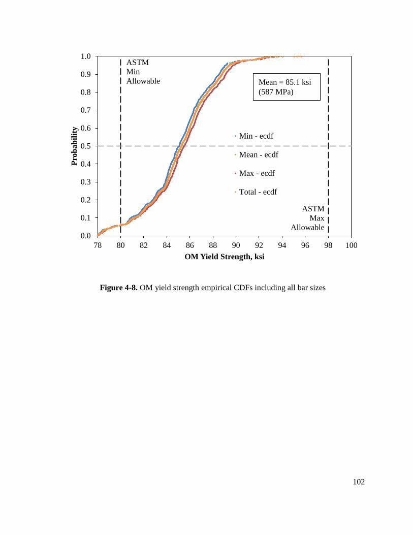
102

Figure 4-8. OM yield strength empirical CDFs including all bar sizes

0.0

0.1

0.2

0.3

0.4

0.5

0.6

0.7

0.8

0.9

1.0

78 80 82 84 86 88 90 92 94 96 98 100

Pro

bab

ilit

y

OM Yield Strength, ksi

Min - ecdf

Mean - ecdf

Max - ecdf

Total - ecdf

Mean = 85.1 ksi

(587 MPa)

ASTM

Max

Allowable

ASTM

Min

Allowable

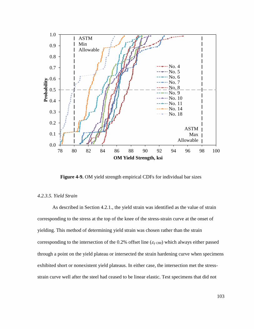
103

Figure 4-9. OM yield strength empirical CDFs for individual bar sizes

4.2.3.5. Yield Strain

As described in Section 4.2.1., the yield strain was identified as the value of strain

corresponding to the stress at the top of the knee of the stress-strain curve at the onset of

yielding. This method of determining yield strain was chosen rather than the strain

corresponding to the intersection of the 0.2% offset line (y OM) which always either passed

through a point on the yield plateau or intersected the strain hardening curve when specimens

exhibited short or nonexistent yield plateaus. In either case, the intersection met the stress-

strain curve well after the steel had ceased to be linear elastic. Test specimens that did not

0.0

0.1

0.2

0.3

0.4

0.5

0.6

0.7

0.8

0.9

1.0

78 80 82 84 86 88 90 92 94 96 98 100

Pro

bab

ilit

y

OM Yield Strength, ksi

No. 4No. 5No. 6No. 7No. 8No. 9No. 10No. 11No. 14No. 18

ASTM

Max

Allowable

ASTM

Min

Allowable

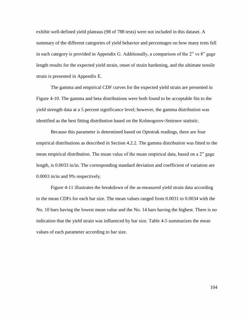
104

exhibit well-defined yield plateaus (98 of 788 tests) were not included in this dataset. A

summary of the different categories of yield behavior and percentages on how many tests fell

in each category is provided in Appendix G. Additionally, a comparison of the 2” vs 8” gage

length results for the expected yield strain, onset of strain hardening, and the ultimate tensile

strain is presented in Appendix E.

The gamma and empirical CDF curves for the expected yield strain are presented in

Figure 4-10. The gamma and beta distributions were both found to be acceptable fits to the

yield strength data at a 5 percent significance level; however, the gamma distribution was

identified as the best fitting distribution based on the Kolmogorov-Smirnov statistic.

Because this parameter is determined based on Optotrak readings, there are four

empirical distributions as described in Section 4.2.2. The gamma distribution was fitted to the

mean empirical distribution. The mean value of the mean empirical data, based on a 2” gage

length, is 0.0033 in/in. The corresponding standard deviation and coefficient of variation are

0.0003 in/in and 9% respectively.

Figure 4-11 illustrates the breakdown of the as-measured yield strain data according

to the mean CDFs for each bar size. The mean values ranged from 0.0031 to 0.0034 with the

No. 10 bars having the lowest mean value and the No. 14 bars having the highest. There is no

indication that the yield strain was influenced by bar size. Table 4-5 summarizes the mean

values of each parameter according to bar size.

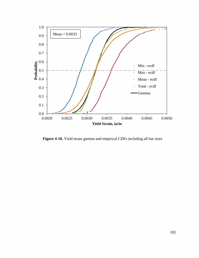
105

Figure 4-10. Yield strain gamma and empirical CDFs including all bar sizes

0.0

0.1

0.2

0.3

0.4

0.5

0.6

0.7

0.8

0.9

1.0

0.0020 0.0025 0.0030 0.0035 0.0040 0.0045 0.0050

Pro

bab

ilit

y

Yield Strain, in/in

Min - ecdf

Max - ecdf

Mean - ecdf

Total - ecdf

Gamma

Mean = 0.0033

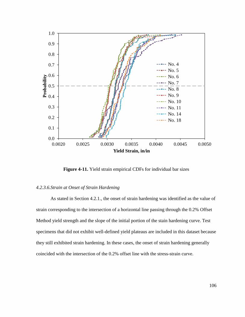
106

Figure 4-11. Yield strain empirical CDFs for individual bar sizes

4.2.3.6.Strain at Onset of Strain Hardening

As stated in Section 4.2.1., the onset of strain hardening was identified as the value of

strain corresponding to the intersection of a horizontal line passing through the 0.2% Offset

Method yield strength and the slope of the initial portion of the stain hardening curve. Test

specimens that did not exhibit well-defined yield plateaus are included in this dataset because

they still exhibited strain hardening. In these cases, the onset of strain hardening generally

coincided with the intersection of the 0.2% offset line with the stress-strain curve.

0.0

0.1

0.2

0.3

0.4

0.5

0.6

0.7

0.8

0.9

1.0

0.0020 0.0025 0.0030 0.0035 0.0040 0.0045 0.0050

Pro

bab

ilit

y

Yield Strain, in/in

No. 4

No. 5

No. 6

No. 7

No. 8

No. 9

No. 10

No. 11

No. 14

No. 18

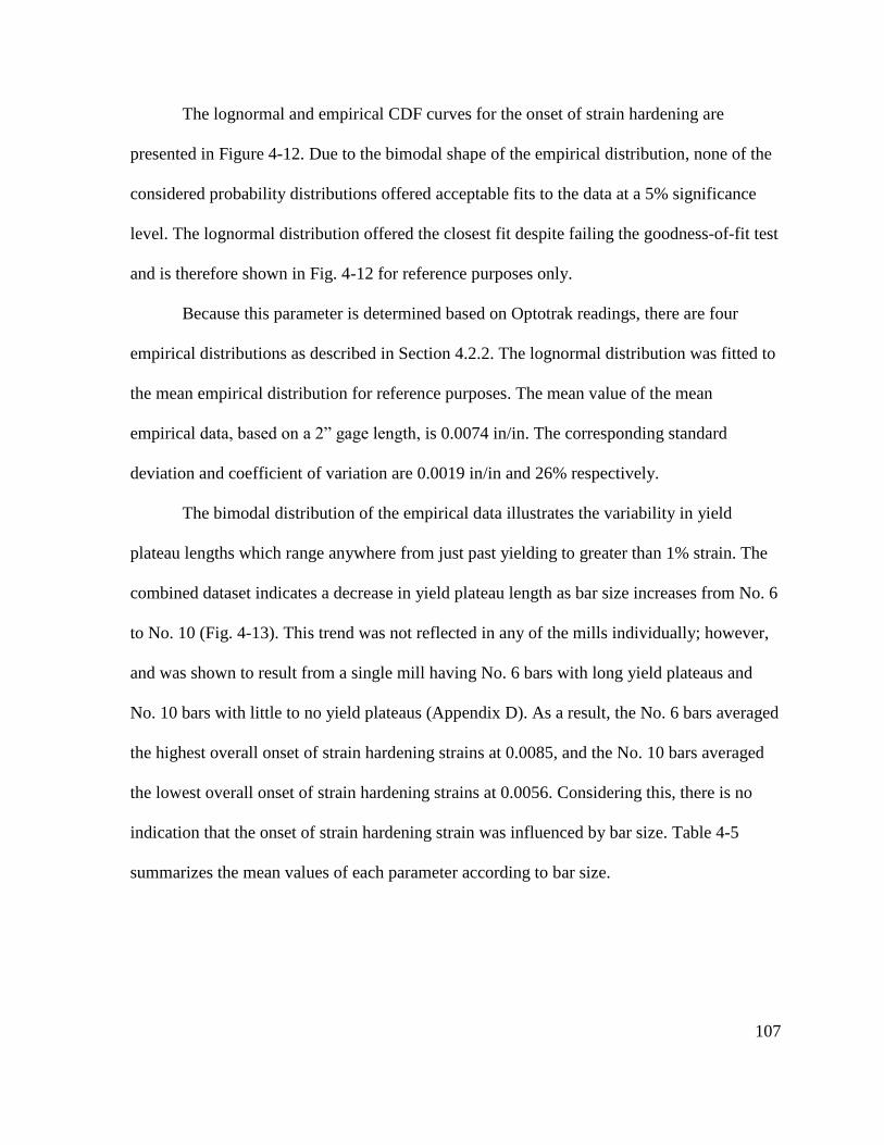
107

The lognormal and empirical CDF curves for the onset of strain hardening are

presented in Figure 4-12. Due to the bimodal shape of the empirical distribution, none of the

considered probability distributions offered acceptable fits to the data at a 5% significance

level. The lognormal distribution offered the closest fit despite failing the goodness-of-fit test

and is therefore shown in Fig. 4-12 for reference purposes only.


empirical distributions as described in Section 4.2.2. The lognormal distribution was fitted to

the mean empirical distribution for reference purposes. The mean value of the mean

empirical data, based on a 2” gage length, is 0.0074 in/in. The corresponding standard

deviation and coefficient of variation are 0.0019 in/in and 26% respectively.

The bimodal distribution of the empirical data illustrates the variability in yield

plateau lengths which range anywhere from just past yielding to greater than 1% strain. The

combined dataset indicates a decrease in yield plateau length as bar size increases from No. 6

to No. 10 (Fig. 4-13). This trend was not reflected in any of the mills individually; however,

and was shown to result from a single mill having No. 6 bars with long yield plateaus and

No. 10 bars with little to no yield plateaus (Appendix D). As a result, the No. 6 bars averaged

the highest overall onset of strain hardening strains at 0.0085, and the No. 10 bars averaged

the lowest overall onset of strain hardening strains at 0.0056. Considering this, there is no

indication that the onset of strain hardening strain was influenced by bar size. Table 4-5

summarizes the mean values of each parameter according to bar size.

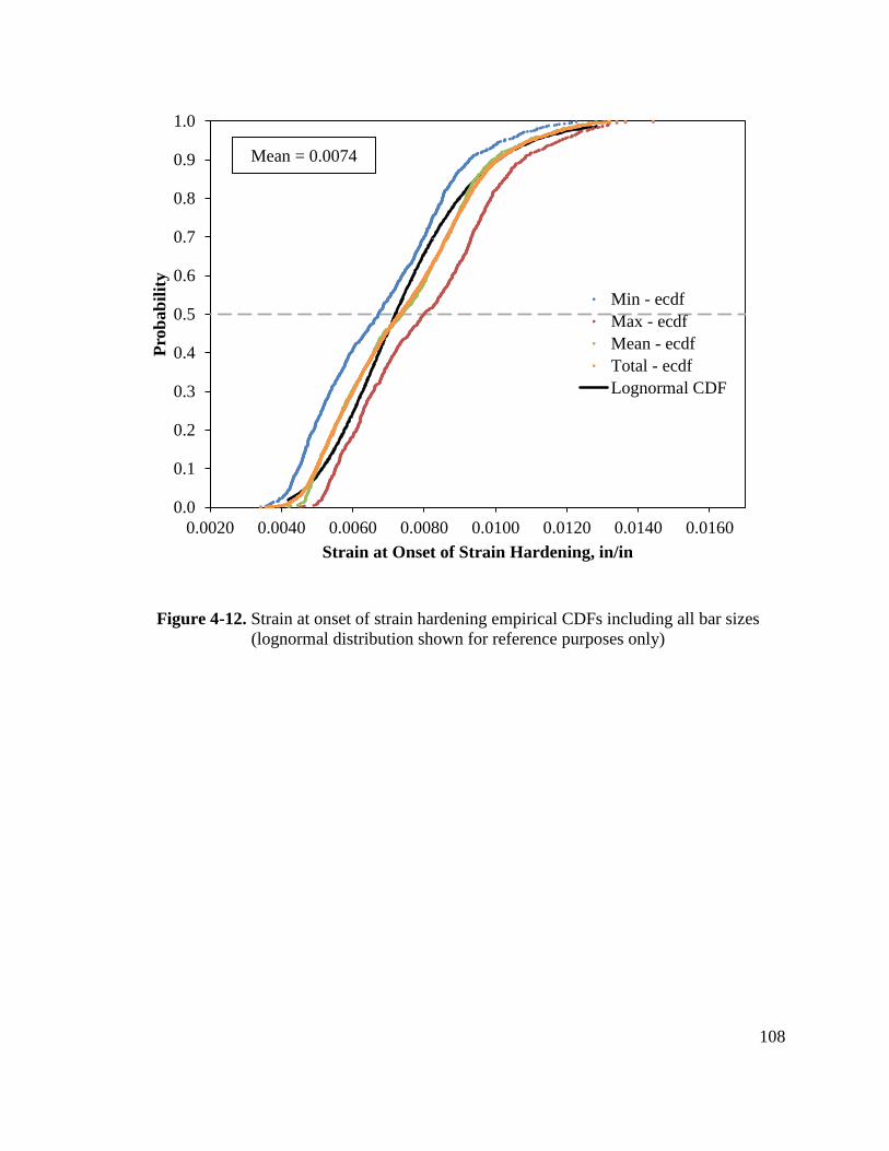
108

Figure 4-12. Strain at onset of strain hardening empirical CDFs including all bar sizes

(lognormal distribution shown for reference purposes only)

0.0

0.1

0.2

0.3

0.4

0.5

0.6

0.7

0.8

0.9

1.0

0.0020 0.0040 0.0060 0.0080 0.0100 0.0120 0.0140 0.0160

Pro

bab

ilit

y

Strain at Onset of Strain Hardening, in/in

Min - ecdf

Max - ecdf

Mean - ecdf

Total - ecdf

Lognormal CDF

Mean = 0.0074

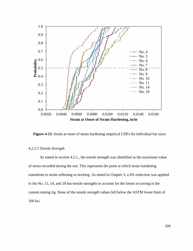
109

Figure 4-13. Strain at onset of strain hardening empirical CDFs for individual bar sizes

4.2.3.7.Tensile Strength

As stated in section 4.2.1., the tensile strength was identified as the maximum value

of stress recorded during the test. This represents the point at which strain hardening

transitions to strain softening or necking. As stated in Chapter 3, a 6% reduction was applied

to the No. 11, 14, and 18 bar tensile strengths to account for the losses occurring in the

custom testing rig. None of the tensile strength values fell below the ASTM lower limit of

100 ksi.

0.0

0.1

0.2

0.3

0.4

0.5

0.6

0.7

0.8

0.9

1.0

0.0020 0.0040 0.0060 0.0080 0.0100 0.0120 0.0140 0.0160

Pro

bab

ilit

y

Strain at Onset of Strain Hardening, in/in

No. 4

No. 5

No. 6

No. 7

No. 8

No. 9

No. 10

No. 11

No. 14

No. 18

110

The lognormal and empirical CDF curves for the tensile strength are presented in

Figure 4-14. The normal, lognormal, beta, and gamma distributions were found to be

acceptable fits to the tensile strength data at a 5 percent significance level. The lognormal

distribution was identified as the best fitting distribution based on the Kolmogorov-Smirnov

statistic, though followed closely by the normal and the beta distributions.

The mean value of the empirical data is 112.5 ksi. The standard deviation and

coefficient of variation are 3.6 ksi and 3.2% respectively. The value corresponding to the

95th percentile of the empirical data is 118.9 ksi. Also included in the graph is the ASTM

minimum allowable tensile strength of 100 ksi (ASTM, 2016). Because this parameter is

determined based on load cell readings as opposed to Optotrak readings, there is only one

fitted and one empirical distribution.

Figure 4-15 illustrates the breakdown of the expected tensile strength data according

to bar size. The mean values ranged from 107.6 ksi to 114.6 ksi with the No. 18 bars having

the lowest mean value and the No. 10 bars having the highest. The adjustment to the No. 11,

14, and 18 bar data previously described revealed a consistent trend for these three sizes to

have the lowest tensile strengths – a combined mean of 108.8 ksi versus a combined mean of

113.7 ksi for the No. 4 through No. 10 bars. There was no indication that bar size had any

effect on tensile strength in the remaining sizes. Table 4-5 summarizes the mean values of

each parameter according to bar size.

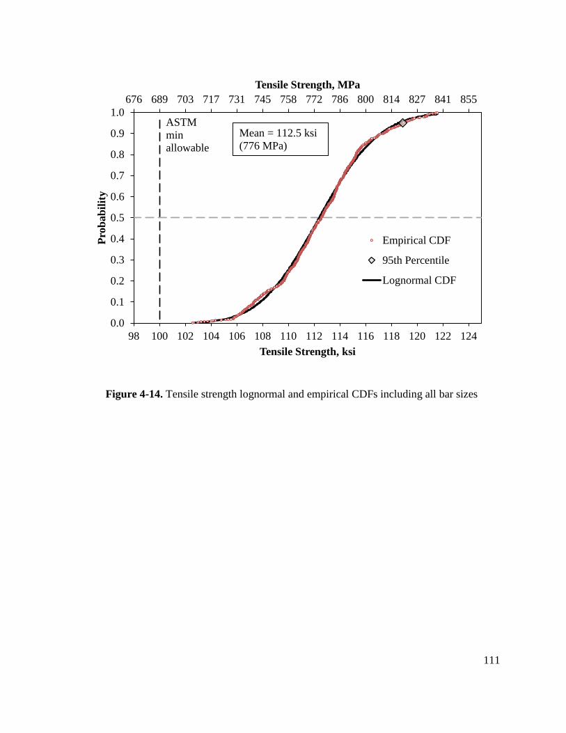
111

Figure 4-14. Tensile strength lognormal and empirical CDFs including all bar sizes

676 689 703 717 731 745 758 772 786 800 814 827 841 855

0.0

0.1

0.2

0.3

0.4

0.5

0.6

0.7

0.8

0.9

1.0

98 100 102 104 106 108 110 112 114 116 118 120 122 124

Tensile Strength, MPa

Pro

bab

ilit

y


Empirical CDF

95th Percentile

Lognormal CDF

Mean = 112.5 ksi

(776 MPa)

ASTM

min

allowable

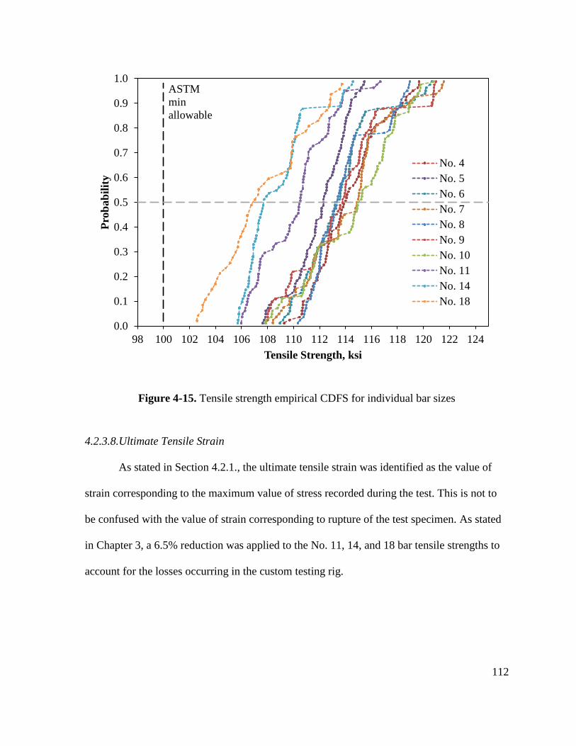
112

Figure 4-15. Tensile strength empirical CDFS for individual bar sizes

4.2.3.8.Ultimate Tensile Strain

As stated in Section 4.2.1., the ultimate tensile strain was identified as the value of

strain corresponding to the maximum value of stress recorded during the test. This is not to

be confused with the value of strain corresponding to rupture of the test specimen. As stated

in Chapter 3, a 6.5% reduction was applied to the No. 11, 14, and 18 bar tensile strengths to

account for the losses occurring in the custom testing rig.

0.0

0.1

0.2

0.3

0.4

0.5

0.6

0.7

0.8

0.9

1.0

98 100 102 104 106 108 110 112 114 116 118 120 122 124

Pro

bab

ilit

y


No. 4

No. 5

No. 6

No. 7

No. 8

No. 9

No. 10

No. 11

No. 14

No. 18

ASTM

min

allowable

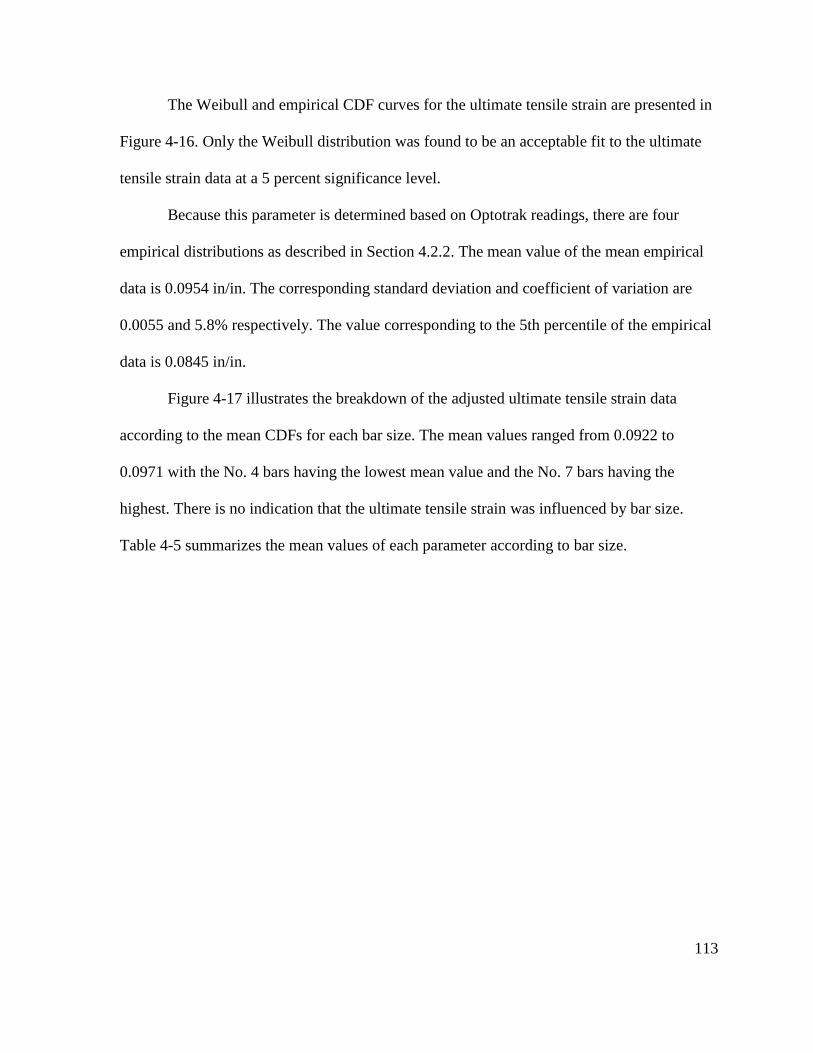
113

The Weibull and empirical CDF curves for the ultimate tensile strain are presented in

Figure 4-16. Only the Weibull distribution was found to be an acceptable fit to the ultimate

tensile strain data at a 5 percent significance level.


empirical distributions as described in Section 4.2.2. The mean value of the mean empirical

data is 0.0954 in/in. The corresponding standard deviation and coefficient of variation are

0.0055 and 5.8% respectively. The value corresponding to the 5th percentile of the empirical

data is 0.0845 in/in.

Figure 4-17 illustrates the breakdown of the adjusted ultimate tensile strain data

according to the mean CDFs for each bar size. The mean values ranged from 0.0922 to

0.0971 with the No. 4 bars having the lowest mean value and the No. 7 bars having the

highest. There is no indication that the ultimate tensile strain was influenced by bar size.

Table 4-5 summarizes the mean values of each parameter according to bar size.

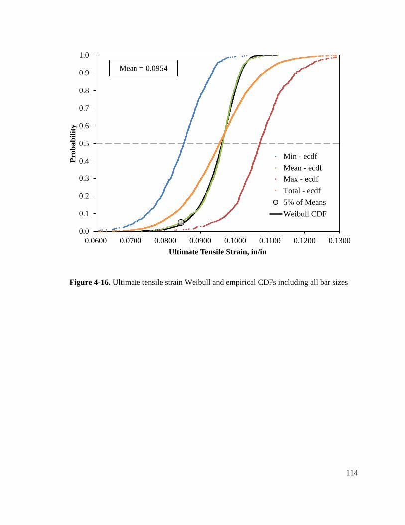
114

Figure 4-16. Ultimate tensile strain Weibull and empirical CDFs including all bar sizes

0.0

0.1

0.2

0.3

0.4

0.5

0.6

0.7

0.8

0.9

1.0

0.0600 0.0700 0.0800 0.0900 0.1000 0.1100 0.1200 0.1300

Pro

bab

ilit

y

Ultimate Tensile Strain, in/in

Min - ecdf

Mean - ecdf

Max - ecdf

Total - ecdf

5% of Means

Weibull CDF

Mean = 0.0954

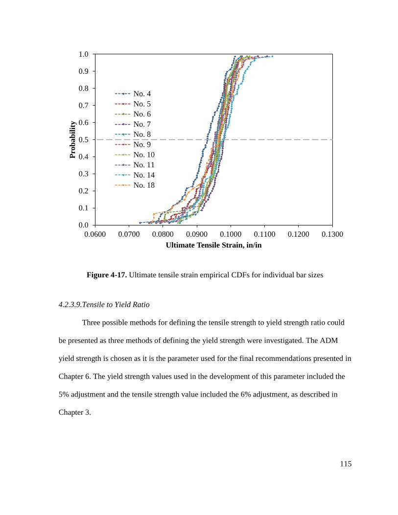
115

Figure 4-17. Ultimate tensile strain empirical CDFs for individual bar sizes

4.2.3.9.Tensile to Yield Ratio

Three possible methods for defining the tensile strength to yield strength ratio could

be presented as three methods of defining the yield strength were investigated. The ADM

yield strength is chosen as it is the parameter used for the final recommendations presented in

Chapter 6. The yield strength values used in the development of this parameter included the

5% adjustment and the tensile strength value included the 6% adjustment, as described in

Chapter 3.

0.0

0.1

0.2

0.3

0.4

0.5

0.6

0.7

0.8

0.9

1.0

0.0600 0.0700 0.0800 0.0900 0.1000 0.1100 0.1200 0.1300

Pro

bab

ilit

y

Ultimate Tensile Strain, in/in

No. 4

No. 5

No. 6

No. 7

No. 8

No. 9

No. 10

No. 11

No. 14

No. 18

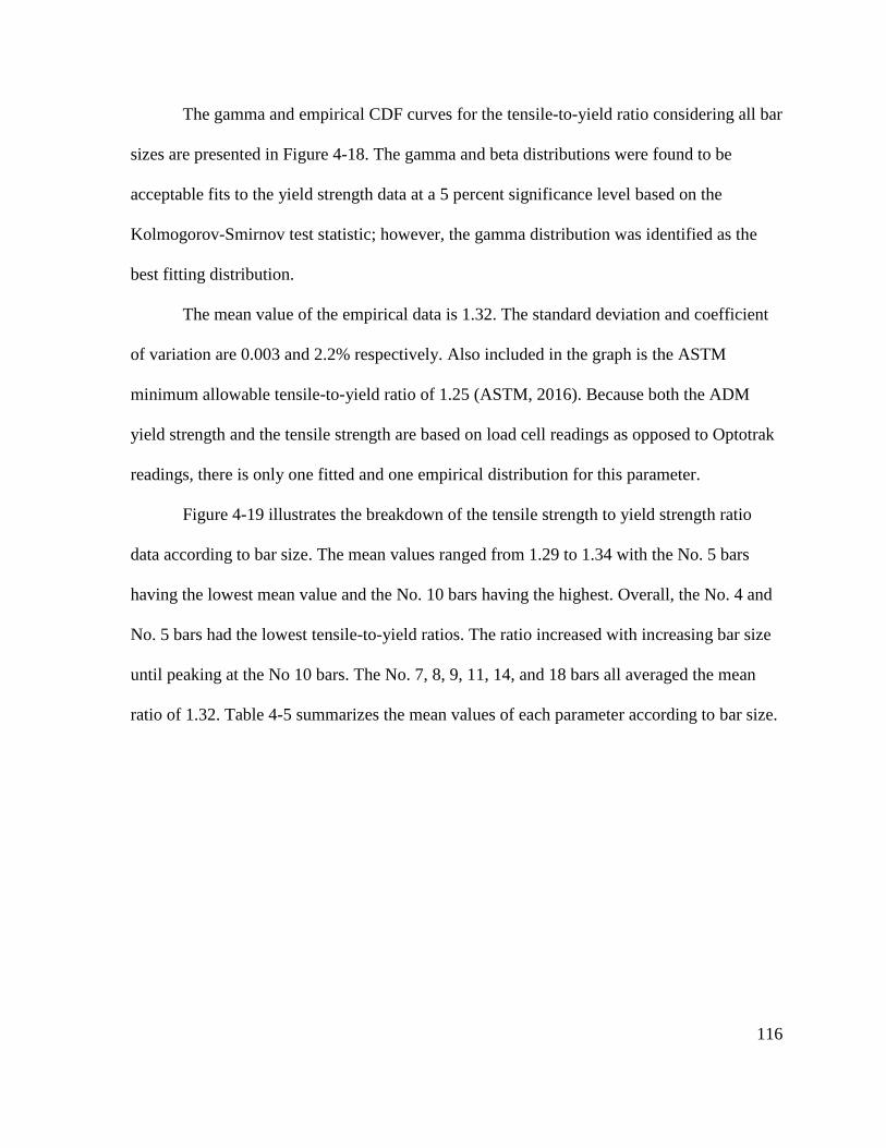
116

The gamma and empirical CDF curves for the tensile-to-yield ratio considering all bar

sizes are presented in Figure 4-18. The gamma and beta distributions were found to be

acceptable fits to the yield strength data at a 5 percent significance level based on the

Kolmogorov-Smirnov test statistic; however, the gamma distribution was identified as the

best fitting distribution.

The mean value of the empirical data is 1.32. The standard deviation and coefficient

of variation are 0.003 and 2.2% respectively. Also included in the graph is the ASTM

minimum allowable tensile-to-yield ratio of 1.25 (ASTM, 2016). Because both the ADM

yield strength and the tensile strength are based on load cell readings as opposed to Optotrak

readings, there is only one fitted and one empirical distribution for this parameter.

Figure 4-19 illustrates the breakdown of the tensile strength to yield strength ratio

data according to bar size. The mean values ranged from 1.29 to 1.34 with the No. 5 bars

having the lowest mean value and the No. 10 bars having the highest. Overall, the No. 4 and

No. 5 bars had the lowest tensile-to-yield ratios. The ratio increased with increasing bar size

until peaking at the No 10 bars. The No. 7, 8, 9, 11, 14, and 18 bars all averaged the mean

ratio of 1.32. Table 4-5 summarizes the mean values of each parameter according to bar size.

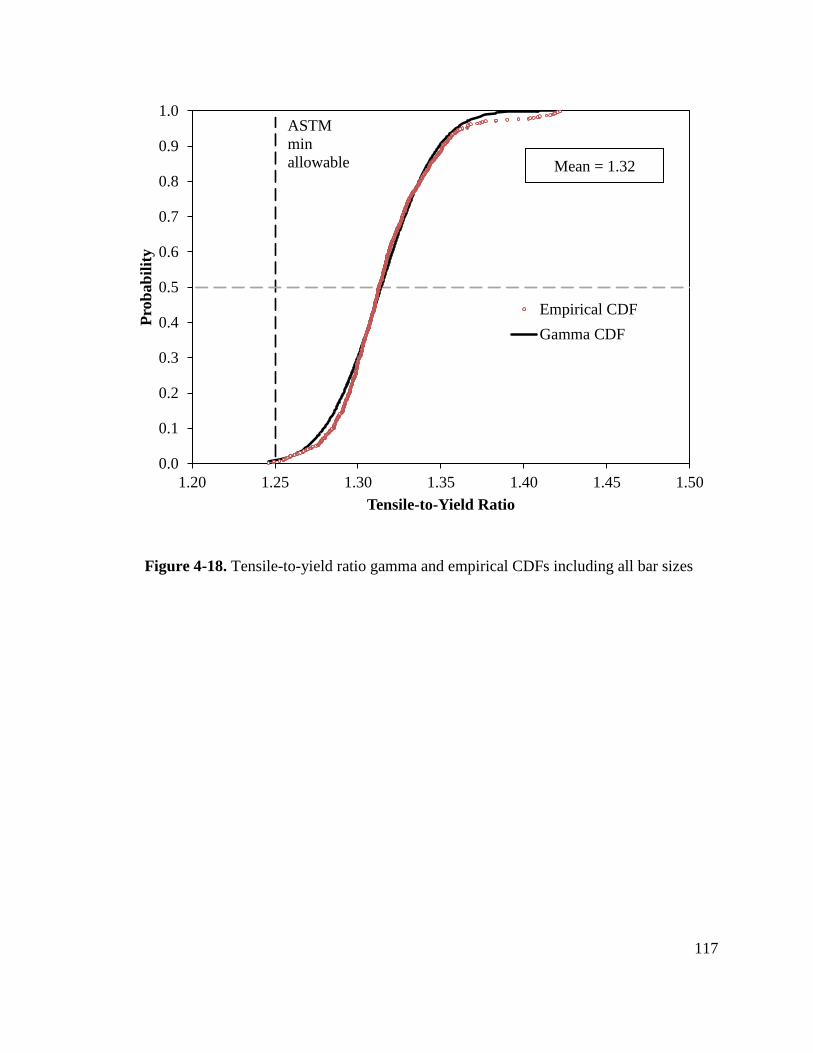
117

Figure 4-18. Tensile-to-yield ratio gamma and empirical CDFs including all bar sizes

0.0

0.1

0.2

0.3

0.4

0.5

0.6

0.7

0.8

0.9

1.0

1.20 1.25 1.30 1.35 1.40 1.45 1.50

Pro

bab

ilit

y

Tensile-to-Yield Ratio

Empirical CDF

Gamma CDF

ASTM

min

allowable Mean = 1.32

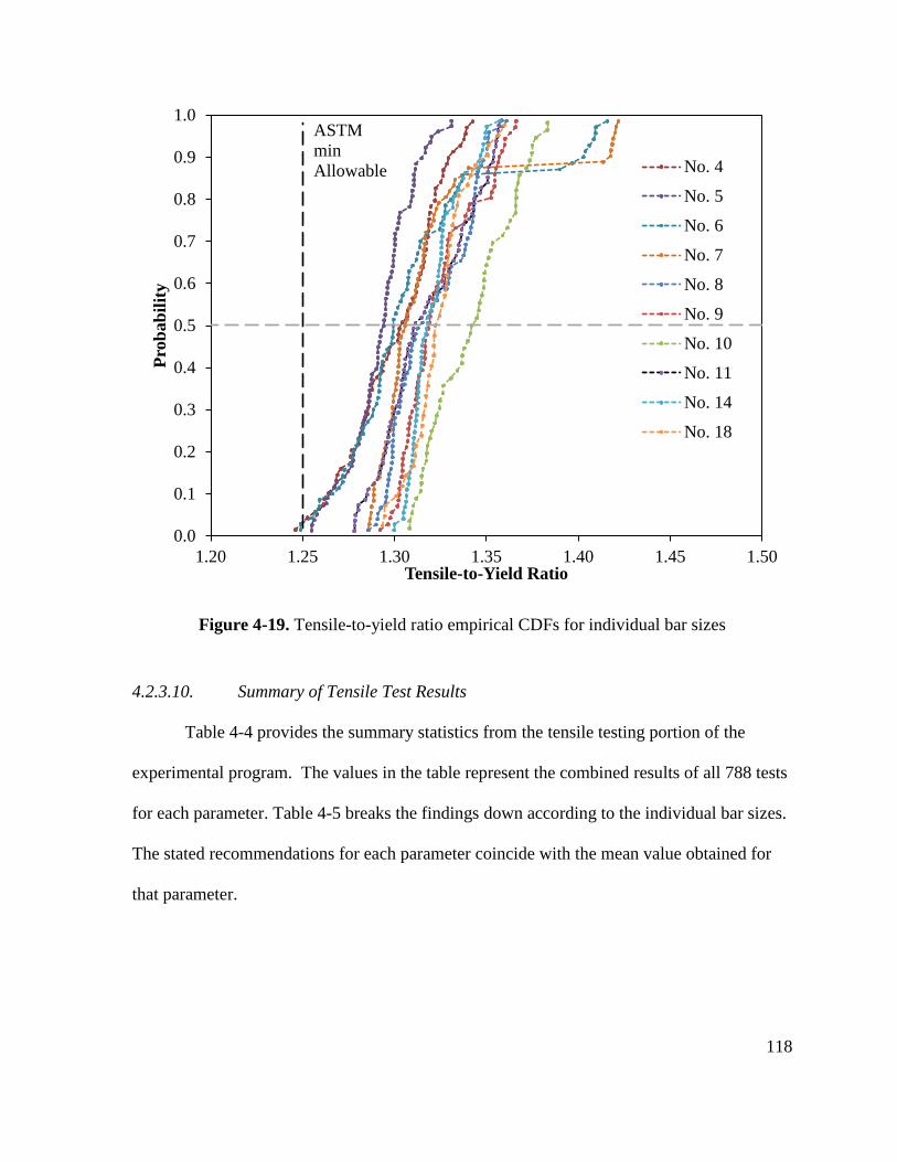
118

Figure 4-19. Tensile-to-yield ratio empirical CDFs for individual bar sizes

4.2.3.10. Summary of Tensile Test Results

Table 4-4 provides the summary statistics from the tensile testing portion of the

experimental program. The values in the table represent the combined results of all 788 tests

for each parameter. Table 4-5 breaks the findings down according to the individual bar sizes.

The stated recommendations for each parameter coincide with the mean value obtained for

that parameter.

0.0

0.1

0.2

0.3

0.4

0.5

0.6

0.7

0.8

0.9

1.0

1.20 1.25 1.30 1.35 1.40 1.45 1.50

Pro

bab

ilit

y


No. 4

No. 5

No. 6

No. 7

No. 8

No. 9

No. 10

No. 11

No. 14

No. 18

ASTM

min

Allowable

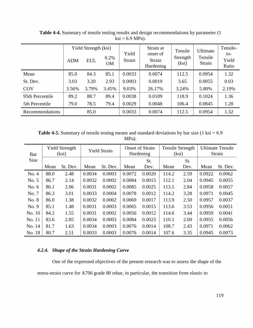
119

Table 4-4. Summary of tensile testing results and design recommendations by parameter (1

ksi = 6.9 MPa).

Yield Strength (ksi)

Yield

Strain

Strain at

onset of

Strain

Hardening

Tensile

Strength

(ksi)

Ultimate

Tensile

Strain

Tensile-

to-

Yield

Ratio ADM EUL

0.2%

OM

Mean 85.0 84.3 85.1 0.0033 0.0074 112.5 0.0954 1.32

St. Dev. 3.03 3.20 2.93 0.0003 0.0019 3.65 0.0055 0.03

COV 3.56% 3.79% 3.45% 9.03% 26.17% 3.24% 5.80% 2.19%

95th Percentile 89.2 88.7 89.4 0.0038 0.0109 118.9 0.1024 1.36

5th Percentile 79.0 78.5 79.4 0.0029 0.0048 106.4 0.0845 1.28

Recommendations 85.0 0.0033 0.0074 112.5 0.0954 1.32

Table 4-5. Summary of tensile testing means and standard deviations by bar size (1 ksi = 6.9

MPa).

Bar

Size

Yield Strength

(ksi) Yield Strain

Onset of Strain

Hardening

Tensile Strength

(ksi)

Ultimate Tensile

Strain

Mean St. Dev. Mean St. Dev. Mean

St.

Dev. Mean

St.

Dev. Mean St. Dev.

No. 4 88.0 2.48 0.0034 0.0003 0.0072 0.0020 114.2 2.59 0.0922 0.0062

No. 5 86.7 2.14 0.0032 0.0002 0.0084 0.0015 112.1 2.04 0.0945 0.0055

No. 6 86.1 2.06 0.0031 0.0002 0.0085 0.0025 113.5 2.84 0.0958 0.0057

No. 7 86.3 3.01 0.0033 0.0004 0.0078 0.0012 114.2 3.28 0.0971 0.0045

No. 8 86.0 1.38 0.0032 0.0002 0.0069 0.0017 113.9 2.50 0.0957 0.0037

No. 9 85.1 1.48 0.0031 0.0003 0.0065 0.0015 113.6 3.53 0.0956 0.0051

No. 10 84.2 1.55 0.0031 0.0002 0.0056 0.0012 114.6 3.44 0.0959 0.0041

No. 11 83.6 2.85 0.0034 0.0003 0.0084 0.0023 110.1 2.69 0.0955 0.0056

No. 14 81.7 1.63 0.0034 0.0003 0.0076 0.0014 108.7 2.43 0.0971 0.0062

No. 18 80.7 2.51 0.0033 0.0003 0.0076 0.0014 107.6 3.35 0.0945 0.0073

4.2.4. Shape of the Strain Hardening Curve

One of the expressed objectives of the present research was to assess the shape of the

stress-strain curve for A706 grade 80 rebar, in particular, the transition from elastic to

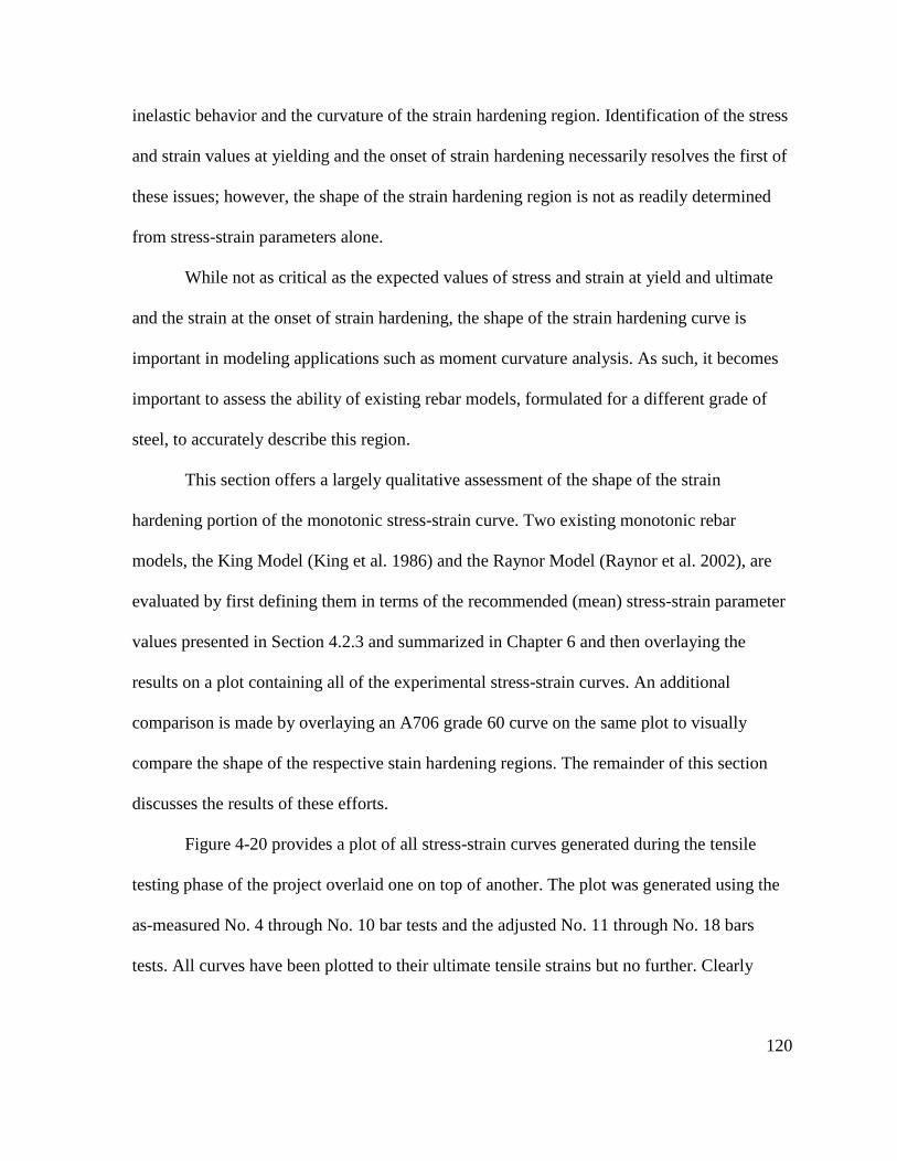
120

inelastic behavior and the curvature of the strain hardening region. Identification of the stress

and strain values at yielding and the onset of strain hardening necessarily resolves the first of

these issues; however, the shape of the strain hardening region is not as readily determined

from stress-strain parameters alone.

While not as critical as the expected values of stress and strain at yield and ultimate

and the strain at the onset of strain hardening, the shape of the strain hardening curve is

important in modeling applications such as moment curvature analysis. As such, it becomes

important to assess the ability of existing rebar models, formulated for a different grade of

steel, to accurately describe this region.

This section offers a largely qualitative assessment of the shape of the strain

hardening portion of the monotonic stress-strain curve. Two existing monotonic rebar

models, the King Model (King et al. 1986) and the Raynor Model (Raynor et al. 2002), are

evaluated by first defining them in terms of the recommended (mean) stress-strain parameter

values presented in Section 4.2.3 and summarized in Chapter 6 and then overlaying the

results on a plot containing all of the experimental stress-strain curves. An additional

comparison is made by overlaying an A706 grade 60 curve on the same plot to visually

compare the shape of the respective stain hardening regions. The remainder of this section

discusses the results of these efforts.

Figure 4-20 provides a plot of all stress-strain curves generated during the tensile

testing phase of the project overlaid one on top of another. The plot was generated using the

as-measured No. 4 through No. 10 bar tests and the adjusted No. 11 through No. 18 bars

tests. All curves have been plotted to their ultimate tensile strains but no further. Clearly

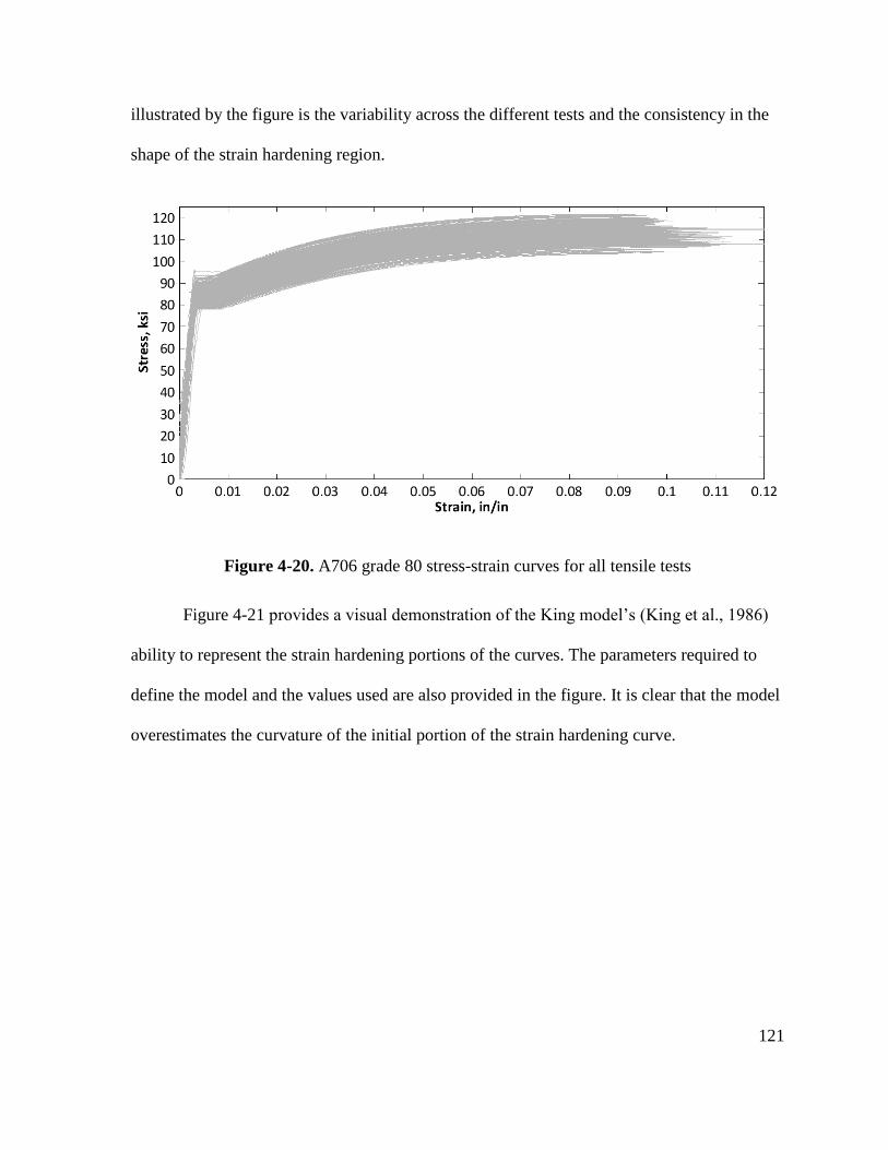
121

illustrated by the figure is the variability across the different tests and the consistency in the

shape of the strain hardening region.

Figure 4-20. A706 grade 80 stress-strain curves for all tensile tests

Figure 4-21 provides a visual demonstration of the King model’s (King et al., 1986)

ability to represent the strain hardening portions of the curves. The parameters required to

define the model and the values used are also provided in the figure. It is clear that the model

overestimates the curvature of the initial portion of the strain hardening curve.

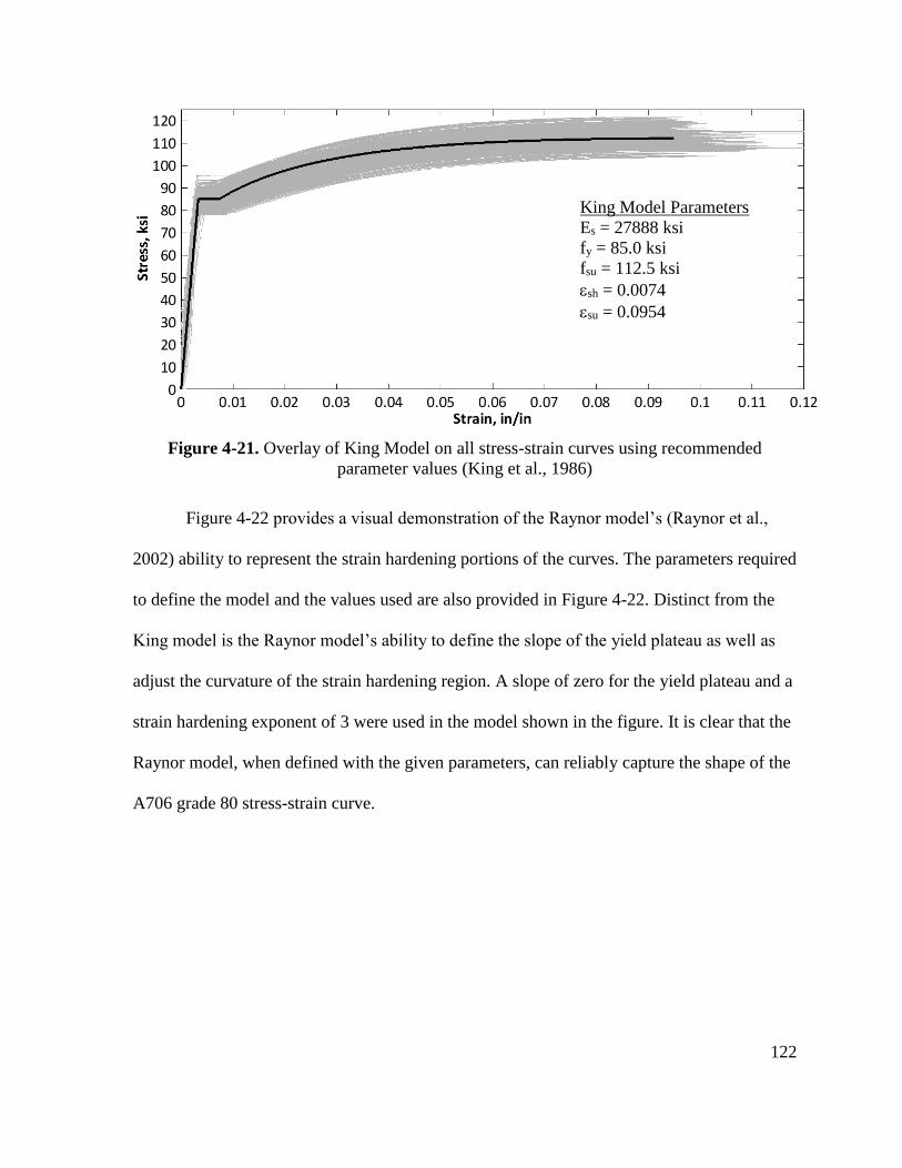
122

Figure 4-21. Overlay of King Model on all stress-strain curves using recommended

parameter values (King et al., 1986)

Figure 4-22 provides a visual demonstration of the Raynor model’s (Raynor et al.,

2002) ability to represent the strain hardening portions of the curves. The parameters required

to define the model and the values used are also provided in Figure 4-22. Distinct from the

King model is the Raynor model’s ability to define the slope of the yield plateau as well as

adjust the curvature of the strain hardening region. A slope of zero for the yield plateau and a

strain hardening exponent of 3 were used in the model shown in the figure. It is clear that the

Raynor model, when defined with the given parameters, can reliably capture the shape of the

A706 grade 80 stress-strain curve.

King Model Parameters

Es = 27888 ksi

fy = 85.0 ksi

fsu = 112.5 ksi

sh = 0.0074

su = 0.0954

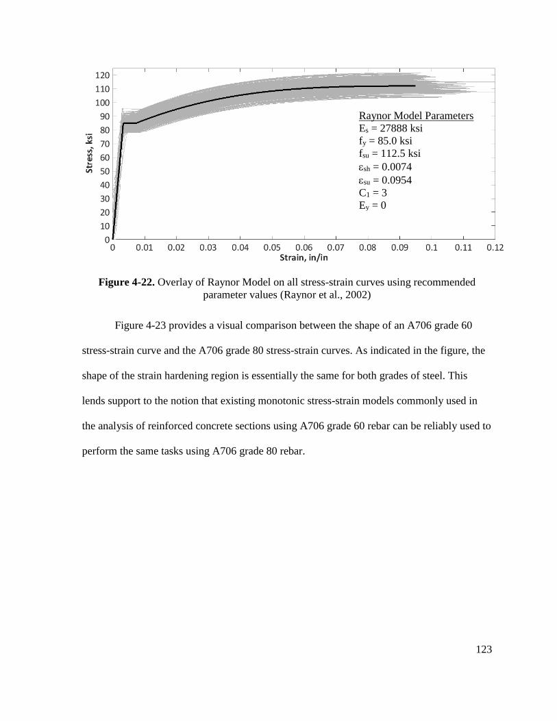
123

Figure 4-22. Overlay of Raynor Model on all stress-strain curves using recommended

parameter values (Raynor et al., 2002)

Figure 4-23 provides a visual comparison between the shape of an A706 grade 60

stress-strain curve and the A706 grade 80 stress-strain curves. As indicated in the figure, the

shape of the strain hardening region is essentially the same for both grades of steel. This

lends support to the notion that existing monotonic stress-strain models commonly used in

the analysis of reinforced concrete sections using A706 grade 60 rebar can be reliably used to

perform the same tasks using A706 grade 80 rebar.

Raynor Model Parameters

Es = 27888 ksi

fy = 85.0 ksi

fsu = 112.5 ksi

sh = 0.0074

su = 0.0954

C1 = 3

Ey = 0

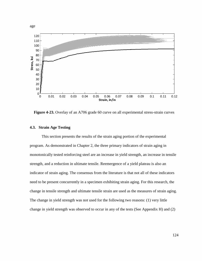
124

age

Figure 4-23. Overlay of an A706 grade 60 curve on all experimental stress-strain curves

4.3. Strain Age Testing

This section presents the results of the strain aging portion of the experimental

program. As demonstrated in Chapter 2, the three primary indicators of strain aging in

monotonically tested reinforcing steel are an increase in yield strength, an increase in tensile

strength, and a reduction in ultimate tensile. Reemergence of a yield plateau is also an

indicator of strain aging. The consensus from the literature is that not all of these indicators

need to be present concurrently in a specimen exhibiting strain aging. For this research, the

change in tensile strength and ultimate tensile strain are used as the measures of strain aging.

The change in yield strength was not used for the following two reasons: (1) very little

change in yield strength was observed to occur in any of the tests (See Appendix H) and (2)

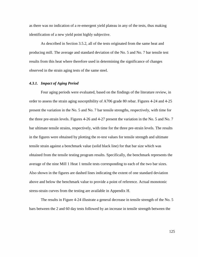
125

as there was no indication of a re-emergent yield plateau in any of the tests, thus making

identification of a new yield point highly subjective.

As described in Section 3.5.2, all of the tests originated from the same heat and

producing mill. The average and standard deviation of the No. 5 and No. 7 bar tensile test

results from this heat where therefore used in determining the significance of changes

observed in the strain aging tests of the same steel.

4.3.1. Impact of Aging Period

Four aging periods were evaluated, based on the findings of the literature review, in

order to assess the strain aging susceptibility of A706 grade 80 rebar. Figures 4-24 and 4-25

present the variation in the No. 5 and No. 7 bar tensile strengths, respectively, with time for

the three pre-strain levels. Figures 4-26 and 4-27 present the variation in the No. 5 and No. 7

bar ultimate tensile strains, respectively, with time for the three pre-strain levels. The results

in the figures were obtained by plotting the re-test values for tensile strength and ultimate

tensile strain against a benchmark value (solid black line) for that bar size which was

obtained from the tensile testing program results. Specifically, the benchmark represents the

average of the nine Mill 1 Heat 1 tensile tests corresponding to each of the two bar sizes.

Also shown in the figures are dashed lines indicating the extent of one standard deviation

above and below the benchmark value to provide a point of reference. Actual monotonic

stress-strain curves from the testing are available in Appendix H.

The results in Figure 4-24 illustrate a general decrease in tensile strength of the No. 5

bars between the 2 and 60 day tests followed by an increase in tensile strength between the

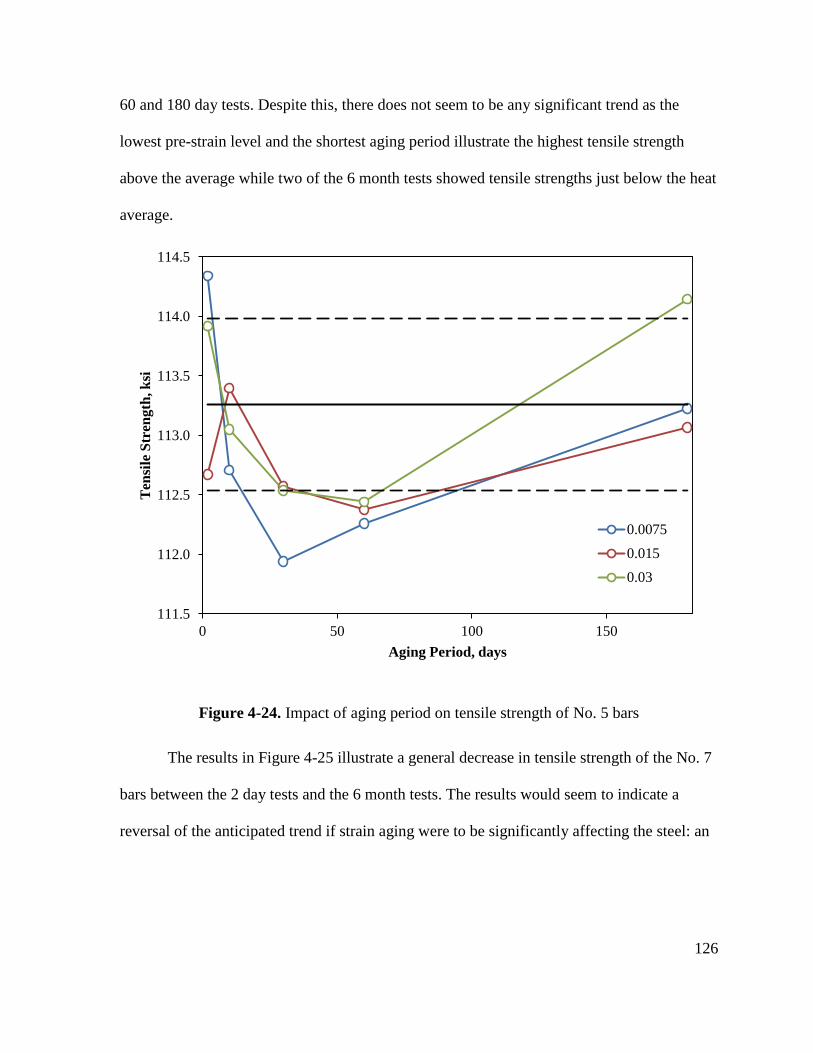
126

60 and 180 day tests. Despite this, there does not seem to be any significant trend as the

lowest pre-strain level and the shortest aging period illustrate the highest tensile strength

above the average while two of the 6 month tests showed tensile strengths just below the heat

average.

Figure 4-24. Impact of aging period on tensile strength of No. 5 bars

The results in Figure 4-25 illustrate a general decrease in tensile strength of the No. 7

bars between the 2 day tests and the 6 month tests. The results would seem to indicate a

reversal of the anticipated trend if strain aging were to be significantly affecting the steel: an

111.5

112.0

112.5

113.0

113.5

114.0

114.5

0 50 100 150

Ten

sile

Str

ength

, k

si

Aging Period, days

0.0075

0.015

0.03

127

increase in tensile strength with increased aging period. Nearly all of the results fell within

one standard deviation of the mean.

Figure 4-25. Impact of aging period on tensile strength of No. 7 bars

The results in Figure 4-26 illustrate a general decrease in ultimate tensile strain of the

No. 5 bars between the 2 day tests and the 30 day tests followed by an increase in ultimate

tensile strain between the 60 and 180 day tests. Observing that all three of the 6 months tests

fell above one standard deviation of the heat mean for all three pre-strain levels, there again

seems to be a reversal of the anticipated trend. Otherwise, nearly all of the results fell within

one standard deviation of the mean.

110.0

110.2

110.4

110.6

110.8

111.0

111.2

111.4

111.6

111.8

0 50 100 150

Ten

sile

Str

eng

th, k

si

Aging Period, days

0.0075

0.015

0.03

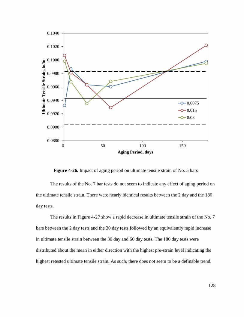
128

Figure 4-26. Impact of aging period on ultimate tensile strain of No. 5 bars

The results of the No. 7 bar tests do not seem to indicate any effect of aging period on

the ultimate tensile strain. There were nearly identical results between the 2 day and the 180

day tests.

The results in Figure 4-27 show a rapid decrease in ultimate tensile strain of the No. 7

bars between the 2 day tests and the 30 day tests followed by an equivalently rapid increase

in ultimate tensile strain between the 30 day and 60 day tests. The 180 day tests were

distributed about the mean in either direction with the highest pre-strain level indicating the

highest retested ultimate tensile strain. As such, there does not seem to be a definable trend.

0.0880

0.0900

0.0920

0.0940

0.0960

0.0980

0.1000

0.1020

0.1040

0 50 100 150

Ult

ima

te T

ensi

le S

tra

in, in

/in

Aging Period, days

0.0075

0.015

0.03

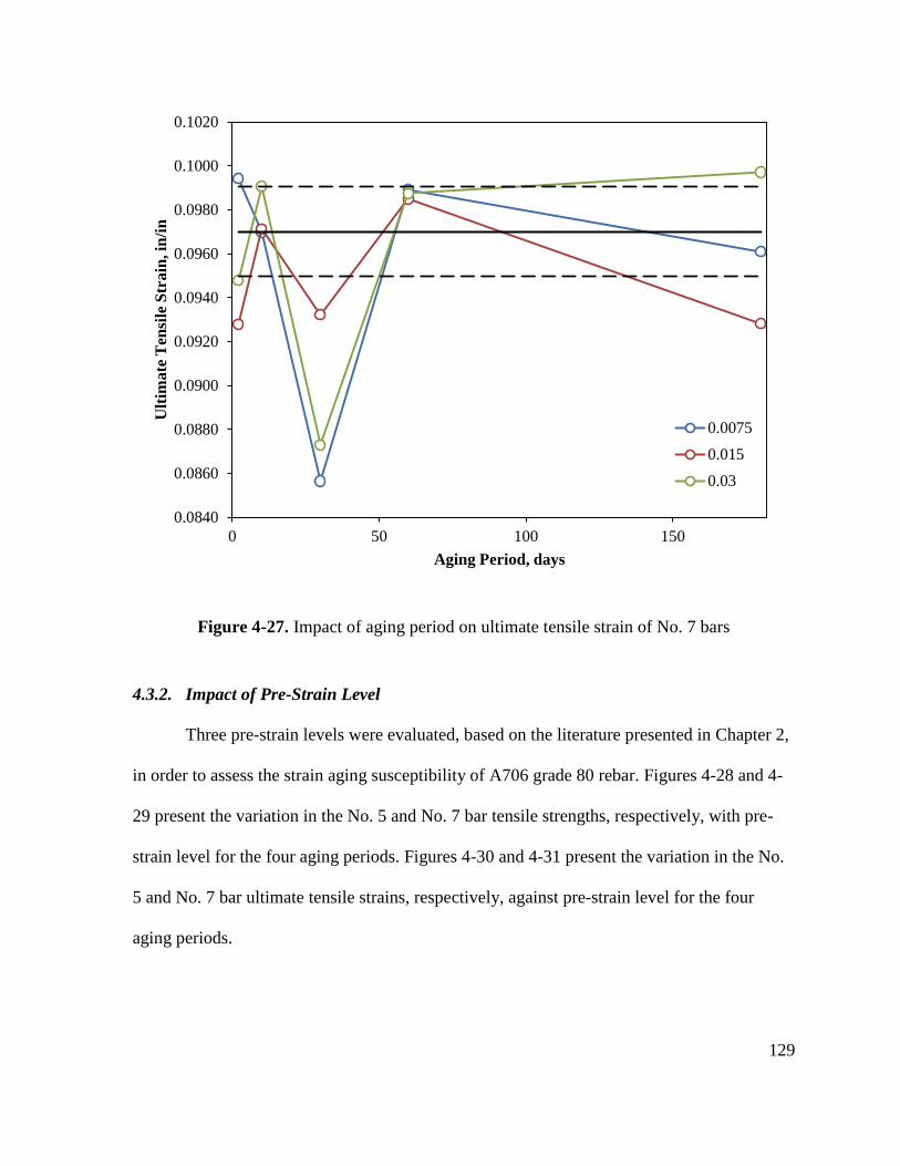
129

Figure 4-27. Impact of aging period on ultimate tensile strain of No. 7 bars

4.3.2. Impact of Pre-Strain Level

Three pre-strain levels were evaluated, based on the literature presented in Chapter 2,

in order to assess the strain aging susceptibility of A706 grade 80 rebar. Figures 4-28 and 4-

29 present the variation in the No. 5 and No. 7 bar tensile strengths, respectively, with pre-

strain level for the four aging periods. Figures 4-30 and 4-31 present the variation in the No.

5 and No. 7 bar ultimate tensile strains, respectively, against pre-strain level for the four

aging periods.

0.0840

0.0860

0.0880

0.0900

0.0920

0.0940

0.0960

0.0980

0.1000

0.1020

0 50 100 150

Ult

ima

te T

ensi

le S

tra

in, in

/in

Aging Period, days

0.0075

0.015

0.03

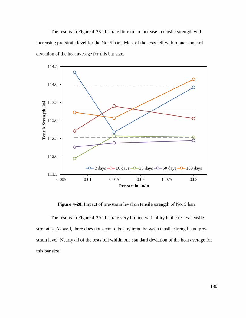
130

The results in Figure 4-28 illustrate little to no increase in tensile strength with

increasing pre-strain level for the No. 5 bars. Most of the tests fell within one standard

deviation of the heat average for this bar size.

Figure 4-28. Impact of pre-strain level on tensile strength of No. 5 bars

The results in Figure 4-29 illustrate very limited variability in the re-test tensile

strengths. As well, there does not seem to be any trend between tensile strength and pre-

strain level. Nearly all of the tests fell within one standard deviation of the heat average for

this bar size.

111.5

112.0

112.5

113.0

113.5

114.0

114.5

0.005 0.01 0.015 0.02 0.025 0.03

Ten

sile

Str

ength

, k

si

Pre-strain, in/in


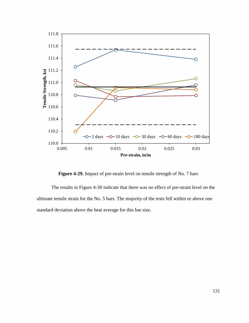
131

Figure 4-29. Impact of pre-strain level on tensile strength of No. 7 bars

The results in Figure 4-30 indicate that there was no effect of pre-strain level on the

ultimate tensile strain for the No. 5 bars. The majority of the tests fell within or above one

standard deviation above the heat average for this bar size.

110.0

110.2

110.4

110.6

110.8

111.0

111.2

111.4

111.6

111.8

0.005 0.01 0.015 0.02 0.025 0.03

Ten

sile

Str

eng

th, k

si

Pre-strain, in/in


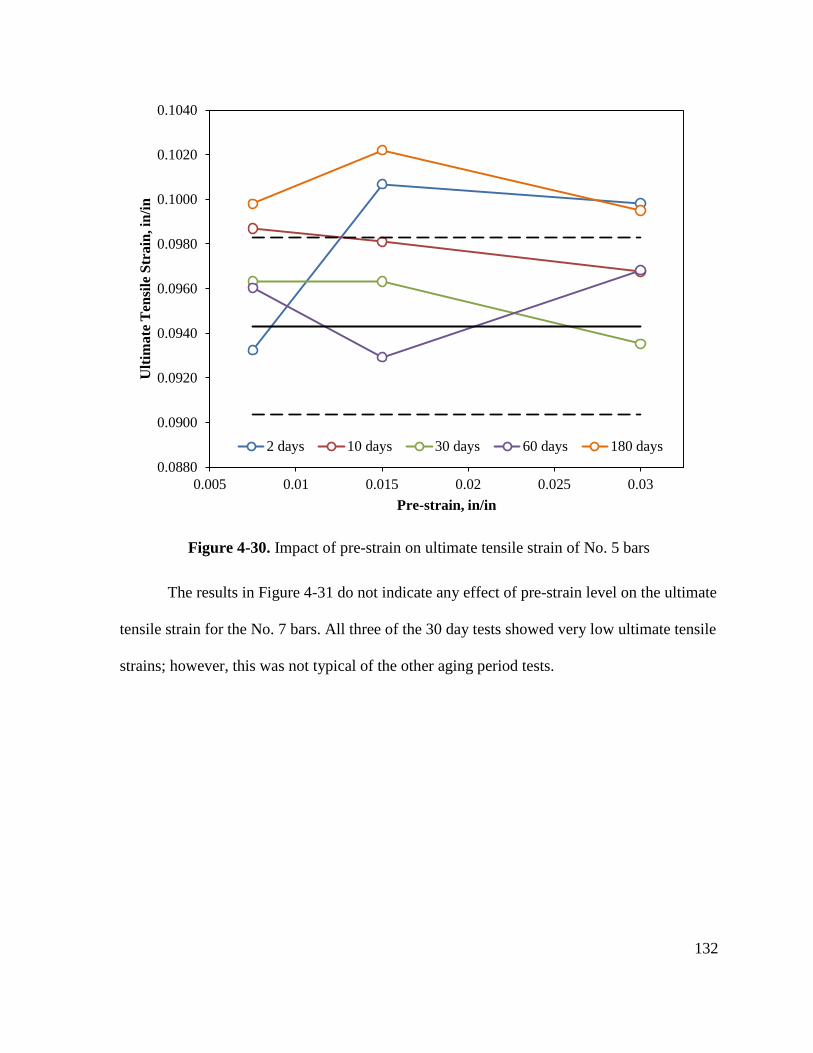
132

Figure 4-30. Impact of pre-strain on ultimate tensile strain of No. 5 bars

The results in Figure 4-31 do not indicate any effect of pre-strain level on the ultimate

tensile strain for the No. 7 bars. All three of the 30 day tests showed very low ultimate tensile

strains; however, this was not typical of the other aging period tests.

0.0880

0.0900

0.0920

0.0940

0.0960

0.0980

0.1000

0.1020

0.1040

0.005 0.01 0.015 0.02 0.025 0.03

Ult

ima

te T

ensi

le S

tra

in, in

/in

Pre-strain, in/in


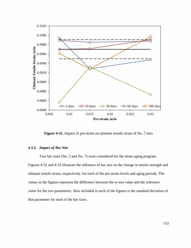
133

Figure 4-31. Impact of pre-strain on ultimate tensile strain of No. 7 bars

4.3.3. Impact of Bar Size

Two bar sizes (No. 5 and No. 7) were considered for the strain aging program.

Figures 4-32 and 4-33 illustrate the influence of bar size on the change in tensile strength and

ultimate tensile strain, respectively, for each of the pre-strain levels and aging periods. The

values in the figures represent the difference between the re-test value and the reference

value for the two parameters. Also included in each of the figures is the standard deviation of

that parameter for each of the bar sizes.

0.0840

0.0860

0.0880

0.0900

0.0920

0.0940

0.0960

0.0980

0.1000

0.1020

0.005 0.01 0.015 0.02 0.025 0.03

Ult

ima

te T

ensi

le S

tra

in, in

/in

Pre-strain, in/in


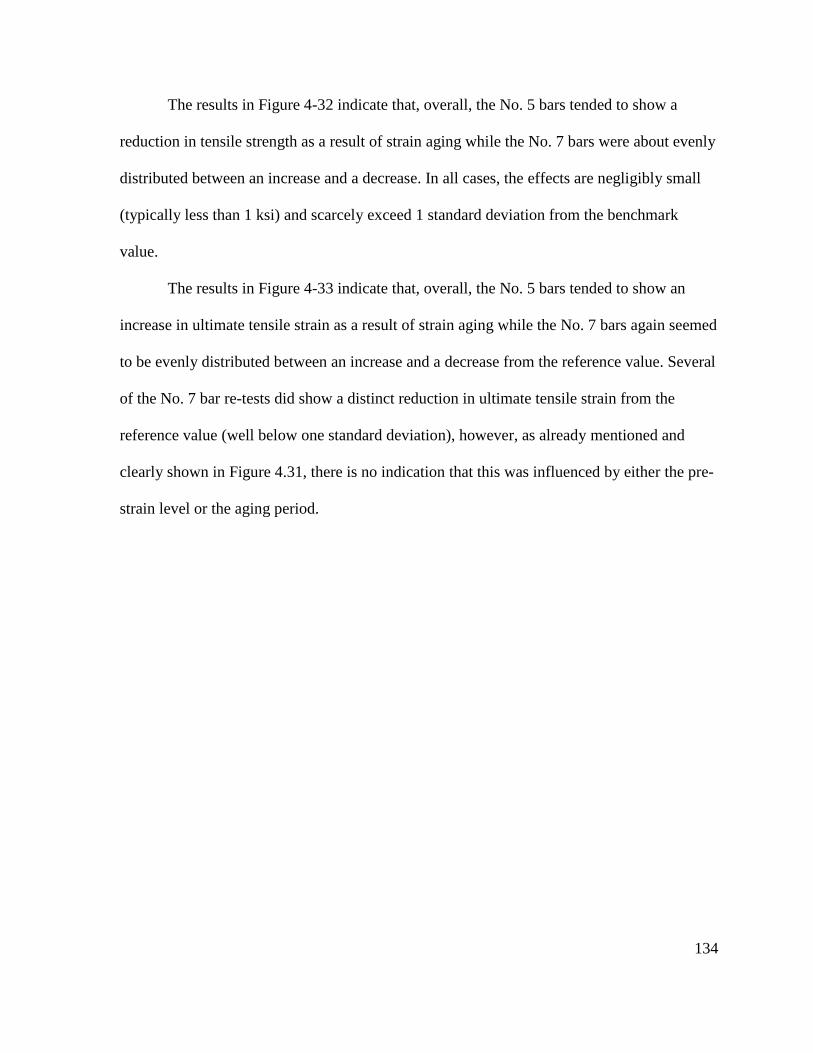
134

The results in Figure 4-32 indicate that, overall, the No. 5 bars tended to show a

reduction in tensile strength as a result of strain aging while the No. 7 bars were about evenly

distributed between an increase and a decrease. In all cases, the effects are negligibly small

(typically less than 1 ksi) and scarcely exceed 1 standard deviation from the benchmark

value.

The results in Figure 4-33 indicate that, overall, the No. 5 bars tended to show an

increase in ultimate tensile strain as a result of strain aging while the No. 7 bars again seemed

to be evenly distributed between an increase and a decrease from the reference value. Several

of the No. 7 bar re-tests did show a distinct reduction in ultimate tensile strain from the

reference value (well below one standard deviation), however, as already mentioned and

clearly shown in Figure 4.31, there is no indication that this was influenced by either the pre-

strain level or the aging period.

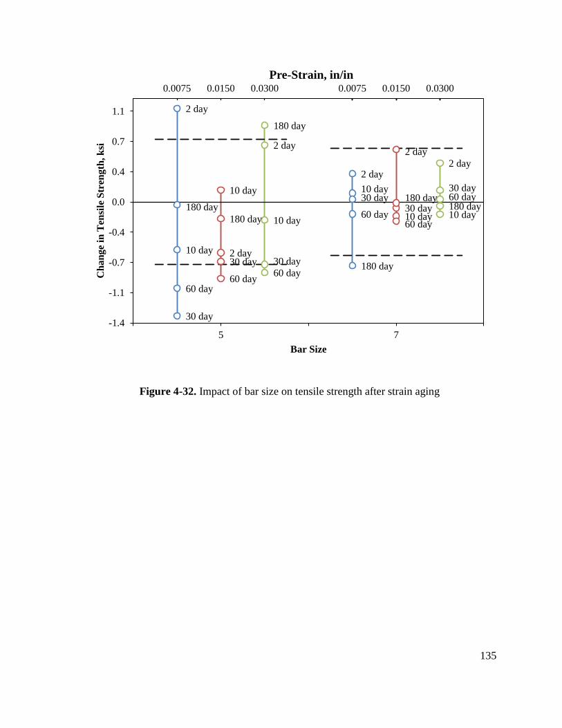
135

Figure 4-32. Impact of bar size on tensile strength after strain aging

2 day

10 day30 day

60 day

180 day

2 day

10 day30 day

60 day

180 day

2 day

10 day

30 day60 day180 day

0.0075 0.0150 0.0300 0.0075 0.0150 0.0300

2 day

10 day

30 day

60 day

180 day

2 day

10 day

30 day

60 day

180 day

2 day

10 day

30 day

60 day

180 day

-1.4

-1.1

-0.7

-0.4

0.0

0.4

0.7

1.1

4 5 6 7 8

Ch

an

ge

in T

ensi

le S

tren

gth

, k

si

Bar Size

Pre-Strain, in/in

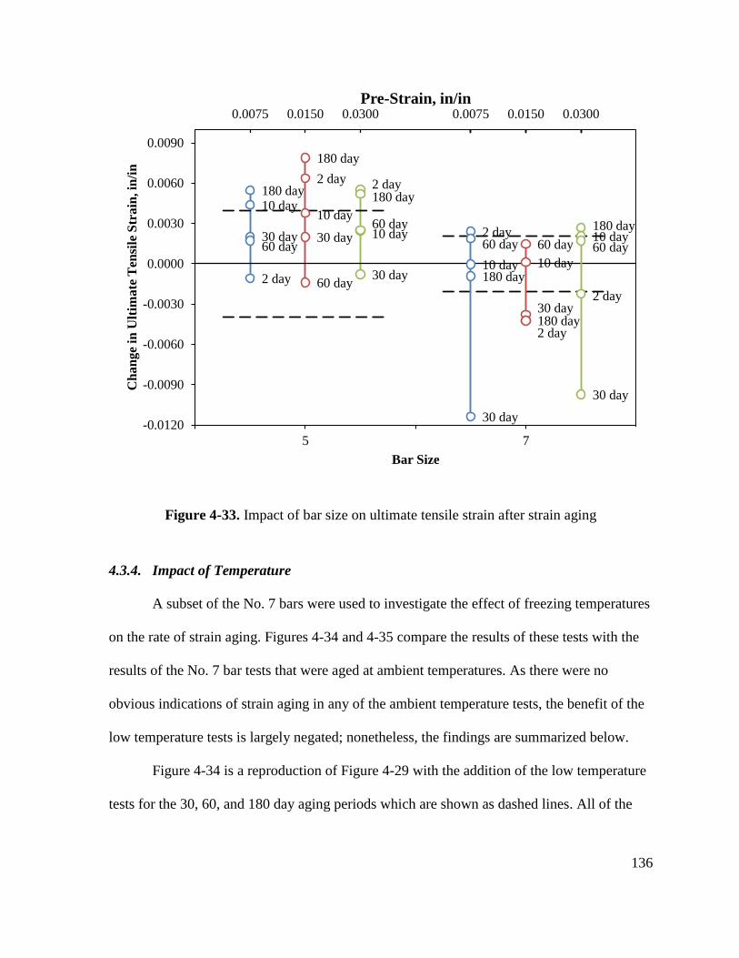
136

Figure 4-33. Impact of bar size on ultimate tensile strain after strain aging

4.3.4. Impact of Temperature

A subset of the No. 7 bars were used to investigate the effect of freezing temperatures

on the rate of strain aging. Figures 4-34 and 4-35 compare the results of these tests with the

results of the No. 7 bar tests that were aged at ambient temperatures. As there were no

obvious indications of strain aging in any of the ambient temperature tests, the benefit of the

low temperature tests is largely negated; nonetheless, the findings are summarized below.

Figure 4-34 is a reproduction of Figure 4-29 with the addition of the low temperature

tests for the 30, 60, and 180 day aging periods which are shown as dashed lines. All of the

2 day

10 day

30 day

60 day

180 day

2 day

10 day

30 day

60 day

180 day

2 day

10 day

30 day

60 day

180 day

0.0075 0.0150 0.0300 0.0075 0.0150 0.0300

2 day

10 day

30 day60 day

180 day2 day

10 day

30 day

60 day

180 day

2 day

10 day

30 day

60 day

180 day

-0.0120

-0.0090

-0.0060

-0.0030

0.0000

0.0030

0.0060

0.0090

4 5 6 7 8

Ch

an

ge

in U

ltim

ate

Ten

sile

Str

ain

, in

/in

Bar Size

Pre-Strain, in/in

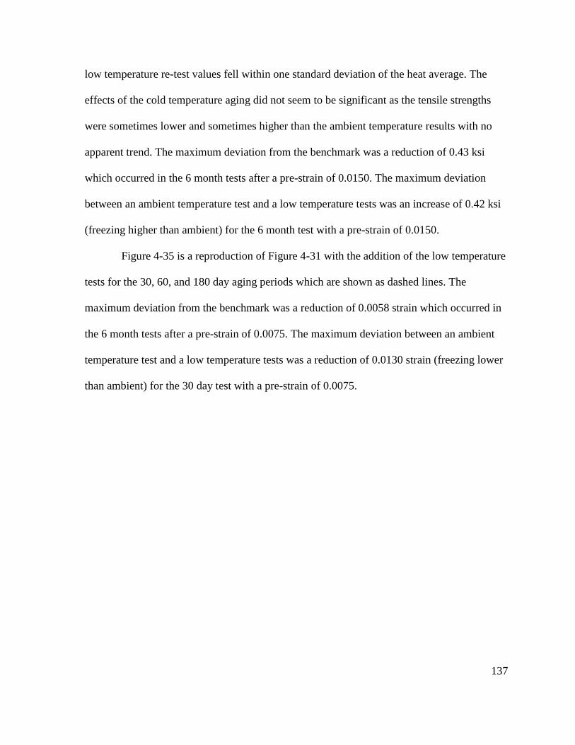
137

low temperature re-test values fell within one standard deviation of the heat average. The

effects of the cold temperature aging did not seem to be significant as the tensile strengths

were sometimes lower and sometimes higher than the ambient temperature results with no

apparent trend. The maximum deviation from the benchmark was a reduction of 0.43 ksi

which occurred in the 6 month tests after a pre-strain of 0.0150. The maximum deviation

between an ambient temperature test and a low temperature tests was an increase of 0.42 ksi

(freezing higher than ambient) for the 6 month test with a pre-strain of 0.0150.

Figure 4-35 is a reproduction of Figure 4-31 with the addition of the low temperature

tests for the 30, 60, and 180 day aging periods which are shown as dashed lines. The

maximum deviation from the benchmark was a reduction of 0.0058 strain which occurred in

the 6 month tests after a pre-strain of 0.0075. The maximum deviation between an ambient

temperature test and a low temperature tests was a reduction of 0.0130 strain (freezing lower

than ambient) for the 30 day test with a pre-strain of 0.0075.

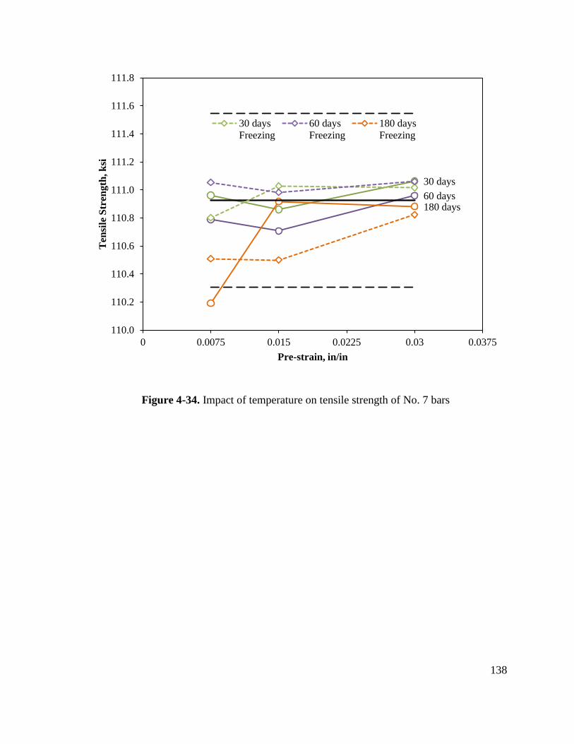
138

Figure 4-34. Impact of temperature on tensile strength of No. 7 bars

30 days

60 days180 days

110.0

110.2

110.4

110.6

110.8

111.0

111.2

111.4

111.6

111.8

0 0.0075 0.015 0.0225 0.03 0.0375

Ten

sile

Str

eng

th, k

si

Pre-strain, in/in

30 days

Freezing

60 days

Freezing

180 days

Freezing

139

Figure 4-35. Impact of temperature on ultimate tensile strain of No. 7 bars

4.4. Cyclic Testing

A limited number of cyclic tests on No. 5 and No. 7 bars were conducted for the

purpose of evaluating the capability of existing rebar models to characterize the A706 grade

80 cyclic material behavior and to investigate the effect of cyclic load history on the ultimate

tensile strain (strain at max stress). This section summarizes the findings of these tests.

30 days

60 days

180 days

0.0840

0.0860

0.0880

0.0900

0.0920

0.0940

0.0960

0.0980

0.1000

0.1020

0.005 0.01 0.015 0.02 0.025 0.03

Ult

ima

te T

ensi

le S

tra

in, in

/in

Pre-strain, in/in

30 days

Freezing

60 days

Freezing

180 days

Freezing

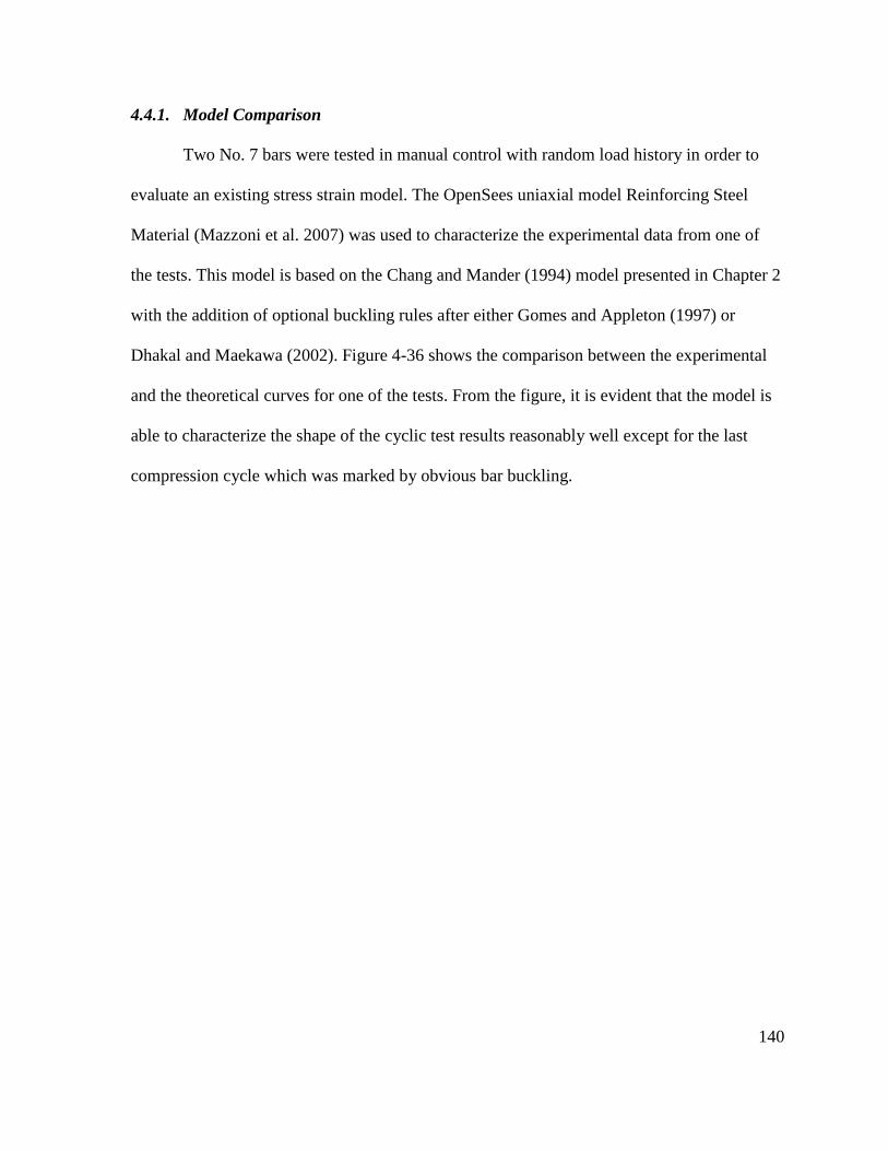
140

4.4.1. Model Comparison

Two No. 7 bars were tested in manual control with random load history in order to

evaluate an existing stress strain model. The OpenSees uniaxial model Reinforcing Steel

Material (Mazzoni et al. 2007) was used to characterize the experimental data from one of

the tests. This model is based on the Chang and Mander (1994) model presented in Chapter 2

with the addition of optional buckling rules after either Gomes and Appleton (1997) or

Dhakal and Maekawa (2002). Figure 4-36 shows the comparison between the experimental

and the theoretical curves for one of the tests. From the figure, it is evident that the model is

able to characterize the shape of the cyclic test results reasonably well except for the last

compression cycle which was marked by obvious bar buckling.

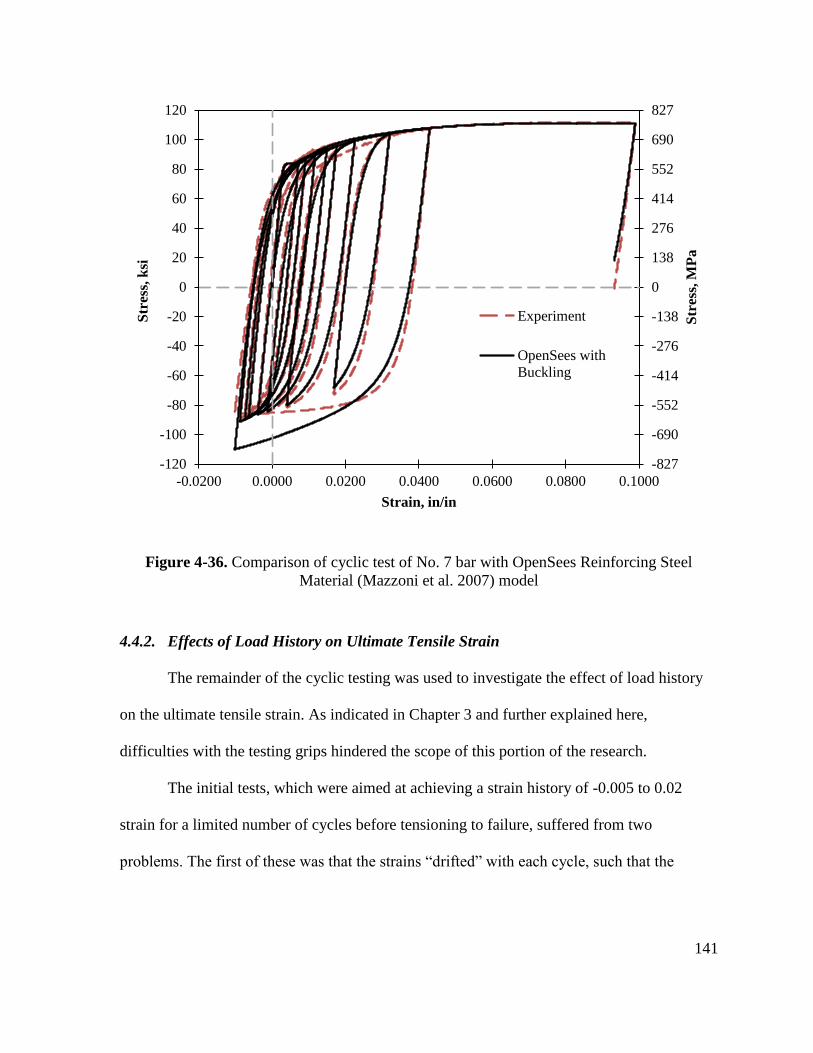
141

Figure 4-36. Comparison of cyclic test of No. 7 bar with OpenSees Reinforcing Steel

Material (Mazzoni et al. 2007) model

4.4.2. Effects of Load History on Ultimate Tensile Strain

The remainder of the cyclic testing was used to investigate the effect of load history

on the ultimate tensile strain. As indicated in Chapter 3 and further explained here,

difficulties with the testing grips hindered the scope of this portion of the research.

The initial tests, which were aimed at achieving a strain history of -0.005 to 0.02

strain for a limited number of cycles before tensioning to failure, suffered from two

problems. The first of these was that the strains “drifted” with each cycle, such that the

-827

-690

-552

-414

-276

-138

0

138

276

414

552

690

827

-120

-100

-80

-60

-40

-20

0

20

40

60

80

100

120

-0.0200 0.0000 0.0200 0.0400 0.0600 0.0800 0.1000

Str

ess,

MP

a

Str

ess,

ksi

Strain, in/in

Experiment

OpenSees with

Buckling

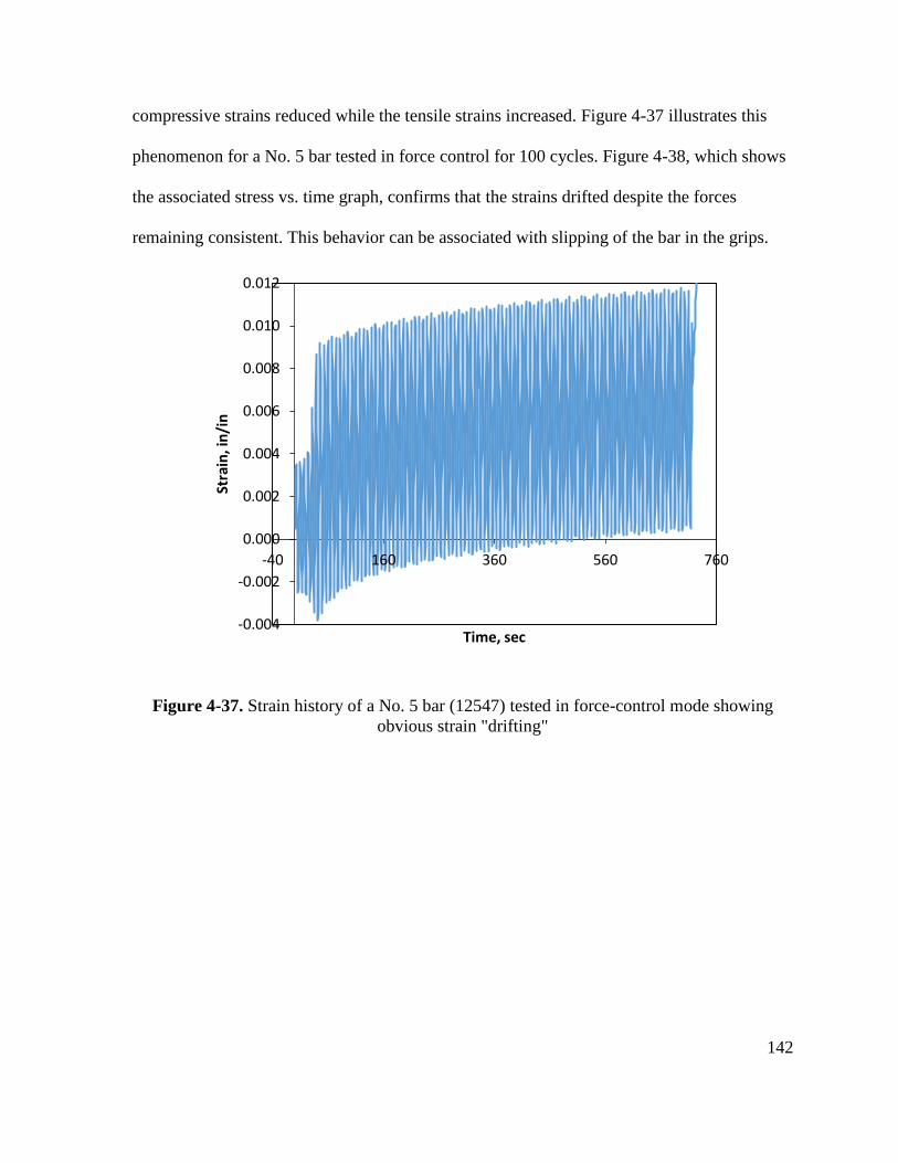
142

compressive strains reduced while the tensile strains increased. Figure 4-37 illustrates this

phenomenon for a No. 5 bar tested in force control for 100 cycles. Figure 4-38, which shows

the associated stress vs. time graph, confirms that the strains drifted despite the forces

remaining consistent. This behavior can be associated with slipping of the bar in the grips.

Figure 4-37. Strain history of a No. 5 bar (12547) tested in force-control mode showing

obvious strain "drifting"

-0.004

-0.002

0.000

0.002

0.004

0.006

0.008

0.010

0.012

-40 160 360 560 760

Stra

in, i

n/i

n

Time, sec

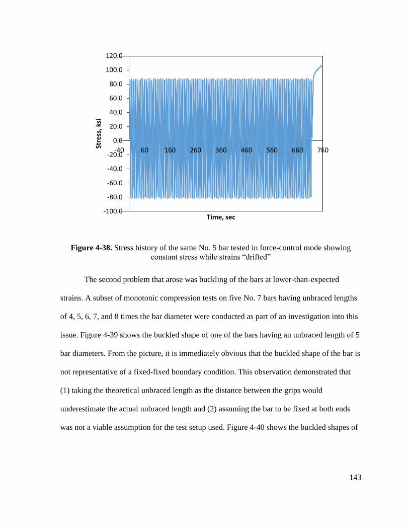
143

Figure 4-38. Stress history of the same No. 5 bar tested in force-control mode showing

constant stress while strains “drifted”

The second problem that arose was buckling of the bars at lower-than-expected

strains. A subset of monotonic compression tests on five No. 7 bars having unbraced lengths

of 4, 5, 6, 7, and 8 times the bar diameter were conducted as part of an investigation into this

issue. Figure 4-39 shows the buckled shape of one of the bars having an unbraced length of 5

bar diameters. From the picture, it is immediately obvious that the buckled shape of the bar is

not representative of a fixed-fixed boundary condition. This observation demonstrated that

(1) taking the theoretical unbraced length as the distance between the grips would

underestimate the actual unbraced length and (2) assuming the bar to be fixed at both ends

was not a viable assumption for the test setup used. Figure 4-40 shows the buckled shapes of

-100.0

-80.0

-60.0

-40.0

-20.0

0.0

20.0

40.0

60.0

80.0

100.0

120.0

-40 60 160 260 360 460 560 660 760Stre

ss, k

si

Time, sec

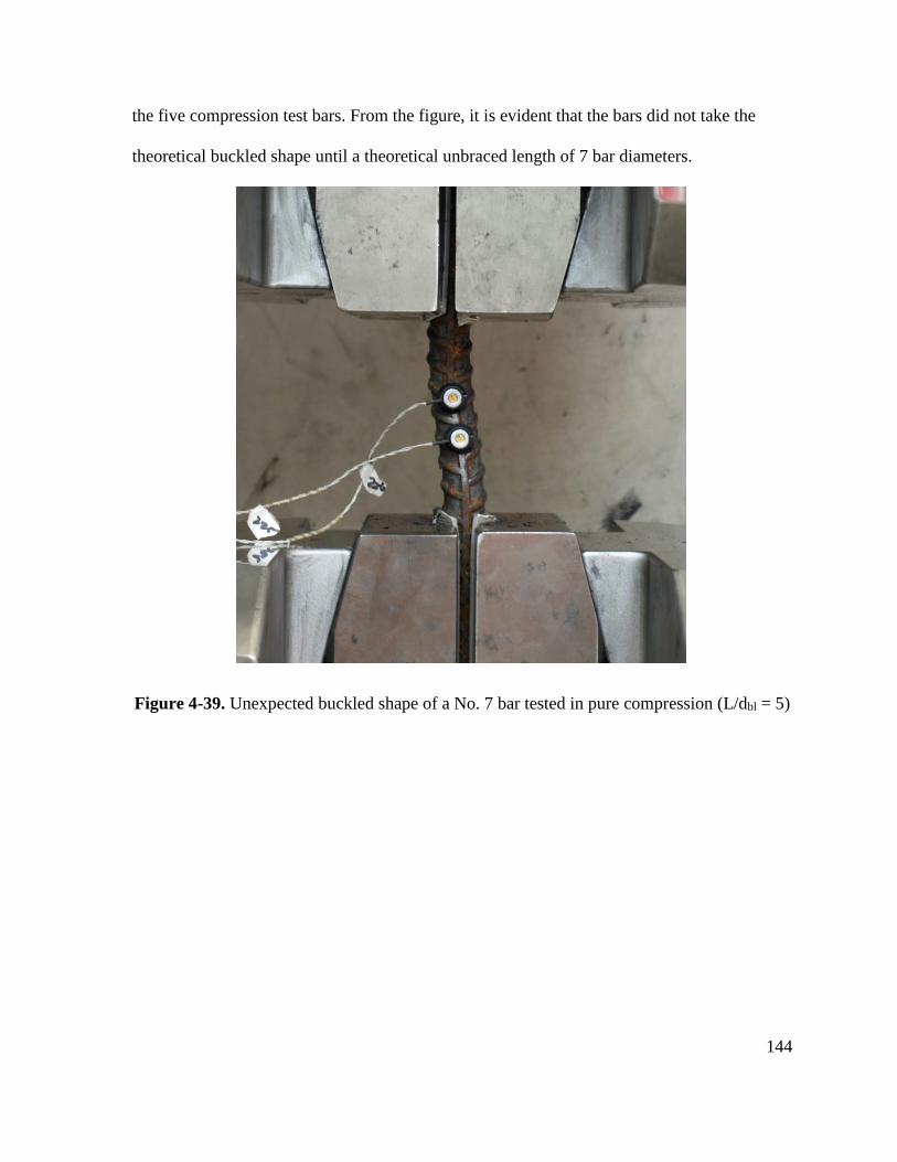
144

the five compression test bars. From the figure, it is evident that the bars did not take the

theoretical buckled shape until a theoretical unbraced length of 7 bar diameters.

Figure 4-39. Unexpected buckled shape of a No. 7 bar tested in pure compression (L/dbl = 5)

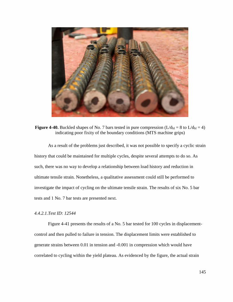
145

Figure 4-40. Buckled shapes of No. 7 bars tested in pure compression (L/dbl = 8 to L/dbl = 4)

indicating poor fixity of the boundary conditions (MTS machine grips)

As a result of the problems just described, it was not possible to specify a cyclic strain

history that could be maintained for multiple cycles, despite several attempts to do so. As

such, there was no way to develop a relationship between load history and reduction in

ultimate tensile strain. Nonetheless, a qualitative assessment could still be performed to

investigate the impact of cycling on the ultimate tensile strain. The results of six No. 5 bar

tests and 1 No. 7 bar tests are presented next.

4.4.2.1.Test ID: 12544

Figure 4-41 presents the results of a No. 5 bar tested for 100 cycles in displacement-

control and then pulled to failure in tension. The displacement limits were established to

generate strains between 0.01 in tension and -0.001 in compression which would have

correlated to cycling within the yield plateau. As evidenced by the figure, the actual strain

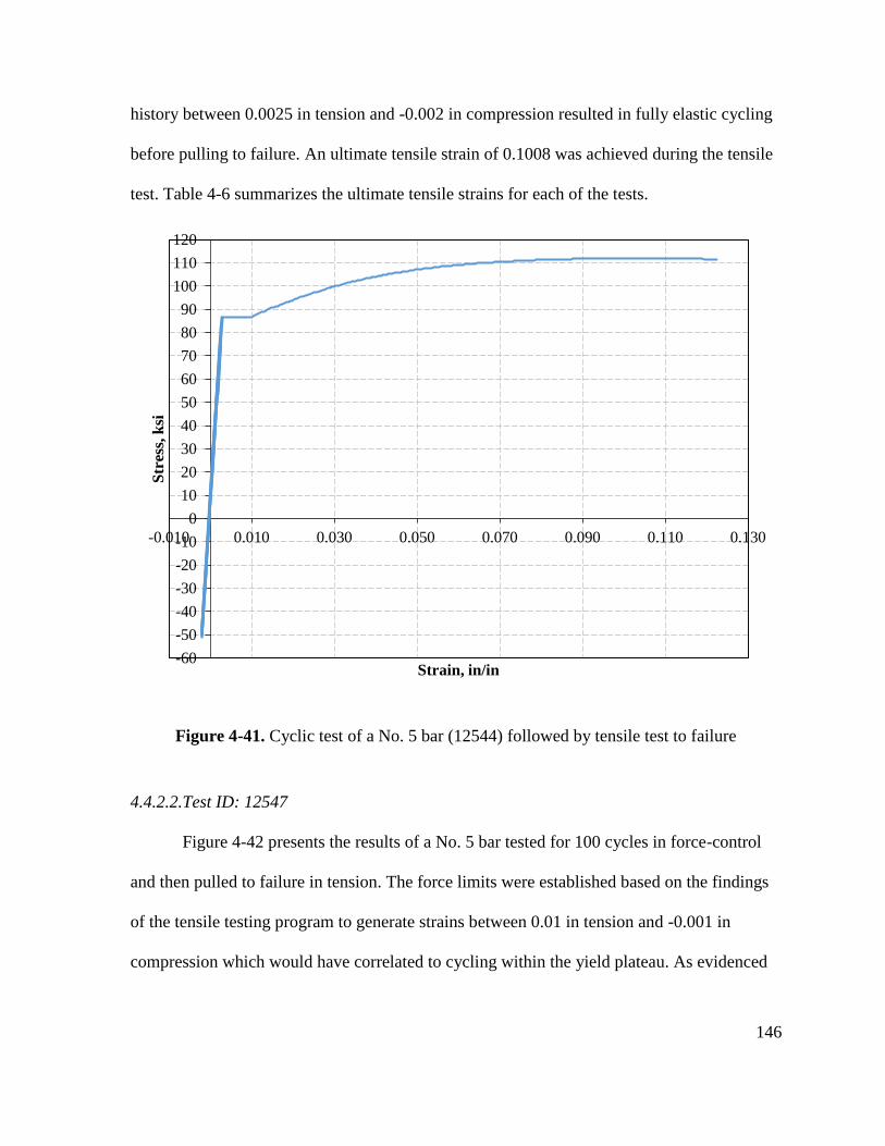
146

history between 0.0025 in tension and -0.002 in compression resulted in fully elastic cycling

before pulling to failure. An ultimate tensile strain of 0.1008 was achieved during the tensile

test. Table 4-6 summarizes the ultimate tensile strains for each of the tests.

Figure 4-41. Cyclic test of a No. 5 bar (12544) followed by tensile test to failure

4.4.2.2.Test ID: 12547

Figure 4-42 presents the results of a No. 5 bar tested for 100 cycles in force-control

and then pulled to failure in tension. The force limits were established based on the findings

of the tensile testing program to generate strains between 0.01 in tension and -0.001 in

compression which would have correlated to cycling within the yield plateau. As evidenced

-60

-50

-40

-30

-20

-10

0

10

20

30

40

50

60

70

80

90

100

110

120

-0.010 0.010 0.030 0.050 0.070 0.090 0.110 0.130

Str

ess,

ksi

Strain, in/in

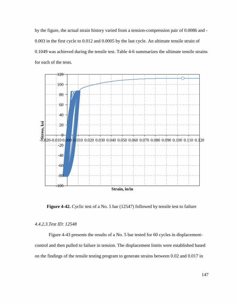
147

by the figure, the actual strain history varied from a tension-compression pair of 0.0086 and -

0.003 in the first cycle to 0.012 and 0.0005 by the last cycle. An ultimate tensile strain of

0.1049 was achieved during the tensile test. Table 4-6 summarizes the ultimate tensile strains

for each of the tests.


4.4.2.3.Test ID: 12548


control and then pulled to failure in tension. The displacement limits were established based

on the findings of the tensile testing program to generate strains between 0.02 and 0.017 in

-100

-80

-60

-40

-20

0

20

40

60

80

100

120

-0.020-0.010 0.000 0.010 0.020 0.030 0.040 0.050 0.060 0.070 0.080 0.090 0.100 0.110 0.120

Str

ess,

ksi

Strain, in/in

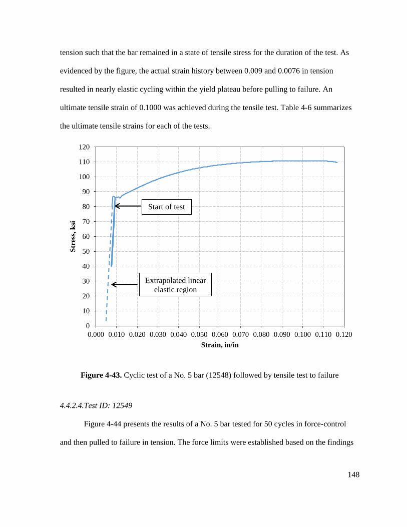
148

tension such that the bar remained in a state of tensile stress for the duration of the test. As

evidenced by the figure, the actual strain history between 0.009 and 0.0076 in tension

resulted in nearly elastic cycling within the yield plateau before pulling to failure. An

ultimate tensile strain of 0.1000 was achieved during the tensile test. Table 4-6 summarizes

the ultimate tensile strains for each of the tests.


4.4.2.4.Test ID: 12549

Figure 4-44 presents the results of a No. 5 bar tested for 50 cycles in force-control

and then pulled to failure in tension. The force limits were established based on the findings

0

10

20

30

40

50

60

70

80

90

100

110

120

0.000 0.010 0.020 0.030 0.040 0.050 0.060 0.070 0.080 0.090 0.100 0.110 0.120

Str

ess,

ksi

Strain, in/in

Start of test

Extrapolated linear

elastic region

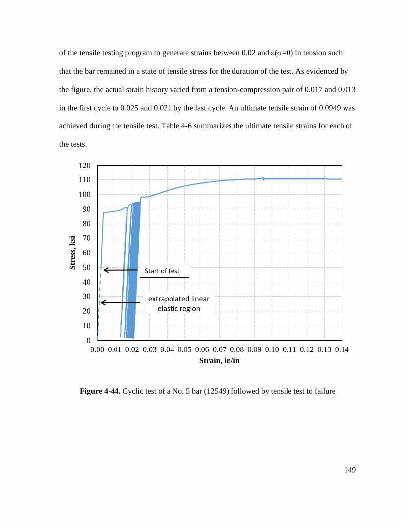
149

of the tensile testing program to generate strains between 0.02 and (s=0) in tension such

that the bar remained in a state of tensile stress for the duration of the test. As evidenced by

the figure, the actual strain history varied from a tension-compression pair of 0.017 and 0.013

in the first cycle to 0.025 and 0.021 by the last cycle. An ultimate tensile strain of 0.0949 was

achieved during the tensile test. Table 4-6 summarizes the ultimate tensile strains for each of

the tests.


0

10

20

30

40

50

60

70

80

90

100

110

120

0.00 0.01 0.02 0.03 0.04 0.05 0.06 0.07 0.08 0.09 0.10 0.11 0.12 0.13 0.14

Str

ess,

ksi

Strain, in/in

Start of test

extrapolated linear elastic region

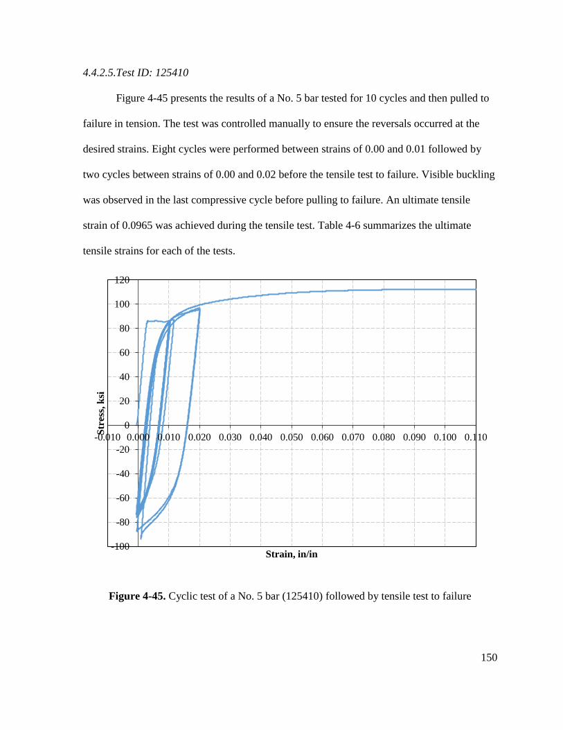
150

4.4.2.5.Test ID: 125410

Figure 4-45 presents the results of a No. 5 bar tested for 10 cycles and then pulled to

failure in tension. The test was controlled manually to ensure the reversals occurred at the

desired strains. Eight cycles were performed between strains of 0.00 and 0.01 followed by

two cycles between strains of 0.00 and 0.02 before the tensile test to failure. Visible buckling

was observed in the last compressive cycle before pulling to failure. An ultimate tensile

strain of 0.0965 was achieved during the tensile test. Table 4-6 summarizes the ultimate

tensile strains for each of the tests.


-100

-80

-60

-40

-20

0

20

40

60

80

100

120

-0.010 0.000 0.010 0.020 0.030 0.040 0.050 0.060 0.070 0.080 0.090 0.100 0.110

Str

ess,

ksi

Strain, in/in

151

4.4.2.6.Test ID: 125411

Figure 4-46 presents the results of a No. 5 bar tested for 30 cycles and then pulled to

failure in tension. The test was controlled manually to ensure the reversals occurred at the

desired strains. Ten cycles were performed between 0.00 and 0.01 strain followed by 10

cycles between 0.01 and 0.02 strain followed by 10 cycles between 0.02 and 0.03 strain

followed by a reversal back to 0.01 strain before the tensile test to failure. Visible buckling

was observed in the last compressive cycle before pulling to failure. An ultimate tensile

strain of 0.1055 was achieved during the tensile test. Table 4-6 summarizes the ultimate

tensile strains for each of the tests.

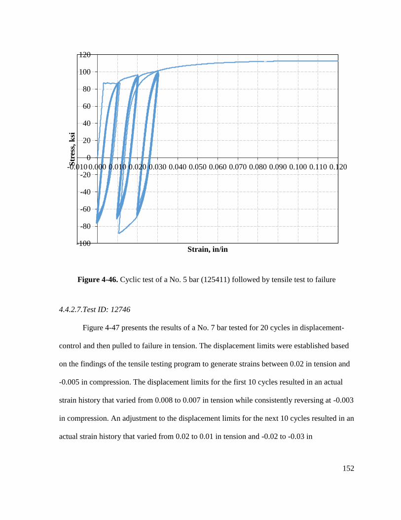
152


4.4.2.7.Test ID: 12746


control and then pulled to failure in tension. The displacement limits were established based

on the findings of the tensile testing program to generate strains between 0.02 in tension and

-0.005 in compression. The displacement limits for the first 10 cycles resulted in an actual

strain history that varied from 0.008 to 0.007 in tension while consistently reversing at -0.003

in compression. An adjustment to the displacement limits for the next 10 cycles resulted in an

actual strain history that varied from 0.02 to 0.01 in tension and -0.02 to -0.03 in

-100

-80

-60

-40

-20

0

20

40

60

80

100

120

-0.010 0.000 0.010 0.020 0.030 0.040 0.050 0.060 0.070 0.080 0.090 0.100 0.110 0.120Str

ess,

ksi

Strain, in/in

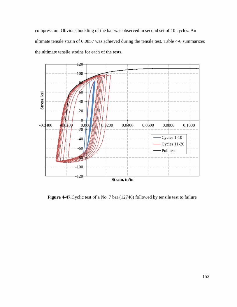
153

compression. Obvious buckling of the bar was observed in second set of 10 cycles. An

ultimate tensile strain of 0.0857 was achieved during the tensile test. Table 4-6 summarizes

the ultimate tensile strains for each of the tests.

Figure 4-47.Cyclic test of a No. 7 bar (12746) followed by tensile test to failure

-120

-100

-80

-60

-40

-20

0

20

40

60

80

100

120

-0.0400 -0.0200 0.0000 0.0200 0.0400 0.0600 0.0800 0.1000

Str

ess,

ksi

Strain, in/in

Cycles 1-10

Cycles 11-20

Pull test

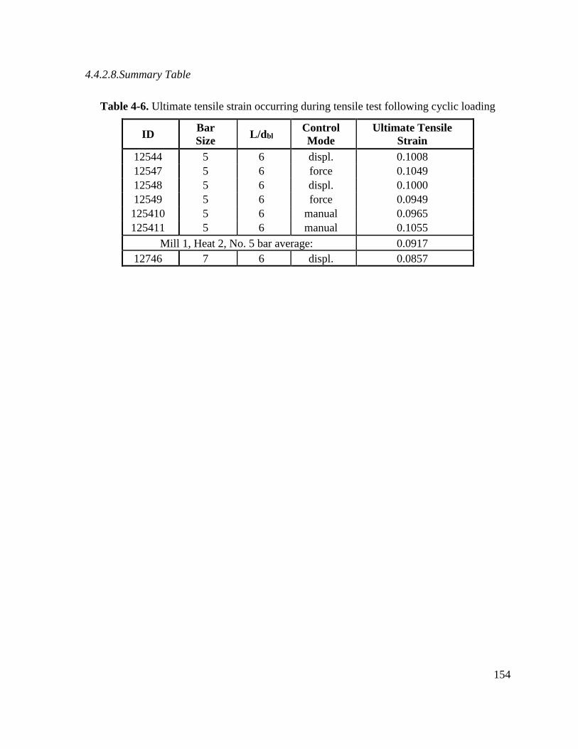
154

4.4.2.8.Summary Table

Table 4-6. Ultimate tensile strain occurring during tensile test following cyclic loading

ID Bar

Size L/dbl

Control

Mode

Ultimate Tensile

Strain

12544 5 6 displ. 0.1008

12547 5 6 force 0.1049

12548 5 6 displ. 0.1000

12549 5 6 force 0.0949

125410 5 6 manual 0.0965

125411 5 6 manual 0.1055

Mill 1, Heat 2, No. 5 bar average: 0.0917

12746 7 6 displ. 0.0857

155

5. DISCUSSION

5.1. Tensile Tests

5.1.1. Comparison with Literature Results

As demonstrated in Chapter 2, several of the literature papers presenting numerical

stress-strain data on A706 grade 80 rebar additionally presented the associated stress-strain

curves. A graphical comparison between these curves and those generated as part of the

current research can be accomplished by superimposing the graphs on top of one another. In

addition to illustrating the similarities in the shape of the strain hardening region, this

exercise also serves as a means of validating the experimental findings.

The results indicate that the experimental findings are consistent with currently

available literature data with respect to the shape of the stress-strain curve. Figure 5-1

highlights the consistency in the length of the yield plateau and the initial slope of the strain

hardening region. Note that the project data curves have been plotted to u in Figures 5-2 and

5-3. Figure 5-2 illustrates a consistency in shape of the strain hardening curve and ultimate

tensile strain. An interesting observation from Figure 5-2 is the fact that the No. 18 bar stress-

strain curve lies near the bottom of the experimental stress-strain curves. This trend for the

larger bars to have lower strength was illustrated in Chapter 3. Figure 5-3 illustrates a

consistency in length of the yield plateau and shape of the strain hardening curve but a

difference in the ultimate tensile strains.

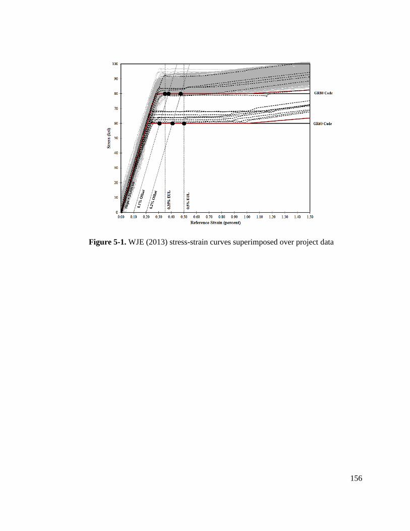
156

Figure 5-1. WJE (2013) stress-strain curves superimposed over project data

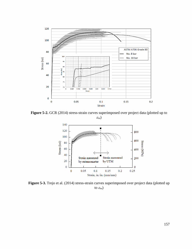
157

Figure 5-2. GCR (2014) stress-strain curves superimposed over project data (plotted up to

su)

Figure 5-3. Trejo et al. (2014) stress-strain curves superimposed over project data (plotted up

to su)

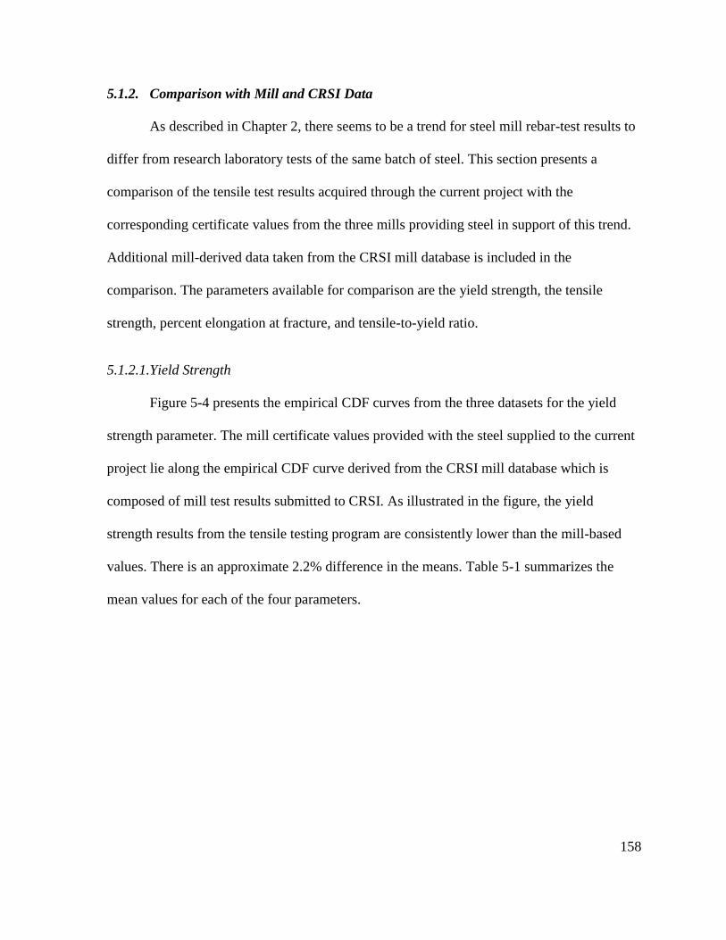
158

5.1.2. Comparison with Mill and CRSI Data

As described in Chapter 2, there seems to be a trend for steel mill rebar-test results to

differ from research laboratory tests of the same batch of steel. This section presents a

comparison of the tensile test results acquired through the current project with the

corresponding certificate values from the three mills providing steel in support of this trend.

Additional mill-derived data taken from the CRSI mill database is included in the

comparison. The parameters available for comparison are the yield strength, the tensile

strength, percent elongation at fracture, and tensile-to-yield ratio.

5.1.2.1.Yield Strength

Figure 5-4 presents the empirical CDF curves from the three datasets for the yield

strength parameter. The mill certificate values provided with the steel supplied to the current

project lie along the empirical CDF curve derived from the CRSI mill database which is

composed of mill test results submitted to CRSI. As illustrated in the figure, the yield

strength results from the tensile testing program are consistently lower than the mill-based

values. There is an approximate 2.2% difference in the means. Table 5-1 summarizes the

mean values for each of the four parameters.

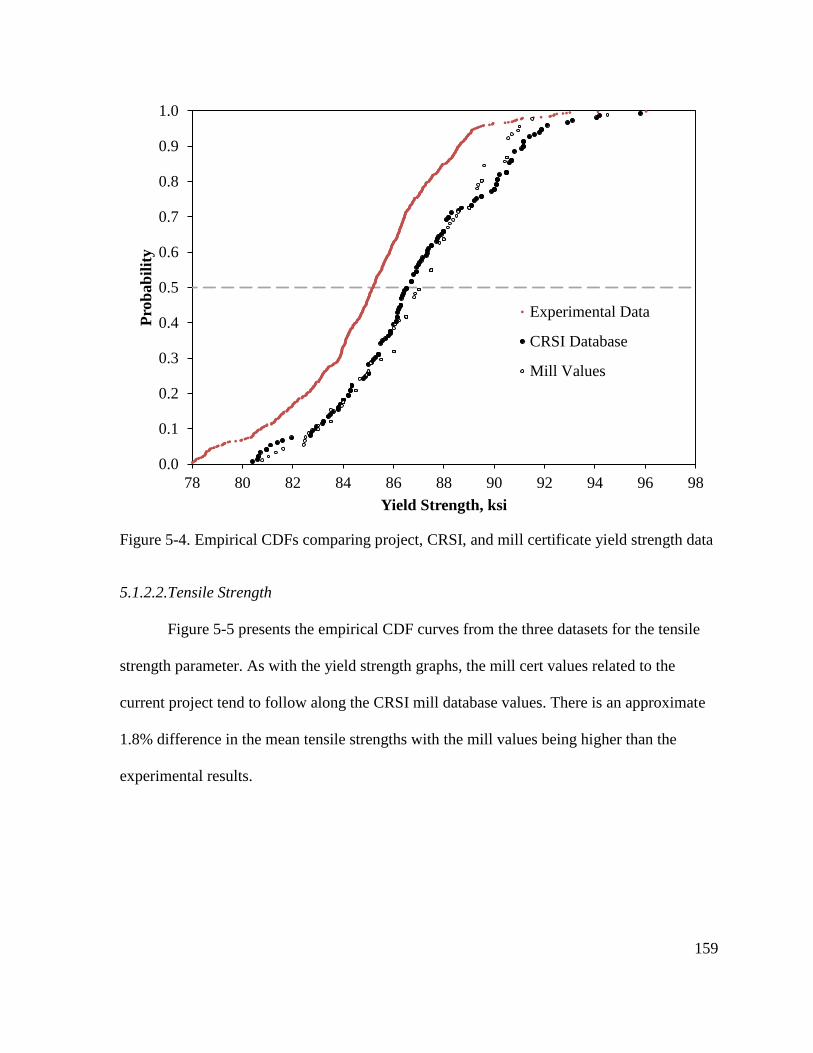
159

Figure 5-4. Empirical CDFs comparing project, CRSI, and mill certificate yield strength data

5.1.2.2.Tensile Strength

Figure 5-5 presents the empirical CDF curves from the three datasets for the tensile

strength parameter. As with the yield strength graphs, the mill cert values related to the

current project tend to follow along the CRSI mill database values. There is an approximate

1.8% difference in the mean tensile strengths with the mill values being higher than the

experimental results.

0.0

0.1

0.2

0.3

0.4

0.5

0.6

0.7

0.8

0.9

1.0

78 80 82 84 86 88 90 92 94 96 98

Pro

bab

ilit

y

Yield Strength, ksi

Experimental Data

CRSI Database

Mill Values

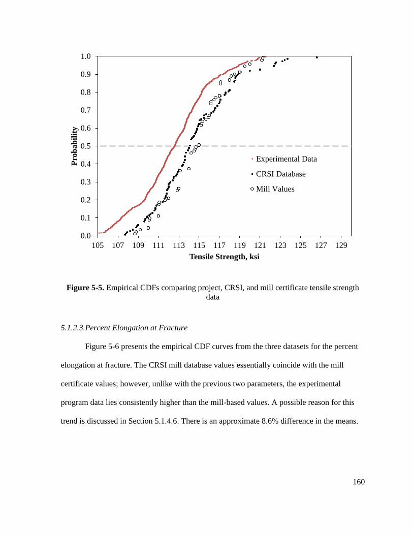
160

Figure 5-5. Empirical CDFs comparing project, CRSI, and mill certificate tensile strength

data

5.1.2.3.Percent Elongation at Fracture

Figure 5-6 presents the empirical CDF curves from the three datasets for the percent

elongation at fracture. The CRSI mill database values essentially coincide with the mill

certificate values; however, unlike with the previous two parameters, the experimental

program data lies consistently higher than the mill-based values. A possible reason for this

trend is discussed in Section 5.1.4.6. There is an approximate 8.6% difference in the means.

0.0

0.1

0.2

0.3

0.4

0.5

0.6

0.7

0.8

0.9

1.0

105 107 109 111 113 115 117 119 121 123 125 127 129

Pro

bab

ilit

y


Experimental Data

CRSI Database

Mill Values

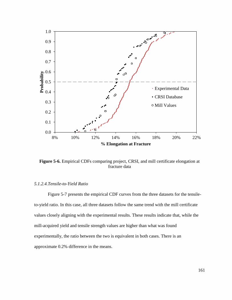
161

Figure 5-6. Empirical CDFs comparing project, CRSI, and mill certificate elongation at

fracture data

5.1.2.4.Tensile-to-Yield Ratio

Figure 5-7 presents the empirical CDF curves from the three datasets for the tensile-

to-yield ratio. In this case, all three datasets follow the same trend with the mill certificate

values closely aligning with the experimental results. These results indicate that, while the

mill-acquired yield and tensile strength values are higher than what was found

experimentally, the ratio between the two is equivalent in both cases. There is an

approximate 0.2% difference in the means.

0.0

0.1

0.2

0.3

0.4

0.5

0.6

0.7

0.8

0.9

1.0

8% 10% 12% 14% 16% 18% 20% 22%

Pro

bab

ilit

y

% Elongation at Fracture

Experimental Data

CRSI Database

Mill Values

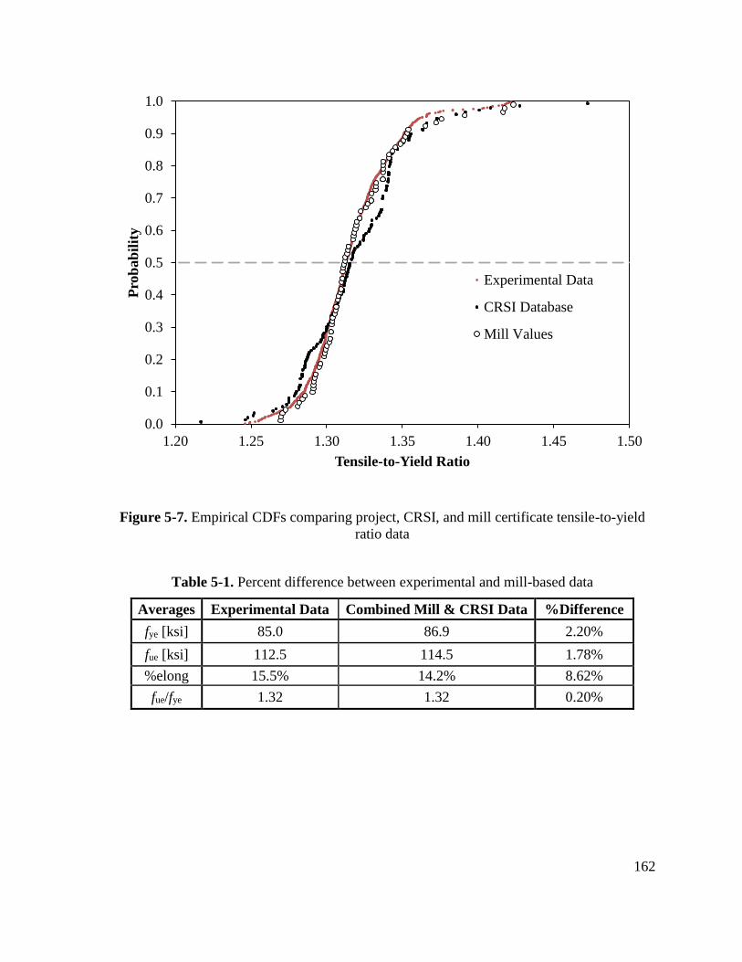
162

Figure 5-7. Empirical CDFs comparing project, CRSI, and mill certificate tensile-to-yield

ratio data

Table 5-1. Percent difference between experimental and mill-based data

Averages Experimental Data Combined Mill & CRSI Data %Difference

fye [ksi] 85.0 86.9 2.20%

fue [ksi] 112.5 114.5 1.78%

%elong 15.5% 14.2% 8.62%

fue/fye 1.32 1.32 0.20%

0.0

0.1

0.2

0.3

0.4

0.5

0.6

0.7

0.8

0.9

1.0

1.20 1.25 1.30 1.35 1.40 1.45 1.50

Pro

bab

ilit

y


Experimental Data

CRSI Database

Mill Values

163

5.1.3. Analysis of Variabilities

As stated in Section 3.4.2., each test specimen was given a unique identification

number indicating its mill, heat, and 20-foot bar of origin. Not only does this allow the data

to be filtered on the basis of one or more common variables (ex: tensile strengths of all No. 6

bar tests from Mill 2 Heat 3), but it also permits the data to be interpreted in terms of those

common variables (ex: standard deviation for all No. 6 bar tests from Mill 2 Heat 3). An

advantage of this is the increased ability to identify trends in the dataset and to detect and/or

explain anomalies.

This section specifically addresses the degree of variability associated with each of

the five main stress-strain parameters in terms of three variables: producing mills, heats

within a mill, and twenty-foot bars within a heat. The coefficient of variation (CV) is used as

the primary indicator of variability. The following eight topics are addressed: variability

between the three mills, average variability within a mill, average variability between heats

from a common mill, average variability between heats from a common mill by bar size,

average variability within a heat, average variability within a heat by bar size, average

variability between three 20’ bars from a common heat, and average variability within a 20-

foot bar (between three specimens from a common 20-foot bar).

5.1.3.1.Mills

Table 5-2 provides the average experimental values corresponding to each of the

three mills and the five main stress-strain parameters. Included at the bottom of the table are

the standard deviation and coefficient of variation (CV) of the mill averages for each of the

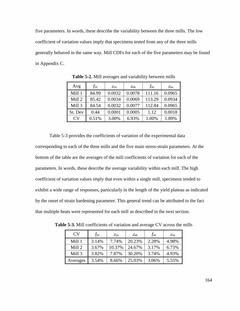
164

five parameters. In words, these describe the variability between the three mills. The low

coefficient of variation values imply that specimens tested from any of the three mills

generally behaved in the same way. Mill CDFs for each of the five parameters may be found

in Appendix C.

Table 5-2. Mill averages and variability between mills

Avg fye ye sh fue su

Mill 1 84.99 0.0032 0.0078 111.16 0.0965

Mill 2 85.42 0.0034 0.0069 113.29 0.0934

Mill 3 84.54 0.0032 0.0077 112.84 0.0965

St. Dev 0.44 0.0001 0.0005 1.12 0.0018

CV 0.51% 3.00% 6.93% 1.00% 1.89%

Table 5-3 provides the coefficients of variation of the experimental data

corresponding to each of the three mills and the five main stress-strain parameters. At the

bottom of the table are the averages of the mill coefficients of variation for each of the

parameters. In words, these describe the average variability within each mill. The high

coefficient of variation values imply that even within a single mill, specimens tended to

exhibit a wide range of responses, particularly in the length of the yield plateau as indicated

by the onset of strain hardening parameter. This general trend can be attributed to the fact

that multiple heats were represented for each mill as described in the next section.

Table 5-3. Mill coefficients of variation and average CV across the mills

CV fye ye sh fue su

Mill 1 3.14% 7.74% 20.23% 2.28% 4.98%

Mill 2 3.67% 10.37% 24.67% 3.17% 6.73%

Mill 3 3.82% 7.87% 30.20% 3.74% 4.93%

Averages 3.54% 8.66% 25.03% 3.06% 5.55%

165

5.1.3.2.Heats

A similar approach to that just described for mills can be used to determine the

variability between and within heats. Note that it would not make sense to compare all 25

heats with one another directly as they are associated with different producing mills. As such,

the variability “between” heats is defined as the average variability between heats from a

common mill. The average variability within a heat, however, is defined the same as for the

mills: average of the coefficients of variation of all the tests associated with each heat.

Two tables of heats analogous to Tables 5-2 and 5-3 for mills could be presented but

would be too large to comfortably fit into the body of the report. Nonetheless, Tables 5-6 and

5-7 summarize what would have been the bottom lines of these tables. The values in Table 5-

6 illustrate that even within a single mill the variability between different heats can be

somewhat high. Compared to the average variability within a mill, the average variability

within a heat is noticeably lower (Table 5-7). It should be noted that it is difficult to make

broad, substantive claims about variation between heats as different heats contained different

bar sizes (refer Appendix A). Section 5.1.3.4 addresses this issue by defining the variability

within and between heats in terms of individual bar sizes. Heat CDFs for each of the five

parameters may be found in Appendix D.

5.1.3.3.Twenty-foot Bars

Table 5-6 summarizes the average variability between twenty-foot bars from a

common heat in terms of the coefficient of variation. Table 5-7 summarizes the average

variability within a single twenty-foot bar. The coefficients of variation presented in these

166

two tables for the twenty-foot bars were defined in the same way as just described for the

heats. At this level of detail, the coefficients of variation for the yield strength, tensile

strength, and onset of strain hardening are lower than in any of the other methods of

comparison.

5.1.3.4.Heats by Bar Size

The primary purpose of this section is to expand on the observations presented in

section 5.1.3.2 by evaluating the variability between and within heats in terms of individual

bar sizes as this offers a more practical interpretation of the data. Table 5-4 summarizes the

variability between heats from a common mill for each bar size. The values in the table are

obtained by finding the coefficient of variation of the heat averages within a mill (ex: M1H1,

M1H2, M1H3 – 9 tests in each) for a given bar size and then taking the average coefficient of

variation across the three mills for that bar size. This represents the case in which a shipment

of steel from a single manufacturer includes multiples heats for a given bar size, and the

variability between those heats is of interest.

Table 5-5 summarizes the average variability within a single heat for each bar size.

The values in this table where obtained by determining the coefficient of variation for each

combination of mill, heat, and bar size (ex: M1H1 No. 4 bars – 9 tests in each) and averaging

across all the heats for that bar size (9 heats for each bar size). This represents the case in

which a shipment of steel includes bars from only one heat, and the variability within that

heat and for a given bar size is of interest.

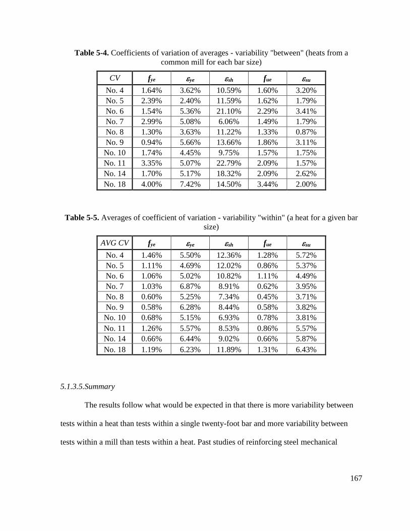
167

Table 5-4. Coefficients of variation of averages - variability "between" (heats from a

common mill for each bar size)

CV fye ye sh fue su

No. 4 1.64% 3.62% 10.59% 1.60% 3.20%

No. 5 2.39% 2.40% 11.59% 1.62% 1.79%

No. 6 1.54% 5.36% 21.10% 2.29% 3.41%

No. 7 2.99% 5.08% 6.06% 1.49% 1.79%

No. 8 1.30% 3.63% 11.22% 1.33% 0.87%

No. 9 0.94% 5.66% 13.66% 1.86% 3.11%

No. 10 1.74% 4.45% 9.75% 1.57% 1.75%

No. 11 3.35% 5.07% 22.79% 2.09% 1.57%

No. 14 1.70% 5.17% 18.32% 2.09% 2.62%

No. 18 4.00% 7.42% 14.50% 3.44% 2.00%

Table 5-5. Averages of coefficient of variation - variability "within" (a heat for a given bar

size)

AVG CV fye ye sh fue su

No. 4 1.46% 5.50% 12.36% 1.28% 5.72%

No. 5 1.11% 4.69% 12.02% 0.86% 5.37%

No. 6 1.06% 5.02% 10.82% 1.11% 4.49%

No. 7 1.03% 6.87% 8.91% 0.62% 3.95%

No. 8 0.60% 5.25% 7.34% 0.45% 3.71%

No. 9 0.58% 6.28% 8.44% 0.58% 3.82%

No. 10 0.68% 5.15% 6.93% 0.78% 3.81%

No. 11 1.26% 5.57% 8.53% 0.86% 5.57%

No. 14 0.66% 6.44% 9.02% 0.66% 5.87%

No. 18 1.19% 6.23% 11.89% 1.31% 6.43%

5.1.3.5.Summary

The results follow what would be expected in that there is more variability between

tests within a heat than tests within a single twenty-foot bar and more variability between

tests within a mill than tests within a heat. Past studies of reinforcing steel mechanical

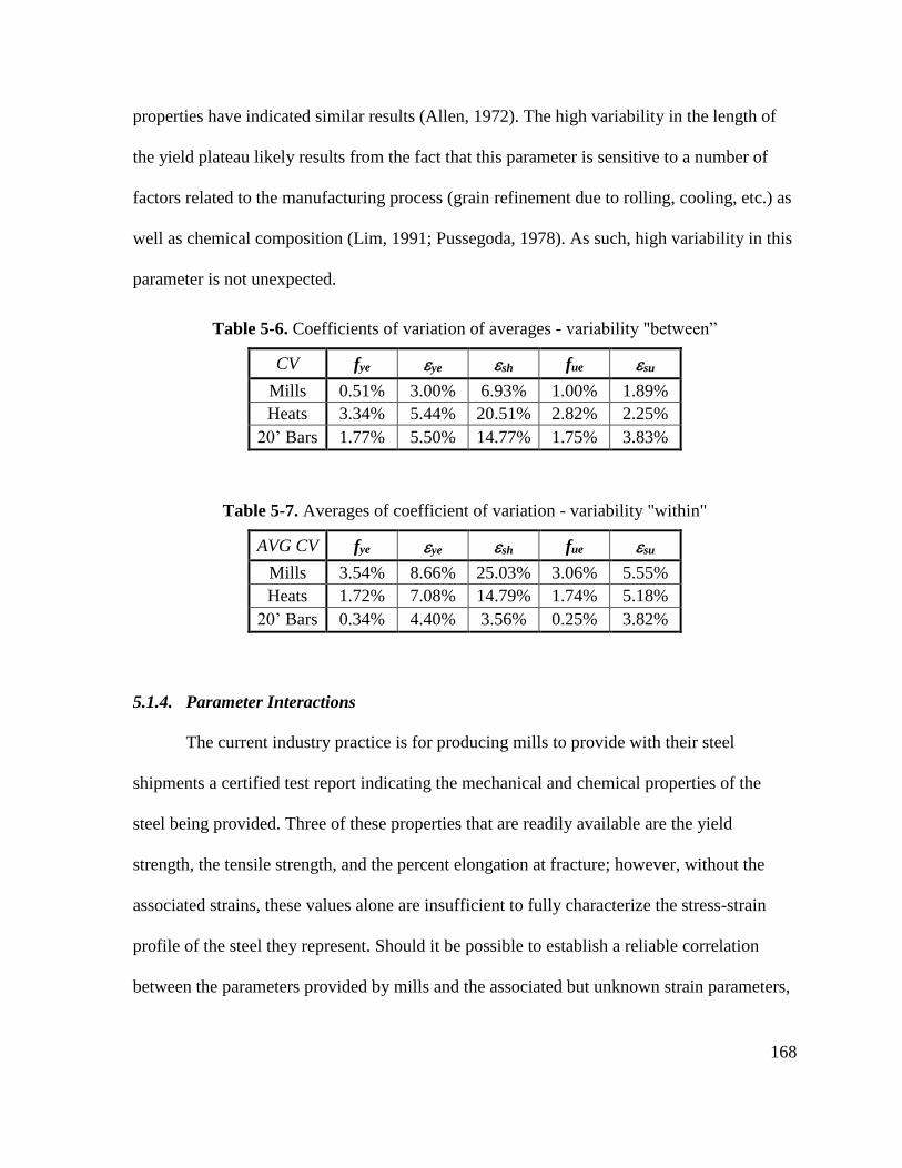
168

properties have indicated similar results (Allen, 1972). The high variability in the length of

the yield plateau likely results from the fact that this parameter is sensitive to a number of

factors related to the manufacturing process (grain refinement due to rolling, cooling, etc.) as

well as chemical composition (Lim, 1991; Pussegoda, 1978). As such, high variability in this

parameter is not unexpected.

Table 5-6. Coefficients of variation of averages - variability "between”

CV fye ye sh fue su

Mills 0.51% 3.00% 6.93% 1.00% 1.89%

Heats 3.34% 5.44% 20.51% 2.82% 2.25%

20’ Bars 1.77% 5.50% 14.77% 1.75% 3.83%

Table 5-7. Averages of coefficient of variation - variability "within"

AVG CV fye ye sh fue su

Mills 3.54% 8.66% 25.03% 3.06% 5.55%

Heats 1.72% 7.08% 14.79% 1.74% 5.18%

20’ Bars 0.34% 4.40% 3.56% 0.25% 3.82%

5.1.4. Parameter Interactions

The current industry practice is for producing mills to provide with their steel

shipments a certified test report indicating the mechanical and chemical properties of the

steel being provided. Three of these properties that are readily available are the yield

strength, the tensile strength, and the percent elongation at fracture; however, without the

associated strains, these values alone are insufficient to fully characterize the stress-strain

profile of the steel they represent. Should it be possible to establish a reliable correlation

between the parameters provided by mills and the associated but unknown strain parameters,

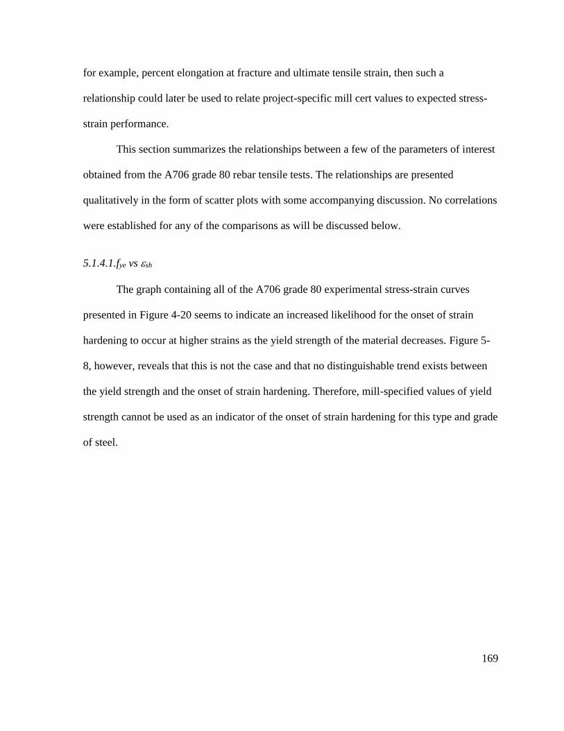
169

for example, percent elongation at fracture and ultimate tensile strain, then such a

relationship could later be used to relate project-specific mill cert values to expected stress-

strain performance.

This section summarizes the relationships between a few of the parameters of interest

obtained from the A706 grade 80 rebar tensile tests. The relationships are presented

qualitatively in the form of scatter plots with some accompanying discussion. No correlations

were established for any of the comparisons as will be discussed below.

5.1.4.1.fye vs sh

The graph containing all of the A706 grade 80 experimental stress-strain curves

presented in Figure 4-20 seems to indicate an increased likelihood for the onset of strain

hardening to occur at higher strains as the yield strength of the material decreases. Figure 5-

8, however, reveals that this is not the case and that no distinguishable trend exists between

the yield strength and the onset of strain hardening. Therefore, mill-specified values of yield

strength cannot be used as an indicator of the onset of strain hardening for this type and grade

of steel.

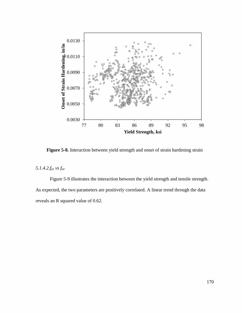
170

Figure 5-8. Interaction between yield strength and onset of strain hardening strain

5.1.4.2.fye vs fue

Figure 5-9 illustrates the interaction between the yield strength and tensile strength.

As expected, the two parameters are positively correlated. A linear trend through the data

reveals an R squared value of 0.62.

0.0030

0.0050

0.0070

0.0090

0.0110

0.0130

77 80 83 86 89 92 95 98

On

set

of

Str

ain

Hard

enin

g, in

/in

Yield Strength, ksi

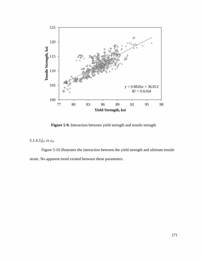
171

Figure 5-9. Interaction between yield strength and tensile strength

5.1.4.3.fye vs su

Figure 5-10 illustrates the interaction between the yield strength and ultimate tensile

strain. No apparent trend existed between these parameters.

y = 0.8826x + 36.812

R² = 0.6164

100

105

110

115

120

125

77 80 83 86 89 92 95 98

Ten

sile

Str

ength

, k

si

Yield Strength, ksi

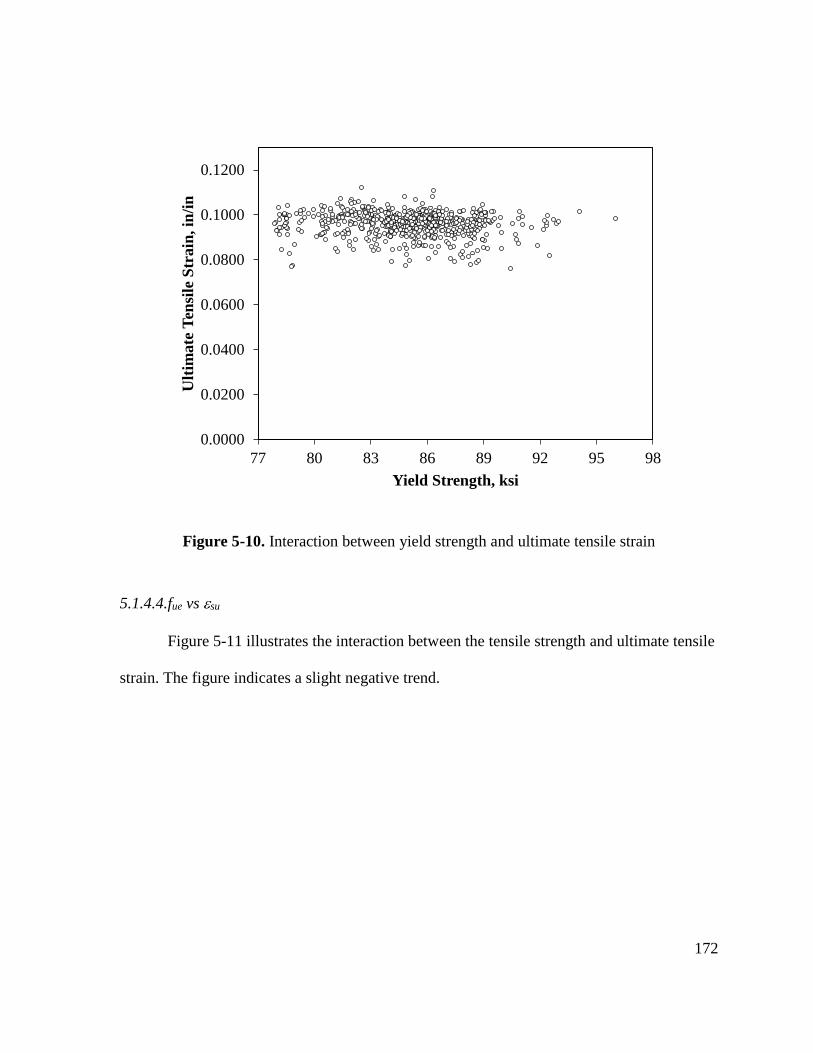
172

Figure 5-10. Interaction between yield strength and ultimate tensile strain

5.1.4.4.fue vs su

Figure 5-11 illustrates the interaction between the tensile strength and ultimate tensile

strain. The figure indicates a slight negative trend.

0.0000

0.0200

0.0400

0.0600

0.0800

0.1000

0.1200

77 80 83 86 89 92 95 98

Ult

imate

Ten

sile

Str

ain

, in

/in

Yield Strength, ksi

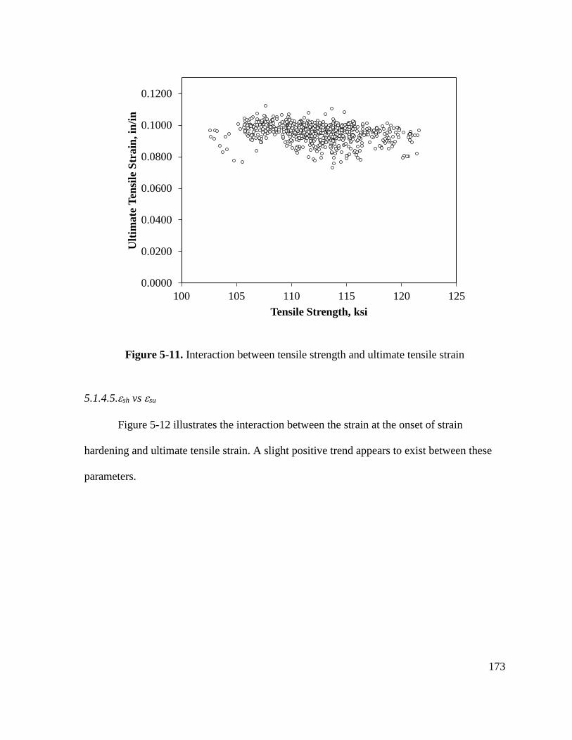
173

Figure 5-11. Interaction between tensile strength and ultimate tensile strain

5.1.4.5.sh vs su

Figure 5-12 illustrates the interaction between the strain at the onset of strain

hardening and ultimate tensile strain. A slight positive trend appears to exist between these

parameters.

0.0000

0.0200

0.0400

0.0600

0.0800

0.1000

0.1200

100 105 110 115 120 125

Ult

imate

Ten

sile

Str

ain

, in

/in


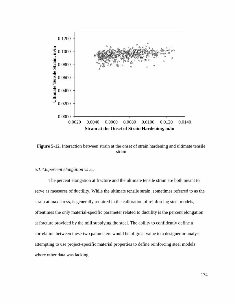
174

Figure 5-12. Interaction between strain at the onset of strain hardening and ultimate tensile

strain

5.1.4.6.percent elongation vs su

The percent elongation at fracture and the ultimate tensile strain are both meant to

serve as measures of ductility. While the ultimate tensile strain, sometimes referred to as the

strain at max stress, is generally required in the calibration of reinforcing steel models,

oftentimes the only material-specific parameter related to ductility is the percent elongation

at fracture provided by the mill supplying the steel. The ability to confidently define a

correlation between these two parameters would be of great value to a designer or analyst

attempting to use project-specific material properties to define reinforcing steel models

where other data was lacking.

0.0000

0.0200

0.0400

0.0600

0.0800

0.1000

0.1200

0.0020 0.0040 0.0060 0.0080 0.0100 0.0120 0.0140

Ult

imate

Ten

sile

Str

ain

, in

/in

Strain at the Onset of Strain Hardening, in/in

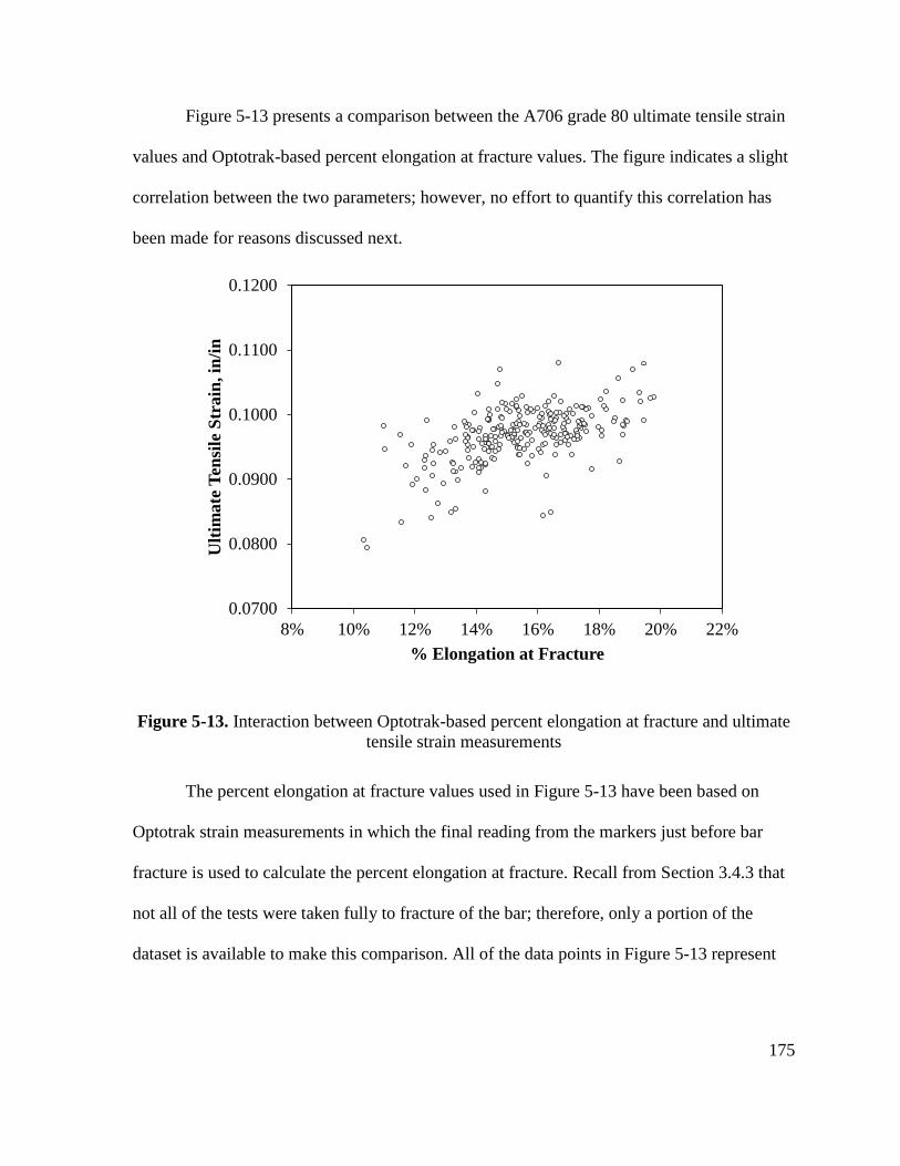
175

Figure 5-13 presents a comparison between the A706 grade 80 ultimate tensile strain

values and Optotrak-based percent elongation at fracture values. The figure indicates a slight

correlation between the two parameters; however, no effort to quantify this correlation has

been made for reasons discussed next.

Figure 5-13. Interaction between Optotrak-based percent elongation at fracture and ultimate

tensile strain measurements

The percent elongation at fracture values used in Figure 5-13 have been based on

Optotrak strain measurements in which the final reading from the markers just before bar

fracture is used to calculate the percent elongation at fracture. Recall from Section 3.4.3 that

not all of the tests were taken fully to fracture of the bar; therefore, only a portion of the

dataset is available to make this comparison. All of the data points in Figure 5-13 represent

0.0700

0.0800

0.0900

0.1000

0.1100

0.1200

8% 10% 12% 14% 16% 18% 20% 22%

Ult

imate

Ten

sile

Str

ain

, in

/in

% Elongation at Fracture

176

fractured bars. A limited number of additional percent elongation at fracture values were

obtained using the conventional method of measuring a predefined 8” gage length prior to the

test and then re-measuring the same gage length after the test in the event that fracture

occurred within the gage length. A comparison of these hand measurements to the Optotrak-

based values reveals that, on average, there is a 14 percent-difference in the percent

elongation measurements. To clarify, this translates into Optotrak-based percent elongation at

fracture values that are, on average, 1.8 percentage points higher than their corresponding

hand measured values. An attempt to explain this observation is provided in the next

paragraph.

Prior to the onset of necking, a tensile test specimen is in a state of combined plastic

and elastic strain. As necking commences (a concentration of plastic deformation) the non-

necked regions of the bar can be observed to relax, essentially recovering some of the

existing elastic strains. Upon fracture of the test specimen, any remaining elastic strains are

recovered and the combined length of the two fractured ends represents the total plastic

elongation. The traditional hand measurement approach to determining percent elongation at

fracture by fitting the fractured ends together and re-measuring the elongated gage length

necessarily captures the plastic strain in the bar. The Optotrak-based method of determining

the percent elongation at fracture by taking the last recording of strain before fracture

necessarily captures the plastic strain in addition to any remaining elastic strains. For this

reason, it can be expected that the Optotrak-based approach would predict a higher percent

elongation at fracture value than the traditional approach, hence the hesitancy to define a

177

quantitative relationship between the percent elongation at fracture values provided in the

mill certificates and those obtained using the Optotrak system.

5.1.5. Yield Strengths Falling Below 80 ksi

As stated in Section 4.2.3.2, a number of the No. 11, 14, and 18 bars had yield

strengths falling below the ASTM lower limit of 80 ksi after accounting for pressure losses

occurring in the large bar testing rig. The additional tests of nine No. 11 bars and nine No. 14

bars described in Section 3.4.4 confirmed that this was an accurate assessment and not a by-

product of the adjustment factor. While no definitive explanation is offered as to why this

behavior revealed itself exclusively in the No. 11, 14, and 18 bar tests, the remainder of this

section describes the extent of the phenomenon.

The number of No. 11 bar tests having yield strength below 80 ksi was limited to a

single heat from Mill 1 (heat 5). In this specific case, there were no other bar sizes

represented in this heat (see Appendix A); therefore, no comparison can be made to

determine if the behavior was related to the bar size or the entire heat. Following the

adjustment, all nine of the test specimens from this heat had yield strengths below 80 ksi with

78.1 ksi being the minimum and 78.6 ksi the maximum.

Similar to the No. 11 bars, the number of No. 14 bar tests having yield strength below

80 ksi was also limited to a single heat, this time from Mill 3 (heat 7). However, unlike the

previous case, there were additional bar sizes represented in this heat. The average yield

strength of Mill 3 Heat 7, which was comprised of No. 10-No. 18 bars (Appendix A), was

80.35 ksi. Table 5-8 summarizes the averages by bar size. From the table, it is clear that

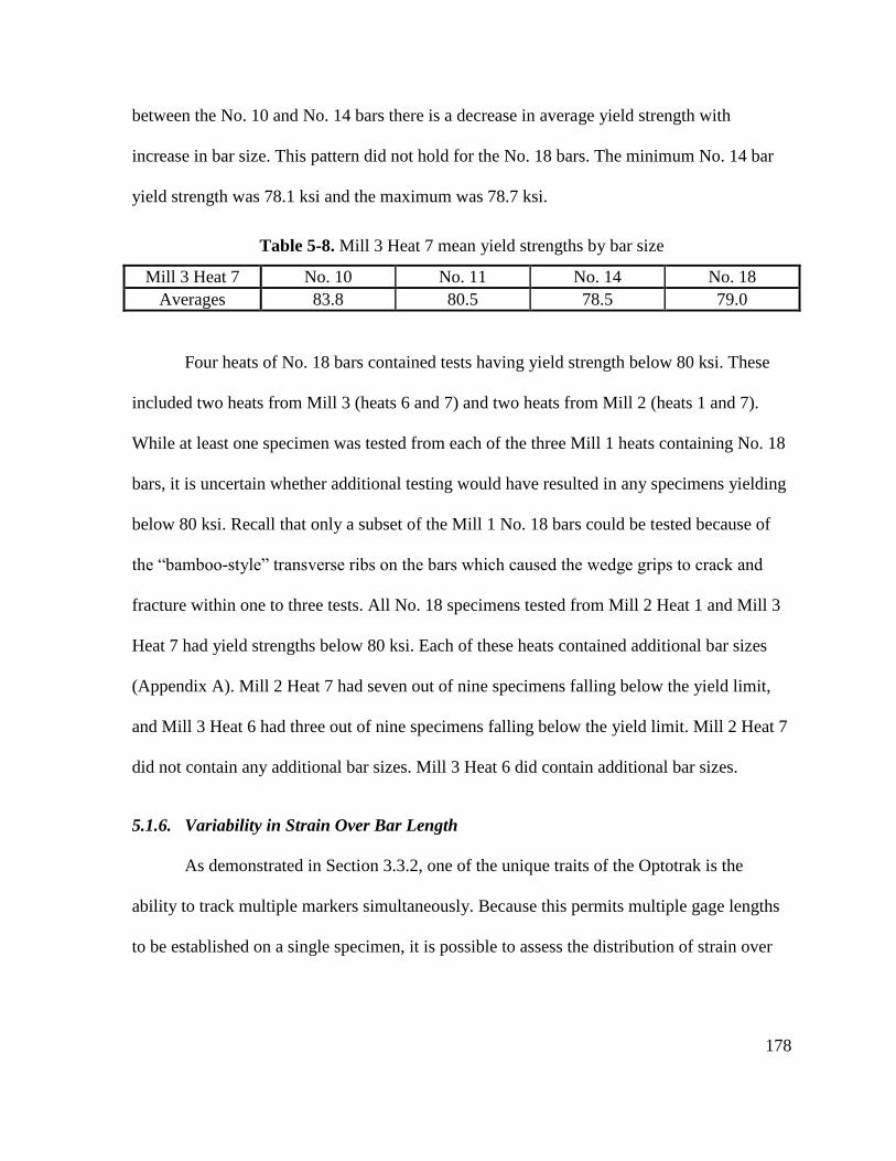
178

between the No. 10 and No. 14 bars there is a decrease in average yield strength with

increase in bar size. This pattern did not hold for the No. 18 bars. The minimum No. 14 bar

yield strength was 78.1 ksi and the maximum was 78.7 ksi.

Table 5-8. Mill 3 Heat 7 mean yield strengths by bar size

Mill 3 Heat 7 No. 10 No. 11 No. 14 No. 18

Averages 83.8 80.5 78.5 79.0

Four heats of No. 18 bars contained tests having yield strength below 80 ksi. These

included two heats from Mill 3 (heats 6 and 7) and two heats from Mill 2 (heats 1 and 7).

While at least one specimen was tested from each of the three Mill 1 heats containing No. 18

bars, it is uncertain whether additional testing would have resulted in any specimens yielding

below 80 ksi. Recall that only a subset of the Mill 1 No. 18 bars could be tested because of

the “bamboo-style” transverse ribs on the bars which caused the wedge grips to crack and

fracture within one to three tests. All No. 18 specimens tested from Mill 2 Heat 1 and Mill 3

Heat 7 had yield strengths below 80 ksi. Each of these heats contained additional bar sizes

(Appendix A). Mill 2 Heat 7 had seven out of nine specimens falling below the yield limit,

and Mill 3 Heat 6 had three out of nine specimens falling below the yield limit. Mill 2 Heat 7

did not contain any additional bar sizes. Mill 3 Heat 6 did contain additional bar sizes.

5.1.6. Variability in Strain Over Bar Length

As demonstrated in Section 3.3.2, one of the unique traits of the Optotrak is the

ability to track multiple markers simultaneously. Because this permits multiple gage lengths

to be established on a single specimen, it is possible to assess the distribution of strain over

179

the entire instrumented region of the specimen at each reading of the data. This poses an

advantage over traditional methods of capturing bar strains such as with strain gages and

extensometers which, while reliable, are limited to a single gage length.

An unanticipated consequence of using this type of instrumentation was the

realization that the strains varied over the length of the test specimens at a given instant in

time and that the variability between gage lengths seemingly increased with increasing strain.

It is perhaps not surprising that the strains should vary over the length of the bar as it is

neither a homogeneous material or of a continuous cross-section (as a result of the

longitudinal and transverse ribs). Additionally, some degree of variability in the different

gage lengths can be attributed to the precision of the instrumentation. Table 5-9 summarizes

the average variation between the six 2” gage lengths for the yield strain, onset of strain

hardening, and ultimate tensile strain considering all tests which is calculated by finding the

coefficient of variation between the six gage lengths for each test and then averaging all of

the coefficients of variation.

Table 5-9 and Figure 5-14 both indicate that the highest variability in the strains was

at the yield point while the lowest was shortly thereafter at the onset of strain hardening. This

trend for the variability to be high towards the beginning of the tests, lowest near the middle,

and high again near the end may be the result of low variability in the strains while they are

small and the precision of the Optotrak is lower coupled with an increased variability in the

strains when they are large and the precision of the Optotrak is higher. This would imply that

the higher variability at the yield point is more a result of instrumentation than actual

variation in the strains. In any case, the point to be emphasized is not so much that the strains

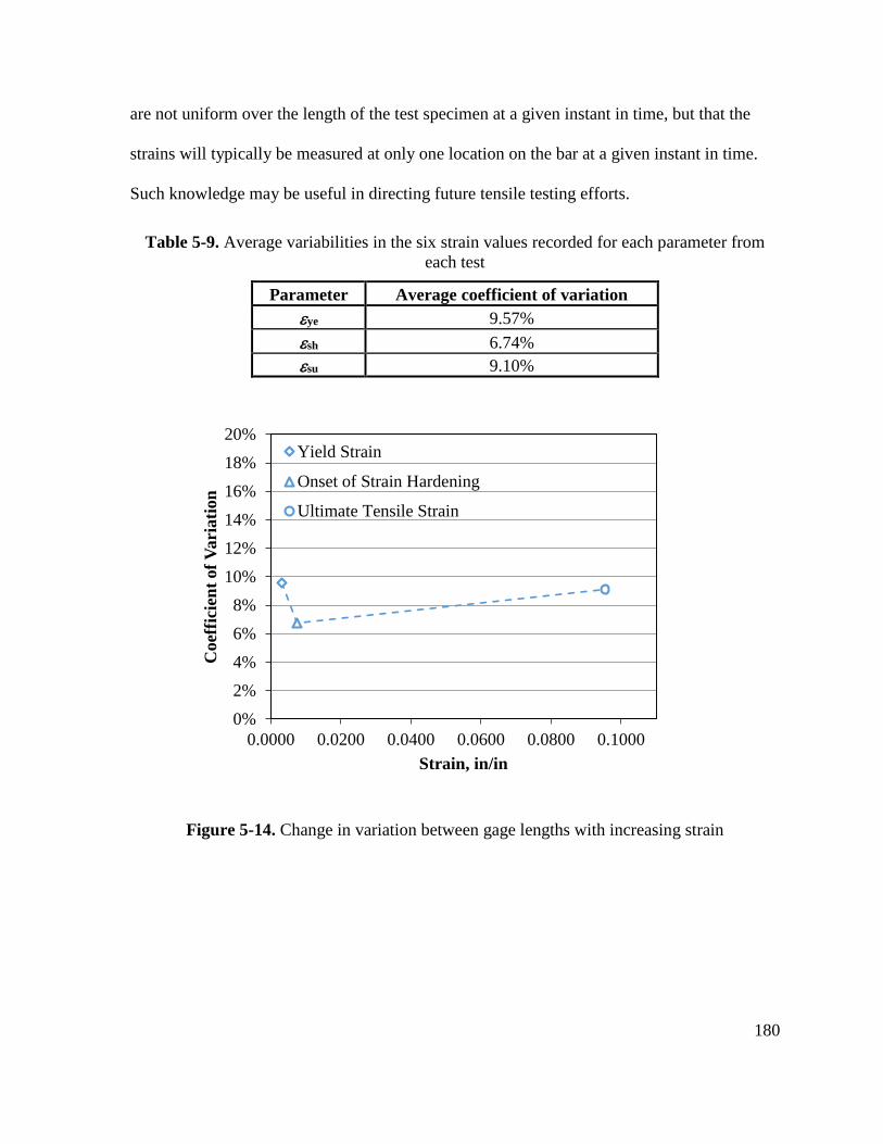
180

are not uniform over the length of the test specimen at a given instant in time, but that the

strains will typically be measured at only one location on the bar at a given instant in time.

Such knowledge may be useful in directing future tensile testing efforts.

Table 5-9. Average variabilities in the six strain values recorded for each parameter from

each test

Parameter Average coefficient of variation

ye 9.57%

sh 6.74%

su 9.10%

Figure 5-14. Change in variation between gage lengths with increasing strain

0%

2%

4%

6%

8%

10%

12%

14%

16%

18%

20%

0.0000 0.0200 0.0400 0.0600 0.0800 0.1000

Coef

fici

ent

of

Vari

ati

on

Strain, in/in

Yield Strain

Onset of Strain Hardening

Ultimate Tensile Strain

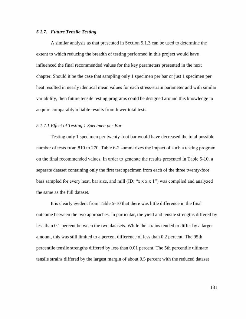
181

5.1.7. Future Tensile Testing

A similar analysis as that presented in Section 5.1.3 can be used to determine the

extent to which reducing the breadth of testing performed in this project would have

influenced the final recommended values for the key parameters presented in the next

chapter. Should it be the case that sampling only 1 specimen per bar or just 1 specimen per

heat resulted in nearly identical mean values for each stress-strain parameter and with similar

variability, then future tensile testing programs could be designed around this knowledge to

acquire comparably reliable results from fewer total tests.

5.1.7.1.Effect of Testing 1 Specimen per Bar

Testing only 1 specimen per twenty-foot bar would have decreased the total possible

number of tests from 810 to 270. Table 6-2 summarizes the impact of such a testing program

on the final recommended values. In order to generate the results presented in Table 5-10, a

separate dataset containing only the first test specimen from each of the three twenty-foot

bars sampled for every heat, bar size, and mill (ID: “x x x x 1”) was compiled and analyzed

the same as the full dataset.

It is clearly evident from Table 5-10 that there was little difference in the final

outcome between the two approaches. In particular, the yield and tensile strengths differed by

less than 0.1 percent between the two datasets. While the strains tended to differ by a larger

amount, this was still limited to a percent difference of less than 0.2 percent. The 95th

percentile tensile strengths differed by less than 0.01 percent. The 5th percentile ultimate

tensile strains differed by the largest margin of about 0.5 percent with the reduced dataset

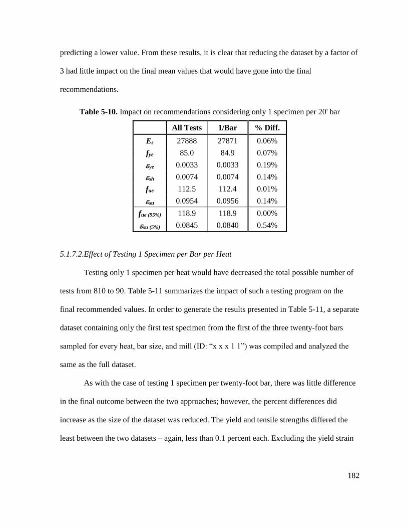
182

predicting a lower value. From these results, it is clear that reducing the dataset by a factor of

3 had little impact on the final mean values that would have gone into the final

recommendations.

Table 5-10. Impact on recommendations considering only 1 specimen per 20' bar

All Tests 1/Bar % Diff.

Es 27888 27871 0.06%

fye 85.0 84.9 0.07%

ye 0.0033 0.0033 0.19%

sh 0.0074 0.0074 0.14%

fue 112.5 112.4 0.01%

su 0.0954 0.0956 0.14%

fue (95%) 118.9 118.9 0.00%

su (5%) 0.0845 0.0840 0.54%

5.1.7.2.Effect of Testing 1 Specimen per Bar per Heat

Testing only 1 specimen per heat would have decreased the total possible number of

tests from 810 to 90. Table 5-11 summarizes the impact of such a testing program on the

final recommended values. In order to generate the results presented in Table 5-11, a separate

dataset containing only the first test specimen from the first of the three twenty-foot bars

sampled for every heat, bar size, and mill (ID: “x x x 1 1”) was compiled and analyzed the

same as the full dataset.

As with the case of testing 1 specimen per twenty-foot bar, there was little difference

in the final outcome between the two approaches; however, the percent differences did

increase as the size of the dataset was reduced. The yield and tensile strengths differed the

least between the two datasets – again, less than 0.1 percent each. Excluding the yield strain

183

parameter, the expected onset of strain hardening strains and the ultimate tensile strains

differed between the two datasets by less than 1 percent. The 95th percentile tensile strengths

differed by less than 0.1 percent. The 5th percentile ultimate tensile strains differed by less

than 0.01 percent with the reduced dataset now predicting a slightly higher value. Reducing

the dataset by a factor of 9 had some impact on the final mean values that would have gone

into the final recommendations; however, the largest percent difference between any two

parameters was still below 1.5 percent. It should be noted that these percentages are

extremely small and, for several of the parameters, no observable difference between the two

datasets is even distinguishable at the provided number of decimal places.

Table 5-11. Impact on recommendations considering only 1 specimen per 20’ bar and 1 20’

bar per heat

All Tests 1/Bar/Heat % Diff.

Es 27888 27970 0.29%

fye 85.0 84.9 0.03%

ye 0.0033 0.0033 1.26%

sh 0.0074 0.0074 0.49%

fue 112.5 112.5 0.06%

su 0.0954 0.0961 0.67%

fue (95%) 118.9 119.0 0.09%

su (5%) 0.0845 0.0845 0.01%

5.2. Strain Age Tests

5.2.1. Comparison with Literature Results

Based on the strain age test results presented in Chapter 4, it was concluded that A706

grade 80 rebar did not display identifiable susceptibility to the strain aging phenomenon. This

184

claim is substantiated based on the following three observations: (1) the anticipated trends of

an increase in yield and tensile strength and/or a decrease in the ultimate tensile strain with

increasing pre-strain and aging period failed to appear in the results plotted in Section 4.3, (2)

the magnitude of the deviations of the strain age test results from the benchmark tests was

negligibly small as compared to the magnitudes presented in the literature (compare Tables

2.6-2.8 with Figures 4.32-4.33), and (3) the difference between the strain age tests and the

benchmark values rarely exceeded the standard deviation of the tensile test represented by

the benchmark value, thus making the effects of strain aging nearly indistinguishable from

variation already present in the tensile test data.

A limitation of the current investigation into the strain aging susceptibility of A706

grade 80 rebar was the inability to define a vanadium to nitrogen (V/N) ratio for the steel as

the percentage of nitrogen is not provided with the mill test certificates. The literature review

demonstrated that microalloying elements such as vanadium, which provides increased

strength to the rebar while still maintaining high ductility, have been shown to inhibit strain

aging in reinforcing steels through bonding with nitrogen, which is a known contributor to

strain aging. Therefore, despite chemical composition playing a major role in the strain aging

susceptibility of reinforcing steel, it could not be properly evaluated within the current

research effort.

5.2.2. Future Strain Age Testing

Based on the literature review observations and the points addressed in the previous

section, two areas of future research into the strain aging susceptibility of A706 grade 80

185

rebar stand out: (1) perform chemical analysis to identify the nitrogen percentage such that a

V/N ratio may be determined and compared with additional tests and (2) investigation of

strain aging embrittlement in bent reinforcing bars used as hooks or transverse reinforcement.

The latter of these items is particularly relevant to earthquake structural engineering as the

current design philosophy relies on the structures ability to dissipate energy through the

ductile behavior of inelastic mechanism strategically located to prevent sudden, brittle

failures. Anchorage and confinement failures resulting from strain aging and early fracture of

bent bars should therefore be avoided.

5.3. Cyclic Tests

5.3.1. Future Cyclic Testing

The two main objectives of the cyclic testing program were the evaluation of existing

reinforcing steel models to be able to characterize the A706 grade 80 cyclic stress-strain

curve and the impact of bar strain history on the ultimate tensile strain. As illustrated in the

previous chapter, the extent of the cyclic testing program was greatly limited by the type and

condition of the testing equipment used. Nonetheless, it was demonstrated that an existing

reinforcing steel model was able to characterize the shape of the stress-strain curve for a

randomly cycled A706 grade 80 rebar specimen. Further research in this area could be

largely analytical and involve the evaluation of additional stress-strain models to the cyclic

data already collected and presented in Chapter 4.

Based on the stated limitations, the impact of load history on the ultimate tensile

strain of the rebar deserves some further investigation. The results in Table 4-6 indicate that

186

the imposed load histories did not cause a reduction in the strain at max stress values for the

No. 5 bars. In fact, it appears that the cyclic tests showed higher ultimate tensile strains than

the tensile test mill-heat-size average. Two possible explanations for this observation are that

(1) the benchmark value was based on nine tests originating from three 20’ bars while the

cyclic tests originated from a fourth 20’ bar from the same heat or (2) the fact that the

benchmark value is based on Optotrak strain readings while the cyclic test strains were

obtained with an extensometer as stated in Section 3.3.2. Thus, the difference could be a

result of difference in instrumentation.

The more strenuous load history of the No. 7 bar in Table 4-6, however, which

included multiple cycles in with the bar visibly buckled, does indicate a reduction in the

ultimate tensile strain during the pull test. As this only represents one data point, future

research could reconsider this issue and address a larger number of bars sizes and load

histories to either confirm or reject this trend.

187

6. CONCLUSIONS

6.1. Summary

An assessment of the stress-strain behavior of ASTM A706 grade 80 reinforcement

was conducted at NC State University through experimental testing and analysis. A total of

788 tensile tests of No. 4 through No. 18 bars, in the as-rolled condition, originating from

three different producing mills and including multiple heats of steel from each mill provided

a substantial dataset of test results that was otherwise lacking in the literature. These results

were used to identify the expected values of key parameters necessary to define the

monotonic stress-strain curve of A706 grade 80 rebar: the yield strength, yield strain, strain at

onset of strain hardening, tensile strength, and ultimate tensile strain. Two subsets of tests

focused on the cyclic and strain aging performance of the steel. Based on the work just

described, the following conclusions are presented:

The current work increased the body of publically available A706 grade 80 stress-

strain data by over 650%. The recommendations for yield stress, yield strain, strain at

the onset of strain hardening, ultimate tensile strain, and tensile strength provided in

Table 6-1 may be used as the basis for future building code requirements.

Best-fit probability distributions were presented for both of the strength parameters as

well as the strain parameters based on the Kolmogorov-Smirnov goodness-of-fit test.

The yield strength values were shown to be well represented by the beta distribution,

while the yield strain values were shown to be well represented by the gamma

distribution. The strain at the onset of strain hardening values showed the highest

188

degree of variability and were not found to be well represented by any of the

considered distributions. The tensile strength values were shown to be well

represented by the lognormal distribution, and lastly, the ultimate tensile strain values

were shown to be well represented by the Weibull distribution.

The A706 grade 80 stress-strain curve is nearly identical in shape to the A706 grade

60 curve.

The cyclic stress-strain curve was accurately predicted using a currently available

cyclic reinforcing steel material model.

The shape of the strain hardening curve may be accurately characterized using

currently available monotonic rebar models.

About 7% of the tests failed to meet the ASTM minimum yield strength requirement

of 80 ksi. This behavior was limited to the No. 11, 14, and 18 bars.

The No. 11, 14, and 18 bars, overall, had lower yield and tensile strength than the No.

4 through No. 10 bars. However, no trends were evident for any other parameters as a

function of bar size.

A706 grade 80 rebar did not show susceptibility to strain aging for any of the

considered pre-strain levels, even up to an aging period of 6 months, however, further

studies on larger bar sizes may be worthwhile.

A706 grade 80 rebar may be reliably specified for capacity protected members and, as

a result, may reduce congestion in joints and provide a potential savings in terms of

reduced material and labor costs.

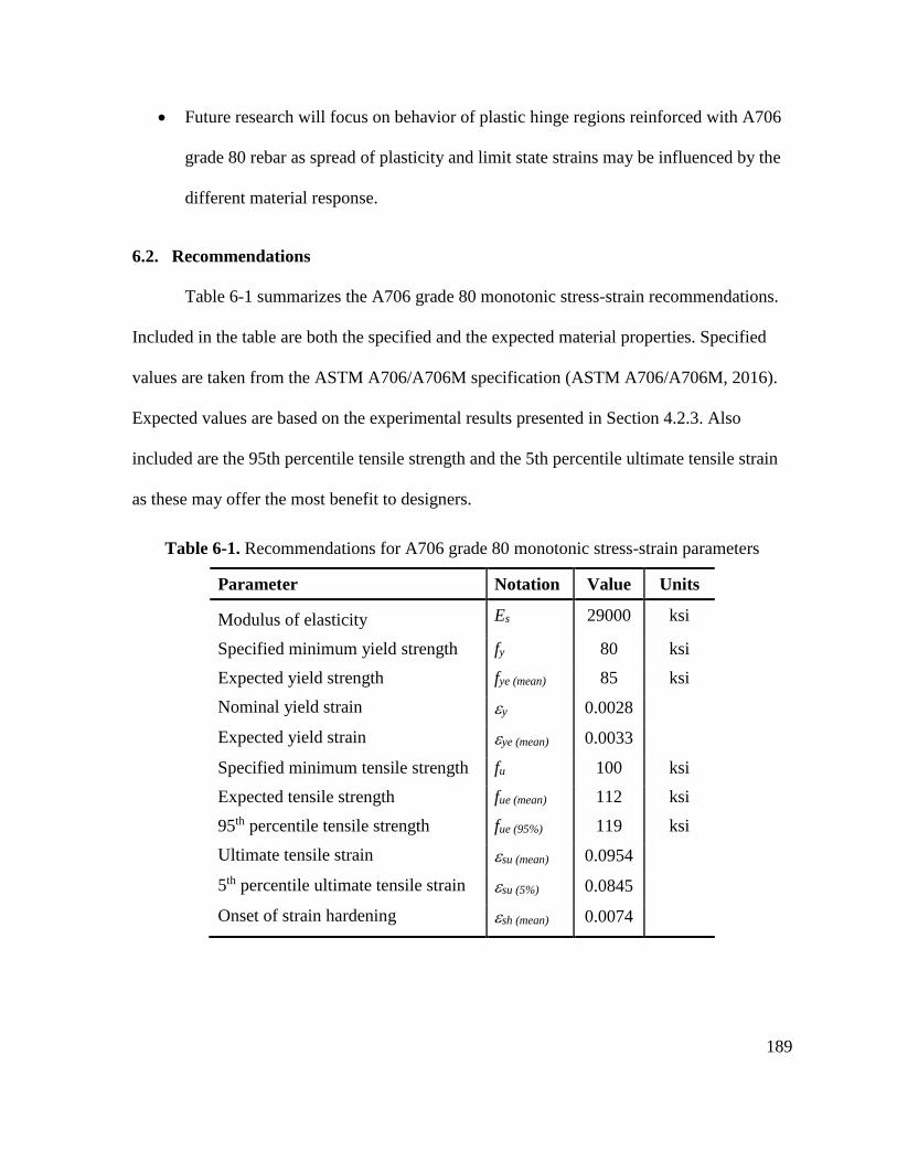
189

Future research will focus on behavior of plastic hinge regions reinforced with A706

grade 80 rebar as spread of plasticity and limit state strains may be influenced by the

different material response.

6.2. Recommendations

Table 6-1 summarizes the A706 grade 80 monotonic stress-strain recommendations.

Included in the table are both the specified and the expected material properties. Specified

values are taken from the ASTM A706/A706M specification (ASTM A706/A706M, 2016).

Expected values are based on the experimental results presented in Section 4.2.3. Also

included are the 95th percentile tensile strength and the 5th percentile ultimate tensile strain

as these may offer the most benefit to designers.

Table 6-1. Recommendations for A706 grade 80 monotonic stress-strain parameters

Parameter Notation Value Units

Modulus of elasticity Es 29000 ksi

Specified minimum yield strength fy 80 ksi

Expected yield strength fye (mean) 85 ksi

Nominal yield strain y 0.0028

Expected yield strain ye (mean) 0.0033

Specified minimum tensile strength fu 100 ksi

Expected tensile strength fue (mean) 112 ksi

95th percentile tensile strength fue (95%) 119 ksi

Ultimate tensile strain su (mean) 0.0954

5th percentile ultimate tensile strain su (5%) 0.0845

Onset of strain hardening sh (mean) 0.0074

190

7. REFERENCES

AASHTO. 2011. Guide Specification for LRFD Seismic Bridge Design, Second Edition with

2012 Interim Revisions. American Association of State Highway and Transportation

Officials, Washington, DC.

AASHTO. 2014. AASHTO LRFD Bridge Design Specifications, Customary U.S. Units,

Seventh Edition with 2016 Interim Revisions. American Association of State

Highway and Transportation Officials, Washington, DC.

ACI Committee 318, “Building Code Requirements for Structural Concrete (ACI318-11) and

Commentary,” American Concrete Institute, Farmington Hills, MI, 2011, 503 pp.

ACI Committee 318, “Building Code Requirements for Structural Concrete (ACI 318-14)

and Commentary,” American Concrete Institute, Farmington Hills, MI, 2014.

Allen, D. E. 1972. “Statistical Study of the Mechanical Properties of Reinforcing Bars,”

Building Research Note No. 85, Division of Building Research, National Research

Council, Ottawa, Canada, April, 8 pp.

ASTM A370 (2015), “Standard Test Methods and Definitions for Mechanical Testing of

Steel Products,” American Society for Testing and Materials, West Conshohocken,

PA, 50 pp.

ASTM A615/A615M-16, “Standard Specification for Deformed and Plain Carbon-Steel Bars

for Concrete Reinforcement,” ASTM International, West Conshohocken, PA, 2016, 8

pp.

191

ASTM A706/A706M-16, “Standard Specification for Deformed and Plain Low-Alloy Steel

Bars for Concrete Reinforcement,” ASTM International, West Conshohocken, PA,

2016, 7 pp.

Barbosa, A.R., T. Link, and D. Trejo. 2015. "Seismic Performance of High-Strength Steel

RC Bridge Columns." J. Bridge Eng., 10.1061/(ASCE)BE.1943-5592.0000769 ,

04015044.

Bournonville, M., J. Dahnke, and D. Darwin. 2004. “Statistical Analysis of the Mechanical

Properties and Weight of Reinforcing Bars.” Research Report SL 04-1. University of

Kansas.

CALTRANS. 2013. CALTRANS Seismic Design Criteria. Version 1.7. California

Department of Transportation.

Chang, G.A. and J.B., Mander. 1994. “Seismic energy based fatigue damage analysis of

bridge columns: Part 1 – Evaluation of seismic capacity.” Tech. Rep.

Multidisciplinary Center for Earthquake Engineering Research, University at Buffalo,

State University of New York.

Coffin, L.F., Jr. 1955. “Design Aspects of High Temperature Fatigue with Particular

Reference to Thermal Stresses, ASME Transactions, V. 78, pp. 527-532.

Cottrell, A.H., and B.A. Bilby. 1949. “Dislocation theory of yielding and strain ageing of

iron.” Proc., Physical Soc., Section A, 62(1), pp. 49-62.

Dhakal, R. and K. Maekawa. 2002. “Modeling of post-yield buckling of reinforcement.”

Tech. Rep. University of Canterbury, Civil and Natural Resources Engineering.

192

Filippou, F.C., V.V. Bertero, and E.P. Popov. 1983. “Effects of Bond Deterioration on

Hysteretic Behavior of Reinforced Concrete Joints.” Report No. UCB/EERC-83/19,

Univ. of California, Berkeley, Calif.

Giuffre, A. and P. Pinto. 1970. “Il Comportamento del Cemento Armato per Sollecitazioni

Cicliche di Forte Intensita.” Giornale del Genio Civile, pp. 391-408.

Goldberg, J. and R. Richard. 1963. “Analysis of Nonlinear Structures.” Journal of the

Structural Division, Proceedings of the American Society of Civil Engineers, pp. 333-

351.

Gomes, A. and J. Appleton. 1997. “Nonlinear cyclic stress strain relation of reinforcing bars

including buckling.” Eng. Struct. V. 19, No. 10, pp. 822-826.

Gustafson, D.P. 2010. “Raising the Grade.” Concrete International V. 32, No. 4, April 2010,

pp. 59-62.

Kent, D.C. and R. Park. 1973. “Cyclic load behavior of reinforcing steel.” Strain V. 9, No. 3,

pp. 98-103.

King, D.J, M. Priestley, and R. Park. 1986. “Computer Programs for Concrete Column

Design.” Research Report 86/12, Department of Civil Engineering University of

Canterbury, New Zealand.

Lim, W. T., “Statistical Analysis of Reinforcing Steel Properties,” Master’s Thesis,

University of Canterbury, Christchurch, New Zealand, June 1991, 151 pp.

Ma, S.M., V.V., Bertero, and E.P, Popov. 1976. “Experimental and Analytical Studies on the

Hysteretic Behavior of Reinforced Concrete Rectangular and T-beams.” Technical

Report Earthquake Engineering Research Center, University of California

193

Mander, J.B. 1983. “Seismic Design of Bridge Piers.” PhD thesis. University of Canterbury.

Mazzoni, S., F. McKenna, M.H. Scott, and G.L. Fenves. 2007. OpenSees command language

manual. Pacific Earthquake Engineering Research (PEER) Center.

Mendez, L. and L. Castro. 2014. “A simplified reinforcing steel model suitable for cyclic

loading including ultra-low-cycle fatigue effects.” Engineering Structures V. 68, pp.

155-164.

Menegotto, M. and P. Pinto. 1973. “Method of Analysis for Cyclically Loaded Reinforced

Concrete Plane Frames Including Changes in Geometry and Non-elastic Behavior of

Elements Under Combined Normal Force and Bending.” IABSE Symposium of

Resistance and Ultimate Deformability of Structures Acted on by Well-Defined

Repeated Loads, International Association of Bridge and Structural Engineering,

Lisbon, Portugal, V. 13, pp. 15-21

Milbourn, D. and L. Yu. 2010. “Metallurgical Benefits of Vanadium Microalloying in

Producing High Strength Seismic Grade Rebar.” Proceedings of International

Seminar on Production and Application of High Strength Seismic Grade Rebar

Containing Vanadium, Beijing, China, pp. 32-43.

Mirza, S.A. and J. MacGregor. 1979. “Variability of Mechanical Properties of Reinforcing

Bars.” Journal of the Structural Division, ASCE, V. 105, pp. 921-937.

Momtahan, A., R.P. Dhakal, and A. Reider. 2009. “Effects of Strain-Ageing on New Zealand

Reinforcing Steel Bars.” Bulletin of the New Zealand Society for Earthquake

Engineering V. 42, No. 2, September 2009, pp. 179-186.

194

Monti, G. and C. Nuti. 1992. “Nonlinear cyclic behavior of reinforcing bars including

buckling.” J. Struct. Eng. V. 118, No. 12, pp. 3268-3284.

NDI. 2011. Optotrak Certus User Guide. Rev. 5. May 2011. Northern Digital Inc.

NEES. 2009. NEES Project Warehouse. http://nees.org/warehouse/project/904. (last accessed

Aug. 21, 2015)

NIST. 2014. “Use of High-Strength Reinforcement in Earthquake-Resistant Concrete

Structures.” NIST GCR 14-917-30 Report, prepared by the NEHRP Consultants Joint

Venture, a partnership of the Applied Technology Council and the Consortium of

Universities for Research in Earthquake Engineering, for the National Institute of

Standards and Technology, Gaithersburg, Maryland.

Nowak, A.S. and M. Szerszen. 2003. “Calibration of Design Code for Buildings (ACI318):

Part 1-Statistical Models for Resistance.” ACI Structural Journal, V. 100, pp. 377-

382.

ODOT. 2015. Bridge Design and Drafting Manual. 2015, rev. April 2015. Oregon

Department of Transportation.

Panthaki, F.D. 1991. “Low cycle fatigue behavior of high strength and ordinary reinforcing

steels.” MS thesis, Dept. of Civil Eng., State Univ. of New York at Buffalo, N.Y.

Paulay, T. and M.J.N. Priestley. 1992. “Seismic Design of Reinforced Concrete and Masonry

Buildings” Wiley, New York, 744 pp.

Pussegoda, L.N. 1978. "Strain Age Embrittlement in Reinforcing Steels." Ph.D. Thesis, Dept.

of Mechanical Eng., University of Canterbury, New Zealand.

http://nees.org/warehouse/project/904

195

Ramberg, W. and W. Osgood.1943. “Description of Stress-Strain Curves by Three

Parameters.” NACA Rep. TN-902, National Advisory Committee on Aeronautics,

Washington, D.C. 27 pp.

Rautenberg, J. M. 2011. “Drift Capacity of Concrete Columns Reinforced with High-

Strength Steel.” PhD dissertation, Purdue University, West Lafayette, IN, May 2011,

263 pp.

Rautenberg, J.M., S. Pujol, H. Tavallali, and A. Lepage. 2013. “Drift Capacity of Concrete

Columns Reinforced with High-Strength Steel.” ACI Structural Journal V. 110, No.

2, March-April 2013, pp. 307-317.

Raynor, D. J., D. Lehman, and J. Stanton. 2002. “Bond Slip Response of Reinforced Bars

Grouted in Ducts.” ACI Structural Journal V. 99, No. 5, 2002.

Restrepo-Posada, J.I., L.L. Dodd, R. Park, and N. Cooke. 1994. “Variables Affecting Cyclic

Behavior of Reinforcing Steel.” J. Struct. Eng. V. 120, No. 11, pp. 3178-3196.

Russwurm, D. and P. Wille. 1995. “High Strength, Weldable Reinforcing Bars.”

Microalloying 95: Proceedings of the International Conference, Pittsburgh, USA, pp.

377-393.

Shahrooz, B.M., R.A. Miller, K.A. Harries, and H.G. Russell. 2011. “Design of Concrete

Structures Using High-Strength Reinforcement.” NCHRP Report 679. Transportation

Research Board, National Research Council, Washington, DC.

Stanton, J.F and H.D. McNiven. 1979. “The development of a mathematical model to predict

the flexural response of R.C. beams to cyclic loads, using system identification.”

Report No. UCB/EERC-79/02, Univ. of California, Berkeley, Calif.

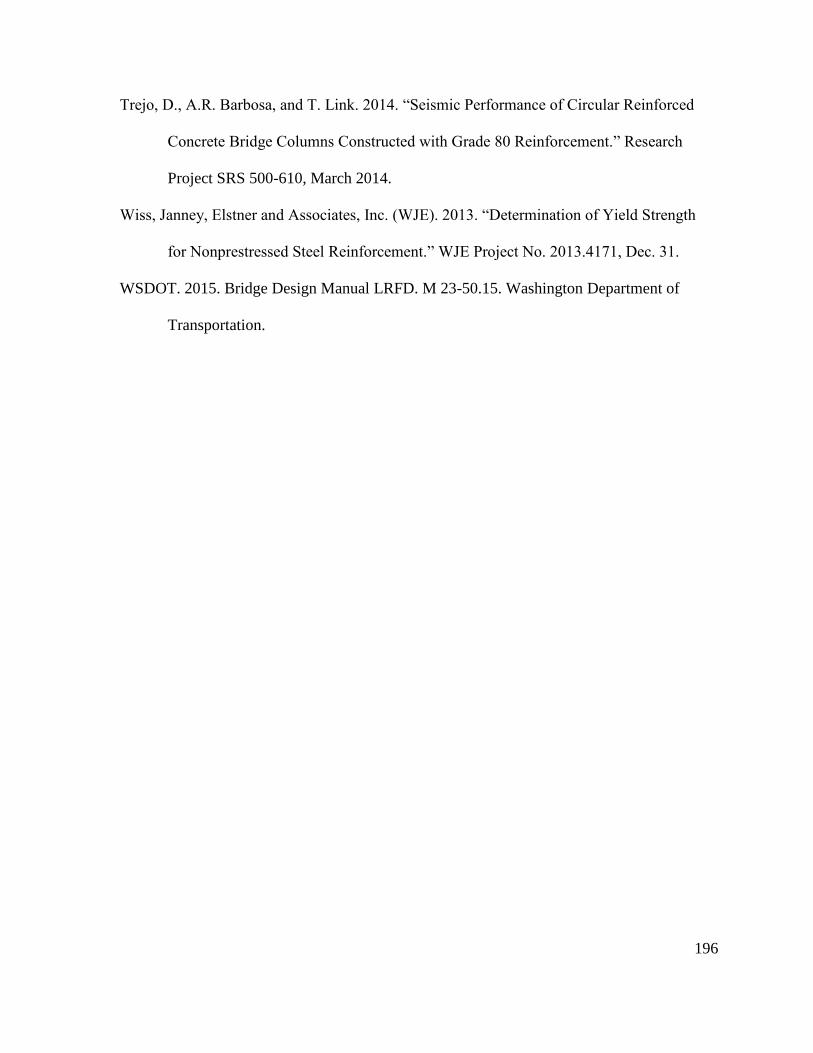
196

Trejo, D., A.R. Barbosa, and T. Link. 2014. “Seismic Performance of Circular Reinforced

Concrete Bridge Columns Constructed with Grade 80 Reinforcement.” Research

Project SRS 500-610, March 2014.

Wiss, Janney, Elstner and Associates, Inc. (WJE). 2013. “Determination of Yield Strength

for Nonprestressed Steel Reinforcement.” WJE Project No. 2013.4171, Dec. 31.

WSDOT. 2015. Bridge Design Manual LRFD. M 23-50.15. Washington Department of

Transportation.

197

APPENDICES

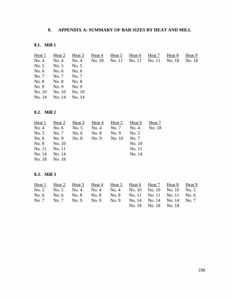
198

8. APPENDIX A: SUMMARY OF BAR SIZES BY HEAT AND MILL

8.1. Mill 1

Heat 1 Heat 2 Heat 3 Heat 4 Heat 5 Heat 6 Heat 7 Heat 8 Heat 9

No. 4 No. 4 No. 4 No. 18 No. 11 No. 11 No. 11 No. 18 No. 18

No. 5 No. 5 No. 5

No. 6 No. 6 No. 6

No. 7 No. 7 No. 7

No. 8 No. 8 No. 8

No. 9 No. 9 No. 9

No. 10 No. 10 No. 10

No. 14 No. 14 No. 14

8.2. Mill 2

Heat 1 Heat 2 Heat 3 Heat 4 Heat 5 Heat 6 Heat 7

No. 4 No. 6 No. 5 No. 4 No. 7 No. 4 No. 18

No. 5 No. 7 No. 6 No. 8 No. 9 No. 5

No. 6 No. 9 No. 8 No. 9 No. 10 No. 7

No. 8 No. 10 No. 10

No. 11 No. 11 No. 11

No. 14 No. 14 No. 14

No. 18 No. 18

8.3. Mill 3

Heat 1 Heat 2 Heat 3 Heat 4 Heat 5 Heat 6 Heat 7 Heat 8 Heat 9




No. 18 No. 18 No. 18

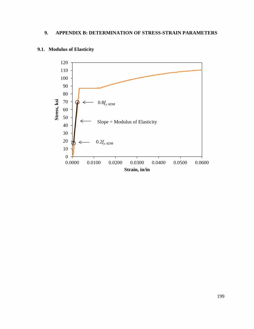
199

9. APPENDIX B: DETERMINATION OF STRESS-STRAIN PARAMETERS

9.1. Modulus of Elasticity

0

10

20

30

40

50

60

70

80

90

100

110

120

0.0000 0.0100 0.0200 0.0300 0.0400 0.0500 0.0600

Str

ess,

ksi

Strain, in/in

0.2fy ADM

0.8fy ADM

Slope = Modulus of Elasticity

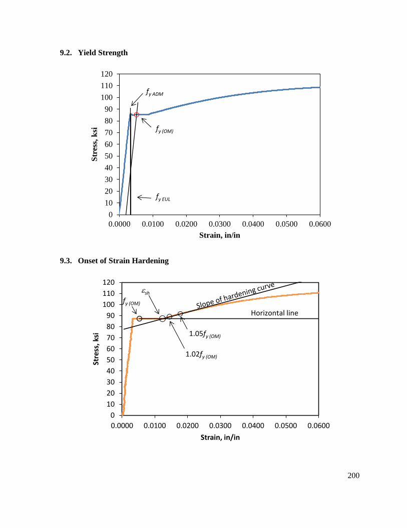
200

9.2. Yield Strength

9.3. Onset of Strain Hardening

0

10

20

30

40

50

60

70

80

90

100

110

120

0.0000 0.0100 0.0200 0.0300 0.0400 0.0500 0.0600

Str

ess,

ksi

Strain, in/in

fy (OM)

fy ADM

fy EUL

0

10

20

30

40

50

60

70

80

90

100

110

120

0.0000 0.0100 0.0200 0.0300 0.0400 0.0500 0.0600

Stre

ss, k

si

Strain, in/in

Horizontal line

sh

fy (OM)

1.02fy (OM)

1.05fy (OM)

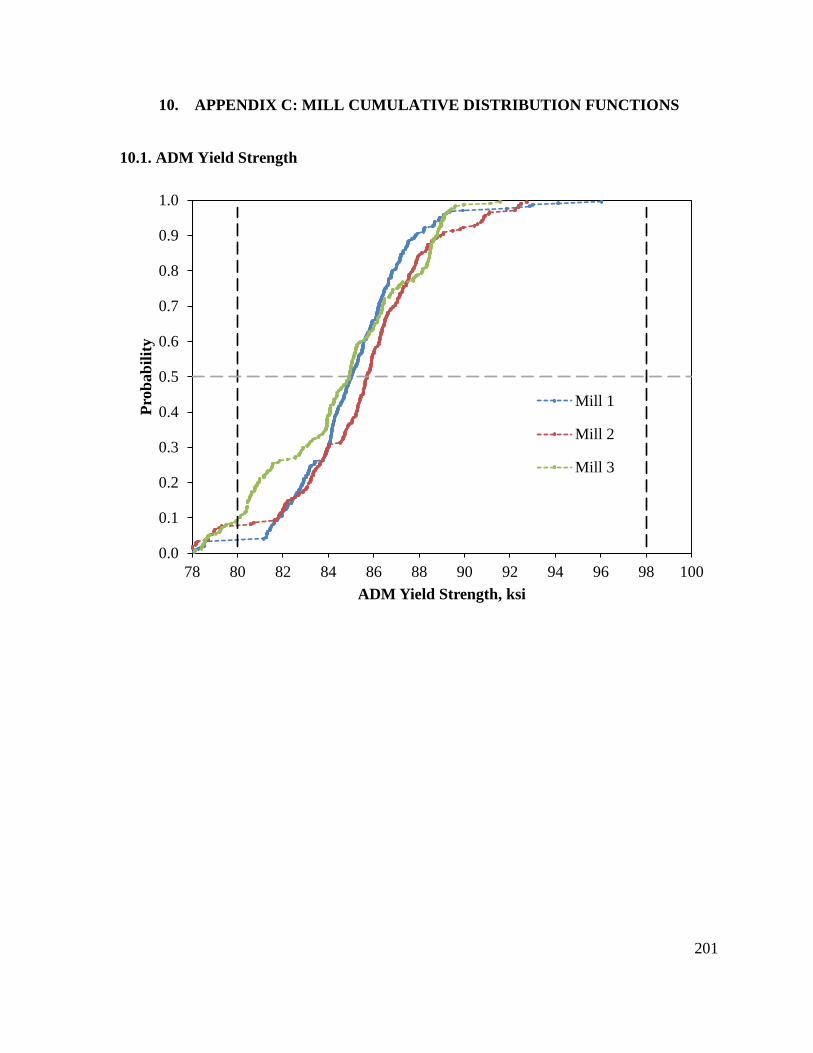
201

10. APPENDIX C: MILL CUMULATIVE DISTRIBUTION FUNCTIONS

10.1. ADM Yield Strength

0.0

0.1

0.2

0.3

0.4

0.5

0.6

0.7

0.8

0.9

1.0

78 80 82 84 86 88 90 92 94 96 98 100

Pro

bab

ilit

y


Mill 1

Mill 2

Mill 3

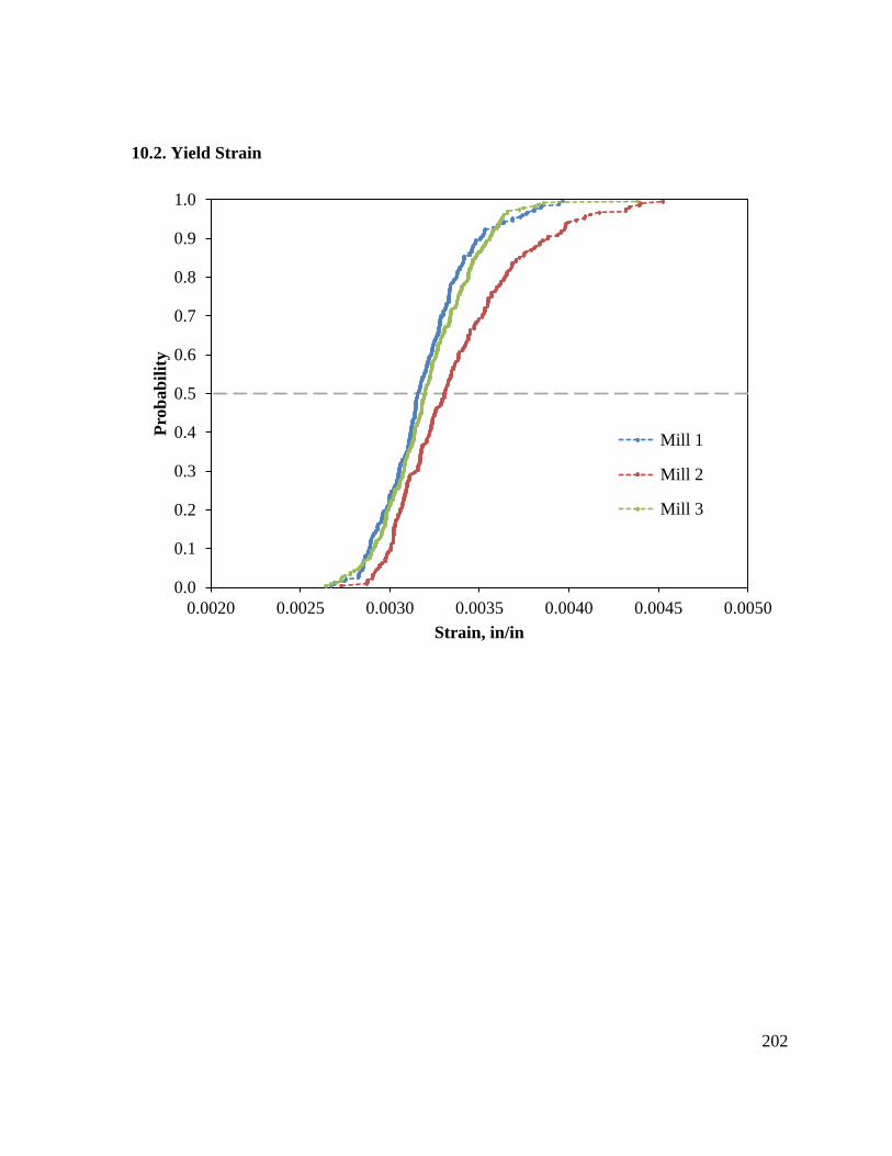
202

10.2. Yield Strain

0.0

0.1

0.2

0.3

0.4

0.5

0.6

0.7

0.8

0.9

1.0

0.0020 0.0025 0.0030 0.0035 0.0040 0.0045 0.0050

Pro

bab

ilit

y

Strain, in/in

Mill 1

Mill 2

Mill 3

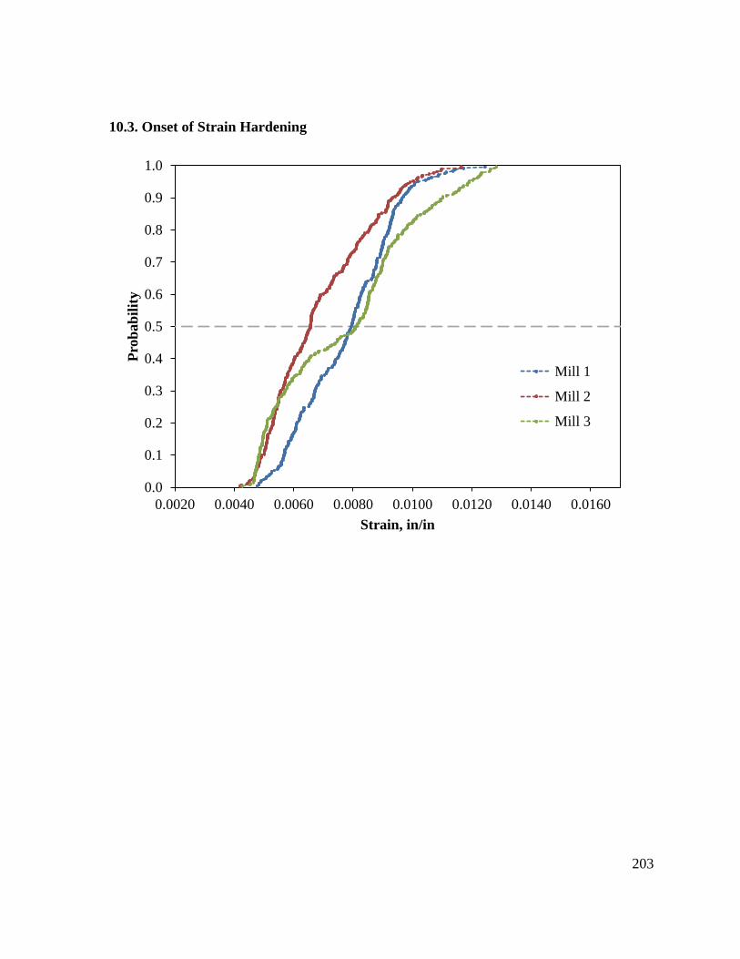
203


0.0

0.1

0.2

0.3

0.4

0.5

0.6

0.7

0.8

0.9

1.0

0.0020 0.0040 0.0060 0.0080 0.0100 0.0120 0.0140 0.0160

Pro

bab

ilit

y

Strain, in/in

Mill 1

Mill 2

Mill 3

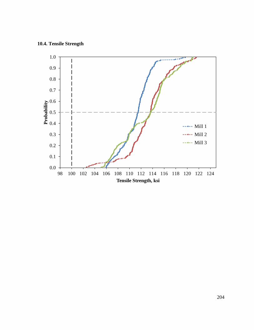
204

10.4. Tensile Strength

0.0

0.1

0.2

0.3

0.4

0.5

0.6

0.7

0.8

0.9

1.0

98 100 102 104 106 108 110 112 114 116 118 120 122 124

Pro

bab

ilit

y


Mill 1

Mill 2

Mill 3

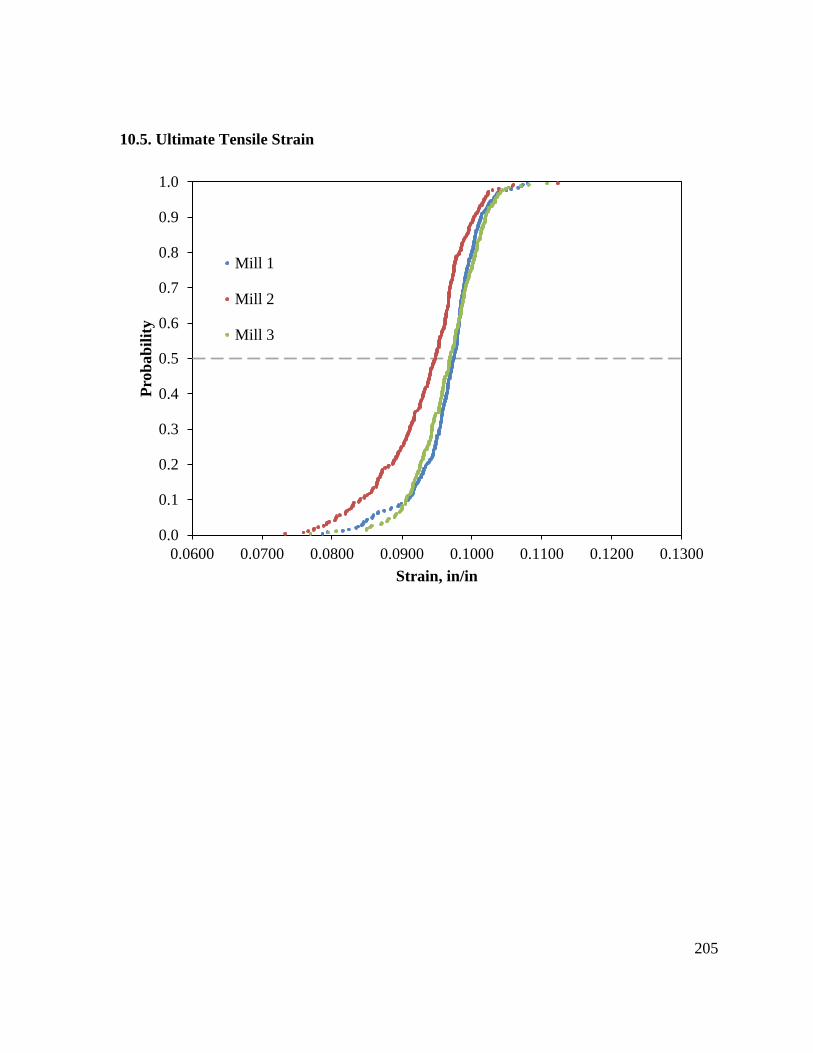
205

10.5. Ultimate Tensile Strain

0.0

0.1

0.2

0.3

0.4

0.5

0.6

0.7

0.8

0.9

1.0

0.0600 0.0700 0.0800 0.0900 0.1000 0.1100 0.1200 0.1300

Pro

bab

ilit

y

Strain, in/in

Mill 1

Mill 2

Mill 3

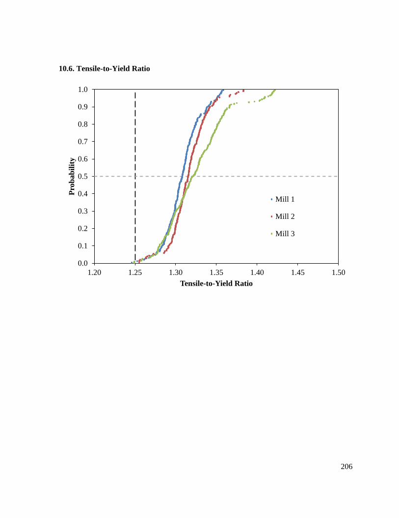
206

10.6. Tensile-to-Yield Ratio

0.0

0.1

0.2

0.3

0.4

0.5

0.6

0.7

0.8

0.9

1.0

1.20 1.25 1.30 1.35 1.40 1.45 1.50

Pro

bab

ilit

y


Mill 1

Mill 2

Mill 3

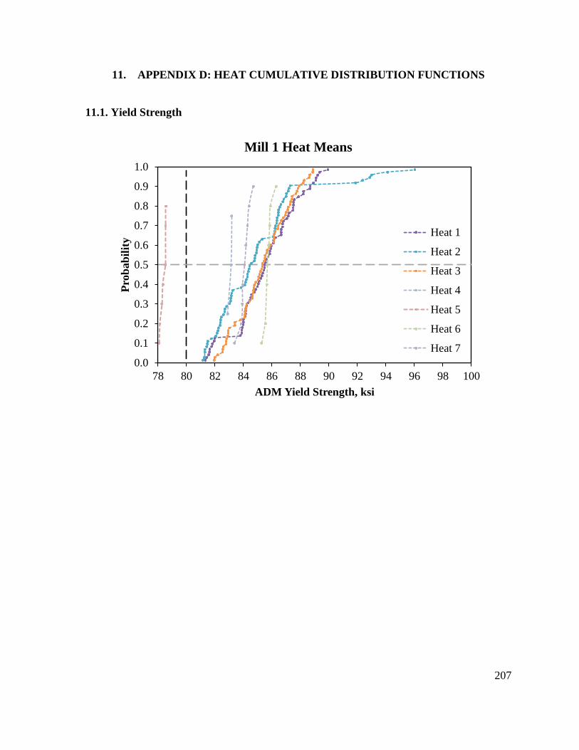
207

11. APPENDIX D: HEAT CUMULATIVE DISTRIBUTION FUNCTIONS

11.1. Yield Strength

0.0

0.1

0.2

0.3

0.4

0.5

0.6

0.7

0.8

0.9

1.0

78 80 82 84 86 88 90 92 94 96 98 100

Pro

bab

ilit

y


Mill 1 Heat Means

Heat 1

Heat 2

Heat 3

Heat 4

Heat 5

Heat 6

Heat 7

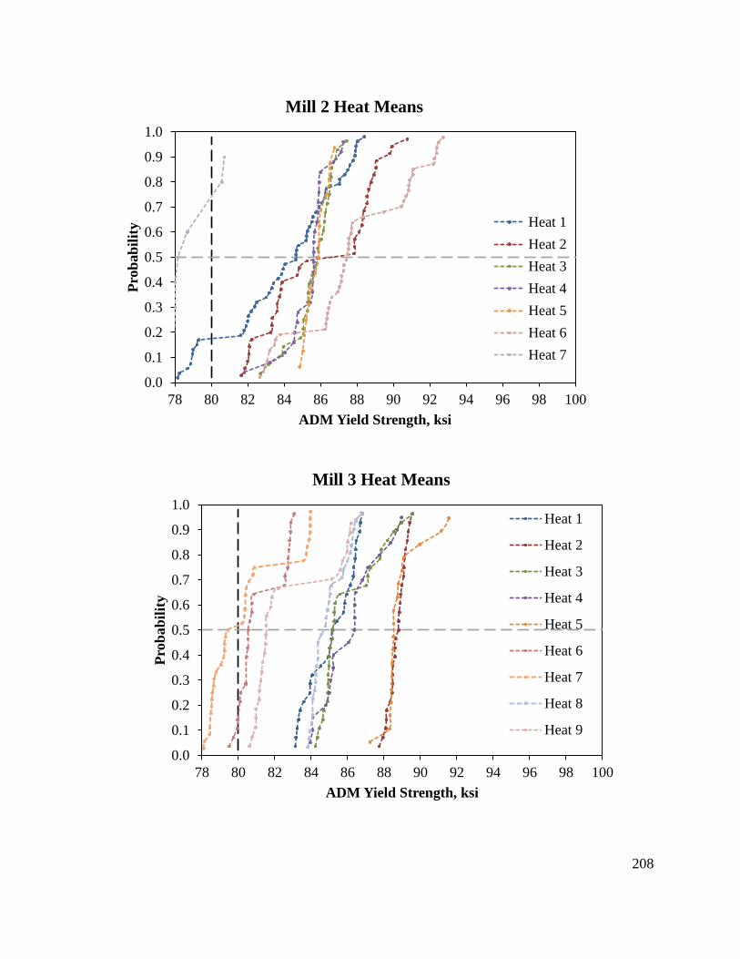
208

0.0

0.1

0.2

0.3

0.4

0.5

0.6

0.7

0.8

0.9

1.0

78 80 82 84 86 88 90 92 94 96 98 100

Pro

bab

ilit

y


Mill 2 Heat Means

Heat 1

Heat 2

Heat 3

Heat 4

Heat 5

Heat 6

Heat 7

0.0

0.1

0.2

0.3

0.4

0.5

0.6

0.7

0.8

0.9

1.0

78 80 82 84 86 88 90 92 94 96 98 100

Pro

bab

ilit

y


Mill 3 Heat Means

Heat 1

Heat 2

Heat 3

Heat 4

Heat 5

Heat 6

Heat 7

Heat 8

Heat 9

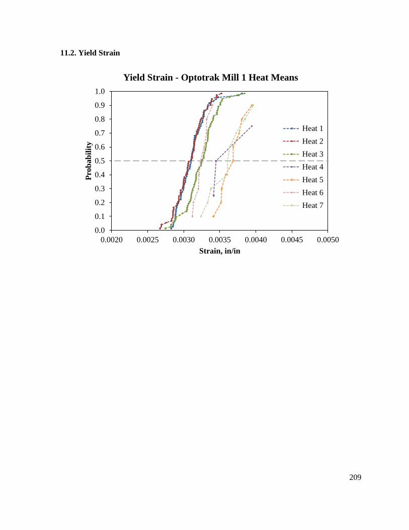
209

11.2. Yield Strain

0.0

0.1

0.2

0.3

0.4

0.5

0.6

0.7

0.8

0.9

1.0

0.0020 0.0025 0.0030 0.0035 0.0040 0.0045 0.0050

Pro

bab

ilit

y

Strain, in/in

Yield Strain - Optotrak Mill 1 Heat Means

Heat 1

Heat 2

Heat 3

Heat 4

Heat 5

Heat 6

Heat 7

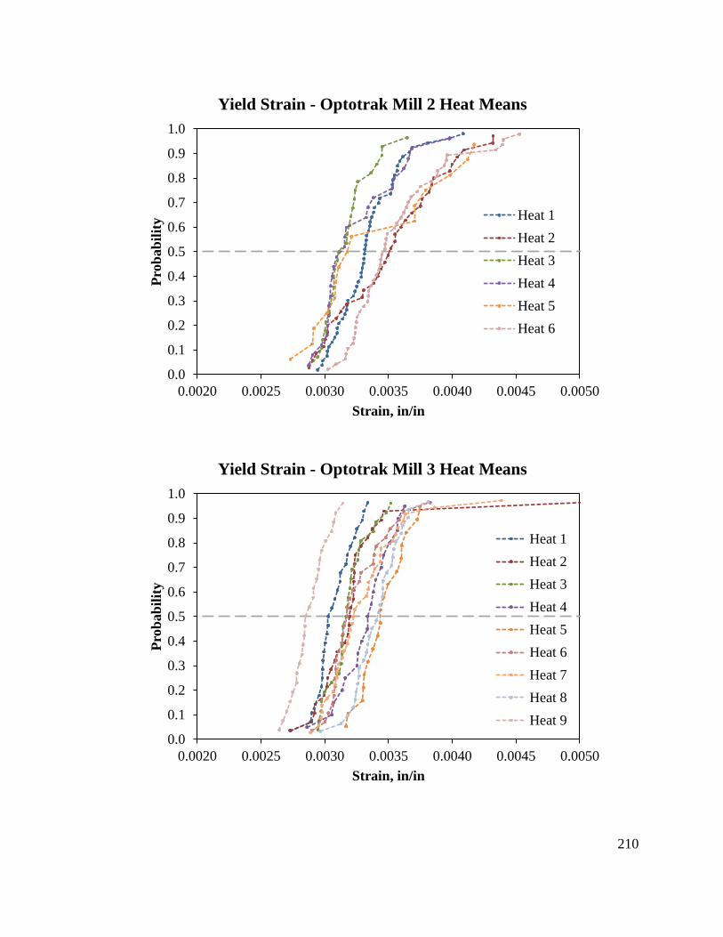
210

0.0

0.1

0.2

0.3

0.4

0.5

0.6

0.7

0.8

0.9

1.0

0.0020 0.0025 0.0030 0.0035 0.0040 0.0045 0.0050

Pro

bab

ilit

y

Strain, in/in


Heat 1

Heat 2

Heat 3

Heat 4

Heat 5

Heat 6

0.0

0.1

0.2

0.3

0.4

0.5

0.6

0.7

0.8

0.9

1.0

0.0020 0.0025 0.0030 0.0035 0.0040 0.0045 0.0050

Pro

bab

ilit

y

Strain, in/in


Heat 1

Heat 2

Heat 3

Heat 4

Heat 5

Heat 6

Heat 7

Heat 8

Heat 9

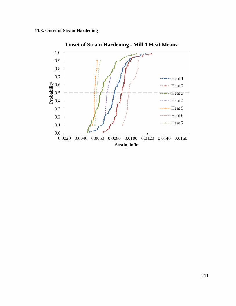
211


0.0

0.1

0.2

0.3

0.4

0.5

0.6

0.7

0.8

0.9

1.0

0.0020 0.0040 0.0060 0.0080 0.0100 0.0120 0.0140 0.0160

Pro

bab

ilit

y

Strain, in/in

Onset of Strain Hardening - Mill 1 Heat Means

Heat 1

Heat 2

Heat 3

Heat 4

Heat 5

Heat 6

Heat 7

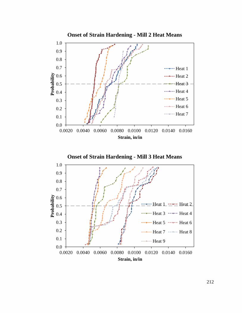
212

0.0

0.1

0.2

0.3

0.4

0.5

0.6

0.7

0.8

0.9

1.0

0.0020 0.0040 0.0060 0.0080 0.0100 0.0120 0.0140 0.0160

Pro

bab

ilit

y

Strain, in/in


Heat 1

Heat 2

Heat 3

Heat 4

Heat 5

Heat 6

Heat 7

0.0

0.1

0.2

0.3

0.4

0.5

0.6

0.7

0.8

0.9

1.0

0.0020 0.0040 0.0060 0.0080 0.0100 0.0120 0.0140 0.0160

Pro

bab

ilit

y

Strain, in/in


Heat 1 Heat 2

Heat 3 Heat 4

Heat 5 Heat 6

Heat 7 Heat 8

Heat 9

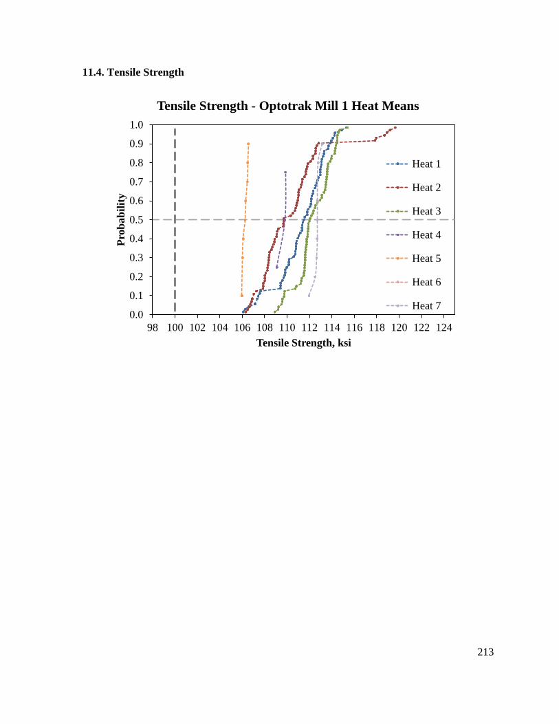
213

11.4. Tensile Strength

0.0

0.1

0.2

0.3

0.4

0.5

0.6

0.7

0.8

0.9

1.0

98 100 102 104 106 108 110 112 114 116 118 120 122 124

Pro

bab

ilit

y


Tensile Strength - Optotrak Mill 1 Heat Means

Heat 1

Heat 2

Heat 3

Heat 4

Heat 5

Heat 6

Heat 7

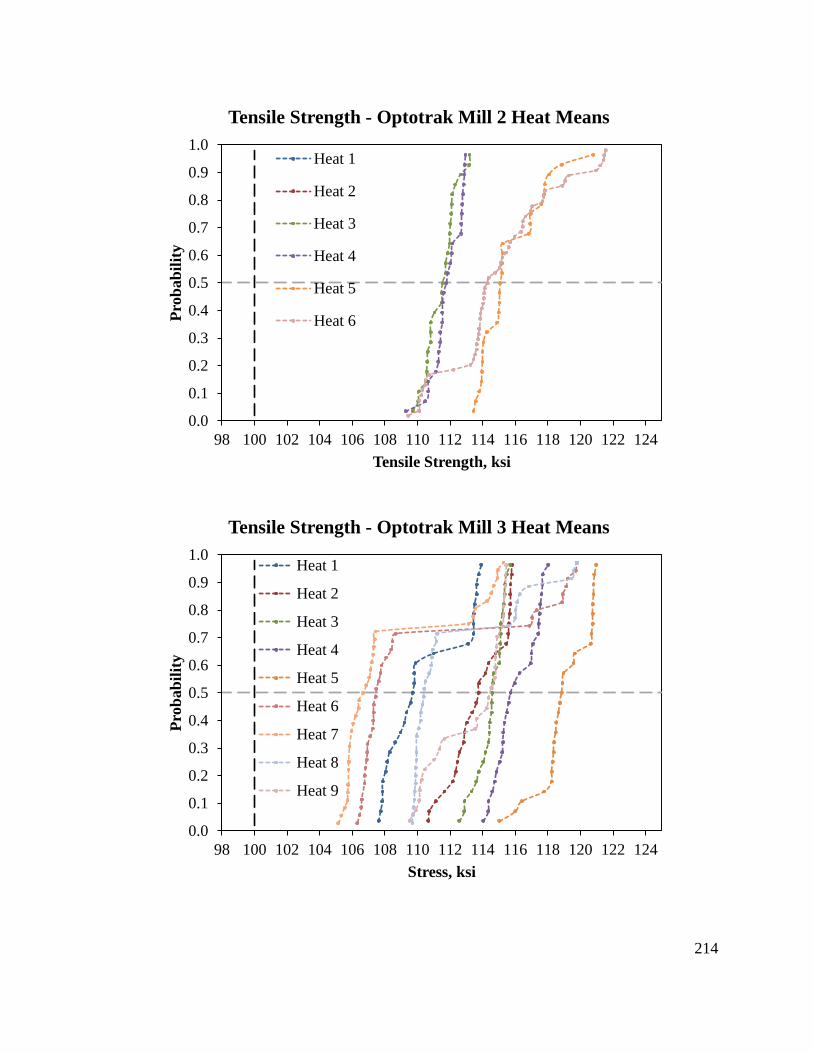
214

0.0

0.1

0.2

0.3

0.4

0.5

0.6

0.7

0.8

0.9

1.0

98 100 102 104 106 108 110 112 114 116 118 120 122 124

Pro

bab

ilit

y



Heat 1

Heat 2

Heat 3

Heat 4

Heat 5

Heat 6

0.0

0.1

0.2

0.3

0.4

0.5

0.6

0.7

0.8

0.9

1.0

98 100 102 104 106 108 110 112 114 116 118 120 122 124

Pro

bab

ilit

y

Stress, ksi


Heat 1

Heat 2

Heat 3

Heat 4

Heat 5

Heat 6

Heat 7

Heat 8

Heat 9

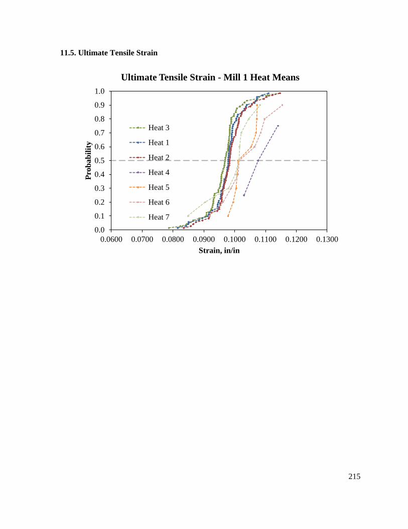
215


0.0

0.1

0.2

0.3

0.4

0.5

0.6

0.7

0.8

0.9

1.0

0.0600 0.0700 0.0800 0.0900 0.1000 0.1100 0.1200 0.1300

Pro

bab

ilit

y

Strain, in/in

Ultimate Tensile Strain - Mill 1 Heat Means

Heat 3

Heat 1

Heat 2

Heat 4

Heat 5

Heat 6

Heat 7

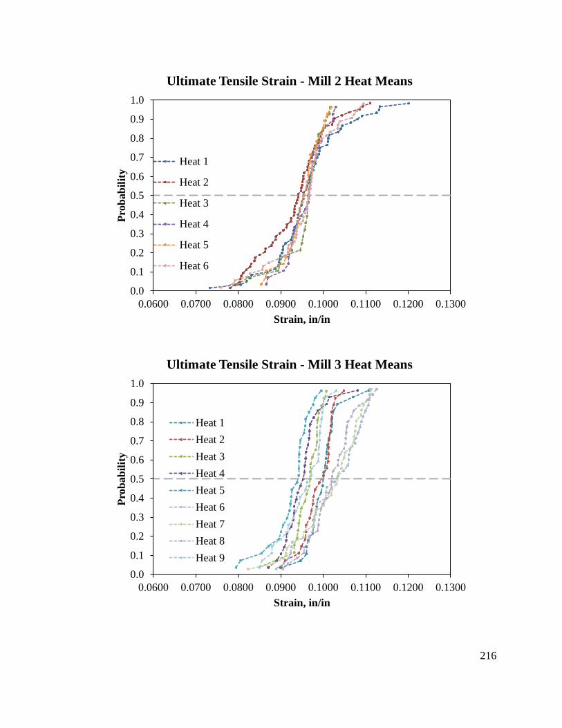
216

0.0

0.1

0.2

0.3

0.4

0.5

0.6

0.7

0.8

0.9

1.0

0.0600 0.0700 0.0800 0.0900 0.1000 0.1100 0.1200 0.1300

Pro

bab

ilit

y

Strain, in/in


Heat 1

Heat 2

Heat 3

Heat 4

Heat 5

Heat 6

0.0

0.1

0.2

0.3

0.4

0.5

0.6

0.7

0.8

0.9

1.0

0.0600 0.0700 0.0800 0.0900 0.1000 0.1100 0.1200 0.1300

Pro

bab

ilit

y

Strain, in/in


Heat 1

Heat 2

Heat 3

Heat 4

Heat 5

Heat 6

Heat 7

Heat 8

Heat 9

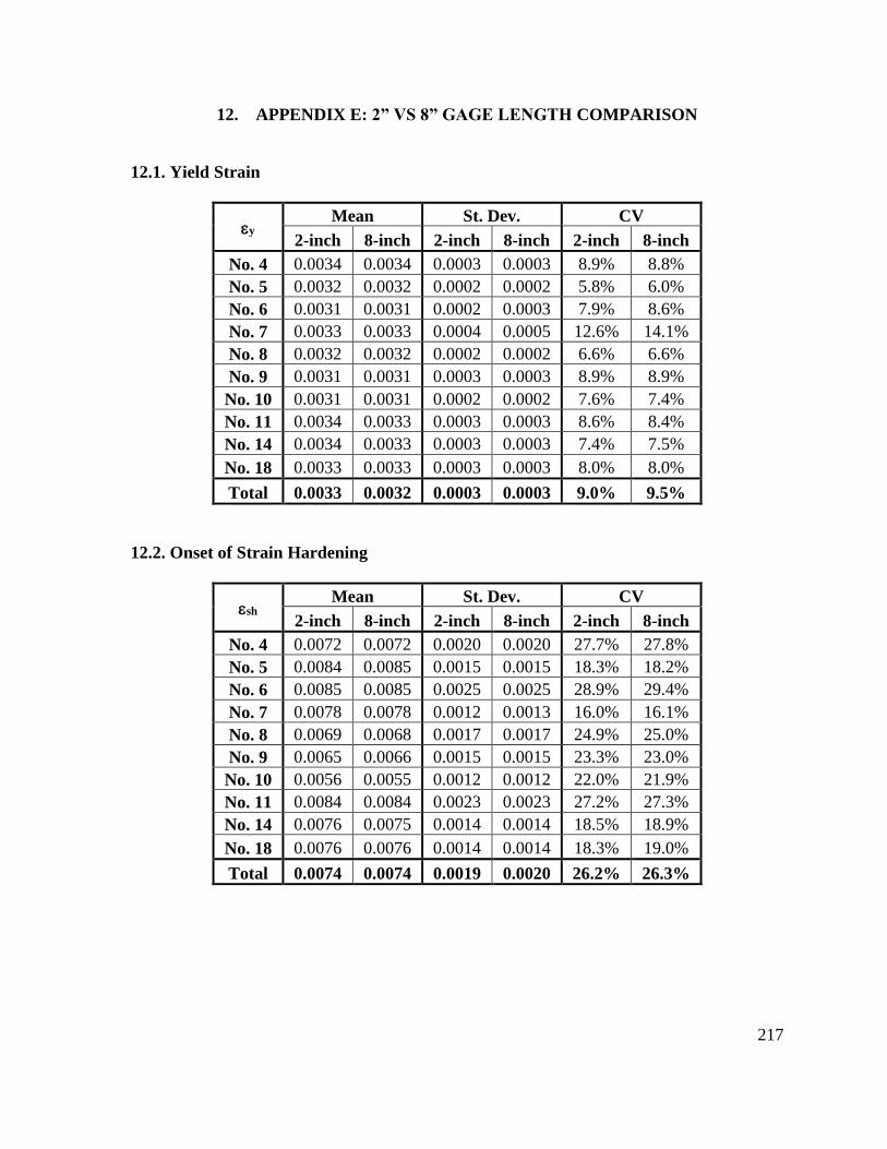
217

12. APPENDIX E: 2” VS 8” GAGE LENGTH COMPARISON

12.1. Yield Strain

y Mean St. Dev. CV

2-inch 8-inch 2-inch 8-inch 2-inch 8-inch

No. 4 0.0034 0.0034 0.0003 0.0003 8.9% 8.8%

No. 5 0.0032 0.0032 0.0002 0.0002 5.8% 6.0%

No. 6 0.0031 0.0031 0.0002 0.0003 7.9% 8.6%

No. 7 0.0033 0.0033 0.0004 0.0005 12.6% 14.1%

No. 8 0.0032 0.0032 0.0002 0.0002 6.6% 6.6%

No. 9 0.0031 0.0031 0.0003 0.0003 8.9% 8.9%

No. 10 0.0031 0.0031 0.0002 0.0002 7.6% 7.4%

No. 11 0.0034 0.0033 0.0003 0.0003 8.6% 8.4%

No. 14 0.0034 0.0033 0.0003 0.0003 7.4% 7.5%

No. 18 0.0033 0.0033 0.0003 0.0003 8.0% 8.0%

Total 0.0033 0.0032 0.0003 0.0003 9.0% 9.5%


sh Mean St. Dev. CV


No. 4 0.0072 0.0072 0.0020 0.0020 27.7% 27.8%

No. 5 0.0084 0.0085 0.0015 0.0015 18.3% 18.2%

No. 6 0.0085 0.0085 0.0025 0.0025 28.9% 29.4%

No. 7 0.0078 0.0078 0.0012 0.0013 16.0% 16.1%

No. 8 0.0069 0.0068 0.0017 0.0017 24.9% 25.0%

No. 9 0.0065 0.0066 0.0015 0.0015 23.3% 23.0%

No. 10 0.0056 0.0055 0.0012 0.0012 22.0% 21.9%

No. 11 0.0084 0.0084 0.0023 0.0023 27.2% 27.3%

No. 14 0.0076 0.0075 0.0014 0.0014 18.5% 18.9%

No. 18 0.0076 0.0076 0.0014 0.0014 18.3% 19.0%

Total 0.0074 0.0074 0.0019 0.0020 26.2% 26.3%

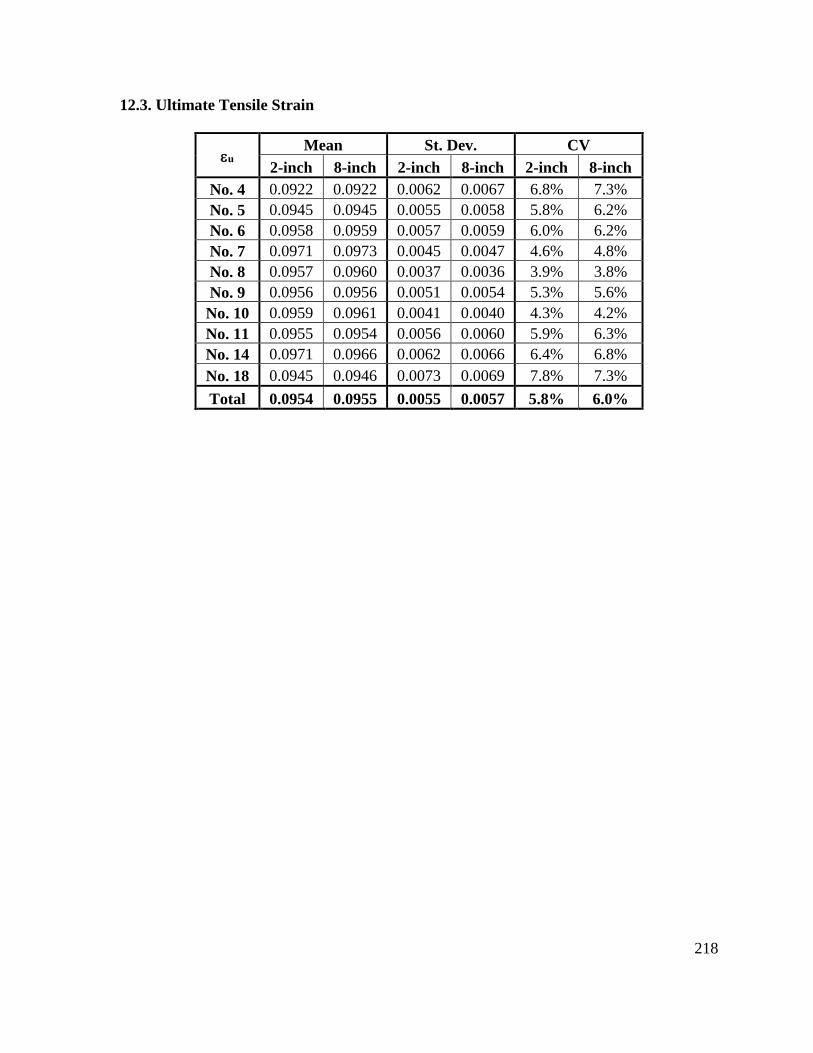
218


u Mean St. Dev. CV


No. 4 0.0922 0.0922 0.0062 0.0067 6.8% 7.3%

No. 5 0.0945 0.0945 0.0055 0.0058 5.8% 6.2%

No. 6 0.0958 0.0959 0.0057 0.0059 6.0% 6.2%

No. 7 0.0971 0.0973 0.0045 0.0047 4.6% 4.8%

No. 8 0.0957 0.0960 0.0037 0.0036 3.9% 3.8%

No. 9 0.0956 0.0956 0.0051 0.0054 5.3% 5.6%

No. 10 0.0959 0.0961 0.0041 0.0040 4.3% 4.2%

No. 11 0.0955 0.0954 0.0056 0.0060 5.9% 6.3%

No. 14 0.0971 0.0966 0.0062 0.0066 6.4% 6.8%

No. 18 0.0945 0.0946 0.0073 0.0069 7.8% 7.3%

Total 0.0954 0.0955 0.0055 0.0057 5.8% 6.0%

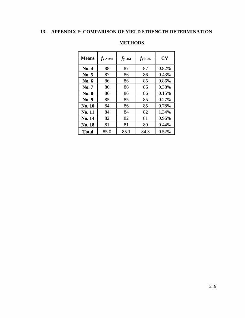
219

13. APPENDIX F: COMPARISON OF YIELD STRENGTH DETERMINATION

METHODS

Means fy ADM fy OM fy EUL CV

No. 4 88 87 87 0.82%

No. 5 87 86 86 0.43%

No. 6 86 86 85 0.86%

No. 7 86 86 86 0.38%

No. 8 86 86 86 0.15%

No. 9 85 85 85 0.27%

No. 10 84 86 85 0.78%

No. 11 84 84 82 1.34%

No. 14 82 82 81 0.96%

No. 18 81 81 80 0.44%

Total 85.0 85.1 84.3 0.52%

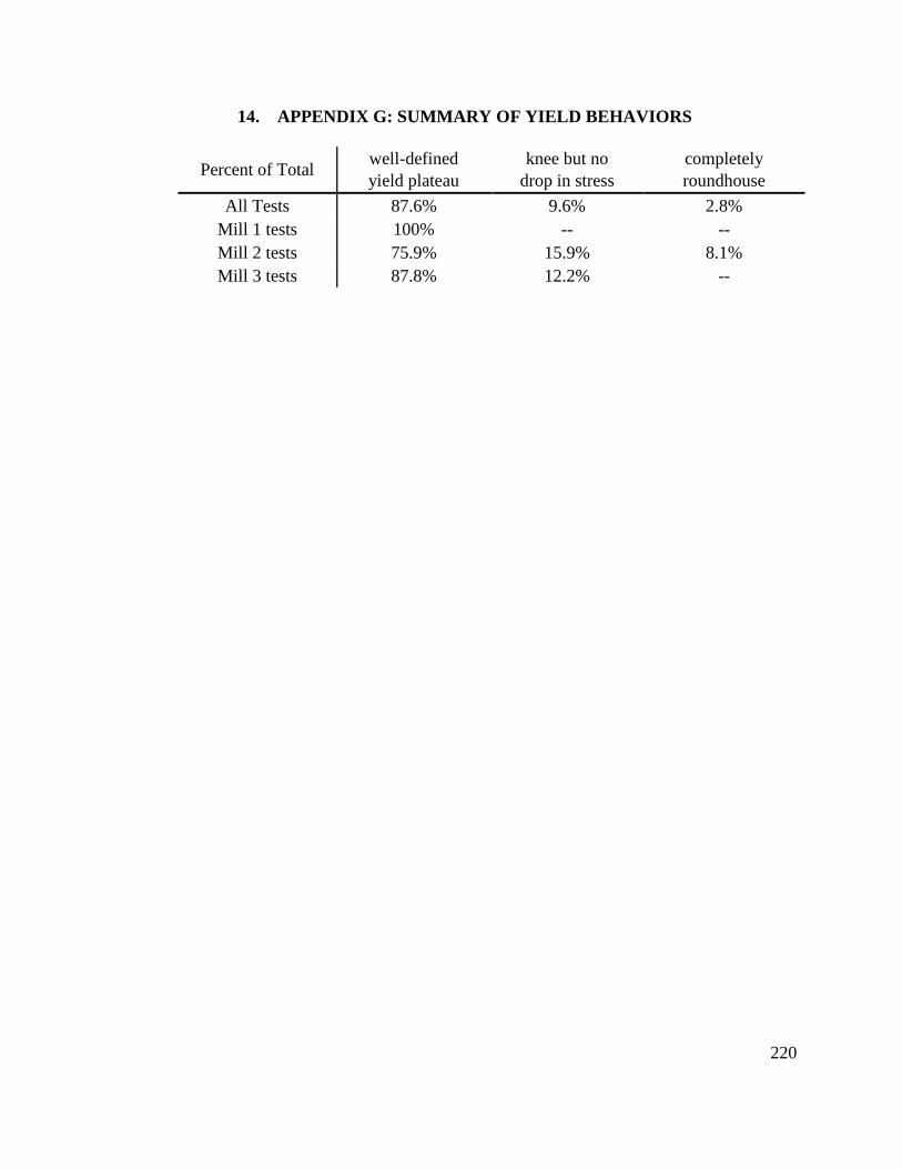
220

14. APPENDIX G: SUMMARY OF YIELD BEHAVIORS

Percent of Total well-defined

yield plateau

knee but no

drop in stress

completely

roundhouse

All Tests 87.6% 9.6% 2.8%

Mill 1 tests 100% -- --

Mill 2 tests 75.9% 15.9% 8.1%

Mill 3 tests 87.8% 12.2% --

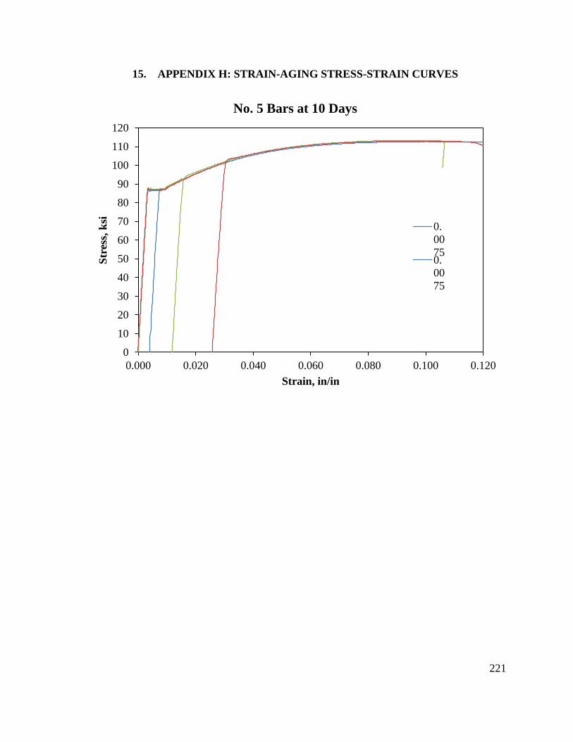
221

15. APPENDIX H: STRAIN-AGING STRESS-STRAIN CURVES

0

10

20

30

40

50

60

70

80

90

100

110

120

0.000 0.020 0.040 0.060 0.080 0.100 0.120

Str

ess,

ksi

Strain, in/in

No. 5 Bars at 10 Days

0.

00

750.

00

75

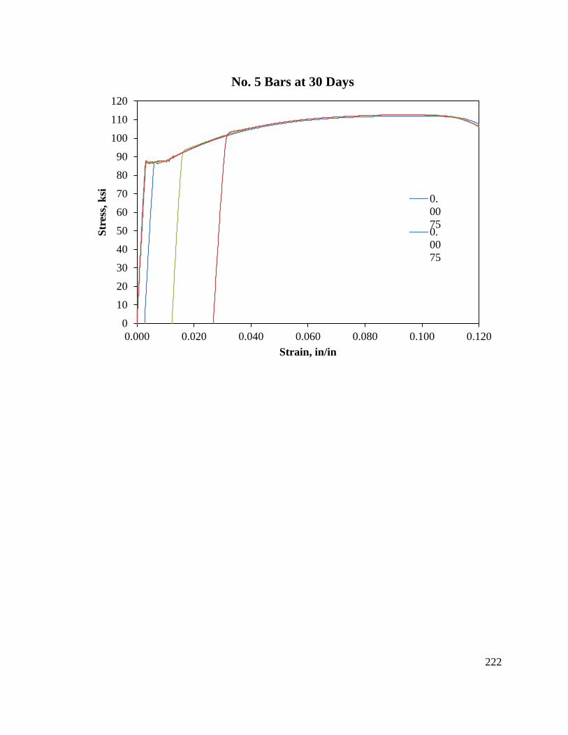
222

0

10

20

30

40

50

60

70

80

90

100

110

120

0.000 0.020 0.040 0.060 0.080 0.100 0.120

Str

ess,

ksi

Strain, in/in


0.

00

750.

00

75

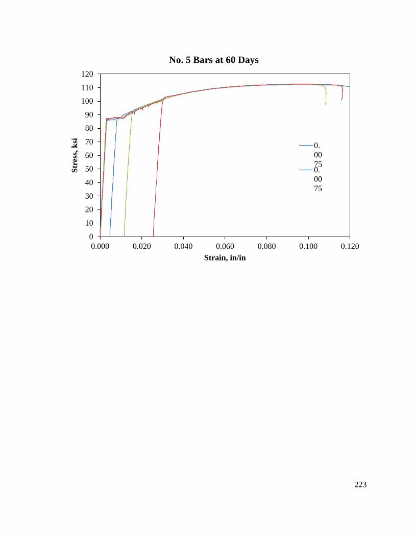
223

0

10

20

30

40

50

60

70

80

90

100

110

120

0.000 0.020 0.040 0.060 0.080 0.100 0.120

Str

ess,

ksi

Strain, in/in


0.

00

750.

00

75

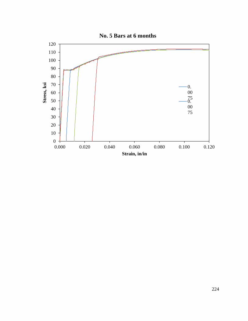
224

0

10

20

30

40

50

60

70

80

90

100

110

120

0.000 0.020 0.040 0.060 0.080 0.100 0.120

Str

ess,

ksi

Strain, in/in

No. 5 Bars at 6 months

0.

00

750.

00

75

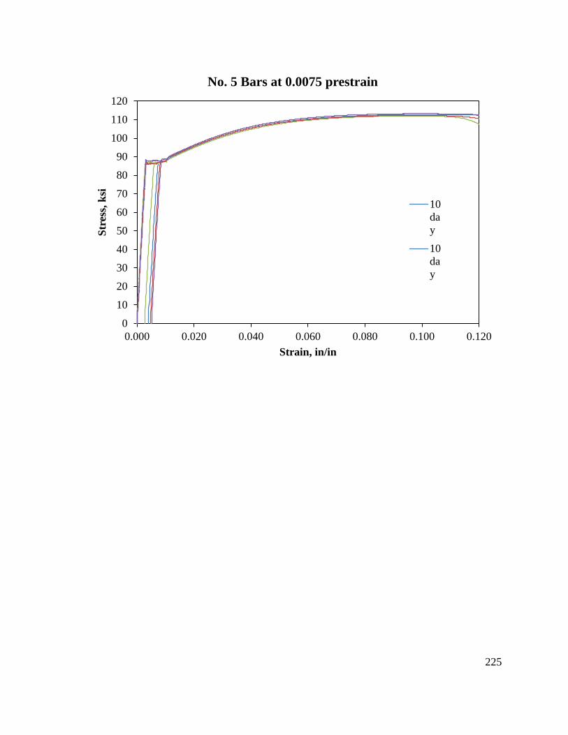
225

0

10

20

30

40

50

60

70

80

90

100

110

120

0.000 0.020 0.040 0.060 0.080 0.100 0.120

Str

ess,

ksi

Strain, in/in

No. 5 Bars at 0.0075 prestrain

10

da

y

10

da

y

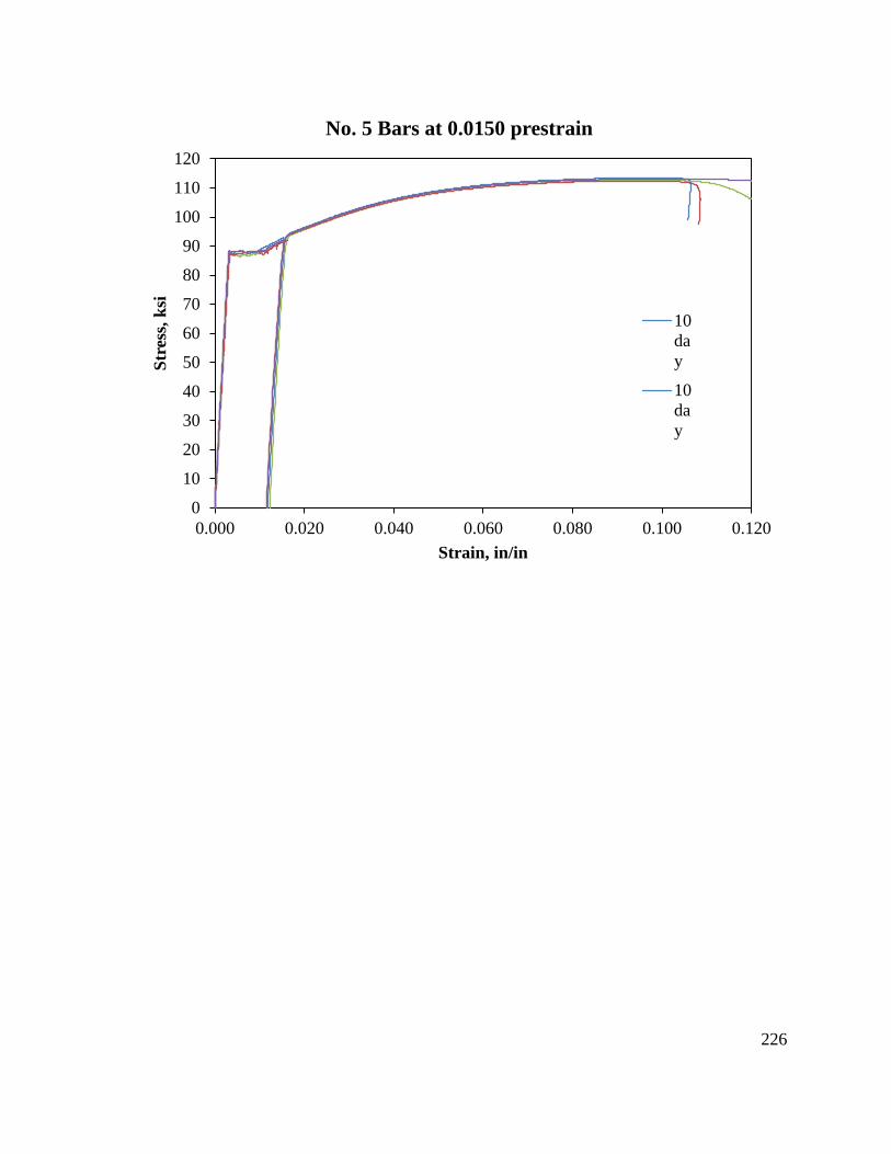
226

0

10

20

30

40

50

60

70

80

90

100

110

120

0.000 0.020 0.040 0.060 0.080 0.100 0.120

Str

ess,

ksi

Strain, in/in


10

da

y

10

da

y

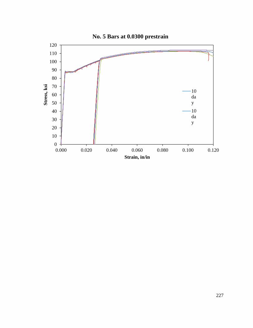
227

0

10

20

30

40

50

60

70

80

90

100

110

120

0.000 0.020 0.040 0.060 0.080 0.100 0.120

Str

ess,

ksi

Strain, in/in


10

da

y

10

da

y

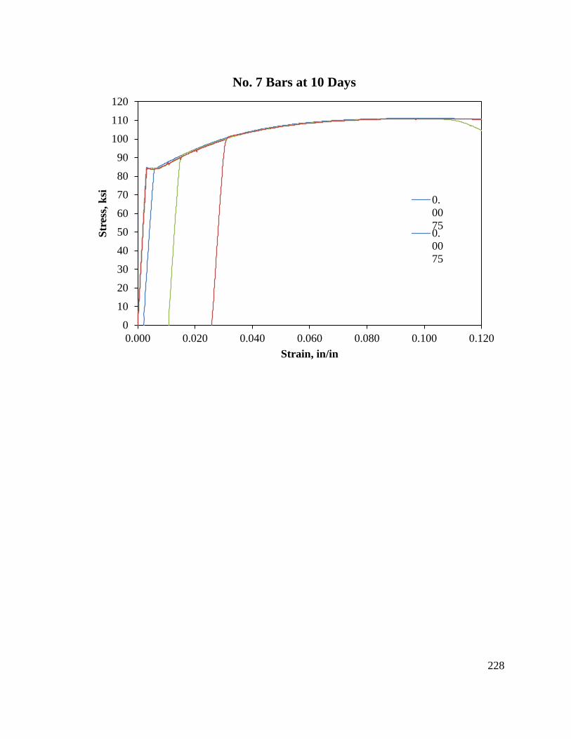
228

0

10

20

30

40

50

60

70

80

90

100

110

120

0.000 0.020 0.040 0.060 0.080 0.100 0.120

Str

ess,

ksi

Strain, in/in


0.

00

750.

00

75

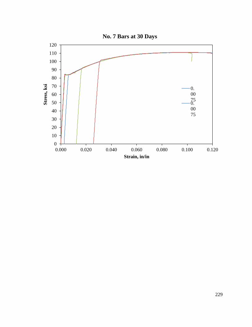
229

0

10

20

30

40

50

60

70

80

90

100

110

120

0.000 0.020 0.040 0.060 0.080 0.100 0.120

Str

ess,

ksi

Strain, in/in


0.

00

750.

00

75

230

0

10

20

30

40

50

60

70

80

90

100

110

120

0.000 0.020 0.040 0.060 0.080 0.100 0.120

Str

ess,

ksi

Strain, in/in


0.

00

750.

00

75

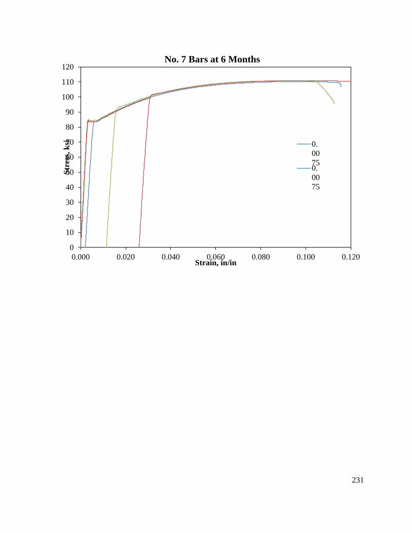
231

0

10

20

30

40

50

60

70

80

90

100

110

120

0.000 0.020 0.040 0.060 0.080 0.100 0.120

Str

ess,

ksi

Strain, in/in

No. 7 Bars at 6 Months

0.

00

750.

00

75

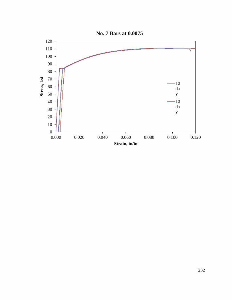
232

0

10

20

30

40

50

60

70

80

90

100

110

120

0.000 0.020 0.040 0.060 0.080 0.100 0.120

Str

ess,

ksi

Strain, in/in

No. 7 Bars at 0.0075

10

da

y

10

da

y

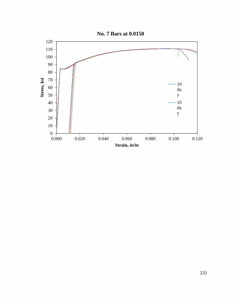
233

0

10

20

30

40

50

60

70

80

90

100

110

120

0.000 0.020 0.040 0.060 0.080 0.100 0.120

Str

ess,

ksi

Strain, in/in


10

da

y

10

da

y

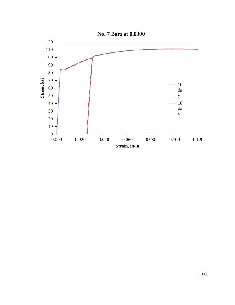
234

0

10

20

30

40

50

60

70

80

90

100

110

120

0.000 0.020 0.040 0.060 0.080 0.100 0.120

Str

ess,

ksi

Strain, in/in


10

da

y

10

da

y

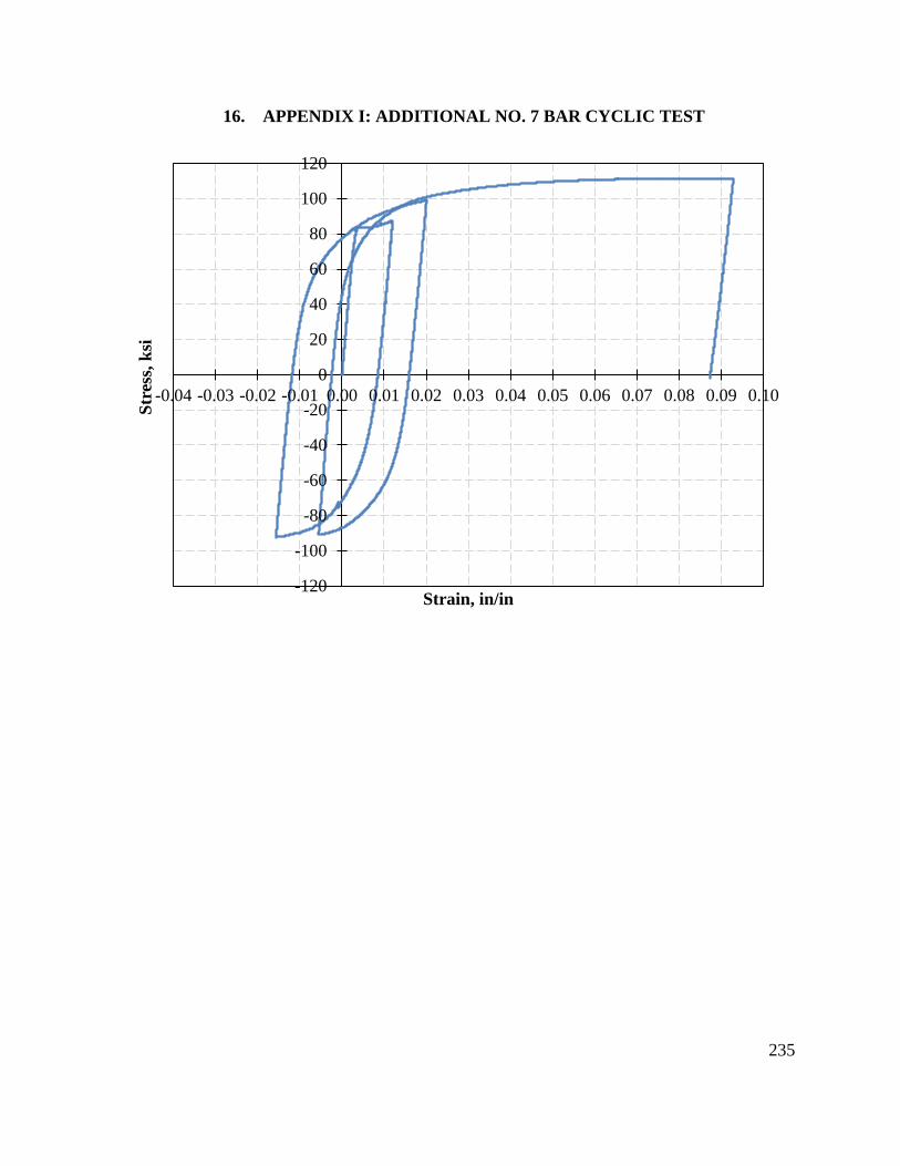
235

16. APPENDIX I: ADDITIONAL NO. 7 BAR CYCLIC TEST

-120

-100

-80

-60

-40

-20

0

20

40

60

80

100

120

-0.04 -0.03 -0.02 -0.01 0.00 0.01 0.02 0.03 0.04 0.05 0.06 0.07 0.08 0.09 0.10

Str

ess,

ksi

Strain, in/in

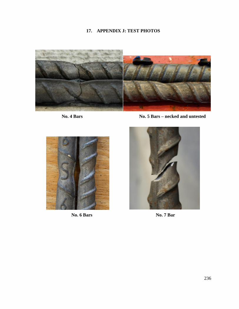
236

17. APPENDIX J: TEST PHOTOS

No. 4 Bars No. 5 Bars – necked and untested

No. 6 Bars No. 7 Bar

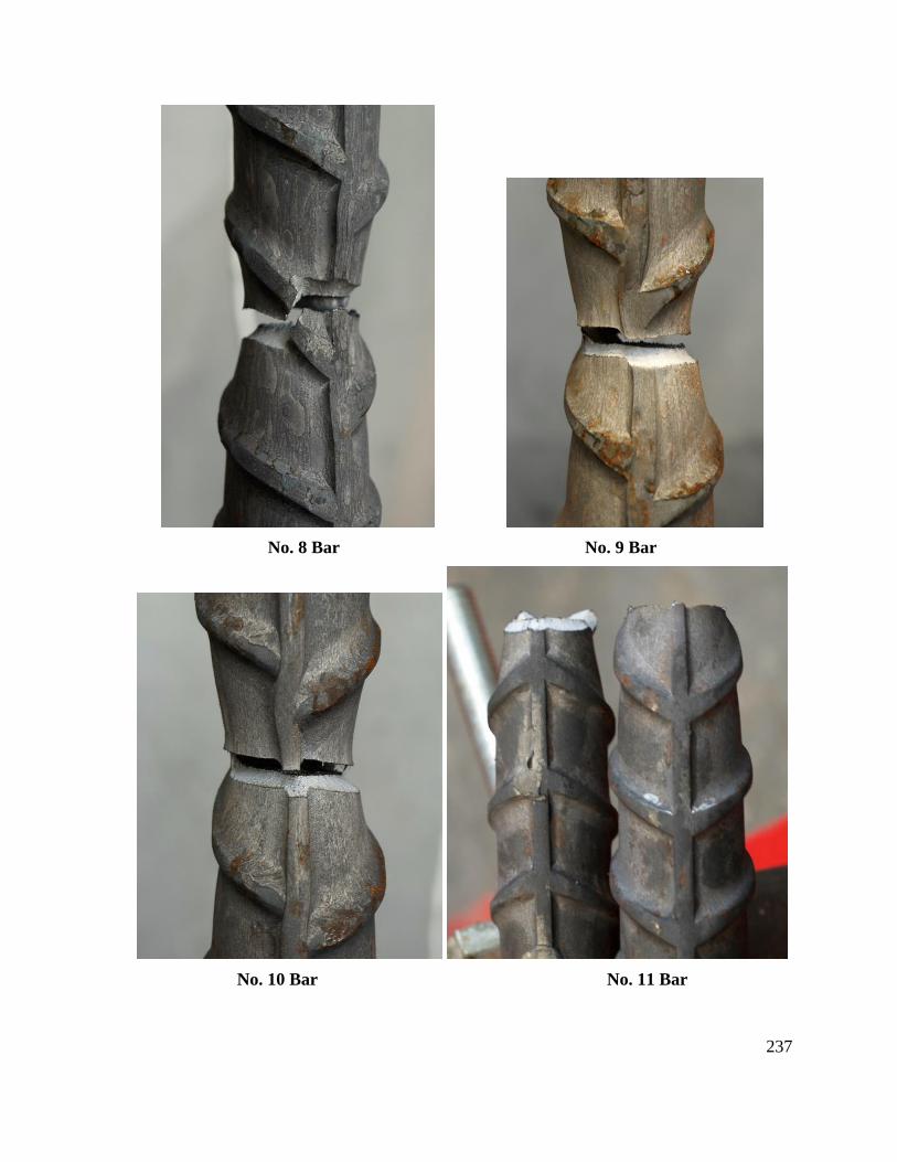
237

No. 8 Bar No. 9 Bar

No. 10 Bar No. 11 Bar

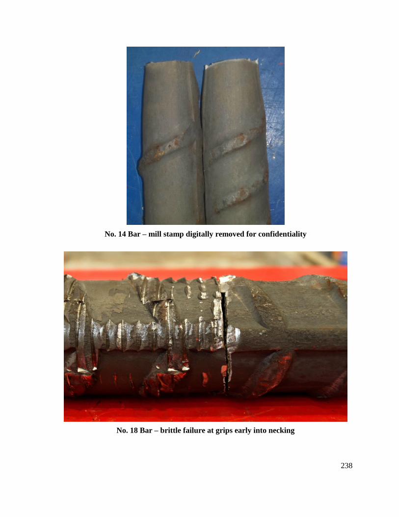
238

No. 14 Bar – mill stamp digitally removed for confidentiality

No. 18 Bar – brittle failure at grips early into necking

ABSTRACT OVERBY, DAVID THOMAS. Stress-Strain ...

Documents

Transcript of ABSTRACT OVERBY, DAVID THOMAS. Stress-Strain ...