About the HELM Project - Mathematics Materials

Production of this 2015 edition, containing corrections and minor revisions of the 2008 edition, was funded by the sigma Network.

About the HELM Project HELM (Helping Engineers Learn Mathematics) materials were the outcome of a three-‐year curriculum development project undertaken by a consortium of five English universities led by Loughborough University, funded by the Higher Education Funding Council for England under the Fund for the Development of Teaching and Learning for the period October 2002 – September 2005, with additional transferability funding October 2005 – September 2006. HELM aims to enhance the mathematical education of engineering undergraduates through flexible learning resources, mainly these Workbooks. HELM learning resources were produced primarily by teams of writers at six universities: Hull, Loughborough, Manchester, Newcastle, Reading, Sunderland. HELM gratefully acknowledges the valuable support of colleagues at the following universities and colleges involved in the critical reading, trialling, enhancement and revision of the learning materials: Aston, Bournemouth & Poole College, Cambridge, City, Glamorgan, Glasgow, Glasgow Caledonian, Glenrothes Institute of Applied Technology, Harper Adams, Hertfordshire, Leicester, Liverpool, London Metropolitan, Moray College, Northumbria, Nottingham, Nottingham Trent, Oxford Brookes, Plymouth, Portsmouth, Queens Belfast, Robert Gordon, Royal Forest of Dean College, Salford, Sligo Institute of Technology, Southampton, Southampton Institute, Surrey, Teesside, Ulster, University of Wales Institute Cardiff, West Kingsway College (London), West Notts College.

HELM Contacts: Post: HELM, Mathematics Education Centre, Loughborough University, Loughborough, LE11 3TU. Email: [email protected] Web: http://helm.lboro.ac.uk

HELM Workbooks List 1 Basic Algebra 26 Functions of a Complex Variable 2 Basic Functions 27 Multiple Integration 3 Equations, Inequalities & Partial Fractions 28 Differential Vector Calculus 4 Trigonometry 29 Integral Vector Calculus 5 Functions and Modelling 30 Introduction to Numerical Methods 6 Exponential and Logarithmic Functions 31 Numerical Methods of Approximation 7 Matrices 32 Numerical Initial Value Problems 8 Matrix Solution of Equations 33 Numerical Boundary Value Problems 9 Vectors 34 Modelling Motion 10 Complex Numbers 35 Sets and Probability 11 Differentiation 36 Descriptive Statistics 12 Applications of Differentiation 37 Discrete Probability Distributions 13 Integration 38 Continuous Probability Distributions 14 Applications of Integration 1 39 The Normal Distribution 15 Applications of Integration 2 40 Sampling Distributions and Estimation 16 Sequences and Series 41 Hypothesis Testing 17 Conics and Polar Coordinates 42 Goodness of Fit and Contingency Tables 18 Functions of Several Variables 43 Regression and Correlation 19 Differential Equations 44 Analysis of Variance 20 Laplace Transforms 45 Non-‐parametric Statistics 21 z-‐Transforms 46 Reliability and Quality Control 22 Eigenvalues and Eigenvectors 47 Mathematics and Physics Miscellany 23 Fourier Series 48 Engineering Case Study 24 Fourier Transforms 49 Student’s Guide 25 Partial Differential Equations 50 Tutor’s Guide

© Copyright Loughborough University, 2015

ContentsContents 2828Differential

Vector Calculus

28.1 Background to Vector Calculus 2

28.2 Differential Vector Calculus 17

28.3 Orthogonal Curvilinear Coordinates 37

Learning

In this Workbook you will learn about scalar and vector fields and how physical quantities can be represented by such fields. You will be able to 'differentiate' such fields i.e. to findhow rapidly the scalar or vector field varies with position. Depending on whether theoriginal function and the intended derivative are scalars or vectors, there are three suchderivatives known as the 'gradient', the 'divergence' and the 'curl'. You will be able to evaluate these derivatives for given fields. In addition, you will be able to work out thederivatives while using polar coordinate systems.

outcomes

Background to VectorCalculus

��

��28.1

IntroductionVector Calculus is the study of the various derivatives and integrals of a scalar or vector function ofthe variables defining position (x,y,z) and possibly also time (t). This Section considers functions ofseveral variables and introduces scalar and vector fields.

'

&

$

%

PrerequisitesBefore starting this Section you should . . .

• be familiar with the concept of a function oftwo variables

• be familiar with the concept of partialdifferentiation

• be familiar with the concept of vectors�

�

�

�Learning Outcomes

On completion you should be able to . . .

• state the properties of scalar and vector fields

• work with a vector function of a variable

2 HELM (2015):Workbook 28: Differential Vector Calculus

®

1. Functions of several variables and partial derivativesThese functions were first studied in 18. As a reminder:

• a function of the two independent variables x and y may be written as f(x, y)

• the first and second order partial derivatives are∂f

∂x,∂f

∂y,∂2f

∂x2,∂2f

∂y2and

∂2f

∂x∂y.

Consider, for example, the function f(x, y) = x2 + 5xy + 3y4 + 1. The first and second partialderivatives are

∂f

∂x= 2x+ 5y (differentiating with respect to x keeping y constant)

∂f

∂y= 5x+ 12y3 (differentiating with respect to y keeping x constant)

∂2f

∂x2=

∂

∂x

(∂f

∂x

)=

∂

∂x(2x+ 5y) = 2

∂2f

∂y2=

∂

∂y

(∂f

∂y

)=

∂

∂y

(5x+ 12y3

)= 36y2

∂2f

∂x∂y=

∂2f

∂y∂x=

∂

∂y

(∂f

∂x

)=

∂

∂y(2x+ 5y) = 5

The number of independent variables is not restricted to two. For example, if u is a function of thethree variables x, y and z, say u = x2 + y2 + z2 then:

∂u

∂x= 2x,

∂u

∂y= 2y,

∂u

∂z= 2z,

∂2u

∂x2= 2,

∂2u

∂y2= 2,

∂2u

∂z2= 2

Similarly, if u is a function of the four variables x, y, z and t say u = xy2z3et then

∂u

∂x= y2z3et,

∂u

∂t= xy2z3et,

∂2u

∂z2= 6xy2zet, etc.

2. Vector functions of a variableVectors were first studied in 9. A vector is a quantity that has magnitude and direction andcombines together with other vectors according to the triangle law. Examples are (i) a velocity of60 mph West and (ii) a force of 98.1 newtons vertically downwards.It is often convenient to express vectors in terms of i, j and k, which are unit vectors in the x, y andz directions respectively. Examples are a = 3i+ 4j and b = 2i− 2j + k

The magnitudes of these vectors are |a| =√32 + 42 = 5 and |b| =

√22 + (−2)2 + 12 = 3 respec-

tively. In this case a and b are constant vectors, but a vector could be a function of an independentvariable such as t (which may represent time in certain applications).

Example 1A particle is at the point A(3,0). At time t = 0 it starts moving at a constantspeed of 2 m s−1 in a direction parallel to the positive y-axis. Find expressions forthe position vector, r, of the particle at time t, together with its velocity v = dr

dt

and acceleration a = d2rdt2

.

HELM (2015):Section 28.1: Background to Vector Calculus

3

Solution

In the first second of its motion the particle moves 2 metres to B and it moves a further 2 metres ineach subsequent second, to C, D, . . .. Because it moves parallel to the y-axis its velocity is v = 2j.As its velocity is constant its acceleration is a = 0.The position of the particle at t = 0, 1, 2, 3 is given in the table.

Time t 0 1 2 3Position r 3i 3i+ 2j 3i+ 4j 3i+ 6j

In general, after t seconds, the position vector of the particle is r = 3i+ 2tj

Example 2The position vector of a particle at time t is given by r = 2ti + t2j . Find itsequation in Cartesian form and sketch the path followed by the particle.

Tabulating r = xi+ yj at different times t:

Time t 0 1 2 3 4x 0 2 4 6 8y 0 1 4 9 16r 0 2i+ j 4i+ 4j 6i+ 9j 8i+ 16j

Solution

To find the Cartesian equation of the curve we eliminate t between x = 2t and y = t2. Re-arrange

x = 2t as t = 12x . Then y = t2 =

(12x)2

= 14x2 , which is a parabola. This is the path followed by

the particle. See Figure 1.

0x

y

2 4 6 8

4

8

16

Figure 1: Path followed by a particle


®

In general, a three-dimensional vector function of one variable t is of the form

u = x(t)i+ y(t)j + z(t)k.

Such functions may be differentiated one or more times and the rules of differentiation are derivedfrom those for ordinary scalar functions. In particular, if u and v are vector functions of t and if c isa constant, then:

Rule 1.d

dt(u+ v) =

du

dt+dv

dt

Rule 2.d

dt(cu) = c

du

dt

Rule 3.d

dt(u · v) = u · dv

dt+du

dt· v

Rule 4.d

dt(u× v) = u× dv

dt+du

dt× v

Also, if a particle moves so that its position vector at time t is r(t) = x(t)i+ y(t)j + z(t)k then thevelocity of the particle is

v =dr

dt= r =

dx(t)

dti+

dy(t)

dtj +

dz(t)

dtk = xi+ yj + zk

and its acceleration is

a =dv

dt=d2r

dt2= r =

d2x(t)

dt2i+

d2y(t)

dt2j +

d2z(t)

dt2k = xi+ yj + zk

Example 3Find the derivative (with respect to t) of the position vector r = t2i + 3tj + 4k.Also find a unit vector tangential to the curve traced out by the position vector atthe point where t = 2.

Solution

Differentiating r with respect to t,

r =dr

dt= 2ti+ 3j

so

r(2) = 4i+ 3j

A unit vector in this direction, which is tangential to the curve, is

r(2)

|r(2)|=

4i+ 3j√42 + 32

=4

5i+

3

5j


5

Example 4For the position vectors (i) r = 3i + 2tj and (ii) r = 2ti + t2j use the generalexpressions for velocity and acceleration to confirm the values of v and a foundearlier in Examples 1 and 2.

Solution

(i) r = 3i+ 2tj. Then

v =dr

dt= r =

d

dt(3i+ 2tj) =

d(3)

dti+

d(2t)

dtj = 0i+ 2j = 2j

and

a =dv

dt= r =

d

dt(2j) =

d(2)

dtj = 0j = 0

which agree with those found earlier.

(ii) r = 2ti+ t2j. Then

v =dr

dt= r =

d

dt(2ti+ t2j) =

d(2t)

dti+

d(t2)

dtj = 2i+ 2tj

and

a =dv

dt= r =

d

dt(2i+ 2tj) =

d(2)

dti+

d(2t)

dtj = 0i+ 2j = 2j

which agree with those found earlier.

Example 5A particle of mass m = 1 kg has position vector r. The torque (moment of force)H relative to the origin acting on the particle as a result of a force F is defined asH = r × F , where, by Newton’s second law, F = mr. The angular momentum(moment of momentum) L of the particle is defined as L = r×mr . Find L andH for the particle where (i) r = 3i+ 2tj and (ii) r = 2ti+ t2j, and show that in

each case the torque law H = L is satisfied.

Solution

(i) Here r = 3i+ 2tj so r = 2j and a = 0. Then

L = r ×mr = (3i+ 2tj)× 2j = 6k so L =d

dt(6)k = 0

and

H = r × F = r ×mr = (3i+ 2tj)× 0 = 0 giving H = L as required.


®

Solution (contd.)

(ii) Here r = 2ti+ t2j so r = 2i+ 2tj and a = 2j. Then

L = r ×mr = (2ti+ t2j)× (2i+ 2tj) = (4t2 − 2t2)k = 2t2k so L = 4tk

and

H = r × F = r ×mr = (2ti+ t2j)× 2j = 4tk giving H = L as required.

TaskA particle moves so that its position vector is r = 12ti+ (19t− 5t2)j.

(a) Finddr

dtand

d2r

dt2.

(b) When is the j-component ofdr

dtequal to zero?

(c) Find a unit vector normal to its trajectory when t = 1.

Your solution

Answer

(a)dr

dt= 12i+ (19− 10t)j,

d2r

dt2= −10j.

(b) The j-component ofdr

dt, (also written r) is zero when t = 1.9.

(c) When t = 1 r = 12i+9j. A vector perpendicular to this is r = 9i−12j. Its magnitude

is√81 + 144 = 15. So a unit vector in this direction is 9

15i− 12

15j = 3

5i− 4

5j. The unit

vector −3

5i+

4

5j is also a solution.


7

TaskA particle moving at a constant speed around a circle moves so that

r = cos(πt)i+ sin(πt)j

(a) Finddr

dtand

d2r

dt2.

(b) Find r · drdt

and r × d2r

dt2.

Your solution

Answer

(a)dr

dt= −π sin πti+ π cos πtj,

d2r

dt2= −π2 cosπti− π2 sin πtj = −π2r,

(b) r.dr

dt= −π cos πt sin πt+ π cos πt sin πt = 0 ⇒ dr

dtis perpendicular to r

r × d2r

dt2=

∣∣∣∣∣∣i j k

cosπt sin πt 0−π2 cosπt −π2 sin πt 0

∣∣∣∣∣∣ = 0 ⇒ d2r

dt2is parallel to r.


®

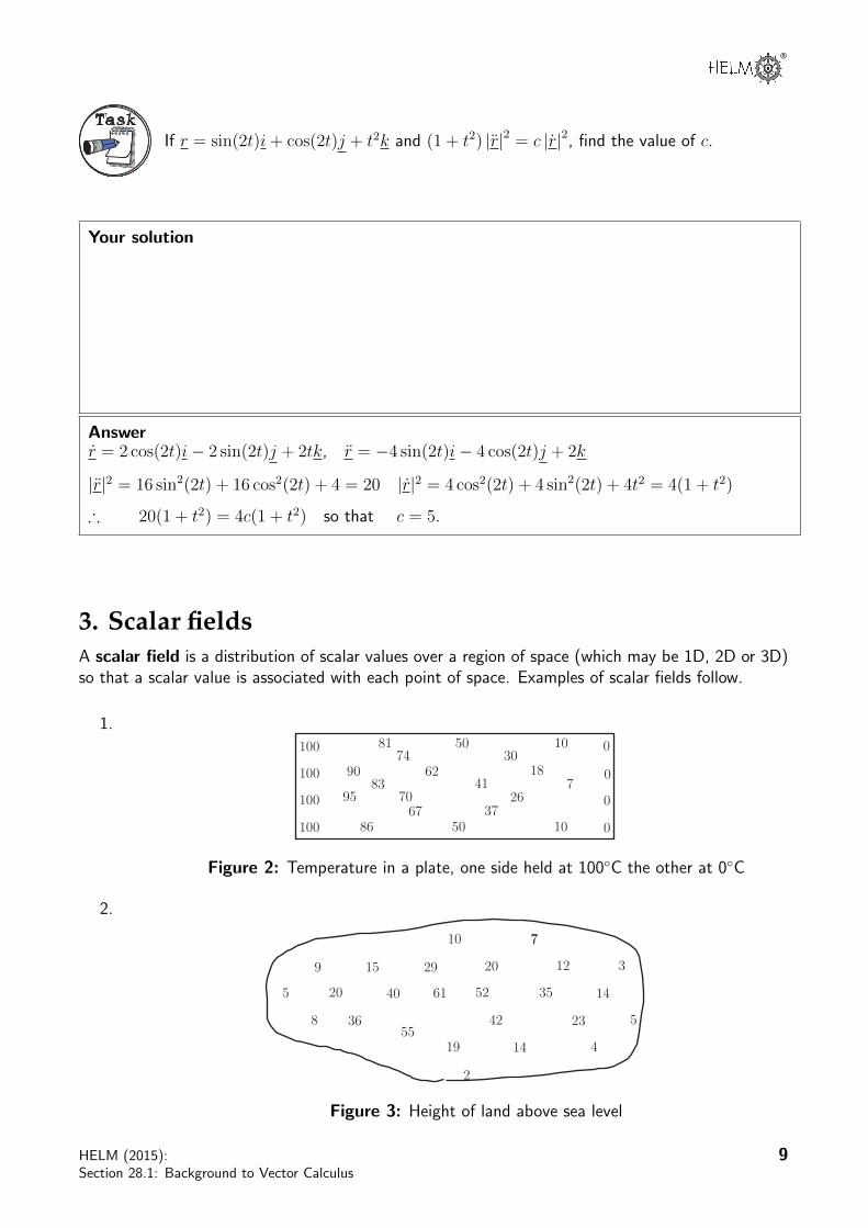
TaskIf r = sin(2t)i+ cos(2t)j + t2k and (1 + t2) |r|2 = c |r|2, find the value of c.

Your solution

Answerr = 2 cos(2t)i− 2 sin(2t)j + 2tk, r = −4 sin(2t)i− 4 cos(2t)j + 2k

|r|2 = 16 sin2(2t) + 16 cos2(2t) + 4 = 20 |r|2 = 4 cos2(2t) + 4 sin2(2t) + 4t2 = 4(1 + t2)

∴ 20(1 + t2) = 4c(1 + t2) so that c = 5.

3. Scalar fieldsA scalar field is a distribution of scalar values over a region of space (which may be 1D, 2D or 3D)so that a scalar value is associated with each point of space. Examples of scalar fields follow.

1.100

100

100

100

81

90

9583

86

74

7067

62

50

50

41

37

30

26

18

10

7

0

0

0

0

10

Figure 2: Temperature in a plate, one side held at 100◦C the other at 0◦C

2.

14

14

23

35

12

42

52

20

61

19

10

29

20

36

40

7

15

5

9

8

2

4

5

7

3

55

Figure 3: Height of land above sea level


9

3. The mean annual rainfall at different locations in Britain.

4. The light intensity near a 100 watt light bulb.

To define a scalar field we need to:

• Describe the region of space where it is found (this is the domain)

• Give a rule to show how the value of the scalar is related to every point in the domain.

Consider the scalar field defined by φ(x, y) = x + y over the rectangle 0 ≤ x ≤ 4, 0 ≤ y ≤ 2. Wecan calculate, and plot, values of φ at different (x, y) points. For example φ(0, 2) = 0 + 2 = 2,φ(4, 1) = 4 + 1 = 5 and so on.

6

4

4

4

4

4.0

3

3

3

3

3.0

2

2

2

2.0

2.0

1.0

1

1.00

5

5

5

x

y

0

1

1 2

2

3 4

Figure 4: The scalar field φ(x, y) = x+ y

ContoursA contour on a map is a curve joining points that are the same height above sea level. These contoursgive far more information about the shape of the land than selected spot heights.

For example, the contours near the top of a hill might look like those shown in Figure 5 where thenumbers are the values of the heights above sea level.

In general for a scalar field φ(x, y, z) , contour curves are the family of curves given by φ = c , fordifferent values of the constant c.

102030405060

Figure 5: Contour lines


®

Example 6Describe contour curves for the following scalar fields and sketch typical contoursfor (a) and (b).

(a) φ(x, y) = x+ y

(b) φ(x, y) = 9− x2 − y2

(c) φ(x, y) =1

x2 + y2 + z2

Solution

(a) The contour curves for φ(x, y) = x+ y are x+ y = c or y = −x+ c.These are straight lines of gradient −1. See Figure 6(a).

(b) For φ(x, y) = 9− x2 − y2, the contour curves are 9− x2 − y2 = c, or x2 + y2 = 9− c.See Figure 6(b). These are circles, centered at the origin, radius

√9− c.

0 1 2 3 4x

y

φ = 1

φ = 2 φ = 3

φ = 4

φ = 5

1

2

(a)

x

y

1 2 3

φ = 5

φ = 8

φ = 0

(b)

Figure 6: Contours for (a) x+ y (b) 9− x2 − y2

(c) For the three-dimensional scalar field φ(x, y, z) =1

x2 + y2 + z2the contour surfaces are

1

x2 + y2 + z2= c or x2 + y2 + z2 =

1

c. These are spheres, centered at the origin and of

radius1√c

.


11

TaskDescribe the contours for the following scalar fields

(a) φ = y − x (b) φ = x2 + y2 (c) φ = y − x2

Your solution

Answer

(a) Straight lines of gradient 1, (b) Circles; centred at origin, (c) Parabolas y = x2 + c.

Key Point 1

A scalar field F (in three-dimensional space) returns a real value for the function F for every point(x, y, z) in the domain of the field.

4. Vector fieldsA vector field is a distribution of vectors over a region of space such that a vector is associated witheach point of the region. Examples are:

1. The velocity of water flowing in a river (Figure 7).

Figure 7: Velocity of water in a river

2. The gravitational pull of the Earth (Figure 8). At every point there is a gravitational pulltowards the centre of the Earth.

Figure 8: Gravitational pull of the Earth

Note: the length of the vector is used to indicate its magnitude (i.e. greater near the centreof the Earth.)


®

3. The flow of heat in a metal plate insulated on its sides (Figure 9). Heat flows from the hotportion on the left to the cool portion on the right.

0!100!

Figure 9: Flow of heat in a metal plate

To define a vector field we need to :

• Describe the region of space where the vectors are found (the domain)

• Give a rule for associating a vector with each point of the domain.

Note that in the case of the heat flowing in a plate, the temperature can be described by a scalarfield while the flow of heat is described by a vector field.Consider the flow of water in different situations.

(a) In a pond where the water is motionless everywhere, the velocity at all points is zero.That is, v(x, y, z) = 0 , or for brevity, v = 0.

(b) Consider a straight river with steady flow downstream (see Figure 10). The surfacevelocity v can be seen by watching the motion of a light floating object, such as a leaf.The leaf will float downstream parallel to the bank so v will be a multiple of j. However,the speed is usually smallest near the bank and fastest in the middle of the river. In thissimple model, the velocity v is assumed to be independent of the depth z. That is, vvaries, in the i, or x, direction so that v will be of the form v = f(x)j.

bank

v

bankj

i x

y

Figure 10: Flow in a straight river

(c) In a more realistic model v would vary as we move downstream and would be different atdifferent depths due to, for example, rocks or bends. The velocity at any point could alsodepend on when the observation was made (for example the speed would be higher shortlyafter heavy rain) and so in general the velocity would be a function of the four variablesx, y, z and t, and be of the form v = f1(x, y, z, t)i + f2(x, y, z, t)j + f3(x, y, z, t)k, forsuitable functions f1, f2 and f3.


13

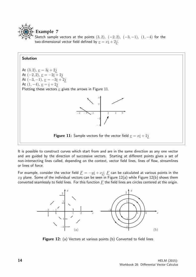
Example 7Sketch sample vectors at the points (3, 2), (−2, 2), (−3,−1), (1,−4) for thetwo-dimensional vector field defined by v = xi+ 2j.

Solution

At (3, 2), v = 3i+ 2jAt (−2, 2), v = −2i+ 2jAt (−3,−1), v = −3i+ 2jAt (1,−4), v = i+ 2jPlotting these vectors v gives the arrows in Figure 11.

2 4 6!2! 4! 6

2

4

!2

! 4

Figure 11: Sample vectors for the vector field v = xi+ 2j

It is possible to construct curves which start from and are in the same direction as any one vectorand are guided by the direction of successive vectors. Starting at different points gives a set ofnon-intersecting lines called, depending on the context, vector field lines, lines of flow, streamlinesor lines of force.

For example, consider the vector field F = −yi + xj; F can be calculated at various points in thexy plane. Some of the individual vectors can be seen in Figure 12(a) while Figure 12(b) shows themconverted seamlessly to field lines. For this function F the field lines are circles centered at the origin.

2

!2 ! 1

1

2

!2

! 1

1

2

!2 !1

1

2

!2

!1

1x

y

x

y

(a) (b)

Figure 12: (a) Vectors at various points (b) Converted to field lines


®

Example 8The Earth is affected by the gravitational force field of the Sun. This vectorfield is such that each vector F is directed towards the Sun and has magnitude

proportional to1

r2, where r =

√x2 + y2 + z2 is the distance from the Sun to the

Earth. Derive an equation for F and sketch some field lines.

Solution

The field has magnitude proportional to r−2 = (x2 + y2 + z2)−1 and points directly towards theSun (the origin) i.e. parallel to a unit vector pointing towards the origin. At the point given by

r = xi+ yj + zk, a unit vector pointing towards the origin is−xi− yj − zk∣∣−xi− yj − zk∣∣ = −xi− yj − zk√

x2 + y2 + z2.

Multiplying the unit vector by the required magnitude r−2 = (x2 + y2 + z2)−1 (and by a constant

of proportionality c) gives F = c−xi− yj − zk(x2 + y2 + z2)3/2

. Figure 13 shows some field lines for F .

Sun

Earth

Figure 13: Gravitational field of the Sun

Key Point 2

A vector field F (x, y, z) (in three-dimensional coordinates) returns a vector F 0 = F (x0, y0, z0) forevery point (x0, y0, z0) in the domain of the field.


15

Exercises

1. Which of the following are scalar fields and which are vector fields?

(a) F = x2 − yz

(b) G =2x− z√

x2 + y2 + z2 + 1

(c) f = xi+ yj + zk

(d) H =y − 1

z2 + 1x+

z − 1

x2 + 1y +

x− 1

y2 + 1z

(e) g = (y + z)i

2. Draw vector diagrams for the vector fields

(a) f = i+ 2j

(b) g = i+ y2j

Answers

1. (a), (b) and (d) are scalar fields as the quantities defined are scalars.

(c) and (e) are vector fields as the quantities defined are vectors.

2.

The vectors point in thesame direction everywhere

As |y| increases, they-component increases

(a) (b)


®

Differential VectorCalculus

��

��28.2

IntroductionA vector field or a scalar field can be differentiated with respect to position in three ways to produceanother vector field or scalar field. This Section studies the three derivatives, that is: (i) the gradientof a scalar field (ii) the divergence of a vector field and (iii) the curl of a vector field.

'

&

$

%

PrerequisitesBefore starting this Section you should . . .

• be familiar with the concept of a function oftwo variables

• be familiar with the concept of partialdifferentiation

• be familiar with scalar and vector fields�

�

�



• find the divergence, gradient or curl of avector or scalar field

HELM (2015):Section 28.2: Differential Vector Calculus

17

1. The gradient of a scalar fieldConsider the height φ above sea level at various points on a hill. Some contours for such a hill areshown in Figure 14.

A

BC

D

E

30 40 50 60

10φ =20

Figure 14: “Contour map” of a hill

We are interested in how φ changes from one point to another. Starting from A and makinga displacement d the change in height (φ ) depends on the direction of the displacement. Themagnitude of each d is the same.

Displacement Change in φAB 40− 30 = 10AC 40− 30 = 10AD 30− 30 = 0AE 20− 30 = −10

The change in φ clearly depends on the direction of the displacement. For the paths shown φincreases most rapidly along AB, does not increase at all along AD (as A and D are both on thesame contour and so are both at the same height) and decreases along AE.

The direction in which φ changes fastest is along the line of greatest slope which is orthogonal (i.e.perpendicular) to the contours. Hence, at each point of a scalar field we can define a vector fieldgiving the magnitude and direction of the greatest rate of change of φ locally.

A vector field, called the gradient, written grad φ, can be associated with a scalar field φ so that atevery point the direction of the vector field is orthogonal to the scalar field contour. This vector fieldis the direction of the maximum rate of change of φ.

For a second example consider a metal plate heated at one corner and cooled by an ice bag at theopposite corner. All edges and surfaces are insulated. After a while a steady state situation exists inwhich the temperature φ at any point remains the same. Some temperature contours are shown inFigure 15.

heat source

ice bag5

101520

253035

heat source

ice bag5

101520

253035

(a) (b)

Figure 15: Temperature contours and heat flow lines for a metal plate


®

The direction of the heat flow is along the flow lines which are orthogonal to the contours (see thedashed lines in Figure 15(b)); this heat flow is proportional to the vector field grad φ.

Definition

The gradient of the scalar field φ = f(x, y, z) is grad φ = ∇φ =∂φ

∂xi+

∂φ

∂yj +

∂φ

∂zk

Often, instead of grad φ, the notation ∇φ is used. (∇ is a vector differential operator called ‘del’ or

‘nabla’ defined by∂

∂xi+

∂

∂yj +

∂

∂zk. As a vector differential operator, it retains the characteristics

of a vector while also carrying out differentiation.)

The vector grad φ gives the magnitude and direction of the greatest rate of change of φ at anypoint, and is always orthogonal to the contours of φ. For example, in Figure 14, grad φ points inthe direction of AB while the contour line is parallel to AD i.e. perpendicular to AB. Similarly, inFigure 15(b), the various intersections of the contours with the lines representing grad φ occur atright-angles.

For the hill considered earlier the direction and magnitude of grad φ are shown at various pointsin Figure 16. Note that the magnitude of grad φ is greatest (as indicated by the length of the arrow)when the hill is at its steepest (as indicated by the closeness of the contours).

Figure 16: Grad φ and the steepest ascent direction for a hill

Key Point 3

φ is a scalar field but grad φ is a vector field.


19

Example 9Find grad φ for

(a) φ = x2 − 3y (b) φ = xy2z3

Solution

(a) grad φ =∂

∂x(x2−3y)i+

∂

∂y(x2−3y)j+

∂

∂z(x2−3y)k = 2xi+(−3)j+0k = 2xi−3j

(b) grad φ =∂

∂x(xy2z3)i+

∂

∂y(xy2z3)j +

∂

∂z(xy2z3)k = y2z3i+ 2xyz3j + 3xy2z2k

Example 10For f = x2 + y2 find grad f at the point A(1, 2). Show that the direction ofgrad f is orthogonal to the contour at this point.

Solution

grad f =∂f

∂xi+

∂f

∂yj +

∂f

∂zk = 2xi+ 2yj + 0k = 2xi+ 2yj

and at A(1, 2) this equals 2× 1i+ 2× 2j = 2i+ 4j.

Since f = x2 + y2 then the contours are defined by x2 + y2 = constant, so the contours are circlescentred at the origin. The vector grad f at A(1, 2) points directly away from the origin and hence

grad f and the contour are orthogonal; see Figure 17. Note that r(A) = i+ 2j =1

2grad f .

gradf

A

1

2

O x

y

Figure 17: Grad f is perpendicular to the contour lines

The change in a function φ in a given direction (specified as a unit vector a) is determined from thescalar product (grad φ) · a. This scalar quantity is called the directional derivative.Note:

• a along a contour implies a is perpendicular to grad φ which implies a · grad φ = 0.

• a perpendicular to a contour implies a · grad φ is a maximum.


®

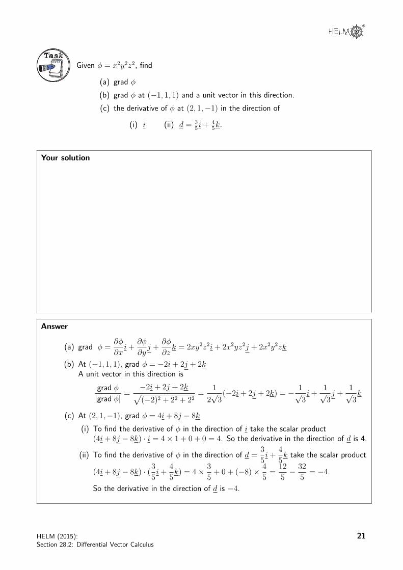
TaskGiven φ = x2y2z2, find

(a) grad φ

(b) grad φ at (−1, 1, 1) and a unit vector in this direction.

(c) the derivative of φ at (2, 1,−1) in the direction of

(i) i (ii) d = 35i+ 4

5k.

Your solution

Answer

(a) grad φ =∂φ

∂xi+

∂φ

∂yj +

∂φ

∂zk = 2xy2z2i+ 2x2yz2j + 2x2y2zk

(b) At (−1, 1, 1), grad φ = −2i+ 2j + 2kA unit vector in this direction is

grad φ

|grad φ|=−2i+ 2j + 2k√(−2)2 + 22 + 22

=1

2√3(−2i+ 2j + 2k) = − 1√

3i+

1√3j +

1√3k

(c) At (2, 1,−1), grad φ = 4i+ 8j − 8k

(i) To find the derivative of φ in the direction of i take the scalar product(4i+ 8j − 8k) · i = 4× 1 + 0 + 0 = 4. So the derivative in the direction of d is 4.

(ii) To find the derivative of φ in the direction of d =3

5i+

4

5k take the scalar product

(4i+ 8j − 8k) · (35i+

4

5k) = 4× 3

5+ 0 + (−8)× 4

5=

12

5− 32

5= −4.

So the derivative in the direction of d is −4.


21

Exercises

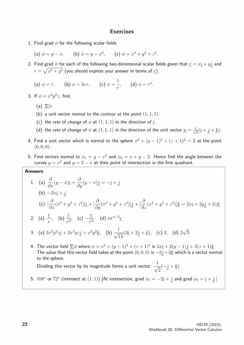
1. Find grad φ for the following scalar fields

(a) φ = y − x. (b) φ = y − x2, (c) φ = x2 + y2 + z2.

2. Find grad φ for each of the following two-dimensional scalar fields given that r = xi+ yj and

r =√x2 + y2 (you should express your answer in terms of r).

(a) φ = r, (b) φ = ln r, (c) φ =1

r, (d) φ = rn.

3. If φ = x3y2z, find,

(a) ∇φ(b) a unit vector normal to the contour at the point (1, 1, 1).

(c) the rate of change of φ at (1, 1, 1) in the direction of i.

(d) the rate of change of φ at (1, 1, 1) in the direction of the unit vector n = 1√3(i+ j + k).

4. Find a unit vector which is normal to the sphere x2 + (y − 1)2 + (z + 1)2 = 2 at the point(0, 0, 0).

5. Find vectors normal to φ1 = y − x2 and φ2 = x + y − 2. Hence find the angle between thecurves y = x2 and y = 2− x at their point of intersection in the first quadrant.

Answers

1. (a)∂

∂x(y − x)i+ ∂

∂y(y − x)j = −i+ j

(b) −2xi+ j

(c) [∂

∂x(x2 + y2 + z2)]i+ [

∂

∂y(x2 + y2 + z2)]j + [

∂

∂z(x2 + y2 + z2)]k = 2xi+ 2yj + 2zk

2. (a)r

r, (b)

r

r2, (c) − r

r3, (d) nrn−2r

3. (a) 3x2y2zi+ 2x3yzj + x3y2k, (b)1√14

(3i+ 2j + k), (c) 3, (d) 2√3

4. The vector field ∇φ where φ = x2 + (y − 1)2 + (z + 1)2 is 2xi+ 2(y − 1)j + 2(z + 1)kThe value that this vector field takes at the point (0, 0, 0) is −2j+2k which is a vector normalto the sphere.

Dividing this vector by its magnitude forms a unit vector:1√2(−j + k)

5. 108◦ or 72◦ (intersect at (1, 1)) [At intersection, grad φ1 = −2i+ j and grad φ2 = i+ j.]


®

2. The divergence of a vector fieldConsider the vector field F = F1i+ F2j + F3k.

In 3D cartesian coordinates the divergence of F is defined to be

div F =∂F1

∂x+∂F2

∂y+∂F3

∂z.

Note that F is a vector field but div F is a scalar.In terms of the differential operator ∇, div F = ∇ · F since

∇ · F = (i∂

∂x+ j

∂

∂y+ k

∂

∂z) · (F1i+ F2j + F3k) =

∂F1

∂x+∂F2

∂y+∂F3

∂z.

Physical Significance of the Divergence

The meaning of the divergence is most easily understood by considering the behaviour of a fluidand hence is relevant to engineering topics such as thermodynamics. The divergence (of the vectorfield representing velocity) at a point in a fluid (liquid or gas) is a measure of the rate per unit volumeat which the fluid is flowing away from the point. A negative divergence is a convergence indicating aflow towards the point. Physically positive divergence means that either the fluid is expanding or thatfluid is being supplied by a source external to the field. Conversely convergence means a contractionor the presence of a sink through which fluid is removed from the field. The lines of flow divergefrom a source and converge to a sink.

If there is no gain or loss of fluid anywhere then div v = 0 which is the equation of continuityfor an incompressible fluid.

The divergence also enters engineering topics such as electromagnetism. A magnetic field (B) hasthe property ∇ ·B = 0, that is there are no isolated sources or sinks of magnetic field (no magneticmonopoles).

Key Point 4

F is a vector field but div F is a scalar field.


23

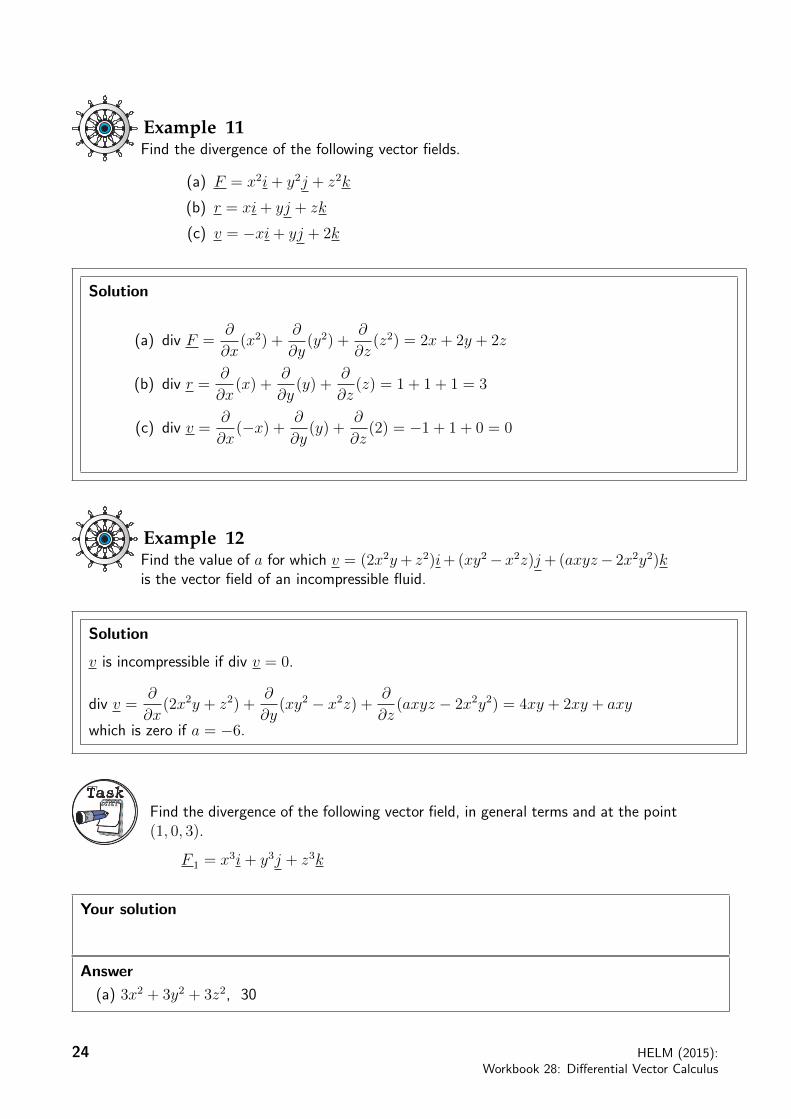
Example 11Find the divergence of the following vector fields.

(a) F = x2i+ y2j + z2k

(b) r = xi+ yj + zk

(c) v = −xi+ yj + 2k

Solution

(a) div F =∂

∂x(x2) +

∂

∂y(y2) +

∂

∂z(z2) = 2x+ 2y + 2z

(b) div r =∂

∂x(x) +

∂

∂y(y) +

∂

∂z(z) = 1 + 1 + 1 = 3

(c) div v =∂

∂x(−x) + ∂

∂y(y) +

∂

∂z(2) = −1 + 1 + 0 = 0

Example 12Find the value of a for which v = (2x2y+ z2)i+(xy2−x2z)j+(axyz− 2x2y2)kis the vector field of an incompressible fluid.

Solution

v is incompressible if div v = 0.

div v =∂

∂x(2x2y + z2) +

∂

∂y(xy2 − x2z) + ∂

∂z(axyz − 2x2y2) = 4xy + 2xy + axy

which is zero if a = −6.

TaskFind the divergence of the following vector field, in general terms and at the point(1, 0, 3).

F 1 = x3i+ y3j + z3k

Your solution

Answer

(a) 3x2 + 3y2 + 3z2, 30


®

TaskFind the divergence of F 2 = x2yi− 2xy2j, in general terms and at (1, 0, 3).

Your solution

Answer

−2xy, 0,

TaskFind the divergence of F 3 = x2zi− 2y3z3j + xyz2k, in general terms and at thepoint (1, 0, 3).

Your solution

Answer

2xz − 6y2z3 + 2xyz, 6

3. The curl of a vector fieldThe curl of the vector field given by F = F1i+ F2j + F3k is defined as the vector field

curl F = ∇× F =

∣∣∣∣∣∣∣∣∣∣∣∣

i j k

∂

∂x

∂

∂y

∂

∂z

F1 F2 F3

∣∣∣∣∣∣∣∣∣∣∣∣=

(∂F3

∂y− ∂F2

∂z

)i+

(∂F1

∂z− ∂F3

∂x

)j +

(∂F2

∂x− ∂F1

∂y

)k

Physical significance of curlThe divergence of a vector field represents the outflow rate from a point; however the curl of a vectorfield represents the rotation at a point.

Consider the flow of water down a river (Figure 18). The surface velocity v of the water is revealedby watching a light floating object such as a leaf. You will notice two types of motion. First theleaf floats down the river following the streamlines of v, but it may also rotate. This rotation maybe quite fast near the bank, but slow or zero in midstream. Rotation occurs when the velocity, and


25

hence the drag, is greater on one side of the leaf than the other.

bank bank

Figure 18: Rotation of a leaf in a stream

Note that for a two-dimensional vector field, such as v described here, curl v is perpendicular to themotion, and this is the direction of the axis about which the leaf rotates. The magnitude of curl vis related to the speed of rotation.

For motion in three dimensions a particle will tend to rotate about the axis that points in the directionof curl v, with its magnitude measuring the speed of rotation.

If, at any point P, curl v = 0 then there is no rotation at P and v is said to be irrotational at P. Ifcurl v = 0 at all points of the domain of v then the vector field is an irrotational vector field.

Key Point 5

Note that F is a vector field and that curl F is also a vector field.

Example 13Find curl v for the following two-dimensional vector fields

(a) v = xi+ 2j (b) v = −yi+ xj

If v represents the surface velocity of the flow of water, describe the motion of afloating leaf.

Solution

(a) ∇× v =

∣∣∣∣∣∣∣∣∣∣i j k

∂∂x

∂∂y

∂∂z

x 2 0

∣∣∣∣∣∣∣∣∣∣=

(∂

∂y(0)− ∂

∂z(2)

)i+

(∂

∂z(x)− ∂

∂x(0)

)j +

(∂

∂x(2)− ∂

∂y(x)

)k = 0

A floating leaf will travel along the streamlines without rotating.


®

Solution (contd.)

(b)

∇× v =

∣∣∣∣∣∣∣∣∣∣i j k

∂∂x

∂∂y

∂∂z

−y x 0

∣∣∣∣∣∣∣∣∣∣=

(∂

∂y(0)− ∂

∂z(x)

)i+

(∂

∂z(−y)− ∂

∂x(0)

)j +

(∂

∂x(x)− ∂

∂y(−y)

)k

= 0i+ 0j + 2k = 2k

A floating leaf will travel along the streamlines (anti-clockwise around the origin ) and will rotateanticlockwise (as seen from above).An analogy of the right-hand screw rule is that a positive (anti-clockwise) rotation in the xy planerepresents a positive z-component of the curl. Similar results apply for the other components.

Example 14(a) Find the curl of u = x2i+ y2j. When is u irrotational?

(b) Given F = (xy− xz)i+ 3x2j + yzk, find curl F at the origin (0, 0, 0)and at the point P = (1, 2, 3).

Solution

(a)

curl u = ∇× F =

∣∣∣∣∣∣∣∣∣∣i j k

∂∂x

∂∂y

∂∂z

x2 y2 0

∣∣∣∣∣∣∣∣∣∣=

(∂

∂y(0)− ∂

∂z(y2)

)i+

(∂

∂z(x2)− ∂

∂x(0)

)j +

(∂

∂x(y2)− ∂

∂y(x2)

)k

= 0i+ 0j + 0k = 0

curl u = 0 so u is irrotational everywhere.


27

Solution (contd.)

(b)

curl F = ∇× F =

∣∣∣∣∣∣∣∣∣∣i j k

∂∂x

∂∂y

∂∂z

xy − xz 3x2 yz

∣∣∣∣∣∣∣∣∣∣=

(∂

∂y(yz)− ∂

∂z(3x2)

)i+

(∂

∂z(xy − xz)− ∂

∂x(yz)

)j

+

(∂

∂x(3x2)− ∂

∂y(xy − xz)

)k

= zi− xj + 5xk

At the point (0, 0, 0), curl F = 0. At the point (1, 2, 3), curl F = 3i− j + 5k.

Engineering Example 1

Current associated with a magnetic field

Introduction

In a magnetic field B, an associated current is given by:

I =1

µ0

(∇×B)

Problem in words

Given the magnetic field B = B0xk find the associated current I.

x

z

Figure 19: Magnetic field profile

Mathematical statement of problem

We need to evaluate the curl of B.


®

Mathematical analysis

∇×B =

∣∣∣∣∣∣∣∣∣∣∣∣

i j k

∂

∂x

∂

∂y

∂

∂z

0 0 B0x

∣∣∣∣∣∣∣∣∣∣∣∣= 0i−B0j + 0k

= −B0j

and so I = −B0

µ0

j.

Interpretation

The current is perpendicular to the field and to the direction of variation of the field.

TaskFind the curl of the following two-dimensional vector field (a) in general terms and(b) at the point (1, 2).

F 2 = y2i+ xyj

Your solution

Answer

(a) ∇× F2 =

∣∣∣∣∣∣∣∣∣∣∣∣

i j k

∂

∂x

∂

∂y

∂

∂z

y2 xy 0

∣∣∣∣∣∣∣∣∣∣∣∣= 0i+ 0j + (y − 2y)k = −yk

(b) −2k


29

Exercises

1. Find the curl of each of the following two-dimensional vector fields. Give each in general termsand also at the point (1, 2).

(a) F 1 = 2xi+ 2yj

(b) F 3 = x2y3i− x3y2j

2. Find the curl of each of the following three-dimensional vector fields. Give each in generalterms and also at the point (2, 1, 3).

(a) F 1 = y2z3i+ 2xyz3j + 3xy2z2k

(b) F 2 = (xy + z2)i+ x2j + (xz − 2)k

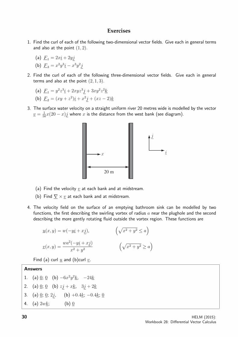
3. The surface water velocity on a straight uniform river 20 metres wide is modelled by the vectorv = 1

50x(20− x)j where x is the distance from the west bank (see diagram).

i

j

x

20 m

(a) Find the velocity v at each bank and at midstream.

(b) Find ∇× v at each bank and at midstream.

4. The velocity field on the surface of an emptying bathroom sink can be modelled by twofunctions, the first describing the swirling vortex of radius a near the plughole and the seconddescribing the more gently rotating fluid outside the vortex region. These functions are

u(x, y) = w(−yi+ xj),(√

x2 + y2 ≤ a)

v(x, y) =wa2(−yi+ xj)

x2 + y2

(√x2 + y2 ≥ a

)Find (a) curl u and (b)curl v.

Answers

1. (a) 0; 0 (b) −6x2y2k, −24k

2. (a) 0; 0 (b) zj + xk, 3j + 2k

3. (a) 0; 0; 2j, (b) +0.4k; −0.4k; 0

4. (a) 2wk; (b) 0


®

4. The LaplacianThe Laplacian of a function φ is written as ∇2φ and is defined as: Laplacian φ = div grad φ, that is

∇2φ = ∇ · ∇φ

= ∇ ·(∂φ

∂xi+

∂φ

∂yj +

∂φ

∂zk

)=

∂2φ

∂x2+∂2φ

∂y2+∂2φ

∂z2

The equation ∇2φ = 0, that is∂2φ

∂x2+∂2φ

∂y2+∂2φ

∂z2= 0 is known as Laplace’s equation and has

applications in many branches of engineering including Heat Flow, Electrical and Magnetic Fieldsand Fluid Mechanics.

Example 15Find the Laplacian of u = x2y2z + 2xz.

Solution

∇2u =∂2u

∂x2+∂2u

∂y2+∂2u

∂z2= 2y2z + 2x2z + 0 = 2(x2 + y2)z


31

5. Examples involving grad, div, curl and the LaplacianThe vector differential operators can be combined in several ways as the following examples show.

Example 16If A = 2yzi− x2yj + xz2k, B = x2i+ yzj − xyk and φ = 2x2yz3, find

(a) (A · ∇)φ (b) A · ∇φ (c) B ×∇φ (d) ∇2φ

Solution

(a)

(A · ∇)φ =

[(2yzi− x2yj + xz2k) · ( ∂

∂xi+

∂

∂yj +

∂

∂zk)

]φ

=

[2yz

∂

∂x− x2y ∂

∂y+ xz2

∂

∂z

]2x2yz3

= 2yz∂

∂x(2x2yz3)− x2y ∂

∂y(2x2yz3) + xz2

∂

∂z(2x2yz3)

= 2yz(4xyz3)− x2y(2x2z3) + xz2(6x2yz2)

= 8xy2z4 − 2x4yz3 + 6x3yz4

(b)

∇φ =∂

∂x(2x2yz3)i+

∂

∂y(2x2yz3)j +

∂

∂z(2x2yz3)k

= 4xyz3i+ 2x2z3j + 6x2yz2k

So A · ∇φ =(2yzi− x2yj + xz2k

)· (4xyz3i+ 2x2z3j + 6x2yz2k)

= 8xy2z4 − 2x4yz3 + 6x3yz4

(c) ∇φ = 4xyz3i+ 2x2z3j + 6x2yz2k so

B ×∇φ =

∣∣∣∣∣∣∣∣∣∣i j k

x2 yz −xy

4xyz3 2x2z3 6x2yz2

∣∣∣∣∣∣∣∣∣∣= i(6x2y2z3 + 2x3yz3) + j(−4x2y2z3 − 6x4yz2) + k(2x4z3 − 4xy2z4)

(d) ∇2φ =∂2

∂x2(2x2yz3) +

∂2

∂y2(2x2yz3) +

∂2

∂z2(2x2yz3) = 4yz3 + 0 + 12x2yz


®

Example 17For each of the expressions below determine whether the quantity can be formedand, if so, whether it is a scalar or a vector.

(a) grad(div A)

(b) grad(grad φ)

(c) curl(div F )

(d) div [ curl (A×grad φ) ]

Solution

(a) A is a vector and divA can be calculated and is a scalar. Hence, grad(div A) can beformed and is a vector.

(b) φ is a scalar so grad φ can be formed and is a vector. As grad φ is a vector, it is notpossible to take grad(grad φ).

(c) F is a vector and hence div F is a scalar. It is not possible to take the curl of a scalarso curl(div F ) does not exist.

(d) φ is a scalar so grad φ exists and is a vector. A×grad φ exists and is also a vector as iscurl A×grad φ. The divergence can be taken of this last vector to givediv [ curl (A×grad φ) ] which is a scalar.

6. Identities involving grad, div and curlThere are numerous identities involving the vector derivatives; a selection are given in Table 1.

Table 1

1 div(φA) = grad φ · A+ φ div A or ∇ · (φA) = (∇φ) · A+ φ(∇ · A)2 curl(φA) = grad φ× A+ φ curl A or ∇× (φA) = (∇φ)× A+ φ(∇× A)3 div (A×B) = B· curl A− A· curl B or ∇ · (A×B) = B · (∇× A)− A · (∇×B)4 curl (A×B) = (B· grad ) A− (A· grad ) B or ∇× (A×B) = (B · ∇)A− (A · ∇)B

+A div B −B div A +A ∇ ·B −B ∇ · A5 grad (A ·B) = (B· grad ) A+ (A· grad ) B or ∇(A ·B) = (B · ∇)A+ (A · ∇)B

+A× curl B +B× curl A +A× (∇×B) +B × (∇× A)6 curl (grad φ)= 0 or ∇× (∇φ) = 07 div (curl A)= 0 or ∇ · (∇× A) = 0


33

Example 18Show for any vector field A = A1i+ A2j + A3k, that div curl A = 0.

Solution

div curl A = div

∣∣∣∣∣∣∣∣∣∣∣∣

i j j

∂

∂x

∂

∂y

∂

∂z

A1 A2 A3

∣∣∣∣∣∣∣∣∣∣∣∣= div

[(∂A3

∂y− ∂A2

∂z

)i+

(∂A1

∂z− ∂A3

∂x

)j +

(∂A2

∂x− ∂A1

∂y

)k

]=

∂

∂x

(∂A3

∂y− ∂A2

∂z

)+

∂

∂y

(∂A1

∂z− ∂A3

∂x

)+

∂

∂z

(∂A2

∂x− ∂A1

∂y

)=

∂2A3

∂x∂y− ∂2A2

∂z∂x+∂2A1

∂y∂z− ∂2A3

∂y∂x+∂2A2

∂z∂x− ∂2A1

∂z∂y= 0

N.B. This assumes∂2A3

∂x∂y=∂2A3

∂y∂xetc.

Example 19Verify identity 1 for the vector A = 2xyi− 3zk and the function φ = xy2.

Solution

φA = 2x2y3i− 3xy2zk so

∇ · φA = ∇ ·(2x2y3i− 3xy2zk

)=

∂

∂x(2x2y3) +

∂

∂z(−3xy2z) = 4xy3 − 3xy2

So LHS = 4xy3 − 3xy2.

∇φ =∂

∂x(xy2)i+

∂

∂y(xy2)j +

∂

∂z(xy2)k = y2i+ 2xyj so

(∇φ) · A = (y2i+ 2xyj) · (2xyi− 3zk) = 2xy3

∇ · A = ∇ · (2xyi− 3zk) = 2y − 3 so φ∇ · A = 2xy3 − 3xy2 giving(∇φ) · A+ φ(∇ · A) = 2xy3 + (2xy3 − 3xy2) = 4xy3 − 3xy2

So RHS = 4xy3 − 3xy2 = LHS.

So ∇ · (φA) = (∇φ) · A+ φ(∇ · A) in this case.


®

TaskIf F = x2yi− 2xzj + 2yzk, find

(a) ∇ · F(b) ∇× F(c) ∇(∇ · F )(d) ∇ · (∇× F )(e) ∇× (∇× F )

Your solution

Answer

(a) 2xy + 2y,

(b) (2x+ 2z)i− (x2 + 2z)k,

(c) 2yi+ (2 + 2x)j (using answer to (a)),

(d) 0 (using answer to (b)),

(e) (2 + 2x)j (using answer to (b))


35

TaskIf φ = 2xz − y2z, find

(a) ∇φ(b) ∇2φ = ∇ · (∇φ)(c) ∇× (∇φ)

Your solution

Answer

(a) 2zi− 2yzj + (2x− y2)k, (b) −2z, (c) 0 where (b) and (c) use the answer to (a).

Exercise

Which of the following combinations of grad, div and curl can be formed? If a quantity can beformed, state whether it is a scalar or a vector.

(a) div (grad φ)

(b) div (div A)

(c) curl (curl F )

(d) div (curl F )

(e) curl (grad φ)

(f) curl (div A)

(g) div (A ·B)

(h) grad (φ1φ2)

(i) curl (div (A× grad φ))

Answers

(a), (d) are scalars;

(c), (e), (h) are vectors;

(b), (f), (g) and (i) are not defined.


®

OrthogonalCurvilinear

Coordinates��

��28.3

IntroductionThe derivatives div, grad and curl from Section 28.2 can be carried out using coordinate systems otherthan the rectangular Cartesian coordinates. This Section shows how to calculate these derivatives inother coordinate systems. Two coordinate systems - cylindrical polar coordinates and spherical polarcoordinates - will be illustrated.

�

�

�

�Prerequisites

Before starting this Section you should . . .

• be able to find the gradient, divergence andcurl of a field in Cartesian coordinates

• be familiar with polar coordinates�

�

�



• find the divergence, gradient or curl of avector or scalar field expressed in terms oforthogonal curvilinear coordinates

HELM (2015):Section 28.3: Orthogonal Curvilinear Coordinates

37

1. Orthogonal curvilinear coordinatesThe results shown in Section 28.2 have been given in terms of the familiar Cartesian (x, y, z) co-ordinate system. However, other coordinate systems can be used to better describe some physicalsituations. A set of coordinates u = u(x, y, z), v = v(x, y, z) and w = w(x, y, z) where the direc-tions at any point indicated by u, v and w are orthogonal (perpendicular) to each other is referred toas a set of orthogonal curvilinear coordinates. With each coordinate is associated a scale factor

hu, hv or hw respectively where hu =

√(∂x∂u

)2+(∂y∂u

)2+(∂z∂u

)2(with similar expressions for hv and

hw). The scale factor gives a measure of how a change in the coordinate changes the position of apoint.

Two commonly-used sets of orthogonal curvilinear coordinates are cylindrical polar coordinatesand spherical polar coordinates. These are similar to the plane polar coordinates introduced in

17.2 but represent extensions to three dimensions.

Cylindrical polar coordinatesThis corresponds to plane polar (ρ, φ) coordinates with an added z-coordinate directed out of thexy plane. Normally the variables ρ and φ are used instead of r and θ to give the three coordinatesρ, φ and z. A cylinder has equation ρ = constant.The relationship between the coordinate systems is given by

x = ρ cosφ y = ρ sinφ z = z

(i.e. the same z is used by the two coordinate systems). See Figure 20(a).

(x, y, z)

!

"

z

x

y!

(x, y, z)

!

"

z

x

y!

!

"

k

(a) (b)

Figure 20: Cylindrical polar coordinates

The scale factors hρ, hφ and hz are given as follows

hρ =

√(∂x

∂ρ

)2

+

(∂y

∂ρ

)2

+

(∂z

∂ρ

)2

=√

(cosφ)2 + (sinφ)2 + 0 = 1

hφ =

√(∂x

∂φ

)2

+

(∂y

∂φ

)2

+

(∂z

∂φ

)2

=√

(−ρ sinφ)2 + (ρ cosφ)2 + 0 = ρ

hz =

√(∂x

∂z

)2

+

(∂y

∂z

)2

+

(∂z

∂z

)2

=√

(02 + 02 + 12) = 1


®

Spherical polar coordinatesIn this system a point is referred to by its distance from the origin r and two angles φ and θ. Theangle θ is the angle between the positive z-axis and the line from the origin to the point. The angleφ is the angle from the x-axis to the projection of the point in the xy plane.

A useful analogy is of latitude, longitude and height on Earth.

• The variable r plays the role of height (but height measured above the centre of Earth ratherthan from the surface).

• The variable θ plays the role of latitude but is modified so that θ = 0 represents the North

Pole, θ = 90◦ =π

2represents the equator and θ = 180◦ = π represents the South Pole.

• The variable φ plays the role of longitude.

A sphere has equation r = constant.The relationship between the coordinate systems is given by

x = r sin θ cosφ y = r sin θ sinφ z = r cos θ. See Figure 21.

(x, y, z)

!

r"

z

y

x,

Figure 21: Spherical polar coordinates

The scale factors hr, hθ and hφ are given by

hr =

√(∂x

∂r

)2

+

(∂y

∂r

)2

+

(∂z

∂r

)2

=√

(sin θ cosφ)2 + (sin θ sinφ)2 + (cos θ)2 = 1

hθ =

√(∂x

∂θ

)2

+

(∂y

∂θ

)2

+

(∂z

∂θ

)2

=√

(r cos θ cosφ)2 + (r cos θ sinφ)2 + (−r sin θ)2 = r

hφ =

√(∂x

∂φ

)2

+

(∂y

∂φ

)2

+

(∂z

∂φ

)2

=√(−r sin θ sinφ)2 + (r sin θ cosφ)2 + 0 = r sin θ


39

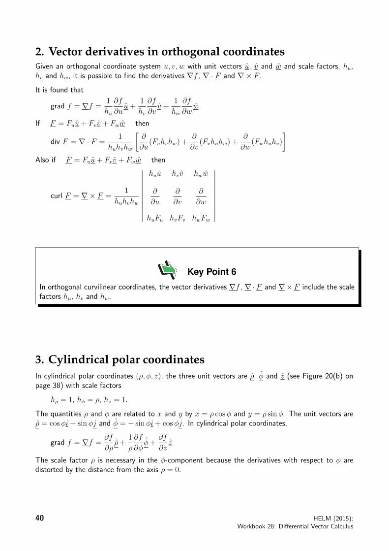
2. Vector derivatives in orthogonal coordinatesGiven an orthogonal coordinate system u, v, w with unit vectors u, v and w and scale factors, hu,hv and hw, it is possible to find the derivatives ∇f , ∇ · F and ∇× F .

It is found that

grad f = ∇f =1

hu

∂f

∂uu+

1

hv

∂f

∂vv +

1

hw

∂f

∂ww

If F = Fuu+ Fvv + Fww then

div F = ∇ · F =1

huhvhw

[∂

∂u(Fuhvhw) +

∂

∂v(Fvhuhw) +

∂

∂w(Fwhuhv)

]Also if F = Fuu+ Fvv + Fww then

curl F = ∇× F =1

huhvhw

∣∣∣∣∣∣∣∣∣∣∣

huu hvv hww

∂

∂u

∂

∂v

∂

∂w

huFu hvFv hwFw

∣∣∣∣∣∣∣∣∣∣∣

Key Point 6

In orthogonal curvilinear coordinates, the vector derivatives ∇f , ∇ ·F and ∇×F include the scalefactors hu, hv and hw.

3. Cylindrical polar coordinatesIn cylindrical polar coordinates (ρ, φ, z), the three unit vectors are ρ, φ and z (see Figure 20(b) onpage 38) with scale factors

hρ = 1, hφ = ρ, hz = 1.

The quantities ρ and φ are related to x and y by x = ρ cosφ and y = ρ sinφ. The unit vectors areρ = cosφi+ sinφj and φ = − sinφi+ cosφj. In cylindrical polar coordinates,

grad f = ∇f =∂f

∂ρρ+

1

ρ

∂f

∂φφ+

∂f

∂zz

The scale factor ρ is necessary in the φ-component because the derivatives with respect to φ aredistorted by the distance from the axis ρ = 0.


®

If F = Fρρ+ Fφφ+ Fz z then

div F = ∇ · F =1

ρ

[∂

∂ρ(ρFρ) +

∂

∂φ(Fφ) +

∂

∂z(ρFz)

]

curl F = ∇× F =1

ρ

∣∣∣∣∣∣∣∣∣∣∣∣

ρ ρφ z

∂

∂ρ

∂

∂φ

∂

∂z

Fρ ρFφ Fz

∣∣∣∣∣∣∣∣∣∣∣∣.

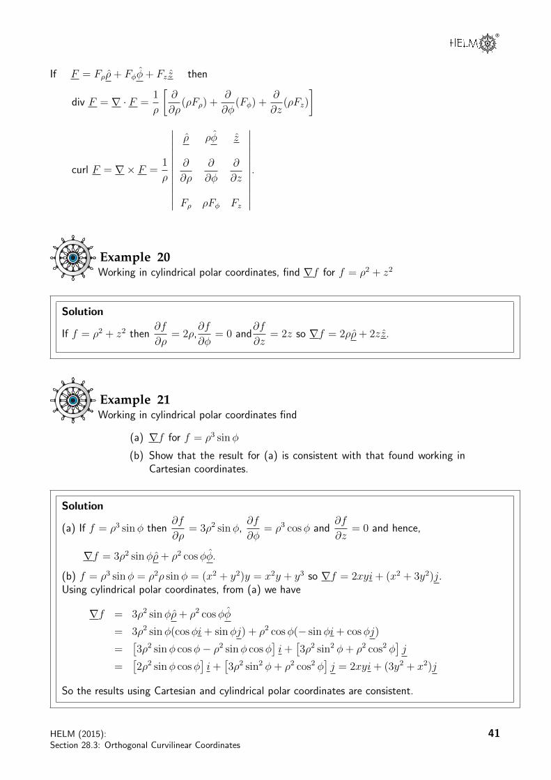
Example 20Working in cylindrical polar coordinates, find ∇f for f = ρ2 + z2

Solution

If f = ρ2 + z2 then∂f

∂ρ= 2ρ,

∂f

∂φ= 0 and

∂f

∂z= 2z so ∇f = 2ρρ+ 2zz.

Example 21Working in cylindrical polar coordinates find

(a) ∇f for f = ρ3 sinφ

(b) Show that the result for (a) is consistent with that found working inCartesian coordinates.

Solution

(a) If f = ρ3 sinφ then∂f

∂ρ= 3ρ2 sinφ,

∂f

∂φ= ρ3 cosφ and

∂f

∂z= 0 and hence,

∇f = 3ρ2 sinφρ+ ρ2 cosφφ.

(b) f = ρ3 sinφ = ρ2ρ sinφ = (x2 + y2)y = x2y + y3 so ∇f = 2xyi+ (x2 + 3y2)j.Using cylindrical polar coordinates, from (a) we have

∇f = 3ρ2 sinφρ+ ρ2 cosφφ

= 3ρ2 sinφ(cosφi+ sinφj) + ρ2 cosφ(− sinφi+ cosφj)

=[3ρ2 sinφ cosφ− ρ2 sinφ cosφ

]i+[3ρ2 sin2 φ+ ρ2 cos2 φ

]j

=[2ρ2 sinφ cosφ

]i+[3ρ2 sin2 φ+ ρ2 cos2 φ

]j = 2xyi+ (3y2 + x2)j

So the results using Cartesian and cylindrical polar coordinates are consistent.


41

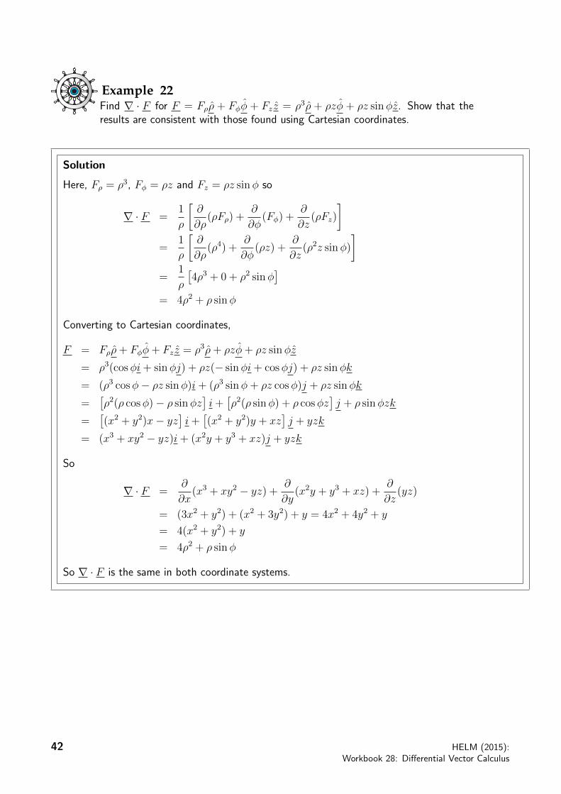
Example 22Find ∇ · F for F = Fρρ + Fφφ + Fz z = ρ3ρ + ρzφ + ρz sinφz. Show that theresults are consistent with those found using Cartesian coordinates.

Solution

Here, Fρ = ρ3, Fφ = ρz and Fz = ρz sinφ so

∇ · F =1

ρ

[∂

∂ρ(ρFρ) +

∂

∂φ(Fφ) +

∂

∂z(ρFz)

]=

1

ρ

[∂

∂ρ(ρ4) +

∂

∂φ(ρz) +

∂

∂z(ρ2z sinφ)

]=

1

ρ

[4ρ3 + 0 + ρ2 sinφ

]= 4ρ2 + ρ sinφ

Converting to Cartesian coordinates,

F = Fρρ+ Fφφ+ Fz z = ρ3ρ+ ρzφ+ ρz sinφz

= ρ3(cosφi+ sinφj) + ρz(− sinφi+ cosφj) + ρz sinφk

= (ρ3 cosφ− ρz sinφ)i+ (ρ3 sinφ+ ρz cosφ)j + ρz sinφk

=[ρ2(ρ cosφ)− ρ sinφz

]i+[ρ2(ρ sinφ) + ρ cosφz

]j + ρ sinφzk

=[(x2 + y2)x− yz

]i+[(x2 + y2)y + xz

]j + yzk

= (x3 + xy2 − yz)i+ (x2y + y3 + xz)j + yzk

So

∇ · F =∂

∂x(x3 + xy2 − yz) + ∂

∂y(x2y + y3 + xz) +

∂

∂z(yz)

= (3x2 + y2) + (x2 + 3y2) + y = 4x2 + 4y2 + y

= 4(x2 + y2) + y

= 4ρ2 + ρ sinφ

So ∇ · F is the same in both coordinate systems.


®

Example 23Find ∇× F for F = ρ2ρ+ z sinφφ+ 2z cosφz.

Solution

∇× F =1

ρ

∣∣∣∣∣∣∣∣∣∣∣∣

ρ ρφ z

∂

∂ρ

∂

∂φ

∂

∂z

Fρ ρFφ Fz

∣∣∣∣∣∣∣∣∣∣∣∣=

1

ρ

∣∣∣∣∣∣∣∣∣∣∣∣

ρ ρφ z

∂

∂ρ

∂

∂φ

∂

∂z

ρ2 ρz sinφ 2z cosφ

∣∣∣∣∣∣∣∣∣∣∣∣=

1

ρ

[ρ

[∂

∂φ(2z cosφ)− ∂

∂z(ρz sinφ)

]+ρφ

[∂

∂zρ2 − ∂

∂ρ(2z cosφ)

]+z

[∂

∂ρ(ρz sinφ)− ∂

∂φρ2]]

=1

ρ

[ρ(−2z sinφ− ρ sinφ) + ρφ(0) + z(z sinφ)

]= −(2z sinφ+ ρ sinφ)

ρρ+

z sinφ

ρz


Divergence of a magnetic field

Introduction

A magnetic field B must satisfy ∇ ·B = 0. An associated current is given by:

I =1

µ0

(∇×B)

Problem in words

For the magnetic field (in cylindrical polar coordinates ρ, φ, z)

B = B0ρ

1 + ρ2φ+ αz

show that the divergence of B is zero and find the associated current.


We must

(a) show that ∇ ·B = 0 (b) find the current I =1

µ0

(∇×B)


43


(a) Express B as (Bρ, Bφ, Bz); then

∇ ·B =1

ρ

[∂

∂ρ(ρBρ) +

∂

∂φ(Bφ) +

∂

∂z(ρBz)

]=

1

ρ

[∂

∂ρ(0) +

∂

∂φ

(B0

ρ

1 + ρ2

)+ ρ

∂

∂z(α)

]=

1

ρ[0 + 0 + 0] = 0 as required.

(b) To find the current evaluate

I =1

µ0

(∇×B) =1

µ0

1

ρ

∣∣∣∣∣∣∣∣∣∣∣∣

ρ ρφ z

∂

∂ρ

∂

∂φ

∂

∂z

Bρ ρBφ Bz

∣∣∣∣∣∣∣∣∣∣∣∣=

∣∣∣∣∣∣∣∣∣∣∣∣∣∣

ρ ρφ z

∂

∂ρ

∂

∂φ

∂

∂z

0 B0ρ2

1 + ρ2α

∣∣∣∣∣∣∣∣∣∣∣∣∣∣=

1

µ0ρ

[0ρ+ 0ρφ+B0

∂

∂ρ

(ρ2

1 + ρ2

)z

]=

1

µ0ρB0

[2ρ

(1 + ρ2)2

]z =

2B0

µ0(1 + ρ2)2z

Interpretation

The magnetic field is in the form of a helix with the current pointing along its axis (Fig 22). Suchan arrangement is often used for the magnetic containment of charged particles in a fusion reactor.

Figure 22: The magnetic field forms a helix


®

Example 24A magnetic field B is given by B = ρ−2φ+ kz. Find ∇ ·B and ∇×B.

Solution

∇ ·B =1

ρ

[∂

∂ρ(0) +

∂

∂φ(ρ−2) +

∂

∂z(kρ)

]=

1

ρ[0 + 0 + 0] = 0

∇×B =1

ρ

∣∣∣∣∣∣∣∣∣∣∣∣

ρ ρφ z

∂

∂ρ

∂

∂φ

∂

∂z

Bρ ρBφ Bz

∣∣∣∣∣∣∣∣∣∣∣∣=

1

ρ

∣∣∣∣∣∣∣∣∣∣∣∣

ρ ρφ z

∂

∂ρ

∂

∂φ

∂

∂z

0 ρ−1 k

∣∣∣∣∣∣∣∣∣∣∣∣= − 1

ρ3z

All magnetic fields satisfy ∇ ·B = 0 i.e. an absence of magnetic monopoles.Note that there is a class of magnetic fields known as potential fields that satisfy ∇×B = 0

TaskUsing cylindrical polar coordinates, find ∇f for f = ρ2z sinφ

Your solution

Answer∂

∂ρ[ρ2z sinφ]ρ+

1

ρ

∂

∂φ[ρ2z sinφ]φ+

∂

∂z[ρ2z sinφ]z = 2ρz sinφρ+ ρz cosφφ+ ρ2 sinφz


45

TaskUsing cylindrical polar coordinates, find ∇f for f = z sin 2φ

Your solution

Answer∂

∂ρ[z sin 2φ]ρ+

1

ρ

∂

∂φ[z sin 2φ]φ+

∂

∂z[z sin 2φ]z =

2

ρz cos 2φφ+ sin 2φz

TaskFind ∇ · F for F = ρ cosφρ− ρ sinφφ+ ρzz

i.e. Fρ = ρ cosφ, Fφ = −ρ sinφ, Fz = ρz

(a) First find the derivatives∂

∂ρ[ρFρ],

∂

∂φ[Fφ],

∂

∂z[ρFz]:

Your solution

Answer

2ρ cosφ, −ρ cosφ, ρ2

(b) Now combine these to find ∇ · F :

Your solution


®

Answer

∇ · F =1

ρ

[∂

∂ρ(ρFρ) +

∂

∂φ(Fφ) +

∂

∂z(ρFz)

]=

1

ρ

[∂

∂ρ(ρ2 cosφ) +

∂

∂φ(−ρ sinφ) + ∂

∂z(ρ2z)

]=

1

ρ

[2ρ cosφ− ρ cosφ+ ρ2

]= cosφ+ ρ

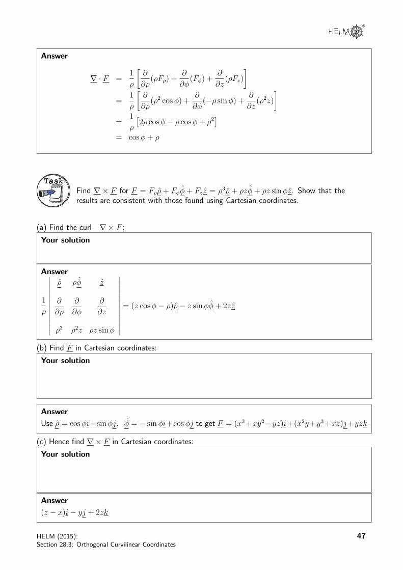
TaskFind ∇× F for F = Fρρ + Fφφ + Fz z = ρ3ρ + ρzφ + ρz sinφz. Show that theresults are consistent with those found using Cartesian coordinates.

(a) Find the curl ∇× F :

Your solution

Answer

1

ρ

∣∣∣∣∣∣∣∣∣∣∣∣

ρ ρφ z

∂

∂ρ

∂

∂φ

∂

∂z

ρ3 ρ2z ρz sinφ

∣∣∣∣∣∣∣∣∣∣∣∣= (z cosφ− ρ)ρ− z sinφφ+ 2zz

(b) Find F in Cartesian coordinates:

Your solution

Answer

Use ρ = cosφi+sinφj, φ = − sinφi+cosφj to get F = (x3+xy2−yz)i+(x2y+y3+xz)j+yzk

(c) Hence find ∇× F in Cartesian coordinates:

Your solution

Answer

(z − x)i− yj + 2zk


47

(d) Using ρ = cosφi+ sinφj and φ = − sinφi+ cosφj, show that the solution to part (a) is equalto the solution for part (c):

Your solution

Answer

(z cosφ−ρ) ρ−z sinφ φ+2z z = (z cosφ−ρ)(cosφ i+sinφ j)−z sinφ(− sinφ i+cosφ j)+2z k

= [zcos2φ− ρ cosφ+ zsin2φ] i+ [zcosφsinφ− ρ sinφ− zsinφcosφ] j + 2z k= [z − ρ cosφ] i− ρ sinφ j + 2z k = (z − x) i− y j + 2z k

Exercises

1. For F = ρρ+ (ρ sinφ+ z)φ+ ρzz, find ∇ · F and ∇× F .

2. For f = ρ2z2 cos 2φ, find ∇× (∇f).

Answers

1. 2 + cosφ+ ρ, −ρ− z φ+ (2 sinφ+z

ρ) z

2. 0

4. Spherical polar coordinatesIn spherical polar coordinates (r, θ, φ), the 3 unit vectors are r, θ and φ with scale factors hr = 1,hθ = r, hφ = r sin θ. The quantities r, θ and φ are related to x, y and z by x = r sin θ cosφ,y = r sin θ sinφ and z = r cos θ. In spherical polar coordinates,

grad f = ∇f =∂f

∂rr +

1

r

∂f

∂θθ +

1

r sin θ

∂f

∂φφ

If F = Frr + Fθθ + Fφφ

then

div F = ∇ · F =1

r2 sin θ

[∂

∂r(r2 sin θFr) +

∂

∂θ(r sin θFθ) +

∂

∂φ(rFφ)

]

curl F = ∇× F =1

r2 sin θ

∣∣∣∣∣∣∣∣∣∣∣∣

r rθ r sin θφ

∂

∂r

∂

∂θ

∂

∂φ

Fr rFθ r sin θFφ

∣∣∣∣∣∣∣∣∣∣∣∣48 HELM (2015):

Workbook 28: Differential Vector Calculus

®

Example 25In spherical polar coordinates, find ∇f for

(a) f = r (b) f =1

r(c) f = r2 sin(φ+ θ)

[Note: parts (a) and (b) relate to Exercises 2(a) and 2(c) on page 22.]

Solution

(a) ∇f =∂f

∂rr +

1

r

∂f

∂θθ +

1

r sin θ

∂f

∂φφ

=∂(r)

∂rr +

1

r

∂(r)

∂θθ +

1

r sin θ

∂(r)

∂φφ

= 1r = r

(b) ∇f =∂f

∂rr +

1

r

∂f

∂θθ +

1

r sin θ

∂f

∂φφ

=∂(1

r)

∂rr +

1

r

∂(1r)

∂θθ +

1

r sin θ

∂(1r)

∂φφ

= − 1

r2r

(c) ∇f =∂f

∂rr +

1

r

∂f

∂θθ +

1

r sin θ

∂f

∂φφ

=∂(r sin(φ+ θ))

∂rr +

1

r

∂(r sin(φ+ θ))

∂θθ +

1

r sin θ

∂(r2 sin(φ+ θ))

∂φφ

= 2r sin(φ+ θ)r +1

rr2 cos(φ+ θ)θ +

1

r sin θr2 cos(φ+ θ)φ

= 2r sin(φ+ θ)r + r cos(φ+ θ)θ +r cos(φ+ θ)

sin θφ


49


Electric potential

Introduction

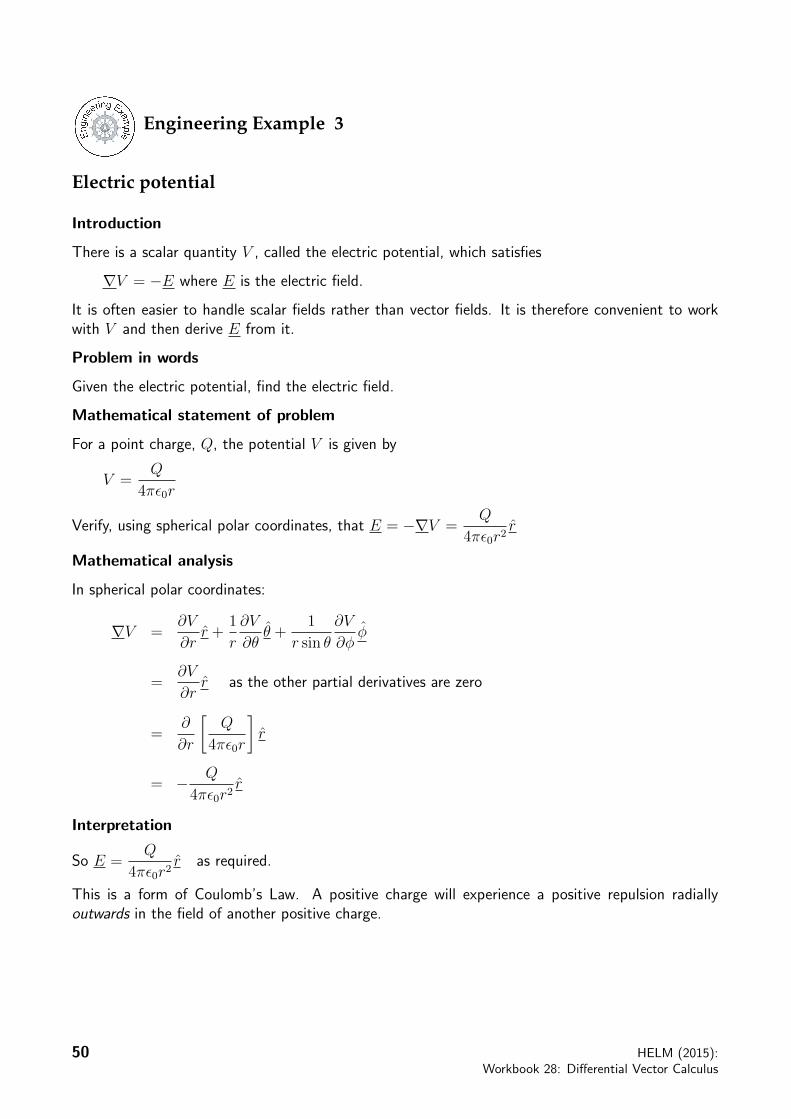
There is a scalar quantity V , called the electric potential, which satisfies

∇V = −E where E is the electric field.

It is often easier to handle scalar fields rather than vector fields. It is therefore convenient to workwith V and then derive E from it.

Problem in words

Given the electric potential, find the electric field.


For a point charge, Q, the potential V is given by

V =Q

4πε0r

Verify, using spherical polar coordinates, that E = −∇V =Q

4πε0r2r


In spherical polar coordinates:

∇V =∂V

∂rr +

1

r

∂V

∂θθ +

1

r sin θ

∂V

∂φφ

=∂V

∂rr as the other partial derivatives are zero

=∂

∂r

[Q

4πε0r

]r

= − Q

4πε0r2r

Interpretation

So E =Q

4πε0r2r as required.

This is a form of Coulomb’s Law. A positive charge will experience a positive repulsion radiallyoutwards in the field of another positive charge.


®

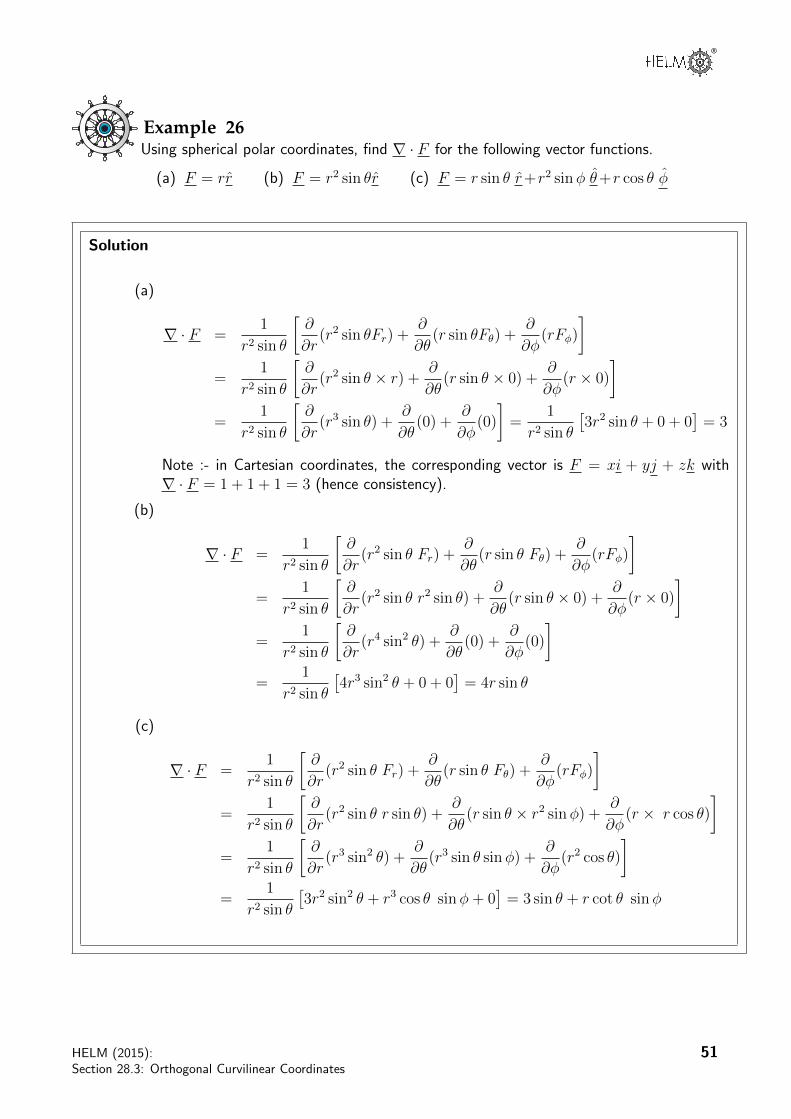
Example 26Using spherical polar coordinates, find ∇ · F for the following vector functions.

(a) F = rr (b) F = r2 sin θr (c) F = r sin θ r+r2 sinφ θ+r cos θ φ

Solution

(a)

∇ · F =1

r2 sin θ

[∂

∂r(r2 sin θFr) +

∂

∂θ(r sin θFθ) +

∂

∂φ(rFφ)

]=

1

r2 sin θ

[∂

∂r(r2 sin θ × r) + ∂

∂θ(r sin θ × 0) +

∂

∂φ(r × 0)

]=

1

r2 sin θ

[∂

∂r(r3 sin θ) +

∂

∂θ(0) +

∂

∂φ(0)

]=

1

r2 sin θ

[3r2 sin θ + 0 + 0

]= 3

Note :- in Cartesian coordinates, the corresponding vector is F = xi + yj + zk with∇ · F = 1 + 1 + 1 = 3 (hence consistency).

(b)

∇ · F =1

r2 sin θ

[∂

∂r(r2 sin θ Fr) +

∂

∂θ(r sin θ Fθ) +

∂

∂φ(rFφ)

]=

1

r2 sin θ

[∂

∂r(r2 sin θ r2 sin θ) +

∂

∂θ(r sin θ × 0) +

∂

∂φ(r × 0)

]=

1

r2 sin θ

[∂

∂r(r4 sin2 θ) +

∂

∂θ(0) +

∂

∂φ(0)

]=

1

r2 sin θ

[4r3 sin2 θ + 0 + 0

]= 4r sin θ

(c)

∇ · F =1

r2 sin θ

[∂

∂r(r2 sin θ Fr) +

∂

∂θ(r sin θ Fθ) +

∂

∂φ(rFφ)

]=

1

r2 sin θ

[∂

∂r(r2 sin θ r sin θ) +

∂

∂θ(r sin θ × r2 sinφ) + ∂

∂φ(r × r cos θ)

]=

1

r2 sin θ

[∂

∂r(r3 sin2 θ) +

∂

∂θ(r3 sin θ sinφ) +

∂

∂φ(r2 cos θ)

]=

1

r2 sin θ

[3r2 sin2 θ + r3 cos θ sinφ+ 0

]= 3 sin θ + r cot θ sinφ


51

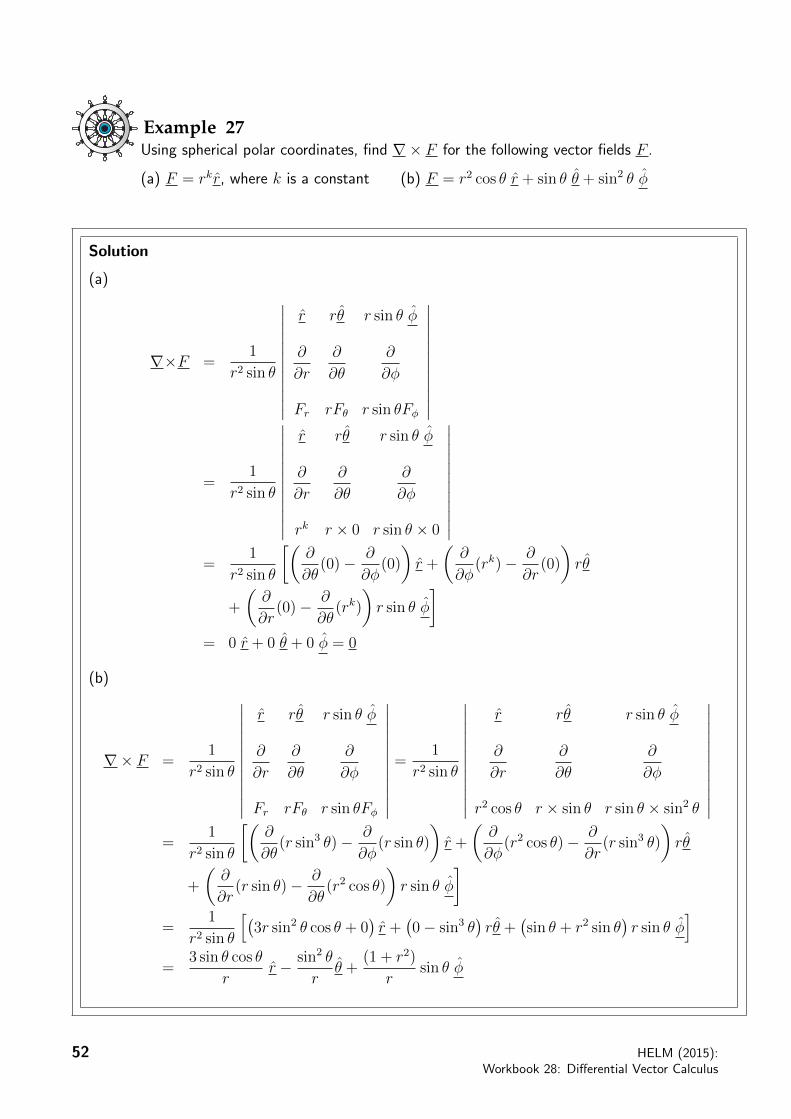
Example 27Using spherical polar coordinates, find ∇× F for the following vector fields F .

(a) F = rkr, where k is a constant (b) F = r2 cos θ r + sin θ θ + sin2 θ φ

Solution

(a)

∇×F =1

r2 sin θ

∣∣∣∣∣∣∣∣∣∣∣∣

r rθ r sin θ φ

∂

∂r

∂

∂θ

∂

∂φ

Fr rFθ r sin θFφ

∣∣∣∣∣∣∣∣∣∣∣∣

=1

r2 sin θ

∣∣∣∣∣∣∣∣∣∣∣∣

r rθ r sin θ φ

∂

∂r

∂

∂θ

∂

∂φ

rk r × 0 r sin θ × 0

∣∣∣∣∣∣∣∣∣∣∣∣=

1

r2 sin θ

[(∂

∂θ(0)− ∂

∂φ(0)

)r +

(∂

∂φ(rk)− ∂

∂r(0)

)rθ

+

(∂

∂r(0)− ∂

∂θ(rk)

)r sin θ φ

]= 0 r + 0 θ + 0 φ = 0

(b)

∇× F =1

r2 sin θ

∣∣∣∣∣∣∣∣∣∣∣∣

r rθ r sin θ φ

∂

∂r

∂

∂θ

∂

∂φ

Fr rFθ r sin θFφ

∣∣∣∣∣∣∣∣∣∣∣∣=

1

r2 sin θ

∣∣∣∣∣∣∣∣∣∣∣∣

r rθ r sin θ φ

∂

∂r

∂

∂θ

∂

∂φ

r2 cos θ r × sin θ r sin θ × sin2 θ

∣∣∣∣∣∣∣∣∣∣∣∣=

1

r2 sin θ

[(∂

∂θ(r sin3 θ)− ∂

∂φ(r sin θ)

)r +

(∂

∂φ(r2 cos θ)− ∂

∂r(r sin3 θ)

)rθ

+

(∂

∂r(r sin θ)− ∂

∂θ(r2 cos θ)

)r sin θ φ

]=

1

r2 sin θ

[(3r sin2 θ cos θ + 0

)r +

(0− sin3 θ

)rθ +

(sin θ + r2 sin θ

)r sin θ φ

]=

3 sin θ cos θ

rr − sin2 θ

rθ +

(1 + r2)

rsin θ φ


®

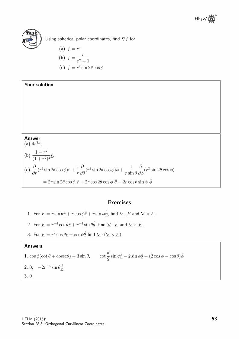
TaskUsing spherical polar coordinates, find ∇f for

(a) f = r4

(b) f =r

r2 + 1

(c) f = r2 sin 2θ cosφ

Your solution

Answer(a) 4r3r,

(b)1− r2

(1 + r2)2r,

(c)∂

∂r(r2 sin 2θ cosφ)r +

1

r

∂

∂θ(r2 sin 2θ cosφ)φ+

1

r sin θ

∂

∂φ(r2 sin 2θ cosφ)

= 2r sin 2θ cosφ r + 2r cos 2θ cosφ θ − 2r cos θ sinφ φ

Exercises

1. For F = r sin θr + r cosφθ + r sinφφ, find ∇ · F and ∇× F .

2. For F = r−4 cos θr + r−4 sin θθ, find ∇ · F and ∇× F .

3. For F = r2 cos θr + cosφθ find ∇ · (∇× F ).

Answers

1. cosφ(cot θ + cosecθ) + 3 sin θ, cotθ

2sinφr − 2 sinφθ + (2 cosφ− cos θ)φ

2. 0, −2r−5 sin θφ

3. 0


53

Index for Workbook 28

Angular momentum 6

Contour curves 10-12Contour map 10Coordinates

- curvilinear 38, 40- cylindrical polar 38, 40- spherical polar 39, 48

Curl 25-26, 33Cylindrical polar coordinates 38, 40

Differentiation rules 5Div 23, 33Divergence 23, 43

Electric potential 50

Field - electric 50- irrotational 26- magnetic 28, 43, 45- scalar 9-12- vector 12-15

Grad 19, 33Gradient 18Gravitational force 12, 15

Heat flow 13

Helix 44

Identities - grad, div, curl 33Irrotational vector field 26

Laplacian 31-33

Magnetic field 28, 43-45

Newton’s second law 6

Orthogonal curvilinear coordinates37-53

Parabola 4Particle 3-8Position vector 3

Scalar field 9-12Spherical polar coordinates 39, 48

Torque 6

Vector - field 12- magnitude 3- position 3- unit 3

Water flow 12, 13, 25, 30

EXERCISES16, 22, 30, 36, 48, 53

ENGINEERING EXAMPLES1 Current associated with

magnetic field 282 Divergence of a magnetic field 433 Electric potential 50

About the HELM Project - Mathematics Materials

Documents

Transcript of About the HELM Project - Mathematics Materials